Embed Size (px)
Citation preview
CSE 541 - Interpolation
Roger Crawfis
April 19, 2023 OSU/CIS 541 2
Taylor’s Series and Interpolation
• Taylor Series interpolates at a specific point:– The function– Its first derivative– …
• It may not interpolate at other points.• We want an interpolant at several f(c)’s.
Basic Scenario
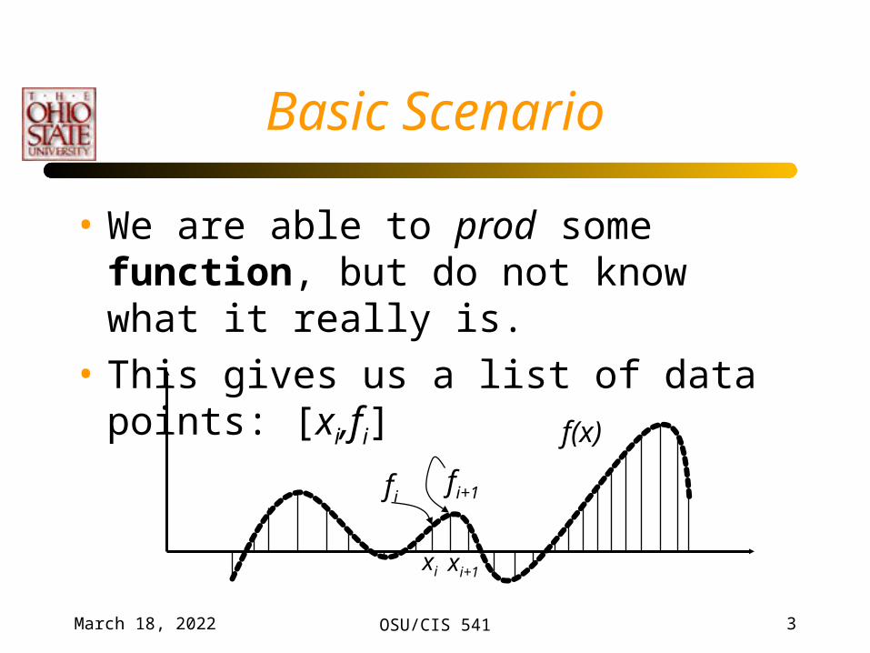
• We are able to prod some function, but do not know what it really is.
• This gives us a list of data points: [xi,fi]
April 19, 2023 OSU/CIS 541 3
f(x)
fifi+1
xi xi+1
April 19, 2023 OSU/CIS 541 4
Interpolation & Curve-fitting
• Often, we have data sets from experimental/observational measurements– Typically, find that the data/dependent variable/output varies…– As the control parameter/independent variable/input varies.
Examples:• Classic gravity drop: location changes with time• Pressure varies with depth• Wind speed varies with time• Temperature varies with location
• Scientific method: Given data identify underlying relationship
• Process known as curve fitting:
April 19, 2023 OSU/CIS 541 5
Interpolation & Curve-fitting
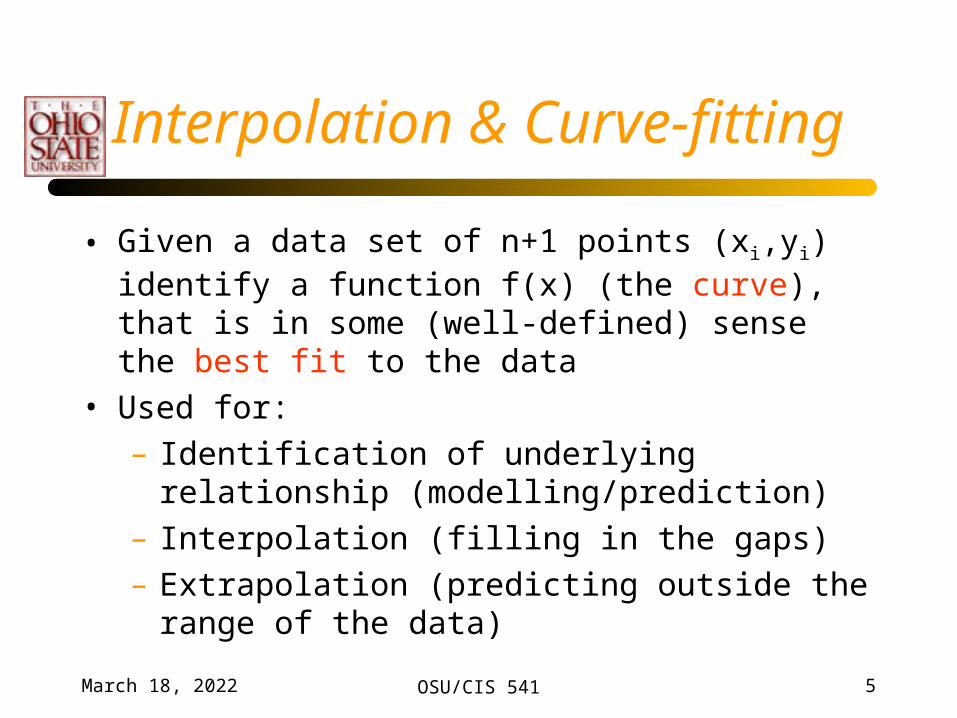
• Given a data set of n+1 points (xi,yi) identify a function f(x) (the curve), that is in some (well-defined) sense the best fit to the data
• Used for:
– Identification of underlying relationship (modelling/prediction)
– Interpolation (filling in the gaps)
– Extrapolation (predicting outside the range of the data)
April 19, 2023 OSU/CIS 541 6
Interpolation Vs Regression
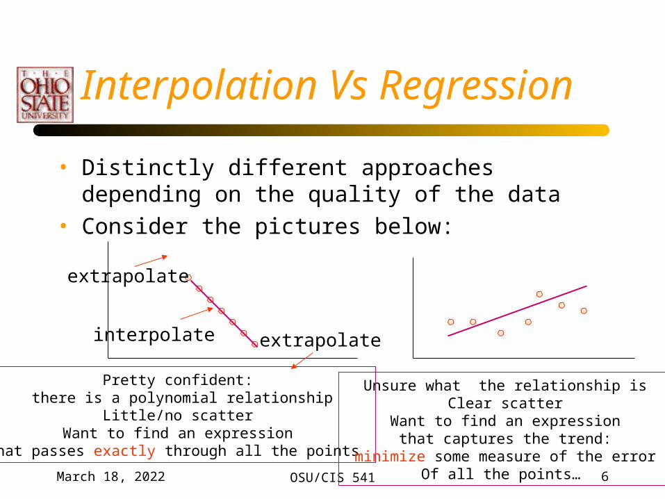
• Distinctly different approaches depending on the quality of the data
• Consider the pictures below:
Pretty confident: there is a polynomial relationship
Little/no scatterWant to find an expression
that passes exactly through all the points
interpolate
extrapolate
extrapolate
Unsure what the relationship isClear scatter
Want to find an expressionthat captures the trend:
minimize some measure of the error Of all the points…

April 19, 2023 OSU/CIS 541 7
Interpolation
• Concentrate first on the case where we believe there is no error in the data (and round-off is assumed to be negligible).
• So we have yi=f(xi) at n+1 points x0,x1…xi,…xn: xj > xj-1 • (Often but not always evenly spaced)• In general, we do not know the underlying function f(x)• Conceptually, interpolation consists of two stages:
– Develop a simple function g(x) that• Approximates f(x)• Passes through all the points xi
– Evaluate f(xt) where x0 < xt < xn
April 19, 2023 OSU/CIS 541 8
Interpolation
• Clearly, the crucial question is the selection of the simple functions g(x)
• Types are: – Polynomials
– Splines
– Trigonometric functions
– Spectral functions…Rational functions etc…
April 19, 2023 OSU/CIS 541 9
Curve Approximation
• We will look at three possible approximations (time permitting):– Polynomial interpolation– Spline (polynomial) interpolation– Least-squares (polynomial) approximation
• If you know your function is periodic, then trigonometric functions may work better.– Fourier Transform and representations
April 19, 2023 OSU/CIS 541 10
Polynomial Interpolation
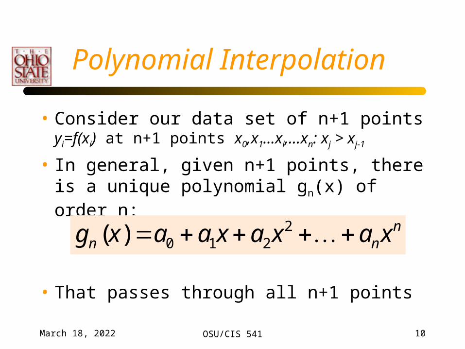
• Consider our data set of n+1 points yi=f(xi) at n+1 points x0,x1…xi,…xn: xj > xj-1
• In general, given n+1 points, there is a unique polynomial gn(x) of order n:
• That passes through all n+1 points
20 1 2( ) n
n ng x a a x a x a x
April 19, 2023 OSU/CIS 541 11
Polynomial Interpolation
• There are a variety of ways of expressing the same polynomial
• Lagrange interpolating polynomials
• Newton’s divided difference interpolating polynomials
• We will look at both forms
April 19, 2023 OSU/CIS 541 12
Polynomial Interpolation
• Existence – does there exist a polynomial that exactly passes through the n data points?
• Uniqueness – Is there more than one such polynomial?– We will assume uniqueness for now and prove
it latter.
April 19, 2023 OSU/CIS 541 13
Lagrange Polynomials
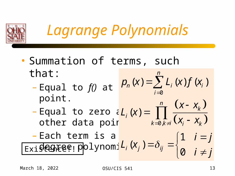
• Summation of terms, such that:– Equal to f() at a data
point.– Equal to zero at all
other data points.– Each term is a nth-
degree polynomial
0
0,
( ) ( ) ( )
( )
1( )
0
n
n i ii
nk
ik k i i k
i j ij
p x L x f x
x xL x
x x
i jL x
i j
Existence!!!
April 19, 2023 OSU/CIS 541 14
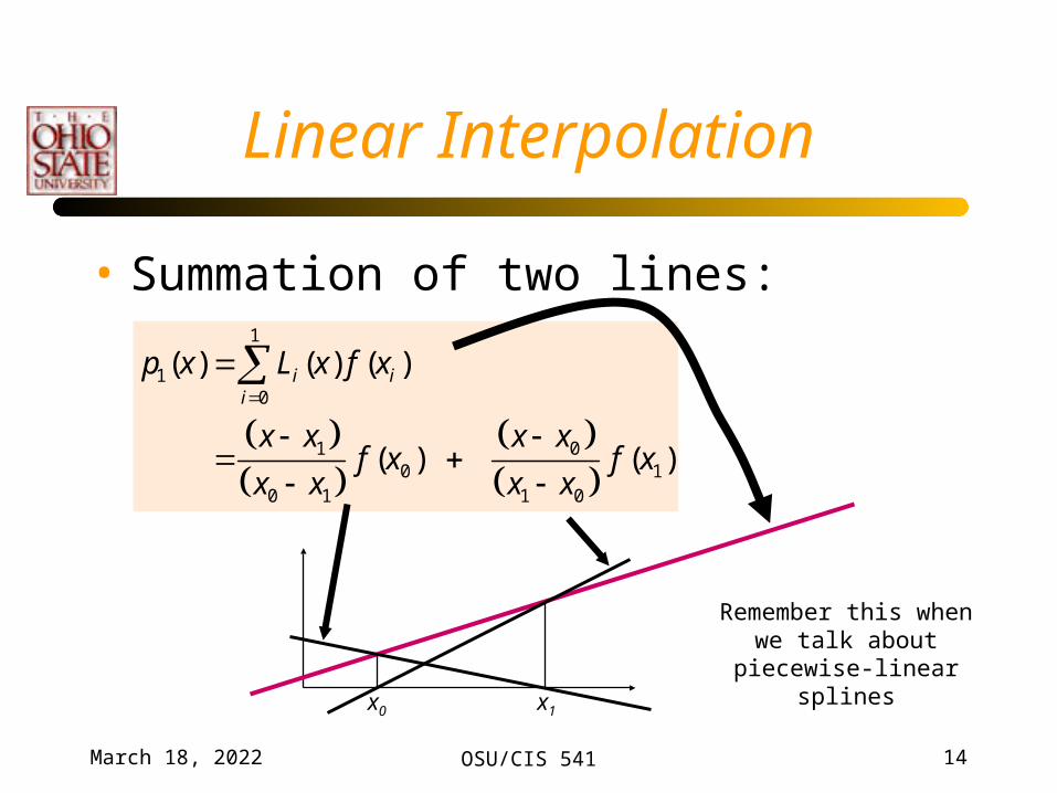
Linear Interpolation
• Summation of two lines:
1
10
1 00 1
0 1 1 0
( ) ( ) ( )
( ) ( )
i ii
p x L x f x
x x x xf x f x
x x x x
x0 x1
Remember this when we talk about piecewise-linear
splines
April 19, 2023 OSU/CIS 541 15
The first quadratic has roots at x1 and x2 and a value equal to the function dataat x0.
• P(x0) = f0
• P(x1) = 0• P(x2) = 0
The second quadratic has roots at x0 and x2 and a value equal to the function data at x1.
• P(x0) = 0• P(x1) = f1
• P(x2) = 0
The third quadratic has roots at x0 and x1 and a value equal to the function data at x2.
• P(x0) = 0• P(x1) = 0• P(x2) = f1
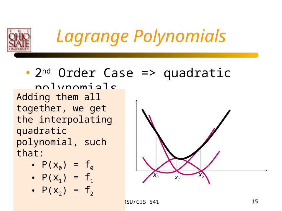
Lagrange Polynomials
• 2nd Order Case => quadratic polynomials
x0 x2x1
Adding them all together, we get the interpolating quadratic polynomial, such that:
• P(x0) = f0
• P(x1) = f1
• P(x2) = f2
April 19, 2023 OSU/CIS 541 16
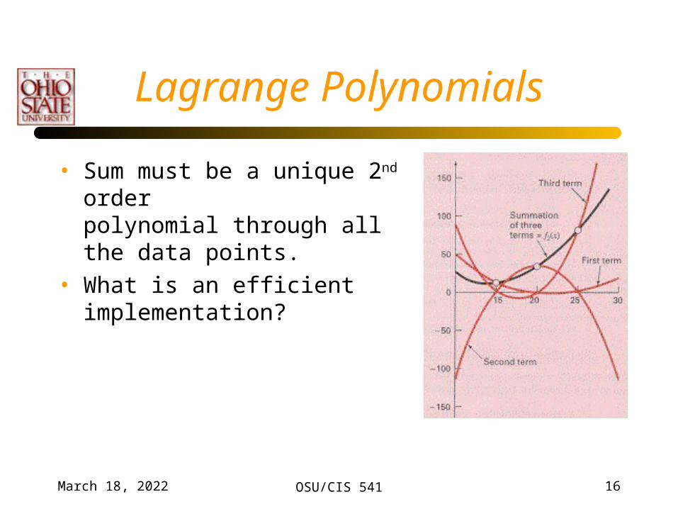
Lagrange Polynomials
• Sum must be a unique 2nd order polynomial through all the data points.
• What is an efficient implementation?
April 19, 2023 OSU/CIS 541 17
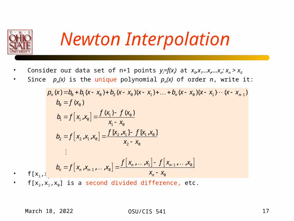
Newton Interpolation
• Consider our data set of n+1 points yi=f(xi) at x0,x1…xi,…xn: xn > x0 • Since pn(x) is the unique polynomial pn(x) of order n, write it:
• f[xi,xj] is a first divided difference• f[x2,x1,x0] is a second divided difference, etc.
0 1 0 2 0 1 0 1 1
0 0
1 01 1 0
1 0
2 1 1 02 2 1 0
2 0
1 1 01 0
0
( ) ( ) ( )( ) ( )( ) ( )
( )
( ) ( ),
[ , ] [ , ], ,
, , , ,, , ,
n n n
n nn n n
n
p x b b x x b x x x x b x x x x x x
b f x
f x f xb f x x
x x
f x x f x xb f x x x
x x
f x x f x xb f x x x
x x
April 19, 2023 OSU/CIS 541 18
Invariance Theorem
• Note, that the order of the data points does not matter.
• All that is required is that the data points are distinct.
• Hence, the divided difference f[x0, x1, …, xk] is invariant under all permutations of the xi‘s.
April 19, 2023 OSU/CIS 541 19
Linear Interpolation
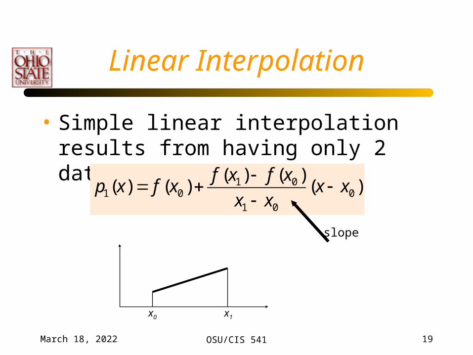
• Simple linear interpolation results from having only 2 data points.
1 01 0 0
1 0
( ) ( )( ) ( ) ( )
f x f xp x f x x x
x x
slope
x0 x1
April 19, 2023 OSU/CIS 541 20
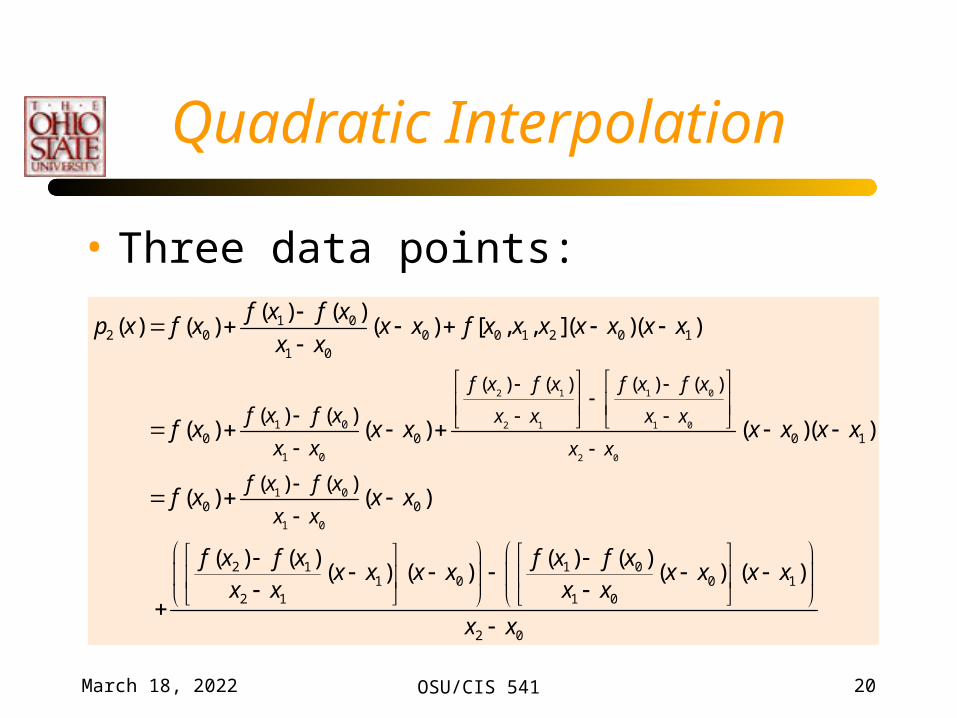
Quadratic Interpolation
• Three data points:
2 1 1 0
2 1 1 0
2 0
1 0
1 0
1 0
1 0
1 02 0 0 0 1 2 0 1
1 0
0 0 0 1
0 0
2 1
2 1
( ) ( ) ( ) ( )
( ) ( )
( ) ( )
( ) ( )( ) ( ) ( ) [ , , ]( )( )
( ) ( ) ( )( )
( ) ( )
( ) ( )(
f x f x f x f x
x x x x
x x
f x f x
x x
f x f x
x x
f x f xp x f x x x f x x x x x x x
x x
f x x x x x x x
f x x x
f x f xx x
x x
1 01 0 0 1
1 0
2 0
( ) ( )) ( ) ( ) ( )
f x f xx x x x x x
x x
x x
April 19, 2023 OSU/CIS 541 21
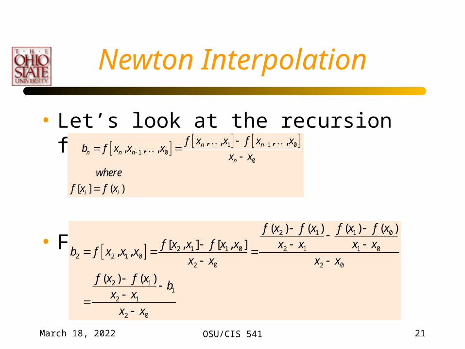
Newton Interpolation
• Let’s look at the recursion formula:
• For the quadratic term:
1 1 01 0
0
, , , ,, , ,
[ ] ( )
n nn n n
n
i i
f x x f x xb f x x x
x x
where
f x f x
1 02 1
2 1 1 0 2 1 1 02 2 1 0
2 0 2 0
2 11
2 1
2 0
( ) ( )( ) ( )[ , ] [ , ]
, ,
( ) ( )
f x f xf x f xf x x f x x x x x x
b f x x xx x x x
f x f xb
x x
x x
April 19, 2023 OSU/CIS 541 22
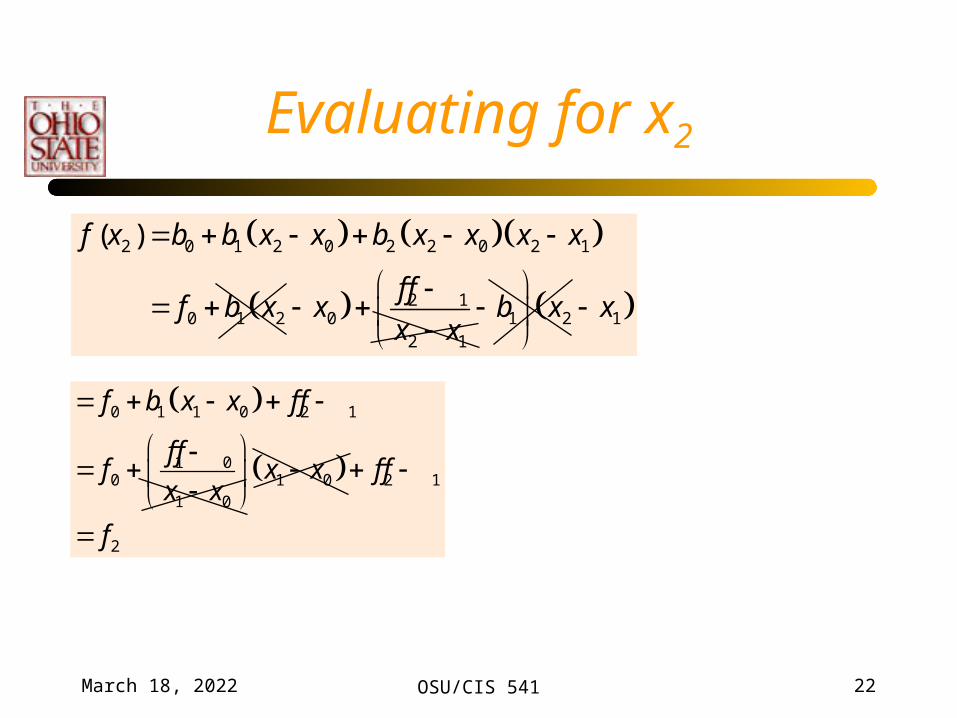
Evaluating for x2
2 0 1 2 0 2 2 0 2 1
2 10 1 2 0 1 2 1
2 1
( )f x b b x x b x x x x
f ff b x x b x x
x x
0 1 1 0 2 1
1 00 1 0 2 1
1 0
2
f b x x f f
f ff x x f f
x x
f
April 19, 2023 OSU/CIS 541 23
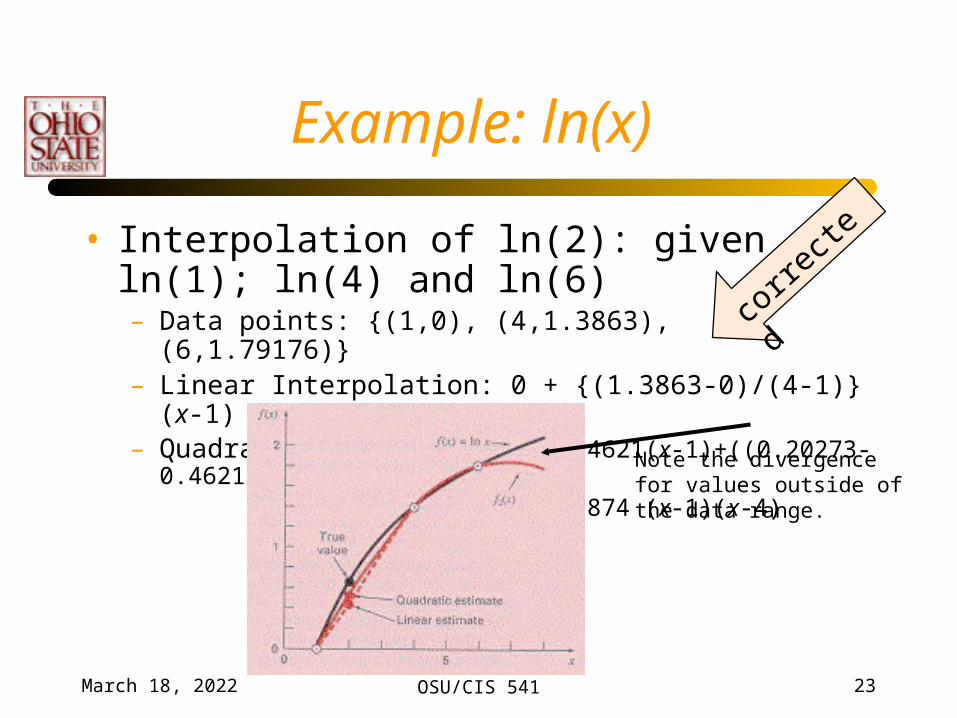
Example: ln(x)
• Interpolation of ln(2): given ln(1); ln(4) and ln(6)– Data points: {(1,0), (4,1.3863), (6,1.79176)} – Linear Interpolation: 0 + {(1.3863-0)/(4-1)}(x-1) = 0.4621(x-1)– Quadratic Interpolation: 0.4621(x-1)+((0.20273-0.4621)/5)(x-1)(x-4)
= 0.4621(x-1) - 0.051874 (x-1)(x-4)
Note the divergence for values outside ofthe data range.
corre
cted
April 19, 2023 OSU/CIS 541 24
Example: ln(x)
• Quadratic interpolation catches some of the curvature
• Improves the result somewhat
• Not always a good idea: see later…
April 19, 2023 OSU/CIS 541 25
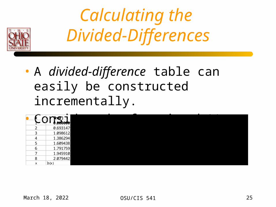
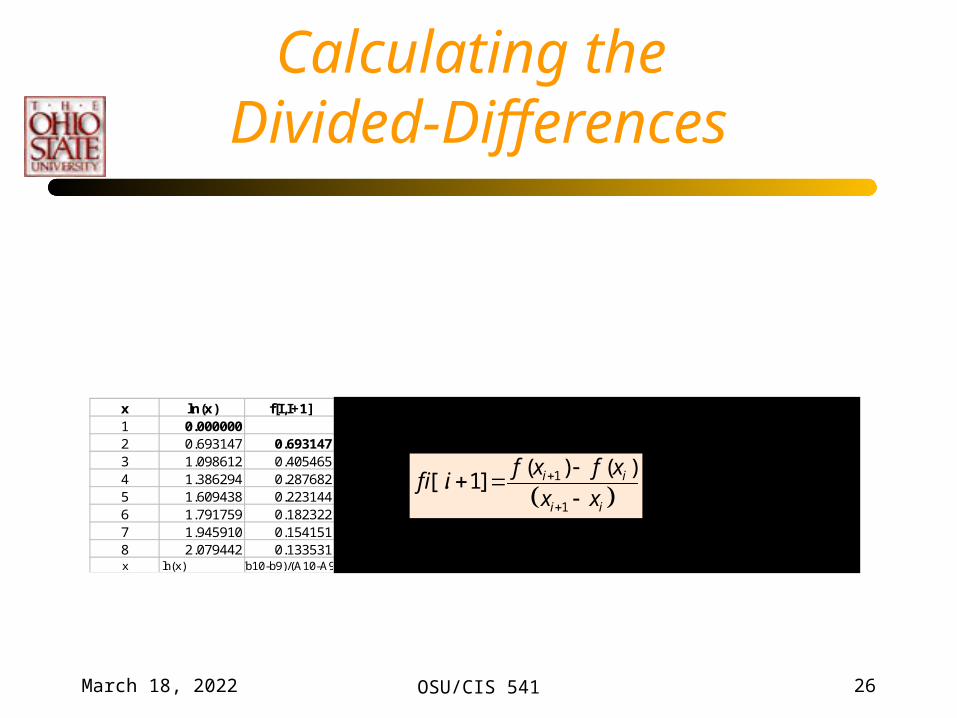
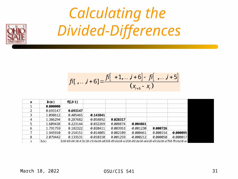
Calculating the Divided-Differences
• A divided-difference table can easily be constructed incrementally.
• Consider the function ln(x).x ln(x) f[I,I+1] f[I,I+1,…,I+7]1 0.0000002 0.693147 0.6931473 1.098612 0.405465 -0.1438414 1.386294 0.287682 -0.058892 0.0283175 1.609438 0.223144 -0.032269 0.008874 -0.0048616 1.791759 0.182322 -0.020411 0.003953 -0.001230 0.0007267 1.945910 0.154151 -0.014085 0.002109 -0.000461 0.000154 -0.0000958 2.079442 0.133531 -0.010310 0.001259 -0.000212 0.000050 -0.000017 0.000013x ln(x) (b10-b9)/(A10-A9)(c10-c9)/(a10-a8)(d10-d9)/(a10-a7)(d10-d9)/(a10-a6)(e10-e9)/(a10-a5)(f10-f9)/(a10-a4) (g10-g9)/(a10-a3)
April 19, 2023 OSU/CIS 541 26
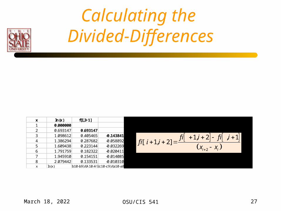
Calculating the Divided-Differences
x ln(x) f[I,I+1] f[I,I+1,…,I+7]1 0.0000002 0.693147 0.6931473 1.098612 0.405465 -0.1438414 1.386294 0.287682 -0.058892 0.0283175 1.609438 0.223144 -0.032269 0.008874 -0.0048616 1.791759 0.182322 -0.020411 0.003953 -0.001230 0.0007267 1.945910 0.154151 -0.014085 0.002109 -0.000461 0.000154 -0.0000958 2.079442 0.133531 -0.010310 0.001259 -0.000212 0.000050 -0.000017 0.000013x ln(x) (b10-b9)/(A10-A9)(c10-c9)/(a10-a8)(d10-d9)/(a10-a7)(d10-d9)/(a10-a6)(e10-e9)/(a10-a5)(f10-f9)/(a10-a4) (g10-g9)/(a10-a3)
1
1
( ) ( )[ . 1] i i
i i
f x f xf i i
x x
April 19, 2023 OSU/CIS 541 27
Calculating the Divided-Differences
x ln(x) f[I,I+1] f[I,I+1,…,I+7]1 0.0000002 0.693147 0.6931473 1.098612 0.405465 -0.1438414 1.386294 0.287682 -0.058892 0.0283175 1.609438 0.223144 -0.032269 0.008874 -0.0048616 1.791759 0.182322 -0.020411 0.003953 -0.001230 0.0007267 1.945910 0.154151 -0.014085 0.002109 -0.000461 0.000154 -0.0000958 2.079442 0.133531 -0.010310 0.001259 -0.000212 0.000050 -0.000017 0.000013x ln(x) (b10-b9)/(A10-A9)(c10-c9)/(a10-a8)(d10-d9)/(a10-a7)(d10-d9)/(a10-a6)(e10-e9)/(a10-a5)(f10-f9)/(a10-a4) (g10-g9)/(a10-a3)
2
1, 2 , 1[ . 1, 2]
i i
f i i f i if i i i
x x
April 19, 2023 OSU/CIS 541 28
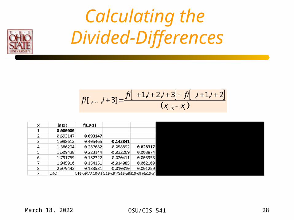
Calculating the Divided-Differences
x ln(x) f[I,I+1] f[I,I+1,…,I+7]1 0.0000002 0.693147 0.6931473 1.098612 0.405465 -0.1438414 1.386294 0.287682 -0.058892 0.0283175 1.609438 0.223144 -0.032269 0.008874 -0.0048616 1.791759 0.182322 -0.020411 0.003953 -0.001230 0.0007267 1.945910 0.154151 -0.014085 0.002109 -0.000461 0.000154 -0.0000958 2.079442 0.133531 -0.010310 0.001259 -0.000212 0.000050 -0.000017 0.000013x ln(x) (b10-b9)/(A10-A9)(c10-c9)/(a10-a8)(d10-d9)/(a10-a7)(d10-d9)/(a10-a6)(e10-e9)/(a10-a5)(f10-f9)/(a10-a4) (g10-g9)/(a10-a3)
3
1, 2, 3 , 1, 2[ , , 3]
i i
f i i i f i i if i i
x x
April 19, 2023 OSU/CIS 541 29
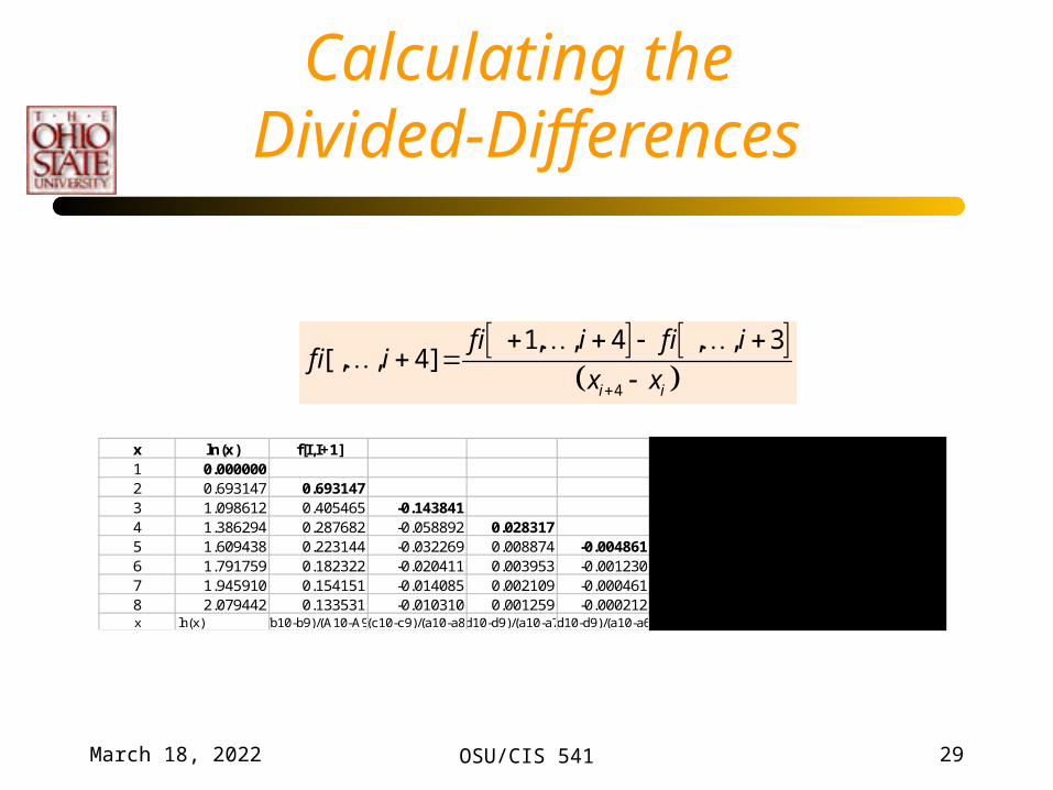
Calculating the Divided-Differences
x ln(x) f[I,I+1] f[I,I+1,…,I+7]1 0.0000002 0.693147 0.6931473 1.098612 0.405465 -0.1438414 1.386294 0.287682 -0.058892 0.0283175 1.609438 0.223144 -0.032269 0.008874 -0.0048616 1.791759 0.182322 -0.020411 0.003953 -0.001230 0.0007267 1.945910 0.154151 -0.014085 0.002109 -0.000461 0.000154 -0.0000958 2.079442 0.133531 -0.010310 0.001259 -0.000212 0.000050 -0.000017 0.000013x ln(x) (b10-b9)/(A10-A9)(c10-c9)/(a10-a8)(d10-d9)/(a10-a7)(d10-d9)/(a10-a6)(e10-e9)/(a10-a5)(f10-f9)/(a10-a4) (g10-g9)/(a10-a3)
4
1, , 4 , , 3[ , , 4]
i i
f i i f i if i i
x x

April 19, 2023 OSU/CIS 541 30
Calculating the Divided-Differences
x ln(x) f[I,I+1] f[I,I+1,…,I+7]1 0.0000002 0.693147 0.6931473 1.098612 0.405465 -0.1438414 1.386294 0.287682 -0.058892 0.0283175 1.609438 0.223144 -0.032269 0.008874 -0.0048616 1.791759 0.182322 -0.020411 0.003953 -0.001230 0.0007267 1.945910 0.154151 -0.014085 0.002109 -0.000461 0.000154 -0.0000958 2.079442 0.133531 -0.010310 0.001259 -0.000212 0.000050 -0.000017 0.000013x ln(x) (b10-b9)/(A10-A9)(c10-c9)/(a10-a8)(d10-d9)/(a10-a7)(d10-d9)/(a10-a6)(e10-e9)/(a10-a5)(f10-f9)/(a10-a4) (g10-g9)/(a10-a3)
5
1, , 5 , , 4[ , , 5]
i i
f i i f i if i i
x x
April 19, 2023 OSU/CIS 541 31
Calculating the Divided-Differences
x ln(x) f[I,I+1] f[I,I+1,…,I+7]1 0.0000002 0.693147 0.6931473 1.098612 0.405465 -0.1438414 1.386294 0.287682 -0.058892 0.0283175 1.609438 0.223144 -0.032269 0.008874 -0.0048616 1.791759 0.182322 -0.020411 0.003953 -0.001230 0.0007267 1.945910 0.154151 -0.014085 0.002109 -0.000461 0.000154 -0.0000958 2.079442 0.133531 -0.010310 0.001259 -0.000212 0.000050 -0.000017 0.000013x ln(x) (b10-b9)/(A10-A9)(c10-c9)/(a10-a8)(d10-d9)/(a10-a7)(d10-d9)/(a10-a6)(e10-e9)/(a10-a5)(f10-f9)/(a10-a4) (g10-g9)/(a10-a3)
6
1, , 6 , , 5[ , , 6]
i i
f i i f i if i i
x x
April 19, 2023 OSU/CIS 541 32
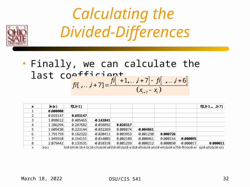
Calculating the Divided-Differences
• Finally, we can calculate the last coefficient.
x ln(x) f[I,I+1] f[I,I+1,…,I+7]1 0.0000002 0.693147 0.6931473 1.098612 0.405465 -0.1438414 1.386294 0.287682 -0.058892 0.0283175 1.609438 0.223144 -0.032269 0.008874 -0.0048616 1.791759 0.182322 -0.020411 0.003953 -0.001230 0.0007267 1.945910 0.154151 -0.014085 0.002109 -0.000461 0.000154 -0.0000958 2.079442 0.133531 -0.010310 0.001259 -0.000212 0.000050 -0.000017 0.000011x ln(x) (b10-b9)/(A10-A9)(c10-c9)/(a10-a8)(d10-d9)/(a10-a7)(d10-d9)/(a10-a6)(e10-e9)/(a10-a5)(f10-f9)/(a10-a4) (g10-g9)/(a10-a3)
7
1, , 7 , , 6[ , , 7]
i i
f i i f i if i i
x x
April 19, 2023 OSU/CIS 541 33
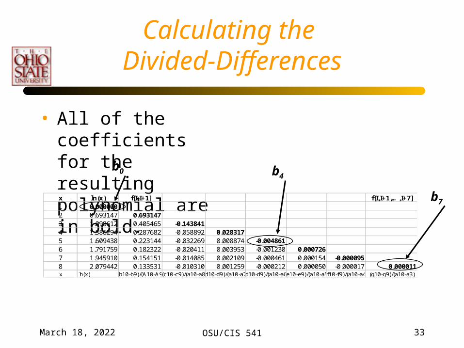
Calculating the Divided-Differences
• All of the coefficients for the resulting polynomial are in bold.x ln(x) f[I,I+1] f[I,I+1,…,I+7]1 0.0000002 0.693147 0.6931473 1.098612 0.405465 -0.1438414 1.386294 0.287682 -0.058892 0.0283175 1.609438 0.223144 -0.032269 0.008874 -0.0048616 1.791759 0.182322 -0.020411 0.003953 -0.001230 0.0007267 1.945910 0.154151 -0.014085 0.002109 -0.000461 0.000154 -0.0000958 2.079442 0.133531 -0.010310 0.001259 -0.000212 0.000050 -0.000017 0.000011x ln(x) (b10-b9)/(A10-A9)(c10-c9)/(a10-a8)(d10-d9)/(a10-a7)(d10-d9)/(a10-a6)(e10-e9)/(a10-a5)(f10-f9)/(a10-a4) (g10-g9)/(a10-a3)
b0 b4
b7
April 19, 2023 OSU/CIS 541 34
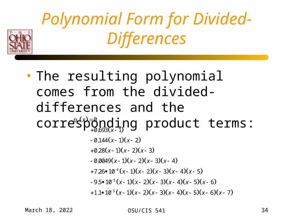
Polynomial Form for Divided-Differences
• The resulting polynomial comes from the divided-differences and the corresponding product terms:
7
4
5
5
0
0.693 1
0.144 1 2
0.28 1 2 3
0.0049 1 2 3 4
7.26 10 1 2 3 4 5
9.5 10 1 2 3 4 5 6
1.1 10 1 2 3 4 5 6 7
p x
x
x x
x x x
x x x x
x x x x x
x x x x x x
x x x x x x x
April 19, 2023 OSU/CIS 541 35
Many polynomials
• Note, that the order of the numbers (xi,yi)’s only matters when writing the polynomial down.– The first column represents the set of linear
splines between two adjacent data points.– The second column gives us quadratics thru
three adjacent points.– Etc.
April 19, 2023 OSU/CIS 541 36
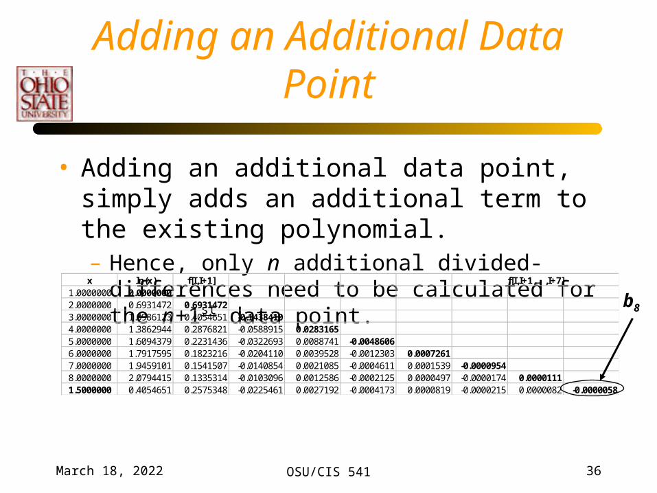
Adding an Additional Data Point
• Adding an additional data point, simply adds an additional term to the existing polynomial.– Hence, only n additional divided-differences need to be
calculated for the n+1st data point.x ln(x) f[I,I+1] f[I,I+1,…,I+7]
1.0000000 0.00000002.0000000 0.6931472 0.69314723.0000000 1.0986123 0.4054651 -0.14384104.0000000 1.3862944 0.2876821 -0.0588915 0.02831655.0000000 1.6094379 0.2231436 -0.0322693 0.0088741 -0.00486066.0000000 1.7917595 0.1823216 -0.0204110 0.0039528 -0.0012303 0.00072617.0000000 1.9459101 0.1541507 -0.0140854 0.0021085 -0.0004611 0.0001539 -0.00009548.0000000 2.0794415 0.1335314 -0.0103096 0.0012586 -0.0002125 0.0000497 -0.0000174 0.00001111.5000000 0.4054651 0.2575348 -0.0225461 0.0027192 -0.0004173 0.0000819 -0.0000215 0.0000082 -0.0000058
b8
April 19, 2023 OSU/CIS 541 37
Adding More Data Points
• Quadratic interpolation: – does linear interpolation– Then add higher-order correction to catch the curvature
• Cubic, …• Consider the case where the data points are
organized such the the first two are the endpoints, the next point is the mid-point, followed by successive mid-points of the half-intervals.– Worksheet: f(x)=x2 from -1 to 3.
April 19, 2023 OSU/CIS 541 38
Uniqueness
• Suppose that two polynomials of degree n (or less) existed that interpolated to the n+1 data points.
• Subtracting these two polynomials from each other also leads to a polynomial of at most n degree.
( ) ( ) ( )n n nr x p x q x
April 19, 2023 OSU/CIS 541 39
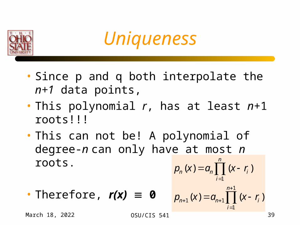
Uniqueness
• Since p and q both interpolate the n+1 data points,
• This polynomial r, has at least n+1 roots!!!
• This can not be! A polynomial of degree-n can only have at most n roots.
• Therefore, r(x) 01
1
1 11
( ) ( )
( ) ( )
n
n n ii
n
n n ii
p x a x r
p x a x r
April 19, 2023 OSU/CIS 541 40
Example
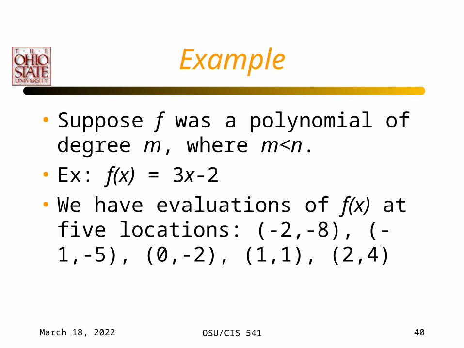
• Suppose f was a polynomial of degree m, where m<n.
• Ex: f(x) = 3x-2
• We have evaluations of f(x) at five locations: (-2,-8), (-1,-5), (0,-2), (1,1), (2,4)
April 19, 2023 OSU/CIS 541 41
Error
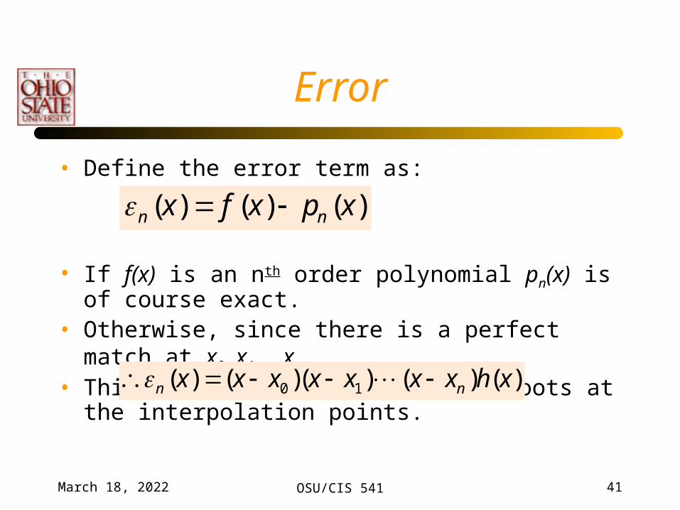
• Define the error term as:
• If f(x) is an nth order polynomial pn(x) is of course exact.• Otherwise, since there is a perfect match at x0, x1,…,xn • This function has at least n+1 roots at the interpolation
points.
( ) ( ) ( )n nx f x p x
0 1( ) ( )( ) ( ) ( )n nx x x x x x x h x
April 19, 2023 OSU/CIS 541 42
Interpolation Errors
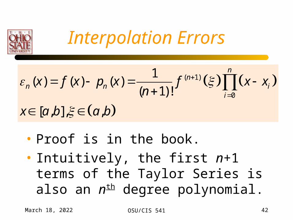
• Proof is in the book.
• Intuitively, the first n+1 terms of the Taylor Series is also an nth degree polynomial.
( 1)
0
1( ) ( ) ( )
( 1)!
[ , ], ,
nn
n n ii
x f x p x f x xn
x a b a b
April 19, 2023 OSU/CIS 541 43
Interpolation Errors
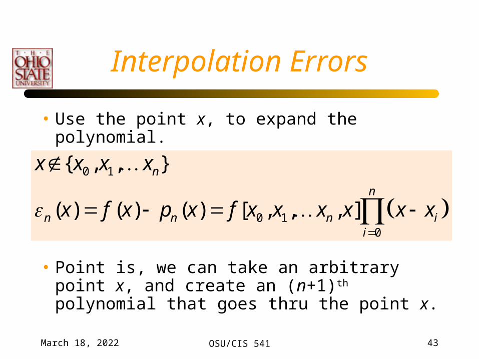
• Use the point x, to expand the polynomial.
• Point is, we can take an arbitrary point x, and create an (n+1)th polynomial that goes thru the point x.
0 1
0 10
{ , , }
( ) ( ) ( ) [ , , , ]
n
n
n n n ii
x x x x
x f x p x f x x x x x x
April 19, 2023 OSU/CIS 541 44
Interpolation Errors
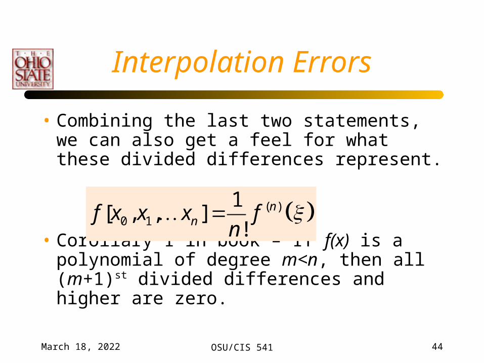
• Combining the last two statements, we can also get a feel for what these divided differences represent.
• Corollary 1 in book – If f(x) is a polynomial of degree m<n, then all (m+1)st divided differences and higher are zero.
( )0 1
1[ , , ]
!n
nf x x x fn
April 19, 2023 OSU/CIS 541 45
Problems with Interpolation
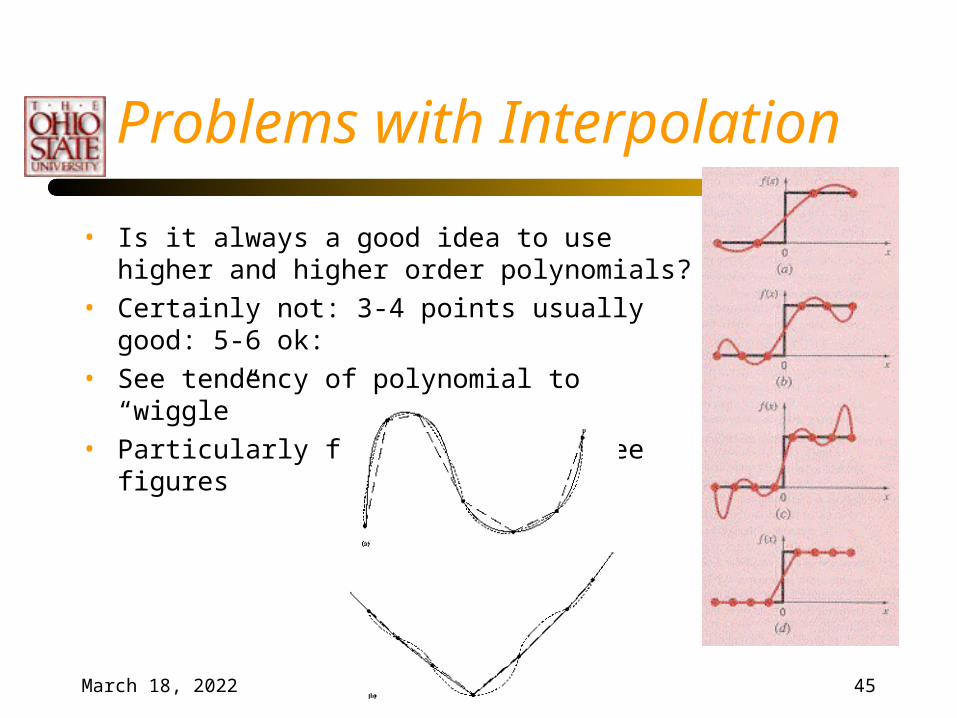
• Is it always a good idea to use higher and higher order polynomials?
• Certainly not: 3-4 points usually good: 5-6 ok:
• See tendency of polynomial to “wiggle”
• Particularly for sharp edges: see figures
April 19, 2023 OSU/CIS 541 46
Chebyshev nodes
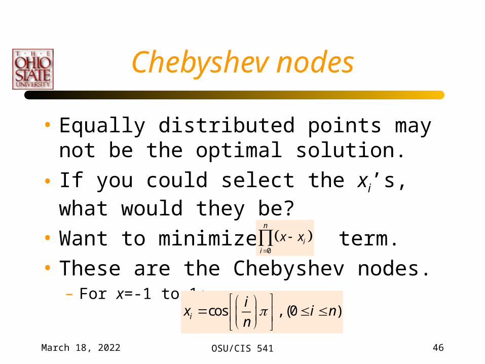
• Equally distributed points may not be the optimal solution.
• If you could select the xi’s, what would they be?
• Want to minimize the term.
• These are the Chebyshev nodes. – For x=-1 to 1:
0
n
ii
x x
cos , (0 )i
ix i n
n
April 19, 2023 OSU/CIS 541 47
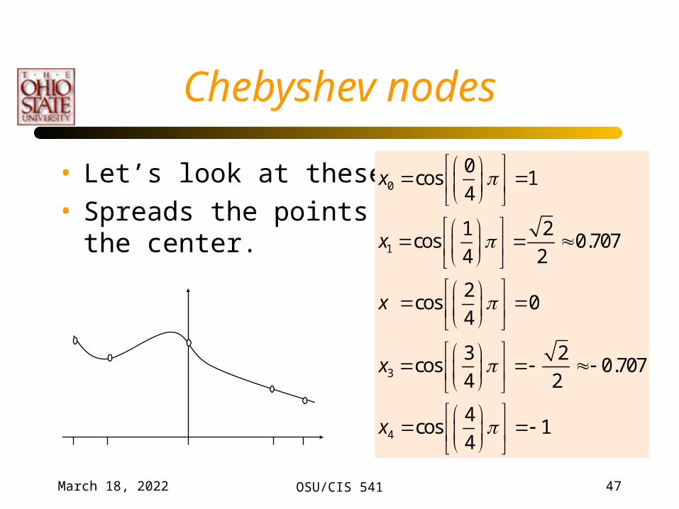
Chebyshev nodes
• Let’s look at these for n=4.• Spreads the points out in
the center.
0
1
3
4
0cos 1
4
1 2cos 0.707
4 2
2cos 0
4
3 2cos 0.707
4 2
4cos 1
4
x
x
x
x
x
April 19, 2023 OSU/CIS 541 48
Polynomial Interpolation in Two-Dimensions
• Consider the case in higher-dimensions.
April 19, 2023 OSU/CIS 541 49
Finding the Inverse of a Function
• What if I am after the inverse of the function f(x)?– For example arccos(x).
• Simply reverse the role of the xi and the fi.