Curiosity, recruitment, and chaos: a tribute to Bill Ricker’s inquiring mind

Jon T. SchnuteFisheries and Oceans Canada, Pacific Biological Station, 3190 Hammond Bay Road, Nanaimo, BC, V9T 6N7,Canada (E-mail: schnutej@pac.dfo-mpo.gc.ca)

Received 17 June 2004 Accepted 27 October 2004

Key words: mathematics, models, biology, fishery management, Ricker curve, yield per recruit, markingexperiment, astronomy

Synopsis

Through three versions of a handbook on computations for biological statistics of fish populations, W.E.‘‘Bill’’ Ricker played a pivotal role in founding the field of quantitative fishery science. His interests,however, extended far beyond the confines of quantifiable events to a deep appreciation for the naturalworld. In this article, I trace his development of fishery models from the 1940s to the 1970s, using examplesthat illustrate his approach to statistics and biological systems analysis. I describe changes in technologyand statistics that have made it possible to extend his research in new directions, although his approach stilllies at the core of all modern fishery models. His gentle, inquiring spirit persisted long after his retirement in1973, as I illustrate from personal experiences with him during the 1990s.

Introduction

In a historical survey of population dynamicsmodels in fisheries, Quinn (2003, p. 355) concludedthat ‘‘nobody has made more contributions tothe development of fisheries models than WilliamE. Ricker.’’ To support this claim, Quinn cited thebreadth, long duration, and statistical focus ofRicker’s work. Generations of fishery scientistsregularly consulted Ricker’s handbooks to findappropriate methods of data analysis. Ricker’s(2006) autobiographical sketch in this issue ofEnvironmental Biology of Fishes places his quan-titative work in the context of a much broadercareer. Based partly on my personal experienceswith him, I write this companion article as a tributeto his spirit of inquiry, which extended far beyondthe confines of quantifiable events to a deepappreciation for the natural world.

The famous handbooks began with an earlycompilation of numerical methods (Ricker 1948)

and grew through two revisions (Ricker 1958,1975). Only the 1958 edition actually includes theword handbook in its title. Ricker (2006) himselfcalled them the ‘‘Green Books,’’ with covers thatwent sequentially from light green to dark green toaquamarine. He also edited a multi-author hand-book that he carried through two editions (Ricker1968, 1971), working with other outstanding fish-ery scientists of that time. All these books, com-bined with extensive journal publications, firmlyestablished his central role in the development ofquantitative models for fish populations.

Ricker’s (2006) autobiographical sketch revealsanother side of this remarkable man. In simplelanguage, he demonstrates his great interest in thenatural world around him. He sees organisms inthe context of geology, hydrology, and other fac-tors that influence their diversity and evolution.He relates personal experiences with vivid histori-cal details that reflect his passion for discoveringthe truth. Unresolved questions stay with him. For

Environmental Biology of Fishes (2006) 75:95–110 � Springer 2006DOI 10.1007/s10641-005-2444-9

example, he mentions school days spent in NorthBay, Ontario along Lake Nipissing, ‘‘whoseextensive beaches shoal out into the water withthree or four underwater sandbars along the way –a phenomenon for which I have not yet seen thephysical explanation.’’ Part of his search entailsmathematical techniques for estimating the ‘‘vitalstatistics’’ of populations, but the driving forcecomes from his curiosity about nature itself.

The down to earth language of his sketchaccurately represents his informal, human style.His friends and acquaintances knew him as ‘‘Bill’’,and I shall often use his familiar name here. Heretired as scientist at the Pacific Biological Stationin Nanaimo, British Columbia, 3 years beforeI began working there in 1976. Because he retainedan office and used it frequently, I didn’t realize atfirst that he was, in fact, retired. Although I knewof his outstanding reputation, it took me years toappreciate the scope of his achievements. I beganworking in fisheries as a naive mathematician, withmuch to learn about biology and the broaderworld of scientific inquiry. Bill had used mathe-matics as a scientific tool for understanding nat-ure, based on a wealth of personal experience. Heknew well the limitations of models, which cangive deceptive estimates and predictions based onassumptions that might be wrong. The Preface tohis second Green Book (Ricker 1958, p. 14) con-tains timeless advice for every fishery scientist:

‘‘... the practising biologist quickly discoversthat the situations he has to tackle tend to bemore complex than those in any Handbook, orelse the conditions differ from any described todate and demand modifications of existingprocedures. It can be taken as a general rule thatexperiments or observations which seem simpleand straightforward will prove to have impor-tant complications when analyzed carefully –complications which stem from the complexityand variability of the living organism, and fromthe changes which take place in it, continuously,from birth to death.

In this article, I trace the development of fisherymodels through the three handbooks, with a par-ticular focus on statistical methods and biologicalsystems analysis. I discuss Ricker’s work in thecontext of science and technology from the 1940s

to the 1970s. Since then, changes in statisticaltheory and computing have made it possible toextend his research in new directions, but hisapproach still lies at the core of all modern fisherymodels. Finally, I relate a few personal experienceswith Bill that illustrate his inquiring spirit, alwaysengaging to friends and colleagues. Some examplesinclude mathematical details, often compiled intotables. Equation numbers reflect this style; forinstance, (T2.3) refers to equation (3) in Table 2.I think readers can safely skip any mathematicalcontent that proves troublesome.

The Green Books and beyond

Bill’s account of his field experiences reminds us oftechnology very different from that availabletoday. For example, he and Fred Ide explored aregion of southern Ontario (Ricker 2006) in avintage 1922 model-T Ford. He recalls starting itwith a crank and driving it up steep hills in reverseto compensate for a gas line fed by gravity from atank under the front seat. I was 8 years old whenBill published his first Green Book in 1948, andmany adults around me could remember drivingsuch vehicles. Some older cars still used cranks forstarting, a procedure that could break someone’sarm if things went wrong. I can also remembermathematical technology of the period. My par-ents used a hand-cranked adding machine in theirflorist business, and it seemed like a big deal toconvert to a model operated by an electric motor. Iregarded slide rules, especially the thick ones withlog–log and trigonometric scales, as the ultimatemathematical hardware.

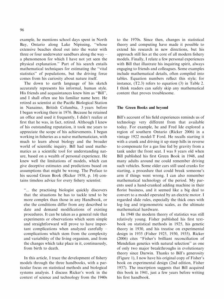
In 1948 the modern theory of statistics was stillrelatively young. Fisher published his first text-book on statistical methods in 1925, his genetictheory in 1930, and his treatise on experimentaldesign in 1935 (Fisher 1925, 1930, 1935). Ricker(2006) cites ‘‘Fisher’s brilliant reconciliation ofMendelian genetics with natural selection’’ as oneof only two major breakthroughs in evolutionarytheory since Darwin. Thanks to Bill’s generosity(Figure 1), I now have his original copy of Fisher’sbook on experimental design (2nd edition, Fisher1937). The inscription suggests that Bill acquiredthis book in 1941, just a few years before writinghis first handbook.

96

These historical details illustrate the world ofscience and technology in the 1940s, when Billbegan writing his Green Books. Ricker (1948)focused on the ‘‘vital statistics’’ of fish populations,including abundance and mortality due to naturaland human causes. He also pointed out (op. cit.,p. 2) that growth may play a role equal to that ofmortality in ‘‘a synthesis which leads to conclusionsof great theoretical and practical interest.’’ Thissmall volume, however, dealt with abundance andmortality much more than growth. It described keyestimation methods, such as measures of abun-dance based on marking experiments.

The second Green Book (Ricker 1958) intro-duced a longer list of ‘‘vital statistics.’’ In additionto abundance and mortality, these includedgrowth, recruitment, and surplus production. Thenew topics led naturally to important fisherymanagement issues, including yield per recruitcalculations (Chapter 10), relationships betweenstock and recruitment (Chapter 11), and equilib-rium yield for a given fishing rate (Chapter 12).Statistical analyses, largely absent in the first book,appeared frequently in the second. For example,where the former gave formulas estimating abun-dance, the latter went on to describe methods ofestimating uncertainty. I suspect that this pro-gression followed the movement of scientificthinking from the 1940s to the 1950s. First, biol-ogists wanted to know feasible methods for mea-suring fish populations. Once these concepts and

practices became firmly established, the need forassessing uncertainty became more compelling.Many of the statistical techniques reported byRicker in 1958 had not been invented when hewrote his first book in 1948.

The Green Books show an interesting languagetransition from ‘‘vital’’ to ‘‘biological’’ statistics.The first uses ‘‘vital’ in its title, but the second andthird use ‘‘biological.’’ The opening sentence of thesecond book (Ricker 1958, p. 17) reads: ‘‘Thetopics which can be considered as vital statistics ofa fish population include the following: ...’’ Thethird book starts with this same sentence, exceptthat ‘‘vital’’ has been changed to ‘‘biological.’’Ricker’s perspective clearly broadened through theyears, starting from an initial focus on mortalityand abundance tables similar to those compiledfor other animal populations, including humans.He gradually extended this framework to encom-pass more aspects of fish biology, such as growthand recruitment. As predicted in his first book(Ricker 1948, p. 2), adding growth to the mix didindeed lead to ‘‘a synthesis ... of great theoreticaland practical interest.’’ Perhaps the realizationthat he was dealing with an entire biological sys-tem caused him to replace ‘‘vital’’ with ‘‘biologi-cal’’ and to include the word ‘‘interpretation’’ inthe title of his third book (Ricker 1975). At last,readers could not only calculate biological statis-tics, but also interpret them in the context of alarger system.

To give this historical analysis more substance,I follow the progression of two distinct threadsthrough the Green Books. First, Ricker’s analysisof a Peterson marking experiment illustrates hisapproach to statistics. Second, his interest in thecomplete biological system finds particularly ele-gant expression in his calculation of fishery yield.In both cases, he compiles the extensive literatureof the time into a single reference book for thebenefit of his readers.

Peterson marking experiments

Ricker (1948, p. 39) cites Peterson (1896) for theidea of tagging fish to estimate abundance. In thesimplest experiment, M marked fish are releasedinto a closed population. Assuming that thesedistribute randomly and that R of them arerecaptured within a total catch C, then

Figure 1. Inscription on the front page of Fisher (1937), when

Bill Ricker gave his copy of that book to the author. Bill had

originally written ‘‘W. E. Ricker, August 1941.’’ Later he

scratched out the date and modified the text to read ‘‘Jon

Schnute from W. E. Ricker 1981.’’ Apparently, Bill acquired

the book in 1941 and gave it to the author 40 years later.

97

N ¼M

RC ð1Þ

gives a reasonable estimate of the total populationN. For example, if 10% of the tags are recovered(M/R=10), then N=10C because the catch Cmust be a 10% sample of the population. In stat-ing this example, I have used notation from laterGreen Books, for consistency with the discussionbelow. The symbols (N, M, C, R) here correspond,respectively, to (P, N, H, R) in Ricker (1948).

Although the first book gives only the formula(1), the second includes

• the abundance estimate (1) stated with properstatistical notation N̂ (Ricker 1958, p. 84,equation (3.5)), and

• an estimate of the variance V½1=N̂� (op. cit. p. 84,equation (3.4)).

I present these in Table 1 as equations (T1.9)–(T1.10). The handbook cautions the reader that

‘‘values of MC/R are not very symmetricallydistributed, whereas those of R/MC are; hence ifthe normal curve of error is used to calculatelimits of confidence, it is best to calculate themfor 1=N̂ . . . and then invert them in order toobtain limits for N̂.’’

Technically the variance of N̂ is infinite, althoughRicker (1958) does not mention this fact. Becausethe number of recoveries R appears in thedenominator of (1) and the value R=0 occurs withnon-zero probability, the estimate N̂ ¼ 1 also hasfinite probability. Consequently, V½N̂� ¼E½ðN̂�NÞ2� ¼ 1.

Table 1 gives some perspective to this analysis.The number R of fish recaptured is a random

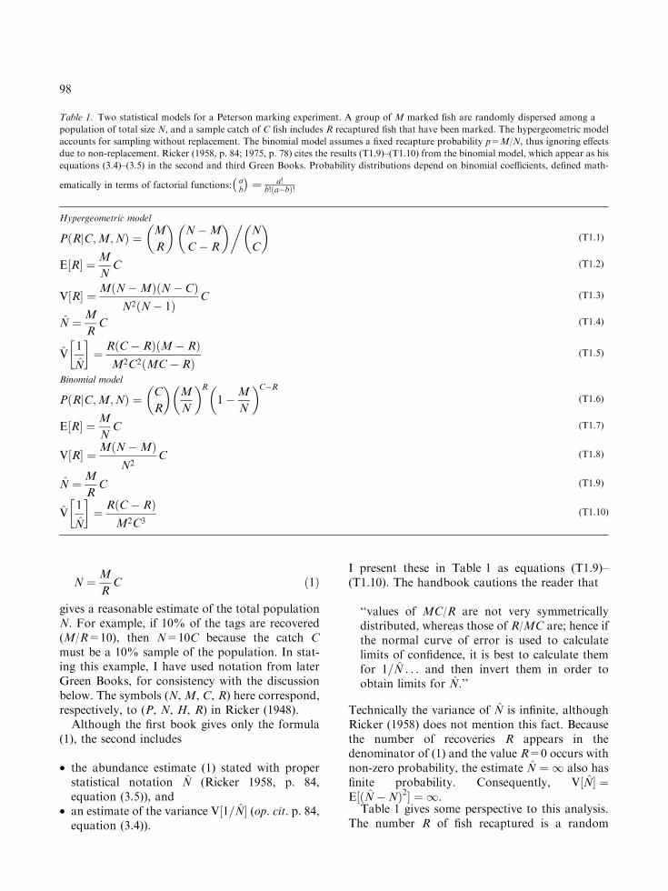
Table 1. Two statistical models for a Peterson marking experiment. A group of M marked fish are randomly dispersed among a

population of total size N, and a sample catch of C fish includes R recaptured fish that have been marked. The hypergeometric model

accounts for sampling without replacement. The binomial model assumes a fixed recapture probability p=M/N, thus ignoring effects

due to non-replacement. Ricker (1958, p. 84; 1975, p. 78) cites the results (T1.9)–(T1.10) from the binomial model, which appear as his

equations (3.4)–(3.5) in the second and third Green Books. Probability distributions depend on binomial coefficients, defined math-

ematically in terms of factorial functions:ab

� �¼ a!

b!ða�bÞ!

Hypergeometric model

PðRjC;M;NÞ ¼ M

R

� �N�M

C� R

� ��N

C

� �(T1.1)

E½R� ¼M

NC (T1.2)

V½R� ¼MðN�MÞðN� CÞN2ðN� 1Þ

C (T1.3)

N̂ ¼M

RC (T1.4)

V̂1

N̂

� �¼ RðC� RÞðM� RÞ

M2C2ðMC� RÞ(T1.5)

Binomial model

PðRjC;M;NÞ ¼ C

R

� �M

N

� �R1�M

N

� �C�R(T1.6)

E½R� ¼M

NC (T1.7)

V½R� ¼MðN�MÞN2

C (T1.8)

N̂ ¼M

RC (T1.9)

V̂1

N̂

� �¼ RðC� RÞ

M2C3(T1.10)

98

variable, determined by the unknown populationN and known numbers M and C of fish markedand caught. Because sampling takes place withoutreplacement, the hypergeometric distribution(T1.1) theoretically represents the distribution ofthe random variable R. This implies the expectedvalue E[R] and variance V[R] in (T1.2)–(T1.3),known from statistical literature (e.g., Mood andGraybill 1963, pp. 110 – 113). The estimate (T1.4)for N̂ comes from equating the observed value R toits mean value (T1.2). The calculation

V1

N̂

� �¼ V

R

MC

� �¼ 1

M2C2V½R�

¼ ðN�MÞðN� CÞMCN2ðN� 1Þ ð2Þ

gives an exact formula for the variance of 1=N̂,and the estimated variance (T1.5) comes fromsubstituting the estimate N̂ into (2). This analysisdepends on the fact that 1=N̂ is proportional to theobserved random variable R, whose statisticalproperties are known exactly.

Results presented in Ricker (1958, pp. 83 – 85)depend on a binomial model for R, in which tagsare recovered with constant probability p=M/N.This simplifying assumption ignores changes inprobability that occur while collecting sampleswithout replacement. The results (T1.7)–(T1.10)follow logically from the model (T1.6), just as(T.2)–(T.5) follow from (T1.1). Both models giveidentical estimates N̂ in (T1.4) and (T1.9). Theestimated variance (T1.5) from the hypergeomet-ric model is smaller that the corresponding vari-ance (T1.10) from the binomial model by thefactor

1� R=M

1� R=ðCMÞ � 1� R

M1� 1

C

� �:

Consequently, Ricker’s approximate model pre-dicts somewhat greater uncertainty than the the-oretically exact hypergeometric model. This extramargin for error might well be justified, given thelogistic difficulties that accompany most fieldstudies. Furthermore, true to his style of compre-hensive scholarship, Ricker (op. cit.) discussesother approaches, such as the following estimatesof N proposed Bailey (1951) and Chapman (1951),respectively:

N̂ 0 ¼MðCþ 1ÞRþ 1

and N̂� ¼ ðMþ 1ÞðCþ 1ÞRþ 1

: ð3Þ

Unlike (1), each of these defines a finite estimate N̂when R=0.

Similar analyses appear in the third handbook(Ricker 1975, pp. 77 – 81), along with a referenceto more recent work by Robson & Regier (1964).Strangely, the hat symbol indicating a statisticalestimate has been dropped, so that N̂ becomessimply N, as in the first book. I don’t know if thisoccurred by error, or if Ricker felt that his readerswould prefer a simpler notation.

Yield calculations

Bill’s son Karl kindly gave me a box of Bill’spapers and books that seemed relevant to myinterests. Among these, I found a paperback(Wilimovsky & Wiklund 1963) with tabulatedvalues of the incomplete beta function B(x; p, q)for

• x ranging from 0 to 1 (in intervals of 0.01),• p from 0.125 to 35.0 (in varying intervals thatincrease as p becomes larger),

• q from 3.5 to 4.5 (in intervals of 0.125).

The book has a three-page preface, partly devotedto an explanation of floating point notation (e.g.,8.8E)02=0.088), followed by 291 pages withabout 115000 tabulated values. The references citean earlier, more extensive compilation by Pearson(1948) with 494 pages. So why did Bill have thisremarkable book, a testament to the realities ofcomputing in 1963?

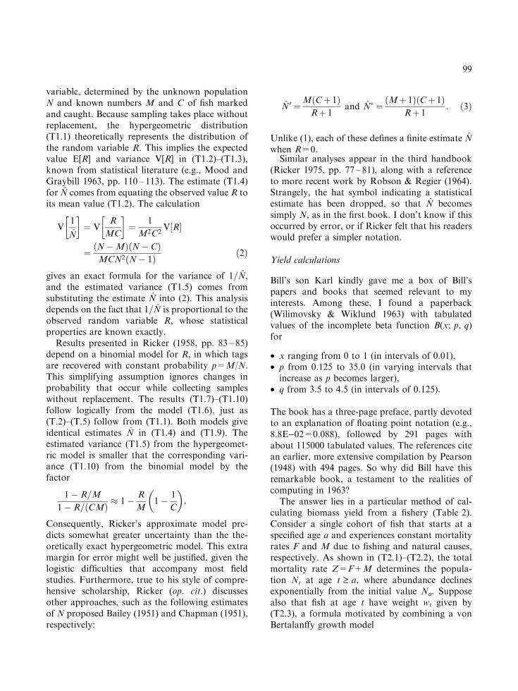
The answer lies in a particular method of cal-culating biomass yield from a fishery (Table 2).Consider a single cohort of fish that starts at aspecified age a and experiences constant mortalityrates F and M due to fishing and natural causes,respectively. As shown in (T2.1)–(T2.2), the totalmortality rate Z=F+M determines the popula-tion Nt at age t ‡ a, where abundance declinesexponentially from the initial value Na. Supposealso that fish at age t have weight wt given by(T2.3), a formula motivated by combining a vonBertalanffy growth model

99

lt ¼ L1 1� e�Kðt�t0Þ�

ð4Þ

for length lt with an exponential weight–lengthrelationship

wt ¼ cl bt : ð5Þ

In (4), fish theoretically have length 0 at age t0 andgrow to asymptotic length L¥ at a rate determinedby the parameter K. The exponent b in (5) relates toallometric growth, where the body shape and den-sity can varywith age. If fish grow isometrically (i.e.,shape and density remain constant), then b=3. Theconstant c scales length to weight, where (4) and (5)imply (T2.3) with W1 ¼ cLb

1.Suppose that regulations determine the fishing

mortality rate F and the recruitment age tR ‡ a.The latter might be implemented by setting a size

limit ltR calculated from (4). Then the fisherycaptures fish with age t ‡ tR at the rate FNt andbiomass at the rate FwtNt. Consequently, totalyield Y from the cohort is given by the integral(T2.5). Assumptions (T2.1)–(T2.5) allow us tocompute this integral analytically, where it sim-plifies matters slightly to define r in (T2.4) as thetime interval between ages t0 and tR. The result(T2.8) depends on the incomplete beta functiondefined as an integral in (T2.6a), with a corre-sponding power series calculation (T2.6b). Thishandy theorem allows a fishery scientist to calcu-late yield, although its early application required atable of the beta function, such as that producedby Wilimovsky & Wiklund (1963).

The case b=3 of isometric growth gives thesimpler expression (T2.9) for Y. To understandthis, notice in (T2.8) that the parameter q in thebeta function corresponds to b+1; thus, q=4

Table 2. Biomass yield calculation for a cohort that experiences constant rates of natural mortality M and fishing mortality F. These

combine to give the total mortality rate Z. Starting at a specified reference age a, the population Nt at age t declines exponentially from

its initial size Na. Fish weight wt follows a modified von Bertalanffy growth relationship with parameters (W¥, K, t0, b), where b

accounts for an exponential relationship between length and weight. The fishery captures fish above the recruitment age tR, where tR‡a‡ t0. A formula for the total yield Y depends involves the incomplete beta function B(x; p, q), which reduces to a rational function

when q is a positive integer (e.g., q=4). Consequently, Y can be expressed analytically in the special case b=3, when weight is

proportional to length cubed.

Model assumptions

Z=F+M (T2.1)

Nt ¼ Nae�Zðt�aÞ (T2.2)

wt ¼W1 1� e�Kðt�t0Þ� �b

(T2.3)

r ¼ tR � t0 (T2.4)

Y ¼ FR1

tR

wtNt dt (T2.5)

Incomplete beta function

Bðx; p; qÞ ¼Rx

0

up�1ð1� uÞq�1du (T2.6a)

¼ xp1

pþ 1� q

pþ 1xþ � � � þ ð1� qÞð2� qÞ � � � ðn� qÞ

n!ðpþ nÞ xn þ � � �� �

(T2.6b)

Bðx; p; 4Þ ¼ xp1

p� 3x

pþ 1þ 3x2

pþ 2� x3

pþ 3

� �(T2.7)

Yield calculation

Y ¼ FW1NaeZrþMða�t0Þ

KB e�Kr;

Z

K; bþ 1

� �(T2.8)

Y p¼3 ¼ FW1Nae

Mða�t0�rÞ 1

Z� 3e�Kr

Zþ Kþ 3e�2Kr

Zþ 2K� e�3Kr

Zþ 3K

� �(T2.9)

100

when b=3. In this case, all terms involving xn inthe power series (T2.6b) vanish when n‡ 4, so thatB(x; p, 4) reduces to (T2.7). Applying this result to(T2.8) gives (T2.9).

Historically, the formula (T2.9) when b=3 wasdiscovered before the general result (T2.8). In hissecond Green Book, Ricker (1958, pp. 220 – 222;equation (10.18)) attributes (T2.9) to Beverton &Holt (1956, 1957), along with earlier literature dat-ing back to Graham (1952). A footnote (Ricker1958, p. 222) also mentions a result by Jones (1957)applicable even when b 6¼ 3 in the growth law(T2.3). Probably this appeared too late for inclusionin that printing of the handbook, but the 3rd edition(Ricker 1975) presents two results (pp. 251 – 254,equation (10.21); p. 255, equation (10.23)) thatcorrespond, respectively, to my equations (T2.9)and (T2.8). Notation varies between the second andthird handbooks, and mine is closer to that in thethird. I have slightly generalized the results to allowa specified base age a for the initial population Na.The equations cited by Ricker (1975) assume thata=t0, although some of his worked examples

require adjustment to a different base age. (I cautionreaders of the historical literature to note that thenotationN0 usually denotes the theoretical numberof fish at age t0, not age t=0.)

The computation in Table 2 achieves the syn-thesis that Ricker (1948) foresaw in his first GreenBook. Biological statistics on mortality, growth,and recruitment imply a definite value for the yieldproduced by a cohort; that is:

ðF;M;W1;K; t0; b; a;Na; tRÞ ) Y:

The specified age a corresponds to an initialbaseline population Na, but regulations determinethe actual recruitment age tR ‡ a for legal capture.Because yield Y is proportional to Na in (T2.9), wecan also regard the formula as a tool for calcu-lating the yield per fish at age a:

ðM; a;W1;K; t0; b;F; tRÞ )Y

Na: ð6Þ

where the parameters have been rearranged todistinguish fish biology (M, a, W¥, K, t0, b) frommanagement policy (F, tR). The relationship (6)

Fishing Mortality

Rec

ruitm

ent A

ge

0.0 0.5 1.0 1.5 2.0 2.5 3.0

02

46

810

12

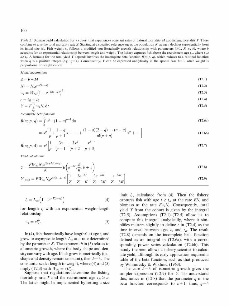
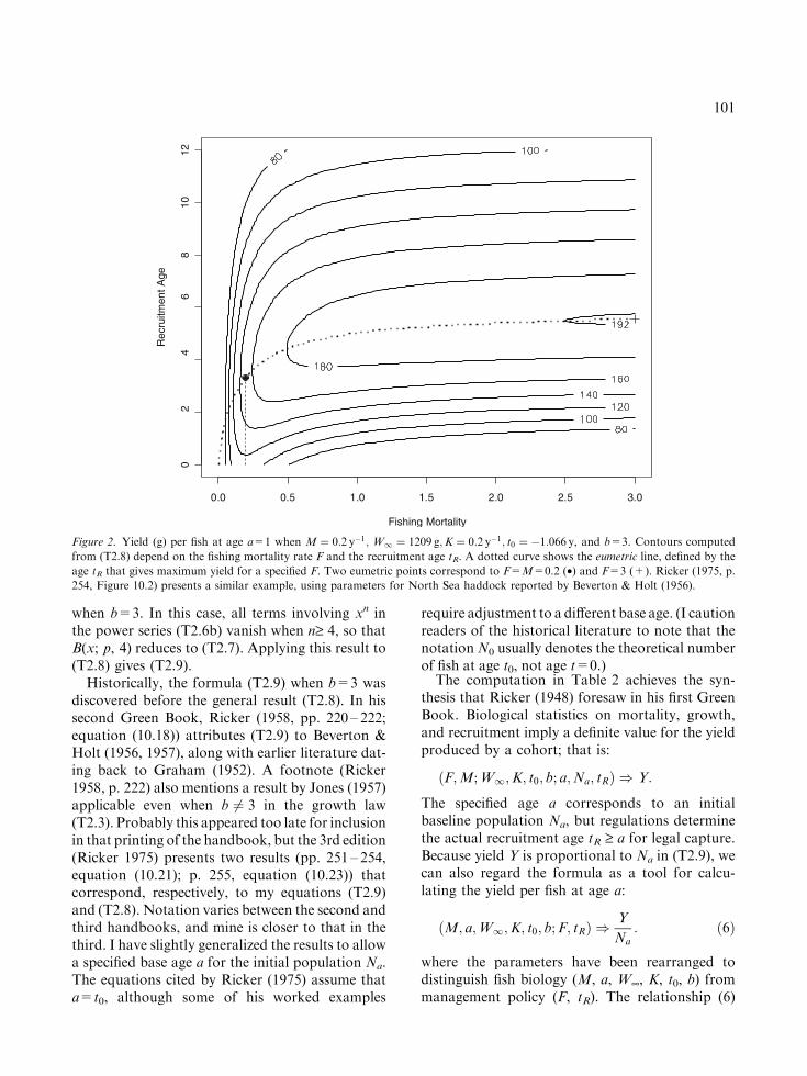
Figure 2. Yield (g) per fish at age a=1 when M ¼ 0:2 y�1; W1 ¼ 1209 g;K ¼ 0:2 y�1; t0 ¼ �1:066 y, and b=3. Contours computed

from (T2.8) depend on the fishing mortality rate F and the recruitment age tR. A dotted curve shows the eumetric line, defined by the

age tR that gives maximum yield for a specified F. Two eumetric points correspond to F=M=0.2 (•) and F=3 (+). Ricker (1975, p.

254, Figure 10.2) presents a similar example, using parameters for North Sea haddock reported by Beverton & Holt (1956).

101

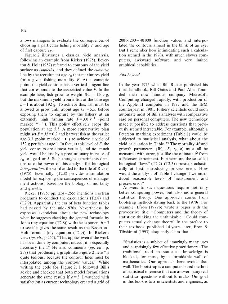
allows managers to evaluate the consequences ofchoosing a particular fishing mortality F and ageof first capture tR.

Figure 2 illustrates a classical yield analysis,following an example from Ricker (1975). Bever-ton & Holt (1957) referred to contours of the yieldsurface as isopleths, and they defined the eumetricline by the recruitment age tR that maximizes yieldfor a given fishing mortality F. At a eumetricpoint, the yield contour has a vertical tangent linethat corresponds to the associated value F. In theexample here, fish grow to weight W¥ =1209 g,but the maximum yield from a fish at the base agea=1 is about 192 g. To achieve this, fish must beallowed to grow until about age tR =5.5, beforeexposing them to capture by the fishery at anextremely high fishing rate F=3.0 y)1 (pointmarked ‘‘+’’). This policy effectively crops thepopulation at age 5.5. A more conservative planmight set F=M=0.2 and harvest fish at the earlierage 3.3 (point marked ‘‘•’’) to achieve a yield of152 g per fish at age 1. In fact, at this level of F, theyield contours are almost vertical, and not muchyield would be lost by a precautionary increase oftR to age 4 or 5. Such thought experiments dem-onstrate the power of this analysis for biologicalinterpretation, the word added to the title of Ricker(1975). Essentially, (T2.8) provides a simulationmodel for exploring the consequences of manage-ment actions, based on the biology of mortalityand growth.

Ricker (1975, pp. 254 – 255) mentions Fortranprograms to conduct the calculations (T2.8) and(T2.9). Apparently the era of beta function tableshad passed by the mid-1970s. Nevertheless, heexpresses skepticism about the new technologywhen he suggests checking the general formula byJones (my equation (T2.8)) with the exponent b=3to see if it gives the same result as the Beverton–Holt formula (my equation (T2.9)). In Ricker’sview (op. cit., p 255), ‘‘This applies even if the workhas been done by computer; indeed, it is especiallynecessary then.’’ He also comments (op. cit., p.257) that producing a graph like Figure 2 here ‘‘isquite tedious, because the contour lines must beinterpolated among the contour values.’’ Whilewriting the code for Figure 2, I followed Bill’sadvice and checked that both model formulationsgenerate the same results if b=3. I watched withsatisfaction as current technology created a grid of

200� 200=40 000 function values and interpo-lated the contours almost in the blink of an eye.But I remember how intimidating such a calcula-tion seemed in the 1970s, with much slower com-puters, awkward software, and very limitedgraphical capabilities.

And beyond

In the year 1975 when Bill Ricker published histhird handbook, Bill Gates and Paul Allen foun-ded their now famous company Microsoft.Computing changed rapidly, with production ofthe Apple II computer in 1977 and the IBMcounterpart in 1981. Fishery scientists could soonautomate most of Bill’s analyses with comparativeease on personal computers. The new technologymade it possible to address questions that previ-ously seemed intractable. For example, although aPeterson marking experiment (Table 1) could besubjected to statistical analysis, what about theyield calculation in Table 2? The mortality M andgrowth parameters (W¥, K, t0, b) must all bemeasured with error, just like the estimate N̂ froma Peterson experiment. Furthermore, the so-calledbiological ‘‘laws’’ (T2.2)–(T2.3) operate stochasti-cally at best, introducing process error. Howwould the analysis of Table 1 change if we intro-duced reasonable levels of measurement andprocess error?

Answers to such questions require not onlybetter computing power, but also more generalstatistical theory. One approach comes frombootstrap methods dating back to the 1970s. Forexample, Efron (1979b) wrote a paper with theprovocative title: ‘‘Computers and the theory ofstatistics: thinking the unthinkable.’’ Could com-puters actually change theory? In the preface totheir textbook published 14 years later, Eron &Tibshirani (1993) eloquently claim that:

‘‘Statistics is a subject of amazingly many usesand surprisingly few effective practitioners. Thetraditional road to statistical knowledge isblocked, for most, by a formidable wall ofmathematics. Our approach here avoids thatwall. The bootstrap is a computer-based methodof statistical inference that can answer many realstatistical questions without formulas. Our goalin this book is to arm scientists and engineers, as

102

well as statisticians, with computational tech-niques that they can use to analyze and under-stand complicated data sets.’’

The bootstrap belongs properly to the frequen-tist approach to statistics. According to this schoolof thought, parameters (like the population N inTable 1) actually exist in nature and estimates (likeN̂) have a distribution that allows us to assessvariability (like the variance estimate (T1.5)). Inpractice, the bootstrap circumvents formulas like(T1.5) by using a computer to draw samples fromthe observed data and generate an empirical dis-tribution of estimates. Historically, we benefitfrom the work of statisticians who obtained ana-lytical results for specialized problems. But similarresults may not be available for more complexstatistical models, and the bootstrap holds promiseas a tool with much greater generality.

Another general approach comes from Bayesianstatistics, which uses probability to describe asubjective understanding of nature. Starting froman initial understanding (called a prior distribu-tion), new data give a revised perspective (theposterior distribution). Parameters (like N inTable 1) become random variables whose distri-bution depends on prior knowledge, plus allavailable data. A sample drawn from the posteriorreflects our current understanding of nature. In thelast two decades, numerous algorithms for pos-terior sampling have been proposed and used. Likebootstraps, these involve computer intensivemethods that can deal with very general statisticalmodels. Clifford (1993, p. 53) described theirpractical impact in dramatic terms:

‘‘...from now on we can compare our data withthe model that we actually want to use ratherthan a model which has some mathematicallyconvenient form. This is surely a revolution...’’

For example, consider the yield calculation inTable 2. As mentioned above, the complicatedmodel (T2.1)–(T2.5) does not lend itself easily tomeasurement and process error. More precisely,given any reasonable error model, an analyticalformula for the variance V[Y] would be hard toobtain. The Bayesian approach, however, treats Yas a random variable with a distribution thatcascades from the inputs. A posterior sample of Y,

along with all random inputs, gives the analyst asense of variability, where contour graphs likeFigure 2 could portray mean values, variances,coefficients of variation, and other statistics.

In summary, the nearly three decades sinceRicker’s (1975) third Green Book have broughthuge changes in technology and theory. As a result,the fishery biological system he described has beeninvestigated with increasing depth. Quinn (2003)gives a readable modern perspective, and Schnute(1994, 2003) provides further background on con-temporary fishery models. Ricker’s foundation liesat the core of all modernwork.His search for a validinterpretation of biological statistics from a fishpopulationhas set the stage for generations to come.

An inquiring mind

Cyrillids

Bill brought a compelling curiosity to any subjectthat interested him. For example, he introduced meto the controversies about crop circles with theinvestigative article byNickell &Fischer (1992).Weco-authored just one paper, and it had nothingwhatever to do with fisheries. Bill’s interest in thenatural world extended to celestial events, such asthe dramatic appearance of fireballs over easternCanada on 9February 1913. The astronomerChant(1913a, 1913b) of the University of Toronto com-piled anecdotal records and used ‘‘the formulas ofspherical trigonometry’’ to determine an approxi-mate trajectory. Later, O’Keefe (1968) found otherhistorical reports, including sightings off north-eastern Brazil. He dubbed the fireballs cyrillidsbecause of their appearance on St. Cyril’s Day.

Bill’s contacts in the Nanaimo Historical Societyled him to a story about a celestial event witnessedover Nanoose, British Columbia (about 20 kmnorthwest of Nanaimo) during the early 1900s.Could this have been a cyrillid sighting? He stop-ped me in the parking lot one evening with thequestion: ‘‘Do you know anything about sphericaltrigonometry?’’ It was my job to extend the cyrillidtrajectory westward and determine its proximity toNanoose. We even did a trivial error analysis totake some account of uncertainty. In the end, wedecided that the Nanoose report had a reasonablechance of extending the 1913 cyrillid event, rather

103

like a range extension for a species. Fortunately,the Editor (Francis Cook) and reviewers at TheCanadian Field-Natualist gave our speculations asympathetic hearing, and the paper found its wayinto print (Ricker & Schnute 1999). To my con-siderable surprise while writing this current paper,a meteor streaked across the skies of northwesternNorth America at about 2:30 AM on 3 June 2004.Momentary brightness appeared on the record ofvideo surveillance cameras monitoring parkinglots in Portland, Oregon. Witnesses from BritishColumbia, Washington, and Oregon reporteddirect sightings, sometimes accompanied withsounds. I thought of Chant in 1913 as I listened toa modern astronomer (David Dodge of the H.R.Macmillan Space Centre in Vancouver, BritishColumbia) compile anecdotal reports during alocal radio program.

Sunflowers

As a mathematician, I had the opportunity to par-ticipate in some of Bill’s mathematical recreations.He would occasionally pass me articles of interest,such as Stewart’s (1995) discussion of flower struc-tures. What algorithm could possibly explain thebeautifully tight packing of seeds on the head of asunflower? The article appeared in the January 1995

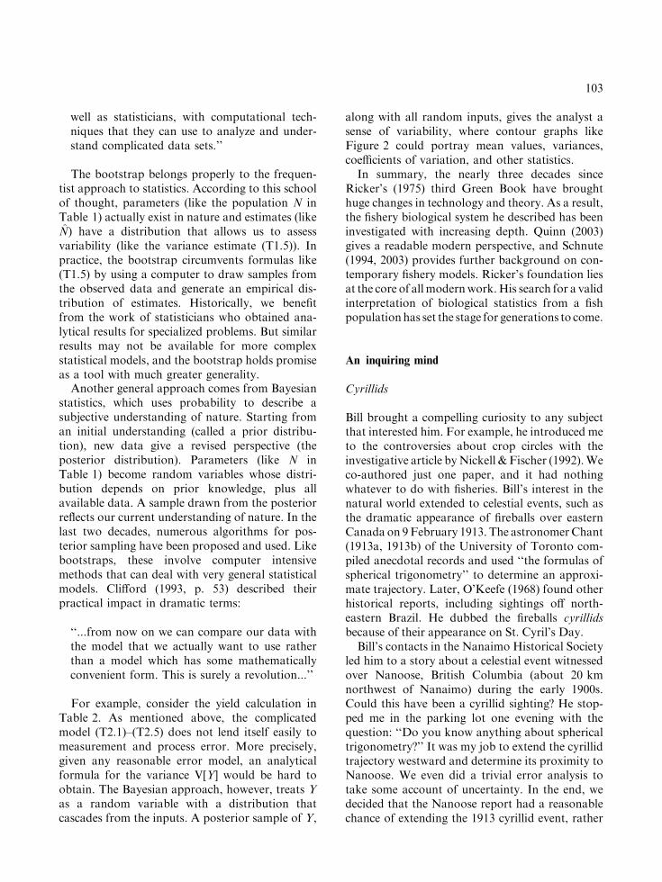
issue of Scientific American, on sale in December1994, so it gaveus somethingamusing to thinkaboutduring the season before Christmas. One approachto the question involves the concepts presented inTable 3. The golden ratio / has a geometric defini-tion (Figure 3) based on a rectangle with certainideal proportions. This implies the mathematicaldefinition (T3.1), a quadratic equation with twosolutions: / ¼ ð

ffiffiffi5pþ 1Þ=2 in (T3.2) and

/� 1 ¼ ðffiffiffi5p� 1Þ=2. The Fibonacci numbers Fn

1; 1; 2; 3; 5; 8; 13; 21; 34; . . . ; ð7Þ

Table 3. The golden ratio / defined in Figure 3, Fibonacci numbers Fn, and the packing algorithm used to produce Figure 4.

Golden ratio

/1¼ 1

/� 1(T3.1)

/ ¼ffiffiffi5pþ 1

2(T3.2)

Fibonacci numbers

F1 ¼ 1; F2 ¼ 1; Fn ¼ Fn�1 þ Fn�2 (T3.3)

Fn ¼/n � ð1� /Þn

2/� 1(T3.4)

/ ¼ limn!1

Fnþ1Fn

(T3.5)

Packing algorithm and golden angle

ðxk; ykÞ ¼ffiffiffik

n

r

ðcos kh; sin khÞ; k ¼ 1; . . . ; n (T3.6)

hg ¼360�

/2¼ 137:507764 . . .� (T3.7)

φ

1

1 1

φ 1–

Figure 3. Rectangle illustrating the golden ratio / . The outer

rectangle with sides / and 1 can be partitioned into a 1� 1

square and an inner rectangle with sides 1 and /)1. The two

rectangles have the same proportion between long and short

sides: / /1=1/(/ )1).

104

have the property (T3.3) that each number is thesum of the previous two. These relate closely to /,as shown in (T3.4)–(T3.5).

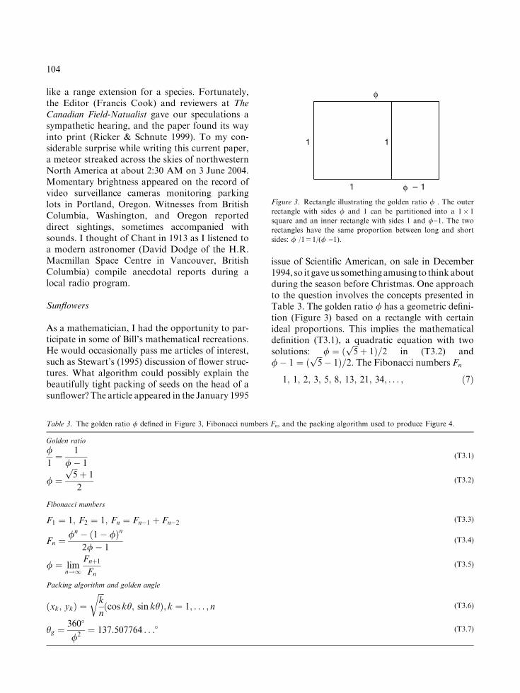
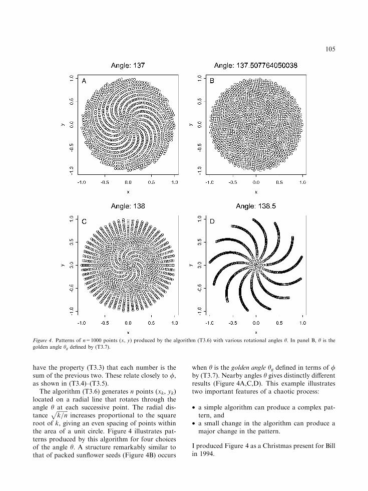
The algorithm (T3.6) generates n points (xk, yk)located on a radial line that rotates through theangle h at each successive point. The radial dis-tance

ffiffiffiffiffiffiffiffik=n

pincreases proportional to the square

root of k, giving an even spacing of points withinthe area of a unit circle. Figure 4 illustrates pat-terns produced by this algorithm for four choicesof the angle h. A structure remarkably similar tothat of packed sunflower seeds (Figure 4B) occurs

when h is the golden angle hg defined in terms of /by (T3.7). Nearby angles h gives distinctly differentresults (Figure 4A,C,D). This example illustratestwo important features of a chaotic process:

• a simple algorithm can produce a complex pat-tern, and

• a small change in the algorithm can produce amajor change in the pattern.

I produced Figure 4 as a Christmas present for Billin 1994.

Figure 4. Patterns of n=1000 points (x, y) produced by the algorithm (T3.6) with various rotational angles h. In panel B, h is the

golden angle hg defined by (T3.7).

105

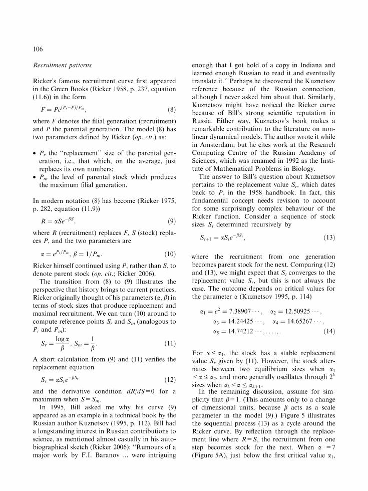
Recruitment patterns

Ricker’s famous recruitment curve first appearedin the Green Books (Ricker 1958, p. 237, equation(11.6)) in the form

F ¼ PeðPr�PÞ=Pm ; ð8Þwhere F denotes the filial generation (recruitment)and P the parental generation. The model (8) hastwo parameters defined by Ricker (op. cit.) as:

• Pr the ‘‘replacement’’ size of the parental gen-eration, i.e., that which, on the average, justreplaces its own numbers;

• Pm the level of parental stock which producesthe maximum filial generation.

In modern notation (8) has become (Ricker 1975,p. 282, equation (11.9))

R ¼ aSe�bS; ð9Þwhere R (recruitment) replaces F, S (stock) repla-ces P, and the two parameters are

a ¼ ePr=Pm ; b ¼ 1=Pm: ð10ÞRicker himself continued using P, rather than S, todenote parent stock (op. cit.; Ricker 2006).

The transition from (8) to (9) illustrates theperspective that history brings to current practices.Ricker originally thought of his parameters (a, b) interms of stock sizes that produce replacement andmaximal recruitment. We can turn (10) around tocompute reference points Sr and Sm (analogous toPr and Pm):

Sr ¼log a

b; Sm ¼

1

b: ð11Þ

A short calculation from (9) and (11) verifies thereplacement equation

Sr ¼ aSre�bSr ð12Þ

and the derivative condition dR/dS=0 for amaximum when S=Sm.

In 1995, Bill asked me why his curve (9)appeared as an example in a technical book by theRussian author Kuznetsov (1995, p. 112). Bill hada longstanding interest in Russian contributions toscience, as mentioned almost casually in his auto-biographical sketch (Ricker 2006): ‘‘Rumours of amajor work by F.I. Baranov ... were intriguing

enough that I got hold of a copy in Indiana andlearned enough Russian to read it and eventuallytranslate it.’’ Perhaps he discovered the Kuznetsovreference because of the Russian connection,although I never asked him about that. Similarly,Kuznetsov might have noticed the Ricker curvebecause of Bill’s strong scientific reputation inRussia. Either way, Kuznetsov’s book makes aremarkable contribution to the literature on non-linear dynamical models. The author wrote it whilein Amsterdam, but he cites work at the ResearchComputing Centre of the Russian Academy ofSciences, which was renamed in 1992 as the Insti-tute of Mathematical Problems in Biology.

The answer to Bill’s question about Kuznetsovpertains to the replacement value Sr, which datesback to Pr in the 1958 handbook. In fact, thisfundamental concept needs revision to accountfor some surprisingly complex behaviour of theRicker function. Consider a sequence of stocksizes St determined recursively by

Stþ1 ¼ aSte�bSt ; ð13Þ

where the recruitment from one generationbecomes parent stock for the next. Comparing (12)and (13), we might expect that St converges to thereplacement value Sr, but this is not always thecase. The outcome depends on critical values forthe parameter a (Kuznetsov 1995, p. 114)

a1 ¼ e2 ¼ 7:38907 � � � ; a2 ¼ 12:50925 � � � ;a3 ¼ 14:24425 � � � ; a4 ¼ 14:65267 � � � ;a5 ¼ 14:74212 � � � ; . . . :; : ð14Þ

For a £ a1, the stock has a stable replacementvalue Sr given by (11). However, the stock alter-nates between two equilibrium sizes when a1<a £ a2, and more generally oscillates through 2k

sizes when ak<a � akþ1.In the remaining discussion, assume for sim-

plicity that b=1. (This amounts only to a changeof dimensional units, because b acts as a scaleparameter in the model (9).) Figure 5 illustratesthe sequential process (13) as a cycle around theRicker curve. By reflection through the replace-ment line where R=S, the recruitment from onestep becomes stock for the next. When a =7(Figure 5A), just below the first critical value a1,

106

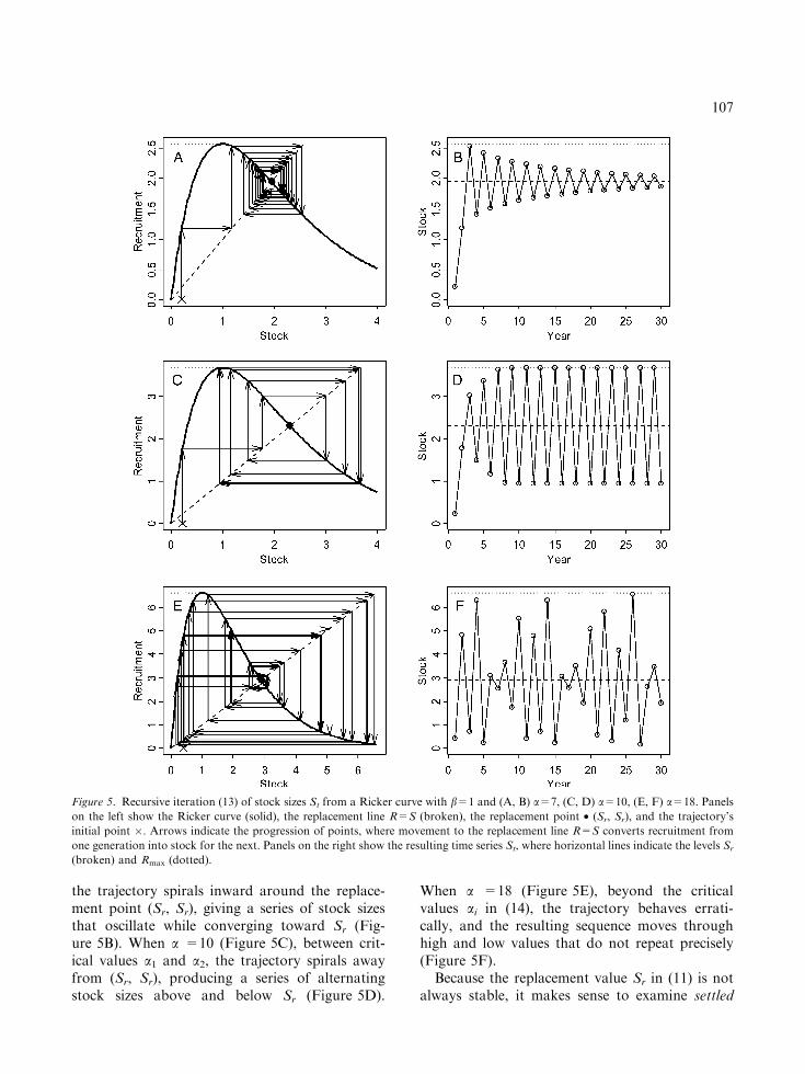
the trajectory spirals inward around the replace-ment point (Sr, Sr), giving a series of stock sizesthat oscillate while converging toward Sr (Fig-ure 5B). When a =10 (Figure 5C), between crit-ical values a1 and a2, the trajectory spirals awayfrom (Sr, Sr), producing a series of alternatingstock sizes above and below Sr (Figure 5D).

When a =18 (Figure 5E), beyond the criticalvalues ai in (14), the trajectory behaves errati-cally, and the resulting sequence moves throughhigh and low values that do not repeat precisely(Figure 5F).

Because the replacement value Sr in (11) is notalways stable, it makes sense to examine settled

Figure 5. Recursive iteration (13) of stock sizes St from a Ricker curve with b=1 and (A, B) a=7, (C, D) a=10, (E, F) a=18. Panels

on the left show the Ricker curve (solid), the replacement line R=S (broken), the replacement point • (Sr, Sr), and the trajectory’s

initial point �. Arrows indicate the progression of points, where movement to the replacement line R=S converts recruitment from

one generation into stock for the next. Panels on the right show the resulting time series St, where horizontal lines indicate the levels Sr

(broken) and Rmax (dotted).

107

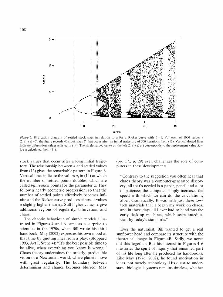
stock values that occur after a long initial trajec-tory. The relationship between a and settled valuesfrom (13) gives the remarkable pattern in Figure 6.Vertical lines indicate the values ai in (14) at whichthe number of settled points doubles, which arecalled bifurcation points for the parameter a. Theyfollow a nearly geometric progression, so that thenumber of settled points effectively becomes infi-nite and the Ricker curve produces chaos at valuesa slightly higher than a5. Still higher values a giveadditional regions of regularity, bifurcation, andchaos.

The chaotic behaviour of simple models illus-trated in Figures 4 and 6 came as a surprise toscientists in the 1970s, when Bill wrote his thirdhandbook. May (2002) expresses his own mood atthat time by quoting lines from a play: (Stoppard1993, Act I, Scene 4): ‘‘It’s the best possible time tobe alive, when everything you know is wrong.’’Chaos theory undermines the orderly, predictablevision of a Newtonian world, where planets movewith great regularity. The boundary betweendeterminism and chance becomes blurred. May

(op. cit., p. 29) even challenges the role of com-puters in these developments:

‘‘Contrary to the suggestion you often hear thatchaos theory was a computer-generated discov-ery, all that’s needed is a paper, pencil and a lotof patience; the computer simply increases thespeed with which we can do the calculations,albeit dramatically. It was with just these low-tech materials that I began my work on chaos,and in those days all I ever had to hand was theearly desktop machines, which seem antedilu-vian by today’s standards.’’

Ever the naturalist, Bill wanted to get a realsunflower head and compare its structure with thetheoretical image in Figure 4B. Sadly, we neverdid this together. But his interest in Figures 4–6illustrates the spirit of inquiry that remained partof his life long after he produced his handbooks.Like May (1976, 2002), he found motivation inideas, not merely technology. His quest to under-stand biological systems remains timeless, whether

Figure 6. Bifurcation diagram of settled stock sizes in relation to a for a Ricker curve with b=1. For each of 1000 values a(2 £ a £ 40), the figure records 40 stock sizes St that occur after an initial trajectory of 500 iterations from (13). Vertical dotted lines

indicate bifurcation values ai listed in (14). The single-valued curve on the left (2 £ a £ a1) corresponds to the replacement value Sr=

log a calculated from (11).

108

it involves recruitment curves, incomplete betafunctions, or sunflowers.

Acknowledgements

GordonMiller, George Pattern, and Brian Krishkahelped me assemble historical materials used inwriting this paper. I also relied on Karl Ricker’s(2001) list of references to his father’s work. PaulRankin kindly loaned me his personal copy ofRicker (1971). My brother David Schnute helpedme recall events from the 1940s. Nick Boers assistedwith graphical software in the statistical languageR. Rowan Haigh and Laura Richards providedhelpful suggestions for improving the text.

References

Bailey, N.J.J. 1951. On estimating the size of mobile popula-

tions from recapture data. Biometrika 38: 293–306.

Beverton, R.J.H. & S.J. Holt. 1956. A review of methods for

estimating mortality rates in fish populations, with special

reference to sources of bias in catch sampling. Rapport P.-V.

Reunion Conseil Permenant International Exploration de le

Mer 140: 67–83.

Beverton, R.J.H. & S.J. Holt. 1957. On the dynamics of

exploited fish populations. U.K. Ministry of Agriculture,

Fish & Fisheries Investigations (Ser. 2) 19: 533 pp.

Chant, C.A. 1913a. An extraordinary meteoric display. J. R.

Astron. Soc. Can. 7: 145–215.

Chant, C.A. 1913b. Further information regarding the meteoric

display of February 9, 1913. J. R. Astron. Soc. Can. 7: 438–

447.

Chapman, D.G. 1951. Some properties of the hypergeometric

distribution with application to zoological sample censuses.

Univ. Calif. Publ. Stat. 1: 131–160.

Clifford, P. 1993. Discussion on the meeting on the Gibbs

sampler and other Markov chain Monte Carlo methods. J. R.

Stat. Soc. (Series B) 55: 53–102.

Efron, B. 1979b. Computers and the theory of statistics:

Thinking the unthinkable. SIAM Rev. 21: 460–480.

Efron, B.E. & R.J. Tibshirani. 1993. An introduction to the

bootstrap. Mongraphs on Statistics and Applied Probability,

Chapman & Hall, New York, 436 pp.

Fisher, R.A. 1925. Statistical Methods for Research Workers.

Oliver & Boyd, Edinburgh. 239 pp.

Fisher, R.A. 1930. The Genetical Theory of Natural Selection.

Clarendon Press, Oxford. 272 pp.

Fisher, R.A. 1935. The Design of Experiments. Oliver & Boyd,

Edinburgh. 252 pp.

Fisher, R.A. 1937. The Design of Experiments. 2 ed. Oliver &

Boyd, Edinburgh. 260 pp.

Graham, M. 1952. Overfishing and optimum fishing. Rapport

P.-V. Reunion Conseil Permanent International Exploration

de le Mer 132: 72–78.

Jones, R. 1957. A much simplified version of the fish yield

equation. Doc. No. P. 21, presented at the Lisbon joint

meeting of International Committee on Northwest Atlantic

Fisheries, International Council for the Exploration of the

Sea, and Food Agriculture Organization, United Nations,

8 pp.

Kuznetsov, Y.A. 1995. Elements of applied bifurcation theory.

Applied Mathematical Sciences, Vol. 112, Springer-Verlag,

New York, 515 pp.

May, R.M. 1976. Simple mathematical models with very com-

plicated dynamics. Nature 261: 459–467.

May, R.M. 2002. The best possible time to be alive. pp. 28–45.

In: G. Farmelo, (ed.), It must be Beautiful: Great Equations

of Modern Science, Granata Books, London. 284 pp.

Mood, A.M. & F.A. Graybill. 1963. Introduction to the Theory

of Statistics. 2 ed. McGraw-Hill, New York. 443 pp.

Nickell, J. & J.F. Fisher. 1992. The crop-circle phenomenon:

An investigative report. Skept. Inquirer 16: 136–149.

O’Keefe, J.A. 1968. New data on cyrillids. J. R. Astron. Soc.

Can. 62: 97–98.

Pearson, K. 1948. Tables of the Incomplete Beta-function. The

University Press, Cambridge, U.K.. 494 pp.

Petersen, C.G.J. 1896. The yearly immigration of young plaice

into the Limfjord from the German Sea, etc. Rep. Danish

Biol. Stat. 6: 1–48.

Quinn, T.J. II 2003. Ruminations on the development and

future of population dynamics models in fisheries. Nat. Res.

Model. 16: 341–392.

Ricker, K. 2001. The scientific and literary publications of W.E.

Ricker, O.O.C., Ph.D., D. Sc. LLD, F.R.S.C. (1929 – 2001

and still ongoing). Fisheries & Oceans Canada, Pacific Bio-

logical Station Library. Bound manuscript.

Ricker, W.E. 1948. Methods of estimating vital statistics of fish

populations. Indiana University Publications, Science Series,

No. 15. 101 pp.

Ricker, W.E. 1958. Handbook of computations for biological

statistics of fish populations. Bulletin of the Fisheries

Research Board of Canada, No. 119. 300 pp.

Ricker, W.E. (ed.) 1968. Methods for assessment of fish pro-

duction in freshwaters. IBP Handbook No. 3. Blackwell

Scientific Publications, Oxford, 313 pp.

Ricker, W.E. (ed.) 1971. Methods for assessment of fish pro-

duction in freshwaters. IBP Handbook No. 3, 2nd edition.

Blackwell Scientific Publications, Oxford, 348 pp.

Ricker, W.E. 1975. Computation and interpretation of bio-

logical statistics of fish populations. Bulletin of the Fisheries

Research Board of Canada, No. 191. 382 pp.

Ricker, W.E. 2006. One man’s journey through the years when

ecology came of age. Environ. Biol. Fishes 75: 7–37.

Robson, D.S. & H.A. Regier. 1964. Sample size in Petersen

mark-recapture experiments. Trans. Amer. Fish. Soc. 93:

215–226.

Schnute, J.T. 1994. A general framework for developing

sequential fisheries models. Can. J. Fish. Aquat. Sci. 51:

1676–1688.

109

Schnute, J.T. 2003. Designing fishery models: A personal

adventure. Nat. Resour. Model. 16: 393–413.

Stewart, I. 1995. Mathematical recreations: Daisy, daisy, give

me your answer, do. Sci. Am. 195: 96–99.

Stoppard, T. 1993. Arcadia. Faber & Faber, London. 97 pp.

Wilimovsky, N.J. & E.C. Wiklund. 1963. Tables of the

incomplete beta function for the calculation of fish popula-

tion yield. Institute of Fisheries, University of British

Columbia, Vancouver, Canada. 291 pp.

110