Embed Size (px)
Citation preview
CUTTER-WORKPIECE ENGAGEMENT IDENTIFICATION
IN MULTI-AXIS MILLING
by
EYYUP ARAS
A THESIS SUBMITTED IN PARTIAL FULFILLEMENT OF
THE REQUIREMENTS FOR THE DEGREE OF
DOCTOR OF PHILOSOPHY
in
THE FACULTY OF GRADUATE STUDIES
(Mechanical Engineering)
THE UNIVERSITY OF BRITISH COLUMBIA
(Vancouver)
July 2008
© Eyyup Aras, 2008
ii
Abstract
This thesis presents cutter swept volume generation, in-process workpiece modeling and
Cutter Workpiece Engagement (CWE) algorithms for finding the instantaneous intersections
between cutter and workpiece in milling. One of the steps in simulating machining operations
is the accurate extraction of the intersection geometry between cutter and workpiece. This
geometry is a key input to force calculations and feed rate scheduling in milling. Given that
industrial machined components can have highly complex geometries, extracting
intersections accurately and efficiently is challenging. Three main steps are needed to obtain
the intersection geometry between cutter and workpiece. These are the Swept volume
generation, in-process workpiece modeling and CWE extraction respectively.
In this thesis an analytical methodology for determining the shapes of the cutter swept
envelopes is developed. In this methodology, cutter surfaces performing 5-axis tool motions
are decomposed into a set of characteristic circles. For obtaining these circles a concept of
two-parameter-family of spheres is introduced. Considering relationships among the circles
the swept envelopes are defined analytically. The implementation of methodology is simple,
especially when the cutter geometries are represented by pipe surfaces.
During the machining simulation the workpiece update is required to keep track of the
material removal process. Several choices for workpiece updates exist. These are the solid,
facetted and vector model based methodologies. For updating the workpiece surfaces
represented by the solid or faceted models third party software can be used. In this thesis
multi-axis milling update methodologies are developed for workpieces defined by discrete
vectors with different orientations. For simplifying the intersection calculations between
discrete vectors and the tool envelope the properties of canal surfaces are utilized.
A typical NC cutter has different surfaces with varying geometries and during the
material removal process restricted regions of these surfaces are eligible to contact the in-
process workpiece. In this thesis these regions are analyzed with respect to different tool
motions. Later using the results from these analyses the solid, polyhedral and vector based
CWE methodologies are developed for a range of different types of cutters and multi-axis
tool motions. The workpiece surfaces cover a wide range of surface geometries including
sculptured surfaces.
iii
Table of Contents
Abstract .............................................................................................................................. ii
Table of Contents ................................................................................................................ iii
List of Tables....................................................................................................................... vii
List of Figures .................................................................................................................... viii
List of Algorithms.............................................................................................................. xiv
Acknowledgements..............................................................................................................xv
Chapter 1 Introduction.......................................................................................................1
1.1 Virtual Machining .......................................................................................................1
1.2 Geometric Modeling ...................................................................................................3
1.2.1 Swept Volume Generation..................................................................................4
1.2.2 In-process Workpiece Modeling ........................................................................5
1.2.3 Cutter Workpiece Engagement Extraction.......................................................10
1.3 Process Modeling ......................................................................................................15
1.4 Scope of this Research ..............................................................................................15
1.5 Organization of Thesis ..............................................................................................16
Chapter 2 Literature Review ...........................................................................................18
2.1 Swept Volume Generation ........................................................................................18
2.1.1 Sweep Differential Equation Approach ...........................................................19
2.1.2 Jacobian Rank Deficiency Approach ...............................................................20
2.1.3 Swept profile based Approaches ......................................................................20
2.1.4 Discussion ........................................................................................................21
2.2 In-process Workpiece Modeling ...............................................................................22
iv
2.2.1 Solid Modeler Based Methodologies ...............................................................22
2.2.2 Approximate Modeler Based Methodologies ..................................................24
2.2.3 Discussion ........................................................................................................28
2.3 Cutter Workpiece Engagement Extraction................................................................29
2.3.1 Solid model Based Methods.............................................................................30
2.3.2 Polyhedral Model Based Methods ...................................................................32
2.3.3 Discrete Vector Based Methods.......................................................................33
2.3.4 Other Existing Methods ...................................................................................34
2.3.5 Discussion ........................................................................................................35
2.4 Summary ...................................................................................................................37
Chapter 3 Cutter Swept Volume Generation .................................................................38
3.1 Canal Surfaces...........................................................................................................38
3.1.1 Explicit Representation of Canal Surfaces.......................................................39
3.1.2 Cutting Tool Geometries as Canal Surfaces ....................................................41
3.2 Two-Parameter-Family of Spheres in Multi-Axis Milling .......................................42
3.2.1 Applying the Methodology on the Cylinder Surface .......................................46
3.2.2 Applying the Methodology on the Frustum of a Cone Surface .......................48
3.2.3 Applying the Methodology on the Toroidal Surface .......................................50
3.3 Closed Form Swept Profile Equations ......................................................................52
3.4 Examples ...................................................................................................................58
3.5 Discussion .................................................................................................................59
Chapter 4 In-process Workpiece Modeling ....................................................................61
4.1 Modeling the In-process Workpiece in Solid
and Facetted Representation......................................................................................62
4.2 Modeling the In-process Workpiece in Vector Based Representation .....................64
4.2.1 Milling Cutter Geometries in Parametric Form ...............................................64
4.2.1.1 Cylinder Surface......................................................................................66
4.2.1.2 Frustum of a Cone Surface......................................................................66
4.2.1.3 Torus Surface ..........................................................................................67
v
4.2.2 Workpiece Model and Localization .................................................................68
4.2.3 Updating In-process Workpiece in Multi-Axis Milling...................................74
4.2.3.1 Updating with Flat-End mill ...................................................................78
4.2.3.2 Updating with Tapered-Flat-End Mill.....................................................84
4.2.3.3 Updating with Fillet-End mill .................................................................87
4.2.4 Implementation.................................................................................................94
4.3 Discussion .................................................................................................................97
Chapter 5 Feasible Contact Surfaces ..............................................................................98
5.1 Tool Motions in Milling............................................................................................99
5.2 Milling Cutter Geometries ......................................................................................102
5.3 Calculating the Feasible Contact Surfaces ..............................................................105
5.3.1 Envelope Boundary of the Upper-Cone .........................................................108
5.3.2 Envelope Boundary of the Corner-Torus .......................................................111
5.3.3 Envelope Boundary of the Lower-Cone.........................................................113
5.4 Analyzing the Distribution of Feasible Contact Surfaces .......................................114
5.5 Discussion ...............................................................................................................124
Chapter 6 Cutter Workpiece Engagements..................................................................125
6.1 Cutter Workpiece Engagements in Solid Models ...................................................127
6.1.1 Engagement Extraction Methodology in 3-Axis Milling...............................128
6.1.2 Implementation...............................................................................................136
6.1.3 Engagement Extraction Methodology in 5 Axis Milling...............................138
6.2 Cutter Workpiece Engagements in Polyhedral Models ..........................................143
6.2.1 Engagement Extraction Methodology in 3-Axis Milling...............................146
6.2.1.1 Mapping M for Linear Toolpath............................................................149
6.2.1.2 Mapping M for Circular Toolpath.........................................................157
6.2.1.3 Mapping M for Helical Toolpath ..........................................................160
6.2.1.4 Implementation......................................................................................163
6.2.2 Engagement extraction Methodology in 5-axis Milling ................................171
6.3 The Cutter Workpiece Engagements in Vector Based Model ................................173
vi
6.3.1 Intersecting Segment Against Plane...............................................................173
6.3.2 Intersecting Segment Against Sphere ............................................................174
6.3.3 Intersecting Segment Against Cylinder..........................................................175
6.3.4 Intersecting Segment Against a Cone ............................................................177
6.3.5 Obtaining the Cutter Workpiece Engagements..............................................179
6.4 Discussion ...............................................................................................................179
Chapter 7 Conclusions....................................................................................................183
7.1 Contributions and Limitations ................................................................................183
7.2 Future Work ............................................................................................................187
Bibliography ......................................................................................................................188
Appendix A ........................................................................................................................193
Appendix B ........................................................................................................................196

vii
List of Tables
Table 1.1: Comparisons between CWE extraction methods ................................................14
Table 5.1: The angular ranges of the feed angle ................................................................116
Table 5.2: CWEK point sets of the generic cutter under different tool motions .................123
Table 6.1: Constituent surfaces of cutter geometries after geometric
decomposition in 3-axis milling..............................................................................131
Table 6.2: Feasible engagement points for cutter surfaces with respect to
the tool motions.......................................................................................................132

viii
List of Figures
Figure 1.1: Virtual Machining ...............................................................................................2
Figure 1.2: Steps in the geometric modeling for extracting CWEs........................................3
Figure 1.3: Swept volumes from 2 ½ -Axis milling ..............................................................4
Figure 1.4: Sweeping the profile curve along tool path (3-Axis helical milling) ................. 5
Figure 1.5: A CSG tree...........................................................................................................6
Figure 1.6: ACIS representational hierarchy .........................................................................7
Figure 1.7: Generation of in-process workpiece and the removal volume ............................8
Figure 1.8: (a) STL file structure, and (b) A tessellated mechanical part ..............................9
Figure 1.9: Updating the workpiece surfaces represented by z-vectors.................................9
Figure 1.10: Cutter Workpiece Engagement parameters .....................................................10
Figure 1.11: (a) CWE boundaries during a rectangular block, and
(b) A sculptured surface machining ..........................................................................11
Figure 1.12: Final machined surfaces with cusps ................................................................12
Figure 1.13: Possible cutter/facet intersections....................................................................13
Figure 1.14: The chordal error in cutter facet intersections .................................................13
Figure 1.15: Z–map calculation errors when the grid size is large ......................................14
Figure 1.16: CWE area for the force prediction ...................................................................15
Figure 1.17: CWE area decompositions for sculptured surfaces..........................................15
Figure 2.1: Decomposing object boundary ..........................................................................19
Figure 2.2: (a) The pseudo-inserts of the toroidal End mill, and (b) the position of a
pseudo-insert at two tool positions............................................................................21
Figure 2.3: Updating in-process workpiece .........................................................................23
Figure 2.4: 3-axis cutter swept volume with the boundary faces.........................................24
Figure 2.5: Simulation of the NC milling by projecting pixels of a computer
graphics image onto the part surface.........................................................................24
Figure 2.6: Updating the workpiece surfaces represented by parallel z-vectors..................26
Figure 2.7: (a) A 3-axis approximation of 5-axis swept volume, and (b) the extended
z-buffer model of workpiece .....................................................................................26
ix
Figure 2.8: DNV and DVV representation of the workpiece surfaces ..................................27
Figure 2.9: Regular mesh decimation for 3-axis NC milling simulation.............................28
Figure 2.10: Extracting CWEs by advancing semi circle approach
for 2 ½ -axis milling..................................................................................................31
Figure 2.11: Extracting CWEs by advancing semi cylinder approach
for 2 ½ -Axis milling.................................................................................................31
Figure 2.12: 3-axis CWE extraction with Ball-End mill ......................................................32
Figure 2.13: Procedure for extracting in-cut segments of the cutting edges........................32
Figure 2.14 :Cutter engagement portion ..............................................................................33
Figure 2.15: (a) Chordal error in the cutter facet intersection,
and (b) the radius enlargement of the cutter..............................................................33
Figure 2.16: The Entry/exit angle calculation for each disc ................................................34
Figure 2.17: The pixel based engagement extraction...........................................................34
Figure 2.18: A linear tool path and region expressed as a Boolean
expression of half spaces...........................................................................................35
Figure 3.1: Geometric description of a canal surface ..........................................................40
Figure 3.2: Some typical milling cutter geometries .............................................................42
Figure 3.3: Generating cutter geometries with a moving sphere .........................................42
Figure 3.4: (a) The characteristic K, and (b) the great S circles...........................................44
Figure 3.5: Intersecting the characteristic (K) and the great (S) circles ...............................45
Figure 3.6: Intersection cases between K and S ...................................................................45
Figure 3.7: The moving sphere of a cylinder surface in 5-axis motion ...............................46
Figure 3.8: The moving sphere of a cone surface in 5-axis motion.....................................48
Figure 3.9: The moving sphere of a toroidal surface in 5-axis motion................................50
Figure 3.10: The characteristic circle K of the torus in the Frenet Frame ...........................53
Figure 3.11: The characteristic circle K in TCS ...................................................................54
Figure 3.12: Limits of the grazing points in the general ......................................................56
Figure 3.13: The characteristic circle K becomes a great circle in (a) torus,
and in (b) cylinder surfaces ......................................................................................57
Figure 3.14: Envelopes surfaces of (a) Flat-End, (b) Ball-End, and
(c) Fillet-End cutters..................................................................................................58
x
Figure 3.15: Envelopes surfaces of a Taper-Ball-End mill from different
point of views in 5-axis milling.................................................................................59
Figure 3.16: Different cutter geometries generated by a moving sphere.............................60
Figure 4.1: A B-rep Solid Modeler based in-process workpiece update ............................63
Figure 4.2: A Polyhedral Modeler based in-process workpiece update..............................63
Figure 4.3: Cutter geometries as canal surfaces: (a) cylinder,
(b) frustum of a cone, and (c) torus..........................................................................65
Figure 4.4: Representing the workpiece surfaces by (a) surface normal vectors
and (b) vertical vectors..............................................................................................69
Figure 4.5: Representing the feature shapes in Discrete Normal vector
and discrete vertical vector approaches.....................................................................70
Figure 4.6: (a) 3-Axis machining, and (b) (3+2) - Axis machining ....................................70
Figure 4.7: Representing initial workpiece with discrete vectors located
in XY, XZ and YZ planes) ....................................................................................... 71
Figure 4.8: AABB of a tool movement in Oxy coordinate system......................................73
Figure 4.9: Decomposing the swept surface into three regions)......................................... 76
Figure 4.10: Envelope surfaces generated by the cylindrical part of a Flat-End mill..........79
Figure 4.11: Possible intersections between a vector and envelope plane:
(a) no intersection, (b) one intersection and (c) vector lies in the plane .................. 80
Figure 4.12: Parameter sets for updating the discrete vector ...............................................81
Figure 4.13: Intersecting the Bottom-Flat surface with a discrete vector ............................82
Figure 4.14: Intersection cases between the Bottom-Flat surface and a discrete vector......84
Figure 4.15: Envelope surfaces generated by the frustum of a cone part ............................86
Figure 4.16: Motion types with respect to the feed vector f: (a) descending,
(b) horizontal and (c) ascending motion ...................................................................87
Figure 4.17: The envelope parameters of a toroidal surface under the plunging motion ....88
Figure 4.18: Envelope /vector intersection cases: two points (1),
one point (2) and no intersection (3) ........................................................................ 91
Figure 4.19: The roots of the nonlinear equation f(t) when the vector intersects
(a) in one point or in (b) two points ..........................................................................92
Figure 4.20: NC milling simulation of a Door mold............................................................95
xi
Figure 4.21: NC milling simulation of an Auto hood ..........................................................95
Figure 4.22: NC milling simulation results for a Gearbox cover with
(a) A Flat-End mill and (b,c) Ball-End mills ........................................................... 96
Figure 4.23: NC milling simulation for 5-axis impeller machining.....................................96
Figure 5.1: Cutter motions in milling: (a) 2 ½-axis, (b) 3-axis, (c) 5-axis ..........................99
Figure 5.2: The local and reference frames of a cutter ......................................................100
Figure 5.3: Geometric definition of the generic cutter.......................................................103
Figure 5.4: Boundary partition of the generic cutter..........................................................106
Figure 5.5: Point sets used in defining engagements .........................................................107
Figure 5.6: Boundaries of the CWEK in the Fillet-End mill...............................................108
Figure 5.7: Arbitrary points IU, IT and IL on the upper-cone, corner-torus
and lower-cone surfaces respectively......................................................................109
Figure 5.8: Instantaneous cutter contact surfaces in (a,b) 5-axis,
and in (c,d) 3-axis plunge motions ..........................................................................115
Figure 5.9: Feed angle ranges ............................................................................................116
Figure 5.10: The corner-torus with upper and lower surface boundaries ..........................118
Figure 5.11: Envelope boundary sets on (a) the front, and (b) the back faces
of the corner- torus ..................................................................................................119
Figure 5.12: Feasible contact surfaces of the toroidal part with
respect to the cutter feed angle................................................................................121
Figure 6.1: CWE Extraction Steps .....................................................................................125
Figure 6.2: CWE area for the force prediction ...................................................................126
Figure 6.3: A B-rep Solid Modeler based CWE extraction................................................128
Figure 6.4: Point sets used in defining Engagements ........................................................129
Figure 6.5: CWE parameters of an arbitrary point P..........................................................130
Figure 6.6: Defining CWE parameters u and v on (a) torus, (b) sphere,
(c) frustum of a cone, (d) cylinder, and (e) flat bottom
surfaces of common milling cutters ........................................................................130
Figure 6.7: Geometric decomposition of the cutter surfaces .............................................131
Figure 6.8: Decomposing the point set CWEK of the torus into three parts .......................132
Figure 6.9: Swept volumes generated by the kinematically feasible
xii
engagement point sets .............................................................................................133
Figure 6.10: Procedure for obtaining the CWEs ................................................................134
Figure 6.11: CWEs for the Flat End mill performing a linear 3-axis descending motion..136
Figure 6.12: CWEs for the Taper-End mill performing a linear 3-axis
ascending motion.....................................................................................................137
Figure 6.13: Helical Tool Motions with a Flat-End Mill and CWEs .................................138
Figure 6.14: Envelope boundary in (a) 5-axis milling, and
in (b) 3-axis milling respectively ...........................................................................139
Figure 6.15: Offsetting the feasible contact surface...........................................................140
Figure 6.16: CWE steps in 5-axis milling methodology ....................................................141
Figure 6.17: 5-axis CWEs during the first pass of the impeller machining .......................142
Figure 6.18: 5-axis CWEs during the second pass of the impeller machining..................142
Figure 6.19: In-process workpieces after the third and fourth passes respectively ...........143
Figure 6.20: Typical intersections between a facet and a cutting tool ...............................143
Figure 6.21: The edges of facets deviate from the real surface .........................................144
Figure 6.22: (a) Constituent surfaces of milling cutters and
(b) some typical milling cutter surfaces .................................................................145
Figure 6.23: CWE parameters ............................................................................................146
Figure 6.24: Point sets CWEK(t), CWE(t) and bCWE(t) used in defining engagements....148
Figure 6.25: CWE calculations in the parametric domain P(φ, d, L) ................................ 148
Figure 6.26: Description of a point on a cutter moving along a Tool Path........................149
Figure 6.27: 3-axis Linear Tool Motions with a BNEM....................................................150
Figure 6.28: Engagement regions of the front (a) and back (b) contact faces ...................151
Figure 6.29: Procedure for performing Mapping MG:E3 → P(φ, d, L) ............................. 151
Figure 6.30: Different cutter locations for I ∈ CWEK(t) ................................................... 154
Figure 6.31: Cylindrical contact face CWEK,C(t) of BNEM...............................................157
Figure 6.32: Moving coordinate frame for circular tool path ............................................158
Figure 6.33: Parameter values of the cutter tool tip ...........................................................159
Figure 6.34: Sweeps for Helical Milling............................................................................160
Figure 6.35: Removal volumes of (a) side face and (b) bottom face.................................161
Figure 6.36: Parameters describing a helical tool motion for the Flat-End mill................162
xiii
Figure 6.37: Different cutter locations for an engagement point I ∈ CWEK(t)................. 163
Figure 6.38: Implementation of CWE extraction methodology.........................................164
Figure 6.39: CWEs for Ball-End mill performing a linear 3-axis move ............................166
Figure 6.40: CWEs for Flat End mill performing a linear 3-axis move.............................166
Figure 6.41: CWEs for Tapered-Flat-End mill performing a linear 3-axis move ..............167
Figure 6.42: Helical Tool Motions with a Flat-End mill and CWEs..................................168
Figure 6.43: CWEs for Flat-End mill performing a circular move ....................................169
Figure 6.44: CWEs for Ball-End mill performing a linear 3-axis move ............................170
Figure 6.45: Helical tool path application with removal volumes for each half turn ........170
Figure 6.46: CWEs of the Helical Tool Motions................................................................171
Figure 6.47: CWE extraction steps for 5-axis milling........................................................172
Figure 6.48: Intersecting a segment against a plane ..........................................................174
Figure 6.49: Different cases in segment/sphere intersections:
(a) Two intersection points, (b) intersecting tangentially,
(c) no intersection, (d) segment starts inside sphere,
and (e) segment starts outside sphere......................................................................175
Figure 6.50: A segment is intersected against the cylinder given by
points B and Q and the radius r ...............................................................................176
Figure 6.51: A cone with defining parameters...................................................................178
Figure 6.52: Decomposing cutter surfaces into grids.........................................................179
Figure 6.53: Removal Volumes and CWEs for different resolutions.................................181
Figure 6.54: The effect of the facet resolutions .................................................................182
Figure B.1: (a) Cylindrical CWEK,c1(t) and (b) bottom CWEK,c2(t),
faces of the Flat End Mill.......................................................................................196
Figure B.2: (a) Front CWEK,co1(t) and (b) back CWEK,co2(t) conical
faces of Tapered Flat End Mill................................................................................198
Figure B.3: (a) Front CWEK,t1(t) and (b) back CWEK,t2(t) contact faces
of Toroidal End Mill ..............................................................................................200
Figure B.4: Cutter interferences with a point in space.......................................................201

xiv
List of Algorithms
Algorithm 4.1: Obtaining the roots of f(t)..................................................................... 94
Algorithm 6.1: Obtaining the closed boundaries of the CWEs....................................135

xv
Acknowledgments
I would like to express my sincere thanks and gratitude to my research co-supervisors Dr.
Derek Yip-Hoi and Dr. Hsi-Yung (Steve) Feng for their invaluable guidance throughout the
study. Also I would like to express my deepest gratitude and thanks to Dr. Yusuf Altintas for
his continuous moral and financial support throughout the course of this research. I would
like to extend my sincere gratitude and appreciation to my colleagues and staff at the
Mechanical Engineering Department for their encouragement and help at various occasions.
My friend (dear brother) Dr. Dimitri Ostafiev deserves special thanks for his various
supportive roles. I would like to thank my family for their unwavering encouragement. I
dedicate this thesis to my son Ibrahim T. Aras.
1
Chapter 1
Introduction
Manufacturing is an integral and indispensable part of the economy. As a result of global
competition, manufacturers are facing challenges for both reducing the production costs and
improving the product quality at the same time. They are trying to reduce the lead time
before the implementation of a new product and also to minimize the cycle of the product
development. Manufacturing contains different areas such as forging, casting, machining etc.
Machining or cutting of metal is a key activity in most manufacturing environments. Today
modern machine tools are CNC (Computer Numeric Control) milling machines and lathes. A
microprocessor in each machine reads the NC-Code program that the user creates and
performs the programmed operations. Traditionally, the NC program is verified and
corrected by a costly time consuming process of machining plastic or wooden models. For
solving this problem a new approach Virtual Machining (VM) has been introduced.
1.1 Virtual Machining
One of the techniques for advancing the productivity and quality of machining processes
is to design, test and produce the parts in a virtual environment. VM is used for simulation of
the machining process prior to actual machining, thereby avoiding costly test trials on the
shop floor. Virtual machining can be considered manufacturing in the computer. Figure 1.1
shows three major components of the VM: Computer Aided Process Planning (CAPP),
Geometric modeling and Process modeling.
Chapter 1. Introduction
2
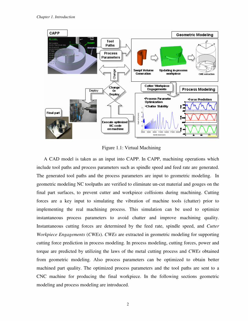
Figure 1.1: Virtual Machining
A CAD model is taken as an input into CAPP. In CAPP, machining operations which
include tool paths and process parameters such as spindle speed and feed rate are generated.
The generated tool paths and the process parameters are input to geometric modeling. In
geometric modeling NC toolpaths are verified to eliminate un-cut material and gouges on the
final part surfaces, to prevent cutter and workpiece collisions during machining. Cutting
forces are a key input to simulating the vibration of machine tools (chatter) prior to
implementing the real machining process. This simulation can be used to optimize
instantaneous process parameters to avoid chatter and improve machining quality.
Instantaneous cutting forces are determined by the feed rate, spindle speed, and Cutter
Workpiece Engagements (CWEs). CWEs are extracted in geometric modeling for supporting
cutting force prediction in process modeling. In process modeling, cutting forces, power and
torque are predicted by utilizing the laws of the metal cutting process and CWEs obtained
from geometric modeling. Also process parameters can be optimized to obtain better
machined part quality. The optimized process parameters and the tool paths are sent to a
CNC machine for producing the final workpiece. In the following sections geometric
modeling and process modeling are introduced.
Chapter 1. Introduction
3
1.2 Geometric Modeling
In geometric modeling CWEs are extracted according to the input requirements from
process modeling. Figure 1.2 illustrates the steps involved in geometric modeling for
extracting CWEs. Inputs from a CAD/CAM system include the geometric representation of
the initial workpiece, the tool path and the geometric description of the cutting tool.
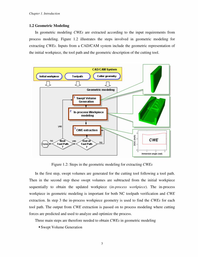
Figure 1.2: Steps in the geometric modeling for extracting CWEs
In the first step, swept volumes are generated for the cutting tool following a tool path.
Then in the second step these swept volumes are subtracted from the initial workpiece
sequentially to obtain the updated workpiece (in-process workpiece). The in-process
workpiece in geometric modeling is important for both NC toolpath verification and CWE
extraction. In step 3 the in-process workpiece geometry is used to find the CWEs for each
tool path. The output from CWE extraction is passed on to process modeling where cutting
forces are predicted and used to analyze and optimize the process.
Three main steps are therefore needed to obtain CWEs in geometric modeling
Swept Volume Generation
Chapter 1. Introduction
4
In-process Workpiece Modeling
CWE Extraction
In the next subsections each step is introduced.
1.2.1 Swept Volume Generation
One of the subtasks in identifying the CWE geometry involves updating the in-process
workpiece geometry after each non-self intersecting tool path (or tool path segment). An
accurate model of the in-process workpiece is therefore important to ensure that correct CWE
geometry is calculated as the simulation progresses and the cutting tool reenters regions
previously milled. Creating the in-process workpiece requires modeling and subtracting the
swept volume generated by each cutter movement along successive tool paths from the
model of the stock, finally yielding the machined surfaces of the final part model.
Mathematically, the swept volume is the set of all points in space encompassed within the
object envelop during its motion. The moving object which is called the generator can be a
curve, a surface or a solid and in this thesis the generator is a rigid milling cutter. The motion
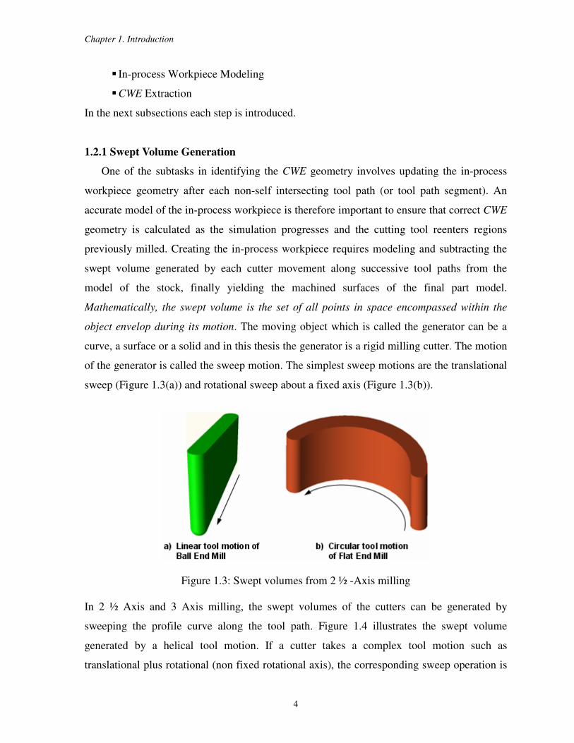
of the generator is called the sweep motion. The simplest sweep motions are the translational
sweep (Figure 1.3(a)) and rotational sweep about a fixed axis (Figure 1.3(b)).
Figure 1.3: Swept volumes from 2 ½ -Axis milling
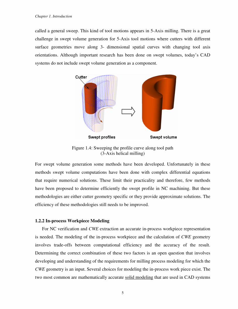
In 2 ½ Axis and 3 Axis milling, the swept volumes of the cutters can be generated by
sweeping the profile curve along the tool path. Figure 1.4 illustrates the swept volume
generated by a helical tool motion. If a cutter takes a complex tool motion such as
translational plus rotational (non fixed rotational axis), the corresponding sweep operation is
Chapter 1. Introduction
5
called a general sweep. This kind of tool motions appears in 5-Axis milling. There is a great
challenge in swept volume generation for 5-Axis tool motions where cutters with different
surface geometries move along 3- dimensional spatial curves with changing tool axis
orientations. Although important research has been done on swept volumes, today’s CAD
systems do not include swept volume generation as a component.
Figure 1.4: Sweeping the profile curve along tool path
(3-Axis helical milling)
For swept volume generation some methods have been developed. Unfortunately in these
methods swept volume computations have been done with complex differential equations
that require numerical solutions. These limit their practicality and therefore, few methods
have been proposed to determine efficiently the swept profile in NC machining. But these
methodologies are either cutter geometry specific or they provide approximate solutions. The
efficiency of these methodologies still needs to be improved.
1.2.2 In-process Workpiece Modeling
For NC verification and CWE extraction an accurate in-process workpiece representation
is needed. The modeling of the in-process workpiece and the calculation of CWE geometry
involves trade-offs between computational efficiency and the accuracy of the result.
Determining the correct combination of these two factors is an open question that involves
developing and understanding of the requirements for milling process modeling for which the
CWE geometry is an input. Several choices for modeling the in-process work piece exist. The
two most common are mathematically accurate solid modeling that are used in CAD systems
Chapter 1. Introduction
6
and approximate modeling such as those used in computer graphics: facetted and z-Map
models. Solid modeling offers the best choice for highly accurate modeling of the geometric
conditions. However challenges exist to making this approach both efficient and generally
robust to handle degenerate geometric conditions that can occur when large numbers of tool
paths need to be simulated. Further, the presence of accurate geometric and topological
(connectivity between geometry) information can potentially be exploited to develop
“intelligent” approaches for CWE geometry extraction. These would search for patterns
(features) in the removal volumes where the engagement geometry is constant or changing in
a predictable way. This is not possible when using approximate models where accurate
geometry and relationships are not maintained in the data structure. The use of solid models
therefore has unstudied potential. The approaches to In-process Workpiece Modeling are
discussed in the following subsections.
Solid Modeling
Solid modeling technique also called volumetric modeling is used in many applications
such as geometric design, NC code generation and visualization. The use of solid models for
manufacturing is becoming more widespread with developing computer technology. The
most popular solid modeling representation schemes are the constructive solid geometry
(CSG) and boundary representation (B-rep) schemes.
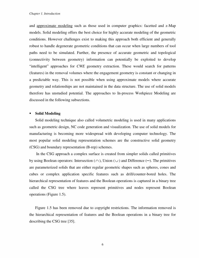
In the CSG approach a complex surface is created from simpler solids called primitives
by using Boolean operators: Intersection ( ∩ ), Union ( ∪ ) and Difference (). The primitives
are parameterized solids that are either regular geometric shapes such as spheres, cones and
cubes or complex application specific features such as drill/counter-bored holes. The
hierarchical representation of features and the Boolean operations is captured in a binary tree
called the CSG tree where leaves represent primitives and nodes represent Boolean
operations (Figure 1.5).
Figure 1.5 has been removed due to copyright restrictions. The information removed is
the hierarchical representation of features and the Boolean operations in a binary tree for
describing the CSG tree [35].
Chapter 1. Introduction
7
In solid modeling, boundary representation (B-rep) is a methodology for representing
shapes using their limits. If it is compared with the CSG representation which uses only
Boolean operations and primitive objects, the B-rep has a much richer set of operations and
because of this for CAD systems it is more appropriate. B-rep models contain two parts:
geometry and topology. The geometry information in the B-rep model is composed of
curve/surface equations and point coordinates. The topology information is the connectivity
between geometric entities FACE, EDGE and VERTEX.
The shape of a FACE is defined by a surface which has a boundary represented by
connected EDGEs.
The shape of an EDGE is defined by a curve which has a boundary represented by
two VERTEXs.
A point represents the location of the VERTEX.
Other elements in the B-rep representation are the SHELL (a set of connected FACEs), the
LUMP (collection of SHELLs) and the LOOP (a circuit or list of EDGEs bounding a FACE).
There are several ways of viewing this data structure. For example it can be considered as a
tree or a hierarchy with BODY as a root. A BODY can have LUMPs which are comprised of
SHELLs formed from a group of FACES.
In this thesis both for updating the in-process workpiece and for extracting the CWEs,
under the solid modeler section, a B-rep methodology is used. For this reason a commercial
geometric modeler ACIS [4] is utilized. ACIS is an object oriented geometric modeling
toolkit designed for use as a geometric engine. Figure 1.6 shows the data structure used in
ACIS.
Figure 1.6 has been removed due to copyright restrictions. The information removed is
the ACIS representational hierarchy [4].
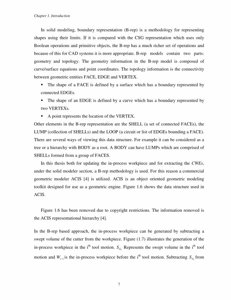
In the B-rep based approach, the in-process workpiece can be generated by subtracting a
swept volume of the cutter from the workpiece. Figure (1.7) illustrates the generation of the
in-process workpiece in the ith
tool motion. iGS Represents the swept volume in the i
th tool
motion and 1−iW is the in-process workpiece before the ith
tool motion. Subtracting iGS from
Chapter 1. Introduction
8
1−iW i.e. )*( 1 iGi WSWi
=−− updates the in-process workpiece for the next tool motion and
also intersecting iGS with 1−iW generates the removal volume iRV .
Figure 1.7: Generation of in-process workpiece and the removal volume
Facetted Models
Another alternative for modeling the in-process geometry that is starting to receive more
attention are Polyhedral Models. These may offer a good compromise between manageable
computational speed, robustness and accuracy. These models have become pervasive in
supporting engineering applications. They are found in all CAD applications as facetted
models for visualization and are used extensively in simulation, CAE and rapid prototyping.
In this modeling approach workpiece surfaces are represented by a finite set of polygonal
planes called facets. The most commonly used shapes are the triangles and because of this
the term facet is usually understood to mean triangular facet. Converting the mathematically
precise models to the triangulated model is called tessellation. For tessellation the original
surfaces of the model are sampled for sets of points and then these points are connected for
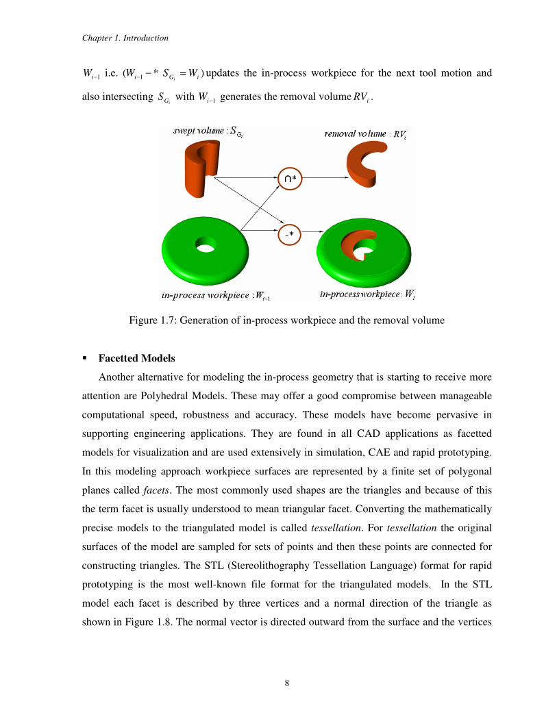
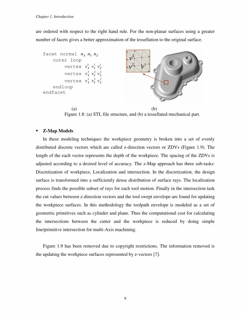
constructing triangles. The STL (Stereolithography Tessellation Language) format for rapid
prototyping is the most well-known file format for the triangulated models. In the STL
model each facet is described by three vertices and a normal direction of the triangle as
shown in Figure 1.8. The normal vector is directed outward from the surface and the vertices
Chapter 1. Introduction
9
are ordered with respect to the right hand rule. For the non-planar surfaces using a greater
number of facets gives a better approximation of the tessellation to the original surface.
facet normal ZYX nnn
outer loop
vertex 111
ZYX vvv
vertex 222
ZYX vvv
vertex 333
ZYX vvv
endloop
endfacet
(a) (b)
Figure 1.8: (a) STL file structure, and (b) a tessellated mechanical part.
Z-Map Models
In these modeling techniques the workpiece geometry is broken into a set of evenly
distributed discrete vectors which are called z-direction vectors or ZDVs (Figure 1.9). The
length of the each vector represents the depth of the workpiece. The spacing of the ZDVs is
adjusted according to a desired level of accuracy. The z-Map approach has three sub-tasks:
Discretization of workpiece, Localization and intersection. In the discretization, the design
surface is transformed into a sufficiently dense distribution of surface rays. The localization
process finds the possible subset of rays for each tool motion. Finally in the intersection task
the cut values between z-direction vectors and the tool swept envelope are found for updating
the workpiece surfaces. In this methodology the toolpath envelope is modeled as a set of
geometric primitives such as cylinder and plane. Thus the computational cost for calculating
the intersections between the cutter and the workpiece is reduced by doing simple
line/primitive intersection for multi-Axis machining.
Figure 1.9 has been removed due to copyright restrictions. The information removed is
the updating the workpiece surfaces represented by z-vectors [7].
Chapter 1. Introduction
10
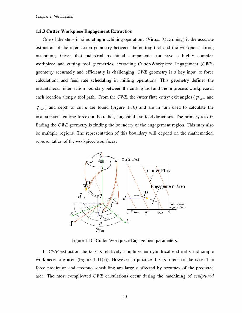
1.2.3 Cutter Workpiece Engagement Extraction
One of the steps in simulating machining operations (Virtual Machining) is the accurate
extraction of the intersection geometry between the cutting tool and the workpiece during
machining. Given that industrial machined components can have a highly complex
workpiece and cutting tool geometries, extracting Cutter/Workpiece Engagement (CWE)
geometry accurately and efficiently is challenging. CWE geometry is a key input to force
calculations and feed rate scheduling in milling operations. This geometry defines the
instantaneous intersection boundary between the cutting tool and the in-process workpiece at
each location along a tool path. From the CWE, the cutter flute entry/ exit angles ( Entryϕ and
Exitϕ ) and depth of cut d are found (Figure 1.10) and are in turn used to calculate the
instantaneous cutting forces in the radial, tangential and feed directions. The primary task in
finding the CWE geometry is finding the boundary of the engagement region. This may also
be multiple regions. The representation of this boundary will depend on the mathematical
representation of the workpiece’s surfaces.
Figure 1.10: Cutter Workpiece Engagement parameters.
In CWE extraction the task is relatively simple when cylindrical end mills and simple
workpieces are used (Figure 1.11(a)). However in practice this is often not the case. The
force prediction and feedrate scheduling are largely affected by accuracy of the predicted
area. The most complicated CWE calculations occur during the machining of sculptured
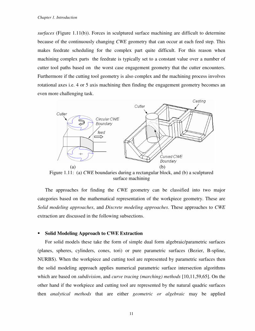
Chapter 1. Introduction
11
surfaces (Figure 1.11(b)). Forces in sculptured surface machining are difficult to determine
because of the continuously changing CWE geometry that can occur at each feed step. This
makes feedrate scheduling for the complex part quite difficult. For this reason when
machining complex parts the feedrate is typically set to a constant value over a number of
cutter tool paths based on the worst case engagement geometry that the cutter encounters.
Furthermore if the cutting tool geometry is also complex and the machining process involves
rotational axes i.e. 4 or 5 axis machining then finding the engagement geometry becomes an
even more challenging task.
(a) (b)
Figure 1.11: (a) CWE boundaries during a rectangular block, and (b) a sculptured
surface machining
The approaches for finding the CWE geometry can be classified into two major
categories based on the mathematical representation of the workpiece geometry. These are
Solid modeling approaches, and Discrete modeling approaches. These approaches to CWE
extraction are discussed in the following subsections.
Solid Modeling Approach to CWE Extraction
For solid models these take the form of simple dual form algebraic/parametric surfaces
(planes, spheres, cylinders, cones, tori) or pure parametric surfaces (Bezier, B-spline,
NURBS). When the workpiece and cutting tool are represented by parametric surfaces then
the solid modeling approach applies numerical parametric surface intersection algorithms
which are based on subdivision, and curve tracing (marching) methods [10,11,59,65]. On the
other hand if the workpiece and cutting tool are represented by the natural quadric surfaces
then analytical methods that are either geometric or algebraic may be applied
Chapter 1. Introduction
12
[33,48,55,56,63]. While solid modelers have been recognized as one approach to finding
CWE geometry, for limited applications, computational complexity and robustness remain
issues that need to be addressed if the approach is to be viable from a practical perspective.
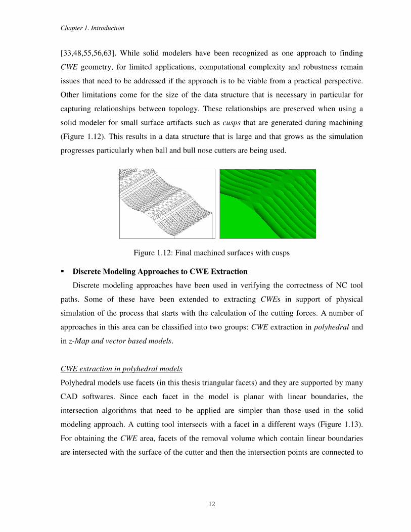
Other limitations come for the size of the data structure that is necessary in particular for
capturing relationships between topology. These relationships are preserved when using a
solid modeler for small surface artifacts such as cusps that are generated during machining
(Figure 1.12). This results in a data structure that is large and that grows as the simulation
progresses particularly when ball and bull nose cutters are being used.
Figure 1.12: Final machined surfaces with cusps
Discrete Modeling Approaches to CWE Extraction
Discrete modeling approaches have been used in verifying the correctness of NC tool
paths. Some of these have been extended to extracting CWEs in support of physical
simulation of the process that starts with the calculation of the cutting forces. A number of
approaches in this area can be classified into two groups: CWE extraction in polyhedral and
in z-Map and vector based models.
CWE extraction in polyhedral models
Polyhedral models use facets (in this thesis triangular facets) and they are supported by many
CAD softwares. Since each facet in the model is planar with linear boundaries, the
intersection algorithms that need to be applied are simpler than those used in the solid
modeling approach. A cutting tool intersects with a facet in a different ways (Figure 1.13).
For obtaining the CWE area, facets of the removal volume which contain linear boundaries
are intersected with the surface of the cutter and then the intersection points are connected to
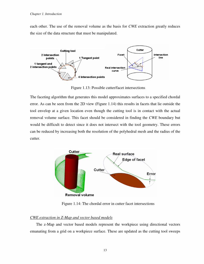
Chapter 1. Introduction
13
each other. The use of the removal volume as the basis for CWE extraction greatly reduces
the size of the data structure that must be manipulated.
Figure 1.13: Possible cutter/facet intersections
The faceting algorithm that generates this model approximates surfaces to a specified chordal
error. As can be seen from the 2D view (Figure 1.14) this results in facets that lie outside the
tool envelop at a given location even though the cutting tool is in contact with the actual
removal volume surface. This facet should be considered in finding the CWE boundary but
would be difficult to detect since it does not intersect with the tool geometry. These errors
can be reduced by increasing both the resolution of the polyhedral mesh and the radius of the
cutter.
Figure 1.14: The chordal error in cutter facet intersections
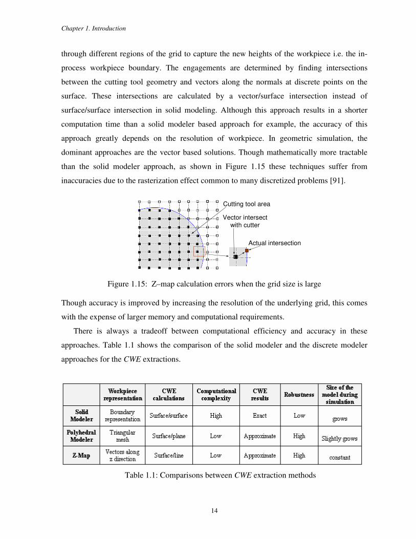
CWE extraction in Z-Map and vector based models
The z-Map and vector based models represent the workpiece using directional vectors
emanating from a grid on a workpiece surface. These are updated as the cutting tool sweeps
Chapter 1. Introduction
14
through different regions of the grid to capture the new heights of the workpiece i.e. the in-
process workpiece boundary. The engagements are determined by finding intersections
between the cutting tool geometry and vectors along the normals at discrete points on the
surface. These intersections are calculated by a vector/surface intersection instead of
surface/surface intersection in solid modeling. Although this approach results in a shorter
computation time than a solid modeler based approach for example, the accuracy of this
approach greatly depends on the resolution of workpiece. In geometric simulation, the
dominant approaches are the vector based solutions. Though mathematically more tractable
than the solid modeler approach, as shown in Figure 1.15 these techniques suffer from
inaccuracies due to the rasterization effect common to many discretized problems [91].
Cutting tool area
Vector intersect with cutter
Actual intersection
Figure 1.15: Z–map calculation errors when the grid size is large
Though accuracy is improved by increasing the resolution of the underlying grid, this comes
with the expense of larger memory and computational requirements.
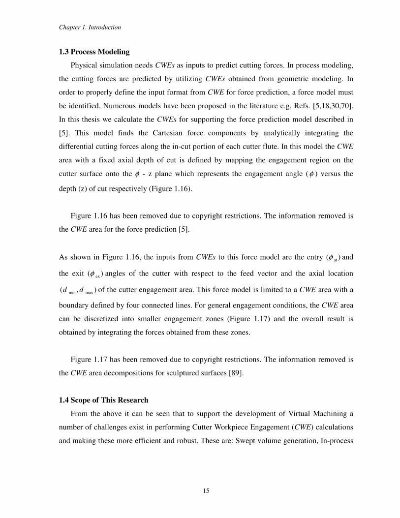
There is always a tradeoff between computational efficiency and accuracy in these
approaches. Table 1.1 shows the comparison of the solid modeler and the discrete modeler
approaches for the CWE extractions.
Table 1.1: Comparisons between CWE extraction methods
Chapter 1. Introduction
15
1.3 Process Modeling
Physical simulation needs CWEs as inputs to predict cutting forces. In process modeling,
the cutting forces are predicted by utilizing CWEs obtained from geometric modeling. In
order to properly define the input format from CWE for force prediction, a force model must
be identified. Numerous models have been proposed in the literature e.g. Refs. [5,18,30,70].
In this thesis we calculate the CWEs for supporting the force prediction model described in
[5]. This model finds the Cartesian force components by analytically integrating the
differential cutting forces along the in-cut portion of each cutter flute. In this model the CWE
area with a fixed axial depth of cut is defined by mapping the engagement region on the
cutter surface onto the φ - z plane which represents the engagement angle (φ ) versus the
depth (z) of cut respectively (Figure 1.16).
Figure 1.16 has been removed due to copyright restrictions. The information removed is
the CWE area for the force prediction [5].
As shown in Figure 1.16, the inputs from CWEs to this force model are the entry )( stφ and
the exit )( exφ angles of the cutter with respect to the feed vector and the axial location
),( maxmin dd of the cutter engagement area. This force model is limited to a CWE area with a
boundary defined by four connected lines. For general engagement conditions, the CWE area
can be discretized into smaller engagement zones (Figure 1.17) and the overall result is
obtained by integrating the forces obtained from these zones.
Figure 1.17 has been removed due to copyright restrictions. The information removed is
the CWE area decompositions for sculptured surfaces [89].
1.4 Scope of This Research
From the above it can be seen that to support the development of Virtual Machining a
number of challenges exist in performing Cutter Workpiece Engagement (CWE) calculations
and making these more efficient and robust. These are: Swept volume generation, In-process
Chapter 1. Introduction
16
work piece modeling and CWE extractions. Considering these challenges together, the
objectives of this thesis are:
To develop a computationally efficient and generic swept volume methodology for multi-
axis milling operations. A toolpath may contain hundreds or thousands of tool motions which
make the computational cost for characterizing the geometry of each tool swept volume
prohibitively expensive. This limitation motivates research in this thesis into methodologies
that provide computationally simple analytical solutions to the swept volume generation
problem.
To develop an efficient and robust in-process workpiece update methodology. During
machining simulation for each tool movement the modification of the workpiece geometry is
required to keep track of the material removal process. Because NC verification and Cutter
Workpiece Engagement (CWE) extraction directly depend on material removal an accurate
in-process workpiece update is needed.
To develop a methodology for identifying regions of the cutter surfaces that have the
potential to engage with the workpiece during machining. A typical NC cutter has different
surfaces with varying geometries and during the material removal process restricted regions
of these cutter surfaces are eligible to contact the in-process workpiece. Identifying these
regions is critical to simplifying the CWE extraction calculations for a wide range of cutters
performing multi-axes machining.
To develop solid (B-rep), polyhedral and vector based multi-axes CWE extraction
methodologies to support the calculation of cutting forces in milling. These methodologies
should be developed using a range of different types of cutters and tool paths defined by 3, 5-
axes tool motions. The workpiece surfaces should cover a wide range of surface geometries
such as the sculptured surfaces.
1.5 Organization of Thesis
Henceforth the thesis is organized as follows: A review of related literature is presented
in Chapter 2, followed by a new generic swept volume methodology for multi-axes milling in
Chapter 3. In Chapter 4 efficient in-process update methodologies are presented. Feasible
engagement regions of the cutter surfaces during the machining are analyzed in Chapter 5,

Chapter 1. Introduction
17
followed by the CWE extraction methodologies for solid, polyhedral and vector based
representations in Chapter 6. The conclusions and possible future research directions are
discussed in Chapter 7. Appendices clarifying some of the computational details are provided
following the Bibliography.
18
Chapter 2
Literature Review
As is shown in Chapter 1, Virtual Machining has two main parts: the geometric modeling
and the process modeling. The process modeling requires Cutter Workpiece Engagement
(CWE) calculations from the geometric modeling to predict the cutting forces in milling. This
becomes a challenging task when the geometry of the cutter and the workpiece are complex
in multi-axis machining. An extensive amount of research has focused on geometric and
physical simulations of the machining process. The important contributions from these
research works are integrated in the virtual machining environment. In this chapter some of
the important research contributions in this field will be reviewed. Specifically research into
swept volume generation, in-process workpiece modeling and CWE extraction
methodologies is reviewed.
2.1 Swept Volume Generation
Mathematically, the swept volume is the set of all points in space encompassed within the
object envelop during its motion. A swept surface is the boundary of the swept volume. The
swept surfaces and volumes are frequently used in graphical modeling, computer aided
design, NC machining verification and robot analysis etc. As mentioned in chapter (1),
swept volume generation is considered one of the important steps in virtual machining, since
removal volume generation and the in-process work piece update require swept volumes.
The mathematical formulation of the swept volume problem has been investigated using
jacobian rank deficiency method [1,2], sweep differential equation (SDE) [15], envelope
theory [53,61,82], implicit modeling [75] and Minkowski sums [25]. Abdel Malek et al. [3]
presented a comprehensive survey and review on the methodologies for the swept volume
generation. Although in the past decades the problem of the swept volume generation has
been studied widely, the problem is still not considered to be sufficiently well solved.
The basic idea in NC verification and simulation is to remove the cutter swept volume
from the workpiece stock and thus to obtain the final machined surfaces. For NC machining

Chapter 2. Literature Review
19
some swept volume generation methods have been developed. Wang et al. [83] computed the
boundary points for the swept volume of APT-type cutter using the sweep envelope
differential equations method (SEDE) [15]. Abdel-Malek et al. [1] and Blackmore et al. [15]
solved systems of the implicit equations numerically for obtaining the swept envelopes.
Wang et al. [82] derived the tangency condition in which the velocity of a point on the
envelope surface must be tangent to the envelope surface.
Unfortunately in these methods swept volume computations have been done with
complex differential equations that require numerical solutions and these limit their
practicality. Therefore, few methods have been proposed to determine the swept profile in
NC machining efficiently. In the following sub-sections some of the dominant techniques
will be discussed.
2.1.1 Sweep Differential Equation Approach
The Sweep Differential Equation (SDE) method and its variants [13,14,15,16,83] were
developed for representing and analyzing swept volumes. The key element of this approach
is the sweep differential equation (SDE). In this method the boundary of the swept volume of
an object can be represented to be the subset of the union of a) the grazing points on the
boundary of the object during the entire sweep at which the vector field of the SDE neither
points into or out of the object interior b) the ingress points at the beginning of the sweep and
c) the egress points on the object boundary (Figure 2.1). The SDE method has been
implemented for 3D swept volume representations generated by a Flat-End and a Ball-End
mill. But the computational cost increased in 3D problems seriously and this affected the
speed of the implementation. In order to overcome this computational difficulty, Blackmore
et al. [15] developed an extension of the SDE method that they called the sweep envelope
differential equation (SEDE) approach. The SEDE algorithm is used to calculate the swept
volume generated by a general 7-parameter APT tool in 5-axis NC milling process.
Figure 2.1 has been removed due to copyright restrictions. The information removed is
the decomposing object boundary [15].
Chapter 2. Literature Review
20
2.1.2 Jacobian Rank Deficiency Approach
The Jacobian Rank Deficiency (JRD) method was presented by Abdel Malek et al. [1].
This approach is based on the singularity theory in differential geometry. A Jacobian rank
deficiency condition is implemented in order to determine all entities that appear internal and
external to the swept volume. A perturbation method is then introduced in order to select
those entities that are boundary to the swept volume. They showed that the implicit surface is
defined when all the 3x3 sub-Jacobians are simultaneously zero. With this approach the exact
boundary envelope of a swept volume in a closed form can be generated. Although the
presented formulation is valid for any number of parameters in an entity, it becomes more
difficult to implement because the non-linear equations resulting from the determinants of the
sub-jacobians also increases and system becomes more difficult to solve.
2.1.3 Swept Profile Based Approaches
Chung et al. [21] developed a methodology for representing the cutter swept surface of a
generalized cutter in a single valued form. They obtained analytical expressions of the
generating curve for different cutter geometries. However this methodology is limited to 3-
axis milling with linear tool motions. Sheltami et al. [67] proposed a method that is based on
identifying generating curves along the toolpath and connecting them into a solid model of
the swept volume. It has been shown that at each instance in time there exists a curve on the
cutter surface that describes the contribution of the tool position to the final bottom swept
surface. This curve represents the imprint of the tool on the machined surface. However this
technique has not yet been extended to include turns or twist of the general 5-axis tool
motions. Also it is assumed that this curve could be approximated by a circle. However this
assumption looses its validity in 5-axis tool motions. Roth et al. [75] presented a geometric
method for generating swept volume of a toroidal end mill performing 5-axis tool motions.
This technique, called imprint or cross product method, uses vector algebra for obtaining the
points on the swept envelope and thus eliminates the use of the complicated SEDE equations.
The method is based on discretizing the tool into pseudo-inserts (Figure 2.2) and identifying
imprint points using a modified principle of silhouettes. For obtaining the imprint curve the
imprint points of each pseudo-insert are connected by a piecewise linear curve. Later the
collection of imprint curves is joined to approximate the swept surface.
Chapter 2. Literature Review
21
Figure 2.2 has been removed due to copyright restrictions. The information removed is
the (a) The pseudo-inserts of the toroidal End mill, and (b) the position of a pseudo-insert at
two tool positions [75].
Pottman and Peternell [61] described an explicit geometric method for computing the
characteristic points of a moving surface of revolution. In this method the plane, normal to
the velocity vector is intersected with a circle chosen from the surface of revolution. The
valid intersections generate the characteristic points on the envelope surface. Later Mann et
al. [52] extended the imprint method to simulate the milling operations with different cutter
geometries. They described that the imprint method can be used with cylinder and torus
cutter geometries for obtaining the swept profiles. Chiou et al. [20] developed a swept profile
methodology for a generalized cutter in 5-axis NC machining by analyzing the machine tool
motions based on the machine configurations. In this work the swept envelope of a cutter is
constructed by integrating the intermediate swept profiles. Later Du et al. [86] introduced a
new B-Rep based approach which is partly derived from Wang’s method [82]. In this work
instantaneous profiles of the Fillet-End cutter are calculated by introducing the basis of the
moving frame. This approach approximates the swept profile of a Fillet-End mill in the
parametric form by interpolating a set of points on the cutter surface.
2.1.4 Discussion
From the above discussion it can be seen that sweep differential equation and jacobian
rank deficiency approaches generate the most precise boundaries of a swept volume in the
parametric or implicit form. But because they contain numerical calculations their application
to NC machining is limited. On the other hand, the nature of the swept profile based
approaches promises an approximation to the swept volume. Though accuracy is improved
by decreasing the distance between consecutive tool locations and by using more grazing
points for the swept profile, this comes at the expense of longer simulation runs. A toolpath
may contain hundreds or thousands of tool motions which make the computational cost for
characterizing the geometry of each tool swept volume prohibitively expensive. This
limitation motivates research in this thesis into methodologies that provide computationally
Chapter 2. Literature Review
22
simple analytical solutions to the swept volume generation. Also in the literature the swept
profile based approaches have concentrated mainly on the simpler milling cutter geometries.
A comprehensive analytical solution in 5-axis milling has not yet been described for the
general surface of revolution which covers the broadest range of cutter geometries.
In this thesis an analytical methodology for determining the shape of the swept envelopes
generated by a general surface of revolution is developed. In this methodology, cutter
surfaces performing 5-axis tool motions are decomposed into a set of characteristic circles.
For obtaining these circles a new concept two-parameter-family of spheres is introduced. In
this concept the center of a moving sphere is a function of two parameters representing the
cutter surface and the tool motion. For a given 5-axis tool motion a member from this family
of spheres generates two circles: a characteristic and a great circle. Considering the
relationship between these circles an analytical formula which describes the swept envelope
is developed. The implementation of the methodology is simple, especially with cutter
geometries represented by pipe surfaces such as the torus and circular cylinder with fewer
calculations being used.
2.2 In-process Workpiece Modeling
For NC simulation and CWE extraction an accurate in-process workpiece representation
is needed. NC simulation usually implies cutting simulation and verification. The cutting
simulation is for visualization of the cutting process and the verification is for comparison of
the machined surface with the design surface. The modeling of the in-process workpiece
geometry involves trade-offs between computational efficiency and the accuracy of the
result. Several choices for modeling the in-process work piece exist. The two most common
are mathematically accurate Solid modeler based methodologies that are used in CAD
systems and approximate modeler based methodologies such as those used in computer
graphics. In the following sub-sections these approaches will be discussed.
2.2.1 Solid Modeler Based Methodologies
Solid modeling theory was developed in the late 1960s and early 1970s. Currently the
most popular schemes used in solid modelers are the Boundary representation (B-rep) and
Constructive Solid Geometry (CSG). In the B-rep methodology an object is represented by
Chapter 2. Literature Review
23
both its boundaries defined by Faces, Edges, Vertices and the connectivity information. In
the CSG representation the Boolean operations and the simple primitives are saved in a
binary tree data structure. Solid modeling methodologies offer the possibility of doing both
simulation and verification. For simulation the swept volumes of the tool movements are
subtracted from the in-process workpiece model. Verification is performed by Boolean
differences between the processed workpiece and the design part. Researchers have in the
past investigated the potential of solid modelers for supporting the machining process [68-
71,73,76,80]. The computational complexity due to the Boolean operations was identified as
one of the difficulties in applying this methodology. Developments in computer processor
speeds and new computational technologies such as parallel computing now make this a
more viable prospect [72].
Voelcker and Hunt [80] did an exploratory study of the feasibility of using CSG
modeling system for NC simulation. It has been reported that the cost of simulation in the
CSG approach is proportional to the fourth power of the number of tool movements. A
typical NC program can contain more than 10000 tool movements. Spence and Altintas [70]
developed a 2 ½-axis instantaneous cutter/workpiece immersion simulation method based on
a CSG model. This work was later transferred to the B-rep modeler [9,64]. Later Spence et
al. [71] presented integrated solid modeler based solutions for machining. In this work,
geometric and milling process simulation combined with online monitoring and control is
illustrated for 2 ½-axis pocket milling application (Figure 2.3). For this purpose the ACIS
solid modeler kernel is utilized.
Figure 2.3 has been removed due to copyright restrictions. The information removed is
the updating in-process workpiece [71].
Elbestawi et al. [37] developed an improved process simulation system for Ball-End
milling of sculptured surfaces. The workpiece, cutter and CWE geometries are modeled using
a geometric simulation system which uses the commercial solid modeler (ACIS) as a
geometric engine. Later Imani et al. [38] presented a method for geometrically simulating a
3-axis Ball-End milling operation. They developed an advanced sweeping/skinning technique
for generating a precise B-rep model of the Ball-End mill swept volume (Figure 2.4). In this
Chapter 2. Literature Review
24
work semi finishing operations are simulated by performing consecutive Boolean operations
between the in-process workpiece and the cutter swept volumes. The critical geometric
information such as the instantaneous chip geometry and the scallop heights are extracted
from the in-process workpiece.
Figure 2.4 has been removed due to copyright restrictions. The information removed is
the 3-axis cutter swept volume with the boundary faces [38].
2.2.2 Approximate Modeler Based Methodologies
For increasing efficiency and robustness in the process of the workpiece update a number
of approximate approaches have been developed. The approaches can be classified into three
major categories: Image space (or view based) methods, Object based methods and
polyhedral model based method.
Image space (or view based) methods
Chappel [19] developed a method called the “point vector technique”. The design
surface is approximated by a set of points and the vectors originating from these points
extend until they reach the boundary of the original stock. For simulating the machining,
each vector on the workpiece surface is intersected with the cutter swept volumes and the
vector length is shortened if it intersects the swept volume. Oliver and Goodman [58,74]
presented an approach similar to Chappel’s. In this approach the workpiece is discretized into
arrays containing the surface coordinates and the corresponding normal vectors. The
discretization of the workpiece surfaces are done according to the computer graphics image
of the workpiece surfaces. Each pixel on the screen is projected onto workpiece surface and
these pixel points on the surface become the approximation of the workpiece (Figure 2.5). In
this work the vector - cutter swept volume intersections are performed with a similar
approach to Chappel’s.
Figure 2.5 has been removed due to copyright restrictions. The information removed is
the simulation of the NC milling by projecting pixels of a computer graphics image onto the
part surface [58].
Chapter 2. Literature Review
25
Later Wang [81,82] developed an image space approach. For each pixel on the screen a
vector is generated and using a scan-line algorithm the intersections between vectors and the
toolpath envelope are calculated. The z-buffer of the workpiece is modified by applying
Boolean difference operations with the z-buffer of the tool swept volumes. Also Van Hook
[78] developed an approach called the “extended z-buffer”. The pixel images of the cutter are
pre-computed and then the cutter is subtracted from the workpiece as it moves along a
toolpath. This method is applied to 3-axis milling in which the orientation of the cutter is
fixed. Later Atherton [6] extended Van Hook’s method to handle 5-axis milling.
The main limitations with the image space methodologies are: Because they are view
dependant, errors not visible in the chosen viewing direction are undetected. For detecting
the errors in another view of the part, the entire simulation must be started again. Also small
machining errors i.e. less than 0.1mm are unlikely to be detected by a visual inspection of the
computer graphics image. Despite their limitations the view based approaches are the best
approximation methodologies for determining how much material is being removed for a
given tool movement. Each pixel can represent a volume of material and, material removal
can be approximated with accuracy dependent on the size of the object and the number of the
pixels [41].
Object based methods
The Object based in-process workpiece update methodologies are developed in [23,
24,32,39,40]. In these methodologies a set of points are chosen on the workpiece surfaces
and using these points actual surfaces are approximated. These methodologies use similar
calculation techniques from Chappel’s [19] and Oliver’s [58] approaches. Using the tool
movements the vectors on the surface of the workpiece are updated. Some of the
advantageous of these approaches are [41]: a) Material removal simulation is efficiently
accomplished by intersecting the surface normals with the tool swept volumes. b) The
machining verification is easily done by the updated vector length. Also using the color
contour map of the workpiece surface, out of tolerance areas can be seen. c) The user can
specify the accuracy of the simulation.
Chapter 2. Literature Review
26
Jerard et al. [40] described a 3-axis machining methodology for simulating the geometric
aspects of numerically controlled machining. The methodology is based on a discrete
approximation of the object into a set of surface points. Vectors passed through these points
are intersected with the tool movements (Figure 2.6). For increasing the efficiency the
localization methodology described in [41] is used.
Figure 2.6 has been removed due to copyright restrictions. The information removed is
the updating the workpiece surfaces represented by parallel z-vectors [40].
Fussell and Jerard in their recent research [32] used an extended z-Buffer model and a
discrete axial slice model for representing the workpiece and the cutting tool (Ball-End mill)
respectively. In this work a 3-axis approximation of the 5-axis tool movement is used to
simplify the calculations while maintaining a desired level of accuracy (Figure 2.7-a). Since
the tool swept volume is modeled as a set of geometric primitives such as natural quadric
surfaces and planes, the intersection calculations are simplified to a set of line/surface
intersections. It is assumed that all primitives are linear and the curvatures in the toolpath and
the tool orientations are neglected. For this reason 5-axis tool paths are subdivided into many
3-axis toolpaths. Although approximating the 5-axis tool moves with 3-axis linear tool
moves is a primary drawback in this work, the comparisons by Quinn [62] to the exact 5-axis
tool moves with the 3-axis approximation method show that the 3-axis method is faster and
robust. Another drawback in this work is that all discrete vectors of the workpiece model lie
in one direction regardless of surface normal directions, where the directions are along the
vertical z-axis of a Cartesian coordinate system (Figure 2.7-b).
Figure 2.7 has been removed due to copyright restrictions. The information removed is
the (a) A 3-axis approximation of 5-axis swept volume, and (b) the extended z-buffer model
of workpiece [32].
Baek et al. presented a z-Map update method for linearly [7] and circularly [8] moving
APT-type tools in 3-axis milling. Machining process is simulated through numerically
calculating the intersection points between the z-Map vectors and the tool swept envelope.
Chapter 2. Literature Review
27
The intersection points are expressed as the solution of a system of nonlinear equations. This
system of equations is transformed into a single-variable function whose zero is a solution of
the system. Also in this work they show how to calculate the candidate interval in which the
unique zero exists. In this methodology both the tool rotation axis and the z-Map vectors are
restricted to lie along the vertical z-axis of a Cartesian coordinate system.
Park et. al. [43] developed a hybrid cutting simulation methodology via the Discrete
Normal Vector (DNV) and the Discrete Vertical Vector (DVV) models. In the DNV approach
a workpice consists of discrete vectors whose direction vectors are surface normal vectors,
where all directions are not necessarily identical. Also spacing may vary depending upon the
surface local properties. On the other hand, in the DVV approach all discrete vectors of the
workpiece model lie in only one direction regardless of surface normal directions, where the
directions are along the vertical z-axis of a Cartesian coordinate system. The DNV approach
generates better surface quality especially when the workpiece model has vertical walls,
sharp edges, and overhang (Figure 2.8). But on the other hand in the DNV representation the
localization of the cutter swept envelope is difficult and this decreases the computational
efficiency. The main idea in this work is to take full advantage of each type’s strengths in
terms of speed. But on the other hand, in this hybrid methodology the cutter swept volumes
are generated by a solid modeler. A typical toolpath may contain thousands of tool motions.
In this case using the solid modeler for the cutter swept volume generation increases the
computational cost during the simulation.
Figure 2.8 has been removed due to copyright restrictions. The information removed is
the DNV and DVV representation of the workpiece surfaces [43].
Polyhedral model based method
Another alternative for updating the in-process workpiece in NC machining is a
polyhedral model based method. In the polyhedral model the workpiece surfaces are
represented by a finite set of polygonal planes called facets. The most commonly used shapes
are triangles and converting the mathematically precise models to the triangulated models is
called tessellation. In this approach in order to achieve real time NC simulation the number
of polygons has to be reduced. But this results in poor image quality. Ong et. al. [49]
Chapter 2. Literature Review
28
developed an approach to reduce the number of polygons without much loss in image quality
(Figure 2.9). They proposed an adaptive regular mesh decimation algorithm which uses a
quadtree to represent the milling surface. This algorithm can automatically adjust the
polygon density to approximate the milling surface during the simulation in real time.
Figure 2.9 has been removed due to copyright restrictions. The information removed is
the regular mesh decimation for 3-axis NC milling simulation [49].
2.2.3 Discussion
During the machining simulation for each tool movement the modification of the
workpiece geometry is required to keep track of the material removal process. Because the
NC verification and Cutter Workpiece Engagement (CWE) extraction directly dependent on
the material removal an accurate in-process workpiece modeling is needed.
From the literature review it can be seen that several choices for modeling the in-process
work piece exist. The two most common are mathematically accurate solid modeling that are
used in CAD systems and approximate modeling such as those used in computer graphics:
facetted and discrete vector models. Each methodology has its own strengths and weaknesses
in terms of computational complexity, representation accuracy and the robustness. It can be
seen from the literature that for updating the workpiece surfaces represented by the solid or
faceted models third party softwares can be used. For example the ACIS solid modeling
kernel is one of these softwares.
But on the other hand for the workpiece geometries represented by discrete vectors
accurate and computationally efficient in-process workpiece update methodologies are
needed. In the literature the discrete vectors have orientations along the z-axis of the standard
bases of R3. But when the in-process workpiece has some features like vertical walls and
sharp edges, representing the workpiece with one directional vectors generates less accurate
results in visualization of the final product and CWE extractions. Also in recent works [7,8]
the tool axis has a fixed orientation along the z-axis of the standard bases of R3 and the
workpiece updates are performed numerically for the common milling cutters. Still needed
are in-process workpiece update methodologies in which the workpiece geometries are
represented by discrete vectors having different orientations and the tool rotation axes have
Chapter 2. Literature Review
29
arbitrary inclinations in space. Also in these methodologies for the given cutter geometry the
calculations, if it is possible, must be analytic for computational efficiency.
In this thesis the discrete vectors with their orientations in the directions of x,y,z-axes of
the standard bases of R3 are used. Therefore in this representation more vectors in different
directions are used and thus the quality in the visualization of the final product has been
increased. A typical milling tool path contains thousands of tool movements and during the
machining simulation for calculating the intersections only a small percentage of all the
discrete vectors is needed. For this purpose for localizing the tool envelope during simulation
the Axis Aligned Bounding Box (AABB) is used. For simplifying the intersection
calculations the properties of canal surfaces are utilized. In the developed methodologies the
tool motions in (3+2)-axis milling in which the cutter can have an arbitrary fixed orientation
in space are considered. The 5-axis tool motions can be approximated by (3+2)-axis tool
motions and an example is given for illustrating this situation. The calculations for the major
cutter geometries such as the sphere, cylinder, frustum of a cone and flat-bottom surfaces are
made analytically. Because of the complexity of the torus shape the calculations are made by
using the numerical root finding methods. For this purpose a root finding analysis is
developed for guaranteeing the root(s) in the given interval.
2.3 Cutter Workpiece Engagement Extraction
The goal in CWE extraction is to obtain engagement conditions between milling cutter
and the in-process workpiece for supporting process modeling. From the CWEs instantaneous
in-cut segments or engaged portions of the cutting edges are obtained. For extracting the in-
cut segments CWE boundaries are intersected with the cutter edges either in 2D or in 3D
Euclidian space. In both approaches edge/edge intersection is performed. In the 2D-space
approach, first the cutter contact face is intersected with the in-process workpiece and CWE
boundary is obtained in 3D Euclidian space. Then this CWE boundary and the cutter edges
are mapped into two dimensional space. Finally for obtaining the in-cut segments, each
cutting edge is intersected with the CWE boundary in this space [70,89]. In the 3D-space
approach intersections between CWE boundary and cutter edges are performed in 3D
Euclidian space [26,37]. In this thesis for extracting in-cut segments the 2D-space approach
is utilized.
Chapter 2. Literature Review
30
In the literature, based on the mathematical representation of the workpiece geometry, the
CWE extraction methodologies can be classified into three major categories: Solid model
based, polyhedral model based and discrete vector based methods. Also some other existing
CWE extraction methods are discussed in section (2.3.4).
2.3.1 Solid model based methods
Some research on Solid model based CWE extraction methodologies for supporting
process modeling has been reported [26,,37,47,70,89]. In these CWE extraction
methodologies the initial workpiece geometry is represented by using the B-rep model.
Geometric and topological algorithms of this model are utilized for both updating the in-
process workpiece and extracting the CWE geometry. For updating the in-process workpiece
geometry first the swept volume of the cutter is generated for a given toolpath segment and
then this volume is subtracted from the current workpiece state using regularized Boolean
subtraction. Cutter workpiece engagement calculations are performed using this new
workpiece state until the start of the following tool path segment. If the toolpath has self
intersections then for obtaining the correct CWEs it may be necessary to decompose the
given toolpath into non-intersecting smaller segments. From the literature the CWE
extractions using a solid modeler can be classified into two groups: 2 ½-axis and 3-axis
methods.
2 ½-Axis methods
For calculating CWEs in 2 ½-axis milling with a Flat-End mill, a B-rep based approach
has been presented by Spence et al. [70]. Figure 2.10(a) illustrates that a Flat-End mill
engages with the in-process workpiece Wi at a constant depth of cut d along the entire
toolpath. It is shown in Figure 2.10(b) that engagements are determined by performing the
intersections between an advancing semi circle Ci moving in the tangential direction of the
toolpath and the boundaries of Wi on an engagement plane PLZ-Top. The engagement
geometry is calculated as entry ( stφ ) and exit ( exφ ) angles for each step of the Flat-End mill
(Figure 2.10(c)). The step taken between each CWE calculation is the feed per revolution of
the cutter. Although this methodology is an important step in applying solid modeling
technology to the CWE extraction problem, it only generates the constant depth of cut.
Chapter 2. Literature Review
31
Figure 2.10 has been removed due to copyright restrictions. The information removed is
the extracting CWEs by advancing semi circle approach for 2 ½ -axis milling [70].
Later Yip-Hoi et al. [89] presented another B-rep based approach for extracting CWEs in
2 ½ - axis milling. He extended Spence’s methodology by performing the regularized
Boolean intersection operation between a semi cylindrical cutter surface and the in-process
workpiece (Figure 2.11). In this work for imprinting the engagement region boundaries on
the cutter surface, the solid modeler’s (ACIS) surface/surface intersection algorithms are
used. Then the engagement boundaries are mapped from 3D Euclidian space into 2D space
defined by the engagement angle and the depth of cut respectively. Later these engagement
regions are decomposed into smaller rectangular regions for fulfilling the requirement of the
force model described in [5]. The advantage of this methodology is that it can be applied to a
wider range of workpiece geometries i.e. the initial workpiece geometry is not rectangular
prismatic. On the other hand it is still a 2 ½ -axis methodology with a Flat-End mill and the
engagement boundaries are limited to straight lines and circular arcs.
Figure 2.11 has been removed due to copyright restrictions. The information removed is
the extracting CWEs by advancing semi cylinder approach for 2 ½ -Axis milling [89].
3-Axis methods
Elbestawi et al. [37] developed a Ball-End milling process simulation system. In this
work the Ball End mill performs 2-axis or an ascending (with different up-hill angles) 3-axis
motion. The geometries of the workpiece, the cutter and CWEs are modeled using (ACIS) as
a geometric engine. The engaged portion of the cutting edge (the instantaneous in-cut
segment) is computed in two steps: In the first step the boundary of the contact face between
the spherical portion of the Ball-End mill and the in-process workpiece is obtained. This
boundary consists of one circular edge and two B-spline edges (Figure 2.12). In the second
step the intersection points between interpolated cutting edge and boundary curves of the
contact face are found. This is performed by using edge/edge intersections with a prescribed
tolerance. Finally the cutting edge is decomposed into in-cut and out-cut segments.
Chapter 2. Literature Review
32
Figure 2.12 has been removed due to copyright restrictions. The information removed is
the 3-axis CWE extraction with Ball-End mill [37].
Also El-Mounayri et al. [26] presented a geometric approach for 3-axis machining
process simulation using a Ball-End mill. In this work solid models are used for representing
the in-process workpiece and the removal volume. The cutting edges are represented by
Bezier curves in 3D Euclidian space. For obtaining the in-cut segments of the cutting edges,
the Bezier curves are intersected with the removal volume (Figure 2.13). Later these
segments are used for evaluating the instantaneous cutting forces.
Figure 2.13 has been removed due to copyright restrictions. The information removed is
the procedure for extracting in-cut segments of the cutting edges [26].
2.3.2 Polyhedral Model Based Methods
Although they are approximate, polyhedral models provide the advantage of simplifying
the workpiece surface geometry to planes which consist of linear boundaries. Thus the
intersection calculations reduce to line / surface intersections. These can be performed
analytically for the geometry found on cutting tools. Some research [88,90] on polyhedral
based CWE extraction methodologies for supporting the process modeling has been reported.
Yao [88] presented geometric algorithms for estimating cutter engagement values for 3-
axis Ball-End milling processes of tessellated free-form surfaces. In this work 3D surface
geometry is represented by an STL (“Stereo lithography”) model in which surfaces are
tessellated or broken down into a series of small triangles. It is assumed that the toolpath is a
linear segment and only the frontier of the Ball-End mill has engagement with the workpiece
(Figure 2.14). The engaged portion of the cutter is estimated in three steps: First finding
triangles that intersect the cutter, then intersecting those triangles with the cutter for obtaining
the intersection curve segments and finally using those curve segments to form the closed
engagement region.

Chapter 2. Literature Review
33
Figure 2.14 has been removed due to copyright restrictions. The information removed is
the cutter engagement portion [88].
Later Yip-Hoi et al. [90] presented a polyhedral model based CWE calculation
methodology in 2 ½-axis and 3-axis millings. For reducing the amount of data and
calculations this methodology works on removal volumes instead of the in-process
workpiece. To further reduce the number of intersections an R*-tree based localization
technique is applied for localizing the facets that have potential intersections with the cutting
tool. The methodology first calculates the intersection points between facet edges and the
cutter, and then using a mark circle method it creates intersection segments between these
intersection points. Finally an undirected graph is used for connecting those intersection
segments to form the boundary of the CWE area. As explained in section (1.2.3) there is a
cordal error in the polyhedral model representations. In this case the cutter does not intersect
the facets on the side-wall surfaces of the removal volume. In this work for solving this
problem the cutter radius is enlarged slightly (Figure 2.15). Therefore the entry angles are
slightly larger while the exit angles are less than what they should be.
Figure 2.15 has been removed due to copyright restrictions. The information removed is
the (a) Chordal error in the cutter facet intersection, and (b) the radius enlargement of the
cutter [90].
2.3.3 Discrete Vector Based Methods
Some research on discrete vector based CWE extraction for supporting process modeling
has been reported [18,31,32,42,91]. In these approaches the workpiece is broken into a set of
evenly distributed parallel lines which have directions along the vertical z axis of the
Cartesian coordinate system. Multiple z values are stored in one vector, allowing extensions
to multi-axis milling with multiple tool passes. The spacing between vectors can be
determined based on the desired accuracy, local surface curvature of the workpiece and the
tool size. CWEs are extracted according to requirements of the mechanistic force model. The
mechanistic force model divides the cutting tool into a set of axial disc elements.
Chapter 2. Literature Review
34
There are two primary concerns for each disc element. First concern is whether or not the
disc element is in contact with the in-process workpiece and the second concern for a disc
engaged with the in-process workpiece is to define the limits of the engagement in terms of
entry/exit angles. The entry and exit angles are calculated by solving for the normal direction
component of each intersection, and storing the maximum and minimum normal positions
found during a given tool move (Figure 2.16).
Figure 2.16 has been removed due to copyright restrictions. The information removed is
the Entry/exit angle calculation for each disc [31].
2.3.4 Other Existing Methods
So far it is shown that there are mainly three major approaches for extracting CWEs. Also
there are some other existing methodologies which are not classified under major
approaches. For example Stori et al. [84] presented a metric based approach for toolpath
optimization in high speed machining. For obtaining cutter engagements a pixel based
simulation procedure is used (Figure 2.17). In this work a Flat-End mill follows a 2D linear
toolpath. Both the local in-process geometry and the cutter is discritized. Any un-machined
area is represented by a 0, and the machined area is represented by a 1. The instantaneous
engagements are estimated by checking the status of the in-process workpiece geometry for
the pixels that overlap the circumference of the cutting tool in the given cutter location point.
Figure 2.17 has been removed due to copyright restrictions. The information removed is
the pixel based engagement extraction [84].
Also Gupta et al. [34] developed an analytical method for computing cutter engagement
functions in 2.5D machining. In this work the analytical approaches are described for
determining the cutter engagements utilizing the engagement functions for individual half
spaces that comprise the workpiece geometry (Figure 2.18). The edges of the workpiece are
represented as half spaces. The formulae are obtained for determining the cutter engagement
functions in the cases: circular cut and linear half space, and circular cut and circular half
space.
Chapter 2. Literature Review
35
Figure 2.18 has been removed due to copyright restrictions. The information removed is
the “A linear tool path and region expressed as a Boolean expression of half spaces” [34].
2.3.5 Discussion
The purpose of Cutter Workpiece Engagement (CWE) extraction is to identify
engagement conditions between the cutter and the in-process workpiece during the milling
operation for predicting the cutting forces. From the above discussion it can be seen that
Research work on CWE extraction can be classified into three main approaches: Solid
modeler based, polyhedral modeler based and vector based methodologies. There is always a
tradeoff between computational efficiency and accuracy in these approaches. For example
the polyhedral and vector based approaches generate approximated CWE results and because
of this they require a shorter computational time than does the solid modeler based approach.
But on the other hand in the solid modeler based approach the most accurate CWEs are
obtained with the cost of higher computational time. These three main approaches to CWE
extraction are discussed in the following parts.
In the literature solid modeling approaches are concentrated on simple workpiece
surfaces such as cylinders and planes. But the most complicated CWE calculations occur
during the machining of sculptured surfaces. Because of continuously changing surface
geometry, modeling CWEs in sculptured surface machining is not so easy. In the given
approaches the cutters perform either 2 ½ -axis machining or 3-axis machining with
ascending motion in which only the front part of the cutter removes material. But sometimes
with respect to the motion type the back side or the bottom-flat part of a cutter may have
contact with the in-process workpiece. For example in a plunging motion of a Flat-End mill
the bottom flat surface removes material. Therefore CWE extraction with different surfaces
of a cutter must be addressed. Also there is a needed for a 5-axis CWE extraction
methodology in which cutter has changing orientations.
From the literature, it can be seen that for the polyhedral model based CWE extractions so
far little work has been conducted. Also there is a robustness issue in CWE extractions
because of the chordal error.
Chapter 2. Literature Review
36
In the literature, the proposed discrete vector based methodologies represent the in-
process workpiece by using discrete vectors which lie in only one direction regardless of the
surface normal direction. But when the orientation of the cutter axis is parallel to these
vectors, for some cutter geometries, extracting CWEs becomes difficult i.e. 3-axis machining
with a Flat-End mill.
From the above discussion it can be seen that comprehensive methods for extracting
CWEs using solid, polyhedral and discrete vector approaches are yet to be fully developed. In
this thesis solid, polyhedral and vector based CWE methodologies are developed using a
range of different types of cutters and tool paths defined by 3, 5-axes tool motions. The
workpiece surfaces cover a wide range of surface geometries such as the sculptured surfaces.
In 3-axis solid and polyhedral model approaches to reduce the size of the data structure that
needs to be manipulated the removal volume is used instead of the in-process workpiece. For
5-axis machining it is the workpiece itself.
In the 3-axis solid modeler methodology the cutter surfaces are decomposed into sub-
constituent surfaces with respect to the feed vector direction. Then these surfaces are
intersected with their removal volumes for obtaining the boundary curves of the closed CWE
area. Decomposing the cutter surfaces allows CWEs for different parts of a given cutter
geometry, i.e. bottom flat or back side of a cutter to be more easily extracted. During the
material removal process only certain parts of the cutter surfaces are eligible to contact the
in-process workpiece. In this thesis for representing these regions of the cutter boundary a
terminology feasible contact surfaces (FCS) is introduced. The word feasible is used because
although these surfaces are eligible to contact the in-process workpiece, they may or may not
remove material depending on the cutter position relative to the workpiece. Because in a
solid model the envelope boundary for 5-axis tool motions are approximated by spline
curves, applying the same methodology described for the 3-axis milling generates non robust
results. Because of this in the 5-axis methodology an offset body obtained from the feasible
contact surface is intersected with the in-process workpiece at a given cutter location point.
Then face/face intersections are performed for obtaining the boundaries of the CWEs.
For addressing the chordal error problem in polyhedral models a 3-axis mapping
technique is developed that transforms a polyhedral model of the removal volume from
Chapter 2. Literature Review
37
Euclidean space to a parametric space defined by location along the tool path, engagement
angle and the depth-of-cut. As a result, intersection operations are reduced to first order
plane-plane intersections. This approach reduces the complexity of the cutter/workpiece
intersections and also eliminates robustness problems found in standard polyhedral modeling.
Because in 5-axis tool motions the direction of the tool axis vector continuously changes
applying the mapping described for the 3-axis milling increases the distortions of the facets.
Therefore an approach similar to that of the 5-axis solid modeler is developed. In this
approach the only difference is the application of the face-face intersections.
In the discrete vector approach the cutter surfaces are sliced along the tool rotation axis
and then the surface of each slice is decomposed into buckets. The sizes of the buckets are
adjusted with respect to the resolution of discrete vectors. Later during the simulation
discrete vectors are intersected with the cutter surfaces for representing the material removal
and the buckets which contain the intersection points are plotted
2.4 Summary
In this chapter, a review of the literature in swept volume generation, in-process
workpiece modeling and CWE extraction are presented. It has been shown that because a
toolpath contains thousands of tool motions the swept volume generation becomes costly in
terms of large memory and computational requirements. For this reason for NC machining
the swept volume construction must be easy and the geometric information for defining the
volume must require less memory. The accuracy of the in-process workpiece modeling
effects the quality of the CWEs. Especially in the object based in-process workpiece update
methods using discrete vectors lying only in one direction generates problems in both
workpiece surface quality and CWE representations. For the CWE extractions there is a need
to develop 3 to 5-axis machining approaches for different types of cutter and workpiece
surfaces in solid, polyhedral and vector based models.
38
Chapter 3
Cutter Swept Volume Generation
This chapter presents an analytical methodology to calculate cutter profiles for modeling
the swept volumes of general surfaces of revolution with respect to 5-axis tool motions. In
this methodology the geometry of a cutter is considered as a canal surface. Briefly a canal
surface is an envelope of a moving sphere with varying radius. In this methodology, cutter
surfaces performing 5-axis tool motions are decomposed into a set of characteristic circles.
For obtaining these circles a new concept two-parameter-family of spheres is introduced. In
this concept the center of a moving sphere is a function of two parameters representing the
cutter surface and the tool motion. On the other hand the radius of the moving sphere is only
a function of one parameter. For a given 5-axis tool motion a member from this family of
spheres generates two circles: a characteristic and a great circle. Considering the relationship
between these circles an analytical formula which describes the swept envelope is developed.
Also applying this methodology, the implicit envelope equations of the common cutter
geometries performing 5-Axis tool motions are derived.
The parametric representations of canal surfaces in one-parameter family of spheres are
presented in section (3.1). The concept of the two-parameter-family of spheres is introduced
in section (3.2), followed by the closed form swept profile equations in section (3.3).
Examples from the implementation of the methodology are shown in section (3.4), and
finally the chapter ends with the discussion in section (3.5).
3.1 Canal Surfaces
A canal surface Ф is the envelope of a moving sphere with varying radius, defined by a
trajectory of its center (spine curve) m(t) and a radius function r(t), where t∈R. When the
radius function r(t) has a constant value, the canal surface is also called as a pipe surface.
Canal surfaces have wide applications in different areas such as shape reconstruction,
construction of blending surfaces, transition surfaces between pipes and robotic path
planning [28,66,83]. Some examples of the canal surfaces are pipe surfaces, tori, natural
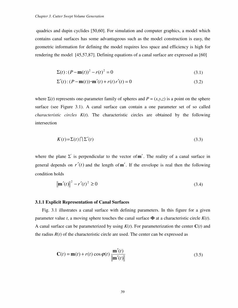
Chapter 3. Cutter Swept Volume Generation
39
quadrics and dupin cyclides [50,60]. For simulation and computer graphics, a model which
contains canal surfaces has some advantageous such as the model construction is easy, the
geometric information for defining the model requires less space and efficiency is high for
rendering the model [45,57,87]. Defining equations of a canal surface are expressed as [60]
0)())((:)( 22 =−−Σ trtPt m (3.1)
0)()()())((:)( =′+′−Σ′ trtrttPt m·m (3.2)
where Σ(t) represents one-parameter family of spheres and P = (x,y,z) is a point on the sphere
surface (see Figure 3.1). A canal surface can contain a one parameter set of so called
characteristic circles K(t). The characteristic circles are obtained by the following
intersection
)()()( tttK Σ′Σ= I (3.3)
where the plane Σ' is perpendicular to the vector of m′ . The reality of a canal surface in
general depends on )(tr ′ and the length of m′ . If the envelope is real then the following
condition holds
0)()( 22≥′−′ trtm (3.4)
3.1.1 Explicit Representation of Canal Surfaces
Fig. 3.1 illustrates a canal surface with defining parameters. In this figure for a given
parameter value t, a moving sphere touches the canal surface Ф at a characteristic circle K(t).
A canal surface can be parameterized by using K(t). For parameterization the center C(t) and
the radius R(t) of the characteristic circle are used. The center can be expressed as
)(
)()(cos)()()(
t
tttrtt
m
mmC
′
′+= ϕ (3.5)
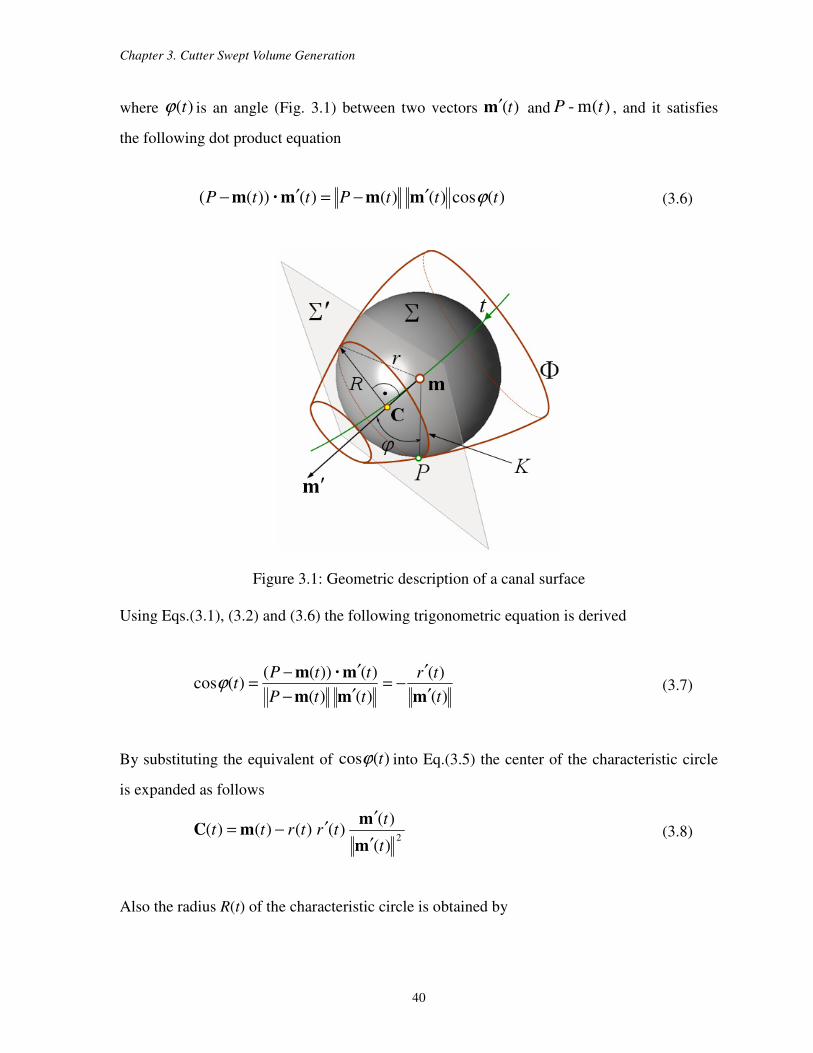
Chapter 3. Cutter Swept Volume Generation
40
where )(tϕ is an angle (Fig. 3.1) between two vectors )(tm′ and )(m- tP , and it satisfies
the following dot product equation
)(cos)()()())(( tttPttP ϕmmm·m ′−=′− (3.6)
Figure 3.1: Geometric description of a canal surface
Using Eqs.(3.1), (3.2) and (3.6) the following trigonometric equation is derived
)(
)(
)()(
)())(()(cos
t
tr
ttP
ttPt
mmm
m·m
′
′−=
′−
′−=ϕ (3.7)
By substituting the equivalent of )(cos tϕ into Eq.(3.5) the center of the characteristic circle
is expanded as follows
2)(
)()()()()(
t
ttrtrtt
m
mmC
′
′′−= (3.8)
Also the radius R(t) of the characteristic circle is obtained by
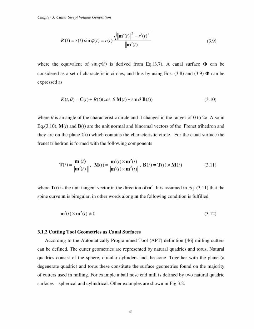
Chapter 3. Cutter Swept Volume Generation
41
)(
)()()()(sin)()(
22
t
trttrttrtR
m
m
′
′−′== ϕ (3.9)
where the equivalent of )(sin tϕ is derived from Eq.(3.7). A canal surface Ф can be
considered as a set of characteristic circles, and thus by using Eqs. (3.8) and (3.9) Ф can be
expressed as
))(sin)()(cos()(),( tttRttK BMC θθθ ++= (3.10)
where θ is an angle of the characteristic circle and it changes in the ranges of 0 to 2π. Also in
Eq.(3.10), M(t) and B(t) are the unit normal and binormal vectors of the Frenet trihedron and
they are on the plane Σ'(t) which contains the characteristic circle. For the canal surface the
frenet trihedron is formed with the following components
)(
)()(
t
tt
m
mT
′
′= ,
)()(
)()()(
tt
ttt
mm
mmM
′′×′
′′×′= , )()()( ttt MTB ×= (3.11)
where T(t) is the unit tangent vector in the direction ofm′ . It is assumed in Eq. (3.11) that the
spine curve m is biregular, in other words along m the following condition is fulfilled
0)()( ≠′′×′ tt mm (3.12)
3.1.2 Cutting Tool Geometries as Canal Surfaces
According to the Automatically Programmed Tool (APT) definition [46] milling cutters
can be defined. The cutter geometries are represented by natural quadrics and torus. Natural
quadrics consist of the sphere, circular cylinders and the cone. Together with the plane (a
degenerate quadric) and torus these constitute the surface geometries found on the majority
of cutters used in milling. For example a ball nose end mill is defined by two natural quadric
surfaces – spherical and cylindrical. Other examples are shown in Fig 3.2.
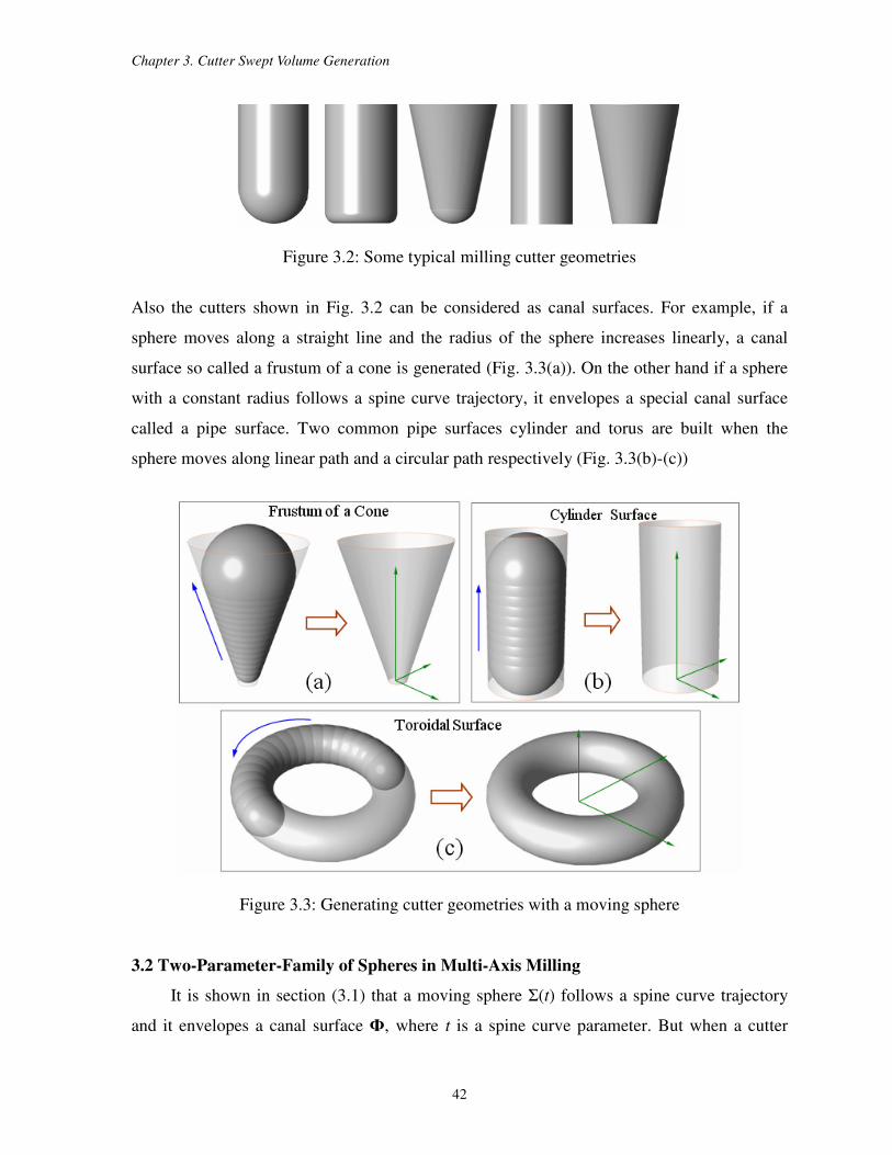
Chapter 3. Cutter Swept Volume Generation
42
Figure 3.2: Some typical milling cutter geometries
Also the cutters shown in Fig. 3.2 can be considered as canal surfaces. For example, if a
sphere moves along a straight line and the radius of the sphere increases linearly, a canal
surface so called a frustum of a cone is generated (Fig. 3.3(a)). On the other hand if a sphere
with a constant radius follows a spine curve trajectory, it envelopes a special canal surface
called a pipe surface. Two common pipe surfaces cylinder and torus are built when the
sphere moves along linear path and a circular path respectively (Fig. 3.3(b)-(c))
Figure 3.3: Generating cutter geometries with a moving sphere
3.2 Two-Parameter-Family of Spheres in Multi-Axis Milling
It is shown in section (3.1) that a moving sphere Σ(t) follows a spine curve trajectory
and it envelopes a canal surface Ф, where t is a spine curve parameter. But when a cutter
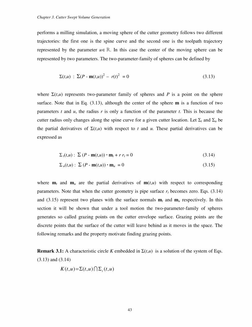
Chapter 3. Cutter Swept Volume Generation
43
performs a milling simulation, a moving sphere of the cutter geometry follows two different
trajectories: the first one is the spine curve and the second one is the toolpath trajectory
represented by the parameter u∈R. In this case the center of the moving sphere can be
represented by two parameters. The two-parameter-family of spheres can be defined by
Σ(t,u) : Σ(P - m(t,u))2
– r(t)2
= 0 (3.13)
where Σ(t,u) represents two-parameter family of spheres and P is a point on the sphere
surface. Note that in Eq. (3.13), although the center of the sphere m is a function of two
parameters t and u, the radius r is only a function of the parameter t. This is because the
cutter radius only changes along the spine curve for a given cutter location. Let Σt and Σu be
the partial derivatives of Σ(t,u) with respect to t and u. These partial derivatives can be
expressed as
Σ t(t,u) : Σ (P - m(t,u)) · mt + r rt = 0 (3.14)
Σ u(t,u) : Σ (P - m(t,u)) · mu = 0 (3.15)
where mt and mu are the partial derivatives of m(t,u) with respect to corresponding
parameters. Note that when the cutter geometry is pipe surface rt becomes zero. Eqs. (3.14)
and (3.15) represent two planes with the surface normals mt and mu respectively. In this
section it will be shown that under a tool motion the two-parameter-family of spheres
generates so called grazing points on the cutter envelope surface. Grazing points are the
discrete points that the surface of the cutter will leave behind as it moves in the space. The
following remarks and the property motivate finding grazing points.
Remark 3.1: A characteristic circle K embedded in Σ(t,u) is a solution of the system of Eqs.
(3.13) and (3.14)
),(),(),( utututK tΣΣ= I
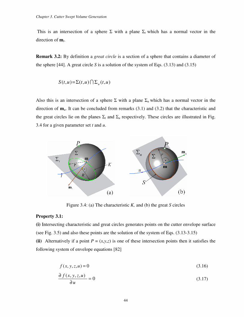
Chapter 3. Cutter Swept Volume Generation
44
This is an intersection of a sphere Σ with a plane Σt which has a normal vector in the
direction of mt.
Remark 3.2: By definition a great circle is a section of a sphere that contains a diameter of
the sphere [44]. A great circle S is a solution of the system of Eqs. (3.13) and (3.15)
),(),(),( utututS uΣΣ= I
Also this is an intersection of a sphere Σ with a plane Σu which has a normal vector in the
direction of mu. It can be concluded from remarks (3.1) and (3.2) that the characteristic and
the great circles lie on the planes Σt and Σu respectively. These circles are illustrated in Fig.
3.4 for a given parameter set t and u.
Figure 3.4: (a) The characteristic K, and (b) the great S circles
Property 3.1:
(i) Intersecting characteristic and great circles generates points on the cutter envelope surface
(see Fig. 3.5) and also these points are the solution of the system of Eqs. (3.13-3.15)
(ii) Alternatively if a point P = (x,y,z) is one of these intersection points then it satisfies the
following system of envelope equations [82]
0),,,( =uzyxf (3.16)
0),,,(
=∂
∂
u
uzyxf (3.17)
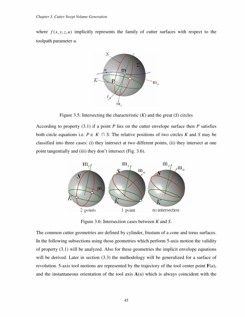
Chapter 3. Cutter Swept Volume Generation
45
where ),,,( uzyxf implicitly represents the family of cutter surfaces with respect to the
toolpath parameter u.
Figure 3.5: Intersecting the characteristic (K) and the great (S) circles
According to property (3.1) if a point P lies on the cutter envelope surface then P satisfies
both circle equations i.e. P ∈ K ∩ S. The relative positions of two circles K and S may be
classified into three cases: (i) they intersect at two different points, (ii) they intersect at one
point tangentially and (iii) they don’t intersect (Fig. 3.6).
Figure 3.6: Intersection cases between K and S.
The common cutter geometries are defined by cylinder, frustum of a cone and torus surfaces.
In the following subsections using those geometries which perform 5-axis motion the validity
of property (3.1) will be analyzed. Also for these geometries the implicit envelope equations
will be derived. Later in section (3.3) the methodology will be generalized for a surface of
revolution. 5-axis tool motions are represented by the trajectory of the tool center point F(u),
and the instantaneous orientation of the tool axis A(u) which is always coincident with the
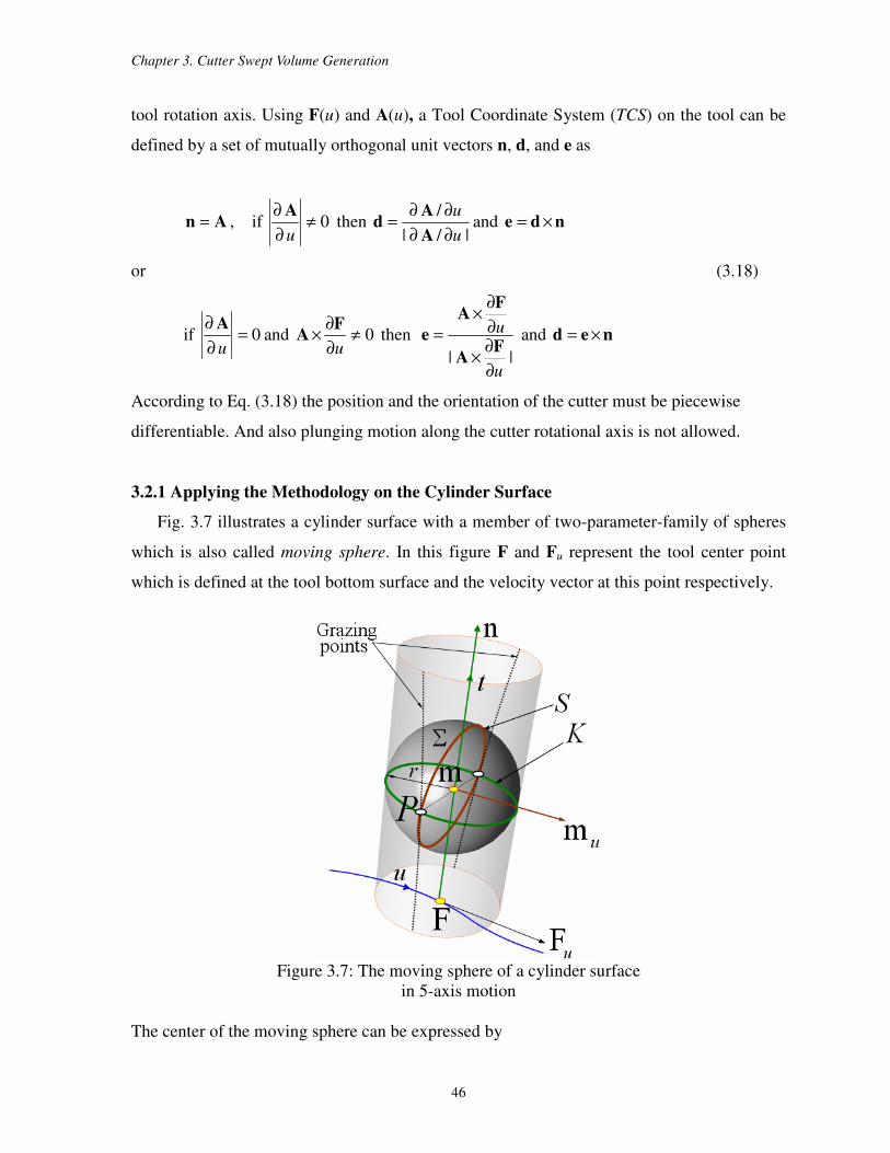
Chapter 3. Cutter Swept Volume Generation
46
tool rotation axis. Using F(u) and A(u), a Tool Coordinate System (TCS) on the tool can be
defined by a set of mutually orthogonal unit vectors n, d, and e as
An = , if 0≠∂
∂
u
A then
|/|
/
u
u
∂∂
∂∂=
A
Ad and nde ×=
or (3.18)
if 0=∂
∂
u
Aand 0≠
∂
∂×
u
FA then
||u
u
∂
∂×
∂
∂×
=F
A
FA
e and ned ×=
According to Eq. (3.18) the position and the orientation of the cutter must be piecewise
differentiable. And also plunging motion along the cutter rotational axis is not allowed.
3.2.1 Applying the Methodology on the Cylinder Surface
Fig. 3.7 illustrates a cylinder surface with a member of two-parameter-family of spheres
which is also called moving sphere. In this figure F and Fu represent the tool center point
which is defined at the tool bottom surface and the velocity vector at this point respectively.
Figure 3.7: The moving sphere of a cylinder surface
in 5-axis motion
The center of the moving sphere can be expressed by
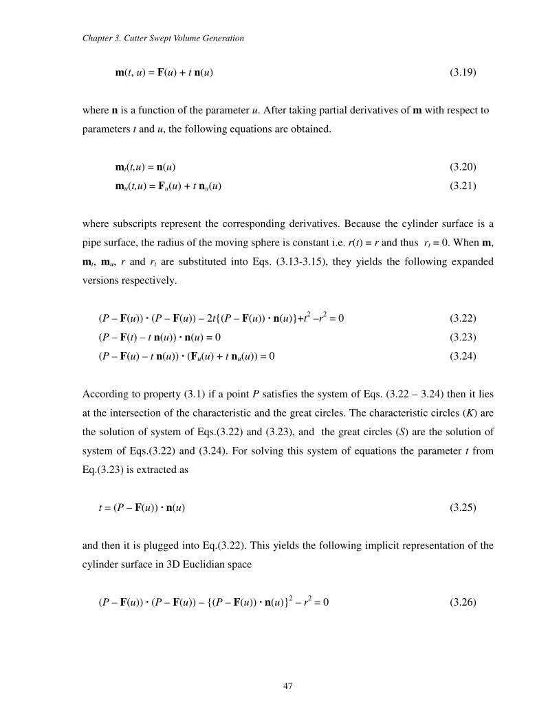
Chapter 3. Cutter Swept Volume Generation
47
m(t, u) = F(u) + t n(u) (3.19)
where n is a function of the parameter u. After taking partial derivatives of m with respect to
parameters t and u, the following equations are obtained.
mt(t,u) = n(u) (3.20)
mu(t,u) = Fu(u) + t nu(u) (3.21)
where subscripts represent the corresponding derivatives. Because the cylinder surface is a
pipe surface, the radius of the moving sphere is constant i.e. r(t) = r and thus rt = 0. When m,
mt, mu, r and rt are substituted into Eqs. (3.13-3.15), they yields the following expanded
versions respectively.
(P – F(u)) · (P – F(u)) – 2t(P – F(u)) · n(u)+t2 –r
2 = 0 (3.22)
(P – F(t) – t n(u)) · n(u) = 0 (3.23)
(P – F(u) – t n(u)) · (Fu(u) + t nu(u)) = 0 (3.24)
According to property (3.1) if a point P satisfies the system of Eqs. (3.22 – 3.24) then it lies
at the intersection of the characteristic and the great circles. The characteristic circles (K) are
the solution of system of Eqs.(3.22) and (3.23), and the great circles (S) are the solution of
system of Eqs.(3.22) and (3.24). For solving this system of equations the parameter t from
Eq.(3.23) is extracted as
t = (P – F(u)) · n(u) (3.25)
and then it is plugged into Eq.(3.22). This yields the following implicit representation of the
cylinder surface in 3D Euclidian space
(P – F(u)) · (P – F(u)) – (P – F(u)) · n(u)2 – r
2 = 0 (3.26)

Chapter 3. Cutter Swept Volume Generation
48
where P is a position of a point (x,y,z) on the cylinder surface. The above equation can also
be denoted by f(x, y, z, u) = 0. By performing dot product operations Eq. (3.24) is expanded
as
(P – F(u)) · Fu(u) – t Fu(u) · n(u)+(P – F(u)) · nu(u) = 0 (3.27)
Notice that in this expansion n(u) · nu(u) = 0. Substituting Eq. (3.25) into Eq. (3.27) yields
(P – F(u)) · Fu(u) – (P – F(u)) · n(u) Fu(u) · n(u) + (P – F(u)) · nu(u) = 0 (3.28)
Eq. (3.28) is the partial derivative of the Eq. (3.26) with respect to u and also it can be
denoted by 0/),,,( =∂∂ uuzyxf .Thus the property (3.1) holds for the cylindrical surface.
3.2.2 Applying the Methodology on the Frustum of a Cone Surface
The 5-axis motion of a conical surface with its moving sphere is illustrated in Fig. 3.8. In
this figure V(u) and α represent tip of the cone and the cone half angle respectively. Also the
tool center point F(u) is the center of the lower base.
Figure 3.8: The moving sphere of a cone surface
in 5-axis motion
Chapter 3. Cutter Swept Volume Generation
49
The tip of the cone can be expressed by (see Fig. 3.8)
)(tan
)()( uα
ruu b n-FV = (3.29)
where rb is the radius of lower base. Also from this figure, the center of the moving sphere
can be obtained by
m(t, u) = V(u) + t n(u) (3.30)
The partial derivatives of m with respect to t and u are derived as
mt(t, u) = n(u) (3.31)
mu(t, u) = Vu(u) + t nu(u) (3.32)
For the frustum of a cone surface the radius of the moving sphere linearly increases. This
radius and its derivative can be expressed by r(t) = t sinα and rt(t) = sinα respectively. By
substitutions of m, mt, mu, r and rt, the system of Eqs. (3.13-3.15) is expanded respectively
as
(P – V(u)) · (P – V(u)) – 2t(P – V(u))· n(u)+t2 cos
2α =0 (3.33)
(P – V(u) – t n(u)) · n(u) + t sin2α = 0 (3.34)
(P – V(u)) · Vu(u) – t Vu(u) · n(u)–(P – V(u)) · nu(u) =0 (3.35)
For solving the system of Eqs. (3.33-3.35), the parameter t from Eq.(3.34) is extracted as
α
uuPt
2cos
)())(( n·V−= (3.36)
Substituting Eq. (3.36) into Eq. (3.33) yields the implicit representation f(x, y, z, u) = 0 of the
frustum of a cone surface in 3D Euclidian space
(P – V(u)) · (P – V(u))–(1+tan2α)(P – V(u)) · n(u)
2 = 0 (3.37)
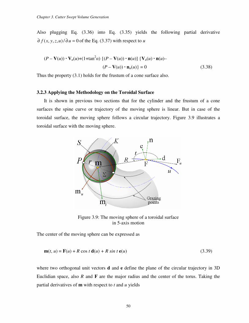
Chapter 3. Cutter Swept Volume Generation
50
Also plugging Eq. (3.36) into Eq. (3.35) yields the following partial derivative
0/),,,( =∂∂ uuzyxf of the Eq. (3.37) with respect to u
(P – V(u)) · Vu(u)+(1+tan2α) (P – V(u)) · n(u)] Vu(u) · n(u)–
(P – V(u)) · nu(u) = 0 (3.38)
Thus the property (3.1) holds for the frustum of a cone surface also.
3.2.3 Applying the Methodology on the Toroidal Surface
It is shown in previous two sections that for the cylinder and the frustum of a cone
surfaces the spine curve or trajectory of the moving sphere is linear. But in case of the
toroidal surface, the moving sphere follows a circular trajectory. Figure 3.9 illustrates a
toroidal surface with the moving sphere.
Figure 3.9: The moving sphere of a toroidal surface
in 5-axis motion
The center of the moving sphere can be expressed as
m(t, u) = F(u) + R cos t d(u) + R sin t e(u) (3.39)
where two orthogonal unit vectors d and e define the plane of the circular trajectory in 3D
Euclidian space, also R and F are the major radius and the center of the torus. Taking the
partial derivatives of m with respect to t and u yields
Chapter 3. Cutter Swept Volume Generation
51
mt(t,u) = –R sint d(u) + R cos t e(u) (3.40)
mu(t,u) = Fu(u) + R cost du(u) + R sin t eu(u) (3.41)
Because the torus is a pipe surface the radius of the moving sphere is constant i.e. r(t) = r and
thus rt = 0. When m, mt, mu, r and rt are plugged into Eqs. (3.13-3.15), the following
expanded versions are obtained respectively.
(P – F(u)) · (P – F(u)) – 2 R cost(P – F(u)) · d
– 2 R sint (P – F(u)) · e + R2 – r
2 = 0 (3.42)
(P – F(u) – R cost d – R sin t e) · (–R sint d + R cos t e) = 0 (3.43)
(P – F(u) – R cost d –R sin t e) · (Fu(u) + R cost du+ R sin t eu) = 0 (3.44)
Solving Eq.(3.43) for the parameter t yields the following two expressions
22 ))(())((
))((cos
·eF·dF
d·F
uPuP
uPt
−+−
−= (3.45)
22 ))(())((
))((sin
·eF·dF
e·F
uPuP
uPt
−+−
−= (3.46)
Plugging cost and sint into Eq. (3.42) yields the following implicit representation f (x, y, z, u)
= 0 of the toroidal surface in 3D Euclidian space.
22
22
))(())((2
))(())((
·eF·dF
F · F
uPuPR
rRuPuP
−+−
=−+−− (3.47)
The above equation can be arranged by squaring the both sides and this yields
0)))(())(((4
))(())((
222
222
=−+−
−−+−−
·eF·dF
F · F
uPuPR
rRuPuP (3.48)

Chapter 3. Cutter Swept Volume Generation
52
For example when P = (x,y,z), F = (0,0,0), d = [1 0 0]T and e = [0 1 0]
T are plugged into the
Eq. (3.48), the well known formula of a torus is obtained in the origin of the Euclidian space
as follows
(x2 + y
2 + z
2 + R
2 – r
2 )
2 –4R
2 (x
2 + y
2 ) = 0
Also plugging cost and sint into Eq. (3.44) yields the following partial derivative
0/),,,( =∂∂ uuzyxf of the Eq. (3.47) with respect to u.
( ) 0))(())((2)())((22 =−+−
∂
∂+− ·eF·dF F · F uPuP
uRuuP u
(3.49)
Thus the property (3.1) holds for the toroidal surface also.
3.3 Closed Form Swept Profile Equations
In section (3.1) a canal surface has been described explicitly by K(t,θ), where the
parameter t represents the spine curve or the trajectory of the moving sphere center. Later in
section (3.2), a methodology based on the two-parameter-family of spheres concept has been
introduced. For describing the motion of the moving sphere, a new parameter u which
represents a toolpath has been introduced. In this section by utilizing the two-parameter
families of spheres, the closed form swept profile equations for the general surface of
revolution will be derived. In general the radius R(t,u) and the center C(t,u) of the
characteristic circle are defined by the following equations.
u),(
)(u),()(),(
22
t
trttrutR
t
tt
m
m −= (3.50)
2),(
),()()(),(),(
ut
uttrtrutut
t
t
t
m
mmC −= (3.51)
where the center of the moving sphere m(t,u) defined by two parameters. Note that these
equations are very similar to those of canal surfaces defined in section (3.1.1), where the
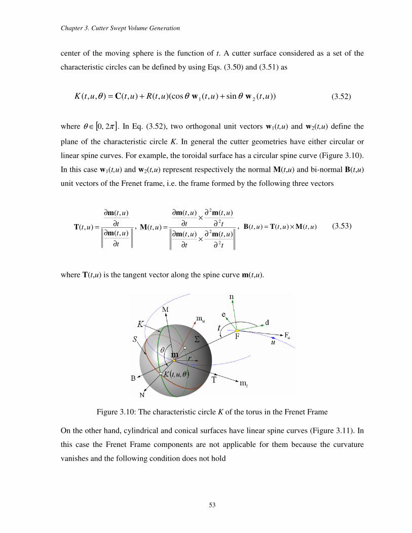
Chapter 3. Cutter Swept Volume Generation
53
center of the moving sphere is the function of t. A cutter surface considered as a set of the
characteristic circles can be defined by using Eqs. (3.50) and (3.51) as
)),(sin),()(cos,(),(),,( 21 utututRututK wwC θθθ ++= (3.52)
where [ ]πθ 2,0∈ . In Eq. (3.52), two orthogonal unit vectors w1(t,u) and w2(t,u) define the
plane of the characteristic circle K. In general the cutter geometries have either circular or
linear spine curves. For example, the toroidal surface has a circular spine curve (Figure 3.10).
In this case w1(t,u) and w2(t,u) represent respectively the normal M(t,u) and bi-normal B(t,u)
unit vectors of the Frenet frame, i.e. the frame formed by the following three vectors
t
ut
t
ut
ut
∂
∂∂
∂
=),(
),(
),(m
m
T ,
t
ut
t
ut
t
ut
t
ut
ut
2
2
2
2
),(),(
),(),(
),(
∂
∂×
∂
∂
∂
∂×
∂
∂
=mm
mm
M , ),(),(),( ututut MTB ×= (3.53)
where T(t,u) is the tangent vector along the spine curve m(t,u).
Figure 3.10: The characteristic circle K of the torus in the Frenet Frame
On the other hand, cylindrical and conical surfaces have linear spine curves (Figure 3.11). In
this case the Frenet Frame components are not applicable for them because the curvature
vanishes and the following condition does not hold
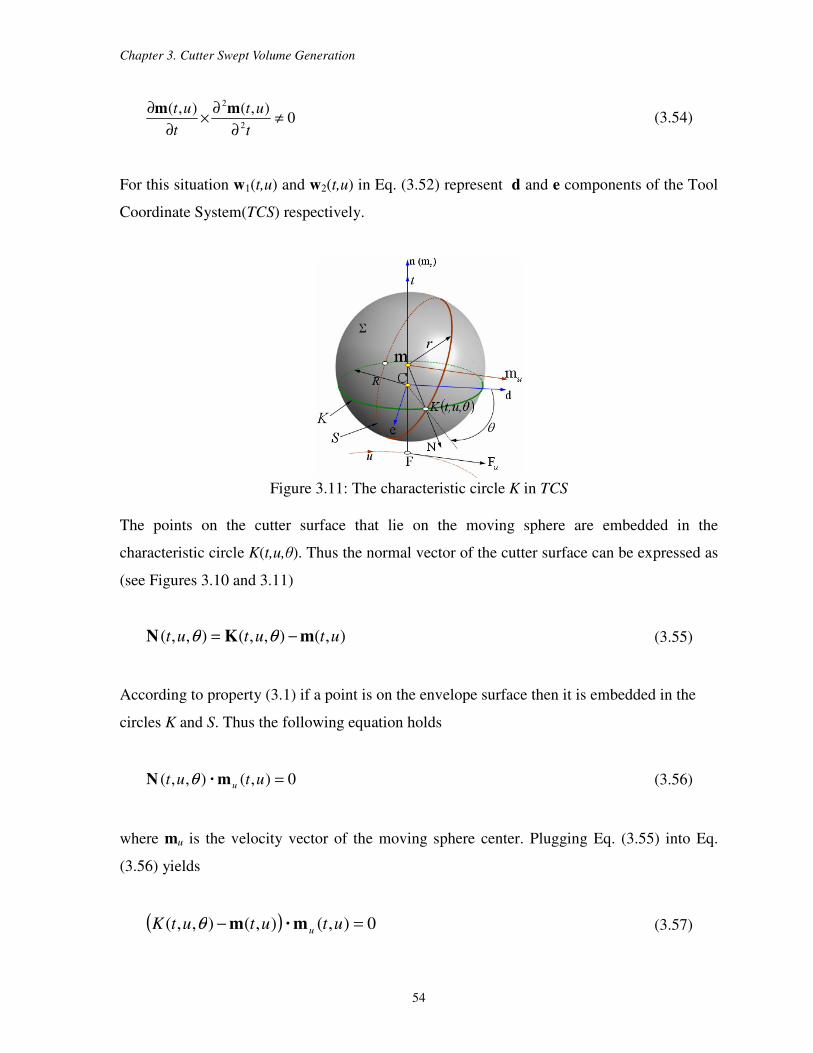
Chapter 3. Cutter Swept Volume Generation
54
0),(),(
2
2
≠∂
∂×
∂
∂
t
ut
t
ut mm (3.54)
For this situation w1(t,u) and w2(t,u) in Eq. (3.52) represent d and e components of the Tool
Coordinate System(TCS) respectively.
Figure 3.11: The characteristic circle K in TCS
The points on the cutter surface that lie on the moving sphere are embedded in the
characteristic circle K(t,u,θ). Thus the normal vector of the cutter surface can be expressed as
(see Figures 3.10 and 3.11)
),(),,(),,( ututut mKN −= θθ (3.55)
According to property (3.1) if a point is on the envelope surface then it is embedded in the
circles K and S. Thus the following equation holds
0),(),,( =utut um·N θ (3.56)
where mu is the velocity vector of the moving sphere center. Plugging Eq. (3.55) into Eq.
(3.56) yields
( ) 0),(),(),,( =− utututK um·mθ (3.57)
Chapter 3. Cutter Swept Volume Generation
55
After replacing K with its equivalent from Eq. (3.52) and taking the dot product, Eq. (3.57)
takes the following trigonometric form
0sincos 012 =−+ AAA θθ (3.58)
where
( ) ( ) ( )( )utututRA u ,,, 12 m·w=
( ) ( ) ( )( )utututRA u ,,, 21 m·w=
( ) ( )
( )( ) ( )( )utut
ut
trtrA ut
t
t ,,,
20 m·mm
=
Equation (3.58) can be written in the following form
( ) 0sin 0
2
2
2
1 =−++ AAA βθ (3.59)
where ( )12
1
2 ,tan AA−=β . Solving Eq. (3.59) for θ yields
−
+−=
−
+=
−
−
βπθ
βθ
2
2
2
1
01
2
2
2
2
1
01
1
sin
sin
AA
A
AA
A
Under the condition of 2
0
2
2
2
1 AAA ≥+ , the inverse function )(sin 1x
− is in the range of
]2/,2/[ ππ− . In this case, there exist real solutions for 2,1θ and the characteristic circle K
contains one or two grazing points. Plugging 2,1θ into Eq. (3.52) yields the closed form
equation of the cutter envelope surface
)),(sin),()(cos,(),(),,( 22,112,1 utututRututK wwC θθθ ++= (3.60)
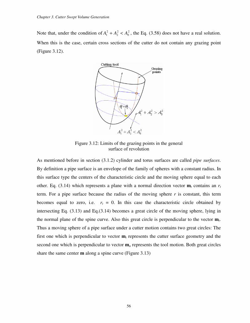
Chapter 3. Cutter Swept Volume Generation
56
Note that, under the condition of 2
0
2
2
2
1 AAA <+ , the Eq. (3.58) does not have a real solution.
When this is the case, certain cross sections of the cutter do not contain any grazing point
(Figure 3.12).
Figure 3.12: Limits of the grazing points in the general
surface of revolution
As mentioned before in section (3.1.2) cylinder and torus surfaces are called pipe surfaces.
By definition a pipe surface is an envelope of the family of spheres with a constant radius. In
this surface type the centers of the characteristic circle and the moving sphere equal to each
other. Eq. (3.14) which represents a plane with a normal direction vector mt contains an rt
term. For a pipe surface because the radius of the moving sphere r is constant, this term
becomes equal to zero, i.e. rt = 0. In this case the characteristic circle obtained by
intersecting Eq. (3.13) and Eq.(3.14) becomes a great circle of the moving sphere, lying in
the normal plane of the spine curve. Also this great circle is perpendicular to the vector mt.
Thus a moving sphere of a pipe surface under a cutter motion contains two great circles: The
first one which is perpendicular to vector mt represents the cutter surface geometry and the
second one which is perpendicular to vector mu represents the tool motion. Both great circles
share the same center m along a spine curve (Figure 3.13)
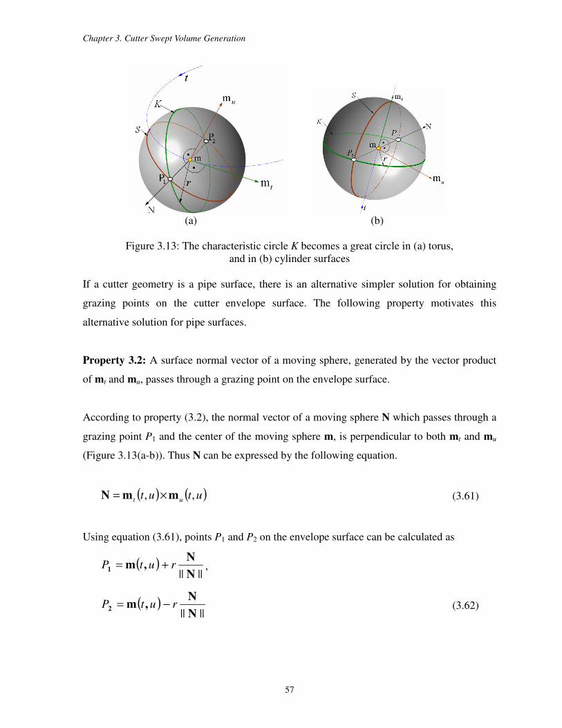
Chapter 3. Cutter Swept Volume Generation
57
(a) (b)
Figure 3.13: The characteristic circle K becomes a great circle in (a) torus,
and in (b) cylinder surfaces
If a cutter geometry is a pipe surface, there is an alternative simpler solution for obtaining
grazing points on the cutter envelope surface. The following property motivates this
alternative solution for pipe surfaces.
Property 3.2: A surface normal vector of a moving sphere, generated by the vector product
of mt and mu, passes through a grazing point on the envelope surface.
According to property (3.2), the normal vector of a moving sphere N which passes through a
grazing point P1 and the center of the moving sphere m, is perpendicular to both mt and mu
(Figure 3.13(a-b)). Thus N can be expressed by the following equation.
( ) ( )utut ut ,, mmN ×= (3.61)
Using equation (3.61), points P1 and P2 on the envelope surface can be calculated as
( )|||| N
N,m1 rutP += ,
( )|||| N
N,m2 rutP −= (3.62)
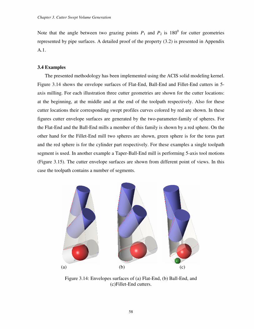
Chapter 3. Cutter Swept Volume Generation
58
Note that the angle between two grazing points P1 and P2 is 1800 for cutter geometries
represented by pipe surfaces. A detailed proof of the property (3.2) is presented in Appendix
A.1.
3.4 Examples
The presented methodology has been implemented using the ACIS solid modeling kernel.
Figure 3.14 shows the envelope surfaces of Flat-End, Ball-End and Fillet-End cutters in 5-
axis milling. For each illustration three cutter geometries are shown for the cutter locations:
at the beginning, at the middle and at the end of the toolpath respectively. Also for these
cutter locations their corresponding swept profiles curves colored by red are shown. In these
figures cutter envelope surfaces are generated by the two-parameter-family of spheres. For
the Flat-End and the Ball-End mills a member of this family is shown by a red sphere. On the
other hand for the Fillet-End mill two spheres are shown, green sphere is for the torus part
and the red sphere is for the cylinder part respectively. For these examples a single toolpath
segment is used. In another example a Taper-Ball-End mill is performing 5-axis tool motions
(Figure 3.15). The cutter envelope surfaces are shown from different point of views. In this
case the toolpath contains a number of segments.
(a) (b) (c)
Figure 3.14: Envelopes surfaces of (a) Flat-End, (b) Ball-End, and
(c)Fillet-End cutters.
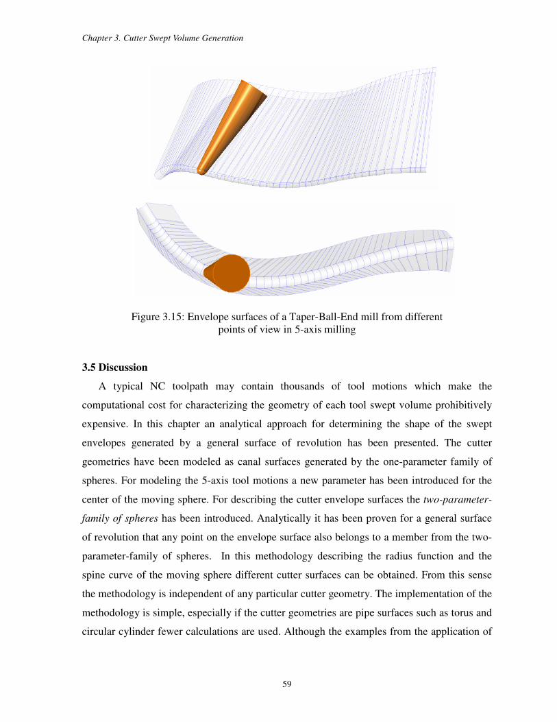
Chapter 3. Cutter Swept Volume Generation
59
Figure 3.15: Envelope surfaces of a Taper-Ball-End mill from different
points of view in 5-axis milling
3.5 Discussion
A typical NC toolpath may contain thousands of tool motions which make the
computational cost for characterizing the geometry of each tool swept volume prohibitively
expensive. In this chapter an analytical approach for determining the shape of the swept
envelopes generated by a general surface of revolution has been presented. The cutter
geometries have been modeled as canal surfaces generated by the one-parameter family of
spheres. For modeling the 5-axis tool motions a new parameter has been introduced for the
center of the moving sphere. For describing the cutter envelope surfaces the two-parameter-
family of spheres has been introduced. Analytically it has been proven for a general surface
of revolution that any point on the envelope surface also belongs to a member from the two-
parameter-family of spheres. In this methodology describing the radius function and the
spine curve of the moving sphere different cutter surfaces can be obtained. From this sense
the methodology is independent of any particular cutter geometry. The implementation of the
methodology is simple, especially if the cutter geometries are pipe surfaces such as torus and
circular cylinder fewer calculations are used. Although the examples from the application of
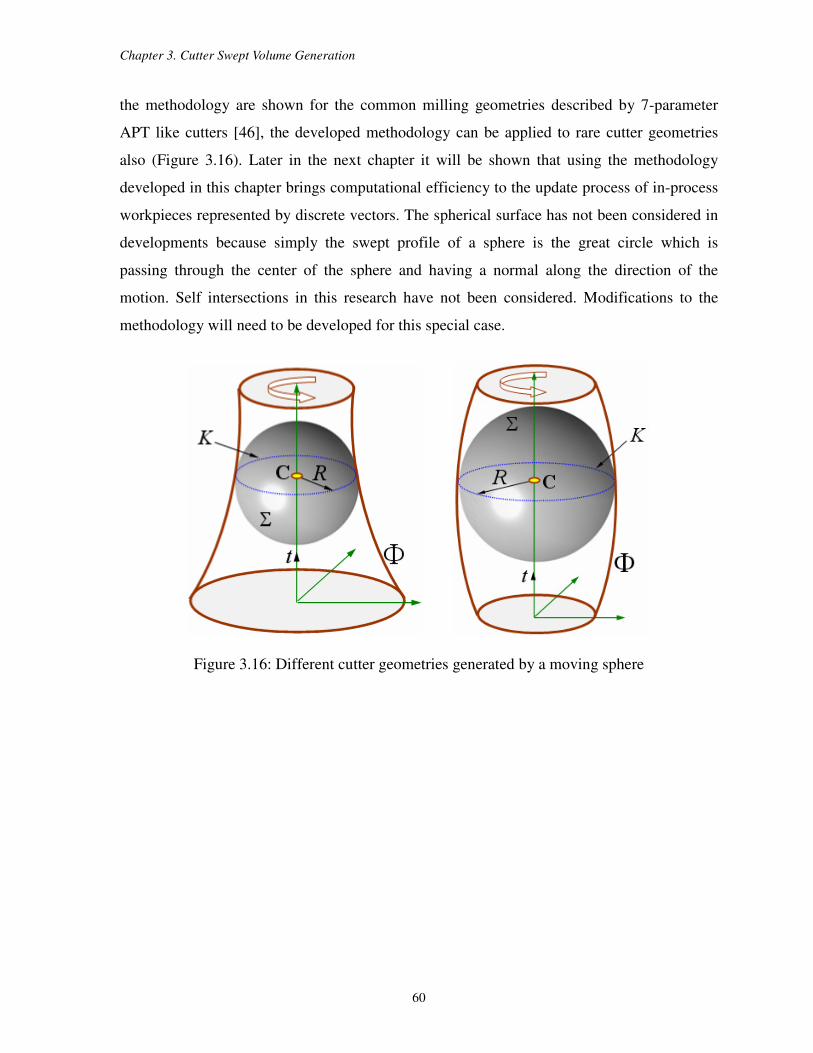
Chapter 3. Cutter Swept Volume Generation
60
the methodology are shown for the common milling geometries described by 7-parameter
APT like cutters [46], the developed methodology can be applied to rare cutter geometries
also (Figure 3.16). Later in the next chapter it will be shown that using the methodology
developed in this chapter brings computational efficiency to the update process of in-process
workpieces represented by discrete vectors. The spherical surface has not been considered in
developments because simply the swept profile of a sphere is the great circle which is
passing through the center of the sphere and having a normal along the direction of the
motion. Self intersections in this research have not been considered. Modifications to the
methodology will need to be developed for this special case.
Figure 3.16: Different cutter geometries generated by a moving sphere
61
Chapter 4
In-process Workpiece Modeling
In this chapter the methodologies for modeling the in-process workpiece in milling
operations are presented. During the machining simulation for each tool movement the
modification of the workpiece geometry is required to keep track of the material removal
process. Because the NC verification and Cutter Workpiece Engagement (CWE) extraction
are directly dependent on the material removal an accurate in-process workpiece modeling is
needed. Several choices for modeling the in-process work piece are exist. The two most
common are mathematically accurate solid modeling that is used in CAD systems and
approximate modeling such as those used in computer graphics: facetted and discrete vector
models. In the workpiece update process first the swept volume of a given tool movement in
the cutter location data file is modeled and then this volume is subtracted from the in-process
workpiece. For updating the workpiece surfaces represented by the solid or faceted models
third party softwares can be used. For example in the solid modeler based approach the cutter
swept volumes can be generated by using the ACIS solid modeling kernel and then using the
Boolean subtraction operation defined in this kernel the cutter swept volumes are subtracted
from the in-process workpiece. These update methodologies are briefly introduced in this
chapter. On the other hand for the workpiece geometries represented by discrete vectors
efficient in-process workpiece update methodologies for different cutter geometries
performing multi-axis machining are needed. In the literature [7,8,18,24,32,41,91] the
discrete vectors have orientations along the z-axis of the standard bases of R3. But when the
in-process workpiece has features like vertical walls and sharp edges, representing the
workpiece with one directional vectors generates less accurate results in visualization of the
final product [43] and CWE extractions. For increasing the accuracy more vectors with
different orientations are needed. But in this case localizing the cutter envelope during the
simulation becomes difficult and therefore the computational time increases. Therefore an
efficient localization methodology is required. Also in recent works [7,8] the tool axis has a
fixed orientation along the z-axis of the standard bases of R3 and the workpiece updates are
performed numerically for the milling cutter geometries. Therefore in this chapter the vector
Chapter 4. In-process Workpiece Modeling
62
based update methodologies are developed for the vectors having different orientations.
These methodologies allow multi-axis milling in which the tool may have an arbitrary
orientation in space. Also for the cutter geometries defined by a circular cylinder, frustum of
a cone, sphere and plane the updating calculations are performed analytically. For the torus
geometry numerical approaches with guaranteed root finding results are utilized.
The common milling cutter geometries are presented in section (4.2.1). In these
representations cutter surfaces are defined parametrically at the origin of the standard bases
of R3. In this section for derivations the properties of canal surfaces given in chapter (3) are
utilized. The vector based workpiece model and the localization of the cutter envelope are
presented in section (4.2.2). In the first part of this section a workpiece modeling strategy is
introduced and in the second part a localization methodology for the cutter envelope surfaces
is presented. The workpiece update methodologies in multi-axis milling for different cutter
geometries are presented in section (4.2.3). In the introduction part of this section the general
formulas for defining the cutter envelopes are derived and then in the following subsections
these formulas are utilized in the intersection calculations of different cutter geometries.
Examples from the implementation of the methodologies are shown in section (4.2.4), and
finally the chapter ends with the discussion in section (4.3).
4.1 Modeling the In-process Workpiece in Solid and Facetted representation
A solid modeler based in-process workpiece update is illustrated in Figure (4.1). Inputs
from a CAD/CAM system include the geometric representation of the initial workpiece, the
tool path and the geometric description of the cutting tool. In the first step, the swept volumes
of the cutting tool are generated for a given tool path. Then in the second step these swept
volumes are subtracted from the initial workpiece sequentially for obtaining the updated
workpiece (in-process workpiece). In this research for modeling the in-process workpiece
and the swept volume the B-rep based geometric modeler ACIS kernel and C++ is utilized.
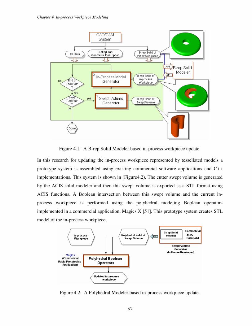
Chapter 4. In-process Workpiece Modeling
63
Figure 4.1: A B-rep Solid Modeler based in-process workpiece update.
In this research for updating the in-process workpiece represented by tessellated models a
prototype system is assembled using existing commercial software applications and C++
implementations. This system is shown in (Figure4.2). The cutter swept volume is generated
by the ACIS solid modeler and then this swept volume is exported as a STL format using
ACIS functions. A Boolean intersection between this swept volume and the current in-
process workpiece is performed using the polyhedral modeling Boolean operators
implemented in a commercial application, Magics X [51]. This prototype system creates STL
model of the in-process workpiece.
Figure 4.2: A Polyhedral Modeler based in-process workpiece update.
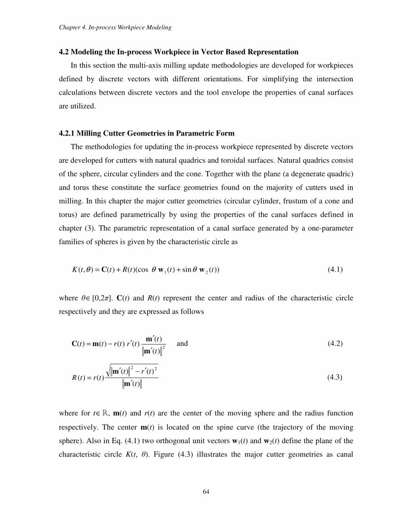
Chapter 4. In-process Workpiece Modeling
64
4.2 Modeling the In-process Workpiece in Vector Based Representation
In this section the multi-axis milling update methodologies are developed for workpieces
defined by discrete vectors with different orientations. For simplifying the intersection
calculations between discrete vectors and the tool envelope the properties of canal surfaces
are utilized.
4.2.1 Milling Cutter Geometries in Parametric Form
The methodologies for updating the in-process workpiece represented by discrete vectors
are developed for cutters with natural quadrics and toroidal surfaces. Natural quadrics consist
of the sphere, circular cylinders and the cone. Together with the plane (a degenerate quadric)
and torus these constitute the surface geometries found on the majority of cutters used in
milling. In this chapter the major cutter geometries (circular cylinder, frustum of a cone and
torus) are defined parametrically by using the properties of the canal surfaces defined in
chapter (3). The parametric representation of a canal surface generated by a one-parameter
families of spheres is given by the characteristic circle as
))(sin)()(cos()(),( 21 tttRttK wwC θθθ ++= (4.1)
where θ∈ [0,2π]. C(t) and R(t) represent the center and radius of the characteristic circle
respectively and they are expressed as follows
2
)(
)()()()()(
t
ttrtrtt
m
mmC
′
′′−= and (4.2)
)(
)()()()(
22
t
trttrtR
m
m
′
′−′= (4.3)
where for t∈R, m(t) and r(t) are the center of the moving sphere and the radius function
respectively. The center m(t) is located on the spine curve (the trajectory of the moving
sphere). Also in Eq. (4.1) two orthogonal unit vectors w1(t) and w2(t) define the plane of the
characteristic circle K(t, θ). Figure (4.3) illustrates the major cutter geometries as canal
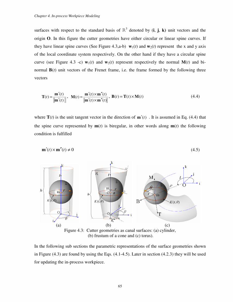
Chapter 4. In-process Workpiece Modeling
65
surfaces with respect to the standard basis of R3 denoted by (i, j, k) unit vectors and the
origin O. In this figure the cutter geometries have either circular or linear spine curves. If
they have linear spine curves (See Figure 4.3,a-b) w1(t) and w2(t) represent the x and y axis
of the local coordinate system respectively. On the other hand if they have a circular spine
curve (see Figure 4.3 -c) w1(t) and w2(t) represent respectively the normal M(t) and bi-
normal B(t) unit vectors of the Frenet frame, i.e. the frame formed by the following three
vectors
)(
)()(
t
tt
m
mT
′
′= ,
)()(
)()()(
tt
ttt
mm
mmM
′′×′
′′×′= , )()()( ttt MTB ×= (4.4)
where T(t) is the unit tangent vector in the direction of )(tm′ . It is assumed in Eq. (4.4) that
the spine curve represented by m(t) is biregular, in other words along m(t) the following
condition is fulfilled
0)()( ≠′′×′ tt mm (4.5)
(a) (b) (c)
Figure 4.3: Cutter geometries as canal surfaces: (a) cylinder,
(b) frustum of a cone and (c) torus).
In the following sub sections the parametric representations of the surface geometries shown
in Figure (4.3) are found by using the Eqs. (4.1-4.5). Later in section (4.2.3) they will be used
for updating the in-process workpiece.
Chapter 4. In-process Workpiece Modeling
66
4.2.1.1 Cylinder Surface
The cylinder surface can be parameterized by using the characteristic circle given in
Eq.(4.1). Two of the variables in this equation C(t) and R(t) depend on the center and the
radius function of a moving sphere. From Figure (4.3 -a), the center of a one-parameter
family of spheres can be written as
==
t
tt 0
0
)( km (4.6)
where the parameter t takes values between zero and the height of the cylinder, i.e. t∈[0,h].
The partial derivative of the Eq. (4.6) with respect to t equals to the unit vector k and
thus 1||)(|| =′ tm . As explained in chapter (3), the cylinder surface is also a pipe surface with a
constant radius r. Therefore the derivative of the radius function is equal to zero i.e. 0)( =′ tr .
Thus the center and the radius of the characteristic circle can be represented by C(t) = tk and
R(t) = r respectively. Plugging the center and the radius into Eq. (4.1) yields the cylinder
surface geometry in the following parametric form
( )
=++=
t
r
r
rttK cylinder θ
θ
θθθ sin
cos
sincos),( jik (4.7)
4.2.1.2 Frustum of a Cone Surface
As illustrated in Figure (4.3 -b), the origin of the standard basis O is located above the
cutter bottom center with distance equal to Rb tan α, where Rb and α represent the radius of
the cutter bottom and the cone half-angle respectively. The center of a moving sphere is
obtained by km tt =)( , where the limits of t from Figure (4.3-b) are defined by
∈
α2cos,0
ht (4.8)

Chapter 4. In-process Workpiece Modeling
67
where h represents the height. For the frustum of a cone surface the radius of a moving
sphere r(t) is given by
α
αcos
sin)( bRttr += (4.9)
When m(t), r(t) and their derivatives with respect to t are plugged into Eqs.(4.2) and (4.3),
the center and the radius of the characteristic circle is obtained as follows
C(t) = (t cos2α – Rb tan α ) k (4.10-a)
R(t) = t sinα cosα + Rb (4.10-b)
Plugging Eqs.(4.10-a,b) into Eq. (4.1) yields the frustum of a cone surface geometry in the
following parametric form
( ) ( ) ( )
( )( )
( )
−
+
+
=
+++−=
αα
θαα
θαα
θθααααθ
tancos
sincossin
coscossin
sincoscossintancos),(
2
2
b
b
b
bbfrustum
Rt
Rt
Rt
RtRttK jik
(4.11)
4.2.1.3 Torus Surface
In Figure (4.3-c) a torus surface is shown with the origin O in the center of the torus. For
a torus the spine curve is a circle and therefore the center of a moving sphere is obtained by
=+=
0
sin
cos
sincos)( t
t
ttt ρ
ρ
ρρ
j i m (4.12)
where ρ is the major radius of the torus and t∈[0, 2π]. The partial derivative of Eq. (4.12)
with respect to t is obtained as follows

Chapter 4. In-process Workpiece Modeling
68
j i m ttt cossin)( ρρ +−=′ (4.13)
As a pipe surface torus has a constant radius r and therefore 0)( =′ tr . When )(tm , )(tm′ , r(t)
and )(tr ′ are plugged into Eqs.(4.2) and (4.3), the center and the radius of the characteristic
circle are obtained as follows
j i C ttt sincos)( ρρ += (4.14-a)
rtR =)( (4.14-b)
Also for describing the characteristic circle of the torus the components of the Frenet frame
are needed. For this purpose the partial derivative of Eq.(4.13) with respect to t is obtained as
follows
j i m tRtRt sincos)( −−=′′ (4.15)
Plugging )(tm , )(tm′ and )(tm ′′ into Eq. (4.4) yields
T(t) = – sint i + cost j, M(t) = k, B(t) = cost i+ sint j (4.16)
Finally plugging Eqs. (4.14-a,b) and (4.16) into Eq. (4.1) yields torus surface geometry in the
following parametric form
( )( )
( )( )
+
+
=
++++=
θ
θρ
θρ
θθρρθ
cos
sinsin
cossin
sincossincoscoscos),(
r
tr
tr
ttrtttK torus jikji
(4.17)
4.2.2 Workpiece Model and Localization
There are two main approaches for representing the in-process workpiece using discrete
vectors [43]: Discrete Normal Vector and Discrete Vertical Vector approaches. In the
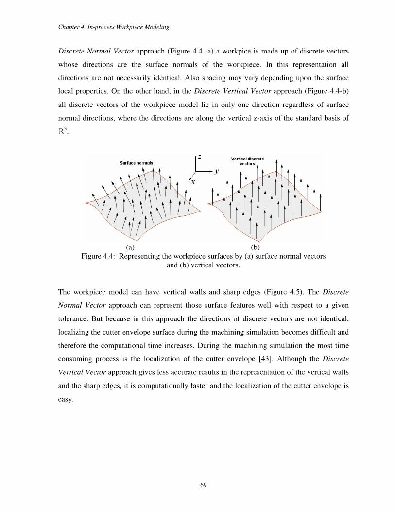
Chapter 4. In-process Workpiece Modeling
69
Discrete Normal Vector approach (Figure 4.4 -a) a workpice is made up of discrete vectors
whose directions are the surface normals of the workpiece. In this representation all
directions are not necessarily identical. Also spacing may vary depending upon the surface
local properties. On the other hand, in the Discrete Vertical Vector approach (Figure 4.4-b)
all discrete vectors of the workpiece model lie in only one direction regardless of surface
normal directions, where the directions are along the vertical z-axis of the standard basis of
R3.
(a) (b)
Figure 4.4: Representing the workpiece surfaces by (a) surface normal vectors
and (b) vertical vectors.
The workpiece model can have vertical walls and sharp edges (Figure 4.5). The Discrete
Normal Vector approach can represent those surface features well with respect to a given
tolerance. But because in this approach the directions of discrete vectors are not identical,
localizing the cutter envelope surface during the machining simulation becomes difficult and
therefore the computational time increases. During the machining simulation the most time
consuming process is the localization of the cutter envelope [43]. Although the Discrete
Vertical Vector approach gives less accurate results in the representation of the vertical walls
and the sharp edges, it is computationally faster and the localization of the cutter envelope is
easy.
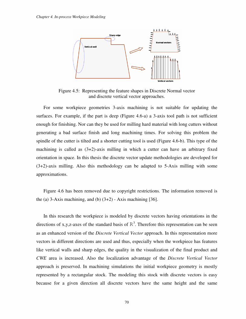
Chapter 4. In-process Workpiece Modeling
70
Figure 4.5: Representing the feature shapes in Discrete Normal vector
and discrete vertical vector approaches.
For some workpiece geometries 3-axis machining is not suitable for updating the
surfaces. For example, if the part is deep (Figure 4.6-a) a 3-axis tool path is not sufficient
enough for finishing. Nor can they be used for milling hard material with long cutters without
generating a bad surface finish and long machining times. For solving this problem the
spindle of the cutter is tilted and a shorter cutting tool is used (Figure 4.6-b). This type of the
machining is called as (3+2)-axis milling in which a cutter can have an arbitrary fixed
orientation in space. In this thesis the discrete vector update methodologies are developed for
(3+2)-axis milling. Also this methodology can be adapted to 5-Axis milling with some
approximations.
Figure 4.6 has been removed due to copyright restrictions. The information removed is
the (a) 3-Axis machining, and (b) (3+2) - Axis machining [36].
In this research the workpiece is modeled by discrete vectors having orientations in the
directions of x,y,z-axes of the standard basis of R3. Therefore this representation can be seen
as an enhanced version of the Discrete Vertical Vector approach. In this representation more
vectors in different directions are used and thus, especially when the workpiece has features
like vertical walls and sharp edges, the quality in the visualization of the final product and
CWE area is increased. Also the localization advantage of the Discrete Vertical Vector
approach is preserved. In machining simulations the initial workpiece geometry is mostly
represented by a rectangular stock. The modeling this stock with discrete vectors is easy
because for a given direction all discrete vectors have the same height and the same
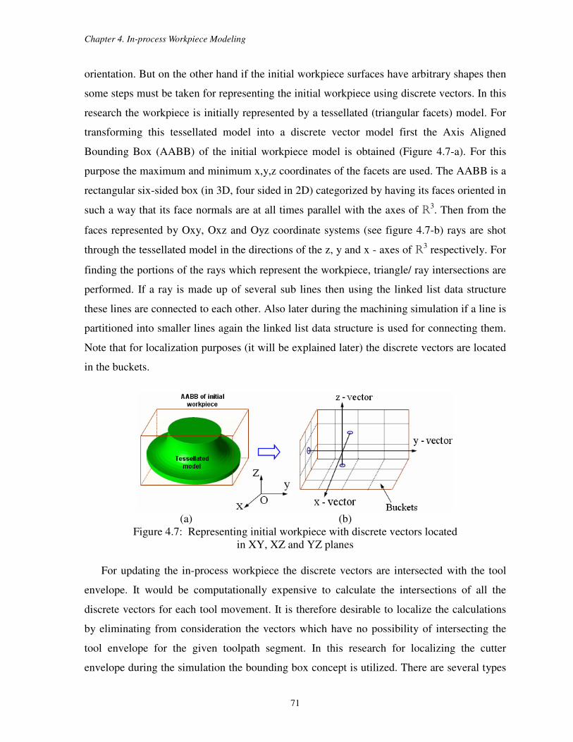
Chapter 4. In-process Workpiece Modeling
71
orientation. But on the other hand if the initial workpiece surfaces have arbitrary shapes then
some steps must be taken for representing the initial workpiece using discrete vectors. In this
research the workpiece is initially represented by a tessellated (triangular facets) model. For
transforming this tessellated model into a discrete vector model first the Axis Aligned
Bounding Box (AABB) of the initial workpiece model is obtained (Figure 4.7-a). For this
purpose the maximum and minimum x,y,z coordinates of the facets are used. The AABB is a
rectangular six-sided box (in 3D, four sided in 2D) categorized by having its faces oriented in
such a way that its face normals are at all times parallel with the axes of R3. Then from the
faces represented by Oxy, Oxz and Oyz coordinate systems (see figure 4.7-b) rays are shot
through the tessellated model in the directions of the z, y and x - axes of R3 respectively. For
finding the portions of the rays which represent the workpiece, triangle/ ray intersections are
performed. If a ray is made up of several sub lines then using the linked list data structure
these lines are connected to each other. Also later during the machining simulation if a line is
partitioned into smaller lines again the linked list data structure is used for connecting them.
Note that for localization purposes (it will be explained later) the discrete vectors are located
in the buckets.
(a) (b)
Figure 4.7: Representing initial workpiece with discrete vectors located
in XY, XZ and YZ planes
For updating the in-process workpiece the discrete vectors are intersected with the tool
envelope. It would be computationally expensive to calculate the intersections of all the
discrete vectors for each tool movement. It is therefore desirable to localize the calculations
by eliminating from consideration the vectors which have no possibility of intersecting the
tool envelope for the given toolpath segment. In this research for localizing the cutter
envelope during the simulation the bounding box concept is utilized. There are several types

Chapter 4. In-process Workpiece Modeling
72
of bounding boxes in 2D space such as a circle, Axis Aligned Bounding Box (AABB),
Oriented Bounding Box (OBB), convex hull etc. There is always a tradeoff between a better
bound and a faster test in these approaches. For this research the AABB approach in 2D
space is utilized. The best feature of the AABB is its fast overlap check, which simply
involves direct comparison of individual coordinate values. In this work for a given tool
movement three AABBs which are the projections of the tool envelope on to Oxy, Oxz and
Oyz coordinate systems are generated. In the following section the steps for obtaining the
AABB of the tool envelope in Oxy coordinate system are given. The AABBs in Oxz and Oyz
coordinate systems can be obtained following the same steps. The localization of the tool
envelope in Oxy coordinate system has four steps. For these steps please refer to Figure (4.8).
In this figure a Taper-Ball-End mill is moving between the cutter locations PS and PE.
Step 1: Finding the bounding cylinder in 3D: In this step at the cutter location point PS the
bounding cylinder of the cutter having an orientation in the direction of the tool axis is found.
The dimensions of the bounding cylinder are defined by the height and the largest radius of
the cutter. For example for the Taper-Ball-End mill shown in (Figure 4.8) the top circle (ctop)
has the largest radius r. Therefore using the same radius r the bottom circle (cbottom) of the
bounding cylinder can be obtained. The center of the cbottom is located at the tool tip point of
the cutter. There is a symmetry plane which contains the tool rotation axis and passes through
the centers of the ctop and cbottom. The normal vector of this plane (Nplane) can be obtained
by ]100[plane ×= nN . Intersecting this plane with ctop and cbottom of the bounding cylinder
generates four points I1, I2, I3, and I4 respectively in 3D space.
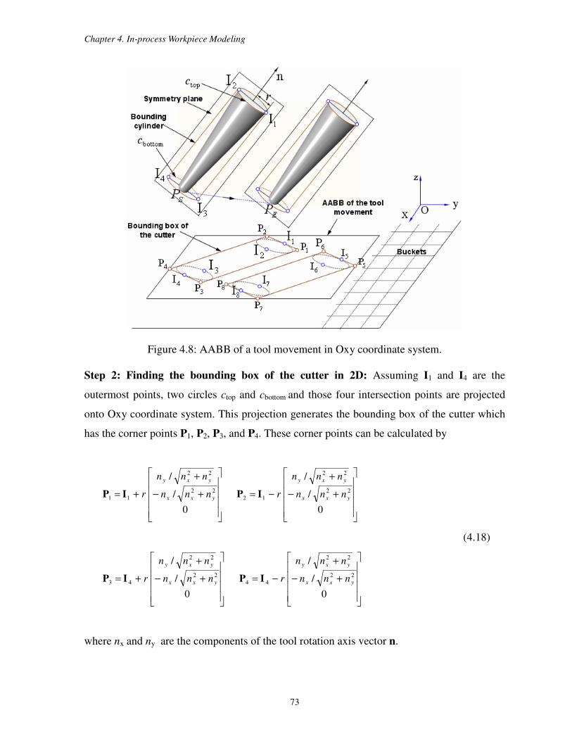
Chapter 4. In-process Workpiece Modeling
73
Figure 4.8: AABB of a tool movement in Oxy coordinate system.
Step 2: Finding the bounding box of the cutter in 2D: Assuming I1 and I4 are the
outermost points, two circles ctop and cbottom and those four intersection points are projected
onto Oxy coordinate system. This projection generates the bounding box of the cutter which
has the corner points P1, P2, P3, and P4. These corner points can be calculated by
+−
+
+=
0
/
/
22
22
11 yxx
yxy
nnn
nnn
rIP
+−
+
−=
0
/
/
22
22
12 yxx
yxy
nnn
nnn
rIP
(4.18)
+−
+
+=
0
/
/
22
22
43 yxx
yxy
nnn
nnn
rIP
+−
+
−=
0
/
/
22
22
44 yxx
yxy
nnn
nnn
rIP
where nx and ny are the components of the tool rotation axis vector n.
Chapter 4. In-process Workpiece Modeling
74
Step 3: Finding the AABB of the tool movement: In this stage first using the same steps (1
and 2) the bounding box of the cutter for the location of PE is found. Now there are two
bounding boxes with eight corner points in Oxy coordinate system. Then using the minimum
and maximum x and y coordinates of those eight corner points (P1 to P8) the AABB of the
tool movement is obtained. Note that because the tool performs a motion with a constant
orientation, the projections of the intermediate tool motions between PS and PE are also
contained in the same AABB of the tool movement.
Step 4: Finding the set of buckets: In this step the overlap check is performed between the
buckets and the AABB of the tool movement. The buckets in Oxy coordinate system can be
thought as AABBs. For finding the overlapping buckets the AABB – AABB intersection is
performed. The algorithm for this test can be found in [27]. If an overlap is found then the
discrete vectors in the overlapping bucket are used for the intersection test for updating the
in-process workpiece. Thus only a small percentage of all the discrete vectors are examined
for each tool movement. The intersections will be shown in the next section for different
cutter geometries.
4.2.3 Updating In-process Workpiece in Multi-Axis Milling
In this section the in-process workpiece surfaces are updated by using different milling
cutters. Although in section (4.2.2) the discrete vectors have orientations along the x, y and z-
axes of the standard basis of R3, in this section the update formulas will be derived for the
general case in which the discrete vectors have arbitrary orientations. Also for the
calculations (3+2)-axis milling in which a cutter can have an arbitrary fixed orientation in
space is considered.
In multi-axis milling tool motions are represented by the trajectory of the tool control
point F(u) and the instantaneous orientation of the tool axis A(u) which is always coincident
with the tool rotation axis, where u∈[0,1]. In section (4.2.1) the major cutter geometries are
parametrically defined with respect to the standard basis of R3 which has an origin at O. In
this section the control points of these geometries are defined with respect to the location
which corresponds to O. For example the location of the control point for the cylindrical
surface is at the bottom radial center, for the frustum of a cone surface it is above the bottom
radial center with distance equals to Rb tanα and for the toroidal surface it is at the center of
Chapter 4. In-process Workpiece Modeling
75
the torus. A complex toolpath can be considered as the combination of line segments, where
each segment represents the linear distance between two consecutive cutter location points.
For a linear tool path (line segment) the control point can be expressed with respect to the
tool path start PS(xS,yS,zS) and end PE(xE, yE,zE) coordinates as follows
F(u) = PS + (PE - PS ) u (4.19)
where the difference of (PE - PS) is called as the instantaneous feed direction denoted by f.
Note that for the (3+2)-axis machining the instantaneous tool orientation A(u) is fixed
between the tool locations PS and PE. Two sets of coordinate systems are used in this paper.
A Work Piece Coordinate System (WCS) which is coincident with the standard basis of
R3denoted by unit vectors [i j k], and a local Tool Coordinate System (TCS) denoted by unit
vectors [d e n]. Using F and A, one can define TCS on the tool defined by a set of mutually
orthogonal unit vectors n, d, and e. The TCS is defined as
|A|/An == ][ zyx nnn (4.20)
if 0≠∂
∂×
u
FA then
||
][
u
ueee zyx
∂
∂×
∂
∂×
==F
A
FA
e and ned ×== ][ zyx ddd
According to above definitions it is not allowed for the cutter to plunge along its rotational
axis A(u). Also it is assumed that the d axis of the TCS is aligned with the instantaneous feed
direction. In this work the discrete vectors which represent the workpiece are defined by
( ) vIIIvI aba −+=)( (4.21)
where v∈[0, 1] and also ( )aaaa zyxI ,, and ( )bbbb zyxI ,, are the start and end points of a vector
respectively. If the cutter surfaces parameterized in section (4.2.1) move with respect to TCS
a point on the cutter surface can be described in WCS as follows
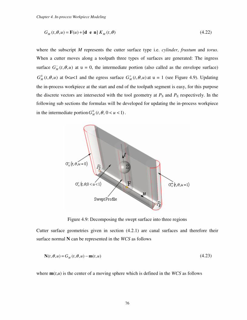
Chapter 4. In-process Workpiece Modeling
76
),(][)(),,( θθ tKuutG MM nedF += (4.22)
where the subscript M represents the cutter surface type i.e. cylinder, frustum and torus.
When a cutter moves along a toolpath three types of surfaces are generated: The ingress
surface ),,( utGM θ− at u = 0, the intermediate portion (also called as the envelope surface)
),,(0 utGM θ at 0<u<1 and the egress surface ),,( utGM θ+ at u = 1 (see Figure 4.9). Updating
the in-process workpiece at the start and end of the toolpath segment is easy, for this purpose
the discrete vectors are intersected with the tool geometry at PS and PE respectively. In the
following sub sections the formulas will be developed for updating the in-process workpiece
in the intermediate portion )10,,(0 << utGM θ .
Figure 4.9: Decomposing the swept surface into three regions
Cutter surface geometries given in section (4.2.1) are canal surfaces and therefore their
surface normal N can be represented in the WCS as follows
),(),,(),,( ututGut M mN −= θθ (4.23)
where m(t,u) is the center of a moving sphere which is defined in the WCS as follows
Chapter 4. In-process Workpiece Modeling
77
)(][)(),( tuut mnedFm += (4.24)
A point on the envelope surface is embedded in ),,( utGM θ and also the surface normal (N)
passing through it is perpendicular to the velocity vector at the center of the moving sphere.
In (3+2)-axis milling with linear toolpath the velocity vector is equal to the feed direction
vector (f). Therefore for an arbitrary point on the envelope surface the following dot product
equation holds
0),,(),,(0 == f·N ututGM θθ (4.25)
Plugging Eq. (4.23) into the above equation yields
( ) 0),(),,( =− f·m ututGM θ (4.26)
The above equation is solved for θ with respect to the given values of parameters u and t.
There are three possible solutions for θ: two distinct real solutions θ1,2 , two equal real
solutions 21 θθ = , and no real solution. Plugging the values of θ into Eq. (4.22) yields the
locations of the points on the envelope surface
),(][)(),,( 2,12,12,1 θθ tKuPutG MM nedF +== (4.27)
where P1,2 represents two points which correspond to θ1,2 respectively. As explained in
chapter (3), the circular cylinder and torus are pipe surfaces. By definition a pipe surface is
described as an envelope of the family of the spheres with a constant radius. The spine curve
(also called as trajectory) of a moving sphere is a line for the cylinder and a circle for the
torus. It has been proven in chapter (3) that for the circular cylinder and torus surfaces there
is an alternative solution in finding the location of an arbitrary point on the envelope surface.
In this alternative solution the normal vector passing through a point on the envelope surface
can be obtained by

Chapter 4. In-process Workpiece Modeling
78
t
ut
u
utut
∂
∂×
∂
∂=
),(),(),(
mmN (4.28)
Then using the above equation the coordinates of an arbitrary point on the envelope surface
with respect to the given values of u and t are found by
||),(||
),(),(2,1
ut
utrutP
N
Nm m= (4.29)
where r is the radius of the moving sphere. In Eq. (4.29) the signs (m ) indicates that there are
two opposite points on the cutter envelope surface with an angular difference equals to 1800.
The formulas developed in this section will be used in the following sub sections for different
cutter geometries.
4.2.3.1 Updating with Flat-End mill
A Flat-End mill is made up of a cylindrical surface at the side and a flat surface at the
bottom. Depending on the feed vector direction the cylindrical and flat surfaces engage with
the workpiece within [0,π] and [0,2π] angular ranges respectively. In the following two
subsections the analytical formulas will be derived for these surfaces.
Cylindrical surface
As explained before the circular cylinder is a pipe surface and a location of a point on the
envelope surface can be found with either Eq. (4.27) or Eq. (4.29). Because of its simplicity
the Eq. (4.29) will be used in derivations. The center of the moving sphere for the cylindrical
surface can be obtained by plugging Eqs. (4.6) and (4.19) into Eq. (4.24)
( )
+−+=
t
uPPPut SES 0
0
][),( nedm (4.30)
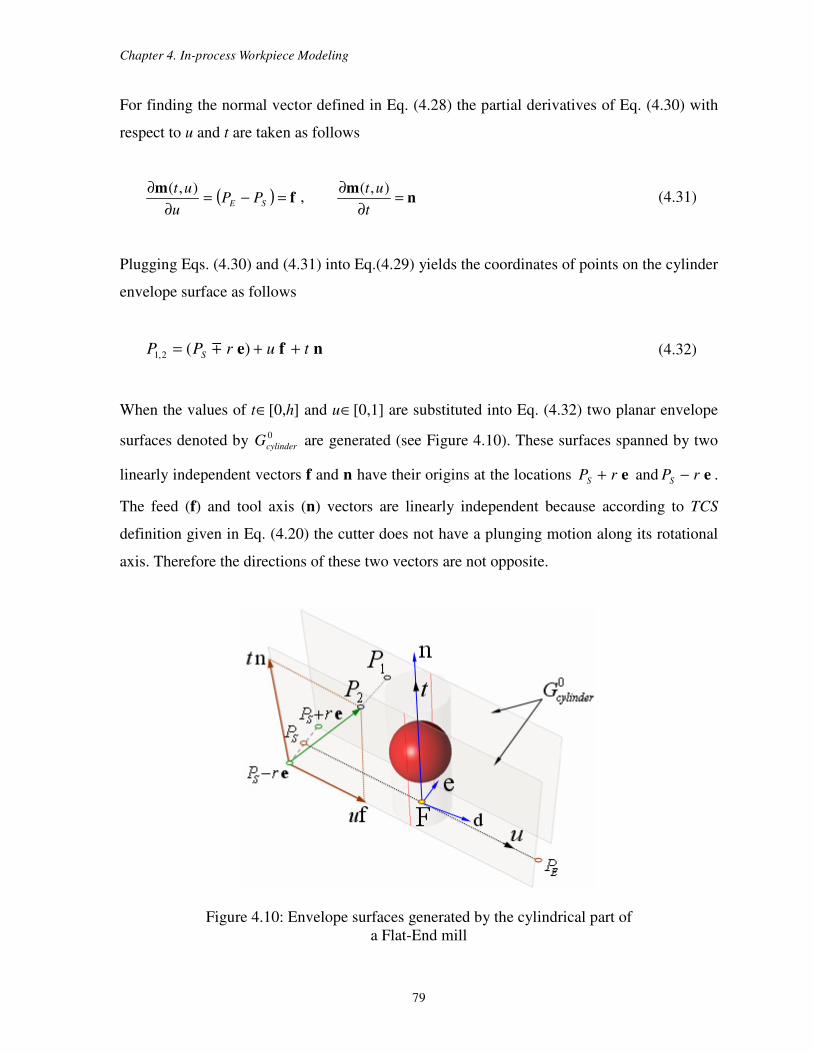
Chapter 4. In-process Workpiece Modeling
79
For finding the normal vector defined in Eq. (4.28) the partial derivatives of Eq. (4.30) with
respect to u and t are taken as follows
( ) fm
=−=∂
∂SE PP
u
ut ),(, n
m=
∂
∂
t
ut ),( (4.31)
Plugging Eqs. (4.30) and (4.31) into Eq.(4.29) yields the coordinates of points on the cylinder
envelope surface as follows
nfe turPP S ++= )(2,1 m (4.32)
When the values of t∈[0,h] and u∈[0,1] are substituted into Eq. (4.32) two planar envelope
surfaces denoted by 0
cylinderG are generated (see Figure 4.10). These surfaces spanned by two
linearly independent vectors f and n have their origins at the locations erPS + and erPS − .
The feed (f) and tool axis (n) vectors are linearly independent because according to TCS
definition given in Eq. (4.20) the cutter does not have a plunging motion along its rotational
axis. Therefore the directions of these two vectors are not opposite.
Figure 4.10: Envelope surfaces generated by the cylindrical part of
a Flat-End mill
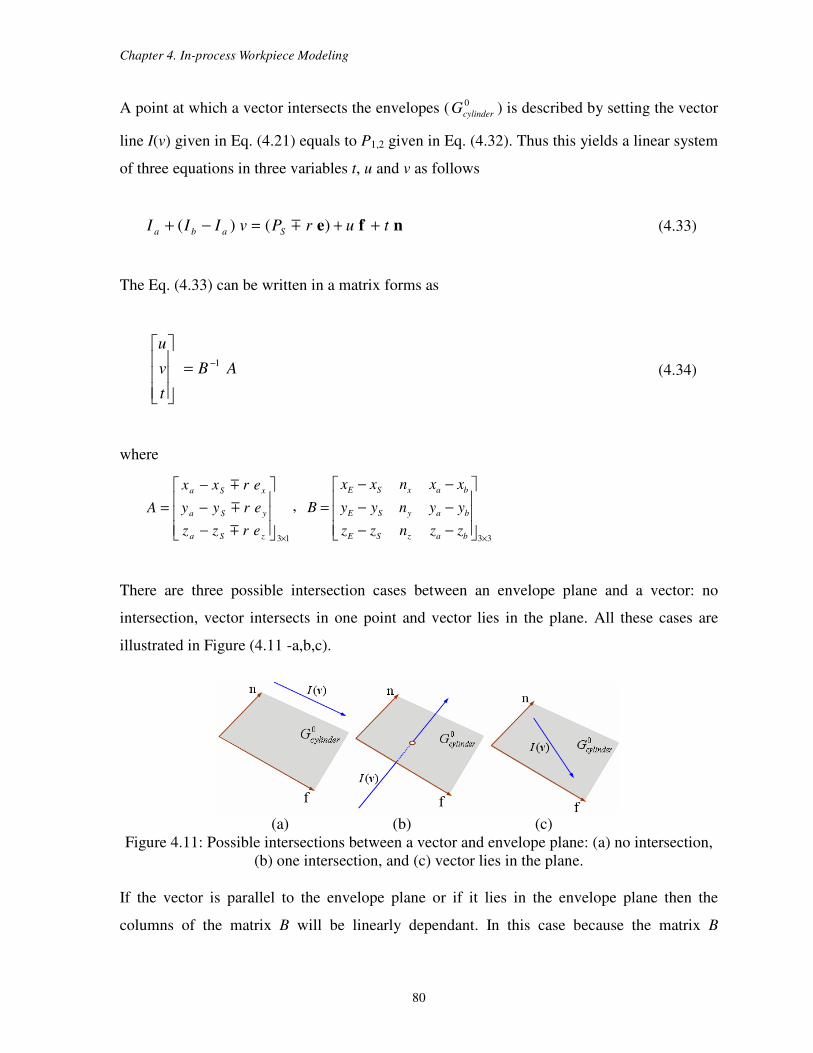
Chapter 4. In-process Workpiece Modeling
80
A point at which a vector intersects the envelopes ( 0
cylinderG ) is described by setting the vector
line I(v) given in Eq. (4.21) equals to P1,2 given in Eq. (4.32). Thus this yields a linear system
of three equations in three variables t, u and v as follows
nfe turPvIII Saba ++=−+ )()( m (4.33)
The Eq. (4.33) can be written in a matrix forms as
AB
t
v
u1−=
(4.34)
where
13×
−
−
−
=
zSa
ySa
xSa
erzz
eryy
erxx
A
m
m
m
,
33×
−−
−−
−−
=
bazSE
baySE
baxSE
zznzz
yynyy
xxnxx
B
There are three possible intersection cases between an envelope plane and a vector: no
intersection, vector intersects in one point and vector lies in the plane. All these cases are
illustrated in Figure (4.11 -a,b,c).
(a) (b) (c)
Figure 4.11: Possible intersections between a vector and envelope plane: (a) no intersection,
(b) one intersection, and (c) vector lies in the plane.
If the vector is parallel to the envelope plane or if it lies in the envelope plane then the
columns of the matrix B will be linearly dependant. In this case because the matrix B
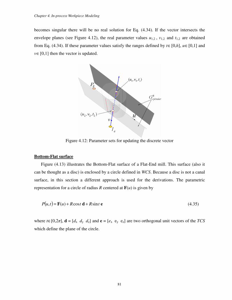
Chapter 4. In-process Workpiece Modeling
81
becomes singular there will be no real solution for Eq. (4.34). If the vector intersects the
envelope planes (see Figure 4.12), the real parameter values u1,2 , v1,2 and t1,2 are obtained
from Eq. (4.34). If these parameter values satisfy the ranges defined by t∈[0,h], u∈[0,1] and
v∈[0,1] then the vector is updated.
Figure 4.12: Parameter sets for updating the discrete vector
Bottom-Flat surface
Figure (4.13) illustrates the Bottom-Flat surface of a Flat-End mill. This surface (also it
can be thought as a disc) is enclosed by a circle defined in WCS. Because a disc is not a canal
surface, in this section a different approach is used for the derivations. The parametric
representation for a circle of radius R centered at F(u) is given by
( ) edF tRtRutuP sincos)(, ++= (4.35)
where t∈[0,2π], d = [dx dy dz] and e = [ex ey ez] are two orthogonal unit vectors of the TCS
which define the plane of the circle.
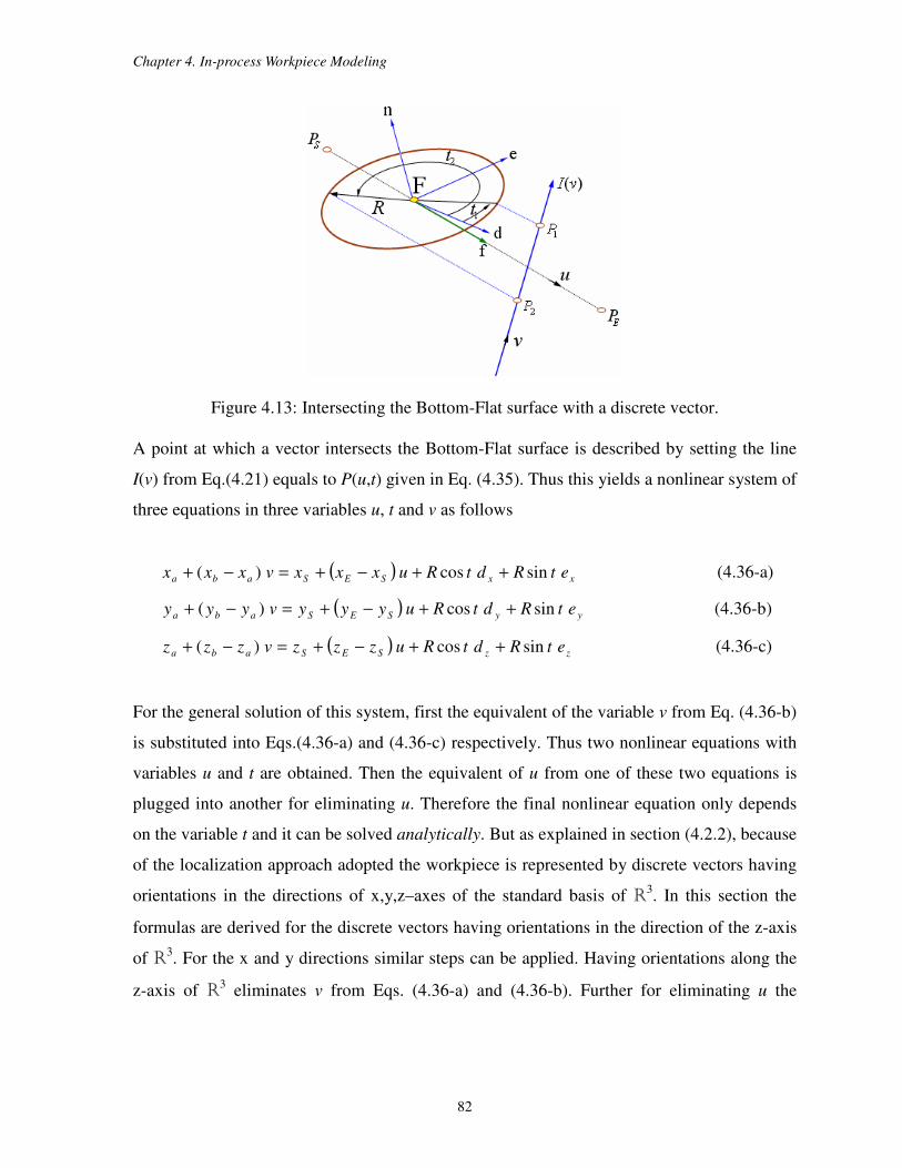
Chapter 4. In-process Workpiece Modeling
82
Figure 4.13: Intersecting the Bottom-Flat surface with a discrete vector.
A point at which a vector intersects the Bottom-Flat surface is described by setting the line
I(v) from Eq.(4.21) equals to P(u,t) given in Eq. (4.35). Thus this yields a nonlinear system of
three equations in three variables u, t and v as follows
( ) xxSESaba etRdtRuxxxvxxx sincos)( ++−+=−+ (4.36-a)
( ) yySESaba etRdtRuyyyvyyy sincos)( ++−+=−+ (4.36-b)
( ) zzSESaba etRdtRuzzzvzzz sincos)( ++−+=−+ (4.36-c)
For the general solution of this system, first the equivalent of the variable v from Eq. (4.36-b)
is substituted into Eqs.(4.36-a) and (4.36-c) respectively. Thus two nonlinear equations with
variables u and t are obtained. Then the equivalent of u from one of these two equations is
plugged into another for eliminating u. Therefore the final nonlinear equation only depends
on the variable t and it can be solved analytically. But as explained in section (4.2.2), because
of the localization approach adopted the workpiece is represented by discrete vectors having
orientations in the directions of x,y,z–axes of the standard basis of R3. In this section the
formulas are derived for the discrete vectors having orientations in the direction of the z-axis
of R3. For the x and y directions similar steps can be applied. Having orientations along the
z-axis of R3 eliminates v from Eqs. (4.36-a) and (4.36-b). Further for eliminating u the
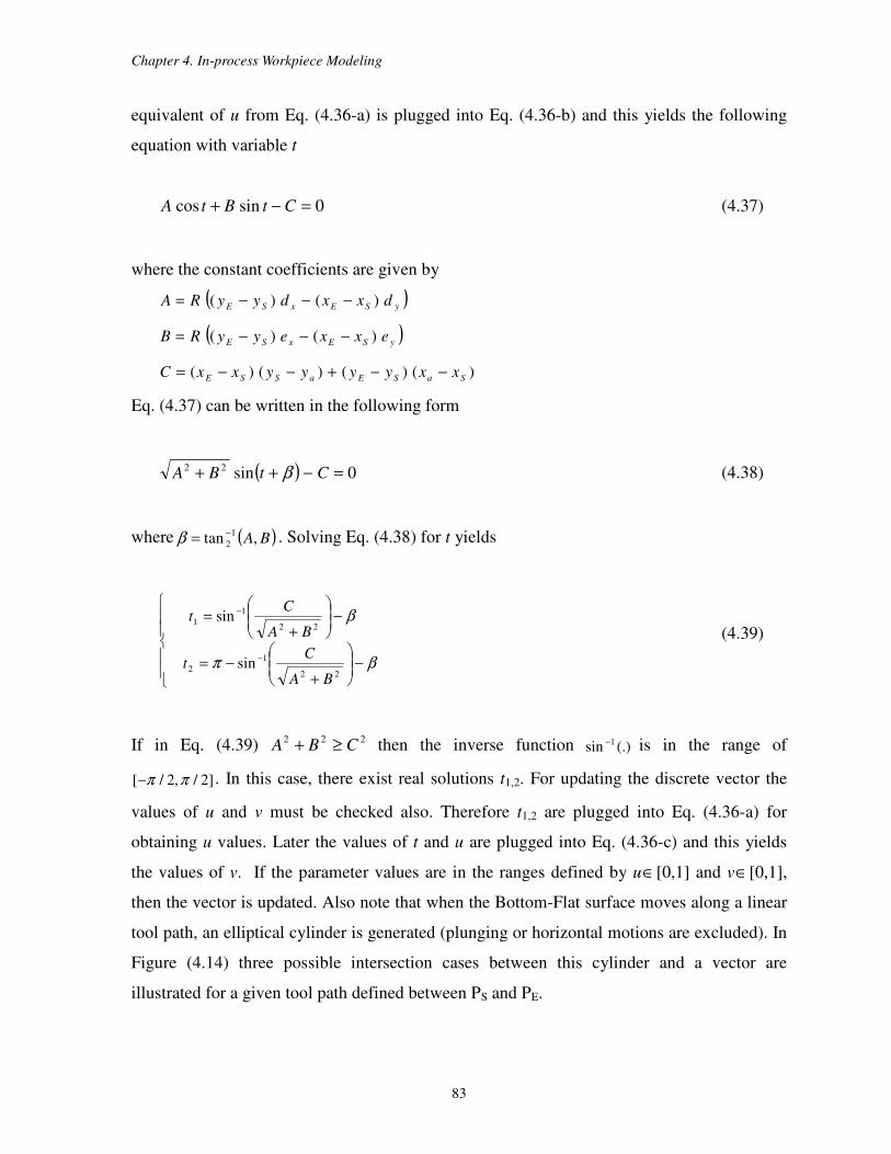
Chapter 4. In-process Workpiece Modeling
83
equivalent of u from Eq. (4.36-a) is plugged into Eq. (4.36-b) and this yields the following
equation with variable t
0sincos =−+ CtBtA (4.37)
where the constant coefficients are given by
( )ySExSE dxxdyyRA )()( −−−=
( )ySExSE exxeyyRB )()( −−−=
)()()()( SaSEaSSE xxyyyyxxC −−+−−=
Eq. (4.37) can be written in the following form
( ) 0sin22 =−++ CtBA β (4.38)
where ( )BA,tan1
2
−=β . Solving Eq. (4.38) for t yields
−
+−=
−
+=
−
−
βπ
β
22
1
2
22
1
1
sin
sin
BA
Ct
BA
Ct
(4.39)
If in Eq. (4.39) 222CBA ≥+ then the inverse function (.)sin 1− is in the range of
]2/,2/[ ππ− . In this case, there exist real solutions t1,2. For updating the discrete vector the
values of u and v must be checked also. Therefore t1,2 are plugged into Eq. (4.36-a) for
obtaining u values. Later the values of t and u are plugged into Eq. (4.36-c) and this yields
the values of v. If the parameter values are in the ranges defined by u∈[0,1] and v∈[0,1],
then the vector is updated. Also note that when the Bottom-Flat surface moves along a linear
tool path, an elliptical cylinder is generated (plunging or horizontal motions are excluded). In
Figure (4.14) three possible intersection cases between this cylinder and a vector are
illustrated for a given tool path defined between PS and PE.
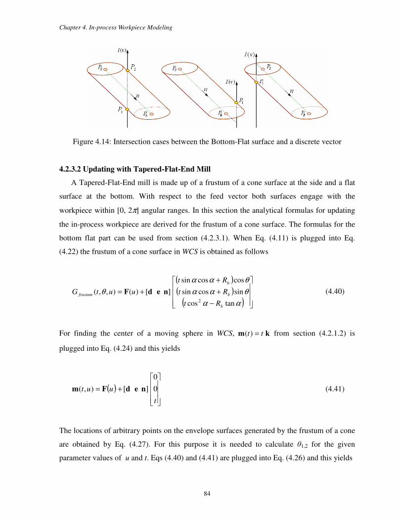
Chapter 4. In-process Workpiece Modeling
84
Figure 4.14: Intersection cases between the Bottom-Flat surface and a discrete vector
4.2.3.2 Updating with Tapered-Flat-End Mill
A Tapered-Flat-End mill is made up of a frustum of a cone surface at the side and a flat
surface at the bottom. With respect to the feed vector both surfaces engage with the
workpiece within [0, 2π] angular ranges. In this section the analytical formulas for updating
the in-process workpiece are derived for the frustum of a cone surface. The formulas for the
bottom flat part can be used from section (4.2.3.1). When Eq. (4.11) is plugged into Eq.
(4.22) the frustum of a cone surface in WCS is obtained as follows
( )( )
( )
−
+
+
+=
αα
θαα
θαα
θ
tancos
sincossin
coscossin
][)(),,(2
b
b
b
frustum
Rt
Rt
Rt
uutG nedF (4.40)
For finding the center of a moving sphere in WCS, km tt =)( from section (4.2.1.2) is
plugged into Eq. (4.24) and this yields
( )
+=
t
uut 0
0
][),( nedFm (4.41)
The locations of arbitrary points on the envelope surfaces generated by the frustum of a cone
are obtained by Eq. (4.27). For this purpose it is needed to calculate θ1,2 for the given
parameter values of u and t. Eqs (4.40) and (4.41) are plugged into Eq. (4.26) and this yields

Chapter 4. In-process Workpiece Modeling
85
(t sinα cosα + Rb )cosθ (d • f) - (t sin2α + Rb tan α )(n • f) = 0 (4.42)
Notice that e • f = 0. When the Eq.(4.42) is solved for θ the following equation is obtained
•
•= −
fd
fnαθ tancos 1
2,1 m (4.43)
Plugging Eqs.(4.43), (4.11) and (4.19) into Eq.(4.27) yields the following envelope surface
equation for the frustum of a cone
Gfrustum(t,θ1,2,u) = PS + (PE - PS ) u + (t sinα cosα + Rb )cosθ1,2 d
+ (t sinα cosα + Rb )sinθ1,2 e + (t cos2α – Rb tan α )n (4.44)
The above equation can be rearranged as follows
Gfrustum(t,θ1,2,u) = O1,2 + u f + k S1,2 (4.45)
where
O1,2 = PS + Rb cosθ1,2 d + Rb sinθ1,2 e – Rb tan α n
S1,2 = sinα cosθ1,2 d + sinα sinθ1,2 e + cosα n
k = t cosα
When the values of ]cos/,0[ 2 αht ∈ and u∈[0,1] are substituted into Eq. (4.45) two planar
envelope surfaces are generated (see Figure 4.15). These envelope surfaces spanned by
linearly independent vectors f and S1,2 have origins at O1,2 .
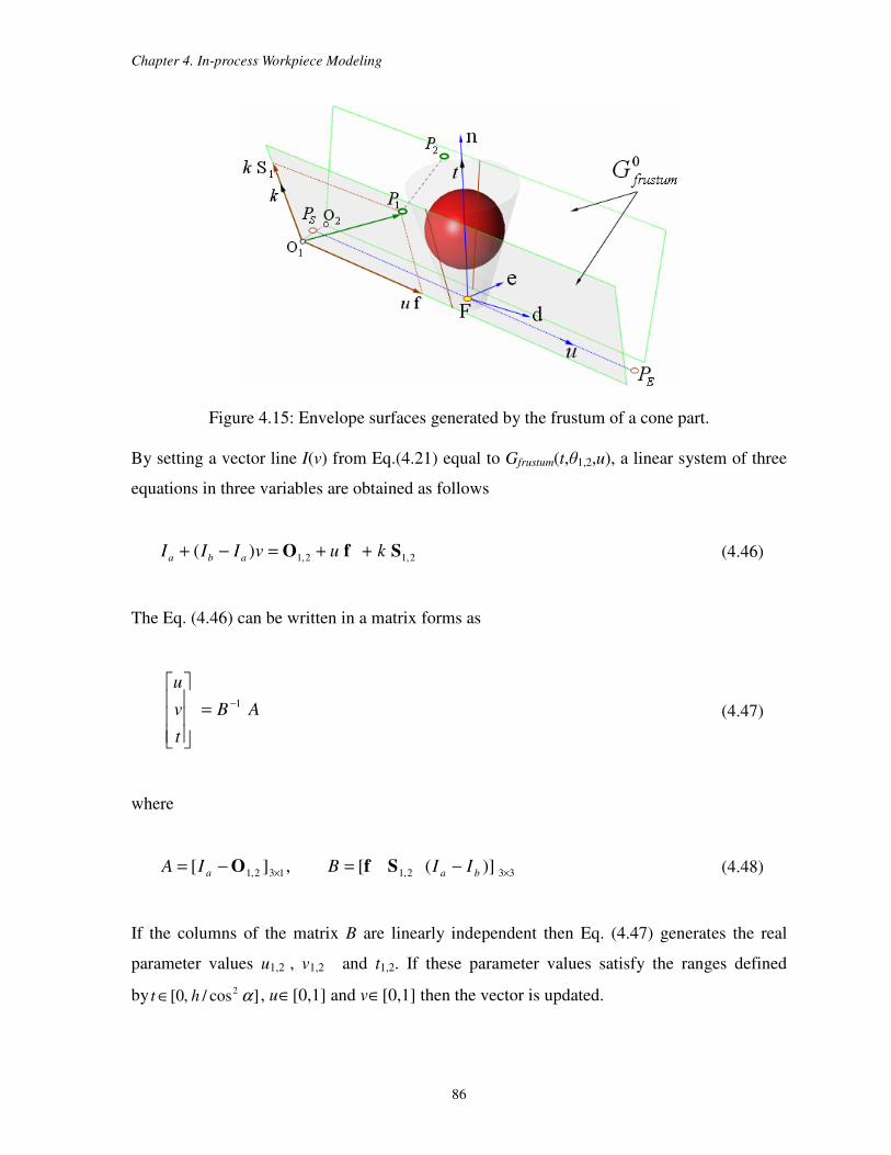
Chapter 4. In-process Workpiece Modeling
86
Figure 4.15: Envelope surfaces generated by the frustum of a cone part.
By setting a vector line I(v) from Eq.(4.21) equal to Gfrustum(t,θ1,2,u), a linear system of three
equations in three variables are obtained as follows
2,12,1)( SfO kuvIII aba ++=−+ (4.46)
The Eq. (4.46) can be written in a matrix forms as
AB
t
v
u1−=
(4.47)
where
332,1132,1 )]([,][ ×× −=−= baa IIBIA SfO (4.48)
If the columns of the matrix B are linearly independent then Eq. (4.47) generates the real
parameter values u1,2 , v1,2 and t1,2. If these parameter values satisfy the ranges defined
by ]cos/,0[ 2 αht ∈ , u∈[0,1] and v∈[0,1] then the vector is updated.
Chapter 4. In-process Workpiece Modeling
87
4.2.3.3 Updating with Fillet-End mill
A Fillet-End mill is made up of a toroidal surface at the lower side, a flat surface at the
bottom and a cylindrical surface at the upper side. Depending on the feed vector direction
each one of these surfaces updates the in-process workpiece. For example in Figure (4.16)
three possible motion types are illustrated with respect to the feed vector f: descending
(plunging), horizontal and ascending motion respectively. In these figures redlines on the
cylindrical surfaces and red curves on the toroidal surfaces represent the grazing points at
which the discrete vectors may intersect the envelope surface 0
torusG . In this section for
calculations the descending motion shown in Figure (4.16 -a) will be used and solutions of
the other motion types can be obtained by using the same steps. In this section the workpiece
update formulas will be derived for the toroidal surface of the Fillet-End mill. The formulas
for the cylindrical and bottom flat parts can be used from section (4.2.3.1).
(a) (b) (c)
Figure 4.16: Motion types with respect to the feed vector f: (a) descending,
(b) horizontal, and (c) ascending motion.
For a toroidal surface the center of a moving sphere in WCS is obtained by plugging Eqs.
(4.12) and (4.19) into Eq. (4.24) and this yields
( )
+−+=
0
sin
cos
][),( t
t
uPPPut SES ρ
ρ
nedm (4.49)
The partial derivatives of Eq.(4.49) with respect to u and t are obtained as follows
( ) fm
=−=∂
∂SE PP
u
ut ),(, ed
mtt
t
utcossin
),(ρρ +−=
∂
∂ (4.50)
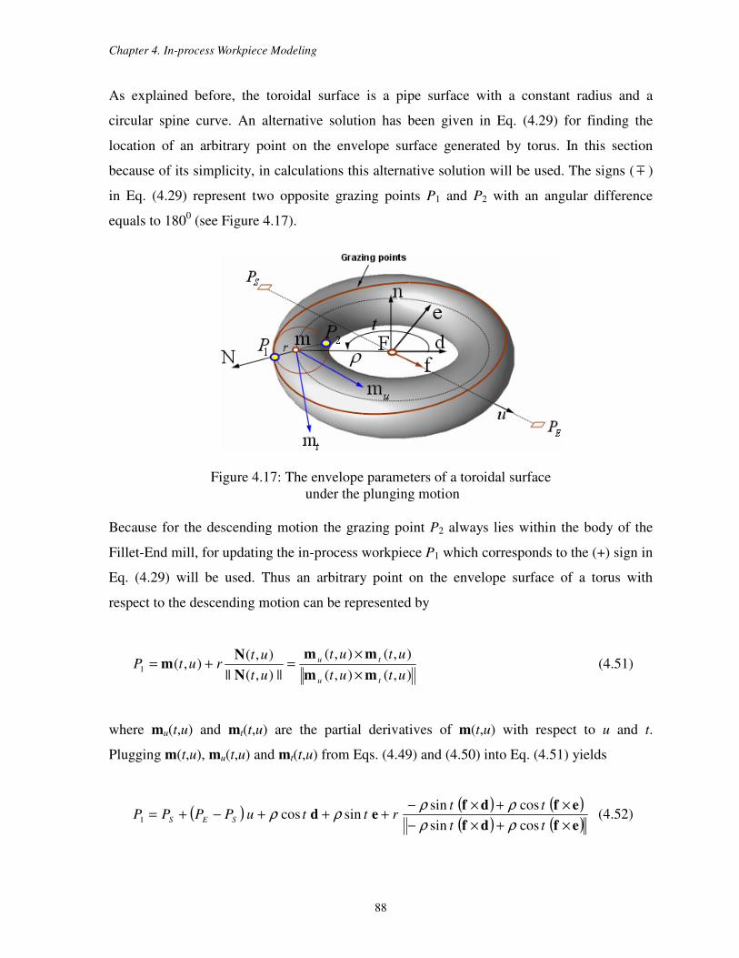
Chapter 4. In-process Workpiece Modeling
88
As explained before, the toroidal surface is a pipe surface with a constant radius and a
circular spine curve. An alternative solution has been given in Eq. (4.29) for finding the
location of an arbitrary point on the envelope surface generated by torus. In this section
because of its simplicity, in calculations this alternative solution will be used. The signs ( m )
in Eq. (4.29) represent two opposite grazing points P1 and P2 with an angular difference
equals to 1800 (see Figure 4.17).
Figure 4.17: The envelope parameters of a toroidal surface
under the plunging motion
Because for the descending motion the grazing point P2 always lies within the body of the
Fillet-End mill, for updating the in-process workpiece P1 which corresponds to the (+) sign in
Eq. (4.29) will be used. Thus an arbitrary point on the envelope surface of a torus with
respect to the descending motion can be represented by
),(),(
),(),(
||),(||
),(),(1
utut
utut
ut
utrutP
tu
tu
mm
mm
N
Nm
×
×=+= (4.51)
where mu(t,u) and mt(t,u) are the partial derivatives of m(t,u) with respect to u and t.
Plugging m(t,u), mu(t,u) and mt(t,u) from Eqs. (4.49) and (4.50) into Eq. (4.51) yields
( ) ( ) ( )( ) ( )ef df
ef dfed
×+×−
×+×−+++−+=
tt
ttrttuPPPP SES
cossin
cossinsincos1
ρρ
ρρρρ (4.52)
Chapter 4. In-process Workpiece Modeling
89
For simplifying the calculations the cross products in Eq. (4.52) will be denoted by
dfk ×== ][ zyx kkk and efq ×== ][ zyx qqq . A point at which a vector intersects the
cutter envelope is described by setting the vector line I(v) described in Eq.(4.21) equals to P1
given in Eq. (4.51). Thus this yields a nonlinear system of three equations in three variables t,
u and v as follows
( )q k
tt
qtktretdtuxxxvxxx xx
xxSESabacossin
cossinsincos)(
+−
+−+++−+=−+ ρρ (4.53-a)
( )q k
tt
qtktretdtuyyyvyyy
yy
yySESabacossin
cossinsincos)(
+−
+−+++−+=−+ ρρ (4.53-b)
( )q k
tt
qtktretdtuzzzvzzz zz
zzSESabacossin
cossinsincos)(
+−
+−+++−+=−+ ρρ (4.53-c)
For solving the above system of equations, first the equivalent of the variable v from Eq.
(4.53-b) is plugged into Eqs.(4.53-a) and (4.53-c) respectively. Thus with this process two
nonlinear equations with variables u and t are obtained. Later the equivalent of u from one of
these equations is plugged into another for eliminating u. Therefore the final nonlinear
equation depends on the variable t only. But in this research, as explained in section (4.2.2),
for representing the in-process workpiece the directions of discrete vector lines are taken
along the x, y and z axes of the standard basis of R3. Therefore in the following parts the
nonlinear system given by Eqs. (4.53-a,b,c) will be solved for discrete vectors having
orientations along the z-axis of R3 and the similar steps can be used for the discrete vectors
pointing in the direction of x and y axes of R3.
When the discrete vectors are oriented in the z-axis direction of R3, the variable v from
Eqs. (4.53-a) and (4.53-b) are eliminated and thus these two equations are only dependent on
u and t. Further for eliminating u the equivalent of u from Eq. (4.53-a) is plugged into Eq.
(4.53-b) and this yields the following nonlinear function with variable t
( ) ( ) ( ) 0sincos =++= CttBttAtf (4.54)
where
Chapter 4. In-process Workpiece Modeling
90
q k tt
xxqyyqrdxxdyytA
SEySEx
ySExSEcossin
)()()()()(
+−
−−−+−−−= ρρ
q k tt
yykxxkrexxeyytB
SExSEy
ySExSEcossin
)()()()()(
+−
−−−+−−−= ρρ
)()()()( aSSESaSE xxyyyyxxC −−+−−=
The following property motivates finding the solution of the nonlinear function f (t)
Property 4.1: For a given linear toolpath the swept envelope of the torus ( 0
torusG ) has a
convex shape and a discrete vector intersects this envelope at most two points.
According to property (4.1) there are three possible intersection cases between an envelope
surface generated by a torus and a discrete vector: vector intersects in two points, vector
intersects in one point and no intersection. All three cases are illustrated in Figure (4.18). In
this figure the envelope surface 0
torusG has two parts, the lower envelope ( 0
, LowertorusG , colored
by green) and the upper envelope ( 0
, UppertorusG , colored by gray) surfaces, i.e.
0
,
0
,
0
UppertorusLowertorustorus GGG ∪= . As explained before the cutter is performing a descending
motion. Therefore for updating the in-process workpiece the lower envelope surface is taken
into account. The upper envelope surface is not considered in the calculations because during
the tool motion it is enclosed within the cylindrical part of the Fillet-End mill. Thus the
intersection points shown in Figure (4.18) are located on the lower envelope surface
( 0
, LowertorusG ).
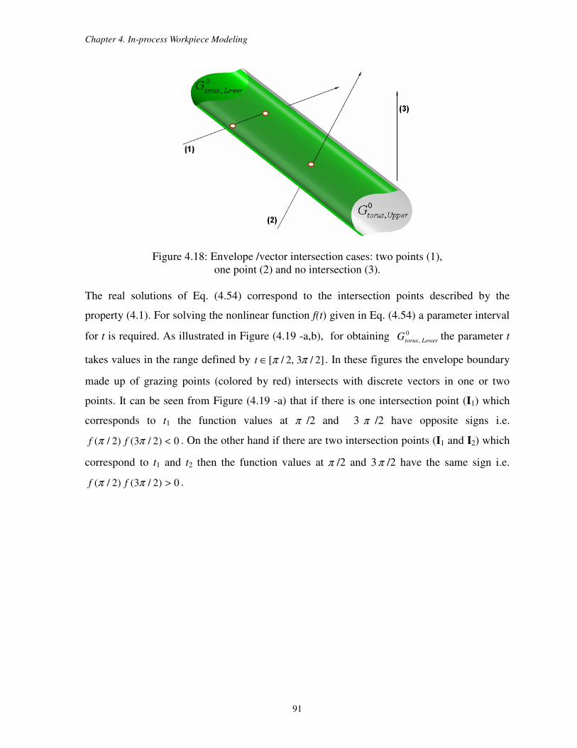
Chapter 4. In-process Workpiece Modeling
91
Figure 4.18: Envelope /vector intersection cases: two points (1),
one point (2) and no intersection (3).
The real solutions of Eq. (4.54) correspond to the intersection points described by the
property (4.1). For solving the nonlinear function f(t) given in Eq. (4.54) a parameter interval
for t is required. As illustrated in Figure (4.19 -a,b), for obtaining 0
, LowertorusG the parameter t
takes values in the range defined by ]2/3,2/[ ππ∈t . In these figures the envelope boundary
made up of grazing points (colored by red) intersects with discrete vectors in one or two
points. It can be seen from Figure (4.19 -a) that if there is one intersection point (I1) which
corresponds to t1 the function values at π /2 and 3 π /2 have opposite signs i.e.
0)2/3()2/( <ππ ff . On the other hand if there are two intersection points (I1 and I2) which
correspond to t1 and t2 then the function values at π /2 and 3π /2 have the same sign i.e.
0)2/3()2/( >ππ ff .
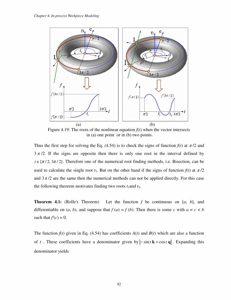
Chapter 4. In-process Workpiece Modeling
92
(a) (b)
Figure 4.19: The roots of the nonlinear equation f(t) when the vector intersects
in (a) one point or in (b) two points.
Thus the first step for solving the Eq. (4.54) is to check the signs of function f(t) at π /2 and
3 π /2. If the signs are opposite then there is only one root in the interval defined by
]2/3,2/[ ππ∈t . Therefore one of the numerical root finding methods, i.e. Bisection, can be
used to calculate the single root t1. But on the other hand if the signs of function f(t) at π /2
and 3π /2 are the same then the numerical methods can not be applied directly. For this case
the following theorem motivates finding two roots t1and t2.
Theorem 4.1: (Rolle's Theorem) Let the function f be continuous on [a, b], and
differentiable on (a, b), and suppose that f (a) = f (b). Then there is some c with a < c < b
such that f'(c) = 0.
The function f(t) given in Eq. (4.54) has coefficients A(t) and B(t) which are also a function
of t . These coefficients have a denominator given by q k tt cossin +− . Expanding this
denominator yields
Chapter 4. In-process Workpiece Modeling
93
( ) ( )22222222 cossincossin zyxzyx qqqtkkkttt +++++=+− q k (4.55)
Note that for the above equation the dot product between k and q equals to zero i.e.
k • q = (f ×d) • (f ×e) = (f • f) (d • e) - (f • e) (d • f) = 0
It can be seen from Eq. (4.55) that the denominator can not be zero. Therefore the function
f(t) given in Eq. (4.54) is continuous.
Also because A(t), cost, B(t), sint and C are differentiable at )2/3,2/( ππ , the nonlinear
function f(t) given in Eq.(4.54) is also differentiable in the open interval given
by )2/3,2/( ππ . Furthermore, if the function f(t) has two roots t1 and t2 in the interval
]2/3,2/[ ππ∈t then 0)()( 21 == tftf . Therefore the Rolle’s Theorem holds for the Eq.
(4.54) and thus there is a value c between two roots t1 and t2 for which f'(c) = 0. If the c value
is found, the interval given by ]2/3,2/[ ππ∈t is partitioned into two sub intervals defined by
],2/[ cπ and ]2/3,[ πc .Now 0)()2/( <cff π and 0)2/3()( <πfcf and thus by applying one
of the numerical root finding methods, i.e. Bisection, into these two sub intervals the roots t1
and t2 can be found. In this research for finding c value, a Matlab [54] function fminbnd is
used. fminbnd finds the minimum of a function of one variable within a fixed interval. The
algorithm used in fminbnd is based on golden section search and parabolic interpolation. See
[29] and [17] for details about the algorithm. Note that when the signs of f(t) at π /2 and
3π /2 are the same i.e. 0)2/3()2/( >ππ ff , then each one of )2/(πf and )2/3( πf has a
minus sign or vice versa. If each one has a minus sign then for finding the local minimum
value at c using fminbnd the nonlinear function f(t) is multiplied by minus. This process only
reflects the function f(t) with respect to t-axis in (t, f(t)) graph and it does not change the
locations of the roots. The whole process for finding the roots of the nonlinear equation f(t)
is given in Algorithm (4.1).
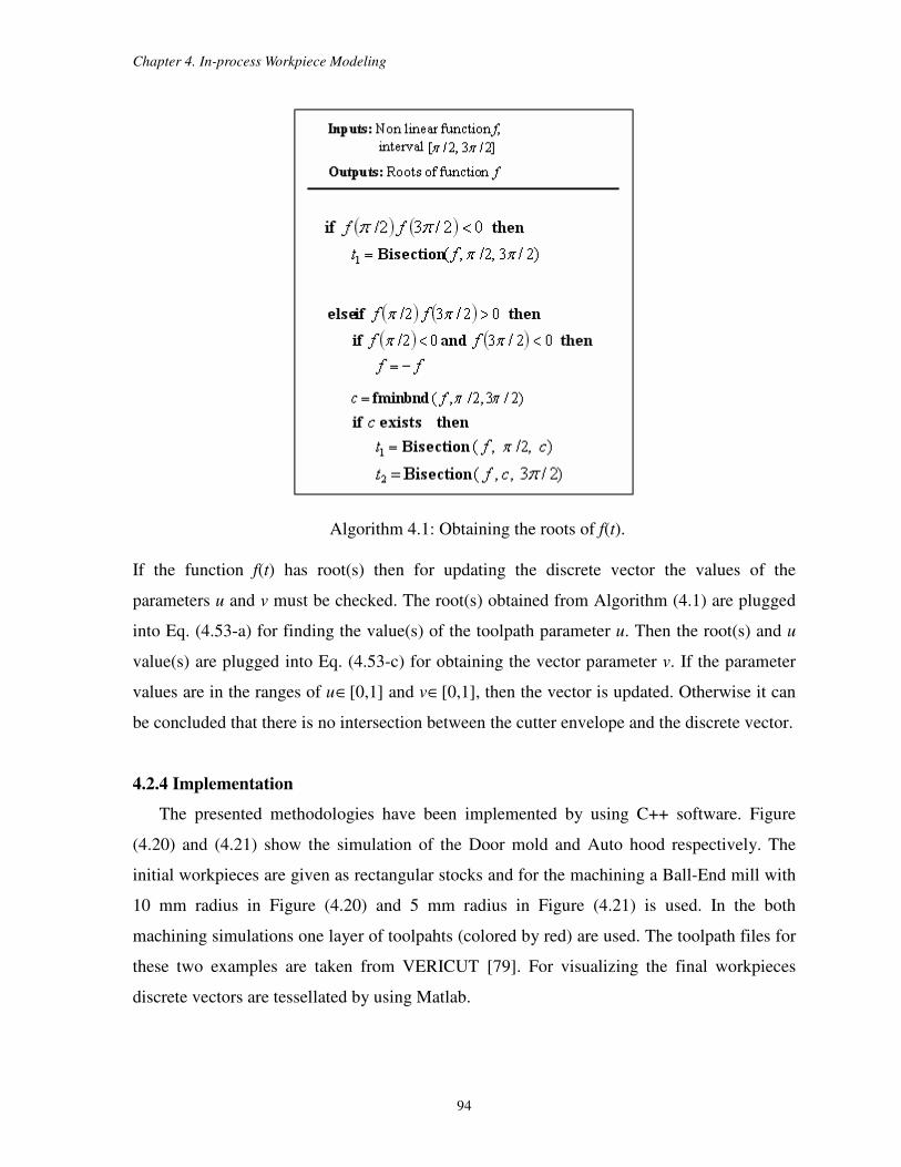
Chapter 4. In-process Workpiece Modeling
94
Algorithm 4.1: Obtaining the roots of f(t).
If the function f(t) has root(s) then for updating the discrete vector the values of the
parameters u and v must be checked. The root(s) obtained from Algorithm (4.1) are plugged
into Eq. (4.53-a) for finding the value(s) of the toolpath parameter u. Then the root(s) and u
value(s) are plugged into Eq. (4.53-c) for obtaining the vector parameter v. If the parameter
values are in the ranges of u∈[0,1] and v∈[0,1], then the vector is updated. Otherwise it can
be concluded that there is no intersection between the cutter envelope and the discrete vector.
4.2.4 Implementation
The presented methodologies have been implemented by using C++ software. Figure
(4.20) and (4.21) show the simulation of the Door mold and Auto hood respectively. The
initial workpieces are given as rectangular stocks and for the machining a Ball-End mill with
10 mm radius in Figure (4.20) and 5 mm radius in Figure (4.21) is used. In the both
machining simulations one layer of toolpahts (colored by red) are used. The toolpath files for
these two examples are taken from VERICUT [79]. For visualizing the final workpieces
discrete vectors are tessellated by using Matlab.
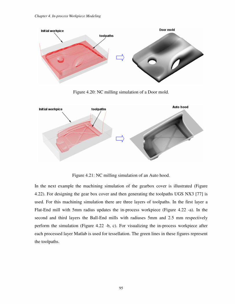
Chapter 4. In-process Workpiece Modeling
95
Figure 4.20: NC milling simulation of a Door mold.
Figure 4.21: NC milling simulation of an Auto hood.
In the next example the machining simulation of the gearbox cover is illustrated (Figure
4.22). For designing the gear box cover and then generating the toolpaths UGS NX3 [77] is
used. For this machining simulation there are three layers of toolpaths. In the first layer a
Flat-End mill with 5mm radius updates the in-process workpiece (Figure 4.22 -a). In the
second and third layers the Ball-End mills with radiuses 5mm and 2.5 mm respectively
perform the simulation (Figure 4.22 -b, c). For visualizing the in-process workpiece after
each processed layer Matlab is used for tessellation. The green lines in these figures represent
the toolpaths.
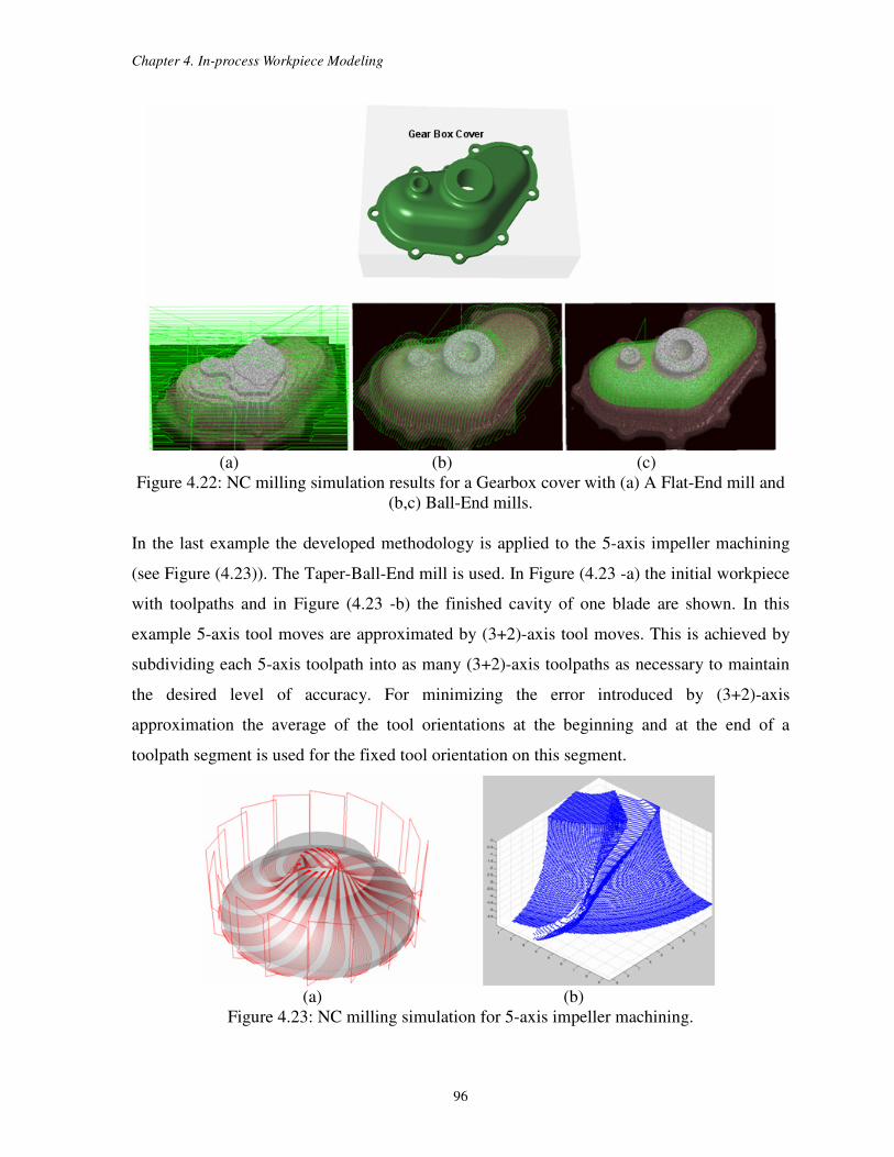
Chapter 4. In-process Workpiece Modeling
96
(a) (b) (c)
Figure 4.22: NC milling simulation results for a Gearbox cover with (a) A Flat-End mill and
(b,c) Ball-End mills.
In the last example the developed methodology is applied to the 5-axis impeller machining
(see Figure (4.23)). The Taper-Ball-End mill is used. In Figure (4.23 -a) the initial workpiece
with toolpaths and in Figure (4.23 -b) the finished cavity of one blade are shown. In this
example 5-axis tool moves are approximated by (3+2)-axis tool moves. This is achieved by
subdividing each 5-axis toolpath into as many (3+2)-axis toolpaths as necessary to maintain
the desired level of accuracy. For minimizing the error introduced by (3+2)-axis
approximation the average of the tool orientations at the beginning and at the end of a
toolpath segment is used for the fixed tool orientation on this segment.
(a) (b)
Figure 4.23: NC milling simulation for 5-axis impeller machining.
Chapter 4. In-process Workpiece Modeling
97
4.3 Discussion
In this chapter discrete vector based in-process workpiece update methodologies have
been presented. The discrete vectors with their orientations in the directions of x,y,z-axes of
R3 have been used. Therefore in this representation more vectors in different directions have
been used and thus, especially when the workpiece has features like vertical walls and sharp
edges, the quality in the visualization of the final product has been increased. Also the
localization advantage of the Discrete Vertical Vector approach has been preserved. A
typical milling tool path contains thousands of tool movements and during the machining
simulation for calculating the intersections only the small percentage of all the discrete
vectors is needed. For this purpose for localizing the tool envelope during the simulation the
Axis Aligned Bounding Box (AABB) has been used. The best feature of the AABB is its fast
overlap check, which simply involves direct comparison of individual coordinate values. As
explained in this chapter for some workpiece geometries 3-axis machining is not suitable for
updating the workpiece surfaces. Because of this in the developed methodologies the tool
motions in (3+2)-axis milling in which the cutter can have an arbitrary fixed orientation in
space have been considered. The exact 5-axis milling motions are not preferable in the
workpiece update simulations because all the calculations require using the nonlinear root
finding algorithms and therefore the computational time becomes high. Under this
consideration 5-axis tool motions can be approximated by (3+2)-axis tool motions. An
example has been given in Figure (4.23) for illustrating this situation. In this chapter for
simplifying the intersection calculations the properties of canal surfaces defined in section (3)
are utilized. The cutter envelope and vector intersection calculations for the cylinder, frustum
of a cone and Flat-Bottom surfaces have been made analytically. Because of the complexity
of the torus shape these calculations have been made by using the numerical root finding
methods. For this purpose a root finding analysis has been developed for guaranteeing the
root(s) in the given interval. The intersection formulas for the sphere surface have not been
developed because when a sphere moves along a linear toolpath it envelopes a cylinder
which has an orientation in the direction of the feed vector. Therefore the update formulas for
the spherical part of a cutter are reduced to cylinder-vector intersection.
98
Chapter 5
Feasible Contact Surfaces
In this chapter the feasible contact surfaces of NC cutters under varying tool motions are
presented. A typical NC cutter has different surfaces with varying geometries. For example a
Flat-End mill has a cylindrical part at the side and a flat part at the bottom. During the
material removal process only certain parts of the cutter surfaces are eligible to contact the
in-process workpiece. In this chapter for representing these so-called certain parts a
terminology feasible contact surfaces (FCS) is introduced. The word feasible is used because
although these surfaces are eligible to contact the in-process workpiece, they may or may not
remove material depending on the cutter position relative to the workpiece. When the FCS
contact the in-process workpiece the Cutter Workpiece Engagements (CWEs) are generated.
Since CWEs are subsets of FCS, formulating the FCS helps us to better understand the CWE
generation process. The boundaries of the FCS are defined by the cutter geometry and the
envelope boundary set. The envelope boundary set contains points that the cutter surface will
leave behind as it moves along a toolpath. Throughout this chapter it is assumed that the
cutter follows a rigid motion. Simply a rigid motion is a transformation over time that does
not change the shape of the cutter, only its location and orientation. Therefore for the given
tool motions the cutter geometry stays fixed but on the other hand the envelope boundary set
may change.
Two factors effect the construction process of the FCS: the cutter geometry and the
motion type. For example for a Flat-End cutter, in 2 ½-axis milling only the cylindrical part
has a FCS, but on the other hand in 3-axis plunge milling both the cylindrical and the flat
parts have a FCS. The general tool motions in milling are presented in section (5.1) and
followed by the milling cutter geometries in section (5.2). For obtaining the FCS the
envelope boundary sets of a generic cutter performing 5-axis tool motions are formulated in
section (5.3). For this purpose a tangency function defined by the surface normal and the tool
velocity is utilized. Later in section (5.4) the distribution of the feasible contact surfaces with
respect to cutter velocity is analyzed. Then finally the chapter ends with the discussion in
section(5.5).
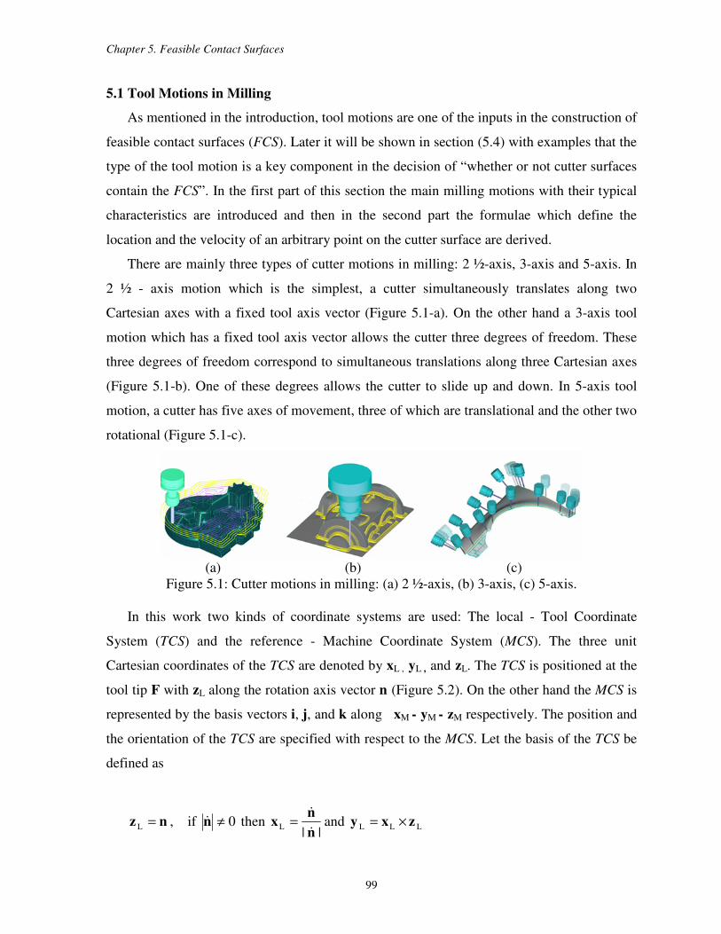
Chapter 5. Feasible Contact Surfaces
99
5.1 Tool Motions in Milling
As mentioned in the introduction, tool motions are one of the inputs in the construction of
feasible contact surfaces (FCS). Later it will be shown in section (5.4) with examples that the
type of the tool motion is a key component in the decision of “whether or not cutter surfaces
contain the FCS”. In the first part of this section the main milling motions with their typical
characteristics are introduced and then in the second part the formulae which define the
location and the velocity of an arbitrary point on the cutter surface are derived.
There are mainly three types of cutter motions in milling: 2 ½-axis, 3-axis and 5-axis. In
2 ½ - axis motion which is the simplest, a cutter simultaneously translates along two
Cartesian axes with a fixed tool axis vector (Figure 5.1-a). On the other hand a 3-axis tool
motion which has a fixed tool axis vector allows the cutter three degrees of freedom. These
three degrees of freedom correspond to simultaneous translations along three Cartesian axes
(Figure 5.1-b). One of these degrees allows the cutter to slide up and down. In 5-axis tool
motion, a cutter has five axes of movement, three of which are translational and the other two
rotational (Figure 5.1-c).
(a) (b) (c)
Figure 5.1: Cutter motions in milling: (a) 2 ½-axis, (b) 3-axis, (c) 5-axis.
In this work two kinds of coordinate systems are used: The local - Tool Coordinate
System (TCS) and the reference - Machine Coordinate System (MCS). The three unit
Cartesian coordinates of the TCS are denoted by xL , yL , and zL. The TCS is positioned at the
tool tip F with zL along the rotation axis vector n (Figure 5.2). On the other hand the MCS is
represented by the basis vectors i, j, and k along xM - yM - zM respectively. The position and
the orientation of the TCS are specified with respect to the MCS. Let the basis of the TCS be
defined as
nz =L , if 0≠n& then ||
Ln
nx
&
&= and LLL zxy ×=
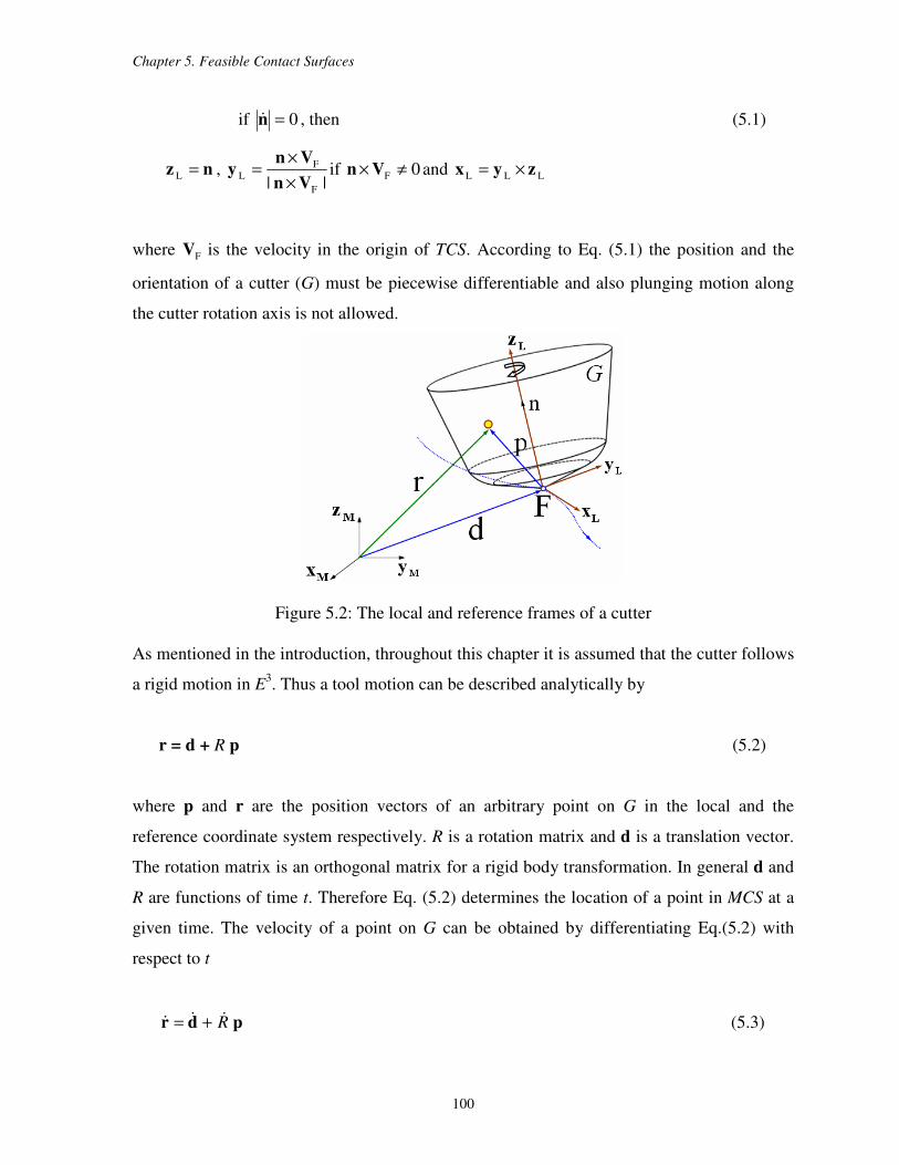
Chapter 5. Feasible Contact Surfaces
100
if 0=n& , then (5.1)
nz =L , || F
FL
Vn
Vny
×
×= if 0F ≠× Vn and LLL zyx ×=
where FV is the velocity in the origin of TCS. According to Eq. (5.1) the position and the
orientation of a cutter (G) must be piecewise differentiable and also plunging motion along
the cutter rotation axis is not allowed.
Figure 5.2: The local and reference frames of a cutter
As mentioned in the introduction, throughout this chapter it is assumed that the cutter follows
a rigid motion in E3. Thus a tool motion can be described analytically by
r = d + R p (5.2)
where p and r are the position vectors of an arbitrary point on G in the local and the
reference coordinate system respectively. R is a rotation matrix and d is a translation vector.
The rotation matrix is an orthogonal matrix for a rigid body transformation. In general d and
R are functions of time t. Therefore Eq. (5.2) determines the location of a point in MCS at a
given time. The velocity of a point on G can be obtained by differentiating Eq.(5.2) with
respect to t
pdr R&&& += (5.3)

Chapter 5. Feasible Contact Surfaces
101
Plugging the equivalent of p from Eq.(5.2) into Eq. (5.3) yields
( )drdr - −+= 1RR&&& (5.4)
where the multiplication of two matrices ( 1-RR& ) is called as the angular velocity matrix
denoted by Ω . Ω is a skew symmetric matrix. This can be proven as follows: Since R is an
orthogonal matrix, RRT = I and R
-1 = R
T. By differentiating RR
T = I, the following equation
is obtained.
0TT =+ RRRR && (5.5)
The second term in Eq.(5.5) can be written as ( ) ( )T1TT1T −− == RRRRRR &&& . And also the first
term in this equation is equal to 1−RR& . Thus Eq. (5.5) takes the following form
( )T11 −− −= RRRR && (5.6)
The above equation proves that Ω is a skew symmetric matrix. The general form of Ω is
given by
ΩΩ−
Ω−Ω
ΩΩ−
=Ω
0
0
0
XY
XZ
YZ
(5.7)
where XΩ , YΩ and ZΩ are three components of the angular velocity in MCS. The skew
symmetric matrix Ω can also be represented as a vector. For example by using the
components of Ω the angular velocity vector ω can be represented by
kjiω ZYX Ω+Ω+Ω= (5.8)

Chapter 5. Feasible Contact Surfaces
102
It can be easily verified that the multiplication of Ω with an arbitrary vector, let say m, in
MCS is equal to the cross product between ω and this vector, i.e.
mωm ×=Ω (5.9)
Therefore Eq. (5.4) which defines the velocity of an arbitrary point on G can be rewritten as
( ) pωddrdr ×+=−Ω+= &&& (5.10)
Later in section (5.3) the instantaneous velocity of the tool axis will be required. It is derived
from the following equation
kn R= (5.11)
Differentiating Eq. (5.11) yields
nnkn Ω=== −1RRR &&& (5.12)
From Eq. (5.9), the above equation takes the following form
nωn ×=& (5.13)
Thus the instantaneous velocity of the tool axis can be calculated in terms of angular velocity
and the rotation axis vector.
5.2 Milling Cutter Geometries
The construction of feasible contact surfaces requires the modeling of the tool geometry.
In this section for obtaining a variety of cutter shapes a parametric model of a generic cutter
is used (Figure 5.3). The geometry of the generic cutter can be described by the following
parameters [46]
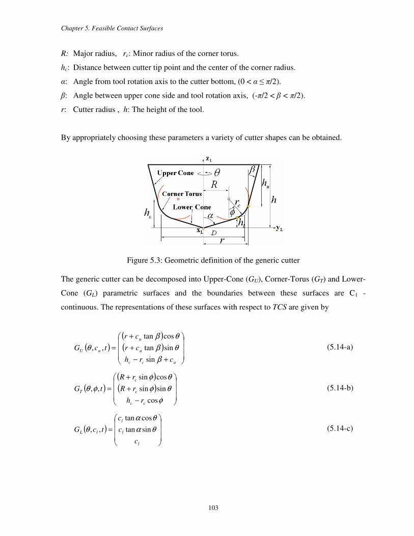
Chapter 5. Feasible Contact Surfaces
103
R: Major radius, rc: Minor radius of the corner torus.
hc: Distance between cutter tip point and the center of the corner radius.
α: Angle from tool rotation axis to the cutter bottom, (0 < α ≤ π/2).
β: Angle between upper cone side and tool rotation axis, (-π/2 < β < π/2).
r: Cutter radius , h: The height of the tool.
By appropriately choosing these parameters a variety of cutter shapes can be obtained.
Figure 5.3: Geometric definition of the generic cutter
The generic cutter can be decomposed into Upper-Cone (GU), Corner-Torus (GT) and Lower-
Cone (GL) parametric surfaces and the boundaries between these surfaces are C1 -
continuous. The representations of these surfaces with respect to TCS are given by
( )( )( )
+−
+
+
=
ucc
u
u
uU
crh
cr
cr
tcG
β
θβ
θβ
θ
sin
sintan
costan
,, (5.14-a)
( )( )( )
−
+
+
=
φ
θφ
θφ
φθ
cos
sinsin
cossin
,,
cc
c
c
T
rh
rR
rR
tG (5.14-b)
( )
=
l
l
l
lL
c
c
c
tcG θα
θα
θ sintan
costan
,, (5.14-c)
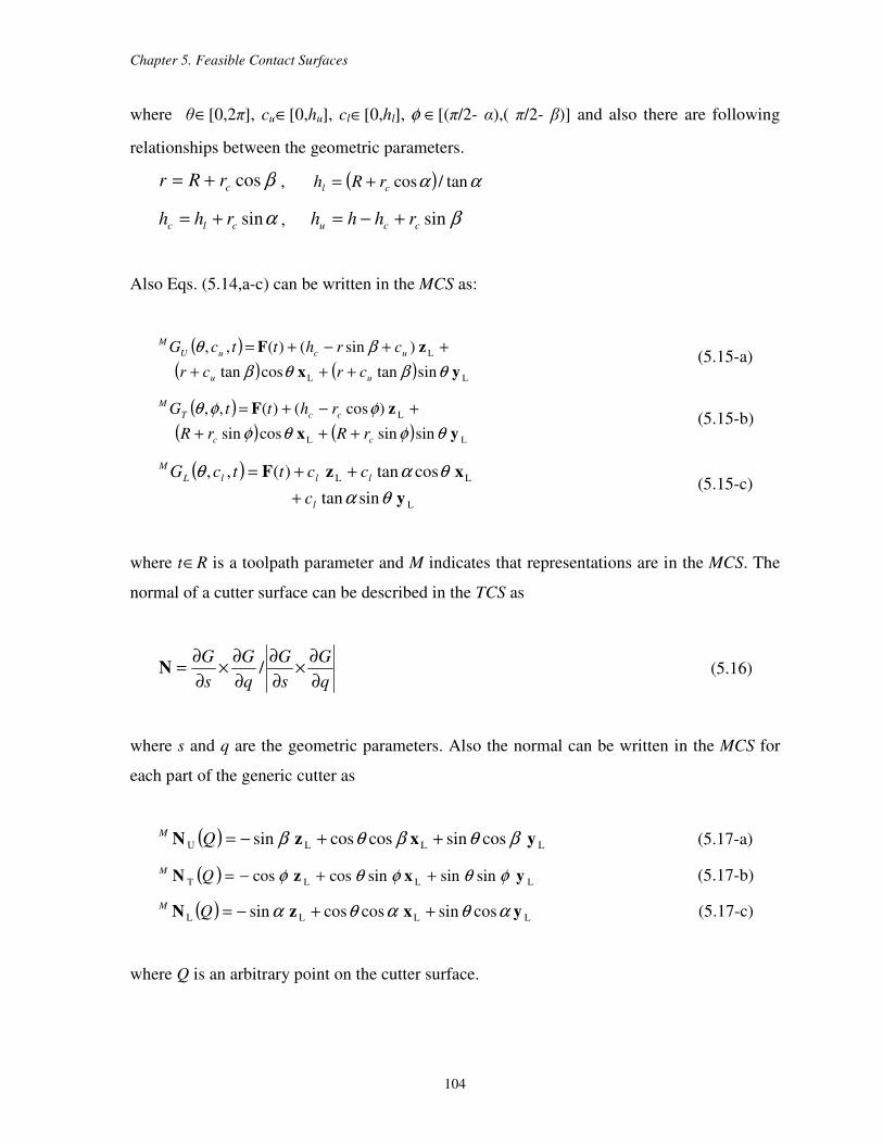
Chapter 5. Feasible Contact Surfaces
104
where θ∈[0,2π], cu∈[0,hu], cl∈[0,hl], φ ∈[(π/2- α),( π/2- β)] and also there are following
relationships between the geometric parameters.
βcoscrRr += , ( ) αα tan/coscl rRh +=
αsinclc rhh += , βsinccu rhhh +−=
Also Eqs. (5.14,a-c) can be written in the MCS as:
( )
( ) ( ) LL
L
sintancostan
)sin()(,,
yx
zF
θβθβ
βθ
uu
ucuU
M
crcr
crhttcG
+++
++−+= (5.15-a)
( )
( ) ( ) LL
L
sinsincossin
)cos()(,,
yx
zF
θφθφ
φφθ
cc
ccT
M
rRrR
rhttG
+++
+−+= (5.15-b)
( )
L
LL
sintan
costan)(,,
y
xzF
θα
θαθ
l
lllL
M
c
ccttcG
+
++= (5.15-c)
where t∈R is a toolpath parameter and M indicates that representations are in the MCS. The
normal of a cutter surface can be described in the TCS as
q
G
s
G
q
G
s
G
∂
∂×
∂
∂
∂
∂×
∂
∂= /N (5.16)
where s and q are the geometric parameters. Also the normal can be written in the MCS for
each part of the generic cutter as
( ) LLLU cossincoscossin yxzN βθβθβ ++−=QM
(5.17-a)
( ) LLLT sinsinsincoscos yxzN φθφθφ ++−=QM (5.17-b)
( ) LLLL cossincoscossin yxzN αθαθα ++−=QM (5.17-c)
where Q is an arbitrary point on the cutter surface.
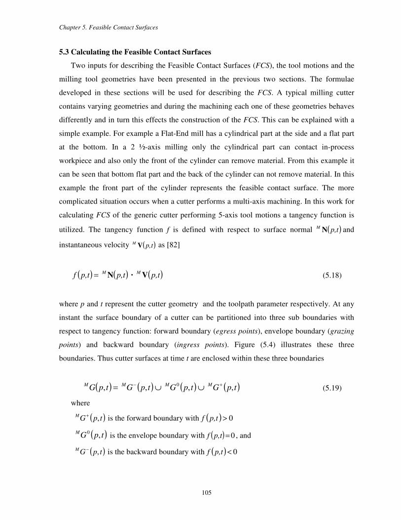
Chapter 5. Feasible Contact Surfaces
105
5.3 Calculating the Feasible Contact Surfaces
Two inputs for describing the Feasible Contact Surfaces (FCS), the tool motions and the
milling tool geometries have been presented in the previous two sections. The formulae
developed in these sections will be used for describing the FCS. A typical milling cutter
contains varying geometries and during the machining each one of these geometries behaves
differently and in turn this effects the construction of the FCS. This can be explained with a
simple example. For example a Flat-End mill has a cylindrical part at the side and a flat part
at the bottom. In a 2 ½-axis milling only the cylindrical part can contact in-process
workpiece and also only the front of the cylinder can remove material. From this example it
can be seen that bottom flat part and the back of the cylinder can not remove material. In this
example the front part of the cylinder represents the feasible contact surface. The more
complicated situation occurs when a cutter performs a multi-axis machining. In this work for
calculating FCS of the generic cutter performing 5-axis tool motions a tangency function is
utilized. The tangency function f is defined with respect to surface normal ( )p,tM N and
instantaneous velocity ( )p,tM
V as [82]
( ) ( ) ( )p,tp,tp,tf MM V·N= (5.18)
where p and t represent the cutter geometry and the toolpath parameter respectively. At any
instant the surface boundary of a cutter can be partitioned into three sub boundaries with
respect to tangency function: forward boundary (egress points), envelope boundary (grazing
points) and backward boundary (ingress points). Figure (5.4) illustrates these three
boundaries. Thus cutter surfaces at time t are enclosed within these three boundaries
( ) ( ) ( ) ( )tpGtpGtpGtpGMMMM ,,,, 0 +− ∪∪= (5.19)
where
( )tpGM ,+
is the forward boundary with ( ) 0>p,tf
( )tpGM ,0
is the envelope boundary with ( ) 0=p,tf , and
( )tpGM ,− is the backward boundary with ( ) 0<p,tf
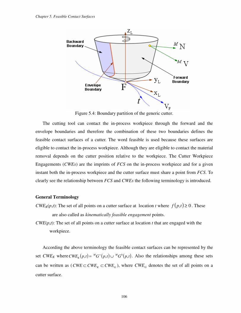
Chapter 5. Feasible Contact Surfaces
106
Figure 5.4: Boundary partition of the generic cutter.
The cutting tool can contact the in-process workpiece through the forward and the
envelope boundaries and therefore the combination of these two boundaries defines the
feasible contact surfaces of a cutter. The word feasible is used because these surfaces are
eligible to contact the in-process workpiece. Although they are eligible to contact the material
removal depends on the cutter position relative to the workpiece. The Cutter Workpiece
Engagements (CWEs) are the imprints of FCS on the in-process workpiece and for a given
instant both the in-process workpiece and the cutter surface must share a point from FCS. To
clearly see the relationship between FCS and CWEs the following terminology is introduced.
General Terminology
CWEK(p,t): The set of all points on a cutter surface at location t where ( ) 0≥p,tf . These
are also called as kinematically feasible engagement points.
CWE(p,t): The set of all points on a cutter surface at location t that are engaged with the
workpiece.
According the above terminology the feasible contact surfaces can be represented by the
set CWEK where ( ) ( ) ( )tpGtpGtpCWEMM
K ,,,0∪= + . Also the relationships among these sets
can be written as (GK CWECWECWE ⊂⊂ ), where GCWE denotes the set of all points on a
cutter surface.
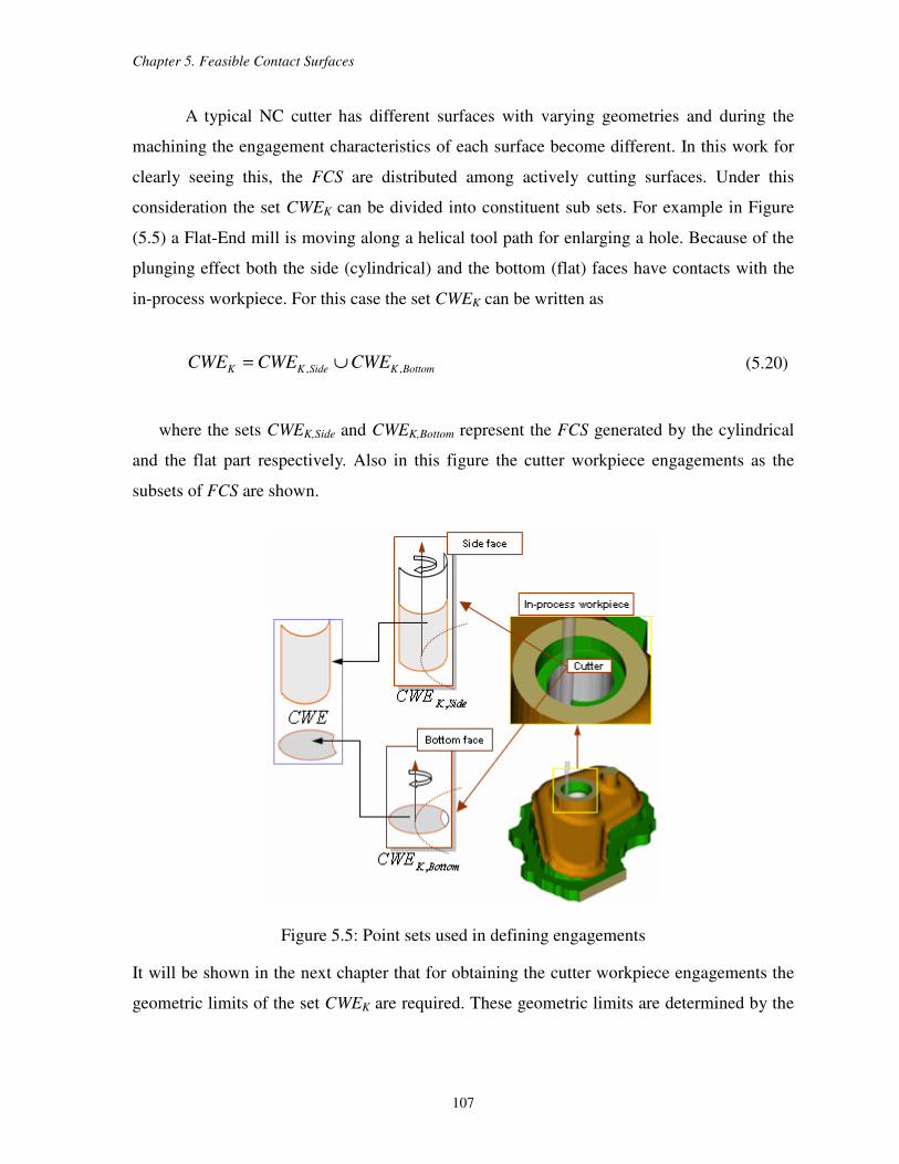
Chapter 5. Feasible Contact Surfaces
107
A typical NC cutter has different surfaces with varying geometries and during the
machining the engagement characteristics of each surface become different. In this work for
clearly seeing this, the FCS are distributed among actively cutting surfaces. Under this
consideration the set CWEK can be divided into constituent sub sets. For example in Figure
(5.5) a Flat-End mill is moving along a helical tool path for enlarging a hole. Because of the
plunging effect both the side (cylindrical) and the bottom (flat) faces have contacts with the
in-process workpiece. For this case the set CWEK can be written as
BottomKSideKK CWECWECWE ,, ∪= (5.20)
where the sets CWEK,Side and CWEK,Bottom represent the FCS generated by the cylindrical
and the flat part respectively. Also in this figure the cutter workpiece engagements as the
subsets of FCS are shown.
Figure 5.5: Point sets used in defining engagements
It will be shown in the next chapter that for obtaining the cutter workpiece engagements the
geometric limits of the set CWEK are required. These geometric limits are determined by the
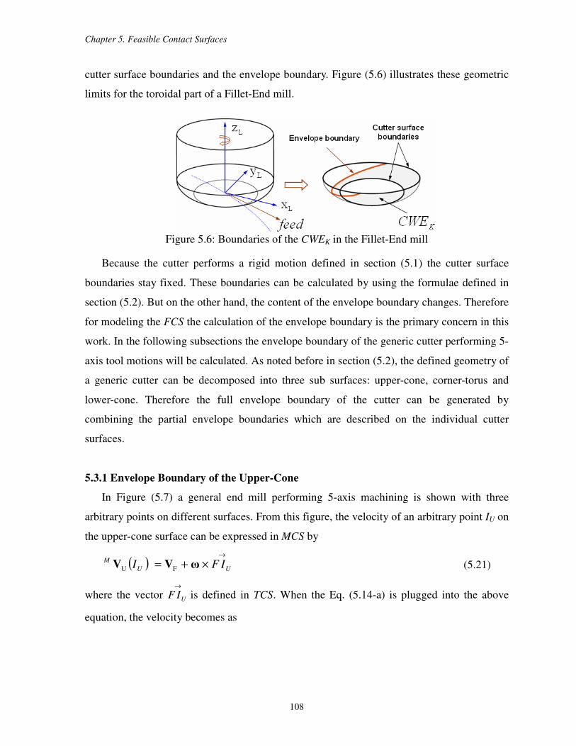
Chapter 5. Feasible Contact Surfaces
108
cutter surface boundaries and the envelope boundary. Figure (5.6) illustrates these geometric
limits for the toroidal part of a Fillet-End mill.
Figure 5.6: Boundaries of the CWEK in the Fillet-End mill
Because the cutter performs a rigid motion defined in section (5.1) the cutter surface
boundaries stay fixed. These boundaries can be calculated by using the formulae defined in
section (5.2). But on the other hand, the content of the envelope boundary changes. Therefore
for modeling the FCS the calculation of the envelope boundary is the primary concern in this
work. In the following subsections the envelope boundary of the generic cutter performing 5-
axis tool motions will be calculated. As noted before in section (5.2), the defined geometry of
a generic cutter can be decomposed into three sub surfaces: upper-cone, corner-torus and
lower-cone. Therefore the full envelope boundary of the cutter can be generated by
combining the partial envelope boundaries which are described on the individual cutter
surfaces.
5.3.1 Envelope Boundary of the Upper-Cone
In Figure (5.7) a general end mill performing 5-axis machining is shown with three
arbitrary points on different surfaces. From this figure, the velocity of an arbitrary point IU on
the upper-cone surface can be expressed in MCS by
( )→
×+= UU
MIFI ωVV FU (5.21)
where the vector →
UIF is defined in TCS. When the Eq. (5.14-a) is plugged into the above
equation, the velocity becomes as
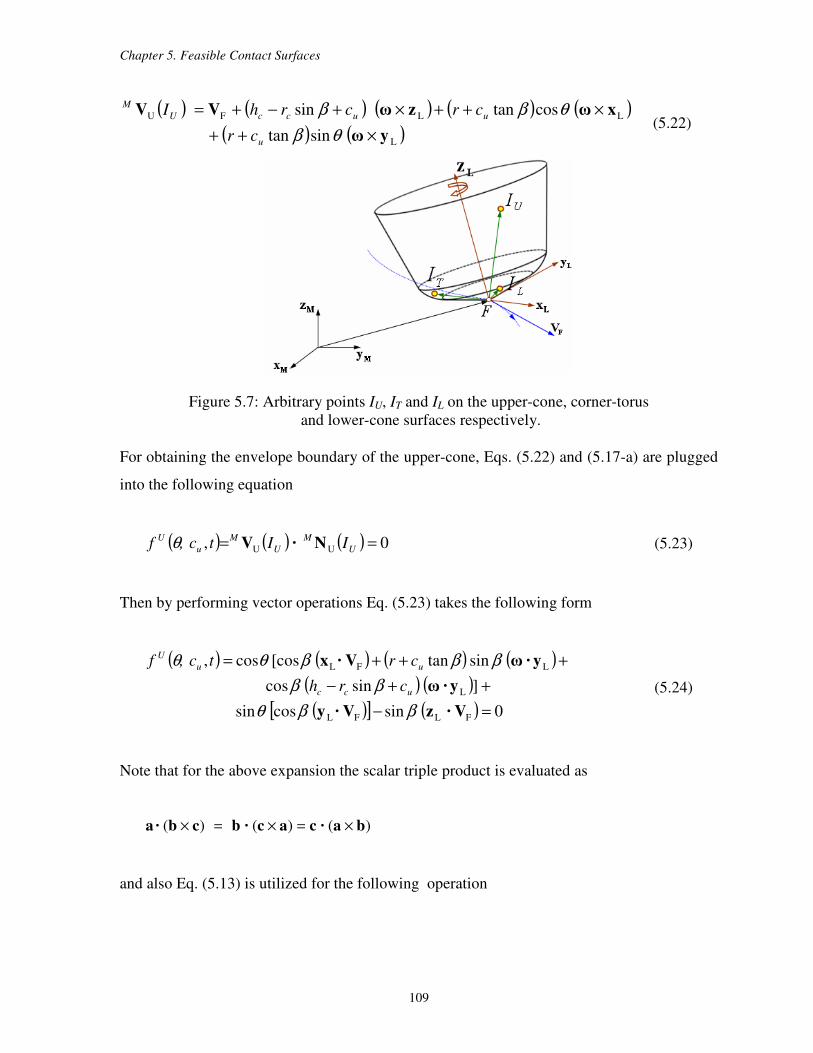
Chapter 5. Feasible Contact Surfaces
109
( ) ( ) ( ) ( ) ( )( ) ( )L
LLFU
sintan
costansin
yω
xωzωVV
×++
×++×+−+=
θβ
θββ
u
uuccU
M
cr
crcrhI (5.22)
Figure 5.7: Arbitrary points IU, IT and IL on the upper-cone, corner-torus
and lower-cone surfaces respectively.
For obtaining the envelope boundary of the upper-cone, Eqs. (5.22) and (5.17-a) are plugged
into the following equation
( ) ( ) ( ) 0, UU == U
M
U
M
u
UIItc,f N·Vθ (5.23)
Then by performing vector operations Eq. (5.23) takes the following form
( ) ( ) ( ) ( )( ) ( )( )[ ] ( ) 0sincossin
]sincos
sintan[coscos,
FLFL
L
LFL
=−
++−
+++=
V·zV·y
y ·ω
y ·ωV·x
ββθ
ββ
βββθθ
ucc
uu
U
crh
crtc,f
(5.24)
Note that for the above expansion the scalar triple product is evaluated as
)()()( ba·cac·bcb·a ×=×=×
and also Eq. (5.13) is utilized for the following operation
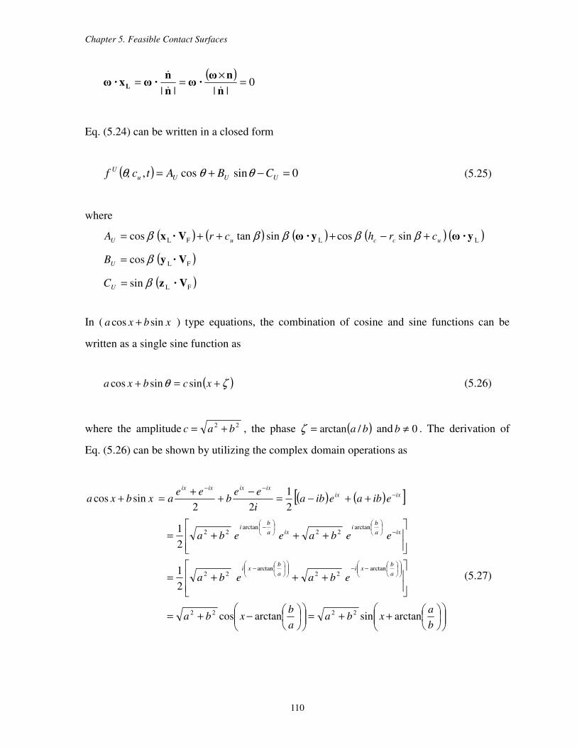
Chapter 5. Feasible Contact Surfaces
110
( )
0||||
=×
==n
nω·ω
n
n·ωx ·ω L
&&
&
Eq. (5.24) can be written in a closed form
( ) 0sincos, =−+= UUUu
UCBAtc,f θθθ (5.25)
where
( ) ( ) ( ) ( ) ( )LLFL sincossintancos y ·ωy ·ωV·x uccuU crhcrA +−+++= βββββ
( )FLcos V·yβ=UB
( )FLsin V·zβ=UC
In ( xbxa sincos + ) type equations, the combination of cosine and sine functions can be
written as a single sine function as
( )ζθ +=+ xcbxa sinsincos (5.26)
where the amplitude 22 bac += , the phase ( )ba /arctan=ζ and 0≠b . The derivation of
Eq. (5.26) can be shown by utilizing the complex domain operations as
( ) ( )[ ]
++=
−+=
+++=
+++=
++−=−
++
=+
−−
−
−
−
−−−
b
axba
a
bxba
ebaeba
eebaeeba
eibaeibai
eeb
eeaxbxa
a
bxi
a
bxi
ixa
bi
ixa
bi
ixixixixixix
arctansinarctancos
2
1
2
1
2
1
22sincos
2222
arctan22
arctan22
arctan22
arctan22
(5.27)

Chapter 5. Feasible Contact Surfaces
111
Note that in the last line of the above equation cosine representation is transformed into sine
representation under the consideration of arctan function as
>
−
<
−−
=
0,1
arctan2
1
0,1
arctan2
1
)arctan(
yfory
yfory
y
π
π
Thus the Eq. (5.25) can be written in the following form
( ) 0sin22 =−++ UUUU CBA κθ (5.28)
where ( )UUU BA /arctan=κ . Solving Eq. (5.28) for θ yields
( )
−
+−
−
+=
−
−
U
UU
U
U
UU
U
u
BA
C
BA
C
tc
κπ
κ
θ
22
1
22
1
sin
sin
, (5.29)
When Eq. (5.29) is plugged into Eq. (5.15-a), for a given cutter location point the
envelope boundary of the upper-cone surface is obtained.
5.3.2 Envelope Boundary of the Corner-Torus
The velocity of arbitrary point IT on the toroidal surface (Figure 5.7) can be expressed in
MCS by
( )→
×+= TT
MIFI ωVV FT (5.30)
Plugging Eq. (5.14-b) into Eq. (5.30) yields
( ) ( ) ( ) ( ) ( )
( ) ( )L
LLFT
sinsin
cossincos
yω
xωzωVV
×++
×++×−+=
θφ
θφφ
c
cccT
M
rR
rRrhI (5.31)
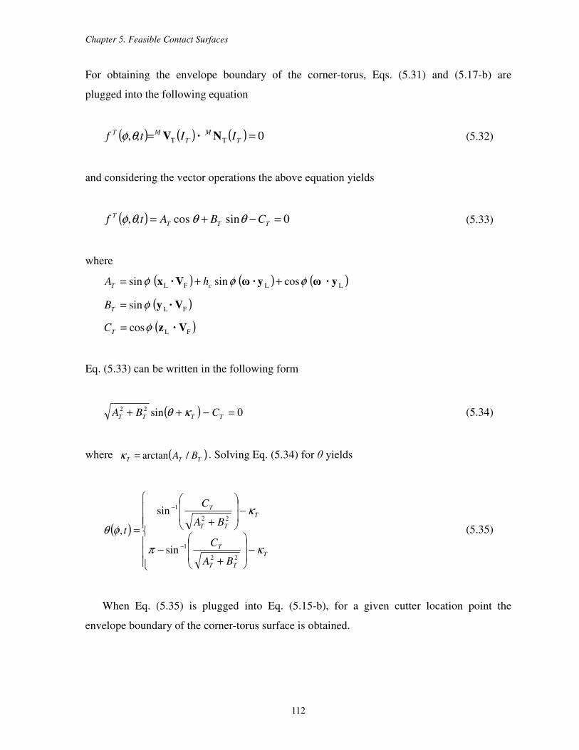
Chapter 5. Feasible Contact Surfaces
112
For obtaining the envelope boundary of the corner-torus, Eqs. (5.31) and (5.17-b) are
plugged into the following equation
( ) ( ) ( ) 0, TT == T
M
T
MT II,tf N·Vθφ (5.32)
and considering the vector operations the above equation yields
( ) 0sincos, =−+= TTT
T CBA,tf θθθφ (5.33)
where
( ) ( ) ( )LLFL cossinsin y·ωy ·ωV ·x φφφ ++= cT hA
( )FLsin V·yφ=TB
( )FLcos V·zφ=TC
Eq. (5.33) can be written in the following form
( ) 0sin22 =−++ TTTT CBA κθ (5.34)
where ( )TTT BA /arctan=κ . Solving Eq. (5.34) for θ yields
( )
−
+−
−
+=
−
−
T
TT
T
T
TT
T
BA
C
BA
C
t
κπ
κ
φθ
22
1
22
1
sin
sin
, (5.35)
When Eq. (5.35) is plugged into Eq. (5.15-b), for a given cutter location point the
envelope boundary of the corner-torus surface is obtained.

Chapter 5. Feasible Contact Surfaces
113
5.3.3 Envelope Boundary of the Lower-Cone
The velocity of a point IL on the lower-cone surface (Figure 5.7) is given by
( )→
×+= LL
MFII ωVV FL (5.36)
The Eq. (5.36) is expanded by substitution of Eq. (5.14-c) as
( ) ( ) ( )
( )L
LLFL
sintan
costan
yω
xωzωVV
×+
×+×+=
θα
θα
l
llL
M
c
ccI (5.37)
Eqs. (5.37) and (5.17-c) are plugged into the following equation
( ) ( ) ( ) 0, LL == L
M
L
M
l
LIItc,f N·Vθ (5.38)
and after the vector operations the envelope boundary of the lower-cone is obtained in the
closed form
( ) 0sincos, =−+= LLLl
LCBAtc,f θθθ (5.39)
where
( ) ( ) ( )LFLL coscostansin y ·ωV ·xy ·ω llL ccA αααα ++=
( )FLcos V·yα=LB
( )FLsin V·zα=LC
The Eq. (5.39) is transformed into the following form
( ) 0sin22 =−++ LLLL CBA κθ (5.40)
where ( )LLL BA /arctan=κ , and it is solved for θ as
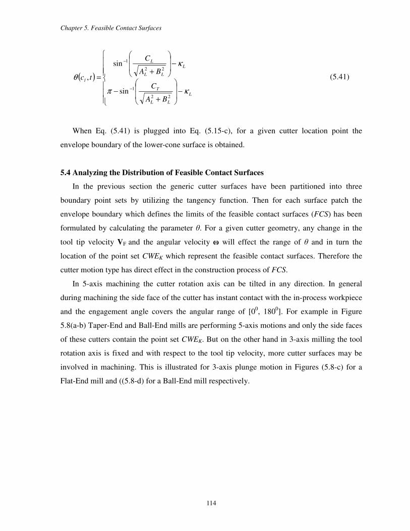
Chapter 5. Feasible Contact Surfaces
114
( )
−
+−
−
+=
−
−
L
LL
T
L
LL
L
l
BA
C
BA
C
tc
κπ
κ
θ
22
1
22
1
sin
sin
, (5.41)
When Eq. (5.41) is plugged into Eq. (5.15-c), for a given cutter location point the
envelope boundary of the lower-cone surface is obtained.
5.4 Analyzing the Distribution of Feasible Contact Surfaces
In the previous section the generic cutter surfaces have been partitioned into three
boundary point sets by utilizing the tangency function. Then for each surface patch the
envelope boundary which defines the limits of the feasible contact surfaces (FCS) has been
formulated by calculating the parameter θ. For a given cutter geometry, any change in the
tool tip velocity VF and the angular velocity ω will effect the range of θ and in turn the
location of the point set CWEK which represent the feasible contact surfaces. Therefore the
cutter motion type has direct effect in the construction process of FCS.
In 5-axis machining the cutter rotation axis can be tilted in any direction. In general
during machining the side face of the cutter has instant contact with the in-process workpiece
and the engagement angle covers the angular range of [00, 180
0]. For example in Figure
5.8(a-b) Taper-End and Ball-End mills are performing 5-axis motions and only the side faces
of these cutters contain the point set CWEK. But on the other hand in 3-axis milling the tool
rotation axis is fixed and with respect to the tool tip velocity, more cutter surfaces may be
involved in machining. This is illustrated for 3-axis plunge motion in Figures (5.8-c) for a
Flat-End mill and ((5.8-d) for a Ball-End mill respectively.
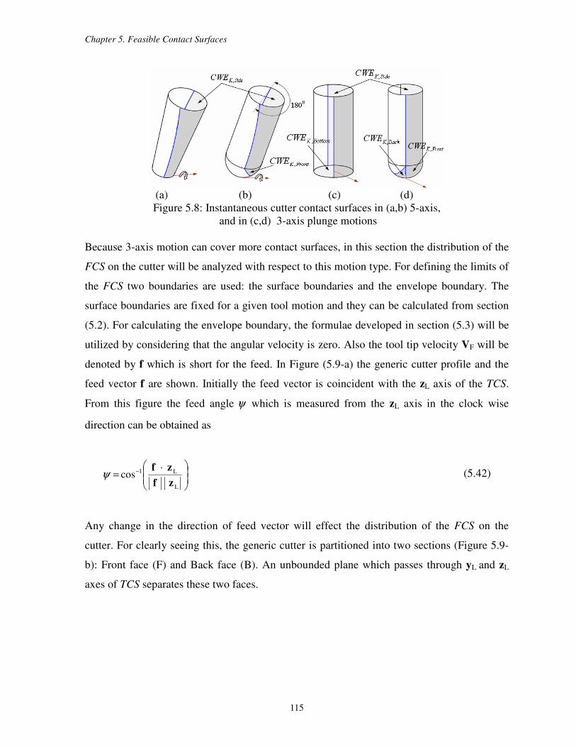
Chapter 5. Feasible Contact Surfaces
115
(a) (b) (c) (d)
Figure 5.8: Instantaneous cutter contact surfaces in (a,b) 5-axis,
and in (c,d) 3-axis plunge motions
Because 3-axis motion can cover more contact surfaces, in this section the distribution of the
FCS on the cutter will be analyzed with respect to this motion type. For defining the limits of
the FCS two boundaries are used: the surface boundaries and the envelope boundary. The
surface boundaries are fixed for a given tool motion and they can be calculated from section
(5.2). For calculating the envelope boundary, the formulae developed in section (5.3) will be
utilized by considering that the angular velocity is zero. Also the tool tip velocity VF will be
denoted by f which is short for the feed. In Figure (5.9-a) the generic cutter profile and the
feed vector f are shown. Initially the feed vector is coincident with the zL axis of the TCS.
From this figure the feed angle ψ which is measured from the zL axis in the clock wise
direction can be obtained as
= −
L
L1 ·cos
zf
zfψ (5.42)
Any change in the direction of feed vector will effect the distribution of the FCS on the
cutter. For clearly seeing this, the generic cutter is partitioned into two sections (Figure 5.9-
b): Front face (F) and Back face (B). An unbounded plane which passes through yL and zL
axes of TCS separates these two faces.
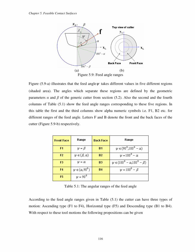
Chapter 5. Feasible Contact Surfaces
116
(a) (b)
Figure 5.9: Feed angle ranges
Figure (5.9-a) illustrates that the feed angleψ takes different values in five different regions
(shaded area). The angles which separate these regions are defined by the geometric
parameters α and β of the generic cutter from section (5.2). Also the second and the fourth
columns of Table (5.1) show the feed angle ranges corresponding to these five regions. In
this table the first and the third columns show alpha numeric symbols i.e. F1, B2 etc. for
different ranges of the feed angle. Letters F and B denote the front and the back faces of the
cutter (Figure 5.9-b) respectively.
Table 5.1: The angular ranges of the feed angle
According to the feed angle ranges given in Table (5.1) the cutter can have three types of
motion: Ascending type (F1 to F4), Horizontal type (F5) and Descending type (B1 to B4).
With respect to these tool motions the following propositions can be given
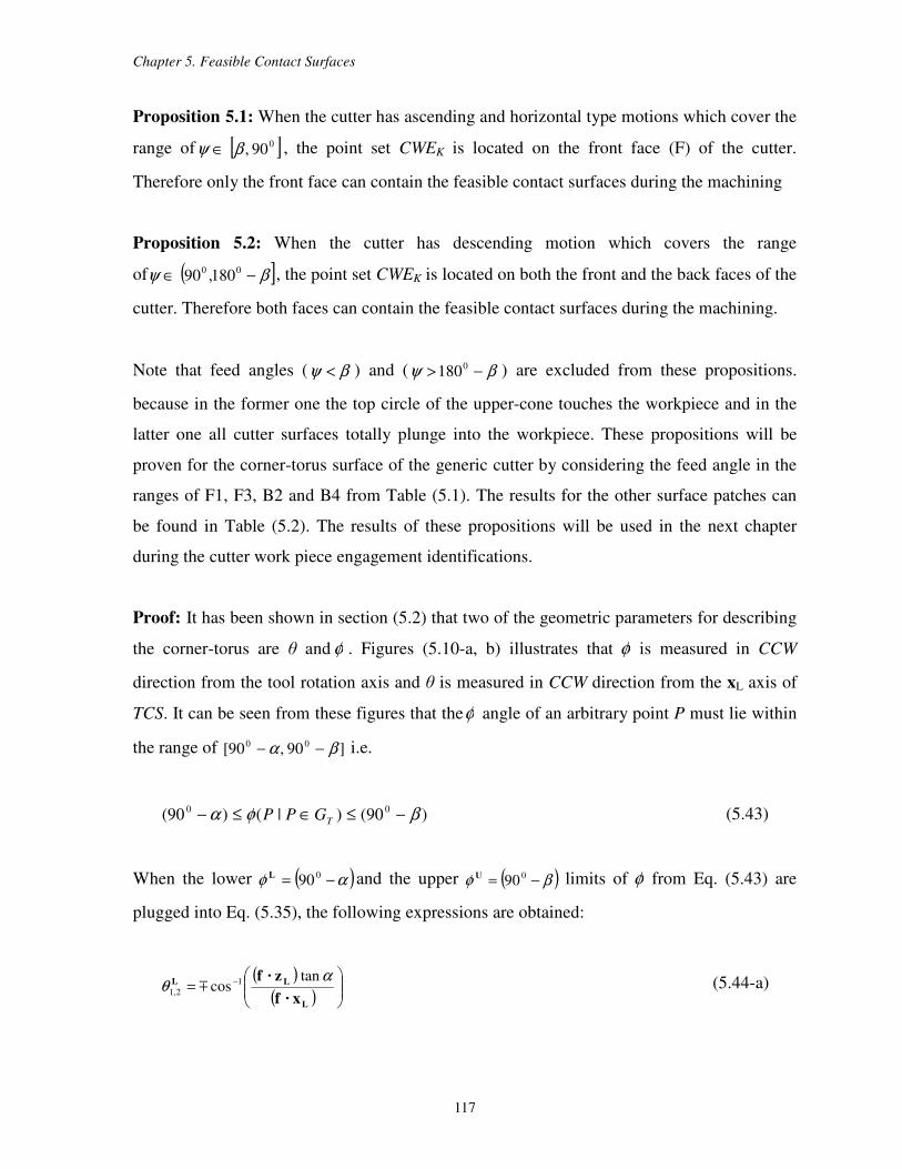
Chapter 5. Feasible Contact Surfaces
117
Proposition 5.1: When the cutter has ascending and horizontal type motions which cover the
range of [ ]090,βψ ∈ , the point set CWEK is located on the front face (F) of the cutter.
Therefore only the front face can contain the feasible contact surfaces during the machining
Proposition 5.2: When the cutter has descending motion which covers the range
of ( ]βψ −∈ 00180,90 , the point set CWEK is located on both the front and the back faces of the
cutter. Therefore both faces can contain the feasible contact surfaces during the machining.
Note that feed angles ( βψ < ) and ( βψ −> 0180 ) are excluded from these propositions.
because in the former one the top circle of the upper-cone touches the workpiece and in the
latter one all cutter surfaces totally plunge into the workpiece. These propositions will be
proven for the corner-torus surface of the generic cutter by considering the feed angle in the
ranges of F1, F3, B2 and B4 from Table (5.1). The results for the other surface patches can
be found in Table (5.2). The results of these propositions will be used in the next chapter
during the cutter work piece engagement identifications.
Proof: It has been shown in section (5.2) that two of the geometric parameters for describing
the corner-torus are θ and φ . Figures (5.10-a, b) illustrates that φ is measured in CCW
direction from the tool rotation axis and θ is measured in CCW direction from the xL axis of
TCS. It can be seen from these figures that theφ angle of an arbitrary point P must lie within
the range of ]90,90[ 00 βα −− i.e.
)90()|()90( 00 βφα −≤∈≤− TGPP (5.43)
When the lower ( )αφ −= 090L and the upper ( )βφ −= 090U limits of φ from Eq. (5.43) are
plugged into Eq. (5.35), the following expressions are obtained:
( )( )
= −
L
LL
x·f
z·f αθ
tancos 1
2,1 m (5.44-a)

Chapter 5. Feasible Contact Surfaces
118
( )( )
= −
L
LU
x·f
z·f βθ
tancos 1
2,1 m (5.44-b)
where superscripts L and U represent the lower and the upper limit respectively. Note that the
angular velocity in Eq. (5.35) becomes zero in 3-axis machining.
(a) (b)
Figure 5.10: The corner-torus with upper and lower surface boundaries.
Cutter has a feed angle ( βψ = )
In this case the angle between the feed vector f and zL axis equals to β and the cutter has
an ascending motion. For this feed angle the dot products in Eqs. (5.44,a-b) are evaluated as
follows
βcos|| LL z||fz·f = )90cos(||0
LL β−= x||fx·f
Plugging the above equations back into Eqs. (5.44-a, b) yields
= −
β
αθ
tan
tancos 1L
2,1 m (5.45-a)
0U
2,1 0=θ (5.45-b)
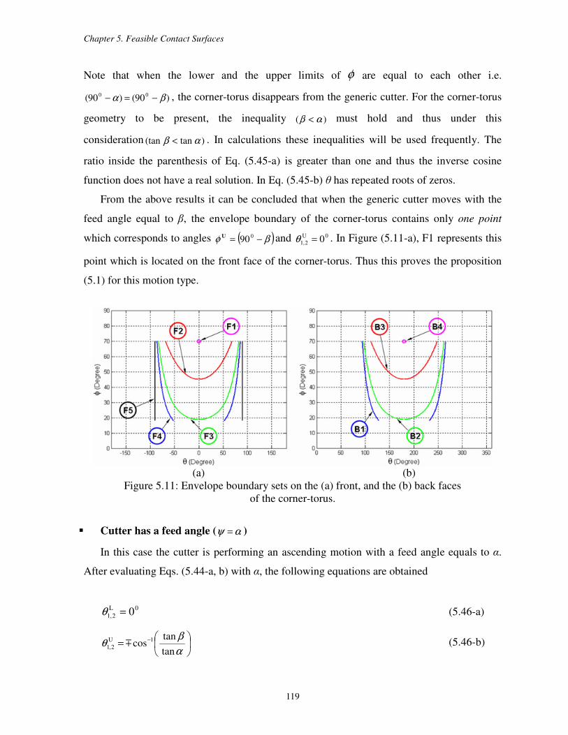
Chapter 5. Feasible Contact Surfaces
119
Note that when the lower and the upper limits of φ are equal to each other i.e.
)90()90( 00 βα −=− , the corner-torus disappears from the generic cutter. For the corner-torus
geometry to be present, the inequality )( αβ < must hold and thus under this
consideration )tan(tan αβ < . In calculations these inequalities will be used frequently. The
ratio inside the parenthesis of Eq. (5.45-a) is greater than one and thus the inverse cosine
function does not have a real solution. In Eq. (5.45-b) θ has repeated roots of zeros.
From the above results it can be concluded that when the generic cutter moves with the
feed angle equal to β, the envelope boundary of the corner-torus contains only one point
which corresponds to angles ( )βφ −= 090U and 0U
2,1 0=θ . In Figure (5.11-a), F1 represents this
point which is located on the front face of the corner-torus. Thus this proves the proposition
(5.1) for this motion type.
(a) (b)
Figure 5.11: Envelope boundary sets on the (a) front, and the (b) back faces
of the corner-torus.
Cutter has a feed angle ( αψ = )
In this case the cutter is performing an ascending motion with a feed angle equals to α.
After evaluating Eqs. (5.44-a, b) with α, the following equations are obtained
0L
2,1 0=θ (5.46-a)
= −
α
βθ
tan
tancos
1U
2,1 m (5.46-b)

Chapter 5. Feasible Contact Surfaces
120
The ratio inside the parenthesis of Eq. (5.46-b) is positive and less than one. Therefore for a
given parameter set ( )βφ −= 090U and U
2,1θ the upper surface boundary of the corner-torus
contains two points which are members of the envelope boundary. These are two symmetric
points with respect to the feed vector and they are located on the front face of the corner-
torus. The repeated roots in Eq. (5.46-a) and the lower limit ofφ , ( )αφ −= 090L generate a
point on the lower surface boundary of the corner-torus. This single point which is also a
member of the envelope boundary is located on the front face. From these results it can be
seen that the upper and the lower surface boundaries of the corner–torus contain envelope
boundary points on the front face. Therefore it can be concluded that changing φ between
( )αφ −= 090L and ( )βφ −= 090U generates new envelope boundary points on the front face.
F3 in Figure (5.11-a) shows an example of the envelope boundary for this motion.
Thus for this motion type the envelope boundary on the front face and the portion of the
upper surface boundary on the front face draw the limits of the point set CWEK. Thus this
proves the proposition (5.1) for this motion type. F3 in Figure (5.12) illustrates the point set
CWEK with shaded area.
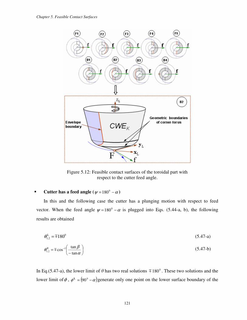
Chapter 5. Feasible Contact Surfaces
121
Figure 5.12: Feasible contact surfaces of the toroidal part with
respect to the cutter feed angle.
Cutter has a feed angle ( αψ −= 0180 )
In this and the following case the cutter has a plunging motion with respect to feed
vector. When the feed angle αψ −= 0180 is plugged into Eqs. (5.44-a, b), the following
results are obtained
0L
2,1 180m=θ (5.47-a)
−= −
α
βθ
tan
tancos 1
2,1 mU (5.47-b)
In Eq.(5.47-a), the lower limit of θ has two real solutions 0180m . These two solutions and the
lower limit ofφ , ( )αφ −= 090L generate only one point on the lower surface boundary of the
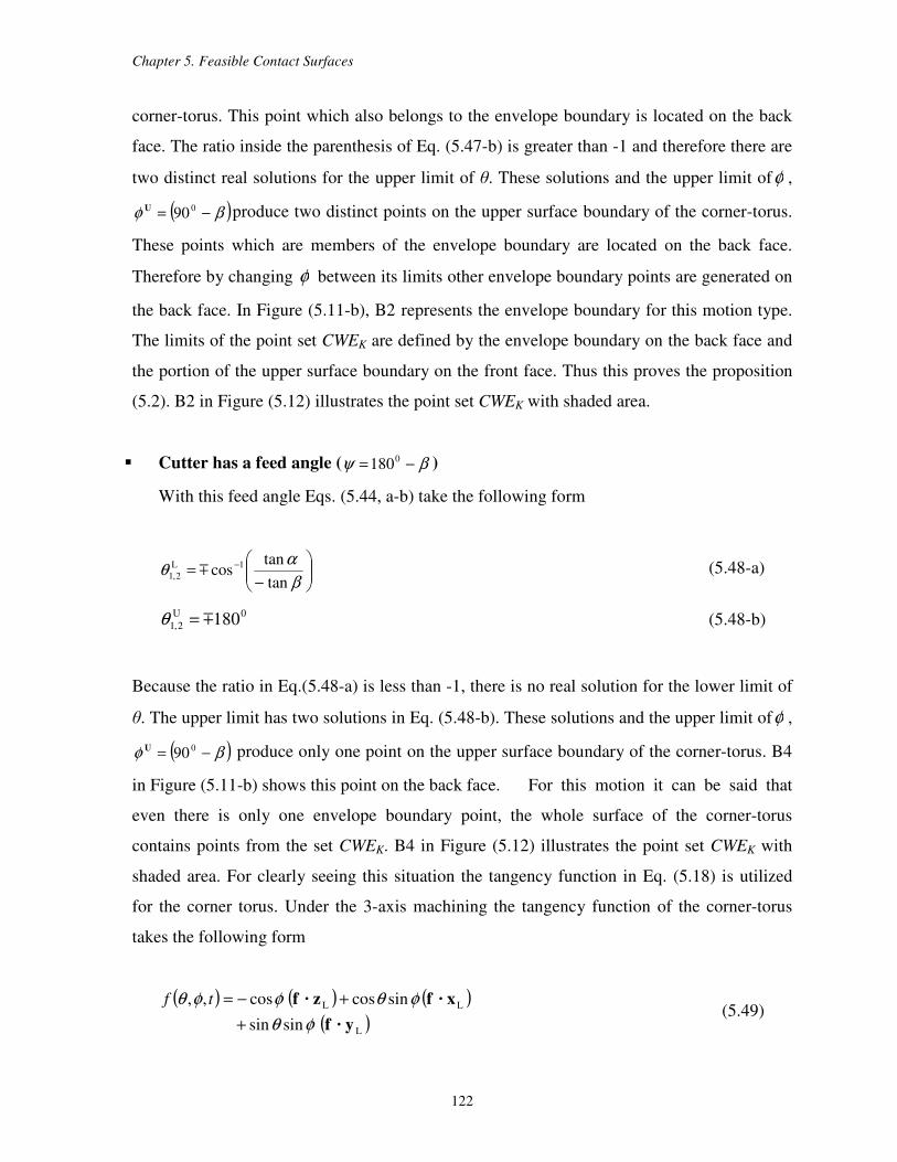
Chapter 5. Feasible Contact Surfaces
122
corner-torus. This point which also belongs to the envelope boundary is located on the back
face. The ratio inside the parenthesis of Eq. (5.47-b) is greater than -1 and therefore there are
two distinct real solutions for the upper limit of θ. These solutions and the upper limit ofφ ,
( )βφ −= 090U produce two distinct points on the upper surface boundary of the corner-torus.
These points which are members of the envelope boundary are located on the back face.
Therefore by changing φ between its limits other envelope boundary points are generated on
the back face. In Figure (5.11-b), B2 represents the envelope boundary for this motion type.
The limits of the point set CWEK are defined by the envelope boundary on the back face and
the portion of the upper surface boundary on the front face. Thus this proves the proposition
(5.2). B2 in Figure (5.12) illustrates the point set CWEK with shaded area.
Cutter has a feed angle ( βψ −= 0180 )
With this feed angle Eqs. (5.44, a-b) take the following form
−= −
β
αθ
tan
tancos 1L
2,1 m (5.48-a)
0U
2,1 180m=θ (5.48-b)
Because the ratio in Eq.(5.48-a) is less than -1, there is no real solution for the lower limit of
θ. The upper limit has two solutions in Eq. (5.48-b). These solutions and the upper limit ofφ ,
( )βφ −= 090U produce only one point on the upper surface boundary of the corner-torus. B4
in Figure (5.11-b) shows this point on the back face. For this motion it can be said that
even there is only one envelope boundary point, the whole surface of the corner-torus
contains points from the set CWEK. B4 in Figure (5.12) illustrates the point set CWEK with
shaded area. For clearly seeing this situation the tangency function in Eq. (5.18) is utilized
for the corner torus. Under the 3-axis machining the tangency function of the corner-torus
takes the following form
( ) ( ) ( )
( )L
LL
sinsin
sincoscos,,
y·f
x·fz·f
φθ
φθφφθ
+
+−=tf (5.49)
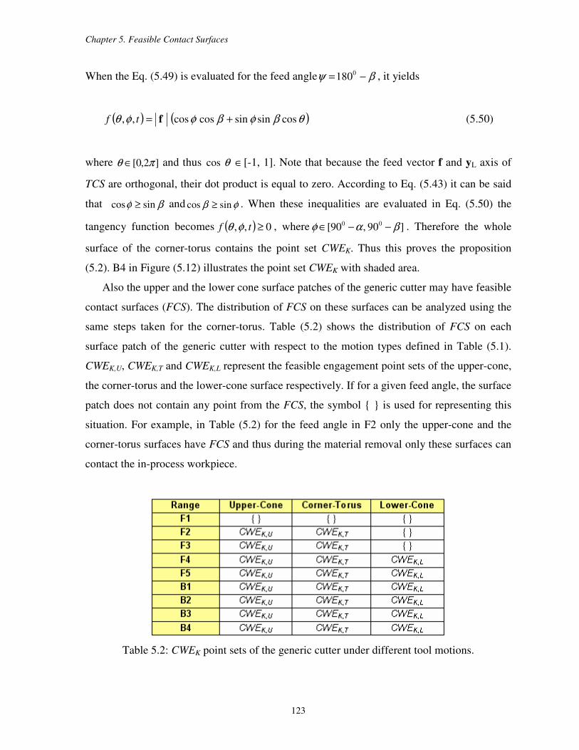
Chapter 5. Feasible Contact Surfaces
123
When the Eq. (5.49) is evaluated for the feed angle βψ −= 0180 , it yields
( ) ( )θβφβφφθ cossinsincoscos,, += ftf (5.50)
where ]2,0[ πθ ∈ and thus θcos ∈[-1, 1]. Note that because the feed vector f and yL axis of
TCS are orthogonal, their dot product is equal to zero. According to Eq. (5.43) it can be said
that βφ sincos ≥ and φβ sincos ≥ . When these inequalities are evaluated in Eq. (5.50) the
tangency function becomes ( ) 0,, ≥tf φθ , where ]90,90[ 00 βαφ −−∈ . Therefore the whole
surface of the corner-torus contains the point set CWEK. Thus this proves the proposition
(5.2). B4 in Figure (5.12) illustrates the point set CWEK with shaded area.
Also the upper and the lower cone surface patches of the generic cutter may have feasible
contact surfaces (FCS). The distribution of FCS on these surfaces can be analyzed using the
same steps taken for the corner-torus. Table (5.2) shows the distribution of FCS on each
surface patch of the generic cutter with respect to the motion types defined in Table (5.1).
CWEK,U, CWEK,T and CWEK,L represent the feasible engagement point sets of the upper-cone,
the corner-torus and the lower-cone surface respectively. If for a given feed angle, the surface
patch does not contain any point from the FCS, the symbol is used for representing this
situation. For example, in Table (5.2) for the feed angle in F2 only the upper-cone and the
corner-torus surfaces have FCS and thus during the material removal only these surfaces can
contact the in-process workpiece.
Table 5.2: CWEK point sets of the generic cutter under different tool motions.
Chapter 5. Feasible Contact Surfaces
124
5.5 Discussion
In this chapter the engagement behaviors of NC cutter surfaces under varying tool
motions have been presented by introducing the feasible contact surfaces (FCS) terminology.
The description of the FCS has been made by utilizing the kinematically feasible engagement
points contained in the set CWEK. In a typical NC cutter the constituent surface geometries
show differences and because of this during the machining the engagement characteristics for
these surfaces become different. Under this consideration the set CWEK has been partitioned
among the constituent surfaces of a cutter. As mentioned in this chapter, the Cutter
Workpiece Engagements (CWEs) are the subsets of the FCS and for calculating CWEs the
boundaries of the FCS must be identified. In this work these boundaries which are limits of
the set CWEK have been defined by the cutter surface boundaries and the envelope
boundaries. Under the rigid tool motions the cutter surface boundaries stay fixed. But on the
other hand the envelope boundaries may change. For modeling the envelope boundaries a
tangency function defined by the surface normal and the tool velocity has been utilized. Later
by changing the tool velocity direction the distributions of the FCS on the cutter have been
analyzed. Also it has been shown with examples that only the certain parts of the cutter
surfaces have contacts with the in-process workpiece. The results from this chapter will be
used in the CWEs generation.
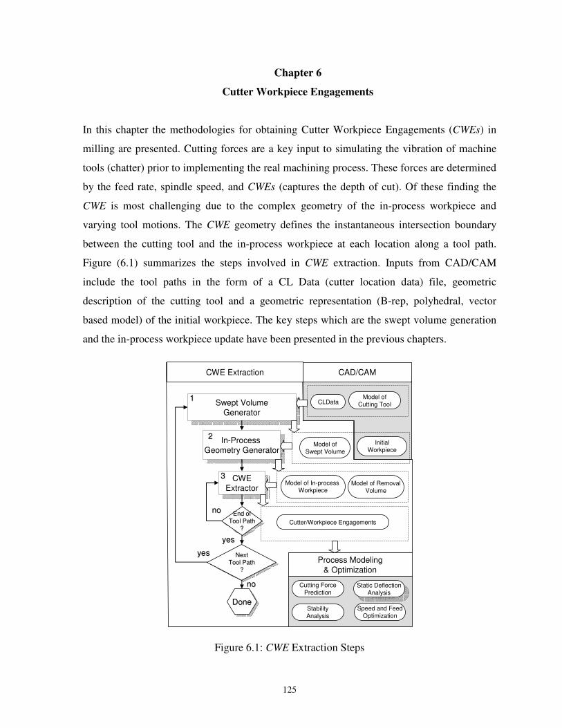
125
Chapter 6
Cutter Workpiece Engagements
In this chapter the methodologies for obtaining Cutter Workpiece Engagements (CWEs) in
milling are presented. Cutting forces are a key input to simulating the vibration of machine
tools (chatter) prior to implementing the real machining process. These forces are determined
by the feed rate, spindle speed, and CWEs (captures the depth of cut). Of these finding the
CWE is most challenging due to the complex geometry of the in-process workpiece and
varying tool motions. The CWE geometry defines the instantaneous intersection boundary
between the cutting tool and the in-process workpiece at each location along a tool path.
Figure (6.1) summarizes the steps involved in CWE extraction. Inputs from CAD/CAM
include the tool paths in the form of a CL Data (cutter location data) file, geometric
description of the cutting tool and a geometric representation (B-rep, polyhedral, vector
based model) of the initial workpiece. The key steps which are the swept volume generation
and the in-process workpiece update have been presented in the previous chapters.
CAD/CAM
Model ofSwept Volume
Model of In-process Workpiece
CWEExtractor
CWEExtractor
End ofTool Path
?
End ofEnd of
Tool PathTool Path??
NextTool Path
?
NextNext
Tool PathTool Path
??
Model ofCutting Tool
DoneDoneDone
11
33
nono
yesyes
yesyes
nono
In-Process Geometry Generator
In-Process Geometry Generator
Swept VolumeGenerator
Swept VolumeGenerator
22
11 CLData
InitialWorkpiece
Cutter/Workpiece Engagements
Process Modeling& Optimization
Cutting ForcePrediction
StabilityAnalysis
Speed and FeedOptimization
Static DeflectionAnalysis
Static DeflectionAnalysis
CWE Extraction
Model of RemovalVolume
Figure 6.1: CWE Extraction Steps
Chapter 6. Cutter Workpiece Engagements
126
In this chapter the CWEs are calculated for supporting the force prediction model
described in [5]. This model finds the Cartesian force components by analytically integrating
the differential cutting forces along the in-cut portion of each cutter flute. In this model CWE
area with a fixed axial depth of cut is defined by mapping the engagement region on the
cutter surface onto X - Y plane which represents the engagement angle versus the depth of
cut respectively (Figure 6.2).
Figure 6.2 has been removed due to copyright restrictions. The information removed is
CWE area for the force prediction, [5].
In this chapter the methodologies for finding the CWEs are developed based on the
mathematical representation of the workpiece geometry. The workpiece geometries are
defined by a solid, a polyhedral and a vector based modeler respectively. Although
polyhedral and vector based approaches require a shorter computational time than does the
solid modeler based approach, the accuracy of these approaches depends greatly on the
resolution of the workpiece. There is always a tradeoff between computational efficiency and
accuracy in these approaches. For example the solid modeler has an advantage in accuracy
because it provides an accurate geometric representation for the workpiece. Therefore in the
solid modeler based approach the most accurate representations of the CWEs are obtained.
But on the other hand this modeler uses numerical techniques that are limited primarily by
efficiency and robustness.
The Cutter Workpiece Engagements in Solid Models are presented in section (6.1). This
section contains two methodologies: Engagement Extraction Methodology in 3-Axis Milling
(section 6.1.1) and Engagement Extraction Methodology in 5-Axis Milling (section 6.1.3)
respectively. In the 3-axis milling methodology the cutter surfaces are decomposed with
respect to the feed direction as explained in chapter (5), and then these decomposed surfaces
are intersected with their removal volumes for obtaining the closed CWE area. In the 5-axis
methodology the similar approach is utilized with one difference. In this case the in-process
workpiece is used instead of cutter removal volumes. The developed solid modeler based
methodologies are implemented using ACIS solid modeling kernel. The both methodologies
are supported by examples.
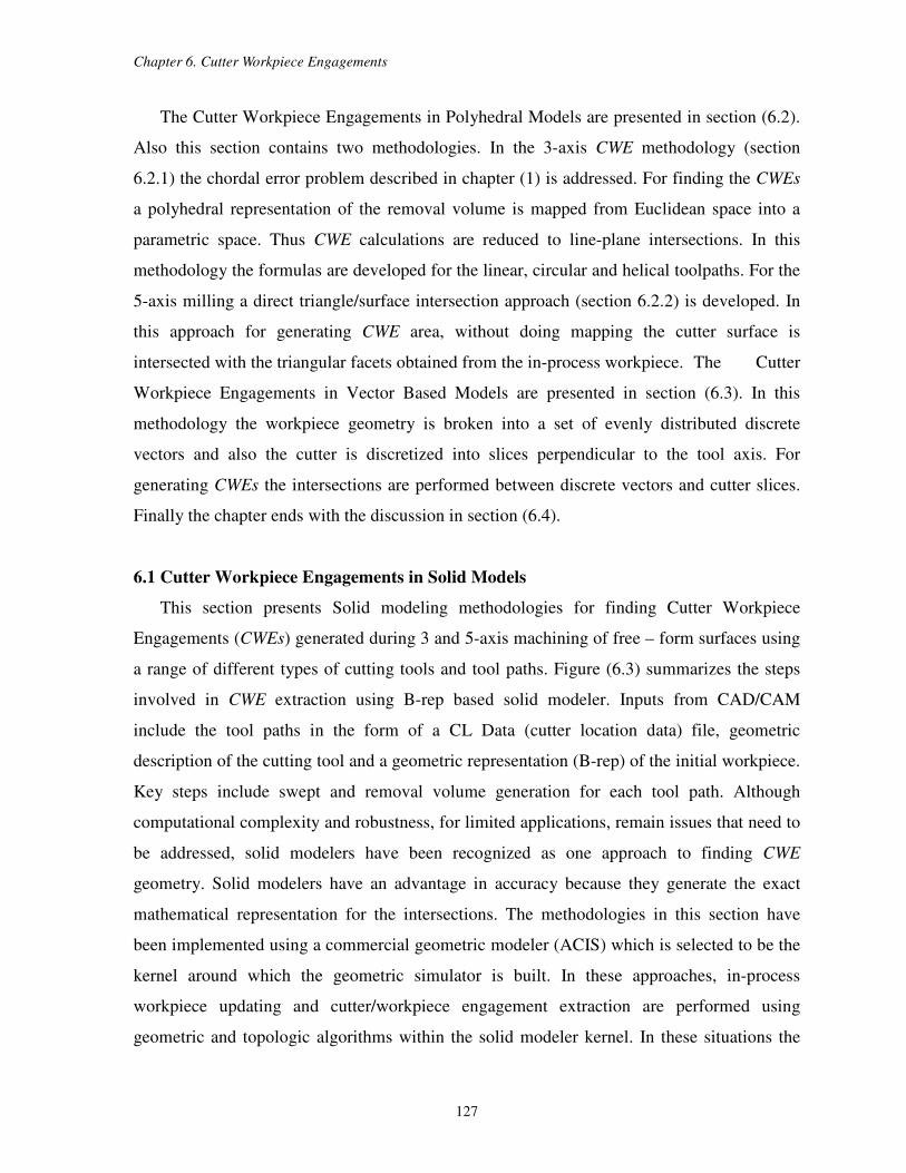
Chapter 6. Cutter Workpiece Engagements
127
The Cutter Workpiece Engagements in Polyhedral Models are presented in section (6.2).
Also this section contains two methodologies. In the 3-axis CWE methodology (section
6.2.1) the chordal error problem described in chapter (1) is addressed. For finding the CWEs
a polyhedral representation of the removal volume is mapped from Euclidean space into a
parametric space. Thus CWE calculations are reduced to line-plane intersections. In this
methodology the formulas are developed for the linear, circular and helical toolpaths. For the
5-axis milling a direct triangle/surface intersection approach (section 6.2.2) is developed. In
this approach for generating CWE area, without doing mapping the cutter surface is
intersected with the triangular facets obtained from the in-process workpiece. The Cutter
Workpiece Engagements in Vector Based Models are presented in section (6.3). In this
methodology the workpiece geometry is broken into a set of evenly distributed discrete
vectors and also the cutter is discretized into slices perpendicular to the tool axis. For
generating CWEs the intersections are performed between discrete vectors and cutter slices.
Finally the chapter ends with the discussion in section (6.4).
6.1 Cutter Workpiece Engagements in Solid Models
This section presents Solid modeling methodologies for finding Cutter Workpiece
Engagements (CWEs) generated during 3 and 5-axis machining of free – form surfaces using
a range of different types of cutting tools and tool paths. Figure (6.3) summarizes the steps
involved in CWE extraction using B-rep based solid modeler. Inputs from CAD/CAM
include the tool paths in the form of a CL Data (cutter location data) file, geometric
description of the cutting tool and a geometric representation (B-rep) of the initial workpiece.
Key steps include swept and removal volume generation for each tool path. Although
computational complexity and robustness, for limited applications, remain issues that need to
be addressed, solid modelers have been recognized as one approach to finding CWE
geometry. Solid modelers have an advantage in accuracy because they generate the exact
mathematical representation for the intersections. The methodologies in this section have
been implemented using a commercial geometric modeler (ACIS) which is selected to be the
kernel around which the geometric simulator is built. In these approaches, in-process
workpiece updating and cutter/workpiece engagement extraction are performed using
geometric and topologic algorithms within the solid modeler kernel. In these situations the
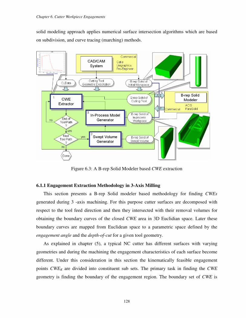
Chapter 6. Cutter Workpiece Engagements
128
solid modeling approach applies numerical surface intersection algorithms which are based
on subdivision, and curve tracing (marching) methods.
Figure 6.3: A B-rep Solid Modeler based CWE extraction
6.1.1 Engagement Extraction Methodology in 3-Axis Milling
This section presents a B-rep Solid modeler based methodology for finding CWEs
generated during 3 -axis machining. For this purpose cutter surfaces are decomposed with
respect to the tool feed direction and then they intersected with their removal volumes for
obtaining the boundary curves of the closed CWE area in 3D Euclidian space. Later these
boundary curves are mapped from Euclidean space to a parametric space defined by the
engagement angle and the depth-of-cut for a given tool geometry.
As explained in chapter (5), a typical NC cutter has different surfaces with varying
geometries and during the machining the engagement characteristics of each surface become
different. Under this consideration in this section the kinematically feasible engagement
points CWEK are divided into constituent sub sets. The primary task in finding the CWE
geometry is finding the boundary of the engagement region. The boundary set of CWE is
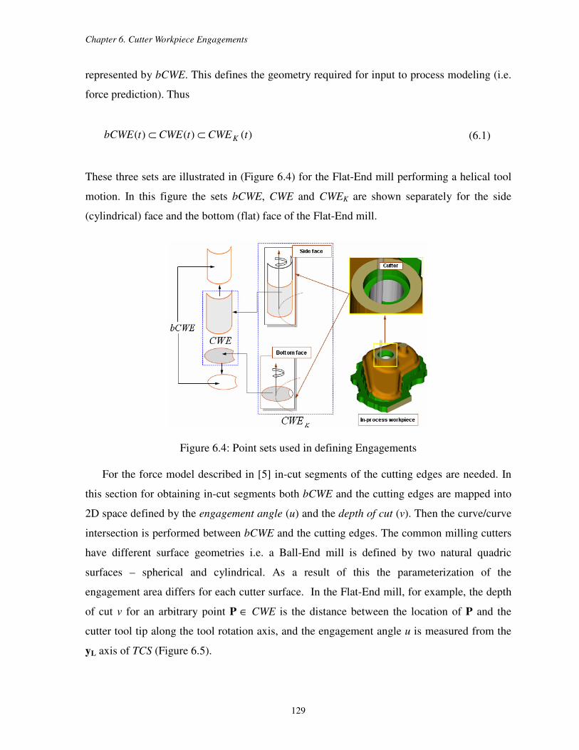
Chapter 6. Cutter Workpiece Engagements
129
represented by bCWE. This defines the geometry required for input to process modeling (i.e.
force prediction). Thus
)()()( tCWEtCWEtbCWE K⊂⊂ (6.1)
These three sets are illustrated in (Figure 6.4) for the Flat-End mill performing a helical tool
motion. In this figure the sets bCWE, CWE and CWEK are shown separately for the side
(cylindrical) face and the bottom (flat) face of the Flat-End mill.
Figure 6.4: Point sets used in defining Engagements
For the force model described in [5] in-cut segments of the cutting edges are needed. In
this section for obtaining in-cut segments both bCWE and the cutting edges are mapped into
2D space defined by the engagement angle (u) and the depth of cut (v). Then the curve/curve
intersection is performed between bCWE and the cutting edges. The common milling cutters
have different surface geometries i.e. a Ball-End mill is defined by two natural quadric
surfaces – spherical and cylindrical. As a result of this the parameterization of the
engagement area differs for each cutter surface. In the Flat-End mill, for example, the depth
of cut v for an arbitrary point P ∈ CWE is the distance between the location of P and the
cutter tool tip along the tool rotation axis, and the engagement angle u is measured from the
yL axis of TCS (Figure 6.5).
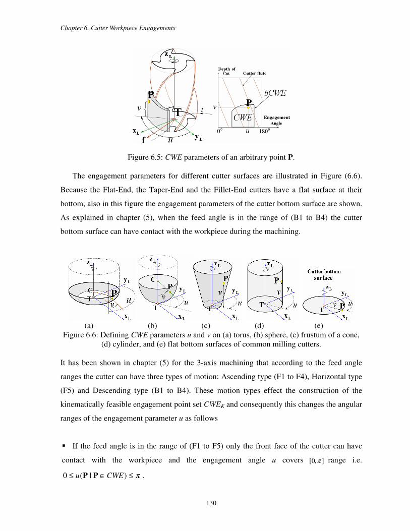
Chapter 6. Cutter Workpiece Engagements
130
Figure 6.5: CWE parameters of an arbitrary point P.
The engagement parameters for different cutter surfaces are illustrated in Figure (6.6).
Because the Flat-End, the Taper-End and the Fillet-End cutters have a flat surface at their
bottom, also in this figure the engagement parameters of the cutter bottom surface are shown.
As explained in chapter (5), when the feed angle is in the range of (B1 to B4) the cutter
bottom surface can have contact with the workpiece during the machining.
(a) (b) (c) (d) (e)
Figure 6.6: Defining CWE parameters u and v on (a) torus, (b) sphere, (c) frustum of a cone,
(d) cylinder, and (e) flat bottom surfaces of common milling cutters.
It has been shown in chapter (5) for the 3-axis machining that according to the feed angle
ranges the cutter can have three types of motion: Ascending type (F1 to F4), Horizontal type
(F5) and Descending type (B1 to B4). These motion types effect the construction of the
kinematically feasible engagement point set CWEK and consequently this changes the angular
ranges of the engagement parameter u as follows
If the feed angle is in the range of (F1 to F5) only the front face of the cutter can have
contact with the workpiece and the engagement angle u covers ],0[ π range i.e.
π≤∈≤ )|(0 CWEu PP .
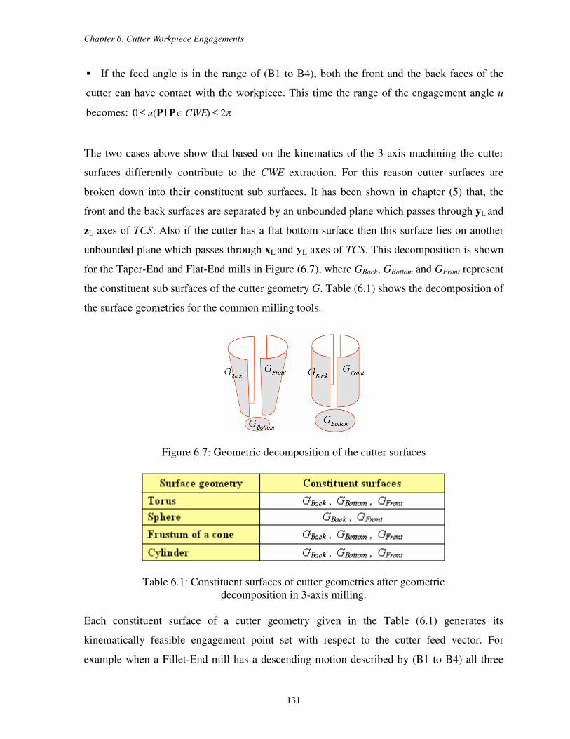
Chapter 6. Cutter Workpiece Engagements
131
If the feed angle is in the range of (B1 to B4), both the front and the back faces of the
cutter can have contact with the workpiece. This time the range of the engagement angle u
becomes: π2)|(0 ≤∈≤ CWEu PP
The two cases above show that based on the kinematics of the 3-axis machining the cutter
surfaces differently contribute to the CWE extraction. For this reason cutter surfaces are
broken down into their constituent sub surfaces. It has been shown in chapter (5) that, the
front and the back surfaces are separated by an unbounded plane which passes through yL and
zL axes of TCS. Also if the cutter has a flat bottom surface then this surface lies on another
unbounded plane which passes through xL and yL axes of TCS. This decomposition is shown
for the Taper-End and Flat-End mills in Figure (6.7), where GBack, GBottom and GFront represent
the constituent sub surfaces of the cutter geometry G. Table (6.1) shows the decomposition of
the surface geometries for the common milling tools.
Figure 6.7: Geometric decomposition of the cutter surfaces
Table 6.1: Constituent surfaces of cutter geometries after geometric
decomposition in 3-axis milling.
Each constituent surface of a cutter geometry given in the Table (6.1) generates its
kinematically feasible engagement point set with respect to the cutter feed vector. For
example when a Fillet-End mill has a descending motion described by (B1 to B4) all three
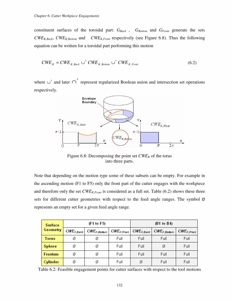
Chapter 6. Cutter Workpiece Engagements
132
constituent surfaces of the toroidal part: GBack , GBottom and GFront generate the sets
CWEK,Back, CWEK,Bottom and CWEK,Front respectively (see Figure 6.8). Thus the following
equation can be written for a toroidal part performing this motion
FrontKBottomKBackKK CWECWECWECWE ,
*
,
*
, ∪∪= (6.2)
where *∪ and later *∩ represent regularized Boolean union and intersection set operations
respectively.
Figure 6.8: Decomposing the point set CWEK of the torus
into three parts.
Note that depending on the motion type some of these subsets can be empty. For example in
the ascending motion (F1 to F5) only the front part of the cutter engages with the workpiece
and therefore only the set CWEK,Front is considered as a full set. Table (6.2) shows these three
sets for different cutter geometries with respect to the feed angle ranges. The symbol Ø
represents an empty set for a given feed angle range.
Table 6.2: Feasible engagement points for cutter surfaces with respect to the tool motions
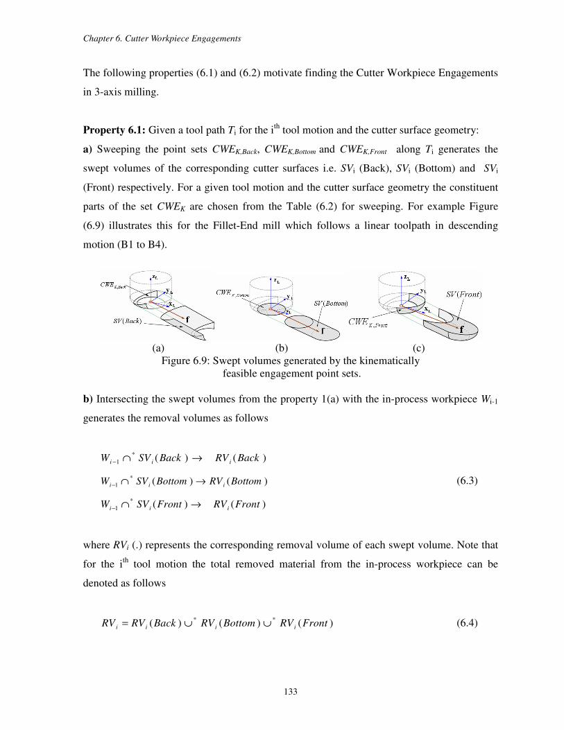
Chapter 6. Cutter Workpiece Engagements
133
The following properties (6.1) and (6.2) motivate finding the Cutter Workpiece Engagements
in 3-axis milling.
Property 6.1: Given a tool path Ti for the ith
tool motion and the cutter surface geometry:
a) Sweeping the point sets CWEK,Back, CWEK,Bottom and CWEK,Front along Ti generates the
swept volumes of the corresponding cutter surfaces i.e. SVi (Back), SVi (Bottom) and SVi
(Front) respectively. For a given tool motion and the cutter surface geometry the constituent
parts of the set CWEK are chosen from the Table (6.2) for sweeping. For example Figure
(6.9) illustrates this for the Fillet-End mill which follows a linear toolpath in descending
motion (B1 to B4).
(a) (b) (c)
Figure 6.9: Swept volumes generated by the kinematically
feasible engagement point sets.
b) Intersecting the swept volumes from the property 1(a) with the in-process workpiece Wi-1
generates the removal volumes as follows
)()(*
1 BackRVBackSVW iii →∩−
)()(*
1 BottomRVBottomSVW iii →∩− (6.3)
)()(*
1 FrontRVFrontSVW iii →∩−
where RVi (.) represents the corresponding removal volume of each swept volume. Note that
for the ith
tool motion the total removed material from the in-process workpiece can be
denoted as follows
)()()( **FrontRVBottomRVBackRVRV iiii ∪∪= (6.4)
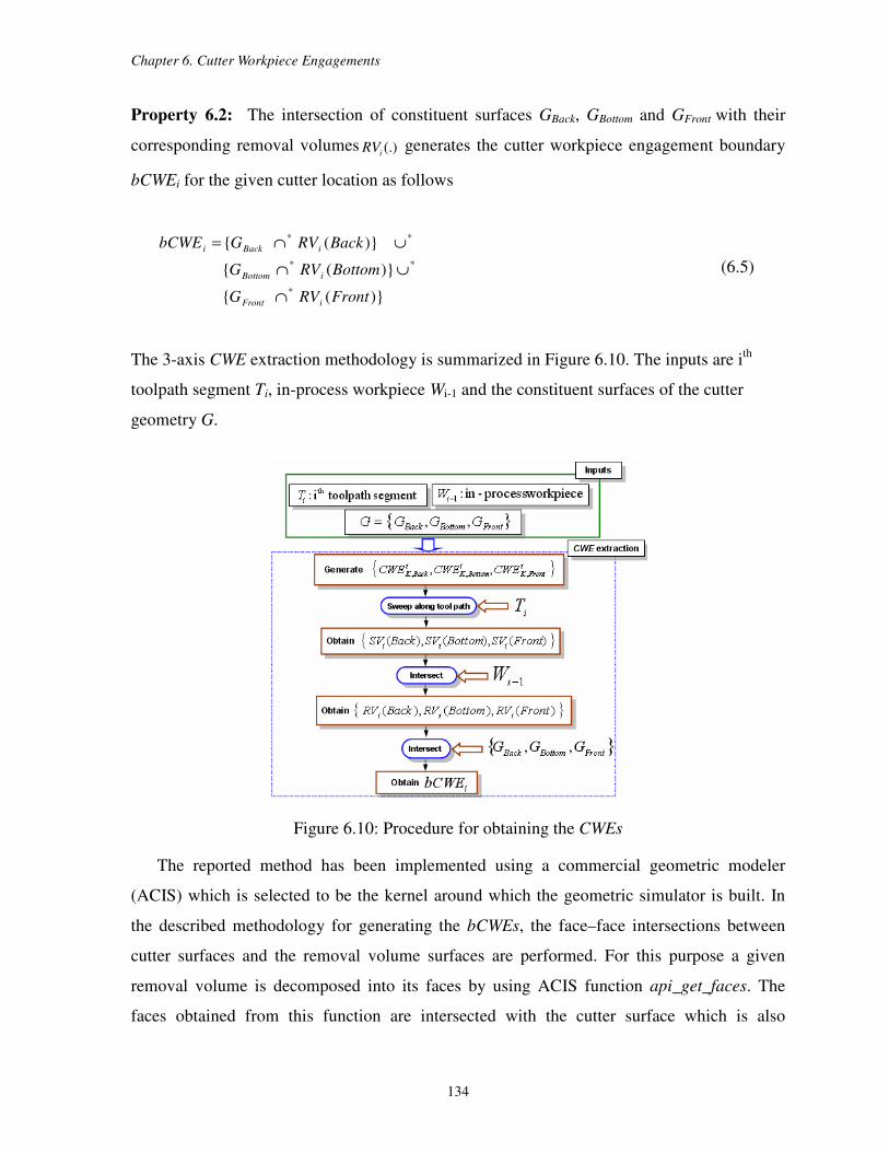
Chapter 6. Cutter Workpiece Engagements
134
Property 6.2: The intersection of constituent surfaces GBack, GBottom and GFront with their
corresponding removal volumes (.)iRV generates the cutter workpiece engagement boundary
bCWEi for the given cutter location as follows
)(
)(
)(
*
**
**
FrontRVG
BottomRVG
BackRVGbCWE
iFront
iBottom
iBacki
∩
∪∩
∪∩=
(6.5)
The 3-axis CWE extraction methodology is summarized in Figure 6.10. The inputs are ith
toolpath segment Ti, in-process workpiece Wi-1 and the constituent surfaces of the cutter
geometry G.
Figure 6.10: Procedure for obtaining the CWEs
The reported method has been implemented using a commercial geometric modeler
(ACIS) which is selected to be the kernel around which the geometric simulator is built. In
the described methodology for generating the bCWEs, the face–face intersections between
cutter surfaces and the removal volume surfaces are performed. For this purpose a given
removal volume is decomposed into its faces by using ACIS function api_get_faces. The
faces obtained from this function are intersected with the cutter surface which is also
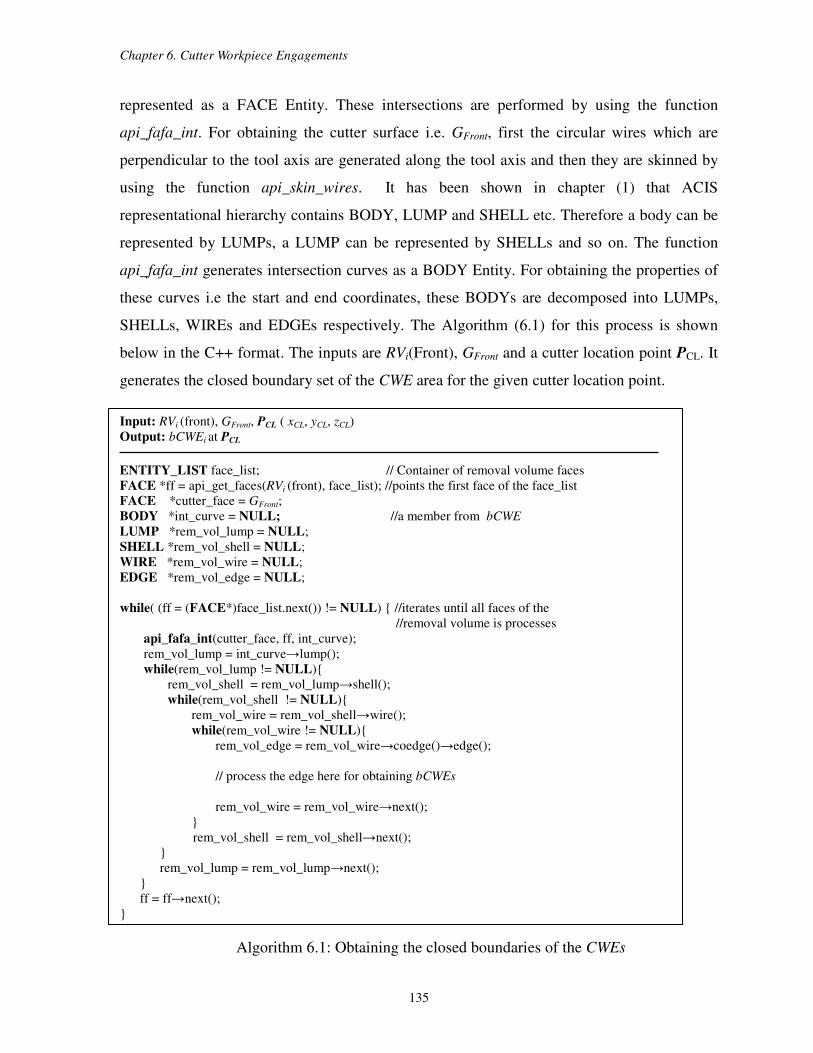
Chapter 6. Cutter Workpiece Engagements
135
represented as a FACE Entity. These intersections are performed by using the function
api_fafa_int. For obtaining the cutter surface i.e. GFront, first the circular wires which are
perpendicular to the tool axis are generated along the tool axis and then they are skinned by
using the function api_skin_wires. It has been shown in chapter (1) that ACIS
representational hierarchy contains BODY, LUMP and SHELL etc. Therefore a body can be
represented by LUMPs, a LUMP can be represented by SHELLs and so on. The function
api_fafa_int generates intersection curves as a BODY Entity. For obtaining the properties of
these curves i.e the start and end coordinates, these BODYs are decomposed into LUMPs,
SHELLs, WIREs and EDGEs respectively. The Algorithm (6.1) for this process is shown
below in the C++ format. The inputs are RVi(Front), GFront and a cutter location point PCL. It
generates the closed boundary set of the CWE area for the given cutter location point.
Input: RVi (front), GFront, PCL ( xCL, yCL, zCL)
Output: bCWEi at PCL
ENTITY_LIST face_list; // Container of removal volume faces
FACE *ff = api_get_faces(RVi (front), face_list); //points the first face of the face_list
FACE *cutter_face = GFront;
BODY *int_curve = NULL; //a member from bCWE
LUMP *rem_vol_lump = NULL;
SHELL *rem_vol_shell = NULL;
WIRE *rem_vol_wire = NULL;
EDGE *rem_vol_edge = NULL;
while( (ff = (FACE*)face_list.next()) != NULL) //iterates until all faces of the
//removal volume is processes
api_fafa_int(cutter_face, ff, int_curve);
rem_vol_lump = int_curve→lump();
while(rem_vol_lump != NULL)
rem_vol_shell = rem_vol_lump→shell();
while(rem_vol_shell != NULL)
rem_vol_wire = rem_vol_shell→wire();
while(rem_vol_wire != NULL)
rem_vol_edge = rem_vol_wire→coedge()→edge();
// process the edge here for obtaining bCWEs
rem_vol_wire = rem_vol_wire→next();
rem_vol_shell = rem_vol_shell→next();
rem_vol_lump = rem_vol_lump→next();
ff = ff→next();
Algorithm 6.1: Obtaining the closed boundaries of the CWEs
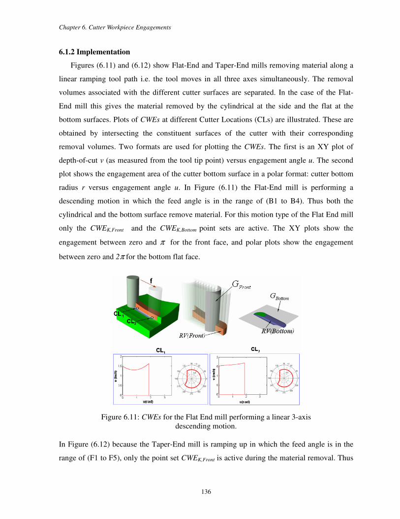
Chapter 6. Cutter Workpiece Engagements
136
6.1.2 Implementation
Figures (6.11) and (6.12) show Flat-End and Taper-End mills removing material along a
linear ramping tool path i.e. the tool moves in all three axes simultaneously. The removal
volumes associated with the different cutter surfaces are separated. In the case of the Flat-
End mill this gives the material removed by the cylindrical at the side and the flat at the
bottom surfaces. Plots of CWEs at different Cutter Locations (CLs) are illustrated. These are
obtained by intersecting the constituent surfaces of the cutter with their corresponding
removal volumes. Two formats are used for plotting the CWEs. The first is an XY plot of
depth-of-cut v (as measured from the tool tip point) versus engagement angle u. The second
plot shows the engagement area of the cutter bottom surface in a polar format: cutter bottom
radius r versus engagement angle u. In Figure (6.11) the Flat-End mill is performing a
descending motion in which the feed angle is in the range of (B1 to B4). Thus both the
cylindrical and the bottom surface remove material. For this motion type of the Flat End mill
only the CWEK,Front and the CWEK,Bottom point sets are active. The XY plots show the
engagement between zero and π for the front face, and polar plots show the engagement
between zero and 2π for the bottom flat face.
Figure 6.11: CWEs for the Flat End mill performing a linear 3-axis
descending motion.
In Figure (6.12) because the Taper-End mill is ramping up in which the feed angle is in the
range of (F1 to F5), only the point set CWEK,Front is active during the material removal. Thus
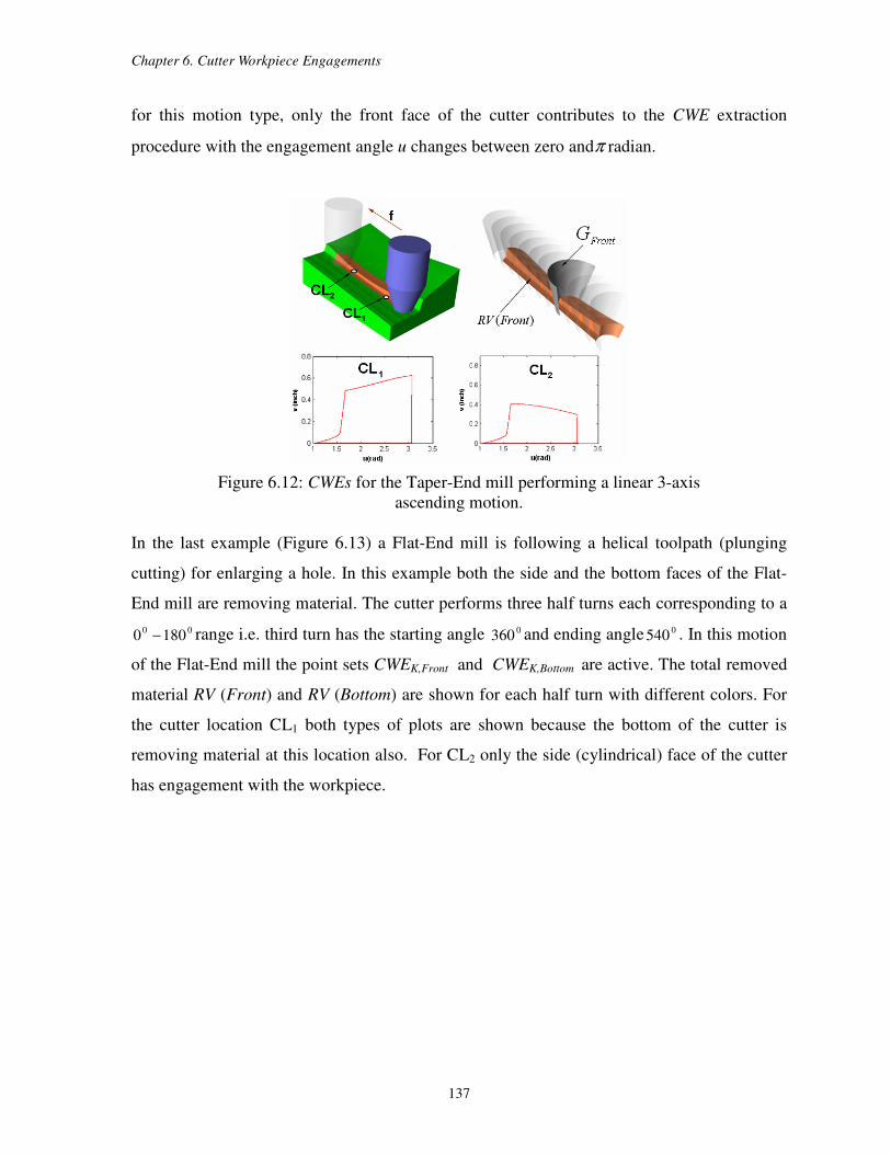
Chapter 6. Cutter Workpiece Engagements
137
for this motion type, only the front face of the cutter contributes to the CWE extraction
procedure with the engagement angle u changes between zero andπ radian.
Figure 6.12: CWEs for the Taper-End mill performing a linear 3-axis
ascending motion.
In the last example (Figure 6.13) a Flat-End mill is following a helical toolpath (plunging
cutting) for enlarging a hole. In this example both the side and the bottom faces of the Flat-
End mill are removing material. The cutter performs three half turns each corresponding to a
001800 − range i.e. third turn has the starting angle 0
360 and ending angle 0540 . In this motion
of the Flat-End mill the point sets CWEK,Front and CWEK,Bottom are active. The total removed
material RV (Front) and RV (Bottom) are shown for each half turn with different colors. For
the cutter location CL1 both types of plots are shown because the bottom of the cutter is
removing material at this location also. For CL2 only the side (cylindrical) face of the cutter
has engagement with the workpiece.
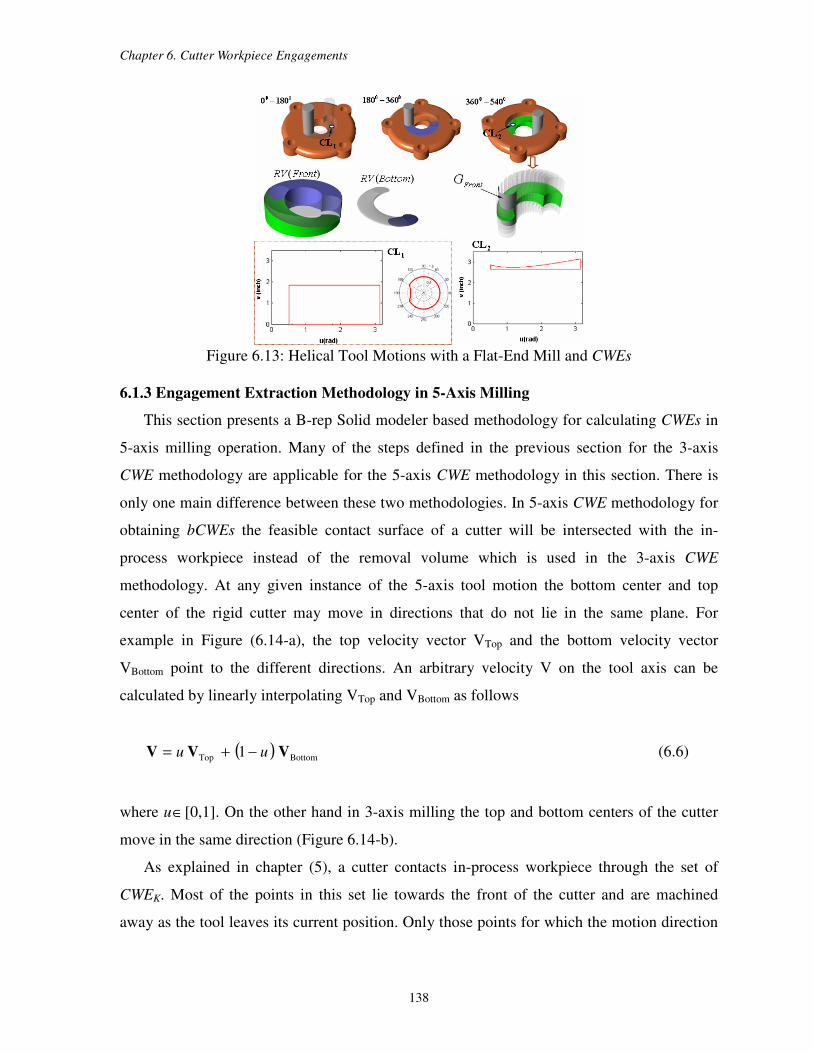
Chapter 6. Cutter Workpiece Engagements
138
Figure 6.13: Helical Tool Motions with a Flat-End Mill and CWEs
6.1.3 Engagement Extraction Methodology in 5-Axis Milling
This section presents a B-rep Solid modeler based methodology for calculating CWEs in
5-axis milling operation. Many of the steps defined in the previous section for the 3-axis
CWE methodology are applicable for the 5-axis CWE methodology in this section. There is
only one main difference between these two methodologies. In 5-axis CWE methodology for
obtaining bCWEs the feasible contact surface of a cutter will be intersected with the in-
process workpiece instead of the removal volume which is used in the 3-axis CWE
methodology. At any given instance of the 5-axis tool motion the bottom center and top
center of the rigid cutter may move in directions that do not lie in the same plane. For
example in Figure (6.14-a), the top velocity vector VTop and the bottom velocity vector
VBottom point to the different directions. An arbitrary velocity V on the tool axis can be
calculated by linearly interpolating VTop and VBottom as follows
( ) BottomTop 1 VVV uu −+= (6.6)
where u∈[0,1]. On the other hand in 3-axis milling the top and bottom centers of the cutter
move in the same direction (Figure 6.14-b).
As explained in chapter (5), a cutter contacts in-process workpiece through the set of
CWEK. Most of the points in this set lie towards the front of the cutter and are machined
away as the tool leaves its current position. Only those points for which the motion direction
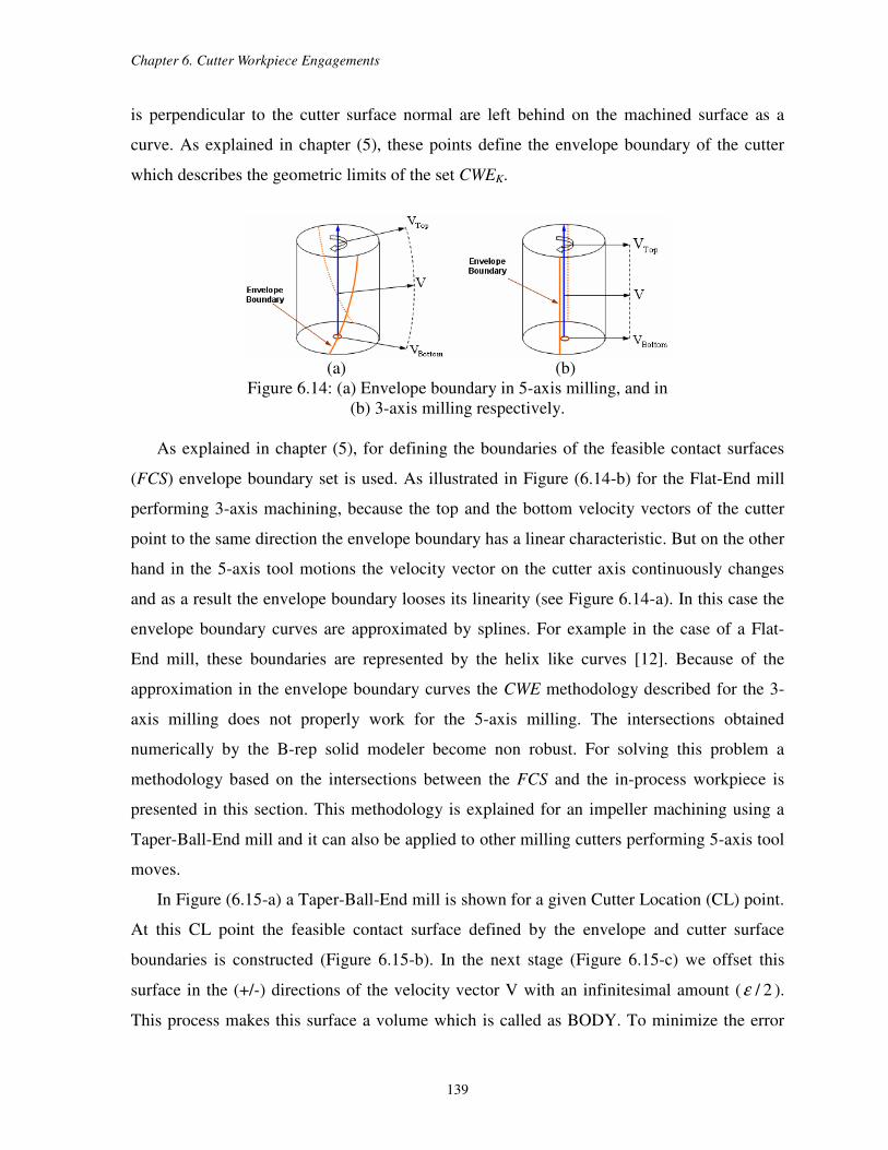
Chapter 6. Cutter Workpiece Engagements
139
is perpendicular to the cutter surface normal are left behind on the machined surface as a
curve. As explained in chapter (5), these points define the envelope boundary of the cutter
which describes the geometric limits of the set CWEK.
(a) (b)
Figure 6.14: (a) Envelope boundary in 5-axis milling, and in
(b) 3-axis milling respectively.
As explained in chapter (5), for defining the boundaries of the feasible contact surfaces
(FCS) envelope boundary set is used. As illustrated in Figure (6.14-b) for the Flat-End mill
performing 3-axis machining, because the top and the bottom velocity vectors of the cutter
point to the same direction the envelope boundary has a linear characteristic. But on the other
hand in the 5-axis tool motions the velocity vector on the cutter axis continuously changes
and as a result the envelope boundary looses its linearity (see Figure 6.14-a). In this case the
envelope boundary curves are approximated by splines. For example in the case of a Flat-
End mill, these boundaries are represented by the helix like curves [12]. Because of the
approximation in the envelope boundary curves the CWE methodology described for the 3-
axis milling does not properly work for the 5-axis milling. The intersections obtained
numerically by the B-rep solid modeler become non robust. For solving this problem a
methodology based on the intersections between the FCS and the in-process workpiece is
presented in this section. This methodology is explained for an impeller machining using a
Taper-Ball-End mill and it can also be applied to other milling cutters performing 5-axis tool
moves.
In Figure (6.15-a) a Taper-Ball-End mill is shown for a given Cutter Location (CL) point.
At this CL point the feasible contact surface defined by the envelope and cutter surface
boundaries is constructed (Figure 6.15-b). In the next stage (Figure 6.15-c) we offset this
surface in the (+/-) directions of the velocity vector V with an infinitesimal amount ( 2/ε ).
This process makes this surface a volume which is called as BODY. To minimize the error
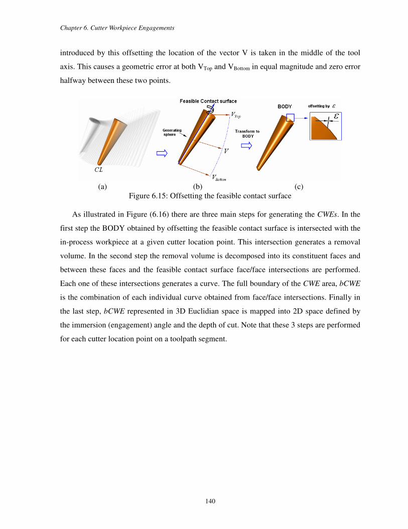
Chapter 6. Cutter Workpiece Engagements
140
introduced by this offsetting the location of the vector V is taken in the middle of the tool
axis. This causes a geometric error at both VTop and VBottom in equal magnitude and zero error
halfway between these two points.
(a) (b) (c)
Figure 6.15: Offsetting the feasible contact surface
As illustrated in Figure (6.16) there are three main steps for generating the CWEs. In the
first step the BODY obtained by offsetting the feasible contact surface is intersected with the
in-process workpiece at a given cutter location point. This intersection generates a removal
volume. In the second step the removal volume is decomposed into its constituent faces and
between these faces and the feasible contact surface face/face intersections are performed.
Each one of these intersections generates a curve. The full boundary of the CWE area, bCWE
is the combination of each individual curve obtained from face/face intersections. Finally in
the last step, bCWE represented in 3D Euclidian space is mapped into 2D space defined by
the immersion (engagement) angle and the depth of cut. Note that these 3 steps are performed
for each cutter location point on a toolpath segment.
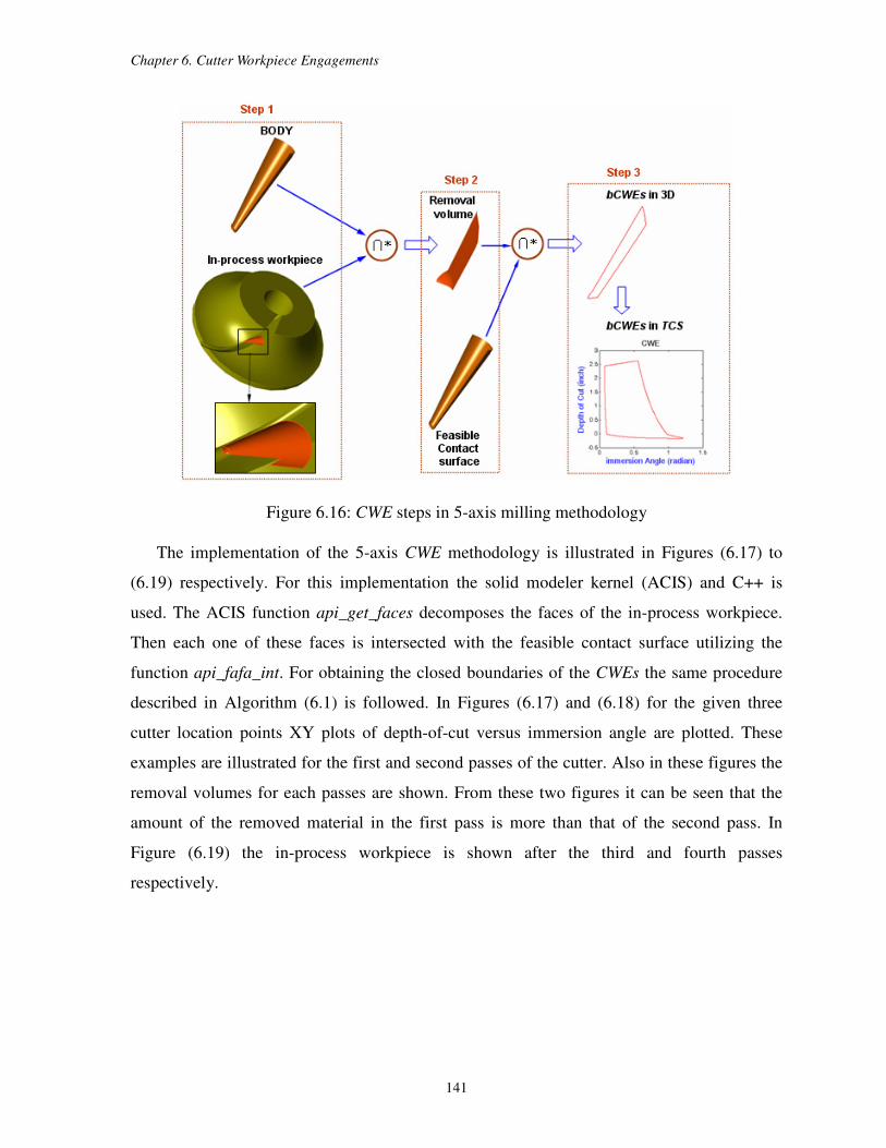
Chapter 6. Cutter Workpiece Engagements
141
Figure 6.16: CWE steps in 5-axis milling methodology
The implementation of the 5-axis CWE methodology is illustrated in Figures (6.17) to
(6.19) respectively. For this implementation the solid modeler kernel (ACIS) and C++ is
used. The ACIS function api_get_faces decomposes the faces of the in-process workpiece.
Then each one of these faces is intersected with the feasible contact surface utilizing the
function api_fafa_int. For obtaining the closed boundaries of the CWEs the same procedure
described in Algorithm (6.1) is followed. In Figures (6.17) and (6.18) for the given three
cutter location points XY plots of depth-of-cut versus immersion angle are plotted. These
examples are illustrated for the first and second passes of the cutter. Also in these figures the
removal volumes for each passes are shown. From these two figures it can be seen that the
amount of the removed material in the first pass is more than that of the second pass. In
Figure (6.19) the in-process workpiece is shown after the third and fourth passes
respectively.
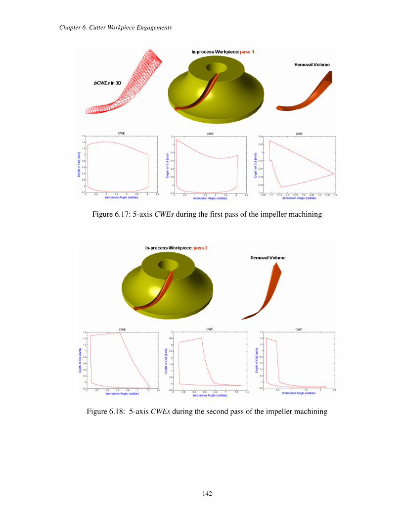
Chapter 6. Cutter Workpiece Engagements
142
Figure 6.17: 5-axis CWEs during the first pass of the impeller machining
Figure 6.18: 5-axis CWEs during the second pass of the impeller machining
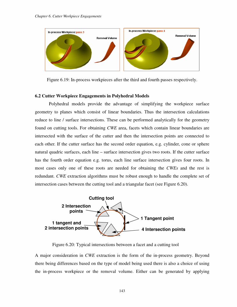
Chapter 6. Cutter Workpiece Engagements
143
Figure 6.19: In-process workpieces after the third and fourth passes respectively.
6.2 Cutter Workpiece Engagements in Polyhedral Models
Polyhedral models provide the advantage of simplifying the workpiece surface
geometry to planes which consist of linear boundaries. Thus the intersection calculations
reduce to line / surface intersections. These can be performed analytically for the geometry
found on cutting tools. For obtaining CWE area, facets which contain linear boundaries are
intersected with the surface of the cutter and then the intersection points are connected to
each other. If the cutter surface has the second order equation, e.g. cylinder, cone or sphere
natural quadric surfaces, each line – surface intersection gives two roots. If the cutter surface
has the fourth order equation e.g. torus, each line surface intersection gives four roots. In
most cases only one of these roots are needed for obtaining the CWEs and the rest is
redundant. CWE extraction algorithms must be robust enough to handle the complete set of
intersection cases between the cutting tool and a triangular facet (see Figure 6.20).
Figure 6.20: Typical intersections between a facet and a cutting tool
A major consideration in CWE extraction is the form of the in-process geometry. Beyond
there being differences based on the type of model being used there is also a choice of using
the in-process workpiece or the removal volume. Either can be generated by applying
4 Intersection points
1 Tangent point
Cutting tool
2 Intersection points
1 tangent and 2 intersection points
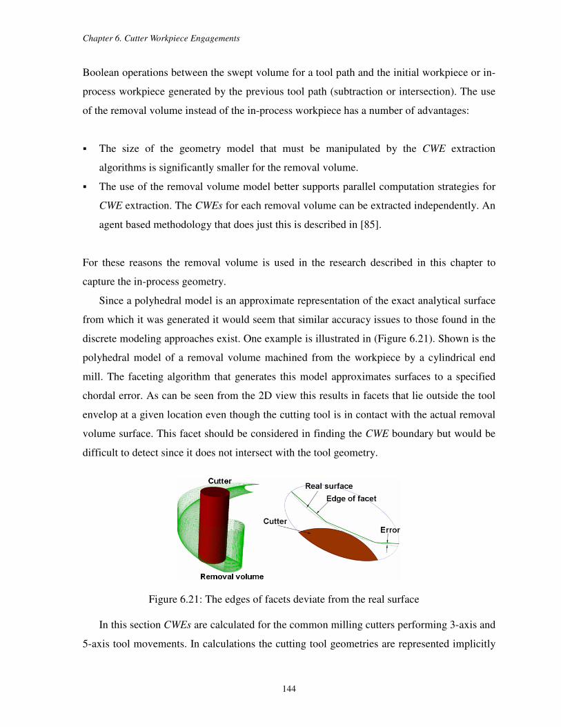
Chapter 6. Cutter Workpiece Engagements
144
Boolean operations between the swept volume for a tool path and the initial workpiece or in-
process workpiece generated by the previous tool path (subtraction or intersection). The use
of the removal volume instead of the in-process workpiece has a number of advantages:
The size of the geometry model that must be manipulated by the CWE extraction
algorithms is significantly smaller for the removal volume.
The use of the removal volume model better supports parallel computation strategies for
CWE extraction. The CWEs for each removal volume can be extracted independently. An
agent based methodology that does just this is described in [85].
For these reasons the removal volume is used in the research described in this chapter to
capture the in-process geometry.
Since a polyhedral model is an approximate representation of the exact analytical surface
from which it was generated it would seem that similar accuracy issues to those found in the
discrete modeling approaches exist. One example is illustrated in (Figure 6.21). Shown is the
polyhedral model of a removal volume machined from the workpiece by a cylindrical end
mill. The faceting algorithm that generates this model approximates surfaces to a specified
chordal error. As can be seen from the 2D view this results in facets that lie outside the tool
envelop at a given location even though the cutting tool is in contact with the actual removal
volume surface. This facet should be considered in finding the CWE boundary but would be
difficult to detect since it does not intersect with the tool geometry.
Figure 6.21: The edges of facets deviate from the real surface
In this section CWEs are calculated for the common milling cutters performing 3-axis and
5-axis tool movements. In calculations the cutting tool geometries are represented implicitly

Chapter 6. Cutter Workpiece Engagements
145
by natural quadrics and toroidal surfaces. Natural quadrics (Figure 6.22-a) consist of the
sphere, circular cylinder and the cone. Together with the plane (a degenerate quadric) and
torus these constitute the surface geometries found on the majority of cutters used in milling.
For example a ball nose end mill (BNEM) is defined by two natural quadric surfaces –
spherical and cylindrical. Other examples are shown in Figure (6.22-b).
(a)
(b)
Figure 6.22: (a) Constituent surfaces of milling cutters and
(b) some typical milling cutter surfaces.
In developing the CWE methodologies for the polyhedral models the implicit equations
of the cutter geometries will be used. These are
Sphere: ( ) ( ) 02 =−−•− rCPCP (6.7-a)
Cylinder: ( ) ( ) ( )[ ] 022 =−•−−−•− rnBPBPBP (6.7-b)
Cone: ( )[ ] ( ) ( ) 0)(cos 22 =−•−−•− VPVPnVP α (6.7-c)
Torus: [ ] 0])[(4( 222222 =−+−• rzzRRr C--)C-P)C-P( (6.7-d)
Plane: 0)( =•− nBP (6.7-e)
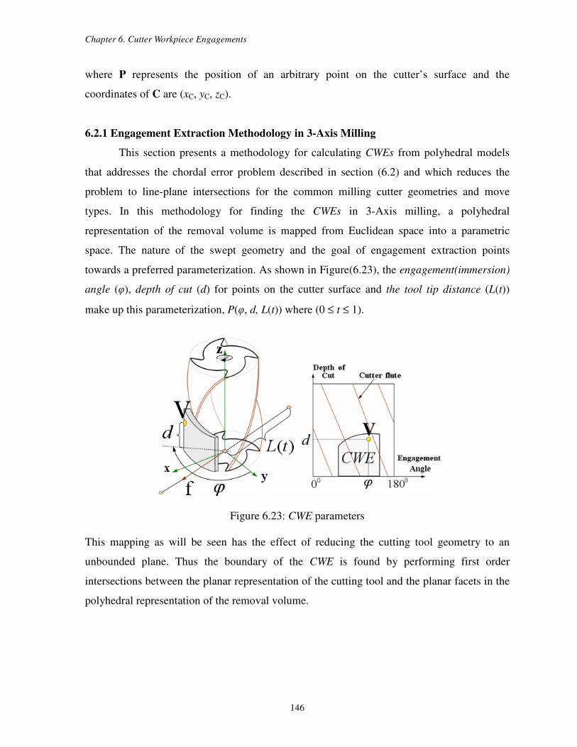
Chapter 6. Cutter Workpiece Engagements
146
where P represents the position of an arbitrary point on the cutter’s surface and the
coordinates of C are (xC, yC, zC).
6.2.1 Engagement Extraction Methodology in 3-Axis Milling
This section presents a methodology for calculating CWEs from polyhedral models
that addresses the chordal error problem described in section (6.2) and which reduces the
problem to line-plane intersections for the common milling cutter geometries and move
types. In this methodology for finding the CWEs in 3-Axis milling, a polyhedral
representation of the removal volume is mapped from Euclidean space into a parametric
space. The nature of the swept geometry and the goal of engagement extraction points
towards a preferred parameterization. As shown in Figure(6.23), the engagement(immersion)
angle (φ), depth of cut (d) for points on the cutter surface and the tool tip distance (L(t))
make up this parameterization, P(φ, d, L(t)) where (0 ≤ t ≤ 1).
Figure 6.23: CWE parameters
This mapping as will be seen has the effect of reducing the cutting tool geometry to an
unbounded plane. Thus the boundary of the CWE is found by performing first order
intersections between the planar representation of the cutting tool and the planar facets in the
polyhedral representation of the removal volume.

Chapter 6. Cutter Workpiece Engagements
147
General Terminology
Ti : Tool path for the ith
tool motion
RVi : Removal volume generated for ith
tool motion in E3.
M : A transformation that maps RVi from E3 to P(φ, d, L) i.e. M: E
3 → P(φ, d, L)
P
iRV : The map of RVi in P(φ, d, L).
N : Surface normal of a point on cutter.
CWEK(t): The set of all points on the surface of a cutter at location t along a tool path where f
• N ≥ 0. These are kinematically feasible engagement points for a given instantaneous
feed vector f.
CWE(t): The set of all points on the surface of a cutter at location t along a tool path that
are engaged with the workpiece.
bCWE(t): Points on the boundary of CWE(t).
In finding engagement geometry the following property of the representations for removal
volumes in the parametric space P(φ, d, L) motivate finding the mapping M: E3 → P(φ, d, L).
Property 6.3: Given P
iRV a representation of the removal volume RVi for tool path Ti in P(φ,
d, L), its intersection with an unbounded plane Q generates a closed set of points CWE(t) that
constitutes all points in engagement with the workpiece at location t along the tool path.
Of interest is the boundary set of CWE(t), bCWE(t). This defines the geometry required
for input to process modeling (i.e. force prediction). Thus
bCWE(t) ⊂ CWE(t) ⊂ CWEK(t) (6.8)
These three sets are illustrated in Figure (6.24).
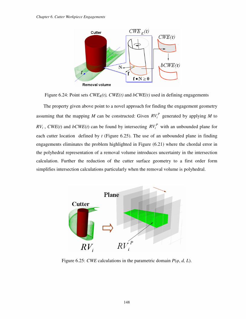
Chapter 6. Cutter Workpiece Engagements
148
Figure 6.24: Point sets CWEK(t), CWE(t) and bCWE(t) used in defining engagements
The property given above point to a novel approach for finding the engagement geometry
assuming that the mapping M can be constructed: Given P
iRV generated by applying M to
RVi , CWE(t) and bCWE(t) can be found by intersecting P
iRV with an unbounded plane for
each cutter location defined by t (Figure 6.25). The use of an unbounded plane in finding
engagements eliminates the problem highlighted in Figure (6.21) where the chordal error in
the polyhedral representation of a removal volume introduces uncertainty in the intersection
calculation. Further the reduction of the cutter surface geometry to a first order form
simplifies intersection calculations particularly when the removal volume is polyhedral.
Figure 6.25: CWE calculations in the parametric domain P(φ, d, L).
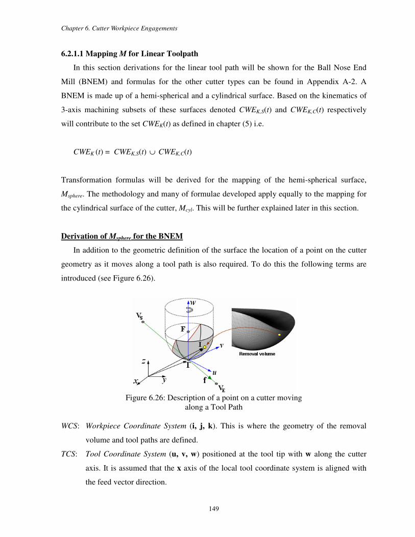
Chapter 6. Cutter Workpiece Engagements
149
6.2.1.1 Mapping M for Linear Toolpath
In this section derivations for the linear tool path will be shown for the Ball Nose End
Mill (BNEM) and formulas for the other cutter types can be found in Appendix A-2. A
BNEM is made up of a hemi-spherical and a cylindrical surface. Based on the kinematics of
3-axis machining subsets of these surfaces denoted CWEK,S(t) and CWEK,C(t) respectively
will contribute to the set CWEK(t) as defined in chapter (5) i.e.
CWEK (t) = CWEK,S(t) ∪ CWEK,C(t)
Transformation formulas will be derived for the mapping of the hemi-spherical surface,
Msphere. The methodology and many of formulae developed apply equally to the mapping for
the cylindrical surface of the cutter, Mcyl. This will be further explained later in this section.
Derivation of Msphere for the BNEM
In addition to the geometric definition of the surface the location of a point on the cutter
geometry as it moves along a tool path is also required. To do this the following terms are
introduced (see Figure 6.26).
Figure 6.26: Description of a point on a cutter moving
along a Tool Path
WCS: Workpiece Coordinate System (i, j, k). This is where the geometry of the removal
volume and tool paths are defined.
TCS: Tool Coordinate System (u, v, w) positioned at the tool tip with w along the cutter
axis. It is assumed that the x axis of the local tool coordinate system is aligned with
the feed vector direction.
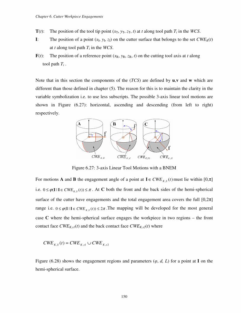
Chapter 6. Cutter Workpiece Engagements
150
T(t): The position of the tool tip point (xT, yT, zT, t) at t along tool path Ti in the WCS.
I: The position of a point (xI, yI, zI) on the cutter surface that belongs to the set CWEK(t)
at t along tool path Ti in the WCS.
F(t): The position of a reference point (xR, yR, zR, t) on the cutting tool axis at t along
tool path Ti .
Note that in this section the components of the (TCS) are defined by u,v and w which are
different than those defined in chapter (5). The reason for this is to maintain the clarity in the
variable symbolization i.e. to use less subscripts. The possible 3-axis linear tool motions are
shown in Figure (6.27): horizontal, ascending and descending (from left to right)
respectively.
Figure 6.27: 3-axis Linear Tool Motions with a BNEM
For motions A and B the engagement angle of a point at )(, tCWE SK∈I must lie within [0,π]
i.e. πϕ ≤∈≤ ))(|(0 , tCWE SKII . At C both the front and the back sides of the hemi-spherical
surface of the cutter have engagements and the total engagement area covers the full [0,2π]
range i.e. πϕ 2))(|(0 , ≤∈≤ tCWE SKII .The mapping will be developed for the most general
case C where the hemi-spherical surface engages the workpiece in two regions – the front
contact face CWEK,s1(t) and the back contact face CWEK,s2(t) where
2,1,, )( sKsKSK CWECWEtCWE ∪=
Figure (6.28) shows the engagement regions and parameters (φ, d, L) for a point at I on the
hemi-spherical surface.
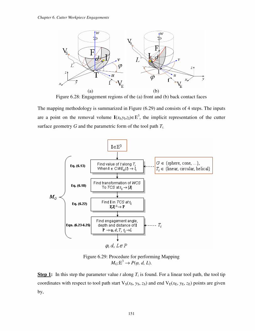
Chapter 6. Cutter Workpiece Engagements
151
(a) (b)
Figure 6.28: Engagement regions of the (a) front and (b) back contact faces
The mapping methodology is summarized in Figure (6.29) and consists of 4 steps. The inputs
are a point on the removal volume I(xI,yI,zI)∈E3, the implicit representation of the cutter
surface geometry G and the parametric form of the tool path Ti.
Figure 6.29: Procedure for performing Mapping
MG:E3 → P(φ, d, L).
Step 1: In this step the parameter value t along Ti is found. For a linear tool path, the tool tip
coordinates with respect to tool path start VS(xS, yS, zS) and end VE(xE, yE, zE) points are given
by,

Chapter 6. Cutter Workpiece Engagements
152
( ) tt )( SES VVVT −+= , 10 ≤≤ t (6.9)
For a BNEM the reference point at F is chosen to be the center of the sphere. Its location can
be expressed using the cutting tool tip coordinates as,
( ) nTF rtt += )( (6.10)
where r and n are the radius of the hemi-sphere and unit normal vector of the tool axis
respectively. When the hemi-spherical surface moves along a tool path, a family GS(t) of
surfaces is generated. An expression for this family of surfaces is obtained by substituting in
the coordinates of the reference point at F from Eq.(6.10) into the implicit form of a sphere
given by Eq.( 6.7-a).
( ) ( ) 0:)( 2 =−−•− rtGS FPFP (6.11)
When the point at P belongs to the set CWEK,S(t), Eq.(6.11) can be rewritten as,
( ) ( ) 0:)( 2
, =−−•− rtCWE SK FIFI (6.12)
Given a point at I that is known to be an engagement point, Eq.(6.12) can be expanded to
take on the following quadratic form,
A2 t2 + A1 t + A0 = 0 (6.13)
where the coefficients A2 , A1 and A0 are given by,
2
2 SE VV −=A
( ) ( )[ ]SES VVnVI −•−−−= rA 21 (6.14)
22
0 rrA −−−= nVI S
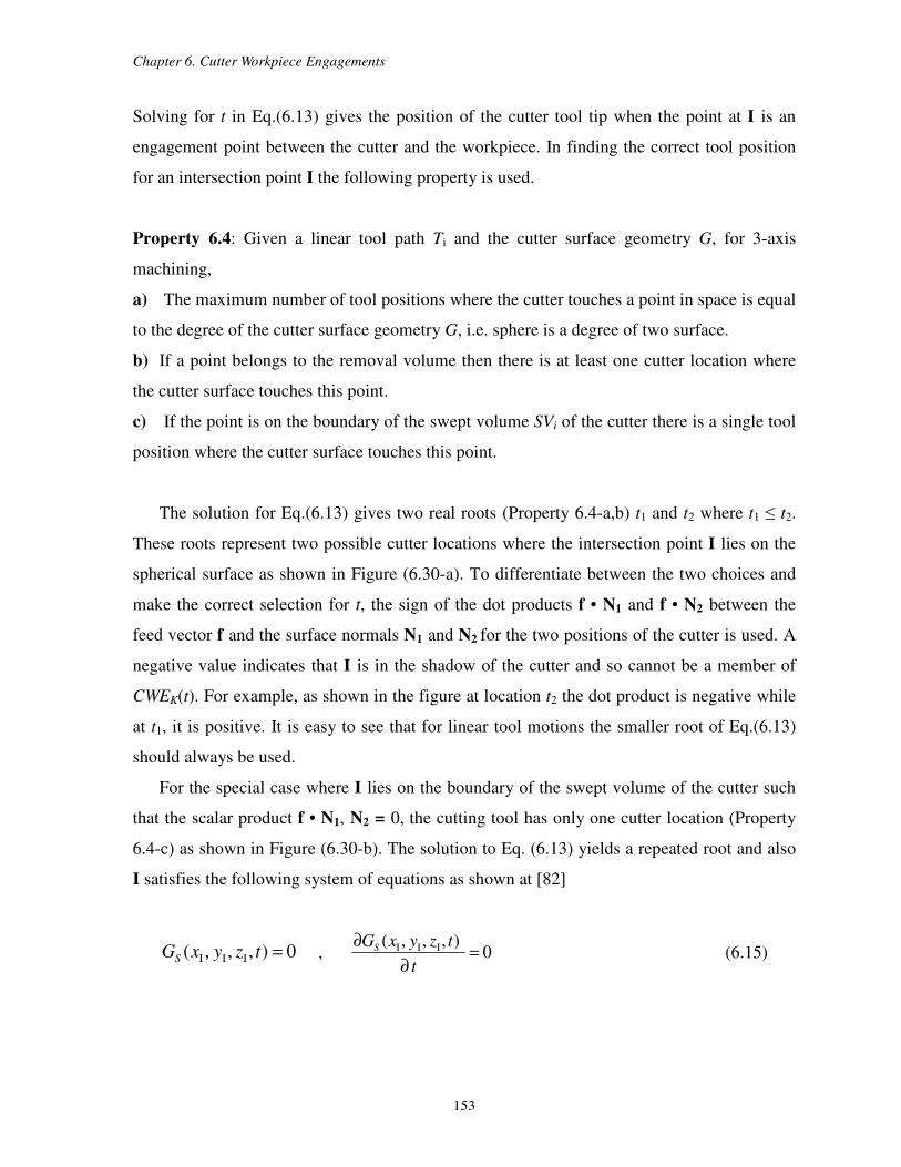
Chapter 6. Cutter Workpiece Engagements
153
Solving for t in Eq.(6.13) gives the position of the cutter tool tip when the point at I is an
engagement point between the cutter and the workpiece. In finding the correct tool position
for an intersection point I the following property is used.
Property 6.4: Given a linear tool path Ti and the cutter surface geometry G, for 3-axis
machining,
a) The maximum number of tool positions where the cutter touches a point in space is equal
to the degree of the cutter surface geometry G, i.e. sphere is a degree of two surface.
b) If a point belongs to the removal volume then there is at least one cutter location where
the cutter surface touches this point.
c) If the point is on the boundary of the swept volume SVi of the cutter there is a single tool
position where the cutter surface touches this point.
The solution for Eq.(6.13) gives two real roots (Property 6.4-a,b) t1 and t2 where t1 ≤ t2.
These roots represent two possible cutter locations where the intersection point I lies on the
spherical surface as shown in Figure (6.30-a). To differentiate between the two choices and
make the correct selection for t, the sign of the dot products f • N1 and f • N2 between the
feed vector f and the surface normals N1 and N2 for the two positions of the cutter is used. A
negative value indicates that I is in the shadow of the cutter and so cannot be a member of
CWEK(t). For example, as shown in the figure at location t2 the dot product is negative while
at t1, it is positive. It is easy to see that for linear tool motions the smaller root of Eq.(6.13)
should always be used.
For the special case where I lies on the boundary of the swept volume of the cutter such
that the scalar product f • N1, N2 = 0, the cutting tool has only one cutter location (Property
6.4-c) as shown in Figure (6.30-b). The solution to Eq. (6.13) yields a repeated root and also
I satisfies the following system of equations as shown at [82]
0),,,( III =tzyxGS , 0),,,( III =
∂
∂
t
tzyxGS (6.15)
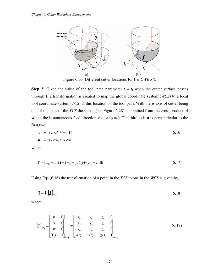
Chapter 6. Cutter Workpiece Engagements
154
(a) (b)
Figure 6.30: Different cutter locations for I ∈ CWEK(t).
Step 2: Given the value of the tool path parameter t = tI when the cutter surface passes
through I, a transformation is created to map the global coordinate system (WCS) to a local
tool coordinate system (TCS) at this location on the tool path. With the w axis of cutter being
one of the axes of the TCS the v axis (see Figure 6.28) is obtained from the cross product of
w and the instantaneous feed direction vector f(t=tI). The third axis u is perpendicular to the
first two.
||/)( fwfwv ××= (6.16)
||/)( wvwvu ××=
where
kjif )()()( SESESE zzyyxx −+−+−= (6.17)
Using Eqs.(6.16) the transformation of a point in the TCS to one in the WCS is given by,
[ ]Itt == JI'I (6.18)
where
[ ]
II
I
TTTT
w
v
u
J
tt
www
vvv
uuu
tt
tt
tztytx
zyx
zyx
zyx
t==
=
≡
=
1)()()(
0
0
0
1
0
0
0
)(
(6.19)
Chapter 6. Cutter Workpiece Engagements
155
and I' are the coordinates of I in the TCS.
Step 3: To find ϕ(t) and d(t) the coordinates of an engagement point in the TCS is required.
This is obtained from Eq.(6.18) as,
[ ] 1
I'
−
== ttJII (6.20)
Given that [ ]Itt=J is orthogonal, its inverse is defined by,
[ ]
I
I
1)()()(
0
0
0
1
tt
wvu
wvu
wvu
tt
ttt
zzz
yyy
xxx
=
−
=
•−•−•−
=
TwTvTu
J (6.21)
Expanding equation (6.20) using (6.21) gives the coordinates of I'(III ,, zyx ′′′ ). These are,
)( II ttx =•−•=′ TuuI
)( II tty =•−•=′ TvvI (6.22)
)( II ttz =•−•=′ TwwI
Step 4: Given the coordinates of I' on the hemi-spherical surface of the BNEM, its tool
engagement angle ϕ(t) is obtained using spherical coordinates. The Engagement angle for the
front contact face CWEK,s1(t) is given by
′+′
′== −
2
I
2
I
I1
I cos)(yx
yttϕ (6.23-a)
and for the back contact face CWEK,s2(t) is given by

Chapter 6. Cutter Workpiece Engagements
156
′+′
′−== −
2
I
2
I
I1
I cos2)(yx
ytt πϕ (6.23-b)
The depth of the engagement point for the spherical part is the angle from T(t) to I' such that:
′−== −
r
zttd I1
I 1cos)( (6.24)
and finally the parameter L(t) of I is obtained using,
SE VV −== tttL )( I (6.25)
Derivation of Mcyl for the BNEM
The mapping for the cylindrical surface of the Ball end cutter is obtained following the
same steps just developed for the hemispherical cutter surface. It can be seen that except for
the first, all steps and equations to accomplish the mapping remain the same. For the first
step, the geometry of the cylinder changes Eqs.(6.11) and (6.12) to,
[ ] 0)()()(:)( 22 =−•−−−•− rtGC nFPFPFP (6.26)
and,
[ ] 0)()()(:)( 22
, =−•−−−•− rtCWE CK nFIFIFI (6.27)
respectively (see Figure 6.31). Where r and n are the radius of the cylindrical surface and the
unit normal vector of the tool rotation axis respectively. As with Eq.(6.13), Eq.(6.27) results
in a quadratic equation in t when I and F are substituted. The solution to this and the
remaining steps in the mapping procedure lead to the representation of a point I on the
cylindrical surface of the BNEM in (ϕ, d, L) coordinates. Detailed transformation formulas
for the cylindrical end mill can be found in the Appendix A.2.
Chapter 6. Cutter Workpiece Engagements
157
Figure 6.31: Cylindrical contact face CWEK,C(t) of BNEM
6.2.1.2 Mapping M for Circular Toolpath
In this section we highlight the mapping procedure for a circular tool path. The steps
summarized in (Figure 6.29) can be followed with some important differences. One in
particular is that the feed direction changes as a function of the tool path parametric variable
t. This impacts the transformation from the WCS to the TCS. The parametric representation
for the tool tip point for a circular tool path of radius R centered at ),,( CCC zyx=C is given by
( ) edCT )sin()cos( tRtRt ++= (6.28)
where [ ]π2,0∈t (see Figure 6.32). d(xd, yd, zd) and e(xe, ye, ze) are two orthogonal unit
vectors defining the plane of the circular tool path. Thus, this representation for T is general
even though circular interpolation on most milling machines is restricted to the XY, XZ and
YZ planes.
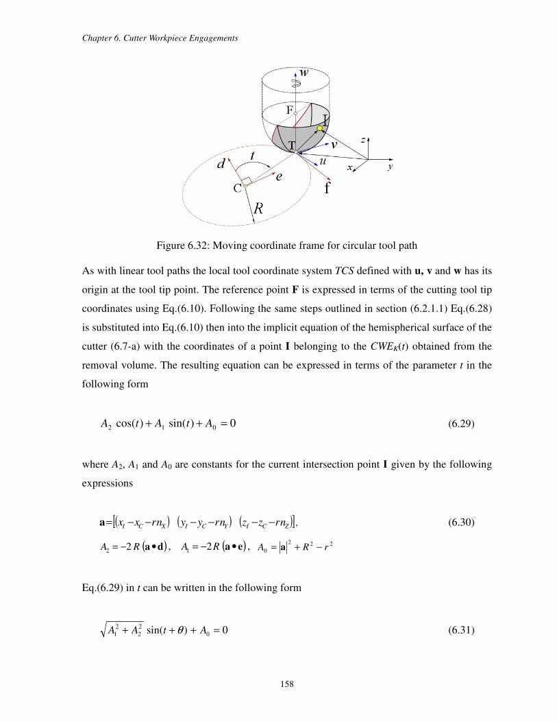
Chapter 6. Cutter Workpiece Engagements
158
Figure 6.32: Moving coordinate frame for circular tool path
As with linear tool paths the local tool coordinate system TCS defined with u, v and w has its
origin at the tool tip point. The reference point F is expressed in terms of the cutting tool tip
coordinates using Eq.(6.10). Following the same steps outlined in section (6.2.1.1) Eq.(6.28)
is substituted into Eq.(6.10) then into the implicit equation of the hemispherical surface of the
cutter (6.7-a) with the coordinates of a point I belonging to the CWEK(t) obtained from the
removal volume. The resulting equation can be expressed in terms of the parameter t in the
following form
0)sin()cos( 012 =++ AtAtA (6.29)
where A2, A1 and A0 are constants for the current intersection point I given by the following
expressions
( ) ( ) ( )[ ]ZCIYCIXCI nrzznryynrxx −−−−−−=a , (6.30)
( )da •−= RA 22, ( )ea •−= RA 21
, 222
0 rRA −+= a
Eq.(6.29) in t can be written in the following form
0)sin( 0
2
2
2
1 =+++ AtAA θ (6.31)
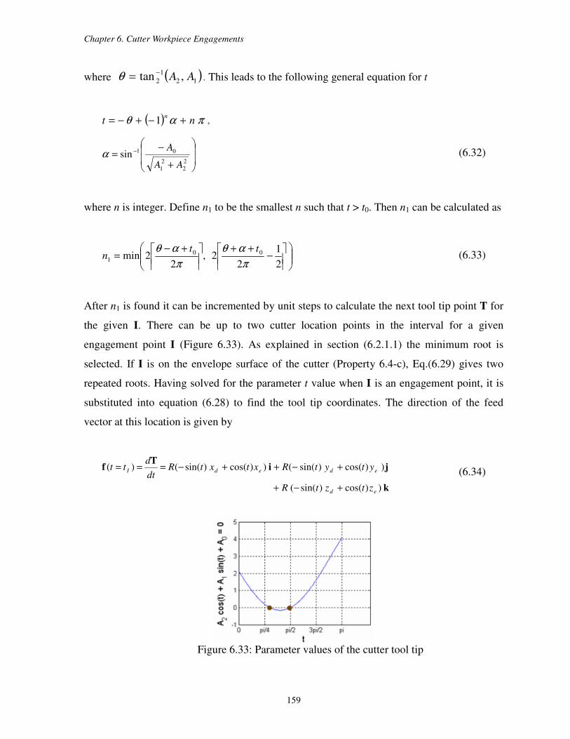
Chapter 6. Cutter Workpiece Engagements
159
where ( )12
1
2 ,tan AA−=θ . This leads to the following general equation for t
( ) παθ ntn
+−+−= 1 ,
+
−= −
2
2
2
1
01sinAA
Aα (6.32)
where n is integer. Define n1 to be the smallest n such that t > t0. Then n1 can be calculated as
−
++
+−=
2
1
22,
22min 00
1π
αθ
π
αθ ttn (6.33)
After n1 is found it can be incremented by unit steps to calculate the next tool tip point T for
the given I. There can be up to two cutter location points in the interval for a given
engagement point I (Figure 6.33). As explained in section (6.2.1.1) the minimum root is
selected. If I is on the envelope surface of the cutter (Property 6.4-c), Eq.(6.29) gives two
repeated roots. Having solved for the parameter t value when I is an engagement point, it is
substituted into equation (6.28) to find the tool tip coordinates. The direction of the feed
vector at this location is given by
k
jiT
f
))cos()sin((
))cos()sin(())cos()sin(()(
ed
ededI
ztztR
ytytRxtxtRdt
dtt
+−+
+−++−=== (6.34)
Figure 6.33: Parameter values of the cutter tool tip
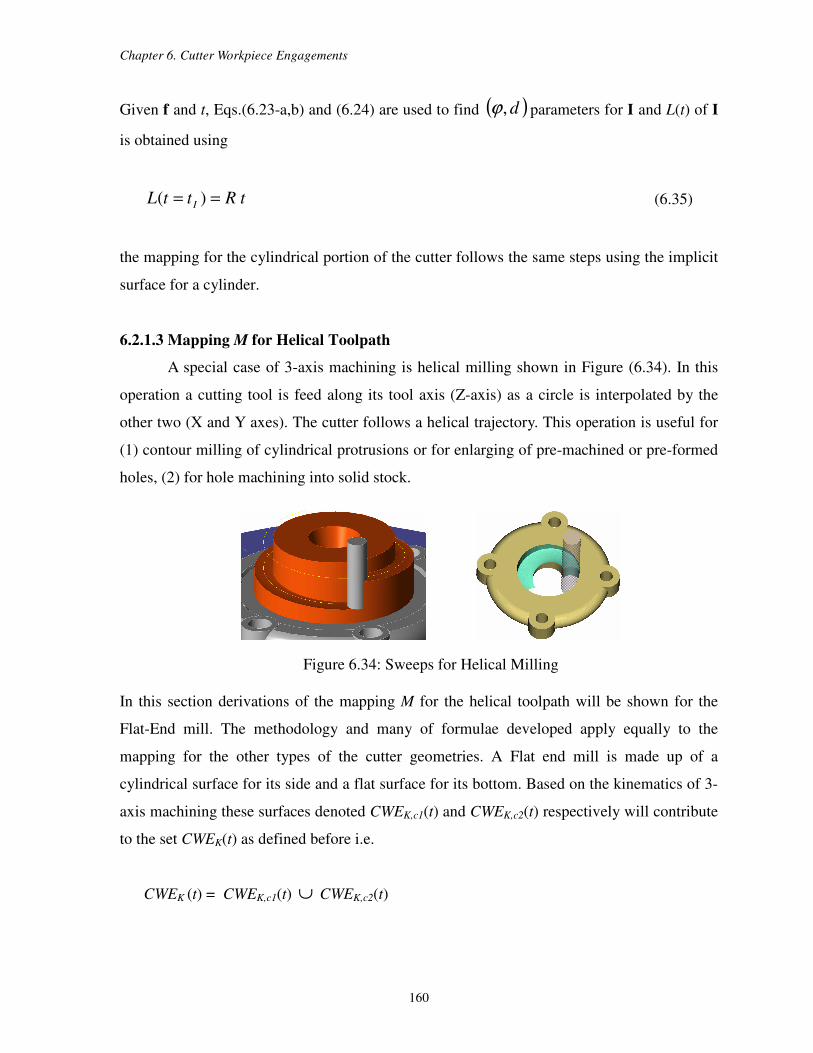
Chapter 6. Cutter Workpiece Engagements
160
Given f and t, Eqs.(6.23-a,b) and (6.24) are used to find ( )d,ϕ parameters for I and L(t) of I
is obtained using
tRttL I == )( (6.35)
the mapping for the cylindrical portion of the cutter follows the same steps using the implicit
surface for a cylinder.
6.2.1.3 Mapping M for Helical Toolpath
A special case of 3-axis machining is helical milling shown in Figure (6.34). In this
operation a cutting tool is feed along its tool axis (Z-axis) as a circle is interpolated by the
other two (X and Y axes). The cutter follows a helical trajectory. This operation is useful for
(1) contour milling of cylindrical protrusions or for enlarging of pre-machined or pre-formed
holes, (2) for hole machining into solid stock.
Figure 6.34: Sweeps for Helical Milling
In this section derivations of the mapping M for the helical toolpath will be shown for the
Flat-End mill. The methodology and many of formulae developed apply equally to the
mapping for the other types of the cutter geometries. A Flat end mill is made up of a
cylindrical surface for its side and a flat surface for its bottom. Based on the kinematics of 3-
axis machining these surfaces denoted CWEK,c1(t) and CWEK,c2(t) respectively will contribute
to the set CWEK(t) as defined before i.e.
CWEK (t) = CWEK,c1(t) ∪ CWEK,c2(t)
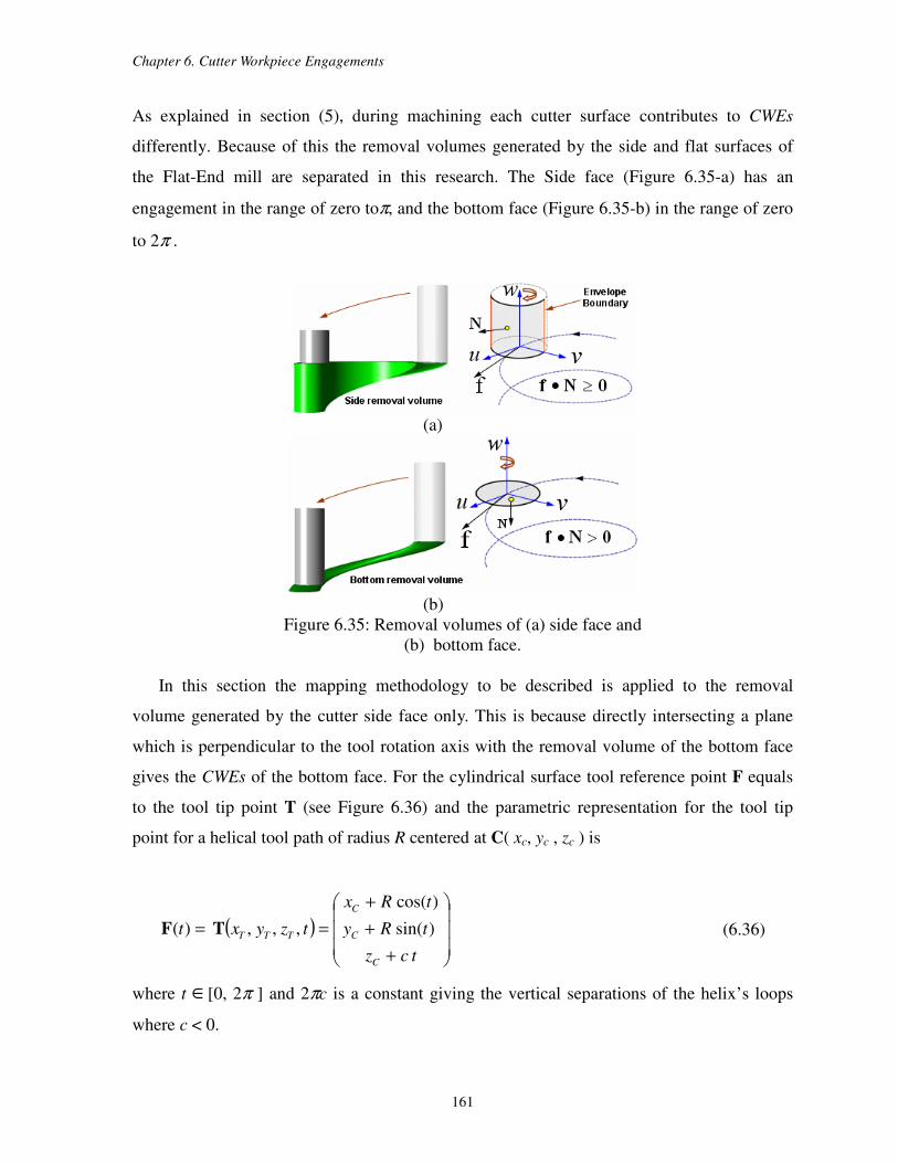
Chapter 6. Cutter Workpiece Engagements
161
As explained in section (5), during machining each cutter surface contributes to CWEs
differently. Because of this the removal volumes generated by the side and flat surfaces of
the Flat-End mill are separated in this research. The Side face (Figure 6.35-a) has an
engagement in the range of zero toπ, and the bottom face (Figure 6.35-b) in the range of zero
to 2π .
(a)
(b)
Figure 6.35: Removal volumes of (a) side face and
(b) bottom face.
In this section the mapping methodology to be described is applied to the removal
volume generated by the cutter side face only. This is because directly intersecting a plane
which is perpendicular to the tool rotation axis with the removal volume of the bottom face
gives the CWEs of the bottom face. For the cylindrical surface tool reference point F equals
to the tool tip point T (see Figure 6.36) and the parametric representation for the tool tip
point for a helical tool path of radius R centered at C( xc, yc , zc ) is
( )
+
+
+
==
tcz
tRy
tRx
tzyxt
C
C
C
TTT )sin(
)cos(
,,,)( T F (6.36)
where t ∈[0, 2π ] and 2πc is a constant giving the vertical separations of the helix’s loops
where c < 0.
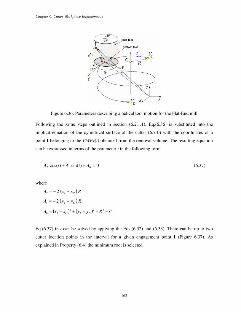
Chapter 6. Cutter Workpiece Engagements
162
Figure 6.36: Parameters describing a helical tool motion for the Flat-End mill
Following the same steps outlined in section (6.2.1.1), Eq.(6.36) is substituted into the
implicit equation of the cylindrical surface of the cutter (6.7-b) with the coordinates of a
point I belonging to the CWEK(t) obtained from the removal volume. The resulting equation
can be expressed in terms of the parameter t in the following form
0)sin()cos( 012 =++ AtAtA (6.37)
where
( ) RxxA CI −−= 22
( ) RyyA CI −−= 21
( ) ( ) 2222
0 rRyyxxA CICI −+−+−=
Eq.(6.37) in t can be solved by applying the Eqs.(6.32) and (6.33). There can be up to two
cutter location points in the interval for a given engagement point I (Figure 6.37). As
explained in Property (6.4) the minimum root is selected.
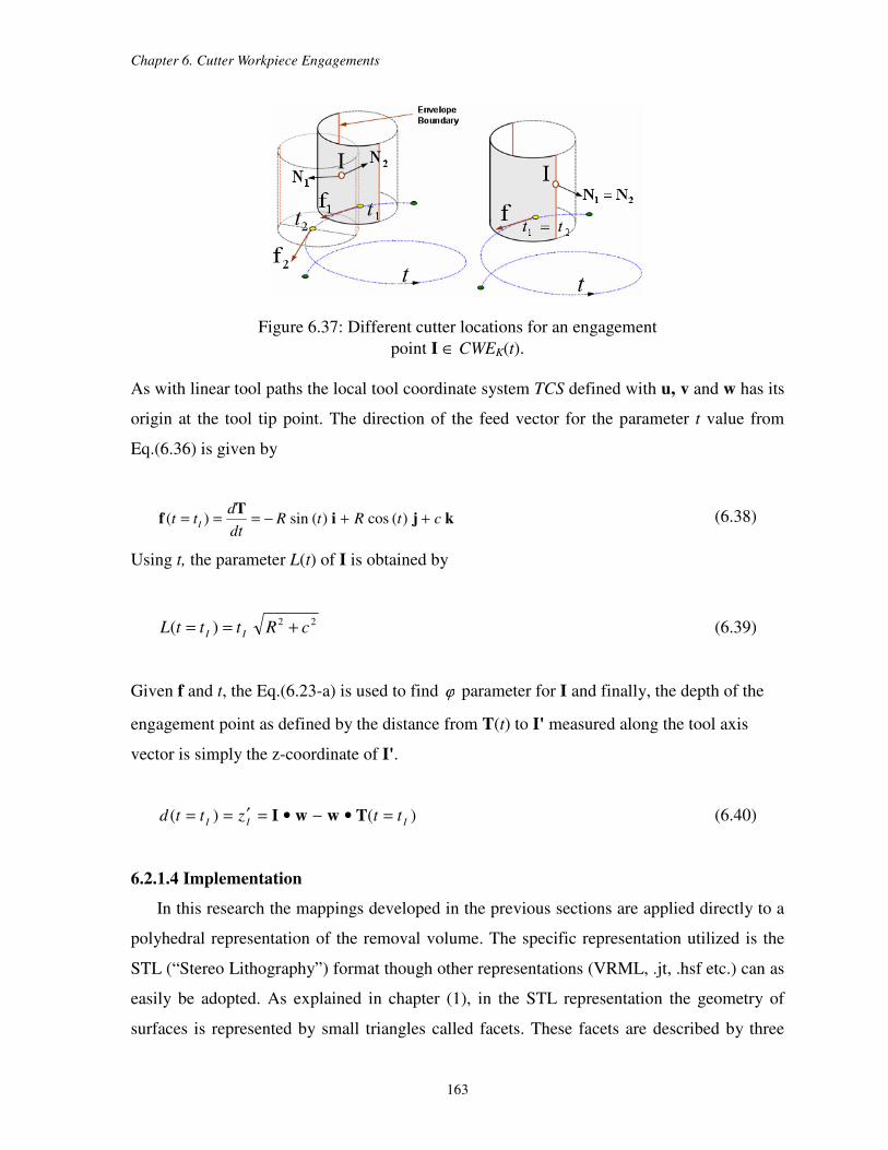
Chapter 6. Cutter Workpiece Engagements
163
Figure 6.37: Different cutter locations for an engagement
point I ∈ CWEK(t).
As with linear tool paths the local tool coordinate system TCS defined with u, v and w has its
origin at the tool tip point. The direction of the feed vector for the parameter t value from
Eq.(6.36) is given by
kjiT
f ctRtRdt
dtt I ++−=== )(cos)(sin)( (6.38)
Using t, the parameter L(t) of I is obtained by
22)( cRtttL II +== (6.39)
Given f and t, the Eq.(6.23-a) is used to find ϕ parameter for I and finally, the depth of the
engagement point as defined by the distance from T(t) to I' measured along the tool axis
vector is simply the z-coordinate of I'.
)()( III ttzttd =•−•=′== TwwI (6.40)
6.2.1.4 Implementation
In this research the mappings developed in the previous sections are applied directly to a
polyhedral representation of the removal volume. The specific representation utilized is the
STL (“Stereo Lithography”) format though other representations (VRML, .jt, .hsf etc.) can as
easily be adopted. As explained in chapter (1), in the STL representation the geometry of
surfaces is represented by small triangles called facets. These facets are described by three
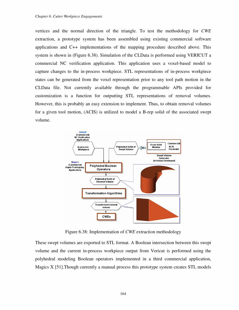
Chapter 6. Cutter Workpiece Engagements
164
vertices and the normal direction of the triangle. To test the methodology for CWE
extraction, a prototype system has been assembled using existing commercial software
applications and C++ implementations of the mapping procedure described above. This
system is shown in (Figure 6.38). Simulation of the CLData is performed using VERICUT a
commercial NC verification application. This application uses a voxel-based model to
capture changes to the in-process workpiece. STL representations of in-process workpiece
states can be generated from the voxel representation prior to any tool path motion in the
CLData file. Not currently available through the programmable APIs provided for
customization is a function for outputting STL representations of removal volumes.
However, this is probably an easy extension to implement. Thus, to obtain removal volumes
for a given tool motion, (ACIS) is utilized to model a B-rep solid of the associated swept
volume.
Figure 6.38: Implementation of CWE extraction methodology
These swept volumes are exported to STL format. A Boolean intersection between this swept
volume and the current in-process workpiece output from Vericut is performed using the
polyhedral modeling Boolean operators implemented in a third commercial application,
Magics X [51].Though currently a manual process this prototype system creates STL models
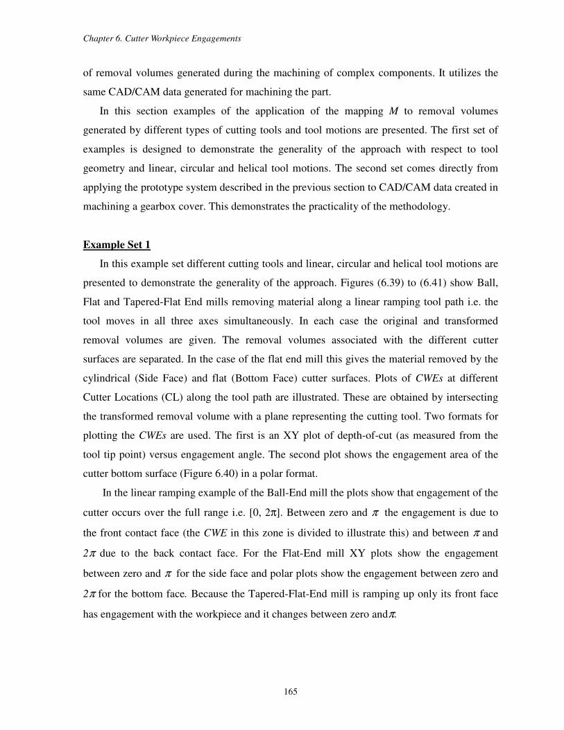
Chapter 6. Cutter Workpiece Engagements
165
of removal volumes generated during the machining of complex components. It utilizes the
same CAD/CAM data generated for machining the part.
In this section examples of the application of the mapping M to removal volumes
generated by different types of cutting tools and tool motions are presented. The first set of
examples is designed to demonstrate the generality of the approach with respect to tool
geometry and linear, circular and helical tool motions. The second set comes directly from
applying the prototype system described in the previous section to CAD/CAM data created in
machining a gearbox cover. This demonstrates the practicality of the methodology.
Example Set 1
In this example set different cutting tools and linear, circular and helical tool motions are
presented to demonstrate the generality of the approach. Figures (6.39) to (6.41) show Ball,
Flat and Tapered-Flat End mills removing material along a linear ramping tool path i.e. the
tool moves in all three axes simultaneously. In each case the original and transformed
removal volumes are given. The removal volumes associated with the different cutter
surfaces are separated. In the case of the flat end mill this gives the material removed by the
cylindrical (Side Face) and flat (Bottom Face) cutter surfaces. Plots of CWEs at different
Cutter Locations (CL) along the tool path are illustrated. These are obtained by intersecting
the transformed removal volume with a plane representing the cutting tool. Two formats for
plotting the CWEs are used. The first is an XY plot of depth-of-cut (as measured from the
tool tip point) versus engagement angle. The second plot shows the engagement area of the
cutter bottom surface (Figure 6.40) in a polar format.
In the linear ramping example of the Ball-End mill the plots show that engagement of the
cutter occurs over the full range i.e. [0, 2π]. Between zero and π the engagement is due to
the front contact face (the CWE in this zone is divided to illustrate this) and between π and
2π due to the back contact face. For the Flat-End mill XY plots show the engagement
between zero and π for the side face and polar plots show the engagement between zero and
2π for the bottom face. Because the Tapered-Flat-End mill is ramping up only its front face
has engagement with the workpiece and it changes between zero andπ.
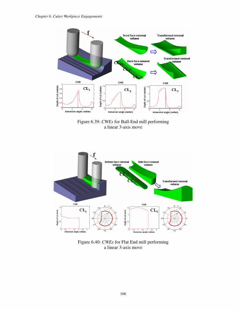
Chapter 6. Cutter Workpiece Engagements
166
Figure 6.39: CWEs for Ball-End mill performing
a linear 3-axis move
Figure 6.40: CWEs for Flat End mill performing
a linear 3-axis move
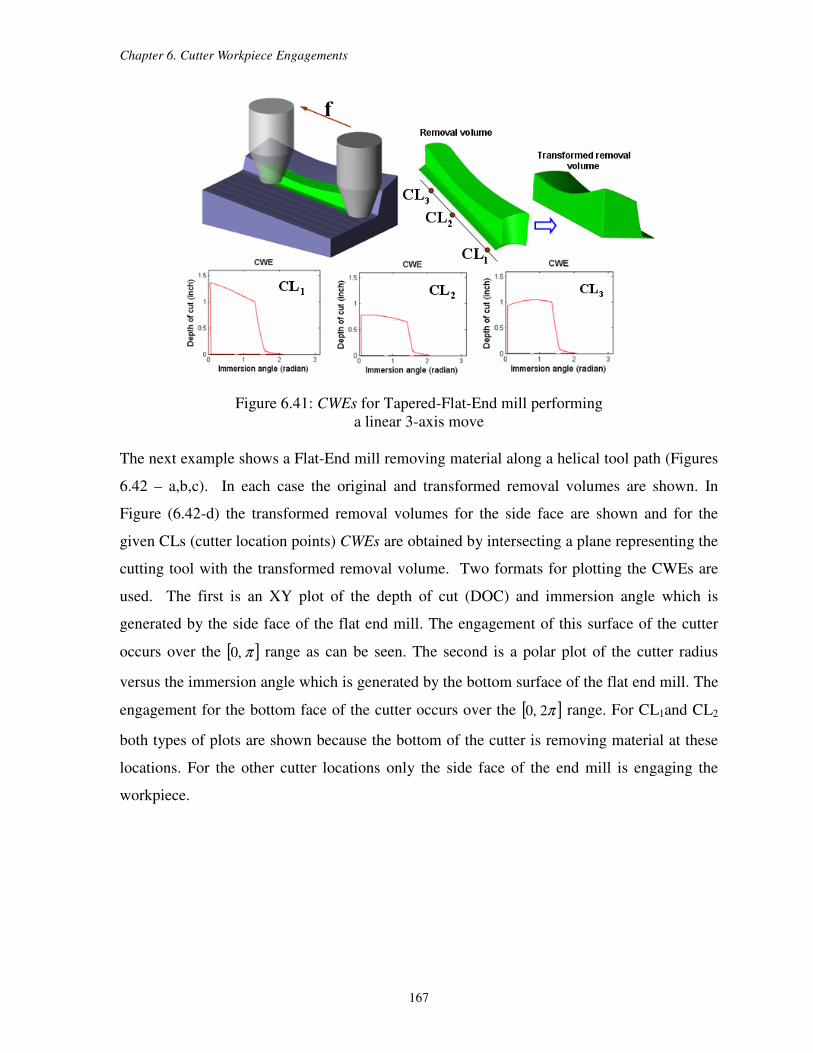
Chapter 6. Cutter Workpiece Engagements
167
Figure 6.41: CWEs for Tapered-Flat-End mill performing
a linear 3-axis move
The next example shows a Flat-End mill removing material along a helical tool path (Figures
6.42 – a,b,c). In each case the original and transformed removal volumes are shown. In
Figure (6.42-d) the transformed removal volumes for the side face are shown and for the
given CLs (cutter location points) CWEs are obtained by intersecting a plane representing the
cutting tool with the transformed removal volume. Two formats for plotting the CWEs are
used. The first is an XY plot of the depth of cut (DOC) and immersion angle which is
generated by the side face of the flat end mill. The engagement of this surface of the cutter
occurs over the [ ]π,0 range as can be seen. The second is a polar plot of the cutter radius
versus the immersion angle which is generated by the bottom surface of the flat end mill. The
engagement for the bottom face of the cutter occurs over the [ ]π2,0 range. For CL1and CL2
both types of plots are shown because the bottom of the cutter is removing material at these
locations. For the other cutter locations only the side face of the end mill is engaging the
workpiece.
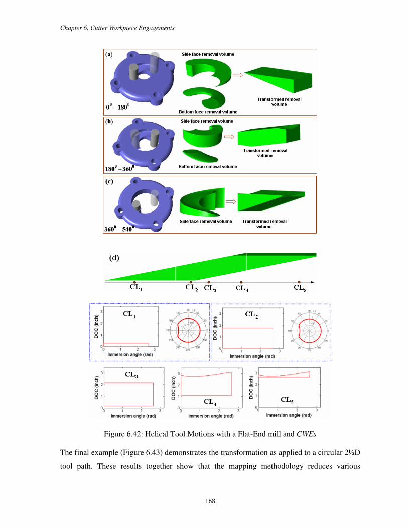
Chapter 6. Cutter Workpiece Engagements
168
Figure 6.42: Helical Tool Motions with a Flat-End mill and CWEs
The final example (Figure 6.43) demonstrates the transformation as applied to a circular 2½D
tool path. These results together show that the mapping methodology reduces various
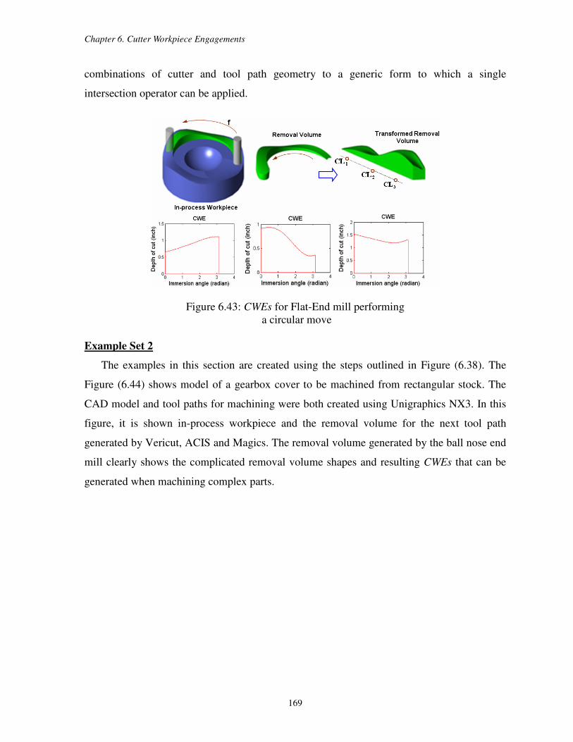
Chapter 6. Cutter Workpiece Engagements
169
combinations of cutter and tool path geometry to a generic form to which a single
intersection operator can be applied.
Figure 6.43: CWEs for Flat-End mill performing
a circular move
Example Set 2
The examples in this section are created using the steps outlined in Figure (6.38). The
Figure (6.44) shows model of a gearbox cover to be machined from rectangular stock. The
CAD model and tool paths for machining were both created using Unigraphics NX3. In this
figure, it is shown in-process workpiece and the removal volume for the next tool path
generated by Vericut, ACIS and Magics. The removal volume generated by the ball nose end
mill clearly shows the complicated removal volume shapes and resulting CWEs that can be
generated when machining complex parts.
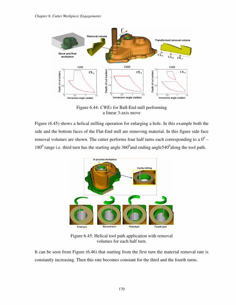
Chapter 6. Cutter Workpiece Engagements
170
Figure 6.44: CWEs for Ball-End mill performing
a linear 3-axis move
Figure (6.45) shows a helical milling operation for enlarging a hole. In this example both the
side and the bottom faces of the Flat-End mill are removing material. In this figure side face
removal volumes are shown. The cutter performs four half turns each corresponding to a 00 –
1800 range i.e. third turn has the starting angle 360
0and ending angle540
0along the tool path.
Figure 6.45: Helical tool path application with removal
volumes for each half turn.
It can be seen from Figure (6.46) that starting from the first turn the material removal rate is
constantly increasing. Then this rate becomes constant for the third and the fourth turns.
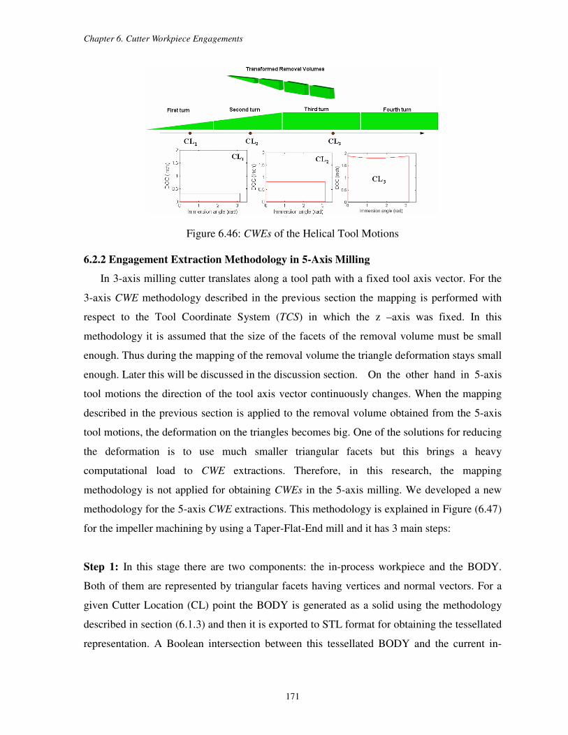
Chapter 6. Cutter Workpiece Engagements
171
Figure 6.46: CWEs of the Helical Tool Motions
6.2.2 Engagement Extraction Methodology in 5-Axis Milling
In 3-axis milling cutter translates along a tool path with a fixed tool axis vector. For the
3-axis CWE methodology described in the previous section the mapping is performed with
respect to the Tool Coordinate System (TCS) in which the z –axis was fixed. In this
methodology it is assumed that the size of the facets of the removal volume must be small
enough. Thus during the mapping of the removal volume the triangle deformation stays small
enough. Later this will be discussed in the discussion section. On the other hand in 5-axis
tool motions the direction of the tool axis vector continuously changes. When the mapping
described in the previous section is applied to the removal volume obtained from the 5-axis
tool motions, the deformation on the triangles becomes big. One of the solutions for reducing
the deformation is to use much smaller triangular facets but this brings a heavy
computational load to CWE extractions. Therefore, in this research, the mapping
methodology is not applied for obtaining CWEs in the 5-axis milling. We developed a new
methodology for the 5-axis CWE extractions. This methodology is explained in Figure (6.47)
for the impeller machining by using a Taper-Flat-End mill and it has 3 main steps:
Step 1: In this stage there are two components: the in-process workpiece and the BODY.
Both of them are represented by triangular facets having vertices and normal vectors. For a
given Cutter Location (CL) point the BODY is generated as a solid using the methodology
described in section (6.1.3) and then it is exported to STL format for obtaining the tessellated
representation. A Boolean intersection between this tessellated BODY and the current in-
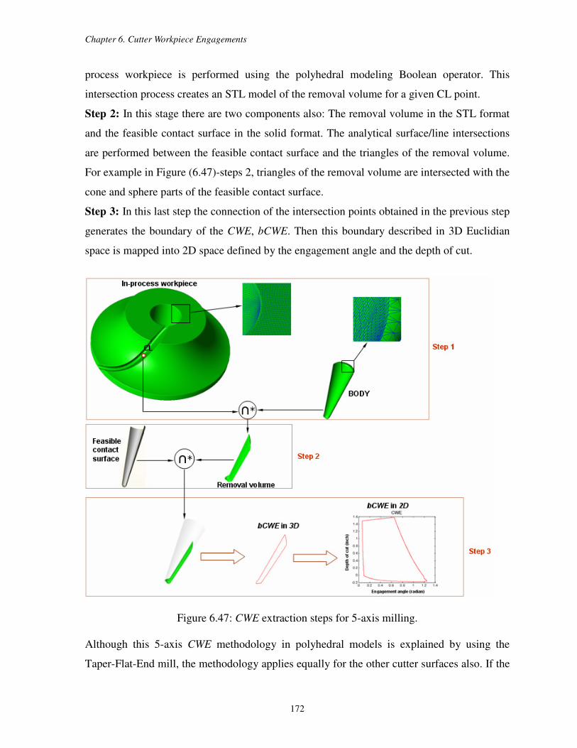
Chapter 6. Cutter Workpiece Engagements
172
process workpiece is performed using the polyhedral modeling Boolean operator. This
intersection process creates an STL model of the removal volume for a given CL point.
Step 2: In this stage there are two components also: The removal volume in the STL format
and the feasible contact surface in the solid format. The analytical surface/line intersections
are performed between the feasible contact surface and the triangles of the removal volume.
For example in Figure (6.47)-steps 2, triangles of the removal volume are intersected with the
cone and sphere parts of the feasible contact surface.
Step 3: In this last step the connection of the intersection points obtained in the previous step
generates the boundary of the CWE, bCWE. Then this boundary described in 3D Euclidian
space is mapped into 2D space defined by the engagement angle and the depth of cut.
Figure 6.47: CWE extraction steps for 5-axis milling.
Although this 5-axis CWE methodology in polyhedral models is explained by using the
Taper-Flat-End mill, the methodology applies equally for the other cutter surfaces also. If the
Chapter 6. Cutter Workpiece Engagements
173
cutter surface has the second order equation, e.g. cylinder, cone or sphere natural quadric
surfaces, each line – surface intersection gives two roots. If the cutter surface has the fourth
order equation e.g. torus, each line surface intersection gives four roots. In most cases only
one of these roots are needed for obtaining the bCWEs and the rest is redundant. During the
implementation the ACIS geometric kernel with C++ is used for creating and tessellating the
BODY and the Magics is used for the polyhedral Boolean intersections and updating the in-
process workpiece. These three steps are performed for each tool path segment. After
processing a toolpath segment for CWE extractions, the material is removed from the in-
process workpiece in the vicinity of the toolpath segment.
6.3 The Cutter Workpiece Engagements in Vector Based Model
In this section for the CWE calculations the cutting tool geometries are represented
implicitly by natural quadrics and the plane (a degenerate quadric). Natural quadrics consist
of the sphere, circular cylinder and the cone.
6.3.1 Intersecting Segment Against Plane
Given a point P with normal n on a planeπ , the following equation can be written for all
points X on this plane
( ) 0=− PX· n (6.41)
In the above equation the vector (X-P) is perpendicular to the vector n. When the dot product
in Eq.(6.41) is distributed across the subtraction the implicit representation of the plane takes
the form of dX =· n where Pd · n= . Let a segment is given by ( ) vIIIvI aba −+=)( for
10 ≤≤ v . For finding the intersection point I (see Figure 6.48) between the segment and the
plane the equivalent of I(v) is substituted for X in the plane equation and then this equation is
solved for v
( )( ) dvIII aba =−+· n (6.42)
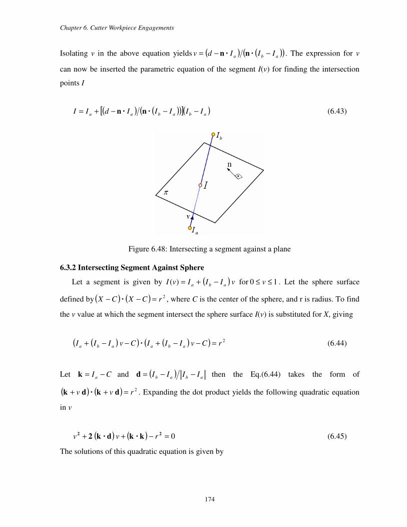
Chapter 6. Cutter Workpiece Engagements
174
Isolating v in the above equation yields ( ) ( )( )aba IIIdv −−= · n· n . The expression for v
can now be inserted the parametric equation of the segment I(v) for finding the intersection
points I
( ) ( )( )[ ]( )ababaa IIIIIdII −−−+= · n· n (6.43)
Figure 6.48: Intersecting a segment against a plane
6.3.2 Intersecting Segment Against Sphere
Let a segment is given by ( ) vIIIvI aba −+=)( for 10 ≤≤ v . Let the sphere surface
defined by ( ) ( ) 2rCXCX =−− · , where C is the center of the sphere, and r is radius. To find
the v value at which the segment intersect the sphere surface I(v) is substituted for X, giving
( )( ) ( )( ) 2rCvIIICvIII abaaba =−−+−−+ · (6.44)
Let CI a −=k and ( ) abab IIII −−=d then the Eq.(6.44) takes the form of
( ) ( ) 2rvv =++ dk·dk . Expanding the dot product yields the following quadratic equation
in v
( ) ( ) 0=−++ 22 k·kd·k2 rvv (6.45)
The solutions of this quadratic equation is given by

Chapter 6. Cutter Workpiece Engagements
175
( ) ( ) ( ) ][2
2,1
2k·kd·kd·k rv −−−= m (6.46)
Solution of the above equation gives three outcomes with respect to the
discriminant ( ) ( ) ][2 2k·kd·k r−−=∆ . If 0>∆ there are two real roots for which segment
intersects the sphere twice (Figure 6.49-a), If 0=∆ there are two equal real roots for which
the segment hits the sphere tangentially (Figure 6.49-b), and if 0<∆ there are no real roots
which corresponds to segment missing the sphere completely (Figure 6.49-c). Although for
the case given by 0>∆ there are two real roots, one of them can be false intersection (Figure
6.49-d,e). In this case the segment can start inside or outside sphere. One of the v values from
Eq.(6.45), its value is in the range of ]1,0[∈v , gives the intersection point.
(a) (b) (c) (d) (e)
Figure 6.49: Different cases in segment/sphere intersections: (a) Two intersection points, (b)
intersecting tangentially, (c) no intersection, (d) segment starts inside sphere, and (e) segment
starts outside sphere.
6.3.3 Intersecting Segment Against Cylinder
A cylinder with an arbitrary orientation can be described by an axis which passes through
points B and Q, and by a radius r (see Figure 6.50). Let X denotes a point on the cylinder
surface. The projection of the vector (X-B) onto the cylinder axis defined the vector (Q-B)
yields
( ) n·BXBP −=− (6.47)
where the unit vector ( ) BQBQ −−=n . Applying Pythagorean Theorem to triangle
defined by the points B, X and P yields

Chapter 6. Cutter Workpiece Engagements
176
( ) ( ) 222rBPBXBXBX +−=−−=− · (6.48)
Plugging Eq.(6.47) into Eq.(6.48) yields the following implicit representation for a cylinder
surface
( ) ( ) ( ) 022=−−−−− rBXBXBX n·· (6.49)
Figure 6.50: A segment is intersected against the cylinder given by points
B and Q and the radius r.
The intersection of a segment ( ) vIIIvI aba −+=)( with the cylinder can be found by
substituting I(v) for X into Eq.(6.49) and solving for v.
( )( ) ( )( ) ( )( ) 022=−−−+−−−+−−+ rBvIIIBvIIIBvIII abaabaaba n·· (6.50)
Setting BI a −=d and ab II −=k in the above equation the above equation can be written in
the following form
A2 v2 + 2A1 v + A0 = 0 (6.51)
where
( )2
2 n·k-k·k=A
( ) ( )n·dn·k-d·k=1A
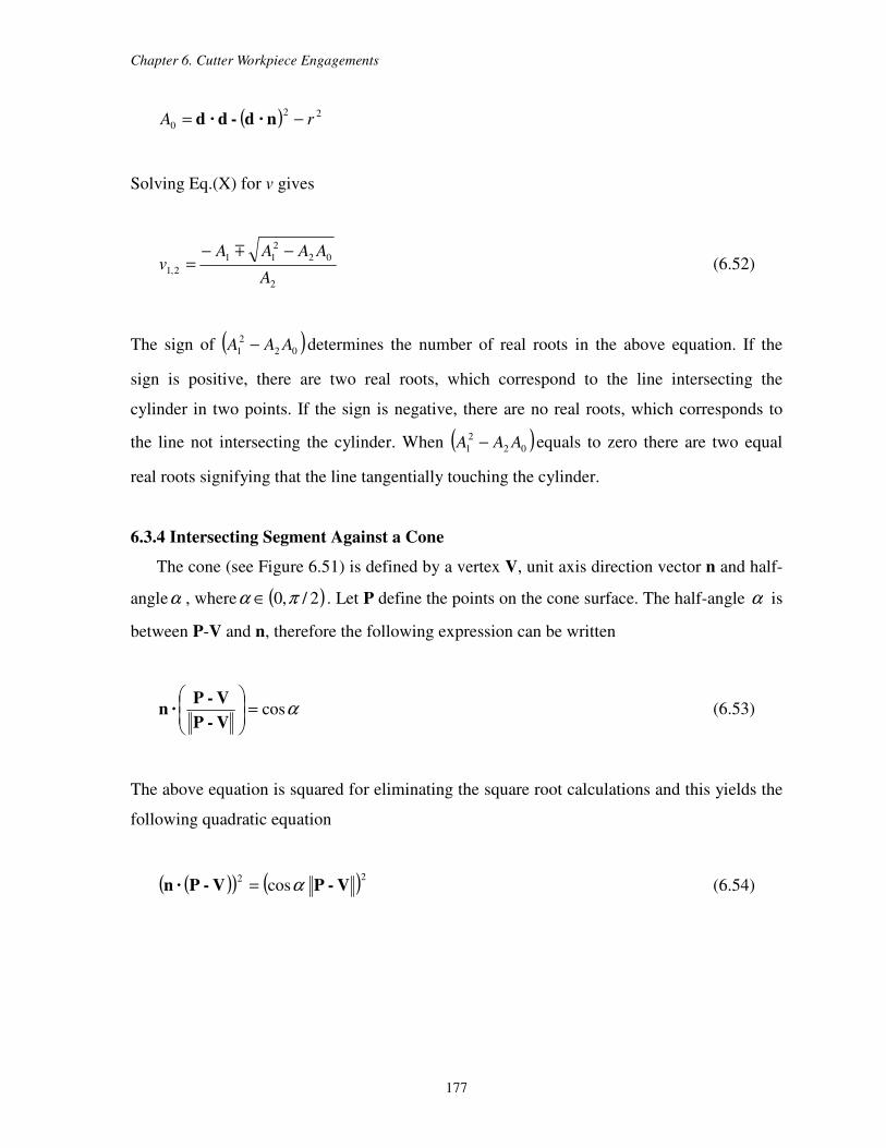
Chapter 6. Cutter Workpiece Engagements
177
( ) 22
0 rA −= n·d-d·d
Solving Eq.(X) for v gives
2
02
2
11
2,1A
AAAAv
−−=
m (6.52)
The sign of ( )02
2
1 AAA − determines the number of real roots in the above equation. If the
sign is positive, there are two real roots, which correspond to the line intersecting the
cylinder in two points. If the sign is negative, there are no real roots, which corresponds to
the line not intersecting the cylinder. When ( )02
2
1 AAA − equals to zero there are two equal
real roots signifying that the line tangentially touching the cylinder.
6.3.4 Intersecting Segment Against a Cone
The cone (see Figure 6.51) is defined by a vertex V, unit axis direction vector n and half-
angleα , where ( )2/,0 πα ∈ . Let P define the points on the cone surface. The half-angle α is
between P-V and n, therefore the following expression can be written
αcos=
V-P
V-P · n (6.53)
The above equation is squared for eliminating the square root calculations and this yields the
following quadratic equation
( )( ) ( )22cos V-PV-P · n α= (6.54)
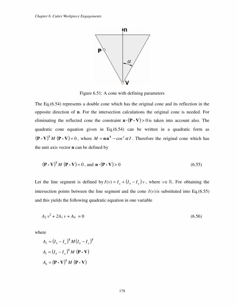
Chapter 6. Cutter Workpiece Engagements
178
Figure 6.51: A cone with defining parameters
The Eq.(6.54) represents a double cone which has the original cone and its reflection in the
opposite direction of n. For the intersection calculations the original cone is needed. For
eliminating the reflected cone the constraint ( ) 0>V-P · n is taken into account also. The
quadratic cone equation given in Eq.(6.54) can be written in a quadratic form as
( ) ( ) 0=V-PV-PT
M , where IM α2cos−= Tnn . Therefore the original cone which has
the unit axis vector n can be defined by
( ) ( ) 0=V-PV-PT
M , and ( ) 0>V-P · n (6.55)
Let the line segment is defined by ( ) vIIIvI aba −+=)( , where v∈R. For obtaining the
intersection points between the line segment and the cone )(vI is substituted into Eq.(6.55)
and this yields the following quadratic equation in one variable
A2 v2 + 2A1 v + A0 = 0 (6.56)
where
( ) ( )TT
abab IIMIIA −−=2
( ) ( )V-PT
MIIA ab −=1
( ) ( )V-PV-PT
MA =0
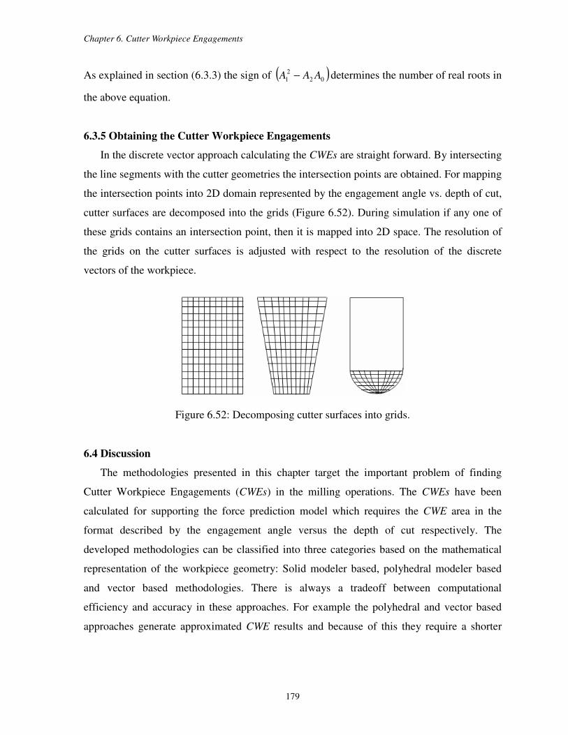
Chapter 6. Cutter Workpiece Engagements
179
As explained in section (6.3.3) the sign of ( )02
2
1 AAA − determines the number of real roots in
the above equation.
6.3.5 Obtaining the Cutter Workpiece Engagements
In the discrete vector approach calculating the CWEs are straight forward. By intersecting
the line segments with the cutter geometries the intersection points are obtained. For mapping
the intersection points into 2D domain represented by the engagement angle vs. depth of cut,
cutter surfaces are decomposed into the grids (Figure 6.52). During simulation if any one of
these grids contains an intersection point, then it is mapped into 2D space. The resolution of
the grids on the cutter surfaces is adjusted with respect to the resolution of the discrete
vectors of the workpiece.
Figure 6.52: Decomposing cutter surfaces into grids.
6.4 Discussion
The methodologies presented in this chapter target the important problem of finding
Cutter Workpiece Engagements (CWEs) in the milling operations. The CWEs have been
calculated for supporting the force prediction model which requires the CWE area in the
format described by the engagement angle versus the depth of cut respectively. The
developed methodologies can be classified into three categories based on the mathematical
representation of the workpiece geometry: Solid modeler based, polyhedral modeler based
and vector based methodologies. There is always a tradeoff between computational
efficiency and accuracy in these approaches. For example the polyhedral and vector based
approaches generate approximated CWE results and because of this they require a shorter
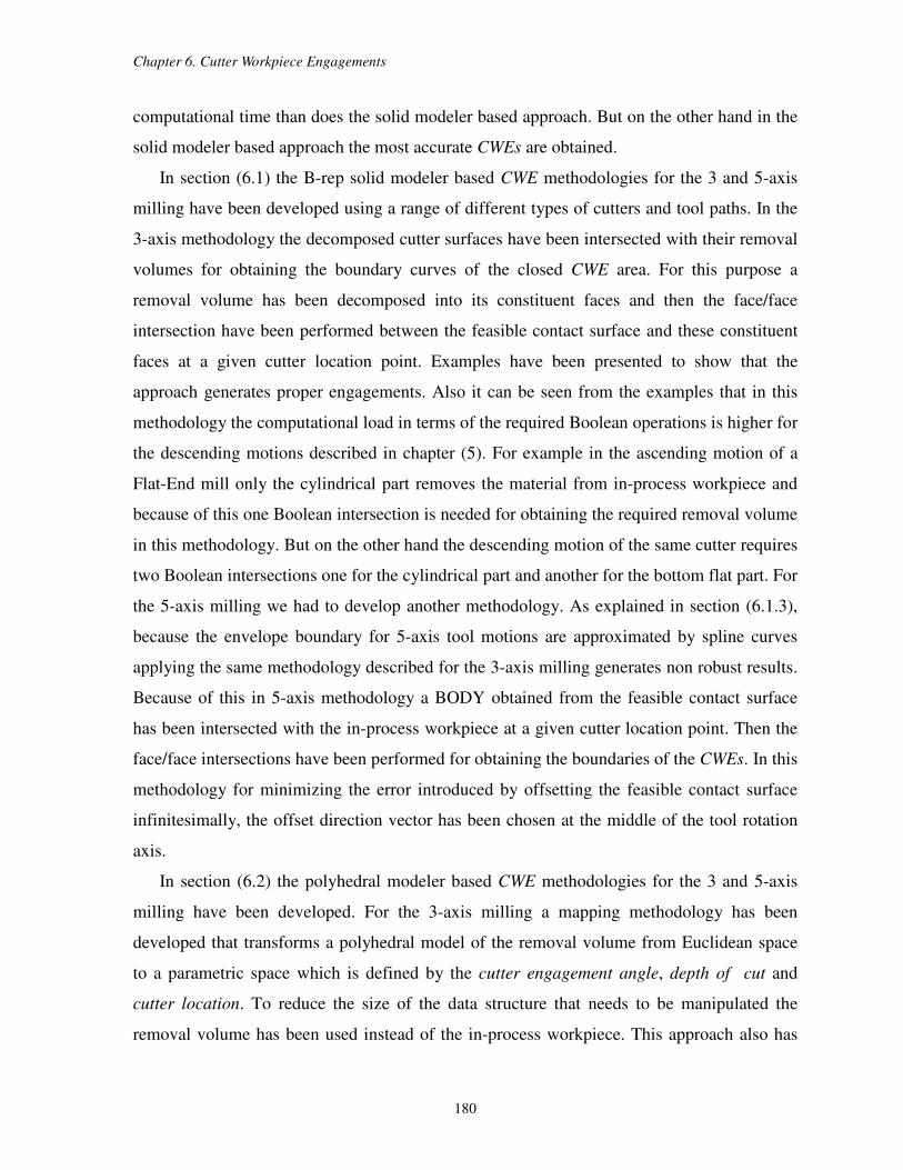
Chapter 6. Cutter Workpiece Engagements
180
computational time than does the solid modeler based approach. But on the other hand in the
solid modeler based approach the most accurate CWEs are obtained.
In section (6.1) the B-rep solid modeler based CWE methodologies for the 3 and 5-axis
milling have been developed using a range of different types of cutters and tool paths. In the
3-axis methodology the decomposed cutter surfaces have been intersected with their removal
volumes for obtaining the boundary curves of the closed CWE area. For this purpose a
removal volume has been decomposed into its constituent faces and then the face/face
intersection have been performed between the feasible contact surface and these constituent
faces at a given cutter location point. Examples have been presented to show that the
approach generates proper engagements. Also it can be seen from the examples that in this
methodology the computational load in terms of the required Boolean operations is higher for
the descending motions described in chapter (5). For example in the ascending motion of a
Flat-End mill only the cylindrical part removes the material from in-process workpiece and
because of this one Boolean intersection is needed for obtaining the required removal volume
in this methodology. But on the other hand the descending motion of the same cutter requires
two Boolean intersections one for the cylindrical part and another for the bottom flat part. For
the 5-axis milling we had to develop another methodology. As explained in section (6.1.3),
because the envelope boundary for 5-axis tool motions are approximated by spline curves
applying the same methodology described for the 3-axis milling generates non robust results.
Because of this in 5-axis methodology a BODY obtained from the feasible contact surface
has been intersected with the in-process workpiece at a given cutter location point. Then the
face/face intersections have been performed for obtaining the boundaries of the CWEs. In this
methodology for minimizing the error introduced by offsetting the feasible contact surface
infinitesimally, the offset direction vector has been chosen at the middle of the tool rotation
axis.
In section (6.2) the polyhedral modeler based CWE methodologies for the 3 and 5-axis
milling have been developed. For the 3-axis milling a mapping methodology has been
developed that transforms a polyhedral model of the removal volume from Euclidean space
to a parametric space which is defined by the cutter engagement angle, depth of cut and
cutter location. To reduce the size of the data structure that needs to be manipulated the
removal volume has been used instead of the in-process workpiece. This approach also has
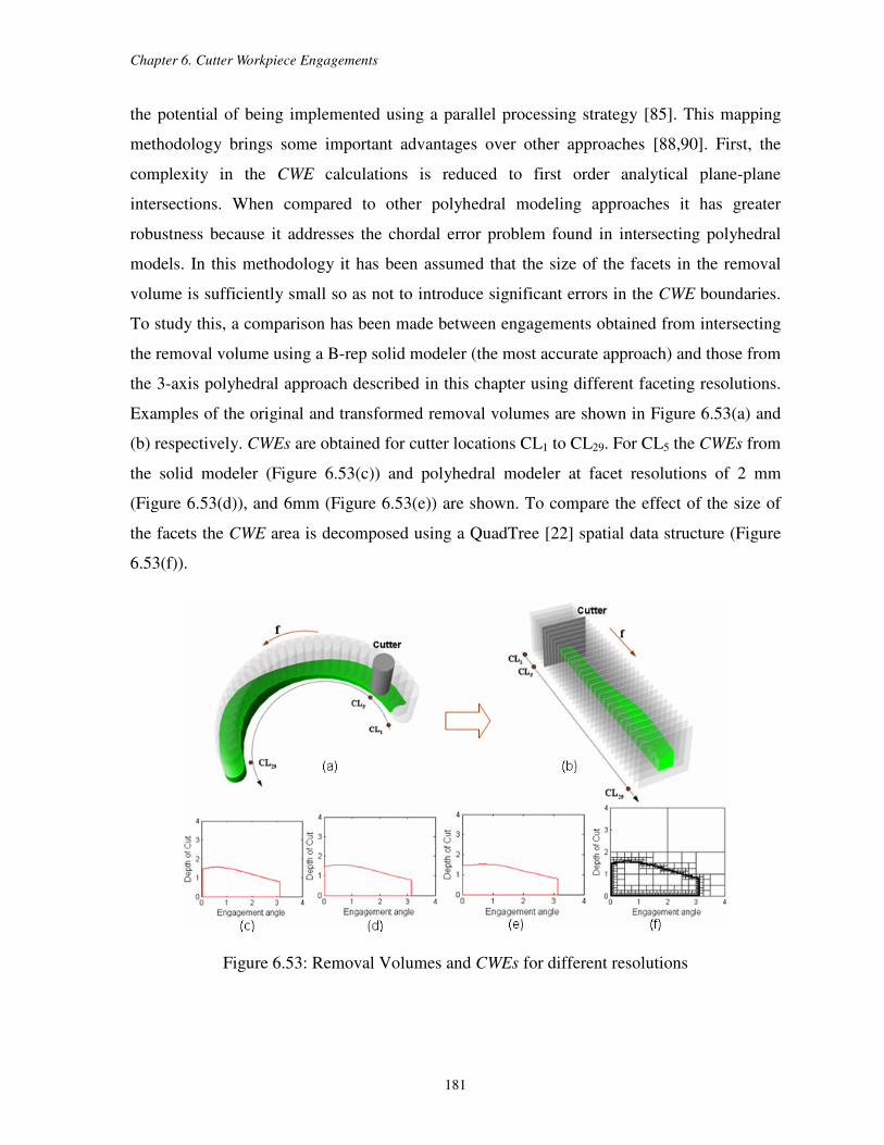
Chapter 6. Cutter Workpiece Engagements
181
the potential of being implemented using a parallel processing strategy [85]. This mapping
methodology brings some important advantages over other approaches [88,90]. First, the
complexity in the CWE calculations is reduced to first order analytical plane-plane
intersections. When compared to other polyhedral modeling approaches it has greater
robustness because it addresses the chordal error problem found in intersecting polyhedral
models. In this methodology it has been assumed that the size of the facets in the removal
volume is sufficiently small so as not to introduce significant errors in the CWE boundaries.
To study this, a comparison has been made between engagements obtained from intersecting
the removal volume using a B-rep solid modeler (the most accurate approach) and those from
the 3-axis polyhedral approach described in this chapter using different faceting resolutions.
Examples of the original and transformed removal volumes are shown in Figure 6.53(a) and
(b) respectively. CWEs are obtained for cutter locations CL1 to CL29. For CL5 the CWEs from
the solid modeler (Figure 6.53(c)) and polyhedral modeler at facet resolutions of 2 mm
(Figure 6.53(d)), and 6mm (Figure 6.53(e)) are shown. To compare the effect of the size of
the facets the CWE area is decomposed using a QuadTree [22] spatial data structure (Figure
6.53(f)).
Figure 6.53: Removal Volumes and CWEs for different resolutions
Chapter 6. Cutter Workpiece Engagements
182
The area of the CWE is obtained by accumulating the square areas that lie within the
QuadTree representation of the CWE boundary. For each CL point the areas obtained from
the different resolutions are compared with that of the B-rep solid modeler (Figure 6.54(a)).
The graph shows a 4% error at 6mm and less than 1% at 2mm. Figure 6.54(b) shows the
facet size vs. intersection time i.e. the time for obtaining the CWE area for a given cutter
location point. While the absolute value would vary depending on the implementation, the
trend should remain the same. This shows that there is a small increase in the intersection
time as the resolution is decreased from 6mm to 2mm after which it increases significantly.
Both the error and intersection time results point to 2mm being a practical limit for the facet
size in this example. We point out that this limit will vary depending on the cutter size. An
expression needs to be developed to calculate the resolution that considers this parameter.
(a) (b)
Figure 6.54: The effect of the facet resolutions
Because in 5-axis tool motions the direction of the tool axis vector continuously changes
applying the mapping described for the 3-axis milling has increased the distortions of the
facets. Therefore an approach similar to that of the 5-axis solid modeler has been developed.
In this approach the only difference was the application of the face-face intersections. These
intersections have been performed between triangular facets of a BODY and a solid
representation of the feasible contact surface.
And finally in section (6.3) a vector based CWE methodology has been developed. In this
methodology the cutter has been discretized into slices perpendicular to the tool axis. For
obtaining the CWEs the intersections have been performed between discrete vectors and
cutter slices. The intersection calculations are straight forward.
183
Chapter 7
Conclusions
7.1 Contributions and Limitations
In this thesis new methodologies have been proposed to facilitate Cutter Workpiece
Engagement (CWE) extractions in milling process modeling. This includes an analytical
methodology for determining the shapes of the cutter swept envelopes in multi-axes milling,
methodologies for updating the in-process workpiece surfaces, analysis of the feasible cutting
faces and finally algorithms for extracting CWEs. More specifically the contributions are
summarized as follows:
An analytical approach for determining the envelope of a swept volume generated by a
general surface of revolution performing multi-axes machining has been developed.
In this approach the cutter geometries are represented using canal surfaces and for
describing the cutter envelope surfaces the two-parameter-family of spheres has been
introduced. Analytically it has been proven that for cutter surfaces performing 5-axis tool
motions any point on the envelope surface is also a member of the point set generated from
the two-parameter-family of spheres formulation. Later the methodology is generalized for
cutters with general surfaces of revolution which performs 5-axis tool motions. In this
methodology, by describing the radius function and the trajectory of the moving sphere,
different cutter surfaces can be obtained. In this sense the methodology is independent of any
particular cutter geometry. The implementation of the methodology is simple. Especially
when the cutter geometries are pipe surfaces, fewer calculations are needed for describing the
cutter envelope surfaces. Although examples from the application of this methodology have
been shown for common milling cutter geometries described by the 7-parameter APT model,
this methodology can be also applied to rare cutter geometries. In some cases of 5-Axis
milling the cutter swept volume maybe self-intersecting, which requires special processing to
handle the topological and geometric problems due to the complex tool motions. Self
intersections in this research have not been considered. Modifications to the methodology
will need to be developed for this special case.
Chapter 7. Conclusions
184
A discrete vector model based in-process workpiece update methodology has been
developed.
During machining simulation, for each tool movement modification of the in-process
workpiece geometry is required to keep track of the material removal process. In this thesis
in-process workpiece modeling (or updating) methodologies have been developed using a
discrete vector representation. These vectors having orientations in the directions of the
x,y,z-axes of R3 are intersected with tool envelopes. With this representation more vectors in
different directions are used when compared to other discrete vector approaches. Therefore
especially when the workpiece has features like vertical walls and sharp edges, the quality in
the visualization of the final product has been increased. Also the localization advantage of
the Discrete Vertical Vector approach has been preserved. For simplifying the intersection
calculations the properties of the canal surfaces have been utilized. For cutter geometries
defined by a circular cylinder, frustum of a cone, sphere and plane the vector intersection
calculations for updating have been made analytically. Because of the complexity of the torus
geometry the calculations in this case have been made by using a numerical root finding
method. For this purpose a root finding analysis has been developed for guaranteeing the
root(s) in the given interval. A typical milling tool path contains thousands of tool
movements and during the machining simulation for calculating the intersections only a
small percentage of all the discrete vectors is needed. For this purpose a localization
methodology, based on the Axis Aligned Bounding Box (AABB) of each tool movement, has
been developed. The best feature of the AABB is its fast overlap check, which simply
involves direct comparison of individual coordinate values. As explained in chapter (4), for
some workpiece geometries 3-axis machining is not suitable for updating the surfaces. Also
exact 5-axis milling tool motions are not preferable in workpiece update simulations because
the calculations require using the nonlinear root finding algorithms and therefore the
computational time becomes high. Therefore in the developed methodologies tool motions
using (3+2)-axis milling are considered instead. Using (3+2)-axis tool motions in which a
cutter can have an arbitrary fixed orientation in space, 5-axis tool motions can be
approximated. An example has been given for illustrating this situation. The Discrete Normal
Vector (DNV) approach has not been considered in this research. The DNV approach can
represent the workpiece surface features well with respect to a given tolerance. But because
Chapter 7. Conclusions
185
in this approach the directions of discrete vectors are not identical, localizing the cutter
envelope surface during machining simulation becomes difficult. If the workpiece surfaces
are represented by DNVs then an efficient localization methodology will need to be
developed.
The engagement behaviors of NC cutter surfaces under varying tool motions have been
analyzed.
A typical NC cutter has different surfaces with varying geometries and during the
material removal process restricted regions of these surfaces are eligible to contact the in-
process workpiece with respect to the tool motions. In this thesis for representing these
regions the terminology feasible contact surfaces (FCS) has been introduced. The word
feasible has been used because although these surfaces are eligible to contact the in-process
workpiece, they may or may not remove material depending on the cutter position relative to
the workpiece. When the FCS contact the in-process workpiece the Cutter Workpiece
Engagements (CWEs) are generated. Since CWEs are subsets of the FCS, formalizing the
FCS helps us to better understand the CWE generation process. The FCS have been
formulized by using the cutter surface and the cutter envelope boundaries. The cutter surface
boundaries are fixed, but on the other hand the cutter envelope boundaries may change
depending on the tool motion. For modeling the cutter envelope boundaries a tangency
function defined by using the surface normal and the tool velocity has been utilized. Later by
changing the tool velocity direction the distributions of the FCS on the cutter have been
analyzed. The results from these analyses are later used in the development of the CWE
extraction methodologies.
Methodologies for obtaining Cutter Workpiece Engagements (CWEs) in milling have
been developed.
A major step in simulating machining operations is the accurate extraction of the CWE
geometries at changing tool locations. These geometries define the instantaneous intersection
boundaries between the cutting tool and the in-process workpiece at each location along a
tool path. The methodologies presented in this thesis target the important problem of finding
CWEs in milling operations. The CWEs are calculated for supporting the force prediction
Chapter 7. Conclusions
186
model requires the CWE area in the format described by the engagement angle versus the
depth of cut. In these methodologies a wide range of cutter geometries, toolpaths including 5-
axis tool motions and workpiece surfaces have been used. The workpiece surfaces cover
different surface geometries including sculptured surfaces. The developed CWE extraction
methodologies can be classified into three categories based on the mathematical
representation of the workpiece geometry: Solid modeler based, polyhedral modeler based
and vector based methodologies. There is always a tradeoff between computational
efficiency and accuracy in these approaches.
In 3-axis solid and polyhedral model based approaches developed in this thesis to reduce
the size of the data structure that needs to be manipulated the removal volume has been used
instead of the in-process workpiece. In the 3-axis solid modeler methodology the cutter
surfaces have been decomposed into different regions with respect to the feed vector
direction. Then these surface regions have been intersected with their removal volumes for
obtaining the boundary curves of the closed CWE area. Decomposing the cutter surfaces in
this way allows CWEs to be obtained for different parts of a given cutter geometry, e.g.
bottom flat or back side of a cutter. Using a solid modeler based representation the envelope
boundaries generated by 5-axis tool motions are approximated by spline curve. Applying the
solid model based methodology described for 3-axis tool motions to the removal volume
obtained from 5-axis tool motions can generate un-expected results because of the non-robust
surface/surface intersections. Therefore in this thesis for 5-axis tool motions in-process
workpiece has been used instead of the removal volume. In this approach the feasible contact
surface generated at a given cutter location point has been offsetted linearly with an
infinitesimal amount. As a result of this linear offsetting a surface volume has been
generated. Then this volume has been intersected with the in-process workpiece. Later
face/face intersections have been performed for obtaining the boundaries of the CWEs. In this
5-axis solid model based methodology by linearly offsetting the feasible contact surfaces, the
CWE extractions have became more robust.
For addressing the chordal error problem in polyhedral models a 3-axis mapping
technique has been developed that transforms a polyhedral model of the removal volume
from Euclidean space to a parametric space defined by location along the tool path,
engagement angle and depth-of-cut. As a result, intersection operations have been reduced to
Chapter 7. Conclusions
187
first order plane-plane intersections. This approach reduces the complexity of the
cutter/workpiece intersections and also eliminates robustness problems found in standard
polyhedral modeling. Because in 5-axis tool motions the direction of the tool axis vector
continuously changes applying the mapping described for the 3-axis milling increases the
distortions of the facets. Therefore a CWE extraction approach similar to the 5-axis solid
modeler based approach has been developed. In the polyhedral model based CWE extractions
2mm was the practical limit for the facet size. Still needed is an expression for finding the
optimal facet size.
7.2 Future Work
The future research work based on this thesis is summarized in the following:
In this thesis for the polyhedral model based CWE extraction methodologies a prototype
system has been assembled using existing commercial software applications and C++
implementations. For future work a standalone polyhedral based CWE extraction approach
that replaces the various commercial components will be developed.
The CWE areas must be decomposed for integrating with the force prediction model.
More efficient decomposition techniques (e.g. Quadtrees) will be investigated as a way for
representing the engagement geometry. A study of such techniques can lead to a new
formulation for the force prediction model that may be more efficient and provide greater
capability to manipulate and interpret the results.
An efficient localization methodology will be developed for localizing the cutter swept
envelopes during the material removal process, in which the workpiece surfaces are
represented by Discrete Normal Vectors (DNV).
The CWE extraction algorithms developed in this thesis will be integrated with the
Virtual Machining.
188
Bibliography
[1] Abdel-Malek K., Yeh H.-J., Geometric representation of the swept volume using
Jacobian rank-deficiency conditions, Computer Aided Design 29 (6) (1997) 457– 468.
[2] Abdel-Malek K., Seaman, W., Yeh H.-J., “NC-verification of up to 5 axis machining
processes using manifold stratification”, ASME Journal of Manufacturing Science and
Engineering 122 (2000) 1–11.
[3] Abdel-Malek K., Blackmore D., Joy K., “Swept volumes: foundations, perspectives and
applications”, International Journal of Shape Modeling, 2004.
[4] ACIS, Spatial Technology, Inc., Boulder, CO.
[5] Altintas, Y., ”Manufacturing Automation: Metal Cutting mechanics, Machine Tool
Vibrations, and CNC Design”, Cambridge University Press, 2000.
[6] Atherton P., Earl C., Fred C., "A Graphical Simulation System for Dynamic Five- Axis
NC Verification," Proc. Autofact, SME, Dearborn, Mich., 1987, pp. 2-1 to 2- 12.
[7] Baek N., Maeng S.R., Shin S.Y., Choi B.K., “ A Z-map update method for linearly
moving tools”, Computer Aided design 35 (2003) 995-1009
[8] Baek N., Maeng S.R., Shin S.Y., Choi B.K., “A fast NC simulation method for
circularly moving tools in the Z-map environment”, Proceeding of the Geometric
Modeling and Processing 2004(GMP’04)
[9] Bailey T.E., Jenkins D.M., Spence A.D., Elbestawi, M.A., Integrated Modeling for
Metal Removal Operations, Proc. IMECE, DSC-58 (Nov. 1996), ASME, 191-198.
[10] Bajaj C.L., Hoffman C.M., Lynch R.E., Hopcroft J.E.H., “Tracing Surface
Intersections”, Computer Aided Geometric Design, v 5, n 4, p 285-307, 1988.
[11] Barnhill R.E., Kersey S.N., “A marching method for parametric surface/surface
intersection”, Computer Aided geometric Design, Vol. 7, Issue 1-4, p 257-280, 1990.
[12] Bedi S., Mann S., “Flank Milling with Flat End Milling Cutters”, Preprint submitted to
Elsevier Preprint, 29 June 2001.
[13] Blackmore, D., Leu, M.C., Wang, K. K., “Applications of Flows and Envelopes to NC
Machining”, 1992, Annals of CIRP, 41/1:493-496.
[14] Blackmore, D., Leu, M.C.,Wang, L.,”The Sweep-Envelope Differential Equation
Algorithm and its Application to NC Machining Verification”, Comp. Aided Des.
1996.
[15]Blackmore D., Leu M.C., Wang L.P., “The sweep-envelope differential equation
algorithm and its application to NC-machining verification”, Computer Aided Design 29
(9) (1997) 629–637.
[16]Blackmore D., Samulyak R., Leu M.C.,“Trimming swept volumes”, Computer Aided
Design, Vol. 31 No.3, 1999, pp.215-224.
[17] Brent Richard. P., “Algorithms for Minimization without Derivatives”, Prentice- Hall,
Englewood Cliffs, New Jersey, 1973.
[18]Choi B.K., Jerard R.B., “Sculptured Surface Machining: Theory and Applications”,
Kluwer Academic Publishers, 1998.
[19]Chappel I.T., "The Use of Vectors to Simulate Material Removed by Numerically
Controlled Milling," Computer-Aided Design, Vol. 15, No. 3, May 1983, pp. 156- 158.
[20] Chiou C-J, Lee Y-S. “Swept surface determination for five-axis numerical control
machining”, Int J Mach Tools Manufact 2002;42: 1497–507.
Bibliography
189
[21] Chung Y.C., Park J.W., Shin H., Choi B.K., “Modeling the surface swept by a
generalized cutter for NC verification”, Computer-Aided Design 1998; 30(8):587- 594
[22] Clifford A. S., Hanan S., “Set operations for Unaligned Linear Quadtrees”, Computer
Vision, Graphics and Image Processing 50, 29-49 (1990)
[23] Drysdale R.L., Jerard R.B., "Discrete Simulation of NC Machining,", Proc. ACM
Symposium Computational Geometry, ACM, New York, 1987, pp. 126-135.
[24]Drysdale, R.L., Jerard, R.B., Schaudt, B.,Hauck, K.,"Discrete simulation of NC
machining", Algorithmica, Vol. 4, pp. 33-60, 1989.
[25] Elber G., Kim M.-S., Offsets, sweeps, and Minkowski sums, Computer Aided Design
31 (3) (1999) 163–173.
[26] El-Mounayri H., Elbestawi M. A., Spence A. D., Bedi S.,” General Geometric
Modelling Approach for Machining Process Simulation”, Int J. Adv. Manuf. Technol.
(1997), 13:237-247.
[27] Ericson. C., “Real-Time Collision Detection”, The Morgan Kaufmann Series in
Interactive 3-D Technology, 2005.
[28] Farouki R.T., Sverrissor R., “Approximation of rolling-ball blends for free-form
parametric surfaces”, Comput.-Aided Design 28 (1996) 871–878.
[29] Forsythe G.E., Malcolm M.A.,Moler C.B., “Computer Methods for Mathematical
Computations”, Prentice Hall, 1976.
[30] Fussell, B. K., Hemmett, J. G., Jerard, R. M., 1994, “Geometric and Mechanistic
Modeling Integration for Five-Axis Milling Force Prediction,” Proceedings of the
Japan-USA Symposium on Flexible Automation, Kobe, Japan, 2,
pp. 747–750.
[31] Fussell B.K., Hemmett J.G., Jerard R.B., “Modeling of five-axis end mill cutting using
axially discretized tool moves”, Proceedings of the 1999 NAMRC Conference, Berkeley,
CA, May 25-28, MR99-160
[32] Fussel B.K., Jerard R.B., Hemmet J.G., “Modeling of cutting geometry and forces for
5- axis sculptured surface machining”, Computer aided design 35 (2003) 333- 346
[33] Goldman R.N., Miller J.R., “Combining Algebraic Rigor with Geometric Robustness for
Detection and Calculation of Conic Sections in the Intersection of two Natural
Quadric Surfaces”, 1991, ACM 089791-427- 9/91/0006/0221.
[34]Gupta S.K., Saini S.K., Spranklin B.W., Yao Z., “Geometric algorithms for computing
cutter engagement functions in 2.5D milling operations”, Computer- Aided Design 37
(2005) 1469–1480.
[35] http://en.wikipedia.org/wiki/Wikipedia:Featured_picture_candidates/Csg_tree
[36] http://www.sescoi.com/us/
[37]Imani B. M., Sadeghi M. H., Elbestawi M. A., “An improved process simulation system
for ball-end milling of sculptured surfaces”, International Journal of Machine Tools
and Manufacture, Vol. 38, Issue 9, 1998, 1089-1107.
[38]Imani B.M., Elbestawi M.A., “Geometric Simulation of Ball-End Milling Operations”,
Journal of Manu. Sci. Eng. ASME, Vol. 123,177- 184, 2001.
[39] Jerard R.B., Hauck K., Drysdale R.L., "Simulation of Numerical Control Machining of
Sculptured Surfaces," 15th Int'l Symposium on Automotive Technology and
Automation, Paper No. 86057, ISATA, Automotive Automation, Ltd., Croydon, UK,
1986.
Bibliography
190
[40] Jerard R.B., Drysdale R.L., Hauck K., "Geometric Simulation of Numerical Control
Machining," Proc. ASME Int'l Computers in Engineering Conf., ASME, New York,
1988, pp. 129-136.
[41]Jerard R.B., Drysdale R.L., Hauck K.E., Schaudt B., Magewick J., “Methods for
detecting errors in numerically controlled machining of sculptured surfaces”, Computer
Graphics and Applications, IEEE, Vol. 9, Issue 1, p 26-39, 1989.
[42] Jerard R.B., Fussel B.K.l, Ercan M.T., “On-Line Optimization of Cutting Conditions for
NC Machining”, NSF Design, Manufacturing & Industrial Innovation Research
Conference, jan 7-10, 2001
[43]Jung W. Park, Yang H. Shin, Yun C. Chung,“ Hybrid cutting simulation via discrete
vector model”, Computer-Aided Design 37 (2005) 419-430.
[44] Kern, W. F., Bland, J. R. “Solid Mensuration with Proofs, 2nd ed.” New York: Wiley,
1948. (page 87).
[45] Kim KU-Jin, Lee In-Kwon, “The Perspective Silhouette of a Canal Surface, Computer
graphics Forum, Vol. 22 (2003),no:1, pp.15-22
[46] Kral I.H., “Numerical Control Programming in APT”, Prentice- Hall, New Jersey,
1986.
[47] Larue A., Altintas Y., 2004, "Simulation of Flank Milling Processes", Int. J. Machine
Tools and Manuf., vol. 45, pp.549-559.
[48] Levin J.Z., “Mathematical Models for Determining the Intersections of Quadrics
Surfaces”, Comput. Graph, Image process. Vol. 11 No 1 1979
[49] Liu S.Q. , Ong S.K., Chen Y.P., Nee A.Y.C., “Real-time, dynamic level-of-detail
management for three-axis NC milling simulation”, Computer-Aided Design, 38 (2006),
378-391.
[50] Maekawa T., Patrikalakis N.M., Sakkalis T., Yu G., “Analysis and applications of
pipe surfaces. Computer Aided Geometric Design, 15:437–458, 1998.
[51] Magics X, developed by Dimensionalize.
[52] Mann S.,Bedi S. “Generalization of the imprint method to general surfaces of
revolution for NC machining”, Computer-Aided Design (March 2002).
[53] Martin R., Stephenson P., “Sweeping of three-dimensional objects”, Computer
Aided Design 22 (4) (1990) 223–234.
[54] Matlab®
, The MathWorks, Inc.
[55] Miller J.R., Goldman R.N., “Geometric Algorithms for Detecting and Calculating
All Conic Sections in the Intersection of Any Two Natural Quadric Surfaces”,
GARPHICAL MODELS AND IMAGE PROCESSING, Vol. 57, No. 1, January, pp.
55-66, 1995
[56] Miller J.R., 1987, “Geometric approaches to Nonplanar Quadric Surface Intersection
Curves”, ACM transactions on Graphics, Vol.6, No.4, pages 274-307.
[57] Nishita T., Johan H., “A scan line algorithm for rendering curved tubular objects. In
Proc. of Pacific Graphics ’99, pp. 92–101. 1999.
[58] Oliver J.H., Goodman E.D., "Color Graphic Verification of N/C Milling Programs for
Sculptured Surface Parts," First Symposium on Integrated Intelligent Manufacturing,
ASME, New York, 1986.
[59] Patrikalakis N.M., Maekawa T., “Shape Interrogation for Computer Aided Design and
Manufacturing”, Springer Verlag, ISBN 3-540-42454-7, February 2002.
Bibliography
191
[60] Peternell M.,Pottmann H. “Computing rational parametrizations of canal surfaces.
Journal of Symbolic Computation, 23:255–266, 1997.
[61] Pottmann H., Peternell M., “Envelopes—computational theory and applications”,
Proceedings, Spring Conference on Computer Graphics and its Applications,
Budmerice, Slovakia, 2000, pp. 3–23.
[62] Quinn J.,“Accurate verification of five-axis numerically controlled machining”, PhD
Thesis, Department of Computer Science, Dartmouth College, Tech Reports PCS-
TR93-191,1993.
[63] Sarraga R.F.“Algebraic methods for intersections of quadric surfaces in GMSOLID”
Comput. Vision Graph. & Image Proc. Vol. 22 No. 2 (1983)
[64] Saturley P.V., Spence, A.D., “Integration of Milling Process Simulation with On-
Line Monitoring and Control”. Int. J. Adv. Manuf. Technol. 16 (2000), 92-99.
[65] Sederberg T.W., “Algorithm for algebraic curve intersection”, Computer Aided
Design, Vol. 21, Issue 9, p 547-554, 1989.
[66] Shani U., Ballard D.H., “Splines as embeddings for generalized cylinders”, Comput.
Vision Graphics Image Process. 27(1984) 129–156.
[67] Sheltami K., Bedi S., Ismail F., “Swept volumes of toroidal cutters using generating
curves”, International Journal of Machine Tools and Manufacture 1998; 38:855-70
[68] Shpitalni M., Fischer A., 1991, “CSG Representation as a Basis for Extraction of
Machining Features,” CIRP Ann., 40, pp. 157–160.
[69] Spence A., Altintas Y., Kirkpatrick D., 1990, “Direct Calculation of Machining
Parameters From a Solid Model,” Comput Ind., 14, pp. 271–280.
[70] Spence A.D., Altintas Y., “A Solid modeler based milling process simulation and
planning system”, Journal of Engineering for Industry, Transactions of the ASME.
Vol. 116 (1) pp.61-69, 1994.
[71] Spence A. D., Abrari F., Elbestawi M. A., 2000, “Integrated Solid Modeller Based
Solutions for Machining,” Comput.-Aided Des., 32_8_, pp. 553–568.
[72] Spence A. D., Li Z., 2001, “Parallel Processing for 2-1/2 D Machining Simulation,”
Proceedings of the6th ACM Symposium on Solid Modeling and Applications, Ann
Arbor , MI, pp. 140–148.
[73] Sungurtekin, U. A., Voelcker, H. B., 1986, “Graphical Simulation and Automatic
Verification of NC Machining Programs,” Proceedings of the IEEE International
Conference on Robotics and Automation, San Francisco, CA. 2, pp. 156–165.
[74] Oliver J.H., “Graphical Verification of Numerically Controlled Milling Programs for
Sculptured Surface Parts”, doctoral dissertation, Michigan State Univ., E. Lansing,
Mich., 1986.
[75] Roth D., Bedi S., Ismail F., Mann S., “Surface swept by a toroidal cutter during 5-
axis machining”, Computer Aided Design 33 (1) (2001) 57–63.
[76] Takata S., 1989, “A Cutting Simulation System for Machinability Evaluation Using a
Workpiece Model” CIRP Ann., 38/1, pp. 417–420.
[77] UGS NX, CAD/CAM/CAE , Siemens.
[78] Van Hook T., "Real-Time Shaded NC Milling Display," Computer Graphics (Proc.
SIGGRAPH), Vol. 20, No. 4, Aug. 1986, pp. 15-20.
[79] VERICUT, CGITech Inc.
Bibliography
192
[80] Voelcker H. B., Hunt W. A., 1981, “Role of Solid Modelling in Machining-Process
Modelling and NC Verification,” SAE Preprints, Vol. 810195.
[81] Wang W.P., Wang K.K., "Real-Time Verification of Multiaxis NC Programs with
Raster Graphics," IEEE Proc. Int'l Conf. Robotics and Automation, CS Press, Los
Alamitos, Calif., 1986, pp. 166-171.
[82] Wang W.P., Wang K.K., “Geometric modeling for swept volume of moving solids”,
IEEE Computer Graphics and Applications 6 (12) (1986) 8–17.
[83] Wang L., Leu M.C., Blackmore D., “Generating sweep solids for NC verification using
the SEDE method, in: Proceedings of the Fourth Symposium on Solid Modeling and
Applications, Atlanta, Georgia, 14–16 May 1997, pp. 364–375.
[84] Wang H., Jang P., Stori J.A.,“ A Metric-Based Approach to Two-Dimensional (2D)
Tool-Path Optimization for High-Speed Machining”, Journal of Manufacturing
Science and Engineering, Vol. 127 33-48 , 2005.
[85] Wang, J., Peng, X., Yip-Hoi, D., “A multi-agent system for distributed, Internet
enabled cutter/workpiece engagement extraction”, Proceedings of the ASME Design
Engineering Technical Conference, v 2006, 11 p.
[86] Weinert K., Du S.-J., Damm P., Stautner M., “Swept volume generation for the
simulation of machining processes”, International Journal of Machine Tools &
Manufacture 44 (6) (2004) 617–628.
[87] Wijk J.J. van. “Ray tracing of objects defined by sweeping a sphere. In Computer
Graphics Forum (Eurographics’84), pp. 73–82. 1984.
[88] Yao, Z., “Finding Cutter Engagement For Ball End Milling of Tesellated Free- Form
Surfaces”, “Proceedings of IDETC/CIE 2005, ASME International Design Engineering
Technical conferences”, DETC2005-84798.
[89] Yip-Hoi D., Huang X., “Cutter/Workpiece Engagement Feature Extraction from Solid
Models for End Milling”, Journal of Manufacturing Science and Engineering,
Transactions of the ASME, Vol. 128, Issue 1, pp. 249-260, 2006.
[90] Yip-Hoi D., Peng X., “R*-Tree Localization for Polyhedral Model Based
Cutter/Workpiece Engagements Calculations in Milling”, ASME CIE, sept 4-7, 2007
[91] Yun Won-Soo, Ko Jeong Hoon, Lee Han UI, Cho Dong-Woo, Ehmann Kornel F.,
“Development of a virtual machining system, Part 3: Cutting process simulation in
transient cuts”, International Journal of Machine Tools and Manufacture, v 42, n15, p
1617-1626, 2002.
193
Appendix A
Obtaining the grazing points for cutter geometries represented by pipe surfaces.
As mentioned in chapter (3), the cylinder and torus surfaces are called as pipe surfaces.
By definition a pipe surface is an envelope of the family of spheres with a constant radius. In
this surface type the centers of the characteristic circle and the moving sphere equal to each
other. In this section because of its complexity the property (3.2) is proven for the torus
surface and for the cylindrical surface similar steps can be used. When the components of the
Frenet frame given in Eq.(3.53) are plugged into Eq. (3.52), the torus surface is obtained as a
set of the characteristic circles in the following form
)),(sin),()(cos,(),(),,( utututRututK BMC θθθ ++= (A.1)
where [ ]πθ 2,0∈ . The radius of the moving sphere for the pipe surfaces is constant.
Therefore the partial derivative of the radius with respect to the toolpath parameter t equals to
zero, i.e. ( ) 0=trt . Thus under this condition the radius and the center of the characteristic
circle from Eqs. (3.50) and (3.51) become as
rutR =),( , ),(),( utut mC = (A.2)
Plugging the equations given in (A.2) into (A.1) yields
)),(sin),((cos),(),,( ututrututK BMm θθθ ++= (A.3)
For obtaining a point (so called grazing point) on the cutter envelope surface Eq.(A.3) is
plugged into Eq. (3.55) and then the resultant equation representing the surface normal is
plugged into Eq. (3.56). These yields
( ) ( ) 0sincos =+ B·mM·m uu θθ (A.4)

Appendix A. Obtaining the grazing points for cutter geometries represented by pipe surfaces.
194
The trigonometric terms from Eq.(A.4) are extracted as follows
( ) ( )22cos
B·mM·m
B·m
uu
u
+=θ ,
( ) ( )22sin
B·mM·m
M·m-
uu
u
+=θ
or (A.5)
( ) ( )22
cosB·mM·m
B·m-
uu
u
+=θ ,
( ) ( )22sin
B·mM·m
M·m
uu
u
+=θ
Plugging θcos and θsin from Eq.(A.5) into Eq.(A.3) yields
( ) ( )
( ) ( )
+=
22),(),,(
B·mM·m
BM·m-MB·mm
uu
uurututK mθ (A.6)
For simplifying the Eq.(A.6) the following cross product representation is used
cb·a-bc·acba )()()( =×× (A.7)
Under the rule given in Eq.(A.7) the nominator and inside the parenthesis of Eq.(A.6) can be
written as follows
( ) ( ) )( BMmBM·m-MB·m ××= uuu (A.8)
Also from Eq.(A.7) the length of the nominator inside the parenthesis can be written as
follows
( ) ( ) ( ) ( )22)(|| B·mM·mBMm||BM·m-MB·m uuuuu +=××= (A.9)
It can be seen that Eq.(A.9) equals to the denominator given inside the parenthesis of
Eq.(A.6). Plugging equivalents of nominator and denominator given inside the parenthesis of
Eq.(A.6). from Eqs.(A.8) and (A.9) yields

Appendix A. Obtaining the grazing points for cutter geometries represented by pipe surfaces.
195
××
××=
||)(||
)(),(),,(
BMm
BMmm
u
urututK mθ (A.10)
In the above equation the cross product of the normal and bi-normal unit vectors are equal to
the tangent vector of the spine curve i.e. BMT ×= . Thus Plugging the equivalent of of T
from Eq.(3.53) into Eq.(A.10) yields two grazing points P1,2
×
×==
||||),(),,( 2,1
tu
turutPutKmm
mmm mθ (A.11)
Thus the property (3.2) is proven for the torus which is also a pipe surface.
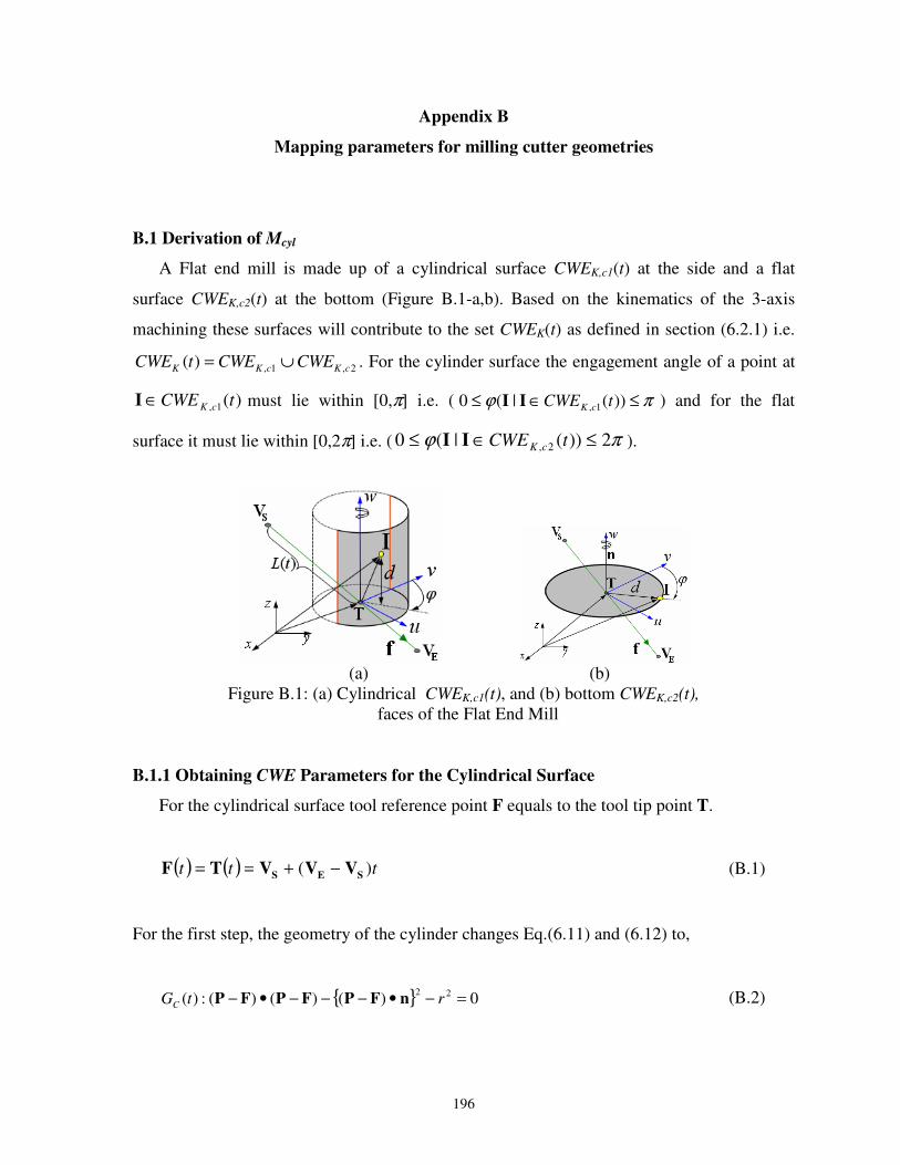
196
Appendix B
Mapping parameters for milling cutter geometries
B.1 Derivation of Mcyl
A Flat end mill is made up of a cylindrical surface CWEK,c1(t) at the side and a flat
surface CWEK,c2(t) at the bottom (Figure B.1-a,b). Based on the kinematics of the 3-axis
machining these surfaces will contribute to the set CWEK(t) as defined in section (6.2.1) i.e.
2,1,)( cKcKK CWECWEtCWE ∪= . For the cylinder surface the engagement angle of a point at
)(1, tCWE cK∈I must lie within [0,π] i.e. ( πϕ ≤∈≤ ))(|(0 1, tCWE cKII ) and for the flat
surface it must lie within [0,2π] i.e. ( πϕ 2))(|(0 2, ≤∈≤ tCWE cKII ).
(a) (b)
Figure B.1: (a) Cylindrical CWEK,c1(t), and (b) bottom CWEK,c2(t),
faces of the Flat End Mill
B.1.1 Obtaining CWE Parameters for the Cylindrical Surface
For the cylindrical surface tool reference point F equals to the tool tip point T.
( ) ( ) ttt )( SES VVVTF −+== (B.1)
For the first step, the geometry of the cylinder changes Eq.(6.11) and (6.12) to,
0)()()(:)( 22=−•−−−•− rtGC nFPFPFP (B.2)
Appendix B. Mapping parameters for milling cutter geometries.
197
and,
0)()()(:)( 22
, =−•−−−•− rtCWE CK nFIFIFI (B.3)
respectively. As with Eq.(6.13), Eq.(B.3) results in a quadratic equation in t when I and F are
substituted. In this case the coefficients 12 , AA and 0A are given by,
( ) ( ) ( )[ ]SISISI zzyyxx −−−=a
( )[ ] 22
2 SESE VVnVV −•−−=A
( ) ( )[ ] ( ) ( )SESE VVaVVnna −•−−••= 221A (B.4)
( ) 222
0 rA −•−= ana
Two real roots of the Eq.(B.3) represent two cutter locations according to Property (6.4) the
minimum of them is taken to be the correct tool position as explained in section (6.2.1.1).
Using Eq.(6.23-a) and (6.25) the parameters ϕ and L are obtained. Finally, the depth of the
engagement point as defined by the distance from T(t) to I' measured along the tool axis
vector is simply the z-coordinate of I'.
)()( tztd I TwwI •−•=′= (B.5)
B.1.2 Obtaining CWE Parameters for the Flat Surface
CWE parameters for the Flat surface are obtained without doing mapping. An unbounded
plane which is perpendicular to the tool rotation axis is intersected with the original removal
volume of the bottom surface for a given cutter location point. Engagement angle ϕ is found
by Eqs.(6.23-a) and (6.23-b). The depth of the cut for the bottom surface is the distance
between the intersection point I and the center of the bottom surface such that
22
II yxd ′+′= (B.6)
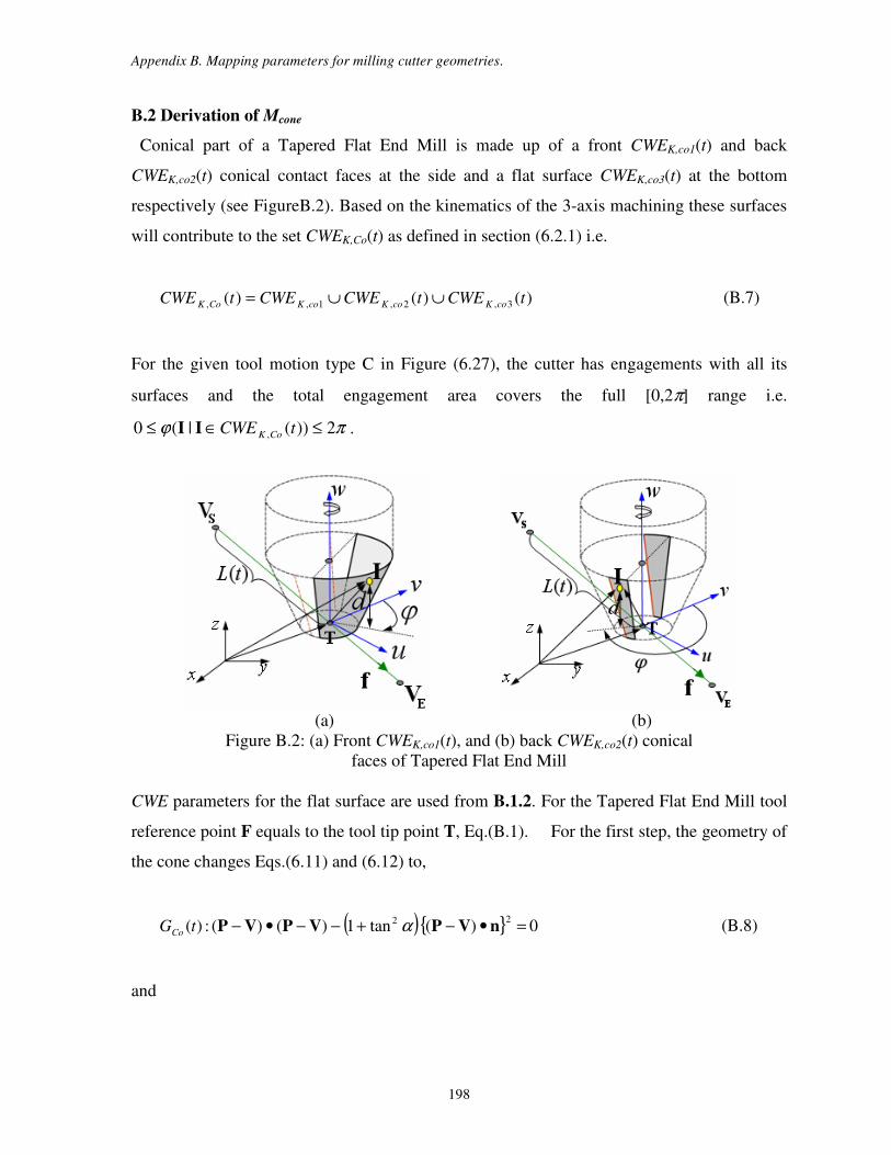
Appendix B. Mapping parameters for milling cutter geometries.
198
B.2 Derivation of Mcone
Conical part of a Tapered Flat End Mill is made up of a front CWEK,co1(t) and back
CWEK,co2(t) conical contact faces at the side and a flat surface CWEK,co3(t) at the bottom
respectively (see FigureB.2). Based on the kinematics of the 3-axis machining these surfaces
will contribute to the set CWEK,Co(t) as defined in section (6.2.1) i.e.
)()()( 3,2,1,, tCWEtCWECWEtCWE coKcoKcoKCoK ∪∪= (B.7)
For the given tool motion type C in Figure (6.27), the cutter has engagements with all its
surfaces and the total engagement area covers the full [0,2π] range i.e.
πϕ 2))(|(0 , ≤∈≤ tCWE CoKII .
(a) (b)
Figure B.2: (a) Front CWEK,co1(t), and (b) back CWEK,co2(t) conical
faces of Tapered Flat End Mill
CWE parameters for the flat surface are used from B.1.2. For the Tapered Flat End Mill tool
reference point F equals to the tool tip point T, Eq.(B.1). For the first step, the geometry of
the cone changes Eqs.(6.11) and (6.12) to,
( ) 0)(tan1)()(:)(22 =•−+−−•− nVPVPVP αtGCo
(B.8)
and

Appendix B. Mapping parameters for milling cutter geometries.
199
( ) 0)(tan1)()(:22
, =•−+−−•− nVIVIVI αCoKCWE (B.9)
whereα , n and V are the cone half angle, unit normal vector of the tool rotation axis and
cone vertex coordinates (see Figure 6.22-a) respectively. The relationship between V and F is
given by
n-FVα
r
tan= (B.10)
where r is the radius of the cone bottom surface. As with Eq.(6.13), Eq.(B.9) results in a
quadratic equation in t when I and F are substituted. In this case the coefficients 12 , AA and
0A are given by,
+−
+−
+−= ZSIYSIXSI n
rzzn
ryyn
rxx
ααα tantantana
( ) ( )[ ] 222
2 tan1 SESE VVnVV −•+−−= αA (B.11)
( ) ( ) ( )( ) ( )[ ]SESE VVnnaVVa −••++−•−= α2
1 tan122A
( ) ( )222
0 tan1 ana •+−= αA
Two real roots of the Eq.(B.9) represent two cutter locations according to property (6.4) and
the minimum of them is taken to be the correct tool position as explained in the section
(6.2.1.1). Using Eqs.(6.23-a,b),(6.25) and (B.5) the parameters (ϕ , d, L) are obtained.
B.3 Derivation of Mtorus
A Toroidal portion of the end mill is made up of front CWEK,t1(t) and back CWEK,t2(t)
contact faces at the side and a flat surface CWEK,t3(t) at the bottom respectively (see Figure
(B.3)). Based on the kinematics of the 3-axis machining these surfaces will contribute to the
set CWEK,T(t) as defined in section (6.2.1) i.e.
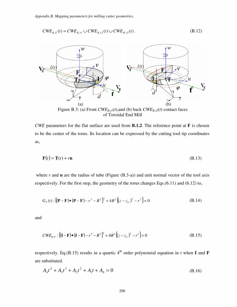
Appendix B. Mapping parameters for milling cutter geometries.
200
)()()( 3,2,1,, tCWEtCWECWEtCWE tKtKtKTK ∪∪= . (B.12)
(a) (b)
Figure B.3: (a) Front CWEK,t1(t),and (b) back CWEK,t2(t) contact faces
of Toroidal End Mill
CWE parameters for the flat surface are used from B.1.2. The reference point at F is chosen
to be the center of the torus. Its location can be expressed by the cutting tool tip coordinates
as,
( ) nTF rtt += )( (B.13)
where r and n are the radius of tube (Figure (B.3-a)) and unit normal vector of the tool axis
respectively. For the first step, the geometry of the torus changes Eqs.(6.11) and (6.12) to,
( ) ( ) ( ) 04:)( 222222 =−−+−−−•− rzzRRrtG CT FPFP (B.14)
and
( ) ( ) ( ) 04: 222222
, =−−+−−−•− rzzRRrCWE CTK FIFI (B.15)
respectively. Eq.(B.15) results in a quartic 4th
order polynomial equation in t when I and F
are substituted.
001
2
2
3
3
4
4 =++++ AtAtAtAtA (B.16)
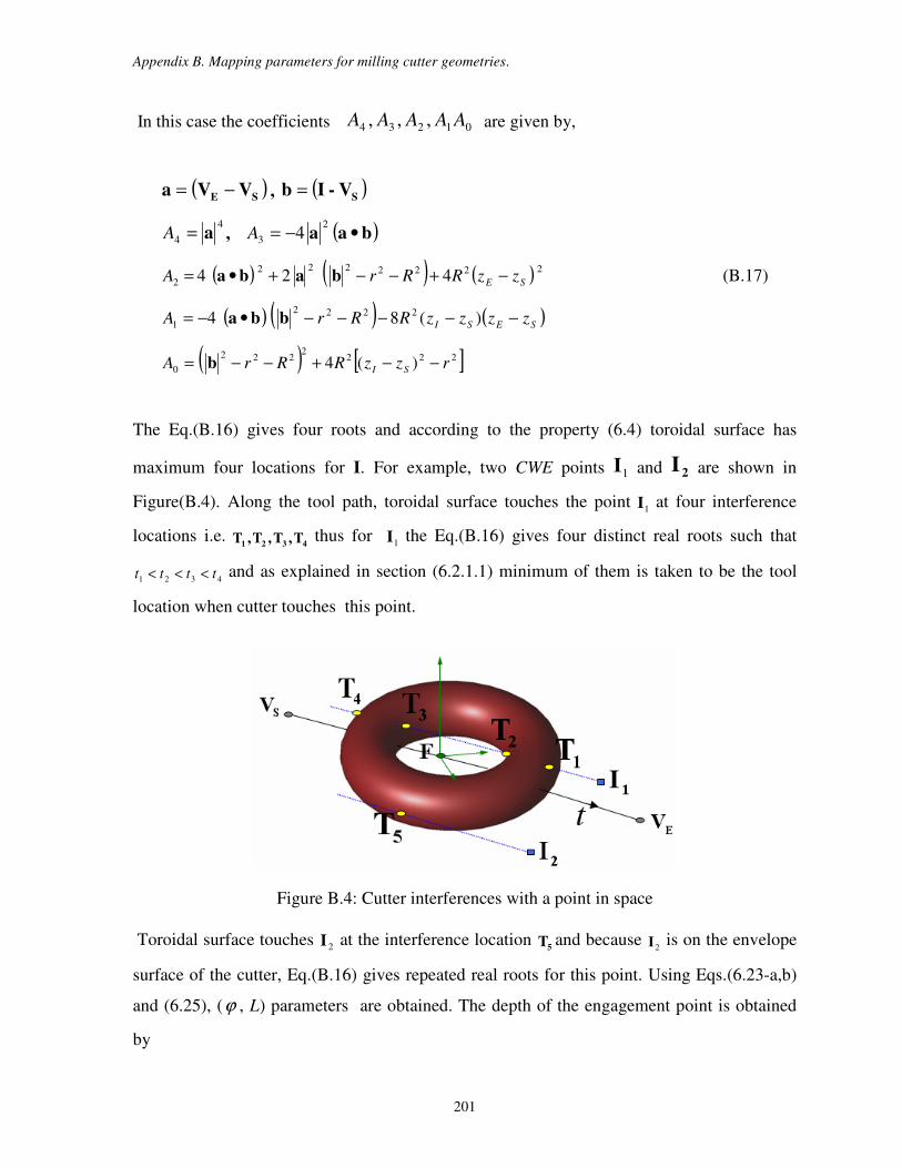
Appendix B. Mapping parameters for milling cutter geometries.
201
In this case the coefficients 01234 ,,, AAAAA are given by,
( )SE VVa −= , ( )SV-Ib =
4
4 a=A , ( )baa •−=2
3 4A
( ) ( ) ( ) 2222222
2 424 SE zzRRrA −+−−+•= baba (B.17)
( ) ( ) ( )SESI zzzzRRrA −−−−−•−= )(84 2222
1 bba
( ) [ ]2222
222
0 )(4 rzzRRrA SI −−+−−= b
The Eq.(B.16) gives four roots and according to the property (6.4) toroidal surface has
maximum four locations for I. For example, two CWE points 1I and 2I are shown in
Figure(B.4). Along the tool path, toroidal surface touches the point 1I at four interference
locations i.e. 4321 T,T,T,T thus for
1I the Eq.(B.16) gives four distinct real roots such that
4321 tttt <<< and as explained in section (6.2.1.1) minimum of them is taken to be the tool
location when cutter touches this point.
Figure B.4: Cutter interferences with a point in space
Toroidal surface touches 2I at the interference location
5T and because 2I is on the envelope
surface of the cutter, Eq.(B.16) gives repeated real roots for this point. Using Eqs.(6.23-a,b)
and (6.25), (ϕ , L) parameters are obtained. The depth of the engagement point is obtained
by

Appendix B. Mapping parameters for milling cutter geometries.
202
′−= −
r
ztd I1cos)(
1 (B.18)