Embed Size (px)
Citation preview
Biogeosciences, 12, 3579–3601, 2015
www.biogeosciences.net/12/3579/2015/
doi:10.5194/bg-12-3579-2015
© Author(s) 2015. CC Attribution 3.0 License.
Daily burned area and carbon emissions from boreal fires in Alaska
S. Veraverbeke1, B. M. Rogers2, and J. T. Randerson1
1Department of Earth System Science, University of California, Irvine, California, USA2Woods Hole Research Center, Falmouth, Massachusetts, USA
Correspondence to: S. Veraverbeke ([email protected])
Received: 7 November 2014 – Published in Biogeosciences Discuss.: 18 December 2014
Revised: 4 April 2015 – Accepted: 7 May 2015 – Published: 10 June 2015
Abstract. Boreal fires burn into carbon-rich organic soils,
thereby releasing large quantities of trace gases and aerosols
that influence atmospheric composition and climate. To bet-
ter understand the factors regulating boreal fire emissions, we
developed a statistical model of carbon consumption by fire
for Alaska with a spatial resolution of 450 m and a temporal
resolution of 1 day. We used the model to estimate variability
in carbon emissions between 2001 and 2012. Daily burned
area was mapped using imagery from the Moderate Reso-
lution Imaging Spectroradiometer combined with perimeters
from the Alaska Large Fire Database. Carbon consumption
was calibrated using available field measurements from black
spruce forests in Alaska. We built two nonlinear multiplica-
tive models to separately predict above- and belowground
carbon consumption by fire in response to environmental
variables including elevation, day of burning within the fire
season, pre-fire tree cover and the differenced normalized
burn ratio (dNBR). Higher belowground carbon consumption
occurred later in the season and for mid-elevation forests. To-
pographic slope and aspect did not improve performance of
the belowground carbon consumption model. Aboveground
and belowground carbon consumption also increased as a
function of tree cover and the dNBR, suggesting a causal link
between the processes regulating these two components of
carbon consumption. Between 2001 and 2012, the median
carbon consumption was 2.54 kgCm−2. Burning in land-
cover types other than black spruce was considerable and
was associated with lower levels of carbon consumption than
for pure black spruce stands. Carbon consumption origi-
nated primarily from the belowground fraction (median =
2.32 kgCm−2 for all cover types and 2.67 kgCm−2 for pure
black spruce stands). Total carbon emissions varied consid-
erably from year to year, with the highest emissions occur-
ring during 2004 (69 TgC), 2005 (46 TgC), 2009 (26 TgC),
and 2002 (17 TgC) and a mean of 15 TgCyear−1 between
2001 and 2012. Mean uncertainty of carbon consumption
for the domain, expressed as 1 standard deviation (SD), was
0.50 kgCm−2. Uncertainties in the multiplicative regression
model used to estimate belowground consumption in black
spruce stands and the land-cover classification were primary
contributors to uncertainty estimates. Our analysis highlights
the importance of accounting for the spatial heterogeneity
of fuels and combustion when extrapolating emissions in
space and time, and the need for of additional field cam-
paigns to increase the density of observations as a function of
tree cover and other environmental variables influencing con-
sumption. The daily emissions time series from the Alaskan
Fire Emissions Database (AKFED) presented here creates
new opportunities to study environmental controls on daily
fire dynamics, optimize boreal fire emissions in biogeochem-
ical models, and quantify potential feedbacks from changing
fire regimes.
1 Introduction
Fire is the most important landscape disturbance in the bo-
real forest (Chapin et al., 2000; Krawchuk et al., 2006). In-
creases in the extent and severity of burning in the last several
decades have been reported for Alaska and Canada (Gillett
et al., 2004; Kasischke and Turetsky, 2006; Kasischke et
al., 2010; Turetsky et al., 2011). Fire regimes are expected
to intensify (Amiro et al., 2009; Balshi et al., 2009; Yuan et
al., 2012; de Groot et al., 2013) with the predicted acceler-
ated warming for the boreal region during the remainder of
the 21st century (Collins et al., 2013), although this may be
mediated in part by changing vegetation cover (Krawchuk
and Cumming, 2011; Mann et al., 2012; Kelly et al., 2013;
Published by Copernicus Publications on behalf of the European Geosciences Union.
3580 S. Veraverbeke et al.: Daily burned area and carbon emissions from boreal fires in Alaska
Héon et al., 2014). Boreal fires have both positive and neg-
ative climate feedbacks (Randerson et al., 2006; Bowman
et al., 2009; Oris et al., 2014; Rogers et al., 2015). Cool-
ing is primarily caused by increases in surface albedo from
more exposed snow cover during spring in young stands
(Jin et al., 2012; Rogers et al., 2013) and the influence of
organic carbon aerosols on tropospheric radiation (Tosca
et al., 2013). Emission of greenhouse gases, black carbon
aerosols (Bowman et al., 2009), and the deposition of black
carbon on snow and ice (Flanner et al., 2007) are the domi-
nant warming feedbacks.
The magnitudes of these feedbacks are tightly linked with
the severity of the disturbance (Beck et al., 2011a; Turetsky
et al., 2011; Jin et al., 2012). Severity is often referred to
in a general way describing the amount of environmental
damage that fire causes to an ecosystem (Key and Benson,
2006). In the context of mostly stand-replacing fires in bo-
real North America, severity is expressed as the degree of
consumption of belowground organic matter. Differences in
ground layer burn depths control the amount of carbon com-
busted, and impact post-fire succession trajectories and con-
sequent albedo feedbacks (Johnstone and Kasischke, 2005;
Johnstone et al., 2010; Jin et al., 2012). Heterogeneity in
fuels, fuel conditions, topography and fire weather can re-
sult in different post-fire effects over the landscape (Rogers
et al., 2015). Resolving the spatial heterogeneity in sever-
ity using post-fire remote-sensing observations can improve
emissions estimates (Michalek et al., 2000; Veraverbeke and
Hook, 2013; Rogers et al., 2014) and more accurate carbon
emissions estimates could lower the uncertainties in estimat-
ing the net climate feedback from boreal fires under the cur-
rent and future climate (Oris et al., 2014).
Fire emissions are generally calculated as the product of
burned area, fuel consumption and emission factors (Seiler
and Crutzen, 1980). Fuel consumption represents the amount
of biomass consumed by the fire, and gas-specific emis-
sion factors describe the amount of gas released per unit of
biomass consumed by the fire. Examples of models build-
ing on this paradigm at continental or global scales include
the Wildland Fire Emissions Information System (WFEIS,
French et al., 2011, 2014) and the Global Fire Emissions
Database version 3 (GFED3, van der Werf et al., 2010), up-
dated with contributions of small fires (GFED3s, Randerson
et al., 2012). Several similar approaches have been devel-
oped specifically for boreal forests (Kasischke et al., 1995;
Amiro et al., 2001; Kajii et al., 2002; Kasischke and Bruh-
wiler, 2002; French et al., 2003; Soja et al., 2004; de Groot
et al., 2007; Tan et al., 2007; Kasischke and Hoy, 2012). The
quantification of fuel consumption in boreal emission mod-
els is often driven by empirical relationships between fire-
weather variables and combustion completeness that vary by
fuel type (Amiro et al., 2001; de Groot et al., 2007; Ottmar,
2014). A defining characteristic of fire emissions in the bo-
real forest is that mass of fuel consumed in the ground layer
(comprised of moss, lichens, litter, and organic soils) is larger
than the consumption of aboveground biomass (McGuire et
al., 2009; Boby et al., 2010; Kasischke and Hoy, 2012). Be-
cause of the seasonal thawing of the permafrost, the active
layer becomes deeper and drier throughout the fire season
and thus more prone to deeper burning (Lapina et al., 2008;
Turetsky et al., 2011; Kasischke and Hoy, 2012). Based on
this rationale, several authors have developed scenarios in
which they assign ground fuel consumption values based on
the seasonality of the burn (Kajii et al., 2002; Kasischke and
Bruhwiler, 2002; Soja et al., 2004). The dryness of the for-
est floor depends both on the time within the season and local
drainage conditions (Kane et al., 2007; Turetsky et al., 2011).
Kasischke and Hoy (2012) incorporated this expert knowl-
edge to derive emissions from a set of Alaskan fires by ac-
counting for differential impacts of fire seasonality on several
topographic classes.
Several studies have demonstrated relatively strong rela-
tionships between post-fire remote-sensing observations and
ground layer consumption in boreal forest ecosystems (Hu-
dak et al., 2007; Verbyla and Lord, 2008; Rogers et al., 2014).
Identification of such relationships may provide opportu-
nities to constrain pyrogenic carbon emission estimates in
boreal forest ecosystems at regional to pan-boreal scales
(Ottmar, 2014). Quantifying relationships between field data
of carbon consumption and pre- and post-fire remote-sensing
observations, in combination with other environmental vari-
ables, may minimize the number of assumptions required
to extrapolate emissions in time and space. In addition, ob-
served variability in relationships between field observations
and environmental variables may allow for a data-driven ap-
proach for uncertainty quantification. Spectral changes af-
ter a fire have shown to be strongly related to field mea-
surements of severity in a wide range of ecosystems (e.g.,
van Wagtendonk et al., 2004; Cocke et al., 2005; De San-
tis and Chuvieco, 2007; Veraverbeke and Hook, 2013), in-
cluding the boreal forest (Epting et al., 2005; Allen and Sor-
bel, 2008; Hall et al., 2008; Soverel et al., 2010). Severity
is often referred to as fire severity or burn severity (Lentile
et al., 2006; Keeley, 2009) with the difference in definition
between the two terms associated with the temporal dimen-
sion of fire effects. By definition, fire severity measures the
immediate impact of the fire, whereas burn severity incorpo-
rates both the immediate fire impact and subsequent recovery
effects (Lentile et al., 2006; French et al., 2008; Veraverbeke
et al., 2010). In particular, the differenced normalized burn
ratio (dNBR) has become accepted as a standard spectral in-
dex to assess severity (López García and Caselles, 1991; Key
and Benson, 2006). dNBR is an index that combines near and
short-wave infrared reflectance values obtained before and
after a fire (Eidenshink et al., 2007). The spectral regions
in dNBR are especially sensitive to the decrease of vegeta-
tion productivity and moisture content after the fire. Because
of this, dNBR is a good indicator of aboveground biomass
consumption, but may be less effective in estimating below-
ground consumption of boreal fires (French et al., 2008; Hoy
Biogeosciences, 12, 3579–3601, 2015 www.biogeosciences.net/12/3579/2015/
S. Veraverbeke et al.: Daily burned area and carbon emissions from boreal fires in Alaska 3581
et al., 2008; Kasischke et al., 2008). Other studies, how-
ever, have reported significant relationships between spec-
tral indices, including dNBR, and belowground consumption
measurements from field sites in boreal ecosystems (Hudak
et al., 2007; Verbyla and Lord, 2008; Rogers et al., 2014).
Rogers et al. (2014) also found a relatively strong correla-
tion between field measurements of aboveground and below-
ground consumption, which partly explained the observed
relationship between dNBR and belowground consumption.
Effective use of dNBR and other remote-sensing observa-
tions requires careful integration with other driver data and
calibration with field observations that span a wide range of
environmental conditions.
The day of burning within the fire season covaries with the
depth of burning in the ground layer, and this temporal in-
formation may aid prediction of belowground consumption
(Turetsky et al., 2011; Kasischke and Hoy, 2012). Convolv-
ing burned area detection algorithms with active fire hotspots
from the multiple overpasses per day from the Moderate Res-
olution Imaging Spectroradiometer (MODIS) allows for the
development of daily burned area estimates (Parks, 2014;
Veraverbeke et al., 2014). Daily burned area products pro-
vided evidence that vapor pressure deficit has an important
influence on several aspects of fire dynamics including ini-
tial spread rate, daily variations in regional burned area, and
fire extinction (Sedano and Randerson, 2014). Kasischke and
Hoy (2012) developed a daily fire emissions time series to
investigate causes of year-to-year variability in carbon con-
sumption for a regional subset of fires during high and low
fire years.
Daily burned area and emissions estimates may allow for
advances in studies investigating the composition and trans-
port of aerosols and greenhouse gases, fire behavior, or fire
modeling. No fire emissions product calibrated using field
observations currently exists for use in studying these pro-
cesses with continuous spatial and temporal coverage, and
public availability. Hyer et al. (2007) found that emissions
from boreal fires averaged over 30-day intervals resulted in
a reduction of 80 % of the variance compared to daily and
weekly data in a fire aerosol transport simulation. The tem-
poral resolution of emission data is especially important for
boreal fires since they often reach most of their burned area in
only a couple of days when the spatiotemporal patterns of ig-
nitions and fire weather optimally coincide (Abatzoglou and
Kolden, 2011; Sedano and Randerson, 2014). The represen-
tation of extreme fire-weather periods and their influence on
burned area in models may allow for more accurate predic-
tions of interannual and decadal changes in the fire regime
caused by climate warming (Jin et al., 2014). High resolu-
tion emission time series may also improve knowledge about
differences in composition of aerosols and trace gases orig-
inating from flaming and smoldering stages of combustion
(Yokelson et al., 2013) as well as allowing for better predic-
tion of human health impacts in downwind areas (Yao and
Henderson, 2014). More fundamentally, daily burned area
estimates are critical for quantitatively examining landscape
and weather controls on fire spread rates and severity.
In this paper we describe the creation of a high reso-
lution time series of fire emissions appropriate for investi-
gating many of the fine-scale fire dynamics questions de-
scribed above. We created a continuous daily time series
of fire emissions during 2001–2012 with a spatial resolu-
tion of 450 m for the state of Alaska. The combined time
span, time step, spatial resolution, spatial domain and cali-
bration with field observations of this product makes it suit-
able for use in many atmospheric studies, and unique from
other published estimates. To estimate carbon consumption
at each location (kgCm−2 burned area), we developed mul-
tiplicative regression models that capture some of the vari-
ability in field measurements using gridded environmental
variables, including post-fire remote-sensing observations of
severity. Our approach also includes uncertainty estimates
derived from the fit of our model with the field observa-
tions, and includes components associated with our scaling
approach used to provide region-wide spatial coverage. The
derived daily burned area and carbon emissions product, re-
ferred to as the Alaskan Fire Emissions Database (AKFED),
is the first wall-to-wall multi-year database with daily tem-
poral resolution that is calibrated using field observations for
Alaska and is publicly available. In our analysis, we com-
pared our model estimates with other regional and global
biomass burning products from WFEIS and GFED3s. We
also show that the set of field observations used does not
adequately sample burned area in open forests with sparse
tree cover. Since these forests tend to have lower levels of
carbon consumption, adjusting for this bias yields lower re-
gional means than what would be inferred directly from the
existing set of observations.
2 Spatiotemporal domain and data
2.1 Spatiotemporal domain
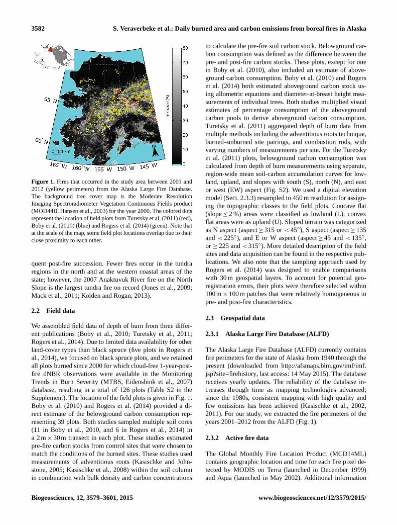
The spatial domain covers the area between 58 and 71.5◦ N,
and 141 and 168◦W. This represents almost the entire main-
land of Alaska with exclusion of the southern part of the
Alaska Peninsula and Southeast Alaska, west of British
Columbia (Fig. 1). The temporal domain of the study in-
cludes the years 2001–2012. Most Alaskan fires occur in the
interior of the state, which consists of a mosaic of vegeta-
tion types (Fig. S1 in the Supplement). Black spruce forest
dominates on cold, poorly drained, north-oriented or lowland
sites, whereas white spruce and deciduous species (mainly
aspen and birch) prevail on warmer, better drained, south-
oriented sites without permafrost (Viereck, 1973; Bonan,
1989). Grass- and shrubland ecosystems occur in early suc-
cessional stands, poorly drained sites, steep slopes and at and
above the treeline. The vegetation mosaic in interior Alaska
is constantly reshaped by the occurrence of fire and subse-
www.biogeosciences.net/12/3579/2015/ Biogeosciences, 12, 3579–3601, 2015
3582 S. Veraverbeke et al.: Daily burned area and carbon emissions from boreal fires in Alaska
Figure 1. Fires that occurred in the study area between 2001 and
2012 (yellow perimeters) from the Alaska Large Fire Database.
The background tree cover map is the Moderate Resolution
Imaging Spectroradiometer Vegetation Continuous Fields product
(MOD44B, Hansen et al., 2003) for the year 2000. The colored dots
represent the location of field plots from Turetsky et al. (2011) (red),
Boby et al. (2010) (blue) and Rogers et al. (2014) (green). Note that
at the scale of the map, some field plot locations overlap due to their
close proximity to each other.
quent post-fire succession. Fewer fires occur in the tundra
regions in the north and at the western coastal areas of the
state; however, the 2007 Anaktuvuk River fire on the North
Slope is the largest tundra fire on record (Jones et al., 2009;
Mack et al., 2011; Kolden and Rogan, 2013).
2.2 Field data
We assembled field data of depth of burn from three differ-
ent publications (Boby et al., 2010; Turetsky et al., 2011;
Rogers et al., 2014). Due to limited data availability for other
land-cover types than black spruce (five plots in Rogers et
al., 2014), we focused on black spruce plots, and we retained
all plots burned since 2000 for which cloud-free 1-year-post-
fire dNBR observations were available in the Monitoring
Trends in Burn Severity (MTBS, Eidenshink et al., 2007)
database, resulting in a total of 126 plots (Table S2 in the
Supplement). The location of the field plots is given in Fig. 1.
Boby et al. (2010) and Rogers et al. (2014) provided a di-
rect estimate of the belowground carbon consumption rep-
resenting 39 plots. Both studies sampled multiple soil cores
(11 in Boby et al., 2010, and 6 in Rogers et al., 2014) in
a 2m× 30m transect in each plot. These studies estimated
pre-fire carbon stocks from control sites that were chosen to
match the conditions of the burned sites. These studies used
measurements of adventitious roots (Kasischke and John-
stone, 2005; Kasischke et al., 2008) within the soil column
in combination with bulk density and carbon concentrations
to calculate the pre-fire soil carbon stock. Belowground car-
bon consumption was defined as the difference between the
pre- and post-fire carbon stocks. These plots, except for one
in Boby et al. (2010), also included an estimate of above-
ground carbon consumption. Boby et al. (2010) and Rogers
et al. (2014) both estimated aboveground carbon stock us-
ing allometric equations and diameter-at-breast height mea-
surements of individual trees. Both studies multiplied visual
estimates of percentage consumption of the aboveground
carbon pools to derive aboveground carbon consumption.
Turetsky et al. (2011) aggregated depth of burn data from
multiple methods including the adventitious roots technique,
burned–unburned site pairings, and combustion rods, with
varying numbers of measurements per site. For the Turetsky
et al. (2011) plots, belowground carbon consumption was
calculated from depth of burn measurements using separate,
region-wide mean soil-carbon accumulation curves for low-
land, upland, and slopes with south (S), north (N), and east
or west (EW) aspect (Fig. S2). We used a digital elevation
model (Sect. 2.3.3) resampled to 450 m resolution for assign-
ing the topographic classes to the field plots. Concave flat
(slope≤ 2 %) areas were classified as lowland (L), convex
flat areas were as upland (U). Sloped terrain was categorized
as N aspect (aspect≥ 315 or < 45◦), S aspect (aspect≥ 135
and < 225◦), and E or W aspect (aspect≥ 45 and < 135◦,
or ≥ 225 and < 315◦). More detailed description of the field
sites and data acquisition can be found in the respective pub-
lications. We also note that the sampling approach used by
Rogers et al. (2014) was designed to enable comparisons
with 30 m geospatial layers. To account for potential geo-
registration errors, their plots were therefore selected within
100m× 100m patches that were relatively homogeneous in
pre- and post-fire characteristics.
2.3 Geospatial data
2.3.1 Alaska Large Fire Database (ALFD)
The Alaska Large Fire Database (ALFD) currently contains
fire perimeters for the state of Alaska from 1940 through the
present (downloaded from http://afsmaps.blm.gov/imf/imf.
jsp?site=firehistory, last access: 14 May 2015). The database
receives yearly updates. The reliability of the database in-
creases through time as mapping technologies advanced;
since the 1980s, consistent mapping with high quality and
few omissions has been achieved (Kasischke et al., 2002,
2011). For our study, we extracted the fire perimeters of the
years 2001–2012 from the ALFD (Fig. 1).
2.3.2 Active fire data
The Global Monthly Fire Location Product (MCD14ML)
contains geographic location and time for each fire pixel de-
tected by MODIS on Terra (launched in December 1999)
and Aqua (launched in May 2002). Additional information
Biogeosciences, 12, 3579–3601, 2015 www.biogeosciences.net/12/3579/2015/
S. Veraverbeke et al.: Daily burned area and carbon emissions from boreal fires in Alaska 3583
on brightness temperature, fire radiative power, scan an-
gle and detection confidence is also provided. The product
is based on a contextual active fire algorithm that exploits
the strong emission in the mid infrared region from fires
(Giglio et al., 2003, 2006). We extracted the fire detections
from all confidence levels for our domain for the months
May–September, the months of the fire season, for all years.
MODIS on Terra experienced an extended outage during our
study period from 16 June through 2 July 2001 (Giglio et
al., 2013).
2.3.3 Environmental variables
Ground layer consumption by fire depends on the amount of
available dry fuels, which is determined by thickness, den-
sity and moisture content of the organic layer. After an ex-
tensive literature review, we selected a set of environmental
variables to predict ground layer consumption over the land-
scape (Table 1). The selected environmental variables were
elevation, slope, northness (defined as the cosine of the as-
pect), tree cover, day of burning, and dNBR.
Topography is a good proxy of site conditions for several
reasons. Elevation influences organic layer thickness, carbon
density, drainage and permafrost thaw by means of its con-
trol on climate. At higher elevations the seasonal permafrost
thaw starts later (Kasischke and Johnstone, 2005; Kasischke
and Hoy, 2012). Uplands generally have shallower organic
layers with a slightly higher carbon density than lowlands
(Kane et al., 2005, 2007; Turetsky et al., 2011). Uplands
are generally also better drained than lowlands (Barrett et
al., 2010; Kasischke and Hoy, 2012). Steep terrain is better
drained than flat land, but above a certain threshold steep-
ness limits the establishment of trees resulting in shallower
organic layers at steeper sites (Hollingsworth et al., 2006).
In crown fire ecosystems, fire severity tends to increase with
steepness when the wind direction aligns upslope (Rother-
mel, 1972; Pimont et al., 2012; Lecina-Diaz et al., 2014),
and this may also affect ground layer consumption. North-
oriented slopes are wetter and colder than south-faced slopes
and have thicker, less dense organic layers (Kane et al., 2007;
Turetsky et al., 2011). Here we derived elevation, slope and
northness from the Advanced Spaceborne Thermal Emission
and Reflection Radiometer Global Digital Elevation Model
Version 2 (ASTER GDEM 2, Tachikawa et al., 2011). The
ASTER GDEM 2 is a 30 m elevation model retrieved from
ASTER stereo-pair images.
Pre-fire tree cover is closely related to site productivity and
stand age, and thus influences organic layer thickness, den-
sity and moisture content (Kasischke and Johnstone, 2005;
Beck et al., 2011b; Rogers et al., 2013). Tree cover gener-
ally increases with stand age and better drainage conditions
(Beck et al., 2011b; Rogers et al., 2013). Tree cover also is
directly related to the amount of biomass available for above-
ground consumption, which has been shown to correlate rea-
sonably well with belowground consumption within a single
fire (Rogers et al., 2014). For the comparison with the field
plots, we used 30 m tree cover data from the Landsat-based
tree cover continuous field product for the year 2000 (Sexton
et al., 2013). For the statewide-extrapolation, tree cover was
downloaded from the annual Terra MODIS Vegetation Con-
tinuous Fields Collection 5 product at 250 m resolution for
the years 2000–2010 (MOD44B, Hansen et al., 2003). The
generation of the MOD44B product was discontinued after
2010, and we therefore used the tree cover layer of the year
2010 as pre-fire tree cover for the year 2012.
The day of burning in the season covaries with the mean
depth of the active layer, and thus may be related to the
amount of dry ground fuels available for burning (Turetsky
et al., 2011; Kasischke and Hoy, 2012). We assigned the day
of burning for each pixel based on the MODIS active fire ob-
servations. We found that the nearest neighbor variant of the
inverse distance weighting technique, in which the pixel is
assigned the value of the closest active fire detection exclud-
ing scan angles larger than 40◦, performed best and with a
within-1-day accuracy for most pixels (Fig. S3). The result-
ing progression maps were binned with a daily time step, at
local solar time.
We investigated the dNBR as an explanatory variable in
our carbon consumption model because extensive literature
suggests that it may have some predictive power in boreal
forest ecosystems. For the comparison with the field plots,
30 m dNBR data was retrieved from the Landsat-based Mon-
itoring Trends in Burn Severity database (MTBS, Eiden-
shink et al., 2007). For the statewide-extrapolation, we cal-
culated NBR from MODIS surface reflectance data in the
near infrared (NIR, centered at 858 nm) and short-wave in-
frared (SWIR, centered at 2130 nm) bands: NBR = (NIR-
SWIR)/(NIR + SWIR). We used the surface reflectance data
contained in the 16-day Terra MODIS Vegetation Indices
Collection 5 product at 500 m resolution for the years 2000–
2013 (MOD13A1, Huete et al., 2002). To account for cloudy
observations in single MODIS composites, we created sum-
mer NBR composites using the five 16-day composites be-
tween days of the year 177 and 256. We only used good data
as indicated by the MOD13A1 quality flags. NBR values
were calculated as the mean of all available good observa-
tions within the five composites. dNBR was calculated using
the 1-year pre-and post-fire NBR layers. Within the MTBS
database, we also only considered 1-year-post-fire dNBR in-
formation. This minimized potential differences in the inter-
pretation of dNBR values from different post-fire years (Ve-
raverbeke et al., 2010; Rogers et al., 2014).
The above six variables (elevation, slope, northness, tree
cover, day of burning and dNBR) were targeted to develop
the belowground carbon consumption model. dNBR and tree
cover were used as predictors of aboveground carbon con-
sumption.
www.biogeosciences.net/12/3579/2015/ Biogeosciences, 12, 3579–3601, 2015
3584 S. Veraverbeke et al.: Daily burned area and carbon emissions from boreal fires in Alaska
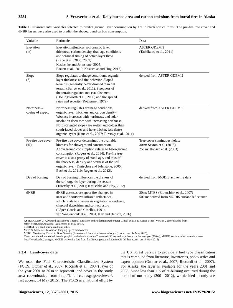
Table 1. Environmental variables selected to predict ground layer consumption by fire in black spruce forest. The pre-fire tree cover and
dNBR layers were also used to predict the aboveground carbon consumption.
Variable Rationale Data
Elevation Elevation influences soil organic layer ASTER GDEM 2
(m) thickness, carbon density, drainage conditions (Tachikawa et al., 2011)
and seasonal timing of active-layer thaw
(Kane et al., 2005, 2007;
Kasischke and Johnstone, 2005;
Barrett et al., 2010; Kasischke and Hoy, 2012)
Slope Slope regulates drainage conditions, organic derived from ASTER GDEM 2
(◦) layer thickness and fire behavior. Sloped
terrain is generally better drained than flat
terrain (Barrett et al., 2011). Steepness of
the terrain regulates tree establishment
(Hollingsworth et al., 2006) and fire spread
rates and severity (Rothermel, 1972).
Northness – Northness regulates drainage conditions, derived from ASTER GDEM 2
cosine of aspect organic layer thickness and carbon density.
Wetness increases with northness, and solar
insolation decreases with increasing northness.
North-oriented slopes are wetter and colder than
south-faced slopes and have thicker, less dense
organic layers (Kane et al., 2007; Turetsky et al., 2011).
Pre-fire tree cover Pre-fire tree cover determines the available Tree cover continuous fields:
(%) biomass for aboveground consumption. 30 m: Sexton et al. (2013)
Aboveground consumption relates to belowground 250 m: Hansen et al. (2003)
consumption (Rogers et al., 2014). Pre-fire tree
cover is also a proxy of stand age, and thus of
the thickness, density and wetness of the soil
organic layer (Kasischke and Johnstone, 2005;
Beck et al., 2011b; Rogers et al., 2013).
Day of burning Day of burning influences the dryness of derived from MODIS active fire data
the soil organic layer during the season
(Turetsky et al., 2011; Kasischke and Hoy, 2012)
dNBR dNBR assesses pre-/post-fire changes in 30 m: MTBS (Eidenshink et al., 2007)
near and shortwave infrared reflectance, 500 m: derived from MODIS surface reflectance
which relate to changes in vegetation abundance,
charcoal deposition and soil exposure
(López García and Caselles, 1991;
van Wagtendonk et al., 2004; Key and Benson, 2006)
ASTER GDEM 2: Advanced Spaceborne Thermal Emission and Reflection Radiometer Global Digital Elevation Model Version 2 (downloaded from
http://reverb.echo.nasa.gov, last access: 14 May 2015),
dNBR: differenced normalized burn ratio,
MODIS: Moderate Resolution Imaging Spectroradiometer,
MTBS: Monitoring Trends in Burn Severity (downloaded from http://www.mtbs.gov/, last access: 14 May 2015),
Tree cover data downloaded from http://glcf.umd.edu/data/landsatTreecover/ (30 m), and http://reverb.echo.nasa.gov (500 m), MODIS surface reflectance data from
http://reverb.echo.nasa.gov, MODIS active fire data from ftp://fuoco.geog.umd.edu/modis (all last access: on 14 May 2015).
2.3.4 Land-cover data
We used the Fuel Characteristic Classification System
(FCCS, Ottmar et al., 2007; Riccardi et al., 2007) layer of
the year 2001 at 30 m to represent land-cover in the study
area (downloaded from http://landfire.cr.usgs.gov/viewer/,
last access: 14 May 2015). The FCCS is a national effort by
the US Forest Service to provide a fuel type classification
that is compiled from literature, inventories, photo series and
expert opinion (Ottmar et al., 2007; Riccardi et al., 2007).
For Alaska, the layer is available for the years 2001 and
2008. Since less than 1 % of re-burning occurred during the
period of our study (2001–2012), we decided to only use
Biogeosciences, 12, 3579–3601, 2015 www.biogeosciences.net/12/3579/2015/
S. Veraverbeke et al.: Daily burned area and carbon emissions from boreal fires in Alaska 3585
the 2001 layer. We aggregated the fuel types into five land-
cover classes: black spruce, white spruce, deciduous, tundra–
grass–shrub and non-vegetated (Table S1, Fig. S1). Other
than the National Land Cover Database in Alaska (Stehman
and Selkowitz, 2010), the FCCS layer discriminates between
black and white spruce fuel types. The uncertainty of the
FCCS layer in Alaska has not been formally assessed.
3 Methods
AKFED provides daily burned area and carbon emissions
for the state of Alaska between 2001 and 2012 at 450 m
resolution. Since unburned islands are not fully accounted
for within perimeters (Kasischke and Hoy, 2012; Kolden
et al., 2012; Rogers et al., 2014; Sedano and Randerson,
2014), and some small fires are not accounted for outside the
perimeters (Randerson et al., 2012), we developed a burned
area mapping approach that screened dNBR values within
the ALFD perimeters and in the vicinity of active fire pixels
outside the perimeters (Sect. 3.1).
The carbon consumption model was formulated for black
spruce based on the relationship between the observed car-
bon consumption at the field locations and the environmental
variables. We extracted the pixel values of elevation, slope,
northness, pre-fire tree cover and dNBR at 30 m at the loca-
tion of the field plots. The day of burning was assigned from
the nearest active fire observation.
To extrapolate the model in space and time, we used a spa-
tial resolution of 450 m. This is the multiple of 30 m closest to
the exact 463 m native resolution of the MOD13A1 product
used to derive the dNBR layers (Masuoka et al., 1998). This
spatial resolution facilitated spatial averaging of 30 m DEM
(digital elevation model), tree cover, dNBR and land-cover
data. The decision to extrapolate the model at this resolution
was driven by data availability. We aimed at complete spatial
coverage. Even with current efforts such as MTBS and the
Web-Enabled Landsat Data (WELD, Roy et al., 2010), initial
exploration of these data sets indicated that complete Land-
sat dNBR coverage for every burned pixel was still partly
constrained by clouds, smoke, snow and gaps caused by the
Landsat 7 scan line corrector failure.
Elevation, aspect and northness were spatially averaged
from the native 30 m resolution of the ASTER GDEM 2
to the 450 m resolution. Similarly, the MOD44B tree cover
product was spatially averaged from its native resolution to
the 450 m resolution. The day of burning was also obtained
at this grid resolution. To account for other land-cover types
than black spruce, the aggregated FCCS product was rescaled
to 450 m in a way that every pixel at 450 m contained the
percentage of black spruce, white spruce, deciduous, tundra–
grass–shrub and non-vegetated land (Fig. S1). All analyses
were performed within the Albers equal area projection for
Alaska (central meridian: 154◦W, standard parallel 1: 55◦ N,
standard parallel 2: 65◦ N, latitude of origin: 50◦ N) with
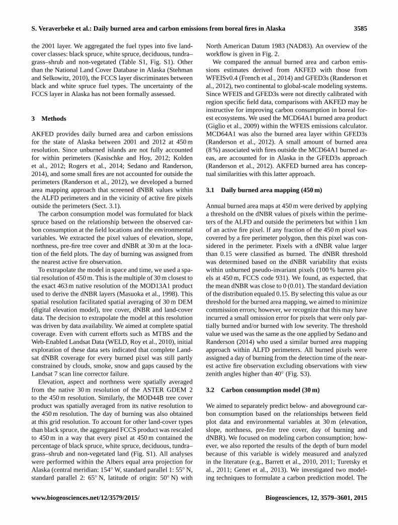
North American Datum 1983 (NAD83). An overview of the
workflow is given in Fig. 2.
We compared the annual burned area and carbon emis-
sions estimates derived from AKFED with those from
WFEISv0.4 (French et al., 2014) and GFED3s (Randerson et
al., 2012), two continental to global-scale modeling systems.
Since WFEIS and GFED3s were not directly calibrated with
region specific field data, comparisons with AKFED may be
instructive for improving carbon consumption in boreal for-
est ecosystems. We used the MCD64A1 burned area product
(Giglio et al., 2009) within the WFEIS emissions calculator.
MCD64A1 was also the burned area layer within GFED3s
(Randerson et al., 2012). A small amount of burned area
(8 %) associated with fires outside the MCD64A1 burned ar-
eas, are accounted for in Alaska in the GFED3s approach
(Randerson et al., 2012). AKFED burned area has concep-
tual similarities with this latter approach.
3.1 Daily burned area mapping (450 m)
Annual burned area maps at 450 m were derived by applying
a threshold on the dNBR values of pixels within the perime-
ters of the ALFD and outside the perimeters but within 1 km
of an active fire pixel. If any fraction of the 450 m pixel was
covered by a fire perimeter polygon, then this pixel was con-
sidered in the perimeter. Pixels with a dNBR value larger
than 0.15 were classified as burned. The dNBR threshold
was determined based on the dNBR variability that exists
within unburned pseudo-invariant pixels (100 % barren pix-
els at 450 m, FCCS code 931). We found, as expected, that
the mean dNBR was close to 0 (0.01). The standard deviation
of the distribution equaled 0.15. By selecting this value as our
threshold for the burned area mapping, we aimed to minimize
commission errors; however, we recognize that this may have
incurred a small omission error for pixels that were only par-
tially burned and/or burned with low severity. The threshold
value we used was the same as the one applied by Sedano and
Randerson (2014) who used a similar burned area mapping
approach within ALFD perimeters. All burned pixels were
assigned a day of burning from the detection time of the near-
est active fire observation excluding observations with view
zenith angles higher than 40◦ (Fig. S3).
3.2 Carbon consumption model (30 m)
We aimed to separately predict below- and aboveground car-
bon consumption based on the relationships between field
plot data and environmental variables at 30 m (elevation,
slope, northness, pre-fire tree cover, day of burning and
dNBR). We focused on modeling carbon consumption; how-
ever, we also reported the results of the depth of burn model
because of this variable is widely measured and analyzed
in the literature (e.g., Barrett et al., 2010, 2011; Turetsky et
al., 2011; Genet et al., 2013). We investigated two model-
ing techniques to formulate a carbon prediction model. The
www.biogeosciences.net/12/3579/2015/ Biogeosciences, 12, 3579–3601, 2015
3586 S. Veraverbeke et al.: Daily burned area and carbon emissions from boreal fires in Alaska
Figure 2. Workflow used to obtain daily burned area and carbon emissions in the Alaskan Fire Emissions Database (AKFED). dNBR:
differenced normalized burn ratio.
first technique was multiplicative nonlinear regression. This
technique is based directly on the interpretation of empiri-
cal relationships that may exist between the environmental
variables and the carbon consumption field data. Multiplica-
tive nonlinear regression has demonstrated to be effective in
a similar application to predict fire occurrence and size in
Southern California (Jin et al., 2014). The second technique
was gradient boosting of regression trees. We applied this
technique because previous work indicated that it may have
value in predicting depth of burning in boreal black spruce
forests (Barrett et al., 2010, 2011). Gradient boosting is a ma-
chine learning technique, which produces a prediction model
in the form of an ensemble of, in our case, multiple regres-
sion trees. We parameterized the gradient boosting of regres-
sion trees with the requirement that each leaf included at
least 10 % of the data per leaf and using 50 weak learner
trees. Both multiplicative nonlinear regression and gradient
boosting of regression trees allow for nonlinear relationships
between the dependent and independent variables, and inter-
actions between the independent variables. We opted to use
the multiplicative nonlinear regression model for our study
because we found it to considerably outperform the gradient
boosting model in predicting observations that were not used
to train the models (Fig. S4).
3.3 Daily carbon emissions, 2001–2012 (450 m)
Once optimized, we extrapolated the carbon consumption
model over the spatiotemporal domain of the study at 450 m
resolution. To do so, we first quantified the linear relation-
ship between Landsat and MODIS dNBR and tree cover
(Fig. S5). The resulting regression equations were applied
to the MODIS-derived dNBR and tree cover layers to allow
direct application in the carbon consumption model that was
optimized using Landsat data.
Due to data paucity of carbon consumption observations
in other land-cover types than black spruce, we developed
separate consumption models for these ecosystems that drew
upon the data-driven approach for black spruce. Decidu-
ous and white spruce stands generally have higher above-
ground and lower belowground fuel loads (Kasischke and
Hoy, 2012; Rogers et al., 2014). We assumed that carbon
consumption in these land-cover types was controlled by
the same variables as from the black spruce consumption
model. However, we multiplied the estimates derived from
our black spruce-based equations by consumption ratios for
above- and belowground deciduous and white spruce stands
that were developed using the Consume 3.0 fuel consumption
model (Ottmar et al., 2006; Prichard et al., 2006) (Fig. S6).
Consumption estimates derived from the black spruce model
were multiplied with the consumption ratios proportional to
the land-cover fractions within each pixel. For the state-wide
extrapolation over pixels classified as tundra–grass–shrub
and non-vegetated, we used the model derived for black
spruce. The mean tree cover value of all 30 m tundra–grass–
shrub and non-vegetated pixels within the ALFD perimeters
between 2001 and 2012 was 11 % (standard deviation, SD,
= 14 %).
We also quantified the influence of applying the nonlin-
ear multiplicative model (developed at 30 m resolution) us-
ing data with a spatial resolution of 450 m to enable state-
wide coverage. For this analysis, we selected all cloud-free
1-year-post-fire observations of the large fire year 2004 from
MTBS. We co-registered these with all good-quality obser-
vations from the Landsat tree cover layer, the 30 m DEM,
Biogeosciences, 12, 3579–3601, 2015 www.biogeosciences.net/12/3579/2015/
S. Veraverbeke et al.: Daily burned area and carbon emissions from boreal fires in Alaska 3587
30 m progression maps (derived using the nearest neighbor
approach), and the 30 m land-cover map. We then estimated
carbon consumption at 30 m and averaged the resulting car-
bon consumption over 450 m pixels for those 450 m pixels
that had complete 30 m dNBR and tree-cover coverage. For
these same pixels, we also first averaged all 30 m input lay-
ers (dNBR, tree cover, DEM, progression, and land cover)
to 450 m, and then estimated carbon consumption at 450 m
resolution.
3.4 Uncertainty
We adopted a Monte Carlo approach to quantify uncertain-
ties in AKFED. We identified four main sources of uncer-
tainty. The first source originates from the unexplained vari-
ance in the black spruce consumption model. The uncertainty
estimate from the black spruce consumption model was de-
rived quantitatively from the regression model and varied
from pixel to pixel as a function of the input variables. The
other sources of uncertainty were related to assumptions and
data required to extrapolate the model over Alaska. These in-
cluded uncertainties in the spatial scaling of a model devel-
oped with 30 m data at 450 m resolution, the land-cover clas-
sification, and assumptions made for deriving carbon con-
sumption for other land-cover types than black spruce. Un-
certainties derived from the spatial scaling were quantita-
tively estimated using the approach described in Sect. 3.3.
For the land-cover classification, because of a lack of quan-
titative information associated with the classification uncer-
tainty, we assumed a best-guess standard deviation uncer-
tainty of 20 % of the pixel-based black spruce fraction. We
also assigned a best-guess uncertainty (one SD) of 20 % of
the value range for the factors developed to estimate car-
bon consumption in other land-cover types than black spruce
(Fig. S6). We ran 1000 simulations at each pixel that burned
between 2001 and 2012 in which we randomly adjusted
the regression model estimates, the land-cover fractions, and
scaling relationships using the uncertainty information de-
scribed above. We conducted three separate Monte Carlo
simulation analyses for belowground, aboveground and total
carbon consumption.
4 Results
4.1 Carbon consumption model
The relationship between the depth of burn and the individ-
ual environmental variables was strongest for dNBR and tree
cover (R2adjusted = 0.25, p < 0.001), with both relationships
modeled using exponential response functions (Fig. S7).
Depth of burn responded with a relatively strong Gaussian
relationship to elevation (R2adjusted = 0.24, p < 0.001), with
the deepest burning occurring in the mid-elevation range be-
tween 300 and 600 m. A weak relationship was found for
slope (R2adjusted = 0.05, p < 0.05), and no relationship was
observed for day of burning or northness. The strongest
individual predictors for belowground carbon consumption
were day of burning (R2adjusted = 0.09, p < 0.001), slope
(R2adjusted = 0.08, p < 0.01) and dNBR (R2
adjusted = 0.06,
p < 0.01). Northness (R2adjusted = 0.04, p < 0.05), elevation
(R2adjusted = 0.04, p < 0.05), and tree cover (R2
adjusted = 0.03,
p < 0.05) had a weaker influence (Fig. S8). The aboveground
carbon consumption demonstrated stronger, also exponen-
tial, relationships with pre-fire tree cover (R2adjusted = 0.53,
p < 0.001) and dNBR (R2adjusted = 0.23, p < 0.001) vari-
ables (Fig. S9).
The optimized multiplicative nonlinear model for the
depth of burn and belowground carbon consumption in black
spruce forest based on the field and 30 m data was formulated
as follows:
depth30 m or Cbelowground, 30 m = c1+ c2 · ec3·dNBR
· eC4·tcec5·DOY· e−(elev−c6)
2
2·c7 , (1)
where c1,...,7 are the optimized coefficients, dNBR is the dif-
ferenced normalized burn ratio, tc is the pre-fire tree cover,
DOY is the day of the year, and elev is the elevation. Two
separate models were developed for depth of burn and be-
lowground carbon consumption using Eq. (1). The depth of
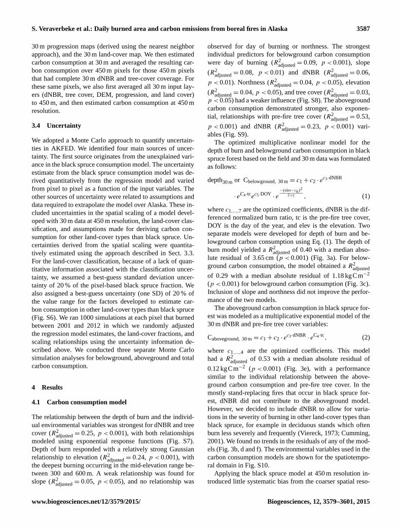
burn model yielded a R2adjusted of 0.40 with a median abso-
lute residual of 3.65 cm (p < 0.001) (Fig. 3a). For below-
ground carbon consumption, the model obtained a R2adjusted
of 0.29 with a median absolute residual of 1.18 kgCm−2
(p < 0.001) for belowground carbon consumption (Fig. 3c).
Inclusion of slope and northness did not improve the perfor-
mance of the two models.
The aboveground carbon consumption in black spruce for-
est was modeled as a multiplicative exponential model of the
30 m dNBR and pre-fire tree cover variables:
Caboveground, 30 m = c1+ c2 · ec3·dNBR
· eC4·tc, (2)
where c1,...,4 are the optimized coefficients. This model
had a R2adjusted of 0.53 with a median absolute residual of
0.12 kgCm−2 (p < 0.001) (Fig. 3e), with a performance
similar to the individual relationship between the above-
ground carbon consumption and pre-fire tree cover. In the
mostly stand-replacing fires that occur in black spruce for-
est, dNBR did not contribute to the aboveground model.
However, we decided to include dNBR to allow for varia-
tions in the severity of burning in other land-cover types than
black spruce, for example in deciduous stands which often
burn less severely and frequently (Viereck, 1973; Cumming,
2001). We found no trends in the residuals of any of the mod-
els (Fig. 3b, d and f). The environmental variables used in the
carbon consumption models are shown for the spatiotempo-
ral domain in Fig. S10.
Applying the black spruce model at 450 m resolution in-
troduced little systematic bias from the coarser spatial reso-
www.biogeosciences.net/12/3579/2015/ Biogeosciences, 12, 3579–3601, 2015
3588 S. Veraverbeke et al.: Daily burned area and carbon emissions from boreal fires in Alaska
Figure 3. Scatter plots between the observed and estimated
(a) depth of burn, (c) belowground and (e) aboveground carbon con-
sumption from the multiplicative nonlinear model, and correspond-
ing regression residuals (b, d and f). The gray line represents the
1 : 1 line in the left panels, and the y = 0 line in the right panels. All
models were significant at p < 0.001.
lution (Fig. S11). Using the consumption ratios derived for
white spruce and deciduous cover (Fig. S6) and slope and
intercept from the 30 to 450 m scaling analysis (Fig. S11),
below- and aboveground carbon consumption at 450 m reso-
lution were calculated as follows:
Cbelowground, 450 m =−0.005+ 1.015
· (frbs+ 0.66 · frws+ 0.31 · frdec) ·Cbelowground, 30 m, (3)
Caboveground, 450 m = 0.023+ 1.077
· (frbs+ 1.56 · frws+ 1.75 · frdec) ·Caboveground, 30 m, (4)
where frbs is the fraction of black spruce within the 450 m
pixel, frws is the fraction of white spruce and frdec is the frac-
tion of deciduous. The black spruce model was also applied
to residual tundra–grass–shrub and non-vegetated parts of
each pixel. Before application of Eqs. (3) and (4), the dNBR
and tree cover from MODIS were first converted into their
Landsat equivalent values using the equations from Fig. S5.
The total carbon consumption was calculated as the sum of
the below- and aboveground carbon consumption.
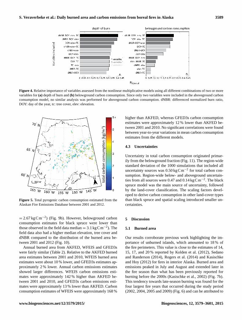
To assess the importance of the individual variables, we
compared all possible multiplicative regression models with
two or more input variables for the depth of burn and below-
ground carbon consumption (Fig. 4). For the depth of burn
model, elevation was the most important explanatory vari-
able. For example, 2-variables models combining elevation
with day of burning and dNBR performed better than the
3-variables models that excluded elevation. For the below-
ground carbon consumption model, the day of burning vari-
able was crucial. All 2-variables models combining day of
burning with any of the other variables performed better than
the 3-variables models that excluded day of burning.
4.2 Daily burned area and carbon emissions,
2001–2012
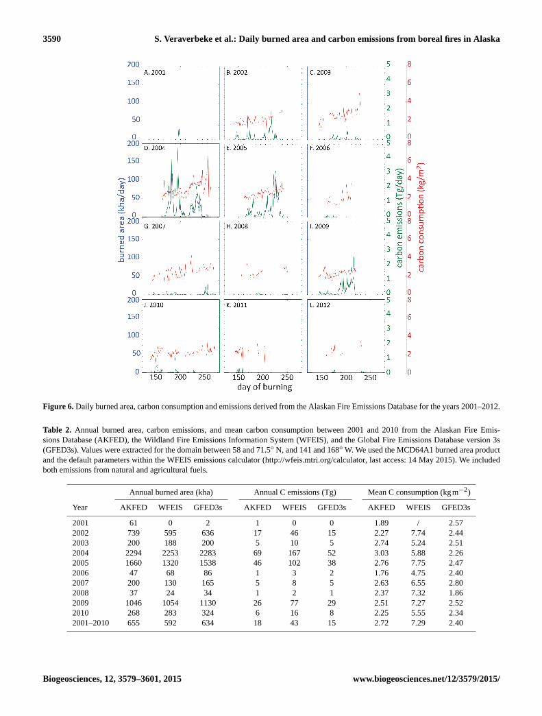
The total carbon emissions and uncertainty for the spatiotem-
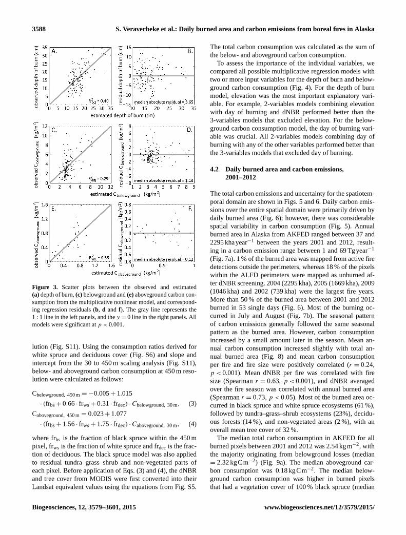
poral domain are shown in Figs. 5 and 6. Daily carbon emis-
sions over the entire spatial domain were primarily driven by
daily burned area (Fig. 6); however, there was considerable
spatial variability in carbon consumption (Fig. 5). Annual
burned area in Alaska from AKFED ranged between 37 and
2295 khayear−1 between the years 2001 and 2012, result-
ing in a carbon emission range between 1 and 69 Tgyear−1
(Fig. 7a). 1 % of the burned area was mapped from active fire
detections outside the perimeters, whereas 18 % of the pixels
within the ALFD perimeters were mapped as unburned af-
ter dNBR screening. 2004 (2295 kha), 2005 (1669 kha), 2009
(1046 kha) and 2002 (739 kha) were the largest fire years.
More than 50 % of the burned area between 2001 and 2012
burned in 53 single days (Fig. 6). Most of the burning oc-
curred in July and August (Fig. 7b). The seasonal pattern
of carbon emissions generally followed the same seasonal
pattern as the burned area. However, carbon consumption
increased by a small amount later in the season. Mean an-
nual carbon consumption increased slightly with total an-
nual burned area (Fig. 8) and mean carbon consumption
per fire and fire size were positively correlated (r = 0.24,
p < 0.001). Mean dNBR per fire was correlated with fire
size (Spearman r = 0.63, p < 0.001), and dNBR averaged
over the fire season was correlated with annual burned area
(Spearman r = 0.73, p < 0.05). Most of the burned area oc-
curred in black spruce and white spruce ecosystems (61 %),
followed by tundra–grass–shrub ecosystems (23%), decidu-
ous forests (14 %), and non-vegetated areas (2 %), with an
overall mean tree cover of 32 %.
The median total carbon consumption in AKFED for all
burned pixels between 2001 and 2012 was 2.54 kgm−2, with
the majority originating from belowground losses (median
= 2.32 kgCm−2) (Fig. 9a). The median aboveground car-
bon consumption was 0.18 kgCm−2. The median below-
ground carbon consumption was higher in burned pixels
that had a vegetation cover of 100 % black spruce (median
Biogeosciences, 12, 3579–3601, 2015 www.biogeosciences.net/12/3579/2015/
S. Veraverbeke et al.: Daily burned area and carbon emissions from boreal fires in Alaska 3589
Figure 4. Relative importance of variables assessed from the nonlinear multiplicative models using all different combinations of two or more
variables for (a) depth of burn and (b) belowground carbon consumption. Since only two variables were included in the aboveground carbon
consumption model, no similar analysis was performed for aboveground carbon consumption. dNBR: differenced normalized burn ratio,
DOY: day of the year, tc: tree cover, elev: elevation.
Figure 5. Total pyrogenic carbon consumption estimated from the
Alaskan Fire Emissions Database between 2001 and 2012.
= 2.67 kgCm−2) (Fig. 9b). However, belowground carbon
consumption estimates for black spruce were lower than
those observed in the field data median= 3.1 kgCm−2). The
field data also had a higher median elevation, tree cover and
dNBR compared to the distribution of the burned area be-
tween 2001 and 2012 (Fig. 10).
Annual burned area from AKFED, WFEIS and GFED3s
were fairly similar (Table 2). Relative to the AKFED burned
area estimates between 2001 and 2010, WFEIS burned area
estimates were about 10 % lower, and GFED3s estimates ap-
proximately 2 % lower. Annual carbon emissions estimates
showed larger differences. WFEIS carbon emissions esti-
mates were approximately 142 % higher than AKFED be-
tween 2001 and 2010, and GFED3s carbon emissions esti-
mates were approximately 13 % lower than AKFED. Carbon
consumption estimates of WFEIS were approximately 168 %
higher than AKFED, whereas GFED3s carbon consumption
estimates were approximately 12 % lower than AKFED be-
tween 2001 and 2010. No significant correlations were found
between year-to-year variations in mean carbon consumption
estimates from the different models.
4.3 Uncertainties
Uncertainty in total carbon consumption originated primar-
ily from the belowground fraction (Fig. 11). The region-wide
standard deviation of the 1000 simulations that included all
uncertainty sources was 0.50 kgCm−2 for total carbon con-
sumption. Region-wide below- and aboveground uncertain-
ties from all sources were 0.47 and 0.14 kgCm−2. The black
spruce model was the main source of uncertainty, followed
by the land-cover classification. The scaling factors devel-
oped to derive carbon consumption in other land-cover types
than black spruce and spatial scaling introduced smaller un-
certainties.
5 Discussion
5.1 Burned area
Our results corroborate previous work highlighting the im-
portance of unburned islands, which amounted to 18 % of
the fire perimeters. This value is close to the estimates of 14,
15, 17, and 20 % reported by Kolden et al. (2012), Sedano
and Randerson (2014), Rogers et al. (2014) and Kasischke
and Hoy (2012) for fires in interior Alaska. Burned area and
emissions peaked in July and August and extended later in
the fire season than what has been previously reported for
burning before the 2000s (Kasischke et al., 2002) (Fig. 7b).
This tendency towards late-season burning was found for the
four largest fire years that occurred during the study period
(2002, 2004, 2005 and 2009) (Fig. 6) and can be attributed to
www.biogeosciences.net/12/3579/2015/ Biogeosciences, 12, 3579–3601, 2015
3590 S. Veraverbeke et al.: Daily burned area and carbon emissions from boreal fires in Alaska
Figure 6. Daily burned area, carbon consumption and emissions derived from the Alaskan Fire Emissions Database for the years 2001–2012.
Table 2. Annual burned area, carbon emissions, and mean carbon consumption between 2001 and 2010 from the Alaskan Fire Emis-
sions Database (AKFED), the Wildland Fire Emissions Information System (WFEIS), and the Global Fire Emissions Database version 3s
(GFED3s). Values were extracted for the domain between 58 and 71.5◦ N, and 141 and 168◦W. We used the MCD64A1 burned area product
and the default parameters within the WFEIS emissions calculator (http://wfeis.mtri.org/calculator, last access: 14 May 2015). We included
both emissions from natural and agricultural fuels.
Annual burned area (kha) Annual C emissions (Tg) Mean C consumption (kgm−2)
Year AKFED WFEIS GFED3s AKFED WFEIS GFED3s AKFED WFEIS GFED3s
2001 61 0 2 1 0 0 1.89 / 2.57
2002 739 595 636 17 46 15 2.27 7.74 2.44
2003 200 188 200 5 10 5 2.74 5.24 2.51
2004 2294 2253 2283 69 167 52 3.03 5.88 2.26
2005 1660 1320 1538 46 102 38 2.76 7.75 2.47
2006 47 68 86 1 3 2 1.76 4.75 2.40
2007 200 130 165 5 8 5 2.63 6.55 2.80
2008 37 24 34 1 2 1 2.37 7.32 1.86
2009 1046 1054 1130 26 77 29 2.51 7.27 2.52
2010 268 283 324 6 16 8 2.25 5.55 2.34
2001–2010 655 592 634 18 43 15 2.72 7.29 2.40
Biogeosciences, 12, 3579–3601, 2015 www.biogeosciences.net/12/3579/2015/
S. Veraverbeke et al.: Daily burned area and carbon emissions from boreal fires in Alaska 3591
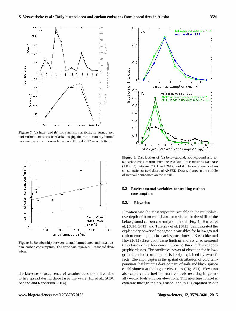
Figure 7. (a) Inter- and (b) intra-annual variability in burned area
and carbon emissions in Alaska. In (b), the mean monthly burned
area and carbon emissions between 2001 and 2012 were plotted.
Figure 8. Relationship between annual burned area and mean an-
nual carbon consumption. The error bars represent 1 standard devi-
ation.
the late-season occurrence of weather conditions favorable
to fire spread during these large fire years (Hu et al., 2010;
Sedano and Randerson, 2014).
Figure 9. Distribution of (a) belowground, aboveground and to-
tal carbon consumption from the Alaskan Fire Emissions Database
(AKFED) between 2001 and 2012, and (b) belowground carbon
consumption of field data and AKFED. Data is plotted in the middle
of interval boundaries on the x axis.
5.2 Environmental variables controlling carbon
consumption
5.2.1 Elevation
Elevation was the most important variable in the multiplica-
tive depth of burn model and contributed to the skill of the
belowground carbon consumption model (Fig. 4). Barrett et
al. (2010, 2011) and Turetsky et al. (2011) demonstrated the
explanatory power of topographic variables for belowground
carbon consumption in black spruce forests. Kasischke and
Hoy (2012) drew upon these findings and assigned seasonal
trajectories of carbon consumption to three different topo-
graphic classes. The predictive power of elevation for below-
ground carbon consumption is likely explained by two ef-
fects. Elevation captures the spatial distribution of cold tem-
peratures that limit the development of soils and black spruce
establishment at the higher elevations (Fig. S7a). Elevation
also captures the fuel moisture controls resulting in gener-
ally wetter fuels at lower elevations. This moisture control is
dynamic through the fire season, and this is captured in our
www.biogeosciences.net/12/3579/2015/ Biogeosciences, 12, 3579–3601, 2015
3592 S. Veraverbeke et al.: Daily burned area and carbon emissions from boreal fires in Alaska
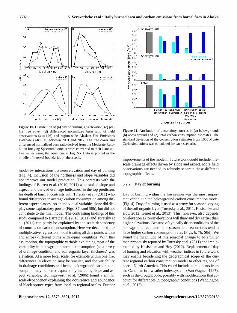
Figure 10. Distribution of (a) day of burning, (b) elevation, (c) pre-
fire tree cover, (d) differenced normalized burn ratio of field
observations (n= 126) and region-wide Alaskan Fire Emissions
Database (AKFED) between 2001 and 2012. The tree cover and
differenced normalized burn ratio derived from the Moderate Reso-
lution Imaging Spectroradiometer were converted to their Landsat-
like values using the equations in Fig. S5. Data is plotted in the
middle of interval boundaries on the x axis.
model by interactions between elevation and day of burning
(Fig. 4). Inclusion of the northness and slope variables did
not improve our model prediction. This contrasts with the
findings of Barrett et al. (2010, 2011) who ranked slope and
aspect, and derived drainage indicators, in the top predictors
for depth of burn. It contrasts with Turetsky et al. (2011) who
found differences in average carbon consumption among dif-
ferent aspect classes. As an individual variable, slope did dis-
play some explanatory power (Figs. S7b and S8b), but did not
contribute to the final model. The contrasting findings of this
study compared to Barrett et al. (2010, 2011) and Turetsky et
al. (2011) can partly be explained by the scale-dependency
of controls on carbon consumption. Here we developed our
mulitplicative regression model treating all data points within
and across different burns with equal weighting. With this
assumption, the topographic variable explaining most of the
variability in belowground carbon consumption (as a proxy
of drainage condition and soil organic layer thickness) was
elevation. At a more local scale, for example within one fire,
differences in elevation may be smaller, and the variability
in drainage conditions and hence belowground carbon con-
sumption may be better captured by including slope and as-
pect variables. Hollingsworth et al. (2006) found a similar
scale-dependency explaining the occurrence and abundance
of black spruce types from local to regional scales. Further
Figure 11. Attribution of uncertainty sources in (a) belowground,
(b) aboveground and (c) total carbon consumption estimates. The
standard deviation of the consumption estimates from 1000 Monte
Carlo simulations was calculated for each scenario.
improvements of the model in future work could include fine-
scale drainage effects driven by slope and aspect. More field
observations are needed to robustly separate these different
topographic effects.
5.2.2 Day of burning
Day of burning within the fire season was the most impor-
tant variable in the belowground carbon consumption model
(Fig. 4). Day of burning is used as a proxy for seasonal drying
of the soil organic layer (Turetsky et al., 2011; Kasischke and
Hoy, 2012; Genet et al., 2013). This, however, also depends
on elevation as lower elevations will thaw and dry earlier than
higher elevations. Because of typically drier conditions of the
belowground fuel later in the season, late-season fires tend to
have higher carbon consumption rates (Figs. 6, 7b, S8d). We
found the magnitude of this seasonal change to be smaller
than previously reported by Turetsky et al. (2011) and imple-
mented by Kasischke and Hoy (2012). Replacement of day
of burning and elevation with weather indices in future work
may enable broadening the geographical scope of the cur-
rent regional carbon consumption model to other regions of
boreal North America. This could include components from
the Canadian fire-weather index system, (Van Wagner, 1987),
such as the drought code, possibly with modifications that ac-
count for differences in topographic conditions (Waddington
et al., 2012).
Biogeosciences, 12, 3579–3601, 2015 www.biogeosciences.net/12/3579/2015/
S. Veraverbeke et al.: Daily burned area and carbon emissions from boreal fires in Alaska 3593
5.2.3 Burn severity (dNBR)
The utility of dNBR in the boreal region has been sub-
ject to much debate (French et al., 2008). We found a rel-
atively strong relationship between dNBR and aboveground
carbon consumption (Fig. S9a). The criticism on the use of
dNBR, however, has focused on its ability to predict be-
lowground carbon consumption (French et al., 2008; Hoy et
al., 2008). Some authors have found relatively strong cor-
relations between field measures of belowground consump-
tion and dNBR (Hudak et al., 2007; Verbyla and Lord, 2008;
Rogers et al., 2014). Barrett et al. (2011) also ranked dNBR
in the top third of predictors of a set of 35 spectral and non-
spectral environmental variables. French et al. (2008) con-
cluded that the use satellite-based assessments of burn sever-
ity, including dNBR, in the boreal region “need to be used
judiciously and assessed for appropriateness based on the
users’ needs”. We found here that, as an individual variable,
dNBR was the top predictor of depth of burn in black spruce
forests together with pre-fire tree cover (Fig. S7). We also
found that including dNBR in the model resulted in addi-
tional explained variance compared to models that excluded
dNBR (Fig. 4). In addition, dNBR and tree cover were found
to vary at a finer spatial scale than elevation or day of burn-
ing (Fig. S12), and their inclusion in the model as such likely
improved the representation of the spatial heterogeneity in
carbon consumption. Previous work has included variables
as fire size and total annual burned area as predictor variables
in pyrogenic carbon consumption model (Barrett et al., 2010,
2011; Kasischke and Hoy, 2012; Genet et al., 2013). The
significant positive correlations between fire size and mean
dNBR (Spearman r = 0.63, p < 0.001) and annual burned
area and mean dNBR (Spearman r = 0.73, p < 0.05) pro-
vided additional support for the inclusion of the dNBR as a
synergistic variable in our carbon emissions modeling frame-
work. The advantage of using dNBR for capturing this vari-
ability compared to fire size or total annual burned area is
that it enables independent assessment of carbon losses at
each pixel. It also provides a more mechanistic underpinning
for exploring relationships that emerge at the fire-wide or re-
gional level, including the relationships described above be-
tween fire size and carbon consumption.
The relatively high correlations between depth of burn,
and dNBR and tree cover suggest that crown fires in high
density black spruce plots may contribute to deeper burning
into the ground layer. Burning into the ground layer is pri-
marily controlled by fuel moisture in the ground layer, which
was modeled here as a function of elevation and day of burn-
ing. For a given moisture condition of the ground layer, de-
termined by elevation and fire seasonality, dNBR thus adds
complementary power for the prediction of the consumption
of the ground layer. This may explain why the dNBR has
performed well in studies that focused on one single fire in
which the elevation and day of burning were relatively con-
stant (Hudak et al., 2007; Verbyla and Lord, 2008; Rogers
et al., 2014). When used over large areas and over a range
of burn conditions, our results suggest that the synergistic
use of the dNBR with other environmental variables is es-
sential. This finding agrees with Barrett et al. (2010, 2011),
who found that a combination of spectral and non-spectral
data optimized depth of burn prediction in black spruce for-
est.
5.2.4 Tree cover
This is the first study to evaluate the potential of tree cover as
a predictor of carbon consumption in black spruce forests.
The relatively strong relationship between tree cover and
aboveground carbon consumption is intuitive as black spruce
forest mostly experience stand-replacing crown fires and tree
cover is directly related to the amount of available biomass
and the probability that the crown fire can spread from tree to
tree. Its utility for predicting belowground carbon consump-
tion is less obvious and more indirect. We included tree cover
in our analysis since we hypothesized that it would be a good
proxy of stand age and site productivity which directly re-
lates to drainage conditions, and thickness and density of
the organic layer (Kasischke and Johnstone, 2005; Beck et
al., 2011b; Rogers et al., 2013). High intensity crown fires
in dense black spruce plots also may provide more radiant
heating (and drying) of the ground layer, enabling deeper
burns. Significant relationships between tree cover and depth
of burn (Fig. S7e), and tree cover and belowground carbon
consumption (Fig. S8e) provided support for these mecha-
nisms.
5.3 Comparison with previous work on spatially
explicit carbon consumption modeling for boreal
fires in Alaska
Here we compare our estimates of carbon emissions and car-
bon consumption with those from Kasischke and Hoy (2012)
and Tan et al. (2007) for the subset of years reported in
these publications. For 2004, we estimated a total emission
of 69 Tg pyrogenic carbon in our domain. This estimate is
slightly higher than the estimate of 65 Tg C from Kasischke
and Hoy (2012), and both our estimate and the estimate of
Kasischke and Hoy (2012) are substantially lower than the
estimate of 81 Tg C reported by Tan et al. (2007). AKFED
and Kasischke and Hoy (2012) also yielded similar estimates
for the small fire years 2006 and 2008. The two models had
diverging predictions for 2007, however, with the domain-
wide AKFED estimate of 5 Tg C substantially higher than
the estimate of approximately 2 Tg C by Kasischke and Hoy
(2012). The discrepancy can be explained in part by the in-
clusion of the large Anaktuvuk tundra fire within the AKFED
domain, whereas the analysis by Kasischke and Hoy (2012)
only considered fires in the boreal interior of Alaska.
We also found close agreement in the regional burned
area estimates from AKFED and Kasischke and Hoy (2012).
www.biogeosciences.net/12/3579/2015/ Biogeosciences, 12, 3579–3601, 2015
3594 S. Veraverbeke et al.: Daily burned area and carbon emissions from boreal fires in Alaska
For example for the large fire years of 2004 and 2005, AK-
FED estimated a burned area of 2295 and 1669 kha, com-
pared to estimates of 2178 and 1492 kha from Kasischke and
Hoy (2012). The close agreement between AKFED and the
Kasischke and Hoy (2012) for burned area is be expected
since they use similar input data. Both approaches, for ex-
ample, use fire perimeter data in combination with spectral
screening to estimate burned area.
Carbon consumption estimates for the large fire year 2004
were fairly similar among estimates from Kasischke and
Hoy (2012) (3.0 kg Cm−2), Tan et al., (2007) (3.1 kgCm−2)
and AKFED (3.0 kgCm−2). Both AKFED and Kasischke
and Hoy (2012) estimated lower consumption values for the
small fire years 2006, 2007 and 2008, although the esti-
mates from Kasischke and Hoy (2012) (1.5–1.9 kgCm−2)
were lower than AKFED (1.8–2.6 kgCm−2) Kasischke and
Hoy (2012) used observations derived conceptually from ob-
servations reported by Turetsky et al. (2011) that indicated
that ground layer consumption increased with fire season
progression. We derived a similar relationship with day of
burning using a different set of data and statistical approach
(Figs. 6 and 7b). We found that, in our application, the non-
linear multiplicative regression model outperformed other
statistical methods for extrapolating carbon consumption in
space and time (Fig. S4). Our depth of burn model achieved
a R2adjusted of 0.40, which is similar to the explained vari-
ance of 50 % in estimating relative loss of the organic layer
by Genet et al. (2013). An important difference between
these estimates is that Genet et al. (2013) aggregated multiple
field locations within the same fire by topographic class. We
aimed at preserving the within-fire variability by using spa-
tially varying dNBR and tree cover observations as model
drivers (Fig. S11). The representation of these higher resolu-
tion dynamics in fuel and consumption variability may partly
explain our slightly lower model performance.
We further compared AKFED burned area, carbon con-
sumption and emissions estimates with estimates from
two larger-scale models, WFEIS and GFED3s. French et
al. (2011) compared 11 different estimates of burned area
and carbon emissions for the 2004 Boundary fire. Fire-wide
burned area estimates ranged between 185 kha and 218 kha,
and carbon emissions between 2.8 and 13.3 Tg. The burned
area and carbon emissions estimates from AKFED were
205 kha and 6.0 Tg C – similar to the multi-model mean. Our
carbon emissions estimate for this fire was slightly higher
than estimates from WFEIS (5.3–5.7 Tg C) and field assess-
ment by E. Kasischke (4.8 Tg C) in French et al. (2011). The
difference between AKFED and the latter estimate is at least
partly explained by differences in burned area, with the field
assessment of E. Kasischke in French et al. (2011) report-
ing a total that was about 10 % lower than AKFED. GFED3
reported 207 ha and 4.64 Tg C emissions for this fire.
Decadal-scale comparison between AKFED, WFEIS and
GFED3s demonstrated fairly similar burned area estimates,
although AKFED and GFED3s were slightly higher than
WFEIS (Table 2). The similarity between the burned area
from AKFED, WFEIS, and GFED3s is not surprising since
they operate with similar algorithms. All algorithms look
at changes in a spectral index derived from MODIS sur-
face reflectance imagery to map burned area. Burned area
in GFED3s and WFEIS were from the MCD64A1 product
(Giglio et al., 2009), complemented with small fire contri-
butions outside the MCD64A1 burned area detections for
GFED3s (Randerson et al., 2012). AKFED used active fire
detections that occurred outside the fire perimeters to include
contributions from small fires. The contribution from small
fires that were included in GFED3s and AKFED may explain
the slightly higher burned area estimates than in WFEIS.
Carbon consumption was not correlated between differ-
ent models (Table 2). In addition, carbon consumption was
slightly lower in GFED3s compared to AKFED, and sig-
nificantly higher in WFEIS compared to AKFED. This sug-
gests that GFED3s slightly underestimates carbon consump-
tion from boreal fires, although the difference in mean car-
bon consumption between AKFED and GFED3s is with
the range of the region-wide mean uncertainty estimate of
0.50 kgCm−2 (Fig. 11). The comparison also indicates that
region-wide WFEIS estimates are several fold higher than
those from AKFED, GFED3s, or Kasischke and Hoy (2012).
The high levels of carbon consumption in WFEIS for Alaska
are consistent with the study of Billmire et al. (2014) that
showed for the contiguous US WFEIS estimates were about
double of GFED3 estimates. Differences in the carbon emis-
sions estimates between approaches result from differences
in the methods and input data to quantify burned area, fuel
type, and carbon consumption. Billmire et al. (2014) found
that the difference between WFEIS and GFED3 carbon emis-
sion estimates in the contiguous US was primarily driven by
the higher fuel loads assigned in WFEIS. This effect may
also explain the discrepancy in Alaska, and further effort is
needed to compare the different modeling approaches. These
findings also highlight the need for synthesis and intercom-
parisons of the different data inputs required for emission
modeling, including fuel load, combustion completeness,
and emission factors. Such efforts are ongoing (van Leeuwen
and van der Werf, 2011; van Leeuwen et al., 2014); van
Leeuwen et al. (2013) for example assessed the impact of
different sets of emission factors on CO mixing ratios. One
constraint with large-scale models is that their coarse spatial
resolution does not allow direct comparison with field mea-
surements. This gap may be filled by regional models like
AKFED that are calibrated with field data at a higher spatial
resolution and can be scaled to a coarser resolution.
5.4 Uncertainties
The domain-wide mean uncertainty for carbon consumption
was slightly lower than 20 % of the mean, and similar to
fire-wide uncertainty reported by Rogers et al. (2014). Our
approach integrated observed and best-guess uncertainty es-
Biogeosciences, 12, 3579–3601, 2015 www.biogeosciences.net/12/3579/2015/
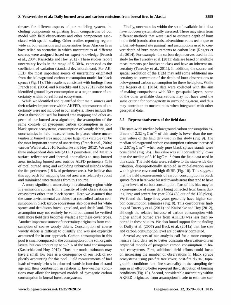
S. Veraverbeke et al.: Daily burned area and carbon emissions from boreal fires in Alaska 3595
timates for different aspects of our modeling system, in-
cluding components originating from comparisons of our
model with field observations and other components asso-
ciated with spatial scaling. Other studies reporting region-
wide carbon emissions and uncertainties from Alaskan fires
have relied on scenarios in which uncertainties of different
sources were assigned based on expert knowledge (French
et al., 2004; Kasischke and Hoy, 2012). These studies report
uncertainty levels in the range of 5–30 %, expressed as the
coefficient of variation (standard deviation/mean). For AK-
FED, the most important source of uncertainty originated
from the belowground carbon consumption model for black
spruce (Fig. 11). This results is consistent with findings from
French et al. (2004) and Kasischke and Hoy (2012) who both
identified ground layer consumption as a major source of un-
certainty within boreal forest ecosystems.
While we identified and quantified four main sources and
their relative importance within AKFED, other sources of un-
certainty were not included in our analysis. These include the
dNBR threshold used for burned area mapping and other as-
pects of our burned area algorithm, the assumption of the
same controls on pyrogenic carbon consumption in non-
black spruce ecosystems, consumption of woody debris, and
uncertainties in field measurements. In places where uncer-
tainties in burned area mapping are large, this variable can be
the most important source of uncertainty (French et al., 2004;
van der Werf et al., 2010; Kasischke and Hoy, 2012). We used
three independent data sets (ALFD perimeters, and MODIS
surface reflectance and thermal anomalies) to map burned
area, including burned area outside ALFD perimeters (1 %
of total burned area) and excluding unburned islands within
the fire perimeters (18 % of perimeter area). We believe that
this approach for mapping burned area was relatively robust
and minimized uncertainties from this source.
A more significant uncertainty in estimating region-wide
fire emissions comes from a paucity of field observations in
ecosystems other than black spruce. Here we assumed that
the same environmental variables that controlled carbon con-
sumption in black spruce ecosystems also operated for white
spruce and deciduous forest, grassland, and shrub land. This
assumption may not entirely be valid but cannot be verified
until more field data becomes available for these cover types.
Another important source of uncertainty originates from con-
sumption of coarse woody debris. Consumption of coarse
woody debris is difficult to quantify and was not explicitly
accounted for in our approach. Carbon consumption in this
pool is small compared to the consumption of the soil organic
layers, but can amount up to 5–7 % of the total consumption
(Kasischke and Hoy, 2012). Thus, our model estimates may
have a small low bias as a consequence of our lack of ex-
plicitly accounting for this pool. Field measurements of fuel
loads of woody debris in unburned stands in function of stand
age and their combustion in relation to fire-weather condi-
tions may allow for improved models of pyrogenic carbon
consumption in boreal forest ecosystems.
Finally, uncertainties within the set of available field data
have not been systematically assessed. These may stem from
different methods that were used to estimate depth of burn
in the field (combustion rods, adventitious roots technique or
unburned–burned site pairing) and assumptions used to con-
vert depth of burn measurements to carbon loss (Rogers et
al., 2014). For example, the carbon-depth curves used in this
study for the Turetsky et al. (2011) data are based on multiple
measurements per landscape class and have an inherent un-
certainty (Turetsky et al., 2011). In addition, the source and
spatial resolution of the DEM may add some additional un-
certainty to conversion of the depth of burn observations to
belowground carbon consumption for these field plots. While
the Rogers et al. (2014) data were collected with the aim
of making comparisons with 30 m geospatial layers, some
of the other available observations may not have used the
same criteria for homogeneity in surrounding areas, and thus
may contribute to uncertainties when integrated with other
geospatial data.
5.5 Representativeness of the field data
The state-wide median belowground carbon consumption es-
timate of 2.32 kgCm−2 of this study is lower than the me-
dian values of the field data used in this study (Fig. 9). The
median belowground carbon consumption estimate increased
to 2.67 kgCm−2 when only pure black spruce stands were
considered (Fig. 9b). This value was still considerably lower
than the median of 3.10 kgCm−2 from the field data used in
this study. The field data were, relative to the state-wide dis-
tribution, disproportionally sampled in mid-elevation areas
with high tree cover and high dNBR (Fig. 10). This suggests
that the field measurements of carbon consumption in black
spruce forest here were biased towards areas that tend to have
higher levels of carbon consumption. Part of this bias may be
a consequence of many data being collected from burns dur-
ing large and severe fire year 2004 (85 out of the 126 plots).
We found that large fires years generally have higher car-
bon consumption estimates (Fig. 8). This corroborates find-
ings of Turetsky et al. (2011) and Kasischke and Hoy (2012),
although the relative increase of carbon consumption with
higher annual burned area from AKFED was less than re-
ported in these studies. We also found support for the finding
of Duffy et al. (2007) and Beck et al. (2011a) that fire size
and carbon consumption level are positively correlated.
Several aspects of our analysis call for a more compre-
hensive field data set to better constrain observation-driven
empirical models of pyrogenic carbon consumption in bo-
real ecosystems. First, additional field efforts could focus
on increasing the number of observations in black spruce
ecosystems using pre-fire tree cover, post-fire dNBR, topo-
graphic conditions, and fire seasonality in the sampling de-
sign in an effort to better represent the distribution of burning
conditions (Fig. 10). Second, considerable uncertainty within
AKFED originated from assumptions made to estimate car-
www.biogeosciences.net/12/3579/2015/ Biogeosciences, 12, 3579–3601, 2015
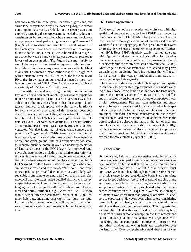
3596 S. Veraverbeke et al.: Daily burned area and carbon emissions from boreal fires in Alaska
bon consumption in white spruce, deciduous, grassland, and
shrub land ecosystems. Very little data on pyrogenic carbon
consumption is currently available for these ecosystems and
explicitly targeting these ecosystems is needed to reduce un-
certainties in future work. For white spruce and deciduous
ecosystems we developed scaling factors using Consume 3.0
(Fig. S6). For grassland and shrub land ecosystems we used
the black spruce model because tree cover is one of our pre-
dictor variables and our model was calibrated for a range of
tree cover between 14 and 64 %. Lower tree cover resulted in
lower carbon consumption (Fig. 7e), and this may justify the
use of the model for non-treed ecosystems until consump-
tion data within these ecosystems becomes available. Mack
et al. (2011) estimated a mean carbon loss of 2.02 kgCm−2
with a standard error of 0.44 kgCm−2 for the Anaktuvuk
River fire. In comparison, our model estimated a mean car-
bon consumption of 2.56 kgCm−2 with a mean pixel-based
uncertainty of 0.54 kgCm−2 for this event.
Even with an abundance of high quality plot data along
key axes of environmental variability, regional extrapolation
requires accurate maps of land-cover. To date, the FCCS clas-
sification is the only classification that for example distin-
guishes between black spruce and white spruce in Alaska.
No formal accuracy assessment of this layer has been con-
ducted; however, we found that, at its native 30 m resolu-
tion, 60 out of the 126 black spruce plots from the field
data set (Sect. 2.2) were misclassified; 29 as white spruce,
14 as tundra–grass–shrub, 12 as deciduous, and 5 as non-
vegetated. We also found that of eight white spruce–aspen
plots from Rogers et al. (2014), seven were classified as
black spruce, and one as shrub-grass-tundra. The sample size
of the land-cover ground truth data available was too small
to robustly quantify potential over- or underrepresentation
of land-cover types in the FCCS layer. An improved land-
cover characterization, including quantitative uncertainty es-
timates, is thus essential for reducing region-wide uncertain-
ties. An underrepresentation of the black spruce cover in the
FCCS would result in lower state-wide average carbon con-
sumption estimates and vice versa. While some land-cover
types, such as spruce and deciduous cover, are likely well
separable from remote-sensing based on spectral and phe-
nological characteristics, more detailed distinctions, for ex-
ample between black and white spruce, may be more chal-
lenging but not impossible with the combined use of struc-
tural and optical attributes (e.g., Goetz et al., 2010). More
than a decade after the call from French et al. (2004) for
more field data, including ecosystems that burn less regu-
larly, more field measurements are still required to better con-
strain pyrogenic carbon consumption in boreal forest ecosys-
tems.
5.6 Future applications
Databases of burned area, severity and emissions with high
spatial and temporal resolution like AKFED are a necessity
to advance several related fields in biogeosciences. They al-
low for a more thorough evaluation of models used to relate
weather, fuels and topography to fire spread rates that were
originally derived using laboratory measurements (Rother-
mel, 1972; Beer, 1991). Spatially explicit burned area data
with high temporal resolution will also allow for quantita-
tive assessments of constraints on fire progression due to
fuel discontinuities and fire weather (Krawchuk et al., 2006).
Knowledge of these constraints on fire spread may prove
valuable when predicting future fire regimes that will result
from changes in fire weather, vegetation dynamics, and in-
herent landscape heterogeneity.
Fire emission databases with high temporal and spatial
resolution also may enable improvements in our understand-
ing of fire aerosol composition and decrease the large uncer-
tainties that currently exist in fire emission factors of differ-
ent gas species by enabling more accurate comparisons with
in situ measurements. Fire emissions estimates and atmo-
spheric transport models need to be convolved at high spa-
tial and temporal resolution to capture interactions between
emissions, transport, chemical transformation, and deposi-
tion of aerosol and trace gas species. In addition, fires in the
boreal region are episodic and most of the burned area and
emissions occur in a relatively short amount of time. High
resolution time series are therefore of paramount importance
to infer and forecast possible health effects in populated areas
exposed to smoke plumes (Hyer et al., 2007).
6 Conclusions
By integrating field and remote-sensing variables at multi-
ple scales, we developed a database of burned area and car-
bon emission by fire at 450 m spatial resolution and daily
temporal resolution for the state of Alaska between 2001
and 2012. We found that, although most of the fires burned
in black spruce forest, considerable burned area in white
spruce forest, deciduous forest, and grassland and shrub land
ecosystems contributed to lower region-wide carbon con-
sumption estimates. This partly explained why the median
carbon consumption of 2.54 kgCm−2 over the spatiotempo-
ral domain was lower than that typically observed in black
spruce ecosystems. However, even when solely considering
pure black spruce pixels, median carbon consumption was
still lower than most field observations. This suggests that
the available field data that were used in this study may have
a bias toward high carbon consumption. We thus recommend
caution in extrapolating these values over large areas with-
out taking into account spatial heterogeneity in tree cover
and other variables influencing fuels and combustion over
the landscape. More comprehensive field databases of car-
Biogeosciences, 12, 3579–3601, 2015 www.biogeosciences.net/12/3579/2015/
S. Veraverbeke et al.: Daily burned area and carbon emissions from boreal fires in Alaska 3597
bon consumption in black spruce and other ecosystems (e.g.,
white spruce, deciduous, and tundra ecosystems) are required
to better constrain region-wide carbon emissions and lower
uncertainties. Further improvements in land-cover character-
ization are also required to remove potential biases that may
originate from uncertainties in this layer.
Our carbon consumption model was driven by four envi-
ronmental variables: elevation, day of burning, differenced
normalized burn ratio (dNBR) and pre-fire tree cover. At the
regional level of our study, elevation controlled fuel moisture
conditions and soil organic layer thickness. Day of burning
within the fire season, in combination with elevation, was
used to estimate the seasonal thawing of the active layer and
subsequent moisture content of organic soil layers. dNBR
and tree cover explained additional model variance, and al-
lowed to capture fine-scale variability in carbon consump-
tion. While the use of dNBR as stand-alone indicator of be-
lowground carbon consumption by fire in boreal ecosystems
may have limitations, our model system benefited from its
use in synergy with other environmental variables. Higher
dNBR values were significantly related to deeper burning
in soil organic carbon layers. The observed relationships
between belowground carbon consumption, dNBR and tree
cover, suggest aboveground fuel consumption and heat re-
lease may influence the drying of surface fuels, and vice
versa, thus contributing to higher levels of carbon consump-
tion.
The Alaskan Fire Emissions Database (AKFED)
is publicly available from sites.google.com/a/uci.edu/
sander-veraverbeke/akfed. This data could further contribute
to the knowledge on spatiotemporal patterns, controls and
limits on fire progression, air pollution and exposure, and
aerosol composition of boreal fires.
The Supplement related to this article is available online
at doi:10.5194/bg-12-3579-2015-supplement.
Author contributions. S. Veraverbeke designed the study, per-
formed the analyses and wrote the manuscript with inputs from
B. M. Rogers and J. T. Randerson at all stages.
Acknowledgements. This work was funded by the National
Aeronautics and Space Administration Carbon in Arctic Reservoirs
Vulnerability Experiment (CARVE) and NNX11AF96G project.
We would like to thank the authors from the Boby et al. (2010)
and Turetsky et al. (2011) papers for making their field data
publicly available. We are grateful to several colleagues of the
University of California, Irvine for discussions on the work. We are
thankful to four reviewers, including E. Kasischke and E. Kane, for
constructive comments that considerably improved the discussions
version of this manuscript.
Edited by: A. Ito
References
Abatzoglou, J. T. and Kolden, C. A.: Relative importance of weather
and climate on wildfire growth in interior Alaska, Int. J. Wildland
Fire, 20, 479–486, doi:10.1071/WF10046, 2011.
Allen, J. L. and Sorbel, B.: Assessing the differenced Normalized
Burn Ratio’s ability to map burn severity in the boreal forest and
tundra ecosystems of Alaska’s national parks, Int. J. Wildland
Fire, 17, 463–475, doi:10.1071/WF08034, 2008.
Amiro, B. D., Todd, J. B., Wotton, B. M., Logan, K. A., Flannigan,
M. D., Stocks, B. J., Mason, J. A., Martell, D. L., and Hirsch,
K. G.: Direct carbon emissions from Canadian forest fires, 1959–
1999, Can. J. Forest Res., 31, 512–525, doi:10.1139/cjfr-31-3-
512, 2001.
Amiro, B. D., Cantin, A., Flannigan, M. D., and de Groot, W. J.:
Future emissions from Canadian boreal forest fires, Can. J. Forest
Res., 39, 383–395, doi:10.1139/X08-154, 2009.
Balshi, M. S., McGuire, A. D., Duffy, P., Flannigan, M., Walsh,
J., and Melillo, J.: Assessing the response of area burned
to changing climate in western boreal North America us-
ing a Multivariate Adaptive Regression Splines (MARS) ap-
proach, Glob. Change Biol., 15, 578–600, doi:10.1111/j.1365-
2486.2008.01679.x, 2009.
Barrett, K., Kasischke, E. S., McGuire, A. D., Turetsky, M. R.,
and Kane, E. S.: Modeling fire severity in black spruce
stands in the Alaskan boreal forest using spectral and non-
spectral geospatial data, Remote Sens. Environ., 114, 1494–
1503, doi:10.1016/j.rse.2010.02.001, 2010.
Barrett, K., McGuire, A. D., Hoy, E. E., and Kasischke, E. S.: Po-
tential shifts in dominant forest cover in interior Alaska driven
by variations in fire severity, Ecol. Appl., 21, 2380–2396, 2011.
Beck, P. S. A., Goetz, S. J., Mack, M. C., Alexander, H. D., Jin,
Y., Randerson, J. T., and Loranty, M. M.: The impacts and im-
plications of an intensifying fire regime on Alaskan boreal for-
est composition and albedo, Glob. Change Biol., 17, 2853–2866,
doi:10.1111/j.1365-2486.2011.02412.x, 2011a.
Beck, P. S. A., Juday, G. P., Alix, C., Barber, V. A., Winslow, S. E.,
Sousa, E. E., Heiser, P., Herriges, J. D., and Goetz, S. J.: Changes
in forest productivity across Alaska consistent with biome shift,
Ecol. Lett., 14, 373–9, doi:10.1111/j.1461-0248.2011.01598.x,
2011b.
Beer, T.: The interaction of wind and fire, Bound.-Lay. Meteorol.,
54, 287–308, 1991.
Billmire, M., French, N. H. F., and Mobley, K.: Comparison of
WFEISv0. 3 and GFED3 fire emissions models, available at:
http://wfeis.mtri.org/media/Docs/Comparison_of_WFEIS_and_
GFED_Fire_Emissions_Models_6-23-2014.pdf, last access:
5 June 2015, 2014.
Boby, L. A., Schuur, E. A. G., Mack, M. C., Verbyla, D., and
Johnstone, J. F.: Quantifying fire severity, carbon, and nitrogen
emissions in Alaska’s boreal forest, Ecol. Appl., 20, 1633–1647,
doi:10.1890/08-2295.1, 2010.
Bonan, G. B.: Environmental factors and ecological processes con-
trolling vegetation patterns in boreal forests, Landscape Ecol., 3,
111–130, doi:10.1007/BF00131174, 1989.
Bowman, D. M. J. S., Balch, J. K., Artaxo, P., Bond, W. J., Carlson,
J. M., Cochrane, M. A., D’Antonio, C. M., Defries, R. S., Doyle,
J. C., Harrison, S. P., Johnston, F. H., Keeley, J. E., Krawchuk,
M. A., Kull, C. A., Marston, J. B., Moritz, M. A., Prentice, I. C.,
Roos, C. I., Scott, A. C., Swetnam, T. W., van der Werf, G. R.,
www.biogeosciences.net/12/3579/2015/ Biogeosciences, 12, 3579–3601, 2015
3598 S. Veraverbeke et al.: Daily burned area and carbon emissions from boreal fires in Alaska
and Pyne, S. J.: Fire in the Earth system, Science, 324, 481–484,
doi:10.1126/science.1163886, 2009.
Chapin, F. S., Mcguire, A. D., Randerson, J., Pielke, R., Bal-
docchi, D., Hobbie, S. E., Roulet, N., Eugster, W., Kasischke,
E., Rastetter, E. B., Zimov, S. A., and Running, S. W.: Arc-
tic and boreal ecosystems of western North America as com-
ponents of the climate system, Glob. Change Biol., 6, 211–223,
doi:10.1046/j.1365-2486.2000.06022.x, 2000.
Cocke, A. E., Fulé, P. Z., and Crouse, J. E.: Comparison of
burn severity assessments using Differenced Normalized Burn
Ratio and ground data, Int. J. Wildland Fire, 14, 189–198,
doi:10.1071/WF04010, 2005.
Collins, M., Knutti, R., Arblaster, J., Dufresne, J.-L., Fichefet, T.,
Friedlingstein, P., Gao, X., Gutowski, W. J., Johns, T., Krinner,
G., Shongwe, M., Tebaldi, C., Weaver, A. J., and Wehner, M.:
Long-term climate change: projections, commitments and irre-
versibility, in: Climate Change 2013: The Physical Science Ba-
sis. Contributions of Working group I to the Fifth Assessment
Report of the Intergovernmental Panel on Climate Change, edited
by: Stocker, F. T., Qin, D., Plattner, G.-K., Tignor, M., Allen,
S. K., Boschung, J., Nauels, A., Xia, Y., Bex, V., and Midgley,
P. M., Cambridge University Press, Cambridge, United King-
dom, 1029–1136, 2013.
Cumming, S.: Forest type and wildfire in the Alberta boreal mixed-
wood: what do fires burn?, Ecol. Appl., 11, 97–110, 2001.
De Groot, W. J., Landry, R., Kurz, W. A., Anderson, K. R., Engle-
field, P., Fraser, R. H., Hall, R. J., Banfield, E., Raymond, D. A.,
Decker, V., Lynham, T. J., and Pritchard, J. M.: Estimating direct
carbon emissions from Canadian wildland fires, Int. J. Wildland
Fire, 16, 593–606, doi:10.1071/WF06150, 2007.
De Groot, W. J., Flannigan, M. D., and Cantin, A. S.: Climate
change impacts on future boreal fire regimes, Forest Ecol.
Manag., 294, 35–44, doi:10.1016/j.foreco.2012.09.027, 2013.
De Santis, A. and Chuvieco, E.: Burn severity estimation
from remotely sensed data: performance of simulation vs.
empirical models, Remote Sens. Environ., 108, 422–435,
doi:10.1016/j.rse.2006.11.022, 2007.
Duffy, P. A., Epting, J., Graham, J. M., Rupp, T. S., and
McGuire, A. D.: Analysis of Alaskan burn severity patterns us-
ing remotely sensed data, Int. J. Wildland Fire, 16, 277–284,
doi:10.1071/WF06034, 2007.
Eidenshink, J., Schwind, B., Brewer, K., Zhu, Z., Quayle, B., and
Howard, S.: A project for monitoring trends in burn severity, Fire
ecology, 3, 3–21, 2007.
Epting, J., Verbyla, D., and Sorbel, B.: Evaluation of remotely
sensed indices for assessing burn severity in interior Alaska using
Landsat TM and ETM+, Remote Sens. Environ., 96, 328–339,
doi:10.1016/j.rse.2005.03.002, 2005.
Flanner, M. G., Zender, C. S., Randerson, J. T., and Rasch,
P. J.: Present-day climate forcing and response from
black carbon in snow, J. Geophys. Res., 112, D11202,
doi:10.1029/2006JD008003, 2007.
French, N. H. F., Kasischke, E. S., and Williams, D. G.: Vari-
ability in the emission of carbon-based trace gases from wild-
fire in the Alaskan boreal forest, J. Geophys. Res., 108, 8151,
doi:10.1029/2001JD000480, 2003.
French, N. H. F., Goovaerts, P., and Kasischke, E. S.: Uncertainty in
estimating carbon emissions from boreal forest fires, J. Geophys.
Res., 109, D14S08, doi:10.1029/2003JD003635, 2004.
French, N. H. F., Kasischke, E. S., Hall, R. J., Murphy, K. A., Ver-
byla, D. L., Hoy, E. E., and Allen, J. L.: Using Landsat data to
assess fire and burn severity in the North American boreal for-
est region: an overview and summary of results, Int. J. Wildland
Fire, 17, 443–462, doi:10.1071/WF08007, 2008.
French, N. H. F., de Groot, W. J., Jenkins, L. K., Rogers, B. M., Al-
varado, E., Amiro, B., de Jong, B., Goetz, S., Hoy, E., Hyer, E.,
Keane, R., Law, B. E., McKenzie, D., McNulty, S. G., Ottmar,
R., Pérez-Salicrup, D. R., Randerson, J., Robertson, K. M., and
Turetsky, M.: Model comparisons for estimating carbon emis-
sions from North American wildland fire, J. Geophys. Res., 116,
G00K05, doi:10.1029/2010JG001469, 2011.
French, N. H. F., McKenzie, D., Erickson, T., Koziol, B., Billmire,
M., Endsley, K. A., Yager Scheinerman, N. K., Jenkins, L.,
Miller, M. E., Ottmar, R., and Prichard, S.: Modeling Regional-
Scale Wildland Fire Emissions with the Wildland Fire Emissions
Information System∗, Earth Interact., 18, 1–26, doi:10.1175/EI-
D-14-0002.1, 2014.
Genet, H., McGuire, A. D., Barrett, K., Breen, A., Euskirchen, E. S.,
Johnstone, J. F., Kasischke, E. S., Melvin, A. M., Bennett, A.,
Mack, M. C., Rupp, T. S., Schuur, A. E. G., Turetsky, M. R., and
Yuan, F.: Modeling the effects of fire severity and climate warm-
ing on active layer thickness and soil carbon storage of black
spruce forests across the landscape in interior Alaska, Environ.
Res. Lett., 8, 045016, doi:10.1088/1748-9326/8/4/045016, 2013.
Giglio, L., Descloitres, J., Justice, C. O., and Kaufman, Y. J.:
An enhanced contextual fire detection algorithm for MODIS,
Remote Sens. Environ., 87, 273–282, doi:10.1016/S0034-
4257(03)00184-6, 2003.
Giglio, L., Csiszar, I., and Justice, C. O.: Global distribu-
tion and seasonality of active fires as observed with the
terra and aqua Moderate Resolution Imaging Spectrora-
diometer (MODIS) sensors, J. Geophys. Res., 111, G02016,
doi:10.1029/2005JG000142, 2006.
Giglio, L., Loboda, T., Roy, D. P., Quayle, B., and Justice,
C. O.: An active-fire based burned area mapping algorithm
for the MODIS sensor, Remote Sens. Environ., 113, 408-420,
doi:10.1016/j.rse.2008.10.006, 2009.
Giglio, L., Randerson, J. T., and van der Werf, G. R.: Analy-
sis of daily, monthly, and annual burned area using the fourth-
generation global fire emissions database (GFED4), J. Geophys.
Res.-Biogeo., 118, 317–328, doi:10.1002/jgrg.20042, 2013.
Gillett, N. P., Weaver, A. J., Zwiers, F. W., and Flannigan, M. D.:
Detecting the effect of climate change on Canadian forest fires,
Geophys. Res. Lett., 31, L18211, doi:10.1029/2004GL020876,
2004.
Goetz, S. J., Sun, M., Baccini, A., and Beck, P. S. A.: Synergistic use
of spaceborne lidar and optical imagery for assessing forest dis-
turbance: an Alaska case study, J. Geophys. Res., 115, G00E07,
doi:10.1029/2008JG000898, 2010.
Hall, R. J., Freeburn, J. T., de Groot, W. J., Pritchard, J. M., Lyn-
ham, T. J., and Landry, R.: Remote sensing of burn severity: ex-
perience from western Canada boreal fires, Int. J. Wildland Fire,
17, 476–489, doi:10.1071/WF08013, 2008.
Hansen, M. C., DeFries, R. S., Townshend, J. R. G., Carroll, M.,
Dimiceli, C., and Sohlberg, R. A.: Global Percent Tree Cover at
a Spatial Resolution of 500 Meters: first Results of the MODIS
Vegetation Continuous Fields Algorithm, Earth Interact., 7, 1–
15, 2003.
Biogeosciences, 12, 3579–3601, 2015 www.biogeosciences.net/12/3579/2015/
S. Veraverbeke et al.: Daily burned area and carbon emissions from boreal fires in Alaska 3599
Héon, J., Arseneault, D. and Parisien, M.-A.: Resistance of the
boreal forest to high burn rates, P. Natl. Acad. Sci. USA, 111,
13888–13893, doi:10.1073/pnas.1409316111, 2014.
Hollingsworth, T. N., Walker, M. D., Chapin III, F. S., and Par-
sons, A. L.: Scale-dependent environmental controls over species
composition in Alaskan black spruce communities, Can. J. Forest
Res., 36, 1781–1796, doi:10.1139/x06-061, 2006.
Hoy, E. E., French, N. H. F., Turetsky, M. R., Trigg, S. N.,
and Kasischke, E. S.: Evaluating the potential of Landsat
TM/ETM+ imagery for assessing fire severity in Alaskan
black spruce forests, Int. J. Wildland Fire, 17, 500–514,
doi:10.1071/WF08107, 2008.
Hu, F. S., Higuera, P. E., Walsh, J. E., Chapman, W. L., Duffy, P. A.,
Brubaker, L. B., and Chipman, M. L.: Tundra burning in Alaska:
linkages to climatic change and sea ice retreat, J. Geophys. Res.,
115, G04002, doi:10.1029/2009JG001270, 2010.
Hudak, A. T., Morgan, P., Bobbitt, M. J., Smith, A. M. S., Lewis,
S. A., Lentile, L. B., Robichaud, P. R., Clark, J. T., and McKin-
ley, R. A.: The relationship of multispectral satellite imagery to
immediate fire effects, Fire Ecol., 3, 64–90, 2007.
Huete, A., Didan, K., Miura, T., Rodriguez, E., Gao, X., and Fer-
reira, L.: Overview of the radiometric and biophysical perfor-
mance of the MODIS vegetation indices, Remote Sens. Environ.,
83, 195–213, doi:10.1016/S0034-4257(02)00096-2, 2002.
Hyer, E. J., Kasischke, E. S., and Allen, D. J.: Effects of source tem-
poral resolution on transport simulations of boreal fire emissions,
J. Geophys. Res., 112, D01302, doi:10.1029/2006JD007234,
2007.
Jin, Y., Randerson, J. T., Goetz, S. J., Beck, P. S. A., Loranty, M. M.,
and Goulden, M. L.: The influence of burn severity on postfire
vegetation recovery and albedo change during early succession in
North American boreal forests, J. Geophys. Res., 117, G01036,
doi:10.1029/2011JG001886, 2012.
Jin, Y., Randerson, J. T., Faivre, N., Capps, S., Hall, A.,
and Goulden, M. L.: Contrasting controls on wildland fires
in Southern California during periods with and without
Santa Ana winds, J. Geophys. Res.-Biogeo., 119, 432–450,
doi:10.1002/2013JG002541, 2014.
Johnstone, J. F. and Kasischke, E. S.: Stand-level effects of soil
burn severity on postfire regeneration in a recently burned
black spruce forest, Can. J. Forest Res., 35, 2151–2163,
doi:10.1139/x05-087, 2005.
Johnstone, J. F., Hollingsworth, T. N., Chapin, F. S., and Mack,
M. C.: Changes in fire regime break the legacy lock on succes-
sional trajectories in Alaskan boreal forest, Glob. Change Biol.,
16, 1281–1295, doi:10.1111/j.1365-2486.2009.02051.x, 2010.
Jones, B. M., Kolden, C. A., Jandt, R., Abatzoglou, J. T., Urban,
F., and Arp, C. D.: Fire behavior, weather, and burn severity of
the 2007 Anaktuvuk River Tundra Fire, North Slope, Alaska,
Arct. Antarct. Alp. Res., 41, 309–316, doi:10.1657/1938-4246-
41.3.309, 2009.
Kajii, Y., Kato, S., Streets, D. G., Tsai, N. Y., Shvidenko, A., Nils-
son, S., McCallum, I., Minko, N. P., Abushenko, N., Altyntsev,
D., and Khodzer, T. V.: Boreal forest fires in Siberia in 1998: Es-
timation of area burned and emissions of pollutants by advanced
very high resolution radiometer satellite data, J. Geophys. Res.,
107, 4745, doi:10.1029/2001JD001078, 2002.
Kane, E. S., Valentine, D. W., Schuur, E. A., and Dutta, K.: Soil car-
bon stabilization along climate and stand productivity gradients
in black spruce forests of interior Alaska, Can. J. Forest Res., 35,
2118–2129, doi:10.1139/x05-093, 2005.
Kane, E. S., Kasischke, E. S., Valentine, D. W., Turetsky, M. R.,
and McGuire, A. D.: Topographic influences on wildfire con-
sumption of soil organic carbon in interior Alaska: implications
for black carbon accumulation, J. Geophys. Res., 112, G03017,
doi:10.1029/2007JG000458, 2007.
Kasischke, E. S. and Bruhwiler, L. P.: Emissions of carbon dioxide,
carbon monoxide, and methane from boreal forest fires in 1998,
J. Geophys. Res., 108, 8146, doi:10.1029/2001JD000461, 2002.
Kasischke, E. S. and Hoy, E. E.: Controls on carbon consumption
during Alaskan wildland fires, Glob. Change Biol., 18, 685–699,
doi:10.1111/j.1365-2486.2011.02573.x, 2012.
Kasischke, E. S. and Johnstone, J. F.: Variation in postfire or-
ganic layer thickness in a black spruce forest complex in interior
Alaska and its effects on soil temperature and moisture, Can. J.
Forest Res., 35, 2164–2177, doi:10.1139/x05-159, 2005.
Kasischke, E. S. and Turetsky, M. R.: Recent changes in the fire
regime across the North American boreal region – Spatial and
temporal patterns of burning across Canada and Alaska, Geo-
phys. Res. Lett., 33, L09703, doi:10.1029/2006GL025677, 2006.
Kasischke, E. S., French, N. H. F., Bourgeau-Chavez, L. L., and
Christensen, N. L.: Estimating release of carbon from 1990
and 1991 forest fires in Alaska, J. Geophys. Res., 100, 2941,
doi:10.1029/94JD02957, 1995.
Kasischke, E. S., Williams, D., and Barry, D.: Analysis of the pat-
terns of large fires in the boreal forest region of Alaska, Int. J.
Wildland Fire, 11, 131–144, doi:10.1071/WF02023, 2002.
Kasischke, E. S., Turetsky, M. R., Ottmar, R. D., French, N. H. F.,
Hoy, E. E., and Kane, E. S.: Evaluation of the composite burn
index for assessing fire severity in Alaskan black spruce forests,
Int. J. Wildland Fire, 17, 515–526, doi:10.1071/WF08002, 2008.
Kasischke, E. S., Verbyla, D. L., Rupp, T. S., McGuire, A. D., Mur-
phy, K. A., Jandt, R., Barnes, J. L., Hoy, E. E., Duffy, P. A., Calef,
M., and Turetsky, M. R.: Alaska’s changing fire regime – impli-
cations for the vulnerability of its boreal forests, Can. J. Forest
Res., 40, 1313–1324, doi:10.1139/X10-098, 2010.
Kasischke, E. S., Loboda, T., Giglio, L., French, N. H. F.,
Hoy, E. E., de Jong, B., and Riano, D.: Quantifying burned
area for North American forests: implications for direct re-
duction of carbon stocks, J. Geophys. Res., 116, G04003,
doi:10.1029/2011JG001707, 2011.
Keeley, J. E.: Fire intensity, fire severity and burn severity: a brief
review and suggested usage, Int. J. Wildland Fire, 18, 116–126,
doi:10.1071/WF07049, 2009.
Kelly, R., Chipman, M. L., Higuera, P. E., Stefanova, I., Brubaker,
L. B. and Hu, F. S.: Recent burning of boreal forests exceeds fire
regime limits of the past 10,000 years, P. Natl. Acad. Sci. USA,
110, , 13055–13060, doi:10.1073/pnas.1305069110, 2013.
Key, C. H. and Benson, N. C.: Landscape assessment: ground mea-
sure of severity; the Composite Burn Index, and remote sens-
ing of severity, the Normalized Burn Index, in: FIREMON: Fire
Effects Monitoring and Inventory System, edited by: Lutes, D.,
Keane, R., Caratti, J., Key, C., Benson, N., Sutherland, S., and
Grangi, L., USDA Forest Service, Fort Collins, CO, 1–51, 2006.
Kolden, C. A. and Rogan, J.: Mapping Wildfire Burn Severity in the
Arctic Tundra from Downsampled MODIS Data, Arct. Antarct.
Alp. Res., 45, 64–76, doi:10.1657/1938-4246-45.1.64, 2013.
www.biogeosciences.net/12/3579/2015/ Biogeosciences, 12, 3579–3601, 2015
3600 S. Veraverbeke et al.: Daily burned area and carbon emissions from boreal fires in Alaska
Kolden, C. A., Lutz, J. A., Key, C. H., Kane, J. T., and van Wag-
tendonk, J. W.: Mapped vs. actual burned area within wildfire
perimeters: characterizing the unburned, Forest Ecol. Manag.,
286, 38–47, doi:10.1016/j.foreco.2012.08.020, 2012.
Krawchuk, M. A. and Cumming, S. G.: Effects of biotic feedback
and harvest management on boreal forest fire activity under cli-
mate change, Ecol. Appl., 21, 122–136, doi:10.1890/09-2004.1,
2011.
Krawchuk, M. A., Cumming, S. G., Flannigan, M. D., and Wein,
R. W.: Biotic and abiotic regulation of lightning fire initita-
tion in the mixedwood boreal forest, Ecology, 87, 458–468,
doi:10.1890/05-1021, 2006.
Lapina, K., Honrath, R. E., Owen, R. C., Val Martín, M., Hyer,
E. J., and Fialho, P.: Late summer changes in burning condi-
tions in the boreal regions and their implications for NOx and
CO emissions from boreal fires, J. Geophys. Res., 113, D11304,
doi:10.1029/2007JD009421, 2008.
Lecina-Diaz, J., Alvarez, A., and Retana, J.: Extreme fire severity
patterns in topographic, convective and wind-driven historical
wildfires of Mediterranean pine forests, PLoS One, 9, e85127,
doi:10.1371/journal.pone.0085127, 2014.
Lentile, L. B., Holden, Z. A., Smith, A. M. S., Falkowski, M. J., Hu-
dak, A. T., Morgan, P., Lewis, S. A., Gessler, P. E., and Benson,
N. C.: Remote sensing techniques to assess active fire charac-
teristics and post-fire effects, Int. J. Wildland Fire, 15, 319–345,
doi:10.1071/WF05097, 2006.
López García, M. J. and Caselles, V.: Mapping burns and natural re-
forestation using thematic Mapper data, Geocarto International,
6, 31–37, doi:10.1080/10106049109354290, 1991.
Mack, M. C., Bret-Harte, M. S., Hollingsworth, T. N., Jandt, R. R.,
Schuur, E. A. G., Shaver, G. R., and Verbyla, D. L.: Carbon loss
from an unprecedented Arctic tundra wildfire, Nature, 475, 489–
92, doi:10.1038/nature10283, 2011.
Mann, D. H., Scott Rupp, T., Olson, M. A., and Duffy,
P. A.: Is Alaska’s Boreal Forest Now Crossing a Major Eco-
logical Threshold?, Arct. Antarct. Alp. Res., 44, 319–331,
doi:10.1657/1938-4246-44.3.319, 2012.
Masuoka, E., Fleig, A., Wolfe, R. E., and Patt, F.: Key character-
istics of MODIS data products, IEEE T. Geosci. Remote, 36,
1313–1323, doi:10.1109/36.701081, 1998.
McGuire, A. D., Anderson, L. G., Christensen, T. R., Dallimore,
S., Guo, L., Hayes, D. J., Heimann, M., Lorenson, T. D., Mac-
donald, R. W., and Roulet, N.: Sensitivity of the carbon cycle
in the Arctic to climate change, Ecol. Monogr., 79, 523–555,
doi:10.1890/08-2025.1, 2009.
Michalek, J. L., French, N. H. F., Kasischke, E. S., Johnson,
R. D., and Colwell, J. E.: Using Landsat TM data to es-
timate carbon release from burned biomass in an Alaskan
spruce forest complex, Int. J. Remote Sens., 21, 323–338,
doi:10.1080/014311600210858, 2000.
Oris, F., Asselin, H., Ali, A. A., Finsinger, W., and Bergeron, Y.:
Effect of increased fire activity on global warming in the boreal
forest, Environ. Rev., 22, 206–219, doi:10.1139/er-2013-0062,
2014.
Ottmar, R. D.: Wildland fire emissions, carbon, and climate:
Modeling fuel consumption, Forest Ecol. Manag., 317, 41–50,
doi:10.1016/j.foreco.2013.06.010, 2014.
Ottmar, R. D., Prichard, S. J., Vihnanek, R. E., and Sandberg,
D. V.: Modification and validation of fuel consumption models
for shrub and forested lands in the Southwest, Pacific Northwest,
Rockies, Midwest, Southeast and Alaska, Seattle, WA, Project
No. 98-1-9-06, 2006.
Ottmar, R. D., Sandberg, D. V., Riccardi, C. L., and Prichard, S. J.:
An overview of the Fuel Characteristic Classification System –
quantifying, classifying, and creating fuelbeds for resource plan-
ning, Can. J. For. Res., 37, 2383–2393, doi:10.1139/X07-077,
2007.
Parks, S. A.: Mapping day-of-burning with coarse-resolution satel-
lite fire-detection data, Int. J. Wildland Fire, 23, 215–223,
doi:10.1071/WF13138, 2014.
Pimont, F., Dupuy, J.-L., and Linn, R. R.: Coupled slope and wind
effects on fire spread with influences of fire size: a numeri-
cal study using FIRETEC, Int. J. Wildland Fire, 21, 828–842,
doi:10.1071/WF11122, 2012.
Prichard, S. J., Ottmar, R. D., and Anderson, G. K.: Consume 3.0
user’s guide, Seattle, WA, USA, 2006.
Randerson, J. T., Liu, H., Flanner, M. G., Chambers, S. D., Jin, Y.,
Hess, P. G., Pfister, G., Mack, M. C., Treseder, K. K., Welp, L. R.,
Chapin, F. S., Harden, J. W., Goulden, M. L., Lyons, E., Neff,
J. C., Schuur, E. A. G., and Zender, C. S.: The impact of bo-
real forest fire on climate warming, Science, 314, 1130–1132,
doi:10.1126/science.1132075, 2006.
Randerson, J. T., Chen, Y., van der Werf, G. R., Rogers, B. M.,
and Morton, D. C.: Global burned area and biomass burning
emissions from small fires, J. Geophys. Res., 117, G04012,
doi:10.1029/2012JG002128, 2012.
Riccardi, C. L., Ottmar, R. D., Sandberg, D. V., Andreu, A., Elman,
E., Kopper, K., and Long, J.: The fuelbed: a key element of the
fuel characteristic classification system, Can. J. Forest Res., 37,
2394–2412, doi:10.1139/X07-143, 2007.
Rogers, B. M., Randerson, J. T., and Bonan, G. B.: High-
latitude cooling associated with landscape changes from North
American boreal forest fires, Biogeosciences, 10, 699–718,
doi:10.5194/bg-10-699-2013, 2013.
Rogers, B. M., Veraverbeke, S., Azzari, G., Czimczik, C. I., Holden,
S. R., Mouteva, G. O., Sedano, F., Treseder, K. K., and Ran-
derson, J. T.: Quantifying fire-wide carbon emissions in interior
Alaska using field measurements and Landsat imagery, J. Geo-
phys. Res., 119, 1608–1629, 2014.
Rogers, B. M., Soja, A. J., Goulden, M. L., and Randerson,
J. T.: Influence of tree species on continental differences in
boreal fires and climate feedbacks, Nat. Geosci., 8, 228–234,
doi:10.1038/ngeo2352, 2015.
Rothermel, R. C.: A mathematical model for predicting fire spread
in wildland fuels, Ogden, UT, Project No. INT-115, 1972.
Roy, D. P., Ju, J., Kline, K., Scaramuzza, P. L., Kovalskyy, V.,
Hansen, M., Loveland, T. R., Vermote, E., and Zhang, C.: Web-
enabled Landsat Data (WELD): Landsat ETM+ composited mo-
saics of the conterminous United States, Remote Sens. Environ.,
114, 35–49, doi:10.1016/j.rse.2009.08.011, 2010.
Sedano, F. and Randerson, J. T.: Multi-scale influence of vapor pres-
sure deficit on fire ignition and spread in boreal forest ecosys-
tems, Biogeosciences, 11, 3739–3755, doi:10.5194/bg-11-3739-
2014, 2014.
Seiler, W. and Crutzen, P. J.: Estimates of gross and net
fluxes of carbon between the biosphere and the atmo-
sphere from biomass burning, Climatic Change, 2, 207–247,
doi:10.1007/BF00137988, 1980.
Biogeosciences, 12, 3579–3601, 2015 www.biogeosciences.net/12/3579/2015/
S. Veraverbeke et al.: Daily burned area and carbon emissions from boreal fires in Alaska 3601
Sexton, J. O., Song, X.-P., Feng, M., Noojipady, P., Anand,
A., Huang, C., Kim, D.-H., Collins, K. M., Channan, S.,
DiMiceli, C., and Townshend, J. R.: Global, 30 m resolu-
tion continuous fields of tree cover: landsat-based rescaling of
MODIS vegetation continuous fields with lidar-based estimates
of error, International Journal of Digital Earth, 6, 427–448,
doi:10.1080/17538947.2013.786146, 2013.
Soja, A. J., Cofer, W. R., Shugart, H. H., Sukhinin, A. I., Stackhouse
Jr., P. W., McRae, D. J., and Conard, S. J.: Estimating fire emis-
sions and disparities in boreal Siberia (1998–2002), J. Geophys.
Res., 109, D14S06, doi:10.1029/2004JD004570, 2004.
Soverel, N. O., Perrakis, D. D. B., and Coops, N. C.: Estimat-
ing burn severity from Landsat dNBR and RdNBR indices
across western Canada, Remote Sens. Environ., 114, 1896–1909,
doi:10.1016/j.rse.2010.03.013, 2010.
Stehman, S. V. and Selkowitz, D. J.: A spatially strati-
fied, multi-stage cluster sampling design for assessing
accuracy of the Alaska (USA) National Land Cover
Database (NLCD), Int. J. Remote Sens., 31, 1877–1896,
doi:10.1080/01431160902927945, 2010.
Tachikawa, T., Kabu, M., Iwasaki, A., Gesch, D., Oimoen, M.,
Zhang, Z., Danielson, J., Krieger, T., Curtis, B., Haase, J.,
Abrams, M., Crippen, R., and Carabajal, C.: ASTER Global Dig-
ital Elevation Model Version 2 – Summary of Validation Results,
2011.
Tan, Z., Tieszen, L. T., Zhu, Z., Liu, S., and Howard, S. M.: An
estimate of carbon emissions from 2004 wildfires across Alaskan
Yukon River Basin, Carbon Balance and Management, 2, 1–8,
2007.
Tosca, M. G., Randerson, J. T., and Zender, C. S.: Global im-
pact of smoke aerosols from landscape fires on climate and
the Hadley circulation, Atmos. Chem. Phys., 13, 5227–5241,
doi:10.5194/acp-13-5227-2013, 2013.
Turetsky, M. R., Kane, E. S., Harden, J. W., Ottmar, R. D., Ma-
nies, K. L., Hoy, E., and Kasischke, E. S.: Recent acceleration of
biomass burning and carbon losses in Alaskan forests and peat-
lands, Nat. Geosci., 4, 27–31, doi:10.1038/ngeo1027, 2011.
van der Werf, G. R., Randerson, J. T., Giglio, L., Collatz, G. J., Mu,
M., Kasibhatla, P. S., Morton, D. C., DeFries, R. S., Jin, Y., and
van Leeuwen, T. T.: Global fire emissions and the contribution of
deforestation, savanna, forest, agricultural, and peat fires (1997–
2009), Atmos. Chem. Phys., 10, 11707–11735, doi:10.5194/acp-
10-11707-2010, 2010.
van Leeuwen, T. T. and van der Werf, G. R.: Spatial and tempo-
ral variability in the ratio of trace gases emitted from biomass
burning, Atmos. Chem. Phys., 11, 3611–3629, doi:10.5194/acp-
11-3611-2011, 2011.
van Leeuwen, T. T., Peters, W., Krol, M. C., and van der Werf, G. R.:
Dynamic biomass burning emission factors and their impact on
atmospheric CO mixing ratios, J. Geophys. Res.-Atmos., 118,
6797–6815, doi:10.1002/jgrd.50478, 2013.
van Leeuwen, T. T., van der Werf, G. R., Hoffmann, A. A., Detmers,
R. G., Rücker, G., French, N. H. F., Archibald, S., Carvalho Jr.,
J. A., Cook, G. D., de Groot, W. J., Hély, C., Kasischke, E. S.,
Kloster, S., McCarty, J. L., Pettinari, M. L., Savadogo, P., Al-
varado, E. C., Boschetti, L., Manuri, S., Meyer, C. P., Siegert,
F., Trollope, L. A., and Trollope, W. S. W.: Biomass burning
fuel consumption rates: a field measurement database, Biogeo-
sciences, 11, 7305–7329, doi:10.5194/bg-11-7305-2014, 2014.
Van Wagner, C. E.: Development and structure of the Canadian for-
est Fire Weather Index system, Canadian Forestry Service, Ot-
tawa, 1987.
van Wagtendonk, J. W., Root, R. R., and Key, C. H.: Com-
parison of AVIRIS and Landsat ETM+ detection capabili-
ties for burn severity, Remote Sens. Environ., 92, 397–408,
doi:10.1016/j.rse.2003.12.015, 2004.
Veraverbeke, S. and Hook, S. J.: Evaluating spectral indices and
spectral mixture analysis for assessing fire severity, combustion
completeness and carbon emissions, Int. J. Wildland Fire, 22,
707–720, doi:10.1071/WF12168, 2013.
Veraverbeke, S., Lhermitte, S., Verstraeten, W. W., and Goossens,
R.: The temporal dimension of differenced Normalized Burn Ra-
tio (dNBR) fire/burn severity studies: the case of the large 2007
Peloponnese wildfires in Greece, Remote Sens. Environ., 114,
2548–2563, doi:10.1016/j.rse.2010.05.029, 2010.
Veraverbeke, S., Sedano, F., Hook, S. J., Randerson, J. T., Jin, Y.,
and Rogers, B. M.: Mapping the daily progression of large wild-
land fires using MODIS active fire data, Int. J. Wildland Fire, 23,
655–667, 2014.
Verbyla, D. and Lord, R.: Estimating post-fire organic soil
depth in the Alaskan boreal forest using the Normal-
ized Burn Ratio, Int. J. Remote Sens., 29, 3845–3853,
doi:10.1080/01431160701802497, 2008.
Viereck, L. A.: Wildfire in the Taiga of Alaska, Quaternary Res., 3,
465–495, 1973.
Waddington, J. M., Thompson, D. K., Wotton, M., Quinton, W. L.,
Flannigan, M. D., Benscoter, B. W., Baisley, S. A., and Turetsky,
M. R.: Examining the utility of the Canadian Forest Fire Weather
Index System in boreal peatlands, Can. J. Forest Res., 42, 47–58,
doi:10.1139/x11-162, 2012.
Yao, J. and Henderson, S. B.: An empirical model to estimate daily
forest fire smoke exposure over a large geographic area using air
quality, meteorological, and remote sensing data, J. Expo. Sci.
Env. Epid., 24, 328–235, doi:10.1038/jes.2013.87, 2014.
Yokelson, R. J., Burling, I. R., Gilman, J. B., Warneke, C., Stock-
well, C. E., de Gouw, J., Akagi, S. K., Urbanski, S. P., Veres,
P., Roberts, J. M., Kuster, W. C., Reardon, J., Griffith, D. W. T.,
Johnson, T. J., Hosseini, S., Miller, J. W., Cocker III, D. R., Jung,
H., and Weise, D. R.: Coupling field and laboratory measure-
ments to estimate the emission factors of identified and uniden-
tified trace gases for prescribed fires, Atmos. Chem. Phys., 13,
89–116, doi:10.5194/acp-13-89-2013, 2013.
Yuan, F.-M., Yi, S.-H., McGuire, A. D., Johnson, K. D., Liang, J.,
Harden, J. W., Kasischke, E. S. and Kurz, W. A.: Assessment
of boreal forest historical C dynamics in the Yukon River Basin:
relative roles of warming and fire regime change, Ecol. Appl.,
22, 2091–2109, 2012.
www.biogeosciences.net/12/3579/2015/ Biogeosciences, 12, 3579–3601, 2015