Data Mining Concepts Advanced Database Management Systems

Data Mining ConceptsData Mining Concepts

Advanced Database Advanced Database Management SystemsManagement Systems

What is data mining?What is data mining?

• It refers to the mining or discovery of new information in terms of patterns or rules from vast amount of data.

• It should be carried out efficiently on larger files or database.

• But, it is not well integrated with DBMS.

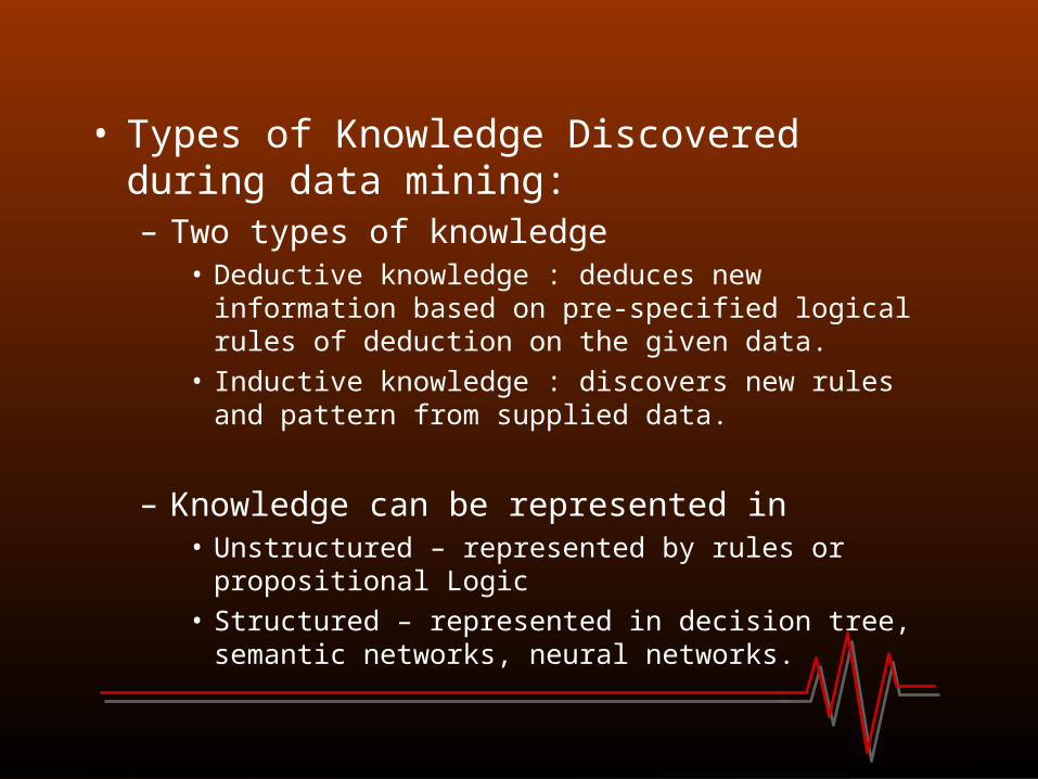
• Types of Knowledge Discovered during data mining:– Two types of knowledge

• Deductive knowledge : deduces new information based on pre-specified logical rules of deduction on the given data.

• Inductive knowledge : discovers new rules and pattern from supplied data.

– Knowledge can be represented in• Unstructured – represented by rules or propositional Logic

• Structured – represented in decision tree, semantic networks, neural networks.

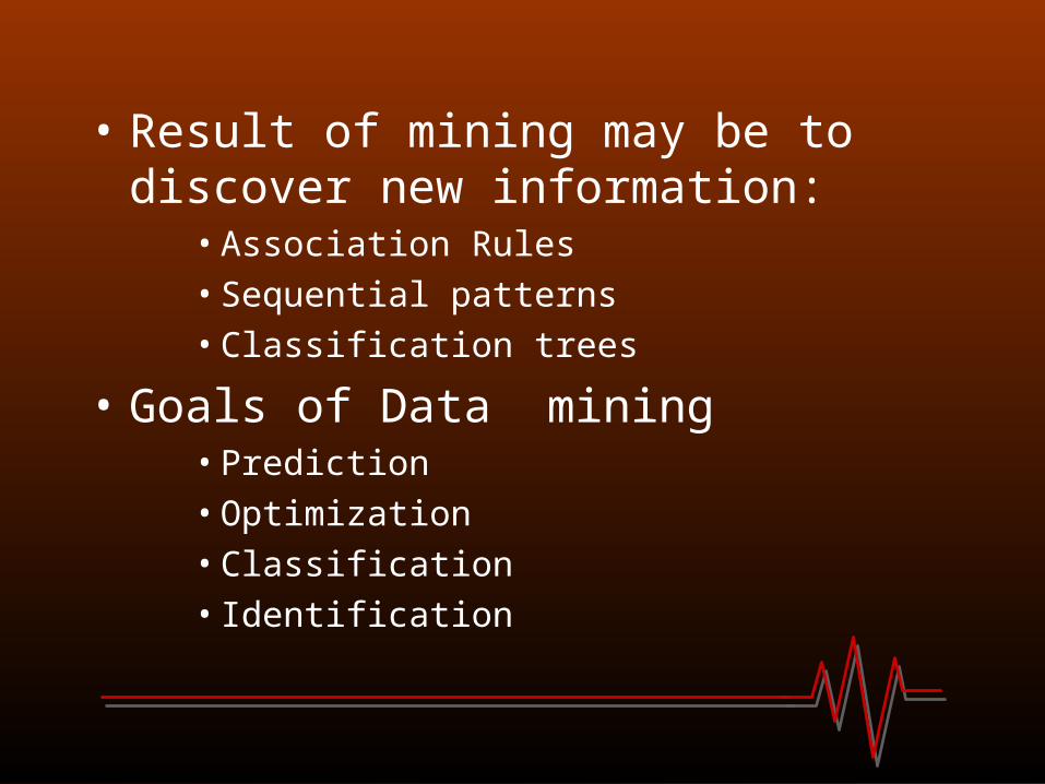
• Result of mining may be to discover new information:

• Association Rules

• Sequential patterns

• Classification trees

• Goals of Data mining• Prediction

• Optimization

• Classification

• Identification

Association RulesAssociation Rules

• Market Based Model, Support and Confidence

• Apriori Algorithm

• Sampling Algorithm

• Frequent – Pattern Algorithm

• Partition Algorithm

Market Based model, Support and Market Based model, Support and confidenceconfidence

• Major technology in data mining involves discovery of association rules.

• XY where X ={x1,x2………,xn}, Y={y1,y2,….,yn}

• If rule: LHSRHS then item set := LHS U RHS

• Association rule should satisfy some interest measures: Support and Confidence

• Support for rule LHSRHS with respect to the itemset. -It refers to how frequently a specific itemset occurs in a database-is the percentage of transactions that contain all of the

items in the itemset.-support is sometimes called “prevalence” of the rule.

• Confidence of implication shown in rule– is computed as Support(LHS U RHS)/Support(LHS).-is the probability that the items in RHS will be purchased

given the item in LHS are purchased.-confidence is also called the “strength” of the rule.

• Generate all rules that exceed user specified confidence and support thresholds by:

(a) Generate all itemsets of support>threshold (called “large” itemsets)

(b) For each large itemset, generate rules of min confidence, by: For large itemset X and Y subset of X, let Z=X-Y. If support(X)/support(Z)>min_confidence THEN Z Y is valid rule.

Problem: combinatorial explosion on # of itemsets

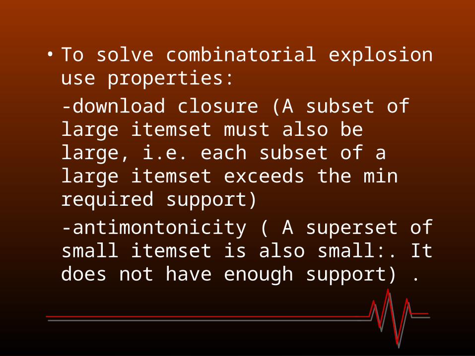
• To solve combinatorial explosion use properties:

-download closure (A subset of large itemset must also be large, i.e. each subset of a large itemset exceeds the min required support)

-antimontonicity ( A superset of small itemset is also small:. It does not have enough support) .

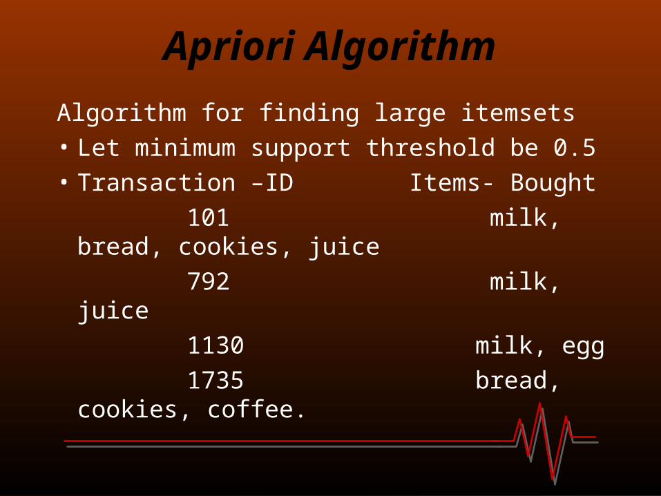
Apriori Algorithm

Algorithm for finding large itemsets

• Let minimum support threshold be 0.5

• Transaction –ID Items- Bought

101 milk, bread, cookies, juice

792 milk, juice

1130 milk, egg

1735 bread, cookies, coffee.

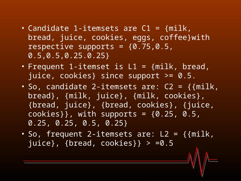
• Candidate 1-itemsets are C1 = {milk, bread, juice, cookies, eggs, coffee}with respective supports = {0.75,0.5, 0.5,0.5,0.25.0.25}

• Frequent 1-itemset is L1 = {milk, bread, juice, cookies} since support >= 0.5.

• So, candidate 2-itemsets are: C2 = {{milk, bread}, {milk, juice}, {milk, cookies}, {bread, juice}, {bread, cookies}, {juice, cookies}}, with supports = {0.25, 0.5, 0.25, 0.25, 0.5, 0.25}

• So, frequent 2-itemsets are: L2 = {{milk, juice}, {bread, cookies}} > =0.5

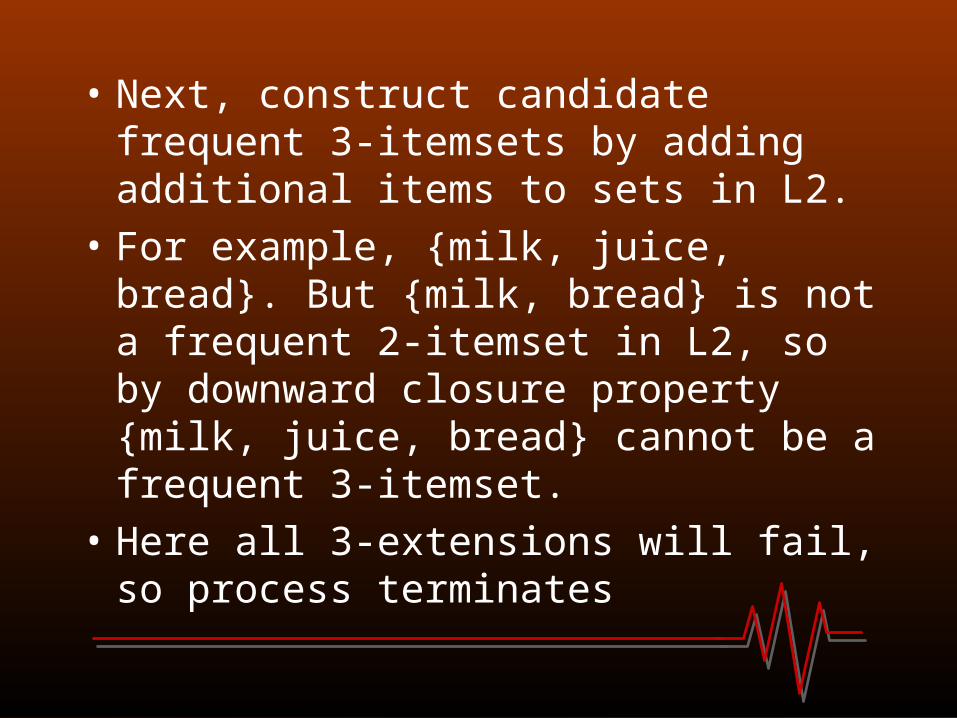
• Next, construct candidate frequent 3-itemsets by adding additional items to sets in L2.

• For example, {milk, juice, bread}. But {milk, bread} is not a frequent 2-itemset in L2, so by downward closure property {milk, juice, bread} cannot be a frequent 3-itemset.

• Here all 3-extensions will fail, so process terminates

Sampling AlgorithmSampling Algorithm((for VLDB-very large databases)for VLDB-very large databases)

• Sampling algorithm selects a sample of the database transactions, small enough to fit in main memory, and then determines the frequent itemsets from that sample.

• If these frequent itemsets form a super set of the frequent itemsets for the entire database, then the real frequent itemsets can be determined by scanning the remainder of the database in order to compute the exact support values for the superset itemsets.

• A superset of the frequent itemsets can be found from the sample by using Apriori algorithm with a lowered minimum support.

• In some cases frequent item sets may be missed, so the concept of negative border is used to decide if any were missed.

• The basic idea is that the negative border of a set of frequent itemsets contains the closest itemsets that could also be frequent.

• Negative border for itemset S and set of items I, is the minimal itemsets contained in Powerset(I) and not in S.

(continued)

• Consider set of Items I = {A,B,C,D,E}• Let combined frequent itemsets of size 1 to 3 be S=

{A,B,C,D,AB,AC,BC,AD,CD,ABC}• Then Negative Border = {E,BD,ACD}• Where {E} is the only 1-itemset not contained in S, {BD}

is the only 2-itemset not in S but whose 1-itemset subsets are, and ACD is the only 3-itemset not in S whose 2-itemset subsets are all in S.

• Scan remaining database to find support of negative border. If an itemset X is found in the negative border which belongs to set of all frequent itemsets, then maybe a superset of X could also be frequent, which can be determined by a second pass over the database.

Frequent Pattern Tree algorithmFrequent Pattern Tree algorithm• It is improves the Apriori algorithm by reducing

number of candidate itemsets that need to be generated and tested whether they are frequent.

• First produces a compressed version of the database in the form of a Frequent Pattern (FP)- tree

• The FP-tree stores relevant itemset information and allows for efficient discovery of frequent itemsets.

• Divide-and-conquer strategy: mining is decomposed into a set of smaller tasks that each operate on a smaller, conditional FP-tree which is a subset of original tree.

• Database is first scanned and frequent 1-itemsets with their support are computed.

• Here, support is defined as the count of transactions containing the item rather than fraction of transactions that contain it as in Apriori.

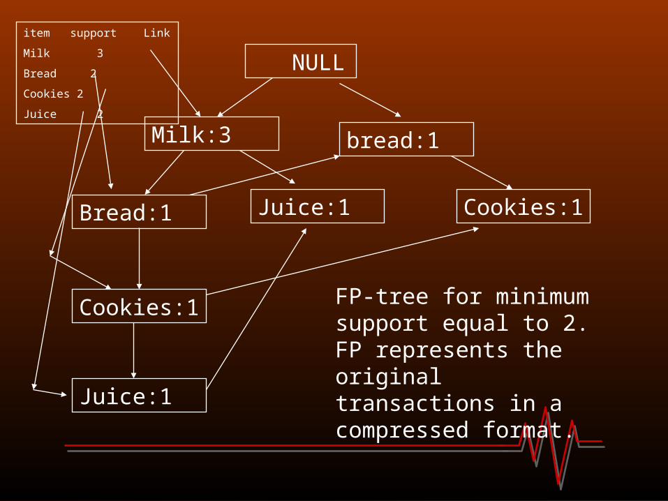
• To construct the FP-tree from transaction table, for a minimum suppor of say =2:-Frequent 1-itemsets are stored in Non increasing order of support{{(milk,3)},{(bread,2)},{(cookies,2)},{(juice,2)}}-For each transaction, construct sorted list of its frequent items and expand tree as needed and update the frequent item index table:First transaction sorted list is T = {milk,bread,cookies,juice}Second Transaction={milk, juice}Third transaction= {milk}(since eggs is not a frequent item)Fourth transaction={bread, cookies}

Resulting FP-tree is as follows:

NULL

Cookies:1

Bread:1

Milk:3

Juice:1

Juice:1

FP-tree for minimum support equal to 2. FP represents the original transactions in a compressed format.

bread:1

Cookies:1

item support Link

Milk 3

Bread 2

Cookies 2

Juice 2

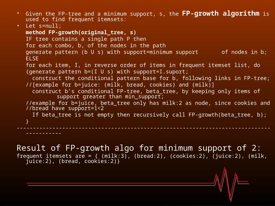
• Given the FP-tree and a minimum support, s, the FP-growth algorithm is used to find frequent itemsets:

• Let s=null;method FP-growth(original_tree, s)IF tree contains a single path P then

for each combo, b, of the nodes in the pathgenerate pattern (b U s) with support=minimum support

of nodes in b;ELSE

for each item, I, in reverse order of items in frequent itemset list, do{generate pattern b=(I U s) with support=I.suport; construct the conditional pattern base for b, following links in FP-tree; //[example for b=juice: (milk, bread, cookies) and (milk)] construct b’s conditional FP-tree, beta_tree, by keeping only items of support greater than min_support;//example for b=juice, beta_tree only has milk:2 as node, since cookies and //bread

have support=1<2 If beta_tree is not empty then recursively call FP-growth(beta_tree, b);}

-----------------------------------------------------------------------------------------

Result of FP-growth algo for minimum support of 2: frequent itemsets are = { (milk:3), (bread:2), (cookies:2), (juice:2), (milk, juice:2), (bread, cookies:2)}

Partition AlgorithmPartition Algorithm

• If a database has a small number of potential frequent itemsets then their support can be found in one scan using Partitioning techniques.

• Partitioning divides the database into non overlapping subsets.

• It can be accommodated in main memory.• Partition is read only once in each pass.• Support used is different from the original value.• Global candidate Large itemset that are identified in pass 1

are verified in pass 2 with support measured for entire database.

• At the end, all global large itemsets are identified.

ClassificationClassification

• Learning a model that describes different classes of data.

• Classes are pre-determined.

• Each model that are designed will be in the form of decision tree or set of rules.

• Decision tree is constructed from the training data set

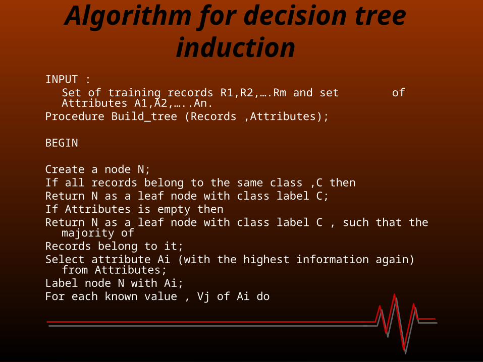
Algorithm for decision tree induction

INPUT :Set of training records R1,R2,….Rm and set of Attributes A1,A2,…..An.

Procedure Build_tree (Records ,Attributes);

BEGIN

Create a node N;If all records belong to the same class ,C thenReturn N as a leaf node with class label C;If Attributes is empty then Return N as a leaf node with class label C , such that the majority ofRecords belong to it;Select attribute Ai (with the highest information again) from Attributes;Label node N with Ai;For each known value , Vj of Ai do

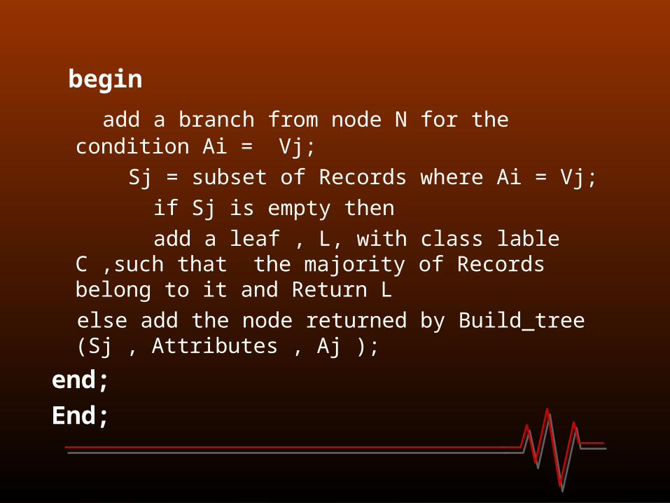
begin

add a branch from node N for the condition Ai = Vj;

Sj = subset of Records where Ai = Vj;

if Sj is empty then

add a leaf , L, with class lable C ,such that the majority of Records belong to it and Return L

else add the node returned by Build_tree (Sj , Attributes , Aj );

end;

End;

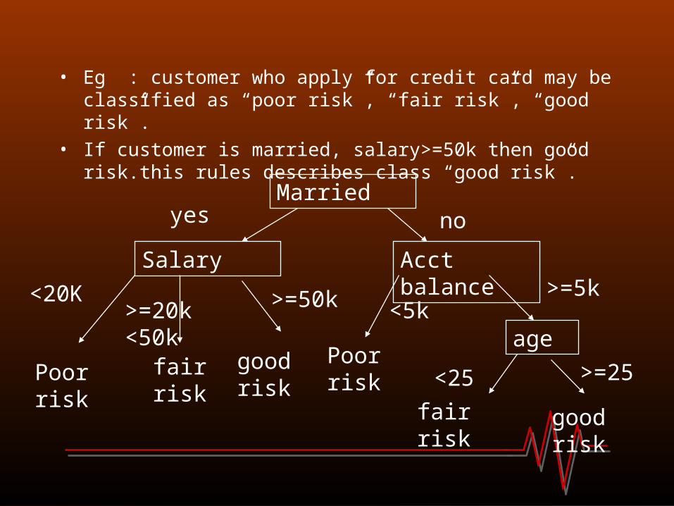
• Eg : customer who apply for credit card may be classified as “poor risk”, “fair risk”, “good risk”.

• If customer is married, salary>=50k then good risk.this rules describes class “good risk”.

Salary

Married

Acct balance

agePoor risk

Poor risk fair risk good risk

fair risk good risk

yes no

<20K>=20k <50k

>=50k <5k>=5k

<25 >=25

ClusteringClustering

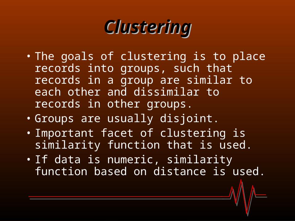
• The goals of clustering is to place records into groups, such that records in a group are similar to each other and dissimilar to records in other groups.

• Groups are usually disjoint.• Important facet of clustering is similarity

function that is used. • If data is numeric, similarity function based

on distance is used.

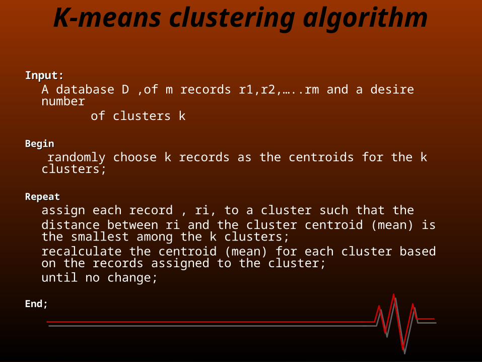
K-means clustering algorithm

Input:Input: A database D ,of m records r1,r2,…..rm and a desire number

of clusters k

BeginBegin

randomly choose k records as the centroids for the k clusters;

RepeatRepeat

assign each record , ri, to a cluster such that the distance between ri and the cluster centroid (mean) is the smallest among the

k clusters; recalculate the centroid (mean) for each cluster based on the records

assigned to the cluster;until no change;

End;End;

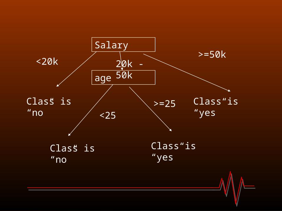
Salary

age

Class is “no”

Class is “no” Class is “yes”

Class is “yes”

<20k>=50k

20k -50k

<25>=25

Approaches to other data mining problemApproaches to other data mining problem

• Discovery of sequential Pattern

• Discovery of patterns in Time series

• Regression

• Neural Networks

• Genetic Algorithms

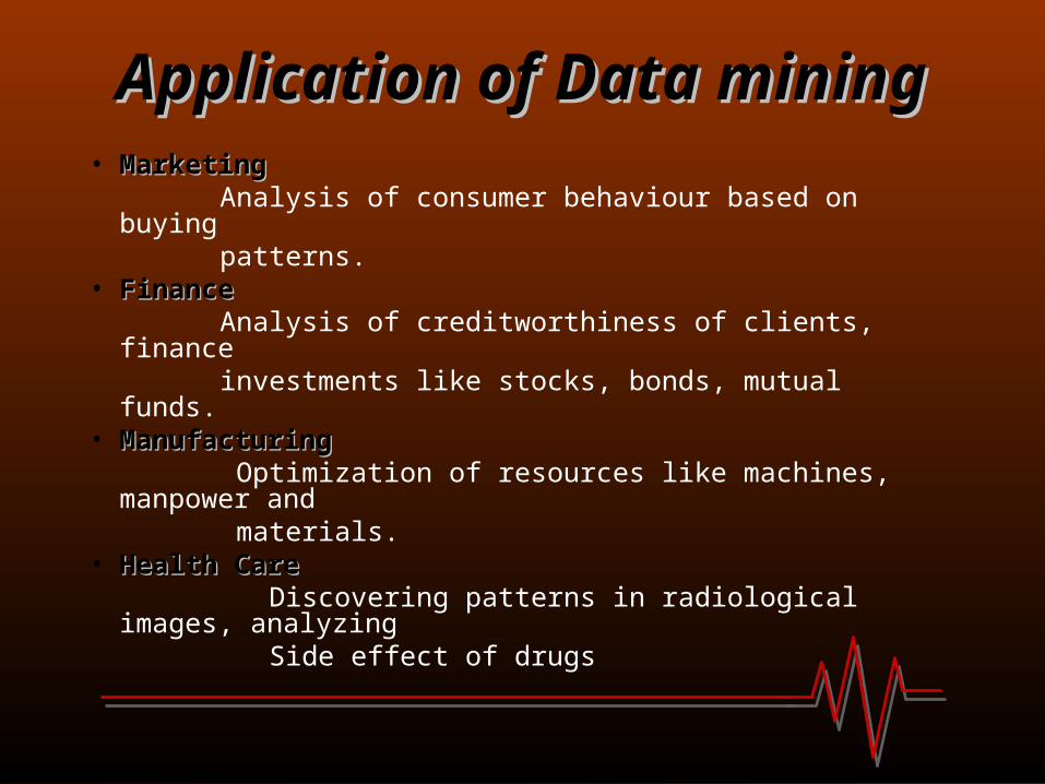
Application of Data miningApplication of Data mining• MarketingMarketing Analysis of consumer behaviour based on buying patterns.• FinanceFinance Analysis of creditworthiness of clients, finance investments like stocks, bonds, mutual funds.• ManufacturingManufacturing Optimization of resources like machines, manpower and materials.• Health CareHealth Care Discovering patterns in radiological images, analyzing Side effect of drugs

Overview of Data Warehousing and Overview of Data Warehousing and OLAPOLAP

What is Data Warehousing?

• Collection of information as well as supporting system.

• Designed precisely to support efficient extraction, processing and presentation for analytic and decision making purpose

Characteristics of Data Warehouse

• Multi dimensional conceptual view• Generic dimensionality• Unlimited dimensions and aggregation levels• Unrestricted cross – dimensional operations• Client-server architecture• Multi user support• Accessibility• Transparency• Intuitive data manipulation• Consistent reporting performance• Flexible reporting

Data modeling for data warehouses

• Multidimensional models – populate data in multidimensional matrices called data cubes.

– Hierarchical views• Roll up display• Drill down display

– Tables• Dimension table - tuples• Fact table – attributes.

– Schemas• Star schema• Snow flake schema

Building Data Warehouse

• Specifically support ad-hock querying

• Factors:– Data -Extracted from multiple, heterogeneous

sources– Formatted for consistency within the warehouse– Cleaned to validity– Fitted into the data model– Loaded into warehouse

Functionality of Data Warehouse

• Roll - up

• Drill – down

• Pivot

• Slice and Dice

• Sorting

• Selection

• Derived attributes

Difficulties of implementing Data warehouse

• Operational issues with data warehousing

– Construction– administration – quality control.

Data Mining versus Data Data Mining versus Data warehousingwarehousing

• Data warehouse – support decision making with data.

• Data mining with data warehousing help with certain types of decision.

• To make data mining efficient, data warehousing should have a summarized collection of data. Data mining extracts meaningful new patterns just by processing and querying data in data warehouse.

• Hence, in large database running in terra bytes, successful application of data mining depends on construction of data warehouse.

DATA WAREHOUSING AND OLAP

Overview Introduction, Definitions, and Terminology Characteristics of Data Warehouses Data Modeling for Data Warehouses Building a Data Warehouse Typical functionality of a Data Warehouse Data Warehouse vs. Views Problems and Open Issues in Data Warehouses Questions / Comments

INTRODUCTION, DEFINITIONS, AND

TERMINOLOGY

Data Warehouse

A data warehouse is also a collection of information as well as supporting system.

They are mainly intended for decision support applications.

Data warehouses provide access to data for complex analysis, knowledge discovery and decision making.

Data warehouses support efficient extraction, processing, and presentation for analytic and decision–making purposes.

CHARACTERISTICS OF DATA WAREHOUSES

Characteristics of Data Warehouse Data warehouse is a store for integrated

data from multiple sources, processed for storage in a multi dimensional model.

Information in data warehouse changes less often and may be regarded as non-real time with periodic updates.

Warehouse update are handled by the warehouse’s acquisition component that provides all required preprocessing.

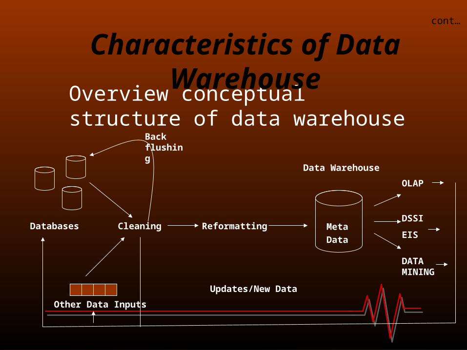
Overview conceptual structure of data warehouse

cont…


OLAP

DSSI

EIS

DATA MINING

Databases Cleaning Reformatting

Back flushing

Other Data Inputs

Updates/New Data

Data Warehouse

Meta

Data

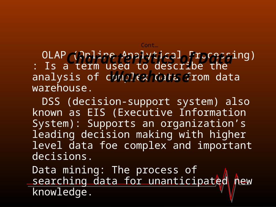
OLAP (Online Analytical Processing) : Is a term used to describe the analysis of complex data from data warehouse.

DSS (decision-support system) also known as EIS (Executive Information System): Supports an organization’s leading decision making with higher level data foe complex and important decisions.

Data mining: The process of searching data for unanticipated new knowledge.

Cont…


It has multidimensional conceptual view. It has unlimited dimensions and aggregate levels. Client server architecture. Multi-user support. Accessibility. Transparency. Intuitive data manipulation. Unrestricted cross-dimensional operations. Flexible reporting.

cont…


They encompass large volumes of data which is an issue that has been dealt with

Enterprise-wide warehouse: Are huge projects requiring massive investment of time and resources.

Virtual data warehouse: Provides views of operational databases that are materialized for efficient access.

Data marts: Are targeted to a subset of the organization, such as a department and are more tightly focused.

Cont…


DATA MODELING OF DATA WAREHOUSES

Data Modeling for Data Warehouses

Data can be populated in multi dimensional matrices called data cubes.

Query processing in multidimensional model can be much better than in the relational data model.

Changing from one dimensional hierarchy to another is easily accomplished in a data cube by a technique called pivoting.

Data cube can be thought of as rotating to show a different orientation of the axes.

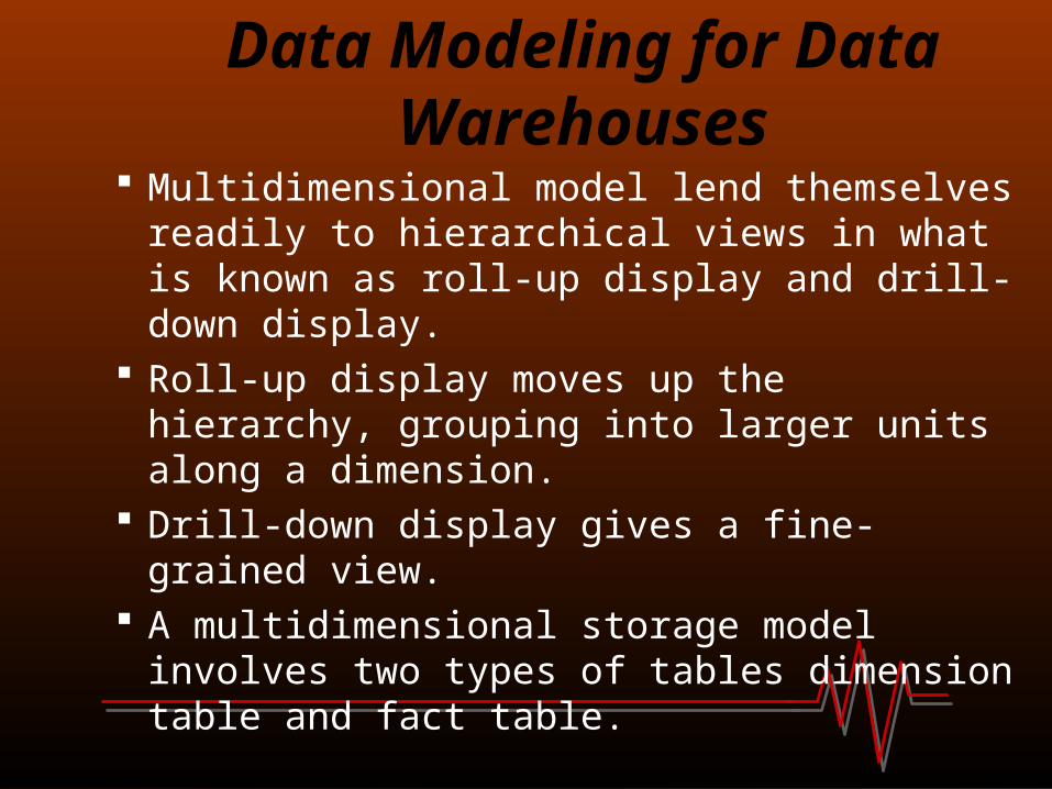
Multidimensional model lend themselves readily to hierarchical views in what is known as roll-up display and drill-down display.

Roll-up display moves up the hierarchy, grouping into larger units along a dimension.

Drill-down display gives a fine-grained view. A multidimensional storage model involves

two types of tables dimension table and fact table.

cont..


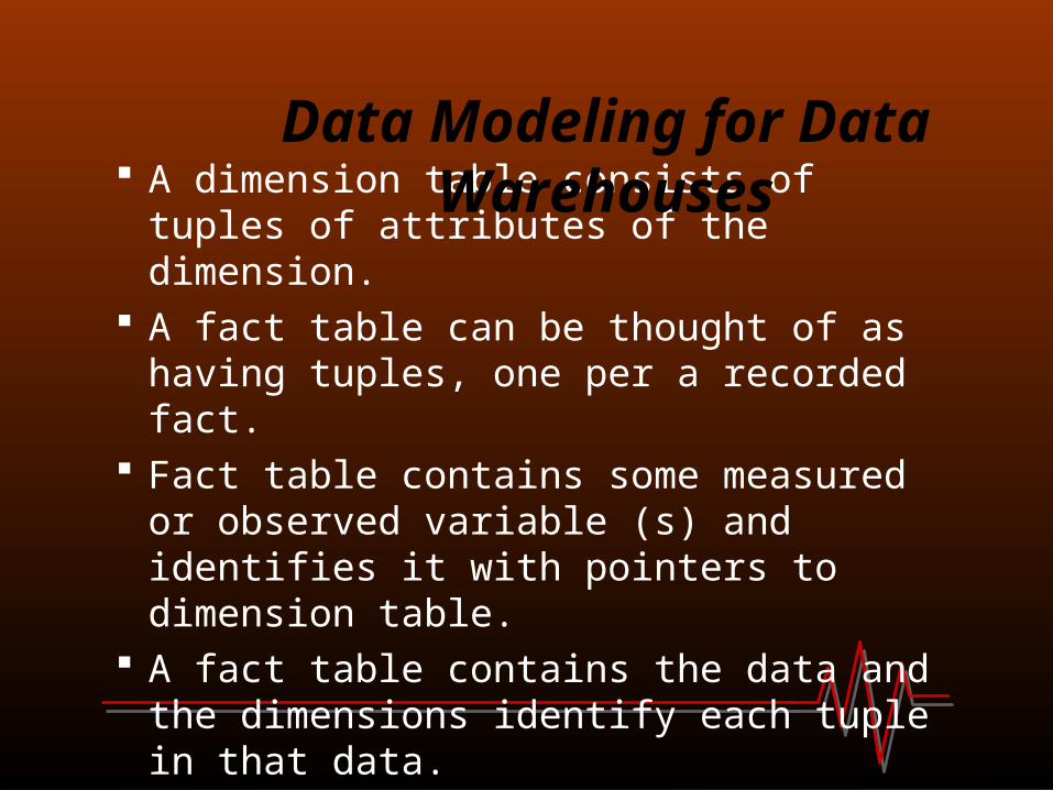
A dimension table consists of tuples of attributes of the dimension.

A fact table can be thought of as having tuples, one per a recorded fact.

Fact table contains some measured or observed variable (s) and identifies it with pointers to dimension table.

A fact table contains the data and the dimensions identify each tuple in that data.

Cont…


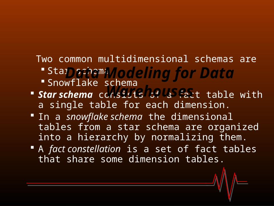
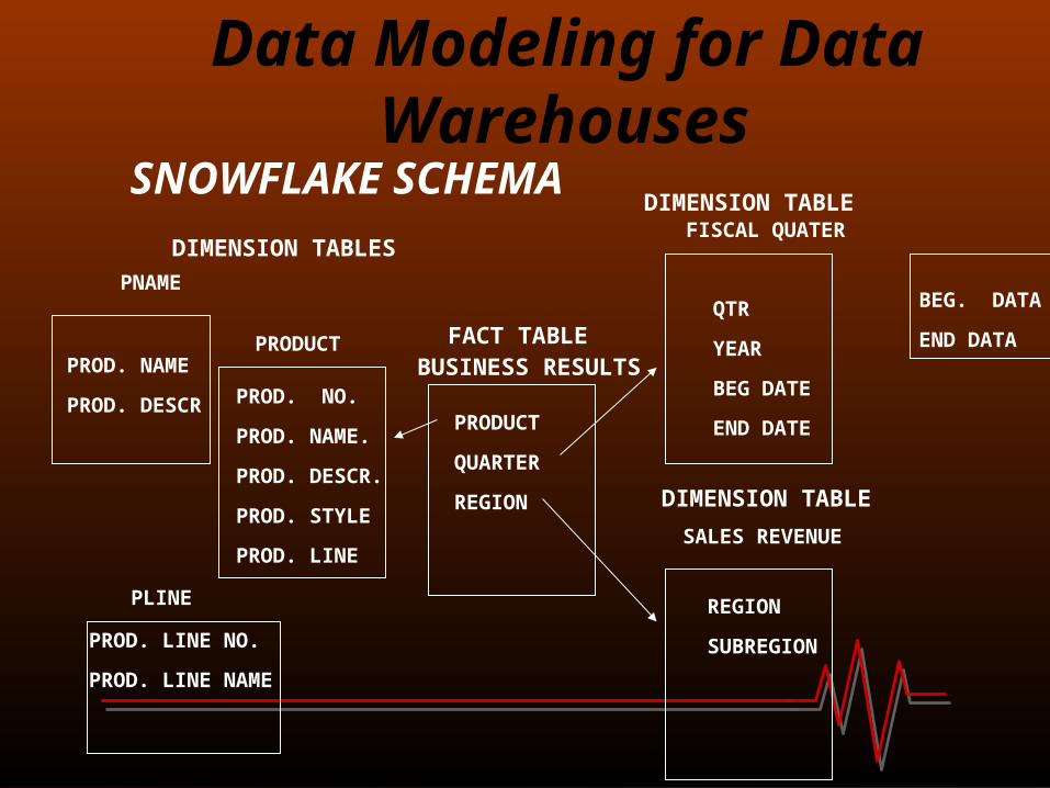
Two common multidimensional schemas are Star schema Snowflake schema

Star schema consists of a fact table with a single table for each dimension.

In a snowflake schema the dimensional tables from a star schema are organized into a hierarchy by normalizing them.

A fact constellation is a set of fact tables that share some dimension tables.

Cont… Data Modeling for Data Warehouses

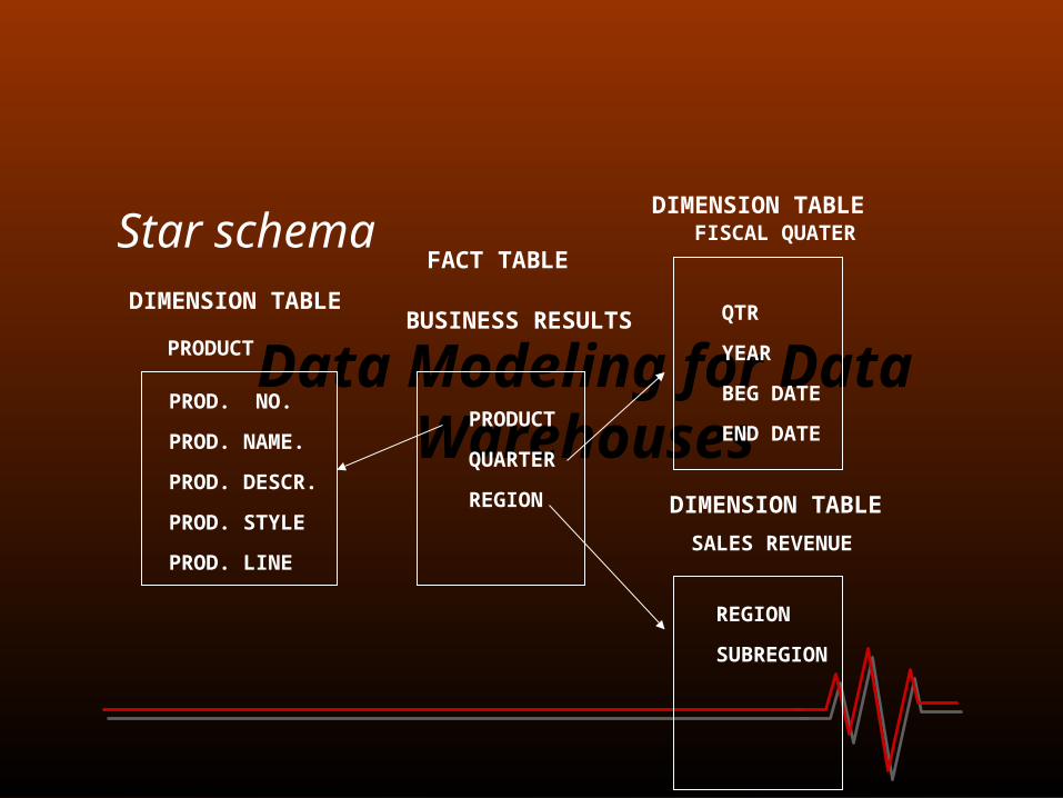
Star schema

Cont…

Data Modeling for Data WarehousesPRODUCT

QUARTER

REGION

PROD. NO.

PROD. NAME.

PROD. DESCR.

PROD. STYLE

PROD. LINE

FACT TABLE

DIMENSION TABLE

DIMENSION TABLE

DIMENSION TABLEBUSINESS RESULTS

FISCAL QUATER

SALES REVENUE

PRODUCT

QTR

YEAR

BEG DATE

END DATE

REGION

SUBREGION

PROD. NO.

PROD. NAME.

PROD. DESCR.

PROD. STYLE

PROD. LINE

FACT TABLE

DIMENSION TABLE

DIMENSION TABLE

DIMENSION TABLES

BUSINESS RESULTS

FISCAL QUATER

SALES REVENUE

PRODUCT

QTR

YEAR

BEG DATE

END DATE

REGION

SUBREGION

PRODUCT

QUARTER

REGION

PROD. NAME

PROD. DESCR

PNAME

PLINE

PROD. LINE NO.

PROD. LINE NAME

BEG. DATA

END DATA

Cont..


SNOWFLAKE SCHEMA

Join indexes relate the values of a dimension of a star schema to rows in the fact table.

Data warehouse storage can facilitate access to summary data .There are 2 approaches Smaller tables including summary data such as

quarterly sales or revenue by product line. Encoding of level into existing tables.

Cont…


BUILDING A DATA WAREHOUSE

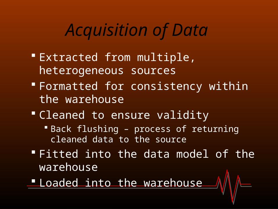
Acquisition of Data

Extracted from multiple, heterogeneous sources

Formatted for consistency within the warehouse

Cleaned to ensure validity Back flushing – process of returning cleaned data to

the source

Fitted into the data model of the warehouse Loaded into the warehouse

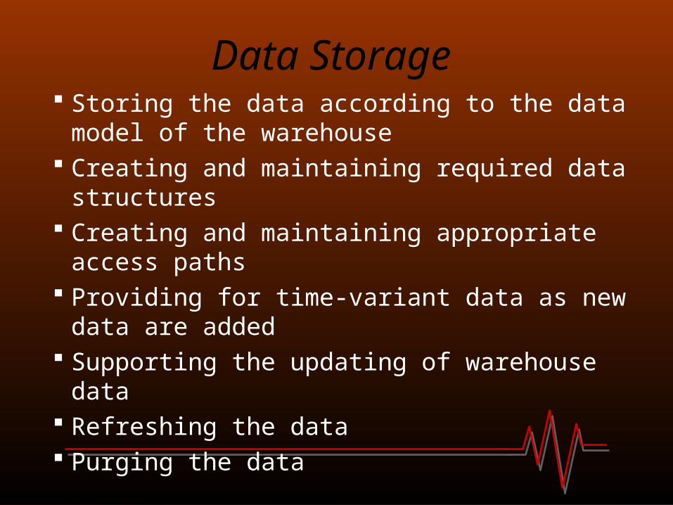
Data Storage Storing the data according to the data model of

the warehouse Creating and maintaining required data structures Creating and maintaining appropriate access paths Providing for time-variant data as new data are

added Supporting the updating of warehouse data Refreshing the data Purging the data

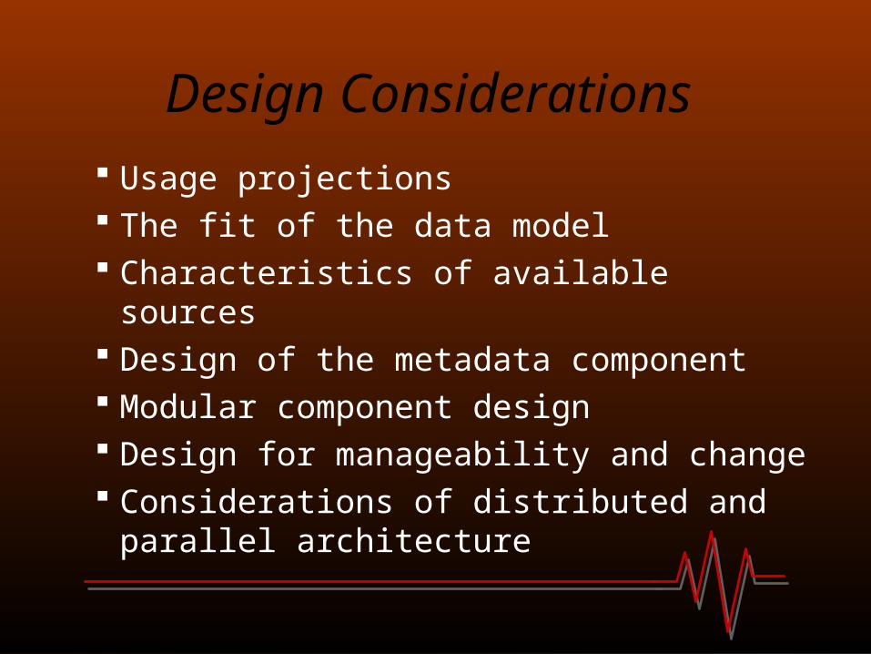
Design Considerations

Usage projections The fit of the data model Characteristics of available sources Design of the metadata component Modular component design Design for manageability and change Considerations of distributed and parallel

architecture

TYPICAL FUNCTIONALITY OF A

DATA WAREHOUSE

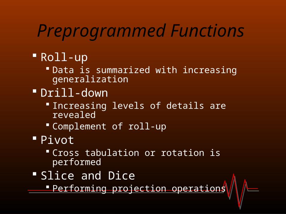
Preprogrammed Functions Roll-up

Data is summarized with increasing generalization

Drill-down Increasing levels of details are revealed Complement of roll-up

Pivot Cross tabulation or rotation is performed

Slice and Dice Performing projection operations

Preprogrammed Functions (contd…)

Sorting Data is sorted by ordinal value

Selection Data is available by value or range

Derived (Computed) Attributes Attributes are computed by operations on stored and

derived values

Other Functions

Efficient query processing Structured queries Ad hoc queries Data mining Materialized views Enhanced spreadsheet functionality

DATA WAREHOUSE vs. VIEWS

Data Warehouses vs. Views

Data warehouses exist as a persistent storage but views are being materialized on demand

Data warehouses are not usually relational but multidimensional. Views of a Relational Database are relational

Data warehouses can be indexed to optimize performance. Views cannot be indexed independent of the underlying databases

Data Warehouses vs. Views (contd…)

Data warehouses provide specific support of functionality but views cannot

Data warehouses provide large amounts of integrated and often temporal data, generally more than is contained in one database, whereas views are an extract of a database

PROBLEMS AND OPEN ISSUES IN DATA WAREHOUSES

Implementation Difficulties

Project Management Design Construction Implementation

Administration Quality control of data Managing a data warehouse

Open Issues

Data cleaning Indexing Partitioning Views Incorporation of domain and business rules

into warehouse creation and maintenance process making it more intelligent, relevant and self governing

Open Issues (contd…)

Automating aspects of the data warehouse Data acquisition Data quality management Selection and construction of appropriate access

paths and structures Self-maintainability Functionality Performance optimization

Documents

Data Mining Concepts Advanced Database Management Systems