Data Modelling and Database Requirements for Geographical Data · Data Modelling and Database Requirements for Geographical Data Håvard Tveite January, 1997 . Abstract An overview

Data Modelling and Database Requirements

for

Geographical Data

Håvard Tveite

January, 1997

Abstract

An overview of the fields of data modelling, database systems and geographical informationsystems is presented as a background. Requirements to a data model and a data modellingmethodology for geographical data are investigated and presented. Another contribution isan extension of the traditional ER-diagrams to better communicate the semantics ofgeographical data. The approach is based on earlier work on Sub-Model Substitution, andadds new symbology that is relevant for geographical data. Database system requirementsfor geographical data servers are investigated and presented, together with new ideas ondistribution of geographical data for parallel processing.

Table of Contents

Chapter 1 Introduction 1Motivation . . . . . . . . . . . . . . . . . . . . . . . . . . . . . . . . . 1Contributions . . . . . . . . . . . . . . . . . . . . . . . . . . . . . . . . 2Related work . . . . . . . . . . . . . . . . . . . . . . . . . . . . . . . . 2How this document is organised . . . . . . . . . . . . . . . . . . . . . . 3

Chapter 2 Database Systems and Data Models 5Data modelling . . . . . . . . . . . . . . . . . . . . . . . . . . . . . . . 5

Modelling concepts 5Infological data models and the infological and datalogical realm 7Metadata versus “ordinary” data 8

Semantic data models . . . . . . . . . . . . . . . . . . . . . . . . . . . . 9ER models and diagrams 9EER models and diagrams 11Object-oriented data models 13

Database systems . . . . . . . . . . . . . . . . . . . . . . . . . . . . . 14Brief history 15Definitions 15The three-schema architecture 16Features/services of database systems 17Distributed database systems 18Database machines 19Status of database systems 19

Database models . . . . . . . . . . . . . . . . . . . . . . . . . . . . . 20Hierarchical DBMSs 20Network DBMSs 21Relational DBMSs 23Object-oriented DBMSs 26Deductive DBMSs 28

Chapter 3 Geographical Information Systems 29History . . . . . . . . . . . . . . . . . . . . . . . . . . . . . . . . . . 29Definitions of GIS . . . . . . . . . . . . . . . . . . . . . . . . . . . . 30The utility of geographical information systems . . . . . . . . . . . . . 31

Local administration GIS, an example application area 32Geographical data . . . . . . . . . . . . . . . . . . . . . . . . . . . . 33

Geographical maps 33Spatial geographical data 34Non-spatial or “catalogue type” GIS data 36Historical data 36Data quality 37Data distribution and sharing 37

Models for geographical data . . . . . . . . . . . . . . . . . . . . . . . 38

The raster paradigm 38The vector paradigm 40Representation of the interior of spatial objects 41

Queries and operations . . . . . . . . . . . . . . . . . . . . . . . . . . . 42GIS queries 42Use of the different GIS query types 44

Current GIS technology . . . . . . . . . . . . . . . . . . . . . . . . . . 45ARC/INFO 45System 9 48TIGRIS 50Smallworld GIS 50GRASS 51Summary 52

Trends . . . . . . . . . . . . . . . . . . . . . . . . . . . . . . . . . . . 53Hardware trends 53Technology trends 54GIS trends 55

The GIS of the future . . . . . . . . . . . . . . . . . . . . . . . . . . . . 55Servers of geographical information 56

Research and research issues . . . . . . . . . . . . . . . . . . . . . . . . 57

Chapter 4 Data model requirements 59Introduction . . . . . . . . . . . . . . . . . . . . . . . . . . . . . . . . 59Geographical data revisited . . . . . . . . . . . . . . . . . . . . . . . . 59

Borders of geographical phenomena 60Features of geographical data 60

Requirements to high level geographical data models . . . . . . . . . . . 65Traditional ER model abstractions 66Geometrical object types 67Spatial relationships 68Implicit geographical relationships 69Topology 69Aggregation 73Generalisation 74Categories 76History and time 76Quality/ accuracy 77Derived objects 79Sharing of geometrical objects among geographical objects 79Roles and scale 80Spatial constraints 81Groups of related objects (themes) 81Distributed ownership 82Behaviour 82

Modelling implications . . . . . . . . . . . . . . . . . . . . . . . . . . . 83Proposed data models and exchange standards for GIS data . . . . . . . 84

ATKIS 84SDTS 86

ii

NGIS and FGIS 90MetaMap 95

Chapter 5 Sub-Structure Abstraction in Geographical Data Modelling 99Context . . . . . . . . . . . . . . . . . . . . . . . . . . . . . . . . . . 99Geographical data modelling using structure abstractions . . . . . . . . 101

Extending ER-diagrams with sub model substitution 102A forestry research example 109

Translation . . . . . . . . . . . . . . . . . . . . . . . . . . . . . . . . 110Conclusion . . . . . . . . . . . . . . . . . . . . . . . . . . . . . . . . 111

Future work 111

Chapter 6 Database management system issues for geographical data 113Basic requirements . . . . . . . . . . . . . . . . . . . . . . . . . . . . 113Data volumes and data types . . . . . . . . . . . . . . . . . . . . . . . 115

Samples 115Raster data 116Vector data 118Time 118Generalisation levels 118Summary 119

Multimedia (integrated) database systems . . . . . . . . . . . . . . . . 119Hypertext 120

Spatio-temporal databases . . . . . . . . . . . . . . . . . . . . . . . . 121Concepts of time in databases 121Representing time in databases 122TQuel 122Time in geographical databases 122

Metadata and data dictionaries . . . . . . . . . . . . . . . . . . . . . . 124Quality in geographical databases 125Data dictionary issues for geographical data 126

Geographical Query Languages . . . . . . . . . . . . . . . . . . . . . 129Different ways of organising geographical information 130Spatial query language proposals 131Query optimisation 134Spatial data types 134Spatial constraints 137Operations 137

Transactions . . . . . . . . . . . . . . . . . . . . . . . . . . . . . . . 142Transactions on temporal geographical data 143Transaction management 143Concurrency Control 144

Distribution issues . . . . . . . . . . . . . . . . . . . . . . . . . . . . 149Parallel processing 150Distribution of spatial data 151Replication 155Heterogeneous database system integration 156Fast geometrical processing 157

iii

Data exchange formats 157Some limitations of currently used database models . . . . . . . . . . 158

Network database models 159The relational database model 160Object-oriented database models 164

Conclusions . . . . . . . . . . . . . . . . . . . . . . . . . . . . . . . 165

Appendix A Data structures for spatial databases 167Basic data structures . . . . . . . . . . . . . . . . . . . . . . . . . . . 167

Digital computer storage media 167Sequences (lists/arrays) 168Randomised sequences 169

Hierarchical structures . . . . . . . . . . . . . . . . . . . . . . . . . . 170Multi-dimensional trees . . . . . . . . . . . . . . . . . . . . . . . . . 171

Points 172Lines 172Regions in 2D 173

Grid partitioning and spatial hashing . . . . . . . . . . . . . . . . . . 175Multi resolution image trees (pyramids) 175Region quad trees 175Linearisation 175EXCELL 176Grid file 176

Appendix B Representation of 3D structures 1793D objects . . . . . . . . . . . . . . . . . . . . . . . . . . . . . . . . 179Storage organisation . . . . . . . . . . . . . . . . . . . . . . . . . . . 180Point sampling . . . . . . . . . . . . . . . . . . . . . . . . . . . . . . 180Wire frame . . . . . . . . . . . . . . . . . . . . . . . . . . . . . . . . 181Triangulated Irregular Network . . . . . . . . . . . . . . . . . . . . . 182Parametric representations . . . . . . . . . . . . . . . . . . . . . . . . 182Constructive Solid Geometry . . . . . . . . . . . . . . . . . . . . . . 184

Appendix C The NHS Electronic Navigational Chart Database 185Introduction . . . . . . . . . . . . . . . . . . . . . . . . . . . . . . . 185Background . . . . . . . . . . . . . . . . . . . . . . . . . . . . . . . . 185Navigational Charts . . . . . . . . . . . . . . . . . . . . . . . . . . . 185

ENC and ECDIS 186The ENCDB 186Data management 187Relating the traditional chart data to other data 188

Structures for the ECDIS database . . . . . . . . . . . . . . . . . . . . 188Data modelling for ECDIS . . . . . . . . . . . . . . . . . . . . . . . . 191DBMS-aspects of an ENC-server . . . . . . . . . . . . . . . . . . . . 193

The amount of data 193The data 193Response time 194Concurrency and recovery 194

iv

Security 194Reliability 195Billing 195The choice of a database system for the ECDIS server 195

Conclusions . . . . . . . . . . . . . . . . . . . . . . . . . . . . . . . . 196

Bibliography 197

Index 217

v

vi

Acknowledgements

I wish to thank my supervisor, professor Kjell Bratbergsengen, for encouragement andsupport through the 8 years that have passed since I started these studies. Without hiscontinuous commitment and goodwill, I would have given up a long time ago. Thanks alsoto professor Ingolf Hådem, who agreed to be my advisor on photogrammetry. The contactwith Hådem has been sporadic after the focus of my work was directed to data modellingand database management.

The first part of this study took place when I was employed as a research assistant at theDepartment of Computer Systems and Telematics, NTH (now a part of NTNU) for two anda half years from 1988 to 1990. Then, I was supported by a research grant from theNorwegian Research Council for one and a half year from 1990 to 1991. The rest of thework has been done now and then while being employed at the Department of Surveyingat the Agricultural University of Norway (NLH).

I would like to thank everyone at the Department of Computer Systems and Telematics inTrondheim for a friendly atmosphere. In particular, I would like to mention the members ofthe database group. They have always been very helpful.

My employer during the last years of this work, the Department of Surveying at NLH, alsodeserves some thanks for encouraging me to finish this work.

I have some "friends" who have been annoying me by asking about the status of my thesiswork on all occasions during the last 4 years. I am not quite sure if I should thank them ornot!

Last, but not least, the friendly atmosphere of "Munkholmens Lægeforening" has been animportant inspiration. Without such a stimulating environment, it would have been difficultto get the necessary inspiration for finishing this work.

vii

viii

Chapter 1

Introduction

Digital geographical data are indispensable for monitoring and managing the environmentand for managing and planning geographically based human activities such as land use,utility networks, long-distance transportation and mining in efficient ways.

Sharing of digital geographical data both between and within organisations is of utmostimportance for the efficient use of geographical information systems (GISs). One reasonfor this is the large efforts and costs that are involved in collecting and maintaining highquality geographical data sets: The more users that can share the data, the easier it is to coverthese expenses. Another important reason for sharing is that the availability of high qualitydata sets has the potential of making environmental (and land use -) planning and manage-ment better and more cost-efficient.

To be able to share digital geographical data, standards are necessary. Standard data modelsfor spatial data, standard encoding formats for the exchange of spatial data and standardcommunication protocols for distributing spatial data are all necessary parts of a foundationfor efficient geographical data sharing, with the spatial data model as the basic component.

A number of national standards for the digital encoding of topographic and thematic mapshave emerged in the last decade. The problem with todays standards is that they cover onlya limited part of the semantics necessary for general purpose exchange of geographical data.The lack of an agreed on data model that covers the essential aspects of spatial data has beenimpeding the development of powerful exchange standards.

This thesis looks into the problems of geographical data models and geographical datamodelling, and outlines some possible solutions.

To be able to share geographical data between organisations and within organisations, it isnecessary to have a system for managing the data. This thesis presents a set of requirementsto database management systems that are to act as servers of geographical data/information.

1.1 Motivation

Research on geographical information systems has suffered under the lack of a solidfoundation. Many GIS concepts need clarification, spatial data modelling methodologiesshould be developed, spatial database systems and data structures need elaboration [Gün-ther90], digital cartography and GIS user interfaces need sophistication and finally, there is

an urgent need for standards. The use of GISs is particularly impeded by the lack of standardsand the resulting limited availability of high quality data sets.

Investments in GISs are risky in such a situation. It is difficult for users to find a suitablesystem for covering their needs for spatial data support when there is no consensus on whatkind of functionality and which kinds of interfaces such a system should provide.

Efforts to develop and market geographical data sets is difficult when there are no generallyaccepted standards for their structuring, storage and exchange. When such standards are inplace, there will be a market for geographical data servers and services. Such servers shouldbe connected to an international public computer network, giving "everyone" access touseful spatial data. An international system of spatial data servers will have to be supportedby mechanisms for finding the right data, and sophisticated spatial database systems arerequired to manage the geographical data on these servers.

Data modelling techniques supporting spatial data become increasingly important as theuse of GISs becomes more and more widespread. There is a need for simple concepts andintuitive models in the communication process between the computer scientists and GISexperts on the one side and the spatial science experts on the other. A standardised high levelapproach to geographical data modelling would be a very useful tool. Such a platform forintegrated use of all kinds of geographical information would be a good starting point forGIS application and database development.

If a more solid foundation for GISs can be achieved, the activity in the field must be expectedto increase significantly. The serious use of GISs could blossom, and GIS related researchand the use of GIS as a tool in other kinds of spatial research would accelerate.

1.2 Contributions

The main contributions of this work are in two areas. The first area is geographical datamodelling, and the second area is database support for geographical data, with specialemphasis on the distribution/partitioning of geographical information.

• Modelling concepts specific to geographical and spatial information are identified.

• Spatial sub-structure abstractions in ER-like diagrams [Tveite92] are proposed.

• Database issues for geographical data are outlined and investigated.

• Distribution issues for geographical data [Tveite93] are identified and a distributionstrategy for geographical data is outlined.

1.3 Related work

Research on databases for spatial data is one of the branches of database system researchthat has been receiving increasing attention during the last decade ([Günther90]). There arenow well attended special purpose conferences for advances in spatial databases (SSD 89[Buchmann90], SSD91 [Günther91], SSD93 [Abel93]), SSD95 [Egenhofer95].

Data models for spatial and geographical databases and geographical information systemshave received some attention in the 1980ies and early 1990ies. As in the database commu-

2 Chapter 1: Introduction

nity, object-oriented methods have been particularly popular recently. Among the earlypublications on these topics are Egenhofer [Egenhofer87] [Egenhofer89a] [Egenhofer89b],Feuchtwanger [Feuchtwanger89] [Feuchtwanger93], Frank [Frank88] [Egenhofer87][Egenhofer89a] [Egenhofer89b], Worboys [Worboys90a] [Worboys90b], Hearnshaw [Wor-boys90a] [Worboys90b], Maguire [Worboys90a] [Worboys90b], Morehouse [More-house90], Orenstein [Orenstein86] [Orenstein88] [Orenstein90b], Peucker [Peucker75][Peucker78], Scholl [Scholl90] and Voisard [Scholl90].

Within the area of distribution and parallelisation, there has been work on the use of paralleltechnology for geographical information analysis at the University of Edinburgh. InEdinburgh, they have been looking into parallelisation of GIS algorithms. Some other effortson algorithms have also been made, for instance by Mower [Mower92], but the use ofparallel technology for organising general purpose spatial databases has not been givenmuch attention.

The main part of this thesis has been written while working with the database technologygroup at IDT, NTH. Distributed database technology (both hardware and software) has beenthe focus of the group, and several prototype parallel database machines have beendeveloped for research purposes. The research performed by this group has providedvaluable input to the “distribution-part” of this thesis.

1.4 How this document is organised

The thesis can roughly be divided into two parts. The first part includes the chapters 2 to 6,and contains the central aspects of the thesis, namely data modelling and database systemtopics for GIS. The second part comprises the appendices A to C.

Appendix A is a very short overview of spatial data structures.

Appendix B is a short presentation of representation techniques for three-dimensional (3D)structures.

Appendix C is a report submitted to the Norwegian Hydrographic Service discussingdatabase issues for an electronic navigational chart database that was under constructionsome years ago. The server was to provide authorised chart information to ships.

How this document is organised 3

4 Chapter 1: Introduction

Chapter 2

Database Systems and Data Models

This chapter is an introduction to the fields of data modelling, database systems and databasemodels, a necessary background for the rest of the thesis. The review will be limited to ashort summary of the most common data modelling approaches, an overview of the featuresexpected from a database system and some short notes on the most popular database models.

2.1 Data modelling

An information system that is to support an activity should cover all aspects of the realworld pertinent to that activity. To be able to develop such an information system, a goodmodel of this so-called mini-world must be developed. Such a high-level data model shouldabstract and structure descriptions of the phenomena in the mini-world in such a way thatthe information becomes manageable and understandable for humans. It is important for auseful data model to [Tsichritzis82]:

“… capture the appropriate amount of meaning as related to the desired use of thedata”.

Much research has been devoted to the development of powerful modelling formalisms,emphasising the communication (presentation and visualisation) of mini-worlds betweenhumans and the translation of the models into formats suitable for computer handling.

2.1.1 Modelling concepts

To be able to talk about the world and our representation of the world in a model, a certainvocabulary must be defined. The following is a blend of terminology taken from differentsources ([Tsichritzis82], [Chen76], [Ng81], [Elmasri89], [Rumbaugh91], [Sindre90]).

Abstraction is used to hide detail, so that one can concentrate on overall structure.Recognised data abstraction mechanisms:Classification is the formation of an object type from a group of similar tokens (thereverse process is called instanciation).Generalisation is the abstraction of similar object types into a higher level objecttype (the reverse process is called specialisation).Aggregation is the abstraction by which an object is constructed from its constituentobjects [Tsichritzis82]. Aggregation and generalisation hierarchies are orthogonal,

and can therefore be specified separately [Tsichritzis82]. The term Association[Elmasri89] is also used for type level aggregations.Association [Sindre90] is related to aggregation, but is a weaker relationship betweenindependent objects (not really structural). Grouping [Hull87] covers the sameabstraction as association. Category [Elmasri89] is also similar to association. Oneuse of association is grouping of different classes that play the same role in arelationship to some other class (the owner of a property can be either an organisationor a person). Associations can often be represented using generalisations.Identification ensures that all abstract concepts and concrete objects can be madeuniquely identifiable. This can be accomplished by unique names or by other means[Elmasri89].

Attribute: A named domain that represents a semantically meaningful object …[Tsichritzis82] (for example the name of a person, the geometry of an area feature,the speed limit of a road, …).

Class: The group of all objects obeying the class’ membership condition/predicate. Theset of all objects of a certain object type. Category [Tsichritzis82] is a similar conceptto class. Data in the same category are supposed to have similarities [Tsichritzis82].

Constraint: In a data modelling context, inherent constraints are limitations imposedby the structures of the data model. Explicit constraints enable the modeller to includemore semantics in the model than the structures of the data model itself conveys.

Datum (plural: Data): an existing description of some phenomenon or phenomena(measurement recordings, images, information catalogues, …).

Domain: In data modelling, homogeneous sets are called domains (examples of sometraditional domains in data modelling: integers with values between 0 and 80, realnumbers, strings of characters of maximum length 15, date, …).

Extensional property: token-/object-level property

Intentional property: (object) type-level property

Object: The human interpretation of a phenomenon in a modelling context (in somemodelling formalisms this is represented as an aggregation of attributes).

(Object) Type: The common characteristics of a set of similar objects can be coveredby a type (Abstraction is used to define a type from a class of similar tokens[Tsichritzis82]). Strictly typed data models are data models where each datum mustbelong to some category; Loosely typed data models do not make any assumptionsof categories [Tsichritzis82].

(Object) Token: An instance of an object type (A token is an actual value or a particularinstance of an object [Tsichritzis82].

Phenomenon: Some interesting “thing” (event, object, …) in the real world (for examplea flow of water, an organism, a building, a car accident, …). The phenomenon conceptcovers the Entity concept (entity: “… something with objective reality which existsor can be thought of”, as suggested by Hall in 1976 [Tsichritzis82]). Phenomenon

6 Chapter 2: Database Systems and Data Models

will be used for references to the real world in this thesis. Entity will be reserved foruse in the context of the Entity-Relationship (ER) modelling formalism.

Relation: A mathematical relation is a set that expresses a correspondence between (oraggregation of -) two or more sets [Tsichritzis82]. In the relational model, both theentities and the relationships from the ER-model are formalised using relations. N-aryrelations can be visualised as tables where n-tuples constitute the rows.

Relationship: An observed or intended connection between phenomena that is interest-ing for the modelling of a mini-world. An n-ary relationship connects n phenomena.The most common relationship type is the binary relation, connecting two phenom-ena. Rumbaugh et al. call the relationship concept an association [Rumbaugh91].

Set: In data modelling, a set is any collection of objects that is properly identified andis characterised by a membership condition [Tsichritzis82]. A classical mathematicalset is not ordered, and duplicates are not allowed. An extended mathematical setallows ordering. Groupings [Vossen91] and sets are similar concepts.

Tuple: The row of a relational table or a list of values. In the relational model, each valuecomes from a pre-defined domain.n-tuple: a set of n values from a set of n domains.

2.1.2 Infological data models and the infological and datalogicalrealm

The concepts of infological and datalogical data models were introduced by Langefors ina series of publications starting in 1963 [Tsichritzis82]. Infological data models representinformation in ways that are supposed to be similar to how people perceive the information(infological realm), without considering their final computer-related representations (data-logical realm).

The ideal situation for an information system designer is to have a powerful infological datamodel that can be easily communicated between humans, and that there is a way to performa non-loss translation of this infological data model into the datalogical realm.

Infological data modelsIn the early theoretical work on infological data models, the concepts of object, property,relationship and time were identified as basic. An elementary fact is in this frameworkrepresented as a triple (a collection of objects + a property or relationship + time), called anelementary constellation.

Structured textual descriptions (natural language), formal logic (specification in for instancethe logic-based programming language Prolog [Clocksin84]) and other structural tech-niques (with visualisation through diagrams) have been proposed as infological datamodels.

Structured textual descriptions can express things in a human readable format, but havesevere limitations when it comes to data structuring and formalisation for translation intothe datalogical realm.

Data modelling 7

Logic has the advantage of being a formal description, having its roots in mathematics. Itis therefore more easily translated into the datalogical realm. A problem is that logic lacksmechanisms for efficient communication of structure.

Diagrams have the advantage that they can show structure (relationships) in a humanreadable way (usually as two-dimensional maps), and diagrams have therefore become verypopular for “semantic” data modelling. A problem with diagrams is that they can be difficultto translate into the datalogical realm, and there is a limit to the amount of information thatcan be put into a diagram without making it difficult to comprehend.

Semantic data models [Hull87] [Peckham88] introduce many useful methods for datastructuring and abstraction, and constitute the most interesting branch of infological datamodels for database modelling. In this chapter, the ER model and an EER model aredescribed to give a background in high level data modelling.

The entity-relationship (ER) approach (or ER diagrams, initially proposed by Chen[Chen76]) has been the most popular diagrammatic representation for data modelling in thelast decade. The expressiveness of the original ER model has been extended in manydirections to capture more real-world semantics in the diagrams.

The latest direction in real world modelling for computer representation is the object-ori-ented approach. Object-oriented methods add encapsulation and behaviour to the traditionalstructuring mechanisms of semantic data models.

The datalogical realmMany different lower level data models (more closely tied to the datalogical realm) havebeen used through the years. They are by definition computer oriented, but the evolutionarytrend of these data models is that they are approaching infological data models in expres-siveness. The first low level data models from the 1950s and 1960s were based on simplefile and record structures. Beginning in the late 1960s, there has been an “evolution” of thedatalogical models, starting with the hierarchical data models and continuing with networkdata models and relational data models. In the last decade the object-oriented data modelshave been proposed. Reaching object-oriented data models, the distinction between thedatalogical and the infological realm is getting fuzzy. Object-oriented models are claimedto cover both the infological and the datalogical realm, being directly implementablethrough object-oriented database systems.

As datalogical data models are approaching infological data models in expressive powerand sophistication, their implementation is becoming more and more complicated.

2.1.3 Metadata versus “ordinary” data

The semantics of data in a database can be described using metadata. In a relational databasesystem, some metadata are available through the data description in the system catalogues,where all the relations (tables) are described (with relation names, field names, field typesand keys).

In the context of geographical information standardisation work within CEN*, the termmetadata is defined as [CEN95b]:


* CEN - Comité Européen de Normalisation (European Committee for Standardisation

Data that describes the content, representation, extent (both geographic and tem-poral), spatial reference, quality and administration of a geographic data set.

The inclusion of more semantics through more elaborate (and higher levels of) datadescription is often desirable. As much as possible of the information from the semanticdata model underlying the database should be available within the final database. Dataquality, the time of validity/acquisition of the data, the constraints that pertain to the data,and the data set location and ownership in a distributed database environment are allexamples of useful metadata.

Metadata could be provided at a separate level, or they could be integrated with the basicdata using attributes or relationships to metadata. In general, it will be difficult to draw asharp line between what constitutes the metadata and what constitutes the “ordinary” data.The method of metadata representation (integrated or separated) will often be a matter ofpreferences, but could also be dictated by the application type. For example: should thespatial extent/position of a geographical object be considered a metadata attribute or a basicattribute of the object.

It is important to arrive at standards for the representation of metadata. If such standardsare available, databases can be more self-contained (representing more of the real worldsemantics), and easier to utilise and validate by a larger class of users.

2.2 Semantic data models

Semantic data models [Hull87] has been a popular investigation topic since the late 1970s.One of the early data models in this category was the ER (Entity Relationship) modelproposed by Chen [Chen76]. The SDM [Hammer78] is an example of a semantically richerdata model, using terminology such as class, entity, object, aggregate, abstraction, event,name, attribute, subclass, restriction and subset.

Semantic data models have a strong advantage over the traditional “database models” forreal-world modelling since they incorporate a wider range of data abstraction mechanisms.Developers and database designers working with complex data (CAD, CASE, GIS) arefacing problems when they try to model their applications and data sets within the limits ofthe network or relational data model.

The semantic data models are useful for infological data modelling, but the translation ofcomplex semantic data models into, for instance, the relational model can be non-trivial. Acommon “solution” to this problem for many application areas has been to avoid traditionaldatabases, developing custom data structures instead.

2.2.1 ER models and diagrams

The basic Entity Relationship (ER) model proposed by Chen [Chen76] and later elaboratedon by Ng [Ng81] and others offer the following primitives for modelling:

• Regular and weak entities. Weak entities are entities that cannot exist in isolation,and depend on other entity types for full identification. In the diagrams, a regularentity is represented by a labelled rectangle, and a weak entity by a double-sidedlabelled rectangle.

Semantic data models 9

• Named relationships, involving two or more entities. In the diagrams, an n-aryrelation is usually represented by a labelled diamond with one line to each of the nparticipating entities.

• Constraints, such as existence dependencies (arrows instead of plain lines in thediagram) and relationship cardinalities (numbers put with the relationship lines in thediagram).

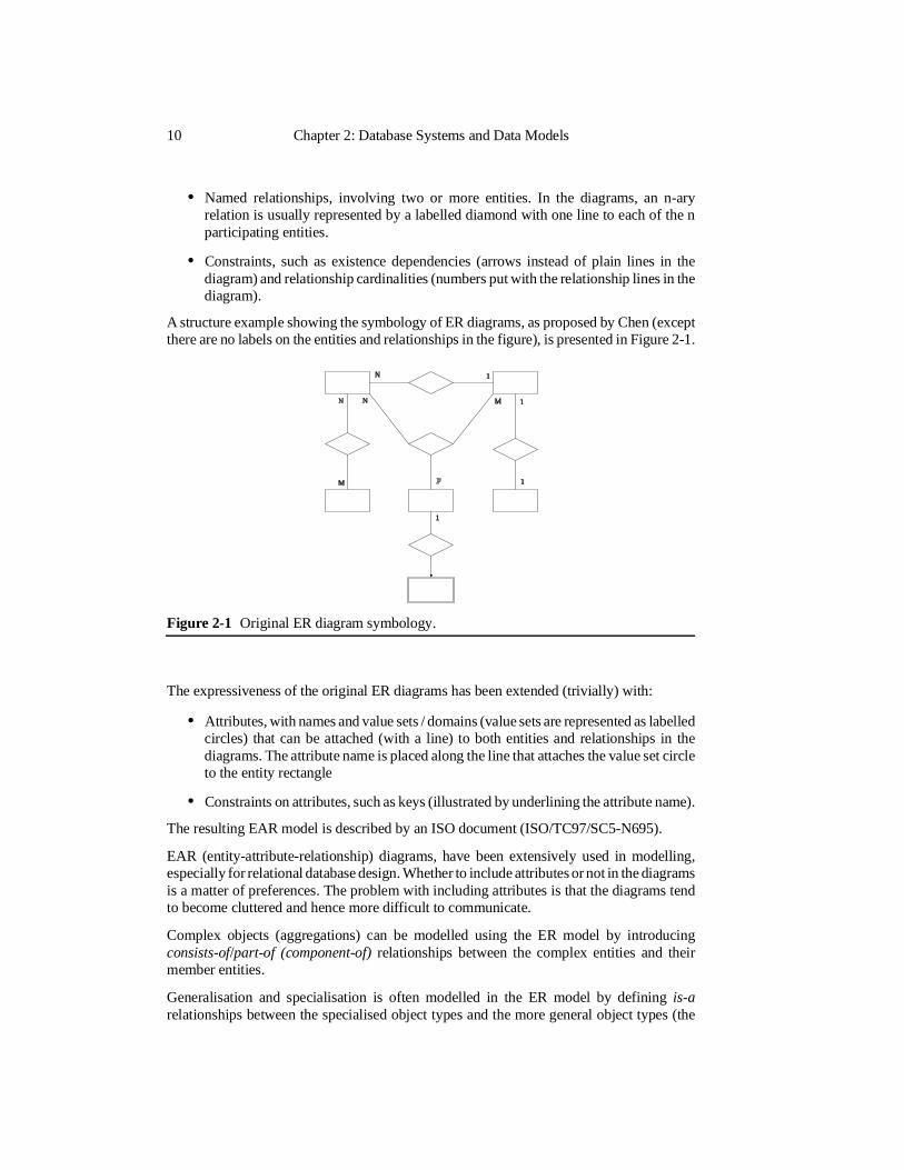
A structure example showing the symbology of ER diagrams, as proposed by Chen (exceptthere are no labels on the entities and relationships in the figure), is presented in Figure 2-1.

The expressiveness of the original ER diagrams has been extended (trivially) with:

• Attributes, with names and value sets / domains (value sets are represented as labelledcircles) that can be attached (with a line) to both entities and relationships in thediagrams. The attribute name is placed along the line that attaches the value set circleto the entity rectangle

• Constraints on attributes, such as keys (illustrated by underlining the attribute name).

The resulting EAR model is described by an ISO document (ISO/TC97/SC5-N695).

EAR (entity-attribute-relationship) diagrams, have been extensively used in modelling,especially for relational database design. Whether to include attributes or not in the diagramsis a matter of preferences. The problem with including attributes is that the diagrams tendto become cluttered and hence more difficult to communicate.

Complex objects (aggregations) can be modelled using the ER model by introducingconsists-of/part-of (component-of) relationships between the complex entities and theirmember entities.

Generalisation and specialisation is often modelled in the ER model by defining is-arelationships between the specialised object types and the more general object types (the

Figure 2-1 Original ER diagram symbology.


vehicle object type is connected via is-a relationships from the more specialised object types:car, bus, bicycle, lorry, tractor, tram, …).

Associations can be modelled using is-member-of relationships.

Temporal relations(ips can be modelled by using precedes relationships, but history data orversioned objects do not have a particular modelling primitive (time is not included in theER model). Time can be supported using attributes (time of creation, time of destruction).

The ER modelling formalism was intended as a data modelling tool. The behavioural partof modelling is not addressed.

The big advantage of the basic ER model is that there are methods for translation of all itsconcepts into many popular database models (hierarchical, network and relational) [Ng81].It is therefore fairly straightforward to implement as a database schema something that hasbeen specified using the original ER model.

Another advantage of the ER model is its limited amount of modelling primitives, whichmakes the model easy to learn. The limited number of modelling primitives is also a problemwith the ER model. The pure ER approach can result in diagrams that are difficult tocomprehend/communicate because of the necessary overloading of the very limited numberof primitives.

An abstraction mechanism that would allow the recognition of overall structure by groupingand hiding independent sub-models is lacking in the ER model. Omission of attributes isthe only information hiding mechanism available, so it is not possible to perform multi-levelmodelling. As the number of entities and relationships in ER models increases, the diagramstend to become visually unmanageable. In psychology it has been found that humans onlycan process 5 to 9 information items at a time (George Millers paper in PsychologicalReview, march 1956, pp. 81-97 [Coad90]). According to this, diagrams with 10 to 100information items will be very hard to digest when there is no apparent way of groupingthem into more manageable pieces. In practical ER modelling of large structures it is alreadynormal to split the diagrams in one way or another. The ER model does, however, not offerany abstraction mechanisms to support such a partitioning of the model into sub-models.

The choice of representation for a phenomenon will in many cases be a matter of prefer-ences. There are no basic rules for when to apply entities and when to apply relationships.All relationships can, in theory, also be represented as entities. This can be confusing to theusers of the data modelling formalism.

2.2.2 EER models and diagrams

Extended Entity Relationship (EER) models and diagrams have been proposed to overcomesome of the deficiencies of the first generation of ER models ([Teorey86], [Batini86],[Elmasri89]). These models provide new abstraction mechanisms in addition to thoseprovided by the original ER model. The EER approach also introduces new symbology forsome of the most common abstractions to produce more easily comprehensible diagrams.Elmasri and Navathe’s proposal for an EER-model [Elmasri89] includes the notion of aclass (that encompasses entity types), subclasses, superclasses (the set of members of asubclass is always a subset of the set of members of the superclass) and categories


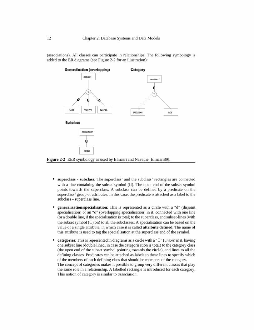
(associations). All classes can participate in relationships. The following symbology isadded to the ER diagrams (see Figure 2-2 for an illustration):

• superclass - subclass: The superclass’ and the subclass’ rectangles are connectedwith a line containing the subset symbol (⊂ ). The open end of the subset symbolpoints towards the superclass. A subclass can be defined by a predicate on thesuperclass’ group of attributes. In this case, the predicate is attached as a label to thesubclass - superclass line.

• generalisation/specialisation: This is represented as a circle with a “d” (disjointspecialisation) or an “o” (overlapping specialisation) in it, connected with one line(or a double line, if the specialisation is total) to the superclass, and subset-lines (withthe subset symbol (⊂ ) on) to all the subclasses. A specialisation can be based on thevalue of a single attribute, in which case it is called attribute defined. The name ofthis attribute is used to tag the specialisation at the superclass end of the symbol.

• categories: This is represented in diagrams as a circle with a “∪ ” (union) in it, havingone subset line (double lined, in case the categorisation is total) to the category class(the open end of the subset symbol pointing towards the circle), and lines to all thedefining classes. Predicates can be attached as labels to these lines to specify whichof the members of each defining class that should be members of the category.The concept of categories makes it possible to group very different classes that playthe same role in a relationship. A labelled rectangle is introduced for each category.This notion of category is similar to association.

Figure 2-2 EER symbology as used by Elmasri and Navathe [Elmasri89].


• constraints:superclass - subclass: A predicate to determine which characteristics a member of thesuperclass should have to be a member of the subclass.specialisations: A double line from the superclass to the circle to indicate that all themembers of the superclass must be members of some subclass. A “d” or an “o” inthe circle to indicate whether the specialisation is disjoint (no superclass member canbe member of more than one subclass) or overlapping.categorisation: A double line from the category class to the circle to indicate that allthe members of the defining classes must be members of the category class; Predi-cates to determine which members of the defining classes should be members of thecategory class.

This EER model does not include aggregation as a special concept, and that must beconsidered a weakness in the context of complex object modelling. By using aggregationsit would be easier to hide detailed information and emphasise overall structure by using alevelled or black-box based method. The structure of the EER model makes it possible todo some sort of multi-level modelling, but it is meant to be a single-level approach, henceit inherits the one-level weakness from the ER model.

The EER model performs reasonably well for semantic modelling when compared to otherpopular modelling formalisms. In an empirical study, comparing data modelling formalisms[Kim95c], the EER model [Teorey86] was compared to the NIAM [Nijssen77] model, oneof the most popular object-relationship (a sort of binary model [Tsichritzis82]) model[Biller77]. The findings of this empirical study can be summarised as follows (six hypothe-sis were tested). (1) There was no significant difference between the NIAM user group andthe EER user group in their model comprehension performance, (2) the NIAM users groupdid not perform significantly better than the EER user group in the discrepancy-checkingtask, (3a) there was no significant difference between the NIAM user group and the EERuser group in their perceived difficulty of formalism, but (3b) the EER users valued theirmodelling formalism significantly more than the NIAM users, (4) EER analysts produceda data model of significantly higher semantic quality than NIAM analysts, (5) EER analystsdid not produce a data model of significantly higher syntactic quality than NIAM analysts,(6) the EER users perceived their modelling formalism to be significantly more useful thanthe NIAM users.

2.2.3 Object-oriented data models

Object-oriented modelling research, starting in the 1980s, had its roots in semantic datamodels and object-oriented programming languages (such as SIMULA [Birtwistle73] andSmalltalk [Goldberg83]). Object-oriented data models incorporate such things as encapsu-lation and behaviour in addition to the structuring mechanisms of semantic data models[Rumbaugh91] [Coad90]. Direct realisations of object-oriented data models into object-ori-ented database systems has received a lot of attention, gaining momentum in the mid 1980s[Abiteboul90]. Ideas of richer database models than the relational model was, however,starting to emerge already in the late 1970ies (e.g. the SIMULA based ASTRA with theASTRAL (extended Pascal) language [Bratbergsengen83] and PASCAL/R [Schmidt83b]).Modelling approaches that incorporate mechanisms from semantic data models are calledstructurally object-oriented, while those using mechanisms from object-oriented program-


ming languages are termed behaviourally object-oriented. An object-oriented modellingapproach should incorporate both the behavioural and the structural aspects.

Object-oriented programming languagesThe behavioural aspect of object-oriented data models has evolved from the field ofobject-oriented programming languages, having their roots in SIMULA [Birtwistle73] inthe late 1960s, and continuing with Smalltalk [Goldberg83] and C++ [Stroustrup91] in the1970s and 1980s.

The key features of object-oriented programming languages are:

• Abstract data types, including methods for presenting and manipulating the state ofthe objects.

• Communication by message passing. To inquire an object about some property, amessage is sent to the object. The messages constitute the interface to the object.

• Encapsulation/information hiding. Access to the internals of the objects is restricted,so information on an object is generally only available through its public interface(methods).

• Generalisation/specialisation hierarchies. A car, a bus and a lorry all have somecommon properties that can be captured by the more general class of vehicles. Cars,busses and lorries are specialised subsets of vehicles.

• Inheritance: properties and methods are inherited from the root of a generalisationtree and out to the leaves.

Object-Oriented modelling and analysisObject-oriented data models combine abstractions from semantic data modelling andobject-oriented programming languages. This makes them useful for many classes of realworld modelling. Their advantage is in areas where behaviour is important. Simulation issuch an application domain, often used in decision support systems. Object-orientedapproaches provide an integrated framework for modelling both applications and the datathe applications will be working on [Coad90]:

… it combines the data and process model into one complete model

Object-oriented methodology has a great potential for GIS modelling, but for the geographi-cal data modelling undertaken in this thesis, structural methods are considered sufficient,as explained further in chapter 5.

2.3 Database systems

Database systems facilitate data sharing and easy access to data. This is made possible byproviding standardised interfaces to the data in the database and applying mechanisms thatensure consistent access to the data for concurrent users. In addition to this, the databasesystems ensure database consistency after system failure.


2.3.1 Brief history

The history of electronic data management started with the “process-oriented” period(1960-1970). In this period, before database systems were introduced, applications and theirdata were tied intimately together. Files could be shared between applications, but thestructuring of the data was embedded within the applications. This meant that in order toapply a small modification to the data structure in a file it was necessary to change all theapplications that were using it. By far the easiest approach for such systems was thereforeto let the data structures remain static. Consequently, new and more efficient data structuringmethods were difficult to take advantage of. In this period, work on data management systemstarted, and early commercial systems emerged (e.g. IDS in 1962, and IMS-2/VS in 1968[Wiederhold81]) with standardised access methods.

The “data-oriented” period (1970-) followed this first period. The necessity of controlledsharing of data was recognised, particularly for business data within large organisations.The introduction of the database system approach, as we know it today, occurred early inthis period. Standard database models with standard interfaces to the data were developed(network, hierarchical and relational), hiding the internal structure of the database (accessstructures and internal data formats) from the applications. The security and integrity ofdata in multi-user centralised - and distributed - database systems has continuously beenenhanced through advances in transaction management research (concurrency controlmechanisms, recovery protocols and commit protocols).

Reaching the beginning of the 1990ies, the database needs of most business type applica-tions have been satisfied by current commercially available database system technology.Engineering applications and other applications based on complex data do, however, seemto have demands on databases that go beyond the capabilities of current database technology[Carey90] [Maier89] [Frank84] [Egenhofer87] [Frank88]. These applications have, forefficiency and modelling reasons, until now not been utilising database systems for themanagement of their data. Some database systems have been constructed to meet the specialneeds of technical application, such as the extended relational system TECHRA[TECHRA93]. During the last decade, the need for database system support has becomeapparent also for applications that work on complex data. To try to meet these needs,extensions to the now maturing relational database management systems have been pro-posed (in competition with object-oriented databases). These new database systems shouldprovide a more flexible and efficient environment for integrating applications and data.

2.3.2 Definitions

There have been many attempts on defining a good and consistent terminology for theresearch field of database systems. The descriptions provided below, taken from Elmasriand Navathe’s book on database systems [Elmasri89], apply for this thesis and reflect themost common terminology in the database literature.

Database“A database is a logically coherent collection of data with some inherent meaning.A random assortment of data cannot be referred to as a database.”“A database is designed, built, and populated with data for a specific purpose. Ithas an intended group of users and some preconceived applications in which these

Database systems 15

users are interested.”“A database represents some aspect of the real world, sometimes called themini-world. Changes to the mini-world are reflected in the database.”

Database management system (DBMS)“A database management system (DBMS) is a collection of programmes thatenables users to create and maintain a database. The DBMS is hence a general-pur-pose software system that facilitates the processes of defining, constructing, andmanipulating databases for various applications.”

Database system ( = database + DBMS)… “ - we usually have a considerable amount of software to manipulate the databasein addition to the database itself. The database and software are together called adatabase system.”

Self-contained nature of a database system“A fundamental characteristic of the database approach is that the database systemcontains not only the database itself but also a complete definition or description ofthe database. This definition is stored in the system catalogue, …”

Distributed DBMS (DDBMS)“A distributed DBMS (DDBMS) can have the actual database and DBMS softwaredistributed over many sites connected by a computer network. HomogeneousDDBMSs use the same software at multiple sites. A recent trend is to developsoftware to access several autonomous pre-existing databases stored under hetero-geneous DDBMSs. This leads to a federated DBMS (or multidatabase system),where the participating DBMSs are loosely coupled and have a degree of localautonomy.”

2.3.3 The three-schema architecture

The three-schema architecture (or the ANSI/X3/SPARC DBMS Framework [Yor-mark77][Tsichritzis78]) is a recognised three level model for database system architecture(Figure 2-3).

The internal schema/level is the direct interface to the data structures used to implementthe database. Low level features, such as pointers, hash tables and other data structures areavailable at this level. All the mechanisms provided by the conceptual schema must betranslated into the operations and data structures of the internal schema. The internal schemais only used by system programmers to implement data formats and operations at theconceptual level of the database system.

The conceptual schema is described as follows [Elmasri89]:

The conceptual schema is a global description of the database that hides the detailsof physical storage structures and concentrates on describing entities, data types,relationships, and constraints. A high-level data model or an implementation datamodel can be used at this level.

The external schema/level provides specialised views of the database. Each external viewis tailored to a user or a group of users, so that only the data and operations that are of interest


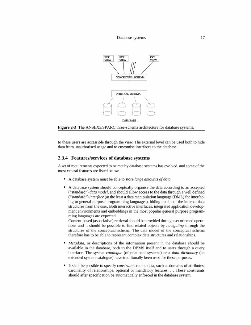
to these users are accessible through the view. The external level can be used both to hidedata from unauthorised usage and to customise interfaces to the database.

2.3.4 Features/services of database systems

A set of requirements expected to be met by database systems has evolved, and some of themost central features are listed below.

• A database system must be able to store large amounts of data

• A database system should conceptually organise the data according to an accepted(“standard”) data model, and should allow access to the data through a well defined(“standard”) interface (at the least a data manipulation language (DML) for interfac-ing to general purpose programming languages), hiding details of the internal datastructures from the user. Both interactive interfaces, integrated application develop-ment environments and embeddings in the most popular general purpose program-ming languages are expected.Content-based (associative) retrieval should be provided through set oriented opera-tions and it should be possible to find related objects by navigating through thestructures of the conceptual schema. The data model of the conceptual schematherefore has to be able to represent complex data structures and relationships.

• Metadata, or descriptions of the information present in the database should beavailable in the database, both to the DBMS itself and to users through a queryinterface. The system catalogue (of relational systems) or a data dictionary (anextended system catalogue) have traditionally been used for these purposes.

• It shall be possible to specify constraints on the data, such as domains of attributes,cardinality of relationships, optional or mandatory features, … These constraintsshould after specification be automatically enforced in the database system.

Figure 2-3 The ANSI/X3/SPARC three-schema architecture for database systems.

Database systems 17

• A database system should provide multiple users with concurrent and controlledaccess to the data through transaction management [Bernstein87]. Transactionmanagement should provide atomic transactions through the recovery system andserialisability or other correctness criteria through concurrency control.An atomic transaction should have the ACID transaction properties. ACID stands for:Atomic, Consistency preserving, Isolated and Durable transactions [Elmasri94]. The notion of atomic transactions imply that either the whole transaction (all of theoperations) is done or nothing is done. No partial execution of transactions areallowed. A recovery system shall monitor transactions and log all changes made tothe database on secure/permanent storage. If the system crashes for some reason, therecovery system will go through this log and bring the database back to a consistentstate. This can be done by making sure that all changes made by committed transac-tions (transactions that have finished as the crash occurred) are reflected in thedatabase (REDO-ing changes made by these transactions that are not reflected in thedatabase), while non of the changes made by transactions that were aborted by thesystem crash are left in the database (UNDO-ing these changes).Serialisability is currently the most recognised correctness criterion for concurrencycontrol mechanisms in database systems. A sequence of database operations belong-ing to different concurrent transactions is serialisable if the resulting state of thedatabase could have been obtained by performing some serial execution of theinvolved transactions.Serialisability does not seem to be a good criteria for co-operative work, such as indesign and planning. New kinds of concurrency control mechanisms are needed tocontrol the complex interactions between co-operating concurrent processes.

• Multiple views on the data should be supported to provide customised interfaces tothe data and to enforce access restrictions, avoiding unauthorised usage of the data.

• Fault tolerance is a desirable feature of database systems containing vital informationthat has to be kept on-line at all hours. Fault tolerance means that the database systemshould be able to continue to operate normally (having the complete databaseavailable) also in the case of failures. Failures could be a disk-crash, memory errors,loss of power, communication failure, program error, etc. Fault tolerance can beobtained through controlled redundancy. Mirroring of disks can be used to take careof disk crashes. RAID* technology provide the same functionality [Chen94][Ganger94] [Patterson88]. Duplication can be used for most hardware elements in adatabase system to provide fault tolerance (processors, communication channels, tapedrives, disk drives and controllers).

In addition to these basic features, monitoring of the database (usage statistics) is providedby most commercial database management systems.

2.3.5 Distributed database systems

Distributed database systems is an active area of research [Özsu91] [Garcia-Molina95]. Bystoring logically connected data at different sites or computers, many interesting issues arise.Distributed transaction management (atomicity, serialisability, concurrency control, com-mit protocols), distributed query optimisation, reliability of distributed databases and the


* Redundant Array of Inexpensive/Independent Disks [Chen94]

use of redundancy are all good examples of the complex problems that are receivingattention in this field [Bernstein87] [Breitbart92] [Ceri88].

Multidatabases or federated database systems are loosely connected database systemswhere the individual databases could be organised according to different database models,and each database system has a high degree of local autonomy [Hsiao92]. Methods forachieving (transparent) data sharing in this kind of environment are emerging, but stillconstitute a topic for research [Breitbart92] [Kim95d].

Object-oriented approaches to distributed data management have been proposed, usingobject-oriented abstractions to specify high level interfaces to the databases through forinstance a distributed conceptual schema [Papazoglou90].

2.3.6 Database machines

The management of large databases has become a problem in many application areas. Thishas encouraged research in reliable, high capacity database systems. Special purposedatabase machines (or database computers) [Su88] have come out of this research. One ofthe most promising approaches are the parallel database machines, where multiple proc-essors are co-operating in storing and retrieving data from a shared database (generallydistributed over a number of disks). Such architectures are used both to achieve betterperformance and to improve availability [Kim84]. This research has lead to commercialproducts, among which the Tandem (NonStop System) was of the first (the NonStopfault-tolerant architecture came in 1976 [Katzman78], the (distributed) transaction managerENCOMPASS came a little later [Kim84]).

Parallel database machines can provide improved performance [DeWitt85] through distri-bution and parallel processing and reliability through duplication of hardware and data.

The relational database model has proved itself as a good model for parallelisation, andmost current parallel database machines are based upon the relational paradigm [Omiecin-ski95]. In Norway there have been experiments on parallel relational database machines,and several generations of experimental parallel database machine have been built at NTHin Trondheim [Bratbergsengen89].

2.3.7 Status of database systems

Vossen gives a short and nice overview of the status of database systems entering the 1990ies[Vossen91]. The following is partly based on his observations.

The database systems of the 1980ies are good at handling:

• Simply structured data objects (record oriented)

• Simple data types (number, character string, …)

• Short transactions

• High transaction rates

• Frequent in-place updates

Database systems 19

New areas of database applications differ significantly from the traditional databaseapplication areas, and need support for:

• Complex (evolving) data models

• New data types, for instance spatial data types, such as images and topologicalstructures, with associated data structures and operators

• Integration of very different data types

• Relaxed consistency constraints

• Long transactions with few serious access conflicts (which must lead to re-evaluationof concurrency control and recovery mechanisms)

• Fault tolerance and 100% availability

• High data rates with guaranteed service, as required by for instance video servers

• Extremely low response times, as demanded by real time applications (“real timeDB”)

These features are not well supported by the database systems of the 1980ies, and must begiven more emphasis in the years to come. Geographical information systems is oneexample of these “new” application areas.

2.4 Database models

The three-schema architecture’s conceptual schema can presently be specified using threeor four major approaches. The different approaches to conceptual schema definition willhere be termed database models. The most popular models, up to 1990, have been the twoset models (the hierarchical and the network model), the relational model, and recently alsoobject-oriented models.

2.4.1 Hierarchical DBMSs

In the middle of the 1960s the first commercial hierarchical database management systemswas on the market, one of them being IMS of IBM* (1968). GIS** of IBM was a hierarchicalquery and update system that was out even earlier (1966). There is no formal theory onhierarchical database models, but some common characteristics of the family can beidentified [Tsichritzis82] [Elmasri89].

The abstractions used in hierarchical models are records (entities) and parent-child rela-tionships. A parent-child relationship type has one owner record type (parent) and onemember record type (child). A record type can act as the owner of many different parent-child relationship types, but can only act as a member of one parent-child relationship type,thereby forming a strict hierarchy. An instance of the parent-child relationship type has aunique owner record (from the owner record type) and zero or many member records (fromthe member record type).


* International Business Machines

** General Information System

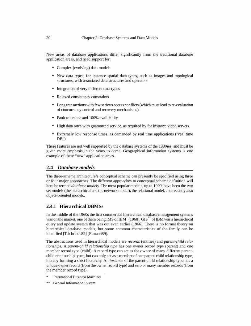
Hierarchical models support one-to-many (1:N) hierarchical relationships in a natural way,but many-to-many (M:N) relationships and non-hierarchical structures are impossible tohandle without introducing some kind of data duplication. N-ary relationships are even moreproblematic. Virtual records have been introduced to allow other relationship types thanone-to-many.

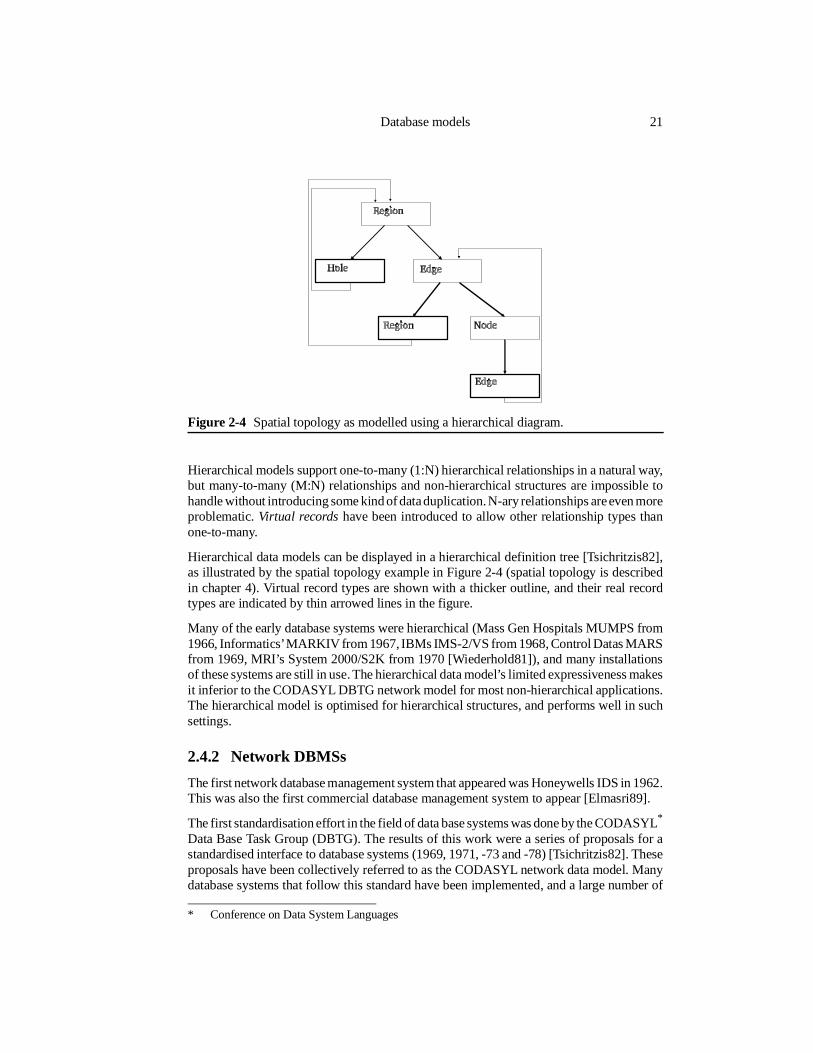
Hierarchical data models can be displayed in a hierarchical definition tree [Tsichritzis82],as illustrated by the spatial topology example in Figure 2-4 (spatial topology is describedin chapter 4). Virtual record types are shown with a thicker outline, and their real recordtypes are indicated by thin arrowed lines in the figure.

Many of the early database systems were hierarchical (Mass Gen Hospitals MUMPS from1966, Informatics’ MARKIV from 1967, IBMs IMS-2/VS from 1968, Control Datas MARSfrom 1969, MRI’s System 2000/S2K from 1970 [Wiederhold81]), and many installationsof these systems are still in use. The hierarchical data model’s limited expressiveness makesit inferior to the CODASYL DBTG network model for most non-hierarchical applications.The hierarchical model is optimised for hierarchical structures, and performs well in suchsettings.

2.4.2 Network DBMSs

The first network database management system that appeared was Honeywells IDS in 1962.This was also the first commercial database management system to appear [Elmasri89].

The first standardisation effort in the field of data base systems was done by the CODASYL*

Data Base Task Group (DBTG). The results of this work were a series of proposals for astandardised interface to database systems (1969, 1971, -73 and -78) [Tsichritzis82]. Theseproposals have been collectively referred to as the CODASYL network data model. Manydatabase systems that follow this standard have been implemented, and a large number of

Figure 2-4 Spatial topology as modelled using a hierarchical diagram.

Database models 21

* Conference on Data System Languages

databases are organised and managed by CODASYL systems. The CODASYL networkdata model is more conveniently called the network model.

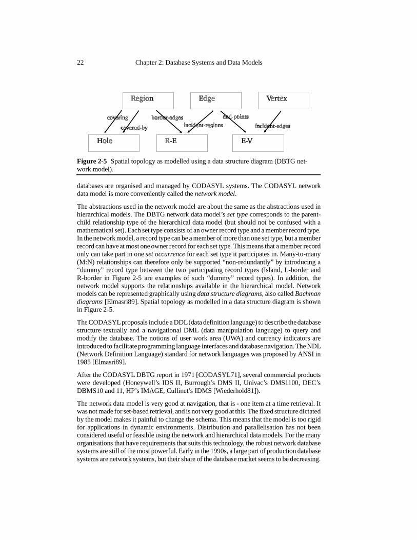
The abstractions used in the network model are about the same as the abstractions used inhierarchical models. The DBTG network data model’s set type corresponds to the parent-child relationship type of the hierarchical data model (but should not be confused with amathematical set). Each set type consists of an owner record type and a member record type.In the network model, a record type can be a member of more than one set type, but a memberrecord can have at most one owner record for each set type. This means that a member recordonly can take part in one set occurrence for each set type it participates in. Many-to-many(M:N) relationships can therefore only be supported “non-redundantly” by introducing a“dummy” record type between the two participating record types (Island, L-border andR-border in Figure 2-5 are examples of such “dummy” record types). In addition, thenetwork model supports the relationships available in the hierarchical model. Networkmodels can be represented graphically using data structure diagrams, also called Bachmandiagrams [Elmasri89]. Spatial topology as modelled in a data structure diagram is shownin Figure 2-5.

The CODASYL proposals include a DDL (data definition language) to describe the databasestructure textually and a navigational DML (data manipulation language) to query andmodify the database. The notions of user work area (UWA) and currency indicators areintroduced to facilitate programming language interfaces and database navigation. The NDL(Network Definition Language) standard for network languages was proposed by ANSI in1985 [Elmasri89].

After the CODASYL DBTG report in 1971 [CODASYL71], several commercial productswere developed (Honeywell’s IDS II, Burrough’s DMS II, Univac’s DMS1100, DEC’sDBMS10 and 11, HP’s IMAGE, Cullinet’s IDMS [Wiederhold81]).

The network data model is very good at navigation, that is - one item at a time retrieval. Itwas not made for set-based retrieval, and is not very good at this. The fixed structure dictatedby the model makes it painful to change the schema. This means that the model is too rigidfor applications in dynamic environments. Distribution and parallelisation has not beenconsidered useful or feasible using the network and hierarchical data models. For the manyorganisations that have requirements that suits this technology, the robust network databasesystems are still of the most powerful. Early in the 1990s, a large part of production databasesystems are network systems, but their share of the database market seems to be decreasing.

Figure 2-5 Spatial topology as modelled using a data structure diagram (DBTG net-work model).


2.4.3 Relational DBMSs

The relational data model, introduced by Codd [Codd70], is a database model that buildson the mathematical concepts of sets and relations. Functional dependencies and keys aretwo other concepts that are important in the modelling and design of relational databases.

• The properties of sets important to the relational model are the following: Duplicatesare not allowed in a set, and a set imposes no ordering on its members.

• A relation establishes a connection between an arbitrary number of domains (n-aryrelations are relations which include n domains). Relations are represented as tuples.A tuple is a collection that contains one instance of each of the domains participatingin the relation. The tuples of a relation are organised as unordered rows in atwo-dimensional table.

• Functional dependencies. If, in a relation R, a set of attributes, B, is functionallydependent on a set of attributes, A, this means that if two tuples of R have the samevalue for A, they must also have the same value for B.

• Keys. A key of a relation is a minimal set of attributes that functionally determinesall the attributes of the tuple (since duplicates are not allowed, no tuples in a relationcan have the same key). A relation can have many keys (e.g. the set of all attributesof a relation makes up a key), in which case one of them is chosen as the primarykey.

Relations are created to describe relevant features of the phenomena being modelled. Thesefeatures include relationships between phenomena in addition to the individual phenomenawith their characteristics/attributes. A person could, in the relational model, be described byattributes such as name, date of birth and colour of the eyes, and by its relationships to otherphenomena such as father, mother, employer and place of living. All these properties canbe grouped together into an (unnormalised) person relation in the relational model.

Relations are used to store most of the system information in a relational database system.A table is established for each relation in the (normalised) data model.

Operations in the relational model are defined in the relational algebra or the relationalcalculus.

The relational algebra consists of the relational operators selection (σ), that is a set-operationthat retrieves tuples based on values of the attributes of a relation, projection (π), that picksout certain domains/attributes/columns from a relation, and join ( ) that is a sophisticationof the cartesian product, where two relations are combined into a new relation on the basisof the values of some common domain(s) of the relations, the new relation will consist ofall the domains of the original relations. In the new relation, a row from the first relation iscombined with all the rows of the second relation that satisfies the condition on the joinattributes.

Natural join (*) is an equi-join (the condition on the join attributes is equality), where thejoin-domains are not duplicated. In addition, the general set operations union (∪ ), intersec-tion (∩) and difference (-) are available in the relational model.

Database models 23

The relational calculus is related to first-order predicate calculus, using the logical symbols∧, ∨, ¬, ∀, ∃ (and, or, not, for all, exists). In tuple relational calculus the variables havetuples as their range, while in domain relational calculus the variables have attribute valuedomains as their range.

pAB(σC=1(R)) in the relational algebra is equivalent to {t.A, t.B | (R(t) ∧ (t.C=1)} in thetuple relational calculus and {A, B | (∃ C) (R(ABC) ∧ C=1) } in the domain relationalcalculus. Both SQL (Structural Query Language) and QUEL (the query language of theINGRES database management system) are related to the tuple relational calculus. QUELis much closer related to the relational calculus than is SQL [Elmasri89]. QBE (Query ByExample) is related to the domain relational calculus.

NormalisationTo avoid the problems that duplication of information can introduce, normalisation isperformed on relational data models before realisation in a database system [Date86][Elmasri89].

A measure of a relational design is provided by the normal form metric, describing theproperties of a relational design. Normal forms were introduced by Codd in 1971-1972[Tsichritzis82]. In this first effort, a series of three normal forms was defined. The notionof functional dependency as introduced in Codd’s original paper [Codd70] is very importantfor specifying these original normal forms.

• The first normal form (1NF) requires that all attributes in a relational scheme areatomic (no group of values are allowed for a single attribute).

• The second normal form (2NF) requires that the relation is on first normal from, andthat all attributes that are not part of the primary key shall be functionally dependenton the primary key of the relation, but not functionally dependent on a subset of theprimary key.

• The third normal form (3NF) requires that the relation is on second normal from, andthat no transitive functional dependencies exist in the relation.

Further normal forms have been specified since then, among them Boyce-Codd normal form(BCNF, which is stronger than 3NF), 4NF (introducing multi-valued dependencies) and5NF (introducing join dependencies). The more normalised a relational schema is, the morewell-behaved it will be in the case of queries and updates. A relational schema can benormalised by splitting the relations that violate the conditions of normalisation. For somekinds of normalisation, it is not possible to split relations without loosing functionaldependencies or introducing replication. There is also a penalty on splitting relations,because of all the joins that must be performed to reconstruct the universal relation (arelation consisting of all the attributes of the relational schema). The choice of how far tonormalise will depend on the application.

SQLSQL (Structured Query Language) is the standard interface to relational databases. The SQL“standard” has been enhanced in a stepwise fashion to meet new user requirements[Melton90].


The traditional SQL (SQL-86 and SQL-89) data types are INTEGER, SMALLINT, CHAR-ACTER, DECIMAL, NUMERIC, REAL, FLOAT and DOUBLE PRECISION. The SQL2standard includes commonly available extensions such as CHARACTER VARYING,DATE, TIME, BIT, TIMESTAMP, INTERVAL and BIT VARYING [Melton90].

Traditional SQL uses the following operators: SELECT, INSERT, UPDATE, DELETE, join(a join between the tables X and Y on the column COL is specified by the conditionX.COL=Y.COL), project (the column in the projection are specified in the SELECT part ofthe query), UNION, comparison (=, ~=, >, >=, ~>, <, <=, ~<, [NOT] LIKE, IS [NOT]NULL, IN (set membership), [NOT] EXISTS), AND, OR, NOT, aggregations (COUNT,SUM, AVG, MAX, MIN), GROUPing, aliasing and ORDERing. SQL2 adds INTERSECT,EXCEPT (difference), OUTER JOIN, CROSS JOIN, NATURAL JOIN.

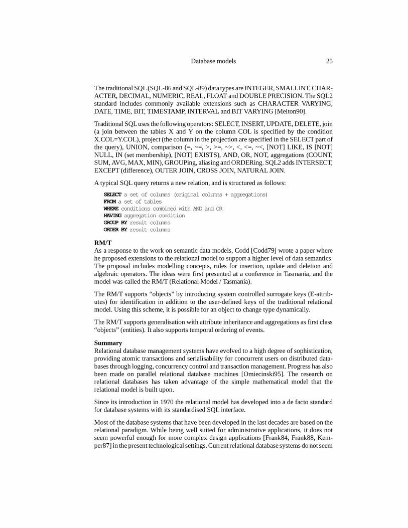
A typical SQL query returns a new relation, and is structured as follows:

SELECT a set of columns (original columns + aggregations)FROM a set of tablesWHERE conditions combined with AND and ORHAVING aggregation conditionGROUP BY result columnsORDER BY result columns

RM/TAs a response to the work on semantic data models, Codd [Codd79] wrote a paper wherehe proposed extensions to the relational model to support a higher level of data semantics.The proposal includes modelling concepts, rules for insertion, update and deletion andalgebraic operators. The ideas were first presented at a conference in Tasmania, and themodel was called the RM/T (Relational Model / Tasmania).

The RM/T supports “objects” by introducing system controlled surrogate keys (E-attrib-utes) for identification in addition to the user-defined keys of the traditional relationalmodel. Using this scheme, it is possible for an object to change type dynamically.

The RM/T supports generalisation with attribute inheritance and aggregations as first class“objects” (entities). It also supports temporal ordering of events.

SummaryRelational database management systems have evolved to a high degree of sophistication,providing atomic transactions and serialisability for concurrent users on distributed data-bases through logging, concurrency control and transaction management. Progress has alsobeen made on parallel relational database machines [Omiecinski95]. The research onrelational databases has taken advantage of the simple mathematical model that therelational model is built upon.

Since its introduction in 1970 the relational model has developed into a de facto standardfor database systems with its standardised SQL interface.

Most of the database systems that have been developed in the last decades are based on therelational paradigm. While being well suited for administrative applications, it does notseem powerful enough for more complex design applications [Frank84, Frank88, Kem-per87] in the present technological settings. Current relational database systems do not seem

Database models 25

to be able to manage large amounts of complex data and long lasting transactions that operateon such data.

Ingres, Oracle, Sybase, Informix, Tandem non-stop (parallel database machine) andDBaseIV (personal computers) are some of the most popular of the currently availablerelational database systems.

2.4.4 Object-oriented DBMSs

The problems of mapping complex data models to database models have lead to a greatinterest in realisations/implementations of high-level data models. One solution has beento build the database system around abstract data types and object-oriented programminglanguages, thereby supporting all the object-oriented programming paradigms [Atkin-son87]. These kinds of database systems have been termed object-oriented databasemanagement systems (OODBMS). OODBMSs were introduced into the field of databasesystems in the middle of the 1980ies. Many of the first systems have been based on C++(often termed persistent C++). Research on OODBMSs has grown tremendously, and iscurrently one of the most pursued in the field of database systems [Banchilon90].

If an object-oriented DBMS could be built, it would save all the efforts currently being spenton translating semantic data models into computer representable mechanisms and struc-tures. With OODBMSs, once the system is modelled, the database schema is also completelyspecified! Not surprisingly, it has been problematic to implement fully object-orientedDBMSs, and the complexity of such systems seems to demand further research beforeOODBMS technology will be really “competitive”.

To be able to function as a proper database system, an OODBMS must support most of thebefore mentioned DBMS features, in addition to the features of object-oriented program-ming languages and semantic data models. Among other things, OODBMSs bring naviga-tion mechanisms as previously used in the network model back to database systems to obtainbetter performance for widely used non-set-based retrievals.

There has been controversy about what OODBMSs are and should be. In order to try tomake the foundations more firm, some of the most active researchers in the field came upwith a list of features OODBMSs should include, the so called “object-oriented databasesystem manifesto” [Atkinson89]. This effort was intended to provide the basis for morefruitful discussions. The key features of OODBMSs, according to this list, are:

• Complex objects

• Unique object identity (preferably with a version mechanism)

• Encapsulation, information hiding

• Types and classes (preferably with type checking)

• Class or type hierarchies with inheritance (preferably multiple inheritance)

• Overriding, overloading, late binding

• Computational completeness


• Extensibility (schema evolution)

• Persistence

• Secondary storage management (very large data sets)

• Concurrency control (preferably long transactions)

• Recovery

• Ad hoc query facilities

Object-oriented database issues divided the database research community into two camps,one in favour of building object-oriented database systems from scratch, the other in favourof extending the existing (relational) database systems to capture more real world semantics(called extended relational database models), as proposed in the “third generation databasesystem manifesto” [Stonebraker90].

Advantages of object-oriented databases are:

• Trivial compilation of semantic high-level data models into the database conceptualschema (they are the same).

• The database is fully integrated within a programming language, and thereforecomputationally complete. The so-called impedance mismatch between program-ming languages and traditional database systems is avoided.

• Possibilities for inclusion of behaviour in the database.

• Uniform interface to all objects through methods specified in the data model. Thismakes them a strong integration tool. It is possible to specify standard interfaces toheterogeneous devices, applications, databases and systems, as long as they offer thenecessary/same functionality.

• Abstraction and encapsulation (information hiding), keeping internal structureshidden from the applications.

• Reuse of code through inheritance.

• Schema evolution is claimed to be easier in OODBMSs than in present DBMSs.

Disadvantages of object-oriented databases are:

• OODBMSs are complex, and therefore difficult to implement.

• There is not yet a production quality OODBMS (?).

• The present lack of a simple, formal object-oriented data model [Beeri90] makesspecification complicated, and leads to a lack of standards for distributed computingand sharing of data.

• The lack of an SQL-like associative set-based query language. Todays OODBMSare advanced network database systems (based on navigation).

Database models 27

• Global optimisation is difficult, because the optimiser should not be allowed to accessthe internal data structures of the objects (encapsulation). E.g. indexing based onattribute values is complicated.

• Encapsulation means security, but also overhead.

The lack of standards in many fields of information management makes the object-orientedapproach attractive for integration [Kim95d]. If good standards for information exchangeevolve, the need for the integration mechanisms of object-oriented technology could beexpected to decrease.

Object-oriented databases take advantage of clustering and buffering in main memory toachieve high performance. Since many of the OODBMSs are aiming at the constructionand design market (CAD), check-in and check-out of complete “drawings” has normallybeen the only level of concurrency control in OODBMSs. By keeping the completeworkspace (all interesting data) in main memory, efficient interactive systems are possible.This kind of clustering and buffering could complicate concurrency control for more generalpurpose databases.

Object Store, O2 [Deux90], Ontos, Gemstone and Postgres [Stonebraker91] are someexamples of early OODBMS products.

2.4.5 Deductive DBMSs

Deductive databases build on deduction in logic, as found in the programming languageProlog [Clocksin84]. Deductive database systems store rules and facts, and are able toanswer queries to the database by combining these rules and facts. Expert systems andknowledge-based systems are application areas that need the support of a deductive databasesystem.

A central constraint in deductive database systems and logic is the closed world assumption(CWA). The CWA is a prerequisite for making deductions on the basis of a set of rules andfacts. It means that one assumes that facts that are not present in the database do not exist,and the same thing applies to rules.

Research in deductive databases has been concentrated on developing fast methods tocombine rules and facts, in order to perform deductions as rapidly as possible. The researchhas encompassed both special purpose hardware, and the development of new algorithmsfor efficient combination of corresponding rules and facts.

Active database systems are database systems that have production rules for integrityconstraint enforcement, derived data maintenance, triggers, alerters, protection, versioncontrol, and others [Dayal95]. The rule processing capabilities of active database systemsalso make them suitable for handling deductive databases.


Chapter 3

Geographical Information Systems

The paper map has for some thousand years been the main carrier of geographically relatedinformation. Increasing demands on availability of information and efficiency of informa-tion processing has lead to a need for better ways of storing and distributing suchinformation.

GISs (Geographical Information Systems) are expected to provide the answer to theseneeds.

This chapter is a short presentation of geographical information system topics and theircurrent status. The last three sections explores future trends, parallelisation issues andgeographical information servers.

3.1 History

People have always had a need for geographically related information. In the earliest times,when man’s principal occupation was hunting and collecting food, geographical informa-tion (for navigating between the “home”, good places for collecting different herbs, fruitsand vegetables, good areas for hunting, …) could normally only be “stored” in the humanbrains. Orientation was probably centred around significant landmarks and landscapefeatures such as rivers, lakes, mountain ranges and vegetation boundaries. The amount ofman-made features and infrastructure started to increase from nearly zero when man settleddown and started with agriculture. From then on, there has been a steady increase in bothinfrastructure and the number of man-made features. In the last couple of centuries, thegrowth has exploded.

Orientation and the organisation of the human society have become more and more complexas the amount of man-made features has increased.

The traditional (paper) map, being an abstraction of the landscape as observed by humans,has been a very important tool for both orientation and land-use planning and - administra-tion. It has always been the main carrier of geographically related information (stonecarvings and paper maps). Today we have an enormous amount of maps of varying scalefor different purposes stored in voluminous archives all over the world.

In parallel with the proliferation of maps, the amount of geographically relatable data hassteadily increased. Information about land-owners, land use, vegetation, mineral reserves,wild-life, infrastructure and all kinds of services is growing day by day. This growth in theamount of infrastructure, utilities and available information has led to a need for morepowerful management tools.

The present situation requires highly skilled personnel with many years of experience tohandle and utilise the available information in an efficient way. This is partly due to the lackof tools for efficient integration of the many information sources, which therefore have tobe integrated “by hand” (or head), and partly due to the complexity of the tasks. There ishope that GISs will provide a means to make geographical information more accessible toa broader class of users.

GISs originated in Canada in the early 1960ies [Tomlinson89] [Nagy79].

3.2 Definitions of GIS

In one of the first wide-spread textbooks on GIS, Burrough uses the following definition ofGIS [Burrough89]:

.. tools for collecting, storing, retrieving at will, transforming, and displaying spatialdata from the real world for a particular set of purposes. This set of tools constitutesa ’Geographical Information System’ (sometimes a Geographic Information System- sic)

Geographical information systems should, by word analysis, be information systems thathave something to do with geography. To provide a definition of GIS, one could thereforestart with the definition of an information system.

A much cited definition of information systems is given by Langefors [Langefors73]:

An information system is a system that collects, stores, processes, and distributesinformation sets

A definition concentrating on geographical data and implicitly referencing Langefors’definition would be:

Geographical information systems are information systems where some of the infor-mation sets acted upon are geographically related (to points, lines, areas, surfaces orvolumes in space)

According to the above definition, GISs constitute a very broad class of informationsystems. A GIS can be anything from a small dedicated information system with a limiteddomain and small amounts of data, to an enormous general purpose information systemencompassing every possible piece of geographical information distributed over manydatabases throughout the world.

30 Chapter 3: Geographical Information Systems

3.3 The utility of geographical information systems

GISs have many potential uses and users. There are, however, some requirements that haveto be satisfied in order to make them generally useful. Burrough [Burrough86] points outthat GISs will have to provide more advanced analysis capabilities than boolean logic, mapoverlay and conventional thematic mapping techniques. He also stresses that statisticsshould be employed to a larger extent when collecting and handling sampling data.Commercial GISs has not yet reached an acceptable level of sophistication when it comesto the incorporation and use of statistics and advanced spatial analysis.

In addition to Burrough’s points, it is a basic requirement that the application of computerbased GIS methods should give results that are of better - or at least the same quality astraditional methods, while being more cost effective and easier to use on an overall basis.

Some additional requirements will also have to be fulfilled before GISs can be considereda mature information system branch.

• An internationally standardised data model for the intrinsic properties of geographi-cal data.

• Standardised modelling tools for both spatial data and applications.

• An internationally standardised thesaurus of geographical terms for use in (global)data dictionaries.

• Integration and analysis of different kinds of spatial data sets (raster, vector, sampledsurfaces).

• Support for advanced (spatial) statistical methods. Some GIS provide interfaces tostatistical packages, but the development of spatial statistical methods has not comevery far.

• The handling of data quality in the context of data sets, processing algorithms andpresentations. This is currently a hot research topic.

• Co-operation in data capture and sharing of geographical data.

• On-line availability (over some public network) of geographical data that users couldbe interested in (on a standard digital format).

• Good support for multiple concurrent users (co-operating and/or independent). Thisissue is currently receiving an increasing amount of attention.

• Standardised user interfaces to simplify the training of GIS personnel. During the1990ies, most GISs have been moving into windows-based user interfaces, and thisis an improvement.

• System performance adequate for interactive usage.

The most pressing problem for the proliferation of GISs is the lack of computerisedgeographical data sets. The pioneer GIS users must normally digitise most of the necessarydata themselves, and this makes the introduction of a GIS very expensive. As soon as thenational mapping authorities and the other vendors of geographical data can provide

The utility of geographical information systems 31

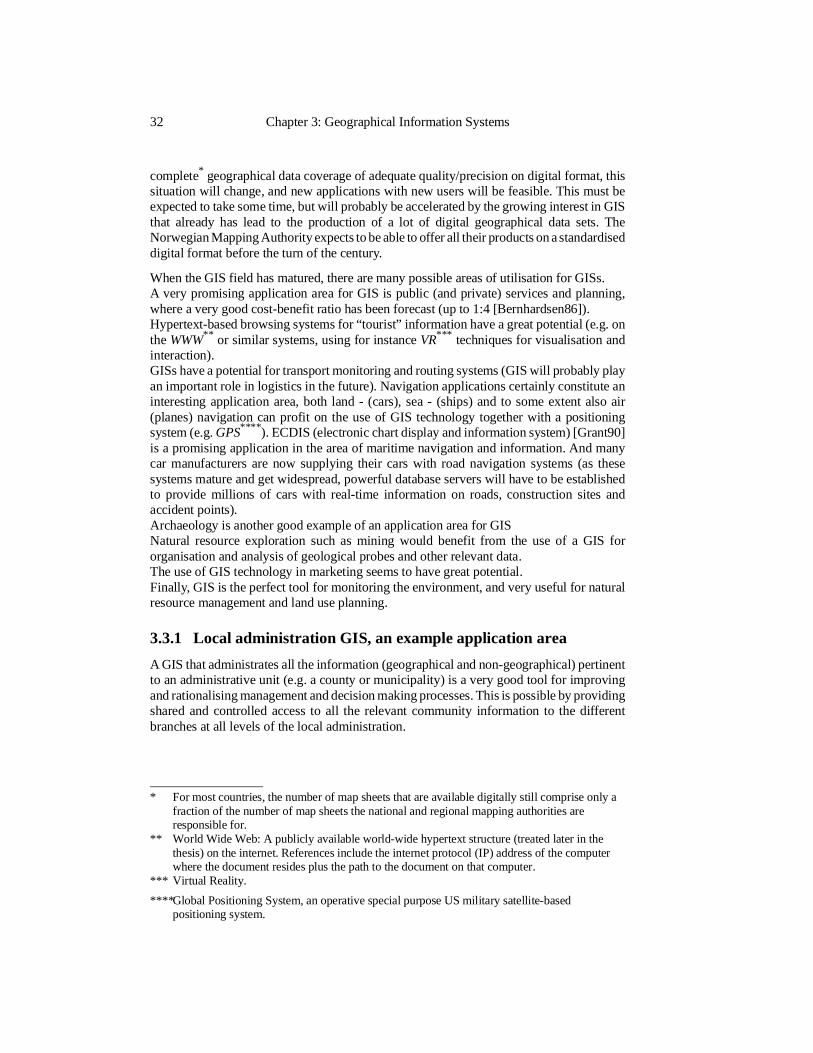
complete* geographical data coverage of adequate quality/precision on digital format, thissituation will change, and new applications with new users will be feasible. This must beexpected to take some time, but will probably be accelerated by the growing interest in GISthat already has lead to the production of a lot of digital geographical data sets. TheNorwegian Mapping Authority expects to be able to offer all their products on a standardiseddigital format before the turn of the century.

When the GIS field has matured, there are many possible areas of utilisation for GISs.A very promising application area for GIS is public (and private) services and planning,where a very good cost-benefit ratio has been forecast (up to 1:4 [Bernhardsen86]).Hypertext-based browsing systems for “tourist” information have a great potential (e.g. onthe WWW** or similar systems, using for instance VR*** techniques for visualisation andinteraction).GISs have a potential for transport monitoring and routing systems (GIS will probably playan important role in logistics in the future). Navigation applications certainly constitute aninteresting application area, both land - (cars), sea - (ships) and to some extent also air(planes) navigation can profit on the use of GIS technology together with a positioningsystem (e.g. GPS****). ECDIS (electronic chart display and information system) [Grant90]is a promising application in the area of maritime navigation and information. And manycar manufacturers are now supplying their cars with road navigation systems (as thesesystems mature and get widespread, powerful database servers will have to be establishedto provide millions of cars with real-time information on roads, construction sites andaccident points).Archaeology is another good example of an application area for GISNatural resource exploration such as mining would benefit from the use of a GIS fororganisation and analysis of geological probes and other relevant data.The use of GIS technology in marketing seems to have great potential.Finally, GIS is the perfect tool for monitoring the environment, and very useful for naturalresource management and land use planning.

3.3.1 Local administration GIS, an example application area

A GIS that administrates all the information (geographical and non-geographical) pertinentto an administrative unit (e.g. a county or municipality) is a very good tool for improvingand rationalising management and decision making processes. This is possible by providingshared and controlled access to all the relevant community information to the differentbranches at all levels of the local administration.


* For most countries, the number of map sheets that are available digitally still comprise only afraction of the number of map sheets the national and regional mapping authorities areresponsible for.

** World Wide Web: A publicly available world-wide hypertext structure (treated later in thethesis) on the internet. References include the internet protocol (IP) address of the computerwhere the document resides plus the path to the document on that computer.

*** Virtual Reality.

****Global Positioning System, an operative special purpose US military satellite-basedpositioning system.

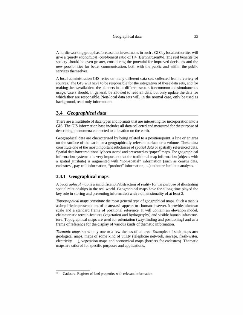
A nordic working group has forecast that investments in such a GIS by local authorities willgive a (purely economical) cost-benefit ratio of 1:4 [Bernhardsen86]. The real benefits forsociety should be even greater, considering the potential for improved decisions and thenew possibilities for better communication, both with the public and within the publicservices themselves.

A local administration GIS relies on many different data sets collected from a variety ofsources. The GIS will have to be responsible for the integration of these data sets, and formaking them available to the planners in the different sectors for common and simultaneoususage. Users should, in general, be allowed to read all data, but only update the data forwhich they are responsible. Non-local data sets will, in the normal case, only be used asbackground, read-only information.

3.4 Geographical data

There are a multitude of data types and formats that are interesting for incorporation into aGIS. The GIS information base includes all data collected and measured for the purpose ofdescribing phenomena connected to a location on the earth.

Geographical data are characterised by being related to a position/point, a line or an areaon the surface of the earth, or a geographically relevant surface or a volume. These dataconstitute one of the most important subclasses of spatial data or spatially referenced data.Spatial data have traditionally been stored and presented as “paper” maps. For geographicalinformation systems it is very important that the traditional map information (objects witha spatial attribute) is augmented with “non-spatial” information (such as census data,cadastres*, pay-roll information, “product” information, …) to better facilitate analysis.

3.4.1 Geographical maps

A geographical map is a simplification/abstraction of reality for the purpose of illustratingspatial relationships in the real world. Geographical maps have for a long time played thekey role in storing and presenting information with a dimensionality of at least 2.

Topographical maps constitute the most general type of geographical maps. Such a map isa simplified representations of an area as it appears to a human observer. It provides a knownscale and a standard frame of positional reference. It will contain an elevation model,characteristic terrain-features (vegetation and hydrography) and visible human infrastruc-ture. Topographical maps are used for orientation (way-finding and positioning) and as aframe of reference for the display of various kinds of thematic information.

Thematic maps show only one or a few themes of an area. Examples of such maps are:geological maps, maps of some kind of utility (telephone network, sewage, fresh-water,electricity, …), vegetation maps and economical maps (borders for cadastres). Thematicmaps are tailored for specific purposes and applications.

Geographical data 33

* Cadastre: Register of land properties with relevant information

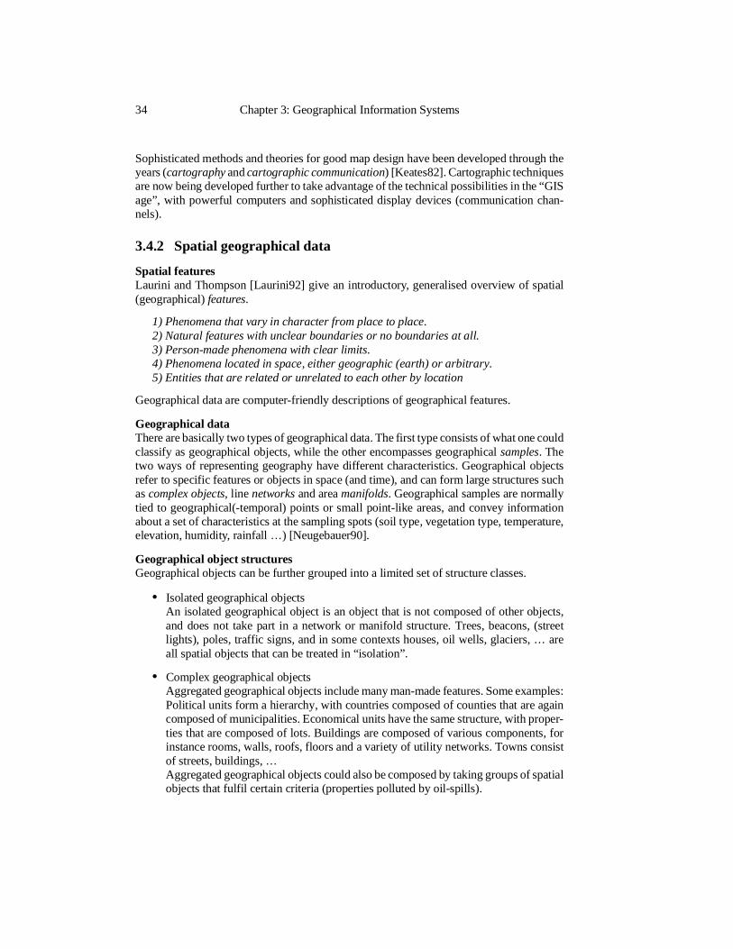
Sophisticated methods and theories for good map design have been developed through theyears (cartography and cartographic communication) [Keates82]. Cartographic techniquesare now being developed further to take advantage of the technical possibilities in the “GISage”, with powerful computers and sophisticated display devices (communication chan-nels).

3.4.2 Spatial geographical data

Spatial featuresLaurini and Thompson [Laurini92] give an introductory, generalised overview of spatial(geographical) features.

1) Phenomena that vary in character from place to place.2) Natural features with unclear boundaries or no boundaries at all.3) Person-made phenomena with clear limits.4) Phenomena located in space, either geographic (earth) or arbitrary.5) Entities that are related or unrelated to each other by location

Geographical data are computer-friendly descriptions of geographical features.

Geographical dataThere are basically two types of geographical data. The first type consists of what one couldclassify as geographical objects, while the other encompasses geographical samples. Thetwo ways of representing geography have different characteristics. Geographical objectsrefer to specific features or objects in space (and time), and can form large structures suchas complex objects, line networks and area manifolds. Geographical samples are normallytied to geographical(-temporal) points or small point-like areas, and convey informationabout a set of characteristics at the sampling spots (soil type, vegetation type, temperature,elevation, humidity, rainfall …) [Neugebauer90].

Geographical object structuresGeographical objects can be further grouped into a limited set of structure classes.

• Isolated geographical objectsAn isolated geographical object is an object that is not composed of other objects,and does not take part in a network or manifold structure. Trees, beacons, (streetlights), poles, traffic signs, and in some contexts houses, oil wells, glaciers, … areall spatial objects that can be treated in “isolation”.

• Complex geographical objectsAggregated geographical objects include many man-made features. Some examples:Political units form a hierarchy, with countries composed of counties that are againcomposed of municipalities. Economical units have the same structure, with proper-ties that are composed of lots. Buildings are composed of various components, forinstance rooms, walls, roofs, floors and a variety of utility networks. Towns consistof streets, buildings, …Aggregated geographical objects could also be composed by taking groups of spatialobjects that fulfil certain criteria (properties polluted by oil-spills).


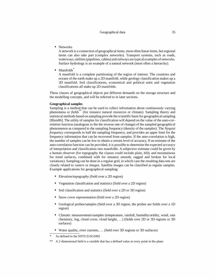
• NetworksA network is a connection of geographical items, most often linear items, but regionalitems can also take part (complex networks). Transport systems, such as roads,waterways, utilities (pipelines, cables) and railways are typical examples of networks.Surface hydrology is an example of a natural network (most often a hierarchy).

• Manifolds*

A manifold is a complete partitioning of the region of interest. The countries andoceans of the earth make up a 2D manifold, while geology classification makes up a3D manifold. Soil classifications, economical and political units and vegetationclassifications all make up 2D manifolds.

These classes of geographical objects put different demands on the storage structure andthe modelling concepts, and will be referred to in later sections.

Geographical samplesSampling is a method that can be used to collect information about continuously varyingphenomena or fields** (for instance natural resources or climate). Sampling theory andstatistical methods based on sampling provide the scientific basis for geographical sampling[Blais86]. The utility of samples for classification will depend on the value of the auto-cor-relation function (analogous to the the inverse rate of change) of the sampled geographicalphenomenon as compared to the sampling frequency (density of the samples). The Nyquistfrequency corresponds to half the sampling frequency, and provides an upper limit for thefrequency information that can be recovered from samples. If the auto-correlation is high,the number of samples can be low to obtain a certain level of accuracy. If an estimate of theauto-correlation function can be provided, it is possible to determine the expected accuracyof interpolation and classification into manifolds. A subjective estimate could be given bya human observer (for topography the classes could include plain, hilly and mountainousfor trend surfaces, combined with for instance smooth, ragged and broken for localvariations). Sampling can be done in a regular grid, in which case the resulting data sets areclosely related to rasters or images. Satellite images can be classified as regular samples.Example applications for geographical sampling:

• Elevation/topography (field over a 2D region)

• Vegetation classification and statistics (field over a 2D region)

• Soil classification and statistics (field over a 2D or 3D region)

• Snow cover representation (field over a 2D region)

• Geological probes/samples (field over a 3D region, the probes are fields over a 1Dregion)

• Climatic measurements/samples (temperature, rainfall, humidity/aridity, wind, rainchemistry, fog, cloud cover, cloud height, …) (fields over 2D or 3D regions or 3Dsurfaces)

• Water quality, river currents, … (field over 3D regions or 3D surfaces)


* As defined in the SDTS [USGS90]

** A 2-dimensional field is a variable that has a defined value at every point in the plane

Geographical samples can be used for direct analysis, or for performing thematic classifi-cations and making thematic maps. A thematic classification is produced by interpolatingand extrapolating the sample data into a classification manifold covering the region ofinterest. This classification manifold can then be presented as a thematic map. Spatialsampling and temporal sampling will have to be combined when monitoring naturalphenomena.

3.4.3 Non-spatial or “catalogue type” GIS data

The term catalogue type data is introduced to give a name to traditional data, as opposedto spatial data in a GIS. All kinds of information traditionally handled by computer databasemanagement systems fit into the catalogue type.

An example of catalogue type data is the supplier-parts databases in [Date86]:

Part (part number, part name, colour, weight, city of storage)Supplier (supplier number, supplier name, status, city)SuppParts (supplier number, part number, quantity)

Catalogue type data can easily be organised into tables of numerical and textual fields, whereeach row describes an object, and each column contains one characteristic or attribute (soit fits perfectly into the relational model). These kinds of data are easy to store andmanipulate in todays information systems, and fit very well into the relational databasemodel. Databases for record keeping in business and administration is a typical example ofwhat is here termed catalogue type information.

Most catalogue type information is spatially relatable (in this example through the cityname) and, as such, potentially interesting for spatial analysis using a GIS. In the supplier-part database, a typical example of this is the optimal transportation routing problem for thevarious parts.

3.4.4 Historical data

Historical data and time-series data can often be of great value in the GIS context. Thismeans that geographical samples that are to be used for time-series analysis should have a4-dimensional reference, including both geographical and temporal positions, while man-made geographical objects such as buildings, roads, canals and land properties that have amore discrete life-cycle could have their history of changes or time of validity attached.

Snapshot databases are not adequate for a general purpose GIS. Historical information couldbe of interest to both researchers, record keepers and planners, both for monitoring and forforecasting. The consequence of this is that all historical versions of geographical objectsshould be kept in the geographical database, and samples should be stored both with theirdate and position of sampling to allow time series analysis and forecasting by analysts inthe future. It is important that both the geographical and temporal dimensions (sometimestermed 4D) are considered when a sampling strategy is determined.


3.4.5 Data quality

Results from a sophisticated GIS analysis will be unreliable in the presence of errors andinaccuracies in the input data (garbage in - garbage out). In his chapter on data quality in[Burrough86], Borrough discuss “the main sources of error and variation in data that cancontribute to unreliable results being produced by a geographical information system”. Itwould be very useful to be able to incorporate into geographical information systemsmethods to automatically determine the fidelity and accuracy of GIS results from the qualityof input data and the characteristics of the applications.

To achieve this, it is necessary to represent errors and accuracy for the input data, to trackthe errors and inaccuracies as they propagate through the various analysis steps of a GISapplication, and finally to communicate (by for instance using advanced visualisationtechniques) the uncertainties embedded in the final results to the user [NCGIA91]. GISapplications might themselves be inaccurate, and this should be taken into account in theerror/accuracy analysis process.

A US initiative on standards for spatial accuracy [Chrisman84] [USGS90] has come up witha taxonomy for data quality. According to this work, data quality can be divided into[USGS90]:

lineage (data sources and transformations performed)positional accuracyattribute accuracylogical consistency (fidelity of relationships, valid values, topology and geometry)completeness

Temporal accuracy has been proposed as an additional accuracy parameter by the CEN TC287 WG2 PT05 [CEN95].

3.4.6 Data distribution and sharing

Geographical data sets are often useful for many purposes and users and at the same timeexpensive to collect. Sharing is therefore very desirable for these kinds of data.

Collection of geographical data are performed by governmental agencies, local authorities,private companies and individuals for private usage or for the benefit of the public. It willnormally be in the responsible collectors interest to keep the data set up to date bycontinuously taking the necessary new measurements and samples.

The responsible collector is the legal owner of the data, and must be given credit for otherorganisations’ use of the data [Carter92]. The owner of the data will therefore want to keepcontrol of the database, preferably by storing it locally and allowing other users access tothe database only on a commercial basis.

This ownership structure of geographical information puts certain constraints on thefreedom of choice when organising and designing database systems for GIS.


3.5 Models for geographical data

Two paradigms for geographical data have been used in GISs through the years. One isimage- or grid-based and is termed the tessellation or raster model, while the other isgeometry- or object-based and is termed the vector model [Peuquet84]. Some GISs utiliseonly one of these paradigms, while others provides for both with “translation” proceduresfor “conversion” between the two models when that is necessary.

3.5.1 The raster paradigm

The basic unit of representation in the raster approach to geographical information manage-ment is a rectangular* region in 2D (or 3D**) geographical space. The size of the basic unitswill depend on the requirements of the applications that are to make use of the information(10 km x 10 km cells can be more useful than 10 m x 10 m cells for certain applications).These equal sized units, called raster elements or pixels***/voxels****, are arranged as theelements of a matrix, hence imposing a tessellation of the geographical region of interestinto a regular grid. The raster approach hence uses a fixed resolution (discrete) repre-sentation of 2D (or 3D) space (R2/R3). Together with the raster one has to store thegeographical location of the raster and the cell size of the raster, in order to make the mappingfrom raster element to geographical location possible.

Rasters can not represent lines in a straightforward fashion, neither can it represent points.In order to be able to represent lines and points in the raster model, one has to treat them asregions.

The raster (or regular tessellation) approach to GIS data storage and representation is, asmentioned earlier, sample- or image-based. It can be termed place-oriented, as opposed toobject-oriented. The traditional raster model can be termed a “2.5D” model. The reason forthis is that it is able to represent how a phenomenon varies over a 2D region (2D fields).

A phenomenon of interest to the user, e.g. soil type, rain-fall or elevation, is measured foreach grid cell, and the resulting matrix of values constitutes a layer in the raster model. Atleast one layer is introduced for each phenomenon that is of interest to the user, and theresulting multi-layer structure constitutes the basis for operations and analysis in the rastermodel. A raster data model of an area will consequently consist of many raster layers, eachcovering a feature of interest to the users.

To be able to do efficient combinatorial analysis on the raster layers of the area of interest,it is important that the tessellation (cell-size and cell-boundaries) of all the raster layers arecompatible (cell borders coincide). If the cell boundaries of one raster layer are differentfrom those of the other raster “layers” (or the cell sizes are different), resampling will haveto be performed to make the raster layers compatible. Resampling takes time.


* Other cell shapes, such as triangles and hexagons can also be used, but this is not common

** The regular tessellation based approach to geographical information representation does nothave to be limited to 2D. 3D representations can also be useful, for instance for atmosphericmodelling, modelling of oceans, lakes and rivers and modelling of geology.

*** Picture element: used for images and 2D rasters.

****Volume element: used for 3D rasters.

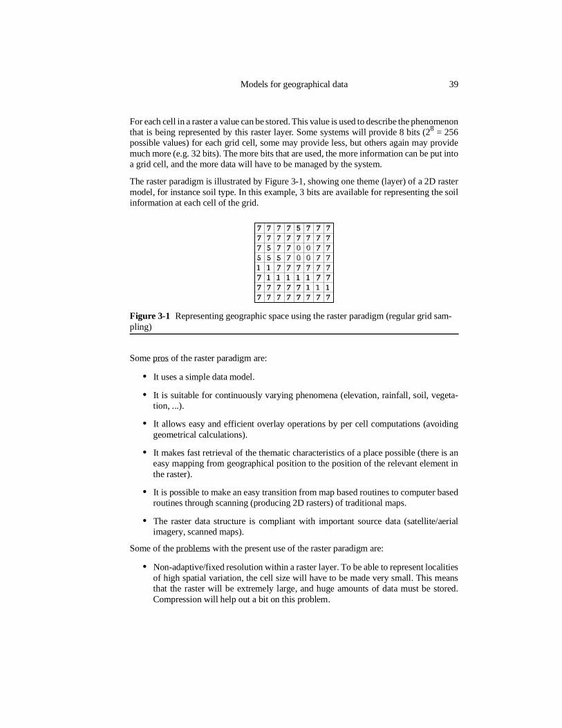
For each cell in a raster a value can be stored. This value is used to describe the phenomenonthat is being represented by this raster layer. Some systems will provide 8 bits (28 = 256possible values) for each grid cell, some may provide less, but others again may providemuch more (e.g. 32 bits). The more bits that are used, the more information can be put intoa grid cell, and the more data will have to be managed by the system.

The raster paradigm is illustrated by Figure 3-1, showing one theme (layer) of a 2D rastermodel, for instance soil type. In this example, 3 bits are available for representing the soilinformation at each cell of the grid.

Some pros of the raster paradigm are:

• It uses a simple data model.

• It is suitable for continuously varying phenomena (elevation, rainfall, soil, vegeta-tion, ...).

• It allows easy and efficient overlay operations by per cell computations (avoidinggeometrical calculations).

• It makes fast retrieval of the thematic characteristics of a place possible (there is aneasy mapping from geographical position to the position of the relevant element inthe raster).

• It is possible to make an easy transition from map based routines to computer basedroutines through scanning (producing 2D rasters) of traditional maps.

• The raster data structure is compliant with important source data (satellite/aerialimagery, scanned maps).

Some of the problems with the present use of the raster paradigm are:

• Non-adaptive/fixed resolution within a raster layer. To be able to represent localitiesof high spatial variation, the cell size will have to be made very small. This meansthat the raster will be extremely large, and huge amounts of data must be stored.Compression will help out a bit on this problem.

Figure 3-1 Representing geographic space using the raster paradigm (regular grid sam-pling)

Models for geographical data 39

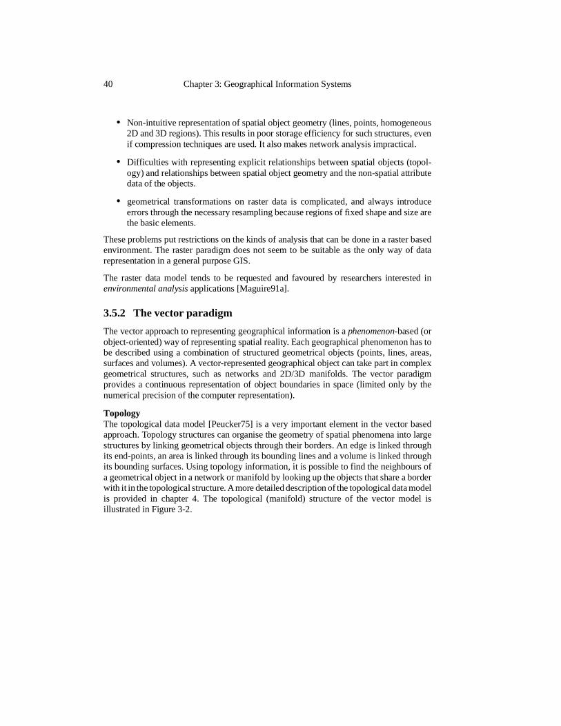
• Non-intuitive representation of spatial object geometry (lines, points, homogeneous2D and 3D regions). This results in poor storage efficiency for such structures, evenif compression techniques are used. It also makes network analysis impractical.

• Difficulties with representing explicit relationships between spatial objects (topol-ogy) and relationships between spatial object geometry and the non-spatial attributedata of the objects.

• geometrical transformations on raster data is complicated, and always introduceerrors through the necessary resampling because regions of fixed shape and size arethe basic elements.

These problems put restrictions on the kinds of analysis that can be done in a raster basedenvironment. The raster paradigm does not seem to be suitable as the only way of datarepresentation in a general purpose GIS.

The raster data model tends to be requested and favoured by researchers interested inenvironmental analysis applications [Maguire91a].

3.5.2 The vector paradigm

The vector approach to representing geographical information is a phenomenon-based (orobject-oriented) way of representing spatial reality. Each geographical phenomenon has tobe described using a combination of structured geometrical objects (points, lines, areas,surfaces and volumes). A vector-represented geographical object can take part in complexgeometrical structures, such as networks and 2D/3D manifolds. The vector paradigmprovides a continuous representation of object boundaries in space (limited only by thenumerical precision of the computer representation).

TopologyThe topological data model [Peucker75] is a very important element in the vector basedapproach. Topology structures can organise the geometry of spatial phenomena into largestructures by linking geometrical objects through their borders. An edge is linked throughits end-points, an area is linked through its bounding lines and a volume is linked throughits bounding surfaces. Using topology information, it is possible to find the neighbours ofa geometrical object in a network or manifold by looking up the objects that share a borderwith it in the topological structure. A more detailed description of the topological data modelis provided in chapter 4. The topological (manifold) structure of the vector model isillustrated in Figure 3-2.


The strength of the vector paradigm is that it is very expressive when it comes to representinggeographical objects. Network and manifold analysis is directly supported by the vectordata model (overlay operations do, however, require massive geometrical computations invector based systems as compared to overlays on raster data).

3.5.3 Representation of the interior of spatial objects

The vector model, as manifested by todays vector-based GISs, is not well suited for therepresentation and analysis of continuously varying phenomena (fields). Current vector-based systems represent geometrical objects by their boundaries/borders, and are thereforenot able to support properties that varies over the interior of an object in an integrated way(for more on point-set topology, interior (X°), boundary (∂X) and co-dimension in a GIScontext, see [Pullar88], [Egenhofer90b], [Egenhofer91a] or [Papadias94]).

• In 1D space, it should be possible to represent phenomena that varies along an interval(the border of an interval is its end-points, and the interior of an interval is the interval,excluding the end-points).

• In 2D space, it should be possible to represent phenomena that varies over the interiorof a 2D region (the border of 2D regions are lines in 2D, while the interior is the 2Dregion, excluding its border lines). In a typical vector GIS you can attach informationto the 2D region as a whole, and to its border lines. The representation of the interiorof 2D regions is not sufficiently integrated into the vector models that are applied incurrent GISs. The interior can be represented using triangulated irregular networks(TINs* [Peucker78]) that are available in some systems, but a TIN is only oneinterpolation method, and there is normally a very limited set of analysis toolsavailable for TINs.Lines in 2D: In a typical vector GIS, it is only possible to attach information to theline as a whole and to its end-points. The ARC/INFO GIS use what they call “dynamicsegmentation” to allow a better representation of the interior of lines in 2D.

• In 3D space, it should be possible to represent phenomena that varies over a 3D region(the border of 3D regions are surfaces in 3D, while the interior is the 3D region,excluding its bounding surfaces). Most current vector GISs do not support 3D

Figure 3-2 Representing geographic space using the vector paradigm (points, edges andregions)

Models for geographical data 41

* Triangulated Irregular Network

functionality at all, let alone the interior of 3D objects.Surfaces in 3D and lines in 3D space: For both lines and surfaces in 3D space, it canbe useful to represent variation over the interior.

In general, it is safe to state that most of the vector models used in todays vector GISs onlyprovide border representations.

3.6 Queries and operations

A geographical information system must be able to handle many sorts of queries. Queriesfor catalogue type information that is prevailing in todays database applications will alwaysbe important in an information system, but in GISs spatial queries will also play a centralrole. A GIS interface should provide mechanisms for both textual and spatial/graphicalinteraction (“image” based queries).

To be able to support all potential queries to a GIS database, a GIS will have to implementa multitude of operations. The most basic operations in a GIS are the data integrationoperations that prepare the different geographical data sets of a study area for analysis (e.g.transformations between different coordinate systems / reference systems and datamodel/format translations). Update, analysis and presentation are also basic tasks that allrequire an extensive set of operations. Berry, taking the raster approach, suggests thefollowing basic set of operations in computer assisted map analysis: reclassification,overlay, distance measurements, connectivity measurements and characterisation of neigh-bourhoods [Berry87].

As a background to the design of data structures and database interfaces for GISs, it is usefulto identify common query types, and to provide an indication of the relative importance(frequency of use) of the different query types. If query information is available, the taskof tailoring database systems for fast execution of the most common geographical querieswill be easier (while not forgetting the less common queries), resulting in more efficientGISs. It will be difficult to get authoritative statistics on these matters, but assessments canbe made based on the nature of the routines performed by various (potential) GIS usergroups.

3.6.1 GIS queries

Classification of queries into high level query types will depend very much upon the pointof view of the classifier. For the purpose of this thesis, the data modelling - and databasepoint of view is taken, so the query types identified below are based on a classification ofthe data types useful in a GIS, rather than thematic or other kinds of classifications. A furthertreatment of GIS queries in the context of a database management system is given in chapter6.

General catalogue queriesThis category includes set oriented queries (both range queries and exact match queries)and direct queries on identified phenomena.The first example is a set based range query, the second is a set based exact match queryand the rest are direct object queries.

• Find all cities with a population greater than 4 000 000.


• Find the address of persons with last name “Olsen” and first name “Vegard”.

• Find the names of the constituent parts of the engine with the identifier “XYZ1”.

• Find the names of the minerals contained in the “Iddefjord granite” together withtheir weight percentage.

Spatial queriesSpatial queries are queries that use position and and spatial relationships (such as distance)as a basis for retrieving information about spatial phenomena. These queries can be dividedinto spatial computations, set oriented (range or exact match) - and instance orientedqueries. Topological queries for network and manifold analysis make up a separate type ofspatial queries.

The first example given below is a spatial computation query, the second is a set queryconstrained by a spatial object (Norway). The third is a set query constrained by a point anda distance operator, the fourth is an instance query, more specifically a nearest neighbourquery (point-point or region-region, depending on the representation) and the fifth is atopological query.

• Find the area of the district “Hordaland” in “Norway”.

• Find all cities in “Norway” with a population exceeding 40 000 people.

• How many grocery stores are there within a radius of 10 km from the city hall in“Trondheim”.

• Find the bank closest to the company X’s office in “Oslo”

• Find the properties that share property border(s) with properties containing hospitalsin “Norway”.

3D model queriesQueries that require manipulation and computations on 3D models form a sub-class ofspatial queries, and can be projection queries (often for display purposes) or “surface-con-strained” computational queries.The first example given below is a projection query, while the second, third and fourth are3D computational queries.

• Show a 3D model of the construction area, “Building-land”, as seen from 1 km to thesouth-west, at a viewing angle of 15 degrees, with default shadows and hidden-sur-face removal.

• What is the volume of the known sand-reserves in “Vestfold”.

• Contour the region with north-east corner (lat1,long1) and south-west corner(lat2,long2) at the scale 1:1000, using a contour interval of 1 meter.

• Perform a simulation of water flow in the snow melting period for the “Gaula” riversystem, using climate and precipitation data from 1986-1987.

Queries and operations 43

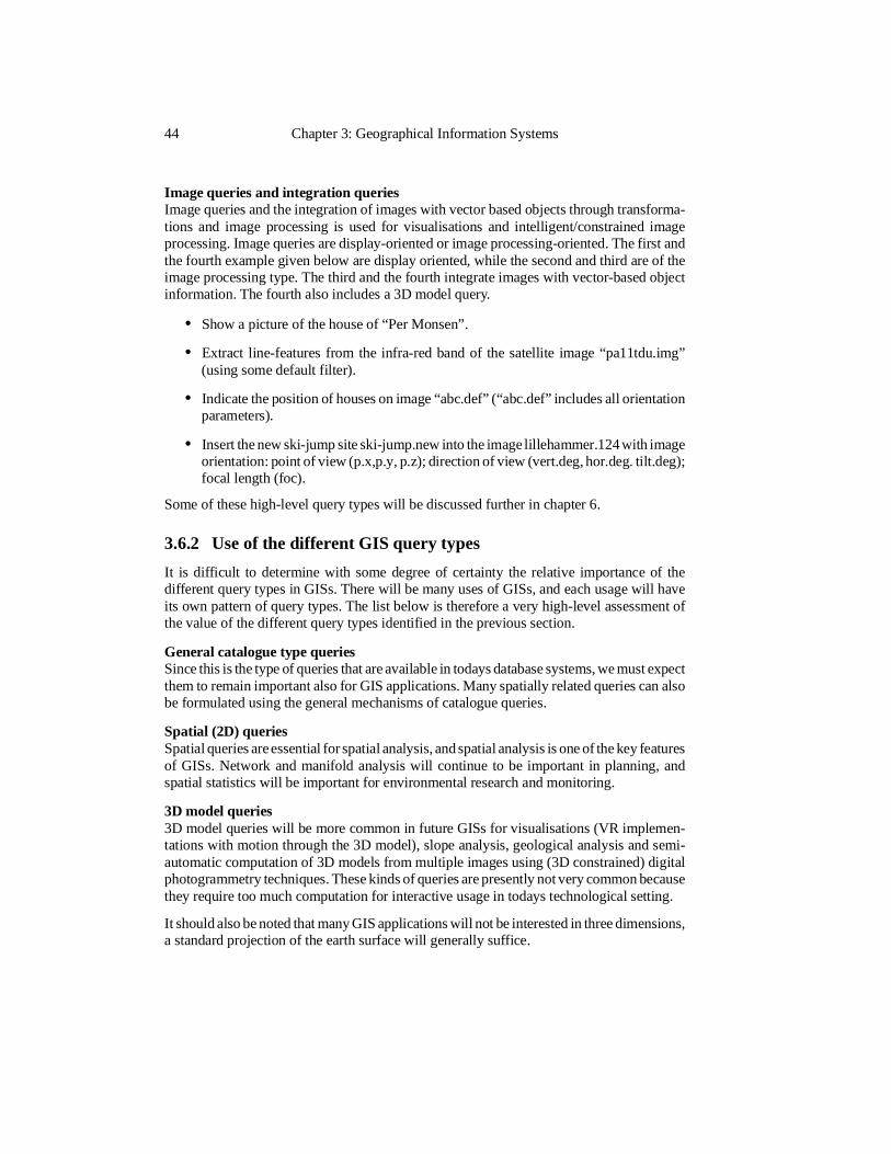
Image queries and integration queriesImage queries and the integration of images with vector based objects through transforma-tions and image processing is used for visualisations and intelligent/constrained imageprocessing. Image queries are display-oriented or image processing-oriented. The first andthe fourth example given below are display oriented, while the second and third are of theimage processing type. The third and the fourth integrate images with vector-based objectinformation. The fourth also includes a 3D model query.

• Show a picture of the house of “Per Monsen”.

• Extract line-features from the infra-red band of the satellite image “pa11tdu.img”(using some default filter).

• Indicate the position of houses on image “abc.def” (“abc.def” includes all orientationparameters).

• Insert the new ski-jump site ski-jump.new into the image lillehammer.124 with imageorientation: point of view (p.x,p.y, p.z); direction of view (vert.deg, hor.deg. tilt.deg);focal length (foc).

Some of these high-level query types will be discussed further in chapter 6.

3.6.2 Use of the different GIS query types

It is difficult to determine with some degree of certainty the relative importance of thedifferent query types in GISs. There will be many uses of GISs, and each usage will haveits own pattern of query types. The list below is therefore a very high-level assessment ofthe value of the different query types identified in the previous section.

General catalogue type queriesSince this is the type of queries that are available in todays database systems, we must expectthem to remain important also for GIS applications. Many spatially related queries can alsobe formulated using the general mechanisms of catalogue queries.

Spatial (2D) queriesSpatial queries are essential for spatial analysis, and spatial analysis is one of the key featuresof GISs. Network and manifold analysis will continue to be important in planning, andspatial statistics will be important for environmental research and monitoring.

3D model queries3D model queries will be more common in future GISs for visualisations (VR implemen-tations with motion through the 3D model), slope analysis, geological analysis and semi-automatic computation of 3D models from multiple images using (3D constrained) digitalphotogrammetry techniques. These kinds of queries are presently not very common becausethey require too much computation for interactive usage in todays technological setting.

It should also be noted that many GIS applications will not be interested in three dimensions,a standard projection of the earth surface will generally suffice.


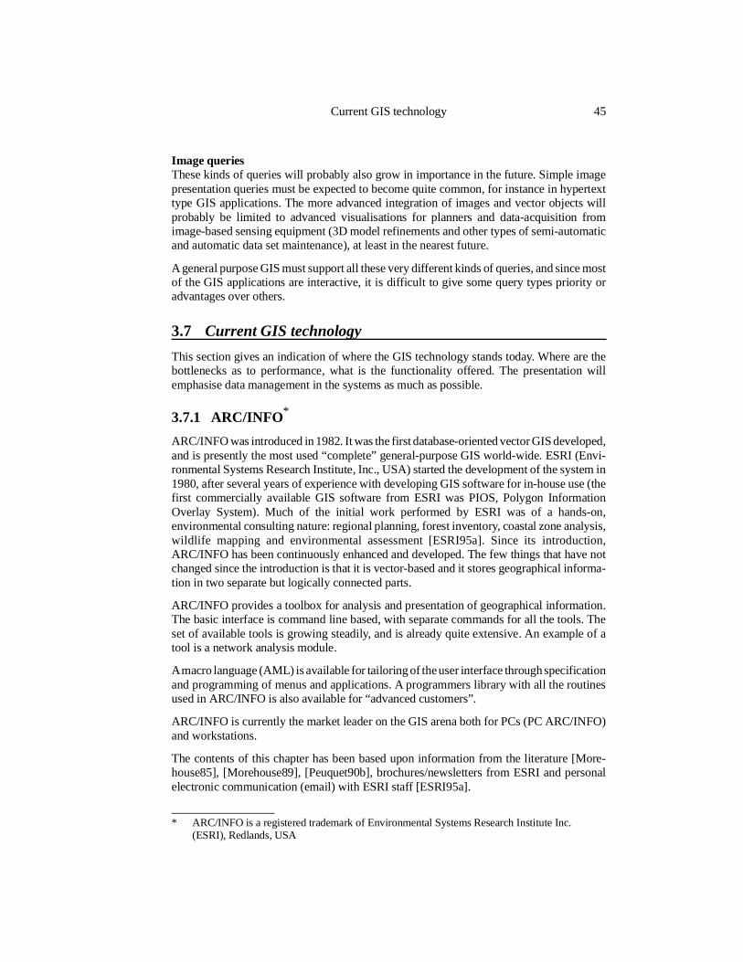
Image queriesThese kinds of queries will probably also grow in importance in the future. Simple imagepresentation queries must be expected to become quite common, for instance in hypertexttype GIS applications. The more advanced integration of images and vector objects willprobably be limited to advanced visualisations for planners and data-acquisition fromimage-based sensing equipment (3D model refinements and other types of semi-automaticand automatic data set maintenance), at least in the nearest future.

A general purpose GIS must support all these very different kinds of queries, and since mostof the GIS applications are interactive, it is difficult to give some query types priority oradvantages over others.

3.7 Current GIS technology

This section gives an indication of where the GIS technology stands today. Where are thebottlenecks as to performance, what is the functionality offered. The presentation willemphasise data management in the systems as much as possible.

3.7.1 ARC/INFO*

ARC/INFO was introduced in 1982. It was the first database-oriented vector GIS developed,and is presently the most used “complete” general-purpose GIS world-wide. ESRI (Envi-ronmental Systems Research Institute, Inc., USA) started the development of the system in1980, after several years of experience with developing GIS software for in-house use (thefirst commercially available GIS software from ESRI was PIOS, Polygon InformationOverlay System). Much of the initial work performed by ESRI was of a hands-on,environmental consulting nature: regional planning, forest inventory, coastal zone analysis,wildlife mapping and environmental assessment [ESRI95a]. Since its introduction,ARC/INFO has been continuously enhanced and developed. The few things that have notchanged since the introduction is that it is vector-based and it stores geographical informa-tion in two separate but logically connected parts.

ARC/INFO provides a toolbox for analysis and presentation of geographical information.The basic interface is command line based, with separate commands for all the tools. Theset of available tools is growing steadily, and is already quite extensive. An example of atool is a network analysis module.

A macro language (AML) is available for tailoring of the user interface through specificationand programming of menus and applications. A programmers library with all the routinesused in ARC/INFO is also available for “advanced customers”.

ARC/INFO is currently the market leader on the GIS arena both for PCs (PC ARC/INFO)and workstations.

The contents of this chapter has been based upon information from the literature [More-house85], [Morehouse89], [Peuquet90b], brochures/newsletters from ESRI and personalelectronic communication (email) with ESRI staff [ESRI95a].

Current GIS technology 45

* ARC/INFO is a registered trademark of Environmental Systems Research Institute Inc.(ESRI), Redlands, USA

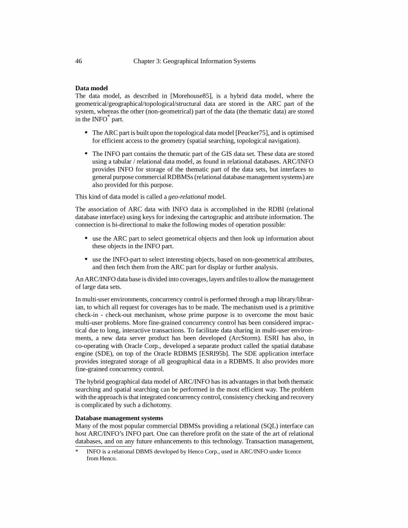
Data modelThe data model, as described in [Morehouse85], is a hybrid data model, where thegeometrical/geographical/topological/structural data are stored in the ARC part of thesystem, whereas the other (non-geometrical) part of the data (the thematic data) are storedin the INFO* part.

• The ARC part is built upon the topological data model [Peucker75], and is optimisedfor efficient access to the geometry (spatial searching, topological navigation).

• The INFO part contains the thematic part of the GIS data set. These data are storedusing a tabular / relational data model, as found in relational databases. ARC/INFOprovides INFO for storage of the thematic part of the data sets, but interfaces togeneral purpose commercial RDBMSs (relational database management systems) arealso provided for this purpose.

This kind of data model is called a geo-relational model.

The association of ARC data with INFO data is accomplished in the RDBI (relationaldatabase interface) using keys for indexing the cartographic and attribute information. Theconnection is bi-directional to make the following modes of operation possible:

• use the ARC part to select geometrical objects and then look up information aboutthese objects in the INFO part.

• use the INFO-part to select interesting objects, based on non-geometrical attributes,and then fetch them from the ARC part for display or further analysis.

An ARC/INFO data base is divided into coverages, layers and tiles to allow the managementof large data sets.

In multi-user environments, concurrency control is performed through a map library/librar-ian, to which all request for coverages has to be made. The mechanism used is a primitivecheck-in - check-out mechanism, whose prime purpose is to overcome the most basicmulti-user problems. More fine-grained concurrency control has been considered imprac-tical due to long, interactive transactions. To facilitate data sharing in multi-user environ-ments, a new data server product has been developed (ArcStorm). ESRI has also, inco-operating with Oracle Corp., developed a separate product called the spatial databaseengine (SDE), on top of the Oracle RDBMS [ESRI95b]. The SDE application interfaceprovides integrated storage of all geographical data in a RDBMS. It also provides morefine-grained concurrency control.

The hybrid geographical data model of ARC/INFO has its advantages in that both thematicsearching and spatial searching can be performed in the most efficient way. The problemwith the approach is that integrated concurrency control, consistency checking and recoveryis complicated by such a dichotomy.

Database management systemsMany of the most popular commercial DBMSs providing a relational (SQL) interface canhost ARC/INFO’s INFO part. One can therefore profit on the state of the art of relationaldatabases, and on any future enhancements to this technology. Transaction management,


* INFO is a relational DBMS developed by Henco Corp., used in ARC/INFO under licencefrom Henco.

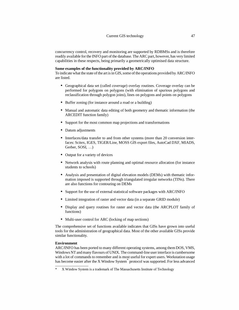
concurrency control, recovery and monitoring are supported by RDBMSs and is thereforereadily available for the INFO part of the database. The ARC part, however, has very limitedcapabilities in these respects, being primarily a geometrically optimised data structure.

Some examples of the functionality provided by ARC/INFOTo indicate what the state of the art is in GIS, some of the operations provided by ARC/INFOare listed.

• Geographical data set (called coverage) overlay routines. Coverage overlay can beperformed for polygons on polygons (with elimination of spurious polygons andreclassification through polygon joins), lines on polygons and points on polygons

• Buffer zoning (for instance around a road or a building)

• Manual and automatic data editing of both geometry and thematic information (theARCEDIT function family)

• Support for the most common map projections and transformations

• Datum adjustments

• Interfaces/data transfer to and from other systems (more than 20 conversion inter-faces: Scitex, IGES, TIGER/Line, MOSS GIS export files, AutoCad DXF, MIADS,Gerber, SOSI, …)

• Output for a variety of devices

• Network analysis with route planning and optimal resource allocation (for instancestudents to schools)

• Analysis and presentation of digital elevation models (DEMs) with thematic infor-mation imposed is supported through triangulated irregular networks (TINs). Thereare also functions for contouring on DEMs

• Support for the use of external statistical software packages with ARC/INFO

• Limited integration of raster and vector data (in a separate GRID module)

• Display and query routines for raster and vector data (the ARCPLOT family offunctions)

• Multi-user control for ARC (locking of map sections)

The comprehensive set of functions available indicates that GISs have grown into usefultools for the administration of geographical data. Most of the other available GISs providesimilar functionality.

EnvironmentARC/INFO has been ported to many different operating systems, among them DOS, VMS,Windows NT and many flavours of UNIX. The command-line user interface is cumbersomewith a lot of commands to remember and is most useful for expert users. Workstation usagehas become easier after the X Window System* protocol was supported. For less advanced


* X Window System is a trademark of The Massachusetts Institute of Technology

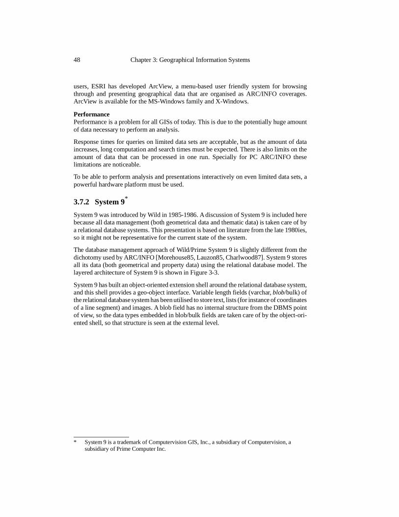
users, ESRI has developed ArcView, a menu-based user friendly system for browsingthrough and presenting geographical data that are organised as ARC/INFO coverages.ArcView is available for the MS-Windows family and X-Windows.

PerformancePerformance is a problem for all GISs of today. This is due to the potentially huge amountof data necessary to perform an analysis.

Response times for queries on limited data sets are acceptable, but as the amount of dataincreases, long computation and search times must be expected. There is also limits on theamount of data that can be processed in one run. Specially for PC ARC/INFO theselimitations are noticeable.

To be able to perform analysis and presentations interactively on even limited data sets, apowerful hardware platform must be used.

3.7.2 System 9*

System 9 was introduced by Wild in 1985-1986. A discussion of System 9 is included herebecause all data management (both geometrical data and thematic data) is taken care of bya relational database systems. This presentation is based on literature from the late 1980ies,so it might not be representative for the current state of the system.

The database management approach of Wild/Prime System 9 is slightly different from thedichotomy used by ARC/INFO [Morehouse85, Lauzon85, Charlwood87]. System 9 storesall its data (both geometrical and property data) using the relational database model. Thelayered architecture of System 9 is shown in Figure 3-3.

System 9 has built an object-oriented extension shell around the relational database system,and this shell provides a geo-object interface. Variable length fields (varchar, blob/bulk) ofthe relational database system has been utilised to store text, lists (for instance of coordinatesof a line segment) and images. A blob field has no internal structure from the DBMS pointof view, so the data types embedded in blob/bulk fields are taken care of by the object-ori-ented shell, so that structure is seen at the external level.


* System 9 is a trademark of Computervision GIS, Inc., a subsidiary of Computervision, asubsidiary of Prime Computer Inc.

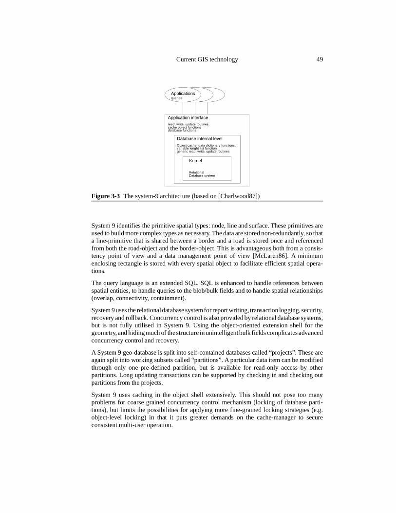
System 9 identifies the primitive spatial types: node, line and surface. These primitives areused to build more complex types as necessary. The data are stored non-redundantly, so thata line-primitive that is shared between a border and a road is stored once and referencedfrom both the road-object and the border-object. This is advantageous both from a consis-tency point of view and a data management point of view [McLaren86]. A minimumenclosing rectangle is stored with every spatial object to facilitate efficient spatial opera-tions.

The query language is an extended SQL. SQL is enhanced to handle references betweenspatial entities, to handle queries to the blob/bulk fields and to handle spatial relationships(overlap, connectivity, containment).

System 9 uses the relational database system for report writing, transaction logging, security,recovery and rollback. Concurrency control is also provided by relational database systems,but is not fully utilised in System 9. Using the object-oriented extension shell for thegeometry, and hiding much of the structure in unintelligent bulk fields complicates advancedconcurrency control and recovery.

A System 9 geo-database is split into self-contained databases called “projects”. These areagain split into working subsets called “partitions”. A particular data item can be modifiedthrough only one pre-defined partition, but is available for read-only access by otherpartitions. Long updating transactions can be supported by checking in and checking outpartitions from the projects.

System 9 uses caching in the object shell extensively. This should not pose too manyproblems for coarse grained concurrency control mechanism (locking of database parti-tions), but limits the possibilities for applying more fine-grained locking strategies (e.g.object-level locking) in that it puts greater demands on the cache-manager to secureconsistent multi-user operation.

Database internal level

Application interface

Object cache, data dictionary functions,

RelationalDatabase system

Kernel

variable lenght list functiongeneric read, write, update routines

Applications

read, write, update routines,cache object functionsdatabase functions

queries

Figure 3-3 The system-9 architecture (based on [Charlwood87])


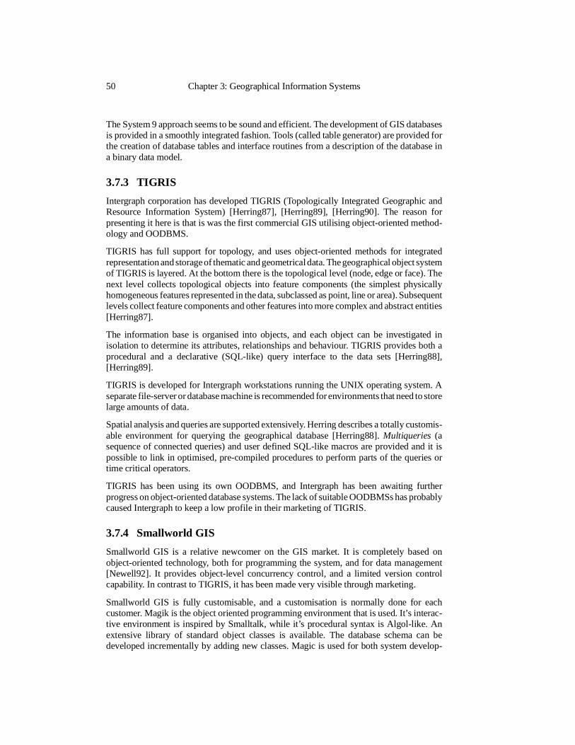
The System 9 approach seems to be sound and efficient. The development of GIS databasesis provided in a smoothly integrated fashion. Tools (called table generator) are provided forthe creation of database tables and interface routines from a description of the database ina binary data model.

3.7.3 TIGRIS

Intergraph corporation has developed TIGRIS (Topologically Integrated Geographic andResource Information System) [Herring87], [Herring89], [Herring90]. The reason forpresenting it here is that is was the first commercial GIS utilising object-oriented method-ology and OODBMS.

TIGRIS has full support for topology, and uses object-oriented methods for integratedrepresentation and storage of thematic and geometrical data. The geographical object systemof TIGRIS is layered. At the bottom there is the topological level (node, edge or face). Thenext level collects topological objects into feature components (the simplest physicallyhomogeneous features represented in the data, subclassed as point, line or area). Subsequentlevels collect feature components and other features into more complex and abstract entities[Herring87].

The information base is organised into objects, and each object can be investigated inisolation to determine its attributes, relationships and behaviour. TIGRIS provides both aprocedural and a declarative (SQL-like) query interface to the data sets [Herring88],[Herring89].

TIGRIS is developed for Intergraph workstations running the UNIX operating system. Aseparate file-server or database machine is recommended for environments that need to storelarge amounts of data.

Spatial analysis and queries are supported extensively. Herring describes a totally customis-able environment for querying the geographical database [Herring88]. Multiqueries (asequence of connected queries) and user defined SQL-like macros are provided and it ispossible to link in optimised, pre-compiled procedures to perform parts of the queries ortime critical operators.

TIGRIS has been using its own OODBMS, and Intergraph has been awaiting furtherprogress on object-oriented database systems. The lack of suitable OODBMSs has probablycaused Intergraph to keep a low profile in their marketing of TIGRIS.

3.7.4 Smallworld GIS

Smallworld GIS is a relative newcomer on the GIS market. It is completely based onobject-oriented technology, both for programming the system, and for data management[Newell92]. It provides object-level concurrency control, and a limited version controlcapability. In contrast to TIGRIS, it has been made very visible through marketing.

Smallworld GIS is fully customisable, and a customisation is normally done for eachcustomer. Magik is the object oriented programming environment that is used. It’s interac-tive environment is inspired by Smalltalk, while it’s procedural syntax is Algol-like. Anextensive library of standard object classes is available. The database schema can bedeveloped incrementally by adding new classes. Magic is used for both system develop-


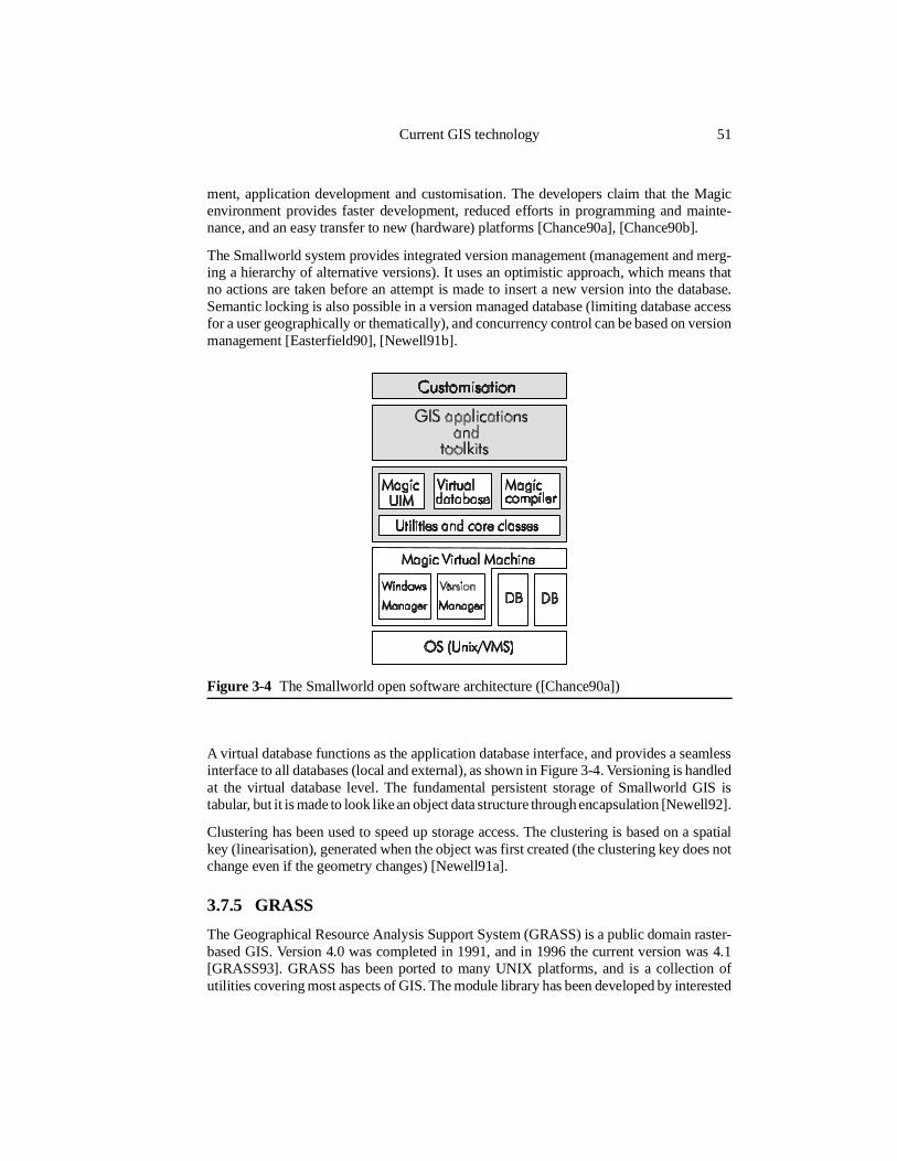
ment, application development and customisation. The developers claim that the Magicenvironment provides faster development, reduced efforts in programming and mainte-nance, and an easy transfer to new (hardware) platforms [Chance90a], [Chance90b].

The Smallworld system provides integrated version management (management and merg-ing a hierarchy of alternative versions). It uses an optimistic approach, which means thatno actions are taken before an attempt is made to insert a new version into the database.Semantic locking is also possible in a version managed database (limiting database accessfor a user geographically or thematically), and concurrency control can be based on versionmanagement [Easterfield90], [Newell91b].

A virtual database functions as the application database interface, and provides a seamlessinterface to all databases (local and external), as shown in Figure 3-4. Versioning is handledat the virtual database level. The fundamental persistent storage of Smallworld GIS istabular, but it is made to look like an object data structure through encapsulation [Newell92].

Clustering has been used to speed up storage access. The clustering is based on a spatialkey (linearisation), generated when the object was first created (the clustering key does notchange even if the geometry changes) [Newell91a].

3.7.5 GRASS

The Geographical Resource Analysis Support System (GRASS) is a public domain raster-based GIS. Version 4.0 was completed in 1991, and in 1996 the current version was 4.1[GRASS93]. GRASS has been ported to many UNIX platforms, and is a collection ofutilities covering most aspects of GIS. The module library has been developed by interested

Figure 3-4 The Smallworld open software architecture ([Chance90a])


users and researchers all over the world, but the initial effort on programming and systemdesign was made by the US Army Construction Engineering Research Laboratory (USA-CERL) [GRASS95].

The source code for all the software components in the system is available to all interestedusers. This means that further development of modules and the total environment can beperformed by everyone, leading to an increasingly more powerful system. CERL has beenco-ordinating the contributions into new releases of GRASS.

The GRASS concept is a toolbox approach, and most of the modules operate independently.

Data are organised in a UNIX file hierarchy and is placed at a user-defined location in theUNIX file system. GRASS uses its own internal formats for vector, raster and site data, butprovides conversion between its internal formats and many other spatial data formats.GRASS is a raster system, and provides a comprehensive set of tools for raster operationsand analysis. Some example applications of GRASS for environmental modelling andvisualisation are presented on the CERL WWW server [CERL95]

The user interface of the GRASS toolbox is by default a command-line based conversation.For some of the GRASS tools, more sophisticated interfaces have been built. An X-Win-dows interface has been used for display purposes (an integration of a subset of the displayroutines), and an integrated X-Windows based environment is under development, and isbeing shipped with the GRASS releases [Gardels88].

3.7.6 Summary

There are now many powerful geographical information systems available, both commer-cially and as public domain software. Many of the systems are still in their infancy, andhave problems with reliability and robustness. The available GISs are continuously improv-ing both in computational power and expressiveness. The analytical capabilities of thesystems are improving, and the systems take advantage of increasingly more powerfulhardware platforms to obtain better performance for all kinds of operations. User interfacesare slowly following up the trends in the rest of the computer science field with multiplewindows and nice graphics. GIS specific features such as spatial interaction techniques(query “languages”), spatial analysis, visualisation of spatial features and spatial dataquality are still challenging areas for research, and need further attention.

The data management part of GIS is the one causing most trouble for both the users and thevendors. Most GIS data sets are complex and huge, and perpetually growing. Traditionaldatabase management systems have been abandoned for managing geometrical data by mostGIS vendors. Instead they have settled for some custom data structure to store the spatialdata. Attribute/thematic data are not so problematic as the geometry data, and suitstraditional relational DBMSs well. DBMS interfaces are therefore provided by manyvendors for the storage of the non-spatial data. This approach to data management has itproblems, particularly for transaction management and multi-user support.

There is limited multi-user concurrency control available in todays GISs, apart from thecheck-in, check-out mechanism in some systems. This means that cooperative work usingGISs is inhibited. The extent to which cooperative work is useful in GIS should determine


the efforts put into this problem area. Transaction management research in related areas,such as Computer-Assisted Software Engineering (CASE) and Computer Assisted Design(CAD) could be useful also within the GIS context.

3.8 Trends

This section tries to outline the trends that are believed to be most influential for GIStechnology in the next twenty years. The predictions for hardware development are not verycontroversial, involving only enhancements to current technology. When it comes totechnology trends the predictions are a little more speculative, but not very controversial.The conclusions reached are in line with previous forecasts [Dangermond86].

3.8.1 Hardware trends

• Less expensive and more powerful processors.The price of micro processors seems to fall without limits. The ultimate limit beingthe price of the piece of “metal” and the energy required to make the wafer andmicroprocessor logic. This limit could be in the order of 10 NOK (1 US$), which ispretty inexpensive.The power of microprocessors will probably finally be limited by the speed of lightand the cooling requirements of the processors. The limit has not yet been reached.

• Less expensive and higher capacity transistor-based memory.By 1994 200,000 NOK (30000 US$) per Gigabyte RAM (Random Access Memory).By 1994 16 MB RAM chips were available off the shelf. 64 MB RAM chips hadalready been tested. The limit does not seem to have been reached. In parallel withthis development, ever faster RAM is emerging.

• Less expensive and higher capacity secondary storage devices (optical and magneticdisks).By 1991 30000 NOK (5000 US$) per Gigabyte of magnetic disk memory, by 1995less than 2000 NOK per Gigabyte, still going down.Disk capacities of several Gigabytes are now common (in 1994, 18 Gigabytes diskswere available), and the technology is still advancing.In 1994, magnetic tapes were able to store about 20 Gigabytes of data per tapecartridge, and the capacity is still increasing.Hierarchical Storage Management (HSM) systems were in 1994 able to store manyPetabytes (1015 bytes) of data in one single system. HSM’s are normally based onextensible robot-operated multi-tape/optical disk archives at the bottom of the hier-archy, and magnetic disks at the top, all integrated into a single cabinet with anadvanced interface (currently SCSI).

• Proliferation of high capacity (speed and volume) local and long haul networks.Optical fibres are being introduced everywhere both in local area networks and forlong distances. Hopefully, the high end ISDN* services will become available forcomputer networks soon. ATM**-based networks also promise new capacity andspeed improvements (ATM bandwidths are currently: 155 Mbit/s, 622Mb/s and 1.2Gb/s).

Trends 53

* Integrated Services Digital Network

The following observation can also be made: The gap between processor speed and I/Ospeed is widening at a fast pace. The increase in CPU-speed has been about 70%/year, whilethe increase in I/O speed (magnetic disk based) has been at +10-20%/year. The I/Osubsystem is therefore becoming more and more of a bottleneck in computers, andoptimisations in this area will be increasingly important (some progress has already beenmade using RAID technology).

3.8.2 Technology trends

• Proliferation of inexpensive and powerful parallel computers.This seems to be a little further away, but transputer-based environments (using forinstance the OCCAM language) have been available for a while, and inexpensivemicroprocessors will accelerate this trend.

• A shift to parallel processing for computationally intensive applications, and intro-duction of new tools for programming parallel computers.Parallel computers have developed from toys to commercial products. Meiko,Parsytec, Siemens, Intel (Paragon), MasPar, Parsys, SGI, Pyramid, Convex, IBM(SP2), Cray (T3D), nCUBE, Hitatchi and NEC are current actors on the hardwareside of this arena. This indicates that the technology has matured, and is takenseriously by the major hardware vendors. It also shows that research in the area ofparallel processing is given priority.

• Use of parallel computers for data management.The Tandem Non-Stop-SQL server was the first product to exploit parallelism fordata management. Teradata has been another actor on the scene with several products(these products were overtaken by AT&T), their first product was DBC1012.Parallelism is used for improving security (by duplication of hardware, software anddata) and for providing better performance. The principal use so far has been in “highvolume - short transactions” environments.

• RAID technology will probably be applied more extensively in the future in order toimprove the performance and reliability/fault tolerance of disk-based I/O subsystems.

• Advances in computer storage methods.If the advances in computer storage technology continue in the future, we must expectnew types of “permanent” storage devices that are orders of magnitude faster thanthe present mechanical disk technology. In the future, “permanent” computer storagemust be expected to reach the same speed of access and the same compactness astodays volatile memory. We have already seen solid state disks (transistor-based) ofseveral hundred megabytes capacity. A further development here will mean thatdatabase technology will be able to move into a new performance dimension.

• Network access to distributed services. A future scenario is that computing willbecome distributed, with application servers and database servers providing all kindsof applications and data (probably for some fee) through standardised interfaces. Theuser chooses which services to use based on his/her requirements (e.g. text process-ing, spatial analysis) and the services that are available. There will probably be a


+ Asyncronous Transfer Mode

reduced need for local software and data.Such an environment requires standardisation of services interfaces and a servicebroker. The Object Management Group* (OMG) is specifying CORBA** [Soley95]to provide such an environment, while Microsoft uses OLE for the same purposes.Schek has done some investigations in a GIS context [Schek93], and the OGC*** isworking on OGIS**** to specify interfaces for geographical information and analysisservices (some information has been available on the internet [OGIS95]). ISO is alsoworking on standards in this area (ISO TC211).

3.8.3 GIS trends

• Ever increasing amounts of digitally available geographical information.

• More advanced users and usage of geographical data.3D visualisations, complex analysis including large amounts of data, …

All these trends will be welcomed by both GIS users and vendors, and should provide agood basis for the development of the GISs of the future. The systems will hopefullycontinue to improve to become capable of more and more demanding tasks.

3.9 The GIS of the future

To be able to cope with the challenges of the future, geographical information systems musttake advantage of the available technology to develop and mature into generally usefulsystems. A list of requirements for the next generation of general purpose GISs follows.

Data model

• full topological capabilities (networks and manifolds)

• full 3D model

• full integration of the raster model and the vector model (support for fields)

• temporal data

• quality measures incorporated into data, procedures and presentations

• advanced support for data sharing

Database

• non-stop operation

The GIS of the future 55

* The OMG comprised over 300 companies early in 1995. It promotes the object-orientedapproach and develops standards for open distributed processing based on object-orientedmethodology [Soley95]

** The Common Object Request Broker Architecture

*** Open GIS Consortium, Inc. Consists of GIS vendors, computer vendors and federal agencies.They are supported by some university research activity. OGC plans to produce a set ofproposed standards by late 1996. These proposals will be submitted to ANSI and ISO.

****Open Geodata Interoperability Specification (trademark)

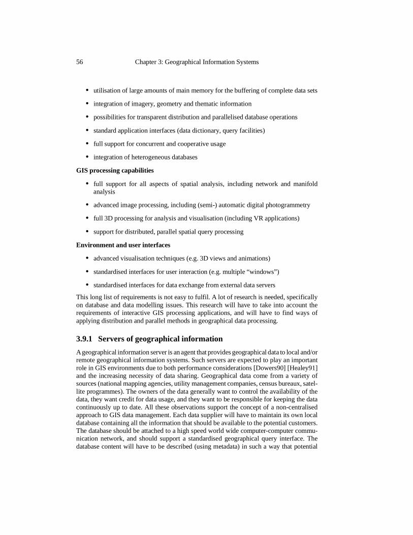
• utilisation of large amounts of main memory for the buffering of complete data sets

• integration of imagery, geometry and thematic information

• possibilities for transparent distribution and parallelised database operations

• standard application interfaces (data dictionary, query facilities)

• full support for concurrent and cooperative usage

• integration of heterogeneous databases

GIS processing capabilities

• full support for all aspects of spatial analysis, including network and manifoldanalysis

• advanced image processing, including (semi-) automatic digital photogrammetry

• full 3D processing for analysis and visualisation (including VR applications)

• support for distributed, parallel spatial query processing

Environment and user interfaces

• advanced visualisation techniques (e.g. 3D views and animations)

• standardised interfaces for user interaction (e.g. multiple “windows”)

• standardised interfaces for data exchange from external data servers

This long list of requirements is not easy to fulfil. A lot of research is needed, specificallyon database and data modelling issues. This research will have to take into account therequirements of interactive GIS processing applications, and will have to find ways ofapplying distribution and parallel methods in geographical data processing.

3.9.1 Servers of geographical information

A geographical information server is an agent that provides geographical data to local and/orremote geographical information systems. Such servers are expected to play an importantrole in GIS environments due to both performance considerations [Dowers90] [Healey91]and the increasing necessity of data sharing. Geographical data come from a variety ofsources (national mapping agencies, utility management companies, census bureaux, satel-lite programmes). The owners of the data generally want to control the availability of thedata, they want credit for data usage, and they want to be responsible for keeping the datacontinuously up to date. All these observations support the concept of a non-centralisedapproach to GIS data management. Each data supplier will have to maintain its own localdatabase containing all the information that should be available to the potential customers.The database should be attached to a high speed world wide computer-computer commu-nication network, and should support a standardised geographical query interface. Thedatabase content will have to be described (using metadata) in such a way that potential


users can assess the suitability of the data before acquisition. It will probably not benecessary to support updates through such a geographical data interface, since all modifi-cation are expected to be done locally.

A functional analysis of this kind of server will have to be based on both our currenttechnological and social context and on a scenario for the future. The analysis has to providea set of functions that a geographical information system has to provide, describe thecomplexity of these functions, and examine the possibility of dividing the workload betweenthe GISs and the geographical data servers. The functional analysis has to give an indicationof the processing power and data storage capacity needed at the different levels of thesystem.

Transaction processingA geographical data server will not have to meet the same requirements as a typicaltransaction system (server for bank-accounts). The transaction rates for geographical datawill generally be lower, but the complexity of the individual transactions will be higher. Thefact that most external transactions will be read-only, and that the database will be ahistorical database simplifies concurrency control and transaction management. Thesetopics are discussed further in chapter 6.

3.10 Research and research issues

The interest for research on GIS has been steadily increasing the last 20 years or so. Themain research conferences to date have been Auto-Carto (from the 70ies), the Symposiumson Spatial Data Handling (SDH, from 1984) and The Symposiums on Large SpatialDatabases (SSD, from 1989). A research journal was established in 1987, the InternationalJournal of Geographical Information Systems (changed its name to the International Journalof Geographical Information Science in 1997).

NCGIAThe NCGIA* was established by the US National Science Foundation (NSF) in 1988, andis run as a co-operation project between three US universities with special interests in GIS.The co-operating universities are: State University of New York, Buffalo; University ofCalifornia, Santa Barbara, University of Maine. The NCGIA has initiated and performed alot of research in the field of GIS, and has been the single most important contributor toGIS research in the world since its establishment. The NCGIA bases its research oninitiatives, and below are the first 16 of them listed:

Initiative 1: Accuracy of Spatial DatabasesInitiative 2: Languages of Spatial RelationsInitiative 3: Multiple RepresentationsInitiative 4: Use and Value of Geographic InformationInitiative 5: Very Large Spatial Databases (VLSDB)Initiative 6: Spatial Decision Support SystemsInitiative 7: Visualisation of the Quality of Spatial InformationInitiative 8: Formalising Cartographic KnowledgeInitiative 9: Institutions Sharing Geographic InformationInitiative 10: Spatio-Temporal Reasoning in GIS

Research and research issues 57

* National Center for Geographic Information and Analysis

Initiative 11: Space-Time Modelling in GISInitiative 12: GIS and Remote SensingInitiative 13: User Interfaces for Geographic Information SystemsInitiative 14: GIS and Spatial AnalysisInitiative 15: Multiple Roles for GIS in US Global Change ResearchInitiative 16: Law, Public Policy and Spatial Databases

The initiatives of the NCGIA are supposed to cover most of the current research issues inGIS.

The results of the work with the initiatives are published in technical reports that aregenerally available.

GISDATAIn Europe, the European Science Foundation (ESF) established a scientific programmecalled GISDATA in 1993, supposed to run until the end of 1996.

GISDATA is meant to play a similar role as NCGIA in Europe, and initially the followingresearch areas were proposed [GISDATA93]:

• Geographical Databases

• Geographical Data Integration

• Social and Environmental Applications

Later, new research areas has been given focus [GISDATA95].

For 1995, the research areas were

• Data Quality

• RS and Urban Change

• Spatial Models & GIS.

For 1996 the research areas will be

• Spatial and Temporal Change in GIS

• Geographical Information the European Dimension

• GIS & Emergency Management.

The GISDATA programme had, as of November 1995 resulted in 6 books and some otherpublications [GISDATA95].


Chapter 4

Data model requirements

4.1 Introduction

Geographical Information Systems should be able to handle complex, real-world informa-tion. Geographical data can have many uses, and different kinds of applications will applythe data in different contexts. To make sharing of geographical information possible,standardised (core) data models for spatial data should be developed and agreed upon. Thesemodels must includes powerful mechanisms for representing geographical phenomena withtheir abstractions, constraints, attributes and relationships. Such a standardised core forgeographical data models would provide a sound basis for the development of specialpurpose data models. The aim of this chapter is to identify requirements to such a core datamodel.

Several national initiatives have been taken to specify data models and exchange formatsfor geographical information in order to facilitate easy exchange and sharing of GIS data.Examples are FGIS/SOSI of Norway, ATKIS of Germany and the SDTS of the USA. Allof these seem to have their limits and weaknesses, and there is not yet consensus on whatkind of a model that should constitute the basis for an internationally acceptable standard.

The lack of a good common (useful for both humans and computers) data model forgeographical information has long impeded GIS technology and use [Peuquet84]. Therehas been much research on data models for geographical data, and some progress has beenmade. Throughout this chapter references to this research will be provided.

In this chapter, a list of properties of geographical data relevant to modelling is put together,and requirements to geographical data modelling tools are identified. The last part of thechapter reviews some national efforts on standardisation for geographical data modellingand exchange.

4.2 Geographical data revisited

Data modelling and GIS have been presented in chapter 2 and 3 respectively. To provide abasis for the discussions on data models for geographical data, some distinctive propertiesof such data relevant to modelling are identified and outlined. The issues presented herewill be elaborated on further in later sections.

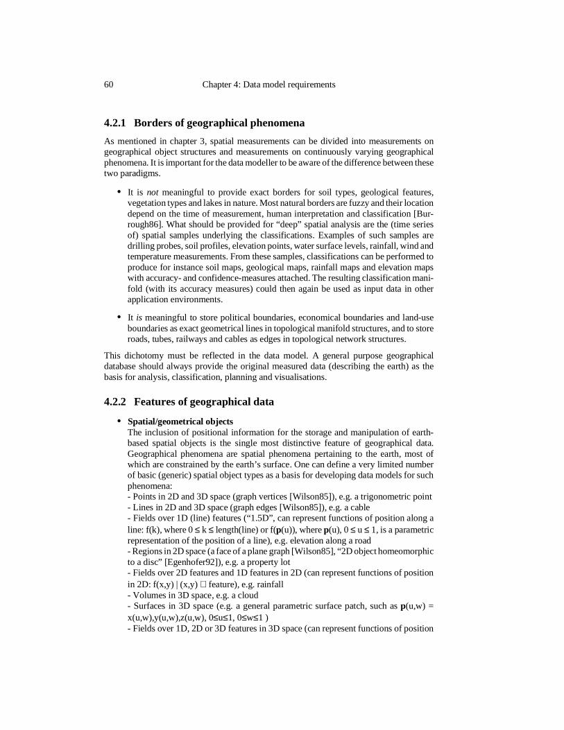
4.2.1 Borders of geographical phenomena

As mentioned in chapter 3, spatial measurements can be divided into measurements ongeographical object structures and measurements on continuously varying geographicalphenomena. It is important for the data modeller to be aware of the difference between thesetwo paradigms.

• It is not meaningful to provide exact borders for soil types, geological features,vegetation types and lakes in nature. Most natural borders are fuzzy and their locationdepend on the time of measurement, human interpretation and classification [Bur-rough86]. What should be provided for “deep” spatial analysis are the (time seriesof) spatial samples underlying the classifications. Examples of such samples aredrilling probes, soil profiles, elevation points, water surface levels, rainfall, wind andtemperature measurements. From these samples, classifications can be performed toproduce for instance soil maps, geological maps, rainfall maps and elevation mapswith accuracy- and confidence-measures attached. The resulting classification mani-fold (with its accuracy measures) could then again be used as input data in otherapplication environments.

• It is meaningful to store political boundaries, economical boundaries and land-useboundaries as exact geometrical lines in topological manifold structures, and to storeroads, tubes, railways and cables as edges in topological network structures.

This dichotomy must be reflected in the data model. A general purpose geographicaldatabase should always provide the original measured data (describing the earth) as thebasis for analysis, classification, planning and visualisations.

4.2.2 Features of geographical data

• Spatial/geometrical objectsThe inclusion of positional information for the storage and manipulation of earth-based spatial objects is the single most distinctive feature of geographical data.Geographical phenomena are spatial phenomena pertaining to the earth, most ofwhich are constrained by the earth’s surface. One can define a very limited numberof basic (generic) spatial object types as a basis for developing data models for suchphenomena:- Points in 2D and 3D space (graph vertices [Wilson85]), e.g. a trigonometric point- Lines in 2D and 3D space (graph edges [Wilson85]), e.g. a cable- Fields over 1D (line) features (“1.5D”, can represent functions of position along aline: f(k), where 0 ≤ k ≤ length(line) or f(p(u)), where p(u), 0 ≤ u ≤ 1, is a parametricrepresentation of the position of a line), e.g. elevation along a road- Regions in 2D space (a face of a plane graph [Wilson85], “2D object homeomorphicto a disc” [Egenhofer92]), e.g. a property lot- Fields over 2D features and 1D features in 2D (can represent functions of positionin 2D: f(x,y) | (x,y) ∈ feature), e.g. rainfall- Volumes in 3D space, e.g. a cloud- Surfaces in 3D space (e.g. a general parametric surface patch, such as p(u,w) =x(u,w),y(u,w),z(u,w), 0≤u≤1, 0≤w≤1 )- Fields over 1D, 2D or 3D features in 3D space (can represent functions of position

60 Chapter 4: Data model requirements

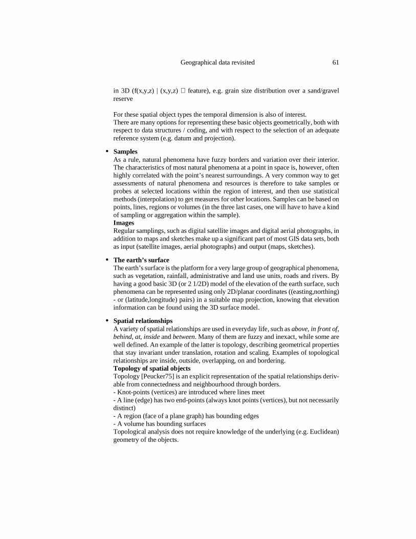
in 3D (f(x,y,z) | (x,y,z) ∈ feature), e.g. grain size distribution over a sand/gravelreserve

For these spatial object types the temporal dimension is also of interest.There are many options for representing these basic objects geometrically, both withrespect to data structures / coding, and with respect to the selection of an adequatereference system (e.g. datum and projection).

• SamplesAs a rule, natural phenomena have fuzzy borders and variation over their interior.The characteristics of most natural phenomena at a point in space is, however, oftenhighly correlated with the point’s nearest surroundings. A very common way to getassessments of natural phenomena and resources is therefore to take samples orprobes at selected locations within the region of interest, and then use statisticalmethods (interpolation) to get measures for other locations. Samples can be based onpoints, lines, regions or volumes (in the three last cases, one will have to have a kindof sampling or aggregation within the sample).ImagesRegular samplings, such as digital satellite images and digital aerial photographs, inaddition to maps and sketches make up a significant part of most GIS data sets, bothas input (satellite images, aerial photographs) and output (maps, sketches).

• The earth’s surfaceThe earth’s surface is the platform for a very large group of geographical phenomena,such as vegetation, rainfall, administrative and land use units, roads and rivers. Byhaving a good basic 3D (or 2 1/2D) model of the elevation of the earth surface, suchphenomena can be represented using only 2D/planar coordinates ((easting,northing)- or (latitude,longitude) pairs) in a suitable map projection, knowing that elevationinformation can be found using the 3D surface model.

• Spatial relationshipsA variety of spatial relationships are used in everyday life, such as above, in front of,behind, at, inside and between. Many of them are fuzzy and inexact, while some arewell defined. An example of the latter is topology, describing geometrical propertiesthat stay invariant under translation, rotation and scaling. Examples of topologicalrelationships are inside, outside, overlapping, on and bordering.Topology of spatial objectsTopology [Peucker75] is an explicit representation of the spatial relationships deriv-able from connectedness and neighbourhood through borders.- Knot-points (vertices) are introduced where lines meet- A line (edge) has two end-points (always knot points (vertices), but not necessarilydistinct)- A region (face of a plane graph) has bounding edges- A volume has bounding surfacesTopological analysis does not require knowledge of the underlying (e.g. Euclidean)geometry of the objects.

Geographical data revisited 61

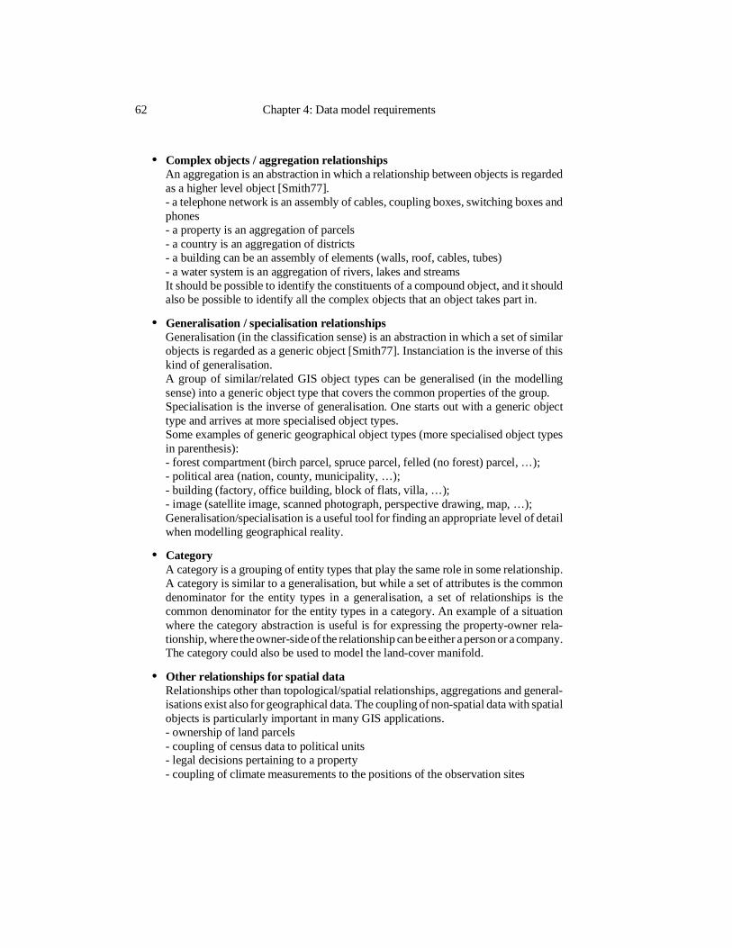
• Complex objects / aggregation relationshipsAn aggregation is an abstraction in which a relationship between objects is regardedas a higher level object [Smith77].- a telephone network is an assembly of cables, coupling boxes, switching boxes andphones- a property is an aggregation of parcels- a country is an aggregation of districts- a building can be an assembly of elements (walls, roof, cables, tubes)- a water system is an aggregation of rivers, lakes and streamsIt should be possible to identify the constituents of a compound object, and it shouldalso be possible to identify all the complex objects that an object takes part in.

• Generalisation / specialisation relationshipsGeneralisation (in the classification sense) is an abstraction in which a set of similarobjects is regarded as a generic object [Smith77]. Instanciation is the inverse of thiskind of generalisation.A group of similar/related GIS object types can be generalised (in the modellingsense) into a generic object type that covers the common properties of the group.Specialisation is the inverse of generalisation. One starts out with a generic objecttype and arrives at more specialised object types.Some examples of generic geographical object types (more specialised object typesin parenthesis):- forest compartment (birch parcel, spruce parcel, felled (no forest) parcel, …);- political area (nation, county, municipality, …);- building (factory, office building, block of flats, villa, …); - image (satellite image, scanned photograph, perspective drawing, map, …);Generalisation/specialisation is a useful tool for finding an appropriate level of detailwhen modelling geographical reality.

• CategoryA category is a grouping of entity types that play the same role in some relationship.A category is similar to a generalisation, but while a set of attributes is the commondenominator for the entity types in a generalisation, a set of relationships is thecommon denominator for the entity types in a category. An example of a situationwhere the category abstraction is useful is for expressing the property-owner rela-tionship, where the owner-side of the relationship can be either a person or a company.The category could also be used to model the land-cover manifold.

• Other relationships for spatial dataRelationships other than topological/spatial relationships, aggregations and general-isations exist also for geographical data. The coupling of non-spatial data with spatialobjects is particularly important in many GIS applications.- ownership of land parcels- coupling of census data to political units- legal decisions pertaining to a property- coupling of climate measurements to the positions of the observation sites


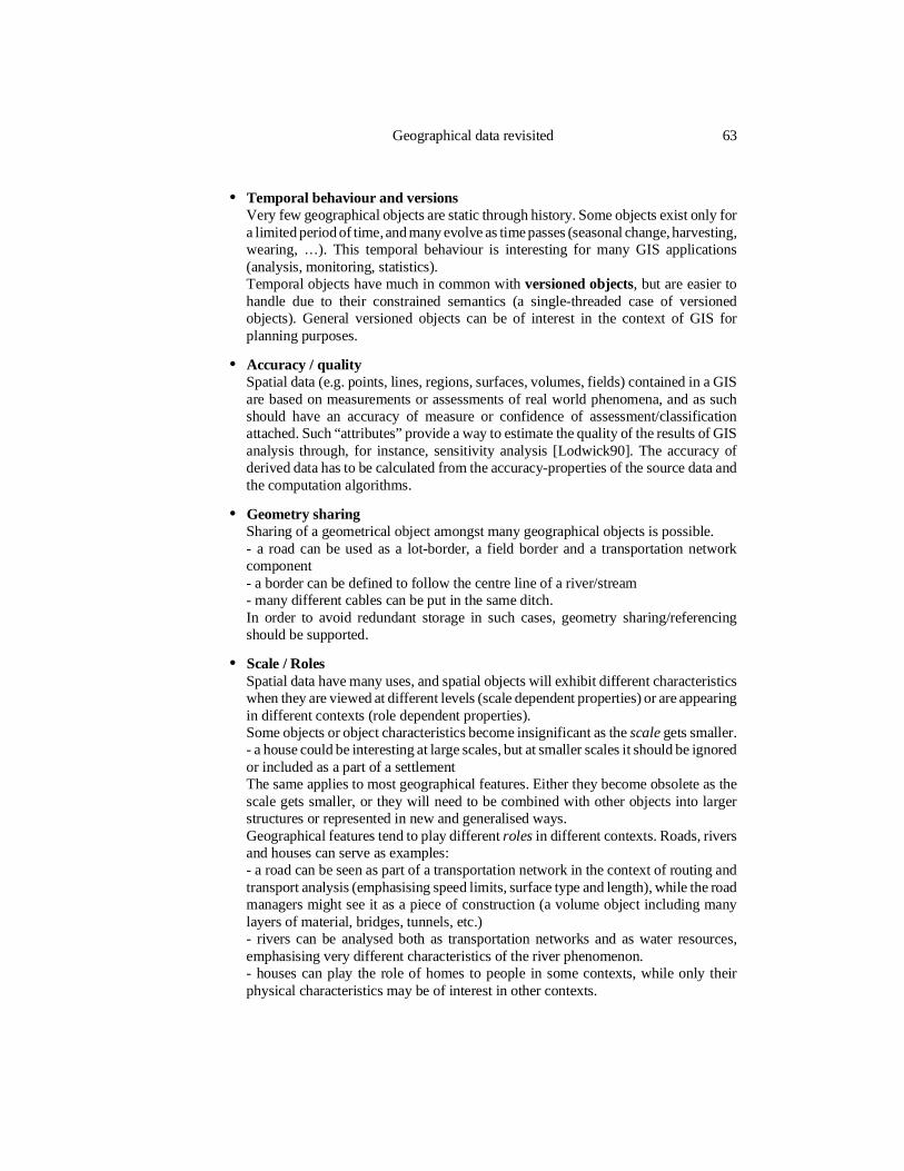
• Temporal behaviour and versionsVery few geographical objects are static through history. Some objects exist only fora limited period of time, and many evolve as time passes (seasonal change, harvesting,wearing, …). This temporal behaviour is interesting for many GIS applications(analysis, monitoring, statistics).Temporal objects have much in common with versioned objects, but are easier tohandle due to their constrained semantics (a single-threaded case of versionedobjects). General versioned objects can be of interest in the context of GIS forplanning purposes.

• Accuracy / qualitySpatial data (e.g. points, lines, regions, surfaces, volumes, fields) contained in a GISare based on measurements or assessments of real world phenomena, and as suchshould have an accuracy of measure or confidence of assessment/classificationattached. Such “attributes” provide a way to estimate the quality of the results of GISanalysis through, for instance, sensitivity analysis [Lodwick90]. The accuracy ofderived data has to be calculated from the accuracy-properties of the source data andthe computation algorithms.

• Geometry sharingSharing of a geometrical object amongst many geographical objects is possible.- a road can be used as a lot-border, a field border and a transportation networkcomponent- a border can be defined to follow the centre line of a river/stream- many different cables can be put in the same ditch.In order to avoid redundant storage in such cases, geometry sharing/referencingshould be supported.

• Scale / RolesSpatial data have many uses, and spatial objects will exhibit different characteristicswhen they are viewed at different levels (scale dependent properties) or are appearingin different contexts (role dependent properties).Some objects or object characteristics become insignificant as the scale gets smaller.- a house could be interesting at large scales, but at smaller scales it should be ignoredor included as a part of a settlementThe same applies to most geographical features. Either they become obsolete as thescale gets smaller, or they will need to be combined with other objects into largerstructures or represented in new and generalised ways.Geographical features tend to play different roles in different contexts. Roads, riversand houses can serve as examples:- a road can be seen as part of a transportation network in the context of routing andtransport analysis (emphasising speed limits, surface type and length), while the roadmanagers might see it as a piece of construction (a volume object including manylayers of material, bridges, tunnels, etc.)- rivers can be analysed both as transportation networks and as water resources,emphasising very different characteristics of the river phenomenon.- houses can play the role of homes to people in some contexts, while only theirphysical characteristics may be of interest in other contexts.

Geographical data revisited 63

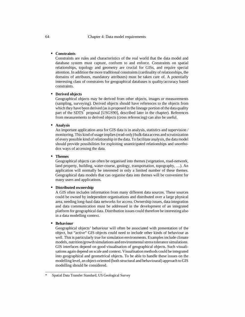
• ConstraintsConstraints are rules and characteristics of the real world that the data model anddatabase system must capture, conform to and enforce. Constraints on spatialrelationships, topology and geometry are crucial for GISs, and require specialattention. In addition the more traditional constraints (cardinality of relationships, thedomains of attributes, mandatory attributes) must be taken care of. A potentiallyinteresting class of constraints for geographical databases is quality/accuracy basedconstraints.

• Derived objectsGeographical objects may be derived from other objects, images or measurements(sampling, surveying). Derived objects should have references to the objects fromwhich they have been derived (as is proposed in the lineage portion of the data qualitypart of the SDTS* proposal [USGS90], described later in the chapter). Referencesfrom measurements to derived objects (cross referencing) can also be useful.

• AnalysisAn important application area for GIS data is in analysis, statistics and supervision /monitoring. This kind of usage implies (read-only) bulk data access and scrutinizationof every possible kind of relationship in the data. To facilitate analysis, the data modelshould provide possibilities for exploiting unanticipated relationships and unortho-dox ways of accessing the data.

• ThemesGeographical objects can often be organised into themes (vegetation, road-network,land property, building, water-course, geology, transportation, topography, …). Anapplication will normally be interested in only a limited number of these themes.Geographical data models that can organise data into themes will be convenient formany users and applications.

• Distributed ownershipA GIS often includes information from many different data sources. These sourcescould be owned by independent organisations and distributed over a large physicalarea, needing long-haul data networks for access. Ownership issues, data integrationand data communication must be addressed in the development of an integratedplatform for geographical data. Distribution issues could therefore be interesting alsoin a data modelling context.

• BehaviourGeographical objects’ behaviour will often be associated with presentation of theobject, but “active” GIS objects could need to include other kinds of behaviour aswell. This is particularly true for simulation environments. Examples include climatemodels, nutrition/growth simulations and environmental stress tolerance simulations.GIS interfaces depend on good visualisation of geographical objects. Such visuali-sations again depend on scale and context. Visualisation methods could be integratedinto geographical and geometrical objects. To be able to handle these issues on themodelling level, an object-oriented (both structural and behavioural) approach to GISmodelling should be considered.


* Spatial Data Transfer Standard, US Geological Survey

4.3 Requirements to high level geographical data models

A high level data model is a tool for modelling/describing interesting aspects of real worldphenomena as accurately, convincingly and completely as possible. For this purpose,adequate structuring and abstraction mechanisms should be provided. For geographicalinformation in particular we want to be able to model geographical phenomena in their rightcontext.

A high level data model should be easily comprehensible for all specialists involved, andshould provide a structuring of the information that is useful for translation into databaseoriented data models (as described in chapter 2).

Through the years, many different approaches have been taken to high level data modelling.In the early 1980ies, entity-relationship (ER) data models, binary data models, semanticnetwork data models and infological data models were considered to be a representativeselection of the methods used [Tsichritzis82]. Semantic extensions to the entity-relationshipapproach have become increasingly popular, and in the late 1980s, these types of modelshave been classified as structurally object-oriented models [Rumbaugh91]. The ER datamodel and some of its extensions will be used as a basis in this thesis.

The GIS information base consists of spatial data objects (with their geometrical andnon-geometrical properties) and traditional (spatially relatable) “catalogue” type of data (forinstance census data and administrative data). A useful high-level data model for the GISinformation base will have to integrate spatial and non-spatial data in a common modellingframework to facilitate full data integration in GIS databases.

Geographical data model requirementsData models for geographical data should cover most of the following topics (in accordancewith the preceding section):

• Basic primitives such as entities, relationships and attributes in the traditional ERmodel.

• Two-dimensional and three-dimensional geographical structures with (shared) geo-metrical data types (points, lines, regions, surfaces, volumes, fields, samples, rasters).The time/temporal dimension should be supported for all geographical structures.

• Two-dimensional and three-dimensional spatial relationships and constraints, includ-ing topological relationships (network and manifold structures).

• Aggregation hierarchies, both at the attribute level and the object level.

• Generalisation/specialisation hierarchies/networks (in the case of multiple inheri-tance).

• Relationships specified on “unions” of different object types (EER categories).

• Historical information.

• Quality (including accuracy) and scale measures.

Requirements to high level geographical data models 65

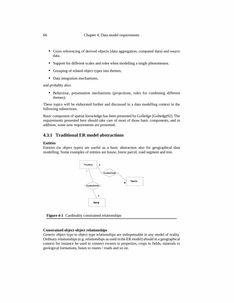
• Cross referencing of derived objects (data aggregation, computed data) and sourcedata.

• Support for different scales and roles when modelling a single phenomenon.

• Grouping of related object types into themes.

• Data integration mechanisms.

and probably also:

• Behaviour, presentation mechanisms (projections, rules for combining differentthemes).

These topics will be elaborated further and discussed in a data modelling context in thefollowing subsections.

Basic component of spatial knowledge has been presented by Golledge [Golledge92]. Therequirements presented here should take care of most of those basic components, and inaddition, some new requirements are presented.

4.3.1 Traditional ER model abstractions

EntitiesEntities (or object types) are useful as a basic abstraction also for geographical datamodelling. Some examples of entities are house, forest parcel, road segment and tree.

Constrained object-object relationshipsGeneric object type to object type relationships are indispensable in any model of reality.Ordinary relationships (e.g. relationships as used in the ER model) should in a geographicalcontext for instance be used to connect owners to properties, crops to fields, minerals togeological formations, buses to routes / roads and so on.

Figure 4-1 Cardinality constrained relationships


For modelling purposes it is also useful to be able to put constraints on relationships, suchas those used in ER models (1:1, 1:N, N:M, compulsory/possible relationships). See Figure4-1 for an illustration of constrained relationships (1:N, N:M) in the ER model.

AttributesProperties of entities and relationships can be represented as attributes. An attribute couldbe the date of birth of a person, the colour of a flower, the surface material of a road or theamount of algae of a certain type at a sampling spot in a lake or river. Attributes andrelationships are our key tools for describing the distinctive features of an entity/object type.

4.3.2 Geometrical object types

All necessary geometrical/spatial object types should be supported in their most generalrepresentation. Object borders/boundaries (∂) and interiors (°) [Egenhofer90b] (as discussedin chapter 3) should be supported, as should continuous variation throughout the interior ofobjects (fields), as discussed earlier in this chapter.

Point. A point needs to be related to some reference system (datum and projection), andits position within this reference system must be given. Either some kind of “global”reference system (where a point is given by for instance latitude, longitude, elevation)or a planar/projected reference system (where a point can is given relative to a certainorigo: north,east,elevation) should be applied. If no elevation value is specified for apoint, it should be assumed to lie on the earth’s surface.

Line. A geometrical line can theoretically be represented as an infinite sequence ofpoints connecting two end-points. A representation will have to be chosen that givesthe desired accuracy and that is reasonably compact when it comes to computerstorage. A sequence of points selected according to for instance the Douglas-Peuckeralgorithm [Douglas73] or a parametric representation (such as spline curves, B-splinecurves or Bezier curves [Mortenson85]) could be used for line representation.A way of representing variation of a property along a line would also be useful formany applications, as mentioned in the preceding summary. A line where therepresentation does not include elevation information should be assumed to lie onthe earth’s surface.

Region. A region can, in a geographical context, be restricted to two dimensions, andcan be defined as all the points that are inside the region’s (closed) boundary lines (aface in a plane graph [Wilson85]). A region can therefore be described by it boundinglines and an indication of where the interior of the region is (the vector approach), orby a finite set of regularly sampled points representing the interior of the region (theraster approach). The raster approach to representing a region can capture continuouschange in a property throughout the region, making it an efficient “2.5D” (or field)representation. Representation of homogeneous regions using raster technology isconsequently a waste of the capabilities of the raster approach, while the currentvector approach to regions only can handle homogeneous regions.

Surface. A geographical surface can be described as a function in three dimensionalspace. It can either be represented by a set of points laying on the surface with someneighbourhood information (topology) attached (to determine how the surface is tobe constructed from the points (e.g. a TIN structure)). Or it can be represented by


functions (e.g. parametric functions such as B-splines or Bezier).An important sub-class of surfaces are those that can be represented as functions oftwo dimensions: z=f(north, east). Such functions can be used to represent “continu-ously” varying geographical phenomena (e.g. elevation, rainfall, surface temperatureand soil depth). Such a representation is an implementation of a field over a 2Dregion.Neugebauer [Neugebauer90] suggests that continuous surfaces should be availabledirectly at the database level, hiding the (sample) data sets that will have to be thebasis for the database system’s or GIS’s interpolations. Such a feature would be veryuseful for many disciplines. However, the underlying samples should also be avail-able for users who want to provide their own interpolation methods. Peucker andChrisman were of the first to emphasise the importance of fields over 2D regions(they called them three-dimensional surfaces) in geographical information systems[Peucker75].

Volume. A geographical volume is the three-dimensional space bounded by a closedset of surfaces (the volume boundary). The representation of volumes can be orientedtowards the surfaces of the volume or the interior of the volume.The vector approach can represent the surfaces of a volume quite easily using forinstance parametric functions or TINs, and it is also possible to represent the interiorof a volume using the same techniques.The raster approach has to represent the interior of the volume, and can do this in astraightforward way. The raster approach to representing volumes makes it possibleto represent continuous changes for a property throughout the volume, making theraster approach to volume modelling a “3.5D” representation (field over a 3D region).

Spatial set. For the important class of spatial samples, a spatial set concept is valuable.Spatial sets could be sets of points, lines, regions or volumes. A spatial set is differentfrom other sets, because all the elements of the set have a position in two- orthree-dimensional space. The members of a spatial set thus have an inherent structure,being spatially related to each other.

Field. Variation throughout the interior of a geographical object should be supported inall relevant dimensions.

4.3.3 Spatial relationships

Spatial relationships are relationships that are a result of the location of objects in space.The importance of spatial relationships in geographical data models and geographicalinformation systems has been emphasised by many researchers [Mark89, Peuquet86].Spatial relationships can be divided into groups on the basis of their characteristics. Threesuch groups could be:

• (Geo)Metric relationships, such as distance and direction

• Topological relationships. These can be derived from geometry (e.g. neighbour andborder)

• Fuzzy spatial relationships. These can be difficult to define accurately and are oftencontext sensitive. Examples are above and in front of.


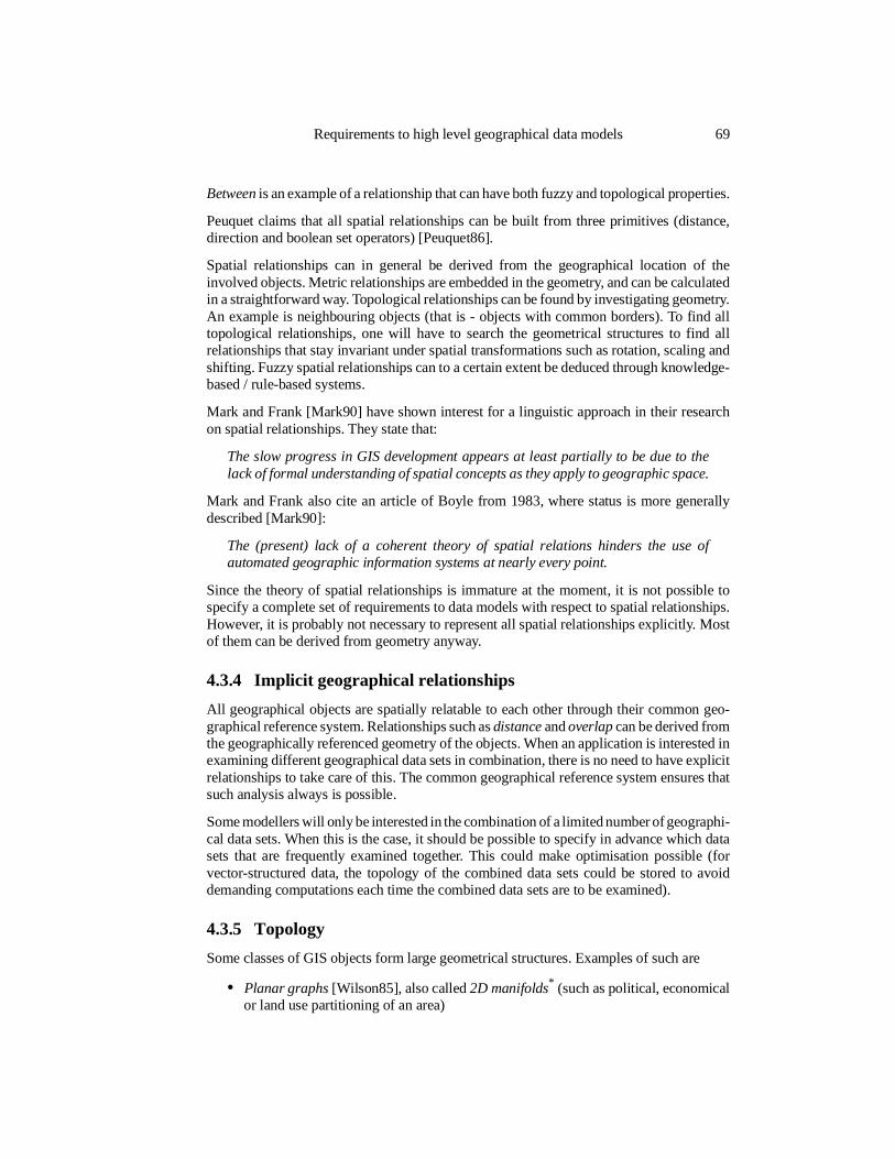
Between is an example of a relationship that can have both fuzzy and topological properties.

Peuquet claims that all spatial relationships can be built from three primitives (distance,direction and boolean set operators) [Peuquet86].

Spatial relationships can in general be derived from the geographical location of theinvolved objects. Metric relationships are embedded in the geometry, and can be calculatedin a straightforward way. Topological relationships can be found by investigating geometry.An example is neighbouring objects (that is - objects with common borders). To find alltopological relationships, one will have to search the geometrical structures to find allrelationships that stay invariant under spatial transformations such as rotation, scaling andshifting. Fuzzy spatial relationships can to a certain extent be deduced through knowledge-based / rule-based systems.

Mark and Frank [Mark90] have shown interest for a linguistic approach in their researchon spatial relationships. They state that:

The slow progress in GIS development appears at least partially to be due to thelack of formal understanding of spatial concepts as they apply to geographic space.

Mark and Frank also cite an article of Boyle from 1983, where status is more generallydescribed [Mark90]:

The (present) lack of a coherent theory of spatial relations hinders the use ofautomated geographic information systems at nearly every point.

Since the theory of spatial relationships is immature at the moment, it is not possible tospecify a complete set of requirements to data models with respect to spatial relationships.However, it is probably not necessary to represent all spatial relationships explicitly. Mostof them can be derived from geometry anyway.

4.3.4 Implicit geographical relationships

All geographical objects are spatially relatable to each other through their common geo-graphical reference system. Relationships such as distance and overlap can be derived fromthe geographically referenced geometry of the objects. When an application is interested inexamining different geographical data sets in combination, there is no need to have explicitrelationships to take care of this. The common geographical reference system ensures thatsuch analysis always is possible.

Some modellers will only be interested in the combination of a limited number of geographi-cal data sets. When this is the case, it should be possible to specify in advance which datasets that are frequently examined together. This could make optimisation possible (forvector-structured data, the topology of the combined data sets could be stored to avoiddemanding computations each time the combined data sets are to be examined).

4.3.5 Topology

Some classes of GIS objects form large geometrical structures. Examples of such are

• Planar graphs [Wilson85], also called 2D manifolds* (such as political, economicalor land use partitioning of an area)


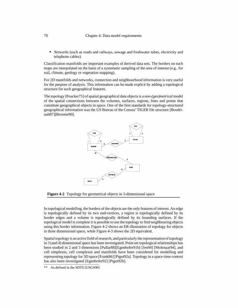
• Networks (such as roads and railways, sewage and freshwater tubes, electricity andtelephone cables).

Classification manifolds are important examples of derived data sets. The borders on suchmaps are interpolated on the basis of a systematic sampling of the area of interest (e.g.. forsoil, climate, geology or vegetation mapping).

For 2D manifolds and networks, connection and neighbourhood information is very usefulfor the purpose of analysis. This information can be made explicit by adding a topologicalstructure for such geographical features.

The topology [Peucker75] of spatial geographical data objects is a non-(geo)metrical modelof the spatial connections between the volumes, surfaces, regions, lines and points thatconstitute geographical objects in space. One of the first standards for topology-structuredgeographical information was the US Bureau of the Census’ TIGER file structure [Boudri-ault87][Broome90].

In topological modelling, the borders of the objects are the only features of interest. An edgeis topologically defined by its two end-vertices, a region is topologically defined by itsborder edges and a volume is topologically defined by its bounding surfaces. If thetopological model is complete it is possible to use the topology to find neighbouring objectsusing this border information. Figure 4-2 shows an ER-illustration of topology for objectsin three dimensional space, while Figure 4-3 shows the 2D equivalent.

Spatial topology is an active field of research, and particularly the representation of topologyin 3 (and 4) dimensional space has been investigated. Point set topological relationships hasbeen studied in 2 and 3 dimensions [Pullar88][Egenhofer91b] [Jen94] [Molenaar94], andcell simplexes, cell complexes and manifolds have been considered for modelling andrepresenting topology for 3D space [Frank86] [Pigot92a]. Topology in a space-time contexthas also been investigated [Egenhofer92] [Pigot92b].

Figure 4-2 Topology for geometrical objects in 3-dimensional space


** As defined in the SDTS [USGS90]

To be able to model spatial connections between and within objects, topological relation-ships are indispensable. Using a layered approach to spatial object modelling, the geomet-rical level would constitute the lowest level in the hierarchy, with its representations ofpoints, lines and surfaces. The spatial objects would be at the highest level, while thetopological level would be an intermediate level in the hierarchy, present only for geographi-cal objects that participate in topological structures.

The topology layer will show how the basic geometrical objects are interconnected to formspatial object structures. It will show how borderlines can be assembled to describe differenteconomical and administrative units, how a hydrological system is an assembly of lakes,rivers, streams and ponds, how different road-segments should be interconnected to formthe road transportation network, and so on. The topology level should be logically self-con-tained, and together with the geometry it will provide the backbone of the geographical datamodel.

By storing topology on a thematic basis, separated from, but connected to the geometry,sharing of the geometrical descriptions (for instance between a river and a lot border) canbe accomplished. The geometry of a river could then be used both in a property manifoldand a river network.

Inter thematic topologyTopological relationships can be incorporated into the data model using two differentapproaches.

• An integration approach, covering all the themes in the GIS database, and therebycausing a very detailed topological model.

• A separation approach, keeping the topology within a theme separated from thetopology of the other themes.

This can be illustrated by a road-network theme and a water-system theme. The separationapproach will result in topological points/nodes (grey circles) at road-crossings and stream-meets (Figure 4-4). The integration approach will introduce additional topological points

Figure 4-3 Topology for geometrical objects in 2-dimensional space


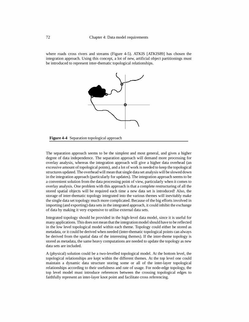
where roads cross rivers and streams (Figure 4-5). ATKIS [ATKIS89] has chosen theintegration approach. Using this concept, a lot of new, artificial object partitionings mustbe introduced to represent inter-thematic topological relationships.

The separation approach seems to be the simplest and most general, and gives a higherdegree of data independence. The separation approach will demand more processing foroverlay analysis, whereas the integration approach will give a higher data overhead (anexcessive amount of topological points), and a lot of work is needed to keep the topologicalstructures updated. The overhead will mean that single data set analysis will be slowed downin the integration approach (particularly for updates). The integration approach seems to bea convenient solution from the data processing point of view, particularly when it comes tooverlay analysis. One problem with this approach is that a complete restructuring of all thestored spatial objects will be required each time a new data set is introduced! Also, thestorage of inter-thematic topology integrated into the various themes will inevitably makethe single data set topology much more complicated. Because of the big efforts involved inimporting (and exporting) data sets in the integrated approach, it could inhibit the exchangeof data by making it very expensive to utilise external data sets.

Integrated topology should be provided in the high-level data model, since it is useful formany applications. This does not mean that the integration model should have to be reflectedin the low level topological model within each theme. Topology could either be stored asmetadata, or it could be derived when needed (inter-thematic topological points can alwaysbe derived from the spatial data of the interesting themes). If the inter-theme topology isstored as metadata, the same heavy computations are needed to update the topology as newdata sets are included.

A (physical) solution could be a two-levelled topological model. At the bottom level, thetopological relationships are kept within the different themes. At the top level one couldmaintain a dynamic data structure storing some or all of the inter-layer topologicalrelationships according to their usefulness and rate of usage. For node-edge topology, thetop level model must introduce references between the crossing topological edges tofaithfully represent an inter-layer knot point and facilitate cross referencing.

Figure 4-4 Separation topological approach


4.3.6 Aggregation

Smith and Smith describe aggregation as [Smith77]:

“… an abstraction in which a relationship between objects is regarded as a higherlevel object. In making such an abstraction, many details of the relationship may beignored. For example, a certain relationship between a person, a hotel, and a datecan be abstracted as the object ”reservation”. It is possible to think about a“reservation” without bringing to mind all details of the underlying relationship -for example, the number of the room reserved, the name of the reserving agent, orthe length of the stay”.

Aggregation, or the construction of an object from its constituent objects, can be illustratedin different ways. In [Tsichritzis82], an aggregation on the type level is shown as in Figure4-6.

Substituting the tokens “Per Jensen” for name, “Ulvefaret 3” for address and ”76” for age,one ends up with a token level object aggregation.

Figure 4-5 Integration topological approach

Figure 4-6 Aggregation


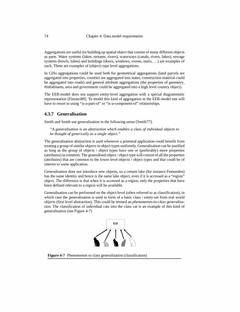
Aggregations are useful for building up spatial object that consist of many different objectsas parts. Water systems (lakes, streams, rivers), waterways (canals, rivers, lakes), sewagesystems (bowls, tubes) and buildings (doors, windows, rooms, stairs, …) are examples ofsuch. These are examples of (object) type level aggregations.

In GISs aggregations could be used both for geometrical aggregations (land parcels areaggregated into properties, counties are aggregated into states, construction material couldbe aggregated into roads) and general attribute aggregations (the properties of geometry,#inhabitants, area and government could be aggregated into a high level country object).

The EER-model does not support entity-level aggregation with a special diagrammaticrepresentation [Elmasri89]. To model this kind of aggregation in the EER-model one willhave to resort to using “is-a-part-of” or “is-a-component-of” relationships.

4.3.7 Generalisation

Smith and Smith use generalisation in the following sense [Smith77]:

“A generalisation is an abstraction which enables a class of individual objects tobe thought of generically as a single object.”

The generalisation abstraction is used whenever a potential application could benefit fromtreating a group of similar objects or object types uniformly. Generalisation can be justifiedas long as the group of objects / object types have one or (preferably) more properties(attributes) in common. The generalised object / object type will consist of all the properties(attributes) that are common to the lower level objects / object types and that could be ofinterest to some application.

Generalisation does not introduce new objects, so a certain lake (for instance Femunden)has the same identity and hence is the same lake object, even if it is accessed as a “region”object. The difference is that when it is accessed as a region, only the properties that havebeen defined relevant to a region will be available.

Generalisation can be performed on the object-level (often referred to as classification), inwhich case the generalisation is used to form of a basic class / entity-set from real worldobjects (first level abstraction). This could be termed an phenomenon-to-class generalisa-tion. The classification of individual cats into the class cat is an example of this kind ofgeneralisation (see Figure 4-7)

Figure 4-7 Phenomenon to class generalisation (classification)


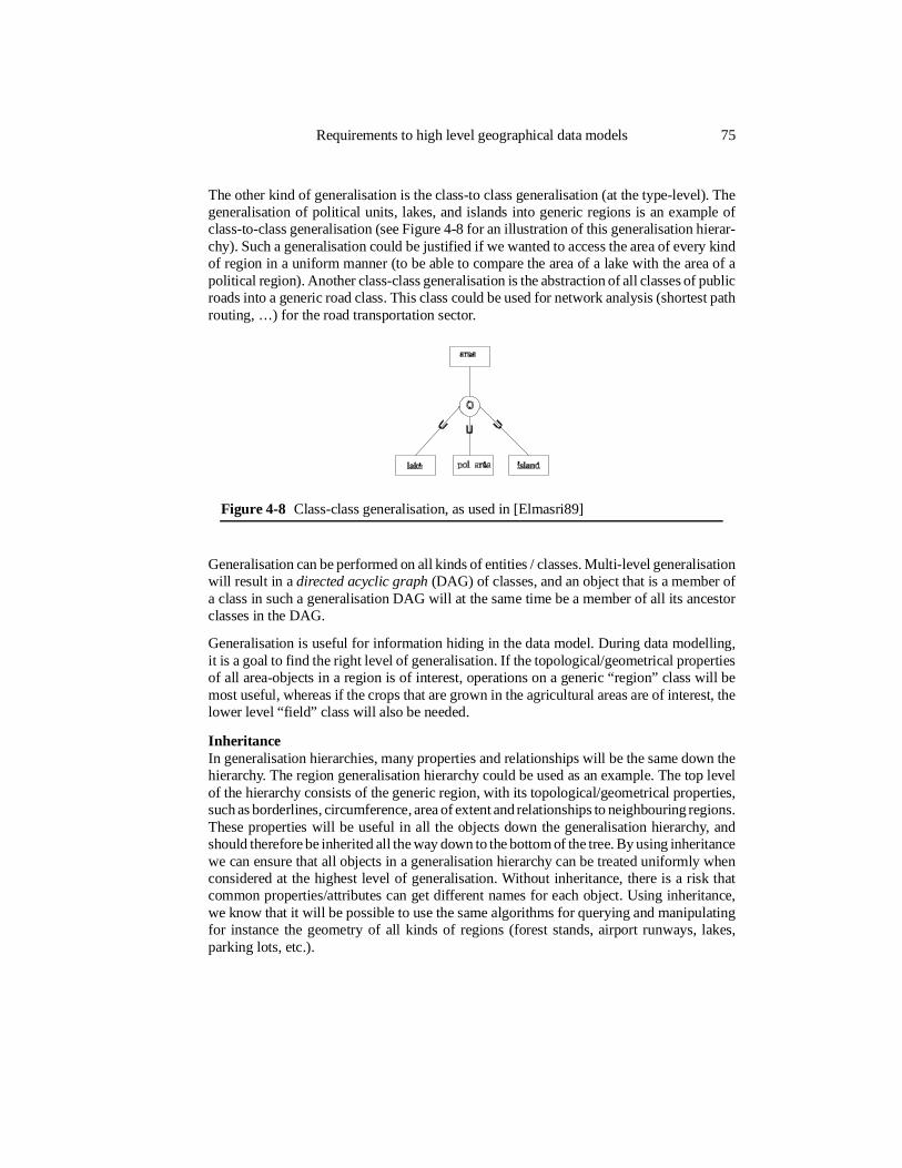
The other kind of generalisation is the class-to class generalisation (at the type-level). Thegeneralisation of political units, lakes, and islands into generic regions is an example ofclass-to-class generalisation (see Figure 4-8 for an illustration of this generalisation hierar-chy). Such a generalisation could be justified if we wanted to access the area of every kindof region in a uniform manner (to be able to compare the area of a lake with the area of apolitical region). Another class-class generalisation is the abstraction of all classes of publicroads into a generic road class. This class could be used for network analysis (shortest pathrouting, …) for the road transportation sector.

Generalisation can be performed on all kinds of entities / classes. Multi-level generalisationwill result in a directed acyclic graph (DAG) of classes, and an object that is a member ofa class in such a generalisation DAG will at the same time be a member of all its ancestorclasses in the DAG.

Generalisation is useful for information hiding in the data model. During data modelling,it is a goal to find the right level of generalisation. If the topological/geometrical propertiesof all area-objects in a region is of interest, operations on a generic “region” class will bemost useful, whereas if the crops that are grown in the agricultural areas are of interest, thelower level “field” class will also be needed.

InheritanceIn generalisation hierarchies, many properties and relationships will be the same down thehierarchy. The region generalisation hierarchy could be used as an example. The top levelof the hierarchy consists of the generic region, with its topological/geometrical properties,such as borderlines, circumference, area of extent and relationships to neighbouring regions.These properties will be useful in all the objects down the generalisation hierarchy, andshould therefore be inherited all the way down to the bottom of the tree. By using inheritancewe can ensure that all objects in a generalisation hierarchy can be treated uniformly whenconsidered at the highest level of generalisation. Without inheritance, there is a risk thatcommon properties/attributes can get different names for each object. Using inheritance,we know that it will be possible to use the same algorithms for querying and manipulatingfor instance the geometry of all kinds of regions (forest stands, airport runways, lakes,parking lots, etc.).

Figure 4-8 Class-class generalisation, as used in [Elmasri89]


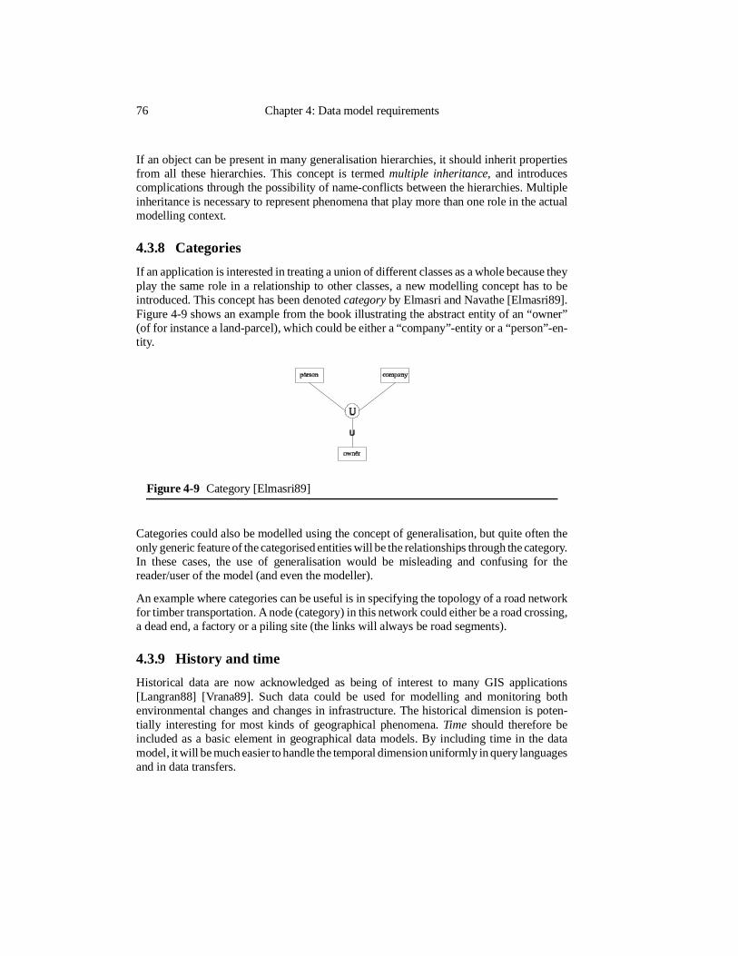
If an object can be present in many generalisation hierarchies, it should inherit propertiesfrom all these hierarchies. This concept is termed multiple inheritance, and introducescomplications through the possibility of name-conflicts between the hierarchies. Multipleinheritance is necessary to represent phenomena that play more than one role in the actualmodelling context.

4.3.8 Categories

If an application is interested in treating a union of different classes as a whole because theyplay the same role in a relationship to other classes, a new modelling concept has to beintroduced. This concept has been denoted category by Elmasri and Navathe [Elmasri89].Figure 4-9 shows an example from the book illustrating the abstract entity of an “owner”(of for instance a land-parcel), which could be either a “company”-entity or a “person”-en-tity.

Categories could also be modelled using the concept of generalisation, but quite often theonly generic feature of the categorised entities will be the relationships through the category.In these cases, the use of generalisation would be misleading and confusing for thereader/user of the model (and even the modeller).

An example where categories can be useful is in specifying the topology of a road networkfor timber transportation. A node (category) in this network could either be a road crossing,a dead end, a factory or a piling site (the links will always be road segments).

4.3.9 History and time

Historical data are now acknowledged as being of interest to many GIS applications[Langran88] [Vrana89]. Such data could be used for modelling and monitoring bothenvironmental changes and changes in infrastructure. The historical dimension is poten-tially interesting for most kinds of geographical phenomena. Time should therefore beincluded as a basic element in geographical data models. By including time in the datamodel, it will be much easier to handle the temporal dimension uniformly in query languagesand in data transfers.

Figure 4-9 Category [Elmasri89]


Trend analysis and time series analysis are new possibilities that arise when time is includedas a basic property of geographical objects. Historical snapshots and history animations willalso be trivial to obtain from geographical data when time is fully integrated into the datamodel.

NatureEnvironmental monitoring is based on measurements over a certain area using varioussampling techniques (air photos, satellite images, climate monitoring stations and otherpoint sampling techniques). Environmental data should be handled statistically since theyrepresent samples of continuously varying natural phenomena. The measurements can bedone in time series at certain points or be taken systematically over an area at well definedpoints in time.

InfrastructureInfrastructure is composed of well defined geometrical structures, and changes in suchstructures can be considered discrete compared to the slow changes that occur in nature.Man made constructions (buildings, bridges, roads) are made over short periods in time,and so are modifications to such constructions. Infrastructure components can be torn downin a day or just left for a gradual decay into ruins.

History could be difficult to handle for infrastructure because of the object-oriented natureof man-made features. The handling of object identity will be one of the problemsencountered when trying to represent changes to geographical objects. Should an objectchange identity when it has been changed? How significant must the change be before wehave a new object?

Environmental data are sample based, so they are not in the same way object-oriented(although it is possible to derive objects from the data using classification techniques).

VersionsVersions can be useful for representing alternatives in the planning of infrastructure andland use. For a planning department it will be convenient to have all plans stored in ageographical database, with the different alternatives that have been considered. This willparticularly be the case for plans under current consideration, but also historical plans canbe of interest in the future. If such a storage shall be possible, a more general purposeversioning mechanism must be available. It must be possible to store an existing roadtogether with a number of alternative placings of the road.

4.3.10 Quality/ accuracy

Geographical data represent phenomena in nature. The level of accuracy that can beachieved with such representations varies, and it is important that this is reflected in the datathemselves [Goodchild91]. To be able to perform sensitivity analysis [Lodwick90] (throughfor instance error propagation and simulation) and in other ways provide measures of thelevel of confidence in results from GIS analysis and classification, quality aspects of thedata - such as accuracy of the underlying measurements and completeness of the data sets- must be available for calculation and propagation through the analysis process.


Quality information for traditional (paper) mapsThe map has always carried with it an implicit measure of positional accuracy through itsscale (scale is not available for digital geographical information, so there is a need foralternative and more direct representations of spatial accuracy). The lineage of the map hasnormally been described somewhere on the map (producer, method of production, time ofdata collection). Other quality measures for paper maps have been manifested in mappingrules and requirements, but normally not described on the map itself.

Geographical data qualityAccuracy and other quality measures for the geographical data in a GIS database is essentialinformation for assessing the usefulness of the results of an integration of differentgeographical data sets, and for reliable and trustworthy GIS analysis and presentations(visualisation of the quality of spatial data processing results will have to be included infuture GISs [Clapham91][NCGIA91]). Work in this area was initiated in the early 1980s(e.g.. [Chrisman84], [Chrisman86], [Beck86] and [Openshaw89]), and has received in-creasing attention in the 1990ies.

The US SDTS (spatial data transfer standard) requires quality measures to be supplied withall kinds of geographical data when they are transferred from one system to another[USGS90]. In the SDTS (see page 86), the following five quality measures are identified:1) Lineage: The origin and history of the data, including methods of measurements/deriva-tion, transformations, control information used and dates of validity/collection. 2) Posi-tional accuracy. 3) Attribute accuracy. Both numerical and classification accuracy iscovered. 4) Logical consistency. Describes the fidelity of the relationships encoded in thedata structure. 5) Completeness. Describes the ratio of the objects represented to the abstractuniverse of all such objects (exhaustiveness).

According to Firns and Benwell, two main types of accuracy can be identified for GIS data[Firns91]. Spatial accuracy involves the accuracy of absolute and relative positioning whiledescriptional accuracy is the accuracy of the representation of the state of objects in termsof non-spatial attribute values and relationships. Spatial accuracy is a geometrical property,and should be tied to the shareable geometry of the spatial objects. Descriptional accuracycould be provided by giving non-spatial attributes and relationships relevant accuracymeasures. This might be a useful way of attacking geographical data quality, but a furtherrefinement of the concepts will have to be introduced. Using this taxonomy, topologicalrelationships would have to be treated as special kinds of non-spatial relationships, and otherquality issues, such as the completeness of a spatial data set, is not covered at all (e.g.. thecompleteness of a road coverage).

Quality information is sometimes associated with a data set, and sometimes with a groupof objects, and sometimes with a single object or an attribute of an object. A method formodelling quality should take this into account, and provide flexibility in representation.Conceptually, as much quality information as possible should be available on the attrib-ute/object level. Where only data set measures are available, a method for inheriting qualitymeasures from the data set level to the level of the individual objects should be madeavailable.


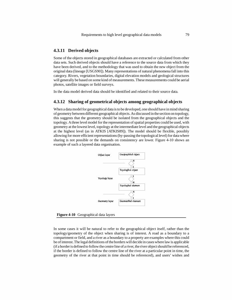
4.3.11 Derived objects

Some of the objects stored in geographical databases are extracted or calculated from otherdata sets. Such derived objects should have a reference to the source data from which theyhave been derived, and to the methodology that was used to obtain the new object from theoriginal data (lineage [USGS90]). Many representations of natural phenomena fall into thiscategory. Rivers, vegetation boundaries, digital elevation models and geological structureswill generally be based on some kind of measurements. These measurements could be aerialphotos, satellite images or field surveys.

In the data model derived data should be identified and related to their source data.

4.3.12 Sharing of geometrical objects among geographical objects

When a data model for geographical data is to be developed, one should have in mind sharingof geometry between different geographical objects. As discussed in the section on topology,this suggests that the geometry should be isolated from the geographical objects and thetopology. A three level model for the representation of spatial properties could be used, withgeometry at the lowest level, topology at the intermediate level and the geographical objectsat the highest level (as in ATKIS [ATKIS89]). The model should be flexible, possiblyallowing for more efficient representations (by-passing the topological level) for data wheresharing is not possible or the demands on consistency are lower. Figure 4-10 shows anexample of such a layered data organisation.

In some cases it will be natural to refer to the geographical object itself, rather than thetopology/geometry of the object when sharing is of interest. A road as a boundary to acompartment or field, and a river as a boundary to a property are examples where this couldbe of interest. The legal definitions of the borders will decide in cases where law is applicable(if a border is defined to follow the centre line of a river, the river object should be referenced,if the border is defined to follow the centre line of the river at a particular point in time, thegeometry of the river at that point in time should be referenced), and users’ wishes and

Figure 4-10 Geographical data layers


convenience of representation will decide elsewhere. A problem with referring to an objectinstead of its topology/geometry is that some extra computations will have to be done atrun-time in order to find the exact geometry of the object.

4.3.13 Roles and scale

The representation of geographical phenomena depends on both the scale of interest andthe role the phenomenon plays in our model.

Both the graphic presentation and storage representation of geographical objects depend onscale and role. The complex challenges of computer-assisted cartographic generalisation[Brassel88] [Muller91] is a part of the scale problem, while role-dependent representationsconstitute a new problem domain.

RolesGeographical phenomena can play various roles, determined by the context in which theyappear.

People of different background/profession will often have different points of view when itcomes to what aspects of a certain phenomenon that are considered interesting for repre-sentation in a data model (an ecologist and a ship owner will generally be interested indifferent characteristics of a river or a lake).

This role problem introduces a new complexity dimension in the modelling and repre-sentation of geographical data. Roles should therefore be covered in a general purpose datamodelling technique (and, if possible, also by geographical data transfer standards).

Role aspects of representation results from the different uses a geographical phenomenonmight have, and the many roles it might play as a part of nature and to humans. Continuingthe example on rivers and lakes, it is evident that water systems play many roles. They arehabitats of many different species of fish, algae and other types of animals and plants. Theycan be used as fresh-water supply to people, cooling water to power-plants, recipients ofmany kinds of waste (industrial and natural), transportation media for boats and timber logs,and sources for hydro-electric power. The possible list of roles is long.

ScaleThe “scale” at which an application works will often determine what aspects of a phenome-non that are considered interesting (e.g.. aggregated information could be most useful whenconsidering large regions, while more detailed information will be considered most usefulwhen working on small areas). Relationships could also be different at different generali-sation levels (this is true for topology).

Scale dependent representation can be illustrated by some examples:

• A building can be generalised from an area (volume) object to a point object at certainscales, and in certain contexts.

• A building can also be combined (or aggregated) with other buildings that are “close”to form a region object (settlement, town) at certain scales, and for certain applica-tions.


• A dirt road can be generalised from an area object to a line object for smaller scales,and can perhaps be excluded at the smallest scales.

A way of handling the scale - and role problem is to include a set of representation-indica-tions for all objects in the data model in order to be able to show what roles are interestingin the applications that are to operate within a certain modelling context. It could also beuseful to include a specification of the scales and contexts for which an existing repre-sentation will be suitable. A generalisation strategy for moving between different geomet-rical structures could be included in the representation whenever techniques for this becomeavailable. Automatic (cartographic) generalisation is a large research area [Brassel88][Muller91] [Bjørke90].

4.3.14 Spatial constraints

There are many possible types of spatial constraints. Some could be between data sets, whileothers could be internal to a data set.

Examples of inter-data set constraints could be: a forest parcel should not overlap with awater surface; a building should be contained in a property (depending on the existing rulesfor the relationship between buildings and properties); a forest compartment with treesshould not overlap a field; where a river crosses a road or railway, there should be a bridgeor a tunnel.

Data set internal constraints could be of the kind: buildings cannot overlap (either for 2Dor for 3D); roads cannot cross if there is no crossroads (road network node) unless there isa bridge or tunnel; properties can not overlap (in 2D); a light point must be connected tothe electricity network; the intersection of a tube for an electricity cable with all other 3Dinfrastructure elements must be empty.

Topological constraints: an edge must have two end-points (not necessarily distinct), anedge in a manifold structure must limit two and only two distinct planar surfaces (faces).

All constraints must be specified in the data model, so that rules can be specified andenforced in the database system.

4.3.15 Groups of related objects (themes)

The pattern of access on geographical data sets is seldom completely random. Each usertends to concentrate on certain themes and/or certain geographical regions. By arrangingGIS-data according to themes or groups, both the use and the management of the data canbe made more efficient. This observation could be utilised in a geographical databasemanagement system, and to be able to achieve the potential benefits, the data modeller willhave to identify groups of data objects and groups of object types that are accessedcoherently.


Thematic groupingSome examples of useful thematic groupings: Political/economical boundaries could con-stitute a theme (World, Continent, Country, District, Municipality, Property, Lot). The watersystem could make up a theme (lake, river, canal, stream), the road-network another (roads,crossroads, parking lots, squares), the topographic surface of the earth yet another (DEM,spot heights, faults, drainage systems), and so on.

Spatial groupingGeographical regions are often useful for limiting data sets. If an application is a munici-pality application, one would presume that only the data that lies within the border of themunicipality are of interest. This could be used when accessing remote databases. Applica-tions that work in the context of water systems (water pollution, hydro-power, fresh-water)could use drainage basins for the same purpose.

In the modelling context, it would consequently be useful to be able to specify a region forconstraining large data sets that are of interest to a set of users/applications.

Another aspect of grouping is the natural grouping that occurs because of the distributednature of geographical databases (ownership). This grouping could also be of interest toapplication developers and geographical data brokers.

It would therefore be useful if a geographical data model could represent distributedownership of data in addition to thematic groupings of spatial object types and structures.

4.3.16 Distributed ownership

Since the geographical data that is of interest to an application might be distributed over alarge number of geographical data servers due to ownership issues, it could be interestingfor the data modeller to be able to specify whether a data set or a set of objects are managedlocally or at an external site. In this context it would be interesting to be able to specify thecharacteristics of the retrieval process for the external data. Alternatives could be on-linedatabase access, off-line access (the data may have to be ordered, introducing a certaindelay) or access to a local copy (that might not be up to date). Pricing information,restrictions on usage and expected network delays for on-line access are also among thethings that could be specified.

4.3.17 Behaviour

The fully object-oriented approach to data modelling makes it possible to associate behav-iour to objects. Behaviour could be a procedure to present the object to the user graphically,or it could be other kinds of analysis or retrievals pertinent to the object.

Behaviour could be useful for simulation environments, as mentioned earlier in this chapter,but the behavioural aspects of geographical data in todays applications seem to be limitedto presentation, cartographic generalisation and some geometrical and statistical computa-tions. Behaviour is useful for the modelling of geographical information systems, but formost kinds of geographical data it has a more limited utility.


4.4 Modelling implications

The requirements put on the modelling environment by geographical data and applications,as outlined in the previous section, are extensive. A model that shall accommodate generalpurpose GIS database development must therefore be very expressive. Non of the datamodelling methodologies mentioned in chapter 2 cover all the aspects treated here. Theentities and relationships provided in the basic ER modelling scheme constitute a too limitedset of structuring mechanisms for the complexity of GIS data. Even the EER model andother sophisticated semantic data models come into trouble when facing the needs ofgeographical data modelling. Semantic or (structurally) object-oriented data models (e.g..ER and EER) are hopefully general enough to provide the basis for a modelling tool forgeographical data.

The EER model provides some of the abstraction mechanisms that we need for describinggeographical data models. Necessary modelling extensions to the EER approach will haveto be investigated in order to arrive at a consistent modelling framework that is able tocapture and structure the semantics of geographical data, as described in the list presentedearlier in this chapter.

The following concepts can be considered as adequately covered by the EER approach andsimilar semantic approaches:

• Entities/object types

• Constrained object-object relationships

• Attributes

• Sharing

• Aggregation

• Categories

• Generalisation

The following concepts are not considered, or not adequately/fully covered:

• Geometrical primitives

• Spatial relationships, including topology (for geometrical objects, these relationshipsdeserve special attention in the modelling formalism)

• Scale and roles

• History/time

• Accuracy/quality

• Derived objects

• Groups of “related” objects (a new structuring/abstraction method is needed)

• Behaviour

Modelling implications 83

One of the most important things to work on is a more powerful method for managing largediagrams with a huge number of entities and relationships. The overall structure must becommunicated, avoiding unmanageably complex diagrams. A solution based on some sortof “black box” principle for hiding self-contained parts at higher levels would be attractive.The key to the problem is the isolation of smaller parts from the total modelling problem.This is not a trivial task.

Spatial objects and their structures often give rise to very complex modelling diagrams whenmodelled using standard data modelling technology. This can partly be overcome bydefining some kernel spatial structures that can be abstracted to symbols in the diagrams.Bédard introduces symbol-based entities to represent spatial structures [Bédard89]. Theapproach is called the sub model substitution (SMS) technique. This approach will beelaborated on in chapter 5, where elements of a data modelling framework for geographicalinformation will be outlined.

4.5 Proposed data models and exchange standards for GIS data

The need for effective transfer of geographical data has resulted in many national projectsto develop powerful and flexible models that can support the exchange of geographical andgeographically related data. Central in these efforts is the specification of a geographicaldata model. In the following sections some of the better known efforts are presented, namelythe German ATKIS and the US SDTS. Norwegian work in this area is also given treatment.

4.5.1 ATKIS

The “Amtliches Topographisch-Kartographisches Informationsystem” (ATKIS) is the re-sponsibility of the Federal German Republic State Survey Working Committee (AdV*)[ATKIS89]. It covers the whole cartographic process, emphasising both collection, storage,presentation and automation.

The storage and exchange of digital spatial information is provided at two levels. The DLM(Digitales Landschaftsmodell) covers the semantics of the real-world data (topographicobjects), while the DKM (Digitales Kartographisches Modell) is a digital representation ofthe paper map, with cartographic symbology (but no semantics). A linkage of the symbolobjects in the DKM to the spatial objects in the DLM is provided in the ATKIS-SK(Signaturenkatalog) to facilitate cross-referencing.

The DLM structures the landscape into objects and object hierarchies. The different objecttypes are described in a catalogue of object types (ATKIS-OK). The OK (Objektartenkata-log) is structured by object themes, object groups and object types. Objects consist ofgeometrical boundaries, attributes and relationships to other objects.

Both the DLM and the DKM are for the time being scale-based (due to the ease ofimplementation?). Separate DLMs are specified for the scales 1:25000, 1:200000 and1:1000000 (DLM25, DLM200 and the DLM1000 respectively).


* Arbeitsgemeinschaft der Vermessungsverwaltungen der Länder der BundesrepublikDeutschland

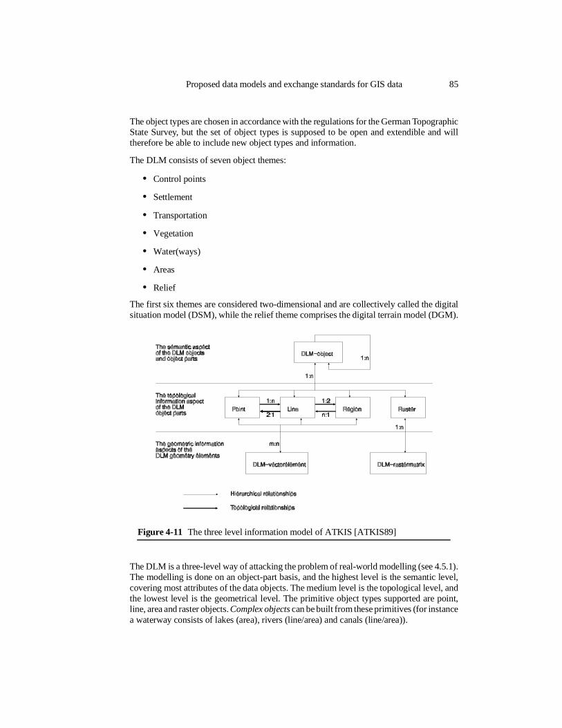
The object types are chosen in accordance with the regulations for the German TopographicState Survey, but the set of object types is supposed to be open and extendible and willtherefore be able to include new object types and information.

The DLM consists of seven object themes:

• Control points

• Settlement

• Transportation

• Vegetation

• Water(ways)

• Areas

• Relief

The first six themes are considered two-dimensional and are collectively called the digitalsituation model (DSM), while the relief theme comprises the digital terrain model (DGM).

The DLM is a three-level way of attacking the problem of real-world modelling (see 4.5.1).The modelling is done on an object-part basis, and the highest level is the semantic level,covering most attributes of the data objects. The medium level is the topological level, andthe lowest level is the geometrical level. The primitive object types supported are point,line, area and raster objects. Complex objects can be built from these primitives (for instancea waterway consists of lakes (area), rivers (line/area) and canals (line/area)).

Figure 4-11 The three level information model of ATKIS [ATKIS89]

Proposed data models and exchange standards for GIS data 85

Every object has a so called global identity.

Object parts has to be topologically atomic, meaning that attributes and relationships cannotchange within an object part.

Non-redundant storage is provided by allowing several object parts to share a vectorelement.

ATKIS does not provide mechanisms for the storage of historical data, but the time of latestchange is maintained for each object.

The Swedish STANLI project (a national project for the standardisation of landscapeinformation) has reviewed the ATKIS DLM through real world case studies [STANLI91].Their comments on ATKIS can be summarised as follows:

+ The topological and geometrical organisation of ATKIS is good.

- ATKIS has no support for non-geometrical objects (and relationships to such data),historical data and quality data.

- ATKIS does not support complexity levels. Such levels should be provided, so thatsimple data (pure geometry) could be organised without the complexity introducedby more sophisticated data (containing object identities and relationships).

CommentaryATKIS is a good attempt at providing a standard data model for geographical information.It may be incomplete, but what it covers, it covers reasonably well. The scale based approachis questionable, and ATKIS needs to include time, quality and 3D objects to become usefulfor most needs. ATKIS seems to be a good starting point for further efforts on standardisationfor geographical data modelling.

4.5.2 SDTS

The Spatial Data Transfer Standard (SDTS) is a standard for spatial data modelling andtransfer for the USA [USGS90]. The US Geological Survey (USGS) has co-ordinated thework with the standard, which has been a long term effort [Moellering86]. The work wasinitiated in 1980 and a final proposal of the SDTS as a FIPS (Federal Information ProcessingStandard) was completed in July 1991. The SDTS was approved as a FIPS (FIPS 173) in1992.

The SDTS specifies modules for describing data organisation, data formats and dataquality.

Data modellingSDTS uses the following modelling concepts from the object-oriented programmingsystems literature [USGS90].

• Phenomenon. A fact, occurrence or circumstance (SDTS transfers information aboutphenomena that are defined in space and time and are described by using a fixedlocation— spatial phenomena).


• Classification. Assignment of similar phenomena to a common class. An individualphenomenon is an instance of its class.

• Generalisation. A process in which classes are assigned to other (higher level)classes. The general class contains all the instances of the constituent classes.

• Aggregation. The operation of constructing more complex phenomena out of com-ponent phenomena.

• Association. The assignment of phenomena to sets, using criteria different from thoseused for classification.

The classes of (spatial) phenomena that are of interest for data modelling are called entitytypes, and the individual phenomena are called entity instances. An entity’s digital repre-sentation consists of one or more spatial objects. A spatial object that represents all of asingle entity instance is an entity object. Entity objects have locational attributes (spatialaddress), non-locational attributes and relationships (e.g.. topology). A feature is defined asthe combination of a phenomenon and its representation.

An attribute is a characteristic of a class. The combination of values of the key attributesforms a unique identifier for each entity instance (as in the relational database model).

A relationship is a special case of an association, and can exist between entity types.

SDTS represents entity instances as static, without a temporal dimension. All temporalcharacteristics are expected to be treated as ordinary attributes, and have not been stand-ardised. Some temporal aspects are taken care of by the lineage part of the quality transportmodule, which incorporates information on data collection and later modifications.

Spatial data typesIn the SDTS, both geometry and topology (or a combination) are defined as valid repre-sentations for objects with spatial attributes.

GeometryThe following geometrical objects are included in the SDTS.

• Point: A zero-dimensional object that specifies geometrical location.

• Line segment: A directed line between two points.

• String: An ordered sequence of points, representing a line.

• Arc: An ordered sequence of points that forms a curve that is defined by a mathe-matical function.

• G-Ring: An ordered sequence of of strings and/or arcs.

• G-Polygon: An area bounded by an outer G-ring and zero or more inner G-rings,none of which are collinear or intersecting.

• Pixel: A two-dimensional picture element that is the smallest non-dividable elementof an image.

• Grid cell: A two-dimensional object that represents an element of a grid.


TopologyThe following topological objects are included in the SDTS.

• Node: A zero-dimensional object, which may bound one or more links or chains.

• Link: A connection between two nodes. A link cannot intersect other links, and maybe directed by ordering the two nodes.

• Chain: A directed non branching sequence of non intersecting line segments and/orarcs connecting two nodes (not necessarily distinct). Can specify start and end node(network chain), left and right polygons (area chain) or both (complete chain).

• GT-Ring: A ring created from complete and/or area chains.

• GT-Polygon: An atomic two-dimensional component of one and only one two-di-mensional manifold, bounded by GT-Rings. The universe polygon is the part of theuniverse that is outside the area covered by other GT-polygons. A void polygon is anarea that is bounded by other GT-polygons, but has the same characteristics as theuniverse polygon.

Aggregate spatial objectsThe following aggregate spatial objects are included in the SDTS.

• Planar graph: A graph that can be drawn on a planar surface without introducingintersections of the links and chains.

• Network: A graph without two-dimensional objects (containing only points andlines).

• Two-dimensional manifold.A planar graph and its associated two-dimensional objects. Each chain bounds two,and only two, not necessarily distinct, GT-polygons. The GT-polygons are mutuallyexclusive and completely exhaust the surface.

• Image: A two-dimensional array of regularly spaced elements constituting a picture.

• Grid: A regular (the repeating pattern is a square, an equilateral triangle or anequiangular and equilateral hexagon) or nearly regular (the repeating pattern consistsof rectangles, parallelograms or non-equilateral triangles) tessellation of a surface.

• Layer: An integrated, spatially distributed set of data representing entity instanceswithin one theme, or having one common attribute value in an association of spatialobjects.

• Raster: A number of overlapping layers for the same grid or image.

Data qualityThe data quality part of SDTS identifies the following aspects of (spatial) data quality. Eachof these aspects is covered by a mandatory transfer module, and the tests that have beenperformed to establish the quality measures shall be described in the modules.


• Lineage: The source and history of the data, including methods of measure-ments/derivation, transformations, control information used and dates of validity/col-lection.

• Positional accuracy. The degree of compliance to the spatial address standard used,including references to the test used to establish the accuracy.

• Attribute accuracy. Both numerical and classification accuracy is covered. The testsused to establish the accuracy shall be described.

• Logical consistency. Describes “the fidelity of the relationships encoded in the datastructure of the digital spatial data”. Tests used to establish the consistency measureshall be described. Graphic data consistency, topological data consistency andgeneral data structure consistency.

• Completeness. Describes “the relationship between the objects represented and theabstract universe of all such objects” (exhaustiveness). Geometrical thresholds used(minimum area, shortest lines, …).

The data quality modules only provide textual descriptions for all the quality measures.Numerical fields are not present in any of the quality modules.

The transfer formatA data transfer using the SDTS consists of a number of files, each containing a transfermodule. Cross referencing between the modules is facilitated by using unique modulenames and by numbering the records within each module. ISO* 8211 is used for encodingthe modules, and the coding scheme is described in the SDTS documentation.

A comprehensive thesaurus contained in the SDTS documentation provides a standardnomenclature of spatial features for use in the SDTS.

For an SDTS data transfer to be valid it will have to include the following modules, eachcontained in a separate file.

Identification module.Internal spatial reference module.External spatial reference module.Catalogue/Directory module.Catalogue/Cross-Reference module.Catalogue/Spatial-Domain module.Spatial-Domain module.All quality modules (lineage, positional accuracy, attribute accuracy, logical consistencyand completeness).

In addition to these mandatory modules, a number of data modules and modules withauxiliary information will be present in a typical transfer.

Non-spatial attributes are organised according to the relational paradigm and the SQLstandard, using foreign keys to facilitate joins.


* International Standards Organisation

CommentaryThe SDTS was, when it was completed, the most comprehensive effort at specifying awell-founded standard for the exchange of geographical information. But, unfortunately, itdoes not provide a standard geographical data model. The introductory parts of thedocument provides concise definitions of geographical data and data modelling concepts.This part is perhaps the most valuable of the whole document.

The SDTS has been specified in such a way that data encoded in all kinds of spatial datamodels can be transported. It does not put any requirements on the structure of the data. Itsupports topologically complete data as well as spaghetti data. This is one of SDTS’sstrengths, but perhaps also its greatest weakness. It has become too comprehensive andcomplicated. There are a lot of different possibilities for even the simplest spatial objects.This means that the job of making an SDTS translation module for import of all kinds ofdata will be very difficult and time consuming. If the SDTS had aimed at specifying a new“standard” data model, limiting the number of alternative terms, it would have been muchmore useful as a standardisation vehicle.

The strong part of the SDTS is that it covers geometry, topology and data quality in a verygeneral fashion, and the same applies to attribute data and cross referencing.

The value of the very detailed and voluminous thesaurus is more questionable. A lessdetailed framework for naming and classifying GIS objects (for instance into hierarchiesand themes), or a standard for geographical data dictionaries would probably have beenmore valuable.

All in all, the SDTS is a valuable step in the direction of an international standard for theexchange of geographical information, but it is not enough.

4.5.3 NGIS and FGIS

The Norwegian Mapping Authority (Statens Kartverk) is also involved in standardisationin the field of geographical information. The NGIS and FGIS projects were the main effortsin Norway in this area around 1990.

NGISNGIS* is a multi-million NOK project run by the Norwegian Mapping Authority. It wasinitiated in 1989, and the aim was to specify a national server for geographical data. Thecentre (NGIS) is meant to provide the basic geographical information contained in thenational map series and registers on a standardised digital format to the community in thelate 1990ies as an on-line database service. The development of NGIS was initiated to meetthe Norwegian society’s future needs for (digital) geographical information. NGIS shalloffer logically integrated 3-dimensional geographical data, and not only spaghetti digitalrepresentations of the traditional paper maps.

NGIS was planned to be main-frame based and centralised. It is planned to have largecapacities for data storage, and other vendors of geographical information are to be offeredto use NGIS as a host for distribution of their data.


* Nasjonalt Geografisk InformasjonsSenter (in Norwegian) = National geographicalinformation centre.

NGIS will encompass information from all the services of the Norwegian MappingAuthority, including:

• Topographic maps in the national map series 1:50000, 1:250000 and other smallerscale maps

• (Sea-) Navigational charts

• Economical maps of scale 1:5000-1:20000 (with detailed infrastructure and bordersfor vegetation, property and administration)

• Registers for addresses, properties and buildings (GAB)

• The road network

• The national mesh of triangulation fixed points

The information contained in NGIS will consist of both alphanumerical data, vector/geo-metrical data and image/raster data. The amount of data contained in the NGIS database isforecast to grow to 100-200 Gigabytes during the first 5 years of operation.

The data will be available to the community through public and private telephone and datanetworks, and it is expected that ISDN with its broad-band services will provide sufficientcapacity for the potentially large transfer volumes. Data selection from the NGIS databasecan be based on geographical criteria (some specified region), thematic criteria (hydrogra-phy, topography, land-use, ...), scale and others. Easy access to the data is one of the mainconcerns of the NGIS work, and a user-friendly and intuitive interface is considered veryimportant. Window based client tools for NGIS access will be developed to accomplish this.

In order to make NGIS as open and available as possible, a relational database with astandard SQL-interface is preferred for data management. The data will be delivered on theNorwegian Mapping Authority’s in-house transfer format (SOSI*) [SOSI90].

NGIS seems to be a useful and necessary project for the society, but it can be argued thatin this case one probably would be better off using a distributed approach to geographicaldata management than the proposed centralist approach (as discussed in chapter 3), becausethe responsibility for updating the data will be geographically distributed. There is, however,a need for a central metadata management site, provining an interface for searching for datasets.

FGISFGIS** was a standardisation project with participants from industry and the NorwegianMapping Authority initiated as a part of the NGIS project to specify the data model, the datastructures and the interfaces of geographical data servers. It was carried out under thesupervision of the Norwegian Mapping Authority. FGIS was initiated in 1989 and finishedin 1990 with specifications covering an exchange format, a data model and a geographicalinformation system kernel application interface [FGIS90].

The goals of the FGIS project were to [FGIS90]:


* Samordnet Opplegg for Stedfestet Informasjon (in Norwegian) = Co-ordinated arrangementfor geographical information

** Felles-GIS (in Norwegian) = shared GIS

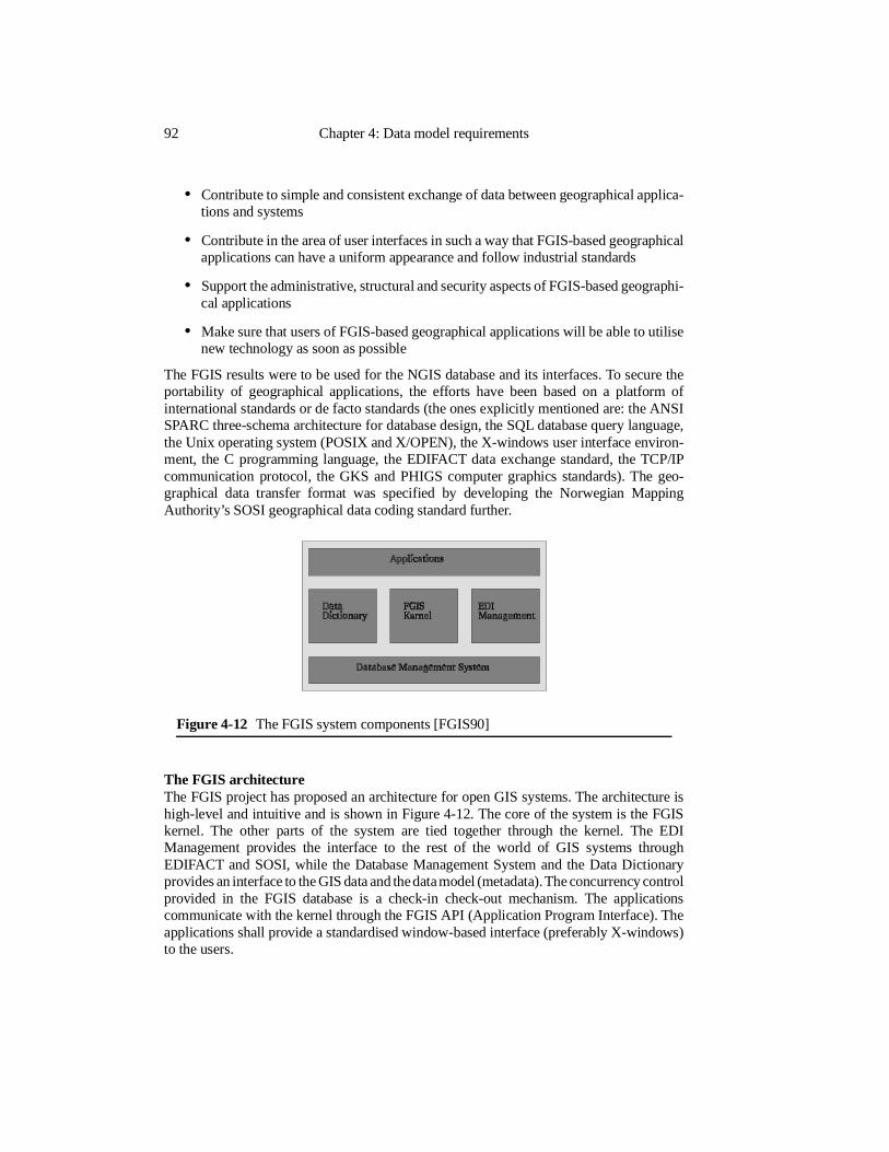
• Contribute to simple and consistent exchange of data between geographical applica-tions and systems

• Contribute in the area of user interfaces in such a way that FGIS-based geographicalapplications can have a uniform appearance and follow industrial standards

• Support the administrative, structural and security aspects of FGIS-based geographi-cal applications

• Make sure that users of FGIS-based geographical applications will be able to utilisenew technology as soon as possible

The FGIS results were to be used for the NGIS database and its interfaces. To secure theportability of geographical applications, the efforts have been based on a platform ofinternational standards or de facto standards (the ones explicitly mentioned are: the ANSISPARC three-schema architecture for database design, the SQL database query language,the Unix operating system (POSIX and X/OPEN), the X-windows user interface environ-ment, the C programming language, the EDIFACT data exchange standard, the TCP/IPcommunication protocol, the GKS and PHIGS computer graphics standards). The geo-graphical data transfer format was specified by developing the Norwegian MappingAuthority’s SOSI geographical data coding standard further.

The FGIS architectureThe FGIS project has proposed an architecture for open GIS systems. The architecture ishigh-level and intuitive and is shown in Figure 4-12. The core of the system is the FGISkernel. The other parts of the system are tied together through the kernel. The EDIManagement provides the interface to the rest of the world of GIS systems throughEDIFACT and SOSI, while the Database Management System and the Data Dictionaryprovides an interface to the GIS data and the data model (metadata). The concurrency controlprovided in the FGIS database is a check-in check-out mechanism. The applicationscommunicate with the kernel through the FGIS API (Application Program Interface). Theapplications shall provide a standardised window-based interface (preferably X-windows)to the users.

Figure 4-12 The FGIS system components [FGIS90]


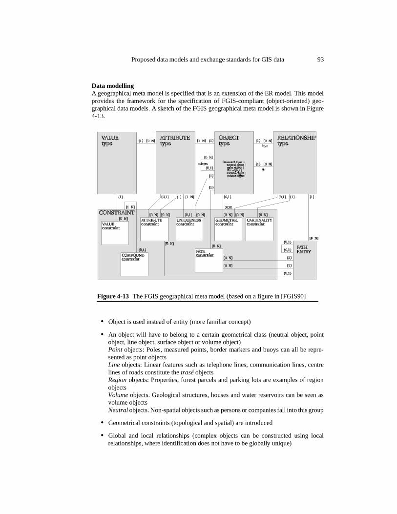
Data modellingA geographical meta model is specified that is an extension of the ER model. This modelprovides the framework for the specification of FGIS-compliant (object-oriented) geo-graphical data models. A sketch of the FGIS geographical meta model is shown in Figure4-13.

• Object is used instead of entity (more familiar concept)

• An object will have to belong to a certain geometrical class (neutral object, pointobject, line object, surface object or volume object)Point objects: Poles, measured points, border markers and buoys can all be repre-sented as point objectsLine objects: Linear features such as telephone lines, communication lines, centrelines of roads constitute the trasé objectsRegion objects: Properties, forest parcels and parking lots are examples of regionobjectsVolume objects. Geological structures, houses and water reservoirs can be seen asvolume objectsNeutral objects. Non-spatial objects such as persons or companies fall into this group

• Geometrical constraints (topological and spatial) are introduced

• Global and local relationships (complex objects can be constructed using localrelationships, where identification does not have to be globally unique)

Figure 4-13 The FGIS geographical meta model (based on a figure in [FGIS90]


• The entities and relationships of the path concept are quite vaguely described, and issupposed to capture “equality-of-path” problems (no matter what path one takes inthe model, using different sequences of relationships between two object-types, oneshould always end up with the same connected objects)

Other (non-geographical) mechanisms available for modelling:

• All objects can have attributes and relationships to all types of objects (including subtyping)

• A variety of constraints are available, among them cardinality of relationships,domains and keys/identifiers

The implementation of the geometrical structure of a spatial object is hidden, and separatedfrom the other properties of the object. Many geographical objects can therefore refer to,and thereby share, the same hidden geometrical structures. This means that the borderbetween two properties can be the same geometrical object as the centre line of a road (ifthe road is moved, the border moves with it).

FGIS suggests the use of only two primitive geometrical objects, namely the point and theline. A line represents a connection between two points. The other spatial objects will haveto be built from these primitives.

The support for a terrain elevation model is only described at a very high level [FGIS90]:

It should be possible to calculate the elevation of any chosen point in the terrainfrom the elevation data in the database.

InterfacesSQL is used for internal database access, but a special purpose object-oriented geographicaldatabase interface called FAPI (FGIS Application Interface) has been specified to hide theSQL interface.

The data exchange between different systems over public and private networks has beeninvestigated, and EDIFACT combined with SOSI is suggested as important interfacecomponents. Remote data must be accessed through the FGIS Kernel and the EDI Manage-ment component. An EDIMS* will govern the interchange of data with external databasesaccording to the X.200** standard.

CommentaryThe “open” approach of FGIS is very useful, allowing integration with other informationsystems by emphasising the use of international standards in all possible areas.

FGIS is very ambitious and comprehensive in its coverage. The geographical meta modelis well formulated (except, perhaps, for the path concepts), but the geometry data modelcould have been more sophisticated.


* Electronic Data Interchange Management System

** Reference Model of Open Systems Interconnection for CCITT Applications

A question is whether two geometrical primitives (point and line) are sufficient for a generalpurpose geographical data model. The lack of an explicit surface representation mechanismmakes 3D support limited. For 3D modelling, e.g.. for geology, a general purpose surfacerepresentation would be useful. The only 3D phenomenon mentioned in the FGIS proposalis terrain elevation, so it seems likely that general 3D objects have not been considered.

The two most important aspects of geographical data that are not covered explicitly by FGISare time and quality.

• Time is never mentioned, but should be an intrinsic part of a general purposegeographical meta model

• The spatial accuracy part of quality could be included as a geometrical constraint inthe FGIS geographical meta model. Completeness and logical consistency are,however, in many instances data set oriented. To be able to accommodate theseconcepts, neutral objects must be introduced by the modeller to represent the dataset aggregations, and quality measures could then be attached as attributes to theseneutral aggregation objects. The problem with this approach is that everything mustbe modelled by the users. All quality aspects should be intrinsic to the geographicalmeta model

Other deficiencies of less importance:

• The meta model does not provide mechanisms for handling samples and interpolation(apart from the vaguely described terrain elevation support). Fields are thus notsupported

• Complex objects / aggregations are not supported directly

• Roles/scale (different representations) is not addressed

• Derived objects are not mentioned

• The grouping of spatial objects into themes is not supported

Even though the FGIS geographical meta model does not cover everything of importanceto geographical data modelling, it did provide a good step in the right direction.

The FGIS results and ideas are being considered, together with several other Europeanefforts, in the CEN* attempt at specifying a standard exchange format and data model forthe European GIS market (CEN TC 287), as well as in similar ISO efforts (ISO/TC211).

4.5.4 MetaMap

MetaMap is a multi resolution model proposed by the research establishment SINTEF SIin Oslo, Norway for representing and handling spatio-temporal information [Misund93].The proposal description is not very detailed, so a lot of questions remain unanswered.


* CEN are the initials of the association of European national standardisation organisation

Delta-representationMetaMap represents temporal multi resolution geometrical objects as a basic object plus anumber of geometrical and temporal deltas/differences. The base geometrical object (M0)in MetaMap is the crudest possible representation of the oldest known instance of the object,and the scale oriented geometrical deltas (Dn) add detail to the geometry for representationat larger scales (increased resolution), while the temporal oriented deltas handle temporalchanges to the geometry. An example of the derivation of a particular object variant, Mi:

Mi = M0 + D1 + D2 + ... + Di

This concept is claimed to give a compact representation of spatio-temporal objects.

Commentary: The combination of the multi resolution and temporal deltas has not beendescribed in [Misund93], so it is difficult to evaluate the benefits of the approach when itcomes to compactness.

Object-oriented featuresAll geographical phenomena are represented in MetaMap as objects in accordance with theCOM* of the OMG** [Soley95]. All geographical objects should have a thematic descrip-tion and a geometrical description. This is the proposed type definition for a geographicalobject/entity that is a specialisation of Object (from COM):

type Entity ≤ Object {nameE : e : Entity) → (a : Attribute);

geoE : e : Entity) → (g : Geometry);

infoE : e : Entity) → (i : Information)}

The geometrical and thematic descriptions are linked using an object identity-based the-matic-geometrical relationship (in addition to the implicit aggregation relationship for thegeographical object). This relationship is to cover both pure geometry and topology. It mustalso ensure that thematic versions are related to the geometrical versions in a correct andconsistent way.

MetaMap shall also be able to accommodate multimedia object types.

Geographical object organisationMetaMap organises geography as a hierarchy of geographical objects that are representablein 3 dimensions. The mother of all geographical objects is the surface of the earth. An objectdoes not have to be explicitly linked to its mother object, the geographical coordinates ofthe object can serve as an implicit reference.

Commentary: A hierarchy of geographical objects makes local geographical referencesystems possible, and can therefore provide a more convenient and compact representationof local objects. The notion of hierarchies is probably more relevant to object structures(CAD type data) than to the structures one may or may not find for natural phenomena.


* Core Object Model

** Object Management Group: A group of representatives from the computer hardware andsoftware industry that develop standards for object-oriented system development

Primitive geometrical objectsMetaMap recognises 3 categories of objects based on their geometrical properties:

• curve/line (implicit/explicit 3D and simple/complex structure)

• surfaces (implicit/explicit 3D and simple/complex structure)

• solids

Points are not mentioned/recognised as an object category.

Implicit 3D representation means that the object inherits the 3D properties (elevation) fromits ancestors, and therefore can be represented using only 2D coordinates.

Simple structure means that there is only one (atomic) element, while complex structure forinstance could indicate a network of geometrical objects.

FutureMetaMap constitutes the core geographical model for a strategic technology developmentprogram on geographical information technology funded by the Norwegian ResearchCouncil. The program aims at developing advanced applications for analysis and presenta-tion of geographical data.

Contributions and problemsA possible contribution of MetaMap is the integrated representation of temporal and multiresolution data in the geometry. It should also be possible to integrate quality into the model,both for geometry and thematics, and this would make it even more innovative. The detailson the implementation will show if this is a fruitful approach or not. A discussion regardingthe support for, and possible consequences of, changes in dimensionality as a result ofchange in resolution (e.g.. from 3D (volume) to 2D (region) and 1D (point) for a house) ispresently lacking.

The object-oriented hierarchical approach to geographical data modelling is of morequestionable value, but could for instance be useful for the inheritance of elevationinformation and for certain classes of man-made features.

The integrated organisation of geometry/topology and thematics for geographical objectsis very vaguely described, but the principle of sharing geometry between objects is a goodone. The handling of topology is not described in sufficient detail for further treatment.

The exclusion of geographical point objects is unfortunate.



Chapter 5

Sub-Structure Abstraction in Geographical DataModelling

The purpose of a high level data model is to model a certain selection of real worldphenomena as accurately, convincingly and completely as possible using various structuringand abstraction mechanisms. For geographical data in particular, we want to be able to modelgeographical phenomena in a context that suits our purposes.

In this chapter, a structuring method for ER diagrams that takes care of some of thepeculiarities of geographical data is proposed. Emphasis is put on providing intuitive andexpressive diagrams. The approach uses sub-structure abstractions, and builds on the workon sub model substitution (SMS) proposed by Bédard [Bédard89]. The method can be usedto emphasise overall structure in large models with a huge number of entities and relation-ships, avoiding too complex diagrams by using multiple levels of abstraction in thespecifications.

Geographical data models, as specified in these diagrams, must be translatable into databaseconceptual schemas. How to automate the translation step has not been investigated in thisthesis.

5.1 Context

The following presentation concentrates on the structural aspects of geographical datamodelling. The resulting methodology is not meant to be a general GIS modelling method.General modelling methods should also incorporate behavioural aspects. There have beenseveral reasons for not including behaviour in this thesis. First of all, data sharing betweenvarious applications is one of the most important goals in current GIS research. Such aco-operation on data usage relies upon a common structural data model for efficient datamanagement and application development. And, as mentioned in chapter 4, behaviour isprobably not the most central aspect of human interpretation of most geographical phenom-ena. Finally, the behavioural aspects of object-oriented modelling are far less understoodthan the structural part [Beeri90], and its inclusion should therefore await further progressin OO research. Consequently, inclusion of behavioural aspects in geographical datamodelling seems to be too ambitious considering the current state of the art in modellingand GIS research, so structural modelling will be the centre of focus. There should, however,

be is a place for behavioural modelling for geographical data, for instance for representingthe seasonal variations of spatial phenomena.

Geographical data modelling methods should incorporate the same set of basic tools andparadigms that are used in other branches of information system data modelling. Theparticular nature of geographical data will have to be reflected by geographical augmenta-tions to the traditional data modelling methodologies. As discussed in chapter 4, spatial,temporal and quality aspects are particularly important for geographical data. Theseconcepts must be covered in such a way that the augmented model keeps its goodcharacteristics with respect to structuring, expressive power, expressive economy and(visual) clarity/perceptibility [Sindre90]. This can partly be achieved by incorporatingquality measures as an implicit part of the structure of the data model, avoiding the extrasymbolism that explicit representation would require. This is an approach akin to the onetaken for temporal data models, where all objects get temporal properties implicitly. Theresult of an integration of quality measures into the data model could be termed a qualitydata model.

Modelling of geographical information can in many cases be relatively easy. Many appli-cation domains see a limited number of interesting phenomena that can be easily structured.A challenge in geographical data modelling is to provide models that allow sharing of digitalrepresentations of “semantically rich” geographical phenomena. In order to meet thischallenge, it will be important to determine a handy set of spatial data types, goodgeneralisation hierarchies, and object groupings. So that the models can be useful both fordata sharing and for communicating ideas in the system- and database design process.

The need for data sharing, through for instance public databases, encourages the develop-ment of standard geographical data models that are relevant for a large spectrum ofgeographical data users. As discussed in chapter 4, geographical phenomena often playmany different roles. Geographical data can therefore be used in a variety of contexts bythe data users. This makes development of a general purpose data model for a geographicalphenomenon difficult, if not impossible. If it should be possible to develop a general purposedata model for a phenomenon, it will very often be a need for multiple views on this complexmodel, each view tailored to the needs of a particular type of user group (role view). As anexample, consider roads.

• For a transport company or an ambulance, a road is a potential part of a route, whichin turn is a connection between two places. The interesting properties of the road arethose determining the suitability for transport (length, cover, roughness, speed limitsand surroundings such as settlements).

• For the construction company, the road consists of many types of foundation andmaterial in several layers, varying along the road.

• For a telecommunications - or some other cable company, roads could act as barriersfor cable ditches.

• For a farmer, a road could act as part of the border of a field.

A forest stand is another example.

100 Chapter 5: Sub-Structure Abstraction in Geographical Data Modelling

• For a harvester, it is a stand of timber at a certain stage and with a certain economicalvalue, and a certain future potential for timber production.

• For a zoologist it is a habitat for various kinds of animals.

• For a geographer and a meteorologist it is a climate factor, buffering water andstabilising temperature.

• For a botanist it could be a collection of individual plants.

• For a landscape architect, it is an important visual element in the landscape.

• ... and so on.

Considering the possibly diverse roles of geographical objects, a general purpose geographi-cal data model will either have to incorporate many subtle representations and relationships,making it very complex, or it will have to give priority to certain properties that will besufficient for most needs, facilitating the more subtle needs in less obvious ways.

A goal for this part of the thesis is to specify some low-level building blocks, on whichgeographical data models can be based, and a framework for building structures out of thesebasic elements in a consistent way.

The modelling approach should reflect the semantical richness of geographical data byallowing individual views, and not constraining the modelling unnecessarily by building afixed and rigid type/class hierarchy. Such a hierarchy should be specified by the modeller,not the modelling methodology. It should also be up to the application modeller to decidewhich views of the data that are of interest within a given setting (houses can for instancebe viewed as point objects, region objects or volume objects).

Another goal of this work is to allow for abstractions and information hiding in the modeldiagrams, by introducing high level structuring mechanisms.

Finally, the model, as specified in the diagrams, should be translatable into database models.

5.2 Geographical data modelling using structure abstractions

The modelling framework chosen is an extended entity relationship approach (see chapter2). Quality measures are expected to be an integrated part of the structure of the data model,in the same way as time is integrated in temporal data models. The result of the integrationof quality measures into the data model could be called a quality data model. When qualityis integrated at the model level, standardisation of the query language interface with respectto quality will also be feasible. How to integrate quality aspects into the data model is be asubject for further research.

The presented method provides more powerful abstractions and thereby information hidingin the model diagrams by introducing symbology in the data model diagrams (the visuali-sation mechanisms of the data model).

Geographical data modelling using structure abstractions 101

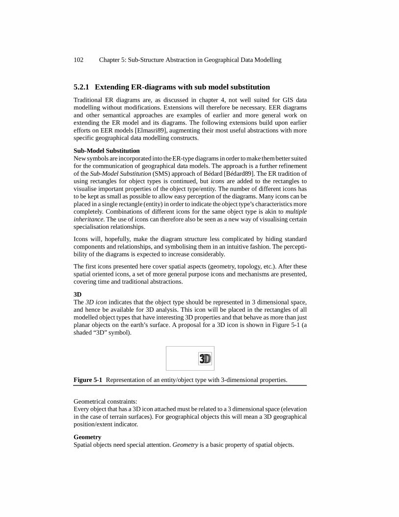
5.2.1 Extending ER-diagrams with sub model substitution

Traditional ER diagrams are, as discussed in chapter 4, not well suited for GIS datamodelling without modifications. Extensions will therefore be necessary. EER diagramsand other semantical approaches are examples of earlier and more general work onextending the ER model and its diagrams. The following extensions build upon earlierefforts on EER models [Elmasri89], augmenting their most useful abstractions with morespecific geographical data modelling constructs.

Sub-Model SubstitutionNew symbols are incorporated into the ER-type diagrams in order to make them better suitedfor the communication of geographical data models. The approach is a further refinementof the Sub-Model Substitution (SMS) approach of Bédard [Bédard89]. The ER tradition ofusing rectangles for object types is continued, but icons are added to the rectangles tovisualise important properties of the object type/entity. The number of different icons hasto be kept as small as possible to allow easy perception of the diagrams. Many icons can beplaced in a single rectangle (entity) in order to indicate the object type’s characteristics morecompletely. Combinations of different icons for the same object type is akin to multipleinheritance. The use of icons can therefore also be seen as a new way of visualising certainspecialisation relationships.

Icons will, hopefully, make the diagram structure less complicated by hiding standardcomponents and relationships, and symbolising them in an intuitive fashion. The percepti-bility of the diagrams is expected to increase considerably.

The first icons presented here cover spatial aspects (geometry, topology, etc.). After thesespatial oriented icons, a set of more general purpose icons and mechanisms are presented,covering time and traditional abstractions.

3DThe 3D icon indicates that the object type should be represented in 3 dimensional space,and hence be available for 3D analysis. This icon will be placed in the rectangles of allmodelled object types that have interesting 3D properties and that behave as more than justplanar objects on the earth’s surface. A proposal for a 3D icon is shown in Figure 5-1 (ashaded “3D” symbol).

Geometrical constraints:Every object that has a 3D icon attached must be related to a 3 dimensional space (elevationin the case of terrain surfaces). For geographical objects this will mean a 3D geographicalposition/extent indicator.

GeometrySpatial objects need special attention. Geometry is a basic property of spatial objects.

Figure 5-1 Representation of an entity/object type with 3-dimensional properties.


Geometrical objects are geographical objects with geometrical properties. They constitutethe basis of spatial information systems. Useful geometrical object types are points, lines,regions in 2D, surfaces in 3 dimensions and volumes/regions in 3D. The first two of theseobject types can have both 2D and 3D properties. This can be shown by using the 3D iconin addition to the geometry icon whenever the third dimension is of interest. A volume isinherently 3-dimensional. A region (2D and 3D) can be uniquely defined by its boundinglines/surfaces. To represent variation over the interior of geometrical objects, a field isneeded. In some contexts it can be interesting to show that a geometrical object isgeographically referenced. This could for instance be accomplished by including a globusicon in the entity box.

PointAn example of an icon to represent a geometrical point is shown in Figure 5-2. A rectanglecontaining a point icon represents a phenomenon that is interesting as a zero-dimensionalgeometrical object.

Constraints:A point should have a reference to a geographical reference system (datum and projection)and at least two dimensional coordinates.A point should contain a single reference to this reference system.

LineA geometrical line can be represented in the diagrams by using a line icon as illustrated inFigure 5-3. A geometrical line can be thought of as a one-dimensional geometrical object.

Constraints:A line should have two well defined end-points.A line should have an internal representation conveying the shape of the line.

RegionFigure 5-4 is a proposal for a 2D region icon. The region is an example of a geometricalobject that is inherently two-dimensional.

Figure 5-2 Representation of a point entity/object type using a point icon.

Figure 5-3 Representation of a line entity/object type using a line icon.


Constraints:A region must have a defined interior and a closed boundary of lines.

SurfaceA surface is similar to a region, being bounded by lines. All points on a surface have alocation in three dimensional space. A surface can be arbitrarily folded. A surface could berepresented using the region icon in combination with the 3D icon (Figure 5-5).

Constraints:A surface must have a closed boundary consisting of (3D) lines.3D coordinates must be available at all positions on the surface.It must be possible to determine the characteristics of the neighbourhood of a surface point(curvature, etc.).

VolumeA volume (3D region) is a three dimensional object bounded by surfaces. It could have itsown icon, and a suggestion is shown in Figure 5-6.

Constraints:A volume must have an interior and a closed boundary consisting of surfaces.

Varying phenomenaPhenomena that varies over the interior of a spatial object (fields) are important, particularlyfor environmental modelling (elevation, rainfall, temperature, soil and geology), but alsofor infrastructure (road information that varies along the road, e.g. speed limit and eleva-tion). Many natural phenomena varies in a continuous fashion. When these changes over

Figure 5-4 Representation of a region entity/object type using the 2D region icon.

Figure 5-5 Representation of a surface entity/object type using the 3D - and region icon.

Figure 5-6 Representation of a volume entity/object type using the volume icon.


the interior of an object are to be represented in the database (for example by sampling), afield icon could be included, as shown for a 2D region object with a non-homogeneousinterior in Figure 5-7 (this entity could for instance represent elevation). To symbolisechange/variation, the sinus curve has been used in this icon.

Constraints: The field icon must be used in combination with a geometrical icon (line, region, surfaceor volume).

Other geometrical objects of interestInitially, two additional useful geometrical object representations have been identified, theraster and the sample-set. Both of these can be combined with the 3D icon.

RasterThe raster icon can be used whenever matrixes of values (measurements) appear, and aproposal is shown in Figure 5-8. It can be used in combination with the 3D icon. This willcover remotely sensed imagery, scanned photographs and other regular (region or volume)samples. A raster is a representation of a field over a 2D/3D region.

Sample setThe sample-set icon shown in Figure 5-9 could be used for sets of samples taken irregularlyin 2Dor 3D geographical space. This icon can be useful for representing point probes forthe purpose of classification, monitoring and taxation of natural resources (continuouslyvarying environmental phenomena).

TopologySpatial objects that take part in structures have topology as an important extra property(chapter 4). All geographical objects that take part in some kind of topology structure must

Figure 5-7 Representation of a varying entity/object type using the field icon.

Figure 5-8 Representation of a raster entity/object type using the raster icon.

Figure 5-9 Representation of a sample-set entity/object type, using the sample-set icon.


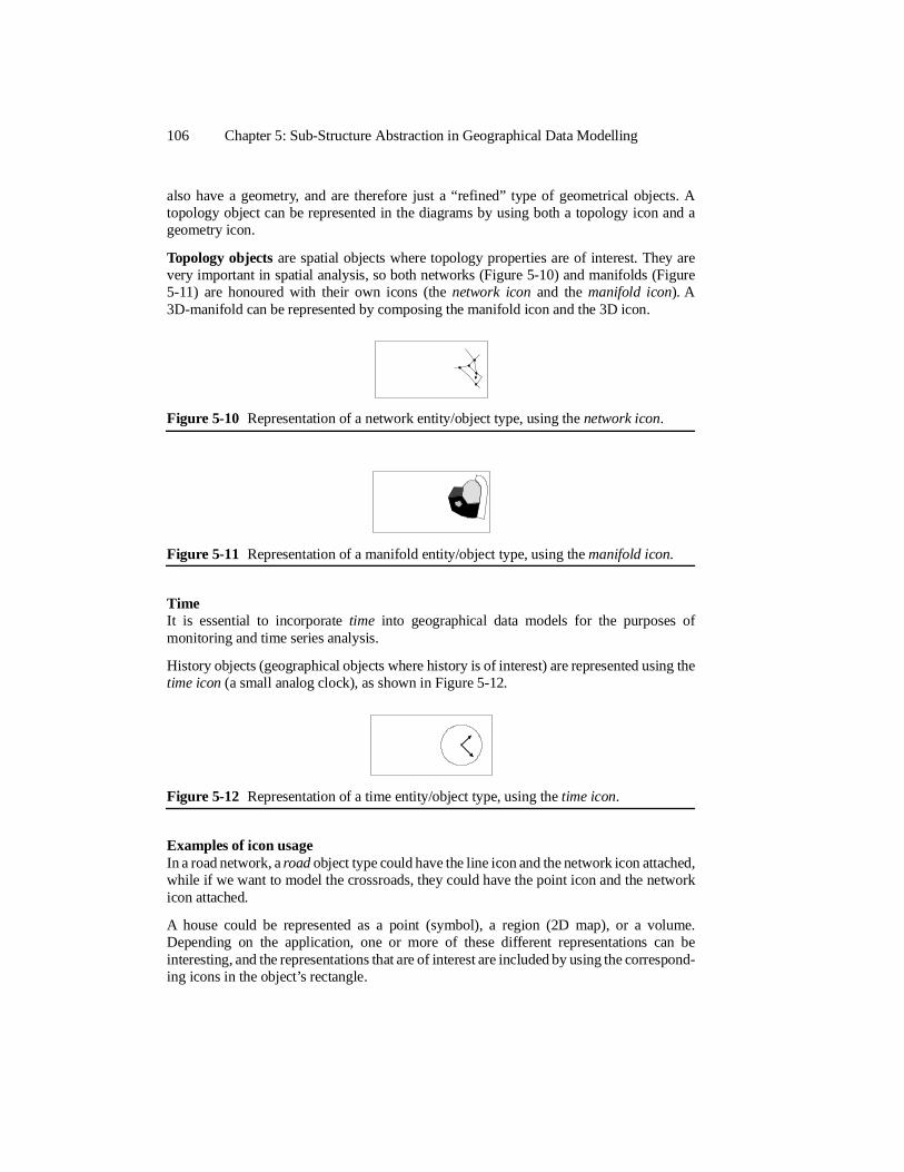
also have a geometry, and are therefore just a “refined” type of geometrical objects. Atopology object can be represented in the diagrams by using both a topology icon and ageometry icon.

Topology objects are spatial objects where topology properties are of interest. They arevery important in spatial analysis, so both networks (Figure 5-10) and manifolds (Figure5-11) are honoured with their own icons (the network icon and the manifold icon). A3D-manifold can be represented by composing the manifold icon and the 3D icon.

TimeIt is essential to incorporate time into geographical data models for the purposes ofmonitoring and time series analysis.

History objects (geographical objects where history is of interest) are represented using thetime icon (a small analog clock), as shown in Figure 5-12.

Examples of icon usageIn a road network, a road object type could have the line icon and the network icon attached,while if we want to model the crossroads, they could have the point icon and the networkicon attached.

A house could be represented as a point (symbol), a region (2D map), or a volume.Depending on the application, one or more of these different representations can beinteresting, and the representations that are of interest are included by using the correspond-ing icons in the object’s rectangle.

Figure 5-10 Representation of a network entity/object type, using the network icon.

Figure 5-11 Representation of a manifold entity/object type, using the manifold icon.

Figure 5-12 Representation of a time entity/object type, using the time icon.


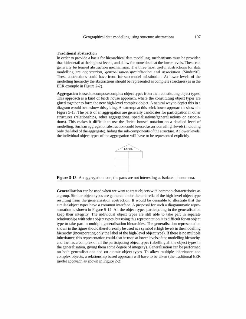
Traditional abstractionIn order to provide a basis for hierarchical data modelling, mechanisms must be providedthat hide detail at the highest levels, and allow for more detail at the lower levels. These cangenerally be termed abstraction mechanisms. The three most useful abstractions for datamodelling are aggregation, generalisation/specialisation and association [Sindre90].These abstractions could have icons for sub model substitution. At lower levels of themodelling hierarchy the abstractions should be represented as complete structures (as in theEER example in Figure 2-2).

Aggregation is used to compose complex object types from their constituting object types.This approach is a kind of brick house approach, where the constituting object types areglued together to form the new high-level complex object. A natural way to depict this in adiagram would be to show this gluing. An attempt at this brick house approach is shown inFigure 5-13. The parts of an aggregation are generally candidates for participation in otherstructures (relationships, other aggregations, specialisations/generalisations or associa-tions). This makes it difficult to use the “brick house” notation on a detailed level ofmodelling. Such an aggregation abstraction could be used as an icon at high levels (includingonly the label of the aggregate), hiding the sub-components of the structure. At lower levels,the individual object types of the aggregation will have to be represented explicitly.

Generalisation can be used when we want to treat objects with common characteristics asa group. Similar object types are gathered under the umbrella of the high-level object typeresulting from the generalisation abstraction. It would be desirable to illustrate that thesimilar object types have a common interface. A proposal for such a diagrammatic repre-sentation is shown in Figure 5-14. All the object types participating in the generalisationkeep their integrity. The individual object types are still able to take part in separaterelationships with other object types, but using this representation, it is difficult for an objecttype to take part in multiple generalisation hierarchies. The generalisation representationshown in the figure should therefore only be used as a symbol at high levels in the modellinghierarchy (incorporating only the label of the high-level object type). If there is no multipleinheritance, this representation could also be used at lower levels of the modelling hierarchy,and then as a complex of all the participating object types (labelling all the object types inthe generalisation, giving them some degree of integrity). Generalisation can be performedon both generalisations and on atomic object types. To allow multiple inheritance andcomplex objects, a relationship based approach will have to be taken (the traditional EERmodel approach as shown in Figure 2-2).

Figure 5-13 An aggregation icon, the parts are not interesting as isolated phenomena.


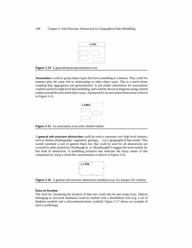
Association is used to group object types that have something in common. They could forinstance play the same role in relationships to other object types. This is a much loosercoupling than aggregation and generalisation. A sub model substitution for associationscould be useful for high level data modelling, and could be shown in diagrams using a dottedoutline around the associated object types. A proposal for an association abstraction is shownin Figure 5-15.

A general sub-structure abstraction could be used to represent very high level features,such as themes (hydrography, vegetation, geology, …) in a geographical data model. Thiswould constitute a sort of general black box that could be used for all abstractions notcovered by other primitives. Rumbaugh et. al. [Rumbaugh91] suggest the term module forthis kind of abstraction. A modelling primitive that indicates the fuzzy nature of thiscomponent by using a cloud-like representation is shown in Figure 5-16.

Data set locationThe need for visualising the location of data sets could also be met using icons. Objectsbelonging to non-local databases could be marked with a distribution icon (e.g. a set ofdatabase symbols and a telecommunications symbol). Figure 5-17 shows an example ofsuch a symbology.

Figure 5-14 A generalisation/specialisation icon.

LABEL

Figure 5-15 An association icon with a dotted outline.

Figure 5-16 A general sub-structure abstraction (module) icon, for instance for a theme.


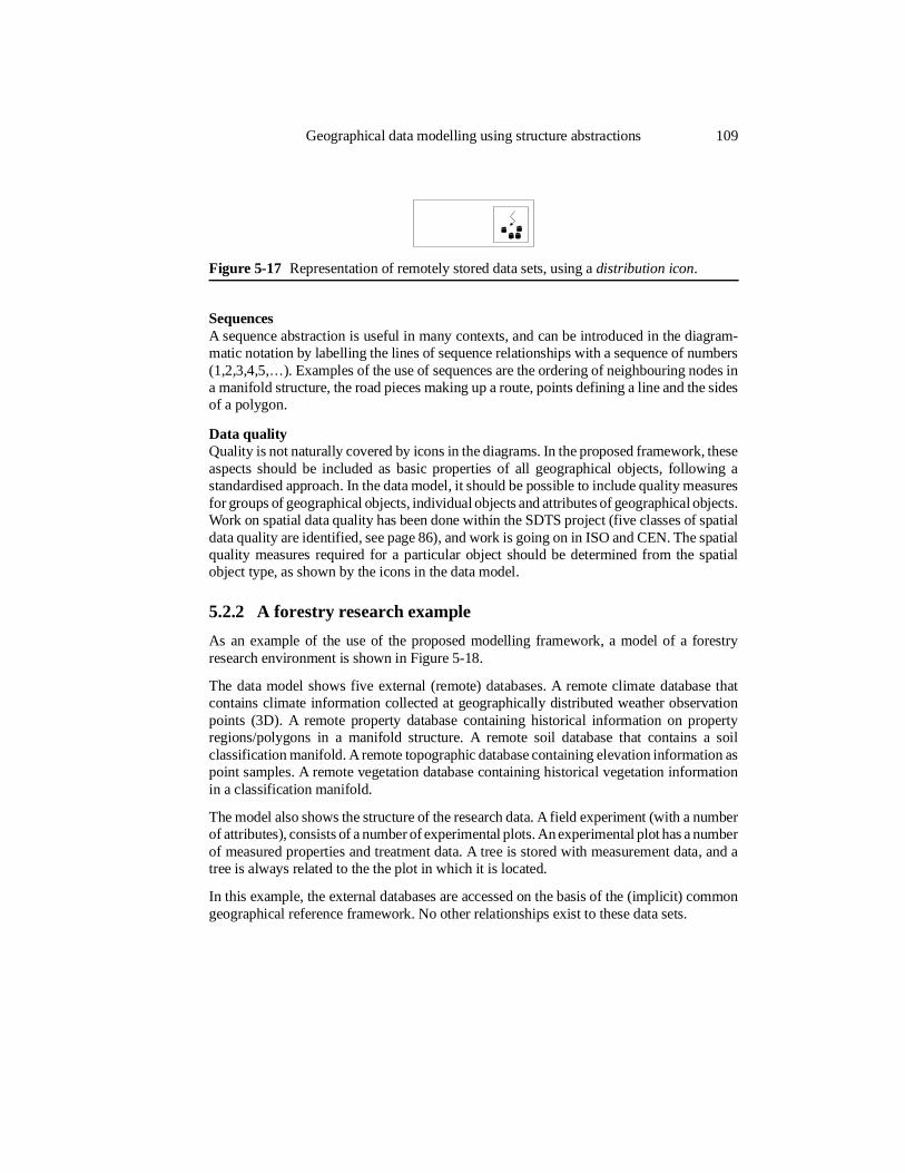
SequencesA sequence abstraction is useful in many contexts, and can be introduced in the diagram-matic notation by labelling the lines of sequence relationships with a sequence of numbers(1,2,3,4,5,…). Examples of the use of sequences are the ordering of neighbouring nodes ina manifold structure, the road pieces making up a route, points defining a line and the sidesof a polygon.

Data qualityQuality is not naturally covered by icons in the diagrams. In the proposed framework, theseaspects should be included as basic properties of all geographical objects, following astandardised approach. In the data model, it should be possible to include quality measuresfor groups of geographical objects, individual objects and attributes of geographical objects.Work on spatial data quality has been done within the SDTS project (five classes of spatialdata quality are identified, see page 86), and work is going on in ISO and CEN. The spatialquality measures required for a particular object should be determined from the spatialobject type, as shown by the icons in the data model.

5.2.2 A forestry research example

As an example of the use of the proposed modelling framework, a model of a forestryresearch environment is shown in Figure 5-18.

The data model shows five external (remote) databases. A remote climate database thatcontains climate information collected at geographically distributed weather observationpoints (3D). A remote property database containing historical information on propertyregions/polygons in a manifold structure. A remote soil database that contains a soilclassification manifold. A remote topographic database containing elevation information aspoint samples. A remote vegetation database containing historical vegetation informationin a classification manifold.

The model also shows the structure of the research data. A field experiment (with a numberof attributes), consists of a number of experimental plots. An experimental plot has a numberof measured properties and treatment data. A tree is stored with measurement data, and atree is always related to the the plot in which it is located.

In this example, the external databases are accessed on the basis of the (implicit) commongeographical reference framework. No other relationships exist to these data sets.

Figure 5-17 Representation of remotely stored data sets, using a distribution icon.


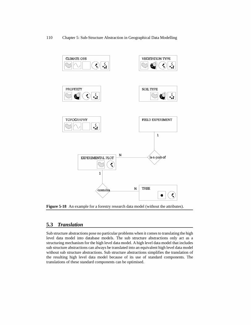
5.3 Translation

Sub structure abstractions pose no particular problems when it comes to translating the highlevel data model into database models. The sub structure abstractions only act as astructuring mechanism for the high level data model. A high level data model that includessub structure abstractions can always be translated into an equivalent high level data modelwithout sub structure abstractions. Sub structure abstractions simplifies the translation ofthe resulting high level data model because of its use of standard components. Thetranslations of these standard components can be optimised.

Figure 5-18 An example for a forestry research data model (without the attributes).


5.4 Conclusion

The complexity of geographical data models require better structuring and abstraction tools,in particular, a way of hiding detail on commonly used structures would be useful.

A framework for including structure abstractions in the ER family of data models has beenpresented. The work builds on sub models substitution, as proposed by Bédard [Bédard89].A set of useful abstractions for geographical data modelling has been proposed. Abstractionicons have been introduced for geometrical objects (point, line, polygon, 3D and varying)and spatial structures (network, manifold, raster and samples). Non-spatial abstraction iconshave also been suggested (generalised object, aggregated object, association object, timeand remotely stored data) to make it easier to communicate over-all structure in ER-typediagrams. The use of symbols has long traditions in cartography, and since most potentialparticipants in a geographical database design process will have experience with map use,the suggested representation should be particularly suitable for geographical data model-ling.

The utility of the method in practical modelling has yet to be proven.

5.4.1 Future work

The sub model substitution framework must be tried out on real world geographical datamodelling problems. An evaluation of the model should be performed, and improvementssuggested. Some questions will need to be answered:

• Is sub model substitution a useful abstraction mechanism for geographical datamodelling?

• What comprises the ideal set of sub models?

• How should the sub models be represented graphically?

An ultimate goal is an intuitive modelling environment that is able to generate (distributed)database schemas from diagrams and auxiliary information.

Conclusion 111


Chapter 6

Database management system issues for geographical data

Huge amounts of structured and unstructured spatial and spatially related data must beorganised and made available to a large set of local and remote users in a GIS environment.The GIS community consists of many potential demanding users of database managementsystems (DBMS). Potential, because DBMSs have not yet been utilised and developed toits full potential by the GIS community.

In this chapter some of the demands geographical data put on database systems are pointedout, and database system research and technology is reviewed with a geographical bias.Distributed database systems are discussed, as well as time, data dictionary issues, querylanguages and transaction processing with concurrency control. The chapter is rounded offwith an assessment of the suitability of different database models for geographical datamanagement, and a short conclusion.

Some research issues in spatial databases have been proposed by Günther and Buchmann[Günther90]. A review of spatial database system research has been given by Güting[Güting94]. A similar overview of spatial database implementations and query languagesfor spatial data has been provided by Samet and Aref [Samet95]

6.1 Basic requirements

The basic requirements that users of geographical data put on a DBMS are similar to thoseof other database system users [Frank84][Frank88][Feuchtwanger89][Frank91]. Some ofthe requirements mentioned below have a special meaning for GIS, and will be furtherelaborated on in later sections.

• Many geographical DBMSs must support interactive operation, that is, less than 2seconds response-time for most data retrievals.

• Storage efficiency is important for large data sets. For geographical databases, theamount of data to be handled could be extreme (Gigabytes, Tigabytes, …). HSM*

methods could be required for some data intensive applications (see page 53).

• A geographical database management system should support and be able to handlestructured and complex data. That is, vector and raster spatial data types, objecthierarchies, data with quality measures and temporal (versioned) data. A BLOB**

* Hierarchical Storage Management

data type could also be useful.Consistency enforcement for all data types should be performed by the geographicalDBMS.

• Operations should be supported by an integrated standard query language, so thatquery optimisation is possible. Geographical data will be subject to both spa-tial/topological queries, image queries, 3D queries and general attribute queries.

• Transaction support. In the case of GISs, long duration transactions will tend todominate, and there will in general not be much updating (the majority of transactionswill be read-only).Concurrency control will be necessary in order to ensure the consistency ofnon-static data sets while providing 24 hour availability. The amount of updating togeographical data sets are often limited, so some “relaxed” concurrency controlmethod would probably suffice.Recovery of the database to a consistent state should be possible after system failures,requiring a transaction log to be kept.

• Transaction capacity. High-volume transaction systems such as banking applica-tions require that the DBMS can handle hundreds or thousands of transactions persecond (TPS) with very short delays. In general transactions on geographical data-bases will not be that frequent, but some public geographical databases could get veryfrequent accesses (e.g. property databases or traffic information systems databasesin large cities and other databases that will be used for real-time navigation),demanding capacity for handling many transactions per second (TPS).

• Data sharing and the resulting data transfers to and from remote databases requiresthe involved databases to be accessible on the network through a standardiseddatabase interface.

• Advanced data dictionary support should be provided (preferably as an integratedpart of the query language) in order to make more of the semantics of the dataavailable and to allow heterogeneous database integration (explicitly or transpar-ently). The data dictionary should support geographically based meta-queries andthematically based meta-queries.

• Accounting and billing on the basis of data access and processing time must bepossible in a data sharing environment. In the case of integrated data sets, it isimportant that the accounting also can be done at the object and attribute levels, onthe basis of ownership of the source data.

• Integrity should be enforced by defining the valid states of the geographical databaseand the (state dependent) valid operations on the geographical database.

• Security against unauthorised access to the data will be necessary, at least for partsof some databases [Jajodia90] [Lunt90].

• Mechanisms for adding, deleting and changing data types and constraints (schemaevolution) is generally nice to have. This is also true for geographical databases since

114 Chapter 6: Database management system issues for geographical data

** Binary Large Object

the totality of interesting roles/uses of the modelled geographical phenomena can bedifficult to predict.

6.2 Data volumes and data types

Our means for collecting geographical data have been steadily improving, and this trend iscontinuing, leading to larger and larger amounts of existing and incoming data. GIS datahave previously been discussed in chapter 3 and 4. This section adds some examplesshowing the order of magnitude of present and future GIS data set volumes.

The storage requirements of geographical databases will vary from application area toapplication area. Global applications will generally require more data than local, andapplications that utilise images or other kinds of (high-volume) automatically sampled data(such as satellite imagery, seismic data and drilling logs) will require more storage spacethan the typical vector-based applications.

6.2.1 Samples

Continuously varying phenomena are conveniently represented by performing regular (suchas raster data) or irregular sampling on them (as discussed in chapter 3 and 4). Sampling isoften applied within such areas as vegetation monitoring and mapping, soil and geologymapping and water and air quality monitoring. Samples are also referred to as measurementdata elsewhere in the literature [Neugebauer90]. The reconstruction of continuously varyingphenomena from samples requires computations. Applications working on samples aretherefore normally not I/O bound.

As long as samples are taken one by one with human assistance, the number of samples willstay reasonably manageable. On the other hand, when sampling can be performed automat-ically and “continuously”, the number of samples will increase significantly. The resultingvolumes of data depend on the sampling frequency, the area sampled and, if temporalmonitoring is involved, the length of the sampling period.

Automatic sampling is, or could be, applied in areas such as: climate measurements (wind,temperature, humidity, precipitation, wave-height, wave-length, solar radiation, …), trafficmonitoring (radars, video), land and seabed topographic mapping, seismic exploration withmulti-sensor measurements and continuous logging during drilling processes. All theseareas are expected to be given higher priority in the future, leading to huge amounts of highresolution (spatial and temporal) data.

The volume of data that is required to represent a continuously varying spatial phenomenonusing point samples should be limited only by the variability of the phenomenon. Thesampling frequency must be twice as high as the frequency of variation of the sampledphenomenon (the Nyquist frequency).

Terrain modelsA special, and important, kind of sampled structure is the terrain surface model (often calleddigital terrain model, DTM). Such a model should provide approximate elevation values atall places within the modelled area. Terrain surface models are very often based on pointsamples of the elevation (traditionally they have been represented with iso-elevation lines

Data volumes and data types 115

or contours on maps). Applications that utilise the 3D properties of terrain models aregenerally extremely computational intensive, and are very seldom I/O bound.

Terrain models are presently not extreme in data volume, because a fully automatic way ofobtaining elevation points on the surface of the earth is just now getting available. Whenrobust methods for automatic digital photogrammetry become widely available, the situ-ation will be different, and very detailed (high resolution) and voluminous terrain modelswill result.

3D models3D models are useful in meteorology, oceanography and geology. To be able to representdetailed 3D information, huge amounts of data must be stored. Some 3D phenomena arealso dynamic of nature (the weather, the ocean), and therefore require frequent temporalsampling. 3D data are normally acquired using equipment such as seismics, echo sounders,lasers and radars. Storage structures for 3D phenomena are reviewed in appendix B.

6.2.2 Raster data

A very important subclass of samples are samples taken in a regular grid/raster. Rasterimages require large amounts storage space.

• For current medium-cost raster display technology, about 1000 rows x 1000 columnsx 1 byte = 1 MegaByte of data is needed to store an image that covers the computerscreen. Both the number of bytes per pixel (e.g. 3 bytes / 24 bits) and the number ofrows and columns are increasing.

• A scene from the Landsat* MSS** contains 3240 x 2340 x 4 (bands) ≈ 30 millionpixels (6 bits/pixel: 23 Mbyte/image) [Lillesand87]. This means less than 50 LandsatMSS scenes per Gigabyte. The Landsat TM*** produces scenes of the same size, butwith 6 bands (+ the lower resolution thermal band), and with a radiometric resolutionof 8 bits/pixel. The MSS generates 15 Mbits/second, while the TM generates 85Mbits/second (about 1⁄2 Gigabyte/minute!).The two sensors of the earth observing satellites in the Spot**** programme delivers6000 8bit pixels per row each in panchromatic mode, and the satellite can transmitdata at a rate of 25 Mbps [Lillesand87]. A square shaped scene/image will take upabout 36 megabyte of storage space.The storage requirements for satellite imagery are enormous compared to other kindsof data.

• Instruments used for scanning “analogue” images are providing higher and highergeometrical and radiometric resolution. Presently, the geometrical resolution used is


* Landsat is a US series of moving earth observing satellites carrying a set of sensors, providingworld-covering multi-band images, currently with a maximum resolution of 30m x 30m[Lillesand87].

** Multi Spectral Scanner.

*** Thematic Mapper.

****Spot is a French series of moving earth observing satellites, providing images where eachpixel represents a patch of 10m x 10m (panchromatic) or 20m x 20m (3 different bands) ofthe earth surface

of the same order of magnitude as the resolution of photographic film (about 10micrometer). A scanned 25 cm by 25 cm air photograph will consequently result in

about

25 . 10−2 m

10 . 10−6 m

2

= 6.25 . 108 pixels. If each pixel is represented using 1 byte,

this will result in over 1 Gigabyte of uncompressed data for a stereo pair of airphotographs (uncompressed).

• Image archives. Due to the large storage space requirements of individual images,image archives that store a large number of images will require enormous amountsof storage space.

The future will probably bring more satellites with more advanced sensors, leading to ahigher rate of data production than today. Airborne digital sensors, proving higher resolutiondata, will probably also become more popular. This would lead to even tougher requirementson local databases and data handling equipment.

CompressionThe data volumes of raster data can be reduced through image compression [Gonzalez87].Non-loss compression methods, such as run-length coding, ensure that the image can becompletely restored, while lossy compression methods, such as fractal [Barnsley88] encod-ings, make full restoration of the original image impossible. Lossy techniques are generallynot eligible for compression of images that are to be used as the basis for further analysis.

Compression techniques can reduce the storage requirements of most pictures, but if animage has been compressed, it will generally have to be restored before usage. Thecomputational load of this restoration depends on the compression algorithm used. Specialpurpose hardware is developed for fast compression and restoration of images.

The Joint Photographic Experts Group (JPEG) has developed a standard for still imagecompression. This standard is also aimed at images for presentations, and therefore allowslossy compression [Kim91]. The compression ratio can be adjusted according to theapplications demands for quality and compactness.

VideoIf raster images/pictures are to be put in series to produce film sequences, a rate of 25-75pictures per second is needed to produce acceptable to very good quality presentations. Fornormal screens this means more than 25 Megabytes of data per second of uncompressedmotion video. Special image compression techniques for highly correlated sequentialimages can, however, reduce this amount significantly.

The Moving Pictures Experts Group (MPEG) are working on standards for this type ofimage compression. The techniques suggested are lossy, and an improvement of thecompression ratio by a factor of 3 to 10 is expected by exploiting the correlation ofsucceeding images in such sequences [Kim91]. The combination of single image compres-sion and difference compression in MPEG-1 are consequently able to reduce the data streamto between 1 and 2 Megabits per second for normal video [Furht95].

Data volumes and data types 117

6.2.3 Vector data

In many cases, the vector model provides a more compact method for storing thematicgeographical information than does the raster model. The “exact” borders of all Norwegianproperties stored on a compact vector format will probably not take up significantly morestorage space than a single uncompressed high-resolution stereo pair of aerial photographs(some Gigabytes for the property database, and about a Gigabyte for the stereo pair)! Thisdoes not mean that vector data sets are small. The order of magnitude of many Norwegiannational vector data sets will be Gigabytes.

The vector format is compact for representing (boundary) lines, but its structure is muchmore complex than the raster format (e.g. topology and line representation). This, combinedwith the significant volume of many vector data sets, is likely to cause performanceproblems for most current database systems.

6.2.4 Time

When the temporal dimension is included in a geographical database, the data volume willaccumulate as new data are included (e.g. 1⁄2 Gigabyte/min. of Landsat data). All historicalinformation is potentially interesting, so no data should be thrown away, leading to aperpetual accumulation of data.

One consequence for the database system is that most data will be read-only. New data setswill generally not replace or correct older data sets, but will be stored together with them.The older data sets are kept as historical information. In a practical implementation, thestorage of the new and the old data sets could be co-ordinated to provide a more compactrepresentation (change-oriented storage).

6.2.5 Generalisation levels

Geographical data can be useful at many levels of generalisation, from the most detailedrepresentation of a garden to an overview representation of a continent, or even the completeearth. Geographical data generalisation can consists of simplification of object repre-sentations, aggregation of objects, and removal of insignificant objects (as the applicationscale gets smaller).

An ideal geographical data server should be able to provide geographical data from a singledata set at many generalisation levels (as requested by the individual queries). The indicationof generalisation level could be (map)scale of application (e.g. 1:10000 for municipal landuse planning and 1:1000000 for global environmental research). Generalisation is a verycomplicated process, requiring the application of a large set of rules, and for good results,it will probably also require generalisation information to be attached to the individualobjects of the database.

Reduction of dimensionality is a more easily implementable kind of generalisation. A usercould request a volume, region or point representation of a house. The server should thenhave operations to derive lower dimensional representations on the basis of its storedrepresentation (volume to region could be done by projecting the volume onto a 2Dreference system, region to point could be done by returning the centre of mass of theregion).


6.2.6 Summary

The challenge of GIS data management is twofold. First, organising and storing the largevolumes of spatial data, and second, finding methods for filtering out “interesting” infor-mation from the global geographical information base. The answer to the first challenge ispowerful geographical data models, sophisticated multimedia database management sys-tems and a suitable data-distribution and -integration method. To answer the secondchallenge, one will have to add efficient data structures (supporting generalisation) andaccess methods on powerful hardware.

6.3 Multimedia (integrated) database systems

The variety of data types within a GIS suggests that a database management system willhave to be a specialised integrated database system (or multimedia database system).

In the preceding sections it has been shown that the volume of geographical data availableto geographical information systems already is enormous, and that the main contributionpresently comes from remotely sensed imagery. Structured vector data will generally bemanageable for local applications, but for wider area analysis, the amount of vector data toconsider could be overwhelming even with state of the art technology. Efficient methodsfor searching for interesting data and for filtering away the rest will therefore be veryimportant for the performance of GISs.

Multimedia information systems shall be able to manage and integrate a variety of datatypes, including for instance textual information, numerical information, all kinds of graphicinformation (e.g. drawings and images), sound and video sequences [Christodoulakis95][Yager91]. Multimedia database systems should be designed to provide much of the samefunctionality as traditional database systems for all these data types. There are presently nosuch systems available.

The GIS branch of multimedia database systems will have to be based on a global frame ofreference, within which the different representations of geographical objects and events canbe localised [Rhind92]. Several global reference systems exist, the latitude-longitudesystem, the UTM system and WGS84* are some of the traditional ones. Other approacheshave also been taken lately, for instance regular hierarchical triangulation of the earth (thequaternary triangular mesh, QTM [Dutton89]). If many different reference systems are tobe used, transformations between these reference systems will have to be performed on thefly by a multimedia system.

Images (rasters), 2D geometry (vectors) and alphanumerical tabular information constitutethe traditional data types useful in a GIS. An important feature of many future GIS databasesystems will be a 3D model of the surface of the earth and possibly also geological features.This 3D model must be truly integrated with the global reference system. In addition, itmust be possible to integrate 3D object geometry (e.g. houses, bridges and trees) with therest of the database in a straightforward manner.

The integration of these different data types is important in order to allow seamless spatialanalysis and presentation. Seamless access to all available information sources gives new

Multimedia (integrated) database systems 119

* World Geodetic System 1984

opportunities for analysis and presentation, for instance by allowing vegetation and soilmaps to be combined with satellite imagery and the 3D terrain model.

Sound has been given some emphasis in multimedia systems, but will probably only be oflimited use for GISs. It could be useful in tourist information systems, for instance thesounds from nature (a waterfall, the cracking of an iceberg, birds) or sounds of humanactivity (traffic, talk, music).

While multimedia research has lead to some results in multimedia user interface design, ithas not yet come up with any standards for multimedia database systems. Image databaseshave attracted most attention, and some work has been done on the integration of imageswith relational databases [Roussopoulos88][Joseph88]. Within ISO, there is work in pro-gress on multimedia extensions to SQL (SQL3/MM [ISO/IEC94a]). The potential ofobject-oriented databases for multimedia applications has also been investigated [Woelk86,Woelk87].

On the GIS arena, no really elegant methods for integrating vector and raster data have beenfound, and in addition to this, the geometry is usually stored separated from the thematicinformation in GIS databases (the geo-relational approach). The status of GIS with respectto multimedia integration is consequently not too encouraging.

6.3.1 Hypertext

Hypertext (or hypermedia) is an approach to multimedia systems that puts emphasis oninformation structuring and user interfaces [Conklin87] [Goyal89]. Hypertext techniquesshould also be interesting for geographical information system design. Incorporation ofthese kinds of structuring methods is likely to make GISs more user friendly and flexible.

Hypertext is first and foremost a browsing tool where information is structured as a web ofnodes and associative links. Each node contains some information on a certain subject andfrom zero to many links to other nodes. From a node you can move to other nodes that areassociated with the current node in some way. A link to another node can be indicatedexplicitly as highlighted text, icons and parts of images, and, in addition, some dictionary-or rule-based approach could be used.

The linking mechanism is intrinsically very flexible, and the structure of the resulting webof links and nodes depends very much on the creator of the web. A big problem in hypertextsystems is how to keep track of where you are in the web. Network browsers that can handlemillions of nodes and links in a user-friendly way are very difficult to implement.

Hypertext has also been investigated in the context of GIS, and it has been suggested to useit as a cartographic product [Lindholm90] [Laurini90].

There is still no agreed upon theory for the implementation of hypertext-structured databasemanagement system. The utility of hypertext techniques is therefore presently limited touser interfaces in browsing applications (e.g. the Internet WWW* and electronic atlases andpublic database interfaces).


* World Wide Web

6.4 Spatio-temporal databases

Time in databases has been investigated extensively during the last 20 years [McKenzie86][Snodgrass90]. By including time in the database it is possible to represent the history ofdatabase objects. Concurrency control and recovery problems can also be solved in anelegant way in temporal databases [Agrawal89, Bernstein87].

Temporal/history data are a kind of versioned data. When handling temporal data there doesnot have to be support for the parallel versions that must be supported for general versioneddata (e.g. for road and land use planning or computer aided software engineering). Temporalversions are linearly ordered along the temporal dimension, and therefore comprise a subsetof versioned data.

Many different ways of including time in databases have been proposed, and most of thework has been based on the relational model.

6.4.1 Concepts of time in databases

During the years, different concepts of time in databases have been identified, the mostimportant being transaction time, valid time and user-defined time [Snodgrass85]. The firsttwo are maintained by and known to the DBMS, while the last one is a user-defined attributethat contains some information about time. Transaction time and valid time will besupported by mechanisms in the query language, while the user will have to take care ofprocessing and administration of the user-defined time attributes without any time-specifichelp from the DBMS.

According to their use of time, databases can be classified into different categories[Snodgrass85] [Snodgrass86] [Snodgrass92]:

• Static databases have no notion of time, they only contain a snapshot of the realitythey are supposed to represent. Past states are discarded and forgotten.

• Static rollback databases support the notion of transaction time. This means that itis possible to find out what the state of the database was at a certain point in the pastby checking the transaction time tags on the different data items (rolling back thedatabase to some state in the past). Only the time of data entry and deletion isrecorded, so the states of a static rollback database does not necessarily reflect thestates of the modelled reality.

• Historical databases support the notion of valid time. In a historical database it ispossible to query about the state of the reality model at a certain point in time. It isalso possible to correct errors from the past and insert new facts about the past.Databases may also include user-defined time. User-defined time will have to beincluded as normal attributes in the schema and maintained and manipulated by theuser, just like any other attribute.

• Temporal databases incorporate both transaction time and valid time. It is possibleto query about the state of the world at a certain point in time, as recorded by thedatabase at a later point in time.

Spatio-temporal databases 121

6.4.2 Representing time in databases

The inclusion of time in relational databases has been extensively investigated, and anumber of suggestions have come up. Most of them use the basic temporal elements timeinterval for database items that have a (limited) lifetime and a single time value for events.A time interval can be specified using the start point and the endpoint of the interval.Temporal attributes are not available for direct manipulation in most of the suggestions fortemporal extensions to the relational model. Such attributes must normally be accessedusing special purpose operations and operators.

Tansel and Clifford include time at the attribute level, as an integral part of the attributes[Clifford85][Tansel86]. In their model, an attribute is either an atom (value), a set of atoms,a triplet (from time, until time, value) or a set of triplets.

Gadia treats relational tuples as atomic with respect to temporal issues [Gadia88]. That is,the same from time and until time are valid for all attributes in a tuple. This approach hasbeen termed a homogeneous model. Snodgrass also attaches time at the tuple level[Snodgrass87].

6.4.3 TQuel

Snodgrass has developed an extension to Quel (a query language used in Ingres®, basedon the relational calculus) incorporating both transaction time and valid time, called TQuel[Snodgrass87]. The new mechanisms/clauses in TQuel are shown below as an example oftemporal extensions to query languages.

as of <time>, for transaction time querying (query on a snapshot of the database)

as of <time> through <time>, for transaction time querying (for examining a sequence oftransactions)

valid at <time>, for valid time (history) querying (query about the state of the reality modelat a point in history)

valid from <time> to <time>, for valid time (history) intervals (query about intervals inhistory)

when <point(s) in time> | <time interval(s)>, for valid time (history) querying (query usinga combination of historical events and intervals)

In TQuel, temporal expressions are used to define the points in time and time intervals tobe used in the temporal clauses: begin of x, end of x, x precede y, x overlap y, a extend b,a equal b. These expressions can be combined using the traditional logical operators (and,or, not) and used in when expressions.

6.4.4 Time in geographical databases

For geographical databases a minimum database requirement should be that historical dataare kept for the future. The more integrated temporal information that is available, the better.

Fully temporal database support can be useful, providing better means for system mainte-nance and database analysis (e.g. analysis on the evolution of the reality model and the


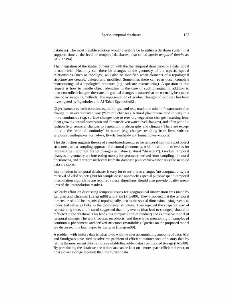
database). The most flexible solution would therefore be to utilise a database system thatsupports time at the level of temporal databases, also called spatio-temporal databases[Al-Taha94].

The integration of the spatial dimension with the the temporal dimension in a data modelis not trivial. Not only can there be changes to the geometry of the objects, spatialrelationships (such as topology) will also be modified when elements of a topologicalstructure are created, deleted and modified. Sometimes there can even occur completerestructurings of a topological structure (e.g. cadastre restructuring). A question in thisrespect is how to handle object identities in the case of such changes. In addition toman-controlled changes, there are the gradual changes in nature that are normally best takencare of by sampling methods. The representation of gradual changes of topology has beeninvestigated by Egenhofer and Al-Taha [Egenhofer92].

Object structures such as cadastres, buildings, land-use, roads and other infrastructure oftenchange in an event-driven way (“abrupt” changes). Natural phenomena tend to vary in amore continuous (e.g. surface changes due to erosion, vegetation changes resulting fromplant growth / natural succession and climate driven water level changes), and often periodicfashion (e.g. seasonal changes to vegetation, hydrography and climate). There are excep-tions to the “rule of continuity” in nature (e.g. changes resulting from fires, volcanoeruptions, earthquakes, tornadoes, floods, landslide and human interventions).

This distinction suggests the use of event-based structures for temporal monitoring of objectstructures, and a sampling approach for natural phenomena, with the addition of events forrepresenting important abrupt changes in nature (natural “disasters”). Gradual temporalchanges to geometry are interesting mostly for geometry derived from sampling of naturalphenomena, and therefore irrelevant from the database point of view when only the sampleddata are stored.

Interpolation in temporal databases is easy for event-driven changes (no computations, justretrieval of valid objects), but for sample-based approaches special purpose spatio-temporalinterpolation algorithms are required (these algorithms should also provide quality meas-ures of the interpolation results).

An early effort on discussing temporal issues for geographical information was made byLangran and Chrisman [Langran88] and Price [Price89]. They proposed that the temporaldimension should be organised topologically, just as the spatial dimension, using events asnodes and states as links in the topological structure. They rejected the snapshot way ofrepresenting time, and instead suggested that only events (that lead to changes) should bereflected in the database. This leads to a compact (non-redundant) and expressive model oftemporal change. The work focuses on objects, and there is no mentioning of samples ofcontinuous phenomena and derived structures (manifolds). Queries on the proposed modelare discussed in a later paper by Langran [Langran89].

A problem with history data is what to do with the ever accumulating amounts of data. Ahnand Snodgrass have tried to solve the problem of efficient maintenance of history data byletting the most recent data be more available than older data (a partitioned storage) [Ahn88].By partitioning the database, the older data can be kept on a more space efficient format, oron a slower storage medium than the current data.

Spatio-temporal databases 123

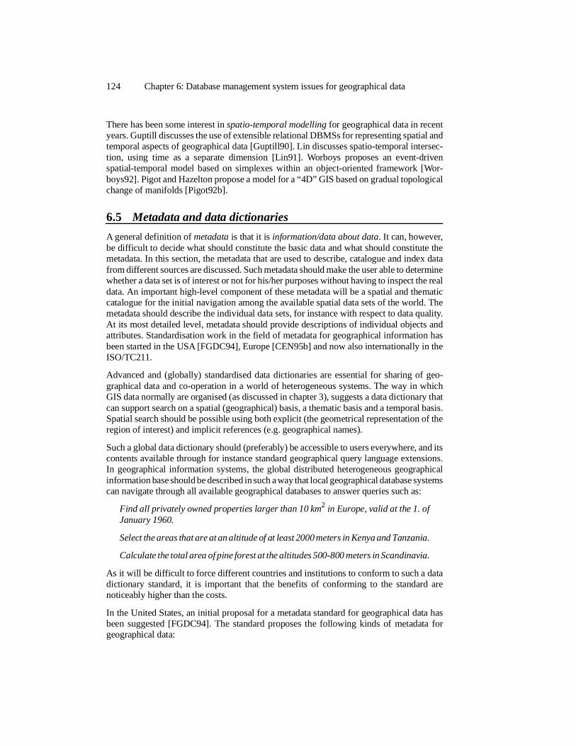
There has been some interest in spatio-temporal modelling for geographical data in recentyears. Guptill discusses the use of extensible relational DBMSs for representing spatial andtemporal aspects of geographical data [Guptill90]. Lin discusses spatio-temporal intersec-tion, using time as a separate dimension [Lin91]. Worboys proposes an event-drivenspatial-temporal model based on simplexes within an object-oriented framework [Wor-boys92]. Pigot and Hazelton propose a model for a “4D” GIS based on gradual topologicalchange of manifolds [Pigot92b].

6.5 Metadata and data dictionaries

A general definition of metadata is that it is information/data about data. It can, however,be difficult to decide what should constitute the basic data and what should constitute themetadata. In this section, the metadata that are used to describe, catalogue and index datafrom different sources are discussed. Such metadata should make the user able to determinewhether a data set is of interest or not for his/her purposes without having to inspect the realdata. An important high-level component of these metadata will be a spatial and thematiccatalogue for the initial navigation among the available spatial data sets of the world. Themetadata should describe the individual data sets, for instance with respect to data quality.At its most detailed level, metadata should provide descriptions of individual objects andattributes. Standardisation work in the field of metadata for geographical information hasbeen started in the USA [FGDC94], Europe [CEN95b] and now also internationally in theISO/TC211.

Advanced and (globally) standardised data dictionaries are essential for sharing of geo-graphical data and co-operation in a world of heterogeneous systems. The way in whichGIS data normally are organised (as discussed in chapter 3), suggests a data dictionary thatcan support search on a spatial (geographical) basis, a thematic basis and a temporal basis.Spatial search should be possible using both explicit (the geometrical representation of theregion of interest) and implicit references (e.g. geographical names).

Such a global data dictionary should (preferably) be accessible to users everywhere, and itscontents available through for instance standard geographical query language extensions.In geographical information systems, the global distributed heterogeneous geographicalinformation base should be described in such a way that local geographical database systemscan navigate through all available geographical databases to answer queries such as:

Find all privately owned properties larger than 10 km2 in Europe, valid at the 1. ofJanuary 1960.

Select the areas that are at an altitude of at least 2000 meters in Kenya and Tanzania.

Calculate the total area of pine forest at the altitudes 500-800 meters in Scandinavia.

As it will be difficult to force different countries and institutions to conform to such a datadictionary standard, it is important that the benefits of conforming to the standard arenoticeably higher than the costs.

In the United States, an initial proposal for a metadata standard for geographical data hasbeen suggested [FGDC94]. The standard proposes the following kinds of metadata forgeographical data:


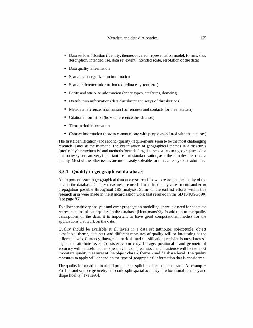
• Data set identification (identity, themes covered, representation model, format, size,description, intended use, data set extent, intended scale, resolution of the data)

• Data quality information

• Spatial data organization information

• Spatial reference information (coordinate system, etc.)

• Entity and attribute information (entity types, attributes, domains)

• Distribution information (data distributor and ways of distributions)

• Metadata reference information (currentness and contacts for the metadata)

• Citation information (how to reference this data set)

• Time period information

• Contact information (how to communicate with people associated with the data set)

The first (identification) and second (quality) requirements seem to be the most challengingresearch issues at the moment. The organisation of geographical themes in a thesaurus(preferably hierarchically) and methods for including data set extents in a geographical datadictionary system are very important areas of standardisation, as is the complex area of dataquality. Most of the other issues are more easily solvable, or there already exist solutions.

6.5.1 Quality in geographical databases

An important issue in geographical database research is how to represent the quality of thedata in the database. Quality measures are needed to make quality assessments and errorpropagation possible throughout GIS analysis. Some of the earliest efforts within thisresearch area were made in the standardisation work that resulted in the SDTS [USGS90](see page 86).

To allow sensitivity analysis and error propagation modelling, there is a need for adequaterepresentations of data quality in the database [Hootsmans92]. In addition to the qualitydescriptions of the data, it is important to have good computational models for theapplications that work on the data.

Quality should be available at all levels in a data set (attribute, object/tuple, objectclass/table, theme, data set), and different measures of quality will be interesting at thedifferent levels. Currency, lineage, numerical - and classification precision is most interest-ing at the attribute level. Consistency, currency, lineage, positional - and geometricalaccuracy will be useful at the object level. Completeness and consistency will be the mostimportant quality measures at the object class -, theme - and database level. The qualitymeasures to apply will depend on the type of geographical information that is considered.

The quality information should, if possible, be split into “independent” parts. An example:For line and surface geometry one could split spatial accuracy into locational accuracy andshape fidelity [Tveite95].

Metadata and data dictionaries 125

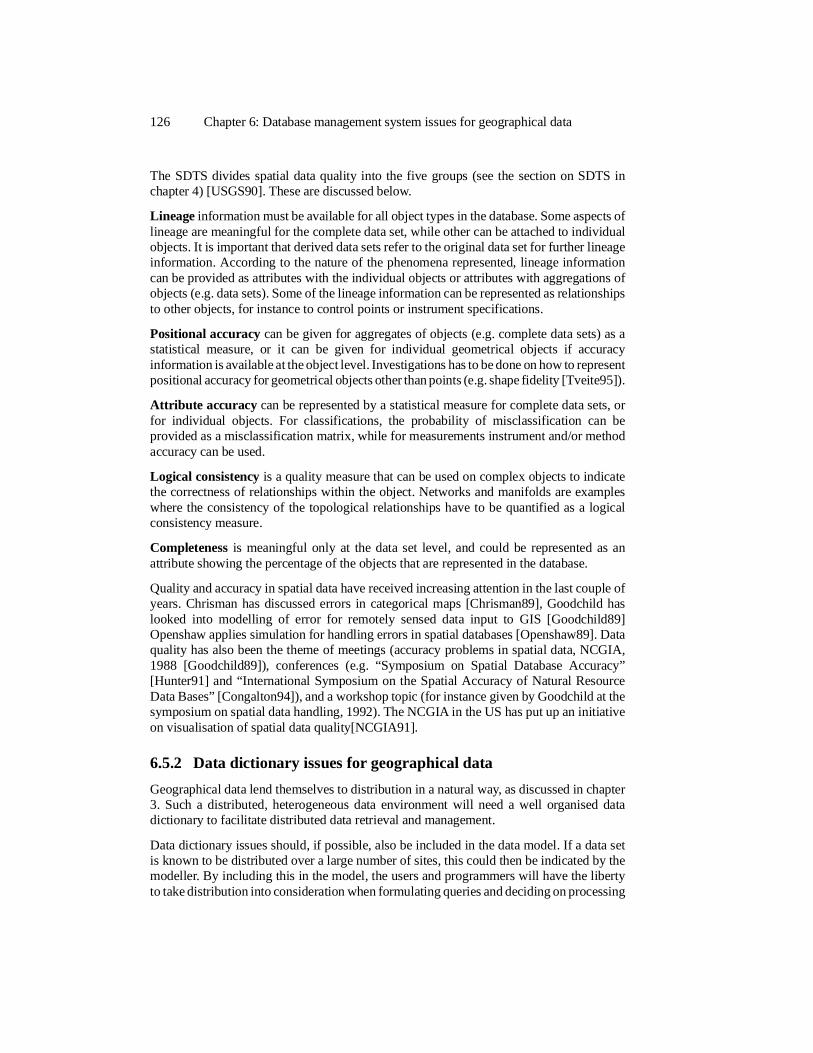
The SDTS divides spatial data quality into the five groups (see the section on SDTS inchapter 4) [USGS90]. These are discussed below.

Lineage information must be available for all object types in the database. Some aspects oflineage are meaningful for the complete data set, while other can be attached to individualobjects. It is important that derived data sets refer to the original data set for further lineageinformation. According to the nature of the phenomena represented, lineage informationcan be provided as attributes with the individual objects or attributes with aggregations ofobjects (e.g. data sets). Some of the lineage information can be represented as relationshipsto other objects, for instance to control points or instrument specifications.

Positional accuracy can be given for aggregates of objects (e.g. complete data sets) as astatistical measure, or it can be given for individual geometrical objects if accuracyinformation is available at the object level. Investigations has to be done on how to representpositional accuracy for geometrical objects other than points (e.g. shape fidelity [Tveite95]).

Attribute accuracy can be represented by a statistical measure for complete data sets, orfor individual objects. For classifications, the probability of misclassification can beprovided as a misclassification matrix, while for measurements instrument and/or methodaccuracy can be used.

Logical consistency is a quality measure that can be used on complex objects to indicatethe correctness of relationships within the object. Networks and manifolds are exampleswhere the consistency of the topological relationships have to be quantified as a logicalconsistency measure.

Completeness is meaningful only at the data set level, and could be represented as anattribute showing the percentage of the objects that are represented in the database.

Quality and accuracy in spatial data have received increasing attention in the last couple ofyears. Chrisman has discussed errors in categorical maps [Chrisman89], Goodchild haslooked into modelling of error for remotely sensed data input to GIS [Goodchild89]Openshaw applies simulation for handling errors in spatial databases [Openshaw89]. Dataquality has also been the theme of meetings (accuracy problems in spatial data, NCGIA,1988 [Goodchild89]), conferences (e.g. “Symposium on Spatial Database Accuracy”[Hunter91] and “International Symposium on the Spatial Accuracy of Natural ResourceData Bases” [Congalton94]), and a workshop topic (for instance given by Goodchild at thesymposium on spatial data handling, 1992). The NCGIA in the US has put up an initiativeon visualisation of spatial data quality[NCGIA91].

6.5.2 Data dictionary issues for geographical data

Geographical data lend themselves to distribution in a natural way, as discussed in chapter3. Such a distributed, heterogeneous data environment will need a well organised datadictionary to facilitate distributed data retrieval and management.

Data dictionary issues should, if possible, also be included in the data model. If a data setis known to be distributed over a large number of sites, this could then be indicated by themodeller. By including this in the model, the users and programmers will have the libertyto take distribution into consideration when formulating queries and deciding on processing


strategies. A distribution icon (a group of databases, or a globe) attached to the diagrammaticrepresentation of the object type could be useful for this (more about icons in chapter 5).

It is normally one of the goals of a database systems to make data distribution invisible tousers (distribution transparency using a distributed conceptual schema, DCS). This can bedesirable for single company/owner databases and distributed databases containing non-commercial (free) data. Geographical data are generally different (see chapter 3).

Geographical data are provided on a commercial basis by a large number of institutions andcompanies, all having different pricing policies and varying thematic interests in themodelled phenomena. This setting is different from most of the settings that are normallydiscussed in the distributed database management literature. The users of geographical datashould be interested in having access to a distribution data dictionary at the conceptual datamodel level. This is desirable because of the need to determine the availability of the datasets and their cost (both in terms of payment/royalties and acquisition time).

At the conceptual level, the data model should provide a standard, abstracted interface tothe (distributed) data dictionary of all relevant geographical databases. This standardinterface should be available through the query language, providing an integrated frame-work for distributed (geographical) data retrieval. That is, the data dictionary will be animportant part of the geographical database system. The data dictionary part of the databaseshould, in addition to quality measures, include other metadata elements, such as theownership, location, availability and cost as standard “attributes” of all data sets.

The setting for a distributed geographical data dictionary will probably be an internationalnetwork of data servers that are able to communicate and exchange data on a commercialbasis. Standardisation efforts within the OSI* framework of ISO** covers communicationprotocols between such servers.

Geographical data can be thought of as hierarchically organised according to location andtheme. Leaf nodes represent individual, generally autonomous, data sets. The data sets areplaced at different levels and branches, according to their thematic contents and theirgeographical extent/location.

Such an indexing/tree structure should, conceptually, be a composition of two orthogonalhierarchies, namely a location hierarchy and a theme hierarchy. In addition to these twohierarchies, it should be possible to specify the time at which the data set should be valid(points and intervals in time must be supported). At each node in the “location” tree thereshould be a full thematic hierarchy available, and from each node in the “theme” tree, itshould be possible to search through a “location” tree for the current theme. Hence, a singledata set could be found from many different places in the structure, and it should be possibleto reach it using different paths.

LocationIn the location hierarchy, one could choose the top level to be a geographical level dividingthe world into continents and oceans. The next levels could then reflect political boundaries,giving a division on the basis of political units such as nations, states, districts, counties andmunicipalities. In this hierarchy, international data sets should be attached to the highest

Metadata and data dictionaries 127

* Open Systems Interconnection

** International Standardisation Organisation

levels, national data sets to the national level, and so on. Such a geographical/politicalhierarchy provides one natural framework for guiding queries to geographical data sets.Another approach could be to base the hierarchy on watersheds. It should be possible toprovide many location hierarchies in the dictionary. The basis for such a solution is furtherdiscussed in connection with distribution of geographical data sets later in this chapter.

An alternative way of organising the spatial part of the dictionary is a global recursivetriangular tiling system, QTM [Dutton89][Goodchild90a]. Within this framework, an easyway of specifying the approximate location and extent of a data set would be to provide theaddress of the smallest triangle enclosing the data set and the largest triangle enclosed bythe data set. The address of a spatial phenomenon in this tiling system will be a very crudeindication of its spatial extent, so a more precise description of the geometry should also beavailable at the dictionary level. The approach also inherits the classical problem of indexingbased on hierarchical tiling, namely the objects that lie on tile boundaries at a high level inthe hierarchy. A solution to this problem could be to represent objects by a point (carefullychosen, so that it does not to lie on any tile boundaries) and an indication of the extent ofthe object. The QTM could then provide every geographical object with a (linearised) globaladdress.

According to the FGDC proposal, data set location should be specified either as a minimumbounding “rectangle” or as a bounding polygon, in both cases using latitude and longitudecoordinates [FGDC94]. Such a location indication will be very useful, if it is made availableto the data dictionary system.

Geographical namesGeographical names are an essential tool for humans when they wish to specify a location.Geographical names should therefore be available for expressing location in query languagefor geographical databases.

For navigation in the data dictionary location hierarchy, one should be able to use thegeographical names of the appropriate regions. Since there are many alternative ways ofwriting geographical names (Norway, Norwegen, Norge, Norvege, Noreg, ...), a nameresolution mechanism will have to be employed.

When specifying location while querying geographical databases it should also be possibleto use other geographical names than those in the dictionary hierarchy (as an alternative tospecifying geometrical locations explicitly through coordinates). A comprehensive indexof names and accompanying places/locations (points, regions or fuzzy regions) must bemade for this purpose. The development of such an index would require a lot of work, andparticularly the specification of fuzzy regions (such as Hardangervidda, Oslomarka, Os-lofjorden and Central Europe) will be demanding, since a lot of interviews will have to bemade for each region to get sufficient statistical material.

More advanced natural language interfaces could be the next step for geographical querylanguages, allowing locational prepositions (e.g. between Hardanger and Bergen) in addi-tion to the geographical names.

ThemeThe equally important theme hierarchy should also be available in the data dictionary fornavigation. In order to specify a hierarchy that allows search for geographical data on athematic basis, an internationally agreed upon taxonomy / thesaurus for GIS information


must be developed. Such a thesaurus will have to be very comprehensive, and will have tobe built in a systematic fashion.

An important first step is to specify a skeleton classification hierarchy, upon which thethesaurus can be based. The first layer of this hierarchy could for instance be made up ofthe following classes: infrastructure, topography/geomorphology, hydrography, oceanog-raphy, meteorology, vegetation, soils and geology. Because of the expected difficulty ofobtaining interdisciplinary consensus on what comprises an ideal theme hierarchy, the goalof the work should be to find a suitable lattice structure. As in the location hierarchy,databases could be attached at all levels of this lattice, and a single database must bereferenced from all the nodes of the tree that describe themes covered by that particulardatabase.

Efforts in this area have thus far only been made at national levels, for instance within theSDTS project in the USA (part 2 and 3 of [USGS90]).

At the European scene (CEN, TC 287), work is in progress to establish international(European) standards for the modelling and exchange of geographical/spatial data. Thisstandard will hopefully provide a better basis for a global geographical data dictionary.

An important practical problem in the design of distributed database systems is to decidewhether the global data dictionary should be centralised or distributed, replicated or notreplicated. This is a very complicated issue, and the pros and cons of these alternativeapproaches are discussed in the distributed database systems literature [Ceri88]. What isimportant is that the data dictionary should be available to all potential users of geographicaldata.

6.6 Geographical Query Languages

A geographical database management system should at least provide an application inter-face (for programming language bindings / application development). If the database systemis to provide a direct interactive query service to end-users, an additional, higher levelgraphic/textual interface to the database will be necessary. With such an interface, theend-users can interact directly with the maps/images using a pointing device to specifylocations (e.g. points, areas or volumes) of interest. This last topic, while interesting andimportant, is user-interface oriented, and will therefore not be elaborated on any furtherhere. It is, however, important that the application interface to the database system providesall the mechanisms that are needed to support these higher level (graphic) interfaces.

Traditional query languages either provide a set-based retrieval mechanisms (operates ongroups of objects, as for instance QUEL and SQL) or a navigation (one object at a time)mechanism (as provided by hierarchical and network DMLs). In a database query languagethat is to be used for retrieval from geographical databases, both of these mechanisms areuseful. The navigation mechanisms are necessary for topological structures, particularly fornetwork analysis, but also for manifold analysis and information browsing. The set-basedmechanisms are useful when performing statistical analysis on thematic data for researchand planning.

A query language standard suitable for geographical data and applications should supportmultimedia data types. A standardisation of the database interface is especially important

Geographical Query Languages 129

for shared distributed databases, because it will allow straightforward access to all externaldata sets stored in databases conforming to the standards.

Image operations and 3D analysis are important application areas that are not adequatelycovered by traditional query mechanisms, but should be given attention when developingquery languages for GIS.

Mechanisms for accessing to non-local data must be expected to become a requirement forfuture general purpose GISs. The query language must be able to help the users in the searchfor interesting data sets (all over the world), by offering queries to data dictionaries formeta-information on the data sets available in external databases (e.g. data describing thedata model used, the spatial and thematic contents of the database and the quality of the datasets contained in the database). This dictionary capability should be integrated with thetraditional DML mechanisms (navigation and set-oriented retrieval).

6.6.1 Different ways of organising geographical information

Depending on the application domain, the spatial component of geographical data can belooked upon in different ways, for instance:

• As geometrical objects, where location, distances and directions, normally in Euclid-ean space or on the geoid* are important.

• As topological structures, where the geometrical properties that stay invariant undersimple transformations (translation, rotation, scaling), such as neighbourhood infor-mation and information about the borders of objects, are of interest.

• As continuous phenomena, where sampling and interpolation methods can be usedto represent the phenomena (e.g. rasters and irregular samples).

Each of these attack-points to geographical data must be supported by a GIS, and a generalpurpose query language should include mechanisms for integrating, querying and manipu-lating all these representations of geographical information.

The geometrical object part of a query language for geographical databases will probablybe the most difficult to specify. The reason for this is that many human questions on spaceand geometry tend to be quite fuzzy, incorporating expression such as “large”, “high”,“long”, “in front of”, “between”, “north of” and so on. It will therefore be difficult to finda good set of spatial/geometrical operations. A good starting point could be to define a setof basic operations, where distance operators would play an important role. An example isan operator that, given a geometrical object and a distance, returns a new geometrical objectcovering the part of space that is within this distance from the original geometrical object(a buffer operation).

Topology, as discussed in chapter 4, is a rather formalised part of geographical data models.Some of the topological operations required are border/endpoint, interior, co-border/bound-ing, intersect and containment.

Rasters (regular samples) and “randomly” sampled data require general purpose and specialpurpose operations on “images” and point-sets, and must be treated in a different way than


* The “sea-level” surface of equal gravity

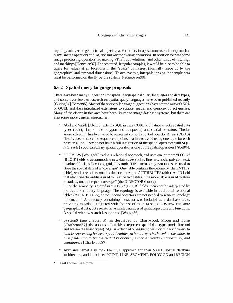
topology and vector-geometrical object data. For binary images, some useful query mecha-nisms are the operators and, or, not and xor for overlay operations. In addition to these comeimage processing operators for making FFTs*, convolutions, and other kinds of filteringsand maskings [Gonzalez87]. For scattered, irregular samples, it would be nice to be able toquery for values at all locations in the “space” of interest (normally made up by thegeographical and temporal dimensions). To achieve this, interpolations on the sample datamust be performed on the fly by the system [Neugebauer90].

6.6.2 Spatial query language proposals

There have been many suggestions for spatial/geographical query languages and data types,and some overviews of research on spatial query languages have been published recently[Güting94] [Samet95]. Most of these query language suggestions have started out with SQLor QUEL and then introduced extensions to support spatial and complex object queries.Many of the efforts in this area have been limited to image database systems, but there arealso some more general approaches.

• Abel and Smith [Abel86] extends SQL in their COREGIS database with spatial datatypes (point, line, simple polygon and composite) and spatial operators. “Inclu-sion/exclusion” has been used to represent complex spatial objects. A raw (BLOB)field is used to store the sequence of points in a line to avoid using one tuple for eachpoint in a line. They do not have a full integration of the spatial operators with SQL.Intersects (a boolean binary spatial operator) is one of the spatial operators [Abel86].

• GEOVIEW [Waugh86] is also a relational approach, and uses one or more “LONG”(BLOB) fields to accommodate new data types (point, line, arc, node, polygon, text,quadtree block, collections, grid, TIN node, TIN patch). Only two tables are used tostore the spatial data of a “coverage”. One table contains the geometry (the ENTITYtable), while the other contains the attributes (the ATTRIBUTES table). An ID fieldthat identifies the entity is used to link the two tables. One more table is used to storemetadata, one tuple per “coverage” (the DIRECTORY table).Since the geometry is stored in “LONG” (BLOB) fields, it can not be interpreted bythe traditional query language. The topology is available in traditional relationaltables (ATTRIBUTES), so no special operators are not needed to retrieve topologyinformation. A directory containing metadata was included as a database table,providing metadata integrated with the rest of the data set. GEOVIEW can storegeographical data, but seem to have limited number of spatial operators and functions.A spatial window search is supported [Waugh86].

• System9 (see chapter 3), as described by Charlwood, Moon and Tulip[Charlwood87], also applies bulk fields to represent spatial data types (node, line andsurface are the basic types). SQL is extended by adding grammar and vocabulary tohandle referencing between spatial entities, to handle queries based on the values inbulk fields, and to handle spatial relationships such as overlap, connectivity, andcontainment [Charlwood87].

• Aref and Samet also took the SQL approach for their SAND spatial databasearchitecture, and introduced POINT, LINE_SEGMENT, POLYGON and REGION


* Fast Fourier Transforms

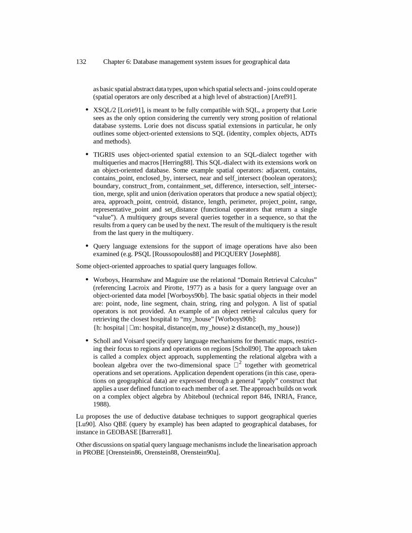
as basic spatial abstract data types, upon which spatial selects and - joins could operate(spatial operators are only described at a high level of abstraction) [Aref91].

• XSQL/2 [Lorie91], is meant to be fully compatible with SQL, a property that Loriesees as the only option considering the currently very strong position of relationaldatabase systems. Lorie does not discuss spatial extensions in particular, he onlyoutlines some object-oriented extensions to SQL (identity, complex objects, ADTsand methods).

• TIGRIS uses object-oriented spatial extension to an SQL-dialect together withmultiqueries and macros [Herring88]. This SQL-dialect with its extensions work onan object-oriented database. Some example spatial operators: adjacent, contains,contains_point, enclosed_by, intersect, near and self_intersect (boolean operators);boundary, construct_from, containment_set, difference, intersection, self_intersec-tion, merge, split and union (derivation operators that produce a new spatial object);area, approach_point, centroid, distance, length, perimeter, project_point, range,representative_point and set_distance (functional operators that return a single“value”). A multiquery groups several queries together in a sequence, so that theresults from a query can be used by the next. The result of the multiquery is the resultfrom the last query in the multiquery.

• Query language extensions for the support of image operations have also beenexamined (e.g. PSQL [Roussopoulos88] and PICQUERY [Joseph88].

Some object-oriented approaches to spatial query languages follow.

• Worboys, Hearnshaw and Maguire use the relational “Domain Retrieval Calculus”(referencing Lacroix and Pirotte, 1977) as a basis for a query language over anobject-oriented data model [Worboys90b]. The basic spatial objects in their modelare: point, node, line segment, chain, string, ring and polygon. A list of spatialoperators is not provided. An example of an object retrieval calculus query forretrieving the closest hospital to “my_house” [Worboys90b]:{h: hospital | ∀ m: hospital, distance(m, my_house) ≥ distance(h, my_house)}

• Scholl and Voisard specify query language mechanisms for thematic maps, restrict-ing their focus to regions and operations on regions [Scholl90]. The approach takenis called a complex object approach, supplementing the relational algebra with aboolean algebra over the two-dimensional space ℜ 2 together with geometricaloperations and set operations. Application dependent operations (in this case, opera-tions on geographical data) are expressed through a general “apply” construct thatapplies a user defined function to each member of a set. The approach builds on workon a complex object algebra by Abiteboul (technical report 846, INRIA, France,1988).

Lu proposes the use of deductive database techniques to support geographical queries[Lu90]. Also QBE (query by example) has been adapted to geographical databases, forinstance in GEOBASE [Barrera81].

Other discussions on spatial query language mechanisms include the linearisation approachin PROBE [Orenstein86, Orenstein88, Orenstein90a].


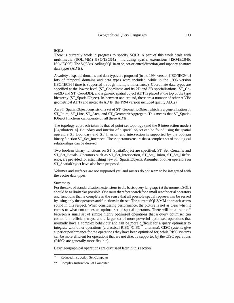
SQL3There is currently work in progress to specify SQL3. A part of this work deals withmultimedia (SQL/MM) [ISO/IEC94a], including spatial extensions [ISO/IEC94b,ISO/IEC96]. The SQL3 is leading SQL in an object-oriented direction, and supports abstractdata types (ADTs).

A variety of spatial domains and data types are proposed (in the 1994 version [ISO/IEC94b]lots of temporal domains and data types were included, while in the 1996 version[ISO/IEC96] time is supported through multiple inheritance). Coordinate data types arespecified at the lowest level (ST_Coordinate and its 2D and 3D specialisations: ST_Co-ord2D and ST_Coord3D), and a generic spatial object ADT is placed at the top of the typehierarchy (ST_SpatialObject). In-between and around, there are a number of other ADTs:geometrical ADTs and metadata ADTs (the 1994 version included quality ADTs).

An ST_SpatialObject consists of a set of ST_GeometricObject which is a generalisation ofST_Point, ST_Line, ST_Area, and ST_GeometricAggregate. This means that ST_Spatia-lObject functions can operate on all these ADTs.

The topology approach taken is that of point set topology (and the 9 intersection model)[Egenhofer91a]. Boundary and interior of a spatial object can be found using the spatialoperators ST_Boundary and ST_Interior, and intersection is supported by the booleanbinary function ST_Set_Intersects. These operators ensure that a complete set of topologicalrelationships can be derived.

Two boolean binary functions on ST_SpatialObject are specified: ST_Set_Contains andST_Set_Equals. Operators such as ST_Set_Intersection, ST_Set_Union, ST_Set_Differ-ence, are provided for establishing new ST_SpatialObjects. A number of other operators onST_SpatialObject have also been proposed.

Volumes and surfaces are not supported yet, and rasters do not seem to be integrated withthe vector data types.

SummaryFor the sake of standardisation, extensions to the basic query language (at the moment SQL)should be as limited as possible. One must therefore search for a small set of spatial operatorsand functions that is complete in the sense that all possible spatial requests can be servedby using only the operators and functions in the set. The current SQL3/MM approach seemssound in this respect. When considering performance, the picture is not as clear when itcomes to what constitutes an optimal set of spatial operators. There will be a trade-offbetween a small set of simple highly optimised operations that a query optimiser cancombine in efficient ways, and a larger set of more powerful optimised operations thatnormally have a complex behaviour and can be more difficult for a query optimiser tointegrate with other operations (a classical RISC*/CISC** dilemma). CISC systems givesuperior performance for the operations they have been optimised for, while RISC systemscan be more efficient for operations that are not directly supported by the CISC operations(RISCs are generally more flexible).

Basic geographical operations are discussed later in this section.


* Reduced Instruction Set Computer

** Complex Instruction Set Computer

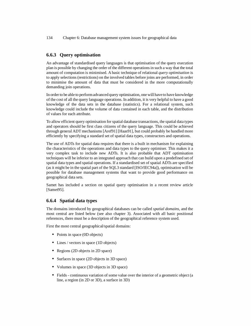
6.6.3 Query optimisation

An advantage of standardised query languages is that optimisation of the query executionplan is possible by changing the order of the different operations in such a way that the totalamount of computation is minimised. A basic technique of relational query optimisation isto apply selections (restrictions) on the involved tables before joins are performed, in orderto minimise the amount of data that must be considered in the more computationallydemanding join operations.

In order to be able to perform advanced query optimisation, one will have to have knowledgeof the cost of all the query language operations. In addition, it is very helpful to have a goodknowledge of the data sets in the database (statistics). For a relational system, suchknowledge could include the volume of data contained in each table, and the distributionof values for each attribute.

To allow efficient query optimisation for spatial database transactions, the spatial data typesand operators should be first class citizens of the query language. This could be achievedthrough general ADT mechanisms [Aref91] [Haas91], but could probably be handled moreefficiently by specifying a standard set of spatial data types, constructors and operations.

The use of ADTs for spatial data requires that there is a built in mechanism for explainingthe characteristics of the operations and data types to the query optimiser. This makes it avery complex task to include new ADTs. It is also probable that ADT optimisationtechniques will be inferior to an integrated approach that can build upon a predefined set ofspatial data types and spatial operations. If a standardised set of spatial ADTs are specified(as it might be in the spatial part of the SQL3 standard [ISO/IEC94a]), optimisation will bepossible for database management systems that want to provide good performance ongeographical data sets.

Samet has included a section on spatial query optimisation in a recent review article[Samet95].

6.6.4 Spatial data types

The domains introduced by geographical databases can be called spatial domains, and themost central are listed below (see also chapter 3). Associated with all basic positionalreferences, there must be a description of the geographical reference system used.

First the most central geographical/spatial domains:

• Points in space (0D objects)

• Lines / vectors in space (1D objects)

• Regions (2D objects in 2D space)

• Surfaces in space (2D objects in 3D space)

• Volumes in space (3D objects in 3D space)

• Fields - continuous variation of some value over the interior of a geometric object (aline, a region (in 2D or 3D), a surface in 3D)


On top of these basic domains, the most important structural domains should be defined:

• Networks of lines in 2D or 3D space (could also include TINs)

• Manifolds (for regions and volumes)

To support integration with rasters or images one can include some additional spatialdomains (similar to/supporting the field):

• Pixel (the atomic element of a raster), usually representing a rectangle or square

• Voxels (volume raster elements)

• Raster/matrix (n by m (by o) grid of pixels(/voxels))

All these domains should be supported by the basic spatial data types of a geographicalquery language.

GEOBASE, an example of an early effort in this area, uses 0-, 1- and 2-dimensionalgeographical objects (points, lines and polygons, termed images by the authors) as basicgeographical data types [Barrera81].

An extended relational approachIf we choose to go for an implementation within the relational framework, we need somespatial data types in addition to the SQL data types mentioned in chapter 2, to make theusers able to formulate efficient queries on spatial databases. As mentioned earlier, the setof new data types should be as small as possible, in order to limit the complexity of theresulting query language syntax.

Geometry can be covered in many ways, and the minimum requirement is a spatial referencetype. The most natural spatial reference type is the point data type, consisting of a group oftwo or three real numbers describing a position on the earth (latitude, longitude (andelevation)) in some reference system. There might be a need for two 0-dimensional objecttypes: one for 2D references (e.g. position) and another one for 3D (e.g. point). The positionwill be a projection of the point onto the plane or earth surface. An easy way out would beto go for only the position type, and include elevation as an ordinary attribute. Such anapproach would limit the possibilities for developing standardised 3D operations.

The other geometrical constructs, such as line, region, surface, volume and field could berepresented using constructors on the point or position type. A general purpose constructorthat is useful for building more complex geometrical and topological items is the sequenceconstructor (as used in TECHRA, a relational database system developed in Norway forscientific and technical applications [TECHRA93]). The use of ADTs for the data types (forinstance line), where the representation of the data type (line) is hidden, but where the ADTinterface could support all imaginable query and update operations, would be very conven-ient. In this way it would truly function as a basic data type. For all the higher-levelgeometrical types (line, region, surface and volume), it would be useful to allow bothattribute variation over the interior of the objects (fields) and homogeneous interiors (as isnormal in current systems) at the conceptual level.

The important class of continuously varying natural phenomena, that normally could berepresented using samples in geographical databases, does deserve a special purpose data


type. This is the field. The field is currently most used for a 2.5D surfaces, but couldtheoretically also be used for representing continuous change along a line in some space,over a 3D surface or over the interior of a 3D volume. Without such a data type, the userswill have to retrieve the underlying samples from the database system and perform theinterpolations themselves.Using the ADT approach for fields, interpolations will be performed by the databasemanagement system. It is therefore very important that the interpolation results are aug-mented by an accuracy measure, from which the user can decide whether the samplingfrequency is high enough to provide a basis for meaningful interpolation over the region ofinterest.

Topology and geometry operations could need some special purpose data types in order tomake geometrical and topological constraints and query language operations a part of thedatabase system. In case this is what is wanted, the database system could profit on knowingabout some of the following data types: node, edge, face, network, TIN and manifold.

Regular grids or rasters is a very common way of representing and storing environmentaldata and measurements, and should be supported by a geographically oriented databasemanagement system for full integration with the other geographical data types. This couldbe done using a matrix type, or a more clumsy sequence of sequence type (one more nestingfor 3D, such as seismic data, atmospheric and marine data). The matrix type could beregarded as a specific implementation of (1.5D,) 2.5D or 3.5D fields.

Data dictionary data typesThere is a need for dictionary data types that can facilitate queries to the data dictionary(and directory) system, providing both geographical and thematic searching. Data types forthematic dictionary search and for geographical dictionary search are therefore necessary.

• The thematic data type should be built according to internationally accepted standardthesauruses of geographical data.

• The geographical data type should be able to index different kinds of geographicalunit hierarchies (e.g. political/administrative or watershed).

Such data types should make hierarchy queries possible. The domain of the data types couldfor instance be a structured string, supporting wild card character searching. By combiningthe domains it should be possible to specify many administrative and thematic restrictionswithin a single query.

A geographical hierarchy could for instance be based on the political/economical units:

Continent - Country - (Landscape -) State / District - County - Municipality - Township -Property- Lot

A natural supplement to this method is region/polygon geometry search. A region expressedusing a hierarchical expression of geographical names could then be translated into a closedpolygon or a volume. Such a geometry could then be used in the next stages of processingof the data dictionary query. An advantage of using polygons is that language expressionsvary from culture to culture, while geometrical descriptions are internationally standardised,and translators are easier to specify.


The data dictionary types should also be used in interactive graphical systems, to providethe user with a friendly browsing environment.

6.6.5 Spatial constraints

In addition to traditional database constraints, such as the nature and cardinality ofrelationships, temporal constraints and identification, spatial constraints are necessary forcomplex spatial objects, topology and other spatial relationships. Some examples of spatialconstraints are given below.

• Networks require that all links have two end-nodes (not necessarily distinct), and thatall nodes are attached to at least one edge. In manifolds, all border segments (edgesor surfaces) should border two and only two regions or volumes (this requires auniversal polygon/volume).

• Complex spatial objects, such as edges, regions, surfaces, volumes and rasters willhave to conform to structural constraints. An edge should be a one-dimensional pathconnecting two points. A 2D region should be a 2-dimensional phenomenon boundedby edges. A raster should be a matrix of objects of a certain domain, representing aregular tessellation (having the same dimensions as the matrix) of a geographicalregion (normally 2D or 3D).

• For spatial database integration, a very important aspect is the identification of spatialobjects contained in multiple databases. The geographical database managementsystem should be able to tell that a river or a road in one database is the same as theriver or the road in another database. The key to this problem could be a combinationof a common spatial reference framework and adequate metadata (with quality/ac-curacy measures) in the database.

• Usage and quality constraints (scale, accuracy, context-dependence) form an equallyimportant class of constraints for geographical data. Different aspects of scale willbe central for these constraints.

Spatial constraints will be important in the design of the spatial operations of geographicalquery languages. It should also be possible to specify spatial constraints that apply to acertain kind of geographical phenomenon/data (e.g. a river cannot flow uphill).

6.6.6 Operations

The traditional set-based operations of relational database management systems are: selec-tion, union, intersection, division, difference, negation, aggregation and join (see chapter2). GISs introduce new domains, outlined in the previous sections, and therefore also needsome spatial variants of the traditional operations.

As mentioned earlier in this section: For the sake of standardisation and optimisation, it isimportant to find a smallest set of spatial operators and functions that is complete in thesense that all possible spatial requests can be served by using combinations of theseoperators and functions.

To find a set of basic spatial operations will have to be the first and most important step indeveloping a full set of spatial operations. Following the ideas of the previous sections, a


starting point could be to divide the operations into geometrical operations (includinggeographical data integration), vector-topological (often navigational) operations and “ras-ter operations”. Basic spatial operations have also been discussed in the literature (e.g.[Egenhofer87], [Egenhofer90b]).

Geometrical operations on objects in spatial databasesGeometrical operations are operations that operate on geometrical elements (points, lines,polygons, surfaces and volumes) and normally use Euclidean geometry to obtain the results.

The first category of geometrical operations return a scalar value, and could therefore becalled geometrical calculations or scalar operations (giving scalar results). Classes ofgeometrical calculations are:

• Distance queries: compute and return the (for instance Euclidean) distance betweengeometrical objects (3D or 2D distance). This operation could in addition return adirection vector. line-queries: compute the length of a line (or a perimeter).

• Extent queries, eg: Length-queries: compute the length of a line. Area-queries:compute the area of a polygon, or a surface. Volume-queries: compute the volumeof 3D-objects.

• Field queries: compute properties, e.g.slope_of_field(field, x, y).elevation_of_field(field, x, y) or value(field, point) that returns the value for the fieldat that point.mean(field, region) that returns the mean value of the field over the specified region.mean(field, line) for lines.These operations should also return a measure for the reliability of the value since itis derived using the field representation/interpolation method.

The second category encompasses operations that return spatial objects. The operations thatcombine two different data sets can be termed integration operations.

A spatial join [Güting94] [Samet95] is an operation that integrates two spatial data sets bymerging their geometries together to form a new (integrated) spatial data set, and perhapsdo operations based on the values of the attributes of the data sets. In traditional geographicalinformation systems, a spatial join is often called an overlay. The union and intersectionoperations listed below are two kinds of spatial joins.

• boundary (object): an operation that returns the boundary of an object (topological[Egenhofer90b]).

• interior (object): a unary operation that returns the interior of an object (topological[Egenhofer90b]).

• exterior (object): a unary operation that returns the exterior of an object (topological[Egenhofer90b])complement (object, [universe]): a unary operator that returns the part of the data set/ space that is “outside” the object. The result will depend on the context (e.g. 1D,2D or 3D) and the universe of discourse.


• union (polygon-polygon, line-line, network-network, manifold-manifold): a binaryoperation that returns the union of two (sets of) geometrical objects.

• intersection (object1,object2): a binary operation, returning the intersection of thetwo (sets of) geometrical objects. The intersection of two sets of areas can be a set ofareas, lines and points (intersection is a valid operation for line, area, surface andvolume objects).

• projection (object, projection description): an operation that returns an object of lowerdimensionality. Should support dimensionality generalisation as discussed in anearlier section.

• 3D queries: operations on volumes and surfaces/fields that return points, lines, areas,fields or volumes, such as drainage_basin(surface, point) and visible_areas(surface,point) (that both return areas).

• clip (object1, object2): Return the parts of object 1 that are within object two. Whenapplied to a field, the dimensionality of the field(object1) will be reduced to thedimensionality of object2.

• generalise (object, scale): an operation that generalises the object(structure) to theindicated scale.

• buffer (object, (Euclidean) distance): an operation that returns a new object (regionor volume, depending on the context/universe) that covers the original geometricalobject and all the space that is within distance from the object. The buffer functioncould for instance be used in conjunction with an “inside” query to perform neigh-bourhood queries (find all houses within 200 meters from the E6 in “Nordlandfylke”).

• neighbour queries: an operation that finds the n nearest neighbours (of some specifiedtype) of a geographical object.

The third category of queries operate on geometrical objects and return a truth value. Thesequeries can in most cases be formulated using the previously mentioned query types[Egenhofer90b].

• equal (x,y) can be determined by (intersection(complement(x),y) = ∅ ) and (intersec-tion(complement(y),x) = ∅ ).

• contains (x,y) can be determined by (intersection(complement(x),y) = ∅ ). (point online, point in polygon, point on surface, point in volume, line in line, line in polygon,line on surface, line in volume, polygon in polygon, polygon in volume, surface onsurface, surface in volume, volume in volume).

• overlaps (x,y) can be determined by (intersection(x,y) ≠ ∅ ).

• touch (x,y) can be determined by ((intersection(boundary(x),boundary(y)) ≠ ∅ ) and(intersection(interior(x), interior(y)) = ∅ )).

• location queries (spatial relationships between two objects): n,s,e,w,ne,nw,se,sw[Roussopoulos88].


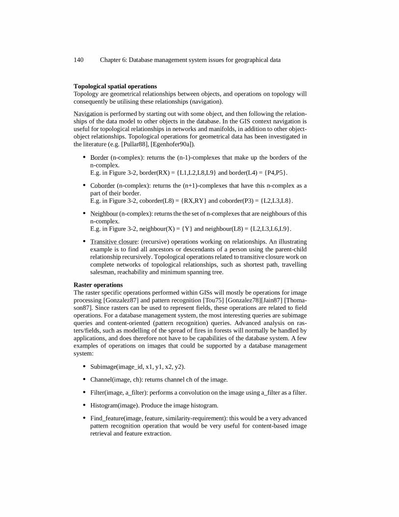
Topological spatial operationsTopology are geometrical relationships between objects, and operations on topology willconsequently be utilising these relationships (navigation).

Navigation is performed by starting out with some object, and then following the relation-ships of the data model to other objects in the database. In the GIS context navigation isuseful for topological relationships in networks and manifolds, in addition to other object-object relationships. Topological operations for geometrical data has been investigated inthe literature (e.g. [Pullar88], [Egenhofer90a]).

• Border (n-complex): returns the (n-1)-complexes that make up the borders of then-complex.E.g. in Figure 3-2, border(RX) = {L1,L2,L8,L9} and border(L4) = {P4,P5}.

• Coborder (n-complex): returns the (n+1)-complexes that have this n-complex as apart of their border.E.g. in Figure 3-2, coborder(L8) = {RX,RY} and coborder(P3) = {L2,L3,L8}.

• Neighbour (n-complex): returns the the set of n-complexes that are neighbours of thisn-complex.E.g. in Figure 3-2, neighbour(X) = {Y} and neighbour(L8) = {L2,L3,L6,L9}.

• Transitive closure: (recursive) operations working on relationships. An illustratingexample is to find all ancestors or descendants of a person using the parent-childrelationship recursively. Topological operations related to transitive closure work oncomplete networks of topological relationships, such as shortest path, travellingsalesman, reachability and minimum spanning tree.

Raster operationsThe raster specific operations performed within GISs will mostly be operations for imageprocessing [Gonzalez87] and pattern recognition [Tou75] [Gonzalez78][Jain87] [Thoma-son87]. Since rasters can be used to represent fields, these operations are related to fieldoperations. For a database management system, the most interesting queries are subimagequeries and content-oriented (pattern recognition) queries. Advanced analysis on ras-ters/fields, such as modelling of the spread of fires in forests will normally be handled byapplications, and does therefore not have to be capabilities of the database system. A fewexamples of operations on images that could be supported by a database managementsystem:

• Subimage(image_id, x1, y1, x2, y2).

• Channel(image, ch): returns channel ch of the image.

• Filter(image, a_filter): performs a convolution on the image using a_filter as a filter.

• Histogram(image). Produce the image histogram.

• Find_feature(image, feature, similarity-requirement): this would be a very advancedpattern recognition operation that would be very useful for content-based imageretrieval and feature extraction.


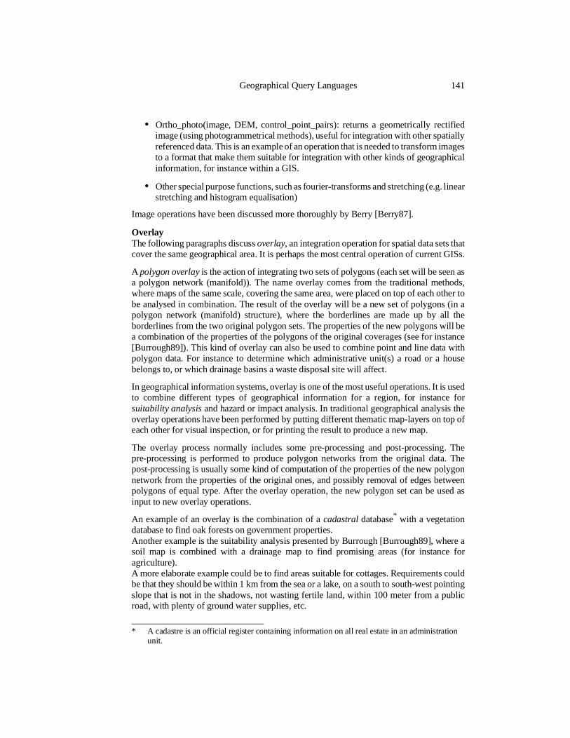
• Ortho_photo(image, DEM, control_point_pairs): returns a geometrically rectifiedimage (using photogrammetrical methods), useful for integration with other spatiallyreferenced data. This is an example of an operation that is needed to transform imagesto a format that make them suitable for integration with other kinds of geographicalinformation, for instance within a GIS.

• Other special purpose functions, such as fourier-transforms and stretching (e.g. linearstretching and histogram equalisation)

Image operations have been discussed more thoroughly by Berry [Berry87].

OverlayThe following paragraphs discuss overlay, an integration operation for spatial data sets thatcover the same geographical area. It is perhaps the most central operation of current GISs.

A polygon overlay is the action of integrating two sets of polygons (each set will be seen asa polygon network (manifold)). The name overlay comes from the traditional methods,where maps of the same scale, covering the same area, were placed on top of each other tobe analysed in combination. The result of the overlay will be a new set of polygons (in apolygon network (manifold) structure), where the borderlines are made up by all theborderlines from the two original polygon sets. The properties of the new polygons will bea combination of the properties of the polygons of the original coverages (see for instance[Burrough89]). This kind of overlay can also be used to combine point and line data withpolygon data. For instance to determine which administrative unit(s) a road or a housebelongs to, or which drainage basins a waste disposal site will affect.

In geographical information systems, overlay is one of the most useful operations. It is usedto combine different types of geographical information for a region, for instance forsuitability analysis and hazard or impact analysis. In traditional geographical analysis theoverlay operations have been performed by putting different thematic map-layers on top ofeach other for visual inspection, or for printing the result to produce a new map.

The overlay process normally includes some pre-processing and post-processing. Thepre-processing is performed to produce polygon networks from the original data. Thepost-processing is usually some kind of computation of the properties of the new polygonnetwork from the properties of the original ones, and possibly removal of edges betweenpolygons of equal type. After the overlay operation, the new polygon set can be used asinput to new overlay operations.

An example of an overlay is the combination of a cadastral database* with a vegetationdatabase to find oak forests on government properties.Another example is the suitability analysis presented by Burrough [Burrough89], where asoil map is combined with a drainage map to find promising areas (for instance foragriculture).A more elaborate example could be to find areas suitable for cottages. Requirements couldbe that they should be within 1 km from the sea or a lake, on a south to south-west pointingslope that is not in the shadows, not wasting fertile land, within 100 meter from a publicroad, with plenty of ground water supplies, etc.


* A cadastre is an official register containing information on all real estate in an administrationunit.

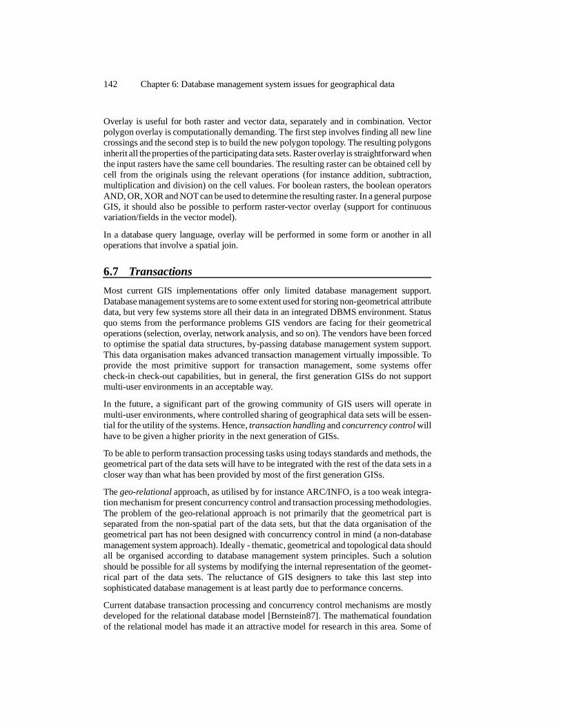
Overlay is useful for both raster and vector data, separately and in combination. Vectorpolygon overlay is computationally demanding. The first step involves finding all new linecrossings and the second step is to build the new polygon topology. The resulting polygonsinherit all the properties of the participating data sets. Raster overlay is straightforward whenthe input rasters have the same cell boundaries. The resulting raster can be obtained cell bycell from the originals using the relevant operations (for instance addition, subtraction,multiplication and division) on the cell values. For boolean rasters, the boolean operatorsAND, OR, XOR and NOT can be used to determine the resulting raster. In a general purposeGIS, it should also be possible to perform raster-vector overlay (support for continuousvariation/fields in the vector model).

In a database query language, overlay will be performed in some form or another in alloperations that involve a spatial join.

6.7 Transactions

Most current GIS implementations offer only limited database management support.Database management systems are to some extent used for storing non-geometrical attributedata, but very few systems store all their data in an integrated DBMS environment. Statusquo stems from the performance problems GIS vendors are facing for their geometricaloperations (selection, overlay, network analysis, and so on). The vendors have been forcedto optimise the spatial data structures, by-passing database management system support.This data organisation makes advanced transaction management virtually impossible. Toprovide the most primitive support for transaction management, some systems offercheck-in check-out capabilities, but in general, the first generation GISs do not supportmulti-user environments in an acceptable way.

In the future, a significant part of the growing community of GIS users will operate inmulti-user environments, where controlled sharing of geographical data sets will be essen-tial for the utility of the systems. Hence, transaction handling and concurrency control willhave to be given a higher priority in the next generation of GISs.

To be able to perform transaction processing tasks using todays standards and methods, thegeometrical part of the data sets will have to be integrated with the rest of the data sets in acloser way than what has been provided by most of the first generation GISs.

The geo-relational approach, as utilised by for instance ARC/INFO, is a too weak integra-tion mechanism for present concurrency control and transaction processing methodologies.The problem of the geo-relational approach is not primarily that the geometrical part isseparated from the non-spatial part of the data sets, but that the data organisation of thegeometrical part has not been designed with concurrency control in mind (a non-databasemanagement system approach). Ideally - thematic, geometrical and topological data shouldall be organised according to database management system principles. Such a solutionshould be possible for all systems by modifying the internal representation of the geomet-rical part of the data sets. The reluctance of GIS designers to take this last step intosophisticated database management is at least partly due to performance concerns.

Current database transaction processing and concurrency control mechanisms are mostlydeveloped for the relational database model [Bernstein87]. The mathematical foundationof the relational model has made it an attractive model for research in this area. Some of


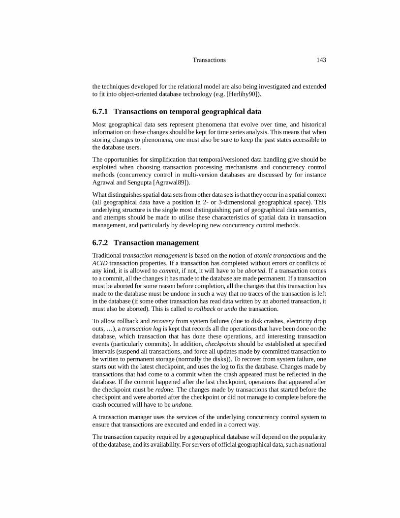
the techniques developed for the relational model are also being investigated and extendedto fit into object-oriented database technology (e.g. [Herlihy90]).

6.7.1 Transactions on temporal geographical data

Most geographical data sets represent phenomena that evolve over time, and historicalinformation on these changes should be kept for time series analysis. This means that whenstoring changes to phenomena, one must also be sure to keep the past states accessible tothe database users.

The opportunities for simplification that temporal/versioned data handling give should beexploited when choosing transaction processing mechanisms and concurrency controlmethods (concurrency control in multi-version databases are discussed by for instanceAgrawal and Sengupta [Agrawal89]).

What distinguishes spatial data sets from other data sets is that they occur in a spatial context(all geographical data have a position in 2- or 3-dimensional geographical space). Thisunderlying structure is the single most distinguishing part of geographical data semantics,and attempts should be made to utilise these characteristics of spatial data in transactionmanagement, and particularly by developing new concurrency control methods.

6.7.2 Transaction management

Traditional transaction management is based on the notion of atomic transactions and theACID transaction properties. If a transaction has completed without errors or conflicts ofany kind, it is allowed to commit, if not, it will have to be aborted. If a transaction comesto a commit, all the changes it has made to the database are made permanent. If a transactionmust be aborted for some reason before completion, all the changes that this transaction hasmade to the database must be undone in such a way that no traces of the transaction is leftin the database (if some other transaction has read data written by an aborted transaction, itmust also be aborted). This is called to rollback or undo the transaction.

To allow rollback and recovery from system failures (due to disk crashes, electricity dropouts, …), a transaction log is kept that records all the operations that have been done on thedatabase, which transaction that has done these operations, and interesting transactionevents (particularly commits). In addition, checkpoints should be established at specifiedintervals (suspend all transactions, and force all updates made by committed transaction tobe written to permanent storage (normally the disks)). To recover from system failure, onestarts out with the latest checkpoint, and uses the log to fix the database. Changes made bytransactions that had come to a commit when the crash appeared must be reflected in thedatabase. If the commit happened after the last checkpoint, operations that appeared afterthe checkpoint must be redone. The changes made by transactions that started before thecheckpoint and were aborted after the checkpoint or did not manage to complete before thecrash occurred will have to be undone.

A transaction manager uses the services of the underlying concurrency control system toensure that transactions are executed and ended in a correct way.

The transaction capacity required by a geographical database will depend on the popularityof the database, and its availability. For servers of official geographical data, such as national

Transactions 143

map series that are often used as background maps for presentations and analysis, severalsimultaneous transactions must be expected to occur throughout the day. Exact numbers aredifficult to predict, as they depend on the future number of GIS users and the way in whichdata distribution and management is organised.

The most primitive transaction management method is check-in check-out, avoiding lowerlevel concurrency control (as used in ARC/INFO LIBRARIAN [Aronson89]). This has beenmuch used in design applications in the past, but does not allow the necessary concurrencyfor sharing of data for cooperative work and on-line access to external data sets.

For more advanced transaction management, involving distributed databases, the 2PC (2phase commit) commit protocol is the most widely used [Bernstein87]. This protocolprovides consistency of a distributed database system by ensuring that a transaction is eithercommitted at all sites or aborted at all sites in the network. To limit application blocking,2PC has a built-in flexibility to handle site failures and network failures/partitions correctly.

6.7.3 Concurrency Control

There are two popular groups of methods that are used for concurrency control in databasesystems. One is based on locking and the other on time-stamp ordering. A third group, thatoften utilises techniques from the first two groups, are the optimistic methods. Traditionalconcurrency control mechanisms are based on the serialisability criterion (page 18) [Bern-stein87].

The locking technique tags all items that are accessed by some transaction with a read tagor a write tag (other tag types are possible, e.g. read-write and increment). All the tags of aparticular transaction are removed before or when the transaction terminates. Access to atagged item by another transaction is allowed or disallowed on the basis of the existing tagtype of the item and the operation requested (e.g. an existing read tag normally blocks allnew write operations on an item until the read tag is removed).

The most popular locking technique is 2PL (Two Phase Locking), and it ensures serialisabil-ity by forbidding transactions to acquire new locks when they have released one or morelocks. There are a variety of different 2PL locking techniques, some liberal and someconservative [Bernstein87]. Liberal techniques allow much concurrency at the risk ofhaving to rollback transactions that conflict (deadlock situations). Conservative techniquesavoid rollbacks by not allowing risky concurrent access. Conservative Strict 2PL is anultra-conservative technique that requires all locks to be acquired before any operations canbe performed (conservative 2PL), and that does not release any locks before the transactionhas committed or aborted (strict 2PL).

Timestamp ordering is a different kind of approach. Each transaction is assigned a times-tamp. When a data item is accessed, the transactions timestamp is assigned to the data itemtogether with the transaction-id and an indication of the kind of operation (read/write). Whena transaction tries to access a data item, the time-stamp of the new transaction is comparedwith the timestamps that are attached to the data item. If the access will lead to a conflictwith some other transaction, it is not allowed (e.g. if an older transaction tries to read anitem that has been written by a younger transaction). As long as there will be no conflicts,the operation is done, and the new timestamp is added to the list of timestamps of the dataitem. There are a lot of variations of timestamp ordering.


Optimistic techniques allows a maximum amount of concurrency. All accesses are allowed,but when a transaction has performed all its operations, it must be check whether or notconflicts have occurred. If there have been conflicts, the transaction is rolled back, if not, itis committed.

Comparisons of the level of concurrency allowed by the different methods illustrate thestrengths and weaknesses of the three approaches [Franaszek85].

Geographical databasesGeographical databases have the following characteristics relevant to concurrency control:

• Transactions will often be spatially localised, by requesting data from a certainregion.

• Data may be distributed between many spatial data servers

• Virtually no updates to non-local data (one will generally not be allowed to updatethe data that belong to another organisation) and even very few local updates.

• Many of the geographical data sets (themes) will be used as background (read-only)data (information/maps), with relaxed requirements with regard to the correctness ofthe data (need not be completely up to date, and could be coarse).

• For updates, long transactions tend to dominate.

• Historical data. Most data should not be changed or deleted. New data are added tothe data set, with the time of validity or acquisition attached. A possible modificationto historical data is to update an attribute that says that the data are not longer current(for instance when a house is torn down). Temporal data lead to very few lockingconflicts.

• Hot spots* are generally not a problem. Different kinds of metadata might be hot spotcandidates.

The characteristics of geographical databases have much in common with other advanceddatabase applications (such as CAD/CAM and software development environments). Agood review of concurrency control in advanced database applications can be found in[Barghouti91]. In the following sections, some issues of transaction processing for geo-graphical databases are discussed.

Ways of allowing more concurrency for long transactionsTraditional serialisable schedulers are very restrictive on concurrency and their limitationsare particularly evident for long transactions [Barghouti91]. The theoretical (and unreach-able) limit of transaction concurrency is the class of correct schedules. To approach thislimit, our knowledge of the data and transaction semantics has to be utilised (Farrag andÖzsu discuss the utilisation of transaction semantics [Farrag89]). This means that forgeographical databases, the temporal nature of data together with their spatial propertiesmust be investigated in order to specify liberal and correct concurrency control methods.

Other correctness criteria than strict serialisability have been proposed for long nestedtransactions on versioned data. Korth and Spiegel suggest that database constraints are used

Transactions 145

* A hot spot is a data item in the database that is very often accessed (e.g. accumulation data)

to partition transactions into independent parts [Korth88]. They also incorporate versioneddata into their method, and exploit the fact that sub-transactions often can be arranged intoa partial order instead of a serial order, allowing a higher degree of concurrency. They stillrequire serialisability among the top-level transactions. CAD transactions have been sug-gested as a potential application area for the method.

Concurrency control mechanisms for GIS databases should take advantage of resultsobtained on more liberal concurrency control methods, and extend those methods inaccordance with the particular semantics of geographical data. Spatial locking methods thatare able to perform locking on a spatial region, perferrably on a per theme basis, should beinvestigated.

Temporal dataIf all data stored in the database are marked with their date of validity, and many generationsof data are present (historical data), all read-transactions can be served immediately withouthaving to lock the data items, provided they do not require up to the minute data. To ensureconsistency of the data sets, such read-transactions should be tagged with a query timestampthat is older than all active write-transactions. The data that were valid at the definedquery-time will be returned to the transaction.

A problem with this approach is the difference between transaction time and valid time.Transaction time poses no special problems to the concurrency control mechanisms, andgives opportunities for time-stamp based concurrency control [Bernstein87]. The solutionsketched in the previous paragraph will work if transaction time is used. Valid time can notbe used as a basis for concurrency control. A data set will often not be inserted into thedatabase at the time of collection, and this means that we cannot know in advance ifinteresting “older” data will be inserted during the transaction. We can get around this byreturning the time-stamp of the query together with the results to indicate that the resultswere consistent with the state of the database (not the world) at a certain point in time(as-of).

Read-only transactionsRead-only transactions will be dominating for most geographical database servers. It istherefore important that read-only transactions are not unnecessarily delayed by the con-currency control process. A strategy for accomplishing this could be to employ optimisticmethods when these kinds of transactions are dominant. Through the concurrency controlprocess, the transaction manager should log information on possible violations of thecorrectness criterion (e.g. serialisability) that occur throughout the life of a transaction. Afterthe transaction has done all its operations (reads), the transaction manager could determinewhat to do (commit or abort), depending on the preferences of the transaction. In the caseof possible conflicts, the transaction should always be warned that an inconsistent data setcould have been returned. If one can determine whether a transaction will be read-only ornot before the transaction starts, read-only transactions could receive special treatmentbased on their nature. A way to accomplish this is to require transactions to state beforehandwhether they will (possibly) perform writes. In many real-world geographical databases,only a limited set of users are allowed to make changes. If a transaction comes from a userthat is not allowed to perform updates, it will have to be a read-only transaction, and allwrites will be refused.


Read-only transactions may also want to be know for certain that they get a consistent viewof the database. A transaction should be able to specify what kind of service it wants.Transactions that want a consistent view of the database may, of course, be delayed andrestarted as necessary, resolving whatever conflicts that may occur. Whether guaranteedconsistency should be the default or not is a matter of taste. In a 1983 paper, Garcia-Molina[Barghouti91] introduces the notion of sensitive transactions in order to be able to treatbrowsing transactions and normal (sensitive) transactions differently. Introduction of a locktype for browsing transactions (that do not require a perfectly consistent view of thedatabase) has been suggested [Kemper94].

ReplicationAs for all other databases, replication can be used to speed up access to non-localgeographical data and to make the global system of geographical data more resilient to siteand network failures. This is achieved by storing copies of the master database at differentlocations in the network, so that the copies can take some of the load during normaloperation, and take over in the case of network failures (see page 155).

Replication gives rise to interesting challenges for concurrency control and transactionmanagement. Different approaches can be taken. By using a master copy, all write-lockswill have to be obtained on a single site, while reads can be performed locally. Anotherapproach is to demand that write-locks are acquired at a majority of the sites that containthe data before an update is allowed. This approach avoids errors when a network partitionoccurs, but imposes more overhead at query time.

For geographical databases, no special issues arise with regard to replication due to thespatial nature of the data. Replication can be used to increase reliability, as for all otherdatabases, and the dominance of read-only users makes concurrency control a fairlyuncomplicated task.

A spatial locking / spatial concurrency control methodAn interesting concurrency control strategy for spatial databases in general, and GIS-data-bases in particular is a locking scheme based on a combination of location and theme.

A query to a spatial database is either an ordinary attribute-qualified query, such as:

select person.namefrom person, buildingwhere building.area > 5000 sqmand building.owner = person.pid;

Or the query is spatially qualified:

select landuse.class, sum(landuse.area)from landuse, districtswhere landuse.region is_inside districts.regionand districts.name = “Akershus”group by landuse.class;

A GIS user that is doing updates to the database will normally be working on a small regionat a time. To ascertain that undesirable interference is avoided, it should be possible to locksome or all objects of a certain theme (or with certain properties) in a specified region.

Transactions 147

GIS applications, with their long transactions and region-based queries pose opportunitiesfor efficient concurrency control techniques. And the dominance of temporal data in GISapplications does not reduce these opportunities.

If a locking scheme (e.g. 2PL*) is employed as a concurrency control mechanism, bothspatial and thematic locking should be made available. This means that a spatial objectshould be locked both when parts of its geometry are accessed and when some of its thematicattributes are accessed by a transaction.

A locking structure that can support this could be organised as follows: Each lock on aspatial object should consist of sufficient metadata to determine its spatial extent (volume,polygon, line or point) and its thematic “class”. The geometries of all the locked objectscould then be maintained in a spatial data structure that would allow efficient intersectionoperations (e.g. an R-tree [Guttman84]). The locking structure should reflect the datastructures used for storing the data. 2- or 3-dimensional hierarchical structures are obviouscandidates. Each node in the tree should have locking sub-structures for all the object-types(themes) in the database. The locking process should traverse the tree from top to bottom,just as for ordinary tree locking [Bernstein87]. Before a spatial object is accessed, thegeometry of the object must be combined with the locking structure using a geometricaloverlay. There will be three possible outcomes of this operation: no intersections, completecontainment (either way) and overlap. If the object does not intersect with any objects inthe locking structure, the operation can be allowed, and the object included in the lockingstructure. If the object is completely contained by objects in the locking structure, thethematic structure is checked. If there is not a thematic clash, the operation can be allowed.If there is a clash, one has to determine whether the operation should be allowed or not onthe basis of the type of operation in question. If an overlap case occurs and there is a clashin thematic content and type of operation, the operation can not be allowed, and the“conflict-region” could be returned to the transaction. The transaction will then havepossibilities for adjusting the region and try again.

A modification to this strategy could be to use the thematic content of the object to beaccessed to select a smaller conflict-group of geometrical objects from the locking structurebefore doing the overlay. This could save time, depending on the implementation of thegeometrical overlay process.

A problem with such object-level approaches as the one outlined above is that a geographicaltransaction often involves a large number of spatial objects. To reduce the locking overhead,such transactions should be able to do the locking on a higher level of granularity(multi-granularity locking [Bernstein87] [Kemper94] or multi-level concurrency control[Weikum86] [Badrinath90]). A transaction could state that it is interested in reading a certainregion, and a certain group of themes within that region, and updating another region(normally a subset of the first region), and a group of themes within that region. The morecoarse grained one gets in this strategy, the more one approaches the check-in, check-outconcurrency control strategy. The method, as outlined, would therefore be very flexible.

Parallel locking and searchingMultiple processor database machines are common today, and for these kinds of architec-tures it is possible to give the locking manager a dedicated set of processors. This could bea useful approach for spatial concurrency control. A way of doing it could be as follows:


* 2 Phase Locking

1. The database-machine/transaction manager gives the locking manager the spatialregions accessed by the transactions, together with the object-types/themes that areinvolved.

2. The locking manager searches for conflicts, and reports them back to the database-machine.

3. The database machine/transaction manager determines what to do with the transac-tions.

To optimise for speed, all spatial objects of the database could be placed in the same datastructure (overlay), and for all points, lines, regions and volumes there should be a list ofall conflicting/overlapping objects.

6.8 Distribution issues

As discussed in chapter 3, geographical data have a potentially large and geographicallywidespread customer base. At the same time, most GIS applications will request local datamost frequently, and updates will generally only be allowed for local data sets. Such a settingis likely to make a distributed approach to global geographical database management moreattractive than isolated huge database servers.

AdvantagesThe following advantages of distribution can be identified for the geographical datascenario:

• Limitations on the size of local databases. Because each site will only use localstorage for locally owned data and perhaps some copies of often used external datasets, the amount of data at each site is more likely to be manageable.

• Reliability. Compared to the centralist approach, the database is less vulnerable tosite failures. If one site goes down, only the local data of that site will becomeunavailable, affecting only a limited number of users. Through replication theavailability of the data can get even better.

• Locality. The geographical and thematic distribution of geographical data willgenerally reflect the data usage patterns. Most user queries will reference local dataonly, saving communication bandwidth.Autonomy. The distribution of geographical data will be determined by ownership.The owners of the data can administrate their data locally, controlling updates andthe availability of the data. The local systems will to a large extent be able to functioneven if one or several remote geographical databases become unavailable for somereason.

• Capacity. The databases in a distributed setting will generally be manageable in size,and in a distributed environment the “global” database can be expanded by addingmore local databases. Performance bottlenecks are also less likely to appear in adistributed system than in centralised systems, since the transaction load will bedistributed among many database systems.

Distribution issues 149

• Controlled replication. By putting copies of the original data sets at the sites wherethey are most frequently requested, the data can be made directly available to thecustomers at their local site, saving communication band width. This is mostadvantageous for static data sets. For dynamic data sets, the update problem forreplicated data sets will be significant.

Disadvantages

• Data administration. Someone (the system data dictionary) must keep track ofwhere the different data sets are located (both the originals and the copies), and thecollection of usage statistics for billing purposes will probably be more complicatedthan in a centralist approach.

• Network delays. Communication among geographically distributed database serversover long-haul networks are presently slow, so the retrieval of distributed data setscan take some time (both for localisation and retrieval). The evolving networks ofhigher capacity networks (e.g. fibre-optic cables) will help to reduce these problems.

• User inconvenience. By distributing the data, a “user” (or perhaps the transactionmanager) will sometimes have to access a number of databases to answer a singlequery.

• Communication overhead. A certain amount of communication is needed fortransaction management and data administration in a distributed system.

Managing huge local databasesEven if geographical data are distributed according to ownership, some local GIS databaseswill become huge by todays standards (for instance national mapping agencies and sitescontaining remotely sensed and other automatically collected data). The size of thesedatabases could make them candidates for distribution. Such a distribution, through thepartitioning of a huge local database into many more manageable databases, is anotheraspect of distribution. This aspect can be covered by parallel database systems or paralleldatabase machines.

6.8.1 Parallel processing

Parallel processing techniques use the divide and conquer strategy to speed up computa-tions. First the problem is divided into sub-tasks that can be performed independently andin parallel. Then the sub-tasks are distributed among the available processors as evenly aspossible. Each processor carries out its part of the job (possibly communicating with alimited number of other processors), and finally the partial results are combined to obtainthe complete result.

There are different ways of obtaining speed-up through parallelism [Quinn87].

The pipeline principle lets a data stream go sequentially through an array of processors,each of which performs its separate task (similar to a factory assembly line). The resultsfrom the first processor is passed on to the next, and the final results appear at the end ofthe processor pipeline. On a stream of data, the speed-up factor will grow, bounded by thenumber of processors (N) in the array, as the amount of data increases. This is due to thefact that all the N processors are working simultaneously on different stages of the


computation. The first processor is working on data item Xi in the sequence, the secondprocessor is working on data item Xi-1, while the last processor in the sequence is workingon data item Xi-N+1. The pipeline is not considered a truly parallel architecture.

In SIMD (Single Instruction stream - Multiple Data stream) processor arrays, data aredistributed among the processors, which all execute the same programme. On MIMD(Multiple Instruction stream - Multiple Data stream) multi-processor systems each proces-sor can be programmed individually.

The processors in a parallel computer can, according to their primary usage and communi-cation patterns, be connected using all-to-all connections, mesh connections, pyramidconnections, hypercubic connections or some other kinds of special purpose connections[Quinn87].

The problem with parallel processing is that one must find ways of partitioning the probleminto an arbitrary number of autonomous sub-tasks. For data processing applications, a veryimportant part of the problem is the partitioning/splitting of the data set.

Geographical Information SystemsParallel processing has not yet been utilised in commercial GISs. There has, however, beensome research activity, for instance in Edinburgh [Dowers90] [Hopkins92]. To be able tohandle the data processing needs of the interactive GISs of the future, very powerfultechnology will have to be employed. There is a need for fast spatial and “traditional”retrieval of large amounts of geographical information, and there is a need for fastgeometrical processing of the spatial data. It will probably be very difficult to meet the futurerequirements of general purpose interactive GISs without utilising parallel processingtechnology.

6.8.2 Distribution of spatial data

As pointed out in the beginning of this chapter, the amount of globally available digitalgeographical information (probably Petabytes of data) is growing enormously, and willcontinue to do so also in the foreseeable future. The information that will be of interest toa single application is, however, normally restricted to some small, manageable subset ofthe global geographical database.

Mechanisms must be devised to facilitate fast and easy retrieval of the interesting data setsfrom the complete GIS information base. One aspect of this is adaptation to scale orgeneralisation. This topic will not be considered in detail here. An aspect, that will beelaborated further, is the organisation of the data for fast retrieval of subsets of the globalgeographical database. By dividing and distributing the global geographical database insuch a way that the local databases become as autonomous as possible, the performancegoals could be fulfilled for the majority of geographical data users.

As discussed in chapter 3, GIS data are spread between many different owners and vendors.The most realistic approach to database management for GIS should therefore be thedistributed database approach. The various producers and owners of GIS data are generallyautonomous, and must be expected to choose different hardware and operating systemplatforms and different DBMS solutions. The resulting collection of (semi-)autonomousdatabases is termed a heterogeneous distributed database system [Ceri88], a distributed


multidatabase system [Özsu91] [Kim95d], or a federated DBMS [Elmasri89] (as mentionedin chapter 2).

Partitioning of the data set can be done at the inter-database level and the intra-databaselevel.

• At the inter-database level one can “distribute” the data between different organisa-tions, parts of organisations and databases to reduce the overall amount of remotedata that will have to be considered during local searching. This is termed a filteringmethod here.

• At the intra-database level, the data can be spread out among available processors ata site. This will be termed a parallelisation method here.

If integration of distributed geographical data sets and communication between geographi-cal data servers shall be possible, a set of standardised interfaces must be supported by allthe participating systems. Such standards will have to be developed both at the modellinglevel (conceptual schema) and at the data-transfer level. Data modelling has been discussedin chapter 4, and data transfer is covered by the seven OSI* layers [Tanenbaum81] andspatial data transfer standards (that are yet to be internationally approved), such as the SDTS[USGS90]. Both the OGC (OGIS) and the ISO (ISO/TC211) are presently working onstandards for allowing distributed processing of geographical information.

FilteringTwo filtering methods are very useful for GIS data, one of them due to the spatial propertiesof the data, and the other due to the many classes of users and owners of GIS data.

• Spatial filtering restricts the search to a geographical region

• Thematic filtering restricts the search to a certain theme or class of themes

Both methods can be realised by physically splitting the global data base (according tospatial and thematic criteria). Such a splitting is very often feasible because it suits thestructure of ownership of geographical data (the number of owners of spatial data sets tendto be of the same order of magnitude as the number of spatial data sets, see for instance,page 37).

Spatial filteringMany GIS applications will operate in a fixed geographical context that in itself providesgood filtering. Such contexts should be reflected in the distribution of the data to providespatial filtering directly in the organisation of the data.

Spatial distribution of geographical data will sometimes even be compulsory, since geo-graphical information often is considered strategic by countries, states and companies (e.g.many nations want to control the use of their national geographical data sets). Such apolitical motivation will have to result in per nation geographical databases, and hencerestricts the freedom of choice for the first levels of filtering for “the global GIS” database.It is possible that such protectionism will occur also at lower levels, thereby demandingfurther political/economical partitioning.


* Open Systems Interconnection, the ISO model for communication between computer systems.

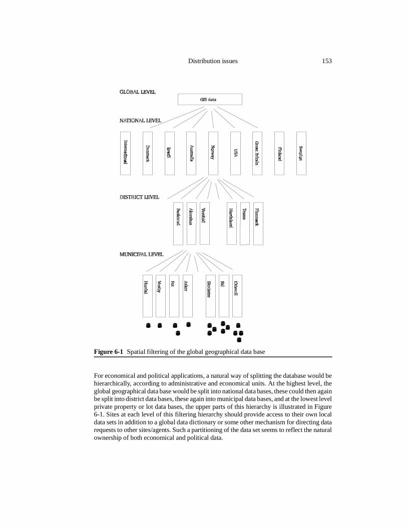
For economical and political applications, a natural way of splitting the database would behierarchically, according to administrative and economical units. At the highest level, theglobal geographical data base would be split into national data bases, these could then againbe split into district data bases, these again into municipal data bases, and at the lowest levelprivate property or lot data bases, the upper parts of this hierarchy is illustrated in Figure6-1. Sites at each level of this filtering hierarchy should provide access to their own localdata sets in addition to a global data dictionary or some other mechanism for directing datarequests to other sites/agents. Such a partitioning of the data set seems to reflect the naturalownership of both economical and political data.

Figure 6-1 Spatial filtering of the global geographical data base


For environmental data, a non-political partitioning scheme could be very useful.Traditional cartographic tiling into map sheets will probably be useful also in the future,but for global tiling of large spatial databases new methods should be considered [Good-child90a]. The Quaternary Triangular Mesh [Dutton89] is presented as a promisingapproach. It is based on hierarchically dividing the globe into triangular tiles, starting withan octahedron with one vertex at each pole, and four vertices on the equator (longitude 0,180, 90 West and 90 East). Each of these triangles is recursively subdivided into four newtriangles by connecting the midpoints of its sides.Tiling based on natural borders is another possibility for environmental data (e.g. water-sheds).

The consequences of spatial filtering can be illustrated by an example: A local authority GISwill be utilising information that is related to geographical locations within the administra-tive unit. Some of the data will have to be extracted from external databases on demand(databases of a specific thematic content, databases on a higher level -, or databases on alower level of the filtering hierarchy), but most of the data will come from its own data sets.Requests on the private information base can be served by accessing the limited localdatabase with acceptable response times. Requests that go beyond the private data will haveto be serviced by retrieving data from remote databases, and will introduce delays from thenetwork and the remote databases before the data becomes available. Non-local data willgenerally be used as read-only information, so if the performance penalties are high forexternal access, copies of frequently accessed external data sets could be stored locally andupdated as needed. By storing external information locally, local access could be sloweddown if it leads to an increased amount of data to consider in a search, while access to the“alien” data sets will be sped up.

Thematic filteringGeographical data can be divided into many classes or themes. Pipelines, railways, tele-phone networks, vegetation and land use are some examples of semi-autonomous spatialdata sets.

Some themes are of general utility. Topographic maps are for instance often used as aread-only frame of reference for other kinds of thematic information, and can therefore beconsidered as the backbone of the geographical information base.

Most thematic data sets will be of little interest to others than the owners of the data or avery limited user group. Assuming this, distributing geographical data for storage on athematic basis is advantageous both because of its filtering effect and because it is practicalwith respect to ownership issues.

Thematic filtering makes many special purpose GISs feasible. A telephone company doesnot have to consider detailed road networks or the vegetation and soil cover for an area toaccomplish most of its tasks, and can therefore limit its local database to the informationon the telephone network and the necessary background (topographic) information. Withthis kind of filtering, the amount of information in the database is dramatically reduced, andit becomes more likely that the data can be accessed in a time-efficient way.

Lower level filters and parallelisationDistribution through the thematic and spatial filters discussed in the previous sections partlycome “for free” as a result of the ownership structure of geographical data. The resulting


local databases can still be very large (e.g. the database of the national mapping authority),demanding distribution between disks (or nodes in a parallel DBMS) using further levelsof filtering to partition the data into manageable units. There are at least two ways ofobtaining further filtering.

One approach is to continue on the earlier threads, and organise the database so that “direct”access to coherent groups of data is possible through the storage structure. This can be doneby organising the data using modified versions of existing associative storage structures(e.g. B-trees, ISAM or k-d trees for thematic filtering and k-d trees, quad-trees, R-trees orgrid-files for spatial filtering). Appendix A contains an overview of data structures forspatial data. Each disk (or node in a parallel DBMS) could for instance store a sub-tree ofthe structure.

Another approach is to use other distribution techniques within a parallel DBMS. Theobjects of the database can be distributed between the available nodes in the paralleldatabase machine according to the (hashed) value of some property/attribute. The hashingattribute could be the identity attribute or a spatial or thematic classification attribute,depending on the application. Hashing is extensively used in parallel relational databasemachines (relational algebra operations are discussed in [Bratbergsengen84] [Brat-bergsengen90]), and could probably also be adopted in other environments. Hashing canbe used in relational databases for all relational algebra operations. In join-operations, thisis done by distributing both of the operand tables among the processors on the basis of thejoin attribute (hash join). The join operation can then be performed autonomously by eachof the active processors. The advantage of this “randomisation” approach is that it is easilyscalable to increasing numbers of processors, while it ensures a decent load balancing, anddoes not require too much synchronisation. A problem with hashing approaches is that theresulting distribution could become very uneven if the hashing method is not able to handlethe distribution of the hashing attribute(s).

6.8.3 Replication

Replication in a distributed database environment can take two different forms. Controlledreplication aims at improving the system performance and the availability of data transpar-ent to the users (maintaining the image of a single database system). The other kind ofreplication could be called autonomous replication, where a local site keeps a snapshot ofa remote database for convenience.

Controlled replication is an important distributed database systems topic [Ceri88] [Bern-stein87] [Bernstein93], but will not be elaborated on any further here.

As discussed in chapter 3, the data used in GISs will often come from many differentsources, and the proprietors of data sets normally want to stay in control of the distributionof the data. So, if outsiders need the information they must buy it from the owners, possiblyunder certain license conditions.

The use of remote data gives rise to an important question: Shall the acquired data be storedon a permanent basis in the local database system or not?

If the data are stored, they can be used to answer future queries where the demands forup-to-date data are relaxed (the data normally goes gradually out-of-date), saving commu-nication bandwidth and the query overhead involved with remote retrieval. A new question


that will have to be answered then is when, and how often, should an updated version of thedata be retrieved from the source database?

The updating of the local copies could be solved either by requesting the remote databaseto send updates when changes have become “considerable”, or by retrieving the completedata set in a systematic fashion (for instance every hour, day, week, month or on demand).This decision will have to depend on to what extent the local applications need up-to-datedata and the expected rate of change of the data. Using this kind of replication, all queriescan be answered by accessing the local database only.

The problem with such an approach is that it is difficult to decide in advance what data willbe interesting to the users, and even if one does find out what will be useful, the databasecould grow so large that it exceeds the capacity of the local database system. The bandwidthbetween the local site and the providers of the data will also tend to be wasted on a lot ofdata that nobody ever will be interested in.

The least complicated solution is, of course, not to use replication at all. This requires allthe databases to be instantaneously accessible at all times. In such an environment data arefetched from their sources when they are asked for (at query time). For such a “no-replica-tion” approach to be efficient in a heterogeneous distributed database system environment,at least the data model and the query language will have to be standardised in some way.The currently dominating query language (“standard” SQL), does not currently haveexpressive power to handle complex data types, such as geometrical data. A standard querylanguage with powerful spatial capabilities would be very useful, because it could use itsknowledge of the data to limit the amount of data transferred in each query.

6.8.4 Heterogeneous database system integration

The goal of heterogeneous database system research is to integrate different databasemanagement systems in such a way that data from one database system can be accessedalso from other, completely different, database systems [Hsiao92].

To be able to achieve such an integration, standards are needed at many levels. The sixlowest layers in the seven level OSI system of ISO provide standards for signal processingand various higher level network protocols, while the seventh layer (the application layer)is meant to cover all application specific standards, in this case database specific standards.Standards for integrating database systems will have to cover dictionaries for distributeddata, data model abstractions with query languages and access protocols to remote data, andpreferably also provide protocols for distributed transaction processing.

For GIS the most interesting aspects of heterogeneous database system integration are datadictionary issues and data model abstractions (with access protocols and query languages).GISs depend upon a model for geometry representation that captures all the aspects of spatialdata that of interest in a GIS context.

Search in remote databases would be significantly more efficient if mechanisms for “joins”were available across database platforms (to allow semi-joins [Ceri88]). This would forinstance allow retrieval of objects in a remote database whose geometry overlaps thegeometry of a given set of local objects. Examples:


• Retrieve all spruce forest stands that lie on government property in Nordland (sendover the geometry of Nordland, do a spatial join with the geometry of the propertydata set, select the governmental properties, send the resulting geometry (of allgovernmental properties in Nordland); do a spatial join with the geometry of sprucestands in the remote vegetation database; send the resulting spruce stands back forfurther processing).

• Find all residential houses with children below the age of 15 that lie more than 4000meters from a school in Ringsaker municipality.

Adapting standard database terminology, these examples could be classified as spatialsemi-joins [Ceri88]. Thematic restrictions as used in traditional relational semi-joins wouldalso be interesting for geographical data (e.g. owner = government in the first example).

Data dictionary issues and query languages for spatial databases have been treated earlierin this chapter.

6.8.5 Fast geometrical processing

Parallel algorithms for geometrical processing of the data selected from the database willprobably be the next step to take in enhancing the processing power of GISs. Not muchresearch has been done in this area, but it should be possible to draw upon the general resultsfrom research in parallel processing [Quinn87].

Parallel geographical data processing should take advantage of both the spatial and thethematic properties of geographical data. The workload should be distributed among theavailable processors in such a way that the amount of work is about the same for allprocessors and at the same time the inter-processor communication is minimised.

A potentially large percentage of the time spent for parallel processing is the initial datadistribution step and the final data collection step. In the distribution step, data are sent tothe participating processors, while in the collection step the results are sent to their finaldestination (processor). One or both of these steps can be avoided if the data are presentlocally at the beginning of the processing and/or can be left locally after the last processingstep has been done. Tailoring of the parallel algorithms to fit the data distribution method-ology will therefore be advantageous.

Parallel applications will often consist of a number of processing steps. It is important toarrange the sequence of steps in such a way that communication is minimised.

At the Edinburgh Parallel Computing Centre and Edinburgh University there has beenresearch activity on the use of parallel technology for GIS [Healey89] [Dowers90]. Analgorithm for polygon overlay has been developed for a parallel computer [Hopkins92][Waugh92].

At the Hypercube Laboratory at NTH in Trondheim, some initial testing has been done onthe parallelisation of spatial database operations. Parallelisation of a spatial join operationwas investigated in a student project [Hagaseth90].


6.8.6 Data exchange formats

Without standard geographical data formats, the use of external geographical databasesbecomes far too complicated to be practical. Standardised formats for geographical datawill have to be agreed upon some time in the not too distant future to facilitate easy exchangeof data between the different suppliers and the customers.

While de facto standards for digital encoding of sound (compact disks) exist and there aremany formats available for image exchange, much work will still have to be done beforestandards for geographical data representation and geographical data exchange will beinternationally agreed upon and available.

A wish-list for GIS-users could consist of the following:

• A standard for the exchange of object geometry (including fields and 3D models ofsurfaces and volumes)

• A standard for the specification of spatial/topological relationships and constraints

• A standard for representing all relevant data quality aspects and temporal aspects ofgeographical data

• A standard way of exchanging object hierarchies and complex objects

• A standard way of exchanging complete geographical objects (all properties -including geometry - in the same framework)

• A nomenclature/thesaurus for the wide variety of geographical objects and themes

• A scheme for inter-database object identification (should preferably be solved byusing the spatial reference of the object in some way)

As discussed in chapter 4, work has been done to provide standards for the exchange ofgeographical data in many parts of the world (e.g. in Germany [ATKIS89], Norway[FGIS90] and the USA [USGS90]), but an international standard has yet to emerge.European countries have started work on a new standard for the European arena. This effortwas initiated by CERCO (European Committee of National Mapping Directors) andorganised through CEN (TC 287), the European sub-organisation of the ISO. This workwas expected to be finished in 1993-1994. Similar work was started by ISO (ISO/TC211)in 1995. The question is if the GIS technology is mature enough to make the specificationof an acceptable standard possible at this point in time. The slow progress of CEN/TC287suggests that this might not have been the case. The GIS standardisation work will probablybe iterative, and the ambitions of standardisation projects should preferably reflect thisassumption.

6.9 Some limitations of currently used database models

A database model (chapter 2) that is to be used for general purpose geographical databasesmust be able to accommodate geographical data according to the requirements outlinedearlier.


In this section, network databases, relational databases and object-oriented databases arebriefly discussed as hosts for geographical databases. Hierarchical models will be left outbecause they are similar to network database models, and provide only a subset of themechanisms offered by these. The problems (and opportunities) of the database models withrespect to geographical data handling are attempted highlighted.

6.9.1 Network database models

In network database models, relationships are explicitly represented, and this makes fastnavigation and transitive closure operations feasible. A set-type in network database modelsrepresents a one-to-many relationship. Network database models are therefore optimisedfor storing one-to-many relationships (strictly hierarchical structures, such as the politicalunit hierarchy with nations consisting counties, and counties consisting of municipalities).For many-to-many relationships, one must introduce extra record types as links, and thesupport for such relationships is therefore not as efficient and a bit more awkward.

A very useful feature of the network database model is the sequence. Sequences aresupported as ordered sets, and could for instance be used for representing geometrical lines(as point sequences) in an efficient way.

Network database management systems are normally optimised for a particular set ofapplications, and a standard interface for ad hoc querying is not available (the standard querylanguage has to be embedded in some host language).

Geometry and topologyNetwork database systems can accommodate topological structures, using explicit links forthe topological relationships. Some examples of the representation of geometrical andtopological records and sets:

Record types:point(x,y{,z}, point-property*) - does also cover nodeslineseg(lineseg-property*)edge(edge-property*) - this is an explicit topology relationshipregion(x,y,region-property*) - x,y gives an interior point for the region

Extra record types used for the topological many-to-many relationships and recursiverelationships:l-p a N:M geometrical relationship connecting lines with their constituting points (it is N:Mbecause the end-points could also be used by multiple lines! Could perhaps also use separatesets for nodes and interior points)e-n a 2:N topology relationship connecting edges with their end-points (nodes/vertices).This record type is redundant, since the end-point also can be found via the line and l-precord typesr-e a 2:N topology relationship connecting regions with their bounding edgesr-h a recursive 1:N topology relationship connecting regions with their holes/islands/em-bedded regions

Set types:line-points (OWNER: line, MEMBER: l-p) - order is significantpoint-lines (OWNER: point, MEMBER: l-p)

Some limitations of currently used database models 159

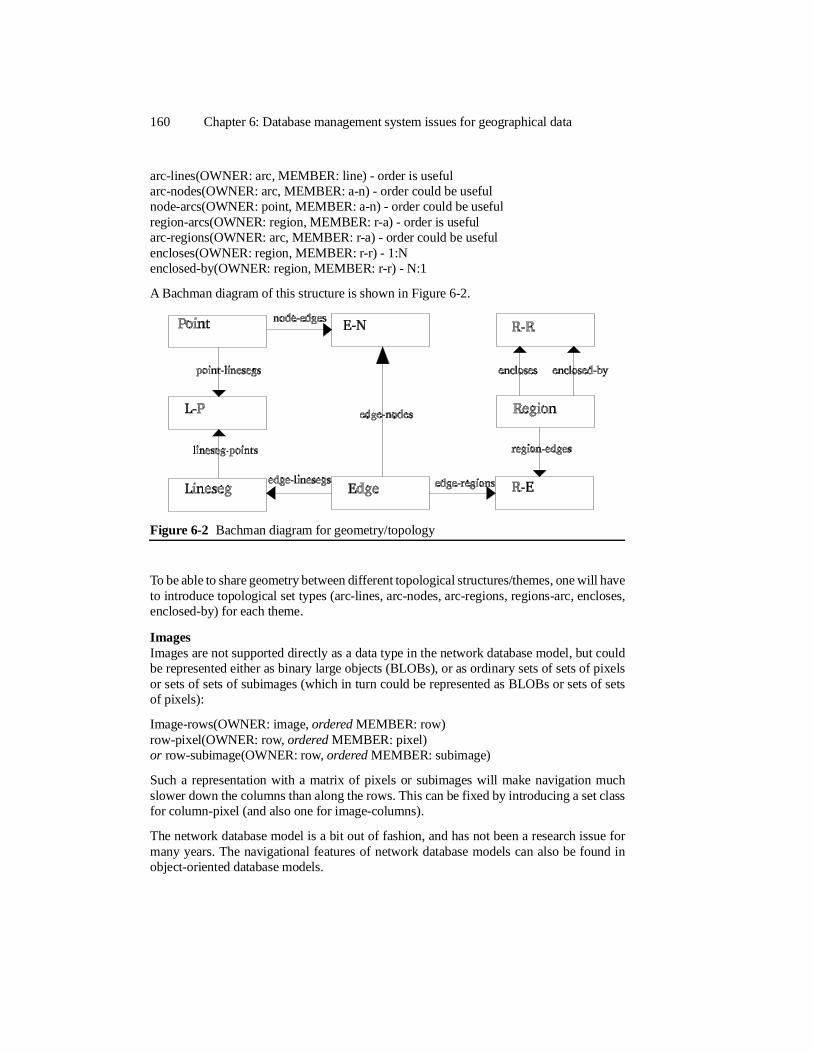
arc-lines(OWNER: arc, MEMBER: line) - order is usefularc-nodes(OWNER: arc, MEMBER: a-n) - order could be usefulnode-arcs(OWNER: point, MEMBER: a-n) - order could be usefulregion-arcs(OWNER: region, MEMBER: r-a) - order is usefularc-regions(OWNER: arc, MEMBER: r-a) - order could be usefulencloses(OWNER: region, MEMBER: r-r) - 1:Nenclosed-by(OWNER: region, MEMBER: r-r) - N:1

A Bachman diagram of this structure is shown in Figure 6-2.

To be able to share geometry between different topological structures/themes, one will haveto introduce topological set types (arc-lines, arc-nodes, arc-regions, regions-arc, encloses,enclosed-by) for each theme.

ImagesImages are not supported directly as a data type in the network database model, but couldbe represented either as binary large objects (BLOBs), or as ordinary sets of sets of pixelsor sets of sets of subimages (which in turn could be represented as BLOBs or sets of setsof pixels):

Image-rows(OWNER: image, ordered MEMBER: row)row-pixel(OWNER: row, ordered MEMBER: pixel)or row-subimage(OWNER: row, ordered MEMBER: subimage)

Such a representation with a matrix of pixels or subimages will make navigation muchslower down the columns than along the rows. This can be fixed by introducing a set classfor column-pixel (and also one for image-columns).

The network database model is a bit out of fashion, and has not been a research issue formany years. The navigational features of network database models can also be found inobject-oriented database models.

Figure 6-2 Bachman diagram for geometry/topology


6.9.2 The relational database model

The relational database model is well equipped to handle catalogue type information. Whatis interesting in the GIS context is the way in which geographical objects can be organised,in particular the geometry and topology.

The relational model has been criticised for spreading the attributes associated with a featurebetween many different relations. This makes operations on single objects complicatedbecause several relational joins are required for reconstructing complete features/objects[Kemper87] [Keating87]. Another consequence of this is that efficient clustering of infor-mation on secondary storage is complicated (Newell et. al. suggests a clustering method,using a spatial “key”, to make relational databases more efficient for geographical data[Newell91a]). Hierarchical data dictionaries based on spatial location and thematic content(as mentioned earlier in this chapter) could also provide some help for clustering data forrelational databases. Healey states that there is presently no alternative to the relationalmodel for GIS databases, but that this might change with the development of object-orientedmodels [Healey91b].

The theory of the relational database model has been developed to a very high level ofsophistication when it comes to query optimization, transaction processing, concurrencycontrol and recovery. One of the reasons for this is that the relational database model hasbeen very popular in the database research community since the 1970ies. Various hashingand indexing schemes have been developed to make set-based retrievals and single tupleretrievals efficient in relational database systems.

Geometry and topologyFor an ordinary (non-extended) relational database, the following geometrical relations arenecessary (provided that the geometry of lines and surfaces can be specified through pointsamples). For points and lines, there could be 2- and 3-dimensional variants (for many pointsand lines the third dimension is not relevant, and for such features it should be possible toskip the third dimension).

Point(Point-Id, X-Coord, Y-Coord[, Z-Coord])

Line(Line-Id, Seq#, X-Coord, Y-Coord[, Z-Coord]) or Line(Line-Id, Seq#, Point-Id)

The Seq# field should (in addition to the Line_Id field) be generated and maintained by thesystem in such a way that there will never be holes in a point sequence representing a line(Seq# 1,2,3,4,5,6 is OK, while Seq# 1,2,5,8,9 should not be allowed). The user will thereforenot have write-access to this field, and the complete line will have to be locked whenupdating a part of a line (updates to existing lines will be very infrequent in a historicalgeographical database system). Such an arrangement will make the handling of incompletelines (that for instance could be a result of a spatial partitioning of the data set) lesscomplicated. The dark side is that more updating is needed when changing the geometry oflines (very seldom occurring, as mentioned earlier).

TopologyIt is straightforward to specify topology within the relational paradigm by introducingrelations that make use of the basic geometrical relationships as presented above.


Some interesting topological relations are those used in network and manifold structures.Conceptually, these structures should be placed in a layer between the geometry objects andthe geographical objects. This can be achieved by not storing geometry in the topology layer,using only references to the underlying geometrical objects. To be able to use a commonborder for two different theme topologies, one will have to have a complete set of topologicalrelations for each topologically structured theme in the database.

Network structures will have to use a node relation, an edge relation and a node-edgerelation. The node relation should include a node identifier (primary key) and a pointidentifier (foreign key). The edge relation should include the edge-id and a set of referencesto line segments constituting the edge. The node-edge relation should include a referenceto the edge and references to one or two end-nodes, and possibly also a direction attribute.2D manifolds will have to provide references between neighbouring polygons through theedges. This can be accomplished by including references to the bounding edges with allmanifold regions. The manifold regions could in addition have a reference to an interiorpoint at the geometrical level. 3D-manifolds could be represented similarly, using surfacesas borders. It could be nice to be able to distinguish between geometrical surface patchesand topological surfaces. Surface could be used for the topological surface, while patchcould be used for the geometrical surface patches. A surface is the combination of geomet-rical surface patches making up the common border of two topological volumes. An interiorpoint attribute could be included also in the volume relation.

An example of “adequately” normalised topological relations follows:

Node(Node-Id, Point-Id) — node-point is a 1:1 relationship within a theme. An alternativerepresentations could be Node(Node_Id, Theme, Point_Id) for integrated topology.Edge(Edge-Id, Seq#, Line-Id) — edge-line is a 1:M relationship, seq.no. makes it a 1:1relationship (a short alternative: Edge(Edge-id, Line-id)). For integrated topology:Edge(Edge-Id, Seq#, Theme, Line-Id)Surface(Surf-Id, Patch-id) — surface-surface_patch is a 1:M relationship within a themeVolumeBoundary(Vol-Id, Surf-Id) — volume-surface is a 2:N relationship within a themeSurfaceBoundary(Surf-Id, Edge-Id) — surface-edge is an N:M relationship within a themeRegionBoundary(Reg-Id, Edge-Id) — region-edge is a 2:N relationship within a theme.For integrated topology: RegionBoundary(Reg-Id, Edge-Id, Theme)EdgeBoundary(Edge-Id, Node-Id) alternatively EdgeBoundary(Edge-Id, StartNode-Id,EndNode-Id) — edge-node is an N:2 relationship. For integrated topology: EdgeBoun-dary(Edge-Id, Node-Id, Theme)

A problem with the relational model with respect to topology is that it does not supporttransitive closure operations. Topological search in the relational model can be performedin a step by step manner by performing joins on the topological relations. In order to providefast search through the topology of spatial data, the number and size of attributes in eachtopological relation should be kept as small as possible (to minimise the data volumesinvolved in the join-operations). An alternative could be to add special purpose transitiveclosure operations to the relational operators*.


* RECURSIVE UNION is proposed in SQL3 to handle hierarchical relationships.

Rasters/ImagesRasters are usually represented using the bulk or blob data type normally present inrelational database systems. This data type treats the raster as a large uninterpreted block ofstorage, and allows no individual treatment of the pixels or subregions of the raster.

A relational representation of a raster should support queries on individual pixels andsub-rasters. If rasters are to be represented in the standard relational model, a somehowwasteful representation would result, as indicated below:

Raster(Raster-Id, row#, col#, pixel_value)

ImageInfo(Raster-Id, #-of-rows, #-of-cols, image_name, …)

The support for image-based operations within a relational database framework has beendiscussed, for instance in “Database system for PSQL” [Roussopoulos88].

Terrain surface model representationThe role of the DBMS in DTM representation is primarily to store the sampled points in anefficient fashion, so that they are available for spatial searching. In addition, it is alsopossible to store the topology of the DTM explicitly, for instance as a TIN model. In therelational database model, the TIN model could be stored simply as a TIN-relation.

TIN(Point-id, Point-id) or the more lengthy: TINPatch(Patch-Id, Point-id, Point-id, Point-id)

A built-in mechanism for spatial searching in the relational database query language wouldbe useful for efficient storage and retrieval of terrain surface data.

QualityCompleteness information and consistency information could be included in the systemtables of relational database systems. Object-/tuple-level quality information could berepresented as a separate quality relation for each relation that should have quality infor-mation attached, using the primary key of the ordinary relation as a foreign key in the qualityrelation. It is not straightforward to include attribute level quality measures in the relationalmodel.

Concurrency controlThe concurrency control and transaction management mechanisms of current relationaldatabase management systems are not flexible enough to handle many long transactions inan efficient way. There has been some research in this area, but the results have not yetpropagated to the industry [Barghouti91].

New trends in relational database technologyRelational databases have in the last couple of years been extended in many directions. Theintroduction of abstract data types into the relational database model will make moreefficient handling of complex objects possible, and will bridge a part of the gap inexpressiveness between the relational database model and object-oriented database models.Relational systems supporting ADTs have been termed extendible relational databasemanagement systems (see also chapter 2). Oosterom has investigated this approach in ageographical context using Postgres [Stonebraker91] [Oosterom91] [Vijlbrief92].


There are many alternative ways of representing the spatial constructs of a geographicaldata model in the extended relational model. A standardised way of handling theseconstructs is essential for straightforward access to external data sets and to allow distributedprocessing of geographical data using the relational database model. Some standard spatialdata types will have to be included to provide a basis for efficient representations of spatialdata. A spatial location/point data type is the most important one, but complex geographicalobjects should also be considered in order to make standardised operations/operators forthese objects possible. The 2- and 3-dimensional geometrical objects: volume, surface,region, line, point and field, must all be supported, preferably as built in data types. Theimportant complex structures: networks, manifolds and rasters could perhaps also besupported.

Standardisation work is in process on extendible relational databases, and in particular onSQL, to determine standard abstract data types for multimedia extensions [ISO/IEC94a].Included in this work is also a part on spatial extensions relevant for GIS: The spatial part(part 3 [ISO/IEC94b]) of the ISO/IEC* standardisation work with SQL/MM (based on thenot yet completed ISO standard proposal SQL3).

6.9.3 Object-oriented database models

Current database technology relies heavily on the relational data model. The relationalmodel is excellent for storing “business” types of data, but has weak support for abstractdata types and the mechanisms of object-oriented modelling, such as inheritance, encapsu-lation and behaviour. Different approaches to object management has been suggested. Oneapproach is to extend the relational database model [Stonebraker90], and another is to startafresh with object-oriented database systems [Atkinson89].

Object-oriented database models are based on, and hence support, the advanced modellingfeatures described in chapter 4 and 5. The realisation of the high level data model in anOODBMS is therefore trivial. The support for concepts such as generalisation/inheritanceand aggregation directly in the database model makes it very flexible and powerful[Mohan88].

To arrive at a standardised object-oriented implementation of geographical databases, theinterfaces of a set of intrinsic geographical classes, for instance based on the icons used inchapter 5, must be specified. When these basic classes are available, an object type in a datamodel diagram can be constructed using inheritance from the intrinsic classes according tothe icons that are attached to the object type in the data model. The task of specifying flexibleinterfaces for intrinsic geographical classes will, however, be complicated. This is partlydue to the wide variety of interpretations that are possible for many geographical phenom-ena.

Many of the structures of geographical data models fit well into the “object”-framework[Egenhofer87]. This is particularly true for human infrastructure (properties, roads, water,electricity, buildings, railways, etc.). On the other hand, many geographical phenomena aredifficult to classify into object structures because they are continuous of nature, with unclearboundaries and many possible interpretations [Goodchild90b] [Aangeenbrug91].


* ISO/IEC JTC1/SC21 Information Retrieval, Transfer and Management for OSI, WG3Database

Object-oriented data models use explicit connections between data objects (object handles).For a GIS, the use of such direct linkages will not be too numerous, due to the limited amountof direct connections a GIS object will have to other GIS objects (most spatial relationshipsare implicit in the spatial location of the objects). The most important linkages in geographi-cal data are the topological linkages. These linkages should be reflected in the database byobject handles and clustering of connected components to increase the speed of topologicaloperations (searching, transitive closure).

The availability of semantic knowledge, inherited from the high-level data model, shouldenable object-oriented database systems to make data management more efficient, forinstance through intelligent buffering and clustering.

A problem with object-oriented databases is the lack of standards. The products that haveemerged so far have been largely experimental and many of the earlier systems include onlyenough mechanisms to make C++ persistent. Concurrency control, query languages andview mechanisms in todays OODBMSs have not been developed to the same level ofsophistication as in the RDBMSs [Kotz-Dittrich95].

Since object-oriented databases are to correspond directly to object-oriented high level datamodels, data types and operators will not be elaborated on.

6.10 Conclusions

The field of database management systems is in a state of rapid change. Until the early1990ies, the typical database system customer was primarily interested in business typedata, that is - numbers, character strings and dates. These kinds of data fits the traditionalrelational model perfectly.

Safe storage of multimedia data is becoming more and more critical for business in manyorganisations. This has resulted in a growing demand among DBMS customers for a richerselection of data types. Spatial data types, supporting geographical data, have been recog-nised as a very important multimedia component, as can be observed in the work on theSQL3/MM standard.

The lack of support for spatial data types in relational DBMSs has always been a greatfrustration for GIS vendors and users. This lack of support has lead to the widespread useof the “geo-relational” approach (only non-spatial attributes (not geometry) is stored in aRDBMS, e.g. Intergraph’s MGE and ESRI’s ArcInfo) and also to the use of BLOBs forstoring geometry in the relational model (System9 and ESRI’s SDE - Spatial DatabaseEngine). Such solutions impose problems, particularly for transaction management/concur-rency control.

Object-oriented DBMSs have always been considered well suited for applications with ademand for a richer and more flexible set of data types than relational DBMSs provide, butthe business community has shown a reluctance to take OODBMSs into use. This isprobably partly due to their legacy systems (hierachical, network or relational DBMSscontaining business data, and with many mission critical applications that work in thisenvironment), and partly due to the immaturity of OODBMS products. To keep theircustomers, the relational DBMS suppliers have had to react. Most RDBMS vendors aretherefore working on multimedia support and some have already prototypes on the market

Conclusions 165

(e.g. Oracle’s multi-dimensional and Informix’s Illustra data blades). Consequently, therehas been a significant support in the RDBMS industry for the SQL3 work.

Geographical data have many important characteristics that will have to be taken intoaccount when designing a supporting DBMS. First of all, a core set of spatial data typeswill have to be fully supported. Support is needed for 0D (point), 1D (line), 2D (region) and3D (volume) geometrical objects in 2D and 3D space with a representation of their interiorthat support (continuous) variation over the interior of the objects. In addition to the spatialdata types, there is a need for (spatio-)temporal support, long spatial transactions andadvanced metadata support. The spatial data types will have to be supported as basic datatypes in order to be able to perform efficient queries. Many GIS environments also havelarge storage space requirements that will have to be addressed, for instance by implement-ing integrated tertiary storage (HSM).

More research is needed on spatial data types, spatial operators, spatial join, spatial queryoptimisation, spatially aware concurrency control (spatial locking) and transaction manage-ment, spatial constraints and spatial data distribution in a networked environment.

The characteristics of spatial data and their particular requirements pose some new prob-lems, but also provide some new opportunities to database researchers, as discussedthroughout this chapter.

The database research community has started to take interest in the management ofgeographical data, and contributions on geographical/spatial data modelling and manage-ment is often requested for database research conferences.


Appendix A

Data structures for spatial databases

This appendix provides a short overview of data structures suitable for the special needs ofspatial information, including geographical data. The first two parts is an introduction tobasic (non-spatial) data structures. In the rest of the chapter some different approaches tothe storage of spatial or multi-dimensional data are presented.

Data sets can vary in structure, content and other characteristics. A very important charac-teristic of a data set, in the context of data structures, is whether it is dynamic or static. Staticdata structures are much easier to build than dynamic data structures, and particularly forhierarchical methods and hashing methods, static data set are much easier to handle. Thefocus here will be on data structures for dynamic data sets.

A.1 Basic data structures

As an introduction, the main categories of data structures for storing simple and morecomplex data items are reviewed. Most of these structures have been developed forone-dimensional data sets, but they provide the basic techniques for developing new datastructures.

In cases where time-complexity of search is discussed, n stands for the number of itemsstored in the structure.

A.1.1 Digital computer storage media

A data structure has to be mapped to a storage medium. An overview of the most commonstorage medias for digital computers will therefore be presented to show the context in whichdata structures operates.

The one-dimensional address space has been the paradigm underlying digital computersever since the von Neuman machine. Our storage media follows this paradigm, and provideaccess to the data accordingly. The media are listed with the slowest at the top (first), andthe fastest at the bottom.

• Magnetic (and optical) tape is a one-dimensional storage medium (a tape consists ofmany tracks, so it is not purely one-dimensional). In order to access a random dataitem the tape has to be read through from the start until the data item is found.

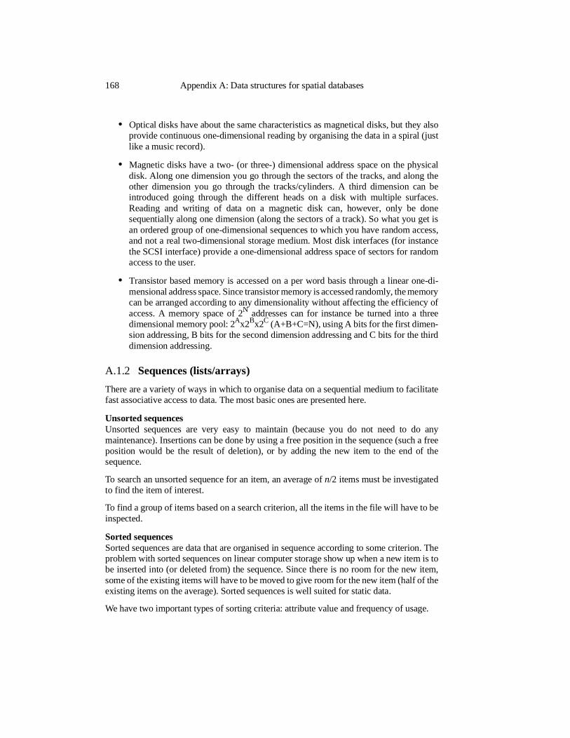
• Optical disks have about the same characteristics as magnetical disks, but they alsoprovide continuous one-dimensional reading by organising the data in a spiral (justlike a music record).

• Magnetic disks have a two- (or three-) dimensional address space on the physicaldisk. Along one dimension you go through the sectors of the tracks, and along theother dimension you go through the tracks/cylinders. A third dimension can beintroduced going through the different heads on a disk with multiple surfaces.Reading and writing of data on a magnetic disk can, however, only be donesequentially along one dimension (along the sectors of a track). So what you get isan ordered group of one-dimensional sequences to which you have random access,and not a real two-dimensional storage medium. Most disk interfaces (for instancethe SCSI interface) provide a one-dimensional address space of sectors for randomaccess to the user.

• Transistor based memory is accessed on a per word basis through a linear one-di-mensional address space. Since transistor memory is accessed randomly, the memorycan be arranged according to any dimensionality without affecting the efficiency ofaccess. A memory space of 2N addresses can for instance be turned into a threedimensional memory pool: 2Ax2Bx2C (A+B+C=N), using A bits for the first dimen-sion addressing, B bits for the second dimension addressing and C bits for the thirddimension addressing.

A.1.2 Sequences (lists/arrays)

There are a variety of ways in which to organise data on a sequential medium to facilitatefast associative access to data. The most basic ones are presented here.

Unsorted sequencesUnsorted sequences are very easy to maintain (because you do not need to do anymaintenance). Insertions can be done by using a free position in the sequence (such a freeposition would be the result of deletion), or by adding the new item to the end of thesequence.

To search an unsorted sequence for an item, an average of n/2 items must be investigatedto find the item of interest.

To find a group of items based on a search criterion, all the items in the file will have to beinspected.

Sorted sequencesSorted sequences are data that are organised in sequence according to some criterion. Theproblem with sorted sequences on linear computer storage show up when a new item is tobe inserted into (or deleted from) the sequence. Since there is no room for the new item,some of the existing items will have to be moved to give room for the new item (half of theexisting items on the average). Sorted sequences is well suited for static data.

We have two important types of sorting criteria: attribute value and frequency of usage.

168 Appendix A: Data structures for spatial databases

• Attribute sorted sequences are sorted according to the value of an attribute or somevalue computed from the attributes of the data item. If the storage device providesdirect access to individual data items, an item can be found after having searchedthrough an average of logn items by using the binary search method (successivelyhalving the search space). An attribute-sorted sequence can be augmented by apermanent index in one or many levels (some sort of tree), also resulting in asearch-complexity of logn. The advantage of this approach over the binary searchmethod is that the index-structure can be clustered (saving disk accesses), and inaddition the highest levels of the structure can be kept in primary memory, savingmany secondary memory accesses (magnetic and optical disks are many orders ofmagnitude slower than transistor based memory).

• Frequency sorted sequences are sorted by the frequency of access. Frequency sortedsequences will show very good average performance for single data item selectionin cases where the probability of access is very varying for the data items in thestructure. The average number of items to search before finding the desired item willbe: SUMfor all items (P(item)*itemseq.no).

A.1.3 Randomised sequences

For randomised sequences, one defines an address space into which a hash function shallmap the data items. This address space is traditionally static, but dynamic address spaceshave also been suggested (e.g. expandable open hashing [Knott71], dynamic hashing[Larson78], extendible hashing [Fagin79] and linear hashing [Litwin80]).

Each address maps into a block of storage (called a bucket) capable of storing a certainnumber of data items. An item is placed in the storage area according to the value obtainedby performing the hash function on a predefined attribute or set of attributes of the data item(often a key).

When a bucket at a certain address is filled up with data items, and a new data item mapsto the same location, bucket overflow occurs. The new data item can not be stored in thecorrect bucket, and will have to be stored elsewhere. There are many solution to the overflowproblem, but no matter what approach is chosen, overflow results in at least one extra blockaccess for storage and retrieval of overflow items.

When designing a randomised data structure, an important aspect is therefore the choice ofstorage utilisation (bucket size / address space), or how much “extra” space one shouldallocate to avoid excessive overflow.

Research has provided a variety of hash functions and overflow strategies. The choice ofhash function will have to be made on the basis of the characteristics of the data set. It isimportant that the hash function spread the data as evenly as possible over the address space,so different hash functions should, if possible, be analysed and tested on the real data beforedeciding which one to use, and with what kind of parameters.

Randomised sequences are particularly good at providing very fast access to single dataitems based on the hash attributes. One or, in the case of overflow, a few accesses is all thatis needed to localise and retrieve an item if its hash attributes are known.

Basic data structures 169

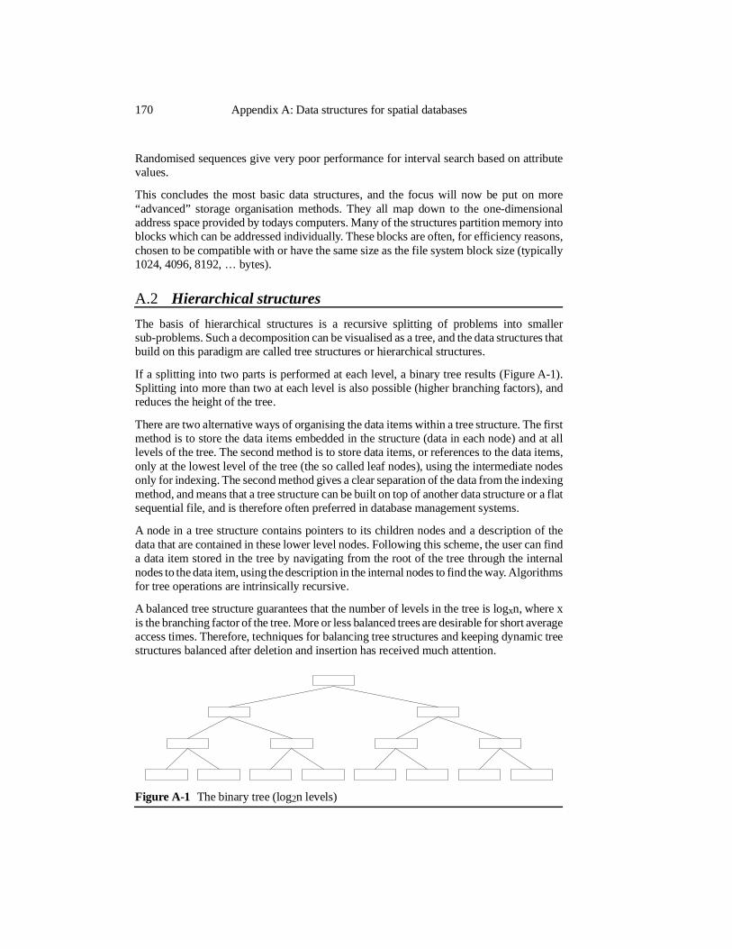
Randomised sequences give very poor performance for interval search based on attributevalues.

This concludes the most basic data structures, and the focus will now be put on more“advanced” storage organisation methods. They all map down to the one-dimensionaladdress space provided by todays computers. Many of the structures partition memory intoblocks which can be addressed individually. These blocks are often, for efficiency reasons,chosen to be compatible with or have the same size as the file system block size (typically1024, 4096, 8192, … bytes).

A.2 Hierarchical structures

The basis of hierarchical structures is a recursive splitting of problems into smallersub-problems. Such a decomposition can be visualised as a tree, and the data structures thatbuild on this paradigm are called tree structures or hierarchical structures.

If a splitting into two parts is performed at each level, a binary tree results (Figure A-1).Splitting into more than two at each level is also possible (higher branching factors), andreduces the height of the tree.

There are two alternative ways of organising the data items within a tree structure. The firstmethod is to store the data items embedded in the structure (data in each node) and at alllevels of the tree. The second method is to store data items, or references to the data items,only at the lowest level of the tree (the so called leaf nodes), using the intermediate nodesonly for indexing. The second method gives a clear separation of the data from the indexingmethod, and means that a tree structure can be built on top of another data structure or a flatsequential file, and is therefore often preferred in database management systems.

A node in a tree structure contains pointers to its children nodes and a description of thedata that are contained in these lower level nodes. Following this scheme, the user can finda data item stored in the tree by navigating from the root of the tree through the internalnodes to the data item, using the description in the internal nodes to find the way. Algorithmsfor tree operations are intrinsically recursive.

A balanced tree structure guarantees that the number of levels in the tree is logxn, where xis the branching factor of the tree. More or less balanced trees are desirable for short averageaccess times. Therefore, techniques for balancing tree structures and keeping dynamic treestructures balanced after deletion and insertion has received much attention.

Figure A-1 The binary tree (log2n levels)


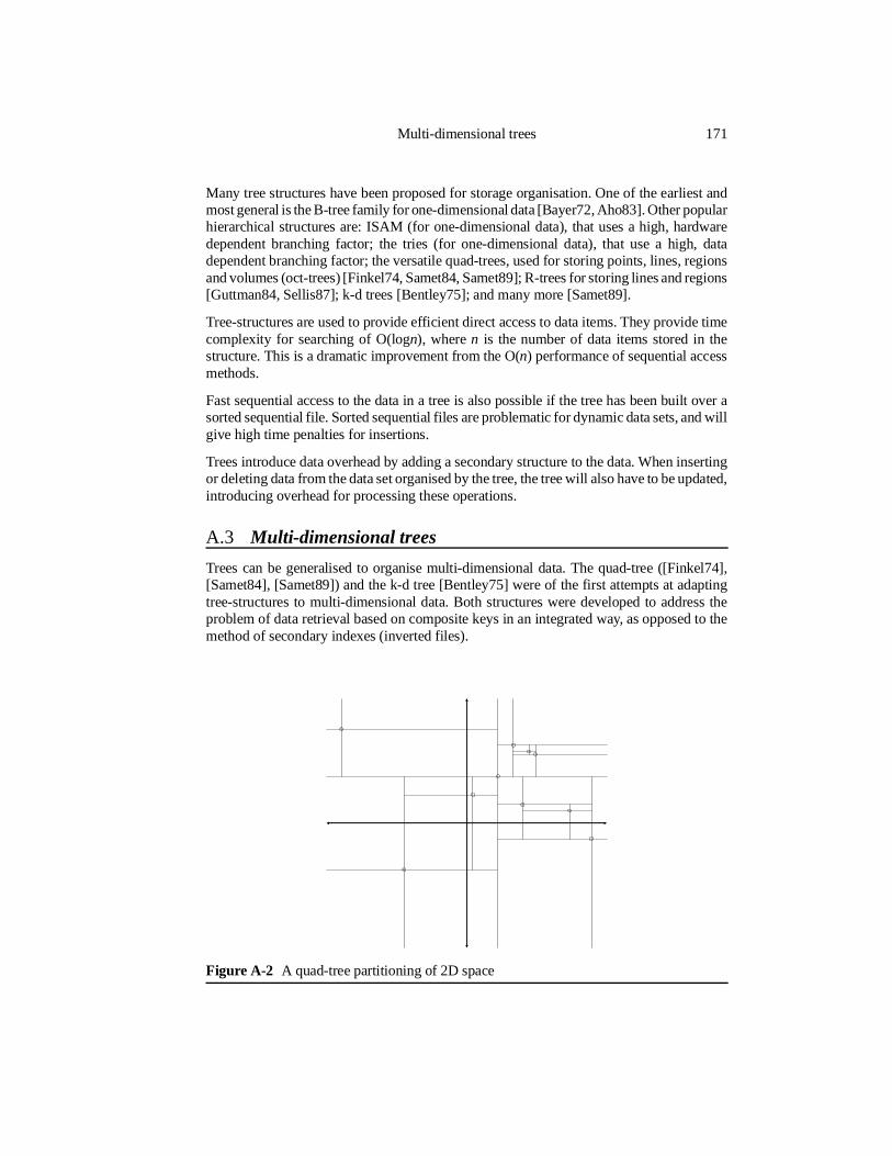
Many tree structures have been proposed for storage organisation. One of the earliest andmost general is the B-tree family for one-dimensional data [Bayer72, Aho83]. Other popularhierarchical structures are: ISAM (for one-dimensional data), that uses a high, hardwaredependent branching factor; the tries (for one-dimensional data), that use a high, datadependent branching factor; the versatile quad-trees, used for storing points, lines, regionsand volumes (oct-trees) [Finkel74, Samet84, Samet89]; R-trees for storing lines and regions[Guttman84, Sellis87]; k-d trees [Bentley75]; and many more [Samet89].

Tree-structures are used to provide efficient direct access to data items. They provide timecomplexity for searching of O(logn), where n is the number of data items stored in thestructure. This is a dramatic improvement from the O(n) performance of sequential accessmethods.

Fast sequential access to the data in a tree is also possible if the tree has been built over asorted sequential file. Sorted sequential files are problematic for dynamic data sets, and willgive high time penalties for insertions.

Trees introduce data overhead by adding a secondary structure to the data. When insertingor deleting data from the data set organised by the tree, the tree will also have to be updated,introducing overhead for processing these operations.

A.3 Multi-dimensional trees

Trees can be generalised to organise multi-dimensional data. The quad-tree ([Finkel74],[Samet84], [Samet89]) and the k-d tree [Bentley75] were of the first attempts at adaptingtree-structures to multi-dimensional data. Both structures were developed to address theproblem of data retrieval based on composite keys in an integrated way, as opposed to themethod of secondary indexes (inverted files).

Figure A-2 A quad-tree partitioning of 2D space

Multi-dimensional trees 171

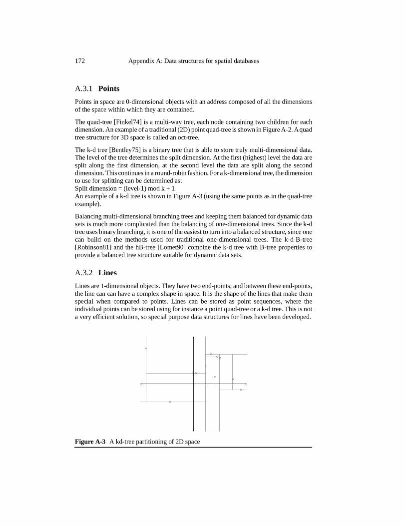
A.3.1 Points

Points in space are 0-dimensional objects with an address composed of all the dimensionsof the space within which they are contained.

The quad-tree [Finkel74] is a multi-way tree, each node containing two children for eachdimension. An example of a traditional (2D) point quad-tree is shown in Figure A-2. A quadtree structure for 3D space is called an oct-tree.

The k-d tree [Bentley75] is a binary tree that is able to store truly multi-dimensional data.The level of the tree determines the split dimension. At the first (highest) level the data aresplit along the first dimension, at the second level the data are split along the seconddimension. This continues in a round-robin fashion. For a k-dimensional tree, the dimensionto use for splitting can be determined as:Split dimension = (level-1) mod k + 1An example of a k-d tree is shown in Figure A-3 (using the same points as in the quad-treeexample).

Balancing multi-dimensional branching trees and keeping them balanced for dynamic datasets is much more complicated than the balancing of one-dimensional trees. Since the k-dtree uses binary branching, it is one of the easiest to turn into a balanced structure, since onecan build on the methods used for traditional one-dimensional trees. The k-d-B-tree[Robinson81] and the hB-tree [Lomet90] combine the k-d tree with B-tree properties toprovide a balanced tree structure suitable for dynamic data sets.

A.3.2 Lines

Lines are 1-dimensional objects. They have two end-points, and between these end-points,the line can can have a complex shape in space. It is the shape of the lines that make themspecial when compared to points. Lines can be stored as point sequences, where theindividual points can be stored using for instance a point quad-tree or a k-d tree. This is nota very efficient solution, so special purpose data structures for lines have been developed.

Figure A-3 A kd-tree partitioning of 2D space


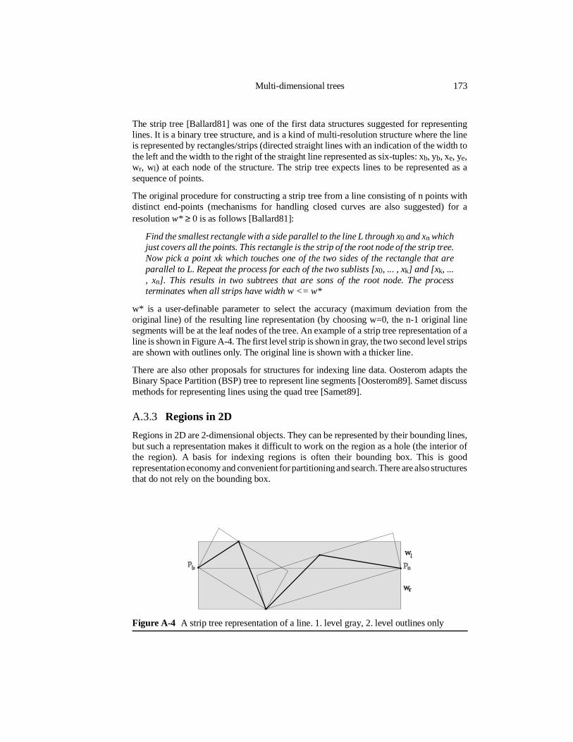
The strip tree [Ballard81] was one of the first data structures suggested for representinglines. It is a binary tree structure, and is a kind of multi-resolution structure where the lineis represented by rectangles/strips (directed straight lines with an indication of the width tothe left and the width to the right of the straight line represented as six-tuples: xb, yb, xe, ye,wr, wl) at each node of the structure. The strip tree expects lines to be represented as asequence of points.

The original procedure for constructing a strip tree from a line consisting of n points withdistinct end-points (mechanisms for handling closed curves are also suggested) for aresolution w* ≥ 0 is as follows [Ballard81]:

Find the smallest rectangle with a side parallel to the line L through x0 and xn whichjust covers all the points. This rectangle is the strip of the root node of the strip tree.Now pick a point xk which touches one of the two sides of the rectangle that areparallel to L. Repeat the process for each of the two sublists [x0, ... , xk] and [xk, ..., xn]. This results in two subtrees that are sons of the root node. The processterminates when all strips have width w <= w*

w* is a user-definable parameter to select the accuracy (maximum deviation from theoriginal line) of the resulting line representation (by choosing w=0, the n-1 original linesegments will be at the leaf nodes of the tree. An example of a strip tree representation of aline is shown in Figure A-4. The first level strip is shown in gray, the two second level stripsare shown with outlines only. The original line is shown with a thicker line.

There are also other proposals for structures for indexing line data. Oosterom adapts theBinary Space Partition (BSP) tree to represent line segments [Oosterom89]. Samet discussmethods for representing lines using the quad tree [Samet89].

A.3.3 Regions in 2D

Regions in 2D are 2-dimensional objects. They can be represented by their bounding lines,but such a representation makes it difficult to work on the region as a hole (the interior ofthe region). A basis for indexing regions is often their bounding box. This is goodrepresentation economy and convenient for partitioning and search. There are also structuresthat do not rely on the bounding box.

Figure A-4 A strip tree representation of a line. 1. level gray, 2. level outlines only

Multi-dimensional trees 173

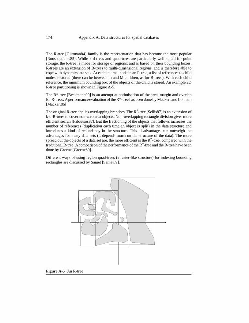
The R-tree [Guttman84] family is the representation that has become the most popular[Roussopoulos85]. While k-d trees and quad-trees are particularly well suited for pointstorage, the R-tree is made for storage of regions, and is based on their bounding boxes.R-trees are an extension of B-trees to multi-dimensional regions, and is therefore able tocope with dynamic data sets. At each internal node in an R-tree, a list of references to childnodes is stored (there can be between m and M children, as for B-trees). With each childreference, the minimum bounding box of the objects of the child is stored. An example 2DR-tree partitioning is shown in Figure A-5.

The R*-tree [Beckmann90] is an attempt at optimisation of the area, margin and overlapfor R-trees. A performance evaluation of the R*-tree has been done by Mackert and Lohman[Mackert86]

The original R-tree applies overlapping branches. The R+-tree [Sellis87] is an extension ofk-d-B-trees to cover non-zero area objects. Non-overlapping rectangle division gives moreefficient search [Faloutsos87]. But the fractioning of the objects that follows increases thenumber of references (duplication each time an object is split) in the data structure andintroduces a kind of redundancy in the structure. This disadvantages can outweigh theadvantages for many data sets (it depends much on the structure of the data). The morespread out the objects of a data set are, the more efficient is the R+-tree, compared with thetraditional R-tree. A comparison of the performance of the R+-tree and the R-tree have beendone by Greene [Greene89].

Different ways of using region quad-trees (a raster-like structure) for indexing boundingrectangles are discussed by Samet [Samet89].

Figure A-5 An R-tree


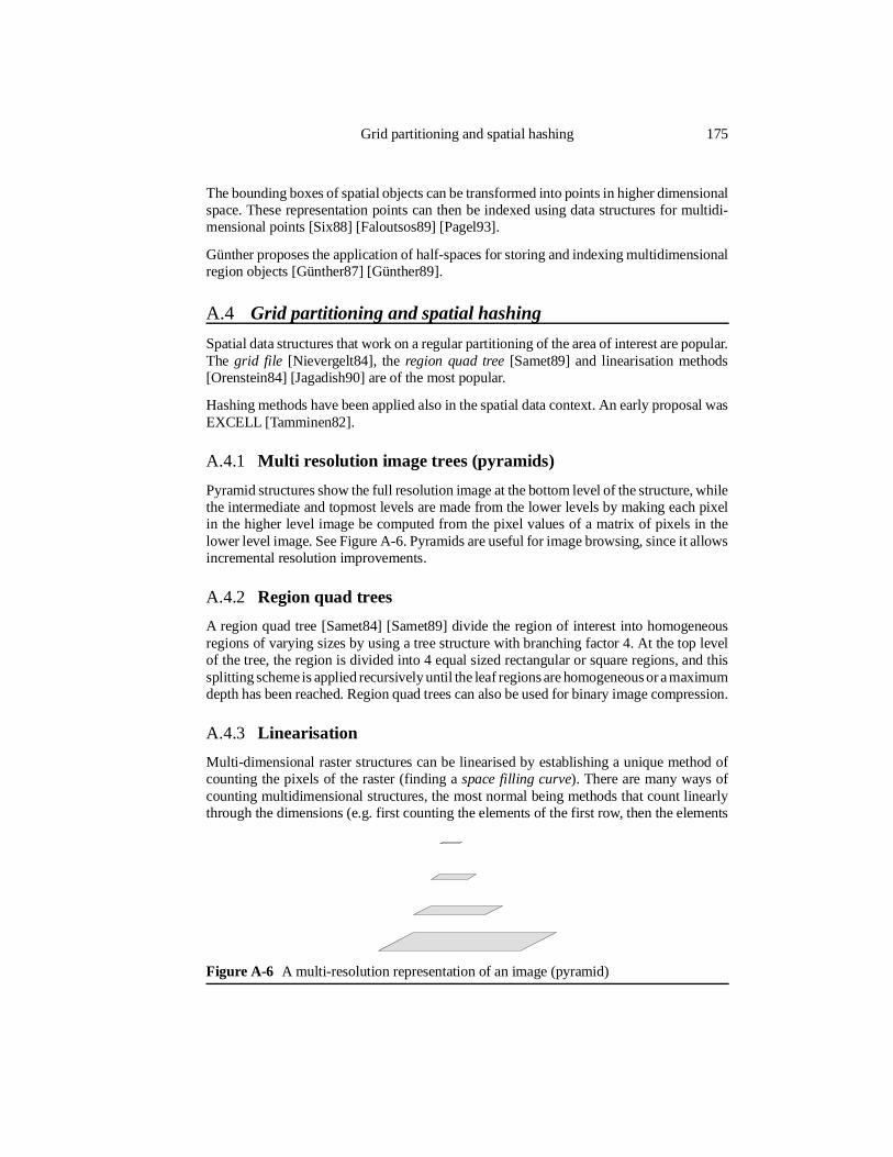
The bounding boxes of spatial objects can be transformed into points in higher dimensionalspace. These representation points can then be indexed using data structures for multidi-mensional points [Six88] [Faloutsos89] [Pagel93].

Günther proposes the application of half-spaces for storing and indexing multidimensionalregion objects [Günther87] [Günther89].

A.4 Grid partitioning and spatial hashing

Spatial data structures that work on a regular partitioning of the area of interest are popular.The grid file [Nievergelt84], the region quad tree [Samet89] and linearisation methods[Orenstein84] [Jagadish90] are of the most popular.

Hashing methods have been applied also in the spatial data context. An early proposal wasEXCELL [Tamminen82].

A.4.1 Multi resolution image trees (pyramids)

Pyramid structures show the full resolution image at the bottom level of the structure, whilethe intermediate and topmost levels are made from the lower levels by making each pixelin the higher level image be computed from the pixel values of a matrix of pixels in thelower level image. See Figure A-6. Pyramids are useful for image browsing, since it allowsincremental resolution improvements.

A.4.2 Region quad trees

A region quad tree [Samet84] [Samet89] divide the region of interest into homogeneousregions of varying sizes by using a tree structure with branching factor 4. At the top levelof the tree, the region is divided into 4 equal sized rectangular or square regions, and thissplitting scheme is applied recursively until the leaf regions are homogeneous or a maximumdepth has been reached. Region quad trees can also be used for binary image compression.

A.4.3 Linearisation

Multi-dimensional raster structures can be linearised by establishing a unique method ofcounting the pixels of the raster (finding a space filling curve). There are many ways ofcounting multidimensional structures, the most normal being methods that count linearlythrough the dimensions (e.g. first counting the elements of the first row, then the elements

Figure A-6 A multi-resolution representation of an image (pyramid)

Grid partitioning and spatial hashing 175

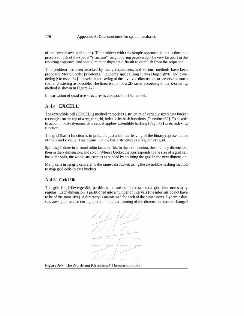
of the second row, and so on). The problem with this simple approach is that it does notpreserve much of the spatial “structure” (neighbouring pixels might be very far apart in theresulting sequence, and spatial relationships are difficult to establish from the sequence).

This problem has been attacked by many researchers, and various methods have beenproposed. Morton order [Morton66], Hilbert’s space filling curves [Jagadish90] and Z-or-dering [Orenstein84] all use bit interleaving of the involved dimensions to preserve as muchspatial clustering as possible. The linearisation of a 2D raster according to the Z-orderingmethod is shown in Figure A-7.

Linearisation of quad tree structures is also possible [Samet89].

A.4.4 EXCELL

The extendible cell (EXCELL) method comprises a structure of variably sized data bucketrectangles on the top of a regular grid, indexed by hash functions [Tamminen82]. To be ableto accommodate dynamic data sets, it applies extendible hashing [Fagin79] as its indexingfunction.

The grid (hash) function is in principle just a bit interleaving of the binary representationof the x and y value. This means that the basic structure is a regular 2D grid.

Splitting is done in a round robin fashion, first in the x dimension, then in the y dimension,then in the x dimension, and so on. When a bucket that corresponds to the size of a grid cellhas to be split, the whole structure is expanded by splitting the grid in the next dimension.

Many cells in the grid can refer to the same data bucket, using the extendible hashing methodto map grid cells to data buckets.

A.4.5 Grid file

The grid file [Nievergelt84] partitions the area of interest into a grid (not necessarilyregular). Each dimension is partitioned into a number of intervals (the intervals do not haveto be of the same size). A directory is maintained for each of the dimensions. Dynamic datasets are supported, so during operation, the partitioning of the dimensions can be changed

Figure A-7 The Z-ordering [Orenstein84] linearisation path


by adding a new interval (expansion) or merging two intervals (contraction). Thesesplittings and mergings can only be applied for one dimension at a time. Merging of intervalsis not expected to be required very often.

Each grid cell is a grid bucket in the grid file system. The central structure in the grid fileis the grid directory. It is responsible for mapping grid cells to the real data buckets. Theassignment of grid cells to data buckets is governed by a rule that states that a data bucketcan only correspond to convex (box shaped) grid regions. The grid directory consists of thek-dimensional grid array of bucket pointers, and one 1-D array for each of the k dimensions(linear scales to take care of the partitioning information).

To manage the data bucket to grid region mapping system, a twin tree can be maintained.Each time a bucket is split, the twin tree is updated, with two children (twins, normallycalled buddies in 1D) under the bucket’s node. Merging will have to proceed from the leavesand up in the twin tree. Different splitting and merging policies are possible.

Grid partitioning and spatial hashing 177


Appendix B

Representation of 3D structures

This appendix is a very short review of traditional methods for organising 3-dimensional(3D) structures [Mortenson85] [Encarnação83], such as volumes, surfaces, lines and pointsusing computer storage devices. It is included as a background for the discussion on spatialdata models and data structures. This section contains an overview of 3D objects and 3Dmodelling, followed by a presentation of some different ways of representing 3D structures.

B.1 3D objects

Four different object types are possible in 3D space. These objects are the point, the line,the surface and the volume. The storage characteristics of these object types are thefollowing:

• Points, or 0-dimensional spatial objects, are trivial to represent using 3D coordinates(e.g. Euclidean (x,y,z) or polar coordinates). Compression techniques can be used tocode sets of points in a more efficient way (differential representations). In additionto the geometry, an indication of the accuracy of measure is necessary to represent ameasured 3D point.

• Lines, or 1-dimensional spatial objects, introduce more complexity. Theoretically aline is made up of an indefinite sequence of points. The representation in computerstorage will have to be a simplification of this indefinite sequence. Two differentmethods have been used for this simplification. The first is the approximation of thewhole line by a parametric function. The second is sampling from the indefinite pointsequence, and then representation of the line segments between these sample pointsby using some kind of function (for instance straight lines or higher order splines).Both regular (fixed intervals) and adaptive/optimal (avoiding sampling of for in-stance straight lines) sampling is possible. The methods will be constrained byuser-defined limits on the maximum deviation allowed from the original line.Generally, the more accurate the representation is required to be, the more storage isneeded for the representation (higher sampling frequency or more complex func-tions). The accuracy of the resulting line is determined by the accuracy of theconstituent points, the sampling frequency and the fidelity of the interpolationmethod.

• Surfaces can be represented in much the same way as lines. Sampling and approxi-mations by functions are the two main methods for representation. Sampling can bedone in a regular pattern (grid) or adaptive (considering the variability or auto-cor-relation of the surface). Functional approximations can be done globally (on theobject as a whole) or on subregions or patches (regular or adaptive). The accuracy ofa surface is determined, as for lines, by the accuracy of the sampling points, thesampling frequency and the fidelity of the interpolation method. It is important forall representations to maintain the topology of the sampled points, particularly forcomplex surfaces. Fractal geometry has also been investigated in the context ofterrain surface modelling [Xia91].

• Volumes, or 3-dimensional spatial objects, can be completely represented by theirbounding surfaces and holes, plus an indication of what constitutes the inside of thevolume. An alternative way of representing volumes is to use simple volumes as basicelements, and transform and combine these to make up the complete volume object.This kind of representation is generally more useful for CAD type objects thangeographical objects, because of the much more regular nature of CAD objects. Theaccuracy of a volume representation is completely determined by the accuracy of itsbounding surfaces or its basic elements and transformations.

B.2 Storage organisation

Efficient analysis and presentation of 3D structures is difficult, and the computer storagerepresentation determines to what extent such operations are feasible at all in an interactiveenvironment.

There is a choice between two paradigms for organising 3D structures using main memoryand background storage.

The homogeneous solution uses the same representation on the background storage device(disk) as in main memory. This solution allows paging and therefore does not constrain thesize of the data structure to the limits of main memory.

The split solution uses two different storage structures for main memory and for secondarystorage. Conversion is then necessary when moving data between secondary storage andmain memory, and this complicates paging. Such a solution will introduce the problems oflimited main memory in addition to more complicated updating of the structure. Theadvantage of this solution is that it is possible to use a more general and flexible structureon secondary storage, allowing easier integration with other applications.

The choice of paradigm will depend on the application context.

B.3 Point sampling

Using points to represent 3D structures is the sampling approach. To represent a line or asurface in space, a set of sample points that lie on the structure will have to be selected.Using these topologically structured sample points, a model of the complete originalstructure can be constructed using interpolation techniques.

180 Appendix B: Representation of 3D structures

There are many kinds of interpolation techniques. The simplest is the linear approach, usingstraight line segments for the interpolation of curves, and flat triangles for interpolating onsurfaces. If we have no knowledge of the auto-correlation of a structure, the linear approachcould be as good as any other interpolation method. If we know that the auto-correlation islarge compared to the sampling frequency, more sophisticated methods for interpolationshould be investigated. B-splines, Bezier curves and other kinds of parametric functionswill then be candidates. Krieging with trend surface and probability estimates is a particu-larly good candidate when the auto-correlation is fairly well known, and accuracy estimatesare required.

Using 3D sampling, the points in the sample set will all lie on the measured structure. Thismeans that an interpolation method that includes the sample points on the surface of themodelled structure is preferable (exact interpolation at the sampling points).

Most geographical sampling is performed at the surface of the earth. In this case, there isnearly always a functional mapping from a position (lat,long) to a sample point, andneighbouring samples can be found on the basis of their latitude and longitude. For general3D surfaces this is not so. Even for simple convex volumes, there will be two sample pointsfor each position in all 2D projection of the volume (except for points on the border of theprojection). There will be one point for each side of the volume (e.g. top and bottom). Forgeneral 3D structures, the samples must therefore be structured in such a way that thetopology is maintained.

Point sampling is the underlying approach for many of the other representation methods.

B.4 Wire frame

The wire frame model is an old method for presenting volumes and rod structures in CADapplications. The method uses “wires” at all edges and lines in a construction (for instancerods). This results in the familiar skeleton appearance of the wire-frame model. A wire framemodel can also be regarded as a kind of unshaded perspective drawing.

Wire frames have been used for visualisation of terrain surfaces, both on computer screensand as drawings. The method is as follows. First, a regular grid sampling of the elevationis done over the terrain area, giving a grid of elevation values. Secondly, a point of viewand a viewing direction is determined for the perspective drawing (the point is often chosenabove and some distance away from the area of interest). Finally, the wire frame model ismade using this perspective, by drawing wires in the x and y direction through the gridelevation points, (linearly) interpolating the elevation between the grid points. The result isa web or a mesh covering the landscape, giving a 3-D appearance.

The wire-frame model is similar to a point sample model with linear interpolation betweenthe samples. It is a nice presentation model, but is lacking expressiveness as a storage modelfor curved and complex surfaces.

Wire frame 181

B.5 Triangulated Irregular Network

The Triangular Irregular Network (TINs) is a method for geographical surface repre-sentation and modelling based on irregular point samples [Peucker78]. The surface pointsare stored together with a triangulation. This method is much used in geographicalinformation systems, for instance in ARC/INFO.

The basic data structure in a TIN model is the node with an attached list of ordered neighbournodes. The neighbour nodes can be ordered by starting north of the node and proceedingclockwise. The world outside the modelled area is represented by a dummy node. It ispossible to extend the basic model in various ways, for instance by introducing explicitreferences to the triangles (convenient for attaching attributes to the triangles). Another oftenused extension is the representation of surface specific points (peaks and pits) and lines(ridges and channels).

The advantage of the TIN is that neighbour information is stored explicitly and compactlyin the data structure, resulting in efficient methods for local search.

The planar Voronoi diagram and the dual of the TIN, the Delaunay triangulation are wellknown methods for establishing TINs from irregularly spaced points [Aurenhammer91].

B.6 Parametric representations

Parametric representations have been widely used for geometrical modelling of curved linesand surfaces [Mortenson85]. These methods are point-based. A set of points (topologicallyordered) comprise the backbone of such structures, and a set of parametric functionsdescribe the lines/surfaces using the points. For representing a line, a sequence of knot pointsmust be found, while for a surface, a grid of points has to be determined. There are manydifferent kinds of parametric representations, some are used to describe complete curvesand surfaces in a single function (global methods), while other divide the structures intopieces and determine these separately (piecewise or local methods). Global methods usehigh order polynomials in the defining functions, and therefore give high order continuity,but are complicated to handle (modifications have global implications) and compute. Localmethods use only lower order polygons resulting in lower order continuity, but theindividual pieces of the structure are easy to compute and handle (modifications have onlylocal implications).

Many kinds of parametric function have been proposed and used for reducing the numberof points necessary to represent a geometrical structure at a certain level of accuracy. Forrepresenting a curved line, one has to determine (sample) points (or knot points) for the line,and for each line-segment or point, a set of parameters that faithfully describe the line-seg-ment must be provided for the function.

Spline curvesA spline curve or a minimum energy curve / elastic curve is a curve that passes through orinterpolates all its control points. A sequence of PC (parametric cubic) curves can be usedas an exact geometrical model of a traditional spline. The derivation of the set of PC curvesrequires that a set of simultaneous equations be solved (using local coordinate systems for


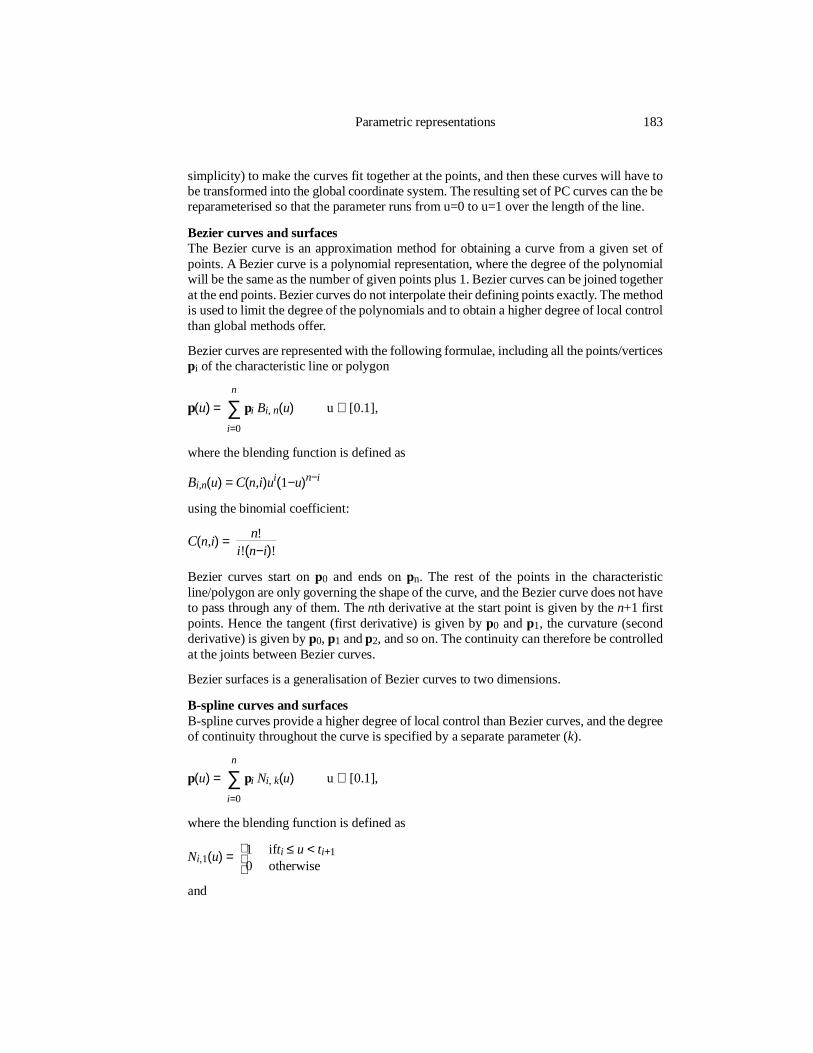
simplicity) to make the curves fit together at the points, and then these curves will have tobe transformed into the global coordinate system. The resulting set of PC curves can the bereparameterised so that the parameter runs from u=0 to u=1 over the length of the line.

Bezier curves and surfacesThe Bezier curve is an approximation method for obtaining a curve from a given set ofpoints. A Bezier curve is a polynomial representation, where the degree of the polynomialwill be the same as the number of given points plus 1. Bezier curves can be joined togetherat the end points. Bezier curves do not interpolate their defining points exactly. The methodis used to limit the degree of the polynomials and to obtain a higher degree of local controlthan global methods offer.

Bezier curves are represented with the following formulae, including all the points/verticespi of the characteristic line or polygon

p(u) = ∑

i=0

n

pi Bi, n(u) u ∈ [0.1],

where the blending function is defined as

Bi,n(u) = C(n,i)ui(1−u)n−i

using the binomial coefficient:

C(n,i) = n!

i!(n−i)!

Bezier curves start on p0 and ends on pn. The rest of the points in the characteristicline/polygon are only governing the shape of the curve, and the Bezier curve does not haveto pass through any of them. The nth derivative at the start point is given by the n+1 firstpoints. Hence the tangent (first derivative) is given by p0 and p1, the curvature (secondderivative) is given by p0, p1 and p2, and so on. The continuity can therefore be controlledat the joints between Bezier curves.

Bezier surfaces is a generalisation of Bezier curves to two dimensions.

B-spline curves and surfacesB-spline curves provide a higher degree of local control than Bezier curves, and the degreeof continuity throughout the curve is specified by a separate parameter (k).

p(u) = ∑

i=0

n

pi Ni, k(u) u ∈ [0.1],

where the blending function is defined as

Ni,1(u) =

1 ifti ≤ u < ti+1

0 otherwise

and

Parametric representations 183

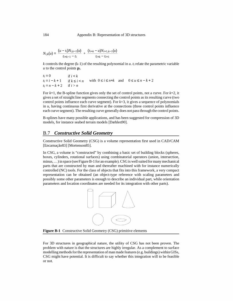
Ni,k(u) = (u − ti)Ni,k−1(u)

ti+k−1 − ti +

(ti+k − u)Ni+1,k−1(u)ti+k − ti+1

k controls the degree (k-1) of the resulting polynomial in u. ti relate the parametric variableu to the control points pi.

ti = 0ti = i − k + 1ti = n − k + 2

if i < kif k ≤ i < nif i > n

with 0 ≤ i ≤ n+k and 0 ≤ u ≤ n − k + 2

For k=1, the B-spline function gives only the set of control points, not a curve. For k=2, itgives a set of straight line segments connecting the control points as its resulting curve (twocontrol points influence each curve segment). For k=3, it gives a sequence of polynomialsin u, having continuous first derivative at the connections (three control points influenceeach curve segment). The resulting curve generally does not pass through the control points.

B-splines have many possible applications, and has been suggested for compression of 3Dmodels, for instance seabed terrain models [Dæhlen90].

B.7 Constructive Solid Geometry

Constructive Solid Geometry (CSG) is a volume representation first used in CAD/CAM[Encarnação83] [Mortenson85].

In CSG, a volume is “constructed” by combining a basic set of building blocks (spheres,boxes, cylinders, rotational surfaces) using combinatorial operators (union, intersection,minus, …) in space (see Figure B-1 for an example). CSG is well suited for many mechanicalparts that are constructed by man and thereafter machined with for instance numericallycontrolled (NC) tools. For the class of objects that fits into this framework, a very compactrepresentation can be obtained (an object-type reference with scaling parameters andpossibly some other parameters is enough to describe an individual part, while orientationparameters and location coordinates are needed for its integration with other parts).

For 3D structures in geographical nature, the utility of CSG has not been proven. Theproblem with nature is that the structures are highly irregular. As a complement to surfacemodelling methods for the representation of man made features (e.g. buildings) within GISs,CSG might have potential. It is difficult to say whether this integration will to be feasibleor not.

Figure B-1 Constructive Solid Geometry (CSG) primitive elements


Appendix C

The NHS Electronic Navigational Chart Database

A couple of years ago, the Norwegian Hydrographic Service (NHS) initiated the specifica-tion of an Electronic Navigational Chart Database (ENCDB), that is - a database that willact as a server for electronic navigational charts all over the world. I investigated thedatabase issues for this kind of server as a case study.

C.1 Introduction

Electronic Navigational Charts (ENCs) are supposed to become an integrated part of bridgeinformation systems for seagoing vessels. The integration of these charts with the globalpositioning system (GPS), active sensors (for instance radar) and other information sources(various databases) will provide better means for safe sea-navigation (through for instancecollision avoidance). The advent of ENCs will also, hopefully, provide better and moreflexible user interfaces to the information that today is carried by paper charts and otherpaper-based information sources (e.g. list of lights). Ways of storing and distributing ENCsand their updates will become important issues in such a setting. After presenting a littlebackground material on ENCs, I will concentrate on the database and data modelling aspectsof a server-database that is to deliver updated ENC information to Electronic Chart Displayand Information Systems (ECDIS) on board the ships.

C.2 Background

The use of electronic navigational charts, and the distribution of chart updates via theINMARSAT C system was first tested in practice in the North Sea Project [NORTH SEA89].The results were encouraging, and accelerated the work on ECDISs. The InternationalHydrographic Organisation (IHO) has set down committees on the standardisation offormats for the exchange of ENCs and their updates. The NHS has been participating in thiswork, and was hoping to be the host of a model ENCDB.The involved people at the NHS have provided me with useful information on these subjects.

C.3 Navigational Charts

A navigational chart is a legal document. To simplify a bit, a ship must, as a rule, carryupdated navigational charts for its insurances to be valid. The oceans of the world arecovered by overlapping sheets of navigational charts of varying scales. It has been estimated

that a ship sailing globally will have to carry about 2000 paper charts. The nationalhydrographic offices have the responsibility for keeping these charts updated, and chartscan be purchased from the responsible hydrographic offices. The charts have a date ofvalidity, and to enable the seagoing vessels to keep their charts updated at all times, thehydrographic offices publish periodic updates to their navigational charts (countries with alarge amount of charts publish updates with only a few days interval, while countries witha smaller amount of charts or resources publish their updates once a month). It is theresponsibility of the crew to manually update the charts accordingly. This updating is verytime-consuming, and hence expensive for a vessel that utilises many charts.

C.3.1 ENC and ECDIS

The IHO has proposed that “ECDIS should be the equivalent to the paper chart” (point 1.3in [IHOSP5288]). All the information from the paper chart should be available, and thesame legal restrictions apply. A cell-structure is suggested [NORTH SEA89] where thecoarsest cells cover an area of 8°x8° (A-cells, for free ocean navigation, scales < 1:250000),and the finest cells cover 15’x15’ (I-cells, for harbour navigation, scale ranges 1:12500 -1:40000). In between there are the 4°x4° B-cells, the 1°x1° C-cells, the 30’x30’ D-cells. Afurther refinement (four sub-cells) of the D- and I-cells into EFGH-cells and JKLM-cellsshould be provided for areas with high data density. Cells are identified by the “scale”-letter,and two numbers. First a 3 digit number: the number of 15’ increments from the south polenorthward, then a 4 digit number: the number of 15’ increments eastward from Greenwich.A cell identification will look like this:I5750016 (I-cell 53°45’N, 4°00’E)

C.3.2 The ENCDB

The IHO working group on ECDIS has proposed guidelines for the logical structure of theENCDB. This database is “The master data base for production and maintenance of theENC, compiled from the national ENCD” [Grant90]. The main purpose of the database isto make ECDIS data (ENCs) available to the customers. Data from the national hydro-graphic offices are to be translated and incorporated into the ENCDB by the ENCDBs host.

It has been suggested ([IHOSP5288], point 7.1) that the information in an ENCDB shouldbe divided into an approved part (resembling the old paper chart), a modifications part(resembling the 14 day update publications to the paper chart) and an administrative part.The administrative part will consist of useful information not normally found on traditionalpaper charts. The administrative part of the database could expand into various new areas,and should be logically connected to the rest of the data as an ordinary information database.

Updates to the on-ship databases could be - and is planned to be - broadcast by worldcovering satellite systems, as tested in the North Sea Project. The INMARSAT system hasso far been tested, and is considered useful for the purpose. In the nearest future, the datawill be distributed on diskettes. The reason for this is that equipment for - and usage ofsatellite systems is too expensive at the moment. No matter whether or not broadcasting ischosen as a distribution strategy for updates in the long term, the format of the exchangewill have to be internationally (IHO) agreed upon. For satellite broadcasting it will beimportant that the format is compact [Sandvik90].

186 Appendix C: The NHS Electronic Navigational Chart Database

The problems of securing successful delivery of the updates to all recipients (thousands ofships) by broadcasting in a noisy environment is in itself a topic. The broadcasting strategyis by far the easiest from the point of view of an ENC server (if messages get through to allsubscribers). More secure, non-broadcasting strategies would put high demands on thetransaction capacity of the ENCDB.

The host of an ENCDB must provide data conforming to the IHO exchange standards forECDIS. The IHO CEDD (committee on the exchange of digital data) is specifying such aformat, known as DX90.

The status of nautical maps as legal documents implies that the security and integrity of thedata must be given high priorities when storing and distributing them in digital form. Thequality control through the production and before the chart can be integrated into thedatabase will also have to be very strict.

C.3.3 Data management

The NHS wants the ECDIS-server to utilise a database management system (DBMS) forthe ENCDB. The advantages of using a DBMS for the ENCDB are the traditional, that is -a standard query language interface, integrity constraints, data dictionary, concurrencycontrol, recovery and various kinds of DBMS utilities.

It could be argued that a DBMS is over-kill for this (basically) file-server application, andwill only impose unnecessary overhead and slow the system down. The chart data are verymodular (cells) and structured (approved data and modification data) and each cell couldconstitute a single file conforming to the CEDD exchange standards of the IHO (presentlyDX90). A file system would therefore cover the needs of a simple chart-server system (asystem for distributing the electronic chart as a pure substitute for the paper chart), but fora complete ECDIS server other issues may arise.

• The ENCs are supposed to be integrated with other kinds of information (the so-calledadministrative part) in ECDIS. If this shall be possible, one needs to have a way ofintegrating the chart data with the rest of the information base. The contents of theadministrative part of ECDIS is expected to evolve over time, and a DBMS providesmechanisms for the integration of new data types into the system with only limitedor no effects on existing applications. In addition, the inclusion of the administrativepart of ECDIS will lead to increased updating activity on the ENCDB. Hence, moresophisticated transaction management is required, as provided by a DBMS.

• For an interactive system, it is important to be able to obtain more information on afeature (e.g. lights, beacons or places) on the screen by pointing to it (for instancetouching the screen). In the file system approach, examining all object in the completeENC, with updates and all is one possible strategy, but this can be time-consumingfor large data sets. Another alternative is to use advanced data structures to organisethe data in order to limit the search space, and hence bring response times down.Many kinds of search structures are supported (in some way) by a DBMS.

• The chart data to be stored in the ENCDB consist of geometric features such as points,lines and regions. It is important for the applications that these geometric features arestored in a consistent manner, ensuring that the topology [Peucker75] of the data is

Navigational Charts 187

explicitly or implicitly present. This requires the use of topological constraints on thedata, and a DBMS could provide such mechanisms, whereas a pure file approachcould not (the applications would have to take care of everything).

• Provision of new (on-line) services to customers and communication/integration withother information systems and databases will be simplified with the standard interfacea DBMS provides.

• A DBMS solution can provide sheetlessness, while the one-chart-per-file approachwill make linkage of map sheets and smooth transitions over sheet boundariesnon-trivial. The tiling of geographical data into map sheets has been discussed in[Chrisman90], and one of his conclusions is that (p.161): “.. tiles are more likely tosurvive in single-purpose, centralist circumstances. Multipurpose use will createpressures for sheetlessness”. In our context single-purpose could correspond to theuse of an ENC in isolation, and multipurpose could correspond to the complete,integrated ECDIS.

With respect to response times for the presentation of a complete ENCs, the DBMS willgenerally be slower than a pure file-system approach, but it is realistic to assume thataffordable computer-technology will be able to master these types of database retrievalswithout unreasonable delays (“instant” retrieval) in some years time (that is, when ECDISbecomes operational). For zooming (that is viewing only a part of a cell) a DBMS approachwould be able to exploit the structuring of the data, and should give better performance.

A DBMS-approach will probably be the best solution in the long run. A DBMS based systemshould be able to provide a seamless integration of all the ECDIS data. For such a seamlessdatabase, ownership issues together with extraction and distribution procedures will haveto be considered carefully. The ENC (CEDD) exchange format will have to support differentlevels of user sophistication (some may want all information available, while others mayonly want what is required by a particular application), and at the same time provide hooksfor ECDIS-relations (that is some kind of global identification of the individual chartobjects).

C.3.4 Relating the traditional chart data to other data

The organisation of the relations between the map elements and the “administrative” partof the database constitute the main challenge of the ECDIS. It must be possible both to startwith the ENC and find additional information pertaining to a specified object (area, line,point), and vice versa.

C.4 Structures for the ECDIS database

In this discussion of data structures I take for granted the partitioning of ECDIS data intoapproved, modification and administration data.

An ECDIS is comprised of different components with different legal restrictions. Thebackbone part of the ECDIS will be the information compulsory for all seagoing vessels(over some minimum size). In addition to this there are possibilities for enhancing theinformation system on-board for safer and more efficient navigation. As the amount of datagrows, the demands on the data structures will grow accordingly.


A data structure for the ENC-database must be efficient enough to support rapid display ofany ENC on the computer screen on the bridge (a response time of maximum 2 secondscould be considered acceptable). It should be reasonable to require the response time to beat most 2 seconds for the display a screen-full of a “representative” chart. A completeENC-cell can consist of up to 30 megabytes of data (reported by the NHS for some cells atthe Norwegian coast including height contours), and with a maximum rate of 2 MBytes persecond for a standard SCSI disk-interface the mere retrieval of a file of this size would takein the order of 10 seconds for a single PC with a single SCSI-disk. With the proposed SCSI-2standard interface [ANSI86], a rate of 8 MBytes per second will be the maximum achiev-able, and the whole operation should take 2.5 seconds. At present, however, computerdisplays are not of the same size as a paper chart sheet (about 1m x 1m), so only a portionof the chart can be displayed to the right scale. This will reduce the amount of data to bedisplayed by at least a factor of 4, and the response times could be acceptable even for themost crowded cells. The “normal” cells of 2 MByte of data should not introduce an I/Obottleneck for todays powerful PCs. 15 to 30 seconds has been reported for the retrieval andpresentation of 2 MByte cells on a standard Intel-386-based PC. Zooming in and out on thedata will result in improved response times for zooming in (without changing cell class),while zooming out (without changing to another class of cells) will introduce large amountsof data from the neighbouring cells for display. Without (cartographic) generalisation,zooming out will lead to unmanageable amounts of data, both for retrieval and display.

Because of the large amounts of data (especially line information) in the ENCs, compressionhas been considered necessary. A special study [Dæhlen90] of the use of splines in linecompression with experimentation on data from the Seatrans Project has resulted in acompression rate of about 20 (that is a 95% reduction compared to the original line data)with no visual effects on the lines of the original (not zoomed) maps. The use of splinesresults in savings in data storage but a little more time spent on processing during dataretrieval (if you do not have special graphics hardware for splines). Most of the lines in anENC are approximations (depth contours, height contours, land-water boundaries) derivedfrom various kinds of measurements. This means that the small losses in accuracy that thespline technique imposes will have very little influence on the utility of the data. Other kindsof data may be more vulnerable to spline compression, for instance man made features suchas docks.

If one shall be able to take advantage of the situation when only a portion of a map isdisplayed, the database has to be structured accordingly. If the database is not structured totake advantage of the spatial position of the data (for instance by “dividing” the databaseinto spatial regions according to the chart cells), the retrieval of data for a single chart cellwould require a search through the complete database to extract the relevant objects. Thisis truly unacceptable.

The file organisation method should take advantage of the structure of the electronicnavigational chart database. Since the data are organisationally divided into cells, a grid-file[Nievergelt84] or Excell [Tamminen82] type of data organisation (regular partitioning ofspace) on the top-level should be efficient for chart retrieval. Other kinds of spatial structures[Samet89], such as quad-trees [Samet84], R-trees [Guttman84] and R*-trees [Sellis87]should also be considered, especially for lower levels of the data structure. A top-levelquad-tree/R-tree could also be used, and it could then for instance be arranged in such a waythat the single chart-cells would show up as sub-trees.

Structures for the ECDIS database 189

The multi-scale aspect of the ENCs can pose problems for the storage of the data. A singleharbour will be covered by charts of many different scales (1:10000, 1:20000, ... 1:500000).When generating a map of 8° x 8°, one would have to filter out many of the features pertinentto the large-scale harbour map. This could be done by marking all the information in thedatabase in accordance with the range of scales it is to be used for. For instance, if a certainbuoy should be included in charts with a scale larger than 1:50000, it will have this“scale-property” as an attribute. In the DX90 format, every object has the MAXSCALE andMINSCALE attributes which determine the range of scales for which the object is valid.Some objects (e.g. an island) will have interest over the whole range of scales. The problemfor these objects is to reduce the amount of detail as the scales get smaller. Efficientline-generalisation methods, both on the data structure side and the presentation side willhave to be developed (multi-resolution structures).

The multi-scale aspect also applies for the symbols used to represent a certain feature. Anobject could be represented quite differently in a small-scale ocean-navigation map com-pared to a large-scale harbour map. Should symbols for presentation of the object for thedifferent chart-scales be stored in the database, or should this be up to the presentation partof the ECDIS?

Another approach to the multi-scale problem is to partition the database according to scale,and hence duplicate some information. This would give rise to update problems, some ofwhich might be remedied by using triggered updates.

The modification part of the database has to be managed with great care in the ENCDB.One solution is to store the updates separately in a temporal sequence of modifications.Each modification will apply to a single cell, and the storage structure for the modificationpart should be similar to or integrated with the storage structure of the approved part.

By integrating the modification data into the approved part, and marking every object inthe ENCDB with its date of creation (and destruction) as in a temporal database, themodification problem could be alleviated. An update-request would then be answered byusing a simple time-based filter. Each update request must be accompanied by a “date oflatest update” for each of the requested chart cells. The server then extracts the modificationdata by using the time-filter, and sends the customer all the updates that have come sincethe specified date.

The administrative part of the database will probably be the most difficult part to handle.This is partly because there are no restrictions on the organisation of the data. In addition,there is no limit as to the amount of data that can be stored. For the time being, a list of lightsis the only thing known to become included in this part. In the future, however, images ofdistinctive features in an area of demanding navigation, information on harbours, politicalissues, maps of land features and other interesting information could become a part of thisadd-on information. The administrative part of ECDIS could also be provided by othersources than the hydrographic offices. It is therefore very important to have a clean interface(data dictionary) to this part of the database.If the ENCDB is to provide all the administrative data, and if an on-line transaction system(communications for instance via satellites) is provided, a powerful database transactionsystem will be needed to handle the traffic. Updates to the database could only be providedby authorised users, e.g. the national hydrographic offices, national surveillance institutionsand other authorised information providers.


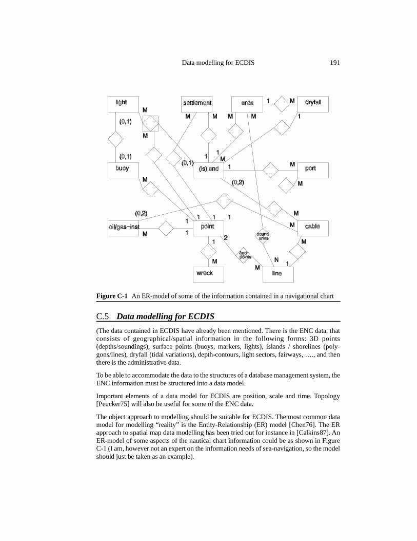
C.5 Data modelling for ECDIS

(The data contained in ECDIS have already been mentioned. There is the ENC data, thatconsists of geographical/spatial information in the following forms: 3D points(depths/soundings), surface points (buoys, markers, lights), islands / shorelines (poly-gons/lines), dryfall (tidal variations), depth-contours, light sectors, fairways, …., and thenthere is the administrative data.

To be able to accommodate the data to the structures of a database management system, theENC information must be structured into a data model.

Important elements of a data model for ECDIS are position, scale and time. Topology[Peucker75] will also be useful for some of the ENC data.

The object approach to modelling should be suitable for ECDIS. The most common datamodel for modelling “reality” is the Entity-Relationship (ER) model [Chen76]. The ERapproach to spatial map data modelling has been tried out for instance in [Calkins87]. AnER-model of some aspects of the nautical chart information could be as shown in FigureC-1 (I am, however not an expert on the information needs of sea-navigation, so the modelshould just be taken as an example).

Figure C-1 An ER-model of some of the information contained in a navigational chart

Data modelling for ECDIS 191

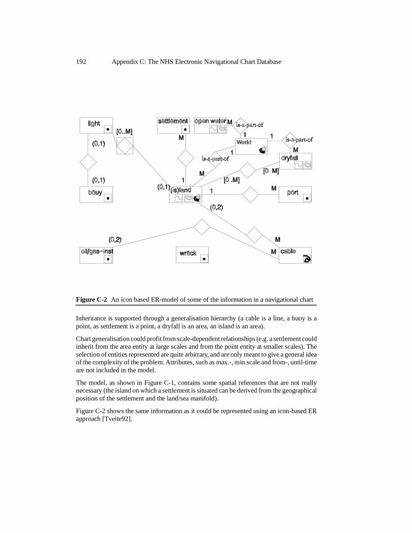
Inheritance is supported through a generalisation hierarchy (a cable is a line, a buoy is apoint, as settlement is a point, a dryfall is an area, an island is an area).

Chart generalisation could profit from scale-dependent relationships (e.g. a settlement couldinherit from the area entity at large scales and from the point entity at smaller scales). Theselection of entities represented are quite arbitrary, and are only meant to give a general ideaof the complexity of the problem. Attributes, such as max.-, min.scale and from-, until-timeare not included in the model.

The model, as shown in Figure C-1, contains some spatial references that are not reallynecessary (the island on which a settlement is situated can be derived from the geographicalposition of the settlement and the land/sea manifold).

Figure C-2 shows the same information as it could be represented using an icon-based ERapproach [Tveite92].

Figure C-2 An icon based ER-model of some of the information in a navigational chart


C.6 DBMS-aspects of an ENC-server

The discussion in the following sections is at an overview level, and is meant only tohighlight the problems and possibilities the management of ECDIS data pose to DBMSs.

C.6.1 The amount of data

The data volumes for storing a total coverage of the oceans and waterways of the earth arehuge. An average of 1-2 Megabyte of data for each chart cell is forecast by the IHO. Onsome parts of the Norwegian coast data volumes in the order of 30 Megabytes has beenreported for the 1:50000 equivalent cell size with height (land) contours included.

In accordance with these figures, one must believe that a minimum navigational chartdatabase will have to store many Gigabytes of data, and that the data volume of an extendeddatabase (including “administrative” data) should be forecast to grow high up in theTerabytes.

Such an extended database could include new kinds of information pertaining to the objectsin the ENC, pictures of harbour approaches, pictures of other significant features, fullcoverage of land features and detailed 3D-models of the seabed and land-surface.

As for the regular updates to the ENCs, the data volume have been forecast to be about 135KBytes pr. week ([Sandvik90], p65) for an international server covering the whole world.This number does only apply to the paper-chart part of the ENC. Updates to extendedservices would give numbers of a higher order of magnitude.

C.6.2 The data

The chart information in the ENCDB is very important (many lives depend on it), so thedata should be handled with great care to avoid errors. A chart error leading to a groundingcould leave the ENCDB host legally responsible.

The “administrative” part of the information base (list of lights, harbour information,national laws, etc.) does not have the same legal restrictions as the “paper chart” part. It cantherefore be handled in a more flexible way.

The ECDIS data will consist of a mixture of different types and formats.

• The geometric part of the database is the most problematic from a database point ofview, and will contains all the geographic properties of the chart data.

• The tabular part of the database will consist of non-spatial information on the objectsin the ENCDB.

• The pictorial part of the database are the images and pictures that could be of use inan ECDIS. This is information found in the administrative part of ECDIS, and couldbe pictures of harbours, lights and other distinct features of interest to the navigator.

All of these data types with their associated operations will have to be supported in thedatabase management system for ECDIS.

DBMS-aspects of an ENC-server 193

Most, if not all, of the data in ECDIS should be temporal, that is they should have a timeof validity. This will also have to be supported by the DBMS.

The accuracy of the data in ECDIS will vary. To enable predictions on the accuracy of theresults of the various operations on - and applications of the ECDIS data, accuracy measuresshould be included in the database.

Indications of the adequate scales of usage will have to be attached to all displayable objects.

C.6.3 Response time

A navigational chart should be displayed immediately at the request of the operator.

Efficient retrieval and integration of the traditional chart data (coast-lines, dryfalls, sound-ings, islands, ..) with other data (the so-called administrative part of the ENCD) is neededto give the navigation systems information in real-time. The traditional, general purposedatabase management systems have not got the power to do this for fast-moving vessels atpresent. In the near future these systems must be expected to provide higher performance.Today, only a database system based on parallel processing and/or storage or a tailor-madesystem will be needed to give the efficiency required.

C.6.4 Concurrency and recovery

The ENC-database on-board ships does not need any concurrency control or recovery[Bernstein87] if the system is to be used as a pure information source. Hence, themanagement of data on-board will be greatly simplified.

The ENCDB will, however, need some kind of concurrency control to ensure that the datathat is sent out is consistent (no partial updates have occurred during the transmission of achart).For the ENCDB, a coarse-granularity, spatial locking system will do (for instance lockingon the cell level, or locking the complete database). If the ENCDB shall allow generaltransactions, a full concurrency control scheme is required. In choosing the granularity andtype of concurrency control, one must take into account the relative large amount of long(read-)transactions that result from the extraction of charts and updates for transmission.A spatially based concurrency control mechanism should be preferred.

Recovery systems for the ENCDB will have to be state of the art, since the demands on thereliability and correctness of the system are so high.

C.6.5 Security

The status of the navigational chart as a legal document puts very high demands on thesecurity and integrity of the data and on monitoring the data communication. The data inthe approved and modification parts should be securely protected. One has to be able todetermine if the data comes from the authorised ENCDB server, or not. 100 percent reliablecommunication is necessary to ensure correct delivery. Cryptographic storing methods andphysical security arrangements in addition to ordinary operating system file-protectionmechanisms would be appropriate to ensure adequate security for the data in the system.


C.6.6 Reliability

The ENCDB should be a non-stop system. It should always be available and resilient tothe most common failures and accidents, such as disk-crashes, power failure, corruption ofinternal memory and failure of cables and components. One will have to assume that thedemands on the mean time between failure (MTBF) should be in the order of years. Toachieve this, parallel/replicated storage and duplicated processors must be used. This kindof database technology has been around for some years.

C.6.7 Billing

ECDIS data will be provided from different sources, and these sources will want credit(often as cash) for the use of their data.

To be able to do efficient billing of the data, suppliers of the data must be recorded withtheir percentage of ownership. Billing at cell level seems the most natural way of organisingthis. A log of all the retrievals in the database has to be kept to perform the billing. A suitablepricing policy must be determined.

C.6.8 The choice of a database system for the ECDIS server

Todays alternatives for DBMSs can be outlined as follows.

The choices of database system can be divided into a hardware - and a model choice. Thehardware choice is of the type of processor or architecture to be utilised, while the modelchoice is between the different data models proposed for database systems. The choices canbe simplified to the following:

• Single-processor versus (centralised) multi-processor

• Relational databases [Codd70] versus Object-oriented databases [Atkinson89](network databases and hierarchical databases seem to be a little out of fashion)

The choice of a single-processor versus a multi-processor database machine will depend onthe expected transaction rates and storage requirements. For efficiency reasons a databasesystem utilising parallel technology could be preferable for demanding systems. Forsecurity and reliability reasons duplication is advantageous, and multi-processor environ-ments are well suited for this.

Relational database management systems (RDBMSs) have the advantage of being the mostmodern of the dominant technologies of today. Modelling for RDBMSs is a well understoodtask, and the models can be modified as new objects, relationships or requirements showup. The interfaces to RDBs are also well defined and partly standardised (SQL). Data storedin relations are trivial to update by insertions, deletions and changes.

Object-oriented database management systems (OODBMS) are quite fresh as commercialproducts, but have proven very fast in comparison with RDBMSs for selected tasks [SI91].Exchange of data with other systems is not trivial because of the lack of standards. We arestill waiting for mature OODBMS technology. CAD, Software Engineering and GIS aresome of the fields suffering under the limits of todays relational DBMSs and where thecontribution of OODBMSs are forecast to be significant. The advantages of OODBMSs

DBMS-aspects of an ENC-server 195

are: intuitive and expressive modelling ((multiple) inheritance), information hiding (accessto data only through methods), object identity, complex objects, a complete programmingenvironment, and direct implementation of the model in the working database. Suggestedfeatures of OODBMSs are described in [Atkinson89].

C.7 Conclusions

The building of an electronic navigational chart server seems to be feasible, and a strippedversion will not require advanced database technology. A general-purpose DBMS is,however, necessary for a full ECDIS. A DBMS approach will give an open-ended system,available to the customers in a more direct manner.

When the exchange standards and the data structures of the ENC are standardised andavailable from the IHO, the provision of data on the specified format from an ENCDB serverwill be straight-forward, provided the necessary data are available.

For the ENCDB, the main effort has to be put into securing safe operation of the systemand efficient data structures.

An interesting topic for further research is the information system part of the ECDIS. Thiscould evolve to a full-grown multimedia database system. The research area of multimediadatabase systems is still in its infancy [IEEECOMPUTER89], so it would be wise to waitfor some of the dust to settle (standardisation) in this area before taking the step into ageneral-purpose multi-media information system.


Bibliography

[Aangeenbrug91] "A Critique of GIS"R.T AangeenbrugIn [Maguire91], pp. 101-107

[Abel86] "A Relational GIS Database Accomodating Independent Partionings of the Region"David J. Abel, John L. SmithSecond Symposium on Spatial Data Handling, Seattle, 1986, pp. 213-225

[Abel93] "Advances in Spatial Databases"David Abel, Beng Chin Ooi (Eds.)Proceedings, Third International Symposium, SSD’93, Singapore, june 1993, Lecture Notes inComputer Science 692, Springer Verlag, 1993, 431p.

[Abiteboul90] "New Hope on Data Models and Types: Report of an NSF-INRIA workshop"Serge Abiteboul, Peter Buneman, Claude Delobel, Richard Hull, Paris Kanellakis, Victor VianuSIGMOD RECORD, Vol. 19, No. 4, Dec. 1990, pp. 41-48

[Agrawal89] "Modular Synchronization in Multiversion Databases: Version Control and ConcurrencyControl"Divyakant Agrawal, Soumitra SenguptaACM, Proc SIGMOD 1989, pp. 408-417

[Ahn88] "Partitioned Storage for Temporal Databases"Ilsoo Ahn, Richard SnodgrassInformation Systems, Vol. 13, No. 4, 1988, pp. 369-391

[Aho83] "Data Structures and Algorithms"Alfred V. Aho, John E. Hopcroft, Jeffrey D. UllmanAddison Wesley, 1983 (first edition 1982)

[Al-Taha94] "Bibliography on Spatiotemporal Databases"Khaled K. Al-Taha, Richard T. Snodgrass, Michael D. SooInternational Journal of Geographical Information Systems, Vol. 8, No.1, 1994, pp. 95-103

[Aref91] "Extending a DBMS with Spatial Operations"Walid G. Aref, Hanan SametIn [Günther91], pp. 299-318

[Aronson89] "The Geographic Database - Logically Continuous and Physically Discrete"Peter AronsonProceedings, Auto-Carto 9, Baltimore, Maryland, 1989, pp. 452-461

[Atkinson87] "Types and Persistence in Database Programming Languages"Malcolm P. Atkinson, O. Peter BunemanACM Computing Surveys, Vol. 19, No. 2, June 1987, pp. 105-190

[Atkinson89] "The Object-Oriented Database System Manifesto"Malcolm Atkinson, François Bancilhon, David DeWitt, Klaus Dittrich, David Maier, StanleyZdonikProceedings of the 1st Intl. Conf. on Deductive and Object-Oriented Databases (DOOD’89),Kyoto, Japan, Dec. 1989, pp. 40-57

[ATKIS89] "Amtliches Topographisch-Kartographisches Informationssystem ATKIS, Teil A Konzeptionund Inhalt des Informationssystems ATKIS"AdV-Arbeitsgruppe ATKISArbeitsgemeinschaft der Vermessungsverwaltungen der Länder der BundesrepublikDeutschland (AdV), Stand 10.1989 (in German), 31p.

[Aurenhammer91] "Voronoi Diagrams - A Survey of a Fundamental Geometric Data Structure"Franz AurenhammerACM Computing Surveys, Vol. 23, No. 3, September 1991, pp. 345-405

[Badrinath90] "Performance Evaluation of Semantics-based Multilevel Concurrency Control Protocols"B.R. Badrinath, Krithi RamamrithamACM, SIGMOD record, vol.19, No. 2, 1990 (Proc. SIGMOD’90), pp. 163-172

[Ballard81] "Strip Trees: A Hierarchical Representation for Curves"Dana H. BallardCommunications of the ACM, Vol. 24, No. 5, May 1981, pp. 310-321

[Bancilhon90] "Object-Oriented Database Systems: In Transit"François Bancilhon, Won KimSIGMOD RECORD, Vol. 19, No. 4, Dec. 1990, pp. 49-53

[Barghouti91] "Concurrency Control in Advanced Database Applications"Naser S. Barghouti, Gail E. KaiserACM Computing Surveys, Vol. 23, No. 3, Sept. 1991, pp. 269-317

[Barnsley88] "Fractals Everywhere"Michael Fielding BarnsleyAcademic Press, 1988, 394p

[Barrera81] "Schema Definition and Query Language for a Geographical Database System"R. Barrera, A. BuchmannIEEE Computer Architecture for Pattern Analysis and Image Database Management, Nov 1981,pp 250-256

[Batini86] "A Comparative Analysis of Methodologies for Database Schema Integration"C. Batini, M. Lenzerini, S.B. NavatheACM Computing Surveys, Vol. 18, No. 4, December 1986, pp. 323-364

[Bayer72] "Organization and Maintenance of Large Ordered Indexes"R. Bayer, E. McCreightActa Informatica, Vol. 1, No. 3, pp. 173-189

[Beck86] "Quality Control and Standards for a National Digital Cartographic Data Base"Francis J. Beck, Randle W. OlsenProceedings, Auto Carto London, 1986, vol. 1, pp. 372-380

[Beckmann90] "An Efficient and Robust Access Method for Points and Rectangles"Nobert Beckmann, Hans-Peter Kriegel, Ralf Schneider, Bernhard SeegerACM, SIGMOD record, vol.19, No. 2, 1990 (Proc. SIGMOD’90), pp. 322-331

[Bédard89] "Extending Entity/Relationship Formalism for Spatial Information Systems"Yvan Bédard, François PaquetteProceedings, Auto Carto 9, Baltimore, Maryland, 1989, pp. 818-827

[Beeri90] "Formal Models for Object Oriented Databases"Catriel BeeriIn: Deductive and Object-Oriented Databases (DOOD89), Editors: Kim, Nicolas, Nishio. Elsevier1990, pp. 405-430

[Bentley75] "Multidimensional Binary Search Trees Used for Associative Searching"Jon Louis BentleyCommunications of the ACM, Vol. 18, No. 9, 1975, pp. 509-517

[Bernhardsen86] "Community Benefit of Digital Spatial Information"T. Bernhardsen, S. TveitdalProceedings, Auto Carto London, 1986, vol. 2, pp. 1-3

[Bernstein93] "Concurrency in Programming and Database Systems"Arthur J. Bernstein, Philip M. LewisJones and Bartlett Publishers, 1993, 548p.

[Bernstein87] "Concurrency Control and Recovery in Database Systems"Philip A. Bernstein, V. Hadzilacos, Nathan GoodmanAddison Wesley, 1987

198 Bibliography

[Berry87] "Fundamental Operations in Computer-assisted Map Analysis"Joseph K. BerryInternational Journal of Geographical Information Systems, Vol. 1, No. 2, 1987, pp. 119-136

[Biller77] "Concepts for the Conceptual Schema"N. Biller, E. NeuholdIn "Architecture and Models in Data Base Management Systems", G. Nijssen, Ed. North-Hol-land, Amsterdam, 1977, pp. 1-30

[Birtwistle73] "SIMULA Begin"Graham M. Birtwistle, Ole-Johan Dahl, Bjørn Myrhaug, Kristen NygaardStudentlitteratur, Lund, Sweden, 1973

[Bjørke90] "Cartographic Zoom"Jan Terje Bjørke, Rune AasgaardProceedings of the 4th International Symposium on Spatial Data Handling, 1990, Zürich,Switzerland, vol.1, pp. 345-353

[Blais86] "Optimal Interval Sampling in Theory and Practice"J.A.R. Blais, M.A. Chapman, W.K. LamSecond Symposium on Spatial Data Handling, Seattle, 1986, pp. 185-192

[Boudriault87] "Topology in the TIGER file"Gerard BoudriaultAuto Carto 8, Baltimore, Maryland, 1987, pp. 258-263

[Brassel88] "A review and conceptual framework of automated map generalization"Kurt E. Brassel, Robert WeibelInternational Journal of Geographical Information Systems, Vol. 2, No. 3, 1988, pp. 229-244

[Bratbergsengen83] "Feature Analysis of ASTRAL"Kjell Bratbergsengen, Tor StålhaneIn [Schmidt83a], pp. 50-75

[Bratbergsengen84] "Hashing Methods and Relational Algebra Operations"Kjell BratbergsengenProc. of the 10th Conference on Very Large Data Bases, Singapore Aug. 1984

[Bratbergsengen89] "The Development of the CROSS8 and HC16-186 Parallel (Database) Comput-ers"Kjell Bratbergsengen, Torgrim GjelsvikThe Sixth International Workshop on Database Machines, France, June19-23 1989

[Bratbergsengen90] "Relational Algebra Operations"Kjell BratbergsengenPRISMA Workshop, Parallel Database Systems, September 24-26 1990, Nordwijk, The Neth-erlands, 1990, 20p

[Breitbart92] "Overview of Multidatabase Transaction Management"Y. Breitbart, H. Garcia-Molina, A. SilberschatzThe VLDB Journal, Vol. 1, No.2, 1992, pp. 181-239

[Broome90] "The TIGER Data Base Structure"Frederick R. Broome, David B. MeixlerCartography and Geographic Information Systems, Vol. 17, No. 1, 1990, pp. 39-47

[Buchmann90] "Design and Implementation of Large Spatial Databases (first symposium SSD ’89,Santa Barbara, California, July 17/18, 1989)"A. Buchmann, O. Günther, T.R. Smith, Y.-F. Wang (Eds.)Lecture Notes in Computer Science 409, Springer Verlag, 1990

[Burrough86] "Five Reasons why Geographical Information Systems are not being Used Efficiently forLand Resources Assessment"P.A. BurroughProceedings, Auto Carto London, 1986, vol. 2, pp. 139-148

[Burrough89] "Principles of Geographical Information Systems for Land Resources Assessment"P.A. BurroughClarendon Press, Oxford, 1989 (first edition 1986)

Bibliography 199

[Calkins87] "The Transition To Automated Production Cartography: Design Of The Master Carto-graphic Database"Hugh W. Calkins, Duane F. MarbleThe American Cartographer, Vol. 14, No.2, 1987, pp. 105-119

[Carey90] "Extensible Database Management Systems"Michael Carey, Laura HaasSIGMOD RECORD, Vol. 19, No. 4, Dec. 1990, pp. 54-60

[Carter92] "Perspectives on Sharing Data in Geographic Information Systems"James R. CarterPhotogrammetric Engineering and Remote Sensing, Vol.58, No. 11, Nov. 1992, pp. 1557-1560

[CEN95] "Geographic Information - Data Description - Quality"CEN/TC287 - Geographic Information, WG2, PT05CEN/TC287, document N369, 1995

[CEN95b] "Geographic Information - Data Description - Metadata"CEN/TC287 - Geographic Information, WG2, PT01CEN/TC287, document N370, 1995

[Ceri88] "Distributed Databases Principles & Systems"Stefano Ceri, Giuseppe PelagattiMcGraw-Hill, third printing 1988 (first edition 1985)

[CERL95] "Environmental Modeling and Visualization With GRASS GIS"CERL, Bill BrownInternet URL: http://softail.cecer.army.mil/grass/viz/VIZ.html, 1995

[Chance90a] "An Object -Oriented GIS - Issues and Solutions"Arthur Chance, Richard Newell, David G. TheriaultConference Proceedings of EGIS, Amsterdam, April 1990

[Chance90b] "An Overview of Smallworld Magic"Arthur Chance, Richard Newell, David G. TheriaultSmallworld Technical Paper no. 9, 1990

[Charlwood87] "Developing a DBMS for Geographic Information: A Review"Gerald Charlwood, George Moon, John TulipAuto Carto 8, Baltimore, Maryland, 1987, 14 p.

[Chen76] "The Entity-Relationship Model - Toward a Unified View of Data"Peter Pin-Shan ChenACM Transaction on Database Systems, Vol. 1, No. 1, March 1976, pp. 9-36

[Chen94] "RAID: High-Performance, Reliable Secondary Storage"Peter M. Chen, Edward K. Lee, Garth A. Gibson, Randy H. Katz, David A. PattersonACM Computing Surveys, vol. 26, no. 2, June 1994, pp. 145-185

[Chrisman84] "The Role of Quality Information in the Long-Term Functioning of a Geographic Informa-tion System"Nicholas R. ChrismanCartographica, vol. 21, No. 2/3, 1984, pp. 79-87

[Chrisman86] "Obtaining Information on Quality of Digital Data"Nicholas R. ChrismanProceedings, Auto Carto London, 1986, vol. 1, pp. 350-358

[Chrisman89] "Modelling Error in Overlaid Categorical Maps"Nicholas R. ChrismanIn [Goodchild89], pp. 21-34

[Chrisman90] "Deficiencies of sheets and tiles: building sheetless databases"Nicholas R. ChrismanInternational Journal of Geographical Information Systems, 1990, vol. 4, no 2, pp 157-167

[Christoduolakis95] "Multimedia Information Systems: Issues and Approaches"Stavros Christoduolakis, Leonidas KoveosIn [Kim95a], pp. 318-337

200 Bibliography

[Clapham91] "The Development of an Initial Framework for the Visualisation of Spatial Data Quality"Sarah B. Clapham, Kate BeardTechnical Papers, 1991 ACSM-ASPRS Annual Convention, Vol. 2, Cartography and GIS/LIS,Baltimore, 1991, pp. 73-82

[Clifford85] "On an Algebra for Historical Relational Databases: Two Views"James Clifford, Abdullah Uz TanselACM, SIGMOD record, vol.14, No. 4, 1985 (Proc. SIGMOD’85), pp. 247-265

[Clocksin84] "Programming in Prolog"W.F. Clocksin, C.S. MellishSpringer-Verlag, 1984

[Coad90] "Object-Oriented Analysis"Peter Coad, Edward YourdonPrentice-Hall, 1990

[CODASYL71] "CODASYL Data Base Task Group. April 1971 Report"Data Base Task Group ACM, 1971

[Codd70] "A Relational Model for Large Shared Data Banks"E.F. CoddCommunications of the ACM, Vol. 13, No. 6, June 1970, pp. 377-387

[Codd79] "Extending the Relational Model to Capture More Meaning"E.F. CoddACM Transactions on Database Systems, Vol. 4, No. 4, Dec. 1979, pp. 397-434

[Congalton94] "International Symposium on the Spatial Accuracy of Natural Resource Data Bases"Russel G. Congalton, Ed. American Society for Photogrammetry and Remote Sensing, 1994, 271p.

[Conklin87] "Hypertext: An Introduction and Survey"Jeff Conklin IEEE, Computer, vol. 20, no. 9, September 1987, pp. 17-41

[Dangermond86] "GIS Trends and Experiences"Jack DangermondSecond Symposium on Spatial Data Handling, Seattle, 1986, pp. 1-4

[Date86] "An Introduction to Database Systems, Volume I"C.J. DateAddison Wesley, fourth edition 1986

[Dayal95] "Active Database Systems"Umeshwar Dayal, Eric Hanson, Jennifer WidomIn [Kim95a], pp. 434-456

[Deux90] "The Story of O2"O. Deux, et al.IEEE Transactions on Knowledge and Data Engineering, Vol. 2, No.1, pp. 91-108

[DeWitt85] "Multiprocessor Hash-Based Join Algorithms"David J. DeWitt, Robert GerberProceedings of VLDB’95, Stockholm, 1985, pp. 151-164

[Douglas73] "Algorithms for the reduction of the number of points required to represent a digitized lineor its caricature"David H. Douglas, Thomas K. PeuckerCanadian Cartographer, Vol.10, No.4, 1973, pp. 110-122

[Dowers90] "Analysis of GIS Performance on Parallel Architectures and Workstation-Server Systems"S. Dowers, B.M. Gittings, T.M. Sloan, T. WaughProceedings, GIS/LIS ’90, 7-10. Nov. 1990, Anaheim, CA, vol. 2, pp. 555-561

[Dutton89] "Planetary Modelling via Hierarchical Tessellation"Geoffrey DuttonProceedings, Auto-Carto 9, Baltimore, Maryland, 1989, pp. 462-471

Bibliography 201

[Dæhlen90] "Compression of Hydrographic Data"Morten Dæhlen, Geir WestgaardSenter for Industrial Research, report no. 900612-1, august 1990, 23p.

[Easterfield90] "Version Management in GIS - Applications and Techniques"Mark E. Easterfield, Richard G. Newell, David G. TheriaultEGIS ’90, EGIS Foundation, Netherlands, 1990, pp. 288-297

[Egenhofer87] "Object-Oriented Databases: Database Requirements for GIS"Max J. Egenhofer, Andrew U. FrankInternational Geographic Information Systems Symposium: The Research Agenda, Crystal City,VA, november 1987, pp. II:189-211

[Egenhofer89a] "Object-Oriented Modeling in GIS: Inheritance and Propagation"Max J. Egenhofer, Andrew U. FrankProceedings, Auto-Carto 9, Baltimore, Maryland, 1989, pp. 588-598

[Egenhofer89b] "Object-Oriented Software Engineering Considerations for Future GIS"Max J. Egenhofer, Andrew U. FrankProceedings, IGIS’89, Baltimore, Maryland, 1989, pp. 55-72

[Egenhofer90a] "A Topological Data Model for Spatial Databases"M.J. Egenhofer, A.U. Frank, J.P. Jacksonin [Buchman90], pp. 271-286

[Egenhofer90b] "A Mathematical Framework for the Definition of Topological Relationships"Max Egenhofer, John R. HerringProceedings of the 4th International Symposium on Spatial Data Handling, 1990, Zürich,Switzerland, pp. 803-813

[Egenhofer91a] "Point-set topological spatial relations"Max J. Egenhofer, Robert D. FranzosaInternational Journal of Geographical Information Systems, Vol. 5, No. 2, 1991, pp. 161-174

[Egenhofer91b] "Reasoning about Binary Topological Relations"Max J. EgenhoferIn [Günther91], pp. 143-160

[Egenhofer92] "Reasoning about Gradual Changes of Topological Relationships"Max J. Egenhofer, Khaled K. Al-TahaIn [Frank92], pp. 196-219

[Egenhofer95] "Advances in Spatial Databases, 4th International Symposium, SSD’95, Portland,Maine, USA, August 6-9, 1995, proceedings"Max J. Egenhofer, John R. Herring (Eds.)Lecture Notes in Computer Science, Vol. 951, Springer, 1995.

[Elmasri89] "Fundamentals of Database Systems"Ramez Elmasri, Shamkant B. NavatheThe Benjamin/Cummings Publishing Company, Inc., California, 1989.

[Elmasri94] "Fundamentals of Database Systems, second edition"Ramez Elmasri, Shamkant B. NavatheThe Benjamin/Cummings Publishing Company, Inc., California, 1989.

[Encarnação83] "Computer Aided Design - Fundamentals and System Architectures"José Encarnação, Ernst G. SchlectendahlSpringer-Verlag, 1983.

[ESRI95a]ESRI (Peter Moran, product marketing)Personal email communication, 1995.

[ESRI95b] ""Spatial Database Engine ReleasedESRI (contact Carl Sylvester)ARC News, Vol.17, No.4, 1995, pp. 1-2

[Fagin79] "Extendible Hashing - A Fast Access Method for Dynamic Files"Donald Fagin, Jurg Nievergelt, Nicholas Pippenger, H. Raymond StrongACM Transactions on Database Systems, Vol.4, No.3, September 1979, pp 315-344

202 Bibliography

[Faloutsos87] "Analysis of Object Oriented Spatial Access Methods"Christos Faloutsos, Timos Sellis, Nick RoussopoulosACM, SIGMOD record, vol.16, No. 3, 1987 (Proc. SIGMOD’87), pp. 426-439

[Faloutsos89] "Tri-Cell - A Data Structure for Spatial Data"Christos Faloutsos, Winston RegoInformation Systems, Vol. 14, No. 2, 1989, pp. 131-139

[Farrag89] "Using Semantic Knowledge of Transactions to Increase Concurrency"Abdel Aziz Farrag, M. Tamer ÖzsuACM Transactions on Database Systems, Vol. 14, No. 4, Dec. 1989, pp. 503-525

[Feuchtwanger89] "Geographic Logical Database Model Requirements"Martin FeuchtwangerProceedings, Auto Carto 9, Baltimore, Maryland, 1989, pp. 599-609

[Feuchtwanger93] "Towards a Geographic Semantic Database Model"Martin FeuchtwangerThesis, Doctor of Philosophy, Geography, Simon Fraser University, July 1993, 186p.

[FGDC94] "Content Standards for Digital Geospatial Metadata"Federal Geographic Data CommitteeDepartment of the Interior, US Geological Survey, Federal Geographic Data Committee(FGDC), June 8, 1994

[FGIS90] "FGIS Konseptbeskrivelse, Versjon 2.0"Statens KartverkStatens Kartverk, Hønefoss, 27/7-1990

[Finkel74] "Quad Trees: A Data Structure for Retrieval on Composite Keys"R.A. Finkel, K.L. BentleyActa Informatica, Vol. 4, No. 1, pp. 1-9

[Firns91] "ER on the Side of Spatial Accuracy"Peter G. Firns, George L. BenwellProceedings, Symposium on Spatial Database Accuracy, June 19-20, 1991, Melbourne,Australia, pp. 192-202

[Franaszek85] "Limitations of Concurrency in Transaction Processing"Peter Franaszek, John T. RobinsonACM Transactions on Database Systems, Vol. 10, No. 1, March 1985, pp. 1-28

[Frank84] "Requirements for Database Systems Suitable to Manage Large Spatial Databases"Andrew U. FrankInternational Symposium on Spatial Data Handling, Zurich, Switzerland, August 1984, pp. 38-60

[Frank86] "Cell Graphs: A Provable Correct Method for the Storage of Geometry"Andrew U. Frank, Werner KuhnProceedings, Second Symposium on Spatial Data Handling, Seattle, 1986, pp. 411-436

[Frank88] "Requirements for a Database Management System for a GIS"Andrew U. FrankPhotogrammetric Engineering and Remote Sensing, Vol.54, No. 11, Nov. 1988, pp. 1557-1564

[Frank91] "Properties of Geographic Data: Requirements for Spatial Access Methods"Andrew FrankIn [Günther91], pp. 225-234

[Frank92] "Theories and Methods of Spatio-Temporal Reasoning in Geographical Space"Andrew U. Frank, Irene Campari, Ubaldo Formentini (Eds.)Proceedings, International Conference GIS - From Space to Territory: Theories and Methodsof Spatio-Temporal Reasoning, Pisa, Italy, September 1992, Lecture Notes in ComputerScience 639, Springer Verlag, 1992, 431p.

[Furht95] "Design Issues for Interactive Television Systems"Borko Furht, Deven Kalra, Frederick L. Kitson, Arturo A. Rodriguez, William E. WallIEEE Computer, Vol.28, No.5, May 1995, pp. 25-39

Bibliography 203

[Gadia88] "A Homogeneous Relational Model and Query Languages for Temporal Databases"Shashi K. GadiaACM Transactions on Database Systems, Vol. 13, No. 4, Dec. 1988, pp. 418-448

[Ganger94] "Disk Arrays: High-Performance, High-Reliability Storage Subsystems"Gregory R. Ganger, Bruce L. Worthington, Robert Y. Hou, Yale N. PattIEEE Computer, Vol. 27, No. 3, March 1994, pp. 30-36

[Garcia-Molina95] "Distributed Databases"Hector Garcia-Molina, Mei HsuIn [Kim95a], pp. 477-493

[Gardels88] "GRASS in the X-Windows Environment: Distributing GIS Data and Technology"Kenneth GardelsGIS/LIS’88 Proceedings, ACSM, ASP/RS, AAG, URISA, San Antonio, TX, Nov. 1988, pp. 751-

[GISDATA93]GISDATA Newsletter No. 1, ESF, March 1993

[GISDATA95]GISDATA Newsletter No. 6, ESF, November 1995

[Goldberg83] "Smalltalk-80: The Language and its Implemtation"Adele Goldberg, David RobsonAddison-Wesley, Reading, MA, 1983

[Golledge92] "Do People Understand Spatial Concepts: The Case of First-Order Primitives"Reginald G. GolledgeIn [Frank92], 1992, pp. 1-21

[Gonzalez78] "Syntactic Pattern Recognition: An Introduction"Rafael C. Gonzales, Michael G. ThomasonAddison-Wesley, 1978, 283p.

[Gonzalez87] "Digital Image Processing"Rafael C. Gonzales, Paul WintzAddison Wesley, 1987, 503p

[Goodchild89] "The Accuracy of Spatial Databases"Michael Goodchild, Sucharita Gopal, eds.Taylor and Francis, London, 1989

[Goodchild90a] "Tiling of Large Geographical Databases"Michael F. GoodchildIn [Buchmann90], pp. 137-146

[Goodchild90b] "Keynote address: Spatial Information Science"Michael F. GoodchildProceedings, 4th International Symposium on Spatial Data Handling, 1990, Zürich, Vol. 1, pp.3-12

[Goodchild91] "Keynote address: Symposium on Spatial Database Accuracy"Michael F. GoodchildProceedings, Symposium on Spatial Database Accuracy, June 19-20, 1991, Melbourne,Australia, pp. 1-16

[Goyal89] "Intelligent Information Systems: The Concept of an Intelligent Document"Pankaj GoyalInformation Systems, Vol. 14, No. 4, 1989, pp. 351-358

[Grant90] "The Management and Dissemination of Electronic Navigational Chart Data in the 1990s"Stephen Grant, Michael Casey, Timothy Evangelatos, Horst HechtInternational Hydrographic Review, Monaco, LXVII(2), July 1990, pp. 17-30

[GRASS93] "Grass 4.1 Reference Manual"GRASS ProjectUS Army Corps of Engineers, Construction Engineering Research Laboratories, Champaign,Illinois, 1993

204 Bibliography

[GRASS95] "GEOGRAPHIC RESOURCES ANALYSIS SUPPORT SYSTEM (GRASS)"GRASS (William D. Goran)Internet URL: http://deathstar.rutgers.edu/grass/what.html

[Greene89] "An Implementation and Performance Analysis of Spatial Data Access Methods"Diane GreeneProc. IEEE, 5th International Conference on Data Engineering, Los Angeles, Calif., 1989, pp.606-615

[Guptill90] "Multiple Representations of Geographic Entities through Space and Time"Stephen C. GuptillProceedings of the 4th International Symposium on Spatial Data Handling, 1990, Zürich,Switzerland, pp. 859-868

[Guttman84] "R-Trees: A Dynamic Index Structure for Spatial Searching"Antonin GuttmanACM, Proc. SIGMOD’84, Boston, MA, June 18-21, 1984, pp. 47-57

[Günther87] "A Dual Space Representation for Geometric Data"Oliver Günther, Eugene WangProc. of the 13th VLDB Conference, Brighton, 1987, pp. 501-506

[Günther89] "The Design of the Cell Tree: An Object-Oriented Index Structure for Geometric Data-bases"Oliver GüntherProc. IEEE, 5th International Conference on Data Engineering, Los Angeles, Calif., 1989, pp.598-605

[Günther90] "Research Issues in Spatial Databases"O. Günther, A. BuchmannSIGMOD RECORD, Vol. 19, No. 4, Dec 1990, pp. 61-68

[Günther91] "Advances in Spatial Databases"O. Günther, H.-J. SchekProceedings, 2nd Symposium, SDD’91, Zurich, Switzerland, August 28-30, 1991, SpringerVerlag 1991, 471p

[Güting94] "An Introduction to Spatial Database Systems"R.H. GütingThe VLDB Journal, Vol. 3, No. 4,1994, pp. 357-399

[Hagaseth90] "Multimedia Databasesystemer for Geografiske Informasjonssystemer"Marianne HagasethUnpublished student report, IDT, NTH, 4/5-1990 (in Norwegian)

[Haas91] "Exploiting Extensible DBMS in Integrated Geographic Information Systems"Laura M. Haas, William F. CodyIn [Günther91], pp. 423-450

[Hammer78] "The Semantic Data Model: A Modelling Mechanism for Data Base Applications"Michael Hammer, Dennis McLeodProceedings of the ACM SIGMOD Conference, Austin, 1978, pp. 26-36

[Healey89] "Transputer Based Parallel Processing for GIS Analysis: Problems and Potentialities"R.G. Healey, G.B. DesaAuto Carto 9, Baltimore, Maryland, April 1989, pp. 90-99

[Healey91a] "Determination of Computing Resource Requirements for GIS Processing in a Worksta-tion-Server Environment"R.G. Healey, S. Dowers, B.M. Gittings, T.M. Sloan, T.C. WaughProceedings EGIS 1991, pp. 422-426

[Healey91b] "Database Management Systems"R.G. HealeyChapter 18, in [Maguire91], pp. 251-267

[Herlihy90] "Apologizing Versus Asking Permission: Optimistic Concurrency Control for Abstract DataTypes"Maurice HerlihyACM Transactions on Database Systems, Vol. 15, No. 1, March 1990, pp. 96-124

Bibliography 205

[Herring87] "TIGRIS: Topologically Integrated Geographic Information System"John R. HerringAuto Carto 8, Baltimore, Maryland, march 1987, pp. 282-291

[Herring88] "Extensions to the SQL Query Language to Support Spatial Analysis in a Topological DataBase"John R. Herring, Robert C. Larsen, Jagadisan ShivakumarGIS/LIS’88 Proceedings, ACSM, ASP/RS, AAG, URISA, San Antonio, TX, Nov. 1988, pp.741-750

[Herring89] "A Fully Integrated Geographic Information System"John R. HerringAuto Carto 9, Baltimore, Maryland, April 1989, pp. 828-837

[Herring90] "The Definition and Development of a Topological Spatial Data System"John R. HerringPhotogrammetry and Land Information Systems, Editor: Otto Kölbl, Lausanne, Switzerland1990, pp. 57-70

[Hootsmans92] "Knowledge-Supported Generation of Meta-Information on Handling Crisp and FuzzyDatasets"Rob M. Hootsmans, Wouter M. de Jong, Frans J.M. van der WelProceedings, 5th International Symposium on Spatial Data Handling, Charleston, SC, August3-7, 1992, pp. 470-479

[Hopkins92] "Algorithm Scalability for Line Intersection Detection in Parallel Polygon Overlay"Sara Hopkins, Richard G. Healey, Thomas WaughProceedings of the 5th International Symposium on Spatial Data Handling, 1992, Charleston,SC, USA, vol.1, pp. 210-218

[Hsiao92] "Tutorial on Federated Databases and Systems (Part I)"D. HsiaoThe VLDB Journal, Vol. 1, No.1, 1992, pp. 127-179

[Hull87] "Semantic Database Modeling: Survey, Applications, and Research Issues"Richard Hull, Roger KingACM Computing Surveys, vol.19, no.3, Sept. 1987, pp. 201-260

[Hunter91] "Proceedings, Symposium on Spatial Database Accuracy"Gary J.Hunter, editorDept. of Surveying and Land Information, Univ. of Melbourne, 1991, 260p.

[IEEECOMPUTER89] "IEEE Computer, special issue on image database management"IEEE Computer, December 1989, p 7-71

[IHOSP5288] "Draft Specifications for ECDIS"IHO special publication 52, 3. draft, October 1988

[ISO/IEC94a] "SQL Multimedia and Application Packages (SQL/MM) Project Plan"ISO/IEC JTC1/WG3, N1677, SQL/MM SOU-002, March 1994

[ISO/IEC94b] "SQL Multimedia and Application Packages (SQL/MM). Part 3: Spatial"ISO/IEC JTC1/WG3, N1677, SQL/MM SOU-005, March 1994

[ISO/IEC96] "SQL Multimedia and Application Packages - Part 3: Spatial"ISO/IEC JTC1/SC21, N10441, ISO/IEC CD 13249-3:199x (E), November 1996

[Jagadish90] "Linear Clustering of Objects with Multiple Attributes"H.V. JagadishACM, SIGMOD record, vol.19, No. 2, 1990 (Proc. SIGMOD’90), pp. 332-342

[Jain87] "Advances in Statistical Pattern Recognition"Anil K. JainNATO ASI Series, Vol. F30, Pattern Recognition Theory and Applications, Edited by P.A.Devijver and J. Kittler, Springer-Verlag, 1987, pp. 1-19

[Jajodia90] "Database Security: Current Status and Key Issues"Sushil Jajodia, Ravi SandhuSIGMOD RECORD, Vol. 19, No. 4, Dec. 1990, pp. 123-126

206 Bibliography

[Jardine77] "The ANSI/SPARC DBMS Model: Proceedings of the Second SHARE Working Conferenceon Data Base Management Systems, Montreal, Canada, April 26-30, 1976"D.A. Jardine (editor)North Holland 1977

[Jen94] "A Model for Handling Topological Relationships in a 2D Environment"Tao-Yuan Jen, Patrice BoursierIn [Waugh94], pp. 73-88

[Joseph88] "PICQUERY: A High Level Query Language for Pictorial Database Management"Thomas Joseph, Alfonso F. CardenasIEEE Transactions on Software Engineering, Vol. 14, No. 5, May 1988, pp. 630-638

[Katzman78] "A Fault-tolerant Computing System"James A. KatzmanProc. of the 11th Hawaii International Conference on System Sciences, volume 3, 1978, pp.85-102

[Keates82] "Understanding Maps"J.S. KeatesLongman, London and New York, 1982

[Keating87] "An Integrated Topological Database Design for Geographic Information Systems"Terrence Keating, William Phillips, Kevin IngramPhotogrammetric Engineering and Remote Sensing, Vol. 53, No. 10, Oct. 1987, pp. 1399-1402

[Kemper87] "An Analysis of Geometric Modeling in Database Systems"Alfons Kemper, Mechtild WallrathACM Computing Surveys, Vol. 19, No. 1, March 1987, pp. 47-91

[Kemper94] "Object-Oriented Database Management, Applications in Engineering and ComputerScience"Alfons Kemper, Guido MoerkottePrentice-Hall, 1994, 680p.

[Kim84] "Highly Available Systems for Database Applications"Won KimACM Computing Surveys, Vol. 16, No. 1, March 1984, pp. 71-98

[Kim89] "Object-Oriented Concepts, Databases, and Applications"Won Kim, Fredrick H. Lochovsky, editorsACM Press, 1989

[Kim95a] "Modern Database Systems: The Object Model, Interoperability and Beyond"Won Kim (editor)ACM Press, Addison Wesley, 1995, 703p.

[Kim95d] "Introduction to Part 2: Technology for Interoperating Legacy Databases"Won KimIn [Kim95a], pp. 515-520

[Kim91] "Chips Deliver Multimedia"Yongmin KimByte, December 1991, pp. 163-173

[Kim95c] "Comparing Data Modelling Formalisms"Young-Gul Kim, Salvatore T. MarchCommunications of the ACM, Vol. 38, No. 6, 1995, pp. 103-115

[Knott71] "Expandable Open Adress Hash Table Storage and Retrieval"Gary D. KnottProc. ACM SIGFIDET workshop on Data Description, Access and Control, 1971, pp 187-206

[Korth88] "Formal Model of Correctness Without Serializability"Henry F. Korth, Gregory D. SpeegleACM, SIGMOD record, vol.17, No. 3, 1988 (Proc. SIGMOD’88), pp. 379-386

Bibliography 207

[Kotz-Dittrich95] "Where Object-Oriented DBMSs Should Do Better: A Critique Based on Early Expe-riences"Angelika Kotz-Dittrich, Klaus R. DittrichIn [Kim95a], pp. 238-254

[Langefors73] "Theoretical analysis of information systems"Börje LangeforsPhiladelpia, Auerbach, 4th ed., 1973, 489 p.

[Langran88] "A Framework for Temporal Geographic Information"Gail Langran, Nicholas R. ChrismanCartographica, Vol. 25, No. 3, 1988, pp. 1-14

[Langran89] "Accessing Spatiotemporal Data in a Temporal GIS"Gail LangranProceedings, Auto-Carto 9, Baltimore, Maryland, 1989, pp. 191-198

[Larson78] "Dynamic Hashing"Per-Åke LarsonBIT, No.18, 1978, pp 184-201

[Laurini90] "Principles of Geomatic Hypermaps"Robert Laurini, Françoise Milleret-RaffortProceedings of the 4th International Symposium on Spatial Data Handling, 1990, Zürich,Switzerland, vol.2, pp. 642-651

[Laurini92] "Fundamentals of Spatial Information Systems"Robert Laurini, Derek ThompsonAcademic Press, 1992

[Lauzon85] "Database Support for Geographic Information Systems: The Wild System 9 Approach"J.P. Lauzon, R. McLaren, C. HarwoodProceedings of ACSM-ASPRS Fall Meeting, Indianapolis, Sept. 8-13, 1985, pp. 583-594

[Lillesand87] "Remote Sensing and Image Interpretation"Thomas M. Lillesand, Ralph W. KieferJohn Wiley & Sons, second edition 1987

[Lin91] "A Rationale for Spatiotemporal Intersection"Hui Lin, Hugh W. CalkinsTechnical Papers, 1991 ACSM-ASPRS Annual Convention, Vol. 2, Cartography and GIS-LIS,Baltimore, 1991, pp. 204-213

[Lindholm90] "Hypermedia as a Cartographic Product - Use and Production"Mikko Lindholm, Tapani SarjakoskiCourse Material, Scandinavian Summer Course in Cartography, August 19-31, 1990, Gol,Norway

[Litwin80] "Linear Hashing: A New Tool for File and Table Adressing"Witold LitwinProceedings of the Sixth International Conference on Very Large Data Bases, Montreal, October1980, pp. 212-223

[Lomet90] "The hB-Tree: A Multiattribute Indexing Method with Good Guaranteed Performance"David B. Lomet, Betty SalzbergACM Transactions on Database Systems, Vol. 15, No. 4, Dec. 1990, pp. 625-658

[Lorie91] "The Use of a Complex Object Language in Geographic Data Management"Raymond A. LorieIn [Günter91], pp. 319-337

[Lu90] "Decomposition of Spatial Database Queries by Deduction and Compilation"Wei Lu, Jiawei HanProceedings of the 4th International Symposium on Spatial Data Handling, 1990, Zürich,Switzerland, vol.2, pp. 579-588

[Lunt90] "Database Security"Teresa F. Lunt, Eduardo B. FernandezSIGMOD RECORD, Vol. 19, No. 4, Dec. 1990, pp. 90-97

208 Bibliography

[Mackert86] "R* Optimizer Validation and Performance Evaluation for Local Queries"Lothar F. Mackert, Guy M. LohmanACM, SIGMOD record, vol.15, No. 2, 1986 (Proc. SIGMOD’86), pp. 84-95

[Maguire91a] "Integrated GIS: The Importance of Raster"David J. Maguire, Barry Kimber, Julian ChickTechnical Papers, 1991 ACSM-ASPRS Annual Convention, Volume 4, GIS, Baltimore, ACSM-ASPRS 1991, pp. 107-116

[Maguire91b] "Geographical Information Systems"David J. Maguire, Michael F. Goodchild, David W. RhindLongman 1991, 2 volumes

[Maier89] "Making Database Systems Fast Enough for CAD Applications"David MaierIn [Kim89], pp. 573-582

[Mark89] "Concepts of Space and Spatial Language"David M. Mark, Andrew U. FrankProceedings, Auto Carto 9, Baltimore, 1989, pp. 538-556

[Mark90] "Experiential and Formal Models of Geographic Space"David M. Mark, Andrew U. FrankSanta Barbara, California: National Center for Geographic Information and Analysis, Report90-10, part 1, 24p.

[McKenzie86] "Bibliography: Temporal Databases"Edwin McKenzie SIGMOD Record, Vol. 15, No. 4, Dec. 1986, pp. 40-52

[McLaren86] "The Next Generation of Manual Data Capture and Editing Techniques: The Wild System9 Approach"Robin A McLaren, Walter BrunnerProceedings 1986 ACSM-ASPRS Annual Convention, Vol. 4, pp. 50-59

[Melton90] "SQL2 The SEQUEL An Emerging Standard"Jim MeltonDatabase Programming and Design, Nov. 1990, pp 24-32

[Misund93] "Multimodels and Metamap - Towards an Augmented Map Concept"Gunnar MisundThesis, Cand Scient, University of Oslo, Nov. 1993, 170p.

[Moellering86] "Developing Digital Cartographic Data Standards for the United States"Harold MoelleringProceedings, Auto-Carto London, 1986, vol. 1, pp. 312-322

[Mohan88] "An Object-Oriented Knowledge Representation for Spatial Information"L. Mohan, L. KashyapIEEE Transactions on Software Engineering, Vol. 14, No. 5, May 1988, pp. 675-681

[Molenaar94] "Modelling Topologic Relationships in Vector Maps"M. Molenaar, O. Kufoniyi, T. BouloucosIn [Waugh94], pp. 112-126

[Morehouse85] "ARC/INFO: A Geo-Relational Model for Spatial Information"Scott MorehouseProceedings, Auto-Carto 7, Washington DC, ACSM, 1985, pp. 388-397

[Morehouse89] "The Architecture of ARC/INFO"Scott MorehouseProceedings, Auto-Carto 9, Baltimore, Maryland, 1989, pp. 266-277

[Morehouse90] "The Role of Semantics in Geographic Data Modelling"Scott MorehouseProceedings of the 4th International Symposium on Spatial Data Handling, 1990, Zürich,Switzerland, pp. 689-698

Bibliography 209

[Mortenson85] "Geometric Modeling"Michael E. MortensonJohn Wiley & Sons, Inc, 1985

[Morton66] "A Computer Oriented Geodetic Data Base and a new Technique in File Sequencing"G.M. MortonInternal document, IBM Canada Ltd., 1966

[Mower92] "Building a GIS for Parallel Computing Environments"James E. MowerProceedings of the 5th International Symposium on Spatial Data Handling, 1992, Charleston,SC, USA, vol.1, pp. 219-229

[Muller91] "Generalisation of Spatial Databases"Jean-Claude MullerIn [Maguire91b], pp. 457-475

[Muller92] "Parallel Distributed Processing: An Application to Geographic Feature Selection"Jean-Claude MullerProceedings of the 5th International Symposium on Spatial Data Handling, 1992, Charleston,SC, USA, vol.1, pp. 230-240

[Nagy79] "Geographic Data Processing"George Nagy, Sharad WagleACM Computing Surveys, Vol. 11, No. 2, 1979, pp. 139-181

[NCGIA91] "Scientific Report for the Specialist Meeting 8-10 June 1991"NCGIA, Initiative 7: Visualization of Spatial Data Quality, technical Paper 91-26, October 1991

[Neugebauer90] "Extending a Database to Support the Handling of Environmental Measurement Data"Leonore NeugebauerIn [Buchmann90], pp. 147-165

[Newell91a] "Integration of Spatial Objects in a GIS"Richard G. Newell, Mark Easterfield, David G. TheriaultProceedings, Auto-Carto 10, Baltimore, 1991, pp. 408-415

[Newell91b] "The Management of Multiple Users of Large Seamless Databases"Richard G. Newell, David G. Theriault, Mark Easterfield, Colin DeanSmallworld technical papers 14, 1991

[Newell92] "Practical Experiences of Using Object-Orientation to Implement a GIS"Richard G. Newell, Mark Easterfield, David G. TheriaultProceedings of GIS/LIS 1992

[Ng81] "Further Analysis of the Entity-Relationship Approach to Database Design"Peter A. NgIEEE Transactions on Software Engineering, Vol. 7, No.1, 1981, pp. 85-99

[Nievergelt84] "The Grid File: An Adaptable, Symmetric Multikey File Structure"J. Nievergelt, H. Hinterberger, K.C. SevcikACM Transactions on Database Systems, Vol. 9, No. 1, March 1984, pp. 38-71

[Nijssen77] "Current Issues in Conceptual Schema Concepts"G.M. NijssenIn "Architecture and Models in Data Base Management Systems", G. Nijssen, Ed. North-Hol-land, Amsetdam, 1977

[NORTH SEA89] "The North Sea Project A test project for electronic navigational charts Experiencesand Conclusions"The Norwegian Hydrographic Service, Stavanger, March 28th, 1989

[OGIS95] "Open GIS Consortium"[email protected] URL: http://www.ogis.org/ogis.html

[Omiecinski95] "Parallel Relational Database Systems"Edward OmiecinskiIn [Kim95a], pp. 494-512

210 Bibliography

[Oosterom89] "A Reactive Data Structure for Geographical Information Systems"Peter van OosteromProceedings, Auto Carto 9, Baltimore, Maryland, 1989, pp. 665-674

[Oosterom91] "Building a GIS on top of the open DBMS "Postgres""Peter van Oosterom, Tom VijlbriefEGIS ’91, Brussels, Belgium, April 2-5, 1991, pp. 775-787

[Openshaw89] "Learning to Live with Errors in Spatial Databases"Stan OpenshawIn [Goodchild89], pp. 263-276

[Orenstein84] "A Class of Data Structures for Associative Searching"Jack A. OrensteinProceedings 3rd ACM SIGACT-SIGMOD Symposium on Principles of Database Systems,1984, pp. 181-190

[Orenstein86] "Spatial Query Processing in an Object-Oriented Database System"Jack A. OrensteinACM, SIGMOD record, vol.15, No. 2, 1986 (Proc. SIGMOD’86), pp. 326-336

[Orenstein88] "PROBE Spatial Data Modeling and Query Processing in an Image Database Applica-tion"Jack A. Orenstein, Frank A. ManolaIEEE Transactions on Software Engineering, Vol. 14, No. 5, May 1988, pp. 611-629

[Orenstein90a] "A Comparison of Spatial Query Processing Techniques for Native and ParameterSpaces"Jack OrensteinACM, SIGMOD record, vol.19, No. 2, 1990 (Proc. SIGMOD’90), pp. 343-352

[Orenstein90c] "An Object-Oriented Approach to Spatial Data Processing"Jack A. OrensteinProceedings of the 4th International Symposium on Spatial Data Handling, 1990, Zürich,Switzerland, pp. 669-678

[Özsu91] "Distributed Database Systems: Where Are We Now?"M. Tamer Özsu, Patric ValduriezIEEE Computer, Vol. 24, No. 8, August 1991, pp. 68-78

[Pagel93] "The Transformation Technique for Spatial Objects Revisited"Bernd-Uwe Pagel, Hans-Werner Six, Henrich TobenIn [Abel93], pp. 73-88

[Papadias94] "Qualitative Representation of Spatial Knowledge in Two-Dimensional Space"Dimitris Papadias, Timos SellisThe VLDB Journal, Vol. 3, No. 4, 1994, pp 479-516

[Papazoglou90] "An Object-Oriented Approach to Distributed Data Management"M.P. Papazoglou, L. MarinosIBM Journal on Systems Software, 11, 1990, pp 95-109

[Patterson88] "A Case for Redundant Arrays of Inexpensive Disks"D. Patterson, G. Gibson, R. KatzProceedings of the SIGMOD Conference, New York, 1988, pp. 109-116

[Peckham88] "Semantic Data Models"J. Peckham, F. MyrianskiACM Computing Surveys, Vol.20, No.3, Sept. 1988, pp. 153-189

[Peucker75] "Cartographic Data Structures"Thomas K. Peucker, Nicholas ChrismanThe American Cartographer, Vol. 2, No. 1, 1975, pp. 55-69

[Peucker78] "The Triangulated Irregular Network"Thomas K. Peucker, Robert J. Fowler, James J. Little, David M. MarkProceedings, Digital Terrain Models (DTM) Symposium, ASP-ACSM, St. Louis, 1978, pp.516-540

Bibliography 211

[Peuquet84] "A Conceptual Framework and Comparison of Spatial Data Models"Donna J. PeuquetCartographica, vol. 21, No. 4, 1984, pp. 66-113

[Peuquet86] "The Use of Spatial Relationships to Aid Spatial Database Retrieval"Donna J. PeuquetProceedings, Second Symposium on Spatial Data Handling, Seattle, 1986, pp. 459-471

[Peuquet90a] "Introductory readings in Geographic Information Systems"Donna J. Peuquet, Duane F. Marble, eds.Taylor & Francis, 1990

[Peuquet90b] "ARC/INFO: an example of a contemporary geographic information system"Donna J. Peuquet, Duane F. MarbleIn [Peuquet90a], pp. 90-99

[Pigot92a] "A Topological Model for a 3D Spatial Information System"Simon PigotProceedings, 5th International Symposium on Spatial Data Handling, Charleston, SC, August3-7, 1992, pp. 344-360

[Pigot92b] "The Fundamentals of a Topological Model for a Four-Dimensional GIS"Simon Pigot, Bill HazeltonProceedings, 5th International Symposium on Spatial Data Handling, Charleston, SC, August3-7, 1992, pp. 580-591

[Price89] "Modelling the Temporal Element in Land Information Systems"S. PriceInternational Journal of Geographical Information Systems, Vol. 3, No. 3, 1989, pp. 233-244

[Pullar88] "Toward Formal Definitions of Topological Relations Among Spatial Objects"David V. Pullar, Max J. EgenhoferProceedings, Third Symposium on Spatial Data Handling, Sydney, Australia, 1988, pp. 225-241

[Quinn87] "Designing Efficient Algorithms for Parallel Computers"Michael J. QuinnMcGraw-Hill, 1987, 288p

[Rhind92] "The Information Infrastructure of GIS""David RhindProceedings, 5th International Symposium on Spatial Data Handling, Charleston, SC, August3-7, 1992, pp. 1-19

[Robinson81] "The K-D-B-Tree: A Search Structure for Large Multidimensional Dynamic Indexes"John T. RobinsonProceedings ACM SIGMOD 1981, pp. 10-19

[Roussopoulos85] "Direct Spatial Search on Pictorial Databases Using Packed R-trees"Nick Roussopoulos, Daniel LeifkerACM, SIGMOD record, vol.14, No. 4, 1985 (Proc. SIGMOD’85), pp. 17-31

[Roussopoulos88] "An Efficient Pictorial Database System for PSQL"Nick Roussopoulos, Christos Faloutsos, Timos SellisIEEE Transaction on Software Engineering, Vol. 14, No. 5, May 1988, pp. 639-650

[Rumbaugh91] "Object-Oriented Modeling and Design"James Rumbaugh, Michael Blaha, William Premerlani, Frederick Eddy, William LorensenPrentice Hall, 1991

[Samet84] "The Quadtree and Related Hierarchical Data Structures"Hanan SametACM Computing Surveys, Vol. 16, No. 2, June 1984, pp. 187-260

[Samet89] "The Design and Analysis of Spatial Data Structures"Hanan SametAddison Wesley, 1989

[Samet95] "Spatial Data Models and Query Processing"Hanan Samet, Walid G. ArefIn [Kim95a], pp. 338-360

212 Bibliography

[Sandvik90] "Updating the Electronic Chart -The Seatrans Project"Robert SandvikInternational Hydrographic Review, Monaco, LXVII(2), July 1990, p 59-67

[Schek93] "From Extensible Databases to Interoperability between Multiple Databases and GISApplications"Hans-J. Schek, Andreas WolfIn [Abel93], pp. 207-238

[Schmidt83a] "Relational Database Systems, Analysis and Comparison"Joachim W. Schmidt, Michael L. Brodie (Eds.)Springer Verlag, 1983, 618p

[Schmidt83b] "Feature Analysis of the PASCAL/R Relational System"J.W. Schmidt, M. Mall, W.H. Dotzek In [Schmidt83a], pp. 332-377

[Scholl90] "Thematic Map Modeling"Michael Scholl, Agnès VoisardIn [Buchmann90], pp. 167-190

[Sellis87] "The R+-tree: A Dynamic Index for Multi-dimensional Objects"Timos Sellis, Nick Roussopoulos, Christos FaloutsosProceedings of the 13th VLDB Conference, Brighton, 1987, pp. 507-518

[SI90]Reported results from engineering benchmarking of some OODBMSs and RDBMSs at SI,Norway.SI, Norway, late autumn 1990

[Sindre90] "HICONS: A General Diagrammatic Framework for Hierarchical Modelling"Guttorm SindreThesis, University of Trondheim, NTH, 1990:31

[Six88] "Spatial Searching in Geometric Databases"Hans-Werner Six, Peter WidmayerProceedings, IEEE, 4th International Conference on Data Engineering, Los Angeles, Calif.,1988, pp. 496-503

[Smith77] "Database Abstractions: Aggregation and Generalization"John Miles Smith, Diane C.P. SmithACM Transactions on Database Systems, Vol. 2, No. 2, June 1977, pp. 105-133

[Snodgrass85] "Taxonomy of Time in Databases"Richard Snodgrass, Ilsoo AhnACM, SIGMOD record, vol.14, No. 4, 1985 (Proc. SIGMOD’85), pp. 236-246

[Snodgrass86] "Temporal Databases"Richard Snodgrass, Ilsoo AhnIEEE Computer, Vol. 19, No. 9, Sept. 1986, pp. 35-42

[Snodgrass87] "The Tempora Query Language TQuel"Richard SnodgrassACM Transactions on Database Systems, Vol. 12, No. 2, June 1987, pp. 247-298

[Snodgrass90] "Temporal Databases Status and Research Directions"Richard SnodgrassSIGMOD RECORD, Vol. 19, No. 4, Dec 1990, pp. 83-89

[Snodgrass92] "Temporal Databases"Richard T. SnodgrassIn [Frank92], pp. 22-64

[Soley95] "The OMG Object Model"Richard Mark Soley, William KentIn [Kim95a], pp. 18-41

[SOSI90] "SOSI, Spesifikasjoner, Brukerveiledning, versjon 1.4"Statens KartverkStatens Kartverk, Hønefoss, mars 1990

Bibliography 213

[STANLI91] "ATKIS-test - test av datamodellen i ATKIS som underlag för val av format för överföringav geografiska data"STANLI, SIS-STGSTANLI Rapport nr 1:1991, TK80 Landskapsinformation, 1991, 65p (in Swedish)

[Stonebraker90] "Third-Generation Database System Manifesto"Michael Stonebraker, Lawrence A. Rowe, Bruce Lindsay, James Gray, Michael Carey, MichaelBrodie, Philip Bernstein, David Beech (The Committee for Advanced DBMS Function)SIGMOD RECORD, Vol. 19, No. 3, Sept 1990, pp. 31-44

[Stonerbraker91] "The POSTGRES Next Generation Database Management System"M. Stonebraker, G. KemnitzCommunications of the ACM, Vol.34, No.10, Oct. 1991, pp. 78-92

[Stroustrup91] "The C++ Programming Language, second edition"Bjarne StroustrupAddison-Wesley, 1991

[Su86] "Modeling Integrated Manufacturing Data with SAM*"Stanley Y.W. SuComputer, Vol. 19, No. 1, Jan. 1986, pp. 34-49

[Su88] "Database Computers: Principles, Architectures, and Techniques"Stanley Y.W. SuMcGraw-Hill, 1988

[Tamminen82] "The EXCELL Method for Efficient Geometric Access to Data"Markku Tamminen, Reijo SulonenACM IEEE 19th Design Automation Conference, Las Vegas, 1982, pp. 345-351

[Tanenbaum81] "Computer Newworks"Andrew S. TanenbaumPrentice/Hall, 1981

[Tansel86] "Adding Time Dimension to Relational Model and Extending Relational Algebra"Abdullah Uz TanselInformation Systems, Vol. 11, No. 4, 1986, pp. 343-355

[TECHRA93] "Techra SQL Reference Manual"KVATRO A/S, T012B, 1993

[Teorey86] "A Logical Design Methodology for Relational Databases Using the Extended Entity-Rela-tionship Model"Toby J. Teorey, Dongqing Yang, James P. FryACM Computing Surveys, Vol. 18, No. 2, June 1986, pp. 197-222

[Thomason87] "Structural Method in Pattern Analysis"Michael G. ThomasonNATO ASI Series, Vol. F30, Pattern Recognition Theory and Applications, Edited by P.A.Devijver and J. Kittler, Springer-Verlag, 1987, pp. 307-321

[Tomlinson89] "Canadian GIS Experience"Roger F. TomlinsonCISM Journal ACSGC, Vol. 43, No.3, Autumn 1989, pp. 227-232

[Tou74] "Pattern Recognition Principles"Julius T. Tou, Rafael C. Gonzalez Addison-Wesley, 1974, 377 p.

[Tsichritzis78] "The ANSI/X3/SPARC DBMS Framework: Report of the Study Group on Data BaseManagement Systems"Dionysios C. Tsichritzis, A. Klug, eds.Information Systems 3, 1978, pp. 173-191

[Tsichritzis82] "Data Models"Dionysios C. Tsichritzis, Frederick H. LochovskyPrentice Hall, Inc., 1982

214 Bibliography

[Tveite92] "Sub-Structure Abstractions in Geographical Data Modelling"Håvard TveiteProc., Neste Generasjons GIS, Trondheim 14-15 des. 1992, pp. 17-35

[Tveite93] "Methods for Partitioning Large Geographical Databases"Håvard TveiteProc., Neste Generasjons GIS, NLH, s, 16-17 Dec. 1992, pp. 193-208

[Tveite95] "Accuracy Assessments of Geographical Line Data Sets, the Case of the Digital Chart of theWorld"Håvard Tveite, Sindre LangaasProc., ScanGIS’95, the 5th Scandinavian Research Conference on Geographical InformationSystems, Trondheim, Norway, 12-14 June, 1995, pp. 145-154

[USGS90] "Spatial Data Transfer Standard, version 12/90"USGSUS Department of the interior, US Geological Survey, National Mapping Division, 1990, 202 p.

[Vijlbrief92] "The GEO++ System: An Extensible GIS""Tom Vijlbrief, Peter van OosteromProceedings, 5th International Symposium on Spatial Data Handling, Charleston, SC, August3-7, 1992, pp. 40-50

[Vossen91] "Data Models, Database Languages and Database Management Systems"Gottfried VossenAddison-Wesley, 1991

[Vrana89] "Historical Data as an Explicit Component of Land Information Systems"Nick VranaInternational Journal of Geographical Information Systems, Vol.3, No.1, 1989, pp. 33-49

[Waugh86] "The GEOVIEW design: a relational database approach to geographical data handling"T.C. Waugh, R.G. HealeySecond Symposium on Spatial Data Handling, Seattle, 1986, pp. 193-212

[Waugh92] "An Algorithm for Polygon Overlay Using Cooperative Parallel Processing"T.C. Waugh, S. HopkinsInternational Journal of Geographical Information Systems, Vol.6, No.6, pp. 457-467

[Waugh94] "Advances in GIS Research"Thomas C. Waugh, Richard G. Healey, Eds.Proceedings of the Sixth International Symposium on Spatial Data Handling, Taylor & Francis1994, 2 vols.

[Weikum86] "A Theoretical Foundation of Multilevel Concurrency Control"G. WeikumProceedings of the Fifth ACM Symposium on Principles of Database Systems, March 1986, pp.31-42

[Wiederhold81] "Database Design"Gio WiederholdMcGraw-Hill, International Student Edition, 1981, 658p.

[Wilson85] "Introduction to Graph Theory, third edition"Robin J. WilsonLongman, 1985, 166p.

[Woelk86] "An Object-Oriented Approach to Multimedia Databases"Darrell Woelk, Won Kim, Willis LutherACM, SIGMOD record, vol.15, No. 2, 1986 (Proc. SIGMOD’86), pp. 311-325

[Woelk87] "Multimedia Information Management in an Object-Oriented Database System"Darrell Woelk, Won KimProc. of the 13th VLDB Conference, Brighton, 1987, pp. 319-329

[Worboys90a] "Object-Oriented Data Modeling for Spatial Databases"Michael F. Worboys, Hilary M. Hearnshaw, David J. MaguireInternational Journal of GIS, vol. 4, No. 4, pp. 369-383

Bibliography 215

[Worboys90b] "Object-Oriented Data and Query Modelling for Geographical Information Systems"M.F. Worboys, H.M. Hearnshaw, D.J. MaguireProceedings of the 4th International Symposium on Spatial Data Handling, 1990, Zürich,Switzerland, vol.2, pp. 679-688

[Worboys92] "A Model for Spatio-Temporal Information"M.F. WorboysProceedings, 5th International Symposium on Spatial Data Handling, Charleston, SC, August3-7, 1992, pp. 602-611

[Xia91] "The Uses and Limitations of Fractal Geometry in Terrain Modeling"Zong-Guo Xia, Keith C. ClarkeTechnical Papers, 1991 ACSM-ASPRS Annual Convention, Vol. 2, Cartography and GIS/LIS,Baltimore, 1991, pp. 336-352

[Yager91] "Information’s Human Dimension"Tom YagerBIT, Dec. 1991, pp. 153-160

[Yormark77] "The ANSI/X3/SPARC/SG DBMS Architecture"B. YormarkIn [Jardine77]

216 Bibliography

Index

Aabort 143aborted transaction 18abstract data type 14abstraction 5accounting 114accuracy 37, 63, 77, 194

descriptional 78spatial 78

ACID transaction 18, 143active database system 28ADT 133AdV 84aggregation 10, 62, 73, 87, 107air photograph 117analysis 64ANSI/X3/SPARC DBMS framework

See: three-schema architecturearc 87ARC/INFO 45archaeology 32ArcStorm 46ArcView 48as of clause (TQuel) 122as-of 146association 6-7, 11, 87, 108associative retrieval 17associative storage structures 155ATKIS 84ATKIS-OK 84ATKIS-SK 84ATM 53atomic transaction 18, 143attribute 6, 10, 67attribute-defined specialisation 12auto-correlation 35, 180automatic sampling 115automatical sampling 115

BB-spline curve 67B-splines 181B-tree 155Bachman diagrams 22background data 145behaviour 64, 82behaviourally object-oriented 14Bezier curve 67, 181Bezier curves 183Bezier surfaces 183billing 195binary large object 160

blob 48, 113, 160blocking 144border 140boundary 41branching factor 170buffer operation 130

CC 92C++ 14CAD 9, 146, 184cadastral database 141cadastre 33, 141capacity 149cardinality of relationships 94cartographical communication 34cartography 34CASE 9catalogue 16catalogue type information 36category 6, 11-12, 62, 76CEDD 187cell 70CEN 8, 129, 158CERCO 158chain 88check-in check-out 144checkpoint 143Chen 9CISC 133cite autonomy 149class 6, 11classification 87co-dimension 41coborder 140CODASYL DBTG network data model 21commit 143committed transactions 18communication overhead 150complex 70complex data 113complex geographical object 34complex object 34, 62complex objects 63, 79computer screen 116conceptual schema 16concurrency control 18, 114, 142, 145, 194conservative 2PL 144consist-of relationship 10consistency 114constraint 6, 9-10, 13, 17, 64, 94constraints 137constructive solid geometry

See: CSGcooperative work 18CORBA 55correct schedule 145correctness criterion 18coverage 47CSG 184currency indicator 22CWA 28

DDAG

See: directed acyclic graphdata 6data administration 150data dictionary 17, 114data models 5, 7data quality 9, 37data replication 149data set location 9data structure diagram 22data volumes 149database 15

monitoring 18database computer 19database machine 19database management system 16, 113database model 15, 20database models 20-21, 23, 25, 27database schema 16database system 14-17, 19datalogical data models 7-8datalogical models 8datum 6, 61DBMS

See: database management systemDCS 127DDBMS

See: distributed DBMSdeadlock 144deductive database management systems 28delta representation 96DEM 47derived object 64, 79descriptional accuracy 78DGM 85diagrams 8digital elevation model 47digital photogrammetry 44directed acyclic graph 75directory 136distance 138distributed conceptual schema 19distributed data 145distributed database systems 18distributed DBMS 16distributed DBMSs 149distribution icon 108distribution transparency 127DKM 84

DLM 84DLM1000 84DLM200 84DLM25 84DML 17domain 6, 94domain relational calculus 24Douglas-Peucker algorithm 67DSM 85duplicates 23DX90 187dynamic segmentation 41

EEAR diagrams 10EAR model 10ECDIS 32, 185-186edge 60-61EDIFACT 92, 94Edinburgh University 157EER diagram 11, 102EER model 11, 102electronic navigational chart 185elementary fact 7ENC

See: electronic navigational chartencapsulation 14ENCDB 185-186entity 6, 9, 66entity instance 87entity object 87entity type 87entity-relationship 8environmental analysis 40ER diagram 9, 102ER model 9, 102event 122Excell 189expert system 28explicit constraint 6extendable relational DBMS 163extended entity-relationship model

See: EER modelextensional property 6external schema 16

FFAPI 94fault tolerance 18feature 87federated database systems 19federated DBMS 16, 151FFT 131FGIS 91fibre-optic cable 150field 35, 41, 60, 67-68, 104, 134, 136filtering 152first normal form 24fractal encoding 117

218 index

fractal geometry 180frank84 113functional dependency 23

GG-Polygon 87G-Ring 87general sub-structure abstraction 108generalisation 10, 12, 14, 62, 74, 87, 107, 118geo-relational 120, 142geo-relational model 46geographical data 33geographical information system 1, 9, 29-30

data properties 59geographical map 33geographical names 124, 128geographical samples 34-35geoid 130geometrical calculations 138geometry 60, 87, 102German Topographic State Survey 85GIS

See: geographical information systemGIS application areas 32GIS queries 42GKS 92GPS 32, 185GRASS 51grid 38, 88grid cell 87grid-file 155, 189grouping 6GT-Polygon 88GT-Ring 88

Hhandle 164hardware trends 53hash function 169hash join 155hB-tree 172heterogeneous DBMS 16heterogeneous distributed database system 151hierarchical database management system 20hierarchical storage management 53, 113, 165historical data 36, 76, 145historical databases 121history 106, 118homogeneous DDBMS 16hot spot 145HSM

See: hierarchical storage managementhypermedia 120hypertext 32, 45, 120

II/O 115IBM 20icon 102identification 6identifier 94

IHOSee: international hydrographic organisation

image 35, 88image archive 117image compression 117image processing 140impedance mismatch 27implicit geographical relationship 69IMS 20INFO 46infological data models 7information hiding 14information system 30Ingres 122inherent constraint 6inheritance 14, 75INMARSAT 185integrated database system 119integrity 114intentional property 6interior 41, 67internal schema 16international hydrographic organisation 185Internet 120is-a relationship 10is-member-of relationship 11ISAM 155ISDN 53, 91ISO 127, 158ISO 8211 89isolated geographical object 34

Jjoin 23join dependency 24JPEG 117

Kk-d tree 155, 172k-d-b tree 172key 23, 94knowledge-based system 28Krieging 181

LLandsat 116Langefors 7latitude-longitude 119layer 38, 88line 60, 67, 134, 163

3D 179line icon 103line object 93line segment 87line-generalisation 190link 88, 120locality 149location hierarchy 127locking-based concurrency control 144log 18, 143logic 8

index 219

long transaction 145, 194long-haul network 150loosely typed 6lossy compression 117

Mmagnetic disk 53manifold 34-35, 69, 88, 106, 135manifold icon 106mathematical set 7matrix 136measurement data 115message passing 14metadata 8, 17, 72, 92, 124MetaMap 95method 14MIMD 151mini-world 5misclassification matrix 126modelling concepts 59module 108monitoring 18MPEG 117MTBF 195multi resolution object 96multidatabase system 16, 151multidatabases 19multigranularity locking 148multilevel concurrency control 148multimedia database system 119multiple inheritance 76, 102multiquery 50multivalued dependency 24

Nn-ary relation 23n-complex 140n-tuple 7naming 6natural disaster 123natural language interface 128navigation 32, 129navigation DML 22navigational chart 185NC 184NCGIA 57, 126neighbour 140nested transaction 145network 34-35, 70, 88, 135network browser 120network database management system 21network database model 159network delays 150network model 22neutral object 93NGIS 90NHS

See: Norwegian Hydrographic Servicenode 88, 120non-loss compression 117normal form 24

normalisation 24North Sea Project 185Norwegian Hydrographic Service 185Norwegian Mapping Authority 32, 91Norwegian Mapping Autority 90numerically controlled

See: NCNyquist frequency 35, 115

Oobject 6-7object token 6object type 6, 66object-oriented 14, 38object-oriented database 195object-oriented database model 160, 164object-oriented modelling 8, 99OGC 55OGIS 55OMG 55OODBMS 26optimistic concurrency control 145OSI 127, 152overlay 138, 141ownership 64

Pparallel database machine 150parallel database machines 19parallel database system 150parallelisation 152parametric function 181-183parent-child relationship 20part-of relationship 10patch 162pattern recognition 140persistent C++ 26phenomenon 6, 86PHIGS 92pipeline 150pixel 87, 135place-oriented 38planar graph 88plane graph 60point 60, 67, 87, 134, 163

3D 179point icon 103point object 93point sampling 180point-set topology 41polygon overlay 141positioning 33Postgres 163preposition 128primary key 23projection 23, 61Prolog 7property 7

220 index

QQBE 24, 132QTM 119quad-tree 155, 172, 189quality 63, 77, 86, 101, 113quality data model 100-101Quaternary Triangular Mesh 153QUEL 24, 129Query By Example

See: QBEquery language 114query optimisation 114, 134

RR*-tree 174, 189R+-tree 174R-tree 155, 174, 189radar 185RAID 18, 54RAM 53raster 35, 88, 130, 135-136, 140raster data 116raster icon 105raster layer 38raster model 38raster paradigm 38read-only transaction 146record 20recovery 18, 114, 143, 194redo 143region 60-61, 67, 134, 163region icon 103region object 93relation 7, 23, 66relational algebra 23relational calculus 23-24relational database 195relational database management system 23relational database model 160relational model 142relationship 7, 10relationships 62reliability 149, 195replication 155-156resampling 38response time 188, 194response-time 113RISC 133role 63, 80roles 100rollback 143

Ssample-set icon 105samples 130sampling 115, 123, 179-180satellite images 116scalar operation 138scale 63, 80, 137, 190, 194scanning 116

schema evolution 114SDE 46, 165SDM 9SDTS 125second normal form 24security 114, 194selection 23semantic data model 9semantic data models 8semi-join 156-157sensitive transaction 147sequence 109, 135, 159serialisability 18, 144-145set 7, 23set type 22set-based retrieval 129SIMD 151simplex 70SIMULA 14SINTEF 95Smalltalk 14SMS 99snapshot database 36SOSI 92, 94sound 120space filling curve 175spatial accuracy 78spatial computations 43spatial constraints 93, 137spatial data 33spatial data types 134spatial filtering 152spatial join 138, 156-157, 166spatial locking 146-147, 166spatial object 87spatial phenomenon 86spatial set 68spatio-temporal 95spatio-temporal databases 123spatio-temporal modelling 124specialisation 10, 12, 14, 62spline 182spline curve 67Spot 116SQL 24-25, 91-92, 129SQL3 133SQL2 25STANLI 86Statens Kartverk 90static databases 121static rollback databases 121STDS 86storage efficiency 113strict 2PL 144strictly typed 6string 87strip tree 173structurally object-oriented 13, 65Structured Query Language

See: SQL

index 221

structured textual descriptions 7sub model substitution 84sub-structure abstraction 99subclass 11-12suitability analysis 141superclass 11-12surfacce

3D 180surface 60, 67, 134, 162-163System 9 48, 165system catalogue 16-17

TTandem 19TC 287 95, 129, 158TCP/IP 92technology trends 54temporal 36, 63temporal data 113temporal databases 121temporal relation 11terrain model 115tessellation models 38thematic filtering 152, 154thematical map 33theme 64theme hierarchy 128thesaurus 89, 128third normal form 243D model 613D icon 1023D modelling 1803D objects 1793D structures 179three-schema architecture 16, 923D model 116TIGRIS 50, 132time 7, 9, 76, 106, 118, 121time icon 106time interval 122time value 122time-series 36timestamp-based concurrency control 144TIN 47, 182token 6topographical map 33topological constraints 93topological data model 40topological queries 43topology 61, 69-70, 88, 105, 130, 187TPS 114TQuel 122transaction 114

atomicity 18transaction handling 142transaction log 114, 143transaction management 18, 143transaction processing 142transaction time 121, 146transitive closure 140, 162, 164

trasé 93tree locking 148trends 53triangular irregular network

See: TINtriangulated irregular network 47tuple 7, 23tuple relational calculus 242.5D model 382PC 144two-dimensional manifold 882PL 144type 6

Uundo 143universal relation 24universe polygon 88unix 92user work area 22user-defined time 121USGS 86USGS90 79UTM 119

Vvalid clause (TQuel) 122valid time 121, 146vector data 118vector GIS 40vector model 38versioned data 113, 121, 145versioned objects 63vertex 60-61video 117Virtual Reality

See: VRvirtual record 21visualisation 64void polygon 88volume 60-61, 68, 134, 163, 180volume object 93voxel 38, 135VR 32, 44, 56

Wway-finding 33weak entity 9web 120WGS84 119when clause (TQuel) 122Wild System 9

See: System 9wire frame 181WWW 32, 120

XX-Windows 92X.200 94

222 index

Documents

Data Modelling and Database Requirements for Geographical Data · Data Modelling and Database Requirements for Geographical Data Håvard Tveite January, 1997 . Abstract An overview