Data warehouses and Online Analytical Processing

Data warehouses and Online Analytical Processing

Lecture Outline

What is a data warehouse?

A multi-dimensional data model

Data warehouse architecture

Data warehouse implementation

From data warehousing to data mining

What is Data Warehouse?

Defined in many different ways, but not rigorously. A decision support database that is maintained

separately from the organization’s operational database

Supports information processing by providing a solid platform of consolidated, historical data for analysis.

“A data warehouse is a subject-oriented, integrated, time-variant, and nonvolatile collection of data in support of management’s decision-making process.”—W. H. Inmon, a leading architect in the DW development

Data warehousing: The process of constructing and using

data warehouses

Subject-Oriented

Organized around major subjects, such as

customer, product, sales.

Focusing on the modeling and analysis of data

for decision makers, not on daily operations or

transaction processing.

Provide a simple and concise view around

particular subject issues by excluding data that

are not useful in the decision support process.

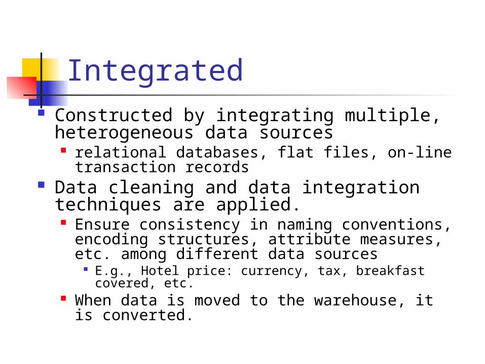
Integrated Constructed by integrating multiple,

heterogeneous data sources relational databases, flat files, on-line

transaction records Data cleaning and data integration

techniques are applied. Ensure consistency in naming conventions,

encoding structures, attribute measures, etc. among different data sources

E.g., Hotel price: currency, tax, breakfast covered, etc.

When data is moved to the warehouse, it is converted.

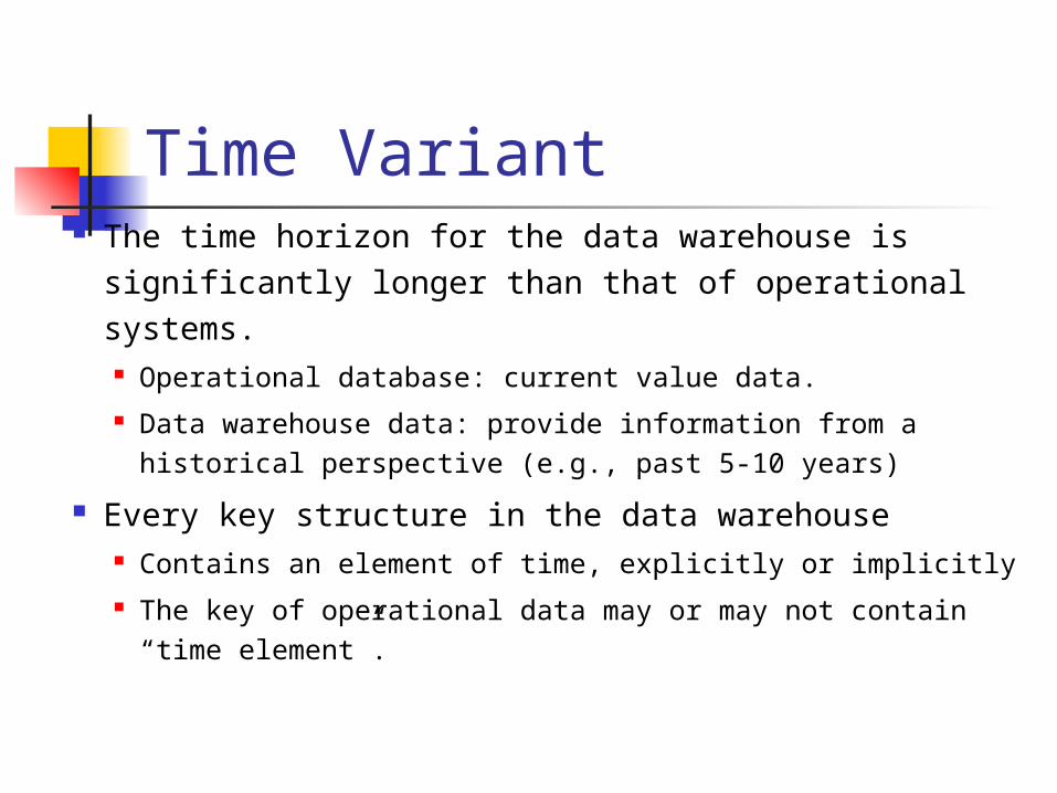
Time Variant The time horizon for the data warehouse is

significantly longer than that of operational systems. Operational database: current value data. Data warehouse data: provide information from a

historical perspective (e.g., past 5-10 years)

Every key structure in the data warehouse Contains an element of time, explicitly or implicitly The key of operational data may or may not contain

“time element”.

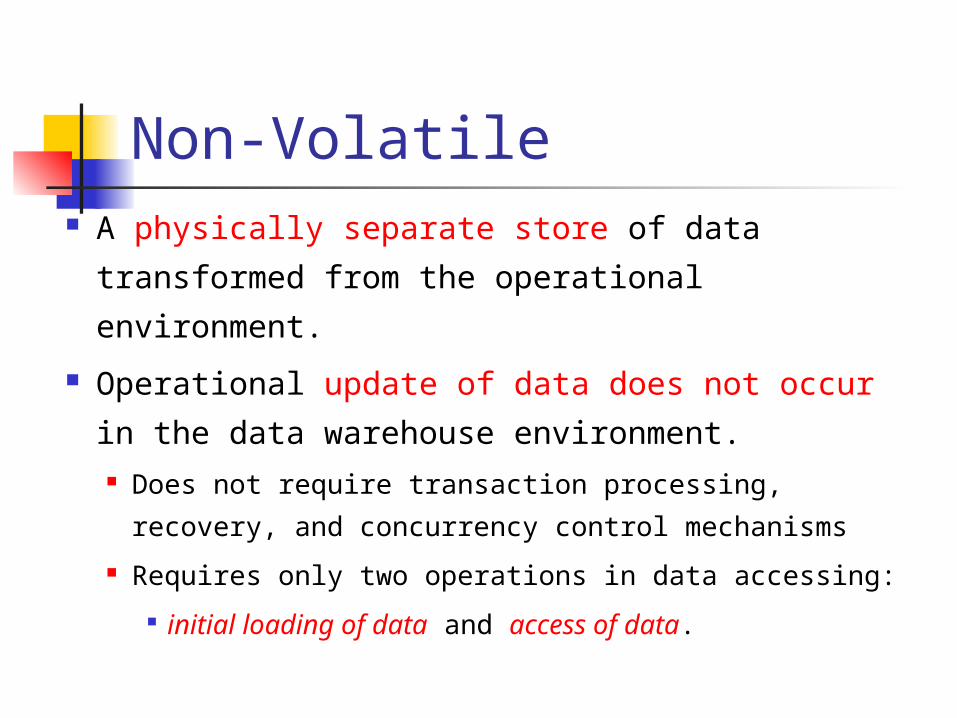
Non-Volatile A physically separate store of data transformed

from the operational environment.

Operational update of data does not occur in

the data warehouse environment. Does not require transaction processing, recovery,

and concurrency control mechanisms

Requires only two operations in data accessing:

initial loading of data and access of data.

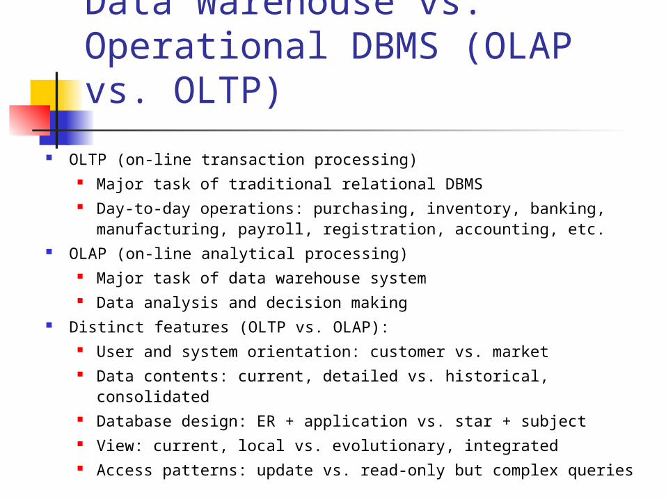
Data Warehouse vs. Operational DBMS (OLAP vs. OLTP)

OLTP (on-line transaction processing) Major task of traditional relational DBMS Day-to-day operations: purchasing, inventory, banking,

manufacturing, payroll, registration, accounting, etc. OLAP (on-line analytical processing)

Major task of data warehouse system Data analysis and decision making

Distinct features (OLTP vs. OLAP): User and system orientation: customer vs. market Data contents: current, detailed vs. historical, consolidated Database design: ER + application vs. star + subject View: current, local vs. evolutionary, integrated Access patterns: update vs. read-only but complex queries

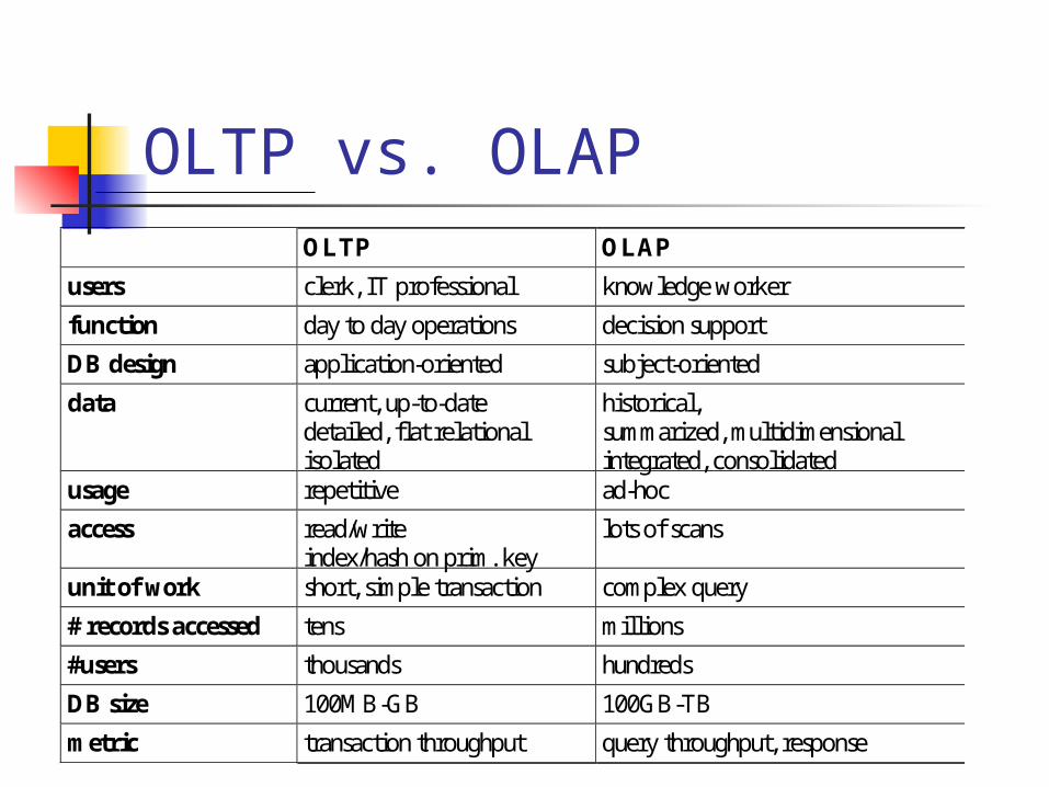
OLTP vs. OLAP OLTP OLAP

users clerk, IT professional knowledge worker

function day to day operations decision support

DB design application-oriented subject-oriented

data current, up-to-date detailed, flat relational isolated

historical, summarized, multidimensional integrated, consolidated

usage repetitive ad-hoc

access read/write index/hash on prim. key

lots of scans

unit of work short, simple transaction complex query

# records accessed tens millions

#users thousands hundreds

DB size 100MB-GB 100GB-TB

metric transaction throughput query throughput, response

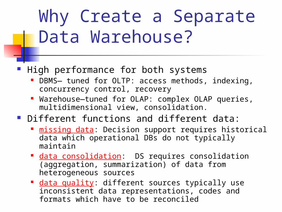
Why Create a Separate Data Warehouse?

High performance for both systems DBMS— tuned for OLTP: access methods, indexing,

concurrency control, recovery Warehouse—tuned for OLAP: complex OLAP queries,

multidimensional view, consolidation. Different functions and different data:

missing data: Decision support requires historical data which operational DBs do not typically maintain

data consolidation: DS requires consolidation (aggregation, summarization) of data from heterogeneous sources

data quality: different sources typically use inconsistent data representations, codes and formats which have to be reconciled

Lecture Outline






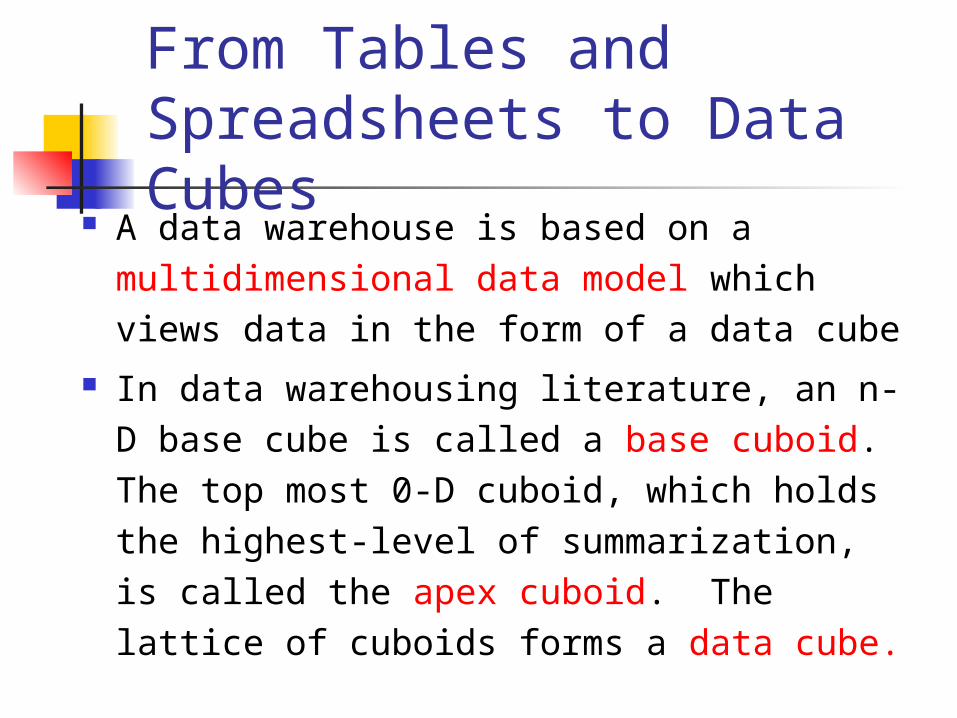
From Tables and Spreadsheets to Data Cubes

A data warehouse is based on a multidimensional data model which views data in the form of a data cube

In data warehousing literature, an n-D base cube is called a base cuboid. The top most 0-D cuboid, which holds the highest-level of summarization, is called the apex cuboid. The lattice of cuboids forms a data cube.

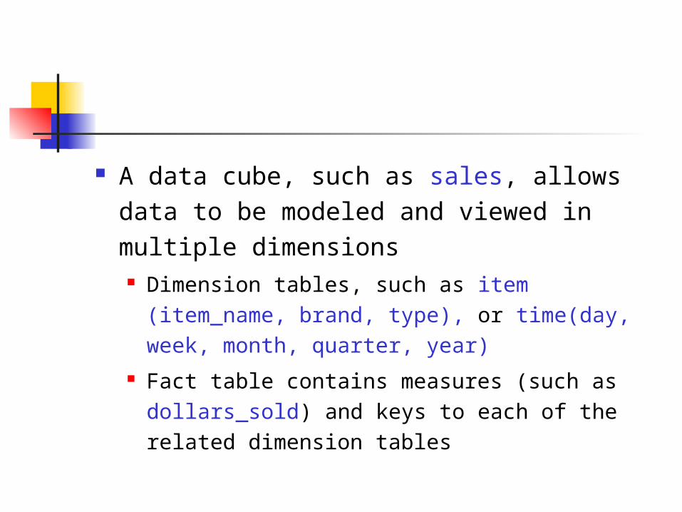
A data cube, such as sales, allows data to be modeled and viewed in multiple dimensions Dimension tables, such as item (item_name,

brand, type), or time(day, week, month, quarter, year)

Fact table contains measures (such as dollars_sold) and keys to each of the related dimension tables

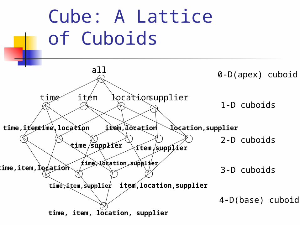
Cube: A Lattice of Cuboids

all

time item location supplier

time,item time,location

time,supplier

item,location

item,supplier

location,supplier

time,item,location

time,item,supplier

time,location,supplier

item,location,supplier

time, item, location, supplier

0-D(apex) cuboid

1-D cuboids

2-D cuboids

3-D cuboids

4-D(base) cuboid

Conceptual Modeling of Data Warehouses

Modeling data warehouses: dimensions & measures Star schema: A fact table in the middle connected to a set of

dimension tables Snowflake schema: A refinement of star schema where some

dimensional hierarchy is normalized into a set of smaller

dimension tables, forming a shape similar to snowflake Fact constellations: Multiple fact tables share dimension

tables, viewed as a collection of stars, therefore called galaxy

schema or fact constellation

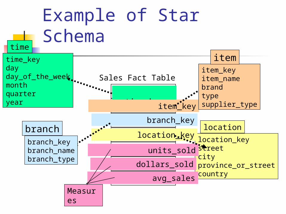
Example of Star Schema time_key

dayday_of_the_weekmonthquarteryear

time

location_keystreetcityprovince_or_streetcountry

location

Sales Fact Table

time_key

item_key

branch_key

location_key

units_sold

dollars_sold

avg_sales

Measures

item_keyitem_namebrandtypesupplier_type

item

branch_keybranch_namebranch_type

branch

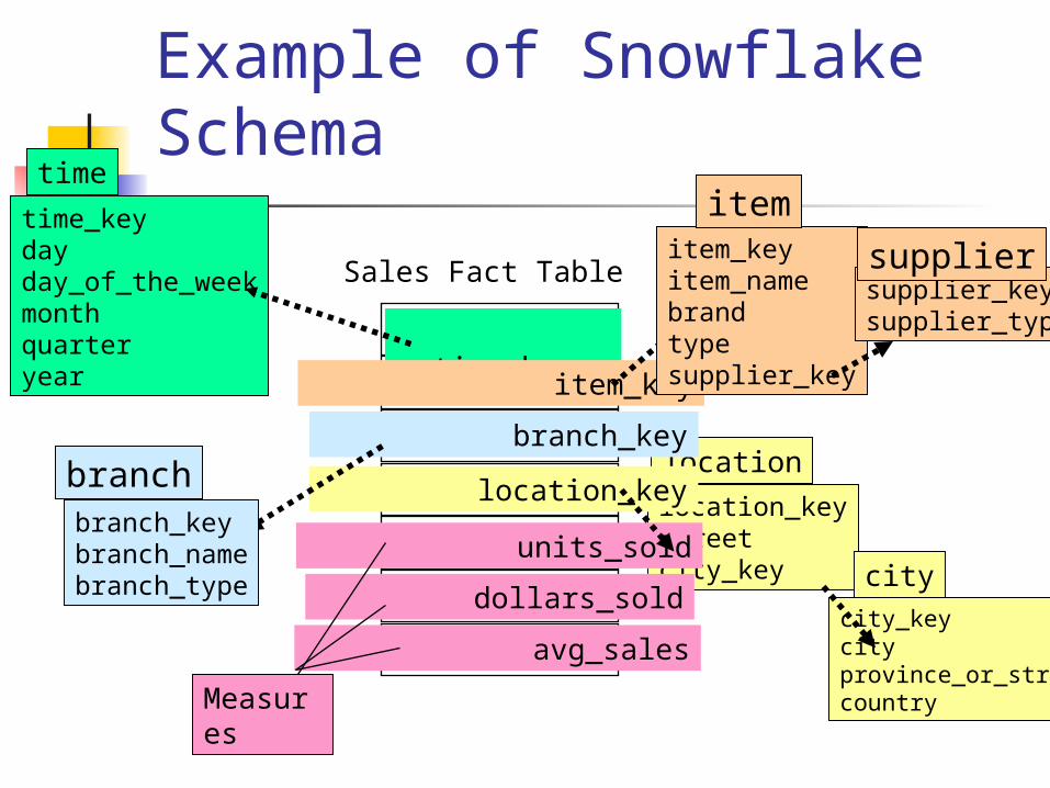
Example of Snowflake Schema

time_keydayday_of_the_weekmonthquarteryear

time

location_keystreetcity_key

location

Sales Fact Table

time_key

item_key

branch_key

location_key

units_sold

dollars_sold

avg_sales

Measures

item_keyitem_namebrandtypesupplier_key

item


branch

supplier_keysupplier_type

supplier

city_keycityprovince_or_streetcountry

city

Note that the only difference between star and snowflake schemas is the normalization of one or more dimension tables, thus reducing redundancy.

Is that worth it? Since dimension tables are small compared to fact tables, the saving in space turns out to be negligible.

In addition, the need for extra joins introduced by the normalization reduces the computational efficiency. For this reason, the snowflake schema model is not as popular as the star schema model.

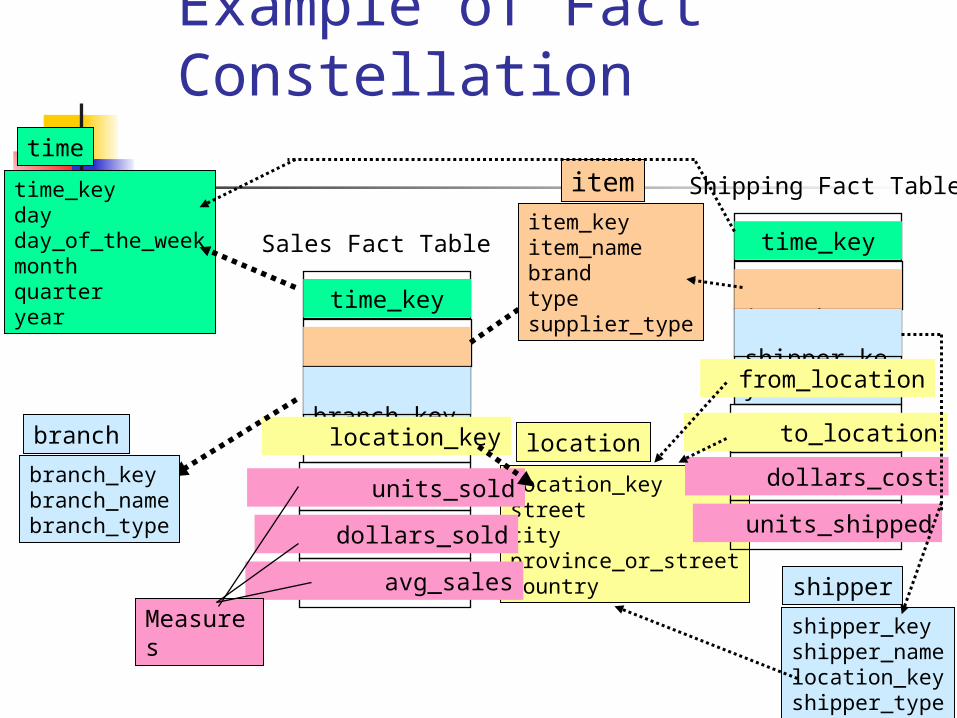
Example of Fact Constellation

time_keydayday_of_the_weekmonthquarteryear

time

location_keystreetcityprovince_or_streetcountry

location

Sales Fact Table

time_key

item_key

branch_key

location_key

units_sold

dollars_sold

avg_sales

Measures

item_keyitem_namebrandtypesupplier_type

item


branch

Shipping Fact Table

time_key

item_key

shipper_key

from_location

to_location

dollars_cost

units_shipped

shipper_keyshipper_namelocation_keyshipper_type

shipper

Note that those designs apply to data warehouses as well as to data marts.

A data warehouse spans an entire enterprise while a data mart is restricted to a single department and is usually a subset of the data warehouse.

The star and snowflakes are more popular for data marts, since they model single objects, with the former being more efficient for the same reasons discussed above.

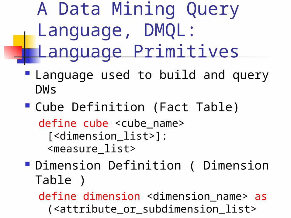
A Data Mining Query Language, DMQL: Language Primitives

Language used to build and query DWs

Cube Definition (Fact Table)define cube <cube_name>

[<dimension_list>]: <measure_list>

Dimension Definition ( Dimension Table )define dimension <dimension_name> as

(<attribute_or_subdimension_list>

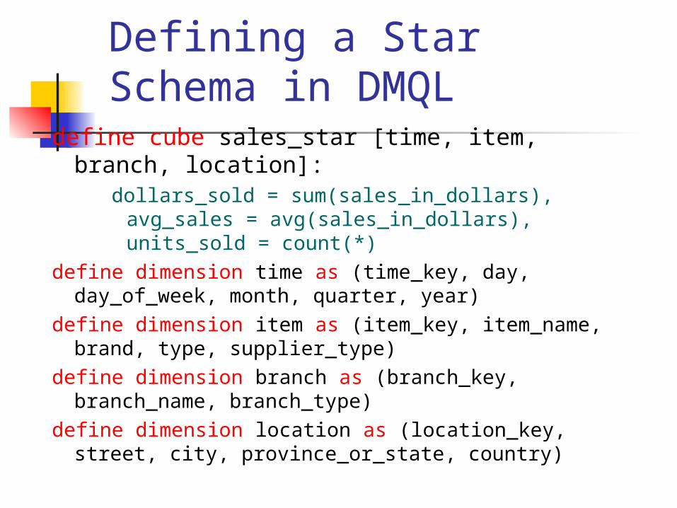
Defining a Star Schema in DMQL

define cube sales_star [time, item, branch, location]:

dollars_sold = sum(sales_in_dollars), avg_sales = avg(sales_in_dollars), units_sold = count(*)

define dimension time as (time_key, day, day_of_week, month, quarter, year)

define dimension item as (item_key, item_name, brand, type, supplier_type)

define dimension branch as (branch_key, branch_name, branch_type)

define dimension location as (location_key, street, city, province_or_state, country)

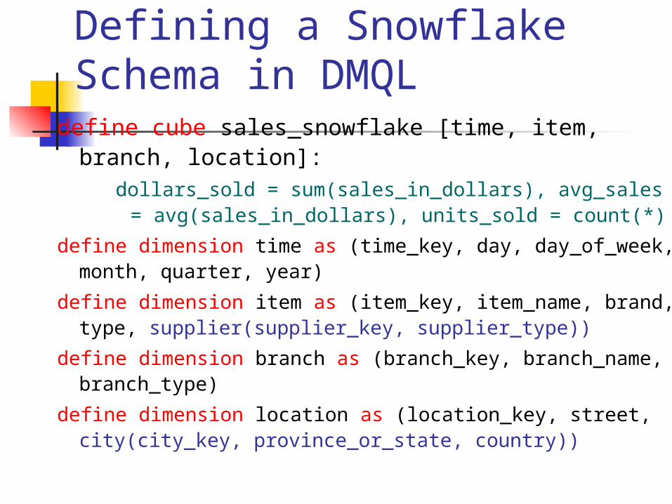
Defining a Snowflake Schema in DMQL

define cube sales_snowflake [time, item, branch, location]:

dollars_sold = sum(sales_in_dollars), avg_sales = avg(sales_in_dollars), units_sold = count(*)

define dimension time as (time_key, day, day_of_week, month, quarter, year)

define dimension item as (item_key, item_name, brand, type, supplier(supplier_key, supplier_type))

define dimension branch as (branch_key, branch_name, branch_type)

define dimension location as (location_key, street, city(city_key, province_or_state, country))

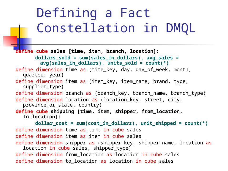
Defining a Fact Constellation in DMQL

define cube sales [time, item, branch, location]:dollars_sold = sum(sales_in_dollars), avg_sales =

avg(sales_in_dollars), units_sold = count(*)define dimension time as (time_key, day, day_of_week, month, quarter,

year)define dimension item as (item_key, item_name, brand, type, supplier_type)define dimension branch as (branch_key, branch_name, branch_type)define dimension location as (location_key, street, city, province_or_state,

country)define cube shipping [time, item, shipper, from_location,

to_location]:dollar_cost = sum(cost_in_dollars), unit_shipped = count(*)

define dimension time as time in cube salesdefine dimension item as item in cube salesdefine dimension shipper as (shipper_key, shipper_name, location as

location in cube sales, shipper_type)define dimension from_location as location in cube salesdefine dimension to_location as location in cube sales

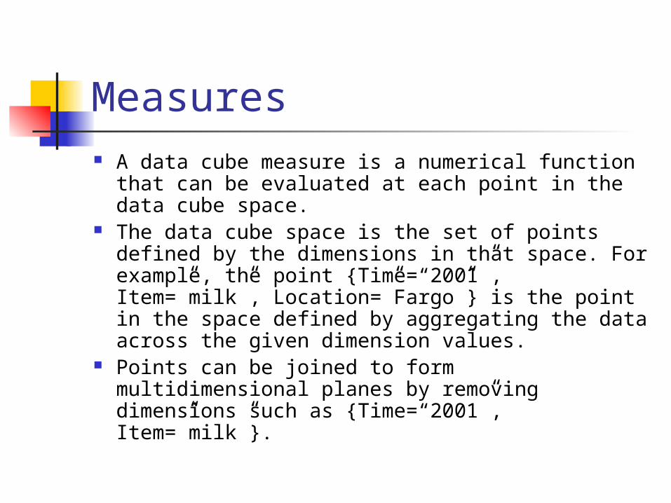
Measures A data cube measure is a numerical function

that can be evaluated at each point in the data cube space.

The data cube space is the set of points defined by the dimensions in that space. For example, the point {Time=“2001”, Item=”milk”, Location=”Fargo”} is the point in the space defined by aggregating the data across the given dimension values.

Points can be joined to form multidimensional planes by removing dimensions such as {Time=“2001”, Item=”milk”}.

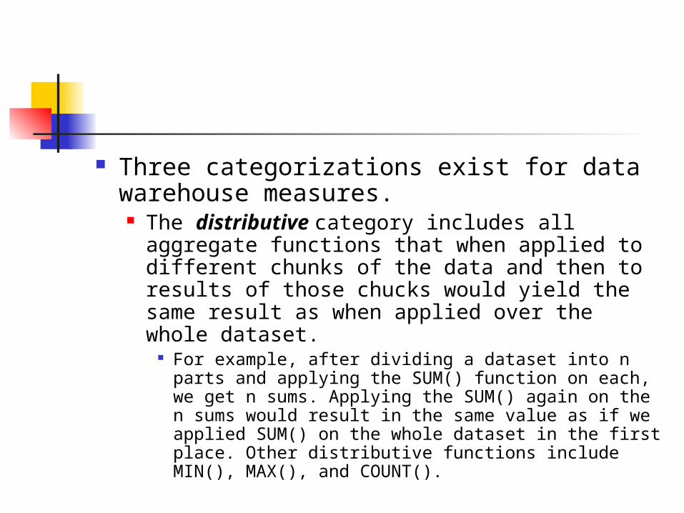
Three categorizations exist for data warehouse measures. The distributive category includes all

aggregate functions that when applied to different chunks of the data and then to results of those chucks would yield the same result as when applied over the whole dataset.

For example, after dividing a dataset into n parts and applying the SUM() function on each, we get n sums. Applying the SUM() again on the n sums would result in the same value as if we applied SUM() on the whole dataset in the first place. Other distributive functions include MIN(), MAX(), and COUNT().

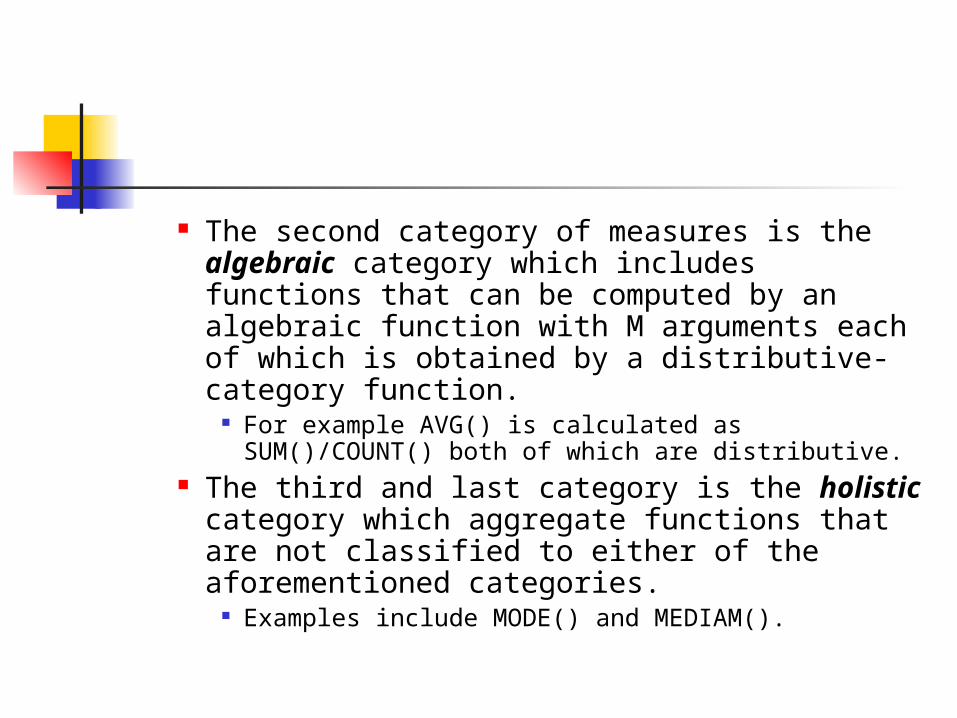
The second category of measures is the algebraic category which includes functions that can be computed by an algebraic function with M arguments each of which is obtained by a distributive-category function.

For example AVG() is calculated as SUM()/COUNT() both of which are distributive.

The third and last category is the holistic category which aggregate functions that are not classified to either of the aforementioned categories.

Examples include MODE() and MEDIAM().

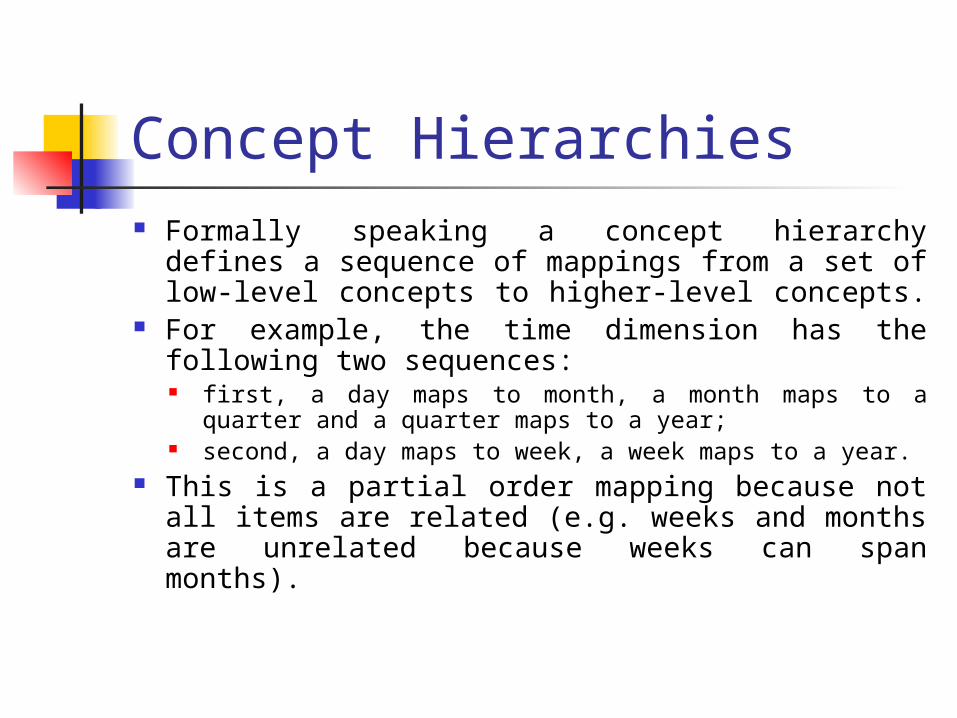
Concept Hierarchies Formally speaking a concept hierarchy defines

a sequence of mappings from a set of low-level concepts to higher-level concepts.

For example, the time dimension has the following two sequences:

first, a day maps to month, a month maps to a quarter and a quarter maps to a year;

second, a day maps to week, a week maps to a year. This is a partial order mapping because not all

items are related (e.g. weeks and months are unrelated because weeks can span months).

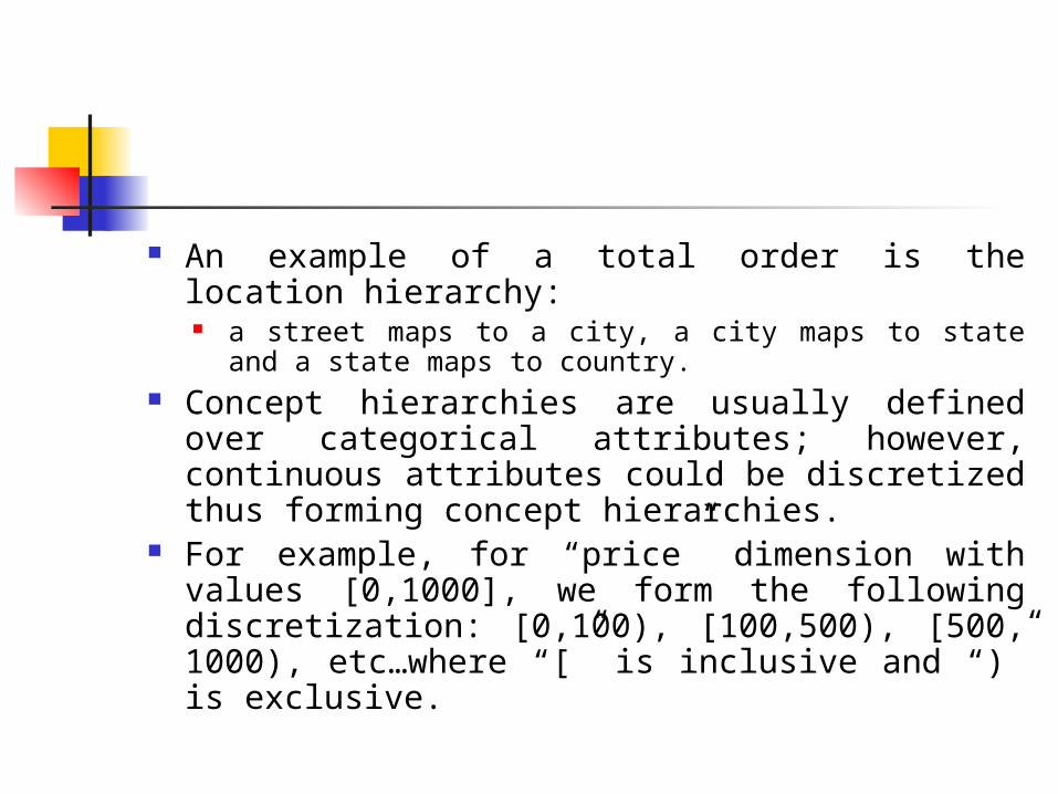
An example of a total order is the location hierarchy:

a street maps to a city, a city maps to state and a state maps to country.

Concept hierarchies are usually defined over categorical attributes; however, continuous attributes could be discretized thus forming concept hierarchies.

For example, for “price” dimension with values [0,1000], we form the following discretization: [0,100), [100,500), [500, 1000), etc…where “[” is inclusive and “)” is exclusive.

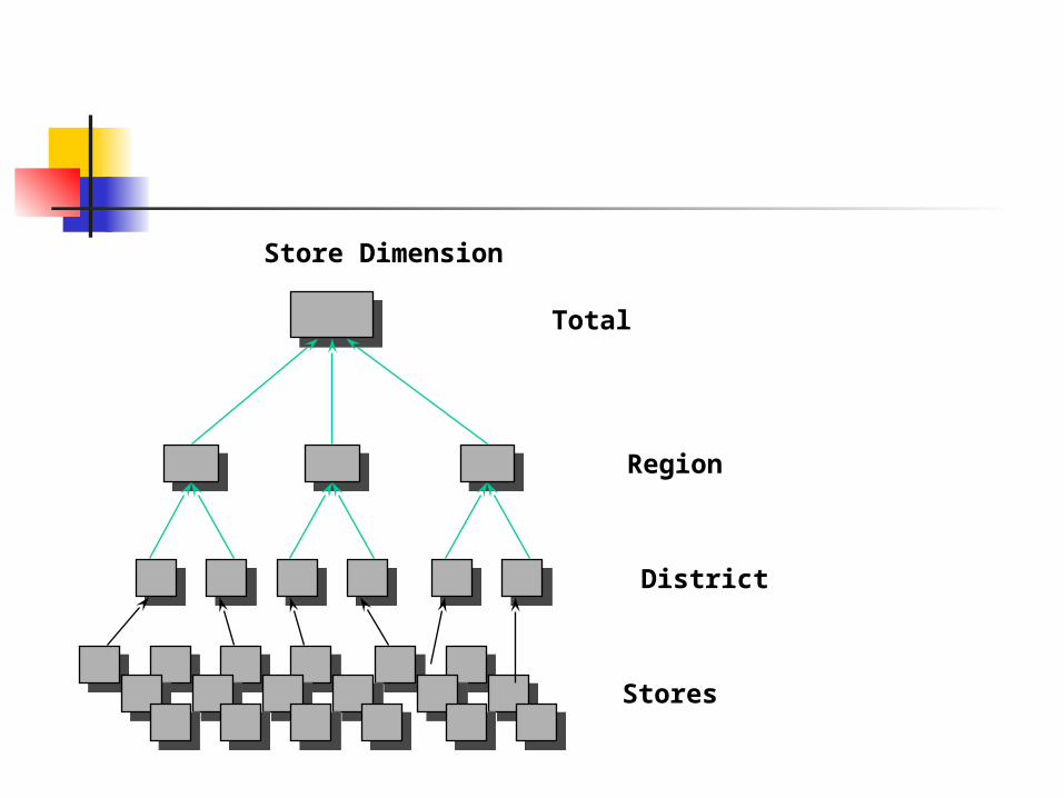
Store Dimension

District

Region

Total

Stores

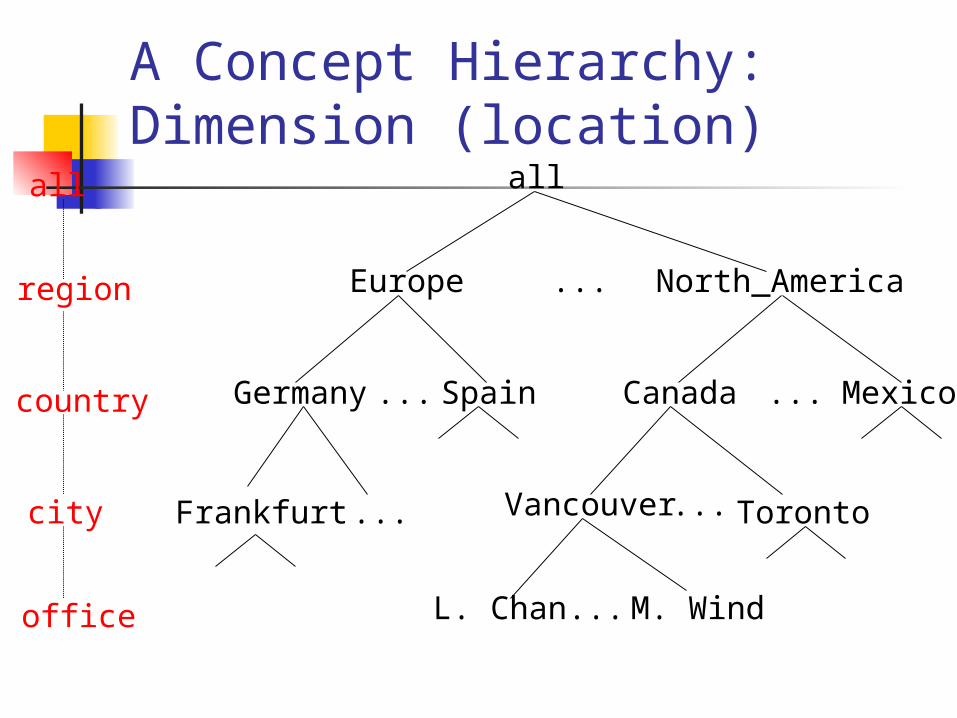
A Concept Hierarchy: Dimension (location)

all

Europe North_America

MexicoCanadaSpainGermany

Vancouver

M. WindL. Chan

...

......

... ...

...

all

region

office

country

TorontoFrankfurtcity

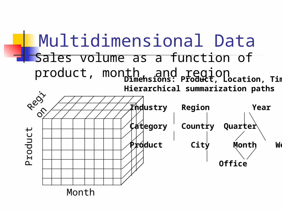
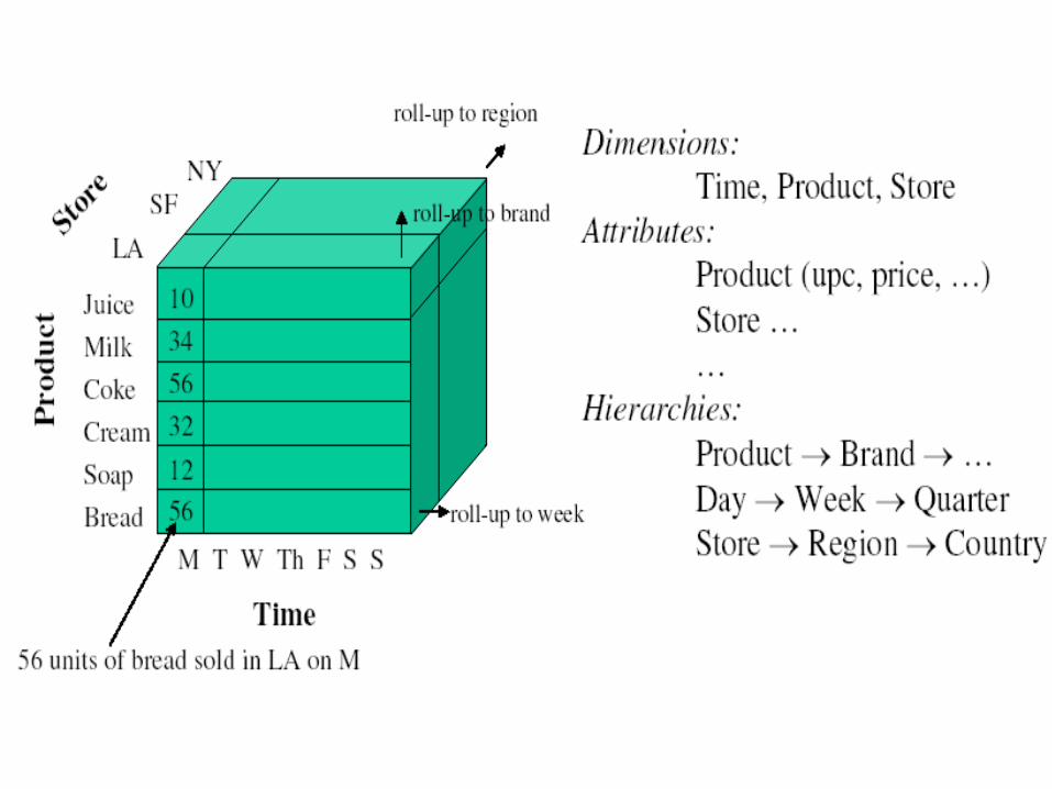
Multidimensional Data Sales volume as a function of

product, month, and region

Pro

duct

Regio

n

Month

Dimensions: Product, Location, TimeHierarchical summarization paths

Industry Region Year

Category Country Quarter

Product City Month Week

Office Day

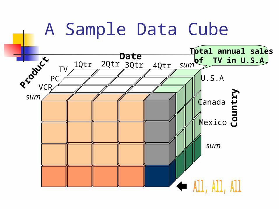
A Sample Data CubeTotal annual salesof TV in U.S.A.Date

Produ

ct

Cou

ntr

ysum

sum TV

VCRPC

1Qtr 2Qtr 3Qtr 4Qtr

U.S.A

Canada

Mexico

sum

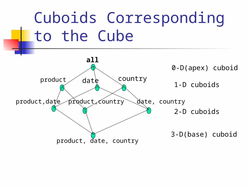
Cuboids Corresponding to the Cube

all

product date country

product,date product,country date, country

product, date, country

0-D(apex) cuboid

1-D cuboids

2-D cuboids

3-D(base) cuboid

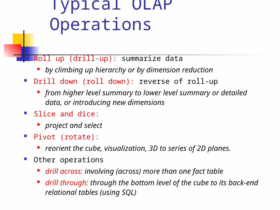
Typical OLAP Operations

Roll up (drill-up): summarize data by climbing up hierarchy or by dimension reduction

Drill down (roll down): reverse of roll-up from higher level summary to lower level summary or

detailed data, or introducing new dimensions Slice and dice:

project and select Pivot (rotate):

reorient the cube, visualization, 3D to series of 2D planes. Other operations

drill across: involving (across) more than one fact table drill through: through the bottom level of the cube to its

back-end relational tables (using SQL)

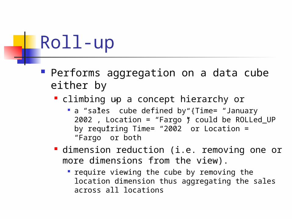
Roll-up Performs aggregation on a data cube

either by climbing up a concept hierarchy or

a “sales” cube defined by {Time= “January 2002”, Location = “Fargo”} could be ROLLed_UP by requiring Time= “2002” or Location = “Fargo” or both

dimension reduction (i.e. removing one or more dimensions from the view).

require viewing the cube by removing the location dimension thus aggregating the sales across all locations

Drill-down Just the opposite of the ROLL-UP operation. navigates from more detailed to less detailed

data views by either stepping down a concept hierarchy or introducing additional dimensions.

a “sales” cube defined by {Time= “January 2002”, Location = “Fargo”} could be DRILLed_DOWN by requiring Time= “24 January 2002” or Location = “Cass County Fargo” or both.

To DOWN-UP by dimension addition, we could require viewing the cube by adding the item dimension

The SLICE operation performs selections on one dimension of a given cube. For example, we can slice over time= “2001” which will give us subcube with time= “2001”.

Similarly, DICE performs selections on but on more than one dimension.

Lecture Outline






Building a Data Warehouse As aforementioned, the process

creating of a warehouse goes through the steps of: data cleaning, data integration, data transformation, data loading and refreshing

Before creating the data warehouse, a design phase usually occurs.

Designing warehouses follows software engineering design standards.

Data Warehouse Design Top-down, bottom-up approaches or a combination of both

Top-down: Starts with overall design and planning (mature) Bottom-up: Starts with experiments and prototypes (rapid)

The most two ubiquitous design models are waterfall and spiral model.

The waterfall model has a number of phases and proceeds from a new phase after

completing of the current phase. rather static and does not give a lot of flexibility for change and only suitable for systems with well-known requirements as in bottom-up

designs. The spiral model

based on incremental development of the data warehouse. A prototype of a part is built, evaluated, modified and then integrated

into the final system. much more flexible in allowing change and is thus more fit to designs

without well-known requirements as in top-down designs. In practice, a combination of both though what is known as

the combined approach is the best solution.

In order to design a data warehouse, we need to follow a certain number of steps: understand the business process we are

modeling, select the fact table (s) by viewing the data at

the atomic level, select the dimensions over which you are

trying to view the data in the fact table(s) and finally choose the measure of interest such as

“amount sold” or “dollars sold”.

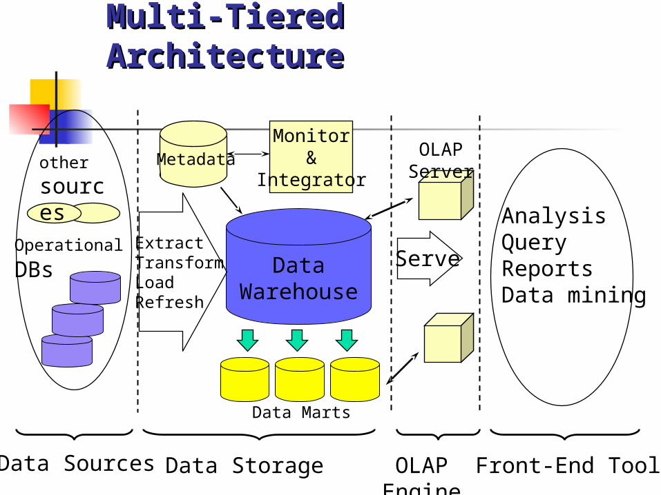
Multi-Tiered ArchitectureMulti-Tiered Architecture

DataWarehouse

ExtractTransformLoadRefresh

OLAP Engine

AnalysisQueryReportsData mining

Monitor&

IntegratorMetadata

Data Sources Front-End Tools

Serve

Data Marts

Operational DBs

other

sources

Data Storage

OLAP Server

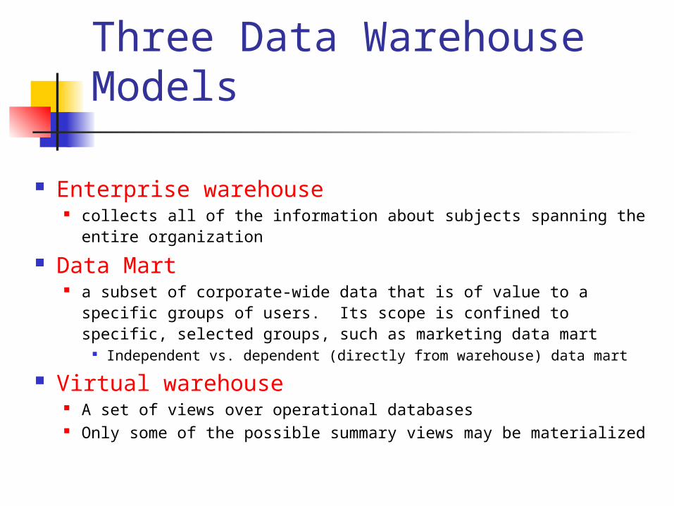
Three Data Warehouse Models

Enterprise warehouse collects all of the information about subjects spanning the entire

organization

Data Mart a subset of corporate-wide data that is of value to a specific

groups of users. Its scope is confined to specific, selected groups, such as marketing data mart

Independent vs. dependent (directly from warehouse) data mart

Virtual warehouse A set of views over operational databases Only some of the possible summary views may be materialized

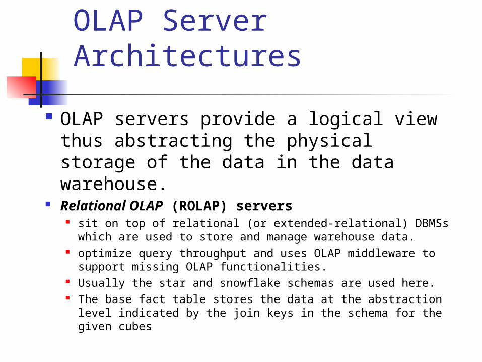
OLAP Server Architectures

OLAP servers provide a logical view thus abstracting the physical storage of the data in the data warehouse.

Relational OLAP (ROLAP) servers sit on top of relational (or extended-relational) DBMSs

which are used to store and manage warehouse data. optimize query throughput and uses OLAP middleware

to support missing OLAP functionalities. Usually the star and snowflake schemas are used here. The base fact table stores the data at the abstraction

level indicated by the join keys in the schema for the given cubes

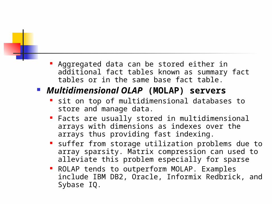
Aggregated data can be stored either in additional fact tables known as summary fact tables or in the same base fact table.

Multidimensional OLAP (MOLAP) servers sit on top of multidimensional databases to store and

manage data. Facts are usually stored in multidimensional arrays

with dimensions as indexes over the arrays thus providing fast indexing.

suffer from storage utilization problems due to array sparsity. Matrix compression can used to alleviate this problem especially for sparse

ROLAP tends to outperform MOLAP. Examples include IBM DB2, Oracle, Informix Redbrick, and Sybase IQ.

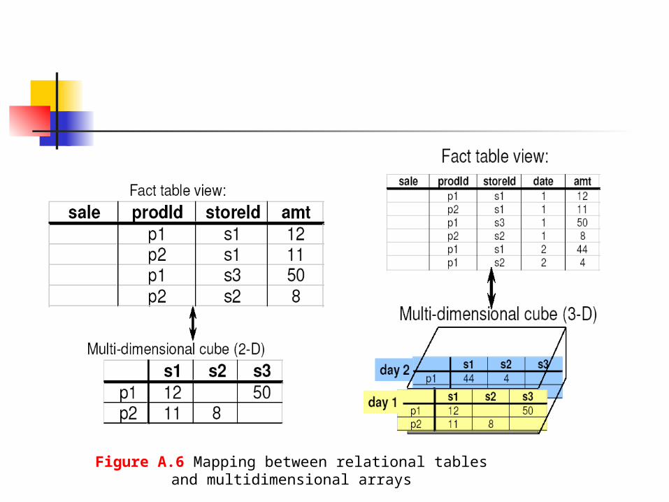
Figure A.6 Mapping between relational tables and multidimensional

arrays

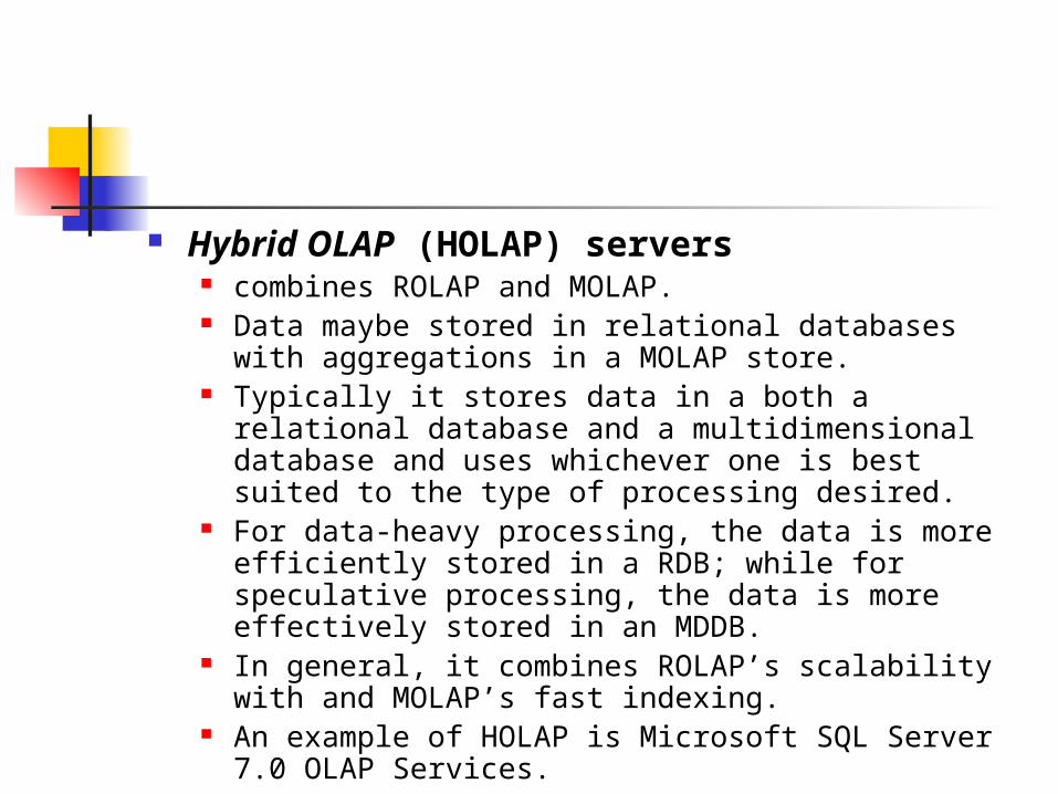
Hybrid OLAP (HOLAP) servers combines ROLAP and MOLAP. Data maybe stored in relational databases with

aggregations in a MOLAP store. Typically it stores data in a both a relational

database and a multidimensional database and uses whichever one is best suited to the type of processing desired.

For data-heavy processing, the data is more efficiently stored in a RDB; while for speculative processing, the data is more effectively stored in an MDDB.

In general, it combines ROLAP’s scalability with and MOLAP’s fast indexing.

An example of HOLAP is Microsoft SQL Server 7.0 OLAP Services.

Lecture Outline






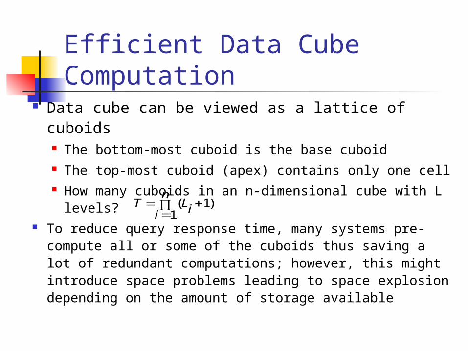
Efficient Data Cube Computation

Data cube can be viewed as a lattice of cuboids The bottom-most cuboid is the base cuboid The top-most cuboid (apex) contains only one cell How many cuboids in an n-dimensional cube with

L levels? To reduce query response time, many systems pre-

compute all or some of the cuboids thus saving a lot of redundant computations; however, this might introduce space problems leading to space explosion depending on the amount of storage available

)11(

n

i iLT

To compromise between time and space, OLAP designers are usually faced with three options: the no materialization option pre-computes no

cuboids ahead of time thus saving a lot space but lagging behind on speed

the full materialization option pre-computes all possible cuboids ahead of time thus saving a lot of time but most probably facing space explosion

the partial materialization options selects a subset of cuboids to materialize and use them to save time in computing other non materialized cuboids

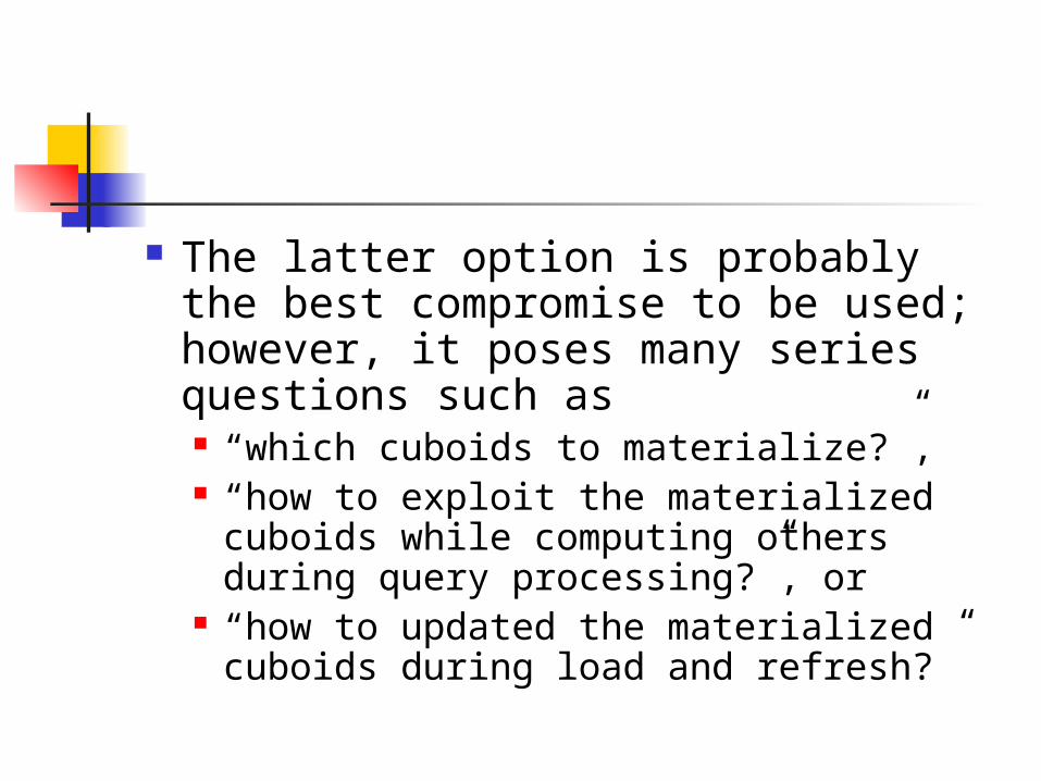
The latter option is probably the best compromise to be used; however, it poses many series questions such as “which cuboids to materialize?”, “how to exploit the materialized

cuboids while computing others during query processing?”, or

“how to updated the materialized cuboids during load and refresh?”

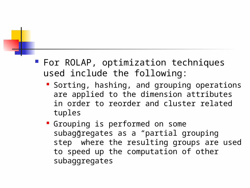
For ROLAP, optimization techniques used include the following: Sorting, hashing, and grouping operations

are applied to the dimension attributes in order to reorder and cluster related tuples

Grouping is performed on some subaggregates as a “partial grouping step” where the resulting groups are used to speed up the computation of other subaggregates

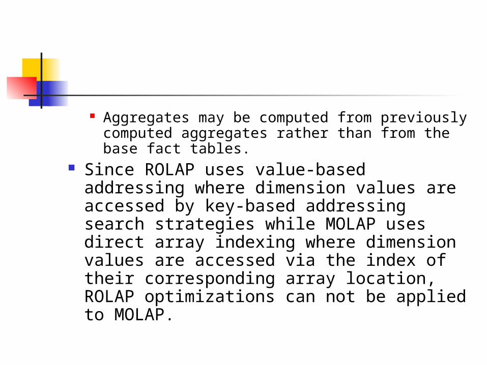
Aggregates may be computed from previously computed aggregates rather than from the base fact tables.

Since ROLAP uses value-based addressing where dimension values are accessed by key-based addressing search strategies while MOLAP uses direct array indexing where dimension values are accessed via the index of their corresponding array location, ROLAP optimizations can not be applied to MOLAP.

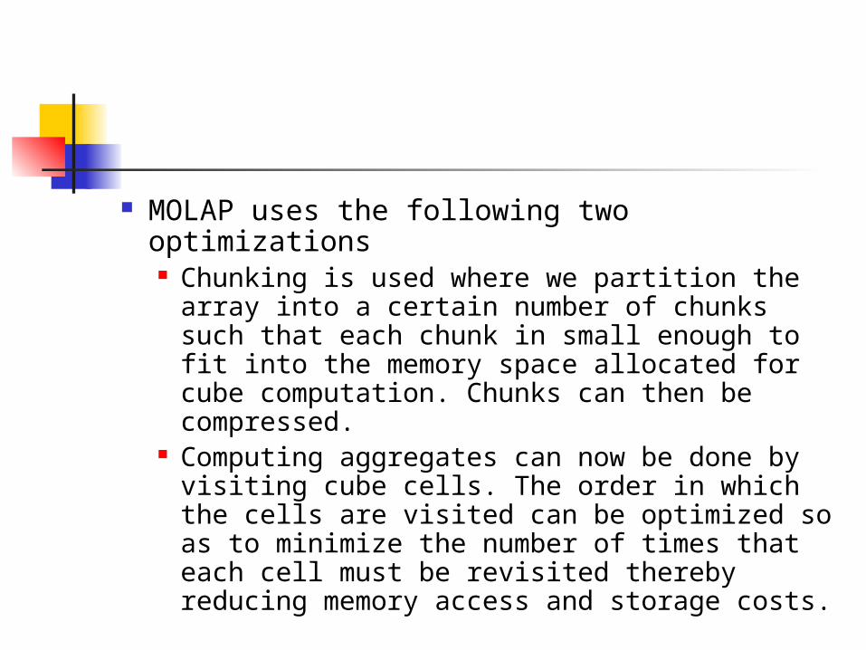
MOLAP uses the following two optimizations Chunking is used where we partition the

array into a certain number of chunks such that each chunk in small enough to fit into the memory space allocated for cube computation. Chunks can then be compressed.

Computing aggregates can now be done by visiting cube cells. The order in which the cells are visited can be optimized so as to minimize the number of times that each cell must be revisited thereby reducing memory access and storage costs.

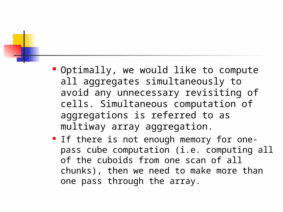
Optimally, we would like to compute all aggregates simultaneously to avoid any unnecessary revisiting of cells. Simultaneous computation of aggregations is referred to as multiway array aggregation.

If there is not enough memory for one-pass cube computation (i.e. computing all of the cuboids from one scan of all chunks), then we need to make more than one pass through the array.

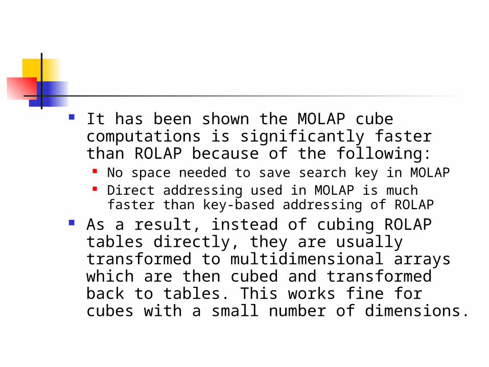
It has been shown the MOLAP cube computations is significantly faster than ROLAP because of the following:

No space needed to save search key in MOLAP Direct addressing used in MOLAP is much faster than

key-based addressing of ROLAP As a result, instead of cubing ROLAP tables

directly, they are usually transformed to multidimensional arrays which are then cubed and transformed back to tables. This works fine for cubes with a small number of dimensions.

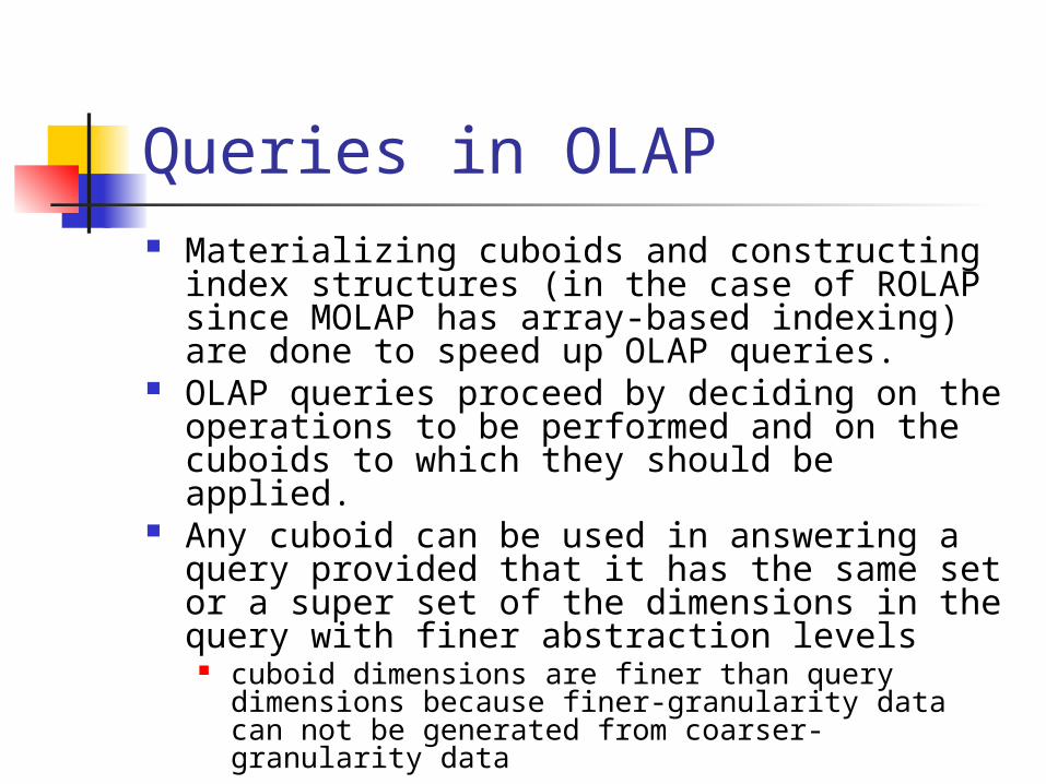
Queries in OLAP Materializing cuboids and constructing index

structures (in the case of ROLAP since MOLAP has array-based indexing) are done to speed up OLAP queries.

OLAP queries proceed by deciding on the operations to be performed and on the cuboids to which they should be applied.

Any cuboid can be used in answering a query provided that it has the same set or a super set of the dimensions in the query with finer abstraction levels

cuboid dimensions are finer than query dimensions because finer-granularity data can not be generated from coarser-granularity data

For ROLAP, join indices, bitmap indices and even bitmapped join indices can be used to optimized query processing.

Lecture Outline






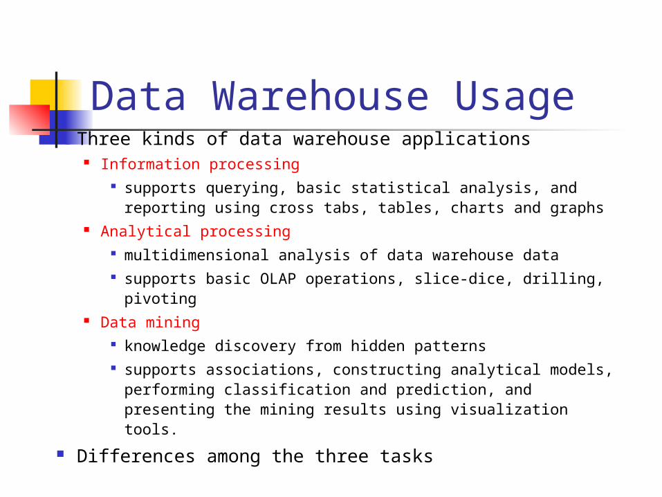
Data Warehouse Usage Three kinds of data warehouse applications

Information processing supports querying, basic statistical analysis, and reporting

using cross tabs, tables, charts and graphs Analytical processing

multidimensional analysis of data warehouse data supports basic OLAP operations, slice-dice, drilling,

pivoting Data mining

knowledge discovery from hidden patterns supports associations, constructing analytical models,

performing classification and prediction, and presenting the mining results using visualization tools.

Differences among the three tasks

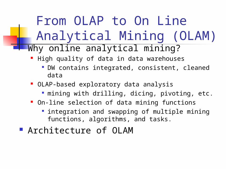
From OLAP to On Line Analytical Mining (OLAM)

Why online analytical mining? High quality of data in data warehouses

DW contains integrated, consistent, cleaned data OLAP-based exploratory data analysis

mining with drilling, dicing, pivoting, etc. On-line selection of data mining functions

integration and swapping of multiple mining functions, algorithms, and tasks.

Architecture of OLAM

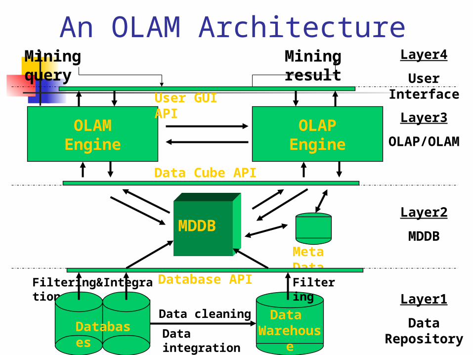
An OLAM Architecture

Data Warehouse

Meta Data

MDDB

OLAMEngine

OLAPEngine

User GUI API

Data Cube API

Database API

Data cleaning

Data integration

Layer3

OLAP/OLAM

Layer2

MDDB

Layer1

Data Repository

Layer4

User Interface

Filtering&Integration Filtering

Databases

Mining query Mining result

Summary Data warehouse

A subject-oriented, integrated, time-variant, and nonvolatile collection of data in support of management’s decision-making process

A multi-dimensional model of a data warehouse Star schema, snowflake schema, fact constellations A data cube consists of dimensions & measures

OLAP operations: drilling, rolling, slicing, dicing and pivoting

OLAP servers: ROLAP, MOLAP, HOLAP Efficient computation of data cubes

Partial vs. full vs. no materialization From OLAP to OLAM (on-line analytical mining)

Documents

Data warehouses and Online Analytical Processing