Database Management Systems: Data Mining

1

Jerry PostCopyright © 2003

Database Management Database Management Systems:Systems:Data MiningData Mining

Data Compression

2

DDAATTAA MMiinniinngg

The Need for Data Compression

Noisy dataNeed to combine data to smooth it (bins)

Too many values in a dimensionNeed to combine data to get smaller number of sets

HierarchiesRollup data into natural hierarchiesCreate additional hierarchies

Data compressionLarge text, images, time series (wavelet compression)

3


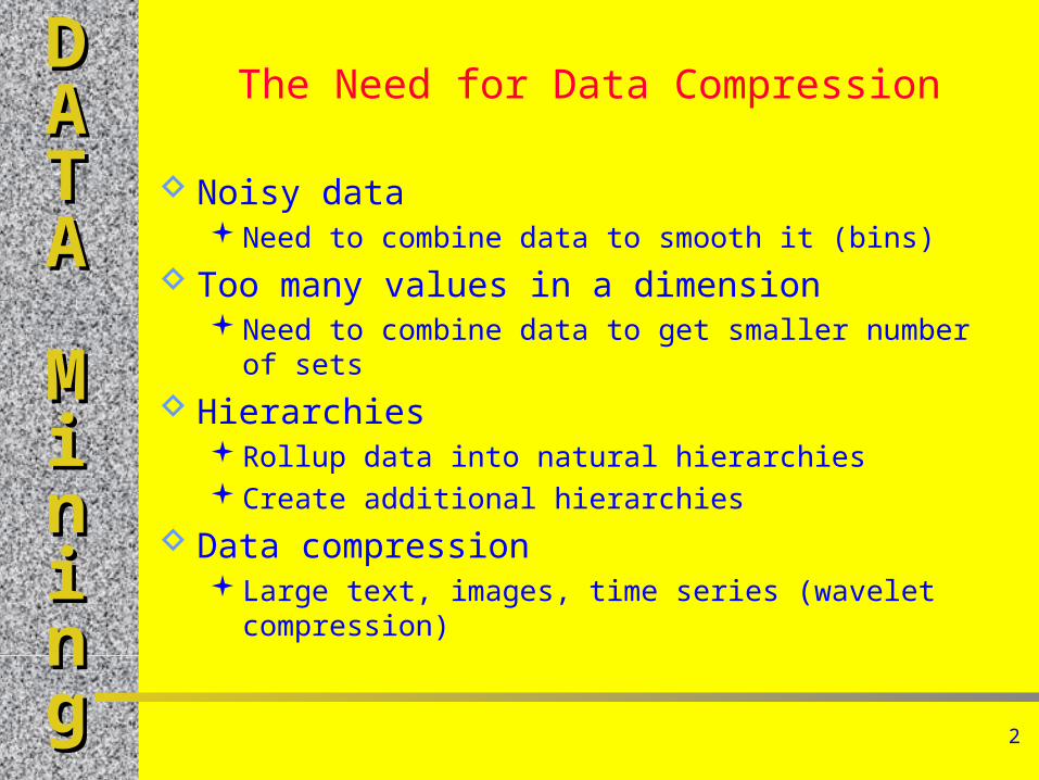
Bins Numerical data Create bins

Equal-depth partitions Equal-width partitions Bin mean/smoothing

Choose number of bins?

Data: 3, 9, 17, 27, 32, 32, 37, 48, 55

Bin 1: 3, 9, 17Bin 2: 27, 32, 32Bin 3: 37, 48, 55

Bin 1: 3 – 20.3 3, 9, 17Bin 2: 20.3 – 37.6 27, 32, 32, 37Bin 3: 37.6 – 55 48, 55

Bin 1: 9.6, 9.6, 9.6Bin 2: 30.3, 30.3, 30.3Bin 3: 46.6, 46.6, 46.6

4


What is Cluster Analysis?

The process of placing items into groups, where items within a group are similar to each other, and dissimilar to items in other groups.

Similar to Classification Analysis, but in classification, the group characteristics are known in advance (e.g., borrowers who successfully repaid loans).

5


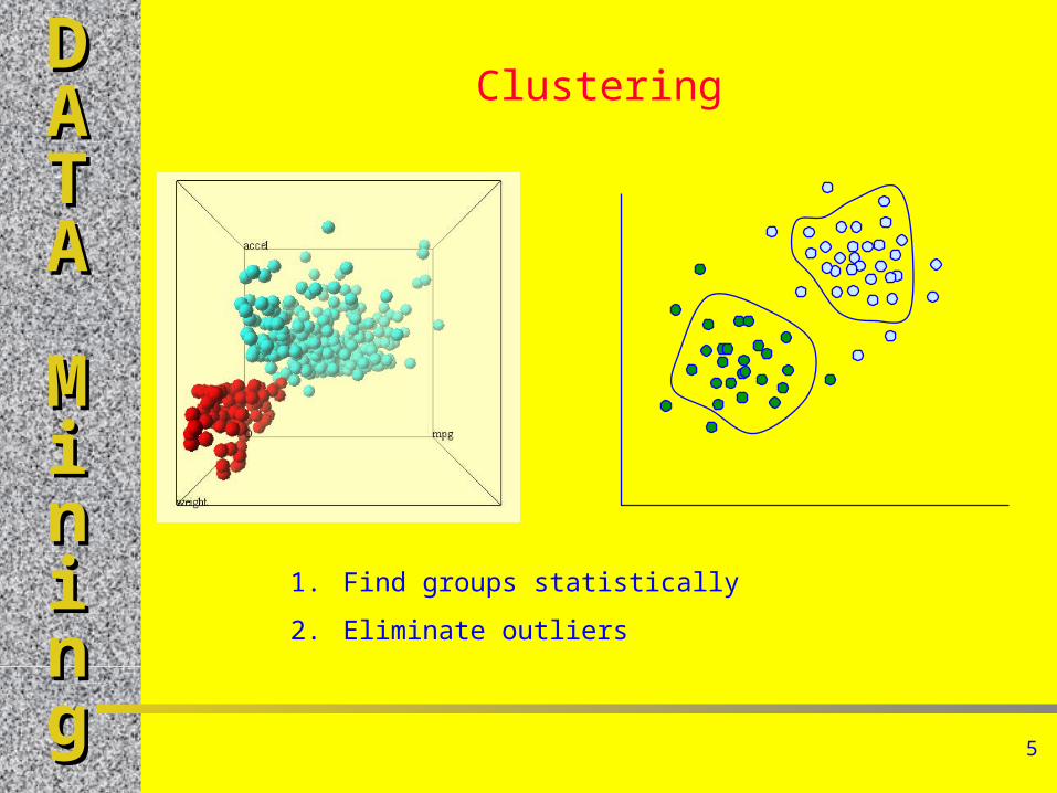
Clustering

1. Find groups statistically

2. Eliminate outliers

6


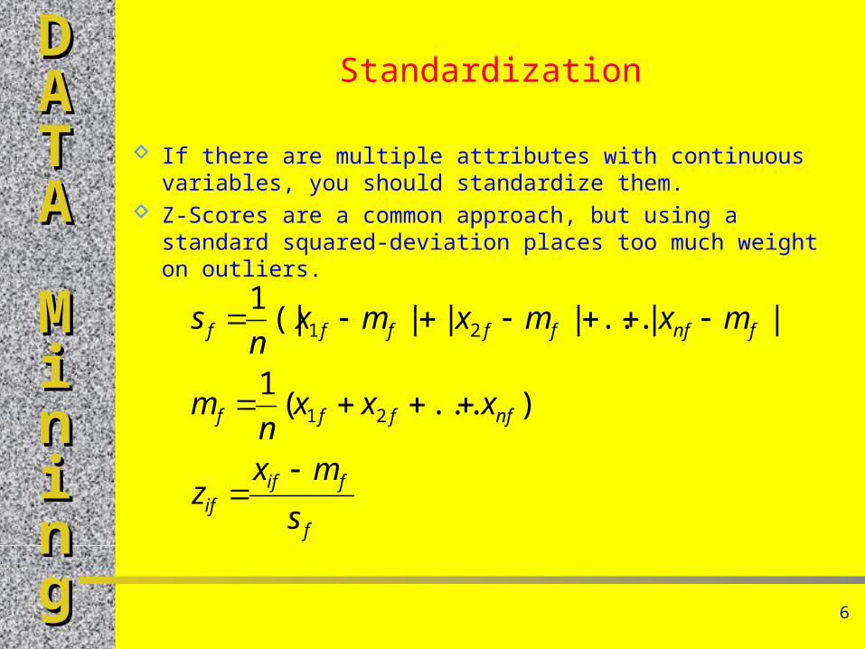
Standardization

If there are multiple attributes with continuous variables, you should standardize them.

Z-Scores are a common approach, but using a standard squared-deviation places too much weight on outliers.

f

fifif

nffff

fnffffff

s

mxz

xxxn

m

mxmxmxn

s

)...(1

|)|...|||(|1

21

21

7


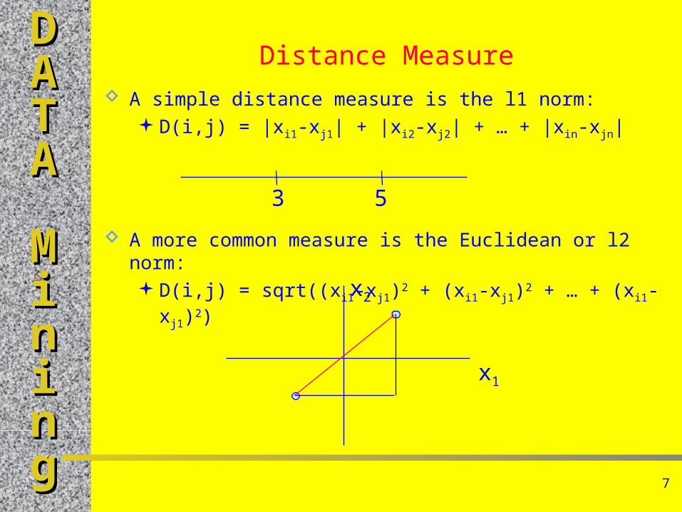
Distance Measure A simple distance measure is the l1 norm:

D(i,j) = |xi1-xj1| + |xi2-xj2| + … + |xin-xjn|

A more common measure is the Euclidean or l2 norm:D(i,j) = sqrt((xi1-xj1)2 + (xi1-xj1)2 + … + (xi1-xj1)2)

3 5

x1

x2

8


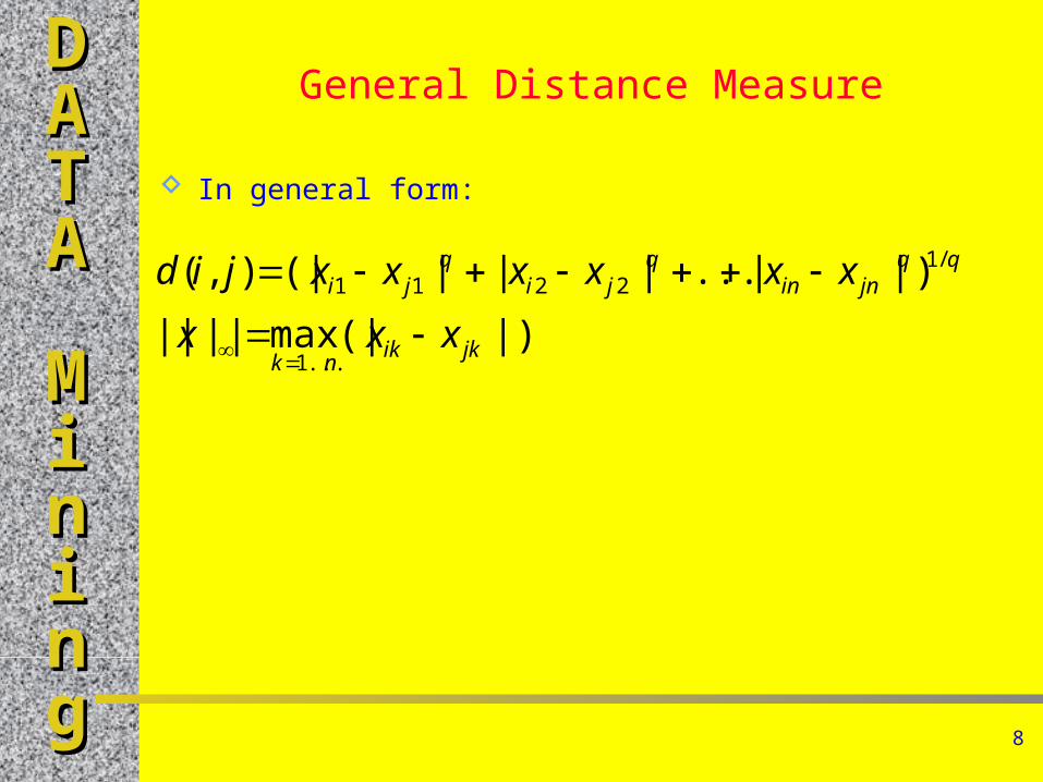
General Distance Measure

In general form:

|)(|max||||

)||...|||(|),(

...1

/12211

jkiknk

qqjnin

qji

qji

xxx

xxxxxxjid

9


Hierarchies

Dates

Year – Quarter – Month – Day

Year – Quarter – Week – Day

Business hierarchies

Division/Product

Function: Marketing, HRM, Production, …

Region

Region hierarchies

World – Continent – Nation – State – City

10


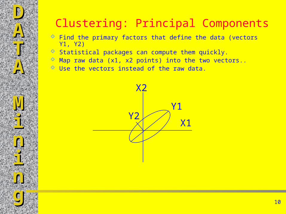
Clustering: Principal Components Find the primary factors that define the data (vectors Y1, Y2) Statistical packages can compute them quickly. Map raw data (x1, x2 points) into the two vectors.. Use the vectors instead of the raw data.

X1

X2

Y1Y2

11


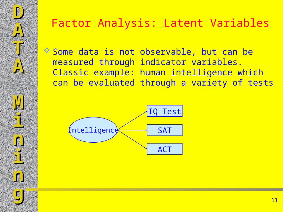
Factor Analysis: Latent Variables

Some data is not observable, but can be measured through indicator variables. Classic example: human intelligence which can be evaluated through a variety of tests

Intelligence

IQ Test

SAT

ACT

12


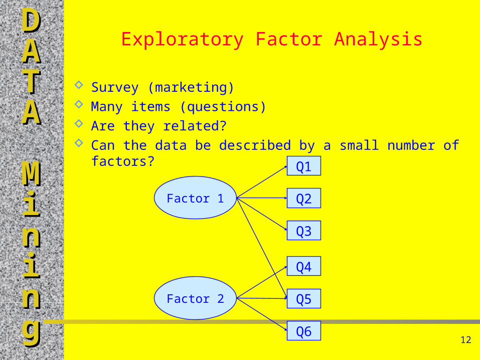
Exploratory Factor Analysis

Survey (marketing) Many items (questions) Are they related? Can the data be described by a small number of factors?

Factor 1

Q1

Q2

Q3

Factor 2

Q4

Q5

Q6

13


Regression to Reduce Values

Estimate regression coefficients If good fit, use the coefficients to pick categories

14


Wavelet Compression

Find patterns (wavelets) in the data Standard compression methods (GIF) Reduces data to a small number of wavelet patterns Particularly useful for complex data

15


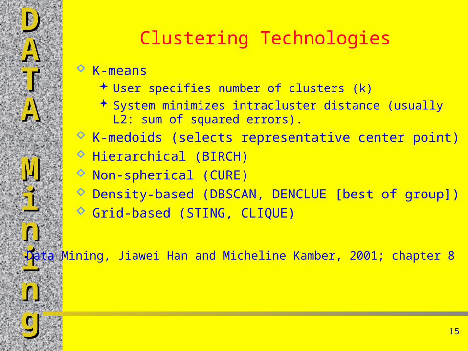
Clustering Technologies

K-means User specifies number of clusters (k) System minimizes intracluster distance (usually L2: sum of squared

errors).

K-medoids (selects representative center point) Hierarchical (BIRCH) Non-spherical (CURE) Density-based (DBSCAN, DENCLUE [best of group]) Grid-based (STING, CLIQUE)

Data Mining, Jiawei Han and Micheline Kamber, 2001; chapter 8

16


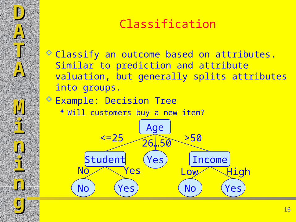
Classification

Classify an outcome based on attributes. Similar to prediction and attribute valuation, but generally splits attributes into groups.

Example: Decision TreeWill customers buy a new item?

Age

Student IncomeYes

No YesNo Yes

<=25 >5026…50

No Yes Low High

17


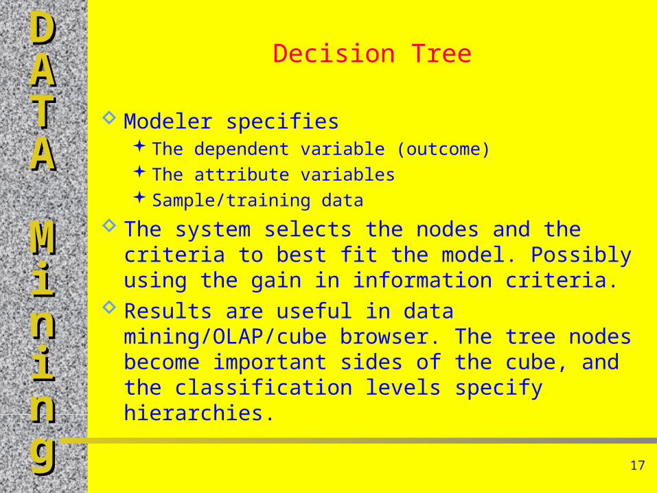
Decision Tree

Modeler specifiesThe dependent variable (outcome)The attribute variablesSample/training data

The system selects the nodes and the criteria to best fit the model. Possibly using the gain in information criteria.

Results are useful in data mining/OLAP/cube browser. The tree nodes become important sides of the cube, and the classification levels specify hierarchies.

18


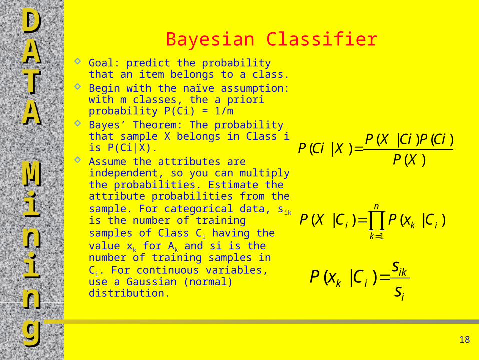
Bayesian Classifier Goal: predict the probability that an

item belongs to a class. Begin with the naïve assumption: with

m classes, the a priori probability P(Ci) = 1/m

Bayes’ Theorem: The probability that sample X belongs in Class i is P(Ci|X).

Assume the attributes are independent, so you can multiply the probabilities. Estimate the attribute probabilities from the sample. For categorical data, sik is the number of training samples of Class Ci having the value xk for Ak and si is the number of training samples in Ci. For continuous variables, use a Gaussian (normal) distribution.

)(

)()|()|(

XP

CiPCiXPXCiP

n

kiki CxPCXP

1

)|()|(

i

ikik s

sCxP )|(

19


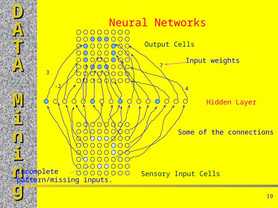
Neural Networks

Output Cells

Sensory Input Cells

Hidden Layer

Some of the connections

3

-2

7

4

Input weights

Incompletepattern/missing inputs.

20


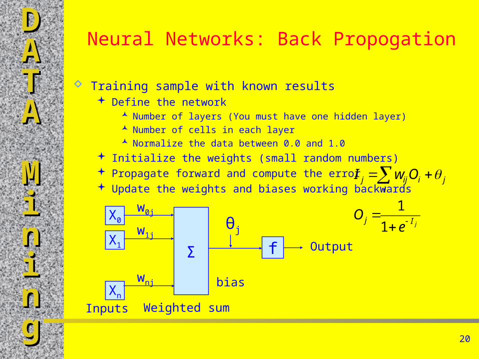
Neural Networks: Back Propogation

Training sample with known results Define the network

Number of layers (You must have one hidden layer) Number of cells in each layer Normalize the data between 0.0 and 1.0

Initialize the weights (small random numbers) Propagate forward and compute the error Update the weights and biases working backwards

X0

X1

Xn

Σ

w0j

w1j

wnj

Inputs Weighted sum

f

bias

θj

Output

jIj

ijiijj

eO

OwI

1

1

21


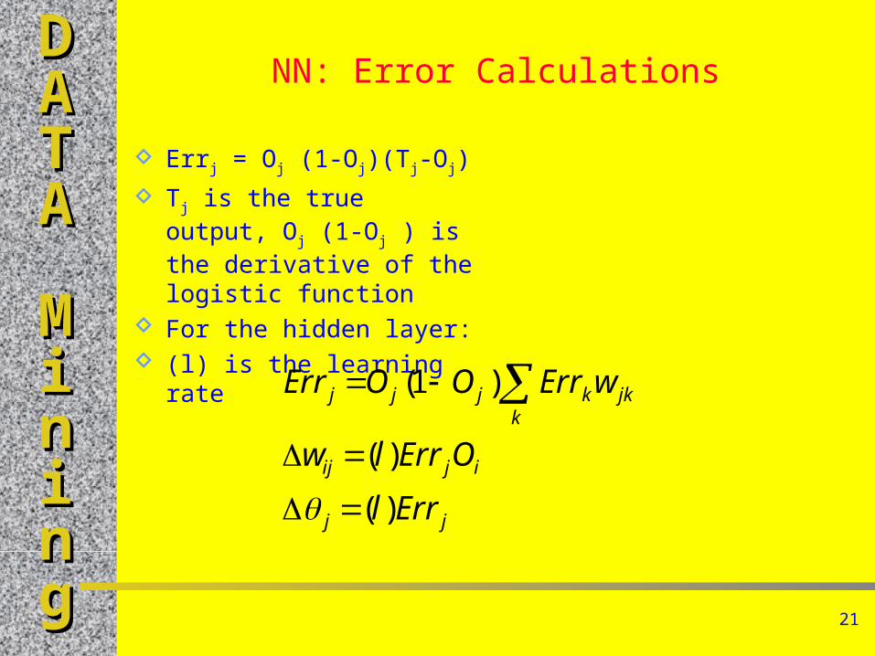
NN: Error Calculations

Errj = Oj (1-Oj)(Tj-Oj)

Tj is the true output, Oj (1-Oj ) is the derivative of the logistic function

For the hidden layer: (l) is the learning rate

jj

ijij

kjkkjjj

Errl

OErrlw

wErrOOErr

)(

)(

)1(

Documents

Database Management Systems: Data Mining