1

Database Management Systems Lecture Notes

UNIT-I

Data:

It is a collection of information.

The facts that can be recorded and which have implicit meaning known as 'data'.

Example:

Customer ----- 1.cname. 2.cno. 3.ccity.

Database:

It is a collection of interrelated data . These can be stored in the form of tables. A database can be of any size and varying complexity.

A database may be generated and manipulated manually or it may be

computerized. Example: Customer database consists the fields as cname, cno, and ccity

Cname Cno Ccity

Database System:

It is computerized system, whose overall purpose is to maintain the information and to make that the information is available on demand.

Advantages:

1.Redundency can be reduced. 2.Inconsistency can be avoided. 3.Data can be shared.

2

4.Standards can be enforced. 5.Security restrictions can be applied. 6.Integrity can be maintained. 7.Data gathering can be possible. 8.Requirements can be balanced.

Database Management System (DBMS):

It is a collection of programs that enables user to create and maintain a database. In other words it is general-purpose software that provides the users with the processes of defining, constructing and manipulating the database for various applications.

Disadvantages in File Processing

Data redundancy and inconsistency.

Difficult in accessing data.

Data isolation.

Data integrity.

Concurrent access is not possible.

Security Problems.

.

Advantages of DBMS:

1.Data Independence.

2.Efficient Data Access.

3.Data Integrity and security.

4.Data administration. 5.Concurrent access and Crash recovery. 6.Reduced Application Development Time.

Applications

Database Applications: Banking: all transactions Airlines: reservations, schedules Universities: registration, grades Sales: customers, products, purchases Online retailers: order tracking, customized recommendations Manufacturing: production, inventory, orders, supply chain Human resources: employee records, salaries, tax deductions

People who deal with databases

Many persons are involved in the design, use and maintenance of any database. These persons can be

classified into 2 types as below. Actors on the scene:

The people, whose jobs involve the day-to-day use of a database are called as 'Actors on the scene', listed as below.

1.Database Administrators (DBA):

The DBA is responsible for authorizing access to the database, for Coordinating and monitoring its use and for acquiring software and hardware resources as

needed. These are the people, who maintain and design the database daily. DBA is responsible for the following issues.

3 a. Design of the conceptual and physical schemas:

The DBA is responsible for interacting with the users of the system to understand what data is to be stored in the DBMS and how it is likely to be used. The DBA creates the original schema by writing a set of definitions and is

Permanently stored in the 'Data Dictionary'. b. Security and Authorization:

The DBA is responsible for ensuring the unauthorized data access is not permitted. The granting of different types of authorization allows the DBA to regulate which parts of the database various users can access.

c. Storage structure and Access method definition:

The DBA creates appropriate storage structures and access methods by writing a set of definitions, which are translated by the DDL compiler.

d. Data Availability and Recovery from Failures:

The DBA must take steps to ensure that if the system fails, users can continue to access as much of the uncorrupted data as possible. The DBA also work to restore the data to consistent state.

e. Database Tuning:

The DBA is responsible for modifying the database to ensure adequate Performance as requirements change.

f. Integrity Constraint Specification:

The integrity constraints are kept in a special system structure that is consulted by the DBA whenever an update takes place in the system.

2.Database Designers: Database designers are responsible for identifying the data to be stored in the database and for choosing appropriate structures to represent and store this data. 3. End Users:

People who wish to store and use data in a database. End users are the people whose jobs require access to the database for querying, updating and generating reports, listed as below.

a. Casual End users:

These people occasionally access the database, but they may need different information each time.

b. Naive or Parametric End Users:

Their job function revolves around constantly querying and updating the database using standard types of queries and updates.

c. Sophisticated End Users:

These include Engineers, Scientists, Business analyst and others familiarize to implement their applications to meet their complex requirements.

d. Stand alone End users:

These people maintain personal databases by using ready-made program packages that provide easy to use menu based interfaces.

4.System Analyst: These people determine the requirements of end users and develop specifications for transactions. 5.Application Programmers (Software Engineers): These people can test, debug, document and maintain the specified transactions. Department of CSE,JBIET

4 b. Workers behind the scene:

Database Designers and Implementers: These people who design and implement the DBMS modules and interfaces as a software package.

2.Tool Developers: Include persons who design and implement tools consisting the packages for design, performance monitoring, and prototyping and test data generation.

3.Operators and maintenance personnel: These re the system administration personnel who are responsible for the actual running and maintenance of the hardware and software environment for the database system.

3.LEVELS OF DATA ABSTRACTION

This is also called as 'The Three-Schema Architecture’, which can be used to separate the user applications and the physical database. 1.Physical Level:

This is a lowest level, which describes how the data is actually stores. Example:

Customer account database can be described. 2.Logical Level:

This is next higher level that describes what data and what relationships in the database. Example:

Each record type customer = record

cust_name: sting; cust_city: string; cust_street: string;

end; 3.Conceptual (view) Level:

This is a lowest level, which describes entire database. Example:

All application programs. 4.DATA MODELS

The entire structure of a database can be described using a data model. A data model is a collection of conceptual tools for describing Data models can be classified into following types.

1.Object Based Logical Models. 2.Record Based Logical Models. 3.Physical Models.

Explanation is as below.

1.Object Based Logical Models: These models can be used in describing the data at the logical and view levels. These models are having flexible structuring capabilities classified into following types.

a) The entity-relationship model. b) The object-oriented model. c) The semantic data model. d) The functional data model.

2.Record Based Logical Models:

These models can also be used in describing the data at the logical and view levels. These models can be used for both to specify the overall logical structure of the database and a higher-level description. These models can be classified into, Department of CSE,JBIET

5 1. Relational model. 2. Network model. 3. Hierarchal model.

3. Physical Models:

These models can be used in describing the data at the lowest level, i.e. physical level. These models can be classified into

1. Unifying model 2. Frame memory model.

UNIT-2

Entity Relational Model (E-R Model)

The E-R model can be used to describe the data involved in a real world enterprise in terms of

objects and their relationships. Uses: These models can be used in database design. It provides useful concepts that allow us to move from an informal description to precise description. This model was developed to facilitate database design by allowing the specification of overall logical structure of a database. It is extremely useful in mapping the meanings and interactions of real world enterprises onto a conceptual schema. These models can be used for the conceptual design of database applications.

OVERVIEW OF DATABSE DESIGN

The problem of database design is stated as below.

6 'Design the logical and physical structure of 1 or more databases to accommodate the information needs of the users in an organization for a defined set of applications'. The goals database designs are as below. 1.Satisfy the information content requirements of the specified users

and applications. 2.Provide a natural and easy to understand structuring of the

information. 3.Support processing requirements and any performance objectives

such as 'response time, processing time, storage space etc..

ER model consists the following 3 steps. a. Requirements Collection and Analysis:

This is the first step in designing any database application. This is an informal process that involves discussions and studies and analyzing the expectations of the users & the intended uses of the database. Under this, we have to understand the following.

1.What data is to be stored n a database? 2.What applications must be built? 3.What operations can be used?

Example: For customer database, data is cust-name, cust-city, and cust-no.

b. Conceptual database design:

The information gathered in the requirements analysis step is used to develop a higher-level description of the data. The goal of conceptual database design is a complete understanding of the database structure, meaning (semantics), inter-relationships and constraints.

Characteristics of this phase are as below.

1.Expressiveness: The data model should be expressive to distinguish different types of data, relationships and

constraints.

2.Simplicity and Understandability: The model should be simple to understand the concepts.

3.Minimality:

The model should have small number of basic concepts. 4.Diagrammatic Representation: The model should have a diagrammatic notation for displaying the conceptual schema. 5.Formality:

A conceptual schema expressed in the data model must represent a formal specification of the data. Example:

Cust_name : string; Cust_no : integer; Cust_city : string;

c. Logical Database Design:

Under this, we must choose a DBMS to implement our database design and convert the conceptual database design into a database schema. The choice of DBMS is governed by number of factors as

below. 1.Economic Factors. 2.Organizational Factors.

Explanation is as below.

Department of CSE,JBIET

7 1.Economic Factors:

These factors consist of the financial status of the applications. a. Software Acquisition Cost:

This consists buying the software including language options such as forms, menu, recovery/backup options, web based graphic user interface (GUI) tools and documentation. b. Maintenance Cost:

This is the cost of receiving standard maintenance service from the vendor and for keeping the DBMS version up to date. c. Hardware Acquisition Cost:

This is the cost of additional memory, disk drives, controllers and a specialized DBMS storage. d. Database Creation and Conversion Cost:

This is the cost of creating the database system from scratch and converting an existing system to the new DBMS software. e. Personal Cost:

This is the cost of re-organization of the data processing department. f. Training Cost: ` This is the cost of training for Programming, Application Development and Database Administration.

g. Operating Cost:

The cost of continued operation of the database system. 2.Organizational Factors: These factors support the organization of the vendor, can be listed as below. a. Data Complexity:

Need of a DBMS. b. Sharing among applications:

The greater the sharing among applications, the more the redundancy among files and hence the greater the need for a DBMS. c. Dynamically evolving or growing data:

If the data changes constantly, it is easier to cope with these changes using a DBMS than using a file system. d. Frequency of ad hoc requests for data:

File systems are not suitable for ad hoc retrieval of data. e. Data Volume and Need for Control:

These 2 factors needs for a DBMS. Example:

Customer database can be represented in the form of tables or diagrams. 3. Schema Refinement:

Under this, we have to analyze the collection of relations in our relational database schema to identify the potential problems.

4.Physical Database Design:

Physical database design is the process of choosing specific storage structures and access paths for the database files to achieve good performance for the various database applications.

This step involves building indexes on some tables and clustering some tables. The physical database design can have the following options. 1.Response Time:

This is the elapsed time between submitting a database transaction for execution and receiving a response.

2.Space Utilization: This is the amount of storage space used by the database files and their access path structures on

disk including indexes and other access paths. Department of CSE,JBIET

8 3.Transaction Throughput:

This is the average number of transactions that can be processed per minute. 5. Security Design:

In this step, we must identify different user groups and different roles played by various users. For each role, and user group, we must identify the parts of the database that they must be able to access, which are as below.

2.ENTITIES

1. It is a collection of objects. 2. An entity is an object that is distinguishable from other objects by a set of attributes. 3. This is the basic object of E-R Model, which is a 'thing' in the real world with an independent existence. 4. An entity may be an 'object' with a physical existence. 5. Entities can be represented by 'Ellipses'.

Example: i. Customer, account etc.

3. ATTRIBUTES

Characteristics of an entity are called as an attribute.

The properties of a particular entity are called as attributes of that specified entity. Example:

Name, street_address, city --- customer database. Acc-no, balance --- account database.

Types: These can be classified into following types.

1.Simple Attributes.

2.Composite Attributes.

3.Single Valued Attributes.

4.Mutivalued Attributes.

5.Stored Attributes.

6.Derived Attributes.

Explanation is as below. 1.Simple Attributes:

The attributes that are not divisible are called as 'simple or atomic attributes'. Example:

cust_name, acc_no etc.. 2.Composite Attributes:

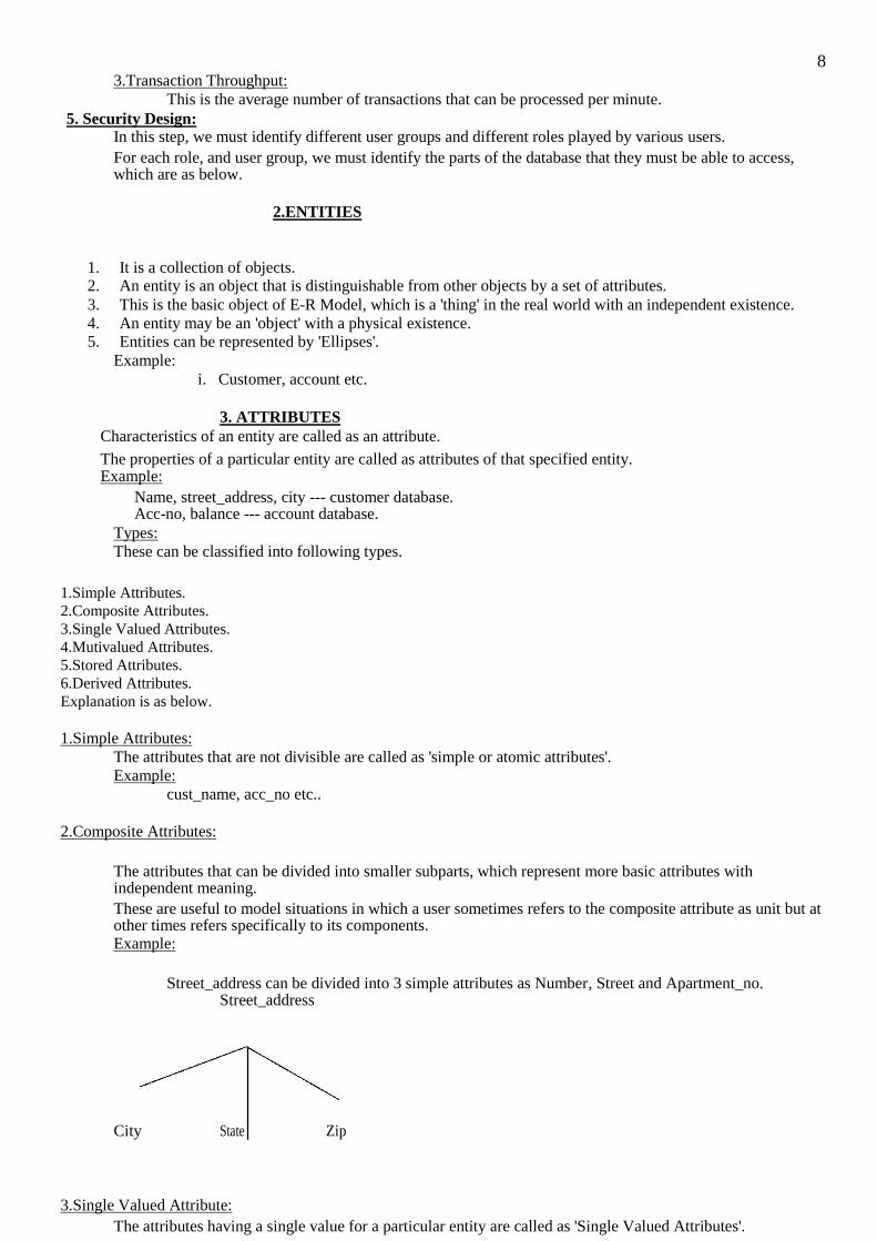
The attributes that can be divided into smaller subparts, which represent more basic attributes with independent meaning. These are useful to model situations in which a user sometimes refers to the composite attribute as unit but at other times refers specifically to its components. Example:

Street_address can be divided into 3 simple attributes as Number, Street and Apartment_no.

Street_address

City State

Zip

3.Single Valued Attribute: The attributes having a single value for a particular entity are called as 'Single Valued Attributes'.

Example: 'Age' is a single valued attribute of 'Person'.

9 4.Muti Valued Attribute:

The attributes, which are having a set of values for the same entity, are called as 'Multi Valued Attributes'. Example:

A 'College Degree' attribute for a person.i.e, one person may not have a college degree, another person may have one and a third person may have 2 or more degrees.

A multi-valued attribute may have lower and upper bounds on the number of values allowed for each individual entity.

5.Derived Attributes:

An attribute which is derived from another attribute is called as a ‘derived attribute. Example:

‘Age’ attribute is derived from another attribute ‘Date’. 6.Stored Attribute:

An attribute which is not derived from another attribute is called as a ‘stored attribute. Example:

In the above example,’ Date’ is a stored attribute.

4. ENTITY SETS Entity Type:

A collection entities that have the same attributes is called as an 'entity type'. Each entity type is described by its name and attributes.

Entity Set:

Collection of all entities of a particular entity type in the database at any point of time is called as an entity set. The entity set is usually referred to using the same name as the entity type. An entity type is represented in ER diagrams as a rectangular box enclosing the entity type name. Example:

Collection of customers.

5. Relationships

It is an association among entities.

6. Relationship Sets

It is a collection of relationships. Primary Key:

The attribute, which can be used to identify the specified information from the tables. Weak Entity: A weak entity can be identified uniquely by considering some of its attributes in conjunction with the primary key of another entity.

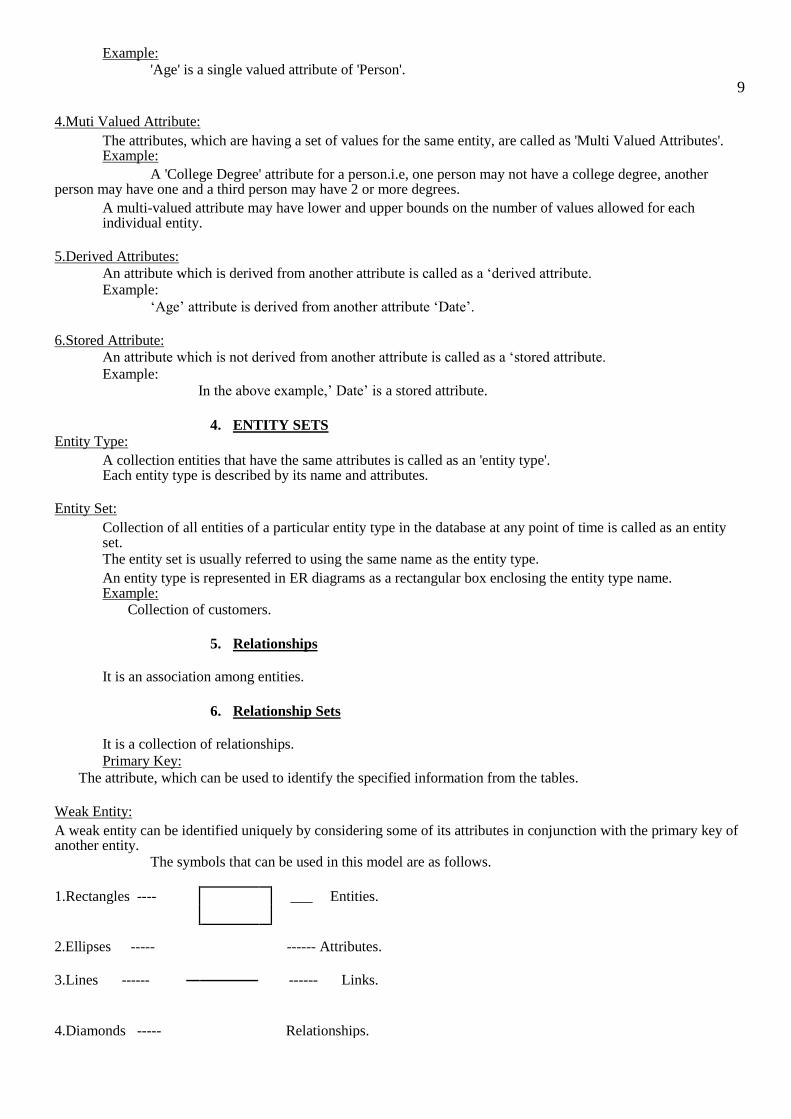
The symbols that can be used in this model are as follows. 1.Rectangles ---- ___ Entities.

2.Ellipses ----- ------ Attributes.

3.Lines ------

------ Links.

4.Diamonds ----- Relationships.

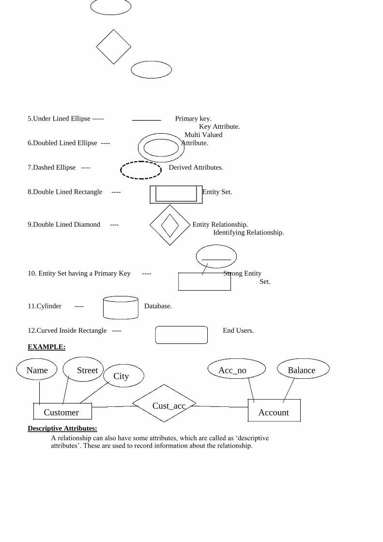
5.Under Lined Ellipse ----- Primary key.

Key Attribute.

6.Doubled Lined Ellipse ---- Multi Valued

Attribute.

7.Dashed Ellipse ---- Derived Attributes.

8.Double Lined Rectangle ----

Entity Set.

9.Double Lined Diamond ---- Entity Relationship.

Identifying Relationship. 10. Entity Set having a Primary Key ---- Strong Entity

Set.

11.Cylinder ---- Database.

12.Curved Inside Rectangle ---- End Users.

EXAMPLE:

Name Street City

Acc_no Balance

Customer Cust_acc

Account

Descriptive Attributes:

A relationship can also have some attributes, which are called as ‘descriptive attributes’. These are used to record information about the relationship.

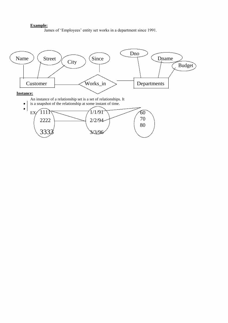
Example: James of ‘Employees’ entity set works in a department since 1991.

Name Dno

Dname

Street City

Since

Budget

Customer Works_in Departments

Instance:

An instance of a relationship set is a set of relationships. It is a snapshot of the relationship at some instant of time.

EX: 1111 1/1/91

2222 2/2/94

3333 3/3/96

60 70 80

11 Ternary Relationship:

A relationship set, which is having 3 entity sets, is called as a ternary relationship.

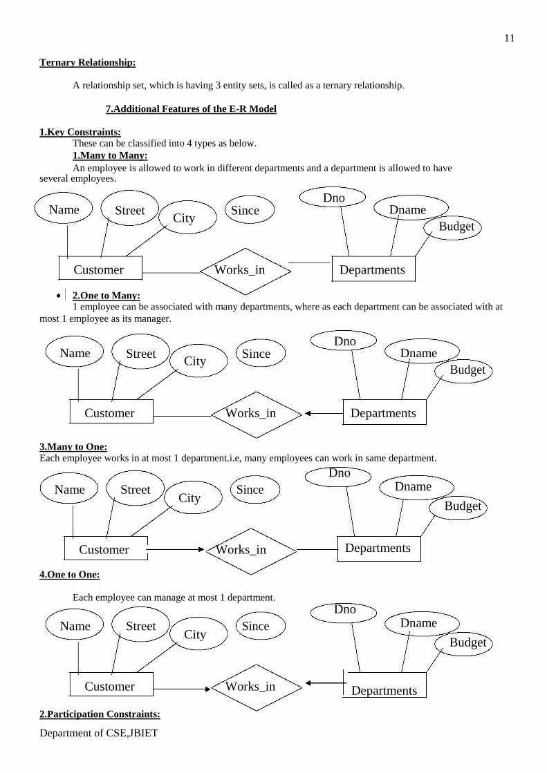
7.Additional Features of the E-R Model 1.Key Constraints:

These can be classified into 4 types as below. 1.Many to Many: An employee is allowed to work in different departments and a department is allowed to have

several employees.

Name Dno

Dname

Street City

Since

Budget

Customer Works_in Departments

2.One to Many: 1 employee can be associated with many departments, where as each department can be associated with at

most 1 employee as its manager.

Name Dno

Dname

Street City

Since

Budget

Customer Works_in Departments

3.Many to One: Each employee works in at most 1 department.i.e, many employees can work in same department.

Name Street City

Since

Customer Works_in 4.One to One:

Each employee can manage at most 1 department.

Name Street City

Since

Customer Works_in

2.Participation Constraints:

Dno

Dname

Budget

Departments

Dno

Dname

Budget

Departments

Department of CSE,JBIET

12

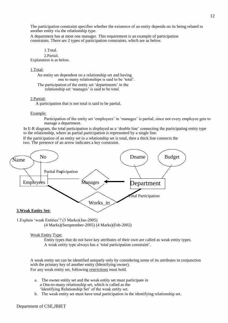
The participation constraint specifies whether the existence of an entity depends on its being related to another entity via the relationship type. A department has at most one manager. This requirement is an example of participation constraints. There are 2 types of participation constraints, which are as below.

1.Total. 2.Partial.

Explanation is as below.

1.Total: An entity set dependent on a relationship set and having

one to many relationships is said to be ‘total’. The participation of the entity set ‘departments’ in the

relationship set ‘manages’ is said to be total.

2.Partial: A participation that is not total is said to be partial.

Example:

Participation of the entity set ‘employees’ in ‘manages’ is partial, since not every employee gets to manage a department.

In E-R diagram, the total participation is displayed as a ‘double line’ connecting the participating entity type to the relationship, where as partial participation is represented by a single line. If the participation of an entity set in a relationship set is total, then a thick line connects the two. The presence of an arrow indicates a key constraint.

Name No Dname Budget

Partial Participation

Employees Manages Department

Total Participation Works_in

3.Weak Entity Set:

1.Explain ‘weak Entities’? (3 Marks)(Jan-2005)

(4 Marks)(Semptember-2005) (4 Marks)(Feb-2002)

Weak Entity Type: Entity types that do not have key attributes of their own are called as weak entity types. A weak entity type always has a ‘total participation constraint’.

A weak entity set can be identified uniquely only by considering some of its attributes in conjunction with the primary key of another entity (Identifying owner). For any weak entity set, following restrictions must hold.

a. The owner entity set and the weak entity set must participate in

a One-to-many relationship set, which is called as the ‘Identifying Relationship Set’ of the weak entity set.

b. The weak entity set must have total participation in the identifying relationship set.

Department of CSE,JBIET

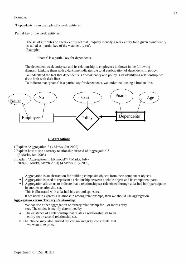
13 Example:

‘Dependents’ is an example of a weak entity set.

Partial key of the weak entity set:

The set of attributes of a weak entity set that uniquely identify a weak entity for a given owner entity is called as ‘partial key of the weak entity set’. Example:

‘Pname’ is a partial key for dependents.

The dependent weak entity set and its relationship to employees is shown in the following diagram. Linking them with a dark line indicates the total participation of dependents in policy. To understand the fact that dependents is a weak entity and policy is its identifying relationship, we draw both with dark lines. To indicate that ‘pname’ is a partial key for dependents, we underline it using a broken line.

No Cost Pname Age

Name --------

Employees Policy Dependents

4.Aggregation:

1.Explain ‘Aggregation’? (3 Marks, Jan-2005) 2.Explain how to use a ternary relationship instead of ‘aggregation’?

(5 Marks, Jan-2005) 3.Explain ‘Aggregation in ER model? (4 Marks, July-

2004) (5 Marks, March-2003) (4 Marks, July-2002)

Aggregation is an abstraction for building composite objects from their component objects. Aggregation is used to represent a relationship between a whole object and its component parts. Aggregation allows us to indicate that a relationship set (identified through a dashed box) participates in another relationship set. This is illustrated with a dashed box around sponsors. If we need to express a relationship among relationships, then we should use aggregation.

Aggregation versus Ternary Relationship: We can use either aggregation or ternary relationship for 3 or more entity sets. The choice is mainly determined by

a. The existence of a relationship that relates a relationship set to an entity set or second relationship set.

b. The choice may also guided by certain integrity constraints that we want to express.

Department of CSE,JBIET

14

Name Employees No

Monitors Until

---------------------------------------------------------------------------------------------------------------------

Pid Budget Since Dname Budget

Sponsors

Departments

Projects

----------------------------------------------------------------------------------------------------------------------

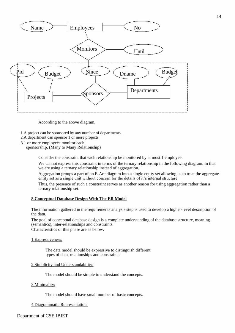
According to the above diagram,

1.A project can be sponsored by any number of departments. 2.A department can sponsor 1 or more projects. 3.1 or more employees monitor each

sponsorship. (Many to Many Relationship)

Consider the constraint that each relationship be monitored by at most 1 employee.

We cannot express this constraint in terms of the ternary relationship in the following diagram. In that we are using a ternary relationship instead of aggregation. Aggregation groups a part of an E-Are diagram into a single entity set allowing us to treat the aggregate entity set as a single unit without concern for the details of it’s internal structure. Thus, the presence of such a constraint serves as another reason for using aggregation rather than a ternary relationship set.

8.Conceptual Database Design With The ER Model

The information gathered in the requirements analysis step is used to develop a higher-level description of the data. The goal of conceptual database design is a complete understanding of the database structure, meaning (semantics), inter-relationships and constraints. Characteristics of this phase are as below.

1.Expressiveness:

The data model should be expressive to distinguish different types of data, relationships and constraints.

2.Simplicity and Understandability:

The model should be simple to understand the concepts.

3.Minimality:

The model should have small number of basic concepts.

4.Diagrammatic Representation:

Department of CSE,JBIET

15 The model should have a diagrammatic notation

for displaying the conceptual schema.

5.Formality:

A conceptual schema expressed in the data model must represent a formal specification of the data.

Example:

Cust_name: string; Cust_no: integer; Cust_city: string;

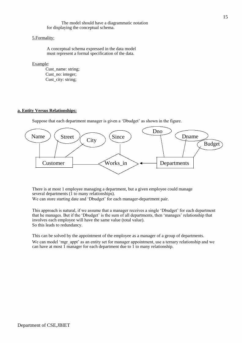
a. Entity Versus Relationships:

Suppose that each department manager is given a ‘Dbudget’ as shown in the figure.

Name Dno

Dname

Street City

Since

Budget

Customer Works_in Departments

There is at most 1 employee managing a department, but a given employee could manage several departments (1 to many relationships). We can store starting date and ‘Dbudget’ for each manager-department pair.

This approach is natural, if we assume that a manager receives a single ‘Dbudget’ for each department that he manages. But if the ‘Dbudget’ is the sum of all departments, then ‘manages’ relationship that involves each employee will have the same value (total value). So this leads to redundancy.

This can be solved by the appointment of the employee as a manager of a group of departments.

We can model ‘mgr_appt’ as an entity set for manager appointment, use a ternary relationship and we can have at most 1 manager for each department due to 1 to many relationship.

Department of CSE,JBIET

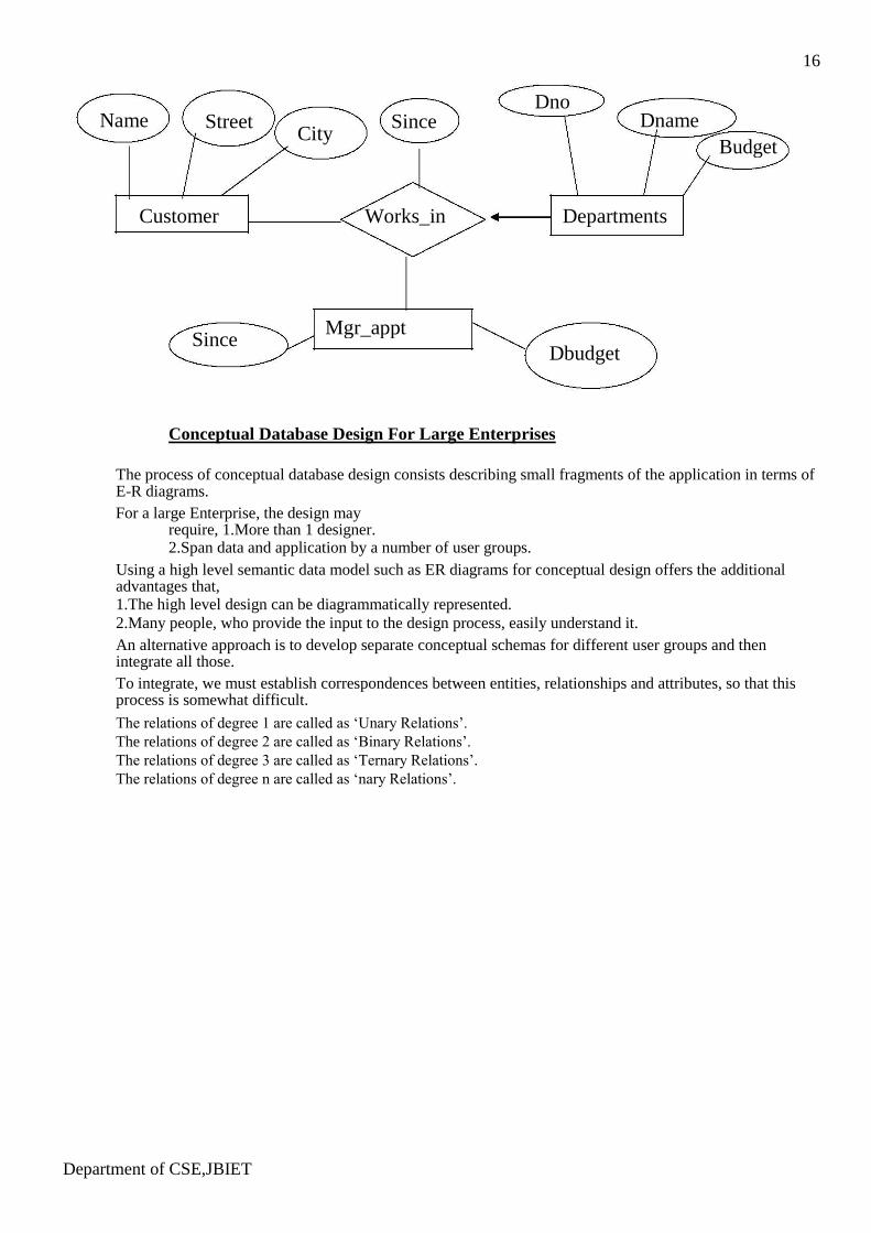
16

Name Dno

Dname

Street City

Since

Budget

Customer Works_in Departments

Since

Mgr_appt

Dbudget

Conceptual Database Design For Large Enterprises

The process of conceptual database design consists describing small fragments of the application in terms of E-R diagrams. For a large Enterprise, the design may

require, 1.More than 1 designer. 2.Span data and application by a number of user groups.

Using a high level semantic data model such as ER diagrams for conceptual design offers the additional advantages that, 1.The high level design can be diagrammatically represented. 2.Many people, who provide the input to the design process, easily understand it. An alternative approach is to develop separate conceptual schemas for different user groups and then integrate all those. To integrate, we must establish correspondences between entities, relationships and attributes, so that this process is somewhat difficult. The relations of degree 1 are called as ‘Unary Relations’.

The relations of degree 2 are called as ‘Binary Relations’.

The relations of degree 3 are called as ‘Ternary Relations’.

The relations of degree n are called as ‘nary Relations’. Department of CSE,JBIET

17 UNIT-3

RELATIONAL MODEL

A database is a collection of 1 or more ‘relations’, where each relation is a table with rows and columns.

This is the primary data model for commercial data processing applications. The major advantages of the relational model over the older data models are,

1.It is simple and elegant. 2.simple data representation. 3.The ease with which even complex queries can be expressed.

Introduction:

The main construct for representing data in the relational model is a ‘relation’.

A relation consists of 1.Relation Schema. 2.Relation Instance.

Explanation is as below. 1.Relation Schema:

The relation schema describes the column heads for the table.

The schema specifies the relation’s name, the name of each field (column, attribute) and the ‘domain’ of each field. A domain is referred to in a relation schema by the domain name and has a set of associated values. Example:

Student information in a university database to illustrate the parts of a relation schema.

Students (Sid: string, name: string, login: string, age: integer, gross: real)

This says that the field named ‘sid’ has a domain named ‘string’. The set of values associated with domain ‘string’ is the set of all character strings.

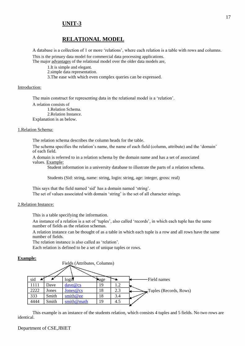
2.Relation Instance:

This is a table specifying the information.

An instance of a relation is a set of ‘tuples’, also called ‘records’, in which each tuple has the same number of fields as the relation schemas. A relation instance can be thought of as a table in which each tuple is a row and all rows have the same number of fields. The relation instance is also called as ‘relation’. Each relation is defined to be a set of unique tuples or rows.

Example:

Fields (Attributes, Columns)

sid login age Field names 1111 Dave dave@cs 19 1.2

2222 Jones Jones@cs 18 2.3 Tuples (Records, Rows) 333 Smith smith@ee 18 3.4

4444 Smith smith@math 19 4.5

This example is an instance of the students relation, which consists 4 tuples and 5 fields. No two rows are

identical. Department of CSE,JBIET

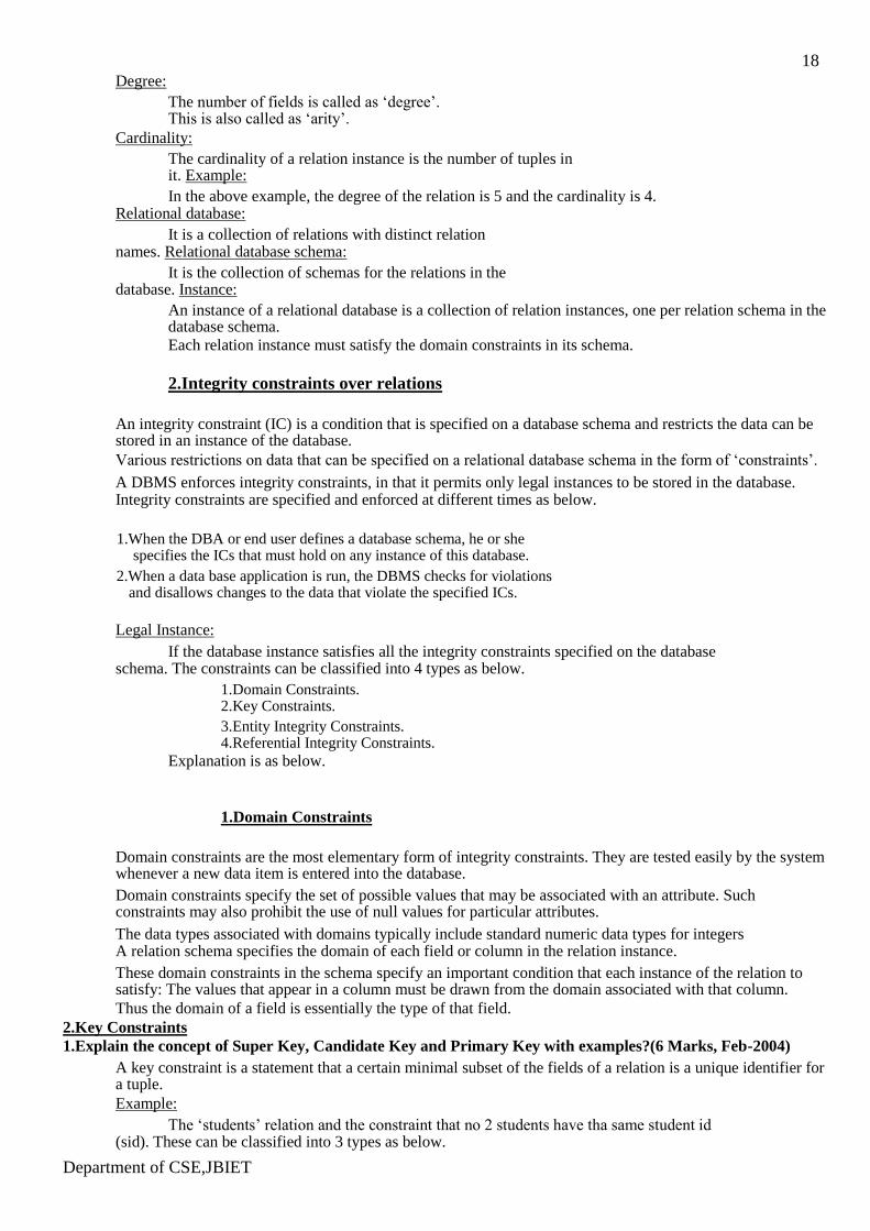
18 Degree:

The number of fields is called as ‘degree’. This is also called as ‘arity’.

Cardinality: The cardinality of a relation instance is the number of tuples in it. Example: In the above example, the degree of the relation is 5 and the cardinality is 4.

Relational database: It is a collection of relations with distinct relation

names. Relational database schema: It is the collection of schemas for the relations in the

database. Instance: An instance of a relational database is a collection of relation instances, one per relation schema in the database schema. Each relation instance must satisfy the domain constraints in its schema.

2.Integrity constraints over relations

An integrity constraint (IC) is a condition that is specified on a database schema and restricts the data can be stored in an instance of the database. Various restrictions on data that can be specified on a relational database schema in the form of ‘constraints’. A DBMS enforces integrity constraints, in that it permits only legal instances to be stored in the database. Integrity constraints are specified and enforced at different times as below.

1.When the DBA or end user defines a database schema, he or she

specifies the ICs that must hold on any instance of this database. 2.When a data base application is run, the DBMS checks for violations

and disallows changes to the data that violate the specified ICs.

Legal Instance: If the database instance satisfies all the integrity constraints specified on the database

schema. The constraints can be classified into 4 types as below. 1.Domain Constraints. 2.Key Constraints. 3.Entity Integrity Constraints. 4.Referential Integrity Constraints.

Explanation is as below.

1.Domain Constraints

Domain constraints are the most elementary form of integrity constraints. They are tested easily by the system whenever a new data item is entered into the database. Domain constraints specify the set of possible values that may be associated with an attribute. Such constraints may also prohibit the use of null values for particular attributes. The data types associated with domains typically include standard numeric data types for integers A relation schema specifies the domain of each field or column in the relation instance. These domain constraints in the schema specify an important condition that each instance of the relation to satisfy: The values that appear in a column must be drawn from the domain associated with that column. Thus the domain of a field is essentially the type of that field.

2.Key Constraints 1.Explain the concept of Super Key, Candidate Key and Primary Key with examples?(6 Marks, Feb-2004)

A key constraint is a statement that a certain minimal subset of the fields of a relation is a unique identifier for a tuple. Example:

The ‘students’ relation and the constraint that no 2 students have tha same student id (sid). These can be classified into 3 types as below.

Department of CSE,JBIET

19 a. Candidate Key or Key. b. Super Key. c. Primary Key.

Explanation is as below. a. Candidate Key or Key: 1.Explain ‘Candidate Key’?(4 Marks, Semptember-2003)

A set of fields that uniquely identifies a tuple according to a key constraint is called as a ‘Candidate Key’ for the relation. This is also called as a ‘key’. From the definition of candidate key, we have,

1.Two distinct tuples in a legal instance cannot have identical values in all the fields of a key.i.e, in any legal instance, the values in the key fields uniquely identify a tuple in the instance. i.e,the values in the key fields uniquely identify a tuple in the instance. 2.

No subset of the set of fields in key is a unique identifier for a tuple, i.e., the set of fields {sid, name} is not a key for

Students. A relation schema may have more than key. Example: In the above Students relation, the ‘sid’ field is a candidate key.

{sid}. The value of a key attribute can be used to identify uniquely each tuple in the relation.

‘A set of attributes constituting a key’ is a property of the relation schema. A key is determined from the meaning of attributes. Every relation is guaranteed to have a key. Since a relation is a set of tuples, the set of all fields is always a super key.

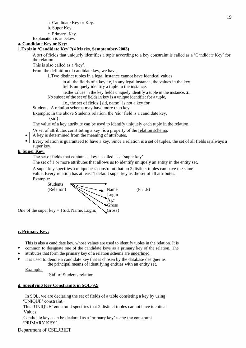
b. Super Key: The set of fields that contains a key is called as a ‘super key’. The set of 1 or more attributes that allows us to identify uniquely an entity in the entity set.

A super key specifies a uniqueness constraint that no 2 distinct tuples can have the same value. Every relation has at least 1 default super key as the set of all attributes. Example:

Students (Relation) Name (Fields)

Login Age Gross

One of the super key = {Sid, Name, Login, Gross}

c. Primary Key:

This is also a candidate key, whose values are used to identify tuples in the relation. It is

common to designate one of the candidate keys as a primary key of the relation. The

attributes that form the primary key of a relation schema are underlined. It is used to denote a candidate key that is chosen by the database designer as

the principal means of identifying entities with an entity set. Example:

‘Sid’ of Students relation. d. Specifying Key Constraints in SQL-92:

In SQL, we are declaring the set of fields of a table consisting a key by using ‘UNIQUE’ constraint. This ‘UNIQUE’ constraint specifies that 2 distinct tuples cannot have identical

Values. Candidate keys can be declared as a ‘primary key’ using the constraint

‘PRIMARY KEY’. Department of CSE,JBIET

20 We can name a constraint by using the syntax as below.

CONSTRAINT constraint_name KEY_NOTATION (key_names);

If the constraint is violated, then the constraint_name is returned and it can

be used to identify the error. Example:

Express ‘sid’ as a primary key and the combination {name, age} as a key.

CREATE TABLE Students (sid CHAR (20), name CHAR (30), login CHAR(20), age INTEGER, gross REAL, UNIQUE (name, age),

` CONSTRAINT sid1 PRIMARY KEY (sid));

3.Entity Integrity Constraints

This states that no primary key value can be null. The primary key value is used to identify individual tuples in a relation. Having null values for the primary key implies that we cannot identify some tuples. NOTE: Key Constraints, Entity Integrity Constraints are specified on individual relations. PRIMARY KEYS comes under this.

4.Referential Integrity Constraints

The Referential Integrity Constraint is specified between 2 relations and is

used to maintain the consistency among tuples of the 2 relations. Informally, the referential integrity constraint states that ‘a tuple in 1

relation that refers to another relation must refer to an existing tuple in

that relation. We can diagrammatically display the referential integrity constraints by

drawing a directed arc from each foreign key to the relation it references.

The arrowhead may point to the primary key of the referenced relation.

SELECT Statement Basics

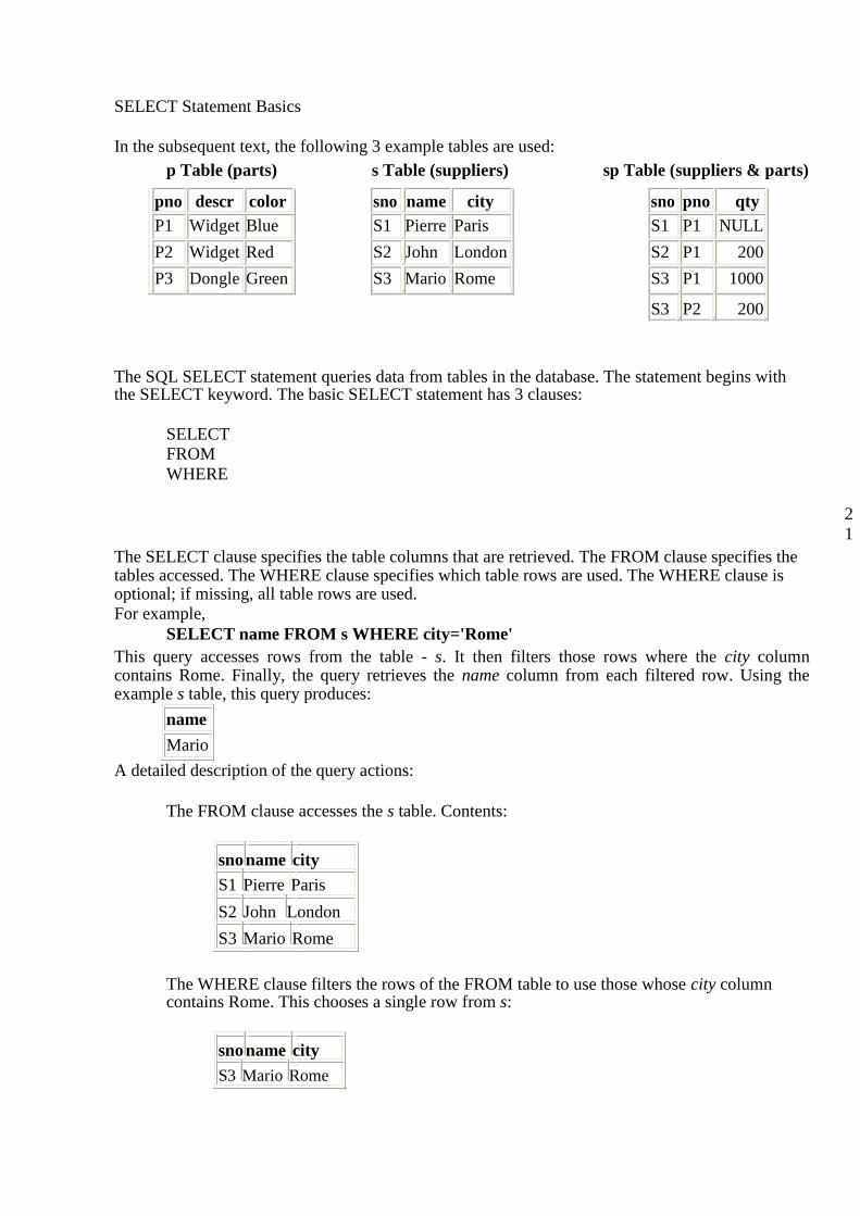
In the subsequent text, the following 3 example tables are used:

p Table (parts) s Table (suppliers) sp Table (suppliers & parts)

pno descr color sno name city sno pno qty

P1 Widget Blue S1 Pierre Paris S1 P1 NULL

P2 Widget Red S2 John London S2 P1 200

P3 Dongle Green S3 Mario Rome S3 P1 1000

S3 P2 200

The SQL SELECT statement queries data from tables in the database. The statement begins with the SELECT keyword. The basic SELECT statement has 3 clauses:

SELECT

FROM WHERE

2

1 The SELECT clause specifies the table columns that are retrieved. The FROM clause specifies the tables accessed. The WHERE clause specifies which table rows are used. The WHERE clause is optional; if missing, all table rows are used. For example,

SELECT name FROM s WHERE city='Rome' This query accesses rows from the table - s. It then filters those rows where the city column contains Rome. Finally, the query retrieves the name column from each filtered row. Using the example s table, this query produces:

name

Mario A detailed description of the query actions:

The FROM clause accesses the s table. Contents:

snoname city

S1 Pierre Paris

S2 John London

S3 Mario Rome

The WHERE clause filters the rows of the FROM table to use those whose city column contains Rome. This chooses a single row from s:

snoname city

S3 Mario Rome

The SELECT clause retrieves the name column from the rows filtered by the WHERE

clause:

name

Mario

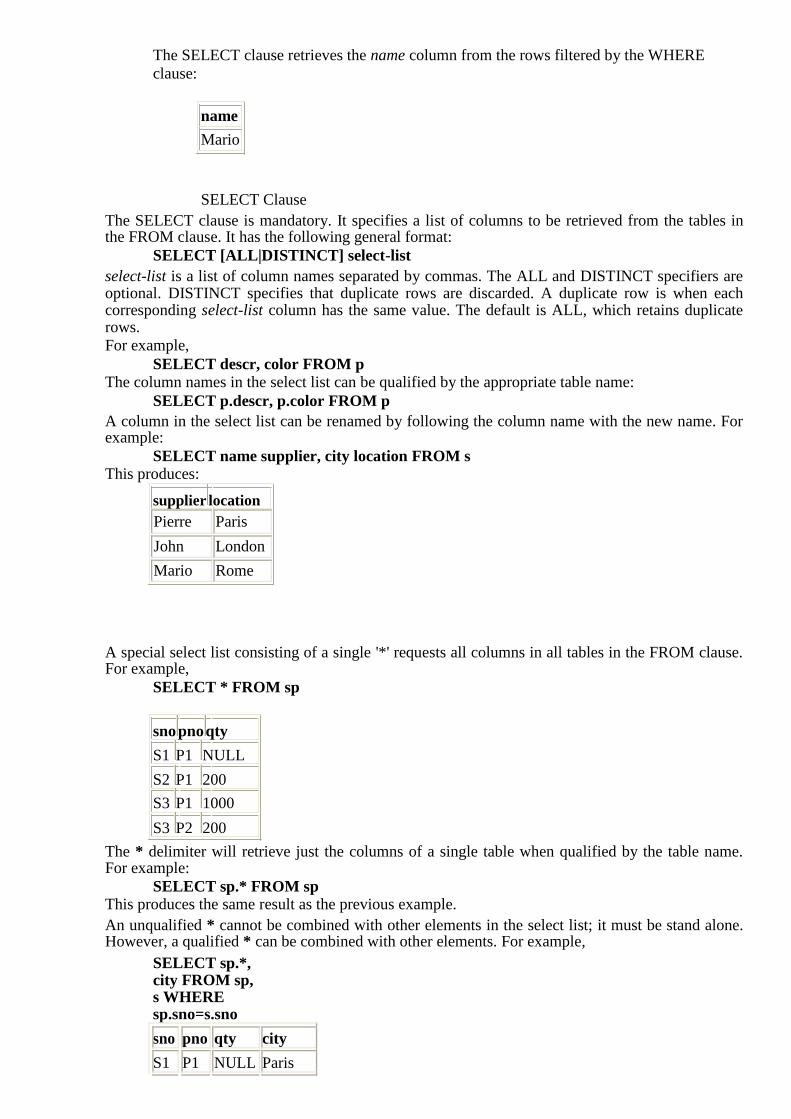
SELECT Clause The SELECT clause is mandatory. It specifies a list of columns to be retrieved from the tables in the FROM clause. It has the following general format:

SELECT [ALL|DISTINCT] select-list select-list is a list of column names separated by commas. The ALL and DISTINCT specifiers are optional. DISTINCT specifies that duplicate rows are discarded. A duplicate row is when each corresponding select-list column has the same value. The default is ALL, which retains duplicate rows. For example,

SELECT descr, color FROM p The column names in the select list can be qualified by the appropriate table name:

SELECT p.descr, p.color FROM p A column in the select list can be renamed by following the column name with the new name. For example:

SELECT name supplier, city location FROM s This produces:

supplier location Pierre Paris

John London

Mario Rome

A special select list consisting of a single '*' requests all columns in all tables in the FROM clause. For example,

SELECT * FROM sp

snopnoqty

S1 P1 NULL

S2 P1 200

S3 P1 1000

S3 P2 200 The * delimiter will retrieve just the columns of a single table when qualified by the table name. For example:

SELECT sp.* FROM sp This produces the same result as the previous example. An unqualified * cannot be combined with other elements in the select list; it must be stand alone. However, a qualified * can be combined with other elements. For example,

SELECT sp.*, city FROM sp, s WHERE sp.sno=s.sno

sno pno qty city

S1 P1 NULL Paris

S2 P1 200 London

S3 P1 1000 Rome

S3 P2 200 Rome

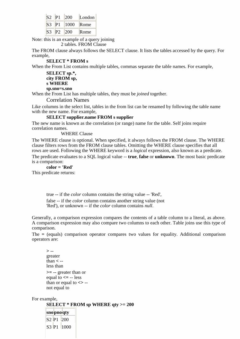
Note: this is an example of a query joining 2 tables. FROM Clause

The FROM clause always follows the SELECT clause. It lists the tables accessed by the query. For example,

SELECT * FROM s When the From List contains multiple tables, commas separate the table names. For example,

SELECT sp.*, city FROM sp, s WHERE sp.sno=s.sno

When the From List has multiple tables, they must be joined together. Correlation Names

Like columns in the select list, tables in the from list can be renamed by following the table name with the new name. For example,

SELECT supplier.name FROM s supplier The new name is known as the correlation (or range) name for the table. Self joins require correlation names.

WHERE Clause The WHERE clause is optional. When specified, it always follows the FROM clause. The WHERE clause filters rows from the FROM clause tables. Omitting the WHERE clause specifies that all rows are used. Following the WHERE keyword is a logical expression, also known as a predicate. The predicate evaluates to a SQL logical value -- true, false or unknown. The most basic predicate is a comparison:

color = 'Red' This predicate returns:

true -- if the color column contains the string value -- 'Red', false -- if the color column contains another string value (not 'Red'), or unknown -- if the color column contains null.

Generally, a comparison expression compares the contents of a table column to a literal, as above. A comparison expression may also compare two columns to each other. Table joins use this type of comparison. The = (equals) comparison operator compares two values for equality. Additional comparison operators are:

> -- greater than < -- less than >= -- greater than or equal to <= -- less than or equal to <> -- not equal to

For example,

SELECT * FROM sp WHERE qty >= 200

snopnoqty

S2 P1 200

S3 P1 1000

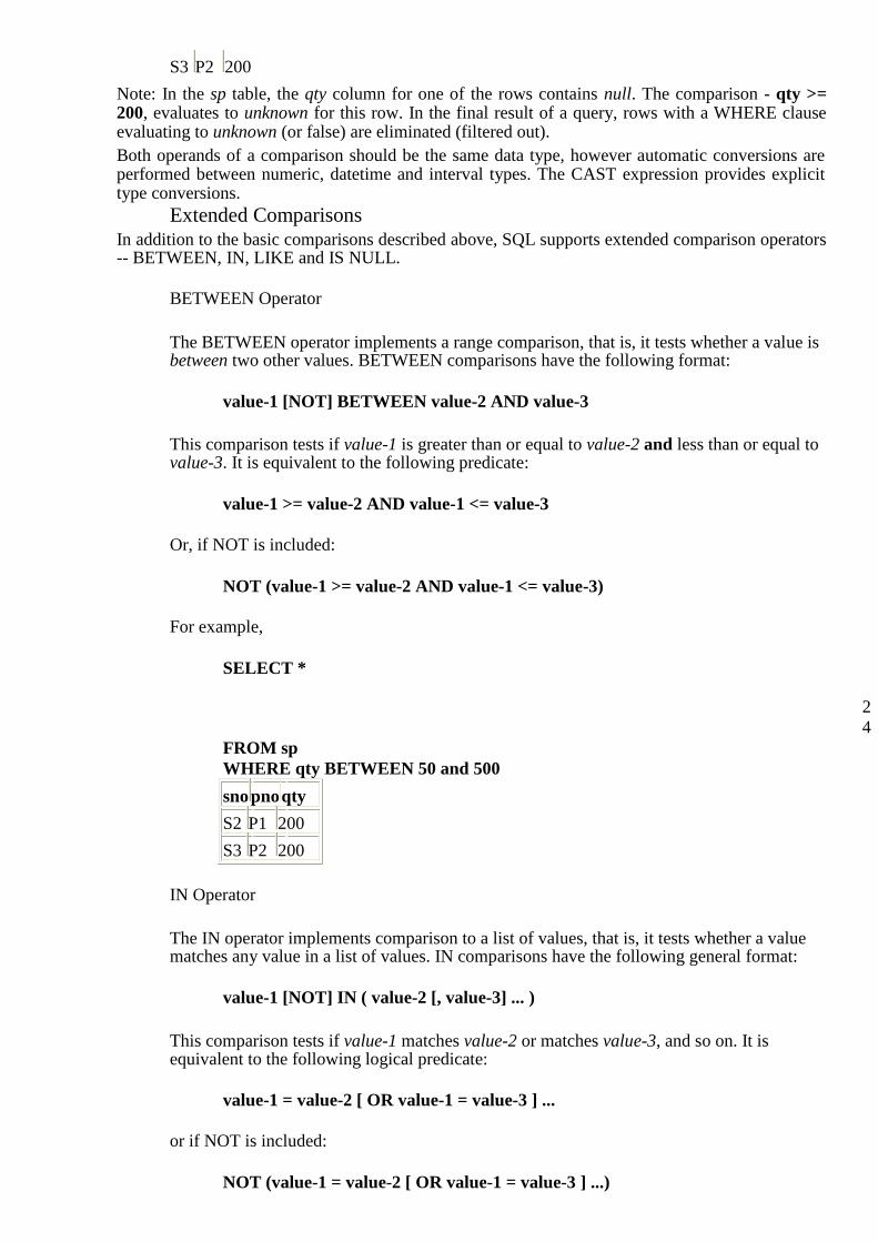
S3 P2 200 Note: In the sp table, the qty column for one of the rows contains null. The comparison - qty >= 200, evaluates to unknown for this row. In the final result of a query, rows with a WHERE clause evaluating to unknown (or false) are eliminated (filtered out). Both operands of a comparison should be the same data type, however automatic conversions are performed between numeric, datetime and interval types. The CAST expression provides explicit type conversions.

Extended Comparisons In addition to the basic comparisons described above, SQL supports extended comparison operators -- BETWEEN, IN, LIKE and IS NULL.

BETWEEN Operator

The BETWEEN operator implements a range comparison, that is, it tests whether a value is between two other values. BETWEEN comparisons have the following format:

value-1 [NOT] BETWEEN value-2 AND value-3

This comparison tests if value-1 is greater than or equal to value-2 and less than or equal to value-3. It is equivalent to the following predicate:

value-1 >= value-2 AND value-1 <= value-3

Or, if NOT is included:

NOT (value-1 >= value-2 AND value-1 <= value-3)

For example,

SELECT *

2

4 FROM sp WHERE qty BETWEEN 50 and 500

snopnoqty

S2 P1 200

S3 P2 200

IN Operator

The IN operator implements comparison to a list of values, that is, it tests whether a value matches any value in a list of values. IN comparisons have the following general format:

value-1 [NOT] IN ( value-2 [, value-3] ... )

This comparison tests if value-1 matches value-2 or matches value-3, and so on. It is equivalent to the following logical predicate:

value-1 = value-2 [ OR value-1 = value-3 ] ...

or if NOT is included:

NOT (value-1 = value-2 [ OR value-1 = value-3 ] ...)

For example,

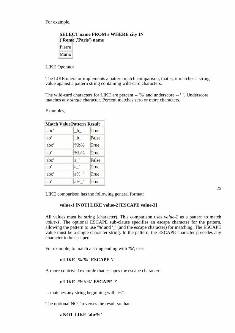
SELECT name FROM s WHERE city IN

('Rome','Paris') name

Pierre

Mario

LIKE Operator

The LIKE operator implements a pattern match comparison, that is, it matches a string value against a pattern string containing wild-card characters.

The wild-card characters for LIKE are percent -- '%' and underscore -- '_'. Underscore matches any single character. Percent matches zero or more characters.

Examples,

Match Value Pattern Result 'abc' '_b_' True

'ab' '_b_' False

'abc' '%b%' True

'ab' '%b%' True

'abc' 'a_' False

'ab' 'a_' True

'abc' 'a%_' True

'ab' 'a%_' True

25 LIKE comparison has the following general format:

value-1 [NOT] LIKE value-2 [ESCAPE value-3]

All values must be string (character). This comparison uses value-2 as a pattern to match value-1. The optional ESCAPE sub-clause specifies an escape character for the pattern, allowing the pattern to use '%' and '_' (and the escape character) for matching. The ESCAPE value must be a single character string. In the pattern, the ESCAPE character precedes any character to be escaped.

For example, to match a string ending with '%', use:

x LIKE '%/%' ESCAPE '/'

A more contrived example that escapes the escape character:

y LIKE '/%//%' ESCAPE '/'

... matches any string beginning with '%/'.

The optional NOT reverses the result so that:

z NOT LIKE 'abc%'

is equivalent to:

NOT z LIKE 'abc%'

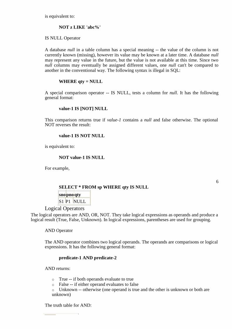
IS NULL Operator

A database null in a table column has a special meaning -- the value of the column is not currently known (missing), however its value may be known at a later time. A database null may represent any value in the future, but the value is not available at this time. Since two null columns may eventually be assigned different values, one null can't be compared to another in the conventional way. The following syntax is illegal in SQL:

WHERE qty = NULL

A special comparison operator -- IS NULL, tests a column for null. It has the following general format:

value-1 IS [NOT] NULL

This comparison returns true if value-1 contains a null and false otherwise. The optional NOT reverses the result:

value-1 IS NOT NULL

is equivalent to:

NOT value-1 IS NULL

For example,

6 SELECT * FROM sp WHERE qty IS NULL

snopnoqty

S1 P1 NULL Logical Operators

The logical operators are AND, OR, NOT. They take logical expressions as operands and produce a logical result (True, False, Unknown). In logical expressions, parentheses are used for grouping.

AND Operator

The AND operator combines two logical operands. The operands are comparisons or logical expressions. It has the following general format:

predicate-1 AND predicate-2

AND returns:

o True -- if both operands evaluate to true o False -- if either operand evaluates to false o Unknown -- otherwise (one operand is true and the other is unknown or both are unknown)

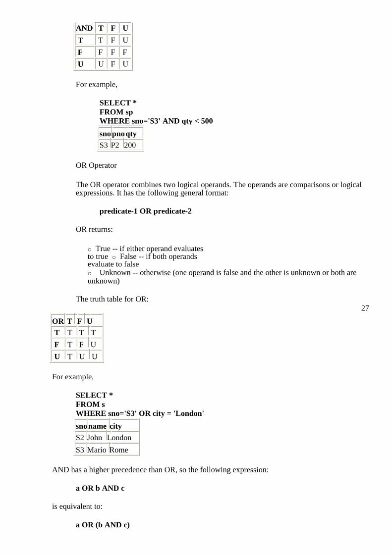
The truth table for AND:

AND T F U

T F U

T

F F F

F

U F U

U

For example,

SELECT * FROM sp

WHERE sno='S3' AND qty < 500

snopnoqty

S3 P2 200

OR Operator

The OR operator combines two logical operands. The operands are comparisons or logical expressions. It has the following general format:

predicate-1 OR predicate-2

OR returns:

o True -- if either operand evaluates to true o False -- if both operands evaluate to false o Unknown -- otherwise (one operand is false and the other is unknown or both are unknown)

The truth table for OR:

27

OR T F U

T T T T

F T F U

U T U U

For example,

SELECT * FROM s

WHERE sno='S3' OR city = 'London'

snoname city

S2 John London

S3 Mario Rome

AND has a higher precedence than OR, so the following expression:

a OR b AND c

is equivalent to:

a OR (b AND c)

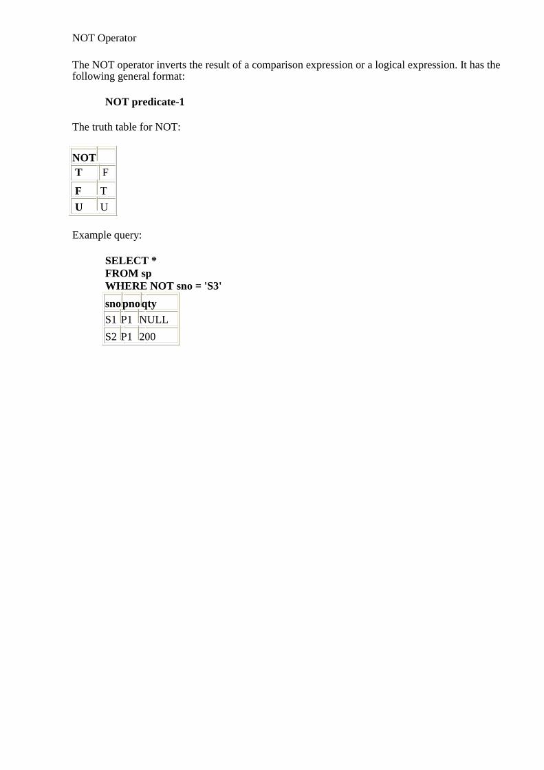
NOT Operator

The NOT operator inverts the result of a comparison expression or a logical expression. It has the following general format:

NOT predicate-1

The truth table for NOT:

NOT T F

F T

U U

Example query:

SELECT *

FROM sp WHERE NOT sno = 'S3'

snopnoqty

S1 P1 NULL

S2 P1 200

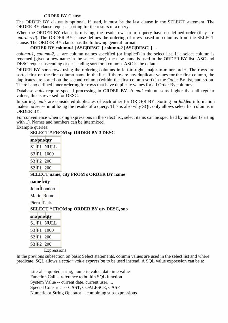
ORDER BY Clause The ORDER BY clause is optional. If used, it must be the last clause in the SELECT statement. The ORDER BY clause requests sorting for the results of a query. When the ORDER BY clause is missing, the result rows from a query have no defined order (they are unordered). The ORDER BY clause defines the ordering of rows based on columns from the SELECT clause. The ORDER BY clause has the following general format:

ORDER BY column-1 [ASC|DESC] [ column-2 [ASC|DESC] ] ... column-1, column-2, ... are column names specified (or implied) in the select list. If a select column is renamed (given a new name in the select entry), the new name is used in the ORDER BY list. ASC and DESC request ascending or descending sort for a column. ASC is the default. ORDER BY sorts rows using the ordering columns in left-to-right, major-to-minor order. The rows are sorted first on the first column name in the list. If there are any duplicate values for the first column, the duplicates are sorted on the second column (within the first column sort) in the Order By list, and so on. There is no defined inner ordering for rows that have duplicate values for all Order By columns. Database nulls require special processing in ORDER BY. A null column sorts higher than all regular values; this is reversed for DESC. In sorting, nulls are considered duplicates of each other for ORDER BY. Sorting on hidden information makes no sense in utilizing the results of a query. This is also why SQL only allows select list columns in ORDER BY. For convenience when using expressions in the select list, select items can be specified by number (starting with 1). Names and numbers can be intermixed. Example queries:

SELECT * FROM sp ORDER BY 3 DESC

snopnoqty

S1 P1 NULL

S3 P1 1000

S3 P2 200

S2 P1 200 SELECT name, city FROM s ORDER BY name

name city

John London

Mario Rome

Pierre Paris SELECT * FROM sp ORDER BY qty DESC, sno

snopnoqty

S1 P1 NULL

S3 P1 1000

S2 P1 200

S3 P2 200 Expressions

In the previous subsection on basic Select statements, column values are used in the select list and where predicate. SQL allows a scalar value expression to be used instead. A SQL value expression can be a:

Literal -- quoted string, numeric value, datetime value Function Call -- reference to builtin SQL function System Value -- current date, current user, ...

Special Construct -- CAST, COALESCE, CASE Numeric or String Operator -- combining sub-expressions

29

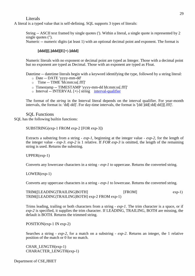
Literals A literal is a typed value that is self-defining. SQL supports 3 types of literals:

String -- ASCII text framed by single quotes ('). Within a literal, a single quote is represented by 2 single quotes (''). Numeric -- numeric digits (at least 1) with an optional decimal point and exponent. The format is

[ddd][[.]ddd][E[+|-]ddd]

Numeric literals with no exponent or decimal point are typed as Integer. Those with a decimal point but no exponent are typed as Decimal. Those with an exponent are typed as Float.

Datetime -- datetime literals begin with a keyword identifying the type, followed by a string literal:

o Date -- DATE 'yyyy-mm-dd' o Time -- TIME 'hh:mm:ss[.fff]' o Timestamp -- TIMESTAMP 'yyyy-mm-dd hh:mm:ss[.fff]' o Interval -- INTERVAL [+|-] string interval-qualifier

The format of the string in the Interval literal depends on the interval qualifier. For year-month intervals, the format is: 'dd[-dd]'. For day-time intervals, the format is '[dd ]dd[:dd[:dd]][.fff]'.

SQL Functions

SQL has the following builtin functions:

SUBSTRING(exp-1 FROM exp-2 [FOR exp-3])

Extracts a substring from a string - exp-1, beginning at the integer value - exp-2, for the length of the integer value - exp-3. exp-2 is 1 relative. If FOR exp-3 is omitted, the length of the remaining string is used. Returns the substring.

UPPER(exp-1)

Converts any lowercase characters in a string - exp-1 to uppercase. Returns the converted string.

LOWER(exp-1)

Converts any uppercase characters in a string - exp-1 to lowercase. Returns the converted string.

TRIM([LEADING|TRAILING|BOTH] [FROM] exp-1) TRIM([LEADING|TRAILING|BOTH] exp-2 FROM exp-1)

Trims leading, trailing or both characters from a string - exp-1. The trim character is a space, or if exp-2 is specified, it supplies the trim character. If LEADING, TRAILING, BOTH are missing, the default is BOTH. Returns the trimmed string.

POSITION(exp-1 IN exp-2)

Searches a string - exp-2, for a match on a substring - exp-2. Returns an integer, the 1 relative position of the match or 0 for no match.

CHAR_LENGTH(exp-1)

CHARACTER_LENGTH(exp-1)

Department of CSE,JBIET

30

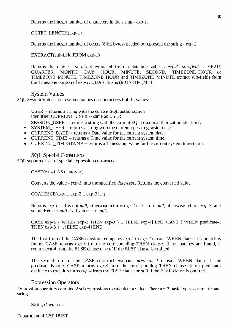
Returns the integer number of characters in the string - exp-1.

OCTET_LENGTH(exp-1)

Returns the integer number of octets (8-bit bytes) needed to represent the string - exp-1.

EXTRACT(sub-field FROM exp-1)

Returns the numeric sub-field extracted from a datetime value - exp-1. sub-field is YEAR, QUARTER, MONTH, DAY, HOUR, MINUTE, SECOND, TIMEZONE_HOUR or TIMEZONE_MINUTE. TIMEZONE_HOUR and TIMEZONE_MINUTE extract sub-fields from the Timezone portion of exp-1. QUARTER is (MONTH-1)/4+1.

System Values

SQL System Values are reserved names used to access builtin values:

USER -- returns a string with the current SQL authorization identifier. CURRENT_USER -- same as USER. SESSION_USER -- returns a string with the current SQL session authorization identifier. SYSTEM_USER -- returns a string with the current operating system user. CURRENT_DATE -- returns a Date value for the current system date. CURRENT_TIME -- returns a Time value for the current system time. CURRENT_TIMESTAMP -- returns a Timestamp value for the current system timestamp.

SQL Special Constructs

SQL supports a set of special expression constructs:

CAST(exp-1 AS data-type)

Converts the value - exp-1, into the specified date-type. Returns the converted value.

COALESCE(exp-1, exp-2 [, exp-3] ...)

Returns exp-1 if it is not null, otherwise returns exp-2 if it is not null, otherwise returns exp-3, and so on. Returns null if all values are null.

CASE exp-1 { WHEN exp-2 THEN exp-3 } ... [ELSE exp-4] END CASE { WHEN predicate-1 THEN exp-3 } ... [ELSE exp-4] END

The first form of the CASE construct compares exp-1 to exp-2 in each WHEN clause. If a match is found, CASE returns exp-3 from the corresponding THEN clause. If no matches are found, it returns exp-4 from the ELSE clause or null if the ELSE clause is omitted.

The second form of the CASE construct evaluates predicate-1 in each WHEN clause. If the predicate is true, CASE returns exp-3 from the corresponding THEN clause. If no predicates evaluate to true, it returns exp-4 from the ELSE clause or null if the ELSE clause is omitted.

Expression Operators Expression operators combine 2 subexpressions to calculate a value. There are 2 basic types -- numeric and string.

String Operators

Department of CSE,JBIET

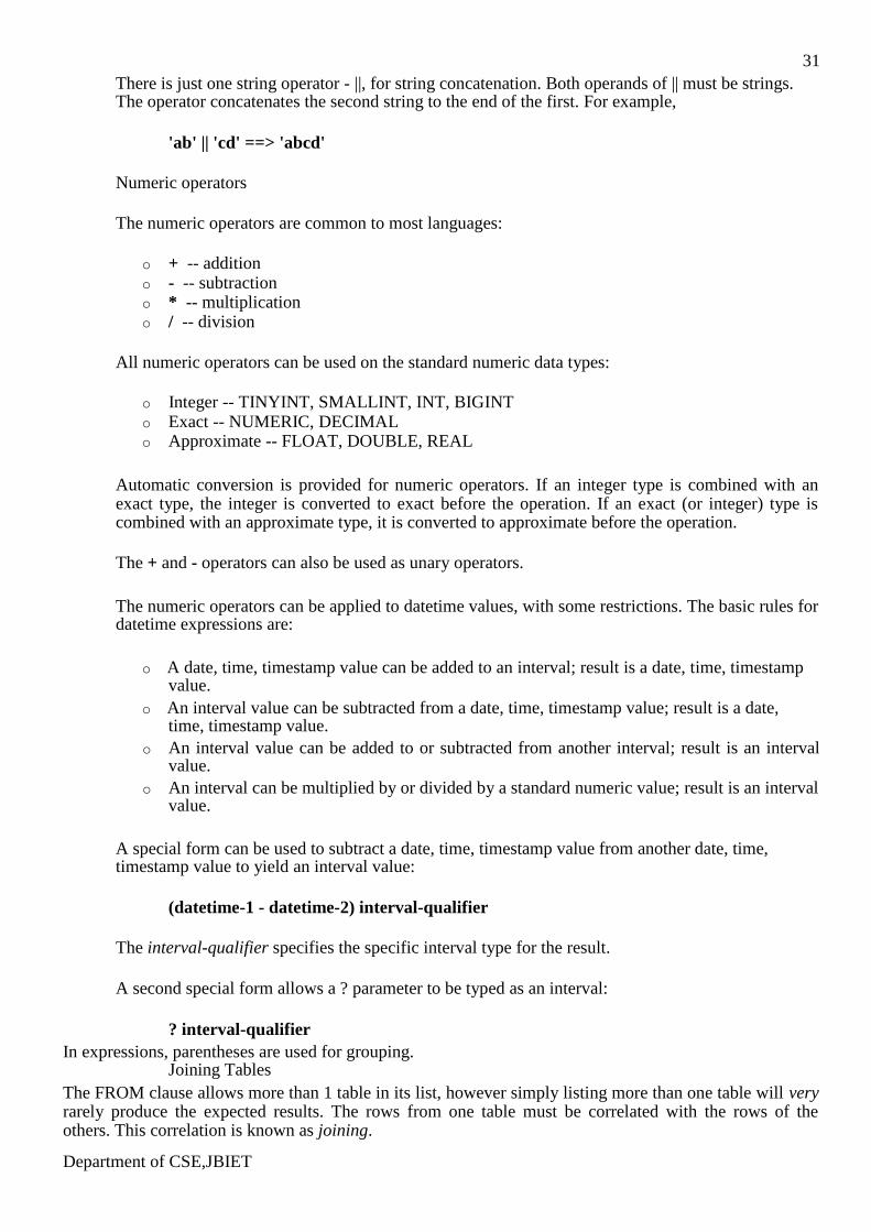
31 There is just one string operator - ||, for string concatenation. Both operands of || must be strings. The operator concatenates the second string to the end of the first. For example,

'ab' || 'cd' ==> 'abcd'

Numeric operators

The numeric operators are common to most languages:

o + -- addition o - -- subtraction o * -- multiplication o / -- division

All numeric operators can be used on the standard numeric data types:

o Integer -- TINYINT, SMALLINT, INT, BIGINT o Exact -- NUMERIC, DECIMAL o Approximate -- FLOAT, DOUBLE, REAL

Automatic conversion is provided for numeric operators. If an integer type is combined with an exact type, the integer is converted to exact before the operation. If an exact (or integer) type is combined with an approximate type, it is converted to approximate before the operation.

The + and - operators can also be used as unary operators.

The numeric operators can be applied to datetime values, with some restrictions. The basic rules for datetime expressions are:

o A date, time, timestamp value can be added to an interval; result is a date, time, timestamp

value. o An interval value can be subtracted from a date, time, timestamp value; result is a date,

time, timestamp value. o An interval value can be added to or subtracted from another interval; result is an interval

value. o An interval can be multiplied by or divided by a standard numeric value; result is an interval

value.

A special form can be used to subtract a date, time, timestamp value from another date, time, timestamp value to yield an interval value:

(datetime-1 - datetime-2) interval-qualifier

The interval-qualifier specifies the specific interval type for the result.

A second special form allows a ? parameter to be typed as an interval:

? interval-qualifier In expressions, parentheses are used for grouping.

Joining Tables The FROM clause allows more than 1 table in its list, however simply listing more than one table will very rarely produce the expected results. The rows from one table must be correlated with the rows of the others. This correlation is known as joining. Department of CSE,JBIET

32

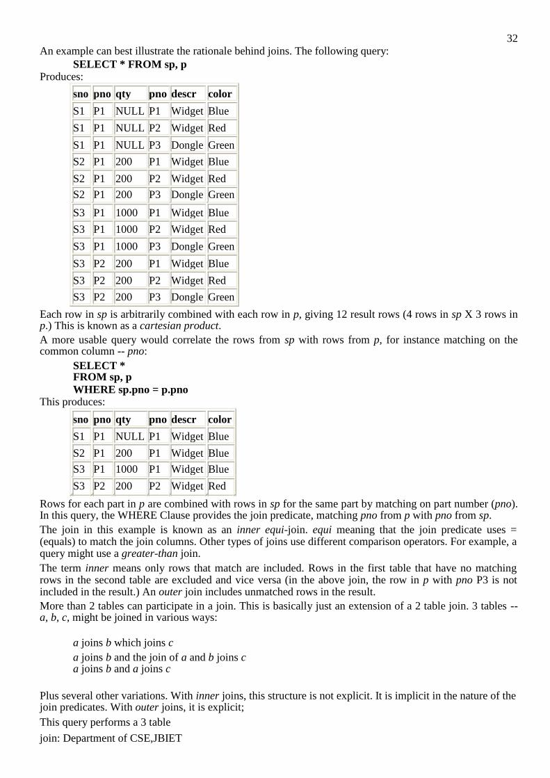
An example can best illustrate the rationale behind joins. The following query: SELECT * FROM sp, p

Produces:

sno pno qty pno descr color

S1 P1 NULL P1 Widget Blue

S1 P1 NULL P2 Widget Red

S1 P1 NULL P3 Dongle Green

S2 P1 200 P1 Widget Blue

S2 P1 200 P2 Widget Red

S2 P1 200 P3 Dongle Green

S3 P1 1000 P1 Widget Blue

S3 P1 1000 P2 Widget Red

S3 P1 1000 P3 Dongle Green

S3 P2 200 P1 Widget Blue

S3 P2 200 P2 Widget Red

S3 P2 200 P3 Dongle Green

Each row in sp is arbitrarily combined with each row in p, giving 12 result rows (4 rows in sp X 3 rows in p.) This is known as a cartesian product. A more usable query would correlate the rows from sp with rows from p, for instance matching on the common column -- pno:

SELECT * FROM sp, p WHERE sp.pno = p.pno

This produces:

sno pno qty pno descr color

S1 P1 NULL P1 Widget Blue

S2 P1 200 P1 Widget Blue

S3 P1 1000 P1 Widget Blue

S3 P2 200 P2 Widget Red

Rows for each part in p are combined with rows in sp for the same part by matching on part number (pno). In this query, the WHERE Clause provides the join predicate, matching pno from p with pno from sp. The join in this example is known as an inner equi-join. equi meaning that the join predicate uses = (equals) to match the join columns. Other types of joins use different comparison operators. For example, a query might use a greater-than join. The term inner means only rows that match are included. Rows in the first table that have no matching rows in the second table are excluded and vice versa (in the above join, the row in p with pno P3 is not included in the result.) An outer join includes unmatched rows in the result. More than 2 tables can participate in a join. This is basically just an extension of a 2 table join. 3 tables -- a, b, c, might be joined in various ways:

a joins b which joins c a joins b and the join of a and b joins c a joins b and a joins c

Plus several other variations. With inner joins, this structure is not explicit. It is implicit in the nature of the join predicates. With outer joins, it is explicit; This query performs a 3 table

join: Department of CSE,JBIET

33

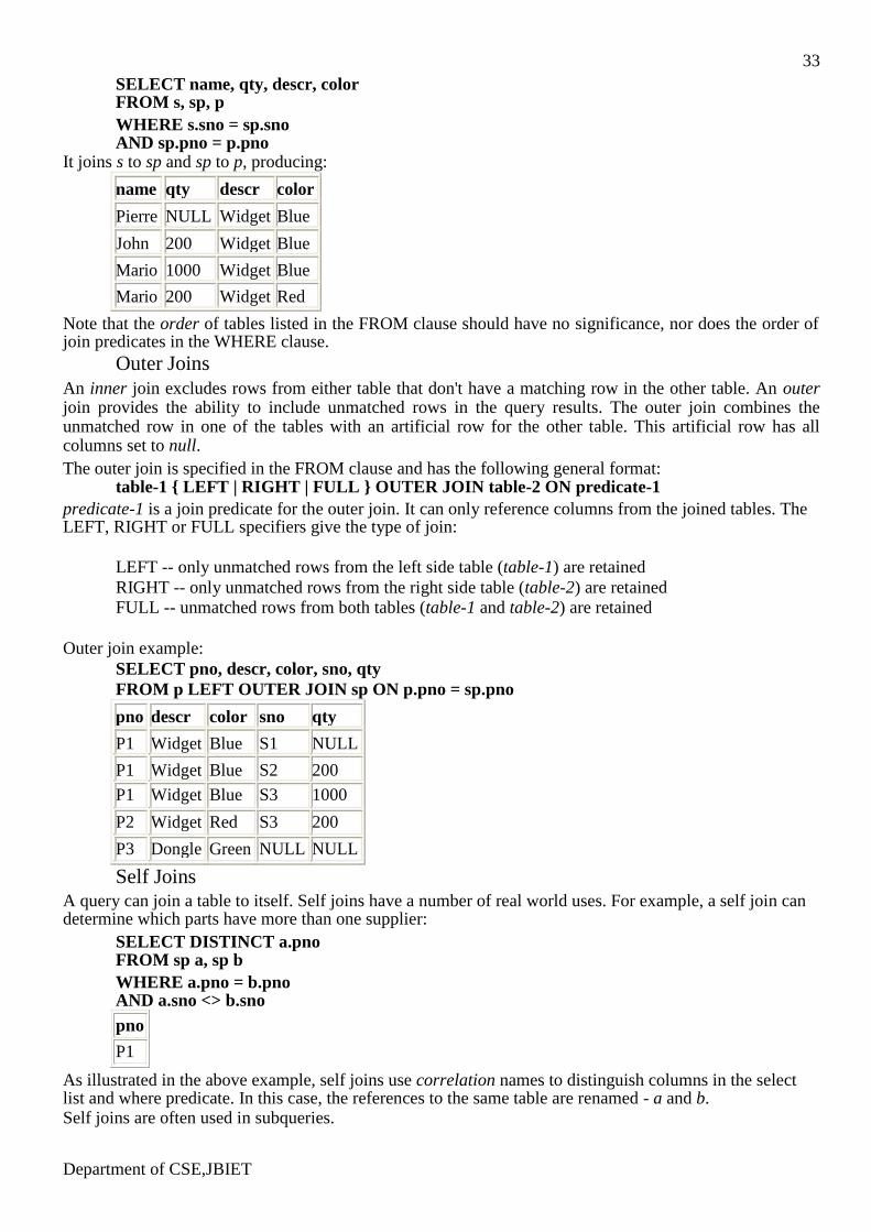
SELECT name, qty, descr, color FROM s, sp, p WHERE s.sno = sp.sno AND sp.pno = p.pno

It joins s to sp and sp to p, producing:

name qty descr color

Pierre NULL Widget Blue

John 200 Widget Blue

Mario 1000 Widget Blue

Mario 200 Widget Red

Note that the order of tables listed in the FROM clause should have no significance, nor does the order of join predicates in the WHERE clause.

Outer Joins An inner join excludes rows from either table that don't have a matching row in the other table. An outer join provides the ability to include unmatched rows in the query results. The outer join combines the unmatched row in one of the tables with an artificial row for the other table. This artificial row has all columns set to null. The outer join is specified in the FROM clause and has the following general format:

table-1 { LEFT | RIGHT | FULL } OUTER JOIN table-2 ON predicate-1 predicate-1 is a join predicate for the outer join. It can only reference columns from the joined tables. The LEFT, RIGHT or FULL specifiers give the type of join:

LEFT -- only unmatched rows from the left side table (table-1) are retained RIGHT -- only unmatched rows from the right side table (table-2) are retained

FULL -- unmatched rows from both tables (table-1 and table-2) are retained

Outer join example:

SELECT pno, descr, color, sno, qty FROM p LEFT OUTER JOIN sp ON p.pno = sp.pno

pno descr color sno qty

P1 Widget Blue S1 NULL

P1 Widget Blue S2 200

P1 Widget Blue S3 1000

P2 Widget Red S3 200

P3 Dongle Green NULL NULL

Self Joins A query can join a table to itself. Self joins have a number of real world uses. For example, a self join can determine which parts have more than one supplier:

SELECT DISTINCT a.pno FROM sp a, sp b WHERE a.pno = b.pno AND a.sno <> b.sno pno

P1

As illustrated in the above example, self joins use correlation names to distinguish columns in the select list and where predicate. In this case, the references to the same table are renamed - a and b. Self joins are often used in subqueries. Department of CSE,JBIET

34

Subqueries Subqueries are an identifying feature of SQL. It is called Structured Query Language because a query can nest inside another query. There are 3 basic types of subqueries in SQL:

Predicate Subqueries -- extended logical constructs in the WHERE (and HAVING) clause. Scalar Subqueries -- standalone queries that return a single value; they can be used anywhere a scalar value is used. Table Subqueries -- queries nested in the FROM clause.

All subqueries must be enclosed in parentheses.

Predicate Subqueries Predicate subqueries are used in the WHERE (and HAVING) clause. Each is a special logical construct. Except for EXISTS, predicate subqueries must retrieve one column (in their select list.)

IN Subquery

The IN Subquery tests whether a scalar value matches the single query column value in any subquery result row. It has the following general format:

value-1 [NOT] IN (query-1)

Using NOT is equivalent to:

NOT value-1 IN (query-1)

For example, to list parts that have suppliers:

SELECT * FROM p

WHERE pno IN (SELECT pno FROM sp)

pnodescr color

P1 Widget Blue

P2 Widget Red

The Self Join example in the previous subsection can be expressed with an IN Subquery:

SELECT DISTINCT pno FROM sp a

WHERE pno IN (SELECT pno FROM sp b WHERE a.sno <> b.sno)

pno

P1

Note that the subquery where clause references a column in the outer query (a.sno). This is known as an outer reference. Subqueries with outer references are sometimes known as correlated subqueries.

Quantified Subqueries

A quantified subquery allows several types of tests and can use the full set of comparison operators. It has the following general format:

Department of CSE,JBIET

35 value-1 {=|>|<|>=|<=|<>} {ANY|ALL|SOME} (query-1)

The comparison operator specifies how to compare value-1 to the single query column value from each subquery result row. The ANY, ALL, SOME specifiers give the type of match expected. ANY and SOME must match at least one row in the subquery. ALL must match all rows in the subquery.

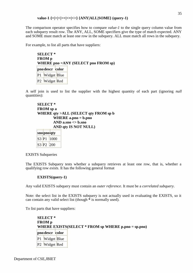
For example, to list all parts that have suppliers:

SELECT *

FROM p WHERE pno =ANY (SELECT pno FROM sp)

pnodescr color

P1 Widget Blue

P2 Widget Red

A self join is used to list the supplier with the highest quantity of each part (ignoring null quantities):

SELECT * FROM sp a

WHERE qty >ALL (SELECT qty FROM sp b WHERE a.pno = b.pno

AND a.sno <> b.sno AND qty IS NOT NULL)

snopnoqty

S3 P1 1000

S3 P2 200

EXISTS Subqueries

The EXISTS Subquery tests whether a subquery retrieves at least one row, that is, whether a qualifying row exists. It has the following general format

EXISTS(query-1)

Any valid EXISTS subquery must contain an outer reference. It must be a correlated subquery.

Note: the select list in the EXISTS subquery is not actually used in evaluating the EXISTS, so it can contain any valid select list (though * is normally used).

To list parts that have suppliers:

SELECT *

FROM p WHERE EXISTS(SELECT * FROM sp WHERE p.pno = sp.pno)

pnodescr color

P1 Widget Blue

P2 Widget Red Department of CSE,JBIET

36

Scalar Subqueries The Scalar Subquery can be used anywhere a value can be used. The subquery must reference just one column in the select list. It must also retrieve no more than one row. When the subquery returns a single row, the value of the single select list column becomes the value of the Scalar Subquery. When the subquery returns no rows, a database null is used as the result of the subquery. Should the subquery retreive more than one row, it is a run-time error and aborts query execution. A Scalar Subquery can appear as a scalar value in the select list and where predicate of an another query. The following query on the sp table uses a Scalar Subquery in the select list to retrieve the supplier city associated with the supplier number (sno column in sp):

SELECT pno, qty, (SELECT city FROM s WHERE s.sno = sp.sno) FROM sp

pnoqty city

P1 NULL Paris

P1 200 London

P1 1000 Rome

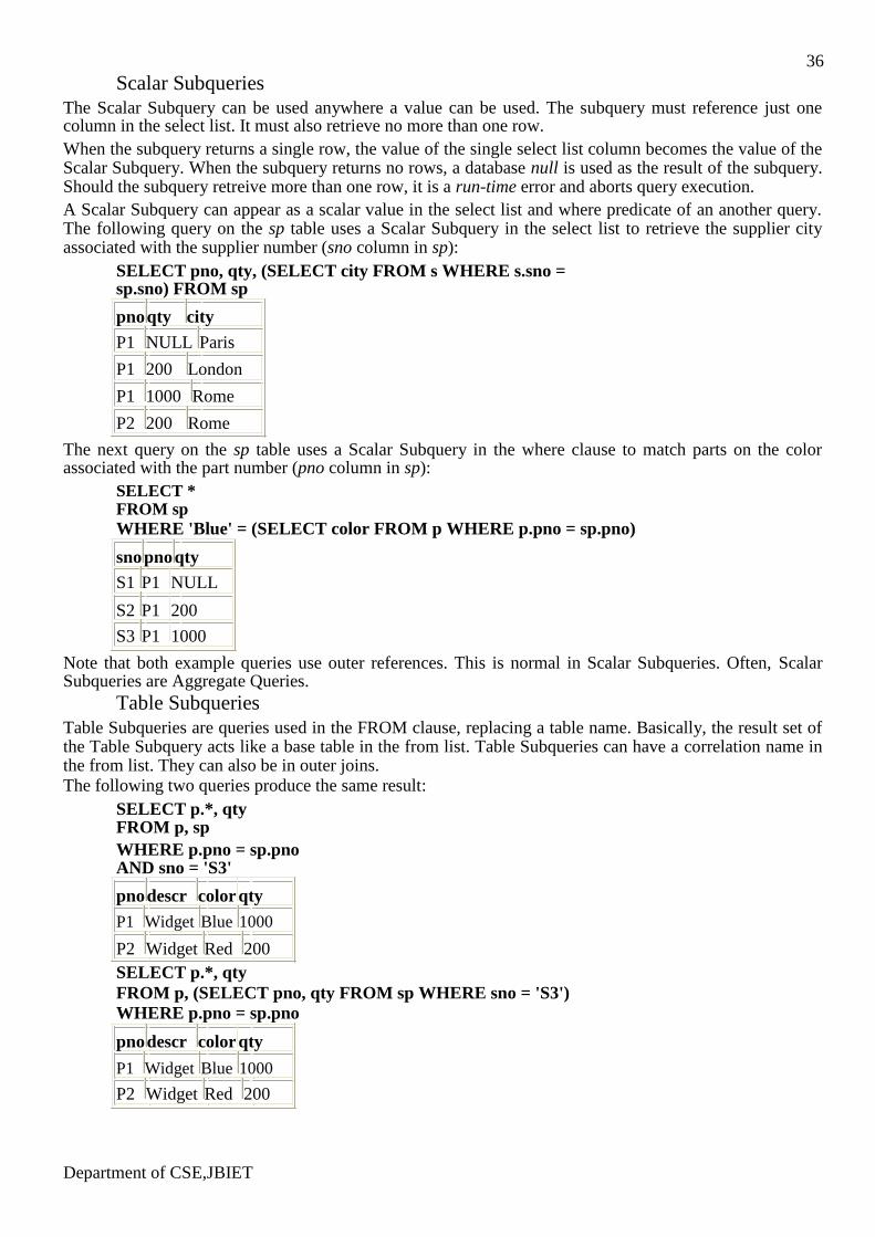
P2 200 Rome The next query on the sp table uses a Scalar Subquery in the where clause to match parts on the color associated with the part number (pno column in sp):

SELECT * FROM sp WHERE 'Blue' = (SELECT color FROM p WHERE p.pno = sp.pno)

snopnoqty

S1 P1 NULL

S2 P1 200

S3 P1 1000 Note that both example queries use outer references. This is normal in Scalar Subqueries. Often, Scalar Subqueries are Aggregate Queries.

Table Subqueries Table Subqueries are queries used in the FROM clause, replacing a table name. Basically, the result set of the Table Subquery acts like a base table in the from list. Table Subqueries can have a correlation name in the from list. They can also be in outer joins. The following two queries produce the same result:

SELECT p.*, qty FROM p, sp WHERE p.pno = sp.pno AND sno = 'S3'

pnodescr color qty

P1 Widget Blue 1000

P2 Widget Red 200 SELECT p.*, qty FROM p, (SELECT pno, qty FROM sp WHERE sno = 'S3')

WHERE p.pno = sp.pno

pnodescr color qty

P1 Widget Blue 1000

P2 Widget Red 200

Department of CSE,JBIET

37

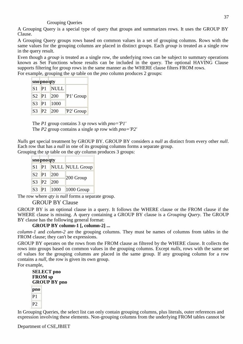
Grouping Queries A Grouping Query is a special type of query that groups and summarizes rows. It uses the GROUP BY Clause. A Grouping Query groups rows based on common values in a set of grouping columns. Rows with the same values for the grouping columns are placed in distinct groups. Each group is treated as a single row in the query result. Even though a group is treated as a single row, the underlying rows can be subject to summary operations known as Set Functions whose results can be included in the query. The optional HAVING Clause supports filtering for group rows in the same manner as the WHERE clause filters FROM rows. For example, grouping the sp table on the pno column produces 2 groups:

snopnoqty

S1 P1 NULL

S2 P1 200 'P1' Group

S3 P1 1000

S3 P2 200 'P2' Group

The P1 group contains 3 sp rows with pno='P1' The P2 group contains a single sp row with pno='P2'

Nulls get special treatment by GROUP BY. GROUP BY considers a null as distinct from every other null. Each row that has a null in one of its grouping columns forms a separate group. Grouping the sp table on the qty column produces 3 groups:

snopnoqty

S1 P1 NULL NULL Group

S2 P1 200 200 Group

S3

P2

200

S3 P1 1000 1000 Group

The row where qty is null forms a separate group.

GROUP BY Clause GROUP BY is an optional clause in a query. It follows the WHERE clause or the FROM clause if the WHERE clause is missing. A query containing a GROUP BY clause is a Grouping Query. The GROUP BY clause has the following general format:

GROUP BY column-1 [, column-2] ... column-1 and column-2 are the grouping columns. They must be names of columns from tables in the FROM clause; they can't be expressions. GROUP BY operates on the rows from the FROM clause as filtered by the WHERE clause. It collects the rows into groups based on common values in the grouping columns. Except nulls, rows with the same set of values for the grouping columns are placed in the same group. If any grouping column for a row contains a null, the row is given its own group. For example,

SELECT pno FROM sp GROUP BY pno

pno

P1

P2

In Grouping Queries, the select list can only contain grouping columns, plus literals, outer references and expression involving these elements. Non-grouping columns from the underlying FROM tables cannot be Department of CSE,JBIET

38 referenced directly. However, non-grouping columns can be used in the select list as arguments to Set Functions. Set Functions summarize columns from the underlying rows of a group.

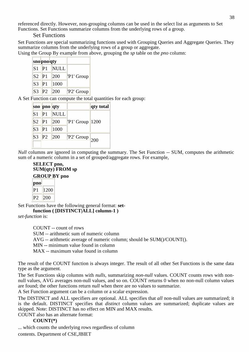
Set Functions Set Functions are special summarizing functions used with Grouping Queries and Aggregate Queries. They summarize columns from the underlying rows of a group or aggregate. Using the Group By example from above, grouping the sp table on the pno column:

snopnoqty

S1 P1 NULL

S2 P1 200 'P1' Group

S3 P1 1000

S3 P2 200 'P2' Group

A Set Function can compute the total quantities for each group:

sno pno qty qty total

S1 P1 NULL

S2 P1 200 'P1' Group 1200

S3 P1 1000

S3 P2 200 'P2' Group 200

Null columns are ignored in computing the summary. The Set Function -- SUM, computes the arithmetic sum of a numeric column in a set of grouped/aggregate rows. For example,

SELECT pno, SUM(qty) FROM sp GROUP BY pno

pno

P1 1200

P2 200

Set Functions have the following general format: set-function ( [DISTINCT|ALL] column-1 )

set-function is:

COUNT -- count of rows SUM -- arithmetic sum of numeric column AVG -- arithmetic average of numeric column; should be SUM()/COUNT().

MIN -- minimum value found in column MAX -- maximum value found in column

The result of the COUNT function is always integer. The result of all other Set Functions is the same data type as the argument. The Set Functions skip columns with nulls, summarizing non-null values. COUNT counts rows with non-null values, AVG averages non-null values, and so on. COUNT returns 0 when no non-null column values are found; the other functions return null when there are no values to summarize. A Set Function argument can be a column or a scalar expression. The DISTINCT and ALL specifiers are optional. ALL specifies that all non-null values are summarized; it is the default. DISTINCT specifies that distinct column values are summarized; duplicate values are skipped. Note: DISTINCT has no effect on MIN and MAX results. COUNT also has an alternate format:

COUNT(*) ... which counts the underlying rows regardless of column

contents. Department of CSE,JBIET

39

Set Function examples:

SELECT pno, MIN(sno), MAX(qty), AVG(qty), COUNT(DISTINCT sno) FROM sp GROUP BY pno

pno

P1 S110006003 P2

S3200 2001 SELECT sno, COUNT(*) parts

FROM sp GROUP BY sno

sno parts

S1 1

S2 1

S3 2 HAVING Clause

The HAVING Clause is associated with Grouping Queries and Aggregate Queries. It is optional in both cases. In Grouping Queries, it follows the GROUP BY clause. In Aggregate Queries, HAVING follows the WHERE clause or the FROM clause if the WHERE clause is missing. The HAVING Clause has the following general format:

HAVING predicate Like the WHERE Clause, HAVING filters the query result rows. WHERE filters the rows from the FROM clause. HAVING filters the grouped rows (from the GROUP BY clause) or the aggregate row (for Aggregate Queries). predicate is a logical expression referencing grouped columns and set functions. It has the same restrictions as the select list for Grouping Queries and Aggregate Queries. If the Having predicate evaluates to true for a grouped or aggregate row, the row is included in the query result, otherwise, the row is skipped (not included in the query result). For example,

SELECT sno, COUNT(*) parts FROM sp GROUP BY sno HAVING COUNT(*) > 1

sno parts

S3 2 Aggregate Queries

An Aggregate Query can use Set Functions and a HAVING Clause. It is similar to a Grouping Query except there are no grouping columns. The underlying rows from the FROM and WHERE clauses are grouped into a single aggregate row. An Aggregate Query always returns a single row, except when the Having clause is used. An Aggregate Query is a query containing Set Functions in the select list but no GROUP BY clause. The Set Functions operate on the columns of the underlying rows of the single aggregate row. Except for outer references, any columns used in the select list must be arguments to Set Functions. An aggregate query may also have a Having clause. The Having clause filters the single aggregate row. If the Having predicate evaluates to true, the query result contains the aggregate row. Otherwise, the query result contains no rows. For example,

SELECT COUNT(DISTINCT pno) number_parts, SUM(qty) total_parts FROM sp

number_parts total_parts Department of CSE,JBIET

40

2 1400

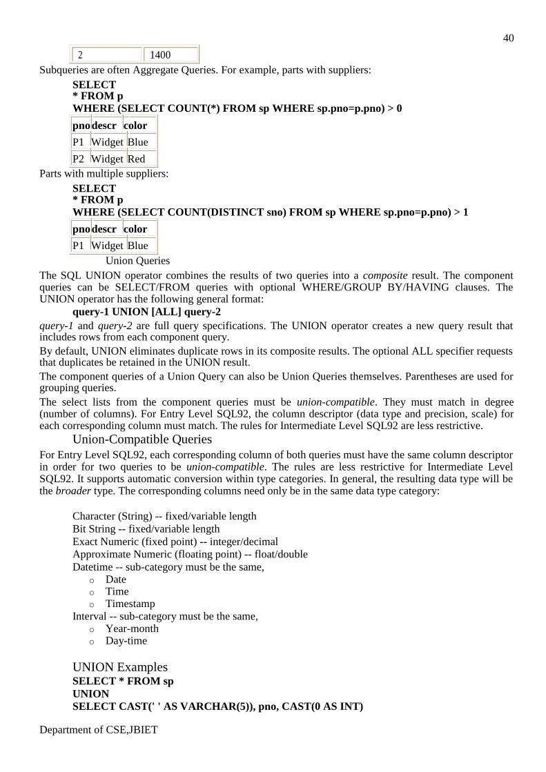
Subqueries are often Aggregate Queries. For example, parts with suppliers:

SELECT * FROM p WHERE (SELECT COUNT(*) FROM sp WHERE sp.pno=p.pno) > 0

pnodescr color

P1 Widget Blue

P2 Widget Red Parts with multiple suppliers:

SELECT * FROM p WHERE (SELECT COUNT(DISTINCT sno) FROM sp WHERE sp.pno=p.pno) > 1

pnodescr color

P1 Widget Blue Union Queries

The SQL UNION operator combines the results of two queries into a composite result. The component queries can be SELECT/FROM queries with optional WHERE/GROUP BY/HAVING clauses. The UNION operator has the following general format:

query-1 UNION [ALL] query-2 query-1 and query-2 are full query specifications. The UNION operator creates a new query result that includes rows from each component query. By default, UNION eliminates duplicate rows in its composite results. The optional ALL specifier requests that duplicates be retained in the UNION result. The component queries of a Union Query can also be Union Queries themselves. Parentheses are used for grouping queries. The select lists from the component queries must be union-compatible. They must match in degree (number of columns). For Entry Level SQL92, the column descriptor (data type and precision, scale) for each corresponding column must match. The rules for Intermediate Level SQL92 are less restrictive.

Union-Compatible Queries For Entry Level SQL92, each corresponding column of both queries must have the same column descriptor in order for two queries to be union-compatible. The rules are less restrictive for Intermediate Level SQL92. It supports automatic conversion within type categories. In general, the resulting data type will be the broader type. The corresponding columns need only be in the same data type category:

Character (String) -- fixed/variable length Bit String -- fixed/variable length Exact Numeric (fixed point) -- integer/decimal

Approximate Numeric (floating point) -- float/double Datetime -- sub-category must be the same,

o Date o Time o Timestamp

Interval -- sub-category must be the same, o Year-month o Day-time

UNION Examples SELECT * FROM sp UNION

SELECT CAST(' ' AS VARCHAR(5)), pno, CAST(0 AS INT) Department of CSE,JBIET

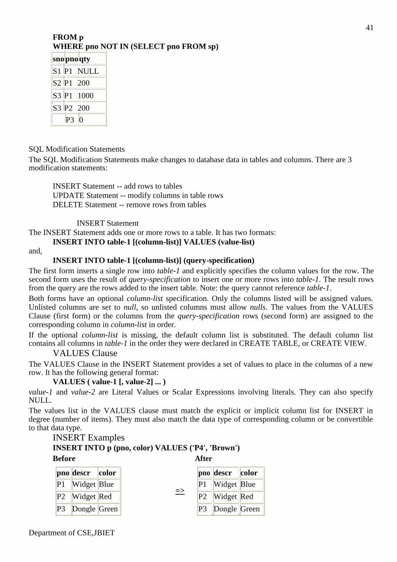
41 FROM p WHERE pno NOT IN (SELECT pno FROM sp)

snopnoqty

S1 P1 NULL

S2 P1 200

S3 P1 1000

S3 P2 200

P3 0

SQL Modification Statements The SQL Modification Statements make changes to database data in tables and columns. There are 3 modification statements:

INSERT Statement -- add rows to tables UPDATE Statement -- modify columns in table rows

DELETE Statement -- remove rows from tables

INSERT Statement

The INSERT Statement adds one or more rows to a table. It has two formats: INSERT INTO table-1 [(column-list)] VALUES (value-list)

and, INSERT INTO table-1 [(column-list)] (query-specification)

The first form inserts a single row into table-1 and explicitly specifies the column values for the row. The second form uses the result of query-specification to insert one or more rows into table-1. The result rows from the query are the rows added to the insert table. Note: the query cannot reference table-1. Both forms have an optional column-list specification. Only the columns listed will be assigned values. Unlisted columns are set to null, so unlisted columns must allow nulls. The values from the VALUES Clause (first form) or the columns from the query-specification rows (second form) are assigned to the corresponding column in column-list in order. If the optional column-list is missing, the default column list is substituted. The default column list contains all columns in table-1 in the order they were declared in CREATE TABLE, or CREATE VIEW.

VALUES Clause The VALUES Clause in the INSERT Statement provides a set of values to place in the columns of a new row. It has the following general format:

VALUES ( value-1 [, value-2] ... ) value-1 and value-2 are Literal Values or Scalar Expressions involving literals. They can also specify NULL. The values list in the VALUES clause must match the explicit or implicit column list for INSERT in degree (number of items). They must also match the data type of corresponding column or be convertible to that data type.

INSERT Examples INSERT INTO p (pno, color) VALUES ('P4', 'Brown') Before After

pno descr color pno descr color

P1 Widget Blue =>

P1 Widget Blue

P2

Widget Red

P2

Widget

Red

P3 Dongle Green P3 Dongle Green

Department of CSE,JBIET

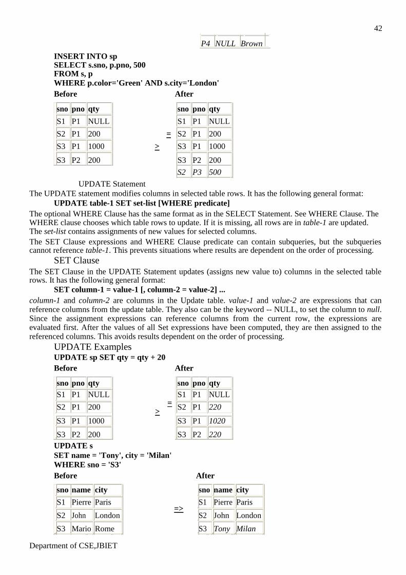
42

P4 NULL Brown

INSERT INTO sp SELECT s.sno, p.pno, 500 FROM s, p WHERE p.color='Green' AND s.city='London' Before After

sno pno qty sno pno qty

S1 P1 NULL S1 P1 NULL

S2 P1 200 = S2 P1 200

>

S3 P1 1000 S3 P1 1000

S3 P2 200 S3 P2 200

S2 P3 500

UPDATE Statement

The UPDATE statement modifies columns in selected table rows. It has the following general format: UPDATE table-1 SET set-list [WHERE predicate]

The optional WHERE Clause has the same format as in the SELECT Statement. See WHERE Clause. The WHERE clause chooses which table rows to update. If it is missing, all rows are in table-1 are updated. The set-list contains assignments of new values for selected columns. The SET Clause expressions and WHERE Clause predicate can contain subqueries, but the subqueries cannot reference table-1. This prevents situations where results are dependent on the order of processing.

SET Clause The SET Clause in the UPDATE Statement updates (assigns new value to) columns in the selected table rows. It has the following general format:

SET column-1 = value-1 [, column-2 = value-2] ... column-1 and column-2 are columns in the Update table. value-1 and value-2 are expressions that can reference columns from the update table. They also can be the keyword -- NULL, to set the column to null. Since the assignment expressions can reference columns from the current row, the expressions are evaluated first. After the values of all Set expressions have been computed, they are then assigned to the referenced columns. This avoids results dependent on the order of processing.

UPDATE Examples UPDATE sp SET qty = qty + 20 Before After

sno pno qty sno pno qty

S1 P1 NULL S1 P1 NULL

=

S2 P1 200 S2 P1 220

>

S3 P1 1000 S3 P1 1020

S3 P2 200 S3 P2 220

UPDATE s

SET name = 'Tony', city = 'Milan'

WHERE sno = 'S3'

Before After

sno name city sno name city

S1 Pierre Paris =>

S1 Pierre Paris

S2 John

London

S2

John

London

S3 Mario Rome S3 Tony Milan

Department of CSE,JBIET

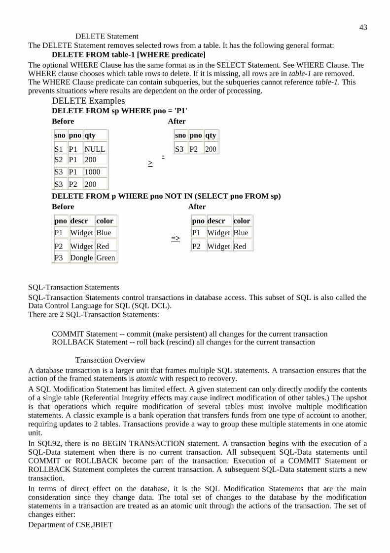
43

DELETE Statement The DELETE Statement removes selected rows from a table. It has the following general format:

DELETE FROM table-1 [WHERE predicate] The optional WHERE Clause has the same format as in the SELECT Statement. See WHERE Clause. The WHERE clause chooses which table rows to delete. If it is missing, all rows are in table-1 are removed. The WHERE Clause predicate can contain subqueries, but the subqueries cannot reference table-1. This prevents situations where results are dependent on the order of processing.

DELETE Examples DELETE FROM sp WHERE pno = 'P1' Before After

sno pno qty sno pno qty

S1 P1 NULL S3 P2 200

S2

P1

200 =

>

S3 P1 1000

S3 P2 200

DELETE FROM p WHERE pno NOT IN (SELECT pno FROM sp) Before After

pno descr color pno descr color

P1 Widget Blue =>

P1 Widget Blue

P2

Widget

Red

P2

Widget

Red

P3 Dongle Green

SQL-Transaction Statements SQL-Transaction Statements control transactions in database access. This subset of SQL is also called the Data Control Language for SQL (SQL DCL). There are 2 SQL-Transaction Statements:

COMMIT Statement -- commit (make persistent) all changes for the current transaction ROLLBACK Statement -- roll back (rescind) all changes for the current transaction

Transaction Overview A database transaction is a larger unit that frames multiple SQL statements. A transaction ensures that the action of the framed statements is atomic with respect to recovery. A SQL Modification Statement has limited effect. A given statement can only directly modify the contents of a single table (Referential Integrity effects may cause indirect modification of other tables.) The upshot is that operations which require modification of several tables must involve multiple modification statements. A classic example is a bank operation that transfers funds from one type of account to another, requiring updates to 2 tables. Transactions provide a way to group these multiple statements in one atomic unit. In SQL92, there is no BEGIN TRANSACTION statement. A transaction begins with the execution of a SQL-Data statement when there is no current transaction. All subsequent SQL-Data statements until COMMIT or ROLLBACK become part of the transaction. Execution of a COMMIT Statement or ROLLBACK Statement completes the current transaction. A subsequent SQL-Data statement starts a new transaction. In terms of direct effect on the database, it is the SQL Modification Statements that are the main consideration since they change data. The total set of changes to the database by the modification statements in a transaction are treated as an atomic unit through the actions of the transaction. The set of changes either: Department of CSE,JBIET

44 Is made fully persistent in the database through the action of the COMMIT Statement, or Has no persistent effect whatever on the database, through:

o the action of the ROLLBACK Statement, o abnormal termination of the client requesting the transaction, or o abnormal termination of the transaction by the DBMS. This may be an action by the system

(deadlock resolution) or by an administrative agent, or it may be an abnormal termination of the DBMS itself. In the latter case, the DBMS must roll back any active transactions during recovery.

The DBMS must ensure that the effect of a transaction is not partial. All changes in a transaction must be made persistent, or no changes from the transaction must be made persistent.

Transaction Isolation In most cases, transactions are executed under a client connection to the DBMS. Multiple client connections can initiate transactions at the same time. This is known as concurrent transactions. In the relational model, each transaction is completely isolated from other active transactions. After initiation, a transaction can only see changes to the database made by transactions committed prior to starting the new transaction. Changes made by concurrent transactions are not seen by SQL DML query and modification statements. This is known as full isolation or Serializable transactions. SQL92 defines Serializable for transactions. However, full serialized transactions can impact performance. For this reason, SQL92 allows additional isolation modes that reduce the isolation between concurrent transactions. SQL92 defines 3 other isolation modes, but support by existing DBMSs is often incomplete and doesn't always match the SQL92 modes. Check the documentation of your DBMS for more details.

SQL-Schema Statements in Transactions The 3rd type of SQL Statements - SQL-Schema Statements, may participate in the transaction mechanism. SQL-Schema statements can either be:

included in a transaction along with SQL-Data statements, required to be in separate transactions, or ignored by the transaction mechanism (can't be rolled back).

SQL92 leaves the choice up to the individual DBMS. It is implementation defined behavior.

COMMIT Statement The COMMIT Statement terminates the current transaction and makes all changes under the transaction persistent. It commits the changes to the database. The COMMIT statement has the following general format:

COMMIT [WORK] WORK is an optional keyword that does not change the semantics of COMMIT.

ROLLBACK Statement The ROLLBACK Statement terminates the current transaction and rescinds all changes made under the transaction. It rolls back the changes to the database. The ROLLBACK statement has the following general format:

ROLLBACK [WORK] WORK is an optional keyword that does not change the semantics of ROLLBACK.

SQL-Schema Statements SQL-Schema Statements provide maintenance of catalog objects for a schema -- tables, views and privileges. This subset of SQL is also called the Data Definition Language for SQL (SQL DDL). There are 6 SQL-Schema Statements:

CREATE TABLE Statement -- create a new base table in the current schema CREATE VIEW Statement -- create a new view table in the current schema

DROP TABLE Statement -- remove a base table from the current schema

Department of CSE,JBIET

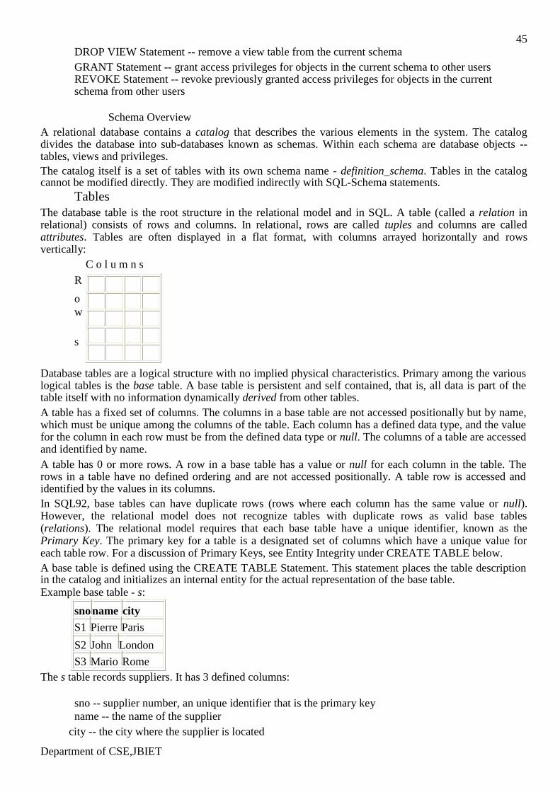
45

DROP VIEW Statement -- remove a view table from the current schema GRANT Statement -- grant access privileges for objects in the current schema to other users REVOKE Statement -- revoke previously granted access privileges for objects in the current schema from other users

Schema Overview

A relational database contains a catalog that describes the various elements in the system. The catalog divides the database into sub-databases known as schemas. Within each schema are database objects -- tables, views and privileges. The catalog itself is a set of tables with its own schema name - definition_schema. Tables in the catalog cannot be modified directly. They are modified indirectly with SQL-Schema statements.

Tables The database table is the root structure in the relational model and in SQL. A table (called a relation in relational) consists of rows and columns. In relational, rows are called tuples and columns are called attributes. Tables are often displayed in a flat format, with columns arrayed horizontally and rows vertically:

C o l u m n s R

o

w

s Database tables are a logical structure with no implied physical characteristics. Primary among the various logical tables is the base table. A base table is persistent and self contained, that is, all data is part of the table itself with no information dynamically derived from other tables. A table has a fixed set of columns. The columns in a base table are not accessed positionally but by name, which must be unique among the columns of the table. Each column has a defined data type, and the value for the column in each row must be from the defined data type or null. The columns of a table are accessed and identified by name. A table has 0 or more rows. A row in a base table has a value or null for each column in the table. The rows in a table have no defined ordering and are not accessed positionally. A table row is accessed and identified by the values in its columns. In SQL92, base tables can have duplicate rows (rows where each column has the same value or null). However, the relational model does not recognize tables with duplicate rows as valid base tables (relations). The relational model requires that each base table have a unique identifier, known as the Primary Key. The primary key for a table is a designated set of columns which have a unique value for each table row. For a discussion of Primary Keys, see Entity Integrity under CREATE TABLE below. A base table is defined using the CREATE TABLE Statement. This statement places the table description in the catalog and initializes an internal entity for the actual representation of the base table. Example base table - s:

snoname city

S1 Pierre Paris

S2 John London

S3 Mario Rome The s table records suppliers. It has 3 defined columns:

sno -- supplier number, an unique identifier that is the primary key name -- the name of the supplier

city -- the city where the supplier is located

Department of CSE,JBIET

46

At the current time, there are 3 rows. Other types of tables in the system are derived tables. SQL-Data statements use internally derived tables in computing results. A query is in fact a derived table. For instance, the query operator - Union, combines two derived tables to produce a third one. Much of the power of SQL comes from the fact that its higher level operations are performed on tables and produce a table as their result. Derived tables are less constrained than base tables. Column names are not required and need not be unique. Derived tables may have duplicate rows. Views are a type of derived table that are cataloged in the database.

Views A view is a derived table registered in the catalog. A view is defined using a SQL query. The view is dynamically derived, that is, its contents are materialized for each use. Views are added to the catalog with the CREATE VIEW Statement. Once defined in the catalog, a view can substitute for a table in SQL-Data statements. A view name can be used instead of a base table name in the FROM clause of a SELECT statement. Views can also be the subject of a modification statement with some restrictions. A SQL Modification Statement can operate on a view if it is an updatable view. An updatable view has the following restrictions on its defining query:

The query FROM clause can reference a single table (or view) The single table in the FROM clause must be:

o a base table, o a view that is also an updatable view, or o a nested query that is updatable, that is, it follows the rules for an updatable view query.

The query must be a basic query, not a: o Grouping Query, o Aggregate Query, or o Union Query.

The select list cannot contain: o the DISTINCT specifier, o an Expression, or o duplicate column references

Subqueries are acceptable in updatable views but cannot reference the underlying base table for the view's FROM clause.

Privileges SQL92 defines a SQL-agent as an implementation-dependent entity that causes the execution of SQL statements. Prior to execution of SQL statements, the SQL-agent must establish an authorization identifier for database access. An authorization identifier is commonly called a user name. A DBMS user may access database objects (tables, columns, views) as allowed by the privileges assigned to that specific authorization identifier. Access privileges may be granted by the system (automatic) or by other users. System granted privileges include:

All privileges on a table to the user that created the table. This includes the privilege to grant privileges on the table to other users. SELECT (readonly) privilege on the catalog (the tables in the schema - definition_schema). This is granted to all users.

User granted privileges cover privileges to access and modify tables and their columns. Privileges can be granted for specific SQL-Data Statements -- SELECT, INSERT, UPDATE, DELETE.

CREATE TABLE Statement The CREATE TABLE Statement creates a new base table. It adds the table description to the catalog. A base table is a logical entity with persistence. The logical description of a base table consists of: Department of CSE,JBIET

47

Schema -- the logical database schema the table resides in Table Name -- a name unique among tables and views in the Schema Column List -- an ordered list of column declarations (name, data type) Constraints -- a list of constraints on the contents of the table

The CREATE TABLE Statement has the following general format:

CREATE TABLE table-name ({column-descr|constraint} [,{column-descr|constraint}]...) table-name is the new name for the table. column-descr is a column declaration. constraint is a table constraint. The column declaration can include optional column constraints. The declaration has the following general format:

column-name data-type [column-constraints] column-name is the name of the column and must be unique among the columns of the table. data-type declares the type of the column. Data types are described below. column-constraints is an optional list of column constraints with no separators.

Constraints Constraint specifications add additional restrictions on the contents of the table. They are automatically enforced by the DBMS. The column constraints are:

NOT NULL -- specifies that the column can't be set to null. If this constraint is not specified, the column is nullable, that is, it can be set to null. Normally, primary key columns are declared as NOT NULL. PRIMARY KEY -- specifies that this column is the only column in the primary key. There can be only one primary key declaration in a CREATE TABLE. For primary keys with multiple columns, use the PRIMARY KEY table constraint. See Entity Integrity below for a detailed description of primary keys. UNIQUE -- specifies that this column has a unique value or null for all rows of the table. REFERENCES -- specifies that this column is the only column in a foreign key. For foreign keys with multiple columns, use the FOREIGN KEY table constraint. See Referential Integrity below for a detailed description of primary keys. CHECK -- specifies a user defined constraint on the table. See the table constraint - CHECK, below.

The table constraints are:

PRIMARY KEY -- specifies the set of columns that comprise the primary key. There can be only one primary key declaration in a CREATE TABLE Statement. See Entity Integrity below for a detailed description of primary keys. UNIQUE -- specifies that a set of columns have unique values (or nulls) for all rows in the table. The UNIQUE specifier is followed by a parenthesized list of column names, separated by commas. FOREIGN KEY -- specifies the set of columns in a foreign key. See Referential Integrity below for a detailed description of foreign keys. CHECK -- specifies a user defined constraint, known as a check condition. The CHECK specifier is followed by a predicate enclosed in parentheses. For Intermediate Level SQL92, the CHECK predicate can only reference columns from the current table row, with no subqueries. Many DBMSs support subqueries in the check predicate.

The check predicate must evaluate to true before a modification or addition of a row takes place. The check is effectively made on the contents of the table after the modification. For INSERT Statements, the predicate is evaluated as if the INSERT row were added to the table. For UPDATE Statements, the predicate is evaluated as if the row were updated. For DELETE Statements, the predicate is evaluated as if the row were deleted (Note: A check predicate is only useful for DELETE if a subquery is used.)

Department of CSE,JBIET

48

Data Type This subsection describes data type specifications. The data type categories are:

Character (String) -- fixed or variable length character strings. The character set is implementation defined but often defaults to ASCII. Numeric -- values representing numeric quantities. Numeric values are divided into these two broad categories:

o Exact (also known as fixed-point) -- Exact numeric values have a fixed number of digits to the left of the decimal point and a fixed number of digits to the right (the scale). The total number of digits on both sides of the decimal are the precision. A special subset of exact numeric types with a scale of 0 is called integer.

o Approximate (also known as floating-point) -- Approximate numeric values that have a fixed precision (number of digits) but a floating decimal point.

All numeric types are signed.

Datetime -- Datetime values include calendar and clock values (Date, Time, Timestamp) and intervals. The datetime types are:

o Date -- calendar date with year, month and day o Time -- clock time with hour, minute, second and fraction of second, plus a timezone

component (adjustment in hours, minutes) o Timestamp -- combination calendar date and clock time with year, month, day, hour,

minute, second and fraction of second, plus a timezone component (adjustment in hours, minutes)

o Interval -- intervals represent time and date intervals. They are signed. An interval value can contain a subset of the interval fields, for example - hour to minute, year, day to second. Interval types are subdivided into:

year-month intervals -- may contain years, months or combination years/months value.

day-time intervals -- days, hours, minutes, seconds, fractions of second.

Data type declarations have the following general format:

Character (String)

CHAR [(length)]

CHARACTER [(length)] VARCHAR (length)

CHARACTER VARYING (length) length specifies the number of characters for fixed size strings (CHAR, CHARACTER); spaces are supplied for shorter strings. If length is missing for fixed size strings, the default length is 1. For variable size strings (VARCHAR, CHARACTER VARYING), length is the maximum size of the string. Strings exceeding length are truncated on the right.

Numeric SMALLINT INT INTEGER

The integer types have default binary precision -- 15 for SMALLINT and 31 for INT, INTEGER. NUMERIC ( precision [, scale] )

DECIMAL ( precision [, scale] ) Fixed point types have a decimal precision (total number of digits) and scale (which cannot exceed the precision). The default scale is 0. NUMERIC scales must be represented exactly. DECIMAL values can be stored internally with a larger scale (implementation defined).

Department of CSE,JBIET

49

FLOAT [(precision)] REAL

DOUBLE The floating point types have a binary precision (maximum significant binary digits). Precision values are implementation dependent for REAL and DOUBLE, although the standard states that the default precision for DOUBLE must be larger than for REAL. FLOAT also uses an implementation defined default for precision (commonly this is the same as for REAL), but the binary precision for FLOAT can be explicit.

Datetime DATE

TIME [(scale)] [WITH TIME ZONE] TIMESTAMP [(scale)] [WITH TIME ZONE] TIME and TIMESTAMP allow an optional seconds fraction (scale). The default scale for TIME is 0, for TIMESTAMP 6. The optional WITH TIME ZONE specifier indicates that the timezone adjustment is stored with the value; if omitted, the current system timezone is assumed. INTERVAL interval-qualifier

Interval Qualifier An interval qualifier defines the specific type of an interval value. The qualifier for an interval type declares the sub-fields that comprise the interval, the precision of the highest (left-most) sub-field and the scale of the SECOND sub-field (if any). Intervals are divided into sub-types -- year-month intervals and day-time intervals. Year-month intervals can only contain the sub-fields - year and month. Day-time intervals can contain day, hour, minute, second. The interval qualifier has the following formats:

YEAR [(precision)] [ TO MONTH ]

MONTH [(precision)]

{DAY|HOUR|MINUTE} [(precision)] [ TO SECOND [(scale)] ]

DAY [(precision)] [ TO {HOUR|MINUTE} ]

HOUR [(precision)] [ TO MINUTE ]

SECOND [ (precision [, scale]) ] The default precision is 2. The default scale is 6.

Entity Integrity As mentioned earlier, the relational model requires that each base table have a Primary Key. SQL92, on the other hand, allows a table to created without a primary key. The advice here is to create all tables with primary keys. A primary key is a constraint on the contents of a table. In relational terms, the primary key maintains Entity Integrity for the table. It constrains the table as follows,

For a given row, the set of values for the primary key columns must be unique from all other rows in the table, No primary key column can contain a null, and A table can have only one primary key (set of primary key columns).

Note: SQL92 does not require the second restriction on nulls in the primary key. However, it is required for a relational system. Department of CSE,JBIET

50 Entity Integrity (Primary Keys) is enforced by the DBMS and ensures that every row has a proper unique identifier. The contents of any column in the table with Entity Integrity can be uniquely accessed with 3 pieces of information:

table identifier primary key value column name

This capability is crucial to a relational system. Having a clear, consistent identifier for table rows (and their columns) distinguishes relational systems from all others. It allows the establishment of relationships between tables, also crucial to relational systems. This is discussed below under Referential Integrity. The primary key constraint in the CREATE STATEMENT has two forms. When the primary key consists of a single column, it can be declared as a column constraint, simply - PRIMARY KEY, attached to the column descriptor. For example:

sno VARCHAR(5) NOT NULL PRIMARY KEY As a table constraint, it has the following format:

PRIMARY KEY ( column-1 [, column-2] ...) column-1 and column-2 are the names of the columns of the primary key. For example,

PRIMARY KEY (sno, pno) The order of columns in the primary key is not significant, except as the default order for the FOREIGN KEY table constraint.

Referential Integrity Foreign keys provide relationships between tables in the database. In relational, a foreign key in a table is a set of columns that reference the primary key of another table. For each row in the referencing table, the foreign key must match an existing primary key in the referenced table. The enforcement of this constraint is known as Referential Integrity. Referential Integrity requires that:

The columns of a foreign key must match in number and type the columns of the primary key in the referenced table. The values of the foreign key columns in each row of the referencing table must match the values of the corresponding primary key columns for a row in the referenced table.

The one exception to the second restriction is when the foreign key columns for a row contain nulls. Since primary keys should not contain nulls, a foreign key with nulls cannot match any row in the referenced table. However, a row with a foreign key of all nulls (all foreign key columns contain null) is allowed in the referencing table. It is a null reference. Like other constraints, the referential integrity constraint restricts the contents of the referencing table, but it also may in effect restrict the contents of the referenced table. When a row in a table is referenced (through its primary key) by a foreign key in a row in another table, operations that affect its primary key columns have side-effects and may restrict the operation. Changing the primary key of or deleting a row which has referencing foreign keys would violate the referential integrity constraints on the referencing table if allowec to proceed. This is handled in two ways,

The referenced table is restricted from making the change (and violating referential integrity in the referencing table), or Rows in the referencing table are modified so the referential integrity constraint is maintained.

These actions are controlled by the referential integrity effects declarations, called referential triggers by SQL92. The referential integrity effect actions defined for SQL are:

NO ACTION -- the change to the referenced (primary key) table is not performed. This is the default.

Department of CSE,JBIET

51 CASCADE -- the change to the referenced table is propagated to the referencing (foreign key) table. SET NULL -- the foreign key columns in the referencing table are set to null.

Update and delete have separate action declarations. For CASCADE, update and delete also operate differently:

For update (the primary key column values have been modified), the corresponding foreign key columns for referencing rows are set to the new values. For delete (the primary key row is deleted), the referencing rows are deleted.

A referential integrity constraint in the CREATE STATEMENT has two forms. When the foreign key consists of a single column, it can be declared as a column constraint, like:

column-descr REFERENCES references-specification As a table constraint, it has the following format:

FOREIGN KEY (column-list) REFERENCES references-specification column-list is the referencing table columns that comprise the foreign key. Commas separate column names in the list. Their order must match the explicit or implicit column list in the references-specification. The references-specification has the following format:

table-2 [ ( referenced-columns ) ] [ ON UPDATE { CASCADE | SET NULL | NO ACTION }]

[ ON DELETE { CASCADE | SET NULL | NO ACTION }] The order of the ON UPDATE and ON DELETE clauses may be reversed. These clauses declare the effect action when the referenced primary key is updated or deleted. The default for ON UPDATE and ON DELETE is NO ACTION. table-2 is the referenced table name (primary key table). The optional referenced-columns list the columns of the referenced primary key. Commas separate column names in the list. The default is the primary key list in declaration order. Contrary to the relational model, SQL92 allows foreign keys to reference any set of columns declared with the UNIQUE constraint in the referenced table (even when the table has a primary key). In this case, the referenced-columns list is required. Example table constraint for referential integrity (for the sp table):

FOREIGN KEY (sno) REFERENCES s(sno) ON DELETE NO ACTION

ON UPDATE CASCADE CREATE TABLE Examples

Creating the example tables: CREATE TABLE s (sno VARCHAR(5) NOT NULL PRIMARY KEY, name VARCHAR(16), city VARCHAR(16)

)

CREATE TABLE p (pno VARCHAR(5) NOT NULL PRIMARY KEY, descr VARCHAR(16), color VARCHAR(8)

)

CREATE TABLE sp (sno VARCHAR(5) NOT NULL REFERENCES s, pno VARCHAR(5) NOT NULL REFERENCES p,

Department of CSE,JBIET

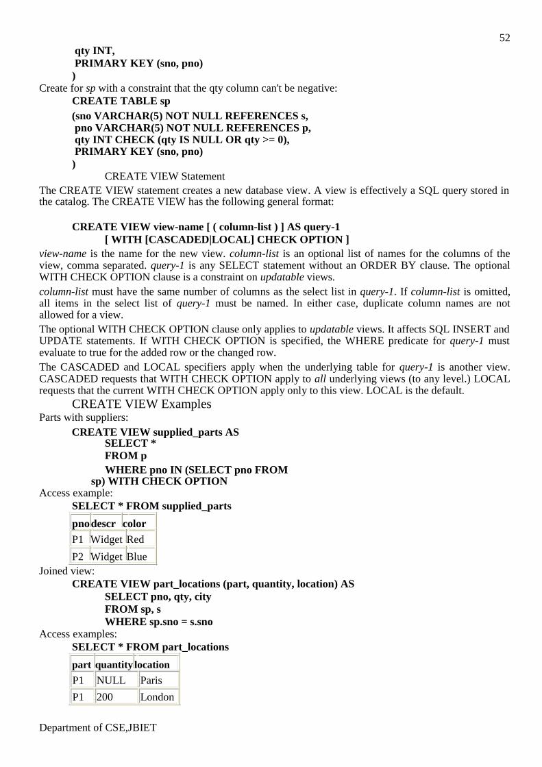
52 qty INT, PRIMARY KEY (sno, pno)

) Create for sp with a constraint that the qty column can't be negative:

CREATE TABLE sp (sno VARCHAR(5) NOT NULL REFERENCES s, pno VARCHAR(5) NOT NULL REFERENCES p, qty INT CHECK (qty IS NULL OR qty >= 0), PRIMARY KEY (sno, pno) )

CREATE VIEW Statement The CREATE VIEW statement creates a new database view. A view is effectively a SQL query stored in the catalog. The CREATE VIEW has the following general format:

CREATE VIEW view-name [ ( column-list ) ] AS query-1 [ WITH [CASCADED|LOCAL] CHECK OPTION ]

view-name is the name for the new view. column-list is an optional list of names for the columns of the view, comma separated. query-1 is any SELECT statement without an ORDER BY clause. The optional WITH CHECK OPTION clause is a constraint on updatable views. column-list must have the same number of columns as the select list in query-1. If column-list is omitted, all items in the select list of query-1 must be named. In either case, duplicate column names are not allowed for a view. The optional WITH CHECK OPTION clause only applies to updatable views. It affects SQL INSERT and UPDATE statements. If WITH CHECK OPTION is specified, the WHERE predicate for query-1 must evaluate to true for the added row or the changed row. The CASCADED and LOCAL specifiers apply when the underlying table for query-1 is another view. CASCADED requests that WITH CHECK OPTION apply to all underlying views (to any level.) LOCAL requests that the current WITH CHECK OPTION apply only to this view. LOCAL is the default.

CREATE VIEW Examples

Parts with suppliers:

CREATE VIEW supplied_parts AS SELECT * FROM p WHERE pno IN (SELECT pno FROM

sp) WITH CHECK OPTION Access example:

SELECT * FROM supplied_parts

pnodescr color

P1 Widget Red

P2 Widget Blue Joined view:

CREATE VIEW part_locations (part, quantity, location) AS SELECT pno, qty, city

FROM sp, s WHERE sp.sno = s.sno

Access examples: SELECT * FROM part_locations

part quantity location

P1 NULL Paris

P1 200 London

Department of CSE,JBIET

53

P1 1000 Rome

P2 200 Rome

SELECT part, quantity FROM part_locations

WHERE location = 'Rome'

part quantity

P1 1000

P2 200 DROP TABLE Statement

The DROP TABLE Statement removes a previously created table and its description from the catalog. It has the following general format:

DROP TABLE table-name {CASCADE|RESTRICT} table-name is the name of an existing base table in the current schema. The CASCADE and RESTRICT specifiers define the disposition of other objects dependent on the table. A base table may have two types of dependencies:

A view whose query specification references the drop table. Another base table that references the drop table in a constraint - a CHECK constraint or REFERENCES constraint.

RESTRICT specifies that the table not be dropped if any dependencies exist. If dependencies are found, an error is returned and the table isn't dropped. CASCADE specifies that any dependencies are removed before the drop is performed:

Views that reference the base table are dropped, and the sequence is repeated for their dependencies. Constraints in other tables that reference this table are dropped; the constraint is dropped but the table retained.

DROP VIEW Statement The DROP VIEW Statement removes a previously created view and its description from the catalog. It has the following general format:

DROP VIEW view-name {CASCADE|RESTRICT} view-name is the name of an existing view in the current schema. The CASCADE and RESTRICT specifiers define the disposition of other objects dependent on the view. A view may have two types of dependencies:

A view whose query specification references the drop view. A base table that references the drop view in a constraint - a CHECK constraint.

RESTRICT specifies that the view not be dropped if any dependencies exist. If dependencies are found, an error is returned and the view isn't dropped. CASCADE specifies that any dependencies are removed before the drop is performed:

Views that reference the drop view are dropped, and the sequence is repeated for their dependencies. Constraints in base tables that reference this view are dropped; the constraint is dropped but the table retained.

Department of CSE,JBIET

5

4

GRANT Statement

The GRANT Statement grants access privileges for database objects to other users. It has the following general format:

GRANT privilege-

list ON [TABLE]

object-list TO

user-list privilege-list is either ALL PRIVILEGES or a comma-separated list of properties: SELECT, INSERT, UPDATE, DELETE. object-list is a comma-separated list of table and view names. user-list is either PUBLIC or a comma-separated list of user names. The GRANT statement grants each privilege in privilege-list for each object (table) in object-list to each user in user-list. In general, the access privileges apply to all columns in the table or view, but it is possible to specify a column list with the UPDATE privilege specifier:

UPDATE [ (

column-1 [,

column-2] ... ) ] If the optional column list is specified, UPDATE

privileges are granted for those columns only. The user-list may specify PUBLIC. This is a general grant, applying to all users (and future users) in the catalog. Privileges granted are

revoked with the

REVOKE Statement. The optional specificier WITH GRANT OPTION may follow user-list in the GRANT statement. WITH GRANT OPTION specifies that, in addition to access privileges, the privilege to grant those

privileges to other users is granted.

GRANT

Statement

Examples GRANT SELECT

ON s,sp TO

PUBLIC

GRANT

SELECT,INSERT

,UPDATE(color)

ON p TO art,nan

GRANT SELECT

ON

supplied_parts

TO sam WITH

GRANT OPTION REVOKE

Statement The REVOKE Statement revokes access privileges for database objects previously granted to other users. It has the following general format:

REVOKE

privilege-list ON

[TABLE] object-

list FROM user-

list The REVOKE Statement revokes each privilege in privilege-list for each object (table) in object-list from each user in user-list. All privileges must have been previously granted. The user-list may specify

PUBLIC. This must apply

to a previous GRANT TO

PUBLIC.

REVOKE

Statement

Examples REVOKE

SELECT ON s,sp

FROM PUBLIC

REVOKE

SELECT,INSERT

,UPDATE(color)

ON p FROM

art,nan

REVOKE

SELECT ON

supplied_parts

FROM sam