Chen, Z.-G., Zhan, Z.-H., Li, H.-H., Du, K.-J., Zhong, J.-H., Foo, Y. W., Li, Y., and Zhang, J. (2015) Deadline Constrained Cloud Computing Resources Scheduling through an Ant Colony System Approach. In: ICCCRI 2015: International Conference on Cloud Computing Research and Innovation, Singapore, 26-27 Oct 2015, pp. 112-119. (doi:10.1109/ICCCRI.2015.14). There may be differences between this version and the published version. You are advised to consult the publisher’s version if you wish to cite from it.

http://eprints.gla.ac.uk/120426/

Deposited on: 24 June 2016

Enlighten – Research publications by members of the University of Glasgow http://eprints.gla.ac.uk

Deadline Constrained Cloud Computing Resources Scheduling Through An Ant Colony

System ApproachZong-Gan Chen1, Zhi-Hui Zhan1* (Corresponding Author), Hai-Hao Li1, Ke-Jing Du2, Jing-Hui Zhong3, Yong Wee Foo4,5,

Yun Li5, Jun Zhang1 1Department of Computer Science, Sun Yat-sen University, Guangzhou, P. R. China, 510275

1Key Laboratory of Machine Intelligence and Advanced Computing, Ministry of Education, P.R. China 1Engineering Research Center of Supercomputing Engineering Software, Ministry of Education, P.R. China

2School of Computer Science and Engineering, South China University of Technology, Guangzhou, P. R. China, 510006 3School of Computer Engineering, Nanyang Technological University, Singapore

4School of Engineering, Nanyang Polytechnic, Singapore 5School of Engineering, University of Glasgow, Glasgow G12 8LT, U.K.

*zhanzhh@mail.sysu.edu.cn

Abstract—Cloud computing resources scheduling is essential for executing workflows in the cloud platform because it relates to both the execution time and execution costs. In solving the problem of optimizing the execution costs while meeting deadline constraints, we developed an efficient approach based on ant colony system (ACS). For scheduling T tasks on R resources, an ant in ACS represents a solution with T dimensions, with each dimension being a task and the value of each dimension being an integer ranges in [1, R] to indicate scheduling the task on which resource. With such solution encoding, the ant in ACS constructs a solution in T steps, with each step optimally selecting one resource from the R resources, according to both the pheromone and heuristic information. Therefore, the solution encoding is very simple and straight to reflect the mapping relation of tasks and resources. Moreover, the solution construct process is very natural to find optimal solution based on the encoding scheme. We have conducted extensive experiments based on workflows with various scales and various cloud resources. We compare the results with those of particle swarm optimization (PSO) and dynamic objective genetic algorithm (DOGA) approaches. The experimental results show that ACS is able to find better solutions with a lower cost than both PSO and DOGA do on various scheduling scales and deadline conditions.

Keywords— cloud computing, resource scheduling, deadline constrained, task scheduling, ant colony system

I. INTRODUCTION Cloud computing has developed rapidly in recent years.

According to the NIST’s definition, cloud computing is “a model for enabling ubiquitous, convenient, on-demand network access to a shared pool of configurable computing resources that can be rapidly provisioned and released with minimal management effort or the interaction of service providers”[1].

Therefore, cloud computing has lots of computing resources, e.g., virtual machine (VM), that users can lease these resources following their demand to execute the workflow [2][3][4].

Now in the era of “Big Data”, the workflows frequently contain large scale of data that may need a large number of computing servers with cloud computing being considered as the best way to deal with such workflows. As is mentioned that the scale of data is large, so how to schedule those tasks to the proper resources is an important problem because good method can generate a scheduling scheme with high efficiency while keeping the cost low. As the workflow scheduling is a complex NP-hard problem, intelligent computing algorithm is a great approach to solving it. Many scientists have done some research on it. For example, the works by Chen and Zhang [5], Malawski et al. [6], Mao and Humphrey [7], and Rahman et al. [8] proposed evolutionary computation based algorithms to solve the resource scheduling problem. However, many of these researches do not consider the elasticity and heterogeneity of the resource in cloud computing. In addition, execution time is always considered as the only optimization objective neglecting the schedule cost. But in fact, the schedule cost should also be taken in to consideration because investment is an important factor in the business that cannot be ignored.

In 2014, a deadline based resource provisioning and scheduling algorithm was proposed by Rodriguez and Buyya [9]. The model attempts to find the solution that can meet the deadline constraint and at an optimal cost. It struck a balance between the cost and time to obtain maximum profit. Although the PSO approach they proposed has some promising results, there are still rooms for enhancement. The PSO approach makes use of the resource index to encode the resource. However, the index is just a symbol which does not represent any character of the resource, which leads to the flight of the PSO with certain blindness. Moreover, the PSO approach does not perform well in the situation of tight deadline for large scale workflow. Later, Li et al. [10] proposed to use renumber strategy to enhance the PSO and also extended the scheduling to multiobjective optimization [11].

This work was partially supported by the National Natural Science Foundations of China (NSFC) with No. 61402545, the Natural Science Foundations of Guangdong Province for Distinguished Young Scholars with No. 2014A030306038, the Project for Pearl River New Star in Science and Technology with No. 201506010047, the NSFC Key Program with No. 61332002, the NSFC for Distinguished Young Scholars with No. 61125205, the Fundamental Research Funds for the Central Universities (15lgzd08), and the National High-Technology Research and Development Program (863 Program) of China No.2013AA01A212.

In Proc IEEE International Conference on Cloud Computing Research and Innovation, Singapore 26-27 Oct 2015, pp. 112-119

DOI 10.1109/CCCRI.2015.14

1

In 2015, Chen et al. [12] proposed a dynamic objective genetic algorithm (DOGA) approach to solve the deadline based cloud resource scheduling model. In DOGA, the encoding problem of PSO has been solved. Moreover, DOGA uses dynamic objective strategy which focuses on execution time first, that is, to find the feasible solution to meet the deadline constraint, and subsequently focus on the execution cost after the feasible solution is found. Therefore, DOGA can find better results than PSO does. Nevertheless, DOGA still cannot obtain solution with execution cost small enough and fails to meet very tight deadline constraint. Moreover, the mutation and crossover are quite inefficiency because they are highly dependent on randomness.

In this paper, we proposed an ant colony system (ACS) based approach to solve the deadline based cloud resource scheduling model. In ACS, heuristic information is used to guide the search. In this paper, we make use of information such as the price of resource, the size of tasks and the topology structure of tasks. With heuristic information, the algorithm can give a good guidance during the construction of the solution. Compared to the random initialization of PSO and DOGA, our ACS approach can find a better solution even in the first generation with the guidance of heuristic value.

For solving the problem of scheduling T tasks on R resources, an ant in ACS represents a solution with T dimensions, with each dimension being a task and the value of each dimension being an integer ranges in [1, R] to indicate scheduling the task on which resource. With such solution encoding, the ant in ACS constructs a solution in T steps, with each step optimally selecting one resource from the R resources, according to both the pheromone and heuristic information. Therefore, the solution encoding is very simple and straight to reflect the mapping relation of tasks and resources. Moreover, the solution construct process is very natural to find optimal solution based on the encoding scheme.

The rest of this paper is organized as follows. Section II presents some background introductions of the deadline based model [9] and fitness evaluation. Section III presents the ACS approach. Section IV presents the experimental results. Finally, Section V presents the conclusion.

II. BACKGROUND

A. The Workflow Scheduling Model Fig. 1 is an example of a workflow model. The tasks of the

workflow have the topology structure, for example, t2 cannot be executed until t1’s execution is finished. Moreover, a parent’s task needs to transfer data to its child tasks when they are executed in different resources. We represent the time to transfer data in the link between parent task and child task.

Fig. 1. A simple workflow model

Two objectives ‘total execution time’ (TET) and ‘total execution cost’ (TEC) are defined in Eqs. (1) and Eqs. (2).

max{ | }it iTET ET t T= ⊂ (1)

| |

1( ( ))

j j j

R

r r rj

TEC C LET LST=

= × −∑ (2)

whereit

ET represents the ‘end time’ that the task ti ends its execution.

jrC represents the cost to lease the resource rj for a unit of time.

jrLST represents the ‘lease start time’ of rj while

jrLET represents the ‘lease end time’ of rj. TET is calculated by the end time of the task which ends its execution lastly. TEC is calculated by the sum of the cost to lease every resource while the cost to lease every resource is calculated by multiplying the cost of the resource by its lease time.

The model’s goal is to minimize the cost and to meet the deadline constraint. The formulation of the optimization objective is shown in Eqs. (3) and Eqs. (4).

Minimize TEC (3) TET deadline< (4)

B. Scheduling Scheme In ACS, the encode scheme of an ant uses the index of the

task and resource to encode the solution. Every dimension represents the corresponding task and its value represents the resource it runs on. A simple example of encoding with 7 tasks and 3 resources is shown in Fig. 2.

Fig. 2. An example of ACS encoding for workflow shceduling

C. Fitness Evaluation As we use Eqs. (3) and Eqs. (4) to evaluate an ant’s fitness,

a function should be declared to obtain TEC and TET. Before we declare the function, we first define some data needed for the function. We define the array exetime to represent the execution time, for example, exetime[i][j] represents the time needed for task ti to run on the resource rj. We also define the array transfertime to represent the time needed for the parent task to transfer data to its child, for example, transfertime[i][j] represents the time needed for task ti to transfer data to task tj.. Fig. 3 shows example of transfertime and exetime arrays, generated based on Fig. 1 and Fig. 2.

Since all the relevant variables are identified, we can obtain the workflow scheduling. Fig. 4 shows the workflow scheduling generated from Fig. 2 and Fig. 3.

2

1

2

3

4

5

6

7

0 2 3 0 0 0 00 0 0 2 0 0 00 0 0 2 0 0 00 0 0 0 3 1 00 0 0 0 0 0 20 0 0 0 0 0 10 0 0 0 0 0 0

ttt

transfertime tttt

⎡ ⎤⎢ ⎥⎢ ⎥⎢ ⎥⎢ ⎥= ⎢ ⎥⎢ ⎥⎢ ⎥⎢ ⎥⎢ ⎥⎣ ⎦

1

2

3

4

5

6

7

1 6 44 5 63 6 82 2 33 1 43 2 65 6 8

ttt

exetime tttt

⎡ ⎤⎢ ⎥⎢ ⎥⎢ ⎥⎢ ⎥= ⎢ ⎥⎢ ⎥⎢ ⎥⎢ ⎥⎢ ⎥⎣ ⎦

1t 2t 3t 4t 5t 6t 1r 2r 3r7t

Fig. 3. An example of transfertime and exetime in a worlflow

Fig. 4. Example of workflow scheduling.

[ ]rt

ant ii

PT exe transfer= +

[ ] ant ir R∉

[ ]r tpos i iLST ST=

[ ]{ }ant iR R r= ∪

[ ]r tpos i iLET ET=

| |

1

C *( )i r ri i

R

i

TEC LET LST=

= −∑{ }max : Tt ii

TET ET t= ⊂

[ ]max(max{ : parents( )}, )

i p ant it t p i rST ET t t LET= ∈

[| |]ant T

∅

[ ][ [ ]]exe exetime i ant i=

[ ]=

i ant it rST LET

[ ][ ]transfer transfertime i c+ =

[ ]rt t t

ant ii i i

ET PT ST= +

Fig. 5. The pseudo-code to calculate TEC and TET

The pseudo-code to calculate TEC and TET is shown in Fig. 5, which is also found in our previous paper [12]. The first step is to initialize TET, TEC, and R. R, which is initialized as ∅ , represents the set of resource that the workflow leases during the execution. Next, every coordinate i is iterate through. For task ti, the resource is obtained from executing the array ant[i]. For ti’s start time

itST , the value is

determined by the following criteria, that is, if ti has no parent,

itST is equal to

[ ]ant irLET . And if ti has parent tp, ti’sit

ST is equal

to the time after tp end its execution. ti’s processing timeit

PT is equal to execution time exe plus the time that ti use to transfer data to its child, named transfer. The end time of ti,

itET , is

calculated by it

ST plus it

PT . If rant [i] isn’t in the set of R, which means rant [i] hasn’t been leased, the lease start time of rant [i] [ ]ant irLST , is equal to

itST while the lease end time

[ ]ant irLET is the end time of ti. Finally, TEC and TET can be obtained through Eqs. (1) and (2).

III. ACS APPROACH

A. Solution Encoding ACS was proposed by Dorigo and Gambardella in 1997,

inspired by the foraging behavior of ants [13]. The ACS algorithm is designed to solve discrete combinational optimization problem (COP), e.g., the traveling salesman problem (TSP). In this paper, we find that the cloud resource scheduling problem for workflow execution is a kind of COP that is much suitable solved by ACS. Comparing to the process of using ACS for TSP, every task selects its execution resource similar to that every city select its path to the next city. As shown in Fig. 6, an ant represents a solution, denoting which resource is executed on for each task. In our proposed ACS approach, it has similar algorithmic structure to traditional ACS for TSP that our ACS selects the optimal resource for each task step by step.

According to the illustration of Fig. 6, ACS uses integer to encode the solution. As shown in Fig. 2, the coordinate i’s value represents the resource that ti runs on. For example, dimi=j represents that ti runs on the resource rj. Therefore, in Fig. 6, task t1 is scheduled on r2, tasks t2 and t3 are scheduled on r1, task t4 is scheduled on r3, task t5 is scheduled on rm, while task tn is scheduled on r2.

Fig. 6. Illustration of a solution of an ant in search.

3

B. Initialization of Pheromone In traditional ACS for TSP, the calculation of 0τ , which is

the initial value of pheromone, is 0 1/ ( )DDD Cτ = × , where D is the number of city and CDD is the route generated by greedy algorithm. In our cloud computing scheduling model, we set the number of task, which is |T|, as D. We first use greedy algorithm to obtain a solution [ ]gS i by Eq. (5). Then we calculate the TEC of [ ]gS i and use it as CDD. As a result, 0τ is calculated by Eq. (6).

( )( )| | 1

0

[ ] , [ ]T

gi

S i arg min exetime i j C j−

=

= ×∑ (5)

0 1/ (| | )SgT TECτ = × (6)

The 0τ is the initial value of all the pheromone ( , )i jτ that deployed on every (task, resource) pair.

C. Construction of Solution After initializing all the pheromone ( , )i jτ with the value

of 0τ , ACS goes to the solution construction process for all the ants.

In this process, ants will construct their solutions in parallel, which means all the ants will select resource for t0, in the first step, then all the ants go to the second step to select resource for t1, and so on, until the |T|th step for all the ants selecting resource for t|T|-1.

In each step, every ant will select resource for the corresponding task in two ways, exploitation and exploration, which is shown in Eq. (7). For ti, we will first generate a random number [0,1]q∈ , if 0q q≤ , the ant will do exploitation, that is, the ant will greedily select the high pheromone value and heuristic value. Otherwise, the ant will select the resource by roulette wheel selection. The formulation of roulette wheel selection is shown in Eq. (8), where ( , )p i j represents the probability for ti to select rj.

( ) ( ) 0

0

{ , , }

tiarg max i j i j q qrRoulette Wheel Selection q q

βτ η⎧⎪ × ≤⎡ ⎤ ⎡ ⎤⎣ ⎦ ⎣ ⎦= ⎨

>⎪⎩ (7)

( )( ) ( )

( ) ( )| | 1

0

, ,,

, ,R

j

i j i jp i j

i j i j

β

β

τ η

τ η−

=

×⎡ ⎤ ⎡ ⎤⎣ ⎦ ⎣ ⎦=×⎡ ⎤ ⎡ ⎤⎣ ⎦ ⎣ ⎦∑

(8)

Herein, the ( , )i jτ is the pheromone value between the task ti and the resource rj. The ( , )i jη is the heuristic information value between the task ti and the resource rj that indicating the desirable of scheduling the task ti on the resource rj. In order to obtain the heuristic information value, we consider the cost for execute time. The cost for execute time of scheduling the task ti on the resource rj is calculated as:

_ [ ][ ] [ ]exe cost exetime i j C j×= (9)

Therefore, the ( , )i jη is calculated as:

1[ ][ ]_

i jexe cost

η = (10)

D. Pheromone Updating Rules 1) Global Updating RuleAfter every generation, we will change the pheromone

value of the globally best solution. The formulation is shown in Eq. (11), where ρ is the evaporation rate and ( , )b i jτΔ is calculated by Eq. (12).

( ) ( ) ( ), 1 , ( , ), ( , )b besti j i j i j i j Sτ ρ τ ρ τ= − × + ×Δ ∀ ∈ (11)

( ), 1 /b besti j TECτΔ = (12)

2) Local Updating RuleDuring the construction of the solution, the pheromone

value changes as volatilization occurs due to both the new pheromone amount deposited by ants on the route and to pheromone evaporation. For example, an ant choses rj for ti, the route (i,j)’s pheromone value will volatilized. The formulation is shown in Eq. (13), where ξ is volatilization rate.

( ) ( ) ( ) 0, 1 ,i j i jτ ξ τ ξ τ= − × + × (13)

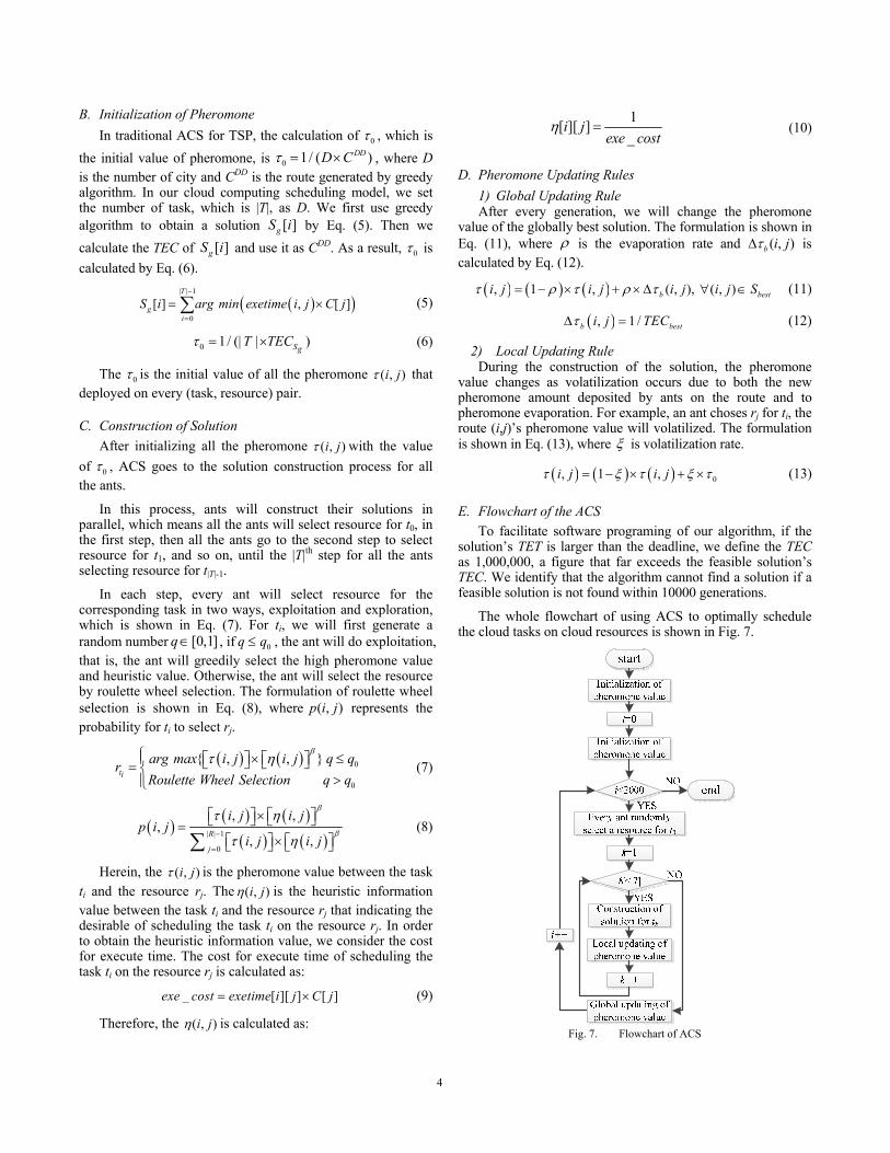
E. Flowchart of the ACS To facilitate software programing of our algorithm, if the

solution’s TET is larger than the deadline, we define the TEC as 1,000,000, a figure that far exceeds the feasible solution’s TEC. We identify that the algorithm cannot find a solution if a feasible solution is not found within 10000 generations.

The whole flowchart of using ACS to optimally schedule the cloud tasks on cloud resources is shown in Fig. 7.

Fig. 7. Flowchart of ACS

4

IV. EXPERIMENTS AND COMPARISONS

In our experiment, for every type of resource rj, we define its processing capability (capj) as Random(1,10) and its cost per unit time as Normal(capj,0.1). Where Normal(a, b) represents the random value generated by the normal (Gaussian) distribution with mean a and standard deviation b. For every task ti, we define its size ti_ as Random(10,30) while its exetime on rj is defined as Normal(ti_size/cap,0.1). We calculate transfertime[i][child(i)] by Eq. (14) while during our experiment, bandwidth is 20.

[ ][ ( )](0. ) _ /1,1 i

transfertime i child iRand t size bandw tom id h= ×

(14)

Fig. 8. Algorithm for generating a topological structure

In cloud computing, the tasks are assumed to have a complex topological structure. We design an algorithm shown in Fig. 8 to generate the topological structure of the tasks where the tasks can be executed successively. For such task ti, its child tasks’ index is greater than i. We set a parameter Pchild to be the probability that a task tk to be the child of ti. Pchild increases with the incensement of i, in order to generate a balance structure. Fig. 8 is similar to the one in [12] except the difference in the probability settings of Pchild.

We use 3 different scales of workflow to do our experiment — small, medium and large. Small workflow has 50 tasks. Medium workflow has 100 tasks. Large workflow has 200 tasks. The type of resource is set to be 6, the same as in [9].

In PSO approach, according to [9], c1=c2=2.0, ω=0.5, and the population is 100. While in DOGA approach, we follow the proposals in [12] as Pc=0.8 and Pm =0.002 when setting TET as optimization objective and Pc =0.15 and Pm =0.008 when setting TEC as optimization objective. The population is also set as 100.

In ACS approach, the parameters are shown in Table I.

Table I Parameter values of ACS Population 10 ρ 0.1

α 1 ξ 0.1 β 5 0q 0.9

A. Comparison with Same Evolutionary Generation The three algorithms may require many generations to find

a feasible solution, named FGEN. If FGEN >10000, we regard that the algorithm cannot find a solution. Otherwise, we let the algorithm to run 2000 more generations after finding a feasible solution to search for the best solution with smallest TEC. We

ran the 3 algorithms under different deadline constraints and compared the results of TEC. We have also plotted the convergence curves of the TEC metric along the 2000 generations for all the three algorithms (see Fig. 9 to Fig. 14). The X-axis means generation, named GEN and the Y-axis means TEC. To reduce the randomness effect, we executed the three algorithms 30 times on each instance and use the average result for comparisons. S_DEV represents the standard deviation of the 30 independent tests. The comparison of 3 algorithms in 3 different scales of workflow is shown subsequently via a table and two figures. The better results in the tables are marked with boldface.

1) Small Scale of WorkflowThe results of small scale of workflow are shown in Table

II, Fig. 9 and Fig. 10. In the table we can see that in small scale of workflow, ACS perform well in generating a better solution with a smaller TEC and meeting a tight deadline constraint. But DOGA shows better stability with smaller standard deviation. While in the figures, we can see that the convergence speed of ACS is the fastest to obtain smaller TEC value. Table II the Comparison of Small Scale of Workflow with the Same

Evolutionary Generation Deadline PSO DOGA ACS

150 TEC 1723.16 1524.56 1288.4S_DEV 36.26 23.4 126.14

120 TEC 1733.65 1538.10 1336.65S_DEV 23.69 19.75 65.00

0 500 1000 1500 20001200

1500

1800

2100

2400

2700

3000

TEC

GEN

PSO DOGA ACS

Fig. 9. The result on small scale of data, deadline=150

0 500 1000 1500 20001200

1500

1800

2100

2400

2700

3000

3300

3600

TEC

GEN

PSO DOGA ACS

Fig. 10. The result on small scale of workflow, deadline=120

5

2) Medium Scale of WorkflowThe results of medium scale of workflow are shown in

Table III, Fig. 11, and Fig. 12. In the table we can see that the gap between ACS and other two algorithms is bigger and ACS has greater stability than the other two algorithms. From the figures, we can conclude that ACS also has the fastest convergence speed to reach a feasible solution quicker.

Table III The Comparision of Medium Scale of Workflow with The Same Evolutionary Generations

Deadline PSO DOGA ACS

700 TEC 5128.70 3702.41 3289.45S_DEV 561.71 119.79 87.93

600 TEC 5184.48 3762.09 3351.18S_DEV 387.53 85.44 59.61

0 500 1000 1500 20002000

4000

6000

8000

10000

12000

14000

16000

TEC

GEN

PSO DOGA ACS

Fig. 11. The result on medium scale of workflow, deadline=700

0 500 1000 1500 20003000

4500

6000

7500

9000

10500

12000

13500

15000

TEC

GEN

PSO DOGA ACS

Fig. 12. The result on medium scale of workflow, deadline=600

3) Large Scale of WorkflowThe results of large scale of workflow are shown in Table

IV, Fig. 13, and Fig. 14. With the growing scale of workflow, ACS shows greater ability in solving the problem. In the table and figures, in terms of stability, TEC solution and convergence speed, ACS is better than the other two algorithms.

Table IV The Comparision of Large Scale of Workflow with The Same Evolutionary Generations

Deadline PSO DOGA ACS

1200 TEC 24043.5 15396.68 14384.8S_DEV 4544.3 1478.1 549.47

1000 TEC 28468.8 15961.69 14498.5S_DEV 6567.5 1029.5 527.07

0 500 1000 1500 2000

20000

30000

40000

50000

60000

70000

80000

90000

100000

TEC

GEN

PSO DOGA ACS

Fig. 13. The result on large scale of workflow, deadline=1200

0 500 1000 1500 2000

20000

30000

40000

50000

60000

70000

80000

90000

100000

TEC

GEN

PSO DOGA ACS

Fig. 14. The result on large scale of workflow, deadline=1000

B. Comparison with Same Execution Time As the population of ACS is far smaller than that of PSO

and DOGA, ACS may have better execution time efficiency. But the operation of ACS in every generation has higher complexity than other two algorithms. In order to show the efficiency of ACS more directly, we set the same executing time as 60 seconds to do the experiments.

Similarly, we performed 30 independent experiments for every algorithm. We again compare the results for TEC and S_ DEV of the 3 algorithms under different deadline constraints and plotted the convergence curves on the TEC metric along the 60 seconds of three algorithms. The X-axis means executing time, named Time and the Y-axis means TEC.

1) Small Scale of WorkflowThe results of small scale of workflow are shown in Table

V, Fig.15, and Fig.16. As the scale of workflow is small, all 3 algorithms have good convergence speed. However, ACS generated a solution with smaller TEC. With the guidance of heuristic value, ACS can find a better solution in the first generation.

Table V Comparision of Small Scale of Workflow with the Same Execution Time

Deadline PSO DOGA ACS

150 TEC 1662.27 1429.55 1261.55S_DEV 30.55 24.00 136.61

120 TEC 1647.73 1404.43 1337.51S_DEV 31.95 10.24 79.53

6

0 10 20 30 40 50 601200

1500

1800

2100

2400

2700

3000TE

C

Time

PSO DOGA ACS

Fig. 15. The result on small scale of workflow, deadline=150 with the same execution time

0 10 20 30 40 50 601200

1500

1800

2100

2400

2700

3000

TEC

Time

PSO DOGA ACS

Fig. 16. The result on small scale of workflow, deadline=150 with the same execution time

2) Medium Scale of WorkflowThe results of medium scale of workflow are shown in

Table VI, Fig.17, and Fig.18. ACS is also able to generate a solution with the smallest TEC.

Table VI The Comparision of Medium Scale of Workflow with the Same Execution Time

Deadline PSO DOGA ACS

150 TEC 4794.67 3448.55 3282.95S_DEV 301.58 103.81 146.20

120 TEC 4829.50 3498.95 3315.83S_DEV 358.43 90.24 89.87

0 10 20 30 40 50 603000

6000

9000

12000

15000

TEC

Time

PSO DOGA ACS

Fig. 17. The result on medium scale of workflow, deadline=700 with the same execution time

0 10 20 30 40 50 60

4000

6000

8000

10000

12000

14000

16000

TEC

Time

PSO DOGA ACS

Fig. 18. The result on medium scale of workflow, deadline=600 with the same execution time

3) Large Scale of WorkflowThe results of large scale of workflow are shown in Table

VII, Fig. 19, and Fig.20. In this case, ACS performed better both in terms of stability and the time taken to find a feasible solution.

Table VII Comparision of Large Scale of Workflow with the Same Execution Time

Deadline PSO DOGA ACS

150 TEC 24134.82 16803.40 14850.3 S_DEV 5931.42 1119.96 656.65

120 TEC 28035.01 16224.48 15102.00S_DEV 4780.08 1279.56 798.85

0 10 20 30 40 50 6010000

20000

30000

40000

50000

60000

70000

80000

90000

100000

TEC

Time

PSO DOGA ACS

Fig. 19. The result on large scale of workflow, deadline=1200 with the same execution time

0 10 20 30 40 50 6010000

20000

30000

40000

50000

60000

70000

80000

90000

100000

TEC

Time

PSO DOGA ACS

Fig. 20. The result on large scale of workflow, deadline=1200 with the same execution time

7

C. Analysis of the Result 1) Convergence

In the case of small scale of workflow, the convergence speed of the three algorithms is nearly the same. But with the increasing scale of workflow, ACS has better convergence speed than PSO and DOGA. This is helped by the heuristic value of ACS to finding a good solution in the first generation.

2) TECIn the 3 different scales of data, ACS can generate a better

solution with smaller TEC value than PSO and DOGA do. The performance of ACS increases considerably with the increasing scale of workflow when compared with the other two algorithms.

3) EfficiencyIn the 3 different scales of workflow, from the Fig. 9~Fig.

20, we can conclude that in most of the cases, ACS can find a solution with smaller TEC within the first few evolutionary generations and seconds.

V. CONCLUSION In this paper, we have developed an ant colony system

based approach to the resource scheduling problem of cloud computing under a cost-minimization and deadline-constrained model. The model has unrestricted availability and can meet the needs of business organizations. Deficiencies of this model encountered by PSO [9] and DOGA [12] approaches have been improved. The experiments under various scheduling scales and deadline constraints show that the ACS is able to find a better solution with a smaller TEC than PSO and DOGA do.

Future work will be concerned with enhancing the stability of the ACS, while the use of other evolutionary computation algorithms such as differential evolution [14][15], artificial bee colony [16], enhanced PSOs [17][18], and brain storm optimization [19] will be investigated. Moreover, dynamic and multi-objective characteristics will be studied using relevant algorithms [20][21].

REFERENCES [1] P. Mell and T. Grance, “The NIST definition of cloud computing,”

Communications of the ACM, vol.53, no.6, pp. 50-50, Jun. 2011. [2] Z. H. Zhan, X. F. Liu, Y. J. Gong, J. Zhang, H. S. H. Chung, and Y. Li,

“Cloud computing resource scheduling and a survey of its evolutionary approaches,” ACM Computing Surveys, vol. 47, no. 4, Article 63, pp. 1-33, Jul. 2015.

[3] Z. H. Zhan, G. Y. Zhang, Y. Lin, Y. J. Gong, and J. Zhang, “Load balance aware genetic algorithm for task scheduling in cloud computing,” in Proc. Simulated Evolution And Learning, 2014, pp. 644-655.

[4] X. F. Liu, Z. H. Zhan, K. J. Du, and W. N. Chen, “Energy aware virtual machine placement scheduling in cloud computing based on ant colony optimization approach,” in Proc. Genetic Evol. Comput. Conf., 2014, pp. 41-47.

[5] W. N. Chen and J. Zhang, “An ant colony optimization approach to a grid workflow scheduling problem with various QoS requirements,” IEEE Trans. Syst., Man, Cybern., Part C: Appl. Rev., vol. 39, no. 1, pp. 29–43, Jan. 2009.

[6] M. Malawski, G. Juve, E. Deelman, and J. Nabrzyski, “Cost-and deadline-constrained provisioning for scientific workflow ensembles in IaaS clouds,” in Proc. Int. Conf. High Perform. Comput., Netw., Storage Anal., 2012, pp. 1–11.

[7] M. Mao and M. Humphrey, “Auto-scaling to minimize cost and meet application deadlines in cloud workflows,” in Proc. Int. Conf. High Perform. Comput., Netw., Storage Anal., 2011, pp. 1–12.

[8] M. Rahman, S. Venugopal, and R. Buyya, “A dynamic critical path algorithm for scheduling scientific workflow applications on global grids,” in Proc. 3rd IEEE Int. Conf. e-Sci. Grid Comput., 2007, pp. 35–42.

[9] M. A. Rodriguez and R. Buyya, “Deadline based resource provisioning and scheduling algorithm for scientific workflows on clouds,” IEEE Transactions on Cloud Computing, vol. 2, no. 2, pp. 222–235 April-June 2014.

[10] H. H. Li, Y. W. Fu, Z. H. Zhan, and J. J. Li, “Renumber strategy enhanced particle swarm optimization for cloud computing resource scheduling,” in Proc. IEEE Congr. Evol. Comput., 2015, Accepted.

[11] H. H. Li, Z. G. Chen, Z. H. Zhan, K. J. Du, and J. Zhang, “Renumber coevolutionary multiswarm particle swarm optimization for multi-objective workflow scheduling on cloud computing environment,” in Proc. Genetic Evol. Comput. Conf., 2015, pp. 1419-1420.

[12] Z. G. Chen, K. J. Du, Z. H. Zhan, and J. Zhang, “Deadline constrained cloud computing resources scheduling for cost optimization based on dynamic objective genetic algorithm,” in Proc. IEEE Congr. Evol. Comput., 2015

[13] M. Dorigo and L. Gambardella, “Ant colony system: a cooperative learning approach to the traveling salesman problem,” IEEE Trans. Evol. Comput., vol. 1, no. 1, pp. 53-66, 1997.

[14] Y. L. Li, Z. H. Zhan, Y. J. Gong, W. N. Chen, J. Zhang, and Y. Li, “Differential evolution with an evolution path: A DEEP evolutionary algorithm,” IEEE Trans. on Cybernetics, vol. 45, no. 9, pp. 1798-1810, Sept. 2015.

[15] Y. L. Li, Z. H. Zhan,Y. J. Gong, J. Zhang, Y. Li, and Q. Li, “Fast micro-differential evolution for topological active net optimization,” IEEE Trans. Cybernetics, DOI:10.1109/TCYB.2015.2437282, 2015.

[16] M. D. Zhang, Z. H. Zhan, J. J. Li, and J. Zhang, “Tournament selection based artificial bee colony algorithm with elitist strategy,” in Proc. Conf. Technologies and Applications of Artificial Intelligence, Taiwan, Nov. 2014, pp. 387-396.

[17] Z. H. Zhan, J. Zhang, Y. Li, and Y. H. Shi, “Orthogonal learning particle swarm optimization,” IEEE Transactions on Evolutionary Computation, vol. 15, no. 6, pp. 832-847, Dec. 2011.

[18] Y. H. Li, Z. H. Zhan, S. J. Lin, J. Zhang, and X. N. Luo, “Competitive and cooperative particle swarm optimization with information sharing mechanism for global optimization problems,” Information Sciences, vol. 293, no. 1, pp. 370-382, 2015.

[19] Z. H. Zhan, J. Zhang, Y. H. Shi, and H. L. Liu, “A modified brain storm optimization,” in Proc. IEEE World Congr. Comput. Intell., Brisbane, Australia, Jun. 2012, pp. 1-8.

[20] Z. H. Zhan, J. Li, J. Cao, J. Zhang, H. Chung, and Y. H. Shi, “Multiple populations for multiple objectives: A coevolutionary technique for solving multiobjective optimization problems,” IEEE Transactions on Cybernetics, vol. 43, no. 2, pp. 445-463, April. 2013.

[21] Z. H. Zhan, J. J. Li, and J. Zhang, “Adaptive particle swarm optimization with variable relocation for dynamic optimization problems,” in Proc. IEEE Congr. Evol. Comput., 2014, pp. 1565-1570.

8