Embed Size (px)
Citation preview
Accepted Manuscript
Deadlock-free scheduling for flexible manufacturing systems using Petri nets
and heuristic search
Hang Lei, Keyi Xing, Libin Han, Fuli Xiong, Zhaoqiang Ge
PII: S0360-8352(14)00113-2
DOI: http://dx.doi.org/10.1016/j.cie.2014.04.002
Reference: CAIE 3681
To appear in: Computers & Industrial Engineering
Received Date: 29 August 2013
Revised Date: 1 April 2014
Accepted Date: 6 April 2014
Please cite this article as: Lei, H., Xing, K., Han, L., Xiong, F., Ge, Z., Deadlock-free scheduling for flexible
manufacturing systems using Petri nets and heuristic search, Computers & Industrial Engineering (2014), doi: http://
dx.doi.org/10.1016/j.cie.2014.04.002
This is a PDF file of an unedited manuscript that has been accepted for publication. As a service to our customers
we are providing this early version of the manuscript. The manuscript will undergo copyediting, typesetting, and
review of the resulting proof before it is published in its final form. Please note that during the production process
errors may be discovered which could affect the content, and all legal disclaimers that apply to the journal pertain.
Deadlock-free scheduling for flexible manufacturing systems using Petri nets and heuristic search Hang Leia, Keyi Xinga, Libin Hana, Fuli Xionga, Zhaoqiang Geb
a The State Key Laboratory for Manufacturing Systems Engineering and the Systems Engineering
Institute, Xi’an Jiaotong University, Xi’an, 710049, PR China b Department of Applied Mathematics, Xi'an Jiaotong University, Xi'an, 710049, PR China; E-mail Addresses: [email protected]
[email protected] (corresponding author) [email protected] [email protected] [email protected]
Tel.: +86 135 7189 7199
��
�
Deadlock-free scheduling for flexible manufacturing systems using Petri nets and
heuristic search
Abstract: Deadlock-free control and scheduling are two different problems for flexible
manufacturing systems (FMSs). They are significant for improving the behaviors of the systems.
Based on the Petri net models of FMSs, this paper embeds deadlock control policies into heuristic
search algorithm, and proposes a deadlock-free scheduling algorithm to minimize makespan for
FMSs. Scheduling is performed as heuristic search in the reachability graph of the Petri net. The
searching process is guided by a heuristic function based on firing count vectors of state equation
for the Petri net. By using the one-step look-ahead method in the optimal deadlock control policy,
the safety of a state is checked. Experimental results are provided to show effectiveness of the
proposed heuristic search approach in deadlock-free scheduling for FMSs.
Keywords: scheduling; Petri net; flexible manufacturing system; deadlock control policy;
heuristic search.
1. Introduction
Flexible manufacturing systems (FMSs) are modern production facilities that are highly
adaptable to different production plans. An FMS includes the material transportation system, the
buffer, the work-piece warehouse and other resources besides the processing equipments. In an
FMS, various parts are concurrently processed and have to share common resources, and then
deadlocks may occur during the processing, which are undesirable phenomena. In deadlock
situations, the whole system or a part of it remains indefinitely blocked and cannot terminate its
task. Therefore, it is highly important to develop efficient control and scheduling algorithms to
��
�
optimize the system performance while preventing deadlock situations.
The deadlock has been extensively studied from the control viewpoint, and many deadlock
control methods have been proposed (Abdallah & Elmaraghy, 1998; Chu & Xie, 1997; Ezpeleta,
Colom, & Martinez, 1995; Fanti, Maione, & Turchiano, 2001; Fanti & Zhou, 2004; Huang et al.,
2001; Piroddi, Cordone, & Fumagalli, 2008; Reveliotis & Ferreira, 1996; Xing, Hu, & Chen, 1996;
Xing et al., 2009; Xing et al., 2011). They can guarantee the deadlock-free operation of FMS, but
do not take operating time into account. Only a few studies address the scheduling problem of
deadlock-prone FMSs. Such a problem involves not only the optimization of certain objective
function but also the handling of deadlock problems, and therefore is more complex. Ramaswamy
and Joshi (1996) provided a mathematical model for a deadlock-free scheduling problem of FMSs
with material handing devices and limited buffers, a Lagrangian relaxation heuristic algorithm was
used in this paper to simplify the models to search for the optimized average flow time. Jeng and
Chen (1998) developed a heuristic algorithm based on the best-first search technique for
scheduling FMSs. Abdallah, Elmaraghy, and Elmekkawy (2002) used timed Petri nets (PNs) to
model FMSs and proposed a scheduling algorithm. The algorithm generates a partial reachability
graph to find the optimal or near-optimal deadlock-free schedule in terms of the firing sequence of
transitions in the PN model. Xu and Wu (2004) developed a genetic algorithm based on PN with
infinite buffers. They analyzed the deadlock that might occur in the obtained scheduling and
added some necessary buffers to avoid the deadlock. Golmakani et al. (2006) proposed an
automata-based approach to minimize the makespan for deadlock-free scheduling of FMSs.
Dashora et al. (2007) applied extended colored timed PN to model the dynamic behavior of simple
sequential processes with resources. A deadlock-free schedule with minimized makespan based on
��
�
an evolutionary endosymbiotic learning automata algorithm was presented. Wu and Zhou (2007)
studied a real-time deadlock-free scheduling problem for semiconductor track systems based on
colored timed resource-oriented PN. A deadlock avoidance policy (DAP) was used as a lower
layer controller. With the support of the DAP, heuristic rules were proposed to schedule the
system in real time. Xing et al. (2012) embedded a deadlock avoidance policy into genetic
algorithm to develop a deadlock-free scheduling algorithm for FMSs to minimize the makespan.
Based on the deadlock search algorithm (Xing et al., 2009), a one-step look-ahead method was
developed to avoid deadlocks by amending the feasibility of chromosomes. A deadlock-free
schedule can be obtained.
Branch-and-bound methods (Hariri & Potts, 1997; Lee & Kim, 2004) can obtain optimal
solutions of scheduling problems. Their main disadvantage is enumerating large number of nodes.
Other search methods such as A* search algorithm (Lee & DiCesare, 1994; Reyes, Yu, & Kelleher,
2002a; Reyes et al., 2002b; Xiong & Zhou, 1998), which is based on branch-and-bound method,
attempts to generate and evaluate fewer number of nodes by branching only the most promising
nodes at each stage of the search. None of the search methods mentioned above takes into account
the deadlock problem. In order to generate deadlock-free schedules, Deadlock detection and
prevention mechanism is required to be incorporated into the searching process. This can be done
by precisely representing the FMS’s discrete-event dynamic behavior to prevent encountering
deadlock states. PNs are commonly accepted technique that can explicitly represent the
characteristics of FMS.
For an FMS modeled by PN, an optimal schedule can be obtained by generating the reachability
graph and finding the optimal path from the initial marking to the final marking based on a given
��
�
measure of performance. When constructing the reachability graph, deadlock states are designated
and the paths to those states are terminated to prevent the system from encountering them. A
hybrid heuristic search (Xiong & Zhou, 1998) based on A* search algorithm was applied to
determining a deadlock-free schedule with respect to the makespan criterion, assuming that each
part has only one route to be produced. For PN methods, deadlock recognition is carried out as the
schedule is generated and thus, it has to be repeated for every new batch of parts.
Based on the literature, deadlock control and scheduling focus on different sides in their
approach. The scheduling emphasizes optimizing the performance of the systems, where the
schedule performance is generally defined in terms of the movement of parts through the entire
system. In contrast, deadlock control focuses on avoiding or preventing the system from entering
into deadlock states. The traditional scheduling of a job shop or a flow shop with the scale m × n,
meaning m machines and n parts, assumes that the system has enough buffers or human presence,
and considers problems with no deadlock (Pineo, 2000). If the given buffer space is limited, the
deadlock freedom of the systems with its obtained schedule cannot be guaranteed. Thus, it is
necessary and useful to integrate deadlock control and scheduling together in practice.
In this paper, a new heuristic search method for deadlock-free scheduling of FMS is proposed.
This method is described as follows. First, an FMS is modeled as a P-timed PN. A deadlock-free
scheduling problem that minimizes the makespan is formulated as searching the reachability graph
of the PN. The searching process is guided by a heuristic function based on solution of the state
equation, called firing count vector, to predict the total time from the initial marking through the
current marking to the final marking. In addition, linear algebraic techniques can be used to obtain
an approximate solution of the state equation. Furthermore, this paper uses a one-step look-ahead
��
�
method for checking the safeness of the next marking in the searching process, and develops a
deadlock-free scheduling algorithm. The primary contributions of this paper are the application of
the heuristic search based on the state equation for PN to the deadlock-free scheduling problem for
the first time and the utilization of DAP in our scheduling problem.
The outline of the paper is organized as follows. Section 2 introduces PN modeling of FMSs for
scheduling and reviews deadlock PN controller used in this paper. Section 3 establishes a
deadlock-free heuristic scheduling method by imbedding DAP into the heuristic search algorithm.
Two examples to show the effectiveness of the proposed scheduling algorithms are given in
Section 4. Section 5 gives conclusions.
2. PN models and their DAPs
This section first introduces some definitions and notations of PNs, and then the P-timed PN
model of FMS and DAPs for FMS used in this paper.
2.1. Basic PN definitions
A PN is a three-tuple N = (P, T, F), where P = {p1, p2, … , pm} is a finite set of places, T = {t1,
t2, … , tn} is a finite set of transitions with P ∪ T ≠ ∅ and P ∩ T = ∅. F ⊆ (P × T) ∪ (T × P) is the set of
directed arcs. Given a net N = (P, T, F), and a node x ∈ P ∪ T, the preset of x is defined as •x = {y ∈ P
∪ T | (y, x) ∈ F}, and the postset of x is defined as x• = {y ∈ P ∪ T | (x, y) ∈ F}. A marking or state of N
is M: P → �+, which denotes the number of tokens in each place, where �+ = {0, 1, 2, �}. A PN N
with an initial marking M0 is called a marked PN, denoted as (N, M0).
A transition t ∈ T is enabled at a marking M, if ∀p ∈ •t, M(p) > 0; this fact will be denoted as M[t >.
An enabled transition t at M can be fired, resulting in a new reachable marking M', denoted by
M[t > M', where M'(p) = M(p) − 1, ∀p ∈ •t \ t•, M'(p) = M(p) + 1, ∀p ∈ t• \ •t, and otherwise, M'(p) =
��
�
M(p). A sequence of transitions α = t1t2 … tk is feasible from a marking M if Mi[ti > Mi+ 1, i = 1,
2, … , k, where M1 = M, and Mi, i = 1, 2, … , k + 1, are called reachable markings from M. Let
R(N, M) denote the set of all reachable markings of N from M.
The incidence matrix D = [cij] of PN is a matrix D: P × T → {−1, 0, 1} such that cij = 1 if tj ∈ •pi \ pi
•,
cij = −1 if tj ∈ pi• \ •pi, and cij = 0 otherwise. The kth firing vector xk is an n × 1 column vector of n − 1
zeros and one nonzero entry, a value of one in the ith position implies that transition ti fires at the
kth firing. The kth column of the incidence matrix D denotes the change of the marking as the
result of firing transition tk, then Mk = Mk-1 + Dxk. Suppose that the final marking Mf is reachable
from the current marking M through a firing sequence x1, x2, … , xs, then the state equation for PN
is written as Mf = M + D(x1 + x2 + … + xs). We obtain
Du = ΔM
where ΔM = Mf – M, u = x1 + x2 + … + xs is an n × 1 column vector of nonnegative integers and is
called the firing count vector.
The composition of two PNs, Ni = (Pi, Ti, Fi), i ∈ {1, 2}, via the same elements, denoted as N1 ⊗
N2 = (P, T, F), where P = P1 ∪ P2, T = T1 ∪ T2, and F = F1 ∪ F2.
2.2. P-Timed PN scheduling models of FMSs
An FMS consists of m types of resources and can processes n types of parts. The set of resource
type is denoted as R = {ri, i = 1, 2, … , m}. The capacity of a resource type ri is an integer,
denoted as C(ri), indicating the maximum number of parts that such type of resources can
simultaneously hold. The set of part type is denoted as Q = {qi, i = 1, 2, … , n}. The number of
type-qi parts to be processed is ϕ(qi). A processing route of a part is a sequence of operations. A
part may have more than one route and can choose its route in the processing. Let a type-q part
�
�
have k processing routes ω1, ω2, … , ωk. Then route ωi can be expressed as a sequence of
operations ωi = Oi1Oi2 … Oij … Oil, where Oij is the jth operation in ωi and l is the length of ωi. Let
R(Oij) be the resource type required by operation Oij. Then, ωi is determined by the sequence of
resources R(Oi1) R(Oi2) … R(Oij) … R(Oil).
To each type of parts, add two fictitious operations, called start and end, which do not require
any resource and represent the storage of raw and processed parts of this type, respectively. So
route ωi with the additional operations can be denoted as ωi = OqsOi1Oi2 … OilOqe, where Oqs and
Oqe are the start and end operations for all type-q parts. Hence, a processing route for a type-q is a
sequence of operations from Oqs to Oqe.
Now let us develop PN models of FMS’s. First, we model a processing route of a type-q part by
a directed path. Each place represents an operation, called an operation place. For example, the PN
model for route ωi = OqsOi1Oi2 … OilOqe is a directed path ωi = pqsti0 pi1ti1 pi2ti2 … pijtij … piltilpqe
where pqs and pqe represent start operation Oqs and end operation Oqe, respectively, pij is an
operation place representing operation Oij, tij is an transition. Hence, the marked PN model of
processing routes for type-q parts can be denoted as
Nq = (Pq ∪ {pqs, pqe}, Tq, Fq, Mq0), q ∈ Q,
where Pq is the set of places corresponding to operations that require resources, Mq0 is the initial
marking, Mq0(p) = 0 ∀p ∈ Pq ∪ {pqe}, and Mq0(pqs) = ϕ(q). A path from pqs to pqe represents a
processing route of a type-q part. In Nq, if p ∈ Pq ∪ pqs, |p•| > 1, p is called a split place. From a split
place, a part can choose its processing route.
To each resource type r, we assign a place, called a resource place and denoted also by r, for
simplicity. Let PR denote the set of all resource places. For a processing route of type-q parts αi
�
�
=pqsti0pi1ti1pi2ti2 … pijtij … piltilpqe, if the operation corresponding to pij requires resource r, denoted
as R(pij) = r, then add an arc from r to transition ti(j-1) and an arc from tij to r.
Let FR denote the set of all arcs related with resource places. Then, the whole system can be
modeled by the following marked PN.
(N, M0) = (P ∪ Ps ∪ Pe ∪ PR, T, F, M0),
where P = ∪q∈Q Pq, Ps = {pqs | q ∈ Q}, Pe= {pqe | q ∈ Q}, T = ∪q∈Q Tq, F = FQ ∪ FR and FQ = ∪q∈Q Fq. The
initial marking M0 is defined as M0(pqs) = ϕ(q), ∀pqs ∈ Ps; M0(p) = 0, ∀p ∈ P ∪ Pe; and M0(r) = C(r), ∀r ∈
PR.
In this paper, P-timed PNs are used to implement the processing times of operations. A time
delay d(p) is assigned to each operation place p to denote its processing time. In particularly, we
define d(p) = 0, ∀p ∈ Ps ∪ Pe ∪ PR. In the following, we refer to the above P-timed PN model as a PN
for scheduling (PNS).
When all operations of all parts are finished, the PNS reaches its final marking Mf. A sequence
of transitions α is called a feasible schedule if M0[α > Mf, where Mf is defined as follows.
Mf(p) = M0(p), ∀p ∈ PR; Mf(p) = 0, ∀p ∈ P ∪ Ps; Mf(pqe) = M0(pqs), ∀pqe ∈ Pe.
Let (o)t and t(o) denote the input and output operation places of transition t, respectively. Let (r)t
and t(r) denote the input and output resource places of t, respectively. For a given marking M ∈ R(N,
M0), t is process-enabled at M if M((o)t) > 0, and t is resource-enabled at M if M((r)t) > 0.
Example 2.1. Consider an FMS consisting of three machines m1, m2, and m3. The system can
process two types of part q1 and q2. Each machine can hold two parts at the same time. Then, the
resource set is R = {m1, m2, m3}, C(mi) = 2, i ∈ {1, 2, 3}. Type-q1 parts are processed first on m1
��
�
and then on m2 and m3. Type-q2 parts are processed first on m3 and then on m2 and m1. Then, the
resource sequences for type-q1parts and type-q2 parts are m1m2m3 and m3m2m1, respectively. The
operation sequence of type-q1 parts is O11O12O13, and the operation sequence of type-q2 parts is
O21O22O23. When the required processing parts of q1 and q2 are both 3, then PNS model of the
system is shown as Fig. 1.
2.3. DAPs of PNSs
Let (N, M0) be a PNS and M ∈ R(N, M0). M is safe if the final marking Mf is reachable from M. A
marking which is not safe will be called an unsafe marking. The set of safe (unsafe) reachable markings
from M0 will be denoted by S(N, M0) (U(N, M0)). An enabled transition t is safe at a marking M ∈ S(N,
M0) if M[t > M' , then M' ∈ S(N, M0).
A DAP is to restrict a PNS to its reachable markings in the set of safe reachable markings S(N,
M0) by disabling an appropriate set of enabled transitions, so that any unsafe marking in U(N, M0)
is not reachable from M0.
Xing et al. (2009) use resource transition circuits (RTC) to characterize deadlock states in FMSs
modeled by a class of PN called sequential processes with resources (S3PRs). For a marked S3PR
without center resources, they derive an optimal PN based polynomial-complexity DAP. For a
marked S3PR with center resources, by reducing it and applying the optimal DAP to the reduced
one, a suboptimal DAP is synthesized, and its computation is also of polynomial-complexity.
Their DAPs can be implemented by PNs.
Definition 2.1. (Xing et al., 2009) Let θ be a directed circuit in a marked PN (N, M0) and M ∈ R(N,
M0). θ is called a resource-transition circuit (RTC) if it contains only resource places and
transitions. Let ℑ[θ] and ℜ[θ] denote the sets of all transitions and all resource places in θ,
���
�
respectively. θ is said to be with resource set ℜ[θ]. An RTC θ is a perfect RTC (PRTC) if it satisfies
((o)ℑ[θ])• = ℜ[θ]. A PRTC is said to be saturated at a reachable marking M if M((o)ℑ[θ]) = M0(ℜ[θ]).
There is a unique maximal PRTC (MPC) with the resource set R1. Let Θ(N) denote the set of all
MPC in N. Let I[θ] and O[θ] denote the sets of input and output transitions of θ, respectively. Let
θ1, θ2, … , θk be a sequence of MPC and R1 = ℜ[θ1] ∩ ℜ[θ2] ⋅⋅⋅ ∩ ℜ[θk] ≠ ∅. If there is a resource r ∈ R1, C(r) ≡
1, and transition ti = ℑ[θi] ∩ ℑ[θi+1], i = {1, 2, … , k}, k ≥ 2, such that (r)ti = r, where the subscript is
mod k and then r is called a center resource.
Example 2.2. Consider the PNS N as shown in Fig. 1. Its resource set is R = {m1, m2, m3}. It
contains three MPC: θ1 = t12m1t23m2t12, θ2 = t13m2t22m3t13, and θ3 = t12m1t23m2t22m3t13m2t12. θ3 = θ1 ∪ θ2.
The set of all MPCs in N is Θ(N) = {θ1, θ2, θ3}. ℜ[θ1] ∩ ℜ[θ2] = {m1, m2} ∩ {m2, m3} = {m2}. Thus, m2 is
a center resource if C(m2) = 1.
Definition 2.2. (Xing et al., 2009) Let (N, M0) = (P ∪ Ps ∪ Pe ∪ PR, T, F, M0) be a PNS and θ ∈ Θ(N).
1) Define a PN controller for θ
(C[θ], Mθ) = ({pθ}, Tθ, Fθ, Mθ),
where pθ is a control place corresponding to θ, its initial marking is Mθ(pθ) = C(ℜ[θ]) − 1, Tθ = I[θ] ∪
O[θ], and Fθ = {(pθ, t) | t ∈ I[θ]} ∪ {(t, pθ) | t ∈ O[θ]}.
2) Define a PN controller for (N, M0)
(C, μC) = ⊗θ∈Θ(N) (C[θ], Mθ) = (PC, TC, FC, μC),
where PC is the set of control places, each corresponds to an MPC, PC = {pθ⏐θ ∈ Θ(N)}, TC = ∪θ∈Θ(N) Tθ,
FC = ∪θ∈Θ(N) Fθ, and μC(pθ) = Mθ(pθ), θ ∈ Θ(N), where Tθ, F
θ and M
θ are the sets of transitions and arcs and
the initial marking of (C[θ], Mθ), respectively.
Example 2.3. Consider the PNS shown in Fig. 1. Since C(mi) = 2, i ∈ {1, 2, 3}, it doesn’t contain
���
�
center resource. Its optimal live controller is shown in Table 1.
To avoid deadlock in a PNS, the control policy only prohibits transition firings that lead the
system from safe markings to deadlock, and the optimal DAP can be obtained by a one-step
look-ahead method: If the resulting marking is deadlock-free, then the firing is permitted. A
polynomial-complexity algorithm, called deadlock search (DS), for determining the safety of a
new reachable marking is presented (Xing et al., 2009). From a safe state, let a transition fire and
result in a new marking. Then Algorithm DS is used to test whether a transition is safe or not. The
Algorithm DS is as follows.
Algorithm DS
Let T1, T2, and T3 denote sets of transitions, respectively, and R1 denote a set of resource places.
Input: a reachable safe marking M of the PNS (N, M0) and an enabled transition t' at M;
Output: χ(M, t'); /* χ(M, t') = permitted if t' is safe or unpermitted if t' is unsafe */
Begin
Initialize: T1 = ∅; T2 = ∅; T3 = ∅; R1 = ∅; χ(M, t') = permitted;
Let r1 = (r)t'; M[t' > Ms;
If (Ms(r1) ≥ 1) then { /* Ms is safe. */
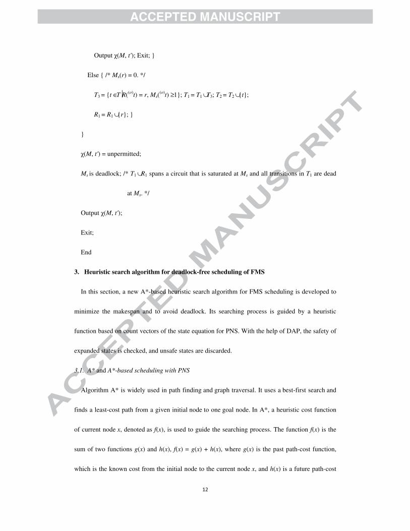
Output χ(M, t'); Exit; }
Else { /* Ms(r1) = 0. */
T1 = {t ∈ T⏐R((o)t) = r1, Ms((o)t) ≥ 1}; R1 = {r1}; }
while (T1 \ T2 ≠ ∅) do {
Choose t ∈ T1 \ T2, let r = (r)t;
If (Ms(r1) ≥ 1) then { /* Ms is safe. */
���
�
Output χ(M, t'); Exit; }
Else { /* Ms(r) = 0. */
T3 = {t ∈ T⏐R((o)t) = r, Ms((o)t) ≥ 1}; T1 = T1 ∪ T3; T2 = T2 ∪ {t};
R1 = R1 ∪ {r}; }
}
χ(M, t') = unpermitted;
Ms is deadlock; /* T1 ∪ R1 spans a circuit that is saturated at Ms and all transitions in T1 are dead
at Ms. */
Output χ(M, t');
Exit;
End
3. Heuristic search algorithm for deadlock-free scheduling of FMS
In this section, a new A*-based heuristic search algorithm for FMS scheduling is developed to
minimize the makespan and to avoid deadlock. Its searching process is guided by a heuristic
function based on count vectors of the state equation for PNS. With the help of DAP, the safety of
expanded states is checked, and unsafe states are discarded.
3.1. A* and A*-based scheduling with PNS
Algorithm A* is widely used in path finding and graph traversal. It uses a best-first search and
finds a least-cost path from a given initial node to one goal node. In A*, a heuristic cost function
of current node x, denoted as f(x), is used to guide the searching process. The function f(x) is the
sum of two functions g(x) and h(x), f(x) = g(x) + h(x), where g(x) is the past path-cost function,
which is the known cost from the initial node to the current node x, and h(x) is a future path-cost
���
�
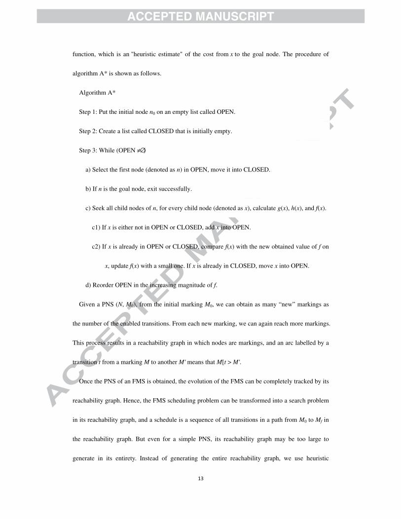
function, which is an "heuristic estimate" of the cost from x to the goal node. The procedure of
algorithm A* is shown as follows.
Algorithm A*
Step 1: Put the initial node n0 on an empty list called OPEN.
Step 2: Create a list called CLOSED that is initially empty.
Step 3: While (OPEN ≠ ∅ )
a) Select the first node (denoted as n) in OPEN, move it into CLOSED.
b) If n is the goal node, exit successfully.
c) Seek all child nodes of n, for every child node (denoted as x), calculate g(x), h(x), and f(x).
c1) If x is either not in OPEN or CLOSED, add x into OPEN.
c2) If x is already in OPEN or CLOSED, compare f(x) with the new obtained value of f on
x, update f(x) with a small one. If x is already in CLOSED, move x into OPEN.
d) Reorder OPEN in the increasing magnitude of f.
Given a PNS (N, M0), from the initial marking M0, we can obtain as many “new” markings as
the number of the enabled transitions. From each new marking, we can again reach more markings.
This process results in a reachability graph in which nodes are markings, and an arc labelled by a
transition t from a marking M to another M' means that M[t > M'.
Once the PNS of an FMS is obtained, the evolution of the FMS can be completely tracked by its
reachability graph. Hence, the FMS scheduling problem can be transformed into a search problem
in its reachability graph, and a schedule is a sequence of all transitions in a path from M0 to Mf in
the reachability graph. But even for a simple PNS, its reachability graph may be too large to
generate in its entirety. Instead of generating the entire reachability graph, we use heuristic
���
�
function to guide the searching process. Hence only a part of the reachability graph is generated
and searched.
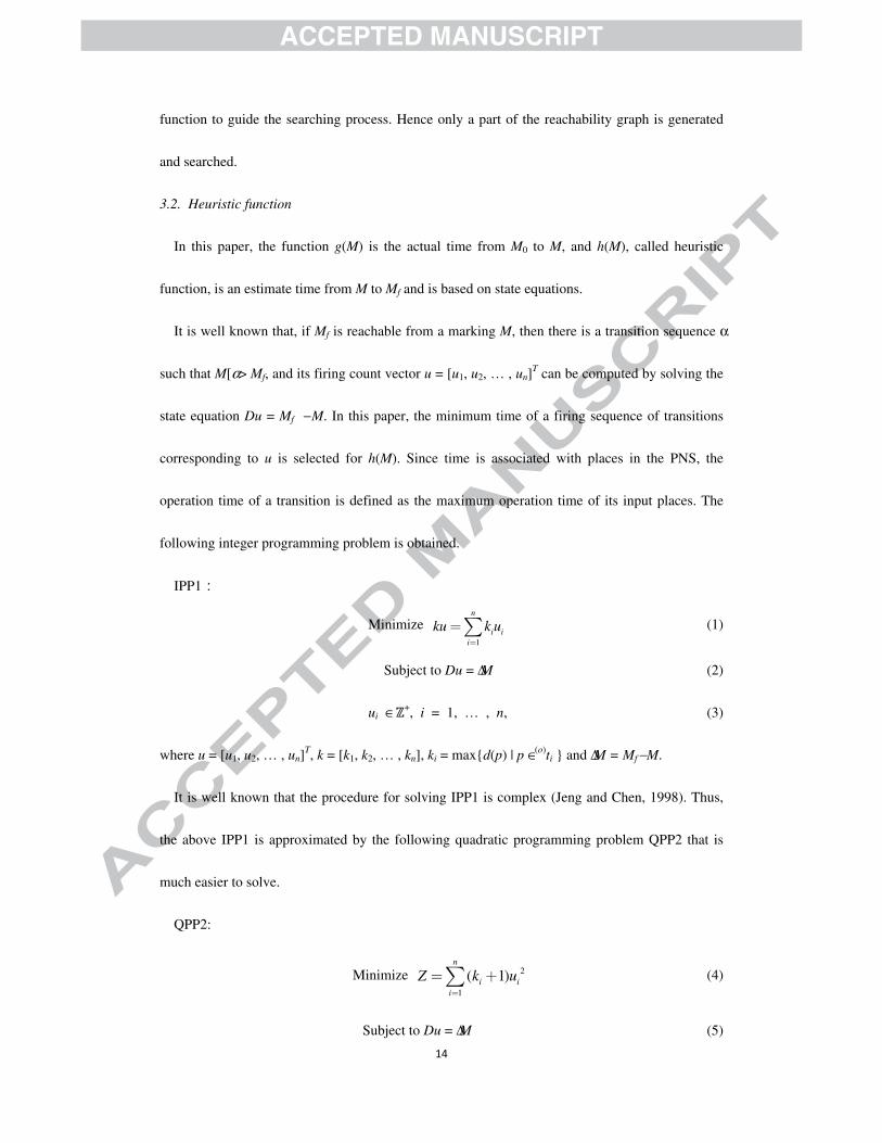
3.2. Heuristic function
In this paper, the function g(M) is the actual time from M0 to M, and h(M), called heuristic
function, is an estimate time from M to Mf and is based on state equations.
It is well known that, if Mf is reachable from a marking M, then there is a transition sequence α
such that M[α > Mf, and its firing count vector u = [u1, u2, … , un]T can be computed by solving the
state equation Du = Mf − M. In this paper, the minimum time of a firing sequence of transitions
corresponding to u is selected for h(M). Since time is associated with places in the PNS, the
operation time of a transition is defined as the maximum operation time of its input places. The
following integer programming problem is obtained.
IPP1�
Minimize 1
n
i ii
ku k u=
=∑ (1)
Subject to Du = ΔM (2)
ui ∈ �+, i = 1, … , n, (3)
where u = [u1, u2, … , un]T, k = [k1, k2, … , kn], ki = max{d(p) | p ∈ (o)ti } and ΔM = Mf − M.
It is well known that the procedure for solving IPP1 is complex (Jeng and Chen, 1998). Thus,
the above IPP1 is approximated by the following quadratic programming problem QPP2 that is
much easier to solve.
QPP2:
Minimize 2
1
( 1)n
i ii
Z k u=
= +∑ (4)
Subject to Du = ΔM (5)
���
�
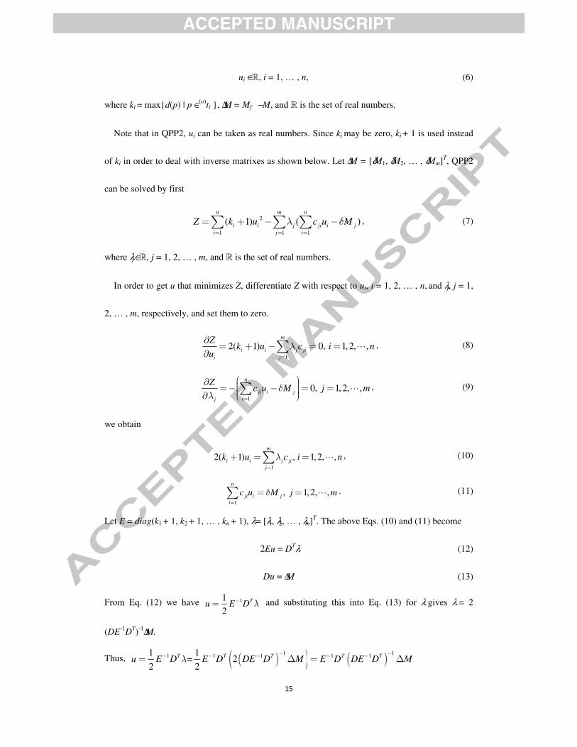
ui ∈ R, i = 1, … , n, (6)
where ki = max{d(p) | p ∈ (o)ti }, ΔM = Mf − M, and R is the set of real numbers.
Note that in QPP2, ui can be taken as real numbers. Since ki may be zero, ki + 1 is used instead
of ki in order to deal with inverse matrixes as shown below. Let ΔM = [δM1, δM2, … , δMm]T, QPP2
can be solved by first
2
1 1 1
( 1) ( )n m n
i i j ji i ji j i
Z k u c u Mλ δ
= = =
= + − −∑ ∑ ∑ , (7)
where λj ∈ R, j = 1, 2, … , m, and R is the set of real numbers.
In order to get u that minimizes Z, differentiate Z with respect to ui, i = 1, 2, … , n, and λj, j = 1,
2, … , m, respectively, and set them to zero.
1
2( 1) 0, 1,2, ,m
i i j jiji
Zk u c i n
uλ
=
∂= + − = =
∂∑ �
, (8)
1
0, 1,2, ,n
ji i jij
Zc u M j mδ
λ=
⎛ ⎞∂ ⎟⎜=− − = =⎟⎜ ⎟⎜ ⎟∂ ⎝ ⎠∑ �
, (9)
we obtain
1
2( 1) , 1,2, ,m
i i j jij
k u c i nλ
=
+ = =∑ �
, (10)
1
, 1,2, ,n
ji i ji
c u M j mδ
=
= =∑ �
. (11)
Let E = diag(k1 + 1, k2 + 1, … , kn + 1), λ = [λ1, λ2, … , λm]T. The above Eqs. (10) and (11) become
2Eu = DTλ (12)
Du = ΔM (13)
From Eq. (12) we have 11
2Tu E D λ
−
= and substituting this into Eq. (13) for λ gives λ = 2
(DE-1DT)-1ΔM.
Thus, ( )( ) ( )1 11 1 1 1 11 1
= 22 2
T T T T Tu E D E D DE D M E D DE D Mλ− −
− − − − −
= Δ = Δ
���
�
As a result, the minimum of ku is approximated by kE−1DT(DE−1DT)−1ΔM = HΔM, where H =
kE−1DT(DE−1DT)−1, and HΔM is used as an estimate of time from the current marking M to the final
marking Mf. That is,
h(M) = ku = HΔM (14)
The function g(M) is obtained as follows. Let α = t0t1t2 … tN-1 denote the transition sequence that
transform M0 to M, and L(tk[Oij]) denote the firing time of tk that is the start time of operation Oij.
Feasibility of the transition sequence α = t0t1t2 … tN-1 implies that, if the time is not considered,
then α can be fired in sequence. Thus, in the PNS, tk[Oij] can be fired only after operation Oi(j-1) is
finished and tk-1 is fired. Suppose that tk-1 corresponds to operation Ouv and ts corresponds to Oi(j-1).
Then,
L(tk[Oij]) = max{L(ts[Oi(j-1)]) + d(Oi(j-1)), L(tk-1[Ouv])}, (15)
g(M) = maxi, j, k{L(tk[Oij]) + d(Oij)}. (16)
3.3. Deadlock-free heuristic scheduling algorithm for FMS
The deadlock-free scheduling algorithm proposed in this paper is a combination of algorithm
A* and the heuristic function based on the state equation for PNS. To avoid deadlocks, one-step
look-ahead method based on the RTC concept is used in the proposed algorithm. Now, our
deadlock-free heuristic scheduling (DHS) algorithm can be summarized as follows.
Algorithm DHS
Input: A PNS (N, M0) and the incidence matrix D of (N, M0);
Output: A deadlock-free schedule α;
Begin
Initialize: α = ε (empty string); g(M0) = 0; Old(M0) = h(M0) (Old is used to store the updated
���
�
value of the f ); OPEN = { (M0, g(M0), Old(M0), α(M0)) }; CLOSED = ∅;
While (OPEN ≠ ∅) do {
Choose (M, g(M), Old(M), α(M)) ∈ OPEN with the minimum value Old(M);
/* In the case of multiple choices, select one arbitrarily.*/
OPEN := OPEN \ { (M, g(M), Old(M), α(M)) }; CLOSED := CLOSED ∪ { (M, g(M), Old(M),
α(M)) };
If (M = = Mf) then {
Output α(M); Exit; }
For t ∈ TE(M) do { /* TE(M) is the set of enabled transitions at M. */
If (DS(M, t) = = permitted) then {
M [t > M′;
Compute g(M′); h(M′) = HΔM′; f(M′) = g(M′) + h(M′); α(M′) = α(M)t;
/* H = kE-1DT(DE-1DT)-1; ΔM′ = Mf − M′. */
If (M′ ∈ CLOSED) then { /* M′ ∈ CLOSED implies that (M′, ⋅, ⋅, ⋅) ∈ CLOSED. */
If (f(M′) < Old(M′)) then {
Old(M′) = f(M′);
CLOSED := CLOSED / { (M′, g(M′), Old(M′), α(M′)) };
OPEN := OPEN ∪ { (M′, g(M′), Old(M′), α(M′)) }; } }
If (M′ ∈ OPEN) then { /* M′ ∈ OPEN implies that (M′, ⋅, ⋅, ⋅) ∈ OPEN. */
If (f(M′) < Old(M′)) then {
Old(M′) = f(M′); } }
If (M′ ∉ OPEN ∪ CLOSED) then {
���
�
Old(M′) = f(M′);
OPEN := OPEN ∪ { M′, g(M′), Old(M′), α(M′)) }; }
}
}
}
End
Algorithm DHS has two lists, OPEN and CLOSED. OPEN maintains all generated markings
that are waiting for expansion. CLOSED is the set of markings that have been expanded. Thus, the
intersection of OPEN and CLOSED is empty, in other words, a marking can’t be in OPEN and
CLOSED at the same time. The basic idea of DHS is partial searching in the reachability graph of
PNS. The algorithm starts with M0 as the current state or marking, and then explores it, that is,
generates as many “new” markings as the number of the enabled and safe transitions at M0, add all
new markings into OPEN. Note that if an enabled transition t at M0 is not safe, i.e., DS(M, t) =
unpermitted, then its firing t is prevented in exploration, since the marking generated by its firing
is a deadlock or from it deadlock markings must have arrived.
From OPEN, select a marking M with the minimum value of f(M), explore it and put it in
CLOSED. That is, from a selected marking M we can again obtain more markings. Then, the
algorithm expands M and checks the safety of its subsequent markings. If a enabled transition t at
M is safe, and M[t > M′, let DS(M, t) = permitted, compute f(M′); otherwise, let DS(M, t) =
unpermitted, discard M′ to avoid unnecessary expansion. If M′ is already in CLOSED, then we
compare f(M′) with Old(M′), and update Old(M′) with small one, move M′ from CLOSED into
OPEN. If M′ is already in OPEN, compare f(M′) with Old(M′), and update Old(M′) with small
���
�
one. If M′ is not either in OPEN or CLOSED, put M′ in OPEN to be expanded later. The algorithm
repeats the above steps until reaching the final marking Mf. DS(M, t) in Algorithm DHS can be
used as a truncation technique to avoid unnecessary expansion.
Theorem 3.1. Algorithm DHS can correctly output a deadlock-free schedule and the time
complexity of DHS is the same as that of algorithm A*.
Proof. Since at a safe marking M, there exists at least one enabled and safe transition. Let t be
such an enabled and safe transition, and M[t > M1, then M1 is safe. Because the initial marking M0
is safe and the number of parts is finite, DHS can find a feasible sequence of transitions from M0
to Mf. DHS is obtained by imbedding Algorithm DS into A*, and DS has the polynomial time
complexity (Xing et al., 2009). Thus, DS does increase the complexity of A*.
4. Illustrative examples
In this section, two FMS examples are used to show the efficiency of Algorithm DHS, and a
heuristic function h1(M) = −depth(M) is utilized to test the effectiveness of heuristic function h2(M)
= HΔM in Algorithm DHS. In addition, the scheduling method based on genetic algorithm in Xing
et al. (2012) is tested on example 2. The comparison results show the superiority of Algorithm
DHS.
Let M be a marking in the reachability graph of PNS. Then there is a sequence of transitions α
such that M0[t > M, and the length of α is equivalent to depth(M), this value is equivalent to
depth(M). The heuristic function h1(M) = −depth(M) prefers markings that are deeper in the
reachability graph of PNS, that is, a marking with a bigger depth is hypothesized to be nearer to
the final marking.
4.1. Example 1
��
�
Reconsider an FMS with two kinds of part to be processed on three machines, its PNS is shown
in Fig. 1. The processing times for machines are given in Table 2, and C(m1) = C(m3) = 2.
There are seven instances with different number of parts to be tested, and the number of each
type of parts are randomly distributed in the ranges of [5, 20]. The performance of the algorithm
was quantified by two indices: (a) the state space in each instance, (b) the near-optimal makespan
in each instance. The state space denotes the total number of markings in OPEN and CLOSED.
Case 1) C(m2) = 2. In this case, there is no center resource, and Algorithm DS can be used
directly. The complete feasible sequence of firing transitions for number of parts (5, 5) is α = (t21,
t21, t22, t21, t22, t21, t23, t24, t22, t21, t23, t24, t22, t23, t24, t11, t12, t13, t14, t11, t12, t13, t14, t11, t12, t13, t14, t11,
t12, t13, t14, t11, t12, t13, t14, t22, t23, t24, t23, t24).
The complete feasible sequence of firing transitions for number of parts (10, 10) is α = ( t21, t21,
t22, t21, t22, t21, t23, t24, t22, t21, t23, t24, t22, t21, t23, t24, t22, t21, t23, t24, t22, t21, t23, t24, t22, t21, t23, t24, t22,
t21, t23, t24, t22, t23, t24, t11, t12, t13, t14, t11, t12, t13, t14, t11, t12, t13, t14, t11, t12, t13, t14, t11, t12, t13, t14, t11,
t12, t13, t14, t11, t12, t13, t14, t11, t12, t13, t14, t11, t12, t13, t14, t11, t12, t13, t14, t22, t23, t24, t23, t24).
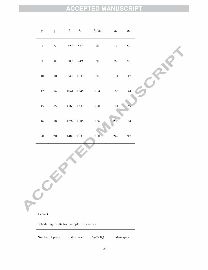
The scheduling results of example 1 without center resource are shown in Table 3.
Case 2) C(m2) = 1. m2 is a center resource. To obtain a deadlock-free controller for this kind of
PNSs, PNSs are reduced by center resources such that the reduced ones do not contain any center
resources but still fall into the class of marked PNs (Xing et al., 2012). The reduced PNS is shown
in Fig. 2. The optimal DAP with polynomial complexity can be obtained by Algorithm DS.
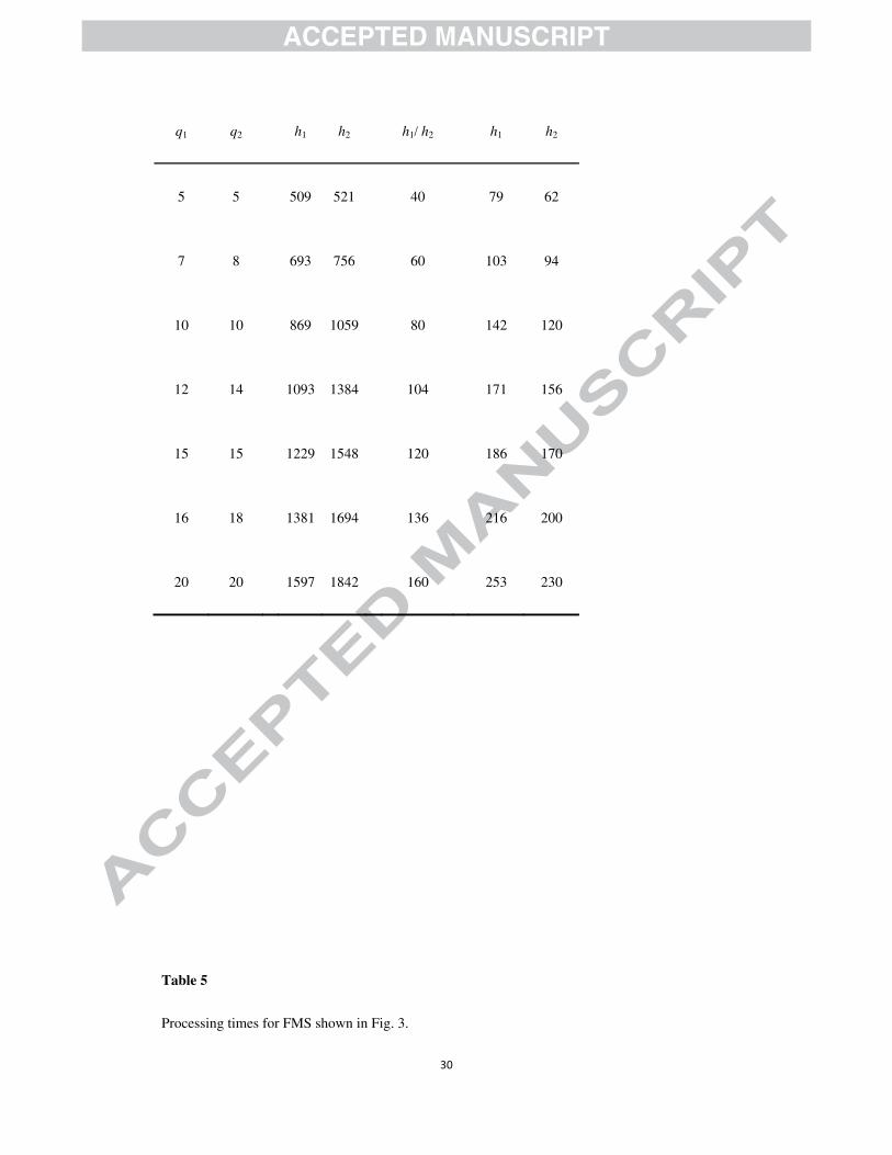
Scheduling results of example 1 with center resource are shown in Table 4.
Scheduling results for different number of parts of example 1 are shown in Table 3 and Table 4.
depth(Mf) in Table 3 and Table 4 indicate the total number of transition firings to reach the final
���
�
marking Mf from the initial marking M0. Let N denote the number of parts in a PNS, xi (i = 1, 2, …
, N) denote the number of parts of type-qi parts, and ni (i = 1, 2, … , N) denote the number of
operations of the type-qi parts. Then, depth(Mf) = x1n1 + x2n2 + ⋅⋅⋅ + xNnN. It is found out that the
state space of using h2(M) is slight bigger than using h1(M), this is because h2(M) contains much
more PNS information than h1(M), the search scope is larger, and many unpromising markings
have been discarded in the early stage of searching process for h1(M). Note that h2(M) produces
better makespan of different number of parts than those obtained by using heuristic function h1(M)
= −depth(M).
4.2. Example 2
The system includes three machines m1, m2, and m3, and three robots r1, r2, and r3. Each
machine holds two parts at the same time. Robots deal with the movements of parts between
machines. Each robot can move one part at a time. The system can process three types of parts, q1,
q2, and q3. Type-q1 parts are processed only on m1. Type-q2 parts can be processed first on m2,
then on m3. Type-q3 parts are processed first on m3, then on m2. Let A → B denote the movement of
a part from machine A to machine B. Then robot r1 handles q2 → m2, and m2 → q3. Robot r2 handles
m3 → m2, m2 → m3, q1 → m1, and m1 → q1. Robot r3 handles q3 → m3, and m3 → q2. The PNS of the whole
FMS is illustrated by Fig. 3. The derived deadlock-free heuristic search scheduling algorithm is
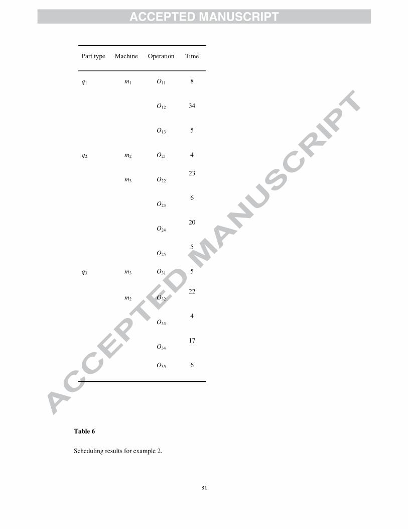
tested by the system in Fig. 3. The processing times for machines and robots are shown in Table 5.
Suppose that C(m1) = C(m2) = C(m3) = 2, C(r1) = 1,C(r2) = 2, and C(r3) = 1, respectively.
Algorithm DS and Algorithm DHS can be used directly. There are seven instances with
different number of parts to be tested, and the number of each type of parts are randomly
distributed in the range of [5, 10]. A near-optimal deadlock-free heuristic scheduling for number
���
�
of parts (5, 5, 5) is obtained with makespan 272. The transition firing sequence gives the
near-optimal schedule, which is shown as follow. The schedule results for different lot sizes are
shown in Table 6.
The complete feasible sequence of firing transitions for number of parts (5, 5, 5) is α = (t31, t32,
t31, t32, t21, t22, t11, t12, t11, t12, t33, t34, t23, t24, t33, t34, t31, t32, t35, t36, t33, t34, t31, t32, t35, t36, t33, t34, t31,
t32, t35, t36, t21, t22, t35, t36, t33, t34, t23, t24, t21, t22, t35, t36, t21, t22, t25, t26, t23, t24, t21, t22, t25, t26, t23, t24,
t25, t26, t23, t24, t25, t26, t25, t26, t13, t14, t11, t12, t13, t14, t11, t12, t13, t14, t11, t12, t13, t14, t13, t14).
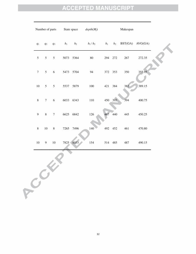
The scheduling results in terms of state spaces and makespans illustrate the advantage of h2(M)
= HΔM in Algorithm DHS. Moreover, the scheduling results of examples 1 and 2 show that the
proposed heuristic function based on the state equation is more suitable to the PNSs in this paper,
because the proposed heuristic function considers global information in the searching process.
The parameters used in GA (Xing et al., 2012) are chosen as a population size of 100, maximum
number of generations of 1000, crossover rate of 0.9, and mutation rate of 0.1. Table 6 displays the
computational results of GA on example 2, where BST and AVG denote the best and the average
makespan of 20 trials, respectively.
From the AVG of GA in Table 6, we can see that the heuristic scheduling algorithm by using
heuristic function h2 outperform GA. Compared to the heuristic scheduling algorithm proposed in
this paper, there are many parameters in GA, such as crossover rate and mutation rate, the choice
of these parameters affect quality of the solution, and most of these parameters are selected by
experience. Moreover, GA belongs to the class of stochastic algorithms which need too many
times of computations to obtain a stable solution.
5. Conclusions
��
�
Based on the marked PN models of FMSs, this paper integrates a deadlock control policy and a
heuristic search algorithm and develops a new deadlock-free scheduling algorithm. In the
proposed heuristic search algorithm, the heuristic function is based on the state equations for PNs.
By one-step look-ahead method in the optimal deadlock control policy, the safety of a marking is
checked, and unsafe markings are discarded to avoid unnecessary expansion in the reachability
graph of PN. Experiments show that the proposed method can obtain near-optimal schedule with
reasonable computation time and requires less searched state space.
Further research is required to explore other heuristic functions and PN models with routing
flexibility.
References
Abdallah, I. B., & Elmaraghy, H. A. (1998). Deadlock prevention and avoidance in FMS: a Petri
net based approach. International Journal of Advanced Manufacturing Technology, 14(10),
704-715.
Abdallah, I. B., Elmaraghy, H. A., & Elmekkawy, T. (2002). Deadlock-free scheduling in flexible
manufacturing system using Petri nets. International Journal of Production Research, 40(12),
2733-2756.
Chu, F., & Xie, X. L. (1997). Deadlock analysis of Petri nets using siphons and mathematical
programming. IEEE Transactions on Robotics and Automation, 13(6), 793-804.
Dashora, Y., Kumar, S., Tiwari, M. K., & Newman, S. T. (2007). Deadlock-free scheduling of an
automated manufacturing system using an enhanced colored time resource Petri-net
model-based evolutionary endosymbiotic learning automata approach. International Journal of
Flexible Manufacturing System, 19(4), 486-515.
���
�
Ezpeleta, J., Colom, J., & Martinez, J. (1995). A Petri net-based deadlock prevention policy for
flexible manufacturing system. IEEE Transaction on Robotics and Automation, 11(2), 173-184.
Fanti, M. P., Maione, G., & Turchiano, B. (2001). Distributed event-control for deadlock
avoidance in automated manufacturing systems. International Journal of Production Research,
39(9), 1993-2021.
Fanti, M. P., & Zhou, M. C. (2004). Deadlock control methods in automated manufacturing
systems. IEEE Transactions on Systems, Man, Cybernetics, Part A: Systems and Humans, 34(1),
5-22.
Golmakani, H. R., Mills, J. K., & Benhabib, B. (2006). Deadlock-free scheduling and control of
flexible manufacturing cells using automata theory. IEEE Transaction on System, Man, and
Cybernetics, Part A: Systems and Humans, 36(2), 327-337.
Hariri, A. M. A., & Potts, C. N. (1997). A branch and bound algorithm for two-stage assembly
scheduling problem. European Journal of Operational Research, 103, 547-556.
Huang, Y., Jeng, M., Xie, X. L., & Chung, S. (2001). Deadlock prevention policy based on Petri
nets and siphons. International Journal of Production Research, 39(2), 283-305.
Jeng, M. D., & Chen, S. C. (1998). A Heuristic Search Approach Using Approximate Solutions to
Petri Net State Equations for Scheduling Flexible Manufacturing Systems. International
Journal of Flexible Manufacturing System, 10(2), 139-162.
Jeng, M. D., & Chen, S. C. (1999). Heuristic search based on petri net structures for FMS
scheduling. IEEE Transaction on Industry Applications, 35(1), 196-202.
Lee, D. Y., & DiCesare, F. (1994). Scheduling Flexible Manufacturing Systems Using Petri Nets
and Heuristic Search. IEEE Transaction on Robotics and Automation, 10(2), 123-132.
���
�
Lee, G. C., & Kim, Y. D. (2004). A branch-and-bound algorithm for a two-stage hybrid
scheduling problem minimizing total tardiness. International Journal of Production Research,
42(22), 4731-4743.
Pearl, J. (1984). Heuristics: Intelligent Search strategies for Computer Problem Solving. Reading,
MA: Addison-Wesley.
Pineo, M. (2000). Scheduling: Theory, Algorithms, and Systems, (2nd ed.). Englewood Cliffs, NJ:
Prentice-Hall.
Piroddi, L., Cordone, R., & Fumagalli, I. (2008). Selective siphon control for deadlock prevention
in Petri nets. IEEE Transactions on Systems, Man, and Cybernetics, Part A: Systems and
Humans, 38(6), 1337-1348.
Ramaswamy, S. E., & Joshi, S. B. (1996). Deadlock-free schedules for automated manufacturing
workstations. IEEE Transaction on Robotics and Automation, 12(3), 391-400.
Reveliotis, S. A., & Ferreira, P. M. (1996). Deadlock avoidance policies for automated
manufacturing cells. IEEE Transactions on Robotics and Automation, 12(6), 845-857.
Reyes, A., Yu, H., & Kelleher, G. (2002a). Hybrid Heuristic Search for the Scheduling of Flexible
Manufacturing Systems Using Petri Nets. IEEE Transaction on Robotics and Automation, 18(2),
240-245.
Reyes, A., Yu, H., Kelleher, G., & Lloyd, S. (2002b). Integrating Petri Nets and hybrid heuristic
search for the scheduling of FMS. Computers in Industry, 47(1), 123-128.
Wu, N. Q., & Zhou, M. C. (2007). Real-time deadlock-free scheduling for semiconductor track
systems based on colored timed PNs. OR Spectrum, 29(3), 421-443.
Xing, K. Y., Hu, B. S., & Chen, H. X. (1996). Deadlock avoidance policy for Petri net modeling
���
�
of flexible manufacturing systems with shared resources. IEEE Transaction on Automation
Control, 41(2), 289-295.
Xing, K. Y., Zhou, M. C., Liu, H. X., & Tian, F. (2009). Optimal Petri net based
polynomial-complexity deadlock avoidance policies for automated manufacturing systems.
IEEE Transaction on System, Man, and Cybernetics, Part A: Systems and Humans, 39(1),
188-199.
Xing, K. Y., Zhou, M. C., Wang, F., Liu, H. X., & Tian, F. (2011). Resource transition circuits
and siphons for deadlock control of automated manufacturing systems. IEEE Transaction on
System, Man, and Cybernetics, Part A: Systems and Humans, 41(1), 74-84.
Xing, K. Y., Han, L. B., Zhou, M. C., & Wang, F. (2012). Deadlock-free genetic scheduling for
automated manufacturing systems based on deadlock control policy. IEEE Transaction on
System, Man, and Cybernetics, Part B: Cybernetics, 42(3), 603-615.
Xiong, H. H., & Zhou, M. C. (1998). Scheduling of semiconductor test facility via Petri nets and
hybrid heuristic search. IEEE Transaction on Semiconductor Manufacturing, 11(3), 384-393.
Xu, G., & Wu, Z. M. (2004). Deadlock-free scheduling strategy for automated production cell.
IEEE Transaction on System, Man, and Cybernetics, Part A: Systems and Humans, 34(1),
113-122.
Figure Captions
Fig. 1. PNS of an FMS.
Fig. 2. Reduced model of PNS in Fig. 1
Fig. 3. The PNS of FMS in example 2
���
�
Table 1
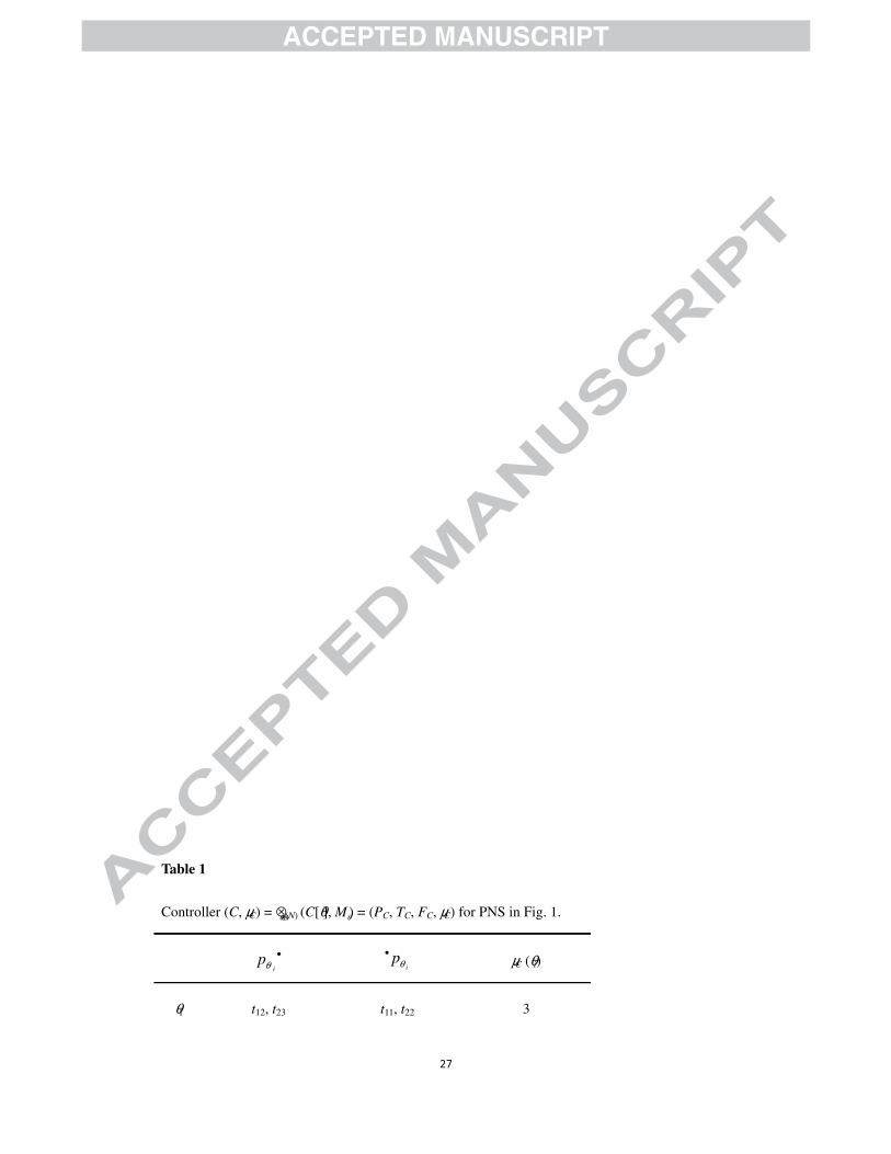
Controller (C, μC) = ⊗θ∈Θ(N) (C[θ], Mθ) = (PC, TC, FC, μC) for PNS in Fig. 1.
i
pθ•
ipθ
• μC (θi)
θ1 t12, t23 t11, t22 3
���
�
θ2 t13, t22 t12, t22 3
θ3 t13, t23 t11, t21 5
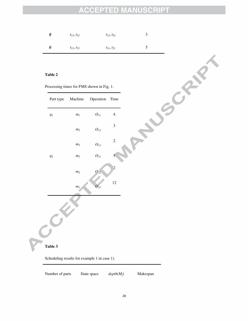
Table 2
Processing times for FMS shown in Fig. 1.
Part type Machine Operation Time
q1 m1
m2
m3
O11 4
O12 3
O13 2
q2 m3
m2
m1
O21 5
O22 2
O23 12
Table 3
Scheduling results for example 1 in case 1).
Number of parts State space depth(Mf) Makespan
���
�
q1 q2 h1 h2 h1/ h2 h1 h2
5 5 529 537 40 74 59
7 8 689 749 60 92 88
10 10 849 1037 80 131 112
12 14 1041 1345 104 163 144
15 15 1169 1537 120 181 159
16 18 1297 1685 136 203 184
20 20 1489 1837 160 242 212
Table 4
Scheduling results for example 1 in case 2).
Number of parts State space depth(Mf) Makespan
�
�
q1 q2 h1 h2 h1/ h2 h1 h2
5 5 509 521 40 79 62
7 8 693 756 60 103 94
10 10 869 1059 80 142 120
12 14 1093 1384 104 171 156
15 15 1229 1548 120 186 170
16 18 1381 1694 136 216 200
20 20 1597 1842 160 253 230
Table 5
Processing times for FMS shown in Fig. 3.
��
�
Part type Machine Operation Time
q1 m1 O11 8
O12 34
O13 5
q2 m2
m3
O21 4
O22 23
O23 6
O24 20
O25 5
q3 m3
m2
O31 5
O32 22
O33 4
O34 17
O35 6
Table 6
Scheduling results for example 2.
��
�
Number of parts State space depth(Mf) Makespan
q1 q2 q3 h1 h2 h1 / h2 h1 h2 BST(GA) AVG(GA)
5 5 5 5073 5364 80 294 272 267 272.35
7 5 6 5473 5704 94 372 353 350 355.95
10 5 5 5537 5879 100 421 384 382 389.15
8 7 6 6033 6343 110 450 393 394 400.75
9 8 7 6625 6842 126 467 440 445 450.25
8 10 8 7265 7496 140 492 452 461 470.80
10 9 10 7825 8033 154 514 485 487 490.15
�
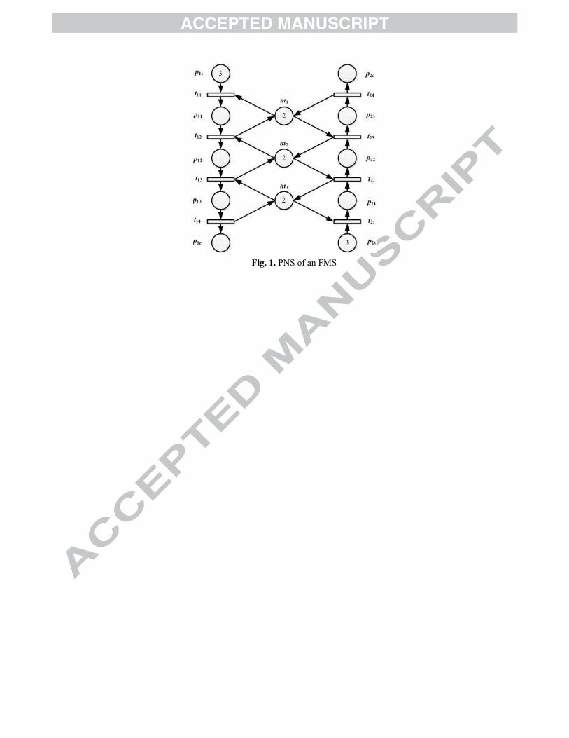
Fig. 1. PNS of an FMS
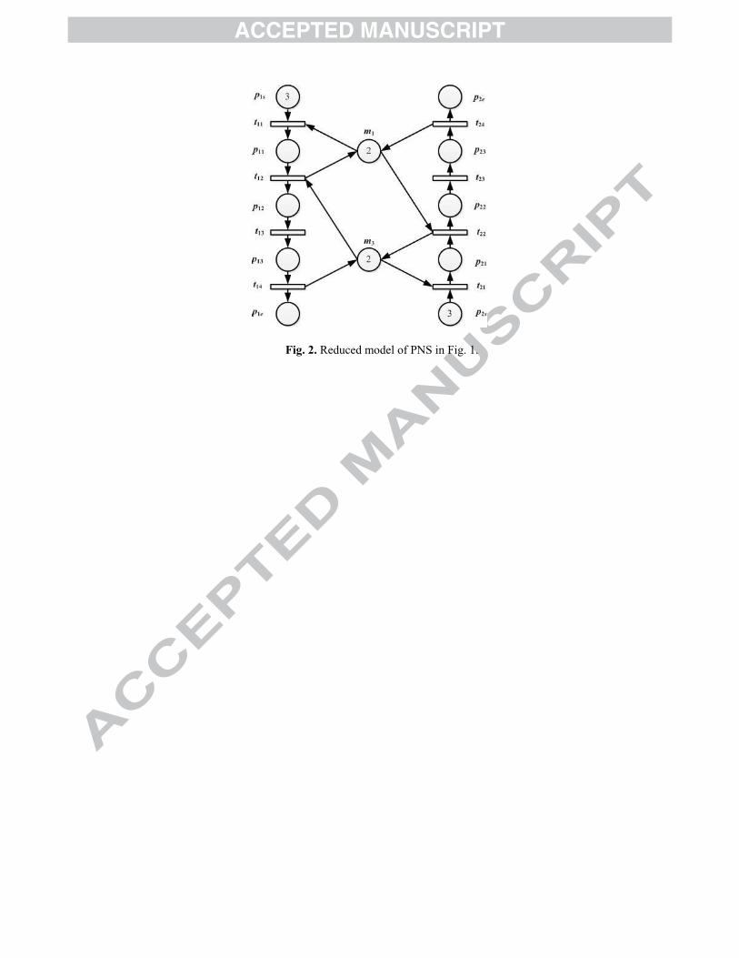
Fig. 2. Reduced model of PNS in Fig. 1.
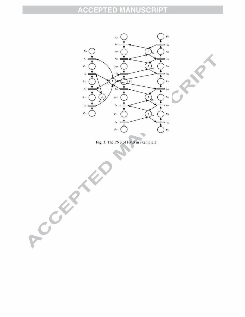
Fig. 3. The PNS of FMS in example 2.

Deadlock control and scheduling for flexible manufacturing system is integrated.
Deadlock control policy is embedded into the heuristic search algorithm.
A deadlock-free scheduling algorithm for flexible manufacturing system is proposed.