Debt and Economic Growth in Developing and Industrial ... · Debt and Economic Growth in Developing and Industrial Countries∗ Alfredo Schclarek† This draft: December 15, 2004

Debt and Economic Growth in Developing and

Industrial Countries∗

Alfredo Schclarek†

This draft: December 15, 2004

∗I want to thank Anders Danielson, Marcelo Delajara, Steven Durlauf, David Edgertonand Luis Rivera Batiz for comments and discussions; and seminar participants at Lund Uni-versity, Universidad E Siglo 21, Universidad Nacional de Cordoba, the Asociacion Argentinade Economıa Polıtica (Buenos Aires, Argentina, 2004), CFS Summer School (Frankfurt, Ger-many, 2004) and the European Central Bank. The present study was accomplished while Iwas visiting Universidad E Siglo 21, Argentina.

†Department of Economics, Lund University, P.O. Box 7082, SE-220 07 Lund, Sweden;tel: +46 (0) 73 689 1311, fax: +46 (0) 46 222 4613; e-mail: [email protected]; webpage:www.nek.lu.se/nekasc.

1

Abstract

This paper empirically explores the relationship between debt andgrowth for a number of developing and industrial economies. For develop-ing countries, we find that lower total external debt levels are associatedwith higher growth rates, and that this negative relationship is driven bythe incidence of public external debt, and not by private external debt.Regarding the channels through which debt accumulation affects growth,we find that this is mainly driven by the capital accumulation growth.There is only limited evidence on the relationship between external debtand total factor productivity growth. In addition, for private savings ratesthere are mixed results. We do not find any support for an inverted-Ushape relationship between external debt and growth. For industrial coun-tries, we do not find any significant relationship between gross governmentdebt and economic growth.

JEL classification: F34; H63; O10; O40

Keywords: External debt; Public debt; Economic growth; Capital accumulation;Productivity growth; Private savings rate

2

1 Introduction

The recent default of Argentina on part of its public debt is the most impor-tant default in history. The reason is that the restructuring process involvedmore than USD 100 billion in government bonds and a wide number of smallprivate bondholders of different nationalities. It was clear that a certain reduc-tion of the public debt would be necessary in order to make the debt situationsustainable. Furthermore, the argentine government did put emphasis that thespecific debt reduction should be large enough so that long run economic growthis not affected by the new debt situation. However, although the relationshipbetween public debt and economic growth is a major concern for policymakers,and public opinion in general, there is little empirical work investigating thisrelationship. Furthermore, there is even less evidence on the specific channelsthrough which debt affects growth.

A recent exception to this lack of empirical evidence is the work by Patilloet al. (2002) and Patillo et al. (2004), which empirically studies the relationshipbetween total external debt and the growth rate of GDP for developing coun-tries. It should be noted that these studies consider total external debt, but doesnot distinguish between public external debt and private external debt. Theyconclude that there is a nonlinear relationship, in the form of an inverted-Ushape relationship, between total external debt and growth in developing coun-tries. At low levels of total external debt, it affects positively growth, but thisrelationship becomes negative at high levels of it. The specific turning pointsare 35-40 percent for the debt-to-GDP ratio and 160-170 percent for the debt-to-exports ratio. Their paper also presents a short survey of the theoretical andempirical literature dealing with debt and growth. Further, Patillo et al. (2004)suggest that the channels through which total external debt affects economicgrowth are total factor productivity and capital accumulation. Other previousempirical studies on the nonlinear effects of debt on growth include Smyth andHsing (1995), Cohen (1997) and Elbadawi et al. (1997).

This paper aims to shed light on these issues by redressing the relationshipbetween debt and growth in both developing and industrial countries, and ex-ploring the channels through which it may manifest itself. The paper providesa comprehensive treatment of this issue by exploring four different dependentvariables (GDP per capita growth rate, total factor productivity growth rate,capital accumulation growth rate, and private savings rate). Further, the debtvariables include debt ratios not commonly used (such as debt to years of gov-ernment revenues) as well as a distinction between public and private externaldebt for developing countries. Further, it investigates the relationship betweengross government debt and economic growth for industrial countries. Note thatwe will estimate these relationships separately for the sample of developing andindustrial countries due to different debt variable definitions. The inclusion ofindustrial countries, the splitting up of total external debt into public externaldebt and private external debt, a different and more comprehensive set of ex-planatory variables, and a longer time span for the data, are the main differencesbetween this paper and Patillo et al. (2002) and Patillo et al. (2004).

3

In order to uncover these relationships, we use the system GMM dynamicpanel econometric technique proposed by Arellano and Bover (1995) and Blun-dell and Bond (1998). Previous applied growth studies that use this economet-ric methodology include among others Beck et al. (2000), Levine et al. (2000),Patillo et al. (2002), and Patillo et al. (2004). The data set consist of a panel of59 developing countries and 24 industrial countries with data averaged over eachof the seven 5-year periods between 1970 and 2002. There are several sourcesof the data, but our main source is the World Development Indicators 2004 ofthe World Bank.

The rest of the paper is organized in six sections. The empirical methodologyand the data used are discussed in sections 2 and 3 respectively. Section 4presents the estimation results for the different dependent variables and debtindicators for the sample of developing countries. Further, we also presents theresults of considering nonlinear effects on GDP growth. In section 5 we presentthe results for the industrial countries. In section 6, we discuss and presentthe results from some consistency test that were made in order to confirm theresults from the benchmark case. Finally, section 7 concludes.

2 Econometric Methodology

The basic regression equation that we use in order to uncover the relationshipbetween debt and economic growth is of the type

Yi,t = αXi,t + γDi,t + ηi + λt + εi,t (1)

where Yi,t is the dependent variable, Xi,t represents the set of explanatory vari-ables, Di,t is the debt variable, ηi is an unobserved country-specific effect, λt

is an unobserved time-specific effect, εi,t is the error term, and the subscripts iand t represent country and time period, respectively.

When estimating equation (1), we use four different dependent variables,namely the growth rate of GDP per capita, the TFP growth rate, the capitalaccumulation growth rate per capita, and the private savings rate. The reasonfor estimating equation (1) for each of these four dependent variables is that wenot only want to study the relationship between debt and growth, but also therelation of debt and the determinants of growth. Regarding Xi,t, we will usefive alternative explanatory variable sets. The first set, which is the base set,includes initial income per capita1, and educational attainment. The second setadds to the base set government size, openness to trade and inflation. The thirdset is like the second set, but also includes the level of financial intermediarydevelopment. The fourth set is equal to the first set plus population growthand the level of investment. The fifth set adds to the fourth set openness totrade, terms of trade growth and fiscal balance. Note that the second andthird set are very similar between each other. The same is valid between the

1The inclusion of initial income per capita when the dependent variable is the real growthrate of GDP per capita makes equation (1) become dynamic in nature. See for exampleDurlauf et al. (2004).

4

fourth set and the fifth set. In addition, when estimating equation (1) for thegrowth determinants, Xi,t includes the lagged dependent variable, which makesthe regressions become dynamic in nature. The sources and definitions of thesevariables are defined more thoroughly in section 3. Further, when using theprivate savings rate as dependent variable (the saving regression), we will usea completely different explanatory variable set. The variables that are used arepresented in section 3.

Evidently, equation (1) is linear in nature. However, we are also interestedin investigating if there is any nonlinear relationship between debt and economicgrowth. Specifically, we are interested in determining whether there exists aninverted-U shape relationship between debt and growth, i.e. low levels of debtare associated with a positive relationship with growth, and high levels of debtare associated with negative growth rates.2 Therefore, in order to allow fornonlinear effects of debt, we included a linear spline function in equation (1).In this case, equation (1) becomes

Yi,t = αXi,t + γDi,t + δdi,t(Di,t −D∗) + ηi + λt + εi,t (2)

where di,t is a dummy variable which equals 1 if the value of the debt variable isabove a certain threshold value D∗ and 0 otherwise. If δ is significantly differentfrom zero, we can conclude that there is a nonlinear relationship. In this case,the impact of debt will be different above and below the threshold D∗, i.e. therewill be a structural break. However, in order for there to be an inverted-U shaperelationship, γ should be positive and δ should be negative. Further, δ should belarger than γ in absolute terms. The specific threshold values for D∗ will dependon the specific debt indicator that is used. However, as there is no theoreticalnor empirical indication on any specific threshold value, we chose to estimateequation 2 for each debt indicator with nine ad-hoc chosen threshold values.In section A.2 of the appendix we display the specific threshold values for eachdebt indicator. In addition, equation 2 was estimated for each threshold valuewith the five alternative explanatory variable sets.

Methodologically, the paper uses the GMM estimator developed by Arellanoand Bover (1995) and Blundell and Bond (1998), called dynamic system GMMpanel estimator.3 Further, we use the robust one-step estimates of the standarderrors, which are consistent in the presence of any pattern of heteroskedasticityand autocorrelation within panels.4 There are two conditions that are necessaryfor the GMM estimator to be consistent, namely that the error term, ε, does notexhibit serial correlation and the validity of the instruments that are used. We

2It has been claimed by Patillo et al. (2002) and Patillo et al. (2004) that such a nonlinearrelationship is present.

3See Bond (2002) for an introduction to the use of GMM dynamic panel data estimators.4The two-step estimates of the standard errors is asymptotically more efficient than the

one-step variant. However, in a finite sample the two-step estimates of the standard errorstend to be severely downward biased (Arellano and Bond, 1991; Blundell and Bond, 1998).Windmeijer (2000) derives a finite-sample correction to the two-step covariance matrix, whichcan make the two-step variant more efficient than one-step variant. We are, however, unableto implement the Windmeijer finite-sample correction because we have a limited number ofcross sections (countries).

5

use two tests proposed by Arellano and Bond (1991) to validate these assump-tions. The first test examines the assumption that the error term is not seriallycorrelated. As this test uses the differenced error term, by construction AR(1)is expected to be present. Therefore, the Arellano-Bond test for autocorrelationdetermines whether the differenced error term has second-order, or higher, serialcorrelation. Under the null hypothesis of no second-order serial correlation, thetest has a standard-normal distribution. The second assumption is corroboratedby a test of over-identifying restrictions, which tests the overall validity of theinstruments. Specifically, we use the Hansen J statistic, which is the minimizedvalue of the two-step GMM criterion function. Under the null hypothesis of thevalidity of the instruments, this test has a χ2 distribution with (J −K) degreesof freedom, where J is the number of instruments and K the number of regres-sors. The reason for using this statistic, as opposed to the Sargan statistic, isthat it is robust to heteroskedasticity and autocorrelation.

There are several reasons for using cross-section time-series data. First,adding the time-series dimension to the data augments the number of observa-tions and the variability of the data. This is especially important for us giventhat we have a limited number of industrial and developing countries. Second,we are able to control for unobserved country specific effects and thereby re-duce biases in the estimated coefficient estimates. Third, the GMM estimatorcontrols for the potential endogeneity of all explanatory variables.5 This is be-cause the estimator controls for endogeneity by using ”internal instruments”,i.e. instruments based on lagged values of the explanatory variables. Note thatit controls for ”weak” endogeneity and not for full endogeneity (Bond, 2002).

3 Data

The data set consists of a panel of 59 developing countries and 24 industrialcountries, with data averaged over each of the seven 5-year periods between 1970and 2002 (1970-74; 1975-80; etc.).67 All the variables that we use are averageddata over non-overlapping 5-year periods, as we want to capture the long runrelationship between growth and debt, and not be subject to short run cyclical

5Recall that by including initial income per capita, the growth regression becomes dynamicin nature. Further, the growth determinant regressions include the lagged dependent variable,which also make them dynamic.

6Note that for the last period (2000-02), only three observations are available.7The developing countries are Algeria, Argentina, Bangladesh, Bolivia, Brazil, Cameroon,

Central African Republic, Chile, China, Colombia, Congo, Dem. Rep., Congo, Rep., CostaRica, Cote d’Ivoire, Dominican Republic, Ecuador, Egypt, Arab Rep., El Salvador, Ethiopia,Gambia, The, Ghana, Guatemala, Guyana, Haiti, Honduras, India, Indonesia, Iran, IslamicRep., Jamaica, Kenya, Lesotho, Madagascar, Malawi, Malaysia, Mali, Malta, Mauritius, Mex-ico, Morocco, Mozambique, Myanmar, Nicaragua, Niger, Nigeria, Pakistan, Panama, PapuaNew Guinea, Paraguay, Peru, Philippines, Rwanda, Senegal, Sierra Leone, South Africa,Sri Lanka, Sudan, Syrian Arab Republic, Tanzania, Thailand, Togo, Trinidad and Tobago,Tunisia, Turkey, Uganda, Uruguay, Venezuela, RB, Zambia, and Zimbabwe. The industrialcountries are Australia, Austria, Belgium, Canada, Cyprus, Denmark, Finland, France, Ger-many, Greece, Ireland, Israel, Italy, Japan, Korea, Rep., Netherlands, New Zealand, Norway,Portugal, Spain, Sweden, Switzerland, United Kingdom, and United States.

6

movements. Therefore, the total number of observations for the developingcountry panel is 413 and for the industrial country panel is 168. However, dueto data availability for some samples we had less than these observations, andin most cases we had unbalanced panels. Note that the two country samples,developing and industrial, will be treated separately, due to differences in thedebt variable definitions and sources.

The dependent variables are real per capita GDP growth rate (growth), to-tal factor productivity growth rate (prod), capital stock growth rate per capita(capgrowth), and private savings rate (psr). For the debt variable, Di,t, weuse 15 different debt indicators for the developing countries: total externaldebt-to-GDP ratio (dbtgdp), total external debt-to-exports ratio (dbtexp), to-tal external debt-to-revenues ratio (dbtrev), public external debt-to-GDP ra-tio (pubdgdp), public external debt-to-exports ratio (pubdexp), public externaldebt-to-revenues ratio (pubdrev), private external debt-to-GDP ratio (privdgdp),private external debt-to-exports ratio (privdexp), private external debt-to-revenuesratio (privdrev), interest payment-to-GDP ratio (intgdp), interest payment-to-exports ratio (intexp), interest payment-to-revenues ratio (intrev), debt service-to-GDP ratio (dbtsergdp), debt service-to-exports ratio (dbtserexp), and debtservice-to-revenues ratio (dbtserrev). In the case of the industrial countries, weuse 6 different debt indicators: gross government debt-to-GDP ratio (opubdgdp),gross government debt-to-exports ratio (opubdexp), gross government debt-to-revenues ratio (opubdrev), interest payment-to-GDP ratio (intgdp), inter-est payment-to-exports ratio (intexp), and interest payment-to-revenues ratio(intrev). Note that the main difference between industrial countries and devel-oping countries is that for the former there exist data on total public debt fromthe OECD Economic Outlook, instead for the later there exists only data forexternal public debt from the WDI. Further, total external debt, private exter-nal debt and debt service data from the WDI is only available for developingcountries. Beside the debt variable, the regressors include several variables tocontrol for other factors associated with economic development. Specifically, wehave five different explanatory variable sets. The first set consists of the ini-tial income per capita to control for convergence (linitial) and average years ofschooling as an indicator of the human capital stock in the economy (lschool).The second set includes, the variables from the first set, as well as governmentsize (lgov) and inflation (lpi), which are used as indicators of macroeconomicstability, and openness to trade (ltrade) to capture the degree of openness ofan economy. The third set adds to the second set a variable for financial in-termediary development (lprivo). The fourth set includes, apart from initialincome and schooling, population growth (lpop) and investment to GDP (linv).The fifth set includes the variables from the fourth set plus openness to trade(ltrade), terms of trade growth (ltot), and fiscal balance to GDP (lfbal).8 Inaddition, the explanatory variable sets for the growth determinant regressions

8Note that the second and third sets are relatively similar to each other. Also, the fourthand fifth sets are related. The variables used in the second and third sets have been used inBeck et al. (2000) and Levine et al. (2000), and the ones in the fourth and fifth sets in Patilloet al. (2002) and Mankiw et al. (1992), among others.

7

include the lagged dependent variable.When using the private savings rate as the dependent variable, we will only

use one explanatory variable set, which will be different from the ones used forthe other regressions. The chosen variables are determined by various theories ofconsumption, including the classical permanent-income and life-cycle hypothesisand the more recent theories accounting for consumption habits, subsistenceconsumption, precautionary saving motives, and borrowing constraints. Thevariables are one-period lag of private savings rate (l.psr), real per capita GrossPrivate Disposable Income (lrpdi), growth rate of real per capita GPDI (grpdi),real interest rate (lrir), terms of trade growth (ltot), old dependency ratio(oldr), young dependency ratio (yngr), urbanization ratio (urbpop), governmentsavings rate (gsr), and inflation (lpi).9

The source for the data is mainly the World Development Indicators 2004of the World Bank. However, we also used data from the OECD EconomicOutlook, the International Financial Statistics database of the IMF, the PennWorld Tables 6.1, the Barro-Lee database on educational attainment, the Fi-nancial Development and Structure database of the World Bank, and the Nehruand Dhareshwa Data Set on physical capital stock from the World Bank. Sec-tion A.1 of the appendix presents more detailed information about the sourcesand definitions of the different variables.

4 Estimation results for developing countries

4.1 Linear effects on GDP growth

Table 1 displays the estimation results of equation (1) for developing countrieswhen the dependent variable is the GDP growth rate and the debt indicatoris the total external debt-to-GDP ratio. The debt coefficient is negative andsignificant for all the five different independent variables sets, with the exceptionof set 2 where it is significant at the 10% level. Specifically, the coefficient valuesrange from -0.864 (column(2)) to -2.146 (column(1)). In the case of the totalexternal debt-to-exports ratio (Table 2), the debt coefficients are also negativeand significant, with the exception of set 2, with values ranging from -0.791(column (5)) to -1.969 (column (1)). These results are confirmed when usingthe total external debt-to-revenues ratio.10 Thus, for developing countries, thereis a significant negative relationship between the level of total external debt andthe growth rate of the economy.

In the case of the public external debt-to-GDP ratio, the results are presentedin table 3. We find a negative relationship with economic growth, with all thecoefficients for the different independent variable sets being significant at leastat the 5% level and ranging from -0.705 (column(5)) to -1.789 (column(1)). We

9These variables, with the exception of the lagged private savings rate, are used in thesaving regressions of Beck et al. (2000).

10These results are not presented due to space considerations, but the tables may be pro-vided upon request from the author.

8

find similar results in the case of the public external debt-to-exports ratio, withcoefficients ranging from -0.639 to -1.983 (table 4). Further, these results arecorroborated for the public external debt-to-revenues ratio.

When analyzing the results for the private external debt indicators, we findthat the relationship with growth is not significant. In table 5, for example,we present the results when using the private external debt-to-GDP variable.Here only the debt coefficient for set 4 (column (4)) is significant. These resultsare supported for the case of the private external debt-to-exports ratio (table6) and the private external debt-to-revenues ratio. As total external debt iscomposed of public external debt and private external debt, this suggests thatthe negative relationship between total external debt and growth is driven bythe negative relationship that exists between public external debt, and not bythe private component of it. In other words, it seems that high levels of publicexternal debt are associated with low economic growth, but that high levels ofprivate external debt are not necessarily associated with low economic growth.

The results of the linear relationship between GDP growth and the in-terest payment-to-GDP ratio, interest payment-to-exports ratio, and interestpayment-to-revenues ratio are not presented due to space considerations.11 How-ever, the findings for the interest payment indicators for all five independentvariables sets suggest that there is no significant relationship between GDPgrowth and interest payments. In the case of the debt indicators involving debtservices, we have also chosen not to present them to save space. The resultsfor all three debt service ratios, and for all five independent variable sets, showthat there is an insignificant association between them and the growth rate ofthe economy.

4.2 Nonlinear effects on GDP growth

In this subsection we present the estimation results for the nonlinear relationshipbetween the debt indicators and economic growth for developing countries usingequation 2. As noted in section 2 nine alternative threshold values were usedfor each debt indicator. In section A.2 of the appendix we display the specificthreshold values for each debt indicator.

When using the total external debt-to-GDP ratio, we find evidence of non-linear effects when using a threshold value of 20%. In this case, however, therewas no evidence supporting the existence of an inverted-U shape relationship.As can be seen in table 7, the debt variable coefficient, dbtgdp, is insignificantlydifferent from zero, and the debt dummy variable coefficient, dbtgdpdum020, isnegative, and significant for all the independent variables sets, i.e. there is norelationship between total external debt and growth when its ratio to GDP isbellow 20%, but there is a negative relationship when its ratio is above 20%.These nonlinear effects dissipated when using the threshold values above 20%.In the case of the total external debt-to-exports ratio, we did not find evidenceof nonlinear relationships for any of the nine different threshold values. In table

11The tables may be provided upon request from the author.

9

8, we present the results for the total external debt-to-export ratio when using athreshold value of 150%.12 We performed the same nonlinear estimation usingthe total external debt-to-revenues ratio with different threshold values. We findsome evidence of nonlinear effects when the total external debt-to-revenues ra-tio was bellow 150%. In these cases, however, the debt variable coefficient wasinsignificantly different from zero, while the debt dummy variable coefficientwas negative and significant, i.e. there is no evidence of an inverted-U shaperelationship. In addition, these nonlinear effects disappeared when estimatingequation 2 with threshold values above 150%. Concluding, we can assert thatthere is some evidence of nonlinear effects when using low debt threshold values,but no evidence of an inverted-U shape relationship between total external debtand growth.

It is to be noted that these results are in stark contrast to the results ofPatillo et al. (2002), who claim that there is a positive relationship between totalexternal debt and growth when the total external debt-to-GDP ratio is bellow35-40%, or when the total external debt-to-exports ratio is bellow 160-170%.One possible explanation for this discrepancy is that Patillo et al. (2002) usesonly one set of explanatory variables when estimating their growth regressions,which corresponds to our fifth explanatory variable set. As can be seen in table9, when estimating the nonlinear relationship between the total external debt-to-GDP ratio and economic growth with a threshold value of 30%, only the debtdummy coefficient for the fifth explanatory variable set (column (5)) is negativeand significant at the 5% level. Therefore, it is possible that their results aredriven by the specific selection of explanatory variables.13

When considering the public external debt indicators, we did not find anyevidence of nonlinear effects for both the ratios to GDP and exports. In thecase of the public external debt-to-revenues ratio, we find evidence of nonlineareffects only when using the threshold value 100%. In this case, however, thedebt variable coefficient was insignificantly different from zero, while the debtdummy variable coefficient was negative and significant, i.e. the inverted-Ushape hypothesis was rejected. For the private external debt indicators, we didnot find any evidence of nonlinear effects for the three ratios and all the ninethreshold values.

In the cases of the interest payment indicators, we did not find any evi-dence of nonlinear effects. In the case of the debt service-to-GDP ratio, thereis evidence of nonlinear effects and an inverted-U shape relationship with thegrowth rate when using threshold values bellow 3%. As can be seen in table10, the debt variable coefficient, dbtsergdp, is positive and significant, while thedebt dummy variable, dbtsergdpdum003, is negative and significant. Further,the debt dummy coefficient is larger in absolute value than the debt variablecoefficient, which would be supporting the inverted-U shape relationship. Theseresults are interesting when considering that when the linear relationship be-

12We decided to show the results for this specific threshold value because Patillo et al.(2002) claim that bellow this threshold there is a positive relationship with growth, and abovethere is a negative relationship.

13This is a common critique to the whole empirical growth literature (Durlauf et al., 2004).

10

tween debt service-to-GDP ratio and growth was estimated, we found an in-significant relationship. The nonlinear evidence is, however, not supported bythe other two debt service ratios (exports and revenues), where the debt dummyvariable coefficients are insignificant in all cases. Therefore, the results for thedebt service-to-GDP ratio should be taken with caution.

4.3 Linear effects on TFP growth

In table 11 we present the results for the estimation of equation (1) when usingthe total factor productivity growth as the dependent variable and the total ex-ternal debt-to-GDP ratio for developing countries. Further, this relationship hasalso been estimated using the total external debt-to-exports ratio and the totalexternal debt-to-revenues ratio. Although all the debt variable coefficients arenegative, they are not significant when using the total external debt-to-GDPratio. Further, for the total external debt-to-exports ratio, the debt variablecoefficients are not significant, but for the first set, which is negative and signifi-cant. However, for the total external debt-to-revenues ratio, the debt coefficientsare negative and significant for the first four sets. Therefore, there is very weakevidence on the significance of the negative relationship between total exter-nal debt and TFP growth. Thus, it is doubtful that the negative relationshipbetween total external debt and GDP growth is driven by the effect of TFPgrowth on GDP growth.

In the case of the debt indicators involving the public external debt, we candraw the same conclusions as for the total external debt indicators. All thecoefficients of the different specifications are insignificant, but for the third andfourth set when using the public external debt-to-revenues ratio. In the caseof the private external debt indicators, the debt coefficients are negative andsignificant for specification one and four for the private external debt-to-GDPratio and specifications one to four for the private external debt-to-revenuesratio. Thus, no robust relationship between private external debt and TFPgrowth is found.

In the case of the interest payment and debt service indicators, none of thecoefficients are significant for the different independent variable sets. Thus, norelationship between these indicators and TFP growth is found.

4.4 Linear effects on capital growth

In this subsection we analyze the relationship between the different debt indi-cators and per capita growth rate of the capital stock for developing countries.In table 12 we present the results of the estimation of equation (1) when usingcapital growth as the dependent variable and the total external debt-to-GDPratio as the debt variable. Note again that we have also estimated this rela-tionship using the total external debt-to-exports ratio and the total externaldebt-to-revenues ratio, but due to space reasons we do not present the results.For both the total external debt-to-GDP ratio and the total external debt-to-exports ratio, we find a significant negative relationship between total external

11

debt and capital stock growth. The coefficients range from -0.672 and -1.000 inthe case of the total external debt-to-GDP ratio, and are all significant at the5% level, but for the fourth set, which is significant at the 10% level. In thecase of the total external debt-to-revenues ratio, although we find that all thecoefficients are negative, only the second and third sets are significant. These re-sults, in combination with the findings presented in subsection 4.3, suggest thatthe main driving factor behind the negative relationship between total externaldebt and GDP growth seems to be the influence of external debt on capitalstock accumulation.

Regarding the indicators of public external debt, the estimation results forthe GDP ratio is presented in table 13. Our findings show that there is asignificant negative relationship between public external debt and capital accu-mulation. The negative coefficients are all significant at the 5% level and rangefrom -0.620 to -1.110 in the case of the public external debt-to-GDP ratio. Theseresults are similar to those obtained for the public external debt-to-exports ra-tio. In the case of the public external debt-to-revenues ratio, we find that thedebt variable coefficient is significant for the first three sets. Regarding theprivate external debt, we do not find any significant relationship between thesedebt indicators and capital accumulation. Thus, we reach the conclusion thatthe negative relationship between total external debt and capital accumulationgrowth is mainly due to the influence of public external debt.

In so far as the interest payment indicators are concerned, there is no ev-idence on any significant relationship between interest payments and capitalaccumulation. For the debt service indicators, we find some evidence that ithas a significant negative relationship with capital accumulation. For the debtservice-to-GDP ratio, the last four sets have a significant debt coefficient. Forthe debt service-to-exports ratio and the debt service-to-revenues ratio, three offive sets and two of five sets have a significant debt variable coefficient, respec-tively.

4.5 Linear effects on private savings rate

In this subsection we will present the results of the savings regression for de-veloping countries. The results for some of the external debt indicators arepresented in table 14. The estimated equation is similar to equation (1) andwe use the same system GMM estimator as before. The difference, however,is that we use a unique and different independent variable set, as explained insection 3. In the case of the total external debt indicators, we only find thatthe debt variable coefficient is significantly different from zero, with a negativevalue of -0.028, for the total external debt-to-exports ratio. The same resultsare obtained for the public external debt indicators, where the only significantdebt coefficient is for the public external debt-to-exports ratio, with a negativevalue of -0.024. The significance of these coefficients in both cases is revertedwhen doing the same estimation with the data set without outliers. Thus, thereseems to be no clear relationship between total and public external debt andthe private savings rate of an economy. Regarding the private external debt

12

indicators, we find that the debt coefficients for all three ratios are positive.However, they are only significant for the private external debt-to-GDP ratio.Therefore, there is no strong evidence that there is a positive relationship be-tween private external debt and the private savings rate. In the case of theinterest payments indicators, as well as for the debt service indicators, we donot find any significant relationship between these ratios and the private savingsrate.

5 Estimation results for industrial countries

5.1 Linear and nonlinear effects on GDP growth

In this subsection we will present the results for industrial countries when es-timating equation (1) with the GDP growth as the dependent variable. Table15 displays the results for the gross government debt-to-GDP ratio, where it isclear that all the debt coefficients are insignificant, except for the debt coeffi-cient when using the fifth independent variable set. The debt coefficient whenusing the fifth independent set is positive and significant at the 1% level with avalue of 0.355. This specific result would be indicating that there is a positiverelationship between gross government debt levels and economic growth. Theseresults are also obtained when using the gross government debt-to-exports ratioand the gross government debt-to-revenues ratio. We conclude therefore that,although we found a positive relationship between the three different debt ra-tios and economic growth for the fifth independent variable set, the evidencetends to support an insignificant relationship between gross government debtand economic growth for industrial countries.

In the case of the relationship between the interest payment ratios and eco-nomic growth for industrial countries, we did not find any evidence supportinga significant relationship between them.

Regarding the possibility of a nonlinear relationship between gross govern-ment debt and growth, we did not find any evidence that supported such anhypothesis.

5.2 Linear effects on TFP growth

From table 16, which shows the results for the gross government debt-to-GDPratio for industrial countries, it is clear that no relationship between governmentdebt and total factor productivity growth is found. All the debt coefficients forthe five different independent variable sets are positive, but insignificant in fourout of five sets. Similar results are found for the gross government debt-to-exports ratio and gross government-to-revenues ratio, which are not shown tosave space.

When using the interest payment-to-GDP ratio, we find no evidence of anysignificant relationship between this ratio and TFP growth. The same applies

13

to the other two ratios (interest payment-to-exports ratio and interest payment-to-revenues ratios).

5.3 Linear effects on capital growth

The estimation of equation (1) when using the capital accumulation growth ra-tio as the dependent variable and the gross government debt-to-GDP ratio asthe debt variable for industrial countries are presented in table 17. All the debtcoefficients, but for the first set, are insignificantly different from zero. In thecase when using the gross government debt-to-exports and the gross governmentdebt-to-revenues ratio, we do not find that any of the debt coefficients are sig-nificant. We can therefore assert that there does not seem to be any significantrelationship between gross government debt and capital accumulation growth.

In the case of the estimation of equation (1) when using the interest paymentratios as the debt variable, we do not find evidence of any relationship betweenthem and capital accumulation growth for any of the three ratios.

5.4 Linear effects on private savings rate

In the case of the saving regression for industrial countries, and when usingthe gross government debt ratios, we find mixed results regarding the signifi-cance of the relationship between the debt ratios and private savings rates. Intable 18 we see that the debt coefficient is insignificant for the gross govern-ment debt-to-GDP ratio, but negative and significant for the gross governmentdebt-to-exports ratio and the gross government debt-to-revenues ratio. Thus,we conclude that there is some evidence supporting the negative relationshipbetween the gross government debt level and private savings rates for industrialcountries.

Table 18 shows also the estimation results when using the interest paymentratios. In this case, only the interest payment-to-exports is significant, and wecan therefore conclude that no strong relationship between interest paymentslevel and private savings rates is found.

6 Consistency tests

In order to corroborate the results of sections 4 and 5, we performed two consis-tency tests. First, all the estimated equations were estimated without outliers.We identified outliers using the method of Hadi (1994). Second, we used 3-yearaverages, instead of using 5-year averages, which increased the time span to 11periods and the sample size to 649 observations for developing countries and 264observations for industrial countries. After performing these consistency tests,we did not obtain results that changed the benchmark case results from sections4 and 5. Consequently, the benchmark case results could not be refuted and arerobust to both consistency tests.14

14The tables may be provided upon request from the author.

14

7 Conclusions

This paper has investigated both the linear and nonlinear relationship betweendebt and economic growth for developing and industrial countries. Further, ithas tried to determine the channels through which debt affects economic growth,by considering its effects on total factor productivity, capital accumulation andprivate savings rates, respectively. In order to specify the growth regression,we have used five alternative independent variables sets commonly used in theempiric growth literature.

The results show that for developing countries there is a negative and signif-icant relationship between total external debt and economic growth, i.e. lowertotal external debt levels are associated with higher growth rates. Further,when distinguishing between public external debt and private external debt, wefind a negative relationship between public external debt and growth, but nosignificant relationship when only considering private external debt. Therefore,we conclude that the negative relationship between total external debt and eco-nomic growth is driven by the incidence of public external debt levels, and notby private external debt levels. Insofar as the channels through which externaldebt accumulation affects growth are concerned, the results suggest that this ismainly driven by the capital accumulation growth, with only limited evidence onthe relationship between external debt and total factor productivity growth. Inaddition, private savings rates are not affected by external debt levels. Further,we have found very limited evidence of nonlinear effects for these relationships.When considering other debt indicators, such as interest payments and debtservices, the results suggest that there is no robust relationship between thesedebt indicators and growth.

Our results for developing countries are in contrast to the results of Patilloet al. (2002), who find evidence of a nonlinear relationship between total exter-nal debt and growth. Moreover, they find that there is a positive relationshipbetween total external debt and economic growth when the external debt levelis bellow a certain threshold, and a negative relationship when it is above thethreshold, i.e. an inverted-U shape relationship. In contrast, we find that thereis only limited support for a nonlinear relationship, and no evidence of a positiverelationship between total external debt and growth at low debt levels, i.e. thereis no indication on the existence of an inverted-U shape relationship betweenexternal debt and growth.

In the case of industrial countries, we did not find any robust linear and non-linear relationship between gross government debt and economic growth (northe growth determinants, with the exception of the private savings rate). Thisis a very interesting result because it would be suggesting that for industrialcountries higher public debt levels are not necessarily associated with lowerGDP growth rates. Clearly, this is in stark contrast to the results for develop-ing countries, where the relationship is negative and significant. The questionthat remains to be answered is what is the reason for the difference betweendeveloping and industrial countries.

Although our results lend partial support to the view that public external

15

debt in developing countries may tend to crowd out economic activity by dis-couraging capital accumulation, it would have been desirable to estimate theserelationships with a complete set of public debt data (i.e. including domesticdebt and not only external). If data were available for a sufficiently long span oftime and large sample of countries, this would be a suitable avenue for furtherresearch on this issue.

A Appendix

A.1 Data sources and definitions

The data was mainly taken from the World Development Indicators 2004 of theWorld Bank (WDI). However, we also used data from the OECD Economic Out-look, the International Financial Statistics database of the IMF (IFS), the PennWorld Tables 6.1 (PWT), the Barro-Lee database on educational attainment,the Financial Development and Structure database of the World Bank, and theNehru and Dhareshwa Data Set on physical capital stock from the World Bank.All the variables are used in log form, with the exception of the growth rate ofGDP, capital accumulation growth, TFP growth, private savings rates, GPDIgrowth, old dependency ratio, young dependency ratio, urbanisation ratio, andgovernment saving rate. Bellow is a list of the sources and definitions of thedifferent variables used in this study.

1. Total external debt (dbt): Debt owed to nonresidents repayable in foreigncurrency, goods, or services. Total external debt is the sum of public,publicly guaranteed, and private nonguaranteed long-term debt, use ofIMF credit, and short-term debt. Short-term debt includes all debt havingan original maturity of one year or less and interest in arrears on long-termdebt. Source: WDI.

2. Government external debt (pubd): Public and publicly guaranteed debtcomprises long-term external obligations of public debtors, including thenational government, political subdivisions (or an agency of either), andautonomous public bodies, and external obligations of private debtors thatare guaranteed for repayment by a public entity. Source: WDI.

3. Private external debt (prid): Private nonguaranteed external debt com-prises long-term external obligations of private debtors that are not guar-anteed for repayment by a public entity. Source: WDI.

4. Gross Government debt (opubd): General government gross financial lia-bilities. Source: OECD Economic Outlook.

5. Interest payment (int): Interest payments by central government to do-mestic sectors and to nonresidents for the use of borrowed money. Source:WDI.

16

6. Debt service (dbtser): Total debt service is the sum of principal repay-ments and interest actually paid in foreign currency, goods, or services onlong-term debt, interest paid on short-term debt, and repayments (repur-chases and charges) to the IMF. Source: WDI.

7. GDP (gdp): Gross domestic product. Source: WDI.

8. Exports (exp): Exports of goods and services. Source: WDI.

9. Revenues (rev): Current revenue, excluding grants for central government.Source: WDI.

10. Real per capita GDP growth rate (growth): Annual percentage growthrate of GDP per capita based on constant local currency. Source: WDI.

11. Real per capita capital stock growth (capgrowth): We estimate the capi-tal stock following the perpetual inventory method with steady-state esti-mates of initial capital (King and Levine, 1994). The initial steady-stateestimates of capital for 1960 are taken from the Nehru and DhareshwaData Set on physical capital stock from the World Bank. We used theGross fixed capital formation series at constant prices from the WDI, andwe assumed a depreciation rate of 7%. The capital stock was divided bytotal population from the WDI. Source: WDI and Nehru and DhareshwaData Set.

12. Total factor productivity growth (prod): In order to compute the data onTFP, a neoclassical production function with physical capital K, labor L,the level of total factor productivity A, and the capital share α is used. Inaddition it is assumed that all the countries have the same Cobb-Douglastype of production function, so that aggregate output for each country i,Yi, is given by

Yi = AiKαi L1−α

i . (3)

Then, equation (3) is divided by L to get per capita production. Sec-ondly, a log transformation is made and the time derivative is taken. Fi-nally, assuming a capital share α = 0.3 and solving for the growth rate ofproductivity, we have

prod = growth − 0.3 ∗ capgrowth.

where growth is the real per capita GDP growth rate and capgrowth is realper capita capital stock growth.

13. Initial income per capita (linitial): The logarithm of lagged real (PPP)per capita GDP (constant prices). Source: PWT.

14. Average years of schooling (lschool): The logarithm of one plus the averageyears of schooling in the total population over 25. Source: Barro-Leedatabase.

17

15. Government size (lgov): The logarithm of the ratio of General governmentfinal consumption expenditure to GDP. Source: WDI.

16. Inflation (lpi): The logarithm of one plus the inflation rate, which is cal-culated using the average annual consumer price index. Source: WDI.

17. Openness to trade (ltrade): The logarithm of the sum of exports of goodsand services and imports of goods and services as a share of GDP. Source:WDI.

18. Terms of trade growth (ltot): The logarithm of one plus the growth rateof the terms of trade. Source: WDI.

19. Financial intermediary development (lprivo): The logarithm of the ratioof Private credit by deposit money banks and other financial institutionsto GDP. Source: Financial Development and Structure database.

20. Private savings rate (psr): The ratio of Gross private saving and Grossprivate disposable income (GPDI). Gross private saving is measured asthe difference between Gross national savings, including NCTR and Over-all budget balance, including grants. GPDI is measured as the differencebetween Gross national disposable income (GNDI) and Gross public dis-posable income. GNDI is the sum of Gross national income and Netcurrent transfers from abroad. Gross public disposable income is the sumof Overall budget balance, including grants and General government fi-nal consumption expenditure. A similar method is used in Loayza et al.(1998). Source: WDI and IFS.

21. Real per capita GPDI (lrpdi): The log of GPDI divided by total pop-ulation and multiplied by a PPP index. The PPP index is constructedby dividing real (PPP) per capita GDP (constant prices) and per capitaGDP (current LCU). Sources: WDI and PWT.

22. Growth rate of GPDI (grpdi): Growth rate of GPDI per capita at con-stant prices, which equals to GPDI divided by total population and GDPdeflator. Source: WDI.

23. Real interest rate (lrir): The logarithm of one plus the real interest rate.Source: WDI.

24. Old dependency ratio (oldr): The share of population over 65 in totalpopulation. Source: WDI.

25. Young dependency ratio (yngr): The share of population under 15 in totalpopulation. Source: WDI.

26. Urbanization ratio (urbpop): The share of population that lives in urbanareas. Source: WDI.

27. Government savings rate (gsr): The ratio of Overall budget balance, in-cluding grants, and GPDI. Source: WDI and IFS.

18

A.2 Alternative threshold values for the dummy variables

As explained in section 2, we estimated equation 2 using alternative thresh-old values for each debt indicator. Specifically, for the total external debt-to-GDP ratio, the public external debt-to-GDP ratio, and the gross governmentdebt-to-GDP ratio, we estimated the equation with nine alternative thresholdvalues ranging from 20% to 100% with 10% intervals. For the total externaldebt-to-exports ratio, the public external debt-to-exports ratio, and the grossgovernment debt-to-exports ratio, the threshold values were 50%, 100%, 150%,200%, 250%, 300%, 350%, 400%, and 500%. For the total external debt-to-revenues ratio, the public external debt-to-revenues ratio, and the gross gov-ernment debt-to-revenues ratio, the threshold values were 100%, 150%, 200%,250%, 300%, 350%, 400%, 450%, and 500%. For the interest payment-to-GDPratio, the threshold values were 0.5%, 1%, 1.5%, 2%, 2.5%, 3%, 4%, 5%, and6%. For both the interest payment-to-exports ratio and the interest payment-to-revenues ratio, the following threshold values were used: 2%, 5%, 8%, 10%,12%, 15%, 16%, 20%, 25%. In the case of the debt service-to-GDP ratio, thethreshold values 2%, 3%, 4%, 5%, 6%, 7%, 8%, 9%, and 10% were used. Forthe debt service-to-exports ratio, the threshold values were 5%, 10%, 15%, 20%,25%, 30%, 35%, 40%, and 45%. Finally, for the debt service-to-revenue, we used10%, 15%, 20%, 25%, 30%, 35%, 40%, 45%, and 50%.

19

References

Arellano, M. and Bond, S. (1991). Some tests of specification for panel data:Monte carlo evidence and an application to employment equations. The Re-view of Economic Studies, 58:277–297.

Arellano, M. and Bover, O. (1995). Another look at the instrumental-variableestimation of error-components model. Journal of Econometrics, 68:29–52.

Beck, T., Levine, R., and Loayza, N. (2000). Finance and the sources of growth.Journal of Financial Economics, 58:261–300.

Blundell, R. and Bond, S. (1998). Initial conditions and moment restrictions indynamic panel data models. Journal of Econometrics, 87:115–143.

Bond, S. (2002). Dynamic panel data models: A guide to micro data methodsand practice. Institute for Fiscal Studies Working Paper No. 09/02, London.

Cohen, D. (1997). Growth and external debt: A new perspective on the africanand latin american tragedies. Centre for Economic Policy Research DiscussionPaper, No. 1753.

Durlauf, S. N., Johnson, P. A., and Temple, J. (2004). Growth econometrics.Vassar College Department of Economics Working Paper Series No 61.

Elbadawi, I., Ndulu, B., and Ndung’u, N. (1997). Debt Overhang and EconomicGrowth in Sub-Saharan Africa. IMF Institute, Washington DC.

Hadi, A. S. (1994). A modification of a method for the detection of outliers inmultivariate samples. Journal of the Royal Statistical Society, 56:393–396.

King, R. G. and Levine, R. (1994). Capital fundamentalism, economic develop-ment , and economic growth. Carnegie-Rochester Conference Series on PublicPolicy, 40:259–292.

Levine, R., Loayza, N., and Beck, T. (2000). Financial intermediation andgrowth: Causality and causes. Journal of Monetary Economics, 46:31–77.

Loayza, N., Lopez, H., Schmidt-Hebbel, K., and Serven, L. (1998). The worldsaving data base. Unpublished working paper. World Bank, Washington, DC.

Mankiw, N. G., Romer, D., and Weil, D. N. (1992). A contribution to the empir-ics of economic growth. The Quarterly Journal of Economics, 107(2):407–437.

Patillo, C., Poirson, H., and Ricci, L. (2002). External debt and growth. IMFWorking Paper 02/69, April 2002.

Patillo, C., Poirson, H., and Ricci, L. (2004). What are the channels throughwhich external debt affects growth? IMF Working Paper 04/15, January2004.

20

Smyth, D. and Hsing, Y. (1995). In search of an optimal debt ratio for economicgrowth. Contemporary Economic Policy, 13:51–59.

Windmeijer, F. (2000). A finite sample correction for the variance of linear two-step gmm estimators. Institute for Fiscal Studies Working Paper No. 00/19,London.

21

Table 1: Total external debt-to-GDP: Linear effects on GDP growth for devel-oping countries

(1) (2) (3) (4) (5)linitial -1.782 -0.553 -1.143 -2.092 -1.276

(0.841)** (0.670) (0.577)* (0.372)*** (0.327)***lschool 4.399 1.862 2.575 1.258 0.817

(1.253)*** (1.077)* (0.777)*** (0.774) (0.450)*dbtgdp -2.146 -0.864 -0.996 -1.202 -0.873

(0.642)*** (0.471)* (0.423)** (0.329)*** (0.314)***lgov -1.371 -0.725

(0.763)* (0.622)ltrade 1.536 1.408 0.087

(0.474)*** (0.463)*** (0.373)lpi -2.076 -1.531

(0.919)** (0.883)*lprivo 0.329

(0.127)**lpop -4.877 -4.612

(3.053) (2.389)*linv 5.545 5.568

(0.668)*** (0.517)***ltot 4.183

(1.274)***lfbal 14.367

(4.507)***Hansen J test 1.000 1.000 1.000 1.000 1.000AR(1) test 0.000 0.000 0.000 0.000 0.012AR(2) test 0.654 0.347 0.343 0.511 0.364Observations 396 366 345 377 282No. of countries 59 59 59 59 47

Estimated using one-step system GMM dynamic panel-data estimator with time dummies(Arellano and Bover, 1995; Blundell and Bond, 1998). Columns (1), (2), (3), (4) and (5) displayestimates for the first, second, third, fourth and fifth independent variables sets respectively.The Hansen J test reports the p-values of a test of over-identifying restrictions. The AR(1)and AR(2) tests report the p-values of the Arellano-Bond test for autocorrelation. Robuststandard errors in parentheses: * significant at 10%; ** significant at 5%; *** significant at1%.

22

Table 2: Total external debt-to-exports: Linear effects on GDP growth fordeveloping countries

(1) (2) (3) (4) (5)linitial -1.974 -0.541 -1.225 -2.213 -1.320

(0.844)** (0.720) (0.651)* (0.527)*** (0.325)***lschool 4.043 1.967 2.765 0.906 0.680

(1.326)*** (1.089)* (0.815)*** (0.853) (0.449)dbtexp -1.969 -0.627 -0.886 -1.252 -0.791

(0.585)*** (0.435) (0.403)** (0.410)*** (0.277)***lgov -1.148 -0.639

(0.795) (0.667)ltrade 0.649 0.364 -0.752

(0.524) (0.528) (0.384)*lpi -2.229 -1.692

(0.910)** (0.895)*lprivo 0.301

(0.110)***lpop -6.156 -4.490

(3.485)* (2.379)*linv 5.199 5.659

(0.779)*** (0.522)***ltot 4.319

(1.259)***lfbal 14.374



23

Table 3: Public external debt-to-GDP: Linear effects on GDP growth for devel-oping countries

(1) (2) (3) (4) (5)linitial -1.773 -0.543 -1.154 -2.142 -1.324

(0.786)** (0.690) (0.596)* (0.323)*** (0.336)***lschool 4.068 1.734 2.719 1.182 0.615

(1.144)*** (1.031)* (0.790)*** (0.754) (0.480)pubdgdp -1.789 -0.868 -0.884 -1.038 -0.705

(0.572)*** (0.392)** (0.355)** (0.286)*** (0.265)**lgov -1.362 -0.723

(0.758)* (0.650)ltrade 1.432 1.306 -0.031

(0.457)*** (0.440)*** (0.360)lpi -2.054 -1.672

(0.906)** (0.883)*lprivo 0.268

(0.099)***lpop -4.475 -4.759

(3.078) (2.394)*linv 5.538 5.622

(0.634)*** (0.525)***ltot 4.577

(1.345)***lfbal 13.911



24

Table 4: Public external debt-to-exports: Linear effects on GDP growth fordeveloping countries

(1) (2) (3) (4) (5)linitial -2.342 -0.379 -1.134 -2.392 -1.360

(0.761)*** (0.726) (0.678)* (0.480)*** (0.336)***lschool 4.006 1.568 2.595 1.255 0.545

(1.258)*** (1.031) (0.838)*** (0.868) (0.495)pubdexp -1.983 -0.639 -0.775 -1.084 -0.664

(0.453)*** (0.365)* (0.336)** (0.324)*** (0.237)***lgov -1.177 -0.597

(0.759) (0.675)ltrade 0.445 0.412 -0.685

(0.524) (0.496) (0.373)*lpi -2.230 -1.765

(0.878)** (0.887)*lprivo 0.265

(0.099)***lpop -5.076 -4.564

(3.681) (2.441)*linv 5.271 5.761

(0.753)*** (0.535)***ltot 4.631

(1.317)***lfbal 14.361



25

Table 5: Private external debt-to-GDP: Linear effects on GDP growth for de-veloping countries

(1) (2) (3) (4) (5)linitial 0.308 -0.421 -0.608 -0.615 -0.929

(0.790) (0.527) (0.494) (0.550) (0.389)**lschool 0.890 1.113 0.751 -0.552 -0.284

(1.116) (0.884) (0.716) (0.791) (0.618)pridgdp -0.355 -0.143 -0.222 -0.424 -0.229

(0.252) (0.168) (0.150) (0.132)*** (0.133)*lgov -1.290 -1.424

(0.765)* (0.577)**ltrade 0.710 0.608 -0.210

(0.495) (0.382) (0.385)lpi -1.789 -0.844

(0.902)* (0.620)lprivo 1.168

(0.303)***lpop -5.023 -5.422

(3.033) (2.665)**linv 5.550 5.273

(0.562)*** (0.540)***ltot 4.310

(1.407)***lfbal 14.901



26

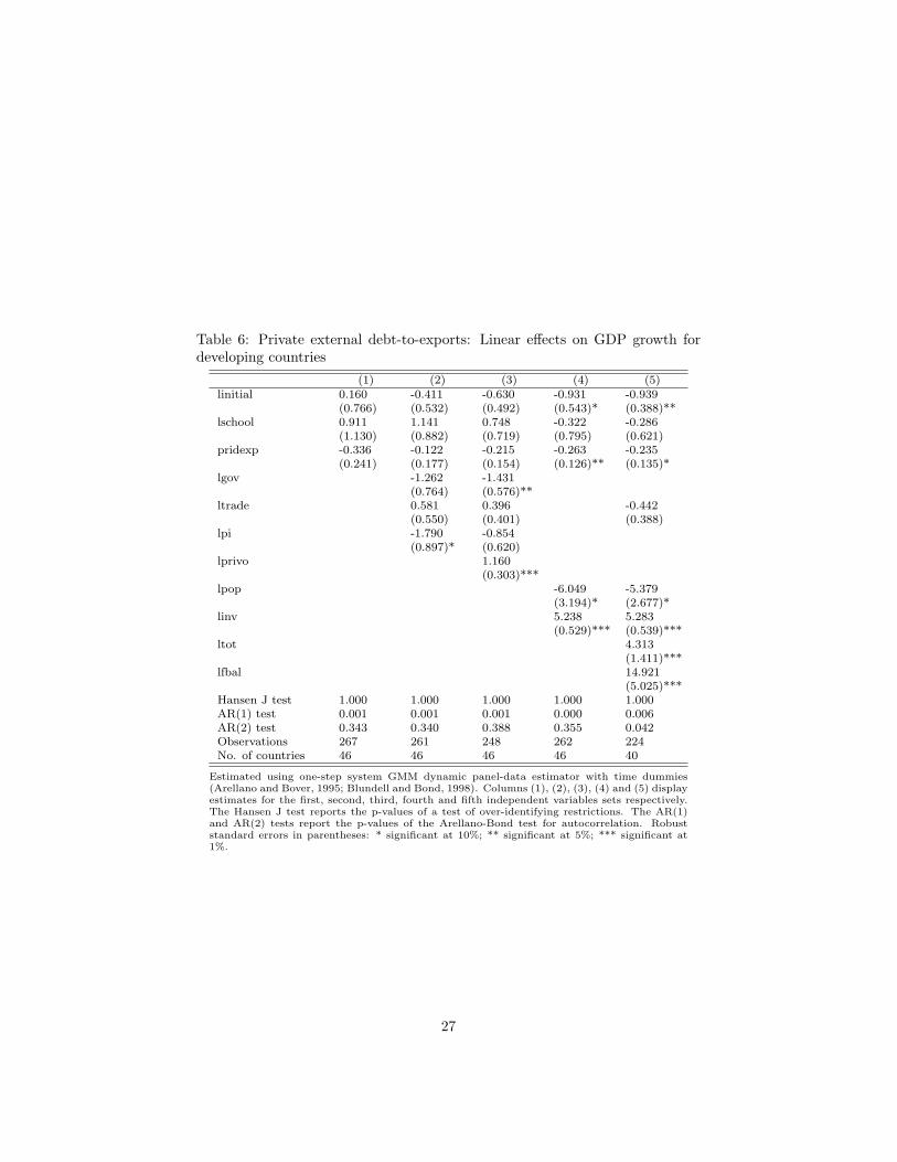
Table 6: Private external debt-to-exports: Linear effects on GDP growth fordeveloping countries

(1) (2) (3) (4) (5)linitial 0.160 -0.411 -0.630 -0.931 -0.939

(0.766) (0.532) (0.492) (0.543)* (0.388)**lschool 0.911 1.141 0.748 -0.322 -0.286

(1.130) (0.882) (0.719) (0.795) (0.621)pridexp -0.336 -0.122 -0.215 -0.263 -0.235

(0.241) (0.177) (0.154) (0.126)** (0.135)*lgov -1.262 -1.431

(0.764) (0.576)**ltrade 0.581 0.396 -0.442

(0.550) (0.401) (0.388)lpi -1.790 -0.854

(0.897)* (0.620)lprivo 1.160

(0.303)***lpop -6.049 -5.379

(3.194)* (2.677)*linv 5.238 5.283

(0.529)*** (0.539)***ltot 4.313

(1.411)***lfbal 14.921



27

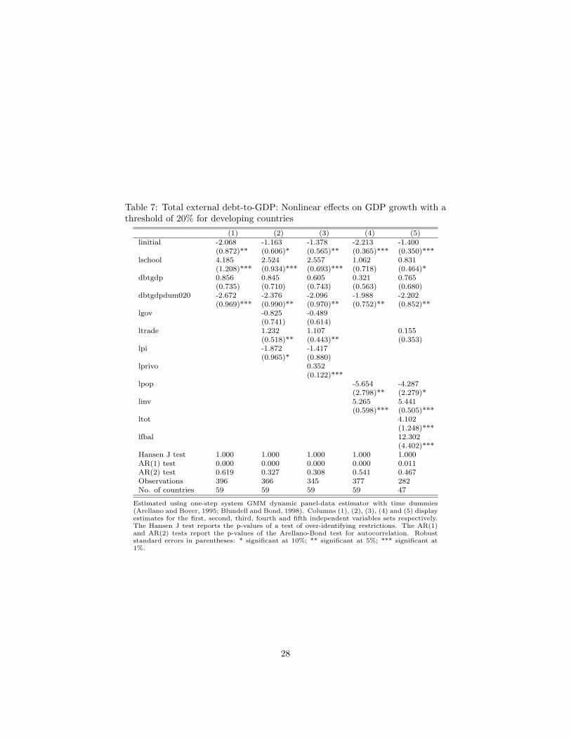
Table 7: Total external debt-to-GDP: Nonlinear effects on GDP growth with athreshold of 20% for developing countries

(1) (2) (3) (4) (5)linitial -2.068 -1.163 -1.378 -2.213 -1.400

(0.872)** (0.606)* (0.565)** (0.365)*** (0.350)***lschool 4.185 2.524 2.557 1.062 0.831

(1.208)*** (0.934)*** (0.693)*** (0.718) (0.464)*dbtgdp 0.856 0.845 0.605 0.321 0.765

(0.735) (0.710) (0.743) (0.563) (0.680)dbtgdpdum020 -2.672 -2.376 -2.096 -1.988 -2.202

(0.969)*** (0.990)** (0.970)** (0.752)** (0.852)**lgov -0.825 -0.489

(0.741) (0.614)ltrade 1.232 1.107 0.155

(0.518)** (0.443)** (0.353)lpi -1.872 -1.417

(0.965)* (0.880)lprivo 0.352

(0.122)***lpop -5.654 -4.287

(2.798)** (2.279)*linv 5.265 5.441

(0.598)*** (0.505)***ltot 4.102

(1.248)***lfbal 12.302



28

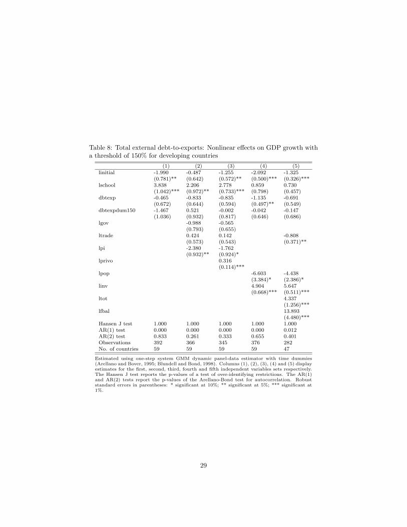
Table 8: Total external debt-to-exports: Nonlinear effects on GDP growth witha threshold of 150% for developing countries

(1) (2) (3) (4) (5)linitial -1.990 -0.487 -1.255 -2.092 -1.325

(0.781)** (0.642) (0.572)** (0.500)*** (0.326)***lschool 3.838 2.206 2.778 0.859 0.730

(1.042)*** (0.972)** (0.733)*** (0.798) (0.457)dbtexp -0.465 -0.833 -0.835 -1.135 -0.691

(0.672) (0.644) (0.594) (0.497)** (0.549)dbtexpdum150 -1.467 0.521 -0.002 -0.042 -0.147

(1.036) (0.932) (0.817) (0.646) (0.686)lgov -0.988 -0.565

(0.793) (0.655)ltrade 0.424 0.142 -0.808

(0.573) (0.543) (0.371)**lpi -2.380 -1.762

(0.932)** (0.924)*lprivo 0.316

(0.114)***lpop -6.603 -4.438

(3.384)* (2.386)*linv 4.904 5.647

(0.668)*** (0.511)***ltot 4.337

(1.256)***lfbal 13.893



29

Table 9: Total external debt-to-GDP: Nonlinear effects on GDP growth with athreshold of 30% for developing countries

(1) (2) (3) (4) (5)linitial -1.836 -0.866 -1.355 -2.179 -1.411

(0.845)** (0.600) (0.545)** (0.383)*** (0.362)***lschool 3.914 2.219 2.601 1.049 0.898

(1.051)*** (0.976)** (0.637)*** (0.757) (0.464)*dbtgdp -0.241 -0.219 -0.289 -0.401 0.136

(0.686) (0.672) (0.651) (0.497) (0.517)dbtgdpdum030 -1.381 -1.145 -1.207 -1.258 -1.653

(0.922) (0.980) (0.954) (0.744)* (0.782)**lgov -0.794 -0.518

(0.714) (0.610)ltrade 1.232 1.183 0.099

(0.473)** (0.467)** (0.348)lpi -1.920 -1.380

(0.931)** (0.899)lprivo 0.362

(0.129)***lpop -5.689 -4.239

(2.863)* (2.283)*linv 5.295 5.493

(0.571)*** (0.508)***ltot 4.128

(1.267)***lfbal 12.348



30

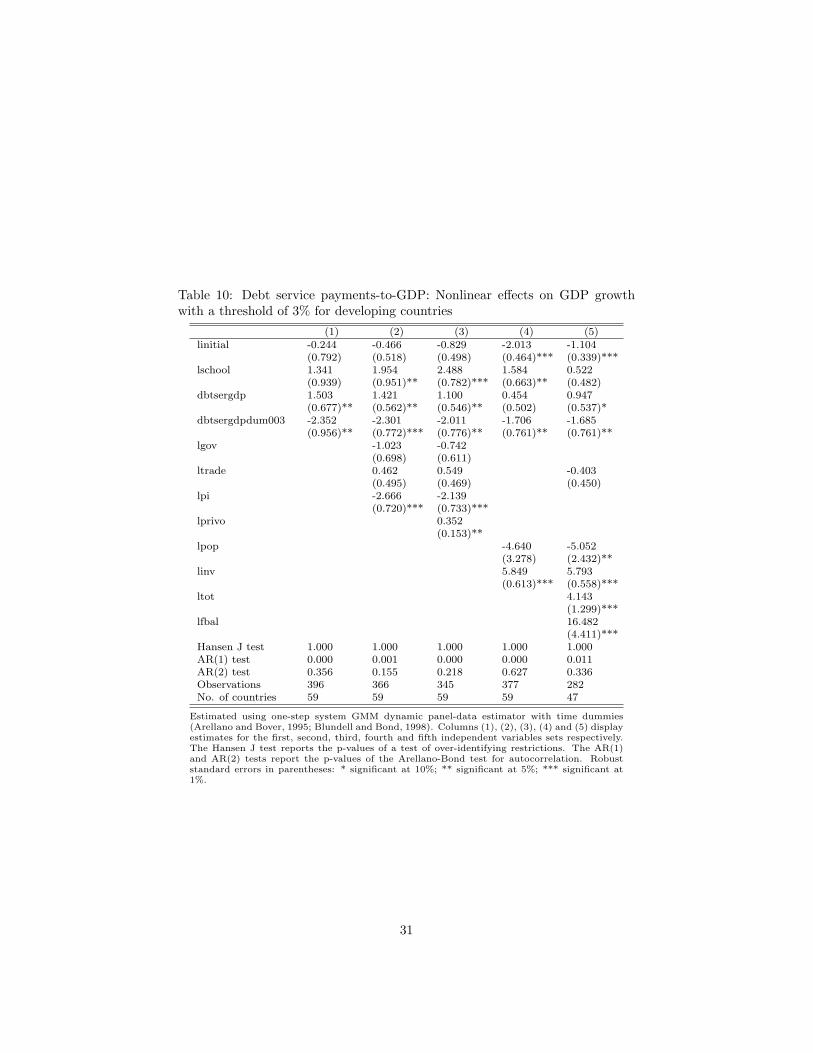
Table 10: Debt service payments-to-GDP: Nonlinear effects on GDP growthwith a threshold of 3% for developing countries

(1) (2) (3) (4) (5)linitial -0.244 -0.466 -0.829 -2.013 -1.104

(0.792) (0.518) (0.498) (0.464)*** (0.339)***lschool 1.341 1.954 2.488 1.584 0.522

(0.939) (0.951)** (0.782)*** (0.663)** (0.482)dbtsergdp 1.503 1.421 1.100 0.454 0.947

(0.677)** (0.562)** (0.546)** (0.502) (0.537)*dbtsergdpdum003 -2.352 -2.301 -2.011 -1.706 -1.685

(0.956)** (0.772)*** (0.776)** (0.761)** (0.761)**lgov -1.023 -0.742

(0.698) (0.611)ltrade 0.462 0.549 -0.403

(0.495) (0.469) (0.450)lpi -2.666 -2.139

(0.720)*** (0.733)***lprivo 0.352

(0.153)**lpop -4.640 -5.052

(3.278) (2.432)**linv 5.849 5.793

(0.613)*** (0.558)***ltot 4.143

(1.299)***lfbal 16.482



31

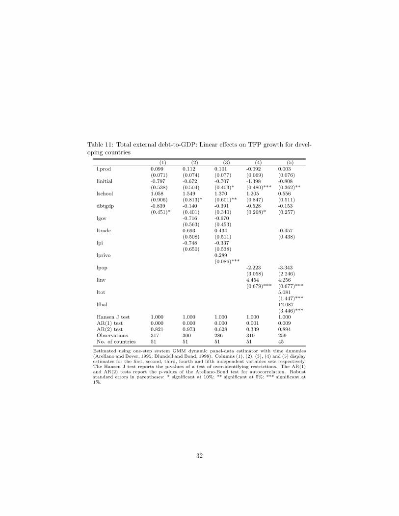
Table 11: Total external debt-to-GDP: Linear effects on TFP growth for devel-oping countries

(1) (2) (3) (4) (5)l.prod 0.099 0.112 0.101 -0.092 0.003

(0.071) (0.074) (0.077) (0.069) (0.076)linitial -0.797 -0.672 -0.707 -1.398 -0.808

(0.538) (0.504) (0.403)* (0.480)*** (0.362)**lschool 1.058 1.549 1.370 1.205 0.556

(0.906) (0.813)* (0.601)** (0.847) (0.511)dbtgdp -0.839 -0.140 -0.391 -0.528 -0.153

(0.451)* (0.401) (0.340) (0.268)* (0.257)lgov -0.716 -0.670

(0.563) (0.453)ltrade 0.693 0.434 -0.457

(0.508) (0.511) (0.438)lpi -0.748 -0.337

(0.650) (0.538)lprivo 0.289

(0.086)***lpop -2.223 -3.343

(3.058) (2.246)linv 4.454 4.256

(0.679)*** (0.677)***ltot 5.081

(1.447)***lfbal 12.087



32

Table 12: Total external debt-to-GDP: Linear effects on capital growth fordeveloping countries

(1) (2) (3) (4) (5)l.capgrowth 0.632 0.599 0.614 0.574 0.640

(0.062)*** (0.063)*** (0.061)*** (0.056)*** (0.051)***linitial -1.277 -0.817 -0.781 -1.368 -1.149

(0.586)** (0.370)** (0.353)** (0.359)*** (0.276)***lschool 1.621 0.594 0.970 -0.080 0.141

(1.119) (0.690) (0.569)* (0.789) (0.462)dbtgdp -1.000 -0.980 -0.961 -0.672 -0.691

(0.371)*** (0.364)*** (0.330)*** (0.341)* (0.333)**lgov -1.181 -1.177

(0.509)** (0.493)**ltrade 1.034 1.195 0.838

(0.377)*** (0.345)*** (0.328)**lpi -0.328 -0.305

(0.389) (0.366)lprivo -0.013

(0.052)lpop -6.935 -5.770

(2.554)*** (2.100)***linv 2.991 2.194

(0.688)*** (0.601)***ltot 3.578

(2.313)lfbal 6.571

(4.259)Hansen J test 1.000 1.000 1.000 1.000 1.000AR(1) test 0.008 0.016 0.025 0.013 0.015AR(2) test 0.306 0.466 0.515 0.320 0.609Observations 321 302 288 314 261No. of countries 51 51 51 51 45


33

Table 13: Public external debt-to-GDP: Linear effects on capital growth fordeveloping countries

(1) (2) (3) (4) (5)l.capgrowth 0.611 0.614 0.640 0.573 0.639

(0.066)*** (0.058)*** (0.056)*** (0.054)*** (0.050)***linitial -1.460 -0.807 -0.762 -1.440 -1.206

(0.620)** (0.378)** (0.371)** (0.350)*** (0.278)***lschool 1.773 0.490 0.684 -0.152 -0.002

(1.165) (0.667) (0.591) (0.764) (0.479)pubdgdp -1.110 -0.839 -0.798 -0.699 -0.620

(0.358)*** (0.310)*** (0.279)*** (0.295)** (0.284)**lgov -1.239 -1.167

(0.501)** (0.489)**ltrade 1.009 1.127 0.801

(0.323)*** (0.333)*** (0.328)**lpi -0.283 -0.302

(0.354) (0.335)lprivo -0.032

(0.050)lpop -7.226 -5.921

(2.641)*** (2.087)***linv 2.920 2.202

(0.662)*** (0.590)***ltot 3.954

(2.343)*lfbal 6.390



34

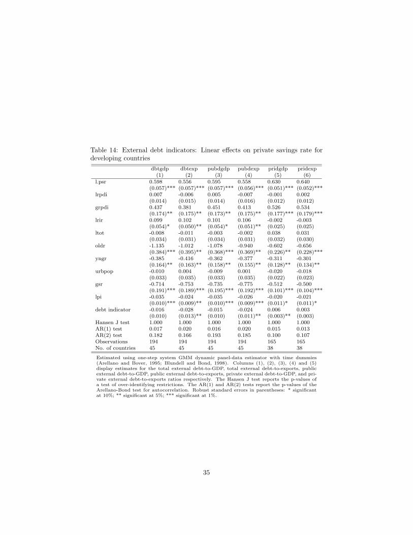
Table 14: External debt indicators: Linear effects on private savings rate fordeveloping countries

dbtgdp dbtexp pubdgdp pubdexp pridgdp pridexp(1) (2) (3) (4) (5) (6)

l.psr 0.598 0.556 0.595 0.558 0.630 0.640(0.057)*** (0.057)*** (0.057)*** (0.056)*** (0.051)*** (0.052)***

lrpdi 0.007 -0.006 0.005 -0.007 -0.001 0.002(0.014) (0.015) (0.014) (0.016) (0.012) (0.012)

grpdi 0.437 0.381 0.451 0.413 0.526 0.534(0.174)** (0.175)** (0.173)** (0.175)** (0.177)*** (0.179)***

lrir 0.099 0.102 0.101 0.106 -0.002 -0.003(0.054)* (0.050)** (0.054)* (0.051)** (0.025) (0.025)

ltot -0.008 -0.011 -0.003 -0.002 0.038 0.031(0.034) (0.031) (0.034) (0.031) (0.032) (0.030)

oldr -1.135 -1.012 -1.078 -0.940 -0.602 -0.656(0.384)*** (0.395)** (0.368)*** (0.369)** (0.226)** (0.228)***

yngr -0.385 -0.416 -0.362 -0.377 -0.311 -0.301(0.164)** (0.163)** (0.158)** (0.155)** (0.128)** (0.134)**

urbpop -0.010 0.004 -0.009 0.001 -0.020 -0.018(0.033) (0.035) (0.033) (0.035) (0.022) (0.023)

gsr -0.714 -0.753 -0.735 -0.775 -0.512 -0.500(0.191)*** (0.189)*** (0.195)*** (0.192)*** (0.101)*** (0.104)***

lpi -0.035 -0.024 -0.035 -0.026 -0.020 -0.021(0.010)*** (0.009)** (0.010)*** (0.009)*** (0.011)* (0.011)*

debt indicator -0.016 -0.028 -0.015 -0.024 0.006 0.003(0.010) (0.013)** (0.010) (0.011)** (0.003)** (0.003)

Hansen J test 1.000 1.000 1.000 1.000 1.000 1.000AR(1) test 0.017 0.020 0.016 0.020 0.015 0.013AR(2) test 0.182 0.166 0.193 0.185 0.100 0.107Observations 194 194 194 194 165 165No. of countries 45 45 45 45 38 38

Estimated using one-step system GMM dynamic panel-data estimator with time dummies(Arellano and Bover, 1995; Blundell and Bond, 1998). Columns (1), (2), (3), (4) and (5)display estimates for the total external debt-to-GDP, total external debt-to-exports, publicexternal debt-to-GDP, public external debt-to-exports, private external debt-to-GDP, and pri-vate external debt-to-exports ratios respectively. The Hansen J test reports the p-values ofa test of over-identifying restrictions. The AR(1) and AR(2) tests report the p-values of theArellano-Bond test for autocorrelation. Robust standard errors in parentheses: * significantat 10%; ** significant at 5%; *** significant at 1%.

35

Table 15: Gross government debt-to-GDP: Linear effects on GDP growth forindustrial countries

(1) (2) (3) (4) (5)linitial -3.598 -3.276 -3.244 -3.327 -2.714

(0.410)*** (0.614)*** (0.641)*** (0.336)*** (0.345)***lschool 1.121 0.237 0.144 1.703 0.557

(0.637)* (0.595) (0.598) (0.796)** (0.909)opubdgdp -0.316 -0.107 -0.116 -0.062 0.355

(0.211) (0.126) (0.124) (0.158) (0.102)***lgov -1.019 -1.038

(0.932) (0.964)ltrade 0.303 0.277 0.106

(0.367) (0.367) (0.398)lpi -16.706 -15.903

(4.071)*** (4.308)***lprivo 0.051

(0.142)lpop -2.718 -2.748

(1.726) (1.811)linv 1.672 2.019

(0.617)** (0.693)***ltot 1.989

(0.723)**lfbal 11.427

(4.249)**Hansen J test 1.000 1.000 1.000 1.000 1.000AR(1) test 0.022 0.006 0.008 0.025 0.025AR(2) test 0.757 0.897 0.991 0.502 0.513Observations 153 153 150 153 140No. of countries 22 22 22 22 22


36

Table 16: Gross government debt-to-GDP: Linear effects on TFP growth forindustrial countries

(1) (2) (3) (4) (5)l.prod 0.000 -0.006 0.149 -0.001 -0.002

(0.007) (0.006) (0.154) (0.009) (0.008)linitial -1.784 -1.805 -1.629 -1.752 -1.100

(0.316)*** (0.618)*** (0.549)*** (0.304)*** (0.365)***lschool 0.601 0.116 0.213 0.651 -0.408

(0.656) (0.666) (0.627) (0.816) (0.911)opubdgdp 0.054 0.120 0.138 0.090 0.422

(0.143) (0.154) (0.156) (0.159) (0.133)***lgov -0.724 -0.717

(0.915) (0.745)ltrade 0.254 0.250 0.173

(0.434) (0.377) (0.392)lpi -11.337 -12.677

(3.983)*** (3.506)***lprivo -0.216

(0.224)lpop 0.020 0.085

(1.590) (1.907)linv 0.355 0.646

(0.856) (0.747)ltot 2.355

(0.804)***lfbal 8.906

(3.692)**Hansen J test 1.000 1.000 1.000 1.000 1.000AR(1) test 0.018 0.008 0.003 0.019 0.024AR(2) test 0.502 0.684 0.327 0.475 0.482Observations 143 143 141 143 130No. of countries 22 22 22 22 22


37

Table 17: Gross government debt-to-GDP: Linear effects on capital growth forindustrial countries

(1) (2) (3) (4) (5)l.capgrowth -0.024 -0.023 0.611 -0.021 -0.021

(0.002)*** (0.002)*** (0.077)*** (0.002)*** (0.002)***linitial -5.176 -4.924 -1.831 -4.944 -4.872

(0.886)*** (0.829)*** (0.743)** (0.856)*** (0.738)***lschool 2.514 1.792 1.212 3.588 3.335

(1.717) (1.743) (0.470)** (1.740)* (2.042)opubdgdp -0.669 -0.489 -0.026 -0.220 0.042

(0.264)** (0.250)* (0.116) (0.256) (0.236)lgov -1.869 -0.384

(0.946)* (0.305)ltrade 0.235 0.069 0.064

(0.481) (0.124) (0.483)lpi -16.561 -3.093

(4.768)*** (3.198)lprivo 0.109

(0.141)lpop -2.098 -2.300

(1.817) (1.777)linv 4.612 4.573

(1.425)*** (1.689)**ltot -1.893

(1.603)lfbal 8.169



38

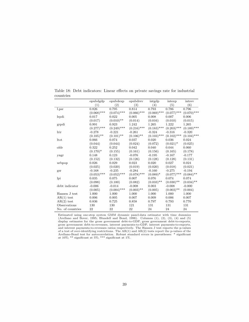
Table 18: Debt indicators: Linear effects on private savings rate for industrialcountries

opubdgdp opubdexp opubdrev intgdp intexp intrev(1) (2) (3) (4) (5) (6)

l.psr 0.826 0.795 0.814 0.793 0.786 0.796(0.068)*** (0.074)*** (0.066)*** (0.069)*** (0.077)*** (0.070)***

lrpdi 0.017 0.022 0.005 0.008 0.007 0.006(0.017) (0.010)** (0.014) (0.016) (0.010) (0.015)

grpdi 0.991 0.923 1.242 1.265 1.222 1.265(0.277)*** (0.249)*** (0.216)*** (0.183)*** (0.203)*** (0.189)***

lrir -0.278 -0.221 -0.261 -0.324 -0.316 -0.320(0.105)** (0.101)** (0.106)** (0.103)*** (0.102)*** (0.104)***

ltot 0.066 0.074 0.037 0.020 0.036 0.024(0.044) (0.044) (0.024) (0.072) (0.021)* (0.025)

oldr 0.322 0.252 0.042 0.040 0.044 0.060(0.170)* (0.155) (0.161) (0.156) (0.165) (0.178)

yngr 0.148 0.123 -0.076 -0.195 -0.167 -0.177(0.152) (0.132) (0.126) (0.128) (0.128) (0.131)

urbpop 0.026 0.029 0.023 0.020 0.027 0.024(0.025) (0.020) (0.019) (0.020) (0.018) (0.021)

gsr -0.168 -0.235 -0.284 -0.160 -0.275 -0.194(0.053)*** (0.052)*** (0.078)*** (0.089)* (0.077)*** (0.084)**

lpi 0.035 0.075 0.007 0.076 0.074 0.074(0.098) (0.100) (0.082) (0.033)** (0.030)** (0.034)**

debt indicator -0.006 -0.014 -0.008 0.003 -0.008 -0.000(0.005) (0.004)*** (0.003)** (0.005) (0.003)** (0.004)

Hansen J test 1.000 1.000 1.000 1.000 1.000 1.000AR(1) test 0.006 0.005 0.007 0.009 0.006 0.007AR(2) test 0.836 0.725 0.858 0.797 0.793 0.770Observations 130 130 121 131 131 131No. of countries 22 22 22 24 24 24

Estimated using one-step system GMM dynamic panel-data estimator with time dummies(Arellano and Bover, 1995; Blundell and Bond, 1998). Columns (1), (2), (3), (4) and (5)display estimates for the gross government debt-to-GDP, gross government debt-to-exports,gross government debt-to-revenues, interest payments-to-GDP, interest payments-to-exports,and interest payments-to-revenues ratios respectively. The Hansen J test reports the p-valuesof a test of over-identifying restrictions. The AR(1) and AR(2) tests report the p-values of theArellano-Bond test for autocorrelation. Robust standard errors in parentheses: * significantat 10%; ** significant at 5%; *** significant at 1%.

39

Documents

Debt and Economic Growth in Developing and Industrial ... · Debt and Economic Growth in Developing and Industrial Countries∗ Alfredo Schclarek† This draft: December 15, 2004