Debt and the Consumption Response to

Household Income Shocks

Scott R. BakerEconomics Department

Stanford University∗

April 2014

Abstract

This paper exploits a detailed new dataset with comprehensive panel financial information onmillions of American households to investigate the interaction between household balance sheets,income, and consumption during the Great Recession. In particular, I test whether consumptionamong households with higher levels of debt is more sensitive to a given change in income. Imatch households to their employers and use shocks to these employers to derive persistent andunanticipated changes in household income. I find that highly-indebted households are moresensitive to these income fluctuations and that a one standard deviation increase in debt-to-assetratios increases the elasticity of consumption by approximately 25%. I employ household savingsand credit availability data to show that these results are driven largely by borrowing and liquidityconstraints. These estimates suggest that the drop in consumption during the 2007-2009 recessionwas approximately 20% greater than what would have been seen with the household balance sheetpositions in 1983.

∗Thanks to Nicholas Bloom, Caroline Hoxby, Luigi Pistaferri, Ran Abramitzky, Steven Davis, Bob Hall, Pablo Kurlat,John Taylor, Itay Saporta, Andrey Fradkin, Pete Troyan, Siddharth Kothari, and Frederic Panier for their invaluableadvice and support. Thanks also to numerous seminar participants at Stanford and the American Economic Associationmeetings for their helpful comments and suggestions. This research was supported by the Bradley Research Fellowshipthrough the Stanford Institute for Economic Policy Research. The author was a paid part-time employee of the firmowning the data utilized for this paper but was not paid for work related to the paper and the paper was not subject toreview by the firm prior to release.

1

1 Introduction

The Great Recession of 2007-2009 featured a historically large buildup in consumer debt (see Figure

1) preceding a dramatic decline in consumer spending. The possibility that higher levels of household

debt induce deeper or longer recessions has important implications for both financial and mortgage

regulation as well as for modeling the business cycle. More broadly, a better understanding of the

dynamic relationship between a household’s spending decisions, income process, and balance sheet, is

imperative to accurately describing microeconomic drivers of business cycles. Despite the importance

of understanding the nature of the relationship between household balance sheets and consumption

behavior, the case for a causal relationship between the two has been difficult to build due to endogeneity

concerns as well as limited data covering the entirety of household finances.

The fact that recessions in the United States have often been preceded by debt buildups has led

to a wide range of research investigating the relationship between household debt and the business

cycle.1 A growing body of research has identified household balance sheets as important channels

through which financial shocks to households can be amplified, with higher debt-to-asset ratios leading

to higher implied elasticities of consumption with respect to wealth. Supporting evidence for this view

can be seen in periods as diverse as recessions in the United States such as the 1990-1991 recession, the

Great Recession, as well as the ‘Lost Decade’ in Japan.2 In addition, theoretical work has described the

pathways through which household debt could influence consumption elasticities, often by appealing to

liquidity constraints or borrowing limits.3

However, many of the most commonly utilized incomplete-markets models take a simplified view of

household balance sheets, with only a single savings instrument that abstracts from simultaneous asset

and debt holdings. For instance, while a standard Bewley model predicts a decline in the elasticity of

consumption with respect to income for households with higher wealth, it fails to predict any consequence

of gross debt buildups or increases in debt to asset ratios conditional on net asset holdings.

This paper analyzes this relationship with new data covering a large number of American households

and their employers over 5 years, from 2008-2012. An important consideration when analyzing income

and consumption interactions is the fact that changes in labor market income are often endogenous,

with individuals and households adjusting labor market participation at both the extensive and intensive

margins in response to anticipated events. To address this endogeneity, I turn to a common source of

1For example, see work by Glick and Lansing (2009), Isaksen et al (2011), the IMF (2012), Igan et al (2012), andChmelar (2012)

2Mishkin (1977, 1978) describes both the Great Depression as well as the 1973 recession through the lens of consumerbalance sheet movements. Others, including Mian and Sufi (2010, 2011, 2013), Dynan (2012), King (1994), Leamer (2007),Koo (2011), and Olney (1999) examine the path of consumption during recessions and find links to debt accumulation.Carroll and Dunn (1997) view the 1990-1991 recession as a consequence of the debt buildup of the 1980s as well as suddenworsening of unemployment rate expectations which ignited household desires for paring down debt levels. See Petev, etal (2011), French, et al (2013) and Figure B1 for discussions of the dramatic drop in income growth expectations since theGreat Recession in the United States.

3Eggertsson and Krugman (2011) are among those to give theoretical evidence for debt-driven recessions where someagents are forced to deleverage, due to revisions in how much debt it is safe for agents to hold, thereby decreasing aggregatedemand in conjunction with nominal rigidities like the zero lower bound. Guerrieri and Lorenzoni (2011), Hall (2011),and Midrigan and Philippon (2011) develop models speaking to household debt as a cause of painful recessions. As analternative explanation, Alan, Crossley and Low (2012) find that a deleveraging and increase in the savings rate is drivenby an increase in income uncertainty, modeled as an upward shift in the variance of permanent income shocks.

2

labor market income variation, firms that employ members of the household (hereafter referred to as

‘employers’). Given the importance of wage income and bonuses to household income, both positive and

negative shocks to employers can drive persistent and nontrivial changes in total household income. I

argue that these shocks are exogenous to any given employee and that the high-frequency nature of the

data allows for explicitly testing, and supporting, the assumption that these shocks are unanticipated

by the household.

In particular, I use this detailed household financial data to provide empirical evidence that both

confirms and expands standard incomplete-markets frameworks. Looking at changes in monthly house-

hold income and consumption, I test whether consumption among households with higher levels of debt

is more sensitive to a given change in income. I find substantial heterogeneity in the consumption

response to income shocks across households and that this heterogeneity is systematically and causally

linked to balance sheet positions.

In total, this paper makes three primary contributions. First, I develop a panel dataset featur-

ing comprehensive and high-frequency financial data from over 150,000 households and match these

households to their employers. I find that ‘firm shocks’ such as large and surprising earnings reports,

layoff announcements, mergers, acquisitions, or write-offs significantly impact household income. As

with other literature studying long term effects of labor market shocks, I present evidence that suggests

these changes in household income are persistent.4 I find less than full support for the strong per-

manent income hypothesis, though estimates in this paper are largely short- to medium-term and thus

may understate eventual consumption adjustments.5

Second, I find that the elasticity of consumption with respect to income is significantly higher

in households with high levels of debt. This heterogeneity persists after conditioning on household

demographics or other household financial characteristics. In addition, significant effects are maintained

when instrumenting for levels of debt, suggesting that the relationship between debt and consumption

elasticities are not driven by unobservable household preferences.

Third, I show that differential household consumption elasticities with respect to income among

households with varying levels of debt and debt-to-asset ratios can be explained primarily by borrowing

and liquidity constraints. I find that as access to liquid assets and consumer credit increases, hetero-

geneity in debt ratios has a much smaller impact on consumption elasticities. This result is consistent

with numerous studies of constrained consumers that exhibit convex elasticities of consumption when

approaching borrowing limits.6 The strong relationship between household balance sheet positions and

4Davis and Von Wachter (2011) and Jacobson, LaLonde, Sullivan (1993) note that job displacement episodes havesizable and persistent effects on earnings, even when quickly transitioning to new firms. Oreopolous, Von Wachter, andHeisz (2008) find that new labor force entrants experience persistently lower wages when first entering the labor marketduring a recession. Roys (2011) estimates a structural model of the firm in which negative firm shocks can drive persistentdeclines in wages.

5Hall and Mishkin (1982) and Agarwal et al. (2007) find that consumers respond too greatly to temporary income shocksto be consistent with the theory. Wilcox (1989) finds increases in consumption when income increases are implemented,not when they are announced, contradicting the income-smoothing predictions of the model. In contrast, Wolpin (1982)and Souleles (2000), among others, find consumption responses and smoothing behavior entirely consistent with the theory.Aguiar and Hearst (2005) carefully document time use following retirement, highlighting the distinction between householdconsumption and household expenditures.

6For one such recent study, Bishop and Park (2010) demonstrate that marginal propensities to consume drop steeplyfollowing a relaxation in binding borrowing constraints. Zeldes (1989), Johnson et al (2006), and Blundell, Pistaferri,

3

consumption behavior stresses the importance of more nuanced models including aspects such as en-

dogenous and heterogeneous borrowing constraints or simultaneous asset and debt holdings. Moreover,

I find that consumption elasticities are more sensitive to liquid wealth and debt levels than to illiq-

uid wealth such as housing assets. This finding implies that simultaneous increases in mortgage debt

and housing wealth, as seen during the mid-2000s, may have driven increased household consumption

elasticities during the Great Recession.7

While I find that much of this variation is driven by borrowing and credit constraints, other channels

may also play roles in influencing the relationship between household balance sheets and consumption

behavior. One possibility is that household utility functions may be directly impacted by levels of debt.

If households are averse to holding large amounts of debt relative to their income, a decline in income

will prompt larger declines in consumption among highly indebted households in order to restore the

desired debt-to-income ratio for a wide range of loss functions.

Overall, this paper’s findings suggest that changes in household balance sheets, such as increases in

gross debt or debt-to-asset ratios, have been important drivers of household behavior during the Great

Recession and the subsequent recovery. Importantly, I provide evidence that the buildup in household

debt in the years leading up to the recession increased sensitivity to declines in household income. These

results point to the possibility of deeper recessions and increased macroeconomic volatility in countries

with higher levels of household debt, especially when the assets purchased with debt are illiquid in

nature.

The remainder of the paper is organized as follows: Section 2 describes the various data utilized in

the empirical analysis. Section 3 details a number of exercises undertaken to validate various components

of the data and Section 4 discusses a basic theoretical framework. Section 5 presents empirical results

while Section 6 discusses a back of the envelope calculation of the aggregate effects of leverage during

the Great Recession. Section 7 concludes.

2 Data

2.1 Household Financial Data

The household financial data used in this paper comes from a large online personal finance website. The

site provides a service that connects users’ financial accounts so that user can see all of their accounts

in a single location. The site allows for users to easily see summaries of their income, spending, debt,

and investments across all of their accounts and has other features such as budgeting or financial goal-

setting. The site has grown rapidly, from under 300,000 users in 2007 to more than 3 million active

users by 2012. This large userbase has yielded a database of more than 5 billion transactions across

over 10 million individual accounts. These accounts span all manner of household financial products

and Preston (2008) all find higher levels of consumption sensitivity to income fluctuations among poorer and more creditconstrained households. While a minority of papers, such as Shea (1995), find differently, the overall literature stronglysupports the impact of credit constraints on the ability for households to smooth consumption across changes in income.

7Kaplan and Violante (2012) develop a model which allows for simultaneous holdings of debt and assets with theintroduction of a high-return housing asset with transaction costs. They use this model to explain why even wealthyhouseholds with substantial net assets may behave as though borrowing-constrained.

4

including checking accounts, savings accounts, credit cards, loans, property and mortgage accounts,

equity portfolios, and retirement accounts.

The basic data elements are individual bank and credit card transactions that are automatically

recorded through links to users’ banks and credit providers. Each transaction is time-stamped and has

information about the other party, whether it was a credit or debit, and contains a full description of the

transaction as you would see on your monthly bank or credit card statement. From this merchant and

descriptive data, the site automatically categorizes each transaction into one of over 100 categories (such

as ‘Groceries’, ‘Gasoline’, ‘Student Loans’, ‘Fast Food’, or ‘Pet Stores’) in order to provide easily readable

spending and income breakdowns to the user. From these data, I derive measures of total household

spending and income as well as subsets of income and spending based on the categorization of the

transactions. This categorized spending and income data provides an invaluable source of information

regarding each individual user’s financial means and behavior.

In addition to transactional data from bank and credit card accounts, the site automatically archives

daily balance data for equity, retirement, property, real estate, and loan accounts. The loan and property

data, in particular, form the basis of important components of analysis in this paper. Loan data consists

primarily of car loans and home mortgages, while property accounts denote the value of home prices

over time for each homeowner. I use this data to determine gross and net housing wealth at a household-

month level. Often accompanying this balance data is information on interest rates, types of accounts

(such as IRA or 401k), and the bank or firm providing the account.

One major advantage of this data source over other sources, such as government survey data like the

Current Population Survey or the Consumer Expenditures Survey, is that the data are obtained directly,

automatically, and continuously from the households’ financial institutions. This greatly minimizes

measurement error and biases in recollection about both financial flows as well as stocks (in terms of

both errors in amounts and errors in timing of consumption or income) that are endemic to survey data.

A second advantage is that it provides comprehensive income and spending data for all households in

the sample, avoiding potential external validity problems when compared to other datasets that solely

include information on, for example, household spending on food. Such narrower datasets may result

in biased estimates when households of different characteristics (e.g. income level) may systematically

differ in the proportion of their budgets that are spent on food, certain types of durables, or other

particular categories of spending. For both of these reasons, this data provides a more comprehensive

and unbiased source of household financial data than other previously used sources.

In addition, household data allows for a much wider range of financial situations relative to geo-

graphically aggregated data. For instance, across counties in 2006, average debt-to-income ratios ranged

from approximately 1 to 3 and average mortgage-to-house value ratios ranged from about 0.30 to 0.95.

In contrast, individual households naturally spanned a wider range of balance sheet positions, with

debt-to-income ratios of 0 and in excess of 15. Similarly, mortgage-to-home value ratios ranged from 0

to over 2, with many households underwater on their homes. Allowing for the consideration of these

more extreme balance sheet positions is crucial for accurately characterizing the microeconomic drivers

of the 2007-2009 recession.

An important consideration when dealing with this data is to control for the number and type of

5

linked accounts for a given user over time. As the site was rapidly expanding in recent with a multitude

of new users who were gradually linking financial accounts, looking at simply the per-user spending

patterns could potentially give a distorted view. If an individual had two credit cards and had only

linked a single one, when they add the second card the site would register a large increase in spending

whereas there was not truly a real spending increase. To combat this bias, I employ three cleaning and

robustness strategies. First, I exclude data from a user’s first 3 months using the site, as this period is

typically when most of the adding of accounts takes place. Second, I exclude users with highly volatile

numbers of accounts or insufficient numbers of accounts (require ≥ 3 accounts), as it seems likely that

there is unobserved actions being taken here that I cannot control for adequately. In addition, I also

perform robustness tests for most specifications where I utilize spending or income per account instead

of total spending or income across accounts as an alternate measure. I find results that are qualitatively

unchanged, suggesting that the mitigating steps taken to address this potential bias achieved their aim.

In addition, I test whether demographics or finances affect how often individuals utilize the website.

This could be an issue if certain types of users utilize the site more frequently and thus any changes to

their financial circumstances are made more salient. I find that younger individuals and higher income

individuals are weakly more likely to check the website. However, these effects are not dramatic, with a

one standard deviation in age or income only yielding a 32% and 14% increase in site visits per quarter,

respectively.

In conjunction with the financial data, users provide demographic information such as age, sex,

marital status, and the size of the household. Users also list whether they are a homeowner, their

profession, their level of education, their income level, and their location. Due to the nature of the

website, usage patterns suggest that it covers the entirety of financial transactions for groups who make

joint financial decisions. Thus, I equate a user of this financial website with a head-of-household in

the Current Population Survey (CPS) or a ‘consumption unit’ in the Consumer Expenditure Survey

(CES). For example, a ‘user’ represents the entirety of household spending for married couples but only

represents an individual’s spending for an unmarried individual living with roommates.

Being a software start-up, the demographics of the website were initially very different than those

of the national as a whole. Key user characteristics like gender and age were starkly different than the

national distribution in 2007 (being younger and more male). The divergence from national averages

presents both benefits and problems. Though the unweighted data cannot be directly used to obtain

unbiased estimates that can be extrapolated to the entirety of the US population, I am able to capture

much of the spending by high-income earners that is often missed in other survey-based datasets like

the Consumer Expenditure Survey that under-sample rich households.

While the demographics of the userbase were initially very different, they have become much closer to

a representative national distribution by 2013 as the userbase grew dramatically. Moreover, conditional

on observable household demographic and locational characteristics, financial behavior among the users

seems to track closely to national averages. Validation of the ability to transform the observed financial

data series into a relevant and representative sample of American households using CPS household

weights is covered extensively in Section 3. CPS-weighted and unweighted summary statistics of the

sample population can be found in Table 1 and Table B1.

6

One drawback of the data is that it does not have as complete a coverage of cash or check transactions

relative to credit and debit transactions. Cash transactions can only be fully observed when a user

manually enters them, though inferences about other cash transactions can be made as cash withdrawals

from banks and ATMs can be directly observed. An estimated 6-8% of total spending is done with cash

in the United States, compared to approximately 3-4% of spending done with cash in the sample data.

A larger omission could potentially stem from check transactions, which can be observed but cannot

be automatically categorized. Such transactions make up about 15% of total observed spending among

households in the sample. Through inspection of manually recategorized checks (check transactions

where the user manually changed the category and description of transaction type), I find that check

transactions are primarily driven by large, regular transactions like mortgage payments, rent, and utility

bills. In my desired sample of employees of publicly-listed firms, paychecks make up a very small portion

of these check transactions, as the vast majority of public firms’ employees are paid by direct deposit (see

NACHA 2010 PayitGreen survey), which can be almost perfectly observed with their correct category

coding.

A second drawback is that I cannot observe withdrawals from an individuals’ paycheck prior to

their receiving it. For example, transactions like healthcare premiums, 401k contributions, and FICA

payments are often unobserved (if I do not see the retirement account itself), as I only see the resultant

paycheck that is deposited into a checking account, not the originating payment. Thus, for all households

drawing a paycheck, I generally measure post-tax and post-benefit (401k, healthcare) pay, thereby

estimating based on take-home income rather than total gross pre-tax income.

2.2 Firm Shocks Measurement

One potential measurement issue with looking at changes in household income is that households may

adjust current spending in anticipation of future changes in household income that are unobserved by

the researcher. To ameliorate this issue, I turn to using shocks originating from household employers to

instrument for changes in household income. I largely employ firm shocks rather than firm stock returns

primarily to help minimize the endogeneity and persistence in stock returns at a high-frequency level,

picking out singularly large shocks to the firm. These shocks have sizeable impacts of household income

and, in addition, there is reason to believe that the exclusion restriction holds and that shocks to the firm

impact household spending solely in ways that are captured by household income. While it is possible

that firm performance may influence future career prospects and thus current spending patterns, it

seems likely that brighter career prospects would be accompanied by higher contemporaneous pay.

I utilize three sources to compile data regarding large shocks to firms, a summary of which can be

found in Table 1. The first source data from the SEC’s required 8-K filings for public firms. These filings

are required by firms for a wide range (over 20 types of events) of firm-specific actions such as firm or

plant closures, changes to the board or principle officer, or significant merger and acquisition activity.

These filings were instituted as an effort to increase mandatory disclosure of pertinent information for

shareholders. Moreover, the filings must be promptly released after any such event, with the SEC

requiring release within the four days following the event itself.

For the purposes of this project, I focus on firm layoffs, acquisitions and sales completions, large

7

write-offs, and large earnings report surprises. These shocks share three beneficial characteristics.

First, they are relatively clear in their interpretation and scope. Second, they have sizable firm equity

movements associated with their occurrence and thus are plausible drivers of employee earnings and

earnings expectations. Finally, both investors and employees do not seem to exhibit any foresight

regarding the announcements and subsequent equity movements, with little change in stock prices or

consumption among employees prior to the shock. Timelines of these events are shown in Figure 2.

The second source for firm shocks is the Institutional Brokers’ Estimate System (I/B/E/S) which

enables me to collect data on quarterly earnings report for all publicly listed firms in my sample. From

this data, I construct indicators for particularly surprising positive or negative earnings report, where

a large positive earnings report surprise is:

(EPS−E[EPS])SharePrice > 0.02

and a large negative earnings report surprise is:

(EPS−E[EPS])SharePrice < −0.02

That is, I categorize an earnings report as a ‘large earnings surprise’ when the difference between earnings

per share and expected earnings per share is larger than 2% of the firm’s share price. A graph of large

positive and negative earnings report surprises over time is displayed in Figure 2. A 2% threshold was

used to approximately capture the top and bottom 1% of earnings announcements. Results are robust

to using cutoffs of 1% or 3%.

Finally, I use a news-based strategy of identifying layoffs in order to provide an alternate measure

of firm layoffs that also gives an intensity scale (rather than simply an indicator of layoffs). I compile a

database of firm layoffs through the use of the Access World News Newspaper database. When reporting

on layoffs, newspapers tend to construct titles using a set format; a practice confirmed through manual

inspection of a large number of known layoffs, extended trials of search terms, and through talking to

business journalists. With this in mind, I use this database of over 1,500 US newspapers to search the

archive for article titles that mention each firm’s name, or common shorthand for the firm’s name, as

well as a set of terms indicative of layoffs.8 Thus, this query compiles a set of all articles that have titles

similar to “Wells Fargo to cut 4,000 jobs” or “Alcoa lays off 2,400 workers”.

This search returns approximately 5,000 articles since 2008 covering almost 400 firms. I attempt to

exclude false positive matches by removing matches with fewer than 3 articles about a layoff on a given

day. Furthermore, given the structure of the title of these articles, I am able to extract the number

of individuals laid off during each episode and validate this number by checking the matched number

of layoffs across articles regarding the same firm and day. The final sample covers 113 firms and 246

separate instances of layoffs in the sample period. A sample of these layoffs are reported in Appendix

Table B2.

Table 2 tests for anticipation of these shocks to firms among both employees and investors. Columns

(1) - (4) regress firm returns and a selection of firm shocks on lags of various pieces of observable

8Articles must contain a term from the set (positions, jobs, employees, workers, notices, roles, staff, personnel) as wellas a term from the set (slash, slashes, slashing, lost, losses, layoffs, sheds, axes, cuts, fires, layoff, shed, axe, cut, cutting,axing, shedding, reduce, ”lay off”)

8

household financial information such as income, wealth, and spending. I find no evidence for changes

in income, spending, or wealth among employees in the months leading up to layoffs or large positive

or negative earnings announcements. Column (5) demonstrates the same principle at a firm level, with

stock returns not reacting to shocks in the months before the shock occurs, suggesting no anticipation

of the shocks by investors. This contrasts with a strong response in the stock price seen after the shocks

take place, as seen in column (6). This paper currently limits the effect of the various firm shocks to

shifts in the level (or growth rate) of employee earnings and assumes that this mean effect is thereafter

anticipated by the affected employee. I do not explicitly consider changes in the variance of employee

earnings over time based on these firm shocks.

In addition to being seemingly unanticipated, I find that these shocks to employers exhibit a high

degree of persistence in terms of their effects on household income. Figure 3 plots logged average

household income levels before and after positive and negative shocks to household employers after

removing a time trend. I find persistent effects on household income remain up to 18 months following

both positive and negative shocks.

Because my data is limited to a 5-year period, I cannot reject that the impact of a given firm shock

dissipates gradually over the ensuing years. However, highly persistent effects on income would be

consistent with much prior work finding that shocks to firms, job displacement episodes, and having bad

initial labor force experiences can affect long-term wages.9 In general, household income derived from

employers is highly persistent. When estimating the wage process as a monthly AR1, I find a coefficient

on lagged firm-related income of over 0.96. Total household income is somewhat less persistent, with

an estimated coefficient on lagged total household income of approximately 0.92.10 This estimate is

consistent with other estimates of the household income process which often find AR(1) coefficients in

excess of 0.90.

2.3 Firm Matching, Firm Shock Power, and User Selection

I match users to their employers using textual descriptions from users’ direct deposit transactions. Direct

deposit transaction descriptions are generally characterized by indicators that the transaction is a direct

deposit, a string representing a firm, and anonymized identifiers.11 Using a flexible natural language

processing algorithm, I compare these paycheck descriptions to a seed list of firms to match to. The pool

of firms used is the universe of publicly listed firms in both the NASDAQ and NYSE. For each firm, the

matching algorithm is allowed to ignore things like punctuation such as hyphens, periods, or apostrophes

and allows for abbreviations of the full firm name. In addition, I include a large number of unconventional

abbreviations obtained through manual inspection of the largest 100 firms by revenue as well as the

largest 100 firms by employment in the sample (e.g. ‘TGT’ is an identifier for a direct deposit from

Target). Looking across all users of the website, the set of users able to be matched to their employers

9Davis and Von Wachter (2011) and Jacobson, LaLonde, Sullivan (1993) note that job displacement episodes havesizable and persistent effects on earnings, even when quickly transitioning to new firms. Oreopolous, Von Wachter, andHeisz (2008) find that new labor force entrants experience persistently lower wages when first entering the labor marketduring a recession. Roys (2011) estimates a structural model of the firm in which negative firm shocks can drive persistentdeclines in wages.

10Both estimates remove month fixed effects to control for seasonality.

9

contains 1948 employers employing over 700,000 household members. The set covers employers from all

major sectors, including retail, technology, banking, industrial/manufacturing, media, and professional

services. Many matched firms employ large numbers of users, with several firms employing over 5,000

users each.

I limit my analysis to a sub-sample of users able to be linked to a publicly listed employer for a period

of at least 12 months. Moreover, I exclude users matched to firms that have fewer than 50 observed

users in my data, ensuring at least a moderate level of within-firm variation across individuals and

making it less likely that a firm was matched to a user erroneously through a rare or custom transaction

description.

One method in which I can jointly test whether the firm-employee matching algorithm was accurate

and whether employees react to their employer’s performance can be seen in Appendix Table B3. This

table displays some quantification of the relationship between employer performance and consumer

spending. Here, I match individuals in my sample to their employers during the duration of their tenure

there. In addition, I construct a variable matching them to the same employer for up to 6 months prior

to their working there and up to 6 months afterward if they leave.

For instance, if I observe an individual working for General Electric from July 2010 to September

2012, I match his consumption behavior to the stock returns for General Electric from January 2010

to December 2012, including the 6 months before he began working for General Electric and 3 months

after he left. If employees do respond to their employers’ performance, captured by their stock price, we

would expect to find that household spending responds to stock prices during the period of employment

with the firm, but not before or afterward. Columns (1) and (2) show results of simply regressing

household spending on employer stock returns for the period before, during, and after employment at

a given firm. We find mild positive impacts of stock returns on spending, though insignificant without

financial controls. Columns (3) and (4) give results from a regression of household consumption on

employer returns (inclusive of the 6 months preceding and following being matched to the employer) as

well as an interaction of employer returns with an indicator for whether the individual currently works

at that firm. Here we see that the interaction term’s coefficient is positive and significant while the

uninteracted term is insignificant. This suggests that individuals are reacting to current employer stock

price and that the firm-employee matching algorithm performed reasonably well given that they do not

react to their future employers’ stock price prior to being hired or following a departure.

Moreover, a household’s employer has little predictive power for household debt-to-asset ratios, with

each firm employing a range of employees with widely varying income, wealth, and debt characteristics

(see Figure 4 for distributions within several selected firms). Running a regression of 2008 household

debt-to-asset ratios on household demographic and locational characteristics, as well as employer fixed

effects, I find unadjusted significant effects for only 5 out of more than 200 employers in the sample.

Households may vary in their financial characteristics, even controlling for employer, demographics,

and income, for a variety of reasons. For instance, households may have had varying shocks in the

past, such as medical incidents, large inheritances, or differing marital circumstances. There may exist

11Some examples of such descriptions are: “21ST CENTURY INS DIR DEP”, “SAVINGS DEPOSIT - DIRECT DE-POSIT FROM TGT PAY REG SALARY”, and “GOOGLE, INC DIRECT DEP”

10

heterogeneity among otherwise similar households in the expectations about future financial paths or in

inherent traits such as risk aversion or discount rates. In addition, households may vary in the degree

to which other behavioral factors such as “mental accounting” or “rule of thumb” behavior influences

spending and asset accumulation decisions. Finally, household characteristics do not seem to predict

being employed by a firm that is subject to more or fewer firm-level shocks. Running a probit of firm

shocks on household demographic and locational characteristics, I find no significant effects.

Shocks to a household’s employer have moderately large impacts on subsequent household income.

In Table 3, I test whether firm-driven shocks impact income of various types among employee households.

I consistently find negative effects on household income following negative shocks such as large negative

earnings surprises, layoffs, and material impairments while finding consistent positive effects of large

positive earnings surprises and completions of acquisitions or dispositions. For instance, from column

(2) I find large positive earnings surprises tend to increase overall income by about 0.7-1.1%. Similarly,

large negative earnings surprises decrease spending by about 1.3%, Column (3) shows that non-firm

based income (such as rental income, stock dividends, or paycheck income from a different firm) is

unaffected by shocks to a household’s employer. Columns (4) and (5) show the impact of these firm

shocks on paycheck income as well as bonus income, which displays much higher effects given the more

dramatic volatility inherent in bonuses. Importantly, paycheck income, a more persistent component of

employee compensation, is significantly affected and points to persistent effects on household income.

Column (6) collects the firm shocks into two bins, with large positive earnings surprises and acqui-

sition/disposition completions defined as positive shocks and large negative earnings surprises, layoff

announcements, and material impairments defined as negative shocks. I again find positive effects of

positive shocks on both spending and income and negative effects of negative shocks, with magnitudes

of the order of 0.8%-1.2% increases or declines in income and spending following a shock. Thus, shocks

to employers are strong drivers of changes in paychecks and bonuses in particular and household income

in general. Moreover, the shocks are moderately persistent, with lower levels of income remaining one

year following the various firm shocks.

3 Data Validation

One concern is whether users have linked sufficient accounts to the site to get an accurate picture of

their finances. A random survey of 3,649 site users in 2011 provides some reassurance on this point. It

found that over 95% of users had linked all or almost all of their checking accounts and over 93% of

users had linked all or almost all of their savings accounts. In addition, 91% of users had linked all or

almost all of their credit cards. While these accounts had the highest coverage rate, over 75% of users

had linked all or almost all of their equity accounts. Similarly, over 90% of users who self-identified as

homeowners included information about their home value or mortgage. This evidence points to near-

complete coverage of active users’ accounts that get the most frequent use and attention. Despite this,

we find less complete coverage of more unconventional asset accounts such as retirement accounts, with

only approximately 50% of users linking all or almost all of this type of account. This pattern seems to

derive from the fact that the most common use of the website is for tracking income and expenditures so

11

categories that see the most frequent transactions are those that are most likely to be linked. Moreover,

when asked why they had not linked all of their financial accounts to the site, the most common answer

given was that there was little activity on the accounts or that they felt no need to track those accounts.

This fact reinforces the view that the unlinked accounts most likely do not account for an appreciable

amount of transactions or activity relative to the linked accounts.

While the demographics of the userbase of the site have become more similar to those of the nation

in recent years, a worry about representativeness still exists. To combat this worry, I benchmark the

aggregate data against several known measures of national consumer behavior and use CPS-derived

weights to synthetically approximate the distribution of households in the United States.

First, I compare observed spending among users to monthly data from the Census Retail Sales

numbers. Census Retail Sales data comes from a monthly survey of 3,000 large retailers and over 9,000

small retailers and data are broken down by type of retailer. I match my observed categorical spending

data to the relevant categories and construct average per-user categorical monthly retail spending,

weighting users by CPS weights for age, sex, income, and state of residence. Figure 5 shows results for

a range of categories like gasoline sales, electronics, restaurants, and clothing sales.

It is important to note divergences from the site’s data from some categories of Census Retail

spending. The motor vehicle spending panel of Figure 5 shows data for automobile and motor vehicle

sales, which do not track well between the two sources. This is primarily because my data observes

payments from a consumer’s side, while Census data measures spending from the retailer’s side. For

some categories like motor vehicles, these two aspects diverge as many individuals purchase cars with

loans or other financing and pay them off over time. Thus, I see more gradual changes in motor vehicle

spending as I often observe monthly payments rather than the lump sum purchases of vehicles that

dealerships and retailers record. This phenomenon is also present, though less pronounced, for other

durables categories in which consumer credit or financing is often used.

For non-motor vehicle categories of spending, the average correlation between my observed spending

data and the Census Retail data is 0.86, with this average correlation rising to 0.89 when also excluding

furniture sales which are also commonly bought on credit. A number of categories, such as Gasoline,

Clothing, and Restaurants, have monthly correlations with the Census Retail data well in excess of

0.90. Finally, the data from the site compares well to annualized data from the Consumer Expenditures

Survey, with a correlation of over 0.87 across all overlapping categories of spending and time periods

(2009-2012).

These validation exercises also serve to further alleviate some worries about the completeness of the

accounts. If there were systematic biases for individuals in terms of the accounts that they chose to

link to the site, overall trends in spending and income would be unlikely to so closely match national

trends. The fact that this holds true for so many categories of spending cements this view.

Individuals in the sample, when weighted by observables, also match national distributions of things

like housing wealth. Figure 7 shows in-sample logged average reported home price by year and zip code

compared with the overall logged average home price by year and zip code provided by Zillow.com.

The two have a correlation of greater than 0.88, showing a strong relationship between reported and

observed house prices. While the unweighted sample displays systematically higher house prices and

12

housing wealth than the overall averages, when weighted by observables, the sample corresponds much

more closely to the national distribution. I also test observed distributions of liquid savings and credit

among households in my data against the 2010 Survey of Consumer Finance, finding close matches (see

also Figure 8, debt ratio figures are also comparable to SCF distributions). These results suggest that

not only do weighted spending trends match national distributions, but observed asset and debt levels

are consistent, as well.

As a result of these validation exercises, all regression results in this paper are weighted on (head-of)

household observables such as age, sex, income range, and state of residence according to CPS weights,

yielding results with a high level of external validity when extrapolating to the nation as a whole.12

Weights are recalculated each year in the sample period (2008-2012).

The final sample is restricted in a number of ways to maximize statistical power as well as minimize

measurement error. Users must also have more than 3 linked financial accounts (e.g. savings, credit

card, or loan accounts) and have filled out demographic information about age, sex, marital status, and

location in order to ensure they are active users with complete account profiles. I exclude users with

more than 25% of their spending deemed as uncategorized or who have persistent transfers of funds to

unlinked accounts (eg. credit card payments to an active credit card that has not been linked). I also

require users to be able to be matched to an employer for at least 12 months and to have logged into

their accounts sometime in the last 6 months of 2012. The latter qualification helps to exclude inactive

users who’s financial information and account linkages are likely to be more out of date. Finally, I

exclude users with large internal discrepancies such as self-identified homeowners who do not enter any

information regarding their home values or users who list income that is 50% less than or 100% more

than their observed level of income. The final sample includes 156,604 households.

4 Theoretical Framework

I turn to the much-studied incomplete markets Bewley model for insight into a framework with hetero-

geneous shocks and household savings as a consumption smoothing device. In a simple version of this

model, agents earn an exogenous stream of wages and have access to savings bonds as their only form

of insurance.

Infinitely lived households maximize utility:

∞∑t=1

U(ct) where U(ct) =c1−γt1−γ

with a budget constraint bt+1 = (1 + r)bt + yt− ct and a borrowing limit of bt ≥ Θ ∀t. Household wages

follow an AR1 process: yt = α+ ρyt−1 + ε with ε ∼ N(0, σ)

I solve this model monthly with standard parameter assumptions.13 I calibrate the income and asset

distribution to match the observed distribution in the data based on the first and second moments of

the data and map the wage process to a discretized 11-point Markov process. In addition, I utilize a

12Results are qualitatively robust to performing regressions without using CPS household weights or using weights basedon the distribution of private sector employees rather than total household numbers.

13

high level of persistence for the wage process, with ρ = 0.9, which is approximately equal to that seen in

the overall wage process in the data. Results are qualitatively similar when varying ρ within reasonable

limits.

While being a useful tool for economists, basic Bewley models and other models with single types

of savings mechanisms does not predict any effects of increasing both gross debt and gross assets, as

households never hold both assets and debt at the same time. For instance, if a household increases

its gross debt and gross assets by $1 each, net worth remains the same and thus behavior would be

predicted to be unchanged. I discuss empirical results that expand on this simple framework in the

following section.

5 Results

5.1 Income Shocks and Debt

In Table 5, I investigate the impact of debt in amplifying the consumption response to household income

during the 2008-2012 period. I use a detailed monthly panel to look closely at the dynamic relationship

between balance sheets, income, and consumption. I employ a panel fixed effects strategy as well as

an instrumental variables approach in order to isolate the causal impact of debt on the sensitivity of

household consumption to income. As noted above, in all specifications run at a household level, I

weight users by various demographic and locational observable factors (age, sex, income bracket, state

of residence).14

Column (1) determines the baseline elasticity of consumption with respect to income in a panel

fixed-effects OLS framework. In column (2), I use the same approach to examine the effects of debt

to asset or debt to income (collectively labeled ‘leverage’ in specifications below) ratios on household

consumption behavior. For all specifications, I denominators of ‘leverage’, household assets or household

income, are derived from 2008 values such that changes in household income or assets over time do not

influence measured ‘leverage’:

∆Spendingit = β0 +β1∆Incomeit+β2∆Incomeit ∗Leverageit+β3Leverageit+βiHHi+βtTimet+uit

In this specification, spending is measured as total logged monthly household spending and income

measured total logged monthly household income. I interact the change in logged monthly household

income with the ratio of total debt to total assets and examine how differences in leverage are associated

with differences in the responsiveness of household spending to income. I find that higher levels of

leverage are significantly related to higher sensitivity of household spending to income. For instance,

an increase of one in the debt-to-asset ratio (about 1.25 of a standard deviation movement) sees an

increase in spending by an additional 20% relative to the baseline change in spending for a given change

in income. Note that all specifications include household fixed effects, so estimates of income and

spending changes are based on deviations from household-level trends. Households generally exhibit

13Parameter choices include γ = 2, annualized β = 0.95, the real interest rate is fixed at 1β− 1.

14All regressions employing income or spending variables will be utilizing natural logs of income and spending. Allhousehold panel specifications also include household fixed effects to control for systematic trends in household spendingpatterns. Unless otherwise noted, standard errors are clustered at a household level.

14

strong trends over time as they age and obtain higher-paying jobs and raises within jobs. Estimates

including only time fixed effects or time fixed effects in combination with demographic characteristics

of households perform qualitatively similarly.

Column (3) performs the same procedure but substituting debt to income ratios for debt to asset

ratios. I find significant and positive effects of debt to income ratios on consumption elasticities.15

These results point to a large degree of heterogeneity in consumption elasticities across households with

differing balance sheet positions.

Instrumental variable results are also shown in Table 5, in columns (4)-(6). In these columns, I

employ instruments in order to isolate exogenous levels of both debt and changes in income. I utilize

positive and negative firm shocks to instrument for changes in household income. In addition, I include

a widely used instrument for household debt in 2008, housing supply elasticity, that I discuss in detail

in the Data Appendix.16 In addition, I interact this variable with each household’s homeowner status

in 2008 to provide additional variation in household debt accumulation paths. In each case, household

and time fixed effects are included:

∆Spendingit = β0 + β1 ˜∆Incomeit + β2 ˜∆Incomei ∗ Leveragei + βiHHi + βtTimet + ξit

Where the variables ∆̃Incomeit and ˜∆Incomei ∗ Leveragei represent fitted values from the following

regressions:17

∆Incomeit = β0 + β1FirmShockPosit + β2FirmShockNegit + β3Saizi ∗ FirmShockPosit + β4Saizi ∗FirmShockNegit + βiHHi + βtTimet + ξit

∆Incomeit ∗ Leveragei = β0 + β1FirmShockPosit + β2FirmShockNegit + β3Saizi ∗FirmShockPosit + β4Saizi ∗ FirmShockNegit + βiHHi + βtTimet + ξit

Column (5) gives results for the 2nd stage of this regression, finding stronger effects of income

changes and income changes interacted with debt-to-asset ratios relative to column (2). I find that both

the coefficient on the change in logged income as well as the coefficient on the interaction term increase.

This increase in measured responsiveness may be partially due to the fact that the changes in income

driven by firm shocks are more unexpected than typical changes in monthly income that households

may anticipate and plan for, thus such shocks produce a stronger short-term consumption response.

Again, spending among highly indebted households is significantly more responsive to changes in income

relative to low-debt households, both economically and statistically. A one standard deviation increase

in debt-to-assets would again raise the elasticity of household spending to household income by about

20% (by about 0.07 from a baseline of 0.37, given a median debt to asset ratio of approximately 0.4).

15The correlation between the Debt-to-Asset ratio and Debt-to-income is 0.669. Correlation taken across 156,604 house-holds in the sample.

16This measure was developed by Albert Saiz (2010) and is derived from geographic differences in the potential elasticityof housing supply across MSAs.

17Also included in the first stage regressions are triple-interactions with the homeowner status of households, includedto increase first stage power, as the Saiz instrument primarily affects homeowners through property price appreciation.

15

Column (6) utilizes the gross debt-to-income ratio as an alternate measure of household indebtedness.

I find that the elasticity of consumption with respect to income is approximately 21% higher for a one

standard deviation increase in debt-to-income.

Finally, columns (7) and (8) give results demonstrating the applicability of the standard Bewley

model to this data. I compare the direct impact of income changes on changes in consumption as well

as the change in income interacted with household net wealth. I find similar effects in my data as in

a simulated sample of households with income persistence calibrated to match my monthly household

financial data. I find evidence that increases in net assets drive down the sensitivity of consumption to

income changes in a model with a persistent AR1 income process and a single savings bond mechanism.

5.2 Robustness

I also employ alternate instruments for household leverage and other control variables in an effort

to better isolate the causal impacts of household debt and leverage. First, I consider two alternate

instrumentation strategies. The first dispenses homeowner interaction with the Saiz housing supply

elasticity measure in the first stage of the instrument, somewhat decreasing first stage power. Column

(1) of Table 6 gives the second stage results for this IV specification.

Column (2) similarly reports second stage results of a regression with a modified first stage. In this

column, I allow for ‘mechanically’ time-varying levels of debt-to-asset ratios by including MSA time

trends in the first stage of the IV regression. Here, I use the following first stage, wherein I regress

time-varying debt-to-asset ratios on the Saiz housing supply elasticity measure as well as this measure

interacted with MSA-specific quadratic time trends from 2008 to 2012:18

Leverageit = β0 + β1Saizi ∗MSATrendit + β2Saizi ∗MSATrendSqit + βiHHi + βtTimet + ξit

Column (3) reports results from a third IV specification. I utilize the Interstate Banking Restrictive-

ness Index which was developed by Johnson and Rice (2008), measuring the extent to which individual

states restricted the ability of out-of-state banks to open in-state branches. This metric was used in

Rice and Strahan (2010), among others, as an instrument for banking competition, finding that it drove

down loan rates. I find that this instrument predicts higher levels of debt buildup among households in

states with higher levels of banking competition. Using this instrument, in conjunction with the Saiz

(2010) measure of housing supply elasticity, I find qualitatively similar results to those which instrument

only for income and not assets or debt ratios.

In columns (4) and (5), I test two specifications that include other household level controls. Column

(4) gives results from a version of the IV regression in Table 5, column (5), that also includes quadratic

age terms as well as quadratic age terms interacted with changes in income. These terms help to

control for variation in consumption elasticity that is driven by the age of the household. For example,

younger households may have higher elasticities of consumption because a persistent change in household

income represents a larger change in lifetime household assets. Finally, column (5) includes controls

18Also included in this first stage regression are all other applicable instruments including firm shocks and their interac-tions and were omitted for brevity.

16

for household income as well as household income interacted with changes in income. In both of these

columns, I find that, while the additional controls can explain some variation in household consumption

elasticity, there remains a strong component of consumption variation related to household debt.19

5.3 Borrowing Constraints and Debt

An important question is whether highly-indebted households cut back on consumption more strongly

after income shocks because of borrowing or liquidity constraints.20 Household models with precaution-

ary motives to save generally feature increasing elasticities of consumption out of income as borrowing

constraints get closer to binding. Failing to take household borrowing constraints into account may

erroneously attribute an increase in the sensitivity of household consumption to levels of leverage (debt-

to-asset ratios) for two reasons.

The first is that a decline in asset prices, especially home prices, may have reduced households’

ability to borrow against their home, thus forcing them to cut consumption. This would be most true

for highly-leveraged households that had the least scope to further rely on home equity borrowing. The

second reason is that households with higher levels of debt may have less access to additional consumer

credit, even absent any decline in asset prices, in an environment where banks and credit card companies

were increasingly wary about new lending. This lack of an ability to access consumer credit can decrease

the ability of households to smooth consumption when subjected to an unanticipated negative income

shocks.

In Table 7, I control for direct measures of liquid assets and credit and also split the sample by

proxies for access to liquid assets and credit. In all columns, I use firm shocks to instrument for changes

in household income.

Column (1) displays results from the baseline instrumental variables specification seen in Table 5.

Columns (2) - (5) include only the firm shocks instrument for income as they break down the debt to

asset ratio to the household’s balance sheet components.

Column (2) separately includes positive and negative balance sheet positions measured as the gross

debt to income ratio and the gross asset to income ratio. I find that household spending is more sensitive

to increases in debt than increases in assets, but that both balance sheet positions are significantly

different than zero and are opposite signed. As the vast majority of households possess more assets

than debt (only approximately 15% of households levels of debt exceed their assets), increases in both

gross debt and gross assets push debt-to-asset ratios upwards towards 1. This points to one mechanism

behind the increasing elasticity of consumption among households with higher levels of debt-to-assets.

In addition, this result is consistent with the standard Bewley model, where increases in net assets

reduce the elasticity of consumption.

19Results are robust to excluding all households residing in California, which exhibited the largest concentration of‘unconventional’ mortgage loans in the nation. Similarly, utilizing the ratio of debt to liquid assets as a measure ofindebtedness yields positive and highly significant results of a similar magnitude to the primary results.

20Possible alternate channels could include differential changes in beliefs about future income or labor market opportu-nities or about future credit availability, mental accounting/rule of thumb budgeting, or leverage and debt being directlyin a households’ utility function. For instance, if a household thinks it is wise to hold debt equal to less than 2 years ofannual income, a decline in income may prompt a paydown of debt even in the absence of binding borrowing constraints.

17

Column (3) looks at household asset holdings in more detail, splitting assets into liquid and non-

liquid assets. Non-liquid assets include vehicles and home values, while liquid assets include bank

balances, reported cash holdings, and equities. Here, I find similar, though opposite signed, coefficients

on both the interaction between changes in income and liquid assets as well as the interaction of income

changes with debt. I find a much smaller coefficient on the interaction term using non-liquid assets.

These results indicate that a $1 increase in both illiquid assets and debt would yield a small increased

sensitivity to household income changes. However, borrowing $1 and holding it as a liquid asset yields

a combined effect in the opposite direction, with household consumption sensitivity dropping signifi-

cantly. Given that the years leading up to the Great Recession featured large increases in debt used to

finance additional housing asset purchases, these results expose a primary driver of increasing aggregate

consumption elasticity with respect to income. Even without any decline in asset prices, the increasing

levels of household wealth being held in illiquid assets would be predicted to increase consumption elas-

ticity. Kaplan and Violante (2011) outline a framework that could rationalize differential responses to

gross debt and gross asset holdings in an incomplete markets model and which is consistent with these

results. They introduce two asset classes, bonds and housing, where housing provides higher returns but

is less liquid, requiring transaction costs to convert into consumption. They find that this framework

can lead to the existence of “wealthy hand-to-mouth” households which possess substantial amounts of

net assets but who still respond strongly to income shocks due to a lack of liquid assets available to

smooth consumption.

Columns (4) and (5) restrict the same to households with high and low credit scores, respectively.

Here, a high credit score is one above the sample median of 725 and a low credit score is one below

the sample median (note not all households are linked to credit scores and so sample populations do

not add to the full sample). I find much stronger effects of high levels of both debt and assets when

interacted with income changes for households with low credit scores, as high credit score households

will tend to have access to larger amounts of additional and unobservable credit.

Column (6) again restricts the sample to households with high credit scores. I find lower coefficients

here on the interaction of debt-to-asset ratios and income than in the full sample, with only marginal

significance. Similarly, column (7) restricts the sample to households in the highest decile when looking

at the ratio of liquid assets and currently available credit to household income.21 Here I find a positive

but insignificant coefficient on the interaction term. These results indicate that, for households with

a higher availability of liquid assets, credit, or potential credit, higher debt to asset ratios have little

effect on the responsiveness of consumption to changes in income.

Figure 9 gives a clear indication of the importance of liquidity constraints to this relationship.

This graph shows results from regressions of the change in log consumption on the change in log

income (instrumented with firm shocks) interacted with 10 indicators of the decile of debt to assets

that a household is in. The baseline regression shows a strongly positive relationship between the

debt to asset ratio and the responsiveness of consumption to a given change in income. The second

line represents coefficients from a similar regression that includes the ratio between liquid assets and

21Available credit is measured as the remaining room to borrow on existing credit cards in addition to open lines ofcredit that the households have access to. Credit cards with no pre-set borrowing limit are measured as having a $200,000credit limit, equal to the 99.9th percentile of credit cards.

18

available credit as well as household credit scores, interacted with changes in income. Here I find a

much weaker relationship, implying that households possessing similar access to liquid assets and credit

behave similarly when subjected to a change in income, even if these households possess different levels

of debt or leverage.

While the measures of credit and liquid savings used here are imperfect, as they cannot fully control

for all aspects of the potential access to credit, I argue that they provide a good measure of immediate

access to credit and liquid savings. For instance, households with high credit scores maintained greater

access to credit markets even during the Great Recession and households with ample liquid savings could

self-finance spending. In addition, I find that high credit scores are correlated with the presence of more

liquid wealth and observable borrowing capabilities, suggesting that to the extent that measurement

error is present, it is largely understating the degree to which high credit households are unconstrained

in their borrowing abilities.

Another test of the impact of liquidity constraints is to examine differential impacts of debt across

different types of income shocks. Table 8 displays results when solely looking at positive or negative

shocks to household income. Columns (2)-(3) and columns (4)-(5) look at different consumption re-

sponses across heterogeneous households, in terms of either debt to income ratios or debt-to-asset ratios,

to solely negative or solely positive shocks. I find much smaller consumption responses to positive income

shocks than to negative shocks. However, I find that even following positive shocks to household income,

more highly-indebted households exhibit higher elasticities of consumption with respect to income than

do low debt households (albeit with marginal significance). This finding is inconsistent with a purely

liquidity or borrowing constraints story, as households always have the ability to smooth consumption

through saving in the presence of unexpected positive innovations to their income process.

Overall, these results indicate that the primary reasons consumption responses are higher among

highly indebted households are borrowing and liquidity constraints. However, the presence of econom-

ically significant effects of higher levels of debt among even the most liquid households and following

positive changes in income suggests that some of this effect may be due to alternate channels. Such chan-

nels could include differential changes in expectations about future income or behavioral explanations

in which households directly target levels of debt as a function of household income.

6 Aggregate Effect Estimates

One important statistic that can be derived from the results of this paper is an estimate of the aggregate

effect of household debt during the Great Recession. Given that increased household debt drives a

steeper decline in consumption in response to decreases in household income, it is useful to note to what

extent the higher levels of debt among households immediately prior to the Great Recession drove a

larger drop in consumption than would otherwise have been seen.

From column (3) from Table 5, combined with measures of the distribution of household balance

sheet positions, I derive a gauge of the impact of heightened debt and illiquid assets on consumption.

Figure 6 displays the distribution of household debt-to-income ratios in 1983 and 2007, as measured by

the Survey of Consumer Finance.

19

Assuming that the entirety of the observed effects of debt-to-income ratios is causal, I utilize data

on a representative sample of households from the SCF to construct household debt, illiquid assets,

and liquid asset distributions for both the 1983 and 2007 populations. I then subject each population

distribution to the observed average decline in household income seen during the Great Recession, which

is approximately 8%.22

With these parameters, I estimate a 3.29% decline in consumption under the assumption that the

population has the debt and asset distribution seen in 1983, and a 4.16% decline in consumption with

the actual debt distribution seen in 2007.23 Thus the estimates from this analysis suggest a potentially

sizable impact of household debt in triggering larger declines in consumption, with the aggregate effect

on the order of a 25% larger fall in consumption. This consumption decline only incorporates the decline

in household income during the Great Recession; the decrease in consumption would be substantially

larger when incorporating the concurrent asset price declines during this period.

Similarly, I can utilize the point estimates obtained from an estimation considering only negative

household income shocks (similar to the exercise undertaken in Column (3) of Table 8, but including

both liquid and illiquid asset ratios), given that the income shock suffered by American households

during the Great Recession was a negative one. Using these estimates, I find that the 1983 households

would see an average decline in consumption of about 4.55% while 2007 households see a decline of

6.10%, a 34% larger decrease.

7 Conclusion

The Great Recession of 2007-2009 featured a large increase in household debt in the years leading up to

its onset and a large decline in household spending during the recession. These two features have led to

a growing number of economists and policymakers linking these two features, describing a recession in

which highly-indebted households were hit by financial shocks, such as asset price or income declines,

and subsequently cut back on consumption while attempting to repair damaged balance sheets.

I evaluate this claim, examining the role that debt played in driving the decline in consumption seen

during the Great Recession and providing new empirical evidence regarding the relationship between

household balance sheets, income, and spending. In doing so, this paper provides a fuller characteriza-

tion of the interaction between household balance sheets and other household financial decision-making

which is crucial to understanding the microeconomic underpinnings of business cycles.

To this end, I employ a dataset with comprehensive financial information on over 150,000 American

households from 2008 to 2012. This data covers household debt and assets as well as information

regarding income and consumption. In addition, I link households to their employers. I utilize variation

in both asset and debt holdings as well as innovations in the household income process in order to

test whether balance sheet positions drove heterogeneous consumption responses to a given change in

income. To address endogeneity concerns, I use shocks originating from employers as well as drivers

22Household income decline from data from the US Dept of Commerce, Census Bureau, using the top to the bottom ofthe market: 2007 to 2011.

23Similar estimates utilizing the leverage distribution in 2001 yield an aggregate fall in consumption of approximately3.75%.

20

of balance sheet positions such as geographically determined housing supply elasticities and inter-state

banking regulations as instruments for household income and balance sheet positions.

This paper presents three primary results. Using a new source of matched employer-employee data

that comprehensively tracks the entirety of household spending, assets, income, and debt, I find that

households are significantly impacted by shocks to their employers such as large and surprising earnings

reports, layoff announcements, and large write-offs by the firm. I find that these shocks are unanticipated

by households and exhibit a high degree of persistence.

Consistent with standard incomplete-markets models, I find that larger net asset holdings mute

consumption elasticities. In a departure from these models, I also find that the elasticity of consump-

tion with respect to income among highly-indebted households is significantly higher than in low debt

households even after controlling for net assets. In conjunction with the distribution of debt immedi-

ately preceding the recent recession as well as the distribution in earlier years, I estimate that higher

levels of debt significantly worsened the decline in household consumption across the country.

Finally, I show that credit constraints play a dominant role in driving differential household con-

sumption responses across households with varying levels of debt. When controlling for various measures

of access to liquid assets and consumer credit, the coefficients on the interaction between changes in in-

come and household leverage generally decline into marginal significance or insignificance. In addition, I

find much lower effects of debt and leverage following positive shocks to income, consistent with a credit

constraints explanation. Consistent with prior work, I find a similar pattern holds when examining

asset price changes.

However, in some specifications, household debt remains a significant predictor of household con-

sumption behavior, even after conditioning on assets and credit. This result implies that the causal

relationship between household leverage and consumption responses may not be entirely an artifact of

increased borrowing and liquidity constraints. One potential alternate channel is that households have

an aversion to holding more debt than a household-specific target, thus causing more highly-indebted

households to adjust consumption to a greater degree following income declines in order to maintain a

target ratio of debt to income or assets.

In total, this paper’s findings suggest that changes in household balance sheets, in particular in-

creases in levels of household debt, have been important drivers of household behavior during the Great

Recession and subsequent recession. Much of this effect was driven by tightened borrowing constraints

and increases in the level of non-liquid assets relative to liquid assets. The buildup in household debt

in the years leading up to the onset of the recession increased sensitivity of household spending to both

income and asset shocks, causing heterogeneous responses to income and asset price declines. Moreover,

this paper points to the importance of models which incorporate heterogeneous households and more

detailed accounts of household balance sheet positions.

21

References

[1] Agarwal, S., C. Liu, and N. S. Souleles. The reaction of consumer spending and debt to tax rebates.Journal of Political Economy, 2007.

[2] Aguiar, Mark and Erik Hearst. Consumption versus Expenditure. Journal of Political Economy, 2005.

[3] Alan, Sule, Thomas Crossley, and Hamish Low Saving on a Rainy Day, Borrowing for a Rainy Day.IFS Working Paper W12/11, 2012.

[4] Bishop, Thomas and Cheolbeom Park. Borrowing Constraints, the Marginal Propensity to Consume,and the Effectiveness of Fiscal Policy. Korean Development Institute (KDI) Journal of EconomicPolicy, 2011.

[5] Blundell R, Pistaferri L, Preston I. Consumption inequality and partial insurance. American Eco-nomic Review, 2008.

[6] Carroll, Christopher D. and Wendy Dunn. Unemployment Expectations, Jumping (S,s) Triggers,and Household Balance Sheets. NBER Macroeconomics Annual, 1997.

[7] Chmelar, Ales. Household Debt in Europes Periphery: The dangers of a prolonged recession. ECRICommentary No. 12, 2012.

[8] Davis, Steven J. and Til von Wachter. Recessions and the Costs of Job Loss. Brookings Papers,2011.

[9] Dynan, Karen Is a Household Debt Overhang Holding Back Consumption?. Brookings Papers onEconomic Activity, 2012.

[10] Eggertsson, Gauti B. and Paul Krugman Debt, Deleveraging, and the Liquidity Trap: A Fisher-Minsky-Koo approach. Quarterly Journal of Economics, 2012.

[11] Flavin, Marjorie A. The Adjustment of Consumption to Changing Expectations About Future In-come. Journal of Political Economy, 1981.

[12] French, Eric, Taylor Kelley and An Qi Expected income growth and the Great Recession. EconomicPerspectives, 2013.

[13] Glaeser, Edward, Joseph Gyourko and Albert Saiz Housing Supply and Housing Bubbles. NBERWorking Paper No. 14193, 2008.

[14] Glick, Reuven and Kevin J. Lansing. Global Household Leverage, House Prices, and Consumption.San Francisco Fed mimeo, 2010.

[15] Guerrieri, Veronica and Guido Lorenzoni Credit Crises, Precautionary Savings, and the LiquidityTrap. NBER Working Paper, 2011.

[16] Hall, Robert and FS Mishkin The sensitivity of consumption to transitory income: estimates frompanel data on households. Econometrica, 1982.

[17] Hall, Robert E. The Long Slump. American Economic Review, 2011.

[18] Igan, Deniz, Daniel Leigh, John Simon, and Petia Topalova. Dealing with Household Debt. IMFmimeo, 2012.

22

[19] Isaksen, Jacob, Paul Lassenius Kramp, Louise Funch Srensen, and Sren Vester Srensen. HouseholdBalance Sheets and DebtAn International Country Study. Denmarks Nationalbank, Monetary Review,2011.

[20] Jacobson, Louis S., Robert J LaLonde and Daniel G. Sullivan Earnings Losses of Displaced Work-ers. American Economic Review, 1993.

[21] Jappelli, Tullio and Luigi Pistaferri The Consumption Response to Income Changes. Journal ofPolitical Economy, 2005.

[22] Johnson, Christian A. and Tara Rice Assessing a Decade of Interstate Bank Branching. WorkingPaper Series WP-07-03., 2008.

[23] Johnson DS, Parker JA, Souleles NS Household expenditure and the income tax rebates of 2001.American Economic Review, 2006.

[24] Kaplan, Greg and Giovanni Violante. A Model of the Consumption Response to Fiscal StimulusPayments. NBER Working Paper Series, 2011.

[25] King, Mervyn Debt deflation: Theory and evidence. European Economic Review, 1994.

[26] Koo, Richard Balance Sheet Recession: Japan’s Struggle with Uncharted Economics and its GlobalImplications. John Wiley and Sons, 2003.

[27] Lazear, Edward and Paul Oyer Personnel Economics . Handbook of Organizational EconomicsChapter, 2010.

[28] Leamer, Edward Housing is the business cycle. NBER Working Paper No. 13428, 2007.

[29] Mian, Atif R., and Amir Sufi Household Leverage and the Recession of 2007 to 2009. IMF EconomicReview. https://www.imf.org/external/np/res/seminars/2009/arc/pdf/mian.pdf, 2010.

[30] Mian, Atif R. and Amir Sufi House Prices, Home Equity-Based Borrowing, and the U.S. HouseholdLeverage Crisis. American Economic Review, 2011.

[31] Mian, Atif R., Kamelesh Rao and Amir Sufi Household Balance Sheets, Consumption, and theEconomic Slump. Quarterly Journal of Economics, 2013.

[32] Mian, Atif R., and Amir Sufi What Explains High Unemployment? The Aggregate Demand Channel.Econometrica, 2013.

[33] Midrigan, Virgiliu and Thomas Philippon Household Leverage and the Recession. NBER WorkingPaper No. 16965, 2012.

[34] Mishkin, Frederic The Household Balance Sheet and the Great Depression. Journal of EconomicHistory, 1978.

[35] Mishkin, Frederic What Depressed the Consumer? The Household Balance Sheet and the 1973-75Recession. Brookings Mimeo, 1977.

[36] Olney, Martha L. Avoiding Default: The Role of Credit in the Consumption Collapse of 1930.Quarterly Journal of Economics, 1999.

[37] Oreopoulos, Philip, Till von Wachter, and Andrew Heisz. The short-and long-term career effects ofgraduating in a recession. American Economic Journal: Applied Economics, 2012.

23

[38] Petev, Ivaylo, Luigi Pistaferri and Itay Saporta Eksten An Analysis of Trends, Perceptions, andDistributional Effects. The Great Recession, Russell Sage Foundation, New York, pp. 161-95., 2011.

[39] Pistaferri, Luigi and Itay Saporta-Eksten. Changes in the Income Distribution and Aggregate Con-sumption. Stanford Working Paper, 2012.

[40] Rice, Tara and Philip E. Strahan. Does Credit Competition Affect Small-Firm Finance?. Journalof Finance, vol. 65, no. 3, pp. 861-889, 2010.

[41] Roys, Nicolas Persistence of Shocks, Employment and Wages. University of Wisconsin-Madisonmimeo, 2013.

[42] Saiz, Albert. The Geographic Determinants of Housing Supply. Quarterly Journal of Economics,2011.

[43] Shea, J. The reaction of household consumption to predictable changes in social security taxes.American Economic Review, 1995.

[44] Souleles, Nicholas S. The Consumption Response to Predictable Changes in Discretionary Income:Evidence from the Repayment of Vehicle Loans. American Economic Review, 1999.

[45] Wilcox DW Social security benefits, consumption expenditure, and the life cycle hypothesis. Journalof Political Economy, 1989.

[46] Wolpin, KI A new test of the permanent income hypothesis: the impact of weather on the incomeand consumption of farm households in India. International Economics Review, 1982.

[47] Zeldes, SP Consumption and liquidity constraints: an empirical investigation. Journal of PoliticalEconomy, 1989.

[48] Zillow.com Average Home Price Data by Zip Code-Year. Zillow.com Database, 2012.

24

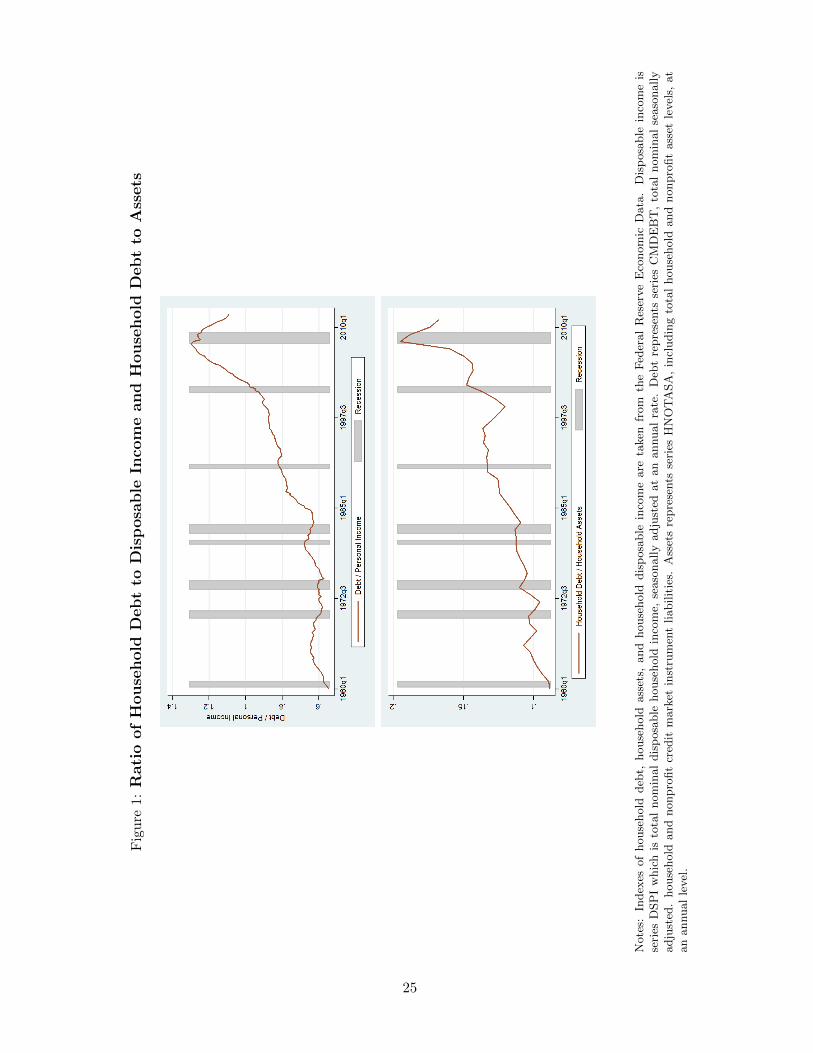
Fig

ure

1:

Rati

oof

House

hold

Debt

toD

isp

osa

ble

Inco

me

and

Hou

seh

old

Deb

tto

Ass

ets

Note

s:In

dex

esof

house

hold

deb

t,house

hold

ass

ets,

and

house

hold

dis

posa

ble

inco

me

are

taken

from

the

Fed

eral

Res

erve

Eco

nom

icD

ata

.D

isp

osa

ble

inco

me

isse

ries

DSP

Iw

hic

his

tota

lnom

inal

dis

posa

ble

house

hold

inco

me,

seaso

nally

adju

sted

at

an

annual

rate

.D

ebt

repre

sents

seri

esC

MD

EB

T,

tota

lnom

inal

seaso

nally

adju

sted

.house

hold

and

nonpro

fit

cred

itm

ark

etin

stru

men

tliabilit

ies.

Ass

ets

repre

sents

seri

esH

NO

TA

SA

,in

cludin

gto

tal

house

hold

and

nonpro

fit

ass

etle

vel

s,at

an

annual

level

.

25

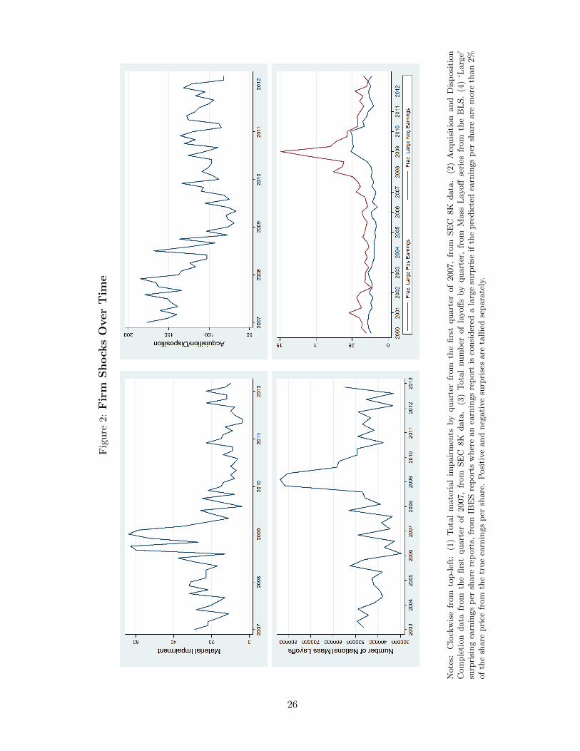
Fig

ure

2:F

irm

Shock

sO

ver

Tim

e

Note

s:C

lock

wis

efr

om

top-l

eft:

(1)

Tota

lm

ate

rial

impair

men

tsby

quart

erfr

om

the

firs

tquart

erof

2007,

from

SE

C8K

data

.(2

)A

cquis

itio

nand

Dis

posi

tion

Com

ple

tion

data

from

the

firs

tquart

erof

2007,

from

SE

C8K

data

.(3

)T

ota

lnum

ber

of

layoff

sby

quart

er,

from

Mass

Lay

off

seri

esfr

om

the

BL

S.

(4)

‘Larg

e’su

rpri

sing

earn

ings

per

share

rep

ort

s,fr

om

IBE

Sre

port

sw

her

ean

earn

ings

rep

ort

isco

nsi

der

eda

larg

esu

rpri

seif

the

pre

dic

ted

earn

ings

per

share

are

more

than

2%

of

the

share

pri

cefr

om

the

true

earn

ings

per

share

.P

osi

tive

and

neg

ati

ve

surp

rise

sare

tallie

dse

para

tely

.

26

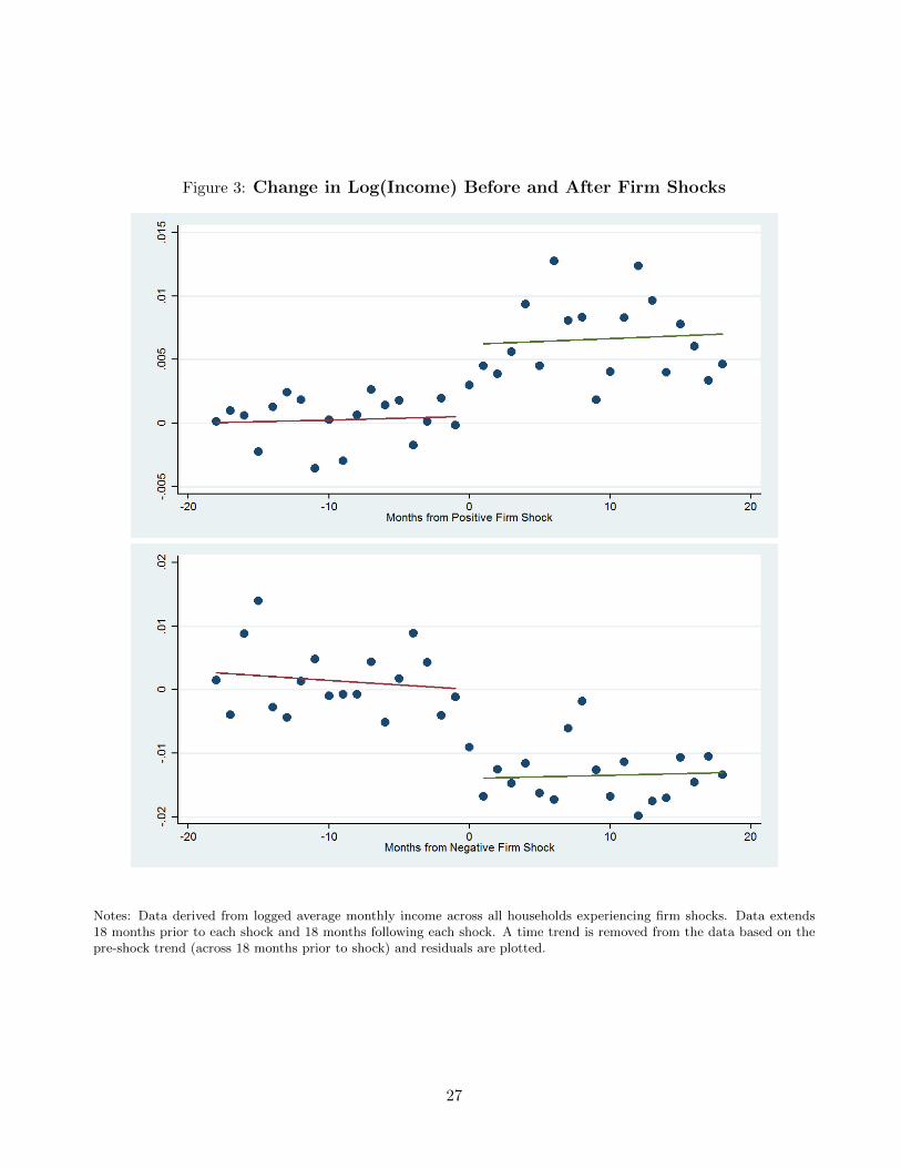
Figure 3: Change in Log(Income) Before and After Firm Shocks

Notes: Data derived from logged average monthly income across all households experiencing firm shocks. Data extends18 months prior to each shock and 18 months following each shock. A time trend is removed from the data based on thepre-shock trend (across 18 months prior to shock) and residuals are plotted.

27

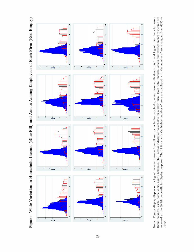
Fig

ure

4:

Wid

eV

ari

ati

on

inH

ouse

hold

Inco

me

(Blu

eF

ill)

and

Ass

ets

Am

ong

Em

plo

yees

of

Each

Fir

m(R

ed

Em

pty

)

Note

s:F

igure

sdis

pla

ydis

per

sion

inlo

gged

inco

me

(inco

me

from

all

sourc

esin

cludin

gpay

chec

ks,

renta

lin

com

e,div

iden

ds,

etc.

)and

logged

tota

lfinanci

al

ass

ets

(bank

bala

nce

s,ca

sh,

hom

eva

lue,

equit

ybala

nce

s,et

c.)

acr

oss

indiv

idual

house

hold

sfo

ra

giv

enfirm

.B

oth

tota

lfinanci

al

ass

ets

and

aver

age

month

lyin

com

eare

censo

red

at

the

99.5

thp

erce

nti

lefo

rdis

pla

ypurp

ose

s.T

he

12

firm

sw

ith

the

hig

hes

tnum

ber

of

use

rsare

dis

pla

yed

,w

ith

the

num

ber

of

use

rsra

ngin

gfr

om

6355

to16464.

28

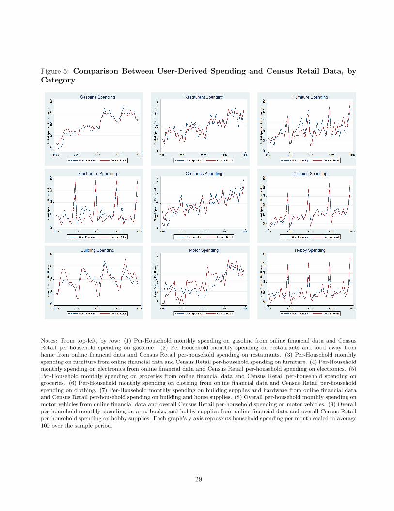
Figure 5: Comparison Between User-Derived Spending and Census Retail Data, byCategory

Notes: From top-left, by row: (1) Per-Household monthly spending on gasoline from online financial data and CensusRetail per-household spending on gasoline. (2) Per-Household monthly spending on restaurants and food away fromhome from online financial data and Census Retail per-household spending on restaurants. (3) Per-Household monthlyspending on furniture from online financial data and Census Retail per-household spending on furniture. (4) Per-Householdmonthly spending on electronics from online financial data and Census Retail per-household spending on electronics. (5)Per-Household monthly spending on groceries from online financial data and Census Retail per-household spending ongroceries. (6) Per-Household monthly spending on clothing from online financial data and Census Retail per-householdspending on clothing. (7) Per-Household monthly spending on building supplies and hardware from online financial dataand Census Retail per-household spending on building and home supplies. (8) Overall per-household monthly spending onmotor vehicles from online financial data and overall Census Retail per-household spending on motor vehicles. (9) Overallper-household monthly spending on arts, books, and hobby supplies from online financial data and overall Census Retailper-household spending on hobby supplies. Each graph’s y-axis represents household spending per month scaled to average100 over the sample period.

29

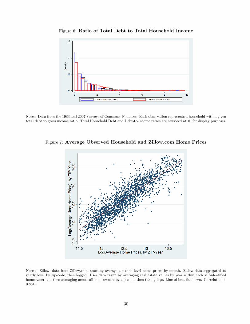
Figure 6: Ratio of Total Debt to Total Household Income

Notes: Data from the 1983 and 2007 Surveys of Consumer Finances. Each observation represents a household with a giventotal debt to gross income ratio. Total Household Debt and Debt-to-income ratios are censored at 10 for display purposes.

Figure 7: Average Observed Household and Zillow.com Home Prices

Notes: ‘Zillow’ data from Zillow.com, tracking average zip-code level home prices by month. Zillow data aggregated toyearly level by zip-code, then logged. User data taken by averaging real estate values by year within each self-identifiedhomeowner and then averaging across all homeowners by zip-code, then taking logs. Line of best fit shown. Correlation is0.881.

30

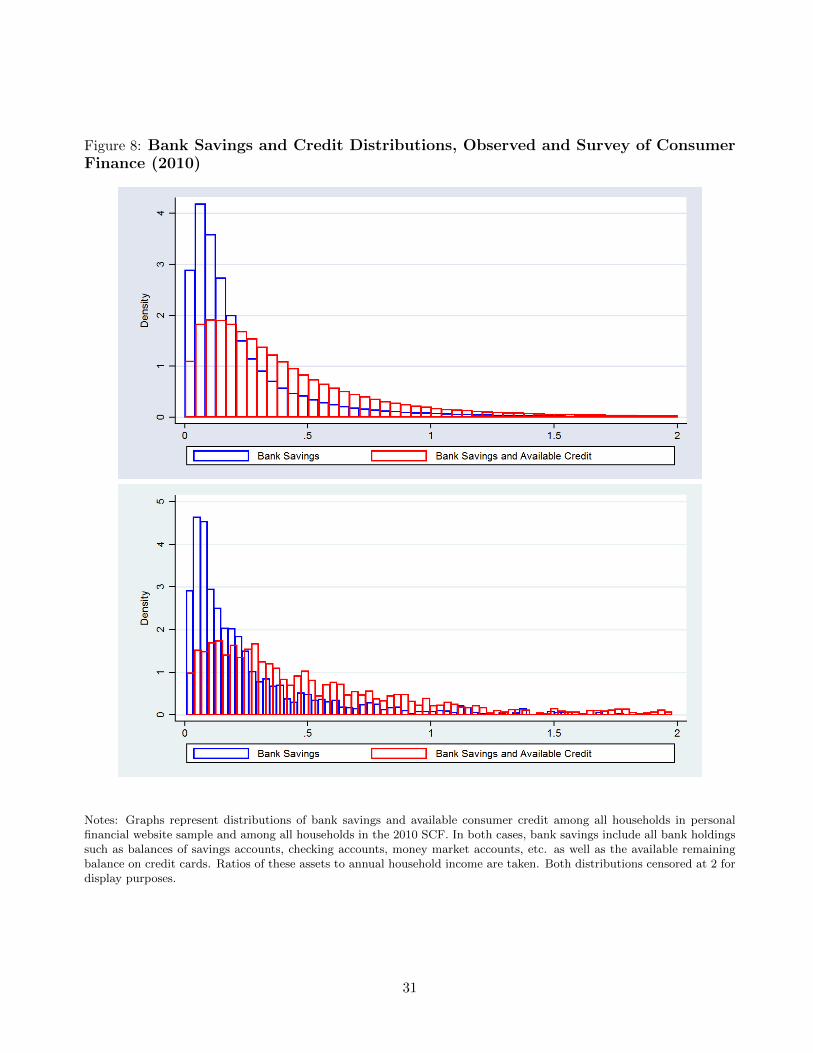
Figure 8: Bank Savings and Credit Distributions, Observed and Survey of ConsumerFinance (2010)

Notes: Graphs represent distributions of bank savings and available consumer credit among all households in personalfinancial website sample and among all households in the 2010 SCF. In both cases, bank savings include all bank holdingssuch as balances of savings accounts, checking accounts, money market accounts, etc. as well as the available remainingbalance on credit cards. Ratios of these assets to annual household income are taken. Both distributions censored at 2 fordisplay purposes.

31

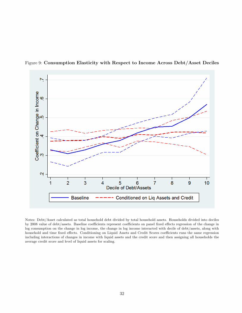
Figure 9: Consumption Elasticity with Respect to Income Across Debt/Asset Deciles

Notes: Debt/Asset calculated as total household debt divided by total household assets. Households divided into decilesby 2008 value of debt/assets. Baseline coefficients represent coefficients on panel fixed effects regression of the change inlog consumption on the change in log income, the change in log income interacted with decile of debt/assets, along withhousehold and time fixed effects. Conditioning on Liquid Assets and Credit Scores coefficients runs the same regressionincluding interactions of changes in income with liquid assets and the credit score and then assigning all households theaverage credit score and level of liquid assets for scaling.

32

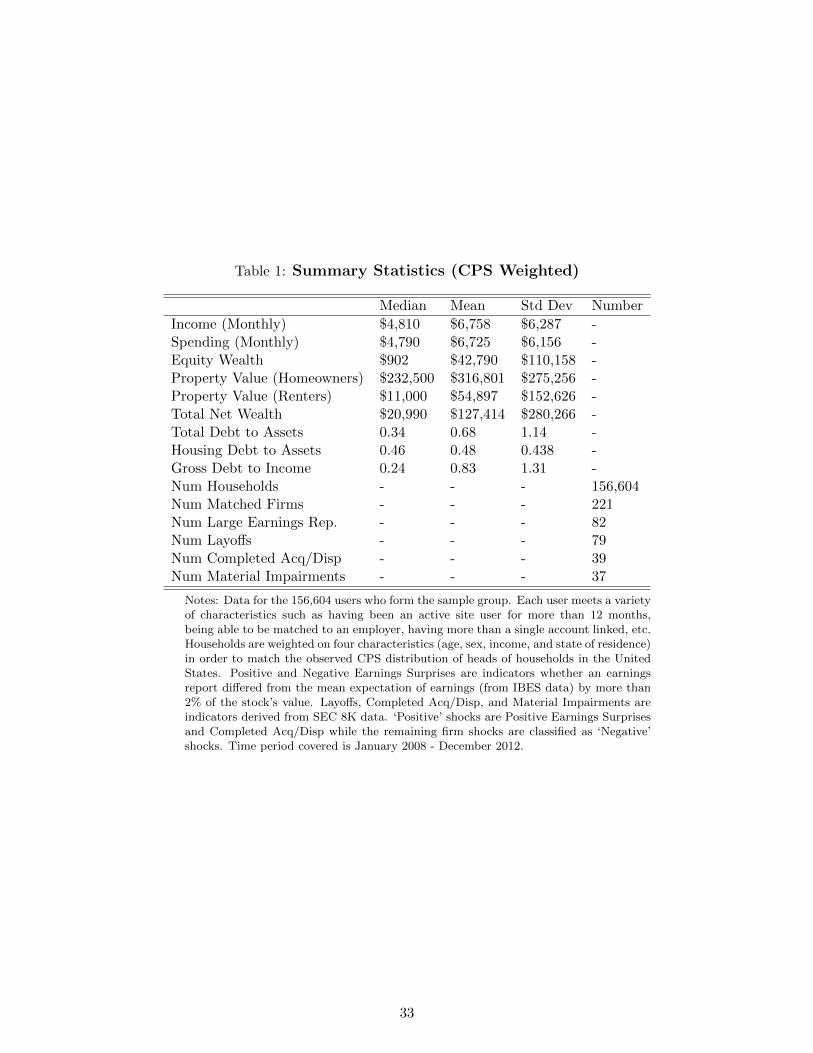
Table 1: Summary Statistics (CPS Weighted)

Median Mean Std Dev Number

Income (Monthly) $4,810 $6,758 $6,287 -Spending (Monthly) $4,790 $6,725 $6,156 -Equity Wealth $902 $42,790 $110,158 -Property Value (Homeowners) $232,500 $316,801 $275,256 -Property Value (Renters) $11,000 $54,897 $152,626 -Total Net Wealth $20,990 $127,414 $280,266 -Total Debt to Assets 0.34 0.68 1.14 -Housing Debt to Assets 0.46 0.48 0.438 -Gross Debt to Income 0.24 0.83 1.31 -Num Households - - - 156,604Num Matched Firms - - - 221Num Large Earnings Rep. - - - 82Num Layoffs - - - 79Num Completed Acq/Disp - - - 39Num Material Impairments - - - 37

Notes: Data for the 156,604 users who form the sample group. Each user meets a varietyof characteristics such as having been an active site user for more than 12 months,being able to be matched to an employer, having more than a single account linked, etc.Households are weighted on four characteristics (age, sex, income, and state of residence)in order to match the observed CPS distribution of heads of households in the UnitedStates. Positive and Negative Earnings Surprises are indicators whether an earningsreport differed from the mean expectation of earnings (from IBES data) by more than2% of the stock’s value. Layoffs, Completed Acq/Disp, and Material Impairments areindicators derived from SEC 8K data. ‘Positive’ shocks are Positive Earnings Surprisesand Completed Acq/Disp while the remaining firm shocks are classified as ‘Negative’shocks. Time period covered is January 2008 - December 2012.

33

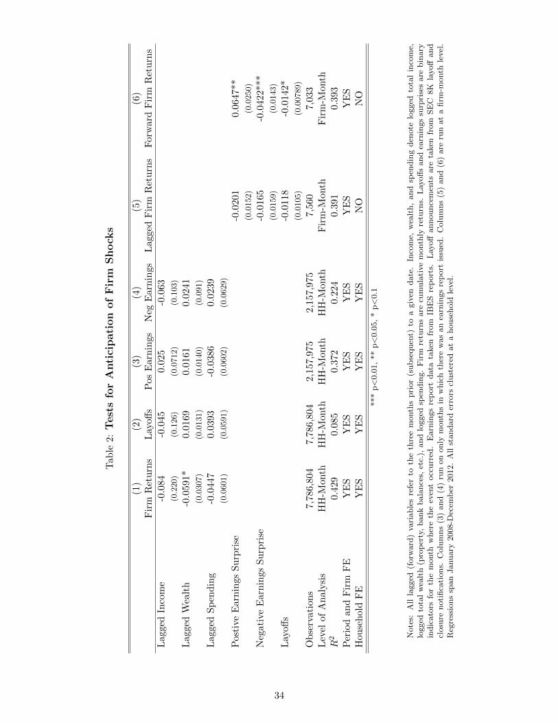
Tab

le2:

Test

sfo

rA

nti

cipati

on

of

Fir

mS

hock

s

(1)

(2)

(3)

(4)

(5)

(6)

Fir

mR

etu

rns

Lay

offs

Pos

Ear

nin

gsN

egE

arn

ings

Lagged

Fir

mR

etu

rns

Forw

ard

Fir

mR

etu

rns

Lag

ged

Inco

me

-0.0

84-0

.045

0.02

5-0

.063

(0.2

20)

(0.1

26)

(0.0

712)

(0.1

03)

Lag

ged

Wea

lth

-0.0

591*

0.01

690.

0161

0.02

41(0

.0307)

(0.0

131)

(0.0

140)

(0.0

91)

Lag

ged

Sp

end

ing

-0.0

447

0.03

93-0

.038

60.

0239

(0.0

601)

(0.0

591)

(0.0

602)

(0.0

629)

Pos

tive

Ear

nin

gsS

urp

rise

-0.0

201

0.0

647**

(0.0

152)

(0.0

250)

Neg

ativ

eE

arnin

gsS

urp

rise

-0.0

165

-0.0

422***

(0.0

159)

(0.0

143)

Lay

offs

-0.0

118

-0.0

142*

(0.0

105)

(0.0

0789)

Ob

serv

atio

ns

7,78

6,80

47,

786,

804

2,15

7,97

52,

157,

975

7,5

60

7,0

33

Lev

elof

An

alysi

sH

H-M

onth

HH

-Mon

thH

H-M

onth

HH

-Mon

thF

irm

-Month

Fir

m-M

onth

R2

0.42

90.

085

0.37

20.

224

0.3

91

0.3

93

Per

iod

and

Fir

mF

EY

ES

YE

SY

ES

YE

SY

ES

YE

SH

ouse

hol

dF

EY

ES

YE

SY

ES

YE

SN

ON

O

***

p<

0.0

1,

**

p<

0.0

5,

*p<

0.1

Note

s:A

llla

gged

(forw

ard

)va

riable

sre

fer

toth

eth

ree

month

spri

or

(subse

quen

t)to

agiv

endate

.In

com

e,w

ealt

h,

and

spen

din

gden

ote

logged

tota

lin

com

e,lo

gged

tota

lw

ealt

h(p

rop

erty

,bank

bala

nce

s,et

c.),

and

logged

spen

din

g.

Fir

mre

turn

sare

cum

ula

tive

month

lyre

turn

s.L

ayoff

sand

earn

ings

surp

rise

sare

bin

ary

indic

ato

rsfo

rth

em

onth

wher

eth

eev

ent

occ

urr

ed.

Earn

ings

rep

ort

data

taken

from

IBE

Sre

port

s.L

ayoff

announce

men

tsare

taken

from

SE

C8K

layoff

and

closu

renoti

fica

tions.

Colu

mns

(3)

and

(4)

run

on

only

month

sin

whic

hth

ere

was

an

earn

ings

rep

ort

issu

ed.

Colu

mns

(5)

and

(6)

are

run

at

afirm

-month

level

.R

egre

ssio

ns

span

January

2008-D

ecem

ber

2012.

All

standard

erro

rscl

ust

ered

at

ahouse

hold

level

.

34

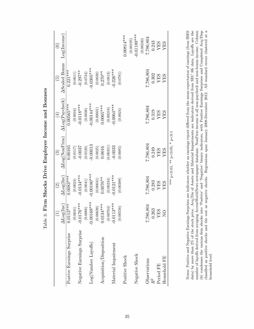
Tab

le3:

Fir

mShock

sD

rive

Em

plo

yee

Inco

me

an

dB

onu

ses

(1)

(2)

(3)

(4)

(5)

(6)

∆L

og(I

nc)

∆L

og(I

nc)

∆L

og(N

onF

irm

)∆

Log(P

aych

eck)

∆S

cale

dB

onu

sL

og(I

nco

me)

Pos

tive

Ear

nin

gsS

urp

rise

0.01

13**

*0.

0083

***

0.00

165

0.0

0565***

0.2

21***

(0.0

041)

(0.0

024)

(0.0

117)

(0.0

016)

(0.0

611)

Neg

ativ

eE

arnin

gsS

urp

rise

-0.0

176*

**-0

.013

4***

-0.0

037

-0.0

118***

-0.2

97**

(0.0

066)

(0.0

041)

(0.0

120)

(0.0

038)

(0.0

734)

Log

(Nu

mb

erL

ayoff

s)-0

.001

69**

*-0

.001

80**

*-0

.000

13-0

.00144***

-0.0

305***

(0.0

0038)

(0.0

0041)

(0.0

025)

(0.0

0031)

(0.0

038)

Acq

uis

itio

n/D

isp

osit

ion

0.01

34**

*0.

0076

**0.

0016

0.0

065***

0.2

70**

(0.0

0704)

(0.0

0234)

(0.0

0351)

(0.0

0218)

(0.0

813)

Mat

eria

lIm

pai

rmen

t-0

.011

3***

-0.0

121*

**-0

.003

3-0

.0064***

-0.2

26***

(0.0

0556)

(0.0

0388)

(0.0

085)

(0.0

024)

(0.0

781)

Pos

itiv

eS

hock

0.0

0814***

(0.0

0195)

Neg

ativ

eS

hock

-0.0

1189***

(0.0

0240)

Ob

serv

atio

ns

7,78

6,80

47,

786,

804

7,78

6,80

47,7

86,8

04

7,7

86,8

04

7,7

86,8

04

R2

0.26

30.

283

0.24

90.3

19

0.3

02

0.2

43

Per

iod

FE

YE

SY

ES

YE

SY

ES

YE

SY

ES

Hou

seh

old

FE

NO

YE

SY

ES

YE

SY

ES

YE

S

***

p<

0.0

1,

**

p<

0.0

5,

*p<

0.1

Note

s:P

osi

tive

and

Neg

ati

ve

Earn

ings

Surp

rise

sare

indic

ato

rsw

het

her

an

earn

ings

rep

ort

diff

ered

from

the

mea

nex

pec

tati

on

of

earn

ings

(fro

mIB

ES

data

)by

more

than

2%

of

the

stock

pri

ce.

Acq

/D

isof

Ass

ets

and

Mate

rial

Impair

men

tsare

indic

ato

rsder

ived

from

SE

C8K

data

.L

ayoff

sare

the

num

ber

of

layoff

sder

ived

from

scra

pin

gA

cces

sWorl

dN

ews

new

spap

erdata

base

.N

onF

irm

inco

me

isall

non-p

aych

eck

and

non-b

onus

inco

me.

Colu

mn

(6)

conden

ses

the

vari

ous

firm

shock

sin

to‘P

osi

tive’

and

‘Neg

ati

ve’

bin

ary

indic

ato

rs,

wit

hP

osi

tive

Earn

ings

Surp

rise

sand

Com

ple

ted

Acq

/D

isp

class

ified

as

posi

tive

shock

sand

the

rest

as

neg

ati

ve

shock

s.R

egre

ssio

ns

span

January

2008-D

ecem

ber

2012.

All

standard

erro

rscl

ust

ered

at

ahouse

hold

level

.

35

Tab

le4:

Fir

mShock

sD

iffere

nti

al

Eff

ect

sT

est

ing

(1)

(2)

(3)

OL

SO

LS

OL

S∆

Log

(In

c)∆

Log(I

nc)

∆L

og(I

nc)

Pos

itiv

eF

irm

Sh

ock

0.00

814*

**0.0

0791***

0.0

0833***

(0.0

0195)

(0.0

0172)

(0.0

0199)

Pos

itiv

eF

irm

Sh

ock

*(D

ebt/

Ass

ets)

0.0

0106

(0.0

043)

Pos

itiv

eF

irm

Sh

ock

*Hou

sin

gE

last

icit

y-0

.00091

(0.0

039)

Neg

ativ

eF

irm

Sh

ock

-0.0

1189

***

-0.0

1071***

-0.0

1153***

(0.0

0240)

(0.0

0233)

(0.0

0278)

Neg

ativ

eF

irm

Sh

ock

*(D

ebt/

Ass

ets)

-0.0

0156

(0.0

0194)

Neg

ativ

eF

irm

Sh

ock

*Hou

sin

gE

last

icit

y0.0

0074

(0.0

0137)

Ob

serv

atio

ns

7,78

6,80

47,7

86,8

04

7,7

86,8

04

Per

iod

FE

YE

SY

ES

YE

SH

ouse

hol

dF

EY

ES

YE

SY

ES

***

p<

0.0

1,

**

p<

0.0

5,

*p<

0.1

Note

s:P

osi

tive

and

Neg

ati

ve

Earn

ings

Surp

rise

sare

indic

ato

rsw

het

her

an

earn

ings

rep

ort

diff

ered

from

the

mea

nex

pec

tati

on

of

earn

ings

(fro

mIB

ES

data

)by

more

than

2%

of

the

stock

pri

ce.

Acq

/D

isof

Ass

ets

and

Mate

rial

Impair

men

tsare

indic

ato

rsder

ived

from

SE

C8K

data

.L

ayoff

sare

the

num

ber

of

layoff

sder

ived

from

scra

pin

gA

cces

sWorl

dN

ews

new

spap

erdata

base

.N

onF

irm

inco

me

isall

non-p

aych

eck

and

non-b

onus

inco

me.

Colu

mn

(6)

conden

ses

the

vari

ous

firm

shock

sin

to‘P

osi

tive’

and

‘Neg

ati

ve’

bin

ary

indic

ato

rs,

wit

hP

osi

tive

Earn

ings

Surp

rise

sand

Com

ple

ted

Acq

/D

isp

class

ified

as

posi

tive

shock

sand

the

rest

as

neg

ati

ve

shock

s.R

egre

ssio

ns

span

January

2008-D

ecem

ber

2012.

All

standard

erro

rscl

ust

ered

at

ahouse

hold

level

.

36

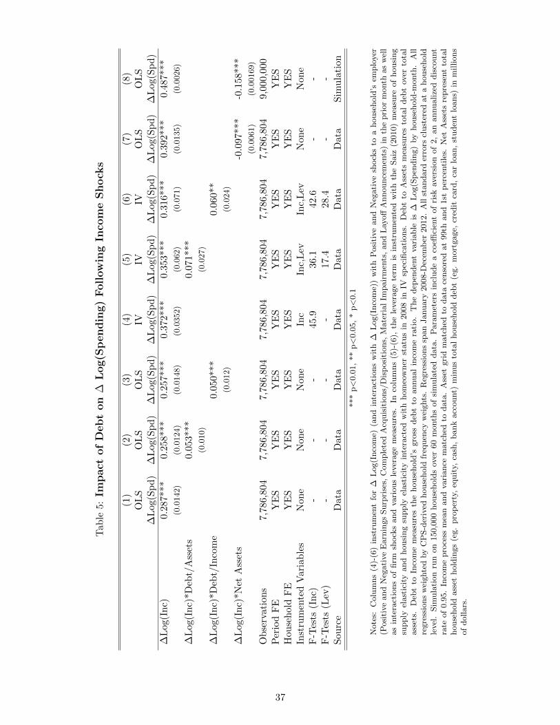
Tab

le5:

Impact

of

Debt

on

∆L

og(S

pendin

g)

Follow

ing

Inco

me

Sh

ock

s

(1)

(2)

(3)

(4)

(5)

(6)

(7)

(8)

OL

SO

LS

OL

SIV

IVIV

OL

SO

LS

∆L

og(S

pd

)∆

Log

(Sp

d)

∆L

og(S

pd

)∆

Log

(Sp

d)

∆L

og(S

pd

)∆

Log(S

pd

)∆

Log(S

pd

)∆

Log(S

pd

)

∆L

og(I

nc)

0.28

7***

0.25

8***

0.25

7***

0.37

2***

0.3

53***

0.3

16***

0.3

92***

0.4

87***

(0.0

142)

(0.0

124)

(0.0

148)

(0.0

352)

(0.0

62)

(0.0

71)

(0.0

135)

(0.0

026)

∆L

og(I

nc)

*Deb

t/A

sset

s0.

053*

**0.0

71***

(0.0

10)

(0.0

27)

∆L

og(I

nc)

*Deb

t/In

com

e0.

050*

**0.0

60**

(0.0

12)

(0.0

24)

∆L

og(I

nc)

*Net

Ass

ets

-0.0

97***

-0.1

58***

(0.0

061)

(0.0

0169)

Ob

serv

atio

ns

7,78

6,80

47,

786,

804

7,78

6,80

47,

786,

804

7,7

86,8

04

7,7

86,8

04

7,7

86,8

04

9,0

00,0

00

Per

iod

FE

YE

SY

ES

YE

SY

ES

YE

SY

ES

YE

SY

ES

Hou

seh

old

FE

YE

SY

ES

YE

SY

ES

YE

SY

ES

YE

SY

ES

Inst

rum

ente

dV

aria

ble

sN

one

Non

eN

one

Inc

Inc,

Lev

Inc,

Lev

Non

eN

on

eF

-Tes

ts(I

nc)

--

-45

.936.1

42.6

--

F-T

ests

(Lev

)-

--

-17.4

28.4

--

Sou

rce

Dat

aD

ata

Dat

aD

ata

Data

Data

Data

Sim

ula

tion

***

p<

0.0

1,

**

p<

0.0

5,

*p<

0.1

Note

s:C

olu

mns

(4)-

(6)

inst

rum

ent

for

∆L

og(I

nco

me)

(and

inte

ract

ions

wit

h∆

Log(I

nco

me)

)w

ith

Posi

tive

and

Neg

ati

ve

shock

sto

ahouse

hold

’sem

plo

yer

(Posi

tive

and

Neg

ati

ve

Earn

ings

Surp

rise

s,C

om

ple

ted

Acq

uis

itio

ns/

Dis

posi

tions,

Mate

rial

Impair

men

ts,

and

Lay

off

Announce

men

ts)

inth

epri

or

month

as

wel

las

inte

ract

ions

of

firm

shock

sand

vari

ous

lever

age

mea

sure

s.In

colu

mns

(5)-

(6),

the

lever

age

term

isin

stru

men

ted

wit

hth

eSaiz

(2010)

mea

sure

of

housi

ng

supply

elast

icit

yand

housi

ng

supply

elast

icit

yin

tera

cted

wit

hhom

eow

ner

statu

sin

2008

inIV

spec

ifica

tions.

Deb

tto

Ass

ets

mea

sure

sto

tal

deb

tov

erto

tal

ass

ets.

Deb

tto

Inco

me

mea

sure

sth

ehouse

hold

’sgro

ssdeb

tto

annual

inco

me

rati

o.

The

dep

enden

tva

riable

is∆

Log(S

pen

din

g)

by

house

hold

-month

.A

llre

gre

ssio

ns

wei

ghte

dby

CP

S-d

eriv

edhouse

hold

freq

uen

cyw

eights

.R

egre

ssio

ns

span

January

2008-D

ecem

ber

2012.

All

standard

erro

rscl

ust

ered

at

ahouse

hold

level

.Sim

ula

tion

run

on

150,0

00

house

hold

sov

er60

month

sof

sim

ula

ted

data

.P

ara

met

ers

incl

ude

aco

effici

ent

of

risk

aver

sion

of

2,

an

annualize

ddis

count

rate

of

0.9

5.

Inco

me

pro

cess

mea

nand

vari

ance

matc

hed

todata

.A

sset

gri

dm

atc

hed

todata

censo

red

at

99th

and

1st

per

centi

les.

Net

Ass

ets

repre

sent

tota

lhouse

hold

ass

ethold

ings

(eg.

pro

per

ty,

equit

y,ca

sh,

bank

acc

ount)

min

us

tota

lhouse

hold

deb

t(e

g.

mort

gage,

cred

itca

rd,

car

loan,

studen

tlo

ans)

inm

illions

of

dollars

.

37

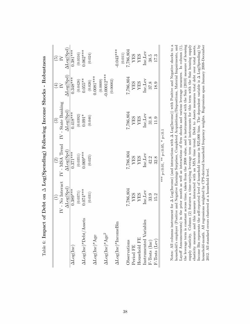
Tab

le6:

Impact

of

Debt

on

∆L

og(S

pendin

g)

Foll

ow

ing

Inco

me

Sh

ock

s-

Rob

ust

ness

(1)

(2)

(3)

(4)

(5)

IV-

No

Inte

ract

IV-

MS

AT

ren

dIV

-S

tate

Ban

kin

gIV

IV∆

Log

(Sp

d)

∆L

og(S

pd

)∆

Log(S

pd

)∆

Log(S

pd

)∆

Log(S

pd

)

∆L

og(I

nc)

0.38

9***

0.37

1***

0.418***

0.3

48***

0.3

81***

(0.0

371)

(0.0

351)

(0.0

392)

(0.0

428)

(0.0

316)

∆L

og(I

nc)

*Deb

t/A

sset

s0.

074*

**0.

069*

**0.0

91*

0.0

55**

0.0

62***

(0.0

31)

(0.0

25)

(0.0

46)

(0.0

26)

(0.0

24)

∆L

og(I

nc)

*Age

0.0

081***

(0.0

009)

∆L

og(I

nc)

*Age

2-0

.00012***

(0.0

0002)

∆L

og(I

nc)

*In

com

eBin

-0.0

43***

(0.0

11)

Ob

serv

atio

ns

7,78

6,80

47,

786,

804

7,786,8

04

7,7

86,8

04

7,7

86,8

04

Per

iod

FE

YE

SY

ES

YE

SY

ES

YE

SH

ouse

hol

dF

EY

ES

YE

SY

ES

YE

SY

ES

Inst

rum

ente

dV

aria

ble

sIn

c,L

evIn

c,L

evIn

c,L

evIn

c,L

evIn

c,L

evF

-Tes

ts(I

nc)

33.9

42.2

31.8

37.8

38.5

F-T

ests

(Lev

)15

.232

.811.9

18.9

17.3

***

p<

0.0

1,

**

p<

0.0

5,

*p<

0.1

Note

s:A

llco

lum

ns

inst

rum

ent

for

∆L

og(I

nco

me)

(and

inte

ract

ions

wit

h∆

Log(I

nco

me)

)w

ith

Posi

tive

and

Neg

ati

ve

shock

sto

ahouse

hold

’sem

plo

yer

(Posi

tive

and

Neg

ati

ve

Earn

ings

Surp

rise

s,C

om

ple

ted

Acq

uis

itio

ns/

Dis

posi

tions,

Mate

rial

Impair

men

ts,

and

Lay

off

Announce

men

ts)

inth

epri

or

month

as

wel

las

inte

ract

ions

of

firm

shock

sand

vari

ous

lever

age

mea

sure

s.In

colu

mn

(1),

the

lever

age

term

isco

nst

ant

acr

oss

tim

e,ta

ken

from

the

2008

valu

e,and

isin

stru

men

ted

wit

hth

eSaiz

(2010)

mea

sure

of

housi

ng

supply

elast

icit

y.C

olu

mn

(2)

featu

res

ati

me-

vary

ing

lever

age

term

and

inst

rum

ents

for

this

term

wit

hth

eSaiz

housi

ng

supply

elast

icit

ym

easu

reand

this

mea

sure

inte

ract

edw

ith

an

MSA

tim

etr

end.

Deb

tto

Ass

ets

mea

sure

sto

tal

deb

tov

erto

tal

ass

ets.

Inco

me

Bin

repre

sents

the

self

-rep

ort

edle

vel

of

house

hold

inco

me

in$25,0

00

bin

s.T

he

dep

enden

tva

riable

is∆

Log(S

pen

din

g)

by

house

hold

-month

.A

llre

gre

ssio

ns

wei

ghte

dby

CP

S-d

eriv

edhouse

hold

freq

uen

cyw

eights

.R

egre

ssio

ns

span

January

2008-D

ecem

ber

2012.

All

standard

erro

rscl

ust

ered

at

ahouse

hold

level

.

38

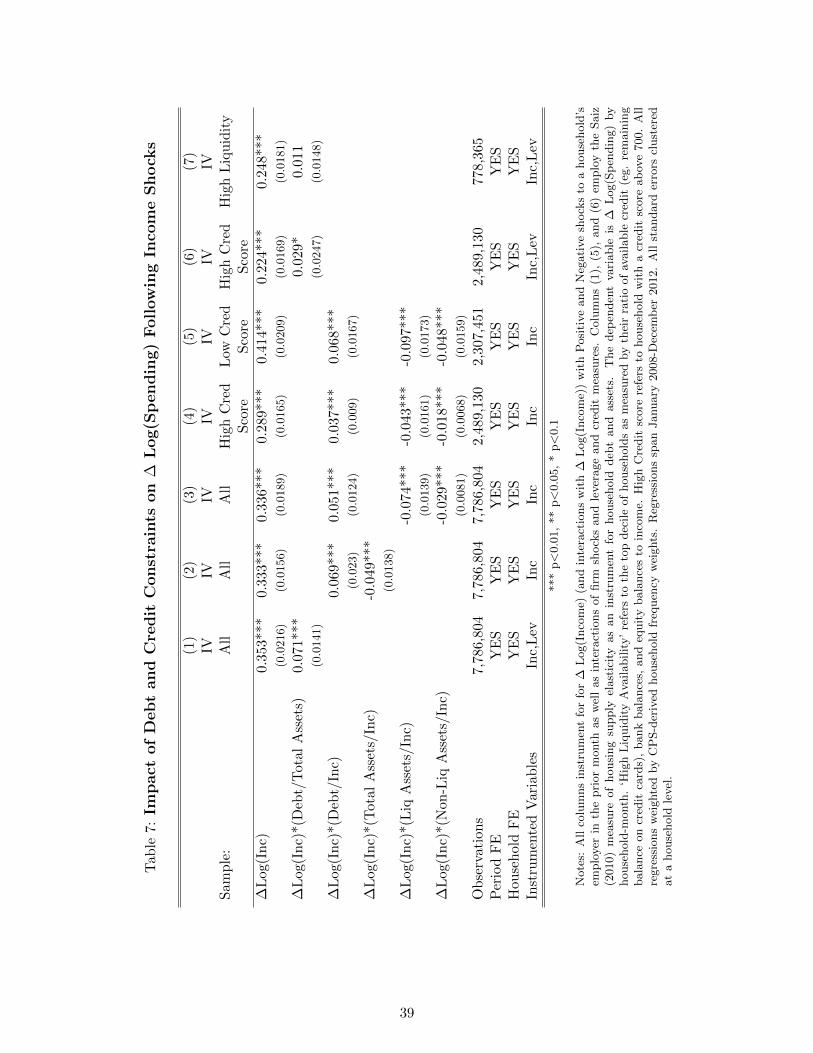
Tab

le7:

Impact

of

Debt

and

Cre

dit

Const

rain

tson

∆L

og(S

pen

din

g)

Follow

ing

Inco

me

Sh

ock

s

(1)

(2)

(3)

(4)

(5)

(6)

(7)

IVIV

IVIV

IVIV

IVS

amp

le:

All

All

All

Hig

hC

red

Low

Cre

dH

igh

Cre

dH

igh

Liq

uid

ity

Sco

reS

core

Sco

re

∆L

og(I

nc)

0.35

3***

0.33

3***

0.33

6***

0.28

9***

0.4

14***

0.2

24***

0.2

48***

(0.0

216)

(0.0

156)

(0.0

189)

(0.0

165)

(0.0

209)

(0.0

169)

(0.0

181)

∆L

og(I

nc)

*(D

ebt/

Tot

alA

sset

s)0.

071*

**0.0

29*

0.0

11

(0.0

141)

(0.0

247)

(0.0

148)

∆L

og(I

nc)

*(D

ebt/

Inc)

0.06

9***

0.05

1***

0.03

7***

0.0

68***

(0.0

23)

(0.0

124)

(0.0

09)

(0.0

167)

∆L

og(I

nc)

*(T

otal

Ass

ets/

Inc)

-0.0

49**

*(0

.0138)

∆L

og(I

nc)

*(L

iqA

sset

s/In

c)-0

.074

***

-0.0

43***

-0.0

97***

(0.0

139)

(0.0

161)

(0.0

173)

∆L

og(I

nc)

*(N

on-L

iqA

sset

s/In

c)-0

.029

***

-0.0

18***

-0.0

48***

(0.0

081)

(0.0

068)

(0.0

159)

Ob

serv

atio

ns

7,78

6,80

47,

786,

804

7,78

6,80

42,

489,

130

2,3

07,4

51

2,4

89,1

30

778,3

65

Per

iod

FE

YE

SY

ES

YE

SY

ES

YE

SY

ES

YE

SH

ouse

hol

dF

EY

ES

YE

SY

ES

YE

SY

ES

YE

SY

ES

Inst

rum

ente

dV

aria

ble

sIn

c,L

evIn

cIn

cIn

cIn

cIn

c,L

evIn

c,L

ev

***

p<

0.0

1,

**

p<

0.0

5,

*p<

0.1

Note

s:A

llco

lum

ns

inst

rum

ent

for

for

∆L

og(I

nco

me)

(and

inte

ract

ions

wit

h∆

Log(I

nco

me)

)w

ith

Posi

tive

and

Neg

ati

ve

shock

sto

ahouse

hold

’sem

plo

yer

inth

epri

or

month

as

wel

las

inte

ract

ions

of

firm

shock

sand

lever

age

and

cred

itm

easu

res.

Colu

mns

(1),

(5),

and

(6)

emplo

yth

eSaiz

(2010)

mea

sure

of

housi

ng

supply

elast

icit

yas

an

inst

rum

ent

for

house

hold

deb

tand

ass

ets.

The

dep

enden

tva

riable

is∆

Log(S

pen

din

g)

by

house

hold

-month

.‘H

igh

Liq

uid

ity

Ava

ilabilit

y’

refe

rsto

the

top

dec

ile

of

house

hold

sas

mea

sure

dby

thei

rra

tio

of

available

cred

it(e

g.

rem

ain

ing

bala

nce

on

cred

itca

rds)

,bank

bala

nce

s,and

equit

ybala

nce

sto

inco

me.

Hig

hC

redit

score

refe

rsto

house

hold

wit

ha

cred

itsc

ore

ab

ove

700.

All

regre

ssio

ns

wei

ghte

dby

CP

S-d

eriv

edhouse

hold

freq

uen

cyw

eights

.R

egre

ssio

ns

span

January

2008-D

ecem

ber

2012.

All

standard

erro

rscl

ust

ered

at

ahouse

hold

level

.

39

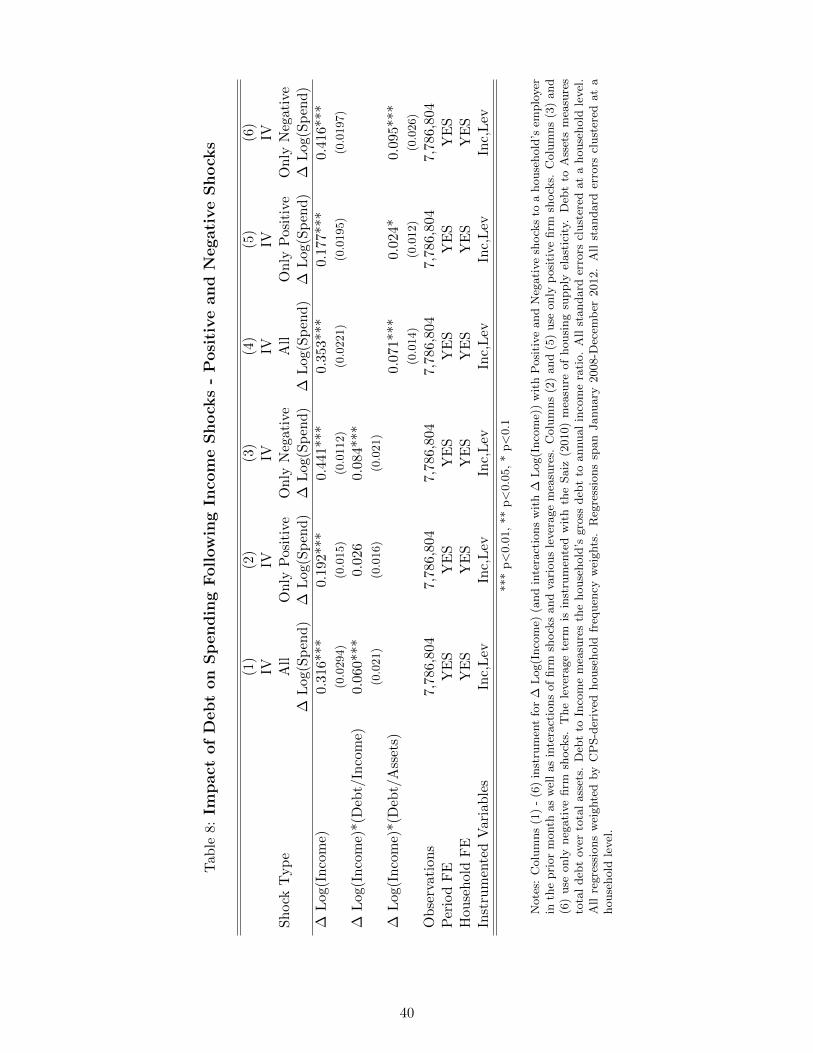
Tab

le8:

Impact

of

Debt

on

Sp

endin

gFoll

ow

ing

Inco

me

Shock

s-

Posi

tive

an

dN

egati

ve

Sh

ock

s

(1)

(2)

(3)

(4)

(5)

(6)

IVIV

IVIV

IVIV

Sh

ock

Typ

eA

llO

nly

Pos

itiv

eO

nly

Neg

ativ

eA

llO

nly

Posi

tive

On

lyN

egati

ve∆

Log

(Sp

end

)∆

Log

(Sp

end

)∆

Log

(Sp

end

)∆

Log(S

pen

d)

∆L

og(S

pen

d)

∆L

og(S

pen

d)

∆L

og(I

nco

me)

0.31

6***

0.19

2***

0.44

1***

0.3

53***

0.1

77***

0.4

16***

(0.0

294)

(0.0

15)

(0.0

112)

(0.0

221)

(0.0

195)

(0.0

197)

∆L

og(I

nco

me)

*(D

ebt/

Inco

me)

0.06

0***

0.02

60.

084*

**(0

.021)

(0.0

16)

(0.0

21)

∆L

og(I

nco

me)

*(D

ebt/

Ass

ets)

0.0

71***

0.0

24*

0.0

95***

(0.0

14)

(0.0

12)

(0.0

26)

Ob

serv

atio

ns

7,78

6,80

47,

786,

804

7,78

6,80

47,7

86,8

04

7,7

86,8

04

7,7

86,8

04

Per

iod

FE

YE

SY

ES

YE

SY

ES

YE

SY

ES

Hou

seh

old

FE

YE

SY

ES

YE

SY

ES

YE

SY

ES

Inst

rum

ente

dV

aria

ble

sIn

c,L

evIn

c,L

evIn

c,L

evIn

c,L

evIn

c,L

evIn

c,L

ev

***

p<

0.0

1,

**

p<

0.0

5,

*p<

0.1

Note

s:C

olu

mns

(1)

-(6

)in

stru

men

tfo

r∆

Log(I

nco

me)

(and

inte

ract

ions

wit

h∆

Log(I

nco

me)

)w

ith

Posi

tive

and

Neg

ati

ve

shock

sto

ahouse

hold

’sem

plo

yer

inth

epri

or

month

as

wel

las

inte

ract

ions

of

firm

shock

sand

vari

ous

lever

age

mea

sure

s.C

olu

mns

(2)

and

(5)

use

only

posi

tive

firm

shock

s.C

olu

mns

(3)

and

(6)

use

only

neg

ati

ve

firm

shock

s.T

he

lever

age

term

isin

stru

men

ted

wit

hth

eSaiz

(2010)

mea

sure

of

housi

ng

supply

elast

icit

y.D

ebt

toA

sset

sm

easu

res

tota

ldeb

tov

erto

tal

ass

ets.

Deb

tto

Inco

me

mea

sure

sth

ehouse

hold

’sgro

ssdeb

tto

annual

inco

me

rati

o.

All

standard

erro

rscl

ust

ered

at

ahouse

hold

level

.A

llre

gre

ssio

ns

wei

ghte

dby

CP

S-d

eriv

edhouse

hold

freq

uen

cyw

eights

.R

egre

ssio

ns

span

January

2008-D

ecem

ber

2012.

All

standard

erro

rscl

ust

ered

at

ahouse

hold

level

.

40

A Data Appendix

A.1 Housing Supply Elasticity

The second instrument utilized for this paper is one designed to identify exogenous variation in levels of

debt and leverage, as well as identifying locations with larger exogenous changes in property prices. I

use a measure of housing-supply elasticity developed by Albert Saiz (2011) that is based on geographic

characteristics of metro areas. Saiz uses satellite-generated data on characteristics such as water bound-

aries, elevation, and elevation changes to construct an index of land unavailability covering the majority

of the population of the United States. Saiz conducts his analysis at a CBSA level, providing an index

for 257 of the 953 CBSAs, containing over 72% of the population of the United States as of 2010. All

samples in this paper are restricted to be from households residing in zip codes that are contained within

these CBSAs.

Glaeser, Gyourko, and Saiz (2008) as well as Mian and Sufi (2010), demonstrate the power of this

instrument in both driving changes in housing prices and coincident changes in household leverage

levels. They demonstrate the linkages between housing supply elasticity, home prices, and housing

bubbles, both during the 1980s as well as during the early 2000s, in the period leading up to the

Great Recession. In areas with relatively inelastic housing supplies, households homes’ appreciated in

value and home equity was often extracted, leading to higher levels of debt and leverage. Mian and Sufi

(2013) demonstrate that housing supply elasticity did not systematically vary with things like local wage

growth, exposure to or growth in housing-related sectors like construction, or large positive population

growth. They find that more inelastic cities have higher per-capita income and per-capita net worth,

but that these correlations are constant over time and thus, for the purposes of my paper, will not play

a direct role in the differenced specifications.

Another concern with this variable is that housing supply elasticity acts as both a driver of household

debt as well as a driver of asset prices. This is due to the nature of the housing boom and bust cycle

during the late 2000s, where inelastic areas saw rapid increases in housing prices and housing-related debt

followed by larger declines in asset prices. In my analysis of the impact of leverage on the responsiveness

of consumption to income shocks, I use the variable to instrument solely for the initial level of leverage

that the household faces. Concerns that the elasticity measure may also proxy for long-run decreases

in housing prices may be mitigated by the fact that I use high-frequency changes in income while

property prices decline only over a period of years. Moreover, the elasticity of local housing supply is

uncorrelated with the firm shocks that drive changes household income, as most of these firms are large

public, and geographically-spread, employers relatively unaffected by the decline in property prices. I

41

also test specifications which include location level trends, property prices, or gross household assets as

further controls for the decline in housing prices, finding no significant change in the magnitudes of my

estimates.

A.2 Layoff Data

Data on the number of layoffs by firm-month are constructed from a search of newspaper articles

regarding large instances of layoffs. The database in question is the Access World News Newsbank

(AWN) database of national and local US newspapers. This database extends back to the 1980’s and

contains well over 1,500 newspapers during the same period of 2008-2012.

I first compile a complete list of full firm names (eg. ’Agilent Technologies Incorporated’) and

construct a complementary list of shortened firm names (eg. ’Agilent’). This shortening is largely done

by removing all common terms and punctuation from firm titles. Using this list of full and shortened

firm names, I search the AWN database for articles in which the title contains three terms. The first

is the firm name (or shortened firm name). The title must also contain at least one term from each of

the following sets: (positions OR jobs OR employees OR workers OR notices OR roles OR staff OR

personnel) and (slash OR slashes OR slashing OR lost OR losses OR layoffs OR sheds OR axes OR

cuts OR fires OR layoff OR shed OR axe OR cut OR cutting OR axing OR shedding OR reduce OR

“lay off” OR “laid off”). Thus, I am attempting to identify news articles which are primarily about

layoffs at a particular firm.

For each resultant article, in addition to the firm name in question, I save two additional pieces of

information. The first is the date that the article was written. The second is the number of layoffs

mentioned in the title. Full article titles regarding layoffs are often written in a formulaic manner (eg.

“Wells Fargo to cut 4,000 jobs” or “Alcoa lays off 2,400 workers”) and contain the number of layoffs

that were announced by the firm. These searches yield approximately 16,000 news articles covering 512

firms from 1985 until 20012. I categorize and count the number of articles by firm-month, discarding

any articles that do not have at least 2 articles regarding layoffs in that firm-month. Manual inspection

reveals that these articles are generally false positives.

Finally, I use the most common number of layoffs, by firm-month, reported by newspaper articles

as the true number of layoffs for that given firm-month instance of layoffs. Approximately 75% of firm-

months have 75% of relevant articles agreeing on the number of layoffs in a given month. Just over 50%

of firm-month observations have 100% agreement, with all articles regarding that layoff reporting the

same number of layoffs. The final sample covers 179 firms and 330 instances of layoffs from

42

A.3 Job Switching

One potential worry in using negative firm shocks is that there are unlikely to be permanent or even

semi-permanent in duration because individuals can switch jobs and negate the negative effects. I find

evidence suggesting this is not the case; the income of users who switch jobs after a negative shock is

insignificantly different than the income of users who switch jobs with no negative shocks.

Overall, users are not more likely to switch jobs after a positive shock, but are more likely to switch

jobs after a negative shock. I test this with a probit of 3 lags of negative shock indicators, 3 leads

of negative shock indicators, and contemporaneous negative shock indicators, finding significant effects

on contemporaneous shocks of switching jobs in the following month. This remains true, though the

coefficient decreases in magnitude, if only using non-layoff negative shocks (large and surprising negative

earnings reports and write-offs by the firm).

I find that, on average income is depressed after leaving a job for the first three months. However,

when transitioning to a new observable job (eg. to another employer from the NYSE or NASDAQ),

income tends to increase in the months after leaving a job. Moreover, leaving a job after a shock does

not significantly alter these relationships, with insignificant coefficients on interactions between negative

shocks to firms and leaving that firm. This suggests that users cannot avoid the entirety of negative

firm shocks simply by leaving their firm.

One explanation for this finding relies on users being rational members of the labor market and

the presence of switching costs and firm-specific human capital exists. In this case, employees will not

remain at a firm if there is an opportunity for a significant raise elsewhere. Moreover, on average,

opportunities and pay at other firms will be lower than at the current firm due to the fact that firm-

specific human capital has been accumulated. Thus, employees at firms hit by a negative shock will

likely have no options to be employed at other firms at a significantly higher wage or else they would

have already left.

Despite a lack of opportunities at higher wages, if household income was subject to large declines

following a negative firm shock, employees may still be induced to change jobs to ameliorate sizable

drops in income (eg. take another job at 10% less rather than endure a 30% decline in income). However,

firm shocks in this paper cause drops in income on the order of 1-3%. Thus, considering a likely loss in

income due to firm-specific human capital and job-switching costs, most users would be unlikely to be

substantially better off if they switched jobs following a negative shock.

43

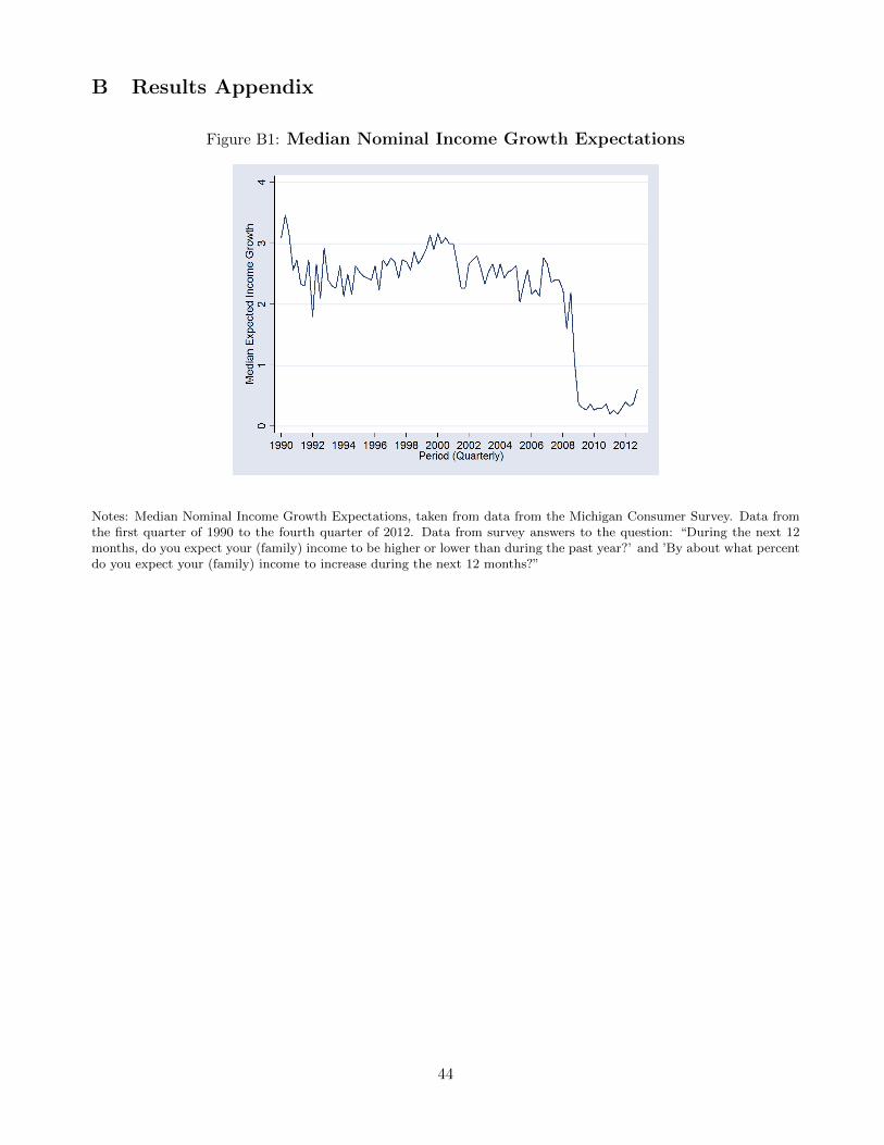
B Results Appendix

Figure B1: Median Nominal Income Growth Expectations

Notes: Median Nominal Income Growth Expectations, taken from data from the Michigan Consumer Survey. Data fromthe first quarter of 1990 to the fourth quarter of 2012. Data from survey answers to the question: “During the next 12months, do you expect your (family) income to be higher or lower than during the past year?’ and ’By about what percentdo you expect your (family) income to increase during the next 12 months?”

44

Table B1: Summary Statistics Weighting Comparison

Mean Median CPS-Weighted Mean CPS-Weighted Median

Male 0.72 1 0.65 1Married 0.56 1 0.48 1Homeowner 0.54 1 0.48 0Income (Monthly) $7,362 $5,678 $6,758 $4,810Spending (Monthly) $7,300 $5,646 $6,725 $4,790Equity Wealth $46,628 $3,391 $42,790 $902Prop. Wealth (Homeowners) $277,454 $220,666 $316,801 $232,500

Notes: CPS weighting is done at a household level based on age, sex, income, and state of residence. Households inpersonal financial website data are equated to head-of-households in the CPS data.

Table B2: Layoffs by Firm

Firm Mon Day Year Layoffs Firm Mon Day Year Layoffs

AT&T 1 1 2010 160 MEDTRONIC 2 19 2011 2000LOCKHEED 1 1 2010 1200 NORTHROP GRU. 2 26 2011 500FOOT LOCKER 1 8 2010 120 WELLS FARGO 3 19 2011 400NYSE 1 8 2010 350 CISCO 4 9 2011 550UPS 1 8 2010 1800 LOCKHEED 6 11 2011 1200HOME DEPOT 1 22 2010 1000 CISCO 7 9 2011 6500VERIZON 1 22 2010 13000 BOSTON SCI. 7 23 2011 1400WALMART 1 22 2010 11200 BANK OF AMER. 8 13 2011 3500HUMANA 2 12 2010 1400 NORTHROP GRU. 8 20 2011 500BOEING 2 19 2010 1000 BANK OF AMER. 9 10 2011 30000IBM 2 26 2010 1518 LOCKHEED 9 24 2011 670CHEVRON 3 5 2010 2000 LOWE’S 10 15 2011 1950NETFLIX 5 14 2010 160 WHIRLPOOL 10 22 2011 5000PFIZER 5 14 2010 6000 AMD 10 29 2011 1400HEWLETT PACK. 5 28 2010 9000 ADOBE 11 5 2011 475NATIONWIDE 7 2 2010 2070 MORGAN STAN. 12 10 2011 1600WELLS FARGO 7 2 2010 3800 ARCHER D.M. 1 8 2012 1000WINN DIXIE 7 23 2010 120 METLIFE 1 8 2012 2575FEDEX 9 10 2010 1700 KRAFT 1 15 2012 1600ABBOTT 9 17 2010 3000 ABBOTT 1 22 2012 700AON 10 8 2010 1800 AMERICAN AIR. 1 29 2012 13000NORTHROP GRU. 11 12 2010 380 MICROSOFT 1 29 2012 200STATE STREET 11 26 2010 1400 NATIONWIDE 2 5 2012 625AMERICAN EXP. 1 15 2011 550 SUPERVALU 2 5 2012 800BOEING 1 15 2011 900 IBM 2 26 2012 1100ABBOTT 1 22 2011 1900 GOODRICH 3 4 2012 500PFIZER 1 29 2011 1100 LEVIS 3 4 2012 500

Notes: Layoffs derived from news-based analysis of layoff announcements. Articles from over 1,500 local, regional, andnational newspapers from the Newsbank news archive service were utilized to determine the announcement date and thenumber of individuals laid off for each firm.

45

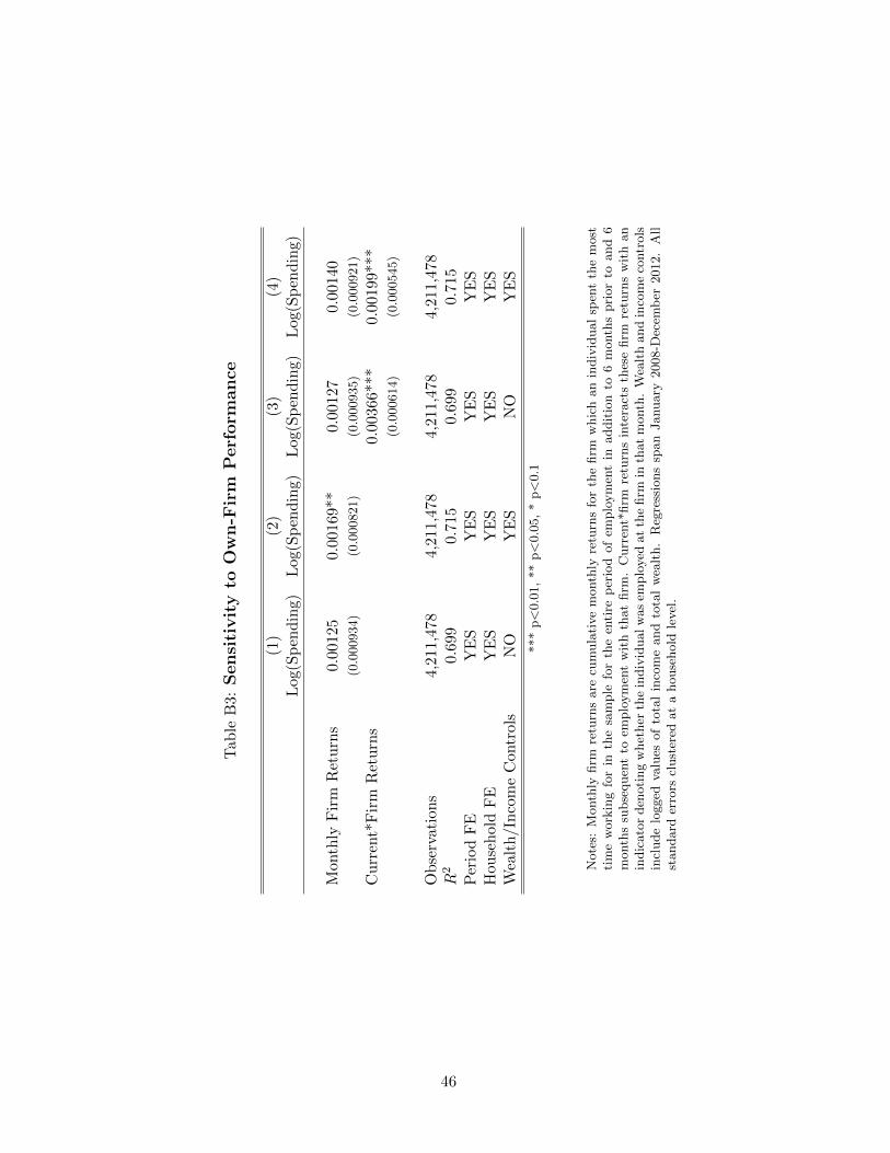
Tab

leB

3:Sensi

tivit

yto

Ow

n-F

irm

Perf

orm

ance

(1)

(2)

(3)

(4)

Log

(Sp

end

ing)

Log

(Sp

end

ing)

Log

(Sp

end

ing)

Log(S

pen

din

g)

Month

lyF

irm

Ret

urn

s0.

0012

50.

0016

9**

0.00

127

0.0

0140

(0.0

00934)

(0.0

00821)

(0.0

00935)

(0.0

00921)

Cu

rren

t*F

irm

Ret

urn

s0.

0036

6***

0.0

0199***

(0.0

00614)

(0.0

00545)

Ob

serv

ati

ons

4,21

1,47

84,

211,

478

4,21

1,47

84,2

11,4

78

R2

0.69

90.

715

0.69

90.7

15

Per

iod

FE

YE

SY

ES

YE

SY

ES

Hou

seh

old

FE

YE

SY

ES

YE

SY

ES

Wea

lth

/In

com

eC

ontr

ols

NO

YE

SN

OY

ES

***

p<

0.0

1,

**

p<

0.0

5,

*p<

0.1

Note

s:M

onth

lyfirm

retu

rns

are

cum

ula

tive

month

lyre

turn

sfo

rth

efirm

whic

han

indiv

idual

spen

tth

em

ost

tim

ew

ork

ing

for

inth

esa

mple

for

the

enti

rep

erio

dof

emplo

ym

ent

inaddit

ion

to6

month

spri

or

toand

6m

onth

ssu

bse

quen

tto

emplo

ym

ent

wit

hth

at

firm

.C

urr

ent*

firm

retu

rns

inte

ract

sth

ese

firm

retu

rns

wit

han

indic

ato

rden

oti

ng

whet

her

the

indiv

idualw

as

emplo

yed

at

the

firm

inth

at

month

.W

ealt

hand

inco

me

contr

ols

incl

ude

logged

valu

esof

tota

lin

com

eand

tota

lw

ealt

h.

Reg

ress

ions

span

January

2008-D

ecem

ber

2012.

All

standard

erro

rscl

ust

ered

at

ahouse

hold

level

.

46