Embed Size (px)
Citation preview
SOFTWARE MAINTENANCE: RESEARCH AND PRACTICEJ. Softw. Maint: Res. Pract.10, 111–150 (1998)
Research
Debugging Program Failure Exhibitedby Voluminous Data
TAT W. CHAN1 and ARUN LAKHOTIA2*1Department of Mathematics and Computer Science, Fayetteville State University, Fayetteville NC 28301,U.S.A.2The Center for Advanced Computer Studies, University of Southwestern Louisiana, Lafayette LA 70504,U.S.A.
SUMMARY
It is difficult to debug a program when the data set that causes it to fail is large (orvoluminous). The cues that may help in locating the fault are obscured by the large amountof information that is generated from processing the data set. Clearly, a smaller data set whichexhibits the same failure should lead to the diagnosis of the fault more quickly than the initial,large data set. We term such a smaller data set adata slice and the process of creating itdata slicing.
The problem of creating a data slice is undecidable. In this paper, we investigate fourgenerate-and-test heuristics for deriving a smaller data set that reproduces the failure exhibitedby a large data set. The four heuristics are: invariance analysis, origin tracking, randomelimination and program-specific heuristics. We also provide a classification of programs basedupon a certain relationship between their input and output. This classification may be used tochoose an appropriate heuristic in a given debugging scenario. As evidence from a databaseof debugging anecdotes at the Open University, U.K., debugging failures exhibited by largedata sets require inordinate amounts of time. Our data slicing techniques would significantlyreduce the effort required in such scenarios. 1998 John Wiley & Sons, Ltd.
KEY WORDS: data slicing; fault reproduction; origin tracking; heuristics for slicing; slicing effectiveness
1. INTRODUCTIONTo find the cause of a failure, i.e., debugging, a programmer often observes the values
of program variables—the state—at various intermediate steps during execution. This isdone by exercising the program through a data set or a sequence of events exhibiting thefailure. For most programs, the number of intermediate steps and the amount of informationin the state at each step depends upon the size of the failure data. A large data set may
* Correspondence to: Arun Lakhotia, The Center for Advanced Computer Studies, University of SouthwesternLouisiana, Lafayette LA 70504, U.S.A. E-mail: [email protected]
Contract/grant sponsor: Louisiana Board of Regents; Contract/grant number: LEQSF (1993–95) RD-A-38Contract/grant sponsor: U.S. Army Research Office; Contract/grant number: DAAH 04-94-G-0334
CCC 1040–550X/98/020111–40$17.50 Received 20 December 1995 1998 John Wiley & Sons, Ltd. Revised 28 September 1997
112 T. W. CHAN and A. LAKHOTIA
cause failure after a large number of iterations, thereby generating a large number ofintermediate steps. Moreover, the size of the intermediate values of variables (such asarrays) may be proportional to the size of the input, thereby generating a large amountof information in each state. Such debugging scenarios may arise even when the programhas been exhaustively tested using one or more testing criteria (be it branch coverage,mutation coverage or dataflow coverage). During actual use one may create data or eventsthat exercise conditions not exercised by the data in the test suite. That the failure-causingdata set is large may just be a matter of chance.
Debugging a program when the failure isexhibitedby a large data set is hard becausethe clues that may help in finding a fault are obscured by the large amount of informationa programmer has to process. Clearly, a smaller data set reproducing the same failurewould ease the debugging. Creating such data set is not always easy. It is especiallydifficult when the program has been tested extensively, because then one has to identifythe specific conditions not exercised by data in the test suite—a task that may requirefinding clues from the vast amount of state information. Creating a smaller, failure-reproducing data set is also not easy when a program’s input is generated by anotherprogram or preprocessor—as happens in applications, such as image processing, statisticalanalysis and compiler backends. In such cases one must create a data set such that thepreprocessor outputs a smaller failure-reproducing data set, a task that further adds to thecomplexity of the problem. The alternative is to isolate the program and manuallyconstruct its input. This can be an equally complex task if the program’s input has acomplex structure.
This relationship betweendebugging effortand the choice of dataused was firstobserved in our earlier work (Chan and Lakhotia, 1993; Lakhotia and Chan, 1993). Inthis paper, we further expand on the preliminary ideas presented earlier and present acollection of methods to ‘create a smaller data set that reproduces a failureexhibitedbya voluminousdata set’. By the phrase ‘large’ or ‘voluminous’ data set, we do not onlymean that the size of the input data set is large. An input data set is voluminous ifprocessing it requires an enormous amount of computation—thereby creating a largenumber of internal states. A data set may also be voluminous if the amount of informationin the internal states is large. The phrase ‘exhibited by’ may be understood by contrastingit with the phrase ‘caused by’. A failure ‘exhibited by’ a large data set may be reproducedby a smaller data set. In contrast a failure ‘caused by’ a large data set implies that thefailure is not reproducible by any smaller data set.
We term a ‘smaller’ data set that reproduces a failure exhibited by a large data set adata slice. The process of creating data slices is calleddata slicing. The term ‘slice’ isintended to draw an analogy with Weiser’s definition of aprogram slice(Weiser, 1984;Chen and Cheung, 1997). A program slice is a ‘smaller’ program—made up of statementscontained in a given program—preserving some syntactic and semantic constraints. Theanalogy between the two is that the ‘smaller’ artefact is created from the elements of agiven artefact while preserving certain semantic constraints. A program slice is not just a‘smaller’ program that preserves certain semantic constraints, it is also a program con-structed from the statements of a given program. Similarly, a data slice is not just asmaller data set that produces the same failure as the original data set, it is also constructedfrom the elements of this data set.
1998 John Wiley & Sons, Ltd. J. Softw. Maint: Res. Pract.10, 111–150 (1998)
113DEBUGGING PROGRAM FAILURE
Chan, the first author, has proposed a framework for debugging that incorporates theuse of data slicing along with program slicing and traditional trace-and-inspection tools(Chan, 1997). A summary of the data slicing techniques presented in this paper is alsoavailable in Chan’s paper.
The rest of the paper is organized as follows. In Section 2, we further motivate thediscussion by means of a case study and the results of two informal surveys. In Section3, we present the constraints influencing the design of our data slicing methods. In Section4, we give (i) a classification of programs and data domains, and (ii) terminology of afailure, same failure and a fault. These classifications are helpful in choosing the appropriatedata slicing method in a particular debugging scenario. Section 5 presents several methodsfor data slicing. In Section 6, the effectiveness of our data slicing methods is assessed.Section 7 surveys various debugging techniques and explains why they are unable to helpin debugging failures exhibited by voluminous data. Section 8 contains our concludingremarks.
2. MOTIVATION
2.1. Case study
The following case study illustrates the difficulty of debugging a failure exhibited bya voluminous data set and how a data slice helps in overcoming the difficulty.
We were once developing a program to recover the architecture of a program basedon the approach suggested by Hutchens and Basili (1985). This program usesclusteranalysis to organize functions of a C program in a hierarchy. It takes as input an × nmatrix whereN is the number of functions in the given program. The matrix containsthe ‘binding’ strength between functions, the number ofglobal variables, typedefs, macrosand symbols used by both the functions, etc. The output of the program is ann-ary treethat can be represented as a binary tree with at mostN − 1 interior nodes. The programcontains a main loop. In each iteration of the main loop,m elements are clustered into anode of then-ary tree and the dimension of the matrix is decreased by (m − 1).
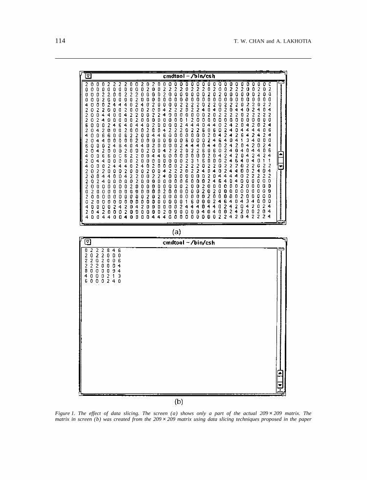
We tested the program on several sample matrices. Once satisfied with its correctness,we started using it in our research. After some time, we observed a failure when a209× 209 matrix was used as input. In order to debug, we useddbx to set breakpointsand to inspect the variables at various points in the execution. Unfortunately, the amountof information output was overwhelming and would rarely fit on a screen. Figure 1(a),for instance, shows what a typical screen looked like. It was cluttered with numbers.Since the program failed after 20 iterations, debugging the program by tracing its executionwas impossible. We did, however, try tracing the program for two days but were noteven able to detect any clues that would allow the debugging to proceed. We then usedinvariance analysis and random elimination techniques (discussed later in this paper) forcreating data slices and were able to create a 7× 7 matrix, see Figure 1(b), that alsoproduced the same failure as the original data. Subsequently, we were able to debug theprogram in just two hours, since the clues—relationships between various elements of thematrix—were easily visible from looking at the intermediate matrices. The creation of
1998 John Wiley & Sons, Ltd. J. Softw. Maint: Res. Pract.10, 111–150 (1998)
114 T. W. CHAN and A. LAKHOTIA
Figure 1. The effect of data slicing. The screen (a) shows only a part of the actual 209× 209 matrix. Thematrix in screen (b) was created from the 209× 209 matrix using data slicing techniques proposed in the paper
115DEBUGGING PROGRAM FAILURE
the data slice itself required about five hours, including the time for developing somespecial code to support the data slicing techniques.
2.2. Results of two informal surveysScenarios similar to the above case study have been experienced by other programmers
too. The database of debugging anecdotes maintained at the Open University in the U.K.contained (as of January 1994) a collection of 163 anecdotes (Eisenstadt, 1993). Of these,12 anecdotes narrate scenarios where the failures were exhibited by large data sets (orsequence of events). The effort required to debug, reported in each of these anecdotes,ranges in weeks and months. There are two extreme cases where the debugging itselfwas terminated.
The difficulty of debugging in these 12 anecdotes is attributed either to (a) the amountof information generated by the program for the failure-causing data set or (b) the vastamount of time required to reproduce the failure.
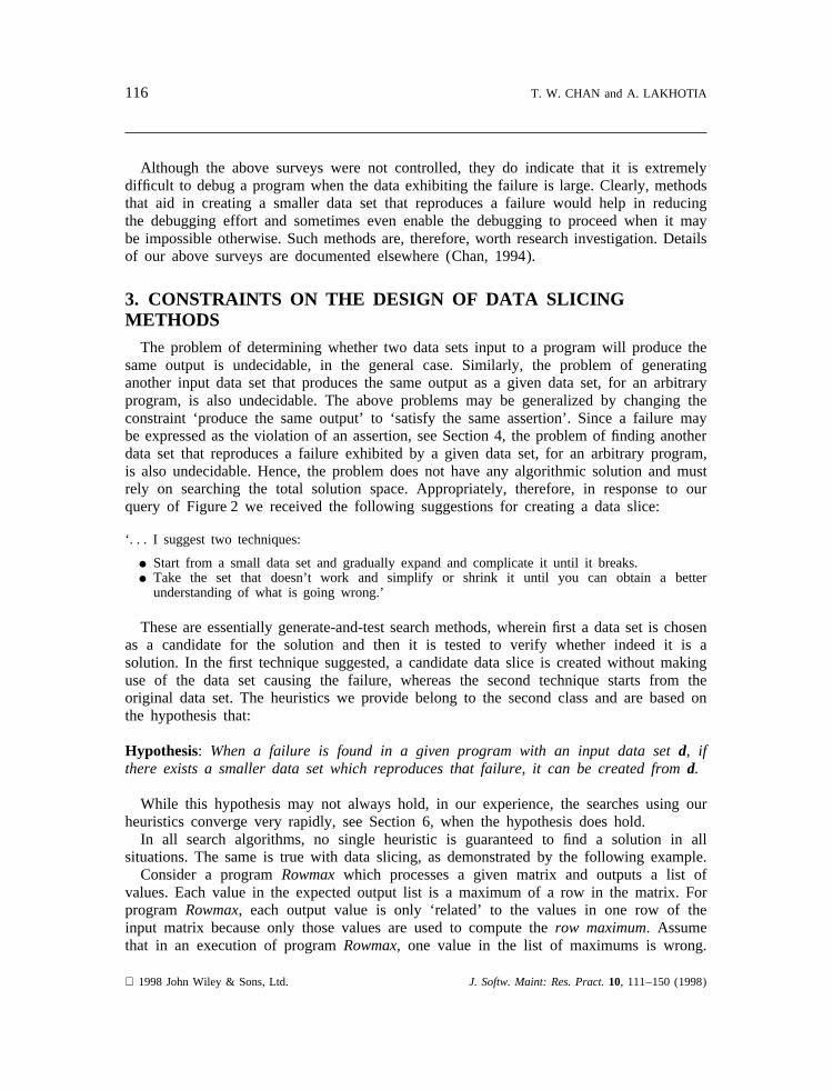
That debugging under the stated scenario is difficult is further corroborated by theresponses to our query, see Figure 2, posted on the Internet newsgroupscomp.bugs.misc,comp.source.bugsand sci.image.processing.
Some typical responses we received were:
‘When debugging an image processing algorithm, conventional debuggers are of little help. The vastamount of data that an image generates makes it fruitless to examine each number.’
‘This sort of bugs ARE difficult to track down.’
‘Your work is definitely interesting, and a real problem in debugging . . . Several of our SERCaffiliates have had problems with programs that ran for a long time or generated lots of outputbefore failures.’
Figure 2. Query posted on the Internet newsgroupscomp.bugs.misc, comp.source.bugsand sci.image.processingto survey the difficulty of debugging failures exhibited by large data
1998 John Wiley & Sons, Ltd. J. Softw. Maint: Res. Pract.10, 111–150 (1998)
116 T. W. CHAN and A. LAKHOTIA
Although the above surveys were not controlled, they do indicate that it is extremelydifficult to debug a program when the data exhibiting the failure is large. Clearly, methodsthat aid in creating a smaller data set that reproduces a failure would help in reducingthe debugging effort and sometimes even enable the debugging to proceed when it maybe impossible otherwise. Such methods are, therefore, worth research investigation. Detailsof our above surveys are documented elsewhere (Chan, 1994).
3. CONSTRAINTS ON THE DESIGN OF DATA SLICINGMETHODS
The problem of determining whether two data sets input to a program will produce thesame output is undecidable, in the general case. Similarly, the problem of generatinganother input data set that produces the same output as a given data set, for an arbitraryprogram, is also undecidable. The above problems may be generalized by changing theconstraint ‘produce the same output’ to ‘satisfy the same assertion’. Since a failure maybe expressed as the violation of an assertion, see Section 4, the problem of finding anotherdata set that reproduces a failure exhibited by a given data set, for an arbitrary program,is also undecidable. Hence, the problem does not have any algorithmic solution and mustrely on searching the total solution space. Appropriately, therefore, in response to ourquery of Figure 2 we received the following suggestions for creating a data slice:
‘. . . I suggest two techniques:
I Start from a small data set and gradually expand and complicate it until it breaks.I Take the set that doesn’t work and simplify or shrink it until you can obtain a better
understanding of what is going wrong.’
These are essentially generate-and-test search methods, wherein first a data set is chosenas a candidate for the solution and then it is tested to verify whether indeed it is asolution. In the first technique suggested, a candidate data slice is created without makinguse of the data set causing the failure, whereas the second technique starts from theoriginal data set. The heuristics we provide belong to the second class and are based onthe hypothesis that:
Hypothesis: When a failure is found in a given program with an input data setd, ifthere exists a smaller data set which reproduces that failure, it can be created fromd.
While this hypothesis may not always hold, in our experience, the searches using ourheuristics converge very rapidly, see Section 6, when the hypothesis does hold.
In all search algorithms, no single heuristic is guaranteed to find a solution in allsituations. The same is true with data slicing, as demonstrated by the following example.
Consider a programRowmaxwhich processes a given matrix and outputs a list ofvalues. Each value in the expected output list is a maximum of a row in the matrix. Forprogram Rowmax, each output value is only ‘related’ to the values in one row of theinput matrix because only those values are used to compute therow maximum. Assumethat in an execution of programRowmax, one value in the list of maximums is wrong.
1998 John Wiley & Sons, Ltd. J. Softw. Maint: Res. Pract.10, 111–150 (1998)
117DEBUGGING PROGRAM FAILURE
If the data slicing methodM creates a data slice using all the input values that are‘related’ to the erroneous output values, then it will find a data slice which is the rightrow in the original input matrix.
While methodM is good for performing a data slice for programRomax, it may notbe good for another program. For example, consider a programDeterm that computes thedeterminant of a given matrix. The determinant is ‘related’ to all the elements in theinput matrix because all the elements areused to compute the determinant. If thedeterminant computed by programDeterm for a given matrix is wrong, using methodM,the data slice obtained may be the whole input. Using this method, therefore, one cannever get a data slice for programP.
We, therefore, present a collection of heuristics for creating data slices. We furtherobserve that the choice of the appropriate heuristics in a debugging situation may beguided by the input and output domains, the program itself, the type of failure and thefault causing the failure. In the next section, we provide a classification scheme for datadomains and programs. This classification may be used in choosing the appropriateheuristics.
4. DATA, PROGRAMS, FAILURES AND FAULTS
In this section we classify data domains and programs. We also give definitions for afailure, same failure and a fault.
4.1. Data
In this subsection, three aspects of data will be discussed: the data domains, dataelements and the size of a data set.
4.1.1. Data domains
The input and output data domains can be classified into three categories:
• primitive types, such as integers and characters;• fixed structures, such as fixed length arrays and records of all types; and• recursive structures, such as lists, trees, graphs and variable length arrays of all types.
Inputs and outputs of any program can be modelled using these categories sinceprograms, in the most general sense, are simply transformers of data.
4.1.2. Data elements
The fixed and recursive structures, when decomposed completely, consist of values ofprimitive types. A primitive value of a data structure is called its data element. A datumof a primitive type has only one data element, the datum itself. The values of primitivedata types contained in a fixed or recursive structure are its data elements. For example,the primitive values in each of a linked list are its data elements. Similarly, the data
1998 John Wiley & Sons, Ltd. J. Softw. Maint: Res. Pract.10, 111–150 (1998)
118 T. W. CHAN and A. LAKHOTIA
elements of a tree consist of the primitive values that comprise its nodes. If data valueswere also associated with the links of the linked list (or the edges of a tree), then theassociated primitive values are data elements too.
4.1.3. Size of a data set
So far the word ‘smaller’ has been used intuitively. A measure for a data set thatquantifies the difficulty of debugging a program with a given data set is needed. A dataset requiring greater debugging effort should have a larger value for this measure. Sucha measure is calleddata size, or just size.
Like any metric, size may be defined in many ways. The most obvious measure ofsize is storage size.
Definition: storage size. The number of bits required to store the data in memory iscalled storage size.
The storage size of an input is usually a good indicator of the number of intermediatestates required to process it. For instance, a factorial program would perform morecomputations to compute the factorial for 100 than for seven. The storage size for 100is seven bits and is greater than the storage size of four bits for 10.
However, storage size is not always a good indicator of the intermediate states andhence of the debugging effort. Consider, for example, a program which reads a list ofintegers denoting consecutive leap years from the year 4 A.D. and generates the remainingleap years up to the 400th leap year. Then an input list containing the first 10 leap yearswill require more processing than the list containing the first 20 leap years. But thestorage size for 20 years is greater than the storage size for 10 years.
Clearly, the debugging effort does not depend solely upon the storage size of the inputdata set; it also depends on the program being debugged.
Definition: processing size.The amount of computation performed by a program toprocess a given input gives the processing size for the input.
Given a program and a data set, the processing size of the data set may be computedby instrumenting the program to get the number of the times a loop (implicit or explicit)is iterated and the depth of recursive function calls. (Count for statements that are not ina loop or recursive function are not significant since (a) if they are not in a loop orrecursive function they can be executed at most one time and (b) if they are in a loopor recursive function then they are executed as many times as the loop is executed.) Testcoverage analysis tools, such asbtool (Hoch, Marick and Schafer, 1990), Asset, andATAC (Horgan and Mathur, 1992), can provide such coverage information. In the absenceof a tool, it may be estimated analytically by using the computational complexity of theprogram and the storage size of the data set. Besides the number of intermediate states,the size of each state—the amount of information at each state—also has an influenceon the debugging effort. It has been our experience that the size of the intermediate statesfor a data set tend to be proportional to its processing size. While this is not conclusive,
1998 John Wiley & Sons, Ltd. J. Softw. Maint: Res. Pract.10, 111–150 (1998)
119DEBUGGING PROGRAM FAILURE
it suggests that the processing size is a good indicator of the debugging effort, since itis proportional to both the complexity of the computation and the storage size of thedata set.
4.2. Programs
4.2.1. Definition of programs
A program is typically defined as a collection of code (in some programming language)that can be compiled into object code and executed on a machine. We use a more generaldefinition. A program can be a single statement or a composition of statements. Astatement may be an assignment statement, an input statement, an output statement, analternation statement or a repetition statement. This general definition is consistent withhow a programmer views a program during debugging. Instead of treating it as amonolithic piece of code, one uses a divide-and-conquer strategy to identify suspectmodules or sets of statements. This strategy is most evident when the program beingdebugged contains a succession of phases in which data are transformed. If a failure isfound in a particular phase, the debugging effort may be focused on that phase only. Insuch cases, if an intermediate phasep is being debugged, then the data slicing methodsmay create smaller data for that phase alone, not necessarily the whole program. Noticethat since phasep is an intermediate phase, its input is the values of all variables whichare (a) read by the input statements in phasep or (b) referenced before modification inphasep.
4.2.2. Program specification
We use Morgan’s notation for specification of program:pre⇒ P post (Morgan, 1988),where conditionpre is the weakest precondition (Dijkstra, 1976) of programP withrespect to a postconditionpost. The specification denotes that if programP is activatedin a state for which conditionpre holds, then it will terminate in a state for whichpost holds.
4.2.3. Classification of programs
The specification of a program gives the relations established between its input and itsoutput. The relations given by the specifications should capture the complete behaviourof a program. These relations may, however, be abstracted to express only the relationsestablished between the primitive elements of the input and output such that:
(a) With every elementei in the input, one can associate a setp(ei) in the outputsuch thatei ‘generates’ the set of elementsp(ei ).
(b) With every elementeo in the output, one can associated a setm(eo) in the inputsuch that elementeo is ‘generated from’ the set of elementsm(eo).
The relationship between an input elementei and p(ei) may be classified as follows:
1998 John Wiley & Sons, Ltd. J. Softw. Maint: Res. Pract.10, 111–150 (1998)
120 T. W. CHAN and A. LAKHOTIA
• Type a1 : p(ei) = f, i.e., ei does not generate any element in the output.• Type a2 : p(ei) = { ei}, i.e., ei generates the element ei itself in the output.• Type a3 : p(ei) = { eo}, i.e., ei ± eo, i.e., ei generates a single elementeo in the output,
where eo is different from ei.• Type a4 : up(ei )u . 1, i.e., ei generates more than one element in the output.
The relationship between an output elementeo and m(eo) may be classified as follows:
• Type b1 : m(eo) = f, i.e., eo is not generated from any element in the input.• Type b2 : m(eo) = { eo}, i.e., eo is generated from the elementeo in the input.• Type b3 : m(eo) = { ei}, ei ± eo i.e., eo is generated from a single elementei in the
input, whereei is not the same aseo.• Type b4 : um(eo)u . 1, i.e., eo is generated from more than one element in the input.
While these relationships can be derived from a program’s specification, in practice, acomplete written specification may not be necessary. Given an element in the input (oroutput), a programmer may be able to intuitivelyclassify its type—ai (or bi), 1 < i < 4—from the knowledge of its expected behaviour.
4.3. Failures and faults
4.3.1. Definition of failures
A failure may be defined as any deviation of a program’s behaviour from the expectedbehaviour. For example, if a program ‘hangs’ when it is expected to terminate, then it isa failure. However, if a program is not expected to terminate—such as an operatingsystem—then its non-termination is not a failure.
When first observed, a failure is associated with some external behaviour of a program.As debugging proceeds, the failure gets associated with one or more subcomponents ofthe program. In the process, the definition of the failure itself changes and becomes moreprecise. For instance, an initial observation that a program does not terminate on debuggingmay be associated with non-termination of a loop. In this case, the failure may be thatthe termination condition of the loop cannot be established (for the given input).
This successive translation of failure may be captured using program specifications. Thespecification of a program (and subprograms) defines assertions that are expected to holdat various program points. A failure is a violation of an assertion. The violation of anassertion at a subcomponent may result in the violation of assertions for its parentcomponent, therefore leading to an externally observable failure.
4.3.2. Same failure
Let a programP be specifed aspre⇒ P post, where pre is its precondition andpostis its postcondition.
The programP is said to fail on a data setd that satisfies the conditionpre if theprogram fails to establish the postconditionpost when invoked with the data setd.
1998 John Wiley & Sons, Ltd. J. Softw. Maint: Res. Pract.10, 111–150 (1998)
121DEBUGGING PROGRAM FAILURE
Two data setsd1 and d2 cause thesame failure if they both violate the samesubconditionspost′ of post, i.e., post′ ⇒ post, d1 causes violations ofpost′ iff d2 causesviolation of post′.
4.3.3. Definition of faults
A fault is also commonly known as a bug, which is the condition in the programwhich causes a failure. A fault is, therefore, manifested by a failure. A failure impliesthat there must be a fault in the program but a fault may not necessarily cause a failure.
5. DATA SLICING METHODS
Definition: data slice. Given a data set d1 that causes a program p to fail, data setd2 is a data sliceof d1 iff
(1) d2 reproduces in p the same failure as d1 and(2) d2 is smaller than d1 when compared using processing size with respect to
program p.
Data slicing is the method of creatingd2 given programp and datad1. In this section,five methods for data slicing are discussed. As stated in Section 3, the methods are basedupon the hypothesis that:when a failure is found in a given program with input datad,if there exists smaller data which reproduces the failure, it can be created fromd.
To debug failures exhibited by a large data set, one would first create a data sliceusing one or more of the data slicing methods, and then use a general purpose debuggingtechnique to debug the program.
The rest of this section discusses the following data slicing methods:
(1) Data slicing by invariance analysis.(2) Data slicing by origin tracking.(3) Data slicing by random elimination.(4) Data slicing by program-specific heuristics.
5.1. Data slicing by invariance analysis
Data slicing by invariance analysis is especially designed to create data slices for loopsin a program. Consider the situation where some computation in a loop fails after 50iterations, where the failure may be defined as a violation of its loop invariant. Whentracing the program using debuggers such asdbx, one would have to step through thecode 50 times before coming to the state when the program fails. The invarianceanalysis method helps in creating a data slice that would cause the loop to fail after asingle iteration.
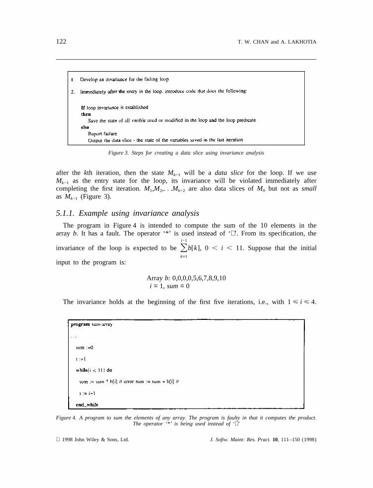
Figure 3 gives the steps for data slicing by invariance analysis. This method has thefollowing formal basis. LetM0 denote the state just before entering the loopM. Insuccessive iteration,M0 is transformed toM1,M2,. . .Mn. If the loop invariance is violated
1998 John Wiley & Sons, Ltd. J. Softw. Maint: Res. Pract.10, 111–150 (1998)
122 T. W. CHAN and A. LAKHOTIA
Figure 3. Steps for creating a data slice using invariance analysis
after the kth iteration, then the stateMk−1 will be a data slice for the loop. If we useMk−1 as the entry state for the loop, its invariance will be violated immediately aftercompleting the first iteration.M1,M2,. . .Mk−2 are also data slices ofM0 but not assmallas Mk−1 (Figure 3).
5.1.1. Example using invariance analysis
The program in Figure 4 is intended to compute the sum of the 10 elements in thearray b. It has a fault. The operator ‘*’ is used instead of ‘+’. From its specification, the
invariance of the loop is expected to beOi−1
k=1
b[k], 0 , i , 11. Suppose that the initial
input to the program is:
Array b: 0,0,0,0,5,6,7,8,9,10i = 1, sum= 0
The invariance holds at the beginning of the first five iterations, i.e., with 1< i < 4.
Figure 4. A program to sum the elements of any array. The program is faulty in that it computes the product.The operator ‘*’ is being used instead of ‘+’
1998 John Wiley & Sons, Ltd. J. Softw. Maint: Res. Pract.10, 111–150 (1998)
123DEBUGGING PROGRAM FAILURE
It violates at the beginning of the sixth iteration. If the loop was re-executed with valuesof sum and i as 0 and 5, respectively, the loop invariance will be violated immediatelyafter the first iteration. These values along with the arrayb (not changed in the loop)form a data slice for the loop.
Notice that although the original input is for the whole program, the data slice is inputonly to the loop.
Reverting the state of the variables to the last iteration before the invariance is violatedcan easily be done with a debugger such as Spyder (Agrawal, DeMillo and Spafford,1991). Thus, using invariance analysis, Spyder may be used for creating limited types ofdata slices.
While this method may create a data slice that violates a loop after the first iteration,it does not always reduce the size of the data significantly. For instance, in the case studygiven in Section 2.1 invariance analysis helped in creating a 198× 198 matrix from a209× 209 matrix. The smaller matrix still had too much information to be usefulin debugging.
Furthermore, the applicability of this method depends upon (a) whether the programmerknows or can derive the loop invariance, (b) the support available for instrumenting theprogram to detect the violation of the invariance, and (c) the computational cost forchecking the violation of the invariant.
5.2. Data slicing by origin tracking
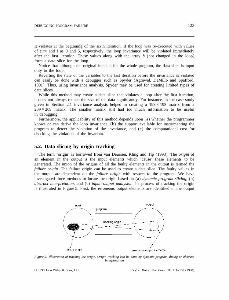
The term ‘origin’ is borrowed from van Deursen, Kling and Tip (1993). Theorigin ofan element in the output is the input elements which ‘cause’ these elements to begenerated. The union of the origins of all the faulty elements in the output is termed thefailure origin. The failure origin can be used to create a data slice. The faulty values inthe output are dependent on thefailure origin with respect to the program. We haveinvestigated three methods to locate the origin based on (a)dynamic program slicing, (b)abstract interpretation, and (c) input–output analysis. The process of tracking the originis illustrated in Figure 5. First, the erroneous output elements are identified in the output
Figure 5. Illustration of tracking the origin. Origin tracking can be done by dynamic program slicing or abstractinterpretation
1998 John Wiley & Sons, Ltd. J. Softw. Maint: Res. Pract.10, 111–150 (1998)
124 T. W. CHAN and A. LAKHOTIA
of a program, then by applying one of the origin tracking methods, the failure isasssociated to some of the data elements in the input.
A failure origin itself is not a data slice; it is only a set of elements that constitute apart of a valid input. The set of all valid inputs to a program is its input domain. Inother words, the origin may not be in the input domain of the program. Therefore, afterobtaining the origin, we try to create a data set that belongs to the input domain of theprogram and contains the origin so that it is more likely to be a data slice. Such a dataset is a candidate data slice. The methods to computecandidate data slicesdepend onthe domain of the input. For a fixed structure, the candidate data slices can be obtainedby ‘filler elements substitution’—replace the elements not in the origin by some ‘small’elements. Data slicing by origin tracking is most rewarding if the failure-causing data setis a recursive structure. However, more careful consideration is needed for a recursivestructure when obtaining candidate data slices from theorigin. This is because thepositions of the erroneous elements in the failure origin may be significant to reproducethe failure. These issues will be discussed in Section 5.2.4. The following summarizesthe steps to perform data slicing by origin tracking:
(1) Track the failure origin using:• dynamic program slicing, or• abstract interpretation, or• input–output analysis.
(2) Create a set of candidate data slices such that each candidate is:• smaller than the original data set and• contains the failure origin.
(3) Test each candidate to see if it reproduces the failure.
In the following, we will describe how the origin may be obtained by dynamicprogram slicing, abstract interpretation and input–output analysis. The methods for selectingcandidate data slices are described after that.
5.2.1. Origin tracking by dynamic program slicing
Agrawal and Horgan’s algorithm for computing a dynamic program slice (Agrawal andHorgan, 1990) is influenced by Horwitz, Prins and Reps’ algorithm for computing thestatic program slice (Horwitz, Prins and Reps, 1988). The latter slicing algorithm representsa program as a program dependence graph (PDG)—a graph denoting the essential controland data dependences between statements of a program. A static program slice over thisgraph for a given statement, sayn, consists of all the statements that can reach the nodecorresponding ton in the PDG.
Agrawal and Horgan’s algorithm maintains a dynamic PDG in which every invocationof a statement is represented by a new vertex and retains only those dependences whichare actually manifested during an execution. Therefore, computing the dynamic slice inthis graph is also a graph reachability problem.
1998 John Wiley & Sons, Ltd. J. Softw. Maint: Res. Pract.10, 111–150 (1998)
125DEBUGGING PROGRAM FAILURE
The origin of a set of faulty elements may be obtained by dynamic slicing using thefollowing steps:
(1) Scan the output of the program to identify parts (or elements) that are faulty. Thisstep is performed by the programmer.
(2) Trace the faulty elements in the output back to the statement instance in thedynamic PDG that output it. If the output is a hard copy or a file, this may be amanual task. If the output is on the screen, this mapping may be maintained bythe system such that a pointing device (e.g., a mouse) may be used to query it.
(3) Compute a dynamic program slice over the set of statement instances identified tohave output faulty elements.
(4) Identify the input statement instances in the dynamic program slice. The dataelements input by these statements is the failure origin for the faulty elements ofthe output.
A more detailed and formal description of the algorithm for origin tracking by dynamicprogram slicing may be found in Chan (1994).
5.2.2. Origin tracking by abstract interpretation
Computing the origin by dynamic program slicing relies on maintaining a dependencygraph during execution. The origin is obtained by traversing this graphbackwards. Theorigin of some output elements can be computed by extending the semantics of thelanguage in which the program is written. This is an abstract interpretation and is aforward approach to obtain the origin.
The principle of the method is to propagate the dependencies of the input elements,during execution, to other variables in the program. Both data and control dependenciesare propagated. The propagation is modelled by changing the standard semantics of thelanguage. In the standard semantics, a variable is associated with a value. The semanticsare extended by associating each variable with, in addition to a value, a set oftagsindicating the transitive data dependencies and control dependencies on elements of theinput data set. The tag is a two-tuple, (,line-number., ,instance number.). The firstfield gives the line number of aread statement and the second field gives the executioninstance of that statement. In the rest of the document, the tag will be represented as,line-number.,instance number.. For instance, if a read statement on line 2 is executed thethird time, then the tag created will be represented by 23.
For each faulty element in the output, the origin can be obtained from the set of tagsassociated with them. The following explains in more detail how the semantics of a simplestructured language withread, assignment, if-then-else, do-while, and write constructs areextended:
(1) At the beginning, the tag set for each variable is made empty. Thecontroldependency setis empty too. The control dependency set contains tags associatedwith variables used in predicates in the program.
(2) When anassignmentstatement is executed, then
1998 John Wiley & Sons, Ltd. J. Softw. Maint: Res. Pract.10, 111–150 (1998)

126 T. W. CHAN and A. LAKHOTIA
(a) if the expression on the right-hand side contains only constants, then theset of tags associated with the variable on the left-hand side will containtags in the control dependency set or
(b) if the expression on the right-hand side contains at least one variable, thenthe variable on the left-hand side is associated with the union of:
(i) the sets of tags, each set of which is associated with a variable used on theright-hand side and
(ii) the set of tags in the control dependency set.(3) When aread statement is executed, a new tag is created and associated with the
input variable, along with the tags in the control dependency set.(4) Upon entry to anif statement, all the tags associated with the variables in the
predicateare added to the control dependency set.(5) Upon exit from anif statement, all the tags added upon its entry are taken out.(6) Upon each iteration of ado-while loop, all the tags used in thepredicateare added
to the control dependency set.(7) Upon exit from ado-while loop, all the tags added upon its entry are taken out.
To compute the origin of a faulty output element, one has to:
(1) Identify the set of tags associated with the variable containing the element.(2) In that set of tags, identify the tags which representread statement instances.(3) The set of values read at theread statement instances is the origin.
The origin of a set of faulty output elements is the union of the origins of each faultyoutput element.
A more formal treatment of the concept of the abstract interpretation and an exampleof its application to find the origin is given in Chan (1994).
5.2.3. Origin tracking by input–output analysis
Tracking the origin by dynamic program slicing and abstract interpretation is compu-tationally expensive. Moreover, if the failure is some ‘missing output’, the failure origincannot be tracked by either of these two methods. In these cases, data slices may becreated by input–output analysis.
Origin tracking by input–output analysis creates candidate data slices based on therelationship between input and output data elements derived from the specification. Theadvantage of this method is that the program code need not be explored to derive acandidate data slice. Therefore, it can be performed quite quickly.
Origin tracking by input–output analysis makes use of the relationships between theinput and output elements to create a data slice. The following are two cases whereinput–output analyses are recommended:
(1) Output elements of typeb2 missing.
From the specifications or expected behaviour, it is determined that an elemente0 of
1998 John Wiley & Sons, Ltd. J. Softw. Maint: Res. Pract.10, 111–150 (1998)
127DEBUGGING PROGRAM FAILURE
type b2 (see Section 4.2.3) is missing from the output, thene0 (being identical to anelement in the input) belongs to the failure origin. Origin tracking by dynamic slicing orby abstract interpretation cannot be applied in this situation since there are no faultyoutput elements in the output. In Section 6, where an assessment of the data slicingmethods is presented, Case Study 1 presents an example of this case.
(2) Failure related to an input element of typea4.
From the specification if it is determined that a wrong output value is ‘generated from’an input elementei which is of Type a4 and up(ei)u is large, then one can derive acandidate data slice by replacingei with e′i such thatup(e′i)u is ‘smaller’ and still containsthe wrong output value. However, the derivation ofe′i without exploring the code ispossible only when it is derivable from the specification. Case Study 3 in Section 6presents an example of this case.
The applicability of input–output analysis is limited by how much we can infer aboutthe relationship between input and output elements from the specification.
5.2.4. Creating data slices from failure origin
A failure origin identifies the elements of an input data set contributing to the creationof faulty elements in the output. A failure origin itself is not a data slice; it is only aset of elements that constitute a part of a valid input. The set of all valid inputs to aprogram is termed itsinput domain. Therefore, the next problem is to create an input tothe program using the elements in the origin such that the input would produce theoriginal failure. If the input domain can be represented by a language, sayL, the problemmay be reduced to creating a stringd P L consisting of elements in the failure origin.There are two causes of concern:
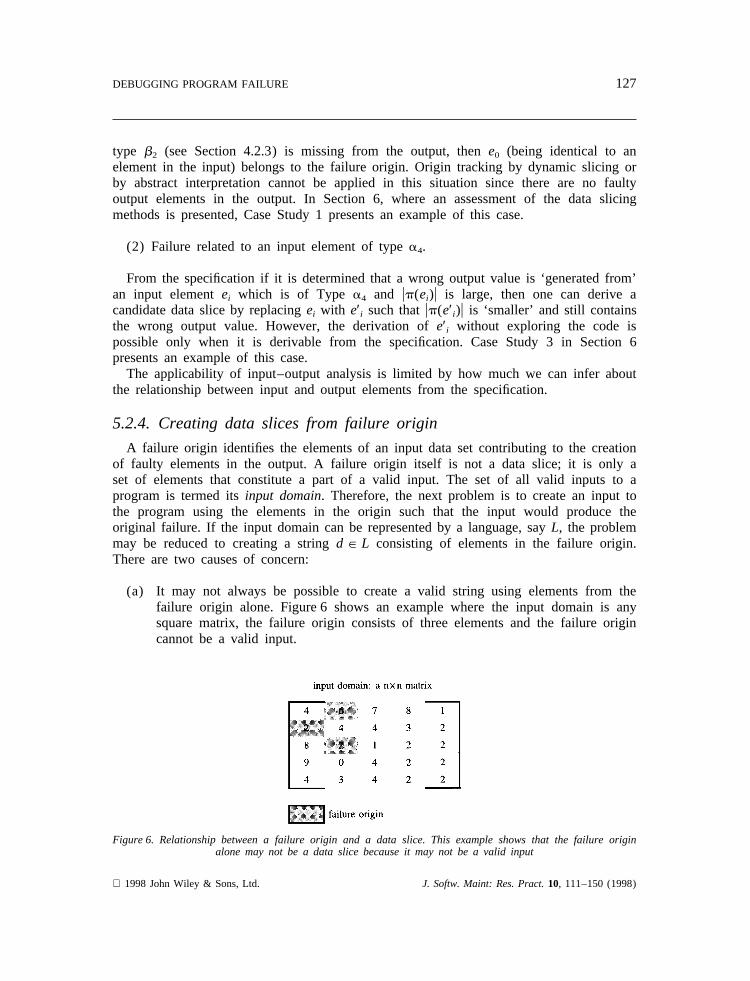
(a) It may not always be possible to create a valid string using elements from thefailure origin alone. Figure 6 shows an example where the input domain is anysquare matrix, the failure origin consists of three elements and the failure origincannot be a valid input.
Figure 6. Relationship between a failure origin and a data slice. This example shows that the failure originalone may not be a data slice because it may not be a valid input
1998 John Wiley & Sons, Ltd. J. Softw. Maint: Res. Pract.10, 111–150 (1998)
128 T. W. CHAN and A. LAKHOTIA
(b) When it is possible to create a valid string using the failure origin, the resultingstring may still not be a data slice.
The first problem can be solved by using some ‘filler’ elements along with the failureorigin to create a syntactically valid string. Ensuring that the resulting string will be adata slice is a harder problem. In the following, we discuss, for each input domain, howone may consider creating data slices after obtaining thefailure origin.
5.2.4.1. Input domain is of primitive typeIf the input domain consists solely of elementsof a primitive type such as integers, the best way to create a data slice is byinvarianceanalysis. Dynamic slicing does not reduce the input data set since the whole input datawould be in the failure origin.
Thus, for a factorial program that fails for input 5, the failure origin would be {5}.
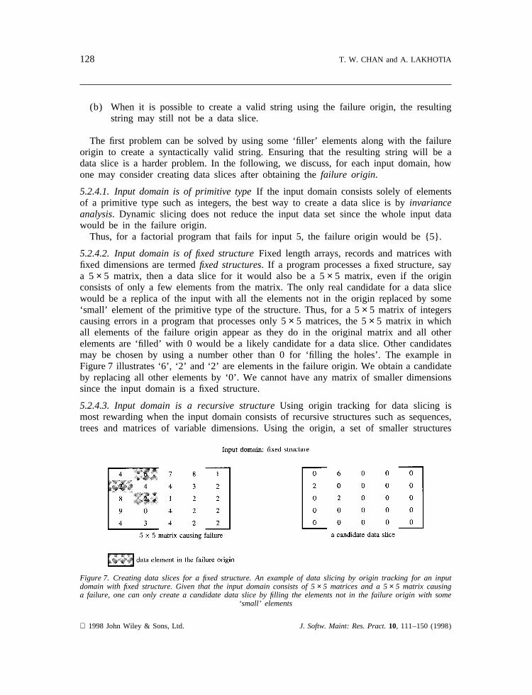
5.2.4.2. Input domain is of fixed structureFixed length arrays, records and matrices withfixed dimensions are termedfixed structures. If a program processes a fixed structure, saya 5× 5 matrix, then a data slice for it would also be a 5× 5 matrix, even if the originconsists of only a few elements from the matrix. The only real candidate for a data slicewould be a replica of the input with all the elements not in the origin replaced by some‘small’ element of the primitive type of the structure. Thus, for a 5× 5 matrix of integerscausing errors in a program that processes only 5× 5 matrices, the 5× 5 matrix in whichall elements of the failure origin appear as they do in the original matrix and all otherelements are ‘filled’ with 0 would be a likely candidate for a data slice. Other candidatesmay be chosen by using a number other than 0 for ‘filling the holes’. The example inFigure 7 illustrates ‘6’, ‘2’ and ‘2’ are elements in the failure origin. We obtain a candidateby replacing all other elements by ‘0’. We cannot have any matrix of smaller dimensionssince the input domain is a fixed structure.
5.2.4.3. Input domain is a recursive structureUsing origin tracking for data slicing ismost rewarding when the input domain consists of recursive structures such as sequences,trees and matrices of variable dimensions. Using the origin, a set of smaller structures
Figure 7. Creating data slices for a fixed structure. An example of data slicing by origin tracking for an inputdomain with fixed structure. Given that the input domain consists of 5× 5 matrices and a 5× 5 matrix causinga failure, one can only create a candidate data slice by filling the elements not in the failure origin with some
‘small’ elements
1998 John Wiley & Sons, Ltd. J. Softw. Maint: Res. Pract.10, 111–150 (1998)
129DEBUGGING PROGRAM FAILURE
can be heuristically generated such that one of its elements may be a data slice. This setis generated based on the following classification of relationships between a failure andthe failure origin.
• Absolute position dependent: the failure depends upon the position of the elementsof the failure origin in the input data.
• Relative position dependent: the failure depends upon the relative position of elementswithin the failure origin.
• Order dependent: the failure depends upon the ordering of elements in the failure ori-gin.
• Content dependent: the failure depends upon just the collection of elements in theirfailure origin.
Notice that the relationships are presented in decreasing order of strength, i.e., arelationship subsumes all subsequent relationships. Thus, if a failure depends upon theabsolute position of the elements of the failure origin, it also depends upon the relativeposition, order and content. A set of candidate data slices may be created by creatingdata items that contain all the elements of the failure origin and also preserve the absoluteposition relation, relative position relation or order relation between them. The strongerthe relationship a data item preserves, the greater chance it has of being a data slice (dueto the subsumption of relations). However, such a data item would also be larger, henceof less value in debugging, than the data items preserving the weaker relationships. Theaim is to find the smallest of these items that is also a data slice. Some of the candidatedata items may be ignored using program specific knowledge. For the remaining dataitems, whether they are data slices may be determined by testing the program with themas input. This testing may be performed in the order of the size of the data items.
Sequences: If the input domain consists of sequences, the set of sequences that maybe considered for data slices, based on the above rules, would be:
(1) The sequences consisting of elements in origin ordered as in the original inputsequence (order dependent).
(2) The smallest subsequence of the original data containing all elements of the origin(relative position dependent).
(3) The smallest prefix of the original data containing all elements of the origin(absolute position dependent).
(4) The smallest suffix of the original data containing all elements of the origin(absolute position dependent).
(5) A sequence generated using techniques for fixed structures (absolute positiondependent).
The first sequence would be a data slice if the error depends only upon the elementsin the origin and their relative order. The second sequence would be a data slice if therelative positions of these elements are important too. If the absolute position of theseelements from the beginning (or end) of the original sequence influences the failure thenthe third (or fourth) sequence would be a data slice. If the absolute positions from both
1998 John Wiley & Sons, Ltd. J. Softw. Maint: Res. Pract.10, 111–150 (1998)
130 T. W. CHAN and A. LAKHOTIA
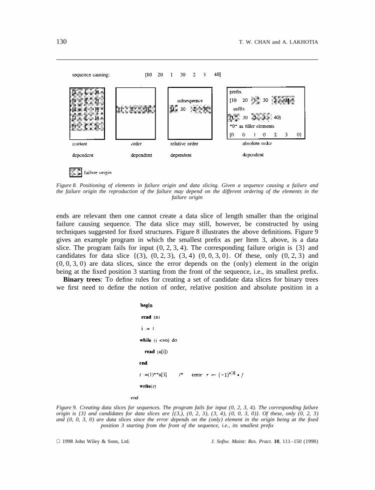
Figure 8. Positioning of elements in failure origin and data slicing. Given a sequence causing a failure andthe failure origin the reproduction of the failure may depend on the different ordering of the elements in the
failure origin
ends are relevant then one cannot create a data slice of length smaller than the originalfailure causing sequence. The data slice may still, however, be constructed by usingtechniques suggested for fixed structures. Figure 8 illustrates the above definitions. Figure 9gives an example program in which the smallest prefix as per Item 3, above, is a dataslice. The program fails for input (0, 2, 3, 4). The corresponding failure origin is {3} andcandidates for data slice {(3), (0, 2, 3), (3, 4) (0, 0, 3, 0}. Of these, only (0, 2, 3) and(0, 0, 3, 0) are data slices, since the error depends on the (only) element in the originbeing at the fixed position 3 starting from the front of the sequence, i.e., its smallest prefix.
Binary trees: To define rules for creating a set of candidate data slices for binary treeswe first need to define the notion of order, relative position and absolute position in a
Figure 9. Creating data slices for sequences. The program fails for input (0, 2, 3, 4). The corresponding failureorigin is {3} and candidates for data slices are {(3,), (0, 2, 3), (3, 4), (0, 0, 3, 0)}. Of these, only (0, 2, 3)and (0, 0, 3, 0) are data slices since the error depends on the (only) element in the origin being at the fixed
position 3 starting from the front of the sequence, i.e., its smallest prefix
1998 John Wiley & Sons, Ltd. J. Softw. Maint: Res. Pract.10, 111–150 (1998)

131DEBUGGING PROGRAM FAILURE
binary tree. The ordering of elements of a tree may be defined based upon the strategyused for traversing its elements. The traversal strategies may be broadly classified as:depth-first and breadth-first. Amongst these there may be further classifications, forinstance, infix, prefix, or postfix depth-first traversal, or left-to-right, or right-to-left breadthfirst traversal.
We use the following for defining the relative and absolute positions.
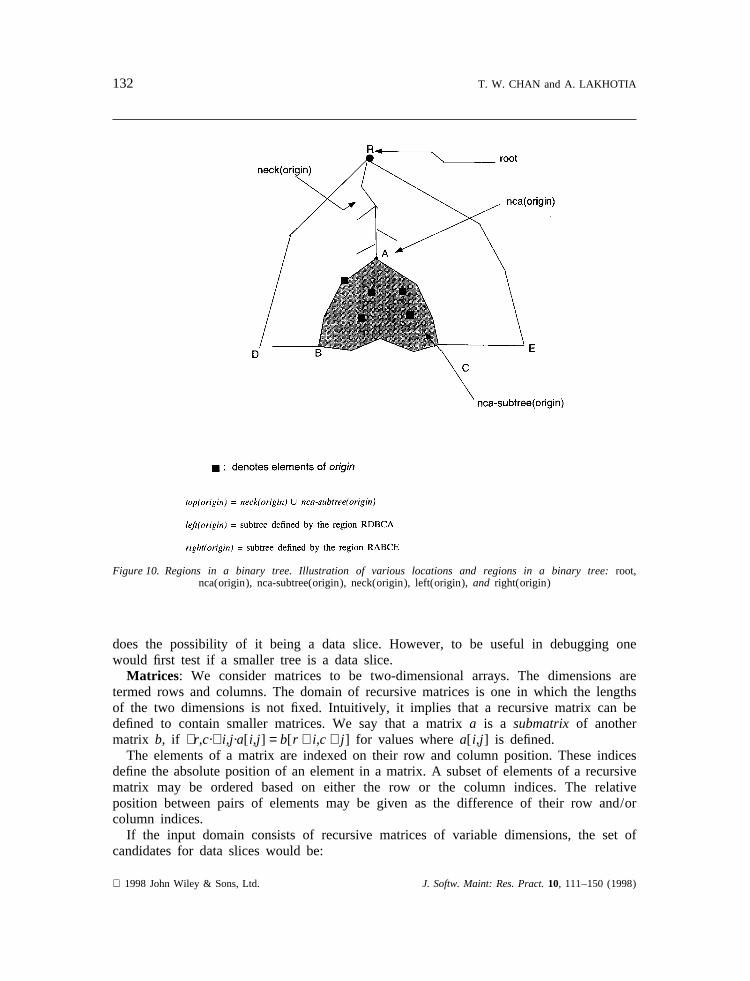
• root: the root node of the original tree.• nca(origin): the nearest common ancestor of all the elements in anorigin.• nca-subtree(origin): the subtree rooted at thenca(origin).• neck(origin): the branch i.e., nodes and edges, on the path from theroot to
nca(origin), both inclusive.• top(origin): the tree consisting ofnca-subtree(origin)and neck(origin).• left(origin): the tree consisting oftop(origin) and all the subtrees rooted on the left
branches of nodes inneck(origin).• right(origin): the tree consisting oftop(origin) and all the subtrees rooted on the
right branches of nodes inneck(origin).
To avoid clutter, the original input tree is left implicit and not specified as a parameter.Figure 10 illustrates the above definition.
The nca(origin) preserves the relative positions between the elements of the failureorigin, for any type of depth-first traversal. Therefore, this tree is used in creating relativeposition dependent candidates for a data slice.
The absolute positions of the elements of the failure origin may be defined relative to(a) the root of the original tree, or (b) its left-most leaf, or (c) its right-most leaf. Anexample of a program failure that depends upon absolute position from the root is afailure that depends on an element appearing at a specific depth in a tree. Similarly, afailure may depend upon an absolute position from the left or right if the failure is causedby an element occurring at a specific position in a depth-first or breadth-first traversal.The subtreestop(origin), left(origin), and right(origin), respectively, preserve these absol-ute positions and may be used to create candidate data slices.
The set of candidates for data slices for a tree therefore consists of:
(1) The smallest tree containing elements from the origin ordered on the traversalstrategy used by the program (order dependent).
(2) The nca-subtree(origin)(relative position dependent).(3) The top(origin) (absolute position dependent).(4) The left(origin) and right(origin) subtrees (absolute position dependent).(5) The trees created by treating the original tree as a fixed structure (absolute
position dependent).
The first subtree is too dependent upon the traversal strategy. In most circumstancesone may first create thenca-subtree, Item 2 above, since it satisfies the requirements forthe first. From the second to the fifth subtree the size of a candidate subtree increases as
1998 John Wiley & Sons, Ltd. J. Softw. Maint: Res. Pract.10, 111–150 (1998)
132 T. W. CHAN and A. LAKHOTIA
Figure 10. Regions in a binary tree. Illustration of various locations and regions in a binary tree:root,nca(origin), nca-subtree(origin), neck(origin), left(origin),and right(origin)
does the possibility of it being a data slice. However, to be useful in debugging onewould first test if a smaller tree is a data slice.
Matrices: We consider matrices to be two-dimensional arrays. The dimensions aretermed rows and columns. The domain of recursive matrices is one in which the lengthsof the two dimensions is not fixed. Intuitively, it implies that a recursive matrix can bedefined to contain smaller matrices. We say that a matrixa is a submatrix of anothermatrix b, if ∃r,c·∀i,j·a[ i,j ] = b[ r + i,c + j ] for values wherea[ i,j ] is defined.
The elements of a matrix are indexed on their row and column position. These indicesdefine the absolute position of an element in a matrix. A subset of elements of a recursivematrix may be ordered based on either the row or the column indices. The relativeposition between pairs of elements may be given as the difference of their row and/orcolumn indices.
If the input domain consists of recursive matrices of variable dimensions, the set ofcandidates for data slices would be:
1998 John Wiley & Sons, Ltd. J. Softw. Maint: Res. Pract.10, 111–150 (1998)

133DEBUGGING PROGRAM FAILURE
(1) The matrix constructed by removing all rows and columns not containing anyelement in the origin (order dependent).
(2) The matrix constructed by removing all columns not containing any element inthe origin (order dependent).
(3) The matrix constructed by removing all rows not containing any element in theorigin (order dependent).
(4) The smallest submatrix containing all elements of the origin (relative positiondependent).
(5) The smallest submatrix containing all rows containing any element of the origin(relative position dependent).
(6) The smallest submatrix containing all columns containing any element of theorigin (relative position dependent).
(7) The smallest submatrix containing the first row of the original matrix and allelements of the origin (absolute position dependent).
(8) The smallest submatrix containing the last row of the original matrix and allelements of the origin (absolute position dependent).
(9) The smallest submatrix containing the first column of the original matrix and allelements of the origin (absolute position dependent).
(10) The smallest submatrix containing a last column of the original matrix and allelements of the origin (absolute position dependent).
(11) The matrices created by treating the original matrix as a fixed structure.
Once again, the size of the candidate matrices, listed above, increases as does theprobability of their being a data slice. For the greatest help in debugging, one would testwhether a smaller candidate matrix is a data slice first. The set may be pruned by usingprogram-specific knowledge.
5.3. Data slicing by random eliminationWhen invariance analysis and origin tracking are not applicable or cannot produce
small enough data slices, data slicing can be done (or further done) by this method. Forrecursive structures, we can randomly eliminate some elements from the input data toobtain candidate data slices. For instance, if ann × n matrix is input to a program, wemay randomly drop some rows and columns and check whether it is a data slice bytesting the program with it as input.
For fixed structures, we may try to obtain a data slice by replacing some elements inthe input by some ‘small’ elements, such as 0’s. The ‘small’ elements used for replacementare called ‘filler’ elements.
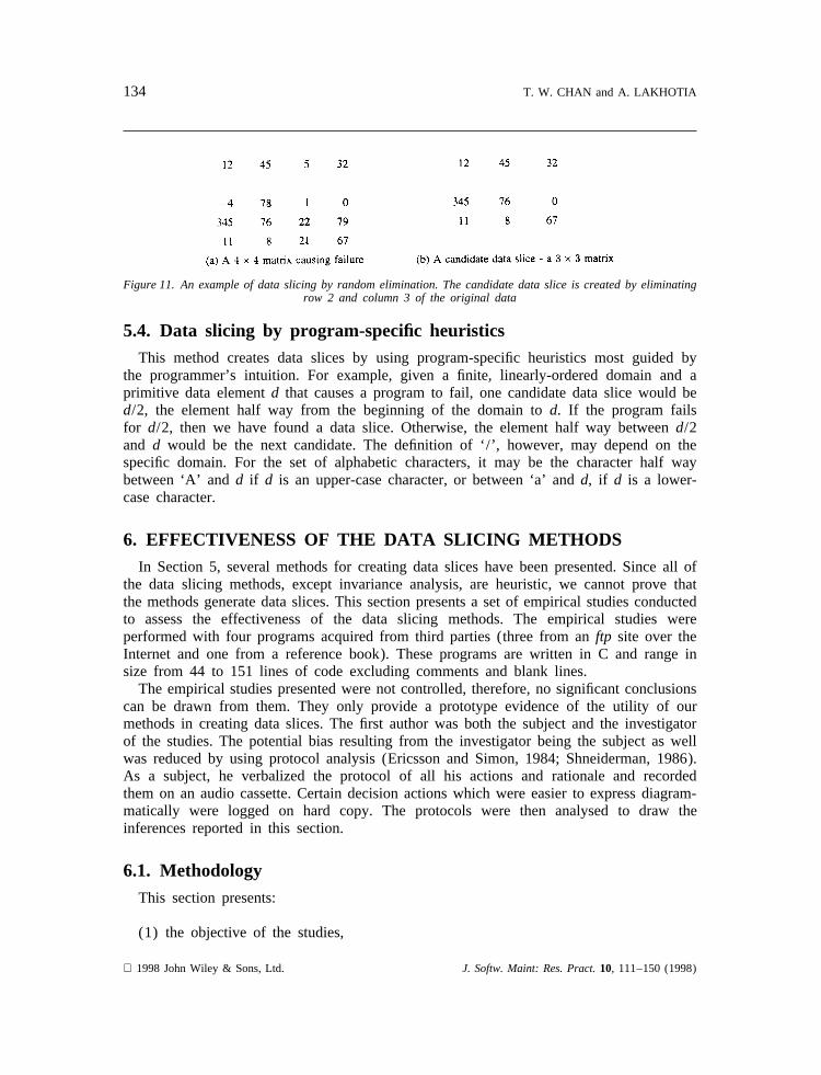
5.3.1. Example using random eliminationConsider a program that processes ann × n matrix and fails on the 4× 4 matrix given
in Figure 11(a). We can randomly eliminate a row and a column, say row 2 and column3 to obtain a candidate data slice. The candidate data slice is shown in Figure 11(b).
Data slicing by random elimination is most applicable where other methods are notapplicable or when a quick attempt at data slicing is desired.
1998 John Wiley & Sons, Ltd. J. Softw. Maint: Res. Pract.10, 111–150 (1998)
134 T. W. CHAN and A. LAKHOTIA
Figure 11. An example of data slicing by random elimination. The candidate data slice is created by eliminatingrow 2 and column 3 of the original data
5.4. Data slicing by program-specific heuristicsThis method creates data slices by using program-specific heuristics most guided by
the programmer’s intuition. For example, given a finite, linearly-ordered domain and aprimitive data elementd that causes a program to fail, one candidate data slice would bed/2, the element half way from the beginning of the domain tod. If the program failsfor d/2, then we have found a data slice. Otherwise, the element half way betweend/2and d would be the next candidate. The definition of ‘/’, however, may depend on thespecific domain. For the set of alphabetic characters, it may be the character half waybetween ‘A’ andd if d is an upper-case character, or between ‘a’ andd, if d is a lower-case character.
6. EFFECTIVENESS OF THE DATA SLICING METHODSIn Section 5, several methods for creating data slices have been presented. Since all of
the data slicing methods, except invariance analysis, are heuristic, we cannot prove thatthe methods generate data slices. This section presents a set of empirical studies conductedto assess the effectiveness of the data slicing methods. The empirical studies wereperformed with four programs acquired from third parties (three from anftp site over theInternet and one from a reference book). These programs are written in C and range insize from 44 to 151 lines of code excluding comments and blank lines.
The empirical studies presented were not controlled, therefore, no significant conclusionscan be drawn from them. They only provide a prototype evidence of the utility of ourmethods in creating data slices. The first author was both the subject and the investigatorof the studies. The potential bias resulting from the investigator being the subject as wellwas reduced by using protocol analysis (Ericsson and Simon, 1984; Shneiderman, 1986).As a subject, he verbalized the protocol of all his actions and rationale and recordedthem on an audio cassette. Certain decision actions which were easier to express diagram-matically were logged on hard copy. The protocols were then analysed to draw theinferences reported in this section.
6.1. MethodologyThis section presents:
(1) the objective of the studies,
1998 John Wiley & Sons, Ltd. J. Softw. Maint: Res. Pract.10, 111–150 (1998)

135DEBUGGING PROGRAM FAILURE
(2) the source of the subject programs used in the study,(3) the criteria for selecting the programs, and(4) the procedure followed:
• to induce faults in each program and• to monitor the activities performed to create data slices.
6.1.1. Objective
The objective of our study was to show that:the data slicing methods presented canbe used to create data slices.
It was not our objective to assess whether the data slices are indeed helpful indebugging, though from the reduction in processing size, one may infer that the data slicewould reduce the debugging time.
6.1.2. Subject programs
Four programs were chosen from a set of 27. Of these, 26 programs were obtainedfrom New York University (made available by Tarak Goradia, currently at Siemens(Goradia, 1993)). Goradia used these programs for his Ph.D. dissertation. One programwas taken from a book on C programming (Burkhard, 1988). The collection of programsfrom NYU (a) spans a diverse application domain, including tax computation, banking,graph algorithms, matrix computation and symbolic algebra, and (b) is available with asuite of test data for each program.
We chose the four programs such that they:
(a) represented different types of input and output domains, i.e., primitive, fixedstructure and recursive structures, and
(b) represented programs establishing different types of relationships between theelements of the input and output, namely Typesai and bi, i = 1,. . .,4 (seeSection 4.2.3).
Table 1 shows the properties of the four subject programs, such as their input, output,the types of relationships between elements of the input and the output, the type offailure, and the data slicing technique used in the study.
6.1.3. Procedure for introducing faults
We were interested in programs which failed on a small set of test cases only (lessthan one third of the total test cases presented). It made the studies more realistic sincethe hypothesis is that failures exhibited by large data in production code—code that hasbeen tested and is released for use—are harder to reproduce by smaller data. If a programfailed for a majority of test cases, then the problem of reproducing the failure withsmaller data would be moot.
Faulty versions of the collection of programs were created by mutating each program(Mathur, 1991; White, 1987; Budd, 1981). To mutate a program means to modify it by
1998 John Wiley & Sons, Ltd. J. Softw. Maint: Res. Pract.10, 111–150 (1998)
136 T. W. CHAN and A. LAKHOTIA
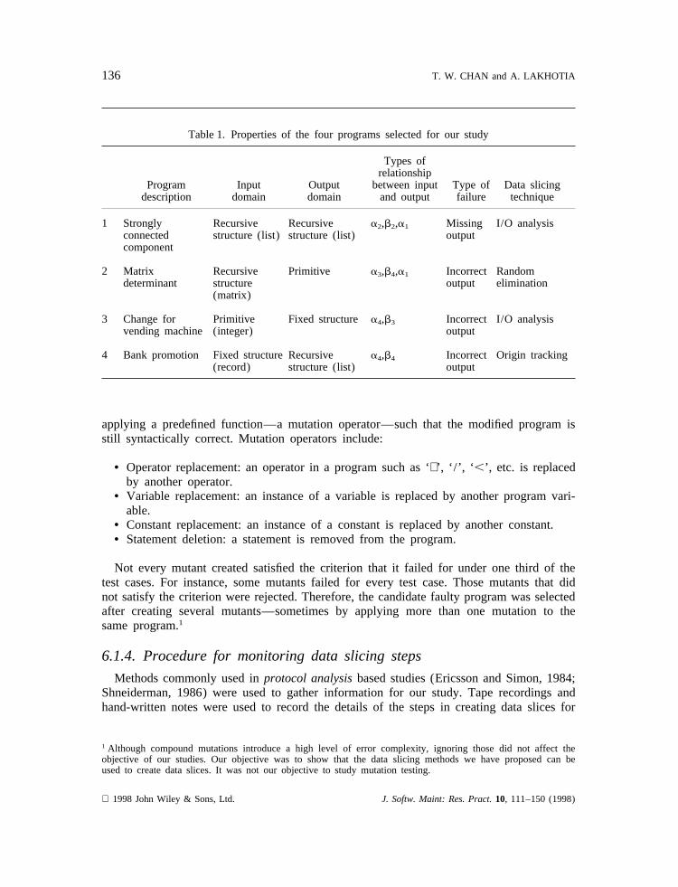
Table 1. Properties of the four programs selected for our study
Types ofrelationship
Program Input Output between input Type of Data slicingdescription domain domain and output failure technique
1 Strongly Recursive Recursive a2,b2,a1 Missing I/O analysisconnected structure (list) structure (list) outputcomponent
2 Matrix Recursive Primitive a3,b4,a1 Incorrect Randomdeterminant structure output elimination
(matrix)
3 Change for Primitive Fixed structurea4,b3 Incorrect I/O analysisvending machine (integer) output
4 Bank promotion Fixed structure Recursive a4,b4 Incorrect Origin tracking(record) structure (list) output
applying a predefined function—a mutation operator—such that the modified program isstill syntactically correct. Mutation operators include:
• Operator replacement: an operator in a program such as ‘+’, ‘/’, ‘ ,’, etc. is replacedby another operator.
• Variable replacement: an instance of a variable is replaced by another program vari-able.
• Constant replacement: an instance of a constant is replaced by another constant.• Statement deletion: a statement is removed from the program.
Not every mutant created satisfied the criterion that it failed for under one third of thetest cases. For instance, some mutants failed for every test case. Those mutants that didnot satisfy the criterion were rejected. Therefore, the candidate faulty program was selectedafter creating several mutants—sometimes by applying more than one mutation to thesame program.1
6.1.4. Procedure for monitoring data slicing steps
Methods commonly used inprotocol analysisbased studies (Ericsson and Simon, 1984;Shneiderman, 1986) were used to gather information for our study. Tape recordings andhand-written notes were used to record the details of the steps in creating data slices for
1 Although compound mutations introduce a high level of error complexity, ignoring those did not affect theobjective of our studies. Our objective was to show that the data slicing methods we have proposed can beused to create data slices. It was not our objective to study mutation testing.
1998 John Wiley & Sons, Ltd. J. Softw. Maint: Res. Pract.10, 111–150 (1998)
137DEBUGGING PROGRAM FAILURE
each program. The recorded information was then analysed and abstracted before presen-tation in this paper.
6.1.5. Effectiveness of data slicing in experiments
In order to evaluate the effectiveness of the data slicing methods, we measured thereduction in processing size achieved by the data slice. The processing size was measuredby instrumenting the program usingbtool—a branch coverage tool intended for softwaretest coverage analysis—to obtain the number of times that various loops (implicit orexplicit) are iterated (Hoch, Marick and Schafer, 1990). The reduction of the number ofiterations of loops in an execution of the program due to the data slice was used tomeasure the effectiveness.
6.2. Details of empirical studies
For each case study we present the following:
• a description of the subject program, its input and the expected output;• a summary observation of the behaviour of the program on our test cases, a description
of the data on which it failed and a description of the failure;• a classification of the program based on the types of its input and output domains;• details of the steps in creating a data slice from the original failure-causing data;• a discussion of lessons learned;• an analysis of the effectiveness of the data slicing methods used.
6.2.1. Case study 1
Program: This study involved program number 24 from NYU. This program finds thestrongly-connected components of a directed graph.
Input : The input consists of two parts. The first part consists of just one integer givingthe maximum number of nodes in the graph. The second part is a variable length list ofedges in the graph, represented as pairs of nodes. A node is represented by an integerbetween one and the maximum number of nodes.
Expected output: The program outputs the set of connected components in graph. Eachconnected component consists of a set of nodes. Every node in the graph is expected tobe in one and only one connected component.
Observed behaviour: Of the 50 test cases, the program worked correctly for 40. Itfailed with an input containing eight nodes and 14 edges. The error was obvious in thatcertain nodes did not appear in the output at all.
Program classification: All elements in the output of this program are of Typeb2 i.e.,they are generated from the same element in the input. Similarly, all elements in thesecond part of the input belong to the Typea2 in that each generates in the output anelement identical to itself. The first part of the input, the number of nodes in the graph,does not generate anything in the output and hence is of Typea1.
Data slicing details: Given that the input and the output elements of this program are
1998 John Wiley & Sons, Ltd. J. Softw. Maint: Res. Pract.10, 111–150 (1998)
138 T. W. CHAN and A. LAKHOTIA
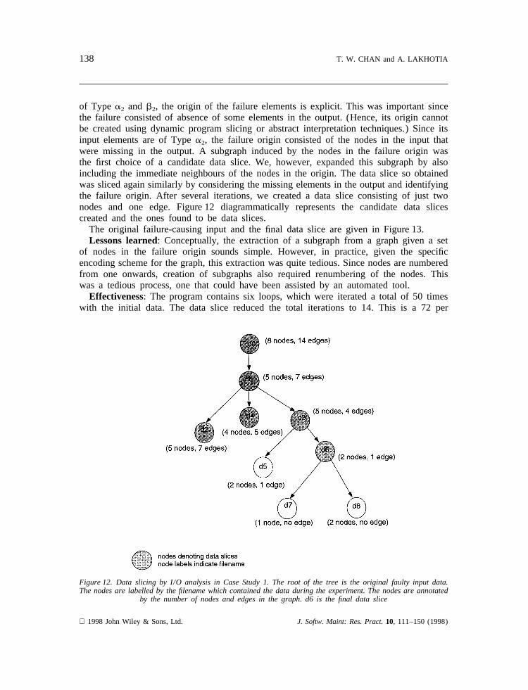
of Type a2 and b2, the origin of the failure elements is explicit. This was important sincethe failure consisted of absence of some elements in the output. (Hence, its origin cannotbe created using dynamic program slicing or abstract interpretation techniques.) Since itsinput elements are of Typea2, the failure origin consisted of the nodes in the input thatwere missing in the output. A subgraph induced by the nodes in the failure origin wasthe first choice of a candidate data slice. We, however, expanded this subgraph by alsoincluding the immediate neighbours of the nodes in the origin. The data slice so obtainedwas sliced again similarly by considering the missing elements in the output and identifyingthe failure origin. After several iterations, we created a data slice consisting of just twonodes and one edge. Figure 12 diagrammatically represents the candidate data slicescreated and the ones found to be data slices.
The original failure-causing input and the final data slice are given in Figure 13.Lessons learned: Conceptually, the extraction of a subgraph from a graph given a set
of nodes in the failure origin sounds simple. However, in practice, given the specificencoding scheme for the graph, this extraction was quite tedious. Since nodes are numberedfrom one onwards, creation of subgraphs also required renumbering of the nodes. Thiswas a tedious process, one that could have been assisted by an automated tool.
Effectiveness: The program contains six loops, which were iterated a total of 50 timeswith the initial data. The data slice reduced the total iterations to 14. This is a 72 per
Figure 12. Data slicing by I/O analysis in Case Study 1. The root of the tree is the original faulty input data.The nodes are labelled by the filename which contained the data during the experiment. The nodes are annotated
by the number of nodes and edges in the graph. d6 is the final data slice
1998 John Wiley & Sons, Ltd. J. Softw. Maint: Res. Pract.10, 111–150 (1998)
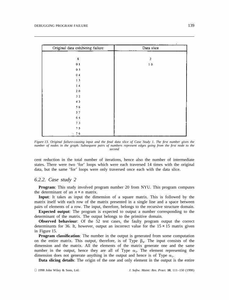
139DEBUGGING PROGRAM FAILURE
Figure 13. Original failure-causing input and the final data slice of Case Study 1. The first number gives thenumber of nodes in the graph. Subsequent pairs of numbers represent edges going from the first node to the
second
cent reduction in the total number of iterations, hence also the number of intermediatestates. There were two ‘for’ loops which were each traversed 14 times with the originaldata, but the same ‘for’ loops were only traversed once each with the data slice.
6.2.2. Case study 2
Program: This study involved program number 20 from NYU. This program computesthe determinant of ann × n matrix.
Input : It takes as input the dimension of a square matrix. This is followed by thematrix itself with each row of the matrix presented in a single line and a space betweenpairs of elements of a row. The input, therefore, belongs to the recursive structure domain.
Expected output: The program is expected to output a number corresponding to thedeterminant of the matrix. The output belongs to the primitive domain.
Observed behaviour: Of the 52 test cases, the faulty program output the correctdeterminants for 36. It, however, output an incorrect value for the 15× 15 matrix givenin Figure 15.
Program classification: The number in the output is generated from some computationon the entire matrix. This output, therefore, is of Typeb4. The input consists of thedimension and the matrix. All the elements of the matrix generate one and the samenumber in the output, hence they are all of Typea3. The element representing thedimension does not generate anything in the output and hence is of Typea1.
Data slicing details: The origin of the one and only element in the output is the entire
1998 John Wiley & Sons, Ltd. J. Softw. Maint: Res. Pract.10, 111–150 (1998)
140 T. W. CHAN and A. LAKHOTIA
matrix, since the output element is of Typeb4. Hence, using origin tracking was ruledout. Since the relationship between the input and output for this program is too complex,using I/O analysis was ruled out too. The only choice we were left with was to userandom elimination and invariance analysis, of which we chose the former. Candidatedata slices were created by randomly eliminating one or more rows and the same numberof columns from a matrix causing a failure.
Starting with the 15× 15 matrix, we produced the 3× 3 matrix, both in Figure 15,where the latter was a data slice of the former. In the course of creating the data slice,10 other matrices were created, of which six were not data slices and the remaining fourwere data slices. To find a smaller data slice, nine other 2× 2 matrices were created fromthe 3× 3 matrix. None of these matrices recreated the failure. The first four candidateswe created, in succession from one another, were data slices, the last one a 5× 5 matrix.To derive a 4× 4 data slice required generating four candidates, three of which were notdata slices. Generating the final 3× 3 data slice also required creating four candidates,three of which were not data slices.
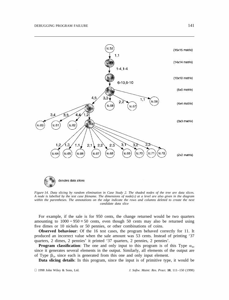
In Figure 14, a tree showing the process of data slicing by random elimination inExperiment 2 is given. All the shaded nodes are data slices. The nodes are labelled bytest case filename. A tree edge (v1, v2) is labelled by the range of rows and columnswhich are dropped to obtain v2 from v1.
The original, failure-causing input and the final data slice are given in Figure 15.Lessons learned: Candidate data slices were created by eliminating rows and columns
from another matrix. This was done with the help of a text editor (in this case ‘vi’).Though possible, the task was very cumbersome at the initial stages when the matriceswere large (15× 15, 14× 14 and 10× 10). Had the initial faulty matrix been larger, say200× 200, as in our case study in Section 2.1, deleting its rows and correspondingcolumns using a text editor would be a torture. Doing so by a program that edits matriceswould be more convenient. If our programs were to be used and supported commercially,we would have built such a program.
Effectiveness: The program contains 10 loops which were iterated a total of 1192 timeswith the initial data. The data slice reduced the total iterations to 36. This is a 96.9 percent reduction in the number of iterations, hence also the number of intermediate states.There was one ‘for’ loop which was traversed 509 times with the original data, but thesame ‘for’ loop was only traversed four times in the data slice.
6.2.3. Case study 3Program: This study involved a program in a book on C programming (Burkhard,
1988). The program computes change returned by a vending machine.Input : The input to the program is an integer representing the cost of an item in cents.Expected output: It outputs the change returned by the vending machine assuming that
the customer pays $10. The change is returned in quarters (25 cents), dimes (10 cents),nickels (5 cents) and pennies (1 cent). The change is computed assuming that there isno shortage of coins of any denomination. The answer is expected to be unique eventhough a given amount of money may be returned using more than one combinationof change. The uniqueness is achieved by returning a coin of higher denominationwhenever possible.
1998 John Wiley & Sons, Ltd. J. Softw. Maint: Res. Pract.10, 111–150 (1998)
141DEBUGGING PROGRAM FAILURE
Figure 14. Data slicing by random elimination in Case Study 2. The shaded nodes of the tree are data slices.A node is labelled by the test case filename. The dimensions of node(s) at a level are also given in the diagramwithin the parentheses. The annotations on the edge indicate the rows and columns deleted to create the next
candidate data slice
For example, if the sale is for 950 cents, the change returned would be two quartersamounting to 1000− 950= 50 cents, even though 50 cents may also be returned usingfive dimes or 10 nickels or 50 pennies, or other combinations of coins.
Observed behaviour: Of the 16 test cases, the program behaved correctly for 11. Itproduced an incorrect value when the sale amount was 53 cents. Instead of printing ‘37quarters, 2 dimes, 2 pennies’ it printed ‘37 quarters, 2 pennies, 2 pennies’.
Program classification: The one and only input to this program is of this Typea4,since it generates several elements in the output. Similarly, all elements of the output areof Type b3, since each is generated from this one and only input element.
Data slicing details: In this program, since the input is of primitive type, it would be
1998 John Wiley & Sons, Ltd. J. Softw. Maint: Res. Pract.10, 111–150 (1998)

142 T. W. CHAN and A. LAKHOTIA
Figure 15. Original failure-causing input and the final data slice of Case Study 2
in the origin of all the elements in the output, hence origin tracking would not provideany new information.
From the analysis of the incorrect output, it appears that the program prints ‘pennies’when it is expected to print ‘dimes’. A sale that requires only dimes to be returned aschange would be a good candidate data slice.
As a first step we created a sale value so as to not return any quarters. This was done
1998 John Wiley & Sons, Ltd. J. Softw. Maint: Res. Pract.10, 111–150 (1998)
143DEBUGGING PROGRAM FAILURE
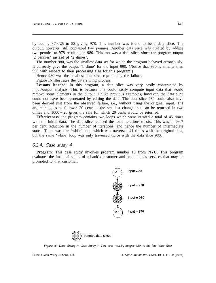
by adding 37× 25 to 53 giving 978. This number was found to be a data slice. Theoutput, however, still contained two pennies. Another data slice was created by addingtwo pennies to 978 resulting in 980. This too was a data slice, since the program output‘2 pennies’ instead of ‘2 dimes’.
The number 980, was the smallest data set for which the program behaved erroneously.It correctly gave the output ‘1 dime’ for the input 990. (Notice that 980 is smaller than990 with respect to their processing size for this program.)
Hence 980 was the smallest data slice reproducing the failure.Figure 16 illustrates the data slicing process.Lessons learned: In this program, a data slice was very easily constructed by
input/output analysis. This is because one could easily compute input data that wouldremove some elements in the output. Unlike previous examples, however, the data slicecould not have been generated by editing the data. The data slice 980 could also havebeen derived just from the observed failure, i.e., without using the original input. Theargument goes as follows: 20 cents is the smallest change that can be returned in twodimes and 1000− 20 gives the sale for which 20 cents would be returned.
Effectiveness: the program contains two loops which were iterated a total of 45 timeswith the initial data. The data slice reduced the total iterations to six. This was an 86.7per cent reduction in the number of iterations, and hence the number of intermediatestates. There was one ‘while’ loop which was traversed 41 times with the original data,but the same ‘while’ loop was only traversed twice with the data slice 980.
6.2.4. Case study 4
Program: This case study involves program number 19 from NYU. This programevaluates the financial status of a bank’s customer and recommends services that may bepromoted to that customer.
Figure 16. Data slicing in Case Study 3. Test case ‘tc.18’, integer 980, is the final data slice
1998 John Wiley & Sons, Ltd. J. Softw. Maint: Res. Pract.10, 111–150 (1998)
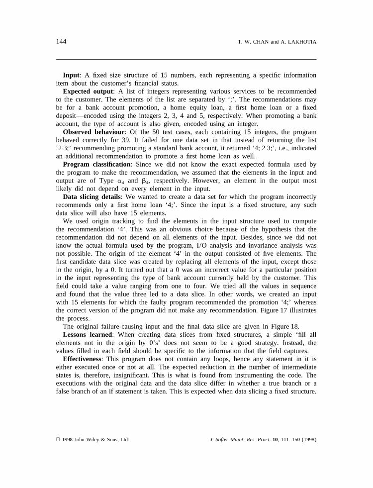
144 T. W. CHAN and A. LAKHOTIA
Input : A fixed size structure of 15 numbers, each representing a specific informationitem about the customer’s financial status.
Expected output: A list of integers representing various services to be recommendedto the customer. The elements of the list are separated by ‘;’. The recommendations maybe for a bank account promotion, a home equity loan, a first home loan or a fixeddeposit—encoded using the integers 2, 3, 4 and 5, respectively. When promoting a bankaccount, the type of account is also given, encoded using an integer.
Observed behaviour: Of the 50 test cases, each containing 15 integers, the programbehaved correctly for 39. It failed for one data set in that instead of returning the list‘2 3;’ recommending promoting a standard bank account, it returned ‘4; 2 3;’, i.e., indicatedan additional recommendation to promote a first home loan as well.
Program classification: Since we did not know the exact expected formula used bythe program to make the recommendation, we assumed that the elements in the input andoutput are of Typea4 and b4, respectively. However, an element in the output mostlikely did not depend on every element in the input.
Data slicing details: We wanted to create a data set for which the program incorrectlyrecommends only a first home loan ‘4;’. Since the input is a fixed structure, any suchdata slice will also have 15 elements.
We used origin tracking to find the elements in the input structure used to computethe recommendation ‘4’. This was an obvious choice because of the hypothesis that therecommendation did not depend on all elements of the input. Besides, since we did notknow the actual formula used by the program, I/O analysis and invariance analysis wasnot possible. The origin of the element ‘4’ in the output consisted of five elements. Thefirst candidate data slice was created by replacing all elements of the input, except thosein the origin, by a 0. It turned out that a 0 was an incorrect value for a particular positionin the input representing the type of bank account currently held by the customer. Thisfield could take a value ranging from one to four. We tried all the values in sequenceand found that the value three led to a data slice. In other words, we created an inputwith 15 elements for which the faulty program recommended the promotion ‘4;’ whereasthe correct version of the program did not make any recommendation. Figure 17 illustratesthe process.
The original failure-causing input and the final data slice are given in Figure 18.Lessons learned: When creating data slices from fixed structures, a simple ‘fill all
elements not in the origin by 0’s’ does not seem to be a good strategy. Instead, thevalues filled in each field should be specific to the information that the field captures.
Effectiveness: This program does not contain any loops, hence any statement in it iseither executed once or not at all. The expected reduction in the number of intermediatestates is, therefore, insignificant. This is what is found from instrumenting the code. Theexecutions with the original data and the data slice differ in whether a true branch or afalse branch of an if statement is taken. This is expected when data slicing a fixed structure.
1998 John Wiley & Sons, Ltd. J. Softw. Maint: Res. Pract.10, 111–150 (1998)
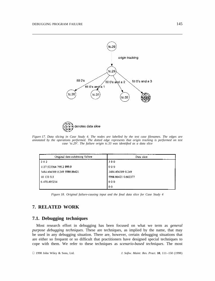
145DEBUGGING PROGRAM FAILURE
Figure 17. Data slicing in Case Study 4. The nodes are labelled by the test case filenames. The edges areannotated by the operations performed. The dotted edge represents that origin tracking is performed on test
case ‘tc.29’. The failure origin tc.33 was identified as a data slice
Figure 18. Original failure-causing input and the final data slice for Case Study 4
7. RELATED WORK
7.1. Debugging techniquesMost research effort in debugging has been focused on what we term asgeneral
purpose debugging techniques. These are techniques, as implied by the name, that maybe used in any debugging situation. There are, however, certain debugging situations thatare either so frequent or so difficult that practitioners have designed special techniques tocope with them. We refer to these techniques asscenario-based techniques. The most
1998 John Wiley & Sons, Ltd. J. Softw. Maint: Res. Pract.10, 111–150 (1998)
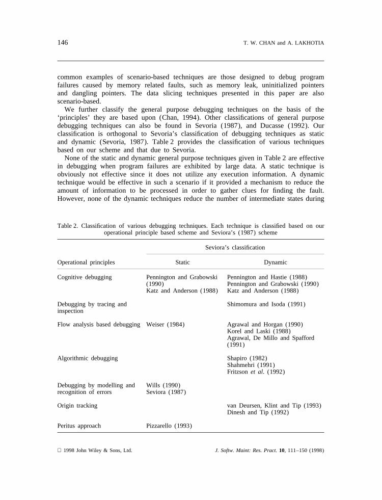
146 T. W. CHAN and A. LAKHOTIA
common examples of scenario-based techniques are those designed to debug programfailures caused by memory related faults, such as memory leak, uninitialized pointersand dangling pointers. The data slicing techniques presented in this paper are alsoscenario-based.
We further classify the general purpose debugging techniques on the basis of the‘principles’ they are based upon (Chan, 1994). Other classifications of general purposedebugging techniques can also be found in Sevoria (1987), and Ducasse (1992). Ourclassification is orthogonal to Sevoria’s classification of debugging techniques as staticand dynamic (Sevoria, 1987). Table 2 provides the classification of various techniquesbased on our scheme and that due to Sevoria.
None of the static and dynamic general purpose techniques given in Table 2 are effectivein debugging when program failures are exhibited by large data. A static technique isobviously not effective since it does not utilize any execution information. A dynamictechnique would be effective in such a scenario if it provided a mechanism to reduce theamount of information to be processed in order to gather clues for finding the fault.However, none of the dynamic techniques reduce the number of intermediate states during
Table 2. Classification of various debugging techniques. Each technique is classified based on ouroperational principle based scheme and Seviora’s (1987) scheme
Seviora’s classification
Operational principles Static Dynamic
Cognitive debugging Pennington and Grabowski Pennington and Hastie (1988)(1990) Pennington and Grabowski (1990)Katz and Anderson (1988) Katz and Anderson (1988)
Debugging by tracing and Shimomura and Isoda (1991)inspection
Flow analysis based debugging Weiser (1984) Agrawal and Horgan (1990)Korel and Laski (1988)Agrawal, De Millo and Spafford(1991)
Algorithmic debugging Shapiro (1982)Shahmehri (1991)Fritzson et al. (1992)
Debugging by modelling and Wills (1990)recognition of errors Seviora (1987)
Origin tracking van Deursen, Klint and Tip (1993)Dinesh and Tip (1992)
Peritus approach Pizzarello (1993)
1998 John Wiley & Sons, Ltd. J. Softw. Maint: Res. Pract.10, 111–150 (1998)
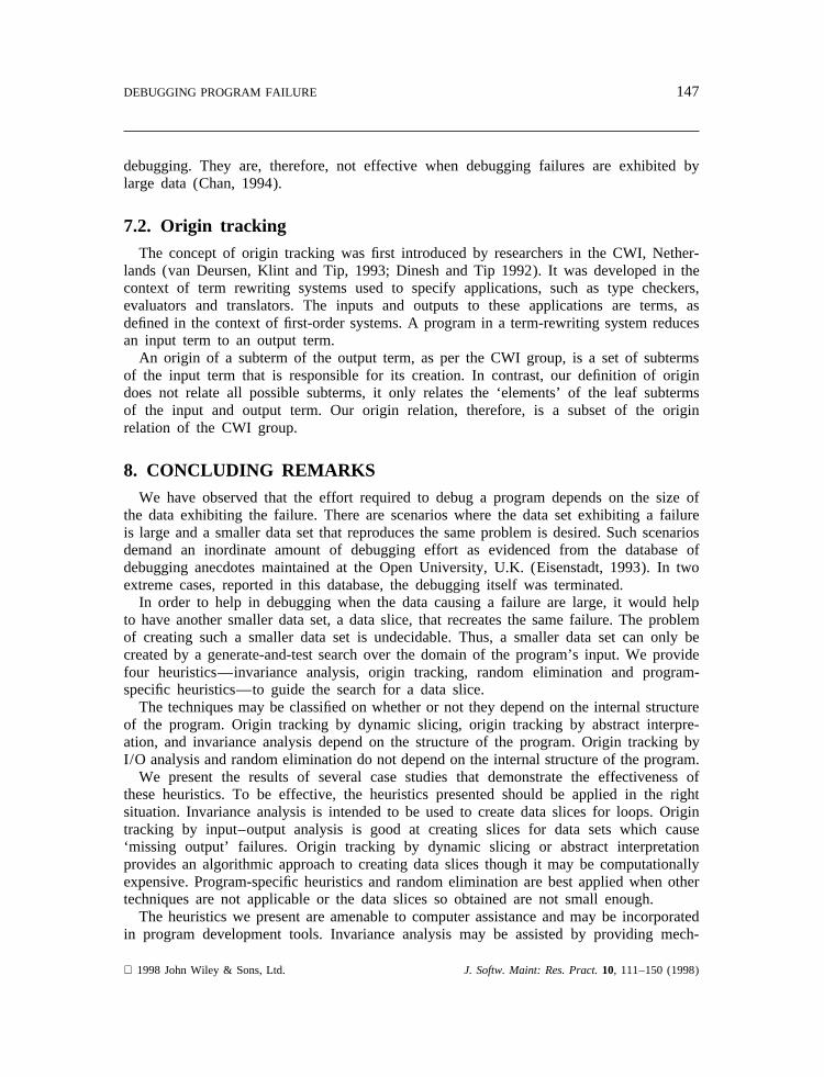
147DEBUGGING PROGRAM FAILURE
debugging. They are, therefore, not effective when debugging failures are exhibited bylarge data (Chan, 1994).
7.2. Origin trackingThe concept of origin tracking was first introduced by researchers in the CWI, Nether-
lands (van Deursen, Klint and Tip, 1993; Dinesh and Tip 1992). It was developed in thecontext of term rewriting systems used to specify applications, such as type checkers,evaluators and translators. The inputs and outputs to these applications are terms, asdefined in the context of first-order systems. A program in a term-rewriting system reducesan input term to an output term.
An origin of a subterm of the output term, as per the CWI group, is a set of subtermsof the input term that is responsible for its creation. In contrast, our definition of origindoes not relate all possible subterms, it only relates the ‘elements’ of the leaf subtermsof the input and output term. Our origin relation, therefore, is a subset of the originrelation of the CWI group.
8. CONCLUDING REMARKSWe have observed that the effort required to debug a program depends on the size of
the data exhibiting the failure. There are scenarios where the data set exhibiting a failureis large and a smaller data set that reproduces the same problem is desired. Such scenariosdemand an inordinate amount of debugging effort as evidenced from the database ofdebugging anecdotes maintained at the Open University, U.K. (Eisenstadt, 1993). In twoextreme cases, reported in this database, the debugging itself was terminated.
In order to help in debugging when the data causing a failure are large, it would helpto have another smaller data set, a data slice, that recreates the same failure. The problemof creating such a smaller data set is undecidable. Thus, a smaller data set can only becreated by a generate-and-test search over the domain of the program’s input. We providefour heuristics—invariance analysis, origin tracking, random elimination and program-specific heuristics—to guide the search for a data slice.
The techniques may be classified on whether or not they depend on the internal structureof the program. Origin tracking by dynamic slicing, origin tracking by abstract interpre-ation, and invariance analysis depend on the structure of the program. Origin tracking byI/O analysis and random elimination do not depend on the internal structure of the program.
We present the results of several case studies that demonstrate the effectiveness ofthese heuristics. To be effective, the heuristics presented should be applied in the rightsituation. Invariance analysis is intended to be used to create data slices for loops. Origintracking by input–output analysis is good at creating slices for data sets which cause‘missing output’ failures. Origin tracking by dynamic slicing or abstract interpretationprovides an algorithmic approach to creating data slices though it may be computationallyexpensive. Program-specific heuristics and random elimination are best applied when othertechniques are not applicable or the data slices so obtained are not small enough.
The heuristics we present are amenable to computer assistance and may be incorporatedin program development tools. Invariance analysis may be assisted by providing mech-
1998 John Wiley & Sons, Ltd. J. Softw. Maint: Res. Pract.10, 111–150 (1998)
148 T. W. CHAN and A. LAKHOTIA
anisms to test for violation of invariance and mechanisms to save and revert the state of aprogram. Origin tracking may obviously be automated since it can be done algorithmically.Automated support is also possible for creating candidate data slices from the origin.Such a support may consist of a data structure editor that can perform operations basedon absolute position, relative position, order and content of data elements. Since there isno standard representation for data, it may be more prudent to develop a data structureeditor generator by enhancing some of the syntax-directed editor. Such a data structureeditor may also be useful in data slicing by random elimination. Developing such anautomated support is part of our future research agenda.
AcknowledgementsThe authors thank the referees for their careful reviews which have helped improve the paper. Wethank Nancy L. Franks for carefully typing the manuscript and preparing the figures. The work waspartially supported by the grant: Louisiana BoR LEQSF (1993–95) RD-A-38, and the grant: ARODAAH04-94-G-0334. The contents of the paper do not necessarily reflect the position or policy ofthe funding agencies, and no official endorsement should be inferred.
ReferencesAgrawal, H., DeMillo, R. and Spafford, E. (1991) ‘An execution-backtracking approach to debugging’,
IEEE Software, 8(3), 21–26.Agrawal, H. and Horgan, J. R. (1990) ‘Dynamic program slicing’,Proceedings of the ACM SIGPLAN
’90 Conference on Programming Language Design and Implementation, ACM SIGPLAN Notices,25(6), 246–256.
Budd, T. A. (1981) ‘Mutation analysis: ideas, examples, problems, and prospects’, in Chandrasekaran,B. and Radicchi, S. (Eds),Computer Program Testing, North-Holland, Amsterdam, pp. 129–148.
Burkhard, W. A. (1988)C for Programmers, Wadsworth Publishing Company, Belmont CA, 562 pp.Chan, T. W. (1994) ‘Debugging program failures exhibited by voluminous data’, Ph.D. dissertation,
University of Southwestern Louisiana, Lafayette LA, 110 pp.Chan, T. W. (1997) ‘A framework for debugging’,Journal of Computer Information Systems, 38(1),
67–73.Chan, T. W. and Lakhotia, A. (1993) ‘Integrating testing and debugging using program and data
slices’, in Proceedings of Computer in Engineering Symposium, ASME 16th Annual Energy-sourcesTechnology Conference and Exhibition, ASME, New York NY, pp. 1–6.
Chen, T. Y. and Cheung, Y. Y. (1997) ‘On program dicing’,Journal of Software Maintenance:Research and Practice, 9(1), 33–46.
Dijkstra, E. W. (1976)A Discipline of Programming, Prentice-Hall, Englewood Cliffs NJ, 217 pp.Dinesh, T. B. and Tip, F. (1992) ‘Animators and error reporters for general programming environ-
ments’, Technical Report CS-R9253, Centrum voor Wiskunde en Informatica (CIW), Amsterdam.Ducasse´, M. (1992) ‘An extendable trace analyser to support automated debugging’, PhD. dissertation,
European Computer-industry Research Center, Universite´ de Rennes I, France.Eisenstadt, M. (1993) ‘Tales of debugging from the front lines’, inProceedings of the Fifth Workshop
on Empirical Studies of Programmers, Ablex Publishing, Norwood NJ, pp. 86–112.Ericsson, K. A. and Simon, H. A. (1984)Protocol Analysis: Verbal Reports as Data, MIT Press,
Cambridge MA, 426 pp.Fritzson, P., Shahmehri, N., Kamkar, M. and Gyimothy, T. (1992) ‘Generalized algorithmic debugging
and testing’,ACM Letters on Programming Languages and Systems, 1(4), 303–322.Goradia, T. (1993) ‘Dynamic impact analysis: analyzing error propagation in program executions’,
Ph.D. dissertation, New York University, NY.Hoch, T., Marick, B. and Schafer, K. W. (1990)Branch Coverage Tool User’s Manual, University
of Illinois at Urbana-Champaign IL.
1998 John Wiley & Sons, Ltd. J. Softw. Maint: Res. Pract.10, 111–150 (1998)

149DEBUGGING PROGRAM FAILURE
Horgan, J. and Mathur, A. P. (1992) ‘An execution-backtracking approach to debugging’,IEEESoftware, 9(5), 61–69.
Horwitz, S., Prins, J. and Reps, T. (1988) ‘Integrating non-interfering versions of programs’, inProceedings of the Fifteenth Annual ACM Symposium on Principles of Programming Lanugages,ACM, New York NY, pp. 133–145.
Hutchens, D. H. and Basili, V. R. (1985) ‘System structure analysis: clustering with data bindings’,IEEE Transactions on Software Engineering, SE-11(8), 749–757.
Katz, I. R. and Anderson, J. R. (1988) ‘Debugging: an analysis of bug-location strategies’,HumanComputer Interaction, 3, 351–359.
Korel, B. and Laski, J. (1988) ‘Dynamic program slicing’, Information Processing Letters,29(3),155–163.
Lakhotia, A. and Chan, T. W. (1993) ‘Data slicing by dynamic program slicing’, inProceedings ofSoftware Engineering Research Forum, University of West Florida, Pensacola FL, pp. 245–253.
Mathur, A. (1991) ‘Mutation testing: a tutorial (i–iii)’,SERC Newsletter, Software EngineeringResearch Center, Purdue University, W. Lafayette IN, 1st, 2nd and 4th quarter.
Morgan, C. (1988) ‘The specification statement’, InOn the Refinement Calculus, Oxford UniversityComputing Laboratory, Oxford, pp. 7–30.
Pennington, A. and Hastie, R. (1988) ‘Explanation-based decision making: effects of memorystructure on judgement’,Journal of Experimental Psychology: learning, memory and cognition,16(3), 521–533.
Pennington, N. and Grabowski, B. (1990) ‘The tasks of programming’, in Hoc, J. M., Green, T.,Samurcay, R. and Gilmore, D. (Eds),Psychology of Programming, Academic Press, London,pp. 45–62.
Pizzarello, A. (1993) A new method for location of software defects, Technical Report, PeritusSoftware Services, Westboro MA.
Sevoria, R. E. (1987) ‘Knowledge-based program debugging systems’,IEEE Software, 4(3), 20–32.Shneiderman, B. (1986) ‘Empirical studies of programmers: the territory, paths, and destinations’,
in Proceedings of the First Workshop of Empirical Studies of Programmers, Ablex Publishing,Norwood NJ, pp. 1–12.
Shahmehri, N. (1991) Generalized algorithmic debugging. Ph.D. Dissertation, Linko¨ping University.Shapiro, E. Y. (1982) Algorithmic program debugging, An ACM Distinguished Dissertation, MIT
Press, Cambridge MA, 232 pp.Shimomura, T. and Isoda, S. (1991) ‘Linked-list visualization for debugging’,IEEE Software, 8(3),
44–51.van Deursen, A., Klint, P. and Tip, F. (1993) ‘Origin tracking’,Journal of Symbolic Computation,
15(5–6), 523–570.Weiser, M. (1984) ‘Program slicing’,IEEE Transactions of Software Engineering, SE-10(4), 352–
357.White, L. J. (1987) ‘Software testing and verification’,Advances in Computers, 26, 335–391.Wills, L. M. (1990) ‘Automated program recognition: a feasibility demonstration’,Artificial Intelli-
gence, 45(1–2), 113–171.
1998 John Wiley & Sons, Ltd. J. Softw. Maint: Res. Pract.10, 111–150 (1998)

150 T. W. CHAN and A. LAKHOTIA
Authors’ biographies:
Tat W. Chan is a faculty member in the Department of Mathematics andComputer Science at Fayetteville State University, Fayetteville, North Carolina.He received his B.S. from the University of Southwestern Louisiana (USL)and his M.S. and Ph.D. degrees from the Center for Advanced ComputerStudies, USL. His research interests include Software Debugging and Testing,Software Engineering Education, and Programming Languages. He is a memberof the IEEE Computer Society and the Society’s Technical Committee onSoftware Engineering.
Arun Lakhotia is an Associate Professor with the Center for AdvancedComputer Studies and the Director of the Software Research Laboratory at theUniversity of Southwestern Louisiana, Lafayette. He received his Ph.D. fromCase Western Reserve University, Cleveland, in 1989. His research interestsare centred around issues related to improving the productivity of programmersand the reliability of their programs. He is currently directing projects to recoverobject-orientated design from the source code of legacy systems. The projectsare funded by grants from the Defense Advanced Research Projects Agencyand the Louisiana Board of Regents. He has also contributed to research inmethods and tools for developing logic programs, partial evaluation of logicprograms, interprocedural flow analyses and software metrics. Dr. Lakhotia isa member of the ACM and the IEEE.
1998 John Wiley & Sons, Ltd. J. Softw. Maint: Res. Pract.10, 111–150 (1998)


![Debugging with gdb · Debugging Data Race Conditions: Section 12.2 [Data Race Detection], page 171. Debugging OpenMP*: Section 12.4 [OpenMP* Debugging], page 177. Extended recording](https://img.pdfslide.net/doc/110x75/5f0b5c707e708231d4302334/debugging-with-gdb-debugging-data-race-conditions-section-122-data-race-detection.jpg)