Embed Size (px)
DESCRIPTION
DECISION MAKING UNDER RISK. Ainhoa Jaramillo Gutiérrez. The Lottery -panel test for bi -dimensional, parameter -free elicitation of risk attitudes. Aurora García-Gallego LEE- Ec. Dpt. , U. Jaume I castellon Nikolaos Georgantzís - PowerPoint PPT Presentation
Citation preview

DECISION MAKING UNDER RISKAinhoa Jaramillo Gutiérrez

Aurora García-GallegoLEE-Ec. Dpt., U. Jaume I castellon
Nikolaos GeorgantzísGLOBE-Economics Dpt., Universidad de Granada & lee castellon
Ainhoa Jaramillo-GutiérrezERICES, Universidad DE VALENCIA
Melanie ParravanoLEE-Economics Dpt., Universitat Jaume I
The Lottery-panel test for bi-dimensional, parameter-free elicitation of risk attitudes
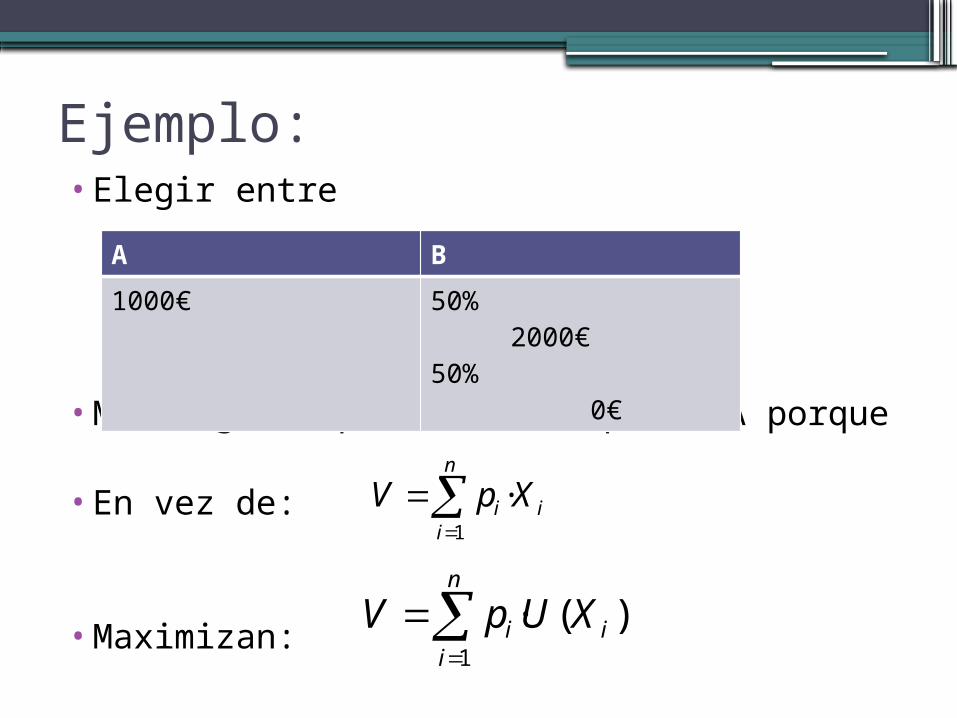
Ejemplo: •Elegir entre
•Mucha gente prefiere la opción A porque
•En vez de:
•Maximizan:
A B
1000€ 50% 2000€ 50% 0€
n
iii XpV
1
·
n
iii XUpV
1
)(·
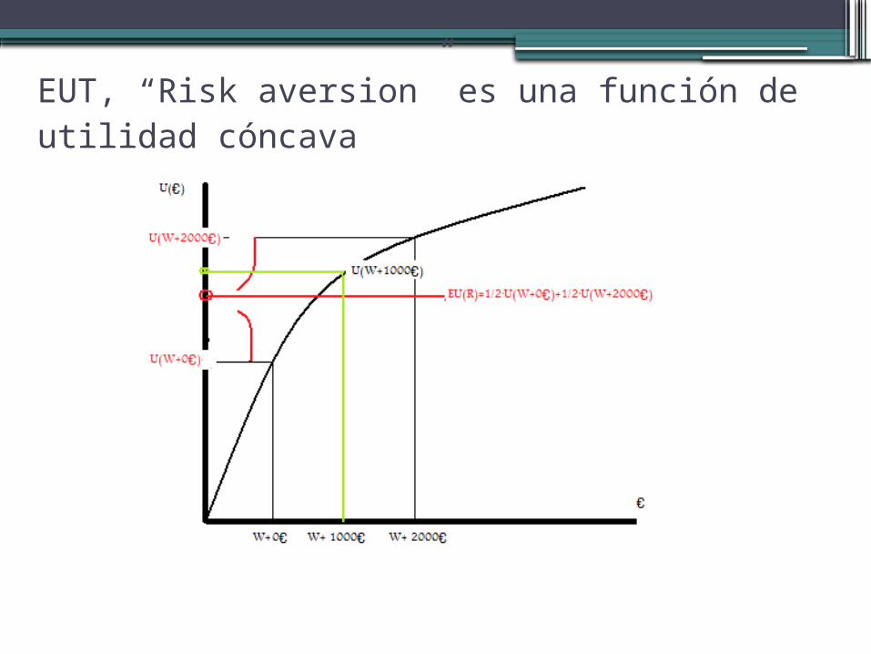
EUT, “Risk aversion” es una función de utilidad cóncava
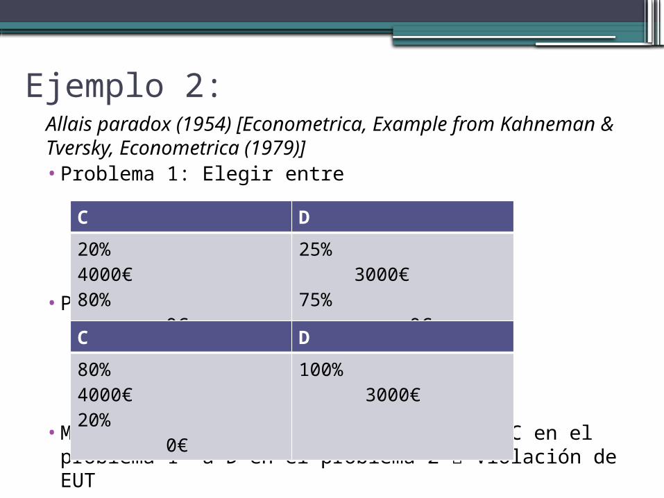
Ejemplo 2:Allais paradox (1954) [Econometrica, Example from Kahneman & Tversky, Econometrica (1979)]• Problema 1: Elegir entre
• Problema 2: Elegir entre
• Más de la mitad de la gente cambia de C en el problema 1 a D en el problema 2 Violación de EUT
C D
20% 4000€80% 0€
25% 3000€ 75% 0€
C D
80% 4000€20% 0€
100% 3000€
LEINCOMPATIBEU
UUPROBL
UUPROBL
Entonces
UUPROBL
UUPROBL
5/4€)4000(/€)3000(2
5/4€)4000(/€)3000(1
:
€)4000(%·80€)3000(%·100:2
€)4000(%·20€)3000(%·25:1
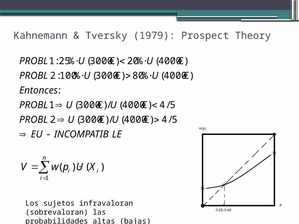
Kahnemann & Tversky (1979): Prospect Theory
n
iii XUpwV
1
)()·(
Los sujetos infravaloran (sobrevaloran) las probabilidades altas (bajas)
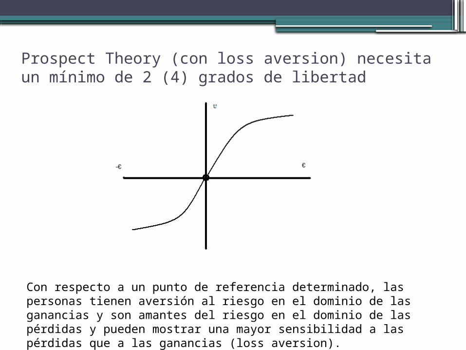
Prospect Theory (con loss aversion) necesita un mínimo de 2 (4) grados de libertad
Con respecto a un punto de referencia determinado, las personas tienen aversión al riesgo en el dominio de las ganancias y son amantes del riesgo en el dominio de las pérdidas y pueden mostrar una mayor sensibilidad a las pérdidas que a las ganancias (loss aversion).
Conclusión•Hay mucho que aprender en la toma de
decisiones económicas bajo riesgo•Existen muchas teorías: EUT, PT, RDU, TAX, …•Pero de momento esta es la mejor parte de
nuestra disciplina que evoluciona en el sentido “Teoría-Disciplina-Teoría”… y en colaboración de más de una disciplina.
•Medición del riesgo Si queremos caracterizar las actitudes individuales de riesgo para su uso como una variable explicativa en cualquier tipo de experimento, se debe tomar esta exigencia de una caracterización multi-dimensional.
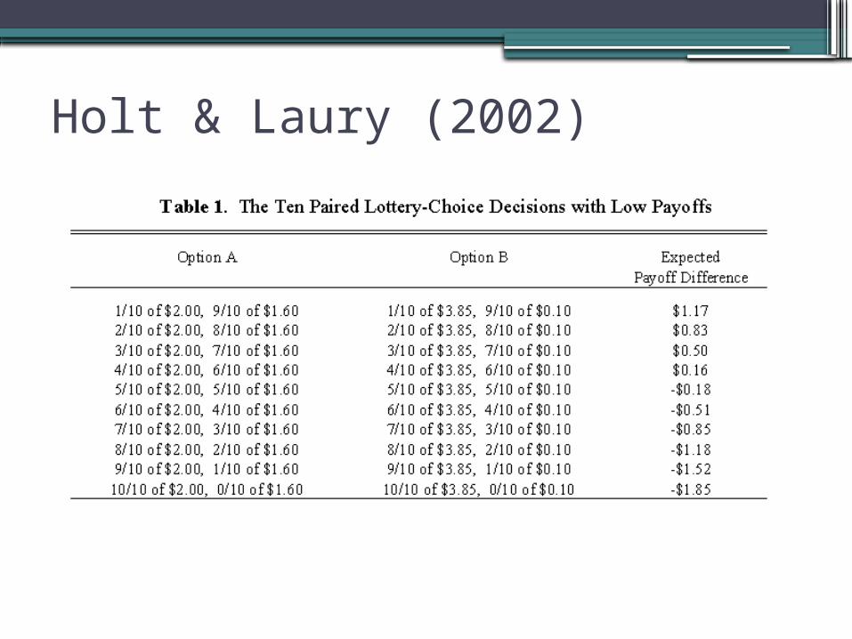
Holt & Laury (2002)
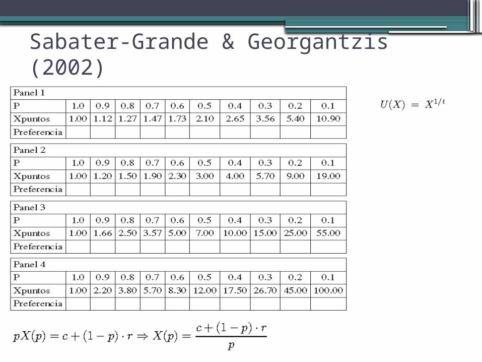
Sabater-Grande & Georgantzis (2002)
.1.2.3.4.5.6.7.8.91
Pa
ne
l 2
.1 .2 .3 .4 .5 .6 .7 .8 .9 1Panel 3
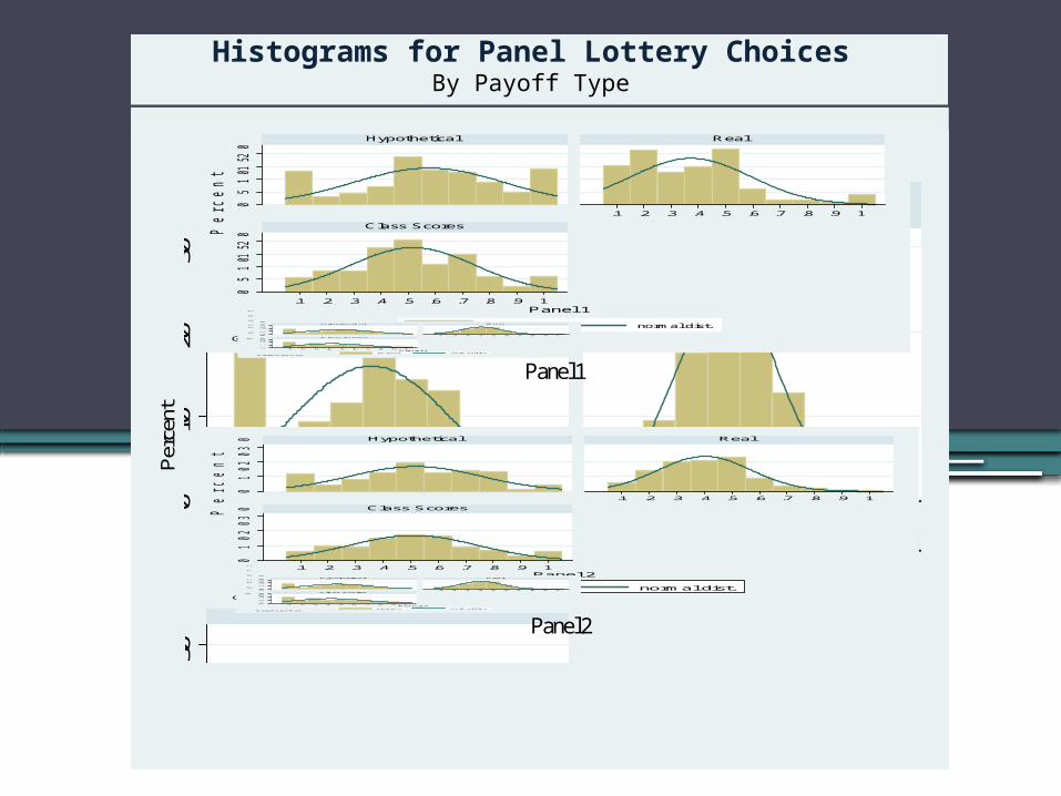
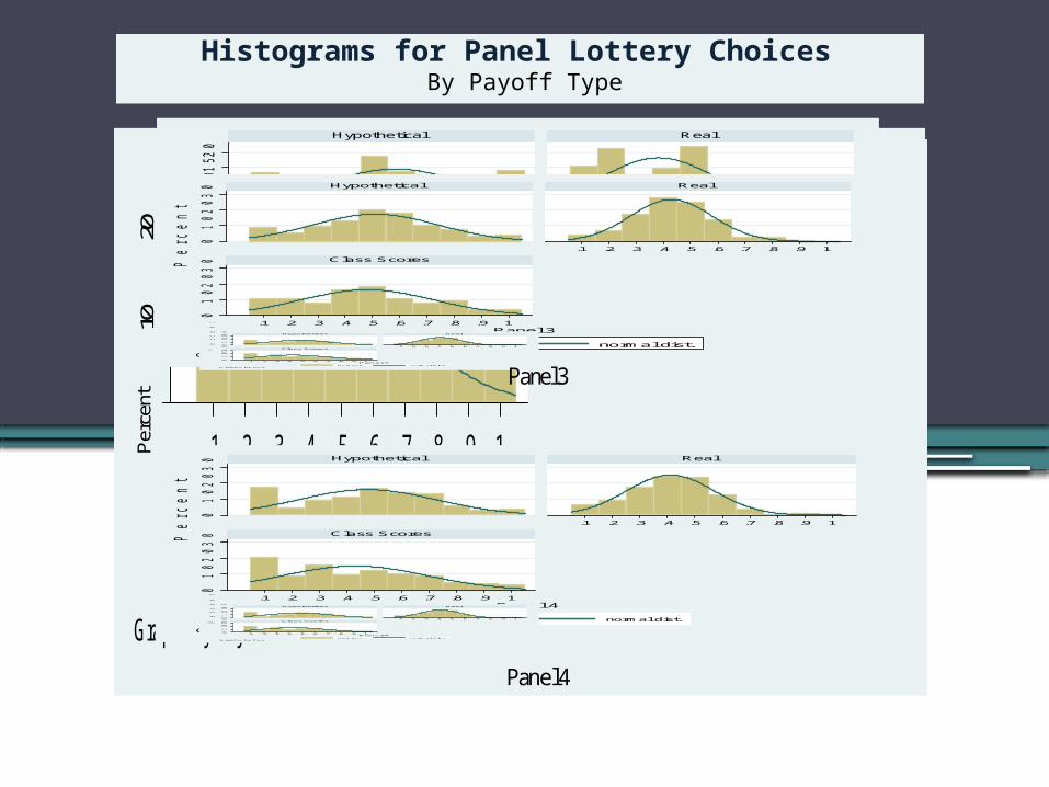
1 obs. Each petal = 1 obs. Each petal = 3 obs. Histograms for Panel Lottery ChoicesBy Payoff Type
010
2030
010
2030
.1 .2 .3 .4 .5 .6 .7 .8 .9 1
.1 .2 .3 .4 .5 .6 .7 .8 .9 1
Hypothetical Real
Class Scores
percent normal dist.
Percent
Panel 4
Graphs by Pay
010
2030
010
2030
.1 .2 .3 .4 .5 .6 .7 .8 .9 1
.1 .2 .3 .4 .5 .6 .7 .8 .9 1
Hypothetical Real
Class Scores
percent normal dist.
Perce
nt
Panel 4
Graphs by Pay
05
101
52
00
51
01
52
0
.1 .2 .3 .4 .5 .6 .7 .8 .9 1
.1 .2 .3 .4 .5 .6 .7 .8 .9 1
Hypothetical Real
Class Scores
percent normal dist.
Pe
rcen
t
Panel 1
Graphs by Pay
01
02
03
00
102
03
0
.1 .2 .3 .4 .5 .6 .7 .8 .9 1
.1 .2 .3 .4 .5 .6 .7 .8 .9 1
Hypothetical Real
Class Scores
percent normal dist.
Pe
rcen
t
Panel 3
Graphs by Pay
01
02
03
00
102
03
0
.1 .2 .3 .4 .5 .6 .7 .8 .9 1
.1 .2 .3 .4 .5 .6 .7 .8 .9 1
Hypothetical Real
Class Scores
percent normal dist.
Pe
rcen
t
Panel 4
Graphs by Pay
01
02
03
001
02
03
0 .1 .2 .3 .4 .5 .6 .7 .8 .9 1
.1 .2 .3 .4 .5 .6 .7 .8 .9 1
Hypothetical Real
Class Scores
percent normal dist.
Pe
rce
nt
Panel 4
Graphs by Pay
01
02
03
001
02
03
0 .1 .2 .3 .4 .5 .6 .7 .8 .9 1
.1 .2 .3 .4 .5 .6 .7 .8 .9 1
Hypothetical Real
Class Scores
percent normal dist.
Pe
rce
nt
Panel 4
Graphs by Pay
01
02
03
001
02
03
0 .1 .2 .3 .4 .5 .6 .7 .8 .9 1
.1 .2 .3 .4 .5 .6 .7 .8 .9 1
Hypothetical Real
Class Scores
percent normal dist.
Pe
rce
nt
Panel 4
Graphs by Pay
010
2030
010
2030
.1 .2 .3 .4 .5 .6 .7 .8 .9 1
.1 .2 .3 .4 .5 .6 .7 .8 .9 1
Hypothetical Real
Class Scores
percent normal dist.
Percent
Panel 4
Graphs by Pay
Panel 1
Panel 2
Panel 3
Panel 4
01
02
03
00
102
03
0
.1 .2 .3 .4 .5 .6 .7 .8 .9 1
.1 .2 .3 .4 .5 .6 .7 .8 .9 1
Hypothetical Real
Class Scores
percent normal dist.
Pe
rcen
t
Panel 2
Graphs by Pay
01
02
03
001
02
03
0 .1 .2 .3 .4 .5 .6 .7 .8 .9 1
.1 .2 .3 .4 .5 .6 .7 .8 .9 1
Hypothetical Real
Class Scores
percent normal dist.
Pe
rcen
t
Panel 4
Graphs by Pay
010
2030
010
2030
.1 .2 .3 .4 .5 .6 .7 .8 .9 1
.1 .2 .3 .4 .5 .6 .7 .8 .9 1
Hypothetical Real
Class Scores
percent normal dist.
Per
cent
Panel 4
Graphs by Pay
.1.2.3.4.5.6.7.8.91
Pa
ne
l 2
.1 .2 .3 .4 .5 .6 .7 .8 .9 1Panel 3
1 obs. Each petal = 1 obs. Each petal = 3 obs.
010
2030
010
2030
.1 .2 .3 .4 .5 .6 .7 .8 .9 1
.1 .2 .3 .4 .5 .6 .7 .8 .9 1
Hypothetical Real
Class Scores
percent normal dist.
Percent
Panel 4
Graphs by Pay
010
2030
010
2030
.1 .2 .3 .4 .5 .6 .7 .8 .9 1
.1 .2 .3 .4 .5 .6 .7 .8 .9 1
Hypothetical Real
Class Scores
percent normal dist.
Perce
nt
Panel 4
Graphs by Pay
05
101
52
00
51
01
52
0
.1 .2 .3 .4 .5 .6 .7 .8 .9 1
.1 .2 .3 .4 .5 .6 .7 .8 .9 1
Hypothetical Real
Class Scores
percent normal dist.
Pe
rcen
t
Panel 1
Graphs by Pay
01
02
03
00
102
03
0
.1 .2 .3 .4 .5 .6 .7 .8 .9 1
.1 .2 .3 .4 .5 .6 .7 .8 .9 1
Hypothetical Real
Class Scores
percent normal dist.
Pe
rcen
t
Panel 3
Graphs by Pay
01
02
03
00
102
03
0
.1 .2 .3 .4 .5 .6 .7 .8 .9 1
.1 .2 .3 .4 .5 .6 .7 .8 .9 1
Hypothetical Real
Class Scores
percent normal dist.
Pe
rcen
t
Panel 4
Graphs by Pay
0102030
0102030 .1 .2 .3 .4 .5 .6 .7 .8 .9 1
.1 .2 .3 .4 .5 .6 .7 .8 .9 1
Hypothetical Real
Class Scores
percent normal dist.
Pe
rce
nt
Panel 4
Graphs by Pay
0102030
0102030 .1 .2 .3 .4 .5 .6 .7 .8 .9 1
.1 .2 .3 .4 .5 .6 .7 .8 .9 1
Hypothetical Real
Class Scores
percent normal dist.
Pe
rce
nt
Panel 4
Graphs by Pay
0102030
0102030 .1 .2 .3 .4 .5 .6 .7 .8 .9 1
.1 .2 .3 .4 .5 .6 .7 .8 .9 1
Hypothetical Real
Class Scores
percent normal dist.
Pe
rce
nt
Panel 4
Graphs by Pay
010
2030
010
2030
.1 .2 .3 .4 .5 .6 .7 .8 .9 1
.1 .2 .3 .4 .5 .6 .7 .8 .9 1
Hypothetical Real
Class Scores
percent normal dist.
Percent
Panel 4
Graphs by Pay
Panel 1
Panel 2
Panel 3
Panel 4
01
02
03
00
102
03
0
.1 .2 .3 .4 .5 .6 .7 .8 .9 1
.1 .2 .3 .4 .5 .6 .7 .8 .9 1
Hypothetical Real
Class Scores
percent normal dist.
Pe
rcen
t
Panel 2
Graphs by Pay
01
02
03
001
02
03
0 .1 .2 .3 .4 .5 .6 .7 .8 .9 1
.1 .2 .3 .4 .5 .6 .7 .8 .9 1
Hypothetical Real
Class Scores
percent normal dist.
Percent
Panel 4
Graphs by Pay
010
2030
010
2030
.1 .2 .3 .4 .5 .6 .7 .8 .9 1
.1 .2 .3 .4 .5 .6 .7 .8 .9 1
Hypothetical Real
Class Scores
percent normal dist.
Perce
nt
Panel 4
Graphs by Pay
05
101
52
00
51
01
52
0.1 .2 .3 .4 .5 .6 .7 .8 .9 1
.1 .2 .3 .4 .5 .6 .7 .8 .9 1
Hypothetical Real
Class Scores
percent normal dist.
Pe
rcen
t
Panel 1
Graphs by Pay
01
02
03
00
102
03
0
.1 .2 .3 .4 .5 .6 .7 .8 .9 1
.1 .2 .3 .4 .5 .6 .7 .8 .9 1
Hypothetical Real
Class Scores
percent normal dist.
Pe
rcen
t
Panel 3
Graphs by Pay
01
02
03
00
102
03
0
.1 .2 .3 .4 .5 .6 .7 .8 .9 1
.1 .2 .3 .4 .5 .6 .7 .8 .9 1
Hypothetical Real
Class Scores
percent normal dist.
Pe
rcen
t
Panel 4
Graphs by Pay
01
02
03
001
02
03
0 .1 .2 .3 .4 .5 .6 .7 .8 .9 1
.1 .2 .3 .4 .5 .6 .7 .8 .9 1
Hypothetical Real
Class Scores
percent normal dist.
Pe
rcen
t
Panel 4
Graphs by Pay
01
02
03
001
02
03
0 .1 .2 .3 .4 .5 .6 .7 .8 .9 1
.1 .2 .3 .4 .5 .6 .7 .8 .9 1
Hypothetical Real
Class Scores
percent normal dist.
Pe
rcen
t
Panel 4
Graphs by Pay
01
02
03
001
02
03
0 .1 .2 .3 .4 .5 .6 .7 .8 .9 1
.1 .2 .3 .4 .5 .6 .7 .8 .9 1
Hypothetical Real
Class Scores
percent normal dist.
Pe
rcen
t
Panel 4
Graphs by Pay
010
2030
010
2030
.1 .2 .3 .4 .5 .6 .7 .8 .9 1
.1 .2 .3 .4 .5 .6 .7 .8 .9 1
Hypothetical Real
Class Scores
percent normal dist.
Percent
Panel 4
Graphs by Pay
Panel 1
Panel 2
Panel 3
Panel 4
01
02
03
00
102
03
0
.1 .2 .3 .4 .5 .6 .7 .8 .9 1
.1 .2 .3 .4 .5 .6 .7 .8 .9 1
Hypothetical Real
Class Scores
percent normal dist.
Pe
rcen
t
Panel 2
Graphs by Pay
01
02
03
001
02
03
0 .1 .2 .3 .4 .5 .6 .7 .8 .9 1
.1 .2 .3 .4 .5 .6 .7 .8 .9 1
Hypothetical Real
Class Scores
percent normal dist.
Pe
rce
nt
Panel 4
Graphs by Pay
010
2030
010
2030
.1 .2 .3 .4 .5 .6 .7 .8 .9 1
.1 .2 .3 .4 .5 .6 .7 .8 .9 1
Hypothetical Real
Class Scores
percent normal dist.
Per
cent
Panel 4
Graphs by Pay
Histograms for Panel Lottery Choices By Payoff Type
.1.2.3.4.5.6.7.8.91
Pa
ne
l 2
.1 .2 .3 .4 .5 .6 .7 .8 .9 1Panel 3
1 obs. Each petal = 1 obs. Each petal = 3 obs.
.1.2
.3.4
.5.6
.7.8
.91
Pan
el 2
.1 .2 .3 .4 .5 .6 .7 .8 .9 1Panel 1
.1.2
.3.4
.5.6
.7.8
.91
Pan
el 3
.1 .2 .3 .4 .5 .6 .7 .8 .9 1Panel 1
.1.2
.3.4
.5.6
.7.8
.91
Pan
el 4
.1 .2 .3 .4 .5 .6 .7 .8 .9 1Panel 1
.1.2
.3.4
.5.6
.7.8
.91
Pan
el 3
.1 .2 .3 .4 .5 .6 .7 .8 .9 1Panel 2
.1.2
.3.4
.5.6
.7.8
.91
Pan
el 4
.1 .2 .3 .4 .5 .6 .7 .8 .9 1Panel 2
.1.2
.3.4
.5.6
.7.8
.91
Pan
el 4
.1 .2 .3 .4 .5 .6 .7 .8 .9 1Panel 3
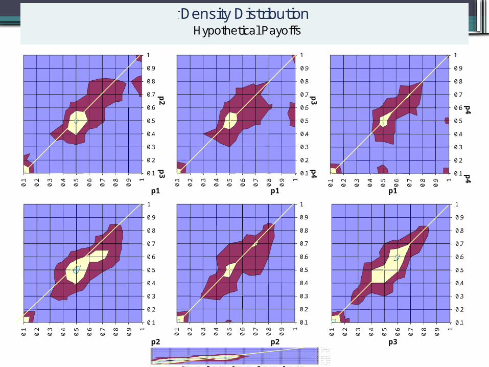
Hypothetical PayoffsSunflower Density Distribution
.1.2
.3.4
.5.6
.7.8
.91
Pan
el 2
.1 .2 .3 .4 .5 .6 .7 .8 .9 1Panel 1
.1.2
.3.4
.5.6
.7.8
.91
Pan
el 3
.1 .2 .3 .4 .5 .6 .7 .8 .9 1Panel 1
.1.2
.3.4
.5.6
.7.8
.91
Pan
el 4
.1 .2 .3 .4 .5 .6 .7 .8 .9 1Panel 1
.1.2
.3.4
.5.6
.7.8
.91
Pan
el 3
.1 .2 .3 .4 .5 .6 .7 .8 .9 1Panel 2
.1.2
.3.4
.5.6
.7.8
.91
Pan
el 4
.1 .2 .3 .4 .5 .6 .7 .8 .9 1Panel 2
.1.2
.3.4
.5.6
.7.8
.91
Pan
el 4
.1 .2 .3 .4 .5 .6 .7 .8 .9 1Panel 3
Hypothetical PayoffsSunflower Density Distribution
0.1
0.2
0.3
0.4
0.5
0.6
0.7
0.8
0.9
1
0.1
0.2
0.3
0.4
0.5
0.6
0.7
0.8
0.9 1
0.1
0.2
0.3
0.4
0.5
0.6
0.7
0.8
0.9
1
0.1
0.2
0.3
0.4
0.5
0.6
0.7
0.8
0.9 1
0.1
0.2
0.3
0.4
0.5
0.6
0.7
0.8
0.9
1
0.1
0.2
0.3
0.4
0.5
0.6
0.7
0.8
0.9 1
0.1
0.2
0.3
0.4
0.5
0.6
0.7
0.8
0.9
1
0.1
0.2
0.3
0.4
0.5
0.6
0.7
0.8
0.9 1
0.1
0.2
0.3
0.4
0.5
0.6
0.7
0.8
0.9
1
0.1
0.2
0.3
0.4
0.5
0.6
0.7
0.8
0.9 1
0.1
0.2
0.3
0.4
0.5
0.6
0.7
0.8
0.9
1
0.1
0.2
0.3
0.4
0.5
0.6
0.7
0.8
0.9 1
p1 p1 p1
p2 p2 p3
p2
p3
p3
p4
p4
p4
P2=0,1
P2=0,2
P2=0,3
P2=0,4
P2=0,5
P2=0,6
P2=0,7
P2=0,8
P2=0,9
P2=1
P1
=0
,1
P1
=0
,2
P1
=0
,3
P1
=0
,4
P1
=0
,5
P1
=0
,6
P1
=0
,7
P1
=0
,8
P1
=0
,9
P1
=1
0.0%-2.0% 2.0%-4.0% 4.0%-6.0% 6.0%-8.0% 8.0%-10.0%
P2=0,1
P2=0,2
P2=0,3
P2=0,4
P2=0,5
P2=0,6
P2=0,7
P2=0,8
P2=0,9
P2=1
P1
=0
,1
P1
=0
,2
P1
=0
,3
P1
=0
,4
P1
=0
,5
P1
=0
,6
P1
=0
,7
P1
=0
,8
P1
=0
,9
P1
=1
0.0%-2.0% 2.0%-4.0% 4.0%-6.0% 6.0%-8.0% 8.0%-10.0%
0.1
0.2
0.3
0.4
0.5
0.6
0.7
0.8
0.9
1
0.1
0.2
0.3
0.4
0.5
0.6
0.7
0.8
0.9 1
0.1
0.2
0.3
0.4
0.5
0.6
0.7
0.8
0.9
1
0.1
0.2
0.3
0.4
0.5
0.6
0.7
0.8
0.9 1
0.1
0.2
0.3
0.4
0.5
0.6
0.7
0.8
0.9
1
0.1
0.2
0.3
0.4
0.5
0.6
0.7
0.8
0.9 1
0.1
0.2
0.3
0.4
0.5
0.6
0.7
0.8
0.9
1
0.1
0.2
0.3
0.4
0.5
0.6
0.7
0.8
0.9 1
0.1
0.2
0.3
0.4
0.5
0.6
0.7
0.8
0.9
1
0.1
0.2
0.3
0.4
0.5
0.6
0.7
0.8
0.9 1
0.1
0.2
0.3
0.4
0.5
0.6
0.7
0.8
0.9
1
0.1
0.2
0.3
0.4
0.5
0.6
0.7
0.8
0.9 1
.1.2.3.4.5.6.7.8.91
Pa
ne
l 2
.1 .2 .3 .4 .5 .6 .7 .8 .9 1Panel 3
1 obs. Each petal = 1 obs. Each petal = 3 obs..1
.2.3
.4.5
.6.7
.8.9
1P
anel
2
.1 .2 .3 .4 .5 .6 .7 .8 .9 1Panel 1
.1.2
.3.4
.5.6
.7.8
.91
Pan
el 3
.1 .2 .3 .4 .5 .6 .7 .8 .9 1Panel 1
.1.2
.3.4
.5.6
.7.8
.91
Pan
el 4
.1 .2 .3 .4 .5 .6 .7 .8 .9 1Panel 1
.1.2
.3.4
.5.6
.7.8
.91
Pan
el 3
.1 .2 .3 .4 .5 .6 .7 .8 .9 1Panel 2
.1.2
.3.4
.5.6
.7.8
.91
Pan
el 4
.1 .2 .3 .4 .5 .6 .7 .8 .9 1Panel 2
.1.2
.3.4
.5.6
.7.8
.91
Pan
el 4
.1 .2 .3 .4 .5 .6 .7 .8 .9 1Panel 3
Hypothetical PayoffsSunflower Density Distribution
.1.2
.3.4
.5.6
.7.8
.91
Pan
el 2
.1 .2 .3 .4 .5 .6 .7 .8 .9 1Panel 1
.1.2
.3.4
.5.6
.7.8
.91
Pan
el 3
.1 .2 .3 .4 .5 .6 .7 .8 .9 1Panel 1
.1.2
.3.4
.5.6
.7.8
.91
Pan
el 4
.1 .2 .3 .4 .5 .6 .7 .8 .9 1Panel 1
.1.2
.3.4
.5.6
.7.8
.91
Pan
el 3
.1 .2 .3 .4 .5 .6 .7 .8 .9 1Panel 2
.1.2
.3.4
.5.6
.7.8
.91
Pan
el 4
.1 .2 .3 .4 .5 .6 .7 .8 .9 1Panel 2
.1.2
.3.4
.5.6
.7.8
.91
Pan
el 4
.1 .2 .3 .4 .5 .6 .7 .8 .9 1Panel 3
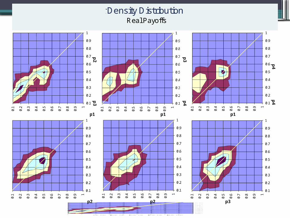
Real PayoffsSunflower Density Distribution
p1 p1 p1
p2 p2 p3p
2p
3
p3
p4
p4
p4
.1.2
.3.4
.5.6
.7.8
.91
Pa
ne
l 2
.1 .2 .3 .4 .5 .6 .7 .8 .9 1Panel 3
1 obs. Each petal = 1 obs. Each petal = 3 obs. Females
05
1015
2025
30
.1 .2 .3 .4 .5 .6 .7 .8 .9 1 .1 .2 .3 .4 .5 .6 .7 .8 .9 1
Hypothetical Real
Percent
normal p1
Per
cent
Panel 1
Graphs by Pay
05
1015
2025
30
.1 .2 .3 .4 .5 .6 .7 .8 .9 1 .1 .2 .3 .4 .5 .6 .7 .8 .9 1
Hypothetical Real
Percent
normal p2
Per
cent
Panel 2
Graphs by Pay
05
1015
2025
30
.1 .2 .3 .4 .5 .6 .7 .8 .9 1 .1 .2 .3 .4 .5 .6 .7 .8 .9 1
Hypothetical Real
Percent
normal p1
Per
cent
Panel 1
Graphs by Pay
05
1015
2025
30
.1 .2 .3 .4 .5 .6 .7 .8 .9 1 .1 .2 .3 .4 .5 .6 .7 .8 .9 1
Hypothetical Real
Percent
normal p2
Per
cent
Panel 2
Graphs by Pay
Males
.1.2.3.4.5.6.7.8.91
Pa
ne
l 2
.1 .2 .3 .4 .5 .6 .7 .8 .9 1Panel 3
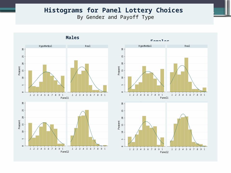
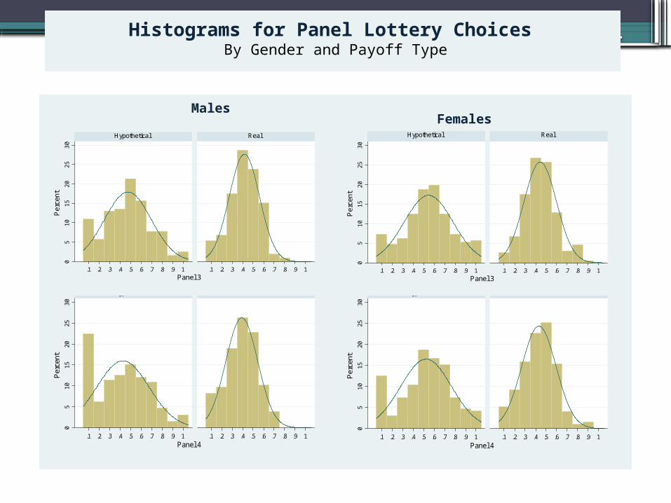
1 obs. Each petal = 1 obs. Each petal = 3 obs. Histograms for Panel Lottery Choices By Gender and Payoff Type
.1.2
.3.4
.5.6
.7.8
.91
Pa
ne
l 2
.1 .2 .3 .4 .5 .6 .7 .8 .9 1Panel 3
1 obs. Each petal = 1 obs. Each petal = 3 obs.
05
1015
2025
30
.1 .2 .3 .4 .5 .6 .7 .8 .9 1 .1 .2 .3 .4 .5 .6 .7 .8 .9 1
Hypothetical Real
Percentnormal p4
Per
cent
Panel 4
Graphs by Pay
05
10
15
20
25
30
.1 .2 .3 .4 .5 .6 .7 .8 .9 1 .1 .2 .3 .4 .5 .6 .7 .8 .9 1
Hypothetical Real
Percent
normal p1
Pe
rcen
t
Panel 1
Graphs by Pay
05
10
15
20
25
30
.1 .2 .3 .4 .5 .6 .7 .8 .9 1 .1 .2 .3 .4 .5 .6 .7 .8 .9 1
Hypothetical Real
Percent
normal p3
Pe
rcen
t
Panel 3
Graphs by Pay
05
1015
2025
30
.1 .2 .3 .4 .5 .6 .7 .8 .9 1 .1 .2 .3 .4 .5 .6 .7 .8 .9 1
Hypothetical Real
Percent
normal p4
Per
cent
Panel 4
Graphs by Pay
05
10
15
20
25
30
.1 .2 .3 .4 .5 .6 .7 .8 .9 1 .1 .2 .3 .4 .5 .6 .7 .8 .9 1
Hypothetical Real
Percent
normal p3
Pe
rcen
t
Panel 3
Graphs by Pay
05
10
15
20
25
30
.1 .2 .3 .4 .5 .6 .7 .8 .9 1 .1 .2 .3 .4 .5 .6 .7 .8 .9 1
Hypothetical Real
Percentnormal p1
Pe
rcen
t
Panel 1
Graphs by Pay
Females Males
.1.2.3.4.5.6.7.8.91
Pa
ne
l 2
.1 .2 .3 .4 .5 .6 .7 .8 .9 1Panel 3
1 obs. Each petal = 1 obs. Each petal = 3 obs. Histograms for Panel Lottery Choices By Gender and Payoff Type
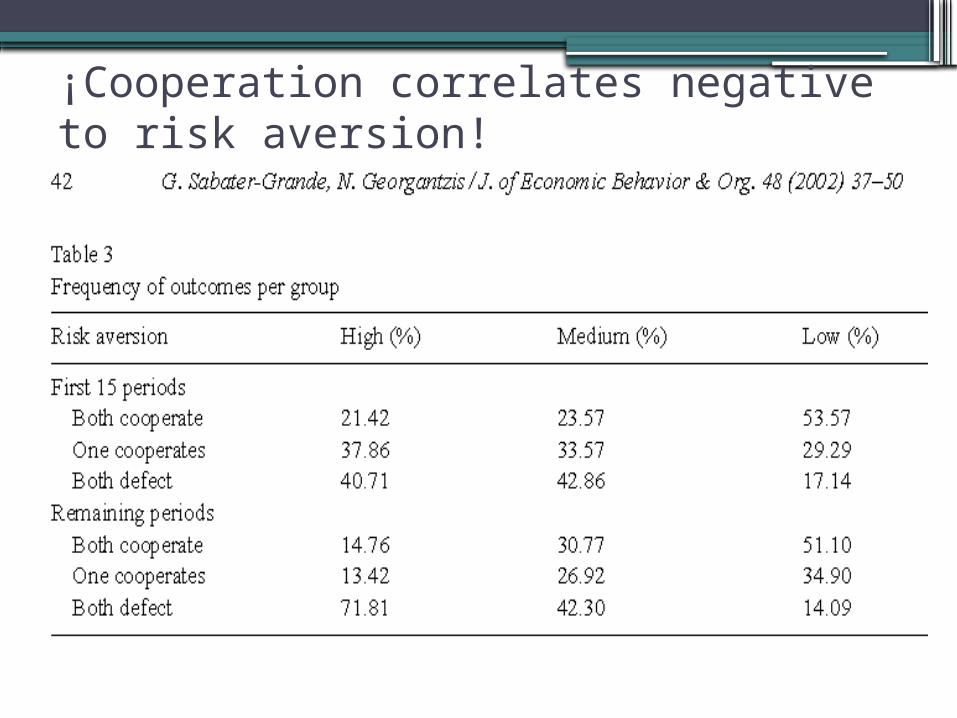
¡Cooperation correlates negative to risk aversion!
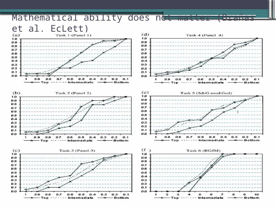
Mathematical ability does not matter (Brañas et al. EcLett)
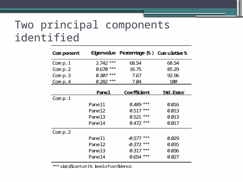
Two principal components identified
Component Cumulative %
Comp. 1 2.742 *** 68.54 68.54Comp. 2 0.670 *** 16.75 85.29Comp. 3 0.307 *** 7.67 92.96Comp. 4 0.282 *** 7.04 100
Std. ErrorComp. 1
0.489 *** 0.0160.517 *** 0.0130.521 *** 0.0130.472 *** 0.017
Comp. 2-0.577 *** 0.029-0.372 *** 0.0350.317 *** 0.0360.654 *** 0.027
*** significant at 1% level of confidence.
Panel 1Panel 2Panel 3Panel 4
Panel 3Panel 4
Eigenvalue
Panel
Panel 1Panel 2
Percentage (%)
Coefficient
010
2030
010
2030
.1 .2 .3 .4 .5 .6 .7 .8 .9 1
.1 .2 .3 .4 .5 .6 .7 .8 .9 1
Hypothetical Real
Class Scores
percent normal dist.
Percent
Panel 4
Graphs by Pay
.1.2.3.4.5.6.7.8.91
Pa
ne
l 2
.1 .2 .3 .4 .5 .6 .7 .8 .9 1Panel 3
1 obs. Each petal = 1 obs. Each petal = 3 obs.
0.2
.4.6
Den
sity
-4 -2 0 2Scores for 2nd PC, Hypothetical and Real Payoffs
Real Hypothetical
kernel = epanechnikov, bandwidth = .16
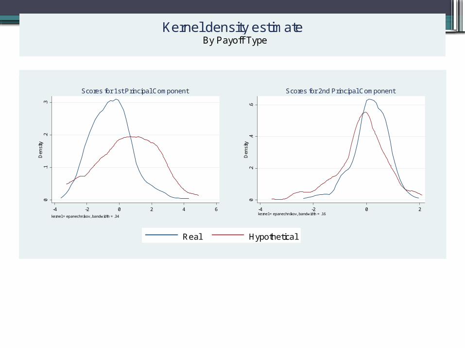
By Payoff TypeKernel Density Estimate for 2nd Principal Component
0.1
.2.3
Den
sity
-4 -2 0 2 4 6Scores for 1st PC, Hypothetical and Real Payoffs
Real Hypothetical
kernel = epanechnikov, bandwidth = .34
By Payoff TypeKernel Density Estimate for 1st Principal Component
0.0
5.1
.15
.2.2
5D
ensi
ty
-4 -2 0 2 4 6Scores for 1st PC, Real Payoffs
Males Females
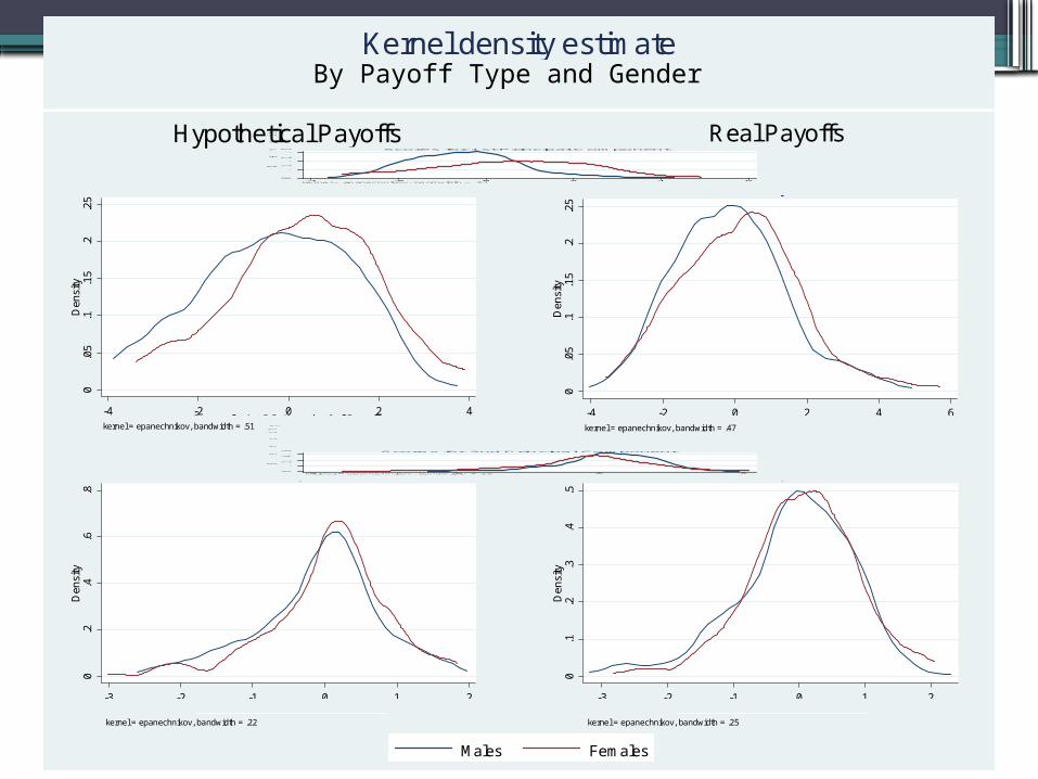
kernel = epanechnikov, bandwidth = .47
Kernel density estimate0
.1.2
.3D
ensi
ty
-4 -2 0 2 4 6
kernel = epanechnikov, bandwidth = .34
Scores for 1st Principal Component
0.2
.4.6
Den
sity
-4 -2 0 2kernel = epanechnikov, bandwidth = .16
Scores for 2nd Principal Component
.1.2
.3.4
.5.6
.7.8
.91
Pa
ne
l 2
.1 .2 .3 .4 .5 .6 .7 .8 .9 1Panel 3
1 obs. Each petal = 1 obs. Each petal = 3 obs.
0.0
5.1
.15
.2.2
5D
ensi
ty
-4 -2 0 2 4Scores for 1st PC, Hypothetical Payoffs
Males Females
kernel = epanechnikov, bandwidth = .51
Kernel density estimate
0.2
.4.6
.8D
ensi
ty
-3 -2 -1 0 1 2Scores for 2nd PC, Hypothetical Payoffs
Males Females
kernel = epanechnikov, bandwidth = .22
Kernel density estimate
0.1
.2.3
.4.5
Den
sity
-3 -2 -1 0 1 2Scores for 2nd PC, Real Payoffs
Males Females
kernel = epanechnikov, bandwidth = .25
Kernel density estimate
.1.2
.3.4
.5.6
.7.8
.91
Pan
el 2
.1 .2 .3 .4 .5 .6 .7 .8 .9 1Panel 1
.1.2
.3.4
.5.6
.7.8
.91
Pan
el 3
.1 .2 .3 .4 .5 .6 .7 .8 .9 1Panel 1
.1.2
.3.4
.5.6
.7.8
.91
Pan
el 4
.1 .2 .3 .4 .5 .6 .7 .8 .9 1Panel 1
.1.2
.3.4
.5.6
.7.8
.91
Pan
el 3
.1 .2 .3 .4 .5 .6 .7 .8 .9 1Panel 2
.1.2
.3.4
.5.6
.7.8
.91
Pan
el 4
.1 .2 .3 .4 .5 .6 .7 .8 .9 1Panel 2
.1.2
.3.4
.5.6
.7.8
.91
Pan
el 4
.1 .2 .3 .4 .5 .6 .7 .8 .9 1Panel 3
Real PayoffsSunflower Density Distribution
.1.2
.3.4
.5.6
.7.8
.91
Pan
el 2
.1 .2 .3 .4 .5 .6 .7 .8 .9 1Panel 1
.1.2
.3.4
.5.6
.7.8
.91
Pan
el 3
.1 .2 .3 .4 .5 .6 .7 .8 .9 1Panel 1
.1.2
.3.4
.5.6
.7.8
.91
Pan
el 4
.1 .2 .3 .4 .5 .6 .7 .8 .9 1Panel 1
.1.2
.3.4
.5.6
.7.8
.91
Pan
el 3
.1 .2 .3 .4 .5 .6 .7 .8 .9 1Panel 2
.1.2
.3.4
.5.6
.7.8
.91
Pan
el 4
.1 .2 .3 .4 .5 .6 .7 .8 .9 1Panel 2
.1.2
.3.4
.5.6
.7.8
.91
Pan
el 4
.1 .2 .3 .4 .5 .6 .7 .8 .9 1Panel 3
Hypothetical PayoffsSunflower Density Distribution
0.0
5.1
.15
.2.2
5D
ensi
ty
-4 -2 0 2 4Scores for 1st PC, Hypothetical Payoffs
Males Females
kernel = epanechnikov, bandwidth = .51
Kernel density estimate
0.2
.4.6
.8D
ensi
ty
-3 -2 -1 0 1 2Scores for 2nd PC, Hypothetical Payoffs
Males Females
kernel = epanechnikov, bandwidth = .22
Kernel density estimate
0.0
5.1
.15
.2.2
5D
ensi
ty
-4 -2 0 2 4 6Scores for 1st PC, Real Payoffs
Males Females
kernel = epanechnikov, bandwidth = .47
Kernel density estimate
0.1
.2.3
.4.5
Den
sity
-3 -2 -1 0 1 2Scores for 2nd PC, Real Payoffs
Males Females
kernel = epanechnikov, bandwidth = .25
Kernel density estimate
0.0
5.1
.15
.2.2
5D
ensi
ty
-4 -2 0 2 4Scores for 1st PC, Hypothetical Payoffs
Males Females
kernel = epanechnikov, bandwidth = .51
By GenderKernel Density Estimate for 1st Principal Component0
.05
.1.1
5.2
.25
Den
sity
-4 -2 0 2 4 6Scores for 1st PC, Real Payoffs
Males Females
kernel = epanechnikov, bandwidth = .47
Kernel density estimate
0.1.2.3
Den
sity
-4 -2 0 2 4 6
kernel = epanechnikov, bandwidth = .34
Scores for 1st Principal Component
0.2.4.6
De
nsity
-4 -2 0 2kernel = epanechnikov, bandwidth = .16
Scores for 2nd Principal Component
.1.2.3.4.5.6.7.8.91
Pa
ne
l 2
.1 .2 .3 .4 .5 .6 .7 .8 .9 1Panel 3
1 obs. Each petal = 1 obs. Each petal = 3 obs.
0.0
5.1
.15
.2.2
5D
ensi
ty
-4 -2 0 2 4 6Scores for 1st PC, Real Payoffs
Males Females
kernel = epanechnikov, bandwidth = .47
Kernel density estimateBy Payoff Type and Gender
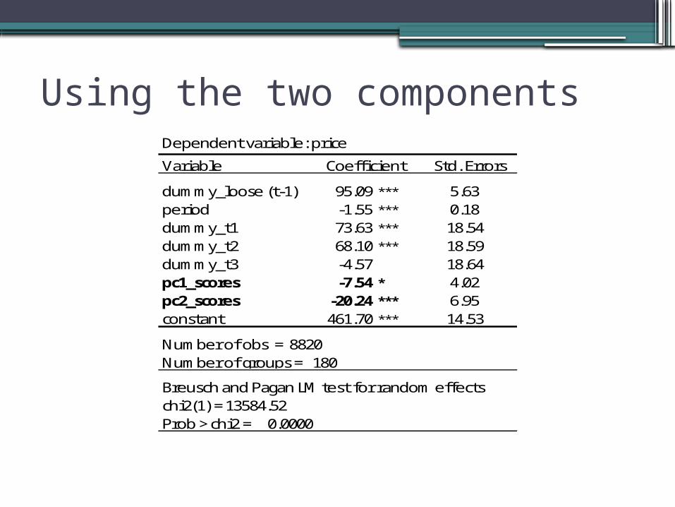
Using the two componentsDependent variable: price
Variable Std. Errors
dummy_loose (t-1) 95.09 *** 5.63period -1.55 *** 0.18dummy_t1 73.63 *** 18.54dummy_t2 68.10 *** 18.59dummy_t3 -4.57 18.64pc1_scores -7.54 * 4.02pc2_scores -20.24 *** 6.95constant 461.70 *** 14.53
Number of obs = 8820
Breusch and Pagan LM test for random effectschi2(1) = 13584.52Prob > chi2 = 0.0000
Coeffi cient
Number of groups = 180
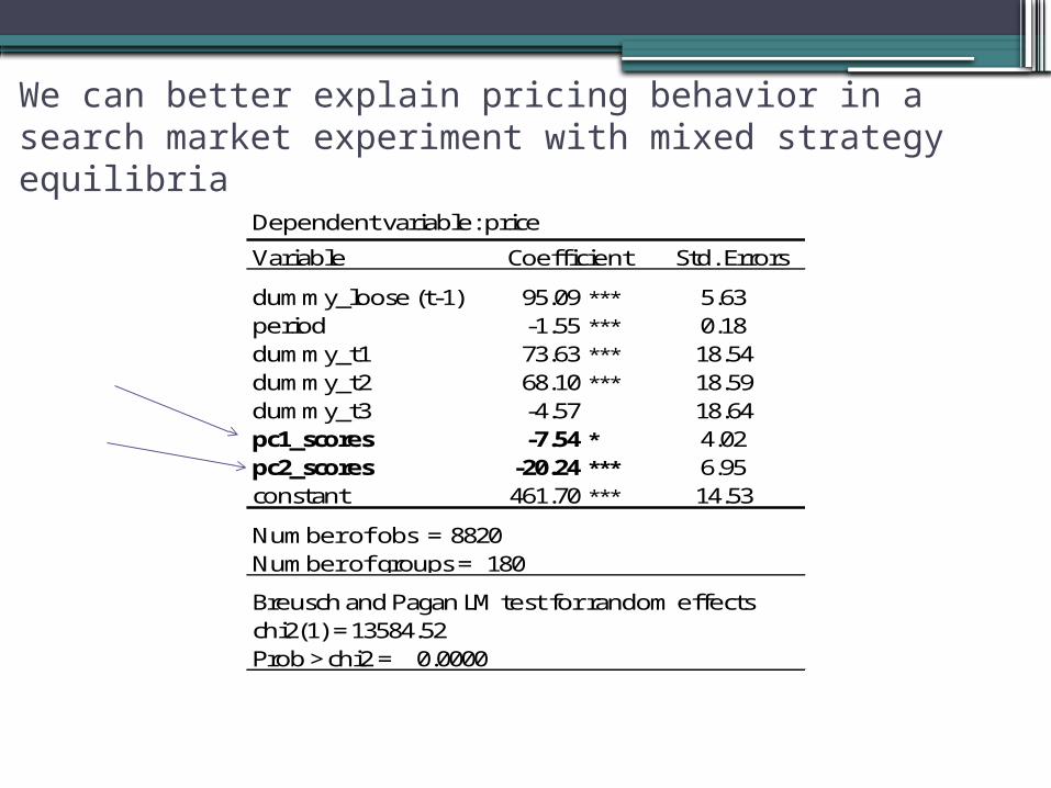
We can better explain pricing behavior in a search market experiment with mixed strategy equilibria
Dependent variable: price
Variable Std. Errors
dummy_loose (t-1) 95.09 *** 5.63period -1.55 *** 0.18dummy_t1 73.63 *** 18.54dummy_t2 68.10 *** 18.59dummy_t3 -4.57 18.64pc1_scores -7.54 * 4.02pc2_scores -20.24 *** 6.95constant 461.70 *** 14.53
Number of obs = 8820
Breusch and Pagan LM test for random effectschi2(1) = 13584.52Prob > chi2 = 0.0000
Coeffi cient
Number of groups = 180
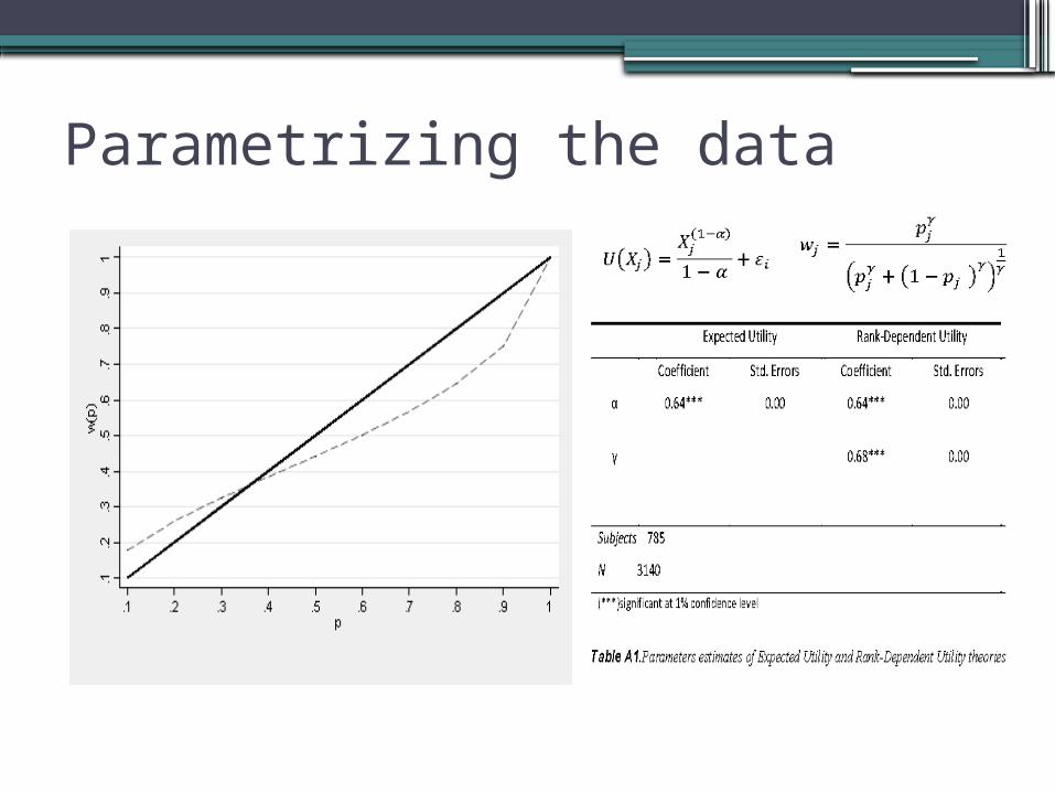
Parametrizing the data
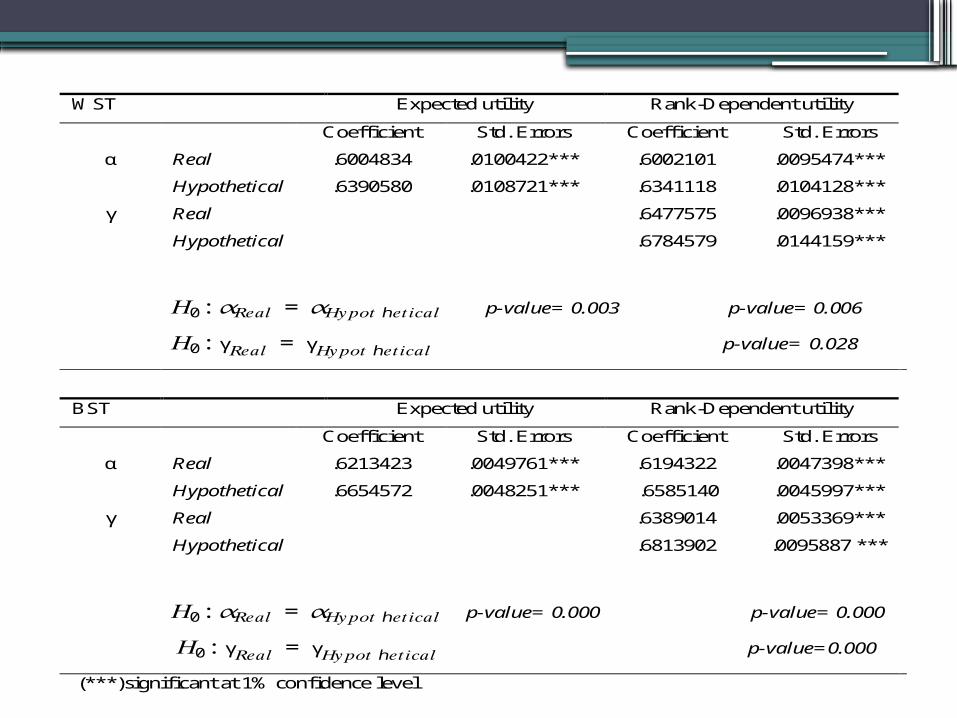
WST Expected utility Rank-Dependent utility
Coefficient Std. Errors Coefficient Std. Errors
α Real .6004834 .0100422*** .6002101 .0095474***
Hypothetical .6390580 .0108721*** .6341118 .0104128***
γ Real .6477575 .0096938***
Hypothetical .6784579 .0144159***
𝐻0: 𝛼𝑅𝑒𝑎𝑙 = 𝛼𝐻𝑦𝑝𝑜𝑡ℎ𝑒𝑡𝑖𝑐𝑎𝑙 p-value= 0.003 p-value= 0.006 𝐻0: γ𝑅𝑒𝑎𝑙 = γ𝐻𝑦𝑝𝑜𝑡ℎ𝑒𝑡𝑖𝑐𝑎𝑙 p-value= 0.028
BST Expected utility Rank-Dependent utility
Coefficient Std. Errors Coefficient Std. Errors
α Real .6213423 .0049761*** .6194322 .0047398***
Hypothetical .6654572 .0048251*** .6585140 .0045997***
γ Real .6389014 .0053369***
Hypothetical .6813902 .0095887 ***
𝐻0: 𝛼𝑅𝑒𝑎𝑙 = 𝛼𝐻𝑦𝑝𝑜𝑡ℎ𝑒𝑡𝑖𝑐𝑎𝑙 p-value= 0.000 p-value= 0.000
𝐻0: γ𝑅𝑒𝑎𝑙 = γ𝐻𝑦𝑝𝑜𝑡ℎ𝑒𝑡𝑖𝑐𝑎𝑙 p-value=0.000
(***)significant at 1% confidence level
Literatura
•Economía Experimental y del Comportamiento, ed. P. Brañas-Garza, xx-xx, Barcelona: Antoni Bosch Editores.
•Risk Aversion in Experiments (Research in Experimental Economics, Volume 12), ed. James C. Cox, Glenn W. Harrison ,Emerald Group Publishing Limited, pp.41-196