Embed Size (px)
Citation preview
Decision Theory in Conservation BiologyCase Studies in Mathematical Conservation
A thesis submitted for the degree of Doctor of Philosophy
at the Department of MathematicsThe University of Queensland
June 1, 2007.
Michael Bode
Principle Supervisor : Prof. Hugh PossinghamAssociate Supervisor: Prof. Kevin Burrage
i
Statement of originality
I, the undersigned, author of this thesis, hereby state that this work is, to the best of my
knowledge, original. No part has been submitted to this university, or to any other
tertiary institution, for any degree or diploma. Information derived from the published,
or unpublished work of others has been acknowledged in the text. With the caveats
outlined in the statement of contribution by others, this thesis is entirely my work.
Contribution of others to the thesis
The chapters in this thesis were written in close collaboration with scientists at the
University of Queensland and other international institutions. In each chapter, the large
majority of the analyses and writing are mine. My primary supervisor, Hugh
Possingham (HP), was involved in each chapter separately, and gave additional editorial
advice about the entire thesis.
I wrote the introduction (Chapter 1), outline (Chapter 2) and conclusion (Chapter
7), with editorial advice from HP.
Chapter 2 is adapted from two sources: a report written for conservation planners at
Conservation International, and a manuscript which has been submitted to the journal
Nature. The analyses contained in this chapter was entirely my work, and were an
extension of methods published in Nature in 2006 (see Journal articles published during
candidature). The report was written with help from Kerrie Wilson (KW) from the
ii
University of Queensland. The manuscript was written with the help of seven other
authors: HP, KW, Marissa McBride, Emma Underwood (from The Nature Conservancy
and the University of California, Davis) Thomas Brooks, Will Underwood and Russell
Mittermeier (Conservation International).
Chapter 3 is based on a conservation planning model developed in the paper
published in Nature in 2006 (see Journal articles published during candidature). The
optimal control approach was conceived of by HP, and applied by me. KW and Lance
Bode provided comments on drafts of this chapter.
Chapter 4 is adapted from papers published in the Proceedings of the 2005
MODSIM conference, and in Ecological Modelling (see Journal articles published
during candidature). The approach was suggested by HP, and applied by me. HP and
several anonymous reviewers provided comments on drafts of this work.
Chapter 5 is adapted from a manuscript currently undergoing review in the journal
Ecological Complexity. The idea and analyses were developed by me, and HP and
Kevin Burrage provided guidance and comments on the manuscript.
Chapter 6 is based on an idea suggested to me by Paul Armsworth, at the
University of Sheffield, and Helen Fox, a senior research scientist at the World Wildlife
Fund. The ideas were developed in collaboration with these authors, Lance Bode, and
HP, who also provided comments on drafts of the chapter. The analyses were
performed, and the chapter was written by me.
............................................Candidate
............................................Principle Supervisor
iii
Journal articles published during candidature
Bode, M., Possingham, H. P. (2005) Optimally managing oscillating predator-prey
systems. In Zerger, A. and Argent, R.M. (eds) Proceedings of the MODSIM 2005 International Congress on Modelling and Simulation. pp. 170-176.
Bode, M., Bode, L., Armsworth, P. R. (2006) Larval dispersal reveals regional sources and sinks in the Great Barrier Reef. Marine Ecology Progress Series 308, 17-25.
Wilson, K. A., McBride, M. F., Bode, M., Possingham, H. P. (2006) Prioritizing global conservation efforts. Nature 440, 337-340.
Bode, M., Possingham, H. P. (2007) Can culling a threatened species increase its chance of persisting? Ecological Modelling 201, 11-18.
McBride, M. F., Wilson, K. A., Bode, M., Possingham, H. P. Conservation priority setting subject to socio-economic uncertainty (In Press: Conservation Biology).
Wilson, K. A., Underwood, E. C., Morrison, S. A., Klausmeyer, K. R., Murdoch, W. W., Reyers, B,. Wardell-Johnson, G., Marquet, P. A., Rundel, P. W., McBride, M. F., Pressey, R. L., Bode, M., Hoekstra, J. M., Andelman, S. J., Looker, M., Rondinini, C., Kareiva, P., Shaw, M. R., Possingham, H. P. (In Press: PLOS Biology) Maximising the conservation of the world's biodiversity: what to do, where and when.
iv

Acknowledgements
I would like to thank the Australian Government, and the Australian taxpayers, for
their unstinting support throughout these three years. The University of Queensland,
The Ecology Centre, The Graduate School and The Department of Mathematics were
similarly generous.
My principle supervisor, Hugh Possingham, has helped me at every stage of this
thesis. He offered knowledge, opinions galore, and many opportunities, within Australia
and internationally. Not only this, but he has been tolerant of a mathematics student
often completely ignorant about ecology in general, and the bird species of south-east
Queensland in particular.
Kevin Burrage, my associate supervisor, provided me with academic advice and
mathematical help. The collaboration and friendship I shared with Paul Armsworth,
John Pandolfi, Sean Connolly, and Dustin Marshall has convinced me (whether they
like it or not) to pursue a career in academia.
I must also thank the members of the Spatial Ecology Lab and the Department of
Mathematics, whose company and quirks were terminally entertaining, in particular
Eddie, Eve, Nadiah and Carlo. Kerrie Wilson was both a friend and a mentor to me, and
this thesis owes much to her patience, guidance and smiles. If not for the pre-university
games of Tekken with my housemates Dan, Josh and Liana, I might have been finished
a lot earlier.
I could not have achieved anything without my parent's support and patience,
especially my Dad's constant interest and interaction with my research. My three sisters'
company and tolerance in Brisbane made it feel like home from the moment I arrived.
Finally, without Jo-Lyn, her love, laughter, and long trips from Kingaroy, I could not
have survived these last three years.
v
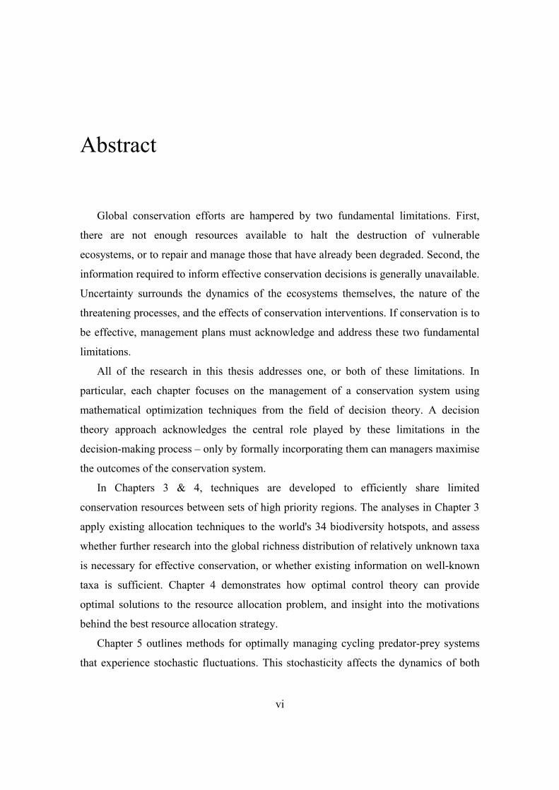
Abstract
Global conservation efforts are hampered by two fundamental limitations. First,
there are not enough resources available to halt the destruction of vulnerable
ecosystems, or to repair and manage those that have already been degraded. Second, the
information required to inform effective conservation decisions is generally unavailable.
Uncertainty surrounds the dynamics of the ecosystems themselves, the nature of the
threatening processes, and the effects of conservation interventions. If conservation is to
be effective, management plans must acknowledge and address these two fundamental
limitations.
All of the research in this thesis addresses one, or both of these limitations. In
particular, each chapter focuses on the management of a conservation system using
mathematical optimization techniques from the field of decision theory. A decision
theory approach acknowledges the central role played by these limitations in the
decision-making process – only by formally incorporating them can managers maximise
the outcomes of the conservation system.
In Chapters 3 & 4, techniques are developed to efficiently share limited
conservation resources between sets of high priority regions. The analyses in Chapter 3
apply existing allocation techniques to the world's 34 biodiversity hotspots, and assess
whether further research into the global richness distribution of relatively unknown taxa
is necessary for effective conservation, or whether existing information on well-known
taxa is sufficient. Chapter 4 demonstrates how optimal control theory can provide
optimal solutions to the resource allocation problem, and insight into the motivations
behind the best resource allocation strategy.
Chapter 5 outlines methods for optimally managing cycling predator-prey systems
that experience stochastic fluctuations. This stochasticity affects the dynamics of both
vi
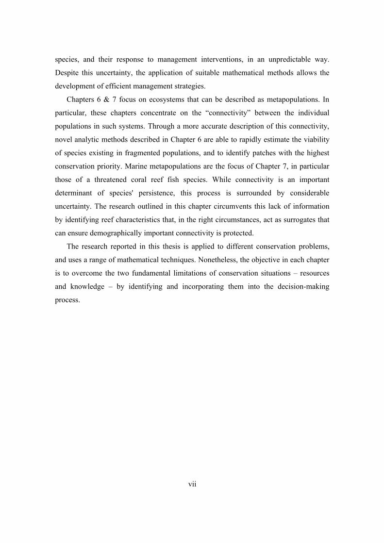
species, and their response to management interventions, in an unpredictable way.
Despite this uncertainty, the application of suitable mathematical methods allows the
development of efficient management strategies.
Chapters 6 & 7 focus on ecosystems that can be described as metapopulations. In
particular, these chapters concentrate on the “connectivity” between the individual
populations in such systems. Through a more accurate description of this connectivity,
novel analytic methods described in Chapter 6 are able to rapidly estimate the viability
of species existing in fragmented populations, and to identify patches with the highest
conservation priority. Marine metapopulations are the focus of Chapter 7, in particular
those of a threatened coral reef fish species. While connectivity is an important
determinant of species' persistence, this process is surrounded by considerable
uncertainty. The research outlined in this chapter circumvents this lack of information
by identifying reef characteristics that, in the right circumstances, act as surrogates that
can ensure demographically important connectivity is protected.
The research reported in this thesis is applied to different conservation problems,
and uses a range of mathematical techniques. Nonetheless, the objective in each chapter
is to overcome the two fundamental limitations of conservation situations – resources
and knowledge – by identifying and incorporating them into the decision-making
process.
vii
Contents
Chapter 1. Introduction 1
1.1. Modern conservation biology 1
1.1.1. A global threat 1
1.1.2. The conservation response 2
1.1.3. Limitations to conservation actions 2
1.2. An illustrative case study: elephants in Kruger National Park 3
1.3. Current conservation practice 5
1.4. Conservation and decision theory 7
1.5. Intended Audience
9
Chapter 2. Overview of the thesis 11
Chapter 3. Allocating conservation resources
using the biodiversity hotspots 17
3.1. Abstract 17
3.2. Global conservation prioritisation 18
3.2.1. Global priority regions 18
3.2.2. The biodiversity hotspots 20
3.2.3. Using dynamic decision theory to allocate funding 22
3.2.4. Appropriate biodiversity choice: the issue of surrogacy 23
3.3. Methods 24
3.3.1. The biodiversity value 25
3.3.2. The cost of conservation action 25
viii
3.3.3. The predicted habitat loss rates 27
3.3.4. The existing land-use distribution 28
3.3.5. Biodiversity returns on conservation investment 29
3.3.6. Expressing the habitat dynamics mathematically 31
3.3.7. Determining efficient funding allocation strategies 32
3.3.8. Null models 34
3.3.9. Calculating the sensitivity of the planning
method to data uncertainty 34
3.4. Results and discussion 35
3.4.1. Efficient conservation funding allocation schedules 35
3.4.2. Taxonomic robustness of allocation schedules 37
3.4.3. Comparison with null models 38
3.4.4. Sensitivity to data uncertainty 40
3.4.5. Considerations when applying these results 41
Chapter 4. Optimal dynamic allocation of conservation funding 45
4.1. Abstract 45
4.2. Introduction 46
4.2.1. Decision theory approaches to conservation prioritisation 46
4.2.2. Limitations to the current optimisation techniques 46
4.2.3. Optimal control theory 48
4.3. Optimal control allocation 49
4.3.1. The optimal control methodology 50
4.3.2. The two-region example 52
4.3.3. Formulating the optimal control approach for two regions 53
4.3.4. Solving the optimal control problem 55
4.3.5. Implementing the optimal control solution 56
4.4. Comparison of optimal control and SDP solutions 58
4.5. Features of the optimal funding allocation schedule 60
4.6. The five-region example 61
4.7. Discussion 63
ix
Chapter 5. Optimal control of oscillating predator-prey systems 67
5.1. Abstract 67
5.2. Predator-prey cycles 68
5.2.1. Predator-prey cycles in conservation systems 68
5.2.2. Stochasticity induced predator-prey cycling 70
5.2.3. Optimal management of cycling predator-prey populations 76
5.3. Methods 77
5.3.1. The population model 77
5.3.2. The system dynamics as a Markov process 81
5.3.3. Application of SDP 82
5.3.4. Example parameters 86
5.4. Results 87
5.5. Management conclusions 90
5.6. Conclusion 93
Chapter 6. Analysing asymmetric metapopulations
using complex network theory 95
6.1. Abstract 95
6.2. Introduction 96
6.2.1. Asymmetric connectivity patterns 96
6.2.2. Dynamic consequences of asymmetric connectivity 96
6.2.3. Simulating asymmetric connectivity 98
6.3. Methods 100
6.3.1. Using complex network metrics to predict
metapopulation dynamics 100
6.4. Results 107
6.4.1. Probability of metapopulation extinction 107
6.4.2. Patch removal strategies 109
6.5. Discussion 112
x
Chapter 7. Can we determine the connectivity value of reefs
using surrogates? 115
7.1. Abstract 115
7.2. Introduction 116
7.2.1. Inter-reef connectivity 116
7.2.2. Planning effective marine reserve networks 119
7.3. Methods 121
7.3.1. The reef fish metapopulation model 121
7.3.2. Effects of protected areas 128
7.3.3. Connectivity surrogates 124
7.3.4. Performance of the reserve networks 128
7.3.5. Testing the robustness of the connectivity surrogates 129
7.4. Results 130
7.4.1. Performance of the different surrogates on the GBR 130
7.4.2. Parameter sensitivity 132
7.4.3. Surrogate performance in subsections of the GBR 132
7.5. Discussion 137
7.5.1. Performance of the surrogates 138
7.5.2. Implications for marine reserve network planning 140
7.5.3. Limitations 143
7.6. Conclusion 144
Chapter 8. Conclusion
8.1. Decision theory in conservation 146
8.2. Conservation resource limitations 147
8.3. Uncertainty in conservation decision-making 150
8.4. Future directions 151
xi

Appendix A: Datasets for the Biodiversity Hotspots 153
Appendix B: Asymmetric connectivity in a
two-patch metapopulation 155
Chapter 9. Bibliography 158
xii
Chapter 1
Introduction
1.1. Modern conservation biology1.1.1. A global threat
As the human population grows, and our per-capita consumption increases, the
demands on the Earth's natural resources become increasingly unsustainable (Dirzo &
Raven 2003; MEA 2005). Habitat degradation and deforestation compromise the purity
of the air and water, decrease soil fertility, and often lead to desertification (Vitousek
1983; Williams 2002). Unrestrained exploitation of the ocean has resulted in the
depletion and collapse of most of the world's fisheries (Jackson 2001; Jackson et al.
2001; Pauly et al. 2002; Pandolfi et al. 2003, 2005). Anthropogenic carbon emissions
are changing the globe's climate, and have already altered temperatures, rainfall patterns
and coastlines (Thomas et al. 2004; IPCC 2007).
Unsustainable demands have already resulted in a highly elevated species extinction
rate (Wilson 1988, 1999; Baillie et al. 2004), yet the effects of the last two industrial
centuries on the Earth's biodiversity have not been fully realised (Tilman et al. 1994).
Human wellbeing, as well as biodiversity, is under threat. The Millennium Ecosystem
Assessment identified the loss of ecosystem services as a major obstacle to achievement
of the United Nations' Millennium Development Goals of reducing hunger, poverty and
disease (MEA 2005).
1
1.1.2. The conservation responseConservation biology is a field of research and practice that aims to mitigate the
harmful effects of humans on the Earth's ecosystems and natural processes, for the
benefit of all life. It has helped coordinate and direct a multi-scale response to these
environmental crises, often successfully. Governments have taken cooperative
conservation action to halt the release of persistent organic pollutants (the Stockholm
Convention), sulphur dioxide emissions (the Convention on Long-Range
Transboundary Air Pollution), wetland degradation (the Ramsar Convention), and
deforestation (the International Tropical Timber Agreement). Non-governmental
conservation organisations have also vastly increased in size, funding and political
leverage. First established in the early 1950s, these NGOs have grown rapidly, and now
wield significant power. The Nature Conservancy, for example, one of the oldest and
largest conservation organisations in the world, controls assets which grew in 2005-
2006 by 9%, to a total of more than USD$4.8 billion (TNC 2006). It owns and manages
terrestrial protected areas that cover more than 47 million hectares, in 21 different
countries.
1.1.3. Limitations to conservation actionsDespite these success stories, environmental degradation continues to accelerate
worldwide (MEA 2005). Worse, efforts taken to reduce or reverse this degradation are
continually frustrated by serious deficiencies. Two of these deficiencies will form the
major themes of my thesis.
1. The first deficiency is of funding. The total resources currently spent on
conservation globally are less than half of what is needed to achieve vital
conservation goals (James et al. 1999a). Available resources must therefore be
spent wisely.
2. The second deficiency is of information. Much of the information required for
effective conservation is currently unknown. The inherent complexity of natural
ecosystems is the cause of much uncertainty (Hastings et al. 1993; Regan et al.
2002), and the response of ecosystems to particular management interventions is
also poorly understood (Possingham et al. 2002; MEA 2005). Conservation
2
decisions must be made in the face of this uncertainty.
These two limitations are found throughout the field of conservation biology, at both
global and local scales. They negatively impact new conservation projects, as well as
the management of existing conservation systems. If the current environmental crisis is
to be halted, conservation biology must be able to cope with these two limitations. The
following example demonstrates how they can complicate conservation actions.
1.2. An illustrative case study: elephants in Kruger
National ParkKruger National Park in South Africa has been protecting African elephant
(Loxodonta africana) herds since the late 1800's. As the largest national park in South
Africa, Kruger represents a well-policed sanctuary for elephants. It maintained large
herds throughout the poaching epidemics that devastated elephant populations across
the continent prior to the 1989 international ban on ivory trading (Stiles 2004). In the
relative safety of the years following the second world war, when European ivory
demand declined with the availability of cheaper artificial substitutes, the elephant
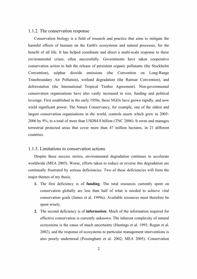
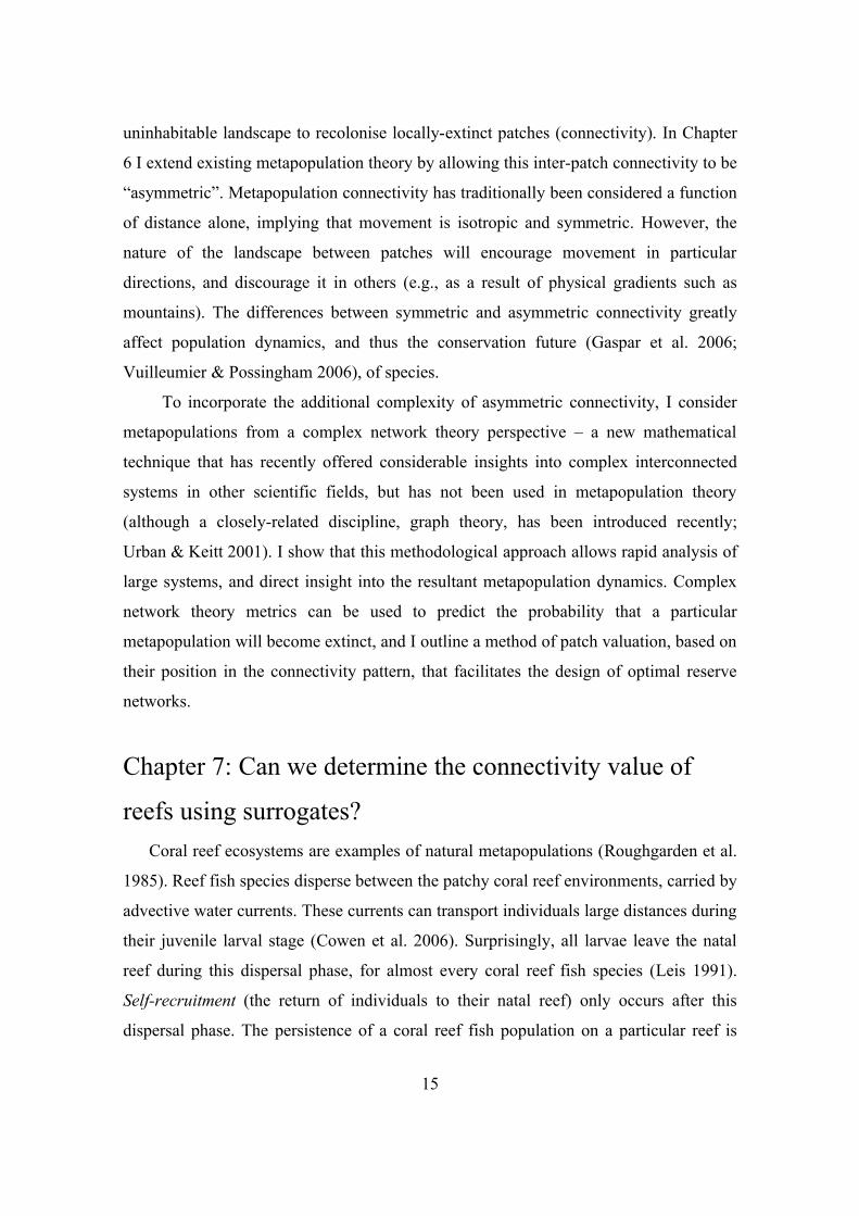
population in Kruger grew exponentially (Figure 1.1).
Elephant density rapidly reached a level that conservation managers considered
threatening to the park's biodiversity, and so in 1967 park managers introduced a culling
regime to keep the population between 7000 and 8500 individuals (Aarde et al. 1999),
resulting in hundreds of individuals being culled each year (Whyte et al. 1998). By
1995, however, international pressure forced wildlife managers in Kruger to cease
culling (Butler 1998), and the population density once again began to increase
dramatically. Most experts agree that even if the current density (estimated at 11,500
individuals in 2004; SANParks 2005) is sustainable, the ongoing rate of increase
(estimated at 7% annually; Mabunda 2005) is not (INDABA 2005). High density
elephant populations threaten their own persistence (Aarde et al. 1999), and that of other
biodiversity through habitat modification and overgrazing (Leuthold 1996; Ebedes
2005).
3
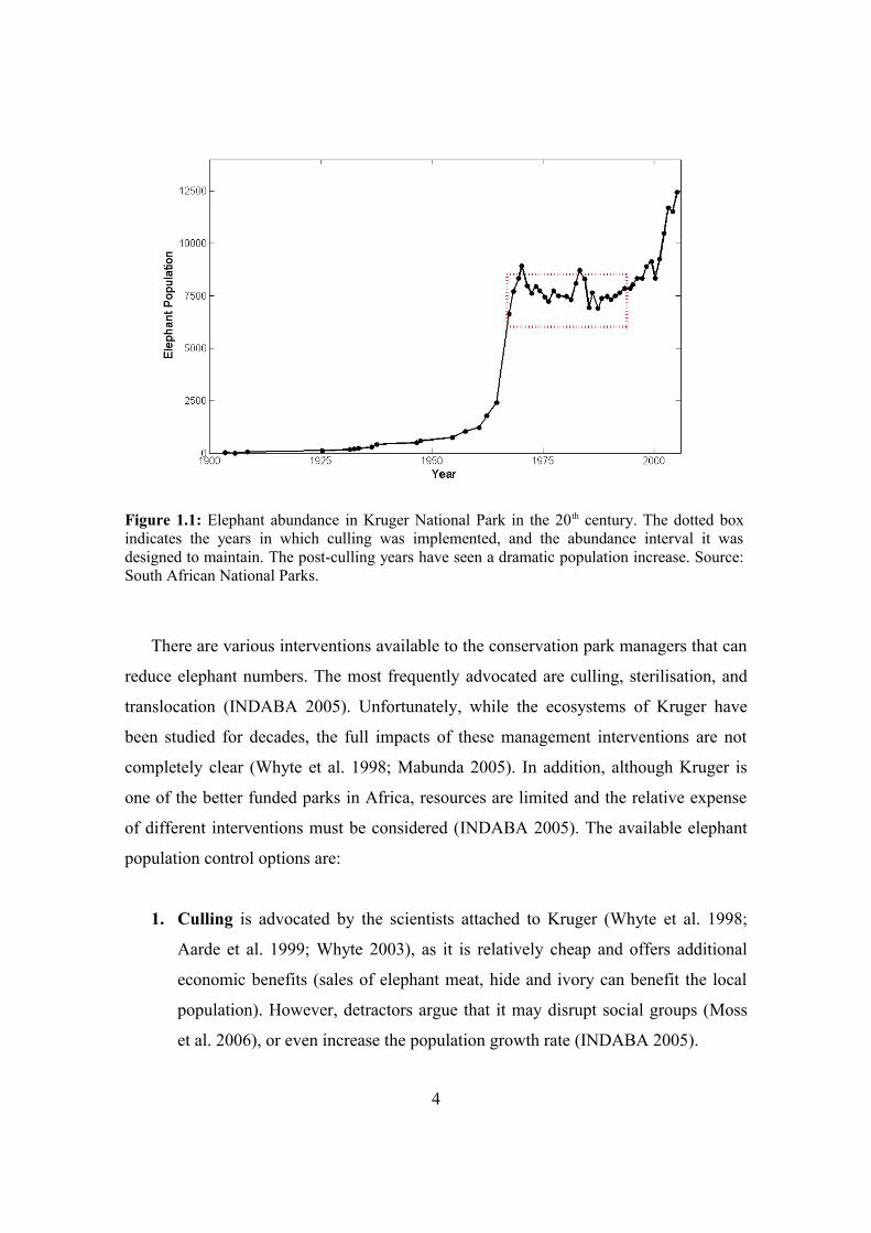
Figure 1.1: Elephant abundance in Kruger National Park in the 20th century. The dotted box indicates the years in which culling was implemented, and the abundance interval it was designed to maintain. The post-culling years have seen a dramatic population increase. Source: South African National Parks.
There are various interventions available to the conservation park managers that can
reduce elephant numbers. The most frequently advocated are culling, sterilisation, and
translocation (INDABA 2005). Unfortunately, while the ecosystems of Kruger have
been studied for decades, the full impacts of these management interventions are not
completely clear (Whyte et al. 1998; Mabunda 2005). In addition, although Kruger is
one of the better funded parks in Africa, resources are limited and the relative expense
of different interventions must be considered (INDABA 2005). The available elephant
population control options are:
1. Culling is advocated by the scientists attached to Kruger (Whyte et al. 1998;
Aarde et al. 1999; Whyte 2003), as it is relatively cheap and offers additional
economic benefits (sales of elephant meat, hide and ivory can benefit the local
population). However, detractors argue that it may disrupt social groups (Moss
et al. 2006), or even increase the population growth rate (INDABA 2005).
4
2. Sterilisation has been trialled extensively since the 1995 culling moratorium,
but it is prohibitively expensive for large reserves (Whyte et al. 1998;
INDABA 2005), and will not begin to halt population growth for more than a
decade (Whyte et al. 1998). It can also have negative consequences: sterilised
females are continually on heat, and disrupt herd behaviour by continually
attracting bulls to the matriarchal herds (Whyte & Grobler 1997).
3. Translocation offers a solution to both the overcrowding that occurs in
successful national parks, and the low numbers of elephants elsewhere on the
continent. However, like sterilisation, this method is quite expensive, and
suitable destinations for the animals are decreasing (Foggin 2003). Even after
the translocation, individuals may return to the park (SANParks 2005).
As of 2007, the often acrimonious debate about the best solution for Kruger's
elephant problem continues, as does the increase of the population (Clayton 2007). I
will return to the issue of ecosystem control in Chapter 5.
1.3. Current conservation practiceThe situation in Kruger National Park is typical of conservation problems
worldwide. Not only is it unclear which interventions will achieve the best conservation
outcomes given the limited resources, but the exact consequences of each intervention
are also uncertain. Unfortunately, while these two limitations are regularly mentioned in
the conservation literature, very few analyses deal with them in a rigorous manner.
This oversight may be a result of conservation biology's origins. Conservation
biology evolved from the discipline of ecology in the early 1980s
(Caughley & Gunn 1996), and researchers are still preoccupied with the ecological
features of conservation. Take, for example, commentary on conservation biology
written by two of the most famous living researchers: E. O. Wilson's (2000) editorial on
the “future of conservation biology” decries the scarcity of information on species
diversity and phylogeny, but does not mention any of the economic, social or political
factors that also affect conservation outcomes, but about which very little is known.
5
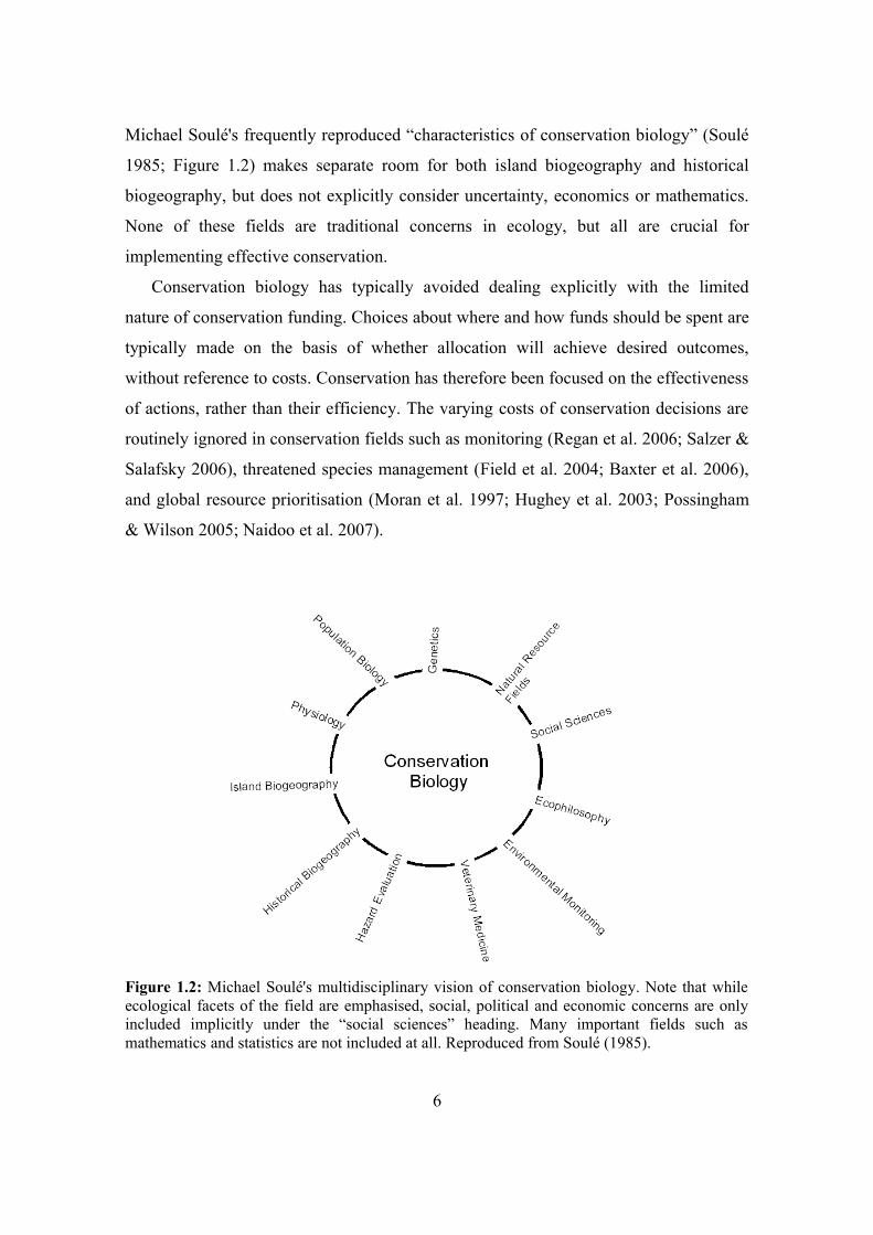
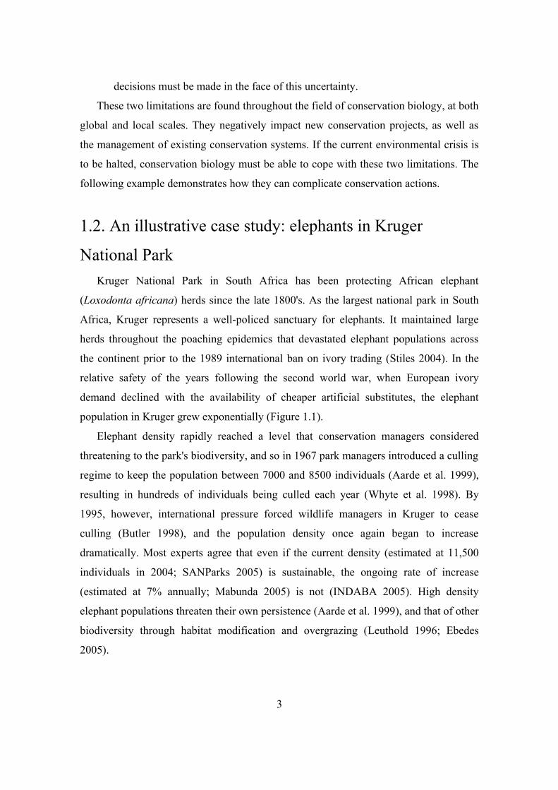
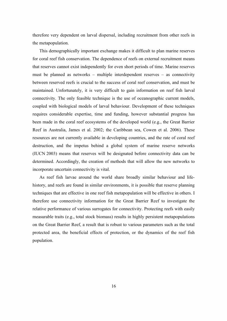
Michael Soulé's frequently reproduced “characteristics of conservation biology” (Soulé
1985; Figure 1.2) makes separate room for both island biogeography and historical
biogeography, but does not explicitly consider uncertainty, economics or mathematics.
None of these fields are traditional concerns in ecology, but all are crucial for
implementing effective conservation.
Conservation biology has typically avoided dealing explicitly with the limited
nature of conservation funding. Choices about where and how funds should be spent are
typically made on the basis of whether allocation will achieve desired outcomes,
without reference to costs. Conservation has therefore been focused on the effectiveness
of actions, rather than their efficiency. The varying costs of conservation decisions are
routinely ignored in conservation fields such as monitoring (Regan et al. 2006; Salzer &
Salafsky 2006), threatened species management (Field et al. 2004; Baxter et al. 2006),
and global resource prioritisation (Moran et al. 1997; Hughey et al. 2003; Possingham
& Wilson 2005; Naidoo et al. 2007).
Figure 1.2: Michael Soulé's multidisciplinary vision of conservation biology. Note that while ecological facets of the field are emphasised, social, political and economic concerns are only included implicitly under the “social sciences” heading. Many important fields such as mathematics and statistics are not included at all. Reproduced from Soulé (1985).
6
Information about many threatened ecosystems is limited, and in some is even
declining (MEA 2005). The effectiveness of many conservation interventions is also
uncertain, but conservation biologists have not generally sought to ascertain
effectiveness experimentally, nor attempted to gather evidence anecdotally when
implementing conservation actions (Ferraro & Pattanayak 2006; Salzer & Salafsky
2006). In addition, conservation biologists have rarely considered how this ubiquitous
uncertainty should affect their decision-making (Williams 2001; Regan et al. 2002;
Hauser et al. 2006). Conservation biologists' response to uncertainty has typically been
to call for improved scientific understanding (e.g., of species distributions, or ecosystem
dynamics).
1.4. Conservation and decision theoryConservation is a “crisis discipline” (Soulé 1985). Although funding and
information shortfalls could be reduced given increased time or resources, neither of
these is likely to become available in sufficient quantities. Fortunately, conservation
research has begun to embrace systematic methods that attempt to achieve as many
conservation outcomes as possible, in the face of these two fundamental impediments.
“Decision theory” methodology has grown more prevalent in conservation biology
(Possingham 1996, 1997; Possingham et al. 2001; Westphal & Possingham 2003), as
has the use of “systematic conservation planning” (Margules & Pressey 2000;
Possingham et al. 2000; Moilanen et al. 2005). These approaches demand that the goals
of conservation, and the uncertainty surrounding the system dynamics, be expressed
explicitly. Techniques are then applied that achieve the best conservation outcomes by
acknowledging and incorporating these limitations.
“Operations Research” is a field of applied mathematics which deals with exactly
these sorts of problems. In fact, many of the methods used in both decision theory and
systematic conservation planning originated from the field of operations research. Born
during the second world war, operations research aimed to maximise the effectiveness
of scarce military resources, while dealing with the uncertainty always present in
military conflict. Although the field of battle is very different from the field in
7
conservation biology, the problem formulation, and the methods used to construct
solutions, are directly applicable. Operations research and decision theory approaches
usually include the following features:
1. A clear objective must be stated that represents the desired state of the system.
This objective is the goal of operations research, but it is formulated externally.
In other words, the objective is subjective: different stakeholders may have
different ideas about what condition they would like the system to be in, or what
they would like it to produce. Decision theory and operations research are useful
only after the objective has been decided. Given a particular objective, the goal
of operations research is optimisation – it is usually not sufficient that a
conservation strategy has positive outcomes (e.g., increasing a species'
persistence); it must represent the most efficient use of the available resources.
2. The condition of the system must be described in some quantitative manner.
This approach is known as “state-dependent decision making”: different
ecosystem states demand different conservation responses (e.g., overpopulation
versus low population).
3. The system dynamics must also be described. Conservation situations do not
remain static, and effective conservation planning therefore requires an
understanding of how the system is likely to change in the future, with and
without conservation interventions (Ferraro & Pattanayak 2006).
4. The interventions available to the conservation manager must be listed.
These interventions are primarily constrained by the available resources. This is
generally the total amount of funding available, but constraints can also be non-
monetary. For example, the number of interventions that park staff can perform
in a year is limited by the capabilities and capacity of the workforce
(Rodrigues et al. 2006).
5. Uncertainty must be addressed. Components of the conservation system are
often only partially known, and therefore the objective cannot be optimised if
this uncertainty is not incorporated into the decision process. The best
conservation outcomes will not be obtained by assuming that available estimates
8
accurately represent reality (Ludwig et al. 1993; Regan et al. 2005). Instead, we
can use our knowledge about the uncertainty (von Neumann & Morgenstern
1947), or simply the recognition of its existence (Ben-Haim 2001), to anticipate
the effects of our ignorance.
Throughout this thesis I will be applying methods from operations research and
decision theory to problems in conservation biology. Operations research and decision
theory perspectives are very similar, but in this introduction I have stressed operations
research to emphasise the wealth of perspectives and techniques that conservation
biology can find in the fields of applied mathematics. In the various chapters of this
thesis, I apply such methods to different fields of conservation: global scale resource
allocation, the persistence of species in fragmented habitats, threatened species
management and marine reserve network design. Despite contextual differences, the
methods I devise to address these conservation scenarios all belong to operations
research and decision theory, and share most or all of the five features outlined above.
1.5. Intended audienceAnalyses that explicitly deal with the fundamental limitations of resources and
information have only recently been introduced to conservation biology, beginning with
“population viability analyses” (Boyce 1992) and “systematic reserve design” (Pressey
et al. 1993). The aim of this thesis is therefore to disseminate information about decision
theory and operations research. The different chapters of the thesis are aimed at two
different types of conservation biologist. Chapters 4 & 6 are concerned with broad
ideas, and approaches to conservation theory; these chapters are aimed at conservation
theorists. Rather than explaining in detail how these methods would be applied to
particular conservation situations, I instead explore their potential in systems that are of
conservation interest. While the analytic methods that I use are not necessarily
mathematically novel, they are both quite new to conservation.
The remaining content Chapters (3, 5 & 7) are intended to be more immediately
applicable, and to be of direct use, to conservation practitioners. The methods applied
9

to these problems are better established in conservation (although they are still not
widely known). In this thesis, however, they are applied to new conservation problems,
where they can play an important role in ensuring efficient management. My hope is
that the research contained in this thesis will help increase the scope, and encourage the
application, of decision theory and operations research approaches to conservation
biology.
10
Chapter 2
Overview of the thesis
The chapters in this thesis were initially developed as individual manuscripts,
without any concerted attempt at thematic consistency. Theoretical conservation biology
is a new field, and there are diverse areas where very little mathematical research has
been done. Some of these conservation subjects are quite new (Chapters 3 & 4),
whereas in other, recently discovered mathematical techniques offer novel insights to
established fields (Chapter 6). Finally, improvements in computing or remote sensing
power allow the application of techniques that were previously unavailable (Chapter 5
& 7). In such circumstances, a theoretical conservation biologist can offer
mathematically straightforward insight that can make considerable practical difference.
As a mathematical graduate, choosing an array of applications, rather than exploring a
particular subject in conservation biology, allowed me to broaden my understanding of
conservation biology's multiple fields. The chapters that follow detail some of the
research that resulted.
Chapter 3: Allocating conservation resources among the
biodiversity hotspots.Habitat destruction and species extinction are occurring on a global scale, and in
response many of the largest non-governmental and transnational conservation agencies
11
have increased the scale of their response. Spending is prioritised at a global scale with
the use of sets of Global Priority Regions (GPRs) – small subsections of the globe that
encompass disproportionately large amounts of valuable biodiversity. The oldest and
most famous of these GPRs are the “biodiversity hotspots” of Conservation
International (Myers et al. 2000).
However, the set of biodiversity hotspots ignore some very important facets of the
current global environmental situation (Possingham & Wilson 2005), most importantly
the taxonomic variation in the global distribution of biodiversity (Grenyer et al. 2006),
the varying cost of conservation actions in different regions (Naidoo et al. 2007), and
the dynamic nature of the biodiversity threats (Kareiva & Marvier 2003). A recent paper
by Wilson et al. (2006) outlined a dynamic decision theory approach that incorporates
these factors into funding allocation plans, and I apply these new methods to the 34
biodiversity hotspots, using seven separate taxonomic measures of biodiversity. To do
so, I use global-scale datasets on endemic species richness, predicted future habitat loss
rates, the cost of land acquisition, and the current distibution of land use in the
biodiversity hotspots. Using the resultant seven funding schedules I demonstrate that the
observed lack of congruence between global species distributions does not translate into
different conservation spending decisions. Using two additional null models, I examine
the relative contribution of biodiversity and socio-economic factors (the cost, habitat
loss rates, and the land use distribution) to efficient funding decisions. I finally perform
sensitivity analyses, to investigate where additional research would most profitably be
directed to ensure better global conservation outcomes.
Chapter 4: Optimal dynamic allocation of conservation
fundingIn Chapter 3, heuristic allocation methods were used to determine efficient
conservation spending among the 34 biodiversity hotspots. An heuristic approach to
conservation funding allocation is unsatisfactory for a number of reasons. Obviously it
would be preferable to be able to calculate optimal allocation strategies, as heuristic
12
solutions are consistently suboptimal (albeit by only a few percentage points). More
importantly, the mathematical technique that was used to formulate the optimal solution
for the smaller two-region problem (SDP) provides solutions that are difficult to
interpret. The resulting optimal allocation schedules (Wilson et al. 2006) had certain
consistent and unusual characteristics. It would be useful to determine whether these
characteristics are common to optimal schedules. This would not only provide some
insight into how optimal conservation returns can be achieved, it would also be useful
for planning future heuristics.
An optimal allocation schedule for large numbers of regions can be calculated with
the application of “optimal control theory” to a subtle reformulation of the conservation
model outlined in Wilson et al. (2006). Optimal control sidesteps the computational
problems that plague the SDP approach, and provides a solution in a form that is
amenable to interpretation. I use optimal control to solve the general conservation
resource allocation problem. Following this, I demonstrate and verify the methodology
by applying it to the two problems analysed in Wilson et al. (2006). I reproduce the
optimal allocation schedule for a two-region system, and then provide an optimal
solution for a five-region system. The particular form of these optimal allocation
schedules is discussed, using the insights provided by the new approach.
Chapter 5: Optimal control of oscillating predator-prey
systemsMany ecosystems contain multiple interacting species that are threatened, and thus
of conservation concern. One of the most commonly encountered threatened species
interaction is the “predator-prey” ecosystem. Predator-prey ecosystems are often cyclic,
as predators overexploit their prey, then themselves fall victim to starvation. In natural
ecosystems, this instability is held in check by various mechanisms, in particular spatial
effects. In the smaller world of conservation reserves and game parks, however,
predator-prey interactions can quickly lead to one or both species becoming extinct.
Other species in the ecosystem that depend on similar resources can also be driven to
13
extinction (Leuthold 1996).
Reserve managers typically avoid this outcome by culling predators once they
reach a particular abundance (§1.2), an approach which results in frequent, expensive
interventions that generate protests from animal-rights groups (e.g., elephants, Moss et
al. 2006; kangaroos and wallabies, Stewart 2001; koalas, Tabart 2000). Although the
dynamics of the predator-prey cycles have been studied extensively in the mathematical
ecology literature (Turchin 2003), an optimal management strategy for these systems
has never been formulated. I demonstrate the application of a Stochastic Dynamic
Programming (SDP) optimisation method to a general predator-prey system, and
develop a management strategy that ensures the persistence of both species. SDP
provides management strategies that ensure a much more persistent ecosystem, with
only a few culling interventions required.
Chapter 6: Analysing asymmetic metapopulations using
complex network metricsMetapopulation theory is a paradigm for analysing spatially fragmented populations,
and has gained particular relevance through its use in conservation biology (Hanski &
Gaggiotti 2004). Populations are frequently distributed heterogeneously through space,
making the use of non-spatial models inappropriate. Conceptually, metapopulation
theory approaches the spatial nature of the population by treating high-density
aggregations of individuals as the fundamental unit of population dynamics, rather than
the individuals themselves (Levins 1966). In metapopulations, space is dichotomized
into inhabitable patches surrounded by uninhabitable landscape, allowing the
application of less complicated spatial mathematical methods (rather than explicitly
spatial mathematical methods such as partial differential equations).
Metapopulations occur naturally (e.g., island archipelagos or coral reefs), however
anthropogenic land modification has created many more of these systems by
fragmenting habitat that was once contiguous (Harrison & Bruna 1999). The small
remaining habitat fragments may be prone to episodic local extinction, and the
persistence of species thus depends on the ability of individuals to transverse
14
uninhabitable landscape to recolonise locally-extinct patches (connectivity). In Chapter
6 I extend existing metapopulation theory by allowing this inter-patch connectivity to be
“asymmetric”. Metapopulation connectivity has traditionally been considered a function
of distance alone, implying that movement is isotropic and symmetric. However, the
nature of the landscape between patches will encourage movement in particular
directions, and discourage it in others (e.g., as a result of physical gradients such as
mountains). The differences between symmetric and asymmetric connectivity greatly
affect population dynamics, and thus the conservation future (Gaspar et al. 2006;
Vuilleumier & Possingham 2006), of species.
To incorporate the additional complexity of asymmetric connectivity, I consider
metapopulations from a complex network theory perspective – a new mathematical
technique that has recently offered considerable insights into complex interconnected
systems in other scientific fields, but has not been used in metapopulation theory
(although a closely-related discipline, graph theory, has been introduced recently;
Urban & Keitt 2001). I show that this methodological approach allows rapid analysis of
large systems, and direct insight into the resultant metapopulation dynamics. Complex
network theory metrics can be used to predict the probability that a particular
metapopulation will become extinct, and I outline a method of patch valuation, based on
their position in the connectivity pattern, that facilitates the design of optimal reserve
networks.
Chapter 7: Can we determine the connectivity value of
reefs using surrogates?Coral reef ecosystems are examples of natural metapopulations (Roughgarden et al.
1985). Reef fish species disperse between the patchy coral reef environments, carried by
advective water currents. These currents can transport individuals large distances during
their juvenile larval stage (Cowen et al. 2006). Surprisingly, all larvae leave the natal
reef during this dispersal phase, for almost every coral reef fish species (Leis 1991).
Self-recruitment (the return of individuals to their natal reef) only occurs after this
dispersal phase. The persistence of a coral reef fish population on a particular reef is
15
therefore very dependent on larval dispersal, including recruitment from other reefs in
the metapopulation.
This demographically important exchange makes it difficult to plan marine reserves
for coral reef fish conservation. The dependence of reefs on external recruitment means
that reserves cannot exist independently for even short periods of time. Marine reserves
must be planned as networks – multiple interdependent reserves – as connectivity
between reserved reefs is crucial to the success of coral reef conservation, and must be
maintained. Unfortunately, it is very difficult to gain information on reef fish larval
connectivity. The only feasible technique is the use of oceanographic current models,
coupled with biological models of larval behaviour. Development of these techniques
requires considerable expertise, time and funding, however substantial progress has
been made in the coral reef ecosystems of the developed world (e.g., the Great Barrier
Reef in Australia, James et al. 2002; the Caribbean sea, Cowen et al. 2006). These
resources are not currently available in developing countries, and the rate of coral reef
destruction, and the impetus behind a global system of marine reserve networks
(IUCN 2003) means that reserves will be designated before connectivity data can be
determined. Accordingly, the creation of methods that will allow the new networks to
incorporate uncertain connectivity is vital.
As reef fish larvae around the world share broadly similar behaviour and life-
history, and reefs are found in similar environments, it is possible that reserve planning
techniques that are effective in one reef fish metapopulation will be effective in others. I
therefore use connectivity information for the Great Barrier Reef to investigate the
relative performance of various surrogates for connectivity. Protecting reefs with easily
measurable traits (e.g., total stock biomass) results in highly persistent metapopulations
on the Great Barrier Reef, a result that is robust to various parameters such as the total
protected area, the beneficial effects of protection, or the dynamics of the reef fish
population.
16
Chapter 3
Allocating conservation resources among
the biodiversity hotspots
3.1. AbstractThe funding available for conservation is insufficient to protect the earth's rapidly
disappearing biological diversity. Despite this shortfall, economic considerations have
had relatively little influence on funding allocation at a global scale. Instead, funding is
directed to sets of “global priority regions”, which are defined primarily by their
biological attributes. By applying dynamic funding allocation methods that incorporate
regionally varying costs of conservation action, as well as traditional metrics of endemic
species richness and rates of habitat loss, I propose the first efficient allocation
schedules for the world's 34 “biodiversity hotspots”. However, global conservation
priority regions have been criticised for using the richness of a single taxon to measure
regional biodiversity value. I therefore determine separate funding allocation schedules
for seven different taxonomic groups, which each have different geographic richness
patterns, to assess whether the incorporation of socio-economic factors (specifically the
cost of land and the rates of habitat loss) results in similar conservation decisions. The
resulting seven funding schedules have broadly similar priorities, suggesting that shared
socio-economic factors overcome much of the variation in biodiversity distribution.
17
Hence, if socio-economic factors are considered in the decision-making process,
conservation organisations can be more confident about the effectiveness of global-scale
spending that is guided by single taxonomic groups. I also perform sensitivity analyses
to assess the effects of data uncertainty on conservation. The results suggest that
conservation outcomes will benefit most from improved information on costs, rather
than threat or biodiversity.
3.2. Global conservation prioritisationThe most pernicious impact of Homo sapiens on the Earth's environment is our
modification of land. Between one-third and one-half of the Earth's natural terrestrial
habitat has been transformed significantly by human activities (Vitousek et al. 1997),
with 10-15% being modified for intensive agriculture alone (Olson et al. 1983). The rate
of alteration has increased over the last few decades, and is projected to intensify further
in the near future (MEA 2005). This is particularly true for certain types of ecosystems,
such as mangroves (UNEP 2006) and freshwater wetlands (Moser et al. 1996).
This level of habitat alteration has been recognised as the greatest single driver of
the current mass-extinction event (Baillie et al. 2004). In response, conservation
organisations – national, multi-national and non-governmental – have decided that the
best available solution is to construct a global network of well-maintained conservation
reserves. At present, this network covers 11.5% of the earth's land surface
(Chape et al. 2003). Despite this significant investment, it is estimated that a
comprehensive global network of conservation reserves will cost an additional US$17
billion annually to create and maintain, over the next 30 years (James et al. 1999a).
Current expenditure (estimated at around US$6 billion per year; James et al. 1999b)
falls far short of requirements; available resources must therefore be prioritised to
protect the most important remaining habitat.
3.2.1. Global priority regionsRecognising this resource limitation, various conservation organisations have
created sets of “Global Priority Regions” (GPRs; Table 3.1). These GPRs are small
18
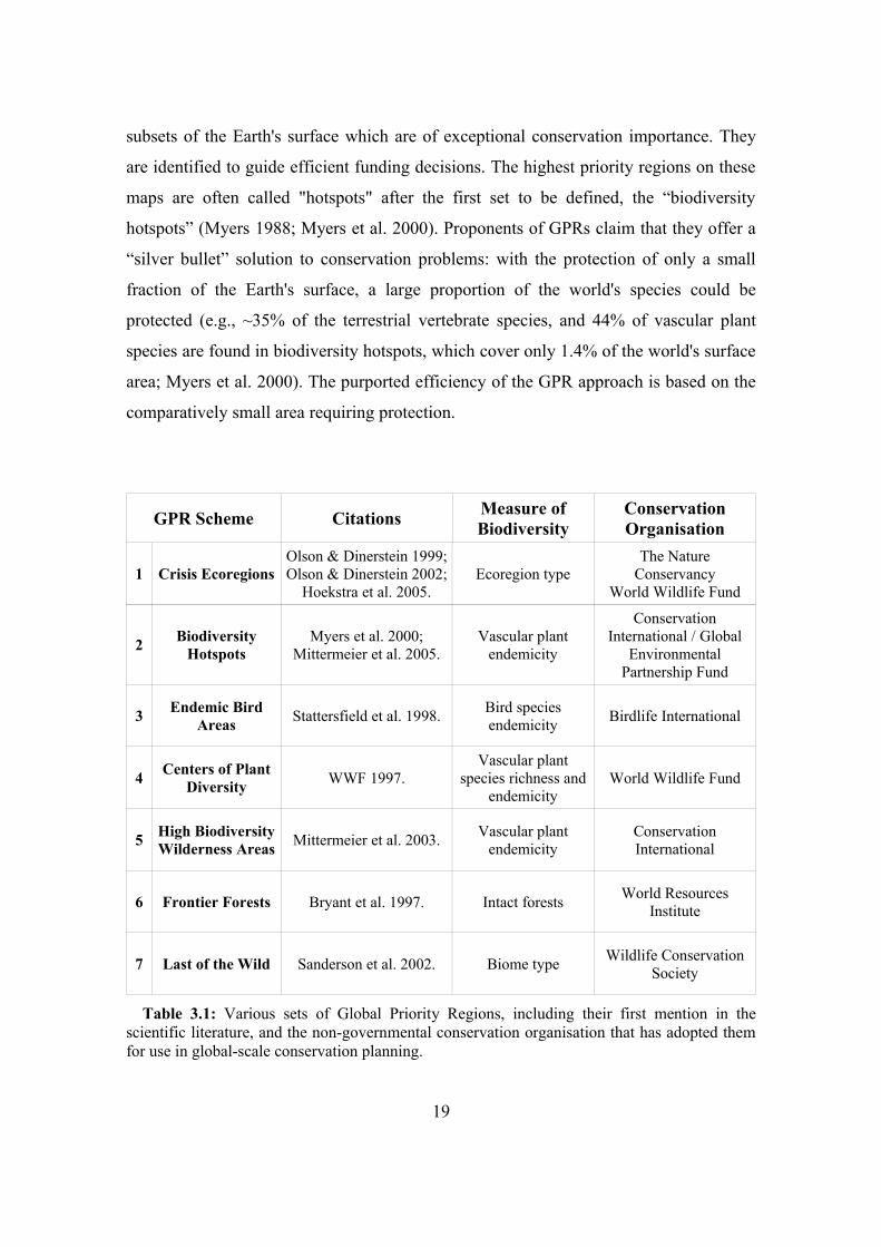
subsets of the Earth's surface which are of exceptional conservation importance. They
are identified to guide efficient funding decisions. The highest priority regions on these
maps are often called "hotspots" after the first set to be defined, the “biodiversity
hotspots” (Myers 1988; Myers et al. 2000). Proponents of GPRs claim that they offer a
“silver bullet” solution to conservation problems: with the protection of only a small
fraction of the Earth's surface, a large proportion of the world's species could be
protected (e.g., ~35% of the terrestrial vertebrate species, and 44% of vascular plant
species are found in biodiversity hotspots, which cover only 1.4% of the world's surface
area; Myers et al. 2000). The purported efficiency of the GPR approach is based on the
comparatively small area requiring protection.
GPR Scheme Citations Measure of Biodiversity
Conservation Organisation
1 Crisis EcoregionsOlson & Dinerstein 1999; Olson & Dinerstein 2002;
Hoekstra et al. 2005.Ecoregion type
The Nature Conservancy
World Wildlife Fund
2 Biodiversity Hotspots
Myers et al. 2000; Mittermeier et al. 2005.
Vascular plant endemicity
Conservation International / Global
Environmental Partnership Fund
3 Endemic Bird Areas Stattersfield et al. 1998. Bird species
endemicity Birdlife International
4 Centers of Plant Diversity WWF 1997.
Vascular plant species richness and
endemicityWorld Wildlife Fund
5 High Biodiversity Wilderness Areas Mittermeier et al. 2003. Vascular plant
endemicityConservation International
6 Frontier Forests Bryant et al. 1997. Intact forests World Resources Institute
7 Last of the Wild Sanderson et al. 2002. Biome type Wildlife Conservation Society
Table 3.1: Various sets of Global Priority Regions, including their first mention in the scientific literature, and the non-governmental conservation organisation that has adopted them for use in global-scale conservation planning.
19
The most powerful feature of GPRs is the flexibility of the funding they attract.
Non-governmental conservation funding is predominantly sourced from private donors
in the developed world (Brooks et al. 2006), but the greatest threats to global
biodiversity are situated in the developing world, as reflected in the location of most
GPRs. For example, approximately 90% of the biodiversity hotspots are situated
entirely in the developing world (Mittermeier et al. 2005), but 90% of global
conservation funds are raised in the developed world (James et al. 1999a). Unlike most
conservation resources, GPR funding is generally not tied to a particular location; it can
therefore reach regions of global importance that would not have been able to raise the
necessary funds locally (although analysis of global spending patterns indicate that
global priority regions are not guiding a large proportion of conservation funding;
Halpern et al. 2006).
While all of the GPRs in Table 3.1 aim to efficiently slow current rates of
biodiversity loss, they have been created and supported by different conservation
agencies, and are designated based on different criteria. This is particularly obvious in
the type of biodiversity targeted by each GPR set (column 3 of Table 3.1). GPRs – and
thus the current prioritisation of global conservation spending – also consistently omit
fundamental factors that should affect the allocation of funds (Kareiva & Marvier 2003;
O'Connor et al. 2003). The purpose of this chapter is twofold: (1) to describe and apply
decision theory methods that can incorporate these omitted factors into GPR priority
setting and (2) to investigate whether the use of different biodiversity objectives result
in different conservation spending decisions. Throughout this chapter I will focus my
attention on the “biodiversity hotspots”, but the results and conclusions will have
relevance to all of the GPRs.
3.2.2. The biodiversity hotspotsBiodiversity hotspots (Figure 3.2a) are the oldest and most famous of the GPRs, and
were the first set to attract official endorsement from a global conservation organisation
(Conservation International). These factors have attracted large amounts of funding and
publicity to the hotspots: it is estimated that they have attracted more than
USD$750 million in funding (Myers 2003) since their inception. This amount includes
20
considerable ongoing funding commitments such as the Global Conservation Fund
(USD$100 million, aimed at the biodiversity hotspots and high biodiversity wilderness
areas; GCF 2006), and the Critical Ecosystems Partnership Fund (USD$150 million
over 5 years, aimed at the hotspots; CEPF 2006). Biodiversity hotspots target
ecoregions with high irreplacibility and high vulnerability (Margules & Pressey 2000).
The irreplacibility of candidate regions is measured by their vascular plant endemicity
(each contains more than 1500 species, or 0.5% of endemic species), while their
vulnerability is determined by the scale of existing habitat degradation (each has lost
more than 70% of its original vegetation cover). Worldwide, 34 ecoregions satisfy both
of these criteria.
There are fundamental problems with the transparency and consistency of the
methods used to delineate the set of 34 biodiversity hotspots (Mace et al. 2000;
Kareiva & Marvier 2003; Possingham & Wilson 2005) – a worrying situation when the
movement of a boundary, or the consideration of an additional factor, can mean the
difference between millions of dollars of investment, and no investment at all.
Nevertheless, so much time and resources have been invested in the designation of the
hotspots that they will be used to guide global funding into the foreseeable future. It is
therefore important that available funding is shared effectively amongst the biodiversity
hotspots, so that their fundamental purpose is achieved as closely as possible:
How should limited conservation funding be shared amongst the biodiversity
hotspots to ensure that the fewest species become extinct?
This question is adapted from Myers et al. (2000), the article which defined the
current set of hotspots. Unfortunately, the biodiversity hotspots cannot answer this
question in their present form. GPRs are lists, and do not explicitly differentiate
between component regions, nor can they provide an unambiguous ranking. While they
can indicate which regions might require urgent funding, they do not offer an explicit,
quantitative method for sharing available resources among them. To answer this
question, additional factors must be considered (primarily the cost of conservation
actions in the different priority regions, and the predicted future rates of biodiversity
21
loss). Dynamic decision theory tools are needed to incorporate these factors into the
GPR concept.
3.2.3. Using dynamic decision theory to allocate fundingAs the aim of the biodiversity hotspots is to halt species extinction, it is important to
consider the relative richness of the different hotspots. However, the limited available
funding, and the dynamic nature of the conservation situation demand that at least two
additional factors be considered:
The cost of conservation: A fundamental limitation of all GPRs to date is that they
do not consider the varying costs of conservation (Possingham & Wilson 2005;
Brooks et al. 2006), but instead consider area to be a suitable proxy. The per-unit-area
costs of conservation action in those hotspots that are situated in the developed world
(e.g., the California Floristic Province) are orders of magnitude higher than in those
situated in the developing world (e.g., Madagascar and the Indian Ocean Islands); up to
seven orders of magnitude higher (Balmford et al. 2003). As a result, allocating the
same amount of money to hotspots in developed countries is less likely to achieve as
many conservation objectives as money spent in developing countries.
Predicted future biodiversity loss rates: Biodiversity hotspots consider threats to
biodiversity by requiring that each hotspot has lost a particular amount of habitat (more
than 70%), as habitat and species persistence are closely related. However, this measure
of vulnerability is based on historical habitat loss, which may not reflect ongoing, or
future loss rates (Kareiva & Marvier 2003). For example, the Amazon rainforest would
not qualify as a hotspot, even though it is subject to the highest absolute rate of habitat
destruction in the world (Laurence et al. 2000), as it is over 80% intact (Mittermeier et
al. 2003). On the other hand, many developed countries in the Mediterranean Basin
hotspot (which has lost 95% of its native habitat; Mittermeier et al. 2005), are
experiencing spontaneous revegetation of native habitat on agricultural land that was
abandoned during the industrial revolution (Piussi & Pettenella 2000).
Dynamic decision theory: Information on the biodiversity, habitat loss rates, and
costs in each biodiversity hotspot must be integrated into a dynamic decision theory
framework. A decision theory approach uses mathematical techniques to optimise a
22
clearly stated objective, subject to constraints on the system, and on the actions
available to the manager. In addition to providing an efficient solution to the problem,
applying decision theory gives the decision-making process exceptional transparency, as
all the objectives and assumptions are stated explicitly. Habitat loss rates in particular
are not constant, but change through time as habitat protection and loss occur
(Armsworth et al. 2006; Etter et al. 2006). An optimal management strategy must
therefore adapt to, and prepare for, the evolving conservation situation. Rather than
being a simple list of priorities, or even a proportional allocation to each biodiversity
hotspot, a dynamic conservation funding allocation strategy must take the form of a
schedule, where the allocation to each region, at each timestep in the funding period, is
planned.
3.2.4. Appropriate biodiversity choice: the issue of surrogacyAs well as the framework of decision theory, GPRs must consider the definition of
biodiversity that they target. Many GPRs, including the biodiversity hotspots, use the
regional richness of endemic species to measure biodiversity. However, most GPRs also
state that they are intended to benefit more than just the taxon used for designation (e.g.,
the biodiversity hotspots are not intended solely for the benefit of vascular plants). The
designation taxon is therefore assumed to be an effective “surrogate” for other taxa of
conservation interest.
The issue of effective surrogacy is the subject of some debate in the conservation
planning literature. Published analyses have claimed that the global-scale distributions
of different biodiversity measures have high congruence, while others have claimed the
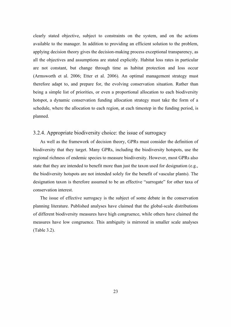
measures have low congruence. This ambiguity is mirrored in smaller scale analyses
(Table 3.2).
23
High congruence Low congruence
Global scale Lamoreux et al. 2006
Orme et al. 2005
Ceballos & Ehrlich 2006
Grenyer et al. 2006
Regional scaleHoward et al. 1998
Moore et al. 2003
Prendergast et al. 1993
van Jaarsveld et al. 1998
Reyers et al. 2000
Table 3.2: Papers presenting results on the spatial congruence of different biodiversity measures. Papers suggesting that priority regions can be designated using only a single measure of biodiversity were considered to indicate high congruence. Papers that suggested this was not possible were considered to indicate low congruence.
“Congruence” is typically measured by the spatial correlation in the species richness
of different taxa (e.g., Grenyer et al. 2006). If this congruence is low, then the authors
frequently argue that GPRs based on the richness of single taxon cannot guide robust
conservation planning decisions. However, as they focus on biodiversity alone, these
analyses belong more to the field of macroecology than conservation planning.
Conservation planning decisions must also consider factors such as cost and threat.
In this chapter I calculate funding strategies for seven different taxonomic measures
of biodiversity, to determine the most effective allocation of conservation funds for
each. These separate strategies allow me to assess whether the differences in richness
distribution translate into different conservation decisions. In addition, I use sensitivity
analyses to ascertain which of the important system parameters is the most sensitive to
error, and use this information to make recommendations about future research
directions.
3.3. MethodsApplication of the decision theory approach to the biodiversity hotspots requires
four datasets. These contain data on (1) the biodiversity value, (2) the cost of
conservation action, (3) the rate of habitat loss and (4) the existing land-use distribution
in each region.
24
3.3.1. The biodiversity valueAlthough biodiversity is an extremely difficult ecological concept to define, the
number of species endemic to a region is generally viewed as a reasonable proxy of its
irreplaceable biodiversity value (Orme et al. 2005). The restricted range of endemic
species makes them especially vulnerable to ongoing habitat loss. To measure the
biodiversity value of the hotspots, I used seven different measures:
1. Mammal endemicity,
2. Bird endemicity,
3. Amphibian endemicity,
4. Reptile endemicity,
5. Tiger beetle endemicity,
6. Freshwater fish endemicity,
7. Vascular plant endemicity.
Analyses were also performed using the total number of endemic terrestrial
vertebrates (the sum of values 1 to 4). These were compiled to provide a dataset at a
phylogenetic scale comparable with the vascular plant endemicity. Information on the
endemic species richness of the biodiversity hotspots was sourced from Mittermeier et
al. (2005). The endemicity of each biodiversity hotspot is shown in Appendix A.
3.3.2. The cost of conservation actionThe cost of conservation action depends on exactly what interventions will be
undertaken to counteract ongoing biodiversity loss. I chose to use the cost of land
acquisition for these analyses, as this is a widely-used conservation response.
Pragmatically, data on the land acquisition costs could be obtained in a consistent
manner for all of the biodiversity hotspots.
The cost of land in each region is considered constant through time. The equation
employed to estimate these costs was initially devised to predict the ongoing costs of
managing conservation reserves (Balmford et al. 2003). Equation (3.1) states that the
ongoing cost of maintaining conservation land is a nonlinear function of the area of the
25
proposed reserve (Area, km2), the Purchasing Power Parity (PPP) of the nation, and the
Gross National Income of the nation (USD$) scaled by the total area of the country
(GNI USD$ km-2):
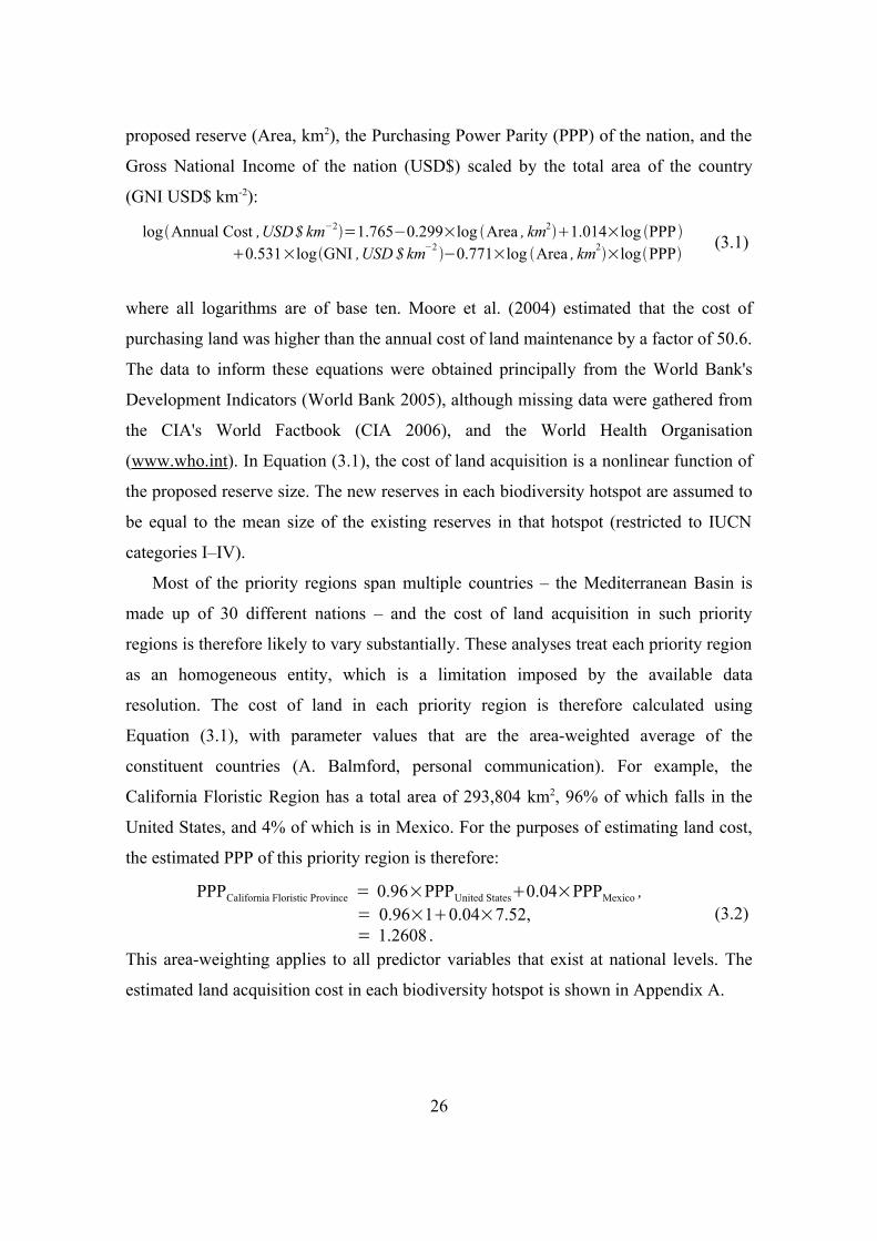
logAnnual Cost ,USD$ km−2=1.765−0.299×log Area , km21.014×log PPP 0.531×logGNI ,USD $ km−2 −0.771×log Area , km2×logPPP ,
(3.1)
where all logarithms are of base ten. Moore et al. (2004) estimated that the cost of
purchasing land was higher than the annual cost of land maintenance by a factor of 50.6.
The data to inform these equations were obtained principally from the World Bank's
Development Indicators (World Bank 2005), although missing data were gathered from
the CIA's World Factbook (CIA 2006), and the World Health Organisation
(www.who.int). In Equation (3.1), the cost of land acquisition is a nonlinear function of
the proposed reserve size. The new reserves in each biodiversity hotspot are assumed to
be equal to the mean size of the existing reserves in that hotspot (restricted to IUCN
categories I–IV).
Most of the priority regions span multiple countries – the Mediterranean Basin is
made up of 30 different nations – and the cost of land acquisition in such priority
regions is therefore likely to vary substantially. These analyses treat each priority region
as an homogeneous entity, which is a limitation imposed by the available data
resolution. The cost of land in each priority region is therefore calculated using
Equation (3.1), with parameter values that are the area-weighted average of the
constituent countries (A. Balmford, personal communication). For example, the
California Floristic Region has a total area of 293,804 km2, 96% of which falls in the
United States, and 4% of which is in Mexico. For the purposes of estimating land cost,
the estimated PPP of this priority region is therefore:
PPPCalifornia Floristic Province = 0.96×PPPUnited States0.04×PPPMexico , = 0.96×10.04×7.52, = 1.2608 .
(3.2)
This area-weighting applies to all predictor variables that exist at national levels. The
estimated land acquisition cost in each biodiversity hotspot is shown in Appendix A.
26
3.3.3. The predicted habitat loss ratesEmpirical data indicate that habitat loss occurs at a rate proportional to the amount
of habitat available for development or conservation (Etter et al. 2006). Theoretical
analyses typically model habitat loss in this manner (Costello et al. 2004; Meir et al.
2004; Wilson et al. 2006), which is equivalent to the assumption that land parcels have a
constant annual probability of being lost. Under this model of habitat loss, the more
habitat that remains unreserved, the faster it will be lost. Mathematically, this means
that the area of available habitat, A, changes according to the differential equation:
dAdt
=− A , (3.3)
which implies that in the absence of conservation actions, the amount of land remaining
available decreases exponentially:
At =A0e−t . (3.4)
The constant δ therefore represents the proportional rate of habitat loss, not the absolute
rate. Ongoing rates of habitat loss are directly available for particular habitat types (e.g.,
Global Forest Watch compiles timeseries data on global forest coverage). Consistent
data are not available for the biodiversity hotspots however, as they span a range of
ecosystem types. Instead I estimate the ongoing rate of habitat loss from the number and
classification of threatened mammal, bird, and amphibian species in each priority
region.
The IUCN Red List (the most recent version can be downloaded from
http://www.iucnredlist.org/) catalogues species that have a high probability of extinction
in the medium term. Each of the Red List classifications corresponds to a quantitative
estimate of the probability that a species will become extinct in the next 10 year period
(Red List Criterion E; Baillie et al. 2004). From these estimates, the expected number of
extinctions over the next 10 years is calculated (E10). The number of endemic mammals,
birds and amphibians that are currently extant in each hotspot is known (S0). The
number of species expected to remain extant in 10 years (S10) can therefore be estimated
according to the equation: S10 = S0 – E10 . The amount of habitat (R) currently in secure
27

reserves (IUCN categories I-IV) is also available. Habitat is being destroyed at a rate
proportional to the amount remaining available (Equation 3.3). With these pieces of
information, the proportional rate of habitat loss (δ) in each biodiversity hotspot can be
calculated:
=−110
log eA10
A0 ,
=−110
log e[S 10
1z−R
S0
1z−R] ,
(3.5)
where A0 is the amount of land currently available in the hotspot, and A10 is the amount
available in 10 years. The values of S0 and S10 are derived using Species-Area
Relationships for each hotspot (see §3.3.5). This method of predicting habitat loss rates
assumes that species are predominantly threatened by habitat loss; according to Baillie
et al. (2004), habitat destruction is the primary threat facing 86-88% of threatened
mammals, birds and amphibians. The estimated value of the habitat loss constant (δ) for
the 34 biodiversity hotspots is given in Appendix A.
3.3.4. The existing land-use distributionThe optimal funding allocation strategy will depend also on the existing distribution
of land use in the priority region. In addition to the effect that this distribution has on
habitat loss rates (i.e., the more land that is available, the faster habitat will be lost), the
amount of land that is currently reserved, degraded, or available for conservation action
will also alter the urgency of funding requirements. Data on existing land use
distribution in each of the biodiversity hotspots are available from the literature
(Mittermeier et al. 2005). Details of the land use distribution data can be found in
Appendix A.
In addition to these four datasets, a decision theory approach requires a process
model that can link management actions with conservation outcomes. For the efficient
28
allocation problem, this process model consists of three main components: (1) a
quantitative link between the land-use distribution (where management interventions are
made) and the biodiversity (where the efficiency of the funding allocation is measured)
of each hotspot (2) a mathematical model of the land-use dynamics that reacts to the
purchase of land by conservation organisations and (3) a mathematical optimisation
procedure. These components are outlined in the next three sections.
3.3.5. Biodiversity returns on conservation investmentThe aim of GPRs is to minimise the loss of biodiversity, but I assume that
management can only achieve this indirectly, through the conservation of land. To
calculate the biodiversity benefit of creating a particular conservation reserve, it is
therefore necessary to understand in a quantitative manner how much biodiversity is
contained in a particular area of land. For this purpose the Species-Area Relationship
(SPAR) is used. The SPAR relationship states that the total number of species (S)
protected in a particular reserve of area R, is a power-law function:
S=R z . (3.6)
The constant parameter α is a measure of the region's total biodiversity value, and the
parameter z is assumed to be a constant (z = 0.18) across all regions (Ovadia 2003). The
value of z is likely to vary with habitat type (Rosenzweig 1995), but sensitivity analyses
indicate that this does not significantly alter allocation schedules (Wilson et al., in
press). The functional form of the SPAR means that as more land is placed in reserves,
the rate that new species are protected decreases. For example, if a region had no pre-
existing reserves, then the first 10-hectare reserve might protect S new species.
However, if that same region already had 100-hectares of reserves, an additional 10-
hectares reserve would not protect S new species. Species-Area relationships represent
diminishing conservation benefits with increasing conservation investment.
29
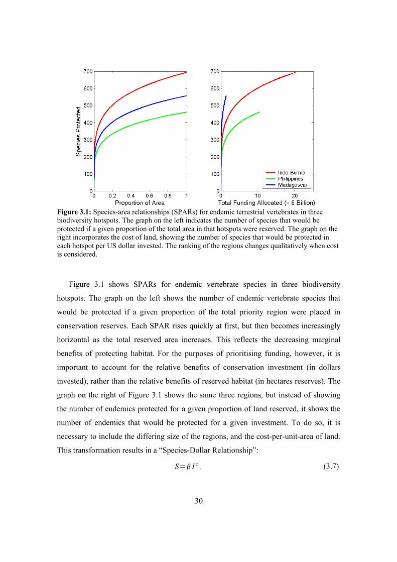
Figure 3.1: Species-area relationships (SPARs) for endemic terrestrial vertebrates in three biodiversity hotspots. The graph on the left indicates the number of species that would be protected if a given proportion of the total area in that hotspots were reserved. The graph on the right incorporates the cost of land, showing the number of species that would be protected in each hotspot per US dollar invested. The ranking of the regions changes qualitatively when cost is considered.
Figure 3.1 shows SPARs for endemic vertebrate species in three biodiversity
hotspots. The graph on the left shows the number of endemic vertebrate species that
would be protected if a given proportion of the total priority region were placed in
conservation reserves. Each SPAR rises quickly at first, but then becomes increasingly
horizontal as the total reserved area increases. This reflects the decreasing marginal
benefits of protecting habitat. For the purposes of prioritising funding, however, it is
important to account for the relative benefits of conservation investment (in dollars
invested), rather than the relative benefits of reserved habitat (in hectares reserves). The
graph on the right of Figure 3.1 shows the same three regions, but instead of showing
the number of endemics protected for a given proportion of land reserved, it shows the
number of endemics that would be protected for a given investment. To do so, it is
necessary to include the differing size of the regions, and the cost-per-unit-area of land.
This transformation results in a “Species-Dollar Relationship”:
S= I z , (3.7)
30
where I is the total amount of money invested in a region, and =/cz . The variable
c represents the per-unit-area cost of the region. Equation (3.7) provides the link
between the total investment in a region (the management action), and the number of
species protected (the conservation objective). Regions that appear to be good
investments in terms of species protected per unit area can become less attractive if cost
and total size are accounted for (e.g., the Indo-Burma hotspot) in Figure 3.1. The
species that occur in such regions may be spread across a larger area, or land may be
more expensive.
3.3.6. Expressing the habitat dynamics mathematicallyThe dynamics of the conservation system can be expressed succinctly using
deterministic differential equations. These differ from the stochastic formulation used in
Wilson et al. (2006), but are considerably more comprehensible. The two
representations are functionally very similar, as I discuss in Chapter 4. The conservation
system consists of P regions, each with a particular set of attributes. For conservation
purposes, in region i at time t, land exists in three states: available, Ai (t), reserved, Ri (t),
and lost, Li (t). Species in reserved areas are considered protected. Lost land has been
degraded to the point that it contains no endemic species, and thus has no more
conservation value (as measured by the current objective). Available land currently has
full conservation value, but will eventually become lost land (through habitat loss), or
reserved land (if funding is allocated for its purchase before degradation occurs). The
flux in this system can be expressed by a system of differential equations, called the
state equations:
dLit dt
=i Ai t ,
dRit dt =
u it bci
,
dAi t dt
=−i Ai t −ui t b
c i,
(3.8)
where b is the total budget, ci is the cost of land, δi is the proportional rate of land loss,
31
and ui (t) is the proportion of funding allocated, in the i th region. Funding allocation
proportions are subject to the additional constraint:
∑i=1
P
u it =1. (3.9)
These proportional allocation variables (ui (t)) are known as the control variables, and
they represent the mechanism by which conservation managers achieve the biodiversity
objective. The optimisation problem is essentially to choose the particular sequence of
ui (t) values that maximises the extant biodiversity at the end of the time period (the total
species ST), measured using each of the regional SPARs:
ST=∑i=1
P
i AiT Ri T z. (3.10)
3.3.7. Determining efficient funding allocation strategiesAlthough it is assumed that funding allocation will be ongoing, I will outline an
efficient allocation strategy for the first 20 years of funding. The dynamic nature of the
conservation landscape means that allocations must be defined at each point in this 20
year period. A fixed annual budget of US$310 million is to be shared among the 34
biodiversity hotspots; I chose this funding rate because it is equivalent to the amount
made available for biodiversity in the fourth phase of the Global Environment Facility
(GEF 2006).
Funding decisions are made using the “minimise short-term loss” heuristic
(minloss). Minloss allocates funding to priority regions in such a way that the
immediate rate of species loss is minimised (Wilson et al. 2006). Rather than focusing
on the amount of biodiversity that will be immediately protected, minloss attempts to
minimise the number of extinctions in the system at the end of each timestep. The
difference between increasing the protection of biodiversity, and reducing the loss of
biodiversity, is subtle but important (Witting & Loeschcke 1993; 1995). If the objective
of an heuristic is to maximise the amount of biodiversity that is protected, funding will
initially be directed to regions with the highest species richness, even though they may
have very low rates of habitat loss (or possibly no habitat loss at all). Regions with
32
lower biodiversity value but higher habitat loss rates (and therefore higher species
extinction rates) will not receive funding and may therefore lose many species. If, on the
other hand, the conservation objective is to minimise the loss of species, then funding
will be first allocated to regions with higher rates of species loss, even if those regions
are slightly less species-rich. The high richness/low threat regions will not be greatly
affected in the meantime, and are therefore still suitable for future investment.
Minloss provides funding allocation schedules that closely approximate the optimal
allocation strategy, calculated using stochastic dynamic programming (Wilson et al.
2006, and Chapter 4). It is a “myopic” heuristic, only considering events in the very
near future when choosing between available conservation actions. The funding
allocated to each region, at each time, is calculated using the following algorithm:
1. The 20 year planning window is discretised into weekly timesteps.
2. At the beginning of each week, the expected species loss in each region is
calculated, in the absence of funding allocation. The value calculated is based on
the ongoing habitat loss and the SPAR. The expected species loss is then re-
calculated, assuming that all available funding for that week was allocated to
each of the regions in turn.
3. The difference between these two values indicates the loss of species that could
have been avoided if funding had been completely allocated to a particular
region.
4. The region with the largest difference is identified (i.e., the most species saved
from extinction by allocation). Minloss directs all available funding to this
region.
5. Steps 2 through 4 are repeated for 20 years. In Wilson et al. (2006), allocation
continued until no more land remained available for conservation. However, the
total allocation time will not alter the implementation of the minloss heuristic,
nor will the funding allocation schedule for the first 20 years change if this time
is extended.
6. These steps are repeated for each of the seven different taxonomic measures of
biodiversity.
33
Once the funding allocation schedules have been constructed, I analyse the results
with the aid of two techniques. First, I compare the funding allocations to two null
models. These null models each consider one particular aspect of the allocation problem
to be invariant, which allows the effects of particular parameters to be isolated.
Secondly, numerical sensitivity analyses are employed to investigate the relative
importance of data quality in each of the three main datasets (biodiversity, cost, and
threat).
3.3.8. Null modelsThe similarity (or dissimilarity) of efficient funding allocation schedules based on
different taxonomic measures of biodiversity is caused by either the endemic species
richness of each biodiversity hotspot, or by its socio-economic characteristics. To better
estimate the relative roles of these two factors, two null models of funding allocation are
created. The first null model does not consider variation in regional endemicity. Each
region is given the same number of endemic species (the exact number did not change
the resulting allocation), and funding is allocated according to the minloss heuristic. The
land distribution, costs and habitat loss rates still vary between the hotspots, and the
annual rate of funding is not changed. The second null model allocates funding based
only on regional biodiversity, with socio-economic factors considered constant across
regions. This was achieved by setting the habitat loss rates equal to their average value
across the hotspots, and by setting the cost of land equal to the average cost of hotspot
land across the globe. None of the hotspots is assumed to have any existing reserves,
and a uniform 70% of native habitat is assumed to be already lost (the threshold amount
used to define the biodiversity hotspots). Funding allocation then proceeds according to
the minloss heuristic.
3.3.9. Calculating the sensitivity of the planning method to data uncertaintyTo evaluate the effect of error in the model parameters on conservation outcomes, I
perform numerical perturbations on the regional values of biodiversity, land cost, and
habitat loss rates. These parameter sensitivity analyses are performed for all two-region
combinations of the 34 biodiversity hotspots. Funding in two-region systems can be
34
constructed using SDP, rather than the minloss approximation. I first assume that
vascular plant endemicity, the estimated habitat loss rates and land cost data represent
“true” parameter values. Conservation funding is then allocated based on “false” values,
which vary proportionally about the true values. (The true values are still driving the
underlying model.) The false values are varied in one percent intervals between 75 and
125 percent of their true values. Each amount of error affects the hotspots separately,
and then simultaneously. Funding is continued until all available land has been either
reserved or converted. The sensitivity of the conservation planning methods to each
dataset is then estimated using the difference between the number of extinct species
after allocation proceeds according to the true parameter values, and the number of
extinct species after allocation proceeds according to the false parameter values. A
linear regression is used to predict the difference between the outcomes for each of the
561 combinations, using the magnitude of the proportional error. The slope of these
regression lines indicates how sensitive the conservation outcome is to data uncertainty.
3.4. Results and Discussion3.4.1. Efficient conservation funding allocation schedules
Efficient funding allocations for each taxa are shown in Figure 3.2, and Table 3.3.
These results represent the first efficient funding strategies for any GPR set. On
average, only eight of the 34 regions receive funding during the first 20 years. Species
extinctions are minimised by initially targeting a small subset of regions, before funds
are extended to other regions in need. Some targeted regions received sufficient funding
to protect all of the land available for conservation before other regions were allocated
any funding. For example, the Eastern Afromontane region received approximately
$110m, using each of the endemic species richnesses: this is the amount of funding
estimated to safeguard all land of conservation value.
35
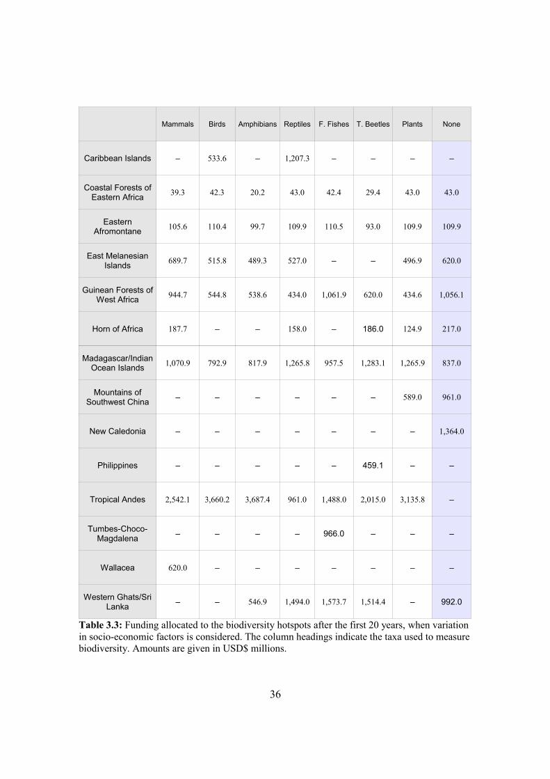
Mammals Birds Amphibians Reptiles F. Fishes T. Beetles Plants None
Caribbean Islands – 533.6 – 1,207.3 – – – –
Coastal Forests of Eastern Africa 39.3 42.3 20.2 43.0 42.4 29.4 43.0 43.0
Eastern Afromontane 105.6 110.4 99.7 109.9 110.5 93.0 109.9 109.9
East Melanesian Islands 689.7 515.8 489.3 527.0 – – 496.9 620.0
Guinean Forests of West Africa 944.7 544.8 538.6 434.0 1,061.9 620.0 434.6 1,056.1
Horn of Africa 187.7 – – 158.0 – 186.0 124.9 217.0
Madagascar/Indian Ocean Islands 1,070.9 792.9 817.9 1,265.8 957.5 1,283.1 1,265.9 837.0
Mountains of Southwest China – – – – – – 589.0 961.0
New Caledonia – – – – – – – 1,364.0
Philippines – – – – – 459.1 – –
Tropical Andes 2,542.1 3,660.2 3,687.4 961.0 1,488.0 2,015.0 3,135.8 –
Tumbes-Choco-Magdalena – – – – 966.0 – – –
Wallacea 620.0 – – – – – – –
Western Ghats/Sri Lanka – – 546.9 1,494.0 1,573.7 1,514.4 – 992.0
Table 3.3: Funding allocated to the biodiversity hotspots after the first 20 years, when variation in socio-economic factors is considered. The column headings indicate the taxa used to measure biodiversity. Amounts are given in USD$ millions.
36
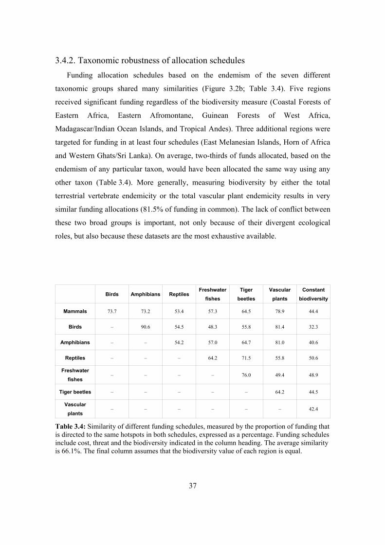
3.4.2. Taxonomic robustness of allocation schedulesFunding allocation schedules based on the endemism of the seven different
taxonomic groups shared many similarities (Figure 3.2b; Table 3.4). Five regions
received significant funding regardless of the biodiversity measure (Coastal Forests of
Eastern Africa, Eastern Afromontane, Guinean Forests of West Africa,
Madagascar/Indian Ocean Islands, and Tropical Andes). Three additional regions were
targeted for funding in at least four schedules (East Melanesian Islands, Horn of Africa
and Western Ghats/Sri Lanka). On average, two-thirds of funds allocated, based on the
endemism of any particular taxon, would have been allocated the same way using any
other taxon (Table 3.4). More generally, measuring biodiversity by either the total
terrestrial vertebrate endemicity or the total vascular plant endemicity results in very
similar funding allocations (81.5% of funding in common). The lack of conflict between
these two broad groups is important, not only because of their divergent ecological
roles, but also because these datasets are the most exhaustive available.
Birds Amphibians ReptilesFreshwater
fishesTiger
beetlesVascular
plantsConstant
biodiversity
Mammals 73.7 73.2 53.4 57.3 64.5 78.9 44.4
Birds – 90.6 54.5 48.3 55.8 81.4 32.3
Amphibians – – 54.2 57.0 64.7 81.0 40.6
Reptiles – – – 64.2 71.5 55.8 50.6
Freshwater fishes
– – – – 76.0 49.4 48.9
Tiger beetles – – – – – 64.2 44.5
Vascular plants
– – – – – – 42.4
Table 3.4: Similarity of different funding schedules, measured by the proportion of funding that is directed to the same hotspots in both schedules, expressed as a percentage. Funding schedules include cost, threat and the biodiversity indicated in the column heading. The average similarity is 66.1%. The final column assumes that the biodiversity value of each region is equal.
37
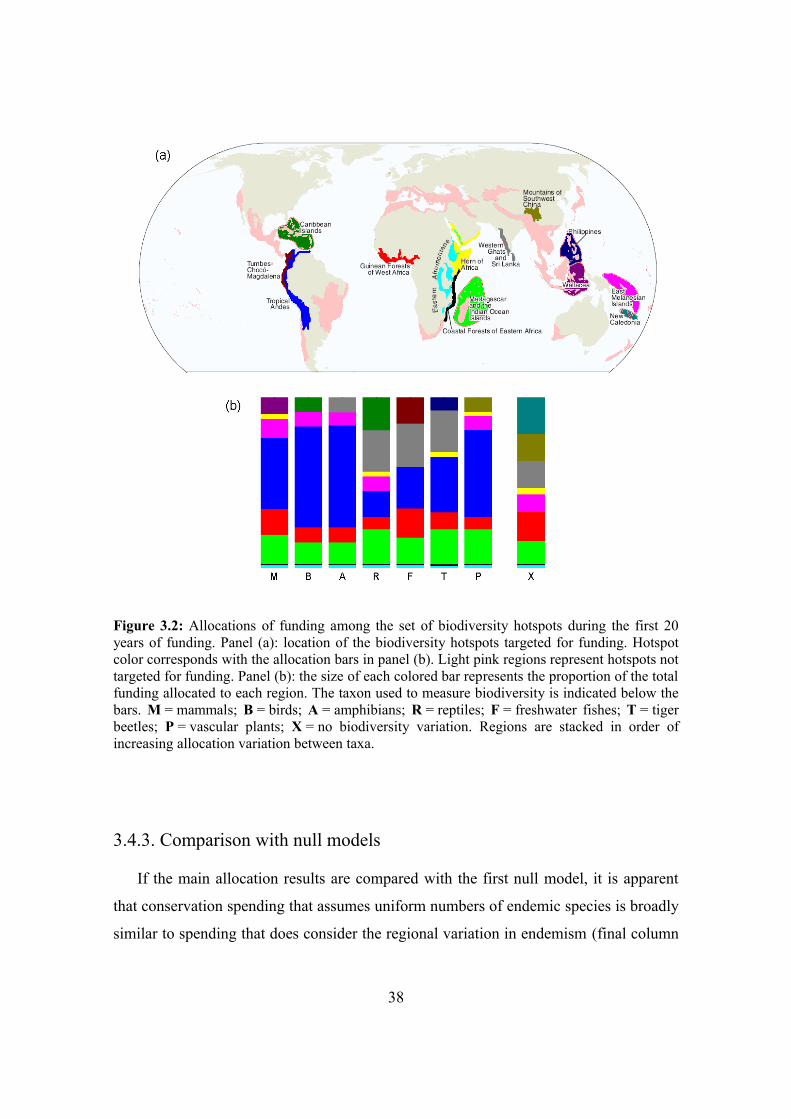
Figure 3.2: Allocations of funding among the set of biodiversity hotspots during the first 20 years of funding. Panel (a): location of the biodiversity hotspots targeted for funding. Hotspot color corresponds with the allocation bars in panel (b). Light pink regions represent hotspots not targeted for funding. Panel (b): the size of each colored bar represents the proportion of the total funding allocated to each region. The taxon used to measure biodiversity is indicated below the bars. M = mammals; B = birds; A = amphibians; R = reptiles; F = freshwater fishes; T = tiger beetles; P = vascular plants; X = no biodiversity variation. Regions are stacked in order of increasing allocation variation between taxa.
3.4.3. Comparison with null models
If the main allocation results are compared with the first null model, it is apparent
that conservation spending that assumes uniform numbers of endemic species is broadly
similar to spending that does consider the regional variation in endemism (final column
38
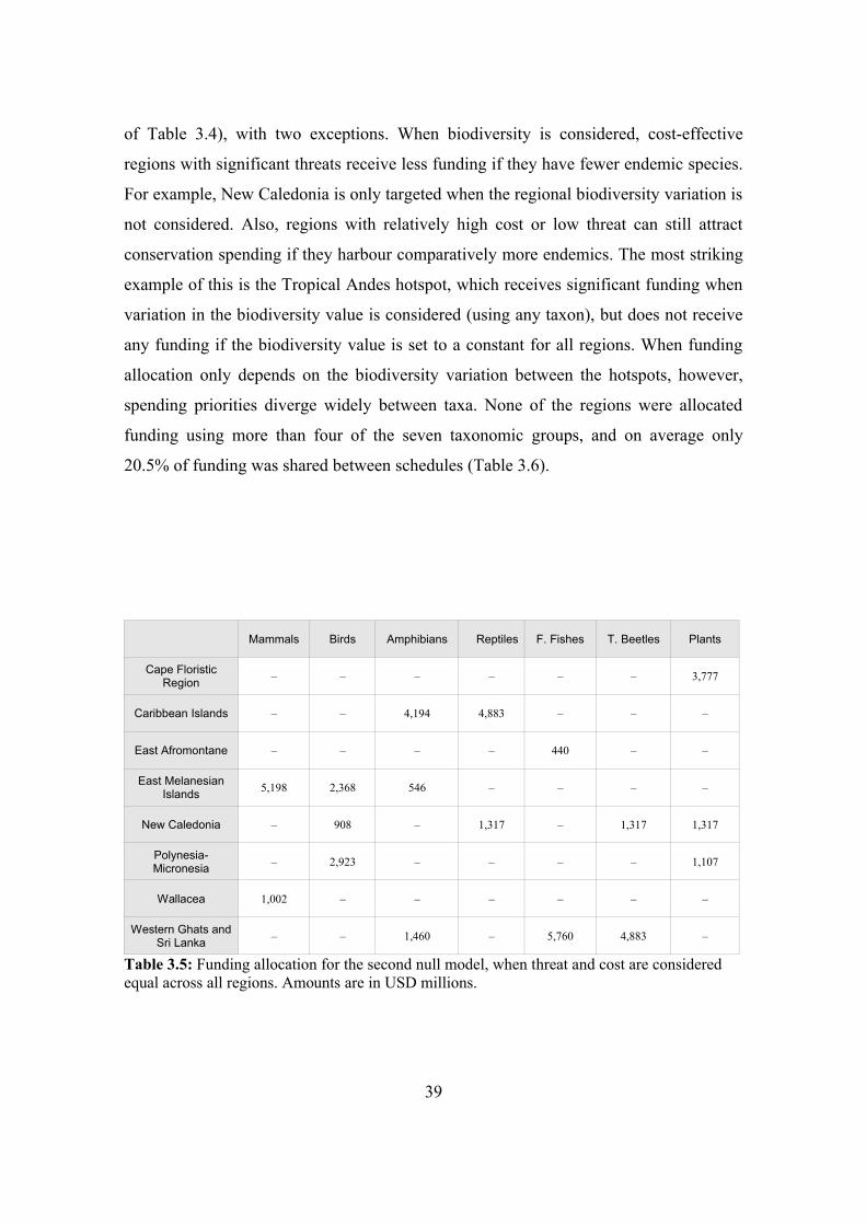
of Table 3.4), with two exceptions. When biodiversity is considered, cost-effective
regions with significant threats receive less funding if they have fewer endemic species.
For example, New Caledonia is only targeted when the regional biodiversity variation is
not considered. Also, regions with relatively high cost or low threat can still attract
conservation spending if they harbour comparatively more endemics. The most striking
example of this is the Tropical Andes hotspot, which receives significant funding when
variation in the biodiversity value is considered (using any taxon), but does not receive
any funding if the biodiversity value is set to a constant for all regions. When funding
allocation only depends on the biodiversity variation between the hotspots, however,
spending priorities diverge widely between taxa. None of the regions were allocated
funding using more than four of the seven taxonomic groups, and on average only
20.5% of funding was shared between schedules (Table 3.6).
Mammals Birds Amphibians Reptiles F. Fishes T. Beetles Plants
Cape Floristic Region – – – – – – 3,777
Caribbean Islands – – 4,194 4,883 – – –
East Afromontane – – – – 440 – –
East Melanesian Islands 5,198 2,368 546 – – – –
New Caledonia – 908 – 1,317 – 1,317 1,317
Polynesia-Micronesia – 2,923 – – – – 1,107
Wallacea 1,002 – – – – – –
Western Ghats and Sri Lanka – – 1,460 – 5,760 4,883 –
Table 3.5: Funding allocation for the second null model, when threat and cost are considered equal across all regions. Amounts are in USD millions.
39
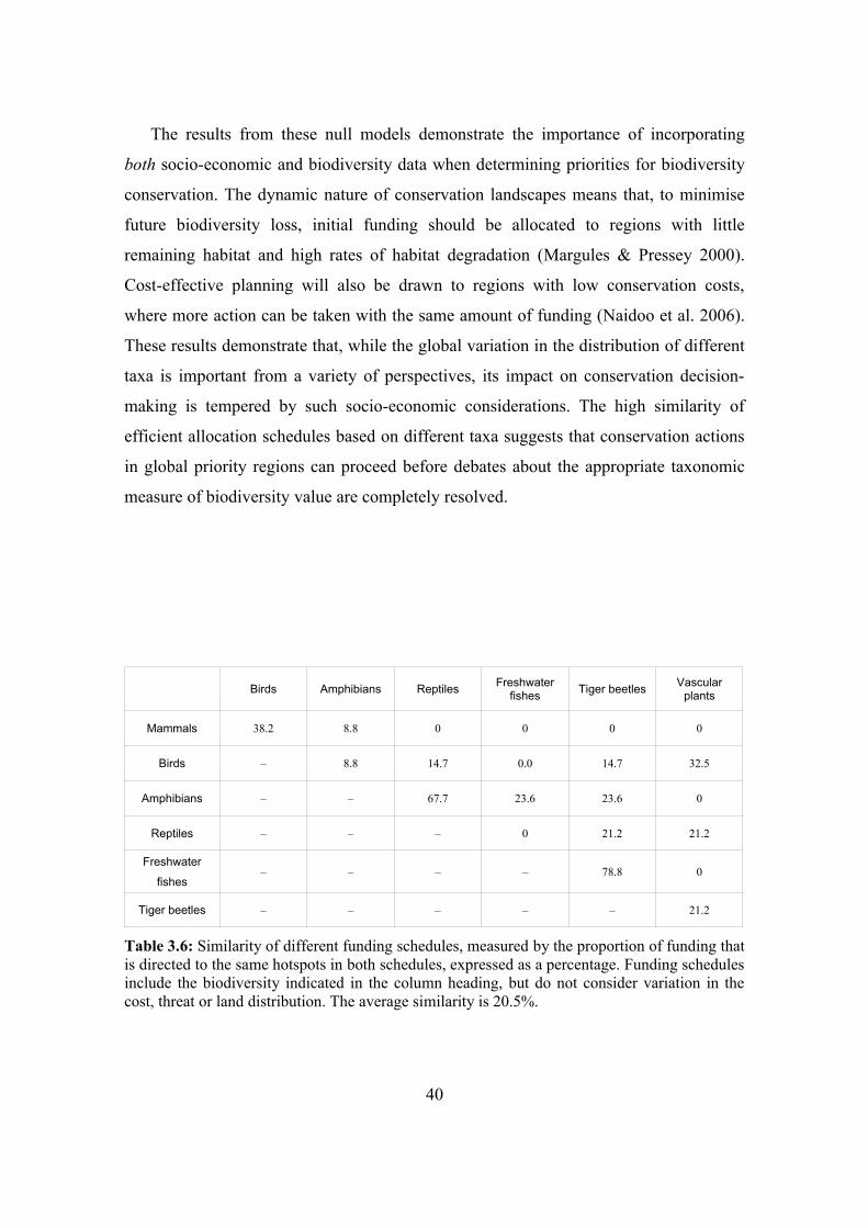
The results from these null models demonstrate the importance of incorporating
both socio-economic and biodiversity data when determining priorities for biodiversity
conservation. The dynamic nature of conservation landscapes means that, to minimise
future biodiversity loss, initial funding should be allocated to regions with little
remaining habitat and high rates of habitat degradation (Margules & Pressey 2000).
Cost-effective planning will also be drawn to regions with low conservation costs,
where more action can be taken with the same amount of funding (Naidoo et al. 2006).
These results demonstrate that, while the global variation in the distribution of different
taxa is important from a variety of perspectives, its impact on conservation decision-
making is tempered by such socio-economic considerations. The high similarity of
efficient allocation schedules based on different taxa suggests that conservation actions
in global priority regions can proceed before debates about the appropriate taxonomic
measure of biodiversity value are completely resolved.
Birds Amphibians Reptiles Freshwater fishes Tiger beetles Vascular
plants
Mammals 38.2 8.8 0 0 0 0
Birds – 8.8 14.7 0.0 14.7 32.5
Amphibians – – 67.7 23.6 23.6 0
Reptiles – – – 0 21.2 21.2
Freshwater
fishes– – – – 78.8 0
Tiger beetles – – – – – 21.2
Table 3.6: Similarity of different funding schedules, measured by the proportion of funding that is directed to the same hotspots in both schedules, expressed as a percentage. Funding schedules include the biodiversity indicated in the column heading, but do not consider variation in the cost, threat or land distribution. The average similarity is 20.5%.
40
3.4.4. Sensitivity to data uncertaintyWhile efficient conservation decisions may be robust to the choice of taxon,
inaccuracies in the input data will still lead to suboptimal funding allocation, and
improved information on any of the important factors will benefit conservation
planning. The structure of the allocation heuristic, and the dynamics of the conservation
landscape may make the outcomes sensitive to particular parameters. The numerical
sensitivity analyses support this contention, revealing that conservation outcomes are
most affected by uncertainty in the land cost data, followed by the habitat loss rates, and
finally the biodiversity values. The mean slopes of the parameter-specific regression
lines are:
1. β cost = 0.86,
2. β habitat loss = 0.13,
3. β biodiversity = 0.04.
Errors in the cost data therefore lead to inefficient funding strategies that result in, on
average, 20 times as many extinctions as similar proportional errors in the biodiversity
data, and six times as many extinctions as similar errors in the habitat loss rates.
Information gathering for conservation has traditionally focused on assessing the
state of biodiversity through the collation of species lists, and more recently, spatially
explicit species ranges. The impact of habitat loss rates on conservation goals has also
been acknowledged, but this has typically led to investigations about how much habitat
has already been lost (e.g., Myers et al. 2000), rather than how much habitat is currently
being lost, or is likely to be lost in the future.
The most striking information gap relates to the cost of conservation actions in
different regions of the world. The economic constraints on conservation action are
inarguably a crucial factor limiting possible action, yet there is very little public
information available on this important aspect. While some information does exist on
the costs of conservation actions in many regions, it has not been collated
systematically, nor is it readily accessible. This sensitivity profile has implications for
future research into the important conservation datasets of biodiversity, cost, and habitat
loss. Given the sensitivity of the cost parameter, and the potential for rapid and cheap
improvement of estimates, improved information on cost will lead to the most rapid
41
improvement in the conservation objective.
3.4.5. Considerations when applying these resultsThe initial development of this decision theory approach to conservation funding
allocation (Wilson et al. 2006) was able to avoid criticism about data quality, as the
research was concerned primarily with methodology – how to integrate multiple
important factors into a consistent framework that could be used as a basis for
mathematical optimisation. This chapter, however, represents the first application of the
resource allocation method that is intended to inform global conservation practice. In
this context, concerns about the quality of the data, and about the assumptions of the
model, become distinctly relevant. I will therefore discuss the important limitations of
the specific model used in this chapter, and the potential effects that these will have on
conservation outcomes.
Data quality: The global scale of GPRs makes it difficult to gather consistent
information for each of the priority regions. The initial choice of vascular plant
endemicity as a surrogate for the biodiversity value of the biodiversity hotspots, for
example, was motivated more by consistency than suitability
(Kareiva & Marvier 2003). Compiling data on habitat loss rates and land costs quickly
encounters similar concerns about quality and consistency. Information that may be
readily available in developed countries is difficult to obtain for developing countries
(Ando et al. 1998). For example, government information gathering may be less
thorough, official land markets may not exist, or countries may have different attitudes
towards private-property rights (Naidoo et al. 2006).
Political economy factors: All GPRs ignore “political economy” considerations.
These are factors that are associated with the social and political systems that overlap
the GPRs, and that will affect the success of conservation investment in the regions. An
example of a political economy factor would be the likelihood that political instability
will lead to a loss of conservation investment, such as a reserved area. Such factors have
long been used by businesses to determine the relative investment potential of different
nations (Bohn & Deacon 2000). Political economy considerations are probably used
implicitly by conservation organisations to guide funding. For example, Deacon &
42
Murphy (1997) showed that debt-for-nature swaps organised by three NGOs –
Conservation International, The Nature Conservancy and the World Wildlife Fund –
were more likely to be approved in nations with democratic regimes. However, some
factors appear not to have been considered – swaps were actually historically more
likely to have occurred in regions that had experienced political assassinations, and
there was no statistically significant avoidance of countries that had experienced
guerrilla warfare, political assassinations, riots, or political purges.
Excluding political economy factors from allocation plans will lead to the proposed
schedules being suboptimal, or being politically untenable. For example, all seven
measures of biodiversity suggested that conservation funding be directed to the Horn of
Africa (Figure 3.2; Table 3.3). Many nations in this biodiversity hotspot have been
afflicted by war (Ethiopia, Eritrea) or civil unrest (Somalia, Sudan) in the last decade
(CIA 2006). If political economy factors were considered, this hotspot would probably
not be considered a suitable destination for conservation investment.
Cost Dynamics: Conservation actions in particular regions, such as land
acquisition, are likely to affect the existing threats to biodiversity. The land-use model
applied in this research included some feedback between conservation investments and
habitat loss rates (Equation 3.3), but the true dynamics will be much more complex.
Purchasing land for conservation purposes may increase its rarity, for example, resulting
in an increase in land cost. This increase will decrease the attractiveness of the region
for resource exploitation such as logging, but the added expense may also hinder direct
conservation actions in the region. On the other hand, protection of land can accelerate
destructive forces on the remaining unreserved regions (Armsworth et al. 2006). If the
capital available for destructive land use is regionally flexible, the construction of
reserves can simply relocate the threat to different areas, as was observed when the
1989 ban on logging in Thailand resulted in an increase in timber exports from
Cambodia, Laos and Myanmar (PER 1992), all of which are regions with fewer existing
institutional protections from unrestrained logging than Thailand.
Conservation resource allocation strategies should consider additional factors such
as these during decision-making. They were omitted from the analyses in this chapter
due to a lack of available data. Inclusion of such considerations will mean that some of
43
the regions identified by these analyses will no longer be considered high conservation
priorities. I believe, however, that despite inaccuracies and omissions, these results and
these decision theory methods have great relevance to prioritisation in the biodiversity
hotspots. Applying decision theory methods allows the consistent and quantitative
incorporation of multiple important factors, which are interacting in a nonlinear manner.
Decision theory methods also result in a transparent and reproducible conservation plan
– a very important factor in a conservation climate increasingly focused on measurable
outcomes (Christensen 2003; Ferraro & Pattanayak 2006). Conservation actions will
proceed, and biodiversity outcomes will be much worse if the uncertain, but available,
information is not used. Ignoring the cost of conservation action or the rate of habitat
loss is itself a decision based on poor information – that these factors are the same for
each of the priority regions. This assumption is far more erroneous than the cost
estimators available.
The results outlined in this chapter provide the first example of cost and dynamic
threats being incorporated into global prioritisation among regions for biodiversity
conservation. The geographically flexible funding attracted by the biodiversity hotspots
has the potential to greatly benefit global conservation into the future, if it is invested
wisely (Brooks et al. 2006). Better data quality is always desirable, and I have shown
that efforts should first be directed at refining our knowledge of the costs of
conservation action, as this information will result in the most marked improvement in
outcomes. Nevertheless, while more accurate biodiversity data will remain essential to
refining global conservation priorities, the results in this chapter also demonstrate that
efficient conservation decisions can be made more confidently with the biodiversity
data currently available.
44
Chapter 4
Optimal dynamic allocation of
conservation funding
4.1. AbstractIn the previous chapter I outlined a dynamic decision theory approach to allocating
conservation funding to global priority regions. The optimal allocation schedule had to
be approximated using the “minloss” heuristic, because the standard mathematical
optimisation technique (stochastic dynamic programming) is unable to accurately cope
with problems consisting of more than two regions. Although the heuristic is known to
be almost optimal for two-region problems, it is unclear whether it is equally accurate in
more complicated systems (i.e., conservation problems involving more regions). To
overcome this limitation and allow optimal allocation strategies to be determined for
larger systems, this chapter solves the same problem using methods from optimal
control theory. An optimal control approach allows more extensive testing of the
minloss heuristic's performance, and provides novel insight into the general properties
of optimal funding allocation strategies.
45
4.2. Introduction4.2.1. Decision theory approaches to conservation prioritisation
The aim of global priority region sets is to allocate limited available global
conservation funding in such a way that the most biodiversity possible is preserved in
perpetuity. This aim will best be achieved if allocation schedules are decided using
transparent decision-making tools, rather than scoring methods or simple intuition
(Wilson et al. 2006). These decision tools must take into account the biodiversity value
of different regions, but this in itself is not enough: among other factors, they must also
consider the varying costs of conservation action, the forces that constrain and impede
conservation, and the forces that erode the potential for future action (e.g., the loss of
native habitat). In Chapter 3, I described how some of these important factors can be
incorporated into a dynamic landscape model, and then applied this to the biodiversity
hotspots. An efficient conservation funding allocation schedule was calculated which
ensured that the least amount of biodiversity was lost.
Such optimisation problems are quite commonly encountered in the field of
operations research. Their optimal solution is often determined using a mathematical
technique called Stochastic Dynamic Programming (SDP). SDP is the most commonly
used dynamic optimisation technique in conservation biology, and in the past has been
applied to problems in fishery research (Clark 1990), habitat and wildlife management
(Richards et al. 1999; Chapter 5), captive breeding programs (Tenhumberg et al. 2004;
Rout et al. 2005), as well as conservation resource allocation problems such as this one
(Costello & Polasky 2004; Meir et al. 2004; McBride et al. 2005; Wilson et al. 2006).
4.2.2. Limitations to the current optimisation techniques Unfortunately, when applied to the resource allocation problem outlined in Chapter
3, SDP becomes computationally intractable if there are more than two regions in the
system. While future advances in computing capabilities will allow more regions to be
considered, it will not be possible to extend the SDP methodology to more than a few
regions in the foreseeable future. Wilson et al. (2006) were able to circumvent this
problem by using “heuristics” to calculate efficient funding schedules, yielding results
46
that were almost as good as the optimal solution for the small systems that can be
solved exactly with SDP. Wilson et al. (2006) postulated that these heuristics would
provide similarly optimal allocation schedules if applied to conservation problems with
many more regions. They then used the heuristic to allocate funds among a set of five
priority regions. Using heuristic methods, rather than optimisation techniques, has
considerable benefits:
1. They are computationally inexpensive to apply. While methods such as SDP
must consider all possible future events when comparing different interventions,
heuristics only consider events in the near future – they are “myopic”. This
means that they can be applied with very little effort to problems that would be
beyond the capabilities of techniques such as SDP. Their simplicity also means
that distributable applications can be compiled for use by conservation decision-
makers.
2. They are easier to explain to conservation practitioners than complicated
optimisation techniques. Heuristics don't rely on high-level mathematics, and
can therefore be understood by conservation practitioners who have little
quantitative expertise.
3. Their simple formulation can provide insight into the role of important system
parameters. For the purposes of simplicity, heuristics often do not consider
certain aspects of the system. Their performance can thus indicate the relative
importance of the omitted aspects.
Despite the utility of heuristics, having the true optimal solution available for more
complicated problems is valuable from an accuracy perspective, and would also allow a
more thorough testing of the heuristic's performance. A number of conservation
organisations are currently applying the heuristic defined by Wilson et al. (2006) to
multi-region allocation problems. It would be reassuring to know that the near-
optimality observed in that paper is retained in these more complicated situations. I
therefore apply techniques from optimal control theory to determine the optimal
allocation strategy for systems with multiple regions. Thereafter, I compare optimal
control allocation schedule with the funding schedules proposed by the minloss
heuristic.
47
4.2.3. Optimal control theoryIn conservation biology, optimisation is frequently applied to static problems. Static
optimisation uses standard calculus: the quantity that needs to be optimised is expressed
as a function of one or more control variables, and the value of those control variables
that optimise the quantity of interest are determined using the derivatives of the
function. However, optimising funding allocation schedules is a dynamic problem, and
is therefore much more complicated. To achieve the best biodiversity outcomes,
spending must respond to the changing conservation situation. For example, as
particular regions become better reserved, habitat loss will slow. Directing funding
elsewhere will then yield superior conservation outcomes. Rather than choosing a static
funding distribution among the priority regions, the best distribution has to be defined at
each instant in time. There is an additional complication: because dynamic controls are
enacted sequentially, the benefits of particular actions at a given time will depend on
previous control decisions. Making decisions at a particular time will also constrain
subsequent control options. Potential solutions to a dynamic optimisation problem must
therefore be defined throughout the time-period before their performances can be
assessed.
Dynamic optimisation was first treated in a mathematically modern way by Jakob
Bernouilli in the late 17th century. His methodologies were expanded significantly in the
1750s by Joseph Lagrange and Leonhard Euler, becoming the “calculus of variations”
(see Goldstine 1980 for a comprehensive history). The mechanisation of industry in the
20th century required dynamic optimisation techniques, but the type of control necessary
exceeded the capabilities of variational calculus. In particular, automated systems
frequently require control that is only piecewise-continuous, or involves directly
constrained state variables. At the time, the calculus of variations could not incorporate
either of these features. A number of mathematicians independently discovered
techniques that dealt with these additional complexities: in the United States, Richard
Bellman developed the theory of dynamic programming; in the Soviet Union, Lev
Pontryagin revolutionised the methodology of variational calculus to create optimal
control theory (Leitmann 1981). It is this latter method that I will apply to determine
optimal conservation funding schedules.
48
The nomenclature of dynamic optimisation can be confusing, as optimal control
theory may refer to the theory of dynamic optimisation in general, or specifically to
methods based on Pontryagin's theorem. I will use the term “optimal control” in the
latter sense throughout this thesis. Despite its long history in ecology (e.g., plant growth
schedules; Iwasa et al. 1984; Cohen 1986), and natural resource management (e.g.,
fisheries; Clark 1990), optimal control theory has rarely been applied to conservation
problems (Loehle 2006; but see Neubert 2003 for a novel application of optimal control
theory to marine reserve planning). The mathematical complexity of the theory is
probably partly to blame. Conservation biology often faces problems that require
dynamic optimisation, but these are usually addressed using SDP (e.g., Chapter 3 and
5). SDP is a particularly versatile and powerful technique, and unlike optimal control
theory, can easily cope with stochastic systems. However, not all conservation problems
are suited to an SDP approach. In particular, SDP requires a discretisation of the system
states, which can be artificial, and can introduce unnecessary complexity. The opacity
of SDP solutions also discourages interpretation (Mangel & Clark 1988). Optimal
control theory is particularly suited to systems that contain continuous variables (e.g.,
the amount of land), and has the additional benefit of providing insight into why
particular management decisions are optimal. Mathematically thorough but readable
expositions of optimal control theory can be found in Leitmann (1981) and Pinch
(1993). An excellent applied analysis of optimal control theory, with applications to
economic examples, can be found in Leonard & Long (1992).
4.3. Optimal control allocationTo demonstrate how optimal control theory can be applied to conservation funding
allocation problems, I repeat, and then extend, the analyses performed in
Wilson et al. (2006). This paper began by using SDP to calculate the optimal allocation
schedule for two priority regions in Indonesia (the islands of Borneo and Sumatra).
Wilson et al. (2006) then considered efficient funding schedules among five priority
regions. Allocation schedules for this second analysis used the minloss heuristic, as the
exact solution could not be generated using SDP. I solve the same two optimisation
problems using optimal control: for the two-region example, I compare optimal
49
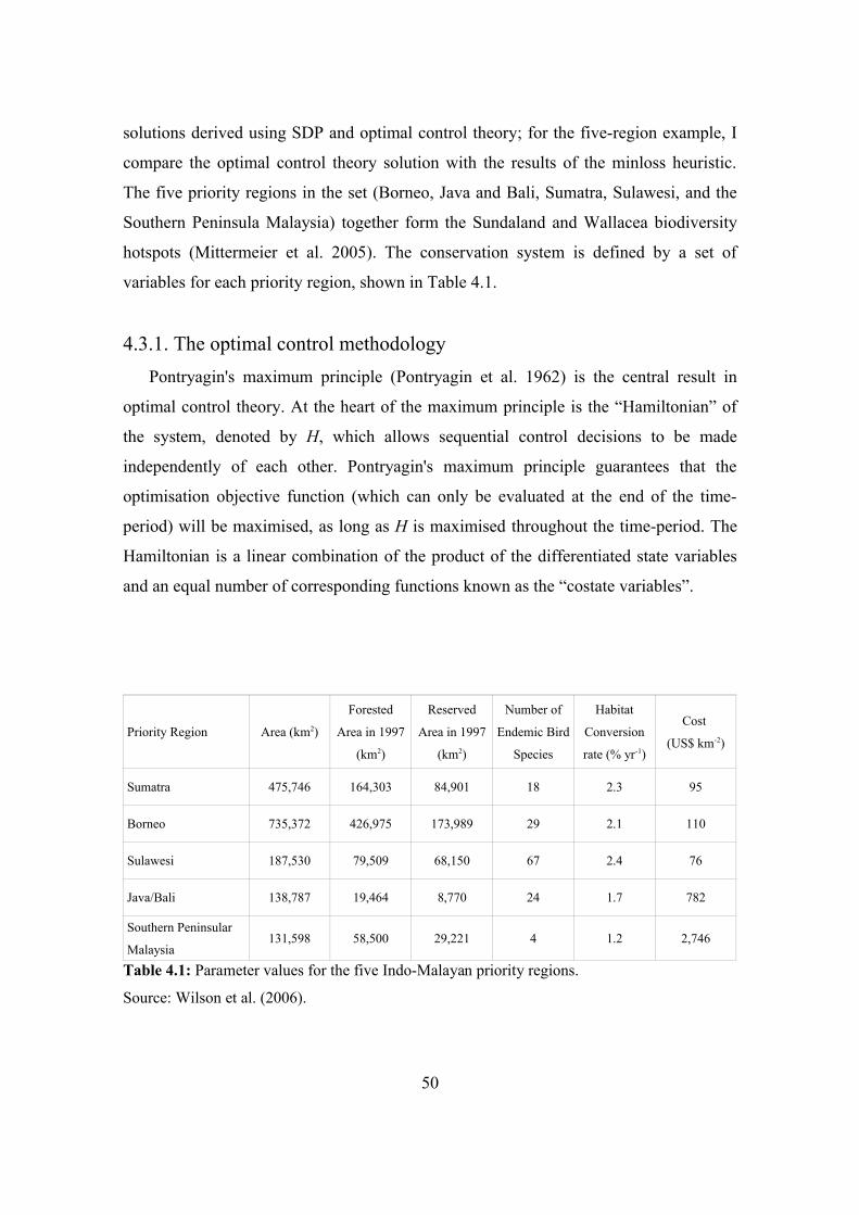
solutions derived using SDP and optimal control theory; for the five-region example, I
compare the optimal control theory solution with the results of the minloss heuristic.
The five priority regions in the set (Borneo, Java and Bali, Sumatra, Sulawesi, and the
Southern Peninsula Malaysia) together form the Sundaland and Wallacea biodiversity
hotspots (Mittermeier et al. 2005). The conservation system is defined by a set of
variables for each priority region, shown in Table 4.1.
4.3.1. The optimal control methodologyPontryagin's maximum principle (Pontryagin et al. 1962) is the central result in
optimal control theory. At the heart of the maximum principle is the “Hamiltonian” of
the system, denoted by H, which allows sequential control decisions to be made
independently of each other. Pontryagin's maximum principle guarantees that the
optimisation objective function (which can only be evaluated at the end of the time-
period) will be maximised, as long as H is maximised throughout the time-period. The
Hamiltonian is a linear combination of the product of the differentiated state variables
and an equal number of corresponding functions known as the “costate variables”.
Priority Region Area (km2)
Forested
Area in 1997
(km2)
Reserved
Area in 1997
(km2)
Number of
Endemic Bird
Species
Habitat
Conversion
rate (% yr-1)
Cost
(US$ km-2)
Sumatra 475,746 164,303 84,901 18 2.3 95
Borneo 735,372 426,975 173,989 29 2.1 110
Sulawesi 187,530 79,509 68,150 67 2.4 76
Java/Bali 138,787 19,464 8,770 24 1.7 782
Southern Peninsular
Malaysia131,598 58,500 29,221 4 1.2 2,746
Table 4.1: Parameter values for the five Indo-Malayan priority regions.
Source: Wilson et al. (2006).
50
Costate variables are functions that are defined throughout the timeseries, and they link
the value of the state variables at each time with their contribution to the objective
function. This is not a simple process: the exact value of each state variable (in the
currency of the terminal objective) depends on decisions that have not yet been made.
For example, while placing land into a reserve will act to reduce the rate of species
extinction (as less available habitat results in slower habitat loss rates; §3.3.3), the exact
quantitative reduction in the number of extinctions will also depend on subsequent
protection decisions. Costate variables can be thought of as dynamic Lagrangian
multipliers – they help to incorporate the constraints imposed by the state dynamics into
the optimisation objective.
The formulation of the conservation resource allocation problem uses the same
underlying landscape dynamics model as Chapter 3 (§3.3.6), as well as the same
objective function (extended in Equation 4.3). The variable and parameter definitions
also remain unchanged. The general form of a Hamiltonian is the sum of the state
functions, each multiplied by their respective costate variables. Following some
calculus, the P-region optimisation problem outlined in §3.3.6 therefore yields a
Hamiltonian of the form:
H=∑i=1
P
2i−1t dRit
dt2it
dAit dt
,
=∑i=1
P
2i−1t u it bi−2it i Ait−ui t b i .(4.1)
The set of costate variables are defined by the partial derivatives of the Hamiltonian
with respect to their corresponding state variables:
d 2i−1
dt=−∂H
∂Ri,
d 2i
dt =−∂H
∂ Ai.
(4.2)
The boundary conditions of the costate variables are calculated by partial differentiation
of the conservation objective function: maximising the total number of extant species
(Equation 4.3).
51
The objective is defined using species-area curves for each region:
ST T =∑i=1
P
i Ai T RiT z . (4.3)
The boundary values of the costate variables are known as “transversality conditions”
(Leonard & Long 1992), and are only defined at the terminal boundary:
2i−1T = ∂ S T T ∂RiT
= ziRiT AiT z−1 ,
2iT = ∂ ST T ∂ AiT
= ziRi T AiT z−1 . (4.4)
The costate variables are unknown at the initial time (but are known at the terminal
time). The state variables are not yet known at the terminal time (but are known at the
initial time). There are therefore a total of 2P boundary conditions, the precise number
required to uniquely define this system of differential equations. The optimal allocation
strategy can thus be determined by solving a two-point boundary value problem.
4.3.2. The two-region exampleIt may not be immediately obvious how the general exposition given in §4.3.1 can
be applied to a particular problem. I will therefore explain the application of the method
to the two-region system of Borneo and Sumatra in some detail. The objective of the
funding allocation between the two regions is to maximise the total biodiversity extant
at some terminal time:
ST T =1 A1T R1T z2 A2T R2T z . (4.5)
Examining the information in Table 4.1 intuitively does not indicate unambiguously
whether Borneo or Sumatra should be given higher funding priority. Although Borneo
contains many more endemic bird species (29, versus 18), land in Sumatra – and
therefore endemic species – can be bought for less investment ($95 km-2, versus $110
km-2), and Sumatra is a smaller region. Sumatra is also experiencing higher rates of
habitat loss (2.3% per year, versus 2.1%), but has a greater proportion of the remaining
52
forested land already reserved (34% versus 29% for Borneo). Until this problem is
formulated using operations research, it is unclear how to best go about minimising
biodiversity loss.
4.3.3. Formulating the optimal control approach for two regionsThere are four independent state equations for this two-region system:
dR1t dt
= u1t b1 ,
dR2t dt = 1−u1t b2 ,
dA1t dt
= −1 A1t −u1t b1 ,
dA2t dt
= −2 A2t −1−u1t b2.
(4.6)
As in §3.3.6, these equations describe the dynamics of the conservation landscape
mathematically. The first two equations indicate that allocating funding results in a
linear increase of reserved land. The third and fourth equations show how the amount of
available land decreases due to reservation by conservation organisations (the
−u1t b1 term, and the −1−u1t b2 term), and with degradation (the
− i Ai t terms). Note that, instead of using a separate control variable for the
proportion of funding directed to the second region (u2(t)),I have used the fact that
allocation proportions sum to unity to substitute u2t =1−u1 t (as the only
remaining control variable, u1(t) will hereafter be called simply u(t)). The amount of
land “lost” to conservation in the two regions is also not explicitly considered, as it does
not contribute to either the system dynamics, nor to the conservation objective. The four
state equations (Equation 4.6) define the Hamiltonian of the optimal control system:
H = 1t u1t b1 − 2t 1 A1t u1t b1 3t 1−u1t b2 − 4t 2 A2t 1−u1t b2 .
(4.7)
53
There are also four costate equations, which can be derived from this Hamiltonian (as
shown in Equation 4.2):
d 1
dt = −∂H
∂ R1 = 0 ,
d 3
dt = − ∂H
∂ R2 = 0 ,
d 2
dt = −∂ H
∂ A1 = 12t ,
d 4
dt = − ∂H
∂ A2 = 24t .
(4.8)
The solution to these differential equations indicates that the value of the costate
variables is either constant, or a simple exponential function of time (Equations 4.9).
These transversality conditions constrain the terminal values of the costate variables
(Equations 4.10):
1t = k1 = 1T = 1T ,
3t = k3 = 3T = 2T ,
2 t = k 2 e1 t = 2
T e−1 T−t ,4t = k 4 e2 t = 4
T e−2 T−t ,(4.9)
1T = z1R1T A1T z−1 ,
3T = z2R2T A2T z−1 ,
2
T = z1R1T A1T z−1 ,4
T = z2R2T A2T z−1 .(4.10)
The iT terms, equivalent to iT , are used for compactness. The transversality
conditions shown in Equation (4.10) indicate that 1T=2
T , and 3T=4
T . Substituting
Equations (4.9) into Equation (4.7), and then rearranging, allows us to express the
Hamiltonian as a linear function of u(t):
H = u t [1T b1 1−e−1 T−t − 3
T b2 1−e−2T−t ] [3
T b2 1−e−2 T−t −3T 2 A2t e
−2T−t −1T 1 A1t e
−1T−t ] , (4.11)
which can be written as:
H = t u t . (4.12)
54
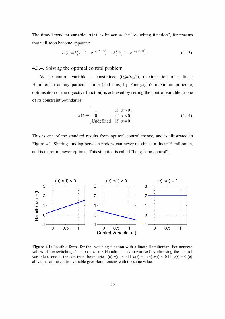
The time-dependent variable t is known as the “switching function”, for reasons
that will soon become apparent:
t =1T b1 1−e−1 T−t − 3
T b2 1−e−2T−t . (4.13)
4.3.4. Solving the optimal control problemAs the control variable is constrained (0≤u(t)≤1), maximisation of a linear
Hamiltonian at any particular time (and thus, by Pontryagin's maximum principle,
optimisation of the objective function) is achieved by setting the control variable to one
of its constraint boundaries:
u t ={ 1 if 0 ,0 if 0 ,
Undefined if =0 . (4.14)
This is one of the standard results from optimal control theory, and is illustrated in
Figure 4.1. Sharing funding between regions can never maximise a linear Hamiltonian,
and is therefore never optimal. This situation is called “bang-bang control”.
Figure 4.1: Possible forms for the switching function with a linear Hamiltonian. For nonzero values of the switching function σ(t), the Hamiltonian is maximised by choosing the control variable at one of the constraint boundaries. (a) σ(t) > 0 ⇒ u(t) = 1 (b) σ(t) < 0 ⇒ u(t) = 0 (c) all values of the control variable give Hamiltonians with the same value.
55
The optimal allocation of funding is piecewise constant, alternating between the two
boundaries. The “switching points”, when funding changes from one region to another,
occur when the sign of the switching function (Equation 4.13) changes. Funding
allocation at any particular time is therefore governed by the sign of the switching
function, which can be expressed as:
sgn t ={1 if 1T b11−e−1 T−t 3
T b21−e−2T−t ,−1 if 1
T b11−e−1T−t 3T b2 1−e−2 T−t .
(4.15)
This format emphasises the importance of the 1T b11−e−1 T−t term (and its
analogue in the second region). In case (c) of Figure 4.1, the value of the switching
function is zero, and thus the Hamiltonian is a constant. This situation obviously
precludes any value of the control variable uniquely maximising the Hamiltonian, a
situation known as “singular control”. Singular control problems are more complicated
to solve than basic bang-bang control, but fortunately a situation of this type cannot
arise using this model. If the switching function (Equation 4.13) were to be zero for any
finite length of time, it would be necessary that:
1T b1 1−e−1T−t = 3
T b2 1−e−2T−t , (4.16)
which can only occur if the two regions have identical habitat loss rates. Even if this is
true, their cost and terminal land distributions would have to satisfy the relationship:
b11R1T A1T z−1 = b22R2T A2T z−1 . (4.17)
This condition would be certainly be satisfied if the two regions are identical in all
respects, but is unlikely to occur otherwise.
4.3.5. Implementing the optimal control solutionThe form of Equation (4.15), and the bang-bang nature of the optimal allocation
strategy make it relatively easy to determine the best funding schedule for this two-
region problem, using a standard “shooting method”. The initial conditions of the state
variables are known (i.e., the initial land distribution of the conservation system), and an
56
arbitrary set of initial conditions is chosen for the costate variables. The following
algorithm is then implemented:
1. The control variable is set to one of its boundaries (u(0) = 1, or u(0) = 0).
2. The system is then forward-simulated until the terminal time using the state and
costate equations, making sure that the control variable obeys Equation (4.14),
and thus implicitly obeys Equation (4.15), at each point in time. If the available
land in either of the regions drops to zero, allocation immediately switches to the
remaining region.
3. At the terminal time, the value of the state and costate variables are recorded,
and their consistency is determined using Equation (4.10). Any discrepancies
between the two sets of variables are used to inform a new set of initial
conditions for the costate variables.
4. These steps are repeated until Equation (4.10) is consistent (or at least until the
discrepancy is smaller than some preset tolerance).
5. If the resulting optimal allocation schedule requires a switch in the control
variable, as soon as allocation begins, the initial choice for the control variable
(made in step 1) was incorrect. If this is the case, the first 4 steps should be
repeated with the control variable initially set at the other boundary.
This algorithm can be sped up considerably by taking advantage of solutions to the
state equations (Equations 4.6). The piecewise constant nature of the control variable
allows the state equations to be solved analytically between switching points. Rather
than forward-simulating the system using discrete time, it is instead possible to exactly
solve the differential equations sequentially. If the time of a particular switching point is
standardised to be t=0, then from Equations (4.6) the values of the state variables
(which are simple first order linear differential equations) can be expressed as analytic
functions (Equations 4.18 & 4.19). The value of these functions at the next switching
point can then be calculated quickly, without the need for forward-simulation.
57
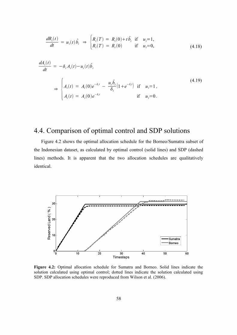
dRit dt = u it bi ⇒ {RiT = Ri0t bi if u i=1,
RiT = Ri 0 if u i=0,
(4.18)
dAit dt
= −i Ait −ui t b i
⇒ {Ait = Ai 0e−i t −
uibi
i1e−i t if u i=1 ,
Ai t = Ai0 e−i t if u i=0 .
(4.19)
4.4. Comparison of optimal control and SDP solutionsFigure 4.2 shows the optimal allocation schedule for the Borneo/Sumatra subset of
the Indonesian dataset, as calculated by optimal control (solid lines) and SDP (dashed
lines) methods. It is apparent that the two allocation schedules are qualitatively
identical.
Figure 4.2: Optimal allocation schedule for Sumatra and Borneo. Solid lines indicate the solution calculated using optimal control; dotted lines indicate the solution calculated using SDP. SDP allocation schedules were reproduced from Wilson et al. (2006).
58
They both propose that funding be allocated entirely to Sumatra for the first 13 years,
after which funding is directed to Borneo for the remaining 26 years. By this time, all
the available land in both regions has been either degraded or reserved. Both of the
allocation schedules concentrate on Sumatra until there is no land remaining available in
that region. Funding is only allocated to Borneo after opportunities to work in Sumatra
have been exhausted. It is interesting to note that this prioritisation order is the opposite
of the endemic species richness ranking.
While there are small discrepancies between the allocation schedules proposed by
the two techniques, these can be ascribed to a minor difference in problem formulation:
SDP tackles the optimal allocation problem by discretising the dimensions of time and
land, whereas optimal control theory considers all of these variables to be continuous.
When SDP is applied to generate the dotted lines in Figure 4.2, the total amount of land
in each region is first discretised into 1000 parcels. The area of these parcels in Sumatra
is approximately 249 square kilometers, each costing US$23,674.38. Thus, in a single
year when funding is allocated to Sumatra, the optimal control approach is able to
purchase 10,526.32 km2 of land (utilising the entire budget of US$1,000,000).
Meanwhile, the SDP approach is able to purchase 42 complete parcels of land (10,458
km2), but US$5,676 of the budget cannot be used. This amount will not cover the cost of
an additional parcel, and parcels are indivisible.
Although this difference in formulation is not large enough to radically alter the
funding schedule, it is the most likely cause of the differences observed in Figure 4.2.
The accumulation of reserved land observed in Sumatra is slower using SDP, and the
ongoing habitat loss means that less land is reserved as a result. Although SDP's
treatment of the temporal dimension requires discretisations that will also result in
rounding errors, a similar discretisation is required in the implementation of optimal
control, and this is therefore less likely to be a source of discrepancy between the two
solutions. However, the computational intensity of the SDP algorithm is likely to make
coarse time-discretisations unavoidable, which is not the case using optimal control
theory.
59
4.5. Features of the optimal funding allocation scheduleWhereas Wilson et al. (2006) were unable to discuss qualitative features of their
optimal allocation schedules (due to the opacity of SDP solutions), calculating
allocation schedules using optimal control theory allows general characteristics of the
best funding schedule to be identified. Perhaps the most surprising feature of the
optimal schedule is its bang-bang nature, which directs funding at any one time to a
single region, rather than sharing it. Although this switching was apparent in the optimal
allocation schedules generated by Wilson et al. (2006), it was not clear whether this was
a general result, or simply a reflection of the Indo-Malayan dataset. The linear nature of
the Hamiltonian proves that bang-bang control is necessary to minimise extinctions.
Analysis of the costate variables provides insight into the optimal nature of bang-
bang allocation. The role of the costate variables is to translate decisions made at
intermediate times into their effects at the terminal time. The costate variables are
therefore often referred to as the shadow value of their corresponding state variables
(Leonard & Long 1992) – they represent the shadow cast by present decisions on the
final outcome. In the conservation resource problem, the beneficial effect of reserving a
unit of land in a particular region is not immediately apparent. The decrease in the
amount of available land will slow the rate of habitat loss, and thus the rate of species
loss, but this effect will only be revealed in the future. The costate variables represent
the value of immediate actions with respect to the terminal objective. They therefore
allow managers to compare the true benefits of different decisions, not just the
immediate benefits (as a myopic heuristic does).
The costate variables (λ1(t) and λ3(t)) that correspond to the amount of land in the
reserves (R1(t) and R2(t)) are constants. This reflects the unchanging effect of reserved
land on the conservation objective (ST (T)) : an additional unit of reserved land will
increase the value of ST (T) by the same amount, regardless of when it is added. In
contrast, the remaining costate variables (λ2(t) and λ4(t)), that correspond to the available
land (A1(t) and A2(t)) increase exponentially as the terminal time approaches. Available
land is continually being lost, and it is therefore worth less to the terminal conservation
objective early in the timeseries . Close to the terminal time, available land is less likely
60
to be lost, and is thus of more value. The equivalence of the costate variable pairs at the
terminal time (λ1(T) = λ2(T) and λ3(T) = λ4(T)) reflects the fact that, at the terminal time,
reserved land and available land both contain extant species, and therefore contribute
equally to the objective function (evident from Equation 4.3). Note that the switching
function (in the form given by Equation (4.7), with separate ui(t) variables for each
region) can be rearranged as:
t = bu1t 1t −2t
c1 u2t
3t −4t c2 . (4.20)
In this form it is clear that the switching function, and in turn the allocation of
conservation funding, is not based on the regional shadow price of either the reserved
land or the available land alone. It is based instead on their relative value, a quantity that
can be thought of as the shadow conversion value. The 1t −2 t /c1 term
represents the increase in the shadow value of the system that results from converting
available land into reserved land in region 1, standardised by the cost of action. The
optimal decision is therefore to allocate all the available funding to the region where the
shadow conversion value of land is the greatest.
4.6. The five-region exampleIf the allocation schedule is viewed from the perspective of the shadow conversion
values, the extension to a general P-region solution is straightforward. Rearranging
Equation (4.1) gives the analogue of Equation (4.20):
t = b∑i=1
P
ui t 2i−1t −2i t
ci. (4.21)
The system Hamiltonian is still linear, and so the bang-bang nature of the optimal
solution is not altered by the inclusion of additional regions.
61
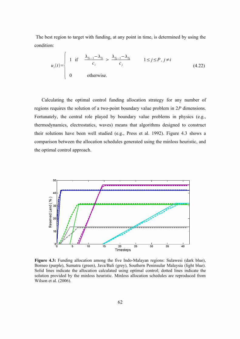
The best region to target with funding, at any point in time, is determined by using the
condition:
u it={ 1 if 2i−1−2i
c i
2j−1−2j
c j 1≤ j≤P , j≠i
0 otherwise.
(4.22)
Calculating the optimal control funding allocation strategy for any number of
regions requires the solution of a two-point boundary value problem in 2P dimensions.
Fortunately, the central role played by boundary value problems in physics (e.g.,
thermodynamics, electrostatics, waves) means that algorithms designed to construct
their solutions have been well studied (e.g., Press et al. 1992). Figure 4.3 shows a
comparison between the allocation schedules generated using the minloss heuristic, and
the optimal control approach.
Figure 4.3: Funding allocation among the five Indo-Malayan regions: Sulawesi (dark blue), Borneo (purple), Sumatra (green), Java/Bali (grey), Southern Peninsular Malaysia (light blue). Solid lines indicate the allocation calculated using optimal control; dotted lines indicate the solution provided by the minloss heuristic. Minloss allocation schedules are reproduced from Wilson et al. (2006).
62
The only significant difference between the optimal control allocation schedule
(solid lines) and the minloss allocation schedule (dashed lines) is the allocation to
Sumatra and Java/Bali. While minloss spreads the allocation simultaneously between
the two regions (between 0 and 5 years after the beginning of funding), the optimal
control allocation schedule allocates funding in the now familiar bang-bang manner.
Funding is first directed to Java/Bali, and only after land in that region is exhausted is it
directed to Sumatra.
4.7. DiscussionConservation takes place in a dynamic world (Possingham et al. 1993;
Costello & Polasky 2004; Meir et al. 2004), but global conservation resource
prioritisation has yet to formally allow the dynamics to affect conservation decisions.
Solving dynamic optimality problems is much more mathematically involved than the
essentially static framework that supported the delineation of the biodiversity hotspots.
Significant progress was made by Wilson et al. (2006), both by explicitly defining the
appropriate resource allocation problem using dynamic decision theory, and by using
SDP to calculate an optimal dynamic allocation schedule for the available funding.
Unfortunately, the opaque nature of SDP precluded an interpretation of the allocation
results, and its complexity meant that problems with more than two regions were
analytically intractable. These problems were addressed by the use of heuristics which
were of uncertain accuracy.
Solving this resource allocation problem using optimal control theory not only
allows the rapid solution of problems with multiple regions, but it also results in
allocation schedules that are more clear in their intent (Figure 4.2), as much of the
solution can be expressed analytically. For example, optimal control analyses show that
the bang-bang allocation suggested by the two-region SDP solution is a general
property of optimal allocation scenarios.
The results outlined in this chapter reflect the particular formulation of the system
dynamics, and the exact nature of the relationship between biodiversity and land area.
However, while alternative formulations of the system might result in different
63
allocation schedules, the conservation model I used is typical of those previously used
in dynamic conservation planning (Costello & Polasky 2004), with a biodiversity
benefit function that is based on accepted and empirically justified ecological theory
(Rosenzweig 1995). In addition, it is reasonable to believe that many of the qualitative
predictions will remain valid if some of these assumptions are relaxed. The bang-bang
nature of the optimal allocation strategy, which is the most striking feature of these
allocation schedules, arises because the Hamiltonian is a linear function of the control
variables. Alterations to the system dynamics that do not alter this linearity will not
change this feature of the optimal solution. For example, it is possible that the cost of
land is not a constant, but is inversely dependent on land availability (Armsworth et al.
2006). While this would change the conservation situation significantly, it would not
alter the linear relationship between the Hamiltonian and the control variable, and it
would therefore not alter the bang-bang nature of the optimal solution.
While bang-bang allocation schedules are likely to be controversial, the approach is
already accepted in conservation planning. The hotspots concept, for example, is based
on the same premise: funding is entirely directed to a small subset of global regions,
with no initial funding being directed to the remainder. Conservation organisations
nevertheless currently distribute funding across the priority regions in a much more
uniform manner than bang-bang optimality would advise. In 2006, the Critical
Ecosystems Partnership Fund invested in 17 of the 34 biodiversity hotspots and all 5
“high biodiversity wilderness areas” (CEPF 2006). Funding was shared in this manner
based on an implicit assumption: achieving fewer conservation outcomes in every
region results in better biodiversity benefits than ignoring some regions altogether.
There are, however, a few well-documented reasons why more uniform allocation is
unlikely to achieve superior results. First, many regions with low levels of threat will
not experience significant land loss if conservation action is delayed, in order to free up
funding for use in other areas. While action in low-threat regions will protect some
biodiversity, opportunities to stop habitat loss in high-threat regions will be wasted. In
the early stages of global conservation planning, poor conservation decisions are
especially dangerous, as initial conservation decisions have disproportionately large
effect on long-term conservation outcomes (Pressey & Tully 1994; Stewart et al. 2003).
64
Second, the varying cost of conservation action in different regions means that funding
allocated to the first world will not achieve significant conservation outcomes,
compared with the same amount spent in the developing world (Naidoo et al. 2007).
While first world priority regions may have significant amounts of biodiversity, the cost
of protecting this biodiversity will be prohibitive. Finally, carrying out conservation
efforts in a single region at a time will also markedly reduce the infrastructure and
administration required by the conservation organisation. A lack of trained
conservationists is often a considerable limitation to conservation in the developing
world (Rodriguez et al. 2006). (However, this factor was not included, and thus could
not have contributed to the optimality of bang-bang control in these analyses.)
There are also significant reasons why bang-bang allocation would not be the best
funding allocation approach for conservation organisations to adopt. For example, if the
objective of conservation is to protect a diverse array of ecosystems, rather than just the
most endemic species (Kareiva & Marvier 2003), funding might be spread more widely.
Conservation organisations also gain publicity and diverse support if they are seen to
address problems in a range of ecosystems. The primary value of demonstrating the
optimality of a bang-bang approach might therefore be to contrast with the tendency of
conservation organisations to spread their funding too widely.
Another very important aspect of conservation by land acquisition, which is not
addressed in the current conservation model, is the dynamic response of land developers
to the involvement and purchasing of land by conservation agencies. It was recognised
quite early in marine settings that reserving areas did not necessarily reduce the total
fishing effort in a region. Instead, effort that would normally have been occurring within
the new reserve was displaced outside, increasing (if only temporarily) the demands on
unreserved regions (Halpern et al. 2004). The same effect might arise in terrestrial
priority regions, and theoretical analyses indicate that under particular types of
uncertainty, this displaced degradation will have a greater detrimental effect on
biodiversity than the lack of any conservation action at all (Armsworth et al. 2006).
Conservation agencies are planning an enormous expansion of their efforts in the
developing world, and the targets being set for the total reserved area are considerable
(IUCN 2003). An effective outcome can only be achieved if the execution of these plans
65

recognises that conservation is a dynamic process. While dynamic optimisation is
considerably more complicated than its static counterpart, this dynamic aspect is crucial
to the success of international conservation efforts, and thus to the persistence of global
biodiversity. As I have demonstrated in this chapter, approaching this problem by using
optimal control theory can offer substantial insights into the most effective conservation
decisions.
66
Chapter 5
Optimal control of oscillating predator-prey
systems
5.1. AbstractMany interacting predator-prey populations have a natural tendency to exhibit
persistent limit-cycles or damped oscillations, especially in the presence of
environmental stochasticity. The restriction of populations into small conservation
reserves, and the resultant reduction in the scale of ecosystems, can induce cycling in
previously stable predator-prey relationships. During the course of these cycles, the
abundances of both predator and prey species regularly decrease to low levels. At these
times, environmental and demographic stochasticity may lead to the extinction of one of
the populations. Could culling one or both species at critical times reduce this
probability of extinction? I use Stochastic Dynamic Programming to determine the
optimal culling strategy for oscillation-prone species pairs. Remarkably, if interventions
are enacted at the appropriate time, infrequent culling of a small number of individuals
significantly reduces the probability that one of the species will go extinct. This
approach can be applied to many different ecosystems, and can incorporate more
complex system dynamics without a significant increase in computational time.
67
5.2. Predator-prey cyclesPredator and prey populations of certain species exhibit naturally cyclic behaviour:
their abundances do not converge to constant values, but change in a manner that
repeats through time. The most famous example of such oscillations is the lynx (Lynx
canadensis) and hare (Lepus americanus) population cycle of North America (Elton &
Nicholson 1942; Emlen 1984). In many systems, it is not clear what processes cause the
cycles, despite the problem receiving considerable attention from theoretical, empirical,
and mathematical ecologists (Kot 2001; Murray 2002; Turchin 2003; Ginsburg &
Colyvan 2004). Although there is dispute about the cause of these cycles, a common
feature is a temporarily abundant predator over-exploiting its prey. Typically, predation
by an elevated predator population leads to low prey abundance, which causes a crash in
the predator population through starvation. This low predator abundance allows the prey
population to rebound, which in turn allows the predators to increase also. The
heightened predator population instigates another cycle, and the process begins again.
Frequently, one or both of the species involved in predator-prey relationships are
threatened and/or are of conservation significance. Examples include Peregrine Falcons
(Falco peregrinus) that prey on California Terns (Sterna antillarum browni) on the
West Coast of America (Goodrich & Buskirk 1995); Indian Wolves (Canis lupus
pallipes) that prey on Blackbuck (Antelope cervicarpa) in Gujarat, India (Jhala 1993);
and predator complexes of lions (Panthera leo), leopards (Panthera pardus) and
cheetah (Lycaon pictus) that prey on various ungulate species in parks and game
reserves throughout southern Africa (Smuts 1978). Systems need not include a
traditional predator (in the sense of a carnivore) to exhibit cycling – it can also arise in
consumer-resource ecosystems. Some of the best-studied population cycles involve
small rodents (voles of the Microtus genus) in northern Europe (Hansson & Henttonen
1988). These cycles have long been considered the result of rodent-grass interactions
(Lack 1954; however see Korpimaki & Norrdahl 1998 for an alternative explanation).
5.2.1. Predator-prey cycles in conservation systemsMost theoretical analyses of predator-prey cycling have focused on deterministic
68
ecosystem models (e.g., Gilpin 1979; Takeuchi & Adachi 1983; Hastings & Powell
1991; Kot 2001; Javier & Sole 2000; Morozov et al. 2004). Predator-prey systems have
been modelled using systems of deterministic differential equations since the 1920s
(Volterra 1926), and much additional research has been undertaken by nonlinear
analysts attracted to ecology (and ecologists attracted to nonlinear dynamics) following
a series of seminal papers by Robert May in the 1970s (May 1973, 1974, 1976, 1977).
Yet much of this modelling has involved two simplifications. First, the modelling
techniques involve “mass-action” models, which do not consider the spatial nature of
ecosystems. Rather, mass-action models consider individuals to be interacting at a
single point in space. Including explicit spatial considerations has been shown to alter
many aspects of the system dynamics; in particular, space dampens population cycles
(Huffaker 1958; Jansen & de Roos 2000). Field observations support these theoretical
arguments, showing that fragmentation exacerbates the cyclic behaviour of populations,
leading to more frequent and severe population fluctuations (Kareiva 1987). The
predator-prey models I analyse in this chapter are mass-action models, but I believe that
the conservation context of these methods does not demand explicit spatial treatment.
This research is intended for use in conservation reserves, which are typically only
small fragments of the historical ecosystem. The small size of these conservation
reserves means that most protected individuals can directly interact, and the mass-action
assumption becomes more realistic.
From a conservation perspective, it is more important to consider the inevitable
stochasticity of ecosystems – the second simplifying assumption made by most
traditional predator-prey models. Unlike spatial factors, the effects of stochasticity will
be heightened in the confines of conservation reserves, as the smaller populations found
in these reserves are more affected by random events. Consequently, in the section of
the limit cycle when a species' abundance is low, a few unfortunate events (e.g.,
accidental deaths, inadequate rainfall, poaching) can be devastating, and extinction
becomes much more likely (e.g., Figure 5.4c). The effects of stochasticity have been
long acknowledged theoretically (Leslie & Gower 1960; May 1973) and observed
empirically (Gause 1934; Utida 1957; Corfield 1973). The models used in this chapter
will therefore be stochastic.
69
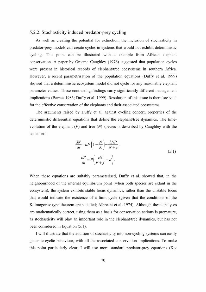
5.2.2. Stochasticity induced predator-prey cyclingAs well as creating the potential for extinction, the inclusion of stochasticity in
predator-prey models can create cycles in systems that would not exhibit deterministic
cycling. This point can be illustrated with a example from African elephant
conservation. A paper by Graeme Caughley (1976) suggested that population cycles
were present in historical records of elephant/tree ecosystems in southern Africa.
However, a recent parametrisation of the population equations (Duffy et al. 1999)
showed that a deterministic ecosystem model did not cycle for any reasonable elephant
parameter values. These contrasting findings carry significantly different management
implications (Barnes 1983; Duffy et al. 1999). Resolution of this issue is therefore vital
for the effective conservation of the elephants and their associated ecosystems.
The arguments raised by Duffy et al. against cycling concern properties of the
deterministic differential equations that define the elephant/tree dynamics. The time-
evolution of the elephant (P) and tree (N) species is described by Caughley with the
equations:
dNdt
=aN 1− NK − bNP
Nc,
dPdt
=P eNP f
−d.
(5.1)
When these equations are suitably parameterised, Duffy et al. showed that, in the
neighbourhood of the internal equilibrium point (when both species are extant in the
ecosystem), the system exhibits stable focus dynamics, rather than the unstable focus
that would indicate the existence of a limit cycle (given that the conditions of the
Kolmogorov-type theorem are satisfied; Albrecht et al. 1974). Although these analyses
are mathematically correct, using them as a basis for conservation actions is premature,
as stochasticity will play an important role in the elephant/tree dynamics, but has not
been considered in Equation (5.1).
I will illustrate that the addition of stochasticity into non-cycling systems can easily
generate cyclic behaviour, with all the associated conservation implications. To make
this point particularly clear, I will use more standard predator-prey equations (Kot
70
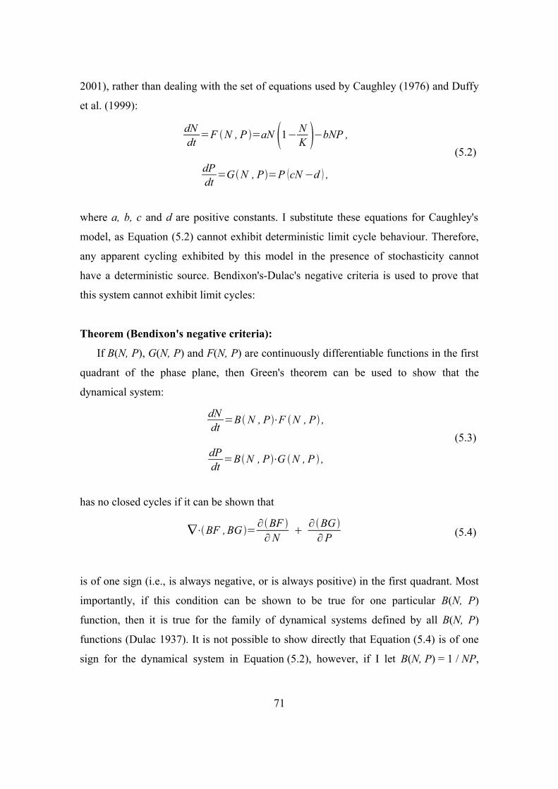
2001), rather than dealing with the set of equations used by Caughley (1976) and Duffy
et al. (1999):
dNdt
=F N , P =aN 1− NK −bNP ,
dPdt
=GN , P=P cN −d ,
(5.2)
where a, b, c and d are positive constants. I substitute these equations for Caughley's
model, as Equation (5.2) cannot exhibit deterministic limit cycle behaviour. Therefore,
any apparent cycling exhibited by this model in the presence of stochasticity cannot
have a deterministic source. Bendixon's-Dulac's negative criteria is used to prove that
this system cannot exhibit limit cycles:
Theorem (Bendixon's negative criteria):
If B(N, P), G(N, P) and F(N, P) are continuously differentiable functions in the first
quadrant of the phase plane, then Green's theorem can be used to show that the
dynamical system:
dNdt
=BN , P⋅F N , P ,
dPdt
=BN , P⋅G N , P ,
(5.3)
has no closed cycles if it can be shown that
∇⋅BF , BG =∂BF ∂N
∂BG ∂P
(5.4)
is of one sign (i.e., is always negative, or is always positive) in the first quadrant. Most
importantly, if this condition can be shown to be true for one particular B(N, P)
function, then it is true for the family of dynamical systems defined by all B(N, P)
functions (Dulac 1937). It is not possible to show directly that Equation (5.4) is of one
sign for the dynamical system in Equation (5.2), however, if I let B(N, P) = 1 / NP,
71
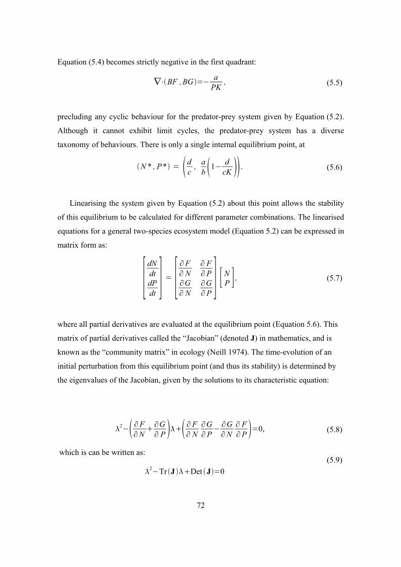
Equation (5.4) becomes strictly negative in the first quadrant:
∇⋅BF , BG =− aPK
, (5.5)
precluding any cyclic behaviour for the predator-prey system given by Equation (5.2).
Although it cannot exhibit limit cycles, the predator-prey system has a diverse
taxonomy of behaviours. There is only a single internal equilibrium point, at
N * , P * = dc
, ab 1− d
cK . (5.6)
Linearising the system given by Equation (5.2) about this point allows the stability
of this equilibrium to be calculated for different parameter combinations. The linearised
equations for a general two-species ecosystem model (Equation 5.2) can be expressed in
matrix form as:
[ dNdtdPdt ] = [ ∂F
∂ N∂ F∂P
∂G∂ N
∂G∂P ] [N
P ] , (5.7)
where all partial derivatives are evaluated at the equilibrium point (Equation 5.6). This
matrix of partial derivatives called the “Jacobian” (denoted J) in mathematics, and is
known as the “community matrix” in ecology (Neill 1974). The time-evolution of an
initial perturbation from this equilibrium point (and thus its stability) is determined by
the eigenvalues of the Jacobian, given by the solutions to its characteristic equation:
2− ∂F∂N
∂G∂ P ∂F
∂ N∂G∂P
− ∂G∂N
∂ F∂P =0, (5.8)
which is can be written as:
2−Tr J Det J=0(5.9)
72
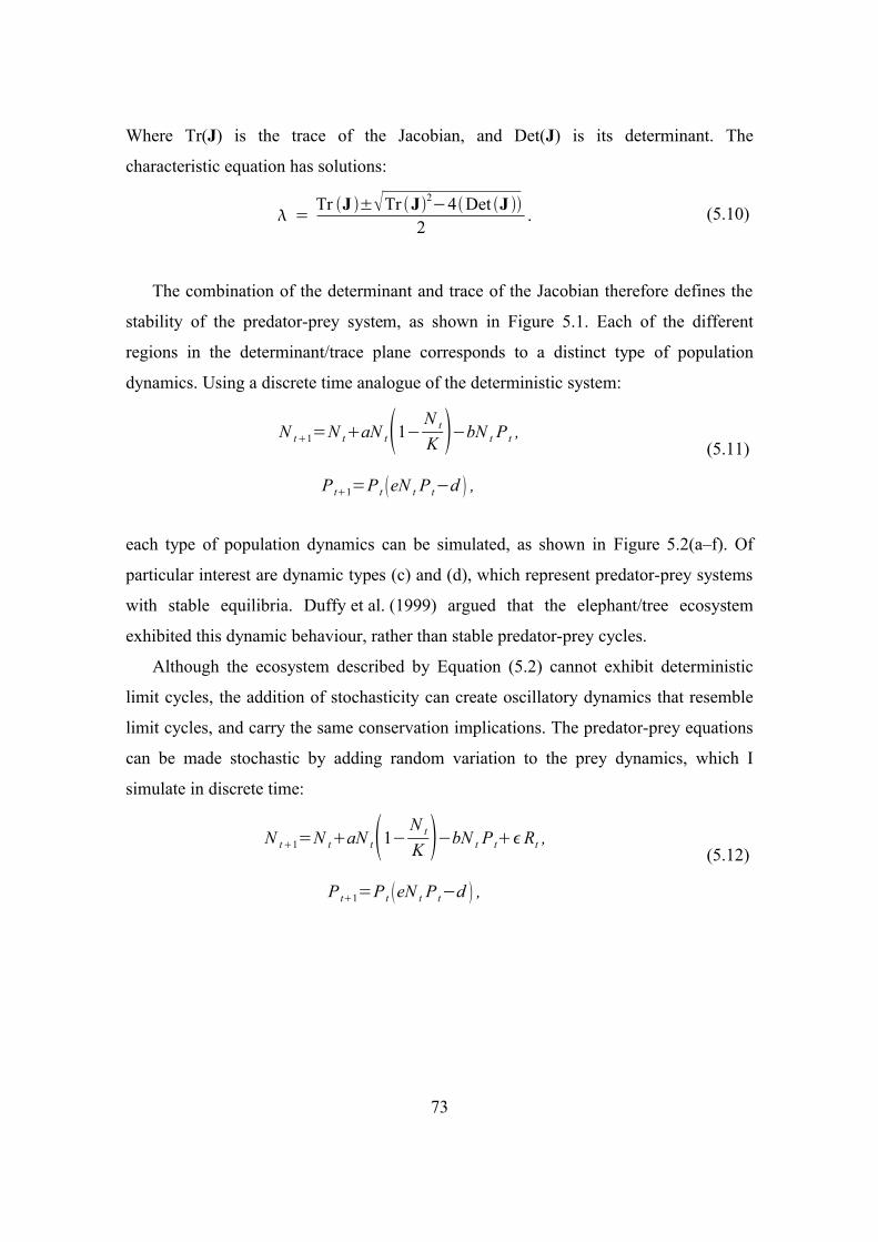
Where Tr(J) is the trace of the Jacobian, and Det(J) is its determinant. The
characteristic equation has solutions:
= Tr J ±Tr J2−4Det J 2
.
(5.10)
The combination of the determinant and trace of the Jacobian therefore defines the
stability of the predator-prey system, as shown in Figure 5.1. Each of the different
regions in the determinant/trace plane corresponds to a distinct type of population
dynamics. Using a discrete time analogue of the deterministic system:
N t1=N taN t1−N t
K −bN t P t ,
P t1=P t eN t P t−d ,
(5.11)
each type of population dynamics can be simulated, as shown in Figure 5.2(a–f). Of
particular interest are dynamic types (c) and (d), which represent predator-prey systems
with stable equilibria. Duffy et al. (1999) argued that the elephant/tree ecosystem
exhibited this dynamic behaviour, rather than stable predator-prey cycles.
Although the ecosystem described by Equation (5.2) cannot exhibit deterministic
limit cycles, the addition of stochasticity can create oscillatory dynamics that resemble
limit cycles, and carry the same conservation implications. The predator-prey equations
can be made stochastic by adding random variation to the prey dynamics, which I
simulate in discrete time:
N t1=N taN t1−N t
K −bN t P tRt ,
P t1=P t eN t P t−d ,
(5.12)
73
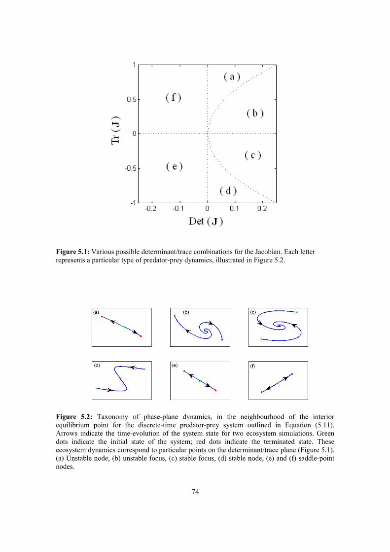
Figure 5.1: Various possible determinant/trace combinations for the Jacobian. Each letter represents a particular type of predator-prey dynamics, illustrated in Figure 5.2.
Figure 5.2: Taxonomy of phase-plane dynamics, in the neighbourhood of the interior equilibrium point for the discrete-time predator-prey system outlined in Equation (5.11). Arrows indicate the time-evolution of the system state for two ecosystem simulations. Green dots indicate the initial state of the system; red dots indicate the terminated state. These ecosystem dynamics correspond to particular points on the determinant/trace plane (Figure 5.1). (a) Unstable node, (b) unstable focus, (c) stable focus, (d) stable node, (e) and (f) saddle-point nodes.
74
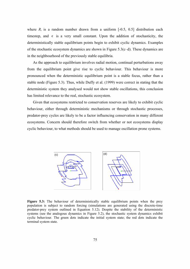
where Rt is a random number drawn from a uniform [-0.5, 0.5] distribution each
timestep, and is a very small constant. Upon the addition of stochasticity, the
deterministically stable equilibrium points begin to exhibit cyclic dynamics. Examples
of the stochastic ecosystem dynamics are shown in Figure 5.3(c–d). These dynamics are
in the neighbourhood of the previously stable equilibria.
As the approach to equilibrium involves radial motion, continual perturbations away
from the equilibrium point give rise to cyclic behaviour. This behaviour is more
pronounced when the deterministic equilibrium point is a stable focus, rather than a
stable node (Figure 5.3). Thus, while Duffy et al. (1999) were correct in stating that the
deterministic system they analysed would not show stable oscillations, this conclusion
has limited relevance to the real, stochastic ecosystem.
Given that ecosystems restricted to conservation reserves are likely to exhibit cyclic
behaviour, either through deterministic mechanisms or through stochastic processes,
predator-prey cycles are likely to be a factor influencing conservation in many different
ecosystems. Concern should therefore switch from whether or not ecosystems display
cyclic behaviour, to what methods should be used to manage oscillation prone systems.
Figure 5.3: The behaviour of deterministically stable equilibrium points when the prey population is subject to random forcing (simulations are generated using the discrete-time predator-prey system outlined in Equation 5.12). Despite the stability of the deterministic systems (see the analogous dynamics in Figure 5.2), the stochastic system dynamics exhibit cyclic behaviour. The green dots indicate the initial system state; the red dots indicate the terminal system state.
75

5.2.3. Optimal management of cycling predator-prey populations Reserve managers want to ensure ecosystem persistence, but a typical management
response is to do nothing until populations are near local extinction (Barnes 1983;
Possingham 2002). Management actions to recover very small populations (e.g., captive
breeding, translocation) are generally expensive and fraught with uncertainty (Regan et
al. 2005). In this chapter, I consider the possibility that culling animals when they are
abundant can increase the persistence of their population. The idea of killing organisms
to prevent their population from going extinct seems counter-intuitive. Certainly, if such
measures are applied at the wrong time, they will have a negative effect on species'
persistence. Nevertheless, careful analysis of the system dynamics can indicate when
judicious culling will benefit the cycling predator-prey system.
Whether or not culling organisms at a particular time can increase population
persistence depends heavily on the abundances of both species. The nonlinear time-
progression of an oscillating system means that all the effects of culling will not be
immediately obvious, and will not necessarily be intuitive. For example, removing
individuals of a particular species might lead to that species developing greater
abundances than would otherwise have occurred, through more violent cycles (i.e.,
cycles with larger amplitudes). Taking into account the progression of the oscillatory
system dynamics is thus crucial to developing management strategies that will
efficiently ensure the persistence of both predator and prey. This problem is therefore an
exercise in dynamic optimal control.
The idea that predator-prey systems require culling interventions is not new. This
logic has lead to the culling of African elephant populations to avoid tree loss (the prey),
and a resultant catastrophic decline in the number of elephants (Aarde et al. 1999).
Experimental reduction of predatory rodents (two small mustelids, Mustela nivalis and
M. erminea), and avipredators (Falco tinnunculus and Aegolius funereus), in northern
Europe reduced the severity of cycles in a rodent complex consisting of voles of the
species Microtus agrestis, M. rossiaemeridionalis and Clethrionomys glareolus
(Korpimaki & Norrdahl 1998). However, although the problem of when to cull
individuals has been discussed in an heuristic fashion, an optimal culling strategy has
never been defined. I use dynamic decision theory to explicitly formulate this
76
management problem, and then apply SDP (Bellman & Dreyfuss 1962) to determine the
management strategy that will best ensure the persistence of both species in the
ecosystem, given certain restrictions on management actions. I ask whether it is better to
cull predator individuals, or prey individuals, and when such actions should be taken.
The SDP strategy addresses the ecosystem's unpredictable evolution, and weighs up the
benefits associated with the two fluctuating populations, as well as the costs associated
with their control.
5.3. Methods5.3.1 The Population Model
To model the effects of management interventions on a predator-prey system using
dynamic decision theory, I must first define a quantitative ecosystem model that
includes important system properties. To illustrate the analysis, I set up a general
predator-prey model. In this model, the time-evolution of the prey population, Nt , is
deterministic, and that of the predator population, Pt, is stochastic. In reality, both
species' dynamics will be unpredictable, but stochasticity will be most important to the
predators, as their population will be much smaller. To allow the application of SDP,
the model is formulated in discrete time. The prey population grows logistically, with
carrying capacity K and growth rate r:
N t1=N t1r1−N t
K −∑i=1
P t
C ti , (5.13)
where C ti represents the number of prey consumed by the ith predator (defined below).
After each time step, the prey population is rounded to the nearest integer abundance.
The predator population grows stochastically. Each time step the predators seek out
prey, a process that becomes more difficult as prey become more scarce. To reflect this,
the amount of prey caught by each predator is drawn from a uniform distribution:
C1i~Uniform 0, Cmax N t /K . The upper bound of this distribution depends on the
density of the prey species: if the prey are at the carrying capacity of the habitat, the first
predator can catch as many as Cmax per time step. This catch is then rounded to the
77
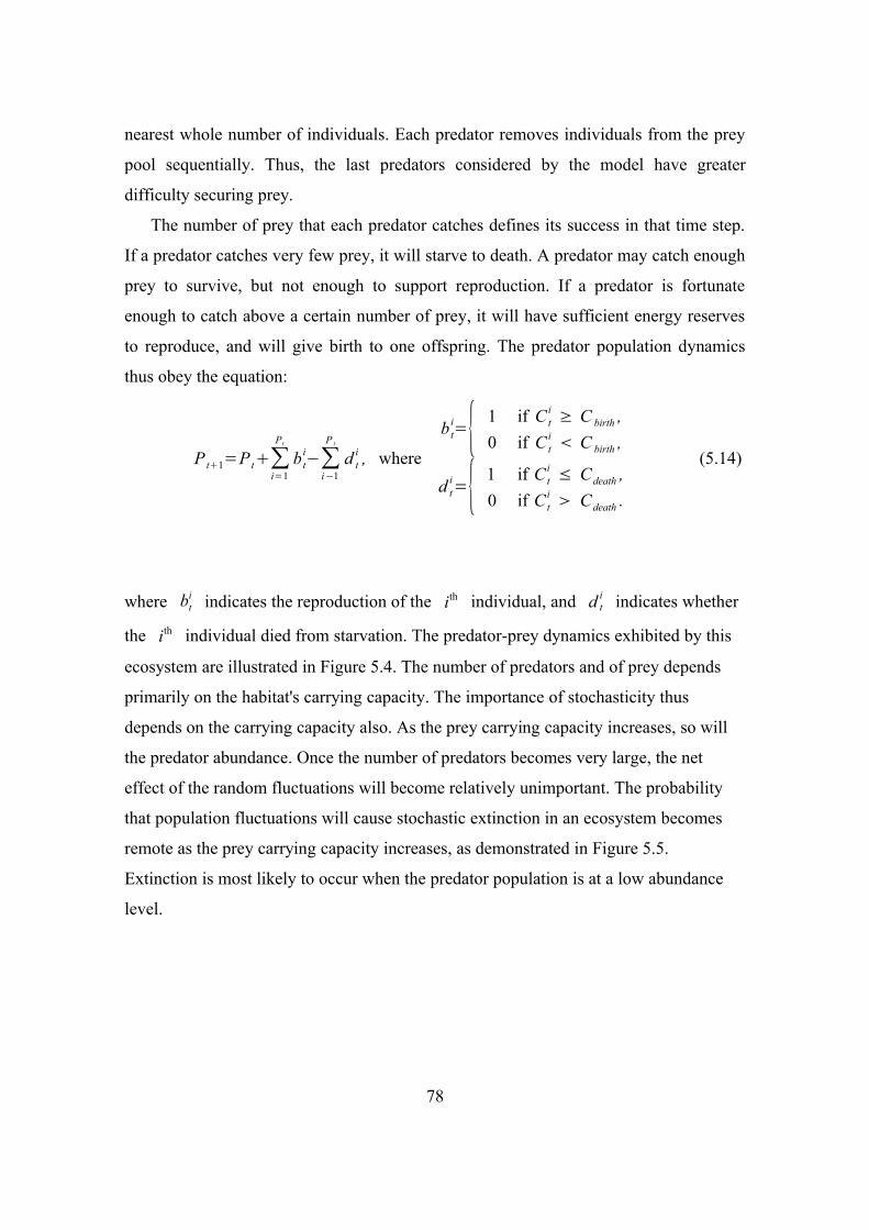
nearest whole number of individuals. Each predator removes individuals from the prey
pool sequentially. Thus, the last predators considered by the model have greater
difficulty securing prey.
The number of prey that each predator catches defines its success in that time step.
If a predator catches very few prey, it will starve to death. A predator may catch enough
prey to survive, but not enough to support reproduction. If a predator is fortunate
enough to catch above a certain number of prey, it will have sufficient energy reserves
to reproduce, and will give birth to one offspring. The predator population dynamics
thus obey the equation:
P t1=P t∑i=1
Pt
b ti−∑
i−1
P t
d ti , where
b ti={ 1 if C t
i ≥ C birth , 0 if C t
i C birth ,
d ti={ 1 if C t
i ≤ Cdeath , 0 if C t
i Cdeath .
(5.14)
where bti indicates the reproduction of the ith individual, and d t
i indicates whether
the ith individual died from starvation. The predator-prey dynamics exhibited by this
ecosystem are illustrated in Figure 5.4. The number of predators and of prey depends
primarily on the habitat's carrying capacity. The importance of stochasticity thus
depends on the carrying capacity also. As the prey carrying capacity increases, so will
the predator abundance. Once the number of predators becomes very large, the net
effect of the random fluctuations will become relatively unimportant. The probability
that population fluctuations will cause stochastic extinction in an ecosystem becomes
remote as the prey carrying capacity increases, as demonstrated in Figure 5.5.
Extinction is most likely to occur when the predator population is at a low abundance
level.
78
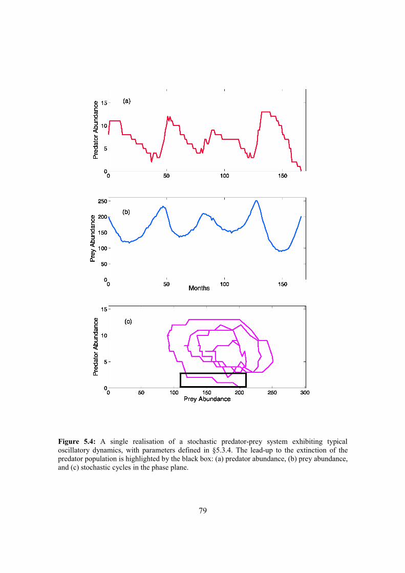
Figure 5.4: A single realisation of a stochastic predator-prey system exhibiting typical oscillatory dynamics, with parameters defined in §5.3.4. The lead-up to the extinction of the predator population is highlighted by the black box: (a) predator abundance, (b) prey abundance, and (c) stochastic cycles in the phase plane.
79
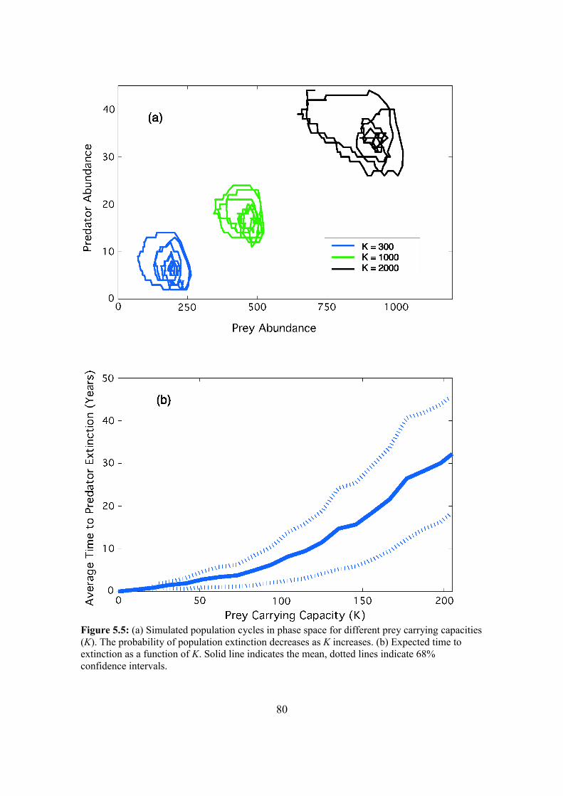
Figure 5.5: (a) Simulated population cycles in phase space for different prey carrying capacities (K). The probability of population extinction decreases as K increases. (b) Expected time to extinction as a function of K. Solid line indicates the mean, dotted lines indicate 68% confidence intervals.
80
5.3.2 The system dynamics as a Markov process: The application of SDP requires that the system dynamics be expressed as a discrete
time Markov process, where the system's evolution is defined by the probability of
transition between system “states”. In this predator-prey system, a state is defined by the
abundance of the two populations. As the changes that the system will undergo (births,
deaths, predation) depend only on the two species' abundances, these two values are
used to uniquely define the states. Regardless of the carrying capacity, the potential
population of both species is theoretically unlimited. However, populations of either
species that are much larger than K are not sustainable for any length of time. I therefore
place a “ceiling” on the abundance of predators, Pc , and on the abundance of prey, Nc .
If the simulated populations exceed these ceilings, their abundances are automatically
reduced to the ceiling value.
Although the ceilings imply that the population dynamics are artificially limited, I
set them at values much higher than the ecosystem will naturally encounter so that they
do not artificially interfere with the system dynamics.
I use the notation Si to represent the ith state of the system. The predator and prey
populations for each state are defined as:
N i=i−1mod N c1 ,
P i=Floor i−1N c1
, (5.15)
Where (a)mod(b) is the remainder of a divided by b, and Floor(x) is the greatest whole
number that is less than x. Conversely, the state index can be calculated from the
predator and prey abundances:
i=Pi N c1N i1. (5.16)
There are a total of Smax = (Nc + 1)(Pc + 1) possible ecosystem states. If Nc = 10, then some
example states would be:
81
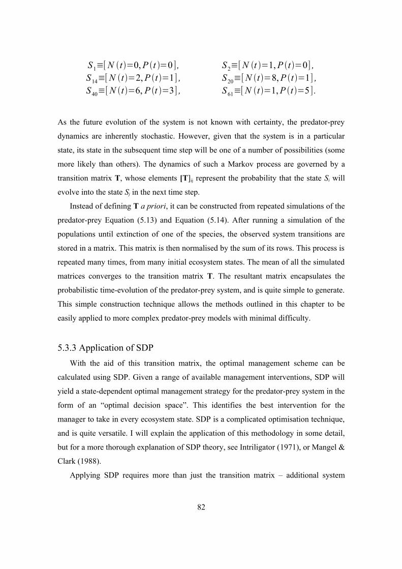
S1≡[N t =0, P t =0 ] , S 2≡[N t =1, P t =0] ,S 14≡[N t =2, P t =1] , S 20≡[N t =8, P t =1] ,S 40≡[N t =6, P t =3] , S 61≡[N t =1, P t =5 ] .
As the future evolution of the system is not known with certainty, the predator-prey
dynamics are inherently stochastic. However, given that the system is in a particular
state, its state in the subsequent time step will be one of a number of possibilities (some
more likely than others). The dynamics of such a Markov process are governed by a
transition matrix T, whose elements [T]ij represent the probability that the state Si will
evolve into the state Sj in the next time step.
Instead of defining T a priori, it can be constructed from repeated simulations of the
predator-prey Equation (5.13) and Equation (5.14). After running a simulation of the
populations until extinction of one of the species, the observed system transitions are
stored in a matrix. This matrix is then normalised by the sum of its rows. This process is
repeated many times, from many initial ecosystem states. The mean of all the simulated
matrices converges to the transition matrix T. The resultant matrix encapsulates the
probabilistic time-evolution of the predator-prey system, and is quite simple to generate.
This simple construction technique allows the methods outlined in this chapter to be
easily applied to more complex predator-prey models with minimal difficulty.
5.3.3 Application of SDPWith the aid of this transition matrix, the optimal management scheme can be
calculated using SDP. Given a range of available management interventions, SDP will
yield a state-dependent optimal management strategy for the predator-prey system in the
form of an “optimal decision space”. This identifies the best intervention for the
manager to take in every ecosystem state. SDP is a complicated optimisation technique,
and is quite versatile. I will explain the application of this methodology in some detail,
but for a more thorough explanation of SDP theory, see Intriligator (1971), or Mangel &
Clark (1988).
Applying SDP requires more than just the transition matrix – additional system
82
quantities are needed, which influence the relative costs and benefits of the different
conservation actions. In particular, the length of the management period (known as the
“terminal time”), the conservation objective, and the constraints on the available
management actions need to be defined.
Terminal Time: SDP calculates the strategy that will best achieve the stated
objective in a set time span ( T years), which must first be defined. The conservation
objective cannot be simply: “we would like to ensure the persistence of the predator
population”. The time span of the management must also be defined (e.g., “we would
like to ensure that the predator species persists for T years”). Theoretically, this means
that the resulting optimal solution is also time-dependent. Thus, the optimal decision
space to ensure persistence over T years will not necessarily be optimal over a different
time interval. In practice however, as T is allowed to increase, the solutions converge
rapidly to a time-independent solution. This solution will best ensure persistence for
perpetual management.
When the end of the management period is close (e.g., when T is small), the optimal
decision may incorporate the impending boundary. Such time-dependence can lead to
strange management decisions when SDP is applied to optimal harvest problems in
natural resource economics. If the terminal time is distant, then the earnings that will
result from a persistent population will be considerable. The extinction of the species
will not be in the best interest of the manager, as future harvests require the existence of
a future population. However, maintaining a population past the system's terminal time
will not be of any use to the manager, as profits beyond T are not considered in the
decision making process. Hence, managers are encouraged to harvest the species to
extinction in the final time step, to gain the maximum resource benefit.
In this management scenario, there is no terminal time – management is in
perpetuity – and so such a boundary effect is undesirable. While including a terminal
time is necessary if SDP is to be applied, it does not reflect an important aspect of the
system. The unwanted effect of the terminal boundary condition can be negated by
using a very large T. If the terminal time is very distant, the potential costs and benefits
at the terminal time become less influential, as the cumulative costs and benefits of the
intervening time steps outweigh those at the terminal time. Once the SDP solution has
83
been constructed, the system is managed according to the single, earliest decision space,
rather than using a separate decision space for every time.
Management Objective: The best decision for a manager to take will depend on
what the management objectives are: different objectives will result in different optimal
management strategies. In this analysis, the manager's primary objective is the
persistence of the predator species. This objective implicitly ensures the other species'
persistence, as prey are required to sustain a predator population. Each state of the
system will have a value assigned to it that reflects how well it fulfills the objective.
If one were interested only in the persistence of the predator population, every state
with a positive number of predators would have the same value assigned to it. However,
if each predator is deemed to be cumulatively valuable, the value assigned to each state
would depend on the quantity of predators. For example, if the predator population were
elephants that attracted tourism income, higher densities (and thus a higher likelihood of
tourists observing them) would be considered more valuable. The value of the ith state is
thus defined as:
i=VP P iVN N i , (5.17)
which represents the value of each predator, VP, multiplied by the predator abundance,
Pi , added to the value of each prey individual, VN , multiplied by the prey abundance in
that state, Ni .
Using SDP, one can assess value at the terminal time alone, or throughout the entire
time series. In the former case, the species abundances throughout the time series are
irrelevant, only the terminal abundances contribute to the system value. In the latter
case, a high predator abundance throughout the time series is desirable, rather than just
predator abundance at the terminal time. Continuing with the elephant example, as
tourism is occurring continually, the value of the system increases each year.
Controls: To best achieve the management objective the manager must make a
decision on how, or even if, they should act at each timestep. Using SDP, the full set of
decisions available to the manager must be outlined, as must the cost that each incurs.
The set of decisions analysed in this chapter is limited to either culling prey individuals,
or culling predator individuals. I will further limit the maximum number that may be
84
culled in one timestep. These decisions are numbered as follows:
1. Do nothing
2. Cull a single predator
3. Cull two predators
4. Cull five prey
5. Cull ten prey
Many more management interventions could be defined. For example, the manager
might be able to cull more than just two predators, or might be able to cull both
predators and prey simultaneously.
Most management actions will have an associated cost that will dissuade managers
from intervening unless it is cost-effective. The cost associated with the kth management
decision is called c(k). At each time step, one of the five decisions must be taken
(although the first decision actually represents taking no action). The effect of each
decision will be to alter the transition matrix T. This management action yields a new
matrix T(k), because after an intervention the predator-prey system will not evolve in
the same way (e.g., if a manager culls two predators, the next year there will be fewer
predator offspring, and more prey individuals). Decision augmented matrices are simple
to define: the system merely changes as though it were in a different state. For example,
if Nc = 10, and the system is in state 16 (S16 ≡ [ N(t) = 4; P(t) = 1] ), then the effect of
decision 2 is to make the state behave as though it were in state 5 (S5 ≡ [ N(t) = 4; P(t) = 0]
), a state with one fewer predators. The desired state dynamics are achieved if the the
16th row of T(2) is set equal to the 5th row of T(1) .
Applying SDP: The optimal strategy is determined by application of the Dynamic
Programming Equation (DPE), which is defined by the system value ψ, the intervention
costs c(k), and the transition matrices T(k):
V i ,t = maxk∈[1,2,3,4,5][i −c k ∑
j=1
S max
[T k ]ij V j , t1] (5.1
8)
The optimal decision, k, is chosen to maximise the expected value of the system in the
following time step, given its value in the current time step. This expected value is the
immediate value of state i, ψ(i), minus the cost of the decision k. Added to this
85
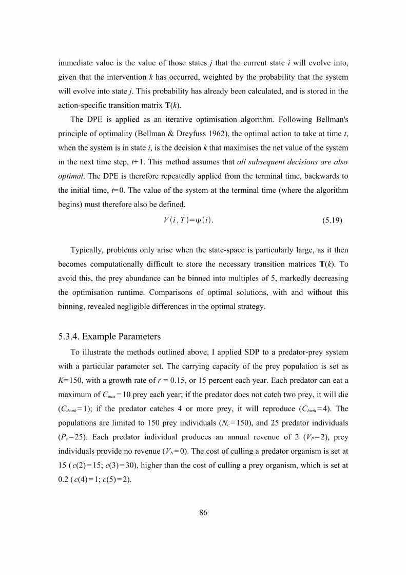
immediate value is the value of those states j that the current state i will evolve into,
given that the intervention k has occurred, weighted by the probability that the system
will evolve into state j. This probability has already been calculated, and is stored in the
action-specific transition matrix T(k).
The DPE is applied as an iterative optimisation algorithm. Following Bellman's
principle of optimality (Bellman & Dreyfuss 1962), the optimal action to take at time t,
when the system is in state i, is the decision k that maximises the net value of the system
in the next time step, t+1. This method assumes that all subsequent decisions are also
optimal. The DPE is therefore repeatedly applied from the terminal time, backwards to
the initial time, t=0. The value of the system at the terminal time (where the algorithm
begins) must therefore also be defined.
V i , T =i . (5.19)
Typically, problems only arise when the state-space is particularly large, as it then
becomes computationally difficult to store the necessary transition matrices T(k). To
avoid this, the prey abundance can be binned into multiples of 5, markedly decreasing
the optimisation runtime. Comparisons of optimal solutions, with and without this
binning, revealed negligible differences in the optimal strategy.
5.3.4. Example ParametersTo illustrate the methods outlined above, I applied SDP to a predator-prey system
with a particular parameter set. The carrying capacity of the prey population is set as
K=150, with a growth rate of r = 0.15, or 15 percent each year. Each predator can eat a
maximum of Cmax = 10 prey each year; if the predator does not catch two prey, it will die
(Cdeath = 1); if the predator catches 4 or more prey, it will reproduce (Cbirth = 4). The
populations are limited to 150 prey individuals (Nc = 150), and 25 predator individuals
(Pc = 25). Each predator individual produces an annual revenue of 2 (VP = 2), prey
individuals provide no revenue (VN = 0). The cost of culling a predator organism is set at
15 ( c(2) = 15; c(3) = 30), higher than the cost of culling a prey organism, which is set at
0.2 ( c(4) = 1; c(5) = 2).
86
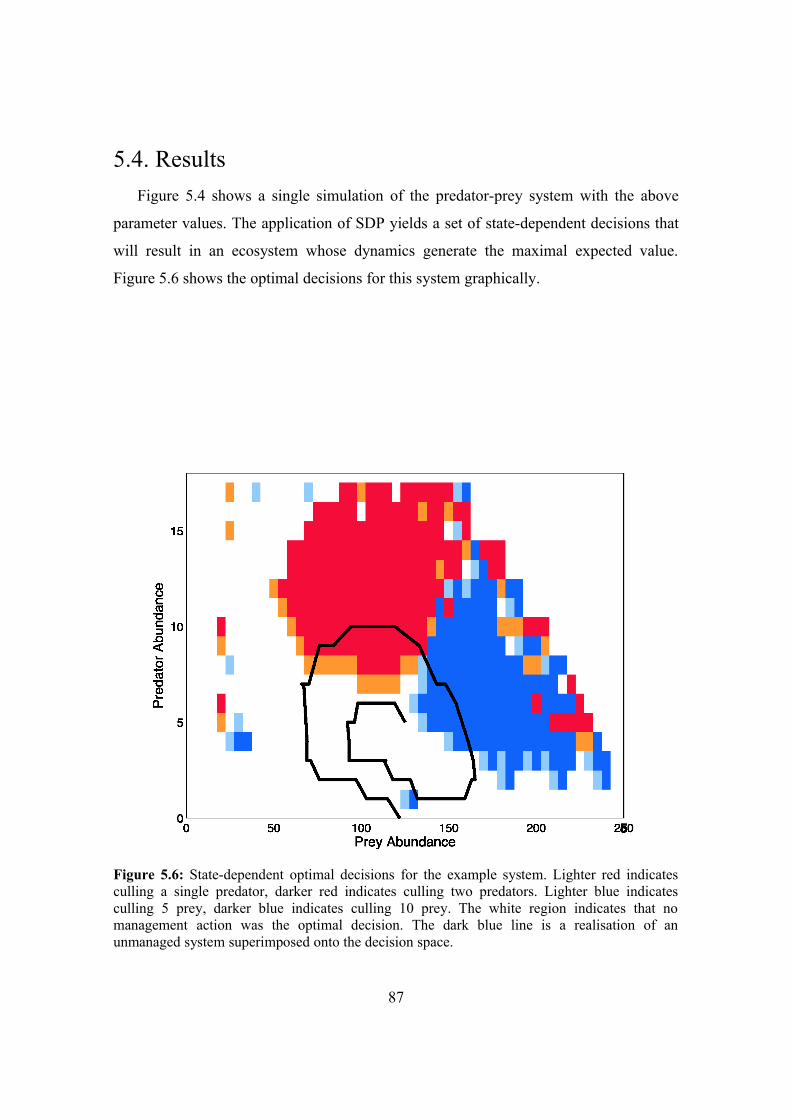
5.4. ResultsFigure 5.4 shows a single simulation of the predator-prey system with the above
parameter values. The application of SDP yields a set of state-dependent decisions that
will result in an ecosystem whose dynamics generate the maximal expected value.
Figure 5.6 shows the optimal decisions for this system graphically.
Figure 5.6: State-dependent optimal decisions for the example system. Lighter red indicates culling a single predator, darker red indicates culling two predators. Lighter blue indicates culling 5 prey, darker blue indicates culling 10 prey. The white region indicates that no management action was the optimal decision. The dark blue line is a realisation of an unmanaged system superimposed onto the decision space.
87
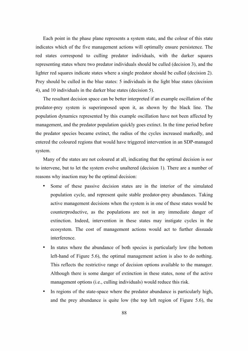
Each point in the phase plane represents a system state, and the colour of this state
indicates which of the five management actions will optimally ensure persistence. The
red states correspond to culling predator individuals, with the darker squares
representing states where two predator individuals should be culled (decision 3), and the
lighter red squares indicate states where a single predator should be culled (decision 2).
Prey should be culled in the blue states: 5 individuals in the light blue states (decision
4), and 10 individuals in the darker blue states (decision 5).
The resultant decision space can be better interpreted if an example oscillation of the
predator-prey system is superimposed upon it, as shown by the black line. The
population dynamics represented by this example oscillation have not been affected by
management, and the predator population quickly goes extinct. In the time period before
the predator species became extinct, the radius of the cycles increased markedly, and
entered the coloured regions that would have triggered intervention in an SDP-managed
system.
Many of the states are not coloured at all, indicating that the optimal decision is not
to intervene, but to let the system evolve unaltered (decision 1). There are a number of
reasons why inaction may be the optimal decision:
• Some of these passive decision states are in the interior of the simulated
population cycle, and represent quite stable predator-prey abundances. Taking
active management decisions when the system is in one of these states would be
counterproductive, as the populations are not in any immediate danger of
extinction. Indeed, intervention in these states may instigate cycles in the
ecosystem. The cost of management actions would act to further dissuade
interference.
• In states where the abundance of both species is particularly low (the bottom
left-hand of Figure 5.6), the optimal management action is also to do nothing.
This reflects the restrictive range of decision options available to the manager.
Although there is some danger of extinction in these states, none of the active
management options (i.e., culling individuals) would reduce this risk.
• In regions of the state-space where the predator abundance is particularly high,
and the prey abundance is quite low (the top left region of Figure 5.6), the
88
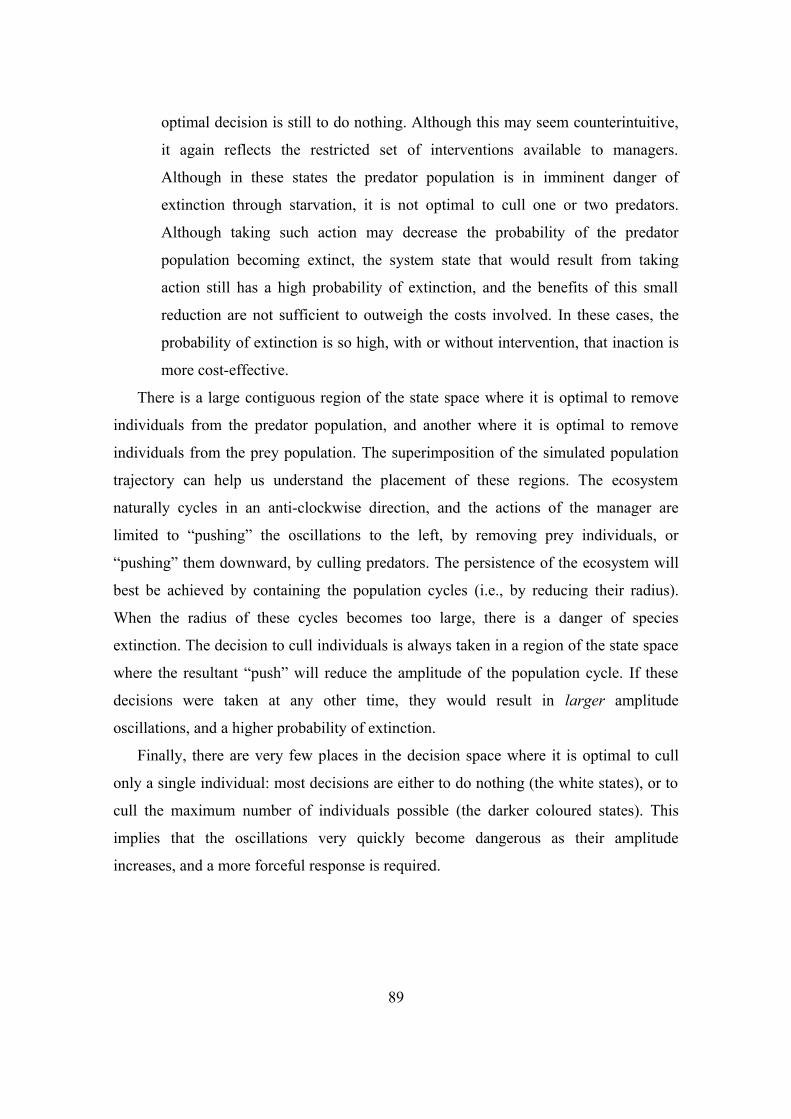
optimal decision is still to do nothing. Although this may seem counterintuitive,
it again reflects the restricted set of interventions available to managers.
Although in these states the predator population is in imminent danger of
extinction through starvation, it is not optimal to cull one or two predators.
Although taking such action may decrease the probability of the predator
population becoming extinct, the system state that would result from taking
action still has a high probability of extinction, and the benefits of this small
reduction are not sufficient to outweigh the costs involved. In these cases, the
probability of extinction is so high, with or without intervention, that inaction is
more cost-effective.
There is a large contiguous region of the state space where it is optimal to remove
individuals from the predator population, and another where it is optimal to remove
individuals from the prey population. The superimposition of the simulated population
trajectory can help us understand the placement of these regions. The ecosystem
naturally cycles in an anti-clockwise direction, and the actions of the manager are
limited to “pushing” the oscillations to the left, by removing prey individuals, or
“pushing” them downward, by culling predators. The persistence of the ecosystem will
best be achieved by containing the population cycles (i.e., by reducing their radius).
When the radius of these cycles becomes too large, there is a danger of species
extinction. The decision to cull individuals is always taken in a region of the state space
where the resultant “push” will reduce the amplitude of the population cycle. If these
decisions were taken at any other time, they would result in larger amplitude
oscillations, and a higher probability of extinction.
Finally, there are very few places in the decision space where it is optimal to cull
only a single individual: most decisions are either to do nothing (the white states), or to
cull the maximum number of individuals possible (the darker coloured states). This
implies that the oscillations very quickly become dangerous as their amplitude
increases, and a more forceful response is required.
89
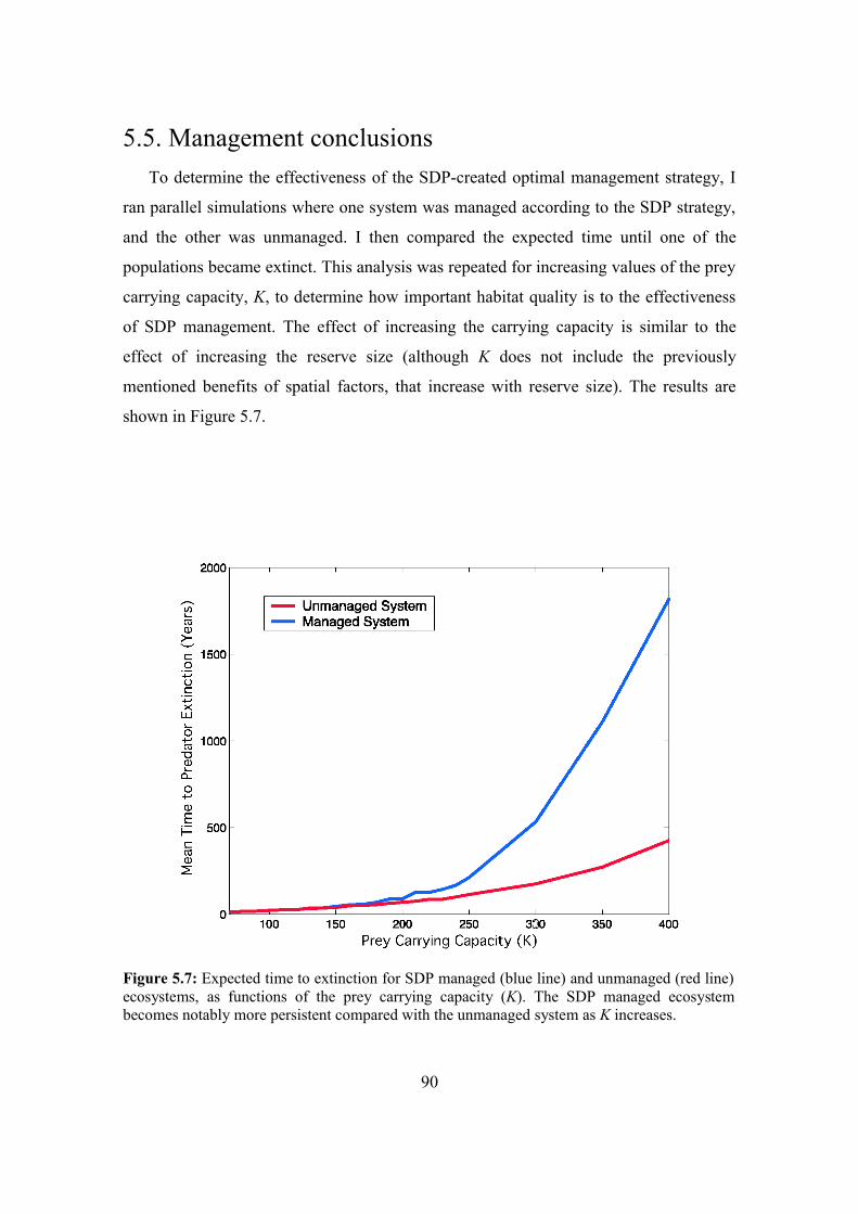
5.5. Management conclusionsTo determine the effectiveness of the SDP-created optimal management strategy, I
ran parallel simulations where one system was managed according to the SDP strategy,
and the other was unmanaged. I then compared the expected time until one of the
populations became extinct. This analysis was repeated for increasing values of the prey
carrying capacity, K, to determine how important habitat quality is to the effectiveness
of SDP management. The effect of increasing the carrying capacity is similar to the
effect of increasing the reserve size (although K does not include the previously
mentioned benefits of spatial factors, that increase with reserve size). The results are
shown in Figure 5.7.
Figure 5.7: Expected time to extinction for SDP managed (blue line) and unmanaged (red line) ecosystems, as functions of the prey carrying capacity (K). The SDP managed ecosystem becomes notably more persistent compared with the unmanaged system as K increases.
90
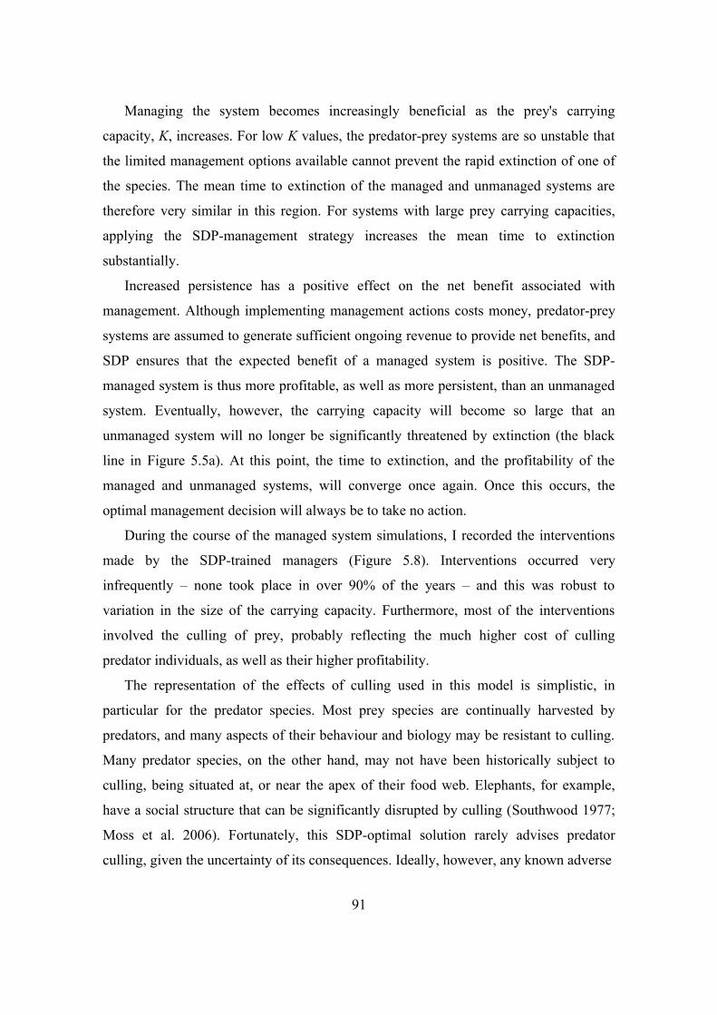
Managing the system becomes increasingly beneficial as the prey's carrying
capacity, K, increases. For low K values, the predator-prey systems are so unstable that
the limited management options available cannot prevent the rapid extinction of one of
the species. The mean time to extinction of the managed and unmanaged systems are
therefore very similar in this region. For systems with large prey carrying capacities,
applying the SDP-management strategy increases the mean time to extinction
substantially.
Increased persistence has a positive effect on the net benefit associated with
management. Although implementing management actions costs money, predator-prey
systems are assumed to generate sufficient ongoing revenue to provide net benefits, and
SDP ensures that the expected benefit of a managed system is positive. The SDP-
managed system is thus more profitable, as well as more persistent, than an unmanaged
system. Eventually, however, the carrying capacity will become so large that an
unmanaged system will no longer be significantly threatened by extinction (the black
line in Figure 5.5a). At this point, the time to extinction, and the profitability of the
managed and unmanaged systems, will converge once again. Once this occurs, the
optimal management decision will always be to take no action.
During the course of the managed system simulations, I recorded the interventions
made by the SDP-trained managers (Figure 5.8). Interventions occurred very
infrequently – none took place in over 90% of the years – and this was robust to
variation in the size of the carrying capacity. Furthermore, most of the interventions
involved the culling of prey, probably reflecting the much higher cost of culling
predator individuals, as well as their higher profitability.
The representation of the effects of culling used in this model is simplistic, in
particular for the predator species. Most prey species are continually harvested by
predators, and many aspects of their behaviour and biology may be resistant to culling.
Many predator species, on the other hand, may not have been historically subject to
culling, being situated at, or near the apex of their food web. Elephants, for example,
have a social structure that can be significantly disrupted by culling (Southwood 1977;
Moss et al. 2006). Fortunately, this SDP-optimal solution rarely advises predator
culling, given the uncertainty of its consequences. Ideally, however, any known adverse
91
Figure 5.8: A record of SDP-optimal management interventions that were taken to conserve an oscillating predator-prey system, as detailed in §5.3.4 (although K varies along the x-axis). Although culling two predators was a common intervention in Figure 5.6, it is rarely enacted.
effects of culling a specific predator species would be included in the decision-
augmented transition matrices, T(k).
In population states where an active decision is necessary, simulated management
records show that intervention involved culling the minimum possible number of
individuals more frequently than the maximum (Figure 5.8). This is despite the
relatively small number of states in Figure 5.6 where culling the lower number of
individuals was the optimal decision. The more severe culling states are typically
avoided with the early application of judicious culling. There are two conclusions that
should be drawn from this. First, the prevalence of particular interventions in decision
space does not necessarily reflect how frequently they will be implemented by a
manager following such a management strategy. For example, although in much of the
state space two predator organisms should be culled (Figure 5.6), this action is
infrequently implemented (Figure 5.8). Previous management interventions work to
keep the system away from this state. This leads to the second conclusion: in dynamic
92
systems, taking pre-emptive action that acknowledges possible future developments can
prevent their occurrence. Static management, which cannot quantitatively include
system dynamics, would find this difficult to achieve. As Barnes (1983) notes, when the
problem of dangerously high levels of predators is recognised, “the time of maximum
cost-effectiveness of culling has passed” (p. 139). It is therefore crucial that the future
evolution of the system dynamics is considered when management strategies are
formulated. The only manner in which this can be quantitatively included is by using
dynamic optimal control.
5.6. ConclusionIn this chapter I have addressed the considerable problems faced by conservationists
attempting to manage oscillating predator-prey ecosystems. While these predator-prey
oscillations can occur for deterministic reasons, they are much more prevalent in
stochastic environments (i.e., realistic environments). However, although this cycling
can endanger species of conservation interest, I have also demonstrated how the
dynamics of such ecosystems can be optimally managed to reduce the probability of
such extinctions. By managing the populations of both species through occasional culls
of a small number of individuals, managers can greatly enhance the persistence of
threatened populations.
Many current methods of ecosystem control attempt to keep a single species
population below a certain threshold, or between fixed bounds (Aarde et al. 1999;
Birkett 2002). This leads to unnecessarily culling, and can generate considerable public
opposition (Hecht & Nickerson 1999). Given the clumsy nature of such static controls,
such opposition may be reasonable. The dynamic control outlined in this chapter has the
substantial benefit of minimising the preventable culling of individuals, and of being
extremely cost-effective. Furthermore, by incorporating the multi-species nature of
ecosystems, it is possible to better understand how population dynamics lead to
undesirable system states. Armed with this knowledge, management can work to
prevent such scenarios with measures that incorporate those dynamics.
Optimal control of dynamic systems is far more complicated than static control,
93

especially when the options available to management are heavily constrained.
Nevertheless, if the objectives of management and the dynamics of the stochastically
oscillating predator-prey system are correctly formulated in a dynamic decision theory
framework, an optimal management strategy can be determined using SDP. The model
shown here was devised to reflect the dynamics of a general predator-prey system, but
the methods outlined can be applied to any particular system. The general conclusions
of the model will thus be applicable to many ecosystems where cycling is driven at least
partly by intrinsic mechanisms.
94
Chapter 6
Analysing asymmetric metapopulations
using complex network metrics
6.1. AbstractAlmost all metapopulation modelling assumes that connectivity between patches is
only a function of distance, and is therefore symmetric. In real metapopulations,
however, interactions between colonising individuals and heterogeneous inter-patch
landscapes will result in connectivity patterns that are invariably asymmetric.
Furthermore, connectivity will not be a simple function of the distance between the
patches, as some paths are easy to traverse, while others are difficult. There have been
few attempts to theoretically assess the effects of asymmetric connectivity patterns on
the dynamics of metapopulations. This chapter will address this deficiency by treating
metapopulations as complex networks. To do so, I define a set of metrics (in particular
“asymmetry”, “average path strength” and “centrality”) that can predict metapopulation
properties directly from their asymmetric connectivity patterns. I test the performance of
these metrics using a canonical protected area design problem, and find that the
resultant reserve networks are highly persistent. These complex network analyses
represent a useful new tool for understanding the dynamics of species existing in
fragmented landscapes, and allow a rapid understanding of the importance of particular
site in large metapopulations with asymmetric connectivity patterns.
95
6.2. Introduction6.2.1. Asymmetric connectivity patterns
Metapopulation theory provides a conceptual framework for predicting and
managing the future of species in fragmented habitats. Given the possibility of a local
patch population becoming extinct, the ability of species to move across uninhabitable
landscapes to recolonise empty patches (“connectivity”) is critical to the viability of
species that exist in metapopulations. The inter-patch landscape greatly affects the
movement of individuals, and thus the connectivity of the metapopulation. Barriers
(e.g., high mountain ranges) can prevent recolonisation between close patches.
Landscapes that hinder connectivity in one direction may help it in the opposite
direction (e.g., topographical gradients or wind and water currents).
This interaction between individuals and the landscape will result in inter-patch
connectivity patterns that are not simply functions of the distances between patches. If
connectivity is modelled solely on distance, the movement of individuals is implicitly
assumed to be isotropic and symmetric. A symmetric connectivity pattern assumes that
the probability of individuals travelling from patch A to patch B (and thus potentially
recolonising it) is the same as the probability of individuals from patch B travelling to
patch A. In a realistic, heterogeneous landscape, such symmetric connectivity will be the
exception, rather than the rule (Gustafson & Gardner 1996). As well as being
asymmetric, connectivity strengths (the probability that a particular colonisation will
occur) will not reflect only the inter-patch distance, but rather a combination of
distance, the ability of the organisms to move through the inter-patch landscape, and
characteristics of the patches themselves (i.e., their visibility). In general, I will call the
connectivity patterns that arise from such a realistic and complex landscape
“asymmetric”.
6.2.2. Dynamic consequences of asymmetric connectivityThe spatial arrangement of patches in a metapopulation has a very important impact
on metapopulation dynamics (Hanski & Gaggiotti 2004). The recent wealth of metrics
that approximate the viability of a metapopulation in a spatially heterogeneous
96
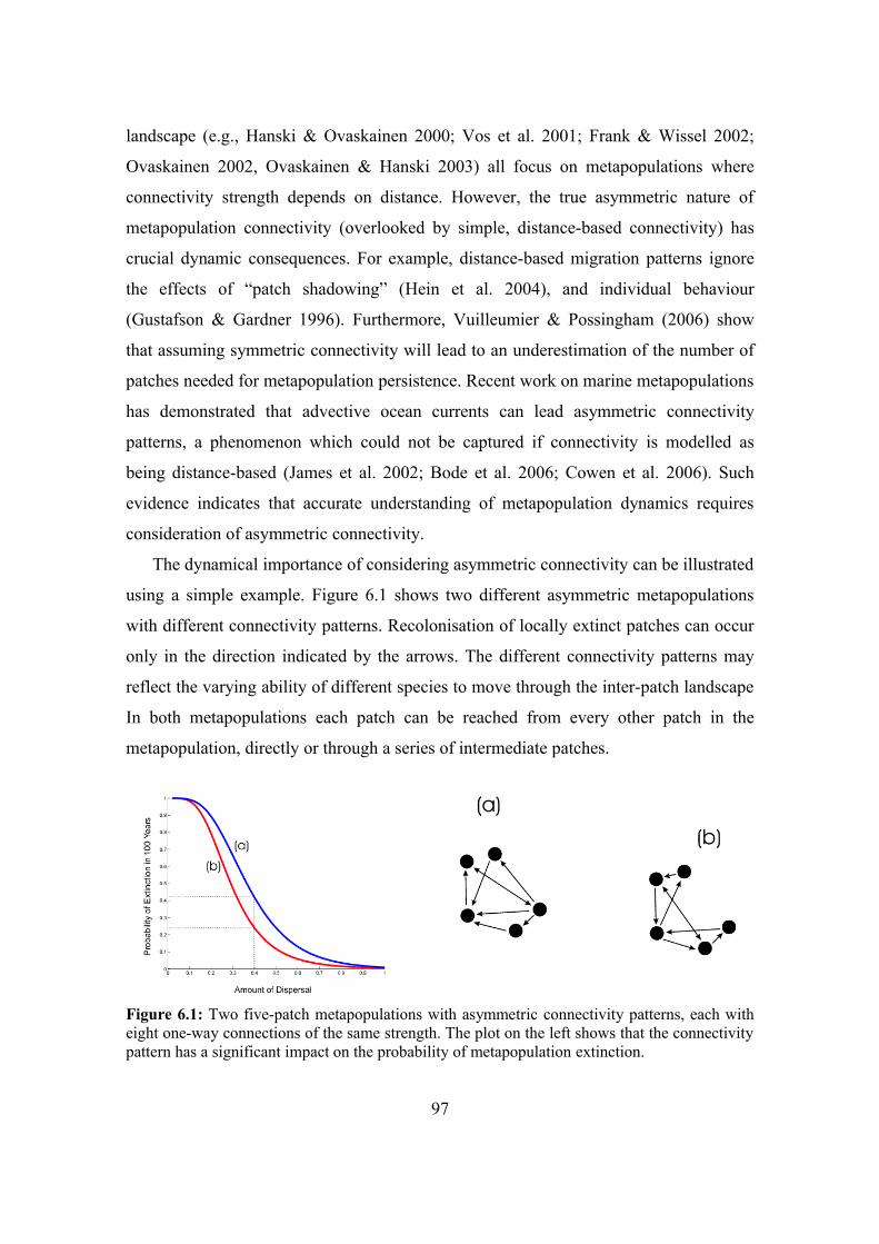
landscape (e.g., Hanski & Ovaskainen 2000; Vos et al. 2001; Frank & Wissel 2002;
Ovaskainen 2002, Ovaskainen & Hanski 2003) all focus on metapopulations where
connectivity strength depends on distance. However, the true asymmetric nature of
metapopulation connectivity (overlooked by simple, distance-based connectivity) has
crucial dynamic consequences. For example, distance-based migration patterns ignore
the effects of “patch shadowing” (Hein et al. 2004), and individual behaviour
(Gustafson & Gardner 1996). Furthermore, Vuilleumier & Possingham (2006) show
that assuming symmetric connectivity will lead to an underestimation of the number of
patches needed for metapopulation persistence. Recent work on marine metapopulations
has demonstrated that advective ocean currents can lead asymmetric connectivity
patterns, a phenomenon which could not be captured if connectivity is modelled as
being distance-based (James et al. 2002; Bode et al. 2006; Cowen et al. 2006). Such
evidence indicates that accurate understanding of metapopulation dynamics requires
consideration of asymmetric connectivity.
The dynamical importance of considering asymmetric connectivity can be illustrated
using a simple example. Figure 6.1 shows two different asymmetric metapopulations
with different connectivity patterns. Recolonisation of locally extinct patches can occur
only in the direction indicated by the arrows. The different connectivity patterns may
reflect the varying ability of different species to move through the inter-patch landscape
In both metapopulations each patch can be reached from every other patch in the
metapopulation, directly or through a series of intermediate patches.
Figure 6.1: Two five-patch metapopulations with asymmetric connectivity patterns, each with eight one-way connections of the same strength. The plot on the left shows that the connectivity pattern has a significant impact on the probability of metapopulation extinction.
97
Both of the metapopulations shown in this figure have the same total amount of
migration (eight directional migration paths). Will the dynamics of the metapopulations
be significantly affected by their different connectivity patterns?
These metapopulations have only a few patches, and so the probability that each will
become extinct before 100 timesteps has passed can be calculated using a Stochastic
Patch Occupancy Model (SPOM, Day & Possingham 1995), discussed in greater detail
in §6.3.1). The graph on the left of Figure 6.1, demonstrates the significant effect that
connectivity patterns have on metapopulation dynamics. This effect becomes
increasingly evident as the number of patches increases. While the probability of
extinction can be calculated using existing SPOMs (as these metapopulations are quite
small), this method offers no insight into why metapopulation (a)'s connectivity pattern
makes it less persistent than metapopulation (b). It would be useful if a new method
could offer a more intuitive explanation of why certain connectivity patterns result in
more persistent metapopulations.
6.2.3. Simulating asymmetric connectivity patternsAs asymmetric connectivity could not be practically measured (Hanski 1994),
connectivity was initially modelled using only the inter-patch distance. However,
simulation of the connectivity in real landscapes is now computationally feasible, and is
becoming increasingly common. The landscape matrix between patches can be quickly
assessed by remote sensing, and individual-based connectivity modelling can then be
used to simulate the responses of migrating species to the landscape. Simulation models
have been use to model crickets (Kindvall 1999), butterflies (Chardon et al. 2003),
rodents (Vuilleumier 2003), grey seals (Austin et al. 2004), and especially marine
organisms (Dight et al. 1990a; Dight et al. 1990b; Cowen et al. 2000; James et al. 2002,
Cowen et al. 2006).
Although these connectivities can now be estimated, making sense of the resulting
asymmetric connectivity patterns remains difficult, and very little metapopulation
theory has been formulated to address this difficulty. “Markovian” methods that can
analytically incorporate asymmetric connectivity (e.g., Day & Possingham 1995) can
only cope with a relatively small number of patches (fewer than ten; Ovaskainen 2002).
98
This presents a considerable limitation, as some marine metapopulations contain
thousands of patches. While Urban & Keitt (2001) find the minimum spanning tree of
the connectivity “graph”, and value patches and connectivity paths accordingly, their
minimum spanning trees are only defined for symmetric connectivity patterns. Much
analysis of population viability relies on Monte Carlo simulation models (e.g., RAMAS,
Ackakaya & Ferson 1999; VORTEX, Lacy 1993; ALEX; Possingham & Davis 1995),
which can cope with asymmetric connectivity patterns and large numbers of patches,
but gaining generalisable insights from the results of such simulations is problematic.
Ovaskainen & Hanski (2003) devised a metric that may cope with asymmetry, but their
analyses consider only distance-based connectivity. The primary aim of this chapter is
to explore the potential of complex network theory as a framework for quantitatively
predicting the dynamics of metapopulations with asymmetric connectivity patterns.
Metapopulations and their connectivity patterns can be modelled as networks (first
proposed by Urban & Keitt 2001), consisting of a number of nodes (metapopulation
patches) connected by a set of edges (the connectivity pattern). Complex network theory
attempts to understand the dynamic properties of such complicated networks by
analysing statistical properties of their interconnections. Using a complex network
framework, I consider the importance of several facets of asymmetric connectivity to
the dynamics of metapopulations. In particular, I am interested in the dynamic
consequences of increasing asymmetry, as well as the consequences of the mean
strength of direct and indirect connections between pairs of patches in the
metapopulation. Several new, easily calculated metrics for these attributes are defined,
and used to predict properties of the metapopulation dynamics. I focus on two problems
often used in theoretical metapopulation ecology, and commonly encountered by
conservation biologists: (1) predicting the expected time until metapopulation
extinction, and (2) making decisions that maximise metapopulation viability in the face
of patch destruction. A complex network approach is simple enough to be rapidly
applied to metapopulations that contains a large numbers of patches. It also allows the
connectivity patterns themselves to be the focus of the analyses, rather than abstractions
such as a Markov state transition matrix. A complex network approach thus offers a
more intuitive understanding of species existing in metapopulations.
99
6.3. Methods6.3.1. Using complex network metrics to predict metapopulation dynamics
I investigate whether three complex network metrics correlate with properties of the
metapopulation dynamics. They are formulated a priori, to quantitatively reflect
features of interest in the asymmetric connectivity matrix. I then assess the predictive
utility of these metrics by using them to estimate the probability of a metapopulation
going extinct. There are four steps to this method:
1. Using a version of the small world network generating algorithm of Watts &
Strogatz (1998), a metapopulation with an asymmetric connectivity pattern is
generated.
2. The three complex network metrics are calculated for this connectivity pattern.
3. A metapopulation model (Day & Possingham 1995) is used to determine the
exact dynamics of the metapopulation with asymmetric connectivity.
4. The predictive ability of the network metrics (calculated in step 2) is tested by
comparing them with the exact metapopulation dynamics (calculated in step 3).
Each of these steps are explained in more detail below. The small world algorithm
that generates asymmetric connectivity in step 1 can result in many different patterns,
and so the method is repeated a large number of times to ensure that a wide range of
possibilities are considered. The predictive capabilities of the metrics are also tested
over a wide range of parameter values.
Step 1: Generating asymmetric connectivity patterns:
In metapopulation theory, connectivity patterns are stored in a connectivity matrix,
which denoted ℂ . If the metapopulation consists of M patches, its connectivity is
represented by an M x M square matrix. Each element pij of the connectivity matrix ℂ
represents the probability at each timestep that the unoccupied patch j will be colonised
from patch i, (conditional on patch i being occupied).
100
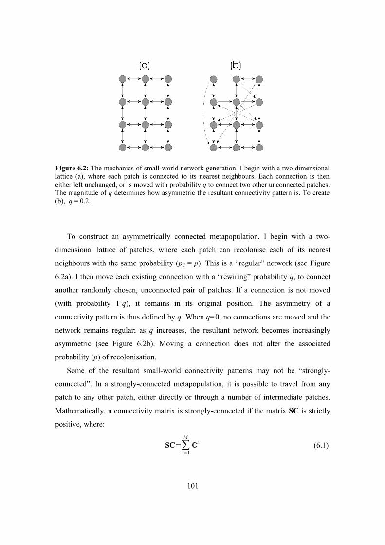
Figure 6.2: The mechanics of small-world network generation. I begin with a two dimensional lattice (a), where each patch is connected to its nearest neighbours. Each connection is then either left unchanged, or is moved with probability q to connect two other unconnected patches. The magnitude of q determines how asymmetric the resultant connectivity pattern is. To create (b), q = 0.2.
To construct an asymmetrically connected metapopulation, I begin with a two-
dimensional lattice of patches, where each patch can recolonise each of its nearest
neighbours with the same probability (pij = p). This is a “regular” network (see Figure
6.2a). I then move each existing connection with a “rewiring” probability q, to connect
another randomly chosen, unconnected pair of patches. If a connection is not moved
(with probability 1-q), it remains in its original position. The asymmetry of a
connectivity pattern is thus defined by q. When q=0, no connections are moved and the
network remains regular; as q increases, the resultant network becomes increasingly
asymmetric (see Figure 6.2b). Moving a connection does not alter the associated
probability (p) of recolonisation.
Some of the resultant small-world connectivity patterns may not be “strongly-
connected”. In a strongly-connected metapopulation, it is possible to travel from any
patch to any other patch, either directly or through a number of intermediate patches.
Mathematically, a connectivity matrix is strongly-connected if the matrix SC is strictly
positive, where:
SC=∑i=1
M
ℂi. (6.1)
101
Biologically, in a non-strongly-connected metapopulation some patches cannot
colonise, or cannot be colonised by, other patches. Rather than acting as a single entity,
these non-strongly-connected metapopulations are actually split into a number of sub-
metapopulations that are not connected, or are connected only in a unidirectional
source-sink manner. Disconnected (i.e., not strongly-connected) metapopulations do not
fit the standard definition of a metapopulation.
The number of patches is a crucial determinant of metapopulation persistence
(Etienne 2004), and so a metapopulation split into two or more unconnected sections
will have a much lower viability than a strongly-connected metapopulation. Non-
strongly-connected metapopulations are more likely to occur when connectivity is
asymmetric, and this will therefore reduce the average persistence of metapopulations
with asymmetric connectivity patterns. For example, it is unclear whether the lower
persistence of asymmetrically connected metapopulations in Vuilleumier & Possingham
(2006) is due to the detrimental effects of asymmetric connectivity, or to the increased
likelihood of disconnected metapopulations. To avoid potential confusion between the
two explanations, all non-strongly-connected metapopulations are discarded.
Step 2: Calculating the network metrics
1. Asymmetry (Z): I will measure the degree of metapopulation asymmetry by
gauging how different a connectivity pattern is from its symmetric counterpart
(the mean of connections in both directions between two patches). I define an
“asymmetry matrix” (Z) and an “asymmetry” metric (Z), as follows:
[Z ]ij = zij = 12∣pij− p ji∣,
Z = ∑i=1
M∑ j=1
Mzij .
(6.2)
(6.3)
When Z=0 the matrix is perfectly symmetric; as the asymmetry increases, Z
also increases to a maximum value ( Zmax = (M 2 – M ) / 2 ).
102
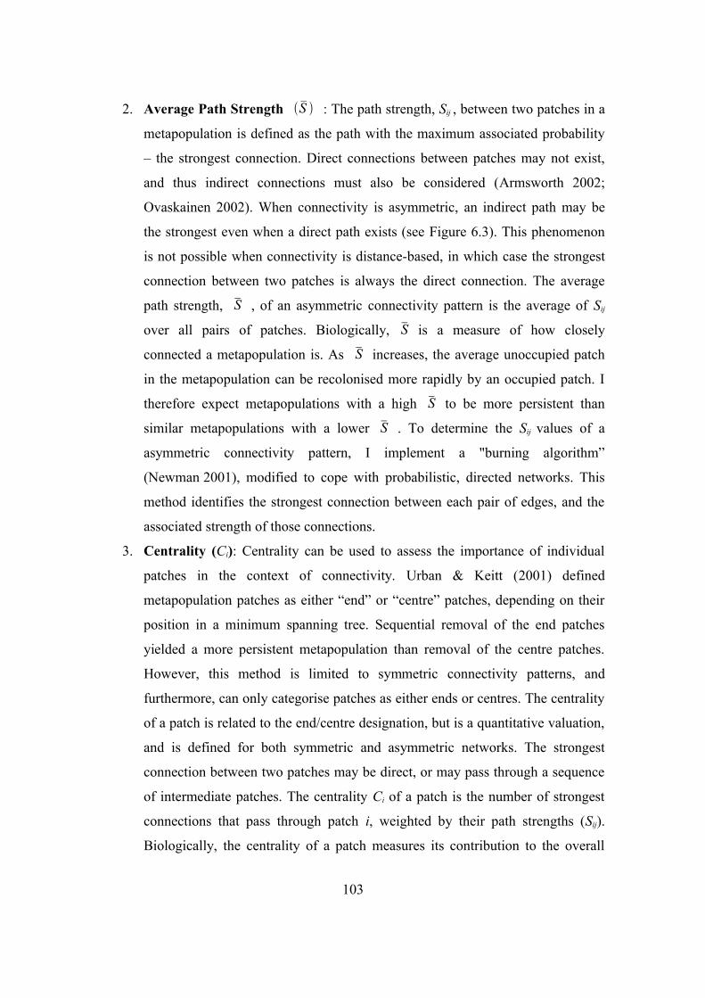
2. Average Path Strength S : The path strength, Sij , between two patches in a
metapopulation is defined as the path with the maximum associated probability
– the strongest connection. Direct connections between patches may not exist,
and thus indirect connections must also be considered (Armsworth 2002;
Ovaskainen 2002). When connectivity is asymmetric, an indirect path may be
the strongest even when a direct path exists (see Figure 6.3). This phenomenon
is not possible when connectivity is distance-based, in which case the strongest
connection between two patches is always the direct connection. The average
path strength, S , of an asymmetric connectivity pattern is the average of Sij
over all pairs of patches. Biologically, S is a measure of how closely
connected a metapopulation is. As S increases, the average unoccupied patch
in the metapopulation can be recolonised more rapidly by an occupied patch. I
therefore expect metapopulations with a high S to be more persistent than
similar metapopulations with a lower S . To determine the Sij values of a
asymmetric connectivity pattern, I implement a "burning algorithm”
(Newman 2001), modified to cope with probabilistic, directed networks. This
method identifies the strongest connection between each pair of edges, and the
associated strength of those connections.
3. Centrality (Ci): Centrality can be used to assess the importance of individual
patches in the context of connectivity. Urban & Keitt (2001) defined
metapopulation patches as either “end” or “centre” patches, depending on their
position in a minimum spanning tree. Sequential removal of the end patches
yielded a more persistent metapopulation than removal of the centre patches.
However, this method is limited to symmetric connectivity patterns, and
furthermore, can only categorise patches as either ends or centres. The centrality
of a patch is related to the end/centre designation, but is a quantitative valuation,
and is defined for both symmetric and asymmetric networks. The strongest
connection between two patches may be direct, or may pass through a sequence
of intermediate patches. The centrality Ci of a patch is the number of strongest
connections that pass through patch i, weighted by their path strengths (Sij).
Biologically, the centrality of a patch measures its contribution to the overall
103
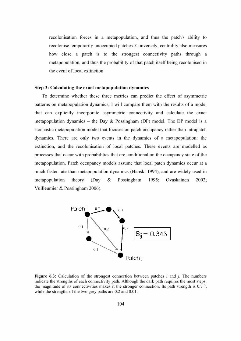
recolonisation forces in a metapopulation, and thus the patch's ability to
recolonise temporarily unoccupied patches. Conversely, centrality also measures
how close a patch is to the strongest connectivity paths through a
metapopulation, and thus the probability of that patch itself being recolonised in
the event of local extinction
Step 3: Calculating the exact metapopulation dynamics
To determine whether these three metrics can predict the effect of asymmetric
patterns on metapopulation dynamics, I will compare them with the results of a model
that can explicitly incorporate asymmetric connectivity and calculate the exact
metapopulation dynamics – the Day & Possingham (DP) model. The DP model is a
stochastic metapopulation model that focuses on patch occupancy rather than intrapatch
dynamics. There are only two events in the dynamics of a metapopulation: the
extinction, and the recolonisation of local patches. These events are modelled as
processes that occur with probabilities that are conditional on the occupancy state of the
metapopulation. Patch occupancy models assume that local patch dynamics occur at a
much faster rate than metapopulation dynamics (Hanski 1994), and are widely used in
metapopulation theory (Day & Possingham 1995; Ovaskainen 2002;
Vuilleumier & Possingham 2006).
Figure 6.3: Calculation of the strongest connection between patches i and j. The numbers indicate the strengths of each connectivity path. Although the dark path requires the most steps, the magnitude of its connectivities makes it the stronger connection. Its path strength is 0.7 3, while the strengths of the two grey paths are 0.2 and 0.01.
104
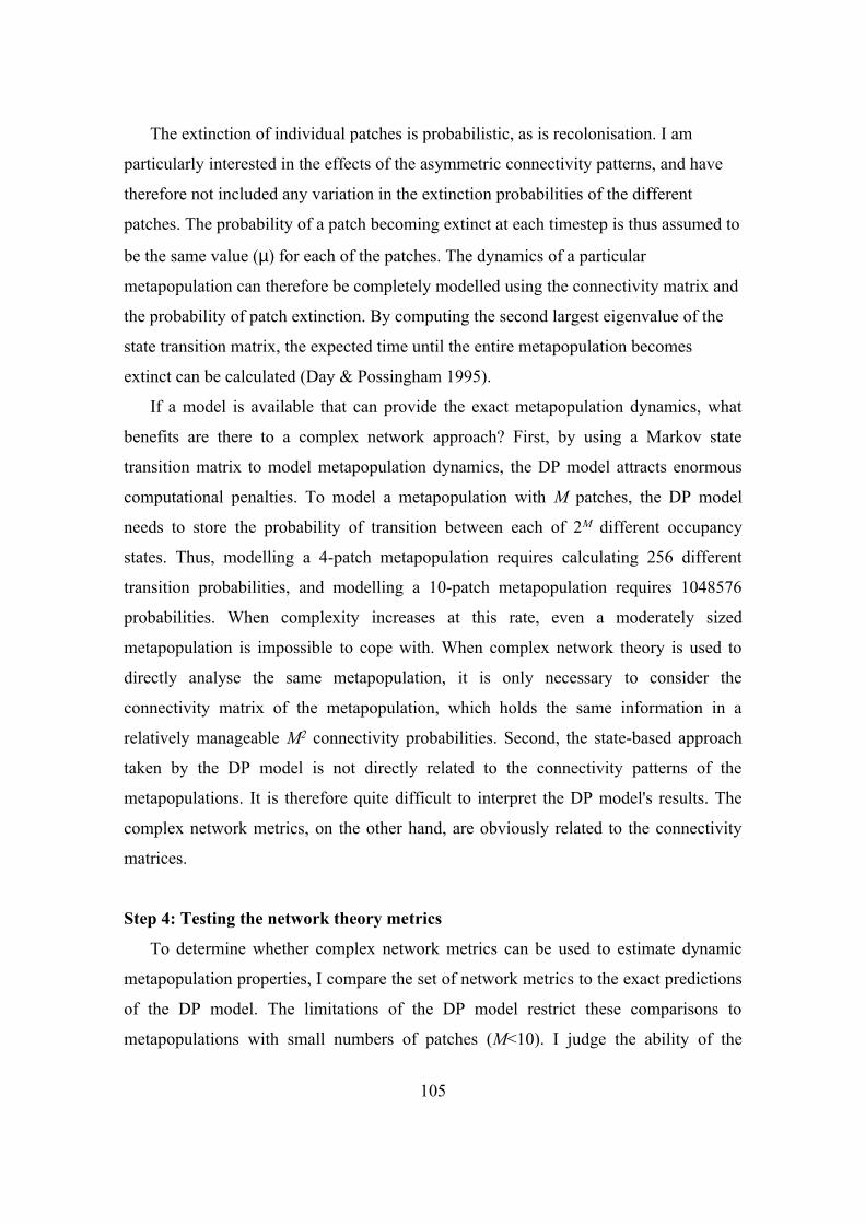
The extinction of individual patches is probabilistic, as is recolonisation. I am
particularly interested in the effects of the asymmetric connectivity patterns, and have
therefore not included any variation in the extinction probabilities of the different
patches. The probability of a patch becoming extinct at each timestep is thus assumed to
be the same value (µ) for each of the patches. The dynamics of a particular
metapopulation can therefore be completely modelled using the connectivity matrix and
the probability of patch extinction. By computing the second largest eigenvalue of the
state transition matrix, the expected time until the entire metapopulation becomes
extinct can be calculated (Day & Possingham 1995).
If a model is available that can provide the exact metapopulation dynamics, what
benefits are there to a complex network approach? First, by using a Markov state
transition matrix to model metapopulation dynamics, the DP model attracts enormous
computational penalties. To model a metapopulation with M patches, the DP model
needs to store the probability of transition between each of 2M different occupancy
states. Thus, modelling a 4-patch metapopulation requires calculating 256 different
transition probabilities, and modelling a 10-patch metapopulation requires 1048576
probabilities. When complexity increases at this rate, even a moderately sized
metapopulation is impossible to cope with. When complex network theory is used to
directly analyse the same metapopulation, it is only necessary to consider the
connectivity matrix of the metapopulation, which holds the same information in a
relatively manageable M2 connectivity probabilities. Second, the state-based approach
taken by the DP model is not directly related to the connectivity patterns of the
metapopulations. It is therefore quite difficult to interpret the DP model's results. The
complex network metrics, on the other hand, are obviously related to the connectivity
matrices.
Step 4: Testing the network theory metrics
To determine whether complex network metrics can be used to estimate dynamic
metapopulation properties, I compare the set of network metrics to the exact predictions
of the DP model. The limitations of the DP model restrict these comparisons to
metapopulations with small numbers of patches (M<10). I judge the ability of the
105
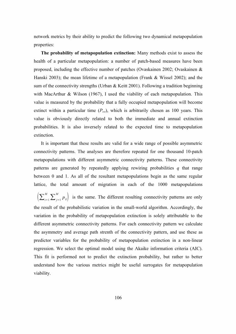
network metrics by their ability to predict the following two dynamical metapopulation
properties:
The probability of metapopulation extinction: Many methods exist to assess the
health of a particular metapopulation: a number of patch-based measures have been
proposed, including the effective number of patches (Ovaskainen 2002; Ovaskainen &
Hanski 2003); the mean lifetime of a metapopulation (Frank & Wissel 2002); and the
sum of the connectivity strengths (Urban & Keitt 2001). Following a tradition beginning
with MacArthur & Wilson (1967), I used the viability of each metapopulation. This
value is measured by the probability that a fully occupied metapopulation will become
extinct within a particular time (Pext), which is arbitrarily chosen as 100 years. This
value is obviously directly related to both the immediate and annual extinction
probabilities. It is also inversely related to the expected time to metapopulation
extinction.
It is important that these results are valid for a wide range of possible asymmetric
connectivity patterns. The analyses are therefore repeated for one thousand 10-patch
metapopulations with different asymmetric connectivity patterns. These connectivity
patterns are generated by repeatedly applying rewiring probabilities q that range
between 0 and 1. As all of the resultant metapopulations begin as the same regular
lattice, the total amount of migration in each of the 1000 metapopulations
∑i=1
M∑ j=1
Mp ij is the same. The different resulting connectivity patterns are only
the result of the probabilistic variation in the small-world algorithm. Accordingly, the
variation in the probability of metapopulation extinction is solely attributable to the
different asymmetric connectivity patterns. For each connectivity pattern we calculate
the asymmetry and average path strenth of the connectivity pattern, and use these as
predictor variables for the probability of metapopulation extinction in a non-linear
regression. We select the optimal model using the Akaike information criteria (AIC).
This fit is performed not to predict the extinction probability, but rather to better
understand how the various metrics might be useful surrogates for metapopulation
viability.
106
Patch removal strategies: I also examine the ability of centrality to predict which
patches are most important for the maintainance of metapopulation viability (a common
test of metapopulation modelling techniques; Hanski 1994; Hanski & Ovaskainen 2000;
Ovaskainen & Hanski 2003). I propose that if patches are removed in ascending order
of centrality, the most important patches in the metapopulation (i.e., those with the
highest centrality) will be preserved, thus minimising the detrimental effects of patch
loss on metapopulation persistence. To gauge the effectiveness of this
“centrality method”, I examine its performance compared with all other removal
methods.
A metapopulation of 10 patches is generated, connected by an asymmetric
connectivity pattern. Nodes are removed sequentially by the centrality method, and the
resultant metapopulation viability is determined after each removal. It is important that
the centrality values of each patch be recomputed after each successive removal, as the
loss of patches – which leads to a re-routing of some strongest connections and the
elimination of others – alters the dynamics of the metapopulation connectivity. To
determine the effectiveness of this centrality method, it is compared to all other possible
removal strategies, which are generated combinatorially. The performance of this
“centrality method” is measured by the percent of removal strategies that have equal or
lower viability. To examine the robustness of the results, these patch experiments are
repeated with many different asymmetric connectivity patterns, generated with different
rewiring probabilities. I also examined how the method performed when the
connectivity strengths (pij) are not all equal, but vary randomly about a mean value.
6.4. Results6.4.1. Probability of metapopulation extinction
First I consider the relationship between metapopulation viability and the complex
network metrics. Figure 6.4 shows the results of this first experiment, estimating the
probability of metapopulation extinction using the asymmetry Z and the average path
strength S of the connectivity patterns. Every point represents the probability of a 10-
107
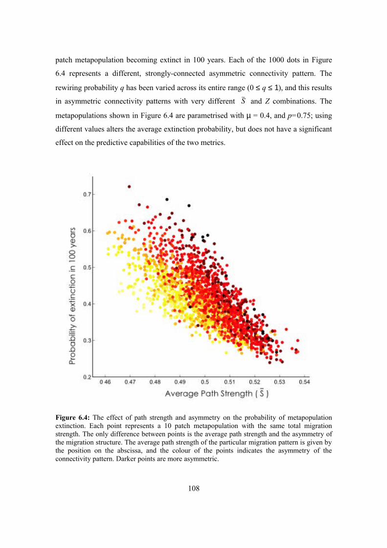
patch metapopulation becoming extinct in 100 years. Each of the 1000 dots in Figure
6.4 represents a different, strongly-connected asymmetric connectivity pattern. The
rewiring probability q has been varied across its entire range (0 ≤ q ≤ 1), and this results
in asymmetric connectivity patterns with very different S and Z combinations. The
metapopulations shown in Figure 6.4 are parametrised with µ = 0.4, and p=0.75; using
different values alters the average extinction probability, but does not have a significant
effect on the predictive capabilities of the two metrics.
Figure 6.4: The effect of path strength and asymmetry on the probability of metapopulation extinction. Each point represents a 10 patch metapopulation with the same total migration strength. The only difference between points is the average path strength and the asymmetry of the migration structure. The average path strength of the particular migration pattern is given by the position on the abscissa, and the colour of the points indicates the asymmetry of the connectivity pattern. Darker points are more asymmetric.
108
It is immediately apparent from Figure 6.4 that connectivity structure has an
important effect on metapopulation viability. Although all of these metapopulations
have the same number of patches and the same total amount of migration, the viability
of the metapopulations ranges from a 25% to a 70% probability of extinction within 100
years. The location of each point on the x-axis indicates S , the average path strength
of the connectivity pattern; the persistence of a metapopulation is positively correlated
with S . Much of the variation around this trend can be explained by Z, the asymmetry
of the connectivity pattern, which is indicated by the colour of the point (lighter dots
indicate more symmetric connectivity patterns). The asymmetry of a connectivity
pattern is negatively correlated with the metapopulation's persistence: the more
asymmetric a connectivity pattern (darker circles), the higher the probability of
metapopulation extinction. Fitting a polynomial regression to the data shown in
Figure 6.4 reveals that both the average path strength and the asymmetry are important
predictor variables. The fit of all subsets of a third degree polynomial model were
calculated:
P ext=a0∑i=1
3
a i S ib iZ i (6.4)
Based on the R2 statistic, AIC chooses the best predictive model as:
P ext=a0a1Sa2S2b1 Z (6.5)
This model has an R2 of about 0.85, indicating that the average path strength and the
asymmetry together account for a large proportion of the variation in the probability of
metapopulation extinction.
6.4.2. Patch removal strategiesIt seems common sense that if patches must be lost from a metapopulation of
conservation interest, the connectedness of the remaining metapopulation should be
maximised, as much as possible. In Figure 6.5, I have used the centrality metric to
decide which patch is the least important for metapopulation connectedness. At each
109
step, the patch with the lowest centrality is removed. Figure 6.5a shows this method
applied to a single asymmetric connectivity pattern. The pattern was generated from a
regular lattice with a rewiring probability of q = 0.3, and colonisation and extinction
parameters of p = 0.7 and µ = 0.6. The triangle indicates the extinction probability of the
full 10-patch metapopulation. As more patches are removed, the probability of
extinction increases. The small dots indicate the results of all possible patch removal
strategies; the open circles indicate the performance of the average removal strategy.
The particular strategy suggested by the centrality method is indicated by the closed,
dark circles. As more patches are removed from the metapopulation, the probability of
extinction increases rapidly under all removal strategies. In terms of extinction
probability, the removal method based on centrality consistently performs much better
than the average strategy, and close to optimally.
As there are many possible patch removal strategies, many dots in Figure 6.5a are
overlaid. A clearer picture of the method's performance can be seen in Figure 6.5b,
which shows the average probability of extinction resulting from applying the centrality
method to many different asymmetric metapopulations. The percentage of removal
strategies that the centrality method performs as well as, or better than, is shown on the
ordinate axis. The centrality method consistently better than, or as well as, 75% of
alternative methods. The performance of this method was investigated under more
general conditions by (1) varying the rewiring probability q, and (2) allowing the values
of pij to vary randomly between 0.6 and 0.8 (±15%). Neither alteration reduced the high
performance of the centrality method.
110
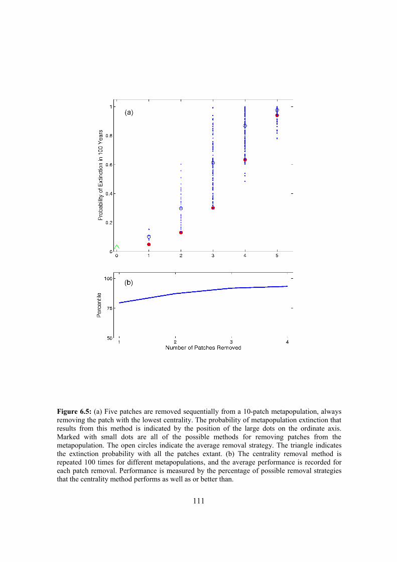
Figure 6.5: (a) Five patches are removed sequentially from a 10-patch metapopulation, always removing the patch with the lowest centrality. The probability of metapopulation extinction that results from this method is indicated by the position of the large dots on the ordinate axis. Marked with small dots are all of the possible methods for removing patches from the metapopulation. The open circles indicate the average removal strategy. The triangle indicates the extinction probability with all the patches extant. (b) The centrality removal method is repeated 100 times for different metapopulations, and the average performance is recorded for each patch removal. Performance is measured by the percentage of possible removal strategies that the centrality method performs as well as or better than.
111
6.5. DiscussionThese results demonstrate that, through a direct analysis of connectivity patterns,
complex network theory can be used to predict aspects of a metapopulation dynamics. A
complex network theory perspective complements existing metapopulation analysis
techniques, as it focuses on statistical properties of the connectivity patterns that have
direct intuitive interpretations. Although it may be difficult to predict dynamical
quantities from static patterns of interaction, these results indicate how an
understandingof metapopulation dynamics can be advanced using this method. The
complex network analyses show that metrics of asymmetry and average path strength
are good surrogates for metapopulation persistence. Together, these two metrics explain
much of the variation in metapopulation persistence when the probability of patch
extinction µ is uniform. The average path strength can be thought of as a measure of
how closely connected the patches are in connectivity space. If the value of S is high,
any patch in the metapopulation can be rapidly recolonised by another patch, either
directly or through a series of intermediate recolonisations.
Increasing asymmetry Z in a connectivity pattern has a negative effect on
metapopulation persistence (Figure 6.4). To help understand this phenomenon, consider
an isolated pair of connected patches. If the sum total of colonisation probabilities is
constant (p12 + p21 = C) then the probability of metapopulation extinction is minimal
when the matrix is perfectly symmetric (p12 = p21 ; see Appendix A). While this analytic
result cannot be easily extended to larger metapopulations, it is feasible that this
mechanism, working between all pairs of patches, helps ensure that large
metapopulations with symmetric connectivity are the most persistent.
The negative effect of asymmetry on persistence is likely to particularly affect
metapopulations in areas with strong landscape gradients. Marine metapopulations, for
example, are especially susceptible, as the unidirectional advective effect of currents in
marine settings can be pronounced (Largier 2003). Migrating individuals are also
frequently in their larval stages, where their ability to counteract these flow-fields is
limited (e.g., coral reef fish; Leis 2002).
Patch removal strategies that discard patches with the lowest centrality ensure that
112
the persistence of the remaining metapopulation is maximised. I have demonstrated that
this result holds for many different asymmetric metapopulations. The removal method
based on centrality is an asymmetric extension of Urban & Keitt's (2001) patch removal
method, which focuses on maintaining core patches. Intuition suggests that patches with
high centrality are more likely to be frequently occupied, and thus cannot be easily
spared from the metapopulation.
The connectivity patterns analysed in this paper are all generated by the small-world
network model of Watts & Strogatz (1998). Small-world network generation can be
summarised in two steps: (1) a regular network is proposed, and (2) edges from this
network are rewired with a set probability q to random positions. The first step reflects
the spatial nature of metapopulations: as a first assumption, each patch is most likely to
be connected to its closest neighbours. Small-world connectivity patterns are thus
rooted in space, distinguishing them from methods that merely assign connections
between patches at random (e.g., Vuilleumier & Possingham 2006). In a real
environment, however, some of these close connections are blocked by obstacles or
difficult terrains. Alternatively, there may be corridors which encourage strong
connectivity between distant patches. Both of these possibilities are simulated in the
second step. The closer q is to one, the greater the influence of the heterogeneous
landscape compared with the physical distances between patches.
To better focus on the effects of connectivity, I have assumed throughout these
analysis that all patches have an equal probability of extinction, an unlikely scenario in
real metapopulations. To adequately incorporate both asymmetric connectivity and
patch variability into a patch removal strategy for example, I could formulate a post-hoc
inclusion of patch area (frequently considered a surrogate for extinction probability),
where the least important patches for connectivity are removed in order of increasing
size (Urban & Keitt 2001). A better method would incorporate both factors into the
same complex network based viability analysis, thus acknowledging their
interdependence. This will be an important direction for future research into complex
networks and metapopulations.
Metapopulation theory has primarily focused its attention at the largest possible
scale, attempting to determine properties such as the persistence proability of the entire
113
metapopulation, or its expected time to extinction (Hanski 1994, Day & Possingham
1995, Ovaskainen 2002, Ovaskainen 2003). Occasionally it deals with the smallest scale
unit – the individual patches – calculating the individual patch incidences (the
probability that a particular patch will not be extinct; Hanski 1994). However, the most
relevant scale, both for ecology and conservation biology, lies somewhere between
these two extremes. Many important metapopulation dynamics involve small numbers
of patches (subgroups) acting in correlated ways, due to interconnections that are
particularly strong or symmetric. Moreover, there may be interdependence between
subgroups, such as the regional scale source-sink structure discovered in the fish
metapopulation on the Great Barrier Reef (Bode et al. 2006). I anticipate that future
directions of research in metapopulation theory will increasingly focus on these issues,
and that complex network theory will play an important role in this development. Much
contemporary research in complex network theory is directed towards determining
interacting subgroups in large networks (Girvan & Newman 2002; Clauset et al. 2004;
Duchs & Arenas 2005; Newman 2006), but few of these developments have yet been
applied to metapopulations.
Analysing metapopulation dynamics by using complex network theory offers a
feasible method for understanding very large metapopulations with asymmetric
connectivity patterns. Nevertheless, deducing system processes from complex network
structure is difficult, and a complete, systematic framework for such analyses does not
yet exist (Newman 2003). This chapter, however, demonstrates the considerable
potential of easily calculated network metrics for determining dynamic properties of
metapopulations.
114
Chapter 7
Can we determine the connectivity value of
reefs using surrogates?
7.1. AbstractMarine reserve networks will form an integral part of conservation planning on
coral reefs. Many organisms in coral reef ecosystems, in particular coral reef fish, rely
on frequent exchanges of individuals between patchy reef habitats. This process is
difficult to measure or predict, yet if reserve networks do not maintain this connectivity,
they will not be able to successfully protect exploited or threatened species. In this
chapter I demonstrate how “connectivity surrogates” can offer a cost-effective method
of incorporating connectivity into the planning of marine reserve networks.
Connectivity surrogates are easily measurable reef qualities; if reserve networks target
reefs that exhibit these qualities, then the connectivity of marine populations can be
maintained within the network. I test a range of surrogates, showing that their
performance is often much better than random expectation, from both an conservation
and a fisheries perspective, and varies with the total size of the reserve network. This
variability offers flexible solutions to incorporating connectivity in a range of reserve
networks, particularly those in developing nations where connectivity information is
likely to remain unavailable.
115
7.2. IntroductionA large proportion of the world's fisheries are currently undergoing dramatic
declines or have already collapsed (Pauly et al. 2002; MEA 2005); this is particularly
true in the world's coral reef ecosystems (McManus 1997; Jackson 2001; Jackson et al.
2001; Hughes et al. 2003; Pandolfi et al. 2003, 2005). Most coral reef fisheries are in
developing nations, and face very high extractive pressure (McManus 1997; Roberts et
al. 2002; Sadovy & Vincent 2002). They are also beset by a number of concurrent
threats: the most visible are coral bleaching events, which are occurring with increasing
frequency due to global warming (Hoegh-Guldberg 2004; IPCC 2007). Increasingly,
scientific consensus agrees that “reserve networks” are integral to achieving future
global marine conservation goals (Fogarty 1999; Russ 2002; Lubchenco et al. 2003;
Fernandes et al. 2005), and should form the basis of most coral reef conservation (Russ
2002). A marine reserve in this context is a “no-take” zone, where extractive activities
are prohibited. Unfortunately, implementing effective reserve networks will require an
understanding of connectivity, the complex and poorly understood exchange of juvenile
individuals between reefs.
7.2.1. Inter-reef connectivityManagement of coral reef fish populations is complicated by a patchy habitat
distribution, and the complex nature of the connectivity between these reefs. Almost all
reef fish species exist in “marine metapopulations” (Roughgarden et al. 1985); adults
are sessile, and do not move between reefs. Each year, however, large numbers of
juveniles are released into the pelagic environment in synchronised spawning events.
During this larval stage, these juveniles disperse on ocean currents before attempting to
settle on a reef and recruit to the local adult population. This connectivity is so
important to population dynamics that reef fish have been described as “pelagic
organisms with a benthic reproductive phase” (Leis 1991). Fully 95% of reef fish
species share this two-stage lifestyle (Leis 1991), and their time as pelagic larval ranges
from days to years, with an average of a month (Leis 2002). During the larval stage,
individuals can travel hundreds of kilometres (Cowen et al. 2006), or remain close to
116
their natal reef (Jones et al.1999; Swearer et al. 1999; Almany et al. 2007). This
connectivity means that fish populations are, to a large extent, demographically open at
the scale of individual reefs. This hypothesis is supported by several pieces of evidence:
(1) local larval production is a poor predictor of recruitment (Mora & Jones 2002); (2)
species can colonise extremely distant localities after unusual meteorological events
(Robertson et al. 1996) and (3) the existence of genetic panmixia over large spatial
scales (Ridgway et al. 2001; Ridgway & Sampayo 2005; Richards et al. 2007).
Maintaining larval connectivity is crucial to the success of reserve networks in coral
reef ecosystems (Roberts et al. 2001; Botsford et al. 2003; Cowen et al. 2006). The most
important conservation implication of connectivity is that reserves on coral reefs cannot
be considered independently. Protecting a reef from direct exploitation cannot guarantee
the persistence of a fish population that depends demographically on larval recruitment
from other reefs. By implication, if reserves are required to persist when non-reserved
areas are heavily degraded, then conservation plans must guarantee that sufficient
connectivity exists between the reefs in the reserve network to maintain the
metapopulation. While the conservation importance of larval connectivity has long been
recognised, the absence of connectivity data has made it impossible to incorporate
connectivity into reserve network planning (Mora & Jones 2002). However, in the last
decade this information gap has begun to close, and connectivity information is now
available from a number of sources:
1. Direct empirical measurements of connectivity, based on either larval mark-
recapture techniques (Jones et al.1999; Jones et al. 2005; Almany et al. 2007), or
the analysis of trace element deposition in otoliths (Swearer et al. 1999).
2. Reconstructions of past connectivity, based on genetic analyses of gene pool
similarity (Cowen et al. 2002) and the parentage of recruiting individuals (Jones
et al. 2005).
117
3. Simulations of larval behaviour, embedded in hydrodynamic models of the
advective current structure (Possingham & Roughgarden 1990; Roberts 1997;
Cowen et al. 2000; James et al. 2002; Cowen et al. 2006; Treml et al. in press):
known as biophysical models. Biophysical connectivity models have been
created for a number of reef systems in the first world, notably the coral reef
systems of the Caribbean Sea (Cowen et al. 2006), the Coral Sea (Treml et al. in
press), and the Great Barrier Reef (the GBR; James et al. 2002).
Larval connectivity over broad spatial and temporal scales will determine the
success of coral reef conservation (Jones 2002), and at present only modelling can
provide this breadth of information. Analyses of gene pool variation can provide
information on evolutionary timescales, but not on demographic timescales, which is of
the most immediate importance to conservation (Cowen 2002; Mora & Jones 2002).
Both genetic and direct empirical techniques are extremely expensive and labour
intensive, even when applied to a single year, at a single reef. Coral reef ecosystems
routinely contain hundreds of reefs (the GBR contains more than 2500 reefs), and their
connectivity is driven by forcings that vary with multi-decadal periods (e.g., ocean
currents and atmospheric conditions; Robertson & Allen 1996). The resources necessary
to apply empirical methods at meaningful temporal and spatial scales are not available
to conservation planners, and the role of empirical analyses will therefore be limited to
providing information for the verification of biophysical models (James et al. 2002).
Nevertheless, we need to be wary of the limitations of biophysical models, which
are based on many assumptions, and are yet to be comprehensively compared with
available empirical information. The limited empirical validation performed to date has
shown both agreement (James et al. 2002) and disagreement (Roberts 1997; although
this was an early model which did not include larval behaviour; Mora & Jones 2002)
between modelled and measured connectivity. In this chapter, I rely on biophysical
models of coral reef fish larval connectivity on the GBR. On the basis of these models, I
make recommendations about reserve network planning for fish species. The
conclusions I draw are therefore dependent on the accuracy of the biophysical models
that produced the connectivity patterns.
118
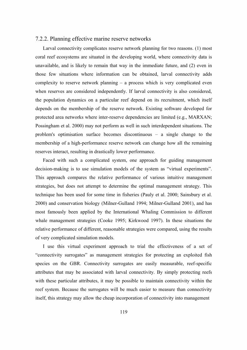
7.2.2. Planning effective marine reserve networksLarval connectivity complicates reserve network planning for two reasons. (1) most
coral reef ecosystems are situated in the developing world, where connectivity data is
unavailable, and is likely to remain that way in the immediate future, and (2) even in
those few situations where information can be obtained, larval connectivity adds
complexity to reserve network planning – a process which is very complicated even
when reserves are considered independently. If larval connectivity is also considered,
the population dynamics on a particular reef depend on its recruitment, which itself
depends on the membership of the reserve network. Existing software developed for
protected area networks where inter-reserve dependencies are limited (e.g., MARXAN;
Possingham et al. 2000) may not perform as well in such interdependent situations. The
problem's optimisation surface becomes discontinuous – a single change to the
membership of a high-performance reserve network can change how all the remaining
reserves interact, resulting in drastically lower performance.
Faced with such a complicated system, one approach for guiding management
decision-making is to use simulation models of the system as “virtual experiments”.
This approach compares the relative performance of various intuitive management
strategies, but does not attempt to determine the optimal management strategy. This
technique has been used for some time in fisheries (Pauly et al. 2000; Sainsbury et al.
2000) and conservation biology (Milner-Gulland 1994; Milner-Gulland 2001), and has
most famously been applied by the International Whaling Commission to different
whale management strategies (Cooke 1995; Kirkwood 1997). In these situations the
relative performance of different, reasonable strategies were compared, using the results
of very complicated simulation models.
I use this virtual experiment approach to trial the effectiveness of a set of
“connectivity surrogates” as management strategies for protecting an exploited fish
species on the GBR. Connectivity surrogates are easily measurable, reef-specific
attributes that may be associated with larval connectivity. By simply protecting reefs
with these particular attributes, it may be possible to maintain connectivity within the
reef system. Because the surrogates will be much easier to measure than connectivity
itself, this strategy may allow the cheap incorporation of connectivity into management
119
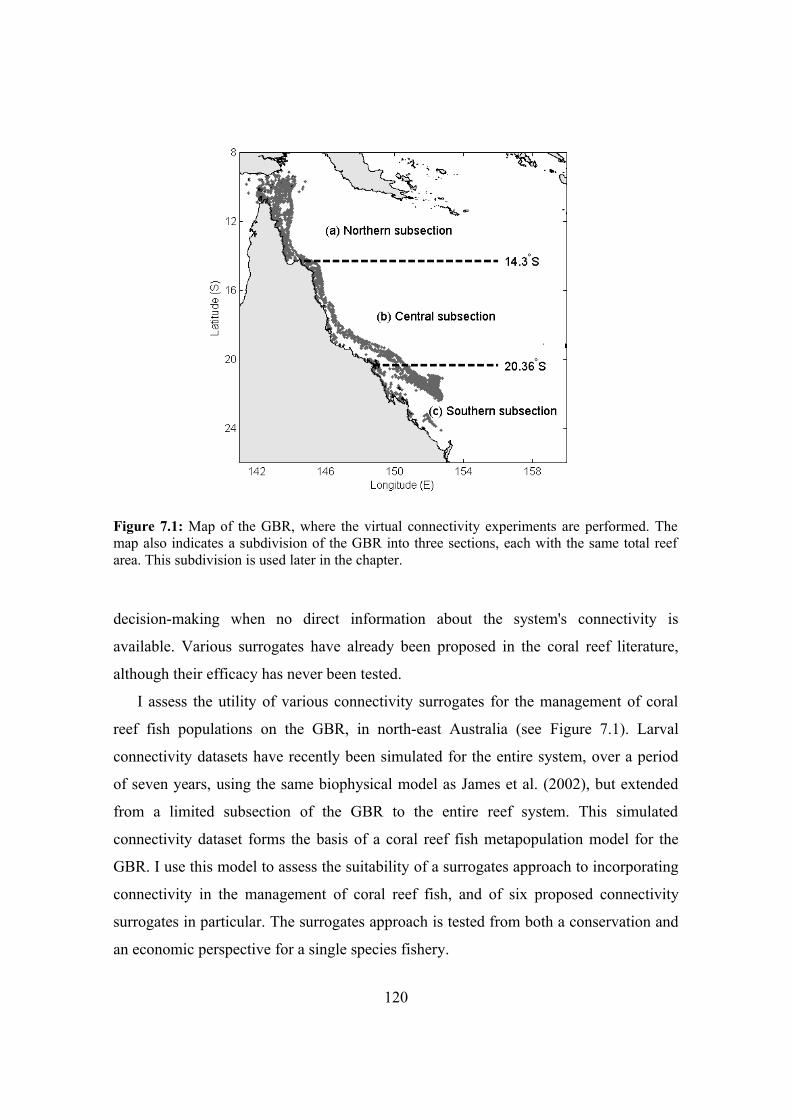
Figure 7.1: Map of the GBR, where the virtual connectivity experiments are performed. The map also indicates a subdivision of the GBR into three sections, each with the same total reef area. This subdivision is used later in the chapter.
decision-making when no direct information about the system's connectivity is
available. Various surrogates have already been proposed in the coral reef literature,
although their efficacy has never been tested.
I assess the utility of various connectivity surrogates for the management of coral
reef fish populations on the GBR, in north-east Australia (see Figure 7.1). Larval
connectivity datasets have recently been simulated for the entire system, over a period
of seven years, using the same biophysical model as James et al. (2002), but extended
from a limited subsection of the GBR to the entire reef system. This simulated
connectivity dataset forms the basis of a coral reef fish metapopulation model for the
GBR. I use this model to assess the suitability of a surrogates approach to incorporating
connectivity in the management of coral reef fish, and of six proposed connectivity
surrogates in particular. The surrogates approach is tested from both a conservation and
an economic perspective for a single species fishery.
120
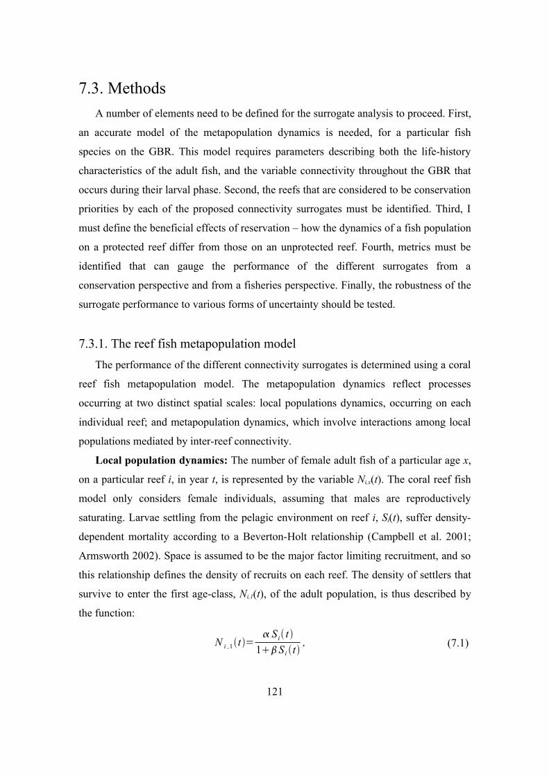
7.3. MethodsA number of elements need to be defined for the surrogate analysis to proceed. First,
an accurate model of the metapopulation dynamics is needed, for a particular fish
species on the GBR. This model requires parameters describing both the life-history
characteristics of the adult fish, and the variable connectivity throughout the GBR that
occurs during their larval phase. Second, the reefs that are considered to be conservation
priorities by each of the proposed connectivity surrogates must be identified. Third, I
must define the beneficial effects of reservation – how the dynamics of a fish population
on a protected reef differ from those on an unprotected reef. Fourth, metrics must be
identified that can gauge the performance of the different surrogates from a
conservation perspective and from a fisheries perspective. Finally, the robustness of the
surrogate performance to various forms of uncertainty should be tested.
7.3.1. The reef fish metapopulation modelThe performance of the different connectivity surrogates is determined using a coral
reef fish metapopulation model. The metapopulation dynamics reflect processes
occurring at two distinct spatial scales: local populations dynamics, occurring on each
individual reef; and metapopulation dynamics, which involve interactions among local
populations mediated by inter-reef connectivity.
Local population dynamics: The number of female adult fish of a particular age x,
on a particular reef i, in year t, is represented by the variable Ni,x(t). The coral reef fish
model only considers female individuals, assuming that males are reproductively
saturating. Larvae settling from the pelagic environment on reef i, Si(t), suffer density-
dependent mortality according to a Beverton-Holt relationship (Campbell et al. 2001;
Armsworth 2002). Space is assumed to be the major factor limiting recruitment, and so
this relationship defines the density of recruits on each reef. The density of settlers that
survive to enter the first age-class, Ni,1(t), of the adult population, is thus described by
the function:
N i ,1t = S i t
1S i t, (7.1)
121
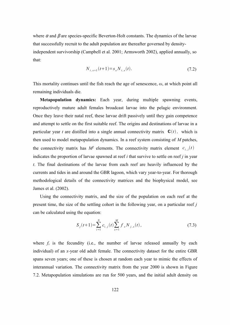
where α and β are species-specific Beverton-Holt constants. The dynamics of the larvae
that successfully recruit to the adult population are thereafter governed by density-
independent survivorship (Campbell et al. 2001; Armsworth 2002), applied annually, so
that:
N i , x1 t1=s x N i , x t . (7.2)
This mortality continues until the fish reach the age of senescence, ω, at which point all
remaining individuals die.
Metapopulation dynamics: Each year, during multiple spawning events,
reproductively mature adult females broadcast larvae into the pelagic environment.
Once they leave their natal reef, these larvae drift passively until they gain competence
and attempt to settle on the first suitable reef. The origins and destinations of larvae in a
particular year t are distilled into a single annual connectivity matrix ℂt , which is
then used to model metapopulation dynamics. In a reef system consisting of M patches,
the connectivity matrix has M2 elements. The connectivity matrix element c i , jt
indicates the proportion of larvae spawned at reef i that survive to settle on reef j in year
t. The final destinations of the larvae from each reef are heavily influenced by the
currents and tides in and around the GBR lagoon, which vary year-to-year. For thorough
methodological details of the connectivity matrices and the biophysical model, see
James et al. (2002).
Using the connectivity matrix, and the size of the population on each reef at the
present time, the size of the settling cohort in the following year, on a particular reef j
can be calculated using the equation:
S j t1=∑i=1
N
ci , j t ∑x=1
M
f x N j , x t , (7.3)
where fx is the fecundity (i.e., the number of larvae released annually by each
individual) of an x-year old adult female. The connectivity dataset for the entire GBR
spans seven years; one of these is chosen at random each year to mimic the effects of
interannual variation. The connectivity matrix from the year 2000 is shown in Figure
7.2. Metapopulation simulations are run for 500 years, and the initial adult density on
122
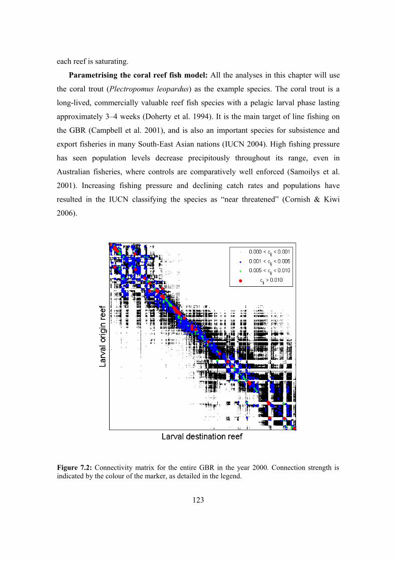
each reef is saturating.
Parametrising the coral reef fish model: All the analyses in this chapter will use
the coral trout (Plectropomus leopardus) as the example species. The coral trout is a
long-lived, commercially valuable reef fish species with a pelagic larval phase lasting
approximately 3–4 weeks (Doherty et al. 1994). It is the main target of line fishing on
the GBR (Campbell et al. 2001), and is also an important species for subsistence and
export fisheries in many South-East Asian nations (IUCN 2004). High fishing pressure
has seen population levels decrease precipitously throughout its range, even in
Australian fisheries, where controls are comparatively well enforced (Samoilys et al.
2001). Increasing fishing pressure and declining catch rates and populations have
resulted in the IUCN classifying the species as “near threatened” (Cornish & Kiwi
2006).
Figure 7.2: Connectivity matrix for the entire GBR in the year 2000. Connection strength is indicated by the colour of the marker, as detailed in the legend.
123
P. leopardus is a comparatively well-studied coral reef fish from a well-studied
group (the groupers, from the family Serranidae), allowing a reasonably well-informed
population model to be constructed. Their maximum recorded age is ω = 14, with
individuals reaching sexual maturity at around a = 3 years of age (Ferreira & Russ
1994). Density-independent post-settlement survivorship is low for juveniles (s1 = 0.6,
s2 = 0.7), but later stabilises at a high value for the remaining years (si = 0.83, 3 ≤ i ≤ 13;
Mapstone et al. 1996).
The fecundity of the mature female groupers can be estimated from their length, l,
which in turn is a function of their age (Ferreira & Russ 1994). From these sources, the
fecundity of a female in the i th age-class is:
l i=52.2 1−exp −0.354 i0.766 ,
f i=0.0129 li3.03.
(7.4)
The mass of the individuals (which will be used below) can be approximated by a
function of their length (Heemstra & Randall 1993):
M i=0.0079 l i3.157 . (7.5)
The two parameters of the Beverton-Holt post-settlement mortality model are not well
known. I therefore arbitrarily set the value of α at 0.5, and set the value of β such that
the population on the fringing reef at Lizard Island (14°40′08″S, 145°27′34″E) is
approximately 17,500 (matching the 1995 census of Zeller & Russ 2000).
7.3.2. Connectivity surrogatesReserve networks will be constructed according to six different connectivity
surrogates. The number of reefs included in the reserve networks will be constrained by
the proportion of total reef area allowed for the reserve network. Reefs are sequentially
added to the set of reserves, as long as the inclusion of another reef into the reserve
network will not violate this constraint.
124
1. Largest reefs
James et al. (2002) showed that the removal of the reefs with the greatest area
had a detrimental effect on metapopulation persistence. It is thought that large
reefs may have exceptionally high self-recruitment (important for ensuring
metapopulation persistence), through hydrodynamic retention at the lee of the
reefs (Black et al. 1990; Black et al. 1993). Area-controlled reserve networks
consisting of the largest reefs will have comparatively few reserves, but
nonlinear benefits associated with area may compensate for their small numbers.
In a review of 81 empirical studies of MPA effectiveness, however, Halpern
(2003) found that the benefits of marine reserves increased linearly with their
size.
Reefs are added to the reserve network in order of decreasing size until the
total area constraint is reached.
2. Smallest reefs
For a given area, reserve networks based on the smallest reefs will create the
largest number of reserves. This will result in reserves that are, on average,
closer to other reserves, and therefore more likely to exchange substantial
amounts of larvae. On the other hand, smaller reefs may have more difficulty
attracting settlers, especially through self-recruitment. These factors may result
in low populations and less persistent metapopulations, and this may act against
the persistence of small-reef reserve networks.
Reefs are added to the reserve network in order of increasing size until the
total area constraint is reached. These two size based surrogates (largest and
smallest reefs) are examples of the SLOSS (single large, or several small)
reserve planning paradigms (Burkey 1989).
3. Clustered reefs
Although hydrodynamic currents can carry larvae long distances in particular
directions, in general the strength of these connections declines isotropically as
the distance from the natal reef increases (James et al. 2002; Cowen et al. 2006).
As a first approximation then, connectivity will depend on distance. Choosing a
reserve network where all the reserves are close together may ensure strong
125
inter-reserve connectivity, and thus the persistence of the metapopulation.
A seed reef is chosen at random from the metapopulation. Reefs are then
added to this reserve network in order of decreasing distance from the seed
reef. The method is performed using each of the reefs in the metapopulation
as a seed reef. The clustered reserve network that spans the smallest area is
then used as the clustered surrogate.
4. Reefs with high biodiversity
Current coral reef reserve network planning is based on biodiversity
representation, and does not consider connectivity (Fernandes et al. 2005).
However, it has been hypothesised that connectivity may be coincidentally
protected by reserve networks that focus on reefs with high extant biodiversity
(Leslie et al. 2003). The recent GBR rezoning was based on biodiversity
representation, and protected “green zoned” reefs from extractive activities.
These reefs are used to represent the high biodiversity surrogate.
5. Reefs with the highest spawning biomass density
Given that only a proportion of the total reefs can be protected, those that have
the highest spawning biomass density are an obvious choice. These reefs might
act as sources (Pulliam 1988), maintaining viable populations in the reserves, as
well as exporting substantial amounts of larvae to the fished sections of the GBR
(Tuck & Possingham 2000). Of course, this surrogate assumes that the observed
density will remain once the non-protected reefs in the system are impacted –
that “representation equals persistence”, which may not be accurate (Cowling et
al. 1999), as the high population density on these reefs might be a result of larval
transport from reefs outside the reserve network.
The metapopulation model is run until it reaches equilibrium, with all reefs
included in the reserve network. The mean density of the spawning biomass
on each reef is then measured (averaged over a period of 25 years). Starting
with no reefs protected, the unprotected reef in the metapopulation with the
highest mean equilibrium spawning biomass density is added sequentially
to the reserve network.
6. Reefs with the highest spawning biomass
126
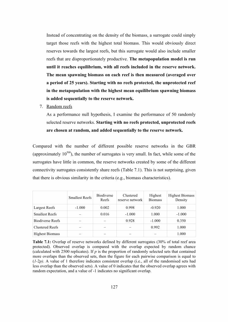
Instead of concentrating on the density of the biomass, a surrogate could simply
target those reefs with the highest total biomass. This would obviously direct
reserves towards the largest reefs, but this surrogate would also include smaller
reefs that are disproportionately productive. The metapopulation model is run
until it reaches equilibrium, with all reefs included in the reserve network.
The mean spawning biomass on each reef is then measured (averaged over
a period of 25 years). Starting with no reefs protected, the unprotected reef
in the metapopulation with the highest mean equilibrium spawning biomass
is added sequentially to the reserve network.
7. Random reefs
As a performance null hypothesis, I examine the performance of 50 randomly
selected reserve networks. Starting with no reefs protected, unprotected reefs
are chosen at random, and added sequentially to the reserve network.
Compared with the number of different possible reserve networks in the GBR
(approximately 10500), the number of surrogates is very small. In fact, while some of the
surrogates have little in common, the reserve networks created by some of the different
connectivity surrogates consistently share reefs (Table 7.1). This is not surprising, given
that there is obvious similarity in the criteria (e.g., biomass characteristics).
Smallest Reefs Biodiverse Reefs
Clustered reserve network
Highest Biomass
Highest Biomass Density
Largest Reefs -1.000 0.002 0.998 -0.920 1.000
Smallest Reefs – 0.016 -1.000 1.000 -1.000
Biodiverse Reefs – – 0.928 -1.000 0.350
Clustered Reefs – – – 0.992 1.000
Highest Biomass – – – – 1.000
Table 7.1: Overlap of reserve networks defined by different surrogates (30% of total reef area protected). Observed overlap is compared with the overlap expected by random chance (calculated with 2500 replicates). If p is the proportion of randomly selected sets that contained more overlaps than the observed sets, then the figure for each pairwise comparison is equal to (1-2p). A value of 1 therefore indicates consistent overlap (i.e., all of the randomised sets had less overlap than the observed sets). A value of 0 indicates that the observed overlap agrees with random expectation, and a value of -1 indicates no significant overlap.
127
7.3.3. Effects of protected areasThe effect that reserves will have on coral reef fish populations remains hotly
debated. Reductions in fishing effort have been shown to clearly benefit species targeted
by fisheries (see reviews by Halpern 2003; Halpern & Warner 2003). Trophic cascades
may result from reservation, making outcomes difficult to predict. In some situations,
these cascades may result in lower populations of non-target fish species (Steneck 1998;
Sala et al. 2002), or may facilitate ecosystem recovery (Mumby et al. 2006; Mumby et
al. 2007). Coral trout are pursued vigorously by both commercial and recreational
fisheries, and so the sanctuary offered by reserves will almost certainly result in
increased population densities. Surveys on the GBR observed coral trout populations in
protected areas that were several-fold greater than populations on unprotected reefs,
although this increase varied regionally (Mapstone et al. 1996).
Populations in areas that are not protected from extractive activities such as fishing
will experience higher mortality than equivalent protected regions. Each year, fish
populations on unprotected reefs experience additional mortality, with a proportion m
removed from the system, subsequent to the natural density-independent mortality. On
the GBR, a size restriction protects all individuals smaller than 38cm (under 3 years),
even on unreserved reefs. Fishing mortality therefore only applies to individuals older
than two (I am therefore ignoring the elevated mortality associated with catch-and-
release of undersized individuals). Campbell et al. (2001) estimate the fishing mortality
on unprotected reefs in the GBR at 17%.
7.3.4. Performance of the reserve networks The relative performance of the various connectivity surrogates is measured
according to two criteria. The first is the conservation benefit provided to the coral trout
population by the reserve network. This is measured by a census of the entire GBR
metapopulation, therefore assuming that more coral trout are preferred by
conservationists. The second performance criteria is the outcome for fisheries. This is
measured by the average annual catch outside the reserve network (tonnage). The inter-
annual variation that results from the fluctuating connectivity means that the values of
128
these two criteria are not constant. I therefore use 50-year averages, after discarding
initial transient dynamics (the first 450 years of each simulation).
7.3.5. Testing the robustness of the connectivity surrogatesIf particular surrogates are shown to be effective at representing connectivity, it is
important to understand whether the preferred surrogate is an artifact of assumptions
made in the modelling, and also whether the surrogate is similarly effective in systems
other than the GBR. I will therefore use a series of robustness analyses to examine the
effect of the most important or uncertain modelling assumptions.
First, the performance of the connectivity surrogates will be determined for different
reserve network sizes. Reserve networks often constitute a set proportion of the total
reef area. For example, “green” zones on the GBR, which protect regions from all non-
scientific exploitative activities, originally made up approximately 5% of the total
marine park area, but were recently increase to 33% (Fernandes et al. 2005). The total
proportion of reef area in the reserve network is therefore varied between 0 and 1 in
intervals of 0.05. Second, the value α in the Beverton-Holt relationship is varied by
±50%. This parameter was the only completely unsubstantiated coral trout life-history
parameter in the model. Third, it is important to assess whether the protective effects of
reserves affect the best surrogate choice. The amount of mortality (m) experienced by
unprotected populations is a parameter that can be chosen with a reasonable degree of
accuracy by fisheries managers. Performing robustness analyses on this parameter will
provide insight into whether the magnitude of the difference in conditions inside and
outside the reserves alters the relative performance of different reserve networks. I
therefore vary the value of m between ±50% of its base value. Finally, it would be
particularly useful to ascertain whether the relative rankings of the connectivity
surrogates are specific to the reef system being studied. If the connectivity surrogates
identified in these analyses are to be useful to marine reserve network planning in other
coral reef systems, then their performance rankings, and their performance relative to
randomly selected reserve networks, cannot be specific to the GBR. My ability to assess
how the ranking of the surrogates might change in different circumstances is limited, as
I do not have access to connectivity information for coral reef systems other than the
129
GBR. Fortunately, the GBR is the largest coral reef systems in the world, with quite
varied regional morphology (Figure 7.3). The consistency of surrogate rankings in
morphologically diverse subregions of the GBR, will allow me to discuss the potential
applicability of these results to coral reef ecosystems in different parts of the world. To
test the consistency of the surrogate rankings in different reef morphologies, the GBR is
divided latitudinally into three parts (Figure 7.1), and the performances of the six
connectivity surrogates are calculated in each subsection. The three subsections each
contain one-third of the total GBR reef area.
7.4. ResultsIn the results that follow, I compare the conservation and economic outcomes of the
different surrogates to the performance of random reserve networks. The conservation
and economic outcomes achieved by these random networks are called “random
expectation”. The total area of reefs in the reserve network area is called the “total
reserve size”.
7.4.1. Performance of the different surrogates on the GBRThe conservation and economic performance of each of the surrogates were
calculated, with unprotected reefs being subject to a direct fishing mortality of 17%
(Figure 7.4). As the highest biodiversity surrogate is only defined for the current GBR
zonation, only a single black point is shown. This reserve network spans 27% of the
total reef area, equal to the total amount of the GBR currently in green zonations. This is
slightly different from the 33% reported by the Great Barrier Reef Marine Park
Authority, who considered all GBR habitat types, and not just reefs.
130
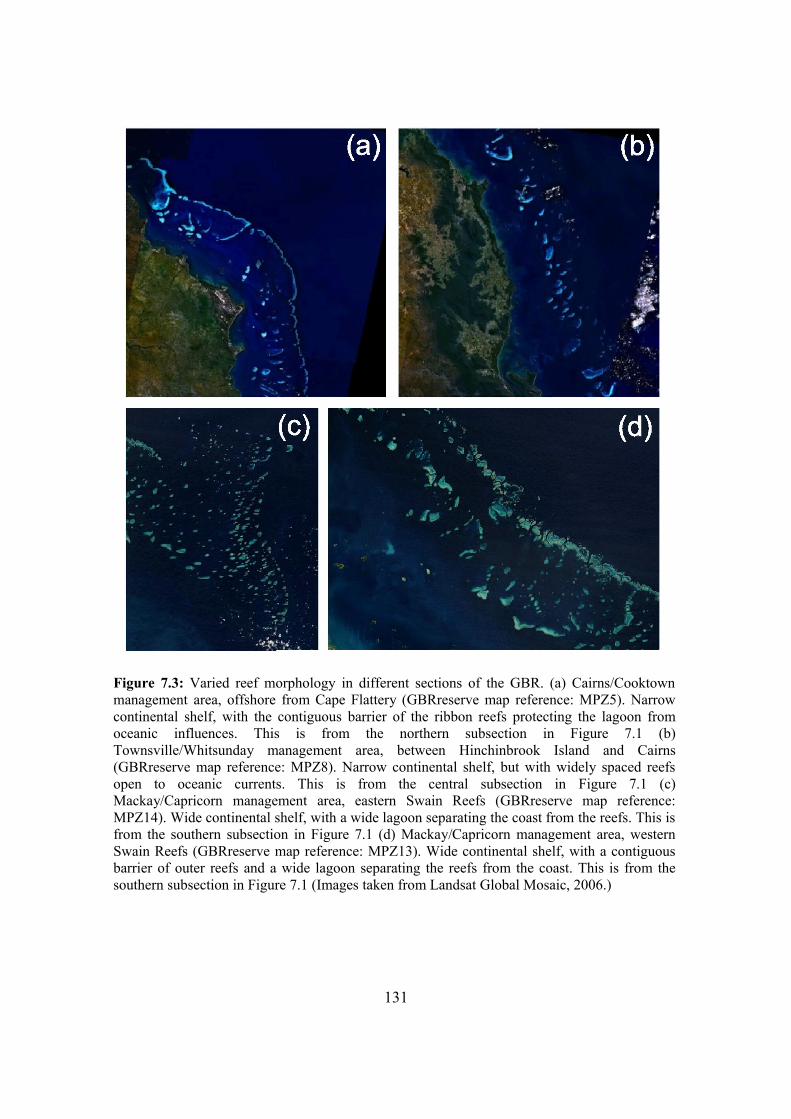
Figure 7.3: Varied reef morphology in different sections of the GBR. (a) Cairns/Cooktown management area, offshore from Cape Flattery (GBRreserve map reference: MPZ5). Narrow continental shelf, with the contiguous barrier of the ribbon reefs protecting the lagoon from oceanic influences. This is from the northern subsection in Figure 7.1 (b) Townsville/Whitsunday management area, between Hinchinbrook Island and Cairns (GBRreserve map reference: MPZ8). Narrow continental shelf, but with widely spaced reefs open to oceanic currents. This is from the central subsection in Figure 7.1 (c) Mackay/Capricorn management area, eastern Swain Reefs (GBRreserve map reference: MPZ14). Wide continental shelf, with a wide lagoon separating the coast from the reefs. This is from the southern subsection in Figure 7.1 (d) Mackay/Capricorn management area, western Swain Reefs (GBRreserve map reference: MPZ13). Wide continental shelf, with a contiguous barrier of outer reefs and a wide lagoon separating the reefs from the coast. This is from the southern subsection in Figure 7.1 (Images taken from Landsat Global Mosaic, 2006.)
131
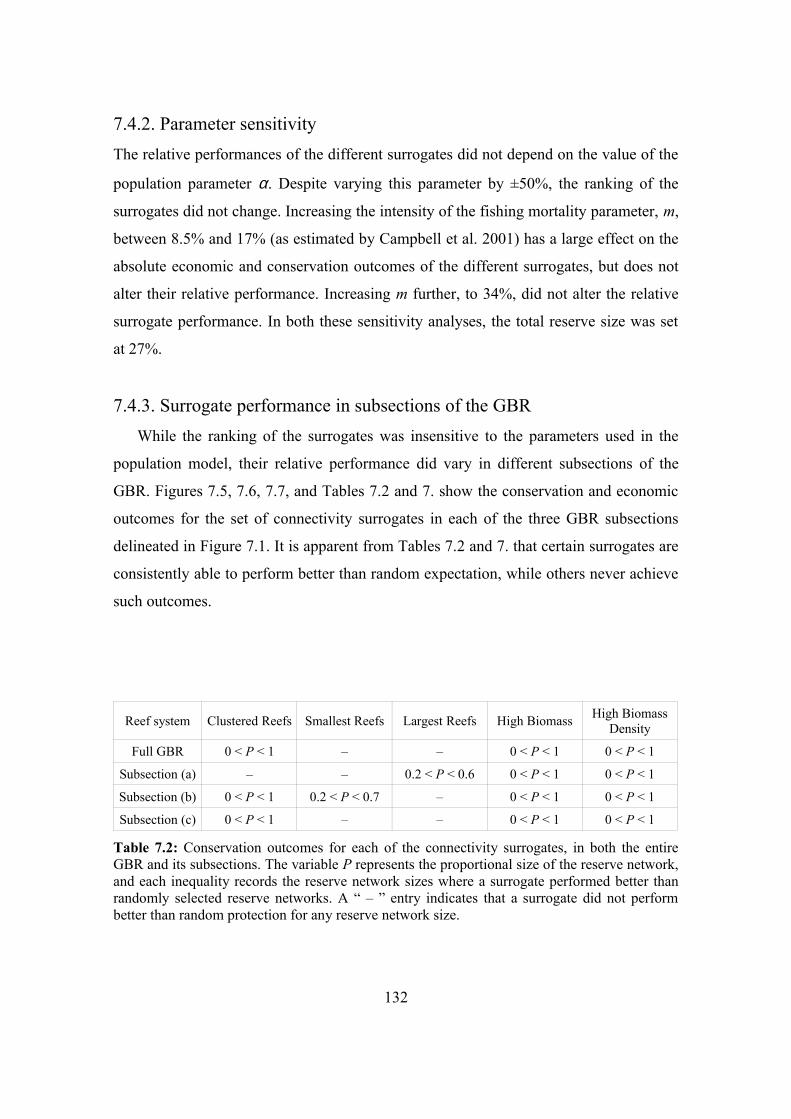
7.4.2. Parameter sensitivityThe relative performances of the different surrogates did not depend on the value of the
population parameter α. Despite varying this parameter by ±50%, the ranking of the
surrogates did not change. Increasing the intensity of the fishing mortality parameter, m,
between 8.5% and 17% (as estimated by Campbell et al. 2001) has a large effect on the
absolute economic and conservation outcomes of the different surrogates, but does not
alter their relative performance. Increasing m further, to 34%, did not alter the relative
surrogate performance. In both these sensitivity analyses, the total reserve size was set
at 27%.
7.4.3. Surrogate performance in subsections of the GBRWhile the ranking of the surrogates was insensitive to the parameters used in the
population model, their relative performance did vary in different subsections of the
GBR. Figures 7.5, 7.6, 7.7, and Tables 7.2 and 7. show the conservation and economic
outcomes for the set of connectivity surrogates in each of the three GBR subsections
delineated in Figure 7.1. It is apparent from Tables 7.2 and 7. that certain surrogates are
consistently able to perform better than random expectation, while others never achieve
such outcomes.
Reef system Clustered Reefs Smallest Reefs Largest Reefs High Biomass High Biomass Density
Full GBR 0 < P < 1 – – 0 < P < 1 0 < P < 1
Subsection (a) – – 0.2 < P < 0.6 0 < P < 1 0 < P < 1
Subsection (b) 0 < P < 1 0.2 < P < 0.7 – 0 < P < 1 0 < P < 1
Subsection (c) 0 < P < 1 – – 0 < P < 1 0 < P < 1
Table 7.2: Conservation outcomes for each of the connectivity surrogates, in both the entire GBR and its subsections. The variable P represents the proportional size of the reserve network, and each inequality records the reserve network sizes where a surrogate performed better than randomly selected reserve networks. A “ – ” entry indicates that a surrogate did not perform better than random protection for any reserve network size.
132
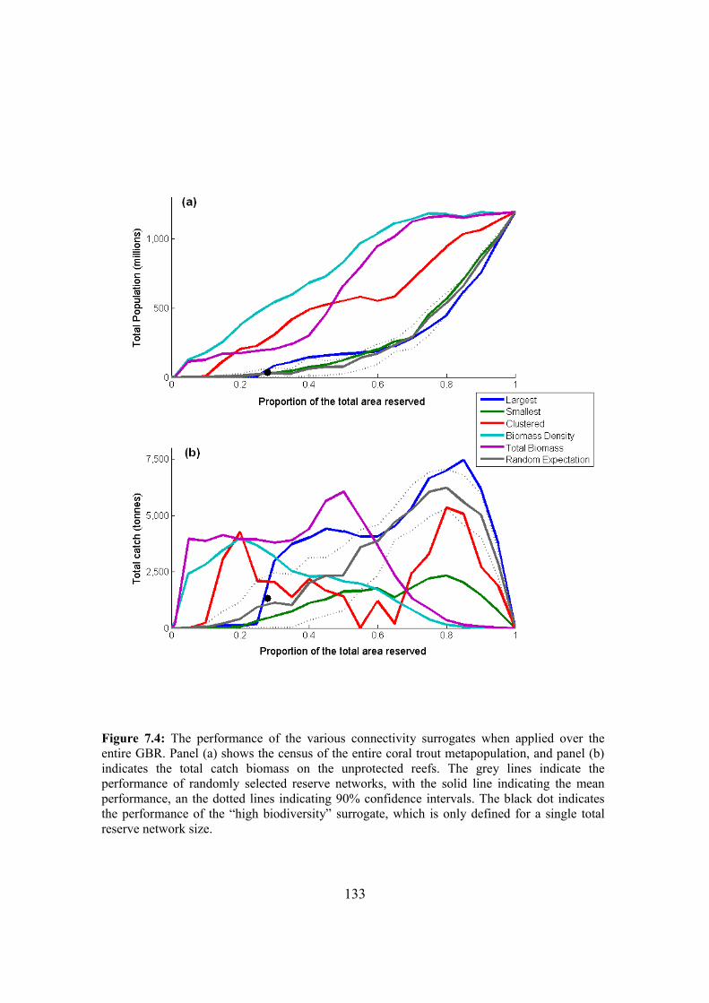
Figure 7.4: The performance of the various connectivity surrogates when applied over the entire GBR. Panel (a) shows the census of the entire coral trout metapopulation, and panel (b) indicates the total catch biomass on the unprotected reefs. The grey lines indicate the performance of randomly selected reserve networks, with the solid line indicating the mean performance, an the dotted lines indicating 90% confidence intervals. The black dot indicates the performance of the “high biodiversity” surrogate, which is only defined for a single total reserve network size.
133
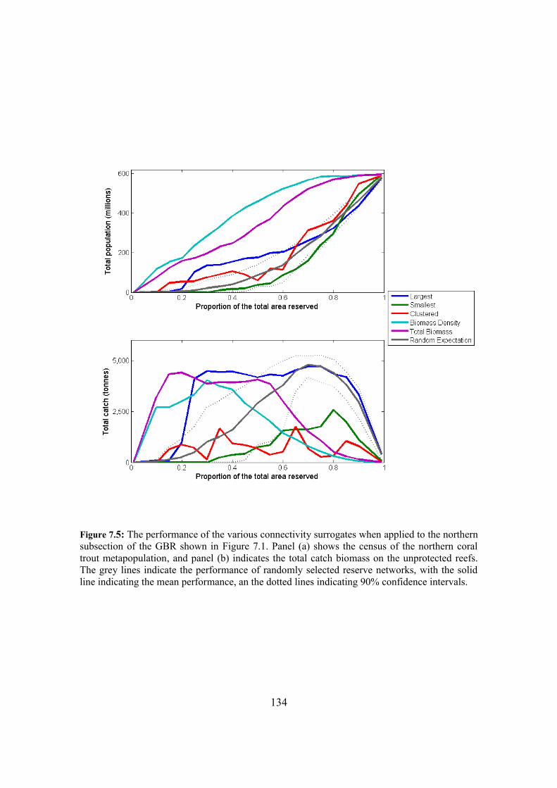
Figure 7.5: The performance of the various connectivity surrogates when applied to the northern subsection of the GBR shown in Figure 7.1. Panel (a) shows the census of the northern coral trout metapopulation, and panel (b) indicates the total catch biomass on the unprotected reefs. The grey lines indicate the performance of randomly selected reserve networks, with the solid line indicating the mean performance, an the dotted lines indicating 90% confidence intervals.
134
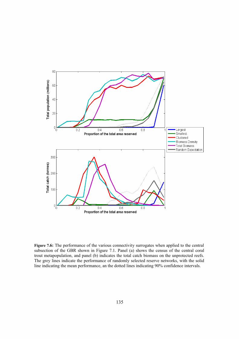
Figure 7.6: The performance of the various connectivity surrogates when applied to the central subsection of the GBR shown in Figure 7.1. Panel (a) shows the census of the central coral trout metapopulation, and panel (b) indicates the total catch biomass on the unprotected reefs. The grey lines indicate the performance of randomly selected reserve networks, with the solid line indicating the mean performance, an the dotted lines indicating 90% confidence intervals.
135
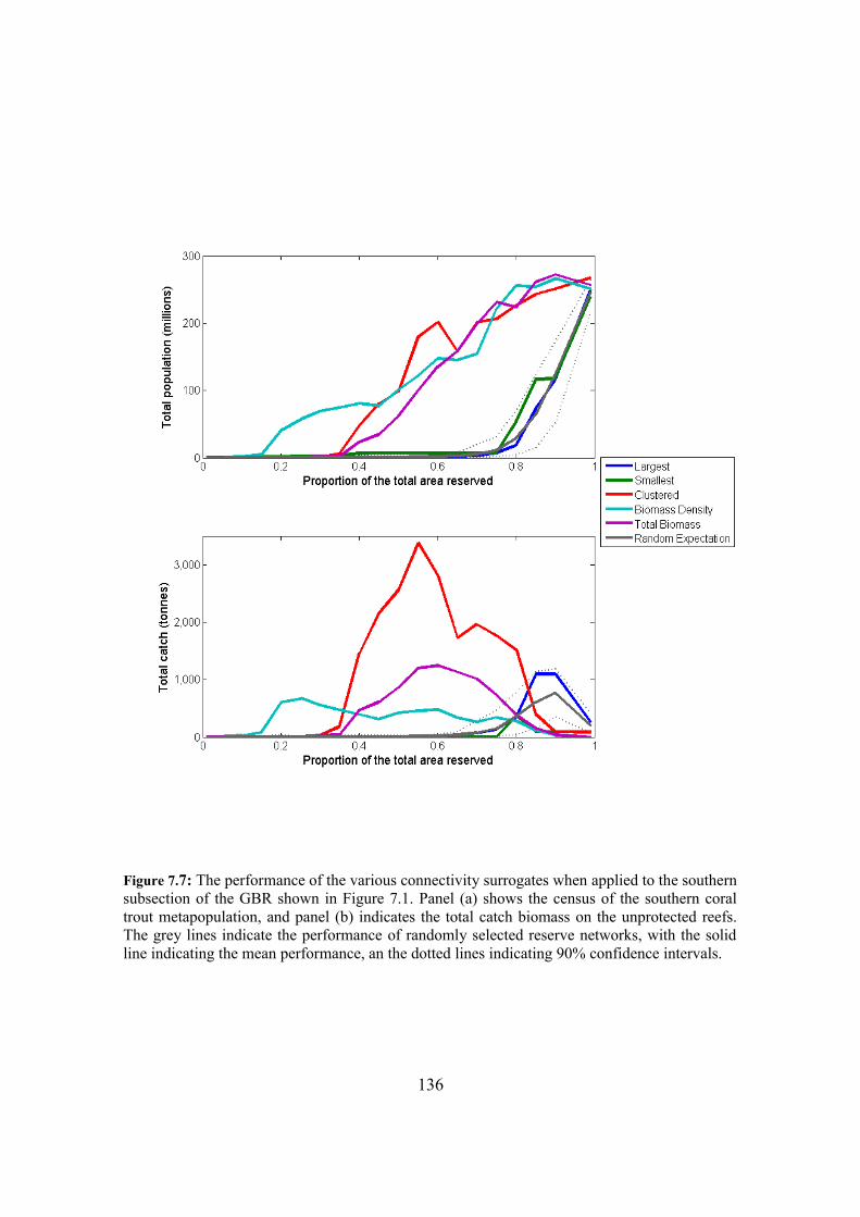
Figure 7.7: The performance of the various connectivity surrogates when applied to the southern subsection of the GBR shown in Figure 7.1. Panel (a) shows the census of the southern coral trout metapopulation, and panel (b) indicates the total catch biomass on the unprotected reefs. The grey lines indicate the performance of randomly selected reserve networks, with the solid line indicating the mean performance, an the dotted lines indicating 90% confidence intervals.
136
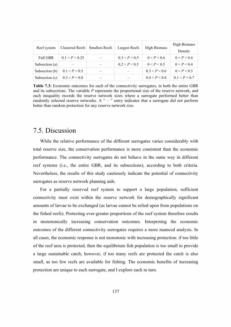
Reef system Clustered Reefs Smallest Reefs Largest Reefs High BiomassHigh Biomass
Density
Full GBR 0.1 < P < 0.25 – 0.3 < P < 0.5 0 < P < 0.6 0 < P < 0.4
Subsection (a) – – 0.2 < P < 0.5 0 < P < 0.5 0 < P < 0.4
Subsection (b) 0.1 < P < 0.5 – – 0.3 < P < 0.6 0 < P < 0.5
Subsection (c) 0.3 < P < 0.8 – – 0.4 < P < 0.8 0.1 < P < 0.7
Table 7.3: Economic outcomes for each of the connectivity surrogates, in both the entire GBR and its subsections. The variable P represents the proportional size of the reserve network, and each inequality records the reserve network sizes where a surrogate performed better than randomly selected reserve networks. A “ – ” entry indicates that a surrogate did not perform better than random protection for any reserve network size.
7.5. DiscussionWhile the relative performance of the different surrogates varies considerably with
total reserve size, the conservation performance is more consistent than the economic
performance. The connectivity surrogates do not behave in the same way in different
reef systems (i.e., the entire GBR, and its subsections), according to both criteria.
Nevertheless, the results of this study cautiously indicate the potential of connectivity
surrogates as reserve network planning aids.
For a partially reserved reef system to support a large population, sufficient
connectivity must exist within the reserve network for demographically significant
amounts of larvae to be exchanged (as larvae cannot be relied upon from populations on
the fished reefs). Protecting ever-greater proportions of the reef system therefore results
in monotonically increasing conservation outcomes. Interpreting the economic
outcomes of the different connectivity surrogates requires a more nuanced analysis. In
all cases, the economic response is not monotonic with increasing protection: if too little
of the reef area is protected, then the equilibrium fish population is too small to provide
a large sustainable catch; however, if too many reefs are protected the catch is also
small, as too few reefs are available for fishing. The economic benefits of increasing
protection are unique to each surrogate, and I explore each in turn.
137
7.5.1. Performance of the surrogatesTargeting reefs with the highest biomass density results in the best conservation
performance. This statement is true for all the reef systems, and for almost all possible
total reserve sizes. The situations where other surrogates yield greater conservation
outcomes constitute only a small proportion of the total range of scenarios and
parameters considered, and the improvement in these rare situations is only marginal.
The performance of this connectivity surrogate is particularly strong when the total
reserve size is quite small. Reserve networks made up of high biomass density reefs are
able to support considerable populations in conditions where the alternatives offer so
little protection that the metapopulation declines to zero. In the southern subsection of
the GBR, for example (Figure 7.7), the biomass density surrogate can support
populations at 25% of the maximum obtainable levels, when the reserve network covers
20% of the total area. At this level of protection, reserve networks constructed using the
other surrogates cannot support any population at all. The relative performance of the
biomass density surrogate is not as impressive when more of the total area is protected.
This is less important, however, because most of the connectivity surrogates, and even
random expectation, yield good conservation outcomes at high levels of protection.
Relatively speaking, the economic returns of the highest biomass density surrogate are
best when the reserve network is less than 40% of the total reef area. If more of the reef
system is protected beyond this point, the economic returns decline rapidly, generally
performing worse than random expectation.
Protecting reefs with the highest biomass also results in consistently good
conservation outcomes, although it is never able to perform as well as the highest
biomass density surrogate. The highest biomass surrogate's conservation performance is
also poor when the total reserve size is small (less than 30% protected). By protecting
larger reefs (as the amount of habitat can support large populations), relatively few reefs
can be protected when the total reserve size is small. Inter-reserve connectivity
consequently suffers as the average distance between reefs increases. The economic
returns from protecting the highest biomass reefs are relatively high when the reserve
networks are of small to intermediate size (less than 60%).
The conservation performance of the clustered surrogate is difficult to synthesise
138
from the observed results. For most of the reef systems examined, protecting reefs
according to this surrogate results in populations that are in the order of, and
occasionally better than, the two biomass surrogates already mentioned. However, in the
northern subsection of the GBR, the clustered surrogate has a conservation performance
that is not significantly better than random expectation (Figure 7.5). The poor
conservation outcomes that result from protecting clustered reefs when the total reserve
size is small is unexpected. If only a small number of reefs can be included in a reserve
network, grouping them close together would appear to provide an intuitively attractive
method for conserving connectivity when the entire region is as large as the GBR.
However, as the results attest, this approach is ineffective. The economic performance
of the clustered surrogate is as variable as its conservation performance. In the central
and southern subsections of the GBR, the surrogate significantly outperforms random
expectation, often gives the best yields for a particular reserve size, and is the surrogate
with the highest overall yields. On the other hand, in the entire GBR, and in its northern
subsection, protecting the most clustered reefs results in fisheries yields that are much
lower than random expectation. Furthermore, unlike the other surrogates, the
relationship between catch and total reserve area is unusual. All of the other surrogates
exhibit a single-humped response to protection levels, with the highest yields resulting
from intermediate levels of protection. The clustered surrogate, on the other hand
exhibits two local maxima, in the entire GBR and its northern subsection, and a single
maximum in the central and southern subsections.
The performance (both conservation and economic) of the surrogates that target the
reefs based on their size was seldom better than random expectation. It would therefore
appear that the size of a reef is not a reliable indicator of its conservation value when the
total reserve network size is constrained, and is probably not a particularly good
indicator of its economic value either. It would seem that for coral reef fish on the GBR,
the SLOSS question does not have an answer, as both alternatives result in poor
outcomes. One point about these size-based surrogates is worth noting: while they
provide equally poor outcomes in most situations, when most of the total area is
protected (> 80%), protecting the largest reefs generates much better catches than does
protecting the smallest. In fact, protecting the largest reefs (and thus allowing fishing on
139
the smallest reefs) consistently outperforms all the other surrogates when most of the
total reef area is protected. This result implies that it is better to have many small fishing
opportunities spread throughout the region, rather than a few large fishing opportunities,
as the former situation provides more opportunities for larval spillover from unfished
reefs to fished reefs. Unfortunately, the relevance of this result is probably slight, as
very few coral reef ecosystems will have reserve networks that protect such a large
proportion of the total reef area. Current objectives for marine conservation aim to
protect 30% of marine habitats in reserve networks (WCPA 2007).
Protecting reefs with the highest biodiversity, the methodology that guides most
current reserve network planning, results in poor outcomes for both conservation and
fisheries. It was not possible to determine the behaviour of the high-biodiversity
surrogate for connectivity in a range of situations, as the zonation was only available for
the current level of GBR protection (approximately 27% of reef area). However, the
observed performance was not encouraging, yielding populations and catches that were
statistically indistinguishable from random expectation (Figure 7.4).
Randomly selected reserve networks performed well economically, but generally
could not sustain very high populations. Randomly protecting less than about 50% of
the total reef area results in such small populations that the available catches are
negligible. Surprisingly, however, when the total reserve size is very large (greater than
about 75%), the economic returns from random reserve networks were higher than those
from reserve networks created by many of the targeted connectivity surrogates, while
conservation outcomes were also relatively good.
7.5.2. Implications for marine reserve network planningFrom the perspective of marine conservation planning, it is reassuring to see that
conservation and economic demands are not necessarily opposing. Effective marine
reserve network planning requires that both are satisfied to some extent, but it is
difficult to translate the two separate results into a single set of planning
recommendations while the conservation and economic outcomes are not expressed in
the same “currency”. The partial concordance encourages hope that the majority of
conservation and economic demands can be satisfied simultaneously – the conservation
140
outcome predictably increases with larger reserve networks, and the best catches are
also often associated with high levels of protection.
One striking difference between the economic and conservation outcomes is that,
while it is possible to obtain good economic outcomes for most reserve network sizes,
good conservation outcomes (populations at least half as large as pristine levels) are
only possible with larger reserves (more than a third protected). This is particularly true
if reefs are protected at random, when conservation and economic outcomes are quite
poor (catches less than half of optimal, and populations less than 25% of pristine) unless
much of the system is reserved. Notably, the high-biodiversity reserve planning method
did not significantly outperform random expectation. Based on the conservation and
economic results of random reserve networks, marine reserve planning using high
biodiversity networks might therefore demand very high levels of protection (70-90%),
much higher than is currently afforded coral reef conservation planning.
An approach that integrates both the conservation and the economic outcomes
requires the two performance measures to be attributed a relative importance (“a
weighting”). The particular weighting will of course depend on the conservation
situation, but it is possible to examine the optimal management response for all possible
weightings by formulating a general reward function:
R=∑i=1
MH i1−∑
i=1
MN i , (7.6)
where κ defines the relative weightings attributed to the equilibrium population on each
reef, N i and the equilibrium catch from each reef, H i (where the yield from reefs
in the reserve network is zero). A κ−value that is close to one places particular
importance on the economic performance of the system, while a κ value close to zero
emphasises conservation returns. The best connectivity surrogate for any value of κ, for
every possible reserve network size, is shown in Figure 7.8 (for the entire GBR). For
typical reserve networks (< 50%), the best connectivity surrogate concentrates on
protecting reefs with the highest biomass, or occasionally the highest biomass density.
141
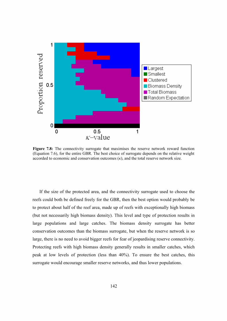
Figure 7.8: The connectivity surrogate that maximises the reserve network reward function (Equation 7.6), for the entire GBR. The best choice of surrogate depends on the relative weight accorded to economic and conservation outcomes (κ), and the total reserve network size.
If the size of the protected area, and the connectivity surrogate used to choose the
reefs could both be defined freely for the GBR, then the best option would probably be
to protect about half of the reef area, made up of reefs with exceptionally high biomass
(but not necessarily high biomass density). This level and type of protection results in
large populations and large catches. The biomass density surrogate has better
conservation outcomes than the biomass surrogate, but when the reserve network is so
large, there is no need to avoid bigger reefs for fear of jeopardising reserve connectivity.
Protecting reefs with high biomass density generally results in smaller catches, which
peak at low levels of protection (less than 40%). To ensure the best catches, this
surrogate would encourage smaller reserve networks, and thus lower populations.
142
7.5.3. Limitations While these results indicate that surrogate methods could potentially be used to
include connectivity in marine reserve network planning, there are several complicating
factors that must be stressed. First, the simulations performed in this chapter focus on a
single species, in this case the coral trout. However, most coral reef ecosystems are the
focus of multiple extractive industries and subsistence industries. Although the coral
trout is the main target of line fishing on the GBR, there are sizeable industries
harvesting several species of crab, sea cucumber, lobster, prawn, among others. The
needs of these industries should also influence the zonation of the GBR, and will have
adverse effects on the coral trout population and habitat. These surrogates are not
intended to prescribe management in systems with multiple harvested species, and may
instead facilitate the inclusion of connectivity into management plans.
Second, the inclusion of social and economic factors into these virtual experiments
is very limited. Importantly, fisheries are interested in the efficiency of harvesting (and
thus its profitability) as well as the total sustainable harvest. The economic performance
of the connectivity surrogates in this chapter does not consider this, and its inclusion
may alter the relative performance of the different surrogates. For example, the distance
of unprotected reefs from population centres is likely to affect travel costs, and thus the
profitability. The spatial distribution of the protected reefs within the GBR under the
various surrogates is quite important to fisheries, and is something that should be further
investigated.
Finally, although these surrogates are far easier to measure than the actual
connectivity in the system, it would cost varying amounts of money to determine their
values on each reef. Surrogates that rely on the reef size will be very simple to calculate,
while the biomass and biodiversity surrogates will be comparatively expensive. Given
that the management of the coral reef ecosystem is being expressed in the language of
efficiency, it would be preferable if the costs of necessary information gathering is also
integrated into the management costs.
143
7.6. ConclusionThe research outlined in this chapter investigates whether connectivity can be
adequately incorporated into the systematic planning of marine reserve networks
through the use of surrogates. These surrogates protect reefs that exhibit certain easily
measurable quantities, with the aim of creating partially fished, partially no-take reef
systems in data-poor situations. The reserve networks need to support large populations,
but must also support sustainable harvests. Virtual experiments using a number of
candidate surrogates were performed on simulated populations of P. leopardus on the
GBR. These virtual experiments yielded complicated, but encouraging results. Despite
the limited range of surrogates investigated, they resulted in conservation and economic
outcomes that were substantially better than random expectation, for most potential
reserve network sizes. Despite the often significant overlap between the reefs selected
by the surrogates, the behaviour of the reserve networks selected by the surrogates is
varied enough to allow flexible decision support.
Some of the surrogates are obviously poor choices, performing badly from both
conservation and economic perspectives. The size of a reef is not an effective indicator
of its importance: reserve networks that focus on a few large reefs, or many small reefs,
both result in uniformly poor outcomes. Effective reserve networks do not result from
protecting reefs with high biodiversity, or protecting reefs that were spatially clustered
either. On the other hand, reserve networks consisting of reefs with high biomass, and
reserve networks consisting of reefs with high biomass density both sustain large
populations, and result in sustainably large catches. Although these two surrogates are
able to satisfy both conservation and economic demands, the conditions under which
they perform well are not identical. Recommendations of the appropriate connectivity
surrogate over a range of situations is therefore possible.
Fishermen and conservationists are often in conflict during the planning of reserve
networks in coral reef systems. This is unfortunate, as their needs often coincide:
fisheries rely on large stock sizes to generate high yields. The relationships
demonstrated between catches and populations for different surrogates on the GBR
reflect this codependence. Both the economic and conservation demands on the reef
144
system are more likely to be satisfied simultaneously if reserve networks are allowed to
cover a sizeable proportion of the total reef area. For most reserve network sizes,
protecting reefs with certain characteristics can guarantee sufficient connectivity to
sustain large populations, while simultaneously providing enough fishing opportunities
to generate large catches.
It is clear that, if there is no way to incorporate connectivity structure, reserve
network planning is likely to result in suboptimal outcomes for both conservation and
fisheries. For any size reserve network, economic and conservation outcomes vary
considerably, depending on which reefs are designated for reservation. Poor reserve
network designation can easily result in the extinction of the stock, even at relatively
high levels of protection. The surrogates chosen in these experiments had been
identified in previous research as potentially important for connectivity, but there are
many more candidates. The consistency of the surrogate performance, both to parameter
uncertainty, and to the morphological characteristics of the reef system, indicates the
potential for coral reef fish connectivity to be robustly accounted for, without the need
for expensive and complex modelling.
145
Chapter 8
Conclusion
8.1. Decision theory in conservationIn brief, this thesis focused on the systematic formulation of problems in
conservation biology, and the subsequent application of mathematical optimisation
methods to determine what management response will best achieve a stated
conservation objective. In mathematics, such a systematic approach to applied problems
with the goal of optimisation is known as “operations research”; in conservation biology
it is typically called “decision theory” (Possingham et al. 2000; Mace et al. 2006).
Despite this formal nomenclature, and despite the complexity of the mathematical
techniques often used, these approaches basically just involve the application of
commonsense.
A decision theory approach has two central elements. The first element is a
mathematical model which describes the conservation system. Formulating appropriate
conservation models is a difficult process (Smith 1968; 1974). Conservation systems are
very complex, consisting of multiple important components, both biological and
anthropogenic, that interact in a nonlinear fashion. However, if the outputs are to be
interpretable, the models must omit unimportant system characteristics – the model
must be “as simple as possible, but no simpler”. These competing needs make the
successful formulation and parameterisation of conservation systems a difficult task.
Nonetheless, without such mathematical models it is impossible to gain insight into
146
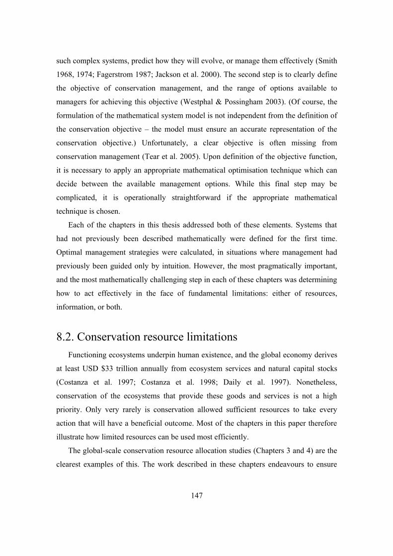
such complex systems, predict how they will evolve, or manage them effectively (Smith
1968, 1974; Fagerstrom 1987; Jackson et al. 2000). The second step is to clearly define
the objective of conservation management, and the range of options available to
managers for achieving this objective (Westphal & Possingham 2003). (Of course, the
formulation of the mathematical system model is not independent from the definition of
the conservation objective – the model must ensure an accurate representation of the
conservation objective.) Unfortunately, a clear objective is often missing from
conservation management (Tear et al. 2005). Upon definition of the objective function,
it is necessary to apply an appropriate mathematical optimisation technique which can
decide between the available management options. While this final step may be
complicated, it is operationally straightforward if the appropriate mathematical
technique is chosen.
Each of the chapters in this thesis addressed both of these elements. Systems that
had not previously been described mathematically were defined for the first time.
Optimal management strategies were calculated, in situations where management had
previously been guided only by intuition. However, the most pragmatically important,
and the most mathematically challenging step in each of these chapters was determining
how to act effectively in the face of fundamental limitations: either of resources,
information, or both.
8.2. Conservation resource limitationsFunctioning ecosystems underpin human existence, and the global economy derives
at least USD $33 trillion annually from ecosystem services and natural capital stocks
(Costanza et al. 1997; Costanza et al. 1998; Daily et al. 1997). Nonetheless,
conservation of the ecosystems that provide these goods and services is not a high
priority. Only very rarely is conservation allowed sufficient resources to take every
action that will have a beneficial outcome. Most of the chapters in this paper therefore
illustrate how limited resources can be used most efficiently.
The global-scale conservation resource allocation studies (Chapters 3 and 4) are the
clearest examples of this. The work described in these chapters endeavours to ensure
147
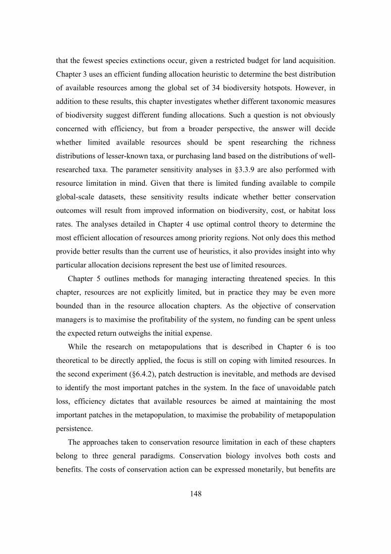
that the fewest species extinctions occur, given a restricted budget for land acquisition.
Chapter 3 uses an efficient funding allocation heuristic to determine the best distribution
of available resources among the global set of 34 biodiversity hotspots. However, in
addition to these results, this chapter investigates whether different taxonomic measures
of biodiversity suggest different funding allocations. Such a question is not obviously
concerned with efficiency, but from a broader perspective, the answer will decide
whether limited available resources should be spent researching the richness
distributions of lesser-known taxa, or purchasing land based on the distributions of well-
researched taxa. The parameter sensitivity analyses in §3.3.9 are also performed with
resource limitation in mind. Given that there is limited funding available to compile
global-scale datasets, these sensitivity results indicate whether better conservation
outcomes will result from improved information on biodiversity, cost, or habitat loss
rates. The analyses detailed in Chapter 4 use optimal control theory to determine the
most efficient allocation of resources among priority regions. Not only does this method
provide better results than the current use of heuristics, it also provides insight into why
particular allocation decisions represent the best use of limited resources.
Chapter 5 outlines methods for managing interacting threatened species. In this
chapter, resources are not explicitly limited, but in practice they may be even more
bounded than in the resource allocation chapters. As the objective of conservation
managers is to maximise the profitability of the system, no funding can be spent unless
the expected return outweighs the initial expense.
While the research on metapopulations that is described in Chapter 6 is too
theoretical to be directly applied, the focus is still on coping with limited resources. In
the second experiment (§6.4.2), patch destruction is inevitable, and methods are devised
to identify the most important patches in the system. In the face of unavoidable patch
loss, efficiency dictates that available resources be aimed at maintaining the most
important patches in the metapopulation, to maximise the probability of metapopulation
persistence.
The approaches taken to conservation resource limitation in each of these chapters
belong to three general paradigms. Conservation biology involves both costs and
benefits. The costs of conservation action can be expressed monetarily, but benefits are
148
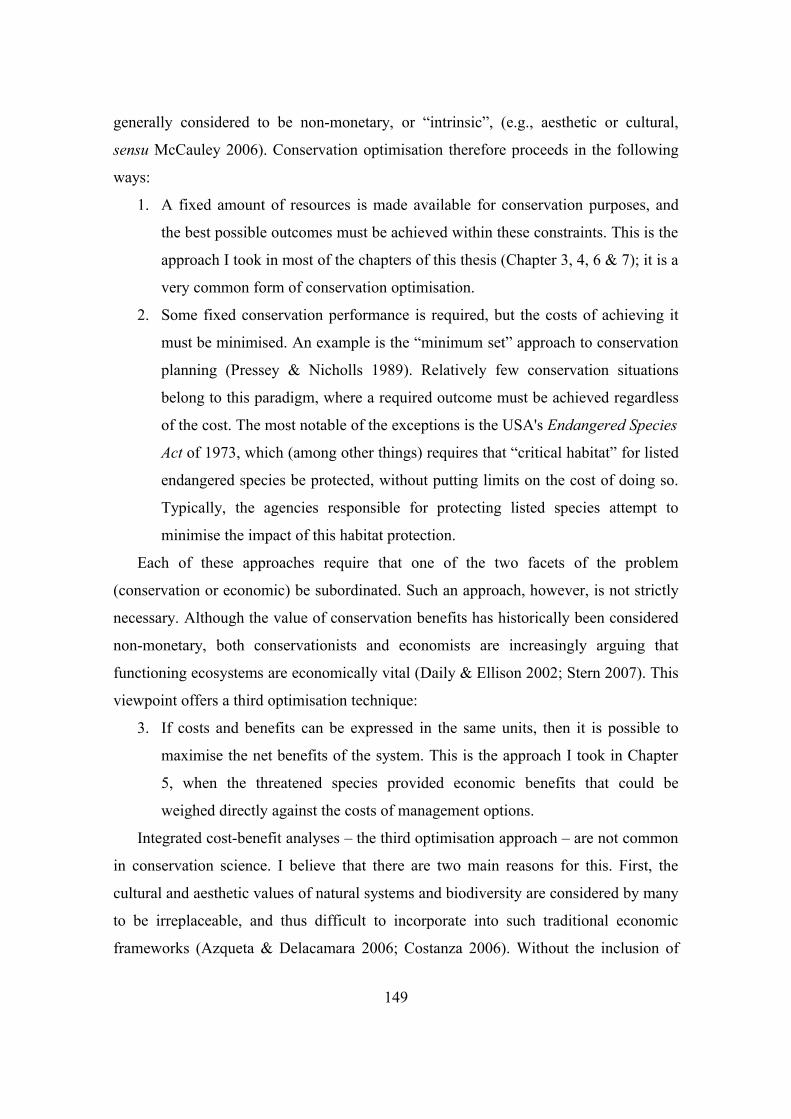
generally considered to be non-monetary, or “intrinsic”, (e.g., aesthetic or cultural,
sensu McCauley 2006). Conservation optimisation therefore proceeds in the following
ways:
1. A fixed amount of resources is made available for conservation purposes, and
the best possible outcomes must be achieved within these constraints. This is the
approach I took in most of the chapters of this thesis (Chapter 3, 4, 6 & 7); it is a
very common form of conservation optimisation.
2. Some fixed conservation performance is required, but the costs of achieving it
must be minimised. An example is the “minimum set” approach to conservation
planning (Pressey & Nicholls 1989). Relatively few conservation situations
belong to this paradigm, where a required outcome must be achieved regardless
of the cost. The most notable of the exceptions is the USA's Endangered Species
Act of 1973, which (among other things) requires that “critical habitat” for listed
endangered species be protected, without putting limits on the cost of doing so.
Typically, the agencies responsible for protecting listed species attempt to
minimise the impact of this habitat protection.
Each of these approaches require that one of the two facets of the problem
(conservation or economic) be subordinated. Such an approach, however, is not strictly
necessary. Although the value of conservation benefits has historically been considered
non-monetary, both conservationists and economists are increasingly arguing that
functioning ecosystems are economically vital (Daily & Ellison 2002; Stern 2007). This
viewpoint offers a third optimisation technique:
3. If costs and benefits can be expressed in the same units, then it is possible to
maximise the net benefits of the system. This is the approach I took in Chapter
5, when the threatened species provided economic benefits that could be
weighed directly against the costs of management options.
Integrated cost-benefit analyses – the third optimisation approach – are not common
in conservation science. I believe that there are two main reasons for this. First, the
cultural and aesthetic values of natural systems and biodiversity are considered by many
to be irreplaceable, and thus difficult to incorporate into such traditional economic
frameworks (Azqueta & Delacamara 2006; Costanza 2006). Without the inclusion of
149
these factors, many conservation biologists worry that economic analyses might not
consider certain ecosystems valuable enough to save (McCauley 2006). Second,
conservationists fear that their inability to adequately identify, and then quantify
ecosystem services will result in conservation being relatively undervalued.
While the first argument has merit, the second cannot be justified. It overlooks the
unfortunate fact that an undervaluation of ecosystem services would represent a
significant improvement on the current situation, as the value of most of these services
is ignored entirely by decision-makers. The increasing number of papers published on
the topic of ecosystem services (Armsworth & Roughgarden 2001; NAS 2004; Diaz et
al. 2006) may see the third optimisation technique become more common.
8.3. Uncertainty in conservation decision-makingMost conservation problems require immediate action, which does not allow time
for extensive information gathering. Conservation is also a new science that is not well-
suited to experimental analyses (Ferraro & Pattanayak 2006). Considerable uncertainty
is often associated with both the ecological and the socio-economic facets of a
conservation problem (Williams 1996; Ferraro & Pattanayak 2006). Methods capable of
coping with uncertainty are therefore fundamental to effective conservation action. In
most of the chapters in this thesis, uncertainty plays an central role.
The global distribution of many taxa is completely unknown. For more charismatic
species, high resolution information is available (e.g., mammals; Ceballos et al. 2005),
while the distributions of less appealing taxa are almost completely unknown (e.g.,
fungi; Hawksworth 2001). Studies have shown that the global richness distributions of
different taxa are quite dissimilar, which raises a difficult question: how can
conservation biologists conserve the breadth of biodiversity, when their knowledge
extends only to a very biased sample of it? Rather than discussing the relative merits of
using different species as surrogates for the remaining biodiversity, I dealt in Chapter 3
with this uncertainty by asking whether it might be possible to circumvent this question
altogether – would different taxonomic groups still result in the same conservation
decisions?
150
The SDP method used to manage the stochastic, oscillating predator-prey
populations in Chapter 5 takes into account unpredictable environmental variation.
Optimal management interventions are those that will most likely result in positive
outcomes. This analysis is an example of a traditional approach to uncertainty –
maximising the expected outcome of a probabilistic system.
In Chapter 7, the connectivity that joins coral reef fish populations was assumed to
be highly uncertain – in many important conservation situations, the connectivity
between fish populations may be completely unknown. I therefore chose to simulate the
relative success of various connectivity surrogates, with the aim of sustaining both a
large catch and a persistent population, even in the complete absence of any direct
connectivity knowledge. I demonstrated the robustness of these surrogates by applying
them to subsets of the Great Barrier Reef with distinctive morphologies and
connectivity patterns.
With the exception of the SDP approach, these are not typical treatments of
uncertainty. The normal approach in conservation is to define probabilistically the
system parameters, dynamics, or models (as in Chapter 5). Once this is done, the
expected outcome of different interventions is calculated, with the optimal decision
being the one that maximises this value. This approach applies the von Neumann-
Morgenstern expected utility theorem, and is excellent in applications where
probabilistic values can be assigned to uncertain system elements. Unfortunately, some
systems are not known to this level of detail, while others are so complex that the
uncertainty becomes difficult to describe in this fashion. In these situations,
conservation scientists cannot ignore the existence of uncertainty, and so need to devise
innovative and adaptive techniques to explore it.
8.4. Future directionsIn conservation biology, all research is done in the hope that the insights and tools
provided will one day be used by conservation practitioners. A significant part of the
work presented in this thesis has direct and immediate conservation implications. Two
chapters in particular contain recommendations that can inform conservation decision-
151
making. Chapter 3 concludes that global priority regions can be used effectively to
prioritise global conservation funding, even though they are based only on the diversity
of a single taxa. This chapter also concludes that future global-scale conservation
research should be directed at improving conservation cost information, rather than
information on biodiversity or habitat loss rates. Chapter 7 demonstrates the utility of
connectivity surrogates, and indicates their potential as planning tools in highly
uncertain environments, such as coral reefs in the developing world.
The other chapters in this thesis are largely theoretical, and their real-world
conservation utility is not as immediate – the lack of empirical data contained in these
chapters is an indication of this. Instead, Chapters 4, 5 & 6 propose novel analytic
techniques, and insights into, important conservation systems. The optimal control
theory analyses outlined in Chapter 4 can be directly applied to conservation resource
allocation problems, much as the heuristics of Wilson et al. (2006) were applied to the
biodiversity hotspots in Chapter 3. The optimal management analyses calculated in
Chapter 5 can be applied to oscillating predator-prey systems in conservation reserves.
The exposition of the method indicates clearly how the technique could be applied to
particular conservation systems. The metapopulation theory investigated in Chapter 6
highlights a facet of metapopulation dynamics which has not been commonly
considered, but which has a significant impact on the conservation outcomes of the
system. However, the techniques used in this chapter require much more work before
they can be used practically in conservation contexts.
Most importantly, this thesis details new applications of decision theory to
conservation problems, illustrating methods for providing the best possible conservation
outcomes when resources and information are limited. While decision theory has not
been around in conservation biology for very long, it is increasingly being recognised as
the rational and responsible approach to conservation problems. This thesis provides
more evidence of, and more arguments for, this perspective.
152
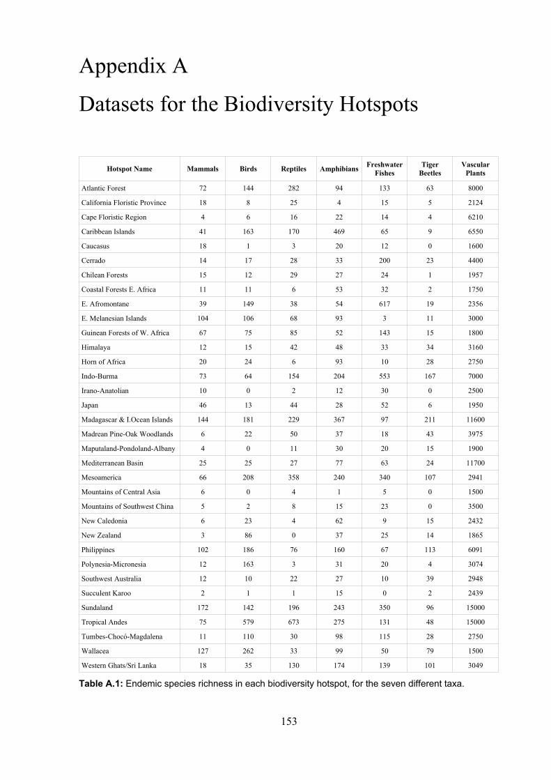
Appendix A
Datasets for the Biodiversity Hotspots
Hotspot Name Mammals Birds Reptiles Amphibians Freshwater Fishes
Tiger Beetles
Vascular Plants
Atlantic Forest 72 144 282 94 133 63 8000
California Floristic Province 18 8 25 4 15 5 2124
Cape Floristic Region 4 6 16 22 14 4 6210
Caribbean Islands 41 163 170 469 65 9 6550
Caucasus 18 1 3 20 12 0 1600
Cerrado 14 17 28 33 200 23 4400
Chilean Forests 15 12 29 27 24 1 1957
Coastal Forests E. Africa 11 11 6 53 32 2 1750
E. Afromontane 39 149 38 54 617 19 2356
E. Melanesian Islands 104 106 68 93 3 11 3000
Guinean Forests of W. Africa 67 75 85 52 143 15 1800
Himalaya 12 15 42 48 33 34 3160
Horn of Africa 20 24 6 93 10 28 2750
Indo-Burma 73 64 154 204 553 167 7000
Irano-Anatolian 10 0 2 12 30 0 2500
Japan 46 13 44 28 52 6 1950
Madagascar & I.Ocean Islands 144 181 229 367 97 211 11600
Madrean Pine-Oak Woodlands 6 22 50 37 18 43 3975
Maputaland-Pondoland-Albany 4 0 11 30 20 15 1900
Mediterranean Basin 25 25 27 77 63 24 11700
Mesoamerica 66 208 358 240 340 107 2941
Mountains of Central Asia 6 0 4 1 5 0 1500
Mountains of Southwest China 5 2 8 15 23 0 3500
New Caledonia 6 23 4 62 9 15 2432
New Zealand 3 86 0 37 25 14 1865
Philippines 102 186 76 160 67 113 6091
Polynesia-Micronesia 12 163 3 31 20 4 3074
Southwest Australia 12 10 22 27 10 39 2948
Succulent Karoo 2 1 1 15 0 2 2439
Sundaland 172 142 196 243 350 96 15000
Tropical Andes 75 579 673 275 131 48 15000
Tumbes-Chocó-Magdalena 11 110 30 98 115 28 2750
Wallacea 127 262 33 99 50 79 1500
Western Ghats/Sri Lanka 18 35 130 174 139 101 3049
Table A.1: Endemic species richness in each biodiversity hotspot, for the seven different taxa.
153
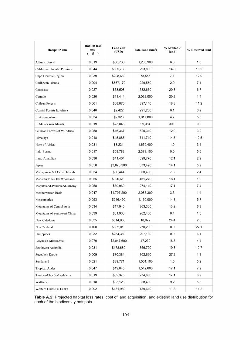
Hotspot NameHabitat loss
rate ( )
Land cost(USD) Total land (km2) % Available
land % Reserved land
Atlantic Forest 0.019 $68,733 1,233,900 6.3 1.8
California Floristic Province 0.044 $865,760 293,800 14.8 10.2
Cape Floristic Region 0.039 $208,660 78,555 7.1 12.9
Caribbean Islands 0.094 $567,170 229,550 2.9 7.1
Caucasus 0.027 $78,508 532,660 20.3 6.7
Cerrado 0.020 $11,414 2,032,000 20.2 1.4
Chilean Forests 0.061 $68,870 397,140 18.8 11.2
Coastal Forests E. Africa 0.040 $2,422 291,250 6.1 3.9
E. Afromontane 0.034 $2,326 1,017,800 4.7 5.8
E. Melanesian Islands 0.019 $23,846 99,384 30.0 0.0
Guinean Forests of W. Africa 0.058 $16,367 620,310 12.0 3.0
Himalaya 0.018 $45,888 741,710 14.5 10.5
Horn of Africa 0.031 $8,231 1,659,400 1.9 3.1
Indo-Burma 0.017 $59,783 2,373,100 0.0 5.6
Irano-Anatolian 0.030 $41,404 899,770 12.1 2.9
Japan 0.058 $3,873,300 373,490 14.1 5.9
Madagascar & I.Ocean Islands 0.034 $30,444 600,460 7.6 2.4
Madrean Pine-Oak Woodlands 0.055 $326,610 461,270 18.1 1.9
Maputaland-Pondoland-Albany 0.058 $89,969 274,140 17.1 7.4
Mediterranean Basin 0.047 $1,707,200 2,085,300 3.3 1.4
Mesoamerica 0.053 $216,490 1,130,000 14.3 5.7
Mountains of Central Asia 0.034 $17,940 863,360 13.2 6.8
Mountains of Southwest China 0.039 $81,933 262,450 6.4 1.6
New Caledonia 0.035 $614,960 18,972 24.4 2.6
New Zealand 0.100 $862,010 270,200 0.0 22.1
Philippines 0.032 $264,380 297,180 0.9 6.1
Polynesia-Micronesia 0.070 $2,047,600 47,239 16.8 4.4
Southwest Australia 0.031 $178,680 356,720 19.3 10.7
Succulent Karoo 0.009 $70,384 102,690 27.2 1.8
Sundaland 0.021 $89,771 1,501,100 1.5 5.2
Tropical Andes 0.047 $19,045 1,542,600 17.1 7.9
Tumbes-Chocó-Magdalena 0.019 $32,375 274,600 17.1 6.9
Wallacea 0.018 $83,126 338,490 9.2 5.8
Western Ghats/Sri Lanka 0.092 $131,980 189,610 11.8 11.2
Table A.2: Projected habitat loss rates, cost of land acquisition, and existing land use distribution for each of the biodiversity hotspots.
154
Appendix B
Asymmetric connectivity in a two-patch
metapopulation
In Chapter 6, I demonstrate that asymmetry in the connectivity pattern of a
metapopulation has a negative effect on its persistence. In this Appendix, I show this to
be analytically true for a two-patch metapopulation. The fundamental events in the
dynamics of a stochastic metapopulation are the extinction and recolonisation of
patches. Extinction of the population on patch i occurs with a probability μ i , and
recolonisation of a patch i from another occupied patch j occurs with probability p ij . We
store all the colonisation probabilities in a metapopulation connectivity matrix ℂ ,
which for two patches takes the form of a 2x2 square matrix:
ℂ2=[ 0 p12
p21 0 ] (B.1)
The current state of a metapopulation defines its future dynamics. For a two-patch
metapopulation we label possible states with an ordered pair: (a,b), where a and b take
the values of 1 or 0, indicating an occupied or unoccupied patch respectively. The value
of a indicates whether the first patch is occupied, while the value of b does the same for
the second patch. Thus, the two-patch metapopulation exists in four different states:
(1,1), (1,0), (0,1) of (0,0). The state (0,0) corresponds to the extinction of the entire
metapopulation. The expected time to metapopulation extinction is inversely
proportional to the second-largest eigenvalue (λ 2) of the state transition matrix (Day &
Possingham 1995).
If the connectivity pattern is symmetric (e.g., if the connectivity depended on the
155
distances between the patches), then the two connectivity values are equal: p 12 = p 21 .
This connectivity matrix has an asymmetry value of Z = 0. To investigate the effects of
asymmetry, we express the colonisation probabilities as deviations from this symmetric
connectivity matrix, so that p 12 = p+ δ, and p 21 = p – δ, where 0 ≤ δ ≤ p. The resulting
asymmetric connectivity matrix is:
ℂ2=[0 pp− 0 ] (B.2)
which has the same total connectivity as the symmetric connectivity pattern,
∑i=1
2 ∑ j=1
2pij=2 p . From Equations (6.2) and (6.3), the degree of asymmetry in the
new matrix is Z ℂ2=2 . The state transition matrix (Day & Possingham 1995)
for this metapopulation can be written as:
T2=[ 1 0 0 0 1−1− p− 0 1−1− p 0 1−1− p 1−1− p−2 1−1−p− 1−1−p 2 p1−1−2] (B.3)
where the probability of patch extinction at each timestep is assumed to be the same for
the two patches. The rate at which this metapopulation becomes extinct can be
calculated by using the second-largest eigenvalue of T2 (which is the largest eigenvalue
of the matrix when the row and column corresponding to metapopulation extinction are
removed ; Darroch & Seneta 1965)).
The characteristic equation of the reduced matrix is a quadratic in δ, and implicit
differentiation gives an equation for ∂2/∂ :
∂2
∂=−
2221−22−12
−12 pA2, p ,B 2, p ,, (B.4)
where
A2, p ,=1−22−21−2 , B 2, p ,=3−2
2−23−52−1−3242
2223222.
(B.5)
156
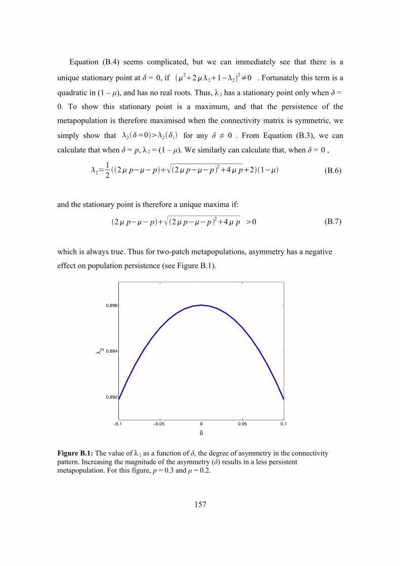
Equation (B.4) seems complicated, but we can immediately see that there is a
unique stationary point at δ = 0, if 2221−22≠0 . Fortunately this term is a
quadratic in (1 – μ), and has no real roots. Thus, λ 2 has a stationary point only when δ =
0. To show this stationary point is a maximum, and that the persistence of the
metapopulation is therefore maximised when the connectivity matrix is symmetric, we
simply show that 2=02i for any δ ≠ 0 . From Equation (B.3), we can
calculate that when δ = p, λ 2 = (1 – μ). We similarly can calculate that, when δ = 0 ,
2=122 p−− p 2 p−−p 24 p21− (B.6)
and the stationary point is therefore a unique maxima if:
2 p−− p 2 p−−p 24 p 0 (B.7)
which is always true. Thus for two-patch metapopulations, asymmetry has a negative
effect on population persistence (see Figure B.1).
Figure B.1: The value of λ 2 as a function of δ, the degree of asymmetry in the connectivity pattern. Increasing the magnitude of the asymmetry (δ) results in a less persistent metapopulation. For this figure, p = 0.3 and μ = 0.2.
157

Chapter 9
Bibliography
Aarde, R. V., I. Whyte & S. Pimm (1999). Culling and the dynamics of the Kruger National
Park African Elephant population. Animal Conservation 2: 287-294.
Ackakaya, H. R. & S. Ferson (1999). RAMAS Red List: Threatened Species Classifications
Under Uncertainty (User Manual for Version 1.0). Applied Biomathematics, New York.
Albrecht, F., H. Gatzke, A. Haddad & N. Wax (1974). The dynamics of two interacting
populations. Journal of Mathematical Analysis and Applications 46: 658-670.
Almany, G. R., M. L. Berumen, S. R. Thurrold, S. Planes & G. P. Jones (2007). Local
replenishment of coral reef fish populations in a marine reserve. Science 316: 742-744.
Ando, A., J. Camm, S. Polasky & A. Solow (1998). Species distributions, land values and
efficiency conservation. Science 279: 2126-2128.
Armsworth, P. R. (2002). Recruitment limitation, population regulation, and larval connectivity
in reef fish metapopulations. Ecology 83: 1092-1104.
Armsworth, P. R., G. C. Daily, P. Kareiva & J. N. Sanchirico (2006). Land market feedbacks
can undermine biodiversity conservation. Proceedings of the National Academy of Sciences
103: 5403-5408.
Armsworth, P. R. & J. Roughgarden (2001). The economic value of ecological stability.
Proceedings of the National Academy of Sciences 100: 7147-7151.
Austin, D., W. D. Bowen, & J. I. McMillan (2004). Intraspecific variation in movement
patterns: modelling individual behaviour in a large marine predator. Oikos 105: 15-30.
Azqueta, D., & G. Delacamara (2006). Ethics, economics and environmental management.
Ecological Economics 56: 524-533.
Baillie, J. E. M, C. Hilton-Taylor & S. N. Stuart (2004). 2004 IUCN Red List of Threatened
Species. A Global Species Assessment. IUCN, Gland.
Balmford, A., K. Gaston, S. Blyth, A. James & V. Kapos (2003). Global variation in terrestrial
conservation costs, conservation benefits, and unmet conservation needs. Proceedings of the
158
National Academy of Sciences 100: 1046-1050.
Barnes, R. F. W. (1983). The Elephant problem in Ruaha National Park, Tanzania. Biological
Conservation 26: 127-148.
Baxter, P. W. J., M. A. McCarthy, H. P. Possingham, P. W. Menkhorst & N. McLean (2006).
Accounting for uncertainty in sensitivity analyses of matrix population models.
Conservation Biology 20: 893-905.
Bellman, R. E. & S. E. Dreyfuss (1962). Applied Dynamic Programming. Princeton University
Press, Princeton.
Ben-Haim, Y. (2001). Information-Gap Decision Theory: Decisions Under Extreme
Uncertainty. Academic Press, London.
Birkett, A. (2002). The impact of giraffe, rhino and elephant on the habitat of a black rhino
sanctuary in Kenya. African Journal of Ecology 40: 276-282.
Black, K. P. (1993). The relative importance of local retention and inter-reef dispersal of
neutrally buoyant material on coral reefs. Coral Reefs 12: 43-53.
Black, K. P., S. L. Gay & J. C. Andrews (1990). Residence times of neutrally-buoyant matter
such as larvae, sewage or nutrients on coral reefs. Coral Reefs 9: 105-114.
Bode, M., L. Bode & P. R. Armsworth (2006). Larval dispersal reveals regional sources and
sinks in the Great Barrier Reef. Marine Ecology Progress Series 308: 17-25.
Bohn, H. & R. T. Deacon (2000). Ownership risk, investment and the use of natural resources.
American Economic Review 90: 526-549.
Botsford, L. W., F. Micheli & A. Hastings (2003). Principles for the design of marine reserves.
Ecological Applications 13: S25-S31.
Boyce, M. S. (1992). Population viability analysis. Annual Review of Ecology and Systematics
23: 481-506
Brooks, T. M., R. A. Mittermeier, G. A. B. da Fonseca, J. Gerlach, M. Hoffmann, J. M.
Lamoreux, C. G. Mittermeier, J. D. Pilgrim & A. S. L. Rodrigues (2006). Global biodiversity
conservation priorities. Science 313: 58-61.
Bryant, D., D. Neilsen & L. Tangley (1997). Last Frontier Forests. World Resources Institute,
Washington.
Burkey, T. V. (1989). Extinction in nature reserves: the effect of fragmentation and the
importance of migration between reserve fragments. Oikos 55: 75-81.
Butler, V. (1998). Elephants: trimming the herd. Bioscience 48: 76-81.
Campbell, R. A., B. D. Mapstone & A. D. M. Smith (2001). Evaluating large-scale
experimental designs for management of coral trout on the Great Barrier Reef. Ecological
159
Applications 11: 1763-1777.
Caughley, G. (1976). The elephant problem - an alternative hypothesis. East African Wildlife
Journal 14: 265-383.
Caughley, G. & A. Gunn (1996). Conservation Biology in Theory and Practice. Blackwell
Science, Cambridge, USA.
Ceballos, G. & P. R. Ehrlich (2006). Global mammal distributions, biodiversity hotspots, and
conservation. Proceedings of the National Academy of Sciences 103: 19374-19379.
Ceballos, G., P. R. Ehrlich, J. Soberon, I. Salazar & J. P. Fay (2005). Global mammal
conservation: what must we manage? Science 309: 603-607.
CEPF (2006). Protecting Nature's Hotspots for People and Prosperity: Annual Report 2006.
Report for the Critical Ecosystems Partnership Fund.
Chape, S., L. Fish, P. Fox & M. Spaulding (2003). United Nations List of Protected Areas.
IUCN/UNEP, Gland.
Chardon, J. P., F. Adriaensen & E. Matthysen (2003). Incorporating landscape elements into a
connectivity measure: a case study for the Speckled wood butterfly (Pararge aegeria L.).
Landscape Ecology 18: 561-573.
Christensen J. (2003). Auditing conservation in an age of accountability. Conservation in
Practice 4: 3-6.
CIA (2006). CIA World Factbook. Central Intelligence Agency, Washington DC.
Clark, C. W. (1990). Mathematical Bioeconomics. Wiley and Sons, New York.
Clauset, A., M. E. J. Newman & C. Moore (2004). Finding community structure in very large
networks. Physical Review E 70: 066111.
Clayton, J. (2007). Elephant cull 'a last resort'. The Australian Newspaper, March 2, 2007, pp.
12.
Cohen, Y. (1986). Optimal reproductive strategies in annual plants. In: Lecture Notes in
Biomathematics: 73. Springer-Verlag, New York.
Cooke, J. G. (1995). The International Whaling Commission's revised management procedure
as an example of a new approach to fishery management. In: Whales, Seals, Fish and Man.
Elsevier Science, London.
Corfield, T. F. (1973). Elephant mortality in Tsavo National Park. East African Wildlife Journal
11: 339-368.
Cornish, A. & L. K. Kiwi (2006). Plectropomus leopardus. Species Report for the IUCN Red
List of Threatened Species. IUCN, Gland.
Costanza, R. (2006). Nature: ecosystems without commodifying them. Nature 443: 749.
160
Costanza, R., R. d’Arge, R. de Groot, S. Farber, M. Grasso, B. Hannon, K. Limburg, S. Naeem,
R. O’Neil, J. Paruelo, R. Raskin, P. Sutton & M. van den Belt (1997). The value of the
world's ecosystem services and natural capital. Nature 387: 253-260.
Costanza, R., R. d’Arge, R. de Groot, S. Farber, M. Grasso, B. Hannon, K. Limburg, S. Naeem,
R. O’Neil, J. Paruelo, R. Raskin, P. Sutton & M. van den Belt (1998). The value of the
world’s ecosystem services and natural capital. Ecological Economics 25: 3-15.
Costello, C. & S. Polasky (2004). Dynamic reserve site selection. Resource and Energy
Economics 26: 157-174.
Cowen, R. K. (2002). Larval dispersal and retention and consequences for population
connectivity. In: Coral Reef Fishes: Dynamics and Diversity in a Complex Ecosystem.
Academic Press, San Diego.
Cowen, R. K., G. Gawarkiewicz, J. Pineda, S. Thurrold & F. Werner (2002). Population
connectivity in marine systems: report of a workshop to develop science recommendations.
Report to the National Science Foundation.
Cowen, R. K., K. M. M. Lwiza, S. Sponaugle, C. B. Paris & D. B. Olsen (2000). Connectivity
of marine populations: open or closed? Science 287: 857-859.
Cowen, R.K., C. B. Paris & A. Srinivasan (2006). Scaling of connectivity in marine
populations. Science 311: 522-527.
Cowling, R. M., R. L. Pressey, A. T. Lombard, P. G. Desmet & A. G. Ellis (1999). From
representation to persistence: requirements for a sustainable reserve system in the species-
rich Mediterranean-climate deserts of southern Africa. Diversity and Distribution 5: 51-71.
Daily, G., S. Alexander, P. Ehrlich, L. Goulder, J. Lubchenco, P. Matson, H. Mooney, S. Postel,
S. Schneider, D. Tilman & G. Woodwell (1997). Ecosystem services: benefits supplied to
human societies by natural ecosystems. Issues in Ecology 1: 1-18.
Daily, G. & K. Ellison (2002). The New Economy of Nature. Island Press, Washington DC.
Darroch, J. N. & E. Seneta (1965). On quasi-stationary distributions in absorbing discrete-time
Markov chains. Journal of Applied Probability 2: 88-100.
Day, J. & H. P. Possingham (1995). A stochastic metapopulation model with variability in patch
size and position. Theoretical Population Biology 48: 333-360.
Deacon, R. T. & P. Murphy (1997). The structure of an environmental transaction: the debt-for-
nature swap. Land Economics 73: 1-24.
Diaz, S., J. Fargione, F. S. Chapin & D. Tilman (2006). Biodiversity loss threatens human well-
being. Public Library of Science: Biology 4: e277.
Dight, I., L. Bode & M. K. James (1990). Modelling the larval dispersal of Acanthaster planci.
161
I. Large scale hydrodynamics, Cairns section, Great Barrier Reef Marine Park. Coral Reefs
9: 115-123.
Dight, I., L. Bode & M. K. James (1990). Modelling the larval dispersal of Acanthaster planci.
II. Patterns of reef connectivity. Coral Reefs 9: 125-134.
Dirzo, R. & P. H. Raven (2003). Global state of biodiversity and loss. Annual review of
environmental resources 28: 137-167.
Doherty, P.J., A. J. Fowler, M. A. Samoilys & D. A. Harris (1994). Monitoring the
replenishment of coral trout (Pisces: Serranidae) populations. Bulletin of Marine Science 54:
343-355.
Duchs, J. & A. Arenas (2005). Community detection in complex networks using extremal
optimisation. Physical Review E 72: 027104.
Duffy, K. J., B. R. Page, J. H. Swart & V. B. Bajic (1999). Realistic parameter assessment for a
well known elephant-tree ecosystem model reveals that limit cycles are unlikely. Ecological
Modelling 121: 115-125.
Dulac, H. (1937). Recherches des cycles limites. Comptes Rendus de l'Acadamie des Sciences
204: 1703-1706.
Ebedes, H. (2005). Please don't forget Tsavo. In: Proceedings of the Great Elephant INDABA,
October 2005. Kruger National Park, South Africa.
Elton, C. & M. Nicholson (1942). The ten-year cycle in numbers of lynx in Canada. Journal of
Animal Ecology 11: 215-244.
Emlen, J. M. (1984). Population Biology: the Coevolution of Population Dynamics and
Behaviour. MacMillan, New York.
Etienne, R. S. (2004). On optimal choices in increase of patch area and reduction of interpatch
distance for metapopulation persistence. Ecological Modelling 179: 77-90.
Etter, A., C. McAlpine, D. Pullar & H. P. Possingham (2006). Modelling the conversion of
Colombian lowland ecosystems since 1940: drivers, patterns and rates. Journal of
Environmental Management. 79: 74-87.
Fagerstrom, T. (1987). On theory, data and mathematics in ecology. Oikos 50: 258-261.
Fernandes, L., J. Day, A. Lewis, S. Slegers, B. Kerrigan, D. Breen, D. Cameron, B. Jago, J.
Hall, D. Lowe, J. Innes, J. Tanzer, V. Chadwick, L. Thompson, K. Gorman, M. Simmons, B.
Barnett, K. Sampson, G. De'ath, B. Mapstone, H. Marsh, H. Possingham, I. Ball, T. Ward,
K. Dobbs, J. Aumend, D. Slater & K. Stapleton (2005). Establishing representative no-take
areas in the Great Barrier Reef: Large scale implementation of theory on marine protected
areas. Conservation Biology 19: 1733-1744.
162
Ferraro, P. J. & S. K. Pattanayak (2006). Money for nothing? A call for empirical evaluation of
biodiversity conservation investments. Public Library of Science: Biology 4: 482-488.
Ferreira, B. P. & G. R. Russ (1994). Age validation and estimation of growth rate of the coral
trout, Plectropomus leopardus from Lizard Island, northern Great Barrier Reef. Fishery
Bulletin 92: 46-57.
Field, S. A., A. J. Tyre, N. Jonzen, J. R. Rhodes & H. P. Possingham (2004). Minimising the
cost of environmental management decisions by optimising statistical thresholds. Ecology
Letters 7: 669-675.
Fogarty, M. J. (1999). Essential habitat, marine reserves and fishery management. Trends in
Ecology and Evolution 14: 133-134.
Foggin, C. M. (2003). The elephant population problem in Zimbabwe: Can there be any
alternative to culling? In: Proceedings of the First Workshop on the Control of Wild
Elephant Populations. Utrecht University, Utrecht.
Frank, K. & C. Wissel (2002). A formula for the mean lifetime of metapopulations in
heterogeneous landscapes. The American Naturalist 159: 530-552.
Gaspar, P., J. Georges, S. Fossette, A. Lenoble, S. Ferraroli & Y. le Maho (2006). Marine
animal behaviour: neglecting currents can lead us up the wrong track. Proceedings of the
Royal Society of London B: Biological Sciences 273: 2697-2702.
Gause, G. F. (1934). The Struggle for Existence. The Williams & Wilkins Company, Baltimore.
GCF (2006). The Global Conservation Fund: Investing in the Earth's Natural Heritage.
Operational Report of the Global Conservation Fund, Arlington.
GEF (2006). GEF Resource Allocation Framework: Indicative Resource Allocations for GEF-
4, for the Biodiversity and Climate Change Focal Areas. Technical report to the Global
Environment Facility.
Gilpin, M. E. (1979). Spiral chaos in a predator prey model. The American Naturalist 55: 135-
154.
Ginsburg, L. & M. Colyvan (2004). Ecological Orbits: How Planets Move and Populations
Grow. Oxford University Press, New York.
Girvan, M. & M. E. J. Newman (2002). Community structure in social and biological networks.
Proceedings of the National Academy of Sciences 99: 7821-7826.
Goldstine, H. H. (1980). A History of the Calculus of Variations From the 17th Through the
19th Century. Springer-Verlag, New York.
Goodrich, J. M. & S. W. Buskirk (1995). Control of abundant native vertebrates for
conservation of endangered species. Conservation Biology 9: 1357-1364.
163
Grenyer, R., C. D. L. Orme, S. F. Jackson, G. H. Thomas, R. G. Davies, T. J. Davies, K. E.
Jones, V. A. Olson, R. S. Ridgely, P. C. Rasmussen, T. Ding, P. M. Bennett, T. M.
Blackburn, K. J. Gaston, J. L. Gittleman & I. P. F. Owens (2006). Global distribution and
conservation of rare and threatened vertebrates. Nature 444: 93-96.
Gustafson, E. J. & R. H. Gardner (1996). The effect of landscape heterogeneity on the
probability of patch colonisation. Ecology 77: 94-107.
Halpern, B. S. (2003). The impact of marine reserves: do reserves work, and does reserve size
matter? Ecological Applications 13: S117-S137.
Halpern, B. S., S. D. Gaines & R. R. Warner (2004). Confounding effects of the export of
production and the displacement of fishing effort from marine reserves. Ecological
Applications 14: 1248-1256.
Halpern, B. S., C. R. Pyke, H. E. Fox, J. C. Haney, M. A. Schlaepfer & P. Zaradic (2006). Gaps
and mismatches between global conservation priorities and spending. Conservation Biology
20: 56-64.
Halpern, B. S. & R. R. Warner (2003). Matching marine reserve design to reserve objectives.
Proceedings of the Royal Society London B: Biological Sciences 270: 1871-1878.
Hanski, I. (1994). A practical model of metapopulation dynamics. The Journal of Animal
Ecology 63: 151-162.
Hanski, I. & O. Gaggiotti (2004). Ecology, Genetics and Evolution of Metapopulations.
Academic Press, Amsterdam.
Hanski, I. & O. Ovaskainen (2000). The metapopulation capacity of a fragmented landscape.
Nature 404: 755-758.
Hansson, L. & H. Henttonen (1988). Rodent dynamics as community processes. Trends in
Ecology and Evolution 3: 195-200.
Harrison, S. & E. Bruna (1999). Habitat fragementation and large-scale conservation: what do
we know for sure? Ecography 22: 225-232.
Hastings, A., C. L. Hom, S. Ellner, P. Turchin, H. & C. J. Godfray (1993). Chaos in ecology: is
mother nature a strange attractor? Annual Review of Ecology and Systematics 24: 1-33.
Hastings, A. & T. Powell (1991). Chaos in a three species food chain. Ecology 72: 896-903.
Hauser, C. E., A. R. Pople & H. P. Possingham (2006). Should managed populations be
monitored every year? Ecological Applications 16: 807-819.
Hawksworth, D. L. (2001). The magnitude of fungal diversity: the 1.5 million species estimate
revisited. Mycological Research 105: 1422-1432.
Hecht, A. & P. R. Nickerson (1999). The need for predator management in conservation of
164
some vulnerable species. Endangered Species Update 16: 114-118.
Heemstra, P.C. & J.E. Randall (1993). FAO species catalogue. Vol. 16. Groupers of the world
(family Serranidae, subfamily Epinephelinae). An Annotated and Illustrated Catalogue of
the Grouper, Rockcod, Hind, Coral Grouper and Lyretail Species Known to Date. Food and
Agriculture Organisation of the United Nations, Rome.
Hein, S., B. Pfenning, T. Hovestadt & H. J. Poethke (2004). Patch density, movement pattern,
and realised dispersal distances in a patch-matrix landscape - a simulation study. Ecological
Modelling 174: 411-420.
Hoegh-Guldberg, O. (2004). Coral reefs in a century of rapid environmental change. Symbiosis
37: 1-31.
Hoekstra, J. M., T. M. Boucher, T. H. Ricketts, & C. Roberts (2005). Confronting a biome
crisis: global disparities of habitat loss and protection. Ecology Letters 8: 23-29.
Howard, P. C., P. Viskanic, T. R. B. Davenport, F. W. Kigenyi, M. Baltzer, C. J. Dickinson, J.
S. Lwanga, R. A. Matthews & A. Balmford (1998). Complementarity and the use of
indicator groups for reserve selection in Uganda. Nature 394: 472-475.
Huffaker, C. B. (1958). Experimental studies on predation: dispersion factors and predator-prey
oscillations. Hilgardia 27: 343-383.
Hughes, T. P., A. H. Baird, D. R. Bellwood, M. Card, S. R. Connolly, C. Folke, R. Grosberg, O.
Hoegh-Guldberg, J. B. C. Jackson, J. Kleypas, J. M. Lough, P. Marshall, M. Nystro, S. R.
Palumbi, J. M. Pandolfi, B. Rosen & J. Roughgarden (2003). Climate change, human
impacts, and the resilience of coral reefs. Science 301: 929-933.
Hughey, K. F. D., R. Cullen & E. Moran (2003). Integrating economics into priority setting and
evaluation in conservation management. Conservation Biology 17: 93-103.
INDABA (2005). Proceedings of the great elephant INDABA. Finding an African Solution to
an African Problem, October 2005. Kruger National Park, South Africa.
Intriligator, M. D. (1971). Mathematical Optimisation and Economic Theory. Prentice-Hall,
New York.
IPCC (2007). Climate Change 2007: Impacts, Adaptation and Vulnerability Summary for
Policymakers. Fourth Assessment Report of the Intergovernmental Panel on Climate
Change, Geneva.
IUCN (2003). Recommendations of the 5th Annual IUCN World Parks Congress. IUCN, Gland.
IUCN (2004). Leopard Coral Grouper. Species Synopsis for the IUCN Red List. IUCN, Gland.
Iwasa, Y. & J. Roughgarden (1984). Shoot/root balance of plants: Optimal growth of a system
with many vegetative organs. Theoretical Population Biology 25: 78-105.
165
Jaarsveld, A. S. v., S. Freitag, S. L. Chown, C. Muller, S. Koch, H. Hull, C. Bellamy, M.
Kruger, S. Endrody-Younga, M. W. Mansell. & C. H. Scholtz (1998). Biodiversity
assessment and conservation strategies. Science 279: 2106-2108.
Jackson, J. B. C. (2001). What was natural in the coastal oceans? Proceedings of the National
Academy of Sciences 98: 5411-5418.
Jackson, L. J., A. S. Trebitz & K. L. Cottingham (2000). An introduction to the practice of
ecological modelling. Bioscience 50: 694-706.
Jackson, J. B. C., M. X. Kirby, W. H. Berger, K. A. Bjorndal, L. W. Botsford, B. J. Bourque, R.
H. Bradbury, R. Cooke, J. Erlandson, J. A. Estes, T. P. Hughes, S. Kidwell, C. B. Lange, H.
S. Lenihan, J. M. Pandolfi, C. H. Peterson, R. S. Steneck, M. J. Tegner & R. W. Warner
(2001). Historical overfishing and the recent collapse of coastal ecosystems. Science 293:
629-638.
James, A. N., K. J. Gaston & A. Balmford (1999a). Balancing the Earth's accounts. Nature 401:
323-324.
James, A. N., M. J. B. Green & J. R. Paine (1999b). Global Review of Protected Areas Budgets
and Staff. WCMC, Cambridge.
James, M. K., P. R. Armsworth, L. B. Mason & L. Bode (2002). The structure of reef fish
metapopulations: modelling larval dispersal and retention patterns. Proceedings of the Royal
Society London B 269: 2079-2086.
Jansen, V. A. A & A. M. de Roos (2000). The role of space in reducing predator-prey cycles.
In: The Geometry of Ecological Interactions. Cambridge University Press, Cambridge.
Javier, G. P. & R. V. Sole (2000). Bifurcations and chaos in ecology: lynx returns revisited.
Ecology Letters 3: 114-121.
Jhala, V. (1993). Predation on blackbuck by wolves in Velvadar National Park, Gujarat, India.
Conservation Biology 7: 874-881.
Jones, G. P. (2002). Marine protected area strategies: issues, divergences and the search for
middle ground. Review in Fish Biology and Fisheries 11: 197-216.
Jones, G. P., M. J. Milicich, M. J. Emslie & C. Lunlow (1999). Self-recruitment in a coral reef
fish population. Nature 402: 802-804.
Jones, G. P., S. Planes & S. R. Thurrold (2005). Coral reef fish larvae settle close to home.
Current biology 15: 1314-1318.
Kareiva, P. (1987). Habitat fragmentation and the stability of predator-prey interactions. Nature
326: 388-390.
Kareiva, P. & M. Marvier (2003). Conserving biodiversity coldspots. American Scientist 91:
166
344-351.
Kindvall, O (1999). Dispersal in a metapopulation of the bush cricket Metrioptera bicolor
(Orthoptera: Tettigoniidae). Journal of Animal Ecology 68: 172-185.
Kirkwood, G. P. (1997). The revised management procedure of the International Whaling
Commission. In: Global Trends: Fishery Management: Proceedings of the 1997 American
Fishery Society Symposium. Monetery.
Korpimaki, E. & K. Norrdahl (1998). Experimental reduction of predators reverses the crash
phase of small-rodent cycles. Ecology 79: 2448-2455.
Kot, M. (2001). Elements of Mathematical Ecology. University Press, Cambridge.
Lack, D. (1954). The Natural Regulation of Animal Numbers. Clarendon Press, London.
Lacy, R. C. (1993). Vortex: a computer simulation model for population viability analyses.
Wildlife Research 20: 45-65.
Lamoreux, J. F., J. C. Morrison, T. H. Ricketts, D. M. Olson, E. Dinerstein, M. W. McKnight
& H. H. Shugart (2006). Global tests of biodiversity concordance and the importance of
endemism. Nature 440: 212-214.
Largier, J. L. (2003). Considerations in estimating larval dispersal distances from oceanographic
data. Ecological Applications 13: S71-S89.
Laurence, W. F., H. L. Vasconcelos & T. E. Lovejoy (2000). Forest loss and fragmentation in
the Amazon: implications for wildlife conservation. Oryx 34: 39-45.
Leis, J. M. (1991). The pelagic stage of reef fishes: the larval biology of coral reef fishes. In:
The Ecology of Fishes on Coral Reefs. Academic Press, San Diego.
Leis, J. M. (2002). Pacific coral-reef fishes: the implications of behaviour and ecology of larvae
for biodiversity and conservation, and a reassessment of the open population paradigm.
Environmental biology of fishes 65: 199-208.
Leitmann, G. (1981). The Calculus of Variations and Optimal Control: An Introduction.
Plenum Press, New York.
Leonard, D. & N. V. Long (1992). Optimal Control Theory and Static Optimization in
Economics. Cambridge University Press, Cambridge.
Leslie, H., M. Ruckelshaus, I. R. Ball, S. Andleman & H. P. Possingham (2003). Using siting
algorithms in the design of marine reserve networks. Ecological Applications 13: S185-
S198.
Leslie, P. H. & J. C. Gower (1960). The properties of a stochastic model for the predator-prey
type of interaction between two species. Biometrika 47: 219-234.
Leuthold, W. (1996). Recovery of woody vegetation in Tsavo national park, Kenya, 1970-1994.
167
African Journal of Ecology 34: 101-112.
Levins, R. (1966). The strategy of model building in population biology. American Scientist 54:
421-431.
Loehle, C. (2006). Control theory and the management of ecosystems. Journal of Applied
Ecology 43: 957-966.
Lubchenco, J., S. R. Palumbi, S. D. Gaines & S. Andleman (2003). Plugging a hole in the
ocean: the emerging science of marine reserves. Ecological Applications 13: S3-S7.
Ludwig, D., R. Hilborn & C. Walters (1993). Uncertainty, resource exploitation, and
conservation: lessons from history. Science 260: 17.
Mabunda, D. (2005). Developing elephant management plans for national parks with
recommendations on the process to be followed. Report to the Minister of Environmental
Affairs and Tourism, South African National Parks, South Africa.
MacArthur, R. A. & E. O. Wilson. The Theory of Island Biogeography. Princeton University
Press, Princeton.
Mace, G. M., A. Balmford, L. Boitani, G. Cowlishaw, A. P. Dobson, D. P. Faith, K. J. Gaston,
C. J. Humphries, R. I. Vane-Wright & P. H. Williams (2000). It's time to work together and
stop duplicating efforts. Nature 405: 393.
Mace, G. M., H. P. Possingham & N. Leader-Williams (2006). Prioritising choices in
conservation. In: Key Topics in Conservation Biology. Blackwell, Malden.
Mangel, M. & C. W. Clark (1988). Dynamic modelling in Behavioural Ecology. Princeton
University Press, Princeton.
Mapstone, B. D., C.R. Davies, L.R. Little, A.E. Punt, A.D.M. Smith, F. Pantus, D.C. Lou, A.J.
Williams, A. Jones, A.M. Ayling, G.R. Russ & A.D. McDonald (2004). The Effects of Line
Fishing on the Great Barrier Reef and Evaluations of Alternative Potential Management
Strategies. Technical Report no 50 to the Reef CRC.
Margules, C. & R. L. Pressey (2000). Systematic conservation planning. Nature 405: 243-253.
May, R. M. (1973). Stability and Complexity in Model Ecosystems. Princeton University Press,
Princeton.
May, R. M. (1974). Biological population with non-overlapping generations: stable points,
stable cycles and chaos. Science 186: 645-647.
May, R. M. (1976). Bifurcations and dynamic complexity in simple ecological models. The
American Naturalist 110: 573-599.
May, R. M. (1977). Thresholds and breakpoints in ecosystems with a multiplicity of stable
states. Nature 269: 471-477.
168
McBride, M., K. A. Wilson & H. P. Possingham (2005). Incorporating investment uncertainty
into the prioritisation of conservation resource allocation. In: Proceedings of the 2005
MODSIM International Congress on Modelling and Simulation, Melbourne.
McCauley, D. J. (2006). Selling out on nature. Nature 443: 27-28.
McManus, J. W. (1997). Tropical marine fisheries and the future of coral reefs: a brief review
with emphasis on Southeast Asia. Coral Reefs 16: S121-S127.
MEA (2005). Millennium Ecosystem Assessment: Ecosystems and Human Well-being Synthesis.
Island Press, Washington DC.
Meir, E., S. Andleman, & H. P. Possingham (2004). Does conservation planning matter in a
dynamic and uncertain world? Ecology Letters, 7: 615-622.
Milner-Gulland, E. J. (1994). A population model for the management of the Saiga antelope.
Journal of Applied Ecology 31: 25-39.
Milner-Gulland, E.J. (2001). A dynamic game model for the decision to join an aggregation.
Ecological Modelling 145: 85-99.
Mittermeier, R. A., C. G. Mittermeier, T. M. Brooks, J. D. Pilgrim, W. R. Konstant, G. A. B. d.
Fonseca & C. Kormos (2003). Wilderness and biodiversity conservation. Proceedings of the
National Academy of Sciences 100: 10309-10313.
Mittermeier, R. A., P. R. Gil, M. Hoffman, J. Pilgrim, T. Brooks, C. Mittermeier, J. Lamoreux
& G. da Fonseca (2005). Hotspots Revisited. University of Chicago Press, Chicago.
Moilanen A., A. Franco, R. Early, R. Fox, B. Wintle & C. Thomas (2005). Prioritising multiple-
use landscapes for conservation: methods for large multi-species planning problems.
Proceedings of the Royal Society of London, B. 272: 1885-1891.
Moore, J., A. Balmford, T. Brooks, N.D. Burgess, L.A. Hansen, C. Rahbek & P.H. Williams
(2003). Performance of sub-Saharan vertebrates as indicator groups for identifying priority
areas for conservation. Conservation Biology 17: 207-218.
Moore, J., A. Balmford, T. Allnutt & N. Burgess (2004). Integrating costs into conservation
planning across Africa. Biological Conservation 117: 343-350.
Mora, C. & P. F. Sale (2002). Are populations of coral reef fish open or closed? Trends in
Ecology and Evolution 17: 422-428.
Moran, D., D. Pearce & A. Wendelaar (1997). Investing in biodiversity: an economic
perspective on global priority setting. Biodiversity and Conservation 6: 1219-1243.
Morozov, A., S. Petrovskii & B. Li (2004). Bifurcations and chaos in a predator-prey system
with the allee effect. Proceedings of the Royal Society B: Biological Sciences 271: 1407-
1414.
169
Moser, M., C. Prentice & S. Frazier (1996). A global overview of wetland loss and degradation.
In: Proceedings of the 6th Meeting of the Contracting Parties of RAMSAR. Brisbane.
Moss, C., J. H. Poole, H. Croze, W. K. Lindsay, P. C. Lee, N. Njiriani, S. Sayialel & C. K.
Sayialel (2006). Statement on Elephant Culling. Statement by the Amboseli Elephant Trust,
Nairobi, Kenya.
Mumby, P. J., C. P. Dahlgren, A. R. Harborne, C. V. Kappel, F. Micheli, D. R. Brumbaugh, K.
E. Holmes, J. M. Mendes, K. Broad, J. N. Sanchirico, K. Buch, S. Box, R. W. Stoffle & A.
B. Gill (2006). Fishing, trophic cascades, and the process of grazing on reefs. Science 311:
98-101.
Mumby, P. J., A. R. Harborne, J. Williams, C. V. Kappel, D. R. Brumbaugh, F. Micheli, K. E.
Holmes, C. P. Dahlgren, C. B. Paris & P. G. Blackwell (2007). Trophic cascade facilitates
coral recruitment in a marine reserve. Proceedings of the National Academy of Sciences 104:
8362-8367.
Murray, J. D. (2002). Mathematical Biology I. Springer-Verlag, Berlin.
Myers, N. (1988). Threatened biotas: hotspots in tropical forests. The Environmentalist 8: 1-20.
Myers, N. (2003). Biodiversity hotspots revisited. Bioscience 53: 916-917.
Myers, N., R. A. Mittermeier, C. G. Mittermeier, G. A. B. d. Fonseca & J. Kent (2000).
Biodiversity hotspots for conservation priorities. Nature 403: 853-858.
Naidoo, R., A. Balmford, P. J. Ferraro, S. Polasky, T. H. Ricketts & M. Rouget (2007).
Integrating economic costs into conservation planning. Trends in Ecology and Evolution 21:
681-687.
Naidoo, R., W. L. Adamowicz (2006). Modelling opportunity costs of conservation in
transitional landscapes. Conservation Biology 20: 490-500.
NAS (2004). Valuing Ecosystem Service: Toward Better Environmental Decision-Making.
Report to the National Research Council of the National Academies, Washington DC.
Neill, W. E. (1974). The community matrix and interdependence of the competition
coefficients. The American Naturalist 108: 399-408.
Neubert, M. (2003). Marine reserves and optimal harvesting. Ecology Letters 6: 843-849.
Neumann, J. v. & O. Morgenstern (1944). Theory of games and economic behaviour. Princeton
University Press, Princeton.
Newman, M. E. J. (2001). Scientific collaboration networks. II. Shortest paths, weighted
networks, and centrality. Physical Review E. 64: 016132.
Newman, M. E. J. (2003). The structure and function of complex networks. SIAM Review 45:
167-256.
170
Newman, M. E. J. (2006). Modularity and community structure in networks. Proceedings of the
National Academy of Sciences 103: 8577-8582.
O'Connor, C., M. Marvier & P. Kareiva (2003). Biological vs. social, economic and political
priority-setting in conservation. Ecology Letters 6: 706-711.
Olson, J. S., J. A. Watts & L. J. Allison (1983). Carbon in Live Vegetation of Major World
Ecosystems. Office of Energy Research, Washington DC.
Olson, D. M. & E. Dinerstein (1999). The global 200: a representation approach to conserving
the Earth's most biologically valuable ecoregions. Conservation Biology 12: 502-515.
Olson, D. M. & E. Dinerstein (2002). The global 200: priority ecoregions for global
conservation. Annals of the Missouri Botanical Garden 89: 199-224.
Orme, C., R. Davies, M. Burgess, F. Eigenbrod, N. Pickup, V. Olson, A. Webster, T. Ding, P.
Rasmussen, R. Ridgely, A. Stattersfield, P. Bennett, T. Blackburn, K. Gaston & I. Owens
(2005). Global hotspots of species endemism are not congruent with endemism or threat.
Nature 436: 1016-1019.
Ovadia, O. (2003). Ranking hotspots of varying sizes: a lesson from the nonlinearity of the
species-area relationship. Conservation Biology 17: 1440-1441.
Ovaskainen, O. (2002). The effective size of a metapopulation living in a heterogeneous patch
network. The American Naturalist 160: 612-628.
Ovaskainen, O. & I. Hanski (2003). How much does an individual habitat fraction contribute to
metapopulation dynamics and persistence? Theoretical Population Biology 64: 481-495.
Pandolfi, J. M., R. H. Bradbury, E. Sala, T. P. Hughes, K. A. Bjorndal, R. G. Cooke, D.
McArdle, L. McClenachan, M. J. H. Newman, G. Paredes, R. R. Warner & J. B. C. Jackson
(2003). Global trajectories of the long-term decline of coral reef ecosystems. Science 301:
955-958.
Pandolfi, J. M., J. B. C. Jackson, N. Baron, R. H. Bradbury, H. M. Guzman, T. P. Hughes, C. V.
Kappel, F. Micheli, J. C. Ogden, H. P. Possingham & E. Sala (2005). Are U.S. Coral Reefs
on the slippery slope to slime? Science 307: 1725-1726.
Pauly, D., V. Christensen & C. Walters (2000). ECOPATH, ECOSIM and ECOSPACE as tools
for evaluating ecosystem impact on fisheries. ICES Journal of Marine Science 57: 697-706.
Pauly, D., V. Christensen, S. Guenette, T. J. Pitcher, U. R. Sumaila, C. J. Walters, R. Watson &
D. Zeller (2002). Towards sustainability in world fisheries. Nature 418: 689-695.
PER (1992). The Future of People and Forests in Thailand After the Logging Ban. Paap Pim
Printing, Bangkok.
Pinch, E. (1993). Optimal control and the calculus of variations. Oxford University Press,
171
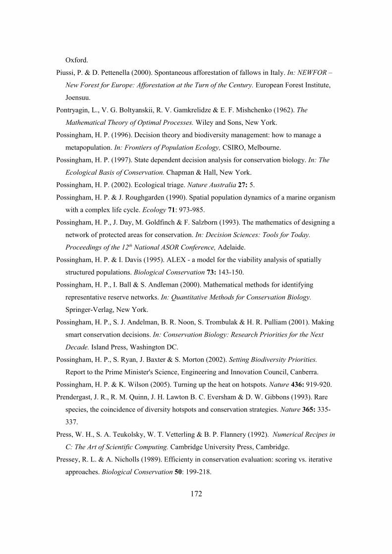
Oxford.
Piussi, P. & D. Pettenella (2000). Spontaneous afforestation of fallows in Italy. In: NEWFOR –
New Forest for Europe: Afforestation at the Turn of the Century. European Forest Institute,
Joensuu.
Pontryagin, L., V. G. Boltyanskii, R. V. Gamkrelidze & E. F. Mishchenko (1962). The
Mathematical Theory of Optimal Processes. Wiley and Sons, New York.
Possingham, H. P. (1996). Decision theory and biodiversity management: how to manage a
metapopulation. In: Frontiers of Population Ecology, CSIRO, Melbourne.
Possingham, H. P. (1997). State dependent decision analysis for conservation biology. In: The
Ecological Basis of Conservation. Chapman & Hall, New York.
Possingham, H. P. (2002). Ecological triage. Nature Australia 27: 5.
Possingham, H. P. & J. Roughgarden (1990). Spatial population dynamics of a marine organism
with a complex life cycle. Ecology 71: 973-985.
Possingham, H. P., J. Day, M. Goldfinch & F. Salzborn (1993). The mathematics of designing a
network of protected areas for conservation. In: Decision Sciences: Tools for Today.
Proceedings of the 12th National ASOR Conference, Adelaide.
Possingham, H. P. & I. Davis (1995). ALEX - a model for the viability analysis of spatially
structured populations. Biological Conservation 73: 143-150.
Possingham, H. P., I. Ball & S. Andleman (2000). Mathematical methods for identifying
representative reserve networks. In: Quantitative Methods for Conservation Biology.
Springer-Verlag, New York.
Possingham, H. P., S. J. Andelman, B. R. Noon, S. Trombulak & H. R. Pulliam (2001). Making
smart conservation decisions. In: Conservation Biology: Research Priorities for the Next
Decade. Island Press, Washington DC.
Possingham, H. P., S. Ryan, J. Baxter & S. Morton (2002). Setting Biodiversity Priorities.
Report to the Prime Minister's Science, Engineering and Innovation Council, Canberra.
Possingham, H. P. & K. Wilson (2005). Turning up the heat on hotspots. Nature 436: 919-920.
Prendergast, J. R., R. M. Quinn, J. H. Lawton B. C. Eversham & D. W. Gibbons (1993). Rare
species, the coincidence of diversity hotspots and conservation strategies. Nature 365: 335-
337.
Press, W. H., S. A. Teukolsky, W. T. Vetterling & B. P. Flannery (1992). Numerical Recipes in
C: The Art of Scientific Computing. Cambridge University Press, Cambridge.
Pressey, R. L. & A. Nicholls (1989). Efficienty in conservation evaluation: scoring vs. iterative
approaches. Biological Conservation 50: 199-218.
172
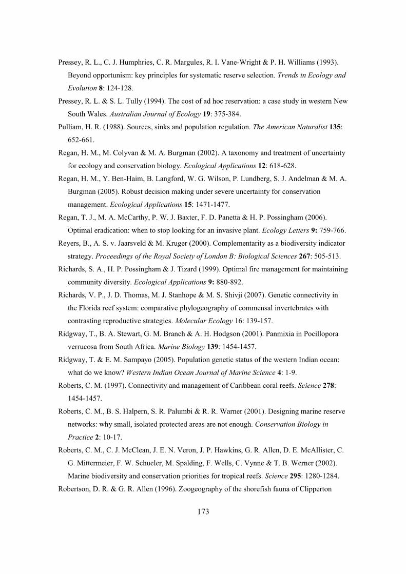
Pressey, R. L., C. J. Humphries, C. R. Margules, R. I. Vane-Wright & P. H. Williams (1993).
Beyond opportunism: key principles for systematic reserve selection. Trends in Ecology and
Evolution 8: 124-128.
Pressey, R. L. & S. L. Tully (1994). The cost of ad hoc reservation: a case study in western New
South Wales. Australian Journal of Ecology 19: 375-384.
Pulliam, H. R. (1988). Sources, sinks and population regulation. The American Naturalist 135:
652-661.
Regan, H. M., M. Colyvan & M. A. Burgman (2002). A taxonomy and treatment of uncertainty
for ecology and conservation biology. Ecological Applications 12: 618-628.
Regan, H. M., Y. Ben-Haim, B. Langford, W. G. Wilson, P. Lundberg, S. J. Andelman & M. A.
Burgman (2005). Robust decision making under severe uncertainty for conservation
management. Ecological Applications 15: 1471-1477.
Regan, T. J., M. A. McCarthy, P. W. J. Baxter, F. D. Panetta & H. P. Possingham (2006).
Optimal eradication: when to stop looking for an invasive plant. Ecology Letters 9: 759-766.
Reyers, B., A. S. v. Jaarsveld & M. Kruger (2000). Complementarity as a biodiversity indicator
strategy. Proceedings of the Royal Society of London B: Biological Sciences 267: 505-513.
Richards, S. A., H. P. Possingham & J. Tizard (1999). Optimal fire management for maintaining
community diversity. Ecological Applications 9: 880-892.
Richards, V. P., J. D. Thomas, M. J. Stanhope & M. S. Shivji (2007). Genetic connectivity in
the Florida reef system: comparative phylogeography of commensal invertebrates with
contrasting reproductive strategies. Molecular Ecology 16: 139-157.
Ridgway, T., B. A. Stewart, G. M. Branch & A. H. Hodgson (2001). Panmixia in Pocillopora
verrucosa from South Africa. Marine Biology 139: 1454-1457.
Ridgway, T. & E. M. Sampayo (2005). Population genetic status of the western Indian ocean:
what do we know? Western Indian Ocean Journal of Marine Science 4: 1-9.
Roberts, C. M. (1997). Connectivity and management of Caribbean coral reefs. Science 278:
1454-1457.
Roberts, C. M., B. S. Halpern, S. R. Palumbi & R. R. Warner (2001). Designing marine reserve
networks: why small, isolated protected areas are not enough. Conservation Biology in
Practice 2: 10-17.
Roberts, C. M., C. J. McClean, J. E. N. Veron, J. P. Hawkins, G. R. Allen, D. E. McAllister, C.
G. Mittermeier, F. W. Schueler, M. Spalding, F. Wells, C. Vynne & T. B. Werner (2002).
Marine biodiversity and conservation priorities for tropical reefs. Science 295: 1280-1284.
Robertson, D. R. & G. R. Allen (1996). Zoogeography of the shorefish fauna of Clipperton
173
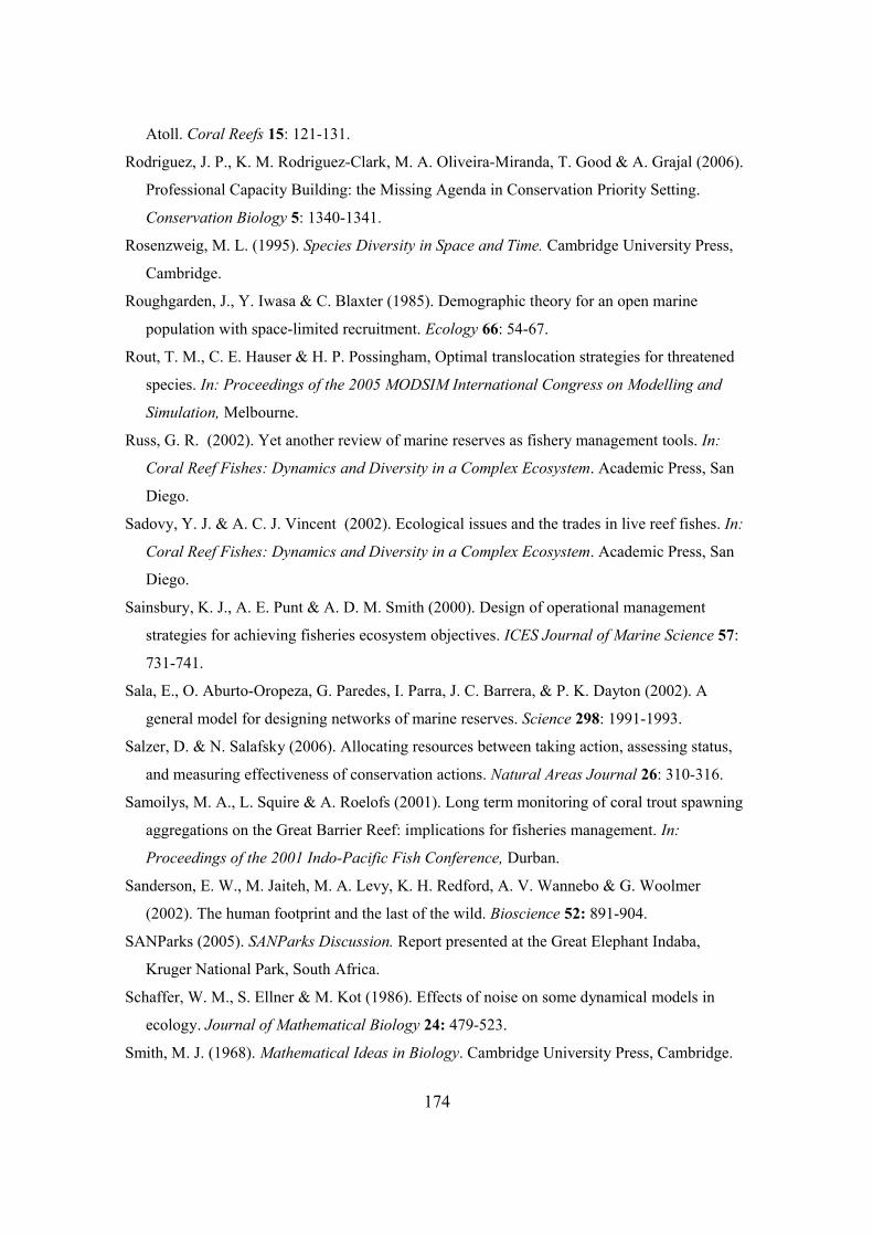
Atoll. Coral Reefs 15: 121-131.
Rodriguez, J. P., K. M. Rodriguez-Clark, M. A. Oliveira-Miranda, T. Good & A. Grajal (2006).
Professional Capacity Building: the Missing Agenda in Conservation Priority Setting.
Conservation Biology 5: 1340-1341.
Rosenzweig, M. L. (1995). Species Diversity in Space and Time. Cambridge University Press,
Cambridge.
Roughgarden, J., Y. Iwasa & C. Blaxter (1985). Demographic theory for an open marine
population with space-limited recruitment. Ecology 66: 54-67.
Rout, T. M., C. E. Hauser & H. P. Possingham, Optimal translocation strategies for threatened
species. In: Proceedings of the 2005 MODSIM International Congress on Modelling and
Simulation, Melbourne.
Russ, G. R. (2002). Yet another review of marine reserves as fishery management tools. In:
Coral Reef Fishes: Dynamics and Diversity in a Complex Ecosystem. Academic Press, San
Diego.
Sadovy, Y. J. & A. C. J. Vincent (2002). Ecological issues and the trades in live reef fishes. In:
Coral Reef Fishes: Dynamics and Diversity in a Complex Ecosystem. Academic Press, San
Diego.
Sainsbury, K. J., A. E. Punt & A. D. M. Smith (2000). Design of operational management
strategies for achieving fisheries ecosystem objectives. ICES Journal of Marine Science 57:
731-741.
Sala, E., O. Aburto-Oropeza, G. Paredes, I. Parra, J. C. Barrera, & P. K. Dayton (2002). A
general model for designing networks of marine reserves. Science 298: 1991-1993.
Salzer, D. & N. Salafsky (2006). Allocating resources between taking action, assessing status,
and measuring effectiveness of conservation actions. Natural Areas Journal 26: 310-316.
Samoilys, M. A., L. Squire & A. Roelofs (2001). Long term monitoring of coral trout spawning
aggregations on the Great Barrier Reef: implications for fisheries management. In:
Proceedings of the 2001 Indo-Pacific Fish Conference, Durban.
Sanderson, E. W., M. Jaiteh, M. A. Levy, K. H. Redford, A. V. Wannebo & G. Woolmer
(2002). The human footprint and the last of the wild. Bioscience 52: 891-904.
SANParks (2005). SANParks Discussion. Report presented at the Great Elephant Indaba,
Kruger National Park, South Africa.
Schaffer, W. M., S. Ellner & M. Kot (1986). Effects of noise on some dynamical models in
ecology. Journal of Mathematical Biology 24: 479-523.
Smith, M. J. (1968). Mathematical Ideas in Biology. Cambridge University Press, Cambridge.
174
Smith, M. J. (1974). Models in Ecology. Cambridge University Press, Cambridge.
Smuts, G. L. (1978). Interrelations between predators, prey and their environment. Bioscience
28: 316-320.
Soulé, M. E. (1985). What is conservation biology? Bioscience 35: 727-734.
Southwood, T. (1977). The relevance of population dynamic theory to pest status. In: Origins of
Pest, Parasite, Disease and Weed Problems. Blackwell Publishing, Oxford.
Stattersfield, A. J., M. J. Crosby, A. J. Long & D. C. Wege (1998). Endemic Bird Areas of the
World. Birdlife International, Cambridge.
Steneck, R. S. (1998). Human influences on coastal ecosystems: does overfishing create trophic
cascades. Trends in Ecology and Evolution 13: 429-430.
Stern, N. (2007). The Economics of Climate Change. Cambridge University Press, Cambridge.
Stewart, K. (2001). Genocide: a Great Australian Tradition? Queensland Culls Make You
Wonder. Report to Animal Liberation Queensland. Downloaded from
http://www.omplace.com/articles/Kangaroo_Cull.html
Stewart, R. R., T. Noyce & H. P. Possingham (2003). Opportunity cost of ad hoc marine reserve
design decisions: an example from South Australia. Marine Ecology Progress Series 253:
25-38.
Stiles, D. (2004). The ivory trade and elephant conservation. Environmental conservation 31:
309-321.
Swearer, S. E., J. E. Caselle, D. E. Lea & R. R. Warner (1999). Larval retention and recruitment
in an island population of coral reef fish. Nature 402: 799-802.
Tabart, D. (2000). Perspective on the management of isolated/island koala populations. In:
Proceedings of the Australian Veterinary Conference. Perth.
Takeuchi, Y. & N. Adachi (1983). Existence and bifurcation of stable equilibrium in two-prey,
one-predator communities. Bulletin of Mathematical Biology 45: 877-900.
Tear, T. H., P. Kareiva & P. Comer (2005). How much is enough? The recurrent problem of
setting measurable objectives in conservation. Bioscience 55: 835-849.
Tenhumberg, B., A. J. Tyre, K. Shea & H. P. Possingham (2004). Linking wild and captive
populations to maximise species persistence: optimal translocation strategies. Conservation
Biology 18: 1-11.
Thomas, C. D., A. Cameron, R. E. Green, M. Bakkenes, L. J. Beaumont, Y. C. Collingham, B.
F. N. Erasmus, M. Ferreira de Siqueira, A. Grainger, L. Hannah, L. Hughes, B. Huntley, A.
S. van Jaarsveld, G. F. Midgley, L. Miles, M. A. Ortega-Huerta, A. T. Peterson, O. L.
Phillips & S. E. Williams (2004). Extinction risk from climate change. Nature 427: 145-148.
175
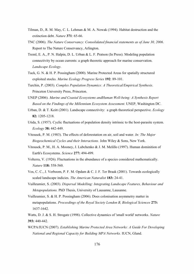
Tilman, D., R. M. May, C. L. Lehman & M. A. Nowak (1994). Habitat destruction and the
extinction debt. Nature 371: 65-66.
TNC (2006). The Nature Conservancy: Consolidated financial statements as of June 30, 2006.
Report to The Nature Conservancy, Arlington.
Treml, E. A., P. N. Halpin, D. L. Urban & L. F. Pratson (In Press). Modeling population
connectivity by ocean currents: a graph theoretic approach for marine conservation.
Landscape Ecology.
Tuck, G. N. & H. P. Possingham (2000). Marine Protected Areas for spatially structured
exploited stocks. Marine Ecology Progress Series 192: 89-101.
Turchin, P. (2003). Complex Population Dynamics: A Theoretical/Empirical Synthesis.
Princeton University Press, Princeton.
UNEP (2006). Marine and Coastal Ecosystems andHuman Well-being: A Synthesis Report
Based on the Findings of the Millennium Ecosystem Assessment. UNEP, Washington DC.
Urban, D. & T. Keitt (2001). Landscape connectivity: a graph theoretical perspective. Ecology
82: 1205-1218.
Utida, S. (1957). Cyclic fluctuations of population density intrinsic to the host-parasite system.
Ecology 38: 442-449.
Vitousek, P. M. (1983). The effects of deforestation on air, soil and water. In: The Major
Biogeochemical Cycles and their Interactions. John Wiley & Sons, New York.
Vitousek, P. M., H. A. Mooney, J. Lubchenko & J. M. Melillo (1997). Human dominition of
Earth's Ecosystems. Science 277: 494-499.
Volterra, V. (1926). Fluctuations in the abundance of a species considered mathematically.
Nature 118: 558-560.
Vos, C. C., J. Verboom, P. F. M. Opdam & C. J. F. Ter Braak (2001). Towards ecologically
scaled landscape indicies. The American Naturalist 183: 24-41.
Vuilleumier, S. (2003). Dispersal Modelling: Integrating Landscape Features, Behaviour and
Metapopulations. PhD Thesis, University of Lausanne, Lausanne.
Vuilleumier, S. & H. P. Possingham (2006). Does colonisation asymmetry matter in
metapopulations. Proceedings of the Royal Society London B, Biological Sciences 273:
1637-1642.
Watts, D. J. & S. H. Strogatz (1998). Collective dynamics of 'small world' networks. Nature
393: 440-442.
WCPA/IUCN (2007). Establishing Marine Protected Area Networks: A Guide For Developing
National and Regional Capacity for Building MPA Networks. IUCN, Gland.
176
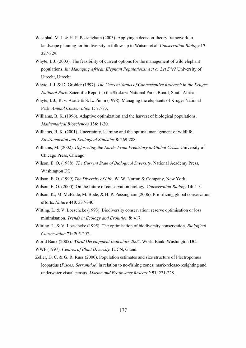
Westphal, M. I. & H. P. Possingham (2003). Applying a decision-theory framework to
landscape planning for biodiversity: a follow-up to Watson et al. Conservation Biology 17:
327-329.
Whyte, I. J. (2003). The feasibility of current options for the management of wild elephant
populations. In: Managing African Elephant Populations: Act or Let Die? University of
Utrecht, Utrecht.
Whyte, I. J. & D. Grobler (1997). The Current Status of Contraceptive Research in the Kruger
National Park. Scientific Report to the Skukuza National Parks Board, South Africa.
Whyte, I. J., R. v. Aarde & S. L. Pimm (1998). Managing the elephants of Kruger National
Park. Animal Conservation 1: 77-83.
Williams, B. K. (1996). Adaptive optimization and the harvest of biological populations.
Mathematical Biosciences 136: 1-20.
Williams, B. K. (2001). Uncertainty, learning and the optimal management of wildlife.
Environmental and Ecological Statistics 8: 269-288.
Williams, M. (2002). Deforesting the Earth: From Prehistory to Global Crisis. University of
Chicago Press, Chicago.
Wilson, E. O. (1988). The Current State of Biological Diversity. National Academy Press,
Washington DC.
Wilson, E. O. (1999).The Diversity of Life. W. W. Norton & Company, New York.
Wilson, E. O. (2000). On the future of conservation biology. Conservation Biology 14: 1-3.
Wilson, K., M. McBride, M. Bode, & H. P. Possingham (2006). Prioritizing global conservation
efforts. Nature 440: 337-340.
Witting, L. & V. Loeschcke (1993). Biodiversity conservation: reserve optimisation or loss
minimisation. Trends in Ecology and Evolution 8: 417.
Witting, L. & V. Loeschcke (1995). The optimisation of biodiversity conservation. Biological
Conservation 71: 205-207.
World Bank (2005). World Development Indicators 2005. World Bank, Washington DC.
WWF (1997). Centres of Plant Diversity. IUCN, Gland.
Zeller, D. C. & G. R. Russ (2000). Population estimates and size structure of Plectropomus
leopardus (Pisces: Serranidae) in relation to no-fishing zones: mark-release-resighting and
underwater visual census. Marine and Freshwater Research 51: 221-228.
177