Decoding codes from curves and cyclic codes

Citation for published version (APA):Duursma, I. M. (1993). Decoding codes from curves and cyclic codes. Eindhoven: Technische UniversiteitEindhoven. https://doi.org/10.6100/IR399251

DOI:10.6100/IR399251

Document status and date:Published: 01/01/1993

Document Version:Publisher’s PDF, also known as Version of Record (includes final page, issue and volume numbers)

Please check the document version of this publication:

• A submitted manuscript is the version of the article upon submission and before peer-review. There can beimportant differences between the submitted version and the official published version of record. Peopleinterested in the research are advised to contact the author for the final version of the publication, or visit theDOI to the publisher's website.• The final author version and the galley proof are versions of the publication after peer review.• The final published version features the final layout of the paper including the volume, issue and pagenumbers.Link to publication

General rightsCopyright and moral rights for the publications made accessible in the public portal are retained by the authors and/or other copyright ownersand it is a condition of accessing publications that users recognise and abide by the legal requirements associated with these rights.

• Users may download and print one copy of any publication from the public portal for the purpose of private study or research. • You may not further distribute the material or use it for any profit-making activity or commercial gain • You may freely distribute the URL identifying the publication in the public portal.

If the publication is distributed under the terms of Article 25fa of the Dutch Copyright Act, indicated by the “Taverne” license above, pleasefollow below link for the End User Agreement:

www.tue.nl/taverne

Take down policyIf you believe that this document breaches copyright please contact us at:

openaccess@tue.nl

providing details and we will investigate your claim.

Download date: 25. Dec. 2019

Decoding Codes from Curves and Cyclic Codes

Iwan M. Duursma

Deco ding

Codes from Curves

and Cyclic Codes

Decoding Codes from Curves and Cyclic Codes

Proefschrift

ter verkrijging van de graad van doctor aan de Technische Universiteit Eindhoven. op gezag van de Rector Magnificus, prof. dr. J .H. van Lint, voor een commissie aangewezen door het College van Dekanen in het openbaar te verdedigen op

maandag 13 september 1993 om 16.00 uur

door

Iwan Maynard Duursma geboren te Bussum

druk: wibro dissertatiedrukkeril. helmond.

Dit proefschrift is goedgekeurd door de promotoren prof. dr. J. H. van Lint en prof. dr. H. Stichtenoth

copromotor: dr. G. R. Pellikaan

CIP-GEGEVENS KONINKLIJKE BIBLIOTHEEK, DEN HAAG

Duursma, Iwan Maynard

Decoding codes from curves and cydic codes/ Iwan Maynard Duursma. - Eindhoven : Technische Universiteit Eindhoven Proefschrift Eindhoven. Met lit. opg. ISBN 90-386-0212-X Trefw. : coderingstheorie / algebraïsche meetkunde.

Pref ace

The thesis describes results of my research on decoding linear codes. This research has been carried out at the Eindhoven University of Technology in the period September 1990 March 1993. It was supported by the Nether­lands Organization for Scientific Research (NWO), through the foundation Stichting Mathematisch Centrum. Some of the results have found their way to international journals. In the order in which they have appeared as preprints they are:

1. "Algebraic decoding using special divisors," IEEE Transactions on Information Theory, volume 39, March 1993.

2. "On the decoding procedure of Feng and Rao," Proceedings Algebraic and Combinatorial Coding Theory 111 Conference, Voneshta Voda, Bulgaria, June 1992.

3. "Majority coset decoding," IEEE Transactions on Information Theory, volume 39, May 1993.

4. with R. Kötter, "Error-locating pairs for cyclic codes," preprint Eindhoven-Linköping, submitted for publication, March 1993.

The papers [1] and [3] each work towards a single theorem, given on page 39 and page 52 respectively of this thesis. The paper [4] has four theorems, on pages 71, 77, 78 and 78. In addition, the tables at pages 86 and 87 give explicit decoding procedures. The introduction further explains the topic and the contributions of the thesis.

I would like to thank the Discrete Mathematics group for the stimula­ting working environment, professor J.H. van Lint for his support and his comments on the preprints and R. Pellikaan for numerous discussions and managing the NWO project. Thanks also to professor G. van der Geer for introducing me to codes from algebra.ic curves and to professor H. Stichtenoth and professor R. Schoof for further discussions on algebra.ic curves. To all, I express my gratitude for judging the final manuscript. For the joint work on cyclic codes, I am grateful to the coauthor R. Kötter.

1 thank the NWO for its financial support. For further support and for hos­pitality I wish to thank the University of Trento and professor R. Schoof, and the University of Linköping and professor T. Ericson.

May, 1993. Iwan Duursma

v

VI

Contents

Preface

Introduction

1 Algebraic decoding

1 A unified description 1.1 Error-locating pairs . 1.2 Error-locating functions 1.3 Error-correcting pairs . . 1.4 Example: projective RM-code 1.5 Additional methods . . . . . .

II Decoding codes from curves

2 Basic algorithm 2.1 Notation ... 2.2 Description . 2.3 Sufficient conditions . 2.4 Decoding and approximation . 2.5 Improvements . . . . . . . . .

3 Modified algorithm 3.1 Special divisors 3.2 Main lemma . . . 3.3 Description . . . 3.4 Additional lemma . 3.5 Plane curves . . . .

4 Majority coset decoding 4.1. Coset decoding . . . . 4.2 Two-dimensional syndromes 4.3 A majority scheme ...

Vil

•.

v

IX

1

3 3 5 7 8

11

15

17 17 19 23 25 27

35 35 38 39 42 43

47 48 49 51

4.4 Description 53 4.5 Comparison 56 4.6 Example .. 60

111 Decoding cyclic codes 67

5 The BCH-bound and beyond 69 5.1 Notation ....... 69 5.2 Decoding BCH-codes . 70 5.3 Recurrences " " " " " " 73 5.4 Correcting more errors 74

6 Pairs from MDS-codes 77 6.1 A class of MDS-codes . .. " " .. 77 6.2 Construction of pairs . " .. " .. 78 6.3 Fundamental iterative algorithm . 79 6.4 Reducing complexity ....... 81

7 Applications 85 7.1 Codes of length less than 63 85 7.2 Sequences of codes " " ... 89

Bibliography 91

Samenvatting (summary in Dutch) 95

Curriculum vitae 96

Vlll

Introd uction

The decoding problem has its roots in communica.tion theory. Two elec­tronic devices exchange information and due to noise or otherwise it will happen that the information received differs from the information sent. It is then assumed that the difference is in general small. In any case it is intended to have small differences by a proper design of the devices and if possible of the channel that connects them. The decoding problem is to attach the proper interpretation to the received information. If the pos­sibilities for the received information are few, the interpretation can be attached to these once and for all and stored in a table. We consider sit­uations where such tables are not feasible. Without a table, i.e. without deciding about interpretations beforehand, one needs a set of rules that can be applied any time information is received. Obviously, one prefers the set of rules to be small and the rules to be such that they can be carried out quickly. These two characteristics determine to a certain extent the size and the speed of a decoding device.

Decoding is not only a problem of the receiver. The sender and receiver together determine how information is to be sent. In air-traffic control it is common use to avoid "yes" and "no" and to say "affirm" and "negative" instead. Sender and receiver have agreed upon this and it greatly enhances the reliability of communication. Similarly, with two electronic devices, the information will be encoded before it is transmitted. The encoding should improve the reliability of the communication and allow easy decoding by the receiver.

The problem has a fruitful translation into mathematics: messa.ge, encoded message and received message are associated with suitable strings of let­ters. The strings of letters are easily transferred into the language of the electronic devices (i.e. strings of zeros and ones) and the rules for encoding and decoding can be formulated in terms of operations that can be carried out by a microprocessor. A small example is obtained with messages of length two that use three different letters A, B, and C. The nine possible messages are:

AA, BA, CA,

AB, BB, CB,

AC, BC, cc.

The messages are very rnuch alike and by changing one letter a messa.ge is transferred into a different message. To enable the receiver to recog­nize that a letter was changed, and thus to improve the reliability of the communication, the messages are encoded as follows:

tX

AAAA, BABC, CACB,

ABBB, BBCA, CBAC,

ACCC, BCAB, CCBA.

The set of possible encoded messages is called a code C, the encoded mes­sages are called codewords. In the example, any two different codewords differ in precisely three positions and agree in the remaining position. If the encoded message reaches the receiver with one letter changed, the receiver can conclude by comparing with all codewords that something went wrong during transmission of the message. Moreover, he can find the message sent as the unique codeword that best resembles the received message, i.e. that differs from the received message in one position. For a given code C, the decoding problem can be formulated as:

• Find the codewords that agree with the received message in a max­imum number of positions. If there is only one such codeword, take

. this codeword for the message sent. Otherwise, leave the interpreta­tion undecided or make a choice.

The bottle-neck in the problem is how to find the codewords that resemble the received message. The most straightforward solution is to compare the received message with all codewords. This is far from e:fficient and we mention two other strategies. The first strategy uses combinatorial properties of the code and is known as permutation decoding. It basically consists of two steps. In genera!, the steps have to be executed several times:

• Guess which letters are correct.

• Find the codewords that match these letters.

Recall, that in the example any two different codewords agree in precisely one position. This combinatorial property tells us how to make suitable guesses: a codeword is determined by any two of its letters and it su:ffices to guess a combination of two letters correctly. Suitable guesses are that ei­ther the first two received letters or the last two received letters are correct. If one error occurred, one of the guesses is true and yields the codeword. For the received messa.ge BBCC, the codewords that match BB-- and --CC are BBCA and ACCC respectively. Thus, the fourth letter was changed and the message sent was BBCA.

Permutation decoding is fast, hut only few examples are known where the strategy works well. The second strategy applies to linear codes, that have the structure of a vector space. It uses algebra.ic properties of the code and is known as algebraic decoding. It consists of two steps, that are executed only once, hut that take more time than the steps in the previous strategy:

x

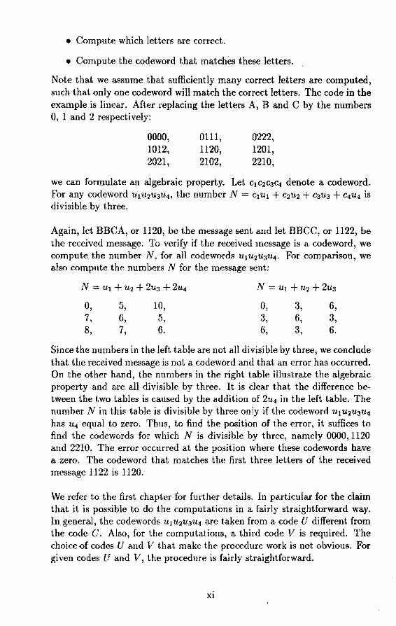
• Compute which letters are correct.

• Compute the codeword that matches these letters.

Note that we assume that sufficiently many correct letters are computed, such that only one codeword will match the correct letters. The code in the example is linear. After replacing the letters A, B and C by the numbers 0, 1 and 2 respectively:

0000, 1012, 2021,

0111, 1120, 2102,

0222, 1201, 2210,

we can formulate an algebra.ic property. Let c1 c2c3c4 denote a codeword. For any codeword u1u2u3u4, the number N = C1U1 + c2u2 + c3u3 + C4U4 is divisible by three.

Again, let BBCA, or 1120, be the messa.ge sent and let BBCC, or 1122, be the received messa.ge. To verify if the received messa.ge is a codeword, we compute the number N, for all codewords u1u2u3u4 • For comparison, we also compute the numbers N for the messa.ge sent:

N = u1 + tt2 + 2u3 + 2tt4 N = u1 + u2 + 2u3

0, 5, 10, o, 3, 6, 7, 6, 5, 3, 6, 3, 8, 7, 6. 6, 3, 6.

Since the numbers in the left table are not all divisible by three, we conclude that the received message is not a codeword and that an error has occurred. On the other hand, the numbers in the right table illustra.te the algebra.ic property and are all divisible by three. lt is clear that the difference be­tween the two tables is caused by the addition of 2u4 in the left table. The number N in this table is divisible by three only if the codeword u1 u2u3u4 has u4 equal to zero. Thus, to find the position of the error, it suffices to find the codewords for which N is divisible by three, namely 0000, 1120 and 2210. The error occurred at the position where these codewords have a zero. The codeword that matches the first three letters of the received messa.ge 1122 is 1120.

We refer to the first chapter for further details. In particular for the claim that it is possible to do the computations in a fairly straightforward way. In general, the codewords u 1 u2u3u4 are taken from a code U different from the code C. Also, for the computations, a third code V is required. The choice of codes U and V that make the procedure work is not obvious. For given codes U and V, the procedure is fairly straightforward.

Xl

In this thesis, 1 give results for the algebraic decoding of two families of linear codes. For each family, methods are given for the construction of de­coding procedures. These can only be obtained by using additional features of a particular family. On the other hand, many questions arise with both families that can be answered for arbitrary linear codes without the restric­tion to a particular family. The results that are valid for arbitrary linear codes are presented in the first part. The first section gives the formulation of a. genera} algebraic decoding procedure. In the next two sections, con­ditions are given tha.t ensure that the procedure works in particular cases. The theory is then applied to an example that is not contained in one of the two families. The last section gives modifications of the general procedure. They apply to some cases where the conditions for the general procedure are not met.

The family of codes /rom curves, also called algebraic geometry codes or simply AG-codes, is in many ways remarkable. The codewords can still be identified with strings of letters, hut they have a more natura} interpreta­tion as rational functions or rational differentials on an algebraic curve. It is immediately clear from the last interpretation and by using well-known results from algebraic-geometry that AG-codes have very good properties. For their application in practice, efficient decoding procedures are required. That algebraic decoding can be applied to AG-codes was noticed ih 1988. The procedure as it was then formulated is called the basic algorithm" AG­codes have an obvious lower bound on the number of errors tha.t can be corrected, called the designed capability. The basic algorithm does not correct up to this bound. For a particular class of AG-codes, a modified algorithm was formulated that corrects more errors hut in general still not up to the designed capability. In Theorem 3.13, 1 give a formulation of the modified algorithm that applies to all AG-codes, rather than toa particular class. Several other improvements of the basic algorithm have been sug­gested. The idea of Feng and Rao is to use different hut related procedures, such that if not the codeword itself at least some more information ahout the codeword will be obtained. Their idea is worked out in Chapter 4. Theorem 4.13 shows that all AG-codes can be decoded up to the designed capability without any further restrictions. The most time consuming cal­culations in the procedure involve solving systems of linear equations. This is not yet fast enough for applications.

For the family of cyclic codes, algebra.ic decoding procedures have been known since the 1960's. Among these procedures, several are fast enough for applications and have been implemented in chips. Similar to AG-codes, cydic codes have an obvious designed capability. The general decoding procedure for cyclic codes does not correct beyond the designed capability. On the other hand, many of the best cyclic codes have an actual capabil-

xii

ity that is better than their designed capability. More recent papers give procedures to decode some of these codes. A simpler and more genera! formulation of these procedures with a shorter proof is given in Theorem 5.6. Two other theorems give decoding procedures for particular classes of cyclic codes. The amount of computation in the procedures compares pre­cisely with the genera! procedure, while the performance is much better for the classes considered. The binary quadratic residue codes of length 23 and 41 can be decoded in this manner. The binary cyclic codes of length less than 63 that have an actual capability exceeding the designed capability have been classified. The theorems in this part yield decoding procedures for all of these hut four.

Part II and Part III are independent and both follow after Part I. Within Part II, the Chapters 3 and 4 are independent. Both follow after Chapter 2. Within Chapter 4, Section 4.5 is independent of the previous sections. One common bibliography is included at the end of the thesis. The results of Part I and Part III were obtained in co-opera.tion with R. Kötter.

The ma.in results appeared in separate preprints and articles and are in­cluded in their original form. They are divided over the thesis as follows: Chapter 3 [9], Chapter 4 [11 ], Section 4.5 [lOJ and Part I and Part llI [12]. Additions in this thesis concern remarks, examples and cross-references. By abuse, we use the phrase decoding up to the minimum dista.nce, where up to half the minimum distance is meant.

xm

XIV

Part 1

Algebraic decoding

1

Chapter 1

A unified description

The most successful methods for decoding linear codes separate the de­coding into the location of the error positions and the determination of the error values. Particular examples are the decoding of cyclic codes up to the BCH-bound and the basic algorithm for the decoding of algebraic­geometric codes. The methods allow a unified description that applies to any linear code. This was noticed by Pellikaan [36], who used it to de­scribe the decoding of AG-codes. Independently but later, Kötter [26] gave a similar description. The location of the error positions is clone with the help of an error-locating pair of vector spaces. To decode a particular linear code, one has to assign such a pair to the code. Fora given error-locating pair, the decoding itself can be performed by solving two systems of linear equations. We first recall the unified description. It applies to any linear code. Thus, it is presented with a minimum of assumptions and notation and the proofs can remain short.

1.1 Error-locating pairs

The n-tuples defined over a field JFform a vector space denoted by lFn. For two vectors u = (uo,u1, ... ,un-d and v = (vo,v1 1 ••• ,vn-1), we define a product u * v = (uovo, U1V1, ... , Un-tVn_i). For two subspaces U, V C IFn, Jet U * V denote the set of vectors { u * v : u E U, v E V}. For a linear code C, we denote the dimension by k(C) and the minimum distance by d(C), or by k and d respectively when no confusion arises.

Definition 1.1 (t-error-locating pair) Let U, V and C be linear codes of length n over the field IF. We call (U, V) a t-error-locating pair for C if the following conditions hold

u * v ç cl., k(U) > t, d(V.L) > t.

3

(1.1) (1.2) (1.3)

Using this definition, we will derive a t-error-locating procedure based on the following central ohservation.

Theorem 1.2 Let (U, V) be a t-error-locating pair for the code C. Let y = c + e be a word in JFn with c E C and e a vector of weight at most t. There exists a non-zero vector u E U such that

n-1

L: YiUjVj = 0, i=O

/or all v EV.

Moreover, any solution u EU of {1.4) satisfies

e*U = 0

(1.4)

(1.5)

Proof. In (1.4) we may replace y bye by condition (1.1). Thus any vector u E U with property (1.5) is a solution to (1.4). Condition (1.2) guarantees the existence of a non-zero vector. This is hecause we impose at most t linear conditions on U. To prove (1.5), we note that (1.4) has the equivalent formulation

Y*UEV.L.

Again replacing y bye and using weight(e)::; tand condition (1.3) we find (1.5). 0

Assume we are given an error-locating pair (U, V) and a received word y. We have to find a solution u E U to the homogeneous system of linea.r equations (1.4). By property (1.5), the coordinates of the vector u take the value zero at the error positions. We will give the matrix defining this system. Let diag(y) denote the n x n matrix which has the elements of y on its main diagonal and which is zero elsewhere. Equation (1.4) ca:n thus he written as:

v · diag(y) · uT = 0, for all v EV.

Obviously, it is enough to consider a set of basis vectors in V, forming a generator matrix Gv for V and we obtain

Gv · diag(y) · uT = 0.

To make this equation solvable with methods of linear algebra we replace u by u = a-Gu, where Gu is a generator matrix for U and u is an element of JFk(U)_ Thus the key equation (1.4) can be rephrased as

S(y). (J'T = 0, (1.6)

where S(y) = Gv · diag(y) · G~.

Any solution O' for (1.6) gives a solution u = uGu for (1.4). The vector u satisfies (1.5). Thus we have descrihed a t-error-locating procedure pro­vided we have a t-error-locating pair. The problem of error-location is now to find the spaces U and V that satisfy conditions (1.1)-(1.3) fora maximal value of t.

4

Remark 1.3 We are completely free in choosing bases for U and V, i.e. in choosing the matrices Gu and Gv, without affecting the space of solutions to the key equation. Nevertheless the choice of Gu and Gv deter­mines the structure of the matrix S(y). We will point out how this affects the computational complexity of solving (1.6) at a later stage.

Remark 1.4 Given a particular error vector e, it is clear from the proof of Theorem 1.2 that the following conditions are sufficient to obtain u E U\O with property (1.5):

C * U ç; VJ..,

3u E U\O : e * u = O, VuEU\O : e*uEVJ..::} e*u=O.

(1.7)

(1.8)

(1.9)

The first condition is equivalent to (1.1). Conditions (1.8) and (1.9) are weaker than conditions (1.2) and (1.3) respectively. We will have to refer to them in some cases where the conditions in Definition 1.1 are too strong.

1.2 Error-locating functions

Theorem 1.2 in the previous subsection gives a possibility to determine the error positions as zeros of a word u E U. This describes the general case. In some known algorithms, in particular for BCH-codes and AG-codes, an error-locating word u is associated in a natural way with an error-locating function. We will need this connection to make some properties of u and the corresponding error-locating function more transparent. Also the relation with functions is helpful in actually finding pairs (U, V). The rest of the section is devoted to this relation. · We have derived two sets of sufficient conditions for an error-locating pair. A pair with (1.1)-(1.3) locates all error patterns of a given weight. Such a pair is hard to find in genera!. Conditions (1.7)-(1.9) are weaker. They are formulated for a particular error pattern however and the verification for a large class of error patterns becomes cumbersome. We formulate a set of conditions that can be seen as a compromise. The conditions depend on the positions of the errors hut not on the particular error values.

Lemma 1.5 For an error vector e, let E (resp. E) be the subspace of JFn consisting of all vectors that have zero components in the error (resp. non-error) positions. The f ollowing conditions are sufficient to locate the error positions with the pair (U, V):

c*uç;v1

UnE=f=O VJ.. n = 0.

Proof. The conditions imply (1.7)-(1.9).

5

0

The conditions of the lemma can be expressed in terms of functions. We need the following.

Notation 1.6 For a field JF, let S be the the JF-algebra of n-tuples defined over IF with component-wise multiplication and addition. Let R be a JF-algebra without zero-divisors, such that there exists a surjective homomorphism Ev: R--+ S, with kemel J. Fora code C C S, let L(C) C R denote a JF-vector space such that the restriction of Ev to L( C) is a IF-vector space isomorphism from L( C) to C. In particular L(C) n 1 = (0).

Remark 1. 7 R will be identified with a ring of functions. Ev is then the evaluation mapping, that means the evaluation of f E R in a set of points. Ev naturally induces an IF-algebra isomorphism between R/ I and s.

Example 1.8 For cyclic codes we take R = IF[x]. Let a E IF be a primitive n-th root of unity. Ev is the evaluation map that evaluates

1 . 1 . . t {1 2 n 1} . po ynom1a s m pom s , a, a , ... , a - , i.e.

Ev(x) = (1,a,a2 , ••• ,an-l).

The ideal I C R is generated by xn 1. Cyclic codes are the subject of Part HL

Example 1.9 For algebra.ic-geometrie codes, an evaluation map Ev occurs in their definition [21],[52]. AG-codes are the subject of Part II. In this chapter we take the conditions (1.1 )-(1.3) as starting point to study decoding, since they are general and apply to any linear code. In Sections 2.2 and 2.3, we point out the particulars of AG-codes and their decoding.

Now, let an algebra-homomorphism Ev: R--+ S be given as in Notation 1.6. The reformulation of Lemma 1.5 becomes

Lemma 1.10 Let L(U), L(VL) and L(C) map to the codes U, v.t and C after evaluation. Let the maps be bijective as in Notation 1.6. For an error vector e, let J (resp. JJ be the ideal in R consisting of all elements that evaluate to zero at the error (resp. non-error) positions. The following conditions are sufficient to locate the error positions with the pair ( U, V):

L(C) * L(U) Ç L(V.L) + !, L(U) n J f:. (0),

L(V.t) n J = (0).

Proof. lmmediate from Lemma 1.5. D

The question arises whether an error-locating procedure can be formulated in terms of error-loca.ting functions. This is indeed the case. The decoding procedures for BCH-codes [4, p.248] or AG-codes [24, 48] use this approach. L( C), L( U) and L(V .L) have here a natural interpretation.

6

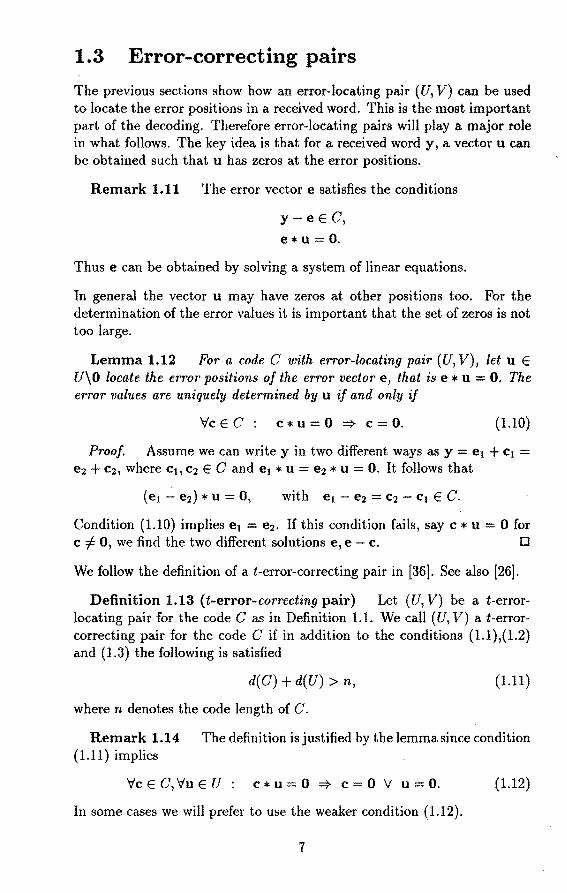
1.3 Error-correcting pairs

The previous sections show how an error-locating pair (U, V) can be used to locate the error positions in a received word. This is the most important part of the decoding. Therefore error-locating pairs will play a major role in what follows. The key idea is that for a received word y, a vector u can be obtained such that u has zeros at the error positions.

Remark 1.11 The error vector e satisfies the conditions

y-e E C,

e*U 0.

Thus e can be obtained by solving a system of linear equations.

In general the vector u may have zeros at other positions too. For the determination of the error values it is important that the set of zeros is not too large.

Lemma 1.12 For a code C with error-locating pair (U, V), let u E U\O locate the error positions of the error vector e, that is e * u = 0. The error values are uniquely determined by u ij and only ij

\Ic E C : c * u = 0 => c = 0. {1.10)

Proof. Assume we can write y in two different ways as y = e1 + c1 = e2 + c2, where c1, c2 E C and e1 * u = e2 * u = 0. It follows that

Condition (1.10) implies e1 = e2• If this condition fails, say c * u = 0 for c i= O, we find the two different solutions e, e - c. D

We follow the definition of a t-error-correcting pair in [36]. See also [26].

Deflnition 1.13 (t-error-correcting pair) Let (U, V) be a t-error­locating pair for the code C as in Definition 1.1. We call (U, V) at-error­correcting pair for the code C if in addition to the conditions (1.1),(1.2) and {1.3) the following is satisfied

d(C) + d(U) > n, (1.11)

where n denotes the code length of C.

Remark 1.14 The definition is justified by the lemma since condition (1.11) implies

\Ic E C, Vu E U c * u = 0 => c = 0 v u = 0. (1.12)

In some cases we will prefer to use the weaker condition (1.12).

7

Remark 1.15 Recall that a pair (U, V) needs to satisfy C * U ç v.i to be error-locating fora code C. By the lemma, an error-locating pair will be error-correcting if it satisfies

C* * U* Ç (V.i )'".

Remark 1.16 In terms of functions, a pair (U, V) needs to satisfy L(C) * L(U) Ç L(V.l) + 1 to be error-locating. By the lemma it will be error-correcting if it satisfies

L(C) * L(U) Ç L(VL).

Here we use the fact that R has no zero-divisors and that L(V.l) n I = (0). Let (L(C) * L(U)) denote the linear space spanned by all functions in L(C) * L(U). The following conditions are then suflicient to guarantee error-correction with a pair (U, V):

L(U) n J =/= (0), (L(C) * L(U)) n J = (0).

(1.13) (1.14)

The dilemma in algebraic decoding is obvious. For (1.13), we want L(U) to be large and for (1.14) we want (L(C) * L(U)} to be small, that means L( U) should be small. ·

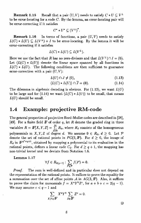
1.4 Example: projective RM-code

The general properties of projective Reed-Muller codes are described in [28], [49]. For a finite field 1F of order q, let R denote the graded ring in three

00

variables R = IF[X, Y, Z] = E Rd, where Rd consists of the homogeneous d=O

polynomials in X, Y, Z of degree d. We assume 0 E ~' d ~ 0. Let P denote the set of rational points in PG(2, JF). For d ~ 0, the image of Rd in 1Fq

2

+q+l, obtained by mapping a polynomial to its evi'Lluation in the rational points, defines a linear code Cd. For d ~ q + 1, the mapping has non-trivia! kemel and we deviate from Notation 1.6.

Lemma 1.17 v f E R2(q-1): L f(P) = 0.

PEP Proof The sum is well-defined and in particular does not depend on

the representation of the rational points. It suflices to prove the equality for a summation over the set of afline points A in AG(3, IF). Also, it suflices to prove the claim for monomials f = xayb ze, fora+ b + c 2(q - 1). We may assume c < q - 1 and

L xayb L ZC=O. X,YelF zelF

D

8

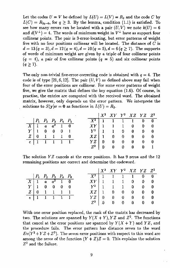
Let the codes U = V be defined by L(U) = L(V) = R2 and the code C by L(C) = R2q_6 , for q 2 3. By the lemma, condition (1.1) is satisfied. To see how many errors can be located with a pair (U, V) we note k(U) = 6 and d(V.L) = 4. The words of minimum weight in V.L have as support four collinear points. The pair is 3-error-locating, hut error patterns of weight five with no four positions collinea.r will be located. The distance of C is d = 13(q = 3),d = 12(q = 4),d = lO(q = 5),d = 6(q 2: 7). The supports of words of minimum weight are given by a triple of four collinear points (q = 4), a pair of five collinear points (q = 5) and six collinea.r points (q 2 7).

The only non-trivial five-error-correcting code is obtained with q = 4. The code is of type [21, 6, 12]. The pair (U, V) as defined above may fail when four of the error positions are collinea.r. For some error patterns of weight five, we give the matrix that defines the key equation (1.6). Of course, in practise, the entries are computed with the received word. The obtained matrix, however, only depends on the error pattern. We interprete the solutions to S(y)u = 0 as functions in L(U) = R2.

x2 XY y2 xz YZ z2 P1 P2 Pa P4 Ps x 1 1 1 1 0 0

x 1 a a 1 0 XY 1 1 1 0 0 0 y 1 0 0 0 1 y2 1 1 0 0 0 0 z 0 1 1 1 0 xz 1 0 0 0 0 0 e 1 1 1 1 1 YZ 0 0 0 0 0 0

z2 0 0 0 0 0 1

The solution Y Z cancels at the error positions. It has 9 zeros and the 12 remaining positions are correct and determine the codeword.

x2 XY y2 xz YZ z2 P1 P2 Pa P4 p6 x2 1 1 1 1 0 0

x 1 a a2 1 0 XY 1 1 1 0 0 0 y 1 0 0 0 0 y2 1 1 1 0 0 0 z 0 1 1 1 1 xz 1 0 0 0 0 0 e 1 1 1 1 1 YZ 0 0 0 0 0 0

z2 0 0 0 0 0 0

With one error position replaced, the rank of the matrix has decreased by two. The solutions are spanned by Y(X + Y), YZ and Z 2• The functions that cancel at the error positions are spanned by Y(X + Y) and YZ, and the procedure fails. The error pattern has distance seven to the word Ev(Y2 + Y Z + Z 2

). The seven error positions with respect to this word are among the zeros of the function (Y + Z)Z = 0. This explains the solution Z 2 and the failure.

9

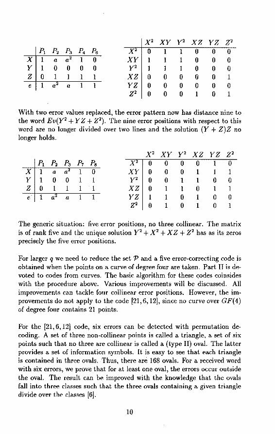
x2 XY y2 xz YZ z2 Pi P2 P3 P4 p6 x 0 1 1 0 0 0

x 1 a a 1 0 XY 1 1 1 0 0 0 y 1 0 0 0 0 y2 1 1 1 0 0 0 z 0 1 1 1 1 xz 0 0 0 0 0 1 e 1 a2 a 1 1 YZ 0 0 0 0 0 0

z2 0 0 0 1 0 1

With two error va.lues replaced, the error pattern now has distance nine to the word Ev(Y2 + Y Z + Z2

). The nine error positions with respect to this word are no longer divided over two lines and the solution (Y + Z)Z no longer holds.

x2 XY y2 xz YZ z2 P1 P2 P3 P1 Ps x 0 0 0 0 1 0

x 1 a a2 1 0 XY 0 0 0 1 1 1 y 1 0 0 1 1 y2 0 0 1 1 0 0 z 0 1 1 1 1 xz 0 1 1 0 1 1 e 1 a2 a 1 1 YZ 1 1 0 1 0 0

Z2 0 1 0 1 0 1

The generic situation: five error positions, no three collinear. The matrix is of rank five and the unique solution Y2 + X 2 + X Z + Z 2 has as its zeros precisely the five error positions.

For larger q we need to reduce the set P and a five error-correcting code is obtained when the points on a curve of degree four are taken. Part II is de­voted to codes from curves. The ba.sic algorithm for these codes coinsides with the procedure above. Various improvements will be discussed. All improvements can tackle four collinear error positions. However, the im­provements do not apply to the code [21,6, 12], since no curve over GF{4) of degree four contains 21 points.

For the [21, 6, 12] code, six errors can be detected with permutation de­coding. A set of three non-collinear points is called a triangle, a set of six points such that no three are collinear is called a (type II) oval. The lat ter provides a set of information symbols. It is easy to see that each triangle is contained in three ovals. Thus, there arè 168 ovals. Fora received word with six errors, we prove that for at least one oval, the errors occur outside the oval. The result can be improved with the knowledge that the ovals fall into three classes such that the three ovals containing a given triangle divide over the classes [6].

10

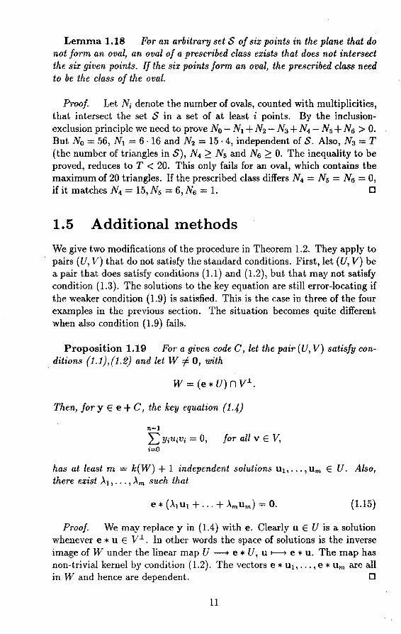
Lemma 1.18 For an arbitrary set S of six points in the plane that do not form an oval, an oval of a prescribed class exists that does not intersect the six given points. IJ the six points form an oval, the prescribed class need to be the class of the oval.

Proof Let Ni denote the number of ovals, counted with multiplicities, that intersect the set S in a set of at least i points. By the inclusion­exclusion principle we need to prove No - N1 + N2 - N3 + N4 - Ns + N6 > 0. But No= 56, Ni = 6·16 and N2 = 15 · 4, independent of S. Also, N3 = T (the number of tria.ngles in S), N4 ~ N5 and N6 ~ 0. The ineqµality to be proved, reduces to T < 20. This only fails for an oval, which contains the maximum of 20 triangles. If the prescribed class differs N4 = N5 = N6 = 0, if it matches N4 = 15, Ns = 6, N6 = 1. D

1.5 Additional methods

We give two modifications of the procedure in Theorem 1.2. They apply to pairs (U, V) that do not satisfy the standard conditions. First, let (U, V) be a pair that does satisfy conditions (1.1) and (1.2), but that may not satisfy condition (1.3). The solutions to the key equation are still error-locating if the weaker condition (1.9) is satisfied. This is the case in three of the four examples in the previous section. The situation becomes quite different when also condition (1.9) fails.

Proposition 1.19 Fora given code C, let the pair (U, V) satisfy con-ditions {1.1},{1.2} and let W iz 0, with

w = (e * U) n v.L.

Then, for y E e + C, the key equation {1.4)

n-1

LYiUiVi = 0, for all v E V, i=O

has at least m = k(W) + 1 independent solutions U1, ... , Um E U. Also, there exist ..\1, ... , Àm such that

(1.15)

Proof. We may replace yin (1.4) with e. Clearly u E U is a solution whenever e * u E V .L. In other words the space of solutions is the inverse image of W under the linear map U--+ e * U, u 1---t e * u. The map has non-trivia! kemel by condition (1.2). The vectors e * u1 , .•• , e * Um are all in W and hence are dependent. D

11

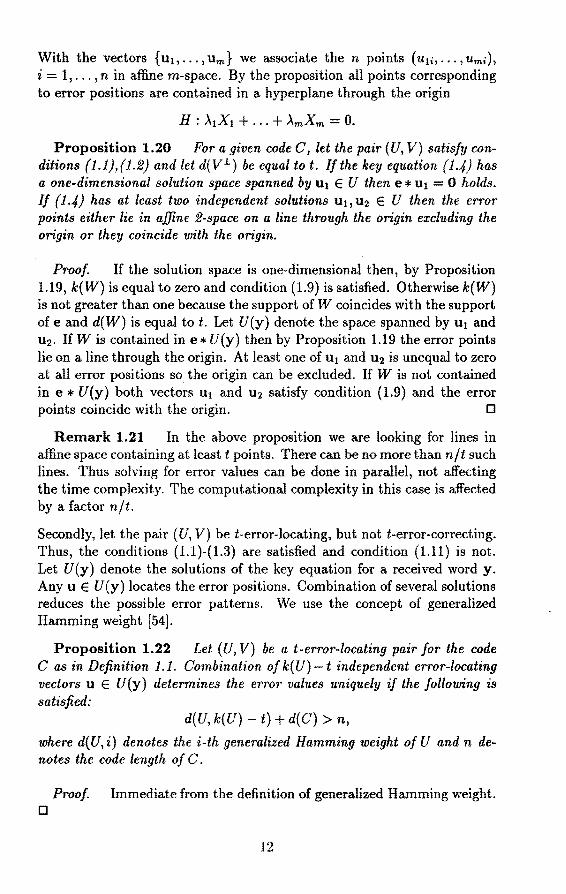
With the vectors {ui, ... , um} we associate the n points (u1;, ••• , Umi),

i = 1, ... , n in affine m-space. By the proposition all points corresponding to error positions are contained in a hyperplane through the origin

H : À1X1 + ... + ÀmXm = 0.

Proposition 1.20 Fora given code C, let the pair (U, V) satisfy con­ditions ( 1.1), ( 1. 2) and let d( V .L) be equal to t. IJ the key equation { LI) has a one-dimensional solution space spanned by Ut E U then e * Ut = 0 holds. lf (1.,/.) has at least two independent solutions Ut, U2 E U then the error points either lie in affine 2-space on a line through the origin excluding the origin or they coincide with the origin.

Proof. If the solution space is one-dimensional then, by Proposition 1.19, k(W) is equal to zero and condition (1.9) is satisfied. Otherwise k(W) is not greater than one because the support of W coincides with the support of e and d(W) is equal tot. Let U(y) denote the space spanned by u 1 and u2 • If Wis contained in e * U(y) then by Proposition 1.19 the error points lie on a line through the origin. At least one of u1 and u2 is unequal to zero at all error positions so the origin can be excluded. If Wis not contained in e * U(y) both vectors u1 and u 2 satisfy condition (1.9) and the error points coincide with the origin. D

Remark 1.21 In the above proposition we are looking for lines in affine space containing at least t points. There can be no more than n/t such lines. Thus solving for error values can be clone in parallel, not affecting the time complexity. The computational complexity in this case is affected by a factor n/t.

Secondly, let the pair (U, V) be t-error-locating, hut not t-error-correcting. Thus, the conditions (1.1)-{1.3) are satisfied and condition {l.11) is not. Let U(y) denote the solutions of the key equation fora received word y. Any u. E U (y) locates the error positions. Combination of several solutions reduces the possible error patterns. We use the concept of generalized Hamming weight [54].

Proposition 1.22 Let (U, V) be a t-error-locating pair for the code Cas in Definition 1.1. Combination of k(U)-t independent error-locating vectors u E U(y) determines the et-rot values uniquely if the following is satisfied:

d(U, k(U) t) + d(C) > n,

where d(U, i) denotes the i-th generalized Hamming weight of U and n de­notes the code length of C.

Proof. Immediate from the definition of generalized Hamming weight. D

12

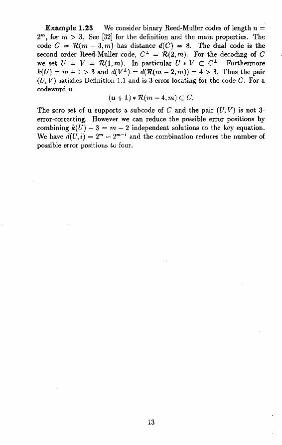
Example 1.23 We consider bina.ry Reed-Muller codes of length n = 2m, for m > 3. See [32] for the definition and the main properties. The code C = 'R( m - 3, m) bas distance d( C) = 8. The dual code is the second order Reed-Muller code, Cl. = 'R(2, m). For the decoding of C we set U = V = 'R(l, m ). In particular U * V C Cl.. Furthermore k(U) = m + 1 > 3 and d(Vl.) = d('R(m - 2,m)) = 4 > 3. Thus the pair (U, V) satisfies Definition 1.1 and is 3-error-locating for the code C. For a codeword u

(u + 1) * 'R(m- 4,m) CC.

The zero set of u supports a subcode of C and the pair (U,V) is not 3-error-correcting. However we can reduce the possible error positions by combining k(U) - 3 = m - 2 independent solutions to the key equation. We have d(U, i) = 2m - 2m-i and the combination reduces the number of possible error positions to four.

13

14

Part II

Decoding codes from curves

15

Chapter 2

Basic algorithm

The basic a.lgorithm (BA) [24], [48] traces the error locations in a received word. It yields a so-called error-locating function and the error locations occur among the zeros of this function. In the original set up, two con­ditions guarantee the determination of an error-locating function with a sufficiently small number of zeros. In Section 2.3, we weaken the two con­ditions and show that they still yield correct decoding. In both cases, the claims follow from the results of the previous part. In the present con­text of codes from curves, we have a natural interpretation of the algebraic decoding procedure. It is discussed in Section 2.4. The basic a.lgorithm does not correct up to the designed capability of a code. In Section 2.5, we recall improvements by Pellikaan [38] and by Ehrhard [16]. Two other improvements are treated in separate chapters.

2.1 Notation

We recall some concepts from the theory of algebra.ic curves and give their notation and some additional assumptions. The concepts are treated in detail in the hooks: [7], [20] and [23]. More recent hooks pay special attention to the case of a finite constant field and to the applications in coding theory: [30],[35],[51] and [52]. Although the concepts are fairly standard, their description may differ a lot from one book to another.

Notation 2.1 In the fol1owing, a curve X, or X/Fq, is always abso­lutely irreducible, non-singular, complete and defined over a fini te field, of q elements. The field of rational functions is denoted by Fq(X), the module of rational differential forms by !l(X). Points on a curve are identified with places of the function field, rational points with places of degree one. Let t denote a generator of the maxima! ideal of a place. For a function /, we define the divisor (/) = L,vt(f)P, where P runs over all places and Vt denotes the discrete valuation at P. For a differential w, we define the divisor (w) = L,vt(w)P, where P runs over all places and Vt(/dt) = Vt(f).

17

A divisor is called principal if it is the divisor of a function. The relation E1 "' E2 if and only if E1 - E2 is principal, defines an equivalence rela­tion on divisors. The unique divisor class containing the divisors (w ), w a rational di:fferential, is called the canonical divisor class. A representative is denoted by K. For a divisor E, the linear spaces f!(E) and L(E) are defined by

f!(E) = {w E f!(X)*: (w) ~ E} U {O},

L(E) = {fEFq(X)*: (f)+E~O} U {0}.

The integers i(E) and l(E) denote the dimension ofthe spaces f!(E) and L(E) respectively. Each differential w induces a natural isomorphism

L(E) ~ f!((w) - E), f 1-+ fw. (2.1)

The divisor K satisfies: deg(K) = 2g - 2 and l(K) = g. The integer g is called the genus of the curve. The genus g of a plane curve of degree m satisfies g = (m - l){m - 2)/2. Fora plane curve, let the divisor L denote the intersection divisor of a line with the curve.

The main results on algebraic curves to be used are

Theorem 2.2 (Residue theorem} The summation over all places of the residues of a differential is well-defined and equal to zero.

Theorem 2.3 ( Approximation theorem} For a divisor E and a finite set of places S, there exists a divisor E' that is linearly equivalent to E and that has support outside S.

Theorem 2.4 (Riemann-Roch theorem) The dimensions of L(E) and f!(E) are related by

l(E) - i(E) = deg(E) + 1 - g.

Theorem 2.5 (Clifford's theorem) For a divisor E with both L(E) and f!(E) non-trivia!, the following holds

l(E) $ deg~E) + 1.

The results and their proofs are described in the literature mentioned above. The latter two theorems are recalled in a different form in the next chapter. For the definition of a linear code with an algebraic curve, we recall the construction of V.D. Goppa.

Let X be a curve. Let P1 , P2 , ••• , Pn be n distinct rational points on the curve. Then for the divisors D( = P1 + P2 + ... + Pn) and G ( defined over Fq) one can define algebraic-geometric codes Co(D, G), known as residue code, and CL(D, G), known as functional code. The pair of divisors {D, G} that we use to define a code, corresponds with a pair {'P, D} in [52].

18

Definition 2.6 (Goppa) We assume that D and G have disjoint sup­port, without loss of generality. By abuse of notation, we will write P ED, rather than P E supp(D). The codes Cn(D, G) and CL(D, G) are defined as the images of the linear maps

an : O(G - D) ---+ F;, w 1-+ ( resp(w) )PeD,

aL: L(G) ---+ F;, ft-+(f(P))PED·

In particular, ao and O'L induce natural isomorphisms

ao O(G-D)/O(G) --.:'...+ Co(D,G), O'L L(G)/L(G-D) --.:'...+ CL(D,G).

The isomorphisms yield expressions for the dimension of the codes.

Theorem 2.7 (Goppa) Fordeg(G) > deg(K), the codeCo(D,G) has parameters

k 2:: deg(K + D - G) + 1 - g, d;:::: d* = deg(G- K).

For deg(D) > deg(G), the code C1(D,G) has parameters

k;:::: deg(G) + 1 - g, d;:::: d* = deg(D - G).

Based on the isomorphism of linear spaces (2.1), a functional code can al­ways be represented by a residue code. The residue code and the functional code are dual by the Residue theorem.

Remark 2.8 In case the divisors D and G have a rational point P in common, we follow the H-construction [52]. Let ordp(G) = i and let t denote a local parameter at P. Then the mappings ao, aL are modified at the coordinate P:

O(G-D) ---+

L(G) ---+ F9 ,

2.2 Description

Fq, w 1-+ ( resp(Ciw) ),

f t-+ ( (ti/)(P))PeD·

Let C be a residue code Co(D, G). It has dual code CJ. = CL(D, G). To apply the procedure of the previous chapter to decode C we need an. error-locating pair (U, V) as in Definition 1.1. We choose a. pair (U, V) of AG-codes. Fora divisor F with support disjoint from D, let U = C1(D,F) and V CL(D,G - F). This will sa.tisfy condition (1.1). The other conditions for a t-error-locating pair are

k(U) > t, d(V-1

) > t.

19

With Goppa's theorem we write

deg( F) + 1 - g 2 t + 1,

deg( G - F - K) 2 t + 1.

Theinequalitiesaresatisfiedonlyif2t ~ deg(G-K)-1-g = d*-I-g. For t in that range they are satisfied with F of degree L ( deg( G - K) - 1 + g) /2 J . The pair is t-error-correcting when condition ( 1.11) is satisfied

d(U) + d(C) > n,

Or deg(D - F) + deg(G - K) > deg(D).

But the pair fulfills already the stronger condition deg( G - F - K) > t and is thus t-error-correcting. The proof is from [36]. The decoding procedure itself is formulated in [24] and [48]. We recall their description in terms of algebraic functions without explicit reference to the pair (U, V).

Say the code C = Cn(D,G) has parity check matrix H. Let y = (yP)PeD denote a received word with error pattern e = ( ep )PeD· Thus,

Het= Hyt. (2.2)

An error-locator function f is defined by the property

f(P)#O => ep=O. (2.3)

The BA consists of finding a nonzero error-locator function J and then solving (2.2,2.3). To explain how f can hè obtained and to formulate the BA we use

Definition 2.9 With a vector y = (yp )PeD we associate a one-dimen sional syndrome S(y),

S(y) L(G) -----+ Fq, h ~ L: yp h(P).

PED

With a divisor P, we associate a two-dimensional syndrome S(F),

S(F) : L(F) x L(G - F) -----+ Fq, (J,g) ~ S(y)(Jg).

Remark 2.10 The syndrome S(F) depends on the vector y, hut this is suppressed in the notation. For a fixed received word y, it will often be necessary to consider the syndrome S(F), for various divisors F, and we anticipate this situation.

20

Lemma 2.11 The syndrome S(y) in the definition is a coset invari-ant, that is

S(y) = S(e) # y E e + Gn(D,G).

A fortiori S(F) is a coset invariant.

Proof. From the definition,

S(y-e)=O # y-eECL(D,G)J.=Co(D,G).

0

Definition 2.12 Fora syndrome S(F), the key equation is defined as

S(F)(f,g) = 0, Vg E L(G - F). (2.4)

The vector spa.ce of solutions f E L(F) to the key equation is denoted by I<(F), its dimension by k(F).

Remark 2.13 The dimension k(F) only depends on the equivalence class of the divisor F. Thus in considering the dimension, we may assume that the divisors F and D have disjoint support. In three of the later improvements of the basic algorithm, in particular in Proposition 2.36, choices of F occur that contain rational points among their support. As long as the evaluation of (f g)(P) takes place after the multiplication of the functions f and g this poses no problem. The interpretation in terms of error-locating pairs only holds when the functions f and g can be evaluated separately. More important, separate evaluation leads to faster procedures [15). This is achieved by following the H-construction and using a local parameter t at P,

(f g)(P) = (ëf)(P) · (rig)(P), for i = ordp(F).

Note that we assume that P is not contained in G.

Lemma 2.14 ([48],[38]) Let the divisor Q consist of the error loca­tions, that is Q = 'Eer#O P. In general, L(F - Q) Ç K(F), and

G0 (Q,G F) = 0 => L(F- Q) = I<(F) (2.5)

Proof. In the definition of S(F), we may replace y bye. Theinclusion L(F Q) Ç I<(F) is obvious. The assumption is needed for the other inclusion. It implies that (0,".,1"."0) E GL(Q,G- F) for all unit vectors of length deg(Q). Thus in the definition of I<(F), if g runs through L( G-F), the unit vector with support the point P E Q poses the restriction K(F) Ç L(F P). Together the unit vectors yield I<(F) Ç L(F - Q). 0

21

Remark 2.)5 ([24, plane curves],[48, general]) The main steps of the BA can be summarized as follows:

{BO) Fixa divisor F. {Bl) Calculation of the key matrix S(F). (B2) Calculation of a nonzero function fin K(F). {B3) Calculation of the zero divisor of the function f. {B4) Calculation of the error values in (2.2,2.3).

In case the curve used is the projective line and the divisors G and F are a multiple of the point at infinity, the algorithm reduces to the Peterson­Gorenstein-Ziegler decoder [4].

The divisor F determines the error patterns that will be corrected. The following theorem gives the degree of the divisor F, that optimizes the algorithm.

Theorem 2.16 ([24, plane curves],[48, general]) Let C = Co(D, G) be a residue code. The BA with F a divisor of degree L(d"' - 1)/2 + g/2J with support disjoint from D will correct any error pattern of weight up to L(d* - 1)/2 - 9/2J.

Proof. Wehavedeg(G-F-Q);::: deg(G)-(d*-1) = deg(I<)+l. Thus Co(Q, G-F) = O and step (B2) yields f E L(F-Q). With deg(F-Q);::: g we can take f nonzero. We may assume that (d* - 1)/2 - g/2 > 0 or deg(F) < d* - 1. Thus in step (B3) at most d"' - 2 possible error locations are obtained and step (B4) has the error vector as a uni que solution. D

The basic algorithm led Pellikaan to the definition of error-locating pairs and the similarity between the two descriptions we have given is obvious. An advantage of the error-locating pairs is their generality. They will be used in the next part on cyclic codes too. The description in terms of func­tions on the other hand is formulated in terms of the divisor Q and makes clear why some error patterns of a given weight are correctly decoded, while others of the sarhe weight are not.

Another approach to the decoding of AG-codes was taken by Porter [40]. His approach mimics the use of a key equation involving differentials as in the decoding of classical Goppa codes. Ina joint paper with Pellikaan and Shen [41 ], the proofs of [40] are completed and in some cases corrected. Ehrhard [14] generalized the approach in [40] to obtain a description of the key equation for arbitrary AG-codes. The similarity of his description with the basic algorithm is less obvious and was established in [14].

22

2.3 Suffi.cient conditions

We study in more detail the dependence of the basic algorithm on the par­ticular error locations, i.e. the divisor Q. In Lemma 2.18, we present two conditions that guarantee error-correction. They have a more general for­mulation in the form of the conditions (1.13) and (1.14).

Lemma 2.17 Let y denote an arbitrary vector of length n = deg(D). Let two different vectors e 1 and e 2 E y + Co(D, G) have as their support the divisors Q1 and Q2 respectively. Then

Proof. We prove the reverse direction and assume F ,.., Q2 + E, for E ~ 0. Let the support of x = e1 - e2 E Co(D, G) be given by Qx ::;; Qi + Q2. Then, x = (resp(w))PeD for some nonzero w E O(G - Qx)· A fortiori w E O(G Qi Q2 - E). D

Lemma 2.18 For a vector e E y + Co ( D, G) with support Q, let the f ollowing be fulfilled

O(G-F-Q)=O, and

L(F Q) =/= 0.

(2.6)

(2.7)

Then the vector e is the unique vector in y + Co(D, G) with (2. 7). Appli­cation of the basic algorithm yields in step {B2) an error-locating function /or e and in step (B4) the vector e itself.

Proof. By (2.6) and the previous lemma, any other vector in the coset does not satisafy (2.7). By (2.6) and Lemma 2.14, the function f E K(F) is error-locating. By (2. 7), we may assume f is non-trivial. The vector e is a solution to the equations (2.2,2.3). Since f is non-trivial, equation (2.3) can only be fulfilled fora vector which support satis:fies (2.7). But we saw that e is the only such vector. D

If the conditions on Q are fulfilled, it is likely to be for a vector e of small weight. But this need not be the vector of smallest weight in the coset. To give an example we use

Notation 2.19 Let the coset y + Co(D, G) contain two vectors e1

and e2 that have disjoint supports. Let the divisors Q1 and Q2 consist of the points in the support of e1 and e2 respectively. Let the weight of the vector e 1 - e2 be equal to the designed minimum distance of the code Co(D, G). In particular, G Qi Q2 "'K.

23

Example 2,20 For the vectors e1 and e2 as above, the implication in Lemma 2.17 is in fact an equivalence. The conditions in Lemma 2.18 can be written as

e = e1: L(F - Q2) = 0, L(F Qi) =I= 0. e = e2 : L(F - Qi) = 0, L(F - Q2) =f: 0.

It is clear that the conditions for e = e2 may very well be satisfied, for deg(Q2) > deg(Q1).

Remark 2.21 In [24],[38],[48],[52, Proposition 3.3.2], uniqueness in step (B4) of the basic algorithm is ensured by posing a restriction on the degree of the divisor F : deg(F) < d*. By the lemma, this condition is redundant. In particular the condition deg( G) ~ 4g - 2 can be dismissed in [38] and the use of the definition of s(H) in the uniqueness proof can be avoided in [48],[52, Exercise 3.3.10].

To show that deg( F) < d* does not follow in general from (2.6, 2. 7) a small example suffices.

Example 2.22 Consider a plane curve of degree four and let R1 , R2

be two different points outside D. Let L be the intersection divisor of a line with the curve. Let G = 2L- R1 and F = L- R2. With K = L, conditions (2.6,2.7) are satisfied for Q of degree one, hut the condition deg(F) < d* is not.

The next lemma is a slightly stronger version of Lemma 2.14.

Lemma 2.23 Fora coset e+Cn(D,G), let K(F) denote the space of solutions to the key equation as in Definition 2.12 and k(F) its dimension. Let the divisor Q consist of the support of e. We have

k(F) s l(F - Q) + i(G - F - Q) - i(G - F). (2.8)

Proof In the definition of S(F) we replace y by e. The inclusion L(F Q) C K(F) is obvious and (2.5) follows from (2.8). For (2.8), we also consider the right null space of S( F) and observe that it indudes L(G - F - Q). Thus, we are led to consider a bilinear form S, defined on the product space L(F)/L(F - Q) x L(G - F)/L(G- F- Q):

s(],g) = E epf(P)g(P). PEQ

The domain is isomorphic to the product of linear codes CL(F, Q) x CL(G­F, Q). A non-trivia! fis contained in the left null space of S if and only if (epf(P))PeQ is contained in Cn(Q, G-F). Thus the factor K(F)/ L(F-Q) has dimension at most

dim Co(Q,G- F) = i(G F Q)-i(G- F).

This proves (2.8). 0

24

It is dear from the proof that the factor J<(F)/ L(F- Q) is determined not only by the error positions hut also by the error values. In the situation of Notation 2.19, we can give a description in terms of positions only. The description is useful not so much for the decoding itself, hut for an analysis of the basic algorithm in the cases where it fails.

Lemma 2.24 Let e1 and e2 be as in Notation 2.19. We have

K(F) = L(F- Q1 ) + L(F- Qz).

Proof. It suffices to prove K(F) C L(F - Qi) + L(F Q2 ). By assumption G ,..., K + Q1 + Q2• With Q = Q1 we find

dim(L(F- Qi) + L(F - Q2))

l(F- Q) + l(F (G - K - Q)) - l(F - (G - K)), = l(F-Q)+i(G F-Q) i(G F).

And we use (2.8). D

Example 2.25 Let X be a plane curve of degree four and let G = 4L. For F = 2L and an error pattern of weight at most five, the conditions (2.6) and (2. 7) are fulfilled, and the basic algorithm corrects the error. With the exception of error patterns that have four collinear error positions, in which case condition (2.6) fails. lndeed, let Q1 ....., L + P and Q2 ,...., 2L - P. By the lemma, K(F) # L(F - Q1 ) and the basic algorithm fails.

2.4 Decoding and approximation

Decoding a received word can be interpreted naturally as an approximation problem. For a residue code C = Cri( G, D) this can be clone in two dif­ferent ways. Either one considers approximation by vectors of finite length (codewords) or by vectors of infinite length (differentials). In the basic algorithm, all data involved are formulated in terms of vectors of finite length. Still, we show that the la.tter interpretation is more appropriate for the basic algortihm.

Let y = (yp )PeD denote a received n-tuple over lFq. The obvious interpre­tation is

(1) find a word (cP)PeD ECC F; that minimizes l{P ED: yp '/= cp}I.

This is the formulation in terms of vector spaces in IF; that defines the task of the decoder. The basic algorithm that we use for the decoding however solves a different approximation problem. Recall the mapping

ao : O(G - D) ---+ C, w ~ ( resp(w) )PeD·

25

We a.ssume that d* = deg( G - K) > 0, therefore the mapping o:n is an isomorphism. Problem (1) is thus equivalent with

(2) find a differential w E O(G - D) that minimizes IQwl, with Qw {P ED: yp # resp(w)}.

Let the mimimum be attained for Qw = Q. If IQI is sufficiently small, that is if 0( G- F C-. Q) = O, the basic algorithm yields a function f E L(F- Q). It is obtained from the equation

Vg E L(G - F): E Ypf(P)g(P) = 0. (2.9) PeD

We adapt the notation and extend the constant field to its algebraic closure. The vector (resp(w))PeD is naturally extended toa vector (resp(w))p~a of infinite length. For w E 0( G - D) this yields an extension with zeros only. The received word (yp )Pen is similarly extended to (yp )P~G· We choose the extended vector to be zero outside P E D, so that it differs from the differential in at most the transmitted symbols P E D. Equation (2.9) is still well-defined if we take the summation over P t/. G instead of P E D and if we substitute for (yp )PeD the extended vector (yp )P~G· Moreover it yields precisely the same equation for f. It is clear that in sol ving for f, the divisor D plays no role. The problem solved with the basic algorithm can be formulated as

(3) find a differential w with at most simple poles outside G, and with (w) G, such that L(F - Qw) # 0, with Qw = {P t/. G: YP # resp(w)}.

We conclude

Lemma 2.26 For an extension JF9, ::> JF9 of the constant field of the curve, let D' ~ D be a sum of rational points. The code Cn(G, D') con­tains Cri( G, D) as a shortened subfield subcode. Let y E e + Cn( G, D) be a received word. Let e' denote the vector e extended with zeros and let y' E e' + Cri(G,D'). Fora divisor F, let K(F) {resp. K'(F)) be defined as in Definition 2.9 as the space of solutions to the key equation, /or the vector y (resp. y'). Then K(F) = K'(F).

Proof. In equation (2.9), we may replace y by e and y' by e' and the equations take the same form. D

Remark 2.27 The lemma shows that if step (B2) of the basic algo­rithm fails for a given code, it will also fail fora shortened subfield subcode. In particular, to make use of the possibly better parameters of a shortened code, the basic algorithm is of no use. In step (B3), the advantages of the shortened code are apparent, hut the basic algorithm only reaches that step if it does so for the non-shortened code.

26

Example 2.28 The Klein quartic over GF(8) is the plane curve de­fined by

X : X 3Y + Y 3 Z + Z3 X = 0.

It has 24 rational points and 7 points of degree 2. Let B1 = (1 : 0 : 0), B2 = (0 : 1 : 0) and B3 = (0 : 0 : 1). Let the divisor D be the sum of the 21 other rational points. The choice G = 3(B1 + B2 + B3 ) yields a residue code C Cn(D, G) of type [21, 14, ~ 5J/GF(8), which actually is of type [21, 14, 6]/GF(8). A longer code is obtained by extending the constant field of the curve to GF(64). Let the divisor D' be the sum of the 21+14 rational points and let G be defined as before. The code C' = Cn(D', G) is of type [35, 28, ~ 5]/GF(64). It has words of weight five at seven mutually disjoint supports. Each of the seven supports contains a pair of two conjugate points over GF(64) and conversely each of the supports is determined by the pair it contains. Let the points P1, P 2 , P 3 , P22, P23 form the support of a codeword in C1 with nonzero coordinates ei, c2, c3 , c22, c23 • We may assume ( after multiplication of the given word by a suitable scalar) that the coordinates ei, c2 , c3 are in GF(8). Let

e = (ei, e2, e3, 0, ... , 0),

e1 =(ei, e2 , e3,0,". ,0, 0, ... ,0),

and let y E e + C and y1 E e1 + C1 be received words for the codes C and C' respectively. The coset of y has the vector e as coset leader, the coset of y 1 has as coset leader the vector (0, O, O, O, ... , 0, c22, c23, O, ... , 0). The basic algorithm applied with F defined over GF(8) leads to the same space of solutions /{ ( F) for both received words. With Lemma 2.24,

It is clear that for the code of length 21, the non-rational points play a role in the basic algorithm. Although the vector eis a unique coset leader, its support cannot be located with the basic algorithm.

2.5 lmprovements

For practical purposes the basic algorithm is not fast enough. Also it does not correct up to the designed distance. In this work we focus on the last problem and mention only briefly contributions to the first problem. The basic algorithm solves systems of linear equations and therefore has com­plexity O(n3 ). This is a worst case complexity and may be improved for special curves or by using more sophisticated algorithms for solving linear equations. In case the curve used is the projective line, the basic algorithm reduces to the Peterson-Gorenstein-Ziegler decoder.

27

For the computations the Berlekamp-Massey algorithm can be used which has complexity O(n2). In general the complexity will depend on the chosen model of the curve: the dimension of the space in which it is embedded and the form of the equations. For plane curves one can use the generalization of the Berlekamp-Massey algorithm given by Sa.kata [45]. This is done in [25], where an algorithm with complexity O(n713 ) is obtained. For Hermi­tian curves, an approach similar to Sakata's algorithm is described in [47]. The paper also discusses efficient encoding of the codes. It is shown in [8] that the approach in [25] can be applied to curves in r-dimensional space with complexity O(n3- 2/(r+l)).

As for correcting more errors, there are several improvements. In the next chapter, we recall a modification given by Skorobogatov and Vladu~ and we give a generalization of their result. In Chapter 4, we work out an idea of Feng and Rao. In this section, we recall improvements given by Pellikaan and by Ehrhard and we make some remarks.

All improvements use the fact that the divisor Fin the basic algorithm can be chosen freely. Pellikaan gives a condition that ensures that a bounded number of suitable applications of the basic algorithm will yield the error pattern. The precise statement is

Proposition 2.29 {{38]} Let Divk = {E E Div(X): E 2 O, deg(E) = k} be the set of effective divisors of degree k. Let Pieo( X) be the gf'!>up of all divisors of degree zero modulo linear equivalence. For s 2 2 a mapping t/Ji. is defined as

.J,B • '1-'k • Divi. Pieo(X)s-1,

(Ei, E2, ... , Es) ([E1 - E2], [E2 - E3], ... ' [Es-1 - Es]).

For k 2 g (and all s 2 2), the mapping is surjective. Let the error pattern e be of weight t and let r d* 2t = deg( G-K)- 2t. Let s be such that the mapping t/J;_r is not surjective. Then, ij (P1, p2, . .. , Ps-1) is without preim­age in 'l/J;_r and has preimage (Fi, F2, ... , Fs) in t/J;+t, the basic algorithm yields the error pattern e at least once when applied with F = F1, F2, ... , F8 •

Proof One can always find a preimage with the mapping tP;. such that the divisors E; are not effective. For k 2 g we may assume that the E; are effective by the Riemann-Roch theorem. For the claim on the basic algorithm it suffices to prove that at least one of the Fi satisfies both (2.6) and (2.7). All Fi satisfy L(Fi-Q) =/::. 0, and we show that O(G F;-Q) =/::. 0 for all F; yields a contradiction. Indeed,

for some effective divisor E; of degree g (Pt,P2, ... ,p"_1) in 1/J;_r•

28

r, and we find a preimage of D

The restriction de9( G) > 49 2 in the original formulation is omitted (see Remark 2.21 ). It is possible to give upper bounds for the parameter s using only the data from the zeta-function [38, 53]. The bottle-neck in the· proposition is to find the element (pi,p2, ... ,ps-1). Once this element is known, one bas a decoding procedure for all codes from the given curve that decodes up to (d* r)/2 errors.

Example 2.30 Recall Example 2.25. For a plane curve of degree four and a residue code defined with G = 4L, the basic algorithm does not correct all errors when applied with F = 2L. The proposition applies with 9 = 3, t = 5, r = 2, s = 2 and P1 :/: [P1 - P2], for any two rational points P1 , P2 • For example, if the tangents of Pi and P2 have empty intersection on the curve, the choice p1 = [2P1 - 2P2] and F1 = 2L, F2 "' 2L + 2P2 - 2P1 will do. For the Klein quartic defined over GF(8), decoding procedures based on the proposition are given in [44].

Ehrhard formulated an effective procedure to decode up to the designed distance. The main idea is contained in the following two lemmas. Propo­sition 2.36 gives the procedure for d* 2: 69. We show that the procedure actually holds for d* 2: 49. Also, a slight modification yields a faster pro­cedure, while the constraint reduces to d* 2: 4g - 2')', where î' denotes the gonality of the curve. For d* < 49 2')', we give a family of examples where the lemmas do not apply.

Lemma 2.31 For an error vector e with support Q, let the space K(F) be as in Definition 2.9, and let

l(F - Q) < k(F) < 2l(F - Q). (2.10)

Let there exist a rational point P, such that for F* = F - P,

k(F*) ~ k(F) - 2. {2.11)

Then l(F* Q) ~ k(F*) < 2l(F* - Q). (2.12)

Proof. The first inequality in (2.12) holds in general by Lemma 2.14 For the second inequality, we have

k(F*) ~ k(F) - 2 < 2l(F - Q) - 2 < 2l(F* - Q).

0

29

Remark 2.32 Let deg( F) < d* or more genera} 0( G F) = 0. In analogy with Lemma 2.17, we note that a vector e E y + Co ( D, G) with (2.10) is unique in its coset. Indeed, let e1 = e and let e2 E e1 +Co(D, G) be a different vector with (2.10). Let their supports be denoted by the divisors Qi = Q and Q2 respectively. Let the support of x = e1 - e2 E Co(D, G) be given by Qx S Q1 + Q2. Then, x = (resp(w))PeD for some nonzero w E !l(G - Qx)· Clearly L(F - Qi) n L(F - Q2) c L(F - Qx) and L(F - Qt) + L(F - Q2 ) C K(F). Application of the bounds (2.10) yields

l(F - Q1) + l(F - Q2) - l(F - Qx) < 2l(F - Q1),

l(F - Qi) + l(F - Q2) - l(F - Qx) < 2l(F - Q2)·

Thus L(F - Qx) # 0 and, for 0 # f E L(F - Qx), we obtain the contra­diction 0 # fw E !l(G F) = 0.

Lemma 2.33 Assume L(F-Q) # 0 and deg(F) S d* - g-1. Then precisely one of the following holds.

K(F) = L(F- Q). (2.13)

There exists a rational point P E Q with

k(F-P) S k(F)-2. (2.14)

Proof Let (2.13) hold. With Lemma 2.14, for an arbitrary rational point P,

k(F - P) ;:::: l(F - P - Q);:::: l(F - Q) 1 = k(F) - 1,

and (2.14) fails. Let (2.13) fa.il. In proving (2.14), we may assume that F has support disjoint from D by Remark 2.13. Then,

f E K(F) # (epf(P))PeQ E Co(Q,G- F).

For f E K(F)\L(F Q), let the set {Pi,P2, ••• ,.P,} denote the support of (epf(P))PeQ· Thus,

J<(F) n L(F - P;) # K(F), i = 1, 2, ... , l. (2.15)

For some P;, i :::::: 1, 2, ... , l, let there exist

f; E L(F - Q)\L(F - P; Q). (2.16)

In particular, f; E J<(F) n L(F - P;). Let g E L(G - F + P;)\L(G F). Note that deg{F) < d* by assumption, and g exists. We obtain f;g E L(G + P; - Q)\L(G - Q) and S(F - P;)(f;,g) = ep,(f;g)(P;) # 0 and f; f/. K(F - P;). We conclude that, provided /; exists,

K(F - P;) # K(F) n L(F - P;). (2.17)

30

Combination of (2.15),(2.17) and P; E Q proves (2.14).

To prove that for some P; a function f; as in (2.16) exists, it suffices that the number of base points bof IF- QI is less than l. We have, O(G-F­P1 - ... - P1) f:. 0 and deg(G -F)-1 $ deg(J<) or l:?: d* - deg(F). Using 9 :?: b as a bound for the number of base points, the claim follows with the assumption deg(F) < d* - 9. a

Remark 2.34 The original proposition claims the existence of P E D. At this stage of the basic algorithm, the divisor D plays no essential role by Lemma 2.26. The divisor Q does. At least when condition (2.10) holds and when 0( G - F) 0, by Remark 2.32. Also, in the proof, the points outside Q play no role. The difference is of no importance in proving the claim. The proof follows the original and yields the stronger daim, namely P E Q. The bound on deg(F) is used twice in the proof. For later use, we note that the existence of the function g follows with the weaker condition O(G- F) = 0.

Remark 2.35 ({16}) We formulate the decoding procedure.

(EO) Fixa divisor F. Take F* =F. (El) Find P ED with k(F*) $ k(F) - 2, for F* = F - P.

Repeat this step till no such P exists. (E2) Apply the basic algorithm with F*.

Proposition 2.36 {[16}} Let a code Co(G, D) be given with d*;::: 69. Let e be an error vector of weight at most t, for 2t < d*. Let F be a divisor of degree 2g + t. The procedure of the remark corrects the error pattern e.

Proof. Let Q denote the support of e. We establish condition (2.12), for F* = F, and use Lemma 2.23. We have deg(G - F - Q) :?: 2g -2 + d* - 2g - t - t > -2, and therefore k(F) $ l(F - Q) + g. Also, deg{F-Q) ;::: 2g, and it follows that k(F) < 2l(F-Q). Next, we establish the condition deg(F) $ d* g 1 in Lemma 2.33. But 69 + 2t $ 2d* 2, and 29 + t $ d* - 9 - 1. It is dear that a divisor F = F* with (2.12) satisfies either (2.13) or (2.11). The conditions of Lemma 2.33 are fulfilled. Thus, in the former case, the divisor is passed to step (E2). In the Jatter case, Lemma 2.31 applies and (2.12) holds for the divisor F* = F - P. After finitely many repetitions, a divisor F* with K(F*) = l(F* Q) f:. 0 is passed to step (E2). The basic algorithm yields f E I<(F*) and with deg(F*) < d* the error vector is uniquely determined by the zeros off. D

31

Remark 2.37 The choice deg( F) = 2g + t implies deg( G - F) = d"' -t-2. By Remarks 2.32 and 2.34, the condition O(G-F) = 0 should hold for the a.pplica.tion of the Lemmas 2.31 and 2.33 respectively. In case d"' ;::: 4g, the condition is satisfied, for any choice of F. In case d* ;::: 2g, the condition is satisfied fora proper choice of F. In case d"' < 2g, no proper choice exists. In the situa.tion d* S 2g however, the choice deg(F) = g + 2t ensures that condition (2.10) will hold. The choice implies deg( G - F) = g - 2 + d* - 2t and O(G - F) = O fora proper choice of F.

Remark 2.38 A closer look at the base points of IF - QI in Lemma 2.33 shows that the proposition in fact holds for d* ;::: 4g. Let P1 , P2 , ••• , P" be b different base points of a non~trivial linear system IEi. Clifford's theorem yields,

deg(E) + 1 - g s l(E) = l(E - P1 - ... - Pb) S (deg(E) - b)/2 + 1.

Or b S 2g - deg(E). (2.18)

In the proof of the lemma., it suffices to prove the inequality

b < d* - deg(F),

where b denotes the number of base points of IF QI. It is trivially fulfilled for b = 0. For b -:j:. O, we a.pply the bound (2.18), with E = F - Q. The inequality holds for 2g + t < d* or d* ;::: 4g.

Remark 2.39 Another way to reduce the constraint on d* to d* ;::: 4g is obtained by using the procedure in parallel with F = F0 and F = G - F0•

For a.t least one of F0 , G - F0 , condition (2.10) holds. Indeed, it suffices by Lemma 2.23 that one of the following holds:

l(Fo - Q) + i(G - Fo - Q) s 2l(Fo - Q), l(G - Fo - Q) + i(Fo - Q) s 2l(G- Fo - Q).

This follows with

l(Fo - Q) - i(G- Fo - Q) + l(G - Fo - Q) -i(Fo - Q) = deg( G - 2Q) + 2 - 2g ;::: d* - 2t > 0.

For Fo of degree g + t, the conditions deg(F) < d* - g, for F = Fo, G - Fo, are fulfilled for d* > 2g + t, or d* ;::: 4g. A further improvement follows by reconsidering the bound g for the nurnber of base points. It is clear that in condition (2.10), the dimension l(F - Q) > 1. A bound on the number of base points of IF- QI is given by deg(F- Q)-b;::: /, where [ denotes the gonality. This irnplies that for the choice deg(Fo) = g + t, the constraint d* ;::: 4g - 21 suffices. With this choice for F0 , deg( G F) ;::: 3g - 1 - [, for F = F0 , G - F0 • A voiding the choices F0 = J(, G - I<, in case the gonality i = g + 1 ensures that O(G - F) = 0.

32

Example 2.40 Recall Example 2.25. For a plane curve of degree four, a residue code is defined with G = 4L. Thus d* = 12 = 4g, and by Remark 2.38, the procedure of Rema.rk 2.35 corrects up to five errors for F in step (EO) of degree 2g+t = 11. Also, by Remark 2.39, the procedure will be successful for F = 2L. In that case, the basic algorithm will in general be applied in step (E2) with F = 2L. Only when four error positions are collinear will F be modified in step (El), and the basic algorithm will be applied with F = 2L P'. Here, P' will be different from the noncollinear error position P.

Example 2.41 The constraint d* ;::: 4g - 27 is sharp. That is, for d* < 4g 27, no P E Q may exist with (2.14), while (2.13) does not hold. Thus, let d* = 4g - 27 1 and let Q = Q1 and Q2 contain the support of error vectors e = e1 and e2 respectively, as in Notation 2.19, such that deg(Qi) = 2g 7- land deg(Q2) = 2g 7. As in the proof of Proposition 2.36, we need a divisor F in step (EO), for which (2.12) holds. Following Remark 2.39, we use F = F0 and F = G - F0 in parallel, for a divisor F0 of degree g + t. We give a special choice for Qi, Q2 and F0 , such that neither (2.13) nor (2.14) holds. To this end, let Q"'I, Qh and Q10 be divisors, such that

deg(Q-y) = 7, deg(Qh) = g - 7, deg(Q10) = g - 1,

l(Q-y) = 2. l(Q-y + Qi.) = 2 ..

l(Q10) = 1.

Let Qi = Qi. + Q10 and let Q2 "" Q"'I + 2Qi... For Fo ,....., Q"'I + 2Qi.. + Q10, the divisor F0 is of degree g + t and (2.12) holds for F"' = F0 • In fact, l(Fo - Qi) = l(Q"'I + Qi..) = 2, l(Fo Q2) = l(Q10) = 1 and k(Fo) = 3 by Lemma 2.24. But P E Q = Qi is a basepoint of either IFo - Q11 or IFo Q21 and no P E Q exists, such that k(Fo - P) :::; k(Fo) - 2, while I<(Fo) =/: L(Fo - Q).

33

34

Chapter 3

Modified algorithm

The modified algorithm (MA) [48] searches for error-locator functions of increasing degree and improves on the BA. The MA can be applied only to a restricted class of codes. The general case was left as an open problem [52, Remark 3.3.13]. In this chapter, we formulate the extended modified algorithm (EMA) that applies to all codes. The bound on error-correction of the MA shows a defect that depends on the particular code. The bound on error-correction of the EMA shows a defect that depends on the curve being used, rather than on the particula.r code.

3.1 Special divisors

We recall two well known results and we define a parameter that will be used later to measure a defect in a bound on error-correction. The parameter is investigated for hyperelliptic curves and for plane curves. For a curve X, let K be a representative of the canonical divisor class.

Theorem 3.1 (Riemann-Roch) For an arbitrary divisor E on the curve, we have

deg(E) - (l(E) - 1) = 2

deg(K - E) _ (l(I< _ E) 2

Proof. See e.g. [7, Chapter 2],[23, Chapter 4].

1). (3.1}

D

Definition 3. 2 A divisor E is called special if it is effective and L( K -E)-/= 0.

Theorem 3.3 (Clifford) Fora special divisor Eon the curve, we have

deg(E) 2

(l(E) -1) 2". 0.

Proof. See e.g. [1, Chapter 3],[23, Chapter 4].

35

(3.2)

D

The curves considered in [23] are defined over an algebraically closed field. From this the result for finite fields follows. The proof in [1] for charac­teristic zero is similar for finite characteristic. Theorem 3.3 provides an upper bound for the dimension of a special divisor on a curve. To obtain a lower bound for the dimension of a special divisor we introduce the Clifford defect of a set of divisors. The defect measures the largest deviation from the upper bound.

Definition 3.4 For a curve X, let & be a fini te set of divisors. We define the Clifford defect s(&) of the set & by s(0) = 0 and, for & =f 0,

s(&) = max { degiE) - ( l(E) - 1 ) : E E & }. (3.3)

For our purpose we consider sets & of special divisors that satisfy

&={Eo,Ei, ... ,E29-2}, deg(E;)=i, i=0,1, ... ,2g-2, (3.4)

with g the genus of the curve (for g = 0 we set & = 0). One verifies that such a set exists if and only if the curve has a rational point. For a fixed &, we write s = s(&) and we define subsets &0 , &1 C & by

E E &o <==> deg(E) = 0 (mod 2).

E E &1 <==> deg(E) = 1 (mod 2).

Also, let so = s(&o) and s1 = s(&1).

Lemma 3.5 Fora divisor E, let s(E) denote s( {E}) = deg(E)/2-( l( E) - 1). A set & as in (3.4} can be modified without increase of its Clifford defect s(&), such that it satisfies

is(E;) - s(E;+i)I = 1/2, i = o, 1,.", 2g - 3. (3.5)

Proof. Besides (3.5), we may distinguish two cases:

(1) (2)

s(E;) - s(E;+i) > 1/2, or s(E;+1 ) - s(E;) > 1/2, or

l(E;+i) - l(E;) > 1. l(I< - E;) - l(I< - E;+1) > 1.

Let P be a rational point. As a modification in each case, we choose

(1) E; "'E;+1 - P, E; 2: 0. (2) E;+1 = E; + P.

With each modification the nonnegative number s(Eo) + s(E1) + ... + s( E 29 _2) will strictly decrease. Regardless of the order of the modifications, after finitely many steps condition (3.5) will hold. D

36

Remark 3.6 For E as in (3.4), the maximum in (3.3) is taken over nonnegative values by Theorem 3.3. With Theorem 3.1 we have

0:5s:5(g-1)/2, forg~l.

Also note that

so = 0 (mod 1) and s1 = 1/2 (mod 1).

A set E as in (3.4,3.5) satisfies lso - s1 I = 1/2. We will later obtain bounds on error-correction, t :5 (de - 1)/2 - s0 and t :5 (de - 1)/2 - s1

respectively, for the cases of odd and even designed minimum dista.nce respectively (Theorem 3.13).

Deftnition 3.7 We define the Clifford defect s(X) of the curve X as

s(X) = min { s(t') : e a.s in (3.4) }.

In particular for elliptic curves we obtain s(X) = 0, with e {O}. From Remark 3.6 we conclude that decoding up to the designed minimum dis­tance is also guaranteed for curves with s(X) = 1/2 (i.e. s0 = 0 and St = 1/2).

Proposition 3.8 The curves with s(X) :5 1/2 can be classified as the curves of genus zero or one and the hyperelliptic curves.

Proof. Curves of genus g ~ 2 with this property have a divisor E, E = E2 E e, that satisfies

deg(E) = 2 and l(E) = 2. (3.6)

That is, the curve is hyperelliptic [23, p.298]. Conversely, for a hyperelliptic curve X the required set e = E0 u &1 is defined by

Eo = {O,E, ... ,(g-l)E}, E1 = {P,E+P, ... ,(g-2)E+P},

with E as in (3.6) and P a rational point. 0

Curves with s(X) = 1 (i.e. s0 = 1 and s 1 = 1/2) allow decoding up to the designed minimum distance de in case de is even. Among these are the plane curves of degree 4.

Proposition 3.9 Let X be a plane curve of degree m with genus g. With the assumption that the curve has a rational point and m ~ 4, a set e can be chosen with .

s(t') = { (m2 - 4m + 8)/8,

(m2 - 4m + 7)/8,

37

if m = 0 (mod 2). if m = 1 (mod 2).

(3.7)

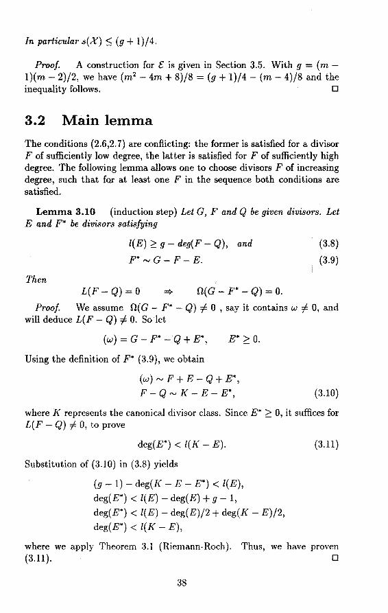
In particular s(X)::; (g + 1)/4.

Proof. A construction for t: is given in Section 3.5. With g = ( m -l)(m - 2)/2, we have (m2

- 4m + 8)/8 = (g + 1)/4 - (m - 4)/8 and the inequality follows. D

3.2 Main lemma

The conditions (2.6,2. 7) are conflicting: the former is satisfied for a divisor F of sufficiently low degree, the latter is satisfied for F of sufficiently high degree. The following lemma allows one to choose divisors F of increasing degree, such that for at least one F in the sequence both conditions are satisfied.

Lemma 3.10 (induction step) Let G, F and Q be given divisors. Let E and F* be divisors satisfying

Then

l(E) ~ g - deg(F - Q), and

F* rvG-F E.

L(F- Q) = O fl(G- F* - Q) = 0.

(3.8)

(3.9)

Proof. We assume fl( G - F* Q) =i 0 , say it contains w =i O, and will deduce L(F - Q) =i 0. So let

( w) = G F* - Q + E*, E* ~ 0.

Using the definition of F* (3.9), we obtain

(w) ""' F + E - Q + E*, F - Q "' K E - E*, (3.10)

where K represents the canonical divisor class. Since E* ~ 0, it suffices for L(F - Q) =i 0, to prove

deg(E*) < l(J< - E).

Substitution of (3.10) in (3.8) yields

(g - 1) - deg(K - E - E*) < l(E),

deg(E*) < l(E) - deg(E) + g 1,

deg(E*) < l(E) deg(E)/2 + deg(/( - E)/2,

deg(E*) < l(I< E),

(3.11)

where we apply Theorem 3.1 (Riemann-Roch). Thus, we have proven (3.11). D

38

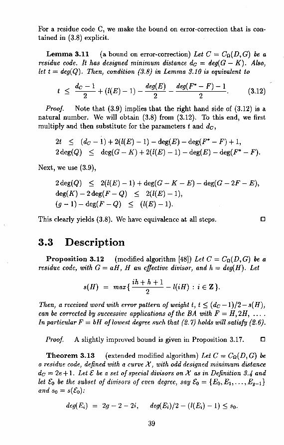
For a residue code C, we make the bound on error-correction that is con­tained in (3.8) explicit.

Lemma 3.11 (a bound on error-correction) Let C = Co(D, G) be a residue code. It has designed minimum distance de = deg(G - K). Also, let t = deg(Q). Then, condition (3.8} in Lemma 3.10 is equivalent to

t ~ de 2- 1 + (l(E) _ l) _ deg~E) _ deg(F*; F) - 1. (3.12)

Proof. Note that (3.9) implies that the right hand side of (3.12) is a natura} number. We will obtain (3.8) from (3.12). To this end, we first multiply and then substitute for the parameterstand de,

2t ~ (de - 1) + 2(l(E) - 1) - deg(E) - deg(F* - F) + 1,

2deg(Q) ~ deg(G - K) + 2(l(E) - 1) - deg(E) - deg(F* - F).

Next, we use (3.9),

2deg(Q) ~ 2(/(E) - 1) + deg(G - K - E) - deg(G - 2F- E),

deg(K) - 2deg(F - Q) ~ 2(l(E) - 1),

(g - 1) - deg(F - Q) ~ (l(E) - 1).

This clearly yields (3.8). We have equivalence at all steps.

3.3 Description

0

Proposition 3.12 (modified algorithm [48]) Let C = Co(D, G) be a residue code, with G = aH, H an effective divisor, and h = deg(H). Let

s(H) = max{ ih +; + 1 - l(iH) : i E Z }.

Then, a received word with error pattern of weight t, t ~ (de - 1) /2 - s( H), can be corrected by successive applications of the BA with F = H, 2H, .... In particular F = bH of lowest degree such that (2. 7} holds will satisfy (2.6).

Proof. A slightly improved bound is given in Proposition 3.17. 0

Theorem 3.13 (extended modified algorithm) Let C = Co(D, G) be a residue code, defined with a curve X, with odd designed minimum distance de = 2e + 1. Let t: be a set of special divisors on X as in Definition 3.4 and let &o be the subset of divisors of even degree, say &0 = { E0 , E1 , • •• , E9 _ 1 }

and so = s(t:o):

deg(E;) = 2g - 2 - 2i, deg(Ei)/2 - (l(Ei) - 1) ~ s0 •

39

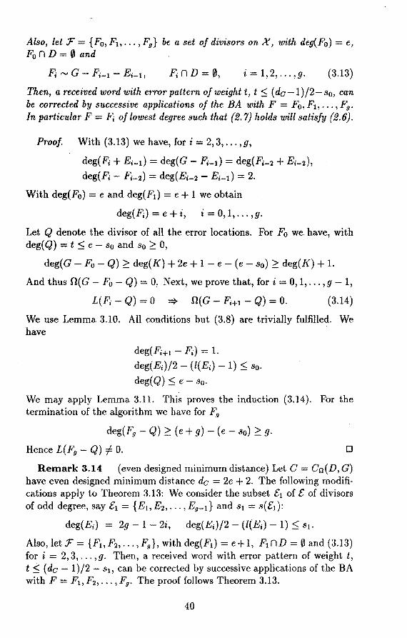
Also, let :F {Fo, Fi, ... , F9 } be a set of divisors on X, with deg(Fo) = e, F0 n D = 0 and

F; n D = 0, i=l,2, ... ,g. (3.13)

Then, a received word with error pattern of weight t, t 5 ( dc-1) /2- s0 , can be corrected by successive applications of the BA with F = F0 , Fi, ... , F9 •

In particular F = F; of lowest degree such that {2. 7) holds will satisfy (2.6).

Proof. With (3.13) we have, for i = 2,3,". ,g,

deg(Fi + E;-1) = deg(G - F;-1) = deg(F;-2 + E;-2),

deg(F; - F;-2) = deg(E;-2 - E;_t) = 2.

With deg(Fo) = e and deg(F1) = e + 1 we obtain

deg(F;)=e+i, i=0,1, ... ,g.

Let Q denote the divisor of all the error locations. For F0 we. have, with deg(Q) = t 5 e - so and so ~ 0,

deg(G - Fo - Q) ~ deg(K) + 2e + 1 - e (e - so) ~ deg(K) + 1.

And thus fl( G F0 - Q) = O~ Next, we prove that, for i = 0, 1, ... , g - 1,

L(F; - Q) = 0 => fl{G - F;+t - Q) = 0. (3.14)

We use Lemma 3.10. All conditions but (3.8) are trivially fulfilled. We have

deg(F;+i - Fï) = 1.

deg(Ei)/2 (l(Ei) - 1) 5 so.

deg( Q) 5 e so.

We may apply Lemma 3.11. This proves the induction (3.14). For the termination of the algorithm we have for F9

deg(F9 Q) ~ (e + g) - (e so) ~ g.

Hence L(F9 - Q) :f: 0. 0

Remark 3.14 (even designed minimum distance) Let C Cn(D, G) have even designed minimum distance de = 2e + 2. The following modifi­cations apply to Theorem 3.13: We consider the subset &1 of & of divisors of odd degree, say &1 ={Ei, E2, ... , E9 _i} and s1 = s(t'1):

deg(E;) = 2g - 1 2i, deg(E;)/2 - (l(E;) - 1) 5 si.

Also, let :F = {Fi, F2 , ••• , F9 }, with deg(F1) = e+ 1, F1 nD = 0 and (3.13) for i = 2, 3, ... , g. Then, a received word with error pattern of weight t, t 5 (de - 1)/2 - si, can be corrected by successive applications of the BA with F = Fi, F2, ... , F9 • The proof follows Theorem 3.13.

40

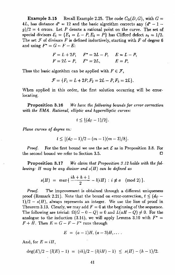
Example 3.15 Recall Example 2.25. The code C0 (D, G), with G = 4L, has distance d* = 12 and the basic algorithm corrects any (tl*" - 1 -g)/2 = 4 errors. Let P denote a rational point on the curve. The set of special divisors &1 = {E1 = L - P,E2 = P} has Clifford defect s1 = 1/2. The set :F of divisors F is defined inductively, starting with F of degree 6 and using F* = G - F - E:

F = L + 2P, F"' = 2L - P, E = L - P,

F = 2L - P, F* = 2L, E = P,

Thus the ba.sic algorithm can be applied with.F E :F,

:F = { F1 = L + 2P, Fz = 2L - P, F3 = 2L}.

When applied in this order, the first solution occurring will be error­locating.

Proposition 3.16 We have the following bounds /or error correction with the EMA. Rational, elliptic and hyperelliptic curves:

t :s; l (de - 1) /2 J. Plane curves of degree m:

t $ l(de - 1)/2 - (m - l)(m - 3)/8J.

Proof. For the first bound we use the set & as in Proposition 3.8. For the second bound we refer to Section 3.5. 0

Proposition 3.17 We claim that Proposition 3.12holds with thefol-lowing: H may be any divisor and s(H) can be defined as

s(H) = max{ ih +; + 1 - l(iH) : i :f:. a (mod 2) }.

Proof The improvement is obtained through a different uniqueness proof (Remark 2.21). Note that the bound on error-correction, t $ (de -1)/2 - s(H), always represents an integer. We use the line of proof in Theorem 3.13. Clearly, we may add F = 0 at the beginning of the sequence. The following are trivia!: O(G 0 - Q) 0 and L(aH - Q) =f:. 0. For the analogue to the induction (3.14), we will apply Lemma 3.10 with F"' = F + H. Then E = G - F F* runs through

E (a - l)Jl, (a - 3)H, ... .

And, for E iH,

deg(E)/2 - (l(E) - 1) = (ih)/2 - (l(iH) - 1) < s(H) (h - 1)/2.

41

Thus we have, at all steps,

deg(F* F) = h, and

deg(E)/2 - (l(E) - 1):::; s(H) - (h - 1)/2, and

deg(Q):::; e s(H).

We may apply Lemma 3.11. This proves the induction. D

3.4 Additional lemma After Lemma 3.10, we present another lemma that allows one to choose divisors F of increasing degree, such that for at least one F in the sequence both conditions (2.6,2. 7) are satisfied. Unlike Lemma 3.10, the application of Lemma 3.18 shows some restrictions, see Remark 3.19.

Lemma 3.18 ( alternate step) Let G, F and Q be given divisors. With P be a rational point on the curve, let F* = F + P and E = G - F - F*. Then l(E) = l(E - P) + 1 implies

L(F* Q) # L(F- Q) O(G- F* - Q) = O(G - F Q).

Proof. By assumption, there exist a function f # 0 with

E 1 ~ 0, hut not E; ~ P.

We assume O(G- F* Q) # O(G-F- Q) and will deduce L(F* -Q) = L(F - Q). Thus, let w # 0 be a differential with divisor

( w) = G - F* - Q + E2,

Then fw E O(F - Q)\O(F* - Q), and L(F* - Q) = L(F - Q). D

Remark 3.19 ( a note on application) The lemma does not apply to two consecutive steps: in case L( F* -Q) = L( F-Q) = 0, no information on !1(G-F*-Q) is obtained and in a next step O(G-F*-Q) = O(G-F Q) provides no useful information. lt is clear from the proof of Theorem 3.13 that, for a given set of special divisor &, only some induction steps (3.14) determine the bound on error-correction. If one succeeds in replacing these steps by alternate steps, the bound may be improved by one.

Lemma 3.20 Replacement of Lemma 3.10 with Lemma 3.18 in prov­ing induction Jor the EMA (Theorem 3.13) yields an improvement only if

s = max{so,s1}

42

if de is odd. if de is even.

For plane curves of degree m the condition becomes

m = 0 (mod 4) m 't 0 (mod 4)

if de is odd. if de is even.

Proof. We consider the case of odd de and we may assume that & satisfies (3.5). With the notation as in (3.4) and Lemma 3.5, let s(E2r) = so. We have improvement, only if s(E2r-2) = s(E2r+2) = so-1. Then by (3.5): s(E2r-i) = s(E2r+i) = so - 1/2. Hence s1 < so. The statement on plane curves is now a consequence of Proposition 3.9. 0

Example 3.21 Let X be the Hermitian curve of degree five over GF(16). Let Po and P1 be two rational points. Their tangents have inter­section divisor Lo = 5Po and L1 = 5P1 respectively. Let G = 2a(Po + P1) be a divisor. The code Cn(D, G) is of type [63, 68 - 4a, 2: 4a - 10] over GF(16), for 3 ::; a ::; 15. Proposition 3.16 tells that the EMA corrects e - 1 errors (one less than the designed capability ). This is obtained with a set of special divisors of Clifford defect one and a half. We may take & = {9Po, 7Po,5Po,3Po,Po}. Only the divisors 7P0 and 3Po have a defect of one and a half. We avoid using Lemma 3.10 with these divisors and use Lemma 3.18 instead. The condition l(E) = l(E - P) + 1 In the lemma is satisfied for

E = 4Po + 3P1, P = P1.

E = 5Po - 2Pi, P =Po.

For the three remaining induction steps, we may use Lemma 3.10 with E = 5Po + 4Pi, 5Po, Po. Let F = a(Po + P1).

F = F - 3Po - 2P1, F* = F - 2P0 - 2P1, E = 5Po + 4P1,

F = F - 2Po - 2P1, F* = F - 2Po - P1, E=4Po+3P1, F = F - 2Po - P1, F* = F - 3Po + P1, E = 5Po,

F = F - 3Po + P1, F* = F - 2Po + P1, E = 5Po -2P1,

F = F - 2Po + P1, F* = F + Po - P1, E=Po.

Thus the basic algorithm can be applied with F E F,

F = { F - 3Po - 2P1, F - 2Po - 2P1, F - 2Po - P1, F - 3Po + P1, F - 2Po + Pi, F + Po - P1 } .

When applied in this order, the first solution occurring will be error­locating.

43

Proof. (Proposition 3.9) We consider the plane curve X of degree m and genus g = (m l)(m - 2)/2. With the assumption m 2 4, we will construct a set e with

s(t') = { (m2

- 4m + 8)/8 if m = 0 (mod 2). (3.15) (m2

- 4m + 7)/8 if m = 1 (mod 2).

Let thus L be an intersection divisor of the curve with a line. Also, let Bi be an effective divisor of degree deg(Bi) i, for i = 0, 1,"., m - 1. We define the set E as the set of divisors E, that satisfy one of the following

E = aL +Bi, Or E = ( a + 1 )L Bm-i , Or E=(m-3)L.

0 < a < m 3 and 0 Si Sm - (a + 2). 0 Sa< m -3 and m - (a + 2) < i <m.

One verifies that t: contains divisors E, with degree deg(E) in the range: 0 S deg(E) S (m - 3)m = 2g - 2. To each degree in the range there corresponds a unique divisor. With m 2 4 we note: in the calculation of the maximum s(t'), we may consider E f:. (m - 3)L. We have l(aL) = (a + 2)(a + 1)/2, and thus for l(E)

l(aL +Bi) 2 (a + 2)(a + 1)/2, and

l((a + l)L - Bm-i) 2 (a + 3)(a + 2)/2 (m - i).

For deg(E)/2- (l(E)- I) we obtain, with i = m- (a + 2) =F b,b 2 0,

deg~E) (l(E) _ l) S -a2 + (m - 4~a + m - 2 b (3.16)

The maximum of the right hand side is obtained for a = (m 4)/2, b = 0. Looking for integer solutions, we see that the maxima are obtained for

( b) = { ((m-4)/2, 0), a, ((m-3)/2, 0),

Substitution in (3.16) yields (3.15).

if m = 0 if m = 1

(rnod 2). (mod 2).

Proof. (Proposition 3.16) From (3.15) we obtain the inequality

(m - l)(m 3)/8::::; s - 1/2.

D

The gap is at most 1/8. Also s 1/2 ::::; s0 and s - 1/2 ::::; si, where one inequality is tight and the other shows a gap of 1 /2. For the cases of odd and even designed minimum distance the following represent tight integer bounds for decoding with the EMA (Theorem 3.13)

t::::; (de 1)/2 - so, for de odd.

t S (de - 1)/2 si, for de even.

44

Hence one verifies by combination of the inequalities that in both cases

t:::; (de - 1)/2 - (m - l)(m - 3)/8,

where the gap is at most 5/8.

45

D

46

Chapter 4

Majority coset decoding

Justesen et al. [24] observed that the Peterson algorithm could be general­ized to codes from plane algebraic curves. As was shown by Skorobogatov and Vla.dut [48], the restriction to plane curves and toa particular class of codes was not essential. Thus a basic algorithm for the decoding of an arbi­trary algebraic geometrie code is available. It corrects up to ( d* -1) /2-g /2 errors. Improvements of this result either are not constructive and of high complexity [38],[53] or do not correct up to the designed minimum distance in general [48],[9]. Both Ehrhard [16] and Feng and Rao [17) formulated procedures that overcome this. Ehrhard's procedure is recalled in Section 2.5. In this chapter, we show that the procedure of Feng and Rao can be applied to an arbitrary algebraic geometrie code. In our set up a reduction step is added to the basic algorithm. In case the basic algorith fails a major­ity scheme is used to obtain an additional syndrome for the error vector. Thus a strictly smaller coset containing the error vector is obtained. In this way the basic algorithm is applied to a decreasing chain of cosets and a.fter finitely many steps the coset will be small enough for succesful application of the basic algorithm. We call the procedure Majority Coset Decoding (in short MCD). The repeated applications of the basic algorithm in the procedure can be carried out with one common set of data. For this, Feng and Rao [17] presented a scheme for the computations. The scheme is referred to as Mo­dified Fundamental Iterative Algorithm (in short MFIA). In the last section we point out that also in the genera! case the computations can be carried out with the MFIA. Thus the decoding procedure has the complexity of the basic algorithm, that is O(t2n + g2n). Although based on the sa.me idea, our procedure does not compare imme­diately with [17] when applied to the the same codes. Our formulation involves square matrices of size t + g, whereas in [17] matrices of size 2t + g are used. In Section 4.5, we present our procedure in the set up of [17], as to establish the relation.

47

4.1 Coset decoding

In the following C1 = Co(D, Gi) C F; is a. fixed residue code [30], [52]. Thus 'P = {Pi, P2, ... , Pn} is a set of n rationa.l points on a non-singular curve X /Fq, D = P1 + P2 + ... + Pn and G1 is a divisor defined over Fq with support disjoint from P. The codewords of C1 are of the form (resp1 (77),resp2 (77), ... ,respn('7)), for 7] E O(G1 -D). With g the genus of the curve X, the code C1 has designed distance di = deg(G1) - (2g - 2). The dual code et is equal to the functional code CL(D, G1) with code­words of the form (h(Pi), h(P2), ... , h(Pn)), for h.E L(G1).

Fora rational point P00 <I, P, let Go= G1 - P00 and let G2 = G1 + P00 • We have an extension of residue codes

Co= Co(D,Go) :::> C1 = Co(D,Gi) :::> C2 = Co(D,Gz). (4.1)

Let e be a vector with wt(e)::; (di - 1)/2. (4.2)

We formulate a coset decoding procedure with respect to the extension of codes C1 :::> C2 : for a given Yt E e + C1 we show how to obta.in Y2 E e + C2. Note that with condition ( 4.2) this is well-defined. In cáse y 2 f:. e the procedure can be repeated, till eventually the error vector is obtained. With a combination of the procedure and known algorithms the number of repetitions required can be bounded by the genus g of the curve (Remark 4.16). Clearly, we may assume that

C1 f:. C2, and L(G2) f:. L(G1),

where the second assumption follows from the first. As :with decoding of linear codes in genera!, syndromes are crucial. We define syndromes as linear maps to the constant field.

Definition 4.1 With a vector y = (yi, y2, ... , Yn) E F; we associate a one-dimensional syndrome Si(y), for i = 0, 1, 2,

is

n

h f-+ E Yi h(P3). j=l

Lemma 4.2 The one-dimensional syndrome is a coset invariant, that

S;(y) = S;(e) <::> y E e + C;,

Proof. From the definition

i = 0, 1, 2.

S;(y - e) = 0 <::> y e E CL(D, Gi)l..

The result follows with CL(D, G;) = C/, D

48

Lemma 4.3 For u E C1 \ C2 and for h E L(G2 ) \ L(G1 ) we have S2(u)(h) :/= o.

Proof G2 = G1 + P oo implies l( G2) - l( G1) ~ 1 and L( G2) = L( G1) 67 (h). With the lemma we have

u E C1 Au t/. C2 => S1(u) = 0 A S2(u) ::f:. 0 => S2(u)(h) ::f:. 0.

D

The following is immediate from the lemmas.

Corollary 4.4 Let u E C1 \ C2 and let y1 E e + C1. There exists a unique À such that Yt - Àu E e + C2. For h E L(G2) it satisfies

.\S2(u)(h) = S2(yi)(h) - S2(e)(h),

where S2(u)(h) ::f:. 0, for h E L(G2) \ L(G1).

By the corollary it suffices for coset decoding to find a function h E L( G2) \ L(Gi) with S2(e)(h) 0. We give a procedure to obtain functions f,g such that h = f g will do.

4.2 Two-dimensional syndromes

Definition 4.5 For a vector e with ( 4.2) we consider the cosets e+Ci with syndromes Si(e), for i = 0,1,2. With a divisor F, that has support disjoint from 'P, we associate a two-dimensional syndrome Si(F), for i = o, 1, 2,

Si(F) : L(F) x L(Gi - F) ----> Fq,

(J,g) t---+ Si(e)(Jg).

Let I<i(F) he defined as the subspace of L(F) with

f E I<i(F) <:} Vg E L(G; - F): Si(F)(J,g) = 0.

Lemma 4.6 The containments

K1(F + P00 ) ::::> I<o(F), Ko(F) ::::> K1 (F), and

K1(F + Poo) ::::> I<2(F + Poo), I<2(F + Poo) :::> K1(F)

define factor spaces of dimension at most one.

Proof. The inclusion relations are immediate from the definition. In particular I<0 (F) I<1(F + P00 ) n L(F). Since I<1(F + Poo) c L(F + Poo), the intersection reduces the dimension by at most one. Similar for I<2(F + P00 ) ::::> I<1 (F). For the inclusion I<o(F) ::::> I<i(F) we observe that K1(F) is obtained by applying at most one linear condition to I<o( F). Similar for K1(F + Poo) ::::> K2(F + Poo)· D

49

The inclusion relations may be depicted as follows

As the next lemma explains, we are interested in the situation where the following conditions are satisfied

(Al) K1(F + Poo) #- Ko(F), (A2) Ko(F) = Ki(F), (A3) L(G1 - F) #- L(G1 - F - Poo)·

(Bl) Ki(F + Poo) = K2(F + Poo), (B2) K2(F + Poo) #- Kt(F).

Let (A) # (Al) A (A2) A (A3). Also let (B) # (Bl) A (B2).

Corollary 4. 7 The conditions satisfy

(Al)A(Bl) # (A2)A(B2).

Proof. Immediate from Lemma 4.6. 0

Remark 4.8 The vector spaces K(F) that occur in the conditions (A) and (B) are all defined as left null spaces of bilinear forms S(F). The duality in the formulation becomes more obvious if we consider the right null spaces as well. For example, we have

However, to save on computations, the formulation in terms of the left null spaces only is to be preferred.

Lemma 4.9 (main lemma) Let the functions f,g satisfy

f E K1 (F + P00 ) \ Ko(F), and

g E L(G1 - F) \ L(G1 - F - Poo)·

Then

and

50

Proof. From f E L(F + Poo) and g E L(G1 - F) we obtain fg E L(G1 + P00 ) = L(G2). For f g (j. L(G1) it suflices to consider the pole order -1100 (/g) at P00 and

-1100(/g) = -voo(/) - Voo(g)

= ordp00 (F + P00 ) + ordp00 (G1 - F) > ordp00 (G1).

Note that g E L(G2 - F- P00 ). With f E K2(F + P00 ) we have

S2(e)(/g) = S2(F + Poo)(f,g) = 0.

D

By the remark following Corollary 4.4 we can choose h = fg with f,g as in the lemma, provided that conditions (Al),(A3) and (Bl) hold. With the corollary the conditions (A) and (B) need to be fulfilled. In the decoding situation we cannot determine I<2(F + P00 ) and we are unable to verify (B). To overcome this we use a majority scheme.

4.3 A majority scheme

Remark 4.10 Let the notation be as in Definition 4.5. Let the divisor Pe = Ee,;o!O Pj. With Definition 4.1 and Definition 4.5 we see, for i = 0, 1, 2,

f E L(F - Pe) V g E L(Gi - F - Pe) => Si(F)(f,g) = 0.

Lemma 4.11 Consider the conditions

Pe) -:f. L(F - Pe), (Cl) L(F + Poo (C2) L(G1 - F Pe) # L(G1 - F - Poo - Pe)•

With the conditions {A1}-{A3} and {81)-(82} as in the previous section the f ollowing holds

(Cl) => (Al)/\ (B2),

(C2) => (A2) /\ (Bl) /\ (A3).

Proof. Let (Cl) hold. For (Al) and (B2) respectively it suflices to give functions f1 E I<1(F+P00 )\L(F) and h E K2(F+P00 )\L(F) respectively. With the remark a function f E L(F + P00 - Pe) \ L(F - Pe) will do in both cases. Let (C2) hold. Recall that Go = G1 - P00 • We may write L(G1 - F) = L(Go F) + L(G1 - F - Pe)· With the remark we ohtain I<0(F) C I<1(F). This proves (A2). For (Bl) we use G1 = G2 -P00 and we write L(G2 -F P00 ) = L(G1 -F-P00 ) + L(G2 -F P00 -Pe) to ohtain K 1(F + P=) C K 2(F + P00 ). The condition (A3) follows immediately with Pe 2:: 0. D

51

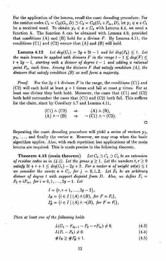
For the application of the lemma, recall the coset decoding procedure: For the residue codes C1 = Cn(Gi,D) ::::> C2 = Cn(G1 +Poo,D), let Y1 E e+C1 be a received word. To obtain Y2 E e + C2 with Lemma 4.4, we need a function h. ·The function h can be obtained with Lemma 4.9, provided that conditions (A) and (B) hold for a divisor F. By Lemma 4.11, the conditions (Cl) and {C2) ensure that (A) and (B) will hold.

Lemma 4.12 Let deg(G1 ) = 2g + 2t - 1 and let deg(Pe) $ t. Let the main lemma be applied with divisors F in the range t - 1 $ deg(F) $ t + 2g 1, starting with a divisor of degree t - 1 and adding a rational point P00 each time. Among the divisors F that satisfy condition {A), the divisors that satisfy condition (B} as well form a majority.

Proof. For the 2g + 1 divisors F in the range, the conditions (Cl) and (C2) will each hold at least g + 1 times and fail at most g times. For at least one divisor they both hold. Moreover, the cases that (Cl) and (C2) both hold outnumber the cases that {Cl) and (C2) both fail. This suffi.ces for the claim, since by Corollary 4.7 and Lemma 4.11,

(Cl) A (C2) =? (A) A (B), (A) A-. (B) => .., (Cl) A.., (C2).

D

Repeating the coset decoding procedure will yield a series of vectors y 2,

y 3 , ••• , and finally the vector e. However, we may stop when the basic algorithm applies. Also, with each repetition less applications of the main lemma are required. This is made precise in the following theorem.

Theorem 4.13 (main theorem) Let Co::::> C1 ::::> è2 be an extension of residue codes as in (4.1). Let the genus g 2 1. Let the numbers t, r 2 0 satisfy 2t + r + 1 $ deg(G1 ) - 2g + 2. Fora vector e of weight wt(e) $ t we consider the cosets e + Ci, for j 0, 1, 2. Let Fo be an arbitrary divisor of degree t with support disjoint from D. Also, we de fine F; = Fo+iP00 , fori=O,l, ... ,2g-l. Let

l={r,r+l,".,2g-2},

lB {i El 1 (A) A (B), for F Fï},

18={iEl1 (A) A -.(B), for F = F;},

Then at least one of the following holds

L(G1 - F29-1 - Pe - rPoo) # 0. L(Fr Pe) # 0.

#lB 2#18+1.

52

(4.3) (4.4)

(4.5)

Proof. The assumption on wt( e) yields

deg(F29 -1 - Pe) ~ 2g - 1,

deg(G1 - Fr - Pe) ~ 2g - 1.

Let the sets Ic and Iê be defined as

Ic= {i EI 1 (Cl)/\ (C2), for F = F;},

Iê = {i EI 1-.(Cl) /\ -.(C2), for F = F;},.

(4.6)

(4.7)

By Corollary 4.7 and Lemma 4.11 we have Ic C IB and I8 C I(:. Thus for ( 4.5) to hold it suffices to prove

#Ic~ #Iê + 1. (4.8)

We may assume that (4.3) and (4.4) do not hold. In that case we have

l(G1 - F29 -1 - Pe) :$ r,

l(Fr - Pe) = 0.

Combination with ( 4.6,4. 7) yields

And

l(F2g-l - Pe) - l(Fr - Pe) ~ g,

l(G1 - Fr - Pe) - l(G1 - F29-1 - Pe) ~ g - r.

#I - #Iê = #{i EI 1 (Cl)}+ #{i EI 1 (C2)} - #Ic, > (2g - r) - #Ic.

With #I = (2g -1- r) we obtain (4.8).

4.4 Description

D

In the following remarks we use the theorem to formulate a decoding pro­cedure. Let y 1 E e + C1 be given. If (4.3) or (4.4) holds we can apply the basic algorithm. If both ( 4.3) and ( 4.4) fail, we can apply majority coset decoding.

Remark 4.14 (basic algorithm) We recall the basic algorithm, Lemma 2.18: an error pattern e for the residue code Cri(D, G) can be corrected if the following are satisfied for a divisor F:

L(F - Pe) # 0, and deg(G - F - Pe) > 2g - 2. (4.9)

53

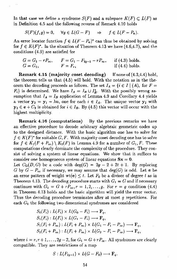
In that case we define a syndrome S(F) and a subspace K(F) C L(F) as in Definition 4.5 and the following reverse of Remark 4.10 holds

S(F)(f,g) = O, Vg E L(G - F) => f E L(F - Pe)·

An error locator function f E L(F - Pe)* can thus be obtained by solving for f E K(F)*. In the situation of Theorem 4.13 we have (4.6,4.7), and the conditions ( 4.9) are satisfied for

G = G1 - rPoo, G= G1,

F G1 - F29-1 - rPoo, F Fn

if ( 4.3) holds. if ( 4.4) holds.

Remark 4.15 (majority coset decoding) If none of (4.3,4.4) hold, the theorem tells us that (4.5) will hold. With the notation as in the the­orem the decoding proceeds as follows. The set IA= {i EI 1 (A), for F = F;} is determined. We have IA = IB U JB. With the possibly wrong as­sumption that IA = IB application of Lemma 4.9 and Corollary 4.4 yields a vector y 2 = y 1 - Àu, one for each i E IA. The unique vector y 2 with y 2 E e + C2 is obtained for i E IB. By ( 4.5) this vector will occur with the highest multiplicity.

Remark 4.16 (computations) By the previous remarks we have an effective procedure to decode arbitrary algebraic geometrie codes up to the designed distance. With the basic algorithm one has to solve for f E K(F)* for suitable G, F. With majority coset decoding one has to solve for f E Ki(F + P00 ) \ Ko(F) in Lemma 4.9 fora number of G1,F. These computations clearly dominate the complexity of the procedure. They con­sist of solving a system of linear equations. We show that it suffices to consider one homogeneous system of linear equations Sx = 0. Let Cri(D, G) be a code with deg(G) = 2g - 2 + 2t + 1. By replacing G by G - P,00 if necessary, we may assume that deg( G) is odd. Let e be an error pattern of weight wt( e) $ t. Let F0 be a divisor of degree t as in Theorem 4.13. The decoding procedure starts with G1 = G and if necessary continues with G1 = G + rP00 , r 1, 2, ... ,g. For r = g condition (4.4) in Theorem 4.13 holds and the basic algorithm will yield the error vector. Thus the decoding procedure terminates after at most g repetitions. For each G1 the following two-dimensional syndromes are considered

So(F;): L(F;) x L(Go - F;)-+ Fq, S1(F;): L(F;) x L(G1 F;)-+ Fq, S1(F; + Poo): L(F; + Poo) x L(G1 - F; - Poo)-+ Fq, S2(F; + Poo): L(F; + Poo} x L(G2 - F; - Poo)-+ Fq,

where i r, r + 1, ... , 2g -2, for G1 G + rP00 • All syndromes are clearly compatible. They are restrictions of a map

S: L(F29-i) x L(G Fo)-+ Fq.

54

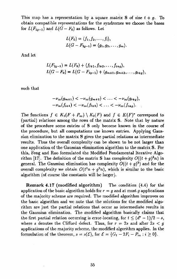
This map has a representation by a square matr'ix S of size t + g. To obtain compatible representations for the syndromes we choose the bases for L(F29_ 1 ) and L(G - F0 ) as follows. Let

And let

such tha.t

L(Fo) = (/i,/2, ... , /1), L(G-F2u-d = (gi,92, ... ,gm}·

L(F29-1) = L(Fo) + (/1+i, f1+2, ... , !t+9 ),

L(G - Fo) = L(G - F29-1) + (9m+i,9m+2, ... ,gt+u),

-voo(9m+i) < -voo(9m+2) < · · · < -voo(Yt+u),

-vooU1+1) < -voo(/1+2) < · · · < -lloo{ft+u)·

The functions f E I<1(F + Poo) \ I<o(F) and f E I<(F)* correspond to (partial) relations among the rows of the matrix S. Note that by nature of the procedure some entries of S only become known in the course of the procedure, hut all computations use known entries. Àpplying Gaus­sian elimination to the matrix S gives the partial relations as intermedia.te results. Thus the overall complexity can be shown to be not la.rger than one application of the Gaussian elimination algorithm to the matrix S. For this, Feng and Rao formulated the Modi:fied Fundamental Iterative Algo­rithm [17]. The definition of the matrix S has complexity 0( ( t + g )2n) in general. The Gaussian elimination has eomplexity O((t + g)3 ) and for the overall complexity we obtain O(t2n + g2n), which is similar to the basic algorithm (of course the constants will be larger ).

Remark 4.17 (modified algorithm) The condition (4.4) for the application of the basic algorithm holds for r = g and at most g applications of the majority scheme are required. The modified algorithm improves on the basic algorithm and we note that the solutions for the modified algo­rithm are just the partial relations that occur as intermedia.te results in the Gaussian elimination. The modified algorithm basically claims that the first partial relation occurring is error-locating, fort :S (d* - 1)/2 - s, where s denotes the Clifford defect. Thus, for r = 2s and after 2s < g

applications of the majority scheme, the modified algorithm applies. In the formulation of the theorem, s = s(l'), for l' = {G1 - 2Fi - Poo : i ~ O}.

55

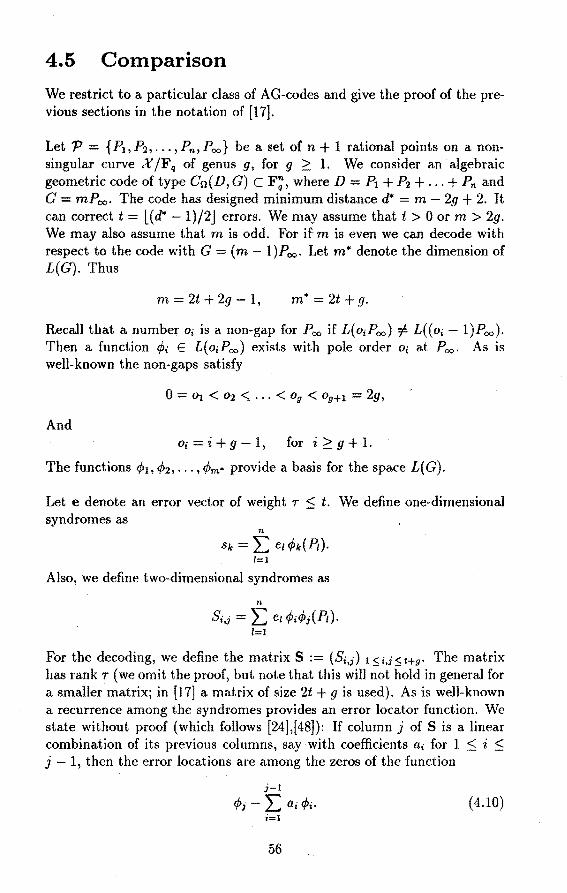
4.5 Comparison

We restrict toa particular class of AG-codes and give the proof of the pre­vious sections in the notation of [17].

Let 'P = {Pi,P2, ... ,Pn,P00 } be a set of n + 1 rationa.l points on a non­singular curve X /F9 of genus g, for g ~ 1. We consider an algebraic geometrie code of type Cn(D, G) C F~, where D = Pi + P2 + ... + Pn and G = mP00 • The code has designed minimum distance d* = m - 2g + 2. It can correct t = L(d* -1)/2J errors. We may assume that t > 0 or m > 2g. We may a.lso assume that m is odd. For if m is even we can decode with respect to the code with G = (m l)P00 • Let m" denote the dimension of L(G). Thus

m = 2t + 2g- l, m* = 2t + g.

Recall that a number Oi is a non-gap for Pr::o if L(oiPoo) ::f L((o; - l)P00 ).

Then a function </>i E L( o; P oo) exists with pole order o; at P 00 • As is well-known the non-gaps satisfy

Ü = Ot < 02 <Ç ••• < Og < Og+l = 2g,

And o; = i + g - 1, for i ~ g + 1.

The functions </>1, t/>2 , ••• , <Pm • provide a basis for the space L( G).

Let e denote an error vector of weight r :::; t. We define one-dimensiona.l syndromes as

n

Sk = :E e1 </>k(P1). l=l

Also, we define two-dimensional syndromes as

n

Si,i = :E e1 r/>;t/>;(P,). l=l

For the decoding, we define the matrix S := (S;,;) I$i,i$t+u· The matrix has rank T (we omit the proof, hut note that this will not hold in general for a smaller matrix; in [17] a matrix of size 2t +gis used). As is well-known a recurrence among the syndromes provides an error locator function. We state without proof (which follows [24],[48]): If column j of S is a linear combination of its previous columns, say with coefficients a; for 1 :::; i :::; j - 1, then the error locations are among the zeros of the function

j-1

</;; - :E a; </>i. (4.10) i=l

56

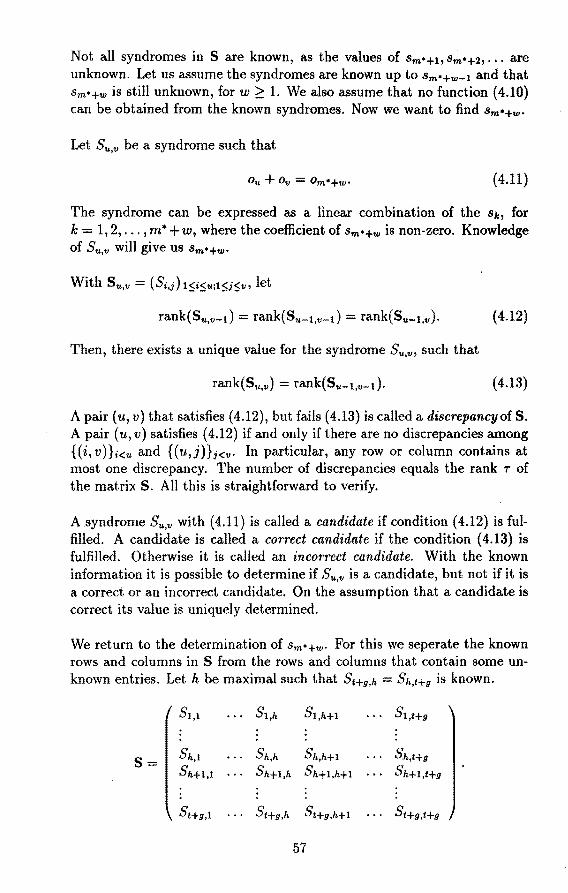
Not all syndromes in S are known, a.s the va.lues of Sm•+i, Sm•+2, ••• are unknown. Let us assume the syndromes are known up to Sm•+w-i and that Sm•+w is still unknown, for w ~ 1. We also assume that no function ( 4.10) can be obtained from the known syndromes. Now we want to find Sm•+w·

Let Su,v be a syndrome such that

(4.11)

The syndrome can be expressed as a linear combination of the Sk, for k = 1, 2, ... , m* +w, where the coefficient of Sm•+w is non-zero. Knowledge of Su,v will give US Sm•+w·

rank(Su,v-1) = rank(Su-1,v-i) = rank(Su-1,v)· (4.12)

Then, there exists a unique value for the syndrome Su,v, such that

rank(Su,v) = rank(Su-1,v-d· (4.13)

A pair ( u, v) that satisfies ( 4.12), but fails ( 4.13) is called a discrepancy of S. A pair ( u, v) satisfies ( 4.12) if and only if there are no discrepancies among {(i, v)}i<u and {(u,j)};<v· In particular, any row or column contains at most one discrepancy. The number of discrepancies equa.ls the rank T of the matrix S. All this is straightforward to verify.

A syndrome Su,v with (4.11) is called a candidate if condition (4.12) is ful­filled. A candidate is called a correct candidate if the condition ( 4.13) is fulfilled. Otherwise it is called an incorrect candidate. With the known information it is possible to determine if Su,v is a candidate, hut not if it is a correct or an incorrect candidate. On the assumption that a candidate is correct its value is uniquely determined.

We return to the determination of Sm•+w· For this we seperate the known rows and columns in S from the rows and columns that contain some un­known entries. Let h be maximal such that St+g,h = Sh,t+g is known.

S1,1 S1,h S1,h+i Si,t+u

S= Sh,1 Sh,h Sh,h+i Sh,t+u sh+i,1 sh+i,h Sh+1,h+1 Sh+i,t+u

St+u,1 St+u.h St+u,h+i St+u,t+u

57

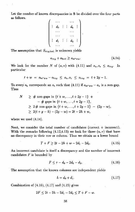
Let the number of known discrepancies in S be divided over the four parts as follows.

The assumption that St+g,h+l is unknown yields

(4.14)

We look for the number N of (u,v) with (4.11) and ou,Ov < Ot+g· In pa.rticular

To every Ou corresponds an o" such that ( 4.11) if Om•+w - Ou is a non-gap. Thus

N > #non-gapsin{t-+w, ... ,t+2g-l} +

- # gaps in { t + w, ... , t + 2g 1},

2:'.: 2# non-gaps in {t+w, ... ,t+2g 1} - (2g w), > 2(t + g - h) - (2g - w) = 2t - 2h + w,

where we used ( 4.14).

Next, we consider the total number of candidates (correct + incorrect). With the rema.rks following (4.12,4.13) we look for those (u,v) that have no discrepancy in their row or column. Thus we obtain as a lower bound

T + F ~ 2t - 2h + w 2d1 -2d2. (4.15)

An incorrect candidate is itself a discrepancy and the number of incorrect ca.ndidates F is bounded by

(4.16)

The assumption that the known columns are independent yields

h =do+ di. (4.17)

Combination of (4.16), (4.17) and (4.15) gives

2F ~ 2t - 2h - 2d1 - 2d2 ~ T + F - W.

58

And T 2:: F + w. With the assumption that all candidates are correct their values can be determined according to (4.13). All correct candidates give the true value and by the obtained inequality this value will occur the most often among the values given by all candidates (correct and incorrect). The idea on which the above procedure is based is presented in [17]. The pa­per contains a scheme for the computations and a complete example. The construction of the example is given in the next section. In the previous sections, the relation to coset decoding is emphasized and a generalisation to all algebraic geometrie codes is formulated.

The square matrix S that we use has size t + g, while the matrix S oc­curring in [17] has size 2t + g. We obtain a majority with the candidates from a smaller matrix with the assumption ( 4.17). Also, the variables h and d0 , d1 and d2 were introduced to shorten the counting argument that leads to the inequality T > F and to avoid having to consider special cases.

The notions candidates, correct candidates and incorrect candidates are introduced in [17]. They correspond with the sets IA,IB and 18 in the previous section. In particular, the inequalities to be proved are T > F and #IB > #18 respectively. The notion of discrepency is more commonly used and is very much related to the way the computations are carried out. The precense of a discrepancy in a row or column means that it is linearly independent of its previous rows or columns respectively. In this section, the numbers of discrepancies d0 , d1 and d2 occur in the two in­equalities (4.15) and (4.16). In the final inequality T > F they disappear, that is they appear in the irrelevant middle term. The use of discrepancies is avoided in the general proof of the previous section, where instead the conditions (Cl) and (C2) are used. These, to the contrary, imply that a certain row or column does depend linearly on its previous rows or columns respectively. There, t.he inequality Ic > Iè is proved. Again, it is irrelevant on its own, hut it implies the required IB > 18.

The two omitted proofs relate to the basic algorithm. The two claims follow immediately with the results from Chapter 2. Finally, the matrix S is symmetrie, while the matrix S occurring in Remark 4.16 is not symmetrie in genera!. In the special case that it is symmetrie, we have G1 - F29-1 = Fr in the proof of Theorem 4.13. In particular, the inequality l( G1 -F29 _ 1 -Pe) ~ r can be replaced with l( G1 -F29-1 -Pe) = 0. And, the obtained inequality IB 2:: I.B+I can be sharpened to IB 2:: I.B+I+r, for r 2:: 0. This corresponds indeed with T 2:: F + w, for w 2:: 1, that was proved as a special case in this section.

59

4.6 Example

Recall the situation of Lemma 2.24. The error patterns e1 and e2 are in the same coset. It is assumed that their supports are disjoint and that the sum of their weights equals the designed minimum distance of the code. In this situation, the obvious inclusion L(F - Qi) + L(F - Q2) C K(F) is in fact an equality. In the same situation, the inequalities in the majority scheme can be proved to be sharp. We present results for this special case and give two explicit examples.

Notation 4.18 Let the majority scheme in Theorem 4.13 be applied with the following: r = 0 and thus deg( G1 ) = 2g + 2t - 1. The divisor Fo is of degree t and ~ Fo + iPoe." for i = 0, 1, ... , 2g - 1. The majority scheme is applied when (4.3) and (4.4) fail, and we may assume

L(G1 - F29 -1 - Pe) = 0,

L(Fo - Pe) = 0.

(4.18)

( 4.19)

Also, we consider the situation of Notation 2.19. To distinguish between the cases e = e1 and e = e2, we write (Cl,e1), if condition (Cl) holds with e =ei. Similarly, with the other- conditions. The sets IB, IÈ,lc and Iè in the theorem are indexed with 1 or 2, for the vectors e1 and e2 respectively. Note that the set IA is the same for both vectors.

Lemma 4.19 With the notation as above, the following equivalences hold:

(Cl,e1) ~ ..., (C2,e2) (C2,e1) ~ ..., (Cl,e2)

Proof. By duality, it suffices to prove the first equivalence, and

l(F + P= - Qi) - l(F Qi) + + l(G1 - F - Q2) - l(G1 F Poo Q2)

= l(F+Poo Qt)-l(F-Q1)+

+l(I<+Q1-F)-l(I<+Q1-F-Poo) = 1.

The claim follows.

Corollary 4.20 We have Ic,1 = Iê,2 and Iè,1 Ic,2·

0

Proposition 4.21 In the situation of Notation 4.18, the set IA has a partition IA = Ic, 1 U Ic,2 • Also, the inclusions Ic C IB and IÈ C Iê, that occur in the proof of Theorem 4.13, are in fact equalities, for both e e1

and e = e2.

60

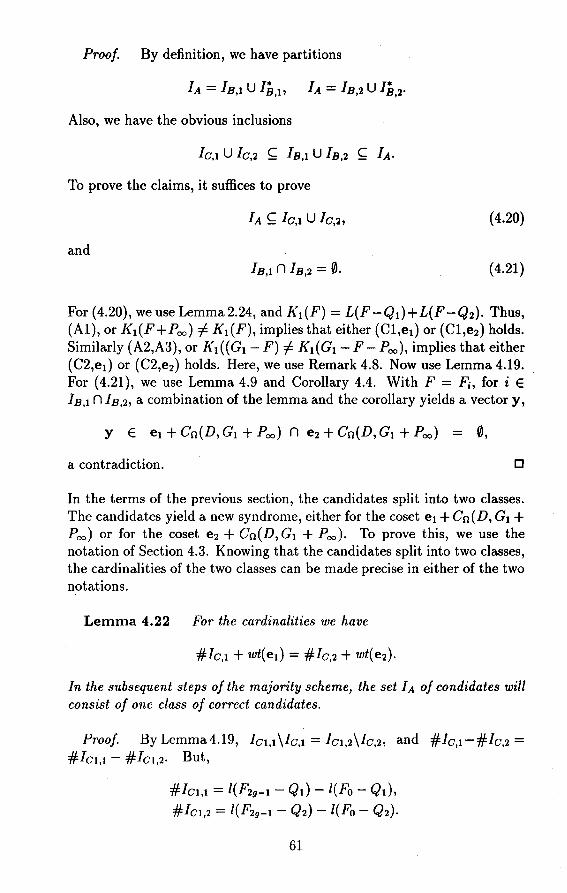
Proof. By definition, we have partitions

Also, we have the obvious inclusions

To prove the claims, it suffices to prove

( 4.20)

and (4.21)

For (4.20), we use Lemma2.24, and I<1(F) = L(F-Q1)+L(F-Q2). Thus, (Al), or I<1(F+P=) f= I<1(F), implies that either (Cl,e1 ) or (Cl,e2 ) holds. Similarly (A2,A3), or I<1((G1 -F) f= I<1(G1 -F-P=), implies that either (C2,e1 ) or (C2,e2 ) holds. Here, we use Remark 4.8. Now use Lemma 4.19. For (4.21), we use Lemma 4.9 and Corollary 4.4. With F = Fi, for i E IB,t n IB,2 , a combination of the lemma and the corollary yields a vector y,

a contradiction. D

In the terms of the previous section, the candidates split into two classes. The candidates yield a new syndrome, either for the coset e1 + Cn(D, G1 + P=) or for the coset e2 + Cn(D, G1 + P=)· To prove this, we use the notation of Section 4.3. Knowing that the candidates split into two classes, the cardinalities of the two classes can be made precise in either of the two notations.

Lemma 4.22 For the cardinalities we have

#Ic,1 + wt(e1) = #Ic,2 + wt(e2).

In the subsequent steps of the majority scheme, the set IA of condidates will consist of one class of correct candidates.

Proof. By Lemma 4.19, Ic1,1 \Ic,1 = Ic1,2 \Ic,2, and #Ic,1 -#Ic,2 = #Ic1,1 - #Ic1,2· But,

#Ic1,1 = l(F29-1 - Qi) - l(Fo - Qi),

#Ic1,2 = l(F29-1 - Q2) - l(Fo - Q2)·

61

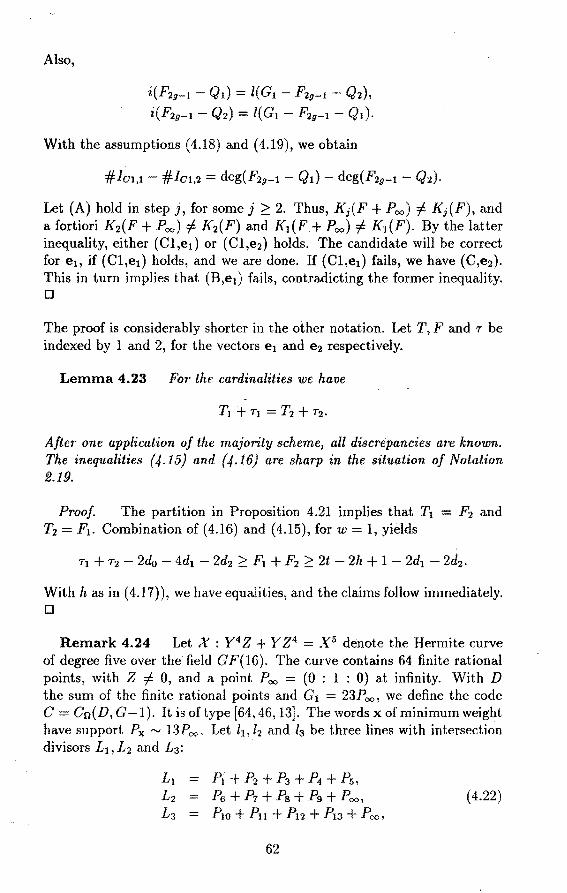
Also,

i(F2u-1 - Qi) = l(G1 - F2u-1 - Q2), i(F29-1 - Q2) = l(G1 - F2u-1 - Qi).

With the assurnptions ( 4.18) and ( 4.19), we ohtain

#Ic1,1 #lc1,2 = deg(F29-1 - Qi) deg(F29-1 Q2)·

Let (A) hold in step j, for some j ~ 2. Thus, Kj(F + P,"°) =f. K;(F), and a fortiori K2(F + P=) =f. K2(F) and I<1(F+ P=) # K1(F). By the latter inequality, either (Cl,e1 ) or (Cl,e2 ) holds. The candidate will be correct for ei, if (Cl,e1 ) holds, and we are clone. If (Cl,e1 ) fails, we have (C,e2).

This in turn implies that (B,e1) fails, contradicting the forrner inequality. D

The proof is considerably shorter in the other notation. Let T, F and r be indexed by 1 and 2, for the vectors e1 and e2 respectively.

Lemma 4.23 For the cardinalities we have

After one application of the majority scheme, all discrepancies are known. The inequalities (4.15} and (4.16} are sharp in the situation of Notation 2.19.

Proof The partition in Proposition 4.21 implies that T1 = F2 and T2 = F1. Combination of (4.16) and (4.15), for w = 1, yiè1ds

With h as in ( 4.17) ), we have equalities, and the claims follow immediately. D

Remark 4.24 Let X : Y 4 Z + Y Z 4 = X 5 denote the Hermite curve of degree five over the field GF(16). The curve contains 64 finite rational points, with Z =f. 0, and a point Po.o (0 : 1 : 0) at infinity. With D the sum of the fini te rational points and G1 23P =, we define the code C = Cn(D, G-1 ). lt is of type [64, 46, 13]. The words x of minimum weight have support Px ,...., l3P=. Let li, 12 and Is be three lines with intersection divisors L1, L2 and L3:

L1 P1 + P2 + P3 + P4 + Ps, L2 = P6 + P1 + Ps + Pg + P =, ( 4.22) L3 = P10+P11+P12+P13+P=,

62

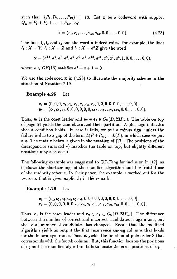
such that l{Pi,P2, ... ,Pi3}i = 13. Let x be a codeword with support Qx = Pi + P2 + ... + P13, say

( 4.23)

The lines li, 12 and /3 and the word x indeed exist. For example, the lines li : X = Y, 12 : X = Z and /3 : X = a3 Z give the word

( i2 4 7 s g g 5 i2 ii 4 7 6 1 0 0 0 0) x= a ,a,a,a,a,a,a,a ,a ,a,a,a,,, , ... ,, ,

where a E GF(16) satisfies a4 + a + 1 = 0.

We use the codeword x in ( 4.23) to illustrate the majority scheme in the situation of Notation 2.19.

Example 4.25 Let

ei = (0, 0, 0, c4, es, es, c7, es, cg, 0, 0, 0, 0, 0, 0, ... , 0, 0), e2 = ( Ci, C2, C3, 0, 0, 0, 0, 0, 0, C10, Cil, Ci2, C13, 0, 0, ... , 0, 0).

Thus, ei is the coset leader and e2 E ei E Cn(D, 23P00 ). The table on top of page 64 yields the candidates and their partition. A plus sign indicates that a condition holds. In case it fails, we put a minus sign, unless the failure is due toa gap of the form L(F + P00 ) = L(F), in which case we put a g. The matrix below is given in the notation of [17]. The positions of the discrepancies (marked *) matches the table on top, hut slightly different positions may also occur.

The following example was suggested to G.L.Feng for inclusion in [17], as it shows the shortcomings of the modified algorithm and the fruitful use of the majority scheme. In their paper, the example is worked out for the vector x that is given explicitly in the remark.

Example 4.26 Let

ei= (ei, C2, C3, C4, C5, es, 0, 0, 0, 0, 0, 0, 0, 0, 0, ... '0, 0), e2 = (0, 0, 0, 0, 0, 0, C7, es, Cg, C10, C11, Ci2, Ci3, 0, 0, ... '0, 0),

Thus, ei is the coset leader and e2 E ei E Cn(D, 23P00 ). The difference between the number of correct and incorrect candidates is again one, hut the total number of candidates has changed. Recall that the modified algorithm yields as output the first recurrence among columns that holds for the known syndromes.Thus, it yields the function of pole order 8 that corresponds with the fourth column. But, this function locates the positions of e2 and the modified algorithm fails to locate the error positions of ei.

63

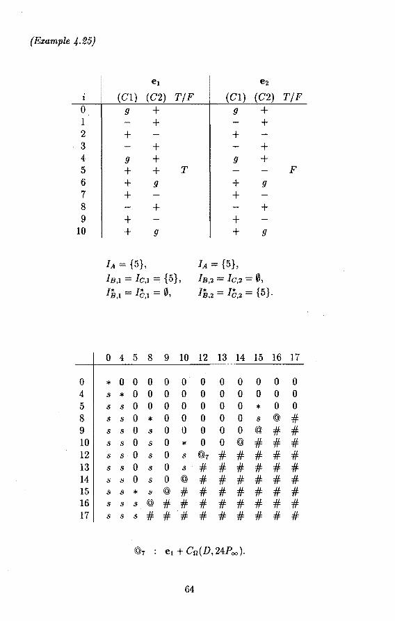
(E:r:ample 4.25)

ei e2

(Cl) (C2) T/F (Cl) (C2) T/F 0 g + g + 1 + + 2 + +

. 3 + + 4 g + g + 5 + + T F 6 + g + g 7 + + 8 + + 9 + +

10 + g + g

IA {5}, IA= {5},

IB,1 = Io,1 = {5}, IB,2 = Ic,2 = 0, I8,1 = Iê,1 = 0, I8,2 Iê,2 = {5}.

0 4 5 8 9 10 12 13 14 15 16 17

0 * 0 0 0 0 0 0 0 0 0 0 0 4 s * 0 0 0 0 0 0 0 0 0 0 5 s s 0 0 0 0 0 0 0 * 0 0 8 s s 0 * 0 0 0 0 0 s @ # 9 s s 0 s 0 0 0 0 0 @ # # 10 s s 0 s 0 * 0 0 @ # # # 12 s s 0 s 0 s @1 # # # # # 13 s s 0 s 0 s # # # # # # 14 s s 0 s 0 @ # # # # # # 15 s s * s @ # # # # # # # 16 s s s @ # # # # # # # # 17 s s s # # # # # # # # #

@1 : e1 + Co(D,24P00 ).

64

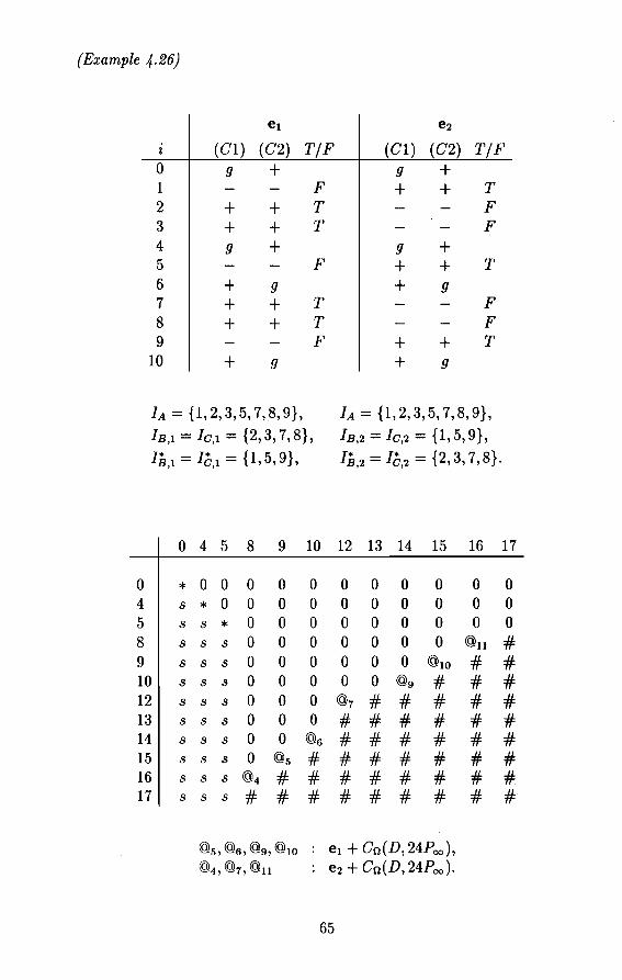
(Example 4.26}

ei e2 (Cl) (C2) T/F (Cl) (C2) T/F

0 g + g + 1 F + + T 2 + + T F 3 + + T F 4 g + g + 5 F + + T 6 + g + g 7 + + T F 8 + + T F 9 F + + T

10 + g + g

IA= {1,2,3,5, 7,8,9}, IA= {1,2,3,5, 7,8,9},

IB,i = Ic,i = {2, 3, 7, 8}, IB,2 = Ic,2 = {l, 5, 9},

I8,i = Iê,i = {l, 5, 9}, I8,2 = Iê,2 = {2,3, 7,8}.

0 4 5 8 9 10 12 13 14 15 16 17

0 * 0 0 0 0 0 0 0 0 0 0 0 4 s * 0 0 0 0 0 0 0 0 0 0 5 s s * 0 0 0 0 0 0 0 0 0 8 s s s 0 0 0 0 0 0 0 @n # 9 s s s 0 0 0 0 0 0 @10 # # 10 s s s 0 0 0 0 0 @g # # # 12 s s s 0 0 0 @1 # # # # # 13 s s s 0 0 0 # # # # # # 14 s s s 0 0 @6 # # # # # # 15 s s s 0 @s # # # # # # # 16 s s s @4 # # # # # # # # 17 s s s # # # # # # # # #

@s,@6,@9,@10 ei+ Cn(D, 24P00 ),

@4,@7,@11 e2 + Cn(D, 24Poo)·

65

66

Part 111

Decoding cyclic codes

67

Chapter 5

The BCH-bound and beyond

5.1 Notation

In this chapter we suggest a general format for error-locating pairs that is h?-sed on the Roos-bound. In the next chapter two different formats are presented. Chapter 7 gives pairs to decode all hut four binary cyclic codes of length less than 63 up to their actual capability.

A cyclic code C C JFn is usually identified with an ideal in the ring JF[x]/(xn - 1) generated by a polynomial g(x), which divides xn - 1. A codeword c = (Co, c1, ... , Cn-l) E C is interpreted as a polynomial by the relation

c(x) =Co+ C1X1 + ... + Cn-1Xn-l, with g(x)lc(x).

The code is determined by the zeros of g( x). We assume ( char JF, n) = 1, so that xn -1 has n different zeros. Let the extension 1F of 1F contain the n-th roots of unity and let a E JFbe a primitive n-th root of unity. Let mi(x) be the minimal polynomial of ai over JF. If g(x) equals lcm{mi(x) : ai ER} then we call R a defining set for C. If R is the maximal defining set for C we call R complete. By abuse of standard notation we will describe the defining set by the exponents occurring in R. With R = { i1, i2, ... , i1} the matrix

(

(ai1 )0 (ai1 )1 . . . (ai1 r-1 ) ( ai2 )0 ( ai2 )1 . . . ( ai2 r-1

M(R) = : : .. : . . . . ( ai1 )o (air )1 . . . (air )n-1

is a parity-check matrix for a code C C JFn. The code C is obtained as the subfield subcode of C, that means C = C n JFn.

Definition 5.1 Let R be a defining set of a cyclic code C / JF. C is then defined as

C = {c E JFn: M(R)cT = O}.

69

We also like to refer toa matrix M(R) as a generator matrix to describe the codes U and Vin an error-locating pair {U, V). To distinguish between the use of M(R) as a parity-check matrix or as a generator matrix, we call R a defining set in the former case and a generating set in the latter case. As it will be seen the notion of generating sets is very convenient to describe error-locating pairs for cyclic codes.

Definition 5.2 Let I be a generating set of a cyclic code U /JF. U is then defined as

-n -III U = {u E lF : u = <7M(I),<7 E lF }.

In the following, generating sets for the codes U and V will be denoted by I and J respectively. We stress that both codes are defined over the large field JF. Thus, their dimensions follow immediately as k(U) = IJl and k(V) = IJ!. Let I = {ii, ... , i1}, where i1 < ... < i,. We define

1={i1,i1+1, ... ,i, -1,i,}.

The following reformulation of the BCH-bound is obvious.

Lemma 5.3 The minimum distance of a cyclic code of length n with generating set I is bounded below by

d ~ n-171+1.

We will freely use the following observations. Let

( ") _ (1 i 2i (n-l)i) ai - ,a,a , ... ,a .

We have a(i) .l a(j) # i + j ";t 0 (mod n).

Let b+ cR ·= {b +ei (mod n) : i E R}. The codes with defining sets R and b + cR are equivalent, for ( c, n) = 1. Also let I + J = {i + j (mod n) : i E J,j E J}. Let U, V and W be cyclic codes with generating sets I, J and I + J respectively. Then U * V is a subset of W.

5.2 Decoding BCH-codes

Theorem 1.2 provides a way to construct a decoding algorithm for a par­ticular linear code. The bottle-neck in the construction is the search for an error-correcting pair ( U, V). As we shall see, there exists an obvious choice which enables us to decode up to the BCH-bound. We can do better however by using a correspondence between the pair of codes (U, V) and the pair of defining sets (A, B) in the lemma below.

70

Lemma 5.4 (Roos-bound, {31, Theorem 3}} IJ A is a defining set /or a cyclic code with minimum distance dA and ij the set B is such that IBI S IBI + dA - 2, then the code with defining set A + B has minimum distance d 2 IBI + dA - 1.

Proof. After replacing A and B by sets of zeros see [31]. 0

Corollary 5.5 Let e1 and e2 satisfy (e1 , n) = {e2, n) = 1. In the lemma, the same bound on the distance holds /or a code with defining set c1A + c2B.

Proof. First it is immediate from the proof in [31] that the constants play no essential role and can be taken equal to one. Also, we may restrict to the case e2 = 1 by passing to an equivalent code. The lemma can now be applied with the sets e1A and B. D

Theorem 5.6 Lets < t. Let the generating sets I, J and I< satisfy

111 = t + 1,

IJl = t-s,

II<I = s + 1,

IJl = t-s,

IKI s t.

Let (c1, n) = (c2, n) = (e3, n) = 1. Then the code C /JF with defining set R = b +ei/+ e2 J + e3I< has a t-error-loeating pair (U, V), where U/JF is defined by the generating set b + ei/ and V / JF by the generating set e2J + c3 I<. For the distance of the code C we have

171 S 2t => d( C) ~ 2t + 1.

The pair (U, V) is t-error-correcting whenever

171 s d(C).

Proof. The verification of conditions (1.1) and (1.2) is straightforward. The distance d(V l.) can be estimated with the lemma. We use it with

A = J, dA = t s + 1 and

B = K, IBI S (s + 1) + (t - s + 1) - 2,

and apply thecorollary. It follows that d(Vl.) 2 (s+l)+(t-s+l)-1 = t+l and (1.3) holds. The distance d(C) follows with another application of the lemma, this time with

A = c2J + e3I<, dA 2 t + 1 and

B = bcï1 + I, IBI s (t + 1) + (t + 1) - 2.

Using the corollary, d(C) 2 (t + 1) + (t + 1) - 1 = 2t + 1. For the last statement, combinationof d(U) 2 n-171+1 (Lemma5.3) and d(C) > 171-1 yields condition (1.11 ). 0

71

Example 5. 7 (Example 1 {19}) Let C be the binary cyclic code of type [39, 15] defined by R :) {l, 3}. In particular

R:) {1,2,3,4,5,6,8,9,10,11,12}.

The BCH-bound yields d ;::: 7 (the Hartmann-Tzeng bound or the Roos bound do not improve on this). The actual distance equals 10 ([39],[31]). In the theorem we may choose I = {1,2,3,8,9},J = {0,1,2,3},K = {O} with t = 4 and s = 0. Since 111 > 2t, the theorem does not yield a better estimate for the distance d( C). Using the knowledge that the distance is equal to 10, it yields that the 4-error-locating pair {U, V) is actually 4-error-correcting. The code C corresponds to entry 45 in Table 1.

A procedure to decode up to the Hartmann-Tzeng bound and in some cases up to the Roos bound is presented in [18]. We recall the two bounds, following [18], and show that the procedure is a special case of Theorem 5.6. Let the defining set for a cyclic code C contain b + c11* + c2J*, with I* = {1, 2,". ,do - 1} and J* = {i1 1h,". ,j"+t}, for ji < h < ". < js+t and is+t -j1 - s <do -1. Also, let (ci,n) = (c2,n) = 1. Then

d(C);::: dRoos =do+ S.

The bound is a special case of Lemma 5.4. With the further restrictions

s + 1 ~ do-1, Js+t - h <(do+ s -1)/2.

(5.1)

(5.2)

the procedure in [18] decodes up to dRow Note that the Hartmann-Tzeng bound corresponds to jh = h, h = 1, 2, ... , s + 1 and in this case the re­strictions can always be fulfilled.

Corollary 5.8 {Theorem 4 and Theorem 5 {18}) In decoding up to the Roos-bound, we may assume that s is such that dRoos is odd and we write d0 + s = 2t + L Let the generating sets I, J, K be defined as

l= {0,1,2, ... ,t},

J = { 1, 2, ... 't - s}' /( = {j1,j2, ... ,js+1}.

The code C with defining set R = b + c1l + cd + c2K has distance d(C) ;::: 2t + 1. A t-error-correcting pair is given by (U, V), where U has generating set b + c1J and V has generating set ei]+ c2J(.

Proof The restriction (5.1) can be written as s < t. In particular the set J is well-defined. The restriction (5.2) yields IKI 1 < t. Thus all conditions of the theorem are fulfilled. D

72

5.3 Recurrences

Some error-locating pairs in Theorem 5.6 do not satisfy the condition 171 S d( C). In that case an error-locating word u E U is obtained hut it is not immediately clear whether the error values are uniquely determined or not. To investigate this we use

Lemma 5.9 Let the vector e have support in a set A and let R contain IAI consecutive integers. Let the syndromes

Si= (e,a(i)}, i ER, (5.3)

be known. Then the set of equations (5.3) determines e uniquely.

Proof. By the BCH-bound the difference of two solutions for e has weight at least IAI + 1 or zero. Hence, a solution with support in A is unique. An efficient way to solve for e is given by Forney's algorithm (39, p.297]. 0

Recall from the computational scheme that in sol ving (1.4) for u E U\ 0 we actually :find a vector u solving the key equation (1.6). With l = { ii, ... , i1} as generating set for U the generator matrix of U is given by Gu = M(I). We are in the situation of Example 1.8 and for u = (uin ... ,ui,) we have u = uGu = Ev(u) for the polynomial

(5.4)

Having found an error-locating polynomial er, the zeros of u are obtained as the zeros of u by e.g. a Chien search. We denote this set with A. The following lemma provides a method to obtain a consecutive syndrome set of size IAI.

Lemma 5.10 Let the polynomial u (5.4) have the support of e among its zeros. Then

/or all integers j.

Proof.

O'i1Si1+i + ... + Ui1 Si1 +i

= ( e, cri1a(i1 + j) + ... + cri1 a(i1 + j)) = ( e, (ui1a(i1) + ... + Uï1 a(i1)) * à(j)) = ( e , u * a(j) ) = ( e * u , a(j) ) = 0.

73

(5.5)

D

Example 5.11 We consider the binary cyclic code C of type [45, 15] with R :::> { 1, 3, 7, 15}. It corresponds to en try 84 in Table 1. We have

R :::> {1,2,3,4,ll,12,13,14,15,16,17,28,29,30,31}.

The BCH-bound gives d ~ 8, while the actual distance d = 9 and four errors can be corrected. The choice

l= {1,11,12,13,14}, J = {0,1,2,3},

defines an error-locating pair ( U, V) by Theorem 5.6. We can therefore compute

such that the error positions are zeros of u. We may assume that there are four errors and therefore that u1 /:- 0. Using (5.5) with j = 17 we find S18•

The syndrome S5 is then obtained with j = 4. By then S1 , 82, • •• , 820 are all known and Lemma 5.9 applies.

Remark 5.12 When using recurrences of type (5.5) we need to know which syndromes have a nonzero coefficient. In general there can be zero coefficients and these cases have to be treated separately. As in the exam­ple, one may be able to show that some coefficients cannot be zero. The procedure is described in [19], hut there zero coefficients are not considered. Thus, the procedure as described in [19] may fail for the entries 17,84 and 121 in Table 1.

Example 5.13 We consider the code C of Example 5.11. The pro­cedure in [19] corresponds to the choices

l= {11,12,13,14,28}, J= {0,1,2,3}.

This defines an error-locating pair. In the case of four errors there will be a unique error-locating polynomial. The polynomial X 28 - X 13 bas fifteen zeros among the 45-th roots of unity. The zeros support a two­dimensional subcode of C and the error va.lues are not uniquely determined from the error positions. In fact, the unknown syndromes { S5 , 810 , 820 , 840 ,

Sas, S2s} cannot be obtained from the known syndromes with a recurrence Sts+i =Si.

5.4 Correcting more errors

Theorem 5.6 gives an error-correcting pair (U, V) to correct errors up to the BCH-bound and in some cases beyond. To achieve the error-correction capability of some cyclic codes we recall a well-known 'trick'. Considering binary cyclic codes, 80 has value either 0 or 1.

74

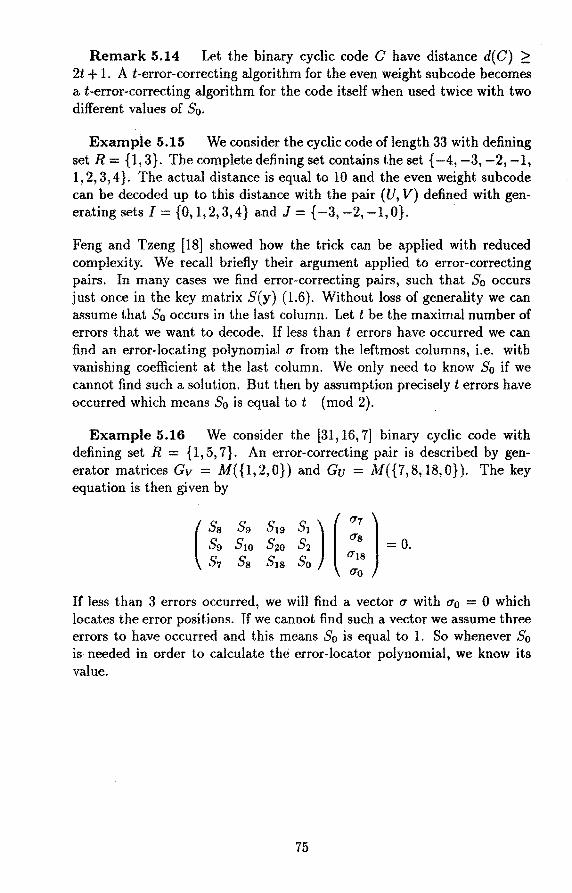
Remark 5.14 Let the binary cyclic code C have distance d(C) ~ 2t + 1. A t-error-correcting algorithm for the even weight subcode becomes a t-error-correcting algorithm for the code itself when used twice with two different values of Bo.

Example 5.15 We consider the cyclic code of length 33 with defining set R = {1, 3}. The complete defining set contains the set {-4, -3, -2, -1, 1, 2, 3, 4}. The actual distance is equal to 10 and the even weight subcode can be decoded up to this distance with the pair (U, V) defined with gen­erating sets I = {O, 1, 2, 3,4} and J = {-3, -2, -1, O}.

Feng and Tzeng [18] showed how the trick can be applied with reduced complexity. We recall briefly their argument applied to error-correcting pairs. In many cases we find error-correcting pairs, such that S0 occurs just once in the key matrix S(y) (1.6). Without loss of generality we can assume that So occurs in the last column. Let t be the maximal number of errors that we want to decode. lf less than t errors have occurred we can find an error-locating polynomial u from the leftmost columns, i.e. with vanishing coefficient at the last column. We only need to know So if we cannot find such a solution. But then by assumption precisely t errors have occurred which means So is equal tot (mod 2).

Example 5.16 We consider the [31, 16, 7] binary cyclic code with defining set R = {1, 5, 7}. An error-correcting pair is described by gen­erator matrices Gv = M({l,2,0}) and Gu = M({7,8,18,0}). The key equation is then given by

= 0.

If less than 3 errors occurred, we will find a vector u with u0 = 0 which locates the error positions. If we cannot find such a vector we assume three errors to have occurred and this means So is equal to 1. So whenever So is needed in order to calculate the error-locator polynomial, we know its value.

75

76

Chapter 6

Pairs from MDS-codes

6.1 A class of MDS-codes

In this section we assume that the field IF is finite of order q. Also let (n, q) = 1. As in the previous section, let IF :::> IF contain the n-th roots of unity.

Theorem 6.1 Let C and A denote two cyclic codes over IF of length n. Let their defining sets be given by

R _ { 1 l 2l rl} c - ,q,q , ... ,q '

/or l,r,s > 0 with r < s. Then

d(C) = min{ IRcl + 1, d(A) }.

In particular the code C is MDS /or IRcl < d(A).

Proof. Clearly d(C) :::; !Rel+ 1 by the Singleton bound. It sQffices to prove for a word c E C of weight wt(c) :::; !Rel that c E A. The columns in M(Re) corresponding to the support of care dependent. Thus the submatrix of M(Rc) formed by these columns has row-rank less than IRcl- The submatrix of M(RA) formed by columns at the support of c has a linear relation among its top IRcl rows. Taking coefficients and rows to the power q1 yields a relation on lower rows and it is seen that the two submatrices have the same row-space. 0

Remark 6.2 The conclusion and the proof of the theorem remain the same when zero is added to the defining sets Re and RA

Exarnple 6.3 The code C over IF = GF(211 ) of length n = 23 with defining set Re = { 0, 1, 4, ... , 4r} is MDS for r :::; 5.

77

6.2 Construction of pairs

For a t-error-correcting BCH-code C with defining set R ::> {1, 2, ... , 2t}, we have by Theorem 5.6 a t-error-correcting pair (U, V). The codes U and V have generating sets 1 = {O, 1, ... , t} and J = {1, 2, ... , t} respectively. More generally, we have

Proposition 6.4 Let the codes U and V be MDS of dimension k(U) t + 1 and k(V) = t respectively. A code C with C J_ U * V has distance d(C) ~ 2t + 1. Moreover it has the t-error-correcting pair (U, V).

Proof. Let c E C have support of weight w. Fort+ 1 < w < 2t + 1, Theorem 5 in [31] yields w ~ (t+I)+t, a contradiction. For 0 < w $ t+l, it yields w ~ w+I, again a contradiction. Thus d(C) ~ 2t+ 1. The conditions (1.1)-(1.3) and {1.11) for an error-correcting pair follow immediately. D

Rèmark 6.5 In case the code U is not MDS, hut otherwise the con-ditions on U and V are satisfied, the pair (U, V) in the lemma is still t-error-locating fora code C with C J_ U *V.

We give two applications of MDS codes obtained with Theorem 6.1. In both cases, U and V are chosen such that the condition C J_ U * V leads to a small defining set for C. Furthermore the key-equation (1.6) can be solved with complexity 0( t 2 ) in both cases. Here the complexity is estimated by the number of required multiplications in the field JF.

Theorem 6.6 (first conjugacy format) Let the codes U / lF and V / lF have generating sets I = {I,q1,q21 , ... ,qt1} and J = {O,q1,q21" .. ,q<t-i)1}, fort ~ 2. Let t = t1 be maxima/ such that both U and V are MDS of dimension k(U) = t + 1 and k(V) t respectively. For 2 $ t $ t1, a code G/JF with

Re ::> {1,2,q1+l,q21+1, ... ,q<t-1)1 + l}

has the t-error-correcting pair (U, V). The key equation (1.6} can be solved with complexity O(t2 ).

Proof. The value of t1 can be obtained with Theorem 6.1. The complete defining set R for C satisfies R ::> 1 + J and thus C J_ U * V. We may use Proposition 6.4. For the solving of the key equation see Section 6.3. D

Theo rem 6. 7 (second conjugacy format) Let the codes U / lF and V / lF have generating sets I = { 0, 1, q21 , q41 , ••• , q(2t-2)1} and J = { O, q1, q31 , ... , qC2t-3)z}, fort ~ 2. Let t = t1 be maxima/ such that both U and V are MDS of dimension k(U) = t + 1 and k(V) = t respectively. For 2 $ t $ t1, a

code C / lF with

Re ::> {O, 1, q1 + 1, q31 + 1, ... 'q(2t-3)1 + 1}

78

has the t-error-correcting pair (U, V). The key equation (1.6} can be solved with complexity O(t2

).

Proof. As in Theorem 6.6. D

Example 6.8 We consider codes of length n = 23 over GF(211 ). Let U and V be as in Theorem 6.7 with q = 2,l = 1,t = 3, or 1={O,1,4, 16} and J = {0,2,8}. By Example 6.3, both U and Vare MDS and we have found a 3-error-correcting pair for the even weight subcode C of the binary Golay code, since Re :::> { 0, 1, 3, 9}.

Lemma 6.9 (recurrences) IJ a pair (U, V) is t-error-locating and the generating sets I and J are of a conjugacy format, then the syndromes si= (e,a(i)) can be determined for

i = ql'1 + 1, /or s 2 1, i = q<2s-l)I + 1 /or s 2 1,

first format {Theorem 6.6). second format {Theorem 6. 7).

Proof. The case s < t is obvious. For s 2 t we use induction. For both formats we may assume that the error-locating word u E U has non-zero coordinate o-1 at a(l). We have, for the first format,

0 = (e*u,a(q81)}

= (e, u * a(q81)}

u1 ( e, a( q81 + 1)) + known terms.

Similarly for the second format. D

Example 6.10 We consider codes oflength n = 39 over GF(212). Let U and V be as in Theorem 6.6 with q = 2, l 1, t = 4, or I = {1, 2, 4,8, 16} and J { 0, 2, 4, 8}. The code V is MDS and we have found a 4-error­locating pair for the binary code C with Re :::> {1, 3, 5,'9}. lt is of type [39, 15, 10]. By the lemma, we can determine syndromes corresponding to the checks 17 and 65 :.::: 26 (mod 39) and the error values can be deter­mined by Lemma 5.9.

6.3 Fundamental iterative algorithm

In their paper [18], Feng and Tzeng proposed a fundamental iterative algo­rithm (FIA). Fora matrix A, it gives the minimal set of dependent leading columns. It basically solves an arbitrary homogeneous system of linear equations and contains the Berlekamp-Massey algorithm as a special case. The algorithm is not required to make our decoding procedure work hut it seems to be a key algorithm in treating complexity aspects.

79

We recall it in a form that allows us to complete the proof of Theorem 6.6 and Theorem 6.7. Whenever it is necessary for reasons of dimension, we extend a vector with a suitable number of zeros. Let the matrix A(a,b)

be the submatrix of A consisting of the elements in the first a rows and the first b columns of A. For a fixed b, we consider column vectors u with non-zero coordinate at position b that solve the equation

Let a = ·a(b) be maximal such that a solution exists and let u = u(b) be such a solution. To assure that a solution exists we use the convention A(O,b) = oT. For these a and u, let 8(b) be defined as

b

8(b) = E Aa+t,k<1'k, k=l

or as 8 (b) = 0 when Au(b) = 0. For given { ( u(b), 8 (b), a(b)) h<i, the idea of the FIA is now to calculate u(i) with help of the u(bJ, b < i. Starting with any vector u of length i and u; unequal to zero, this is achieved by subtracting suitable scalar multiples of the known u(b) from u thereby obtaining a new u. More precisely, whenever u solves

• d = E Aj+J,kO"k f= 0,

k=l

and there exists a triple ( a(b), 8 <6>, j), we construct

O" - (1' - _:!._O"(b) 8(b) '

which now solves A(j+1,i)u = 0.

Finally we will obtain the triple ( u<i), 8 (i), a<il). For details and proofs see [18].

Let us assume that Ais a Hankel matrix. By starting the calculation of u(i)

with a particular choice for u, namely a shifted version of u<i-t) with zero · in the lowest position, we get the well-known Berlekamp-Massey algorithm.

The calculations of most d are not necessary - they are zero or already known by the structure of Hankel matrices. This is the crucial point in saving complexity. In the next section we will show how to apply the FIA to matrices S(y) obtained with Theorem 6.6 and Theorem 6.7. It turns out that solving the linear systems described by these matrices is achieved with basically the same complexity as used for the Berlekamp-Massey algorithm.

80

6.4 Reducing complexity

In general the complexity of the procedure described in Section 1.1 equals 0( n3). This is due to the fact that only matrix inversions and multiplica­tions are involved. We found two possibilities to improve on the number of computations. One approach uses regular structures of the matrix S(y) and the other approach reduces the size of the field that contains the entries of S(y).

In the case of the conjugacy format, the matrix S(y) has a highly regular structure. We explicitly treat the first conjugacy format. For the second conjugacy format similar considerations hold. We write the generating sets de:fining U and V for the first conjugacy format in the following ordered form

J - {ql(t-1) ql(t-2) ql(t-3) q'} - ' , ,"., ' I { 1 1 21 tl} = ,q ,q , ... ,q '

excluding the zero in J. We recall the de:finition of Si given in Lemma 5.9.

S; = (e,a(i)), i ER.

Obviously S; = (y,a(i)) holds for all i ER.

Lemma 6.11 With generator matrices for U and V corresponding to the above ordering, the entries in S(y) satisfy

S(y)i,i = (S(y)H1,;-1/, j 1, "., t - 2 , i = 2, ... , t + 1.

Proof. The entry S(y )J,i is equal to the syndrome Sh(i,i) with

h(j, i) = ql(t-j) + ql(i-1).

Obviously h(j, i) is equal to q1h(j + 1, i 1). The vector y was assumed to be defined over a field lF of cardinality q. Hence Sq1h = Sh q

1 and the lemma.

follows. 0

We see from Lemma 6.11 that the format of S(y) is very similar toa Hankel matrix. Thus to find S(y) we only have to calculate the entries in the first row and the last column. The other entries are found using the lemma. This structure is now used in finding the space of solutions to the key equation in the sa.me way as in the Berlekamp-Massey algorithm. Recall that the complexity gain in using the Berlekamp-Massey algorithm was due to the fact that given a vector O'(b), which solves equation

A(a,1>)0' = O,

we find a vector <T that solves equation

A(a-1,ó+t)u = o as a shifted version of O'(b) with zero in the lowest position.

81

Proposition 6.12 Let S(y) be the (t -1) x (t + 1)-matrix of Lemma 6.11. Solving

S(y)u=O

for O' can be done with complexity 0( t 2).

Proof. Consider a typical step in the FIA. Given a solution O"(i-l) to the equation S(y)(a,i-l)u = O, we also have a solution to the equation S(y)(a-l,i)u = 0. The latter solution is obtained by taking all elements in O"(i-t) to the q1-power and shifting them by one position. Using normal bases for the field, raising a number to the q1-th power can be performed by a cyclic shift, not requiring computational complexity. Whenever possible, we now perform an update of O'. This is done by performing the following operation

and the calculation of a new d. The whole step requires at most O(t) operations and we find a solution to S(y)(a,i). Thus in every complexity demanding step, starting from a solution to the system S(y)(a,b) we find a solution to the system S(y)(a',b') such that a' + b' is equal toa+ b + 1. On the other hand a' + b' is bounded by 2t which is the sum of the number of rows and the number of columns in S(y ). So we have to perform at most 2t times a calculation requiring O(t) operations. The proposition follows. D

Remark 6.13 (on the proof of Theorem 6.6 and Theorem 6.7) To complete the proof of Theorem 6.6, we have to add a row to S(y) of Lemma 6.11. This row caused by the zero in J does not fit into the quasi Hankel format. This causes one additional step in the FIA with complexity 0( t). Theorem 6. 7 requires not only an additional row hut also an additional column. We add this column as the rightmost column of S(y ). The FIA needs at most 0( t) operations for every position in this column. In both cases the overall complexity is still ruled by O(t2 ).

Example 6.14 The quadratic residue code of length 41 is a good exarnple for the second conjugacy format. We find I = {1, 23, 37, 31, O} and J = {8, 20, 9, O} with q1 = 23 . By the results of section 3 we can set S0 = 0 whenever it is needed. An error-locating polynomial is found by solving the system

(

Ss5+1 Ssz(ss+l) Ss•(s+l) Sss(s+i) Sss ) S83+t Ssics+i) Ss3(s+i) Ss3(s3+i) Ss3 _ O Ss+i Ss(s+i) Ss(ss+i) Sscss+i) Ss "' - ·

S1 Ssi Ssf Ss6 So

We see that the submatrix S(y)C3•4) has a quasi Hankel structure which can be utilized to solve the system.

82

In considering cyclic codes of length n, in most cases codes U and V will be defined over the smallest field IF containing an n-th root of unity. In some cases however U and V can be taken to be codes defined over IF C IF. This implies that S(y) has entries from IF rather than from IF which allows us to perform these operations faster.

Example 6.15 Let n = 15. Let C be the double error-correcting BCH-code with Re= {1,2,3,4,6,8,9,12}. To show how the choice of I and J influences the decoding, we notice two possible choices. First we see that we can choose J = {1, 2} and I = {O, 1, 2} and this would correspond to the usual decoding as a subcode of a RS-code. A different choice is I = { 2, 8, 0} and J = { 1, 4, 0}. This choice corresponds to cyclotomic cosets with respect to GF(4). S0 is only needed if two errors occurred which gives S0 = 0. S(y) will be a matrix over GF(4) and all calculations will only involve computations over GF(4).

83

84

Chapter 7

Applications

7.1 Codes of length less than 63

Table 1 gives error-correcting pairs for binary cyclic codes which have error­correction capability exceeding the error-correction capability given by the BCH bound. We use the same numbering for codes as in [31]. Equivalent codes and subcodes with the same error correction capability use the sa.me pair. Usage of hyperpla.nes (Proposition 1.20) or usage of the unknown syndrome 80 is indicated as remark. The remark FT indicates that the same error-correcting pair is given by Feng and Tzeng in [19]. In four cases (no. 92,123,132,146) we stay one short of the actual error-correction capability. All other pairs allow decoding up to half the actual minimum distance of the code. To check conditions (1.1) and (1.2) of Definition 1.1 is straightforward. In all hut four cases (no. 85,106,107,137), the code V is MDS. This follows either immediately using the BCH-bound or with Theorem 6.1. Thus, also condition (1.3) is easily verified in these cases. In the cases 85 and 137, the distance d(V .l) is obtained with the Hartmann-Tzeng bound and Theorem 6.1 respectively. Cases 106 and 107 are treated in Example 7.3 and Example 7 .4 respectively. To show that the pairs are error-correcting we use either the BCH-bound to show that condition (1.11) is satisfied or we use recurrences to determine unknown syndromes until we can apply Lemma 5.9. Whenever we use the conjugacy format, Lemma 6.9 provides us with a possibility to determine some unknown syndromes. Cases that require other recurrences are listed in Ta.ble 2. For brevity we introduce the following notation. Ui -::/: 0 : R(j) -+ Si+i means that we use equation (5.5) in Lemma 5.10,

ui1si1+i + ... + ui2si2+i +ui, si,+;= o, with the indicated j and tha.t Si+i will be the only unknown in the equation. Thus it can be obtained provided O'i -::/: O. Recurrences separated by a. comma can be computed in parallel.

85

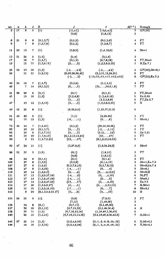
no. n k d R J I d yJ. Re mark 3 17 9 5 {1} {-1,+1} -3,0,+3} 3 GF(l6)

{0,8} {1,8,13} 3

8 21 9 8 {0,1,3,7} {0,1,2} {0,1,2,6} 4 FT 9 7 8 {1,3,7,9} {0,1,2} {1,2,6,7} 4 FT

11 23 12 7 {1} {2,8,0} {1,4,16,0} 4 SO=l

13 31 21 5 {1,5} {1,4} {0,1,4} 3 17 16 7 {1,5,7} {0,1,2} {0,7,8,18} 4 FT,SO=l 19 11 11 {1,3,5,11} {O, ... ,3} {l ,2,3,8,9,10} 5 H,Ex.7.1

25 33 13 10 {1,3} {-2, ... ,+2} {-2, .•. ,+2} 5 GF(32),SO=O,l 26 11 11 {1,3,11} { 0,10,20,30,40} {1,2,11,15,24,25} 6 FT

{-2, ... ,2} {-13,-12,-11,+tl,+12,+13} 6 GF(32),Ex.7.2

36 35 16 7 {l,5,7} {0,3,6} {l,2,4,5} 4 FT 40 7 14 {0,1,3,5} {o, ... ,5} {31, ... ,34,0,1,8} 7 FT

41 39 26 6 {0,1} {0,1} {0,1,4} 3 FT,SO=O 45 15 10 {1,3} {0,2,4,8} {1,2,4,8,16} 5 Ex.6.10

{O, ... ,3} {1,2,3,8,9} 5 FT,Ex.5.7 47 13 12 {1,3,13} {O, ... ,3} {l,2,3,8,9,10} 5 H

49 41 21 9 {1} {8,20,9,0} {1,23,37,31,0} 5

51 43 29 6 {1} {1,2} {0,20,40} 3 FT 52 15 13 {1,3} {-6,". ,-1} {O, ... ,6} 7 S0=0,1

73 45 23 7 {1,5,21} {0,1,2} {31,32,33,38} 4 FT 83 16 10 {0,1,3,7} {0, .. "3} {-2, ... ,1,11} 5 FT 84 15 9 {1,3,7,15} {0". "3} {1,11, .. "14} 5 Ex.5.11 85 15 10 {1,7,9,15} {0,1,2,13,14,15} {13, ... ,17} 5 FT 90 9 12 {1,5,7,9,15} {13, .. "17} {0,1,2,13,14,15} 6

92 47 24 11 {1} {3,27,8,0} {l,9,34,24,0} 5 SO=O

96 51 35 5 {l,9} {0,1} {1,8,15} 3 FT {0,8} {1,8,13} 3

98 34 6 {0,1,5} {0,1} {0,1,4} 3 FT 106 27 8 {1,3,9} {0,2,8} {0,1,4,16} 3 SO=l,Ex.7.3 107 27 9 {1,5,9} {0,2,7,8,13} {0,2,7,8,13} 5 SO=O,Ex.7.4 108 27 9 {1,3,19} {-4, ... ,-1} {o, ... ,4} 5 S0=0,1 119 19 14 {1,3,5,9} {0, ... ,4} {O, ... ,4,12,6} 6 SO=O,H 121 17 12 {1,3,9,17,19} {-4, .. :,O} {O, ... ,4,19} 6 SO,FT 122 17 14 {1,3,5,17,19} {-4, .. "1} {0, ... ,6} 7 S0=0,1 123 17 14 {1,5,9,17,19} {13" .. ,17} {O, ... ,4,19} 6 Ex.7.5 124 17 16 {1,3,5,9,17} {O, ... ,5} {o, ... ,5,12,13} 7 H,SO=l 128 11 15 {1,3,5,11,19} {-7". "-1} {O, ... ,7} 8 80=0,1 132 8 24 {0,1,3,5,9,11,17} {O, ... ,8} {O, ... ,10} 10 H

135 55 35 5 {1} {0,9} {7,8,9} 3 FT {7,13} {l,49,36} 3

136 34 8 {0,1} {0,7,13} {0,1,49,36} 4 137 30 10 {0,1,11} {0,7,13,32} {0,1,49,36,4} 4 H 138 25 11 {1,5} {0,7,16,13,14} {1,18,49,2,36,43} 6 140 21 15 {1,5,11} {0,7,16,13,14,32} {0,1,18,49,2,36,43,4} 7 H,SO=l

144 57 21 14 {1,3} {0,2,4,8,16} { 0,-1,-2,-4,-8,-16,-32} 6 H,S0=0,1 146 19 16 {l,3,19} {0,2,4,8,16} {0,-1,-2,-4,-8,-16,-32} 6 H,SO=O,l

86

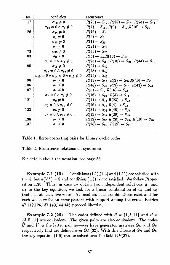
no. condition recurrence 17 0'18 f. 0 R(25)-+ 812, R(28) -+ 815; R(24)-+ Su

0'1s = 0 /\ us f. 0 R(7)-+ 815, R(9)-+ 811,R(l8)-+ S26

26 0'24 f: 0 R(16)-+ S1 0'1 f. 0 R(6)-+ 81 0'25 f. 0 R(l)-+ 826 0'2 f. 0 R(24)-+ S26

73 0'3s f:. 0 R(33)-+ S26 83 O'Q f: 0 R(5)-+ S5,R{l8)-+ Sis

ao = 0 /\ 0'11 f:. 0 R(25)-+ S36; R(lO)-+ S21i R(44)-+ S10 90 0'15 f:. 0 R(27)-+ 842

0'15 = 0 /\ 0'14 f. 0 R(28)-+ S42 0'15 = 0 /\ 0'14 = 0 /\ 0"13 f. 0 R(29)-+ 842

96 0'1 f. 0 R(13)-+ S14i R(2)-+ 83; R(40)-+ S41 106 0'1 f 0 R( 48) -+ 849; R(9) -+ Sm, R( 43) -+ 844 107 0"7 f:. 0 R(5) -+ S12;R(l6)-+ 823

u1 = 0 /\ as f:. 0 R(16)-+ S24; R(3)-+ Sn 121 O"Q f 0 R(14)-+ 814,R(23)-+ 823

uo = 0 /\ 0-19 f 0 R(46)-+ 814;R(4)-+ S23 123 O'Q f. 0 R(31)-+ S31,R(48)-+ S4s

O'Q = 0 /\ 0"19 f. 0 . R(12)-+ 831;R(29)-+ 84s 136 0'1 f. 0 R(32)-+ S33;R(28)-+ 829; R(19)-+ S20 137 0"1 f. 0 R(28)-+ 829; R(19) -+ S20

Table l. Error-correcting pairs for binary cyclic codes.

Table 2. Recurrence relations on syndromes.

For details about the notation, see page 85.

Example 7.1 (19) Conditions (1.1),(1.2) and (1.11) are satisfied with t = 5, hut d(V.l) = 5 and condition (1.3) is not satisfied. We follow Propo­sition 1.20. Thus, in case we obtain two independent solutions u1 and u 2 to the key equation, we look for a linear combination of u 1 and U2

that has at least five zeros. At most six such combinations exist and for each we solve for an error pattern with support among the zeros. Entries 4 7,119,124,137 ,140,144,146 proceed likewise.

Example 7.2 (26) The codes defined with R = {1,3, 11} and R = {3, 5, 11} are equivalent. The given pairs are also equivalent. The codes U and V in the latter pair however have generator matrices Gu and Gv respectively that are defined over GF(32). With this choice of Gu and Gv the key equation (1.6) can be solved over the field GF(32).

87

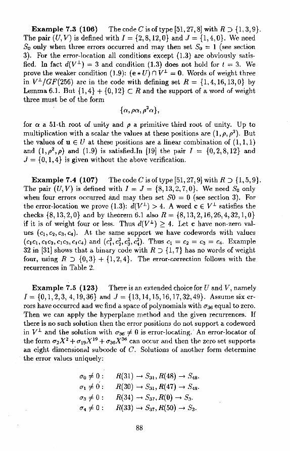
Example 7.3 (106) The code Cis of type [51, 27, 8] with R :::> {l, 3, 9}. The pair (U, V) is defined with I = {2,8, 12,0} and J = {1,4,0}. We need S0 only when three errors occurred and may then set S0 = 1 ( see section 3). For the error-location all conditions except (1.3) are obviously satis­fied. In fact d(Vl.) = 3 and condition {1.3) does not hold fort= 3. We prove the weaker condition (1.9): (e * U) n Vl. = 0. Words of weight three in VJ./GF(256) are in the code with defining set R {1,4,16,13,0} by Lemma 6.1. But {1, 4} + {O, 12} C Rand the support of a word of weight three must be of the form

{a,pa,p2a},

for a a 51-th root of unity and p a primitive third root of unity. Up to multiplication with a scalar the values at these positions are (1, p, p2

). But the values of u E U at these positions area linear combination of (1, 1, 1) and (1,p2 ,p) and (1.9) is satisfied.In [19] the pair I {0,2,8,12} and J {O, 1,4} is given without the above verification.

Example 7.4 (107) The code Cis of type [51, 27, 9] with R :::> {1, 5, 9}. The pair (U, V) is defined with I = J = {8, 13, 2, 7, O}. We need So only when four errors occurred and may then set SO = 0 (see section 3). For the error-location we prove (1.3): d(V l.) > 4. A word c E Vl. satisfies the checks {8, 13, 2, O} and by theorem 6.1 also R = {8, 13, 2, 16, 26, 4, 32, 1, O} if it is of weight four or less. Thus d(V l.) 2: 4. Let c have non-zero val­ues (ei, c2 , c3 , c4). At the same support we have codewords with values (c1c1,c1c2,c1c3,c1c4) and (ci,c~,c~,cD. Thus c1 = c2 = C3 c4. Example 32 in [31] shows that a binary code with R :::> {1, 7} has no words of weight four, using R :::> { 0, 3} + { 1, 2, 4}. The error-correction follows with the recurrences in Table 2.

Example 7.5 (123) There is an extended choicefor U and V, namely I = {O, 1, 2, 3, 4, 19, 36} and J {13, 14, 15, 16, 17, 32, 49}. Assume six er­rors have occurred and we find a space of polynomials with o-36 equal to zero. Then we can apply the hyperplane method and the given recurrences. If there is no such solution then the error positions do not support a codeword in Vl. and the solution with o-36 f= 0 is error-locating. An error-locator of the form u2X2 + o-19X 19 + 0'36X36 can occur and then the zero set supports an eight dimensional subcode of C. Solutions of another form determine the error values uniquely:

O"o # 0:

0'1 # 0:

0"3 # 0: 0"4 i= 0 :

R(31) -+ S3" R( 48) -+ S4s.

R(30) -+ S3i, R(41)-+ S4s·

R(34) -+ S31, R(O)-+ 83. R(33) -+ 831, R(50) -+ 83.

88

7 .2 Sequences of codes

In a certain range of the minimum distance, the conjugacy formats of Chap­ter 6 allow the construction of sequences of cyclic codes with the same designed distance and redundancy as BCH-codes.

Proposition 7.6 Let n be equal to 2m - 1, m = 21 + 1. For a bi­nary cyclic code C with defining set Re :::> {1, 21 +1,21- 1 + 1} we have a 3-error-correcting pair ( U, V) with generating sets I = { 0, 1, 221 , 241 } and J = {0,21,231 }.

Proof. The code is defined in [32, Ch.9 §11]. There it is also proved that the distance d = 7. For the even weight subcode we may write R :::> { 0, 1, 21 + 1, 231 + 1}. Thus we find the formats of Theorem 6. 7, except that the code U is not MDS. In fact the codes U and V are equivalent to codes with generating sets I' = 4·I={0,4,2,1} and J' = 4 · 21 ·J={0,2,1}. The conditions (1.1)-(1.3) and (1.11) are fulfilled. Since S0 occurs only once in the key matrix S(y), by the results of Section 5.4 we can assume that S0 = 3 (mod 2). D

Rem ark 7. 7 ( QR-codes) It is clear from Table 1, that the second conjugacy format yields good pairs for the smaller binary QR-codes. The conjugacy formats require defining sets of size t, while the BCH-format re­quires sets of size 2t (the largest set of consecutive quadratic residues is in genera! not formed by the residues {1, 2, . " , 2t} and the usual argument that only { 1, 3, ... , 2t - 1} need to be in the defining set does not apply ). With a uniform distribution of the quadratic residues, the conjugacy for­mats should correct about twice the number of errors of the BCH-format. Calculations for codes of length less than 1024 agree with this. For ex­ample, for the codes of length n = 863 and n = 887, we apply Theorems 6.6 and 6. 7 with q = 2. They yield pairs to correct t = 10 (l = 57) and t = 7 (l = 62) errors for n = 863 and t = 8 ( l = 182) and t = 11 ( l = 206) errors for n = 887. For both values of n, the BCH-format corrects t = 4 errors. Also, it is clear that both the BCH-format and the conjugacy for­mats have a capability that is of order log( n) for large codelength n. This is way below the square root bound.

In addition to these we give the following sequences.

Proposition 7.8 Let C be a binary cyclic code of length n where 3 does not divide n. Let Re contain the set { -1, 1}. Then a ~-error­correcting pair (U, V) is given through generating sets I = {-3, 0, 3} and J={-1,1}.

89

Proof. The complete defining set R for C satisfies R :::> l + J. 3 does not divide the length and it follows that U and V are both MDS. The proof follows from Lemma 6.4. D

Example 7.9 (Zetterberg codes [55]) Let n be equal to 22m + 1. The Zetterberg code C with defining set Re = { 1} has the 2-error­correcting pair (U, V) given in Proposition 7.8.

Example 7.10 (Melas codes [34]) Let n be equal to 2m - 1 and let m be odd. The Melas code C with defining set Re = {l, -1} has the 2-error-correcting pair (U, V) given in Proposition 7.8.

The following sequence of reversible codes contains as members binary codes of type [73,37,~ 11] and [85,45,~ 11].

Proposition 7.11 Let C be a binary cyclic code of length n where 3 does not divide n. Let Re contain the set {-7, -5, 1, 1, 5, 7}. Then a 5-error-correcting pair ( U, V) is given through generating sets l = { -4, -2, -1, 1, 2,4} and J = {-6, -3, -0,3, 6}.

Proof. Use Theorem 5.6. D

90

Bibliography

[1] E. Arbarello, M. Cornalba, P.A. Griffiths and J. Harris, Geometry of algebraic curves l. New York: Springer-Verlag, 1985.

[2] E.R. Berlekamp, "Decoding algorithms for block codes," in Key Papers in the Development of Coding Theory, E.R. Berlekamp, Ed" New York: IEEE Press, 1974.

[3] E.R. Berlekamp, Algebraic coding theory. New York: McGraw-Hill, 1968.

[4] R.E. Blahut, Theory and practice of error control codes. Reading, Ma.: Addison-Wesley, 1983.

[5] P. Bours, J.C.M. Janssen, M. van Asperdt, and H.C.A. van Tilborg, "Algebraic decoding beyond eBcH of some binary cyclic codes, when e > eBcH," IEEE Trans. Inform. Theory, vol.IT-36, pp.214-222, 1990.

[6] P.J. Cameron and J.H. van Lint, Designs, Graphs, Codes and their Links. Cambridge: Cambridge University Press, 1991.

[7] C. Chevalley, Introduction to the theory of algebraic functions of one variable. New York: AMS, 1951.

[8] C. Dahl, Codes and Geometry. Thesis, Technical University of Den­mark, 1991.

[9] I.M. Duursma, "Algebraic decoding using special divisors," IEEE Trans. lnform. Theory, vol.IT-39, March 1993.

(10] I.M. Duursma, "On the decoding procedure of Feng and Rao," Pro­ceedings Algebraic and Combinatorial Coding Theory, Voneshta Voda, Bulgaria, 1992.

[11] I.M. Duursma, "Majority coset decoding," IEEE Trans. Inform. The­ory, vol.IT-39, May 1993.

[12] I.M. Duursma, and R. Kötter, Error-locating pairs for cyclic codes. Eindhoven, Linköping: preprint, 1993.

91

[13] M. Elia, "Algebraic decoding of the (23,12,7) Golay code," IEEE Trans. Inform. Theory, vol.IT-33, pp.150-151, 1987.

[14] D. Ehrhard, "Decoding algebraic-geometric codes by solving a key equation," Proceedings Algebraic Geometry and Coding Theory, Lu­miny, France, 1991.

[15] D. Ehrhard, "Decoding Hermitia.n Codes over lFq2 up to designed error capability," Proceedings Algebraic and Combinatorial Coding Theory, Voneshta Voda, Bulgaria, 1992.

[16] D. Ehrhard, "Achieving the designed error capacity in decoding algebraic-geometric codes," to appear in IEEE Trans. Inform. The­ory.

[17] G.L. Feng and T.R.N.Rao, "Decoding algebraic geometrie codes up to the designed minimumdistance," IEEE Trans. Inform. Theory, vol.IT-39, January 1993.

[18] G.L. Feng and K.K. Tzeng, "A generalization of the Berlekamp-Massey a.lgorithm for multisequence shift-register synthesis with applications to decoding cyclic codes," IEEE Trans. Inform. Theory, vol.IT-37, pp.1274-1287, 1991.

[19] G.L. Feng and K.K. Tzeng, "Decoding Cyclic and BCH codes up to Actua.l Minimum Distance Using Nonrecurrent Syndrome Depen­dence Relations," IEEE Trans. lnform. Theory, vol.IT-37, pp.1716-1723, 1991.

[20] W. Fulton, Algebraic curves. Reading, MA: Benjamin, 1969.

[21] V.D. Goppa, "Codes on algebraic curves," Soviet Math. Dokl., vol. 24, pp.170-172, 1981.

[22] C.R.P. Hartmann and K.K. Tzeng, "Genera.lizations of the BCH bound," lnform. Contr., vol.20, pp.489-498, 1972.

[23] R. Hartshorne, Algebraic geometry. New York: Springer-Verlag, 1977.

[24] J. Justesen, K.J. Larsen, H.E. Jensen, A. Havemose and T. Hf')holdt, "Construction and decoding of a class of algebra.ic geometrie codes," IEEE Trans. lnform. Theory, vol.IT-35, pp.811-821, 1989.

[25] J. Justesen, K.J. Larsen, H.E. Jensen, and T. H9.1holdt, "Fast decoding of codes from plane algebra.ic curves," IEEE Trans. lnform. Theory, vol.IT-38, pp.111-119, 1992.

92

[26] R. Kötter, "A unified description of an error locating procedure for lin­ear codes", Proceedings Algebraic and Combinatorial Coding Theory, Voneshta Voda, Bulgaria 1992.

[27] V.Yu. Krachkovskii, Decoding of codes on algebraic curves. In Russian, preprint, 1988.

[28] G. Lachaud, "Projective Reed-Muller codes," in Leet. Notes in Comp. Sci" vol.311. Berlin: Springer, 1988.

[29] J .H. van Lint, Introduction to Coding Theory. New York: Springer­Verlag, 1982.

[30] J.H. van Lint and G. van der Geer, Introduction to coding theory and algebraic geometry. Basel: Birkhäuser Verlag, 1988.

[31] J.H. van Lint and R.M. Wilson, "On the minimum distance of cyclic codes," IEEE Trans. Inform. Theory, vol.IT-32, pp.23-40, 1986.

[32] F.J. MacWilliams and N.J.A. Slone, The Theory of Error-Correcting Codes. Amsterdam: North-Holland, 1977.

[33] J.L. Massey, "Shift-register synthesis and BCH decoding," IEEE Trans. In/or. Theory, vol.IT-15, pp.122-127, 1969.

[34] C. M. Melas, "A cyclic code for double error correction,'' IBM J. Res. Devel., 4, pp.364-366, 1960.

[35] C. Moreno, Algebraic curves over finite fields. Cambridge: Cambridge University Press, 1991.

[36] R. Pellikaan, "On decoding linear codes by error correcting pairs," Eindhoven University of Technology, preprint, 1988.

[37] R. Pellikaan, "On decoding by error location and dependent sets of error positions,'' Discrete Mathematics, vol.106-107, pp.369-381, 1992.

[38] R. Pellikaan, "On a decoding algorithm for codes on maxima! curves," IEEE Trans. Inform. Theory, vol.IT-35, pp.1228-1232, 1989.

[39] W.W. Peterson and E.J. Weldon Jr" Error-correcting codes. Cam­bridge, MA: M.l.T. Press, 1971.

[40] S.C. Porter, Decoding codes arising /rom Goppa 's construction on al­gebraic curves. Thesis, Yale University, 1988.

[41] S.C. Porter, B. Shen and R. Pellikaan, "On decoding geometrie Goppa codes using an extra place," IEEE Trans. lnform. Theory, vol.IT-38, pp.1663-1676, 1992.

93

[42] l.S. Reed, T.K. Truong, X. Chen and X. Yin, "The algebraic decoding of the [41, 21, 9] quadratic residue code,'' IEEE Trans. Inform. Theory, vol.IT-38, pp.974-986, 1992.

[43] C. Roos, "A new lower bound for the minimum distance of a cyclic code," IEEE Trans. lnform. Theory, vol.IT-29, pp.330-332, 1983.

[44] D. Rotillon and J.A. Thiong Ly, "Decoding of codes on the Klein quartic,'' in Leet. Notes in Comp. Sei" vol.514. Berlin: Springer, 1991.

[45] S. Sakata, "Finding a minimal set of linear recurring relations capable of generating a given finite two-dimensional array," Journal of Sym­bolie Computation, vol.5, pp.321-337, 1988.

[46] S. Sakata, "Extension of the Berlekamp-Massey algorithm to N di­mensions,'' Information and Computation, vol.84, pp.207-239, 1990.

[47] B. Shen, "On encoding and decoding of the codes from Hermitian curves,'' in Cryptography and Coding II!, M. Ganley, Ed" Oxford: Ox­ford University Press, 1993.

[48] A.N. Skorobogatov and S.G. Vladut, "On the decoding of algebraic­geometric codes," IEEE Trans. lnform. Theory, vol.IT-36, pp.1051-1060, 1990.

[49] A. B. S!1irensen, "Projective Reed-Muller Codes,'' IEEE Trans. lnform. Theory, vol.IT-37, pp.1567-1576, 1991.

[50] P. Stevens, "Extension of the BCH decoding algorithm to decode bi­nary cyclic codes up to their maximum error-correction capacity,'' IEEE Trans. lnform. Theory, vol.IT-34, pp.1332-1340, 1988.

[51] H. Stichtenoth, Algebraie Funetion Fields and Codes. Springer Univer­sitext, 1993.

[52] M.A. Tsfasman and S.G. Vladut, Algebraie Geometrie Codes. Dor­drecht: Kluwer Acad. Publ" 1991.

[53] S.G. Vladut, "On the decoding of algebraic-geometric codes over Fq for q ~ 16,'' IEEE Trans. lnform. Theory, vol.IT-36, pp.1461-1463, 1990.

[54] V. K. Wei, "Generalized Hamming weights for linear codes,'' IEEE Trans. lnform. Theory, vol.IT-37, pp.1412-1418, 1991.

[55] L. H. Zetter berg, "Cyclic codes from irreducible polynomials for correc­tion of multiple errors,'' IEEE Trans. lnform. Theory, vol.IT-8, pp.13-20, 1962.

94

Samenvatting

Het proefschrift beschrijft de resultaten van mijn onderzoek aan decodeer­algori tmen voor lineaire codes. De algoritmen worden toegepast bij het corrigeren van fouten die onbedoeld optreden bij het verzenden of opslaan van informatie.

Algebraïsch-meetkundige codes (in de zin van Goppa) kennen een eenvoudig te bepalen ondergrens voor het aantal fouten dat gecorrigeerd kan worden. Deze ondergrens wordt de ontwerpcapaciteit genoemd. Bij aanvang van het onderzoek waren twee nauw verwante algoritmen beschikbaar: het ba­sis algoritme en het gemodificeerde algoritme. Beide algoritmen zijn in het algemeen niet in staat om fouten te corrigeren tot de ontwerpcapaciteit van de code. De gemodificeerde versie corrigeert meer fouten maar is slechts toepasbaar op een beperkte klasse van codes. Voor het gemodificeerde al­goritme is een formulering gevonden die het toepasbaar maakt op alle alge­braïsch-meetkundige codes. Voor de gevallen waarbij de herformulering het algoritme niet wezenlijk verandert wordt bewezen dat de prestaties van het algoritme in feite beter zijn dan aanvankelijk was aangetoond. Gedurende het onderzoek suggereerden Feng en Rao een wezenlijke verbetering van de bestaande algoritmen. Hiermee kunnen fouten worden gecorrigeerd tot de ontwerpcapaciteit. In een voorpublikatie lichten zij dit toe aan de hand van een voorbeeld en ontbreekt een bewijs. Uitwerking van hun idee heeft geresulteerd in een algemeen toepasbaar algoritme met een volledig bewijs. Het huidige bewijs van Feng en Rao gaat uit van een beperkt toepasbaar algoritme, dat een groter beslag legt op computergeheugen en rekentijd.

In samenwerking met R. Kötter, werkzaam aan de universiteit van Lin­köping, zijn resultaten bereikt voor het decoderen van cyclische codes. Algemene stellingen worden gegeven voor het construeren van decodeer­algoritmen voor deze codes. In het bijzonder worden algoritmen gegeven die meer fouten corrigeren dan het Berlekamp-Massey algoritme als de op­tredende eenheidswortels verdeeld zijn over een beperkt aantal grote conju­gatieklassen. De complexiteit is die van het Berlekamp-Massey algoritme. Toetsing van de stellingen aan binaire codes van lengte kleiner dan 63 leert dat alle codes op vier na gedecodeerd kunnen worden tot de werkelijke capaciteit.

95

Curriculum vitae

Iwan Maynard Duursma was born on April 19, 1963, in Bussum. He attended the rijksscholengemeenschap Schoonoord in Zeist and com­pleted the gymnasium in 1980. From September 1980 till August 1986, he studied aerospace engineering at the Technische Hogeschool Delft and graduated with the master's thesis: Satellite orbit perturbations due to tidal forces (cum laude, professor K.F. Wakker). From September 1983 till February 1989, he studied mathematics at the Universiteit van Amsterdam and graduated with the master's thesis: Some remarks on Goppa codes (cum laude, professor G. van der Geer). During his study, he was appointed as student assistant (for September 1985 April 1987, by professor H.W. Lenstra jr., and for January 1988 - November 1988, by A.M. Cohen). While applying for a position as a Ph.D. student, he was a full-time teacher of mathematics at the Instituut Blankestijn in Utrecht. Since September 1990, he has worked in the Dis­crete Mathematics group at the Technische Universiteit Eindhoven, with support from the Netherlands Organization for Scientific Research.

96

Stellingen behorende bij het proefschrift

DECO DING

CODES FROM CURVES

AND CYCLIC CODES

van Iwan M. Duursma

1.

Het projectieve vlak over het lichaam GF(B) bevat 73 rationale punten. Hieron­der bevinden zich acht drietallen van de vorm {(X : Y : Z), (X2 : Y 2 : Z2 ),

( X 4 : Y 4 : Z4)} met de eigenschap dat de drie punten niet op een lijn liggen. De overige 49 punten liggen op de zeven lijnen gedefinieerd over het lichaam GF(2). De automorfismengroep van de acht drietallen en de automorfismengroep van de zeven lijnen zijn identiek (als ondergroep van de automorfismengroep van het projectieve vlak). Het zijn L2(7), respectievelijk La(2).

II.

Zij k een lichaam van karakteristiek 2. Zij S;, Ti E k[X, Y, Z] gedefinieerd door S; = Xi + yi + zî en T; = S; + (St)Ï, voor i > O. Zij q en r machten van 2. Er geldt.

III.

Zij K de Klein kromme, gedefinieerd door /( : X 3Y + Y3 Z + Z3 X = 0 over het lichaam der rationale getallen. De 24 flexpunten van K bevinden zich in de doorsnijding met de kromme H : X 5 Z + Y 5 X + Z5Y - 5X2Y2 Z2 = 0. Zij K* de duale kromme van/(. Na reductie modulo p = 2, factoriseert het mor:fisme K--t K* als

K ~ H i~ /(*.

(In [Ha,p.305] wordt opgemerkt dat na reductie modulo p = 3, het morfisme K - K* volledig inseparabel is.)

[Ha.] Hartshorne, R., Algebraic geometry. New York: Springer-Verlag, 1977.

IV.

De kromme met affiene vergelijking y2 + y = x5 over het lichaam GF(16) heeft 32 eindige rationale punten en een punt P 00 in oneindig. De ondergroep van de Picard groep voortgebracht door de divisoren van graad nul is elementair abels van orde 625. De elementen van de vorm [P P00] en hun tweevouden, met Peen eindig rationaal punt, vormen een klasse in een partitie design van regulariteit vier. Dit impliceert voor algebraïsch-meetkundige codes gedefinieerd met de kromme en de 32 rationale punten, dat ten hoogste zes verschillende gewichtsverdelingen optreden bij codes va.n een gegeven dimensie.

[Ca) Camion, P., Courteau, B" and Delsarte, P., On r-partition designs in Hamming spaces, Applica.ble Algebra in Eng" Commun. and Comput., vol.2, pp.147-162, 1992.

v.

De Fermat kromme van graad m over het lichaam G F( q2) bevat ten hoogste q2 + 1 + (m - l)(m - 2)q rationale punten. Het maximum wordt bereikt als m 1 q + 1. Een elementair bewijs wordt gegeven in [We]. De classificatie van supersinguliere Fermat variëteiten [Sh) laat zien dat de voorwaarde m 1 q + 1 noodzakelijk is voor het bereiken van het maximum. Een elementair bewijs van de noodzakelijkheid wordt gegeven in [DuJ. De tabel in [SeJ van maximale Fermat krommen van graad m ::;; 7 blijkt bij toetsing aan het criterium m 1 q + 1 niet compleet. De versie van dezelfde tabel in [Go, p.130] bevat enkele krommen die niet maximaal zijn.

[We) Weil, A., Numbers of solutions of equations in finite fields, Bull. Am. Math. Soc" vol.55, pp.497-508, 1949.

[Sh] Shioda, T., and Katsura, T., On Fermat varieties, Töhoku Math. J., vol.31, pp.97-115, 1979.

[Du] Duursma, LM., Afstudeerverslag, Universiteit van Amsterdam, 1989. [Se] Segre, B., Arithmetische Eigenschaften von Galois-Räumen 1,

Mathematische Annalen, vol.154, pp.195-256, 1964. [Go] Goppa, V.D" Geometry and Codes. Dordrecht: Kluwer, 1988.

VI.

Zij 7r : Y ---. X een Galois overdekking met groep G van krommen over een eindig lichaam k. Voor een ondergroep H van G beschouwen we de kromme Y / H. Zij Pieo(Y / H) het homogene deel van de Picard groep van een kromme Y/H. Zij

{, }H,m : Pico(Y/H)m X Pico(Y/H)/mPico(Y/H)--. k/km

de Tate paring, gedefinieerd als in [Fr). De groep Pic0(Y) wordt op de groep Pico(Y/H) afgebeeld door restrictie. Op Pico(Y)m x Pico(Y)/mPico(Y) defi­nieren we een samengestelde afbeelding

(, )H,m = {, }H,m · (Res,Res).

Zij fH E Q[G] de idempotent van een ondergroep H van G, gedefinieerd als in [KaJ. Laat een relatie op de idempotenten gegeven zijn door L: aHfH = 0. Er

H geldt

II L }n~m = i. H

[Fr] Frey, G" and Rück, H., A Remark Concerning m-Divisibility and the Discrete Logarithm in the Divisor Class Group of Curves. Essen: Institut für Experimentelle Mathematik, 1991.

[Ka] Kani, E., and Rosen, M., Idempotent relations and factors of Jacobians, Mathematische Annalen, vol.284, pp.307-327, 1989.

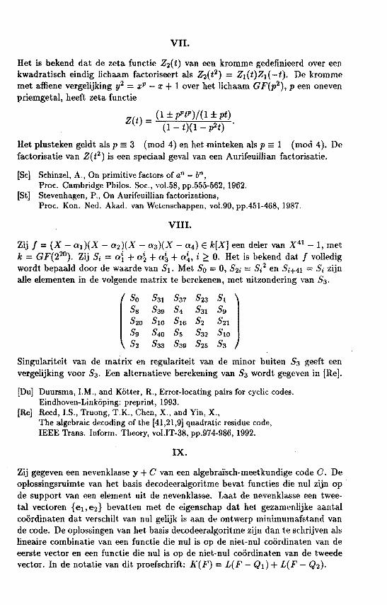
VII.

Het is bekend dat de zeta functie Z2(t) van een kromme gedefinieerd over een kwadratisch eindig lichaam factoriseert als Z2(t2 ) = Z1(t)Z1(-t). De kromme met afliene vergelijking y2 = xP - x + 1 over het lichaam GF(p2), peen oneven priemgetal, heeft zeta functie

Z( t) = (1 ± pPtP)/(1 ± pt). (1 t)(l - p2t)

Het plusteken geldt als p = 3 (rood 4) en het minteken als p 1 (rood 4). De factorisatie van Z ( t 2) is een speciaal geval van een A urif euillian factorisatie.

[Se] Schinzel, A., On primitive factors of an - bn, Proc. Cambridge Philos. Soc., vol.58, pp.555-562, 1962.

[St] Stevenhagen, P., On Aurifeuillian factorizations, Proc. Kon. Ned. Akad. van Wetenschappen, vol.90, pp.451-468, 1987.

VIII.

Zij f = (X - a1)(X a2)(X - a3)(X - a4) E k[XJ een deler van X41 - 1, met k = GF(220

). Zij S; = ai + a~ + a& + a~, i ;::: 0. Het is bekend dat f volledig wordt bepaald door de waarde van S1. Met Bo = 0, S2i = Si2 en Si+4t = S; zijn alle elementen in de volgende matrix te berekenen, met uitzondering van 83.

Singulariteit van de matrix en regulariteit van de minor buiten 83 geeft een vergelijking voor S3. Een alternatieve berekening van 83 wordt gegeven in [Re].

[Du] Duursma, I.M" and Kötter, R., Error-locating pairs for cyclic codes. Eindhoven-Linköping: preprint, 1993.

[Re] Reed, l.S., Truong, T.K., Chen, X., and Yin, X., The algebra.ic decoding of the [41,21,9] quadratic residue code, IEEE Trans. Inform. Theory, vol.IT-38, pp.974-986, 1992.

IX.

Zij gegeven een nevenkla.sse y + C van een algebraïsch-meetkundige code C. De oplossingsruimte van het basis decodeeralgoritme bevat functies die nul zijn op de support van een element uit de nevenklasse. Laat de nevenklasse een twee­tal vectoren {ei,e2} bevatten met de eigenschap dat het gezamenlijke aantal coördinaten dat verschilt va.n nul gelijk is aan de ontwerp minimumafstand van de code. De oplossingen van het basis decodeeralgoritme zijn dan te schrijven als lineaire combinatie van een functie die nul is op de niet-nul coördinaten van de eerste vector en een functie die nul is op de niet.nul coördinaten van de tweede vector. In de nota.tie van dit proefschrift: K(F) = L(F - Q 1 ) + L(F - Q2)·