1

Deep Learning Methods for Parallel MagneticResonance Image Reconstruction

Florian Knoll, Kerstin Hammernik, Chi Zhang, Student Member, IEEE, Steen Moeller, Thomas Pock,Daniel K. Sodickson, and Mehmet Akcakaya, Member, IEEE

Abstract—Following the success of deep learning in awide range of applications, neural network-based machinelearning techniques have received interest as a meansof accelerating magnetic resonance imaging (MRI). Anumber of ideas inspired by deep learning techniquesfrom computer vision and image processing have beensuccessfully applied to non-linear image reconstruction inthe spirit of compressed sensing for both low dose com-puted tomography and accelerated MRI. The additionalintegration of multi-coil information to recover missingk-space lines in the MRI reconstruction process, is stillstudied less frequently, even though it is the de-facto stan-dard for currently used accelerated MR acquisitions. Thismanuscript provides an overview of the recent machinelearning approaches that have been proposed specificallyfor improving parallel imaging. A general backgroundintroduction to parallel MRI is given that is structuredaround the classical view of image space and k-space basedmethods. Both linear and non-linear methods are covered,followed by a discussion of recent efforts to furtherimprove parallel imaging using machine learning, andspecifically using artificial neural networks. Image-domainbased techniques that introduce improved regularizers arecovered as well as k-space based methods, where the focusis on better interpolation strategies using neural networks.Issues and open problems are discussed as well as recentefforts for producing open datasets and benchmarks forthe community.

Index Terms—Accelerated MRI, Parallel Imaging, It-erative Image Reconstruction, Numerical Optimization,Machine Learning, Deep learning.

F. Knoll and D. K. Sodickson are with the Center for BiomedicalImaging, Department of Radiology, New York University. K. Ham-mernik and T. Pock are with the Institute of Computer Vision andGraphics, Graz University of Technology. C. Zhang and M. Akcakayaare with the Department of Electrical and Computer Engineering,and Center for Magnetic Resonance Research, University of Min-nesota, Minneapolis, MN. S. Moeller is with the Center for Mag-netic Resonance Research, University of Minnesota, Minneapolis,MN. e-mails: florian.knoll@nyumc.org, hammernik@icg.tugraz.at,zhan4906@umn.edu, moeller@cmrr.umn.edu, pock@icg.tugraz.at,daniel.sodickson@nyumc.org, akcakaya@umn.edu. This work waspartially supported by NIH R01EB024532, NIH R00HL111410,NIH P41EB015894, NIH P41EB027061, NIH P41EB017183, NSFCAREER CCF-1651825

I. INTRODUCTION

During recent years, there has been a substantialincrease of research activity in the field of medicalimage reconstruction. One particular application area isthe acceleration of Magnetic Resonance Imaging (MRI)scans. This is an area of high impact, because MRI is theleading diagnostic modality for a wide range of exams,but the physics of its data acquisition process make itinherently slower than modalities like X-Ray, ComputedTomography or Ultrasound. Therefore, the shortening ofscan times has been a major driving factor for routineclinical application of MRI.

One of the most important and successful technicaldevelopments to decrease MRI scan time in the last 20years was parallel imaging [1–3]. Currently, essentiallyall clinical MRI scanners from all vendors are equippedwith parallel imaging technology, and it is the defaultoption for a large number of scan protocols. As a conse-quence, there is a substantial benefit of using multi-coildata for machine learning based image reconstruction.Not only does it provide a complementary source ofacceleration that is unavailable when operating on singlechannel data, or on the level of image enhancement andpost-processing, it also is the scenario that ultimatelydefines the use-case for accelerated clinical MRI, whichmakes it a requirement for clinical translation of newreconstruction approaches. The drawback is that workingwith multi-coil data adds a layer of complexity thatcreates a gap between cutting edge developments in deeplearning [4] and computer vision, where the default datatype are images. The goal of this manuscript is to bridgethis gap by providing both a comprehensive review of theproperties of parallel MRI, together with an introductionhow current machine learning methods can be used forthis particular application.

A. Background on multi-coil acquisitions in MRI

The original motivation behind phased array receivecoils [5] was to increase the SNR of MR measurements.These arrays consist of nc multiple small coil elements,where an individual coil element covers only a part ofthe imaging field of view. These individual signals are

arX

iv:1

904.

0111

2v1

[ee

ss.S

P] 1

Apr

201

9

2

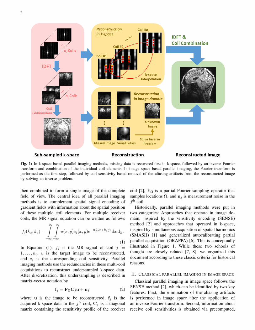
Fig. 1: In k-space based parallel imaging methods, missing data is recovered first in k-space, followed by an inverse Fouriertransform and combination of the individual coil elements. In image space based parallel imaging, the Fourier transform isperformed as the first step, followed by coil sensitivity based removal of the aliasing artifacts from the reconstructed imageby solving an inverse problem.

then combined to form a single image of the completefield of view. The central idea of all parallel imagingmethods is to complement spatial signal encoding ofgradient fields with information about the spatial positionof these multiple coil elements. For multiple receivercoils, the MR signal equation can be written as follows

fj(kx, ky) =

∞∫−∞

∞∫−∞

u(x, y)cj(x, y)e−i(kxx+kyy) dx dy.

(1)In Equation (1), fj is the MR signal of coil j =1, . . . , nc, u is the target image to be reconstructed,and cj is the corresponding coil sensitivity. Parallelimaging methods use the redundancies in these multi-coilacquisitions to reconstruct undersampled k-space data.After discretization, this undersampling is described inmatrix-vector notation by

fj = FΩCju + nj , (2)

where u is the image to be reconstructed, fj is theacquired k-space data in the jth coil, Cj is a diagonalmatrix containing the sensitivity profile of the receiver

coil [2], FΩ is a partial Fourier sampling operator thatsamples locations Ω, and nj is measurement noise in thejth coil.

Historically, parallel imaging methods were put intwo categories: Approaches that operate in image do-main, inspired by the sensitivity encoding (SENSE)method [2] and approaches that operated in k-space,inspired by simultaneous acquisition of spatial harmonics(SMASH) [1] and generalized autocalibrating partialparallel acquisition (GRAPPA) [6]. This is conceptuallyillustrated in Figure 1. While these two schools ofthought are closely related [7, 8], we organized thisdocument according to these classic criteria for historicalreasons.

II. CLASSICAL PARALLEL IMAGING IN IMAGE SPACE

Classical parallel imaging in image space follows theSENSE method [2], which can be identified by two keyfeatures. First, the elimination of the aliasing artifactsis performed in image space after the application ofan inverse Fourier transform. Second, information aboutreceive coil sensitivities is obtained via precomputed,

3

explicit coil sensitivity maps from either a separate ref-erence scan or from a fully sampled block of data at thecenter of k-space (all didactic experiments that are shownin this manuscript follow the latter approach). Morerecent approaches jointly estimate coil sensitivity profilesduring the image reconstruction process [9, 10], but forthe rest of this manuscript, we assume that sensitivitymaps were precomputed. The reconstruction in imagedomain in Figure 1 shows three example undersampledcoil images, corresponding coil sensitivity maps and thefinal reconstructed images from a brain MRI dataset. Thecoil sensitivities were estimated using ESPIRiT [8].

MRI reconstruction in general and parallel imagingin particular can be formulated as an inverse problem.This provides a general framework that allows easyintegration of the concepts of regularized and constrainedimage reconstruction as well as machine learning that arediscussed in more detail in later sections. Equation (1)can be discretized and then written in matrix-vectorform:

f = Eu + n, (3)

where f contains all k-space measurement data pointsand E is the forward encoding operator that includesinformation about the sampling trajectory and the receivecoil sensitivities and n is measurement noise. The taskof image reconstruction is to recover the image u. Inclassic parallel imaging one generally operates under thecondition that the number of receive elements is largerthan the acceleration factor. Therefore, Equation (3)corresponds to an over-determined system of equations.However, the rows of E are linearly dependent becauseindividual coil elements do not measure completelyindependent information. Therefore the inversion of Eis an ill-posed problem, which can lead to severe noiseamplification, described via the g-factor in the originalSENSE paper [2]. Equation (3) is usually solved in aniterative manner, which is the topic of the followingsections.

A. Overview of conjugate gradient SENSE (CG-SENSE)

The original SENSE approach is based on equidis-tant or uniform Cartesian k-space sampling, where thealiasing pattern is defined by a point spread functionthat has a small number of sharp equidistant peaks.This property leads to a small number of pixels thatare folded on top of each other, which allows a veryefficient implementation [2]. When using alternative k-space sampling strategies like non-Cartesian acquisitionsor random undersampling, this is no longer possibleand image reconstruction requires a full inversion ofthe encoding matrix in Equation (3). This operation is

demanding both in terms of compute and memory re-quirements (the dimensions of E are the total number ofacquired k-space points times N2 where N is the size ofthe image matrix that is to be reconstructed), which leadto the development of iterative methods, in particularthe CG-SENSE method introduced by Pruessmann etal. as a follow up of the original SENSE paper [11].In iterative image reconstruction the goal is to find au that is a minimizer of the following cost function,which corresponds to the quadratic form of the systemin Equation (3):

u ∈ arg minu

1

2‖Eu− f‖22. (4)

In standard parallel imaging, E is linear and Equa-tion (4) is a convex optimization problem that can besolved with a large number of numerical algorithmslike gradient descent, Landweber iterations [12], primal-dual methods [13] or the alternating direction method ofmultipliers (ADMM) algorithm [14] (a detailed reviewof numerical methods is outside the scope of this article).In the original version of CG-SENSE [11], the conjugategradient method [15] is employed. However, since MRk-space data are corrupted by noise, it is commonpractice stop iterating before theoretical convergence isreached, which can be seen as a form of regularization.Regularization can be also incorportated via additionalconstraints in Equation (4), which will be covered in thenext section.

As a didactic example for this manuscript, we willuse a single slice of a 2D coronal knee exam to illus-trate various reconstruction approaches. This data wereacquired on a clinical 3T system (Siemens Skyra) usinga 15 channel phased array knee coil. A turbo spinecho sequence was used with the following sequenceparameters: TR=2750ms, TE=27m, echo train length=4,field of view 160mm2 in-plane resolution 0.5mm2, slicethickness 3mm. Readout oversampling with a factor of2 was used, and all images were cropped in the fre-quency encoding direction (superior-inferior) for displaypurposes. In the spirit of reproducible research, data,sampling masks and coil sensitivity estimations that wereused for the numerical results in this manuscript areavailable online1. Figure 3 shows an example of a retro-spectively undersampled CG-SENSE reconstruction withan acceleration factor of 4 for the data from Figure 3.Early stopping was employed by setting the numerictolerance of the iteration to 5 · 10−5, which resulted inthe the algorithm stopping after 14 CG iterations.

1https://app.globus.org/: Endpoint: NYULH Radiology Reconstruc-tion Data, coronal pd data, subject 17, slice 25.

4

B. Nonlinear regularization and compressed sensing

Equation (4) can be extended by including a-prioriknowledge via additional penalty terms, which resultsin a constrained optimization problem defined in Equa-tion (5), which forms the cornerstone of almost allmodern MRI reconstruction methods

u ∈ arg minu

1

2‖Eu− f‖22 +

∑i

λiΨi(u). (5)

Here, Ψi are dedicated regularization terms and λiare regularization parameters that balance the trade-offbetween data fidelity and prior. Since the introductionof compressed sensing [16, 17] and its adoption forMRI [18–20], nonlinear regularization terms, in particu-lar `1-norm based ones, are popular in image reconstruc-tion and are commonly used in parallel imaging [19, 21–26]. The goal of these regularization terms is to providea separation between the target image that is to be re-constructed from the aliasing artifacts that are introduceddue to an undersampled acquisition. Therefore, they areusually designed in conjunction with a particular datasampling strategy. The classic formulation of compressedsensing in MRI [18] is based on sparsity of the imagein a transform domain (Wavelets are a popular choicefor static images) in combination with pseudo-randomsampling, which introduces aliasing artifacts that areincoherent in the respective domain. For dynamic acqui-sitions where periodic motion is encountered, sparsity inthe Fourier domain common choice [27]. Total Variationbased methods have been used successfully in combina-tion with radial [19] and spiral [28] acquisitions as wellas in dynamic imaging [29]. More advanced regularizersbased on low-rank properties have also been utilized[30].

Figure 3 shows an example of a nonlinear combinedparallel imaging and compressed sensing reconstructionwith a Total Generalized Variation [22] constraint. Theregularization parameter λ was set to 2.5 · 10−5 andthe reconstruction was using 1000 primal-dual [13] it-erations. The used equidistant sampling was chosen forconsistency with the other reconstruction methods is notoptimal for the incoherence condition in compressedsensing. Nevertheless, the nonlinear regularization stillprovides a superior reduction of aliasing artifacts andnoise suppression in comparison to the CG-SENSE re-construction from the last section.

III. CLASSICAL PARALLEL IMAGING IN K-SPACE

Parallel imaging reconstruction can also be formulatedin k-space as an interpolation procedure. The initial con-nections between the SENSE-type image-domain inverse

problem approach and k-space interpolation has beenmade more than a decade ago [7], where it was notedthat the forward model in Equation (3) can be restatedin terms of the Fourier transform, κ of the combinedimage, u as

f = AF∗κ , Gacqκ, (6)

where f corresponds to the acquired k-space lines acrossall coils, and Gacq is a linear operator. Similarly, the un-acquired k-space lines across all coils can be formulatedusing

funacq = Gunacqκ (7)

Combining these two equations yield

funacq = GunacqG†acqf . (8)

Thus, the unaccquired k-space lines across all coilscan be interpolated based on the acquired lines acrossall coils, assuming the pseudo-inverse, G†acq, of Gacq

exists [7]. Thus, the main difference between the k-spaceparallel imaging methods and the aforementioned imagedomain parallel imaging techniques is that the formerproduces k-space data across all coils at the output,whereas the latter typically produces one image thatcombines the information from all coils.

A. Linear k-space interpolation in GRAPPA

The most clinically used k-space reconstructionmethod for parallel imaging is GRAPPA, which useslinear shift-invariant convolutional kernels to interpolatemissing k-space lines using uniformly-spaced acquiredk-space lines [6]. For the jth coil k-space data, κj , wehave

κj(kx, ky −m∆ky)

=

nc∑c=1

Bx∑bx=−Bx

By∑by=−By

gj,m(bx, by, c)

κc(kx − bx∆kx, ky −Rby∆ky), (9)

where R is the acceleration rate of the uniformly under-samped acquisition; m ∈ 1, . . . , R− 1; gj,m(bx, by, c)are the linear convolutional kernels for estimating themth spacing location in jth coil; nc is the number ofcoils; and Bx, By are parameters determined from theconvolutional kernel size. A high-level overview of suchinterpolation is shown in the reconstruction in k-spacesection of Figure 1.

Similar to the coil sensitivity estimation inSENSE-type reconstruction, the convolutional kernels,gj,m(bx, by, c) are estimated for each subject, from eithera separate reference scan or from a fully-sampled blockof data at the center of k-space, called autocalibrating

5

signal (ACS) [6]. A sliding window approach is usedin this calibration region to identify the fully-sampledacquisition locations specified by the kernel size andthe corresponding missing entries. The former, takenacross all coils, is used as rows of a calibration matrix,A; while the latter, for a specific coil, yields a singleentry in the target vector, b. Thus for each coil j andmissing location m ∈ 1, . . . , R − 1, a set of linearequations are formed, from which the vectorized kernelweights gj,m(bx, by, c), denoted gj,m, are estimatedvia least squares, as gj,m ∈ arg ming ||b−Ag||22.GRAPPA has been shown to have several favorableproperties compared to SENSE, including lower g-factors, sometimes even less than unity at certain partsof the image [31], and more smoothly varying g-factormaps [32]. Furthermore, k-space interpolation is oftenless sensitive to motion [33]. Due to these favorableproperties, GRAPPA has found utility in multiplelarge-scale projects, such as the Human ConnectomeProject [34].

B. Advances in k-space interpolation methods

Though GRAPPA is widely used in clinical practice,it is a linear method that suffers from noise amplificationbased on the coil geometry and the acceleration rate[2]. Therefore, several alternative strategies have beenproposed in the literature to reduce the noise in recon-struction.

Iterative self-consistent parallel imaging reconstruc-tion (SPIRiT) is a strategy for enforcing self-consistencyamong the k-space data in multiple receiver coils by ex-ploiting correlations between neighboring k-space points[21]. Similar to GRAPPA, SPIRiT also estimates a linearshift-invariant convolutional kernel from ACS data. InGRAPPA, this convolutional kernel used informationfrom acquired lines in a neighborhood to estimate amissing k-space point. In SPIRiT, the kernel includescontributions from all points, both acquired and missing,across all coils for a neighborhood around a given k-space point. The self-consistency idea suggests that thefull k-space data should remain unchanged under thisconvolution operation. SPIRiT objective function alsoincludes a term that enforces consistency with the ac-quired data, where the undersampling can be performedwith arbitrary patterns, including random patterns thatare typically employed in compressed sensing [18, 19].Additionally, this formulation allows incorporation ofregularizers, for instance based on transform-domainsparsity, in the objective function to reduce reconstruc-tion noise via non-linear processing [21]. Furthermore,SPIRiT has facilitated the connection between coil sensi-tivities used in image-domain parallel imaging methods

and the convolutional kernels used in k-space methodsvia a subspace analysis [8].

An alternative line of work utilizes non-linear k-spaceinterpolation for estimating missing k-space points foruniformly undersampled parallel imaging acquisitions[35]. It was noted that during GRAPPA calibration, boththe regressand and the regressor have errors in them dueto measurement noise in the acquisition of calibrationdata, which leads to a non-linear relationship in theestimation. Thus, the reconstruction method, called non-linear GRAPPA, uses a kernel approach to map thedata to a higher-dimensional feature space, where linearinterpolation is performed, which also corresponds to anon-linear interpolation in the original data space. Theinterpolation function is estimated from the ACS data,although this approach typically required more ACSdata than GRAPPA [35]. This method was shown toreduce reconstruction noise compared to GRAPPA. Notethat non-linear GRAPPA, through its use of the kernelapproach, is a type of machine learning approach, thoughthe non-linear kernel functions were empirically fixed a-priori and not learned from data.

C. k-space reconstruction via low-rank matrix comple-tion

While k-space interpolation methods remain the preva-lent method for k-space parallel imaging reconstruction,there has been recent efforts on recasting this type ofreconstruction as a matrix completion problem. Simul-taneous autocalibrating and k-space estimation (SAKE)is an early work in this direction, where local neigh-borhoods in k-space across all coils are restructuredinto a matrix with block Hankel form [36]. Then low-rank matrix completion is performed on this matrix,subject to consistency with acquired data, enabling k-space parallel imaging reconstruction without additionalcalibration data acquisition. Low-rank matrix modelingof local k-space neighborhoods (LORAKS) is anothermethod exploiting similar ideas, where the motivation isbased on utilizing finite image support and image phaseconstraints instead of correlations across multiple coils[37]. This method was later extended to parallel imagingto further include the similarities between image supportsand phase constraints across coils [38]. A further gen-eralization to LORAKS is annihilating filter-based lowrank Hankel matrix approach (ALOHA), which extendsthe finite support constraint to transform domains [39].By relating transform domain sparsity to the existenceof annihilating filters in a weighted k-space, where theweighting is determined by the choice of transformdomain, ALOHA recasts the reconstruction problem asthe low-rank recovery of the associated Hankel matrix.

6

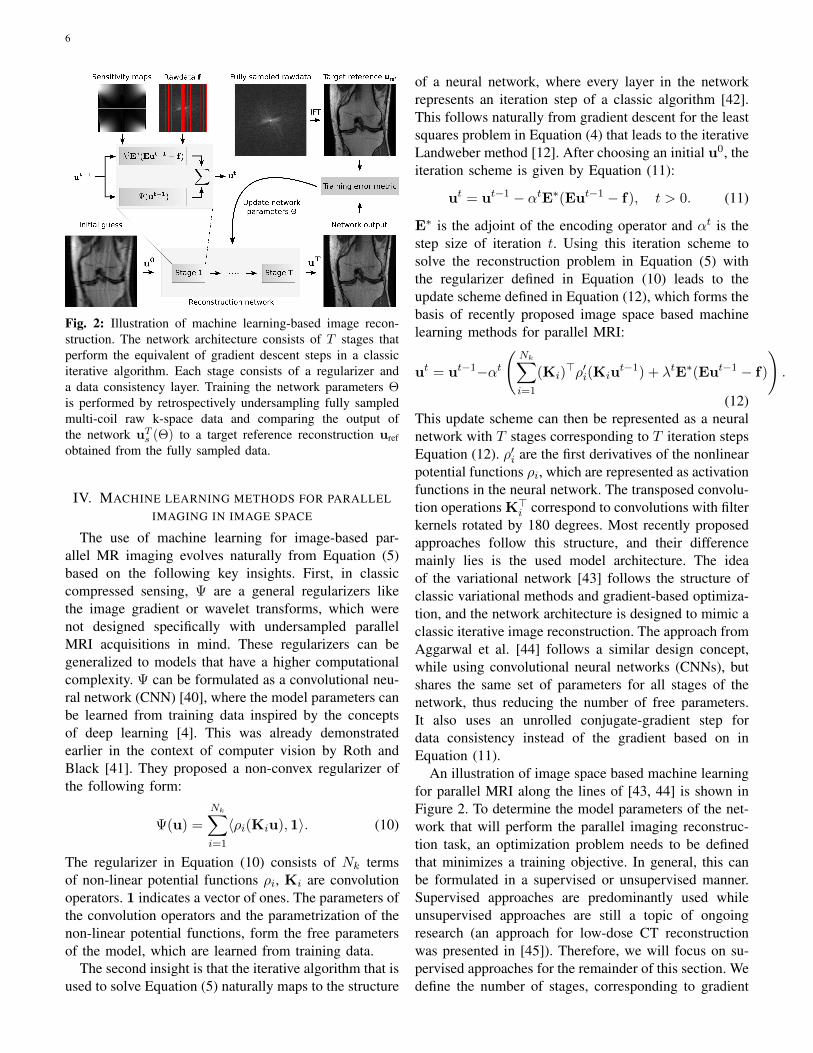
Fig. 2: Illustration of machine learning-based image recon-struction. The network architecture consists of T stages thatperform the equivalent of gradient descent steps in a classiciterative algorithm. Each stage consists of a regularizer anda data consistency layer. Training the network parameters Θis performed by retrospectively undersampling fully sampledmulti-coil raw k-space data and comparing the output ofthe network uT

s (Θ) to a target reference reconstruction urefobtained from the fully sampled data.

IV. MACHINE LEARNING METHODS FOR PARALLEL

IMAGING IN IMAGE SPACE

The use of machine learning for image-based par-allel MR imaging evolves naturally from Equation (5)based on the following key insights. First, in classiccompressed sensing, Ψ are a general regularizers likethe image gradient or wavelet transforms, which werenot designed specifically with undersampled parallelMRI acquisitions in mind. These regularizers can begeneralized to models that have a higher computationalcomplexity. Ψ can be formulated as a convolutional neu-ral network (CNN) [40], where the model parameters canbe learned from training data inspired by the conceptsof deep learning [4]. This was already demonstratedearlier in the context of computer vision by Roth andBlack [41]. They proposed a non-convex regularizer ofthe following form:

Ψ(u) =

Nk∑i=1

〈ρi(Kiu),1〉. (10)

The regularizer in Equation (10) consists of Nk termsof non-linear potential functions ρi, Ki are convolutionoperators. 1 indicates a vector of ones. The parameters ofthe convolution operators and the parametrization of thenon-linear potential functions, form the free parametersof the model, which are learned from training data.

The second insight is that the iterative algorithm that isused to solve Equation (5) naturally maps to the structure

of a neural network, where every layer in the networkrepresents an iteration step of a classic algorithm [42].This follows naturally from gradient descent for the leastsquares problem in Equation (4) that leads to the iterativeLandweber method [12]. After choosing an initial u0, theiteration scheme is given by Equation (11):

ut = ut−1 − αtE∗(Eut−1 − f), t > 0. (11)

E∗ is the adjoint of the encoding operator and αt is thestep size of iteration t. Using this iteration scheme tosolve the reconstruction problem in Equation (5) withthe regularizer defined in Equation (10) leads to theupdate scheme defined in Equation (12), which forms thebasis of recently proposed image space based machinelearning methods for parallel MRI:

ut = ut−1−αt

(Nk∑i=1

(Ki)>ρ′i(Kiu

t−1) + λtE∗(Eut−1 − f)

).

(12)This update scheme can then be represented as a neuralnetwork with T stages corresponding to T iteration stepsEquation (12). ρ′i are the first derivatives of the nonlinearpotential functions ρi, which are represented as activationfunctions in the neural network. The transposed convolu-tion operations K>i correspond to convolutions with filterkernels rotated by 180 degrees. Most recently proposedapproaches follow this structure, and their differencemainly lies is the used model architecture. The ideaof the variational network [43] follows the structure ofclassic variational methods and gradient-based optimiza-tion, and the network architecture is designed to mimic aclassic iterative image reconstruction. The approach fromAggarwal et al. [44] follows a similar design concept,while using convolutional neural networks (CNNs), butshares the same set of parameters for all stages of thenetwork, thus reducing the number of free parameters.It also uses an unrolled conjugate-gradient step fordata consistency instead of the gradient based on inEquation (11).

An illustration of image space based machine learningfor parallel MRI along the lines of [43, 44] is shown inFigure 2. To determine the model parameters of the net-work that will perform the parallel imaging reconstruc-tion task, an optimization problem needs to be definedthat minimizes a training objective. In general, this canbe formulated in a supervised or unsupervised manner.Supervised approaches are predominantly used whileunsupervised approaches are still a topic of ongoingresearch (an approach for low-dose CT reconstructionwas presented in [45]). Therefore, we will focus on su-pervised approaches for the remainder of this section. Wedefine the number of stages, corresponding to gradient

7

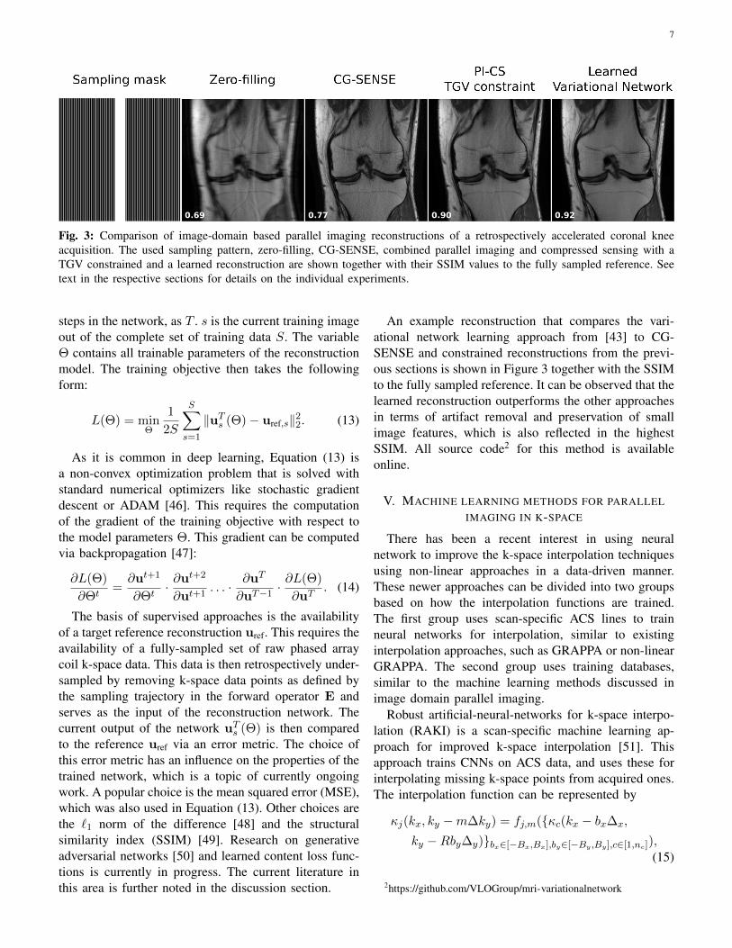
Fig. 3: Comparison of image-domain based parallel imaging reconstructions of a retrospectively accelerated coronal kneeacquisition. The used sampling pattern, zero-filling, CG-SENSE, combined parallel imaging and compressed sensing with aTGV constrained and a learned reconstruction are shown together with their SSIM values to the fully sampled reference. Seetext in the respective sections for details on the individual experiments.

steps in the network, as T . s is the current training imageout of the complete set of training data S. The variableΘ contains all trainable parameters of the reconstructionmodel. The training objective then takes the followingform:

L(Θ) = minΘ

1

2S

S∑s=1

‖uTs (Θ)− uref,s‖22. (13)

As it is common in deep learning, Equation (13) isa non-convex optimization problem that is solved withstandard numerical optimizers like stochastic gradientdescent or ADAM [46]. This requires the computationof the gradient of the training objective with respect tothe model parameters Θ. This gradient can be computedvia backpropagation [47]:

∂L(Θ)

∂Θt=∂ut+1

∂Θt· ∂u

t+2

∂ut+1. . . · ∂uT

∂uT−1· ∂L(Θ)

∂uT. (14)

The basis of supervised approaches is the availabilityof a target reference reconstruction uref. This requires theavailability of a fully-sampled set of raw phased arraycoil k-space data. This data is then retrospectively under-sampled by removing k-space data points as defined bythe sampling trajectory in the forward operator E andserves as the input of the reconstruction network. Thecurrent output of the network uT

s (Θ) is then comparedto the reference uref via an error metric. The choice ofthis error metric has an influence on the properties of thetrained network, which is a topic of currently ongoingwork. A popular choice is the mean squared error (MSE),which was also used in Equation (13). Other choices arethe `1 norm of the difference [48] and the structuralsimilarity index (SSIM) [49]. Research on generativeadversarial networks [50] and learned content loss func-tions is currently in progress. The current literature inthis area is further noted in the discussion section.

An example reconstruction that compares the vari-ational network learning approach from [43] to CG-SENSE and constrained reconstructions from the previ-ous sections is shown in Figure 3 together with the SSIMto the fully sampled reference. It can be observed that thelearned reconstruction outperforms the other approachesin terms of artifact removal and preservation of smallimage features, which is also reflected in the highestSSIM. All source code2 for this method is availableonline.

V. MACHINE LEARNING METHODS FOR PARALLEL

IMAGING IN K-SPACE

There has been a recent interest in using neuralnetwork to improve the k-space interpolation techniquesusing non-linear approaches in a data-driven manner.These newer approaches can be divided into two groupsbased on how the interpolation functions are trained.The first group uses scan-specific ACS lines to trainneural networks for interpolation, similar to existinginterpolation approaches, such as GRAPPA or non-linearGRAPPA. The second group uses training databases,similar to the machine learning methods discussed inimage domain parallel imaging.

Robust artificial-neural-networks for k-space interpo-lation (RAKI) is a scan-specific machine learning ap-proach for improved k-space interpolation [51]. Thisapproach trains CNNs on ACS data, and uses these forinterpolating missing k-space points from acquired ones.The interpolation function can be represented by

κj(kx, ky −m∆ky) = fj,m(κc(kx − bx∆x,

ky −Rby∆y)bx∈[−Bx,Bx],by∈[−By,By],c∈[1,nc]),(15)

2https://github.com/VLOGroup/mri-variationalnetwork

8

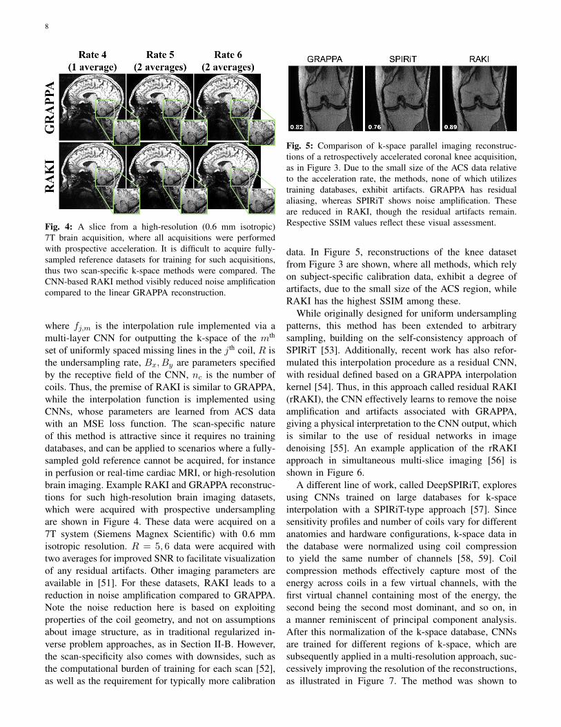
Fig. 4: A slice from a high-resolution (0.6 mm isotropic)7T brain acquisition, where all acquisitions were performedwith prospective acceleration. It is difficult to acquire fully-sampled reference datasets for training for such acquisitions,thus two scan-specific k-space methods were compared. TheCNN-based RAKI method visibly reduced noise amplificationcompared to the linear GRAPPA reconstruction.

where fj,m is the interpolation rule implemented via amulti-layer CNN for outputting the k-space of the mth

set of uniformly spaced missing lines in the jth coil, R isthe undersampling rate, Bx, By are parameters specifiedby the receptive field of the CNN, nc is the number ofcoils. Thus, the premise of RAKI is similar to GRAPPA,while the interpolation function is implemented usingCNNs, whose parameters are learned from ACS datawith an MSE loss function. The scan-specific natureof this method is attractive since it requires no trainingdatabases, and can be applied to scenarios where a fully-sampled gold reference cannot be acquired, for instancein perfusion or real-time cardiac MRI, or high-resolutionbrain imaging. Example RAKI and GRAPPA reconstruc-tions for such high-resolution brain imaging datasets,which were acquired with prospective undersamplingare shown in Figure 4. These data were acquired on a7T system (Siemens Magnex Scientific) with 0.6 mmisotropic resolution. R = 5, 6 data were acquired withtwo averages for improved SNR to facilitate visualizationof any residual artifacts. Other imaging parameters areavailable in [51]. For these datasets, RAKI leads to areduction in noise amplification compared to GRAPPA.Note the noise reduction here is based on exploitingproperties of the coil geometry, and not on assumptionsabout image structure, as in traditional regularized in-verse problem approaches, as in Section II-B. However,the scan-specificity also comes with downsides, such asthe computational burden of training for each scan [52],as well as the requirement for typically more calibration

Fig. 5: Comparison of k-space parallel imaging reconstruc-tions of a retrospectively accelerated coronal knee acquisition,as in Figure 3. Due to the small size of the ACS data relativeto the acceleration rate, the methods, none of which utilizestraining databases, exhibit artifacts. GRAPPA has residualaliasing, whereas SPIRiT shows noise amplification. Theseare reduced in RAKI, though the residual artifacts remain.Respective SSIM values reflect these visual assessment.

data. In Figure 5, reconstructions of the knee datasetfrom Figure 3 are shown, where all methods, which relyon subject-specific calibration data, exhibit a degree ofartifacts, due to the small size of the ACS region, whileRAKI has the highest SSIM among these.

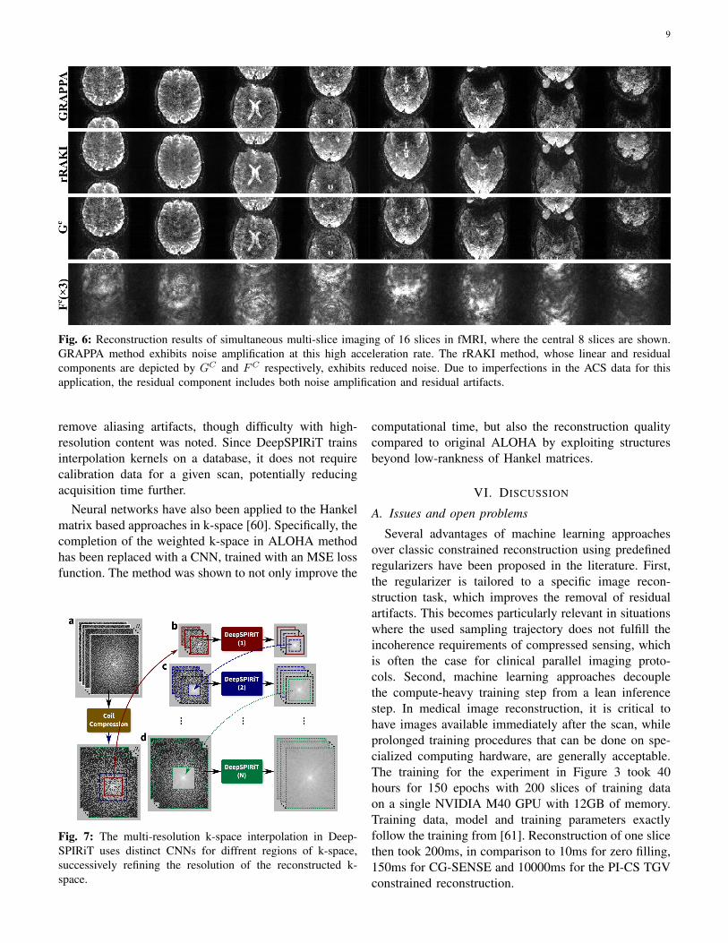
While originally designed for uniform undersamplingpatterns, this method has been extended to arbitrarysampling, building on the self-consistency approach ofSPIRiT [53]. Additionally, recent work has also refor-mulated this interpolation procedure as a residual CNN,with residual defined based on a GRAPPA interpolationkernel [54]. Thus, in this approach called residual RAKI(rRAKI), the CNN effectively learns to remove the noiseamplification and artifacts associated with GRAPPA,giving a physical interpretation to the CNN output, whichis similar to the use of residual networks in imagedenoising [55]. An example application of the rRAKIapproach in simultaneous multi-slice imaging [56] isshown in Figure 6.

A different line of work, called DeepSPIRiT, exploresusing CNNs trained on large databases for k-spaceinterpolation with a SPIRiT-type approach [57]. Sincesensitivity profiles and number of coils vary for differentanatomies and hardware configurations, k-space data inthe database were normalized using coil compressionto yield the same number of channels [58, 59]. Coilcompression methods effectively capture most of theenergy across coils in a few virtual channels, with thefirst virtual channel containing most of the energy, thesecond being the second most dominant, and so on, ina manner reminiscent of principal component analysis.After this normalization of the k-space database, CNNsare trained for different regions of k-space, which aresubsequently applied in a multi-resolution approach, suc-cessively improving the resolution of the reconstructions,as illustrated in Figure 7. The method was shown to

9

Fig. 6: Reconstruction results of simultaneous multi-slice imaging of 16 slices in fMRI, where the central 8 slices are shown.GRAPPA method exhibits noise amplification at this high acceleration rate. The rRAKI method, whose linear and residualcomponents are depicted by GC and FC respectively, exhibits reduced noise. Due to imperfections in the ACS data for thisapplication, the residual component includes both noise amplification and residual artifacts.

remove aliasing artifacts, though difficulty with high-resolution content was noted. Since DeepSPIRiT trainsinterpolation kernels on a database, it does not requirecalibration data for a given scan, potentially reducingacquisition time further.

Neural networks have also been applied to the Hankelmatrix based approaches in k-space [60]. Specifically, thecompletion of the weighted k-space in ALOHA methodhas been replaced with a CNN, trained with an MSE lossfunction. The method was shown to not only improve the

Fig. 7: The multi-resolution k-space interpolation in Deep-SPIRiT uses distinct CNNs for diffrent regions of k-space,successively refining the resolution of the reconstructed k-space.

computational time, but also the reconstruction qualitycompared to original ALOHA by exploiting structuresbeyond low-rankness of Hankel matrices.

VI. DISCUSSION

A. Issues and open problems

Several advantages of machine learning approachesover classic constrained reconstruction using predefinedregularizers have been proposed in the literature. First,the regularizer is tailored to a specific image recon-struction task, which improves the removal of residualartifacts. This becomes particularly relevant in situationswhere the used sampling trajectory does not fulfill theincoherence requirements of compressed sensing, whichis often the case for clinical parallel imaging proto-cols. Second, machine learning approaches decouplethe compute-heavy training step from a lean inferencestep. In medical image reconstruction, it is critical tohave images available immediately after the scan, whileprolonged training procedures that can be done on spe-cialized computing hardware, are generally acceptable.The training for the experiment in Figure 3 took 40hours for 150 epochs with 200 slices of training dataon a single NVIDIA M40 GPU with 12GB of memory.Training data, model and training parameters exactlyfollow the training from [61]. Reconstruction of one slicethen took 200ms, in comparison to 10ms for zero filling,150ms for CG-SENSE and 10000ms for the PI-CS TGVconstrained reconstruction.

10

The focus in Section IV and Section V were onmethods that were developed specifically in the con-text of parallel imaging. Some architectures for imagedomain machine learning have been designed specifi-cally towards a target application, for example dynamicimaging [62, 63]. In their current form, these were notyet demonstrated in the context of multi-coil data. Theapproach recently proposed by Zhu et al. learns thecomplete mapping from k-space raw data to the recon-structed image [64]. The proposed advantage is that sinceno information about the acquisition is included in theforward operator A, it is more robust against systematiccalibration errors during the acquisition. This comes atthe price of a significantly higher number of modelparameters. The corresponding memory requirementsmake it challenging use this model for matrix sizes thatare currently used in clinical applications. We also notethat there are fewer works in k-space machine learningmethods for MRI reconstruction. This may be due to thedifferent nature of k-space signal that usually has verydifferent intensity characteristics in the center versusthe outer k-space, which makes it difficult to generalizethe plethora of techniques developed in computer visionand image processing that exploit properties of naturalimages.

Machine learning reconstruction approaches alsocome with a number of drawbacks when compared toclassic constrained parallel imaging. First, they requirethe availability of a curated training data set that isrepresentative so that the trained model generalizedtowards new unseen test data. While recent approachesfrom the literature [43, 44, 62, 63, 65] have eitherbeen trained with hundreds of examples rather thanmillions of examples as it is common in deep learningfor computer vision [4, 66], or trained on syntheticnon-medical data [64] that is publicly available fromexisting databases. However, this is still a challengethat will potentially limit the use of machine learningto certain applications. Several applications in imagingof moving organs, such as the heart, or in imaging ofthe brain connectivity, such as diffusion MRI, cannot beacquired with fully-sampled data due to constraints onspatio-temporal resolutions. This hinders the use of fully-sampled training labels for such datasets, highlightingapplications for scan-specific approaches or unsuper-vised training strategies.

These reconstruction methods also require the avail-ability of computing resources during the training stage.This is a less critical issue due to the increased avail-ability and reduced prices of GPUs. The experimentsin this paper were made with computing resources thatare available for less than 10,000 USD, which are

usually available in academic institutions. In addition, theavailability of on-demand cloud based machine learningsolutions is constantly increasing.

A more severe issue is that in contrast to conven-tional parallel imaging and compressed sensing, machinelearning models are mostly non-convex. Their properties,especially regarding their failure modes and generaliza-tion potential for daily clinical use, are understood lesswell than conventional iterative approaches based onconvex optimization. For example, it was recently shownthat while reconstructions generalize well with respectto changes in image contrast between training and testdata, they are susceptible towards systematic deviationsin SNR [61]. It is also still an open question how specifictrained models have to be. Is it sufficient to train asingle model for all types of MR exams, or are separatemodels required for scans of different anatomical areas,pulse sequences, acquisition trajectories and accelerationfactors as well as scanner manufacturers, field strengthsand receive coils? [67] While pre-training a large numberof separate models for different exams would be feasiblein clinical practice, if certain models do not generalizewith respect to scan parameter settings that are usuallytailored to the specific anatomy of an individual patientby the MR technologist, this will severely impact theirtranslational potential and ultimately their clinical use.

Finally, the choice of the loss function that is usedduring the training has an impact on the properties ofthe trained network, and a particular ongoing researchdirection is the use of GANs [50, 68–70]. This is aninteresting direction because these models have the po-tential to create images that are visually indistinguishablefrom fully sampled reference images, where featuresin the images that are not supported by the amountof acquired data, are hallucinated by the network. Thissituation obviously must be avoided in any application inmedical imaging. Strategies to mitigate this effect are thecombination of GANs with conventional error metricslike MSE [71, 72]. Comparable approaches were usedin the context of MRI reconstruction [73–78].

B. Availability of training databases and communitychallenges

As mentioned in the previous section, one open issuein the field of machine learning reconstruction for paral-lel imaging is the lack of publicly available databases ofmulti-channel raw k-space data. This restricts the numberof researchers who can work in this field to those whoare based at large academic medical centers where thisdata is available, and for the most part excludes thecore machine learning community that has the necessary

11

theoretical and algorithmic background to advance thefield. In addition, since the used training data becomes anessential part of the performance of a certain model, it iscurrently almost impossible to compare new approachesthat are proposed in the literature with each other ifthe training data is not shared when publishing themanuscript. While the momentum in initiatives for publicreleases of raw k-space data is growing [79], the numberof available data sets is still on the order of hundredsand limited to very specific types of exams. Examplesof publicly available rawdata sets are mridata.org3 andthe fastMRI dataset4.

VII. CONCLUSION

Machine learning methods have recently been pro-posed to improve the reconstruction quality in parallelimaging MRI. These techniques include both imagedomain approaches for better image regularization andk-space approaches for better k-space completion. Whilethe field is still in its development, there are manyopen problems and high-impact applications, which arelikely to be of interest to the broader signal processingcommunity.

REFERENCES

[1] D. K. Sodickson and W. J. Manning, “SimultaneousAcquisition of Spatial Harmonics (SMASH): FastImaging with Radiofrequency Coil Arrays,” MagnReson Med, vol. 38, no. 4, pp. 591–603, 1997.

[2] K. P. Pruessmann, M. Weiger, M. B. Scheidegger,and P. Boesiger, “SENSE: Sensitivity encoding forfast MRI,” Magn Reson Med, vol. 42, no. 5, pp.952–962, 1999.

[3] M. A. Griswold, M. Blaimer, F. Breuer, et al.,“Parallel magnetic resonance imaging using theGRAPPA operator formalism,” Magn Reson Med,vol. 54, no. 6, pp. 1553–1556, 2005.

[4] Y. LeCun, Y. Bengio, and G. Hinton, “DeepLearning,” Nature, vol. 521, no. 7553, pp. 436–444, 2015.

[5] P. B. Roemer, W. A. Edelstein, C. E. Hayes, S. P.Souza, and O. M. Mueller, “The NMR phasedarray,” Magn Reson Med, vol. 16, no. 2, pp. 192–225, nov 1990.

[6] M. A. Griswold, P. M. Jakob, R. M. Heidemann,et al., “Generalized autocalibrating partially parallelacquisitions (GRAPPA),” Magn Reson Med, vol.47, no. 6, pp. 1202–1210, jun 2002.

3https://mridata.org4https://fastmri.med.nyu.edu/

[7] E. G. Kholmovski and D. L. Parker, “Spatiallyvariant GRAPPA,” in Proc. 14th Scientific Meetingand Exhibition of ISMRM, Seattle, 2006, p. 285.

[8] M. Uecker, P. Lai, M. J. Murphy, et al., “ESPIRiT– An Eigenvalue Approach to Autocalibrating Par-allel MRI: Where SENSE meets GRAPPA,” MagnReson Med, vol. 71, no. 3, pp. 990–1001, 2014.

[9] L. Ying and J. Sheng, “Joint image reconstructionand sensitivity estimation in SENSE (JSENSE),”Magn Reson Med, vol. 57, no. 6, pp. 1196–1202,jun 2007.

[10] M. Uecker, T. Hohage, K. T. Block, and J. Frahm,“Image reconstruction by regularized nonlinearinversion–joint estimation of coil sensitivities andimage content,” Magn Reson Med, vol. 60, no. 3,pp. 674–682, sep 2008.

[11] K. P. Pruessmann, M. Weiger, P. Boernert, andP. Boesiger, “Advances in sensitivity encoding witharbitrary k-space trajectories,” Magn Reson Med,vol. 46, no. 4, pp. 638–651, 2001.

[12] L. Landweber, “An Iteration Formula for FredholmIntegral Equations of the First Kind,” AmericanJournal of Mathematics, vol. 73, no. 3, pp. 615–624, 1951.

[13] A. Chambolle and T. Pock, “A first-order primal-dual algorithm for convex problems with appli-cations to imaging,” Journal of MathematicalImaging and Vision, vol. 40, no. 1, pp. 120–145,2010.

[14] S. Boyd, N. Parikh, B. P. E Chu, and J. Eckstein,“Distributed Optimization and Statistical Learningvia the Alternating Direction Method of Multipli-ers,” Foundations and Trends in Machine Learning,vol. 3, no. 1, pp. 1–122, 2011.

[15] M. R. Hestenes and E. Stiefel, “Methods ofConjugate Gradients for Solving Linear Systems,”Journal of Research of the National Bureau ofStandards, vol. 49, no. 6, pp. 409–436, 1952.

[16] E. J. Candes, J. Romberg, and T. Tao, “Robust Un-certainty Principles: Exact Signal ReconstructionFrom Highly Incomplete Frequency Information,”IEEE Transactions on Information Theory, vol. 52,no. 2, pp. 489–509, 2006.

[17] D. L. Donoho, “Compressed Sensing,” IEEETransactions on Information Theory, vol. 52, no.4, pp. 1289–1306, apr 2006.

[18] M. Lustig, D. Donoho, and J. M. Pauly, “SparseMRI: The application of compressed sensing forrapid MR imaging,” Magn Reson Med, vol. 58, no.6, pp. 1182–1195, 2007.

[19] K. T. Block, M. Uecker, and J. Frahm, “Undersam-pled radial MRI with multiple coils. Iterative image

12

reconstruction using a total variation constraint.,”Magn Reson Med, vol. 57, no. 6, pp. 1086–1098,2007.

[20] M. Lustig, D. L. Donoho, J. M. Santos, and J. M.Pauly, “Compressed Sensing MRI,” IEEE SignalProcessing Magazine, vol. 25, no. 2, pp. 72–82,2008.

[21] M. Lustig and J. M. Pauly, “SPIRiT: Iterativeself-consistent parallel imaging reconstruction fromarbitrary k-space,” Magn Reson Med, vol. 64, no.2, pp. 457–471, aug 2010.

[22] F. Knoll, K. Bredies, T. Pock, and R. Stollberger,“Second order total generalized variation (TGV) forMRI,” Magnetic Resonance in Medicine, vol. 65,no. 2, pp. 480–491, 2011.

[23] F. Knoll, C. Clason, K. Bredies, M. Uecker, andR. Stollberger, “Parallel imaging with nonlinearreconstruction using variational penalties,” MagnReson Med, vol. 67, no. 1, pp. 34–41, 2012.

[24] M. Akcakaya, T. A. Basha, B. Goddu, et al., “Low-dimensional-structure self-learning and threshold-ing: Regularization beyond compressed sensing forMRI reconstruction,” Magn Reson Med, vol. 66,no. 3, pp. 756–767, Sep 2011.

[25] M. Akcakaya, T. A. Basha, R. H. Chan, W. J. Man-ning, and R. Nezafat, “Accelerated isotropic sub-millimeter whole-heart coronary MRI: compressedsensing versus parallel imaging,” Magn Reson Med,vol. 71, no. 2, pp. 815–822, Feb 2014.

[26] H. Jung, K. Sung, K. S. Nayak, E. Y. Kim, andJ. C. Ye, “k-t FOCUSS: A general compressedsensing framework for high resolution dynamicMRI,” Magn Reson Med, vol. 61, no. 1, pp. 103–116, 2009.

[27] U. Gamper, P. Boesiger, and S. Kozerke, “Com-pressed Sensing in Dynamic MRI,” Magn ResonMed, vol. 59, no. 2, pp. 365–373, 2008.

[28] G. Valvano, N. Martini, L. Landini, and M. F.Santarelli, “Variable density randomized stack ofspirals (VDR-SoS) for compressive sensing MRI,”Magn Reson Med, 2016.

[29] L. Feng, R. Grimm, K. Tobias Block, et al.,“Golden-Angle Radial Sparse Parallel MRI: Com-bination of Compressed Sensing, Parallel Imaging,and Golden-Angle Radial Sampling for Fast andFlexible Dynamic Volumetric MRI,” Magn ResonMed, vol. 72, no. 3, pp. 707–717, 2014.

[30] S. G. Lingala, Y. Hu, E. DiBella, and M. Jacob,“Accelerated dynamic MRI exploiting sparsity andlow-rank structure: k-t SLR,” IEEE Trans MedImaging, vol. 30, no. 5, pp. 1042–1054, May 2011.

[31] P. M. Robson, A. K. Grant, A. J. Madhuranthakam,

et al., “Comprehensive quantification of signal-to-noise ratio and g-factor for image-based andk-space-based parallel imaging reconstructions,”Magn Reson Med, vol. 60, no. 4, pp. 895–907, Oct2008.

[32] F. A. Breuer, S. A. R. Kannengiesser, M. Blaimer,et al., “General formulation for quantitative G-factor calculation in GRAPPA reconstructions,”Magn Reson Med, vol. 62, no. 3, pp. 739–746, sep2009.

[33] F. A. Breuer, P. Kellman, M. A. Griswold, andP. M. Jakob, “Dynamic autocalibrated parallelimaging using temporal GRAPPA (TGRAPPA),”Magn Reson Med, vol. 53, no. 4, pp. 981–985, apr2005.

[34] K. Ugurbil, J. Xu, E. J. Auerbach, et al., “Pushingspatial and temporal resolution for functional anddiffusion MRI in the Human Connectome Project,”Neuroimage, vol. 80, pp. 80–104, Oct 2013.

[35] Y. Chang, D. Liang, and L. Ying, “NonlinearGRAPPA: A kernel approach to parallel MRI re-construction,” Magn Reson Med, vol. 68, no. 3, pp.730–740, Sep 2012.

[36] P. J. Shin, P. E. Larson, M. A. Ohliger, et al., “Cal-ibrationless parallel imaging reconstruction basedon structured low-rank matrix completion,” MagnReson Med, vol. 72, no. 4, pp. 959–970, Oct 2014.

[37] J. P. Haldar, “Low-rank modeling of local k-spaceneighborhoods (LORAKS) for constrained MRI,”IEEE Trans Med Imaging, vol. 33, no. 3, pp. 668–681, Mar 2014.

[38] J. P. Haldar and J. Zhuo, “P-LORAKS: Low-rank modeling of local k-space neighborhoods withparallel imaging data,” Magn Reson Med, vol. 75,no. 4, pp. 1499–1514, Apr 2016.

[39] K. H. Jin, D. Lee, and J. C. Ye, “A generalframework for compressed sensing and parallelMRI using annihilating filter based low-rank hankelmatrix,” IEEE Transactions on ComputationalImaging, vol. 2, no. 4, pp. 480–495, Dec 2016.

[40] Y. LeCun, “Handwritten Digit Recognition with aBack-Propagation Network,” Advances in NeuralInformation Processing Systems, 1989.

[41] S. Roth and M. J. Black, “Fields of Experts,”International Journal of Computer Vision, vol. 82,no. 2, pp. 205–229, 2009.

[42] K. Gregor and Y. LeCun, “Learning fast approxi-mations of sparse coding,” in Proc. 27th Interna-tional Conference on International Conference onMachine Learning, USA, 2010, ICML’10, pp. 399–406, Omnipress.

[43] K. Hammernik, T. Klatzer, E. Kobler, et al., “Learn-

13

ing a variational network for reconstruction ofaccelerated MRI data,” Mag Reson Med, vol. 79,pp. 3055–71, 2018.

[44] H. K. Aggarwal, M. P. Mani, and M. Jacob,“MoDL: Model-Based Deep Learning Architecturefor Inverse Problems,” IEEE Transactions on Med-ical Imaging, 2019.

[45] D. Wu, K. Kim, G. El Fakhri, and Q. Li, “IterativeLow-dose CT Reconstruction with Priors Trainedby Artificial Neural Network,” IEEE Transactionson Medical Imaging, vol. 36, no. 12, pp. 2479–2486, 2017.

[46] D. P. Kingma and J. Ba, “Adam: A Method forStochastic Optimization,” arXiv, dec 2014.

[47] Y. A. LeCun, L. Bottou, G. B. Orr, and K. R.Muller, “Efficient BackProp,” in Neural Networks:Tricks of the Trade, pp. 9–50. Springer BerlinHeidelberg, 2012.

[48] K. Hammernik, F. Knoll, D. Sodickson, andT. Pock, “L2 or Not L2: Impact of Loss FunctionDesign for Deep Learning MRI Reconstruction,” inProceedings of the International Society of MagnReson Med (ISMRM), 2017, p. 687.

[49] Z. Wang, A. C. Bovik, H. R. Sheikh, and E. P.Simoncelli, “Image quality assessment: From errorvisibility to structural similarity,” IEEE TransImage Proc, vol. 13, no. 4, pp. 600–612, 2004.

[50] I. Goodfellow, J. Pouget-Abadie, M. Mirza, et al.,“Generative Adversarial Nets,” Advances in NeuralInformation Processing Systems 27, pp. 2672–2680,2014.

[51] M. Akcakaya, S. Moeller, S. Weingartner, andK. Ugurbil, “Scan-specific robust artificial-neural-networks for k-space interpolation (RAKI) re-construction: Database-free deep learning for fastimaging,” Magn Reson Med, vol. 81, no. 1, pp.439–453, Jan 2019.

[52] C. Zhang, S. Weingrtner, S. Moeller, K. Uurbil, andM. Akakaya, “Fast gpu implementation of a scan-specific deep learning reconstruction for acceler-ated magnetic resonance imaging,” in 2018 IEEEInternational Conference on Electro/InformationTechnology (EIT), May 2018, pp. 0399–0403.

[53] S. A. H. Hosseini, S. Moeller, S. Weingartner,K. Ugurbil, and M. Akcakaya, “Accelerated coro-nary MRI using 3D SPIRiT-RAKI with sparsityregularization,” in Proc. IEEE International Sym-posium on Biomedical Imaging, 2019.

[54] C. Zhang, S. Moeller, S. Weingartner, K. Ugurbil,and M. Akcakaya, “Accelerated MRI using residualRAKI: Scan-specific learning of reconstruction arti-facts,” in Proc. 27th Annual Meeting of the ISMRM,

Montreal, Canada, 2019.[55] K. Zhang, W. Zuo, Y. Chen, D. Meng, and

L. Zhang, “Beyond a gaussian denoiser: Residuallearning of deep cnn for image denoising,” IEEETransactions on Image Processing, vol. 26, no. 7,pp. 3142–3155, July 2017.

[56] C. Zhang, S. Moeller, S. Weingrtner, K. Uurbil,and M. Akakaya, “Accelerated simultaneous multi-slice mri using subject-specific convolutional neuralnetworks,” in 2018 52nd Asilomar Conference onSignals, Systems, and Computers, Oct 2018, pp.1636–1640.

[57] J. Y. Cheng, M. Mardani, M. T. Alley, J. M. Pauly,and S. S. Vasanawala, “DeepSPIRiT: Generalizedparallel imaging using deep convolutional neuralnetworks,” in Proc. 26th Annual Meeting of theISMRM, Paris, France, 2018.

[58] M. Buehrer, K. P. Pruessmann, P. Boesiger, andS. Kozerke, “Array compression for MRI withlarge coil arrays,” Magn Reson Med, vol. 57, no.6, pp. 1131–1139, jun 2007.

[59] F. Huang, S. Vijayakumar, Y. Li, S. Hertel, andG. R. Duensing, “A software channel compres-sion technique for faster reconstruction with manychannels,” Magn Reson Imaging, vol. 26, no. 1, pp.133–141, Jan 2008.

[60] Y. Han and J. C. Ye, “k-space deep learningfor accelerated MRI,” CoRR, vol. abs/1805.03779,2018.

[61] F. Knoll, K. Hammernik, E. Kobler, et al., “As-sessment of the generalization of learned image re-construction and the potential for transfer learning,”Magnetic Resonance in Medicine, 2019.

[62] J. Schlemper, J. Caballero, J. V. Hajnal, A. N. Price,and D. Rueckert, “A deep cascade of convolutionalneural networks for dynamic MR image reconstruc-tion,” IEEE Trans Med Imaging, vol. 37, no. 2, pp.491–503, 2018.

[63] C. Qin, J. Schlemper, J. Caballero, et al., “Con-volutional recurrent neural networks for dynamicMR image reconstruction,” IEEE Transactions onMedical Imaging, 2019.

[64] B. Zhu, J. Z. Liu, S. F. Cauley, B. R. Rosen, andM. S. Rosen, “Image reconstruction by domain-transform manifold learning,” Nature, vol. 555, no.7697, pp. 487–492, 2018.

[65] F. Chen, V. Taviani, I. Malkiel, et al., “Variable-Density Single-Shot Fast Spin-Echo MRI withDeep Learning Reconstruction by Using VariationalNetworks,” Radiology, p. 180445, 2018.

[66] J. Deng, W. Dong, R. Socher, et al., “ImageNet: Alarge-scale hierarchical image database,” in 2009

14

IEEE Conference on Computer Vision and PatternRecognition, 2009, pp. 248–255.

[67] Y. C. Eldar, A. O. Hero III, L. Deng, et al., “Chal-lenges and open problems in signal processing:Panel discussion summary from icassp 2017 [paneland forum],” IEEE Signal Processing Magazine,vol. 34, no. 6, pp. 8–23, Nov 2017.

[68] M. Arjovsky, S. Chintala, and L. Bottou, “Wasser-stein Generative Adversarial Networks,” Proc. 34thInternational Conference on Machine Learning, pp.1–32, 2017.

[69] I. Gulrajani, F. Ahmed, M. Arjovsky, V. Dumoulin,and A. Courville, “Improved Training of Wasser-stein GANs,” arXiv preprint arXiv:1704.00028,2017.

[70] X. Mao, Q. Li, H. Xie, et al., “Least Squares Gener-ative Adversarial Networks,” in IEEE InternationalConference on Computer Vision, 2017, pp. 2794–2802.

[71] P. Isola, J.-Y. Zhu, T. Zhou, and A. A.Efros, “Image-to-image translation with con-ditional adversarial networks,” arXiv preprintarXiv:1611.07004, 2016.

[72] C. Ledig, L. Theis, F. Huszar, et al., “Photo-Realistic Single Image Super-Resolution Using aGenerative Adversarial Network,” Cvpr, pp. 4681–4690, 2017.

[73] T. M. Quan, T. Nguyen-Duc, and W.-K. Jeong,“Compressed Sensing MRI Reconstruction usinga Generative Adversarial Network with a CyclicLoss,” IEEE Transactions on Medical Imaging, vol.early view, 2018.

[74] O. Shitrit and T. Riklin Raviv, “Acceleratedmagnetic resonance imaging by adversarial neuralnetwork,” in Lecture Notes in Computer Science(including subseries Lecture Notes in Artificial In-telligence and Lecture Notes in Bioinformatics),2017, vol. 10553 LNCS, pp. 30–38.

[75] G. Yang, S. Yu, H. Dong, et al., “DAGAN: DeepDe-Aliasing Generative Adversarial Networks forFast Compressed Sensing MRI Reconstruction,”IEEE Transactions on Medical Imaging, 2018.

[76] K. Hammernik, E. Kobler, T. Pock, et al., “Varia-tional Adversarial Networks for Accelerated MRImage Reconstruction,” in Proceedings of theInternational Society of Magnetic Resonance inMedicine (ISMRM), 2018, p. 1091.

[77] K. H. Kim, W. J. Do, and S. H. Park, “Improvingresolution of MR images with an adversarial net-work incorporating images with different contrast,”Medical Physics, vol. 45, no. 7, pp. 3120–3131,2018.

[78] M. Mardani, E. Gong, J. Y. Cheng, et al., “DeepGenerative Adversarial Neural Networks for Com-pressive Sensing (GANCS) MRI,” IEEE Transac-tions on Medical Imaging, vol. PP, no. c, pp. 1,2018.

[79] J. Zbontar, F. Knoll, A. Sriram, et al., “fastMRI:An open dataset and benchmarks for acceleratedMRI,” arXiv:1811.08839 preprint, 2018.