Defect Detection using Nonparametric Regression

Siana Halim Industrial Engineering Department-Petra Christian University

Siwalankerto 121-131 Surabaya- Indonesia halim@petra.ac.id

Abstract: To compare signals, we first model them as nonparametric regression setup, we then wish to test either those signals are significantly the same against they are significantly different. To perform a test, first we need to measure the distance between two nonparametric regression and use this distance as test statistic for testing the null hypothesis. Typically, the distribution of test statistic under the hypothesis null is not known. This problem can be handled by deriving the asymptotic approximation for unknown distribution that holds for sample size infinitely. However, this approach practically cannot be applied in signal, since the structure of the data is frequently too complicated. We then used bootstrap tests, we move from our original data to the bootstrap world of pseudo data vector or resample. We apply this method to image processing for detecting defect on the texture. We model the images as 2D Gasser-Mueller Kernel Density with rotational-ellipsoidal support function, to estimate the regression function. Moreover, we let the errors correlated in their neighborhoods. We use standardized the modification of the Mallows distance between these two estimates, to test the hypothesis and construct spatial bootstrap to get the distribution of the test statistic. The spatial bootstrap is needed to preserve the bound of a pixel to its neighborhood. Keywords: 2D nonparametric regression, testing hypothesis for signals, bootstrap.

AMS subject: 62P30

Introduction

Comparing signals have been studied for a long time and applied in many disciplined of science. In this

study we applied the comparing signal for modeling defect on the texture, especially the pattern defect

on the texture. The idea of detecting defect on the texture`s pattern is the same as we compare the not

defected “signal” or series of the texture to the defected one.

We first model those signals as nonparametric regression setup, we then wish to test either those

signals are significantly the same against they are significantly different. To perform a test, first we need

to measure the distance between two nonparametric regression and use this distance as test statistic

for testing the null hypothesis.

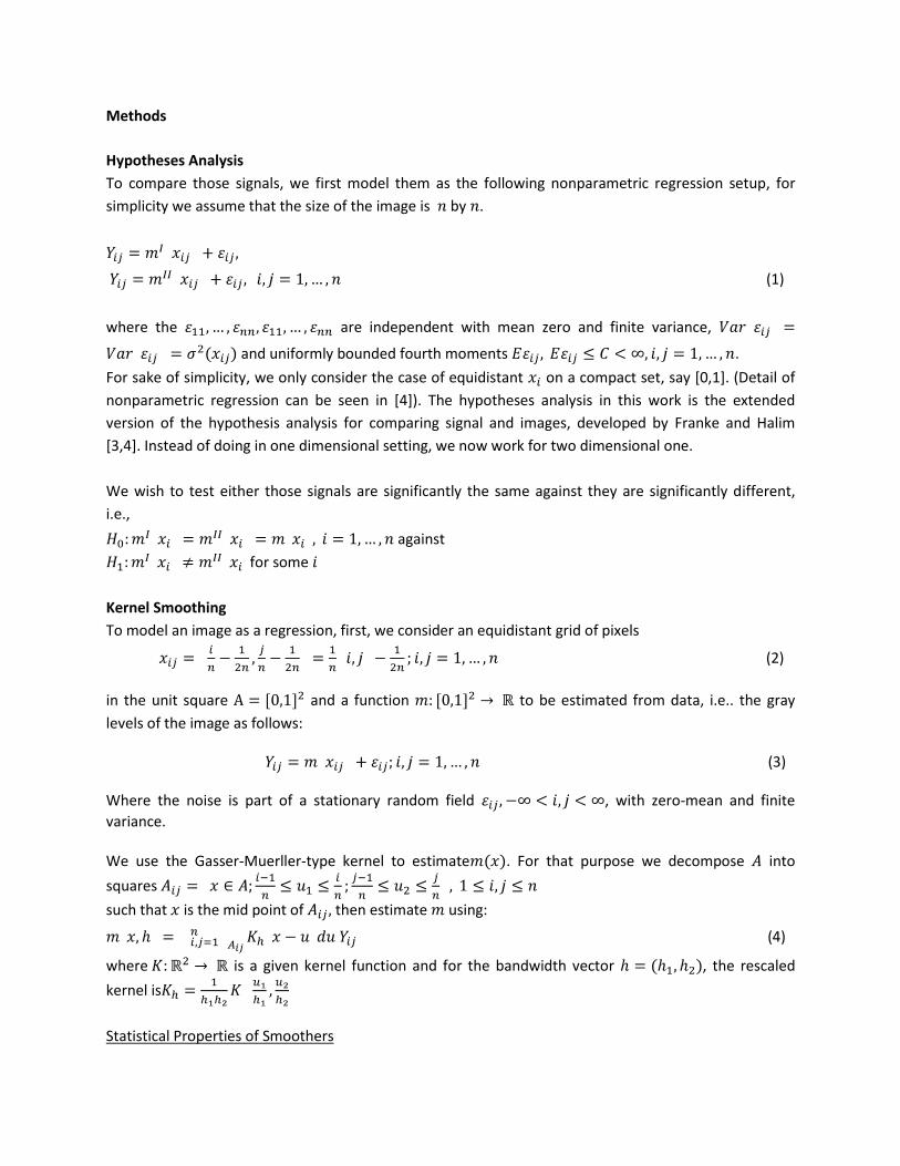
Methods

Hypotheses Analysis

To compare those signals, we first model them as the following nonparametric regression setup, for

simplicity we assume that the size of the image is by .

(1)

where the are independent with mean zero and finite variance,

and uniformly bounded fourth moments .

For sake of simplicity, we only consider the case of equidistant on a compact set, say [0,1]. (Detail of

nonparametric regression can be seen in [4]). The hypotheses analysis in this work is the extended

version of the hypothesis analysis for comparing signal and images, developed by Franke and Halim

[3,4]. Instead of doing in one dimensional setting, we now work for two dimensional one.

We wish to test either those signals are significantly the same against they are significantly different,

i.e.,

against

for some

Kernel Smoothing

To model an image as a regression, first, we consider an equidistant grid of pixels

(2)

in the unit square and a function to be estimated from data, i.e.. the gray

levels of the image as follows:

(3)

Where the noise is part of a stationary random field , with zero-mean and finite

variance. We use the Gasser-Muerller-type kernel to estimate . For that purpose we decompose into

squares

such that is the mid point of then estimate using:

(4)

where is a given kernel function and for the bandwidth vector , the rescaled

kernel is

Statistical Properties of Smoothers

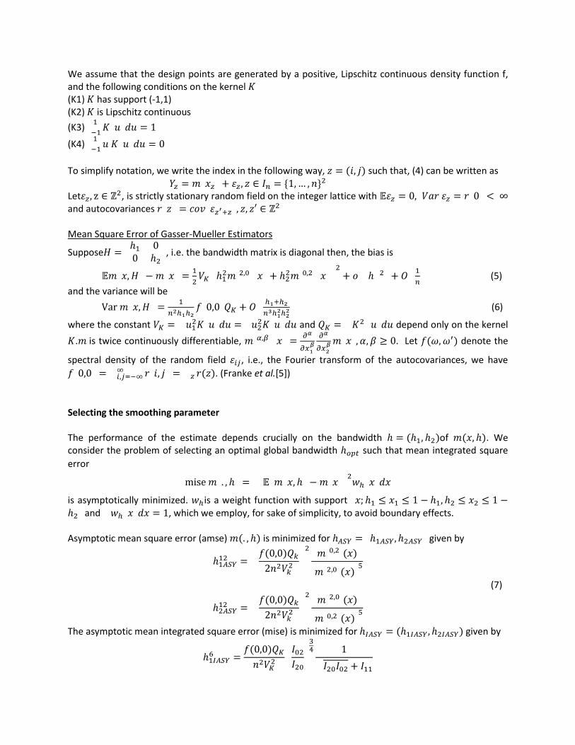
We assume that the design points are generated by a positive, Lipschitz continuous density function f, and the following conditions on the kernel (K1) has support (-1,1) (K2) is Lipschitz continuous

(K3)

(K4)

To simplify notation, we write the index in the following way, such that, (4) can be written as Let , is strictly stationary random field on the integer lattice with and autocovariances Mean Square Error of Gasser-Mueller Estimators

Suppose , i.e. the bandwidth matrix is diagonal then, the bias is

(5)

and the variance will be

(6)

where the constant and depend only on the kernel

. is twice continuously differentiable, . Let denote the

spectral density of the random field , i.e., the Fourier transform of the autocovariances, we have

. (Franke et al.[5])

Selecting the smoothing parameter The performance of the estimate depends crucially on the bandwidth of . We consider the problem of selecting an optimal global bandwidth such that mean integrated square

error

is asymptotically minimized. is a weight function with support and , which we employ, for sake of simplicity, to avoid boundary effects.

Asymptotic mean square error (amse) is minimized for given by

(7)

The asymptotic mean integrated square error (mise) is minimized for given by

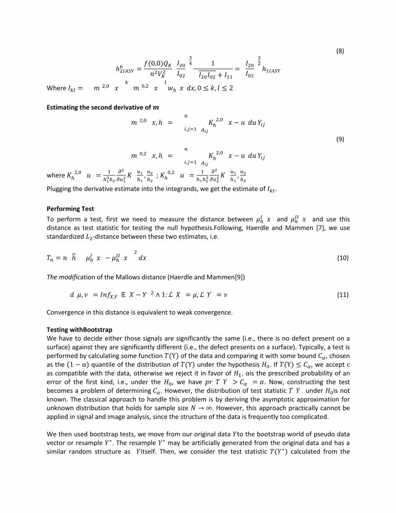
(8)

Where

Estimating the second derivative of

(9)

where ;

Plugging the derivative estimate into the integrands, we get the estimate of .

Performing Test

To perform a test, first we need to measure the distance between and and use this distance as test statistic for testing the null hypothesis.Following, Haerdle and Mammen [7], we use standardized -distance between these two estimates, i.e.

(10)

The modification of the Mallows distance (Haerdle and Mammen[9])

(11)

Convergence in this distance is equivalent to weak convergence. Testing withBootstrap We have to decide either those signals are significantly the same (i.e., there is no defect present on a surface) against they are significantly different (i.e., the defect presents on a surface). Typically, a test is performed by calculating some function of the data and comparing it with some bound , chosen as the quantile of the distribution of under the hypothesis . If , we accept as compatible with the data, otherwise we reject it in favor of . is the prescribed probability of an error of the first kind, i.e., under the , we have . Now, constructing the test becomes a problem of determining . However, the distribution of test statistic under is not known. The classical approach to handle this problem is by deriving the asymptotic approximation for unknown distribution that holds for sample size . However, this approach practically cannot be applied in signal and image analysis, since the structure of the data is frequently too complicated. We then used bootstrap tests, we move from our original data to the bootstrap world of pseudo data vector or resample . The resample may be artificially generated from the original data and has a similar random structure as itself. Then, we consider the test statistic calculated from the

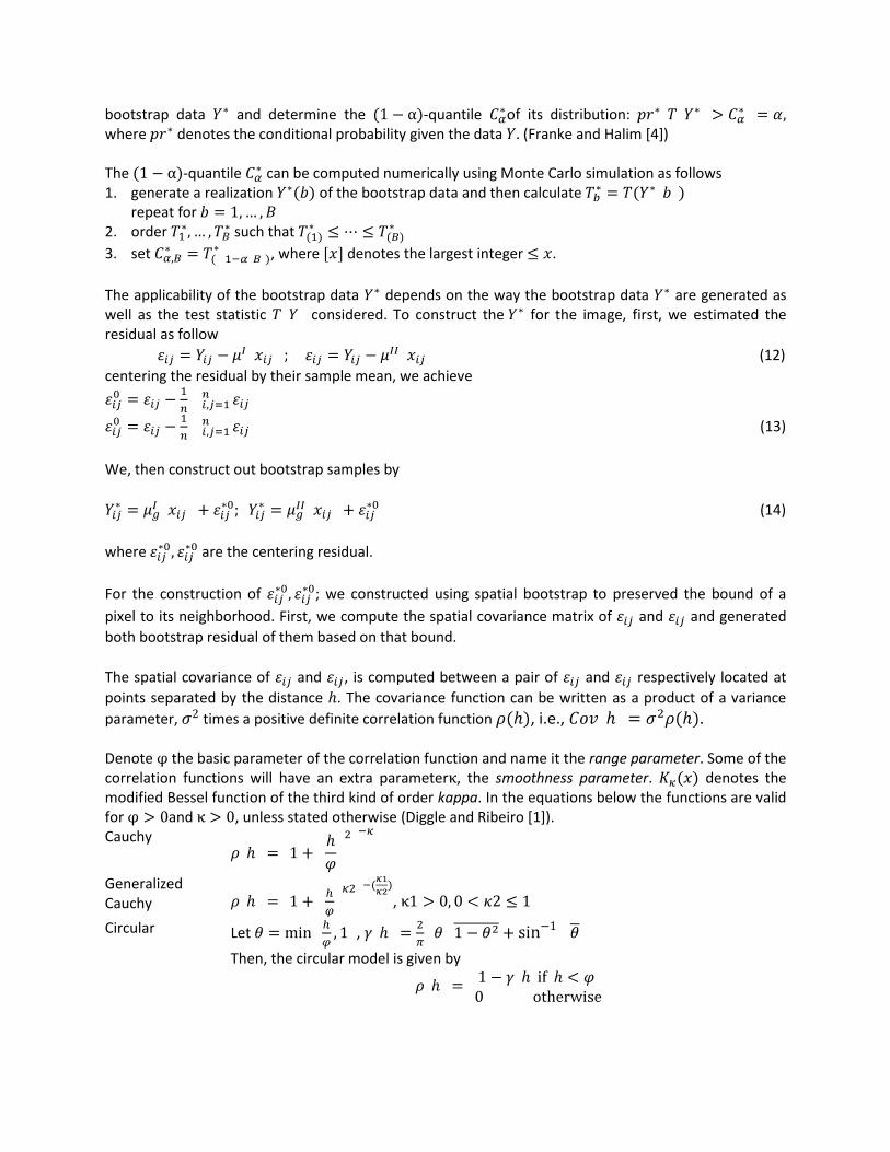
bootstrap data and determine the -quantile of its distribution: where denotes the conditional probability given the data (Franke and Halim [4]) The -quantile can be computed numerically using Monte Carlo simulation as follows 1. generate a realization of the bootstrap data and then calculate

repeat for 2. order such that

3. set , where denotes the largest integer .

The applicability of the bootstrap data depends on the way the bootstrap data are generated as well as the test statistic considered. To construct the for the image, first, we estimated the residual as follow

(12)

centering the residual by their sample mean, we achieve

(13)

We, then construct out bootstrap samples by

(14)

where are the centering residual.

For the construction of ; we constructed using spatial bootstrap to preserved the bound of a

pixel to its neighborhood. First, we compute the spatial covariance matrix of and and generated

both bootstrap residual of them based on that bound.

The spatial covariance of and , is computed between a pair of and respectively located at

points separated by the distance . The covariance function can be written as a product of a variance

parameter, times a positive definite correlation function , i.e., .

Denote the basic parameter of the correlation function and name it the range parameter. Some of the correlation functions will have an extra parameter , the smoothness parameter. denotes the modified Bessel function of the third kind of order kappa. In the equations below the functions are valid for and , unless stated otherwise (Diggle and Ribeiro [1]). Cauchy

Generalized Cauchy ,

Circular Let ,

Then, the circular model is given by

Cubic if , 0 otherwise

Gaussian

Exponential Matern

Spherical if , 0 otherwise

In this work we chose the correlation as Gaussian model. Now, the bootstrap test statistics can be constructed as follows (Franke and Halim [3,4]).

(15a)

(15b)

(15c)

(15d)

(15e)

Under the hypothesis we use two forms of the test statistics based on (15b) or (15d)with the bootstrap samples. From now on, we call them as and respectively, and we set

(16)

(17)

Using one of these two functions then we can set the or and

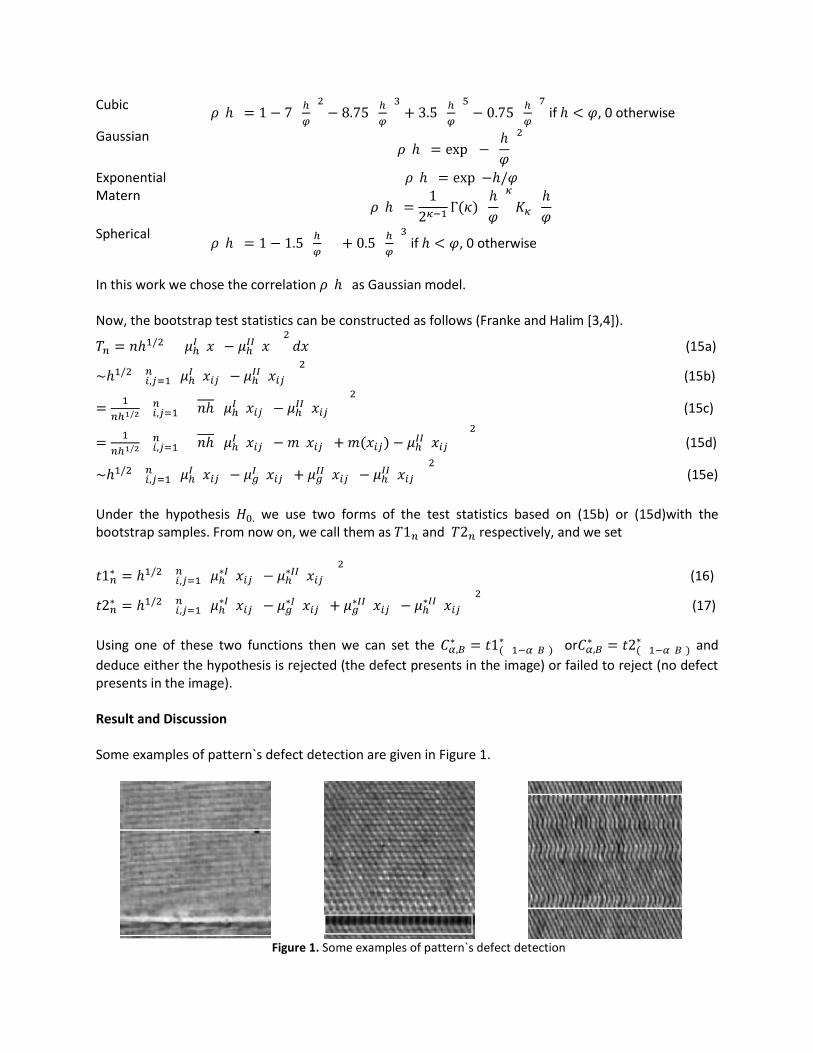
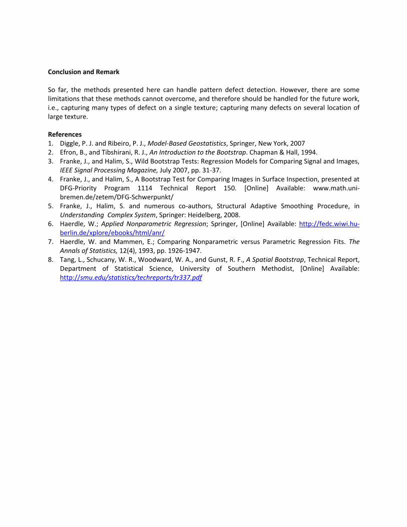
deduce either the hypothesis is rejected (the defect presents in the image) or failed to reject (no defect presents in the image). Result and Discussion Some examples of pattern`s defect detection are given in Figure 1.

Figure 1. Some examples of pattern`s defect detection

Conclusion and Remark So far, the methods presented here can handle pattern defect detection. However, there are some limitations that these methods cannot overcome, and therefore should be handled for the future work, i.e., capturing many types of defect on a single texture; capturing many defects on several location of large texture. References 1. Diggle, P. J. and Ribeiro, P. J., Model-Based Geostatistics, Springer, New York, 2007 2. Efron, B., and Tibshirani, R. J., An Introduction to the Bootstrap. Chapman & Hall, 1994. 3. Franke, J., and Halim, S., Wild Bootstrap Tests: Regression Models for Comparing Signal and Images,

IEEE Signal Processing Magazine, July 2007, pp. 31-37. 4. Franke, J., and Halim, S., A Bootstrap Test for Comparing Images in Surface Inspection, presented at

DFG-Priority Program 1114 Technical Report 150. [Online] Available: www.math.uni-bremen.de/zetem/DFG-Schwerpunkt/

5. Franke, J., Halim, S. and numerous co-authors, Structural Adaptive Smoothing Procedure, in Understanding Complex System, Springer: Heidelberg, 2008.

6. Haerdle, W.; Applied Nonparametric Regression; Springer, [Online] Available: http://fedc.wiwi.hu-berlin.de/xplore/ebooks/html/anr/

7. Haerdle, W. and Mammen, E.; Comparing Nonparametric versus Parametric Regression Fits. The Annals of Statistics, 12(4), 1993, pp. 1926-1947.

8. Tang, L., Schucany, W. R., Woodward, W. A., and Gunst, R. F., A Spatial Bootstrap, Technical Report, Department of Statistical Science, University of Southern Methodist, [Online] Available: http://smu.edu/statistics/techreports/tr337.pdf