Delft University of Technology

Carbon Emissions and Economic Growth: Production-based versus Consumption-based Evidence on Decoupling

Storm, Servaas; Mir, G.U.R.

Publication date2016Document VersionFinal published version

Citation (APA)Storm, S. (Author), & Mir, G. U. R. (Author). (2016). Carbon Emissions and Economic Growth: Production-based versus Consumption-based Evidence on Decoupling. Institute for new economic thinking.

Important noteTo cite this publication, please use the final published version (if applicable).Please check the document version above.

CopyrightOther than for strictly personal use, it is not permitted to download, forward or distribute the text or part of it, without the consentof the author(s) and/or copyright holder(s), unless the work is under an open content license such as Creative Commons.

Takedown policyPlease contact us and provide details if you believe this document breaches copyrights.We will remove access to the work immediately and investigate your claim.

This work is downloaded from Delft University of Technology.For technical reasons the number of authors shown on this cover page is limited to a maximum of 10.

!

!

Carbon Emissions and Economic Growth: Production-based

versus Consumption-based Evidence on Decoupling

Goher-Ur-Rehman Mir1 and Servaas Storm2

Working Paper No. 41

April 2016

ABSTRACT

We assess the Carbon-Kuznets-Curve hypothesis using internationally consistent and comparable production-based versus consumption-based CO2 emissions data for 40 countries (and 35 industries) during 1995-2007 from the World Input Output Database (WIOD). The estimates for per capita CO2 emissions are truly comprehensive as these include all carbon emissions embodied in international trade and global commodity chains. Even if we find evidence suggesting a decoupling of production-based CO2 emissions and growth, consumption-based CO2 emissions are monotonically increasing with per capita GDP. We draw out the implications of these findings for climate policy and binding emission reduction obligations.

!!!!!!!!!!!!!!!!!!!!!!!!!!!!!!!!!!!!!!!!!!!!!!!!!!!!!!!!!!!!!1 Ecofys Consulting, Kanaalweg 15G, 3526 KL Utrecht, The Netherlands. Email: G.Mir@Ecofys.com 2 Corresponding author: Department of Economics of Technology and Innovation, Faculty TBM, Delft University of Technology, Jaffalaan 5, 2628 BX Delft, The Netherlands. Email: s.t.h.storm@tudelft.nl

!

Keywords: Carbon Kuznets Curve; Climate change; Economic growth; Production-based CO2

emissions, Consumption-based CO2 emissions; Decoupling. JEL codes: F64, Q54, Q55, Q56.

!!

2!!

1. Introduction

Most scientists consider it extremely likely that the Earth’s climate will become warmer if

atmospheric concentrations of carbon dioxide (CO2) continue to increase because of emissions

by human (economic) activity.1 In its fifth assessment report, the Intergovernmental Panel on

Climate Change (IPCC 2014) predicts that in a business-as-usual scenario the mean global

surface temperature will increase by 4oC or more above pre-industrial levels by the end of 21st

century (Collins et al. 2013)—with a non-negligible risk of far higher dangerous warming

(Wagner and Weitzman 2015). To avoid the risk of dangerous and irreversible climate change,

the consensus view is that the global average temperature should not rise above pre-industrial

temperatures by more than 2oC (Edenhofer et al. 2013). This consensus view which has recently

been endorsed by 195 nations at the 21st session of the Conference of Parties (COP21) to the

United Nations Framework Convention on Climate Change (UNFCC) in Paris in December

2015, implies that anthropogenic greenhouse gas (GHG) emissions have to be reduced by 41 to

72 percent in 2050 compared to emissions levels in 2010, and by as much as 78 to 118 percent in

2100 (IPCC 2014; COP21). These major emission reductions over the coming decades will need

a dramatic decarbonization of our energy systems as well as a historically unprecedented

ramping up of energy efficiency, the more so the higher is the rate of global economic growth

(Grubb 2014, p. 14). This points to a major global challenge: is it possible to decarbonize and

halve emissions by mid-century so as to keep below the 2°C limit while maintaining global

economic growth (Martinez Alier 2009, 2015; Grubb 2014; Spash 2015)?

The issue of whether economic growth can be delinked from GHG emissions is usually

framed in terms of the Carbon Kuznets Curve (CKC)—the inverted U-shaped relationship

between per capita income and GHG emissions per capita (Dinda 2004; Müller-Fürstenberger &

Wagner 2007; Kaika & Zervas, 2013a, 2013b). The CKC hypothesis holds that GHG emissions

per person do initially increase with rising per capita income (due to industrialization), then peak

and decline after a threshold level of per capita GDP, as countries become more energy efficient,

more technologically sophisticated and more inclined to and able to reduce emissions by

corresponding legislation. The large empirical and methodological literature on the CKC does !!!!!!!!!!!!!!!!!!!!!!!!!!!!!!!!!!!!!!!!!!!!!!!!!!!!!!!!!!!!!1 Ribes et al. (2016) provide a novel corroboration of the IPCC’s (2014) conclusion that it

“is extremely likely [95 percent confidence] more than half of the observed increase in global average surface temperature from 1951 to 2010 was caused by the anthropogenic increase in greenhouse gas concentrations and other anthropogenic forcings together …”

!!

3!!

not provide unambiguous and robust evidence of a CKC peaking for carbon dioxide (see Kaika

& Zervas (2013a, 2013b) for a recent review), if only because of well documented but yet

unresolved econometric problems concerning the appropriateness of model specification and

estimation strategies (Wagner 2008).

We will leave these econometric issues aside however and instead focus on the fact that

the overwhelming majority of empirical CKC studies use domestic production-based CO2

emissions data to test the Kuznets hypothesis—and hence overlook the emissions embodied in

international trade and in global commodity chains. Based on IPCC (2007) guidelines, GHG

emissions are counted as the national emissions coming from domestic production. This

geographical definition hides the GHG emissions embodied in international trade and obscures

the empirical fact that domestic production-based GHG emissions in (for example) the EU have

come down, but consumption-based emissions associated with EU standards of livings have

actually increased (Peters and Hertwich 2008; Boitier 2012). Rich countries including the EU-27

and the U.S.A. with high average consumption levels are known to be net carbon importers as

the CO2 emissions embodied in their exports are lower than the emissions embodied in their

imports (Nakano et al. 2009; Boitier 2012; Agrawala et al. 2014). Vice versa, most developing

(and industrializing) countries are net carbon exporters. What this implies is that, because of

cross-border carbon leakages, consumption-based CO2 emissions are higher than production-

based emissions in the OECD countries, but lower in the developing countries (Aichele &

Felbermayr 2012). This indicates that while there may well be a Kuznets-like delinking between

economic growth and per capita production-based GHG emissions, it is as yet unclear whether

such delinking is also occurring in terms of consumption-based GHG emissions. If not, the

notion of “carbon decoupling” has to be rethought—in terms of a delinking between growth and

consumption-based GHG emissions. After all, it is no great achievement to reduce domestic per

capita carbon emissions by outsourcing carbon-intensive activities to other countries and by

being a net importer of GHG, while raising consumption and living standards. This also does not

constitute a viable global strategy of meeting the GHG emission reduction obligations implied by

COP21. Hence, this paper assesses the CKC hypothesis using internationally comparable and

consistent production-based versus consumption-based CO2 emissions data for 40 countries (and

35 industries) for 1995-2007 from the World Input Output Database (WIOD). We argue that the

notion of a decoupling of economic growth and carbon emissions is meaningful (for climate

!!

4!!

change mitigation) only when we define it in terms of consumption-based CO2 emissions (and

not production-based emissions). The rest of the paper is organized as follows. Section 2 reviews

the literature on the CKC. Section 3 provides salient features of the WIOD data used and outlines

the Fixed Effects Model used in the regression analysis. Section 4 compares the estimation

results of the production-based and the consumption-based CKC. Section 5 draws out the policy

implications and concludes.

2. The CKC: a review of the empirical literature

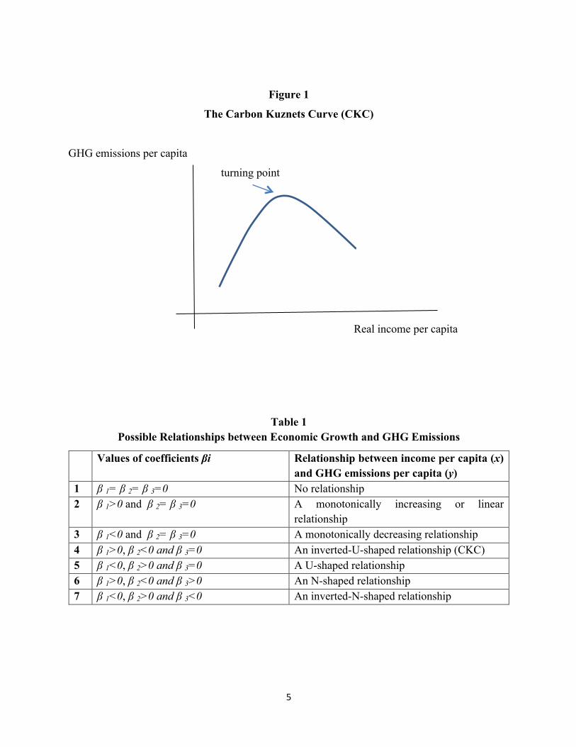
The Carbon Kuznets Curve (CKC) hypothesis postulates an inverted U-shaped relationship

between CO2 emissions and per capita income (as is shown in Figure 1): emissions per person

increase up to a certain threshold level as per capita income goes up, after which they start to

decrease (Dinda 2004; Müller-Fürstenberger & Wagner 2007; Kaika & Zervas, 2013a, 2013b).

Typically, most of the CKC studies use the following general reduced-form model in which

GHG emissions per person is a polynomial cubic function (of degree three) of per capita income:

(1) yit = αi + β1 xit + β2 x2it + β3x3

it + β4zit + eit

where i = 1, ....., n countries, and t = 1, ….., T years. We note that equation (1) is a reduced-

form equation (Kaika & Zervas, 2013a). Most studies do not explicitly specify the underlying

structural equations of the system that lead to (1). The structural causes underlying the CKC have

been widely debated however. While a detailed review of this literature is beyond the scope of

our paper, the debate on the driving forces of the CKC pattern has focused on changes in income

distribution during the process of per capita income growth (Torras and Boyce 1998; Scruggs

1998; Magnani 2000; Gangadhran & Valenzuela 2001; Bimonte 2002), the income elasticity of

demand for environmental quality (Dinda 2004; Kaika & Zervas 2013a), structural and

technological change from a specialization in primary activities to secondary activities and

further to the more environmentally friendly tertiary sector (de Bruyn, van den Bergh &

Opschoor 1998; Dinda 2004), the diffusion of more carbon efficient technology through

international trade and FDI (Muradian & Martinez-Alier 2001; Stavins et al. 2014), and changes

in institutions and governance during the process of economic development (Dasgupta, Laplante,

Wang & Wheeler 2002; Dutt 2009). However, most of the empirical evidence depends only on

the reduced-form equation (1) and not on the underlying (larger) structural model (Dinda 2004).

!!

5!!

Figure 1

The Carbon Kuznets Curve (CKC)

GHG emissions per capita

turning point

Real income per capita

Table 1

Possible Relationships between Economic Growth and GHG Emissions

Values of coefficients βi Relationship between income per capita (x) and GHG emissions per capita (y)

1 β 1= β 2= β 3=0 No relationship 2 β 1>0 and β 2= β 3=0 A monotonically increasing or linear

relationship 3 β 1<0 and β 2= β 3=0 A monotonically decreasing relationship 4 β 1>0, β 2<0 and β 3=0 An inverted-U-shaped relationship (CKC) 5 β 1<0, β 2>0 and β 3=0 A U-shaped relationship 6 β 1>0, β 2<0 and β 3>0 An N-shaped relationship 7 β 1<0, β 2>0 and β 3<0 An inverted-N-shaped relationship

!!

6!!

In equation (1), y is the dependent variable indicating GHG emissions per person, x is the

independent variable (which is per capita income in real terms), z represents control variables

that might influence y, α is the constant term or country-specific intercept, βi are the estimated

coefficients of the k explanatory variables and e represents the error term. The final choice of the

functional form (whether or not to include higher order terms and natural logarithms) depends on

the model that best fits the data available and has a higher explanatory power within the data

range (Lieb 2003). Depending on the values of βi and their combinations, equation (1) can take

several relevant forms which are given in Table 1 (Kijima, Nishide & Ohyama 2010). It can be

seen that the CKC is only one of various possible numerical outcomes for equation (1), namely

outcome 4 in Table 1, which occurs when we find that β1>0, β2<0 and β3 = 0. Using (1), the

turning point or threshold level of per capita income can be calculated as (assuming 0xy

i

i =dd ):!

(2) x*=− !!!"!!, or in logarithmic version x*= !!

!"!"!

The (mechanistic) assumption underlying the CKC curve is that developing countries (which

have low per capita incomes and are usually found on the rising slope of the curve) will follow

the same development trajectory as the one followed by the developed countries (which feature

higher per capita GDP and are found on the downward-sloping side of the curve). It is possible

of course that due to some new technological breakthrough developing countries may be able to

leapfrog to higher levels of per capita income (Grossman & Krueger 1995). At the same time,

however, in our finite world, the poor countries of today will be unable to find further countries

from which to import carbon-intensive products as they themselves grow richer. Thus these

countries would face the difficult task of abating pollution activities rather than outsourcing

them to other countries (Arrow et al. 1995; Stern et al. 1996). Therefore, today’s developing

(and industrializing) countries may not be able to follow in the steps of the developed countries.

!!

7!!

There is a voluminous econometric literature estimating the CKC equation (1), which

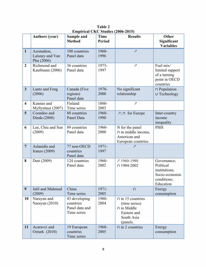
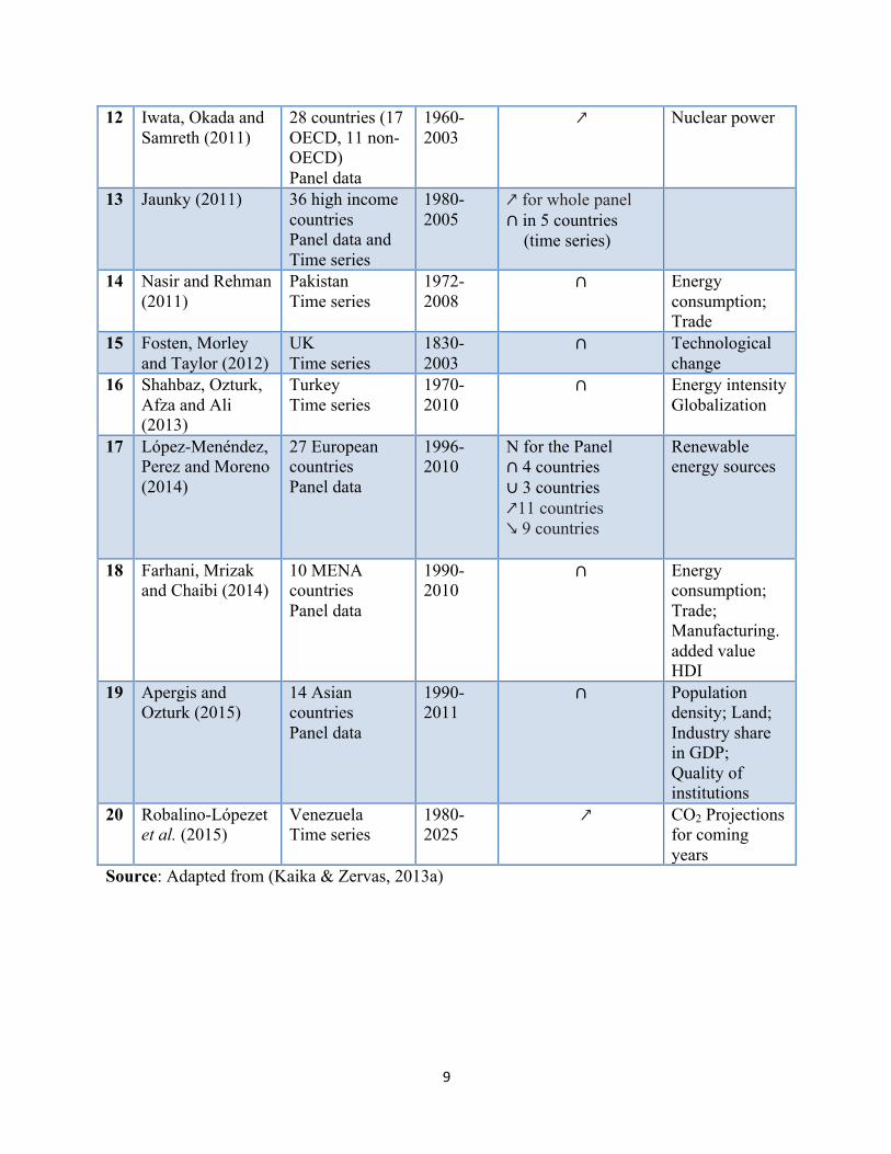
goes back to the 1990s and reports mixed (inconclusive) results.2 Table 2 summarizes twenty

recent (post-2006) empirical studies on the CKC. It highlights authors’ names, year of

publication of article, sample used and econometric method employed for analysis,

outcomes/relationships between CO2 emissions and economic growth and other explanatory

variables incorporated in the study or descriptions added to explain the observed relationship

between carbon emissions and economic growth. While a detailed review of each separate study

is not possible here, a few general observations are in order. First, most studies use panel data

analysis, mainly because of a lack of time-series data for a long enough period of time for

individual countries. Second, outcomes are clearly sensitive to the exact sample of countries used

as well as the time period chosen for investigation. It is fair to conclude, finally, that there is no

unambiguous and robust evidence in support of the CKC—notwithstanding the fact that eleven

out of 20 studies report findings (partly) in support of the CKC.

What all the studies reported in Table 2 share in common (and perhaps surprisingly so) is

that they rely on (domestic) production-based emissions data to test the CKC hypothesis. Doing

so has two drawbacks. The first drawback of using production-based emission data is that it

ignores non-trivial emissions associated with international transportation and international trade

(Peters & Hertwich, 2008). CO2 Emissions from the production of traded goods and services

have increased from 4.3 GtCO2 in 1990 (20% of global CO2 emissions) to 7.8 GtCO2 in 2008

(26% of global CO2 emissions) (see Peters, Minx, Weber & Edenhofer, 2011). This shows that

international trade cannot be ignored while determining the underlying driving forces behind

global, regional and national emissions. However, attributing emissions from international

transportation to countries is controversial and as of now there is no transparent and agreed-upon

method to allocate these emissions to (trading) countries (Peters et al. 2011; Boitier 2012).

!!!!!!!!!!!!!!!!!!!!!!!!!!!!!!!!!!!!!!!!!!!!!!!!!!!!!!!!!!!!!2!!!!!!!! The older (pre-2006) literature includes Shafik & Bandyopadhyay (1992), Holtz-Eakin &

Selden (1995), Roberts &Grimes (1997), Schmalensee et al. (1998), De Bruyn et al. (1998), Agras & Chapman (1999), Galeotti & Lanza (1999), Borghesi (2000), Perrings & Ansuategi (2000), Panayotou et al.(2000), Pauli (2003) and Aldy (2005).!

!!

8!!

Table 2 Empirical CKC Studies (2006-2015)

Authors (year) Sample and Method

Time Period

Results Other Significant Variables

1 Azomahou, Laisney and Van Phu (2006)

100 countries Panel data

1960-1996

↗

2 Richmond and Kaufmann (2006)

36 countries Panel data

1973-1997

↗ Fuel mix/ limited support of a turning point in OECD countries

3 Lantz and Feng (2006)

Canada (Five regions) Panel data

1970-2000

No significant relationship

∩ Population ∪ Technology

4 Kunnas and Myllyntaus (2007)

Finland Time series

1800-2003

↗

5 Coondoo and Dinda (2008)

88 countries Panel Data

1960-1990

↗;#∩ for Europe Inter-country income inequality

6 Lee, Chiu and Sun (2009)

89 countries Panel data

1960-2000

N for the panel ∩ in middle income, American and European countries

PHH

7 Aslanidis and Iranzo (2009)

77 non-OECD countries Panel data

1971-1997

↗

8 Dutt (2009) 124 countries Panel data

1960-2002

↗ 1960-1980 ∩ 1984-2002

Governance; Political institutions; Socio-economic conditions; Education

9 Jalil and Mahmud (2009)

China Time series

1971-2005

∩ Energy consumption

10 Narayan and Narayan (2010)

43 developing countries Panel data and Time series

1980-2004

∩ in 15 countries (time series) ∩ in Middle Eastern and South Asia (panels_

11 Acaravci and Ozturk (2010)

19 European countries Time series

1960-2005

∩ in 2 countries Energy consumption

!!

9!!

12 Iwata, Okada and Samreth (2011)

28 countries (17 OECD, 11 non-OECD) Panel data

1960-2003

↗ Nuclear power

13 Jaunky (2011) 36 high income countries Panel data and Time series

1980-2005

↗ for whole panel ∩ in 5 countries (time series)

14 Nasir and Rehman (2011)

Pakistan Time series

1972-2008

∩ Energy consumption; Trade

15 Fosten, Morley and Taylor (2012)

UK Time series

1830-2003

∩ Technological change

16 Shahbaz, Ozturk, Afza and Ali (2013)

Turkey Time series

1970-2010

∩ Energy intensity Globalization

17 López-Menéndez, Perez and Moreno (2014)

27 European countries Panel data

1996-2010

N for the Panel ∩ 4 countries ∪ 3 countries ↗11 countries ↘ 9 countries

Renewable energy sources

18 Farhani, Mrizak and Chaibi (2014)

10 MENA countries Panel data

1990-2010

∩ Energy consumption; Trade; Manufacturing. added value HDI

19 Apergis and Ozturk (2015)

14 Asian countries Panel data

1990-2011

∩ Population density; Land; Industry share in GDP; Quality of institutions

20 Robalino-Lópezet et al. (2015)

Venezuela Time series

1980-2025

↗ CO2 Projections for coming years

Source: Adapted from (Kaika & Zervas, 2013a)

!!

10!!

The second drawback of using production-based CO2 emissions is that this ignores the

fact that the reduction in per capita carbon emissions in (especially) the rich countries committed

to the Kyoto Protocol (the so-called Annex I Parties) has been (at least partly) offset by an

increase in emissions in the (industrializing and exporting) developing countries which are not

committed to any binding emission targets (the non-Annex I Parties), as has been shown by

Aichele & Felbermayr (2012) and Blanco et al. (2014). Specifically, due to the dramatic

internationalization of trade in global production chains, the Annex I countries have been able to

reduce their national production-based carbon emissions by importing carbon-intensive industrial

products from abroad. Hence, for most countries production-based and consumption-based

emissions are found to differ considerably (for evidence, see Peters 2008; Davis & Caldeira

2010; Ahmad & Wyckoff 2003; Peters, Minx, Weber & Edenhofer 2011). We define how we

measure production-based and consumption-based GHG emissions below, but we can already

observe here that net carbon imports (and exports) have grown substantially in recent years. To

illustrate, in 1990, the territorial production-based emissions of the Annex I Parties to the Kyoto

Protocol amounted to 14.2 GtCO2; their consumption-based emissions were higher (14.6 GtCO2)

which implies these rich countries had a carbon import surplus of 0.4 GtCO2 (or 2.8% of their

production-based emissions). In 2008, production-based emissions of the Annex I Parties had

declined to 13.9 GtCO2, but their consumption-based emissions had increased to 15.5 GtCO2; net

carbon imports amounted to 1.6 GtCO2 (or 11.5% of production-based emissions). Trends were

the reverse in the non-Annex I Parties which are net carbon exporters. Their production-based

emissions increased from 7.7 GtCO2 in 1990 to 16.4 GtCO2 in 2008, while their consumption-

based emissions rose from 7.3 GtCO2 to 14.8 GtCO2 over the same period. In 2008, the non-

Annex I countries were exporting about 10% of their production-based emissions to the Annex I

countries (Peters et al. 2011). In general, the increasing carbon-import surplus in the OECD

countries has been made possible by an increasing carbon-export surplus in developing countries

(Boitier 2012; Agrawala et al. 2014; Nakano et al. 2009). In light of the above, it is vitally

important to statistically test for any decoupling between CO2 emissions and economic growth

using both consumption-based and production-based emission data.

!!

11!!

3. Data and Econometric Model

The data on production-based and consumption-based CO2 emissions by country are from the

World Input Output Database (WIOD), which provides consistent annualized inter-country

input-output accounts covering the period 1995-2009 for 40 countries (27 EU member states and

13 non-European countries). The WIOD data are broken down across 36 different sectors (35

industries and one household sector) and 26 energy commodities plus one entry for non-energy

related CO2 emissions to complete the emission matrix (see Timmer et al. 2015). For the

countries covered, the database uses economic linkages between industries, which are portrayed

by a set of harmonized supply and use tables (SUTs), together with data on international trade in

goods and services to integrate them into sets of inter-country input output tables (IOTs). These

input output tables are then used to develop environmental accounts including for GHG

emissions. The main source of information for WIOD’s energy accounts is the energy balances

from the IEA (2011a), which have been made compatible with WIOD’s inter-country input-

output tables (see Timmer et al. 2015 for details) The WIOD data notably do account for

emissions arising from international aviation, fishing vessels and marine bunkers. The WIOD

database uses standard production-based CO2 emission factors provided by the IPCC Guidelines

for National Greenhouse Gas Inventories (IPCC, 2014a), complemented by country-specific

production-based emission factors provided in national CO2 emission reports by the UNFCCC.

Boitier (2012) has calculated annual production-based and consumption-based CO2 emissions for

40 countries during 1995-2009 using the WIOD database. We use his estimations to calculate

CO2 emissions per capita (using population data from the World Bank database). GDP per capita

is given in constant 2011 international dollars (measured in Purchasing Power Parity terms).

Because the data from World Bank do not cover Taiwan, Taiwan was dropped from the panel of

countries. We further excluded the crisis years 2008 and 2009 from the sample, because

emissions behavior and economic growth are out of line with the earlier period 1995-2007. Our

panel, which has observations for 39 countries during 1995-2007 (n = 507), covers 79.7% of the

world’s anthropogenic production-based CO2 emissions and 80.7% of consumption-based CO2

emissions in 2007.

Boitier (2012) follows standard Leontief input-output model (IOM) methodology to

calculate emissions intensities. The IOM can be represented by:

!!

12!!

(3) fxx += A

where x = (x1, …xM, … xN) is the vector of total output in country m = 1, …N; f = (f1M, …fVM, …

fNM) is the vector of total final demand in country m addressed to country v, m = 1, …N; and A is

the inter-industry matrix of which the representative element MVA stands for intermediate inputs

supplied by country m to country v (measured per unit of output of country v). The solution to

equation (3) is given by:

(4) ffx )1( -1 RA =−=

where -1) 1( AR −= is the (multi-country) Leontief inverse. The column sum ∑=

N

1MMVR gives the

total (direct and indirect) increase in production in all industries in all 39 countries due to a

unitary increase in all elements of final demand in country v. This is known as the backward

production linkage of fV. If we next define Me as an element of the row vector ( 'e ) of GHG

emissions by country m (measured per unit of output in country m), we can calculate a matrix of

embodied emissions f 'ReE = of which the diagonal elements MME are the (direct and indirect)

domestic GHG emissions in country m, the column sum of the off-diagonal elements ∑≠=

N

VM1 V

MVE

stands for the (direct and indirect) emissions embodied in the intermediate imports of country m,

and the row sum of the off-diagonal elements ∑≠=

N

VM1 M

MVE stands for the (direct and indirect)

emissions embodied in the exports of country m (Boitier 2012). Using these definitions, national

production-based GHG emissions of country m are computed as:

(5) ∑≠=

++=N

VM1 M

HMVMM

prod EEE E

where HE are national emissions directly originating from households’ consumption. We must

emphasize that Eprod is a truly comprehensive measure of production-based GHG emissions,

because it includes all direct and indirect emissions associated with the production and export of

!!

13!!

goods and services by country v. Likewise, national consumption-based GHG emissions of

country m are estimated as:

(6) ∑≠=

++=N

VM1 V

HMVMM

cons EEE E

Econs comprehensively measures all the direct and indirect GHG emissions occurring throughout

global commodity chains of consumption spending in country v. To illustrate, if German

consumers buy goods produced in France and if the French producers of these goods use

intermediate inputs produced in the U.S.A., Brazil and China, and if Chinese producers of these

intermediate goods source components in Japan and South Korea, then the estimate of Econs

includes all carbon emissions associated with producing those goods in France, the U.S.A.,

Brazil, China, Japan and South Korea, as well as all emissions occurring in the actual

transportation of components, intermediates and the goods themselves between the various

countries in this hypothetical global production chain (Timmer et al. 2015).

In Figure 2 appears the difference ( prodcons E E − ) or net GHG imports ( ∑∑≠=

≠=

−NN

VM1 M

MV

VM1 V

MV EE )

for 5 aggregated regions: the EU-27, the USA, the OECD countries, the BRICs, and the rest of

the world (RoW) for the period 1995-2007. It can be seen that the EU-27, the USA and the

OECD countries are carbon importers (as emissions from production are lower than total

emissions from consumption), while the developing countries (including the BRICs) are carbon

exporters. The gap between CO2 consumed and CO2 produced has widened continuously and

rapidly during 1995-2007. Net carbon imports into the EU-27 doubled from 11% of production-

based emissions in 1995 to 22% in 2007, while for the U.S. net carbon imports increased from

6% of production-based emissions in 1995 to 16.3 % in 2007. (For all OECD countries, some of

which are net carbon exporters, e.g. Canada, net carbon imports increased from 7% of

production-based emissions in 1995 to 13.6% in 2007.) The rich countries are mostly importing

carbon from Brazil, Russia, India and China: net carbon exports by the BRICs increased from

17% of their production-based emissions in 1995 to more than 20% in 2007 (Boitier 2012).

!!

14!!

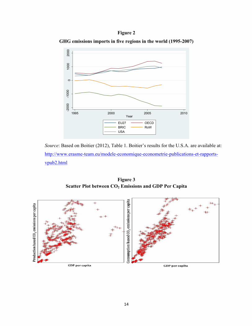
Figure 2

GHG emissions imports in five regions in the world (1995-2007)

Source: Based on Boitier (2012), Table 1. Boitier’s results for the U.S.A. are available at:

http://www.erasme-team.eu/modele-economique-econometrie-publications-et-rapports-

vpub2.html

Figure 3 Scatter Plot between CO2 Emissions and GDP Per Capita

-2000

-1000

01000

2000

1995 2000 2005 2010Year

EU27 OECDBRIC RoWUSA

!!

15!!

Figure 3 presents the scatter plots between CO2 emissions per capita and GDP per capita.

In the left-hand panel appear production-based CO2 emissions (calculated using equation (5))

and the data points visually suggest a non-linear (inverted U-shaped) association between

emissions and GDP per person (which is suggestive of decoupling). In contrast, in the right-hand

panel in which we have plotted consumption-based CO2 emissions (based on equation (6)), the

correlation appears to be a linear one. The nature and the statistical significance of the

relationship between emissions and income per capita will be tested in the next section. Table 3

provides the descriptive statistics of our data panel. It can be seen that the distribution of GDP

per capita is skewed towards the right, as median income ($25,885) is lower than average income

per capita ($26,357); we observe that 95% of the countries in the sample have per capita income

lower than $45,983. We note that the mean level of production-based and consumption-based

CO2 emissions for the world as a whole must be identical (because global production- and

consumption-based emissions must be equal after all); in our sample of 39 countries, however,

average per capita consumption-based emissions exceed average production-based carbon

emissions per person.

Table 3 Descriptive Statistics

Variable Mean Median Minimum Maximum Std.

dev. 5%

Perc. 95% Perc.

GDP Per Capita 26356.9 25884.9 2069.2 96245.5 14942.8 5463.12 45983.2 Production-based CO2

Emissions Per Capita 8.724 8.291 0.844 19.887 4.50 1.57 18.41

Consumption-based CO2

Emissions Per Capita 9.519 9.677 0.770 22.114 4.91 1.50 18.84

We used linear, quadratic as well as cubic functional forms to study the relationship

between growth and (per capita) emissions to see which specification better explains the variance

in CO2 emissions (Galeotti and Lanza 1999). Our prime objective is to observe the relationship

between income per capita and CO2 emissions per person, while controlling for the unobserved

heterogeneity across countries and for time-specific effects. We rejected the Pooled Ordinary

!!

16!!

Least Squares (OLS) model for our full sample, because country- and time-specific effects are

non-zero (Borghesi 2000). The Pooled OLS model also assumes that the variance of country-

specific errors is zero, i.e. the error term is independently and identically distributed in the panel.

However, this condition is unlikely to be met in a panel context. If (unobservable) country-

specific characteristics are correlated with real per capita income (our explanatory variable), the

Fixed Effects model is consistent and efficient (Dutt 2009) and should be preferred to the

Random Effects model. For all specifications, the Random Effects model is rejected in favour of

the Fixed Effects model based on the Hausman specification test. We also rejected the

Generalized Least Squares method model based on the Breusch-Pagan LM test. Accordingly,

given the nature of the data in our full sample of 39 countries, the Fixed Effects model (which

works under the condition of strict exogeneity) is found to be consistent and efficient. In the case

of cubic functional form our Fixed Effect regression model can be written as:

(7) (CO2 pc)it = βo + β1(GDPpc) it + β2(GDPpc)2 it + β3(GDPpc)3

it + ui+ γt + εit

where i =1,……, N and t =1,………, T. ui denotes country specific effects, γt offers time

specific effects and εit is the error term. “pc” stands for per capita. We report Hubert-White

heteroskedasticity and auto-correlation adjusted (HAC) robust standard errors and note that the

computed R2 represents the ‘with-in variance’3. The overall R2 of the model with Fixed Effects is

usually high, because the addition of country-specific effects increases the coefficient of

determination considerably. We do not report the estimation results for the country- and time-

related control variables introduced in the model. The 39 countries included in our panel are

listed in Appendix I.4

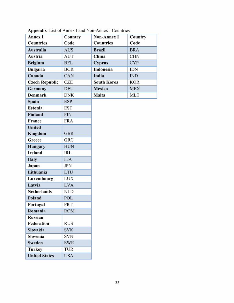
!!!!!!!!!!!!!!!!!!!!!!!!!!!!!!!!!!!!!!!!!!!!!!!!!!!!!!!!!!!!!3 With-in variance measures the variation with in one country over time. 4 The panel is sub-divided into Annex I and non-Annex I countries. Annex I countries are

developed countries which are less vulnerable to the adverse effects of climate change, whereas non-Annex I countries are mostly developing countries which are more vulnerable to the adverse impacts of climate change and also rely more heavily on fossil fuel production and commerce. The estimation results for each of these groups separately are available upon request from the authors.!!

!!

17!!

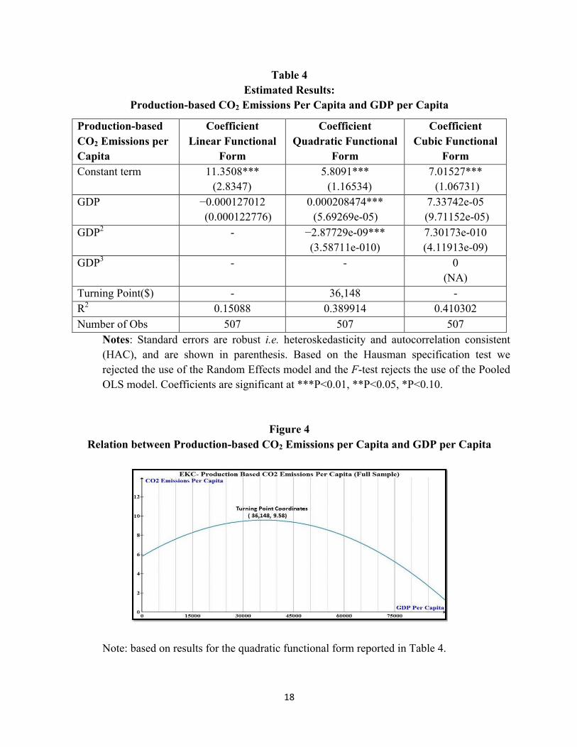
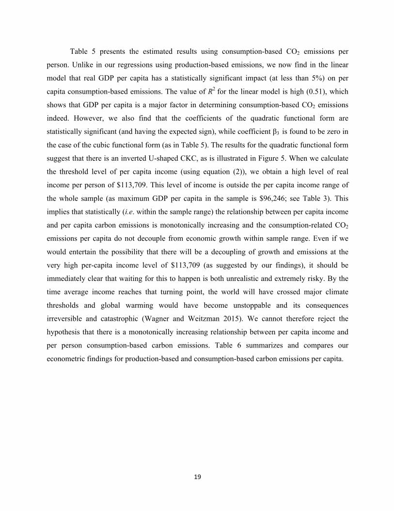
4. Estimation Results

Table 4 presents the estimated results for the linear, quadratic and cubic model, using

production-based CO2 emissions per capita. The goodness of fit of the linear model, as given by

the coefficient of determination R2, is not very high and GDP per capita is not found to be a

statistically significant determinant of production-based CO2 emissions per capita. We can hence

reject the hypothesis that there is a monotonically increasing relationship between per capita

income and per person production-based carbon emissions. Using the quadratic functional form,

all the coefficients are found to be statistically significantly different from zero and they also

have the expected sign; the value of R2 of 0.39 indicates that GDP is a major explanatory factor

in determining production-based CO2 emissions. In the third case of the cubic functional form, β3

is found to be zero and the other coefficients (β1 and β2) are statistically insignificant. Hence, the

quadratic functional form provides the best fit for the relation between production-based CO2

emissions per capita and GDP per capita, which suggests an inverted-U shaped pattern.

Using Equation (2), we can calculate the threshold level of income at which production-

based carbon emissions start to decouple from per capita income growth at $36,148 (see Figure 4

for an illustration). This turning point lies within the sample range of GDP (see Table 4), but it is

well above the sample average (of $26,356 in Table 3). This indicates that overall production-

based emissions will continue to increase until the sample average per capita income has reached

the threshold.

!!

18!!

Table 4 Estimated Results:

Production-based CO2 Emissions Per Capita and GDP per Capita

Production-based CO2 Emissions per Capita

Coefficient Linear Functional

Form

Coefficient Quadratic Functional

Form

Coefficient Cubic Functional

Form Constant term 11.3508***

(2.8347) 5.8091***

(1.16534) 7.01527***

(1.06731) GDP −0.000127012

(0.000122776) 0.000208474***

(5.69269e-05) 7.33742e-05

(9.71152e-05) GDP2 - −2.87729e-09***

(3.58711e-010) 7.30173e-010 (4.11913e-09)

GDP3 - - 0 (NA)

Turning Point($) - 36,148 - R2 0.15088 0.389914 0.410302 Number of Obs 507 507 507

Notes: Standard errors are robust i.e. heteroskedasticity and autocorrelation consistent (HAC), and are shown in parenthesis. Based on the Hausman specification test we rejected the use of the Random Effects model and the F-test rejects the use of the Pooled OLS model. Coefficients are significant at ***P<0.01, **P<0.05, *P<0.10.

Figure 4 Relation between Production-based CO2 Emissions per Capita and GDP per Capita

Note: based on results for the quadratic functional form reported in Table 4.

!!

19!!

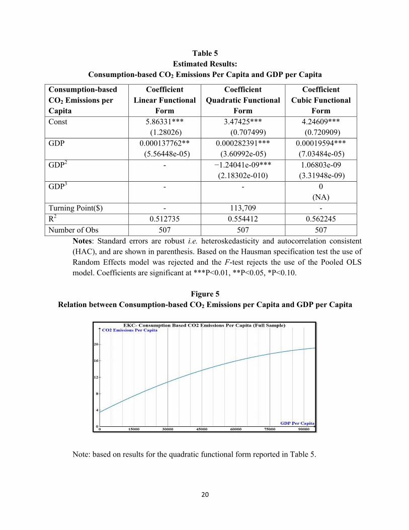
Table 5 presents the estimated results using consumption-based CO2 emissions per

person. Unlike in our regressions using production-based emissions, we now find in the linear

model that real GDP per capita has a statistically significant impact (at less than 5%) on per

capita consumption-based emissions. The value of R2 for the linear model is high (0.51), which

shows that GDP per capita is a major factor in determining consumption-based CO2 emissions

indeed. However, we also find that the coefficients of the quadratic functional form are

statistically significant (and having the expected sign), while coefficient β3 is found to be zero in

the case of the cubic functional form (as in Table 5). The results for the quadratic functional form

suggest that there is an inverted U-shaped CKC, as is illustrated in Figure 5. When we calculate

the threshold level of per capita income (using equation (2)), we obtain a high level of real

income per person of $113,709. This level of income is outside the per capita income range of

the whole sample (as maximum GDP per capita in the sample is $96,246; see Table 3). This

implies that statistically (i.e. within the sample range) the relationship between per capita income

and per capita carbon emissions is monotonically increasing and the consumption-related CO2

emissions per capita do not decouple from economic growth within sample range. Even if we

would entertain the possibility that there will be a decoupling of growth and emissions at the

very high per-capita income level of $113,709 (as suggested by our findings), it should be

immediately clear that waiting for this to happen is both unrealistic and extremely risky. By the

time average income reaches that turning point, the world will have crossed major climate

thresholds and global warming would have become unstoppable and its consequences

irreversible and catastrophic (Wagner and Weitzman 2015). We cannot therefore reject the

hypothesis that there is a monotonically increasing relationship between per capita income and

per person consumption-based carbon emissions. Table 6 summarizes and compares our

econometric findings for production-based and consumption-based carbon emissions per capita.

!!

20!!

Table 5 Estimated Results:

Consumption-based CO2 Emissions Per Capita and GDP per Capita

Consumption-based CO2 Emissions per Capita

Coefficient Linear Functional

Form

Coefficient Quadratic Functional

Form

Coefficient Cubic Functional

Form Const 5.86331***

(1.28026) 3.47425***

(0.707499) 4.24609***

(0.720909) GDP 0.000137762**

(5.56448e-05) 0.000282391***

(3.60992e-05) 0.00019594***

(7.03484e-05) GDP2 - −1.24041e-09***

(2.18302e-010) 1.06803e-09

(3.31948e-09) GDP3 - - 0

(NA) Turning Point($) - 113,709 - R2 0.512735 0.554412 0.562245 Number of Obs 507 507 507

Notes: Standard errors are robust i.e. heteroskedasticity and autocorrelation consistent (HAC), and are shown in parenthesis. Based on the Hausman specification test the use of Random Effects model was rejected and the F-test rejects the use of the Pooled OLS model. Coefficients are significant at ***P<0.01, **P<0.05, *P<0.10.

Figure 5

Relation between Consumption-based CO2 Emissions per Capita and GDP per Capita

Note: based on results for the quadratic functional form reported in Table 5.

!!

21!!

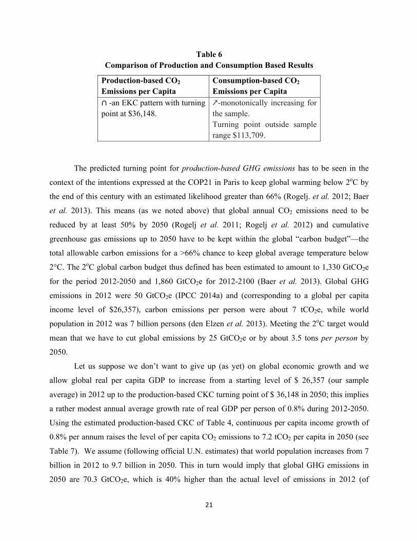
Table 6 Comparison of Production and Consumption Based Results

Production-based CO2

Emissions per Capita Consumption-based CO2

Emissions per Capita ∩ -an EKC pattern with turning point at $36,148.

↗-monotonically increasing for the sample. Turning point outside sample range $113,709.

The predicted turning point for production-based GHG emissions has to be seen in the

context of the intentions expressed at the COP21 in Paris to keep global warming below 2oC by

the end of this century with an estimated likelihood greater than 66% (Rogelj. et al. 2012; Baer

et al. 2013). This means (as we noted above) that global annual CO2 emissions need to be

reduced by at least 50% by 2050 (Rogelj et al. 2011; Rogelj et al. 2012) and cumulative

greenhouse gas emissions up to 2050 have to be kept within the global “carbon budget”—the

total allowable carbon emissions for a >66% chance to keep global average temperature below

2°C. The 2oC global carbon budget thus defined has been estimated to amount to 1,330 GtCO2e

for the period 2012-2050 and 1,860 GtCO2e for 2012-2100 (Baer et al. 2013). Global GHG

emissions in 2012 were 50 GtCO2e (IPCC 2014a) and (corresponding to a global per capita

income level of $26,357), carbon emissions per person were about 7 tCO2e, while world

population in 2012 was 7 billion persons (den Elzen et al. 2013). Meeting the 2oC target would

mean that we have to cut global emissions by 25 GtCO2e or by about 3.5 tons per person by

2050.

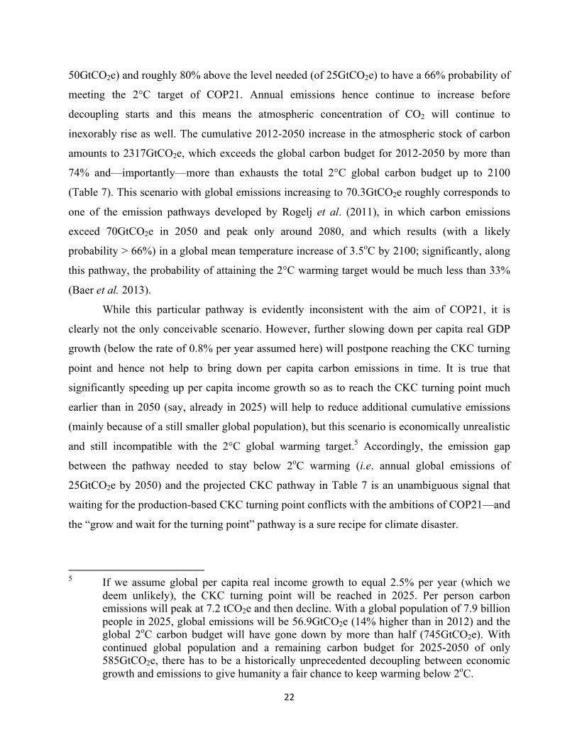
Let us suppose we don’t want to give up (as yet) on global economic growth and we

allow global real per capita GDP to increase from a starting level of $ 26,357 (our sample

average) in 2012 up to the production-based CKC turning point of $ 36,148 in 2050; this implies

a rather modest annual average growth rate of real GDP per person of 0.8% during 2012-2050.

Using the estimated production-based CKC of Table 4, continuous per capita income growth of

0.8% per annum raises the level of per capita CO2 emissions to 7.2 tCO2 per capita in 2050 (see

Table 7). We assume (following official U.N. estimates) that world population increases from 7

billion in 2012 to 9.7 billion in 2050. This in turn would imply that global GHG emissions in

2050 are 70.3 GtCO2e, which is 40% higher than the actual level of emissions in 2012 (of

!!

22!!

50GtCO2e) and roughly 80% above the level needed (of 25GtCO2e) to have a 66% probability of

meeting the 2°C target of COP21. Annual emissions hence continue to increase before

decoupling starts and this means the atmospheric concentration of CO2 will continue to

inexorably rise as well. The cumulative 2012-2050 increase in the atmospheric stock of carbon

amounts to 2317GtCO2e, which exceeds the global carbon budget for 2012-2050 by more than

74% and—importantly—more than exhausts the total 2°C global carbon budget up to 2100

(Table 7). This scenario with global emissions increasing to 70.3GtCO2e roughly corresponds to

one of the emission pathways developed by Rogelj et al. (2011), in which carbon emissions

exceed 70GtCO2e in 2050 and peak only around 2080, and which results (with a likely

probability > 66%) in a global mean temperature increase of 3.5oC by 2100; significantly, along

this pathway, the probability of attaining the 2°C warming target would be much less than 33%

(Baer et al. 2013).

While this particular pathway is evidently inconsistent with the aim of COP21, it is

clearly not the only conceivable scenario. However, further slowing down per capita real GDP

growth (below the rate of 0.8% per year assumed here) will postpone reaching the CKC turning

point and hence not help to bring down per capita carbon emissions in time. It is true that

significantly speeding up per capita income growth so as to reach the CKC turning point much

earlier than in 2050 (say, already in 2025) will help to reduce additional cumulative emissions

(mainly because of a still smaller global population), but this scenario is economically unrealistic

and still incompatible with the 2°C global warming target.5 Accordingly, the emission gap

between the pathway needed to stay below 2oC warming (i.e. annual global emissions of

25GtCO2e by 2050) and the projected CKC pathway in Table 7 is an unambiguous signal that

waiting for the production-based CKC turning point conflicts with the ambitions of COP21—and

the “grow and wait for the turning point” pathway is a sure recipe for climate disaster.

!!!!!!!!!!!!!!!!!!!!!!!!!!!!!!!!!!!!!!!!!!!!!!!!!!!!!!!!!!!!!5 If we assume global per capita real income growth to equal 2.5% per year (which we

deem unlikely), the CKC turning point will be reached in 2025. Per person carbon emissions will peak at 7.2 tCO2e and then decline. With a global population of 7.9 billion people in 2025, global emissions will be 56.9GtCO2e (14% higher than in 2012) and the global 2oC carbon budget will have gone down by more than half (745GtCO2e). With continued global population and a remaining carbon budget for 2025-2050 of only 585GtCO2e, there has to be a historically unprecedented decoupling between economic growth and emissions to give humanity a fair chance to keep warming below 2oC.

!!

23!!

Table 7

The “grow and wait for the turning point” pathway:

Production-based CKC estimates 2012-2050

Average real

global GDP per

capita (in constant

2011 PPP$)

Annual per

capita CO2

emissions

World

population

(billions of

persons)

Annual

global CO2

emissions

(GtCO2e)

2012 26,357 7.0 7.0 50.0

2050 36,148 7.2 9.7 70.3

Average annual growth rate 0.8% 0.1% 0.8% 0.9%

Cumulative emissions

(in GtCO2e) 2012-2050

2,317

Global carbon budget:

2012-2050 (in GtCO2e)

2012-2100 (in GtCO2e)

1,330

1,860

Source: Authors’ estimation based on Tables 3 and 4. The growth rate of world population (2012-2050) is based on estimates by the United Nations Department of Economic and Social Affairs (UN-DESA); see: http://www.un.org/en/development/desa/news/population/2015-report.html. Data on the global carbon budget are from Baer et al. 2013.

5. Conclusions and Policy Implications

We estimated the relationship between CO2 emissions and economic growth using input-output-

based production- and consumption-related CO2 emission inventories from WIOD’s

environmental accounts for 39 different countries for a period of 13 years (1995-2007). Our CO2

emissions data include emissions embodied in international trade and along internationally

fragmented commodity chains—and hence represent the most comprehensive accounting of both

production- and consumption-based GHG emissions to date. While there is econometric

evidence in support of a CKC pattern for production-based CO2 emissions, the estimated per-

capita income turning point implies a level of annual global GHG emissions of 70.3GtCO2e,

!!

24!!

which is 40% higher than the 2012 level and not compatible with the COP21 emissions reduction

pathway consistent with keeping global warming below 2oC. The production-based inverted U-

shaped CKC is, in other words, not a relevant framework for climate change mitigation. In

addition, we do not find any support for a decoupling between living standards and per capita

consumption levels on the one hand and GHG emissions per person on the other hand. This

means that the Annex-I countries (which are mostly the rich OECD countries) have managed to

some extent to delink their production systems from GHG emissions by relocating and

outsourcing carbon-intensive production activities to the non-Annex I countries—as is indicated

in the growing carbon-import surplus of the former and the growing carbon-export surplus of the

latter group of countries (Figure 2). The generally used production-based GHG emissions data

ignore the highly fragmented nature of global production chains (and networks) and are unable to

reveal the ultimate driver of increasing CO2 emissions: consumption growth (or “affluenza”) in

the rich economies. What appears (at first sight) to be the result of structural change in the

economy is in reality just a relocation of carbon-intensive production to other regions—or carbon

leakage. In terms of consumption patterns, we find no noticeable structural change as (direct and

indirect) consumption-based GHG emissions continue to rise with higher per capita GDP.

These results should be sobering as they strongly indicate that there is no such thing as an

automatic decoupling between economic growth and GHG emissions. It means we have to give

up on the notion of the CKC (see also Storm 2009; Lohmann 2009). To keep warming below 2oC

de-carbonization has to be drastic and it has to be organized by deliberate (policy) interventions

and conscious change in consumption and production patterns. Grubb (2014), Mazzucato and

Perez (2014) and the Global Apollo Programme (2014) formulate potentially feasible innovation

agendas to bring about the needed transformative change, away from fossil fuels and toward

renewable energy systems, which all rely on some form of “entrepreneurial state intervention”.

The rich Annex-I countries which are in the forefront of technological innovation, are in the

position to take the lead and also encourage the developing non-Annex-I countries to participate

by investing heavily in the development of new energy technologies that are clean, efficient, and

are also affordable for the developing countries. Without such change, the business-as-usual

scenario looks bleak, as GHG emissions will continue to increase with economic growth and

world population growth (Figure 5) and there is hardly any time or global carbon budget left.

Recent projections, based on new modeling using long-term average projections of economic

!!

25!!

growth, population growth and energy use per person, by Wagner, Ross, Foster and Hankamer

(2016), point to a 2oC rise in global mean temperatures already by 2030. Their results suggest

that we may be much closer than we realized to breaching the 2oC limit and have already used up

all of our room for maneuver (see Pfeiffer et al. 2016 for a similar warning). This carries

considerable risk, as warming becomes self-reinforcing and dangerous beyond the 2oC limit, and

it is the precise outcome COP21 wishes to avoid—but quite in line with our findings.

There is therefore no escape from deep reforms of the global economy which speed up

the process of de-carbonization (Grubb 2014) as well as lower carbon-intensive consumption

(Global Apollo Programme 2014)—and perhaps even restrict economic growth itself (Martinez

Alier 2009, 2015; von Arnim and Rada 2011; Spash 2015). The active participation of and

commitment by both the (carbon-importing) developed countries and the (carbon-exporting)

developing countries is critical—it is in this respect that the COP21 agreement between 195

countries is a source of some hope. However, to make the agreement work, global action to

reduce GHG emissions and to share the burden of adjusting to a low- or zero-carbon economy

should be fair (Baer et al. 2009) and ideally be based on an assessment of capacity (a country’s

ability to pay) and historical responsibility (a country’s cumulative contribution to the problem

of excess GHG concentrations in the atmosphere). As a starting point, this requires

comprehensively accounting for the total (direct and indirect) carbon pollution over global

commodity chains as a whole and distinguishing between a country’s production-based and

consumption-based CO2 emissions to enable the working out of a “fair” sharing of the

responsibility between the various actors operating in the global commodity chain (on this, see

Rodriguez et al. 2006; Lenzen et al. 2007; Marques et al. 2008; Andrew and Forgie 2008). Our

analysis must hence not just be read as a falsification of the Carbon Kuznets Hypothesis (which

we think is important in and of itself), but more broadly as pointing out the urgent need to come

to a global agreement on shared producer and consumer responsibility on CO2 emissions (see

Lenzen et al. 2007; Grubb 2014).

!

!

!

!

!

!!

26!!

References Acaravci, A., & Ozturk, I. (2010) On the relationship between energy consumption, CO2

emissions and economic growth in Europe. Energy 35(12): 5412-5420. Agras, J., Chapman, D. (1999) A dynamic approach to the Environmental Kuznets

Curve hypothesis. Ecological Economics, 28, 267–277. Agrawala, S., Klasen, S., Acosta Moreno, R., Barreto, L., Cottier, T., Guan, D., Gutierrez-

Espeleta, E., Gámez Vázquez, A., Jiang, L., Kim, Y., Lewis, J., Messouli, M., Rauscher, M., Uddin, N., & Venables, A. (2014): Regional Development and Cooperation. In: Climate Change 2014: Mitigation of Climate Change. Contribution of Working Group III to the Fifth Assessment Report of the Intergovernmental Panel on Climate Change [Edenhofer, O., Pichs-Madruga, R., Sokona, Y., Farahani, E., Kadner, S., Seyboth, K., Adler, A., Baum, I., Brunner, S., Eickemeier, P., Kriemann, B., Savolainen, J., Schlömer, S., von Stechow, C., Zwickel, T., & Minx, J. (eds.)]. Cambridge University Press, Cambridge, United Kingdom and New York, NY, USA.

Ahmad, N. & Wyckoff, A. (2003) Carbon Dioxide Emissions Embodied in International Trade of Goods. OECD Science, Technology and Industry Working Papers, 2003/15, OECD Publishing. http://dx.doi.org/10.1787/421482436815

Aichele, R., & Felbermayr, G. (2012). Kyoto and the carbon footprint of nations. Journal Of Environmental Economics And Management, 63(3), 336-354.

Aichele, R., & Felbermayr, G. (2013). Estimating the Effects of Kyoto on Bilateral Trade Flows Using Matching Econometrics. The World Economy, 36(3), 303-330.

Aldy, J., (2005). An Environmental Kuznets Curve analysis of U.S. state-level carbon dioxide emissions. The Journal of Environment Development, 14, 48–72.

Andrew and Forgie (2008) Arrow, K., Bolin, B., Costanza, R., Dasgupta, P., Folke, C., & Holling, C. et al. (1995) Economic

Growth, Carrying Capacity, and the Environment. Science, 268 (5210), 520-521. Aslanidis, N., & Iranzo, S. (2009) Environment and development: is there a Kuznets

curve for CO2 emissions? Applied Economics, 41: 803–810. Apergis, N., & Ozturk, I. (2015) Testing Environmental Kuznets Curve hypothesis in Asian

countries. Ecological Indicators 52: 16-22. Azomahou, T., Laisney, F., & Van Phu, N. (2006) Economic development and CO2

emissions: a nonparametric panel approach. Journal of Public Economics, 90: 1347–1363.

Baer, P., Kartha, S., Athanasiou, T., & Kemp-Benedict, E. (2009) The Greenhouse Development Rights Framework: Drawing Attention to Inequality within Nations in the Global Climate Policy Debate. Development and Change 40 (6): 1121-1138.

Baer, P., Kartha, S., and Athanasiou, T. (2013) The three salient global mitigation pathways assessed in light of the IPCC carbon budgets. SEI Discussion Brief. Stockholm Environment Institute.

!!

27!!

Bimonte, S. (2002) Information access, income distribution, and the Environmental Kuznets Curve. Ecological Economics, 41(1), 145-156.

Blanco, G., Gerlagh, R., Suh, S., Barrett, J., de Coninck, H., Diaz Morejon, C., Mathur, R., Nakicenovic, N., Ofosu Ahenkora, A., Pan, J., Pathak, H., Rice, J., Richels, R., Smith, S., Stern, D., Toth, F.,& Zhou, P. (2014) Drivers, Trends and Mitigation. In: Climate Change 2014: Mitigation of Climate Change. Contribution of Working Group III to the Fifth Assessment Report of the Intergovernmental Panel on Climate Change [Edenhofer, O., Pichs-Madruga, R., Sokona, Y., Farahani, E., Kadner, S., Seyboth, K., Adler, A., Baum, I., Brunner, S., Eickemeier, P., Kriemann, B., Savolainen, J., Schlömer, S., von Stechow, C., Zwickel, T., & Minx, J. (eds.)]. Cambridge University Press, Cambridge, United Kingdom and New York, NY, USA.

Boitier, B. (2012) CO2 emissions production-based accounting vs consumption: Insights from the WIOD databases. Paper presented at the Final WIOD Conference: Causes and Consequences of Globalization (April 24-26, 2012), Groningen, The Netherlands.

Borghesi, S. (2000) Income Inequality and the Environmental Kuznets Curve. Fondazione Eni Enrico Mattei, Milan, Italy. (Nota di Lavoro 83.2000).

Collins, M., Knutti, R., Arblaster, J., Dufresne, J.-L. , Fichefet, T., Friedlingstein, P., Gao, X. , Gutowski, W., Johns, T., Krinner, G., Shongwe, M., Tebaldi, C., Weaver A., & Wehner, M. (2013) Long-term Climate Change: Projections, Commitments and Irreversibility. In: Climate Change 2013: The Physical Science Basis. Contribution of Working Group I to the Fifth Assessment Report of the Intergovernmental Panel on Climate Change [Stocker, T., Qin, D., Plattner, G.-K., Tignor, M., Allen, S., Boschung, J., Nauels, A., Xia, Y., Bex, V. & Midgley, P. (eds.)]. Cambridge University Press, Cambridge, United Kingdom and New York, NY, USA.

Coondoo, D., & Dinda, S. (2008) Carbon dioxide emissions and income: a temporal analysis of cross-country distributional patterns. Ecological Economics, 65: 375–385.

de Bruyn, S., van den Bergh, J., & Opschoor, J. (1998) Economic growth and emissions: reconsidering the empirical basis of environmental Kuznets curves. Ecological Economics, 25(2), 161-175.

Dasgupta, S., Laplante, B., Wang, H., & Wheeler, D. (2002) Confronting the Environmental Kuznets Curve. Journal of Economic Perspectives, 16 (1), 147–168.

Davis, S., & Caldeira, K. (2010) Consumption-based accounting of CO2 emissions. Proceedings Of The National Academy Of Sciences 107(12): 5687-5692.

den Elzen, M., Olivier, J., Höhne, N., & Janssens-Maenhout, G. (2013) Countries’ contributions to climate change: effect of accounting for all greenhouse gases, recent trends, basic needs and technological progress. Climatic Change 121(2): 397-412.

Dinda, S. (2004) Environmental Kuznets Curve Hypothesis: A Survey. Ecological Economics, 49(4), 431-455. doi:10.1016/j.ecolecon.2004.02.011.

!!

28!!

Dutt, K. (2009) Governance, institutions and the environment-income relationship: a cross-country study. Environment, Development and Sustainability, 11: 705–723.

Edenhofer, O., Flachsland,C., Jakob, M., & Lessmann,K. (2013) The Atmosphere as a Global Commons – Challenges for International Cooperation and Governance. Harvard Project on Climate Agreements, Discussion Paper 2013-58. Cambridge, Mass.

Farhani, S., Mrizak, S., Chaibi, A., & Rault, C. (2014) The environmental Kuznets curve and sustainability: A panel data analysis. Energy Policy 71: 189-198.

Fosten, J., Morley, B., & Taylor, T. (2012) Dynamic misspecification in the environmental Kuznets curve: Evidence from CO2 and SO2 emissions in the United Kingdom. Ecological Economics 76: 25-33.

Galeotti, M., Lanza, A. (1999) Richer and cleaner? A study on carbon dioxide emissions in developing countries. Energy Policy, 27, 565–573.

Galeotti, M., Lanza, A., & Pauli, F. (2006) Reassessing the environmental Kuznets curve for CO2 emissions: A robustness exercise. Ecological Economics, 57(1), 152-163.

Gallego, B., & Lenzen, M. (2005) A consistent input–output formulation of shared producer and consumer responsibility. Economic Systems Research, 17(4), 365-391.

Gangadharan, L., & Valenzuela, M. (2001) Interrelationships between income, health and the environment: extending the Environmental Kuznets Curve hypothesis. Ecological Economics, 36(3), 513-531.

Global Apollo Programme. (2015). A Global Apollo Programme to Combat Climate Change. CEP. London School of Economics and Political Science.

Grossman, G., & Krueger, A. (1995) Economic growth and the environment. The Quarterly Journal Of Economics, 110 (2): 353-377.

Grubb, M. (2014) Planetary Economics. Energy, Climate Change and the Three Domains of Sustainable Development. London: Earthscan. (With J.-Ch. Hourcade and K. Neuhoff).

Holtz-Eakin, D., & Selden, T. (1995) Stoking the fires? CO2 emissions and economic growth. Journal of Public Economics, 57(1): 85-101.

IEA (2011a) Energy balances of OECD and non-OECD countries, 2011 Edition, available at: http://www.iea.org/index.asp

IPCC (2007) Climate Change 2007: Synthesis Report. Contribution of Working Groups I, II and III to the Fourth Assessment Report of the Intergovernmental Panel on Climate Change [Core Writing Team, Pachauri, R.K, & Reisinger, A. (eds.)]. IPCC, Geneva, Switzerland, 104 pp.

IPCC (2014a). 2013 Supplement to the 2006 IPCC Guidelines for National Greenhouse Gas Inventories: Wetlands, Hiraishi, T., Krug, T., Tanabe, K., Srivastava, N., Baasansuren, J., Fukuda, M. and Troxler, T.G. (eds). Published: IPCC, Switzerland.

IPCC (2014b). Summary for policymakers. In: Climate Change 2014: Impacts, Adaptation, and Vulnerability.Part A: Global and Sectoral Aspects. Contribution of Working Group II to the Fifth Assessment Report of the Intergovernmental Panel on Climate Change [Field,

!!

29!!

C., Barros, V., Dokken, D., Mach, K., Mastrandrea, M., Bilir, T., Chatterjee, M., Ebi, K., Estrada, Y., Genova, R., Girma, B., Kissel, E., Levy, A., MacCracken, S., Mastrandrea, P., & White, L. (eds.)] . Cambridge University Press, Cambridge, United Kingdom and New York, NY, USA, pp. 1-32.

IPCC (2014c). Summary for Policymakers. In: Climate Change 2014: Mitigation of Climate Change. Contribution of Working Group III to the Fifth Assessment Report of the Intergovernmental Panel on Climate Change [Edenhofer, O., Pichs-Madruga, R., Sokona, Y., Farahani, E., Kadner, S., Seyboth, K., Adler, A., Baum, I., Brunner, S., Eickemeier, P., Kriemann, B., Savolainen, J., Schlömer, S., von Stechow, C., Zwickel, T., & Minx, J. (eds.)]. Cambridge University Press, Cambridge, United Kingdom and New York, NY, USA.

IPCC (2014d). Climate Change 2014: Synthesis Report. Contribution of Working Groups I, II and III to the Fifth Assessment Report of the Intergovernmental Panel on Climate Change [Core Writing Team, Pachauri, R. & Meyer, L. (eds.)]. IPCC, Geneva, Switzerland, 151 pp.

Iwata, H., Okada, K., & Samreth, S. (2011) A note on the Environmental Kuznets Curve for CO2: a pooled mean group approach. Applied Energy 88: 1986–1996.

Jaunky, V. (2011) The CO2 emissions-income nexus: evidence from rich countries. Energy Policy 39: 1228–1240.

Jalil, A., & Mahmud, S. (2009) Environment Kuznets curve for CO2 emissions: a cointegration analysis for China. Energy Policy, 37: 5167–5172.

Kaika, D., & Zervas, E. (2013a) The Environmental Kuznets Curve (EKC) theory— Part A: Concept, causes and the CO2 emissions case. Energy Policy, 62, 1392–1402.

Kaika, D., & Zervas, E. (2013b) The environmental Kuznets curve (EKC) theory. Part B: Critical issues. Energy Policy, 62, 1403-1411.

Kijima, M., Nishide, K., & Ohyama, A. (2010) Economic models for the environmental Kuznets curve: A survey. Journal Of Economic Dynamics And Control 34 (7): 1187-1201.

Kunnas, J., & Myllyntaus, T. (2007) The Environmental Kuznets Curve hypothesis and air pollution in Finland. Scandinavian Economic History Review, 55 (2), 101–127.

Lantz, V., & Feng, Q. (2006) Assessing income, population, and technology impacts on CO2 emissions in Canada: Where’s the EKC? Ecological Economics 57: 229–238.

Lee, C-C., Chiu, Y-B., & Sun, C-H. (2009) Does one size fit all? A reexamination of the Environmental Kuznets Curve using the dynamic panel data approach. Review of Agricultural Economics, 31 (4): 751–778.

Lenzen, M., Murray, J., Sack, F., & Wiedmann, T. (2007) Shared producer and consumer responsibility — Theory and practice. Ecological Economics 61(1): 27-42.

Lieb, C. (2003) The Environmental Kuznets Curve- A Survey of the Empirical Evidence and of Possible Causes. Discussion Paper Series No. 391, Department of Economics, University of Heidelberg.

!!

30!!

Lohmann, L. (2009). Climate as investment. Development and Change 40 (6): 1063-84. López-Menéndez, A., Pérez, R., & Moreno, B. (2014) Environmental costs and renewable

energy: Re-visiting the Environmental Kuznets Curve. Journal Of Environmental Management 145: 368-373.

Magnani, E. (2000) The Environmental Kuznets Curve, environmental protection policy and income distribution. Ecological Economics, 32(3), 431-443.

Martínez-Alier, J. (2009) Socially sustainable economic de-growth. Development and Change 40 (6): 1099–1119.

Martinez Alier, J. (2015). Climate justice. Development and Change 46 (2), 381-386. Mazzucato, M. and Perez, C. (2014). Innovation as growth policy: the challenge for Europe.

SPRU Working Paper Series SWPS 2014-13. Müller-Fürstenberger, G., & Wagner, M. (2007) Exploring the environmental Kuznets

hypothesis: Theoretical and econometric problems. Ecological Economics, 62(3-4), 648-660.

Muradian, R., & Martinez-Alier, J. (2001) Trade and the environment: from a ‘Southern’ perspective. Ecological Economics 36 (2), 281-297.

Nakano, S., Okamura, A., Sakurai, N., Suzuki, M., Tojo, Y, & Yamano, N. (2009) The Measurement of CO2 Embodiments in International Trade: Evidence From the Harmonized Input-Output and Bilateral Trade Database. STI WORKING PAPER 2009/3, OECD Directorate for Science, Technology and Industry.

Narayan, P-K., Narayan, S. (2010) Carbon dioxide emissions and economic growth: panel data evidence from developing countries. Energy Policy 38: 661–666.

Nasir, M., & Rehman, F. (2011) Environmental Kuznets Curve for carbon emissions in Pakistan: An empirical investigation. Energy Policy 39 (3): 1857-1864.

Panayotou, T., Peterson, A., & Sachs, J. (2000) Is the Environmental Kuznets Curve Driven by Structural Change? What Extended Time Series May Imply for Developing Countries. CAER II Discussion Paper No. 80, Harvard Institute for International Development.

Pauli, F. (2003) Environmental Kuznets Curve investigation using a varying coefficient AR-model. EEE Working Papers Series No.12.

Perrings, C., & Ansuategi, A. (2000) Sustainability, growth and development. Journal of Economic Studies, 27 (1/2): 19–54.

Peters, G. (2008) From production-based to consumption-based national emission inventories. Ecological Economics 65(1): 13-23.

Peters, G., & Hertwich, E. (2008) CO2 Embodied in International Trade with Implications for Global Climate Policy. Environmental Science & Technology, 42(5), 1401-1407.

Peters, G., Minx, J., Weber, C., & Edenhofer, O. (2011) Growth in emission transfers via international trade from 1990 to 2008. Proceedings Of The National Academy Of Sciences, 108(21), 8903-8908.

!!

31!!

Pfeiffer, A., Millar, R., Hepburn, C. and Beinhocker, E. 2016. The ‘2°C capital stock’ for electricity generation: Committed cumulative carbon emissions from the power sector and the transition to a green economy. INET Oxford Working Paper no. 2015-09.

Ribes, A., Zwiers, F.W., Azaïs, J.-M., Naveau, P. 2016. A new statistical approach to climate change detection and attribution. Climate Dynamics, First-online April 6.

Richmond, A., & Kaufmann, R. (2006) Is there a turning point in the relationship between income and energy use and/or carbon emissions? Ecological Economics, 56: 176–189.

Robalino-López, A., Mena-Nieto, Á., García-Ramos, J., & Golpe, A. (2015) Studying the relationship between economic growth, CO2 emissions, and the environmental Kuznets curve in Venezuela (1980–2025). Renewable And Sustainable Energy Reviews 41: 602-614.

Roberts, J., & Grimes, P. (1997) Carbon intensity and economic development 1962–1991: A brief exploration of the environmental Kuznets curve. World Development, 25(2): 191-198.

Rodrigues, J., Domingos, T., Giljum, S., & Schneider, F. (2006) Designing an indicator of environmental responsibility. Ecological Economics 59 (3): 256-266.

Rogelj, J., Hare, W., Lowe, J., van Vuuren, D., Riahi, K., & Matthews, B. et al. (2011) Emission pathways consistent with a 2 °C global temperature limit. Nature Climate Change 1(8): 413-418.

Rogelj, J., Meinshausen, M., & Knutti, R. (2012) Global warming under old and new scenarios using IPCC climate sensitivity range estimates. Nature Climate Change 2(4): 248-253.

Schmalensee, R., Stoker, T., & Judson, R. (1998) World carbon dioxide emissions: 1950–2050. The Review of Economics and Statistics, 80, 15–27.

Scruggs, L. (1998) Political and economic inequality and the environment. Ecological Economics,26(3), 259-275.

Selden, T. and Song, D. (1994) Environmental quality and development: is there a Kuznets curve for air pollution emissions? Journal of Environmental Economics and Management, 27 (2), 147–162.

Shahbaz, M., Ozturk, I., Afza, T., & Ali, A. (2013) Revisiting the environmental Kuznets curve in a global economy. Renewable And Sustainable Energy Reviews 25:494-502.

Shafik, N., & Bandyopadhyay, S. (1992). Economic Growth and Environmental Quality. Time-series and Cross Country Evidence. Policy Research Working Paper No. 904, World Development Report 1992: The World Bank.

Spash, C.L. (2015). The future post-growth society. Development and Change 46 (2), 366-380. Stavins, R., Zou, J., Brewer, T., Conte Grand, M. , den Elzen, M., Finus, M., Gupta, J., Höhne,

N., Lee, M.-K., Michaelowa, A., Paterson, M., Ramakrishna, K., Wen, G., Wiener, J., & Winkler, H. (2014): International Cooperation: Agreements and Instruments. In: Climate Change 2014: Mitigation of Climate Change. Contribution of Working Group III to the Fifth Assessment Report of the Intergovernmental Panel on Climate Change. [Edenhofer,

!!

32!!

O., Pichs-Madruga, R., Sokona, Y., Farahani, E., Kadner, S., Seyboth, K., Adler, A., Baum, I., Brunner, S., Eickemeier, P., Kriemann, B., Savolainen, J., Schlömer, S., von Stechow, C., Zwickel, T., & Minx, J. (eds.)]. Cambridge University Press, Cambridge, United Kingdom and New York, NY, USA.

Stern, D., & Common, M., Barbier, E. (1996) Economic growth and environmental degradation: a critique of the environmental Kuznets curve. World Development 24: 1151–1160.

Storm, S. (2009) Capitalism and Climate Change: Can the Invisible Hand Adjust the Natural Thermostat? Development and Change 40 (6): 1011-1038. Timmer, M., Dietzenbacher, E., Los, B., Stehrer, R. & de Vries, G. (2015) An Illustrated User

Guide to the World Input–Output Database: the Case of Global Automotive Production. Review of International Economics, 23(3): 575–605.

Torras, M., & Boyce, J. (1998) Income, inequality, and pollution: a reassessment of the environmental Kuznets Curve. Ecological Economics, 25(2), 147-160.

Von Arnim, Rudiger and Codrina Rada. 2011. Labour productivity growth and energy use in a three-sector model: an application to Egypt. Development and Change 42 (6): 1323-1348.

Wagner, M. (2008) The Carbon Kuznets Curve: A cloudy picture emitted by bad econometrics? Resource and Energy Economics 30 (3): 388-408.

Wagner, G. and Weitzman, M.L. (2015) Climate Shock: The Economic Consequences of a Hotter Planet. Princeton University Press.

Wagner, L., Ross, I., Foster, J. and Hankamer, B. (2016) Trading off global fuel supply, CO emissions and sustainable development. PLoS ONE 11 (3): e0149406. doi:10.1371/journal.pone.0149406

!!

33!!

Appendix List of Annex I and Non-Annex I Countries Annex I Countries

Country Code

Non-Annex I Countries

Country Code

Australia AUS Brazil BRA Austria AUT China CHN Belgium BEL Cyprus CYP Bulgaria BGR Indonesia IDN Canada CAN India IND Czech Republic CZE South Korea KOR Germany DEU Mexico MEX Denmark DNK Malta MLT Spain ESP Estonia EST Finland FIN France FRA United Kingdom GBR Greece GRC Hungary HUN Ireland IRL Italy ITA Japan JPN Lithuania LTU Luxembourg LUX Latvia LVA Netherlands NLD Poland POL Portugal PRT Romania ROM Russian Federation RUS Slovakia SVK Slovenia SVN Sweden SWE Turkey TUR United States USA