Embed Size (px)
Citation preview

Retek® Demand Forecasting™ Retek® Curve™
Retek® Promote™ 11.1
User Guide


Corporate Headquarters:
Retek Inc. Retek on the Mall 950 Nicollet Mall Minneapolis, MN 55403 USA 888.61.RETEK (toll free US) Switchboard: +1 612 587 5000 Fax: +1 612 587 5100
European Headquarters:
Retek 110 Wigmore Street London W1U 3RW United Kingdom Switchboard: +44 (0)20 7563 4600 Sales Enquiries: +44 (0)20 7563 46 46 Fax: +44 (0)20 7563 46 10
The software described in this documentation is furnished under a license agreement, is the confidential information of Retek Inc., and may be used only in accordance with the terms of the agreement. No part of this documentation may be reproduced or transmitted in any form or by any means without the express written permission of Retek Inc., Retek on the Mall, 950 Nicollet Mall, Minneapolis, MN 55403, and the copyright notice may not be removed without the consent of Retek Inc. Information in this documentation is subject to change without notice. Retek provides product documentation in a read-only-format to ensure content integrity. Retek Customer Support cannot support documentation that has been changed without Retek authorization. The functionality described herein applies to this version, as reflected on the title page of this document, and to no other versions of software, including without limitation subsequent releases of the same software component. The functionality described herein will change from time to time with the release of new versions of software and Retek reserves the right to make such modifications at its absolute discretion. Retek® Demand Forecasting™, Retek Curve™, and Retek PromoteTM are trademarks of Retek Inc. Retek and the Retek logo are registered trademarks of Retek Inc. This unpublished work is protected by confidentiality agreement, and by trade secret, copyright, and other laws. In the event of publication, the following notice shall apply: ©2005 Retek Inc. All rights reserved. All other product names mentioned are trademarks or registered trademarks of their respective owners and should be treated as such. Printed in the United States of America.

Retek Demand Forecasting, Retek Curve, Retek Promote
Customer Support Customer Support hours
Customer Support is available 7x24x365 via email, phone, and Web access.
Depending on the Support option chosen by a particular client (Standard, Plus, or Premium), the times that certain services are delivered may be restricted. Severity 1 (Critical) issues are addressed on a 7x24 basis and receive continuous attention until resolved, for all clients on active maintenance. Retek customers on active maintenance agreements may contact a global Customer Support representative in accordance with contract terms in one of the following ways.
Contact Method Contact Information
E-mail [email protected]
Internet (ROCS) rocs.retek.com Retek’s secure client Web site to update and view issues
Phone +1 612 587 5800
Toll free alternatives are also available in various regions of the world:
Australia +1 800 555 923 (AU-Telstra) or +1 800 000 562 (AU-Optus) France 0800 90 91 66 Hong Kong 800 96 4262 Korea 00 308 13 1342 United Kingdom 0800 917 2863 United States +1 800 61 RETEK or 800 617 3835
Mail Retek Customer Support Retek on the Mall 950 Nicollet Mall Minneapolis, MN 55403
When contacting Customer Support, please provide:
• Product version and program/module name.
• Functional and technical description of the problem (include business impact).
• Detailed step-by-step instructions to recreate.
• Exact error message received.
• Screen shots of each step you take.
Contents
i
Contents Chapter 1 – Introduction .................................................................. 1
Overview....................................................................................................................... 1
Forecasting challenges and RDF solutions ................................................................... 2 Selecting the best forecasting method ................................................................................ 2 Overcoming Data Sparsity through Source Level Forecasting .......................................... 2 Handling lost sales and unusually high demand................................................................. 3 Forecasting demand for new products and locations.......................................................... 4 Managing forecasting results through automated exception reporting............................... 4 Incorporating the effects of promotions and other event-based challenges on demand..... 4 Providing detailed sales predictions based on an assortment plan ..................................... 5
Retek Demand Forecasting Architecture ...................................................................... 5 The Retek Predictive Application Server and RDF............................................................ 5 Global Domain vs. Simple Domain Environment.............................................................. 6
Retek Demand Forecasting Workbook Template Groups ............................................ 7 Forecast .............................................................................................................................. 7 Promote .............................................................................................................................. 7 Curve .................................................................................................................................. 8
RDF Solution and Business Process Overview ............................................................ 8 RDF and the Retek Enterprise............................................................................................ 8 RDF Primary Workflow..................................................................................................... 9 RDF Administration and Maintenance............................................................................... 9
Chapter 2 – Preparing data for forecasting.................................. 11
Overview..................................................................................................................... 11 Automated preprocessing of data ..................................................................................... 11
Manual Adjustment of Sales History.......................................................................... 14 Viewing Adjusted Sales Measures in a Workbook .......................................................... 15 Inserting Adjusted Sales Measures into an existing workbook. ....................................... 15
Retek Demand Forecasting, Retek Curve, Retek Promote
ii
Chapter 3 – Setting Forecast Parameters .................................... 17
Overview..................................................................................................................... 17 Forecast Administration Workbook Overview ................................................................ 17
Forecast Administration Workbook............................................................................ 20 Procedures ........................................................................................................................ 20 Window descriptions........................................................................................................ 21
Forecast Maintenance Workbook ............................................................................... 31 Overview .......................................................................................................................... 31 Procedures ........................................................................................................................ 31 Window descriptions........................................................................................................ 32
Forecast Like-Item, Sister-Store Workbook ............................................................... 36 Overview .......................................................................................................................... 36 Procedure.......................................................................................................................... 36 Window descriptions........................................................................................................ 37 Steps Required for Forecasting using each of the Like SKU / Sister Store Methods ...... 42
Chapter 4 – Generating and Approving a Forecast..................... 45
Overview..................................................................................................................... 45
Run a Batch Forecast .................................................................................................. 45 Overview .......................................................................................................................... 45 Procedures ........................................................................................................................ 46
Delete Forecasts .......................................................................................................... 47 Overview .......................................................................................................................... 47 Procedure.......................................................................................................................... 47
Forecast Approval Workbook..................................................................................... 48 Overview .......................................................................................................................... 48 Procedures ........................................................................................................................ 49 Window descriptions........................................................................................................ 51
Approving Forecasts through Alerts (Exception Management) ................................. 59 Overview .......................................................................................................................... 59 Procedure.......................................................................................................................... 60
Contents
iii
Chapter 5 – Forecast Analysis Tools............................................ 61
Overview..................................................................................................................... 61
Interactive Forecasting Workbook.............................................................................. 61 Overview .......................................................................................................................... 61 Procedure.......................................................................................................................... 61 Window descriptions........................................................................................................ 62
Forecast Scorecard Workbook.................................................................................... 65 Overview .......................................................................................................................... 65 Procedure.......................................................................................................................... 65 Window descriptions........................................................................................................ 67
Chapter 6 – Promote (Promotional Forecasting)......................... 71
Overview..................................................................................................................... 71 What is Promotional Forecasting?.................................................................................... 71 Comparison between promotional and statistical forecasting .......................................... 72 Developing promotional forecast methods....................................................................... 72 Retek’s approach to promotional forecasting................................................................... 73 Promotional forecasting terminology and workflow........................................................ 74 Promote Workbooks and wizards..................................................................................... 75
Promotion Planner Workbook Template .................................................................... 76 Overview .......................................................................................................................... 76 Procedure.......................................................................................................................... 76 Window descriptions........................................................................................................ 77
Promotion Maintenance Workbook Template............................................................ 78 Overview .......................................................................................................................... 78 Procedure.......................................................................................................................... 78 Window descriptions........................................................................................................ 79
Promotion Effectiveness Workbook Template........................................................... 81 Overview .......................................................................................................................... 81 Procedure.......................................................................................................................... 81 Window descriptions........................................................................................................ 82
Procedures in Promotional Forecasting ...................................................................... 85 Set up the system to run a promotional forecast............................................................... 85 View a forecast that includes promotion effects .............................................................. 86 View and edit Promotion System-Calculated Effects: ..................................................... 86 Promotion Simulation (“What-If?”) and Analysis ........................................................... 87

Retek Demand Forecasting, Retek Curve, Retek Promote
iv
Chapter 7 – Profile Generation using Curve ................................ 89
Overview..................................................................................................................... 89 Dynamic Profiles.............................................................................................................. 89
Profile Administration Workbook .............................................................................. 90 Overview .......................................................................................................................... 90 Procedure.......................................................................................................................... 90 Window descriptions........................................................................................................ 91
Profile Maintenance Workbook.................................................................................. 96 Overview .......................................................................................................................... 96 Procedure.......................................................................................................................... 96 Window descriptions........................................................................................................ 97
Generate Profiles......................................................................................................... 99 Overview .......................................................................................................................... 99 Procedures ........................................................................................................................ 99
Profile Approval Workbook ..................................................................................... 100 Overview ........................................................................................................................ 100 Procedure........................................................................................................................ 100 Window descriptions...................................................................................................... 101
Chapter 8 – Retek Demand Forecasting Methods..................... 105
Forecasting techniques used in RDF......................................................................... 105 Exponential smoothing................................................................................................... 105 Regression analysis ........................................................................................................ 105 Bayesian analysis ........................................................................................................... 105 Prediction intervals......................................................................................................... 106 Automatic method selection ........................................................................................... 106 Source level forecasting ................................................................................................. 106 Promotional forecasting ................................................................................................. 106
Contents
v
Time series (statistical) forecasting methods............................................................ 107 Why use statistical forecasting? ..................................................................................... 108 Exponential Smoothing (ES) forecasting methods......................................................... 108 Definitions of equation notation used in this section ..................................................... 109 Components of exponential smoothing .......................................................................... 110 Average .......................................................................................................................... 110 Simple exponential smoothing ....................................................................................... 111 Croston’s method ........................................................................................................... 112 Simple/Intermittent Exponential Smoothing.................................................................. 112 Holt exponential smoothing ........................................................................................... 113 Multiplicative Winters exponential smoothing .............................................................. 113 Additive Winters exponential smoothing....................................................................... 114 Seasonal Exponential Smoothing (SeasonalES) ............................................................ 115 Seasonal Regression ....................................................................................................... 116 Bayesian Information Criterion (BIC)............................................................................ 117
Profile-based forecasting .......................................................................................... 123 Forecast method ............................................................................................................. 123 Profile based method and new items .............................................................................. 123 Example.......................................................................................................................... 124
Bayesian forecasting ................................................................................................. 124 Sales plans vs. historic data ............................................................................................ 125 Bayesian algorithm......................................................................................................... 126 Guidelines....................................................................................................................... 127
Causal (promotional) forecasting method................................................................. 128 The causal forecasting algorithm.................................................................................... 129 Causal forecasting algorithm process............................................................................. 129 Causal forecasting array interface description ............................................................... 131 Causal forecasting at the daily level............................................................................... 131 Final considerations about causal forecasting ................................................................ 133
Glossary ........................................................................................ 135


Chapter 1 – Introduction
1
Chapter 1 – Introduction Overview Retek® Demand Forecasting™ is a Windows-based statistical and causal (via Promote) forecasting solution. It uses state-of-the-art modeling techniques to produce high quality forecasts – with minimal human intervention. Forecasts produced by the Demand Forecasting system enhance the retailer’s supply-chain planning, allocation, and replenishment processes, enabling a profitable and customer-oriented approach to predicting and meeting product demand.
Today’s progressive retail organizations know that store-level demand drives the supply chain. The ability to forecast consumer demand productively and accurately is vital to a retailer’s success. The business requirements for consumer responsiveness mandate a forecasting system that more accurately forecasts at the point of sale, handles difficult demand patterns, forecasts promotions and other causal events, processes large numbers of forecasts, and minimizes the cost of human and computer resources.
Forecasting drives the business tasks of planning, replenishment, purchasing, and allocation. As forecasts become more accurate, businesses run more efficiently by buying the right inventory at the right time. This ultimately lowers inventory levels, improves safety stock requirements, improves customer service, and increases the company’s profitability.
The competitive nature of business requires that retailers find ways to cut costs and improve profit margins. The accurate forecasting methodologies provided with Retek Demand Forecasting can provide tremendous benefits to businesses.
A connection from Retek Demand Forecasting to Retek’s Advanced Retail Planning and Optimization (ARPO) solutions is built directly into the business process by way of the automatic approvals of forecasts, which may then fed directly to any ARPO solution. This process allows you to accept all or part of a generated sales forecast. Once that decision is made, the remaining business measures may be planned within an ARPO solution such as Merchandise Financial Planning, for example.

Retek Demand Forecasting, Retek Curve, Retek Promote
2
Forecasting challenges and RDF solutions A number of challenges affect the ability of organizations to forecast product demand accurately. These challenges include selecting the best forecasting method to account for level, trending, seasonal, and spiky demand; generating forecasts for items with limited demand histories; forecasting demand for new products and locations; incorporating the effects of promotions and other event-based challenges on demand; and accommodating the need of operational systems to have sales predictions at more detailed levels than planning programs provide.
Selecting the best forecasting method One challenge to accurate forecasting is the selection of the best model to account for level, trending, seasonal, and spiky demand. Retek’s AutoES (Automatic Exponential Smoothing) forecasting method eliminates this complexity.
The AutoES method evaluates multiple forecast models, such as Simple Exponential Smoothing, Holt Exponential Smoothing, Additive and Multiplicative Winters Exponential Smoothing, Croston’s Intermittent Demand Model, and Seasonal Regression forecasting to determine the optimal forecast method to use for a given set of data. The accuracy of each forecast and the complexity of the forecast model are evaluated in order to determine the most accurate forecast method. You simply select the AutoES forecast generation method, and the system finds the best model.
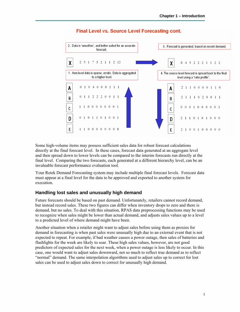
Overcoming Data Sparsity through Source Level Forecasting It is a common misconception in forecasting that forecasts must be directly generated at the lowest levels (final levels) of execution. Problems can arise when historic sales data for these items is too sparse and noisy to identify clear selling patterns. In such cases, generating a reliable forecast requires aggregating sales data from a final level up to a higher level (source level) in the hierarchy in which demand patterns can be seen, then generate a forecast at this source level. After a forecast is generated at the source level, the resulting data can be allocated (spread) back down to the lower level, based on the lower level’s (final level) relationship to the total. This relationship can then be determined through generating an additional forecast (interim forecast) at the final level. Curve is then used to dynamically generate a profile based on the interim forecasts. As well, a non-dynamic profile can be generated and approved to be used as this profile. It is this profile that determines how the source level forecast is spread down to the final level. For more information on Curve, see chapter 7.
Chapter 1 – Introduction
3
Some high-volume items may possess sufficient sales data for robust forecast calculations directly at the final forecast level. In these cases, forecast data generated at an aggregate level and then spread down to lower levels can be compared to the interim forecasts run directly at the final level. Comparing the two forecasts, each generated at a different hierarchy level, can be an invaluable forecast performance evaluation tool.
Your Retek Demand Forecasting system may include multiple final forecast levels. Forecast data must appear at a final level for the data to be approved and exported to another system for execution.
Handling lost sales and unusually high demand Future forecasts should be based on past demand. Unfortunately, retailers cannot record demand, but instead record sales. These two figures can differ when inventory drops to zero and there is demand, but no sales. To deal with this situation, RPAS data preprocessing functions may be used to recognize when sales might be lower than actual demand, and adjusts sales values up to a level to a predicted level of where demand might have been.
Another situation when a retailer might want to adjust sales before using them as proxies for demand in forecasting is when past sales were unusually high due to an external event that is not expected to repeat. For example, if bad weather causes a power outage, then sales of batteries and flashlights for the week are likely to soar. These high sales values, however, are not good predictors of expected sales for the next week, when a power outage is less likely to occur. In this case, one would want to adjust sales downward, not so much to reflect true demand as to reflect “normal” demand. The same interpolation algorithms used to adjust sales up to correct for lost sales can be used to adjust sales down to correct for unusually high demand.

Retek Demand Forecasting, Retek Curve, Retek Promote
4
Forecasting demand for new products and locations Retek Demand Forecasting can also forecast demand for new products and locations for which no sales history exists. You can model a new product’s demand behavior based on that of an existing similar product for which you do have a history. Forecasts can thus be generated for the new product based on the history and demand behavior of the existing one. Likewise, the sales histories of existing store locations can be used as the forecast foundation for new locations in the chain. For more details, see the section on Forecast Like-Item, Sister-Store Workbook in chapter 3.
Managing forecasting results through automated exception reporting The RDF end user may be responsible for managing the forecast results for thousands of items, at hundreds of stores, across many weeks at a time. The Retek Predictive Application Server (RPAS) provides users with an automated exception reporting process (called Alert Management) that indicates to the user where a forecast value may lie above or below an established threshold, thereby reducing the level of interaction needed from the user.
Alert management is a feature that provides user-defined and user-maintained exception reporting. Through the process of alert management, you define measures that are checked daily to see if any values fall outside of an acceptable range or do not match a given value. When this happens, an alert is generated to let you know that a measure may need to be examined and possibly amended in a workbook.
The Alert Manager is a dialog box that is displayed automatically when you log on to the system. This dialog provides a list of all identified instances in which a given measure’s values fall outside of the defined limits. You may pick an alert from this list and have the system automatically build a workbook containing that alert’s measure. In the workbook, you can examine the actual measure values that triggered the alert and make decisions about what needs to be done next.
For more information on the Alert Manager, see the RPAS 11.1 User Guide.
Incorporating the effects of promotions and other event-based challenges on demand Promotions, non-regular holidays, and other causal events create another significant challenge to accurate forecasting. Promotions such as advertised sales and free gifts with purchase might have a significant impact on a product’s sales history, as can irregularly occurring holidays such as Easter.
Using Promote (an optional, add-on module to Retek Demand Forecasting) promotional models of forecasting can be developed to take these and other factors into account when forecasts are generated. Promote attempts to identify the causes of deviations from the established seasonal profile, quantify these effects, and use the results to predict future sales when conditions in the selling environment will be similar. This type of advanced forecasting identifies the behavioral relationship of the variable you want to forecast (sales) to both its own past and explanatory variables such as promotion and advertising.
Suppose that your company has a large promotional event during the Easter season each year. The exact date of the Easter holiday varies from year to year; as a result, the standard time-series forecasting model often has difficulty representing this effect in the seasonal profile. Promote tool allows you to identify the Easter season in all years of your sales history, and then define the upcoming Easter date. By doing so, you can causally forecast the Easter-related demand pattern shift.

Chapter 1 – Introduction
5
Providing detailed sales predictions based on an assortment plan The planning process attempts to establish the correct balance between different products in order to maximize sales opportunities within the available selling space. To facilitate this process, an assortment plan is often created. The assortment plan provides details of anticipated sales volumes and stock needs at aggregated levels. However, many operational systems require base data at much lower hierarchical levels, because these systems are responsible for ensuring that proper quantities of individual products are present in the right stores at the right time.
To address this need, RPAS contains an optional predictive solution (Curve) that transforms organization-level assortment plans into base-level weekly sales forecasts. Curve generates these lower level sales predictions by applying sets of profiles, or spreading ratios, to the assortment plan. The plan is thus allocated, across the product, location, and time hierarchies.
Retek Demand Forecasting Architecture The Retek Predictive Application Server and RDF The Retek Demand Forecasting application is a member of the Advanced Retail Planning and Optimization Suite (ARPO), including other solutions such as Merchandise Financial Planning, Item Planning, Assortment Planning and Space Optimization. The ARPO solutions share a common platform called the Retek Predictive Application Server (RPAS). RDF leverages the versatility, power, and speed of the RPAS engine and interface. Features such as the following characterize RPAS:
• Multidimensional databases and database components (dimensions, positions, hierarchies)
• Product, location, and calendar hierarchies
• Aggregation and spreading of sales data
• Client-server architecture and master database
• Workbooks and worksheets for displaying and manipulating forecast data
• Wizards for creating and formatting workbooks and worksheets
• Menus, quick menus, and toolbars for working with sales and forecast data
• An automated alert system that provides user-defined and user-maintained exception reporting
• Charting and graphing capabilities
More details about the use of these features can be found in the RPAS 11.1 User’s Guide and online help provided within your RDF solution.
Retek Demand Forecasting, Retek Curve, Retek Promote
6
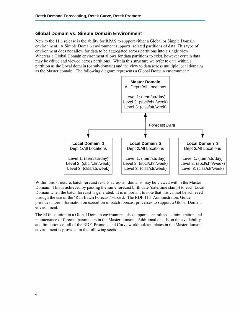
Global Domain vs. Simple Domain Environment New to the 11.1 release is the ability for RPAS to support either a Global or Simple Domain environment. A Simple Domain environment supports isolated partitions of data. This type of environment does not allow for data to be aggregated across partitions into a single view. Whereas a Global Domain environment allows for data partitions to exist, however certain data may be edited and viewed across partitions. Within this structure we refer to data within a partition as the Local domain (or sub-domain) and the view to data across multiple local domains as the Master domain. The following diagram represents a Global Domain environment:
Forecast Data
Master DomainAll Depts/All Locations
Level 1: (item/str/day)Level 2: (sbcl/chn/week)Level 3: (clss/str/week)
Local Domain 1Dept 1/All Locations
Level 1: (item/str/day)Level 2: (sbcl/chn/week)Level 3: (clss/str/week)
Local Domain 3Dept 3/All Locations
Level 1: (item/str/day)Level 2: (sbcl/chn/week)Level 3: (clss/str/week)
Local Domain 2Dept 2/All Locations
Level 1: (item/str/day)Level 2: (sbcl/chn/week)Level 3: (clss/str/week)
Within this structure, batch forecast results across all domains may be viewed within the Master Domain. This is achieved by passing the same forecast birth date (date/time stamp) to each Local Domain when the batch forecast is generated. It is important to note that this cannot be achieved through the use of the ‘Run Batch Forecast’ wizard. The RDF 11.1 Administrators Guide provides more information on execution of batch forecast processes to support a Global Domain environment.
The RDF solution in a Global Domain environment also supports centralized administration and maintenance of forecast parameters in the Master domain. Additional details on the availability and limitations of all of the RDF, Promote and Curve workbook templates in the Master domain environment is provided in the following sections.
Chapter 1 – Introduction
7
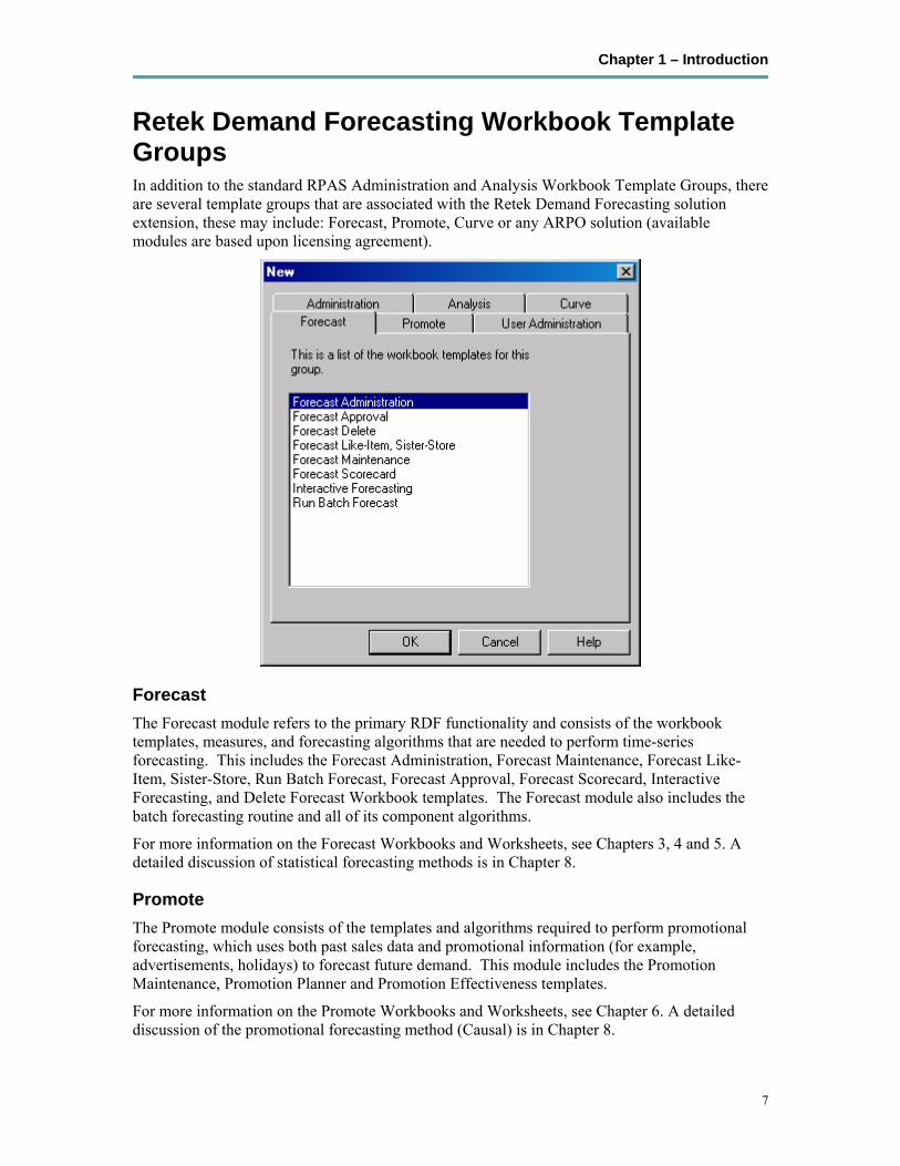
Retek Demand Forecasting Workbook Template Groups In addition to the standard RPAS Administration and Analysis Workbook Template Groups, there are several template groups that are associated with the Retek Demand Forecasting solution extension, these may include: Forecast, Promote, Curve or any ARPO solution (available modules are based upon licensing agreement).
Forecast The Forecast module refers to the primary RDF functionality and consists of the workbook templates, measures, and forecasting algorithms that are needed to perform time-series forecasting. This includes the Forecast Administration, Forecast Maintenance, Forecast Like-Item, Sister-Store, Run Batch Forecast, Forecast Approval, Forecast Scorecard, Interactive Forecasting, and Delete Forecast Workbook templates. The Forecast module also includes the batch forecasting routine and all of its component algorithms.
For more information on the Forecast Workbooks and Worksheets, see Chapters 3, 4 and 5. A detailed discussion of statistical forecasting methods is in Chapter 8.
Promote The Promote module consists of the templates and algorithms required to perform promotional forecasting, which uses both past sales data and promotional information (for example, advertisements, holidays) to forecast future demand. This module includes the Promotion Maintenance, Promotion Planner and Promotion Effectiveness templates.
For more information on the Promote Workbooks and Worksheets, see Chapter 6. A detailed discussion of the promotional forecasting method (Causal) is in Chapter 8.
Retek Demand Forecasting, Retek Curve, Retek Promote
8
Curve The Curve module consists of the workbook templates and batch algorithms necessary for the creation, approval, and application of profiles that may be used to spread source level forecasts down to final levels as well to generate profiles, which may be used in any RPAS solution. The types of profiles typically used to support forecasting are: Store Contribution, Product and Daily profiles. These profiles may also be used to support Profile-Based Forecasting. However, Curve may be used to generate profiles that are used by other ARPO solutions for reasons other than forecasting. These types of profiles include: Daily Seasonal, Lifecycle, Size, Hourly, and User-Defined profiles. This module includes the Profile Administration, Profile Maintenance, Profile Approval and Run Batch Profile Workbook templates, as well as the profile generation algorithm.
For more information on the Curve Workbooks and Worksheets, see Chapter 7. A detailed discussion of the Profile-Based forecasting method is in Chapter 8.
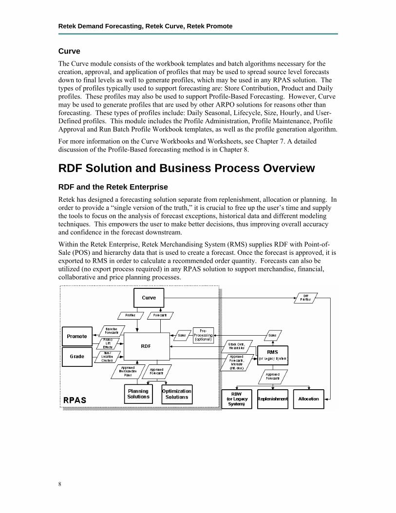
RDF Solution and Business Process Overview RDF and the Retek Enterprise Retek has designed a forecasting solution separate from replenishment, allocation or planning. In order to provide a “single version of the truth,” it is crucial to free up the user’s time and supply the tools to focus on the analysis of forecast exceptions, historical data and different modeling techniques. This empowers the user to make better decisions, thus improving overall accuracy and confidence in the forecast downstream.
Within the Retek Enterprise, Retek Merchandising System (RMS) supplies RDF with Point-of-Sale (POS) and hierarchy data that is used to create a forecast. Once the forecast is approved, it is exported to RMS in order to calculate a recommended order quantity. Forecasts can also be utilized (no export process required) in any RPAS solution to support merchandise, financial, collaborative and price planning processes.
Chapter 1 – Introduction
9
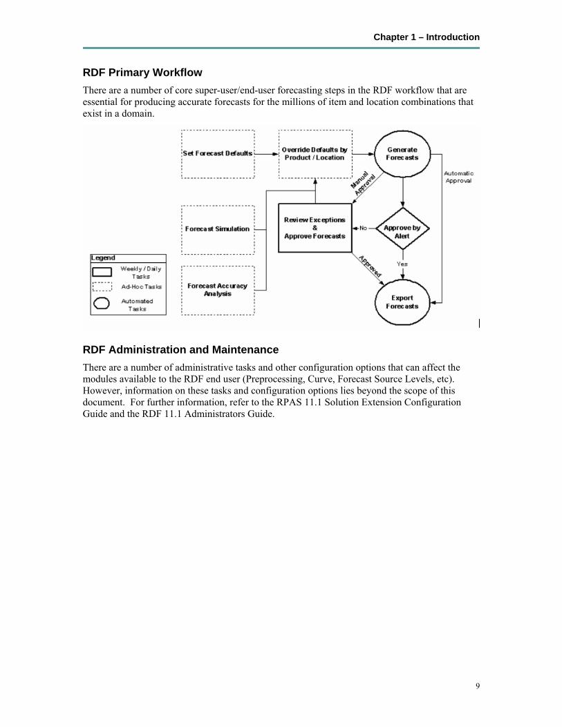
RDF Primary Workflow There are a number of core super-user/end-user forecasting steps in the RDF workflow that are essential for producing accurate forecasts for the millions of item and location combinations that exist in a domain.
RDF Administration and Maintenance There are a number of administrative tasks and other configuration options that can affect the modules available to the RDF end user (Preprocessing, Curve, Forecast Source Levels, etc). However, information on these tasks and configuration options lies beyond the scope of this document. For further information, refer to the RPAS 11.1 Solution Extension Configuration Guide and the RDF 11.1 Administrators Guide.

Chapter 2 – Preparing data for forecasting
11
Chapter 2 – Preparing data for forecasting Overview The accuracy of any given forecast is directly impacted by the quality and integrity of the data on which the forecast is based. Data that is excessively noisy or sparse will result in forecasts that may not accurately reflect true demand patterns. Retek Demand Forecasting provides two methods to “smooth” data and remove unwanted spikes and dips in the demand history. These two methods are:
• Automated Preprocessing of data.
• Manual adjustment of sales history.
This chapter addresses each of these methods, and details how a RDF user may leverage either of these two methods.
Automated preprocessing of data Preprocessing, as the name implies, is an optional process that may occur prior to data being used in any RPAS solution. The process corrects past data points that represent unusual sales values not representative of a general demand pattern. Such correction may be necessary either when an item is out of stock and cannot be sold, resulting in unusually low sales. Conversely, correction of data may also be necessary in a period when demand is unusually high. Preprocessing allows the system to automatically make adjustments to raw POS (Point of Sales) data, so that subsequent demand forecasts do not replicate undesired patterns caused by lost sales or unusually high demand.
Consider the following examples:
Retek Demand Forecasting, Retek Curve, Retek Promote
12
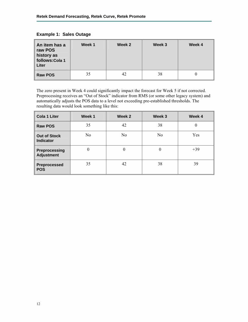
Example 1: Sales Outage
An item has a raw POS history as follows:Cola 1 Liter
Week 1 Week 2 Week 3 Week 4
Raw POS 35 42 38 0
The zero present in Week 4 could significantly impact the forecast for Week 5 if not corrected. Preprocessing receives an “Out of Stock” indicator from RMS (or some other legacy system) and automatically adjusts the POS data to a level not exceeding pre-established thresholds. The resulting data would look something like this:
Cola 1 Liter Week 1 Week 2 Week 3 Week 4
Raw POS 35 42 38 0
Out of Stock Indicator
No No No Yes
Preprocessing Adjustment
0 0 0 +39
Preprocessed POS
35 42 38 39
Chapter 2 – Preparing data for forecasting
13
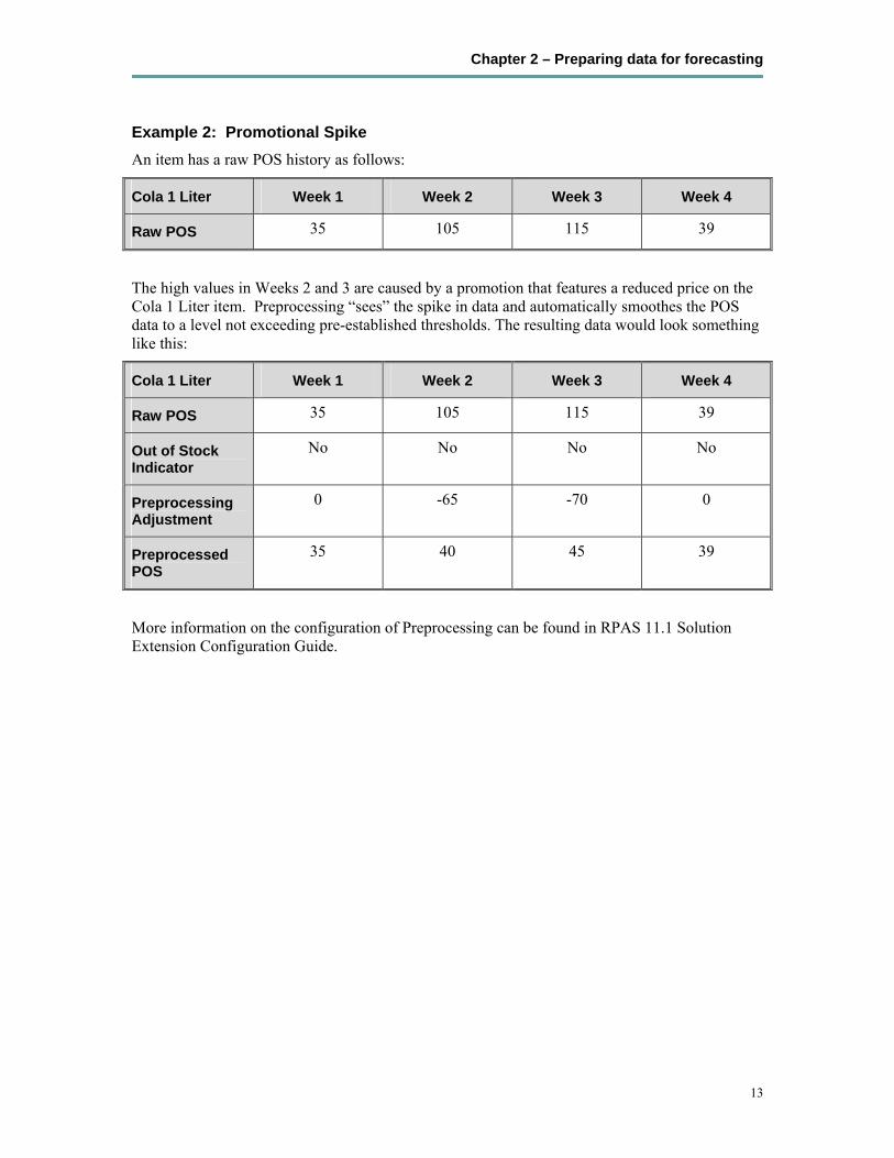
Example 2: Promotional Spike An item has a raw POS history as follows:
Cola 1 Liter Week 1 Week 2 Week 3 Week 4
Raw POS 35 105 115 39
The high values in Weeks 2 and 3 are caused by a promotion that features a reduced price on the Cola 1 Liter item. Preprocessing “sees” the spike in data and automatically smoothes the POS data to a level not exceeding pre-established thresholds. The resulting data would look something like this:
Cola 1 Liter Week 1 Week 2 Week 3 Week 4
Raw POS 35 105 115 39
Out of Stock Indicator
No No No No
Preprocessing Adjustment
0 -65 -70 0
Preprocessed POS
35 40 45 39
More information on the configuration of Preprocessing can be found in RPAS 11.1 Solution Extension Configuration Guide.
Retek Demand Forecasting, Retek Curve, Retek Promote
14
Manual Adjustment of Sales History In addition to the automated preprocessing of sales data that may occur prior to use in RDF, there may still be reasons for additional user adjustment to sales histories. Some of these reasons might include:
• The need to create a fake history for an item that has no Like Item if not using RDF’s Like Item functionality.
• Smoothing spikes or dips in demand data that weren’t sufficiently smoothed during preprocessing.
• Manually creating a lift effect on a promoted item’s history, so that the lift will be replicated in the appropriate forecast horizon.
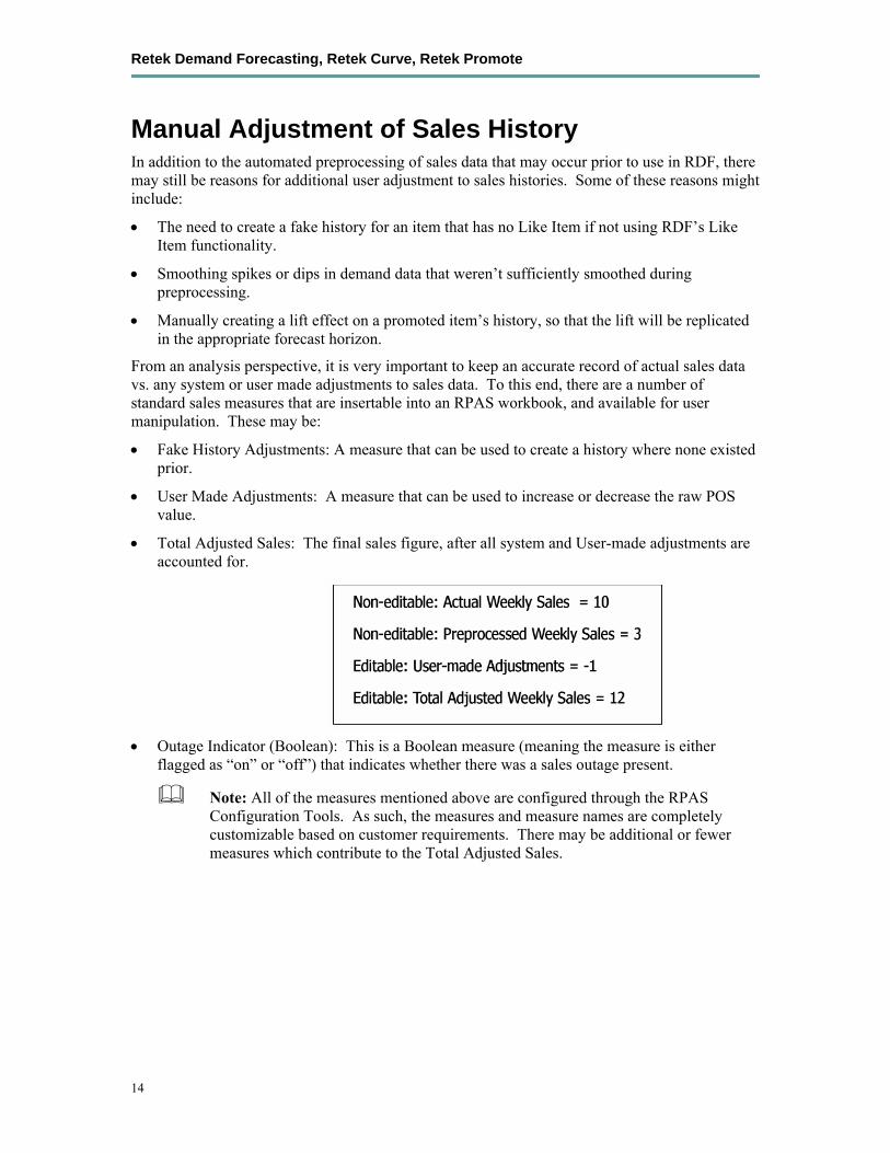
From an analysis perspective, it is very important to keep an accurate record of actual sales data vs. any system or user made adjustments to sales data. To this end, there are a number of standard sales measures that are insertable into an RPAS workbook, and available for user manipulation. These may be:
• Fake History Adjustments: A measure that can be used to create a history where none existed prior.
• User Made Adjustments: A measure that can be used to increase or decrease the raw POS value.
• Total Adjusted Sales: The final sales figure, after all system and User-made adjustments are accounted for.
• Outage Indicator (Boolean): This is a Boolean measure (meaning the measure is either flagged as “on” or “off”) that indicates whether there was a sales outage present.
Note: All of the measures mentioned above are configured through the RPAS Configuration Tools. As such, the measures and measure names are completely customizable based on customer requirements. There may be additional or fewer measures which contribute to the Total Adjusted Sales.
Chapter 2 – Preparing data for forecasting
15
Viewing Adjusted Sales Measures in a Workbook Since sales measures and measures for adjustments are completely customizable, the customer has the option to configure workbooks to support their individual needs. However, for analysis purposes only, the Measure Analysis workbook is a free-form workbook that can be used for many purposes, and more importantly, has access to all measures in a domain. This makes it the easiest workbook to use when one needs to review sales measures. The Measure Analysis workbook in found by clicking on the Analysis tab. However, for adjusting and committing sales measures, a workbook may need to be configured with Commit rules. See the RPAS Configuration Tools User’s Guide for information on workbook template creation.
Inserting Adjusted Sales Measures into an existing workbook. Adjusted Sales measures may be inserted into many other workbooks. For example, a user may wish to view the Adjusted Sales Measures in the Forecast Approval workbook.
To insert a measure into an open workbook, follow these steps:
1. Open the workbook where you wish to insert the Adjusted Sales measures.
2. Click Edit in the menu bar, and select Edit>Insert Measure. The Insert Measure dialogue box opens.
3. Select the Adjusted Sales measure.
4. Click OK.
The Adjusted Sales measures selected now appears in your workbook.


Chapter 3 – Setting Forecast Parameters
17
Chapter 3 – Setting Forecast Parameters Overview The Forecast Workbook template group allows you to perform functions related to statistical time series forecasting. This chapter provides information on defining and maintaining the parameters that govern the generation of forecasts in RDF.
Forecast Administration Workbook Overview
Basic vs. Advanced Tabs Forecast Administration is the first workbook used in setting up RDF to generate forecasts. It provides access to forecast settings and parameters that govern the whole domain (database). These settings and parameters are divided into two areas, accessed through the Basic and Advanced tabs beneath main tool bar.
The Basic Tab is used to establish a final level forecast horizon, the commencement and frequency of forecast generation; and the specification of aggregation levels (Source Levels) and spreading (Profile) methods used to yield the final level forecast results.
The Advanced Tab is used to set default values for parameters affecting the algorithm and other forecasting techniques used to yield final level and source level forecasts, thus eliminating the need to define these parameters individually for each product and location in the database. If certain products or locations require parameter values other than the defaults, these fields can be amended on a case-by-case basis in the Forecast Maintenance Workbook. The Forecast Maintenance Workbook will be discussed in more detail later in this chapter.
Final Forecasts vs. a Source Level Forecasts Often, forecast information is required for items at a very low level in the hierarchy. Problems can arise, however, in that data is often too sparse and noisy to identify clear patterns at these lower levels. For this reason, it sometimes becomes necessary to aggregate sales data from a low level to a higher level in the hierarchy in order to generate a reasonable forecast. Once this forecast is created at the higher or source level, the results can be allocated to the lower or final level dimension based on the lower level’s relationship to the total.
In order to spread this forecasted information back down to the lower level, it is necessary to have some idea about the relationship between the final level and the source level dimensions. Often, an additional interim forecast is run at the low level in order to determine this relationship. Forecast data at this low level might be sufficient to generate reliable percentage-to-whole information, but the actual forecast numbers are more robust when generated at the aggregate level.
The Final Level Worksheet represents forecast parameters for the lower (final) level, the level to which source forecast values are ultimately spread. Forecast data must appear at some final level in order for the data to be approved or exported to some other system. The Source Level Worksheet represents the default values for forecast parameters at the more robust aggregate (source) level.

Retek Demand Forecasting, Retek Curve, Retek Promote
18
Forecasting Methods available in Retek Demand Forecasting A forecasting system’s main goal is to produce accurate predictions of future demand. Retek’s Demand Forecasting solution utilizes the most advanced forecasting algorithms to address many different data requirements across all retail verticals. Furthermore, the system can be configured to automatically select the best algorithm and forecasting level to yield the most accurate results.
The following section summarizes the use of the various forecasting methods employed in the system. This section is referenced throughout this document when the selection of a forecasting method is required in a workflow process. Some of these methods may not be visible in your solution based on configuration options set in the RPAS Configuration Tools. See also Chapter 8 for more details on forecasting algorithms and the RPAS 11.1 Solution Extension Configuration Guide for configuration options.
Average
Retek Demand Forecasting uses a simple moving average model to generate forecasts.
AutoES
Retek Demand Forecasting fits the sales data to a variety of exponential smoothing models of forecasting, and the best model is chosen for the final forecast. The candidate methods considered by AutoES are: Simple ES, Intermittent ES, Trend ES, Multiplicative Seasonal, Additive Seasonal, and Seasonal ES. The final selection between the models is made according to a performance criterion (Bayesian Information Criterion) that involves a tradeoff between the model’s fit over the historic data and its complexity.
Simple ES
Retek Demand Forecasting uses a simple exponential smoothing model to generate forecasts. Simple ES ignores seasonality and trend features in the demand data and is the simplest model of the exponential smoothing family. This method can be used when less than one year of historic demand data is available.
Intermittent ES
Retek Demand Forecasting fits the data to the Croston's model of exponential smoothing. This method should be used when the input series contains a large number of zero data points (that is, intermittent demand data). The original time series is split into a Magnitude and Frequency series, then the Simple ES model is applied to determine level of both series. The ratio of the magnitude estimate over the frequency estimate is the forecast level reported for the original series.
Simple/IntermittentES
A combination of the Simple ES and Intermittent ES methods. This method applies the Simple ES model unless a large number of zero data points are present, in which case the Croston’s model is applied.

Chapter 3 – Setting Forecast Parameters
19
TrendES
Retek Demand Forecasting fits the data to the Holt model of exponential smoothing. The Holt model is useful when data exhibits a definite trend. This method separates base demand from trend, then provides forecast point estimates by combining an estimated trend and the smoothed level at the end of the series. For instance where the forecast engine cannot produce a forecast using the Trend ES method, the Simple/Intermittent ES method is used to evaluate the time series.
Multiplicative Seasonal
Also referred to as Multiplicative Winters Model, this model extracts seasonal indices that are assumed to have multiplicative effects on the un-seasonalized series.
Additive Seasonal
Also referred to as Additive Winters Model, this model is similar to the Multiplicative Winters model, but is used when zeros are present in the data. This model adjusts the un-seasonalized values by adding the seasonal index (for the forecast horizon).
Seasonal ES
This method, a combination of several Seasonal methods, is generally used for known seasonal items or forecasting for long horizons. This method applies the Multiplicative Seasonal model unless zeros are present in the data, in which case the Additive Winters model of exponential smoothing is used. If less than 2 years of data is available, then a Seasonal Regression model is used. If there is too little data to create a seasonal forecast (in general, less than 52 weeks), then the system will select from the Simple ES, Trend ES and Intermittent ES methods.
Seasonal Regression
Seasonal Regression cannot be selected as a forecasting method, but is a candidate model used only when the Seasonal ES method is selected. This model requires a minimum of 52 weeks of history to determine seasonality. Simple Linear Regression is used to estimate the future values of the series based on a past series. The independent variable is the series history one-year or one cycle length prior to the desired forecast period, and the dependent variable is the forecast. This model assumes that the future is a linear combination of itself one period before plus a scalar constant.
Causal
Causal is used for promotional forecasting and can only be selected if Promote is implemented. Causal uses a Stepwise Regression sub-routine to determine the promotional variables that are relevant to the time series and their lift effect on the series. AutoES utilizes the time series data and the future promotional calendar to generate future baseline forecasts. By combining the future baseline forecast and each promotion’s effect on sales (lift), a final promotional forecast is computed. For instances where the forecasting engine cannot produce a forecast using the Causal method, the system will evaluate the time series using the Seasonal ES method. See Chapter 6 for more information on promotional forecasting (Promote).
No Forecast
No forecast will be generated for the product/location combination.

Retek Demand Forecasting, Retek Curve, Retek Promote
20
Bayesian
Useful for short lifecycle forecasting and for new products with little or no historic sales data, the Bayesian method requires a product’s known sales plan (created externally to RDF) and considers a plan’s shape (the selling profile or lifecycle) and scale (magnitude of sales based on Actuals). The initial forecast is equal to the sales plan but as sales information comes in, the model generates a forecast by merging the sales plan with the sales data. The forecast is adjusted so that the sales magnitude is a weighted average between the original plan’s scale and the scale reflected by known history. A Data Plan must be specified when using the Bayesian method. For instances where the Data Plan equals zero (0), the system will evaluate the time series using the Seasonal ES method.
Profile-Based
Retek Demand Forecasting generates a forecast based on a seasonal profile that can be created in RPAS or legacy system. Profiles can also be copied from another profile and adjusted. Using historic data and the profile, the data is de-seasonalized and then fed to the Simple ES method. The Simple forecast is then re-seasonalized using the profiles. A Seasonal Profile must be specified when using the Profile-Based method. For instances where the Seasonal Profile equals zero (0), the system will evaluate the time series using the Seasonal ES method.
Forecast Administration Workbook Procedures
Create a Forecast Administration Workbook 1. Within the Master or Local Domain, select New from the File menu.
2. Select the Forecast tab to display a list of workbook templates for statistical forecasting.
3. Select Forecast Administration.
4. Click OK.
5 The Forecast Administration wizard opens and prompts you to select the level of the final forecast. The final forecast level is a level at which approvals and data exports can be performed. Depending on your organization’s setup, you may be offered a choice of several final forecast levels. Make the appropriate selection.
6. Click Finish to open the workbook.
Chapter 3 – Setting Forecast Parameters
21
Window descriptions
Basic Settings workflow tab The Basic Settings workflow tab contains forecast administration settings. On the Basic Settings workflow tab, there are two worksheets:
• Final Level Parameters Worksheet
• Final and Source Level Parameters Worksheet
Final Level Worksheet – Basic Settings
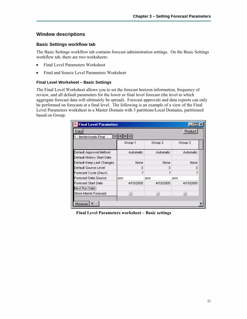
The Final Level Worksheet allows you to set the forecast horizon information, frequency of review, and all default parameters for the lower or final level forecast (the level to which aggregate forecast data will ultimately be spread). Forecast approvals and data exports can only be performed on forecasts at a final level. The following is an example of a view of the Final Level Parameters worksheet in a Master Domain with 3 partitions/Local Domains, partitioned based on Group:
Final Level Parameters worksheet – Basic settings

Retek Demand Forecasting, Retek Curve, Retek Promote
22
Field descriptions The following is a description of the Basic Settings contained in the Final Level Parameters Worksheet:
Default Approval Method
This field is a drop-down list from which you select the default automatic approval policy for forecast items. Valid values are:
• Manual – The system-generated forecast will not be automatically approved. Forecast values must be manually approved by accessing and amending the Forecast Approval Workbook.
• Automatic – The system-generated quantity will be automatically approved as-is.
• By Alert – This list of values may also include any ‘Forecast Approval’ alerts that have been configured for use in the forecast approval process. Alerts are configured during the implementation. See the RPAS Configuration Tools User’s Guide for more information on the Alert Manager.
Default History Start Date
This field indicates to the system the point in the historical sales data at which to use in the forecast generation process. If no date is indicated, the system will default to the first date in your calendar. It is also important to note that the system ignores leading zeros that begin at the history start date. For example, if your history start date is January 1, 1999 and an item/location does not have sales history until February 1, 1999, the system will consider the starting point in that item/location’s history to be the first data point where there is a non-zero sales value.
Default Keep Last Changes
This field is a drop-down list from which you select the default change policy for forecast items. Valid values are:
• Keep Last Changes (None) –There are no changes that are introduced into the adjusted forecast.
• Keep Last Changes (Total) –Considers only the Last Approved Forecast in determining change policy. For each forecasted item/week-combination, Retek Demand Forecasting automatically introduces the same quantity that was approved in the Last Approved Forecast into the change, only if that quantity differed from that in the Last System Forecast. If the quantities are the same, then Retek Demand Forecasting will introduce the current system-generated forecast into the adjusted forecast.
• Keep Last Changes (Diff) –Considers both the Last System Forecast and the Last Approved Forecast in determining approval policy. For each forecasted item/week-combination, Retek Demand Forecasting determines the difference between the Last System Forecast and the Last Approved Forecast. This difference (positive or negative) is then added to the current system forecast, and calculated as the adjusted forecast.
• Keep Last Changes (Ratio) –Considers both the Last System Forecast and the Last Approved Forecast in determining change. For each forecasted item/week-combination, Retek Demand Forecasting determines the difference between the Last System Forecast and the Last Approved Forecast; this difference is expressed as a percentage. This same percentage is used to calculate the adjusted forecast.
Chapter 3 – Setting Forecast Parameters
23
Default Source Level
The pick list of values displayed in this field allows the user to change the forecast level that will be used as the primary level to generate the source forecast. The source levels are set up in the RPAS Configuration Tool. A value from the pick list is required in this field at the time of forecast generation.
Forecast Cycle
The Forecast Cycle is the amount of time (measured in days) that the system waits between each forecast generation. Once a scheduled forecast has been generated, this field is used to automatically update the Next Run Date field. A non-zero value is required in this field at the time of forecast generation.
Forecast Data Source
This is a read-only value that displays the sales measure (the measure name) that will be the data used for the generation of forecasts (for example, pos). The measure that will be displayed here is determined at configuration time in the RPAS Configuration Tools.
Forecast Start Date
This is the starting date of the forecast. If no value is specified at the time of forecast generation the system will use the data/time at which the batch is executed as the default value. If a value is specified in this field and it is used to successfully generate the batch forecast, this value will be cleared.
Next Run Date
The Next Run Date is the date on which the next batch forecast generation process will automatically be run. Retek Demand Forecasting automatically triggers a set of batch processes to be run at a pre-determined time period. When a scheduled batch is run successfully, the Next Run Date automatically updates based on the Start Date value and the Forecast Cycle. No value is required in this field when the ‘Run Batch Forecast’ wizard is used to generate the forecast or if the batch forecast is run from the backend of the domain(s) using the ‘override true’ option (see the RDF 11.1 Administrators Guide for more information on forecast generation).
Store Interim Forecast
A check should be placed in this field if the interim forecast will be stored. The Interim Forecast is the forecast generated at the Final Level. This forecast is used as the Source Data within Curve to generate the profile (spreading ratios) for spreading the source level forecast to the final level. It is recommended that the interim forecast be stored if it is necessary for any analysis purposes, otherwise it should not be stored.
Retek Demand Forecasting, Retek Curve, Retek Promote
24
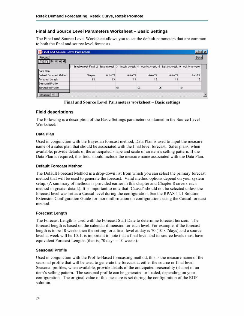
Final and Source Level Parameters Worksheet – Basic Settings The Final and Source Level Worksheet allows you to set the default parameters that are common to both the final and source level forecasts.
Final and Source Level Parameters worksheet – Basic settings
Field descriptions The following is a description of the Basic Settings parameters contained in the Source Level Worksheet:
Data Plan
Used in conjunction with the Bayesian forecast method, Data Plan is used to input the measure name of a sales plan that should be associated with the final level forecast. Sales plans, when available, provide details of the anticipated shape and scale of an item’s selling pattern. If the Data Plan is required, this field should include the measure name associated with the Data Plan.
Default Forecast Method
The Default Forecast Method is a drop-down list from which you can select the primary forecast method that will be used to generate the forecast. Valid method options depend on your system setup. (A summary of methods is provided earlier in this chapter and Chapter 8 covers each method in greater detail.). It is important to note that ‘Causal’ should not be selected unless the forecast level was set as a Causal level during the configuration. See the RPAS 11.1 Solution Extension Configuration Guide for more information on configurations using the Causal forecast method.
Forecast Length
The Forecast Length is used with the Forecast Start Date to determine forecast horizon. The forecast length is based on the calendar dimension for each level. For example, if the forecast length is to be 10 weeks then the setting for a final level at day is 70 (10 x 7days) and a source level at week will be 10. It is important to note that a final level and its source levels must have equivalent Forecast Lengths (that is, 70 days = 10 weeks).
Seasonal Profile
Used in conjunction with the Profile-Based forecasting method, this is the measure name of the seasonal profile that will be used to generate the forecast at either the source or final level. Seasonal profiles, when available, provide details of the anticipated seasonality (shape) of an item’s selling pattern. The seasonal profile can be generated or loaded, depending on your configuration. The original value of this measure is set during the configuration of the RDF solution.
Chapter 3 – Setting Forecast Parameters
25
Spreading Profile
Used for Source Level Forecasting, the value of this measure indicates the profile level that will be used to determine how the source level forecast is spread down to the final level. No value is needed to be entered at the final level. For dynamically generated profiles, this value is the number associated with the final profile level (for example 01)—note that profiles 1 through 9 have a zero (0) preceding them in Curve—this is different than the forecasting level numbers. For profiles that must be approved, this is the measure associated with the final profile level. This measure is defined as “apvp”+level (for example: apvp01 for the approved profile for level 01 in Curve).
Advanced Settings workflow tab The Forecast Administration Advanced Settings workflow tab is used to set parameters related to either the data that is stored in the system or the forecasting methods that will be used at the final or source levels. The parameters on this workflow tab aren’t as likely to be changed on a regular basis as the ones on the Basic Settings workflow tab.
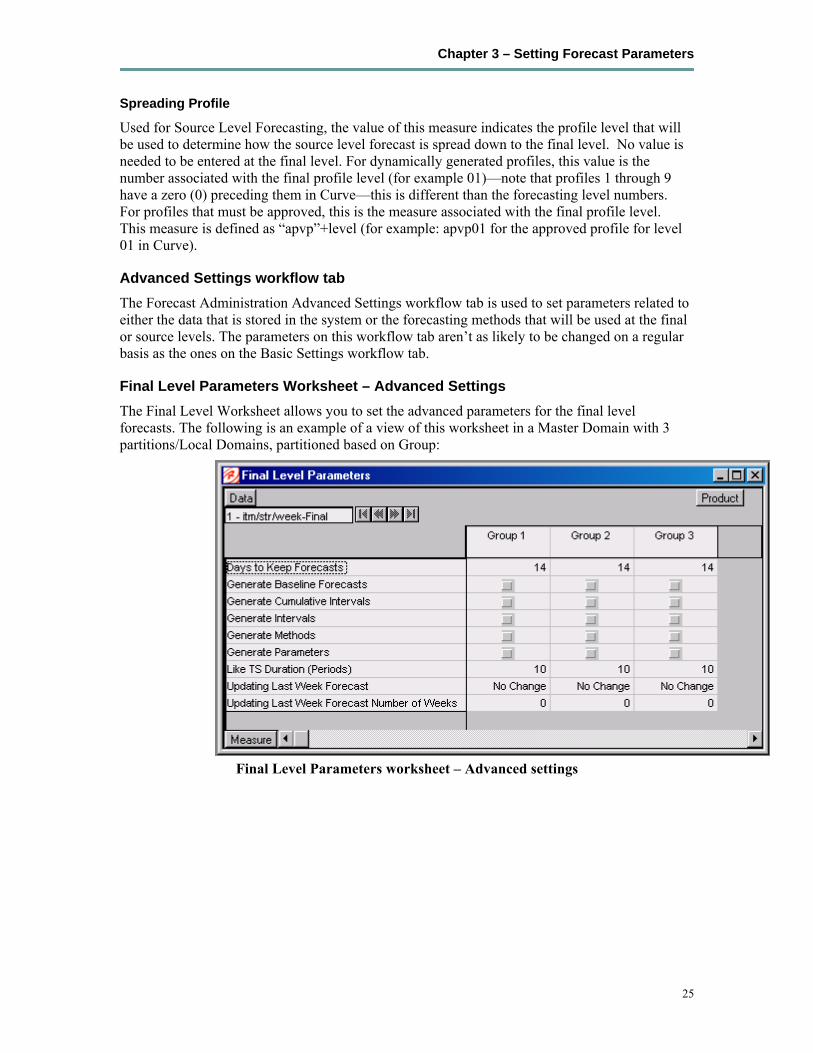
Final Level Parameters Worksheet – Advanced Settings The Final Level Worksheet allows you to set the advanced parameters for the final level forecasts. The following is an example of a view of this worksheet in a Master Domain with 3 partitions/Local Domains, partitioned based on Group:
Final Level Parameters worksheet – Advanced settings

Retek Demand Forecasting, Retek Curve, Retek Promote
26
Field descriptions The Final Level Worksheet – Advanced Settings contains the following parameters:
Days to Keep Forecasts
This field is used to set the number of days that the system will store forecasts based on the date/time the forecast is generated. The date/time of forecast generation is also referred to as ‘birth date’ of the forecast. A forecast is deleted from the system if the birth date plus the number of days since the birth date is greater than the Days to Keep Forecast. This process occurs when either the ‘Run Batch Forecast’ wizard is used to generate the forecast or when ‘PreGenerateForecast’ is executed. See the RDF 11.1 Administrators Guide for more information on ‘PreGenerateForecast’.
Generate Baseline Forecasts
A check should be indicated in this field if the baseline forecast is to be generated to be viewed in any workbook. This parameter should be set if the level is to be used for Causal forecasting and the baseline will be needed for analysis purposes. See Chapter 6 for more information on Promote.
Generate Cumulative Interval
A check in this field specifies whether you want Retek Demand Forecasting to generate cumulative intervals (this is similar to cumulative standard deviations) during the forecast generation process. Cumulative Intervals are a running total of Intervals. The cumulative interval is necessary if forecast information is to be exported to a Retek Replenishment solution. If you do not need cumulative intervals, you can eliminate excess processing time and save disk space by clearing the check box. The calculated cumulative intervals can be viewed within RDF. (See Forecast Approval Workbook in chapter 4 for more details on the calculation of Cumulative Intervals when the user adjusts forecasts.)
Generate Interval
A check in this field indicates that intervals (similar to Standard Deviations) should be stored as part of the batch forecast process. Intervals can be displayed in the Forecast Approval Workbook. If you do not need intervals, excess processing time and disk space may be eliminated by clearing the check box. For many forecasting methods, intervals are calculated as standard deviation but for Simple, Holt, and Winters the calculation is more complex. Intervals are not exported. See Chapter 6 for more details on interval calculations.
Generate Methods
A check in this field indicates that when an ES forecast method is used, the chosen forecast method for each fitted time series should be stored. The chosen method can be displayed in the Forecast Approval Workbook.
Generate Parameters
A check in this field indicates that the alpha, level, and trend parameters for each fitted time series should be stored. These parameters can be displayed in the Forecast Approval Workbook.

Chapter 3 – Setting Forecast Parameters
27
Like TS Duration (weeks)
The Like TS Duration is the number of weeks of history required after which Retek Demand Forecasting stops using the substitution method and starts using the system forecast generated by the forecast engine. A value must be entered in this field if using Like-Item/Sister-Store functionality. See Forecast Like-Item, Sister-Store Workbook in chapter 3 for more information on like time-series functions.
Updating Last Week Forecast
This field is a drop-down list from which you can select the method for updating the Approved Forecast for the last specified number of week(s) of the forecast horizon. This option is valid only if the Approval Method Override (set in the Forecast Maintenance Workbook) is set to Manual or Approve by alert and the alert was rejected. This parameter is used with the ‘Updating Last Week Forecast Number of Weeks’.
• No Change – When using this method the last week(s) in the forecast horizon will not have an Approved Forecast value. The number of weeks is determined by the value set in the ‘Updating Last Week Forecast Number of Weeks’ parameter.
• Replicate – When using this method the last week(s) in the forecast horizon will be forecasted using the Approved Forecast for the week prior to this time period. To determine the appropriate forecast time period the value set in ‘Updating Last Week Forecast Number of Weeks’ is subtracted from the Forecast Length. For example, if your Forecast Length is set to 52 weeks and ‘Updating Last Week Forecast Number of Weeks’ is set to 20, week 32’s Approved Forecast will be copied into the Approved Forecast for the next 20 weeks.
• Use Forecast – When using this method the System Forecast for the last week(s) in the forecast horizon is approved.
Updating Last Week Forecast Number of Weeks
The Approved Forecast for the last week(s) in the forecast horizon is updated using the method specified from the ‘Updating Last week Forecast’ pick list.
Retek Demand Forecasting, Retek Curve, Retek Promote
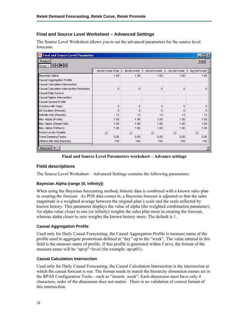
28
Final and Source Level Worksheet – Advanced Settings The Source Level Worksheet allows you to set the advanced parameters for the source level forecasts.
Final and Source Level Parameters worksheet – Advance settings
Field descriptions The Source Level Worksheet – Advanced Settings contains the following parameters:
Bayesian Alpha (range (0, infinity))
When using the Bayesian forecasting method, historic data is combined with a known sales plan in creating the forecast. As POS data comes in, a Bayesian forecast is adjusted so that the sales magnitude is a weighted average between the original plan’s scale and the scale reflected by known history. This parameter displays the value of alpha (the weighted combination parameter). An alpha value closer to one (or infinity) weights the sales plan more in creating the forecast, whereas alpha closer to zero weights the known history more. The default is 1.
Causal Aggregation Profile
Used only for Daily Causal Forecasting, the Causal Aggregation Profile is measure name of the profile used to aggregate promotions defined at “day” up to the “week”. The value entered in this field is the measure name of profile. If this profile is generated within Curve, the format of the measure name will be “apvp”+level (for example: apvp01).
Causal Calculation Intersection
Used only for Daily Causal Forecasting, the Causal Calculation Intersection is the intersection at which the causal forecast is run. The format needs to match the hierarchy dimension names set in the RPAS Configuration Tools—such as “itemstr_week”. Each dimension must have only 4 characters; order of the dimension does not matter. There is no validation of correct format of this intersection.

Chapter 3 – Setting Forecast Parameters
29
Causal Calculation Intersection Periodicity
Used only for Daily Causal Forecasting, the Causal Calculation Intersection Periodicity must be set to the periodicity of Causal Calculation Intersection. Periodicity is the number of periods within 1 year that correspond to the calendar dimension (for example, 52 if the Causal Calculation Intersection is defined with the week dimension).
Causal Data Source
Used only for Daily Causal Forecasting, the Causal Data Source is an optional setting that contains the measure name of the sales data to be used if the data to be used for calculating the causal forecast is different than the Data Source specified at the Final level. If needed, this field should contain the measure name of the source data measure (for example: dpos).
Causal Higher Intersection
An optional setting for Causal Forecasting, this intersection is the aggregate level to model promotions if the causal intersection cannot produce a meaningful causal effect. This intersection will apply to promotions that have a Promotion Type is set to “Override From Higher Level” (set in the Promotion Maintenance workbook). The format of this intersection needs to match the hierarchy dimension names set in the RPAS Configuration Tools—such as “sclsrgn_” (Subclass\Region), and must not contain the calendar dimension. Each dimension must have only 4 characters; order of the dimension does not matter. There is no validation of correct format of this intersection.
Causal Spread Profile
Used only for Daily Causal Forecasting, the Causal Spread Profile is the measure name of the profile used to spread the causal baseline forecast from the Causal Calculation Intersection to the Final Level. If this profile is generated in Curve, this measure value will be “apvp”+level (for example: apvp01).
Croston Min Gaps
The Croston Min Gaps is the default minimum number of gaps between intermittent sales for the batch forecast to consider Croston’s as a potential AutoES forecasting method for a time series. If there are not enough gaps between sales in a given product’s sales history, then the Croston’s model is not considered a valid candidate model. The system default is five minimum gaps between intermittent sales. The value must be set based on the calendar dimension of the level. For example, if the value is to be 5 weeks then the setting for a final level at day is 35 (5x7days) and a source level at week will be 5.
DD Duration (weeks)
Used with Profile Based forecast method, the DD Duration is the number of weeks of history required after which the system stops using the DD (De-seasonalized Demand) approach and defaults to the “normal” Profile-Based method. The value must be set based on the calendar dimension of the level. For example, if the value is to be 10 weeks then the setting for a final level at day is 70 (10x7days) and a source level at week will be 10.

Retek Demand Forecasting, Retek Curve, Retek Promote
30
Holt Min Hist (Periods)
Used with the AutoES forecast method, Holt Min Hist is the minimum number of periods of historical data necessary for the system to consider Holt as a potential forecasting method. Retek Demand Forecasting fits the given data to a variety of AutoES candidate models in an attempt to determine the best method; if not enough periods of data are available for a given item, then Holt will not be considered as a valid option. The system default is 13 periods. The value must be set based on the calendar dimension of the level. For example, if the value is to be 13 weeks then the setting for a final level at day is 91 (13x7days) and a source level at week will be 13.
Max Alpha (Profile) (range (0,1])
In the Profile based model fitting procedure, alpha, which is a model parameter capturing the level, is determined by optimizing the fit over the de-seasonalized time series. The time series is de-seasonalized based on a seasonal profile. This field displays the maximum value (that is, cap value) of alpha allowed in the model fitting process. An alpha cap value closer to 1 allows more reactive models (alpha = 1, repeats the last data point), whereas alpha cap closer to 0 only allows less reactive models. The default is 1.
Max Alpha (Simple, Holt) (range (0,1])
In the Simple or Holt model fitting procedure, alpha, which is a model parameter capturing the level, is determined by optimizing the fit over the time series. This field displays the maximum value (that is, cap value) of alpha allowed in the model fitting process. An alpha cap value closer to 1 allows more reactive models (alpha = 1, repeats the last data point), whereas alpha cap closer to 0 only allows less reactive models. The default is 1.
Max Alpha (Winters) (range (0,1])
In the Winters model fitting procedure, alpha, which is a model parameter capturing the level, is determined by optimizing the fit over the time series. This field displays the maximum value (that is, cap value) of alpha allowed in the model fitting process. An alpha cap value closer to 1 allows more reactive models (alpha = 1, repeats the last data point), whereas alpha cap closer to 0 only allows less reactive models. The default is 1.
Trend Damping Factor (range (0,1])
This parameter determines how reactive the forecast is to trending data. A value close to 0 is a high damping, while a value if 1 implies no damping. The default is 0.5.
Winters Min Hist (Periods)
Used with the AutoES forecast method, the value in this field is the minimum number of periods of historical data necessary for Winters to be considered as a potential forecast method. If not enough years of data are available for a given time series, Winters will not be used. The system default is two years of required history. The value must be set based on the calendar dimension of the level. For example, if the value is to be 104 weeks/2 years then the setting for a final level at day is 728 (104 weeks x 7 days) and a source level at week will be 104.

Chapter 3 – Setting Forecast Parameters
31
Forecast Maintenance Workbook Overview The Forecast Maintenance Workbook allows you to select and modify forecasting parameters for product/location combinations when the values of these parameters differ from the default values that are assigned in the Forecast Administration Workbook.
Suppose, for example, that the default forecast method of all the products in the database was set in the Forecast Administration Workbook to be AutoES. For a particular product, however, you know that a SeasonalES model is a better predictor of sales performance. To make this change, you must access the Forecast Maintenance Workbook, select the product / location intersection to be reviewed, make the appropriate change to the forecast method.
The Forecast Maintenance Workbook is split into two workflow tabs:
• Basic Settings – Includes all Final Level Worksheets and their respective Source Level Worksheets.
• Advanced Settings –This tab includes the Forecast Start Date, End Date and History Start Date measures for the selected Final Level.
Procedures
Create a Forecast Maintenance workbook 1. Within the Master or Local Domain, select New from the File menu.
2. Select the Forecast tab to display a list of workbook templates for statistical forecasting. Highlight Forecast Maintenance
3. Click OK. The Forecast Maintenance wizard opens and prompts you to select the level of the final forecast. Depending on your organization's setup, you may be offered a choice of several final forecast levels.
4. Select the final forecast level to be viewed in the workbook.
5. Click Next.
6. Select the locations to include in the workbook.
7. Click Next.
8. Select the products to include in the workbook.
9. Click Next.
10. Select any additional measures (that is, measures not standard in the Forecast Maintenance Workbook) that you would like included. The measure options available in this screen are set in the RPAS Security Administration Workbook / Workbook Template Measure Rights Worksheet.
11. Click Finish to display the workbook.
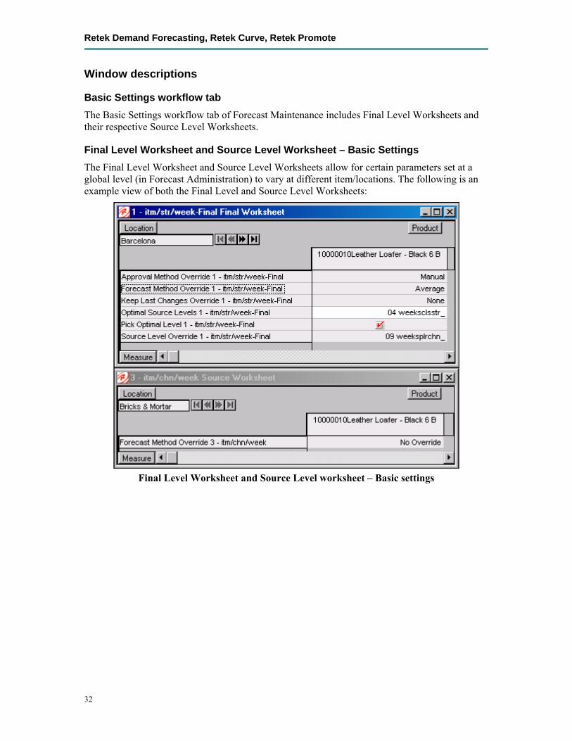
Retek Demand Forecasting, Retek Curve, Retek Promote
32
Window descriptions
Basic Settings workflow tab The Basic Settings workflow tab of Forecast Maintenance includes Final Level Worksheets and their respective Source Level Worksheets.
Final Level Worksheet and Source Level Worksheet – Basic Settings The Final Level Worksheet and Source Level Worksheets allow for certain parameters set at a global level (in Forecast Administration) to vary at different item/locations. The following is an example view of both the Final Level and Source Level Worksheets:
Final Level Worksheet and Source Level worksheet – Basic settings

Chapter 3 – Setting Forecast Parameters
33
Field descriptions The Final Level Worksheet and Source Level Worksheet – Basic Settings contains the following parameters:
Approval Method Override
Set only at the final level, the Approval Method Override is a drop-down list from which you select the approval policy for individual product/location combinations. No value will be in this field if the system default set in the Forecast Administration Workbook is to be used. Valid values are:
• Manual – The System Forecast and Adjusted Forecast are not automatically approved. Forecast values must be manually approved by accessing and amending the Forecast Approval Workbook.
• Automatic – The Adjusted Forecast is automatically approved as-is.
• By alert “name of the alert” - This list of values may also include any ‘Forecast Approval’ alerts that have been configured for use in the forecast approval process. Alerts are configured during the implementation. See the RPAS Configuration Tools User’s Guide for more information on the Alert Manager.
Note: If you select a specific alert as your approval method and later on you delete the alert, the approval will work as manual. The same will happen if the alert is on a wrong intersection.
Forecast Method Override
Set at both final and source levels, the Forecast Method Override is a drop-down list from which you can select a different forecast method than the Default Forecast Method set in the Forecast Administration workbook. ‘No Override’ will be set in this field if the system default set in the Forecast Administration Workbook is to be used. Valid options depend on your system setup. A summary of methods is provided earlier in this chapter and Chapter 8 covers each method in greater detail.
Keep Last Changes Override
Set only at final levels, Keep Last Changes Override field may be used to override the default setting at a product/location intersection. ‘None’ will be displayed in this field if there is no override applied to the intersection.
Optimal Source Levels
Displayed only at final levels, a value will be populated in this field if ‘AutoSource’ has been run on the final level. The ‘AutoSource’ executable evaluates all levels associated to a final level and returns the source level that yields the optimal forecast results. For more information on ‘AutoSource’ see the RDF 11.1 Administrators Guide.
Pick Optimal Level
Set only at final levels, a checkmark in this field indicates that the batch forecast should use the ‘Optimal Source Level’ selected by ‘AutoSource’. For more information on ‘AutoSource’ see the RDF 11.1 Administrators Guide.
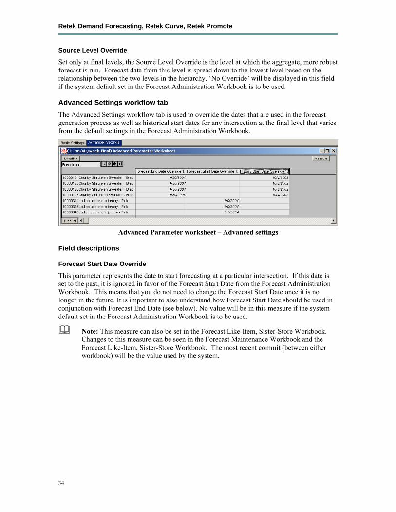
Retek Demand Forecasting, Retek Curve, Retek Promote
34
Source Level Override
Set only at final levels, the Source Level Override is the level at which the aggregate, more robust forecast is run. Forecast data from this level is spread down to the lowest level based on the relationship between the two levels in the hierarchy. ‘No Override’ will be displayed in this field if the system default set in the Forecast Administration Workbook is to be used.
Advanced Settings workflow tab The Advanced Settings workflow tab is used to override the dates that are used in the forecast generation process as well as historical start dates for any intersection at the final level that varies from the default settings in the Forecast Administration Workbook.
Advanced Parameter worksheet – Advanced settings
Field descriptions
Forecast Start Date Override
This parameter represents the date to start forecasting at a particular intersection. If this date is set to the past, it is ignored in favor of the Forecast Start Date from the Forecast Administration Workbook. This means that you do not need to change the Forecast Start Date once it is no longer in the future. It is important to also understand how Forecast Start Date should be used in conjunction with Forecast End Date (see below). No value will be in this measure if the system default set in the Forecast Administration Workbook is to be used.
Note: This measure can also be set in the Forecast Like-Item, Sister-Store Workbook. Changes to this measure can be seen in the Forecast Maintenance Workbook and the Forecast Like-Item, Sister-Store Workbook. The most recent commit (between either workbook) will be the value used by the system.
Chapter 3 – Setting Forecast Parameters
35
Forecast End Date Override
This parameter represents the last point in time for which the forecasting engine will forecast for a particular intersection. Should this parameter be set to a date less than the Forecast Start Date plus the Forecast Length (in Forecast Administration), the engine will forecast 0 past this date. If Forecast End Date is more than Forecasting Start Date plus Forecasting Length, you do NOT get a forecast outside Forecasting Start Date plus Forecasting Length. In other words, both Forecast Start Date and Forecasting End Date are relevant for time periods within the forecast horizon set at the global level. No value will be in this measure if the system default set in the Forecast Administration Workbook is to be used.
Note: This measure can also be set in the Forecast Like-Item, Sister-Store Workbook. Changes to this measure can be seen in the Forecast Maintenance Workbook and the Forecast Like-Item, Sister-Store Workbook. The most recent commit (in either workbook) will be the value used by the system.
History Start Date Override
This parameter represents the first point in time from which the Forecasting Engine will begin training and modeling (that is, if there are 2 years of history but you only want to use one year, you will set the start date to a year ago). This parameter will override the History Start Date set in the Forecast Administration Workbook the desired item/location intersection. For example, if you have a large spike in the first 3 weeks of sales for an item was on sale, you can set the Historical Start Date to one week past that period, and those first few weeks will not be used when generating the forecast.
It is also important to note that the system ignores leading zeros that begin at the history start date. For example, if your history start date is January 1, 1999 and an item/location does not have sales history until February 1, 1999, the system will consider the starting point in that item/location’s history to be the first data point where there is a non-zero sales value.
If this parameter is set into the future, there would be no forecast as the history training window is read as zero.
Note: This measure can also be set in the Forecast Like-Item, Sister-Store Workbook. Changes to this measure can be seen in the Forecast Maintenance Workbook and the Forecast Like-Item, Sister-Store Workbook. The most recent commit (between either workbook) will be the value used by the system.
Retek Demand Forecasting, Retek Curve, Retek Promote
36
Forecast Like-Item, Sister-Store Workbook Overview The Forecast Like-Item, Sister-Store Workbook provides the ability to model a new product’s demand after an existing product. Forecasts can thus be generated for the new product based on the selected history or the forecast of the existing product plus an Adjustment Ratio. Likewise, the sales history or the forecast of existing store locations can be used as the forecast foundation for new locations. This workbook includes the following worksheets:
• The Like-Item Worksheet
• The Sister-Store Worksheet
• The Advanced Parameter Worksheet
Note: This workbook is only valid at final levels. Therefore this workbook may include hierarchy dimensions that are at higher positions that item or store (for example: subclass or region)
Procedure
Create a Forecast Like-Item, Sister-Store Workbook 1. Within the Simple or Local Domain, select New from the File menu.
2. Select the Forecast tab to display a list of workbook templates for statistical forecasting. Highlight Forecast Like-Item, Sister-Store
3. Click OK. The wizard opens and prompts you to select the level of the final forecast. Depending on your organization's setup, you may be offered a choice of several final forecast levels.
4. Select the final forecast level to be viewed in the workbook
5. Click Next.
6. Select the locations to include in the workbook.
7. Click Next.
8. Select the products to include in the workbook.
9. Click Next.
10. Select any additional measures (that is, measures not standard in the Forecast Like-Item, Sister-Store Workbook) to be included. The measure options available in this screen are set in the RPAS Security Administration Workbook / Workbook Template Measure Rights Worksheet.
11. Click Finish to display the workbook.
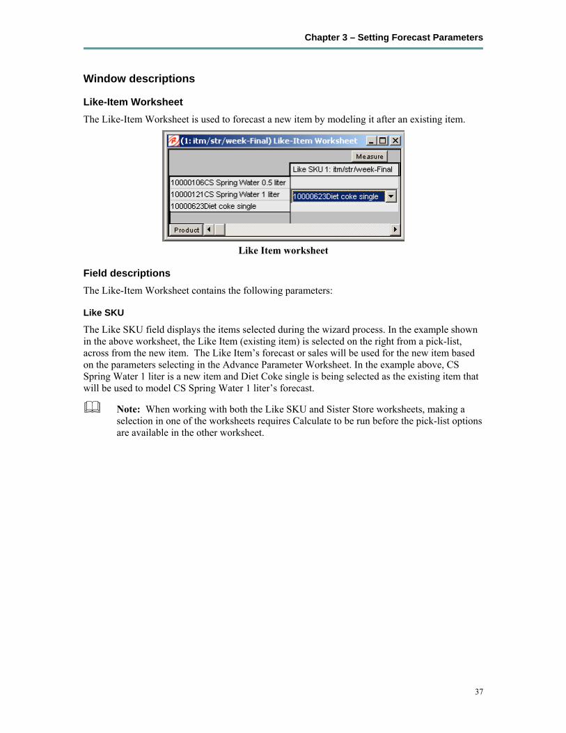
Chapter 3 – Setting Forecast Parameters
37
Window descriptions
Like-Item Worksheet The Like-Item Worksheet is used to forecast a new item by modeling it after an existing item.
Like Item worksheet
Field descriptions The Like-Item Worksheet contains the following parameters:
Like SKU
The Like SKU field displays the items selected during the wizard process. In the example shown in the above worksheet, the Like Item (existing item) is selected on the right from a pick-list, across from the new item. The Like Item’s forecast or sales will be used for the new item based on the parameters selecting in the Advance Parameter Worksheet. In the example above, CS Spring Water 1 liter is a new item and Diet Coke single is being selected as the existing item that will be used to model CS Spring Water 1 liter’s forecast.
Note: When working with both the Like SKU and Sister Store worksheets, making a selection in one of the worksheets requires Calculate to be run before the pick-list options are available in the other worksheet.
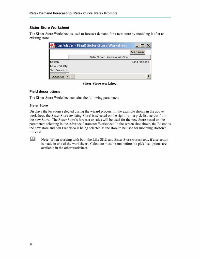
Retek Demand Forecasting, Retek Curve, Retek Promote
38
Sister-Store Worksheet The Sister-Store Worksheet is used to forecast demand for a new store by modeling it after an existing store.
Sister-Store worksheet
Field descriptions The Sister-Store Worksheet contains the following parameter:
Sister Store
Displays the locations selected during the wizard process. In the example shown in the above worksheet, the Sister Store (existing Store) is selected on the right from a pick-list, across from the new Store. The Sister Store’s forecast or sales will be used for the new Store based on the parameters selecting in the Advance Parameter Worksheet. In the screen shot above, the Boston is the new store and San Francisco is being selected as the store to be used for modeling Boston’s forecast.
Note: When working with both the Like SKU and Sister Store worksheets, if a selection is made in one of the worksheets, Calculate must be run before the pick-list options are available in the other worksheet.
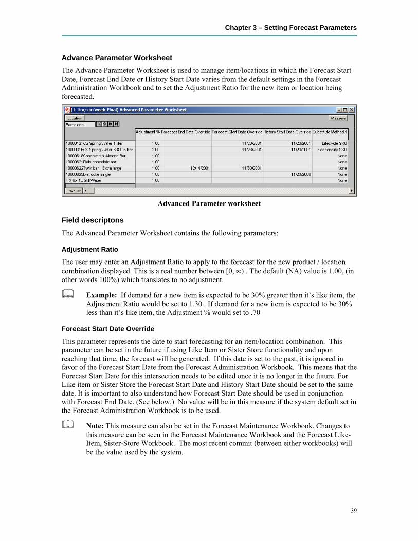
Chapter 3 – Setting Forecast Parameters
39
Advance Parameter Worksheet The Advance Parameter Worksheet is used to manage item/locations in which the Forecast Start Date, Forecast End Date or History Start Date varies from the default settings in the Forecast Administration Workbook and to set the Adjustment Ratio for the new item or location being forecasted.
Advanced Parameter worksheet
Field descriptons The Advanced Parameter Worksheet contains the following parameters:
Adjustment Ratio
The user may enter an Adjustment Ratio to apply to the forecast for the new product / location combination displayed. This is a real number between [0, ∞) . The default (NA) value is 1.00, (in other words 100%) which translates to no adjustment.
Example: If demand for a new item is expected to be 30% greater than it’s like item, the Adjustment Ratio would be set to 1.30. If demand for a new item is expected to be 30% less than it’s like item, the Adjustment % would set to .70
Forecast Start Date Override
This parameter represents the date to start forecasting for an item/location combination. This parameter can be set in the future if using Like Item or Sister Store functionality and upon reaching that time, the forecast will be generated. If this date is set to the past, it is ignored in favor of the Forecast Start Date from the Forecast Administration Workbook. This means that the Forecast Start Date for this intersection needs to be edited once it is no longer in the future. For Like item or Sister Store the Forecast Start Date and History Start Date should be set to the same date. It is important to also understand how Forecast Start Date should be used in conjunction with Forecast End Date. (See below.) No value will be in this measure if the system default set in the Forecast Administration Workbook is to be used.
Note: This measure can also be set in the Forecast Maintenance Workbook. Changes to this measure can be seen in the Forecast Maintenance Workbook and the Forecast Like-Item, Sister-Store Workbook. The most recent commit (between either workbooks) will be the value used by the system.
Retek Demand Forecasting, Retek Curve, Retek Promote
40
Forecast End Date Override
This parameter represents the last point in time for which the Forecasting Engine will forecast for an item/location combination. Should this parameter be set to a date less than the Forecast Start Date plus the Forecast Length (in Forecast Administration), the engine will forecast 0 past this date. If Forecast End Date is more than Forecasting Start Date plus Forecasting Length, NO forecast will be generated outside Forecasting Start Date plus Forecasting Length window. In other words, both Forecast Start Date and Forecasting End Date are relevant for time periods within the forecast horizon set at the global level. No value will be in this measure if the system default set in the Forecast Administration Workbook is to be used.
Forecast End Date can be used for new item or location forecasting if the item or location needs to be forecasted for a period shorter than the Like TS Duration (set globally in Forecast Administration).
Note: This measure can also be set in the Forecast Maintenance Workbook. Changes to this measure can be seen in the Forecast Maintenance Workbook and the Forecast Like-Item, Sister-Store Workbook. The most recent commit (between either workbook) will be the value used by the system.
History Start Date Override
This parameter represents the first point in time from which the Forecasting Engine will begin training and modeling (that is, if there are 2 years of history but only one year is required, set the start date to a year ago). This parameter overrides at the item/store level from the global settings in the Forecast Administration Workbook. This can be used to level out past sales. For example, if there is a large spike in the first 3 weeks of sales for an item was on sale, set the Historical Start Date to one week past that period, and those first few weeks will not be used when generating the forecast.
It is also important to note that the system ignores leading zeros that begin at the history start date. For example, if your history start date is January 1, 1999 and an item/location does not have sales history until February 1, 1999, the system will consider the starting point in that item/location’s history to be the first data point where there is a non-zero sales value.
The History Start Date for the new item or new store should be set with the same date as the Forecast Start Date.
Note: When using any of the Lifecycle Methods (see Substitute Methods below) the History Start Date for the substitute item or location must be set to the point in the sales history that the new item or location will begin using as its sales.
Note: This measure can also be set in the Forecast Maintenance Workbook. Changes to this measure can be seen in the Forecast Maintenance Workbook and the Forecast Like-Item, Sister-Store Workbook. The most recent commit (between either workbook) will be the value used by the system.
Chapter 3 – Setting Forecast Parameters
41
Substitute Method
Displays a drop-down list from which the user can select the substitute method. When a Substitute Method is used to forecast, the method set for an intersection will be cleared once the Default Forecast Start Date is greater than the Forecast Start Date Override plus the Like TS Duration for the intersection. Valid options are:
• None – There is no substitution for this product/location combination. This is the default value.
• Seasonality/New Item – The user provides a Like Item that has a similar seasonality pattern that sells at the same store. The new product’s forecast will be the like item’s demand forecast with the applied adjustment. The forecast will be set to 0 for all dates before the new product’s start date.
• Seasonality/New Store – The user provides a Sister Store that has a similar seasonality pattern that sells the same product. The product’s forecast at the new store will be the demand forecast of the same product at the Sister Store with the applied adjustment. The forecast will be set to 0 for all dates before the new store’s open date.
• Seasonality/New Item /New Store – The user provides a Like Item that sells at a Sister Store that has a similar seasonality pattern. The new product’s forecast at the new store will be the demand forecast of the Like Item at the Sister Store with the applied adjustment. The forecast will be set to 0 for all dates before the new product’s start date after the new store opens.
• Lifecycle/New Item – The user provides a Like Item that had a similar lifecycle pattern that sells at the same store. The new product’s forecast will be the like items actual sales with the applied adjustment shifted such that the like item’s first sales matches the new product’s start date.
• Lifecycle/New Store – The user provides a Sister Store that had a similar lifecycle pattern that sells the same product. The product’s forecast at the new store will be the products actual sales at the Sister Store with the applied adjustment shifted such that the Sister Store’s first sales matches the new store’s open date.
• Lifecycle/New Item /New Store – The user provides a Like Item that sells at a Sister Store that has a similar lifecycle pattern. The new product’s forecast at the new store will be Like Item’s actual sales at a Sister Store with the applied adjustment shifted such that the Like Item’s first sales at the Sister Store matches the new product’s start date after the new store opens.
Retek Demand Forecasting, Retek Curve, Retek Promote
42
Steps Required for Forecasting using each of the Like SKU / Sister Store Methods The following outlines the steps required for using each of the above Substitution Methods:
To support Like SKU / Sister Store functionality the Like TS Duration must be set in the Forecast Administration Workbook – Advance Tab. This parameter sets the number of weeks of history required after which Retek Demand Forecasting stops using the substitution method and starts using the system forecast generated by the forecast engine.
Procedures
Seasonality/SKU: Introduction of a new item at an existing store (like item with a similar forecast)
1. Like-Item Worksheet: Select a like item from the drop-down list, across from the new item.
2. Advanced Parameter Worksheet: Set the Forecast Start Date for the new item at an existing store.
3. Advanced Parameter Worksheet: Set the History Start Date for the new item at the existing store to the same date as the Forecast Start Date.
4. Advance Parameter Worksheet: Set the Adjustment % (optional) for the new item at the existing store.
Seasonality/STR: Introduction of an existing item at a new store (sister store with similar forecast)
1 Sister-Store Worksheet: Select a Sister Store from the drop-down list, across from the new store.
2. Advanced Parameter Worksheet: Set the Forecast Start Date for the existing item at the new store.
3. Advanced Parameter Worksheet: Set the History Start Date for the existing item at the new store to the same date as the Forecast Start Date.
4. Advance Parameter Worksheet: Set the Adjustment % (optional) for the existing item at the new store.
Seasonality/SKU_STR: Introduction of a new item at a new store (like item and sister store with a similar forecast).
1 Like-Item Worksheet: Select a like item from the drop-down list, across from the new item.
2. Sister-Store Worksheet: Select a Sister Store from the drop-down list, across from the new store.
3. Advanced Parameter Worksheet: Set the Forecast Start Date at the intersection of the new item and the new store.
4. Advanced Parameter Worksheet: Set the History Start at the intersection of the new item and new store.
5. Advance Parameter Worksheet: Set the Adjustment % (optional) at the intersection of the new item and new store.

Chapter 3 – Setting Forecast Parameters
43
Lifecycle/SKU - Introduction of a new item at an existing store (Like item’s sales history to be used as the forecast for the new item)
1. Like-Item Worksheet: Select a like item from the drop-down list, across from the new item.
2. Advanced Parameter Worksheet: Set the Forecast Start Date for the new item at the existing store.
3. Advanced Parameter Worksheet: Set the History Start Date for the new item at the existing store to the same date as the Forecast Start Date.
4. Advanced Parameter Worksheet: Set the History Start Date for the Like item at the existing store to the point in its sales history that will map to the new item’s forecast.
5. Advance Parameter Worksheet: Set the Adjustment % (optional) for the new item at the existing store.
Lifecycle/STR: Introduction of an existing item at new store (Sister Store’s sales history to be used as the forecast for the new store)
1. Sister-Store Worksheet: Select a Sister Store from the drop-down list, across from the new Store.
2. Advanced Parameter Worksheet: Set the Forecast Start Date for the existing item at the new store.
3. Advanced Parameter Worksheet: Set the History Start Date for the existing item at the new store to the same date as the Forecast Start Date.
4. Advanced Parameter Worksheet: Set the History Start Date at the intersection of the Sister Store and existing item to the date in its sales history that will map to the new store’s forecast.
5. Advance Parameter Worksheet: Set the Adjustment % (optional) for the existing item at the new store.
Lifecycle/SKU_STR: Introduction of a new item at a new store (Like item’s and Sister Store’s sales history to be used as the forecast for a new item at a new store)
1. Like-Item Worksheet: Select a like item from the drop-down list, across from the new item.
2. Sister-Store Worksheet: Select a Sister Store from the drop-down list, across from the new store.
3. Advanced Parameter Worksheet: Set the Forecast Start Date at the intersection of the new item and new store.
4. Advanced Parameter Worksheet: Set the History Start Date at the intersection of the new item and new store to the same date as the Forecast Start Date.
5. Advanced Parameter Worksheet: Set the History Start Date at the intersection of the Like item and Sister Store to the date in its sales history that will map to the new item’s and new store’s forecast.
6. Advance Parameter Worksheet: Set the Adjustment % (optional) at the intersection of the new item and new store.

Chapter 4 – Generating and Approving a Forecast
45
Chapter 4 – Generating and Approving a Forecast Overview Once a user has completed setting all global and individual forecast parameters (see chapter 3 for more details), a forecast must be generated and approved. The Forecast Workbook template group provides the workbooks necessary to support these tasks.
Run a Batch Forecast Overview The forecast generation process creates demand forecasts for all product/location combinations that are set to forecast within the forecast horizon window. Forecasts are typically run automatically as scheduled batch jobs. Retek Demand Forecasting regularly triggers a set of processes to be run at a pre-determined time when system use is at a minimum, such as overnight.
Scheduling of the automatic batch forecasting process is supported in part through the Forecast Administration Workbook, where a default value is set for the forecast cycle (number of days between forecast runs). The Forecast Cycle measure and Next Run Date field in the Forecast Administration Workbook support the automatic scheduling of batch forecasting jobs in the Retek Demand Forecasting solution. Refer to the Forecast Administration Workbook description for further information.
The Run Batch Forecast wizard allows the user to manually execute the forecast generation process at a time other than the regularly scheduled batch job. If a Global Domain environment is implemented, forecasts generated in the Local domain can be viewed in the Master domain, however this forecast is isolated to the data in the Local domain. The execution of ‘PreGenerateForecast’ at the Master domain, then passing the output of the process to ‘Generate’ from the backend of each Local domain allows for the Local domains to share a birth date, thus supporting a view to forecast data across Local domains in the Master domain. See the RDF 11.1 Administrators Guide for more information on ‘PreGenerateForecast’ and ‘Generate’.

Retek Demand Forecasting, Retek Curve, Retek Promote
46
Prior to using the Run Batch Forecast wizard, at minimum the following tasks must be performed:
1 Create or access a Forecast Administration Workbook.
2. In the Forecast Start Date measure, enter the starting date of the forecast horizon; otherwise the system will default to the system date (today).
3. Set a Default Forecasting Method for the Final and Source Level.
4. Set a Default Source Level for the Final Level
5. Set the Forecast Length if there is no value already in this measure.
6. Set the Spreading Profile if the Source Level(s) are at aggregate dimensions above the Final Level.
7. Commit any changes by selecting File > Commit Now.
8. Close the workbook.
Procedures
Run a batch forecast manually 1. With the Local or Simple domain, select New from the File menu.
2. Select the Forecast tab to display a list of workbook templates for statistical forecasting. Highlight Run Batch Forecast and click OK.
3. The Run Batch Forecast Wizard opens and prompts the user to select the Final Level(s) to forecast. Select ‘Next’ or ‘Finish’.
The Run Batch wizard automatically executes ‘PreGenerateForecast’ and ‘Generate’ within the Simple or Local Domain. If ‘Next’ is selected from the last wizard screen, the wizard will not advance to the completion message until the forecast has been generated. Depending on the amount of product/locations to be forecasted and the forecast horizon, it may take a several minutes before the system advances to the final screen. When the forecast generation is completed, the wizard will display a screen that notifies the user of the forecast generation ID.
After a forecast is generated, the Forecast Start Date field is cleared. This ensures that the same forecast will not be generated again on the same date. The Next Run Date field is also updated based on the birth date of the forecast plus the Forecast Cycle. Both fields can be viewed in the Forecast Administration workbook.

Chapter 4 – Generating and Approving a Forecast
47
Delete Forecasts Overview The ‘Days to Keep Forecasts’ parameter set in the Forecast Administration workbook, supports the automatic deletion of old forecasts when the Run Batch wizard or ‘PreGenerateForecast’ are executed. Occasionally a user may have a need to manually delete a forecast. Some reasons for this might include:
• A forecast was run with the wrong source levels selected.
• The forecast horizon was not properly set.
• Old forecasts need to be deleted to save space on the server.
The Delete Forecasts Wizard guides the user through the process of deleting unwanted forecasts from the system. Deletions of forecasts are permanent.
Procedure
Permanently remove a forecast from the Retek Demand Forecasting system 1. From the Simple domain, Master domain or Local domain select New from the File menu.
2. Select the Forecast tab to display a list of workbook templates for demand forecasting.
3. Select Delete Forecasts
4. Click OK.
5. Select the forecast generation date(s) of the forecast to delete.
6. Click Next.
7. Select Yes to verify forecast deletion, or No to cancel deletion and exit the Forecast Deletion Wizard.
Note: The deletion of forecasts from Retek Demand Forecasting is permanent.
8. Click Finish to process the request. If Yes was selected on the final wizard screen, the forecast is deleted.
If the Delete Forecast wizard is used in a Global Domain environment, deleting a forecast in the Master domain deletes the selected birth date within all domains. Deleting a forecast in the Local domain deletes the selected birth date only within the Local domain.

Retek Demand Forecasting, Retek Curve, Retek Promote
48
Forecast Approval Workbook Overview After the forecast is generated, the next steps in the forecasting process are analysis and approval. Approval of forecasts is required before the forecasted data can be exported to other processes, such as replenishment programs. The Forecast Approval Workbook allows you to view, analyze, adjust, and approve forecast results.
Some system forecasts may be set to be automatically approved by the system. The default approval method for items in a forecast is set in the Forecast Administration Workbook, and these policies can be amended for individual product/location combinations in the Forecast Maintenance Workbook. Any forecasts not set to Automatic Approval may require evaluation, adjustments, and ultimately approval before subsequent processes are executed.
You can view and analyze forecast data at multiple forecast levels (source level and final level) simultaneously. Revisions to and approvals of final level forecast values are made on the appropriate worksheets in the Forecast Approval Workbook. The Forecast Approval Workbook can contain up to five types of worksheets:
• Final Forecast Worksheet – Allows you to review final level system-forecasted quantities and make revisions to them if needed
• Source Level Worksheet – Displays the system-generated source level forecast, and allows you to compare this data with final level forecast values.
• Approval Worksheet – Allows you to specify the manual approval policy of forecasts by product and location.
• Final System Parameters Worksheet – this option is only available if “Generate System Parameters” or “Generate Methods” is turned on in the Forecast Administration Workbook.
• Source System Parameters Worksheet(s) – this option is only available if “Generate System Parameters” or “Generate Methods” is turned on in the Forecast Administration Workbook, and a Source Level was designated in Forecast Administration.
• Valid Forecast Run Worksheet – Allows you to review the partition dimensions in which the generated forecast was run.
When the Forecast Approval Workbook is displayed, you may review the system-generated forecast and measures for any levels included in the workbook and make adjustments to forecast values at the final level. Forecast values are overwritten in the Adjusted Forecast measure on the Final Forecast Worksheet. Approvals are made for each product/location combination in the Approval Method measure of the Forecast Approval Worksheet.
After you complete your work, you can save the workbook using the Save function on the File menu. To update the master database with the approved forecast values, you must commit the workbook using the Commit Now or Commit Later option on the File menu. Once the workbook is committed, the forecast values are stored in the master database and can be used by other processes.

Chapter 4 – Generating and Approving a Forecast
49
Procedures • Select Open from the File menu to bypass the Forecast Approval Wizard and open an existing
Forecast Approval Workbook OR
1. Within the Master domain, Simple domain or Local Domain, select New from the File menu.
2. Select the Forecast tab to display a list of workbook templates for statistical forecasting.
3. Select Forecast Approval.
4. Click OK.
5. The Forecast Approval wizard opens and prompts you to select the final level at which to approve forecast values. Make your selection
6. Click Next.
7. Select the forecast level(s) to include in the Forecast Approval Workbook. Select as many forecast levels as necessary for comparison
8. Click Next.
9. Select the birth date of the forecast you wish to approve.
Select “Use the most recently generated forecast” to build a workbook containing the most recent forecast values
Note: “Use the most recently generated forecast” must be selected if the workbook supports an AutoWorkbook build.
Click “Select from a list of forecast” to select from a list of previously generated forecasts stored in the system.
10. Click Next.
11. Select the specific locations you want to view. It is important to include all locations that are members of the location dimensions in the forecast levels to be analyzed. For example, if you select to view a forecast level that is defined at item/chain/week, you should include all locations that are members of the particular chain to be analyzed. It is recommended that ‘Position Query’ functionality or selection from aggregate levels in the Location hierarchy is employed if the workbook supports an AutoWorkbook build.
12. Click Next.
13. Select the merchandise you want to view. It is important to include all products that are members of the Merchandise dimensions in the forecast levels to be analyzed. For example, if you select to view a forecast level that is defined at subclass/store/week, you must include all items that are members of the particular subclass to be analyzed. It is recommended that ‘Position Query’ functionality or selection from aggregate levels in the Merchandise hierarchy is employed if the workbook supports an AutoWorkbook build.
14. Click Next.

Retek Demand Forecasting, Retek Curve, Retek Promote
50
15. Select the first date of history to include in the workbook. You may either choose to set the “Forecast Start Date minus the number of periods” or select the first date of history from the displayed list. It is recommended that the “Forecast Start Date minus the number of periods” is set if the workbook supports an AutoWorkbook build.
16. Click Next.
17. Select the last date in the forecast horizon to include in the workbook. You may either choose to “Include the following number of time periods of the forecast horizon” or select the last date to include of the horizon from the displayed list. It is recommended that “Include the following number of time periods of the forecast horizon” is set if the workbook supports an AutoWorkbook build.
18. Click Next.
19. Select the last date in the calendar to include in the workbook. You may either choose to set the “Forecast end date plus the following number of time periods” or select the last date to include of the post-horizon calendar from the displayed list. It is recommended that “Forecast end date plus the following number of time periods” is set if the workbook supports an AutoWorkbook build.
20. Click Next.
21. Place checkmarks next to any additional registered measures you would like to view in your workbook. The valid values of these measures may only be viewed if “Generate Intervals”, “Generate Cumulative Intervals”, “Generate Methods”, “Generate Parameters”, “Generate Baselines” or “Store Interim Forecasts” were selected in the Forecast Administration Workbook.
22. Click Next.
23. From the list provided, select any additional measures beyond the default measures in the workbook that you would like to view.
24. Click Finish to build and open the workbook.
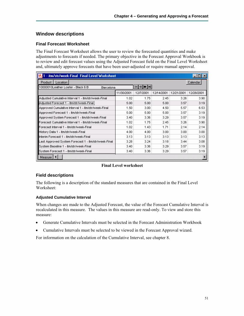
Chapter 4 – Generating and Approving a Forecast
51
Window descriptions
Final Forecast Worksheet The Final Forecast Worksheet allows the user to review the forecasted quantities and make adjustments to forecasts if needed. The primary objective in the Forecast Approval Workbook is to review and edit forecast values using the Adjusted Forecast field on the Final Level Worksheet and, ultimately approve forecasts that have been user-adjusted or require manual approval.
Final Level worksheet
Field descriptions The following is a description of the standard measures that are contained in the Final Level Worksheet:
Adjusted Cumulative Interval
When changes are made to the Adjusted Forecast, the value of the Forecast Cumulative Interval is recalculated in this measure. The values in this measure are read-only. To view and store this measure:
• Generate Cumulative Intervals must be selected in the Forecast Administration Workbook
• Cumulative Intervals must be selected to be viewed in the Forecast Approval wizard.
For information on the calculation of the Cumulative Interval, see chapter 8.
Retek Demand Forecasting, Retek Curve, Retek Promote
52
Adjusted Forecast
The value in this field initially defaults to the System Forecast if the forecast is automatically approved by the system or via a Forecast Approval Alert. Otherwise the value in the Adjusted Forecast will be different than the System Forecast if:
1. Adjusted Forecast has been updated by the user
2. Keep Last Changes is set to ‘Total’, ‘Difference’ or ‘Ratio’
3. Update Last Week(s) Forecast is set to ‘Replicate’
Changes to the Adjusted Forecast will be automatically approved. The Approval Worksheet will update with the date of the adjustment the name of the user to make the adjustment.
Note: Changes to the Adjusted Forecast for periods outside of the forecast horizon will not be committed.
Note: Edits to any non-committed values in the Forecast Approval workbook are overwritten when data is ‘Refreshed’.
Approved Cumulative Interval
The Approved Cumulative Interval is the cumulative interval that was approved at the time of the workbook build. The values contained in this measure are read-only. If changes are made to the Adjusted Forecast, the Approved Cumulative Interval will reflect the recalculated values when the workbook is committed and data is refreshed.
Approved Forecast
The Approved Forecast is the forecast quantity that was approved at the time of the workbook build. The values contained in this measure are read-only. If changes are made to the Adjusted Forecast, the Approved Forecast will update with the new values when the workbook is committed and data is refreshed.
Approved System Forecast
The Approved System Forecast is populated with the last System Forecast approved for a time series. :
1. Approval Method set to Automatic Approval
2. Approval Method set to a Forecast Approval Alert and the alert is not triggered
3. Update Last Week(s) Forecast is set to ‘Use Forecast’
The values in this measure are read-only.
Forecast Cumulative Interval
Cumulative Intervals are used in safety stock calculation within allocation and replenishment systems. This value is similar to a running total of the Forecast Interval and is read-only. To see this measure:
• Generate Cumulative Intervals must be selected in the Forecast Administration Workbook
• Cumulative Intervals must be selected to be viewed in the Forecast Approval wizard.
For information on the calculation of the Cumulative Interval, see chapter 8.

Chapter 4 – Generating and Approving a Forecast
53
Forecast Interval
The Forecast Interval is calculated on the particular forecast region as capped standard deviation for some methods. It takes into consideration the system forecast for capping (the default capping is no less than 30% of forecast and no more than 100% of forecast). When we approve forecasts we approve the corresponding Intervals and Cumulative Interval measures. To see this measure:
• Generate Intervals must be selected in the Forecast Administration Workbook
• Intervals must be selected to be viewed in the Forecast Approval wizard.
History Data
History Data is a read-only measure is the sales data used to generate the forecast. This allows the user to compare Actuals to forecasted values. When the workbook is created, the Data Source measure is copied into History Data.
Interim Forecast
The Interim Forecast is the forecast generated at the final level that is used as the Data Source in Curve to produce the Spreading Profile. This profile will determine how the Source Forecast will be spread down to the Final Forecast level. The values in this measure are read-only. To see this measure:
• Generate Interim Forecast must be selected in the Forecast Administration Workbook
• Interim Forecast must be selected to be viewed in the Forecast Approval wizard.
Last Approved System Forecast
The Last Approved System Forecast is the approved system forecast value when an approval occurred on a previous batch forecast for the time series. The values contained in this measure are read-only.
System Baseline
The System Baseline is a forecast generated on past sales data that contains no promotions (that is, normal demand given no causal effects). To see a generated Baseline Forecast:
• Promote must be implemented
• Generate Baseline must be selected in the Forecast Administration Workbook
• The System Baseline must be selected to be viewed in the Forecast Approval wizard.
For more information on the calculation of the System Baseline, see chapter 8.
System Forecast
The System Forecast displays the system generated forecast for the time series. The values contained in this field are read-only.
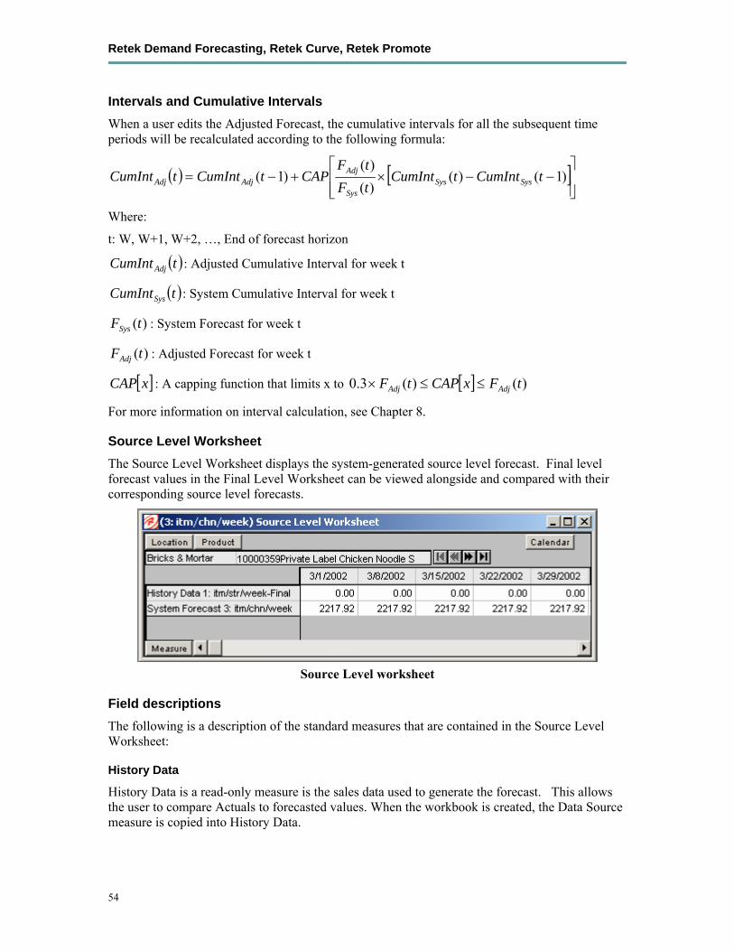
Retek Demand Forecasting, Retek Curve, Retek Promote
54
Intervals and Cumulative Intervals When a user edits the Adjusted Forecast, the cumulative intervals for all the subsequent time periods will be recalculated according to the following formula:
( ) [ ]⎥⎥⎦
⎤
⎢⎢⎣
⎡−−×+−= )1()(
)()(
)1( tCumInttCumInttFtF
CAPtCumInttCumInt SysSysSys
AdjAdjAdj
Where:
t: W, W+1, W+2, …, End of forecast horizon
( )tCumInt Adj : Adjusted Cumulative Interval for week t
( )tCumIntSys : System Cumulative Interval for week t
)(tFSys : System Forecast for week t
)(tFAdj : Adjusted Forecast for week t
[ ]xCAP : A capping function that limits x to [ ] )()(3.0 tFxCAPtF AdjAdj ≤≤×
For more information on interval calculation, see Chapter 8.
Source Level Worksheet The Source Level Worksheet displays the system-generated source level forecast. Final level forecast values in the Final Level Worksheet can be viewed alongside and compared with their corresponding source level forecasts.
Source Level worksheet
Field descriptions The following is a description of the standard measures that are contained in the Source Level Worksheet:
History Data
History Data is a read-only measure is the sales data used to generate the forecast. This allows the user to compare Actuals to forecasted values. When the workbook is created, the Data Source measure is copied into History Data.
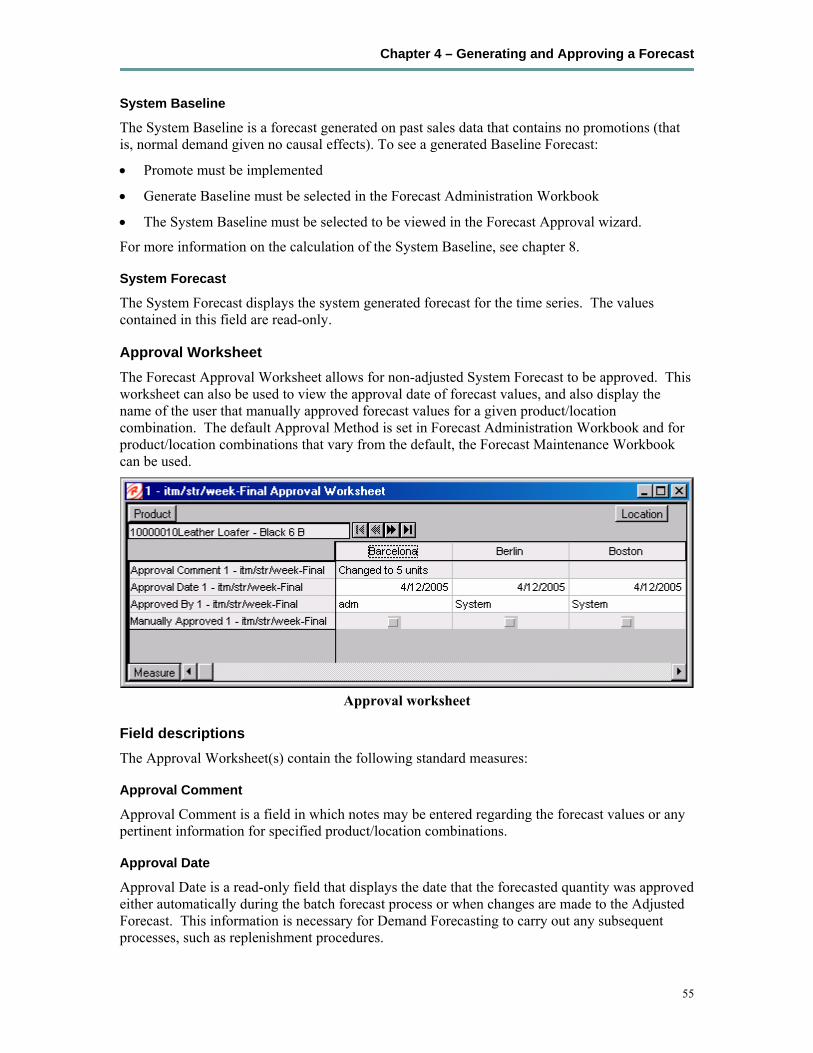
Chapter 4 – Generating and Approving a Forecast
55
System Baseline
The System Baseline is a forecast generated on past sales data that contains no promotions (that is, normal demand given no causal effects). To see a generated Baseline Forecast:
• Promote must be implemented
• Generate Baseline must be selected in the Forecast Administration Workbook
• The System Baseline must be selected to be viewed in the Forecast Approval wizard.
For more information on the calculation of the System Baseline, see chapter 8.
System Forecast
The System Forecast displays the system generated forecast for the time series. The values contained in this field are read-only.
Approval Worksheet The Forecast Approval Worksheet allows for non-adjusted System Forecast to be approved. This worksheet can also be used to view the approval date of forecast values, and also display the name of the user that manually approved forecast values for a given product/location combination. The default Approval Method is set in Forecast Administration Workbook and for product/location combinations that vary from the default, the Forecast Maintenance Workbook can be used.
Approval worksheet
Field descriptions The Approval Worksheet(s) contain the following standard measures:
Approval Comment
Approval Comment is a field in which notes may be entered regarding the forecast values or any pertinent information for specified product/location combinations.
Approval Date
Approval Date is a read-only field that displays the date that the forecasted quantity was approved either automatically during the batch forecast process or when changes are made to the Adjusted Forecast. This information is necessary for Demand Forecasting to carry out any subsequent processes, such as replenishment procedures.
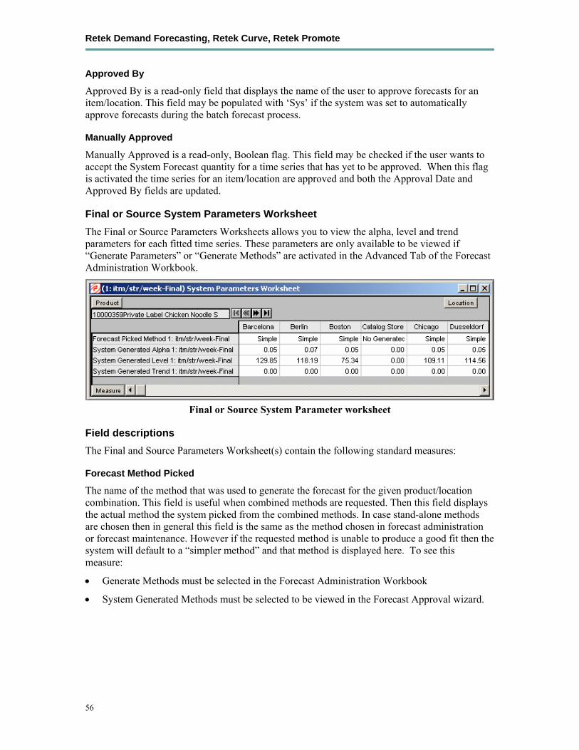
Retek Demand Forecasting, Retek Curve, Retek Promote
56
Approved By
Approved By is a read-only field that displays the name of the user to approve forecasts for an item/location. This field may be populated with ‘Sys’ if the system was set to automatically approve forecasts during the batch forecast process.
Manually Approved
Manually Approved is a read-only, Boolean flag. This field may be checked if the user wants to accept the System Forecast quantity for a time series that has yet to be approved. When this flag is activated the time series for an item/location are approved and both the Approval Date and Approved By fields are updated.
Final or Source System Parameters Worksheet The Final or Source Parameters Worksheets allows you to view the alpha, level and trend parameters for each fitted time series. These parameters are only available to be viewed if “Generate Parameters” or “Generate Methods” are activated in the Advanced Tab of the Forecast Administration Workbook.
Final or Source System Parameter worksheet
Field descriptions The Final and Source Parameters Worksheet(s) contain the following standard measures:
Forecast Method Picked
The name of the method that was used to generate the forecast for the given product/location combination. This field is useful when combined methods are requested. Then this field displays the actual method the system picked from the combined methods. In case stand-alone methods are chosen then in general this field is the same as the method chosen in forecast administration or forecast maintenance. However if the requested method is unable to produce a good fit then the system will default to a “simpler method” and that method is displayed here. To see this measure:
• Generate Methods must be selected in the Forecast Administration Workbook
• System Generated Methods must be selected to be viewed in the Forecast Approval wizard.

Chapter 4 – Generating and Approving a Forecast
57
System Generated Alpha
The system-calculated alpha value (which is an internal optimization parameter which corresponds to the rate of decay of the weighting on the historical values) for the corresponding product/location combination if the chosen method is one of the following methods: Simple, Holt, Additive Winters, Multiplicative Winters, and Profile Based. To see this measure:
• Generate Parameters must be selected in the Forecast Administration Workbook
• System Generated Parameters must be selected to be viewed in the Forecast Approval wizard.
System Generated Level
The system-calculated level (which is the constant baseline forecast) if the chosen method is one of the following methods: Simple, Holt, Additive Winters, Multiplicative Winters, and Seasonal Regression. To see this measure:
• Generate Parameters must be selected in the Forecast Administration Workbook
• System Generated Parameters must be selected to be viewed in the Forecast Approval wizard.
System Generated Trend
The system-calculated trend (which is the rate of change of the baseline forecast with time) if the chosen method is one of the following methods: Holt, Additive Winters, Multiplicative Winters, and Seasonal Regression. To see this measure:
• Generate Parameters must be selected in the Forecast Administration Workbook
• System Generated Parameters must be selected to be viewed in the Forecast Approval wizard.
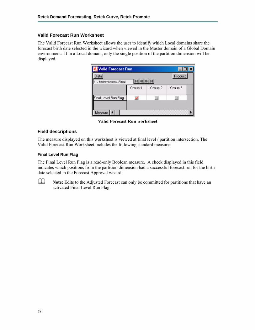
Retek Demand Forecasting, Retek Curve, Retek Promote
58
Valid Forecast Run Worksheet The Valid Forecast Run Worksheet allows the user to identify which Local domains share the forecast birth date selected in the wizard when viewed in the Master domain of a Global Domain environment. If in a Local domain, only the single position of the partition dimension will be displayed.
Valid Forecast Run worksheet
Field descriptions The measure displayed on this worksheet is viewed at final level / partition intersection. The Valid Forecast Run Worksheet includes the following standard measure:
Final Level Run Flag
The Final Level Run Flag is a read-only Boolean measure. A check displayed in this field indicates which positions from the partition dimension had a successful forecast run for the birth date selected in the Forecast Approval wizard.
Note: Edits to the Adjusted Forecast can only be committed for partitions that have an activated Final Level Run Flag.

Chapter 4 – Generating and Approving a Forecast
59
Approving Forecasts through Alerts (Exception Management) Overview Retek Demand Forecasting provides the user with ability to manually approve every single product/location forecast value. However, due to the extremely large volume of product/location forecast values that will be generated each forecast cycle, RPAS also provides additional functionality that enhances a user’s ability to evaluate and approve a forecast.
When configuring a RDF solution, specific Forecast Approval Alerts and alert parameters may be defined and applied during the batch process and may also be inserted into the Forecast Approval Workbook. In effect, alerts act as watchdogs and report product/location forecast values that exceed expected thresholds. If a specific product/location forecast value exceeds a threshold, the alert measure is flagged as “on” and visible to the user as a check mark in the appropriate product/location intersection on the interface.
The complexities of retail operations can result in the need to define many alerts; each designed to watch for a specific scenario that would require a user’s evaluation of a forecast value. For example:
• Alert 1: Forecast Value for a specific product/location has increased more than 30% since last week’s system forecast.
• Alert 2: Forecast Value for a specific product/location is zero although there is sales activity on the same product/location.
• Alert 3: Forecast Value is x% higher than Last Years Sales.
• Alert 4: A Forecast Value was generated for a product/location combination where no prior sales history exits.
For more information on how these measures are defined and registered as Alert measures, refer to the RPAS 11.1 Configuration Tools User Guide.
User-Defined Formatting Exceptions In addition to system defined alert measures, users can also leverage the RPAS Format functions to create user-specific exception alerts. For example, a user can format a workbook to show any value that is greater that 1000 to be displayed in bold red. This would make it easier for a user to scroll through forecast values, only stopping at the values in red for further evaluation.
The assumption is made that a user will understand their business, and be able to create simple formatting exceptions that will further enhance their ability to see the forecast values that need further evaluation prior to approval.

Retek Demand Forecasting, Retek Curve, Retek Promote
60
Procedure
Create a formatting exception 1. Click the Format button from the toolbar.
2. Click on Exceptions in the Formatting window.
3. Select the appropriate measure.
4. Enter a value for the low exception and the high exception.
5. Select the various font/color buttons to designate how these values should be displayed.
6. Once formatting is complete, make sure to save your formatting changes by clicking Format > Save Format > User/Template/Group
See the RPAS 11.1 User’s Guide or online help for more information on using RPAS formatting functionality.
Chapter 5 – Forecast Analysis Tools
61
Chapter 5 – Forecast Analysis Tools Overview Retek Demand Forecasting provides the user with a number of tools that may be used for additional forecast analysis. The Forecast Workbook template group provides the workbooks necessary to complete these tasks.
Interactive Forecasting Workbook Overview The Interactive Forecasting Workbook is a forecast simulation tool that allows the user to make changes to forecast parameters and see the results, without having to wait for the batch run. In this workbook, the user can edit various forecast parameters including sales history and forecast method. A new forecast is produced based on the changed parameters. In addition to forecasts, the Interactive Forecasting Workbook can also generate fit in historical region and the system picked model if an ES forecast method is used.
Procedure
Open the Interactive Forecasting workbook 1. Within the Local or Simple domain, select New from the File menu.
2. Select the Forecast tab to display a list of workbook templates.
3. Select Interactive Forecasting.
4. Click OK.
5. Select the forecast level.
6. Click Next.
7. Select the forecast starting date.
8. Click Next.
9. Select the first date in the historical data to use for generating the forecast.
10. Click Next.
11. Select the end date for the forecast horizon.
12. Click Next.
13. Specify future time periods beyond the forecast horizon to include in your workbook or Select Do not include dates after the horizon if no future dates are to be included in the workbook.
14. Click Next.
15. Select the products to be included in the workbook.
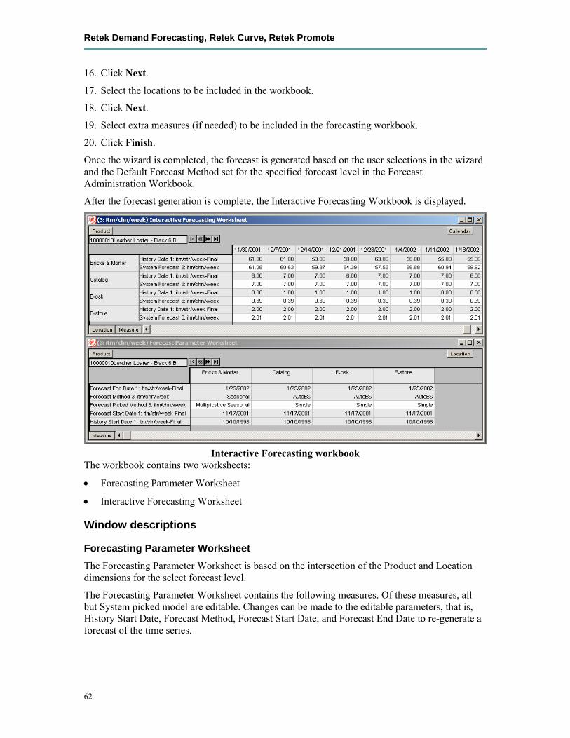
Retek Demand Forecasting, Retek Curve, Retek Promote
62
16. Click Next.
17. Select the locations to be included in the workbook.
18. Click Next.
19. Select extra measures (if needed) to be included in the forecasting workbook.
20. Click Finish.
Once the wizard is completed, the forecast is generated based on the user selections in the wizard and the Default Forecast Method set for the specified forecast level in the Forecast Administration Workbook.
After the forecast generation is complete, the Interactive Forecasting Workbook is displayed.
Interactive Forecasting workbook The workbook contains two worksheets:
• Forecasting Parameter Worksheet
• Interactive Forecasting Worksheet
Window descriptions
Forecasting Parameter Worksheet The Forecasting Parameter Worksheet is based on the intersection of the Product and Location dimensions for the select forecast level.
The Forecasting Parameter Worksheet contains the following measures. Of these measures, all but System picked model are editable. Changes can be made to the editable parameters, that is, History Start Date, Forecast Method, Forecast Start Date, and Forecast End Date to re-generate a forecast of the time series.
Chapter 5 – Forecast Analysis Tools
63
Field descriptions
Forecast Method
A drop-down list from which you can select the method used to generate the forecast. The workbook defaults to the method selected in the Forecast Administration Workbook for the specified level. A summary of methods is provided in the overview of chapter 2, and chapter 8 covers each method in detail.
Forecast Picked Method
This is the method that was used to generate the forecast for the given product/location combination. This field is useful when combined methods are requested (for example ES methods). Then this field displays the actual method the system picked from the combined methods. In case stand-alone methods are chosen then in general this field is the same as the method chosen in Forecast Administration or Forecast Maintenance. However if the requested method is unable to produce a good fit then the system will default to a “simpler method” and that method is displayed here.
History Start Date
The starting date for historical sales data. For example, if your system start date is January 1, 2003, but you only want to use historical sales data from the beginning of 1999, then you need to set your History Start Date to January 1, 1999. Only history after this date is used for generating the forecast. The default is the system start date unless otherwise specified. If sales data is collected weekly or monthly, Retek Demand Forecasting generates forecasts only using data from sales periods after the one containing the history start date.
It is also important to note that the system ignores leading zeros that begin at the history start date. For example, if your history start date is January 1, 1999 and an item/location does not have sales history until February 1, 1999, the system will consider the starting point in that item/location’s history to be the first data point where there is a non-zero sales value.
Forecast Start Date
This is first date of the forecast horizon. The default is the start date selected in the wizard.
Forecast End Date
This is the last date of the forecast horizon. The default is the end date selected in the wizard.
Interactive Forecasting Worksheet The Interactive Forecasting Worksheet is based on the intersection of the Product, Location, and Calendar dimensions for the forecast level selected in the wizard process. The Interactive Forecasting Worksheet contains the History Data and the System Forecast. Of these measures, only History Data is editable.

Retek Demand Forecasting, Retek Curve, Retek Promote
64
Field descriptions
History Data
This is the historical sales data set in the Forecast Administration workbook. This field is editable so you can change out-of-character sales if needed. For example, if your battery sales went up during a major power outage, you can lower the sales data back to a more normal level so the unusually high sales will adversely affect your forecast. However these changes are for simulation purposes only and cannot be committed.
System Forecast
The quantity that the system predicts will be required for the product, location, and calendar combination displayed. Changes to: History Data, History Start Date, Forecast Start Date, Forecast End Date and Forecast Method will cause the System Forecast to re-calculate when ‘Calculate’ is selected from the tool bar.

Chapter 5 – Forecast Analysis Tools
65
Forecast Scorecard Workbook Overview This section describes the purpose and content of the Forecast Scorecard and the steps required in order to create and access this workbook. This section also discusses the two types of worksheets contained in the Forecast Scorecard Workbook, as well as the definitions of parameters that exist in each. Evaluating forecast accuracy through the use of error statistics is discussed, as is the process of comparing historical forecasts to actual sales data.
The purpose of the Forecast Scorecard is to monitor the accuracy of both system-generated forecasts and approved final forecasts. Once a forecast has been generated and actual point-of-sale data is received for the forecasted period, statistical information can be reviewed to help you analyze the accuracy of forecasting models and methods.
The Forecast Scorecard template consists of a wizard and two worksheets.
Based on your selections in the wizard, the Forecast Scorecard provides statistical information and comparison data that allow you to monitor the accuracy of system-generated forecasts and final approved forecasts.
• The Final Error Measure Worksheet displays statistical information, such as mean error and root mean squared error, that reflects the accuracy of the forecast.
• The Final Actuals vs. Forecasts Worksheet displays forecast results and actual point-of-sale values for specified product/location/calendar combinations.
Procedure
Open Forecast Scorecard
• Select Open from the File menu to bypass the Forecast Scorecard Wizard OR
1. Within the Master, Local or Simple domain, select New from the File menu.
2. Select the Forecast tab to display a list of workbook templates.
3. Select Forecast Scorecard
4. Click OK. The Forecast Scorecard wizard opens.
5. You are prompted to select the forecast level that you want to evaluate. Make a selection
6. Click Next.
7. Select the generation date of the forecast you wish to review.
Click “Use the most recent generated forecast” to build a workbook containing the most recent forecast values.
Click “Select from a list of forecast” to select from a list of previously generated forecasts stored in the system.
8. Click Next.
9. Select the measures associated with the forecast results to be evaluated.

Retek Demand Forecasting, Retek Curve, Retek Promote
66
10. Click Next.
11. Check the boxes corresponding to the error statistics that you want calculated for the forecast data.
12. Click Next.
13. Select the specific locations you want to view. It is important to include all locations that are members of the location dimensions in the forecast levels to be analyzed. For example, if you select to view a forecast level that is defined at item/chain/week, you should include all locations that are members of the particular chain to be analyzed. It is recommended that ‘Position Query’ functionality or selection from aggregate levels in the Location hierarchy is employed if the workbook supports an AutoWorkbook build. Make your selection.
14. Click Next.
15. Select the merchandise you want to view. It is important to include all products that are members of the Merchandise dimensions in the forecast levels to be analyzed. For example, if you select to view a forecast level that is defined at subclass/store/week, you must include all items that are members of the particular subclass to be analyzed. It is recommended that ‘Position Query’ functionality or selection from aggregate levels in the Merchandise hierarchy is employed if the workbook supports an AutoWorkbook build. Make your selection.
16. Click Next.
17. Select the first date of history to include in the workbook. You may either choose to set the “Forecast Start Date minus the number of periods” or select the first date of history from the displayed list. It is recommended that the “Forecast Start Date minus the number of periods” is set if the workbook supports an AutoWorkbook build. Make your selection.
18. Click Next.
19. Select the last date in the forecast horizon to include in the workbook.
Choose “Include the following number of time periods of the forecast horizon”
Note: It is recommended that “Include the following number of time periods of the forecast horizon” is set if the workbook supports an AutoWorkbook build.
Select the last date to include of the horizon from the displayed list.
20. Click Next.
21. Select the last date in the calendar to include in the workbook.
Set the “Forecast end date plus the following number of time periods”
Note: It is recommended that “Forecast end date plus the following number of time periods” is set if the workbook supports an AutoWorkbook build.
Select the last date to include of the post-horizon calendar from the displayed list.
22. Click Next.
23. Select any additional measures to be included in the workbook.
24. Click Finish.
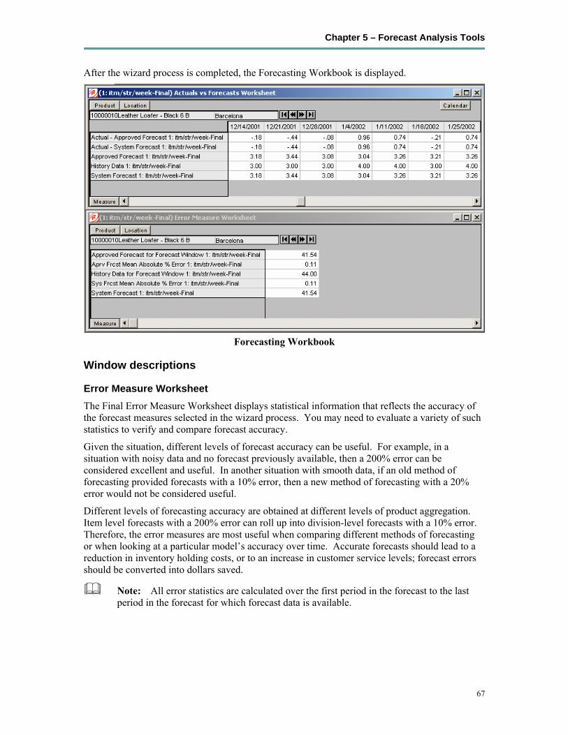
Chapter 5 – Forecast Analysis Tools
67
After the wizard process is completed, the Forecasting Workbook is displayed.
Forecasting Workbook
Window descriptions
Error Measure Worksheet The Final Error Measure Worksheet displays statistical information that reflects the accuracy of the forecast measures selected in the wizard process. You may need to evaluate a variety of such statistics to verify and compare forecast accuracy.
Given the situation, different levels of forecast accuracy can be useful. For example, in a situation with noisy data and no forecast previously available, then a 200% error can be considered excellent and useful. In another situation with smooth data, if an old method of forecasting provided forecasts with a 10% error, then a new method of forecasting with a 20% error would not be considered useful.
Different levels of forecasting accuracy are obtained at different levels of product aggregation. Item level forecasts with a 200% error can roll up into division-level forecasts with a 10% error. Therefore, the error measures are most useful when comparing different methods of forecasting or when looking at a particular model’s accuracy over time. Accurate forecasts should lead to a reduction in inventory holding costs, or to an increase in customer service levels; forecast errors should be converted into dollars saved.
Note: All error statistics are calculated over the first period in the forecast to the last period in the forecast for which forecast data is available.

Retek Demand Forecasting, Retek Curve, Retek Promote
68
Field descriptions The following is a description of the measures that can be included in the Final Error Measure Worksheet: The error statistics will be shown for each forecast you chose to include in the workbook (such as System Forecast, Final Forecast, etc.).
History Data for Forecast Window
The sum of all actual sales from the first period in the forecast to the last period in the forecast for which point-of-sale data is available.
System Forecast, Adjusted Forecast, Approved Forecast, Approved System Forecast, Interim Forecast
Your workbook may include one or all of the above forecast measures. These measures are selected in the wizard process. This is the average value of these measures over the forecast horizon select in the wizard process.
Mean Error
The error of a forecast observation is the difference between the forecasted value and the actual POS value. The Mean Error statistic is a measure of the average error over time, calculated by summing the errors for all observations, then by dividing by the number of observations to obtain the average. It measures forecast accuracy by calculating the error in units. Because a positive error in one period can cancel out a negative error in another period, this measure is useful when you are interested in how well the forecast predicts over the forecast horizon rather than on a period-to-period basis. Mean error is, however, useful as a measure of forecast bias; a negative mean error suggests that, overall, the forecasting model overstates the forecast, while a positive mean error indicates forecasts that are generally too low.
∑=
−nsobservatioof#
1)(
nsobservatioof#1
iii ForecastActual
Mean Absolute Error
The absolute error of a forecast observation is the absolute value of the difference between the forecasted value and the actual POS value. The Mean Absolute Error statistic is a measure of the average absolute error, calculated by summing the absolute errors for all observations, then by dividing by the number of observations to obtain the average. Mean Absolute Error gives you a better indication of how the forecast performed period by period, because the absolute value function ensures that negative errors in one period are not canceled out by positive errors in another. Mean Absolute Error is most useful for comparing two forecast methods for the same series.
∑=
−nsobservatioof#
1nsobservatioof#1
iii ForecastActual
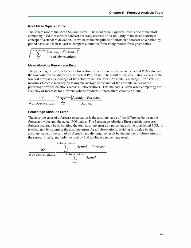
Chapter 5 – Forecast Analysis Tools
69
Root Mean Squared Error
The square root of the Mean Squared Error. The Root Mean Squared Error is one of the most commonly used measures of forecast accuracy because of its similarity to the basic statistical concept of a standard deviation. It evaluates the magnitude of errors in a forecast on a period-by-period basis, and is best used to compare alternative forecasting models for a given series.
( )∑=
nsobservatio of #
1
2
nsobservatio of #i
ii t - ForecasActual
Mean Absolute Percentage Error
The percentage error of a forecast observation is the difference between the actual POS value and the forecasted value, divided by the actual POS value. The result of this calculation expresses the forecast error as a percentage of the actual value. The Mean Absolute Percentage Error statistic measures forecast accuracy by taking the average of the sum of the absolute values of the percentage error calculations across all observations. This method is useful when comparing the accuracy of forecasts for different volume products (it normalizes error by volume).
∑=
−nsobservatio of #
1nsobservatio of #100
i i
ii
ActualForecastActual
Percentage Absolute Error
The absolute error of a forecast observation is the absolute value of the difference between the forecasted value and the actual POS value. The Percentage Absolute Error statistic measures forecast accuracy by calculating the total absolute error as a percentage of the total actual POS. It is calculated by summing the absolute errors for all observations, dividing this value by the absolute value of the sum of all Actuals, and dividing the result by the number of observations in the series. Finally, multiply the total by 100 to obtain a percentage result.
∑
∑
=
=−
nsobservatioof#
1
nsobservatioof#
1nsobservatioof#
100
ii
iii
Actual
ForecastActual

Retek Demand Forecasting, Retek Curve, Retek Promote
70
Actuals vs. Forecasts Worksheet This worksheet displays forecast results and actual point-of-sale values for each product, location, and time period specified in the Forecast Scorecard Wizard. This worksheet allows you to compare the results of both system-generated forecasts and final approved forecasts to actual sales quantities.
The Actuals vs. Forecasts Worksheet may contain the following measures:
Actuals – (minus) System Forecast, Adjusted Forecast, Approved Forecast, Approved System Forecast, Interim Forecast
Displays the difference between the actual sales quantities and the committed forecast values for the forecast measures selected during the wizard process. Negative values indicate that the final forecast exceeded actual sales.
History Data
History Data displays the actual point-of-sale quantities for the product, location, and calendar combinations displayed.
System Forecast, Adjusted Forecast, Approved Forecast, Approved System Forecast, Interim Forecast
Your workbook may include one or all of the above forecast measures. These measures are selected in the wizard process. These measures display the forecasted quantity for the product, location, and calendar combinations included in the workbook.

Chapter 6 – Promote (Promotional Forecasting)
71
Chapter 6 – Promote (Promotional Forecasting) Overview Promote is an optional add-on automated predictive solution that allows you to incorporate the effects of promotional and causal events, such as radio advertisements and holiday occurrences, into your time-series forecasts. The promotional forecasting process uses both past sales data and promotional information to forecast future demand.
This chapter provides an introduction to promotional forecasting and explains how it differs from the traditional statistical forecasting methodology. It discusses the advantages and limitations of both statistical and promotional forecasting models, and outlines the use of Retek’s Causal method of forecasting demand. It describes terminology used in the context of promotional forecasting, and concludes with detailed descriptions of the workbook templates contained in the Promote Workbook Template Group.
What is Promotional Forecasting? Traditional statistical forecasting methods provide significant benefits to the process of forecasting consumer demand, because they are good at predicting level, trend, and seasonality based on sales history. The limitation of traditional statistical methods is that they forecast with less accuracy when there are special events that cause significant deviations in selling patterns.
For example, the Easter holiday, for which companies often run promotions, occurs on a different date each year. Traditional statistical forecast methods can identify seasonality in sales history, but this seasonality is based on periodic similarities in the sales pattern. Since Easter occurs on different dates from year to year (that is, its period of recurrence is not regular), manual intervention is required to predict change in demand using the traditional statistical forecasting method. Events like this are called promotion events. Promotion events, such as advertisements, irregularly occurring holidays, competitor information, free gift with purchase offers, etc., are events that drive businesses from the normal selling cycle. The goal of a promotional forecasting system is to improve time series forecasting by:
• Providing the forecasting system with visibility as to when certain promotion events were active in the past (for example, identifying which weeks of a given year were affected by an Easter promotion).
• Automatically determining the statistical effect, if any, of these events.
• Incorporating significant effects into the future forecasts for time periods also associated with the observed promotion event.
The Promote module combines the automation of statistical time series forecasting with the improved accuracy found in customized causal forecasting. Promote uses both past sales data and promotional information (for example, advertisements, holidays) to forecast future demand. In order to understand the underlying rationale for the promotional forecasting process, it is important to understand the advantages and limitations of its underlying components.

Retek Demand Forecasting, Retek Curve, Retek Promote
72
Comparison between promotional and statistical forecasting Statistical time series forecasting uses past demand to predict future demand. The most basic component of the time series forecast is the level of sales. This is usually determined by looking at demand in the recent past. Often there also exists an underlying trend that can be detected within sales history. This is usually determined by looking at the change in demand in the recent past. A third factor influencing retail demand is seasonality. A forecasting algorithm trying to determine the effects of seasonality can only look for periodic similarities in the sales pattern. For example, December sales from previous years can be used to adjust the forecast for December only because December occurs regularly every 12 months. At every step the time series approach is limited to using historical demand to predict future demand, without regard to the underlying causes that are driving demand in the first place.
Promotional events, however, can create problems in estimating level, trend, and seasonality. Certain events, such as irregularly occurring holidays, newspaper/radio advertisements, free gift with purchase offers, and special discounts can cause significant deviations from the selling pattern.
Promotional forecasting unlike statistical forecasting attempts to predict future demand by identifying the factors that influence spikes and lulls of past demand. Once these factors are known, the magnitude and direction of their effect can be evaluated. Their presence can then be incorporated into forecasting models for use during times when the causal factors are again expected to be present.
Developing promotional forecast methods This section describes how custom promotional forecast models have been developed in the past, leading to the discovery of several consistent findings. These findings have been incorporated into Retek’s development of the Promote forecasting module.
Promotional forecasting uses promotional factors to predict future demand. The first step is to determine all of the pertinent information affecting sales and transform this information into variables that the system understands. Seasonality, for instance, can be represented by a single seasonal continuous variable, such as the number of daylight hours or average daily temperature.
Alternatively, it can be represented by 12 different indicator variables representing each of the months. An indicator variable consists only of 0’s and 1’s, a 1 indicating that the event is “on”. For example, a monthly indicator variable for January would consist of a 1 during the first month of the year and 0’s for the remaining months.
Once a list of variables is determined, the model needs to represent the promotion events in terms of their influence on overall demand. For example, if a set of promotional variables has a multiplicative promotional effect on demand, a log transformation may be needed to improve the model. After a suitable model is developed, it must be implemented using multivariate linear regression or neural network architecture, with custom code handling the data loading and variable transformations. The final custom model may be quite accurate over the data set on which it was developed. However, this model may not be general enough to be used universally across all data sets, thus requiring the development of multiple custom models to cover a client’s entire domain. This has been found to be very time consuming and costly.

Chapter 6 – Promote (Promotional Forecasting)
73
The process of developing custom promotional models has, however, brought to light a number of consistent patterns:
• Level, trend, and seasonality are universal components of almost any forecast.
• Including a time-series forecast as an input variable often improves promotional models.
• Indicator variables are robust in that they can represent both additive and multiplicative effects.
These findings have led Retek to develop a novel approach to promotional forecasting that combines the automation and generalization of time series forecasting with the improved (albeit data set specific) accuracy met through customized causal forecasting.
Retek’s approach to promotional forecasting Retek’s approach to promotional forecasting is somewhat unusual. Retek combines time series forecast methods with causal forecast methods, resulting in a new forecast method supported by the Promote module. Promote uses the AutoES method of forecast generation to determine a baseline time series forecast, and then uses indicator variables to represent promotional events of interest. By giving the forecasting routine visibility as to when certain events occurred in the past, the system can correlate changes in the sales demand with these events and determine each promotional event’s effect on sales. Then whenever these events occur in the future, the promotional effects can be incorporated into the forecast.
The Promote module has been developed to produce generalized promotional models automatically, with little human intervention. Combined with the system’s ability to allow you to develop your own data loading routines, Promote provides a cost-effective means for producing forecasts using promotional information.
More detailed information on promotional forecasting methods is in Chapter 8.
Retek Demand Forecasting, Retek Curve, Retek Promote
74
Promotional forecasting terminology and workflow Promote is designed to produce sales forecasts using both past sales history and event on/off information, both of which you provide. Using the sales data, the system first determines a seasonal time series model to describe the purchasing behavior of consumers. Differences between the seasonal model and the actual sales are then correlated with known events. Events that are found to have a statistically significant impact on sales are then included in a promotional forecast model as promotion events. For each promotion event, its promotion effect on sales is determined. The final promotional model consists of the seasonal model, promotion event on/off information, and each promotion event’s resulting effect on sales. By combining these three, a final promotional forecast is computed.
Examples of promotion events The following are examples of promotional variables that could be created and the manner in which their associated on/off event status is specified:
Example 1: Christmas Day applies to all products/locations. The Christmas promotional variable will therefore have only one dimension – Day. Because Christmas Day falls on the 359th day of each non-leap year, the Day359 variable will be set to TRUE for every such year (all other days will be set to FALSE).
Example 2: A television advertisement is run locally in the New York/New Jersey area for the four weeks at the beginning of the spring fashion season. The TVAD promotional variable will have two associated dimensions – State and Week. Week13, Week14, Week15, and Week16 will be set to TRUE only for states NY and NJ (all other states/weeks will be set to FALSE). Since no product dimension exists, the TV ad is assumed to have an effect on all products.
Example 3: A holiday promotion is run involving all sporting goods items for the two weeks prior to Father’s Day. The Father's Day promotional variable has two associated dimensions – item and Week. For this year, Week23 and Week24 will be set to TRUE only for individual items related to sporting goods items (all other weeks and all other items will be set to FALSE). Since no location dimension exists, the Father’s Day promotion is assumed to apply to all stores.
After promotional variables have been loaded into Retek Demand Forecasting, you can use the Promotion Planner workbook to view, edit, and update associated values without having to reload new data.

Chapter 6 – Promote (Promotional Forecasting)
75
Promote Workbooks and wizards The Promote Workbooks and wizards allow you to manage the promotion events used in the system’s promotional forecasting processes, and view/edit the system’s analysis of the effects of these events on demand. The Promote Workbook templates include:
• Promotion Planner - Allows you to specify when certain promotional events were active in the past, and when they will be active in the future.
• Promotion Maintenance– Allows you to review the system-calculated promotional lift effects, edit these effects and determine how changes will be factored into the promotional model.
• Promotion Effectiveness – Our promotional what-ifing workbook. Allows the user to analyze the performance of previous promotions and simulate future promotions by editing when promotional events will be active for an item/location, and by modifying the promotion lift effects.
• Forecast Administration – External to Promote, the Forecast Administration workbook includes several parameters that may be used as additional configuration options for promotional forecasting:
Causal Aggregation Profile
Causal Calculation Intersection
Causal Calculation Intersection Periodicity
Causal Data Source
Causal Higher Intersection
Casual Spread Profile
Note: For more information on the Causal parameters external to Promote, please see the section on the Forecast Administration workbook (Chapter 1).

Retek Demand Forecasting, Retek Curve, Retek Promote
76
Promotion Planner Workbook Template Overview In order to correlate deviations from the seasonal forecast with the occurrence of historic promotion events, the system needs visibility as to when these events were active. The system must also be informed of dates on which the status of upcoming promotion events will again be “on,” so the anticipated promotion effects can be built into the forecasting model.
The Promotion Planner Workbook allows you to indicate to the system when certain events were active in the past, and when they will be active in the future. All promotional events should be represented as accurately as possible so the modeling routine can more precisely detect correlations between event occurrences and changes in sales values.
The Promotion Planner Workbook consists of as many worksheets as are necessary to represent all unique dimensional intersections associated with the promotion events contained in the workbook. A separate worksheet is constructed for each of the required intersections. For example, promotion events such as Advertisement and Gift with Purchase may be loaded at the [Item/Store/Week] intersection, while an event such as Christmas is loaded at the [Day] level.
In this setup, the Advertisement and Gift with Purchase promotions would appear on one worksheet, and Christmas would appear on another. Whenever a hierarchy is not included in the base intersection (as in the case of the Christmas promotional event) the event is assumed to apply to all positions in the undefined hierarchy. Thus, Christmas is assumed to apply to all products and all locations, but only to the Day-level calendar position(s) specified in the Promotion Planner Worksheet.
Procedure The Promotion Planner wizard steps you through the process of creating a new Promotion Planner Workbook from a template. To access the Promotion Planner, select Open from the File menu to bypass the wizard and open an existing Promotion Planner Workbook, or perform the following steps:
1. Within the Local or Simple domain, select New from the File menu.
2. On the Promote tab, select Promotion Planner.
3. Click OK.
4. The Promotion Planner wizard opens and prompts you to select the promotion events to edit or review.
5. Click Next.
6. Select the locations that need to have promotions planned.
7. Click Next.
8. Select the products that need to have promotions planned.
9. Click Next.
10. Select the dates that need to have promotions planned.
11. Click Next.
12. Click Finish to build the workbook.
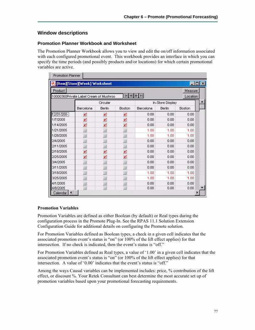
Chapter 6 – Promote (Promotional Forecasting)
77
Window descriptions
Promotion Planner Workbook and Worksheet The Promotion Planner Workbook allows you to view and edit the on/off information associated with each configured promotional event. This workbook provides an interface in which you can specify the time periods (and possibly products and/or locations) for which certain promotional variables are active.
Promotion Variables
Promotion Variables are defined as either Boolean (by default) or Real types during the configuration process in the Promote Plug-In. See the RPAS 11.1 Solution Extension Configuration Guide for additional details on configuring the Promote solution.
For Promotion Variables defined as Boolean types, a check in a given cell indicates that the associated promotion event’s status is “on” (or 100% of the lift effect applies) for that intersection. If no check is indicated, then the event’s status is “off.”
For Promotion Variables defined as Real types, a value of ‘1.00’ in a given cell indicates that the associated promotion event’s status is “on” (or 100% of the lift effect applies) for that intersection. A value of ‘0.00’ indicates that the event’s status is “off.”
Among the ways Causal variables can be implemented includes: price, % contribution of the lift effect, or discount %. Your Retek Consultant can best determine the most accurate set up of promotion variables based upon your promotional forecasting requirements.
Retek Demand Forecasting, Retek Curve, Retek Promote
78
Promotion Maintenance Workbook Template Overview The Promotion Maintenance workbook provides a view to the system-calculated and adjusted lift effects. You can edit effects at any product/location intersection and determine how these changes will be factored into the promotional models. The Promotion Maintenance Workbook contains one worksheet. There may be multiple versions of this worksheet, defined at various causal levels.
Procedure
Open the Promotion Maintenance Workbook Template
The Promotion Maintenance wizard steps you through the process of creating a new Promotion Maintenance Workbook from a template.
1. Within the Local or Simple domain, select New from the File menu.
2. On the Promote tab, select Promotion Maintenance.
3. Click OK.
4. Select the promotion events to analyze.
5. Click Next.
6. Select the causal forecast level for analysis.
7. Click Next.
8. Select the locations to analyze.
9. Click Next.
10. Select the products to analyze.
11. Click Next.
12. Select additional measures to view in the workbook (if necessary).
13. Click Finish.
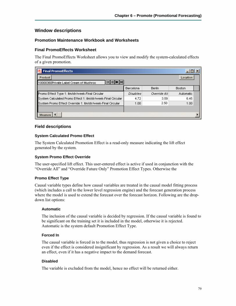
Chapter 6 – Promote (Promotional Forecasting)
79
Window descriptions
Promotion Maintenance Workbook and Worksheets
Final PromoEffects Worksheet The Final PromoEffects Worksheet allows you to view and modify the system-calculated effects of a given promotion.
Field descriptions
System Calculated Promo Effect
The System Calculated Promotion Effect is a read-only measure indicating the lift effect generated by the system.
System Promo Effect Override
The user-specified lift effect. This user-entered effect is active if used in conjunction with the “Override All” and “Override Future Only” Promotion Effect Types. Otherwise the
Promo Effect Type
Causal variable types define how causal variables are treated in the causal model fitting process (which includes a call to the lower level regression engine) and the forecast generation process where the model is used to extend the forecast over the forecast horizon. Following are the drop-down list options:
Automatic
The inclusion of the causal variable is decided by regression. If the causal variable is found to be significant on the training set it is included in the model, otherwise it is rejected. Automatic is the system default Promotion Effect Type.
Forced In
The causal variable is forced in to the model, thus regression is not given a choice to reject even if the effect is considered insignificant by regression. As a result we will always return an effect, even if it has a negative impact to the demand forecast.
Disabled
The variable is excluded from the model, hence no effect will be returned either.

Retek Demand Forecasting, Retek Curve, Retek Promote
80
Override All
This type allows the user to specify a causal effect that will be used during the fitting and forecasting process. This is a directive that is recognized only by the causal engine and not by the lower level regression engine. For causal variables specified as Override All, the user also specifies the corresponding causal effect in the Promotion Effect Override. The causal engine then de-causalizes the training data using the user-specified effect. The variable then is internally set Disabled to calculate the fit. During forecast generation the user-specified effect is used to determine the causal forecast. Therefore, the user must change the Promotion Effect Type when this user-specified effect is no longer to be used.
Override Future Only
This type allows the user to specify a causal effect that will be used only during forecasting process and not during the fitting process. This is also a directive that is recognized only by the causal engine and not by the lower level regression engine. For causal variables specified as Override Future, the user also specifies the corresponding causal effect in the Promotion Effect Override. The causal engine then internally sets the causal variable to Automatic to calculate the fit. The calculated effect is not however written back to the effects array (so as to not overwrite the user specified effect). During forecast generation the calculated effect is ignored and instead the user-specified effect is used to produce a causal forecast. Therefore, the user must change the Promotion Effect Type when this user-specified effect is no longer to be used.
Override From Higher Level
Used in conjunction with the Causal Higher Intersection set in the Forecast Administration Workbook, this promotion type allows the system to use an average value of causal effects computed from product/location combination in the same group (the intersection level specified in the Causal Higher Intersection during system setup) for product/location combinations for which sales history alone a causal effect is unable to be computed for that causal variable. The way the system handles this is by having the effects array filled in with higher-level effects for those variable specified as “Override Higher Level” and which did not have an effect returned in the previous run. The effect array is passed to the causal engine. If the engine succeeds in computing a significant effect it writes back the system computed effect and uses it for generating a forecast. Otherwise it uses the effect passed in (which as mentioned is the average effect among product stores belonging to the same group) for generating the forecast.
Automatic Boolean
If the promotion variable will always be set to 0.00 or 1.00 (meaning inactive or active respectively), this type will produce the same results as the Automatic type described above, however Automatic Boolean will improve the performance (speed) of the forecasting engine during the batch run of the forecast.
Note: Changes that are committed in the Promotion Maintenance Workbook will not be incorporated into the forecast until another forecast is generated in RDF batch forecast process.
Chapter 6 – Promote (Promotional Forecasting)
81
Promotion Effectiveness Workbook Template Overview The Promotion Effectiveness Workbook Template is a historical and future view to the effects of a planned promotion.
This workbook has two worksheets:
• View of promotion effects
• Visibility to Actuals, forecasts, baselines and promotion variable/event information
In this workbook a user views the promotional forecast. There is also the ability to analyze the effects on the forecast if a promotion does or does not occur. This analysis is performed by turning a promotional event or attribute on or off for dates in the future plans, and/or by modifying the Simulated Promo Effect. This workbook is intended for simulation and analysis purposes only. There is no Commit functionality.
Procedure
Open the Promotion Effectiveness Workbook Template
The Promotion Effectiveness wizard steps you through the process of creating a new Promotion Effectiveness Workbook from a template.
1. Within the Local or Simple domain, select New from the File menu.
2. On the Promote tab, select Promotion Effectiveness
3. Click OK.
4. Select the promotion events to analyze.
5. Click Next.
6. Select the forecast level for analysis.
7. Click Next.
8. Select the dates to analyze.
9. Click Next.
10. Select the locations to analyze.
11. Click Next.
12. Select the products to analyze.
13. Click Next.
14. Select any additional measures that to be included in the workbook (if necessary).
15. Click Finish.
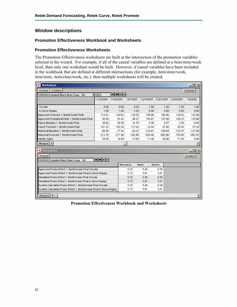
Retek Demand Forecasting, Retek Curve, Retek Promote
82
Window descriptions
Promotion Effectiveness Workbook and Worksheets
Promotion Effectiveness Worksheets The Promotion Effectiveness worksheets are built at the intersection of the promotion variables selected in the wizard. For example, if all of the causal variables are defined at a item/store/week level, then only one worksheet would be built. However, if causal variables have been included in the workbook that are defined at different intersections (for example, item/store/week, item/store, item/class/week, etc.), then multiple worksheets will be created.
Promotion Effectiveness Workbook and Worksheets

Chapter 6 – Promote (Promotional Forecasting)
83
Field descriptions The Promotion Effectiveness Worksheets contain the following measures:
Approved Forecast
Read-only measure. This is the latest forecast quantity approved for the product/location combination.
Note: Changes that are committed in the Promotion Maintenance Workbook are used to determine values for the System Calculated Promo Effect and the Approved Promo Effect. However, if a forecast has not been generated in RDF since the changes were made in the Promotion Maintenance Workbook, the Approved Forecast will not include these changes.
Approved Promotional Peak
Read-only measure. The Approved Promotional Peak is the unit-lift over the Baseline Forecast calculated during the forecast generation process.
The process of approving any time series with a promotional peak also approves both the forecast and the associated promotional peak. Approval can be automatic, manual or by a forecast approval alert (see the Forecast Approval Workbook in Chapter 4 for more details).
Future Baseline
Read-only measure. Calculated as the Approved Forecast minus (–) the Approved Promotional Peaks. User-changes to the editable measures in the Promotion Effects workbook do not affect this value.
Future Forecast
Read-only measure. The Future Promo Forecast equals the Future Promo Baseline multiplied by the Simulated Promo Effect if the promotion variable is greater than 0 (zero). If there are more than one promotion variables, the sum of the Simulated Promo Effects for the variables is multiplied by the Future Promo Baseline.
If there is no promotion variable, then the Future Promo Forecast equals the Future Promo Baseline.
Historical Baseline
Read-only measure. Calculated in one of two ways depending on the value of the Approved Forecast:
1. Historical Promo Baseline equals Sales minus the Approved Promotion Peak, if the Approved Forecast is greater than 0 (zero).
2. Historical Promo Baseline equals Sales with the Moving Average applied if the Approved Forecast equals 0 (zero). If Sales are also 0 (zero), then the Historical Promo Baseline will also equal 0 (zero).

Retek Demand Forecasting, Retek Curve, Retek Promote
84
Historical Forecast
Read-only measure. The Historical Promo Forecast equals the Historical Promotion Baseline multiplied by the Simulated Promo Effect if the promotion variable is greater than 0 (zero). If there are more than one promotion variables, the sum of the Simulated Promo Effects for the variables is multiplied by the Historical Promo Baseline.
If there is no promotion variable, then the Historical Promo Forecast equals the Historical Promo Baseline.
Approved Promo Effect
A read-only measure. This is the approved promotion lift effect used in the generation of the current Approved Forecast in RDF.
Simulated Promo Effect
A read/write measure. The Simulated Promo Effect will default to the Approved Promo Effect. Changes to this measure will recalculate the Historical Promo Forecast and the Future Promo Forecast.
System Calculated Promo Effect
The System Calculated Effect is a read-only measure. This is the promotion lift effect originally calculated by the system during the forecast generation process. This value can be different than the Approved Promo Effect if the user edited the Promotion System Effect Override in the Promotion Maintenance workbook, then another batch forecast was ran.
Note: Changes to the Promotion Effects Workbook cannot be committed back to the master database, however this workbook is useful for:
• Reporting on the performance of past promotions
• Simulating the effects of future promotions to support more accurate promotional modeling

Chapter 6 – Promote (Promotional Forecasting)
85
Procedures in Promotional Forecasting The following outlines the standard procedures performed in order to set up the system to run a promotional forecast (more detailed steps follow in the next section):
• Set up the system to run a promotional forecast
• Set forecast parameters in the Forecast Administration Workbook
• Set forecast parameters in the Forecast Maintenance Workbook
• Set promotions to be active in the Promotion Planner Workbook
• Run the batch forecast
• View and Edit Causal Forecast results
• Analyze forecasts in the Forecast Approval Workbook
• Analyze and edit causal effects in the Promotion Maintenance Workbook
• Promotion Simulation (what-ifing) and Analysis
Set up the system to run a promotional forecast 1. On the Forecast tab, select and build a Forecast Administration Workbook
a. In the Forecast Administration Workbook: Advance Parameter Worksheet, select Generate Baseline.
b. Optional: Set the Default Forecast Method to “Causal” for the desired level if the level is to be use only for Promotional Forecasting.
c. Optional: Set the Causal Higher Intersection for the desired level if the Override from Higher Level promotion type will be used.
d. Optional for use with Daily Causal Forecasting: Set the values for the following parameters:
Causal Aggregation Profile
Causal Calculation Intersection
Causal Calculation Intersection Periodicity
e. Commit your changes to the master database by selecting Commit Now from the File menu.
2. On the Forecast tab, select and build a Forecast Maintenance Workbook
a. Set the Forecast Method Override to “Causal” for any items/locations at the desired levels that will utilize Promotional Forecasting.
b. Commit your changes to the master database by selecting Commit Now from the File menu.

Retek Demand Forecasting, Retek Curve, Retek Promote
86
3. On the Forecast tab, select and build a Promotion Planner Workbook
a. Set causal variables for items and locations historically in that the selected promotions are active.
b. Commit your changes to the master database by selecting Commit Now from the File menu.
4. On the Forecast tab, select Run Batch
Generate a Forecast
View a forecast that includes promotion effects 1. On the Forecast tab, select and build a Forecast Approval Workbook and include System
Baseline in your workbook.
2. In the Final Level Worksheet review the System Baseline and the System Forecast. The System Baseline is predicted demand given no causal effects. The System Forecast is the sum of the System Baseline and the Promotional Peak calculated during the forecast generation process based on the causal data and settings.
View and edit Promotion System-Calculated Effects: 1. On the Promote tab, select and build a Promotion Maintenance Workbook
a. In the PromoEffects Worksheet review the Promotion System-Calculated Effect.
b. If the Sys Calculated Promo Effect is to be modeled using a method other than Automatic, edit the Promotion Effect Type.
c. If the user chooses to adjust the system-calculated effect, adjustments can be made to the Promotion System Effect Override. The user must also set the Promotion Effect Type to Override All or Override Future Only.
2. On the Forecast tab, select Run Batch.
Generate a Forecast.

Chapter 6 – Promote (Promotional Forecasting)
87
Promotion Simulation (“What-If?”) and Analysis Follow this procedure to perform analysis on past promotions and simulate the effects of historic or future promotions:
1. On the Promote tab, select and build a Promotion Effectiveness Workbook
2. In the PromoEffects Worksheet review the Promotion System-Calculated Effect and edit the Simulated Promo Effect, then select Calculate to recalculate the following:
Future Promo Baseline
Future Promo Forecast
Historical Promo Baseline
Historical Promo Forecast
3. On the Promotional Forecasting Worksheet, review and modify the causal variable information, then select Calculate to recalculate the following:
Future Promo Baseline
Future Promo Forecast
Historical Promo Baseline
Historical Promo Forecast
Note: Changes to the Promotion Effects Workbook cannot be committed back to the master database, however this workbook is useful for:
Reporting on the performance of past promotions
Simulating the effects of future promotions to support more accurate promotional modeling.


Chapter 7 – Profile Generation using Curve
89
Chapter 7 – Profile Generation using Curve Overview Curve is an optional automated predictive solution that can generate ratio arrays from historical data at user-specified intersections. The profiles generated by Curve can be used for various purposes; for example, to convert the organization-level assortment plans into base-level weekly sales forecasts, and to generate seasonal forecasts, daily forecasts, or new product forecasts using lifecycle profiles.
Curve meets the need of operational systems (such as RDF and Retek Merchandising System RMS) to have sales unit predictions at a more detailed level than those provided by planning programs. The planning process attempts to establish the correct balance between different products in order to maximize sales opportunities in the available sales space. The planning process is supported by the generation of an assortment plan, which provides details of your anticipated sales volumes and stock requirements at aggregated levels. However, operational systems like RDF and RMS require data to be at the lowest level of execution (that is, item/store/week or item/store/day), because these systems are responsible for ensuring that the right quantity of each product is in the right store at the right time.
In the most basic sense, a profile represents the ratio of an aggregate dimension to the dimension for execution. For example, you may have a forecast generated at the item/store/week level, but for execution purposes the data must be spread down to the item/store/day level. It is the point of aggregation (source level) and the desired destination intersection (final profile) that are the unique identifiers of each profile. For this example the point of aggregation of the data (where the data equals 100%) is item/store/week, and the desired destination intersection (where all data ratios sum to 100%) is item/store/day.
There are several parameters within RDF that may take a Curve-generated profile as an input, these are: Causal Aggregation Profile, Causal Spread Profile, Seasonal Profile and Spreading Profile. The most common input from Curve that is required by RDF is the Spreading Profile. This profile can either be manually generated and approved by the user or dynamically generated as part of the RDF batch forecast process. For more information on the different profile parameters in RDF see the Forecast Administration Workbook.
Dynamic Profiles Dynamic Profiles are profiles generated as part of the forecast batch process to produce ratios used to spread source level forecasts to a final forecast level. To specify a profile to be generated in such a manner the profile name (the level number of the profile, 01 for example) is entered in Spreading Profile field in RDF. When the batch forecast is executed, RDF produces an interim forecast at the final forecast level. This interim forecast becomes the Profile Data Source in Curve and is used to generate the final profile. The final profile is then passed back to RDF to determine the final forecast results.

Retek Demand Forecasting, Retek Curve, Retek Promote
90
Profile Administration Workbook Overview The Profile Administration Workbook allows you to set default parameters for profile generation, the first step in profile generation. These parameters are typically set during system implementation, and are configured based on your business practices and needs. This configuration can be updated if you need to change certain parameters over time. However, it is not practical to change the configuration on a regular basis. The Profile Administration Workbook gives you the flexibility to change profiling parameters as the need arises to improve both forecasting accuracy and computational efficiency.
Procedure
Select a final profiled to edit The Profile Administration wizard requires you to select the final profile that you wish to edit. These profiles are determined during the system implementation/configuration.
1. Within the Master, Local or Simple domain, select New from the File menu.
2. On the Curve tab, select Profile Administration.
3. Click OK.
4. Select the final profile to analyze.
5. Click Finish.
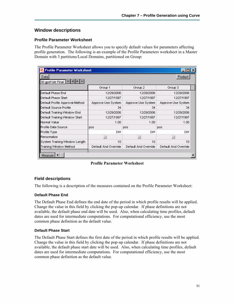
Chapter 7 – Profile Generation using Curve
91
Window descriptions
Profile Parameter Worksheet The Profile Parameter Worksheet allows you to specify default values for parameters affecting profile generation. The following is an example of the Profile Parameters worksheet in a Master Domain with 3 partitions/Local Domains, partitioned on Group:
Profile Parameter Worksheet
Field descriptions The following is a description of the measures contained on the Profile Parameter Worksheet:
Default Phase End
The Default Phase End defines the end date of the period in which profile results will be applied. Change the value in this field by clicking the pop-up calendar. If phase definitions are not available, the default phase end date will be used. Also, when calculating time profiles, default dates are used for intermediate computations. For computational efficiency, use the most common phase definition as the default value.
Default Phase Start
The Default Phase Start defines the first date of the period in which profile results will be applied. Change the value in this field by clicking the pop-up calendar. If phase definitions are not available, the default phase start date will be used. Also, when calculating time profiles, default dates are used for intermediate computations. For computational efficiency, use the most common phase definition as the default value.

Retek Demand Forecasting, Retek Curve, Retek Promote
92
Default Profile Approval Method
The Default Profile Approval Method displays the primary approval policy that will be used for the profile. Select “Approve Use System” if profile results are to be automatically approved during the batch profile generation. Select “Do Not Approve” if profile results are to be manually approved by the user. If a profile is being generated dynamically (to support Source Level Forecasting) as part of the RDF batch forecast process, the Default Profile Approval Method should be set to “Approve Use System”.
Default Source Profile
The Default Source Profile determines the primary source level that will be used to generate the profile. When only a single source is configured for a profile, all profile results will be calculated using the same intersections. When multiple sources are defined for a profile, some profile results will be calculated using different intersections. The Profile Maintenance Workbook may be used to define exceptions to the Default Source Profile.
Default Training Window End
The Default Training Window End defines the last date in history that will be used to calculate profile results. Change the value in this field by clicking the pop-up calendar. The default date will be used only if the training window method is set to “Defaults and Overrides”.
Default Training Window Start
The Default Training Window Start defines the first date in history that will be used to calculate profile results. Change the value in this field by clicking the pop-up calendar. The default date will be used only if the training window method is set to “Defaults and Overrides”.
Normal Value
If the profile is aggregated to the Aggregation Intersection this will be the value in all the cells (or zero outside of the phase window.) The desired setting for Normal Value is usually 1.00 (100%), however there may be instances where it is desired to have the profile normalize to a value different than 1.00..
Profile Data Source
The Profile Data Source displays the name of the measure that contains the data that will be used to generate the profile.
Chapter 7 – Profile Generation using Curve
93
Profile Type
The Profile Type is a read-only measure that displays the value for this measure set in the Curve Plug-In. The Profile Type is used to determine the profile algorithm and validation required by the profile level. Profile Types are represented with pre-defined configuration information.
The following Profile Types share the same profile algorithm. The rationale for providing different types that have the same behavior is strictly to remind the user of the intent of the profile while using this workbook:
• Store Contribution Profile - The Store Contribution Profile is used to determine the data relationship between stores to aggregate dimensions in the location hierarchy.
• Hourly Profile - The Hourly Profile is used to determine the data relationship between hour to an aggregate dimension in the calendar hierarchy (for example, hour to week).
• Daily Profile - The Daily Profile is used to determine the data relationship between a given day to the week in which it belongs.
• Product Profile - The Product Profile is used to determine the data relationship between any two dimensions along the product hierarchy.
• Size Profile - The Size Profile is used to determine the data relationship between any dimension in the size hierarchy and any dimension in the product hierarchy. A size hierarchy must be defined to use this profile type.
• User Defined Profile - The User Defined Profile may be used to support any basic profile configuration.
The following Profile Types have unique behavior:
• Diff Profile – Diff Profiles are used to determine spreading ratios from aggregate dimensions in the Product hierarchy to diff dimensions. Used to support the spreading of data in RMS Allocation, Diff Profiles exhibit the same behavior as the previous profile types. However, unique to Diff Profiles is special validation of the relationship between the defined diff dimensions to dimensions along the main branch of the Product hierarchy (see the RDF Administrator’s Guide for more information on validation criteria).
• Daily Seasonal Profile - The Daily Seasonal Profile is used to determine the data relationship between a given day of the week to aggregate dimensions in the calendar hierarchy. This profile type uses training window data to compute the profile. The resulting profile is then clipped to fit within the defined phase window.
• Life Cycle Profile - The Life Cycle Profile uses data along a user-defined training window, then stretches or shrinks data to fit a user-defined phase window.
Retek Demand Forecasting, Retek Curve, Retek Promote
94
Renormalize
Renormalize is a Boolean measure. When set to TRUE, it will automatically renormalize the calculated profile result at the corresponding final level. Normally the renormalization is not necessary. For example, if you have a source profile at week of season and its final profile is at day of season, you would need to renormalize the final level because going from week to day will do replication. Now at day level the profile will sum up to greater than 1 for a season (since it was a week to day it will probably sum up to seven). The renormalize will force the final profile to sum to 1.00 (100%).
System Training Window Length
The System Training Window Length necessary when “Use Training Window” is set as the Training Window Method for the profile. This field specifies the number of weeks of the most recent data to use as the training window for calculation the profile. The System Training Window Length defaults to 10 weeks.
Training Window Method
The Training Window Method is used to determine the default method used to define the training window. The options are:
• Default and Overrides: Uses the default dates as set in the Training Window Start Date and Training Window End Date measures.
• Phase Definitions and Overrides: Calculates the Training Window Start Date and Training Window End Date based on the Phase Start Date and Phase End Date measures.
• Use Training Window: Used with 'System Training Window Length' to specify the number of weeks of the most recent data to use for calculating the profile.
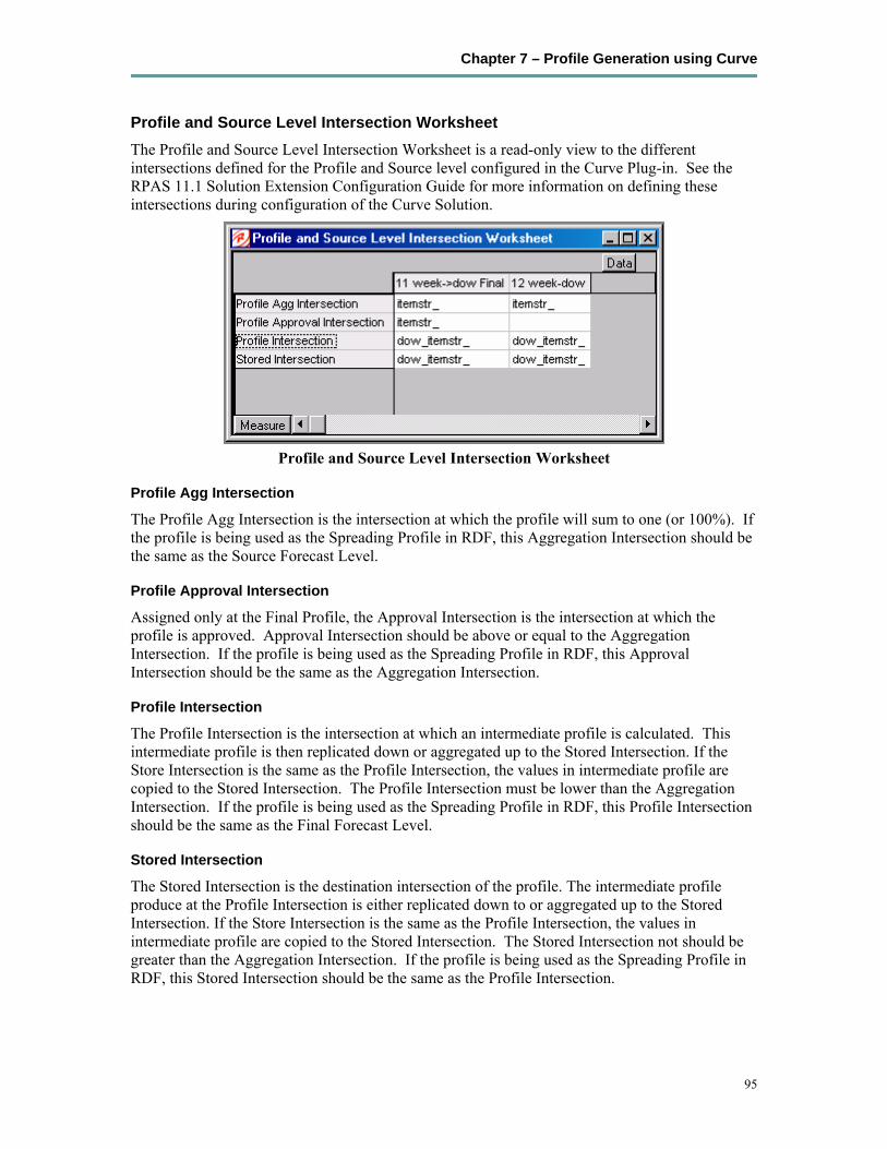
Chapter 7 – Profile Generation using Curve
95
Profile and Source Level Intersection Worksheet The Profile and Source Level Intersection Worksheet is a read-only view to the different intersections defined for the Profile and Source level configured in the Curve Plug-in. See the RPAS 11.1 Solution Extension Configuration Guide for more information on defining these intersections during configuration of the Curve Solution.
Profile and Source Level Intersection Worksheet
Profile Agg Intersection
The Profile Agg Intersection is the intersection at which the profile will sum to one (or 100%). If the profile is being used as the Spreading Profile in RDF, this Aggregation Intersection should be the same as the Source Forecast Level.
Profile Approval Intersection
Assigned only at the Final Profile, the Approval Intersection is the intersection at which the profile is approved. Approval Intersection should be above or equal to the Aggregation Intersection. If the profile is being used as the Spreading Profile in RDF, this Approval Intersection should be the same as the Aggregation Intersection.
Profile Intersection
The Profile Intersection is the intersection at which an intermediate profile is calculated. This intermediate profile is then replicated down or aggregated up to the Stored Intersection. If the Store Intersection is the same as the Profile Intersection, the values in intermediate profile are copied to the Stored Intersection. The Profile Intersection must be lower than the Aggregation Intersection. If the profile is being used as the Spreading Profile in RDF, this Profile Intersection should be the same as the Final Forecast Level.
Stored Intersection
The Stored Intersection is the destination intersection of the profile. The intermediate profile produce at the Profile Intersection is either replicated down to or aggregated up to the Stored Intersection. If the Store Intersection is the same as the Profile Intersection, the values in intermediate profile are copied to the Stored Intersection. The Stored Intersection not should be greater than the Aggregation Intersection. If the profile is being used as the Spreading Profile in RDF, this Stored Intersection should be the same as the Profile Intersection.

Retek Demand Forecasting, Retek Curve, Retek Promote
96
Profile Maintenance Workbook Overview After setting default parameters for profile generation in the Profile Administration Workbook, the next step in profile generation is to select any subset of positions for which the values set in Profile Administration differ from the defaults. This step is necessary in those situations where it is not efficient to use the same parameters for all positions in the hierarchy data.
Procedure As in Profile Administration, the first Profile Maintenance wizard screen prompts you to select a final profile level.
Create a Profile Maintenance Workbook 1. Within the Master, Local or Simple domain, select New from the File menu.
2. Select the Curve tab to display a list of workbook templates for Profiling.
3. Select Profile Maintenance.
4. Click OK.
5. The Profile Maintenance Wizard opens and prompts you to select the final profile. Make the appropriate selection.
6. Click Next.
7. If the Location hierarchy is defined in the profile, select the locations to include in the workbook.
8. Click Next.
9. If the Merchandise hierarchy is defined in the profile, select the products to include in the workbook.
10. Click Next.
11 If the Calendar hierarchy is defined in the profile, select the time periods to include in the workbook.
12. Click Next.
13. An additional wizard screen will prompt you to select any additional measures (that is, measures not standard in the Profile Maintenance Workbook) that you would like included. The measure options available in this screen are set in the RPAS Security Administration Workbook / Workbook Template Measure Rights Worksheet. Make the appropriate selections (if any).
14. Click Finish to display the workbook.

Chapter 7 – Profile Generation using Curve
97
Window descriptions
Profile Maintenance Workbook The Profile Maintenance Workbook allows edits to intersections that vary from the default values set in the Profile Administration Workbook.
Final Approval and Sourcing Worksheet
Final Approval and Sourcing Worksheet
Field descriptions The following is a description of the measures contained in the Final Approval and Sourcing Worksheet:
Profile Approval Method
The Profile Approval Method displays the primary approval policy that will be used for the profile. “No Override” will be displayed in this field if the Default Approval Method will be used. Select “Approve Use System” if profile results are to be automatically approved during the batch profile generation. Select “Do Not Approve” if profile results are to be manually approved by the user. If a profile is being generated dynamically (to support Source Level Forecasting) as part of the RDF batch forecast process, the Default Profile Approval Method should be set to “Approve Use System”.
Source Profile Override
Make edits to the Source Profile Override if the source level for an intersection varies from the Default Source Profile. “No Override” will be displayed in this field if the value set in the Default Source Profile is to be used. When only a single source is configured for a profile, all profile results will be calculated using the same intersections, thus edits to this parameter are not required. When multiple sources are defined for a profile, some profile results will be calculated using different intersections. Select the appropriate source level for an intersection.
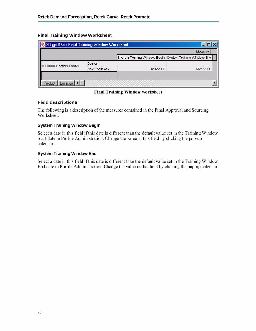
Retek Demand Forecasting, Retek Curve, Retek Promote
98
Final Training Window Worksheet
Final Training Window worksheet
Field descriptions The following is a description of the measures contained in the Final Approval and Sourcing Worksheet:
System Training Window Begin
Select a date in this field if this date is different than the default value set in the Training Window Start date in Profile Administration. Change the value in this field by clicking the pop-up calendar.
System Training Window End
Select a date in this field if this date is different than the default value set in the Training Window End date in Profile Administration. Change the value in this field by clicking the pop-up calendar.

Chapter 7 – Profile Generation using Curve
99
Generate Profiles Overview The batch profile generation process creates profile results for all hierarchy positions set in the Profile Intersection. Profiles may be run from the backend of the domain using the ‘curvebatch’ executable or run manually using the Run Batch Profile template. For more information on ‘curvebatch’ see the RDF 11.1 Administrators Guide.
Procedures Generate a profile manually
1. With the Local or Simple domain, select New from the File menu.
2. Select the Curve tab to display a list of workbook templates. Highlight Run Batch Profile and click OK.
3. The Run Batch Profile Wizard opens and prompts you to select the profile(s) to generate.
4. Select ‘Next’ or ‘Finish’.
The Run Batch Profile wizard automatically executes ‘curvebatch’ within the Simple or Local Domain. If ‘Next’ is selected from the last wizard screen, the wizard will not advance to the completion message until the profile(s) have been generated. Depending on the data set, this process may take a several minutes before the system advances to the final screen.

Retek Demand Forecasting, Retek Curve, Retek Promote
100
Profile Approval Workbook Overview The profiles generated at the historic levels must be viewed, analyzed, revised, and approved using the Profile Approval Workbook. In the approval process, you select the appropriate source level for each product/location combination. After you make any necessary changes to the profiles and commit the workbook, the profiles are normalized to preserve the appropriate ratios. At this time, Curve automatically spreads the source level profiles to the final level and combines them. After you commit your changes, you can refresh the data in your workbook to display the newly generated final level profiles.
Use the Profile Approval Workbook to view, analyze, revise, and approve the profiles generated at the historic levels. This workbook contains three tabs for each worksheet displayed:
• Final Worksheet
• Source Worksheet
• Approval Worksheet
Procedure
Create a new Profile Approval Workbook 1. With the Local or Simple domain, select New from the File menu.
2. Select the Curve tab to display a list of workbook templates.
3. Select Profile Approval.
4. Click OK.
5. The Profile Approval Wizard opens and prompts you to select the final profile. Make the appropriate selection.
6. Click Next.
7. If the Location hierarchy is defined in the profile, select the locations to include in the workbook.
8. Click Next.
9. If the Merchandise hierarchy is defined in the profile, select the products to include in the workbook.
10. Click Next.

Chapter 7 – Profile Generation using Curve
101
11. If the Calendar hierarchy is defined in the profile, select the time periods to include in the workbook.
12. Click Next.
13. An additional wizard screen will prompt you to select any additional measures (that is, measures not standard in the Profile Approval Workbook) that you would like included. The measure options available in this screen are set in the RPAS Security Administration Workbook / Workbook Template Measure Rights Worksheet. Make the appropriate selections (if any).
14. Click the Finish button to display the workbook.
Window descriptions
Final Profile Worksheet Through this worksheet, you can view the system calculated final profile and make adjustments to this profile. Following is an example Final Profile Worksheet for a day of week profile.
Final Profile worksheet
Field descriptions
Adjusted Profile
This is the user-adjusted profile. If edits are necessary to the Adjusted Profile, it is first required to lock the Adjust Profile at the Aggregation Intersection. This will prevent the Normal Value from recalculating to a value different than 1.00 (100%) when the adjustments are made. To determine the Aggregation Intersection, view the intersection displayed on the Approval worksheet. Once adjustments are made to the profile, the user must go to the Final Profile Approval Worksheet and set the ‘Do Not Approve’ flag to true for the adjusted intersection. The Approved Profile measure will update with these changes.
Approved Profile
The Approve Profile displays the approved profile values. If a profile intersection is set to ‘Do Not Approve’, no value will be displayed in this field. The system will automatically approve all profile intersections set to ‘Approve Use System’. If changes are made to the Adjusted Profile, the values in this measure will update once the Manually Approved flag is set to true the Final Profile Approval worksheet.
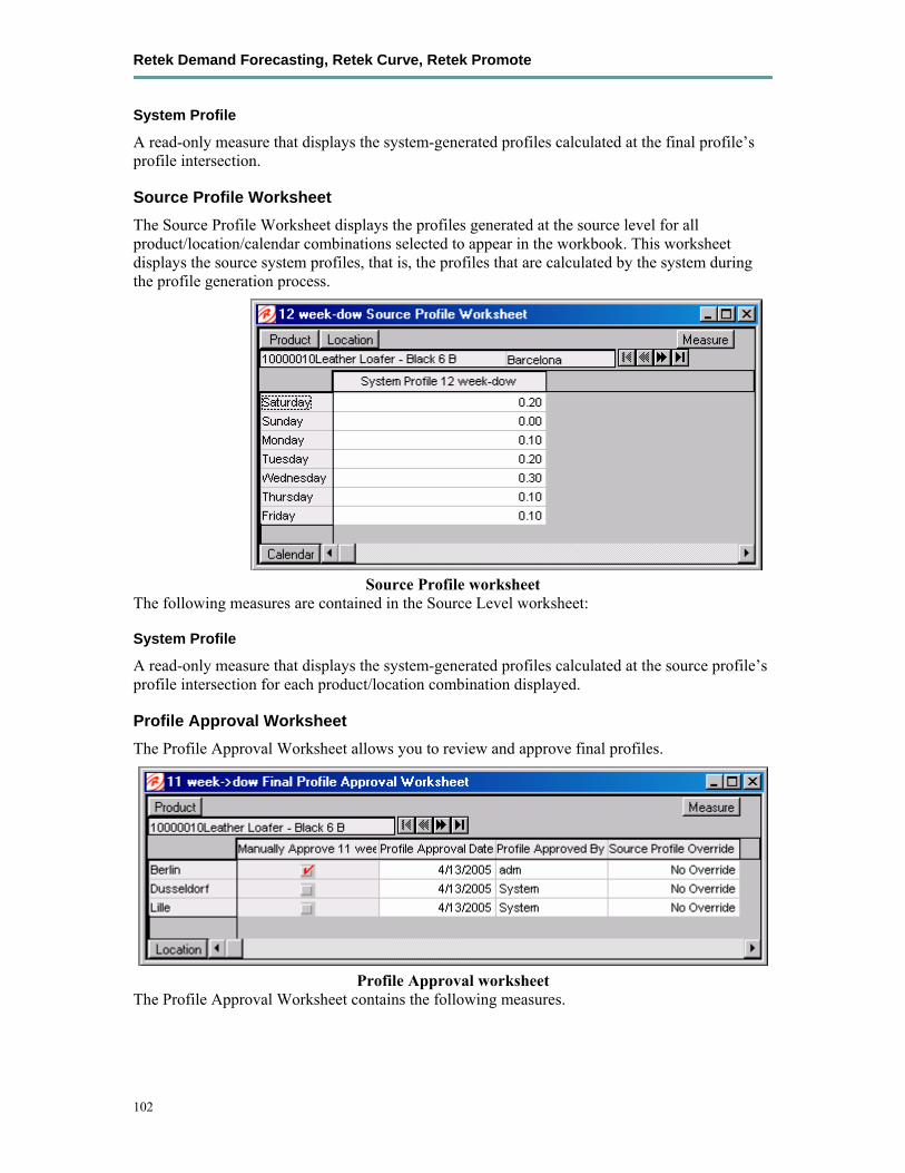
Retek Demand Forecasting, Retek Curve, Retek Promote
102
System Profile
A read-only measure that displays the system-generated profiles calculated at the final profile’s profile intersection.
Source Profile Worksheet The Source Profile Worksheet displays the profiles generated at the source level for all product/location/calendar combinations selected to appear in the workbook. This worksheet displays the source system profiles, that is, the profiles that are calculated by the system during the profile generation process.
Source Profile worksheet The following measures are contained in the Source Level worksheet:
System Profile
A read-only measure that displays the system-generated profiles calculated at the source profile’s profile intersection for each product/location combination displayed.
Profile Approval Worksheet The Profile Approval Worksheet allows you to review and approve final profiles.
Profile Approval worksheet The Profile Approval Worksheet contains the following measures.

Chapter 7 – Profile Generation using Curve
103
Profile Approved By
This measure displays who approved the profile for a given product/location combination. For all profile intersections with an Approval Method set to Approve Use System and no adjustment occurs, the Approved By measure will contain “System”.
Profile Approval Date
Displays the date on which a profile was approved whether it is automatically approved by the system or manually approved by the user.
Manually Approve
A Boolean measure that must be activated (checked) for all profile intersections that are set to “Do not approve” or for intersections in which the user makes changes to the “Adjusted Profile” on the Final Profile worksheet.
Source Profile Override
This field displays the source level that was used to generate the profile. If the Default Source Level was used, this measure will display ‘No Override’.

Chapter 8 – Retek Demand Forecasting Methods
105
Chapter 8 – Retek Demand Forecasting Methods This chapter discusses the forecasting methods used in Retek Demand Forecasting in detail.
Forecasting techniques used in RDF Retek Demand Forecasting uses a variety of predictive techniques to generate forecasts of demand. The technical methods used are driven by the goal to provide the most accurate forecasts possible in an automatic and efficient manner. These methods have been analyzed, optimized, and refined over years of research on retail specific data.
The primary techniques RDF uses include:
• Exponential smoothing
• Regression analysis
• Bayesian analysis
• Prediction intervals
• Automatic method selection
• Source level forecasting
• Promotional forecasting
Exponential smoothing Exponential smoothing models fit basic features of the demand pattern such as level, trend, and seasonality, and project these into the future. These models provide computational benefits and have been chosen for their ability to handle different types of time series, including short and/or noisy series that are characteristic of retail sales. They are "smoothing" models because they use weighted averages on historic data. They are "exponential smoothing" models because the weighting used decays at an exponential rate. That is, more recent data is weighted more heavily than the past.
Regression analysis Regression analysis is another standard technique used in prediction. Regression uses a least-squares estimator to fit a model of predictor variables to another set of target variables. Seasonal Regression is a Retek specific extension of this procedure for use in seasonal models with between one and two years of history. Causal Forecasting uses stepwise regression to determine which causal variables are significant.
Bayesian analysis Bayesian analysis considers a priori information as a starting point in development of a prediction. Bayesian forecasting, as developed by Retek, uses a sales plan as the starting point that is adjusted based on observed data. This method fills a gap in standard time series forecasting when new, short lifecycle, or products with significant lifecycles are being forecast.
Retek Demand Forecasting, Retek Curve, Retek Promote
106
Prediction intervals Prediction from these various models gives the estimated mean outcome. By using standard statistical distributional assumptions, RDF develops measures of uncertainty associated with forecast point estimates from these models. While this is of key concern for various optimization solutions of the forecast, the technical details are beyond the scope of this document. For further details on prediction interval calculations, see Char&Yatfield, International Journal of Forecasting, March 1992.
Automatic method selection Providing multiple forecasting methods is only valuable if the appropriate model can be selected in an accurate and efficient manner. In order to make this feasible in a retail environment Retek has developed a number of different Meta-Methods that can automatically select the best method among a number of competing models. Automatic Exponential Smoothing (AutoES) is an example of one such method that clients can select. The final selection between the competing models is made according to a performance criterion that involves a tradeoff between the model’s fit over the historic data and its complexity (a description of the competing models used within AutoES is described in section two of this document). In academia this discipline is known as Information Theory and is used in the combination and selection of various competing models.
Source level forecasting Sometimes it is difficult to capture seasonality, trend, or causal effects on the final level (item/Store) due to scarcity of the data. Also, time series are often too noisy at that level. To overcome these issues RDF utilizes source level forecasting. In source level forecasting, data is aggregated first to a higher level across the product or location hierarchy (or both). Then the forecast is generated and proportionally spread down to the final level. We have experimentally proven that source level forecasting technique very often improves the accuracy on the final level.
Promotional forecasting In some instances, especially in retail, pure time series techniques are inadequate for forecasting demand. Instead of using only historic demand patterns to forecast future demand, additional causal or promotional factors are used to better explain past performance. With the help of a promotional calendar, an indication of when promotions will be run in the future, these promotional forecasting techniques can better predict demand in the future.
For more information on promotional forecasting methods, see page 128.
Chapter 8 – Retek Demand Forecasting Methods
107
Time series (statistical) forecasting methods This section describes those techniques within RDF that generate forecasts directly from only a single time series. Generally the time series provided is past sales history for a given item/Store that is used to predict what future demand might be. In actual practice these algorithms have been and can be used to forecast a myriad of different data streams at any product/location level (shipment data at item/warehouse, financial data at dept./chain, etc.).
The following topics present fundamentals of the Retek Demand Forecasting statistical forecasting processes. Included is a discussion of the importance of confidence intervals and confidence limits, the time series methods used to generate forecasts, and how the best forecasting method is selected from a list of candidate models.
A wide variety of statistical forecasting techniques are available, ranging from very simple to very sophisticated. All of these methods attempt to best capture the statistical probability distribution discussed above, and they do this by fitting quantitative models to statistical patterns from historical data. Put simply, the better the history of the variable being forecasted, the stronger these statistical patterns will be. Increased forecast accuracy depends on the strength of these patterns in relation to background irregularities.
Retek Demand Forecasting is able to use several time series methods to produce forecasts. Time series methods extrapolate features from the past (in this case, past sales data) to the future. The time series methods that the system offers include:
• Auto Exponential Smoothing Forecasting (AutoES)
• Seasonal Exponential Smoothing Forecasting (SeasonalES)
• Simple Moving Average
• Simple Exponential Smoothing
• Croston’s Method
• Holt Exponential Smoothing
• Multiplicative Winters Exponential Smoothing
• Additive Winters Exponential Smoothing
• Seasonal Regression
• Bayesian Information Criterion
Retek Demand Forecasting, Retek Curve, Retek Promote
108
Why use statistical forecasting? The purpose of statistical forecasting is to make the process of predicting future events both objective and quantitative. Statistical forecasting utilizes information from the past (such as sales data) to predict what will happen in the future. Forecast accuracy depends on the degree to which a mathematical model can detect and extract statistical patterns from historic data. The most common statistical methodologies used are univariate. This means that they are based solely on the history of one variable, such as sales. Each forecast observation reflects a future value of the sole input variable. Statistical forecasting processes are relatively easy to implement, and the better the historical data, the better the resulting forecasts.
Businesses benefit greatly from the use of systematic statistical forecasting techniques that aim to accurately predict product demand, enabling these businesses to maintain sufficient product inventory levels. When inventory levels are optimized, lost sales due to product stock-outs are greatly reduced, as are the costs incurred by overstocking.
Exponential Smoothing (ES) forecasting methods The primary process by which RDF automatically fits an exponential smoothing model to a time series is called Automatic Exponential Smoothing (AutoES). When AutoES forecasting is chosen in RDF, a collection of candidate models is initially considered. The models in the candidate list include
• Simple (One Parameter) Exponential Smoothing
• Croston’s Method (Intermittent ES)
• Holt (Two Parameter) Exponential Smoothing (Trend ES)
• Winters (Three Parameter) Exponential Smoothing (Seasonal ES)
• Seasonal Regression
These models include level information, level and trend information, and level, trend and seasonality information, respectively. The optimal smoothing parameters for each model form are determined automatically (that is, greater smoothing will be applied to noisier data). The final selection between the resulting models is made according to a performance criterion that involves a tradeoff between the model’s fit over the historic data and its complexity.
The amount of available historic information can affect the complexity of the model that can be fit. For example, fitting a seasonal model would not be appropriate without a complete year of historic data. In fact, one prefers to see each “season” occur multiple times. For a particular series, even if the amount of available history allows one to fit a complex model (that is, one with seasonal components), the resulting model is not necessarily superior to a simpler model. If a simpler model (for example, a model with only a level component, or level and trend components) fits “as well” as a seasonal model, then the AutoES forecasting process will find the simpler model to be preferable. In such a case, the simpler model captures the basic features supported by the data without over fitting and therefore will generally project better forecasts.

Chapter 8 – Retek Demand Forecasting Methods
109
Definitions of equation notation used in this section The following notation is used in equations throughout this section.
tY - Observed value at time t.
h - Number of periods ahead for which to forecast.
tL - Smoothed level component at end of time t.
tT - Smoothed trend component at end of time t.
tS - Smoothed seasonal index component at end of time t.
α - Smoothing parameter for level of series.
γ - Smoothing parameter for trend.
δ - Smoothing parameter for seasonal indexes.
ϕ - Damped trend constant.
p - Number of periods per year.
)(ˆ hYt - Forecast for time t+h from base t.
htS +~
- Most recent seasonal index for time t+h
Retek Demand Forecasting, Retek Curve, Retek Promote
110
Components of exponential smoothing Several features of the data can be incorporated into exponential smoothing models using the following structural components:
The level ( tL ) of the series estimates the non-seasonal, slowly changing process of the time series. This data feature represents a flat value for the data when noise, trend and seasonality effects are excluded from the data.
The trend ( tT ) of a series reflects the rate of change of the series from one point to another. RDF uses a damping factor with its trend component to curtail exaggerated effects over long forecast horizons.
Smoothed seasonal indexes ( tS ) estimate periodic patterns in the demand data. Using these estimated values, a model can extrapolate the seasonal features of a series. A seasonal index can be derived as an additive or multiplicative feature of the data.
For a particular time series, a more complex model might consider seasonality and/or trend. For all models, a form of the level of the series is used.
Average A simple moving average forecast involves taking the average of the past n time periods and using that average as the forecast for all future time periods (where n is the length of fitting period). Simple moving average forecasts are frequently used in the system because they make few assumptions about the historical time series, they can be generated with little historical data, and because they are very fast to generate. Typically, moving average forecasts are generated at the final forecast level (for example, item/Store) and their results used to spread more sophisticated higher-level forecasts (for example, those generated with exponential smoothing).
A Simple Moving Average model assumes that historical data is too short or noisy to consider seasonal effects or local trend, and is based on the level of the series. Since this model does not use a smoothing parameter to place added weight on more recent historic values, a Simple Moving Average model is not actually in the exponential smoothing family. However, it is an adequate model to use when low-level (final forecast) ratios are needed for RDF’s spreading of high-level (aggregate) forecasts. That is, when aggregate forecasts can be calculated for long and less noisy aggregate time series, Simple Moving Average models provide an adequate (and computationally quick) forecast to determine the ratios needed for RDF spreading. User input in overriding the automatic training horizon further enhances the simple robustness of this model for base-level data.
Overall, a forecast is evaluated as:
( ) ∑−
=−=
1
0
1ˆn
kktt Y
nhY
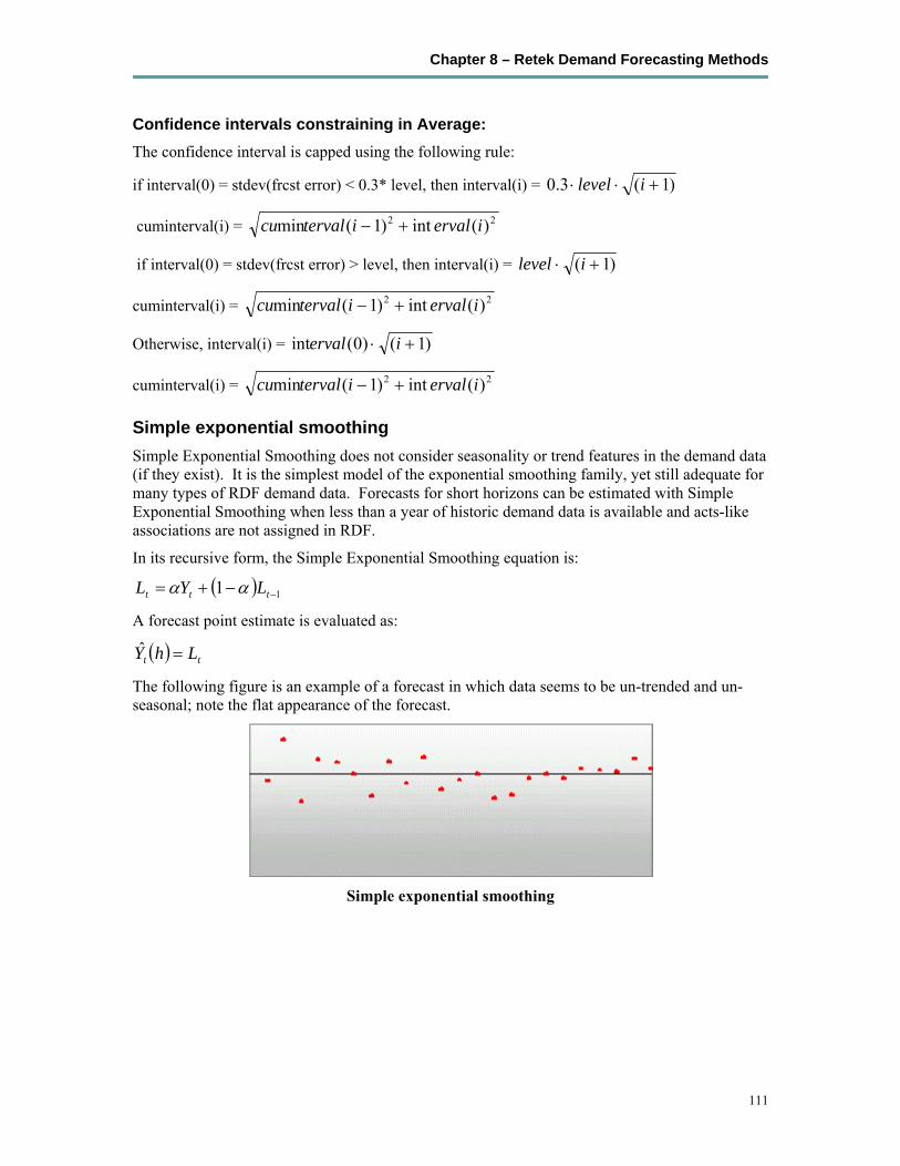
Chapter 8 – Retek Demand Forecasting Methods
111
Confidence intervals constraining in Average: The confidence interval is capped using the following rule:
if interval(0) = stdev(frcst error) < 0.3* level, then interval(i) = )1(3.0 +⋅⋅ ilevel
cuminterval(i) = 22 )(int)1(min iervalitervalcu +−
if interval(0) = stdev(frcst error) > level, then interval(i) = )1( +⋅ ilevel
cuminterval(i) = 22 )(int)1(min iervalitervalcu +−
Otherwise, interval(i) = )1()0(int +⋅ ierval
cuminterval(i) = 22 )(int)1(min iervalitervalcu +−
Simple exponential smoothing Simple Exponential Smoothing does not consider seasonality or trend features in the demand data (if they exist). It is the simplest model of the exponential smoothing family, yet still adequate for many types of RDF demand data. Forecasts for short horizons can be estimated with Simple Exponential Smoothing when less than a year of historic demand data is available and acts-like associations are not assigned in RDF.
In its recursive form, the Simple Exponential Smoothing equation is:
( ) 11 −−+= ttt LYL αα
A forecast point estimate is evaluated as:
( ) tt LhY =ˆ
The following figure is an example of a forecast in which data seems to be un-trended and un-seasonal; note the flat appearance of the forecast.
Simple exponential smoothing
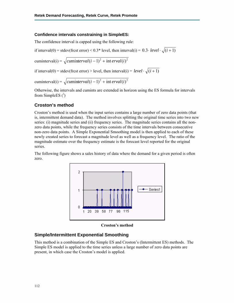
Retek Demand Forecasting, Retek Curve, Retek Promote
112
Confidence intervals constraining in SimpleES: The confidence interval is capped using the following rule:
if interval(0) = stdev(frcst error) < 0.3* level, then interval(i) = )1(3.0 +⋅⋅ ilevel
cuminterval(i) = 22 )(int)1(min iervalitervalcu +−
if interval(0) = stdev(frcst error) > level, then interval(i) = )1( +⋅ ilevel
cuminterval(i) = 22 )(int)1(min iervalitervalcu +−
Otherwise, the intervals and cumints are extended in horizon using the ES formula for intervals from SimpleES (i)
Croston’s method Croston’s method is used when the input series contains a large number of zero data points (that is, intermittent demand data). The method involves splitting the original time series into two new series: (i) magnitude series and (ii) frequency series. The magnitude series contains all the non-zero data points, while the frequency series consists of the time intervals between consecutive non-zero data points. A Simple Exponential Smoothing model is then applied to each of these newly created series to forecast a magnitude level as well as a frequency level. The ratio of the magnitude estimate over the frequency estimate is the forecast level reported for the original series.
The following figure shows a sales history of data where the demand for a given period is often zero.
Croston’s method
Simple/Intermittent Exponential Smoothing This method is a combination of the Simple ES and Croston’s (Intermittent ES) methods. The Simple ES model is applied to the time series unless a large number of zero data points are present, in which case the Croston’s model is applied.
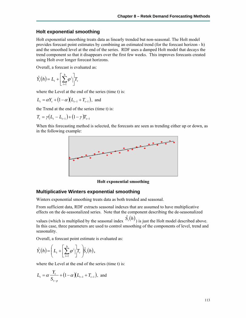
Chapter 8 – Retek Demand Forecasting Methods
113
Holt exponential smoothing Holt exponential smoothing treats data as linearly trended but non-seasonal. The Holt model provides forecast point estimates by combining an estimated trend (for the forecast horizon - h) and the smoothed level at the end of the series. RDF uses a damped Holt model that decays the trend component so that it disappears over the first few weeks. This improves forecasts created using Holt over longer forecast horizons.
Overall, a forecast is evaluated as:
( ) t
h
i
itt TLhY ⎥
⎦
⎤⎢⎣
⎡+= ∑
=1
ˆ ϕ
where the Level at the end of the series (time t) is:
( )( )111 −− +−+= tttt TLYL αα , and
the Trend at the end of the series (time t) is:
( ) ( ) 11 1 −− −+−= tttt TLLT γγ When this forecasting method is selected, the forecasts are seen as trending either up or down, as in the following example:
Holt exponential smoothing
Multiplicative Winters exponential smoothing Winters exponential smoothing treats data as both trended and seasonal.
From sufficient data, RDF extracts seasonal indexes that are assumed to have multiplicative effects on the de-seasonalized series. Note that the component describing the de-seasonalized
values (which is multiplied by the seasonal index ( )hStˆ
) is just the Holt model described above. In this case, three parameters are used to control smoothing of the components of level, trend and seasonality.
Overall, a forecast point estimate is evaluated as:
( ) ( )hSTLhY tt
h
i
itt
ˆˆ1
⎟⎟⎠
⎞⎜⎜⎝
⎛⎥⎦
⎤⎢⎣
⎡+= ∑
=
ϕ ,
where the Level at the end of the series (time t) is:
( )( )111 −−−
+−+= ttpt
tt TL
SYL αα , and
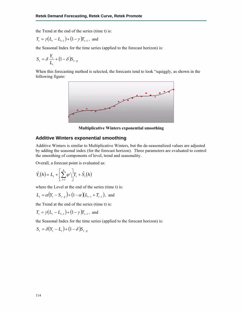
Retek Demand Forecasting, Retek Curve, Retek Promote
114
the Trend at the end of the series (time t) is:
( ) ( ) 11 1 −− −+−= tttt TLLT γγ , and
the Seasonal Index for the time series (applied to the forecast horizon) is:
( ) ptt
tt S
LY
S −−+= δδ 1
When this forecasting method is selected, the forecasts tend to look “squiggly, as shown in the following figure:
Multiplicative Winters exponential smoothing
Additive Winters exponential smoothing Additive Winters is similar to Multiplicative Winters, but the de-seasonalized values are adjusted by adding the seasonal index (for the forecast horizon). Three parameters are evaluated to control the smoothing of components of level, trend and seasonality.
Overall, a forecast point is evaluated as:
( ) ( )hSTLhY tt
h
i
itt
ˆˆ1
+⎥⎦
⎤⎢⎣
⎡+= ∑
=
ϕ
where the Level at the end of the series (time t) is:
( ) ( )( )111 −−− +−+−= ttpttt TLSYL αα , and
the Trend at the end of the series (time t) is:
( ) ( ) 11 1 −− −+−= tttt TLLT γγ , and
the Seasonal Index for the time series (applied to the forecast horizon) is:
( ) ( ) ptttt SLYS −−+−= δδ 1

Chapter 8 – Retek Demand Forecasting Methods
115
Confidence intervals constraining in HoltES, AWinters, MWinters: The confidence interval is capped using the following rule:
if interval(0) < 0.3* forecast(i), then interval(i) = )1()(3.0 +⋅⋅ iiforecast
cuminterval(i) = 22 )(int)1(min iervalitervalcu +−
if interval(0) > forecast(i), then interval(i) = )1()( +⋅ iiforecast
cuminterval(i) = 22 )(int)1(min iervalitervalcu +− from the first constrained interval until the end of the forecast horizon
Otherwise, the intervals and cumints are extended in horizon using the interval ES formulas (i, ii,iii)
Seasonal Exponential Smoothing (SeasonalES) In certain instances, it is known that seasonal models will generally outperform non-seasonal models in forecast accuracy. When this is true (generally used for known seasonal items or for forecasts with a long horizon), it is advantageous to prevent AutoES from selecting from the Simple/Holt/Croston’s methods. Choosing SeasonalES does just this. In instances where there exists too little data to create a seasonal forecast (less than 52 weeks of history), the SeasonalES method will cascade to select between Simple/Holt/Croston. In all other instances, a seasonal model (Winter’s or Seasonal Regression) will be chosen. See the following section for more information on Seasonal Regression.
Confidence intervals constraining in Seasonal method: The confidence interval is constrained using the following rule:
if interval(0) = stdev(frcst error) < 0.3* forecast(i), then interval(i) = )1()(3.0 +⋅⋅ iiforecast
if interval(0) > forecast(i), then interval(i) = )1()( +⋅ iiforecast
Otherwise, interval(i) = )1()0(int +⋅ ierval
cuminterval(i) = 22 )(int)1(min iervalitervalcu +−
Retek Demand Forecasting, Retek Curve, Retek Promote
116
Seasonal Regression A common benchmark in seasonal forecasting methods is sales last year. A sales last year forecast is based entirely on sales from the same time period of last year. Forecasting using only sales last year involves simple calculations and often outperforms other more sophisticated seasonal forecasting models. This method performs best when dealing with highly seasonal sales data with a relatively short sales history.
The seasonal models used in earlier releases of Retek Demand Forecasting (Additive and Multiplicative Winters) were designed to determine seasonality. However, they were not designed to work with sales histories of shorter than two years. Because sales histories of longer than two years are often difficult to obtain, many retail environments need a seasonal forecast that can accommodate sales data histories of between one and two years. In addition, the Additive and Multiplicative Winters models search for short-term trends and have difficulties with trends occurring inside the seasonal indices themselves. The current Retek Demand Forecasting Seasonal Regression forecasting model is designed to address these needs.
The Seasonal Regression Model uses simple linear regression with last year's data as the predictor variable and this year's sales as the target variable. The system determines the multiplicative and additive weights that best fit the data on hand. When optimizing the Seasonal Regression Model, the sales last year forecast is inherently considered, and will automatically be used if it is the model that best fits the data. If there have been significant shifts in the level of sales from one year to the next, the model will learn that shift and appropriately weight last year's data (keeping the same shape from last year, but adjusting its scale).
As with other seasonal models, you can forecast demand for products with insufficient sales histories using this method if:
• You paste in fake history as needed, providing a seasonal profile for the previous year.
• You also forecast for a source level (with the same seasonality profile as the forecasted item and with more than one year of history), using seasonal regression and spread these forecast results down to the member products.
The Seasonal Regression Model is included in the AutoES family of forecasting models, and is thus a candidate model that will be selected if it best fits the data.
More formally, for a series xr of length N , define ( )jx as the value of xr at time ,j Nj ≤≤1 , and let p be the length of the seasonal cycle in series xr , Np ≤≤1 , which is assumed to be known apriori. The forecast for the series at time hl + is represented by )(ˆ hxl where l ,
Nl ≤≤1 , is the location in the series at which forecasting begins and h is the position in the forecast window. Using this terminology the forecast is defined as:
( ) BphlxAhxl +−+⋅≡ )(ˆ ,
where A and B are the constants calculated by linear regression.
Plotting the series where one axis is the value of the series at time t (that is, )(tx ) and the other axis is the value of the series at time pt − (that is, )( ptx − ) yields a scatter plot. As can be determined by visual inspection the series plotted against itself shifted by a single cycle falls along a rough line. It is this line that is captured by the linear regression where A is the slope of the line and B is the point of intersection.
Chapter 8 – Retek Demand Forecasting Methods
117
Thus, this method captures the trend of a series through the slope of the regression line while the series shifted by a cycle provides its seasonal profile. Using this method the resulting forecast for the original series is calculated. The regression method provides a much better forecast of the series than was possible with the other exponential smoothing algorithms.
Based on the assumptions of the model that this method is trying to describe, versus the noisy data it is likely to receive, several exceptions to this regression technique are caught and corrected. First, since it is logically impossible to receive a negative value for the slope (such a value suggesting an inverse seasonality) any time a negative slope is detected the regression is rerun with the intercept fixed to zero. This guarantees that a positive slope will be calculated and thus a more logical forecast will be given.
The second noise-driven concession is to check the slope to determine if it is either too slight or too great. If this is the case, then the method rejects itself out of hand and allows one of the other competing methods to provide the forecast.
Thus, the full forecasting algorithm is:
1. For the series xr of length N with seasonality occurring with cycle length p form the pairs =X ))1(),1(( pxx + , K , ))(),(( NxpNx − .
2. Perform regression on the pairs in X to retrieve the slope, A , and the intercept, B , using the equation above.
3. Check the slope of the regression. If the slope is negative then rerun the regression on X fixing the intercept to zero.
4. Check the slope of the regression to determine if it is in the accepted range. If not this method fails to produce a forecast.
5. Build the forecast for the horizon of length l as lhBhpNxAhxN ≤≤++−⋅= 1,)()(ˆ .
Bayesian Information Criterion (BIC) Within AutoES, the model that minimizes the Bayesian Information Criterion (BIC) is selected as the final model. The BIC criterion attempts to balance model complexity with goodness-of-fit over the historical data. The BIC criterion rewards a model for goodness-of-fit and penalizes a model for its complexity. The complexity penalty is necessary to avoid over fitting.
There are various equivalent versions of the Bayesian Information Criterion, but RDF minimizes the following:
nk
nsBIC 2⋅=
where n is the number of periods in the available data history, k is the number of parameters to be estimated in the model (a measure of model complexity), and s is the root mean squared error computed with one-step-ahead forecast errors resulting from the fitted model (a measure of goodness-of-fit). Note that since each member of the model candidate list is actually a family of models, an optimization routine to select optimal smoothing parameters is required to minimize s for each model form (that is, to select the best model).
Within RDF, a few modifications to the standard selection criteria have been made. These include reducing the number of parameters the Winter’s model is penalized by discounting seasonal indices that have little impact on the forecast (multiplicative indices close to 1, additive indices close to 0). These changes tend to favor the seasonal models to a slightly higher degree that improves the forecasts on retail data, especially for longer forecast horizons.

Retek Demand Forecasting, Retek Curve, Retek Promote
118
AutoES Flowchart The following outlines the processing routine the system runs through to evaluate each time series set to forecast using the AutoES method. See Chapter 2: Forecast Administration/Advance Settings for more information on adjusting the parameters used to qualify a time series for Croston’s, Holt or Winters methods:
Step 1: Filter all leading zeros in the input data that is within the training window. Go to Step 2.
Step 2: Does the time series contain the minimum data points to qualify to forecast using the Croston’s method? If yes, generate the forecast and statistics using the Croston’s method, and move on to the next time series. If no, move on to Step 3.
Step 3: Does the time series contain enough relevant data to generate a forecast? If yes, generate a forecast and statistics using the Simple ES method and move on to Step 4. If no, do not forecast, then go to the next time series.
Step 4: Does the time series contain the minimum data points to qualify to forecast using the Holt method? If yes, generate a forecast and statistics using the Holt method and move on to Step 5. If no, move on to Step 5.
Step 5: Does the time series contain more than 52 weeks of input data? If yes, generate a forecast and statistics using the Seasonal Regression method and move on to Step 6. If no, move on to Step 9.
Step 6: Does the time series contain the minimum data points to qualify to forecast using Winters methods? If yes, move on to Step 7. If no, move on to Step 9.
Step 7: Does the time series contain any data point with sales equal qualify to forecast using Additive Winters method? If yes, generate the forecast and statistics using the Additive Winters method, and move on to Step 9. If no, move on to Step 8.
Step 8: Does the time series qualify to forecast using the Multiplicative Winters method? If yes, generate the forecast and statistics using both the Additive Winters and Multiplicative Winters methods, and move on to Step 9.
Step 9: Compare all candidate forecasts using BIC Criterion.
Step 10: Return the corresponding forecast and statistics for the system-selected forecast method, and move on to the next time series.
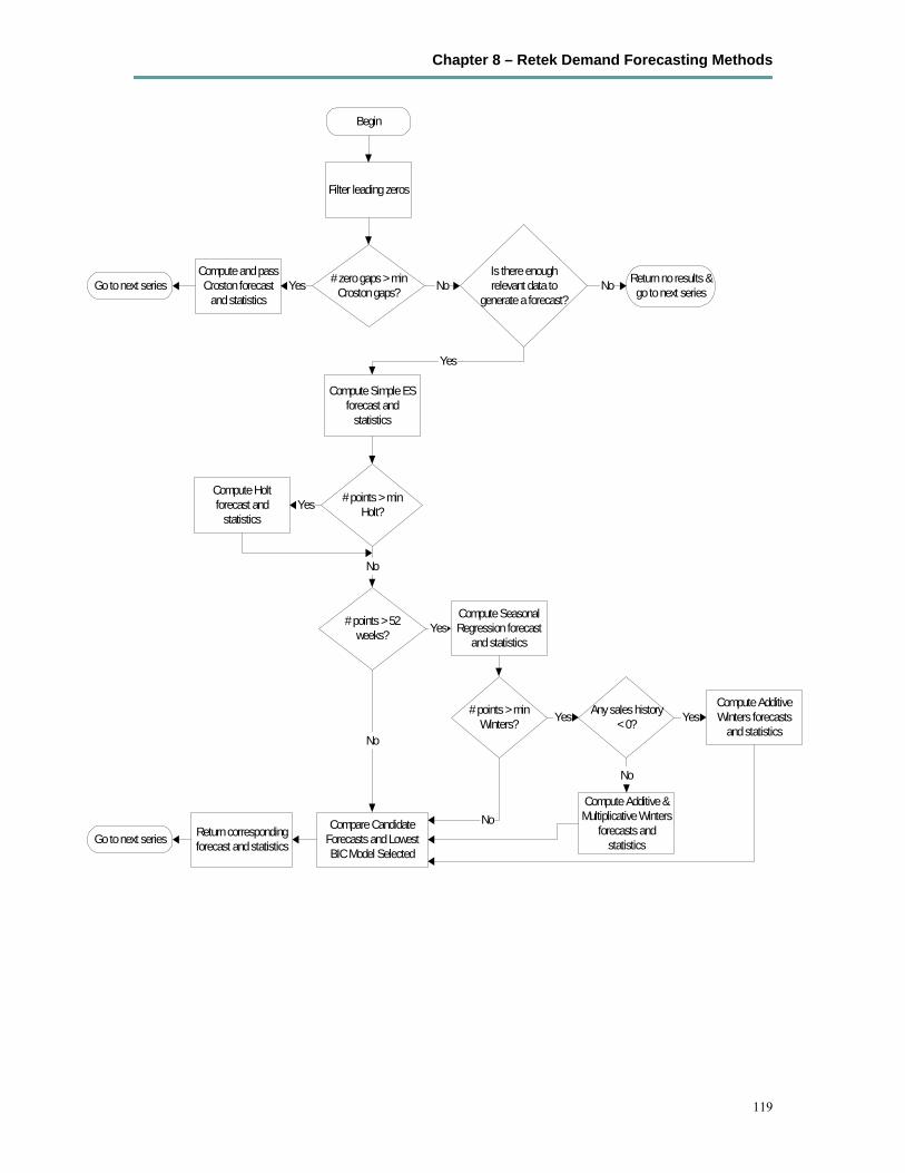
Chapter 8 – Retek Demand Forecasting Methods
119
Begin
Filter leading zeros
Compute Simple ESforecast and
statistics
# zero gaps > minCroston gaps?
Compute and passCroston forecast
and statisticsGo to next series
Compute Holtforecast and
statistics
Compare CandidateForecasts and LowestBIC Model Selected
Return correspondingforecast and statisticsGo to next series
Yes
Compute AdditiveWinters forecasts
and statistics
# points > minHolt?
# points > minWinters?
# points > 52weeks?
Compute SeasonalRegression forecast
and statistics
Is there enoughrelevant data to
generate a forecast?
Any sales history< 0?
Compute Additive &Multiplicative Winters
forecasts andstatistics
Yes
Yes
No
Yes
No Return no results &go to next seriesNo
Yes
No
Yes
No
No
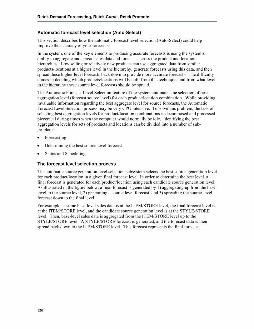
Retek Demand Forecasting, Retek Curve, Retek Promote
120
Automatic forecast level selection (Auto-Select) This section describes how the automatic forecast level selection (Auto-Select) could help improve the accuracy of your forecasts.
In the system, one of the key elements to producing accurate forecasts is using the system’s ability to aggregate and spread sales data and forecasts across the product and location hierarchies. Low selling or relatively new products can use aggregated data from similar products/locations at a higher level in the hierarchy, generate forecasts using this data, and then spread these higher level forecasts back down to provide more accurate forecasts. The difficulty comes in deciding which products/locations will benefit from this technique, and from what level in the hierarchy these source level forecasts should be spread.
The Automatic Forecast Level Selection feature of the system automates the selection of best aggregation level (forecast source level) for each product/location combination. While providing invaluable information regarding the best aggregate level for source forecasts, the Automatic Forecast Level Selection process may be very CPU intensive. To solve this problem, the task of selecting best aggregation levels for product/location combinations is decomposed and processed piecemeal during times when the computer would normally be idle. Identifying the best aggregation levels for sets of products and locations can be divided into a number of sub-problems:
• Forecasting
• Determining the best source level forecast
• Status and Scheduling
The forecast level selection process The automatic source generation level selection subsystem selects the best source generation level for each product/location in a given final forecast level. In order to determine the best level, a final forecast is generated for each product/location using each candidate source generation level. As illustrated in the figure below, a final forecast is generated by 1) aggregating up from the base level to the source level, 2) generating a source level forecast, and 3) spreading the source-level forecast down to the final level.
For example, assume base-level sales data is at the ITEM/STORE level, the final forecast level is at the ITEM/STORE level, and the candidate source generation level is at the STYLE/STORE level. Then, base-level sales data is aggregated from the ITEM/STORE level up to the STYLE/STORE level. A STYLE/STORE forecast is generated, and the forecast data is then spread back down to the ITEM/STORE level. This forecast represents the final forecast.
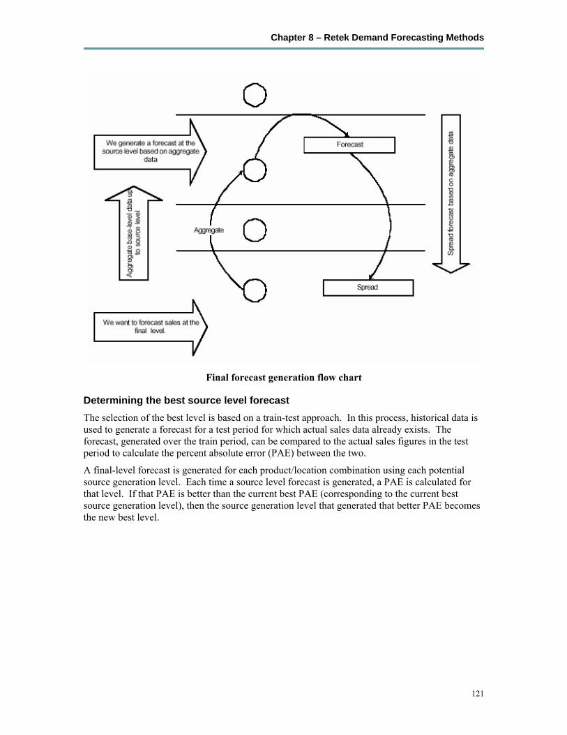
Chapter 8 – Retek Demand Forecasting Methods
121
Final forecast generation flow chart
Determining the best source level forecast The selection of the best level is based on a train-test approach. In this process, historical data is used to generate a forecast for a test period for which actual sales data already exists. The forecast, generated over the train period, can be compared to the actual sales figures in the test period to calculate the percent absolute error (PAE) between the two.
A final-level forecast is generated for each product/location combination using each potential source generation level. Each time a source level forecast is generated, a PAE is calculated for that level. If that PAE is better than the current best PAE (corresponding to the current best source generation level), then the source generation level that generated that better PAE becomes the new best level.

Retek Demand Forecasting, Retek Curve, Retek Promote
122
Status & scheduling Identifying the best aggregation level for a given set of products and locations may take a significant amount of time (that is, an amount of time that is greater than the duration of the computer’s shortest idle period). This task, however, can be partitioned; that is, the problem of selecting the best aggregation levels can be decomposed into smaller sub problems to be solved piecemeal during times when the computer would normally be idle.
For each product/location combination at the final forecast level, the problem consists of 1) generating forecasts at each unique aggregation level and 2) using the train-test approach to evaluate the percent absolute error statistics for each. One or more of these subtasks will be performed during each period that the computer is idle. The best aggregation status keeps track of which sub problems have been performed and which sub problems remain. In this way, when the best aggregation procedure is run, the procedure knows what the next sub problem is.
Best aggregation level procedures are run during idle computer periods. The scheduling of the Automatic Forecast Level Selection process must be integrated with the schedules of other machine processes. In general, you should select a schedule so that source generation level selection does not conflict with other activities. The following is an example of a typical schedule for the Automatic Forecast Level Selection process: Monday through Thursday, the selection process starts at midnight and runs for 8 hours; on Friday and Saturday, the process is allowed to run for 20 hours; Sunday is reserved for generating forecasts.
Using the system-selected forecast level You have the option of accepting the system-generated source level selection or manually selecting a different source level to be used. The value for the source forecast level can be manipulated in the Final Level Worksheet of the Forecast Maintenance Workbook. For each product/location combination, the best source forecast level identified by Retek Demand Forecasting will appear in the Suggested Generation Level measure on this worksheet. You can enable the use of this level by placing a checkmark in the Use Suggested Generation Level measure for that product/location. The absence of a checkmark in this measure causes the system to select the source level chosen in the Generation Level measure, which you can specify using a drop-down list.

Chapter 8 – Retek Demand Forecasting Methods
123
Profile-based forecasting The Profile-based forecasting method generates a forecast based on a seasonal profile. The profile may be loaded, manually entered, or generated by Curve. It can also be copied from another profile and adjusted.
Forecast method The Profile-based forecasting method proceeds as follows:
1. The historical data and the profile are loaded.
2. The data are de-seasonalized using the profile and then fed to Simple method.
3. The alpha is capped by 0.5
4. The Simple forecast is then re-seasonalized using the profiles.
Confidence intervals constraining in Profile Based method: In Profile Based method, the intervals are taken from the baseline SimpleES forecast. However, the Profile Based forecasts are obtained by multiplying the baseline forecasts with the profiles, thus a new interval constraining is required after the multiplication. The confidence interval is constrained using the following rule:
if interval(0) = stdev(frcst error) < 0.3* forecast(i) ( = Simple forecast * profile), then interval(i) = )1()(3.0 +⋅⋅ iiforecast
if interval(0) > forecast(i), then interval(i) = )1()( +⋅ iiforecast
Otherwise, interval(i) = )1()0(int +⋅ ierval
cuminterval(i) = 22 )(int)1(min iervalitervalcu +−
Profile based method and new items The Profile-based forecasting method can be successfully used to forecast new items. In order to do that we need to have a profile (which can be copied from a item that shares the same seasonality), and a number that specifies the de-seasonalized demand (DD value). The forecast is calculated using the DD value multiplied by the profile. The confidence interval is set to 1/3 of the DD value.
If the DD value is used to forecast, the history (if exists) of the product is ignored. Once we have enough history (number of data points exceed a global parameter), the forecast stops using the DD value and it defaults to the “normal” Profile Based method.
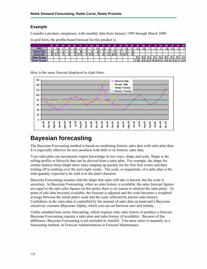
Retek Demand Forecasting, Retek Curve, Retek Promote
124
Example Consider a product, sunglasses, with monthly data from January 1999 through March 2000.
In grid form, the profile-based forecast for this product is:
Here is the same forecast displayed in chart form:
Bayesian forecasting The Bayesian Forecasting method is based on combining historic sales data with sales plan data. It is especially effective for new products with little or no historic sales data.
Your sales plan can incorporate expert knowledge in two ways, shape and scale. Shape is the selling profile or lifecycle that can be derived from a sales plan. For example, the shape for certain fashion items might show sales ramping up quickly for the first four weeks and then trailing off to nothing over the next eight weeks. The scale, or magnitude, of a sales plan is the total quantity expected to be sold over the plan's duration.
Bayesian Forecasting assumes that the shape that sales will take is known, but the scale is uncertain. In Bayesian Forecasting, when no sales history is available, the sales forecast figures are equal to the sales plan figures (at this point, there is no reason to mistrust the sales plan). As point of sale data becomes available, the forecast is adjusted and the scale becomes a weighted average between the initial plan's scale and the scale reflected by known sales history. Confidence in the sales plan is controlled by the amount of sales data on hand and a Bayesian sensitivity constant (Bayesian Alpha), which you can set between zero and infinity.
Unlike standard time series forecasting, which requires only sales history to produce a forecast, Bayesian Forecasting requires a sales plan and sales history (if available). Because of this difference, Bayesian Forecasting is not included in AutoES. You must select it manually as a forecasting method, in Forecast Administration or Forecast Maintenance.

Chapter 8 – Retek Demand Forecasting Methods
125
Obtaining accurate short life-cycle product forecasts is very difficult, and standard statistical time series forecasting models frequently do not offer an adequate solution for many retailers. Major problems in automatically developing these forecasts include:
• The lack of substantial sales history for a product (which especially makes obtaining seasonal forecasts very difficult),
• The difficulty of automatically matching a new product to a previous product or profile
• The inability to include planners’ intuition (for example, the overall sales level of the product, how quickly the product will take off, how the product’s sales will be affected by planned promotions) into a forecasting model.
Using a Bayesian approach, a short life-cycle forecasting algorithm has been developed that begins with a product’s seasonal sales plan (that is developed externally to the system by the planner). As sales information arrives during the first few days or weeks of the season, the model generates a forecast by merging the information contained in the sales plan with the information contained in the initial sales data. These forecast updates can be critical to a company’s success and can be used to increase or cancel vendor orders.
As forecasting consultants and software providers, Retek assists clients in obtaining “good” forecasts for future demands for their products based upon historical sales data and available causal information. Depending upon the information available, Retek’s software supports various forms of exponential smoothing and regression based forecasting. Frequently, however, clients already have some expectations of future demands in the form of sales plans. Depending upon the quality of their plans, they can provide very useful information to a forecasting algorithm (especially when only limited historical sales data is available). A forecasting algorithm has been developed that merges a customers sales plans with any available historical sales in a Bayesian fashion (that is, it uses new information to update or revise an existing set of probabilities).
Sales plans vs. historic data In most retail situations, clients are interested in obtaining good product forecasts automatically with little or no human intervention. For stable products with years of historic sales data our time series approaches (Simple, Holt, Winters, Regression based Causal, etc.) produce adequate results. The problem arises when attempting to forecast products with little or no history. In such instances expert knowledge is required, generally in the form of sales plans. Given that both sales plans and time series forecasts are available, an obvious question exists: When should the transition from sales plan to time series forecasting occur? Suppose that in answer to that question (in a particular scenario) we have determined that thirteen weeks of history is the transition point. Does that mean that at 12 weeks the time series results are irrelevant and that at 14 weeks the sales plan has no value? Our intuition tells us that instead of there existing a hard-edge boundary; there is actually a steady continuum where the benefits from the sales plan decrease as we gather more historic sales data. This was the motivation for developing an approach that would combine the two forecasts in a reasonable manner.
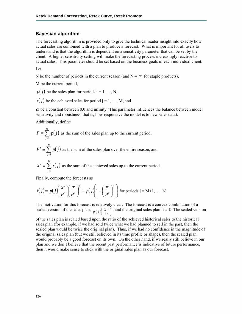
Retek Demand Forecasting, Retek Curve, Retek Promote
126
Bayesian algorithm The forecasting algorithm is provided only to give the technical reader insight into exactly how actual sales are combined with a plan to produce a forecast. What is important for all users to understand is that the algorithm is dependent on a sensitivity parameter that can be set by the client. A higher sensitivity setting will make the forecasting process increasingly reactive to actual sales. This parameter should be set based on the business goals of each individual client.
Let:
N be the number of periods in the current season (and N = ∞ for staple products),
M be the current period,
( )jp be the sales plan for periods j = 1, …, N,
( )jx be the achieved sales for period j = 1, …, M, and
α be a constant between 0.0 and infinity (This parameter influences the balance between model sensitivity and robustness, that is, how responsive the model is to new sales data).
Additionally, define
( )∑=
≡M
jjpP
1' as the sum of the sales plan up to the current period,
( )∑=
≡′′N
jjpP
1 as the sum of the sales plan over the entire season, and
( )∑=
≡′M
jjxX
1
as the sum of the achieved sales up to the current period.
Finally, compute the forecasts as
( ) ( ) ( ) ⎟⎟⎠
⎞⎜⎜⎝
⎛⎟⎠⎞
⎜⎝⎛
′′′
−+⎟⎠⎞
⎜⎝⎛
′′′
⎟⎠⎞
⎜⎝⎛
′′
≡αα
PPjp
PP
PXjpjx 1ˆ for periods j = M+1, …, N.
The motivation for this forecast is relatively clear. The forecast is a convex combination of a scaled version of the sales plan, ( ) ⎟
⎠⎞
⎜⎝⎛
′′
PXjp , and the original sales plan itself. The scaled version
of the sales plan is scaled based upon the ratio of the achieved historical sales to the historical sales plan (for example, if we had sold twice what we had planned to sell in the past, then the scaled plan would be twice the original plan). Thus, if we had no confidence in the magnitude of the original sales plan (but we still believed in its time profile or shape), then the scaled plan would probably be a good forecast on its own. On the other hand, if we really still believe in our plan and we don’t believe that the recent past performance is indicative of future performance, then it would make sense to stick with the original sales plan as our forecast.

Chapter 8 – Retek Demand Forecasting Methods
127
In our forecasting algorithm, the weights assigned to the scaled and original plans represent the confidence in the respective portions. As ⎟
⎠⎞
⎜⎝⎛
′′′
PP becomes larger (that is, the portion of the plan
that we can compare to historical sales increases), we tend to have more confidence in the scaled plan. For example, if ⎟
⎠⎞
⎜⎝⎛
′′′
PP = 0.01, then we really don’t have much information upon which to
base the scaled plan.
On the other hand, for example, as the quantity approaches 0.5 (that is, the season is half way over), then we really should start seriously considering why the plan was incorrect and we may have greater belief in the scaled plan. Additionally, the α parameter is used to tweek the sensitivity of the forecasting method. As α increases, the forecast will tend to stick closer to the original plan, and for small values of α the forecast will move rapidly towards the scaled plan as historical sales data becomes available. Clients should use their own data and judgement to determine an appropriate α for their particular business problem at hand.
Guidelines Bayesian forecasting is primarily designed for use with new product/location positions. The following guidelines should be followed:
1. No more than one plan should exist for a given product/location position. If multiple plans are to be set up for different time periods, the domain should be set up with different forecasting levels for each time period of interest.
2. Any time period with non-zero Actuals for a given product/location position should have a corresponding plan component (otherwise the system will assume a plan exists and equals zero and will act accordingly).
3. Any non-zero Actuals not within the time period of interest should be overridden to zero.

Retek Demand Forecasting, Retek Curve, Retek Promote
128
Causal (promotional) forecasting method Causal, or promotional, forecasting requires three input streams:
• Time Series Data
• Historical Promotional Calendar
• Future Promotional Calendar
Promote decomposes the problem of promotional forecasting into two sub-tasks: estimating the effect promotions have on demand and forecasting baseline (that is no promotions) demand.
To accomplish the first task a stepwise regression sub-routine is used. This routine will take a time series and a collection of promotional variables and determine which variables are most relevant and what effect those relevant variables have on the series. Thus, the output from the algorithm is a selection of promotional variables and the effects of those variables on the series. In the second step the time series is de-causalized using the promo effects. Then, AutoES is used to calculate the baseline demand. Once we know the effects and we have the baseline demand we can generate a promotional forecast by applying the effects wherever the promotion is active in the future.
It should be noted that just because promotional forecasting is selected it doesn’t necessarily imply that a “promotional” forecast will result. In some instances no promotional variables will be found to be statistically significant. In these cases the forecast ends up equivalent to a standard time series forecasts. (If users wish to force in certain promotional variables into the model this can be managed through forecasting maintenance parameters.)
Retek’s experience in promotional forecasting has led us to believe that there are a few requirements that are necessary to successfully forecast retail promotions:
• Baseline forecasts need to consider seasonality; otherwise “normal” seasonal demand will be attributed to promotional effects.
• Promotional Effects need to be able to be analyzed at higher levels in the retail product and location hierarchies. This produces cleaner signals and alleviates issues involved in forecasting new items and new Stores and issues involving data sparsity.
• Users need to be aware that the forecasting models cannot tell the difference between causal effects and correlated effects. What this means is that users should be wary of promotional effects attributed to an event that occurs at the same time every year. The system cannot distinguish between the promotional effect and the normal seasonality of the product. The same can be said for any two events that always occur at the same time (the combined effect will most likely be attributed to one or the other event).
Following is a description of the causal, or promotional forecasting, including the following topics:
• A description of the causal forecasting algorithm process
• The array interface between the Acumate environment and the AliAutoES binary
• Causal forecasting at the daily level
• Final considerations about causal forecasting

Chapter 8 – Retek Demand Forecasting Methods
129
The causal forecasting algorithm For purposes of understanding the algorithm, a promotional variable is defined as a causal event that is only active for certain series at certain points in time. It is assumed that these events are entered into the system independently of the forecasting algorithm and that a vehicle exists for determining which promotional variable are relevant to a particular series.
The core of the causal forecasting algorithm uses a stepwise regression sub-routine. This routine takes a time series and a collection of promotional variables, and determines which variables are most relevant and what effect those relevant variables have on the series. Thus, the output from the algorithm is a selection of promotional variables and the effects of those variables on the series.
Causal variable types define how causal variables are treated in the causal model fitting process (which includes a call to the lower level regression engine) and the forecast generation process where the model is used to extend the forecast over the forecast horizon. See chapter 6 for information on each of the causal variable types:
• Automatic
• Force In The Model
• Disabled
• Override All
• Override Future
• Override Higher Level
Types of causal models Two different types of causal models are possible. The first type is an additive model in which each effect is considered to add a constant amount to the sales of the product. The second type of model is the multiplicative model in which the system determines a baseline value that is multiplied by each effect to get the final forecast value.
Causal forecasting algorithm process The causal forecasting algorithm itself lies in the AutoES binary code, and executes in the following manner.
1. The binary reads the history of the time series.
2. The binary reads the type of each promotional variable into the system.
3. The binary reads in all the promotional variables that apply to the series.
4. The binary creates the internal promotional variable to allow the modeling of trend.
5. Promotional variables, internal promotional variables, promotional variable types, and the series itself are passed to the stepwise regression routine with the historic data serving as the dependent variables. Stepwise regression is run for both the additive and multiplicative models [Note: for the multiplicative model the logarithm of the historic data is used].
6. If the regression finds no significant promotional variables for either the additive or the multiplicative models then the casual method is considered to have failed to fit. In this case, the standard time series methods are used to generate a forecast and we skip to step 15.

Retek Demand Forecasting, Retek Curve, Retek Promote
130
7. The fit region is calculated for both models (additive and multiplicative). The fit at time t, fit(t), is defined in terms of β0, the intercept of the regression, βI, the effect corresponding to promotional variable i, and pi(t), is the value of promo variable I, in time t as: fit(t) = β0 + ∑ βi * pi(t) for the additive model fit(t) = β0 * π βi ^ pi(t) for the multiplicative model
8. The RMSE is determined across the two fit regions and the winning model is the one that produces the least RMSE.
9. The Time Series is de-causalized in the fit region of the history, by removing the causal effects (that is subtracting the additive causal effects, respectively dividing by the multiplicative causal effects for the product/location/time positions where the corresponding promo variables are “on”)
10. A seasonal model is fitted to the de-causalized series. The seasonal model is the winner of a competition between Seasonal ES, Additive Winters and Multiplicative Winters. The RMSE is determined across the fit region on the de-causalized series and the winning model is the one that produces the least RMSE.
11. The winning seasonal model is then used to determine the seasonal forecast by applying the fit(t) function across the forecast horizon. This forecast is also exported as the baseline forecast (that is forecast without any causal influences).
12. The forecast is obtained by re-causalizing the seasonal forecast. This is done by adding back the additive causal effects, respectively multiplying by the multiplicative causal effects for the product/location/time positions where the corresponding promo variables are “on” in the forecast region.
13. The binary writes the winning promotional variables effects back to the database.
14. The selected model is recorded in the database.
15. The binary records the forecast and the baseline in the database.
Confidence intervals constraining in Causal: The confidence interval is capped using the following rule:
if interval(0) ) = stdev(frcst error) < 0.3* forecast(i), then interval(i) = )1()(3.0 +⋅⋅ iiforecast
if interval(0) > forecast(i), then interval(i) = )1()( +⋅ iiforecast
Otherwise, interval(i) = )1()0(int +⋅ ierval
cuminterval(i) = 22 )(int)1(min iervalitervalcu +−
Besides the interval constraining, in Causal.cpp the interval calculation was changed. Specifically, to the extension formula:
2)(int ierval = )1( +⋅ imse

Chapter 8 – Retek Demand Forecasting Methods
131
Causal forecasting array interface description The promotional variables are stored in the database named promo. In the database named pmaint, the following arrays are stored:
• The promotional variables aggregated to the forecast level, along with promotional effects arrays. Both the additive and multiplicative effects are saved for promotional effectiveness assessment.
• The type arrays (arrays in which the type of each variable – see “Algorithm Description” - is stored for each product/location intersection at the forecast level).
• The list of variables to be considered in the stepwise regression.
The promotional variables (located in the promo database) are aggregated at the forecast level and saved in pmaint by the forecasting wrapper, fbatch.wrapautoes.
For causal forecasting the path to the database “pmaint” is passed as input to the AliAutoES binary. From pmaint the binary reads the promotion list and the promotional variables, and writes back the additive and multiplicative causal effects and intercept in the right arrays.
Forecast and baseline forecast are stored in separate databases.
Causal forecasting at the daily level The causal forecasting at the daily level is calculated by spreading the weekly causal forecast down to day. The spreading utilizes causal daily profiles thus obtaining a causal forecast at the day granularity.
The daily casual forecast process executes in the following manner.
1. Preprocess the day level promotional variables by multiplication with daily profiles. Aggregate the preprocessed continuous day level promotional variables to the week level.
2. Calculate the causal forecast at the weekly level. Set promotional effects if desired. Use the RDF causal engine to generate the forecast.
3. Calculate the multiplicative promotional effects at the item/store level for every promo variable. The effects can be either
Manually preset (See step 1.)
Calculated. When calculating the causal forecast, the calculated causal effects are written back to the database. If the effects are calculated at higher level than item/store, the effects will be replicated down to item/store – reasonable assumption since the effects are multiplicative. If source level forecasting is used and causal method is used both at the source level and at the final level then the effects from the final level will be used.
4. Daily profiles are calculated, using the Curve module. Since we use as much history as possible and we average it over seven days we assume these profiles are de-causalized. The de-causalized daily profiles capture the day of week effect and should be quite stable.
5. Causal effects are applied to the daily profiles. We multiply the profiles by the causal effects. Then, we have to renormalize the profiles.
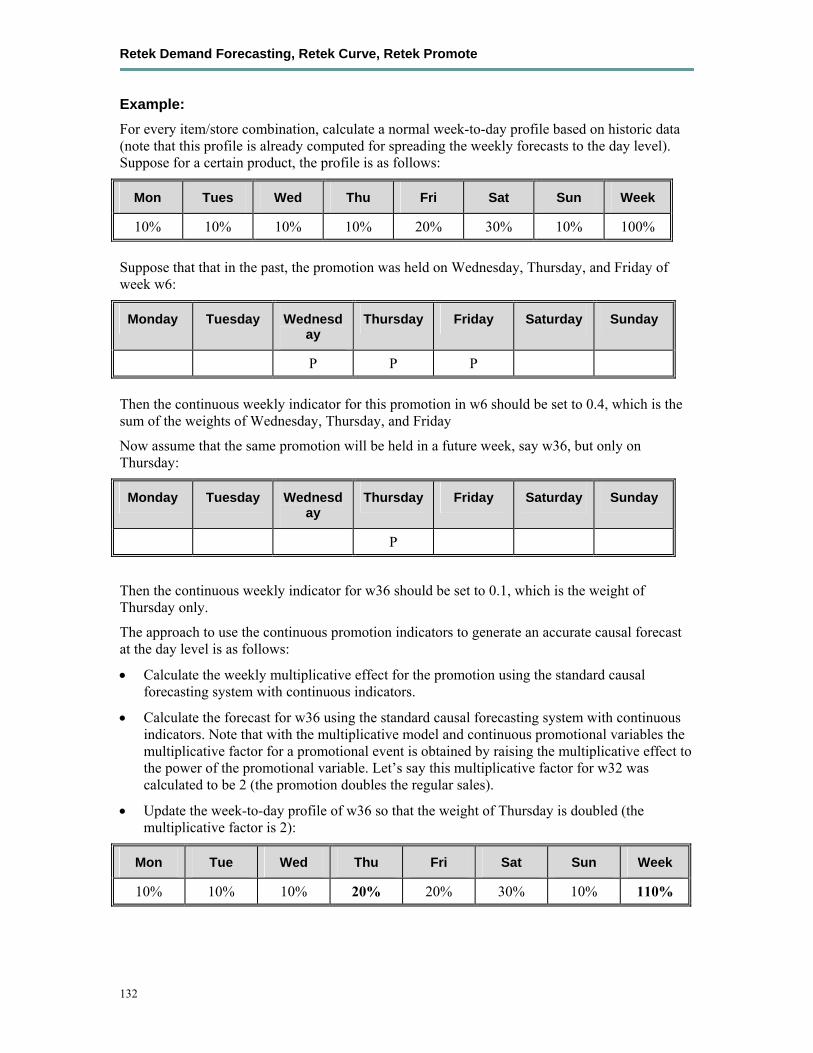
Retek Demand Forecasting, Retek Curve, Retek Promote
132
Example: For every item/store combination, calculate a normal week-to-day profile based on historic data (note that this profile is already computed for spreading the weekly forecasts to the day level). Suppose for a certain product, the profile is as follows:
Mon Tues Wed Thu Fri Sat Sun Week
10% 10% 10% 10% 20% 30% 10% 100% Suppose that that in the past, the promotion was held on Wednesday, Thursday, and Friday of week w6:
Monday Tuesday Wednesday
Thursday Friday Saturday Sunday
P P P Then the continuous weekly indicator for this promotion in w6 should be set to 0.4, which is the sum of the weights of Wednesday, Thursday, and Friday
Now assume that the same promotion will be held in a future week, say w36, but only on Thursday:
Monday Tuesday Wednesday
Thursday Friday Saturday Sunday
P
Then the continuous weekly indicator for w36 should be set to 0.1, which is the weight of Thursday only.
The approach to use the continuous promotion indicators to generate an accurate causal forecast at the day level is as follows:
• Calculate the weekly multiplicative effect for the promotion using the standard causal forecasting system with continuous indicators.
• Calculate the forecast for w36 using the standard causal forecasting system with continuous indicators. Note that with the multiplicative model and continuous promotional variables the multiplicative factor for a promotional event is obtained by raising the multiplicative effect to the power of the promotional variable. Let’s say this multiplicative factor for w32 was calculated to be 2 (the promotion doubles the regular sales).
• Update the week-to-day profile of w36 so that the weight of Thursday is doubled (the multiplicative factor is 2):
Mon Tue Wed Thu Fri Sat Sun Week
10% 10% 10% 20% 20% 30% 10% 110%

Chapter 8 – Retek Demand Forecasting Methods
133
• Normalize the profile for w36:
Mon Tue Wed Thu Fri Sat Sun Week
9% 9% 9% 18% 18% 27% 9% 100% Finally, spread the forecast of w36 using the normalized profile.
Final considerations about causal forecasting In Retek’s approach to causal forecasting, the causal effects are obtained by fitting a stepwise linear regression model that determines which variables are most relevant and what effect those relevant variables have on the series. The data used to fit the regression is the fit history of each time series, so basically we fit a model per time series. A problem arises due to potential lack of significant data, that is, when a promotional variable is not represented in the history but is present in the forecast region. In that case, the effect for that variable would not be computed at all, thus affecting the accuracy of the forecast. There are a few solutions that make use of the effects from other similar time series. One solution would be to do source level causal forecasting and then spread down to the final level. This would be equivalent to using the effects at the source level for time series that have no causal variable instances in the history. However, this has a serious conceptual drawback: by aggregating the promotional variables at the source level, we would force the effects on the other time series in the same aggregation class that otherwise would not have the causal variables on at the same time. An alternate solution is whenever a causal effect cannot be computed because of lack of significant data an averaged effect from another time-series in the same aggregation class is going to be used instead – see Override Higher Level type.


Glossary
135
Glossary Note: With a few exceptions, this glossary contains definitions of terms specific to Retek
Demand Forecasting. For further definitions of terms and concepts relating to the RPAS user interface, see the Retek Predictive Application Server online help or User Guide.
additive seasonal method
Also referred to as Additive Winters Model, this model is similar to the Multiplicative Winters model, but is used when zeros are present in the data. This model adjusts the un-seasonalized values by adding the seasonal index (for the forecast horizon).
alert
A notice displayed to system users that a forecasted value is above or below user-defined limits (an exception).
Alert Manager window
A window that displays the alerts assigned to you. This dialog provides a list of all identified instances in which a monitored measure’s values fall outside a set of defined limits. You may pick an alert from this list and have RCS automatically build a workbook containing the measure values that triggered the alert.
AutoES Method or Automatic Exponential Smoothing Method
Retek Demand Forecasting fits the sales data to a variety of exponential smoothing (time series) models of forecasting, and the best model is chosen for the final forecast. The candidate methods considered by AutoES are: Simple ES, Intermittent ES, Trend ES, Multiplicative Seasonal, Additive Seasonal and Seasonal ES. The final selection between the models is made according to a performance criterion (Bayesian Information Criterion) that involves a tradeoff between the model’s fit over the historic data and its complexity.
Bayesian Method
Useful for short lifecycle forecasting and for new products with little or no historic sales data. The Bayesian method requires a product’s known sales plan (created externally to RDF) and considers a plan’s shape (the selling profile or lifecycle) and scale (magnitude of sales based on Actuals). The initial forecast is equal to the sales plan but as sales information comes in, the model generates a forecast by merging the sales plan with the sales data. The forecast is adjusted so that the sales magnitude is a weighted average between the original plan’s scale and the scale reflected by known history.
Causal Method
Causal is a forecasting method used for promotional forecasting and can only be selected if Promote is implemented. (See Chapter 3 for more information on Promote.) Typically, the Causal method is used at the Final Levels (that is, item/week/week). Causal uses a Stepwise Regression sub-routine to determine the promotional variables that are relevant to the time series and their lift effect on the series. AutoES utilizes the time series data and the future promotional calendar to generate future baseline forecasts. By combining the future baseline forecast and each promotion’s effect on sales (lift), a final promotional forecast is computed.
confidence interval
The confidence percentage value used to calculate the value of the upper confidence limit. A different confidence level can be set for every forecast level appearing in the workbook

Retek Demand Forecasting, Retek Curve, Retek Promote
136
confidence limit
The upper bound of a normal probability distribution that is centered about the forecast value. It is calculated based on the Default Confidence % parameter value entered in the Forecast Administration Workbook, or on the Confidence Level value entered in the Confidence Worksheet of the Forecast Approval Workbook (if such a value has been entered to override the default).
Croston’s model of exponential smoothing
See Intermittent Exponential Smoothing.
Curve
An optional automated predictive solution that transforms organization-level assortment plans into base-level weekly sales forecasts.
exception
A forecast value that is greater than or less than a user-defined limit.
exponential smoothing
Α form of a weighted moving average. It weights decline in data exponentially. Most recent data weighted more heavily. Requires smoothing constant (α). Ranges from 0 to 1. Subjectively chosen.
final forecast level
A low level in a hierarchy from which a forecast is generated, and at which approvals and data exports can be performed. Often, data from forecasts at a low level is insufficient to generate reliable forecasts without first aggregating the data to a higher level and then spreading the data back to the low level.
forecast-driven planning
Planning that keys off of forecasts fed directly into a planning system. Connection to Retek Demand Forecasting (RDF) is built directly into the business process supported by Retek Predictive Planning through an automatic approval of a forecast that is fed directly in the planning system. This allows you to accept all or part of Sales Value forecast. Once that decision is made, the balance of business measures are planned within Retek Predictive Planning.
Holt’s model of exponential smoothing
See Trend Exponential Smoothing
interactive forecasting
A workbook in RDF used to simulate forecast by modifying parameters such as Forecast Method and History Start Date
IntermittentES or Intermittent Exponential Smoothing.
Retek Demand Forecasting fits the data to the Croston's model of exponential smoothing. This method should be used when the input series contains a large number of zero data points (that is, intermittent demand data). The original time series is split into a Magnitude and Frequency series, then the Simple ES model is applied to determine level of both series. The ratio of the magnitude estimate over the frequency estimate is the forecast level reported for the original series.
Glossary
137
like item or like SKU
An item that will be used as a model to forecast a new item introduction.
lost sales
Periods in sales data in which there was no inventory to meet consumer demand.
measure
Any item of data that can be represented on a grid in worksheets.
measure description
The description of the measure that can be viewed in a workbook. This description may contain relationships and calculations.
measure function
Internal functions that can be used to simplify building calculations for a measure.
measure identifier
The combination of role, version, metric, and units that uniquely specifies a single measure.
metric
A measure definition with the role, version, and units omitted.
Multiplicative Seasonal
(also referred to as Multiplicative Winters Model) This model extracts seasonal indices that are assumed to have multiplicative effects on the un-seasonalized series.
Forecast
In Retek Demand Forecasting (RDF), Forecast refers to RDF’s statistical forecasting capabilities.
Preprocessing
In Retek Demand Forecasting (RDF), Preprocessing refers to a module that processes data before forecasts are generated to adjust for situations such as lost sales and unusually high demand.
profile
Spreading ratios that are used in the Curve process. Typical profiles can include store participation, size distribution, and time (phase-to-week) profiles, as well as other information. Profiles are generated using historical data and phase definitions, based on your system configuration.
Profile Based
Retek Demand Forecasting generates a forecast based on a seasonal profile that can be created in Curve or a legacy system. Profiles can also be copied from another profile and adjusted. Using historic data and the profile, the data is de-seasonalized and then fed to the Simple ES method. The Simple forecast is then re-seasonalized using the profiles.
Profile Spread
Used at the final level to utilize a profile (either generated externally or with Curve) to determine the spreading ratios from the Source level forecast down to the Final level.

Retek Demand Forecasting, Retek Curve, Retek Promote
138
Promote
Promote is an optional add-on automated predictive solution that allows you to incorporate the effects of promotional and causal events, such as radio advertisements and holiday occurrences, into your time series forecasts. The promotional forecasting process uses both past sales data and promotional information to forecast future demand.
promotion planning
A workbook template and simulation process used within the context of promotional forecasting. Promotion planning involves specifying whether the event status for a particular promotional variable is active (on) or inactive (off) for a specific product/location/calendar combination. When past promotional events are represented as accurately as possible, the modeling routine can more precisely detect correlation between event occurrences and changes in sales values.
promotional effectiveness
A workbook template used in the context of promotional forecasting. This workbook allows you to analyze the effects of promotions on items at both the micro and the macro level. “What if” analysis can also be performed on the results of promotional forecasts, as you can modify future and past promotional inputs, the system-estimated effects of promotions, and the promotional forecasts themselves.
promotional forecasting
Promote’s forecasting technique (also referred to as Causal forecasting) uses promotional factors and events to predict future demand. Promotion events are events such as advertisements, holidays, competitor information, and other factors that affect the normal selling cycle for a business.
promotion group
A set of products or locations that are believed to exhibit similar effects during common causal events. Promotion groups should be established to maximize the number of time series for each group (so each promotional event can be evaluated from as many different observations as possible) while ensuring that each time series is affected by causal events to the same degree.
Seasonal ES Method
A combination of several Seasonal methods. This method is generally used for known seasonal items or forecasting for long horizons. This method applies the Multiplicative Seasonal model unless zeros are present in the data, in which case the Additive Winters model of exponential smoothing is used. If less than 2 years of data is available, then a Seasonal Regression model is used. If there is too little data to create a seasonal forecast (in general, less than 52 weeks), then the system will select from the Simple ES, Trend ES and Intermittent ES methods.
Seasonal Regression
Seasonal Regression cannot be selected as a forecasting method, but is only a candidate model used when the Seasonal ES method is selected. This model requires a minimum of 52 weeks of history to determine seasonality. Simple Linear Regression is used to estimate the future values of the series based on a past series. The independent variable is the series history one-year or one cycle length prior to the desired forecast period, and the dependent variable is the forecast. This model assumes that the future is a linear combination of itself one period before plus a scalar constant.

Glossary
139
Simple/Intermittent ES Method
A combination of the Simple ES and Intermittent ES methods. This method applies the Simple ES model unless a large number of zero data points are present, in which case the Croston’s model is applied.
SimpleES or Simple Exponential Smoothing Method
Retek Demand Forecasting uses a simple exponential smoothing model to generate forecasts. Simple ES ignores seasonality and trend features in the demand data and is the simplest model of the exponential smoothing family. This method can be used when less than 1 year of historic demand data is available.
simple moving average
See Average Method
sister store
A store that will be used as a model to forecast a new store.
source level forecast
The level at which the aggregate, more robust forecast is run.
Time series
Set of evenly spaced numerical data obtained by observing response variable at regular time periods. This data is used to forecast based only on past values. It assumes that factors influencing past and present will continue influence in future
training window
The number of weeks of historical sales data to use in generating a forecast.
Trend Exponential Smoothing or TrendES
(Also referred to as Holt’s Model.) Retek Demand Forecasting fits the data to the Holt model of exponential smoothing. The Holt model is useful when data exhibits a definite trend. This method separates out base demand from trend, then provides forecast point estimates by combining an estimated trend and the smoothed level at the end of the series.
wizard
A set of screens that guide you through the process of creating a new workbook or performing other actions in an solution, by asking you various questions and having you select values.
workbook
The framework used for displaying data and user functions. Workbooks are task-specific and may contain one or more worksheets. Users define the format of their workbooks. See also workbook template, worksheet.
workbook template
The framework for creating a workbook. You build each new workbook from an existing workbook template, such as Pre-Season Financial Plan or Forecasting Administration. Several workbook templates are supplied with the Retek Predictive Solutions, and are available for selection when you choose File+New to create a new workbook.

Retek Demand Forecasting, Retek Curve, Retek Promote
140
worksheet
A multidimensional spreadsheet used to display workbook-specific information. Worksheet data can also be displayed in chart format.
i Chatfield, C. and M.Yar, 1990, “Prediction intervals for the Holt-Winters forecasting procedure”, International Journal of Forecasting, 6, 127-137 ii Chatfield, C. and M.Yar, 1990, “The Holt-Winters forecasting procedure”, Applied Statistics, 27, 264-279 iii Chatfield, C. and M.Yar, 1990, “Holt-Winters forecasting: theory and practice”, The Statistician, 37, 129-140


![Retek Merchandising System 11.0 Operations Guide – Volume 4 · Retek Merchandising System iv SWIFT file conversion [lcmt730].....485 SWIFT file conversion [lcmt798].....491](https://img.pdfslide.net/doc/110x75/5fc32d4cda22981b3210f23b/retek-merchandising-system-110-operations-guide-a-volume-4-retek-merchandising.jpg)