Demand Response for Residential Appliances via … · controlling their loads based on time varying price ... Demand Response for Residential Appliances via ... Real-Time Home Energy

School of Electrical Engineering and Computer Science

Faculty of Science and Engineering

Queensland University of Technology

DEMAND RESPONSE FOR RESIDENTIAL

APPLIANCES IN A SMART ELECTRICITY

DISTRIBUTION NETWORK: UTILITY AND

CUSTOMER PERSPECTIVES

Cynthujah Vivekananthan

Bachelor of Science (Electrical and Electronic Engineering) (Hons.)

University of Peradeniya-2010

Thesis submitted in accordance with regulations of the Degree of Doctor of

Philosophy in the Faculty of Science and Engineering, Queensland University of

Technology.

September, 2014

Supervisor: Dr. Yateendra Mishra

ii

iii

KEYWORDS

Action space, Adjustability of appliances, Advanced metering infrastructure,

Ancillary services, Appliance flexibility, Appliance priority, attributes of appliances,

Customer discomfort, Customer Reward, Customer satisfaction, day-ahead bid,

Decision making, Demand Response, Direct load control, Dispatch signal,

Distributed generation, Electricity price, Forecast, Frequency, Grey variable, In-

home display unit, Load adjustments, Market operator, Markov process, Optimal

policy, Overload, Pairwise probabilistic comparison, Peak load, Power consumption,

Preferred order of appliances, Ramp rate, Real-time price, Real-time, Rebate,

Regulation services, Renewable generation, Retailer, Seasonal flat pricing, Smart

grid, Smart meter, State space, Stochastic ranking, Stochastic scheduler, Tariff,

Transition Probability, Uncertainty, Utility, Voltage violation, Wholesale electricity

price, Zigbee interface

iv

v

ABSTRACT

Recent advancements in Advanced Metering Infrastructure (AMI) enable

optimum utilization of existing electricity network via Demand Response (DR). A

flexible and reliable electricity network can be created by allowing open access

information sharing and independent decentralized decision-making for unbundled

market participants including utility and end-users. The massive rollout of AMI

(such as smart meters) alone, however, may not be sufficient and there is a need for

well thought algorithms to achieve desired benefits. This research work introduces

efficient algorithms for residential appliances to achieve economic as well as

network benefits for all participants.

Firstly, a new technique based on a customer reward mechanism is proposed,

where the network provider controls residential appliances to achieve peak shaving

and improve voltage profile. Then, an improved Real-Time Pricing (RTP) scheme

for residential customers is introduced. Home energy management systems are

proposed to account for the uncertainties in RTP and appliance power consumption.

Finally, a control method to provide regulation services in the market via DR is

proposed. These methods are tested using mathematical simulation models

representing a cluster of demand responsive proactive customers.

Initial study focuses on load control method via a customer reward scheme.

The network peak shaving and improvement in the voltage profile while maintaining

customer satisfaction is achieved. Customer survey information of appliance

characteristics and real-time appliance operation data are used to calculate indices.

These indices combined with the sensitivity based house ranking are used for load

selection in a network feeder. As customers participate in the direct load control,

rebates are awarded in return. A network level economic analysis is proposed for the

calculation of rebates.

Secondly, a new price based DR technique to handle peak demand and

voltage violations. In contrast to first phase, customers have their own choice of

controlling their loads based on time varying price signals. An improved RTP

scheme for residential customers with three components based on power

consumption, adverse wholesale price variation and feeder voltage violation is

vi

proposed. Using broadcasted price information, Smart meters and in-home display

units provide appropriate load adjustment signals, which give customers an

opportunity to respond to price signals.

Uncertainties in RTP variation and power consumption pattern of appliances

have a significant implication on decision making during DR. Hence, a stochastic

Home Energy Management (HEM) system is proposed next, which facilitates

customers to adjust their loads while considering uncertainties in RTP and appliance

power status. The proposed HEM scheduler aims to reduce the cost of energy

consumption in a house while maintaining customer satisfaction. It works in three

subsequent steps namely real-time monitoring, stochastic scheduling and real-time

control of appliances. In the first step of real-time monitoring, characteristics of

available controllable appliances are monitored in real-time and stored in HEM

scheduler. In second step, HEM scheduler computes an optimal policy using

stochastic dynamic programming to select a set of appliances to be controlled with an

objective of minimizing customer discomfort as well as the total cost of energy

consumption in a house. In third step, HEM scheduler initiates the control of the

selected appliances ultimately providing an efficient house based energy

management by appropriate load adjustments utilizing stochastic information.

Finally, the control method for appliances to provide regulation services is

proposed. Registered retailers schedule their loads to match a dispatch regulation

signal offered by the wholesale electricity market operator. Stochastic DR method

using a pool of thermostatically controllable appliances is proposed, where the

selection of appliances is based on a probabilistic ranking technique.

Various findings from this research work have multi-faceted benefit and are

helpful for (1) policy makers to develop proper power pricing scheme; (2)

distribution network providers to utilize AMI effectively and (3) end-users by

making them aware of the associated financial benefits.

vii

TABLE OF CONTENTS

KEYWORDS ...................................................................................................... iii

ABSTRACT .......................................................................................................... v

TABLE OF CONTENTS ...................................................................................vii

LIST OF FIGURES ............................................................................................. xi

LIST OF TABLES ............................................................................................. xiv

LIST OF ABBREVIATIONS ............................................................................. xv

VARIABLES AND NOTATIONS ................................................................... xvii

CONTRIBUTIONS ........................................................................................... xix

LIST OF PUBLICATIONS ............................................................................... xxi

STATEMENT OF ORIGINAL AUTHORSHIP ............................................. xxii

ACKNOWLEDGEMENTS .............................................................................xxiii

Chapter 1 .......................................................................................................... 1

Introduction .......................................................................................................... 1

1.1. Background .................................................................................................... 1

1.2. Research Problem .......................................................................................... 3

1.3. Research Method ........................................................................................... 5

1.4. Research Significance .................................................................................... 8

1.5. Thesis outline ................................................................................................. 9

1.5.1. Outline of Chapter 2 ................................................................................ 9

1.5.2. Outline of Chapter 3 ................................................................................ 9

1.5.3. Outline of Chapter 4 ...............................................................................10




Chapter 2 ........................................................................................................ 12

Literature Review for Demand Response .......................................................... 12

viii

2.1. Historical Background and Recent Developments in Electricity System .. 13

2.1.1. Liberalization of Electricity Sector ......................................................... 13

2.1.2. Smart Grid Concept ................................................................................ 14

2.2. DR Approach ............................................................................................... 16

2.2.1. DR in the Smart Electricity Distribution Network ................................... 17

2.2.2. DR Options ............................................................................................. 18

2.2.3. Analysis of DR techniques for residential distribution system - Direct Load

Control, RTP, HEM system and DR for ancillary services ...................... 20

2.3. Summary and Implications ......................................................................... 26

Chapter 3 ........................................................................................................ 28

Demand Response for Residential Appliances via Customer Reward Scheme 28

3.1. Introduction and Related Work.................................................................. 28

3.2. CR based Demand Response for Residential Appliances .......................... 30

3.2.1. Seeking customer preferences for demand response ................................ 31

3.2.2. Calculation of various criteria indices from customer survey .................. 32

3.2.3. Using house ranking and criteria indices for load adjustment ................. 37

3.2.4. Customer reward (CR) Scheme ............................................................... 39

3.2.5. Implementation and operation of load control algorithm ........................ 40

3.3. Critical Assessment of CR Scheme ............................................................. 43

3.3.1. Significance of indices in control scheme ................................................ 43

3.3.2. Evaluation of cost coefficients for CR ..................................................... 45

3.3.3. Customer rewards .................................................................................. 47

3.3.4. Implementation and operations of CR scheme......................................... 48

3.3.5. Scalability .............................................................................................. 50

3.3.6. Prevention from customers misusing this scheme .................................... 50

3.4. Case Study ................................................................................................... 51

3.4.1. Impact on feeder voltage and transformer overload ................................ 52

3.4.2. Power loss reduction in the network ....................................................... 54

3.4.3. Effect on customer loads and its impact on ASI ....................................... 54

3.4.4. Robustness of CR scheme under increasing PEV penetration .................. 57

3.4.5. Effectiveness of this scheme on overloading due to load growth .............. 58

3.5. Summary and Conclusion ........................................................................... 58

ix

Chapter 4 ........................................................................................................ 60

A Novel Real-Time Pricing Scheme for Demand Response in Residential

Distribution Systems .................................................................................... 60

4.1. Introduction and Related Work .................................................................. 60

4.2. The Novel Real-Time Pricing Scheme ......................................................... 63

4.2.1. Price component for actual load consumption (П1it) ................................63

4.2.2. Price component for Voltage Violation (П2it) ..........................................64

4.2.3. Price component for reflection of wholesale price (П3it) ..........................65

4.3. Practical Implementation of this Scheme.................................................... 66

4.4. Identification of Critical House Loads for Possible Adjustment................ 67

4.4.1. Adjustability (X1ij) ...................................................................................68

4.4.2. Customer preferred order of appliances (X2tij) ........................................68

4.4.3. The operational state of appliances (X3tij)................................................69

4.5. Simulation Results ....................................................................................... 71

4.6. Summary and Conclusion ........................................................................... 75

Chapter 5 ........................................................................................................ 77

Real-Time Home Energy Management Scheduler Using Stochastic Dynamic

Programming ............................................................................................... 77

5.1. Introduction and Related Work .................................................................. 78

5.2. Proposed Real-Time HEMS using SDP ...................................................... 80

5.2.1. Real-Time Monitoring (RTM) Phase .......................................................82

5.2.2. Stochastic Scheduling (STS) phase ..........................................................85

5.2.3. Real-Time Control (RTC) Phase .............................................................92

5.3. Description of Overall Control Process....................................................... 97

5.4. Test System and Simulation Results ........................................................... 98

5.4.1. Results related to HEMS .........................................................................98

5.4.2. Results related to appliances connected to HEMS ................................. 106

5.5. Summary and Conclusion ......................................................................... 109

Chapter 6 ...................................................................................................... 111

x

Stochastic Ranking Method for Thermostatically Controllable Appliances to

Provide Regulation Services ...................................................................... 111

6.1. Introduction and Related Work................................................................ 112

6.2. Stochastic Ranking Method for TCAs to Provide Regulation Services... 114

6.2.1. Background on Regulation Services ...................................................... 114

6.2.2. SR algorithm performed by Aggregators ............................................... 116

6.3. Modeling and Simulation Results ............................................................. 124

6.3.1. Mathematical models for TCAs (ACs and WHs) .................................... 124

6.3.2. Small network with 30 houses ............................................................... 129

6.3.3. Providing regulation services in different season in a year ................... 131

6.4. Conclusion and Summary ......................................................................... 133

Chapter 7 ...................................................................................................... 134

Conclusion ........................................................................................................ 134

7.1. Research Summary and Contributions .................................................... 134

7.2. Proposed Future Work and Suggestions .................................................. 137

APPENDICES .................................................................................................. 141

Appendix A ....................................................................................................... 142

Appendix B ....................................................................................................... 149

Appendix B ....................................................................................................... 152

BIBLIOGRAPHY ............................................................................................ 154

xi

LIST OF FIGURES

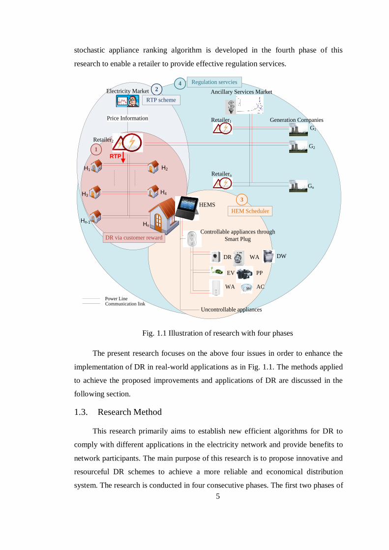
Fig. 1.1 Illustration of research with four phases ............................................. 5

Fig. 2.1 Conceptual design of a smart grid environment .................................15

Fig. 2.2. Available DR Options ......................................................................18

Fig. 3.1 API of houses in phase-A of feeder 1 ................................................33

Fig. 3.2 Time schematic of the load control process .......................................40

Fig. 3.3 Load control process with CR scheme for a particular day ................42

Fig. 3.4 API during each control (a) without (b) with API in decision process 44

Fig. 3.5 Error in (a) API (b) AFI when API (or AFI) is considered or not .......44

Fig. 3.6 Supply and demand curve with and without CR scheme ....................45

Fig. 3.7 A smart meter at each house connected with appliances ....................48

Fig. 3.8 Hierarchical control scheme for CR based Demand response ............51

Fig. 3.9 The voltage profile of the residential feeder at peak time (1940 hrs) ..52

Fig. 3.10 Loading of 500kVA transformer without and with controller ..........53

Fig. 3.11 Voltage profile at the end bus of feeder- 1 without and with control 53

Fig. 3.12 The active power loss of the network with and without control........54

Fig. 3.13 ASI of 3 selected PEVs in phase- A of feeder 1 ...............................55

Fig. 3.14 ASI of Inverter type Air Conditioners in phase- A of feeder 1 .........55

Fig. 3.15 Set point variation of inverter type AC in house 2, 4,7 (phase A).....56

Fig. 3.16 ASI of a water heater in House 7 of Phase- A of feeder 1 ................56

Fig. 3.17 Set point and actual tank temperature variation of a WH in House 7 56

Fig. 3.18 Voltage profile at the end- bus at phase- C with and without control57

Fig. 3.19 Appliance Satisfaction Index verses increased peak demand ...........58

Fig. 4.1 The Available retail pricing scheme ..................................................61

Fig. 4.2 Three price components of proposed pricing scheme .........................63

Fig. 4.3 First price components verses energy consumption ...........................64

Fig. 4.4 Third price components verses energy consumption ..........................66

Fig. 4.5 Communication Capability of the network ........................................67

Fig. 4.6 Appliance Preferred order House 1, phase A, feeder 1 at 1900hrs......69

Fig. 4.7 Algorithm for appropriate indication of appliances in each house ......70

Fig. 4.8 RRP of QLD on 29th November 2012 ................................................71

Fig. 4.9 (a) Power (b) 1st (c) 2

nd (d) 3

rd price component of house 5- feeder 1 .72

xii

Fig. 4.10 Loading level of the 500kVA distribution transformer .................... 73

Fig. 4.11 Voltage profile at the end bus of feeder 1 ........................................ 73

Fig. 4.12 selected PEV battery charge in phase- A of feeder 1 ....................... 74

Fig. 4.13 Temperature set point adjustment of selected AC ............................ 74

Fig. 4.14 Water Heater tank temperature change of a selected house .............. 75

Fig. 5.1 Descriptive diagram of HEMS and utility interference ...................... 81

Fig. 5.2 Timing diagram of control process.................................................... 82

Fig. 5.3 Block of transition probability (Tr) ................................................... 89

Fig. 5.4 Operating statuses of appliances before RTM and after RTC phase... 93

Fig. 5.5. Linear droop curve for set point adjustment of a cooling load .......... 95

Fig. 5.6. Linear droop curve for set point adjustment of a heating load .......... 95

Fig. 5.7. Exponential droop curve for set point adjustment of a cooling load .. 96

Fig. 5.8. Exponential droop curve for set point adjustment of a heating load .. 96

Fig. 5.9 Operation of HEM Scheduler with RTM, STC and RTC phases ....... 97

Fig. 5.10 Defining boundaries of states .......................................................... 99

Fig. 5.11 Definition of states for CoEC .......................................................... 99

Fig. 5.12 State changes in three typical days of a house in summer ................ 99

Fig. 5.13. Transition probability of CoEC states at 2000 hrs in winter day ... 100

Fig. 5.14 Reward when there is no curtailment and maximum curtailment ... 100

Fig. 5.15. The Real-Time Price considered for real-time model ................... 101

Fig. 5.16. Optimal policy values for two consecutive days ........................... 101

Fig. 5.17. Optimal policy values for a time frame withing a day .................. 102

Fig. 5.18. Power profile of the house without and with HEMS ..................... 103

Fig. 5.19 CoEC of the house without and with control ................................. 103

Fig. 5.20 Dish Washer Power Profile of the house with HEMS (Cat 1) ........ 104

Fig. 5.21 Water Heater Power Profile of the house with HEMS (Cat 3) ....... 105

Fig. 5.22 CoEC data of a house in winter season.......................................... 106

Fig. 5.23 CDF of CoEC of a house during winter ........................................ 107

Fig. 5.24. Linear droop curve obtained for each season for HEMS ............... 107

Fig. 5.25 . Exponential droop curve obtained for each season for HEMS ..... 108

Fig. 5.26 Hot water temperature variation with exponential droop control ... 108

Fig. 5.27 Room temperature variation with exponential droop control ......... 109

Fig. 6.1. Comparison of AEMO and North American markets ..................... 114

xiii

Fig. 6.2. Providing regulation services via DR ............................................. 115

Fig. 6.3. Schematic Control Diagram of Aggregator Controller .................... 116

Fig. 6.4. Obtaining PMF from transition block ............................................. 120

Fig. 6.5. Categorizing the possible results into groups .................................. 123

Fig. 6.6. Normal operation of an AC of a house ........................................... 126

Fig. 6.7. Normal operation of a WH of a house ............................................ 126

Fig. 6.8. Maximum available loads for regulation in 30 houses network ....... 126

Fig. 6.9. Regulation requirement for network with 30 houses ....................... 127

Fig. 6.10. Comparing network performance for a sample regulation service . 127

Fig. 6.11. Number of controls during regulation ........................................... 127

Fig. 6.12. Comfort of TCAs in the network as per (1) .................................. 128

Fig. 6.13. Operation of an AC when providing regulation services ............... 128

Fig. 6.14. Operation of a WH when providing regulation services ................ 128

Fig. 6.15. Decision Probability at 1000 hrs (regulation raise services) .......... 129

Fig. 6.16. Ranking of appliances at 1000 hrs ................................................ 129

xiv

LIST OF TABLES

Table 3.1 Sample customer survey questionnaire ........................................... 31

Table 3.2 Required data from customers ........................................................ 32

Table 3.3 Priority of Appliances in House 1 .................................................. 33

Table 3.4 Flexibility of appliances ................................................................. 34

Table 3.5 Calculation of ASI for different appliances .................................... 35

Table 3.6 PSI calculation of house- 1 for a particular instant .......................... 36

Table 3.7 Detailed Calculation of Rebate for 5 Houses in one feeder ............. 49

Table 3.8 Cost of electricity consumption in a peak day for few houses ......... 49

Table 4.1 Adjustability and Preferred Order of Appliances ............................ 68

Table 4.2 Variation of Price of selected houses per day ................................. 74

Table 5.1 Changes in appliance statuses when they are subjected to control . 103

Table 5.2 Appliance status changes at 1940 hours........................................ 104

Table 5.3 Energy and CoEC savings with HEMS ....................................... 105

Table 5.4 Effect of HEMS on COEC due to uncertainty (A winter day) ....... 105

Table 5.5 Calculation of Ctotal

lim and Ctotal

max of each season for HEMS ....... 107

Table 6.1 Definition of Grey Variables for AT1in .......................................... 118

Table 6.2 Categorizing possible results ........................................................ 123

Table 6.3 Comparison of regulation services with three different networks .. 130

xv

LIST OF ABBREVIATIONS

AC Air Conditioner

AEMO Australian Energy Market Operator

AFI Appliance Flexibility Index

AMI Advanced Metering Infrastructure

API Appliance Priority Index

ASI Appliance Satisfaction Index

AU Appliance Unit

BESS Battery Energy Storage System

CDF Cumulative Distribution Function

CoEC Cost of Energy Consumption

CPP Critical Peak Price

CR Customer Reward

DLC Direct Load Control

DR Demand Response

FCAS Frequency Control Ancillary Services

HEM Home Energy Management

HEMS Home Energy Management Scheduler

HPSI High Power Consumption Index

LV Lower Voltage

MDP Markov Decision Process

NERC North American Reliability Corporation

PEV Plug- in Electric Vehicle

PMF Probability Mass Function

PMU Phasor Measurement Unit

xvi

PRD Price Response Demand

PSI Power Similarity Index

PV Photovoltaic cells

RRP Regional Reference price

RTC Real-Time Control

RTM Real-Time Monitoring

RTP Real-Time Price

SDP Stochastic Dynamic Programming

SOC State of Charge

SR Stochastic Ranking

STS STochastic Scheduling

TCA Thermostatically Controllable Appliances

TOU Time Of Use

WH Water Heater

xvii

VARIABLES AND NOTATIONS

Variable Meaning

C(i,j,k) kth criteria of i

th house and the j

th controllable load

APIij API for ith house and j

th appliance

Prij priority value for ith house and j

th appliance

Twh Water heater, hot water temperature

Tr Room temperature

Twhset

and Twhdb

Temperature set point and dead-band of water heater

Tacset

and Tacdb

Temperature set point and dead-band of AC

PSIij PSI for ith house and j

th appliance

HPCIij HPCI for ith house and j

th appliance

ρip Voltage sensitivity of i

th house in p

th phase

rijp Rank of i

th house and j

th appliance in p

th phase

eij Status (On/Off) signal of jth appliance in i

th house

G Conductance of feeder

B Susceptance of feeder

θ Bus angle

P Real power

Q Reactive power

V Voltage

Decij Decision for ith house and j

th controllable load

Rebatei Rebate in $/day for ith

house

Eil Shifted energy for i

th house at the l

th load adjustment

Пavg constant tariff or flat rate price of electricity

Пi

t Real-time price for i

th house at t

th time

xviii

Lcapacity Network capacity

ПBL baseline of wholesale electricity price

Пtwholesale Wholesale electricity price at t

th time

N Number of houses in the network

Xkij kth criteria for i

th house, j

th appliance for PRD scheme

Dj jth

appliance

INTRPDj Interrupt signal of Appliance Dj

ζmaxintrp

maximum number of interruptions for an appliance

WDjmax

Maximum allowable waiting time of appliance Dj

tDjconnect

Time when appliance Dj in plugged into HEMS

Cntotal

CoEC of a house at nth time step

Sk kth state of CoEC

Anq q

th action (sets of appliances) at n

th time step

TR Transition probability of state changes

R A state (S) dependent reward function

P Probability

βnDj

Operating status of appliance Dj at nth time step

Regn dispatch instructions at n

th time step

ATkin k

th attribute for i

th appliance at n

th time step

ATGkin k

th grey attribute for i

th appliance at n

th time step

gin(ATk) PMF for i

th appliance at n

th time, k

th (k=1,2) attribute

fijn(ATGk) PMF of (ATGki

n-ATGkj

n) representing comparison of i

th and j

th

appliances with respect to kth attribute

Napp Number of total available appliances in the network

PDn decision probability matrix at n

th time step

Prankn Probability for appliance ranking at n

th time step

xix

CONTRIBUTIONS

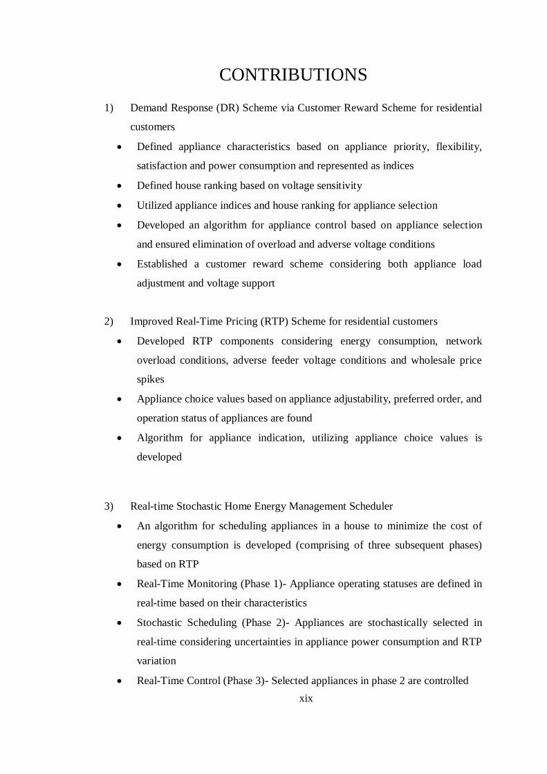
1) Demand Response (DR) Scheme via Customer Reward Scheme for residential

customers

Defined appliance characteristics based on appliance priority, flexibility,

satisfaction and power consumption and represented as indices

Defined house ranking based on voltage sensitivity

Utilized appliance indices and house ranking for appliance selection

Developed an algorithm for appliance control based on appliance selection

and ensured elimination of overload and adverse voltage conditions

Established a customer reward scheme considering both appliance load

adjustment and voltage support

2) Improved Real-Time Pricing (RTP) Scheme for residential customers

Developed RTP components considering energy consumption, network

overload conditions, adverse feeder voltage conditions and wholesale price

spikes

Appliance choice values based on appliance adjustability, preferred order, and

operation status of appliances are found

Algorithm for appliance indication, utilizing appliance choice values is

developed

3) Real-time Stochastic Home Energy Management Scheduler

An algorithm for scheduling appliances in a house to minimize the cost of

energy consumption is developed (comprising of three subsequent phases)

based on RTP

Real-Time Monitoring (Phase 1)- Appliance operating statuses are defined in

real-time based on their characteristics

Stochastic Scheduling (Phase 2)- Appliances are stochastically selected in

real-time considering uncertainties in appliance power consumption and RTP

variation

Real-Time Control (Phase 3)- Selected appliances in phase 2 are controlled

xx

4) Stochastic Ranking Method for thermostatically controllable appliances to

provide regulation services

Developed a stochastic ranking algorithm based on pairwise probabilistic

comparison of appliances

Probabilistic decision based on appliance attributes such as temperature

variation, switching status and power rating are considered.

Average possible regulation services for a network with 30, 120 and 960

houses are computed

xxi

LIST OF PUBLICATIONS

(Related to research work presented in this thesis)

Publications:

1. C. Vivekananthan, Y. Mishra, et al., “Demand Response for Residential

Appliances via Customer Reward Scheme”, IEEE Transactions on Smart Grid,

vol. 5, no. 2, Mar. 2014.

2. C. Vivekananthan, Y. Mishra, et al., “Aggregated Control of Thermostatically

Controllable Appliances for regulation purposes utilizing Home Energy

Management Systems,” accepted for IEEE Transactions on Power Systems, 2014.

3. C. Vivekananthan, Y. Mishra, et al., “Real-Time Price Based Home Energy

Management Scheduler,” currently under review of IEEE Transactions on Power

Systems, 2014.

4. C. Vivekananthan, Y. Mishra, et al., “Real-Time Stochastic Coordination of

Home Energy Management Schedulers to alleviate Network Peaks,” Abstract

currently under review of IEEE Transactions on Smart Grid, 2014.

Conferences:

1. C. Vivekananthan, Y. Mishra, et al., “A Novel Real-Time Pricing Scheme for

Demand Response in Residential Distribution Systems,” 39th

International

Conference on Industrial Electronics (IECON), Vienna, Austria, Nov. 2013.

2. C. Vivekananthan, Y. Mishra, et al., “Using multi objective genetic algorithm for

the optimal arrangement and size of a feeder level battery energy storage in the

distribution system for voltage improvement,” 4th International Conference on

Computational Methods, Gold Coast, Australia, Nov. 2012.

3. C. Vivekananthan, Y. Mishra, et al., “Energy Efficient Home with price sensitive

stochastically programmable TCAs,” accepted for 40th

International Conference

on Industrial Electronics (IECON), Dallas, TX, USA, Oct. 2014.

xxii

STATEMENT OF ORIGINAL AUTHORSHIP

The work contained in this thesis has not been previously submitted to meet

requirements for an award at this or any other higher education institution. To the

best of my knowledge and belief, the thesis contains no material previously

published or written by another person except where due reference is made.

Copyrights in relation to this Thesis

Copyright © Cynthujah Vivekananthan, 2014.

This work may not be copied without written permission of the author or

university (Queensland University of Technology).

QUT Verified Signature

xxiii

ACKNOWLEDGEMENTS

This research work is conducted during my PhD candidature in Queensland

University of Technology (QUT) with the immense support and guidance of various

personalities. First and foremost, I offer my sincere gratitude to my supervisor, Dr.

Yateendra Mishra, for the continuous support throughout my PhD candidature with

his motivation, patience, technical contribution and excellent guidance. His

indispensable assistance and priceless advice greatly shaped my professional career

as a successful researcher.

I also would like to extend my gratitude to Power Engineering academics at

QUT including Prof. Arindam Ghosh, Prof. Gerard Ledwich, Dr. Ghavameddin

Nourbakhsh and Associate Prof. Geoffrey Walker for their kind support. I offer my

sincere thanks to Dr. Lasantha Perera for his guidance at the early stages of my

research. My heartfelt thanks go to Prof. Fangxing Li (University of Tennessee) for

helping me in the initial phase of my research. I am thankful to Dr. Farhad Shahnia

and Dr. Mike Wishart for helping me in residential appliance model development. I

am thankful for my fellow research mates especially Ms. Dinesha Chathurani, Mr.

Nayim Kabir and Ms. Xu Yang for always giving their valuable time to help me

when I was in need.

Further, I acknowledge QUT staff members especially Ms. Judy Liu, Ms.

Elaine Reyes, Ms. Joanne Kelly and Ms. Joanne Reaves for their support in creating

a productive research environment. I also acknowledge the financial support offered

by QUT under QUTPRA fee-waiver scholarship and living allowance scholarship to

make this research a success. I thank Ms. Helen Whittle for editing the thesis. I

would like to thank all that whom I could not mention separately and have supported

in countless number of ways.

Finally, I thank my parents and my brother for motivating me throughout my

research. My special thanks go to my fiancé for encouraging me and making this

research, a reality.

1

Chapter 1

Introduction

This chapter outlines the background in section 1.1 and research problem in

section 1.2. Research methodology and significance is explained in sections 1.3 and

1.4 respectively. Finally, section 1.5 includes an outline of the remaining chapters of

the thesis.

1.1. Background

The traditional electricity network is being transformed to a smart grid

environment characterized by the utilization of advanced metering, sensing

frameworks and wireless two-way communication facilities in electricity generation,

transmission and distribution infrastructure. Smart grid enables to deal with the

complex nature of the present electricity network, with a goal to achieve stability,

reliability and security. A smart electricity network can self-repair during adverse

network conditions, prevent power leakages and allow flexible market augmentation.

Decentralized power generation and Demand Response (DR) are the key features of

the smart distribution grid.

Decentralized generation can be any source of power generation connected in a

distribution network such as roof top PV cells micro wind turbines. DR refers to a

temporary load curtailment scheme to minimize energy consumption during adverse

network conditions. It is a promising scheme in future smart grid environment due to

the benefits it offers. The DR scheme is made possible by the massive rollout of

2

advanced metering infrastructure. The present research focuses on DR schemes in a

residential distribution system and its benefits for both electricity customers and

electric utilities.

DR is primarily used to reduce network peaks. An increasing trend of peak

electricity demand is observed in present residential distribution systems. Therefore,

DR is utilized to handle network peaks by time-shifting residential loads. This

provides benefits to an electric utility by deferring the investment cost of network

upgrades and the usage of expensive generation plants to cater to peak demand.

Customers who participate in a DR scheme through load curtailments receive

benefits through incentives.

Furthermore, DR is capable of responding to uncertainties in electricity

consumption and supply, thus preventing unexpected system instability. The

unpredictable nature of electricity demand is detected on a daily and seasonal basis.

The integration of renewable energy generation and distributed generation also

increases system uncertainty to a further extent. DR easily handles uncertainties and

prevents the use of expensive generators to maintain the capacity margin during

uncertainties. In addition, DR can considerably reduce the wholesale price spikes.

Fluctuations in fuel price and the uncertain nature of electricity demand and supply

are the main causes for wholesale price spikes. A real-time curtailment of loads in

the residential distribution system consistently reduces the possibility of wholesale

price spikes and provides immense cost benefits to an electric utility. A Real-Time

Pricing (RTP) scheme for residential customers reflecting the wholesale price

variation is used for this purpose. Here, customers tend to reduce their electricity

bills by scheduling their loads through Home Energy Management (HEM) units

when the electricity price becomes high. Therefore, it provides benefits to customers

who incur a reduced cost for energy consumption when they create an energy

efficient home.

DR has an added advantage of providing regulation services in the ancillary

services market in order to maintain the supply and demand balance. Electricity

retailers get benefit through this scheme by obtaining profit from the ancillary

services market and customers are given rebates for load curtailment.

3

1.2. Research Problem

DR is becoming increasingly important in the current electricity grid as it is the

key to unlocking market flexibility and empowering electricity customer choices.

Moreover, it is a very cost effective technique. An immense amount of research has

been carried out on DR in recent years but the implementation of DR schemes is still

in the preliminary stage and needs to be explored further. Among the ongoing

research problems related to DR, the present study focuses on the following four

areas: incentive based DR; the Real-Time Pricing (RTP) method (price based DR);

Home Energy Management (HEM) schedulers; and DR for regulation services.

Incentive based DR

Studies related to DR in residential distribution systems are mostly conducted

with the aim to reduce network peaks and adverse feeder voltage conditions by time-

shifting residential appliances. Such efforts are based on optimization techniques to

maximize electric utility benefits or customer satisfaction. However, optimization

techniques may be time consuming and it may be difficult to simulate load

curtailments within a short timeframe. Therefore, an efficient load selection method

is required considering both electric utility and customer benefits. Furthermore, most

of the techniques consider particular appliances such as water-heaters, air-

conditioners and plug-in electric vehicles in the DR process. However, the

engagement of most residential appliances is possible. A detailed model of appliance

engagement is essential to validate this statement. Moreover, a comprehensive

customer reward scheme for load curtailment based on both overload prevention and

voltage support has not yet been studied. Therefore, the first phase of this research

focuses on an effective real-time DR method considering a detailed residential load

model. It considers both electric utility and customer benefits during load selection

for curtailment. A guaranteed rebate scheme is also developed for participating

customers to provide incentives.

RTP Methods

A number of price-responsive demand techniques have been proposed in the

past, including time of use pricing, critical peak pricing and real-time pricing. RTP is

a promising option as it reflects the wholesale price variation within short

4

timeframes, creating a bridge between the wholesale and retail electricity market.

Recently, RTP has been applied in the residential distribution sector with the

deployment of smart meters and in-home display units. Most of the available RTP

schemes reflect the average wholesale price. This may adversely affect customers

when there are unacceptably high wholesale price spikes. Therefore, a rational price

component for RTP is essential. In the majority of available RTP schemes, the prices

are broadcast on an hourly basis. This may not reflect the actual network conditions

and hence the RTP scheme may not be able to achieve the required demand shift.

This gives rise to the need to increase the frequency of RTP broadcasting. Moreover,

the RTP concept can be applied to prevent overload and improve voltage conditions

in the electricity network. Therefore, an improved RTP scheme is developed in the

second phase of this research based on a consideration of wholesale price variations,

network peaks and adverse voltage conditions.

HEM Scheduler

A HEM system helps customers to react to RTP variations efficiently by scheduling

residential appliances to reduce the cost of energy consumption. Recent studies in

HEM systems were based on real-time techniques and did not consider the uncertain

nature of appliance usage or RTP variation during appliance scheduling. Some of the

available HEM systems use predictive techniques for appliance scheduling, which

may deviate from the real system. Therefore, a fully-fledged HEM scheduling

algorithm which handles the uncertainty in both appliance power consumption and

RTP variation is developed in the third phase of this research.

DR for regulation services

The DR technique can also be used to provide regulation services. Studies in

the literature indicate the utilization of thermostatically controllable loads for

appliances such as water-heaters and air-conditioners. The selection of these loads is

based on real-time temperature ranking methods. This technique is only valid with

short time step controls such as one minute. However, in the Australian ancillary

services market, regulation services are scheduled to a five minute dispatch

framework. This gives rise to the need for an accurate stochastic appliance ranking

scheme to predict the appliance status in the five minute timeframe. Therefore, a

5

stochastic appliance ranking algorithm is developed in the fourth phase of this

research to enable a retailer to provide effective regulation services.

Electricity Market

Retailer2

Controllable appliances through

Smart Plug

Uncontrollable appliances

EV

WA

PP

DR DW

WA

Price Information

AC

HEMS

H1 H2

H3H4

Hn-1 Hn

Power LineCommunication link

RTP

Ancillary Services Market

G1

G2

Gn

Retailer1

Retailern

Generation Companies

1

2

3

4

DR via customer reward

RTP scheme

HEM Scheduler

Regulation servcies

Fig. 1.1 Illustration of research with four phases

The present research focuses on the above four issues in order to enhance the

implementation of DR in real-world applications as in Fig. 1.1. The methods applied

to achieve the proposed improvements and applications of DR are discussed in the

following section.

1.3. Research Method

This research primarily aims to establish new efficient algorithms for DR to

comply with different applications in the electricity network and provide benefits to

network participants. The main purpose of this research is to propose innovative and

resourceful DR schemes to achieve a more reliable and economical distribution

system. The research is conducted in four consecutive phases. The first two phases of

6

this research are based on the DR techniques used for peak shaving and eradicating

adverse voltage conditions. A new direct load control technique based on a customer

reward mechanism is introduced in the first phase of the research. Here, the electric

utility can have complete control of residential appliances in the network. The second

phase of the research proposes a price-responsive technique providing greater

customer choices in comparison with the first phase. It also introduces an improved

RTP scheme for residential customers. The third phase mainly focuses on house-

level stochastic energy management systems. It deals with the uncertainties in RTP

and appliance power consumption. Unlike the first three phases, the fourth phase

proposes a new application of DR in the ancillary services market for providing

frequency regulation considering load uncertainty. A brief conceptual outline of the

above four phases is discussed next.

The initial study focuses on a direct load control method for DR via a customer

reward scheme for peak shaving and the mitigation of adverse voltage conditions in

the network while also maintaining customer satisfaction within allowable limits.

Information from a customer survey on appliance characteristics and real-time

appliance operation data are used to calculate indices reflecting appliance priority,

flexibility, customer satisfaction and power statuses. These indices and the

sensitivity-based house ranking are used for appropriate load selection in a network

feeder for DR. As customers are forced to accept direct load control, they are given a

reward in the form of a rebate. A network-level economic analysis is used for rebate

formulation and it is found that rebates can be paid based on the load shift and

voltage improvement due to load adjustments.

The second phase of the research focuses on a new detailed price-based DR

technique to handle peak demand and adverse voltage conditions. In contrast to the

first phase, customers have their own choice in controlling their loads based on time-

varying price signals. An improved RTP scheme for residential customers with three

components based on power consumption, adverse wholesale price variation and

feeder voltage violation is proposed. Smart meters and in-home display units can be

used to broadcast price information and appropriate load adjustment signals so that

customers have an opportunity to respond to price signals optimally by choosing the

appropriate load adjustments broadcast by the electric utility.

7

Uncertainties in RTP variation and the power consumption patterns of

appliances have a significant impact on decision-making during DR. Hence, a

stochastic HEM system is proposed in the third phase which enables customers to

adjust their loads based on RTP while also considering uncertainties in RTP and

appliance power status. The proposed real-time HEM scheduler aims to reduce the

cost of energy consumption in a house while maintaining customer satisfaction. It

works in three steps, namely, real-time monitoring, stochastic scheduling and the

real-time control of appliances. In the first step of real-time monitoring, the

characteristics of the available controllable appliances are monitored in real-time and

stored in the HEM scheduler. In the second step, the HEM scheduler computes an

optimal policy using stochastic dynamic programming to select a set of appliances to

be controlled with the objective of minimizing customer discomfort as well as the

total cost of energy consumption in a house. In the third step, the HEM scheduler

initiates the control of the selected appliances, ultimately providing efficient house-

based energy management by appropriate load adjustments utilizing stochastic

information.

The fourth phase of this research focuses on a different dimension of DR used

in the ancillary services market to provide fast frequency regulation services.

Registered retailers are urged to stochastically schedule their loads to match a time

step-ahead of the dispatch regulation signal offered by the ancillary services market.

Hence, a new stochastic DR methodology applied on a pool of thermostatically

controllable appliances is proposed. It considers water-heaters and air-conditioners as

they are in operation most of the time during a day and are available for control. The

selection of appliances is based on a probabilistic ranking technique whereby three

attributes of appliances related to temperature variation, appliance power status and

appliance power rating are analyzed for decision-making. The first two attributes are

stochastically forecasted for the next time step and follow a Markov process.

The performance of the proposed methods is clarified by applying them in a

real-time simulation environment representing a cluster of demand-responsive

proactive customers. Realistic mathematical residential load models are utilized for

this purpose.

8

1.4. Research Significance

This research provides significant benefits and outcomes in four different

phases of this study.

The algorithm developed for DR in first phase of this research can be

implemented efficiently in real-time environment within short time frame. In

comparison with past studies, it considers both customer and utility perspectives

during decision making for appliance curtailment. It provides benefit to customers by

maintaining appliance satisfaction, flexibility and priority within allowable limits.

The utility benefits by eliminating overload and adverse voltage conditions in the

network. A fully guaranteed customer reward scheme, considering both load

adjustment and voltage support is established which makes this DR scheme

economically feasible.

The RTP method developed in second phase of this research is significant from

existing methods as it considers power consumption, overloading conditions, voltage

violations along with wholesale price spike in RTP. Active participation in this RTP

guarantees elimination of overload, adverse voltage conditions and wholesale price

spikes. Customers benefit from reduction in cost of energy consumption. The

appliance indication developed for load curtailment is unique from existing methods

which ease the appliance control process for customers via in-home energy

management units.

A novel stochastic HEM scheduling algorithm developed in third phase of this

research provides significant benefit to customers by appropriately acting according

to proposed RTP variation. It is unique from the existing methods as it considers

uncertainties in appliance power consumption and RTP variation effectively. It

ensures reduced cost of energy consumption in a house.

The algorithm developed for providing regulation services via DR is distinctive

as it uses stochastic appliance ranking method to predict appliance controls for

regulation. It is very useful in ancillary services market which broadcasts offers

every five minutes, necessitating the prediction of appliance status for next five

minutes.

9

1.5. Thesis outline

The remaining chapters of this thesis are organised as follows. Chapter 2 is a

comprehensive literature review which leads to the development of the research

hypotheses presented in this thesis. This is followed by the original work in Chapters

3, 4, 5 and 6. The thesis concludes with a summary of the research work and findings

in Chapter 7.

1.5.1. Outline of Chapter 2

Chapter 2 presents a detailed study of existing electricity infrastructure which

provides the motivation for this research. Recent developments in the electricity

sector such as market liberalization, the smart grid concept and DR schemes are

discussed in detail. An in-depth study on DR in residential distribution systems is

carried out, as it is the main focus of this thesis. The benefits and applications of DR

in a smart grid environment are identified. A comprehensive literature review is

conducted on existing and proposed DR options in the electricity market. The

drawbacks in present DR schemes are highlighted and the need for an improved DR

technique is elaborated upon, which leads to the generation of the hypotheses to be

tested in the subsequent research work in Chapters 3, 4, 5 and 6.


Chapter 3 proposes a novel customer reward-based DR technique which can be

easily implemented in a residential distribution system to prevent overload and

adverse voltage conditions in the feeder. Customer preferences are considered during

the selection of appliances for curtailment. For this purpose, customer survey

information and real-time power consumption data are used to calculate appliance-

based indices such as appliance flexibility, satisfaction and priority. This ensures that

customer comfort is maintained within acceptable limits. A voltage sensitivity-based

ranking is used along with the indices to improve voltage in the residential feeder. A

novel reward scheme for customer load adjustments is also proposed, with rewards

paid in the form of rebates based on voltage improvement and power curtailment.

The analysis and results to validate the efficacy of the proposed technique are also

presented in this chapter.

10


Chapter 4 proposes a new “price response demand” technique which can be

applied in a residential distribution system with the purpose of preventing overload

and adverse voltage conditions. It is achieved by introducing a novel real-time

pricing scheme, reflecting the actual power consumption, feeder voltage deviation

and wholesale electricity price. Customers are given the opportunity to react to the

real-time price signals broadcast through in-home display units. This scheme offers

more benefits than the direct load control technique in Chapter 3, as it provides

flexibility for customers during load adjustments.


There is a necessity for an efficient HEM system for residential customers, in

order to react efficiently to the real-time pricing scheme proposed in Chapter 2.

Hence, Chapter 5 proposes a real-time HEM scheduler with the aim to reduce the

cost of consumption in a house while at the same time maintaining customer

satisfaction. This technique considers the stochastic behavior of appliance usage and

real-time pricing during appliance selection. Stochastic dynamic programming is

used to incorporate uncertainties in pricing and appliance usage. Real-time appliance

monitoring, stochastic appliance scheduling and real-time appliance control are the

main steps used in the proposed HEM scheduler. It ensures the reduced cost of

consumption and minimal customer discomfort.


Chapter 6 utilizes the residential DR option as an operating reserve in the

ancillary services market for the purpose of providing regulation services. Retailers

can bid in the day-ahead market and respond to the real-time regulation offered by

appropriate load control. This part of the study proposes a method for the stochastic

ranking of appliances in a retail network in order to select appropriate appliances for

regulation purposes. A pool of thermostatically controllable loads such as air-

conditioners and water-heaters are used for load adjustments. The ranking method is

based on the pairwise probabilistic comparison of appliances. The attributes of

appliances such as comfort, switching state and power rating are used for decision-

making. System performance is verified for a given regulation signal. The network

11

capability for regulation is also analyzed during various seasons to show the

robustness of the system for regulation.


Chapter 7 summarises the original research work presented in Chapters 3, 4, 5

and 6. The techniques and algorithms proposed to achieve the objectives of the study

are briefly reviewed. The significant research findings and analysis are specified. The

benefits and importance of the proposed techniques are summarised, demonstrating

the relevance of the research findings to the present electricity industry. Suggestions

for implementing the proposed methods in the real world are also made. Finally,

future directions in research that can be carried out to extend and improve the present

study are suggested.

12

Chapter 2

Literature Review for Demand Response

This chapter delineates the historical background and recent developments in

the electricity industry as a motivation for the research work presented in this thesis.

Initially, a brief overview of past and present trends in the electric power system is

presented. Recent developments in the electricity network such as market

liberalization, the introduction of renewable energy and the development of the smart

grid concept are discussed in detail. A comprehensive study of the DR mechanism in

the smart grid environment is conducted as it is the main target of this research work.

Problems and constraints associated with the recent developments in the electricity

market are analyzed and the DR solutions proposed in the literature are extensively

analyzed. This theoretical outline of DR helps to develop a conceptual framework for

the generation of the hypotheses in this study and helps to define the research

structure of this thesis as well as setting the scene for the following chapters.

This chapter begins with the historical background and recent developments in

the electric power system in Section 2.1, followed by a review of the literature in

section 2.2. Concluding this chapter, Section 2.3 highlights the implications of the

findings in the literature and develops the conceptual framework of the study.

13

2.1. Historical Background and Recent Developments in Electricity

System

Electricity is increasingly important in the modern globalized economy and

serves as an essential resource in the day-to-day life of every individual. Hence,

electricity supply is expected to be reliable and affordable with a minimum impact on

the environment. As electricity is a non-storable commodity, a comprehensive and

careful focus on policy actions is vital in order to have an accurate balance between

electricity supply and demand. This is made possible by the liberalization of the

electricity sector [1].

2.1.1. Liberalization of Electricity Sector

In the early 1990s, many power systems were characterized by a vertically

integrated structure, whereby electricity generation, transmission and distribution

belonged to one electric utility. Electricity prices for these three sectors were bundled

together, reflecting the cost of the provided services [2].

However, in most countries, this monopolistic market structure has been

replaced by a deregulated and competitive market arrangement. This involved the act

of breaking the electricity market into components, based on each component’s

functionality or physical structure. Ownership of these unbundled market

components is provided to authorized and independent operators. This liberalization

of the market structure provides flexibility to end-users to choose their provider.

Trading between market components is well organized. Market based competition

are created such that electricity can be bought or sold, similar to other commodities.

It leads to efficient operations of the electricity system with more effective

investment decisions in terms of timing, sizing and technological improvements.

Furthermore, the transparency created by the competitive environment addresses

critical policy challenges related to environmental issues and network reliability.

Liberalization of the electricity market has been successfully practiced in the real-

world and is being augmented by more appropriate policy prescriptions [3], [4].

However, the present electricity network has drawbacks. Increased carbon

emission leads to global warming and there is a need to introduce renewable energy

sources to the electricity grid. The integration of renewable energy sources and the

14

increasing demand for electricity due to the fast growing world population make the

present electricity system more vulnerable. Hence, the reestablishment of the power

grid with increased flexibility and efficiency via the smart grid concept is essential to

provide intelligent services to end-users [5].

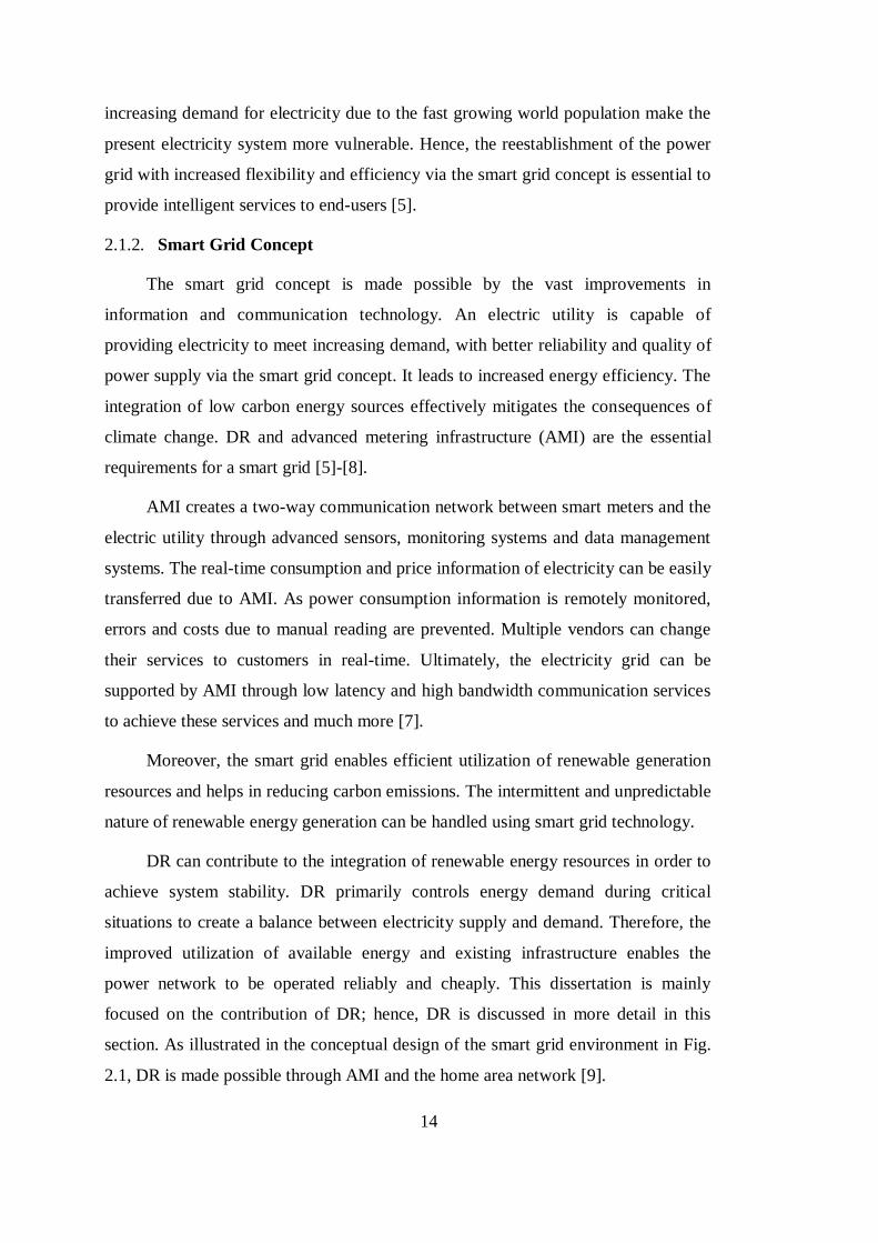
2.1.2. Smart Grid Concept

The smart grid concept is made possible by the vast improvements in

information and communication technology. An electric utility is capable of

providing electricity to meet increasing demand, with better reliability and quality of

power supply via the smart grid concept. It leads to increased energy efficiency. The

integration of low carbon energy sources effectively mitigates the consequences of

climate change. DR and advanced metering infrastructure (AMI) are the essential

requirements for a smart grid [5]-[8].

AMI creates a two-way communication network between smart meters and the

electric utility through advanced sensors, monitoring systems and data management

systems. The real-time consumption and price information of electricity can be easily

transferred due to AMI. As power consumption information is remotely monitored,

errors and costs due to manual reading are prevented. Multiple vendors can change

their services to customers in real-time. Ultimately, the electricity grid can be

supported by AMI through low latency and high bandwidth communication services

to achieve these services and much more [7].

Moreover, the smart grid enables efficient utilization of renewable generation

resources and helps in reducing carbon emissions. The intermittent and unpredictable

nature of renewable energy generation can be handled using smart grid technology.

DR can contribute to the integration of renewable energy resources in order to

achieve system stability. DR primarily controls energy demand during critical

situations to create a balance between electricity supply and demand. Therefore, the

improved utilization of available energy and existing infrastructure enables the

power network to be operated reliably and cheaply. This dissertation is mainly

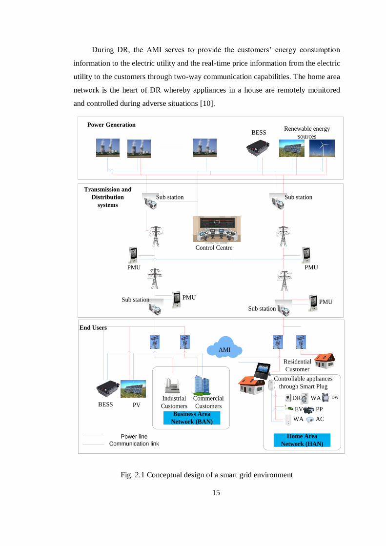
focused on the contribution of DR; hence, DR is discussed in more detail in this

section. As illustrated in the conceptual design of the smart grid environment in Fig.

2.1, DR is made possible through AMI and the home area network [9].

15

During DR, the AMI serves to provide the customers’ energy consumption

information to the electric utility and the real-time price information from the electric

utility to the customers through two-way communication capabilities. The home area

network is the heart of DR whereby appliances in a house are remotely monitored

and controlled during adverse situations [10].

Power Generation

Transmission and

Distribution

systems

Renewable energy

sources

Industrial

Customers

Commercial

Customers

Residential

Customer

Sub station Sub station

Control Centre

PMU PMU

BESS

PMUPMUSub station

Sub station

AMI

Controllable appliances

through Smart Plug

EV

WA

PP

DR DW

WA AC

Home Area

Network (HAN)

Business Area

Network (BAN)

BESS PV

End Users

Power line

Communication link

Fig. 2.1 Conceptual design of a smart grid environment

16

2.2. DR Approach

DR is an integral component of the envisioned smart grid infrastructure. It

primarily refers to activities related to active load control during high market price or

when grid reliability and stability are jeopardized.

DR provides a number of key benefits for both the electric utility and

customers. For the electric utility, DR maintains electricity system reliability by

lowering the likelihood of consequences arising from unexpected outages which

create financial losses and inconvenience to customers. For example, DR

compensates for the uncertainty brought by intermittent renewable energy sources. It

can also react to problems caused by distributed generation instantaneously. Network

overloads and adverse feeder voltage conditions can also be mitigated. Furthermore,

financial benefits are obtained by lowering wholesale market prices by preventing

the use of costly generation [11].

Customers also benefit from DR schemes in many ways. Careful attention to

home energy consumption leads to energy efficient buildings. Participating

customers can save considerable amounts of money due to load adjustments by

means of reduced electricity prices or incentive payments.

Currently, electric utilities have focused most of their DR efforts on industrial

or commercial buildings based on the reasonable argument that large customers can

provide more savings with fewer numbers of load adjustments [12], [13]. However,

residential customers can be incorporated into DR schemes for equally valid reasons.

Residential customers make the large contribution to peak load in the network.

Hence, overload prevention can be performed by DR in the residential electricity

network [14]. Adverse voltage conditions in residential feeders can also be mitigated

by residential DR. Flexible house appliances such as plug-in electric vehicles, air-

conditioners and water-heaters are easy to incorporate in residential DR schemes.

Hence, residential DR can play an important role in the smart grid environment. The

next sub-section provides a brief description of DR in the smart electricity

distribution network.

17

2.2.1. DR in the Smart Electricity Distribution Network

A smart distribution network is an important part of the smart grid which

connects the main network with the user-oriented supply. With emerging

technological improvements, the smart distribution system is made possible by the

large-scale deployment of smart meters and HEM units, intelligent assets for

condition monitoring, distributed generation and DR. Data acquisition and real-time

monitoring and analysis make it a reality [15], [16].

The smart distribution network should be able to handle variation in electricity

demand which is changing instantaneously due to changes in electricity-driven

activities at different times. There is a major peak demand for electricity between

1800 to 2100 hrs. Further, daily variations throughout the year occur due to seasonal

factors (such as the temperature and rainfall), the level of industrial and agricultural

activities and other causes such as holidays and festivals. [17].

Furthermore, plug-in electric vehicles could have a significant impact on the

smart distribution grid by adding a new load on the existing primary and secondary

distribution networks, many of which do not have any spare capacity. The additional

charging load of plug-in electric vehicles is typically behind either an existing

secondary distribution transformer in a residential neighbourhood or a transformer

connected to a distribution feeder. The vehicles range in battery capacity from 16

kWh to 53 kWh. They require a full charge within a reasonable time which is usually

3 to 4 hours plugged in with 6.6 kW or 16 kW capacities [18]. The use of a plug-in

electric vehicle more than doubles the average household load during charging, as

found in [18].

Hence, handling the peaking scenario will be a principal concern in electricity

systems in the future due to the expected rapid penetration of plug-in electric

vehicles. In the worst case, it will lead to the overloading of transformers at the

distribution level, potentially causing outages and could even lead to voltage

collapse. The smart distribution grid is capable of handling such adverse conditions

by creating a self-healing environment [19]. The DR techniques that are available to

be implemented in the residential electricity system are discussed next.

18

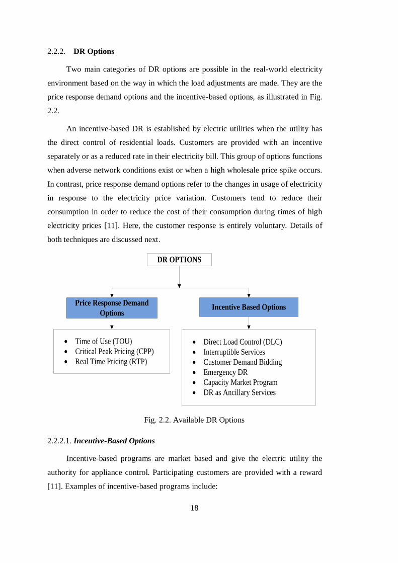
2.2.2. DR Options

Two main categories of DR options are possible in the real-world electricity

environment based on the way in which the load adjustments are made. They are the

price response demand options and the incentive-based options, as illustrated in Fig.

2.2.

An incentive-based DR is established by electric utilities when the utility has

the direct control of residential loads. Customers are provided with an incentive

separately or as a reduced rate in their electricity bill. This group of options functions

when adverse network conditions exist or when a high wholesale price spike occurs.

In contrast, price response demand options refer to the changes in usage of electricity

in response to the electricity price variation. Customers tend to reduce their

consumption in order to reduce the cost of their consumption during times of high

electricity prices [11]. Here, the customer response is entirely voluntary. Details of

both techniques are discussed next.

DR OPTIONS

Price Response Demand

OptionsIncentive Based Options

Time of Use (TOU)

Critical Peak Pricing (CPP)

Real Time Pricing (RTP)

Direct Load Control (DLC)

Interruptible Services

Customer Demand Bidding

Emergency DR

Capacity Market Program

DR as Ancillary Services

Fig. 2.2. Available DR Options

2.2.2.1. Incentive-Based Options

Incentive-based programs are market based and give the electric utility the

authority for appliance control. Participating customers are provided with a reward

[11]. Examples of incentive-based programs include:

19

Direct load control

In a direct load control scheme, the electric utility remotely shuts down

or adjusts residential appliances on short notice. Customers are

provided with rebates or reduced bills for the forced load adjustments.

Interruptible services

In the interruptible services approach, the electric utility provides

flexibility to customers to adjust their loads during critical conditions.

Curtailment options are broadcast to the customers in advance with

appropriate retail tariffs and discounts or rebates. Customers automate

their loads for control according to curtailment options. If the customers

fail to curtail their loads, penalties are applied to the customers.

Customer demand bidding

In customer demand bidding, an opportunity is given to residential

customers to offer bids based on the wholesale price or an equivalent

price signal. The electric utility selects loads based on the bids and

remotely controls the loads of selected customers.

Emergency DR

In an emergency DR scheme, customer load adjustments are conducted

during a power shortfall and incentives are provided for affected

customers.

Capacity market program

In a capacity market program, customers offer bids according to

possible load curtailments in the capacity market as a replacement for

expensive generators. The electric utility selects the customers based on

the bids and sends prior notice of curtailment. Customers automate their

loads for control in order to match with the prior notice for curtailment.

Penalties may apply if the customers fail to curtail their loads during the

given time.

DR for ancillary services

Unlike the capacity market program, customers in a DR for ancillary

services scheme bid for load curtailment as operating reserves. Upon

the acceptance of bids by the ancillary services market, offers are

20

provided to customers during selected dispatch time steps. Finally,

loads are subjected to control based on the offers.

2.2.2.2. Price Response Demand Options

Price response demand options include:

Time of Use (TOU) Pricing

In the time of use pricing approach, different blocks of prices are broadcast

for different timeframes within a day. The prices reflect the average cost of

generation and power delivery during each timeframe.

RTP

RTP is a tariff scheme for customers reflecting real-time variations in

wholesale price. The real-time price is broadcast on a day-ahead or hour-

ahead basis which helps the customers to take decisions for their optimal

power consumption.

Critical peak pricing

Critical peak pricing is a pricing scheme that combines the time of use and

RTP techniques. During a normal day, customers are provided with a time of

use pricing scheme. However, during a critical peak day, the customer tariff

is switched to the RTP scheme. This reduces the likelihood of adverse

network conditions.

2.2.3. Analysis of DR techniques for residential distribution system - Direct

Load Control, RTP, HEM system and DR for ancillary services

Among the incentive-based DR techniques, the interruptible services,

emergency DR, customer demand bidding and capacity market programs are found

to be the most suitable for large-scale industrial or commercial customers. These may

not be appropriate for residential customers due to the lack of customer flexibility,

complex bidding mechanism and unacceptable penalties. Hence, the direct load

control is best suited for a residential distribution system. The direct load control

technique is discussed in more detail in the next Section 2.2.3.1

21

Among the price response demand options, the RTP scheme is also a

promising mechanism for residential customers. A more detailed discussion of RTP

is also presented in the next Section 2.2.3.2. HEM system and DR for ancillary

services are discussed in Section 2.2.3.3 and 2.2.3.4 respectively.

2.2.3.1. Analysis and Argument in Recent Studies on Direct Load Control (DLC)

To date, a considerable amount of research has been carried out on direct load

control, with a major focus on optimizing appliance scheduling for DR. Most of the

studies aim to eliminate system peaks, minimize system operating costs and

maximize profit for electric utilities [20], [21]. Some of the DLC techniques are

discussed here.

A DLC scheme to manage a virtual power plant was proposed in [22] which

also aimed to find the optimal control schedules of thermostatically controllable

appliances. Residential heating/cooling is one of the major constituents of electricity

demand from residences. Efficient thermal management of home heating

applications with peak load shifting and consumption during low wholesale prices

can be achieved with maximum consumer satisfaction. This scheme can also provide

energy efficiency gains and could possibly result in energy cost savings [23].

Savings in electricity bills can be achieved by the installation of a storage tank,

since the air-conditioning load is shifted from the daytime to the evening discount

period [24]. A new control structure called the group-direct load control (g-DLC)

method was proposed to achieve minimum discomfort while implementing load

control. The g-DLC method arranges the schedule of the air-conditioner loads being

controlled in such a way as to maintain thermal comfort at a rational level [25].

A vehicle-to-grid control of grid-connected plug-in electric vehicles as a direct

load control method in the ubiquitous power grid was proposed in [26]. It is based on

simple droop characteristics against the power system frequency at the plug-in

terminal, considering the risks in the use of the vehicle and battery condition. This

approach flattens the natural variability, ensuring grid-wide frequency stability, and

suppressing the rise in voltage caused by reverse power flow [27]. These studies only

considered particular selected appliances such as air-conditioners and electric

vehicles. However, most house appliances have the capacity for load adjustments.

22

Hence, a detailed study which considers most residential controllable appliances is

essential.

Various algorithms have been proposed in formulating direct load control

methods with the objectives of finding a dynamic programming-based solution [28]

and a fuzzy logic-based solution [29]. In some solutions, the direct load control

problem has also been integrated with other traditional electric utility objectives. For

instance, direct load control is combined with unit commitment and the integrated

problem is solved through dynamic programming [30]. Furthermore, a load control

problem was modelled from an electric utility perspective as a profit maximization

problem and linear programming was applied to solve it [31]. Optimization programs

are used for the load selection process in most studies in the literature. It may be

cumbersome to implement these schemes in real-world environments with short

timeframes, as it may be time consuming.

In order to solve that issue, an intelligent direct DR technique was developed

with the primary objective of limiting peak load on the network below the rated

value. This intelligent control system uses the instantaneous load level and not price

as the control signal to initiate load management. It assumes that consumers are

given an incentive to participate in the scheme. Here, plug-in electric vehicles are

considered as just another component of the system. This holistic approach

recognizes the potential of complex interactions to solve overload problems. The

system employs low-cost intelligent controllers in each house as well as at the supply

transformer [32]. The authors of [32] used a realistic system with time-varying

appliance models and proposed a direct DR technique for peak shaving. This

approach mitigates the overloading problem of the transformer but the voltage

violations remain towards the end of the feeder.

All of the above approaches considered only the prevention of overloading of

the transformers as the main objective. However, it is observed that the voltage

violations still exist towards the end of the feeder. Therefore, Masoum carried out an

extensive study on DR for overload prevention and loss minimisation to achieve

voltage control but with only the coordination of plug-in electric vehicle charging

patterns [33]. Power quality issues for a distribution system with high penetration of

plug-in electric vehicles during DR are also considered in [34] as an extended

23

research of [33]. Lopes proposed some strategies for load shedding for coordinated

voltage support which is achieved through an optimisation program [35]. In both

cases, a realistic system involving other appliances was not considered during the

analysis.

Hence, the present study proposes a full investigation that includes most of the

controllable appliances in residences. An easy computation method for appliance

selection based on benefits for both the electric utility and the customer is used with

the primary objective of peak shaving and voltage support. In addition, a customer

rebate scheme is also studied in detail.

2.2.3.2. Analysis and Arguments in recent studies on RTP

RTP is a dynamic pricing scheme which directly reflects the marginal cost variation

of electricity production at each dispatch time interval. It efficiently bridges the link

between the wholesale and retail electricity market by updating price signals every

hour or less. The RTP concept was introduced by Schweppe [36]. Although RTP was

introduced in the 1980s, implementing this concept took time due to the lack of

building automation.

Some pilot studies or permanent programs on RTP have been applied on large

customers in commercial and industrial applications [37], [38]. These have not yet

been applied on residential customers as there are some implications related to

ensuring customers get sufficient time to respond to price changes. However, due to

improvements in the communication infrastructure, researchers have begun to focus

their attention on residential customers as well. Initially, a two-part RTP scheme was

designed including a flat rate or time of use price, layered with the wholesale price

when the consumption rises above a predefined baseline value. It allows customers to

hedge a part of their loads above the baseline [39].

Another study in [40], proposed an RTP scheme with inclined block rates in

order to have balanced residential loads with a lower peak to average ratio. In that

scheme, a price prediction filter is also used for scheduling loads on an hourly basis.

However, the price prediction may create errors compared to real-time results. The

authors of [41], proposed a method which provides prices not only on the power

24

consumption but also changes in consumption. This helps to resolve market

clearance issues.

Updating the “cycle of price” is an important aspect in defining an RTP

scheme for electricity. The shorter the updating cycle, the more efficient are the

required load control outcomes. However, the studies in [39]- [41] used an hourly

cycle of price and hence the schemes proposed in those studies may not respond

accurately to achieve the required demand reduction.

In contrast, a pilot study by the US Department of Energy, teamed with an

electricity service provider, tested an RTP scheme on a residential distribution

system by providing smart equipment for each residence [42]. They succeeded in

maintaining a cycle of price of five minutes. In another recent study, the real-time

price was published every 15 minutes and air-conditioners were automatically

controlled in response to price changes [43]. Research findings in [42], [43] showed

the efficacy of the system with a shorter cycle of price.

However, these past studies have proposed the real-time price as a

representation of the average change in the wholesale electricity price. The direct

application of the average wholesale price may have some adverse effects on

residential customers. For example, wholesale price spikes may lead to unacceptable

increases in the real-time price.

Hence, an efficient RTP scheme is proposed in the present study to price the

excess load consumption, voltage violation in the feeder and also a sensible

representation of the wholesale price spike. The proposed method also has a short

cycle of price (five minutes). It is made possible by a short simulation time for price

and simulation for appropriate load adjustments in a house.

2.2.3.3. Home Energy Management (HEM) Units

A significant amount of studies have been conducted to reduce cost of energy

consumption in a house by appropriate scheduling of appliances. They show that

HEM unit is essential for appliance scheduling to handle the uncertain nature in RTP

variation and appliance power consumption.

A real-time HEM system is proposed using ‘particle swarm optimization’ and

‘genetic algorithm’ in [44], [45]. However, authors did not consider the uncertain

25

behavior of RTP or power consumption of appliance in their algorithm. A decision

support tool using linear programming technique is developed in [46]. An hour-

ahead price predictor to plan the energy consumption is used but it is not included in

the appliance scheduling process. This issue is resolved by [47], [48] by using a

predictive tool in real-time appliance scheduling process. However, a predictive

method for HEM system may lead to erroneous results when the predicted outcomes

do not match with the actual network conditions.

As a solution to the above issue, a stochastic optimization to minimize the

expected electricity payment is proposed in [49], [50] incorporating uncertainty in

RTP via expected downside risk and price prediction noise respectively.

Nevertheless, uncertainties in appliance power consumption pattern are not

incorporated. Therefore, the authors of [51] develop an algorithm as a bottom up

approach considering both uncertainties in appliance power consumption and RTP

variation. This method considerably increases number of controls due to its

individual appliance based control scheme and affects customer satisfaction.

Therefore, it necessitates the need of an efficient HEM scheduler incorporating both

uncertainties in RTP variation and appliance power consumption. An algorithm

based on minimizing total cost of energy consumption in a house rather than

individual appliance based optimization may effectively optimize the number of

controls. Hence, this research focuses on a house based stochastic optimization

scheme to achieve energy management effectively.

2.2.3.4. DR for providing regulation services

DR can be effectively used for regulation services as it has the capability of

responding faster than conventional generators. Some of the studies for DR utilized

for regulation purposes are explained here. Aggregated water heaters used to provide

regulation services is proposed in [52] using a day-ahead forecasted model. Here,

selection of loads is based on predicted outcomes. A detection mismatch rate of

33.3% is observed due to its forecasted model and it may fail to provide accurate

regulation services.

The authors of [53] develop a deterministic minute to minute regulation service

utilizing water heaters. Here, loads are ranked based on water heater tank

temperature. Coordination of expected control signals are based on thermostat status

26

of previous and next time step. The authors of [53] uses appliance ON/OFF

switching to accomplish control, whereas the authors of [54] consider temperature

set point adjustments. However, these processes fails to predict appliance status on

the next time step which is vital as the appliance consumption pattern and

temperature variation are highly uncertain. In order to resolve this issue, a probability

function for water consumption rate is taken in [55]. However, appliance selection

method is still deterministic based on a power tracking method and did not consider

the uncertainties in appliance power consumption.

Hence, this research proposes a probabilistic pairwise appliance ranking

method for selecting appliance for regulation purposes. It incorporated uncertainties

in appliance power consumption and temperature variation.

2.3. Summary and Implications

The available techniques for DR in the current electricity market are applied

for the purpose of handling network peaks and adverse feeder voltage issues. Most of

the existing studies are based on optimization techniques to maximize electric utility

benefits or customer satisfaction. However, optimization techniques may be time

consuming and it may be difficult to simulate load controls within a short timeframe.

Hence, a simplified method that considers the benefits for both the electric utility and

the customer is required. Furthermore, most of the existing techniques consider

particular appliances such as water-heaters, air conditioners and plug-in electric

vehicles in the DR process. Hence, a study is required to ensure the participation of

most of the controllable appliances in a house. Moreover, a comprehensive customer

reward scheme for load curtailment, based on both overload prevention and voltage

support, has not yet been studied.

RTP is a promising option as it reflects the wholesale price variation within

short timeframes. In most of the available RTP schemes, the real-time price reflects

the average wholesale price. This may adversely affect the customers when there are

unacceptable wholesale price spikes. Hence, a rational price component for RTP

should be studied. Furthermore, in most of the available RTP schemes, the real-time

prices are broadcast on an hourly basis. This may not reflect the actual network

conditions and hence the scheme may not be able to achieve the required demand

27

shift. This gives rise to the need to increase the time steps of RTP broadcasting.

Moreover, the RTP concept can be applied to prevent overload and improve voltage

conditions in the electricity network. Therefore, an improved RTP scheme can be

developed by considering the wholesale price variation, network peak and adverse

voltage conditions. Such a scheme can be extended with the addition of an electric

vehicle charging rate and feed-in tariff for PV cells.

A HEM system helps customers to react to RTP variations efficiently. Recent

studies on HEM systems are based on real-time techniques and do not consider the

uncertain nature of appliance usage or RTP variation during appliance scheduling.

Some of the available HEM systems use predictive techniques for appliance

scheduling, which may cause errors. Hence, a fully-fledged HEM system which

handles the uncertainty in both appliance power consumption and RTP variation

should be studied.

The DR technique can also be used for the provision of regulation services.

Studies in the literature indicate the utilization of thermostatically controllable loads

in appliances such as water-heaters and air-conditioners. The selection of these loads

is based on real-time temperature ranking methods. This technique is only valid with

short time step controls such as one minute. However, in the Australian ancillary

services market, regulation services are scheduled to a five minute dispatch

framework. Hence, there is a need for an accurate stochastic appliance ranking

scheme to predict the appliance status in the next five minute timeframe.

28

Chapter 3

Demand Response for Residential Appliances via

Customer Reward Scheme

This chapter illustrates a reward based demand response algorithm for

residential customers to shave network peaks. Customer survey information is used

to calculate various criteria indices reflecting their priority and flexibility. Criteria

indices and sensitivity based house ranking is used for appropriate load selection in

the feeder for demand response. Customer Rewards (CR) are paid based on load shift

and voltage improvement due to load adjustment. The proposed algorithm can be

deployed in residential distribution networks using a two-level hierarchical control

scheme. Realistic residential load model consisting of non-controllable and

controllable appliances is considered in this study. The effectiveness of the proposed

demand response scheme on the annual load growth of the feeder is also

investigated. Simulation results show that reduced peak demand, improved network

voltage performance, and customer satisfaction can be achieved.

3.1. Introduction and Related Work

Concerns regarding the stability and reliability of an electricity network arise

due to the adverse effect of peak power demand. Demand response is one way to

deal with peak events and prevent network overloading because it provides the

flexibility required to time shift loads [56]-[57]. It is a cost effective technique and

29

can be achieved by either price based (indirect load control) or incentive based

(direct load control) demand response programs.

Indirect load control or price based demand response can be achieved through

electricity price changes which encourage customers to regulate their consumption

patterns [58]. Real time pricing, Time Of Use (TOU) tariffs, and critical peak pricing

can be categorized under, price based demand response where the fluctuations and

risks in wholesale electricity prices are imposed on the end consumers [59]. The non-

residential critical peak pricing scheme is shown to reduce peak demand [60]. The

real time pricing scheme has equity problems due to highly varying day-time and

night-time prices [11]. Moreover, it was also found that consumers are less likely to

make active decisions about their load on an hourly basis under the real time pricing

scheme [61].

Direct Load Control (DLC) or incentive based demand response can be used by

utilities to adjust and time shift customer load directly during network peak events

[62]-[64]. Although incentives are provided to consumers for their participation in

the DLC program, recent field experiences showed some resentment due to

mandatory interruption of electricity services [65]. Few pilot studies involving peak

time rebates were conducted in the past where a priori fixed rebate structure is used

which neglects the actual supply-demand status [66]. A variable rebate based

demand response was proposed recently in [67], which took into account the

variability of customer participation and offered coupons and incentives to achieve

peak shaving.

None of the models considered above investigated the detailed appliance

modeling and customer satisfaction, which is necessary for residential demand

response. Air conditioners (ACs) were modeled and proposed to adjust the

temperature for demand response in [68]. Similarly, the charging profile of electric

vehicles as a load in distribution networks was considered in [69]-[71]. A real-time

appliance scheduling scheme using time sensitivities and duty cycles of appliances

was considered in [72]. These previous studies considered only a few selected

appliances in the network. However, a holistic study, incorporating all major

appliances has yet to be investigated.

30

Moreover, approaches in the literature aimed at network peak shaving via

overload reduction completely neglected feeder voltage issues. In another study,

Peças Lopes proposed a strategy for load shedding with coordinated voltage support

using an optimization program [73], which was limited to a small system with few

appliances. Optimizing the decision vector handling multi-layers of the demand

response using customer priority criteria and satisfying both utility and consumer

was proposed in [74]. ACs, water heaters and clothes dryers were the only

controllable appliances considered in this study. Another attempt to bring the actual

load consumption curve closer to the desired load consumption curve through an

optimization process was proposed in [75], but it neglected the effect on customer

satisfaction.

This chapter proposes a new incentive based residential demand response using

a Customer Rewards (CR) scheme, which not only achieves peak shaving but also

improves the feeder voltage profile under different spatial distributions of residential

loads. The proposed load control strategy does not depend on the cost of electricity

consumption. Various indices reflecting customer priority, satisfaction, and

flexibility are included in this research. Houses are ranked with a factor reflecting

their impact on voltage due to their load. A low voltage distribution network, subject

to real-time load adjustment, is considered in this chapter. Rewards for each

customer are based on their willingness to participate in the scheme and are

calculated dynamically every day.

The chapter is organized as follows. The detailed description of demand

response for residential appliances is proposed in Section 3.2. Specifically, the

concept of a customer reward (CR) scheme is explained in Section 3.2.4. A critical

assessment on the CR scheme is discussed in Section 0. The realistic residential load

model including the distribution feeder and the corresponding results are presented in

Section 3.4 and Section 3.5 concludes the chapter.

3.2. CR based Demand Response for Residential Appliances

Customer participation is usually encouraged through a detailed survey at the

beginning of the demand response program. The information obtained is then used to

calculate various indices to incorporate customer preferences and hence satisfaction

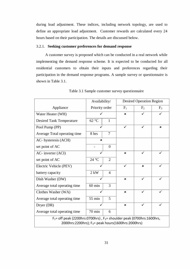
31

during load adjustment. These indices, including network topology, are used to

define an appropriate load adjustment. Customer rewards are calculated every 24

hours based on their participation. The details are discussed below.

3.2.1. Seeking customer preferences for demand response

A customer survey is proposed which can be conducted in a real network while

implementing the demand response scheme. It is expected to be conducted for all

residential customers to obtain their inputs and preferences regarding their

participation in the demand response programs. A sample survey or questionnaire is

shown in Table 3.1.

Table 3.1 Sample customer survey questionnaire

Appliance

Availability/

Priority order

Desired Operation Region

F1 F2 F3

Water Heater (WH)

Desired Tank Temperature 62 °C 1

Pool Pump (PP)

Average Total operating time 8 hrs 7

AC- hysteresis (ACH)

set point of AC - 0

AC- inverter (ACI)

set point of AC 24 °C 2

Electric Vehicle (PEV)

battery capacity 2 kW 4

Dish Washer (DW)

Average total operating time 60 min 3

Clothes Washer (WA)


Dryer (DR)


F1= off peak (2200hrs:0700hrs) , F2= shoulder peak (0700hrs:1600hrs, 2000hrs:2200hrs); F3= peak hours(1600hrs:2000hrs)

32

Utilities are interested to know appliance preferences of various customers and

their time of operation. For simplicity, the survey may divide a day into three

separate operation regions namely F1, F2, and F3 representing off peak, shoulder

peak, and peak hours respectively. The survey should be designed to collect

important information such as the items listed in Table 3.2. In order to verify the

collected data from customers, past and current appliance usage patterns can be

carefully studied for each house. Customer priority and the flexible range of usage

time for appliances can be extracted from the above data. Details in the customer

questionnaire can be verified with the extracted values. Moreover, these extracted

values can be used when the information provided is inconsistent and/or ambiguous.

Table 3.2 Required data from customers

Data in Customer Survey Required Instance

Total operating time of pool pump For appliance satisfaction calculations

Set point of AC and water heater

Battery capacity of electric vehicle

Average total operating time of dishwasher, clothes washer and dryer

Ordered list of appliances that the customer likes to connect between 16:00-22:00 hrs (peak and shoulder peak

time)

For appliance priority calculations

Adjustable range of time for each appliance within a day For flexibility calculations

Customer preferences are taken into account before designing the load control

algorithm. It is assumed in this study that each house has ten non-controllable loads

(lighting, fridge, freezer, cooker, electric oven, microwave, television, computer,

stand-by appliance, and miscellaneous appliance) and seven controllable loads

(swimming pool pump, PEV, electric water heater, dish washer, clothes washer,

dryer, and AC). They are modeled according to residential load modeling data

provided in [76]-[77], [32]. Appliance modelling is discussed in detail in Appendix

A.

3.2.2. Calculation of various criteria indices from customer survey

Information from customers is used to define various indices for appropriate

load selection. Therefore, five criteria indices (C(i,j,k) for the kth

criteria index of the

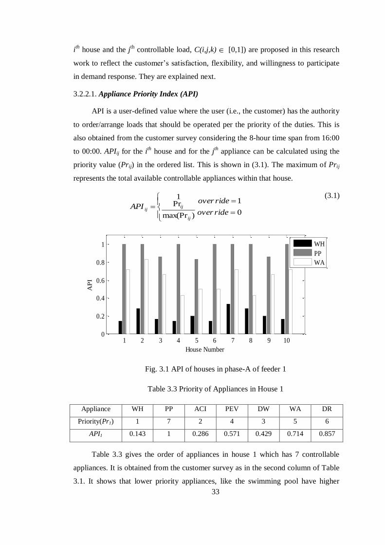
33

ith

house and the jth

controllable load, C(i,j,k) [0,1]) are proposed in this research

work to reflect the customer’s satisfaction, flexibility, and willingness to participate

in demand response. They are explained next.

3.2.2.1. Appliance Priority Index (API)

API is a user-defined value where the user (i.e., the customer) has the authority

to order/arrange loads that should be operated per the priority of the duties. This is

also obtained from the customer survey considering the 8-hour time span from 16:00

to 00:00. APIij for the ith

house and for the jth

appliance can be calculated using the

priority value (Prij) in the ordered list. This is shown in (3.1). The maximum of Prij

represents the total available controllable appliances within that house.

0

1

)max(Pr

Pr1

rideover

rideoverAPI

ij

ijij

(3.1)

Fig. 3.1 API of houses in phase-A of feeder 1

Table 3.3 Priority of Appliances in House 1

Appliance WH PP ACI PEV DW WA DR

Priority(Pr1) 1 7 2 4 3 5 6

API1 0.143 1 0.286 0.571 0.429 0.714 0.857

Table 3.3 gives the order of appliances in house 1 which has 7 controllable

appliances. It is obtained from the customer survey as in the second column of Table

3.1. It shows that lower priority appliances, like the swimming pool have higher

1 2 3 4 5 6 7 8 9 100

0.2

0.4

0.6

0.8

1

House Number

AP

I

WH

PP

WA

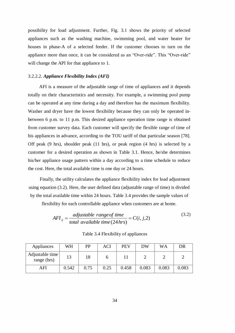
34

possibility for load adjustment. Further, Fig. 3.1 shows the priority of selected

appliances such as the washing machine, swimming pool, and water heater for

houses in phase-A of a selected feeder. If the customer chooses to turn on the

appliance more than once, it can be considered as an “Over-ride”. This “Over-ride”

will change the API for that appliance to 1.

3.2.2.2. Appliance Flexibility Index (AFI)

AFI is a measure of the adjustable range of time of appliances and it depends

totally on their characteristics and necessity. For example, a swimming pool pump

can be operated at any time during a day and therefore has the maximum flexibility.

Washer and dryer have the lowest flexibility because they can only be operated in-

between 6 p.m. to 11 p.m. This desired appliance operation time range is obtained

from customer survey data. Each customer will specify the flexible range of time of

his appliances in advance, according to the TOU tariff of that particular season [78].

Off peak (9 hrs), shoulder peak (11 hrs), or peak region (4 hrs) is selected by a

customer for a desired operation as shown in Table 3.1. Hence, he/she determines

his/her appliance usage pattern within a day according to a time schedule to reduce

the cost. Here, the total available time is one day or 24 hours.

Finally, the utility calculates the appliance flexibility index for load adjustment

using equation (3.2). Here, the user defined data (adjustable range of time) is divided

by the total available time within 24 hours. Table 3.4 provides the sample values of

flexibility for each controllable appliance when customers are at home.

)2,,()24(

jiChrstimeavailabletotal

timeofrangeadjustableAFI ij

(3.2)

Table 3.4 Flexibility of appliances

Appliances WH PP ACI PEV DW WA DR

Adjustable time

range (hrs) 13 18 6 11 2 2 2

AFI 0.542 0.75 0.25 0.458 0.083 0.083 0.083

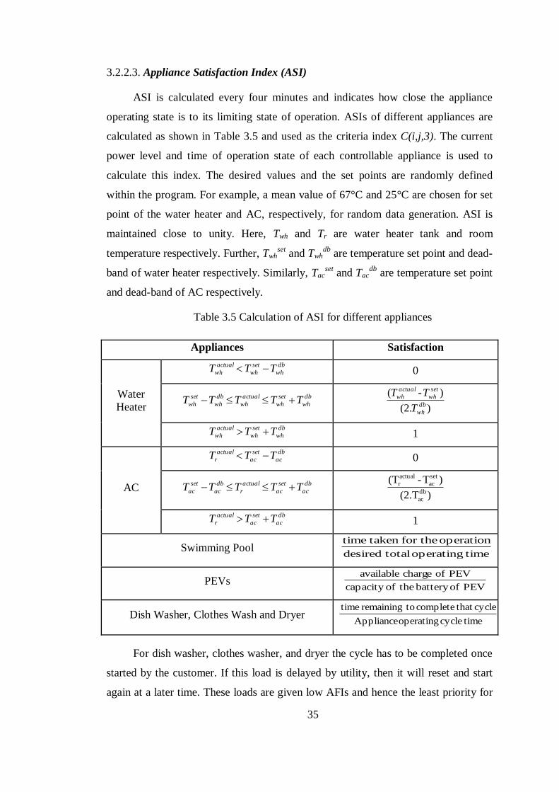
35

3.2.2.3. Appliance Satisfaction Index (ASI)

ASI is calculated every four minutes and indicates how close the appliance

operating state is to its limiting state of operation. ASIs of different appliances are

calculated as shown in Table 3.5 and used as the criteria index C(i,j,3). The current

power level and time of operation state of each controllable appliance is used to

calculate this index. The desired values and the set points are randomly defined

within the program. For example, a mean value of 67°C and 25°C are chosen for set

point of the water heater and AC, respectively, for random data generation. ASI is

maintained close to unity. Here, Twh and Tr are water heater tank and room

temperature respectively. Further, Twhset

and Twhdb

are temperature set point and dead-

band of water heater respectively. Similarly, Tacset

and Tacdb

are temperature set point

and dead-band of AC respectively.

Table 3.5 Calculation of ASI for different appliances

Appliances Satisfaction

Water

Heater

db

wh

set

wh

actual

wh TTT 0

db

wh

set

wh

actual

wh

db

wh

set

wh TTTTT )(2.

)-(db

wh

set

wh

actual

wh

T

TT

db

wh

set

wh

actual

wh TTT 1

AC

db

ac

set

ac

actual

r TTT 0

db

ac

set

ac

actual

r

db

ac

set

ac TTTTT )(2.T

)T-(Tdb

ac

set

ac

actual

r

db

ac

set

ac

actual

r TTT 1

Swimming Pool

PEVs

Dish Washer, Clothes Wash and Dryer

For dish washer, clothes washer, and dryer the cycle has to be completed once

started by the customer. If this load is delayed by utility, then it will reset and start

again at a later time. These loads are given low AFIs and hence the least priority for

timeoperating totaldesired

operation for the taken time

PEV ofbattery theofcapacity

PEV of charge available

timecycle operating Appliance

cycle that complete toremaining time

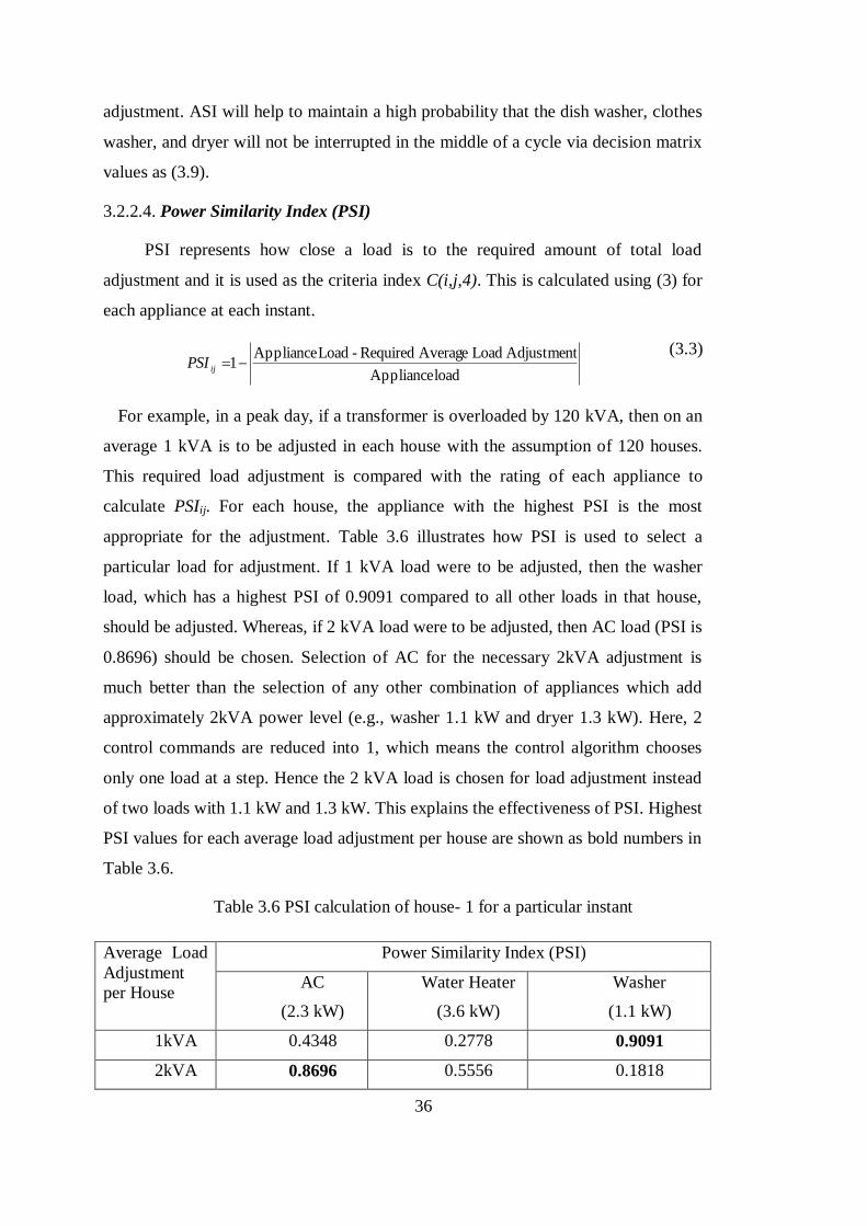
36

adjustment. ASI will help to maintain a high probability that the dish washer, clothes

washer, and dryer will not be interrupted in the middle of a cycle via decision matrix

values as (3.9).

3.2.2.4. Power Similarity Index (PSI)

PSI represents how close a load is to the required amount of total load

adjustment and it is used as the criteria index C(i,j,4). This is calculated using (3) for

each appliance at each instant.

load Appliance

Adjustment Load Average Required-Load Appliance1ijPSI

(3.3)

For example, in a peak day, if a transformer is overloaded by 120 kVA, then on an

average 1 kVA is to be adjusted in each house with the assumption of 120 houses.

This required load adjustment is compared with the rating of each appliance to

calculate PSIij. For each house, the appliance with the highest PSI is the most

appropriate for the adjustment. Table 3.6 illustrates how PSI is used to select a

particular load for adjustment. If 1 kVA load were to be adjusted, then the washer

load, which has a highest PSI of 0.9091 compared to all other loads in that house,

should be adjusted. Whereas, if 2 kVA load were to be adjusted, then AC load (PSI is

0.8696) should be chosen. Selection of AC for the necessary 2kVA adjustment is

much better than the selection of any other combination of appliances which add

approximately 2kVA power level (e.g., washer 1.1 kW and dryer 1.3 kW). Here, 2

control commands are reduced into 1, which means the control algorithm chooses

only one load at a step. Hence the 2 kVA load is chosen for load adjustment instead

of two loads with 1.1 kW and 1.3 kW. This explains the effectiveness of PSI. Highest

PSI values for each average load adjustment per house are shown as bold numbers in

Table 3.6.

Table 3.6 PSI calculation of house- 1 for a particular instant

Average Load

Adjustment

per House

Power Similarity Index (PSI)

AC

(2.3 kW)

Water Heater

(3.6 kW)

Washer

(1.1 kW)

1kVA 0.4348 0.2778 0.9091

2kVA 0.8696 0.5556 0.1818

37

PSI is required to select the closest and most appropriate load to be adjusted to

eliminate overload. Use of PSI will minimize overall control commands in the

network.

3.2.2.5. High Power Consumption Index (HPCI)

HPCI aims at identifying the house which is consuming the highest power at a

time when load adjustment is required. HPCIij for ith house and j

th appliance is

calculated as in (3.4) and is used as the criteria index C(i,j,5). For example, if a house

has 5 kVA of connected load and the load consumption is 5 kVA at that time, then

HPCI is 1 at that time. At other time instants, if load consumption is 3 kVA, HPCI is

0.6 (=3/5). HPCI is one way to socialize the load adjustment such that network

overload is effectively mitigated.

(3.4)

3.2.3. Using house ranking and criteria indices for load adjustment

Houses are ranked with a factor to replicate the impact of load on voltage

violation. The random selection of house loads will result in a number of

unnecessary load adjustments when voltage violation exists. Hence, this ranking

mechanism is introduced for each house to avoid unnecessary load adjustment during

voltage problems. Traditionally, the sensitivity method [79], [80] has been used for

load ranking and can be used here to choose the most suitable house for required load

adjustment.

The rank for each house at each instant is calculated using the voltage

magnitude and angle of each house from a three-phase unbalance load flow program.

Voltage sensitivity is considered as an appropriate voltage measure in this process.

Voltage sensitivity parameter (ρ) is the average change in the voltages of all houses

in a feeder due to load adjustment at that house. Inverse Jacobian matrix parameters

[81] are used to calculate the voltage sensitivity at each house. The parameter ρ of

the ith

house in the pth

phase for a three-phase unbalanced system is derived using

(3.5).

networktheinnconsumptiowithloadHouse

houseiofloadTotalHPCI

th

ijmax

38

p

n

h m

p

ip

i

m

hp

ip

i

m

h

p

in

QQ

VP

P

V

3

)(1

3

1

(3.5)

Where, np is the total of number of houses in one phase. Maximum and

minimum values of the sensitivity parameter in each phase is calculated and used in

(3.6) to define rank, rijp, for the i

th house and the j

th appliance in the p

th phase.

ijp

ii

p

ii

p

ii

p

ip

ij er

)(min)(max

)(min

(3.6)

Where, eij is the appliance status (On/Off) signal at a particular time for the ith

house and the jth

appliance and can be obtained from smart meters. P and Q are real

and reactive power, respectively. Value of eij is 1 if the appliance is on at a particular

time and 0 otherwise.

The overall control process maintains voltage and network power levels within

limits. Here, 0.94 p.u. and 1.06 p.u. are the minimum and maximum voltage levels,

respectively, because +/- 6% are the Australian standards [82]. Also, network power

limits are taken as the capacity of the transformer (chosen here as 500 kVA). Power

flow equations used during the three-phase unbalanced load flow program is

provided here. The derived mismatch equations for the load buses are (3.7)-(3.8).

n

h m

m

h

p

i

pm

ih

m

h

p

i

pm

ih

m

h

p

i

p

i

p

i BGVVPP1

3

1

)sin()cos( (3.7)

n

h m

m

h

p

i

pm

ih

m

h

p

i

pm

ih

m

h

p

i

p

i

p

i BGVVQQ1

3

1

)}cos()sin( (3.8)

Here, Gihpm

and Bihpm

are conductance and susceptance of the feeder connecting

the ith

and the hth

house in phase p due to the effect of phase m, respectively; θip is the

bus angle at the ith

house in phase p; and V is the bus voltage. The rank of each house

is then multiplied with the decision value for the appropriate selection of load.

Overall, the above parameters provide the decision for load adjustment. These

indices (as discussed in Section 3.2.2) along with the appropriate rank (as discussed

in this Section) for each house are used in decision matrix calculation. Decij, the

decision for the ith

house and the jth controllable load, is defined as in (3.9).

39

5

1

),,(k

p

ijij kjiCrDec (3.9)

Where, C(i,j,k) is the criteria raking matrix for the kth

criteria index of the ith

house and the jth controllable load (C(i,j,k) [0,1]). An efficient solution can be

achieved with the combination of multiple criteria indices into a single criterion by

multiplying each criterion with a positive weight and summing the weighted criteria

[83]. For simplicity, this research considers unity weights for all five criteria.

For the i0th

house in the p0th

phase, if ρi0 p

0 is the minimum ρ in that phase, then

rijp=0 and hence Decij=0. This means that the corresponding appliance will not be

selected for load adjustment at that time instant. This is reasonable because at that

time instant, the i0th

house is the least sensitive to the voltage violation in the feeder.

Since the voltage sensitivity depends on house locations as well as load consumption,

at other time instants the same house may not have the minimum sensitivity and

hence the corresponding load can be selected for adjustment at that time.

3.2.4. Customer reward (CR) Scheme

CR scheme provides rebates to residential customers for their participation in

the demand response. The proposed rebate is a function of both shifted energy and

voltage improvement due to load adjustments as shown in (3.10). The shifted energy

of the house is the sum of the product of all load adjustments and the respective

waiting times. Here, waiting time is the time that is delayed by the controller to re-

connect the appliance to the system. The effective change in voltage within the

network due to a particular load adjustment is taken as the ratio of voltage deviation

of the ith

house to the voltage improvement from the lower limit.

Nadj

l

Nv

im

l

l

l

lNadj

l

l

i

i

m

m

i

i

E

E

f

V

V

V

V

1 11 limlim,lim,

*1exp*

)timprovemenvoltage,energyshifted(Rebate

(3.10)

Here, Rebatei is the rebate in $ for a given day of ith

house; Eil is the shifted

energy for the ith

house measured at the lth

load adjustment; Elim is the limit of

maximum shifted energy (chosen to be 12kWhr in this case); ∆Vil is the voltage

deviation in p.u. and ∆Vi,liml is the voltage improvement (from lower limit of 0.94) in

p.u of the ith

house measured at the lth

load adjustment; Nadj is the total number of

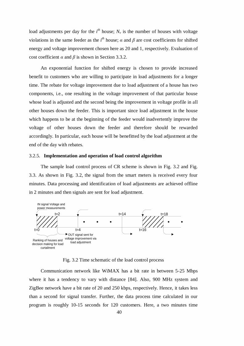
40

load adjustments per day for the ith

house; Nv is the number of houses with voltage

violations in the same feeder as the ith

house; α and β are cost coefficients for shifted

energy and voltage improvement chosen here as 20 and 1, respectively. Evaluation of

cost coefficient α and β is shown in Section 3.3.2.

An exponential function for shifted energy is chosen to provide increased

benefit to customers who are willing to participate in load adjustments for a longer

time. The rebate for voltage improvement due to load adjustment of a house has two

components, i.e., one resulting in the voltage improvement of that particular house

whose load is adjusted and the second being the improvement in voltage profile in all

other houses down the feeder. This is important since load adjustment in the house

which happens to be at the beginning of the feeder would inadvertently improve the

voltage of other houses down the feeder and therefore should be rewarded

accordingly. In particular, each house will be benefitted by the load adjustment at the

end of the day with rebates.

3.2.5. Implementation and operation of load control algorithm

The sample load control process of CR scheme is shown in Fig. 3.2 and Fig.

3.3. As shown in Fig. 3.2, the signal from the smart meters is received every four

minutes. Data processing and identification of load adjustments are achieved offline

in 2 minutes and then signals are sent for load adjustment.

t=0 t=4

t=2

Ranking of houses and

decision making for load

curtailment

IN signal Voltage and

power measurements

OUT signal sent for

voltage improvement via

load adjustment

t=16

t=14 t=18

Fig. 3.2 Time schematic of the load control process

Communication network like WiMAX has a bit rate in between 5-25 Mbps

where it has a tendency to vary with distance [84]. Also, 900 MHz system and

ZigBee network have a bit rate of 20 and 250 kbps, respectively. Hence, it takes less

than a second for signal transfer. Further, the data process time calculated in our

program is roughly 10-15 seconds for 120 customers. Here, a two minutes time

41

frame is selected as a reasonable time for data collection and processing and another

2 minutes for sending back data and load curtailment. Hence, load curtailment

happens every 4 minutes. The 4-minute time window is chosen in this research to

make it roughly aligned with the DMS updates, which usually occur every tens of

seconds to a few minutes.

From time t=0 minute, at each instant t=t1, signals from the primary controllers

(smart meters) are received by a secondary controller. Received appliance state and

power data are used in the load flow program to calculate voltage at each house.

Total network power and voltage at each house are checked to insure that they are

kept within standard limits. The above measurement and data processing occurs

every 2 minutes.

Offline load flow studies are performed to obtain the appropriate load

adjustments in the case that the power level and/or voltage at each house are violated.

The offline load flow block is an iterative process that selects multiple sets of

loads for adjustment in that time step as summarized in Fig. 3.3. The criteria indices

and rankings and hence decision value (Decij) are calculated for each iteration. The

maximum value of Decij is used to find the corresponding j0 th

load of the i0th

house

for load adjustment. The power and voltages are recalculated after this load is

adjusted in the offline load flow program. If violations exist, another load is selected

for adjustment by recalculating the updated criteria indices and decision values. This

process is repeated until violations are removed. At the end of the “offline selection

of load” block, multiple sets of appliances that need to be adjusted are identified to

keep the voltage and power within limits.

All the selected appliances for adjustments are saved and signals are sent at

t=t+2 minutes to relevant smart meters. If loads are adjustable (such as AC and

water heater loads), then the AC set point is increased by 1 °C and the water heater

set point is decreased by 1 °C for 15 minutes. Whereas, the non-adjustable loads are

switched off for 4 minutes. The process is repeated for the whole day and after 24

hours. Rebates to the customer are calculated as per (3.10). Set point adjustments

would result in the reduction of power consumption, which will be used along with

associated waiting time to calculate the shifted power. Fig. 3.3 summarizes the load

control process with CR scheme for a particular day.

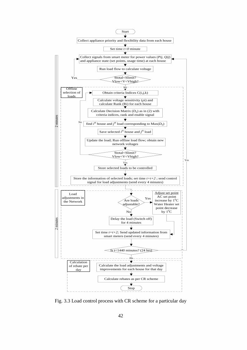
42

Start

Collect signals from smart meter for power values (Pij, Qij)

and appliance state (set points, usage time) at each house

Obtain criteria Indices C(i,j,k)

Calculate Decision Matrix (Dij) as in (2) with

criteria indices, rank and enable signal

Update the load; Run offline load flow; obtain new

network voltages

Store selected loads to be controlled

Are loads

adjustable?

Adjust set point

AC set point

increase by 10C

Water Heater set

point decrease

by 10C

Store the information of selected loads; set time t=t+2 ; send control

signal for load adjustments (send every 4 minutes)

Delay the load (Switch off)

for 4 minutes

Calculate the load adjustments and voltage

improvements for each house for that day

Is t<1440 minutes? (24 hrs)

Calculate rebates as per CR scheme

Stop

Yes

No

No

Yes

Offline

selection of

loads

Load

adjustments in

the Network

Calculation

of rebate per

day

find ith house and jth load corresponding to Max(Dij)

Stotal<Slimit?

Vlow<V<Vhigh?

No

Set time t=t+2; Send updated information from

smart meters (send every 4 minutes)

2 m

inut

es2

min

utes

Calculate voltage sensitivity (ρi) and

calculate Rank (Ri) for each house

Collect appliance priority and flexibility data from each house

Run load flow to calculate voltage

Stotal<Slimit?

Vlow<V<Vhigh?

No

Yes

Save selected ith house and jth load

Yes

Set time t=0 minute

Fig. 3.3 Load control process with CR scheme for a particular day

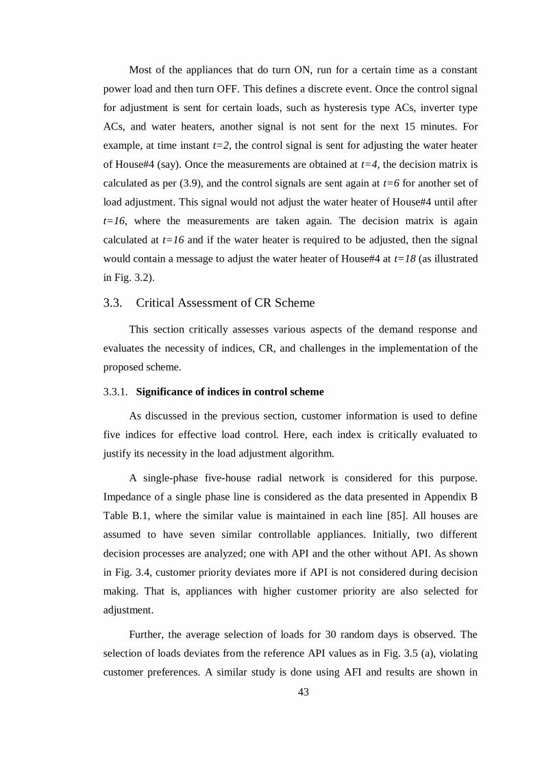
43

Most of the appliances that do turn ON, run for a certain time as a constant

power load and then turn OFF. This defines a discrete event. Once the control signal

for adjustment is sent for certain loads, such as hysteresis type ACs, inverter type

ACs, and water heaters, another signal is not sent for the next 15 minutes. For

example, at time instant t=2, the control signal is sent for adjusting the water heater

of House#4 (say). Once the measurements are obtained at t=4, the decision matrix is

calculated as per (3.9), and the control signals are sent again at t=6 for another set of

load adjustment. This signal would not adjust the water heater of House#4 until after

t=16, where the measurements are taken again. The decision matrix is again

calculated at t=16 and if the water heater is required to be adjusted, then the signal

would contain a message to adjust the water heater of House#4 at t=18 (as illustrated

in Fig. 3.2).

3.3. Critical Assessment of CR Scheme

This section critically assesses various aspects of the demand response and

evaluates the necessity of indices, CR, and challenges in the implementation of the

proposed scheme.

3.3.1. Significance of indices in control scheme

As discussed in the previous section, customer information is used to define

five indices for effective load control. Here, each index is critically evaluated to

justify its necessity in the load adjustment algorithm.

A single-phase five-house radial network is considered for this purpose.

Impedance of a single phase line is considered as the data presented in Appendix B

Table B.1, where the similar value is maintained in each line [85]. All houses are

assumed to have seven similar controllable appliances. Initially, two different

decision processes are analyzed; one with API and the other without API. As shown

in Fig. 3.4, customer priority deviates more if API is not considered during decision

making. That is, appliances with higher customer priority are also selected for

adjustment.

Further, the average selection of loads for 30 random days is observed. The

selection of loads deviates from the reference API values as in Fig. 3.5 (a), violating

customer preferences. A similar study is done using AFI and results are shown in

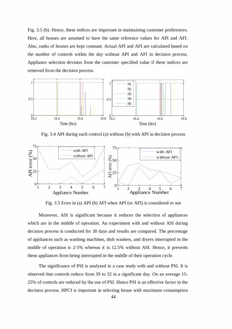
44

Fig. 3.5 (b). Hence, these indices are important in maintaining customer preferences.

Here, all houses are assumed to have the same reference values for API and AFI.

Also, ranks of houses are kept constant. Actual API and AFI are calculated based on

the number of controls within the day without API and AFI in decision process.

Appliance selection deviates from the customer specified value if these indices are

removed from the decision process.

Fig. 3.4 API during each control (a) without (b) with API in decision process

Fig. 3.5 Error in (a) API (b) AFI when API (or AFI) is considered or not

Moreover, ASI is significant because it reduces the selection of appliances

which are in the middle of operation. An experiment with and without ASI during

decision process is conducted for 30 days and results are compared. The percentage

of appliances such as washing machines, dish washers, and dryers interrupted in the

middle of operation is 2-5% whereas it is 12.5% without ASI. Hence, it prevents

these appliances from being interrupted in the middle of their operation cycle.

The significance of PSI is analyzed in a case study with and without PSI. It is

observed that controls reduce from 39 to 32 in a significant day. On an average 15-

25% of controls are reduced by the use of PSI. Hence PSI is an effective factor in the

decision process. HPCI is important in selecting house with maximum consumption

19.2 19.4 19.6 19.80

0.5

1

Time (hrs)

19.2 19.4 19.6 19.80

0.5

1

Time (hrs)

H1

H2

H3

H4

H5

1 2 3 4 5 6 70

25

50

75

AP

I err

or

(%)

Appliance Number

with API

without API

1 2 3 4 5 6 70

25

50

75

Appliance Number

AF

I er

ror

(%)

with AFI

without AFI

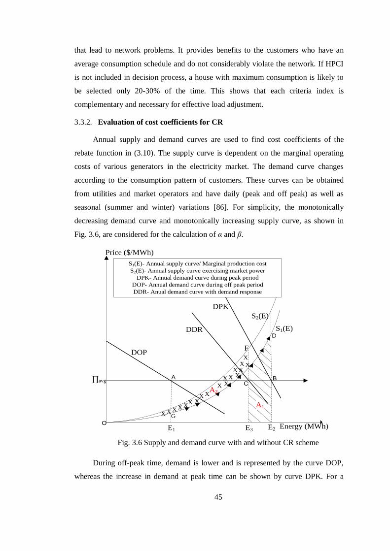
45

that lead to network problems. It provides benefits to the customers who have an

average consumption schedule and do not considerably violate the network. If HPCI

is not included in decision process, a house with maximum consumption is likely to

be selected only 20-30% of the time. This shows that each criteria index is

complementary and necessary for effective load adjustment.

3.3.2. Evaluation of cost coefficients for CR

Annual supply and demand curves are used to find cost coefficients of the

rebate function in (3.10). The supply curve is dependent on the marginal operating

costs of various generators in the electricity market. The demand curve changes

according to the consumption pattern of customers. These curves can be obtained

from utilities and market operators and have daily (peak and off peak) as well as

seasonal (summer and winter) variations [86]. For simplicity, the monotonically

decreasing demand curve and monotonically increasing supply curve, as shown in

Fig. 3.6, are considered for the calculation of α and β.

S2(E)

S1(E)

Price ($/MWh)

Energy (MWh)E1 E2

∏avg

DPK

DOP

S1(E)- Annual supply curve/ Marginal production cost

S2(E)- Annual supply curve exercising market power

DPK- Annual demand curve during peak period

DOP- Annual demand curve during off peak period

DDR- Anual demand curve with demand response

A1

XX XXX

X XXXX

XXXX

XXXXX

D

CA B

DDR

OE3

F

A2

G

Fig. 3.6 Supply and demand curve with and without CR scheme

During off-peak time, demand is lower and is represented by the curve DOP,

whereas the increase in demand at peak time can be shown by curve DPK. For a

46

constant tariff (flat rate), the price is fixed at Пavg and therefore the market during

off-peak time operates at point A for quantity demanded E1. The increase in demand

causes a shortage of supply, which leads to an increase in price. Due to the increased

price, the utility will increase the quantity of supply from point G to point D, as

shown in Fig. 3.6, to cater to the increase in quantity demanded from E1 to E2.

However, due to flat rate, the market operates at point B. The demand response will

reduce the demand and shift the demand curve to the left, which can be represented

as DDR [87]. At the same time, the supply price increases and shifts the supply curve

to S2. This is because the suppliers are provided with reduced incentives to exercise

market power [88]. Finally, the market operates at point C after demand response

achieves the reduction from E2 to E3.

The cost of supply due to demand response is reduced and it is the difference

between ODE2 (area under the supply curve S1) and OFE3 (area under supply curve

S2). For simplicity, it can be represented as (A1-A2) as shown in Fig. 3.6.

Energy values E1, E2, and E3 are found using annual supply curves mapped to

the intersection of demand curves with a fixed price. A1 and A2 are found after the

computation of E2 and E3, respectively.

The total rebate in the network for a day should be less than the reduction in

cost of supply due to demand response. Hence, the total rebate for the network,

Rebatetotal, that can be offered by the utilities to their customers should be less than

the cost savings because of demand response. That is, (A1-A2) should satisfy (3.11).

21..* AARebateandVENRebate total

avg

imp

avg

shifttotal (3.11)

Here, N is the number of houses in the network. Eshiftavg

and ΔVimpavg

are

components related to the average shift in energy and voltage improvement that is

calculated from offline load flow studies using the annual demand and supply curves.

For example, if a 500kVA network is overloaded by 150 kVA, then E2 and E3

are 650 kVA and 500 kVA, respectively. The reduction in cost, i.e., (A1-A2), is $100

using a sample supply curves from [89]. Eshiftavg

and ΔVimpavg

are found to be 0.041

and 2.0, respectively, for an average house using offline load flow studies. If β is

kept at 1.0, the value of α is found to be 20 to satisfy (3.11). Note that the utility can

choose appropriate values of α and β to incentivize the increase of customer

47

participation. This depends on the network layout, the number of customers, and the

existing tariff. The rebate pattern can be changed by the utility for every quarter of

the year to accommodate seasonal load changes.

3.3.3. Customer rewards

A single-phase five-house model is considered to evaluate rebate calculations.

For simplicity, houses are assumed to have similar appliances of 1 kVA each. The

power consumption profile in each house is assumed to be the same. API and AFI

are fixed in every house as in Table 3.3 and Table 3.4.

A rebate for each house is calculated every 24 hours by the utility to provide

benefit to the customers as discussed in Section 3.2.4. The results obtained for 5

houses are tabulated in Table 3.7. H2 pool pump (#2) and electric vehicle (#5) are

adjusted for 12 minutes and for 4 minutes with 1 kW of shifted power, respectively.

Hence, the rebate for the total shifted energy and the voltage improvement is $0.45

and $0.51, respectively. So, H2 will get a total rebate of $0.96 ($0.45+$0.51). It

shows an increased rebate towards the end of the feeder in case 1. Customers towards

the end of the feeder will be benefitted with an increased rebate due to more load

adjustments. Here, the total rebate paid by the utility to all five houses is $9.99. It is

interesting to note that H1, at the beginning of the feeder, has fewer rebates for

voltage improvement than H5 at the end of the feeder. H5 will have significant effect

on the feeder voltage due to load adjustment and, hence, will have a higher rebate

component for voltage improvement than the corresponding energy component.

Scenarios with traditional demand response (no rebates) and CR scheme are

compared for Australian residential tariff 11, which is 0.25 $/kWhr [90]. The cost of

consumption is calculated based on the price of electricity and energy consumed

every hour. Table 3.8 shows the cost of electricity for a few selected customers for a

peak day. For instance, with constant tariff, the consumption cost of H1 is $10.45.

If H1 participates in the traditional demand response, the cost is reduced to

$9.85, due to reduced or delayed load consumption on that peak day. In the absence

of any rebates the customer is not rewarded for their participation in load adjustment.

With the proposed CR scheme, the rebate obtained due to load adjustment of H1 is

$0.52 ($9.85 -$9.33=$0.52). Hence, H1 will pay only $9.33. Note that the rebate

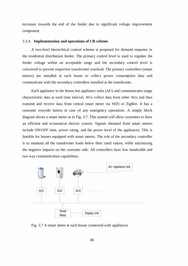
48

increases towards the end of the feeder due to significant voltage improvement

component.

3.3.4. Implementation and operations of CR scheme

A two-level hierarchical control scheme is proposed for demand response in

the residential distribution feeder. The primary control level is used to regulate the

feeder voltage within an acceptable range and the secondary control level is

conceived to prevent respective transformer overload. The primary controllers (smart

meters) are installed at each house to collect power consumption data and

communicate with the secondary controllers installed at the transformer.

Each appliance in the house has appliance units (AU) and communicates usage

characteristic data at each time interval. AUs collect data from other AUs and then

transmit and receive data from central smart meter via WiFi or ZigBee. It has a

customer override button in case of any emergency operations. A simple block

diagram shows a smart meter as in Fig. 3.7. This system will allow customers to have

an efficient and economical electric system. Signals obtained from smart meters

include ON/OFF time, power rating, and the power level of the appliances. This is

feasible for houses equipped with smart meters. The role of the secondary controller

is to maintain all the transformer loads below their rated values, while minimizing

the negative impacts on the customer side. All controllers have low bandwidth and

two way communication capabilities.

AU1 AU2 AU3

Smart

MeterDisplay Unit

AU- Appliance Unit

Fig. 3.7 A smart meter at each house connected with appliances

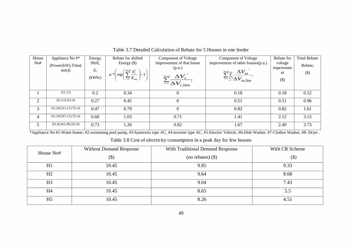
49

Table 3.7 Detailed Calculation of Rebate for 5 Houses in one feeder

House

No#

Appliance No #*

(Power(kW),Time(

min))

Energy

Shift,

Ei

(kWhr)

Rebate for shifted

Energy ($)

Component of Voltage

improvement of that house

(p.u.)

Component of Voltage

improvement of other houses(p.u.)

Rebate for

voltage

improveme

nt

($)

Total Rebate

Rebatei

($)

1 2(1,12) 0.2 0.34 0 0.18 0.18 0.52

2 2(1,12),5(1,4) 0.27 0.45 0 0.51 0.51 0.96

3 2(1,20),5(1,12),7(1,4) 0.47 0.79 0 0.82 0.82 1.61

4 2(1,20),5(1,12),7(1,4) 0.60 1.03 0.71 1.41 2.12 3.15

5 2(1,8),4(1,28),5(1,8) 0.73 1.26 0.82 1.67 2.49 3.73

*Appliance No #1-Water heater; #2-swimming pool pump, #3-hysteresis type AC, #4-inverter type AC, #5-Electric Vehicle, #6-Dish Washer, #7-Clothes Washer, #8- Dryer .

Table 3.8 Cost of electricity consumption in a peak day for few houses

House No# Without Demand Response

($)

With Traditional Demand Response

(no rebates) ($)

With CR Scheme

($)

H1 10.45 9.85 9.33

H2 10.45 9.64 8.68

H3 10.45 9.04 7.43

H4 10.45 8.65 5.5

H5 10.45 8.26 4.51

1exp*1 lim

Nadj

l

l

i

E

E

Nadj

ll

l

i

i

V

V

1lim,

Nadj

l

Nv

im

l

l

m

m

V

V

1 1

lim,

50

Programmable Logic Controllers (PLC) can be used for this purpose which has

the many more advantages. PLC is cost effective for complex control systems and

flexible which can be reapplied to control other parameters in future. Further, it has

computation ability to allow more sophisticated control. Trouble shooting aids with

reliable components in PLC helps it for long lasting applications. It can mainly

contain inbuilt Ethernet cards, RS232 ports for hardware links, good memory and I/O

(analogue and digital) cards for complex programming.

Although the transient effect can be important during the demand response,

voltages and currents transients caused by load change may last for no more than 50

and 20 milliseconds, respectively. In the 4 minute timeframe for load adjustment, this

effect is not considered at this stage.

The step by step load control process, as discussed in the load control section

above, is more efficient because it removes the rebound effect from the decision of

which loads are to be curtailed. It also provides an appropriate control of power and

voltage as it constantly checks for violation during the offline process.

3.3.5. Scalability

This decision process can be separated for subsystems (For example, each 500

kVA network). Load curtailment can be made separately for each subsystem when it

is subject to overloads or voltage violations. This is made possible by having a main

controller at each transformer level which has access to relevant smart meters in the

houses. Hence, it can be deployed at a range of scales in small and large

configurations easily. Data processing can be done in parallel for each system and

therefore the time consumed in processing data is minimal.

3.3.6. Prevention from customers misusing this scheme

Possible gaming can be avoided by restricting customer load switching by

introducing an override command. This will dynamically change the API to 1 for that

load and therefore it will not be selected for adjustment for the rest of the day. If a

customer chooses to operate a particular load more than two times in the peak period,

then the information is send back to the utility as an override and rebate would not be

paid for that load shift.

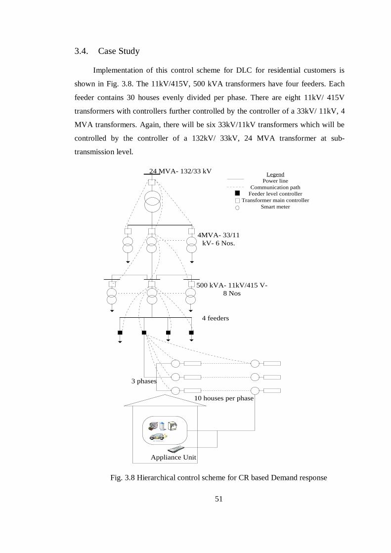
51

3.4. Case Study

Implementation of this control scheme for DLC for residential customers is

shown in Fig. 3.8. The 11kV/415V, 500 kVA transformers have four feeders. Each

feeder contains 30 houses evenly divided per phase. There are eight 11kV/ 415V

transformers with controllers further controlled by the controller of a 33kV/ 11kV, 4

MVA transformers. Again, there will be six 33kV/11kV transformers which will be

controlled by the controller of a 132kV/ 33kV, 24 MVA transformer at sub-

transmission level.

10 houses per phase

24 MVA- 132/33 kV

4MVA- 33/11

kV- 6 Nos.

500 kVA- 11kV/415 V-

8 Nos

Appliance Unit

Legend

Power line

Communication path

Feeder level controller

Transformer main controller

Smart meter

4 feeders

3 phases

Fig. 3.8 Hierarchical control scheme for CR based Demand response

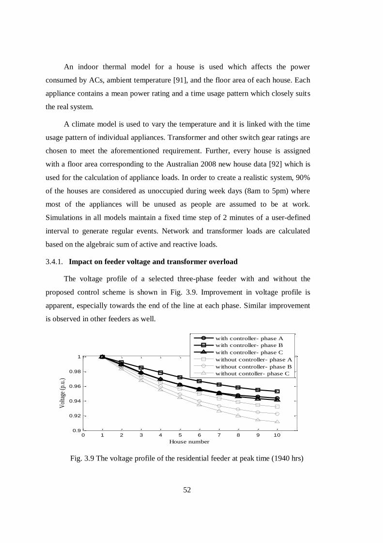
52

An indoor thermal model for a house is used which affects the power

consumed by ACs, ambient temperature [91], and the floor area of each house. Each

appliance contains a mean power rating and a time usage pattern which closely suits

the real system.

A climate model is used to vary the temperature and it is linked with the time

usage pattern of individual appliances. Transformer and other switch gear ratings are

chosen to meet the aforementioned requirement. Further, every house is assigned

with a floor area corresponding to the Australian 2008 new house data [92] which is

used for the calculation of appliance loads. In order to create a realistic system, 90%

of the houses are considered as unoccupied during week days (8am to 5pm) where

most of the appliances will be unused as people are assumed to be at work.

Simulations in all models maintain a fixed time step of 2 minutes of a user-defined

interval to generate regular events. Network and transformer loads are calculated

based on the algebraic sum of active and reactive loads.

3.4.1. Impact on feeder voltage and transformer overload

The voltage profile of a selected three-phase feeder with and without the

proposed control scheme is shown in Fig. 3.9. Improvement in voltage profile is

apparent, especially towards the end of the line at each phase. Similar improvement

is observed in other feeders as well.

Fig. 3.9 The voltage profile of the residential feeder at peak time (1940 hrs)

0 1 2 3 4 5 6 7 8 9 100.9

0.92

0.94

0.96

0.98

1

House number

Vol

tage

(p.

u.)

with controller- phase A

with controller- phase B

with controller- phase C

without controller- phase A

without controller- phase B

without contoller- phase C

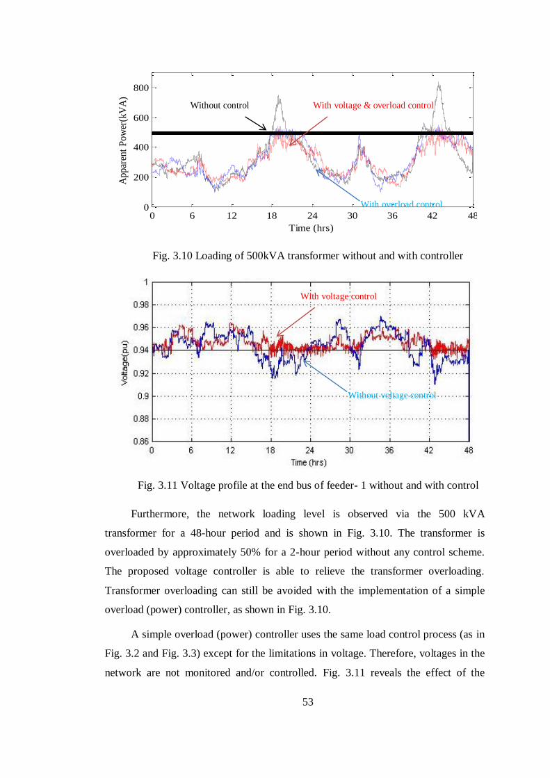
53

Fig. 3.10 Loading of 500kVA transformer without and with controller

Fig. 3.11 Voltage profile at the end bus of feeder- 1 without and with control

Furthermore, the network loading level is observed via the 500 kVA

transformer for a 48-hour period and is shown in Fig. 3.10. The transformer is

overloaded by approximately 50% for a 2-hour period without any control scheme.

The proposed voltage controller is able to relieve the transformer overloading.

Transformer overloading can still be avoided with the implementation of a simple

overload (power) controller, as shown in Fig. 3.10.

A simple overload (power) controller uses the same load control process (as in

Fig. 3.2 and Fig. 3.3) except for the limitations in voltage. Therefore, voltages in the

network are not monitored and/or controlled. Fig. 3.11 reveals the effect of the

0 6 12 18 24 30 36 42 480

200

400

600

800

Time (hrs)

Appar

ent

Pow

er(k

VA

)

With voltage control

Without voltage control

With voltage & overload control

With overload control

Without control

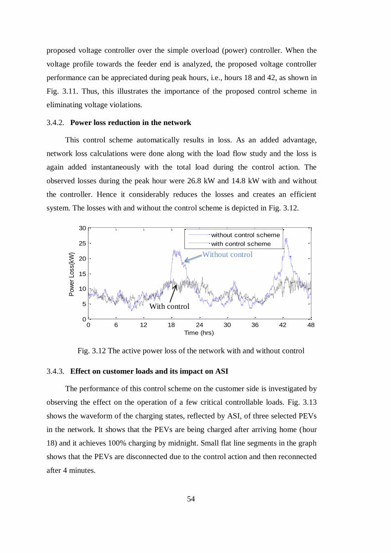
54

proposed voltage controller over the simple overload (power) controller. When the

voltage profile towards the feeder end is analyzed, the proposed voltage controller

performance can be appreciated during peak hours, i.e., hours 18 and 42, as shown in

Fig. 3.11. Thus, this illustrates the importance of the proposed control scheme in

eliminating voltage violations.

3.4.2. Power loss reduction in the network

This control scheme automatically results in loss. As an added advantage,

network loss calculations were done along with the load flow study and the loss is

again added instantaneously with the total load during the control action. The

observed losses during the peak hour were 26.8 kW and 14.8 kW with and without

the controller. Hence it considerably reduces the losses and creates an efficient

system. The losses with and without the control scheme is depicted in Fig. 3.12.

Fig. 3.12 The active power loss of the network with and without control

3.4.3. Effect on customer loads and its impact on ASI

The performance of this control scheme on the customer side is investigated by

observing the effect on the operation of a few critical controllable loads. Fig. 3.13

shows the waveform of the charging states, reflected by ASI, of three selected PEVs

in the network. It shows that the PEVs are being charged after arriving home (hour

18) and it achieves 100% charging by midnight. Small flat line segments in the graph

shows that the PEVs are disconnected due to the control action and then reconnected

after 4 minutes.

0 6 12 18 24 30 36 42 480

5

10

15

20

25

30

Time (hrs)

Pow

er

Loss(k

W)

without control scheme

with control scheme

With control

Without control

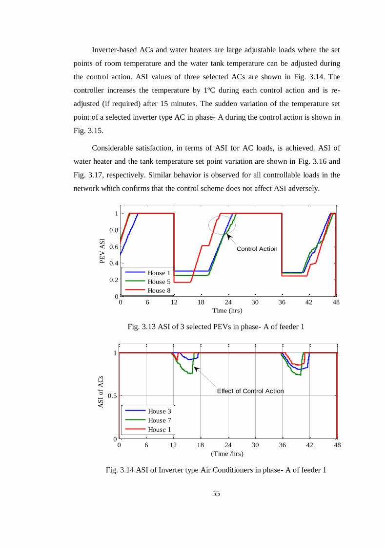
55

Inverter-based ACs and water heaters are large adjustable loads where the set

points of room temperature and the water tank temperature can be adjusted during

the control action. ASI values of three selected ACs are shown in Fig. 3.14. The

controller increases the temperature by 1ºC during each control action and is re-

adjusted (if required) after 15 minutes. The sudden variation of the temperature set

point of a selected inverter type AC in phase- A during the control action is shown in

Fig. 3.15.

Considerable satisfaction, in terms of ASI for AC loads, is achieved. ASI of

water heater and the tank temperature set point variation are shown in Fig. 3.16 and

Fig. 3.17, respectively. Similar behavior is observed for all controllable loads in the

network which confirms that the control scheme does not affect ASI adversely.

Fig. 3.13 ASI of 3 selected PEVs in phase- A of feeder 1

Fig. 3.14 ASI of Inverter type Air Conditioners in phase- A of feeder 1

0 6 12 18 24 30 36 42 480

0.2

0.4

0.6

0.8

1

Time (hrs)

PE

V A

SI

House 1

House 5

House 8

Control Action

0 6 12 18 24 30 36 42 480

0.5

1

AS

I of

AC

s

(Time /hrs)

House 3

House 7

House 1

Effect of Control Action

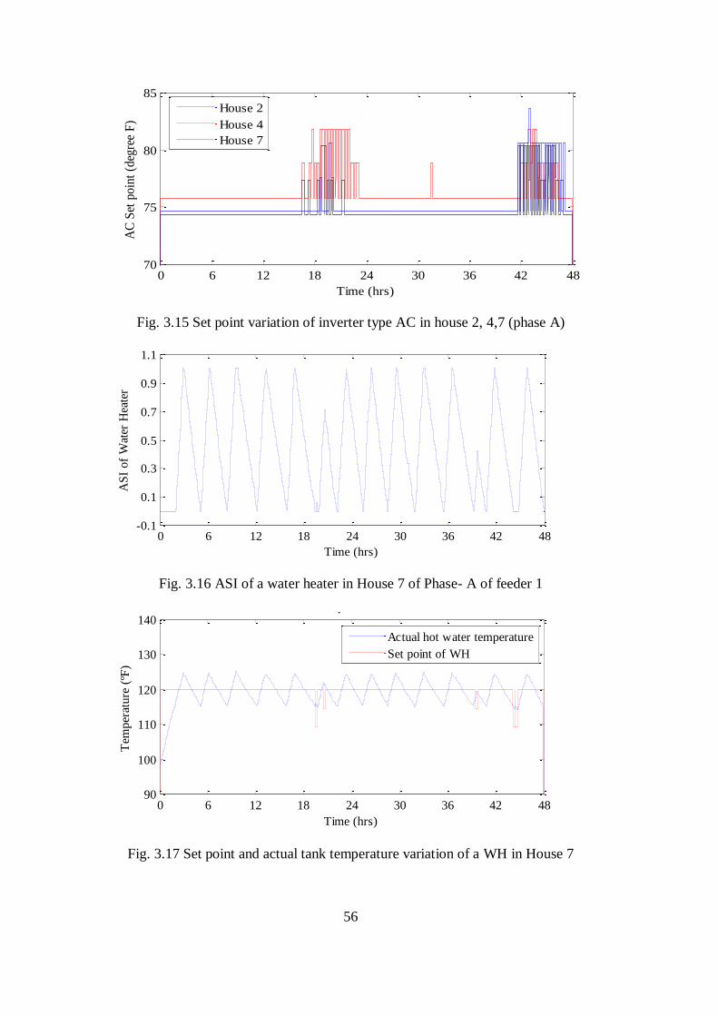
56

Fig. 3.15 Set point variation of inverter type AC in house 2, 4,7 (phase A)

Fig. 3.16 ASI of a water heater in House 7 of Phase- A of feeder 1

Fig. 3.17 Set point and actual tank temperature variation of a WH in House 7

0 6 12 18 24 30 36 42 4870

75

80

85

Time (hrs)

AC

Set

po

int

(deg

ree

F)

House 2

House 4

House 7

0 6 12 18 24 30 36 42 48-0.1

0.1

0.3

0.5

0.7

0.9

1.1ASI of WH

Time (hrs)

AS

I of

Wat

er H

eate

r

0 6 12 18 24 30 36 42 4890

100

110

120

130

140Water Heater Tank Temperature of a selected House

Time (hrs)

Tem

per

ature

(ºF

)

Actual hot water temperature

Set point of WH

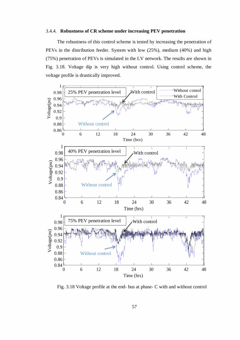
57

3.4.4. Robustness of CR scheme under increasing PEV penetration

The robustness of this control scheme is tested by increasing the penetration of

PEVs in the distribution feeder. System with low (25%), medium (40%) and high

(75%) penetration of PEVs is simulated in the LV network. The results are shown in

Fig. 3.18. Voltage dip is very high without control. Using control scheme, the

voltage profile is drastically improved.

Fig. 3.18 Voltage profile at the end- bus at phase- C with and without control

0 6 12 18 24 30 36 42 480.86

0.88

0.9

0.92

0.94

0.96

0.98

1

Time (hrs)

Vo

ltag

e(p

u)

Without contol

With Control

0 6 12 18 24 30 36 42 480.84

0.86

0.88

0.9

0.92

0.94

0.96

0.98

1

Time (hrs)

Volt

age(p

u)

0 6 12 18 24 30 36 42 480.84

0.86

0.88

0.9

0.92

0.94

0.96

0.98

1

Time (hrs)

Vo

ltag

e(p

u)

25% PEV penetration level



Without control

With control

Without control

With control

Without control

With control

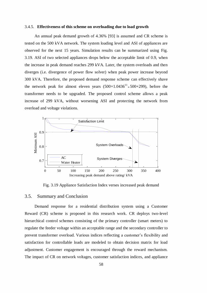
58

3.4.5. Effectiveness of this scheme on overloading due to load growth

An annual peak demand growth of 4.36% [93] is assumed and CR scheme is

tested on the 500 kVA network. The system loading level and ASI of appliances are

observed for the next 15 years. Simulation results can be summarized using Fig.

3.19. ASI of two selected appliances drops below the acceptable limit of 0.9, when

the increase in peak demand reaches 299 kVA. Later, the system overloads and then

diverges (i.e. divergence of power flow solver) when peak power increase beyond

300 kVA. Therefore, the proposed demand response scheme can effectively shave

the network peak for almost eleven years (500×1.043611

500+299), before the

transformer needs to be upgraded. The proposed control scheme allows a peak

increase of 299 kVA, without worsening ASI and protecting the network from

overload and voltage violations.

Fig. 3.19 Appliance Satisfaction Index verses increased peak demand

3.5. Summary and Conclusion

Demand response for a residential distribution system using a Customer

Reward (CR) scheme is proposed in this research work. CR deploys two-level

hierarchical control schemes consisting of the primary controller (smart meters) to

regulate the feeder voltage within an acceptable range and the secondary controller to

prevent transformer overload. Various indices reflecting a customer’s flexibility and

satisfaction for controllable loads are modeled to obtain decision matrix for load

adjustment. Customer engagement is encouraged through the reward mechanism.

The impact of CR on network voltages, customer satisfaction indices, and appliance

0 50 100 150 200 250 300 350 400

0.7

0.8

0.9

1

Increasing peak demand above rating/ kVA

Min

imum

AS

I

AC

Water Heater

Satisfaction Limit

System Overloads

System Diverges

59

usage patterns are investigated. Customers are rewarded based on their participation

for load shifting and associated voltage improvement in the feeder. The proposed

demand response via CR scheme can effectively shave the network peak for several

years, before the feeder transformer needs to be upgraded.

60

Chapter 4

A Novel Real-Time Pricing Scheme for Demand

Response in Residential Distribution Systems

Price based technique is one way to handle increase in peak demand and deal

with voltage violations in residential distribution systems. This chapter proposes an

improved real-time pricing scheme for residential customers with demand response

option. Smart meters and in-home display units are used to broadcast the price and

appropriate load adjustment signals. Customers are given an opportunity to respond

to the signals and adjust the loads. This scheme helps distribution companies to deal

with overloading problems and voltage issues in a more efficient way. Also,

variations in wholesale electricity prices are passed on to electricity customers to

take collective measure to reduce network peak demand. It provides customers to

make their own choices during appliance adjustments comparing to Direct Load

Control (DLC) technique in Chapter 3. It is ensures that customers and utility benefit

by this scheme.


Increase in network peak demand, leading to overloading and poor voltage

profile is one of the major problems faced by the present electricity distribution

system operators. Direct Load Control (DLC) approach has been used to curtail the

customer loads and avoid network overload [94]-[97]. Another option is the Price

Response Demand (PRD) scheme, where the customers will be adversely affected by

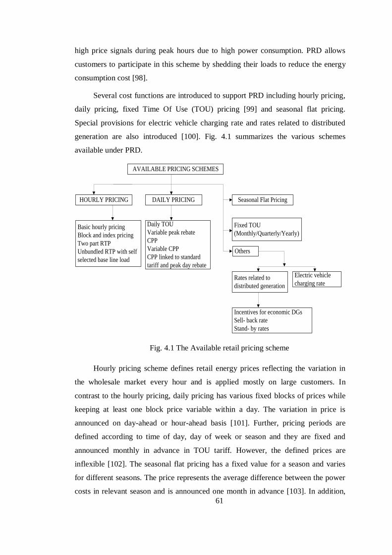
61

high price signals during peak hours due to high power consumption. PRD allows

customers to participate in this scheme by shedding their loads to reduce the energy

consumption cost [98].

Several cost functions are introduced to support PRD including hourly pricing,

daily pricing, fixed Time Of Use (TOU) pricing [99] and seasonal flat pricing.

Special provisions for electric vehicle charging rate and rates related to distributed

generation are also introduced [100]. Fig. 4.1 summarizes the various schemes

available under PRD.

AVAILABLE PRICING SCHEMES

HOURLY PRICING DAILY PRICING Seasonal Flat Pricing

Basic hourly pricing

Block and index pricing

Two part RTP

Unbundled RTP with self

selected base line load

Daily TOU

Variable peak rebate

CPP

Variable CPP

CPP linked to standard

tariff and peak day rebate

Fixed TOU

(Monthly/Quarterly/Yearly)

Others

Rates related to

distributed generation

Electric vehicle

charging rate

Incentives for economic DGs

Sell- back rate

Stand- by rates

Fig. 4.1 The Available retail pricing scheme

Hourly pricing scheme defines retail energy prices reflecting the variation in

the wholesale market every hour and is applied mostly on large customers. In

contrast to the hourly pricing, daily pricing has various fixed blocks of prices while

keeping at least one block price variable within a day. The variation in price is

announced on day-ahead or hour-ahead basis [101]. Further, pricing periods are

defined according to time of day, day of week or season and they are fixed and

announced monthly in advance in TOU tariff. However, the defined prices are

inflexible [102]. The seasonal flat pricing has a fixed value for a season and varies

for different seasons. The price represents the average difference between the power

costs in relevant season and is announced one month in advance [103]. In addition,

62

Critical Peak Price (CPP) and peak day rebate programs provide price signals to

consumers reflecting wholesale prices only on critical peak day and the fixed

standard tariff is used in the rest of the days [104].

The above methods have their own pros and cons. For instance the hourly

pricing scheme has fixed blocks of prices which are inflexible and does not reflect

the actual demand. TOU price does not provide incentives for critical days with

actual power system conditions and unusual wholesale prices. Flat seasonal rates are

the average of low and high cost of energy within a season and hence do not reflect

the actual demand variation. CPP and peak day rebate rates have some implications

on energy providers and customers. Customers have less risk on peak day rebate than

facing unpredictable high price during CPP. But billing under CPP is much easier

than peak day rebate for the energy providers [100].

A Real-Time Pricing (RTP) is introduced in [105] where price is calculated

based on previous demand and then any deviation from actual consumption after a

time step is reimbursed. Due to predicted price components, this pricing scheme may

not be suitable for a system with more uncertainties and information asymmetry.

However, RTP proposed in our research work has price components with

instantaneous data analysis and hence accurately provide price information. The

authors of [106] propose a new RTP to reduce peak to average load ratio. It is based

on a two stage optimization technique, considering both customers to maximize

payoff and retailers to maximize their profit. Another study proposes an optimal and

automatic energy consumption scheduling of residences to minimize both electricity

price and waiting time of appliances. Here, the RTP with inclined block rates are

used [107]. However instantaneous optimization may consume more simulation time

for decision making. However, method proposed in our research work has

comparatively less data processing time due to simple calculations. It also considers

not only excess load consumption but also voltage violations and wholesale price

spikes while defining price unlike in other studies mentioned above.

Overall, this part of the research work proposes a new pricing scheme

reflecting the actual load consumption of a residential customer, the wholesale price

of the network and voltage violations in the network. Section 4.2 describes the new

pricing scheme and Section 4.3 proposes the actual implementation of it. Section 4.4

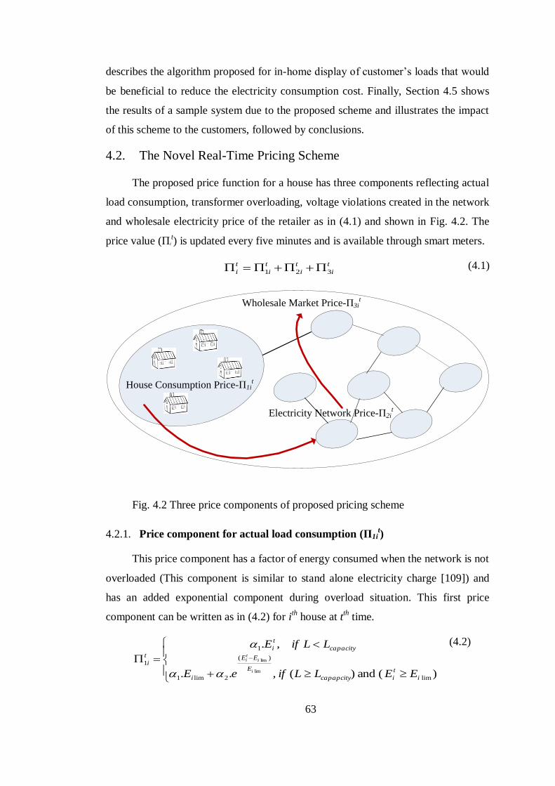
63

describes the algorithm proposed for in-home display of customer’s loads that would

be beneficial to reduce the electricity consumption cost. Finally, Section 4.5 shows

the results of a sample system due to the proposed scheme and illustrates the impact

of this scheme to the customers, followed by conclusions.

4.2. The Novel Real-Time Pricing Scheme

The proposed price function for a house has three components reflecting actual

load consumption, transformer overloading, voltage violations created in the network

and wholesale electricity price of the retailer as in (4.1) and shown in Fig. 4.2. The

price value (Пi

t) is updated every five minutes and is available through smart meters.

t

i

t

i

t

i

t

i 321 (4.1)

Wholesale Market Price-П3it

Electricity Network Price-П2it

House Consumption Price-П1it

Fig. 4.2 Three price components of proposed pricing scheme

4.2.1. Price component for actual load consumption (П1it)

This price component has a factor of energy consumed when the network is not

overloaded (This component is similar to stand alone electricity charge [109]) and

has an added exponential component during overload situation. This first price

component can be written as in (4.2) for ith house at t

th time.

)(and)(,..

,.

lim

)(

2lim1

1

1

lim

lim

i

t

icapapcity

E

EE

i

capacity

t

it

i

EELLifeE

LLifE

i

iti

(4.2)

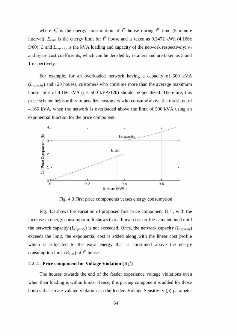
64

where Ei

t is the energy consumption of i

th house during t

th time (5 minute

interval); Ei lim is the energy limit for ith

house and is taken as 0.3472 kWh (4.166x

5/60); L and Lcapacity is the kVA loading and capacity of the network respectively; α1

and α2 are cost coefficients, which can be decided by retailers and are taken as 5 and

1 respectively.

For example, for an overloaded network having a capacity of 500 kVA

(Lcapacity) and 120 houses, customers who consume more than the average maximum

house limit of 4.166 kVA (i.e. 500 kVA/120) should be penalized. Therefore, this

price scheme helps utility to penalize customers who consume above the threshold of

4.166 kVA, when the network is overloaded above the limit of 500 kVA using an

exponential function for the price component.

Fig. 4.3 First price components verses energy consumption

Fig. 4.3 shows the variation of proposed first price component П1it , with the

increase in energy consumption. It shows that a linear cost profile is maintained until

the network capacity (Lcapacity) is not exceeded. Once, the network capacity (Lcapacity)

exceeds the limit, the exponential cost is added along with the linear cost profile

which is subjected to the extra energy that is consumed above the energy

consumption limit (Ei lim) of ith house.

4.2.2. Price component for Voltage Violation (П2it)

The houses towards the end of the feeder experience voltage violations even

when their loading is within limits. Hence, this pricing component is added for those

houses that create voltage violations in the feeder. Voltage Sensitivity (ρ) parameter

0 0.2 0.4 0.60

1

2

3

4

Energy (kWh)

1st

Price C

om

poenent

($)

E lim

Lcapacity

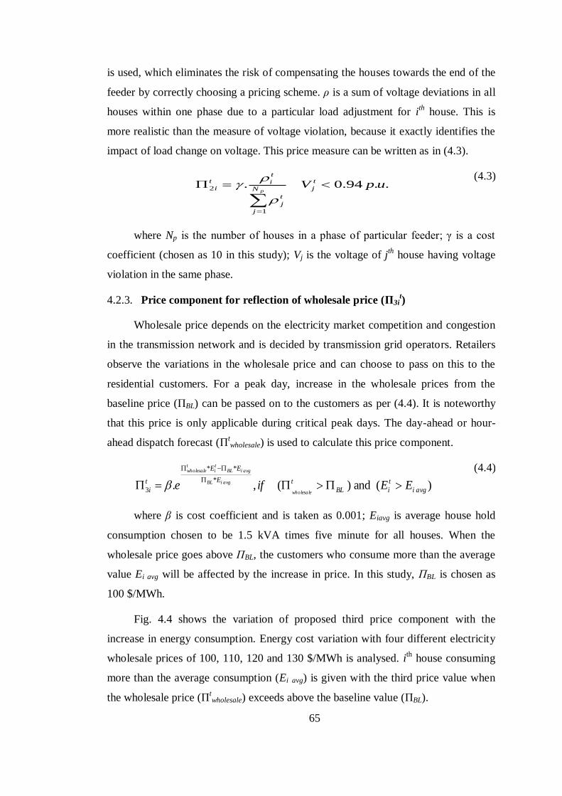
65

is used, which eliminates the risk of compensating the houses towards the end of the

feeder by correctly choosing a pricing scheme. ρ is a sum of voltage deviations in all

houses within one phase due to a particular load adjustment for ith

house. This is

more realistic than the measure of voltage violation, because it exactly identifies the

impact of load change on voltage. This price measure can be written as in (4.3).

..94.0.

1

2 upV t

jN

j

t

j

t

it

ip

(4.3)

where Np is the number of houses in a phase of particular feeder; γ is a cost

coefficient (chosen as 10 in this study); Vj is the voltage of jth

house having voltage

violation in the same phase.

4.2.3. Price component for reflection of wholesale price (П3it)

Wholesale price depends on the electricity market competition and congestion

in the transmission network and is decided by transmission grid operators. Retailers

observe the variations in the wholesale price and can choose to pass on this to the

residential customers. For a peak day, increase in the wholesale prices from the

baseline price (ПBL) can be passed on to the customers as per (4.4). It is noteworthy

that this price is only applicable during critical peak days. The day-ahead or hour-

ahead dispatch forecast (Пtwholesale) is used to calculate this price component.

)(and)(,.*

**

3 avgi

t

iBL

tE

EE

t

i EEifewholesale

avgiBL

avgiBLti

twholesale

(4.4)

where β is cost coefficient and is taken as 0.001; Eiavg is average house hold

consumption chosen to be 1.5 kVA times five minute for all houses. When the

wholesale price goes above ПBL, the customers who consume more than the average

value Ei avg will be affected by the increase in price. In this study, ПBL is chosen as

100 $/MWh.

Fig. 4.4 shows the variation of proposed third price component with the

increase in energy consumption. Energy cost variation with four different electricity

wholesale prices of 100, 110, 120 and 130 $/MWh is analysed. ith house consuming

more than the average consumption (Ei avg) is given with the third price value when

the wholesale price (Пtwholesale) exceeds above the baseline value (ПBL).

66

Fig. 4.4 Third price components verses energy consumption

Overall, the utility benefits when the customers willingly participate in this

scheme by preventing overloads and voltage violations and also the risk due to

critical day wholesale prices. Risk in the network is avoided so that a reduced price

will be provided to the customers. The customers who are not willing to take part in

this program considerably violate the network conditions and hence should pay a

higher price due to the risk in the network. Therefore, this pricing scheme doesn’t

need another risk premium on pricing and it is advantageous for both customers and

utility.

4.3. Practical Implementation of this Scheme

Advanced metering infrastructure having two ways communication capabilities

can be used to implement the algorithm presented in Section 4.4. The voltage and

power data from smart meters is sent in five minute intervals to the main controller

and the calculated price signals and appliance indication details are sent back to

smart meters located at each house. The communication capability of the network

can be shown as in Fig. 4.5.

Collective points with low cost air interface (ZigBee) are much more feasible

because it reduces the expensive modules of broadband wireless interfaces. The in-

home display units have the capability of showing the details of current electricity

cost and indicate the appropriate lamps when the price goes high to identify the

appropriate appliance which can be switched off by the customers [109].

0 0.2 0.4 0.6 0.80

0.2

0.4

0.6

0.8

1

Energy (kWh)

3rd

Price C

om

poenent

($)

120 $/MWh

110 $/MWh

100 $/MWh

Price wholesale=130 $/MWh

E avg

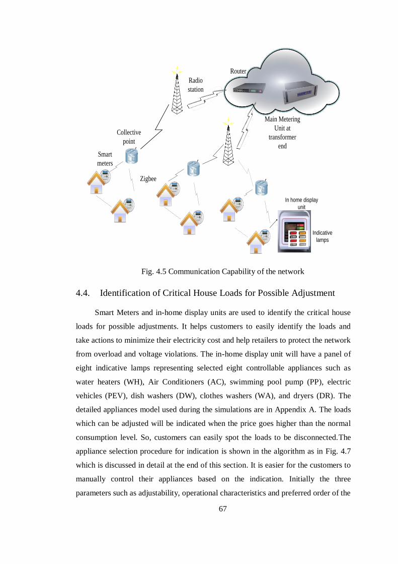
67

Smart

meters

Zigbee

Collective

point

Radio

station

Main Metering

Unit at

transformer

end

Router

In home display

unit

Indicative

lamps

Fig. 4.5 Communication Capability of the network

4.4. Identification of Critical House Loads for Possible Adjustment

Smart Meters and in-home display units are used to identify the critical house

loads for possible adjustments. It helps customers to easily identify the loads and

take actions to minimize their electricity cost and help retailers to protect the network

from overload and voltage violations. The in-home display unit will have a panel of

eight indicative lamps representing selected eight controllable appliances such as

water heaters (WH), Air Conditioners (AC), swimming pool pump (PP), electric

vehicles (PEV), dish washers (DW), clothes washers (WA), and dryers (DR). The

detailed appliances model used during the simulations are in Appendix A. The loads

which can be adjusted will be indicated when the price goes higher than the normal

consumption level. So, customers can easily spot the loads to be disconnected.The

appliance selection procedure for indication is shown in the algorithm as in Fig. 4.7

which is discussed in detail at the end of this section. It is easier for the customers to

manually control their appliances based on the indication. Initially the three

parameters such as adjustability, operational characteristics and preferred order of the

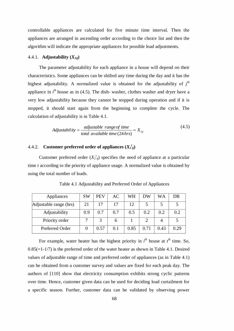
68

controllable appliances are calculated for five minute time interval. Then the

appliances are arranged in ascending order according to the choice list and then the

algorithm will indicate the appropriate appliances for possible load adjustments.

4.4.1. Adjustability (X1ij)

The parameter adjustability for each appliance in a house will depend on their

characteristics. Some appliances can be shifted any time during the day and it has the

highest adjustability. A normalized value is obtained for the adjustability of jth

appliance in ith

house as in (4.5). The dishwasher, clothes washer and dryer have a

very low adjustability because they cannot be stopped during operation and if it is

stopped, it should start again from the beginning to complete the cycle. The

calculation of adjustability is in Table 4.1.

ijXhrstimeavailabletotal

timeofrangeadjustableityAdjustabil 1

)24(

(4.5)

4.4.2. Customer preferred order of appliances (X2tij)

Customer preferred order (X2tij) specifies the need of appliance at a particular

time t according to the priority of appliance usage. A normalized value is obtained by

using the total number of loads.

Table 4.1 Adjustability and Preferred Order of Appliances

Appliances SW PEV AC WH DW WA DR

Adjustable range (hrs) 21 17 17 12 5 5 5

Adjustability 0.9 0.7 0.7 0.5 0.2 0.2 0.2

Priority order 7 3 6 1 2 4 5

Preferred Order 0 0.57 0.1 0.85 0.71 0.43 0.29

For example, water heater has the highest priority in ith house at t

th time. So,

0.85(=1-1/7) is the preferred order of the water heater as shown in Table 4.1. Desired

values of adjustable range of time and preferred order of appliances (as in Table 4.1)

can be obtained from a customer survey and values are fixed for each peak day. The

authors of [110] show that electricity consumption exhibits strong cyclic patterns

over time. Hence, customer given data can be used for deciding load curtailment for

a specific season. Further, customer data can be validated by observing power

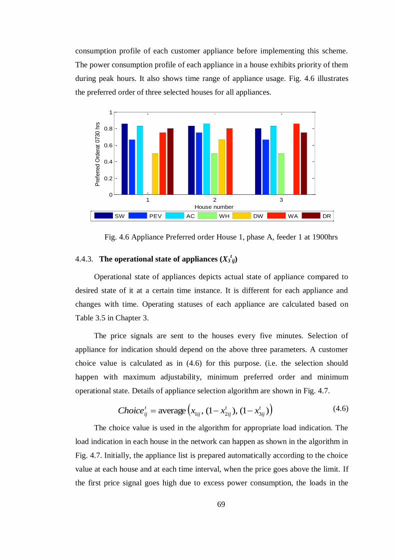
69

consumption profile of each customer appliance before implementing this scheme.

The power consumption profile of each appliance in a house exhibits priority of them

during peak hours. It also shows time range of appliance usage. Fig. 4.6 illustrates

the preferred order of three selected houses for all appliances.

Fig. 4.6 Appliance Preferred order House 1, phase A, feeder 1 at 1900hrs

4.4.3. The operational state of appliances (X3tij)

Operational state of appliances depicts actual state of appliance compared to

desired state of it at a certain time instance. It is different for each appliance and

changes with time. Operating statuses of each appliance are calculated based on

Table 3.5 in Chapter 3.

The price signals are sent to the houses every five minutes. Selection of

appliance for indication should depend on the above three parameters. A customer

choice value is calculated as in (4.6) for this purpose. (i.e. the selection should

happen with maximum adjustability, minimum preferred order and minimum

operational state. Details of appliance selection algorithm are shown in Fig. 4.7.

)1(),1(,average 321

t

ij

t

ijij

t

ij xxxChoice (4.6)

The choice value is used in the algorithm for appropriate load indication. The

load indication in each house in the network can happen as shown in the algorithm in

Fig. 4.7. Initially, the appliance list is prepared automatically according to the choice

value at each house and at each time interval, when the price goes above the limit. If

the first price signal goes high due to excess power consumption, the loads in the

1 2 30

0.2

0.4

0.6

0.8

1

House number

Pre

ferr

ed O

rdera

t 0730 h

rs

SW PEV AC WH DW WA DR

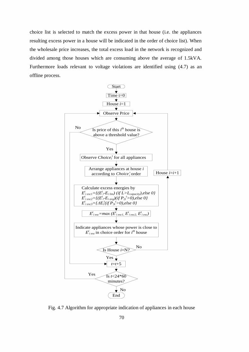
70

choice list is selected to match the excess power in that house (i.e. the appliances

resulting excess power in a house will be indicated in the order of choice list). When

the wholesale price increases, the total excess load in the network is recognized and

divided among those houses which are consuming above the average of 1.5kVA.

Furthermore loads relevant to voltage violations are identified using (4.7) as an

offline process.

Start

Observe Price

Is price of this ith house is

above a threshold value?

Observe Choiceit for all appliances

Yes

Time t=0

Arrange appliances at house i

according to order

House i=1

Eti exc=max (Et

i exc1, Eti exc2, E

ti exc)

Yes

End

No

t

iChoice

Indicate appliances whose power is close to

Eti exc in choice order for ith house

House i=i+1

No

Is t<24*60

minutes?

No

Calculate excess energies by

Eti exc1={(Et

i-Ei lim) (if L>Lcapacity),else 0}

Eti exc2={(Et

i-Ei avg)(if P2it>0),else 0}

Eti exc3={ΔEi

t(if P3it>0),else 0}

Is House i=N?

Yes

t=t+5

Fig. 4.7 Algorithm for appropriate indication of appliances in each house

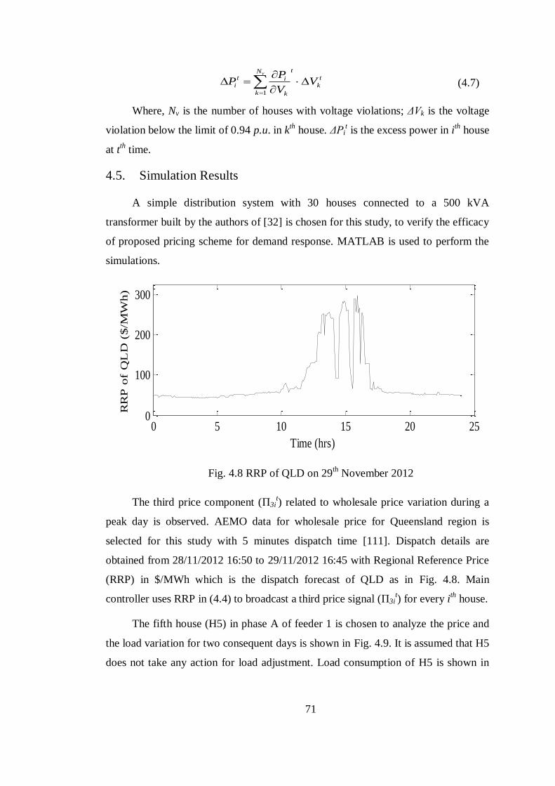
71

(4.7)

Where, Nv is the number of houses with voltage violations; ΔVk is the voltage

violation below the limit of 0.94 p.u. in kth

house. ΔPit is the excess power in i

th house

at tth

time.

4.5. Simulation Results

A simple distribution system with 30 houses connected to a 500 kVA

transformer built by the authors of [32] is chosen for this study, to verify the efficacy

of proposed pricing scheme for demand response. MATLAB is used to perform the

simulations.

Fig. 4.8 RRP of QLD on 29th November 2012

The third price component (П3it) related to wholesale price variation during a

peak day is observed. AEMO data for wholesale price for Queensland region is

selected for this study with 5 minutes dispatch time [111]. Dispatch details are

obtained from 28/11/2012 16:50 to 29/11/2012 16:45 with Regional Reference Price

(RRP) in $/MWh which is the dispatch forecast of QLD as in Fig. 4.8. Main

controller uses RRP in (4.4) to broadcast a third price signal (П3it) for every i

th house.

The fifth house (H5) in phase A of feeder 1 is chosen to analyze the price and

the load variation for two consequent days is shown in Fig. 4.9. It is assumed that H5

does not take any action for load adjustment. Load consumption of H5 is shown in

vN

k

t

k

t

k

it

i VV

PP

1

0 5 10 15 20 250

100

200

300

Time (hrs)

RR

P o

f Q

LD

($/M

Wh)

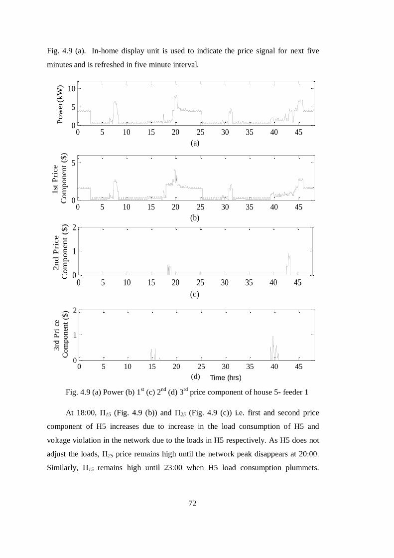
72

Fig. 4.9 (a). In-home display unit is used to indicate the price signal for next five

minutes and is refreshed in five minute interval.

Fig. 4.9 (a) Power (b) 1st (c) 2

nd (d) 3

rd price component of house 5- feeder 1

At 18:00, П15 (Fig. 4.9 (b)) and П25 (Fig. 4.9 (c)) i.e. first and second price

component of H5 increases due to increase in the load consumption of H5 and

voltage violation in the network due to the loads in H5 respectively. As H5 does not

adjust the loads, П25 price remains high until the network peak disappears at 20:00.

Similarly, П15 remains high until 23:00 when H5 load consumption plummets.

0 5 10 15 20 25 30 35 40 450

5

10

(a)

Pow

er(

kW

)

0 5 10 15 20 25 30 35 40 450

5

(b)

1st

Pri

ce

Co

mpo

nent

($)

0 5 10 15 20 25 30 35 40 450

1

2

(c)

2nd P

rice

Com

ponent

($)

0 5 10 15 20 25 30 35 40 450

5

10

(a)

Pow

er(

kW

)

0 5 10 15 20 25 30 35 40 450

5

(b)

1st

Pri

ce

Com

ponent

($)

0 5 10 15 20 25 30 35 40 450

1

2

(c)

2nd P

rice

Com

ponent

($)

0 5 10 15 20 25 30 35 40 450

1

2

(d)

3rd

Pri

ce

Com

ponen

t ($

)

Time (hrs)

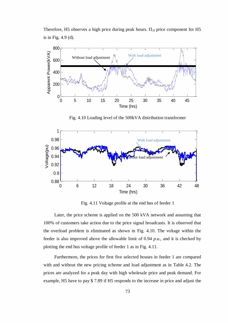
73

Therefore, H5 observes a high price during peak hours. П35 price component for H5

is in Fig. 4.9 (d).

Fig. 4.10 Loading level of the 500kVA distribution transformer

Fig. 4.11 Voltage profile at the end bus of feeder 1

Later, the price scheme is applied on the 500 kVA network and assuming that

100% of customers take action due to the price signal broadcasts. It is observed that

the overload problem is eliminated as shown in Fig. 4.10. The voltage within the

feeder is also improved above the allowable limit of 0.94 p.u., and it is checked by

plotting the end bus voltage profile of feeder 1 as in Fig. 4.11.

Furthermore, the prices for first five selected houses in feeder 1 are compared

with and without the new pricing scheme and load adjustment as in Table 4.2. The

prices are analyzed for a peak day with high wholesale price and peak demand. For

example, H5 have to pay $ 7.89 if H5 responds to the increase in price and adjust the

0 5 10 15 20 25 30 35 40 450

200

400

600

800

Time (hrs)

Appare

nt

Pow

er(

kV

A)

0 6 12 18 24 30 36 42 480.88

0.9

0.92

0.94

0.96

0.98

1

Time (hrs)

Voltage(p

u)

0 5 10 15 20 25 30 35 40 450

200

400

600

800

Time (hrs)

Appare

nt

Pow

er(

kV

A)

0 6 12 18 24 30 36 42 480.88

0.9

0.92

0.94

0.96

0.98

1

Time (hrs)

Voltage(p

u)

Without load adjustment With load adjustment

With load adjustment

Without load adjustment

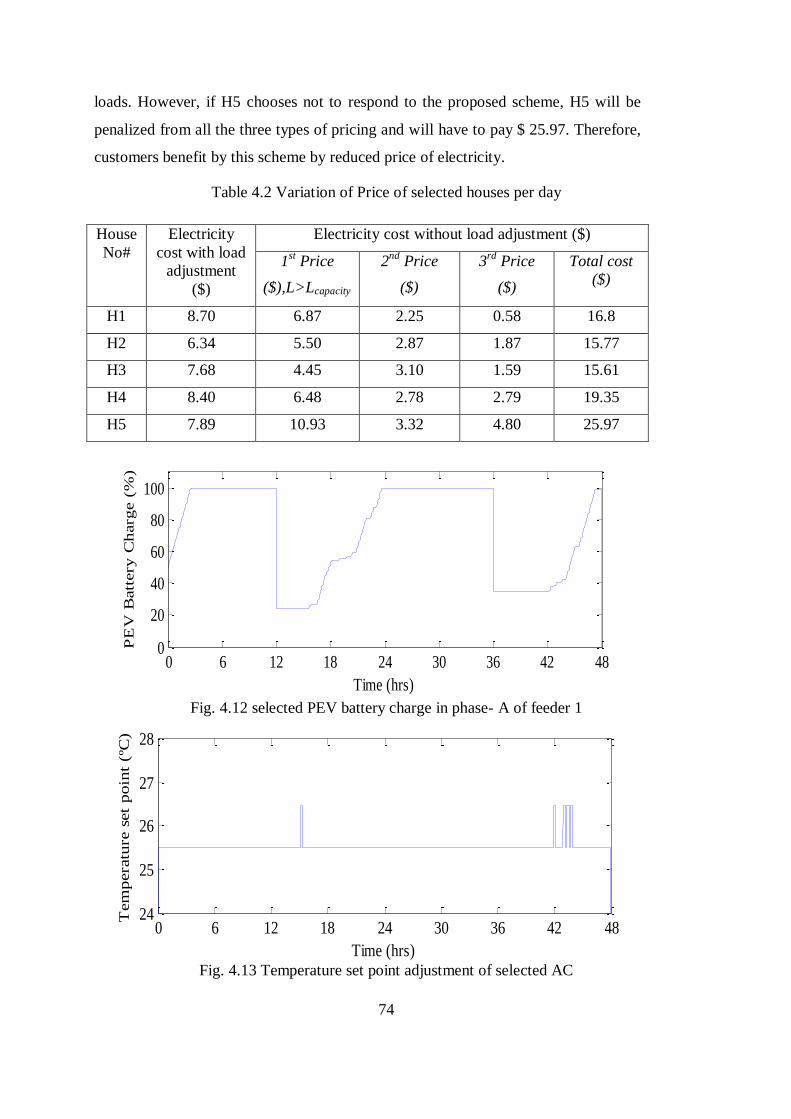
74

loads. However, if H5 chooses not to respond to the proposed scheme, H5 will be

penalized from all the three types of pricing and will have to pay $ 25.97. Therefore,

customers benefit by this scheme by reduced price of electricity.

Table 4.2 Variation of Price of selected houses per day

House

No#

Electricity

cost with load

adjustment

($)

Electricity cost without load adjustment ($)

1st Price

($),L>Lcapacity

2nd

Price

($)

3rd

Price

($)

Total cost

($)

H1 8.70 6.87 2.25 0.58 16.8

H2 6.34 5.50 2.87 1.87 15.77

H3 7.68 4.45 3.10 1.59 15.61

H4 8.40 6.48 2.78 2.79 19.35

H5 7.89 10.93 3.32 4.80 25.97

Fig. 4.12 selected PEV battery charge in phase- A of feeder 1

Fig. 4.13 Temperature set point adjustment of selected AC

0 6 12 18 24 30 36 42 480

20

40

60

80

100

Time (hrs)

PE

V B

att

ery

Ch

arg

e (

%)

0 6 12 18 24 30 36 42 4824

25

26

27

28

Time (hrs)

Tem

pera

ture

set

poin

t (º

C)

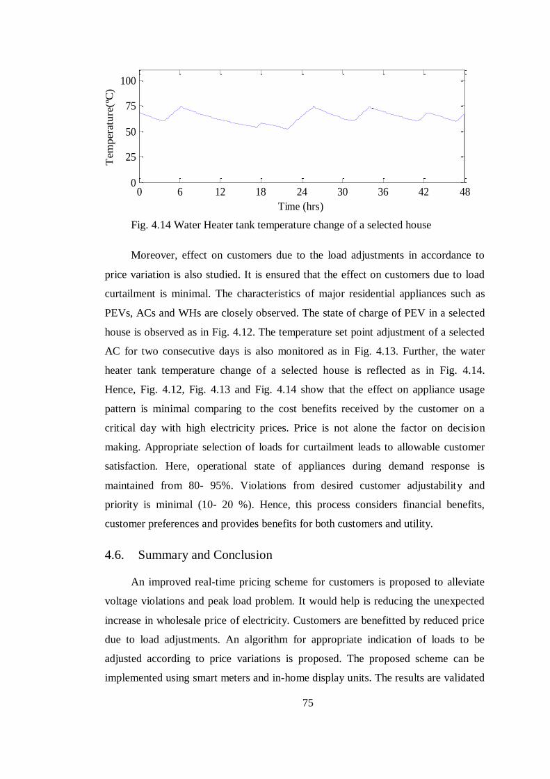
75

Fig. 4.14 Water Heater tank temperature change of a selected house

Moreover, effect on customers due to the load adjustments in accordance to

price variation is also studied. It is ensured that the effect on customers due to load

curtailment is minimal. The characteristics of major residential appliances such as

PEVs, ACs and WHs are closely observed. The state of charge of PEV in a selected

house is observed as in Fig. 4.12. The temperature set point adjustment of a selected

AC for two consecutive days is also monitored as in Fig. 4.13. Further, the water

heater tank temperature change of a selected house is reflected as in Fig. 4.14.

Hence, Fig. 4.12, Fig. 4.13 and Fig. 4.14 show that the effect on appliance usage

pattern is minimal comparing to the cost benefits received by the customer on a

critical day with high electricity prices. Price is not alone the factor on decision

making. Appropriate selection of loads for curtailment leads to allowable customer

satisfaction. Here, operational state of appliances during demand response is

maintained from 80- 95%. Violations from desired customer adjustability and

priority is minimal (10- 20 %). Hence, this process considers financial benefits,

customer preferences and provides benefits for both customers and utility.


An improved real-time pricing scheme for customers is proposed to alleviate

voltage violations and peak load problem. It would help is reducing the unexpected

increase in wholesale price of electricity. Customers are benefitted by reduced price

due to load adjustments. An algorithm for appropriate indication of loads to be

adjusted according to price variations is proposed. The proposed scheme can be

implemented using smart meters and in-home display units. The results are validated

0 6 12 18 24 30 36 42 480

25

50

75

100

Time (hrs)

Tem

pera

ture

(ºC

)

76

in a sample distribution system. The impact on customer side due to the proposed

real-time pricing scheme does not hamper the appliance usage patterns of customers.

77

Chapter 5

Real-Time Home Energy Management Scheduler

Using Stochastic Dynamic Programming

With the recent development of advanced metering infrastructure, Real-Time

Pricing (RTP) scheme is anticipated to be introduced in future retail electricity

market. Home Energy Management (HEM) facilitates customers to adjust their loads

based on RTP. This research work proposes a real-time Home Energy Management

Scheduler (HEMS) aiming to reduce the cost of energy consumption in a house while

maintaining customer satisfaction. The proposed HEMS works in three subsequent

phases namely real-time monitoring (RTM), stochastic scheduling (STS) and real-

time control (RTC) of appliances. In RTM phase, characteristics of available

controllable appliances are monitored in real-time and stored in HEMS. In STS

phase, HEMS computes an optimal policy using stochastic dynamic programming

(SDP) to select a set of appliances to be controlled with an objective of minimizing

customer discomfort as well as the total cost of energy consumption in a house.

Finally, in RTC phase, HEMS initiates the control of the selected appliances. The

proposed real-time HEMS is unique as it intrinsically considers uncertainties in RTP

and power consumption pattern of various appliances. In RTM phase, appliances are

categorized according to their characteristics to ease the control process, thereby

minimizing the number of control commands issued by HEMS. Simulation results

validate the proposed method for HEMS.

78


Retailers in most electricity markets, provide a fixed electricity tariff scheme

for customers, independent of the cost of electricity generation during the time of

consumption. However, the true opportunity cost of electricity consumption varies

with the marginal cost of electricity production. This causes inelastic behavior in

customer electricity demand within short time frames which may ultimately lead to

losses for both retailers and customers during adverse conditions such as price

spikes/falls [112].

Introducing a time varying electricity retail price, known as Real-Time Pricing

(RTP) is one of the solution. The concept of RTP was introduced long ago, but it has

been only recently possible for practical implementation due to vast technological

improvements in advance metering infrastructure [113], [114]. RTP provides benefit

to retailers by reflecting marginal cost of production and encourages customers to

control their electricity consumption [115]. Smart meters and in- home display units

aim to help customers in reducing their Cost of Energy Consumption (CoEC) and

control their appliances on a regular basis [116]. However, due to uncertainty in price

variation and electricity demand, appropriate control of appliances is cumbersome.

A Home Energy Management (HEM) system helps residential customers to

respond to RTP by reducing CoEC [117]. The authors of [44] and [45] have

proposed a real-time HEM system with a complex scheduler, using ‘particle swarm

optimization’ and ‘genetic algorithm’. However, the uncertainties in RTP of

electricity or the power consumption of appliances are not considered during their

appliance scheduling processes. The authors of [46], however, propose a decision

support tool using linear programming optimization and a price predictor to get hour-

ahead price information and plan the upcoming energy consumption. However, the

predicted price is not included in the optimal scheduling of appliances. This problem

is mitigated by [47] and [48], where a predictive tool along with real-time

optimization is proposed. Nevertheless, the real-time optimization and control along

with predictive techniques is cumbersome and may lead to less accurate results.

In another study, stochastic optimization with an objective of minimizing

expected electricity payment using Monte Carlo simulations [49] and Markov

79

Decision Process (MDP) [50] is proposed. The uncertainty in RTP is incorporated

via expected downside risk [49] and price prediction noise [50]. However, the

uncertainty in appliance power usage is not considered. Taking a step further, the

authors of [51] propose a bottom up approach to represent several house appliances

in a network incorporating uncertainties in both appliance power consumption and

RTP. This model nonetheless increases the number of control commands issued for

adjusting appliance thereby affecting customer comfort.

Contributions: The objective of this part of research, therefore, is to find a

desired tradeoff between incurred cost of energy consumption and customer comfort

level. This chapter proposes a real-time Home Energy Management Scheduler

(HEMS), which aims to reduce the cost of energy consumption in a house while

maintaining customer satisfaction. This research work is different from [44]-[50], as

it considers the uncertainties in both RTP and residential appliance power

consumption pattern during appliance scheduling. Unlike [51], a top down approach

from house to appliance level is taken. I. e. a set of appliances is selected optimally

for control based on their stochastic behavior, with an overall objective of reducing

the total cost of energy consumption in a house. Similar to [49], [50], appliances are

categorized to ease the process of control in this part of research.

Another contribution of this work is that the dimensionality of stochastic

scheduling is reduced. Real-time monitoring is used and that leads to an efficient

control system. The proposed real-time HEMS works in three subsequent phases i.e.

real-time monitoring (RTM), stochastic scheduling (STC) and real-time control

(RTC). Similar to [50]- [51], MDP is used for stochastic optimization.

In section 5.2, the proposed real-time HEMS is described. The operation of

HEMS with these three subsequent phases is summarized in Section 5.3. A test

system description and simulation results are presented in Section 5.4 followed by

conclusions in Section 5.5.

80

5.2. Proposed Real-Time HEMS using SDP

This section introduced a new real-time HEMS using SDP and can be deployed

in houses. Retailers bid in the wholesale electricity market on a day-ahead/real-time

basis to cater their load demand. The customers/end-users, whereas, have a choice to

either take fixed price or RTP based tariff from demand aggregator or retailer. In

some cases, the demand aggregator uses RTP signal from retailers and provide

demand-response/load-reduction by adjusting customers’ load and provide

coupons/incentives in return. Although promising, this method may not be attractive

to the customers who want to have the flexibility to modulate their loads themselves

and be rewarded accordingly.

This chapter, therefore, proposes RTP signals (from either demand aggregators

or retailers) to be send directly to customers/end-users to adjust the loads themselves,

giving them flexibility to choose the level of load adjustments and achieve the

reduced cost of energy consumption. The optimal decision to control the appliance is

taken by HEMS in order to reduce the cost of energy consumption. As the control of

appliances is dependent of individual HEMS, the network scalability is not an issue

and it is easy to implement regardless of the size of the distribution network. This

process is made possible with the advanced metering infrastructure and there are no

additional communication requirements for the proposed algorithm. HEMS collect

the relevant information about the appliances at regular intervals using home area

networks such as Zigbee, HomePlug Wifi, Z-wave etc. The demand

aggregator/retailers broadcast the RTP signal to respective customers, who use

HEMS to adjust the loads using the proposed algorithm. As HEMS only

communicate to demand aggregators/retailers, the current low power radiofrequency

transmitters working in the 900MHz-2.4 GHz band is sufficient.

Appliance control process is performed by HEMS at house level where every

HEMS in a network are remotely connected to the utility to obtain RTP information.

Thereby, a large network with utility connected HEMS at each residence is possible

due to the independent operation of HEMS. It has better performance than a centrally

controlled algorithm for residential appliances in a large network which may raise

scalability issue.

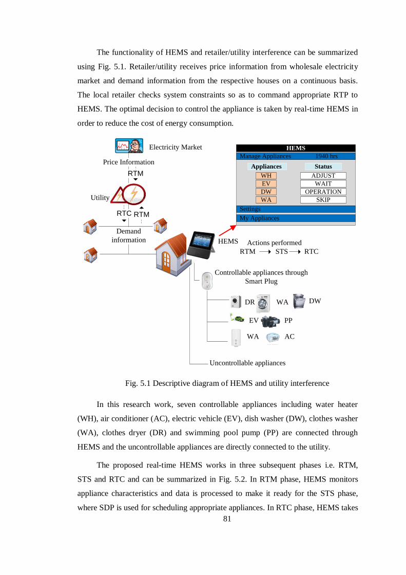
81

The functionality of HEMS and retailer/utility interference can be summarized

using Fig. 5.1. Retailer/utility receives price information from wholesale electricity

market and demand information from the respective houses on a continuous basis.

The local retailer checks system constraints so as to command appropriate RTP to

HEMS. The optimal decision to control the appliance is taken by real-time HEMS in

order to reduce the cost of energy consumption.

Electricity Market

Utility

Controllable appliances through

Smart Plug

Uncontrollable appliances

EV

WA

PP

DR DW

WA

Price Information

Demand

information

AC

HEMS

RTM

RTM

RTC

Actions performed

RTM STS RTC

My Appliances

Settings

HEMS

Manage Appliances 1940 hrs

Appliances

WH

EV

DW

WA

ADJUST

WAIT

OPERATION

SKIP

Status

Fig. 5.1 Descriptive diagram of HEMS and utility interference

In this research work, seven controllable appliances including water heater

(WH), air conditioner (AC), electric vehicle (EV), dish washer (DW), clothes washer

(WA), clothes dryer (DR) and swimming pool pump (PP) are connected through

HEMS and the uncontrollable appliances are directly connected to the utility.

The proposed real-time HEMS works in three subsequent phases i.e. RTM,

STS and RTC and can be summarized in Fig. 5.2. In RTM phase, HEMS monitors

appliance characteristics and data is processed to make it ready for the STS phase,

where SDP is used for scheduling appropriate appliances. In RTC phase, HEMS takes

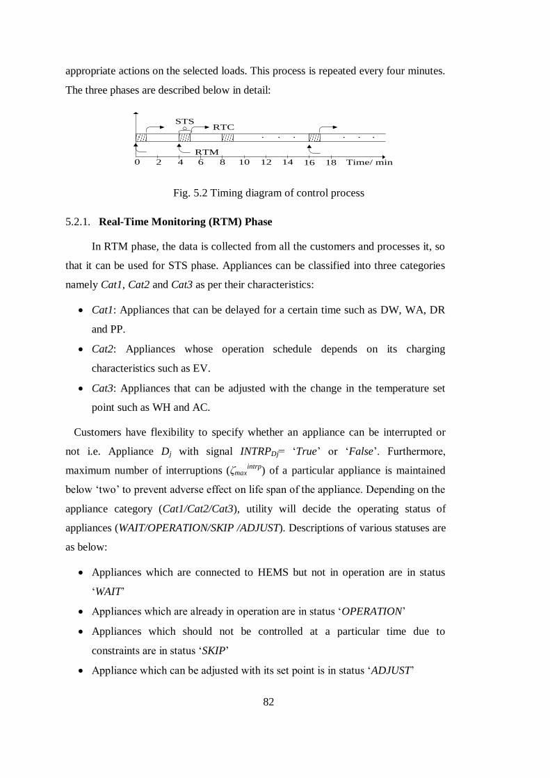
82

appropriate actions on the selected loads. This process is repeated every four minutes.

The three phases are described below in detail:

0 2 4 6 8 10 12 14 16 18

RTC

RTM

STS

Time/ min

. . .. . .

Fig. 5.2 Timing diagram of control process

5.2.1. Real-Time Monitoring (RTM) Phase

In RTM phase, the data is collected from all the customers and processes it, so

that it can be used for STS phase. Appliances can be classified into three categories

namely Cat1, Cat2 and Cat3 as per their characteristics:

Cat1: Appliances that can be delayed for a certain time such as DW, WA, DR

and PP.

Cat2: Appliances whose operation schedule depends on its charging

characteristics such as EV.

Cat3: Appliances that can be adjusted with the change in the temperature set

point such as WH and AC.

Customers have flexibility to specify whether an appliance can be interrupted or

not i.e. Appliance Dj with signal INTRPDj= ‘True’ or ‘False’. Furthermore,

maximum number of interruptions (ζmaxintrp

) of a particular appliance is maintained

below ‘two’ to prevent adverse effect on life span of the appliance. Depending on the

appliance category (Cat1/Cat2/Cat3), utility will decide the operating status of

appliances (WAIT/OPERATION/SKIP /ADJUST). Descriptions of various statuses are

as below:

Appliances which are connected to HEMS but not in operation are in status

‘WAIT’

Appliances which are already in operation are in status ‘OPERATION’

Appliances which should not be controlled at a particular time due to

constraints are in status ‘SKIP’

Appliance which can be adjusted with its set point is in status ‘ADJUST’

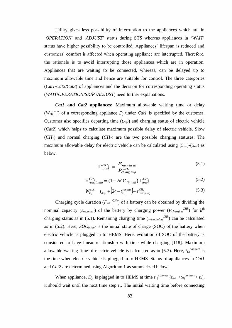
83

Utility gives less possibility of interruption to the appliances which are in

‘OPERATION’ and ‘ADJUST’ status during STS whereas appliances in ‘WAIT’

status have higher possibility to be controlled. Appliances’ lifespan is reduced and

customers’ comfort is affected when operating appliance are interrupted. Therefore,

the rationale is to avoid interrupting those appliances which are in operation.

Appliances that are waiting to be connected, whereas, can be delayed up to

maximum allowable time and hence are suitable for control. The three categories

(Cat1/Cat2/Cat3) of appliances and the decision for corresponding operating status

(WAIT/OPERATION/SKIP /ADJUST) need further explanations.

Cat1 and Cat2 appliances: Maximum allowable waiting time or delay

(WDjmax

) of a corresponding appliance Dj under Cat1 is specified by the customer.

Customer also specifies departing time (tdept) and charging status of electric vehicle

(Cat2) which helps to calculate maximum possible delay of electric vehicle. Slow

(CH1) and normal charging (CH2) are the two possible charging statuses. The

maximum allowable delay for electric vehicle can be calculated using (5.1)-(5.3) as

below.

k

k

CH

ingch

alnoCH

totalP

E

arg

min (5.1)

kk CH

totalinitial

CH

remaining SOC ).1( (5.2)

k

jj

CH

remaining

connect

DdeptD ttW 24max (5.3)

Charging cycle duration (ГtotalCHk

) of a battery can be obtained by dividing the

nominal capacity (Enominal) of the battery by charging power (PchargingCHk

) for kth

charging status as in (5.1). Remaining charging time (τremainingCHk

) can be calculated

as in (5.2). Here, SOCinitial is the initial state of charge (SOC) of the battery when

electric vehicle is plugged in to HEMS. Here, evolution of SOC of the battery is

considered to have linear relationship with time while charging [118]. Maximum

allowable waiting time of electric vehicle is calculated as in (5.3). Here, tDjconnect

is

the time when electric vehicle is plugged in to HEMS. Status of appliances in Cat1

and Cat2 are determined using Algorithm 1 as summarized below.

When appliance, Dj, is plugged in to HEMS at time tDjconnect

(tn-1 <tDjconnect

< tn),

it should wait until the next time step tn. The initial waiting time before connecting

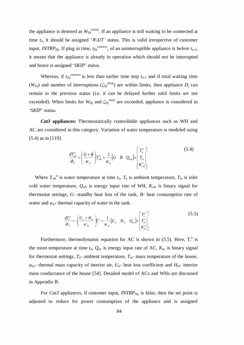
84

the appliance is denoted as WDjinitial

. If an appliance is still waiting to be connected at

time tn, it should be assigned ‘WAIT’ status. This is valid irrespective of customer

input, INTRPDj. If plug in time, tDjconnect

, of an uninterruptible appliance is before tn-1,

it means that the appliance is already in operation which should not be interrupted

and hence is assigned ‘SKIP’ status.

Whereas, if tDjconnect

is less than earlier time step tn-1 and if total waiting time

(WDj) and number of interruptions (ζDjintrp

) are within limits, then appliance Dj can

remain in the previous status (i.e. it can be delayed further until limits are not

exceeded). When limits for WDj and ζDjintrp

are exceeded, appliance is considered in

‘SKIP’ status.

Cat3 appliances: Thermostatically controllable appliances such as WH and

AC are considered in this category. Variation of water temperature is modeled using

(5.4) as in [119].

n

wh

in

n

a

wh

w

n

wh

wn

n

wh

K

T

T

QBGTBG

dt

dT

1.

(5.4)

Where Twhn is water temperature at time tn, Ta is ambient temperature, Tin is inlet

cold water temperature, Qwh is energy input rate of WH, Kwh is binary signal for

thermostat settings, G- standby heat loss of the tank, B- heat consumption rate of

water and ψw- thermal capacity of water in the tank.

n

ac

n

m

n

a

acma

ac

n

r

ac

ma

n

n

r

K

T

T

QHUTHU

dt

dT

1

(5.5)

Furthermore, thermodynamic equation for AC is shown in (5.5). Here, Trn is

the room temperature at time tn, Qac is energy input rate of AC, Kac is binary signal

for thermostat settings, Ta- ambient temperature, Tm- mass temperature of the house,

ψac- thermal mass capacity of interior air, Ua- heat loss coefficient and Hm- interior

mass conductance of the house [54]. Detailed model of ACs and WHs are discussed

in Appendix B.

For Cat3 appliances, if customer input, INTRPDj, is false, then the set point is

adjusted to reduce for power consumption of the appliance and is assigned

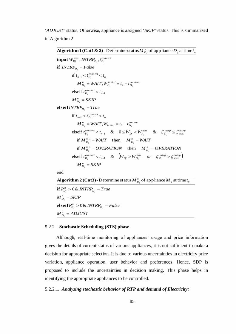
85

‘ADJUST’ status. Otherwise, appliance is assigned ‘SKIP’ status. This is summarized

in Algorithm 2.

ADJUSTM

FalseINTRPP

SKIPM

TrueINTRPP

tMM

SKIPM

orWWtt

OPERATIONMOPERATIONM

WAITMWAITM

WWtt

ttWWAITM

ttt

TrueINTRP

SKIPM

tt

ttWWAITM

ttt

FalseINTRP

tINTRPW

tDM

n

D

D

n

D

n

D

D

n

D

nj

n

D

n

D

rprp

DDDjn

connect

D

n

D

n

D

n

D

n

D

rprp

DADjn

connect

D

connect

Dinitial

n

D

n

connect

Dn

D

n

D

n

connect

D

connect

D

initial

D

n

D

n

connect

Dn

D

connect

DDDj

nj

n

D

j

jj

j

jj

j

j

jjj

jj

jj

jjj

jj

j

j

j

j

jjj

j

j

jj

j

&0

&0

timeatapplianceof status Determine-

end

&elseif

thenif

thenif

&0&elseif

,

if

elseif

,

if

,,

timeatapplianceof status Determine-

int

max

intmax

1

1

1

int

max

intmax

1

2

1

1

2

1

max

elseif

if

(Cat3) 2 Algorithm

elseif

if

input

2)&(Cat1 1 Algorithm

5.2.2. Stochastic Scheduling (STS) phase

Although, real-time monitoring of appliances’ usage and price information

gives the details of current status of various appliances, it is not sufficient to make a

decision for appropriate selection. It is due to various uncertainties in electricity price

variation, appliance operation, user behavior and preferences. Hence, SDP is

proposed to include the uncertainties in decision making. This phase helps in

identifying the appropriate appliances to be controlled.

5.2.2.1. Analyzing stochastic behavior of RTP and demand of Electricity:

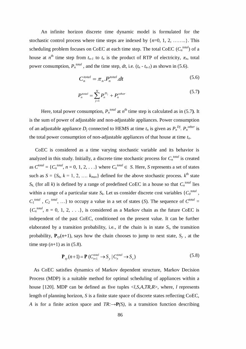
86

An infinite horizon discrete time dynamic model is formulated for the

stochastic control process where time steps are indexed by {n=0, 1, 2, ……..}. This

scheduling problem focuses on CoEC at each time step. The total CoEC (Cntotal

) of a

house at nth time step from tn-1 to tn is the product of RTP of electricity, πn, total

power consumption, Pntotal

, and the time step, dt, i.e. (tn - tn-1) as shown in (5.6).

dtPC total

nn

total

n .. (5.6)

other

n

N

j

D

n

total

n PPP j 1

(5.7)

Here, total power consumption, Pntotal

at nth time step is calculated as in (5.7). It

is the sum of power of adjustable and non-adjustable appliances. Power consumption

of an adjustable appliance Dj connected to HEMS at time tn is given as PnDj

. Pnother

is

the total power consumption of non-adjustable appliances of that house at time tn.

CoEC is considered as a time varying stochastic variable and its behavior is

analyzed in this study. Initially, a discrete time stochastic process for Cntotal

is created

as Ctotal

= {Cntotal

, n = 0, 1, 2, . . .} where Cntotal

S. Here, S represents a set of states

such as S = {Sk, k = 1, 2, …. kmax} defined for the above stochastic process. kth

state

Sk, (for all k) is defined by a range of predefined CoEC in a house so that Cntotal

lies

within a range of a particular state Sk. Let us consider discrete cost variables {C0total

,

C1total

, C2 total

, …} to occupy a value in a set of states (S). The sequence of Ctotal

=

{Cntotal

, n = 0, 1, 2, . . .}, is considered as a Markov chain as the future CoEC is

independent of the past CoEC, conditioned on the present value. It can be further

elaborated by a transition probability, i.e., if the chain is in state Si, the transition

probability, Pxy(n+1), says how the chain chooses to jump to next state, Sy , at the

time step (n+1) as in (5.8).

)|()1( 1 x

total

ny

total

nxy SCSCn ΡΡ (5.8)

As CoEC satisfies dynamics of Markov dependent structure, Markov Decision

Process (MDP) is a suitable method for optimal scheduling of appliances within a

house [120]. MDP can be defined as five tuples <l,S,A,TR,R>, where, l represents

length of planning horizon, S is a finite state space of discrete states reflecting CoEC,

A is for a finite action space and TR:→P(S), is a transition function describing

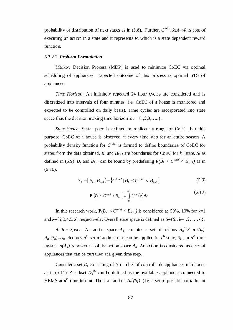
87

probability of distribution of next states as in (5.8). Further, Ctotal

:SxA→R is cost of

executing an action in a state and it represents R, which is a state dependent reward

function.

5.2.2.2. Problem Formulation

Markov Decision Process (MDP) is used to minimize CoEC via optimal

scheduling of appliances. Expected outcome of this process is optimal STS of

appliances.

Time Horizon: An infinitely repeated 24 hour cycles are considered and is

discretized into intervals of four minutes (i.e. CoEC of a house is monitored and

expected to be controlled on daily basis). Time cycles are incorporated into state

space thus the decision making time horizon is n={1,2,3,…..}.

State Space: State space is defined to replicate a range of CoEC. For this

purpose, CoEC of a house is observed at every time step for an entire season. A

probability density function for Ctotal

is formed to define boundaries of CoEC for

states from the data obtained. Bk and Bk+1 are boundaries for CoEC for kth

state, Sk as

defined in (5.9). Bk and Bk+1 can be found by predefining P(Bk ≤ Ctotal

< Bk+1) as in

(5.10).

11 |, k

total

k

total

kkk BCBCBBS (5.9)

dxxCBCBk

k

B

B

total

k

total

k . 1

1

Ρ (5.10)

In this research work, P(Bk ≤ Ctotal

< Bk+1) is considered as 50%, 10% for k=1

and k={2,3,4,5,6} respectively. Overall state space is defined as S={Sk, k=1,2, …, 6}.

Action Space: An action space An, contains a set of actions Anq:S→σ(An).

Anq(Sk)An denotes q

th set of actions that can be applied in k

th state, Sk , at n

th time

instant. σ(An) is power set of the action space An. An action is considered as a set of

appliances that can be curtailed at a given time step.

Consider a set D, consisting of N number of controllable appliances in a house

as in (5.11). A subset Dnav

can be defined as the available appliances connected to

HEMS at nth

time instant. Then, an action, Anq(Sk), (i.e. a set of possible curtailment

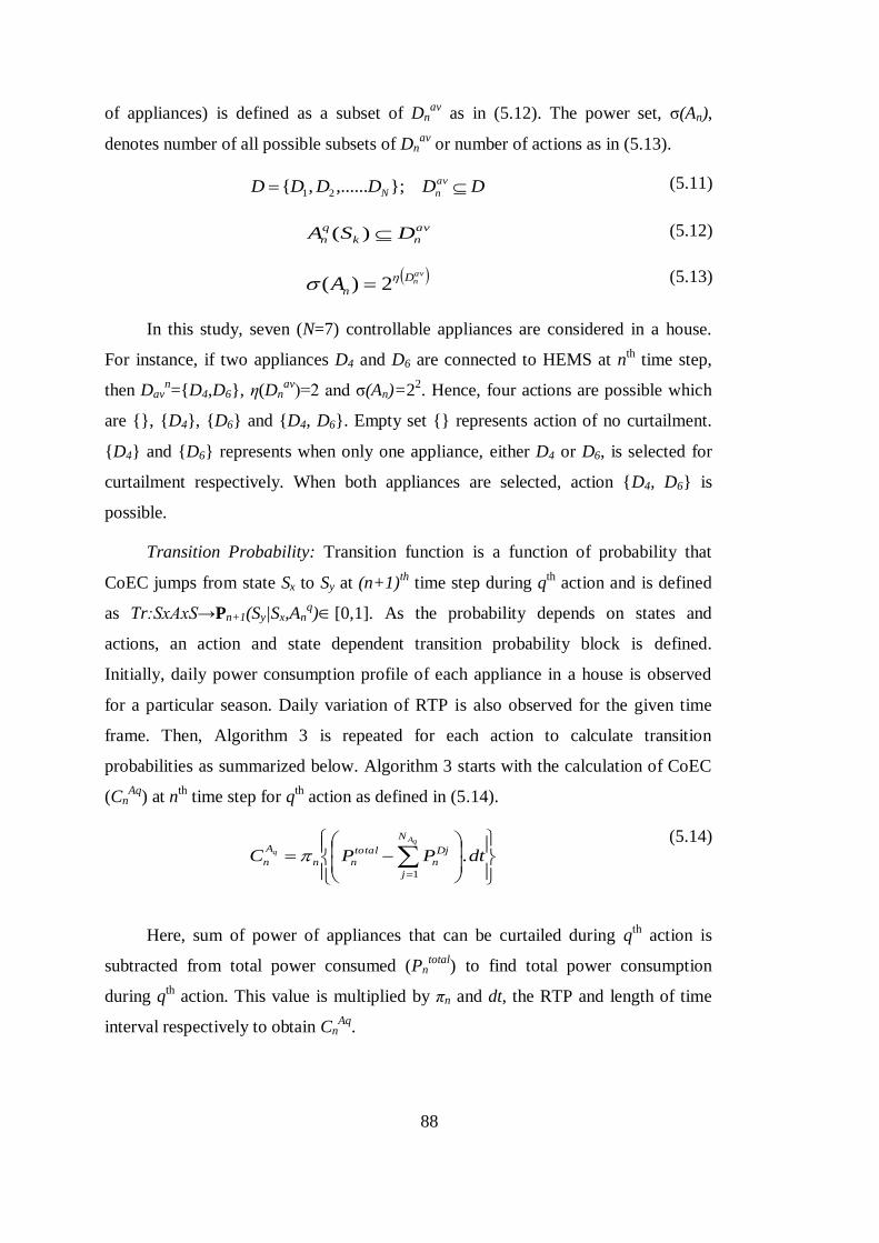
88

of appliances) is defined as a subset of Dnav

as in (5.12). The power set, σ(An),

denotes number of all possible subsets of Dnav

or number of actions as in (5.13).

DDDDDD av

nN };,......,{ 21 (5.11)

av

nk

q

n DSA )( (5.12)

avnD

nA 2)(

(5.13)

In this study, seven (N=7) controllable appliances are considered in a house.

For instance, if two appliances D4 and D6 are connected to HEMS at nth time step,

then Davn={D4,D6}, η(Dn

av)=2 and σ(An)=2

2. Hence, four actions are possible which

are {}, {D4}, {D6} and {D4, D6}. Empty set {} represents action of no curtailment.

{D4} and {D6} represents when only one appliance, either D4 or D6, is selected for

curtailment respectively. When both appliances are selected, action {D4, D6} is

possible.

Transition Probability: Transition function is a function of probability that

CoEC jumps from state Sx to Sy at (n+1)th

time step during qth action and is defined

as Tr:SxAxS→Pn+1(Sy|Sx,Anq)[0,1]. As the probability depends on states and

actions, an action and state dependent transition probability block is defined.

Initially, daily power consumption profile of each appliance in a house is observed

for a particular season. Daily variation of RTP is also observed for the given time

frame. Then, Algorithm 3 is repeated for each action to calculate transition

probabilities as summarized below. Algorithm 3 starts with the calculation of CoEC

(CnAq

) at nth time step for q

th action as defined in (5.14).

dtPPCqA

q

N

j

Dj

n

total

nn

A

n .1

(5.14)

Here, sum of power of appliances that can be curtailed during qth

action is

subtracted from total power consumed (Pntotal

) to find total power consumption

during qth action. This value is multiplied by πn and dt, the RTP and length of time

interval respectively to obtain CnAq

.

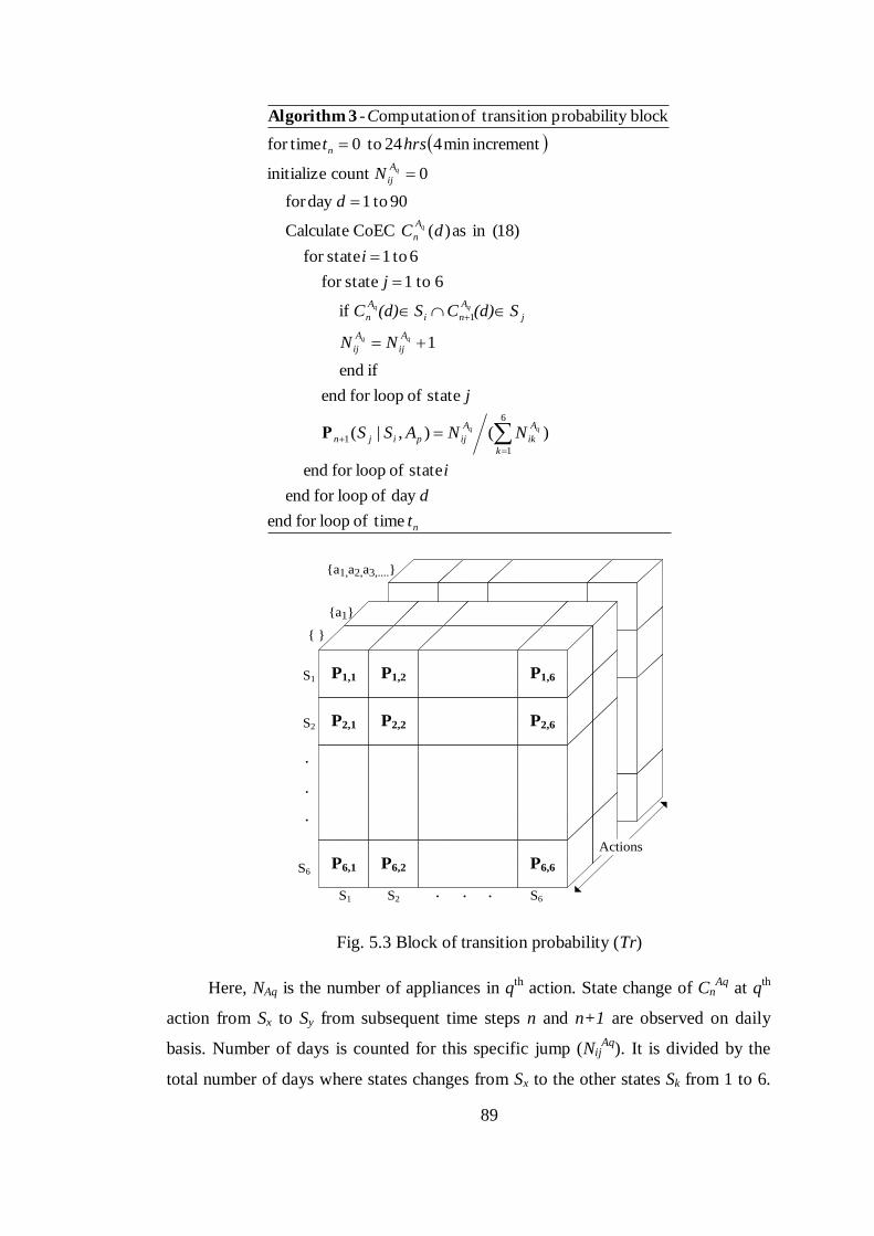
89

n

k

A

ik

A

ijpijn

A

ij

A

ij

j

A

ni

A

n

A

n

A

ij

n

t

d

i

NNASS

j

NN

S(d)CS(d)C

j

i

dC

d

N

hrst

C

qq

qq

qq

q

q

timeof loopfor end

day of loopfor end

state of loopfor end

)(),|(


if end

1

if

6to1 statefor

6 to1 statefor

)18(in as)( CoEC Calculate

90to1dayfor

0countinitialize

incrementmin424to0timefor

blocky probabilitn transitioof omputation-

6

1

1

1

Ρ

3 Algorithm

P6,1 P6,2

P2,1 P2,2

P1,1 P1,2

P6,6

P2,6

P1,6

. . .

S1

S2

S6

..

.

Actions

{ }

{a1}

{a1,a2,a3,....}

S6S2S1

Fig. 5.3 Block of transition probability (Tr)

Here, NAq is the number of appliances in qth

action. State change of CnAq

at qth

action from Sx to Sy from subsequent time steps n and n+1 are observed on daily

basis. Number of days is counted for this specific jump (NijAq

). It is divided by the

total number of days where states changes from Sx to the other states Sk from 1 to 6.

90

(∑NikAq

) to obtain the transition probability Pn+1(Sy|Sx,Anq). This process is repeated

at each time step. Further, Algorithm 3 is repeated for each action to obtain the

transition probabilities of all possible state changes or jumps for the whole action

space and is shown in Fig. 5.3.

Reward Function: Accurate definition of reward function (rewardxyAqR) is

vital in MDP due to its importance in decision making. It helps to choose best

possible action, Anq, for appropriate selection of appliances. A reward value is

defined as in (5.15), which is four tuples,<Si/Sj, βk, Pk,Wk>.

{}

){}and(1..1

max

q

n

y

x

nn

N

j D

n

Drating

D

D

n

y

x

A

xy

AS

S

AAW

WP

S

S

nreward

qA

j

j

j

j

q

(5.15)

(i) Reward component 1(Si/Sj) - Ratio of state change from Sx to Sy as an effect on

jumps from one state to another. Purpose of this component is to provide less reward

for a state changing from low to high value (for i<j) and to provide more reward for a

state changing from high to low value (for i>j). As an effect of this reward

component, an action which causes furthest state change from high to low value will

be chosen. (ii) Reward component 2 (βnDj

) - Status of appliances which are ‘WAIT’ /

‘OPERATION’ / ‘ADJUST’. Appliance in ‘WAIT’ status is given with a higher

reward value comparing to the other statuses ‘ADJUST’ and ‘OPERATION’. In our

study, values for βnDj

for WAIT, OPERATION and ADJUST are considered as 1, 0.5

and 0.75 respectively. Purpose of appliance status βnDj

in reward function is to

prioritize appliances which are in ‘WAIT’ status and still not in operation rather than

appliances which are in operation. It allows in maintaining appliance comfort and

reduces the possibility of appliances being interrupted in the middle of their

operation. (iii) Reward component 3 (∑PDjrating

) - Summation of power ratings of

appliances, involved in a particular action. Reward depends on the availability of

power curtailment in a particular action. Purpose of this component is to provide

higher reward for an action with more curtailment of loads comparing to actions with

less curtailment of loads. Therefore, an action with highest available power for

curtailment will be prioritized for control. (iv) Reward component 4 (1-WDjn/WDj

max)

– A function of waiting time of an appliance. Appliance which is delayed more is

91

considered to have less reward comparing to appliance which is delayed less. Time

varying term (1-WDjn/WDj

max) provides this function. Here, WDj

max is the maximum

allowable waiting time of appliance Dj. Purpose of this component is to prioritize

appliance which is delayed less comparing to other appliances which are delayed

more. As an effect, appliance that can be sufficiently delayed is chosen to be

controlled.

Coefficient α is chosen by utility according to their requirement. Overall, reward

function is designed so that it provides benefit to customer by satisfying their need

and by reducing cost.

Markov Decision Process (MDP): Objective of MDP in this study is to

maximize the reward function, so that customer indirectly minimizes CoEC while

satisfying their needs. Reward of execution (R) is the sum of all rewards along the

path from Sinitial (initial state) to the first goal state. SG

S is the set of goal states (i.e.

SgG S

G which terminates an execution) [121]. Here, transitions are managed

stochastically by transition block, TR. A policy λn:S→An is defined as a mapping

from state space S to action space An and at nth time step, an optimal action is mapped

to all possible states. An optimal policy (λn*:S→A) is obtained from MDP. A value

iteration algorithm is used to evaluate optimal policy to satisfy the objective.

Algorithm 4 explains the value iteration and is summarized below.

V

SresidualBellmanerrorBellmanerrorBellman

VSVSresidualBellman

SVSSTRASRSV

SVV

SS

rorBellman er

rorBellman er

V

RTrAS

y

prevyy

xxyAqySAa

y

yprev

y

n

qyq

return

whileend

))(,max(

)()(

)()|(),(max)(

)(

stateeach for

While

0

Initialize

valuethreshold,,,, MDP aInput

Iteration Value-

*

)(

4 Algorithm

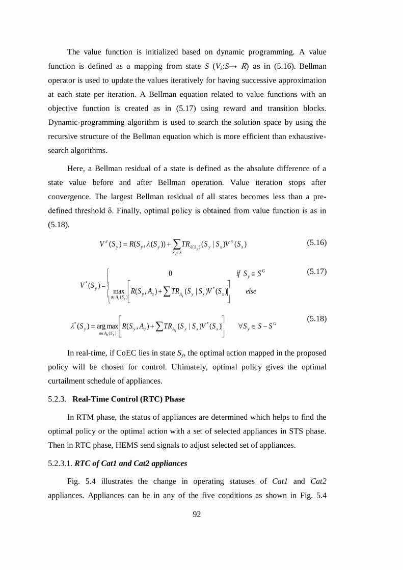
92

The value function is initialized based on dynamic programming. A value

function is defined as a mapping from state S (Vλ:S→ R) as in (5.16). Bellman

operator is used to update the values iteratively for having successive approximation

at each state per iteration. A Bellman equation related to value functions with an

objective function is created as in (5.17) using reward and transition blocks.

Dynamic-programming algorithm is used to search the solution space by using the

recursive structure of the Bellman equation which is more efficient than exhaustive-

search algorithms.

Here, a Bellman residual of a state is defined as the absolute difference of a

state value before and after Bellman operation. Value iteration stops after

convergence. The largest Bellman residual of all states becomes less than a pre-

defined threshold δ. Finally, optimal policy is obtained from value function is as in

(5.18).

SS

xxySyyy

y

ySVSSTRSSRSV )()|())(,()( )(

(5.16)

elseSVSSTRASR

SSif

SVxxyAqy

SAa

G

y

y

qyq

)()|(),(max

0

)(*

)(

*

(5.17)

G

yxxyAqySAa

y SSSSVSSTRASRSq

yq

)()|(),(maxarg)( *

)(

* (5.18)

In real-time, if CoEC lies in state Sy, the optimal action mapped in the proposed

policy will be chosen for control. Ultimately, optimal policy gives the optimal

curtailment schedule of appliances.

5.2.3. Real-Time Control (RTC) Phase

In RTM phase, the status of appliances are determined which helps to find the

optimal policy or the optimal action with a set of selected appliances in STS phase.

Then in RTC phase, HEMS send signals to adjust selected set of appliances.

5.2.3.1. RTC of Cat1 and Cat2 appliances

Fig. 5.4 illustrates the change in operating statuses of Cat1 and Cat2

appliances. Appliances can be in any of the five conditions as shown in Fig. 5.4

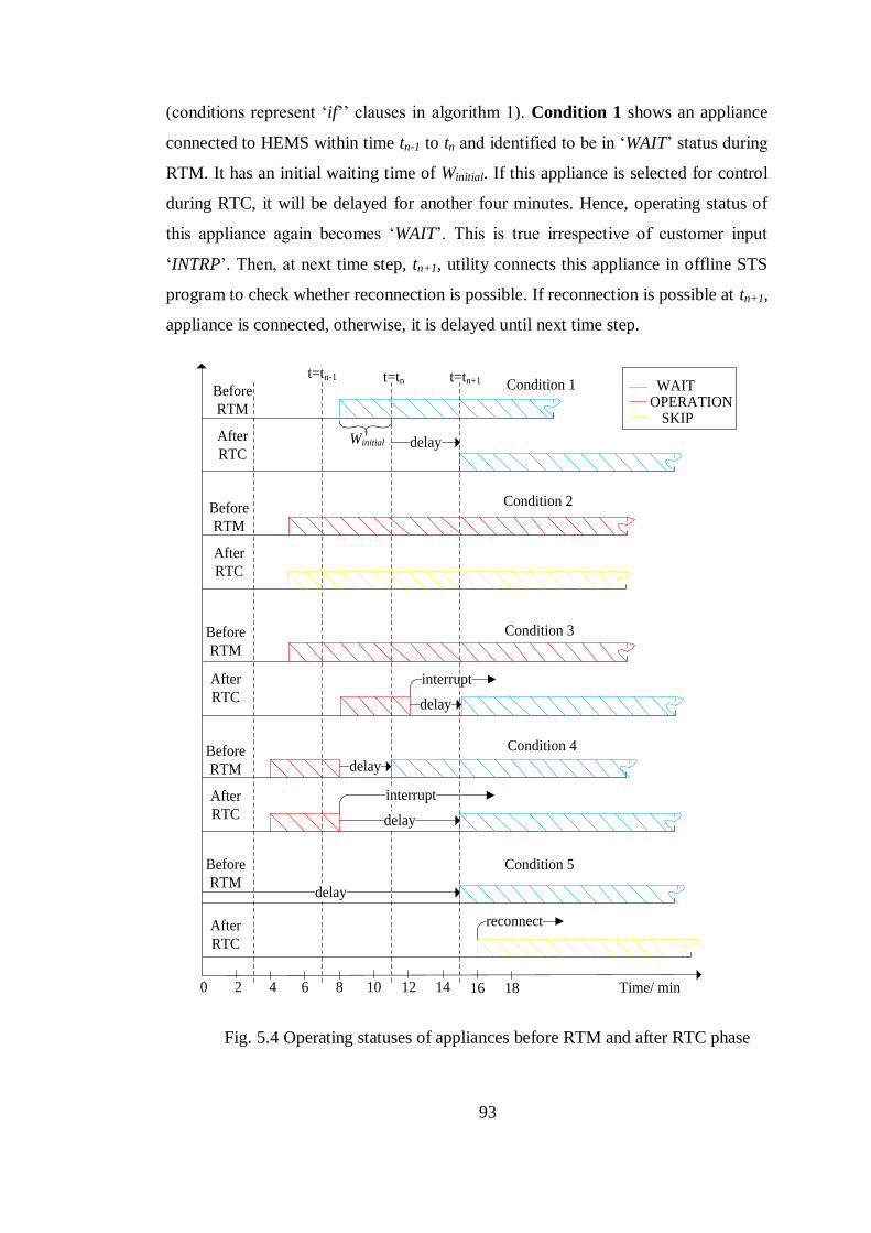
93

(conditions represent ‘if’’ clauses in algorithm 1). Condition 1 shows an appliance

connected to HEMS within time tn-1 to tn and identified to be in ‘WAIT’ status during

RTM. It has an initial waiting time of Winitial. If this appliance is selected for control

during RTC, it will be delayed for another four minutes. Hence, operating status of

this appliance again becomes ‘WAIT’. This is true irrespective of customer input

‘INTRP’. Then, at next time step, tn+1, utility connects this appliance in offline STS

program to check whether reconnection is possible. If reconnection is possible at tn+1,

appliance is connected, otherwise, it is delayed until next time step.

0 2 4 6 8 10 12 14

Condition 3

Condition 1

16 18

t=tn-1

delay

interrupt

Time/ min

t=tn

Winitial

Condition 2

delay

Condition 4

interrupt

delay

delay

Condition 5

reconnect

delay

t=tn+1 WAITOPERATION

SKIP

Before

RTM

After

RTC

Before

RTM

After

RTC

Before

RTM

After

RTC

Before

RTM

After

RTC

Before

RTM

After

RTC

Fig. 5.4 Operating statuses of appliances before RTM and after RTC phase

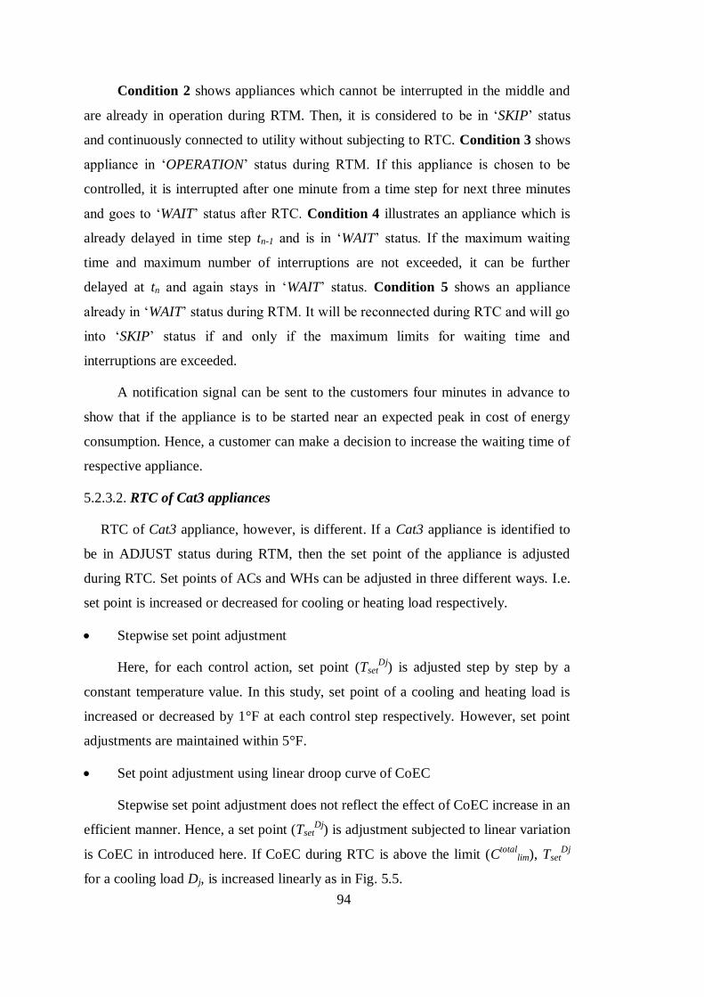
94

Condition 2 shows appliances which cannot be interrupted in the middle and

are already in operation during RTM. Then, it is considered to be in ‘SKIP’ status

and continuously connected to utility without subjecting to RTC. Condition 3 shows

appliance in ‘OPERATION’ status during RTM. If this appliance is chosen to be

controlled, it is interrupted after one minute from a time step for next three minutes

and goes to ‘WAIT’ status after RTC. Condition 4 illustrates an appliance which is

already delayed in time step tn-1 and is in ‘WAIT’ status. If the maximum waiting

time and maximum number of interruptions are not exceeded, it can be further

delayed at tn and again stays in ‘WAIT’ status. Condition 5 shows an appliance

already in ‘WAIT’ status during RTM. It will be reconnected during RTC and will go

into ‘SKIP’ status if and only if the maximum limits for waiting time and

interruptions are exceeded.

A notification signal can be sent to the customers four minutes in advance to

show that if the appliance is to be started near an expected peak in cost of energy

consumption. Hence, a customer can make a decision to increase the waiting time of

respective appliance.

5.2.3.2. RTC of Cat3 appliances

RTC of Cat3 appliance, however, is different. If a Cat3 appliance is identified to

be in ADJUST status during RTM, then the set point of the appliance is adjusted

during RTC. Set points of ACs and WHs can be adjusted in three different ways. I.e.

set point is increased or decreased for cooling or heating load respectively.

Stepwise set point adjustment

Here, for each control action, set point (TsetDj

) is adjusted step by step by a

constant temperature value. In this study, set point of a cooling and heating load is

increased or decreased by 1°F at each control step respectively. However, set point

adjustments are maintained within 5°F.

Set point adjustment using linear droop curve of CoEC

Stepwise set point adjustment does not reflect the effect of CoEC increase in an

efficient manner. Hence, a set point (TsetDj

) is adjustment subjected to linear variation

is CoEC in introduced here. If CoEC during RTC is above the limit (Ctotal

lim), TsetDj

for a cooling load Dj, is increased linearly as in Fig. 5.5.

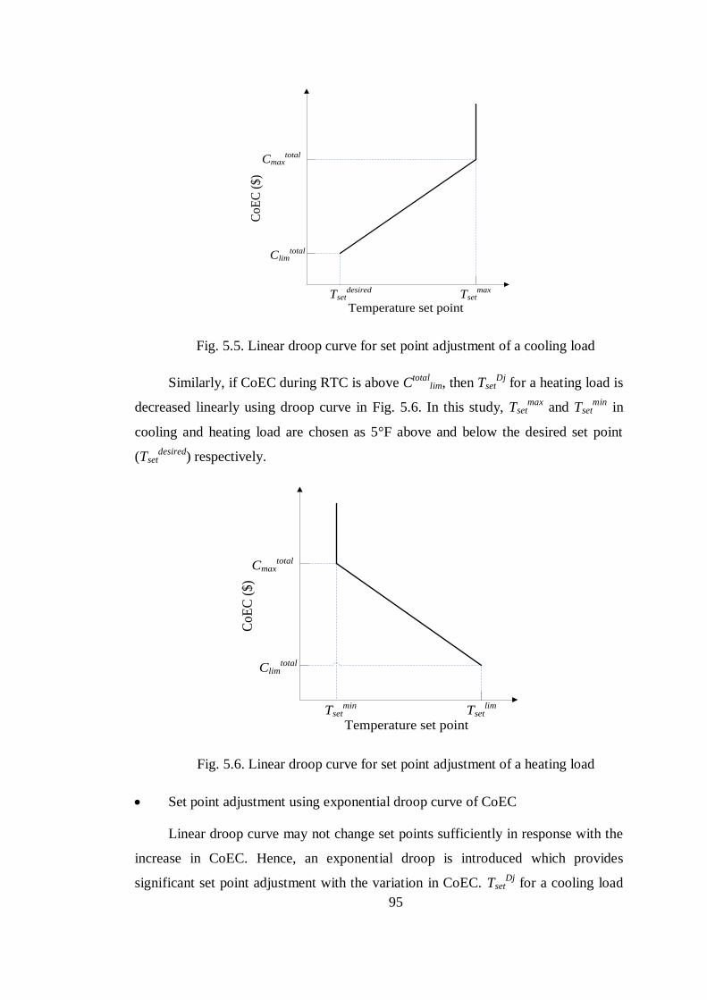
95

Temperature set point

Co

EC

($

)

Tsetdesired Tset

max

Climtotal

Cmaxtotal

Fig. 5.5. Linear droop curve for set point adjustment of a cooling load

Similarly, if CoEC during RTC is above Ctotal

lim, then TsetDj

for a heating load is

decreased linearly using droop curve in Fig. 5.6. In this study, Tsetmax

and Tsetmin

in

cooling and heating load are chosen as 5°F above and below the desired set point

(Tsetdesired

) respectively.


Co

EC

($

)

Tsetmin Tset

lim

Climtotal

Cmaxtotal

Fig. 5.6. Linear droop curve for set point adjustment of a heating load

Set point adjustment using exponential droop curve of CoEC

Linear droop curve may not change set points sufficiently in response with the

increase in CoEC. Hence, an exponential droop is introduced which provides

significant set point adjustment with the variation in CoEC. TsetDj

for a cooling load

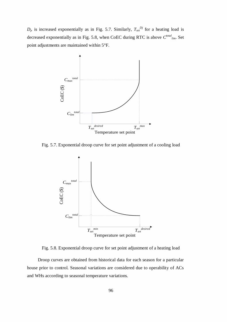
96

Dj, is increased exponentially as in Fig. 5.7. Similarly, TsetDj

for a heating load is

decreased exponentially as in Fig. 5.8, when CoEC during RTC is above Ctotal

lim. Set

point adjustments are maintained within 5°F.


CoE

C (

$)

Tsetdesired Tset

max

Climtotal

Cmaxtotal

Fig. 5.7. Exponential droop curve for set point adjustment of a cooling load


CoE

C (

$)

Tsetmin Tset

desired

Climtotal

Cmaxtotal

Fig. 5.8. Exponential droop curve for set point adjustment of a heating load

Droop curves are obtained from historical data for each season for a particular

house prior to control. Seasonal variations are considered due to operability of ACs

and WHs according to seasonal temperature variations.

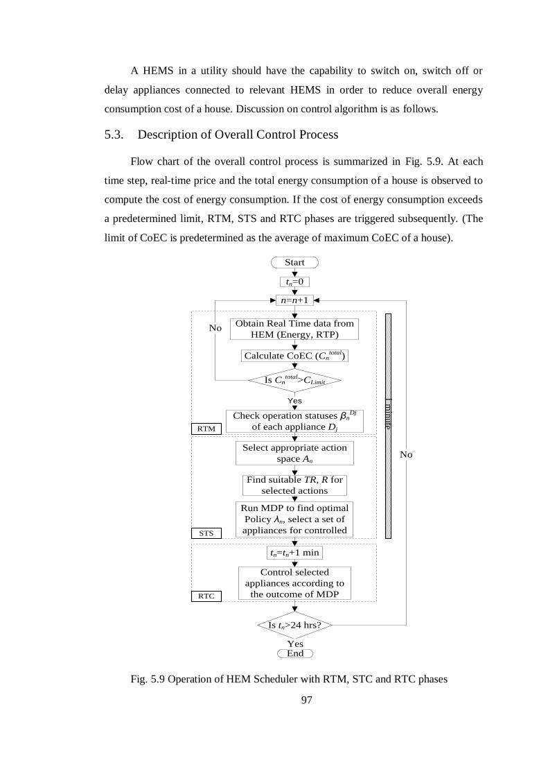
97

A HEMS in a utility should have the capability to switch on, switch off or

delay appliances connected to relevant HEMS in order to reduce overall energy

consumption cost of a house. Discussion on control algorithm is as follows.

5.3. Description of Overall Control Process

Flow chart of the overall control process is summarized in Fig. 5.9. At each

time step, real-time price and the total energy consumption of a house is observed to

compute the cost of energy consumption. If the cost of energy consumption exceeds

a predetermined limit, RTM, STS and RTC phases are triggered subsequently. (The

limit of CoEC is predetermined as the average of maximum CoEC of a house).

Start

tn=0

Obtain Real Time data from

HEM (Energy, RTP)

Is Cntotal>CLimit

Calculate CoEC (Cntotal)

Check operation statuses βnDj

of each appliance Dj

Select appropriate action

space An

Find suitable TR, R for

selected actions

Run MDP to find optimal

Policy λn, select a set of

appliances for controlled

Control selected

appliances according to

the outcome of MDP

tn=tn+1 min

n=n+1

Is tn>24 hrs?

End

No

No

Yes

Yes

1 minute

RTM

STS

RTC

Fig. 5.9 Operation of HEM Scheduler with RTM, STC and RTC phases

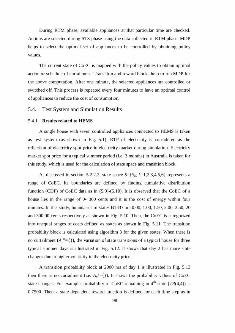
98

During RTM phase, available appliances at that particular time are checked.

Actions are selected during STS phase using the data collected in RTM phase. MDP

helps to select the optimal set of appliances to be controlled by obtaining policy

values.

The current state of CoEC is mapped with the policy values to obtain optimal

action or schedule of curtailment. Transition and reward blocks help to run MDP for

the above computation. After one minute, the selected appliances are controlled or

switched off. This process is repeated every four minutes to have an optimal control

of appliances to reduce the cost of consumption.

5.4. Test System and Simulation Results

5.4.1. Results related to HEMS

A single house with seven controlled appliances connected to HEMS is taken

as test system (as shown in Fig. 5.1). RTP of electricity is considered as the

reflection of electricity spot price in electricity market during simulation. Electricity

market spot price for a typical summer period (i.e. 3 months) in Australia is taken for

this study, which is used for the calculation of state space and transition block.

As discussed in section 5.2.2.2, state space S={Sk, k=1,2,3,4,5,6} represents a

range of CoEC. Its boundaries are defined by finding cumulative distribution

function (CDF) of CoEC data as in (5.9)-(5.10). It is observed that the CoEC of a

house lies in the range of 0- 300 cents and it is the cost of energy within four

minutes. In this study, boundaries of states B1-B7 are 0.00, 1.00, 1.50, 2.00, 3.50, 20

and 300.00 cents respectively as shown in Fig. 5.10. Then, the CoEC is categorized

into unequal ranges of costs defined as states as shown in Fig. 5.11. The transition

probability block is calculated using algorithm 3 for the given states. When there is

no curtailment (Anq={}), the variation of state transitions of a typical house for three

typical summer days is illustrated in Fig. 5.12. It shows that day 2 has more state

changes due to higher volatility in the electricity price.

A transition probability block at 2000 hrs of day 1 is illustrated in Fig. 5.13

then there is no curtailment (i.e. Anq={}). It shows the probability values of CoEC

state changes. For example, probability of CoEC remaining in 4th

state (TR(4,4)) is

0.7500. Then, a state dependent reward function is defined for each time step as in

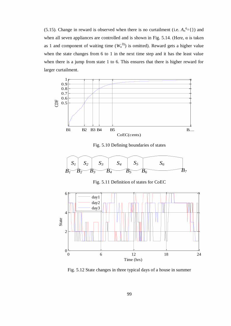
99

(5.15). Change in reward is observed when there is no curtailment (i.e. Anq={}) and

when all seven appliances are controlled and is shown in Fig. 5.14. (Here, α is taken

as 1 and component of waiting time (WnDj

) is omitted). Reward gets a higher value

when the state changes from 6 to 1 in the next time step and it has the least value

when there is a jump from state 1 to 6. This ensures that there is higher reward for

larger curtailment.

Fig. 5.10 Defining boundaries of states

S1 S2 S3 S4 S5 S6

B1 B2 B3 B4 B5 B6 B7

Fig. 5.11 Definition of states for CoEC

Fig. 5.12 State changes in three typical days of a house in summer

B1 B2 B3 B4 B5 B....

0.5

0.6

0.7

0.8

0.9

1

CoEC(cents)

CD

F

CDF

0 6 12 18 240

2

4

6

State Change

Time (hrs)

Sta

te

day1

day2

day3

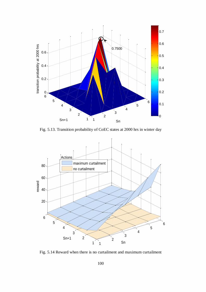
100

Fig. 5.13. Transition probability of CoEC states at 2000 hrs in winter day

Fig. 5.14 Reward when there is no curtailment and maximum curtailment

12

34

56

1

2

3

4

5

60

0.2

0.4

0.6

Sn

total transition probability

Sn+1

transitio

n p

robabili

ty a

t 2000 h

rs

0

0.1

0.2

0.3

0.4

0.5

0.6

0.7

0.7500

12

34

56

1

2

3

4

5

6

20

40

60

80

SnSn+1

rew

ard

maximum curtailment

no curtailment

Actions

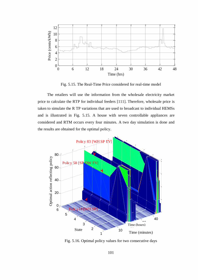
101

Fig. 5.15. The Real-Time Price considered for real-time model

The retailers will use the information from the wholesale electricity market

price to calculate the RTP for individual feeders [111]. Therefore, wholesale price is

taken to simulate the R TP variations that are used to broadcast to individual HEMSs

and is illustrated in Fig. 5.15. A house with seven controllable appliances are

considered and RTM occurs every four minutes. A two day simulation is done and

the results are obtained for the optimal policy.

Fig. 5.16. Optimal policy values for two consecutive days

0 6 12 18 24 30 36 42 480

2

4

6

8

10

12

Time (hrs)

Pri

ce (

cen

ts/k

Wh

)

1020

3040

1

2

3

4

5

60

20

40

60

80

Time (minutes)

OPTIMAL ACTION FOR ALL STATES

State

Op

tim

al a

ctio

n r

efle

ctin

g p

oli

cy

0

20

40

60

80

100

120

Policy14 [WH SP]

Policy 58 [SP DW EV]

Policy 83 [WH SP EV]

Time (hours)

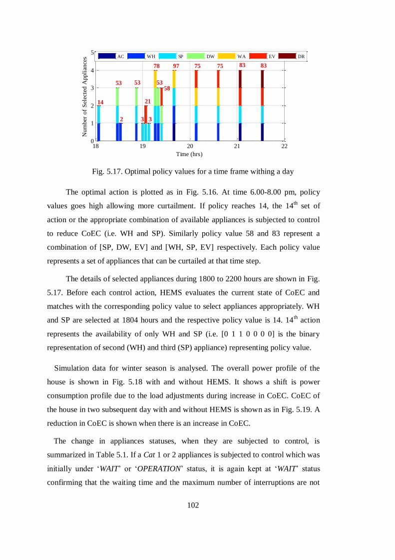
102

Fig. 5.17. Optimal policy values for a time frame withing a day

The optimal action is plotted as in Fig. 5.16. At time 6.00-8.00 pm, policy

values goes high allowing more curtailment. If policy reaches 14, the 14th set of

action or the appropriate combination of available appliances is subjected to control

to reduce CoEC (i.e. WH and SP). Similarly policy value 58 and 83 represent a

combination of [SP, DW, EV] and [WH, SP, EV] respectively. Each policy value

represents a set of appliances that can be curtailed at that time step.

The details of selected appliances during 1800 to 2200 hours are shown in Fig.

5.17. Before each control action, HEMS evaluates the current state of CoEC and

matches with the corresponding policy value to select appliances appropriately. WH

and SP are selected at 1804 hours and the respective policy value is 14. 14th action

represents the availability of only WH and SP (i.e. [0 1 1 0 0 0 0] is the binary

representation of second (WH) and third (SP) appliance) representing policy value.

Simulation data for winter season is analysed. The overall power profile of the

house is shown in Fig. 5.18 with and without HEMS. It shows a shift is power

consumption profile due to the load adjustments during increase in CoEC. CoEC of

the house in two subsequent day with and without HEMS is shown as in Fig. 5.19. A

reduction in CoEC is shown when there is an increase in CoEC.

The change in appliances statuses, when they are subjected to control, is

summarized in Table 5.1. If a Cat 1 or 2 appliances is subjected to control which was

initially under ‘WAIT’ or ‘OPERATION’ status, it is again kept at ‘WAIT’ status

confirming that the waiting time and the maximum number of interruptions are not

18 19 20 21 220

1

2

3

4

5

Time (hrs)

Nu

mb

er o

f S

elec

ted

Ap

pli

ance

s

AC WH SP DW WA EV DR

83757597

14

2

53 53

21

3

5358

83

3

78

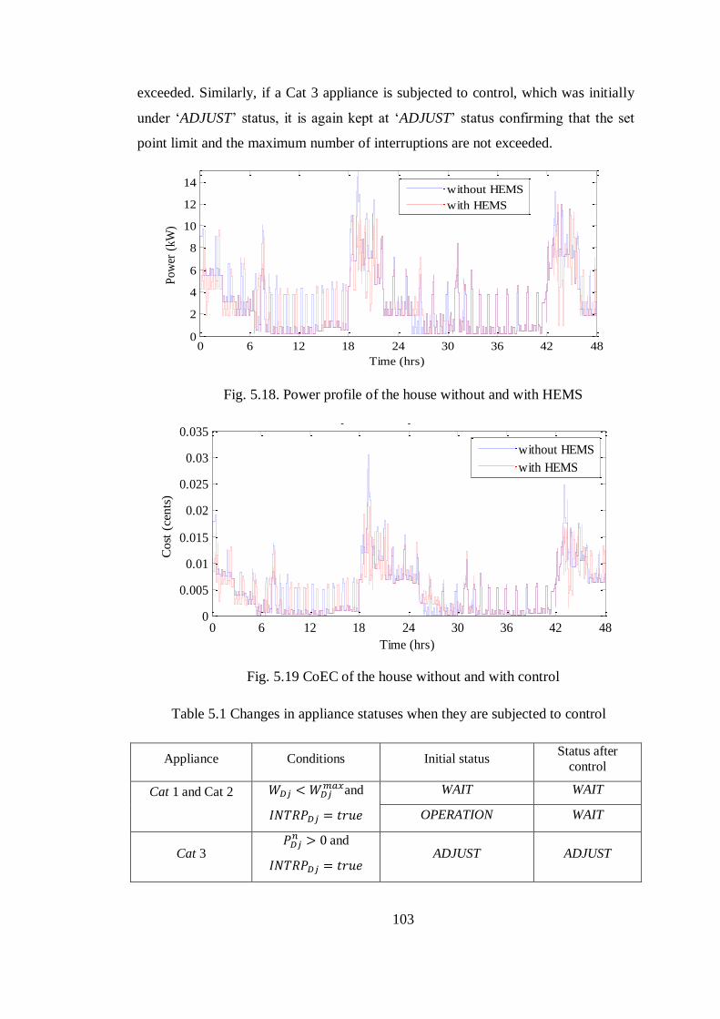
103

exceeded. Similarly, if a Cat 3 appliance is subjected to control, which was initially

under ‘ADJUST’ status, it is again kept at ‘ADJUST’ status confirming that the set

point limit and the maximum number of interruptions are not exceeded.

Fig. 5.18. Power profile of the house without and with HEMS

Fig. 5.19 CoEC of the house without and with control

Table 5.1 Changes in appliance statuses when they are subjected to control

Appliance Conditions Initial status Status after

control

Cat 1 and Cat 2

and

WAIT WAIT

OPERATION WAIT

Cat 3 and

ADJUST ADJUST

0 6 12 18 24 30 36 42 480

2

4

6

8

10

12

14

House power consumption with and without control

Time (hrs)

Po

wer

(k

W)

without HEMS

with HEMS

0 6 12 18 24 30 36 42 480

0.005

0.01

0.015

0.02

0.025

0.03

0.035cost of power consumption without control

Time (hrs)

Co

st (

cen

ts)

without HEMS

with HEMS

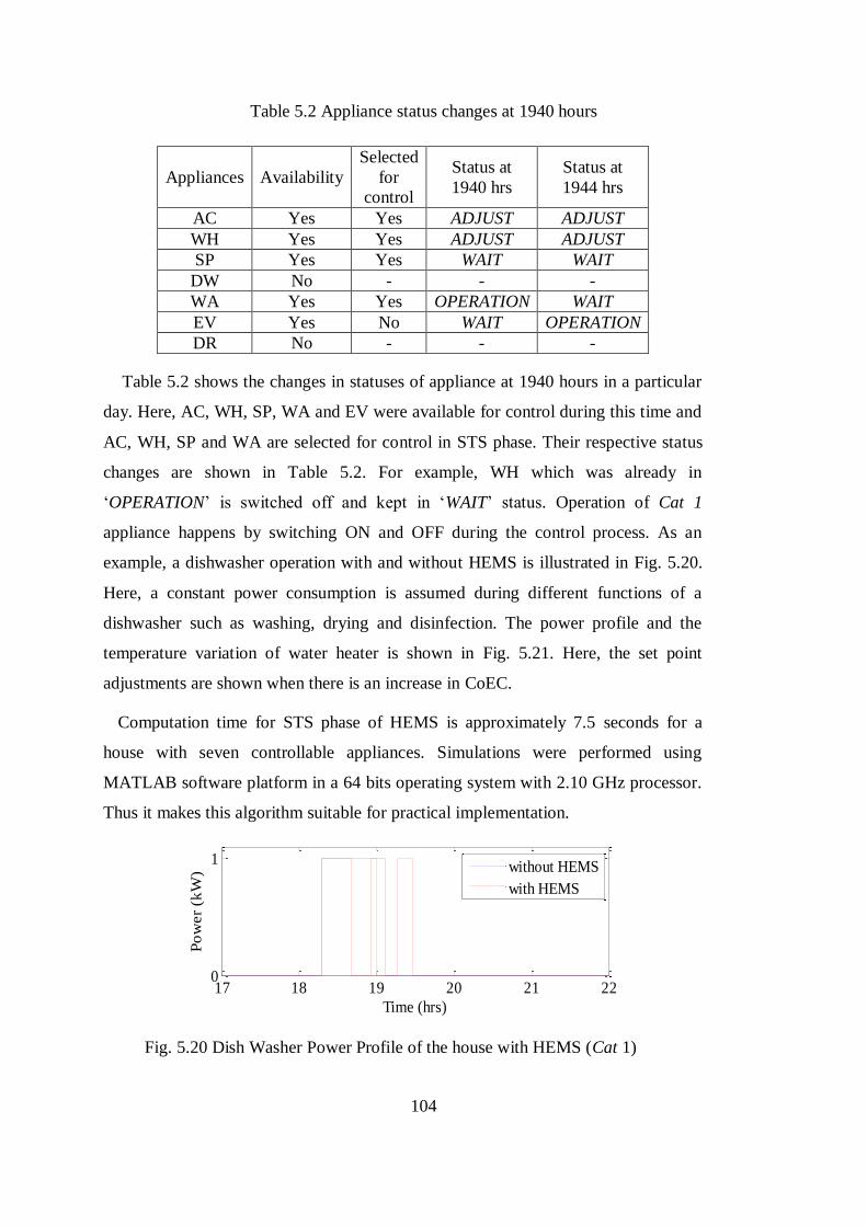
104

Table 5.2 Appliance status changes at 1940 hours

Appliances Availability

Selected

for

control

Status at

1940 hrs

Status at

1944 hrs

AC Yes Yes ADJUST ADJUST

WH Yes Yes ADJUST ADJUST

SP Yes Yes WAIT WAIT

DW No - - -

WA Yes Yes OPERATION WAIT

EV Yes No WAIT OPERATION

DR No - - -

Table 5.2 shows the changes in statuses of appliance at 1940 hours in a particular

day. Here, AC, WH, SP, WA and EV were available for control during this time and

AC, WH, SP and WA are selected for control in STS phase. Their respective status

changes are shown in Table 5.2. For example, WH which was already in

‘OPERATION’ is switched off and kept in ‘WAIT’ status. Operation of Cat 1

appliance happens by switching ON and OFF during the control process. As an

example, a dishwasher operation with and without HEMS is illustrated in Fig. 5.20.

Here, a constant power consumption is assumed during different functions of a

dishwasher such as washing, drying and disinfection. The power profile and the

temperature variation of water heater is shown in Fig. 5.21. Here, the set point

adjustments are shown when there is an increase in CoEC.

Computation time for STS phase of HEMS is approximately 7.5 seconds for a

house with seven controllable appliances. Simulations were performed using

MATLAB software platform in a 64 bits operating system with 2.10 GHz processor.

Thus it makes this algorithm suitable for practical implementation.

Fig. 5.20 Dish Washer Power Profile of the house with HEMS (Cat 1)

17 18 19 20 21 220

1

DW power

Time (hrs)

Po

wer

(kW

)

without HEMS

with HEMS

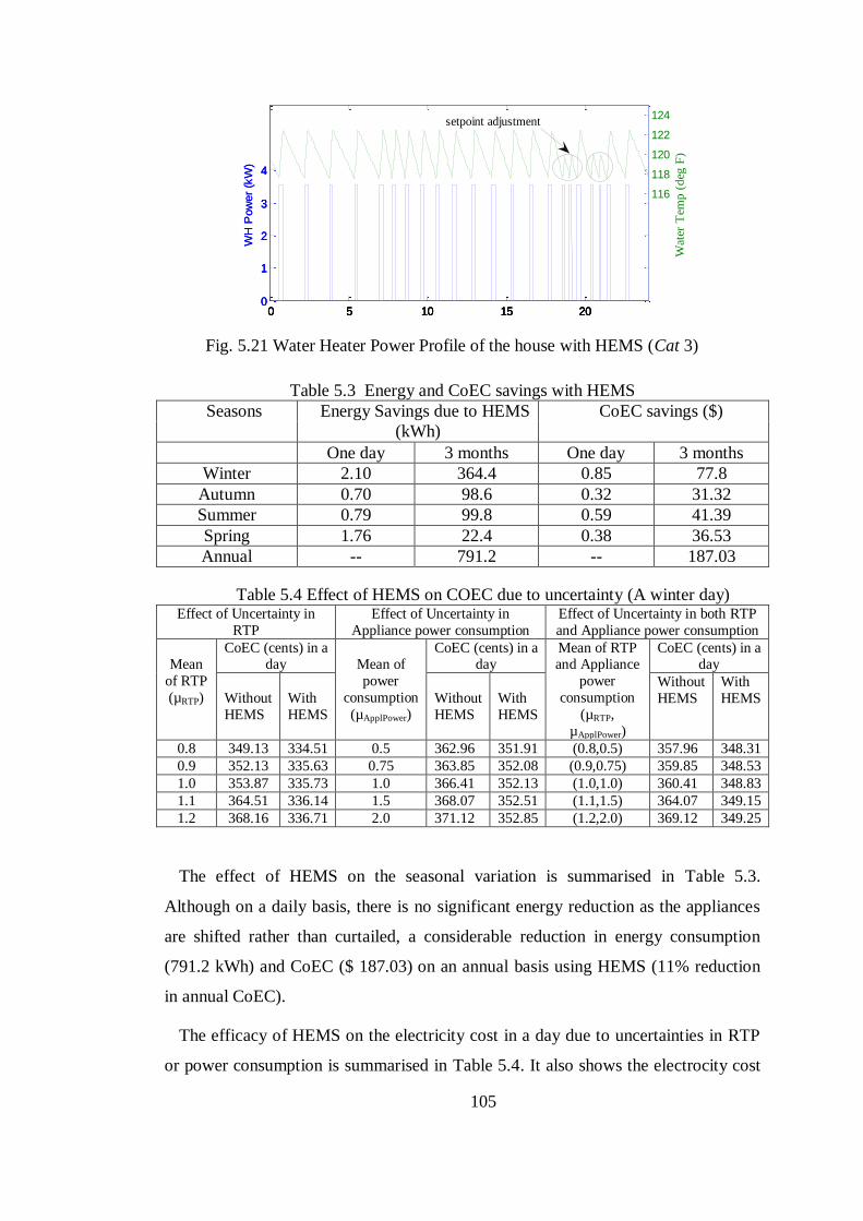
105

Fig. 5.21 Water Heater Power Profile of the house with HEMS (Cat 3)

Table 5.3 Energy and CoEC savings with HEMS

Seasons Energy Savings due to HEMS

(kWh)

CoEC savings ($)

One day 3 months One day 3 months

Winter 2.10 364.4 0.85 77.8

Autumn 0.70 98.6 0.32 31.32

Summer 0.79 99.8 0.59 41.39

Spring 1.76 22.4 0.38 36.53

Annual -- 791.2 -- 187.03

Table 5.4 Effect of HEMS on COEC due to uncertainty (A winter day) Effect of Uncertainty in

RTP

Effect of Uncertainty in

Appliance power consumption

Effect of Uncertainty in both RTP

and Appliance power consumption

Mean

of RTP

(µRTP)

CoEC (cents) in a day Mean of

power

consumption

(µApplPower)

CoEC (cents) in a day

Mean of RTP and Appliance

power

consumption

(µRTP,

µApplPower)

CoEC (cents) in a day

Without

HEMS

With

HEMS

Without

HEMS

With

HEMS

Without

HEMS

With

HEMS

0.8 349.13 334.51 0.5 362.96 351.91 (0.8,0.5) 357.96 348.31

0.9 352.13 335.63 0.75 363.85 352.08 (0.9,0.75) 359.85 348.53

1.0 353.87 335.73 1.0 366.41 352.13 (1.0,1.0) 360.41 348.83

1.1 364.51 336.14 1.5 368.07 352.51 (1.1,1.5) 364.07 349.15

1.2 368.16 336.71 2.0 371.12 352.85 (1.2,2.0) 369.12 349.25

The effect of HEMS on the seasonal variation is summarised in Table 5.3.

Although on a daily basis, there is no significant energy reduction as the appliances

are shifted rather than curtailed, a considerable reduction in energy consumption

(791.2 kWh) and CoEC ($ 187.03) on an annual basis using HEMS (11% reduction

in annual CoEC).

The efficacy of HEMS on the electricity cost in a day due to uncertainties in RTP

or power consumption is summarised in Table 5.4. It also shows the electrocity cost

0 5 10 15 200

1

2

3

4

WH

Pow

er

(kW

)

0 5 10 15 200

1

2

3

4

WH

Pow

er

(kW

)

0 5 10 15 200

1

2

3

4

0 5 10 15 20

116

118

120

122

124

Wat

er T

emp (

deg

F)

setpoint adjustment

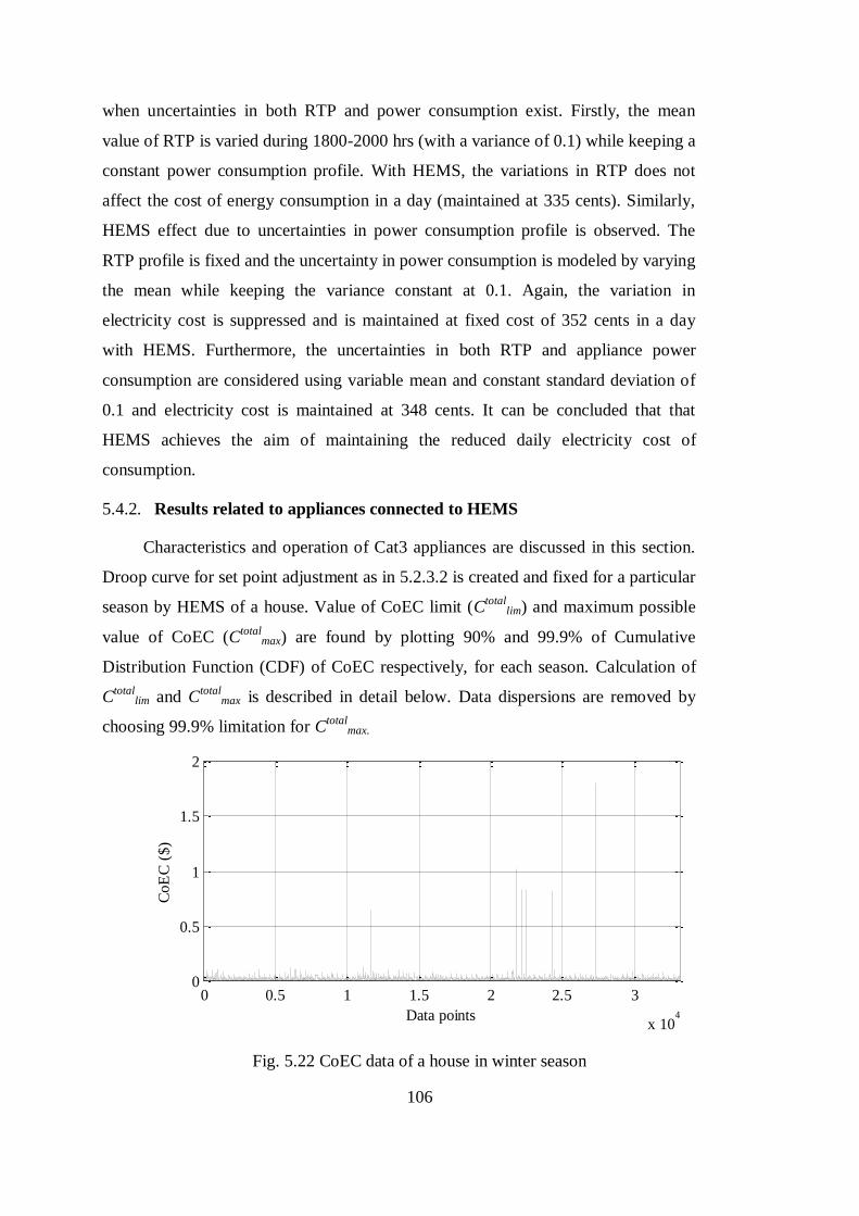
106

when uncertainties in both RTP and power consumption exist. Firstly, the mean

value of RTP is varied during 1800-2000 hrs (with a variance of 0.1) while keeping a

constant power consumption profile. With HEMS, the variations in RTP does not

affect the cost of energy consumption in a day (maintained at 335 cents). Similarly,

HEMS effect due to uncertainties in power consumption profile is observed. The

RTP profile is fixed and the uncertainty in power consumption is modeled by varying

the mean while keeping the variance constant at 0.1. Again, the variation in

electricity cost is suppressed and is maintained at fixed cost of 352 cents in a day

with HEMS. Furthermore, the uncertainties in both RTP and appliance power

consumption are considered using variable mean and constant standard deviation of

0.1 and electricity cost is maintained at 348 cents. It can be concluded that that

HEMS achieves the aim of maintaining the reduced daily electricity cost of

consumption.

5.4.2. Results related to appliances connected to HEMS

Characteristics and operation of Cat3 appliances are discussed in this section.

Droop curve for set point adjustment as in 5.2.3.2 is created and fixed for a particular

season by HEMS of a house. Value of CoEC limit (Ctotal

lim) and maximum possible

value of CoEC (Ctotal

max) are found by plotting 90% and 99.9% of Cumulative

Distribution Function (CDF) of CoEC respectively, for each season. Calculation of

Ctotal

lim and Ctotal

max is described in detail below. Data dispersions are removed by

choosing 99.9% limitation for Ctotal

max.

Fig. 5.22 CoEC data of a house in winter season

0 0.5 1 1.5 2 2.5 3

x 104

0

0.5

1

1.5

2data dispersion in winter

Data points

Co

EC

($

)

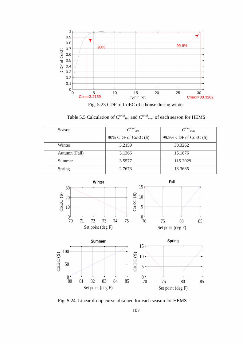
107

Fig. 5.23 CDF of CoEC of a house during winter

Table 5.5 Calculation of Ctotal

lim and Ctotal

max of each season for HEMS

Season Ctotal

lim

90% CDF of CoEC ($)

Ctotal

max

99.9% CDF of CoEC ($)

Winter 3.2159 30.3262

Autumn (Fall) 3.1266 15.1876

Summer 3.5577 115.2029

Spring 2.7673 13.3685

Fig. 5.24. Linear droop curve obtained for each season for HEMS

0 5 10 15 20 25 300

0.1

0.2

0.3

0.4

0.5

0.6

0.7

0.8

0.9

1CDF of CoEC

CoEC ($)

CD

F o

f C

oE

C

99.9%90%

Cmax=30.3262Clim=3.2159

70 71 72 73 74 750

10

20

30

Winter

Set point (deg F)

CoE

C (

$)

70 75 80 850

5

10

15Fall

Set point (deg F)

CoE

C (

$)

80 81 82 83 84 850

50

100

Summer

Set point (deg F)

CoE

C (

$)

70 75 80 850

5

10

15Spring

Set point (deg F)

CoE

C (

$)

70 71 72 73 74 750

10

20

30

Winter

Set point (deg F)

CoE

C (

$)

70 75 80 850

5

10

15Fall

Set point (deg F)

CoE

C (

$)

80 81 82 83 84 850

50

100

Summer

Set point (deg F)

CoE

C (

$)

70 75 80 850

5

10

15Spring

Set point (deg F)

CoE

C (

$)

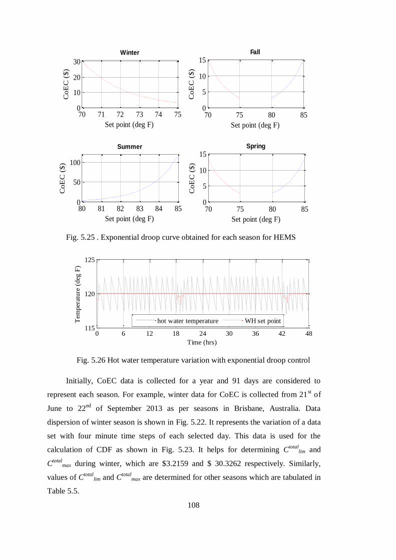
108

Fig. 5.25 . Exponential droop curve obtained for each season for HEMS

Fig. 5.26 Hot water temperature variation with exponential droop control

Initially, CoEC data is collected for a year and 91 days are considered to

represent each season. For example, winter data for CoEC is collected from 21st of

June to 22nd

of September 2013 as per seasons in Brisbane, Australia. Data

dispersion of winter season is shown in Fig. 5.22. It represents the variation of a data

set with four minute time steps of each selected day. This data is used for the

calculation of CDF as shown in Fig. 5.23. It helps for determining Ctotal

lim and

Ctotal

max during winter, which are $3.2159 and $ 30.3262 respectively. Similarly,

values of Ctotal

lim and Ctotal

max are determined for other seasons which are tabulated in

Table 5.5.

70 71 72 73 74 750

10

20

30

Winter

Set point (deg F)

Co

EC

($

)

70 75 80 850

5

10

15Fall

Set point (deg F)

Co

EC

($

)

80 81 82 83 84 850

50

100

Summer

Set point (deg F)

Co

EC

($

)

70 75 80 850

5

10

15Spring

Set point (deg F)

Co

EC

($

)

70 71 72 73 74 750

10

20

30

Winter

Set point (deg F)

Co

EC

($

)

70 75 80 850

5

10

15Fall

Set point (deg F)

Co

EC

($

)

80 81 82 83 84 850

50

100

Summer

Set point (deg F)

Co

EC

($

)

70 75 80 850

5

10

15Spring

Set point (deg F)

Co

EC

($

)

0 6 12 18 24 30 36 42 48115

120

125

Time (hrs)

Tem

per

ature

(deg

F)

0 6 12 18 24 30 36 42 4873

74

75

76

77

Time (hrs)

Tem

per

ature

(deg

F)

Room temperature AC set point

hot water temperature WH set point

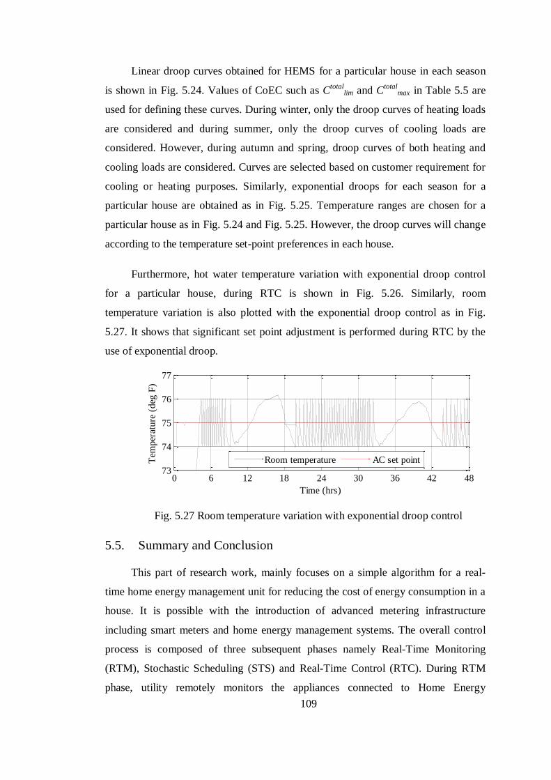
109

Linear droop curves obtained for HEMS for a particular house in each season

is shown in Fig. 5.24. Values of CoEC such as Ctotal

lim and Ctotal

max in Table 5.5 are

used for defining these curves. During winter, only the droop curves of heating loads

are considered and during summer, only the droop curves of cooling loads are

considered. However, during autumn and spring, droop curves of both heating and

cooling loads are considered. Curves are selected based on customer requirement for

cooling or heating purposes. Similarly, exponential droops for each season for a

particular house are obtained as in Fig. 5.25. Temperature ranges are chosen for a

particular house as in Fig. 5.24 and Fig. 5.25. However, the droop curves will change

according to the temperature set-point preferences in each house.

Furthermore, hot water temperature variation with exponential droop control

for a particular house, during RTC is shown in Fig. 5.26. Similarly, room

temperature variation is also plotted with the exponential droop control as in Fig.

5.27. It shows that significant set point adjustment is performed during RTC by the

use of exponential droop.

Fig. 5.27 Room temperature variation with exponential droop control


This part of research work, mainly focuses on a simple algorithm for a real-

time home energy management unit for reducing the cost of energy consumption in a

house. It is possible with the introduction of advanced metering infrastructure

including smart meters and home energy management systems. The overall control

process is composed of three subsequent phases namely Real-Time Monitoring

(RTM), Stochastic Scheduling (STS) and Real-Time Control (RTC). During RTM

phase, utility remotely monitors the appliances connected to Home Energy

0 6 12 18 24 30 36 42 48115

120

125

Time (hrs)

Tem

per

ature

(deg

F)

0 6 12 18 24 30 36 42 4873

74

75

76

77

Time (hrs)

Tem

per

ature

(deg

F)

Room temperature AC set point

hot water temperature WH set point

110

Management Unit (HEMS) of a house at every time step. It also obtains price

information from electricity market. When there is an increase in cost of energy

consumption, utility defines the operating status of each controllable appliances

according to its operating characteristics and customer input. Although RTM provides

information of current status of appliances, it may not be sufficient for making

appropriate control decisions. It is due to the uncertainties in electricity price

variation, appliance operation, user behavior and preferences. Hence, a STS process

is performed next utilizing the information of operating status of appliances. Markov

Decision Process is used to minimize cost of energy consumption by predicting the

appropriate curtailment of appliances based on the stochastic behavior of cost of

consumption. Customer priorities are also intrinsically considered during the control

process by adding constraints. Furthermore, interrupting an appliance while it is in

operation reduces its life span and customer comfort. Constraints for appliance

interruption are also included in STS phase. Subsequently, selected appliances are

controlled at the third phase of RTC. Outcomes show that a significant reduction in

cost of energy consumption is achieved also maintaining customer comfort.

111

Chapter 6

Stochastic Ranking Method for Thermostatically

Controllable Appliances to Provide Regulation

Services

Demand Response (DR) is preliminarily used for peak load shaving and

alleviating voltage issues in an electricity feeder. However, DR can also be used for

providing regulation services in the electricity markets. The retailers can bid in day-

ahead market and respond to real-time regulation signal by load control. This part of

research work, proposes a new stochastic ranking method to provide regulation

services via demand response. A pool of Thermostatically Controllable Appliances

(TCAs) such as air-conditioners and water-heaters are adjusted using the direct load

control method. The selection of appliances is based on a probabilistic ranking

technique utilizing attributes such as temperature variation and statuses of TCAs.

These attributes are stochastically forecasted for the next time step using day-ahead

information. System performance is analyzed with a given regulation signal.

Network capability to provide regulation services under various seasons is analyzed.

The effect of network size on the regulation services is also investigated. Customer

comfort is maintained by keeping the temperature within allowable limits.

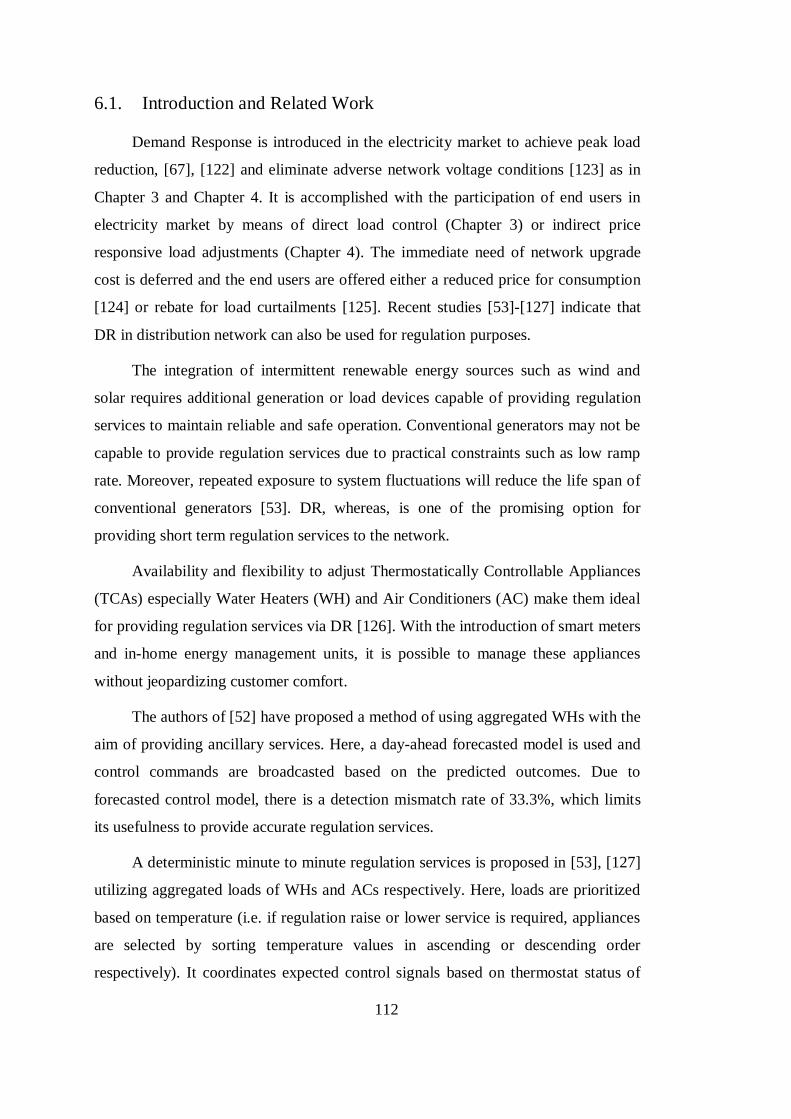
112


Demand Response is introduced in the electricity market to achieve peak load

reduction, [67], [122] and eliminate adverse network voltage conditions [123] as in

Chapter 3 and Chapter 4. It is accomplished with the participation of end users in

electricity market by means of direct load control (Chapter 3) or indirect price

responsive load adjustments (Chapter 4). The immediate need of network upgrade

cost is deferred and the end users are offered either a reduced price for consumption

[124] or rebate for load curtailments [125]. Recent studies [53]-[127] indicate that

DR in distribution network can also be used for regulation purposes.

The integration of intermittent renewable energy sources such as wind and

solar requires additional generation or load devices capable of providing regulation

services to maintain reliable and safe operation. Conventional generators may not be

capable to provide regulation services due to practical constraints such as low ramp

rate. Moreover, repeated exposure to system fluctuations will reduce the life span of

conventional generators [53]. DR, whereas, is one of the promising option for

providing short term regulation services to the network.

Availability and flexibility to adjust Thermostatically Controllable Appliances

(TCAs) especially Water Heaters (WH) and Air Conditioners (AC) make them ideal

for providing regulation services via DR [126]. With the introduction of smart meters

and in-home energy management units, it is possible to manage these appliances

without jeopardizing customer comfort.

The authors of [52] have proposed a method of using aggregated WHs with the

aim of providing ancillary services. Here, a day-ahead forecasted model is used and

control commands are broadcasted based on the predicted outcomes. Due to

forecasted control model, there is a detection mismatch rate of 33.3%, which limits

its usefulness to provide accurate regulation services.

A deterministic minute to minute regulation services is proposed in [53], [127]

utilizing aggregated loads of WHs and ACs respectively. Here, loads are prioritized

based on temperature (i.e. if regulation raise or lower service is required, appliances

are selected by sorting temperature values in ascending or descending order

respectively). It coordinates expected control signals based on thermostat status of

113

previous and next time instant. However, this technique fails to focus on prediction

of appliance status on the next time step. Prediction of appliances is extremely

important as the appliance consumption patterns and temperature variations are

highly uncertain.

Regulation technique in [53], [127] is accomplished by switching selected

appliances ON and OFF at each control step. The authors of [54] propose

temperature set point adjustments to reduce switching actions and uses day-ahead

load profile of appliances in the network, while neglecting the uncertainty in

appliance consumption. A probability function for water consumption rate is taken in

[55], but the appliance selection procedure is based on a power tracking method,

which does not consider uncertainties in appliance power consumption.

Contribution: Hence, research work in presented in this chapter proposes a

new stochastic ranking method based on pairwise probabilistic comparison of TCAs

with respect to different appliance attributes during decision making. The two

attributes i.e. temperature variation and appliance switching status, are time varying

and hence, their expected values are stochastically determined for next time step. As

these attributes closely follow Markov process, the values for next time step depends

only on the values of current time step. The probabilistic comparison of appliances

based on various attributes is used to compute appliance ranking for a given

regulation requirement. Customer comfort is maintained by keeping the temperature

within allowable limits. Similar to the proposed method in [53]- [127], this research

also considers the direct load control via instantaneous switching actions, but uses

probabilistic measure to predict the status of attributes. Hence, this scheme

incorporates uncertainty and hence provides better regulation services.

The detailed background of the regulation services as well as the proposed

stochastic ranking method is discussed in section 6.2. The mathematical models used

for simulation and results are analyzed in section 6.3 followed by conclusions in

section 6.4.

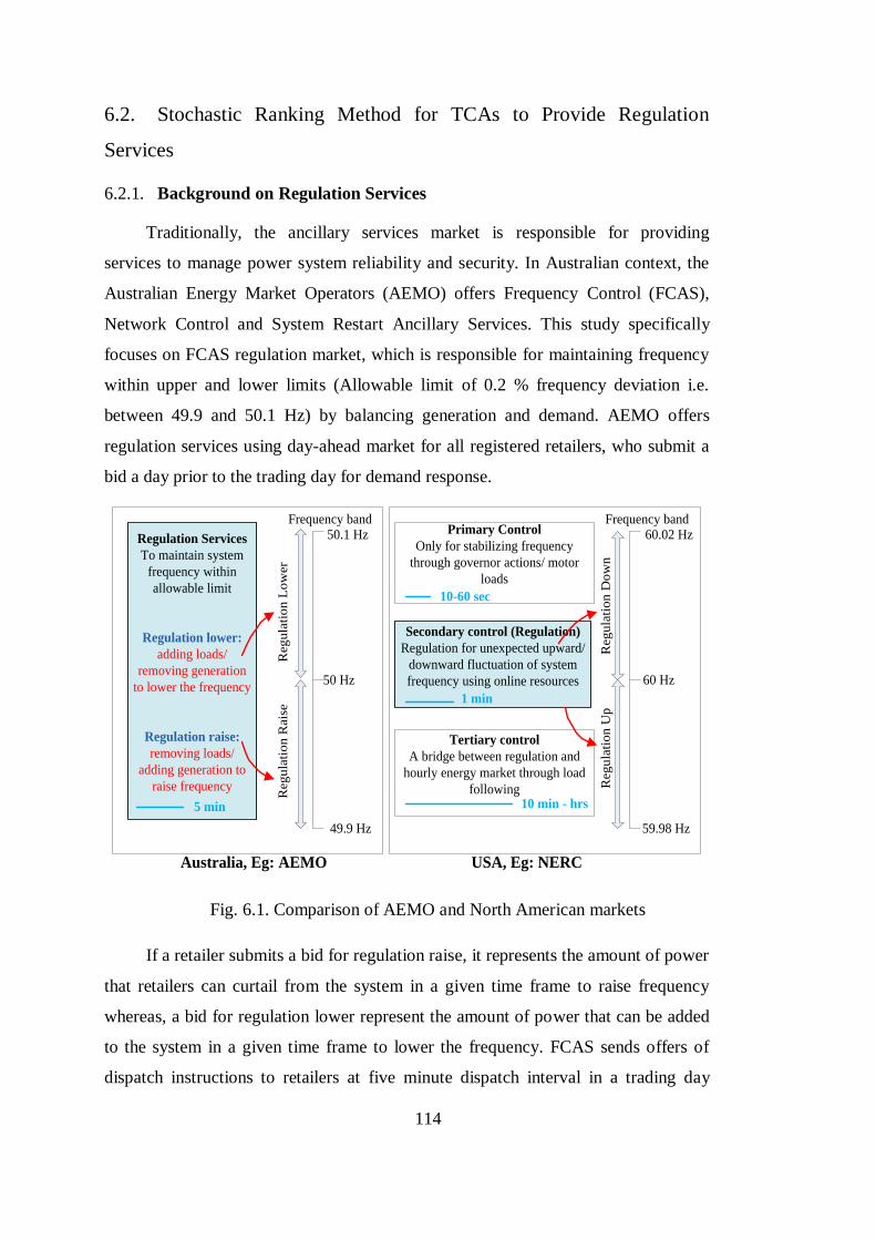
114

6.2. Stochastic Ranking Method for TCAs to Provide Regulation

Services

6.2.1. Background on Regulation Services

Traditionally, the ancillary services market is responsible for providing

services to manage power system reliability and security. In Australian context, the

Australian Energy Market Operators (AEMO) offers Frequency Control (FCAS),

Network Control and System Restart Ancillary Services. This study specifically

focuses on FCAS regulation market, which is responsible for maintaining frequency

within upper and lower limits (Allowable limit of 0.2 % frequency deviation i.e.

between 49.9 and 50.1 Hz) by balancing generation and demand. AEMO offers

regulation services using day-ahead market for all registered retailers, who submit a

bid a day prior to the trading day for demand response.

Frequency band Frequency band

50 Hz

50.1 Hz

49.9 Hz

60 Hz

60.02 Hz

59.98 Hz

Reg

ula

tio

n R

ais

e

Regulation Services

To maintain system

frequency within

allowable limit

Regulation lower:

adding loads/

removing generation

to lower the frequency

Regulation raise:

removing loads/

adding generation to

raise frequency

Primary Control

Only for stabilizing frequency

through governor actions/ motor

loads

Secondary control (Regulation)

Regulation for unexpected upward/

downward fluctuation of system

frequency using online resources

Tertiary control

A bridge between regulation and

hourly energy market through load

following

Australia, Eg: AEMO USA, Eg: NERC

5 min

1 min

10-60 sec

10 min - hrs

Reg

ula

tio

n L

ow

er

Reg

ula

tio

n D

ow

nR

eg

ula

tio

n U

p

Fig. 6.1. Comparison of AEMO and North American markets

If a retailer submits a bid for regulation raise, it represents the amount of power

that retailers can curtail from the system in a given time frame to raise frequency

whereas, a bid for regulation lower represent the amount of power that can be added

to the system in a given time frame to lower the frequency. FCAS sends offers of

dispatch instructions to retailers at five minute dispatch interval in a trading day

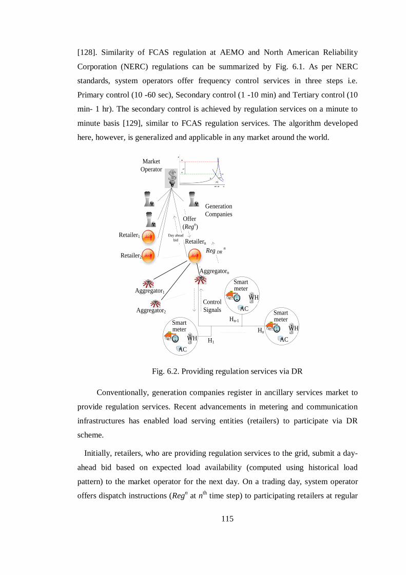
115

[128]. Similarity of FCAS regulation at AEMO and North American Reliability

Corporation (NERC) regulations can be summarized by Fig. 6.1. As per NERC

standards, system operators offer frequency control services in three steps i.e.

Primary control (10 -60 sec), Secondary control (1 -10 min) and Tertiary control (10

min- 1 hr). The secondary control is achieved by regulation services on a minute to

minute basis [129], similar to FCAS regulation services. The algorithm developed

here, however, is generalized and applicable in any market around the world.

Market

Operator

Retailern

Generation

Companies

Day ahead

bid

Offer

(Regn)

Control

Signals

Aggregator1

Aggregator2

Hn-1

H1

Hn

Smart meter

WH

AC

Smart meter

WH

AC

Smart meter

WH

AC

Aggregatorn

Retailer1

Retailer2

Reg DR n

Fig. 6.2. Providing regulation services via DR

Conventionally, generation companies register in ancillary services market to

provide regulation services. Recent advancements in metering and communication

infrastructures has enabled load serving entities (retailers) to participate via DR

scheme.

Initially, retailers, who are providing regulation services to the grid, submit a day-

ahead bid based on expected load availability (computed using historical load

pattern) to the market operator for the next day. On a trading day, system operator

offers dispatch instructions (Regn at n

th time step) to participating retailers at regular

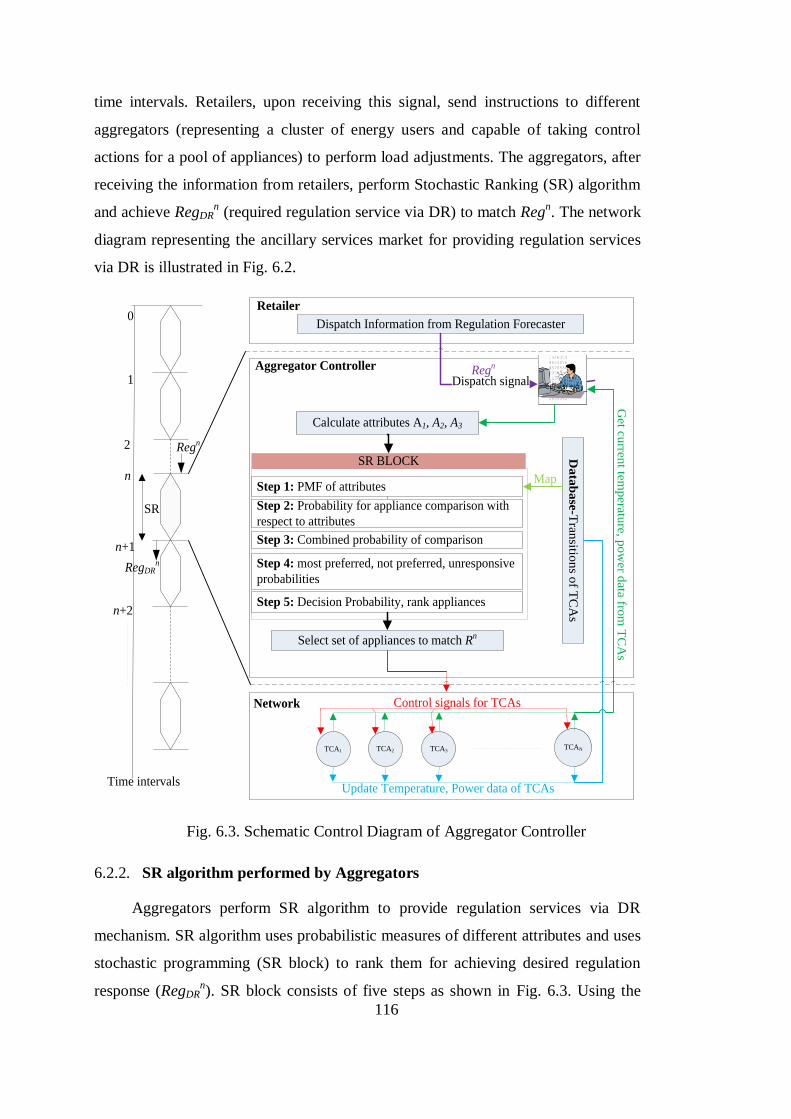
116

time intervals. Retailers, upon receiving this signal, send instructions to different

aggregators (representing a cluster of energy users and capable of taking control

actions for a pool of appliances) to perform load adjustments. The aggregators, after

receiving the information from retailers, perform Stochastic Ranking (SR) algorithm

and achieve RegDRn (required regulation service via DR) to match Reg

n. The network

diagram representing the ancillary services market for providing regulation services

via DR is illustrated in Fig. 6.2.

Retailer

Aggregator Controller

Network

Dispatch Information from Regulation Forecaster

TCANTCA3TCA2

Update Temperature, Power data of TCAs

Step 1: PMF of attributes

SR BLOCK

Da

tab

ase

-Tra

nsitio

ns o

f TC

As

Map

Step 2: Probability for appliance comparison with

respect to attributes

Step 3: Combined probability of comparison

Step 4: most preferred, not preferred, unresponsive

probabilities

Step 5: Decision Probability, rank appliances

Select set of appliances to match Rn

TCA1

Dispatch signal

Calculate attributes A1, A2, A3

Control signals for TCAs

Get c

urre

nt te

mp

era

ture

, po

wer d

ata

from

TC

As

0

1

2

Time intervals

n

n+1

n+2

Regn

RegDRn

SR

Regn

Fig. 6.3. Schematic Control Diagram of Aggregator Controller

6.2.2. SR algorithm performed by Aggregators

Aggregators perform SR algorithm to provide regulation services via DR

mechanism. SR algorithm uses probabilistic measures of different attributes and uses

stochastic programming (SR block) to rank them for achieving desired regulation

response (RegDRn). SR block consists of five steps as shown in Fig. 6.3. Using the

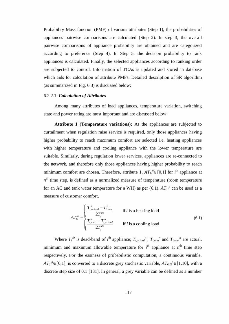
117

Probability Mass function (PMF) of various attributes (Step 1), the probabilities of

appliances pairwise comparisons are calculated (Step 2). In step 3, the overall

pairwise comparisons of appliance probability are obtained and are categorized

according to preference (Step 4). In Step 5, the decision probability to rank

appliances is calculated. Finally, the selected appliances according to ranking order

are subjected to control. Information of TCAs is updated and stored in database

which aids for calculation of attribute PMFs. Detailed description of SR algorithm

(as summarized in Fig. 6.3) is discussed below:

6.2.2.1. Calculation of Attributes

Among many attributes of load appliances, temperature variation, switching

state and power rating are most important and are discussed below:

Attribute 1 (Temperature variations): As the appliances are subjected to

curtailment when regulation raise service is required, only those appliances having

higher probability to reach maximum comfort are selected i.e. heating appliances

with higher temperature and cooling appliance with the lower temperature are

suitable. Similarly, during regulation lower services, appliances are re-connected to

the network, and therefore only those appliances having higher probability to reach

minimum comfort are chosen. Therefore, attribute 1, AT1in∈ [0,1] for i

th appliance at

nth time step, is defined as a normalized measure of temperature (room temperature

for an AC and tank water temperature for a WH) as per (6.1). AT1in can be used as a

measure of customer comfort.

loadcooling aisif2

loadheating a isif2

,max,

min,,

1

iT

TT

iT

TT

AT

db

n

actuali

n

i

db

n

i

n

actuali

n

i

i

i (6.1)

Where Tidb

is dead-band of ith

appliance; Ti,actualn

, Ti,minn and Ti,max

n are actual,

minimum and maximum allowable temperature for ith appliance at n

th time step

respectively. For the easiness of probabilistic computation, a continuous variable,

AT1in∈ [0,1], is converted to a discrete grey stochastic variable, ATG1i

n∈ [1,10], with a

discrete step size of 0.1 [131]. In general, a grey variable can be defined as a number

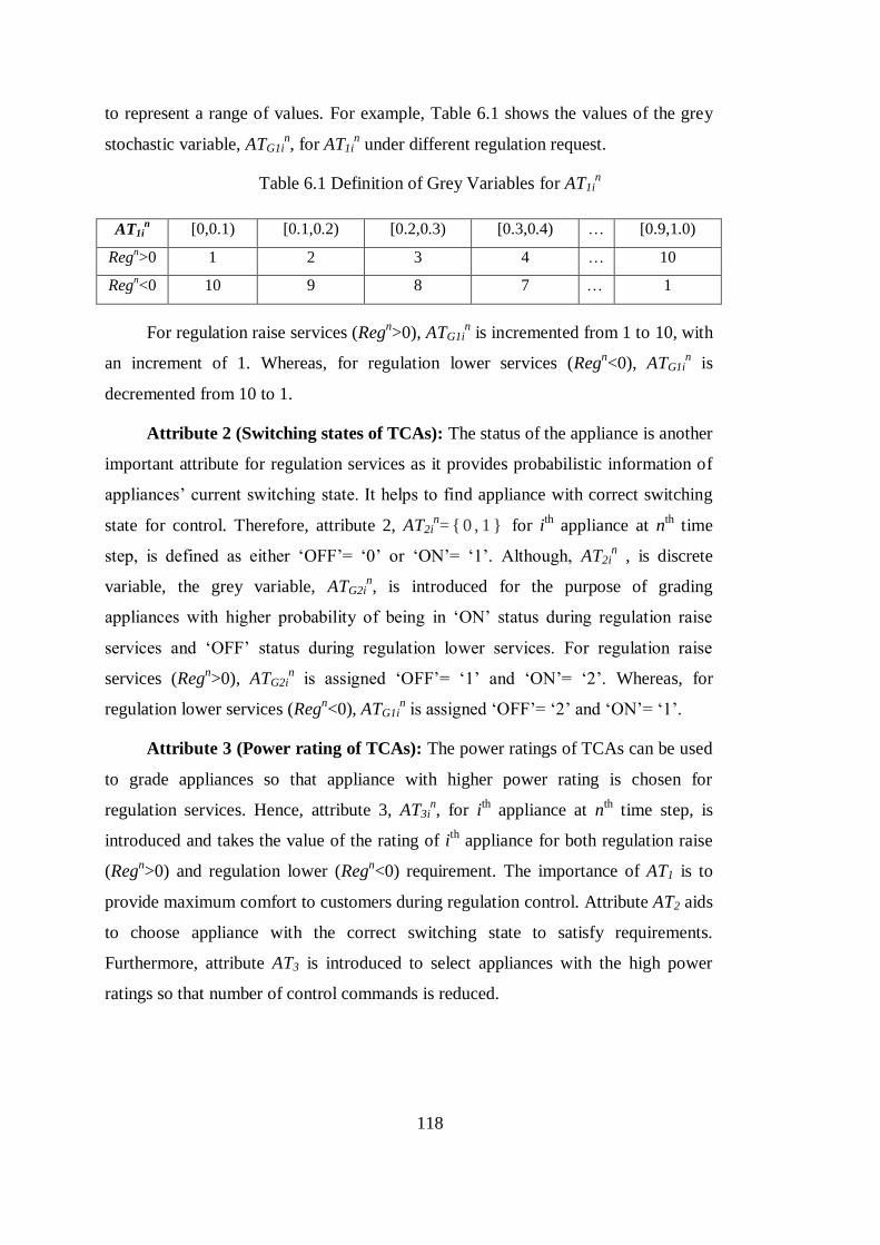
118

to represent a range of values. For example, Table 6.1 shows the values of the grey

stochastic variable, ATG1in, for AT1i

n under different regulation request.

Table 6.1 Definition of Grey Variables for AT1in

AT1in [0,0.1) [0.1,0.2) [0.2,0.3) [0.3,0.4) … [0.9,1.0)

Regn>0 1 2 3 4 … 10

Regn<0 10 9 8 7 … 1

For regulation raise services (Regn>0), ATG1i

n is incremented from 1 to 10, with

an increment of 1. Whereas, for regulation lower services (Regn<0), ATG1i

n is

decremented from 10 to 1.

Attribute 2 (Switching states of TCAs): The status of the appliance is another

important attribute for regulation services as it provides probabilistic information of

appliances’ current switching state. It helps to find appliance with correct switching

state for control. Therefore, attribute 2, AT2in= { 0 , 1 } for i

th appliance at n

th time

step, is defined as either ‘OFF’= ‘0’ or ‘ON’= ‘1’. Although, AT2in , is discrete

variable, the grey variable, ATG2in, is introduced for the purpose of grading

appliances with higher probability of being in ‘ON’ status during regulation raise

services and ‘OFF’ status during regulation lower services. For regulation raise

services (Regn>0), ATG2i

n is assigned ‘OFF’= ‘1’ and ‘ON’= ‘2’. Whereas, for

regulation lower services (Regn<0), ATG1i

n is assigned ‘OFF’= ‘2’ and ‘ON’= ‘1’.

Attribute 3 (Power rating of TCAs): The power ratings of TCAs can be used

to grade appliances so that appliance with higher power rating is chosen for

regulation services. Hence, attribute 3, AT3in, for i

th appliance at n

th time step, is

introduced and takes the value of the rating of ith

appliance for both regulation raise

(Regn>0) and regulation lower (Reg

n<0) requirement. The importance of AT1 is to

provide maximum comfort to customers during regulation control. Attribute AT2 aids

to choose appliance with the correct switching state to satisfy requirements.

Furthermore, attribute AT3 is introduced to select appliances with the high power

ratings so that number of control commands is reduced.

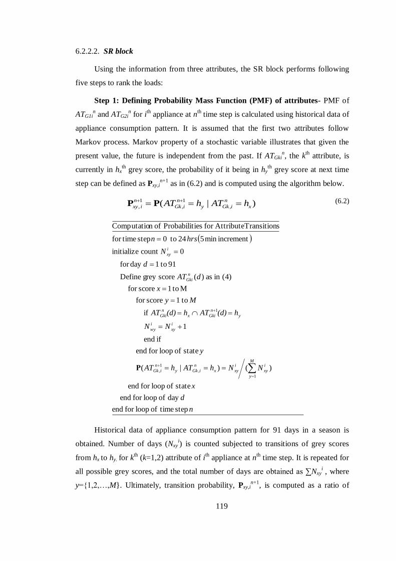
119

6.2.2.2. SR block

Using the information from three attributes, the SR block performs following

five steps to rank the loads:

Step 1: Defining Probability Mass Function (PMF) of attributes- PMF of

ATG1in and ATG2i

n for i

th appliance at n

th time step is calculated using historical data of

appliance consumption pattern. It is assumed that the first two attributes follow

Markov process. Markov property of a stochastic variable illustrates that given the

present value, the future is independent from the past. If ATGkin, the k

th attribute, is

currently in hxth grey score, the probability of it being in hy

th grey score at next time

step can be defined as Pxy,in+1

as in (6.2) and is computed using the algorithm below.

)|( ,

1

,

1

, x

n

iGky

n

iGk

n

ixy hAThAT PP (6.2)

n

d

x

NNhAThAT

y

NN

h(d)ATh(d)AT

M y

x

dAT

d

N

hrsn

M

y

i

xy

i

xyx

n

iGky

n

iGk

i

xy

i

wy

y

n

Gkix

n

Gki

n

Gki

i

xy

step timeof loopfor end

day of loopfor end


)()|(


if end

1

if

to1 scorefor

M to1 scorefor

)4(inas)(scoregreyDefine

91to1dayfor

0countinitialize

incrementmin524to0step timefor

sTransition Attributefor iesProbabilit ofn Computatio

1

,

1

,

1

Ρ

Historical data of appliance consumption pattern for 91 days in a season is

obtained. Number of days (Nxyi) is counted subjected to transitions of grey scores

from hx to hy. for k

th (k=1,2) attribute of i

th appliance at n

th time step. It is repeated for

all possible grey scores, and the total number of days are obtained as ∑Nxyi , where

y={1,2,…,M}. Ultimately, transition probability, Pxy,in+1

, is computed as a ratio of

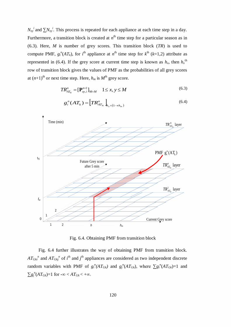
120

Nxyi and ∑Nxy

i. This process is repeated for each appliance at each time step in a day.

Furthermore, a transition block is created at nth time step for a particular season as in

(6.3). Here, M is number of grey scores. This transition block (TR) is used to

compute PMF, gin(ATk), for i

th appliance at n

th time step for k

th (k=1,2) attribute as

represented in (6.4). If the grey score at current time step is known as hx, then hxth

row of transition block gives the values of PMF as the probabilities of all grey scores

at (n+1)th or next time step. Here, hm is M

th grey score.

MyxTR MM

n

ixy

n

ATki

,1][ 1

,P (6.3)

mx

ki hh

n

ATk

n

i TRATg

1

)( (6.4)

Current Grey score

Future Grey score

after 5 min

Time (min)

0

tn

tN

1 2 h hm

1

2

layerN

ATkiTR

)(ATg PMF k

n

i

layer1

kiATTR

layern

ATkiTR

Fig. 6.4. Obtaining PMF from transition block

Fig. 6.4 further illustrates the way of obtaining PMF from transition block.

ATGkin and ATGkj

n of i

th and j

th appliances are considered as two independent discrete

random variables with PMF of gin(ATGk) and gj

n(ATGk), where ∑gi

n(ATGk)=1 and

∑gjn(ATGk)=1 for -∞ < ATGk < +∞.

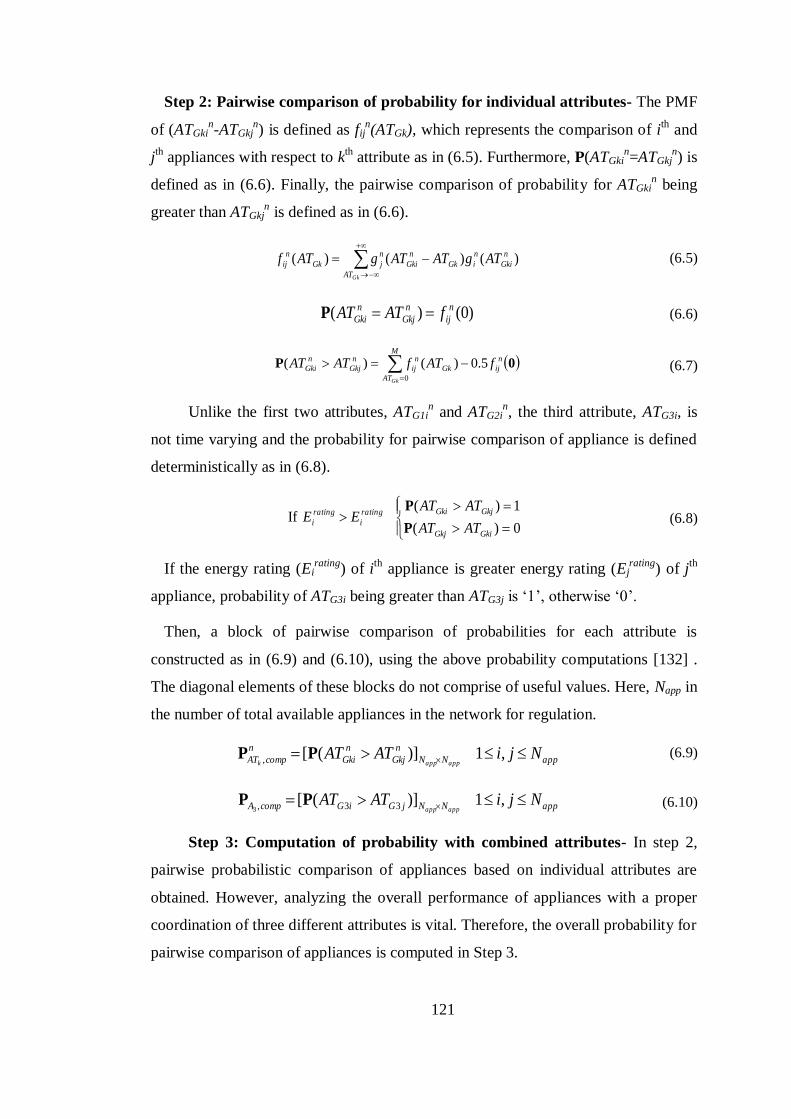
121

Step 2: Pairwise comparison of probability for individual attributes- The PMF

of (ATGkin-ATGkj

n) is defined as fij

n(ATGk), which represents the comparison of i

th and

jth appliances with respect to k

th attribute as in (6.5). Furthermore, P(ATGki

n=ATGkj

n) is

defined as in (6.6). Finally, the pairwise comparison of probability for ATGkin being

greater than ATGkjn is defined as in (6.6).

GkAT

n

Gki

n

iGk

n

Gki

n

jGk

n

ij ATgATATgATf )()()( (6.5)

)0()( n

ij

n

Gkj

n

Gki fATAT P (6.6)

M

AT

n

ijGk

n

ij

n

Gkj

n

Gki

Gk

fATfATAT0

5.0)()( 0P (6.7)

Unlike the first two attributes, ATG1in and ATG2i

n, the third attribute, ATG3i, is

not time varying and the probability for pairwise comparison of appliance is defined

deterministically as in (6.8).

0)(

1)(If

GkiGkj

GkjGkirating

i

rating

iATAT

ATATEE

P

P (6.8)

If the energy rating (Eirating

) of ith

appliance is greater energy rating (Ejrating

) of jth

appliance, probability of ATG3i being greater than ATG3j is ‘1’, otherwise ‘0’.

Then, a block of pairwise comparison of probabilities for each attribute is

constructed as in (6.9) and (6.10), using the above probability computations [132] .

The diagonal elements of these blocks do not comprise of useful values. Here, Napp in

the number of total available appliances in the network for regulation.

appNN

n

Gkj

n

Gki

n

compAT NjiATATappappk

,1)]([, PP (6.9)

appNNjGiGcompA NjiATATappapp

,1)]([ 33,3PP (6.10)

Step 3: Computation of probability with combined attributes- In step 2,

pairwise probabilistic comparison of appliances based on individual attributes are

obtained. However, analyzing the overall performance of appliances with a proper

coordination of three different attributes is vital. Therefore, the overall probability for

pairwise comparison of appliances is computed in Step 3.

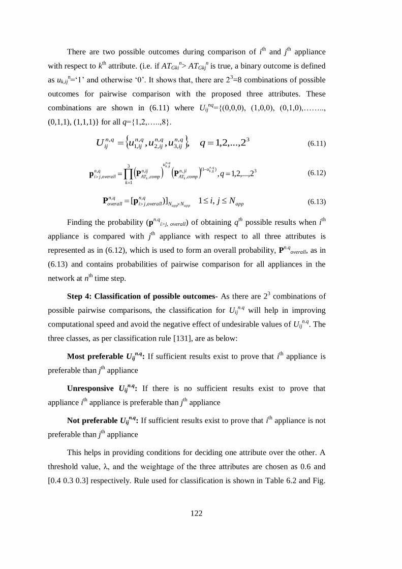
122

There are two possible outcomes during comparison of ith and j

th appliance

with respect to kth

attribute. (i.e. if ATGkin> ATGkj

n is true, a binary outcome is defined

as uk,ijn=‘1’ and otherwise ‘0’. It shows that, there are 2

3=8 combinations of possible

outcomes for pairwise comparison with the proposed three attributes. These

combinations are shown in (6.11) where Uijnq

={(0,0,0), (1,0,0), (0,1,0),……..,

(0,1,1), (1,1,1)} for all q={1,2,…..,8}.

3,

,3

,

,2

,

,1

, 2,...,2,1,,, quuuU qn

ij

qn

ij

qn

ij

qn

ij (6.11)

3)1(,

,

3

1

,

,

,

, 2,...,2,1,,,

,,

qqnijk

k

qnijk

k

ujin

compAT

u

k

ijn

compAT

qn

overallji PPp (6.12)

appNN

qn

overallji

qn

overall Njiappapp

,1)][ ,

,

,pP (6.13)

Finding the probability (pn.q

i>j, overall) of obtaining qth

possible results when ith

appliance is compared with jth appliance with respect to all three attributes is

represented as in (6.12), which is used to form an overall probability, Pn.q

overall, as in

(6.13) and contains probabilities of pairwise comparison for all appliances in the

network at nth time step.

Step 4: Classification of possible outcomes- As there are 23 combinations of

possible pairwise comparisons, the classification for Uijn.q

will help in improving

computational speed and avoid the negative effect of undesirable values of Uijn.q

. The

three classes, as per classification rule [131], are as below:

Most preferable Uijn.q

: If sufficient results exist to prove that ith appliance is

preferable than jth appliance

Unresponsive Uijn.q

: If there is no sufficient results exist to prove that

appliance ith appliance is preferable than j

th appliance

Not preferable Uijn.q

: If sufficient results exist to prove that ith appliance is not

preferable than jth appliance

This helps in providing conditions for deciding one attribute over the other. A

threshold value, λ, and the weightage of the three attributes are chosen as 0.6 and

[0.4 0.3 0.3] respectively. Rule used for classification is shown in Table 6.2 and Fig.

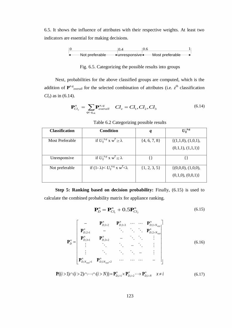
123

6.5. It shows the influence of attributes with their respective weights. At least two

indicators are essential for making decisions.

0 0.4 0.6 1

Not preferable unresponsive Most preferable

Fig. 6.5. Categorizing the possible results into groups

Next, probabilities for the above classified groups are computed, which is the

addition of Pn.q

overall for the selected combination of attributes (i.e. zth

classification

Clz) as in (6.14).

321

, ,, ClClClClz

qq

qn

overall

n

Cl

clz

z

PP (6.14)

Table 6.2 Categorizing possible results

Classification Condition q Uijn,q

Most Preferable if Uijn,q

x wT

λ {4, 6, 7, 8} {(1,1,0), (1,0,1),

(0,1,1), (1,1,1)}

Unresponsive if Uijn,q

x wT

λ {} {}

Not preferable if (1- λ)< Uijn,q

x wT<λ {1, 2, 3, 5} {(0,0,0), (1,0,0),

(0,1,0), (0,0,1)}

Step 5: Ranking based on decision probability: Finally, (6.15) is used to

calculate the combined probability matrix for appliance ranking.

n

Cl

n

Cl

n

D 215.0 PPP (6.15)

n

ND

n

ND

n

D

n

D

n

ND

n

D

n

ND

n

D

n

D

n

D

appapp

app

app

21,1,

23,13,

2,12,

1,31,21,

PP

PP

PP

PPP

P (6.16)

ixNiii n

NiD

n

iD

n

iD ,2,1,))()2()1(( PPPP (6.17)

124

app

N

N

ixx

n

xiD

n

rank Ni

app

app

,.......,2,1

1,1

,

PP (6.18)

The decision probability matrix, PDn, is the addition of most preferred

probability matrix and 50% of the unresponsive matrix as shown in (6.15) and gives

the probabilities of ith

appliance being greater than the jth

appliance in nth

time step as

shown in (5.16). PDn, comprises of overall stochastic comparison of appliances

which is used for ranking appliances.

The events represented by each row of PDn, are independent such that

probability of occurrence of one event does not influence the probability of other.

Hence, the probability of ith

appliance is being greater than xth

appliance where

x=1,2,…….,N x i can be easily obtained as using (6.17). Finally, the probability of

every appliance being greater than the ith

appliance is calculated using (6.18) using

PDn. The appliances are ranked from the maximum to minimum probability of Prank

n.

Appliance with a highest rank has the maximum probability to be greater than other

appliances considering all attributes.

6.3. Modeling and Simulation Results

A test aggregator network consisting of 30 houses is considered to verify the

algorithm for regulation services. Network topology as in chapter 3 is considered

during the study with 10 houses per phase in a feeder. A sample regulation signal is

taken, which is send from a retailer to the aggregator. All houses are assumed to have

both ACs and WHs and are connected through in-home energy management units.

These units have the capability to obtain time varying temperature and appliance

power data, which is required by retailers for providing regulation services.

MATLAB software is used to perform all simulations with 5 minute time step for 24

hours.

6.3.1. Mathematical models for TCAs (ACs and WHs)

ACs and WHs are considered as TCAs which operate within a predefined

dead-band around a temperature set point. A continuous time varying models of WH

and AC are used in this study and are discussed below.

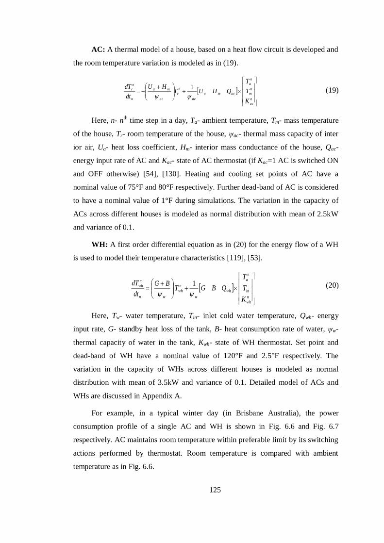
125

AC: A thermal model of a house, based on a heat flow circuit is developed and

the room temperature variation is modeled as in (19).

n

ac

n

m

n

a

acma

ac

n

r

ac

ma

n

n

r

K

T

T

QHUTHU

dt

dT

1

(19)

Here, n- nth time step in a day, Ta- ambient temperature, Tm- mass temperature

of the house, Tr- room temperature of the house, ψac- thermal mass capacity of inter

ior air, Ua- heat loss coefficient, Hm- interior mass conductance of the house, Qac-

energy input rate of AC and Kac- state of AC thermostat (if Kac=1 AC is switched ON

and OFF otherwise) [54], [130]. Heating and cooling set points of AC have a

nominal value of 75°F and 80°F respectively. Further dead-band of AC is considered

to have a nominal value of 1°F during simulations. The variation in the capacity of

ACs across different houses is modeled as normal distribution with mean of 2.5kW

and variance of 0.1.

WH: A first order differential equation as in (20) for the energy flow of a WH

is used to model their temperature characteristics [119], [53].

n

wh

in

n

a

wh

w

n

wh

wn

n

wh

K

T

T

QBGTBG

dt

dT

1. (20)

Here, Tw- water temperature, Tin- inlet cold water temperature, Qwh- energy

input rate, G- standby heat loss of the tank, B- heat consumption rate of water, ψw-

thermal capacity of water in the tank, Kwh- state of WH thermostat. Set point and

dead-band of WH have a nominal value of 120°F and 2.5°F respectively. The

variation in the capacity of WHs across different houses is modeled as normal

distribution with mean of 3.5kW and variance of 0.1. Detailed model of ACs and

WHs are discussed in Appendix A.

For example, in a typical winter day (in Brisbane Australia), the power

consumption profile of a single AC and WH is shown in Fig. 6.6 and Fig. 6.7

respectively. AC maintains room temperature within preferable limit by its switching

actions performed by thermostat. Room temperature is compared with ambient

temperature as in Fig. 6.6.

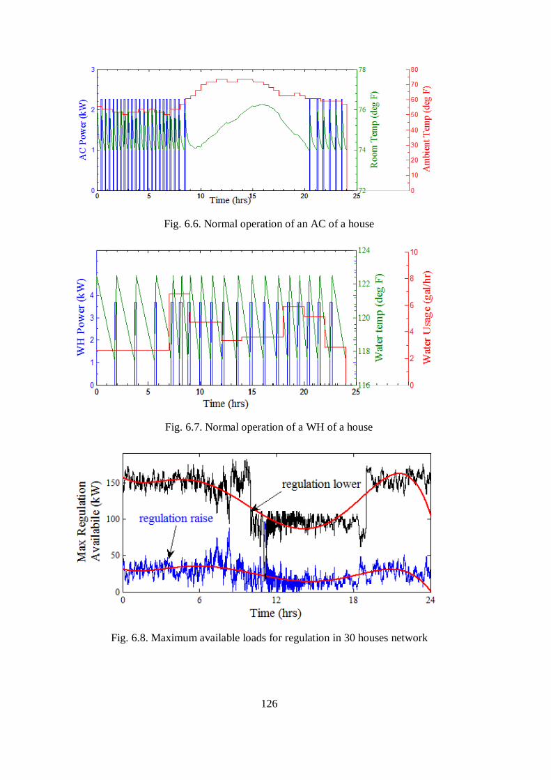
126

Fig. 6.6. Normal operation of an AC of a house

Fig. 6.7. Normal operation of a WH of a house

Fig. 6.8. Maximum available loads for regulation in 30 houses network

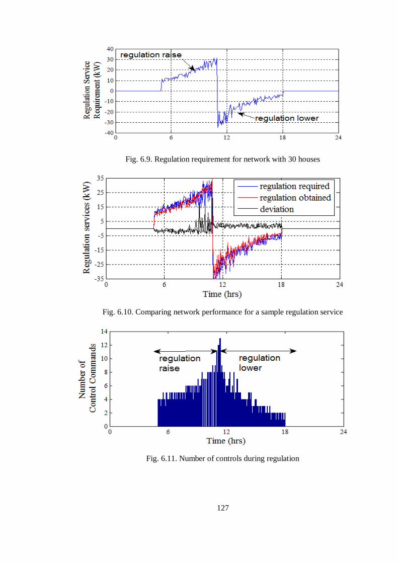
127

Fig. 6.9. Regulation requirement for network with 30 houses

Fig. 6.10. Comparing network performance for a sample regulation service

Fig. 6.11. Number of controls during regulation

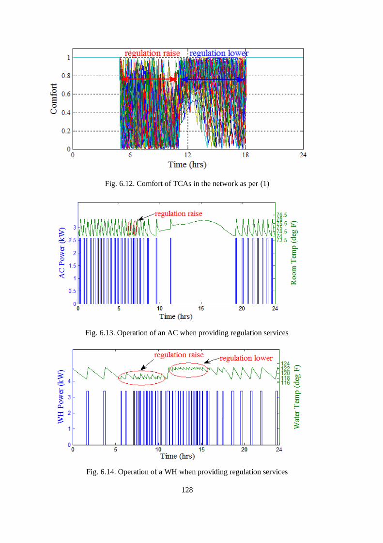
128

Fig. 6.12. Comfort of TCAs in the network as per (1)

Fig. 6.13. Operation of an AC when providing regulation services

Fig. 6.14. Operation of a WH when providing regulation services

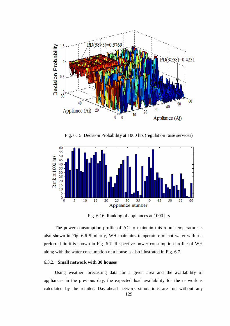
129

Fig. 6.15. Decision Probability at 1000 hrs (regulation raise services)

Fig. 6.16. Ranking of appliances at 1000 hrs

The power consumption profile of AC to maintain this room temperature is

also shown in Fig. 6.6 Similarly, WH maintains temperature of hot water within a

preferred limit is shown in Fig. 6.7. Respective power consumption profile of WH

along with the water consumption of a house is also illustrated in Fig. 6.7.

6.3.2. Small network with 30 houses

Using weather forecasting data for a given area and the availability of

appliances in the previous day, the expected load availability for the network is

calculated by the retailer. Day-ahead network simulations are run without any

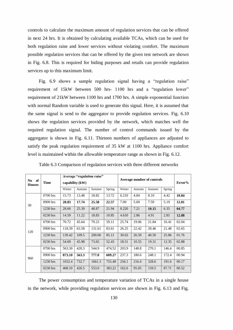
130

controls to calculate the maximum amount of regulation services that can be offered

in next 24 hrs. It is obtained by calculating available TCAs, which can be used for

both regulation raise and lower services without violating comfort. The maximum

possible regulation services that can be offered by the given test network are shown

in Fig. 6.8. This is required for biding purposes and retails can provide regulation

services up to this maximum limit.

Fig. 6.9 shows a sample regulation signal having a “regulation raise”

requirement of 15kW between 500 hrs- 1100 hrs and a “regulation lower”

requirement of 21kW between 1100 hrs and 1700 hrs. A simple exponential function

with normal Random variable is used to generate this signal. Here, it is assumed that

the same signal is send to the aggregator to provide regulation services. Fig. 6.10

shows the regulation services provided by the network, which matches well the

required regulation signal. The number of control commands issued by the

aggregator is shown in Fig. 6.11. Thirteen numbers of appliances are adjusted to

satisfy the peak regulation requirement of 35 kW at 1100 hrs. Appliance comfort

level is maintained within the allowable temperature range as shown in Fig. 6.12.

Table 6.3 Comparison of regulation services with three different networks

No of

Houses Time

Average “regulation raise”

capability (kW) Average number of controls

Error%

Winter Autumn Summer Spring Winter Autumn Summer Spring

30

0700 hrs 15.73 13.48 18.82 13.72 6.210 4.84 8.10 4.42 10.84

0900 hrs 28.83 17.74 25.58 22.57 7.00 5.69 7.59 5.19 12.01

1230 hrs 28.60 25.39 48.87 21.94 8.220 7.21 10.15 6.35 04.77

0230 hrs 14.59 11.22 18.83 10.85 4.610 2.86 4.91 2.85 12.88

120

0700 hrs 70.72 45.64 79.23 59.11 25.74 19.06 21.84 16.41 02.04

0900 hrs 118.39 63.58 131.61 83.61 26.25 22.42 28.46 21.48 02.65

1230 hrs 139.42 109.5 200.06 85.11 30.63 26.59 40.50 25.86 01.76

0230 hrs 54.69 45.98 73.65 52.43 18.51 10.55 19.31 12.35 02.88

960

0700 hrs 563.30 428.3 544.9 474.52 203.9 148.8 270.1 146.4 00.85

0900 hrs 873.10 563.3 777.0 609.27 237.3 180.6 248.1 172.4 00.94

1230 hrs 1032.4 732.7 1661.3 755.48 256.1 216.4 328.6 191.6 00.17

0230 hrs 468.10 426.5 553.0 383.22 162.6 95.05 159.5 87.71 00.52

The power consumption and temperature variation of TCAs in a single house

in the network, while providing regulation services are shown in Fig. 6.13 and Fig.

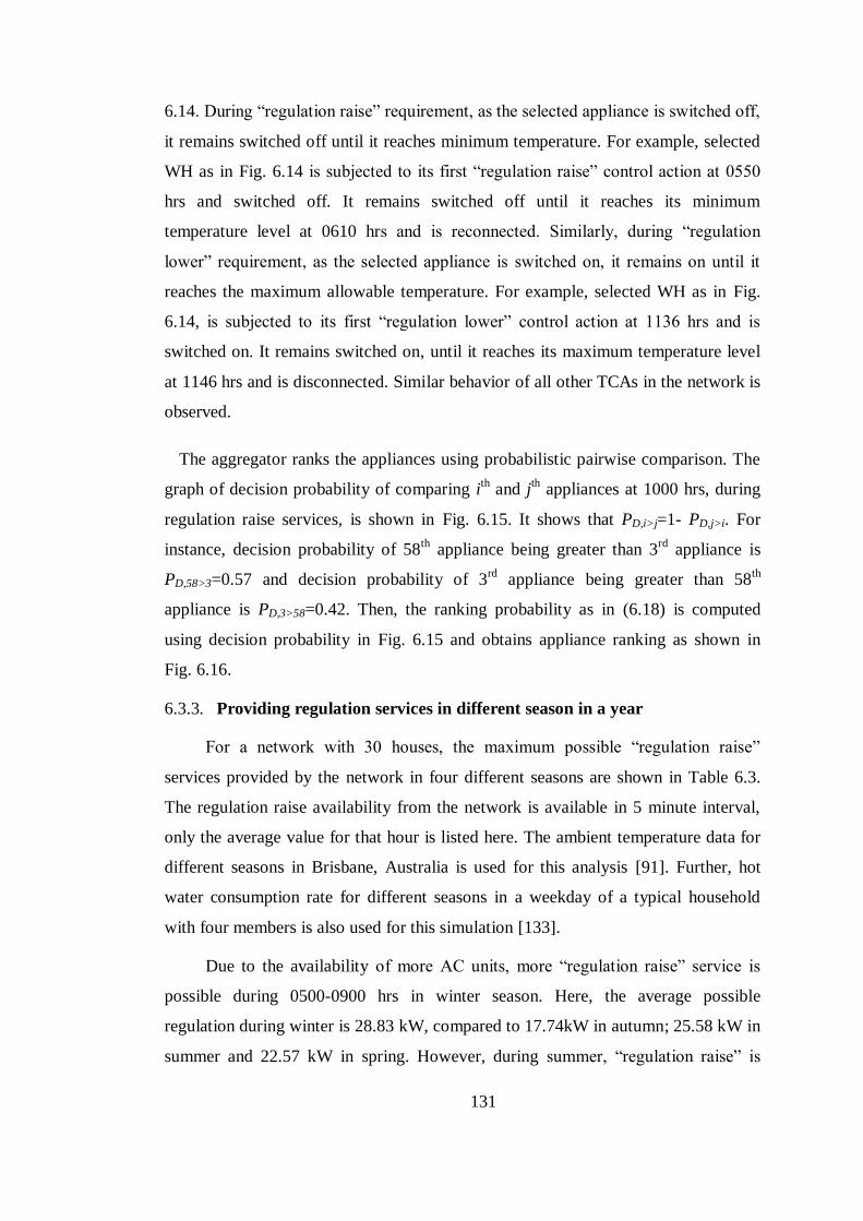
131

6.14. During “regulation raise” requirement, as the selected appliance is switched off,

it remains switched off until it reaches minimum temperature. For example, selected

WH as in Fig. 6.14 is subjected to its first “regulation raise” control action at 0550

hrs and switched off. It remains switched off until it reaches its minimum

temperature level at 0610 hrs and is reconnected. Similarly, during “regulation

lower” requirement, as the selected appliance is switched on, it remains on until it

reaches the maximum allowable temperature. For example, selected WH as in Fig.

6.14, is subjected to its first “regulation lower” control action at 1136 hrs and is

switched on. It remains switched on, until it reaches its maximum temperature level

at 1146 hrs and is disconnected. Similar behavior of all other TCAs in the network is

observed.

The aggregator ranks the appliances using probabilistic pairwise comparison. The

graph of decision probability of comparing ith

and jth appliances at 1000 hrs, during

regulation raise services, is shown in Fig. 6.15. It shows that PD,i>j=1- PD,j>i. For

instance, decision probability of 58th

appliance being greater than 3rd

appliance is

PD,58>3=0.57 and decision probability of 3rd

appliance being greater than 58th

appliance is PD,3>58=0.42. Then, the ranking probability as in (6.18) is computed

using decision probability in Fig. 6.15 and obtains appliance ranking as shown in

Fig. 6.16.

6.3.3. Providing regulation services in different season in a year

For a network with 30 houses, the maximum possible “regulation raise”

services provided by the network in four different seasons are shown in Table 6.3.

The regulation raise availability from the network is available in 5 minute interval,

only the average value for that hour is listed here. The ambient temperature data for

different seasons in Brisbane, Australia is used for this analysis [91]. Further, hot

water consumption rate for different seasons in a weekday of a typical household

with four members is also used for this simulation [133].

Due to the availability of more AC units, more “regulation raise” service is

possible during 0500-0900 hrs in winter season. Here, the average possible

regulation during winter is 28.83 kW, compared to 17.74kW in autumn; 25.58 kW in

summer and 22.57 kW in spring. However, during summer, “regulation raise” is

132

possible due to the availability of AC units mostly throughout the day. For instance,

at 1230 hrs, the average possible regulation during summer is 48.87 kW, which is the

highest value comparing to other seasons (winter: 28.60, autumn: 25.39, spring:

21.94 kW). This is true for any time during a day except 0500-0900 hrs.

Error percentage in Table 6.3 shows the deviation of required average

regulation with the actual regulation provided by the network (using regulation signal

of Fig. 3.9). The value shown is an average for all four seasons. For example, in a

network with 30 houses, the error percentage is minimum (4.77%) at 1230 hrs

compared to any other time of the day (0700 hrs: 10.84%, 0900 hrs: 12.01%, 0230

hrs: 12.88%). The more is the “regulation raise” available capability, the lesser is the

error percentage. The network has more availability of distributed loads to match the

required signal at noon time. Further, the average number of control actions for the

network with 30 houses can reach up to 10.15, during summer season, when there is

48.87 kW of “regulation raise” capability.

6.3.4. Providing “regulation raise” services from the network of different sizes

Analysis of regulation data for three networks of 30, 120, 960 houses is

presented in Table 6.3 for four seasons. During winter, more regulation service is

possible during 0500-0900 hrs. For instance, consider network with 960 houses at

0900 hrs. There is a maximum possible regulation of 873.10 kW in comparison with

only 563.3 kW in autumn and 777 kW in summer. During summer season, average

“regulation raise” capability of the network is at its maximum of 1661.3 kW at 1230

hrs when compared with other seasons in a year (winter: 1032.4 kW, autumn: 732.7

kW, spring: 755.48 kW).

Furthermore, the error percentage is reduced as the number of appliances

available for regulation services increase. This is because of the accuracy in

balancing power signals with increased number of controls. Hence, the network with

960 houses has a reduced error percentage, compared to the networks with 30 and

120 houses. For example, at 1230 hrs, the error percentage is 0.17% in 960 house

network, compared to 4.77% in 30 house network.

133

6.4. Conclusion and Summary

This part of research work, proposes a new control method for a pool of TCAs

utilized for regulation services. Market operator will broadcast the regulation signal

to retailer in real-time. The retailers pass it on to the aggregators, who perform direct

load control using stochastic ranking method.

A stochastic pairwise comparison of appliances is conducted based on three

attributes such as temperature variation, status and power rating of TCAs.

Probabilistic nature of these attributes are computed using Markov property where

probability of attribute at a future time step can be found based on its current status.

Efficiency of this scheme is verified through network simulations for a given

“regulation raise” and “regulation lower” signals. Required regulation is achieved

with the allowable limit of overrides. It shows the robustness of the system. A

minimum deviation of less than 1% from expected regulation services is obtained

and system robustness is assured with the capability of providing regulation even

with 10-40% of unexpected customer override signals.

The TCAs connected to the network are adjusted for the next time step.

However, uncertainty in appliance consumption and seasonal temperature variations

make appliance selection process difficult.

134

Chapter 7

Conclusions

In this thesis, the four important contributions made by DR to the future smart

distribution grid are addressed and efficient approaches are proposed to improve

system reliability and customer satisfaction. This chapter summarizes the proposed

methods and draws the conclusions from the research. The limitations of the study

are noted, and recommendations are made for future work.

7.1. Research Summary and Contributions

The initial part of this research proposed an improved DR option for a

residential distribution system using a customer reward scheme. This work was done

with the primary purpose of reducing network peaks and improving voltage in

residential feeders. The deployment of two-way communication infrastructure with

smart meters and in-home display units is required for this scheme. A decision-

making process to appropriately adjust residential appliances was developed,

reflecting appliance flexibility, satisfaction and priority. Customers would be

encouraged to participate in this scheme through a fully-fledged reward mechanism.

This reward mechanism is based on customer participation in load shifting and

associated voltage improvement within the feeder. The impacts of the proposed

method on both the electric utility and customers were analyzed. It was concluded

that the electric utility would benefit from the improved feeder voltage and removal

of the network peaks. Customer satisfaction and appliance usage patterns in this

reward scheme were investigated. The results showed that considerable discomfort

135

was tolerated by customers, which was compensated by the proposed rebate

program. Hence, the proposed DR via customer reward scheme can be successfully

implemented in a real electricity distribution network to defer the transformer

upgrade costs and also maintain network reliability. In addition, customer

satisfaction can be confirmed through the rebate scheme.

Current electricity networks apply price-responsive demand schemes for the

residential distribution network. RTP is a promising option which benefits the

electric utility by removing the peak demand and wholesale price spikes in the

network. It has an added advantage of providing flexibility to customers to adjust

their loads in contrast with the proposed reward-based DR scheme. Hence, an

improved real-time pricing scheme for customers is proposed to alleviate voltage

violations, peak load problems and unexpected wholesale price spikes. This RTP

scheme contains three price components reflecting power consumption, adverse

network voltage conditions and unexpected wholesale price spikes. It was tested on a

sample residential distribution system and the performance was analyzed. The results

showed that the active participation of customers can lead to a reduction in the cost

of their consumption through appropriate load adjustments. In addition, an algorithm

was proposed for indicating appropriate loads that can be controlled by a customer.

In the proposed RTP scheme, customers are given the flexibility to make decisions

for appliance control in a smart home environment. The results validated that the

impact of the proposed RTP scheme did not hamper the appliance usage patterns

among customers. The proposed scheme also ensured the elimination of network

peaks, adverse feeder voltage conditions and wholesale price spikes.

DR via customer reward scheme and the RTP scheme provides benefit to

customers through incentives and cost reduction respectively. Incentive provided to

an average household through a DR via customer reward is found to be 28.9 %

whereas the cost reduction achieved by an average household from a RTP scheme is

20.8 %. Hence, DR via customer reward provides more economic benefit to the

customers for allowing forced load adjustments in comparison with RTP scheme.

Residential customers are only considered for both studies.

Active and effective customer participation in the proposed RTP scheme would

only be possible with a guaranteed automated HEM system. Hence, this research

136

continued to focus on an efficient algorithm for real-time HEM units for reducing the

cost of energy consumption in a house. This research work is unique in regard to the

proposed appliance scheduling, as it considers the uncertain nature of RTP and

appliance power consumption. The operation of the proposed HEM scheduler is

divided into three phases, namely, real-time monitoring, stochastic scheduling and

real-time control of appliances. Simulations are conducted every four minutes in a

day. During the real-time monitoring phase, the electric utility remotely monitors

appliances connected to the HEM system at every time step. The electric utility also

obtains wholesale price information from the electricity market to broadcast the real-

time price to customers. When the cost of consumption in a house is above an

average limit, the electric utility defines the operating status of appliances

considering the operating characteristics and customer input of controllable

appliances connected to HEM system. The information obtained during the real-time

monitoring phase may not be sufficient to make appropriate control decisions for

scheduling appliances. This is due to the uncertainties in electricity price variation,

appliance operation, user behavior and preferences. Hence, the real-time monitoring

phase is followed by a stochastic scheduling process which utilizes the information

obtained in the real-time monitoring phase to stochastically schedule the appliances.

The main objective of the stochastic scheduling phase is to minimize the cost of the

energy consumption. The Markov decision process is used to achieve the objective

by accurately predicting the appropriate curtailment of appliances based on the

stochastic behavior of the cost of consumption. Constraints are added to intrinsically

maintain customer comfort and appliance priority. Constraints for allowable

interruptions are also included in order to prevent reducing the life-span of the

appliances while also maintaining customer satisfaction. Subsequently, the appliance

selected during stochastic scheduling phase is subjected to control in the real-time

control phase. The stochastic decision process ensures the incorporation of

uncertainties. Simulations are conducted in short timeframes to achieve the four

minute control steps. The outcomes validated a significant reduction in the cost of

energy consumption and the maintenance of customer satisfaction. This ensures the

efficient utilization of the RTP scheme.

The DR option can be utilized for the purpose of providing regulation services.

Hence, a new control method applied on a pool of thermostatically controllable

137

appliances for providing regulation services was recommended as part of this

research. In the proposed method, an ancillary services market environment is

created with a market operator, broadcasting regulation signals to retailers in real

time. Retailers pass the obtained signal to aggregators, who are responsible for

performing load control actions using a stochastic ranking method. A probabilistic

pairwise comparison of appliances is conducted based on appliance attributes

(namely, temperature variation, appliance power status and appliance power rating).

The Markov property is utilized to compute the probabilistic nature of these

attributes. This is done by assuming that the probability of an attribute at a future

time step can be found based on its current status. The ranking method incorporates

the contribution of all three attributes. The efficiency of this scheme is verified

through a given regulation raise and lower signals. This ensures that the required

regulation can be achieved by allowing limited overrides in the network. In this

study, the deviation of the actual load curtailment from the required regulation signal

was calculated. It confirmed that less than one percent of deviation can be expected

in a network with 960 houses. It also allows 10-40% of unexpected customer

override signals during simulations.

7.2. Proposed Future Work and Suggestions

The initial part of this research proposed a DR technique via a customer reward

scheme. This reward scheme is based on the benefits obtained by the electric utility

by time-shifting demand and removing voltage violations. However, the benefits

obtained by deferring the system upgrade costs were not studied. The investment in

communication infrastructure in the residential distribution network should also be

considered when identifying the benefits of this scheme. Hence, a detailed study

based on the cost-benefit analysis should be conducted.

In addition, the proposed RTP scheme reflects power consumption, adverse

voltage conditions and wholesale price spikes. It can be further improved by

including the feed-in tariffs from roof-top PV cells and special provisions for plug-in

electric vehicles. The introduction of PV cells and plug-in electric vehicles to the

residential distribution network has a significant impact on creating adverse network

conditions. Hence, improvement in RTP is a promising research area which can be

studied on a future electricity grid.

138

The proposed RTP scheme in Chapter 4, considers fixed energy limit for every

house, in order to define the electricity price components. Similarly, rebate scheme

developed in Chapter 3, considers a fixed energy limit for every house to define the

rebate values due to load curtailments. However, different energy limit for each

house should be considered in order to prevent adverse effect on customers who

consume less than the average customer. This can be achieved by computing the

annual average energy consumption limit for each house. Therefore, energy limit for

each house due to diversified load profiles is expected to be included in future.

The proposed HEM scheduler to facilitate the RTP scheme ensures that the

cost of energy consumption in a residence is reduced. However, the uncoordinated

control of the proposed HEM scheduler may create unexpected network peaks during

off-peak periods. Hence, the stochastic coordination of the HEM scheduler in a

residential electricity network should be studied extensively to ensure a reliable

network.

HEM scheduler developed in third phase of the research can include both

market variability and weather forecast as separate Markov processes. The stochastic

nature of market variability, temperature sensitivity effects scholastic scheduling of

loads. Therefore, an improved HEM scheduler can be developed in future, with the

incorporation of both variables.

Furthermore, different perceptions of appliance models can be included. For

example, characteristics of air-conditioners such as fan and cooling operation can be

considered. The lock-out time of air-conditioners has an implication in real time

control. Therefore, a delay should be added during the control actions, reflecting the

lock-out time. Moreover, different operation status of clothes washer can also be

considered such as ‘cold water wash’.

This research is carried out in four different phases. Reducing network peak

and voltage violations are the main objective of first research phase. Second phase

includes the reduction of wholesale price spikes as well. Reduction in the cost of

energy consumption in each house is considered in third phase whereas the fourth

phase considers frequency regulation services. However, a demand response method

considering all four objectives together is not yet studied. Therefore, a study which

considers the objectives of all four phases should be conducted in future.

139

Incorporation of batteries with the demand response developed by the integration of

four objectives can also be studied in future.

Additionally, communication capabilities of the DR schemes developed during

this research should be studies. Sociological aspects of the developed schemes

should also be focused to find the customer interest and participation rates.

140

141

APPENDICES

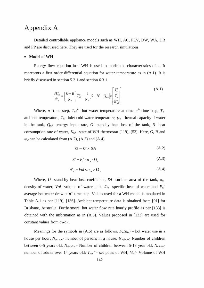
142

Appendix A

Detailed controllable appliance models such as WH, AC, PEV, DW, WA, DR

and PP are discussed here. They are used for the research simulations.

Model of WH

Energy flow equation in a WH is used to model the characteristics of it. It

represents a first order differential equation for water temperature as in (A.1). It is

briefly discussed in section 5.2.1 and section 6.3.1.

n

wh

in

n

a

wh

n

w

n

wh

wn

n

wh

K

T

T

QBGTBG

dt

dT

1.

(A.1)

Where, n- time step, Twhn- hot water temperature at time n

th time step, Ta-

ambient temperature, Tin- inlet cold water temperature, ψw- thermal capacity if water

in the tank, Qwh- energy input rate, G- standby heat loss of the tank, B- heat

consumption rate of water, Kwh- state of WH thermostat [119], [53]. Here, G, B and

ψw can be calculated from (A.2), (A.3) and (A.4).

SAUG (A.2)

ww

nnwFB (A.3)

www Vol (A.4)

Where, U- stand-by heat loss coefficient, SA- surface area of the tank, σw-

density of water, Vol- volume of water tank, Ωw- specific heat of water and Fwn

average hot water draw at nth time step. Values used for a WH model is tabulated in

Table A.1 as per [119], [136]. Ambient temperature data is obtained from [91] for

Brisbane, Australia. Furthermore, hot water flow rate hourly profile as per [133] is

obtained with the information as in (A.5). Values proposed in [133] are used for

constant values from a1-a13.

Meanings for the symbols in (A.5) are as follows. Fw(nH) – hot water use in a

house per hour; Nperson- number of persons in a house; Ninfants- Number of children

between 0-5 years old; Nchildren- Number of children between 5-13 year old; Nadults-

number of adults over 14 years old; TsetnH

- set point of WH; Vol- Volume of WH

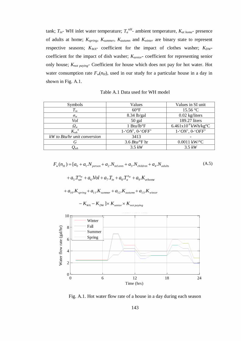
143

tank; Tin- WH inlet water temperature; TanH

- ambient temperature, Kat home- presence

of adults at home; Kspring, Ksummer, Kautumn and Kwinter are binary state to represent

respective seasons; KWA- coefficient for the impact of clothes washer; KDW-

coefficient for the impact of dish washer; Ksenior- coefficient for representing senior

only house; Knot paying- Coefficient for house which does not pay for hot water. Hot

water consumption rate Fw(nH), used in our study for a particular house in a day in

shown in Fig. A.1.

Table A.1 Data used for WH model

Symbols Values Values in SI unit

Tin 60°F 15.56 °C

σw 8.34 lb/gal 0.02 kg/liters

Vol 50 gal 189.27 liters

Ωw 1 Btu/lb°F 6.461x10-4

kWh/kg°C

Kwhn 1-‘ON’, 0-‘OFF’ 1-‘ON’, 0-‘OFF’

kW to Btu/hr unit conversion 3413 -

G 3.6 Btu/°F hr 0.0011 kW/°C

Qwh 3.5 kW 3.5 kW

adultschildrenantspersonHw NaNaNaNaanF ....[)( 43inf210

eat

n

ain

n

set KaTaTaVolaTa HH

hom98765 .....

erwautumnsummerspring KaKaKaKa int13121110 ....

payingnotseniorDWWA KKKK ]

(A.5)

Fig. A.1. Hot water flow rate of a house in a day during each season

0 6 12 18 240

2

4

6

8

10Water Flow rate

Time (hrs)

Wat

er f

low

rat

e (g

al/h

r)

Winter

Fall

Summer

Spring

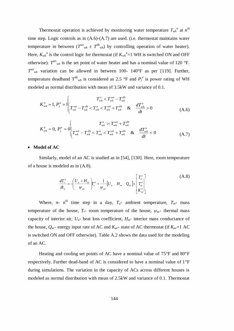
144

Thermostat operation is achieved by monitoring water temperature Twhn at n

th

time step. Logic controls as in (A.6)-(A.7) are used. (i.e. thermostat maintains water

temperature in between (Tset

wh ± Tdb

wh) by controlling operation of water heater).

Here, Kwhn is the control logic for thermostat (if Kwh

n=1 WH is switched ON and OFF

otherwise). Tset

wh is the set point of water heater and has a nominal value of 120 °F.

Tset

wh variation can be allowed in between 100- 140°F as per [119]. Further,

temperature deadband Tdb

wh is considered as 2.5 °F and Pjn is power rating of WH

modeled as normal distribution with mean of 3.5kW and variance of 0.1.

0&

1,1

dt

dTTTTTT

TTT

PK n

whdb

wh

set

wh

n

wh

db

wh

set

wh

db

wh

set

wh

n

whn

j

n

wh

(A.6)

0&

:

0,0

dt

dTTTTTT

TTT

PK n

whdb

wh

set

wh

n

wh

db

wh

set

wh

db

wh

set

wh

n

whn

j

n

wh

(A.7)

Model of AC

Similarly, model of an AC is studied as in [54], [130]. Here, room temperature

of a house is modeled as in (A.8).

n

ac

n

m

n

a

acma

ac

n

r

ac

ma

n

n

r

K

T

T

QHUTHU

dt

dT

1

(A.8)

Where, n- nth

time step in a day, Ta- ambient temperature, Tm- mass

temperature of the house, Tr- room temperature of the house, ψac- thermal mass

capacity of interior air, Ua- heat loss coefficient, Hm- interior mass conductance of

the house, Qac- energy input rate of AC and Kac- state of AC thermostat (if Kac=1 AC

is switched ON and OFF otherwise). Table A.2 shows the data used for the modeling

of an AC.

Heating and cooling set points of AC have a nominal value of 75°F and 80°F

respectively. Further dead-band of AC is considered to have a nominal value of 1°F

during simulations. The variation in the capacity of ACs across different houses is

modeled as normal distribution with mean of 2.5kW and variance of 0.1. Thermostat

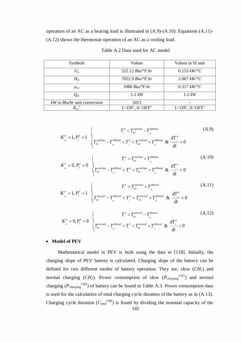
145

operation of an AC as a heating load is illustrated in (A.9)-(A.10). Equations (A.11)-

(A.12) shows the thermostat operation of an AC as a cooling load.

Table A.2 Data used for AC model

Symbols Values Values in SI unit

Ua 522.12 Btu/°F.hr 0.153 kW/°C

Hm 7052.9 Btu/°F.hr 2.067 kW/°C

ψac 1080 Btu/°F.hr 0.317 kW/°C

Qac 1.2 kW 1.2 kW

kW to Btu/hr unit conversion 3413 -

Kacn 1-‘ON’, 0-‘OFF’ 1-‘ON’, 0-‘OFF’

0&

1,1

dt

dTTTTTT

TTT

PK n

heatdbheatset

ac

nheatdbheatset

ac

heatdbheatset

ac

n

n

j

n

r

acrac

acr

ac

(A.9)

0&

0,0

dt

dTTTTTT

TTT

PK n

heatdbheatset

ac

nheatdbheatset

ac

heatdbheatset

ac

n

n

j

n

r

acrac

acr

ac

(A.10)

0&

1,1

dt

dTTTTTT

TTT

PK n

cooldbcoolset

ac

ncooldbcoolset

ac

cooldbcoolset

ac

n

n

j

n

r

acrac

acr

ac

(A.11)

0&

0,0

dt

dTTTTTT

TTT

PK n

cooldbcoolset

ac

ncooldbcoolset

ac

cooldbcoolset

ac

n

n

j

n

r

acrac

acr

ac

(A.12)

Model of PEV

Mathematical model in PEV is built using the data in [118]. Initially, the

charging slope of PEV battery is calculated. Charging slope of the battery can be

defined for two different modes of battery operation. They are, slow (CH1) and

normal charging (CH2). Power consumption of slow (PchargingCH1

) and normal

charging (PchargingCH2

) of battery can be found in Table A.3. Power consumption data

is used for the calculation of total charging cycle duration of the battery as in (A.13).

Charging cycle duration (ГtotalCHk

) is found by dividing the nominal capacity of the

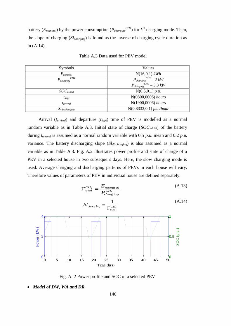
146

battery (Enominal) by the power consumption (PchargingCHk

) for kth charging mode. Then,

the slope of charging (Slcharging) is found as the inverse of charging cycle duration as

in (A.14).

Table A.3 Data used for PEV model

Symbols Values

Enominal N(16,0.1) kWh

PchargingCHk

PchargingCH1

– 2 kW

PchargingCH2

– 3.3 kW

SOCinitial N(0.5,0.1) p.u.

tdept N(0800,0006) hours

tarrival N(1900,0006) hours

Sldischarging N(0.3333,0.1) p.u./hour

Arrival (tarrival) and departure (tdept) time of PEV is modelled as a normal

random variable as in Table A.3. Initial state of charge (SOCinitial) of the battery

during tarrival is assumed as a normal random variable with 0.5 p.u. mean and 0.2 p.u.

variance. The battery discharging slope (Sldischarging) is also assumed as a normal

variable as in Table A.3. Fig. A.2 illustrates power profile and state of charge of a

PEV in a selected house in two subsequent days. Here, the slow charging mode is

used. Average charging and discharging patterns of PEVs in each house will vary.

Therefore values of parameters of PEV in individual house are defined separately.

k

k

CH

ingch

alnoCH

totalP

E

arg

min (A.13)

kCH

total

ingchSl

1

arg (A.14)

Fig. A. 2 Power profile and SOC of a selected PEV

Model of DW, WA and DR

0 5 10 15 20 25 30 35 40 45 500

2

4

Po

wer

(k

W)

0 5 10 15 20 25 30 35 40 45 500

0.5

1

SO

C (

p.u

.)

Time (hrs)

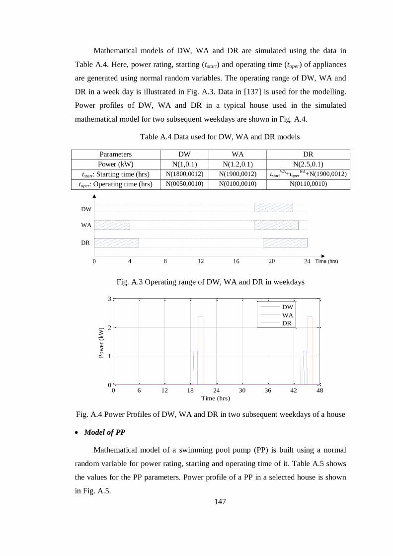
147

Mathematical models of DW, WA and DR are simulated using the data in

Table A.4. Here, power rating, starting (tstart) and operating time (toper) of appliances

are generated using normal random variables. The operating range of DW, WA and

DR in a week day is illustrated in Fig. A.3. Data in [137] is used for the modelling.

Power profiles of DW, WA and DR in a typical house used in the simulated

mathematical model for two subsequent weekdays are shown in Fig. A.4.

Table A.4 Data used for DW, WA and DR models

Parameters DW WA DR

Power (kW) N(1,0.1) N(1.2,0.1) N(2.5,0.1)

tstart: Starting time (hrs) N(1800,0012) N(1900,0012) tstartWA+toper

WA+N(1900,0012)

toper: Operating time (hrs) N(0050,0010) N(0100,0010) N(0110,0010)

0 4 8 12 16 20 24

DR

WA

DW

Time (hrs)

Fig. A.3 Operating range of DW, WA and DR in weekdays

Fig. A.4 Power Profiles of DW, WA and DR in two subsequent weekdays of a house

Model of PP

Mathematical model of a swimming pool pump (PP) is built using a normal

random variable for power rating, starting and operating time of it. Table A.5 shows

the values for the PP parameters. Power profile of a PP in a selected house is shown

in Fig. A.5.

0 6 12 18 24 30 36 42 480

1

2

3

Time (hrs)

Pow

er (

kW

)

DW

WA

DR

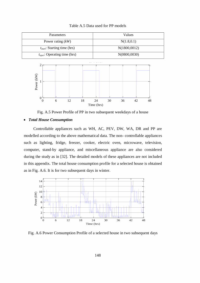
148

Table A.5 Data used for PP models

Parameters Values

Power rating (kW) N(1.8,0.1)

tstart: Starting time (hrs) N(1800,0012)

toper: Operating time (hrs) N(0800,0030)

Fig. A.5 Power Profile of PP in two subsequent weekdays of a house

Total House Consumption

Controllable appliances such as WH, AC, PEV, DW, WA, DR and PP are

modelled according to the above mathematical data. The non- controllable appliances

such as lighting, fridge, freezer, cooker, electric oven, microwave, television,

computer, stand-by appliance, and miscellaneous appliance are also considered

during the study as in [32]. The detailed models of these appliances are not included

in this appendix. The total house consumption profile for a selected house is obtained

as in Fig. A.6. It is for two subsequent days in winter.

Fig. A.6 Power Consumption Profile of a selected house in two subsequent days

0 6 12 18 24 30 36 42 480

1

2SP Power

Time (hrs)

Pow

er (

kW

)

0 6 12 18 24 30 36 42 480

2

4

6

8

10

12

14

House power consumption with and without control

Time (hrs)

Pow

er (

kW)

149

Appendix B

Three Phase Load flow program

Three phase load flow program is based on Newton Raphson algorithm. It

solves a three phase nonlinear load flow problem assuming the loads are considered

as constant power sinks in a specific unbalanced state. It is also assumed that the

system contains only PQ buses and a slack bus. The mismatch equations and the

Jacobian matrix for the load buses are derived separately for all three phases. The

three phase Y- bus matrix is simplified to a 3Nx3N matrix using Kron’s reduction

[134], where n is the number of buses. Instantaneous voltage values are calculated

according to the time varying power values at each node/ house. The per- unit

complex power for pth

phase at bus bar k at all nodes n is given by equation (B.1).

n

i m

m

i

pm

ki

p

k

p

k

p

k

p

k VYVIVS1

3

1

** )()( (B.1)

Here, Y represents the admittance matrix and the negative sign indicates that

the total current is entering the network. This proposed method is better for a

distribution system due to large voltage angles and non-convergence problems in.

The derived mismatch equations for the load buses are (B.2) and (B.3).

n

i m

m

i

p

k

pm

ki

m

i

p

k

pm

ki

m

i

p

k

p

k

p

k BGVVPP1

3

1

)sin()cos( (B.2)

n

i m

m

i

p

k

pm

ki

m

i

p

k

pm

ki

m

i

p

k

p

k

p

k BGVVQQ1

3

1

)}cos()sin( (B.3)

A Jacobian matrix(J) for a 3- phase system is derived with matrix blocks of

6x6 with diagonal and off- diagonal block elements following the similar pattern as

in [135]. The above mismatch equations are used to form a 6Nx6N Jacobian matrix.

The mismatch quantities ( M ) and J is used to form incremental voltage quantities

V as in (B.4). Iterative procedure is used to achieve convergence and the voltages

are updated as in (B.5). The form of M and V are given in (B.6) and (B.7).

VJM (B.4)

VVV (B.5)

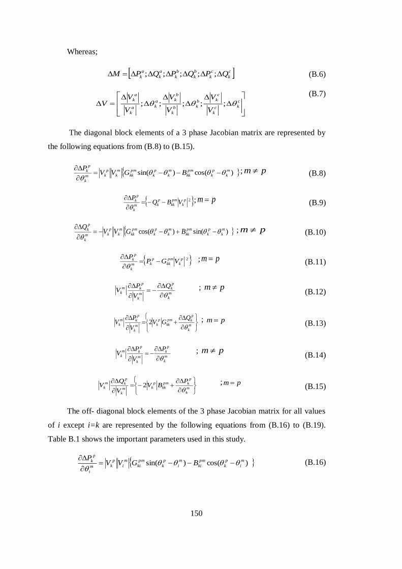
150

Whereas;

c

k

c

k

b

k

b

k

a

k

a

k QPQPQPM ;;;;; (B.6)

c

kc

k

c

kb

kb

k

b

ka

ka

k

a

k

V

V

V

V

V

VV ;;;;;

(B.7)

The diagonal block elements of a 3 phase Jacobian matrix are represented by

the following equations from (B.8) to (B.15).

)cos()sin( m

k

p

k

pm

kk

m

k

p

k

pm

kk

m

k

p

km

k

p

k BGVVP

; pm (B.8)

2p

k

pm

kk

p

km

k

p

k VBQP

; pm (B.9)

)sin()cos( m

k

p

k

pm

kk

m

k

p

k

pm

kk

m

k

p

km

k

p

k BGVVQ

; pm (B.10)

2p

k

pm

kk

p

km

k

p

k VGPP

; pm (B.11)

m

k

p

k

m

k

p

km

k

Q

V

PV

; pm (B.12)

m

k

p

kpm

kk

p

km

k

p

km

k

QGV

V

PV

2 ; pm

(B.13)

m

k

p

k

m

k

p

km

k

P

V

PV

; pm (B.14)

m

k

p

kpm

kk

p

km

k

p

km

k

PBV

V

QV

2 ; pm

(B.15)

The off- diagonal block elements of the 3 phase Jacobian matrix for all values

of i except i=k are represented by the following equations from (B.16) to (B.19).

Table B.1 shows the important parameters used in this study.

)cos()sin( m

i

p

k

pm

ki

m

i

p

k

pm

ki

m

i

p

km

i

p

k BGVVP

(B.16)

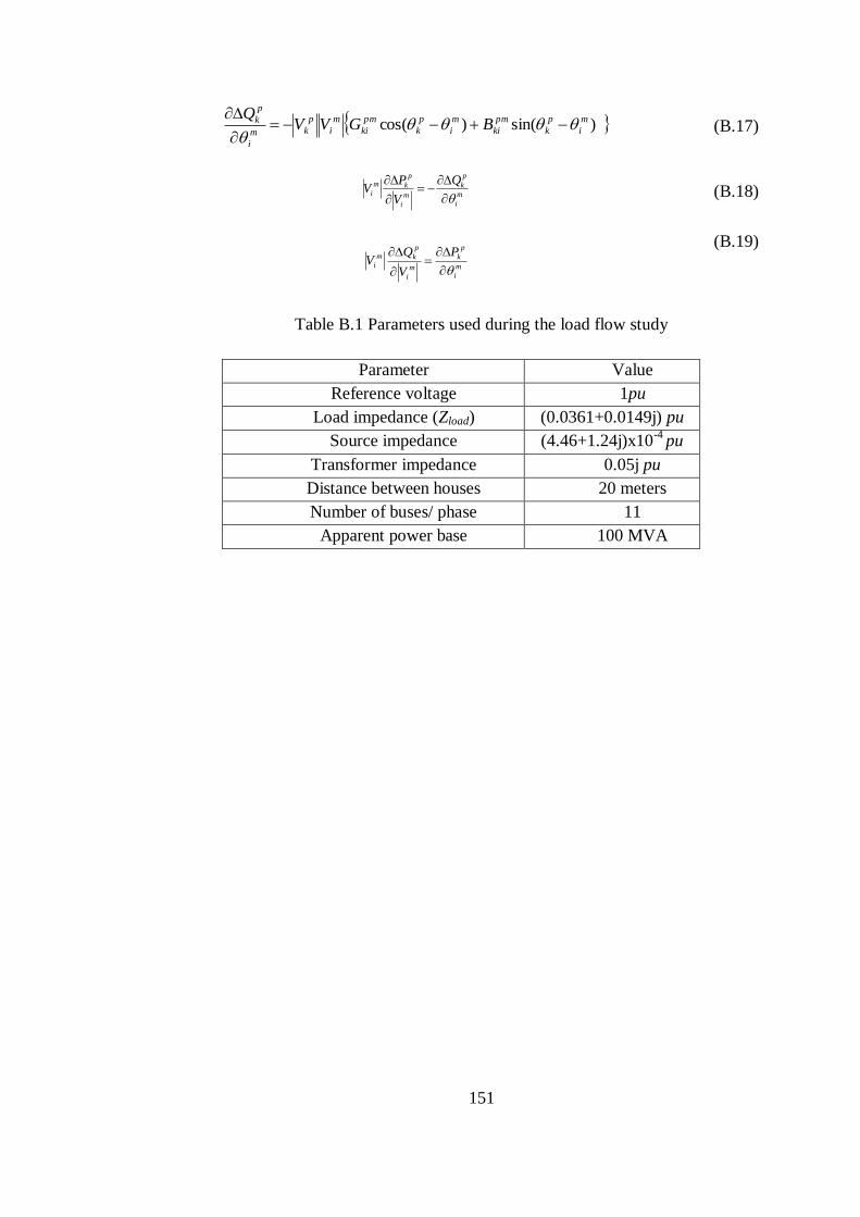
151

)sin()cos( m

i

p

k

pm

ki

m

i

p

k

pm

ki

m

i

p

km

i

p

k BGVVQ

(B.17)

m

i

p

k

m

i

p

km

i

Q

V

PV

(B.18)

m

i

p

k

m

i

p

km

i

P

V

QV

(B.19)

Table B.1 Parameters used during the load flow study

Parameter Value

Reference voltage 1pu

Load impedance (Zload) (0.0361+0.0149j) pu

Source impedance (4.46+1.24j)x10-4

pu

Transformer impedance 0.05j pu

Distance between houses 20 meters

Number of buses/ phase 11

Apparent power base 100 MVA

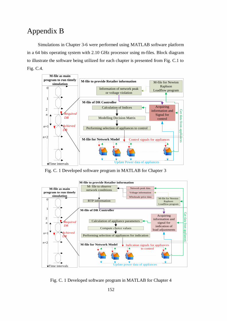
152

Appendix B

Simulations in Chapter 3-6 were performed using MATLAB software platform

in a 64 bits operating system with 2.10 GHz processor using m-files. Block diagram

to illustrate the software being utilized for each chapter is presented from Fig. C.1 to

Fig. C.4.

M-file to provide Retailer information

M-file of DR Controller

M-file for Network Model

Information of network peak

or voltage violation

Update Power data of appliances

Modelling Decision Matrix

Performing selection of appliances to control

Calculation of Indices

Control signals for appliances

Get d

ata from

app

liances

0

1

2

Time intervals

n

n+1

n+2

Achieved

DR

Acquiring

information and

Signal for

control

M-file as main

program to run timely

simulationM-file for Newton

Raphson

Loadflow program

Required

DR

Fig. C. 1 Developed software program in MATLAB for Chapter 3


M-file of DR Controller


RTP information

Update power data of appliances

Compute choice values

Performing selection of appliances for indication

Calculation of appliance parameters

Indication signals for appliances

to control

Get data from

appliances

0

1

2

Time intervals

n

n+1

n+2

Achieved

DR

Acquiring

information and

signal for

indication of

load adjustments

M-file as main


simulationM-file for Newton

Raphson

Loadflow program

Required

DR

M- file to observe

network conditionsVoltage information

Wholesale price data

Network peak data


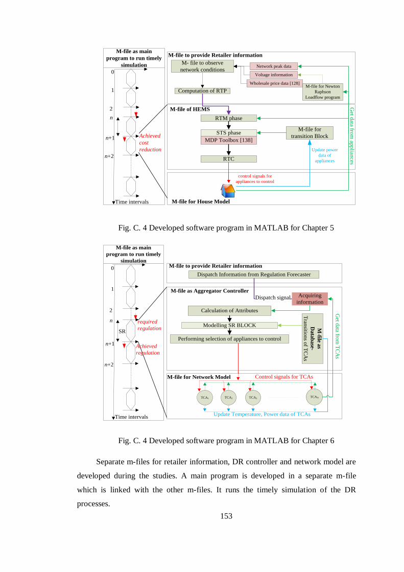
153


M-file of HEMS

M-file for House Model

Computation of RTP

Update power

data of

appliances

STS phase

RTC

RTM phase

control signals for

appliances to control

Get d

ata from

app

liances

0

1

2

Time intervals

n

n+1

n+2

Achieved

cost

reduction

M-file as main


simulation

M-file for Newton

Raphson

Loadflow program

M- file to observe

network conditionsVoltage information

Wholesale price data [128]

Network peak data

M-file for

transition BlockMDP Toolbox [138]



M-file as Aggregator Controller


Dispatch Information from Regulation Forecaster

TCANTCA3TCA2

Update Temperature, Power data of TCAs

Modelling SR BLOCK M-file a

s

Da

tab

ase-

Tran

sition

s of T

CA

s

Performing selection of appliances to control

TCA1

Dispatch signal

Calculation of Attributes

Control signals for TCAs

Get d

ata from

TC

As

0

1

2

Time intervals

n

n+1

n+2

Achieved

regulation

SR

Acquiring

information

M-file as main


simulation

required

regulation


Separate m-files for retailer information, DR controller and network model are

developed during the studies. A main program is developed in a separate m-file

which is linked with the other m-files. It runs the timely simulation of the DR

processes.

154

BIBLIOGRAPHY

[1] R. Weron, “Complex Electricity Market,” in Modelling and forecasting

electricity loads and prices: A statistical Approach, 1st ed. vol. 1, John Wiley

and Sons Ltd Ed., England: 2006, pp. 1-23.

[2] T. Dang, R. Cheramy, "Impacts of electricity market liberalization on

centralized generation and telecontrol infrastructure," in Proceedings of 2006

IEEE International Conference on Industrial Informatics, Singapore, Aug.

2006, pp. 955-959.

[3] International Energy Agency, “Electricity Market Liberalization has delivered

long term benefits,” in Energy Market Experience, 1st ed. vol. 1, IEA. Ed.,

Paris, France, 2005, pp. 31–44.

[4] M. Heddenhausen, “Privatizations in Europe’s liberalized electricity markets-

the cases of the United Kingdom, Sweden, Germany, and France,” Research

Unit EU Integration, German Institute for International and Security Affairs,

Berlin, Tech. Rep. CIT5-CT-2005-028647, Dec. 2007.

[5] C. W. Tsai, A. Pelov, M. C. Chiang, C. S. Yang, T.P. Hong, "A Brief

Introduction to Classification for Smart Grid," in Proceedings of 2013 IEEE

International Conference on Man, and Cybernetics (SMC), Oct. 2013,

Manchester, UK, pp. 2905-2909.

[6] V. C. Gungor, D. Sahin, T. Kocak, S. Ergut, C. Buccella, C. Cecati, G. P.

Hancke, "A Survey on Smart Grid Potential Applications and Communication

Requirements," IEEE Transaction on Industrial Informatics, vol. 9, no. 1,

pp.28-42, Feb. 2013.

[7] Y. Yan, Y. Qian, H. Sharif, D. Tipper, "A Survey on Smart Grid

Communication Infrastructures: Motivations, Requirements and

Challenges," IEEE Communications Surveys & Tutorials, vol. 15, no. 1, pp.5-

20, Apr. 2013.

[8] F. Xi, M. Satyajayant, X. Guoliang, Y. Dejun, "Smart Grid — The New and

Improved Power Grid: A Survey," IEEE Communications Surveys & Tutorials,

vol. 14, no. 4, pp. 944-980, Dec. 2012.

[9] Heart Electronic Products, (2013), “FPGA enhance smart grid design,”

[Online], Available:

http://www.electronicproducts.com/Digital_ICs/Standard_and_Programmable_

Logic/FPGAs_enhance_smart_grid_equipment_design.aspx

[10] Z. Fan, P. Kulkarni, S. Gormus, C. Efthymiou, G. Kalogridis, M.

Sooriyabandara, Z. Ziming, S. Lambotharan, W.H. Chin, "Smart Grid

Communications: Overview of Research Challenges, Solutions, and

Standardization Activities," IEEE Communications Surveys & Tutorials, vol.

15, no. 1, pp. 21-38, Mar. 2013.

[11] U. S. Department of Energy, “Benefits of Demand Response in Electricity

Markets and Recommendations for Achieving them,” United Stated Congress,

USA, Tech. Rep. 1252, Feb. 2006.

[12] Z. Zhou, F. Zhao, J. Wang, "Agent-Based Electricity Market Simulation with

Demand Response from Commercial Buildings," IEEE Transaction on Smart

Grid, vol. 2, no. 4, pp. 580-588, Dec. 2011.

155

[13] S. Mohagheghi, N. Raji, "Managing Industrial Energy Intelligently: Demand

Response Scheme," IEEE Industry Applications Magazine, vol. 20, no. 2, pp.

53-62, Mar. 2014.

[14] D. Menniti, A. Pinnarelli, N. Sorrentino, A. Burgio, G. Brusco, "Demand

response program implementation in an energy district of domestic

prosumers,” in Proceedings of 2013 IEEE International Conference on

AFRICON, Sep. 2013, pp. 1-7.

[15] G. A. Taylor, M. R. Irving, N. Nusrat, R. Liao, S. Panchadcharam, "Smart

distribution network operation: Emerging techniques and standards,"

in Proceedings of 2011 IEEE Power and Energy Society General Meeting, Jul.

2011, pp. 1-6.

[16] J. DongLi, M. Xiaoli, S. Xiaohui, "Study on technology system of self-healing

control in smart distribution grid," in Proceedings of 2011 IEEE International

Conference on Advanced Power System Automation and Protection (APAP),

Oct. 2011, pp. 26-30.

[17] Y. G. Yohanis, D. M. Jayanta, A. Wright, B. Norton, “Real-life energy use in

the UK: How occupancy and dwelling characteristics affect domestic

electricity use,” Elvester Transaction on Energy and Buildings,. vol. 40, no. 6,

pp. 1053-1059, Jan. 2008.

[18] A. Ipakchi, F. Albuyeh, “Grid of the Future,” IEEE Power and Engineering

Magazine, vol. 7, no. 2, pp. 52- 62, Mar. 2009.

[19] P. S. Moses, M. A. S. Masoum, S. Hajforoosh, "Overloading of distribution

transformers in smart grid due to uncoordinated charging of plug-In electric

vehicles," in Proceedings of 2012 IEEE International Conference on 2012

IEEE Innovative Smart Grid Technologies (ISGT), Washington DC, USA, Jan.

2012, pp. 1-6.

[20] A. Gomes, C. H. Antunes, G. A. Martins, “A multiple objective evolutionary

approach for the design and selection of load control strategies,” IEEE

Transaction on Power System, vol. 19, no. 2, pp. 1173–1180, May 2004.

[21] A. Gomes, C. H. Antunes, G. A. Martins, “A multiple objective approach to

direct load control using an interactive evolutionary algorithm,” IEEE

Transaction on Power System, vol. 22, no. 3, pp. 1004–1011, Aug. 2007.

[22] N. Ruiz, I. Cobelo, J. Oyarzabal, “A direct load control model for virtual power

plant management,” IEEE Transaction on Power System, vol. 24, no. 2, pp.

959–966, May 2009.

[23] W. A. Qureshi, N.K.C. Nair, M.M. Farid, “Demand Side Management through

efficient thermal energy storage using phase change material,” in Proceedings

of Australian 2008 IEEE Power Engineering Conference (AUPEC), Dec. 2008,

pp. 1-6.

[24] Y. Y. Hsu, “Design and Implementation of an Air-Conditioning System with

Storage Tank for Load Shifting,” IEEE Transaction on Power Systems, vol. 2,

no. 4, pp. 973-979, Nov. 1987.

[25] C. C. Min, J. Tai-Lang, H. Yue-Wei. “Mitigating DLC Constraints of Air-

conditioning Loads Using a group-DLC Method,” in Proceedings of 2007

IEEE Power Engineering Society General Meeting, Tampa FL, USA, Jun.

2007, pp. 1-6.

[26] T. Xidong, X. Zhang, B. Koch, D. Frisch, “Modeling and estimation of

Nickel Metal Hydride battery hysteresis for SOC estimation,” in Proceedings

156

of 2008 IEEE International Conference on Prognostics and Health

Management, Denver CO, USA, Oct. 2008, pp. 1-12.

[27] Y. Ota, H. Taniguchi, T. Nakajima, K. M. Liyanage, J. Baba, A.

Yokoyama, “Autonomous distributed V2G (vehicle-to-grid) considering

charging request and battery condition,” in Proceedings of 2010 IEEE

Innovative Smart Grid Technologies Conference Europe (ISGT Europe),

Gothenburg, Sweden, Oct. 2010, pp. 1-6.

[28] H. Yuan-Yih, S. C. Ching, “Dispatch of direct load control using dynamic

programming,” IEEE Transaction on Power Systems, vol. 6, no. 3, pp. 1056-

1061, Aug. 1991.

[29] K. Bhattacharyya, M.L. Crow, “A fuzzy logic based approach to direct load

control,” IEEE Transaction on Power Systems, vol. 11, no. 2, pp. 708-714,

May 1996.

[30] H. Salehfar, A. D. Patton, “A production costing methodology for evaluation of

direct load control,” IEEE Transaction on Power Systems, vol. 6, no. 1, pp.

278-284, Feb. 1991.

[31] K. H. Ng, G. B. Sheble, “Direct load control-A profit-based load management

using linear programming. IEEE Transaction on Power Systems, vol. 13, no. 2,

pp. 688-694, May 1998.

[32] F. Shahnia, M. T. Wishart, A. Ghosh, G. Ledwich, F. Zare, "Smart demand

side management of low-voltage distribution networks using multi-objective

decision making," IET Transaction on Generation, Transmission &

Distribution, vol. 6, no. 10, pp. 968-1000, Oct. 2012.

[33] A. S. Masoum, S. Deilami, P. S. Moses, M. A. S. Masoum, A. Abu-Siada,

"Smart load management of plug-in electric vehicles in distribution and

residential networks with charging stations for peak shaving and loss

minimisation considering voltage regulation," IET Transaction on Generation,

Transmission & Distribution, vol. 5, no. 8, pp. 877-888, Aug. 2011.

[34] S. Deilami, A. S. Masoum, P. S. Moses, M. A. S. Masoum, "Voltage profile

and THD distortion of residential network with high penetration of Plug-in

Electrical Vehicles," in Proceedings of 2010 IEEE International Conference on

Innovative Smart Grid Technologies (ISGT Europe), Gothenburg, Sweden,

Oct. 2010, pp. 1-6.

[35] A. G. Madureira, J. A. P. Lopes, "Coordinated voltage support in distribution

networks with distributed generation and microgrids," IET Transaction on

Renewable Power Generation, vol. 3, pp. 439-454, Dec. 2009.

[36] Q. Zhang, J. Li, "Demand response in electricity markets: A review,"

in proceedings of 2012 IEEE International Conference on European Energy

Market (EEM), Florence, Italy, May. 2012, pp. 1-8.

[37] Electricity Market and Policy Group. (2004). Industrial and Commercial

Customer Response to Real-Time Electricity Prices. [Online]. Available:

http://emp.lbl.gov/publications/industrial-and-commercial-customer-response-

real-time-electricity-prices

[38] The National Bureau of Economic Research. (2009). Electricity Pricing that

Reflects Its Real-Time Cost. [Online]. Available:

http://www.nber.org/reporter/2009number1/borenstein.html

[39] G. Barbose, C. Goldman, B. Neenan, Lawrence Berkeley National Laboratory:

(2004, Dec.,). A survey of utility experience with real-time pricing. [Online].

Available: http://eetd.lbl.gov/ea/EMS/reports/54238.pdf.

http://emp.lbl.gov/publications/industrial-and-commercial-customer-response-real-time-electricity-prices

http://emp.lbl.gov/publications/industrial-and-commercial-customer-response-real-time-electricity-prices

http://www.nber.org/reporter/2009number1/borenstein.html

http://eetd.lbl.gov/ea/EMS/reports/54238.pdf

157

[40] A. H. Mohsenian-Rad, A. Leon-Garcia "Optimal Residential Load Control

With Price Prediction in Real-Time Electricity Pricing Environments," IEEE

Transaction on Smart Grid, vol. 1, no. 2, pp. 120-133, Sep. 2010.

[41] O. Dalkilic, A. Eryilmaz, L. Xiaojun "Stable real-time pricing and scheduling

for serving opportunistic users with deferrable loads," in Proceedings of 2013

IEEE International Conference on Communication, Control, and Computing

(Allerton), Monticello IL, USA, Oct. 2013, pp.1200-1207.

[42] S. Widergren, C. Marinovici, T. Berliner, A. Graves, "Real-time pricing

demand response in operations," in Proceedings of 2012 IEEE Power and

Energy Society General Meeting, Jul. 2012, pp.1-5.

[43] J. H. Yoon, R. Baldick, A. Novoselac, "Dynamic Demand Response Controller

Based on Real-Time Retail Price for Residential Buildings," IEEE Transaction

on Smart Grid, vol. 5, no. 1, pp. 121-129, Jan. 2014.

[44] M. A. A. Pedrasa, T. D. Spooner, I. F. MacGill, "Coordinated scheduling of

residential distributed energy resources to optimize smart home energy

services," IEEE Transaction on Smart Grid, vol. 1, no. 2, pp. 134-143, Sept.

2010.

[45] Z. Zhao, W. C. Lee, Y. Shin, K.-B. Song, "An optimal power scheduling

method for demand response in home energy management system," IEEE

Transaction on Smart Grid, vol. 4, no. 3, pp. 1391-1400, Sept. 2013.

[46] A. H. Mohsenian-Rad, A. Leon-Garcia, "Optimal Residential Load Control

With Price Prediction in Real-Time Electricity Pricing Environments," IEEE

Transaction on Smart Grid, vol. 1, no. 2, pp. 120-133, Sept. 2010.

[47] T. Hubert, S. Grijalva, "Modeling for residential electricity optimization in

dynamic pricing environments," IEEE Transaction on Smart Grid, vol. 3, no.

4, pp. 2224-2231, Dec. 2012.

[48] Z. Yu, L. Jia, M. C. Mrphy-Hoye, A. Pratt, L. Tong, "Modeling and Stochastic

Control for Home Energy Management," IEEE Transaction on Smart Grid,

vol. 4, no. 4, pp. 2244-2255, Dec. 2013.

[49] Z. Chen, L. Wu, Y. Fu, "Real-time price based demand response management

for residential appliances via stochastic optimization and robust optimization,"

IEEE Transaction on Smart Grid, vol. 3, no. 4, pp. 1822-1831, Dec. 2012.

[50] T. T. Kim, H. V. Poor, "Scheduling power consumption with price

uncertainty," IEEE Transaction on Smart Grid, vol. 2, no. 3, pp. 519-527, Sep.

2011.

[51] T. H. Chang, M. Alizadeh, A. Scaglione, "Real-Time Power Balancing Via

Decentralized Coordinated Home Energy Scheduling," IEEE Transaction on

Smart Grid, vol. 4, no. 3, pp. 1490-1504, Sep. 2013.

[52] C. Diduch, S. Mostafa, E. Rachid, M. E. Kaye, J. Meng, C. Liuchen,

"Aggregated domestic electric water heater control - building on smart grid

infrastructure," in Proceedings of 2012 IEEE 7th International conference on

IPEMC, Harbin, China, Jun. 2012, pp. 128-135.

[53] J. Kondoh, L. Ning, D. J. Hammerstrom, "An Evaluation of the Water Heater

Load Potential for Providing Regulation Service," IEEE Transaction on Power

System, vol. 26, no. 3, pp. 1309-1316, Aug. 2011.

[54] N. Lu, Y. Zhang, "Design Considerations of a Centralized Load Controller

Using Thermostatically Controlled Appliances for Continuous Regulation

Reserves," IEEE Transaction on Smart Grid, vol. 4, no. 2, pp. 914-921, Jun.

2013.

158

[55] E. Vrettos, S. Koch, G. Andersson, "Load frequency control by aggregations of

thermally stratified electric water heaters," in Proceedings of 2012 IEEE 3rd

PES International Conference and Exhibition on Innovative Smart Grid

Technologies (ISGT Europe), Oct. 2012, pp. 1-8.

[56] B. Ramanathan, V. Vittal, “A Framework for Evaluation of Advanced Direct

Load Control With Minimum Disruption,” IEEE Transaction on Power

System, vol. 23, no. 4, pp. 1681–1688, Nov. 2008.

[57] A. Khodaei, M. Shahidehpour, S. Bahramirad, “SCUC With Hourly Demand

Response Considering Intertemporal Load Characteristics,” IEEE Transaction

on Smart Grid, vol. 2, no. 3, pp. 564-571, Sept. 2011.

[58] Z. Zhou, F. Zhao, J. Wang, "Agent-Based Electricity Market Simulation With

Demand Response From Commercial Buildings," IEEE Transaction on Smart

Grid, vol. 2, no. 4, pp. 580-588, Dec. 2011.

[59] G. Naraghi, A. Javadian, “Logarithmic Real- Time Pricing Programs Modeling

for Eectricity Customers”, Journal on Basic and Applied Scientific Research,

vol. 1, no. 10, pp. 1563-1568, Dec. 2011.

[60] S. G. Stephen, B. Josh, S. Josh, H. Sam, “2010 California statewide Non-

residential Critical Peak Pricing evaluation,” Freeman, Sullivan & Co., San

Francisco, Tech. Rep. SCE0297, Apr. 2011.

[61] H. Allcott, “Real-time Pricing and Electricity Markets,” Harward University,

Cambridge, Tech. rep., Feb. 2009.

[62] P. Du, N. Lu, “Appliance Commitment for Household Load Scheduling,” IEEE

Transaction on Smart Grid, vol. 2, no. 2, pp. 411-419, Jun 2011.

[63] N. Gatsis, G. B. Giannakis, “Residential Load Control: Distributed Scheduling

and Convergence with Lost AMI Messages,” IEEE Transaction on Smart Grid,

vol. 3, no. 2, pp. 770-786, Jun. 2012.

[64] K. H. Ng, G. B. Sheble, “Direct load control-A profit-based load management

using linear programming,” IEEE Transaction on Power System, vol. 3, no. 2,

pp. 688-694, Jun 2008.

[65] California ISO. (2003). Summer Assessment. [online]. Available:

http://www.caiso.com

[66] F. A. Wolak, “Residential customer response to real-time pricing: The

Anaheim Critical peak pricing experiment,” Department of Economics,

Stanford University, Stanford, Tech. rep., May 2006.

[67] H. Zhong, L. Xie, Q. Xia, "Coupon Incentive-Based Demand Response:

Theory and Case Study," IEEE Transaction on Power Systems, vol. 28, no. 2,

pp. 1266-1276, May 2013.

[68] K. Bhattacharyya, M. L. Crow, "A fuzzy logic based approach to direct load

control” IEEE Transaction on Power Syst., vol. 11, no. 2, pp. 708-714, May

1996.

[69] Z. Fan, "A Distributed Demand Response Algorithm and Its Application to

PHEV Charging in Smart Grids," IEEE Transaction on Smart Grid, vol. 3, no.

3, pp. 1280-1290, Sep. 2012.

[70] P. Richardson, D. Flynn, A. Keane, “Local Versus Centralized Charging

Strategies for Electric Vehicles in Low Voltage Distribution Systems,” IEEE

Transaction on Smart Grid, vol. 3, no. 2, pp. 1020-1028, Jun 2012.

[71] S. Shengnan, M. Pipattanasomporn, S. Rahman, “Grid Integration of Electric

Vehicles and Demand Response With Customer Choice,” IEEE Transaction on

Smart Grid, vol. 3, no. 1, pp. 543-550, Mar 2012.

159

[72] P. Yi, X. Dong, A. Iwayemi, C. Zhou, S. Li, "Real-Time Opportunistic

Scheduling for Residential Demand Response," IEEE Transaction on Smart

Grid, vol. 4, no. 1, pp. 227-234, Mar. 2013.

[73] A. G. Madureira, J. A. P. Lopes, “Coordinated voltage support in distribution

networks with distributed generation and microgrids,” IET Transaction on

Renewables and Power Generation, vol. 3, no. 4, pp. 439-454, Dec. 2009.

[74] S. Shao, M. Pipattanasomporn, S. Rahman, "An approach for demand response

to alleviate power system stress conditions," in proceedings of 2011 IEEE

Power and Energy General Meeting, Jul. 2011, pp. 1-7.

[75] T. Logenthiran, D. Srinivasan, T. Z Shun, "Demand Side Management in

Smart Grid Using Heuristic Optimization,", IEEE Transaction on Smart Grid,

vol. 3, no. 3, pp. 1244-1252, Sep. 2012.

[76] J. V. Paatero, P. D. Lund, "A model for generating household electricity load

profiles," International Journal on Energy Research, vol. 30, no. 5, pp. 273–

290, Apr. 2006.

[77] R Herman, S.W. Heunis, "Load models for mixed–class domestic and fixed,

constant power loads for use in probabilistic LV feeder analysis," Transaction

on Electric Power Systems Research, vol. 66, no. 2, pp. 149–153, Aug. 2003.

[78] D. S. R. Ferreira, L. A. Barroso, P. R. Lino, M. M. Carvalho, P. Valenzuela,

"Time-of-Use Tariff Design Under Uncertainty in Price-Elasticities of

Electricity Demand: A Stochastic Optimization Approach," IEEE Transaction

on Smart Grid, vol. 4, no. 4, pp.2285-2295, Dec. 2013.

[79] Y Mishra, Z. Y. Dong, J. Ma, D. J. Hill, “Induction model load impact on

power system eigenvalue sensitivity analysis”, IET Transaction on Generation,

Transmission and Distribution, vol. 3, no. 7, pp. 690-700, Jul. 2009.

[80] P. Juanuwattanakul, M. A. S. Masoum, "Analysis and comparison of bus

ranking indices for balanced and unbalanced three-phase distribution

networks," in Proceedings of 2011 IEEE 21st International Conference on

Australian Universities Power Engineering Conference (AUPEC), Sep. 2011,

pp. 1-5.

[81] R. G. Wasley, M. A. Shlash, "Newton-Raphson algorithm for 3-phase load

flow," Proceedings of the Institution of Electrical Engineers, vol. 121, no. 7,

pp. 630-638, Jul. 1974.

[82] Electrical Connection. (Oct. 2012). When voltage varies. [Online]. Available:

http://electricalconnection.com.au/article/10017796/when-voltage-varies

[83] S. Gass, T. Saaty, “Parametric Objective Function Part II,” Journal on

Operations Research in America, vol. 3, no. 1, pp. 316–319, May 1955.

[84] K. A. Shuaib, “A Performance Evaluation Study of WiMAX Using Qualnet”,

in Proceedings of the World Congress on Engineering (WCE), Jul. 2009, pp. 1-

5.

[85] DTI Distributed Generation Programme (Contractor: EA Technology),

Network Losses and Distributed Generation, Contact Number:

DG/CGI/00038/00/00, URN number: 06/1238; Jan. 2006.

[86] S. Fan, R. Hyndman, “The price elasticity of electricity demand in South

Australia,” Elsevier journal on Energy Policy, vol. 39, no. 1, pp. 3709–3719,

2011.

[87] M. H. Albadi, E. F. E. Saadany, “A summary of demand response in electricity

market,” Transaction on Electric Power System Research, vol. 78, no.11, pp

1989-1996, Apr. 2008.

160

[88] F. M. Andersen, S. G. Jensen, H. V. Larsen, P. Meibom, “Analysis of Demand

Response in Denmark,” Riso National Laboratory, Ea Energy Analysis,

Denmark, Tech. Rep. Riso-R-1565 (EN), Oct. 2006.

[89] Department of Nuclear Engineering and Management. (2007). University of

Tokyo, Investment in Electricity Markets: Equilibrium Price and Supply

Function. [Online]. Available:

http://www.realoptions.org/Academic/takashima.pdf

[90] Origin, (2013). Electricity tariff for residential customers: [Online]. Available:

http://www.originenergy.com.au/2087/Electricity-tariffs-QLD

[91] Weather Underground. (2011). Brisbane weather data. [Online]. Available:

http://www.wunderground.com/history/

[92] Australian Bureau of Statistics. (2009). Average Floor Area of New Residential

Dwellings, [Online]. Available: http://www.abs.gov.au/ausstats/

[93] Energex. (2015). Regulatory Propasal for the Period July 2010-June. [Online].

Available:

http://www.energex.com.au/data/assets/pdf_file/0010/31789/ENERGEX_s_Re

gulatory_Proposal_2010-2015.pdf

[94] T. Facchinetti, D. M. L. Vedova, "Real-Time Modeling for Direct Load

Control in Cyber-Physical Power Systems," IEEE Transaction on Industrial

Informatics, vol. 7, no. 4, pp.689-698, Nov. 2011.

[95] M. P. Sanchez, G. Sanchez, and G. Morales-Espana, “Direct Load Control

Decision Model for Aggregated EV charging points,” IEEE Transaction on

Power Systems, vol. 7, no. 4, pp. 1577- 1584, Aug. 2012.

[96] A. Molina-Garcia, M. Kessler, J. Fuentes, E. Gomez-Lazaro,

“Probabilistic characterization of thermostatically controlled loads to model the

impact of demand response programs,” IEEE Transaction on Power Systems,

vol. 26, pp. 241–251, Feb. 2011.

[97] N Lu “An Evaluation of the HVAC Load Potential for Providing Load

Balancing Service,” IEEE Transaction on Smart Grid, vol. 3, no. 3, Sep. 2012.

[98] O. Corradi, H. Ochsenfeld, H. Madsen, P. Pinson, "Controlling Electricity

Consumption by Forecasting its Response to Varying Prices," IEEE

Transaction on Power Systems, vol. 28, no. 1, pp. 421-429, May. 2012.

[99] P. Yang, G. Tang, A. Nehorai, “A Game-T heoret ic Approach fo r

Opt imalTime-of-Use Electricity Pricing,” IEEE Transaction on Power

Systems, vol. 28, no. 2, pp. 884 - 892 , May 2013.

[100] S. Braithwait, D. Hansen, M. O’Sheasy. (Jul. 2007.). Retail electricity pricing

and rate design in evolving markets. [Online].

Available:http://sites.energetics.com/madri/toolbox/pdfs/background/eei_retail

_elec_pricing.pdf

[101] L. Cai, Z. Chen, B. B. Jensen, "Daily load response model to electricity price

for customers," in Proceedings of 2008 IEEE 43rd

International Conference on

Universities Power Engineering, Padova, Italy, Sep. 2008, pp. 1-5.

[102] B. Mozafari, M. Bashirvand, M. Nikzad, S. Solaymani, "A SCUC-based

approach to determine time-of-use tariffs," in Proceedings of 2012 IEEE 11th

International Conference on Environment and Electrical Engineering

(EEEIC), Venice, May 2012, pp.429-433.

[103] D. Prins. (Feb. 2012). Flexible pricing of electricity for residential and small

business customers. [Online]. Available:http://www.dpi.vic.gov.au/smart-

meters/publications/reports-and-consultations/flexible-pricing-of-electricity

http://www.realoptions.org/Academic/takashima.pdf

http://www.originenergy.com.au/2087/Electricity-tariffs-QLD

http://www.wunderground.com/history/

http://www.abs.gov.au/ausstats/

http://www.energex.com.au/data/assets/pdf_file/0010/31789/ENERGEX_s_Regulatory_Proposal_2010-2015.pdf

http://www.energex.com.au/data/assets/pdf_file/0010/31789/ENERGEX_s_Regulatory_Proposal_2010-2015.pdf

161

[104] J. Y. Joo, S. H. Ahn, Y. T. Yoon, J. W. Choi "Option Valuation Applied to

Implementing Demand Response via Critical Peak Pricing," in Proceedings of

2007 IEEE Power Engineering Society General Meeting, Tampa FL, USA,

Jun. 2007, pp. 1-7.

[105] M. Roozbehanit, M. Rinehart, M. A. Dahleh, S. K. Mitter, D. Obradovic, H.

Mangesius, "Analysis of competitive electricity markets under a new model of

real-time retail pricing," in Proceedings of 2011 IEEE 8th International

Conference on the European Energy Market, Zagreb, Croatia, May 2011,

pp.250-255.

[106] L. P. Qian, Y. J. A. Zhang, H. Jianwei, W. Yuan, "Demand Response

Management via Real-Time Electricity Price Control in Smart Grids," IEEE

Transaction on Selected Areas in Communications, vol. 31, no. 7, pp.1268-

1280, Jul. 2013.

[107] A. H. M. Rad, A. L. Garcia, "Optimal Residential Load Control with Price

Prediction in Real-Time Electricity Pricing Environments," IEEE Transaction

on Smart Grid, vol. 1, no. 2, pp.120-133, Sep. 2010.

[108] Z. Wang, F. Li, "Developing trend of domestic electricity tariffs in Great

Britain," in Proceedings of 2011 2nd IEEE International Conference on PES

Innovative Smart Grid Technologies, Manchester, UK, Dec. 2011, pp.1-5.

[109] R. Mao, V. Julka, “Wireless Broadband Architecture Supporting Advanced

Metering Infrastructure” in Proceedings of 2011 73rd

IEEE International

Conference on Vehicular Technology, Budapest, Hungary, May 2011, pp 1- 13.

[110] G. Gross, F. D. Galiana, "Short-term load forecasting," Proceedings of IEEE,

vol. 75, no. 12, pp. 1558-1573, De. 1987.

[111] AEMO. (2012-2013). Price and Demand: Australian Energy Market Operator.

[Online]. Available: http://www.aemo.com.au/Electricity/Data

[112] E. Celebi, J. D. Fuller, "A Model for Efficient Consumer Pricing Schemes in

Electricity Markets," IEEE Transaction on Power System, vol. 22, no. 1, pp.

60-67, Feb. 2007.

[113] P. Tarasak, "Optimal real-time pricing under load uncertainty based on utility

maximization for smart grid," in Proceedings of 2011 IEEE International

Conference on Smart Grid Communications (SmartGridComm.), Brussels,

Belgium, Oct. 2011, pp. 321-326.

[114] H. Sui, H. Wang, M.-S. Lu, W.-J. Lee, "An AMI System for the deregulated

electricity markets," IEEE Transaction on Industrial Applications, vol. 45, no.

6, pp. 2104-2108, Nov. 2009.

[115] M. Roozbehani, M. A. Dahleh, S. K. Mitter, "Volatility of power grids under

real-time pricing," IEEE Transaction on Power System, vol. 27, no. 4, pp.

1926-1940, Nov. 2012.

[116] K. Samarakoon, J. Ekanayake, N. Jenkins, "Investigation of domestic load

control to provide primary frequency response using smart meters," IEEE

Transaction on Smart Grid, vol. 3, no. 1, pp. 282-292, Mar 2012.

[117] D.-M. Han, J.-H. Lim, "Design and implementation of smart home energy

management systems based on zigbee," IEEE Transaction on Consumer

Electronics, vol. 56, no. 3, pp. 1417,1425, Aug. 2010.

[118] N. Saker, M. Petit, J. C. Vannier, "Electric vehicles charging scenarios

associated to direct load control programs (DLC)," in Proceedings of 2011

IEEE North American Power Symposium (NAPS), Boston MA, USA, Aug.

2011, pp. 1-7.

http://www.aemo.com.au/Electricity/Data

162

[119] K. Elamari, L. A. C. Lopes, "Frequency based control of electric water heaters

in small PV-diesel hybrid mini-grids," in Proceedings of IEEE Canadian

Conference on Electrical and Computer Engineering (CCECE), Montreal QC,

Canada, May. 2012, pp. 1-4.

[120] H. S. Chang, J. Hu, M. C. Fu, S. I. Marcus, “Markov Decision Process”, in

Simulation-Based Algorithms for Markov Decision Processes, 2nd ed., vol. 1,

Springer Ed., London, 2006, pp. 1-229.

[121] P. Dai, M. D. S. Weld, J. Goldsmith. “Topological Value Iteration

Algorithms,” Journal of artificial intelligent research, vol. 42, no.1, pp. 181-

209, Oct. 2011.

[122] K. Samarakoon, J. Ekanayake, N. Jenkins, "Reporting Available Demand

Response," IEEE Transaction on Smart Grid, vol. 4, no. 4, pp. 1842-1851,

Dec. 2013.

[123] K. Christakou, D. C. Tomozei, J. Y. L. Boudec, M. Paolone, "GECN: Primary

Voltage Control for Active Distribution Networks via Real-Time Demand-

Response," IEEE Transaction on Smart Grid, vol. 5, no. 2, pp. 622-631, Mar.

2014.

[124] Z. Chen, L. Wu, Y. Fu, "Real-Time Price-Based Demand Response

Management for Residential Appliances via Stochastic Optimization and

Robust Optimization," IEEE Transaction on Smart Grid, vol. 3, no. 4, pp.

1822-1831, Dec. 2012.

[125] C. Vivekananthan, Y. Mishra, G. Ledwich, F. Li, “Demand Response for

Residential Appliances via Customer Reward Scheme”, ," IEEE Transaction

on Smart Grid, vol. 5, no. 2, pp. 809-820, Mar. 2014.

[126] L. Ning, D. J. Hammerstrom, "Design Considerations for Frequency

Responsive Grid FriendlyTM

Appliances," in Proceedings of 2005/2006 IEEE

PES International Conference and Exhibition on Transmission and

Distribution, Dallas TX, USA, May 2006.

[127] L. Ning, D. Pengwei, Y. V. Makarov, "The potential of thermostatically

controlled appliances for intra-hour energy storage applications," in

Proceedings of 2012 IEEE Power and Energy Society General Meeting, San

Diego, Canada, Jul. 2012, pp. 1-6.

[128] Australian Energy Market Operators (AEMO). (2013). Ancillary Services.

[Online]. Available: http://www.aemo.com.au/Electricity/Market-

Operations/Ancillary-Ser vices

[129] NERC. (2011). Balancing and Frequency Control. [Online]. Available:

http://www.nerc.com/docs/oc/rs/NERC%20Balancing%20and%20Frequency%

20Control%20040520111.pdf

[130] GridLAB-D. (2013). HVAC Systems. [Online]. Available:

http://sourceforge.net/apps/mediawiki/gridlab-d/index.php?title= Reside

ntial_module_user's_guide#Total_.E2.80.9CAir.E2.80.9D_Mass_.28Ca.29

[131] J. Q. Wang, H. Y. Zhang, S. C. Ren, “Grey stochastic multi-criteria decision-

making approach based on expected probability degree”, Elsevier Journal on

Scientia Iranica, vol. 20, no. 3, pp. 873-878, Jun. 2013.

[132] H. Junhua, L. Yang, “Dynamic stochastic multi-criteria decision making

method based on cumulative prospect theory and set pair analysis”, Elsevier

Journal on Systems Engineering Procedia, vol. 1, no. 1, Dec. 2011.

[133] J. D. Lutz, X. Liu, E. M. James,C. Dunham, J. S. Leslie, Q. T. McGrue,

“Modelling Patterns of Hot Water Use in Households”, Energy Analysis

163

Program, Ernest Orlando Lawrence Berkeley National Laboratory Berkeley,

California, Tech. Rep. LBL-37805 Rev., Nov. 1996.

[134] A. D. Filomena, M. Resener, R. H. Salim, A. S. Bretas, "Extended impedance-

based fault location formulation for unbalanced underground distribution

systems," in Proceedings of 2008 IEEE Power and Energy Society General

Meeting - Conversion and Delivery of Electrical Energy in the 21st Century,

Pittsburge PA, USA, Jul. 2008, pp. 1-8.

[135] R. G. Wasley, M. A. Shlash, "Newton-Raphson algorithm for 3-phase load

flow," IEEE Transaction on Electrical Engineering, vol. 121, no. 7, pp. 630-

638, Jul. 1974.

[136] Concordia University. (2011). Using Electric Water Heaters (EWHs) for Power

Balancing and Frequency Control in PV- Diesal Hybrid Mini-Grids. [Online].

Available: http://spectrum.library.concordia.ca/35817/

[137] A. Grandjean, G. Binet, J. Bieret, J. Adnot, B. Duplessis, “A functional

analysis of electrical load curve modelling for some households specific

electric end-uses” in proceedings of 6th

international conference on Energy

Efficinecy in Domestic Appliances and Lighting (EEDAL’11), Copenhague,

Denmark, Jan, 2011, pp. 1-24.

[138] MATLAB Central. (2014). Markov Decision Process (MDP) Toolbox.

[Online]. Available:

http://www.mathworks.com.au/matlabcentral/fileexchange/25786-markov-

decision-processes--mdp--toolbox

http://spectrum.library.concordia.ca/35817/

http://www.mathworks.com.au/matlabcentral/fileexchange/25786-markov-decision-processes--mdp--toolbox

http://www.mathworks.com.au/matlabcentral/fileexchange/25786-markov-decision-processes--mdp--toolbox

164

Documents

Demand Response for Residential Appliances via … · controlling their loads based on time varying price ... Demand Response for Residential Appliances via ... Real-Time Home Energy