Depixelizing Pixel Art

Johannes KopfMicrosoft Research

Dani LischinskiThe Hebrew University

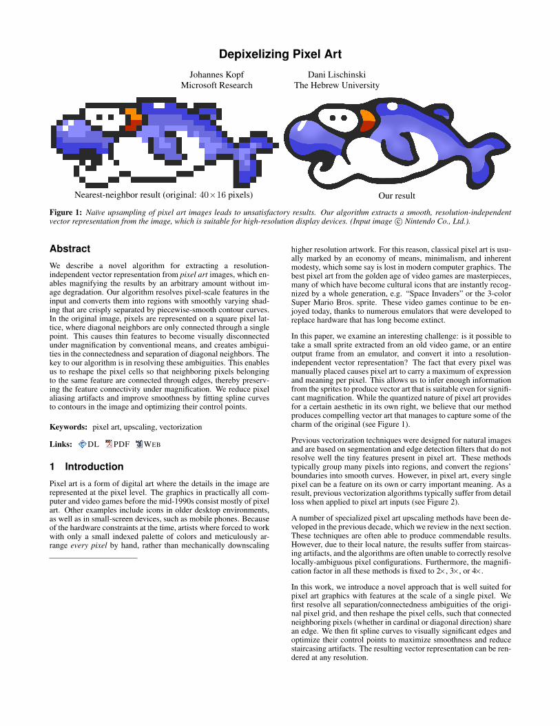
Nearest-neighbor result (original: 40×16 pixels) Our result

Figure 1: Naıve upsampling of pixel art images leads to unsatisfactory results. Our algorithm extracts a smooth, resolution-independentvector representation from the image, which is suitable for high-resolution display devices. (Input image c© Nintendo Co., Ltd.).

Abstract

We describe a novel algorithm for extracting a resolution-independent vector representation from pixel art images, which en-ables magnifying the results by an arbitrary amount without im-age degradation. Our algorithm resolves pixel-scale features in theinput and converts them into regions with smoothly varying shad-ing that are crisply separated by piecewise-smooth contour curves.In the original image, pixels are represented on a square pixel lat-tice, where diagonal neighbors are only connected through a singlepoint. This causes thin features to become visually disconnectedunder magnification by conventional means, and creates ambigui-ties in the connectedness and separation of diagonal neighbors. Thekey to our algorithm is in resolving these ambiguities. This enablesus to reshape the pixel cells so that neighboring pixels belongingto the same feature are connected through edges, thereby preserv-ing the feature connectivity under magnification. We reduce pixelaliasing artifacts and improve smoothness by fitting spline curvesto contours in the image and optimizing their control points.

Keywords: pixel art, upscaling, vectorization

Links: DL PDF WEB

1 Introduction

Pixel art is a form of digital art where the details in the image arerepresented at the pixel level. The graphics in practically all com-puter and video games before the mid-1990s consist mostly of pixelart. Other examples include icons in older desktop environments,as well as in small-screen devices, such as mobile phones. Becauseof the hardware constraints at the time, artists where forced to workwith only a small indexed palette of colors and meticulously ar-range every pixel by hand, rather than mechanically downscaling

higher resolution artwork. For this reason, classical pixel art is usu-ally marked by an economy of means, minimalism, and inherentmodesty, which some say is lost in modern computer graphics. Thebest pixel art from the golden age of video games are masterpieces,many of which have become cultural icons that are instantly recog-nized by a whole generation, e.g. “Space Invaders” or the 3-colorSuper Mario Bros. sprite. These video games continue to be en-joyed today, thanks to numerous emulators that were developed toreplace hardware that has long become extinct.

In this paper, we examine an interesting challenge: is it possible totake a small sprite extracted from an old video game, or an entireoutput frame from an emulator, and convert it into a resolution-independent vector representation? The fact that every pixel wasmanually placed causes pixel art to carry a maximum of expressionand meaning per pixel. This allows us to infer enough informationfrom the sprites to produce vector art that is suitable even for signifi-cant magnification. While the quantized nature of pixel art providesfor a certain aesthetic in its own right, we believe that our methodproduces compelling vector art that manages to capture some of thecharm of the original (see Figure 1).

Previous vectorization techniques were designed for natural imagesand are based on segmentation and edge detection filters that do notresolve well the tiny features present in pixel art. These methodstypically group many pixels into regions, and convert the regions’boundaries into smooth curves. However, in pixel art, every singlepixel can be a feature on its own or carry important meaning. As aresult, previous vectorization algorithms typically suffer from detailloss when applied to pixel art inputs (see Figure 2).

A number of specialized pixel art upscaling methods have been de-veloped in the previous decade, which we review in the next section.These techniques are often able to produce commendable results.However, due to their local nature, the results suffer from staircas-ing artifacts, and the algorithms are often unable to correctly resolvelocally-ambiguous pixel configurations. Furthermore, the magnifi-cation factor in all these methods is fixed to 2×, 3×, or 4×.

In this work, we introduce a novel approach that is well suited forpixel art graphics with features at the scale of a single pixel. Wefirst resolve all separation/connectedness ambiguities of the origi-nal pixel grid, and then reshape the pixel cells, such that connectedneighboring pixels (whether in cardinal or diagonal direction) sharean edge. We then fit spline curves to visually significant edges andoptimize their control points to maximize smoothness and reducestaircasing artifacts. The resulting vector representation can be ren-dered at any resolution.

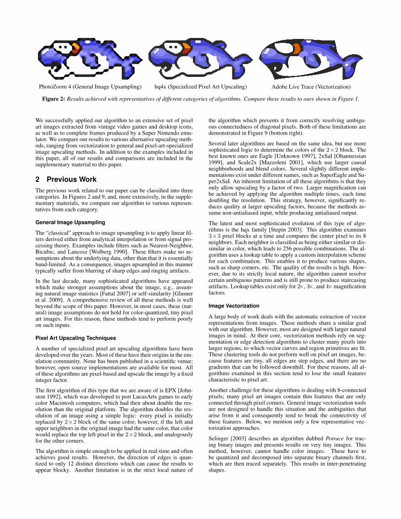
PhotoZoom 4 (General Image Upsampling) hq4x (Specialized Pixel Art Upscaling) Adobe Live Trace (Vectorization)

Figure 2: Results achieved with representatives of different categories of algorithms. Compare these results to ours shown in Figure 1.

We successfully applied our algorithm to an extensive set of pixelart images extracted from vintage video games and desktop icons,as well as to complete frames produced by a Super Nintendo emu-lator. We compare our results to various alternative upscaling meth-ods, ranging from vectorization to general and pixel-art-specializedimage upscaling methods. In addition to the examples included inthis paper, all of our results and comparisons are included in thesupplementary material to this paper.

2 Previous WorkThe previous work related to our paper can be classified into threecategories. In Figures 2 and 9, and, more extensively, in the supple-mentary materials, we compare our algorithm to various represen-tatives from each category.

General Image Upsampling

The “classical” approach to image upsampling is to apply linear fil-ters derived either from analytical interpolation or from signal pro-cessing theory. Examples include filters such as Nearest-Neighbor,Bicubic, and Lancosz [Wolberg 1990]. These filters make no as-sumptions about the underlying data, other than that it is essentiallyband-limited. As a consequence, images upsampled in this mannertypically suffer from blurring of sharp edges and ringing artifacts.

In the last decade, many sophisticated algorithms have appearedwhich make stronger assumptions about the image, e.g., assum-ing natural image statistics [Fattal 2007] or self-similarity [Glasneret al. 2009]. A comprehensive review of all these methods is wellbeyond the scope of this paper. However, in most cases, these (nat-ural) image assumptions do not hold for color-quantized, tiny pixelart images. For this reason, these methods tend to perform poorlyon such inputs.

Pixel Art Upscaling Techniques

A number of specialized pixel art upscaling algorithms have beendeveloped over the years. Most of these have their origins in the em-ulation community. None has been published in a scientific venue;however, open source implementations are available for most. Allof these algorithms are pixel-based and upscale the image by a fixedinteger factor.

The first algorithm of this type that we are aware of is EPX [John-ston 1992], which was developed to port LucasArts games to earlycolor Macintosh computers, which had then about double the res-olution than the original platform. The algorithm doubles the res-olution of an image using a simple logic: every pixel is initiallyreplaced by 2×2 block of the same color; however, if the left andupper neighbors in the original image had the same color, that colorwould replace the top left pixel in the 2×2 block, and analogouslyfor the other corners.

The algorithm is simple enough to be applied in real-time and oftenachieves good results. However, the direction of edges is quan-tized to only 12 distinct directions which can cause the results toappear blocky. Another limitation is in the strict local nature of

the algorithm which prevents it from correctly resolving ambigu-ous connectedness of diagonal pixels. Both of these limitations aredemonstrated in Figure 9 (bottom right).

Several later algorithms are based on the same idea, but use moresophisticated logic to determine the colors of the 2×2 block. Thebest known ones are Eagle [Unknown 1997], 2xSaI [Ohannessian1999], and Scale2x [Mazzoleni 2001], which use larger causalneighborhoods and blend colors. Several slightly different imple-mentations exist under different names, such as SuperEagle and Su-per2xSaI. An inherent limitation of all these algorithms is that theyonly allow upscaling by a factor of two. Larger magnification canbe achieved by applying the algorithm multiple times, each timedoubling the resolution. This strategy, however, significantly re-duces quality at larger upscaling factors, because the methods as-sume non-antialiased input, while producing antialiased output.

The latest and most sophisticated evolution of this type of algo-rithms is the hqx family [Stepin 2003]. This algorithm examines3×3 pixel blocks at a time and compares the center pixel to its 8neighbors. Each neighbor is classified as being either similar or dis-similar in color, which leads to 256 possible combinations. The al-gorithm uses a lookup table to apply a custom interpolation schemefor each combination. This enables it to produce various shapes,such as sharp corners, etc. The quality of the results is high. How-ever, due to its strictly local nature, the algorithm cannot resolvecertain ambiguous patterns and is still prone to produce staircasingartifacts. Lookup tables exist only for 2×, 3×, and 4×magnificationfactors.

Image Vectorization

A large body of work deals with the automatic extraction of vectorrepresentations from images. These methods share a similar goalwith our algorithm. However, most are designed with larger naturalimages in mind. At their core, vectorization methods rely on seg-mentation or edge detection algorithms to cluster many pixels intolarger regions, to which vector curves and region primitives are fit.These clustering tools do not perform well on pixel art images, be-cause features are tiny, all edges are step edges, and there are nogradients that can be followed downhill. For these reasons, all al-gorithms examined in this section tend to lose the small featurescharacteristic to pixel art.

Another challenge for these algorithms is dealing with 8-connectedpixels; many pixel art images contain thin features that are onlyconnected through pixel corners. General image vectorization toolsare not designed to handle this situation and the ambiguities thatarise from it and consequently tend to break the connectivity ofthese features. Below, we mention only a few representative vec-torization approaches.

Selinger [2003] describes an algorithm dubbed Potrace for trac-ing binary images and presents results on very tiny images. Thismethod, however, cannot handle color images. These have tobe quantized and decomposed into separate binary channels first,which are then traced separately. This results in inter-penetratingshapes.

(a) (b) (c) (d) (e) (f)

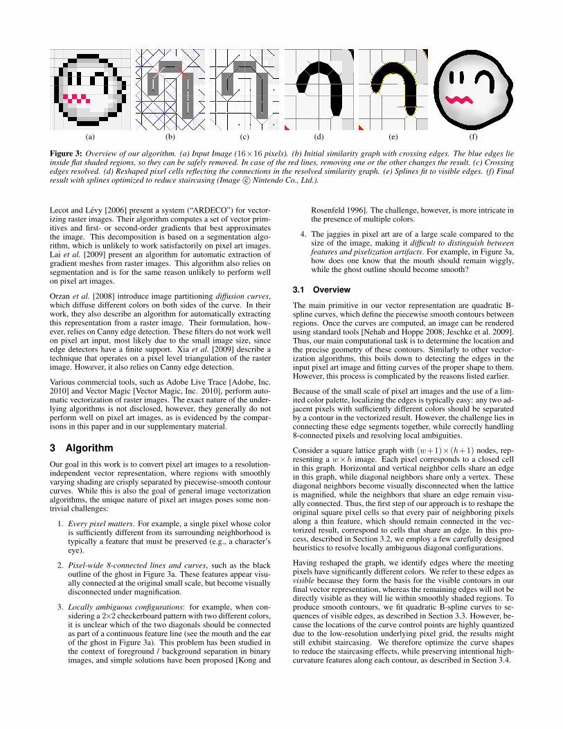
Figure 3: Overview of our algorithm. (a) Input Image (16×16 pixels). (b) Initial similarity graph with crossing edges. The blue edges lieinside flat shaded regions, so they can be safely removed. In case of the red lines, removing one or the other changes the result. (c) Crossingedges resolved. (d) Reshaped pixel cells reflecting the connections in the resolved similarity graph. (e) Splines fit to visible edges. (f) Finalresult with splines optimized to reduce staircasing (Image c© Nintendo Co., Ltd.).

Lecot and Levy [2006] present a system (“ARDECO”) for vector-izing raster images. Their algorithm computes a set of vector prim-itives and first- or second-order gradients that best approximatesthe image. This decomposition is based on a segmentation algo-rithm, which is unlikely to work satisfactorily on pixel art images.Lai et al. [2009] present an algorithm for automatic extraction ofgradient meshes from raster images. This algorithm also relies onsegmentation and is for the same reason unlikely to perform wellon pixel art images.

Orzan et al. [2008] introduce image partitioning diffusion curves,which diffuse different colors on both sides of the curve. In theirwork, they also describe an algorithm for automatically extractingthis representation from a raster image. Their formulation, how-ever, relies on Canny edge detection. These filters do not work wellon pixel art input, most likely due to the small image size, sinceedge detectors have a finite support. Xia et al. [2009] describe atechnique that operates on a pixel level triangulation of the rasterimage. However, it also relies on Canny edge detection.

Various commercial tools, such as Adobe Live Trace [Adobe, Inc.2010] and Vector Magic [Vector Magic, Inc. 2010], perform auto-matic vectorization of raster images. The exact nature of the under-lying algorithms is not disclosed, however, they generally do notperform well on pixel art images, as is evidenced by the compar-isons in this paper and in our supplementary material.

3 AlgorithmOur goal in this work is to convert pixel art images to a resolution-independent vector representation, where regions with smoothlyvarying shading are crisply separated by piecewise-smooth contourcurves. While this is also the goal of general image vectorizationalgorithms, the unique nature of pixel art images poses some non-trivial challenges:

1. Every pixel matters. For example, a single pixel whose coloris sufficiently different from its surrounding neighborhood istypically a feature that must be preserved (e.g., a character’seye).

2. Pixel-wide 8-connected lines and curves, such as the blackoutline of the ghost in Figure 3a. These features appear visu-ally connected at the original small scale, but become visuallydisconnected under magnification.

3. Locally ambiguous configurations: for example, when con-sidering a 2×2 checkerboard pattern with two different colors,it is unclear which of the two diagonals should be connectedas part of a continuous feature line (see the mouth and the earof the ghost in Figure 3a). This problem has been studied inthe context of foreground / background separation in binaryimages, and simple solutions have been proposed [Kong and

Rosenfeld 1996]. The challenge, however, is more intricate inthe presence of multiple colors.

4. The jaggies in pixel art are of a large scale compared to thesize of the image, making it difficult to distinguish betweenfeatures and pixelization artifacts. For example, in Figure 3a,how does one know that the mouth should remain wiggly,while the ghost outline should become smooth?

3.1 Overview

The main primitive in our vector representation are quadratic B-spline curves, which define the piecewise smooth contours betweenregions. Once the curves are computed, an image can be renderedusing standard tools [Nehab and Hoppe 2008; Jeschke et al. 2009].Thus, our main computational task is to determine the location andthe precise geometry of these contours. Similarly to other vector-ization algorithms, this boils down to detecting the edges in theinput pixel art image and fitting curves of the proper shape to them.However, this process is complicated by the reasons listed earlier.

Because of the small scale of pixel art images and the use of a lim-ited color palette, localizing the edges is typically easy: any two ad-jacent pixels with sufficiently different colors should be separatedby a contour in the vectorized result. However, the challenge lies inconnecting these edge segments together, while correctly handling8-connected pixels and resolving local ambiguities.

Consider a square lattice graph with (w+1)×(h+1) nodes, rep-resenting a w×h image. Each pixel corresponds to a closed cellin this graph. Horizontal and vertical neighbor cells share an edgein this graph, while diagonal neighbors share only a vertex. Thesediagonal neighbors become visually disconnected when the latticeis magnified, while the neighbors that share an edge remain visu-ally connected. Thus, the first step of our approach is to reshape theoriginal square pixel cells so that every pair of neighboring pixelsalong a thin feature, which should remain connected in the vec-torized result, correspond to cells that share an edge. In this pro-cess, described in Section 3.2, we employ a few carefully designedheuristics to resolve locally ambiguous diagonal configurations.

Having reshaped the graph, we identify edges where the meetingpixels have significantly different colors. We refer to these edges asvisible because they form the basis for the visible contours in ourfinal vector representation, whereas the remaining edges will not bedirectly visible as they will lie within smoothly shaded regions. Toproduce smooth contours, we fit quadratic B-spline curves to se-quences of visible edges, as described in Section 3.3. However, be-cause the locations of the curve control points are highly quantizeddue to the low-resolution underlying pixel grid, the results mightstill exhibit staircasing. We therefore optimize the curve shapesto reduce the staircasing effects, while preserving intentional high-curvature features along each contour, as described in Section 3.4.

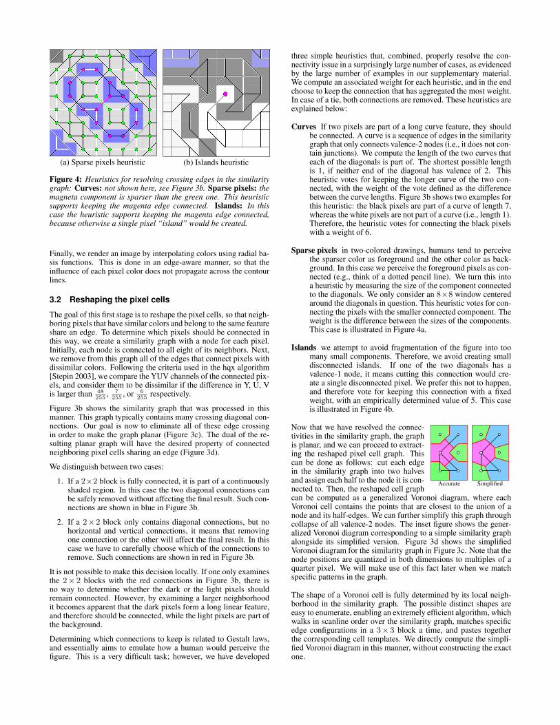
(a) Sparse pixels heuristic (b) Islands heuristic

Figure 4: Heuristics for resolving crossing edges in the similaritygraph: Curves: not shown here, see Figure 3b. Sparse pixels: themagneta component is sparser than the green one. This heuristicsupports keeping the magenta edge connected. Islands: In thiscase the heuristic supports keeping the magenta edge connected,because otherwise a single pixel “island” would be created.

Finally, we render an image by interpolating colors using radial ba-sis functions. This is done in an edge-aware manner, so that theinfluence of each pixel color does not propagate across the contourlines.

3.2 Reshaping the pixel cells

The goal of this first stage is to reshape the pixel cells, so that neigh-boring pixels that have similar colors and belong to the same featureshare an edge. To determine which pixels should be connected inthis way, we create a similarity graph with a node for each pixel.Initially, each node is connected to all eight of its neighbors. Next,we remove from this graph all of the edges that connect pixels withdissimilar colors. Following the criteria used in the hqx algorithm[Stepin 2003], we compare the YUV channels of the connected pix-els, and consider them to be dissimilar if the difference in Y, U, Vis larger than 48

255, 7255

, or 6255

respectively.

Figure 3b shows the similarity graph that was processed in thismanner. This graph typically contains many crossing diagonal con-nections. Our goal is now to eliminate all of these edge crossingin order to make the graph planar (Figure 3c). The dual of the re-sulting planar graph will have the desired property of connectedneighboring pixel cells sharing an edge (Figure 3d).

We distinguish between two cases:

1. If a 2×2 block is fully connected, it is part of a continuouslyshaded region. In this case the two diagonal connections canbe safely removed without affecting the final result. Such con-nections are shown in blue in Figure 3b.

2. If a 2×2 block only contains diagonal connections, but nohorizontal and vertical connections, it means that removingone connection or the other will affect the final result. In thiscase we have to carefully choose which of the connections toremove. Such connections are shown in red in Figure 3b.

It is not possible to make this decision locally. If one only examinesthe 2× 2 blocks with the red connections in Figure 3b, there isno way to determine whether the dark or the light pixels shouldremain connected. However, by examining a larger neighborhoodit becomes apparent that the dark pixels form a long linear feature,and therefore should be connected, while the light pixels are part ofthe background.

Determining which connections to keep is related to Gestalt laws,and essentially aims to emulate how a human would perceive thefigure. This is a very difficult task; however, we have developed

three simple heuristics that, combined, properly resolve the con-nectivity issue in a surprisingly large number of cases, as evidencedby the large number of examples in our supplementary material.We compute an associated weight for each heuristic, and in the endchoose to keep the connection that has aggregated the most weight.In case of a tie, both connections are removed. These heuristics areexplained below:

Curves If two pixels are part of a long curve feature, they shouldbe connected. A curve is a sequence of edges in the similaritygraph that only connects valence-2 nodes (i.e., it does not con-tain junctions). We compute the length of the two curves thateach of the diagonals is part of. The shortest possible lengthis 1, if neither end of the diagonal has valence of 2. Thisheuristic votes for keeping the longer curve of the two con-nected, with the weight of the vote defined as the differencebetween the curve lengths. Figure 3b shows two examples forthis heuristic: the black pixels are part of a curve of length 7,whereas the white pixels are not part of a curve (i.e., length 1).Therefore, the heuristic votes for connecting the black pixelswith a weight of 6.

Sparse pixels in two-colored drawings, humans tend to perceivethe sparser color as foreground and the other color as back-ground. In this case we perceive the foreground pixels as con-nected (e.g., think of a dotted pencil line). We turn this intoa heuristic by measuring the size of the component connectedto the diagonals. We only consider an 8×8 window centeredaround the diagonals in question. This heuristic votes for con-necting the pixels with the smaller connected component. Theweight is the difference between the sizes of the components.This case is illustrated in Figure 4a.

Islands we attempt to avoid fragmentation of the figure into toomany small components. Therefore, we avoid creating smalldisconnected islands. If one of the two diagonals has avalence-1 node, it means cutting this connection would cre-ate a single disconnected pixel. We prefer this not to happen,and therefore vote for keeping this connection with a fixedweight, with an empirically determined value of 5. This caseis illustrated in Figure 4b.

Now that we have resolved the connec-tivities in the similarity graph, the graphis planar, and we can proceed to extract-ing the reshaped pixel cell graph. Thiscan be done as follows: cut each edgein the similarity graph into two halvesand assign each half to the node it is con-nected to. Then, the reshaped cell graphcan be computed as a generalized Voronoi diagram, where eachVoronoi cell contains the points that are closest to the union of anode and its half-edges. We can further simplify this graph throughcollapse of all valence-2 nodes. The inset figure shows the gener-alized Voronoi diagram corresponding to a simple similarity graphalongside its simplified version. Figure 3d shows the simplifiedVoronoi diagram for the similarity graph in Figure 3c. Note that thenode positions are quantized in both dimensions to multiples of aquarter pixel. We will make use of this fact later when we matchspecific patterns in the graph.

The shape of a Voronoi cell is fully determined by its local neigh-borhood in the similarity graph. The possible distinct shapes areeasy to enumerate, enabling an extremely efficient algorithm, whichwalks in scanline order over the similarity graph, matches specificedge configurations in a 3× 3 block a time, and pastes togetherthe corresponding cell templates. We directly compute the simpli-fied Voronoi diagram in this manner, without constructing the exactone.

(a) (b)

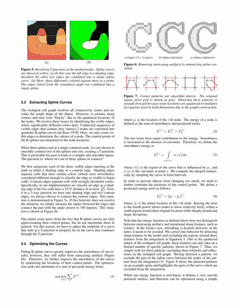
Figure 5: Resolving T-junctions at the marked nodes. Spline curvesare shown in yellow. (a) In this case the left edge is a shading edge,therefore the other two edges are combined into a single splinecurve. (b) Here, three differently colored regions meet at a point.The edges which form the straightest angle are combined into asingle spline.

3.3 Extracting Spline Curves

The reshaped cell graph resolves all connectivity issues and en-codes the rough shape of the object. However, it contains sharpcorners and may look “blocky” due to the quantized locations ofthe nodes. We resolve these issues by identifying the visible edges,where significantly different colors meet. Connected sequences ofvisible edges that contain only valence-2 nodes are converted intoquadratic B-spline curves [de Boor 1978]. Here, we only count vis-ible edges to determine the valence of a node. The control points ofthe B-splines are initialized to the node locations.

When three splines end at a single common node, we can choose tosmoothly connect two of the splines into one, creating a T-junction.This is preferable because it leads to a simpler and smoother figure.The question is: which two out of three splines to connect?

We first categorize each of the three visible edges meeting at thenode as either a shading edge or a contour edge. Shading edgesseparate cells that have similar colors (which were neverthelessconsidered different enough to classify the edge as visible to beginwith). Contour edges separate cells with strongly dissimilar colors.Specifically, in our implementation we classify an edge as a shad-ing edge if the two cells have a YUV distance of at most 100

255. Now,

if at a 3-way junction we have one shading edge and two contouredges, we always choose to connect the contour edges. This situa-tion is demonstrated in Figure 5a. If this heuristic does not resolvethe situation, we simply measure the angles between the edges andconnect the pair with the angle closest to 180 degrees. This situa-tion is shown in Figure 5b.

One minor issue arises from the fact that B-spline curves are onlyapproximating their control points, but do not interpolate them ingeneral. For this reason, we have to adjust the endpoint of a curvethat ends at a T-junction to properly lie on the curve that continuesthrough the T-junction.

3.4 Optimizing the Curves

Fitting B-spline curves greatly improves the smoothness of our re-sults; however, they still suffer from staircasing artifacts (Figure6b). Therefore, we further improve the smoothness of the curvesby optimizing the locations of their control points. The optimiza-tion seeks the minimum of a sum of per-node energy terms:

argmin{pi}

∑i

E(i), (1)

(a) Input (13×15 pixels) (b) Splines Initialized (c) Splines Optimized

Figure 6: Removing staircasing artifacts by minimizing spline cur-vature.

Figure 7: Corner patterns our algorithm detects. The originalsquare pixel grid is shown in gray. Detecting these patterns isstraight forward because node locations are quantized to multiplesof a quarter pixel in both dimensions due to the graph construction.

where pi is the location of the i-th node. The energy of a node isdefined as the sum of smoothness and positional terms:

E(i) = E(i)s + E(i)

p (2)

The two terms have equal contribution to the energy. Smoothnessis measured as the absence of curvature. Therefore, we define thesmoothness energy as

E(i)s =

∫s∈r(i)

|κ (s)| ds, (3)

where r(i) is the region of the curve that is influenced by pi, andκ (s) is the curvature at point s. We compute the integral numeri-cally by sampling the curve at fixed intervals.

In order to prevent objects from changing too much, we need tofurther constrain the positions of the control points. We define apositional energy term as follows:

E(i)p = ‖pi − pi‖4, (4)

where, pi is the initial location of the i-th node. Raising the termto the fourth power allows nodes to move relatively freely within asmall region around their original location while sharply penalizinglarger deviations.

Note that the energy function as defined above does not distinguishbetween staircasing artifacts and intentional sharp features, such ascorners. In the former case, smoothing is desired, however, in thelatter, it needs to be avoided. We correct this behavior by detectingsharp features in the model and excluding the regions around thesefeatures from the integration in Equation 3. Due to the quantizednature of the reshaped cell graph, sharp features can only take on alimited number of specific patterns, shown in Figure 7. Thus, wesimply look for these patterns (including their rotations and reflec-tions) in the reshaped cell graph. Having detected a pattern, weexclude the part of the spline curve between the nodes of the pat-tern from the integration (3). Figure 8 shows the detected patternson an example sprite and highlights the parts of the curve which areexcluded from the integration.

While our energy function is non-linear, it defines a very smoothpotential surface, and therefore can be optimized using a simple

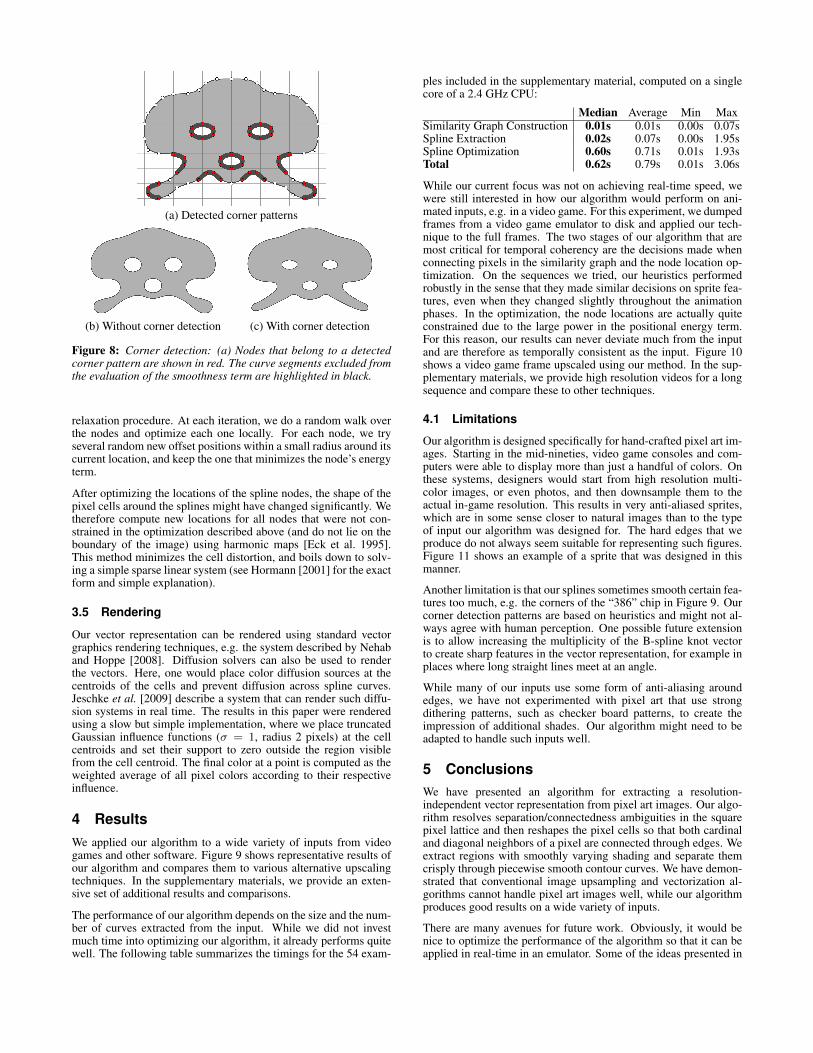
(a) Detected corner patterns

(b) Without corner detection (c) With corner detection

Figure 8: Corner detection: (a) Nodes that belong to a detectedcorner pattern are shown in red. The curve segments excluded fromthe evaluation of the smoothness term are highlighted in black.

relaxation procedure. At each iteration, we do a random walk overthe nodes and optimize each one locally. For each node, we tryseveral random new offset positions within a small radius around itscurrent location, and keep the one that minimizes the node’s energyterm.

After optimizing the locations of the spline nodes, the shape of thepixel cells around the splines might have changed significantly. Wetherefore compute new locations for all nodes that were not con-strained in the optimization described above (and do not lie on theboundary of the image) using harmonic maps [Eck et al. 1995].This method minimizes the cell distortion, and boils down to solv-ing a simple sparse linear system (see Hormann [2001] for the exactform and simple explanation).

3.5 Rendering

Our vector representation can be rendered using standard vectorgraphics rendering techniques, e.g. the system described by Nehaband Hoppe [2008]. Diffusion solvers can also be used to renderthe vectors. Here, one would place color diffusion sources at thecentroids of the cells and prevent diffusion across spline curves.Jeschke et al. [2009] describe a system that can render such diffu-sion systems in real time. The results in this paper were renderedusing a slow but simple implementation, where we place truncatedGaussian influence functions (σ = 1, radius 2 pixels) at the cellcentroids and set their support to zero outside the region visiblefrom the cell centroid. The final color at a point is computed as theweighted average of all pixel colors according to their respectiveinfluence.

4 ResultsWe applied our algorithm to a wide variety of inputs from videogames and other software. Figure 9 shows representative results ofour algorithm and compares them to various alternative upscalingtechniques. In the supplementary materials, we provide an exten-sive set of additional results and comparisons.

The performance of our algorithm depends on the size and the num-ber of curves extracted from the input. While we did not investmuch time into optimizing our algorithm, it already performs quitewell. The following table summarizes the timings for the 54 exam-

ples included in the supplementary material, computed on a singlecore of a 2.4 GHz CPU:

Median Average Min MaxSimilarity Graph Construction 0.01s 0.01s 0.00s 0.07sSpline Extraction 0.02s 0.07s 0.00s 1.95sSpline Optimization 0.60s 0.71s 0.01s 1.93sTotal 0.62s 0.79s 0.01s 3.06s

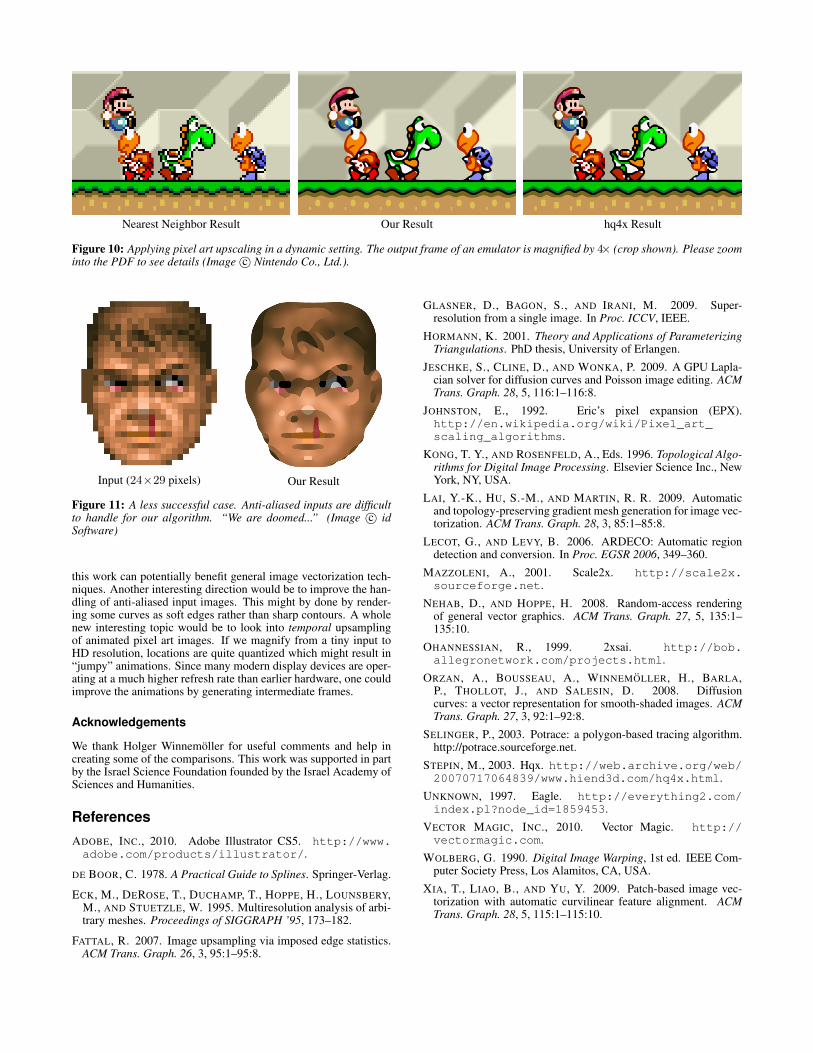
While our current focus was not on achieving real-time speed, wewere still interested in how our algorithm would perform on ani-mated inputs, e.g. in a video game. For this experiment, we dumpedframes from a video game emulator to disk and applied our tech-nique to the full frames. The two stages of our algorithm that aremost critical for temporal coherency are the decisions made whenconnecting pixels in the similarity graph and the node location op-timization. On the sequences we tried, our heuristics performedrobustly in the sense that they made similar decisions on sprite fea-tures, even when they changed slightly throughout the animationphases. In the optimization, the node locations are actually quiteconstrained due to the large power in the positional energy term.For this reason, our results can never deviate much from the inputand are therefore as temporally consistent as the input. Figure 10shows a video game frame upscaled using our method. In the sup-plementary materials, we provide high resolution videos for a longsequence and compare these to other techniques.

4.1 Limitations

Our algorithm is designed specifically for hand-crafted pixel art im-ages. Starting in the mid-nineties, video game consoles and com-puters were able to display more than just a handful of colors. Onthese systems, designers would start from high resolution multi-color images, or even photos, and then downsample them to theactual in-game resolution. This results in very anti-aliased sprites,which are in some sense closer to natural images than to the typeof input our algorithm was designed for. The hard edges that weproduce do not always seem suitable for representing such figures.Figure 11 shows an example of a sprite that was designed in thismanner.

Another limitation is that our splines sometimes smooth certain fea-tures too much, e.g. the corners of the “386” chip in Figure 9. Ourcorner detection patterns are based on heuristics and might not al-ways agree with human perception. One possible future extensionis to allow increasing the multiplicity of the B-spline knot vectorto create sharp features in the vector representation, for example inplaces where long straight lines meet at an angle.

While many of our inputs use some form of anti-aliasing aroundedges, we have not experimented with pixel art that use strongdithering patterns, such as checker board patterns, to create theimpression of additional shades. Our algorithm might need to beadapted to handle such inputs well.

5 ConclusionsWe have presented an algorithm for extracting a resolution-independent vector representation from pixel art images. Our algo-rithm resolves separation/connectedness ambiguities in the squarepixel lattice and then reshapes the pixel cells so that both cardinaland diagonal neighbors of a pixel are connected through edges. Weextract regions with smoothly varying shading and separate themcrisply through piecewise smooth contour curves. We have demon-strated that conventional image upsampling and vectorization al-gorithms cannot handle pixel art images well, while our algorithmproduces good results on a wide variety of inputs.

There are many avenues for future work. Obviously, it would benice to optimize the performance of the algorithm so that it can beapplied in real-time in an emulator. Some of the ideas presented in

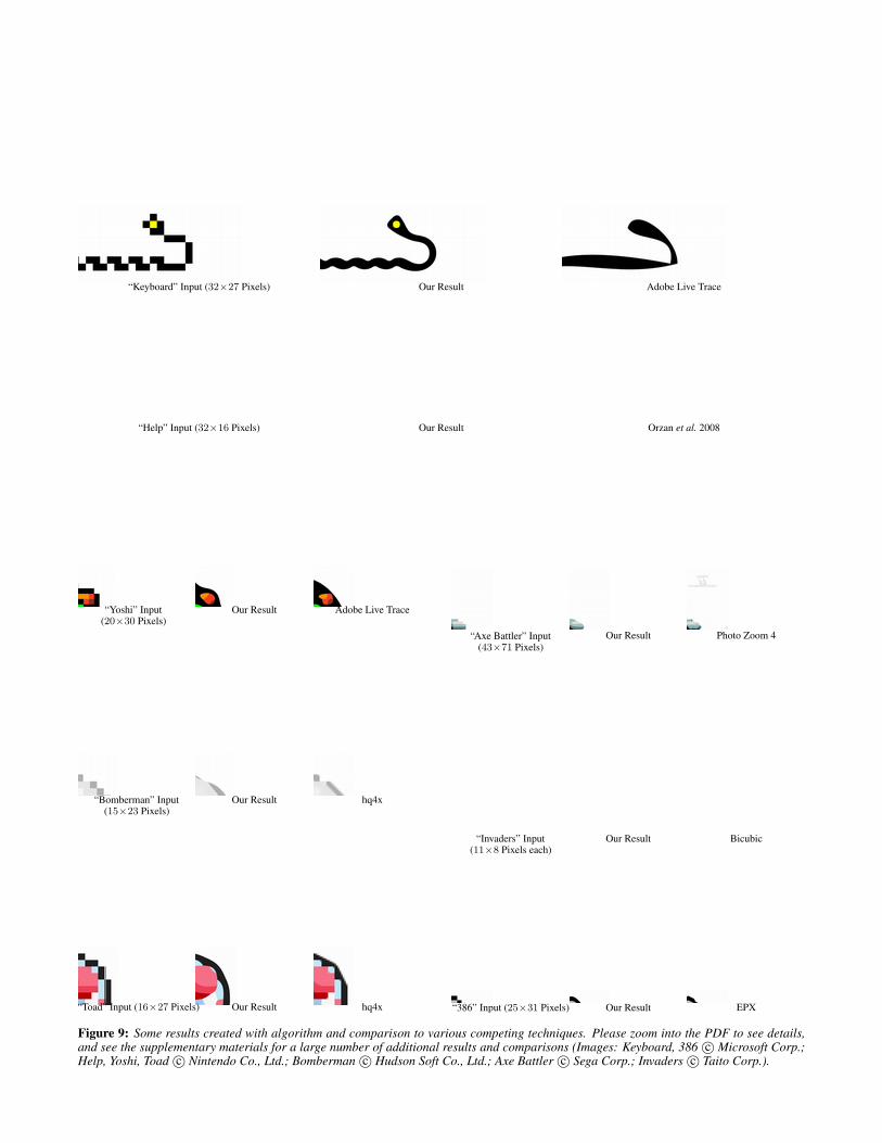
Figure 9: Some results created with algorithm and comparison to various competing techniques. Please zoom into the PDF to see details,and see the supplementary materials for a large number of additional results and comparisons (Images: Keyboard, 386 c© Microsoft Corp.;Help, Yoshi, Toad c© Nintendo Co., Ltd.; Bomberman c© Hudson Soft Co., Ltd.; Axe Battler c© Sega Corp.; Invaders c© Taito Corp.).

Nearest Neighbor Result gOur Resultg hq4x Result

Figure 10: Applying pixel art upscaling in a dynamic setting. The output frame of an emulator is magnified by 4× (crop shown). Please zoominto the PDF to see details (Image c© Nintendo Co., Ltd.).

Input (24×29 pixels) Our Result

Figure 11: A less successful case. Anti-aliased inputs are difficultto handle for our algorithm. “We are doomed...” (Image c© idSoftware)

this work can potentially benefit general image vectorization tech-niques. Another interesting direction would be to improve the han-dling of anti-aliased input images. This might by done by render-ing some curves as soft edges rather than sharp contours. A wholenew interesting topic would be to look into temporal upsamplingof animated pixel art images. If we magnify from a tiny input toHD resolution, locations are quite quantized which might result in“jumpy” animations. Since many modern display devices are oper-ating at a much higher refresh rate than earlier hardware, one couldimprove the animations by generating intermediate frames.

Acknowledgements

We thank Holger Winnemoller for useful comments and help increating some of the comparisons. This work was supported in partby the Israel Science Foundation founded by the Israel Academy ofSciences and Humanities.

References

ADOBE, INC., 2010. Adobe Illustrator CS5. http://www.adobe.com/products/illustrator/.

DE BOOR, C. 1978. A Practical Guide to Splines. Springer-Verlag.

ECK, M., DEROSE, T., DUCHAMP, T., HOPPE, H., LOUNSBERY,M., AND STUETZLE, W. 1995. Multiresolution analysis of arbi-trary meshes. Proceedings of SIGGRAPH ’95, 173–182.

FATTAL, R. 2007. Image upsampling via imposed edge statistics.ACM Trans. Graph. 26, 3, 95:1–95:8.

GLASNER, D., BAGON, S., AND IRANI, M. 2009. Super-resolution from a single image. In Proc. ICCV, IEEE.

HORMANN, K. 2001. Theory and Applications of ParameterizingTriangulations. PhD thesis, University of Erlangen.

JESCHKE, S., CLINE, D., AND WONKA, P. 2009. A GPU Lapla-cian solver for diffusion curves and Poisson image editing. ACMTrans. Graph. 28, 5, 116:1–116:8.

JOHNSTON, E., 1992. Eric’s pixel expansion (EPX).http://en.wikipedia.org/wiki/Pixel_art_scaling_algorithms.

KONG, T. Y., AND ROSENFELD, A., Eds. 1996. Topological Algo-rithms for Digital Image Processing. Elsevier Science Inc., NewYork, NY, USA.

LAI, Y.-K., HU, S.-M., AND MARTIN, R. R. 2009. Automaticand topology-preserving gradient mesh generation for image vec-torization. ACM Trans. Graph. 28, 3, 85:1–85:8.

LECOT, G., AND LEVY, B. 2006. ARDECO: Automatic regiondetection and conversion. In Proc. EGSR 2006, 349–360.

MAZZOLENI, A., 2001. Scale2x. http://scale2x.sourceforge.net.

NEHAB, D., AND HOPPE, H. 2008. Random-access renderingof general vector graphics. ACM Trans. Graph. 27, 5, 135:1–135:10.

OHANNESSIAN, R., 1999. 2xsai. http://bob.allegronetwork.com/projects.html.

ORZAN, A., BOUSSEAU, A., WINNEMOLLER, H., BARLA,P., THOLLOT, J., AND SALESIN, D. 2008. Diffusioncurves: a vector representation for smooth-shaded images. ACMTrans. Graph. 27, 3, 92:1–92:8.

SELINGER, P., 2003. Potrace: a polygon-based tracing algorithm.http://potrace.sourceforge.net.

STEPIN, M., 2003. Hqx. http://web.archive.org/web/20070717064839/www.hiend3d.com/hq4x.html.

UNKNOWN, 1997. Eagle. http://everything2.com/index.pl?node_id=1859453.

VECTOR MAGIC, INC., 2010. Vector Magic. http://vectormagic.com.

WOLBERG, G. 1990. Digital Image Warping, 1st ed. IEEE Com-puter Society Press, Los Alamitos, CA, USA.

XIA, T., LIAO, B., AND YU, Y. 2009. Patch-based image vec-torization with automatic curvilinear feature alignment. ACMTrans. Graph. 28, 5, 115:1–115:10.