1

Depreciation of Business R&D Capital

Bureau of Economic Analysis/National Science Foundation R&D Satellite Account Paper

By

Wendy C.Y. Li Bureau of Economic Analysis

U.S. Department of Commerce

U.S. DEPARTMENT OF COMMERCE Rebecca Blank

Acting Secretary

ECONOMIC AND STATISTICS ADMINISTRATION Mark Doms

Under Secretary for Economic Affairs

BUREAU OF ECONOMIC ANALYSIS J. Steven Landefeld

Director

Brian C. Moyer Deputy Director

October 2012 www.bea.gov

2

Depreciation of Business R&D Capital

Wendy C.Y. Li

U.S. Bureau of Economic Analysis

Abstract

Research and development (R&D) depreciation rates are critical to calculating the rates

of return to R&D investments and capital service costs, both of which are important for

capitalizing R&D investments in the national income and product accounts. Although important,

measuring R&D depreciation rates is extremely difficult because both the price and output of

R&D capital are generally unobservable. To resolve these difficulties, economists have adopted

various approaches to estimate industry-specific R&D depreciation rates, but the differences in

their results cannot easily be reconciled. In addition, many of their calculations rely on

unverifiable assumptions.

Unlike tangible capital which depreciates due to physical decay or wear and tear,

business R&D capital depreciates because its contribution to a firm’s profit declines over time.

Based on this understanding, I developed a forward-looking profit model with a gestation lag to

derive both constant and time-varying industry-specific R&D depreciation rates for ten R&D

intensive industries that are identified in BEA’s R&D Satellite Account. I used two data sources,

a Compustat SIC-based database and a BEA-NSF NAICS-based database, to perform model

calculations. The data cover the period from 1989 to 2008. The results align with the major

conclusions from recent studies that R&D depreciation rates are higher than the traditionally

assumed 15 percent and vary across industries. Moreover, the industry-specific time-varying

R&D depreciation rates provide information about the dynamics of technological evolution and

competition across industries.

Acknowledgments. I would like to thank Ernie Berndt, Wesley Cohen, Erwin Diewert, Bronwyn

Hall, Brian Sliker, and many seminar participants in 2010 NBER Summer Institute CRIW

Workshop and 2011 ASSA Conference for helpful comments. I am grateful to Brian Moyer and

Carol Moylan for their support to this project, and to Jennifer Lee and Jeff Young for excellent

assistance with data compilation. The views expressed herein are those of the author and do not

necessarily reflect the views of Bureau of Economic Analysis.

3

1. Introduction

In an increasingly knowledge-based U.S. economy, measuring intangible

assets, including research and development (R&D) assets, is critical to capturing this

development and explaining its sources of growth. Corrado et al. (2006) pointed out that

after 1995, intangible assets reached parity with tangible assets as a source of growth.

Despite the increasing impact of intangible assets on economic growth, it is difficult to

capitalize intangible assets in the national income and product accounts (NIPAs) and

capture their impacts on economic growth. The difficulties arise because the

capitalization involves several critical but difficult measurement issues. One of them is

the measurement of the depreciation rate of intangible assets, including R&D assets.

The depreciation rate of R&D assets is critical to capitalizing R&D investments in

the NIPAs for two reasons. First, the depreciation rate is required to construct knowledge

stocks and is also the only asset-specific element in the commonly adopted user cost

formula. This user cost formula is used to calculate the flow of capital services

(Jorgenson (1963), Hall and Jorgenson (1967), Corrado et al. (2006), Aizcorbe et al.

(2009)), which is important for examining how R&D capital affects the productivity

growth of the U.S. economy (Okubo et al (2006)). Second, the depreciation rate is

required in the current commonly adopted approaches of measuring the rate of return to

R&D (Hall 2007).

As Griliches (1996) concludes, the measurement of R&D depreciation is the

central unresolved problem in the measurement of the rate of return to R&D. The

problem arises from the fact that both the price and output of R&D capital are

unobservable. Additionally, there is no arms-length market for most R&D assets and

4

the majority of R&D capital is developed for own use by the firms. It is, hence, hard to

independently calculate the depreciation rate of R&D capital (Corrado et al. 2006).

Moreover, unlike tangible capital which depreciates due to physical decay or wear and

tear, R&D, or intangible, capital depreciates because its contribution to a firm’s profit

declines over time. And, the main driving forces are obsolescence and competition (Hall

2007), both of which reflect individual industry technological and competitive

environments. Given that these environments can vary immensely across industries and

over time, the resulting R&D depreciation rates should also vary across industries and

over time.

In response to these measurement difficulties, previous research adopted four

major approaches to calculate R&D depreciation rates: patent renewal, production

function, amortization, and market valuation approaches (Mead 2007). As summarized

by Mead (2007), all approaches encounter the problem of insufficient data on variation

and thus cannot separately identify R&D depreciation rates without imposing strong

identifying assumptions. In addition, the patent renewal approach cannot capture all

innovation activities and suffers from the identification problem of an unknown skewed

distribution of patent values. Lastly, the production function approach relies on the

questionable assumption of initial R&D stock and depreciation rate (Hall, 2007).

Currently, there is no consensus on which approach can provide the best solution.

Furthermore, because of the complexity involved in incorporating the gestation

lag into the model, most research fails to deal with the issue of the gestation lag by

treating it as zero or one year to calculate the R&D capital stock (Corrado et al. 2006).

5

Because product life cycle varies across industries, this treatment is questionable for

R&D assets.

The Bureau of Economic analysis (BEA) plans to start treating R&D as

investment in its Input-Output accounts and other core accounts in 2013. As a prelude to

this change in the treatment of R&D expenditures, BEA developed an R&D satellite

account (R&DSA) to help economists gain a better understanding of R&D activity and its

effect on economic growth. A satellite account format provides a means of exploring the

impact of adjusting the treatment of R&D activity on the economy and a framework

through which various methodological and conceptual issues can be examined. Through

the R&DSA format, BEA developed and analyzed various methodologies to measure

R&D depreciation rates. In the 2006 R&DSA, BEA used an aggregate depreciation rate

for all R&D capital. In the baseline scenario, BEA used 15 percent as the annual

depreciation rate for all R&D capital. In the alternative scenarios, BEA used the

depreciation rate of nonresidential equipment and software for all R&D capital before

1987 and the depreciation rate of information processing equipment after that date. In the

2007 R&DSA, BEA adopted a two-step process to derive industry-specific R&D

depreciation rates. In the first step, BEA chose the midpoints of the range of estimates

given by existing studies calculated for each industry (Mead 2007). In the second step,

those midpoints were scaled down so that the recommended rates were more closely

centered on a value of 15 percent and that the overall ranking of industry-level rates

suggested by the literature was preserved. The resulting R&D depreciation rates are: 18

percent for transportation equipment, 16.5 percent for computer and electronics, 11

percent for chemicals, and 15 percent for all other industries. However, this approach

6

assumes that each set of estimates from the existing research is equally valid and future

depreciation patterns will be identical to those in the study period. Moreover, the most

recent studies conclude that depreciation rates for business R&D are likely to be more

variable due to different competition environments across industries and higher than the

traditional 15 percent assumption (Hall 2007).

This paper introduces a new approach by developing a forward-looking profit

model that can be used to calculate both constant and time-varying industry-specific

R&D depreciation rates. The model is built on the core concept that, unlike tangible

assets which depreciate due to physical decay or wear and tear, R&D capital depreciates

because its contribution to a firm’s profit declines over time. Without employing any

unverifiable assumptions adopted by other methods, this forward-looking profit model

contains very few parameters and allows us to utilize data on sales, industry output, and

R&D investments.

To test the new model, I first use the model to derive industry-specific R&D

depreciation rates for pharmaceutical, IT hardware, semiconductor, and software

industries. The calculation used Compustat data over the period from 1989 to 2008. The

constant industry-specific R&D depreciation rates are: 11.82 ± 0.73 percent for the

pharmaceutical industry, 37.64 ± 1.00 percent for the IT hardware industry, 17.95 ± 1.78

percent for the semiconductor industry, and 30.17 ± 1.89 percent for the software

industry. The calculation results show that, first, the derived R&D depreciation rates fall

within the range of estimates from existing literature. Second, they align with the major

conclusions from recent studies that the rates should be higher than the traditional

assumption, 15 percent, and vary across industries. Third, each industry’s time-varying

7

R&D depreciation rates exhibit its depreciation pattern, which is normally consistent with

the industry’s observations on the pace of technological progress or reflects the

appropriability condition of its intellectual property.

The above test demonstrates the capability of the new model in estimating R&D

depreciation rates from industry data. The model is then applied to two independent

datasets to calculate the R&D depreciation rates for all ten R&D intensive industries

identified in BEA’s R&DSA. The first dataset contains Compustat SIC-based firm-level

sales and R&D investments in nine R&D intensive industries. The second dataset

contains BEA-NSF NAICS-based establishment-level industry output and R&D

investments in ten R&D intensive industries.

This paper is organized as follows. Section 2 sets out the R&D investment model,

followed by the description of data analysis. Section 3 presents an industry-level data

analysis. Section 4 presents the set of recommended R&D depreciation rates for BEA’s

ten R&D intensive industries, and concluding remarks are given in Section 5.

2. Forward-looking Profit Model

The premise of my model is that business R&D capital depreciates because its

contribution to a firm’s profit declines over time. R&D capital generates privately

appropriable returns; thus, it depreciates when its appropriable return declines over time.

R&D depreciation rate is a necessary and important component of a firm’s R&D

investment model. A firm pursuing profit maximization will invest in R&D optimally

such that the marginal benefit equals the marginal cost. That is, in each period i, a firm

8

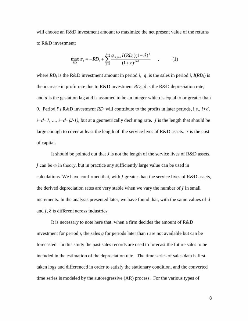
will choose an R&D investment amount to maximize the net present value of the returns

to R&D investment:

1

0 )1(

)1)((max

J

jdj

j

idji

iiRD r

RDIqRD

i

, (1)

where RDi is the R&D investment amount in period i, i is the sales in period i, I(RDi) is

the increase in profit rate due to R&D investment RDi, δ is the R&D depreciation rate,

and d is the gestation lag and is assumed to be an integer which is equal to or greater than

0. Period i’s R&D investment RDi will contribute to the profits in later periods, i.e., i+d,

i+d+1, …, i+d+(J-1), but at a geometrically declining rate. is the length that should be

large enough to cover at least the length of the service lives of R&D assets. r is the cost

of capital.

It should be pointed out that J is not the length of the service lives of R&D assets.

can be ∞ in theory, but in practice any sufficiently large value can be used in

calculations. We have confirmed that, with greater than the service lives of R&D assets,

the derived depreciation rates are very stable when we vary the number of in small

increments. In the analysis presented later, we have found that, with the same values of

and , δ is different across industries.

It is necessary to note here that, when a firm decides the amount of R&D

investment for period i, the sales q for periods later than i are not available but can be

forecasted. In this study the past sales records are used to forecast the future sales to be

included in the estimation of the depreciation rate. The time series of sales data is first

taken logs and differenced in order to satisfy the stationary condition, and the converted

time series is modeled by the autoregressive (AR) process. For the various types of

9

industrial data included in this study, the optimal order of the AR model as identified by

the Akaike Information Criterion [Mills, 1990] is found to range from 0 to 2. To

maintain the consistency throughout the study, AR(1) is used to forecast future sales.

The forecast error of the AR model will also affect the estimation of the

depreciation rate. To examine this effect, I performed a Monte Carlo calculation with

1000 replications. In each replication, the forecast error of AR(1) at k steps ahead,

, was calculated with where was obtained by AR estimation.

This error is then added to the forecast values based on the AR(1) model. For every

industry included in this study, the 1000 estimates of the depreciation rate exhibit a

Gaussian distribution.

In the following, the predicted sales in period i is denoted as iq . In addition, the

choice of J can be a large number as long as it well covers the duration of R&D assets’

contribution to a firm’s profit. In this study, I use 20 for J except for the pharmaceutical

industry where J = 25 is used due to the longer product life cycle.

To derive the optimal solution, I define as a concave function:

RDIRDI exp1][ (2)

RD when . The functional form of has very few parameters but

still gives us the required concave property to derive the optimality condition, an

approach adopted by Cohen and Klepper (1996).

10

is the upper bound of increase in profit rate due to R&D investments. And,

defines the investment scale for increases in RD. That is, can indicate how fast the

R&D investment helps a firm achieve a higher profit rate. Note that based on equation (2)

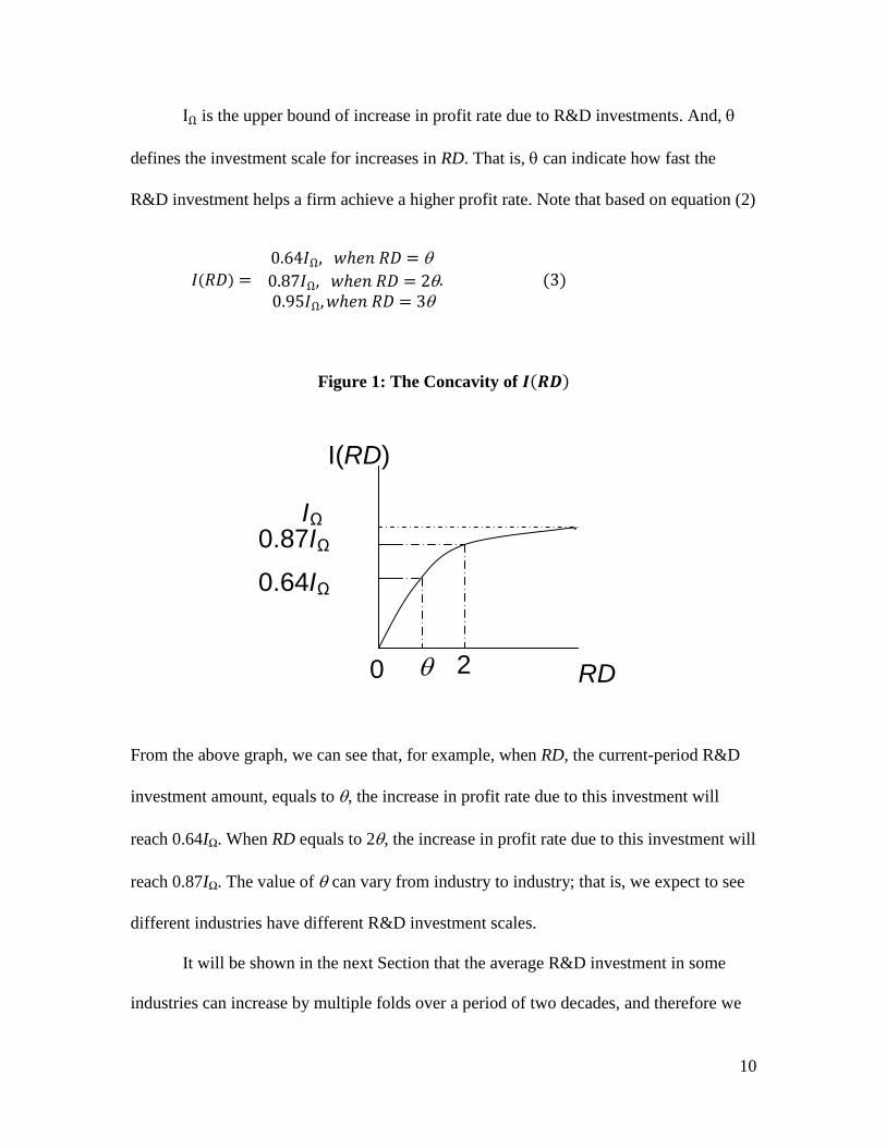
Figure 1: The Concavity of

From the above graph, we can see that, for example, when RD, the current-period R&D

investment amount, equals to , the increase in profit rate due to this investment will

reach 0.64IΩ. When RD equals to 2, the increase in profit rate due to this investment will

reach 0.87IΩ. The value of can vary from industry to industry; that is, we expect to see

different industries have different R&D investment scales.

It will be shown in the next Section that the average R&D investment in some

industries can increase by multiple folds over a period of two decades, and therefore we

IΩ

0 2

0.64IΩ

0.87IΩ

RD

I(RD)

11

expect that the investment scale to achieve the same increase in profit rate should grow

accordingly. For this reason I model the time-dependent feature of by

, in which is the value of in year

2000. The coefficient is estimated by linear regression of for each

industry. Note that c is a constant.

The R&D investment model becomes:

1

02000

1

0

)1(

1ˆ

),(exp1

)1(

1)(ˆ

J

jdj

j

dji

i

ii

J

jdj

j

idji

ii

r

qRDIRD

r

RDIqRD

(4)

The optimal condition is met when 0 ii RD , that is,

1

0

2000

2000

)1(

1ˆ

),(exp

),( J

jdj

j

dji

i

i

i

r

q

RDI

(5),

and through this equation we can estimate the depreciation rate .

3. Industry-Level Analysis – Initial Test

As a first step in our empirical analysis, I estimate the constant R&D depreciation

rate δ for four industries (pharmaceuticals, semiconductor, IT hardware, and software) by

using the data from 1989 to 2008 to check whether my model gives us R&D depreciation

rates in line with rates in past studies. These industries are important for the initial test of

my model because the combined R&D investments of these four industries account for

12

54.56% of U.S. total business R&D investments in 2004. I take the average values of

annual sales and R&D investment in each industry from Compustat for estimation.1

The Compustat dataset contains firm-level sales and R&D investments for SIC-

based industries: pharmaceutical, IT hardware, semiconductor, and software. Their

corresponding SIC codes listed below:

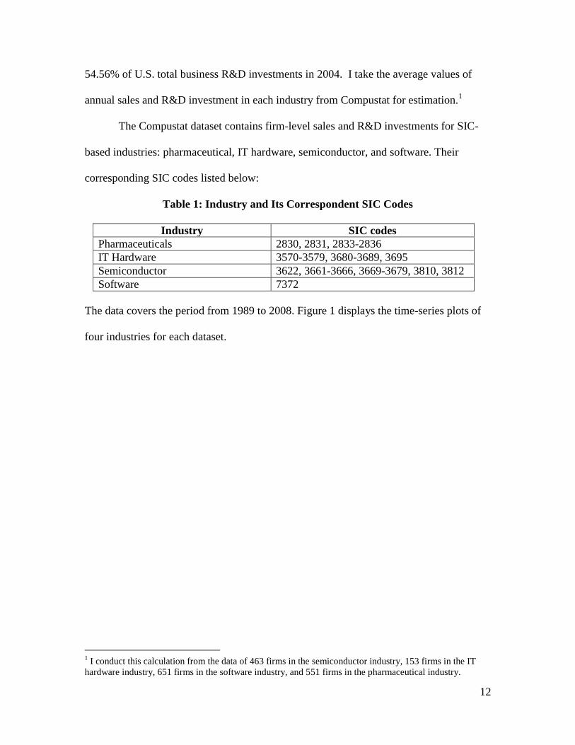
Table 1: Industry and Its Correspondent SIC Codes

Industry SIC codes

Pharmaceuticals 2830, 2831, 2833-2836

IT Hardware 3570-3579, 3680-3689, 3695

Semiconductor 3622, 3661-3666, 3669-3679, 3810, 3812

Software 7372

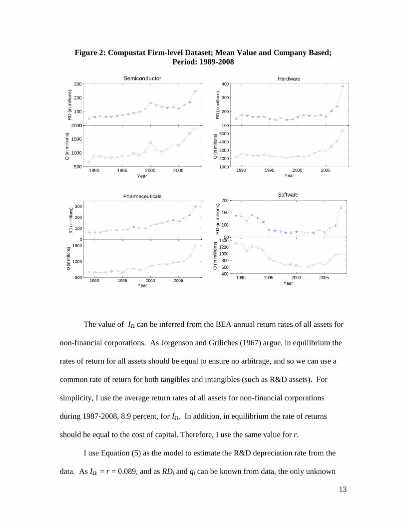
The data covers the period from 1989 to 2008. Figure 1 displays the time-series plots of

four industries for each dataset.

1 I conduct this calculation from the data of 463 firms in the semiconductor industry, 153 firms in the IT

hardware industry, 651 firms in the software industry, and 551 firms in the pharmaceutical industry.

13

Figure 2: Compustat Firm-level Dataset; Mean Value and Company Based;

Period: 1989-2008

The value of IΩ can be inferred from the BEA annual return rates of all assets for

non-financial corporations. As Jorgenson and Griliches (1967) argue, in equilibrium the

rates of return for all assets should be equal to ensure no arbitrage, and so we can use a

common rate of return for both tangibles and intangibles (such as R&D assets). For

simplicity, I use the average return rates of all assets for non-financial corporations

during 1987-2008, 8.9 percent, for IΩ. In addition, in equilibrium the rate of returns

should be equal to the cost of capital. Therefore, I use the same value for r.

I use Equation (5) as the model to estimate the R&D depreciation rate from the

data. As IΩ = r = 0.089, and as RDi and qi can be known from data, the only unknown

1990 1995 2000 20050

100

200

300

RD

(in

mill

ions)

Semiconductor

1990 1995 2000 2005500

1000

1500

2000

Year

Q (

in m

illio

ns)

1990 1995 2000 2005100

200

300

400

RD

(in

mill

ions)

Hardware

1990 1995 2000 20051000

2000

3000

4000

5000

Year

Q (

in m

illio

ns)

1990 1995 2000 20050

100

200

300

RD

(in

mill

ions)

Pharmaceuticals

1990 1995 2000 2005500

1000

1500

Year

Q (

in m

illio

ns)

1990 1995 2000 200550

100

150

200

RD

(in

millio

ns)

Software

1990 1995 2000 2005400

600

800

1000

1200

1400

Year

Q (

in m

illio

ns)

14

parameters in the equation are and . Because Equation (5) holds when the true values

of and are given, the difference between the left hand side and the right hand side of

Equation (5) is expected to be zero or close to zero when we conduct a least square fitting

to derive the optimal solution. Therefore, we can estimate these unknowns by

minimizing the following quantity:

5

1

2

1

0

2000

2000

)1(

1

),(exp

),(N

i

J

jdj

j

dji

i

i

i

r

q

RDI

(6),

in which N is the length of data in years.

Minimizing Equation (6) is therefore least squares fitting between the model and

the data. As the functional form is nonlinear, the calculation needs to be carried out

numerically, and in this study the downward simplex method is applied. In each

numerical search of the optimal solution of and , several sets of start values are tried to

ensure the stability of the solution.

In this study I use a 2-year gestation lag, which is consistent with the finding in

Pakes and Schankerman (1984) who examined 49 manufacturing firms across industries

and reported that gestation lags between 1.2 and 2.5 years were appropriate values to use.

As mentioned previously, the value of is set to be 25 for pharmaceuticals and 20 for

other industries. The estimated value of constant δ is 11.82 ± 0.73 percent for the

pharmaceutical industry, 37.64 ± 1.00 percent for the IT hardware industry, 17.95 ± 1.78

percent for the semiconductor industry, and 30.17 ± 1.89 percent for the software

industry. These results indicate that the ranking of R&D depreciation rates across

15

industries in a descending order is: IT hardware, software, semiconductor, and

pharmaceutical industries.

Since the technological and competition environments change over time, the

R&D depreciation rates are expected to vary through the 20 years of data studied.

Therefore, there is a need to calculate industry-specific and time-dependent R&D

depreciation rates. I use the same industry average sales and R&D investment data from

Compustat. The time-dependent feature of was obtained by minimizing Equation (6)

with subsets of data. Instead of using all years of data, I performed least squares fitting

over a five-year interval each time, in addition to the five prior years used for sales

forecasts. Four more subsets of data are examined in the same way, each with a step of 2

years in progression. As a result there are five subsets of data where data-model fit is

carried out, and the estimated depreciation rates are the mid-years of time windows,

which are years of 1997, 1999, 2001, 2003, and 2005. The values of d, J, IΩ, and r are

defined in the same manner as before.

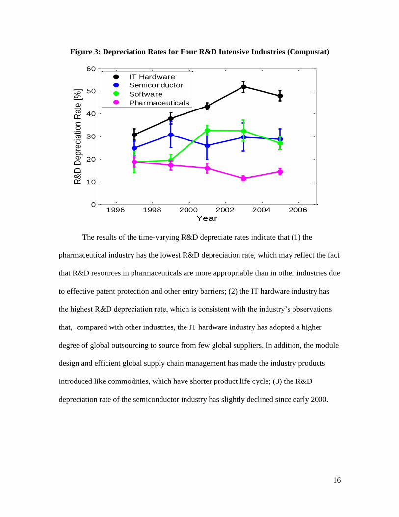
The best-fit time-varying R&D depreciation rates for the studied four industries

show that the ranking order of the depreciation rates is in general maintained over time

(See Figure 3). The vertical error bar is the standard deviation of the estimated R&D

depreciation rate estimated through the Monte-Carlo calculation in the same fashion.

16

Figure 3: Depreciation Rates for Four R&D Intensive Industries (Compustat)

The results of the time-varying R&D depreciate rates indicate that (1) the

pharmaceutical industry has the lowest R&D depreciation rate, which may reflect the fact

that R&D resources in pharmaceuticals are more appropriable than in other industries due

to effective patent protection and other entry barriers; (2) the IT hardware industry has

the highest R&D depreciation rate, which is consistent with the industry’s observations

that, compared with other industries, the IT hardware industry has adopted a higher

degree of global outsourcing to source from few global suppliers. In addition, the module

design and efficient global supply chain management has made the industry products

introduced like commodities, which have shorter product life cycle; (3) the R&D

depreciation rate of the semiconductor industry has slightly declined since early 2000.

1996 1998 2000 2002 2004 20060

10

20

30

40

50

60

Year

R&

D D

epre

ciat

ion

Rat

e [%

]

IT Hardware

Semiconductor

Software

Pharmaceuticals

17

This is consistent with the industry’s consensus that the rate of technological progress in

the microprocessor industry has slowed down after 20002.

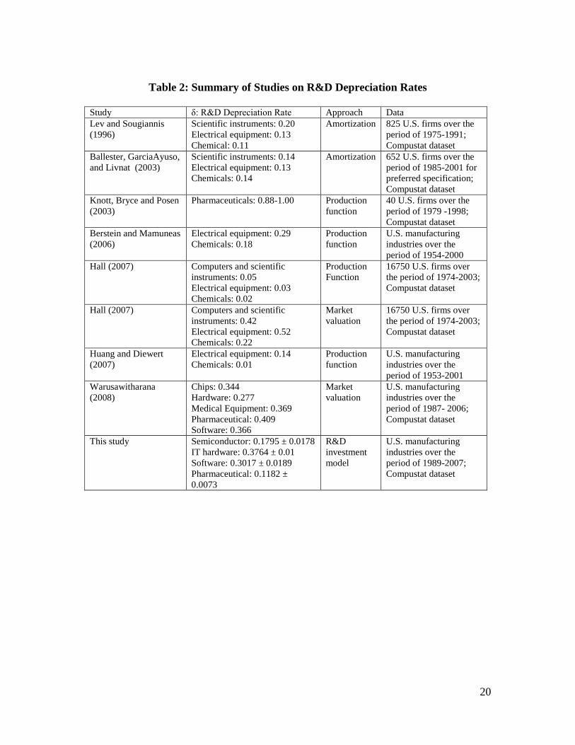
Table 2 compares the constant R&D depreciation rates estimated by this study

with those obtained from other recent studies. The comparison highlights several key

results from this study. First, the derived industry-specific R&D depreciation rates fall

within the range of recent research estimates based on commonly-adopted production

function and market valuation approaches (Berstein and Mamuneas, 2006; Hall, 2007;

Huang and Diewert, 2007; Warusawitharana, 2008). Second, my results are consistent

with those of recent studies, which indicate that depreciation rates for business R&D are

likely to vary across industries due to the different competition environments that each

industry faces. Third, most industries have R&D depreciation rates higher than the

traditional 15% assumption derived using the data of the 1970s (Berstein and Mamuneas,

2006; Corrado et al., 2006; Hall, 2007; Huang and Diewert, 2007; Warusawitharana,

2008; Grilliches and Mairesse, 1984).

Given that the results based on Compustat dataset align with the conclusions with

existing studies and industry observations on the pace of technological progress and the

degree of market competition, the next step is to perform the same calculations for all ten

R&D intensive industries identified in BEA’s R&D Satellite Account.

4. Industry-Level Analysis – All Ten BEA R&D Intensive Industries

There are three steps to derive a complete set of the recommended depreciation

rates of business R&D assets. In the first step, I estimate two sets of the industry-specific

2 Professor Pillai, who used to work for AMD and is now at SUNY University at Albany, confirmed this

trend.

18

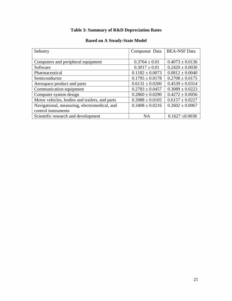
R&D depreciation rates based on the Compustat company-based data and the BEA-NSF

establishment-based data (See Table 3). The values based on the two datasets are

plausible for most industries. Among the R&D depreciation rates in the ten analyzed

R&D intensive industries, the values for the aerospace and auto industries are usually

large compared to those for other industries. For example, based on both Compustat and

BEA-NSF datasets, the estimated R&D depreciation rates for the auto industry are 39.88%

and 61.57%, respectively, and these results are not inconsistent to the result of the UK’s

ONS (office of National Statistics) survey on the R&D service life (Haltiwanger et al.,

2010). The average R&D service life for the auto industry in the UK’s ONS survey is 4.3

years, which implies an R&D depreciation rate over 40 percent. Note that the response

rate of the UK’s ONS survey, however, is merely 10-200 firms out of 989 firms, or

equivalently 1.0-20.2 percent of the surveyed firms.

In the second step, because the profit rates of these two industries are significantly

lower than those of other industries, I relax the criterion based on the argument by

Jorgenson and Griliches’ with regard to using the common rate of return for both tangible

and intangible assets and reduce the upper bound of the return rate by 50% in the model.

The justifications are given by the two facts: First, the U.S. auto industry had negative

return rates during the data period3. Second, in its August 2011 report on the Aerospace

and Defense industrial base assessments, the Office of Technology Evaluation at

Department of Commerce reports that the industry’s profit margin is around 1% and may

be only 10% of the performance of high-tech industries in Silicon Valley. After the

relaxation, for the auto industry, the estimated result based on the BEA-NSF dataset is

3 Brian Sliker at BEA, an expert in the return rate of industry assets, indicated this negative trend in the

auto industry.

19

close to the estimated range by Bernstein and Mamuneas (2006) and by Huang and

Diewert (2007). For the aerospace industry, this study may be the first to have estimated

its depreciation rate, and the result is consistent with the general belief that the

depreciation rate decreases when the development cycle is longer or the degree of

competition is lower. Compared with the pharmaceutical industry, the aerospace industry

has a shorter development cycle which results in a higher R&D depreciation rate. On the

other hand, in comparison with the auto industry, the aerospace industry has a longer

development cycle and a lower degree of competition, resulting in a lower R&D

depreciation rate.

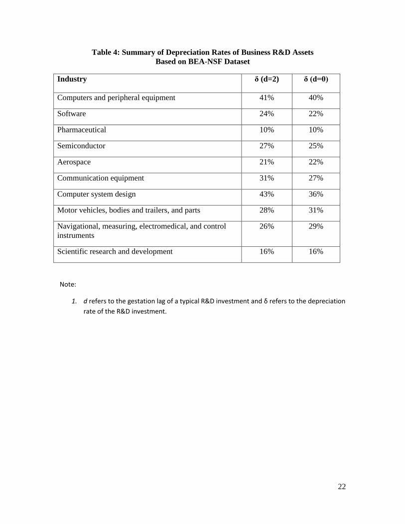
In the third step, the number of J is chosen based on the robustness check of the

stability of optimal solutions. When J is 20, the optimal solutions are stable for all

industries except the pharmaceutical industry, where J needs to be 40. So, the optimal

solution for the pharmaceutical industry is updated with J equals to 40.

Table 4 is the summary of the recommended depreciation rates of R&D assets

based on the BEA-NSF dataset. The results in this table are based on two scenarios of the

average gestation lag of R&D projects. In addition, I assume that the R&D assets

depreciate at this rate geometrically. Lastly, it is considered that when a firm invests in

R&D, whether the investment is successful or not, the R&D investment should contribute

to the firm’s knowledge stock. Therefore, we recommend the use of the calculated rates

with a zero gestation lag.

20

Table 2: Summary of Studies on R&D Depreciation Rates

Study δ: R&D Depreciation Rate Approach Data

Lev and Sougiannis

(1996)

Scientific instruments: 0.20

Electrical equipment: 0.13

Chemical: 0.11

Amortization 825 U.S. firms over the

period of 1975-1991;

Compustat dataset

Ballester, GarciaAyuso,

and Livnat (2003)

Scientific instruments: 0.14

Electrical equipment: 0.13

Chemicals: 0.14

Amortization 652 U.S. firms over the

period of 1985-2001 for

preferred specification;

Compustat dataset

Knott, Bryce and Posen

(2003)

Pharmaceuticals: 0.88-1.00 Production

function

40 U.S. firms over the

period of 1979 -1998;

Compustat dataset

Berstein and Mamuneas

(2006)

Electrical equipment: 0.29

Chemicals: 0.18

Production

function

U.S. manufacturing

industries over the

period of 1954-2000

Hall (2007) Computers and scientific

instruments: 0.05

Electrical equipment: 0.03

Chemicals: 0.02

Production

Function

16750 U.S. firms over

the period of 1974-2003;

Compustat dataset

Hall (2007) Computers and scientific

instruments: 0.42

Electrical equipment: 0.52

Chemicals: 0.22

Market

valuation

16750 U.S. firms over

the period of 1974-2003;

Compustat dataset

Huang and Diewert

(2007)

Electrical equipment: 0.14

Chemicals: 0.01

Production

function

U.S. manufacturing

industries over the

period of 1953-2001

Warusawitharana

(2008)

Chips: 0.344

Hardware: 0.277

Medical Equipment: 0.369

Pharmaceutical: 0.409

Software: 0.366

Market

valuation

U.S. manufacturing

industries over the

period of 1987- 2006;

Compustat dataset

This study Semiconductor: 0.1795 ± 0.0178

IT hardware: 0.3764 ± 0.01

Software: 0.3017 ± 0.0189

Pharmaceutical: 0.1182 ±

0.0073

R&D

investment

model

U.S. manufacturing

industries over the

period of 1989-2007;

Compustat dataset

21

Table 3: Summary of R&D Depreciation Rates

Based on A Steady-State Model

Industry Compustat Data BEA-NSF Data

Computers and peripheral equipment 0.3764 ± 0.01 0.4073 ± 0.0136

Software 0.3017 ± 0.01 0.2420 ± 0.0030

Pharmaceutical 0.1182 ± 0.0073 0.0812 ± 0.0040

Semiconductor 0.1795 ± 0.0178 0.2708 ± 0.0175

Aerospace product and parts 0.6131 ± 0.0200 0.4539 ± 0.0314

Communication equipment 0.2783 ± 0.0457 0.3089 ± 0.0223

Computer system design 0.2860 ± 0.0290 0.4272 ± 0.0056

Motor vehicles, bodies and trailers, and parts 0.3988 ± 0.0105 0.6157 ± 0.0227

Navigational, measuring, electromedical, and

control instruments

0.3408 ± 0.0216 0.2602 ± 0.0067

Scientific research and development NA 0.1627 ±0.0038

22

Table 4: Summary of Depreciation Rates of Business R&D Assets

Based on BEA-NSF Dataset

Industry δ (d=2) δ (d=0)

Computers and peripheral equipment 41% 40%

Software 24% 22%

Pharmaceutical 10% 10%

Semiconductor 27% 25%

Aerospace 21% 22%

Communication equipment 31% 27%

Computer system design 43% 36%

Motor vehicles, bodies and trailers, and parts 28% 31%

Navigational, measuring, electromedical, and control

instruments

26% 29%

Scientific research and development 16% 16%

Note:

1. d refers to the gestation lag of a typical R&D investment and δ refers to the depreciation

rate of the R&D investment.

23

5. Conclusion

R&D depreciation rates are critical to calculating rates of return to R&D

investments and capital service costs, which are important for capitalizing R&D

investments in the national income accounts. Although important, measuring R&D

depreciation rates is extremely difficult because both the price and output of R&D capital

are generally unobservable. BEA adopted two simplified methods based on existing

studies to temporarily resolve the problem of measuring R&D depreciation rates in its

2006 Research & Development Satellite Account (R&DSA) and 2007 R&DSA. BEA

chose the rates following two rules: First, the rates were close to traditional 15 percent

assumption. Second, the overall ranking of the rates suggested by the literature was

preserved. However, the most recent studies conclude that depreciation rates for business

R&D are likely to be more variable due to different competition environments across

industries and higher than the traditional 15 percent assumption.

In this research, I develop a forward-looking profit model to derive industry-

specific R&D depreciation rates. Without any unverifiable assumptions adopted by other

methods, this model contains very few parameters and allows us to utilize Compustat

data on sales and R&D investments, and BEA-NSF data on industry output and R&D

investments. The new methodology allows us to calculate not only industry-specific

constant R&D depreciation rates but also time-varying rates.

My research results highlight several promising features of the new forward-

looking profit model: First, the derived constant industry-specific R&D depreciation rates

fall within the range of estimates from previous studies. The time-varying results also

24

capture the heterogeneous nature of industry environments in technology and competition.

In addition, the results are consistent with conclusions from recent studies that

depreciation rates for business R&D are likely to be more variable due to different

competition environments across industries and higher than traditional 15 percent

assumption (Berstein and Mamuneas 2006, Corrado et al 2006, Hall 2007, Huang and

Diewert 2007 and Warusawitharana 2008). Lastly, for the purpose of implementation,

this paper recommends a preliminary set of R&D depreciation rates for the ten R&D

intensive industries identified in BEA’s R&D Satellite Account.

25

References

Aizcorbe, A., Moylan, C., and Robbins, C. Toward Better Measurement of Innovation

and Intangibles, Survey of Current Business, January 2009, pp. 10-23.

Copeland, A., & Fixler, D. Measuring the Price of Research and Development

Output, U.S. Bureau of Economic Analysis Working Paper, October, 2008.

Corrado, C., Hulten, C., & Sichel, D. Intangible Capital and Economic Growth, National

Bureau of Economic Research working paper 11948, January 2006.

Griliches, Z. 1996. R&D and Productivity: The Econometric Evidence, Chicago: Chicago

University Press.

Hall, B. Measuring the Returns to R&D: The Depreciation Problem, National Bureau of

Economic Research Working Paper 13473, October 2007.

Haltiwanger, J., Haskel, J., & Robb, A. Extending Firm Surveys to Measure Intangibles:

Evidence from the United Kingdom and United States, 2010 American Economic

Association Session on Data Watch: New Developments in Measuring Innovation

Activity, Altlanta, GA, January 4.

Huang, N. and Diewert, E. 2007. Estimation of R&D Depreciation Rates for the US

Manufacturing and Four Knowledge Intensive Industries, working paper for the

Sixth Annual Ottawa Productivity Workshop held at the Bank of Canada, May 14-

15, 2007.

Jorgenson, D. and Griliches, Z. 1967. The Explanation of Productivity Change, Review of

Economic Studies, 34 (July): 349-83.

Mead, C. R&D Depreciation Rates in the 2007 R&D Satellite Account, Bureau of

Economic Analysis/National Science Foundation: 2007 R&D Satellite Account

26

Background Paper, November 2007.

Mills, T. C. 1990. Time Series Techniques for Economists. Cambridge: Cambridge

University Press.

Robbins, C., and Moylan, C. 2007. Research and Development Satellite Account Update:

Estimates for 1959-2004, New Estimates for Industry, Regional, and International

Accounts, Survey of Current Business, October 2007.

Sliker, B. 2007 R&D Satellite Account Methodologies: R&D Capital Stocks and Net

Rates of Return, Bureau of Economic Analysis/National Science Foundation:

R&D Satellite Account Background Paper, December 2007.

Sumiye, O., Robbins, C., Moylan, C., Sliker, B., Schultz, L., and Mataloni, L. BEA’s

2006 Research and Development Satellite Account: Preliminary Estimates of

R&D for 1959-2002 Effect on GDP and Other Measures, Survey of Current

Business, December 2006, pp. 14-27.

Warusawitharana, M. Research and Development, Profits and Firm Value: A Structural

Estimation, Federal Reserve Board working paper, December 2008.