Embed Size (px)
Citation preview
Technical ReportNumber 546
Computer Laboratory
UCAM-CL-TR-546ISSN 1476-2986
Depth perception in computer graphics
Jonathan David Pfautz
September 2002
15 JJ Thomson Avenue
Cambridge CB3 0FD
United Kingdom
phone +44 1223 763500
http://www.cl.cam.ac.uk/

c© 2002 Jonathan David Pfautz
This technical report is based on a dissertation submitted May2000 by the author for the degree of Doctor of Philosophy to theUniversity of Cambridge, Trinity College.
Technical reports published by the University of CambridgeComputer Laboratory are freely available via the Internet:
http://www.cl.cam.ac.uk/TechReports/
Series editor: Markus Kuhn
ISSN 1476-2986

iii

iv
v
ABSTRACT
With advances in computing and visual display technology, the interface between man and machine has become increasingly complex. The usability of a modern interactive system depends on the design of the visual display. This dissertation aims to improve the design process by examining the relationship between human perception of depth and three-dimensional computer-generated imagery (3D CGI). Depth is perceived when the human visual system combines various different sources of information about a scene. In Computer Graphics, linear perspective is a common depth cue, and systems utilising binocular disparity cues are of increasing interest. When these cues are inaccurately and inconsistently presented, the effectiveness of a display will be limited. Images generated with computers are sampled, meaning they are discrete in both time and space. This thesis describes the sampling artefacts that occur in 3D CGI and their effects on the perception of depth. Traditionally, sampling artefacts are treated as a Signal Processing problem. The approach here is to evaluate artefacts using Human Factors and Ergonomics methodology; sampling artefacts are assessed via performance on relevant visual tasks. A series of formal and informal experiments were performed on human subjects to evaluate the effects of spatial and temporal sampling on the presentation of depth in CGI. In static images with perspective information, the relative size of an object can be inconsistently presented across depth. This inconsistency prevented subjects from making accurate relative depth judgements. In moving images, these distortions were most visible when the object was moving slowly, pixel size was large, the object was located close to the line of sight and/or the object was located a large virtual distance from the viewer. When stereo images are presented with perspective cues, the sampling artefacts found in each cue interact. Inconsistencies in both size and disparity can occur as the result of spatial and temporal sampling. As a result, disparity can vary inconsistently across an object. Subjects judged relative depth less accurately when these inconsistencies were present. An experiment demonstrated that stereo cues dominated in conflict situations for static images. In moving imagery, the number of samples in stereo cues is limited. Perspective information dominated the perception of depth for unambiguous (i.e., constant in direction and velocity) movement. Based on the experimental results, a novel method was developed that ensures the size, shape and disparity of an object are consistent as it moves in depth. This algorithm manipulates the edges of an object (at the expense of positional accuracy) to enforce consistent size, shape and disparity. In a time-to-contact task using only stereo and perspective depth cues, velocity was judged more accurately using this method. A second method manipulated the location and orientation of the viewpoint to maximise the number of samples of perspective and stereo depth in a scene. This algorithm was tested in a simulated air traffic control task. The experiment demonstrated that knowledge about where the viewpoint is located dominates any benefit gained in reducing sampling artefacts. This dissertation provides valuable information for the visual display designer in the form of task-specific experimental results and computationally inexpensive methods for reducing the effects of sampling.

vi

vii
PREFACE
This dissertation is the result of my own work and includes nothing that is the outcome of work done in collaboration. I hereby declare that this dissertation is not substantially the same as any other I have submitted for a degree or a diploma or other qualification at any other University. I further state that no part of this dissertation has already been or is being concurrently submitted for any such degree, diploma or other qualification. This dissertation does not exceed sixty thousand words, including tables, footnotes and bibliography. PUBLICATIONS
Sections of this work have been published previously [Pfautz & Robinson 1999].
TRADEMARKS
All trademarks contained in this dissertation are hereby acknowledged.
Jonathan D. Pfautz

viii

ix
ACKNOWLEDGEMENTS
Financial support for this work was generously provided by Trinity College, the Cambridge University Computer Laboratory, the Cambridge Overseas Trust, the Overseas Research Student scheme offered by the Committee of Vice-Chancellors and Principals of U.K. Universities and my parents, Glenn and Virginia Pfautz. I would like to express my thanks to my supervisor, Peter Robinson, Neil Dodgson, the members of the Rainbow Research Group and the many others who have contributed to this dissertation.

x
xi
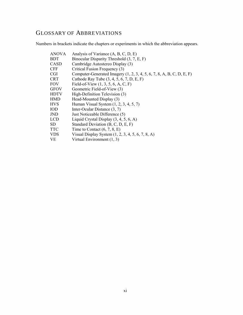
GLOSSARY OF ABBREVIATIONS
Numbers in brackets indicate the chapters or experiments in which the abbreviation appears. ANOVA Analysis of Variance (A, B, C, D, E) BDT Binocular Disparity Threshold (3, 7, E, F) CASD Cambridge Autostereo Display (3) CFF Critical Fusion Frequency (3) CGI Computer-Generated Imagery (1, 2, 3, 4, 5, 6, 7, 8, A, B, C, D, E, F) CRT Cathode Ray Tube (3, 4, 5, 6, 7, D, E, F) FOV Field-of-View (1, 3, 5, 6, A, C, F) GFOV Geometric Field-of-View (3) HDTV High-Definition Television (3) HMD Head-Mounted Display (3) HVS Human Visual System (1, 2, 3, 4, 5, 7) IOD Inter-Ocular Distance (3, 7) JND Just Noticeable Difference (5) LCD Liquid Crystal Display (3, 4, 5, 6, A) SD Standard Deviation (B, C, D, E, F) TTC Time to Contact (6, 7, 8, E) VDS Visual Display System (1, 2, 3, 4, 5, 6, 7, 8, A) VE Virtual Environment (1, 3)

xii
xiii
CONVENTIONS
This thesis adopts some conventions for clarity:
• [ ]xr denotes the nearest integer function or round of a number, x.
• x denotes the floor of a number, x.
• [ ]Vr
n denotes the Euclidean norm of a vector, Vr
.
• ),( mnx ∈ denotes the interval mxn << ],[ mnx ∈ denotes the interval mxn ≤≤
• Small visual angles will be expressed in minutes, m, and seconds, s:
m's"
• Results of analyses of variance will be presented as follows:
F(m,n) = j, p < 0.01 Where m is the degrees of freedom of the independent variable being analysed, n is the residual degrees of freedom, j is the F-value and p is the significance level. Significance levels of p < 0.01 will be reported. Graphs reporting statistical data will have error bars representing a 95% confidence interval.
• In this thesis, we present many graphs that show the effects of sampling for typical viewing parameters and display characteristics. For brevity, we will not explicitly state the values of the parameters used. Generally, they are chosen to demonstrate common trends and behaviours.
• Data for experiments A � F can be found at:
http://mit.edu/jpfautz/www/phd/

xiv

xv
TABLE OF CONTENTS
Chapter 1: Introduction........................................................................................................................... 1
1.1 Depth in Computer Graphics.......................................................................................................................2 1.2 Applications of 3D CGI ..............................................................................................................................2 1.3 Displaying Digital Imagery.........................................................................................................................3 1.4 Methodology ...............................................................................................................................................5 1.5 Aims............................................................................................................................................................6 1.6 Layout of Dissertation.................................................................................................................................6
Chapter 2: Human Depth Perception ...................................................................................................... 7
2.1 Pictorial Depth Cues ...................................................................................................................................7 2.2 Oculomotor Depth Cues............................................................................................................................10 2.3 Binocular Depth Perception ......................................................................................................................10 2.4 Depth from Motion ...................................................................................................................................11 2.5 Combination and Application of Depth Cues ...........................................................................................12 2.6 Depth Acuity .............................................................................................................................................14 2.7 Conclusions ...............................................................................................................................................15
Chapter 3: Display System Engineering............................................................................................... 17
3.1 Display Types ...........................................................................................................................................17 3.2 Display Parameters....................................................................................................................................19 3.3 Tradeoffs in Display Design .....................................................................................................................27 3.4 Conclusion ................................................................................................................................................30
Chapter 4: Sampling and Antialiasing .................................................................................................. 31
4.1 Sampling Theory.......................................................................................................................................31 4.2 Sampling Images.......................................................................................................................................32 4.3 Image Quality Metrics...............................................................................................................................36 4.4 A Human Factors Approach to Sampling .................................................................................................37 4.5 Conclusion ................................................................................................................................................38
Chapter 5: Sampling Static Perspective Cues....................................................................................... 39
5.1 Background ...............................................................................................................................................39 5.2 Analysis.....................................................................................................................................................41 5.3 Experimentation ........................................................................................................................................48 5.4 Solutions....................................................................................................................................................52 5.5 Conclusion ................................................................................................................................................61

xvi
xvii
Chapter 6: Spatio-Temporal Sampling of Perspective.......................................................................... 63
6.1 Background ...............................................................................................................................................63 6.2 Analysis.....................................................................................................................................................65 6.3 Experimentation ........................................................................................................................................71 6.4 Solutions....................................................................................................................................................75 6.5 Conclusion ................................................................................................................................................79
Chapter 7: Sampling of Stereo and Perspective Depth......................................................................... 81
7.1 Background ...............................................................................................................................................81 7.2 Analysis.....................................................................................................................................................83 7.3 Experimentation ........................................................................................................................................97 7.4 Solutions..................................................................................................................................................102 7.5 Conclusion ..............................................................................................................................................105
Chapter 8: Conclusions and Further Work ......................................................................................... 107
8.1 Major Results ..........................................................................................................................................107 8.2 Future Work ............................................................................................................................................109
Experiment A: Detectability of Sampled Perspective Cues................................................................ 111
Experiment B: Judging Alignment in Perspective Depth ................................................................... 117
Experiment C: Interactive Alignment in Depth .................................................................................. 125
Experiment D: Stereo and Perspective Depth Acuity......................................................................... 129
Experiment E: Judging Alignment in Stereo and Perspective Depth ................................................. 135
Experiment F: Air Traffic Control...................................................................................................... 143
Bibliography ....................................................................................................................................... 151

xviii
1
C H A P T E R 1
1:Introduction Over the past forty years, advances in display and computing technology have revolutionised the interface between man and machine. Now that people can interact with rich, realistic, 3D graphics with relatively low cost equipment, the time has come to focus on designing our systems so that we maximise their capabilities in the ways most effective for the user. Man-machine interfaces found in simulator and teleoperation systems have laid the groundwork for completely computer-generated or �virtual� environments. Simulators are training systems that display computer-generated scenes based on real-world situations. Teleoperation systems extend a person�s ability to sense and manipulate the world to a remote location. The control and display devices in these systems are often computer-controlled. Virtual environments(VEs) are computer-generated experiences that may seem real but are not required to match any of the rules of the real world. As Kalawsky says:
�[Virtual environments are] synthetic sensory experiences that communicate physical and abstract components to a human operator or participant. The synthetic sensory experience is generated by a computer system that one day may present an interface to the human sensory systems that is indistinguishable from the real physical world� [Kalawsky 1993].
VEs, like many simulators and teleoperation systems, rely on the visual display system�s (VDS�s) ability to match the user�s sensory channels. In VEs, the visual channel is often the most prominent. Therefore, improving the quality and capabilities of the VDSs used in VEs is vital. Unfortunately, while advances in processing power have occurred at an exponential rate in recent years, advances in
2
visual display technology have not. This has led to a variety of problems in how to effectively and efficiently present realistic 3D, computer-generated imagery (CGI). This dissertation studies how visual display systems can better meet the requirements of the human visual system (HVS). Specifically, we argue that:
1) HVS requirements are a function of the type of task performed in a VE.
2) There is a relationship between task performance and VDS characteristics.
3) Task-centred analysis can lead to new, more efficient techniques for improving the design and display of 3D imagery.
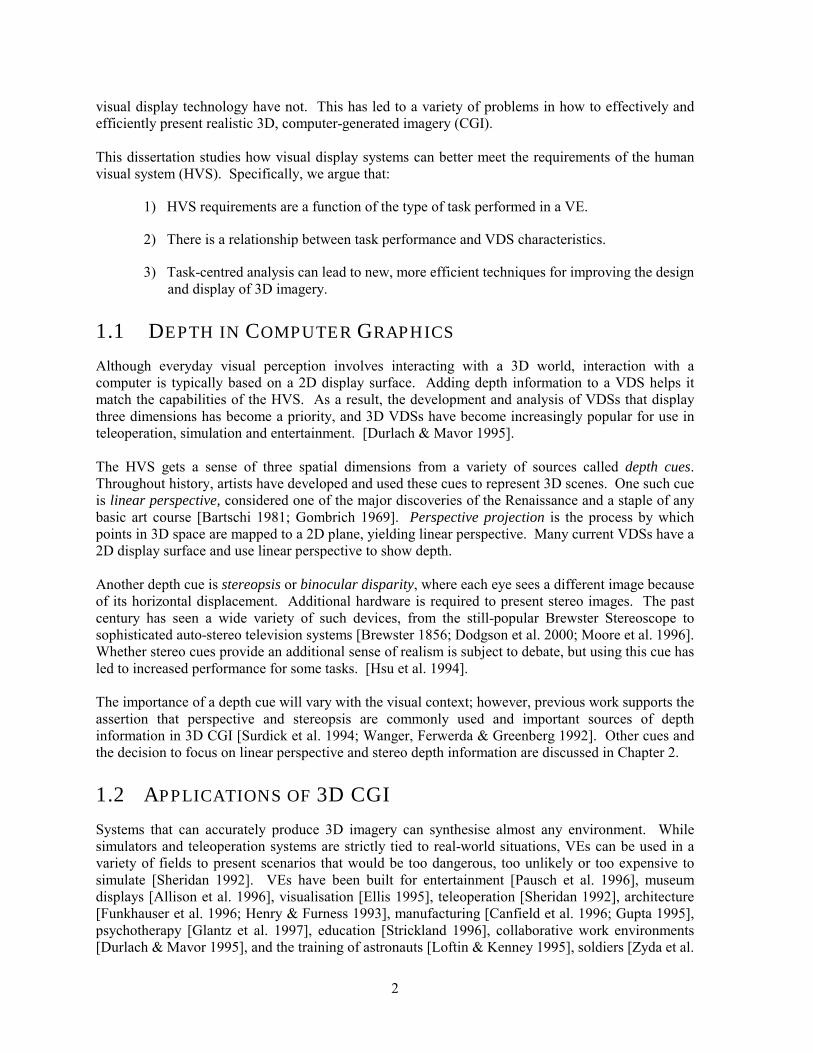
1.1 DEPTH IN COMPUTER GRAPHICS
Although everyday visual perception involves interacting with a 3D world, interaction with a computer is typically based on a 2D display surface. Adding depth information to a VDS helps it match the capabilities of the HVS. As a result, the development and analysis of VDSs that display three dimensions has become a priority, and 3D VDSs have become increasingly popular for use in teleoperation, simulation and entertainment. [Durlach & Mavor 1995]. The HVS gets a sense of three spatial dimensions from a variety of sources called depth cues. Throughout history, artists have developed and used these cues to represent 3D scenes. One such cue is linear perspective, considered one of the major discoveries of the Renaissance and a staple of any basic art course [Bartschi 1981; Gombrich 1969]. Perspective projection is the process by which points in 3D space are mapped to a 2D plane, yielding linear perspective. Many current VDSs have a 2D display surface and use linear perspective to show depth. Another depth cue is stereopsis or binocular disparity, where each eye sees a different image because of its horizontal displacement. Additional hardware is required to present stereo images. The past century has seen a wide variety of such devices, from the still-popular Brewster Stereoscope to sophisticated auto-stereo television systems [Brewster 1856; Dodgson et al. 2000; Moore et al. 1996]. Whether stereo cues provide an additional sense of realism is subject to debate, but using this cue has led to increased performance for some tasks. [Hsu et al. 1994]. The importance of a depth cue will vary with the visual context; however, previous work supports the assertion that perspective and stereopsis are commonly used and important sources of depth information in 3D CGI [Surdick et al. 1994; Wanger, Ferwerda & Greenberg 1992]. Other cues and the decision to focus on linear perspective and stereo depth information are discussed in Chapter 2.
1.2 APPLICATIONS OF 3D CGI
Systems that can accurately produce 3D imagery can synthesise almost any environment. While simulators and teleoperation systems are strictly tied to real-world situations, VEs can be used in a variety of fields to present scenarios that would be too dangerous, too unlikely or too expensive to simulate [Sheridan 1992]. VEs have been built for entertainment [Pausch et al. 1996], museum displays [Allison et al. 1996], visualisation [Ellis 1995], teleoperation [Sheridan 1992], architecture [Funkhauser et al. 1996; Henry & Furness 1993], manufacturing [Canfield et al. 1996; Gupta 1995], psychotherapy [Glantz et al. 1997], education [Strickland 1996], collaborative work environments [Durlach & Mavor 1995], and the training of astronauts [Loftin & Kenney 1995], soldiers [Zyda et al.
CHAPTER 1: Introduction
3
1994], surgeons [Johnston et al. 1996; Lasko-Harvill et al. 1995], and aeroplane [Furness 1986] and submarine pilots [Levison et al. 1995; Zelzter et al. 1994]. This plethora of applications indicates that the VDS used for VEs must accommodate all manner of visual tasks, from simple target detection to more complex processes like collision detection. This dissertation studies visual tasks at a simple but practical level. For example, rather than studying how well a pilot lands his simulated aeroplane, we measure how accurately a user estimates an approaching object�s velocity. We believe that understanding the sub-tasks of a complex process leads to a better understanding of the system requirements [Wilson 1998].
1.3 DISPLAYING DIGITAL IMAGERY
Computer-generated images are always sampled; that is, they are represented by quantized values in a machine�s memory and discrete locations on the display surface. Sampling results in unrealistic images and limits the user�s ability to perform certain tasks. The types of image degradation caused by sampling are called sampling artefacts. Spatial sampling artefacts are generated when the VDS� resolution (i.e., pixel size and the number of pixels) is not as high as the HVS� acuity. Similarly, in computer-generated animations, the scene-generation and screen refresh rates interact with the VDS� spatial resolution to produce spatio-temporal sampling artefacts. These artefacts appear as a function of decisions made in designing both the display hardware and the software to drive it. The interactions among display parameters like field-of-view (FOV), spatial resolution, frame rate and refresh rate determine the VDS� spatial and temporal characteristics and therefore the magnitude and type of sampling artefacts that occur. Chapter 3 addresses the effects that some display parameters and their interactions have on the sampling of CGI.
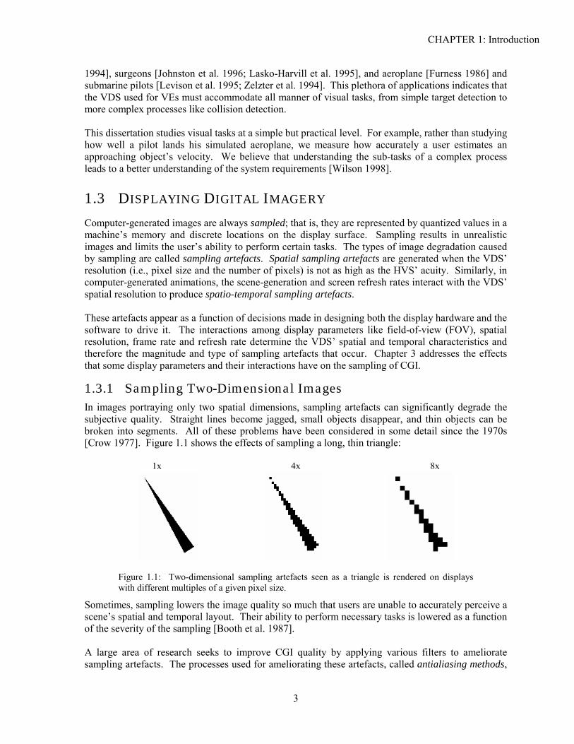
1.3.1 Sampling Two-Dimensional Images In images portraying only two spatial dimensions, sampling artefacts can significantly degrade the subjective quality. Straight lines become jagged, small objects disappear, and thin objects can be broken into segments. All of these problems have been considered in some detail since the 1970s [Crow 1977]. Figure 1.1 shows the effects of sampling a long, thin triangle:
1x 4x 8x
Figure 1.1: Two-dimensional sampling artefacts seen as a triangle is rendered on displays with different multiples of a given pixel size.
Sometimes, sampling lowers the image quality so much that users are unable to accurately perceive a scene�s spatial and temporal layout. Their ability to perform necessary tasks is lowered as a function of the severity of the sampling [Booth et al. 1987]. A large area of research seeks to improve CGI quality by applying various filters to ameliorate sampling artefacts. The processes used for ameliorating these artefacts, called antialiasing methods,
4
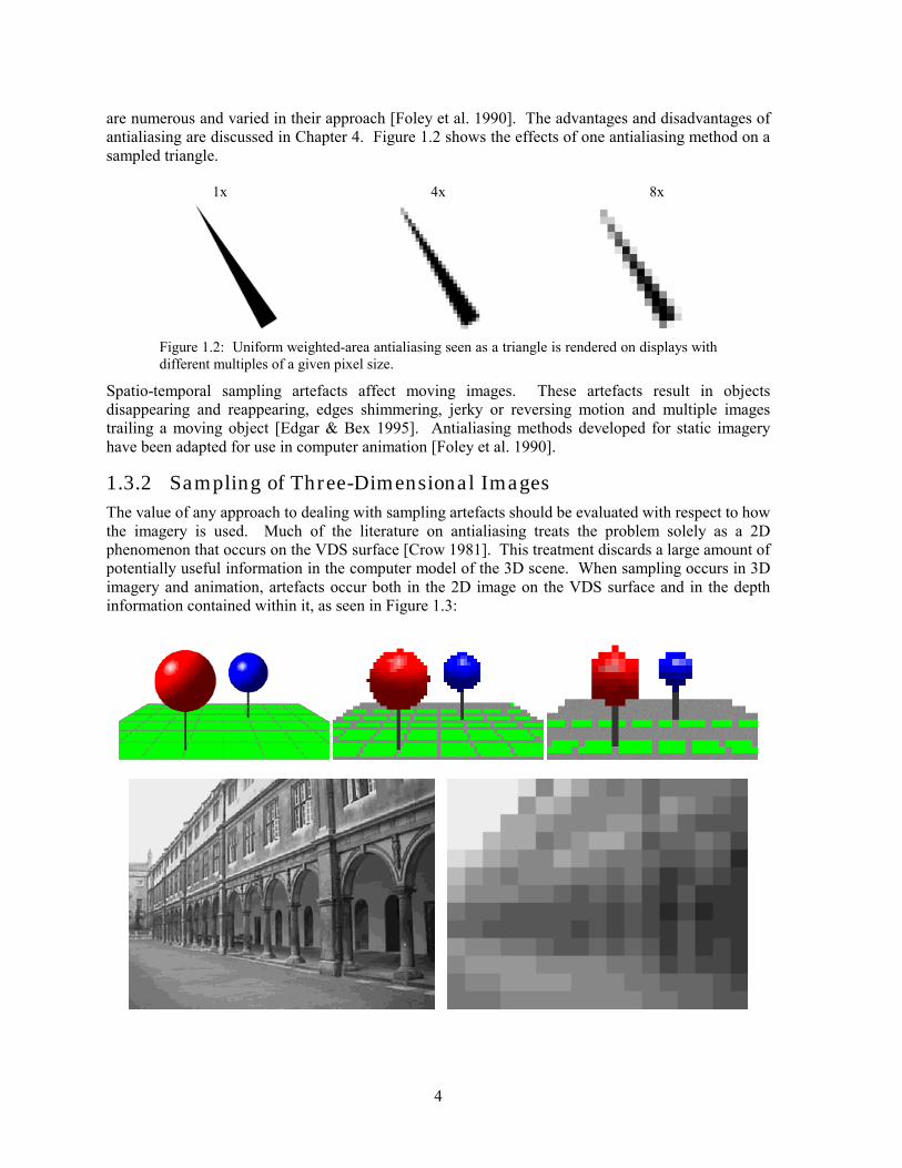
are numerous and varied in their approach [Foley et al. 1990]. The advantages and disadvantages of antialiasing are discussed in Chapter 4. Figure 1.2 shows the effects of one antialiasing method on a sampled triangle.
1x 4x 8x
Figure 1.2: Uniform weighted-area antialiasing seen as a triangle is rendered on displays with different multiples of a given pixel size.
Spatio-temporal sampling artefacts affect moving images. These artefacts result in objects disappearing and reappearing, edges shimmering, jerky or reversing motion and multiple images trailing a moving object [Edgar & Bex 1995]. Antialiasing methods developed for static imagery have been adapted for use in computer animation [Foley et al. 1990].
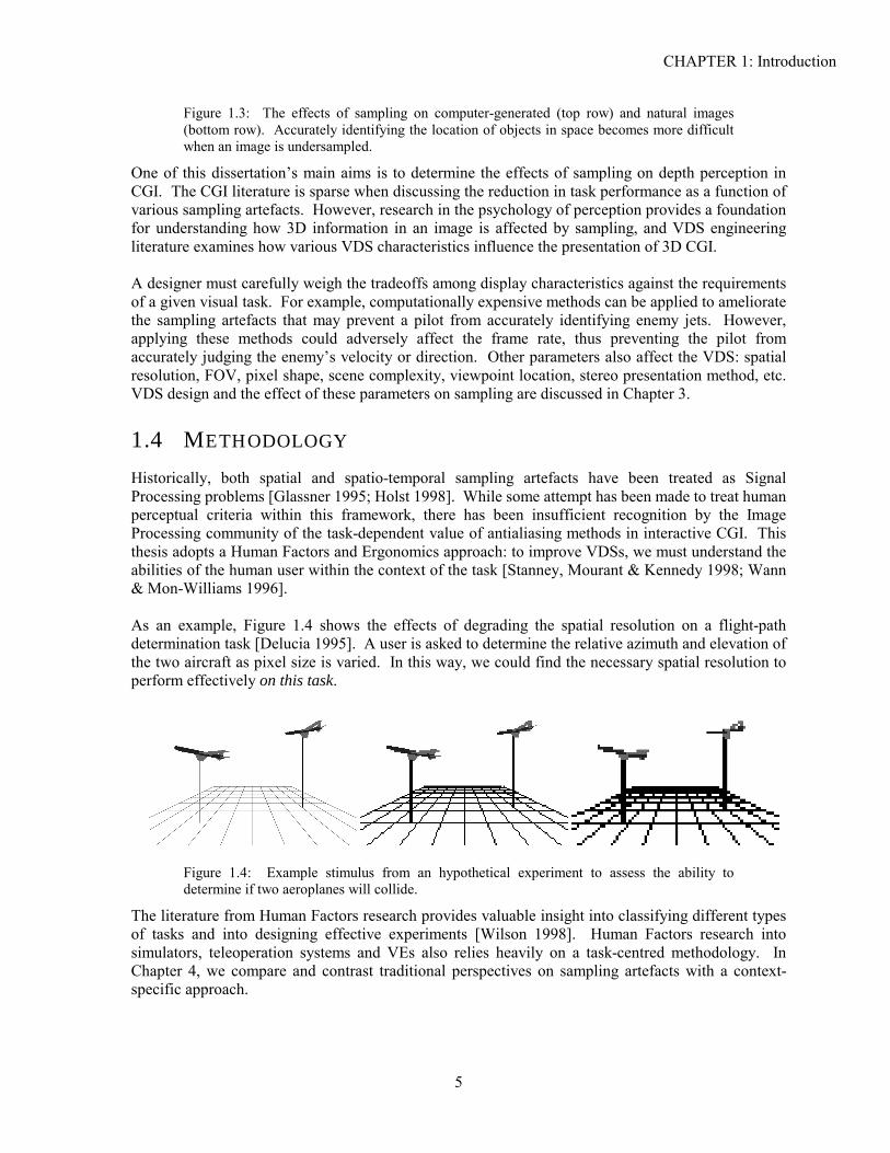
1.3.2 Sampling of Three-Dimensional Images The value of any approach to dealing with sampling artefacts should be evaluated with respect to how the imagery is used. Much of the literature on antialiasing treats the problem solely as a 2D phenomenon that occurs on the VDS surface [Crow 1981]. This treatment discards a large amount of potentially useful information in the computer model of the 3D scene. When sampling occurs in 3D imagery and animation, artefacts occur both in the 2D image on the VDS surface and in the depth information contained within it, as seen in Figure 1.3:
CHAPTER 1: Introduction
5
Figure 1.3: The effects of sampling on computer-generated (top row) and natural images (bottom row). Accurately identifying the location of objects in space becomes more difficult when an image is undersampled.
One of this dissertation�s main aims is to determine the effects of sampling on depth perception in CGI. The CGI literature is sparse when discussing the reduction in task performance as a function of various sampling artefacts. However, research in the psychology of perception provides a foundation for understanding how 3D information in an image is affected by sampling, and VDS engineering literature examines how various VDS characteristics influence the presentation of 3D CGI. A designer must carefully weigh the tradeoffs among display characteristics against the requirements of a given visual task. For example, computationally expensive methods can be applied to ameliorate the sampling artefacts that may prevent a pilot from accurately identifying enemy jets. However, applying these methods could adversely affect the frame rate, thus preventing the pilot from accurately judging the enemy�s velocity or direction. Other parameters also affect the VDS: spatial resolution, FOV, pixel shape, scene complexity, viewpoint location, stereo presentation method, etc. VDS design and the effect of these parameters on sampling are discussed in Chapter 3.
1.4 METHODOLOGY
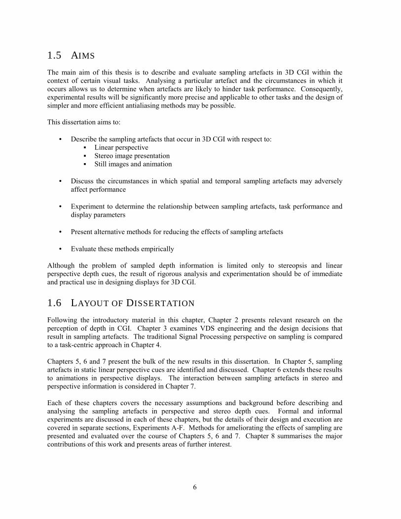
Historically, both spatial and spatio-temporal sampling artefacts have been treated as Signal Processing problems [Glassner 1995; Holst 1998]. While some attempt has been made to treat human perceptual criteria within this framework, there has been insufficient recognition by the Image Processing community of the task-dependent value of antialiasing methods in interactive CGI. This thesis adopts a Human Factors and Ergonomics approach: to improve VDSs, we must understand the abilities of the human user within the context of the task [Stanney, Mourant & Kennedy 1998; Wann & Mon-Williams 1996]. As an example, Figure 1.4 shows the effects of degrading the spatial resolution on a flight-path determination task [Delucia 1995]. A user is asked to determine the relative azimuth and elevation of the two aircraft as pixel size is varied. In this way, we could find the necessary spatial resolution to perform effectively on this task.
Figure 1.4: Example stimulus from an hypothetical experiment to assess the ability to determine if two aeroplanes will collide.
The literature from Human Factors research provides valuable insight into classifying different types of tasks and into designing effective experiments [Wilson 1998]. Human Factors research into simulators, teleoperation systems and VEs also relies heavily on a task-centred methodology. In Chapter 4, we compare and contrast traditional perspectives on sampling artefacts with a context-specific approach.
6
1.5 AIMS
The main aim of this thesis is to describe and evaluate sampling artefacts in 3D CGI within the context of certain visual tasks. Analysing a particular artefact and the circumstances in which it occurs allows us to determine when artefacts are likely to hinder task performance. Consequently, experimental results will be significantly more precise and applicable to other tasks and the design of simpler and more efficient antialiasing methods may be possible. This dissertation aims to:
• Describe the sampling artefacts that occur in 3D CGI with respect to: ▪ Linear perspective ▪ Stereo image presentation ▪ Still images and animation
• Discuss the circumstances in which spatial and temporal sampling artefacts may adversely affect performance
• Experiment to determine the relationship between sampling artefacts, task performance and
display parameters
• Present alternative methods for reducing the effects of sampling artefacts • Evaluate these methods empirically
Although the problem of sampled depth information is limited only to stereopsis and linear perspective depth cues, the result of rigorous analysis and experimentation should be of immediate and practical use in designing displays for 3D CGI.
1.6 LAYOUT OF DISSERTATION
Following the introductory material in this chapter, Chapter 2 presents relevant research on the perception of depth in CGI. Chapter 3 examines VDS engineering and the design decisions that result in sampling artefacts. The traditional Signal Processing perspective on sampling is compared to a task-centric approach in Chapter 4. Chapters 5, 6 and 7 present the bulk of the new results in this dissertation. In Chapter 5, sampling artefacts in static linear perspective cues are identified and discussed. Chapter 6 extends these results to animations in perspective displays. The interaction between sampling artefacts in stereo and perspective information is considered in Chapter 7. Each of these chapters covers the necessary assumptions and background before describing and analysing the sampling artefacts in perspective and stereo depth cues. Formal and informal experiments are discussed in each of these chapters, but the details of their design and execution are covered in separate sections, Experiments A-F. Methods for ameliorating the effects of sampling are presented and evaluated over the course of Chapters 5, 6 and 7. Chapter 8 summarises the major contributions of this work and presents areas of further interest.
7
C H A P T E R 2
2:Human Depth Perception In this chapter, we introduce the perceptual issues relevant to seeing three dimensions in digital imagery. Technological constraints like limited field-of-view and spatial resolution prevent the display of images that match the real world in all respects. Therefore, only some elements of real world depth perception are utilised when viewing 3D CGI. Depth Cue Theory is the main theory of depth perception. It states that different sources of information, or depth cues, combine to give a viewer the 3D layout of a scene [Goldstein 1989]. Alternatively, the Ecological Theory takes a generalised approach to depth perception. It states that the HVS relies on more than the image on the retina; it requires an examination of the entire state of the viewer and their surroundings (i.e., the context of viewing) [Gibson 1986]. In this thesis, we rely on Depth Cue Theory, although we acknowledge the importance of visual context where appropriate. As seen later, the type of visual environment and the viewer�s task play a significant part in the effectiveness of a 3D VDS. Both theories assert that there are some basic sources of information about 3D layout. These are generally divided into three types: pictorial, oculomotor and stereo depth cues [Gillam 1995]. The perceptual process by which these cues combine to form a sense of depth is a complicated and oft-debated issue [Cutting & Vishton 1995]. Different approaches to measuring the ability to perceive depth have also been posited [Roscoe 1984]. We discuss these issues with respect to CGI below.
2.1 PICTORIAL DEPTH CUES
Pictorial or monocular depth cues are 2D sources of information that the visual system interprets as three-dimensional. Because pictorial cues are 2D, the depth information they present may be ambiguous. Many common optical illusions are based on these ambiguities [Gillam 1980]. Despite the potential for ambiguity, combining many pictorial depth cues produces a powerful sense of three-dimensionality.
8
Perspective-Based Cues Other Cues Partially Perspective-Based Cues
Familiar Size
Distance to Horizon
Relative Brightness
Shading
Focus
Shadow and Foreshortening
Occlusion
Colour
Atmosphere
Texture Gradient Relative Size
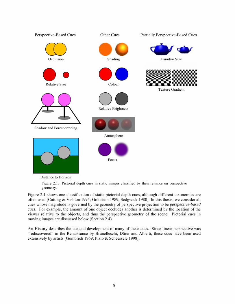
Figure 2.1: Pictorial depth cues in static images classified by their reliance on perspective geometry.
Figure 2.1 shows one classification of static pictorial depth cues, although different taxonomies are often used [Cutting & Vishton 1995; Goldstein 1989; Sedgwick 1980]. In this thesis, we consider all cues whose magnitude is governed by the geometry of perspective projection to be perspective-based cues. For example, the amount of one object occludes another is determined by the location of the viewer relative to the objects, and thus the perspective geometry of the scene. Pictorial cues in moving images are discussed below (Section 2.4). Art History describes the use and development of many of these cues. Since linear perspective was �rediscovered� in the Renaissance by Brunelleschi, Dürer and Alberti, these cues have been used extensively by artists [Gombrich 1969; Pizlo & Scheessele 1998].
CHAPTER 2: Human Depth Perception
9
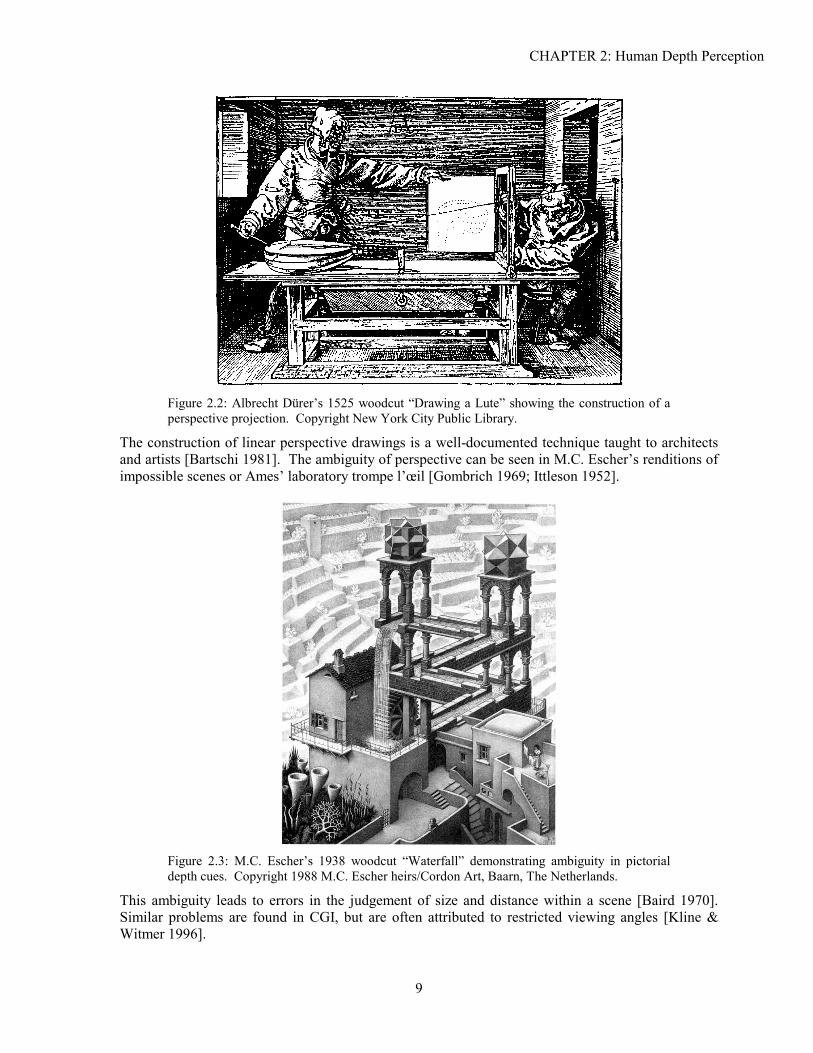
Figure 2.2: Albrecht Dürer�s 1525 woodcut �Drawing a Lute� showing the construction of a perspective projection. Copyright New York City Public Library.
The construction of linear perspective drawings is a well-documented technique taught to architects and artists [Bartschi 1981]. The ambiguity of perspective can be seen in M.C. Escher�s renditions of impossible scenes or Ames� laboratory trompe l��il [Gombrich 1969; Ittleson 1952].
Figure 2.3: M.C. Escher�s 1938 woodcut �Waterfall� demonstrating ambiguity in pictorial depth cues. Copyright 1988 M.C. Escher heirs/Cordon Art, Baarn, The Netherlands.
This ambiguity leads to errors in the judgement of size and distance within a scene [Baird 1970]. Similar problems are found in CGI, but are often attributed to restricted viewing angles [Kline & Witmer 1996].
10
Pictorial cues are often used to convey depth in CGI because most commonly available VDSs are only capable of presenting 2D images. However, even a simple 2D VDS is capable of presenting a compelling 3D image by using many redundant pictorial cues and combining them with depth information from object or viewer motion. Producing a variety of detailed pictorial depth cues is often computationally expensive. To correctly compute the shading, colour and lighting for a complex scene and thus accurately present depth cues derived from these features is difficult to do in real time. Even with specialised hardware systems, rendering a large number of polygons, using only perspective depth information can be computationally intractable. As a result, real-time applications often forego the level of realism attainable with algorithms that are more complex. In some cases, this means that depth cues are presented less accurately. For example, wireframe models may be substituted for shaded models to improve performance, but doing so removes occlusion depth cues. Alternatively, texture maps may be reduced in size (and thus resolution), which results in degraded texture gradient depth cues. To help designers make these kinds of choices, the relative effectiveness of depth cues in CGI has been investigated [Surdick et al. 1994; Wanger, Ferwerda & Greenberg 1992]. Among pictorial depth cues, linear perspective is widely regarded as one of the most effective sources of depth information in 3D CGI [Hone & Davies 1995].
2.2 OCULOMOTOR DEPTH CUES
Oculomotor depth cues include convergence and accommodation. Convergence is the rotation of the eyes towards a single location in space. Accommodation is the focusing of the eyes at a particular distance. Because these cues are dependent on each other and on binocular depth cues, their effect on depth perception is difficult to measure [Gillam 1995]. Although including oculomotor cues is considered important for immersive viewing, compelling scenes can be constructed without these depth cues, at the cost of producing visual after-effects [Rushton & Wann 1993]. VDSs using stereo imagery also have to account for problems related to oculomotor cues. These conflicts are discussed in Chapter 3.
2.3 BINOCULAR DEPTH PERCEPTION
�[T]he mind perceives an object of three dimensions by means of two dissimilar pictures projected by it on the two retinae� [Wheatstone 1838].
Stereopsis, or the use of the binocular disparity depth cue, is the process by which the angular disparity between the images in the left and right eye is used to compute the depth of points within an image.
CHAPTER 2: Human Depth Perception
11
Left Eye Right Eye
Focal depth
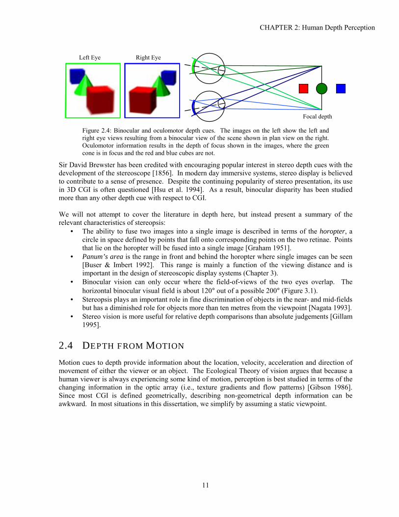
Figure 2.4: Binocular and oculomotor depth cues. The images on the left show the left and right eye views resulting from a binocular view of the scene shown in plan view on the right. Oculomotor information results in the depth of focus shown in the images, where the green cone is in focus and the red and blue cubes are not.
Sir David Brewster has been credited with encouraging popular interest in stereo depth cues with the development of the stereoscope [1856]. In modern day immersive systems, stereo display is believed to contribute to a sense of presence. Despite the continuing popularity of stereo presentation, its use in 3D CGI is often questioned [Hsu et al. 1994]. As a result, binocular disparity has been studied more than any other depth cue with respect to CGI. We will not attempt to cover the literature in depth here, but instead present a summary of the relevant characteristics of stereopsis:
• The ability to fuse two images into a single image is described in terms of the horopter, a circle in space defined by points that fall onto corresponding points on the two retinae. Points that lie on the horopter will be fused into a single image [Graham 1951].
• Panum’s area is the range in front and behind the horopter where single images can be seen [Buser & Imbert 1992]. This range is mainly a function of the viewing distance and is important in the design of stereoscopic display systems (Chapter 3).
• Binocular vision can only occur where the field-of-views of the two eyes overlap. The horizontal binocular visual field is about 120° out of a possible 200° (Figure 3.1).
• Stereopsis plays an important role in fine discrimination of objects in the near- and mid-fields but has a diminished role for objects more than ten metres from the viewpoint [Nagata 1993].
• Stereo vision is more useful for relative depth comparisons than absolute judgements [Gillam 1995].
2.4 DEPTH FROM MOTION
Motion cues to depth provide information about the location, velocity, acceleration and direction of movement of either the viewer or an object. The Ecological Theory of vision argues that because a human viewer is always experiencing some kind of motion, perception is best studied in terms of the changing information in the optic array (i.e., texture gradients and flow patterns) [Gibson 1986]. Since most CGI is defined geometrically, describing non-geometrical depth information can be awkward. In most situations in this dissertation, we simplify by assuming a static viewpoint.
12
Motion cues to depth are the same as discussed above, but considered in terms of how they change over time:
• Motion parallax: objects moving parallel to the viewer move faster in the near visual field and slower in the far field.
• Deletion/accretion or kinetic occlusion: change in the amount one object obstructs the view of another [Goldstein 1989].
• Motion perspective: movement of points in space according to the laws of linear perspective. • Familiar speed: perception of layout given a velocity that is familiar to the viewer (e.g., the
second hand on a watch or a person walking) [Hochberg 1986]. Motion of stereo information is especially important since the visual system is more sensitive to binocular disparity when it is changing (i.e., the object is moving in depth) [Yeh 1993]. The literature suggests some general characteristics of the depth perception derived from motion cues in experimental settings. In some cases, this research can be extended to situations that are more practical. To better understand the temporal aspects of depth perception and sampling in 3D CGI, we examine perspective and stereo cues in tasks requiring accurate perception of motion.
2.5 COMBINATION AND APPLICATION OF DEPTH CUES
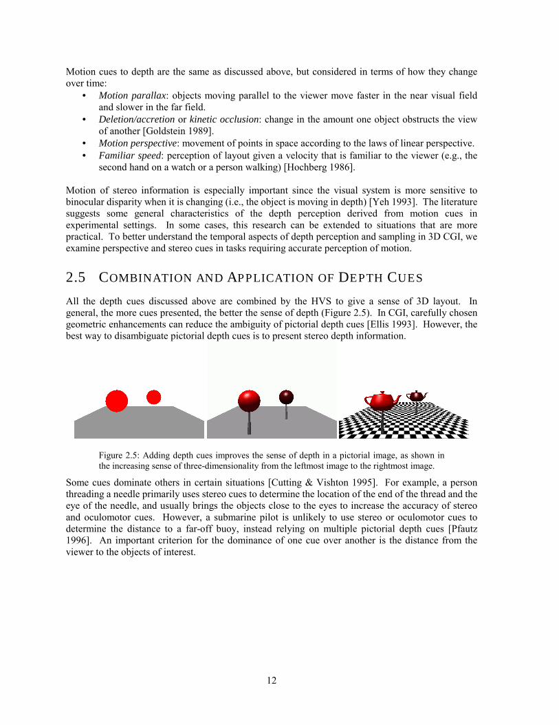
All the depth cues discussed above are combined by the HVS to give a sense of 3D layout. In general, the more cues presented, the better the sense of depth (Figure 2.5). In CGI, carefully chosen geometric enhancements can reduce the ambiguity of pictorial depth cues [Ellis 1993]. However, the best way to disambiguate pictorial depth cues is to present stereo depth information.
Figure 2.5: Adding depth cues improves the sense of depth in a pictorial image, as shown in the increasing sense of three-dimensionality from the leftmost image to the rightmost image.
Some cues dominate others in certain situations [Cutting & Vishton 1995]. For example, a person threading a needle primarily uses stereo cues to determine the location of the end of the thread and the eye of the needle, and usually brings the objects close to the eyes to increase the accuracy of stereo and oculomotor cues. However, a submarine pilot is unlikely to use stereo or oculomotor cues to determine the distance to a far-off buoy, instead relying on multiple pictorial depth cues [Pfautz 1996]. An important criterion for the dominance of one cue over another is the distance from the viewer to the objects of interest.
CHAPTER 2: Human Depth Perception
13
1
10
100
1000
1 10 100 1000 Viewing Distance (m)
Vis
ual D
epth
Sen
sitiv
ity (D
/?D)
Convergence
Size
Binocular Disparity
Brightness
Texture
Motion Parallax
Accommodation Atmosphere
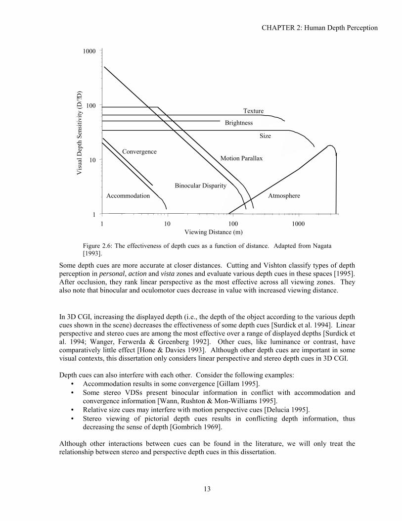
Figure 2.6: The effectiveness of depth cues as a function of distance. Adapted from Nagata [1993].
Some depth cues are more accurate at closer distances. Cutting and Vishton classify types of depth perception in personal, action and vista zones and evaluate various depth cues in these spaces [1995]. After occlusion, they rank linear perspective as the most effective across all viewing zones. They also note that binocular and oculomotor cues decrease in value with increased viewing distance.
In 3D CGI, increasing the displayed depth (i.e., the depth of the object according to the various depth cues shown in the scene) decreases the effectiveness of some depth cues [Surdick et al. 1994]. Linear perspective and stereo cues are among the most effective over a range of displayed depths [Surdick et al. 1994; Wanger, Ferwerda & Greenberg 1992]. Other cues, like luminance or contrast, have comparatively little effect [Hone & Davies 1993]. Although other depth cues are important in some visual contexts, this dissertation only considers linear perspective and stereo depth cues in 3D CGI. Depth cues can also interfere with each other. Consider the following examples:
• Accommodation results in some convergence [Gillam 1995]. • Some stereo VDSs present binocular information in conflict with accommodation and
convergence information [Wann, Rushton & Mon-Williams 1995]. • Relative size cues may interfere with motion perspective cues [Delucia 1995]. • Stereo viewing of pictorial depth cues results in conflicting depth information, thus
decreasing the sense of depth [Gombrich 1969]. Although other interactions between cues can be found in the literature, we will only treat the relationship between stereo and perspective depth cues in this dissertation.
14
Other research investigates the perception of conflicting and complementary depth cues in moving imagery. Estimating time-to-collision can be performed more effectively as more depth cues are provided, regardless of potential conflicts [Kappé, Korteling & Van de Grind 1995]. Dynamic stereo information has been shown to improve the ability to accurately track objects in 3D CGI when combined with potentially conflicting perspective cues [Kim et al. 1987]. As with static depth cues, the accuracy of judgements about an object�s motion will increase with the number of different depth cues describing that motion. Applying and combining depth cues to create a 3D scene is a complex process. A designer has to consider all of the following:
• Increasing the number of pictorial cues decreases a scene�s ambiguity. • Binocular disparity cues may disambiguate pictorial cues, but are difficult to present without
conflicts with accommodation and convergence. • Different cues are more effective at different distances. • And, most importantly, the value of a depth cue varies with the type of task.
2.6 DEPTH ACUITY
To evaluate a depth cue�s effectiveness, we need a measure of accuracy of depth perception. In 2D, spatial acuity refers to the HVS� ability to discriminate points and objects. Spatial acuity varies with the type of test, viewing conditions and a number of other factors [Boff & Lincoln 1988]. The most common spatial acuity test is the Snellen test, where different sizes of letters must be identified and standard acuity (for a 20 year old at 20 feet) is expressed as 20/20 (equivalent to 1' of visual angle in other tests). A viewer with 20/300 vision would be able to see details at 20 feet that a normal 20/20 viewer could see at 300 feet. In this dissertation, we will use degrees of visual angle rather than Snellen acuity, as it is more common in Psychophysics and Human Factors literature. Depth acuity is the ability to discriminate points in depth. Depth acuity is tested in a variety of ways [Nagata 1993]. Stereo acuity is the ability to differentiate two points in depth using only binocular disparity. Stereo acuity ranges as a function of viewing distance, from 0.05mm at 0.25m to 550mm at 25m [Buser & Imbert 1992]. In terms of visual angle, standard stereo acuity means a viewer can discriminate disparity differences of around 2' of arc [Yeh 1993]. The Howard-Doleman apparatus is the canonical method for measuring both stereo and depth acuity. A subject views two cylindrical posts through a rectangular aperture and adjusts distance of one to match the other [Graham 1951]. With this method, depth cues can be added or removed to measure their individual effects on acuity [Nagata 1993]. Variations on the Howard-Doleman apparatus have also been used to evaluate the accuracy of depth judgements [Utsumi et al. 1994]. A peg-in-hole manipulation task is a common variation [Matsunaga, Shidoji & Matsubara 1999], as are 3D tracking tasks [Zhai, Milgram & Rastogi 1997]. Like spatial acuity, the thresholds found for depth acuity are often a function of the type of experimental task [Surdick et al. 1994; Wanger, Ferwerda & Greenberg 1992]. Perhaps the greatest difficulty with measuring depth acuity is effectively dealing with multiple depth cues. The inherent ambiguity of many pictorial cues means experiment design can be frustrating. Testing cues individually may reveal biases not seen in the presence of other cues. As a result, experiments on artificial scenes with overly sparse depth information may not generalise well.

CHAPTER 2: Human Depth Perception
15
2.7 CONCLUSIONS
In this chapter, the relevant foundations of visual depth perception were presented. We discussed the different depth cues and their application in CGI. In part because of their ubiquity in 3D CGI and in part because previous work has emphasised their importance, we will consider the effects of sampling on only linear perspective and stereo depth cues in this dissertation.

16
17
C H A P T E R 3
3:Display System Engineering This chapter addresses how VDS design affects sampling of 3D CGI. In general, lack of proper consideration of a VDS design�s ergonomic impact can make it difficult for a user to perform certain visual tasks, and can even result in serious health hazards. [Fleischman & Sola 1999; Panel on Impact of Video Viewing on Vision of Workers 1983].
�In designing a visual display system� it is important to remember the specific task to be undertaken and, in particular, the visual requirements inherent in these tasks. None of the available technologies is capable of providing the operator with imagery that is in all important respects indistinguishable from a direct view of complex, real-world scene. In other words, significant compromises must be made� [VETREC 1992].
Parameters such as field-of-view (FOV), number of pixels, pixel size, use of stereo imagery, frame rate and refresh rate determine the spatial and temporal capabilities of a VDS and thus have significant effects on VDS usability [Clapp 1987; McKenna & Zeltzer 1992; Rogowitz 1983]. These parameters are not independent; a designer must also assess their interactions to optimise for a given task. Luckily, human sensorimotor systems are highly adaptable, so a designer has some flexibility in engineering a VDS [Dolezal 1982; Held & Durlach 1993]. In this chapter, we first identify and characterise the main types of VDSs used in 3D CGI: desktop VDS and immersive VDS. Then, we describe the parameters that determine the spatial and temporal capabilities of a VDS. The value of each parameter is presented in terms of task performance and how it interacts with other parameters.
3.1 DISPLAY TYPES
Different types of tasks lead to different classes of VDS designs. Methods for task analysis abound in the Human Factors and Ergonomics literature [Stammers & Shepherd 1998]. In the simulation and
18
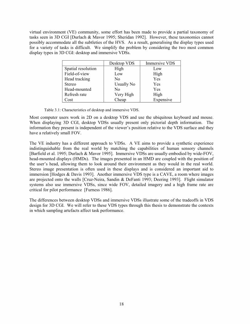
virtual environment (VE) community, some effort has been made to provide a partial taxonomy of tasks seen in 3D CGI [Durlach & Mavor 1995; Sheridan 1992]. However, these taxonomies cannot possibly accommodate all the subtleties of the HVS. As a result, generalising the display types used for a variety of tasks is difficult. We simplify the problem by considering the two most common display types in 3D CGI: desktop and immersive VDSs.
Desktop VDS Immersive VDS Spatial resolution High Low Field-of-view Low High Head tracking No Yes Stereo Usually No Yes Head-mounted No Yes Refresh rate Very High High Cost Cheap Expensive
Table 3.1: Characteristics of desktop and immersive VDS.
Most computer users work in 2D on a desktop VDS and use the ubiquitous keyboard and mouse. When displaying 3D CGI, desktop VDSs usually present only pictorial depth information. The information they present is independent of the viewer�s position relative to the VDS surface and they have a relatively small FOV. The VE industry has a different approach to VDSs. A VE aims to provide a synthetic experience indistinguishable from the real world by matching the capabilities of human sensory channels [Barfield et al. 1995; Durlach & Mavor 1995]. Immersive VDSs are usually embodied by wide-FOV, head-mounted displays (HMDs). The images presented in an HMD are coupled with the position of the user�s head, allowing them to look around their environment as they would in the real world. Stereo image presentation is often used in these displays and is considered an important aid to immersion [Hodges & Davis 1993]. Another immersive VDS type is a CAVE, a room where images are projected onto the walls [Cruz-Neira, Sandin & DeFanti 1993; Deering 1993]. Flight simulator systems also use immersive VDSs, since wide FOV, detailed imagery and a high frame rate are critical for pilot performance [Furness 1986]. The differences between desktop VDSs and immersive VDSs illustrate some of the tradeoffs in VDS design for 3D CGI. We will refer to these VDS types through this thesis to demonstrate the contexts in which sampling artefacts affect task performance.
CHAPTER 3: Display System Engineering
19
3.2 DISPLAY PARAMETERS
In this section, we cover the main VDS parameters affecting spatio-temporal sampling of 3D CGI: • Field-of-View: The visual angle subtended by the display surface • Spatial resolution: The number, angular size and spacing of the pixels • Refresh rate: The frequency with which the display hardware can draw the image on the
display surface • Frame rate: The frequency with which the image can be rendered into the framebuffer (i.e.,
the rate at which a new, updated scene is prepared for drawing to the screen) • Stereo image presentation: Presenting binocular disparity information by displaying separate
images for each eye
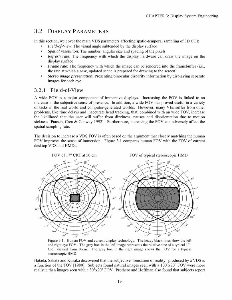
3.2.1 Field-of-View A wide FOV is a major component of immersive displays. Increasing the FOV is linked to an increase in the subjective sense of presence. In addition, a wide FOV has proved useful in a variety of tasks in the real world and computer-generated worlds. However, many VEs suffer from other problems, like time delays and inaccurate head tracking, that, combined with an wide FOV, increase the likelihood that the user will suffer from dizziness, nausea and disorientation due to motion sickness [Pausch, Crea & Conway 1992]. Furthermore, increasing the FOV can adversely affect the spatial sampling rate. The decision to increase a VDS FOV is often based on the argument that closely matching the human FOV improves the sense of immersion. Figure 3.1 compares human FOV with the FOV of current desktop VDS and HMDs.
FOV of 17" CRT at 50 cm FOV of typical stereoscopic HMD
180o
165o
150o
135o
120o
105o90
o
0o
15o
30o
60o
75o
45o
195o
210o
225o
240o
255o
270o
345o
330o
300o
285o
315o
90o
80o
70o
60o
50o
40o
30o
20o
10o
180o
165o
150o
135o
120o
105o90
o
0o
15o
30o
60o
75o
45o
195o
210o
225o
240o
255o
270o
345o
330o
300o
285o
315o
90o
80o
70o
60o
50o
40o
30o
20o
10o
Figure 3.1: Human FOV and current display technology. The heavy black lines show the left and right eye FOV. The grey box in the left image represents the relative size of a typical 17" CRT viewed from 50cm. The grey box in the right image shows the FOV for a typical stereoscopic HMD.
Hatada, Sakata and Kusaka discovered that the subjective �sensation of reality� produced by a VDS is a function of the FOV [1980]. Subjects found natural images seen with a 100°x80° FOV were more realistic than images seen with a 30°x20° FOV. Prothero and Hoffman also found that subjects report
20
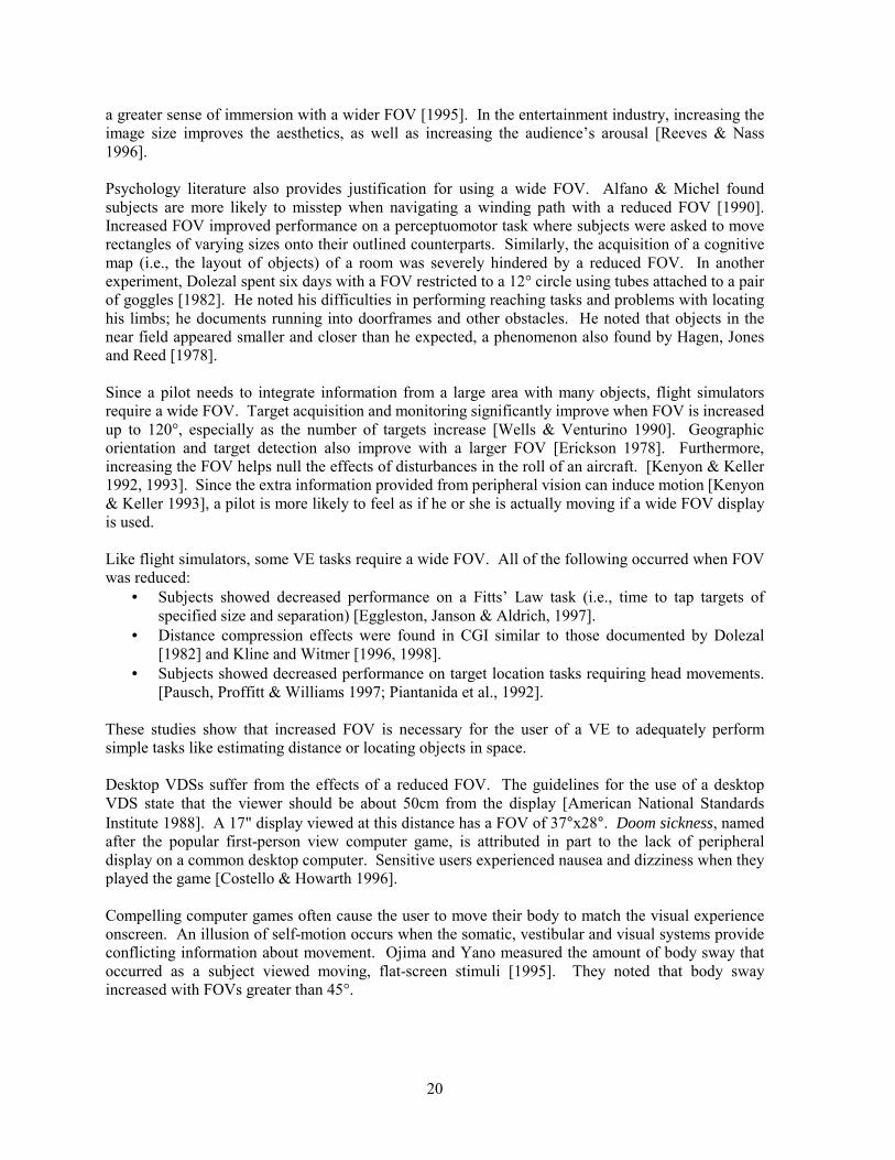
a greater sense of immersion with a wider FOV [1995]. In the entertainment industry, increasing the image size improves the aesthetics, as well as increasing the audience�s arousal [Reeves & Nass 1996]. Psychology literature also provides justification for using a wide FOV. Alfano & Michel found subjects are more likely to misstep when navigating a winding path with a reduced FOV [1990]. Increased FOV improved performance on a perceptuomotor task where subjects were asked to move rectangles of varying sizes onto their outlined counterparts. Similarly, the acquisition of a cognitive map (i.e., the layout of objects) of a room was severely hindered by a reduced FOV. In another experiment, Dolezal spent six days with a FOV restricted to a 12° circle using tubes attached to a pair of goggles [1982]. He noted his difficulties in performing reaching tasks and problems with locating his limbs; he documents running into doorframes and other obstacles. He noted that objects in the near field appeared smaller and closer than he expected, a phenomenon also found by Hagen, Jones and Reed [1978]. Since a pilot needs to integrate information from a large area with many objects, flight simulators require a wide FOV. Target acquisition and monitoring significantly improve when FOV is increased up to 120°, especially as the number of targets increase [Wells & Venturino 1990]. Geographic orientation and target detection also improve with a larger FOV [Erickson 1978]. Furthermore, increasing the FOV helps null the effects of disturbances in the roll of an aircraft. [Kenyon & Keller 1992, 1993]. Since the extra information provided from peripheral vision can induce motion [Kenyon & Keller 1993], a pilot is more likely to feel as if he or she is actually moving if a wide FOV display is used. Like flight simulators, some VE tasks require a wide FOV. All of the following occurred when FOV was reduced:
• Subjects showed decreased performance on a Fitts� Law task (i.e., time to tap targets of specified size and separation) [Eggleston, Janson & Aldrich, 1997].
• Distance compression effects were found in CGI similar to those documented by Dolezal [1982] and Kline and Witmer [1996, 1998].
• Subjects showed decreased performance on target location tasks requiring head movements. [Pausch, Proffitt & Williams 1997; Piantanida et al., 1992].
These studies show that increased FOV is necessary for the user of a VE to adequately perform simple tasks like estimating distance or locating objects in space. Desktop VDSs suffer from the effects of a reduced FOV. The guidelines for the use of a desktop VDS state that the viewer should be about 50cm from the display [American National Standards Institute 1988]. A 17" display viewed at this distance has a FOV of 37°x28°. Doom sickness, named after the popular first-person view computer game, is attributed in part to the lack of peripheral display on a common desktop computer. Sensitive users experienced nausea and dizziness when they played the game [Costello & Howarth 1996]. Compelling computer games often cause the user to move their body to match the visual experience onscreen. An illusion of self-motion occurs when the somatic, vestibular and visual systems provide conflicting information about movement. Ojima and Yano measured the amount of body sway that occurred as a subject viewed moving, flat-screen stimuli [1995]. They noted that body sway increased with FOVs greater than 45°.
CHAPTER 3: Display System Engineering
21
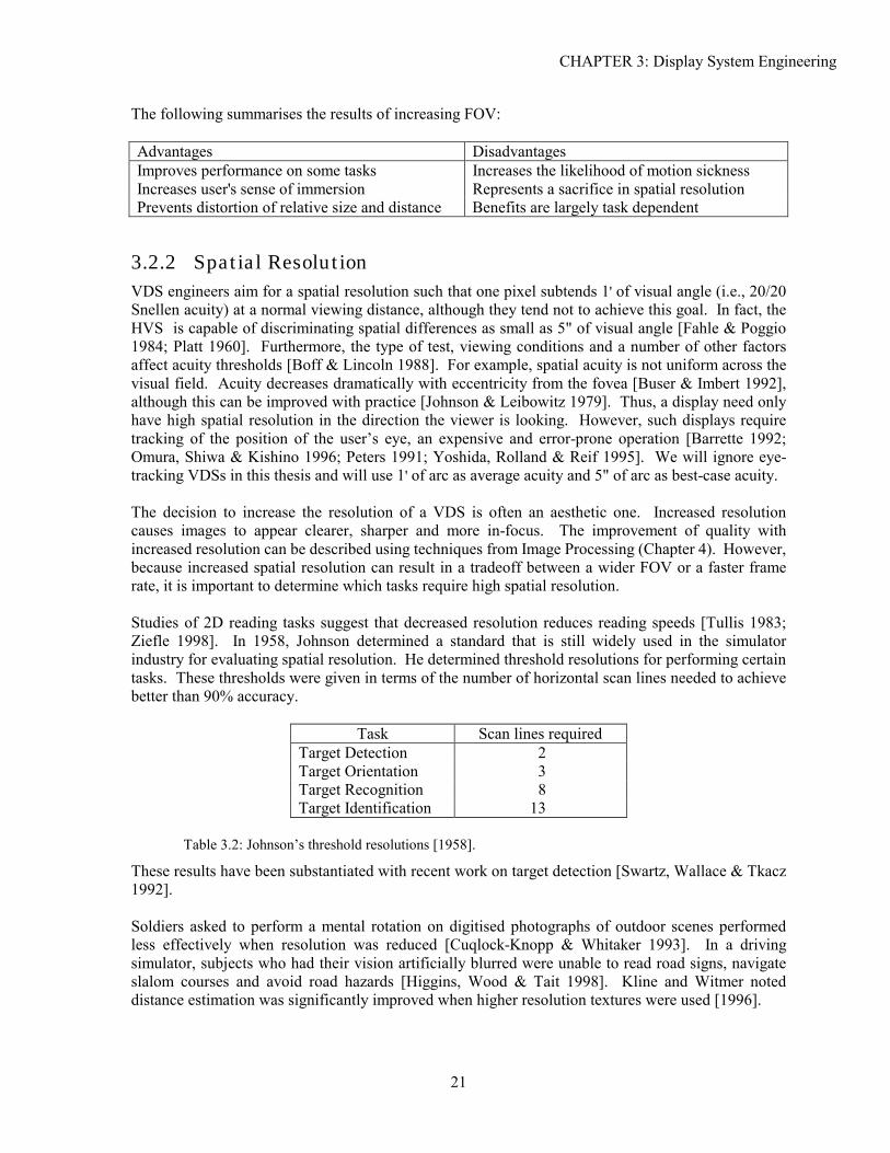
The following summarises the results of increasing FOV: Advantages Disadvantages Improves performance on some tasks Increases the likelihood of motion sickness Increases user's sense of immersion Represents a sacrifice in spatial resolution Prevents distortion of relative size and distance Benefits are largely task dependent
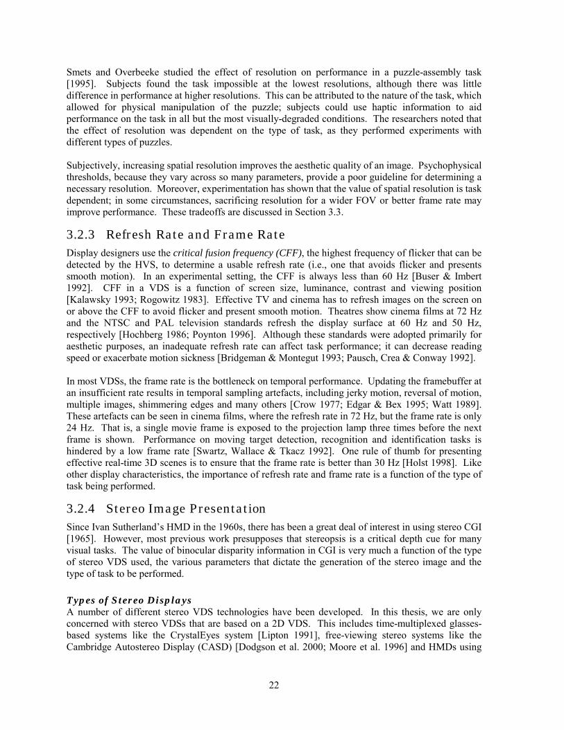
3.2.2 Spatial Resolution VDS engineers aim for a spatial resolution such that one pixel subtends 1' of visual angle (i.e., 20/20 Snellen acuity) at a normal viewing distance, although they tend not to achieve this goal. In fact, the HVS is capable of discriminating spatial differences as small as 5" of visual angle [Fahle & Poggio 1984; Platt 1960]. Furthermore, the type of test, viewing conditions and a number of other factors affect acuity thresholds [Boff & Lincoln 1988]. For example, spatial acuity is not uniform across the visual field. Acuity decreases dramatically with eccentricity from the fovea [Buser & Imbert 1992], although this can be improved with practice [Johnson & Leibowitz 1979]. Thus, a display need only have high spatial resolution in the direction the viewer is looking. However, such displays require tracking of the position of the user�s eye, an expensive and error-prone operation [Barrette 1992; Omura, Shiwa & Kishino 1996; Peters 1991; Yoshida, Rolland & Reif 1995]. We will ignore eye-tracking VDSs in this thesis and will use 1' of arc as average acuity and 5" of arc as best-case acuity. The decision to increase the resolution of a VDS is often an aesthetic one. Increased resolution causes images to appear clearer, sharper and more in-focus. The improvement of quality with increased resolution can be described using techniques from Image Processing (Chapter 4). However, because increased spatial resolution can result in a tradeoff between a wider FOV or a faster frame rate, it is important to determine which tasks require high spatial resolution. Studies of 2D reading tasks suggest that decreased resolution reduces reading speeds [Tullis 1983; Ziefle 1998]. In 1958, Johnson determined a standard that is still widely used in the simulator industry for evaluating spatial resolution. He determined threshold resolutions for performing certain tasks. These thresholds were given in terms of the number of horizontal scan lines needed to achieve better than 90% accuracy.
Task Scan lines required Target Detection 2 Target Orientation 3 Target Recognition 8 Target Identification 13
Table 3.2: Johnson�s threshold resolutions [1958].
These results have been substantiated with recent work on target detection [Swartz, Wallace & Tkacz 1992]. Soldiers asked to perform a mental rotation on digitised photographs of outdoor scenes performed less effectively when resolution was reduced [Cuqlock-Knopp & Whitaker 1993]. In a driving simulator, subjects who had their vision artificially blurred were unable to read road signs, navigate slalom courses and avoid road hazards [Higgins, Wood & Tait 1998]. Kline and Witmer noted distance estimation was significantly improved when higher resolution textures were used [1996].
22
Smets and Overbeeke studied the effect of resolution on performance in a puzzle-assembly task [1995]. Subjects found the task impossible at the lowest resolutions, although there was little difference in performance at higher resolutions. This can be attributed to the nature of the task, which allowed for physical manipulation of the puzzle; subjects could use haptic information to aid performance on the task in all but the most visually-degraded conditions. The researchers noted that the effect of resolution was dependent on the type of task, as they performed experiments with different types of puzzles. Subjectively, increasing spatial resolution improves the aesthetic quality of an image. Psychophysical thresholds, because they vary across so many parameters, provide a poor guideline for determining a necessary resolution. Moreover, experimentation has shown that the value of spatial resolution is task dependent; in some circumstances, sacrificing resolution for a wider FOV or better frame rate may improve performance. These tradeoffs are discussed in Section 3.3.
3.2.3 Refresh Rate and Frame Rate Display designers use the critical fusion frequency (CFF), the highest frequency of flicker that can be detected by the HVS, to determine a usable refresh rate (i.e., one that avoids flicker and presents smooth motion). In an experimental setting, the CFF is always less than 60 Hz [Buser & Imbert 1992]. CFF in a VDS is a function of screen size, luminance, contrast and viewing position [Kalawsky 1993; Rogowitz 1983]. Effective TV and cinema has to refresh images on the screen on or above the CFF to avoid flicker and present smooth motion. Theatres show cinema films at 72 Hz and the NTSC and PAL television standards refresh the display surface at 60 Hz and 50 Hz, respectively [Hochberg 1986; Poynton 1996]. Although these standards were adopted primarily for aesthetic purposes, an inadequate refresh rate can affect task performance; it can decrease reading speed or exacerbate motion sickness [Bridgeman & Montegut 1993; Pausch, Crea & Conway 1992]. In most VDSs, the frame rate is the bottleneck on temporal performance. Updating the framebuffer at an insufficient rate results in temporal sampling artefacts, including jerky motion, reversal of motion, multiple images, shimmering edges and many others [Crow 1977; Edgar & Bex 1995; Watt 1989]. These artefacts can be seen in cinema films, where the refresh rate in 72 Hz, but the frame rate is only 24 Hz. That is, a single movie frame is exposed to the projection lamp three times before the next frame is shown. Performance on moving target detection, recognition and identification tasks is hindered by a low frame rate [Swartz, Wallace & Tkacz 1992]. One rule of thumb for presenting effective real-time 3D scenes is to ensure that the frame rate is better than 30 Hz [Holst 1998]. Like other display characteristics, the importance of refresh rate and frame rate is a function of the type of task being performed.
3.2.4 Stereo Image Presentation Since Ivan Sutherland�s HMD in the 1960s, there has been a great deal of interest in using stereo CGI [1965]. However, most previous work presupposes that stereopsis is a critical depth cue for many visual tasks. The value of binocular disparity information in CGI is very much a function of the type of stereo VDS used, the various parameters that dictate the generation of the stereo image and the type of task to be performed. Types of Stereo Displays A number of different stereo VDS technologies have been developed. In this thesis, we are only concerned with stereo VDSs that are based on a 2D VDS. This includes time-multiplexed glasses-based systems like the CrystalEyes system [Lipton 1991], free-viewing stereo systems like the Cambridge Autostereo Display (CASD) [Dodgson et al. 2000; Moore et al. 1996] and HMDs using
CHAPTER 3: Display System Engineering
23
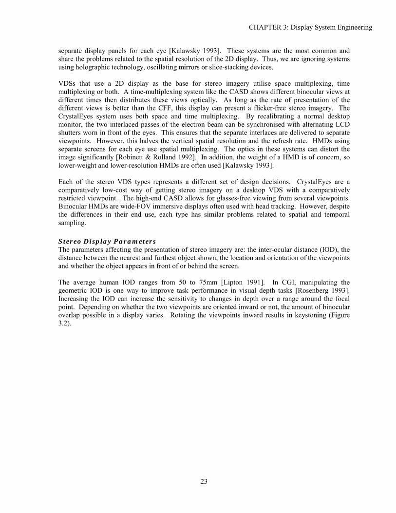
separate display panels for each eye [Kalawsky 1993]. These systems are the most common and share the problems related to the spatial resolution of the 2D display. Thus, we are ignoring systems using holographic technology, oscillating mirrors or slice-stacking devices. VDSs that use a 2D display as the base for stereo imagery utilise space multiplexing, time multiplexing or both. A time-multiplexing system like the CASD shows different binocular views at different times then distributes these views optically. As long as the rate of presentation of the different views is better than the CFF, this display can present a flicker-free stereo imagery. The CrystalEyes system uses both space and time multiplexing. By recalibrating a normal desktop monitor, the two interlaced passes of the electron beam can be synchronised with alternating LCD shutters worn in front of the eyes. This ensures that the separate interlaces are delivered to separate viewpoints. However, this halves the vertical spatial resolution and the refresh rate. HMDs using separate screens for each eye use spatial multiplexing. The optics in these systems can distort the image significantly [Robinett & Rolland 1992]. In addition, the weight of a HMD is of concern, so lower-weight and lower-resolution HMDs are often used [Kalawsky 1993]. Each of the stereo VDS types represents a different set of design decisions. CrystalEyes are a comparatively low-cost way of getting stereo imagery on a desktop VDS with a comparatively restricted viewpoint. The high-end CASD allows for glasses-free viewing from several viewpoints. Binocular HMDs are wide-FOV immersive displays often used with head tracking. However, despite the differences in their end use, each type has similar problems related to spatial and temporal sampling. Stereo Display Parameters The parameters affecting the presentation of stereo imagery are: the inter-ocular distance (IOD), the distance between the nearest and furthest object shown, the location and orientation of the viewpoints and whether the object appears in front of or behind the screen. The average human IOD ranges from 50 to 75mm [Lipton 1991]. In CGI, manipulating the geometric IOD is one way to improve task performance in visual depth tasks [Rosenberg 1993]. Increasing the IOD can increase the sensitivity to changes in depth over a range around the focal point. Depending on whether the two viewpoints are oriented inward or not, the amount of binocular overlap possible in a display varies. Rotating the viewpoints inward results in keystoning (Figure 3.2).
24
Convergent Lines of Sight
left right combined
+ =
Parallel Lines of Sight
left right combined
+ =
Figure 3.2: Parallel vs. Convergent eyepoint orientations and the resulting stereo pairs.
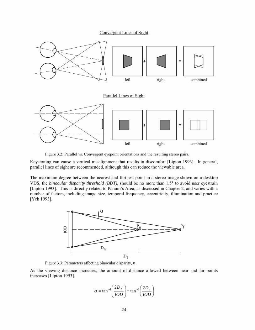
Keystoning can cause a vertical misalignment that results in discomfort [Lipton 1993]. In general, parallel lines of sight are recommended, although this can reduce the viewable area. The maximum degree between the nearest and furthest point in a stereo image shown on a desktop VDS, the binocular disparity threshold (BDT), should be no more than 1.5° to avoid user eyestrain [Lipton 1993]. This is directly related to Panum�s Area, as discussed in Chapter 2, and varies with a number of factors, including image size, temporal frequency, eccentricity, illumination and practice [Yeh 1993].
Pn Pf
Dn
Df
IOD
α
Figure 3.3: Parameters affecting binocular disparity, α.
As the viewing distance increases, the amount of distance allowed between near and far points increases [Lipton 1993].
−
= −−
IODD
IODD nf 2
tan2
tan 11α
CHAPTER 3: Display System Engineering
25
Different perceptual mechanisms are used for crossed and uncrossed disparity [Patterson & Martin 1992]. However, differences are only likely to be seen for short-duration stimulus [Patterson et al. 1996]. Thus, we assume the BDT in front of the screen is the same as for behind the screen:
-1.5° < α < 1.5°
Many other parameters are described in the vast literature on the perception of stereo CGI [Siegel, Tobinga & Akiya 1999]. Failure to adhere to rules of good stereo image composition results in significant viewer discomfort [Lipton 1993]. In this dissertation, we use the assumptions stated above in our discussion of sampling artefacts. The Value of Stereo Image Presentation Many researchers argue that additional immersiveness and realism is gained by the use of stereo imagery [Hatada, Sakata & Kusaka 1980]. However, throughout this thesis we argue that the value of a VDS parameter is a function of the visual task to be performed. The usefulness of stereo, therefore, is task dependent. Many sources discuss the benefits of stereo for a variety of display types and tasks. An additional consideration for the use of stereoscopic VDSs is that a significant portion of the population is unable to use the binocular disparity depth cue. Richards showed that 4% of a population of 150 students could not use stereopsis and that 10% had great difficulty in perceiving depth in a random dot stereogram [1970]. No differences due to gender were reported. Furthermore, stereo VDSs can result in more visual fatigue than monocular displays [Okuyama 1999]. One reason for this is the conflict between oculomotor depth cues. In the stereo VDSs mentioned above, the viewer�s eyes focus on the plane of the VDS but may converge at a different distance. Because of this crosstalk, even short periods (~10 min) of stereo viewing results in eyestrain [Wann, Rushton & Mon-Williams 1995]. In addition to eyestrain, ill-calibrated stereo in immersive VDSs is a likely source of simulator sickness [Robinett & Rolland 1992]. Despite these difficulties, stereo cues have improved performance in a variety of tasks, including:
• 3D tracking tasks [Kim et al. 1987; Liu, Tharp & Stark 1992] • Fitts� Law and teleoperation tasks [Merritt, Cole & Ikehara 1992] • Distance estimation [Lampton et al. 1995] • Relative depth judgements [Yeh & Silverstein 1992] • Azimuth and elevation judgements [Barfield & Rosenberg 1995] • Path tracing tasks [Sollenberger & Milgram 1993] • 3D pointer positioning accuracy [Drascic & Milgram 1991] • Detection of subtle features in medical images [Hsu et al. 1994]
The variety of these tasks indicates that stereo, despite the potential for visual fatigue, can be a valuable depth cue. Whether the benefit of stereo image presentation outweighs the additional hardware costs is a critical design decision. The effects of sampling on binocular disparity provide another way to evaluate this cost-performance relationship.
3.2.5 Other Viewing Parameters While spatial resolution, binocular disparity, FOV, refresh rate and frame rate are the main parameters affecting sampling in 3D CGI, other characteristics of a VDS are also important. These additional characteristics can have a significant effect VDS� usability for a given task. Therefore, we
26
briefly discuss below the effects of geometric field-of-view, viewpoint location and the use of head tracking. Geometric Field-of-view The physical viewing angle of the VDS is a major parameter in VDS design, but the geometric representation of that angle is also of critical importance. The perspective projection specifies the geometric FOV (GFOV). When the GFOV does not match the real world FOV, effects like a fish-eye lens on a camera are produced. This changes the spatial sampling of an image; more pixels will be devoted to different parts of the scene. However, the benefits of distorting the GFOV are not clear. A series of studies were conducted to evaluate the role of the GFOV in accurate spatial judgements. Size and distance judgements in the real world were significantly affected by physically restricting the GFOV [Meehan & Triggs 1992; Roscoe 1984]. Relative azimuth and elevation judgements in a perspective VDS were less accurate for GFOVs greater than the real FOV [McGreevy & Ellis 1986]. This effect has been noted in see-through stereo VDSs that match real-world viewing with synthetic elements [Rolland, Gibson & Ariely 1995]. Alternatively, room size estimation and distance estimation tasks were aided by a larger GFOV [Neale 1996]. The sense of presence also appears to be linked to an increased GFOV [Hendrix & Barfield 1995]. For other tasks, like estimating the relative skew of two lines, a disparity between real and geometric FOVs was less useful [Barfield & Kim 1991; Rosenberg & Barfield 1995]. The usefulness of distorting the GFOV, like the usefulness of other VDS parameters, is task-dependent. In this thesis, we assume the geometry of the perspective projection matches the geometry of the real-world perspective and stereo viewing volume. Viewing Location In the real world, the location of the viewer significantly affects the perception of spatial layout [Toye 1986]. However, when viewing paintings or photographs, the viewer may be located somewhere other than the geometric eyepoint, yet still perceive correct relationships between the objects in the screen [Haber 1980; Pirenne 1970]. These studies suggest that viewing a 3D image from other than the intended viewpoint does not affect the perception of object relationships as much as the geometry of perspective projection implies [Ellis, Smith & McGreevy 1987; Perkins 1973; Pizlo & Scheessele 1998; Rosinski et al. 1980]. This is highly relevant to viewing 3D images monocularly on a desktop VDS, as we would expect similar perceptual effects to occur in this context. Stereo viewing can reduce the perceptual effects of viewing off-angle [Ellis et al. 1992]. Throughout this thesis, we assume that viewer is stationary relative to the image on the screen. Head Tracking Head tracking appears to solve the viewpoint location problem by tying it to the user�s head position and orientation. While a head-tracked image presents a number of potential problems to the VDS designer, the benefits are clear:
• Users report a greater sense of immersion [Hendrix & Barfield 1996]. • Spatial knowledge acquisition may be improved by controlling the viewpoint with head
movements rather than hand-held devices [Allen, McDonald & Singer 1997]. • Head tracking aided performance on a simple assembly task [Smets & Overbeeke 1995]. • By changing head orientation while maintaining position, some improvement was noted on a
target location task [Pausch, Proffitt & Williams 1997]. In head-tracked systems, if the synthetic viewpoint does not accurately portray the real viewpoint, discomfort and illness can occur [DiZio & Lackner 1992]. This can be avoided by correctly modelling the parameters of the VDS surface, viewing optics and perspective geometry so that real
CHAPTER 3: Display System Engineering
27
and virtual viewpoints are effectively matched [Deering 1992]. Even with ideal modelling, head tracking can exacerbate other problems. If the frame rate is inadequate, head tracking in wide FOV systems is more likely to cause sickness [Hettinger & Riccio 1992].
3.3 TRADEOFFS IN DISPLAY DESIGN
Having covered the main VDS parameters affecting spatial and temporal sampling in 3D CGI, we can now discuss how these parameters interact. An effective VDS design results from trading off these parameters, in terms of both economics and visual perception [Miller 1976]. For a given number of pixels, FOV and spatial resolution are inversely related; a wide FOV system has a low spatial resolution and vice versa. Similarly, maintaining interactive frame rates means that the scene complexity (which may include spatial resolution and the use of stereo imagery) is limited. These tradeoffs are discussed in detail below.
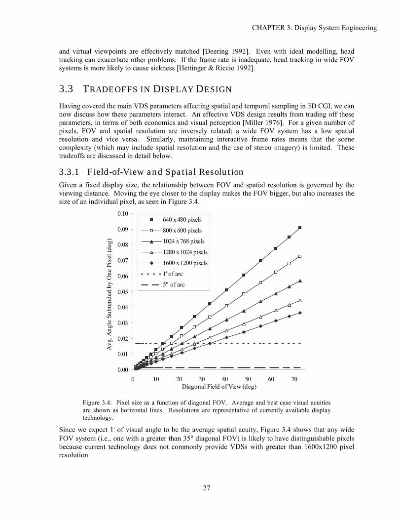
3.3.1 Field-of-View and Spatial Resolution Given a fixed display size, the relationship between FOV and spatial resolution is governed by the viewing distance. Moving the eye closer to the display makes the FOV bigger, but also increases the size of an individual pixel, as seen in Figure 3.4.
0.00
0.01
0.02
0.03
0.04
0.05
0.06
0.07
0.08
0.09
0.10
0 10 20 30 40 50 60 70Diagonal Field of View (deg)
Avg
. Ang
le S
ubte
nded
by
One
Pix
el (d
eg)
640 x 480 pixels
800 x 600 pixels
1024 x 768 pixels
1280 x 1024 pixels
1600 x 1200 pixels
1' of arc
5" of arc
Figure 3.4: Pixel size as a function of diagonal FOV. Average and best case visual acuities are shown as horizontal lines. Resolutions are representative of currently available display technology.
Since we expect 1' of visual angle to be the average spatial acuity, Figure 3.4 shows that any wide FOV system (i.e., one with a greater than 35° diagonal FOV) is likely to have distinguishable pixels because current technology does not commonly provide VDSs with greater than 1600x1200 pixel resolution.
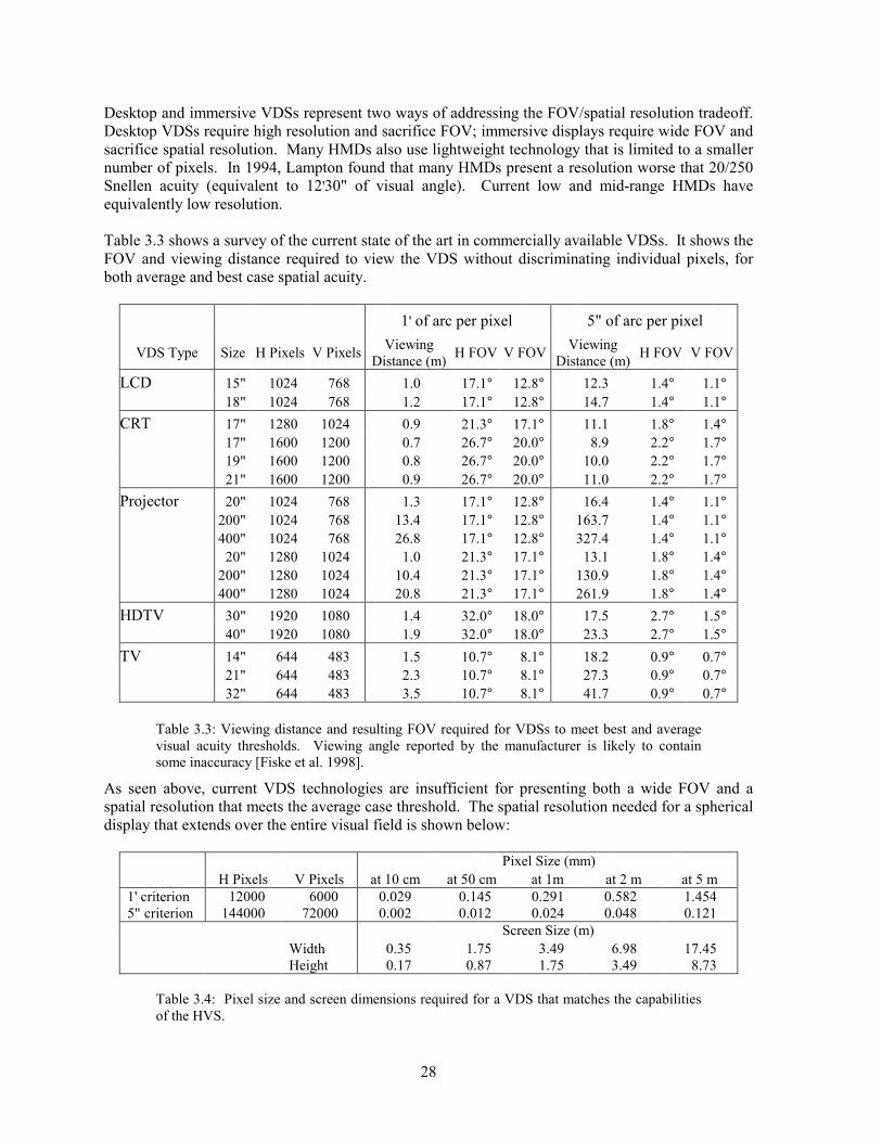
28
Desktop and immersive VDSs represent two ways of addressing the FOV/spatial resolution tradeoff. Desktop VDSs require high resolution and sacrifice FOV; immersive displays require wide FOV and sacrifice spatial resolution. Many HMDs also use lightweight technology that is limited to a smaller number of pixels. In 1994, Lampton found that many HMDs present a resolution worse that 20/250 Snellen acuity (equivalent to 12'30" of visual angle). Current low and mid-range HMDs have equivalently low resolution. Table 3.3 shows a survey of the current state of the art in commercially available VDSs. It shows the FOV and viewing distance required to view the VDS without discriminating individual pixels, for both average and best case spatial acuity.
1' of arc per pixel 5" of arc per pixel
VDS Type Size H Pixels V Pixels Viewing Distance (m) H FOV V FOV Viewing
Distance (m) H FOV V FOV
LCD 15" 1024 768 1.0 17.1° 12.8° 12.3 1.4° 1.1° 18" 1024 768 1.2 17.1° 12.8° 14.7 1.4° 1.1° CRT 17" 1280 1024 0.9 21.3° 17.1° 11.1 1.8° 1.4°
17" 1600 1200 0.7 26.7° 20.0° 8.9 2.2° 1.7° 19" 1600 1200 0.8 26.7° 20.0° 10.0 2.2° 1.7° 21" 1600 1200 0.9 26.7° 20.0° 11.0 2.2° 1.7°
Projector 20" 1024 768 1.3 17.1° 12.8° 16.4 1.4° 1.1° 200" 1024 768 13.4 17.1° 12.8° 163.7 1.4° 1.1° 400" 1024 768 26.8 17.1° 12.8° 327.4 1.4° 1.1° 20" 1280 1024 1.0 21.3° 17.1° 13.1 1.8° 1.4° 200" 1280 1024 10.4 21.3° 17.1° 130.9 1.8° 1.4° 400" 1280 1024 20.8 21.3° 17.1° 261.9 1.8° 1.4°
HDTV 30" 1920 1080 1.4 32.0° 18.0° 17.5 2.7° 1.5° 40" 1920 1080 1.9 32.0° 18.0° 23.3 2.7° 1.5° TV 14" 644 483 1.5 10.7° 8.1° 18.2 0.9° 0.7° 21" 644 483 2.3 10.7° 8.1° 27.3 0.9° 0.7° 32" 644 483 3.5 10.7° 8.1° 41.7 0.9° 0.7°
Table 3.3: Viewing distance and resulting FOV required for VDSs to meet best and average visual acuity thresholds. Viewing angle reported by the manufacturer is likely to contain some inaccuracy [Fiske et al. 1998].
As seen above, current VDS technologies are insufficient for presenting both a wide FOV and a spatial resolution that meets the average case threshold. The spatial resolution needed for a spherical display that extends over the entire visual field is shown below:
Pixel Size (mm) H Pixels V Pixels at 10 cm at 50 cm at 1m at 2 m at 5 m 1' criterion 12000 6000 0.029 0.145 0.291 0.582 1.454 5" criterion 144000 72000 0.002 0.012 0.024 0.048 0.121 Screen Size (m) Width 0.35 1.75 3.49 6.98 17.45 Height 0.17 0.87 1.75 3.49 8.73
Table 3.4: Pixel size and screen dimensions required for a VDS that matches the capabilities of the HVS.
CHAPTER 3: Display System Engineering
29
In terms of task performance, some tasks suffer more from a lack of spatial resolution than a narrow FOV and vice versa. Normal 2D graphic user interfaces require a high resolution but are unaffected by FOV. Alternatively, a sense of immersion requires a wide FOV and can be achieved without a particularly high spatial resolution [Hatada, Sakata & Kusaka 1980]. Most of the tasks listed above (Section 3.2.1) measured the value of FOV without varying spatial resolution. They argued a wide FOV was necessary, but their experiments reduced both FOV and spatial resolution [Kenyon & Keller 1993; Wells & Venturino 1990]. The tradeoff between spatial resolution and FOV is a prominent issue in the design of immersive VDSs, yet few studies have adequately studied this relationship. In this thesis, we will describe how and when spatial sampling artefacts adversely affect performance in 3D CGI. This information can be used to evaluate the consequences of sacrificing spatial resolution for FOV.
3.3.2 Frame Rate and Spatial Resolution Most modern immersive and desktop VDSs are capable of presenting images at better than the CFF. Thus, the frame rate constrains the temporal resolution of a VDS. The rate at which a scene can be generated is a function of its complexity. The traditional measure of scene complexity is the number of polygons rendered. However, this method is faulty since it fails to take into account the use of lighting models, antialiasing methods, texture mapping or other procedures used to improve the realism of an image. Even with specialised graphics hardware, rendering a realistic 3D scene to the screen can take hours. In interactive 3D CGI, significant compromises in realism must be made to achieve a sufficient frame rate. One of the simplest ways of reducing scene complexity is to reduce the number of pixels in the rendered image. However, reducing the spatial resolution introduces spatial sampling artefacts. A designer must choose whether the temporal artefacts (i.e., lag, reversal of motion, etc.) are more important than spatial artefacts and decreased scene complexity. Similarly, when images need to be transmitted over a limited-bandwidth channel, the information must be reduced to achieve adequate frame rates. A designer may reduce colour or spatial information to improve frame rate [Swartz, Wallace & Tkacz 1992]. In transmitted stereo images, judgements of image quality were more dependent on frame rate than spatial degradation [Stelmach, Tam & Meegan 1999]. The value of any method used to improve visual realism has to be weighed against its computational cost and the resultant decrease in frame rate. Generally, frame rate is a more important VDS parameter than spatial resolution for many interactive tasks. Methods that alleviate sampling artefacts should be evaluated in terms of both spatial fidelity and the effect on frame rate.
3.3.3 Stereo Image Presentation and Frame Rate As mentioned above, one of the main disadvantages in using stereo, outside of the difficulties in properly accounting for oculomotor depth cues, is the cost of the additional hardware needed for stereo display. After considering the increased complexity due to hardware requirements, the next biggest tradeoff in using stereo is the need to render the scene twice. In the worst case, this could mean that the frame rate is halved. Typically, the HVS still fuses two views into a stereo image even if one image is spatially degraded. An argument has been made that the result of degrading half of a stereo pair spatially is more aesthetically acceptable than subsequent reductions in frame rate [Stelmach, Tam & Meegan 1999].
30
Thus, the rate at which stereo images can be presented may be better than previously supposed, assuming methods to degrade half of a stereo pair are not computationally expensive. Another problem with single screen-based stereo VDSs is the likelihood ghosting will occur. In time-multiplexed displays, ghosting occurs when the image intended for one viewpoint remains visible during the presentation of the other viewpoint. This is caused by CRT phosphor persistence and leads to difficulties in fusion [Bos 1993]. If the refresh rate is slowed to allow the phosphor glow to die out, then flicker will be seen. Using stereo depth cues in 3D CGI adds a layer of complexity to a VDS. The hardware requires additional calibration, the rendering process takes longer and the possibility for visual fatigue and nausea increases. A cost-performance evaluation for a given task will reveal if the improvement in task performance from using stereo justifies a considerable increase in VDS complexity.
3.4 CONCLUSION
This chapter has shown that a usable VDS requires sacrificing some display parameters to improve the quality of others. We have focussed on the tradeoffs between FOV, frame rate, stereo and spatial resolution because they change the spatial and temporal sampling rates of a VDS. The importance of these tradeoffs varies with the type of task and the type of VDS. In general, desktop VDS design is dominated by the need for high frame rates and spatial resolutions. Immersive VDS designs are governed by the need for lightweight systems with wide FOVs and high frame rates. In this thesis, we investigate how the presentation of depth in both types of systems is affected by reduced temporal and spatial sampling rate.
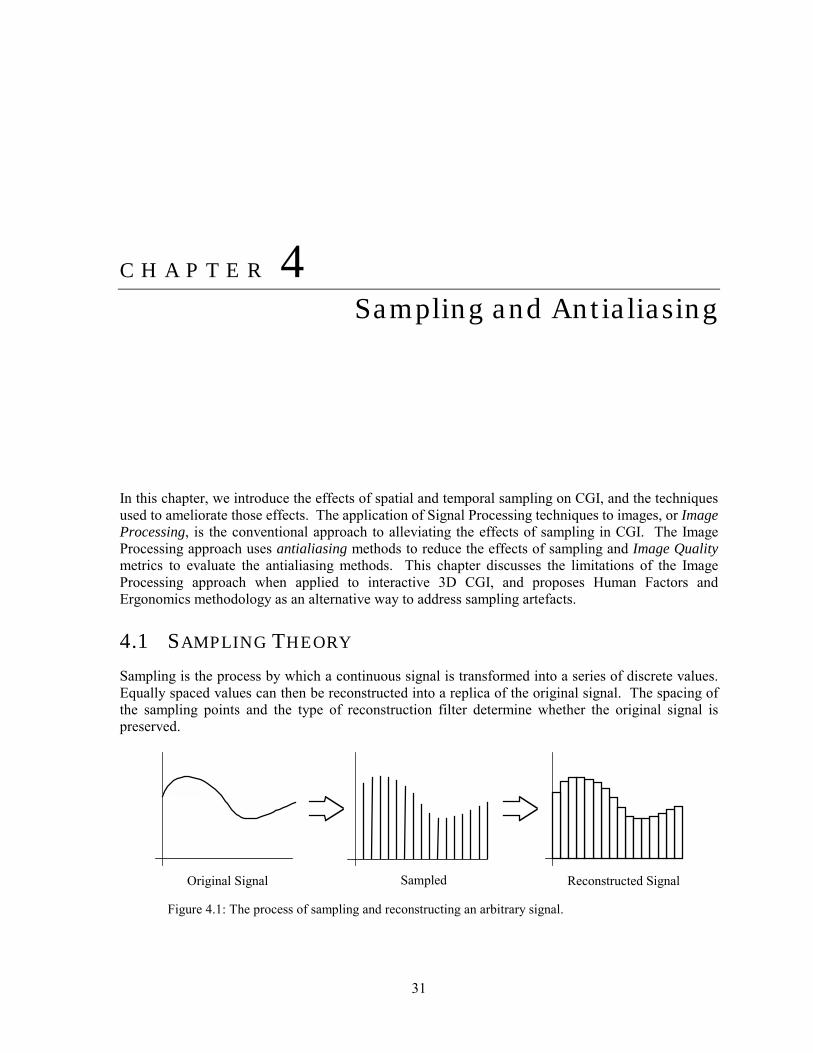
31
C H A P T E R 4
4:Sampling and Antialiasing In this chapter, we introduce the effects of spatial and temporal sampling on CGI, and the techniques used to ameliorate those effects. The application of Signal Processing techniques to images, or Image Processing, is the conventional approach to alleviating the effects of sampling in CGI. The Image Processing approach uses antialiasing methods to reduce the effects of sampling and Image Quality metrics to evaluate the antialiasing methods. This chapter discusses the limitations of the Image Processing approach when applied to interactive 3D CGI, and proposes Human Factors and Ergonomics methodology as an alternative way to address sampling artefacts.
4.1 SAMPLING THEORY
Sampling is the process by which a continuous signal is transformed into a series of discrete values. Equally spaced values can then be reconstructed into a replica of the original signal. The spacing of the sampling points and the type of reconstruction filter determine whether the original signal is preserved.
Sampled Reconstructed Signal Original Signal
Figure 4.1: The process of sampling and reconstructing an arbitrary signal.
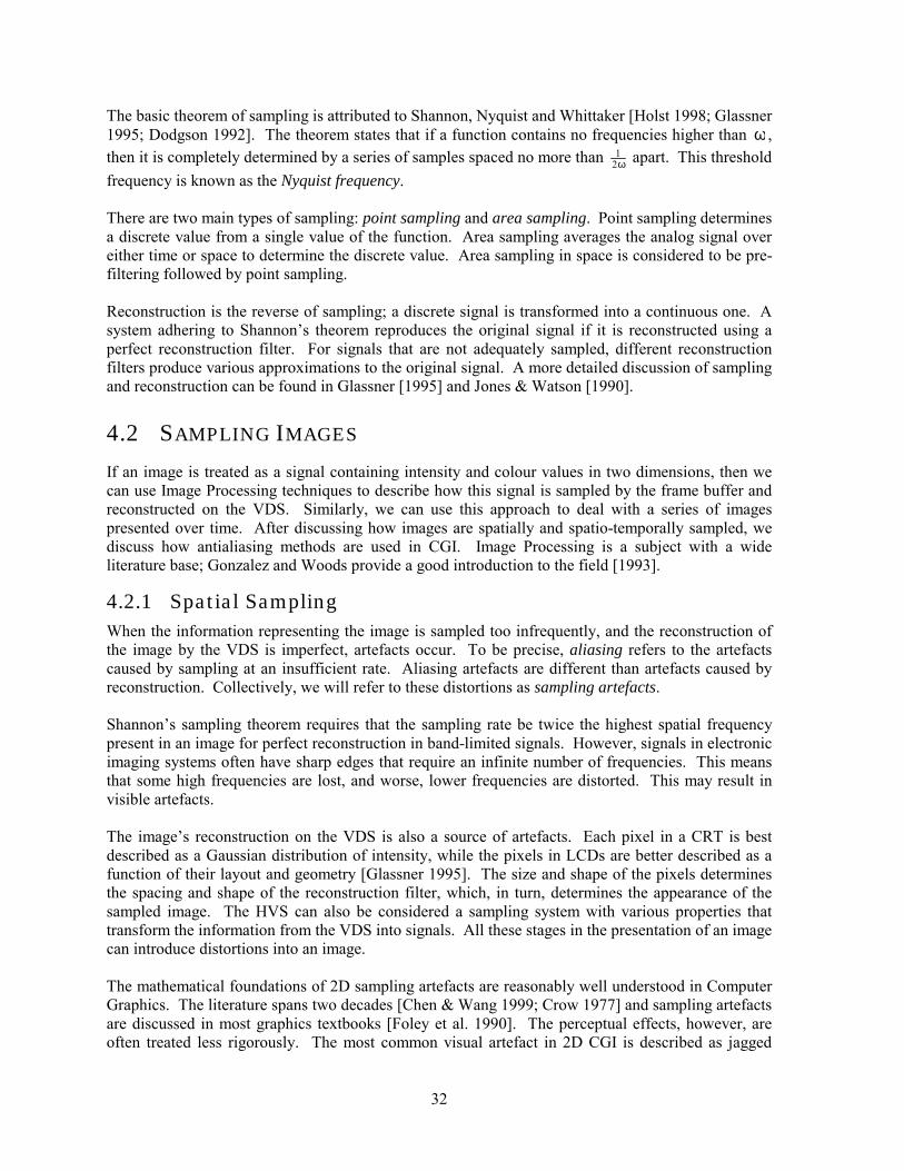
32
The basic theorem of sampling is attributed to Shannon, Nyquist and Whittaker [Holst 1998; Glassner 1995; Dodgson 1992]. The theorem states that if a function contains no frequencies higher than ω, then it is completely determined by a series of samples spaced no more than ω2
1 apart. This threshold frequency is known as the Nyquist frequency. There are two main types of sampling: point sampling and area sampling. Point sampling determines a discrete value from a single value of the function. Area sampling averages the analog signal over either time or space to determine the discrete value. Area sampling in space is considered to be pre-filtering followed by point sampling. Reconstruction is the reverse of sampling; a discrete signal is transformed into a continuous one. A system adhering to Shannon�s theorem reproduces the original signal if it is reconstructed using a perfect reconstruction filter. For signals that are not adequately sampled, different reconstruction filters produce various approximations to the original signal. A more detailed discussion of sampling and reconstruction can be found in Glassner [1995] and Jones & Watson [1990].
4.2 SAMPLING IMAGES
If an image is treated as a signal containing intensity and colour values in two dimensions, then we can use Image Processing techniques to describe how this signal is sampled by the frame buffer and reconstructed on the VDS. Similarly, we can use this approach to deal with a series of images presented over time. After discussing how images are spatially and spatio-temporally sampled, we discuss how antialiasing methods are used in CGI. Image Processing is a subject with a wide literature base; Gonzalez and Woods provide a good introduction to the field [1993].
4.2.1 Spatial Sampling When the information representing the image is sampled too infrequently, and the reconstruction of the image by the VDS is imperfect, artefacts occur. To be precise, aliasing refers to the artefacts caused by sampling at an insufficient rate. Aliasing artefacts are different than artefacts caused by reconstruction. Collectively, we will refer to these distortions as sampling artefacts. Shannon�s sampling theorem requires that the sampling rate be twice the highest spatial frequency present in an image for perfect reconstruction in band-limited signals. However, signals in electronic imaging systems often have sharp edges that require an infinite number of frequencies. This means that some high frequencies are lost, and worse, lower frequencies are distorted. This may result in visible artefacts. The image�s reconstruction on the VDS is also a source of artefacts. Each pixel in a CRT is best described as a Gaussian distribution of intensity, while the pixels in LCDs are better described as a function of their layout and geometry [Glassner 1995]. The size and shape of the pixels determines the spacing and shape of the reconstruction filter, which, in turn, determines the appearance of the sampled image. The HVS can also be considered a sampling system with various properties that transform the information from the VDS into signals. All these stages in the presentation of an image can introduce distortions into an image. The mathematical foundations of 2D sampling artefacts are reasonably well understood in Computer Graphics. The literature spans two decades [Chen & Wang 1999; Crow 1977] and sampling artefacts are discussed in most graphics textbooks [Foley et al. 1990]. The perceptual effects, however, are often treated less rigorously. The most common visual artefact in 2D CGI is described as jagged
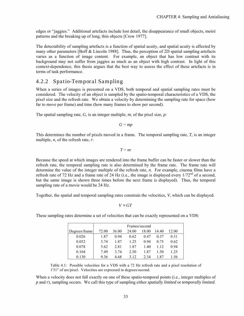
CHAPTER 4: Sampling and Antialiasing
33
edges or �jaggies.� Additional artefacts include lost detail, the disappearance of small objects, moiré patterns and the breaking up of long, thin objects [Crow 1977]. The detectability of sampling artefacts is a function of spatial acuity, and spatial acuity is affected by many other parameters [Boff & Lincoln 1988]. Thus, the perception of 2D spatial sampling artefacts varies as a function of image content. For example, an object that has low contrast with its background may not suffer from jaggies as much as an object with high contrast. In light of this context-dependence, this thesis argues that the best way to assess the effect of these artefacts is in terms of task performance.
4.2.2 Spatio-Temporal Sampling When a series of images is presented on a VDS, both temporal and spatial sampling rates must be considered. The velocity of an object is sampled by the spatio-temporal characteristics of a VDS, the pixel size and the refresh rate. We obtain a velocity by determining the sampling rate for space (how far to move per frame) and time (how many frames to show per second). The spatial sampling rate, G, is an integer multiple, m, of the pixel size, p:
G = mp This determines the number of pixels moved in a frame. The temporal sampling rate, T, is an integer multiple, n, of the refresh rate, r:
T = nr
Because the speed at which images are rendered into the frame buffer can be faster or slower than the refresh rate, the temporal sampling rate is also determined by the frame rate. The frame rate will determine the value of the integer multiple of the refresh rate, n. For example, cinema films have a refresh rate of 72 Hz and a frame rate of 24 Hz (i.e., the image is displayed every 1/72nd of a second, but the same image is shown three times before the next frame is displayed). Thus, the temporal sampling rate of a movie would be 24 Hz. Together, the spatial and temporal sampling rates constrain the velocities, V, which can be displayed.
GTV = These sampling rates determine a set of velocities that can be exactly represented on a VDS:
Frames/second Degrees/frame 72.00 36.00 24.00 18.00 14.40 12.00
0.026 1.87 0.94 0.62 0.47 0.37 0.310.052 3.74 1.87 1.25 0.94 0.75 0.620.078 5.62 2.81 1.87 1.40 1.12 0.940.104 7.49 3.74 2.50 1.87 1.50 1.250.130 9.36 4.68 3.12 2.34 1.87 1.56
Table 4.1: Possible velocities for a VDS with a 72 Hz refresh rate and a pixel resolution of 1'31" of arc/pixel. Velocities are expressed in degrees/second.
When a velocity does not fall exactly on one of these spatio-temporal points (i.e., integer multiples of p and r), sampling occurs. We call this type of sampling either spatially limited or temporally limited.
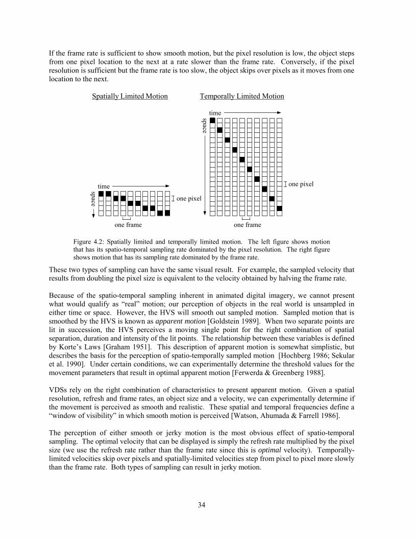
34
If the frame rate is sufficient to show smooth motion, but the pixel resolution is low, the object steps from one pixel location to the next at a rate slower than the frame rate. Conversely, if the pixel resolution is sufficient but the frame rate is too slow, the object skips over pixels as it moves from one location to the next.
Spatially Limited Motion Temporally Limited Motion
.
timespace one pixel
one frame
timespace
one pixel
one frame
Figure 4.2: Spatially limited and temporally limited motion. The left figure shows motion that has its spatio-temporal sampling rate dominated by the pixel resolution. The right figure shows motion that has its sampling rate dominated by the frame rate.
These two types of sampling can have the same visual result. For example, the sampled velocity that results from doubling the pixel size is equivalent to the velocity obtained by halving the frame rate. Because of the spatio-temporal sampling inherent in animated digital imagery, we cannot present what would qualify as �real� motion; our perception of objects in the real world is unsampled in either time or space. However, the HVS will smooth out sampled motion. Sampled motion that is smoothed by the HVS is known as apparent motion [Goldstein 1989]. When two separate points are lit in succession, the HVS perceives a moving single point for the right combination of spatial separation, duration and intensity of the lit points. The relationship between these variables is defined by Korte�s Laws [Graham 1951]. This description of apparent motion is somewhat simplistic, but describes the basis for the perception of spatio-temporally sampled motion [Hochberg 1986; Sekular et al. 1990]. Under certain conditions, we can experimentally determine the threshold values for the movement parameters that result in optimal apparent motion [Ferwerda & Greenberg 1988]. VDSs rely on the right combination of characteristics to present apparent motion. Given a spatial resolution, refresh and frame rates, an object size and a velocity, we can experimentally determine if the movement is perceived as smooth and realistic. These spatial and temporal frequencies define a �window of visibility� in which smooth motion is perceived [Watson, Ahumada & Farrell 1986]. The perception of either smooth or jerky motion is the most obvious effect of spatio-temporal sampling. The optimal velocity that can be displayed is simply the refresh rate multiplied by the pixel size (we use the refresh rate rather than the frame rate since this is optimal velocity). Temporally-limited velocities skip over pixels and spatially-limited velocities step from pixel to pixel more slowly than the frame rate. Both types of sampling can result in jerky motion.
CHAPTER 4: Sampling and Antialiasing
35
Although we have focused on the appearance of jerky motion, other artefacts can occur as the result of spatio-temporal sampling. The direction of motion can appear to reverse (the �wagon-wheel� illusion), or multiple objects can be seen rather than a single one [Edgar & Bex 1995; Watt 1989]. Edges of objects may appear to �shimmer� as an object rotates or moves. Thin objects will rejoin and separate and small objects will blink on and off as they move across pixel boundaries [Crow 1977].
4.2.3 Antialiasing Methods that remove the visual artefacts resulting from inadequate sampling rates are collectively known as antialiasing. Antialiasing methods effectively remove sampling artefacts in some visual contexts. However, implementing an antialiasing method can be a complex procedure and may result in an unwanted computational cost. Furthermore, the effectiveness of an antialiasing technique varies with the user, the image content and the VDS type. Applying a low-pass filter to the input image is the simplest antialiasing method [Crow 1981]. Visually, this blurs the image. If the viewer is a sufficient distance away, this blurriness is not visible and the image appears smoother and sharper. Other methods involve types of area sampling (supersampling, weighted-area sampling, stochastic sampling) and have similar visual results [Watt & Watt 1992]. These methods can be mathematically expressed as filters applied to the input image. In addition, the reconstruction filter (i.e., the size, shape and layout of the VDS pixels) can be manipulated to remove sampling artefacts [Holst 1998]. Antialiasing can also be applied to moving images. Motion blur techniques combine information over many frames to avoid overly jerky motion but are computationally expensive [Foley et al. 1990]. Another method used in television alternately interlaces lines on the screen to effectively double the refresh rate. Combined with the decay times of the screen phosphors, this allows for a blurring effect over time, effectively reducing spatio-temporal sampling artefacts [Ferwerda & Greenberg 1988]. In VDS design, the use of antialiasing methods represents a significant computational cost. A vast number of techniques have been developed to improve the speed of antialiasing methods, but currently only hardware-based systems are capable of achieving real-time antialiasing. As a result, the usefulness of antialiasing is determined by frame rate requirements. If a spatial antialiasing method is used and ends up reducing frame rate so that equivalent temporal sampling artefacts are introduced, then antialiasing has no benefit. The effectiveness of an antialiasing method generally increases with its complexity. Stochastic area sampling, for example, improves on uniform area sampling by randomly choosing sampling points. This replaces regular artefacts with random artefacts. The HVS is more tolerant of this kind of artefact. However, the implementation and computation costs of stochastic area sampling are greater than simple point or uniform-area sampling. Similar costs are incurred with motion blur techniques [Korein & Badler 1983]. Commonly-used antialiasing methods are not always the most effective way to combat the artefacts caused by sampling. Removing high spatial frequencies from an image can result in images that are blurred beyond usefulness. Since focus is a pictorial cue to depth, an antialiased image may include unwanted or conflicting depth information. Marshall et al. showed that blurring the boundary where one object occludes another significantly affects the perception of the objects� depths [1996]. Furthermore, if the pixel size is sufficiently large or sufficiently small, antialiasing does not always offer an appreciable visual benefit over a sampled image.
36
Certain VDSs are better suited to particular types of antialiasing since they represent different kinds of reconstruction filters. A CRT, because its pixels are Gaussian functions of intensity, accomplishes some blurring automatically. An LCD, on the other hand, requires different methods depending on the layout of the red, green and blue elements. Depending on the type of VDS, a designer has to make an intelligent choice about which antialiasing method to use. User variation also plays a part in the effectiveness of an antialiasing method. Since 20/20 Snellen acuity is only an average of human spatial acuity, methods that are based on this criterion result in only a percentage of users correctly seeing the image. Furthermore, different methods for testing human spatial acuity lead to different thresholds [Boff & Lincoln 1988]. The most commonly used reference measure for acuity (in Image Processing) is the sine wave grating. This allows an experimenter to obtain a just-detectable spatial frequency that can be easily used in signal processing analysis. However, Green criticised �gratingologists,� showing that using gratings that are more complex resulted in drastic overestimations of the amount of aliasing present in an image [1992]. The number of high-contrast edges affect the amount of degradation due to sampling [Boff & Lincoln 1988]. Furthermore, antialiasing methods are often designed for natural, rather than computer-generated images. Using these methods in CGI disregards potentially useful information contained in the model of the scene. The content of the image, whether it is a natural image, an experimental image or a computer-generated image, helps to determine the impact of aliasing on the perception of the image. The disadvantages of traditional antialiasing methods are:
• Increased computational cost • Increased implementation cost • Effectiveness varies with:
! Image content ! User ! VDS type ! Task
• Failure to exploit internal model of computer-generated scene Despite the disadvantages listed above, antialiasing methods are widely used in CGI. However, antialiasing is most often used in systems where real-time performance is not critical (e.g., producing animations off-line), or where efficient methods have been developed to maintain interactive frame rates (e.g., antialiasing text). In virtual environments, simulators and teleoperation systems, antialiasing methods are not always used because of the many other computational demands on the system.
4.3 IMAGE QUALITY METRICS
Image Processing techniques are assessed using a metric called Image Quality. Image Quality measures include both mathematical models of quality derived from psychophysical data and subjective quality judgements. Subjective quality ratings (i.e., �poor� to �excellent�) are made by viewers about the image. Alternatively, experimental data from psychophysical experimentation is used to derive a mathematical model of quality [Taylor, Pizlo & Allebach 1998]. These metrics are the primary method for evaluating antialiasing and image compression methods [Dodgson 1992; Schreiber & Troxel 1985]. However, these metrics make fundamental assumptions that need to be clearly stated.
CHAPTER 4: Sampling and Antialiasing
37
One underlying assumption of Image Quality is that the HVS can be modelled and these models can be used to improve antialiasing methods [Rogowitz 1985]. Often borrowing from Psychophysics literature, they treat a VDS as a process including a model of the digitiser, a model of the VDS surface and a model of the HVS. In this manner, they aim to measure the effectiveness of antialiasing methods. This type of assessment has several disadvantages. Mathematical models of the HVS are large in number and diverse in application [Li, Meyer & Klassen 1998]. None are comprehensive models of the entire process of human perception and often fail to account for user variation. As a result, the effectiveness of a quality metric depends on the relevance of the vision model used, the content of the image, and the situation in which the image is viewed. Some quality metrics rely on user judgements. However, subjective impressions are a learned phenomenon, subject to a variety of societal and personal factors. Variation in the set of images to be judged is often ignored; some images may suffer more from sampling artefacts than others [Ridder 1998]. Subjective metrics are inherently noisy; different questioning strategies can result in widely varying results. Like mathematical models of quality, subjective judgements vary with the content of the image and the viewing situation. Measuring Image Quality is not the same as measuring task performance; the subjective impression a user has of an image may not affect their ability to accomplish a specific task [Holst 1998]. Previous research supports the assertion that the spatial and temporal resolutions suggested by Image Quality metrics may bear little relation to the practical requirements of a VDS [Booth et al. 1987]. Thus, the assumptions underlying these methods should be considered before using them to evaluate CGI.
4.4 A HUMAN FACTORS APPROACH TO SAMPLING
In this dissertation, we evaluate the quality of a VDS based on task performance, an approach fundamental to Human Factors and Ergonomics research. VDS hardware engineers have long understood the importance of analysing not just the observer or the image presented, but also the task to be accomplished [Debons 1968]. Thus, analysing and decomposing the task is an important element of this approach [Stammers & Shepard 1998]. Some previous work has addressed sampling and antialiasing using a task-centric approach. In an experiment to determine a user�s ability to detect and recognise targets transmitted from an unmanned aerial vehicle, spatial and temporal resolutions were lowered because of limited bandwidth [Swartz, Wallace & Tkacz 1992]. A reduced frame rate had a greater negative effect than reduced resolution; therefore, the researchers argued for reducing the image resolution to improve transmission speed (and thus improve frame rate). On a mental rotation task, Booth et al. showed that performance was not significantly affected by an increase in pixel size [1987]. In addition, antialiasing methods did not result in significant improvement for high and low spatial resolutions. Clearly, traditional antialiasing methods are not useful in all contexts. Tiana, Pavel and Ahumada showed that some low-pass filtering might be useful when aligning CGI with real-world imagery [1994]. They showed that antialiasing in head-up cockpit VDSs reduced misregistration errors. In this context, the blurriness introduced by antialiasing actually improved task performance. As seen in these examples, task performance is a valuable way to evaluate spatial and temporal sampling artefacts and antialiasing methods. Many of the difficulties in Image Quality metrics are
38
avoided and practical results can be obtained. In this thesis, we describe and evaluate spatio-temporal sampling artefacts in 3D CGI with a task-centric approach. By analysing the effects of sampling on the presentation of linear perspective and stereo depth information, we hope to provide context-specific design guidelines.
4.5 CONCLUSION
In this chapter, we presented the Image Processing approach to describing and ameliorating sampling artefacts. The limitations of the antialiasing methods and Image Quality metrics used in Image Processing are significant and led us to propose using a Human Factors and Ergonomics approach to analysing the effects of sampling. By evaluating how performance on a relevant task varies with parameters that affect spatial and temporal sampling artefacts, we can offer practical, context-specific advice to the VDS designer.
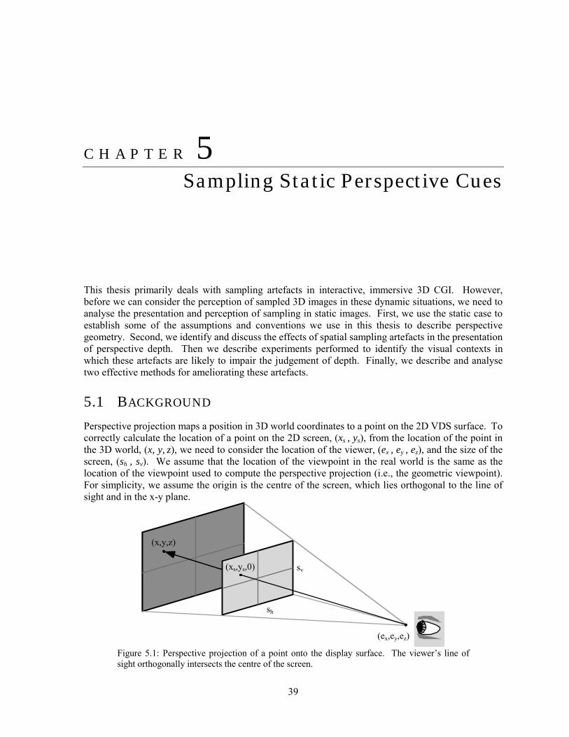
39
C H A P T E R 5
5:Sampling Static Perspective Cues This thesis primarily deals with sampling artefacts in interactive, immersive 3D CGI. However, before we can consider the perception of sampled 3D images in these dynamic situations, we need to analyse the presentation and perception of sampling in static images. First, we use the static case to establish some of the assumptions and conventions we use in this thesis to describe perspective geometry. Second, we identify and discuss the effects of spatial sampling artefacts in the presentation of perspective depth. Then we describe experiments performed to identify the visual contexts in which these artefacts are likely to impair the judgement of depth. Finally, we describe and analyse two effective methods for ameliorating these artefacts.
5.1 BACKGROUND
Perspective projection maps a position in 3D world coordinates to a point on the 2D VDS surface. To correctly calculate the location of a point on the 2D screen, (xs , ys), from the location of the point in the 3D world, (x, y, z), we need to consider the location of the viewer, (ex , ey , ez), and the size of the screen, (sh , sv). We assume that the location of the viewpoint in the real world is the same as the location of the viewpoint used to compute the perspective projection (i.e., the geometric viewpoint). For simplicity, we assume the origin is the centre of the screen, which lies orthogonal to the line of sight and in the x-y plane.
sv
sh
(ex,ey,ez)
(xs,ys,0)
(x,y,z)
Figure 5.1: Perspective projection of a point onto the display surface. The viewer�s line of sight orthogonally intersects the centre of the screen.
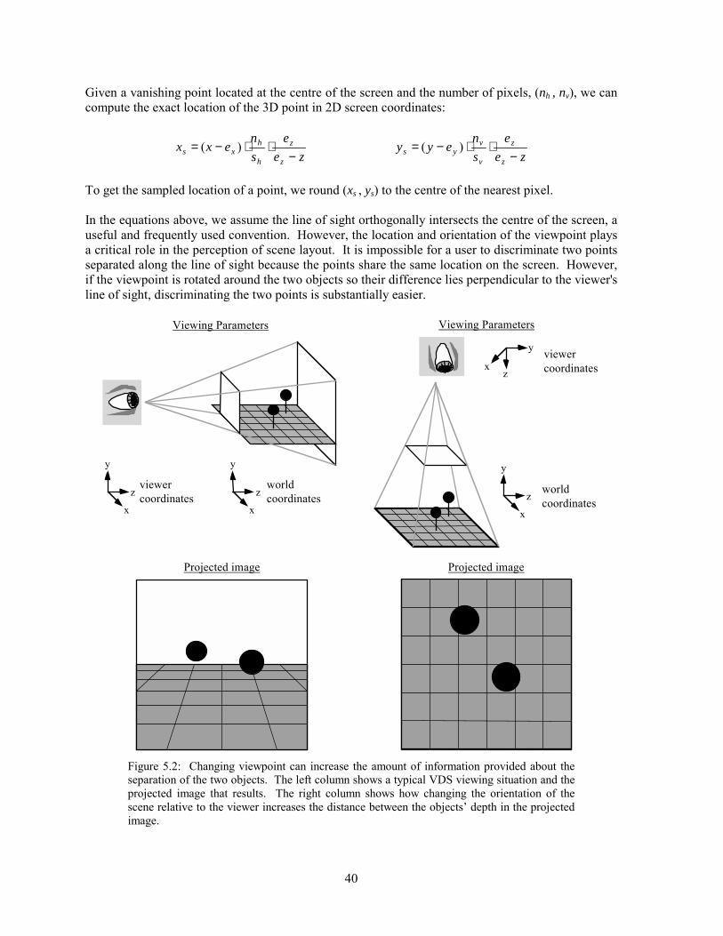
40
Given a vanishing point located at the centre of the screen and the number of pixels, (nh , nv), we can compute the exact location of the 3D point in 2D screen coordinates:
zee
sn
exxz
z
h
hxs −
⋅⋅−= )( ze
esn
eyyz
z
v
vys −
⋅⋅−= )(
To get the sampled location of a point, we round (xs , ys) to the centre of the nearest pixel. In the equations above, we assume the line of sight orthogonally intersects the centre of the screen, a useful and frequently used convention. However, the location and orientation of the viewpoint plays a critical role in the perception of scene layout. It is impossible for a user to discriminate two points separated along the line of sight because the points share the same location on the screen. However, if the viewpoint is rotated around the two objects so their difference lies perpendicular to the viewer's line of sight, discriminating the two points is substantially easier.
Projected image Projected image
y
z xviewer coordinates
y
z x
y
z x
world coordinates
viewer coordinates
y
z x
worldcoordinates
Viewing Parameters Viewing Parameters
Figure 5.2: Changing viewpoint can increase the amount of information provided about the separation of the two objects. The left column shows a typical VDS viewing situation and the projected image that results. The right column shows how changing the orientation of the scene relative to the viewer increases the distance between the objects� depth in the projected image.
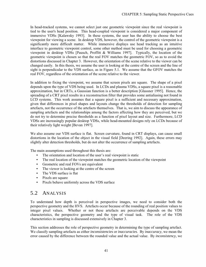
CHAPTER 5: Sampling Static Perspective Cues
41
In head-tracked systems, we cannot select just one geometric viewpoint since the real viewpoint is tied to the user's head position. This head-coupled viewpoint is considered a major component of immersive VDSs [Kalawsky 1993]. In these systems, the user has the ability to choose the best viewpoint for viewing a scene. In desktop VDS, however, the control of the geometric viewpoint is a significantly more difficult matter. While immersive displays use head tracking as an intuitive interface to geometric viewpoint control, some other method must be used for choosing a geometric viewpoint in desktop VDSs [Pausch, Proffitt & Williams 1997]. Typically, the location of the geometric viewpoint is chosen so that the real FOV matches the geometric FOV, so as to avoid the distortions discussed in Chapter 3. However, the orientation of the scene relative to the viewer can be changed easily. In this thesis, we assume the user is looking at the centre of the screen and the line of sight is perpendicular to the VDS surface, as in Figure 5.1. We assume that the GFOV matches the real FOV, regardless of the orientation of the scene relative to the viewer. In addition to fixing the viewpoint, we assume that screen pixels are square. The shape of a pixel depends upon the type of VDS being used. In LCDs and plasma VDSs, a square pixel is a reasonable approximation, but in CRTs, a Gaussian function is a better description [Glassner 1995]. Hence, the spreading of a CRT pixel results in a reconstruction filter that provides some antialiasing not found in LCD systems. This work assumes that a square pixel is a sufficient and necessary approximation, given that differences in pixel shapes and layouts change the thresholds of detection for sampling artefacts, not the occurrence of the artefacts themselves. That is, we aim to discuss the appearance of sampling artefacts and the relationships among the factors affecting how they are perceived, but we do not try to determine precise thresholds as a function of pixel layout and size. Furthermore, LCD VDSs are increasingly popular desktop VDSs, while head-mounted designs rely on LCDs because of their relatively light weight [Bevan 1997]. We also assume our VDS surface is flat. Screen curvature, found in CRT displays, can cause small distortions in the location of the object in the visual field [Deering 1992]. Again, these errors may slightly alter detection thresholds, but do not alter the occurrence of sampling artefacts. The main assumptions used throughout this thesis are:
• The orientation and location of the user�s real viewpoint is static • The real location of the viewpoint matches the geometric location of the viewpoint • Geometric and real FOVs are equivalent • The viewer is looking at the centre of the screen • The VDS surface is flat • Pixels are square • Pixels behave uniformly across the VDS surface
5.2 ANALYSIS
To understand how depth is perceived in perspective images, we need to consider both the perspective geometry and the HVS. Artefacts occur because of the rounding of real position values to integer pixel values. Whether or not these artefacts are perceivable depends on the VDS characteristics, the perspective geometry and the type of visual task. The role of the VDS characteristics in sampling is discussed extensively in Chapter 3. This section addresses the role of perspective geometry in determining the type of sampling artefact. We classify sampling artefacts as either inconsistencies or inaccuracies. By inaccuracy, we mean the error caused by the difference between the rounded value and the actual value. By inconsistency, we
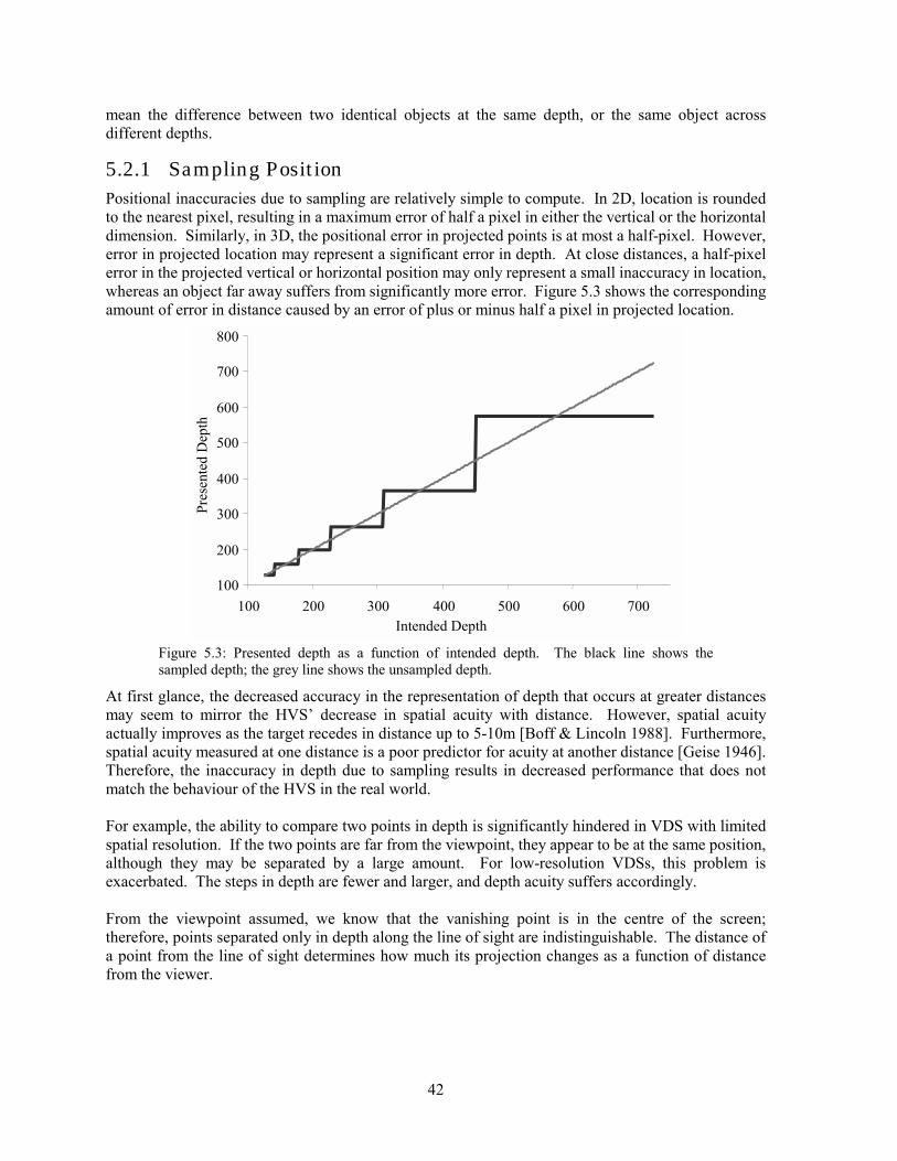
42
mean the difference between two identical objects at the same depth, or the same object across different depths.
5.2.1 Sampling Position Positional inaccuracies due to sampling are relatively simple to compute. In 2D, location is rounded to the nearest pixel, resulting in a maximum error of half a pixel in either the vertical or the horizontal dimension. Similarly, in 3D, the positional error in projected points is at most a half-pixel. However, error in projected location may represent a significant error in depth. At close distances, a half-pixel error in the projected vertical or horizontal position may only represent a small inaccuracy in location, whereas an object far away suffers from significantly more error. Figure 5.3 shows the corresponding amount of error in distance caused by an error of plus or minus half a pixel in projected location.
100
200
300
400
500
600
700
800
100 200 300 400 500 600 700 Intended Depth
Pres
ente
d D
epth
Figure 5.3: Presented depth as a function of intended depth. The black line shows the sampled depth; the grey line shows the unsampled depth.
At first glance, the decreased accuracy in the representation of depth that occurs at greater distances may seem to mirror the HVS� decrease in spatial acuity with distance. However, spatial acuity actually improves as the target recedes in distance up to 5-10m [Boff & Lincoln 1988]. Furthermore, spatial acuity measured at one distance is a poor predictor for acuity at another distance [Geise 1946]. Therefore, the inaccuracy in depth due to sampling results in decreased performance that does not match the behaviour of the HVS in the real world. For example, the ability to compare two points in depth is significantly hindered in VDS with limited spatial resolution. If the two points are far from the viewpoint, they appear to be at the same position, although they may be separated by a large amount. For low-resolution VDSs, this problem is exacerbated. The steps in depth are fewer and larger, and depth acuity suffers accordingly. From the viewpoint assumed, we know that the vanishing point is in the centre of the screen; therefore, points separated only in depth along the line of sight are indistinguishable. The distance of a point from the line of sight determines how much its projection changes as a function of distance from the viewer.
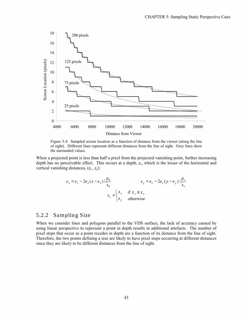
CHAPTER 5: Sampling Static Perspective Cues
43
0
2
4
6
8
10
12
14
16
18
4000 6000 8000 10000 12000 14000 16000 18000 20000
Distance from Viewer
Scre
en L
ocat
ion
(pix
els)
200 pixels
125 pixels
75 pixels
25 pixels
Figure 5.4: Sampled screen location as a function of distance from the viewer (along the line of sight). Different lines represent different distances from the line of sight. Grey lines show the unrounded values.
When a projected point is less than half a pixel from the projected vanishing point, further increasing depth has no perceivable effect. This occurs at a depth, zv, which is the lesser of the horizontal and vertical vanishing distances, (zx , zy):
h
hxzzx s
nexeez ⋅−−= )(2
v
vyzzy s
neyeez ⋅−−= )(2
≥
=otherwise
if yx
y
xv
zzzz
z
5.2.2 Sampling Size When we consider lines and polygons parallel to the VDS surface, the lack of accuracy caused by using linear perspective to represent a point in depth results in additional artefacts. The number of pixel steps that occur as a point recedes in depth are a function of its distance from the line of sight. Therefore, the two points defining a size are likely to have pixel steps occurring at different distances since they are likely to be different distances from the line of sight.
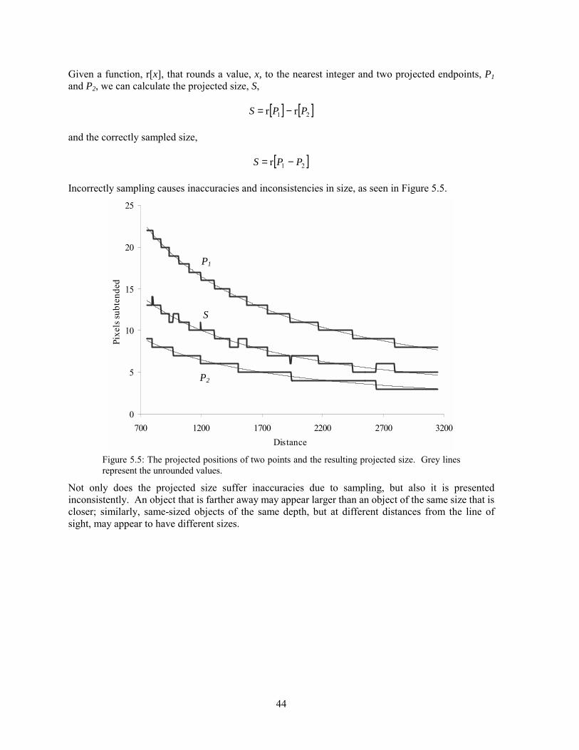
Given a function, r[x], that rounds a value, x, to the nearest integer and two projected endpoints, P1 and P2, we can calculate the projected size, S,
[ ] [ ]21 rr PPS −=
and the correctly sampled size,
[ ]21r PPS −=
Incorrectly sampling causes inaccuracies and inconsistencies in size, as seen in Figure 5.5.
0
5
10
15
20
25
700 12
Pixe
ls su
bten
ded
Figure 5.5: The projectedrepresent the unrounded v
Not only does the projected inconsistently. An object that icloser; similarly, same-sized osight, may appear to have diffe
P1
S
44
00 1700 2200 2700 3200Distance
positions of two points and the resulting projected size. Grey lines alues.
size suffer inaccuracies due to sampling, but also it is presented s farther away may appear larger than an object of the same size that is bjects of the same depth, but at different distances from the line of rent sizes.
P2
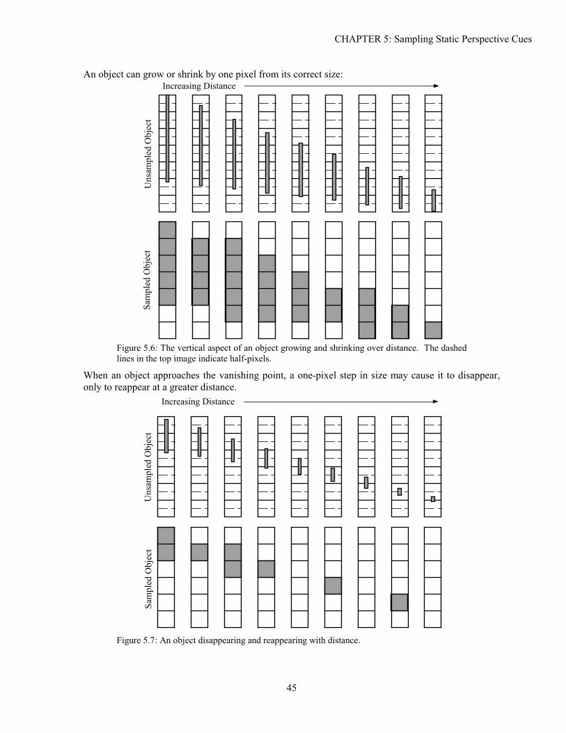
CHAPTER 5: Sampling Static Perspective Cues
45
An object can grow or shrink by one pixel from its correct size:
.
Sam
pled
Obj
ect
Uns
ampl
ed O
bjec
t
Increasing Distance
Figure 5.6: The vertical aspect of an object growing and shrinking over distance. The dashed lines in the top image indicate half-pixels.
When an object approaches the vanishing point, a one-pixel step in size may cause it to disappear, only to reappear at a greater distance.
Sam
pled
Obj
ect
Uns
ampl
ed O
bjec
t
Increasing Distance
Figure 5.7: An object disappearing and reappearing with distance.
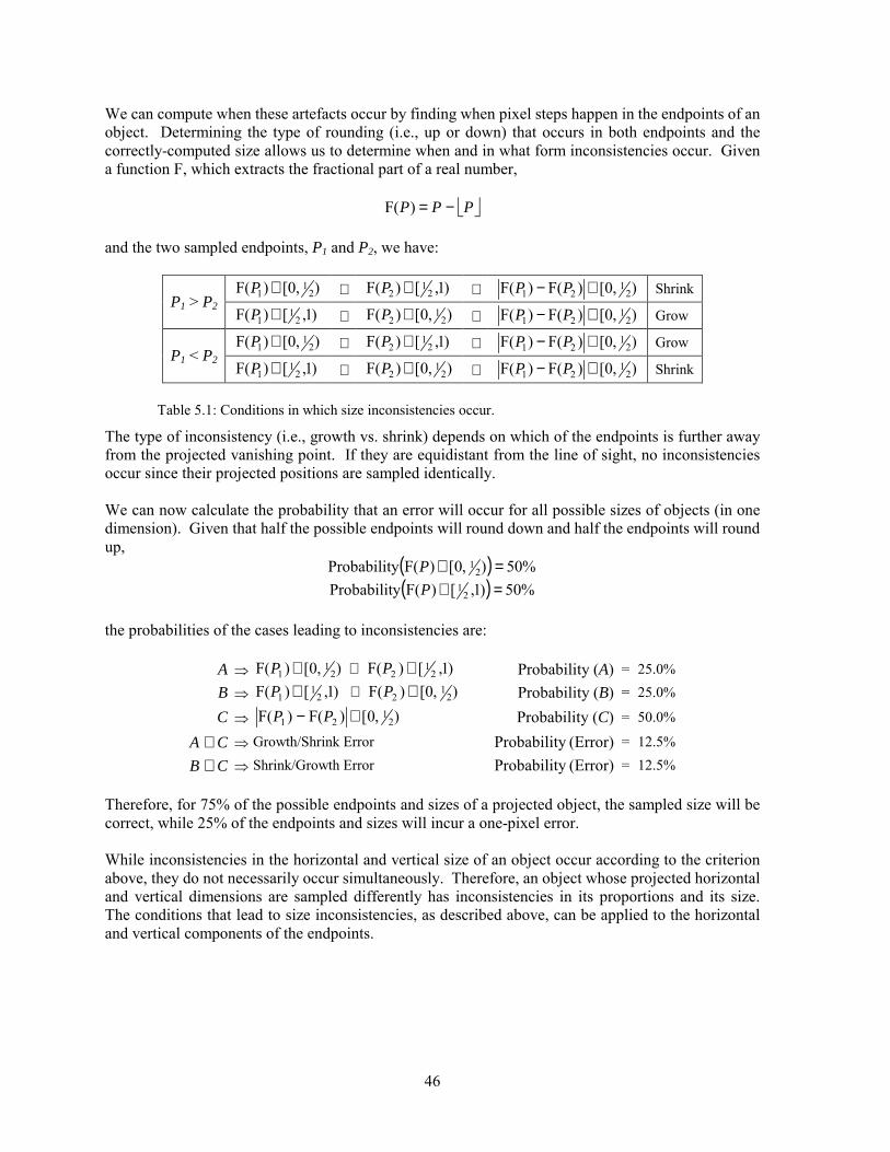
46
We can compute when these artefacts occur by finding when pixel steps happen in the endpoints of an object. Determining the type of rounding (i.e., up or down) that occurs in both endpoints and the correctly-computed size allows us to determine when and in what form inconsistencies occur. Given a function F, which extracts the fractional part of a real number,
PPP −=)F( and the two sampled endpoints, P1 and P2, we have:
),0[)F( 21
1 ∈P ∧ )1,[)F( 21
2 ∈P ∧ ),0[)F()F( 21
21 ∈− PP Shrink P1 > P2 )1,[)F( 2
11 ∈P ∧ ),0[)F( 2
12 ∈P ∧ ),0[)F()F( 2
121 ∈− PP Grow
),0[)F( 21
1 ∈P ∧ )1,[)F( 21
2 ∈P ∧ ),0[)F()F( 21
21 ∈− PP Grow P1 < P2 )1,[)F( 2
11 ∈P ∧ ),0[)F( 2
12 ∈P ∧ ),0[)F()F( 2
121 ∈− PP Shrink
Table 5.1: Conditions in which size inconsistencies occur.
The type of inconsistency (i.e., growth vs. shrink) depends on which of the endpoints is further away from the projected vanishing point. If they are equidistant from the line of sight, no inconsistencies occur since their projected positions are sampled identically. We can now calculate the probability that an error will occur for all possible sizes of objects (in one dimension). Given that half the possible endpoints will round down and half the endpoints will round up,
( ) %50),0[)F(yProbabilit 21 =∈P
( ) %50)1,[)F(yProbabilit 21 =∈P
the probabilities of the cases leading to inconsistencies are:
A ⇒ ),0[)F( 21
1 ∈P ∧ )1,[)F( 21
2 ∈P Probability (A) = 25.0%
B ⇒ )1,[)F( 21
1 ∈P ∧ ),0[)F( 21
2 ∈P Probability (B) = 25.0%
C ⇒ ),0[)F()F( 21
21 ∈− PP Probability (C) = 50.0%
A ∧ C ⇒ Growth/Shrink Error Probability (Error) = 12.5%
B ∧ C ⇒ Shrink/Growth Error Probability (Error) = 12.5% Therefore, for 75% of the possible endpoints and sizes of a projected object, the sampled size will be correct, while 25% of the endpoints and sizes will incur a one-pixel error. While inconsistencies in the horizontal and vertical size of an object occur according to the criterion above, they do not necessarily occur simultaneously. Therefore, an object whose projected horizontal and vertical dimensions are sampled differently has inconsistencies in its proportions and its size. The conditions that lead to size inconsistencies, as described above, can be applied to the horizontal and vertical components of the endpoints.
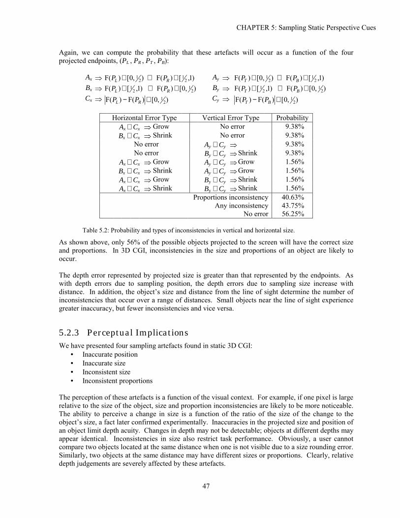
CHAPTER 5: Sampling Static Perspective Cues
47
Again, we can compute the probability that these artefacts will occur as a function of the four projected endpoints, (PL , PR , PT , PB):
Ax ⇒ ),0[)F( 21∈LP ∧ )1,[)F( 2
1∈RP Ay ⇒ ),0[)F( 21∈TP ∧ )1,[)F( 2
1∈BP Bx ⇒ )1,[)F( 2
1∈LP ∧ ),0[)F( 21∈RP By ⇒ )1,[)F( 2
1∈TP ∧ ),0[)F( 21∈BP
Cx ⇒ ),0[)F()F( 21∈− RL PP Cy ⇒ ),0[)F()F( 2
1∈− BT PP
Horizontal Error Type Vertical Error Type Probability Ax ∧ Cx ⇒ Grow No error 9.38% Bx ∧ Cx ⇒ Shrink No error 9.38%
No error Ay ∧ Cy ⇒ 9.38% No error By ∧ Cy ⇒ Shrink 9.38%
Ax ∧ Cx ⇒ Grow Ay ∧ Cy ⇒ Grow 1.56% Bx ∧ Cx ⇒ Shrink Ay ∧ Cy ⇒ Grow 1.56% Ax ∧ Cx ⇒ Grow By ∧ Cy ⇒ Shrink 1.56% Ax ∧ Cx ⇒ Shrink By ∧ Cy ⇒ Shrink 1.56%
Proportions inconsistency 40.63% Any inconsistency 43.75% No error 56.25%
Table 5.2: Probability and types of inconsistencies in vertical and horizontal size.
As shown above, only 56% of the possible objects projected to the screen will have the correct size and proportions. In 3D CGI, inconsistencies in the size and proportions of an object are likely to occur. The depth error represented by projected size is greater than that represented by the endpoints. As with depth errors due to sampling position, the depth errors due to sampling size increase with distance. In addition, the object�s size and distance from the line of sight determine the number of inconsistencies that occur over a range of distances. Small objects near the line of sight experience greater inaccuracy, but fewer inconsistencies and vice versa.
5.2.3 Perceptual Implications We have presented four sampling artefacts found in static 3D CGI:
• Inaccurate position • Inaccurate size • Inconsistent size • Inconsistent proportions
The perception of these artefacts is a function of the visual context. For example, if one pixel is large relative to the size of the object, size and proportion inconsistencies are likely to be more noticeable. The ability to perceive a change in size is a function of the ratio of the size of the change to the object�s size, a fact later confirmed experimentally. Inaccuracies in the projected size and position of an object limit depth acuity. Changes in depth may not be detectable; objects at different depths may appear identical. Inconsistencies in size also restrict task performance. Obviously, a user cannot compare two objects located at the same distance when one is not visible due to a size rounding error. Similarly, two objects at the same distance may have different sizes or proportions. Clearly, relative depth judgements are severely affected by these artefacts.
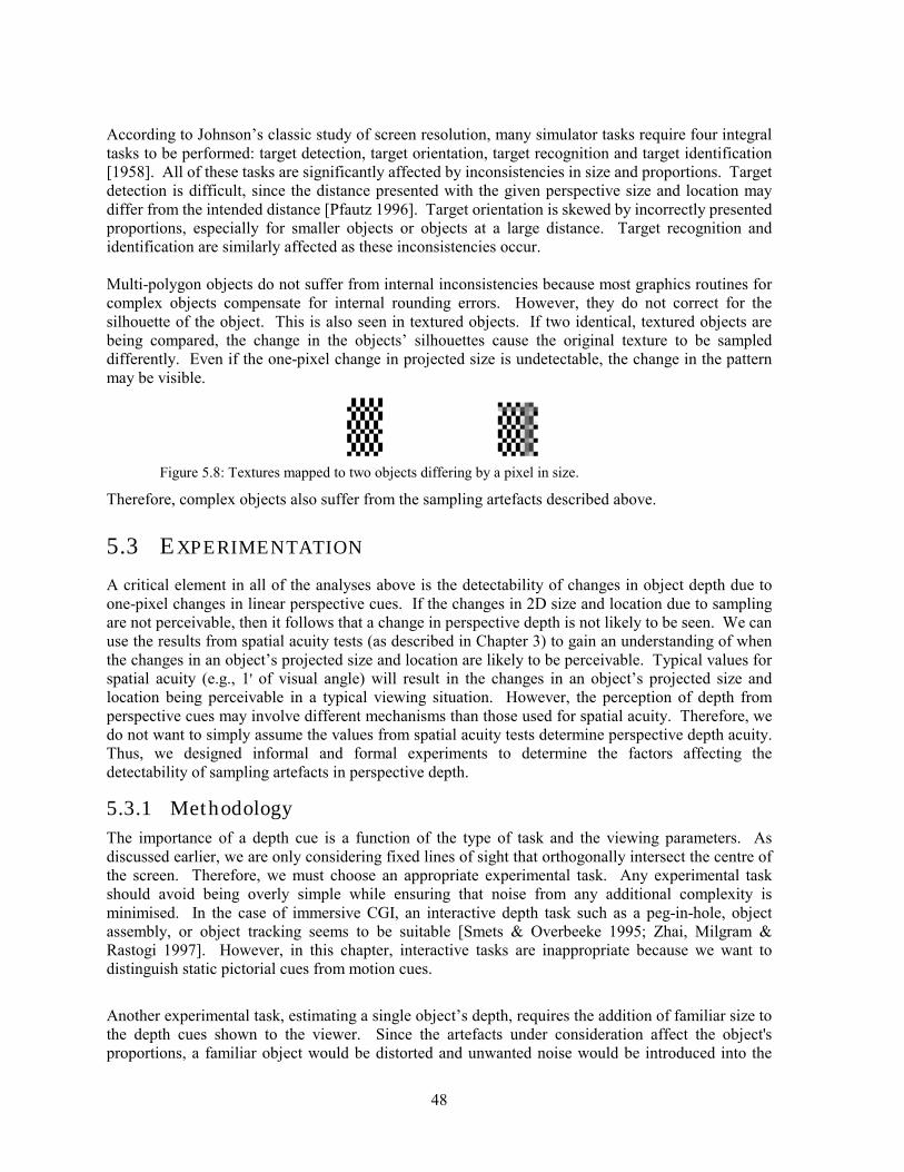
48
According to Johnson�s classic study of screen resolution, many simulator tasks require four integral tasks to be performed: target detection, target orientation, target recognition and target identification [1958]. All of these tasks are significantly affected by inconsistencies in size and proportions. Target detection is difficult, since the distance presented with the given perspective size and location may differ from the intended distance [Pfautz 1996]. Target orientation is skewed by incorrectly presented proportions, especially for smaller objects or objects at a large distance. Target recognition and identification are similarly affected as these inconsistencies occur. Multi-polygon objects do not suffer from internal inconsistencies because most graphics routines for complex objects compensate for internal rounding errors. However, they do not correct for the silhouette of the object. This is also seen in textured objects. If two identical, textured objects are being compared, the change in the objects� silhouettes cause the original texture to be sampled differently. Even if the one-pixel change in projected size is undetectable, the change in the pattern may be visible.
Figure 5.8: Textures mapped to two objects differing by a pixel in size.
Therefore, complex objects also suffer from the sampling artefacts described above.
5.3 EXPERIMENTATION
A critical element in all of the analyses above is the detectability of changes in object depth due to one-pixel changes in linear perspective cues. If the changes in 2D size and location due to sampling are not perceivable, then it follows that a change in perspective depth is not likely to be seen. We can use the results from spatial acuity tests (as described in Chapter 3) to gain an understanding of when the changes in an object�s projected size and location are likely to be perceivable. Typical values for spatial acuity (e.g., 1' of visual angle) will result in the changes in an object�s projected size and location being perceivable in a typical viewing situation. However, the perception of depth from perspective cues may involve different mechanisms than those used for spatial acuity. Therefore, we do not want to simply assume the values from spatial acuity tests determine perspective depth acuity. Thus, we designed informal and formal experiments to determine the factors affecting the detectability of sampling artefacts in perspective depth.
5.3.1 Methodology The importance of a depth cue is a function of the type of task and the viewing parameters. As discussed earlier, we are only considering fixed lines of sight that orthogonally intersect the centre of the screen. Therefore, we must choose an appropriate experimental task. Any experimental task should avoid being overly simple while ensuring that noise from any additional complexity is minimised. In the case of immersive CGI, an interactive depth task such as a peg-in-hole, object assembly, or object tracking seems to be suitable [Smets & Overbeeke 1995; Zhai, Milgram & Rastogi 1997]. However, in this chapter, interactive tasks are inappropriate because we want to distinguish static pictorial cues from motion cues.
Another experimental task, estimating a single object�s depth, requires the addition of familiar size to the depth cues shown to the viewer. Since the artefacts under consideration affect the object's proportions, a familiar object would be distorted and unwanted noise would be introduced into the
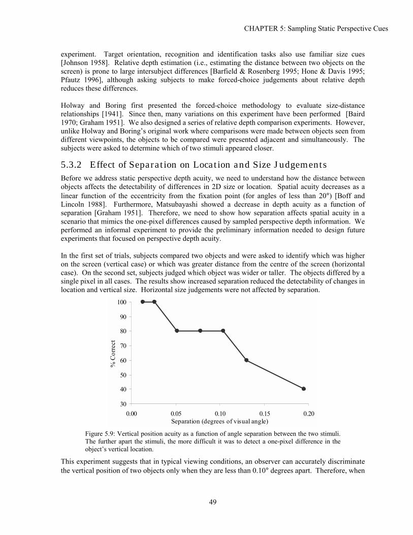
CHAPTER 5: Sampling Static Perspective Cues
49
experiment. Target orientation, recognition and identification tasks also use familiar size cues [Johnson 1958]. Relative depth estimation (i.e., estimating the distance between two objects on the screen) is prone to large intersubject differences [Barfield & Rosenberg 1995; Hone & Davis 1995; Pfautz 1996], although asking subjects to make forced-choice judgements about relative depth reduces these differences. Holway and Boring first presented the forced-choice methodology to evaluate size-distance relationships [1941]. Since then, many variations on this experiment have been performed [Baird 1970; Graham 1951]. We also designed a series of relative depth comparison experiments. However, unlike Holway and Boring�s original work where comparisons were made between objects seen from different viewpoints, the objects to be compared were presented adjacent and simultaneously. The subjects were asked to determine which of two stimuli appeared closer.
5.3.2 Effect of Separation on Location and Size Judgements Before we address static perspective depth acuity, we need to understand how the distance between objects affects the detectability of differences in 2D size or location. Spatial acuity decreases as a linear function of the eccentricity from the fixation point (for angles of less than 20°) [Boff and Lincoln 1988]. Furthermore, Matsubayashi showed a decrease in depth acuity as a function of separation [Graham 1951]. Therefore, we need to show how separation affects spatial acuity in a scenario that mimics the one-pixel differences caused by sampled perspective depth information. We performed an informal experiment to provide the preliminary information needed to design future experiments that focused on perspective depth acuity. In the first set of trials, subjects compared two objects and were asked to identify which was higher on the screen (vertical case) or which was greater distance from the centre of the screen (horizontal case). On the second set, subjects judged which object was wider or taller. The objects differed by a single pixel in all cases. The results show increased separation reduced the detectability of changes in location and vertical size. Horizontal size judgements were not affected by separation.
30
40
50
60
70
80
90
100
0.00 0.05 0.10 0.15 0.20Separation (degrees of visual angle)
% C
orre
ct
Figure 5.9: Vertical position acuity as a function of angle separation between the two stimuli. The further apart the stimuli, the more difficult it was to detect a one-pixel difference in the object�s vertical location.
This experiment suggests that in typical viewing conditions, an observer can accurately discriminate the vertical position of two objects only when they are less than 0.10° degrees apart. Therefore, when
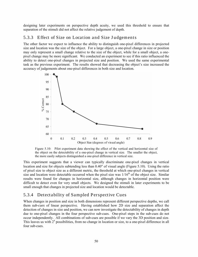
50
designing later experiments on perspective depth acuity, we used this threshold to ensure that separation of the stimuli did not affect the relative judgement of depth.
5.3.3 Effect of Size on Location and Size Judgements The other factor we expect to influence the ability to distinguish one-pixel differences in projected size and location was the size of the object. For a large object, a one-pixel change in size or position may only represent a small change relative to the size of the object, while for a small object, a one-pixel change may be more significant. We conducted an experiment to see if this ratio influenced the ability to detect one-pixel changes in projected size and position. We used the same experimental task as the previous experiment. The results showed that decreasing the object�s size increased the accuracy of judgements about one-pixel differences in both size and location.
60
65
70
75
80
85
90
95
100
0 0.1 0.2 0.3 0.4 0.5 0.6 0.7 0.8 0.9Object Size (degrees of visual angle)
% C
orre
ct
Figure 5.10: Pilot experiment data showing the effect of the vertical and horizontal size of the object on the detectability of a one-pixel change in vertical size. The smaller the object, the more easily subjects distinguished a one-pixel difference in vertical size.
This experiment suggests that a viewer can typically discriminate one-pixel changes in vertical location and size for objects subtending less than 0.40° of visual angle (Figure 5.10). Using the ratio of pixel size to object size as a different metric, the threshold at which one-pixel changes in vertical size and location were detectable occurred when the pixel size was 1/16th of the object size. Similar results were found for changes in horizontal size, although changes in horizontal position were difficult to detect even for very small objects. We designed the stimuli in later experiments to be small enough that changes in projected size and location would be detectable.
5.3.4 Detectability of Sampled Perspective Cues When changes in position and size in both dimensions represent different perspective depths, we call them sub-cues of linear perspective. Having established how 2D size and separation affect the detection of changes in size and position, we can now investigate the detectability of changes in depth due to one-pixel changes in the four perspective sub-cues. One-pixel steps in the sub-cues do not occur independently. All combinations of sub-cues are possible if we vary the 3D position and size. This leaves us with 24 possibilities, from no change in location or size, to a one-pixel difference in all four sub-cues.
CHAPTER 5: Sampling Static Perspective Cues
51
A formal experiment was conducted to determine how the ability to detect differences in depth varies with the 15 different possibilities in which a pixel step occurs. Pixel size was also varied. Subjects judged which of two objects in a scene appeared closer as different possible combinations of sub-cues were presented. The size and separation of the objects were chosen based on the results of the two previous informal experiments. Details of the experiment design and analysis of the results are presented in Experiment A. The main results can be summarised:
• Decreasing pixel size reduced detectability of a fixed change in depth • Vertical position sub-cues significantly increased accuracy when presented individually; the
other sub-cues did not • Combining sub-cues increased the detectability of changes in depth
5.3.5 Discussion These experiments have characterised the detectability of sampling artefacts in perspective depth. Increasing the visual angle subtended by a pixel increases the viewer�s sensitivity to changes in depth. Given that we expect perspective depth acuity to be related to spatial acuity, this increased sensitivity is unsurprising. Notably, the 1' pixel size threshold used by many VDS designers results in visibly sampled perspective depth. Given that changes in depth were perceived for one-pixel changes in perspective sub-cues, inconsistencies in these sub-cues are also detectable. Therefore, the artefacts in the size and proportions of an object distort the depth of an object as a function of the pixel size. In some conditions, the effect of these sampling artefacts is less severe. Differences in perspective sub-cues are less likely to be perceived for objects that are sufficiently separated on the VDS surface. Therefore, judgements of objects that are far apart in a 3D scene suffer less. However, perspective geometry dictates that the separation between two objects shrinks as depth increases. Therefore, inconsistencies and inaccuracies in location and size are more noticeable at large distances from the viewer. Similarly, the ratio of the object size to the pixel size affects the perception of these artefacts. Differences in size are less likely to be perceived for objects that are many times the size of a pixel. Small objects in a 3D scene suffer more from artefacts in perspective depth. Furthermore, projected size decreases with increased depth, therefore size and proportion inconsistencies in objects far from the viewer are more noticeable. On VDSs with low contrast between object and surround, depth acuity, like spatial acuity, would be expected to degrade. Similarly, we expect low luminance to detract from performance. In this thesis, we consider only the geometrical implications of depth perception, and thus we leave an analysis of these other factors for future research. For high resolution VDSs with narrow FOVs (e.g., desktop VDSs), sampling artefacts are more difficult to detect, except for objects near the vanishing point. For a wide FOV VDS, many objects in the scene may suffer from errors in sampled depth. For all VDS types, task-critical objects located at a distance or near the line of sight are not effectively presented. The inconsistencies in the object�s size and proportions are detectable. In cases where an object disappears, comparisons between objects are impossible. These conclusions are consistent with earlier research on a distance estimation task [Pfautz 1996].
52
5.4 SOLUTIONS
In this section, methods for improving depth information in CGI are presented. These methods are more efficient than traditional antialiasing in certain contexts. By focusing on the geometry of viewing rather than the frequency content of an image, serious computational costs can be avoided. Focusing on task-critical elements of an image (i.e., the perceived location and size of an object) improves the image�s effectiveness, if not necessarily improving its aesthetics. Although solutions that are geometrically simple and efficient are desirable, any solution is task-dependent. Therefore, we also discuss the types of tasks and viewing situations for which these methods are effective.
5.4.1 Endpoint Manipulation As seen above, lack of consistency in the size of an object affects relative depth judgements. Some of these artefacts can be removed by adaptively scaling an object so the first disappearance occurs at the correct distance [Pfautz 1996]. The scale factor varies so that distortion is minimised in the near field. While eliminating disappearance-reappearance artefacts, this method does not address growth-shrinkage inconsistencies and introduces positional error. Its aim was to improve the representation of the vanishing point since the continued appearance of objects at a large distance was task-critical for boat navigation (i.e., not being able to see enough landmarks hindered the ability to steer the boat). This method illustrates that size consistency can be enforced by moving sampling error from size to position. Methods To ensure that the correct sampled size is presented over all distances, we choose one endpoint and use the projected size to determine the other endpoint. This would guarantee a consistent size at the cost of introducing positional irregularities. As above, the projected endpoints of an object, (P1 , P2), give the projected size, S:
[ ] [ ]21 rr PPS −= Rounding in this equation leads to size inconsistencies. The method we propose to remove inconsistency in the size of the object computes the new projected endpoints, ′ P 1 and ′ P 2 , and the new projected size, S ′ , as follows:
[ ]11 r PP =′ [ ]21r PPS −=′
SPP ′+′=′ 12 In this case, we are choosing ′ P 1 as the base endpoint. One variation of this method is to always choose the projected endpoint that is the greatest distance from the vanishing point: the furthest-endpoint method. This ensures that the positional inaccuracies result in unevenly sized steps, not in inconsistencies.
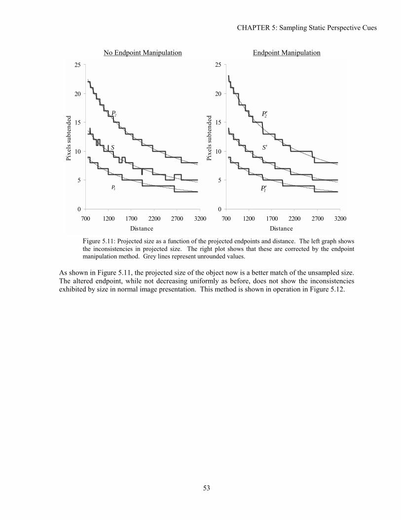
CHAPTER 5: Sampling Static Perspective Cues
No Endpoint Manipulation Endpoint Manipulation
0
5
10
15
20
25
700 12
Pixe
ls su
bten
ded
15
20
25
s sub
tend
ed
Figure 5.1the inconmanipulat
As shown in FiguThe altered endpexhibited by size
P2 ′ P 2
5
10
Pixe
l ′ S S
53
00 1700 2200 2700 3200Distance
0700 1200
1: Projected size as a function of the projected endpointsistencies in projected size. The right plot shows that ion method. Grey lines represent unrounded values.
re 5.11, the projected size of the object now is a beoint, while not decreasing uniformly as before, do in normal image presentation. This method is show
P1
1700 2200 2700 3200Distance
s and distance. The left graph shows these are corrected by the endpoint
tter match of the unsampled size. es not show the inconsistencies n in operation in Figure 5.12.
′ P 1
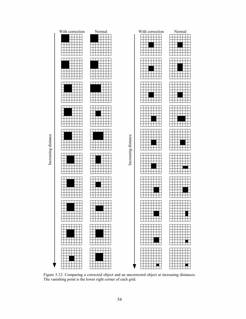
54
With correction Normal With correction Normal
Incr
easi
ng d
ista
nce
Incr
easi
ng d
ista
nce
Figure 5.12: Comparing a corrected object and an uncorrected object at increasing distances. The vanishing point is the lower right corner of each grid.
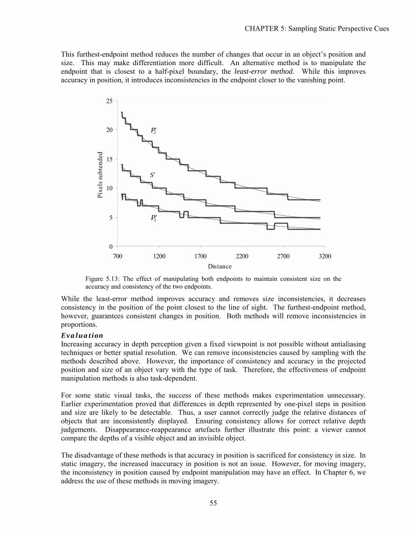
CHAPTER 5: Sampling Static Perspective Cues
This furthest-endpoint method reduces the number of changes that occur in an object�s position and size. This may make differentiation more difficult. An alternative method is to manipulate the endpoint that is closest to a half-pixel boundary, the least-error method. While this improves accuracy in position, it introduces inconsistencies in the endpoint closer to the vanishing point.
0
5
10
15
20
25
700
Pixe
ls su
bten
ded
Figure 5.13: The effeaccuracy and consisten
While the least-error methconsistency in the position however, guarantees consisproportions. Evaluation Increasing accuracy in depthtechniques or better spatial methods described above. position and size of an objemanipulation methods is also For some static visual taskEarlier experimentation proand size are likely to be deobjects that are inconsistenjudgements. Disappearanccompare the depths of a visi The disadvantage of these mstatic imagery, the increasedthe inconsistency in positionaddress the use of these meth
′ P 2
′ S
55
1200 1700 2200 2700 3200Distance
ct of manipulating both endpoints to maintain consistent size on the cy of the two endpoints.
od improves accuracy and removes size inconsistencies, it decreases of the point closest to the line of sight. The furthest-endpoint method, tent changes in position. Both methods will remove inconsistencies in
perception given a fixed viewpoint is not possible without antialiasing resolution. We can remove inconsistencies caused by sampling with the However, the importance of consistency and accuracy in the projected ct vary with the type of task. Therefore, the effectiveness of endpoint task-dependent.
s, the success of these methods makes experimentation unnecessary. ved that differences in depth represented by one-pixel steps in position tectable. Thus, a user cannot correctly judge the relative distances of tly displayed. Ensuring consistency allows for correct relative depth e-reappearance artefacts further illustrate this point: a viewer cannot ble object and an invisible object.
ethods is that accuracy in position is sacrificed for consistency in size. In inaccuracy in position is not an issue. However, for moving imagery, caused by endpoint manipulation may have an effect. In Chapter 6, we ods in moving imagery.
′ P 1
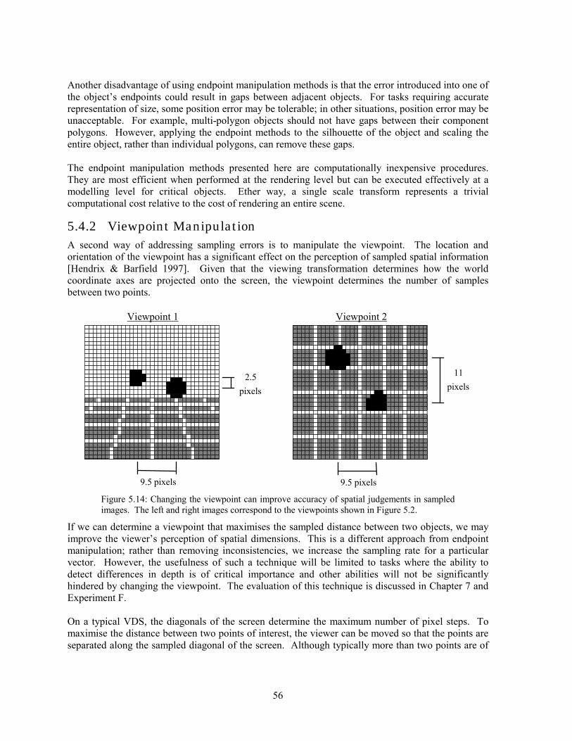
56
Another disadvantage of using endpoint manipulation methods is that the error introduced into one of the object�s endpoints could result in gaps between adjacent objects. For tasks requiring accurate representation of size, some position error may be tolerable; in other situations, position error may be unacceptable. For example, multi-polygon objects should not have gaps between their component polygons. However, applying the endpoint methods to the silhouette of the object and scaling the entire object, rather than individual polygons, can remove these gaps. The endpoint manipulation methods presented here are computationally inexpensive procedures. They are most efficient when performed at the rendering level but can be executed effectively at a modelling level for critical objects. Ether way, a single scale transform represents a trivial computational cost relative to the cost of rendering an entire scene.
5.4.2 Viewpoint Manipulation A second way of addressing sampling errors is to manipulate the viewpoint. The location and orientation of the viewpoint has a significant effect on the perception of sampled spatial information [Hendrix & Barfield 1997]. Given that the viewing transformation determines how the world coordinate axes are projected onto the screen, the viewpoint determines the number of samples between two points.
9.5 pixels
2.5 pixels
Viewpoint 1
11 pixels
Viewpoint 2
9.5 pixels
Figure 5.14: Changing the viewpoint can improve accuracy of spatial judgements in sampled images. The left and right images correspond to the viewpoints shown in Figure 5.2.
If we can determine a viewpoint that maximises the sampled distance between two objects, we may improve the viewer�s perception of spatial dimensions. This is a different approach from endpoint manipulation; rather than removing inconsistencies, we increase the sampling rate for a particular vector. However, the usefulness of such a technique will be limited to tasks where the ability to detect differences in depth is of critical importance and other abilities will not be significantly hindered by changing the viewpoint. The evaluation of this technique is discussed in Chapter 7 and Experiment F. On a typical VDS, the diagonals of the screen determine the maximum number of pixel steps. To maximise the distance between two points of interest, the viewer can be moved so that the points are separated along the sampled diagonal of the screen. Although typically more than two points are of
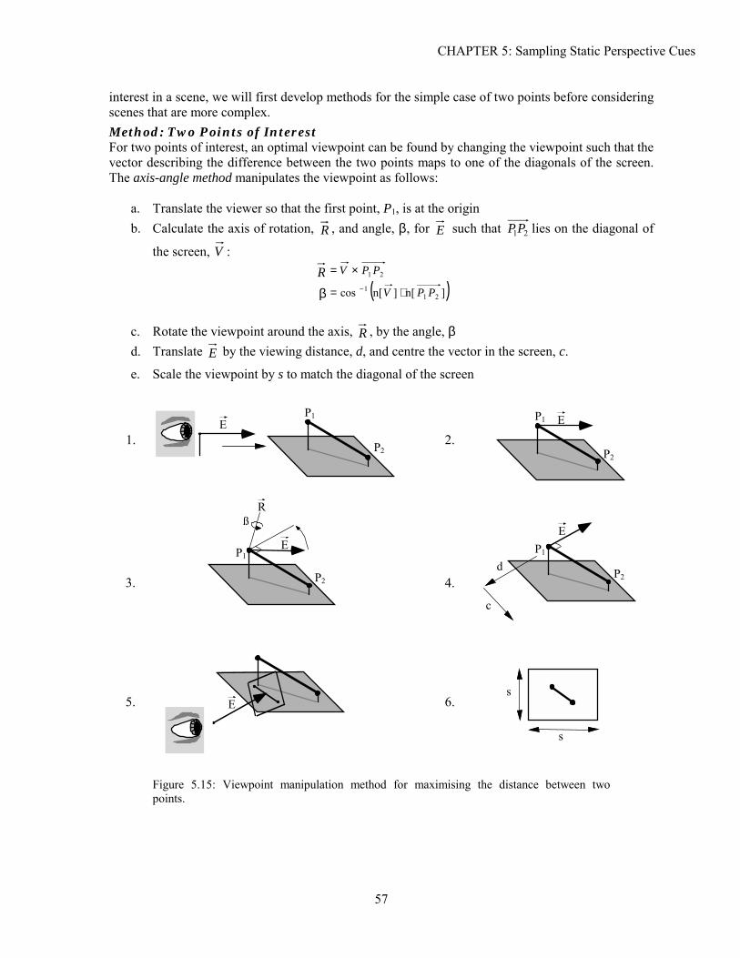
CHAPTER 5: Sampling Static Perspective Cues
57
interest in a scene, we will first develop methods for the simple case of two points before considering scenes that are more complex. Method: Two Points of Interest For two points of interest, an optimal viewpoint can be found by changing the viewpoint such that the vector describing the difference between the two points maps to one of the diagonals of the screen. The axis-angle method manipulates the viewpoint as follows:
a. Translate the viewer so that the first point, P1, is at the origin b. Calculate the axis of rotation, R , and angle, β, for E such that 21PP lies on the diagonal of
the screen, V : R 21 PPV ×=
β ( )]n[]n[cos 211 PPV ⋅= −
c. Rotate the viewpoint around the axis, R , by the angle, β d. Translate E by the viewing distance, d, and centre the vector in the screen, c.
e. Scale the viewpoint by s to match the diagonal of the screen
E
R
P1
P2
ßE
P1
P2d
c
E P1
P2
E
P1
P2
E
2.
3. 4.
5.
s
s 6.
1.
Figure 5.15: Viewpoint manipulation method for maximising the distance between two points.
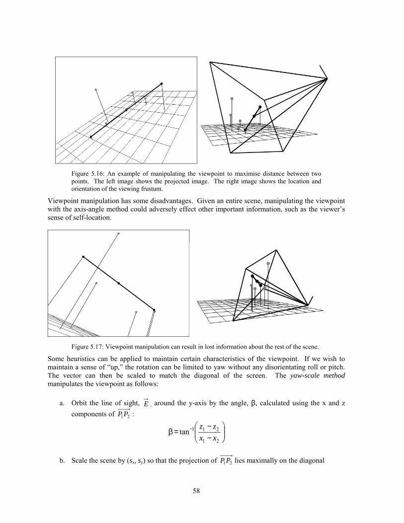
58
Figure 5.16: An example of manipulating the viewpoint to maximise distance between two points. The left image shows the projected image. The right image shows the location and orientation of the viewing frustum.
Viewpoint manipulation has some disadvantages. Given an entire scene, manipulating the viewpoint with the axis-angle method could adversely effect other important information, such as the viewer�s sense of self-location.
Figure 5.17: Viewpoint manipulation can result in lost information about the rest of the scene.
Some heuristics can be applied to maintain certain characteristics of the viewpoint. If we wish to maintain a sense of �up,� the rotation can be limited to yaw without any disorientating roll or pitch. The vector can then be scaled to match the diagonal of the screen. The yaw-scale method manipulates the viewpoint as follows:
a. Orbit the line of sight, E , around the y-axis by the angle, β, calculated using the x and z components of 21PP :
−−
=β −
21
211tanxxzz
b. Scale the scene by (sx, sy) so that the projection of 21PP lies maximally on the diagonal
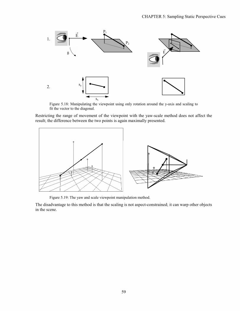
CHAPTER 5: Sampling Static Perspective Cues
59
E
2.
1.
sx
sy
E P1
P2
ß
Figure 5.18: Manipulating the viewpoint using only rotation around the y-axis and scaling to fit the vector to the diagonal.
Restricting the range of movement of the viewpoint with the yaw-scale method does not affect the result; the difference between the two points is again maximally presented.
Figure 5.19: The yaw and scale viewpoint manipulation method.
The disadvantage to this method is that the scaling is not aspect-constrained; it can warp other objects in the scene.
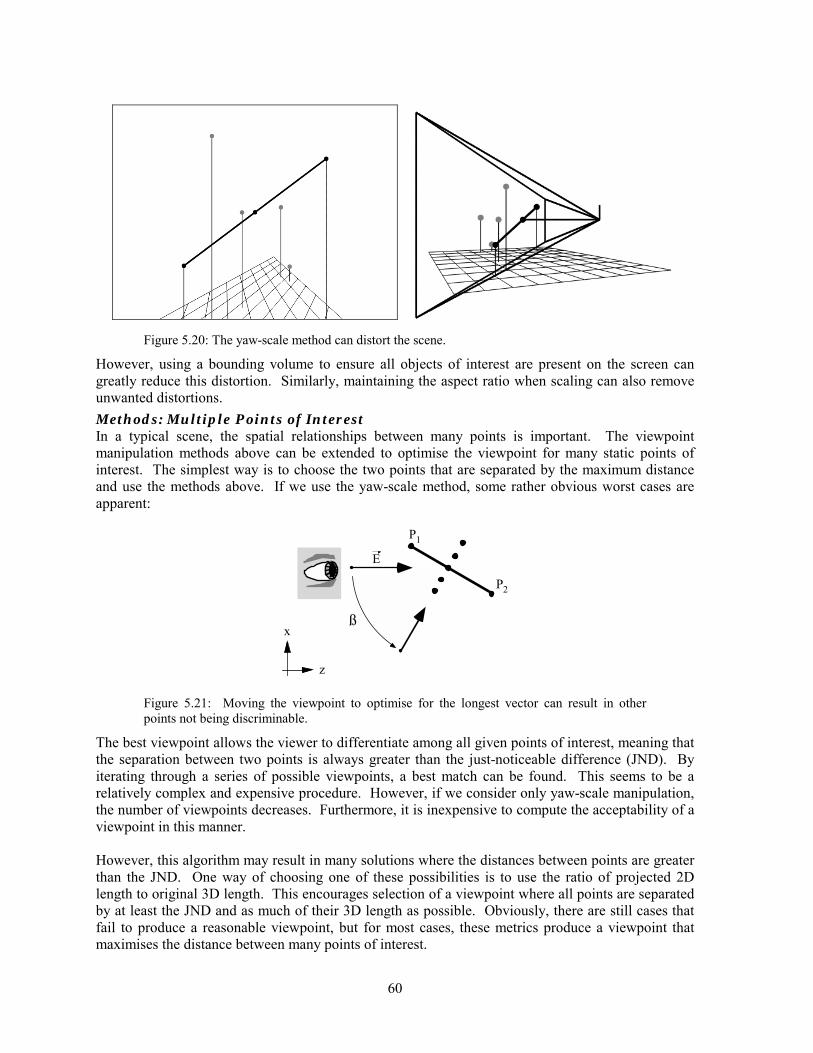
60
Figure 5.20: The yaw-scale method can distort the scene.
However, using a bounding volume to ensure all objects of interest are present on the screen can greatly reduce this distortion. Similarly, maintaining the aspect ratio when scaling can also remove unwanted distortions. Methods: Multiple Points of Interest In a typical scene, the spatial relationships between many points is important. The viewpoint manipulation methods above can be extended to optimise the viewpoint for many static points of interest. The simplest way is to choose the two points that are separated by the maximum distance and use the methods above. If we use the yaw-scale method, some rather obvious worst cases are apparent:
z
x
E
ß
P1
P2
Figure 5.21: Moving the viewpoint to optimise for the longest vector can result in other points not being discriminable.
The best viewpoint allows the viewer to differentiate among all given points of interest, meaning that the separation between two points is always greater than the just-noticeable difference (JND). By iterating through a series of possible viewpoints, a best match can be found. This seems to be a relatively complex and expensive procedure. However, if we consider only yaw-scale manipulation, the number of viewpoints decreases. Furthermore, it is inexpensive to compute the acceptability of a viewpoint in this manner. However, this algorithm may result in many solutions where the distances between points are greater than the JND. One way of choosing one of these possibilities is to use the ratio of projected 2D length to original 3D length. This encourages selection of a viewpoint where all points are separated by at least the JND and as much of their 3D length as possible. Obviously, there are still cases that fail to produce a reasonable viewpoint, but for most cases, these metrics produce a viewpoint that maximises the distance between many points of interest.
CHAPTER 5: Sampling Static Perspective Cues
61
Evaluation As with endpoint manipulation methods, empirically evaluating the value of viewpoint manipulation is difficult. With two points of interest, any difference in depth is magnified to the diagonal of the screen; therefore, any difference is detectable. With many points of interest, the algorithm�s effectiveness varies with the metric used to evaluate a viewpoint. In addition, more points of interest mean a new viewpoint is less valuable. Maintaining a sense of self-location may also prove to be important to the success of a viewpoint manipulation algorithm. Experimental evaluation of these techniques is presented in Chapter 7 and Experiment F. Computationally, these methods are more expensive than the endpoint manipulation method, given that they require the computation of rotation angles and scale factors. However, these computations are still insignificant when compared with the number of rotations and scale transforms present in a complex scene. In addition, a viewpoint can be pre-computed for a scene to eliminate run-time computations.
5.5 CONCLUSION
This chapter has described and evaluated the effects of sampling on static linear perspective depth cues in 3D CGI. Rounding errors in the projected size and position of a 3D object cause inaccurate representation of depth. These errors also result in inconsistently presented size and shape. Experimentation demonstrated that these artefacts influence relative depth judgements in some situations. Small objects, close to the line of sight and a large distance from the viewer are the most susceptible. Two methods for alleviating these artefacts have been presented. Manipulating the projected position of an object�s endpoints ensures an object�s size is consistently presented. Moving the viewpoint to an optimal location maximises the number of pixels differentiating points of interest. Both of these methods are computationally inexpensive for static scenes.

62
63
C H A P T E R 6
6:Spatio-Temporal Sampling of Perspective This chapter builds on the analysis and experiments presented in Chapter 5 by describing and evaluating sampling artefacts in dynamic 3D CGI. As interactivity becomes more important in 3D CGI, we need to understand how to accurately present sampled motion. A moving object is sampled by the VDS� pixel resolution, refresh rate and frame rate. In this chapter, we identify and discuss artefacts in spatio-temporally sampled perspective depth cues. We present experiments that describe the perception of these artefacts and suggest contexts where they are likely to hinder task performance. Finally, we extend the endpoint and viewpoint manipulation methods from the previous chapter to correct spatio-temporal sampling artefacts in perspective depth information.
6.1 BACKGROUND
In Chapter 4, we introduced spatio-temporal sampling in 2D CGI. A spatial resolution and a refresh rate define the 2D velocities that can be presented exactly on the VDS. Velocities that are not integer multiples of the refresh rate and pixel size are either spatially limited (i.e., frames are repeated) or temporally limited (i.e., pixel steps are skipped). In 3D CGI, information about depth is projected onto the screen according to perspective geometry. Movements in 3D are thus represented by 2D motion. For example, the projection of a point some distance from the line of sight that is moving at constant velocity away from the viewer decelerates along a line between its starting point and the vanishing point. Movement in perspective depth is ambiguous. A point moving in perspective depth cannot be distinguished from a point moving in the plane of the screen (Figure 6.1). Similarly, an object moving away from the viewer along the line of sight cannot be distinguished from an object shrinking in the plane of the screen. To remove these ambiguities, we assume all motion is parallel to the line of sight (i.e., perpendicular to the x-y plane).
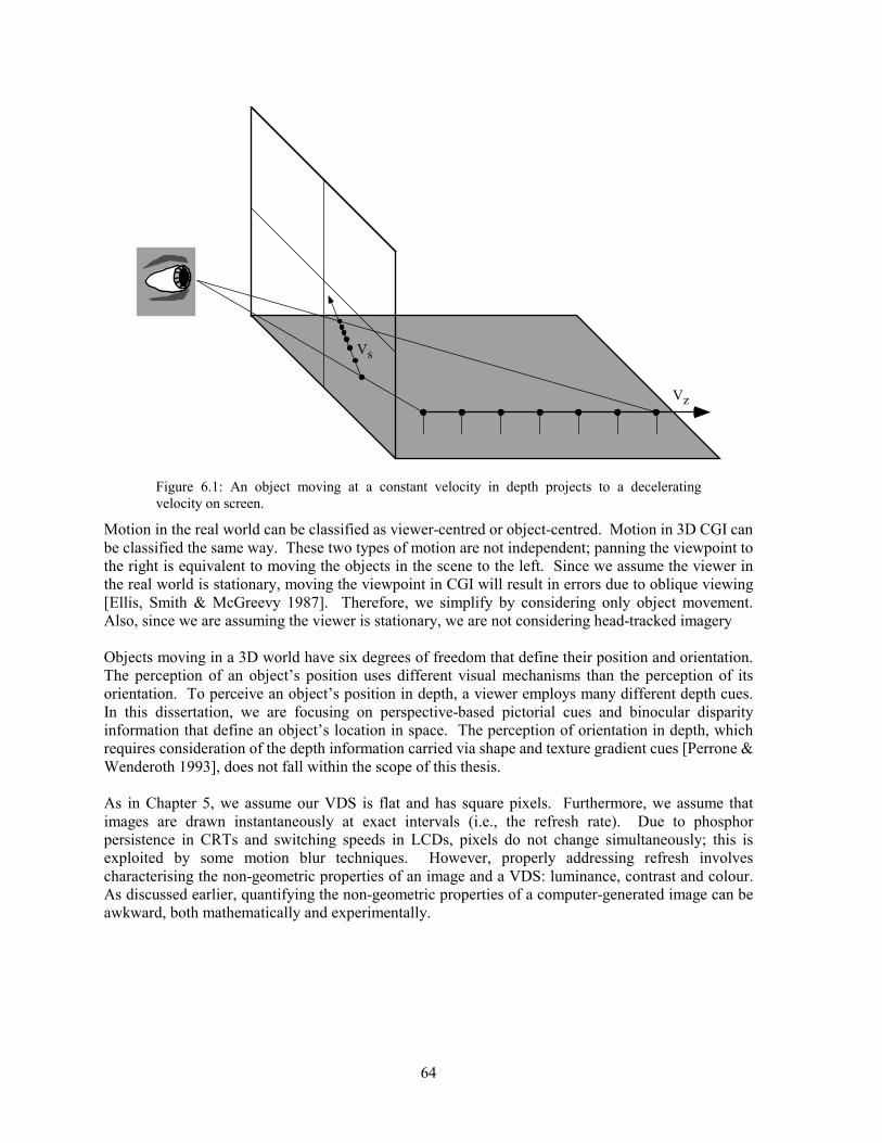
64
Vz
Vs
Figure 6.1: An object moving at a constant velocity in depth projects to a decelerating velocity on screen.
Motion in the real world can be classified as viewer-centred or object-centred. Motion in 3D CGI can be classified the same way. These two types of motion are not independent; panning the viewpoint to the right is equivalent to moving the objects in the scene to the left. Since we assume the viewer in the real world is stationary, moving the viewpoint in CGI will result in errors due to oblique viewing [Ellis, Smith & McGreevy 1987]. Therefore, we simplify by considering only object movement. Also, since we are assuming the viewer is stationary, we are not considering head-tracked imagery Objects moving in a 3D world have six degrees of freedom that define their position and orientation. The perception of an object�s position uses different visual mechanisms than the perception of its orientation. To perceive an object�s position in depth, a viewer employs many different depth cues. In this dissertation, we are focusing on perspective-based pictorial cues and binocular disparity information that define an object�s location in space. The perception of orientation in depth, which requires consideration of the depth information carried via shape and texture gradient cues [Perrone & Wenderoth 1993], does not fall within the scope of this thesis. As in Chapter 5, we assume our VDS is flat and has square pixels. Furthermore, we assume that images are drawn instantaneously at exact intervals (i.e., the refresh rate). Due to phosphor persistence in CRTs and switching speeds in LCDs, pixels do not change simultaneously; this is exploited by some motion blur techniques. However, properly addressing refresh involves characterising the non-geometric properties of an image and a VDS: luminance, contrast and colour. As discussed earlier, quantifying the non-geometric properties of a computer-generated image can be awkward, both mathematically and experimentally.
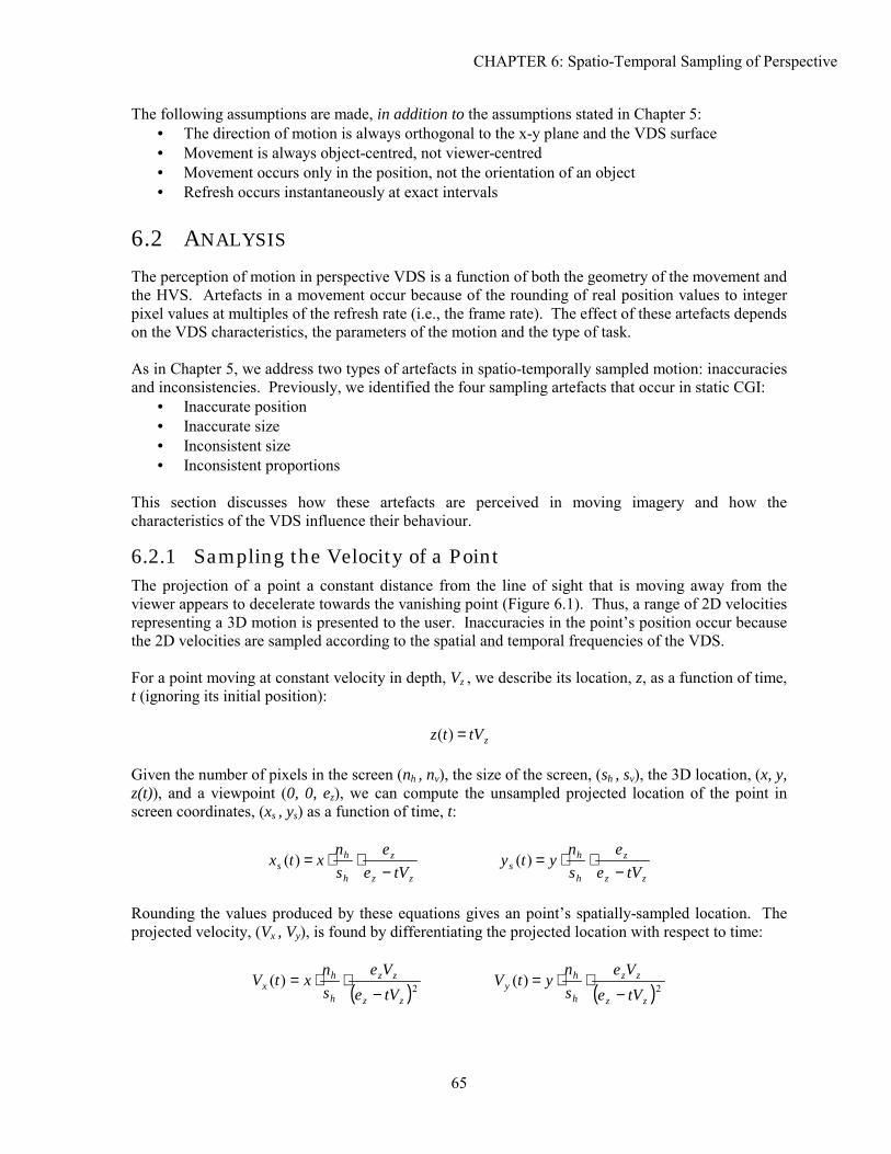
CHAPTER 6: Spatio-Temporal Sampling of Perspective
65
The following assumptions are made, in addition to the assumptions stated in Chapter 5: • The direction of motion is always orthogonal to the x-y plane and the VDS surface • Movement is always object-centred, not viewer-centred • Movement occurs only in the position, not the orientation of an object • Refresh occurs instantaneously at exact intervals
6.2 ANALYSIS
The perception of motion in perspective VDS is a function of both the geometry of the movement and the HVS. Artefacts in a movement occur because of the rounding of real position values to integer pixel values at multiples of the refresh rate (i.e., the frame rate). The effect of these artefacts depends on the VDS characteristics, the parameters of the motion and the type of task. As in Chapter 5, we address two types of artefacts in spatio-temporally sampled motion: inaccuracies and inconsistencies. Previously, we identified the four sampling artefacts that occur in static CGI:
• Inaccurate position • Inaccurate size • Inconsistent size • Inconsistent proportions
This section discusses how these artefacts are perceived in moving imagery and how the characteristics of the VDS influence their behaviour.
6.2.1 Sampling the Velocity of a Point The projection of a point a constant distance from the line of sight that is moving away from the viewer appears to decelerate towards the vanishing point (Figure 6.1). Thus, a range of 2D velocities representing a 3D motion is presented to the user. Inaccuracies in the point�s position occur because the 2D velocities are sampled according to the spatial and temporal frequencies of the VDS. For a point moving at constant velocity in depth, Vz , we describe its location, z, as a function of time, t (ignoring its initial position):
ztVtz =)( Given the number of pixels in the screen (nh , nv), the size of the screen, (sh , sv), the 3D location, (x, y, z(t)), and a viewpoint (0, 0, ez), we can compute the unsampled projected location of the point in screen coordinates, (xs , ys) as a function of time, t:
zz
z
h
hs tVe
esn
xtx−
⋅⋅=)( zz
z
h
hs tVe
esn
yty−
⋅⋅=)(
Rounding the values produced by these equations gives an point�s spatially-sampled location. The projected velocity, (Vx , Vy), is found by differentiating the projected location with respect to time:
( )2)(zz
zz
h
hx tVe
VesnxtV
−⋅⋅=
( )2)(zz
zz
h
hy tVe
Vesn
ytV−
⋅⋅=
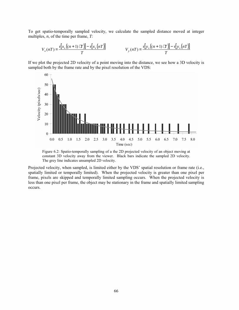
66
To get spatio-temporally sampled velocity, we calculate the sampled distance moved at integer multiples, n, of the time per frame, T:
( )[ ] ( )[ ]T
nTxTnxnTV ss
xr)1(r
)(−⋅+
= ( )[ ] ( )[ ]
TnTyTny
nTV ssy
r)1(r)(
−⋅+=
If we plot the projected 2D velocity of a point moving into the distance, we see how a 3D velocity is sampled both by the frame rate and by the pixel resolution of the VDS:
0
10
20
30
40
50
60
0.0 0.5 1.0 1.5 2.0 2.5 3.0 3.5 4.0 4.5 5.0 5.5 6.0 6.5 7.0 7.5 8.0Time (sec)
Vel
ocity
(pix
els/
sec)
Figure 6.2: Spatio-temporally sampling of a the 2D projected velocity of an object moving at constant 3D velocity away from the viewer. Black bars indicate the sampled 2D velocity. The grey line indicates unsampled 2D velocity.
Projected velocity, when sampled, is limited either by the VDS� spatial resolution or frame rate (i.e., spatially limited or temporally limited). When the projected velocity is greater than one pixel per frame, pixels are skipped and temporally limited sampling occurs. When the projected velocity is less than one pixel per frame, the object may be stationary in the frame and spatially limited sampling occurs.
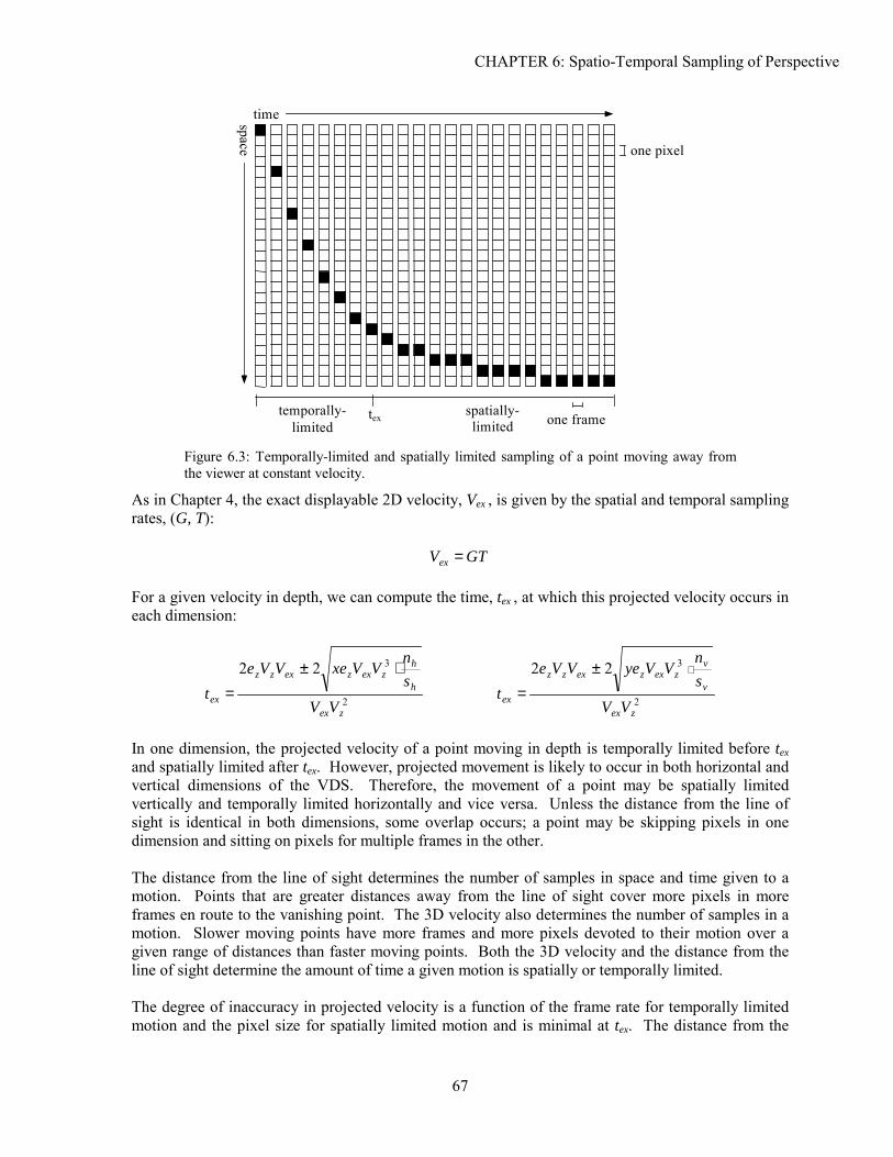
CHAPTER 6: Spatio-Temporal Sampling of Perspective
67
time space one pixel
temporally-limited
spatially-limited
tex one frame
Figure 6.3: Temporally-limited and spatially limited sampling of a point moving away from the viewer at constant velocity.
As in Chapter 4, the exact displayable 2D velocity, Vex , is given by the spatial and temporal sampling rates, (G, T):
GTVex = For a given velocity in depth, we can compute the time, tex , at which this projected velocity occurs in each dimension:
2
322
zex
h
hzexzexzz
ex VVsn
VVxeVVet
⋅±= 2
322
zex
v
vzexzexzz
ex VVsn
VVyeVVet
⋅±=
In one dimension, the projected velocity of a point moving in depth is temporally limited before tex and spatially limited after tex. However, projected movement is likely to occur in both horizontal and vertical dimensions of the VDS. Therefore, the movement of a point may be spatially limited vertically and temporally limited horizontally and vice versa. Unless the distance from the line of sight is identical in both dimensions, some overlap occurs; a point may be skipping pixels in one dimension and sitting on pixels for multiple frames in the other. The distance from the line of sight determines the number of samples in space and time given to a motion. Points that are greater distances away from the line of sight cover more pixels in more frames en route to the vanishing point. The 3D velocity also determines the number of samples in a motion. Slower moving points have more frames and more pixels devoted to their motion over a given range of distances than faster moving points. Both the 3D velocity and the distance from the line of sight determine the amount of time a given motion is spatially or temporally limited. The degree of inaccuracy in projected velocity is a function of the frame rate for temporally limited motion and the pixel size for spatially limited motion and is minimal at tex. The distance from the
68
viewer and the line of sight also affects the amount of inaccuracy in a movement. The perceptual implications of these relationships, including the smoothing done by the HVS (described in Chapter 4), is discussed below.
6.2.2 Sampling the Velocity of an Object Inaccuracies in the projected position of a point cause inaccuracies and inconsistencies in projected size. The endpoints of an object are likely to be at different distances from the line of sight and are spatially sampled differently. Their projected velocities and accelerations also differ. Therefore, the velocity of the projected size accelerates inconsistently as an object moves in depth. Given the size of an object in 3D, (ah , av), we can compute the projected size of the object, (Sh , Sv):
zz
z
h
hhh tVe
esn
atS−
⋅⋅=)( zz
z
v
vvv tVe
esn
atS−
⋅⋅=)(
Differentiating with respect to time gives the velocity of the size, (Vh , Vv):
( )2)(zz
zz
h
hhh tVe
Vesn
atV−
⋅⋅= ( )2)(
zz
zz
v
vvv tVe
Vesn
atV−
⋅⋅=
These equations show the unsampled magnitude and velocity of the projected size. The sampled velocity of the size is a function of the sampled endpoints. The rounded size is computed from the sampled horizontal and vertical endpoints of the object, (PL , PR) and (PT , PB):
[ ] [ ])(r)(r)( nTPnTPnTS RLh −= [ ] [ ])(r)(r)( nTPnTPnTS BTv −= where time is sampled at integer multiples, n, of the time per frame, T. The sampled 2D velocity for each frame is:
( )[ ] ( )[ ]T
nTSTnSnTV hhh
r)1(r)(
−⋅+=
( )[ ] ( )[ ]T
nTSTnSnTV vvv
r)1(r)(
−⋅+=
When computed in this manner, the rate of size change does not show the consistency seen in the velocity of a single point.
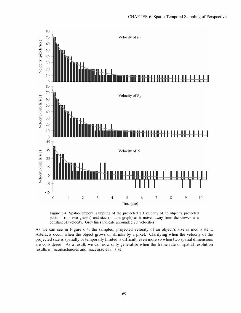
CHAPTER 6: Spatio-Temporal Sampling of Perspective
69
010
203040
5060
7080
Vel
ocity
(pix
els/
sec)
010
203040
5060
7080
Vel
ocity
(pix
els/
sec)
-15
-5
5
15
25
35
45
0 1 2 3 4 5 6 7 8 9 10Time (sec)
Vel
ocity
(pix
els/
sec)
Figure 6.4: Spatio-temporal sampling of the projected 2D velocity of an object�s projected position (top two graphs) and size (bottom graph) as it moves away from the viewer at a constant 3D velocity. Grey lines indicate unrounded 2D velocities.
As we can see in Figure 6.4, the sampled, projected velocity of an object�s size is inconsistent. Artefacts occur when the object grows or shrinks by a pixel. Clarifying when the velocity of the projected size is spatially or temporally limited is difficult, even more so when two spatial dimensions are considered. As a result, we can now only generalise when the frame rate or spatial resolution results in inconsistencies and inaccuracies in size.
Velocity of P1
Velocity of P2
Velocity of S
70
The following factors determine what type of sampling is likely in certain conditions:
• Distance from the viewer ▪ Spatially limited in the far field ▪ Temporally limited in the near field
• Object size ▪ Spatially limited for small objects ▪ Temporally limited for large objects
• Distance from the line of sight ▪ Spatially limited near the line of sight ▪ Temporally limited far from the line of sight
• 3D velocity ▪ Spatially limited for low 3D velocities ▪ Temporally limited for high 3D velocities
These factors also affect the magnitude of the inconsistencies and inaccuracies in size. The closer the velocity of the projected size is to Vex, the smaller the inaccuracies due to insufficient frame rate or pixel size.
6.2.3 Perceptual Implications The perception of spatio-temporal sampling in 3D motion is governed by the perception of the projected motion. Because a range of 2D velocities is projected for a 3D movement, we expect the perception of the sampled motion to be a function of either the frame rate or pixel size. Whether it is a function of the frame rate or pixels size depends on whether spatially limited or temporally limited sampling occurs over the range of 2D velocities. The same four sampling artefacts that occur in static CGI occur in moving images: inaccurate position, inaccurate size, inconsistent size and inconsistent proportions. These artefacts have equivalent visual results when seen in spatially and temporally limited motion. A perceivable change in the perspective projection leads to a perceivable change in the depth of an object. At slow projected velocities, large or infrequent changes in position and size result in increased detectability of sampling artefacts. Since the frame rate and pixel size determine how often changes in position and size occur, we can predict when artefacts will be seen as a function of the frame rate for temporally limited motion and pixel size for spatially limited motion. Inaccuracies of sufficient magnitude in position and size result in the perception of jerky motion. If we were considering a 2D motion with constant velocity, we could use published spatial and temporal frequency thresholds for the detection of smooth motion [Sekuler 1990]. However, projected objects are not moving at constant velocity; they decelerate on screen as they approach the vanishing point. Therefore, thresholds are difficult to establish; we can only suggest what conditions are likely to lead to perceivable inaccuracies. Inconsistencies in projected size also result in the perception of jerky motion. Because the changes are inconsistent, they may be more perceivable than consistent changes in position, especially for objects that are small relative to the size of a pixel. For slow projected velocities, size inconsistencies make the direction of movement ambiguous. Furthermore, the detection of inconsistencies in size and proportion is task-dependent.
CHAPTER 6: Spatio-Temporal Sampling of Perspective
71
The perception of sampling artefacts in an object�s motion are affected by: • location of the 3D object relative to the line of sight • location of the 3D object relative to the viewer • size of the 3D object • 3D velocity
As discussed above, these factors determine whether a motion is spatially or temporally limited. They also determine the magnitude of the error in depth represented by the projected size and location. As we have discussed throughout this work, the tolerance for a type of sampling artefact is dependent upon the type of task. For animation and immersive environments, smooth motion is critical. Users of virtual environments become disorientated and ill if imagery is presented at an insufficient frame rate [Pausch, Crea & Conway 1992]. However, there may be tasks for which jerky motion is completely acceptable in terms of performance, if not in terms of aesthetics. Furthermore, some tasks may even be aided by jerky motion; for example, snap-to grids are a popular user interface method for aiding alignment tasks in commercial vector drawing packages. In general, however, jerky motion is problematic, rather than useful. The conditions that determine whether a movement is spatially or temporally limited tell us whether frame rate or pixel resolution affects task performance. For example, a task with a lot of near-field interaction requires an increased frame rate because this motion is likely to be temporally limited. Conversely, tasks that involve small objects moving at a large distance require a better spatial resolution. Spatio-temporal sampling artefacts also affect multi-polygon and textured objects presented with linear perspective. Size inconsistencies affect the proportions of a multi-polygon object, as well as distorting the effects of texture mapping (Figure 5.8). This can result in internal distortions that further inhibit the accurate perception of movement in depth. These distortions, while interesting, do not fall within the scope of this dissertation.
6.3 EXPERIMENTATION
A major goal of this work has been to describe spatio-temporal sampling artefacts and the conditions in which they occur. The above analysis has suggested some visual contexts in which artefacts in perspective information are likely to affect task performance. To describe the artefacts in these contexts, we must choose an appropriate experimental task. After discussing this choice, we describe two formal experiments and a number of informal experiments that were conducted to determine the effects of spatio-temporal sampling on the perception of motion in 3D CGI.
72
6.3.1 Methodology To understand the effects of spatio-temporal sampling on moving perspective depth cues, a proper experimental task must be selected. Bullimore, Howarth and Fulton proposed three fundamental visual tasks: detection, recognition and interpretation [1998]. By modifying these basic visual tasks, we can create a list of potential spatio-temporal tasks in 3D CGI:
• Detection ▪ Is it moving?
• Estimation ▪ Location: Where is it now? ▪ Direction: In which direction is it moving? ▪ Velocity: How fast/slow is it moving? ▪ Acceleration: How fast is it getting faster or slower?
• Prediction ▪ Location: Where will it be at time t? ▪ Direction: In which direction will it be moving at time t? ▪ Velocity: How far away will it be at time t? ▪ Acceleration: How fast will it be going at time t?
• Comparison ▪ Location: Is it at the same location as X? ▪ Direction: Is it moving in the same direction as X? ▪ Velocity: Is it moving faster or slower than X? ▪ Acceleration: Is it getting faster or slower at the same rate as X?
• Recognition ▪ Proportions: What are the proportions of the moving object? ▪ Identification: What object is moving?
Determining how VDS characteristics affect spatio-temporal sampling is simply not practical for all of these experimental tasks. As a result, we want a representative visual task that is resistant to noise and other confounding factors. In the Psychophysics literature, experiments focus on constant-velocity, single-direction motion because human perception of acceleration is poor and awkward to measure effectively [Graham 1951]. High-level, potentially noisy perceptual mechanisms are used to detect an object�s orientation and path. Since an optimal experimental method should minimise noise and complexity without sacrificing generality, the following experiments concern movements that are constant in both velocity and direction. In addition, we want to present unambiguous perspective depth information. Other tasks involving manual tracking of objects moving in 3D [Liu, Tharp & Stark 1992] or relative location judgements [Barfield & Rosenberg 1995] do not isolate depth information from information about the distance from the line of sight. To remove ambiguities, we must restrict the motion of an object to be parallel to the line of sight. Moreover, experiments that ask subjects to make absolute rather than relative judgements of depth have large inter-subject differences [Pfautz 1996]. Given these considerations, we designed a task asking subjects to compare the locations of a moving and stationary object. This is akin to time-to-contact (TTC) tasks where subjects judge when an object will reach the viewpoint or other reference point [Tresilian 1991]. This task was adapted to examine the effects of spatio-temporal sampling on the perception of velocity. However, before
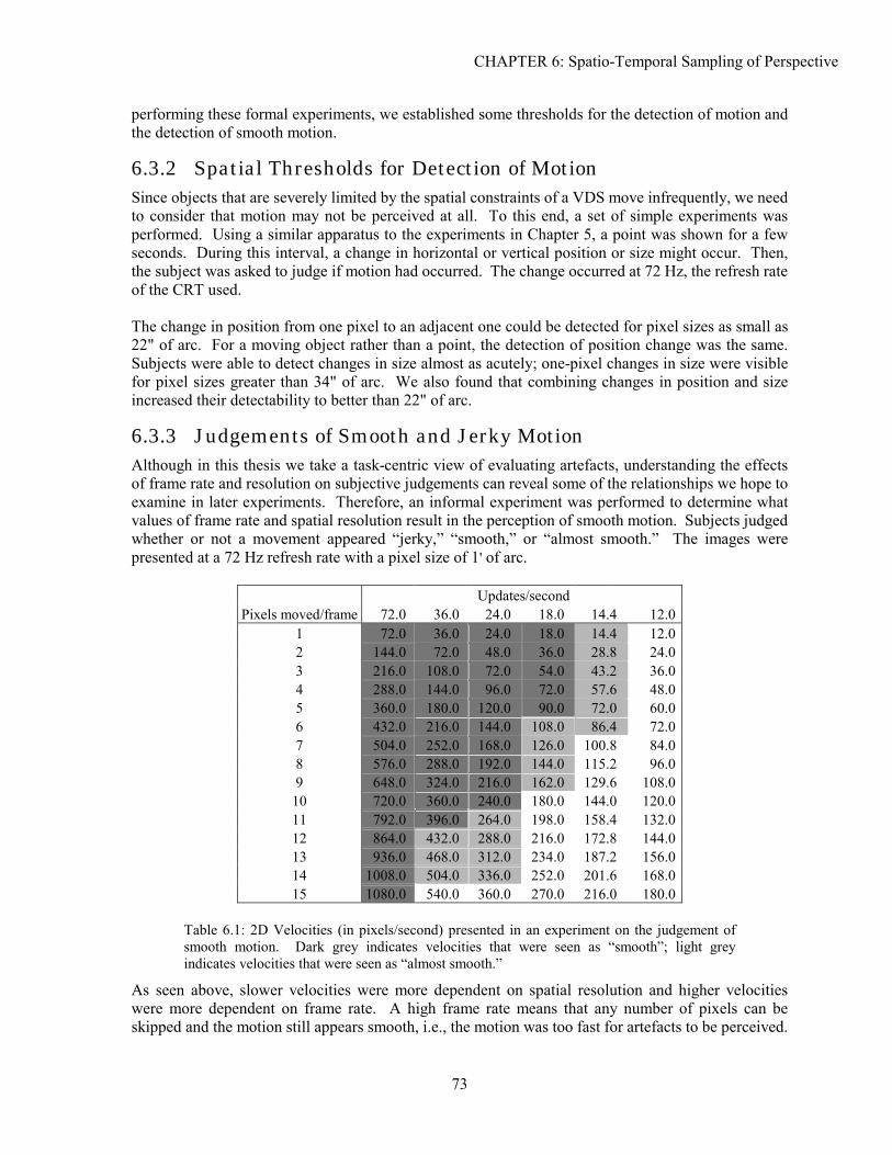
CHAPTER 6: Spatio-Temporal Sampling of Perspective
73
performing these formal experiments, we established some thresholds for the detection of motion and the detection of smooth motion.
6.3.2 Spatial Thresholds for Detection of Motion Since objects that are severely limited by the spatial constraints of a VDS move infrequently, we need to consider that motion may not be perceived at all. To this end, a set of simple experiments was performed. Using a similar apparatus to the experiments in Chapter 5, a point was shown for a few seconds. During this interval, a change in horizontal or vertical position or size might occur. Then, the subject was asked to judge if motion had occurred. The change occurred at 72 Hz, the refresh rate of the CRT used. The change in position from one pixel to an adjacent one could be detected for pixel sizes as small as 22" of arc. For a moving object rather than a point, the detection of position change was the same. Subjects were able to detect changes in size almost as acutely; one-pixel changes in size were visible for pixel sizes greater than 34" of arc. We also found that combining changes in position and size increased their detectability to better than 22" of arc.
6.3.3 Judgements of Smooth and Jerky Motion Although in this thesis we take a task-centric view of evaluating artefacts, understanding the effects of frame rate and resolution on subjective judgements can reveal some of the relationships we hope to examine in later experiments. Therefore, an informal experiment was performed to determine what values of frame rate and spatial resolution result in the perception of smooth motion. Subjects judged whether or not a movement appeared �jerky,� �smooth,� or �almost smooth.� The images were presented at a 72 Hz refresh rate with a pixel size of 1' of arc.
Updates/second Pixels moved/frame 72.0 36.0 24.0 18.0 14.4 12.0
1 72.0 36.0 24.0 18.0 14.4 12.0 2 144.0 72.0 48.0 36.0 28.8 24.0 3 216.0 108.0 72.0 54.0 43.2 36.0 4 288.0 144.0 96.0 72.0 57.6 48.0 5 360.0 180.0 120.0 90.0 72.0 60.0 6 432.0 216.0 144.0 108.0 86.4 72.0 7 504.0 252.0 168.0 126.0 100.8 84.0 8 576.0 288.0 192.0 144.0 115.2 96.0 9 648.0 324.0 216.0 162.0 129.6 108.0
10 720.0 360.0 240.0 180.0 144.0 120.0 11 792.0 396.0 264.0 198.0 158.4 132.0 12 864.0 432.0 288.0 216.0 172.8 144.0 13 936.0 468.0 312.0 234.0 187.2 156.0 14 1008.0 504.0 336.0 252.0 201.6 168.0 15 1080.0 540.0 360.0 270.0 216.0 180.0
Table 6.1: 2D Velocities (in pixels/second) presented in an experiment on the judgement of smooth motion. Dark grey indicates velocities that were seen as �smooth�; light grey indicates velocities that were seen as �almost smooth.�
As seen above, slower velocities were more dependent on spatial resolution and higher velocities were more dependent on frame rate. A high frame rate means that any number of pixels can be skipped and the motion still appears smooth, i.e., the motion was too fast for artefacts to be perceived.
74
Viewers were more sensitive to a reduction in frame rate than a reduction in the number of pixels moved per frame. For a VDS that can maintain a high frame rate, sampling artefacts in spatio-temporally limited motion are not readily visible. The experiment suggested a frame rate above 36 Hz is sufficient to present a wide range of smooth velocities, paralleling Holst�s recommendation of 30 Hz [1998]. Using the results of this informal experiment on 2D motion, we can predict when a movement in depth will appear jerky or smooth. Over a movement in depth, a range of 2D velocities will be displayed. We can compare these to the values in Table 6.1 to predict if the motion in depth is likely to be seen as smooth or jerky.
6.3.4 Judging Alignment in Depth We then designed a formal experiment to determine the effects of spatio-temporal sampling on the ability to judge velocity. As mentioned above, we designed a TTC task where subjects indicated when a moving object was adjacent to a stationary object by clicking the mouse. The spatio-temporal sampling rate was varied by simultaneous changes in the frame rate, the pixels moved per frame and the desired 2D velocity at the reference point. Three types of movement were presented: spatially limited, temporally limited and both spatially and temporally limited. A detailed discussion of the experiment can be found in Experiment B. The significant results were:
• Decreasing the spatio-temporal sampling rate (i.e. simultaneously lowering the frame rate and increasing the pixel size) decreased accuracy.
• Decreasing the projected distance moved before the reference point was reached decreased accuracy.
• Spatially-limited motion was less accurate than temporally-limited motion.
6.3.5 Interactive Alignment in Depth Since the previous experiment demonstrated the dominance of spatial resolution in determining the spatio-temporal sampling rate, the second formal experiment focussed on the spatial sampling rate in an interactive task. The need for interactive frame rates is a motivating factor for much work in improving the efficiency of CGI methods. Therefore, the task chosen was similar to the one used in many other depth acuity experiments [Drascic & Milgram 1991; Graham 1951; Nagata 1993]. The subject manipulates the depth of one object to match a stationary object. In this experiment, clicking and dragging with the mouse manipulated the object. The correctness of a response was judged in two ways: accuracy in 3D location and accuracy in 2D position and size. Since accuracy in 3D varies with the distance of the reference object, accuracy in 2D was the primary measure. We measured accuracy in 2D by summing the difference in pixels of the four perspective sub-cues. The full details of this experiment are given in Experiment C. The main results of this experiment were:
• Decreasing pixel size decreased accuracy in depth. • Increasing pixel size increased accuracy in matching 2D position and size.
6.3.6 Discussion The first informal experiments demonstrated the detectability of spatially limited motion. A change of one pixel in size or position can be detected for pixels smaller than those in typical desktop VDSs or HMDs. For objects moving in 3D that are experiencing spatially limited motion, this means that
CHAPTER 6: Spatio-Temporal Sampling of Perspective
75
the individual jumps in position are seen by the user. Furthermore, inaccuracy and inconsistency artefacts are detectable. The second informal experiment provides insight into the relationship between frame rate, 2D velocity and pixel size on the perception of smooth or jerky 2D motion. High frame rates allowed us to present velocities above Vex without any sampling artefacts, regardless of pixel size. The maximum refresh rate of a typical VDS (> 60 Hz) is sufficient to see that the artefacts are not visible. When lower frame rates (i.e., integer multiples of the refresh rate) occur due to computational requirements, a rapid drop-off in quality occurs. At lower velocities, pixel size is more important. A typical VDS has difficulty presenting slow velocities in a smooth and accurate manner. The implications for 3D CGI are clear when we consider that perspective geometry results in a constant velocity in depth being projected to acceleration in 2D. Thus, an object moving in depth experiences a range of velocities, some of which may appear jerky. The formal TTC experiment showed that subjects could judge 3D velocity more accurately when sampling rates and projected 2D velocities were high. We already know that maintaining a high frame rate and low pixel size is important for many 3D tasks. However, since we manipulated the range of motion as a function of whether it was spatially or temporally limited, we could also see which type of sampling had a greater effect. Spatially limited sampling results in the most inaccuracy. This suggests that 2D velocities should be kept above a threshold value determined by the accuracy required for the task. This can be accomplished by avoiding objects moving in the far field and relatively small objects located near the line of sight. In addition, the experiment revealed that the larger the 2D distance covered for a uniform amount of time before a judgement was made, the better the performance. We could thus improve task performance by increasing the 3D velocity (i.e., the number of spatial samples shown), or by increasing the distance from the line of sight and/or the object�s size. The final experiment showed that an interactive task, like the TTC task, was subject to limitations due to spatio-temporal sampling. Again, accuracy on a 3D task decreased with lower sampling rates. However, lower spatial resolution actually improved performance when comparing 2D size and location. Even though the accuracy in depth represented by perspective cues decreases with increased pixel size, the accuracy with which the perspective sub-cues are matched increases. That is, although it was more difficult to be accurate in depth with a large pixel size, it was easier to match the projected size and location. These experiments provide information that a VDS designer can use to determine the necessary characteristics of a VDS for a given task. Accurately portraying velocities for objects far away from the viewer is the most consistent problem and the most difficult to correct without a large computational cost. Similarly, small objects or objects near the line of sight have limited perspective depth information. Avoiding these situations improves the accuracy with which moving objects are perceived.
6.4 SOLUTIONS
The experiments above demonstrated that decreased sampling rates hinder the accurate perception of motion in depth. In Chapter 5, we described two methods for alleviating sampling artefacts in static imagery. The endpoint and viewpoint manipulation methods can be adapted to address spatio-temporal sampling artefacts. This section describes these changes and presents experimental evidence to justify their use for some tasks. Finally, we discuss how traditional antialiasing methods can be used in certain contexts.
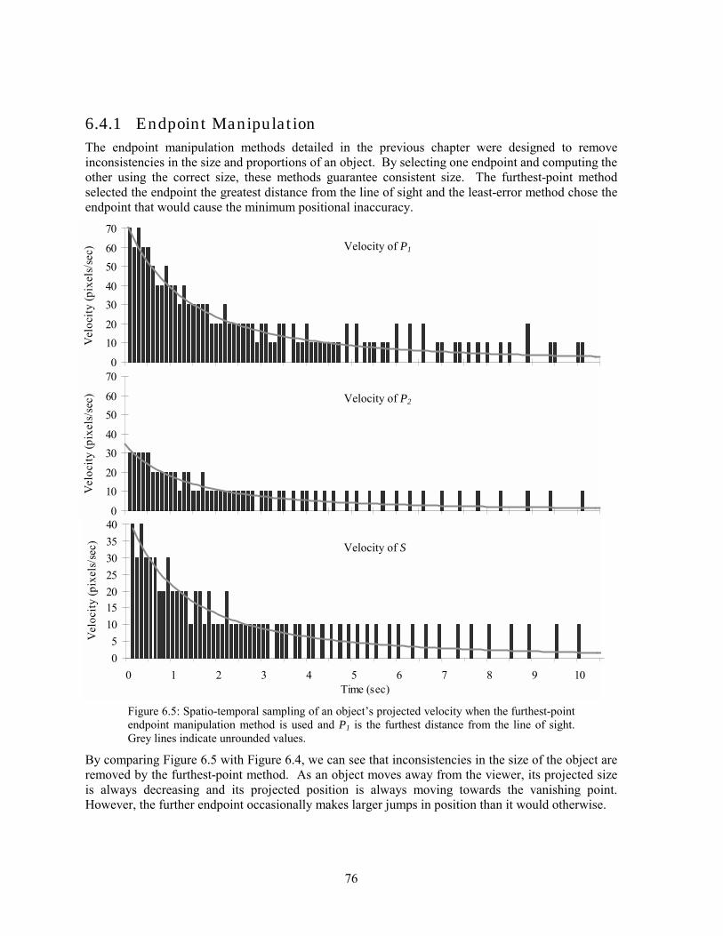
6.4.1 Endpoint Manipulation The endpoint manipulation methods detailed in the previous chapter were designed to remove inconsistencies in the size and proportions of an object. By selecting one endpoint and computing the other using the correct size, these methods guarantee consistent size. The furthest-point method selected the endpoint the greatest distance from the line of sight and the least-error method chose the endpoint that would cause the minimum positional inaccuracy.
0
1020
3040
5060
70
Vel
ocity
(pix
els/
sec)
0
1020
3040
5060
70
Vel
ocity
(pix
els/
sec)
05
10152025303540
0 1 2 3 4
Vel
ocity
(pix
els/
sec)
Figure 6.5: Spatio-temporal sampling of an endpoint manipulation method is used and Grey lines indicate unrounded values.
By comparing Figure 6.5 with Figure 6.4, we caremoved by the furthest-point method. As an ois always decreasing and its projected positioHowever, the further endpoint occasionally mak
Velocity of P1
Velocity of P2
76
5 6 7 8 9 10Time (sec)
object�s projected velocity when the furthest-point P1 is the furthest distance from the line of sight.
n see that inconsistencies in the size of the object are bject moves away from the viewer, its projected size n is always moving towards the vanishing point.
es larger jumps in position than it would otherwise.
Velocity of S
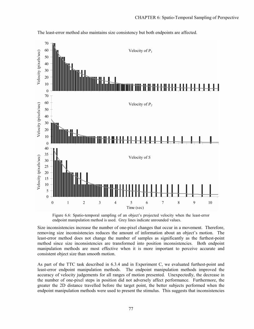
CHAPTER 6: Spatio-Temporal Sampling of Perspective
The least-error method also maintains size consistency but both endpoints are affected.
0
10
20
3040
50
60
70V
eloc
ity (p
ixel
s/se
c)
0
10
20
3040
50
60
70
Vel
ocity
(pix
els/
sec)
05
10152025303540
0 1 2 3 4
Vel
ocity
(pix
els/
sec)
Figure 6.6: Spatio-temporal sampling of anendpoint manipulation method is used. Grey
Size inconsistencies increase the number of oneremoving size inconsistencies reduces the amoleast-error method does not change the numbmethod since size inconsistencies are transformanipulation methods are most effective whconsistent object size than smooth motion. As part of the TTC task described in 6.3.4 anleast-error endpoint manipulation methods. Taccuracy of velocity judgements for all ranges the number of one-pixel steps in position did greater the 2D distance travelled before the taendpoint manipulation methods were used to pre
Velocity of P1
Velocity of P2
77
5 6 7 8 9 10Time (sec)
object�s projected velocity when the least-error lines indicate unrounded values.
-pixel changes that occur in a movement. Therefore, unt of information about an object�s motion. The er of samples as significantly as the furthest-point med into position inconsistencies. Both endpoint en it is more important to perceive accurate and
d in Experiment C, we evaluated furthest-point and he endpoint manipulation methods improved the
of motion presented. Unexpectedly, the decrease in not adversely affect performance. Furthermore, the rget point, the better subjects performed when the sent the stimulus. This suggests that inconsistencies
Velocity of S
78
in projected size play an important role in the perception of accurate motion and that their correct presentation is therefore critical. Using endpoint manipulation methods represents a trivial computational cost compared to the cost of generating a scene. They also are dramatically more efficient than traditional antialiasing methods. They can be applied to objects of interest, rather than an entire scene, and can be applied to the silhouettes of complex or textured objects.
6.4.2 Viewpoint Manipulation The experiments discussed in this chapter have shown that the greater the 2D distance the object travels, the higher the accuracy with which the velocity is perceived. Therefore, by moving the viewpoint to a location that maximises the 2D distance an object travels over a certain distance, we can present movement more accurately. In Chapter 5, we developed the axis-angle and yaw-scale viewpoint manipulation methods. These methods moved the viewpoint so that the maximum number of pixel steps separates two points. If we manipulate the viewpoint based on the starting and ending points of a piece of motion, we can ensure that the maximum number of pixel steps are devoted to displaying that motion. This provides a static viewpoint that can be pre-computed if the motion of an object is adequately described. An alternative extension of the viewpoint methods is to maintain the maximum spatial separation between two moving points. This requires that the viewpoint be calculated each frame and that coherency is maintained between frames. If the viewpoint jumps dramatically, any sense of self-location is destroyed. Furthermore, the calculation to determine the optimal viewpoint must be efficient or the frame rate is adversely affected. Coherence of viewpoint is easily maintained for the two-point case by constraining the location to be within some criterion of the previous frame�s value. When many points are of interest, coherence can be added as constraint on the metric used to pick the best viewpoint. When the ratio of projected distance to 3D distance is used as a metric, an optimal viewpoint is found by iterating through a number of viewpoints, and selecting the one with the largest average ratio for all pairs of points. Coherency in this case can be enforced by only testing viewpoints within a threshold distance of the current one. This also reduces the number of viewpoints to check. The computational efficiency of these methods is a function of the number of viewpoints tested in each frame. For N points, finding the longest vector between points is an O(N) procedure. Maximising the average ratio of 2D to 3D distance will be O(NM), where N is the number of points and M is the number of viewpoints tested. Suboptimal viewpoints may be chosen by this method if the number of viewpoints chosen is too small. The yaw-scale method limits the number of dimensions in which to consider viewpoints and guarantees a sense of �up� is maintained. Experimental evaluation of the viewpoint manipulation method was performed as part of an air traffic control task described in Chapter 7 and Experiment F.
6.4.3 Other Methods The above methods are two examples of task-specific improvements. Endpoint manipulation may cause difficulties in determining when two objects abut, and viewpoint manipulation cannot be used for tasks where the user controls the viewing position (e.g., flight simulators). However, the experiments presented earlier suggest other approaches to ameliorating spatio-temporal artefacts which can be used in these cases.
CHAPTER 6: Spatio-Temporal Sampling of Perspective
79
For example, other parameters that affect the motion can be optimised to present accurate motion for a particular range of depths. We have mentioned the object size, the distances from the line of sight and from the viewer and the 3D velocities as the factors affecting the severity of spatio-temporal sampling artefacts. If objects of interest in a scene can be placed nearer the viewer and far from the line of sight, more pixel steps are devoted to their motion. Similarly, if the object is larger, size inconsistencies are less noticeable. Another approach is to use traditional antialiasing methods selectively in a context-specific manner. If the object is skipping a number of frames between movements (i.e., spatially limited motion), then there is sufficient extra time to perform what would otherwise be computationally prohibitive antialiasing. In contexts where motion is severely spatially limited, like objects in the far field or near the line of sight, traditional antialiasing methods can be of great benefit. We evaluated a typical antialiasing method in the context of the interactive alignment task (Section 6.3.5 and Experiment C). The experiment showed that antialiasing significantly increases accuracy. However, at the largest (6'03") and smallest (1'15") pixel sizes, antialiasing was of less use. In severely sampled cases, antialiasing may present no benefit. Similarly, in cases where sampling is barely detectable, antialiasing may present no advantage. Therefore, even though traditional antialiasing methods can be used in some contexts without affecting the spatio-temporal sampling rate, their advantages are limited to a range of spatial resolutions.
6.5 CONCLUSION
This chapter has described and evaluated the spatio-temporal sampling artefacts in static linear perspective depth cues. In 3D CGI, a moving object is sampled by the pixel resolution, the refresh rate and frame rate of the VDS. Depending on the 3D velocity, the distance from the line of sight, the distance from the viewer and the size of the object, either the frame rate or the pixel size causes sampling artefacts in motion. This sampling causes errors in the velocities of the projected size and location of an object. It therefore results in inaccurate representation of motion in perspective depth. Furthermore, these inaccuracies lead to inconsistencies in the size and proportions of an object. Experimentation demonstrated the contexts where these artefacts are likely to hinder task performance. The endpoint and viewpoint manipulation methods from the previous chapter were extended to ameliorate artefacts in moving 3D imagery. We evaluated these computationally inexpensive methods and discussed the situations in which they are effective. The role of traditional antialiasing was also evaluated.

80
81
C H A P T E R 7
7:Sampling of Stereo and Perspective Depth
This chapter extends the analysis and experimentation in previous chapters by describing and evaluating sampling artefacts in the stereo presentation of CGI. For some tasks, providing stereo information can significantly improve performance. However, if stereo information is presented using a flat VDS, then the VDS� frame rate and pixel array sample the stereo information. Sampling artefacts hinder the correct perception of binocular disparity information in both static and moving imagery.
Stereo cues are seldom presented without perspective depth cues. However, since perspective projection may hinder the perception of parallelism and perpendicularity, orthographic projection can be used. Simultaneously sampling perspective and stereo information introduces additional inaccuracies and inconsistencies in the presentation of depth. The analysis of sampling on perspective cues in the previous two chapters provides a basis for considering these interactions. In this chapter, we identify and discuss artefacts in spatially and spatio-temporally sampled stereo and perspective depth cues. An analysis is performed to assess the contexts in which sampling is likely to cause significant deficits in performance. Experiments are presented that describe the perception of these artefacts and the contexts in which they occur. Finally, we extend endpoint and viewpoint manipulation methods to remove artefacts in stereo and perspective depth information. These methods are then evaluated empirically.
7.1 BACKGROUND
In Chapter 3, we introduced the foundations of stereo image presentation. A separate image is calculated for both viewpoints and special hardware is used to deliver the corresponding image to
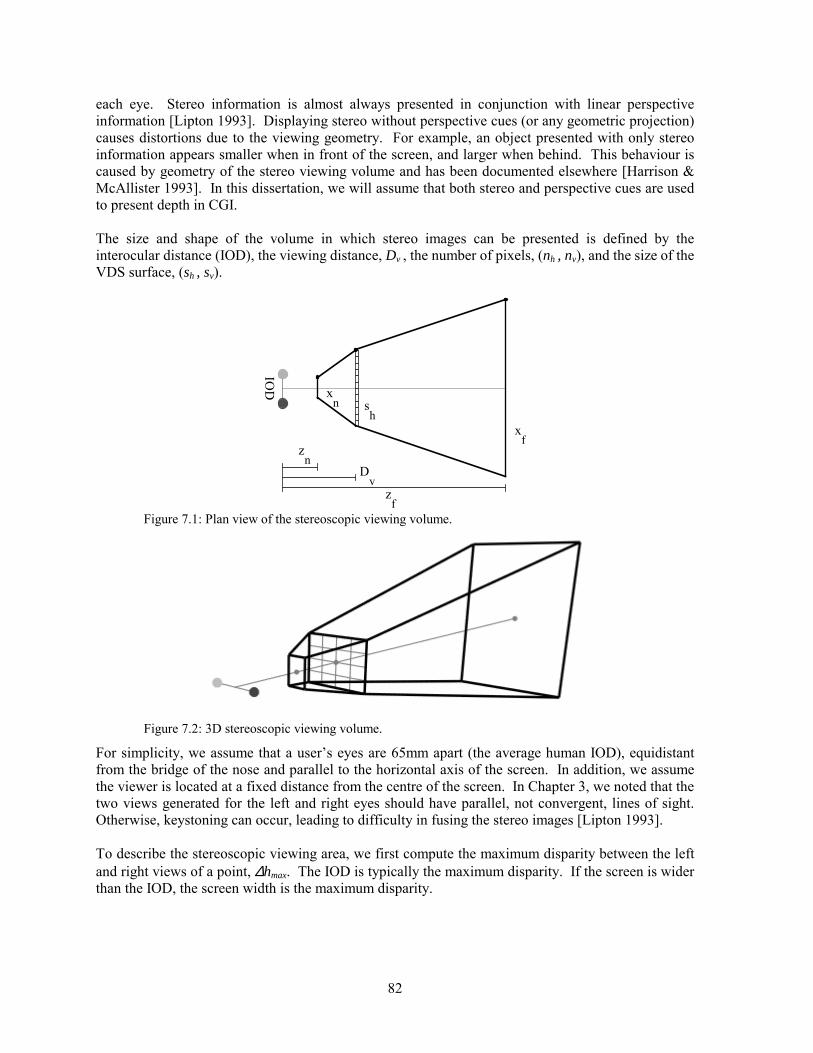
82
each eye. Stereo information is almost always presented in conjunction with linear perspective information [Lipton 1993]. Displaying stereo without perspective cues (or any geometric projection) causes distortions due to the viewing geometry. For example, an object presented with only stereo information appears smaller when in front of the screen, and larger when behind. This behaviour is caused by geometry of the stereo viewing volume and has been documented elsewhere [Harrison & McAllister 1993]. In this dissertation, we will assume that both stereo and perspective cues are used to present depth in CGI. The size and shape of the volume in which stereo images can be presented is defined by the interocular distance (IOD), the viewing distance, Dv , the number of pixels, (nh , nv), and the size of the VDS surface, (sh , sv).
IOD x
n
zf
sh
xf
zn
Dv
Figure 7.1: Plan view of the stereoscopic viewing volume.
Figure 7.2: 3D stereoscopic viewing volume.
For simplicity, we assume that a user�s eyes are 65mm apart (the average human IOD), equidistant from the bridge of the nose and parallel to the horizontal axis of the screen. In addition, we assume the viewer is located at a fixed distance from the centre of the screen. In Chapter 3, we noted that the two views generated for the left and right eyes should have parallel, not convergent, lines of sight. Otherwise, keystoning can occur, leading to difficulty in fusing the stereo images [Lipton 1993]. To describe the stereoscopic viewing area, we first compute the maximum disparity between the left and right views of a point, ∆hmax. The IOD is typically the maximum disparity. If the screen is wider than the IOD, the screen width is the maximum disparity.
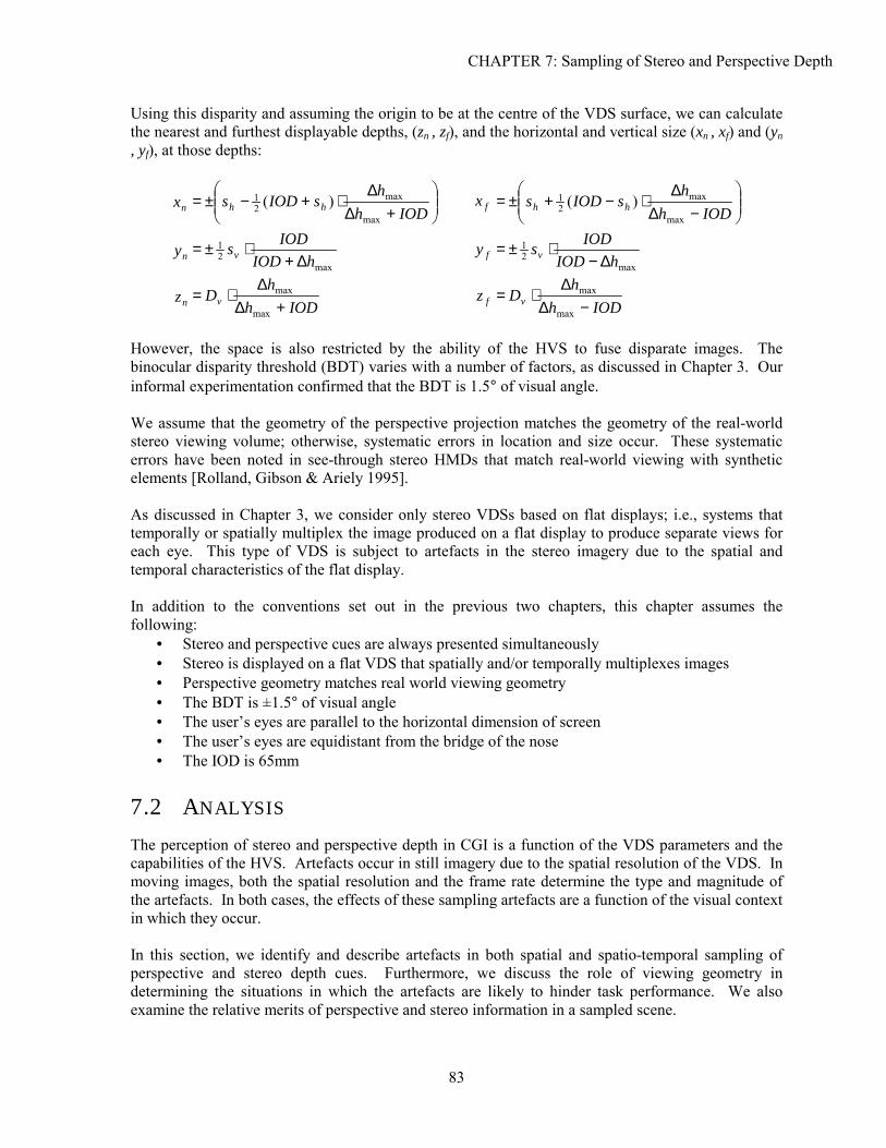
CHAPTER 7: Sampling of Stereo and Perspective Depth
83
Using this disparity and assuming the origin to be at the centre of the VDS surface, we can calculate the nearest and furthest displayable depths, (zn , zf), and the horizontal and vertical size (xn , xf) and (yn , yf), at those depths:
nx
+∆
∆⋅+−±=
IODhh
sIODs hhmax
max21 )( fx
−∆
∆⋅−+±=
IODhh
sIODs hhmax
max21 )(
ny max
21
hIODIODsv ∆+
⋅±= fymax
21
hIODIODsv ∆−
⋅±=
nz IODh
hDv +∆
∆⋅=
max
max fzIODh
hDv −∆
∆⋅=
max
max
However, the space is also restricted by the ability of the HVS to fuse disparate images. The binocular disparity threshold (BDT) varies with a number of factors, as discussed in Chapter 3. Our informal experimentation confirmed that the BDT is 1.5° of visual angle. We assume that the geometry of the perspective projection matches the geometry of the real-world stereo viewing volume; otherwise, systematic errors in location and size occur. These systematic errors have been noted in see-through stereo HMDs that match real-world viewing with synthetic elements [Rolland, Gibson & Ariely 1995]. As discussed in Chapter 3, we consider only stereo VDSs based on flat displays; i.e., systems that temporally or spatially multiplex the image produced on a flat display to produce separate views for each eye. This type of VDS is subject to artefacts in the stereo imagery due to the spatial and temporal characteristics of the flat display. In addition to the conventions set out in the previous two chapters, this chapter assumes the following:
• Stereo and perspective cues are always presented simultaneously • Stereo is displayed on a flat VDS that spatially and/or temporally multiplexes images • Perspective geometry matches real world viewing geometry • The BDT is ±1.5° of visual angle • The user�s eyes are parallel to the horizontal dimension of screen • The user�s eyes are equidistant from the bridge of the nose • The IOD is 65mm
7.2 ANALYSIS
The perception of stereo and perspective depth in CGI is a function of the VDS parameters and the capabilities of the HVS. Artefacts occur in still imagery due to the spatial resolution of the VDS. In moving images, both the spatial resolution and the frame rate determine the type and magnitude of the artefacts. In both cases, the effects of these sampling artefacts are a function of the visual context in which they occur. In this section, we identify and describe artefacts in both spatial and spatio-temporal sampling of perspective and stereo depth cues. Furthermore, we discuss the role of viewing geometry in determining the situations in which the artefacts are likely to hinder task performance. We also examine the relative merits of perspective and stereo information in a sampled scene.
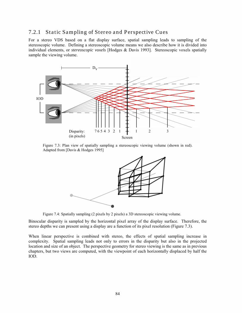
84
7.2.1 Static Sampling of Stereo and Perspective Cues For a stereo VDS based on a flat display surface, spatial sampling leads to sampling of the stereoscopic volume. Defining a stereoscopic volume means we also describe how it is divided into individual elements, or stereoscopic voxels [Hodges & Davis 1993]. Stereoscopic voxels spatially sample the viewing volume.
ScreenDisparity:(in pixels)
7 6 1345 2 31 2
IOD
Dv
Figure 7.3: Plan view of spatially sampling a stereoscopic viewing volume (shown in red). Adapted from [Davis & Hodges 1995]
Figure 7.4: Spatially sampling (2 pixels by 2 pixels) a 3D stereoscopic viewing volume.
Binocular disparity is sampled by the horizontal pixel array of the display surface. Therefore, the stereo depths we can present using a display are a function of its pixel resolution (Figure 7.3). When linear perspective is combined with stereo, the effects of spatial sampling increase in complexity. Spatial sampling leads not only to errors in the disparity but also in the projected location and size of an object. The perspective geometry for stereo viewing is the same as in previous chapters, but two views are computed, with the viewpoint of each horizontally displaced by half the IOD.
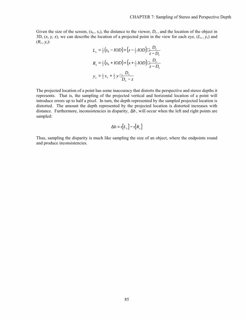
CHAPTER 7: Sampling of Stereo and Perspective Depth
85
Given the size of the screen, (sh , sv), the distance to the viewer, Dv , and the location of the object in 3D, (x, y, z), we can describe the location of a projected point in the view for each eye, (Ls , ys) and (Rs , ys):
sL ( ) ( )v
vh Dz
DIODxIODs−
⋅−+−= 21
21
sR ( ) ( )v
vh Dz
DIODxIODs−
⋅+++= 21
21
sy zD
Dys
v
vv −
⋅+= 21
21
The projected location of a point has some inaccuracy that distorts the perspective and stereo depths it represents. That is, the sampling of the projected vertical and horizontal location of a point will introduce errors up to half a pixel. In turn, the depth represented by the sampled projected location is distorted. The amount the depth represented by the projected location is distorted increases with distance. Furthermore, inconsistencies in disparity, h∆ , will occur when the left and right points are sampled:
[ ] [ ]ss RLh rr −=∆ Thus, sampling the disparity is much like sampling the size of an object, where the endpoints round and produce inconsistencies.
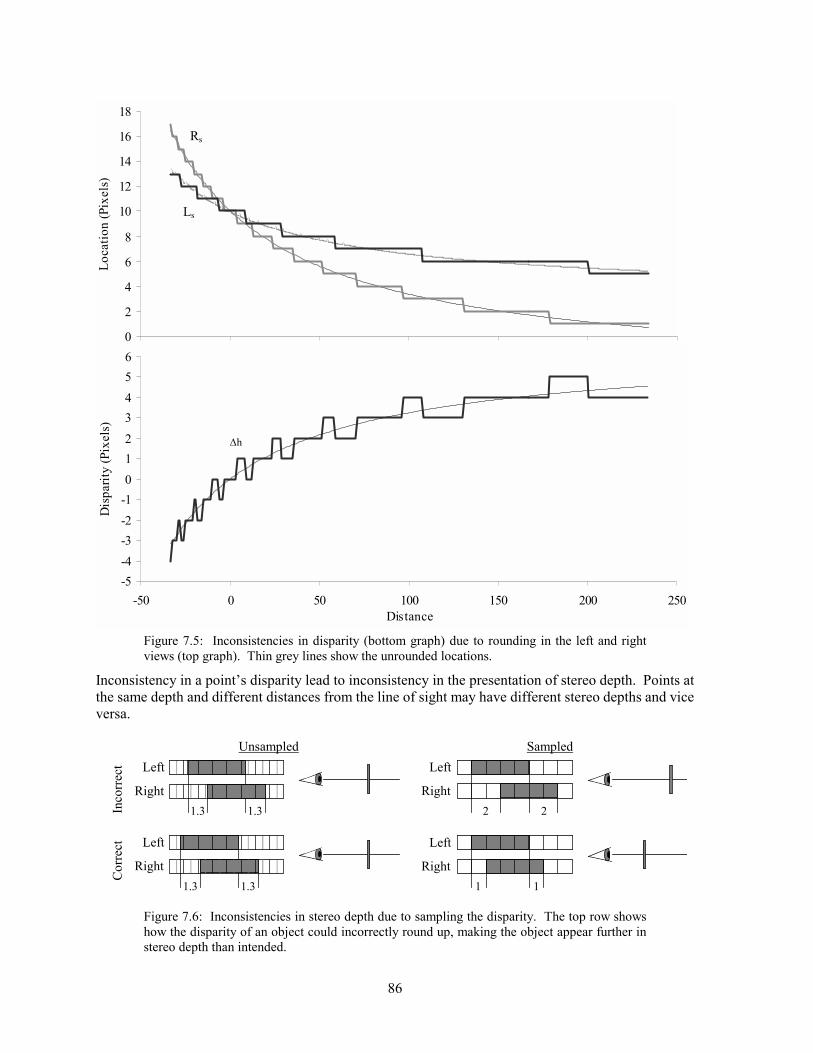
86
0
2
4
6
8
10
12
14
16
18Lo
catio
n (P
ixel
s)
-5-4-3-2-10123456
-50 0 50 100 150 200 250Distance
Dis
parit
y (P
ixel
s)
Figure 7.5: Inconsistencies in disparity (bottom graph) due to rounding in the left and right views (top graph). Thin grey lines show the unrounded locations.
Inconsistency in a point�s disparity lead to inconsistency in the presentation of stereo depth. Points at the same depth and different distances from the line of sight may have different stereo depths and vice versa.
Unsampled Sampled
Inco
rrec
t
1.31.3
Left
Right
22
Left
Right
Cor
rect
1.31.3
Left
Right
1 1
Left
Right
Figure 7.6: Inconsistencies in stereo depth due to sampling the disparity. The top row shows how the disparity of an object could incorrectly round up, making the object appear further in stereo depth than intended.
Ls
Rs
∆h
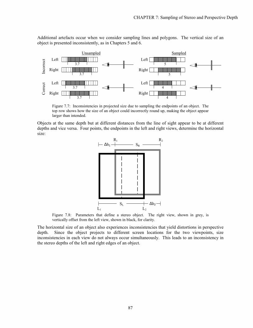
CHAPTER 7: Sampling of Stereo and Perspective Depth
87
Additional artefacts occur when we consider sampling lines and polygons. The vertical size of an object is presented inconsistently, as in Chapters 5 and 6.
Unsampled Sampled
Inco
rrec
t
3.7
3.7Left
Right 5
5Left
Right
Cor
rect
3.7
3.7Left
Right 4
4Left
Right
Figure 7.7: Inconsistencies in projected size due to sampling the endpoints of an object. The top row shows how the size of an object could incorrectly round up, making the object appear larger than intended.
Objects at the same depth but at different distances from the line of sight appear to be at different depths and vice versa. Four points, the endpoints in the left and right views, determine the horizontal size:
SR ∆h1
R1 R2
L2L1
∆h2 SL
Figure 7.8: Parameters that define a stereo object. The right view, shown in grey, is vertically offset from the left view, shown in black, for clarity.
The horizontal size of an object also experiences inconsistencies that yield distortions in perspective depth. Since the object projects to different screen locations for the two viewpoints, size inconsistencies in each view do not always occur simultaneously. This leads to an inconsistency in the stereo depths of the left and right edges of an object.
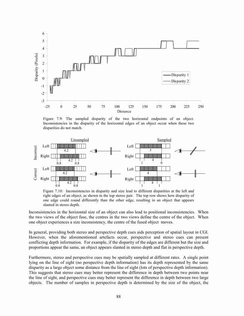
88
-3
-2
-1
0
1
2
3
4
5
6
-25 0 25 50 75 100 125 150 175 200 225 250Distance
Dis
parit
y (P
ixel
s)
Disparity 1Disparity 2
Figure 7.9: The sampled disparity of the two horizontal endpoints of an object. Inconsistencies in the disparity of the horizontal edges of an object occur when these two disparities do not match.
Unsampled Sampled
Inco
rrec
t
4.2
4.2
0.80.8
Left
Right
5
401
Left
Right
Cor
rect
4.2
4.2
0.80.8
Left
Right
4
411
Left
Right
Figure 7.10: Inconsistencies in disparity and size lead to different disparities at the left and right edges of an object, as shown in the top stereo pair. The top row shows how disparity of one edge could round differently than the other edge, resulting in an object that appears slanted in stereo depth.
Inconsistencies in the horizontal size of an object can also lead to positional inconsistencies. When the two views of the object fuse, the centres in the two views define the centre of the object. When one object experiences a size inconsistency, the centre of the fused object moves. In general, providing both stereo and perspective depth cues aids perception of spatial layout in CGI. However, when the aforementioned artefacts occur, perspective and stereo cues can present conflicting depth information. For example, if the disparity of the edges are different but the size and proportions appear the same, an object appears slanted in stereo depth and flat in perspective depth. Furthermore, stereo and perspective cues may be spatially sampled at different rates. A single point lying on the line of sight (no perspective depth information) has its depth represented by the same disparity as a large object some distance from the line of sight (lots of perspective depth information). This suggests that stereo cues may better represent the difference in depth between two points near the line of sight, and perspective cues may better represent the difference in depth between two large objects. The number of samples in perspective depth is determined by the size of the object, the
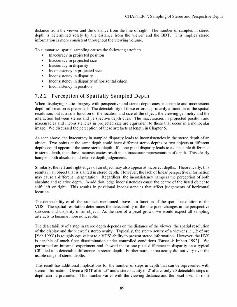
CHAPTER 7: Sampling of Stereo and Perspective Depth
89
distance from the viewer and the distance from the line of sight. The number of samples in stereo depth is determined solely by the distance from the viewer and the BDT. This implies stereo information is more consistent throughout the viewing volume. To summarise, spatial sampling causes the following artefacts:
• Inaccuracy in projected position • Inaccuracy in projected size • Inaccuracy in disparity • Inconsistency in projected size • Inconsistency in disparity • Inconsistency in disparity of horizontal edges • Inconsistency in position
7.2.2 Perception of Spatially Sampled Depth When displaying static imagery with perspective and stereo depth cues, inaccurate and inconsistent depth information is presented. The detectability of these errors is primarily a function of the spatial resolution, but is also a function of the location and size of the object, the viewing geometry and the interaction between stereo and perspective depth cues. The inaccuracies in projected position and inaccuracies and inconsistencies in projected size are equivalent to those that occur in a monocular image. We discussed the perception of these artefacts at length in Chapter 5. As seen above, the inaccuracy in sampled disparity leads to inconsistencies in the stereo depth of an object. Two points at the same depth could have different stereo depths or two objects at different depths could appear at the same stereo depth. If a one-pixel disparity leads to a detectable difference in stereo depth, then these inconsistencies result in an inaccurate representation of depth. This clearly hampers both absolute and relative depth judgements. Similarly, the left and right edges of an object may also appear at incorrect depths. Theoretically, this results in an object that is slanted in stereo depth. However, the lack of linear perspective information may cause a different interpretation. Regardless, the inconsistency hampers the perception of both absolute and relative depth. In addition, edge inconsistencies cause the centre of the fused object to shift left or right. This results in positional inconsistencies that affect judgements of horizontal location. The detectability of all the artefacts mentioned above is a function of the spatial resolution of the VDS. The spatial resolution determines the detectability of the one-pixel changes in the perspective sub-cues and disparity of an object. As the size of a pixel grows, we would expect all sampling artefacts to become more noticeable. The detectability of a step in stereo depth depends on the distance of the viewer, the spatial resolution of the display and the viewer�s stereo acuity. Typically, the stereo acuity of a viewer (i.e., 2' of arc [Yeh 1993]) is roughly equivalent to a VDS� ability to present stereo information. However, the HVS is capable of much finer discrimination under controlled conditions [Buser & Imbert 1992]. We performed an informal experiment and showed that a one-pixel difference in disparity on a typical CRT led to a detectable difference in stereo depth. Furthermore, stereo acuity did not vary over the usable range of stereo depths. This result has additional implications for the number of steps in depth that can be represented with stereo information. Given a BDT of ± 1.5° and a stereo acuity of 2' of arc, only 90 detectable steps in depth can be presented. This number varies with the viewing distance and the pixel size. In most
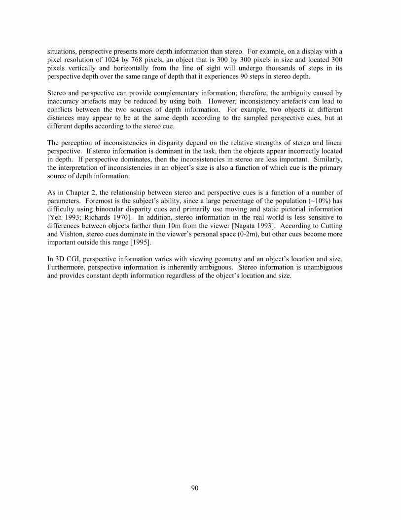
90
situations, perspective presents more depth information than stereo. For example, on a display with a pixel resolution of 1024 by 768 pixels, an object that is 300 by 300 pixels in size and located 300 pixels vertically and horizontally from the line of sight will undergo thousands of steps in its perspective depth over the same range of depth that it experiences 90 steps in stereo depth. Stereo and perspective can provide complementary information; therefore, the ambiguity caused by inaccuracy artefacts may be reduced by using both. However, inconsistency artefacts can lead to conflicts between the two sources of depth information. For example, two objects at different distances may appear to be at the same depth according to the sampled perspective cues, but at different depths according to the stereo cue. The perception of inconsistencies in disparity depend on the relative strengths of stereo and linear perspective. If stereo information is dominant in the task, then the objects appear incorrectly located in depth. If perspective dominates, then the inconsistencies in stereo are less important. Similarly, the interpretation of inconsistencies in an object�s size is also a function of which cue is the primary source of depth information. As in Chapter 2, the relationship between stereo and perspective cues is a function of a number of parameters. Foremost is the subject�s ability, since a large percentage of the population (~10%) has difficulty using binocular disparity cues and primarily use moving and static pictorial information [Yeh 1993; Richards 1970]. In addition, stereo information in the real world is less sensitive to differences between objects farther than 10m from the viewer [Nagata 1993]. According to Cutting and Vishton, stereo cues dominate in the viewer�s personal space (0-2m), but other cues become more important outside this range [1995]. In 3D CGI, perspective information varies with viewing geometry and an object�s location and size. Furthermore, perspective information is inherently ambiguous. Stereo information is unambiguous and provides constant depth information regardless of the object�s location and size.
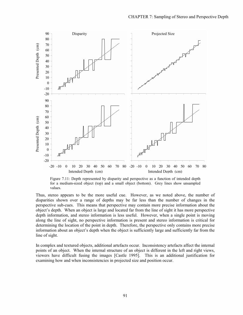
CHAPTER 7: Sampling of Stereo and Perspective Depth
91
-20-10
0102030405060708090
-20-10
0102030405060708090
-20 -10 0 10 20 30 40 50 60 70 80 -20 -10 0 10 20 30 40 50 60 70 80
Figure 7.11: Depth represented by disparity and perspective as a function of intended depth for a medium-sized object (top) and a small object (bottom). Grey lines show unsampled values.
Thus, stereo appears to be the more useful cue. However, as we noted above, the number of disparities shown over a range of depths may be far less than the number of changes in the perspective sub-cues. This means that perspective may contain more precise information about the object�s depth. When an object is large and located far from the line of sight it has more perspective depth information, and stereo information is less useful. However, when a single point is moving along the line of sight, no perspective information is present and stereo information is critical for determining the location of the point in depth. Therefore, the perspective only contains more precise information about an object�s depth when the object is sufficiently large and sufficiently far from the line of sight. In complex and textured objects, additional artefacts occur. Inconsistency artefacts affect the internal points of an object. When the internal structure of an object is different in the left and right views, viewers have difficult fusing the images [Castle 1995]. This is an additional justification for examining how and when inconsistencies in projected size and position occur.
Pres
ente
d D
epth
(cm
) Pr
esen
ted
Dep
th (
cm)
Intended Depth (cm) Intended Depth (cm)
Disparity Projected Size
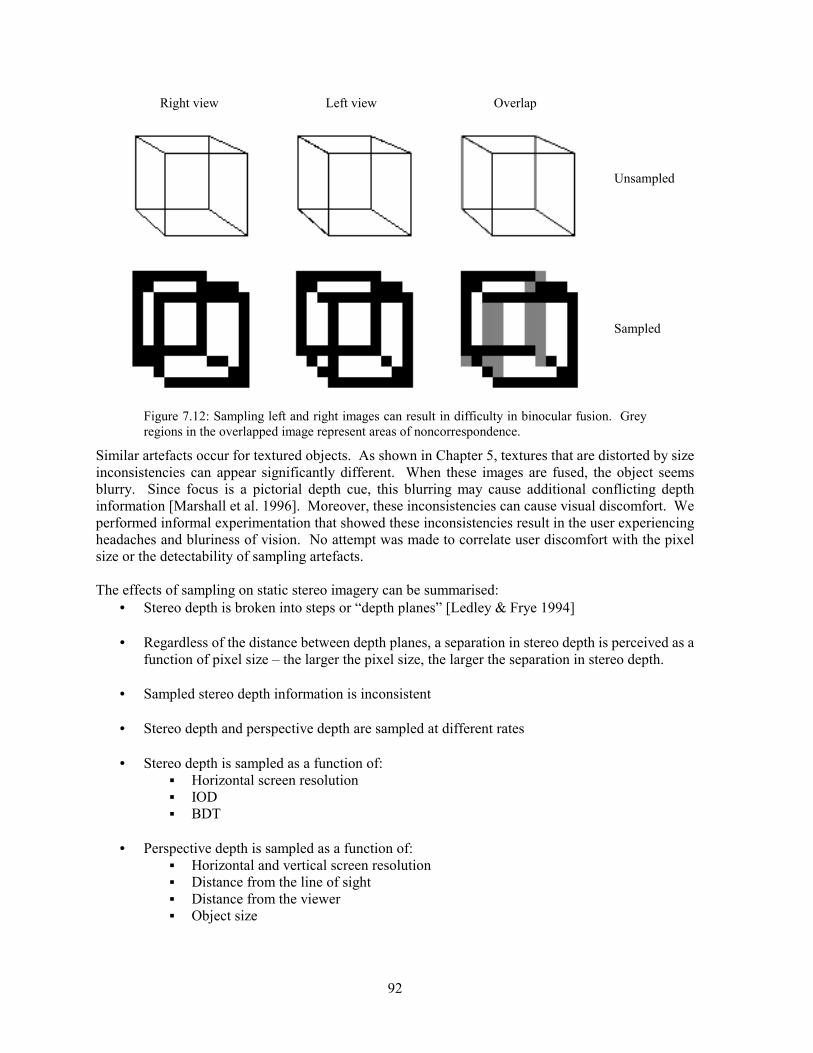
92
Left viewRight view Overlap
Unsampled
Sampled
Figure 7.12: Sampling left and right images can result in difficulty in binocular fusion. Grey regions in the overlapped image represent areas of noncorrespondence.
Similar artefacts occur for textured objects. As shown in Chapter 5, textures that are distorted by size inconsistencies can appear significantly different. When these images are fused, the object seems blurry. Since focus is a pictorial depth cue, this blurring may cause additional conflicting depth information [Marshall et al. 1996]. Moreover, these inconsistencies can cause visual discomfort. We performed informal experimentation that showed these inconsistencies result in the user experiencing headaches and bluriness of vision. No attempt was made to correlate user discomfort with the pixel size or the detectability of sampling artefacts. The effects of sampling on static stereo imagery can be summarised:
• Stereo depth is broken into steps or �depth planes� [Ledley & Frye 1994] • Regardless of the distance between depth planes, a separation in stereo depth is perceived as a
function of pixel size � the larger the pixel size, the larger the separation in stereo depth. • Sampled stereo depth information is inconsistent • Stereo depth and perspective depth are sampled at different rates • Stereo depth is sampled as a function of:
▪ Horizontal screen resolution ▪ IOD ▪ BDT
• Perspective depth is sampled as a function of: ▪ Horizontal and vertical screen resolution ▪ Distance from the line of sight ▪ Distance from the viewer ▪ Object size
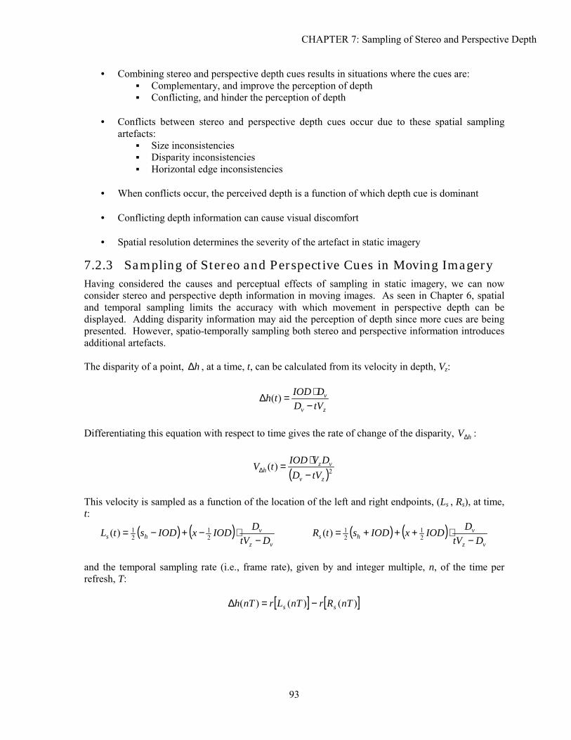
CHAPTER 7: Sampling of Stereo and Perspective Depth
93
• Combining stereo and perspective depth cues results in situations where the cues are: ▪ Complementary, and improve the perception of depth ▪ Conflicting, and hinder the perception of depth
• Conflicts between stereo and perspective depth cues occur due to these spatial sampling artefacts:
▪ Size inconsistencies ▪ Disparity inconsistencies ▪ Horizontal edge inconsistencies
• When conflicts occur, the perceived depth is a function of which depth cue is dominant • Conflicting depth information can cause visual discomfort • Spatial resolution determines the severity of the artefact in static imagery
7.2.3 Sampling of Stereo and Perspective Cues in Moving Imagery Having considered the causes and perceptual effects of sampling in static imagery, we can now consider stereo and perspective depth information in moving images. As seen in Chapter 6, spatial and temporal sampling limits the accuracy with which movement in perspective depth can be displayed. Adding disparity information may aid the perception of depth since more cues are being presented. However, spatio-temporally sampling both stereo and perspective information introduces additional artefacts. The disparity of a point, h∆ , at a time, t, can be calculated from its velocity in depth, Vz:
zv
v
tVDDIODth
−⋅=∆ )(
Differentiating this equation with respect to time gives the rate of change of the disparity, hV∆ :
( )2)(zv
vzh tVD
DVIODtV−⋅=∆
This velocity is sampled as a function of the location of the left and right endpoints, (Ls , Rs), at time, t:
( ) ( )vz
vhs DtV
DIODxIODstL−
⋅−+−= 21
21)( ( ) ( )
vz
vhs DtV
DIODxIODstR−
⋅+++= 21
21)(
and the temporal sampling rate (i.e., frame rate), given by and integer multiple, n, of the time per refresh, T:
[ ] [ ])()()( nTRrnTLrnTh ss −=∆
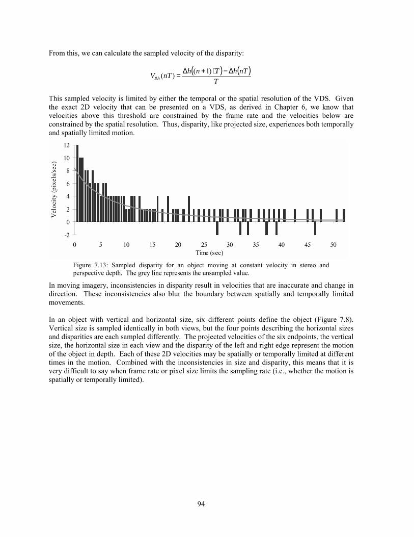
94
From this, we can calculate the sampled velocity of the disparity:
( ) ( )T
nThTnhnTV h∆−⋅+∆=∆
)1()(
This sampled velocity is limited by either the temporal or the spatial resolution of the VDS. Given the exact 2D velocity that can be presented on a VDS, as derived in Chapter 6, we know that velocities above this threshold are constrained by the frame rate and the velocities below are constrained by the spatial resolution. Thus, disparity, like projected size, experiences both temporally and spatially limited motion.
-2
0
2
4
6
8
10
12
0 5 10 15 20 25 30 35 40 45 50Time (sec)
Vel
ocity
(pix
els/
sec)
Figure 7.13: Sampled disparity for an object moving at constant velocity in stereo and perspective depth. The grey line represents the unsampled value.
In moving imagery, inconsistencies in disparity result in velocities that are inaccurate and change in direction. These inconsistencies also blur the boundary between spatially and temporally limited movements. In an object with vertical and horizontal size, six different points define the object (Figure 7.8). Vertical size is sampled identically in both views, but the four points describing the horizontal sizes and disparities are each sampled differently. The projected velocities of the six endpoints, the vertical size, the horizontal size in each view and the disparity of the left and right edge represent the motion of the object in depth. Each of these 2D velocities may be spatially or temporally limited at different times in the motion. Combined with the inconsistencies in size and disparity, this means that it is very difficult to say when frame rate or pixel size limits the sampling rate (i.e., whether the motion is spatially or temporally limited).
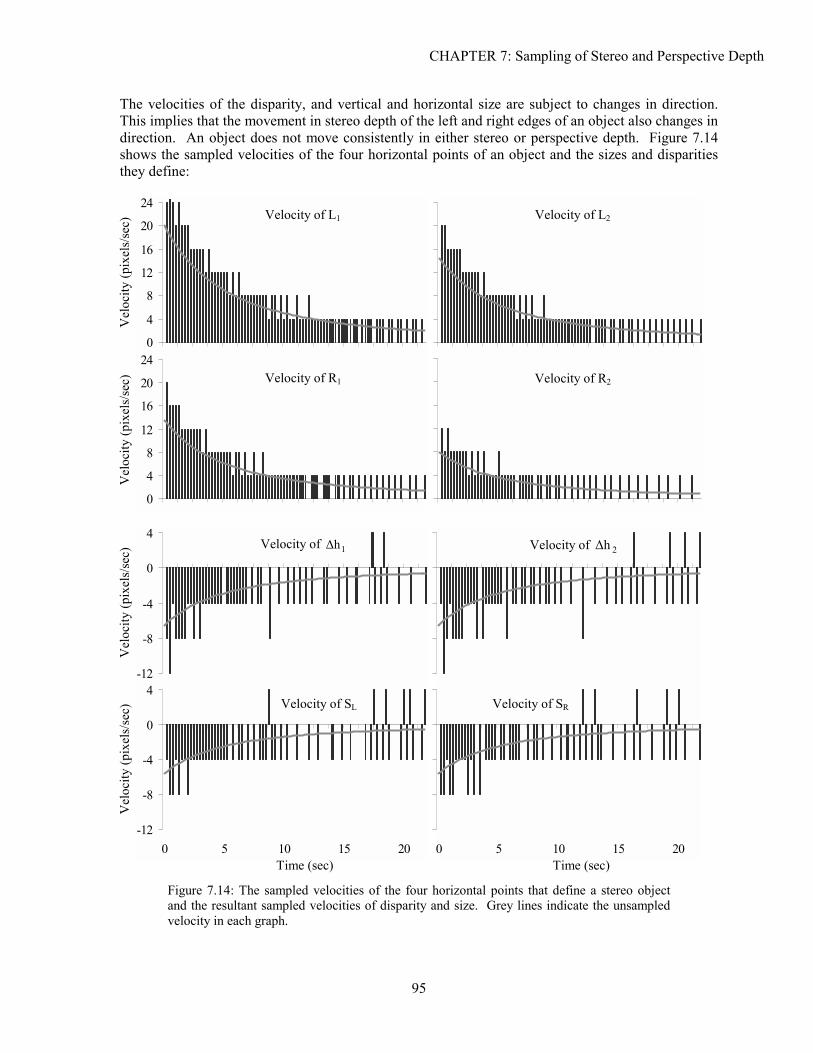
CHAPTER 7: Sampling of Stereo and Perspective Depth
The velocities of the disparity, and vertical and horizontal size are subject to changes in direction. This implies that the movement in stereo depth of the left and right edges of an object also changes in direction. An object does not move consistently in either stereo or perspective depth. Figure 7.14 shows the sampled velocities of the four horizontal points of an object and the sizes and disparities they define:
0
4
8
12
16
20
24
0
4
8
12
16
20
24
-12
-8
-4
0
4
-12
-8
-4
0
4
0 5
Figure 7.14: Thand the resultanvelocity in each
Velocity of L1
Velocity of R2
1∆h Velocity of 2∆h
Velocity of L2
Velocity of R1
Vel
ocity
(pix
els/
sec)
V
eloc
ity (p
ixel
s/se
c)
Vel
ocity
(pix
els/
sec)
V
eloc
ity (p
ixel
s/se
c)
Velocity of
95
10 15 20 0 5
e sampled velocities of the four horizontal pointst sampled velocities of disparity and size. Grey ligraph.
Velocity of SL Veloc
Time (sec)
10 15 20
that define a stereo object nes indicate the unsampled
ity of SR
Time (sec)
96
Inconsistencies in size and disparity are likely to occur in a typical scene. Size inconsistencies do not occur when the object is centred on the line of sight. However, an object cannot travel along both lines of sight if binocular disparity information is presented. Thus, size inconsistencies are likely to occur in practically all viewing situations. Similarly, disparity inconsistencies do not occur when an object is centred on the line of sight between the two eyes. Then, the location of the two points always changes at the same time. However, a scene with all objects lying on a single line is improbable, so disparity inconsistencies are expected. Stereo and perspective cues are sampled at different rates. As in the static case, the number of samples for a movement in perspective depth is a function of the 3D velocity, the object size and the distance from the viewer and the line of sight. The number of samples for a movement in stereo depth is a function of the 3D velocity, the IOD, the BDT and the viewer distance. While stereo may be more consistently presented, perspective generally presents more fine-grained information about depth than stereo since most objects have non-zero size and are located some distance from the line of sight (thus resulting in significantly more steps in perspective depth than in stereo depth).
7.2.4 Perception of Spatio-Temporally Sampled Depth The perception of spatio-temporally sampled perspective cues was discussed in Chapter 6. Here, we focus on the perception of sampled stereo information and the combination of stereo and perspective. Sampling the disparity of a point moving in depth results in a point that steps from one stereo depth to the next, as seen with moving perspective cues. The severity of these steps in stereo depth is a function of the spatio-temporal resolution of the VDS and the velocity of the object. Visually, both spatially and temporally limited motion seem the same; the object appears to �jump� from one depth to another, resulting in jerky motion. Like movement in perspective depth, smooth stereo motion is achieved with a sufficiently high frame rate and spatial resolution. However, many stereo displays use time multiplexing to show binocular images, thus reducing the maximum refresh rate. Furthermore, frame rate can be affected by displaying stereo depth. The time to render two separate views may as much as double the rendering time, thus halving the frame rate. Because of the temporal sampling rate in a stereo display is likely to be slower, temporally limited motion is more significant for displaying stereo depth than for displaying monocular perspective information. The perception of stereo depth uses different psychological and physiological mechanisms from monocular viewing; therefore, we expect the sensitivity to sampled stereo depth to be different than sensitivity to sampled perspective depth. For example, sensitivity to stereo depth increases with object movement [Gillam 1995], but stereo vision is less acute than spatial vision [Boff & Lincoln 1988]. That is, the ability to discriminate two points separated orthogonal to the line of sight is better than the ability to discriminate two points separated along the line of sight using binocular disparity information. Thus, we expect perspective information to dominate for fine judgements. However, perspective information can be ambiguous. The additional precision found in perspective depth is useless if it can represent many locations. In moving imagery, we expect stereo information to disambiguate the perspective information, which is then used for fine judgements. The different sampling densities on perspective and stereo depth further support this expectation. As stated above, perspective depth is likely to be represented with more one-pixel steps than stereo information. Therefore, fine judgements of depth are difficult but unambiguous with stereo information and easy but ambiguous with perspective information. Clearly, combining these two cues should improve the overall perception of depth, as long as there are no perceivable inconsistencies and inaccuracies. Furthermore, the cue with the greater number of samples over a movement should dominate the perception of depth.
CHAPTER 7: Sampling of Stereo and Perspective Depth
97
In complex or textured objects, additional artefacts occur as the object moves. Users are more likely to have difficulty fusing images when the internal structure of the object differs between views (Figure 7.12). The object appears to flicker and the user may experience substantial visual discomfort. The severity of these artefacts varies primarily with the type of object or texture and its susceptibility to artefacts.
7.3 EXPERIMENTATION
This dissertation has aimed to describe spatio-temporal sampling artefacts in stereo and perspective depth in CGI. The above analysis has suggested some visual contexts in which artefacts in perspective and stereo information are likely to affect task performance. In this section, we want to experimentally evaluate the behaviour of these artefacts and the situations in which they occur. The choice of experimental tasks follows the same rationale as in Chapters 5 and 6. We want relevant, noise-resistant tasks that illustrate the effects of sampling on the perception of stereo and perspective depth. We conducted three formal experiments and two informal experiments to determine effects of spatial and spatio-temporal sampling on the perception of stereo and perspective depth in 3D CGI.
7.3.1 Tolerance for Inconsistency in Horizontal Edge Disparity As discussed above, inconsistencies in stereo depth caused by sampling the binocular disparity can cause the left and right edges of an object to appear at different depths. An informal experiment was performed to see how this artefact is perceived when the difference in disparity between the two edges changes. Subjects commented on the appearance of a square as the stereo depth of the right edge was manipulated. The object in one stereo view remained constant as the width of the object grew or shrank in the other view. The subjects reported that the square�s size appeared to grow or shrink when disparity differed by less than 0.38°; for larger disparities, stereo fusion was impossible. That is, subjects saw a change in the size of the fused square, not a change in its depth. This occurred for both negative and positive differences in disparity. A second experiment was conducted using a textured object to provide stereo cues across the object. The results were the same as for the untextured object. This experiment explored one possible conflict between perspective and stereo depth information. Had the object been slanted in perspective as well as in stereo, the shape of the object would have become trapezoidal. Also, the texture information added to the perception that the object was flat and not slanted. In both the textured and the untextured cases, the perspective information indicating the object was flat dominated the stereo cues indicating the object was slanted.
7.3.2 Stereo and Perspective Depth Acuity As discussed earlier, combining stereo and perspective depth information leads to inaccuracies and inconsistencies in the depth presented. This experiment was designed to examine the detectability of inconsistencies in an object�s size, disparity and horizontal edges. In addition, we want to identify whether stereo or perspective information dominates when these inconsistencies lead to conflicting depth information.
98
The experiment was divided into four sections: a set of trials each for disparity and size inconsistencies and two sets of trials on horizontal edge inconsistencies. In each case, subjects made relative depth judgements on conflicting or complementary perspective and stereo depth cues. Details of the experiment can be found in Experiment D. The main results of each experiment can be summarised as:
• Disparity inconsistency, �Which is closer?� ▪ Complementary stereo and perspective cues resulted in near-perfect accuracy ▪ Stereo cues dominated perspective cues in conflict situations
• Size inconsistency, �Which is closer?�
▪ Complementary stereo and perspective cues resulted in near-perfect accuracy ▪ Stereo cues dominated perspective cues in conflict situations
• Edge inconsistency, �Are they at the same depth?� ▪ Complementary stereo and perspective cues improved accuracy ▪ Differences in the inner edges of the objects were more detectable than differences in
the outer edges of the objects ▪ Subjects reported visual discomfort
• Edge inconsistency, �Which is closer?� ▪ No statistically significant results ▪ Subjects reported visual discomfort
7.3.3 Judgements of Smooth and Jerky Motion in Stereo Depth Chapter 6 described an informal experiment that assessed the effect of spatio-temporal sampling on the perception of smooth motion. This experiment was adapted for motion in stereo depth; no perspective cues were presented. An object�s disparity was varied by changing the frame rate and spatial resolution to find threshold velocities at which smooth motion in depth was perceived. Subjects were shown an object continuously moving in and out of the screen in stereo depth. To adhere to the BDT, disparity varied from ±1.5°. The smallest pixel size was 1'31" of arc and the maximum frame rate was 30 Hz. Stereo information was presented with CrystalEyes shutter glasses. Subjects reported whether the movement in depth was �smooth,� �somewhat smooth,� or �not smooth.� An additional case tested if the use of textures to provide stereo information across the object would help or hinder the perception of smooth motion. Two cases were considered: one, where no position inconsistencies were allowed (i.e., disparity always changed by an even number) and two, where position inconsistencies were allowed. The first case would have fewer overall steps in stereo depth for a given movement but would not appear to shift horizontally as it moved.
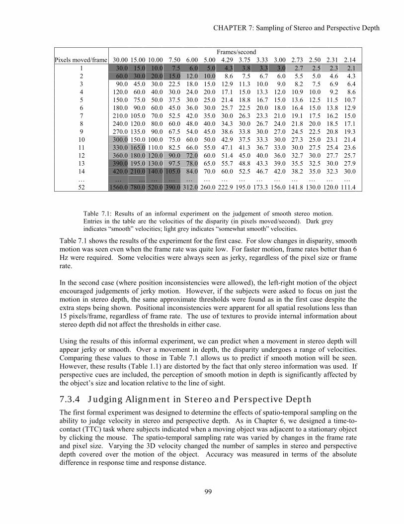
CHAPTER 7: Sampling of Stereo and Perspective Depth
99
Frames/second Pixels moved/frame 30.00 15.00 10.00 7.50 6.00 5.00 4.29 3.75 3.33 3.00 2.73 2.50 2.31 2.14
1 30.0 15.0 10.0 7.5 6.0 5.0 4.3 3.8 3.3 3.0 2.7 2.5 2.3 2.12 60.0 30.0 20.0 15.0 12.0 10.0 8.6 7.5 6.7 6.0 5.5 5.0 4.6 4.33 90.0 45.0 30.0 22.5 18.0 15.0 12.9 11.3 10.0 9.0 8.2 7.5 6.9 6.44 120.0 60.0 40.0 30.0 24.0 20.0 17.1 15.0 13.3 12.0 10.9 10.0 9.2 8.65 150.0 75.0 50.0 37.5 30.0 25.0 21.4 18.8 16.7 15.0 13.6 12.5 11.5 10.76 180.0 90.0 60.0 45.0 36.0 30.0 25.7 22.5 20.0 18.0 16.4 15.0 13.8 12.97 210.0 105.0 70.0 52.5 42.0 35.0 30.0 26.3 23.3 21.0 19.1 17.5 16.2 15.08 240.0 120.0 80.0 60.0 48.0 40.0 34.3 30.0 26.7 24.0 21.8 20.0 18.5 17.19 270.0 135.0 90.0 67.5 54.0 45.0 38.6 33.8 30.0 27.0 24.5 22.5 20.8 19.3
10 300.0 150.0 100.0 75.0 60.0 50.0 42.9 37.5 33.3 30.0 27.3 25.0 23.1 21.411 330.0 165.0 110.0 82.5 66.0 55.0 47.1 41.3 36.7 33.0 30.0 27.5 25.4 23.612 360.0 180.0 120.0 90.0 72.0 60.0 51.4 45.0 40.0 36.0 32.7 30.0 27.7 25.713 390.0 195.0 130.0 97.5 78.0 65.0 55.7 48.8 43.3 39.0 35.5 32.5 30.0 27.914 420.0 210.0 140.0 105.0 84.0 70.0 60.0 52.5 46.7 42.0 38.2 35.0 32.3 30.0� � � � � � � � � � � � � � � 52 1560.0 780.0 520.0 390.0 312.0 260.0 222.9 195.0 173.3 156.0 141.8 130.0 120.0 111.4
Table 7.1: Results of an informal experiment on the judgement of smooth stereo motion. Entries in the table are the velocities of the disparity (in pixels moved/second). Dark grey indicates �smooth� velocities; light grey indicates �somewhat smooth� velocities.
Table 7.1 shows the results of the experiment for the first case. For slow changes in disparity, smooth motion was seen even when the frame rate was quite low. For faster motion, frame rates better than 6 Hz were required. Some velocities were always seen as jerky, regardless of the pixel size or frame rate. In the second case (where position inconsistencies were allowed), the left-right motion of the object encouraged judgements of jerky motion. However, if the subjects were asked to focus on just the motion in stereo depth, the same approximate thresholds were found as in the first case despite the extra steps being shown. Positional inconsistencies were apparent for all spatial resolutions less than 15 pixels/frame, regardless of frame rate. The use of textures to provide internal information about stereo depth did not affect the thresholds in either case. Using the results of this informal experiment, we can predict when a movement in stereo depth will appear jerky or smooth. Over a movement in depth, the disparity undergoes a range of velocities. Comparing these values to those in Table 7.1 allows us to predict if smooth motion will be seen. However, these results (Table 1.1) are distorted by the fact that only stereo information was used. If perspective cues are included, the perception of smooth motion in depth is significantly affected by the object�s size and location relative to the line of sight.
7.3.4 Judging Alignment in Stereo and Perspective Depth The first formal experiment was designed to determine the effects of spatio-temporal sampling on the ability to judge velocity in stereo and perspective depth. As in Chapter 6, we designed a time-to-contact (TTC) task where subjects indicated when a moving object was adjacent to a stationary object by clicking the mouse. The spatio-temporal sampling rate was varied by changes in the frame rate and pixel size. Varying the 3D velocity changed the number of samples in stereo and perspective depth covered over the motion of the object. Accuracy was measured in terms of the absolute difference in response time and response distance.
100
The details of the experiment can be found in Experiment E. The main results can be summarised as: • Decreasing the pixel size increased accuracy in time • Increasing the 3D velocity increased accuracy in time and distance • Increasing the frame rate increased accuracy in distance • At slow velocities, changing the pixel size had more of an effect on the accuracy in time. • At high frame rates, changing the 3D velocity had little effect on the accuracy in distance
7.3.5 Velocity Perception and the Utility of Stereo Imagery The results of the TTC experiment paralleled those from Chapter 6, indicating the task was probably dominated by perspective information. An informal follow-up experiment was run to clarify this assumption. The literature suggests that increasing the IOD increases performance on tasks using stereo information [Drascic & Milgram 1991; Rosenberg 1993; Schloerb 1997]. Hence, we repeated the TTC experiment with the amount of stereo disparity ranging from zero to the maximum allowed within the BDT. The results showed that stereo had no effect on the perception of velocity in this scene.
7.3.6 Air Traffic Control Throughout this thesis, the analysis and experimentation on spatio-temporal sampling in 3D imagery has focused on relatively simple tasks. Air traffic control (ATC) is a more complex task that requires effective presentation of the location and movement of objects in 3D space. In current ATC VDSs, the relative location of aeroplanes is shown two-dimensionally using a symbol for the aircraft and an accompanying altitude. Much research has been devoted to modernising these systems by including 3D representations of the airspace [Delucia 1995]. The use of a 3D VDS has been proposed as being superior for reducing avoidance manoeuvres and presenting 3D information more intuitively [Grunwald, Ellis & Smith 1988; Hendrix & Barfield 1997]. Furthermore, geometric enhancements can enrich the perspective information in the scene and aid spatial judgements [Ellis 1993]. However, ATC VDSs rely on the accurate representation of depth information. Two types of errors occur when presenting information on a perspective display: those due to perceptual biases and those due to the VDS characteristics. The perceptual biases are well documented [Ellis et al. 1992; Hendrix &Barfield 1997; McGreevy & Ellis 1986; Yeh & Silverstein 1992], but the effects of the spatial and temporal characteristics of the VDS are generally ignored. In many ways, ATC VDSs are a good example of the kind of tasks that can benefit from the information and experimentation in this dissertation. Other depth information in the scene is sparse. Perspective is the dominant depth cue used, but stereo cues could also be added if their use can be justified. The experiment was designed around a number of different scenarios. Subjects judged if a collision was imminent as two aircraft travelled along intersecting flight paths. Since the scenarios were repeated, some training was expected. Therefore, we provided feedback on the correctness of a response and extra blocks of training trials. Frame rate was varied; and stereo imagery was used for half the trials. The details of the experiment are described in Experiment F. The main results were:
• Decreasing frame rate decreased accuracy • Using stereo imagery did not improve accuracy • Which scenario was presented significantly affected accuracy
CHAPTER 7: Sampling of Stereo and Perspective Depth
101
7.3.7 Discussion The initial informal experiment examined the perception of inconsistencies in the disparity between the left and right edges of an object that result from spatial sampling. Small differences were seen as changes in the object�s size, while large differences led to difficulty in stereo fusion. As seen in Chapter 5, small distortions in the horizontal size of an object are unlikely to have a significant effect on the perception of its depth. In typical VDSs, the difference in disparity between edges is small. Thus, the actual distortion in the depth of an object is minimal unless the pixel size is large enough to cause difficulties in stereo fusion. These difficulties are exacerbated for complex and textured objects. The first formal experiment assessed the detectability of changes in stereo and perspective depth cues due to inconsistencies in size, disparity and horizontal edges. These inconsistencies can cause conflicts between stereo and perspective depth cues; therefore, cue dominance was also evaluated for each type of inconsistency. Subjects judged the relative depths of two static objects. When size and disparity cues were complementary, subjects achieved near-perfect accuracy. This implies that combining depth cues improve the perception of depth. When size and disparity were inconsistent, stereo dominated perspective. In static images, we expect stereo to be the stronger cue, since perspective cues are particularly aided by disambiguation due to movement. The inconsistency between the disparities of the horizontal edges of an object confused the subjects. Even when complementary information was present, judgements were still difficult. Again, since stereo was the dominant cue in this situation and was ambiguous across the object, this led to decreased accuracy. Edge inconsistencies also led to more complaints about visual fatigue and discomfort. In moving imagery, both the spatial and temporal sampling rate combine to present motion in stereo depth. When the spatio-temporal sampling rate is too low, jerky or stepping motion is perceived. We conducted an informal experiment to examine the thresholds at which smooth stereo motion is perceived. The results showed that smooth motion was seen only for sufficiently high frame rates and velocities (on the VDS used, above 6 Hz and 21'05" of arc per frame). One-pixel changes in disparity looked smooth for a larger range of frame rates, although some combinations of resolutions and frame rates always portrayed jerky motion. Inconsistencies in horizontal position of the object exacerbated the jerkiness of the motion. These artefacts disappeared when the size of the step taken per frame exceeded 22'35" of arc. This experiment implies that thresholds for the perception of smooth stereo motion can be established as a function of the spatial and temporal characteristics of a VDS. The second formal experiment evaluated the accuracy of velocity perception when perspective and stereo depth cues are spatio-temporally sampled. As in Chapter 6, subjects judged when an object moving in depth was aligned with a stationary object. Accuracy of this judgement was proportional to the spatio-temporal sampling rate (i.e., the frame rate and pixel size). Faster 3D velocities improved accuracy since more samples in space were displayed before the objects were aligned. We expect that showing the movement for a longer time would improve accuracy since more samples would be displayed. A follow-up experiment revealed one of the major limitations of stereo image presentation. When good stereo composition rules are followed (i.e., BDT < ±1.5°), the number of sampled stereo depths presented are usually far less than the number of perspective depths. If the perspective information in
102
a scene is unambiguous, then stereo may not be a valuable additional cue. In the TTC task, the ambiguity in the scene was minimised before the addition of stereo cues. Since only constant-velocity motion in depth was presented, the results of the follow-up experiment are unsurprising; stereo cues did not significantly affect accuracy. However, in a typical scene, movement in location will indicate 3D location, not just perspective depth, and stereo will be useful for reducing ambiguities about the direction of motion. Finally, we designed the ATC experiment to explore the effects of sampling on a more practical, real-world task. The main result of the experiment was to confirm that an insufficient sampling rate adversely affects performance on complex as well as simple tasks. The sampling rate required, however, still varies with the type of task. Even within the experiment, the scenario presented affected the accuracy. Thus, rules of thumb such as �around 20-30 Hz� seem to be the best way of describing the need for frame rate. The use of stereo imagery did not significantly improve performance in this experiment. In scenes where rich perspective imagery is present, subjects rely on the pictorial information instead of stereo information. We have demonstrated that sampling artefacts interfere with performance on tasks using perspective and stereo depth information. Frame rate and pixel size requirements are a function of the type of task and the level of performance required. In general, static images are the most affected by artefacts caused by inadequate sampling rates. Stereo is the dominant source of information in static images, although inconsistencies result in cue conflicts. These conflicts distort relative depth judgements and cause visual discomfort. In moving images, binocular disparity cues are less useful than expected, particularly when perspective cues are relatively unambiguous. Even in more complex tasks, rich perspective cues are the dominant source of depth information. Avoiding the contexts where perspective information is reduced (i.e., close to the line of sight, at a large distance, etc.) improves the accuracy of depth perception.
7.4 SOLUTIONS
Having described sampling artefacts in stereo and perspective depth cues and identified the contexts in which they are significant, we can now suggest some methods for combating these problems. This section revisits the methods suggested in the previous two chapters, endpoint manipulation and viewpoint manipulation. These methods can be adapted to reduce the effect of sampling artefacts in stereo and perspective depth cues. In this section, we describe these adaptations and evaluate these methods and the contexts in which they are likely to be useful.
7.4.1 Endpoint Manipulation The previous two chapters describe endpoint manipulation as a technique for removing size inconsistencies from static and moving imagery. In stereo imagery, additional inconsistencies occur in the disparity and edges of an object. All of these inconsistencies are detectable and result in distorted representations of depth. Therefore, we adapt our endpoint manipulation methods to address these additional artefacts.
CHAPTER 7: Sampling of Stereo and Perspective Depth
103
In the perspective case, we noted that the size of an object was a function of the two rounded endpoints. We corrected for disparities by choosing an endpoint and calculating the other from the rounded size. In the stereo case, this works for the vertical dimension. However, we have seen that the horizontal size and disparity of an object are a function of four rounded points, (L1 , L2 , R1 , R2):
[ ] [ ]111 rr RLh −=∆ [ ] [ ]12 rr LLSL −= [ ] [ ]222 rr RLh −=∆ [ ] [ ]12 rr RRSR −=
By selecting one of these four points and correctly calculating the rounded size and disparity, we can compute the other three endpoints and thus ensure size and disparity are consistently presented. Alternatively, we could select the midpoints in either view, Lmid , Rmid , or the midpoint of all four points Xmid. We present three computationally inexpensive endpoint manipulation methods, each with a different method of selecting the base point: the midpoint method, the least-steps method and the least-error method. The midpoint method simply uses the overall midpoint as the basis for computing the endpoints:
midX ( )212141 RRLL +++=
h∆ [ ] [ ]2211 rr LRLR −=−=S [ ] [ ]1212 rr RRLL −=−=
midL [ ] [ ]hX mid ∆−= 21rr
1L [ ] [ ]SLmid 21rr −=
2L [ ] [ ]SLmid 21rr +=
midR [ ] [ ]hX mid ∆+= 21rr
1R [ ] [ ]SRmid 21rr −=
2R [ ] [ ]SRmid 21rr +=
Using this algorithm, the midpoint of the stereo object always steps towards the vanishing point and the size and disparity are consistent. However, the difference between the relocated endpoints and their unrounded location can increase significantly. This may cause inconsistencies in the position of the endpoints, meaning that an object shifts horizontally as it moves in depth. The least-error method chooses the point that introduces the least error in the location of the endpoints. This requires computing the other points from the one selected and comparing the results. Although this represents a significant increase in computation from the previous method, these calculations are still trivial when compared to those regularly used for generating a scene. This method, however, exacerbates the positional inconsistencies. Since different points may be chosen as a function of distance, the object sometimes experiences more significant shifts in horizontal position than with the previous method. In an effort to minimise positional inaccuracy, the furthest-point method was adapted for the stereo case. The endpoint that moves the fewest one-pixel steps over a range of depths causes the most position inconsistencies if it is not selected as the base endpoint. The furthest endpoint is calculated
104
relative to each view�s vanishing point (i.e., ± 0.5 IOD). In this manner, the perceivable errors in horizontal position are minimised. In static imagery, all of these algorithms remove inconsistency artefacts. We have shown experimentally that inconsistencies in disparity and size distort the perception of depth even when position is correct. Thus, trading off positional accuracy for consistency in disparity and size is justified for static imagery. In moving images, inaccuracies in position may affect the perception of velocity. As shown in the experimentation on the perception of jerky motion, horizontal movement in stereo imagery is detectable for low velocities. Thus, manipulations introducing positional inconsistencies affect the subjective perception of smooth motion. In particular, the least-error method can introduce large jumps in horizontal position as different endpoints are chosen from frame to frame. Thus, it is clearly unsuitable for moving images. Additional cases were constructed for the TTC experiment (Section 7.3.4) to investigate the effects of removing these inconsistencies (Experiment E). If the furthest-point or midpoint method adversely affect the judgement of velocity, then we know positional inaccuracies are unacceptable. However, both endpoint manipulation methods significantly improved performance. A Sheffe post-hoc analysis showed that the furthest-point method was a significant improvement over the normal and midpoint method cases. The midpoint method did not significantly improve accuracy within the 5% confidence interval used. This experiment demonstrated that, for a velocity judgement task, the least-steps endpoint manipulation method improves the accuracy of depth perception. A further advantage to using endpoint manipulation to guarantee correct size and disparity comes with the use of texture and complex objects. Objects that are the same proportions and size in both views are more easily fused. This means that visual discomfort due to non-correspondence between views can be eliminated.
7.4.2 Viewpoint Manipulation In the last chapter, we presented methods for manipulating viewpoint to optimise the number of spatial and temporal samples devoted to a movement. These methods can be modified for the presentation of both stereo and perspective depth information. To maximise perspective depth cues, the viewpoint was chosen so that projected distances between objects of interest are maximised. This minimises the distance between the objects in depth. To maximise stereo depth information, the binocular disparity should be maximised. This would maximise the distance between the objects in depth. Clearly, optimising the viewpoint to improve the number of both stereo and perspective samples cannot be done. As a result of the experimentation presented above, we have asserted that the relative value of stereo information in depth perception may be less than generally assumed, especially when displaying unambiguous perspective cues. Thus, manipulating the viewpoint solely to optimise the stereo information does not result in the most accurate representation of the scene. Instead, we propose using the viewpoint manipulation methods as proposed previously, to optimise for perspective depth. The stereo information in the scene can be improved by manipulating the IOD. By finding the nearest and furthest objects, we can calculate the IOD and viewing distance to give the greatest amount of stereo information within the BDT. Manipulating the IOD is not a novel concept;
CHAPTER 7: Sampling of Stereo and Perspective Depth
105
it has been discussed at length elsewhere [Drascic & Milgram 1991; Rosenberg 1993; Schloerb 1995]. For a scene with both perspective and stereo information, we can apply viewpoint manipulation as follows: Using one of the methods discussed in the last chapter, manipulate the viewpoint such that perspective cues are maximised. Then, modify the geometric IOD such that the disparity ranges from ±1.5° of arc. Adding the IOD modification to previous viewpoint manipulation methods is simple and does not significantly affect the computational requirements of the algorithm. One potential application of such viewpoint manipulation is the ATC task discussed earlier. Previous studies have suggested that the viewpoint is an important determiner of performance in perspective displays [Yeh & Silverstein 1992]. This implies that an effective viewpoint manipulation algorithm should improve performance on the ATC task. Therefore, we evaluated a variation of the method discussed above as part of the ATC task described in Section 7.3.6 and Experiment F. Unexpectedly, the algorithm did not result in improved performance. However, this can be attributed in part to the experimental design. Viewpoint manipulation clearly increased accuracy for some scenarios, but did not perform universally better than an arbitrary viewpoint that was consistent for all trials. Training a viewer to recognise certain scenarios is easier when a single viewpoint was used. This implies that knowledge of the viewpoint�s location may be more important than the advantage in pixel steps gained by moving the viewpoint. Clearly, the viewer�s knowledge of self-location is critical for making spatial judgements.
7.5 CONCLUSION
Presenting stereo depth information in moving and static images may both help and hinder the perception of a spatial and temporally sampled scene. We have shown sampling causes artefacts in binocular disparity that result in points being inconsistently located in depth. When perspective information is added to a stereo image, the interaction between the two types of depth cues can often improve the sense of layout. However, the sampling artefacts found in each type of cue can also interact, leading to conflicting depth information. Experiments performed in this chapter showed that stereo cues dominated perspective cues in static images. Conversely, perspective information is more important in moving imagery. Two methods for ameliorating these artefacts have been presented. Endpoint manipulation algorithms ensure that the disparity and size of an object is presented consistently over a range of distances. Endpoint methods significantly improved the judgement of velocity in stereo and perspective depth. Viewpoint manipulation maximises the relative distances of projected points, while maximising the disparity of the entire scene. This method was evaluated in the context of an air traffic control display. Training a user to recognise collisions from a single viewpoint was more effective than using an optimised viewpoint that was different in each situation. Both of these methods are more computationally efficient than typical antialiasing methods, although only the endpoint manipulation method actually improved performance.

106
107
C H A P T E R 8
8:Conclusions and Further Work This dissertation has identified and described sampling artefacts found in both stereo and perspective depth cues used in 3D CGI. As a VDS samples these cues, depth is inaccurately and inconsistently represented. We have described how the viewing geometry, VDS characteristics and visual context all affect the perception of these artefacts in both still and moving images. To evaluate the effects of sampling artefacts on the perception of stereo and perspective depth, we conducted numerous formal and informal experiments. These experiments demonstrated how task performance is a function of the spatial and temporal VDS characteristics. The experiments also illustrated the visual contexts in which the sampling of depth cues is most likely to hinder performance. Two methods were developed that ameliorate some of these artefacts. One algorithm constrained the endpoints of an object to remove inconsistencies in size and disparity. Experimental evaluation showed that this method improves the accurate perception of depth. The other method manipulated the viewpoint so that the maximum spatial information was devoted to objects of interest in a scene. Both algorithms were developed to be more computationally efficient than traditional antialiasing methods.
8.1 MAJOR RESULTS
8.1.1 Static Images with Perspective Depth Cues As a foundation for later work, we began by analysing still images with only perspective depth cues. Spatial sampling introduces inaccuracy into the projected location and size of an object. Projected inaccuracy translates into larger errors in perspective depth. The magnitude of the inaccuracy is governed by the pixel size. Furthermore, analysis and experimentation revealed that the size of an
108
object is inconsistently represented across depth. Objects appear larger or smaller than their correct size, and the proportions of the object distort. These artefacts occur frequently and are exacerbated when an object is small, close to the line of sight or at a large virtual distance from the viewer. Manipulating the endpoints that define the left, right, top and bottom edges of an object ensures a correct and consistent size is displayed at the cost of increased inaccuracy in position. Alternatively, choosing an optimal viewpoint maximises the projected distance between points and therefore increases the accuracy of relative depth judgements.
8.1.2 Moving Images with Perspective Depth Cues In moving images, the frame rate and pixel size determine the accuracy of movement in perspective depth. The constant velocity of an object moving in 3D projects to a 2D velocity that is accelerating or decelerating. The value of this projected velocity determines whether frame rate or spatial resolution is the primary cause of artefacts. The motion of small objects, located near to the line of sight and far from the viewer is likely to be limited by pixel size. Conversely, the motion of large objects far from the line of sight and near the viewer is likely to be limited by frame rate. In these conditions, the frame rate or pixel size determine the degree of inaccuracy in perspective depth, as well as the detectability of inconsistencies in size. A time-to-contact (TTC) experiment was conducted to evaluate how the visibility of the size inconsistencies found in static images varied with spatial and temporal sampling rates and on-screen velocity. As expected, the conditions described above determined the accuracy of velocity perception. The endpoint and viewpoint manipulation methods introduced for static images were then adapted for moving images. Experiments with the TTC task demonstrated that the endpoint manipulation method improves the perception of constant-velocity movement in depth. Other experiments demonstrated that traditional antialiasing methods might be selectively applied to optimise computational efficiency.
8.1.3 Images with Stereo and Perspective Cues The addition of stereo cues to perspective VDSs is generally expected to improve the perception of depth. However, stereo depth cues are sampled by the frame rate and pixel size, introducing additional inaccuracies and inconsistencies into the representation of an object�s depth. Disparity, like size, is inconsistently presented across depth. Furthermore, sampling can cause the left and right edge of an object to have different disparities. This leads to inconsistencies in horizontal position. Moreover, these inconsistencies can result in conflicts between stereo and perspective depth information. These artefacts are likely to cause both visual discomfort and errors in depth perception. Experiments were conducted to explore these artefacts and the relationship between stereo and perspective depth cues. In these experiments, detectability of sampling artefacts was always a function of the frame rate or pixel size. In static images, stereo information dominated in conflict situations, even when geometric enhancements were provided. Conversely, perspective information was more useful in moving images. The addition of binocular disparity cues to some tasks did not significantly improve performance, indicating that the relatively low fidelity of stereo cues may inhibit their usefulness. The endpoint manipulation method was modified to enforce consistent disparity, size and proportions across depth. The adapted endpoint manipulation method improved performance on a TTC task, even though ensuring consistent disparity in addition to consistent size may not have been necessary. The viewpoint method was altered to adjust the interocular distance and viewing distance so that the
CHAPTER 8: Conclusions and Further Work
109
maximum comfortable range of stereo depths was presented. A more practical experimental task, air traffic control, was used to test the usefulness of this method. The modified viewpoint method did not significantly improve the ability to judge whether a collision would occur. Training the viewer with a single viewpoint resulted in better performance than optimising the perspective and disparity information. This implies knowledge about self-location is more important than optimising the number of pixel steps that occur over a movement.
8.2 FUTURE WORK
By re-examining some of the main constraints and assumptions of this work, we can outline areas of future research. We have focused on constant-velocity motion in stereo and perspective depth as seen from a static viewpoint. Only desktop and immersive VDSs have been discussed and square pixels have been assumed. The discussion of stereo imaging has been limited to time-multiplexed devices. The most obvious area for future research is to extend the analysis of sampling artefacts to a wider variety of tasks. Describing sampling artefacts in depth information for different and increasingly complex tasks will clarify general VDS requirements. Task analysis and decomposition methods could be used to inform VDS design. Depth cues other than binocular disparity and linear perspective may not be as critical to task performance, yet are commonly used in CGI. These other cues could be evaluated with the task-centric methodology espoused here. In particular, texture gradient depth cues could be evaluated with respect to the manner in which the original textures are sampled. This would require further investigation into Gibson�s theories of optic flow and perceptual invariants [Gibson 1986]. Also, motion cues to depth require more in-depth treatment than given in this dissertation, especially if viewpoint motion is considered. The value of using stereo information in 3D CGI was not conclusively determined in this thesis. A large body of literature justifies the use of stereo for a variety of tasks, although the effects of sampling and the relatively low fidelity of stereo information are rarely discussed. Similarly, the value of using geometric enhancements to improve perspective displays could be more rigorously analysed. This dissertation has focused on constant-velocity linear motion. Objects in typical scenes are likely to experience acceleration and changes in direction. Thus, the effects of sampling on the perception of acceleration and direction of motion should be considered. Similarly, the viewpoint in an immersive VDS is likely to be fixed to the user�s head position. For single objects, viewpoint motion is equivalent to object motion. However, in complex scenes, sampling the movement of the viewpoint may distort the user�s sense of self-location. As seen in the air traffic control experiment, knowledge about the relative location of the viewpoint can be critical to task performance. A better understanding of the relationship between the viewer�s sense of location and the geometric viewpoint is clearly needed. Assuming a square pixel as the basis for the analysis of sampling provided a critical reduction of complexity in the analysis. However, extensive evaluation of non-square pixel shapes and alternative layouts has been documented with the aim of improving VDS quality [Glassner 1995]. Interpreting our results for non-square pixel arrangements would be an obvious extension of this work.

110
Finally, traditional antialiasing techniques are known to provide important benefits to image quality [Crow 1977]. However, the manner in which these methods are evaluated relies on models of human vision and subjective testing methodologies. Within the context of a given task, testing the change in performance caused by the use of antialiasing algorithms would allow for an improved cost-value assessment. Thus, we propose revisiting traditional antialiasing and elucidating the contexts in which these methods are both effective and efficient.
111
E X P E R I M E N T A A Detectability of Sampled Perspective Cues
The experiment described in this section was designed to determine how pixel size affects the detectability of changes in perspective depth. Projected linear perspective cues can be divided into four sub-cues:
• Vertical Size • Horizontal Size • Vertical Position • Horizontal Position
Each sub-cue experiences one-pixel changes that represent changes in the depth of an object. The changes in these sub-cues can occur simultaneously, so fifteen possibilities must be evaluated. By asking viewers to judge the relative depth of an object in a sampled 3D scene, the detectability of a change in depth as a function of a one-pixel change in one or more sub-cues can be determined.
A.1 METHOD
A depth comparison experiment was designed with the objects to be compared presented simultaneously. The subjects were asked to determine which of two stimuli appeared closer. The choice of this experimental task is discussed in Chapter 5 (Section 5.3.1).
A.2 SUBJECTS
Six subjects were recruited from among the students and staff at the University of Cambridge Computer Laboratory. All had either normal vision or vision corrected to normal (self-reported). The subjects all had substantial experience viewing 3D CGI.
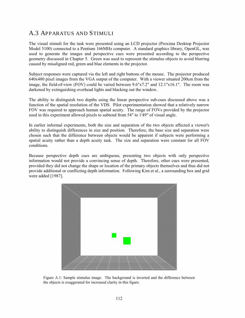
112
A.3 APPARATUS AND STIMULI
The visual stimuli for the task were presented using an LCD projector (Proxima Desktop Projector Model 5100) connected to a Pentium 166MHz computer. A standard graphics library, OpenGL, was used to generate the images and perspective cues were presented according to the perspective geometry discussed in Chapter 5. Green was used to represent the stimulus objects to avoid blurring caused by misaligned red, green and blue elements in the projector. Subject responses were captured via the left and right buttons of the mouse. The projector produced 640x480 pixel images from the VGA output of the computer. With a viewer situated 200cm from the image, the field-of-view (FOV) could be varied between 9.6°x7.2° and 12.1°x16.1°. The room was darkened by extinguishing overhead lights and blacking out the window. The ability to distinguish two depths using the linear perspective sub-cues discussed above was a function of the spatial resolution of the VDS. Pilot experimentation showed that a relatively narrow FOV was required to approach human spatial acuity. The range of FOVs provided by the projector used in this experiment allowed pixels to subtend from 54" to 1'49" of visual angle. In earlier informal experiments, both the size and separation of the two objects affected a viewer's ability to distinguish differences in size and position. Therefore, the base size and separation were chosen such that the difference between objects would be apparent if subjects were performing a spatial acuity rather than a depth acuity task. The size and separation were constant for all FOV conditions. Because perspective depth cues are ambiguous, presenting two objects with only perspective information would not provide a convincing sense of depth. Therefore, other cues were presented, provided they did not change the shape or location of the primary objects themselves and thus did not provide additional or conflicting depth information. Following Kim et al., a surrounding box and grid were added [1987].
Figure A.1: Sample stimulus image. The background is inverted and the difference between the objects is exaggerated for increased clarity in this figure.
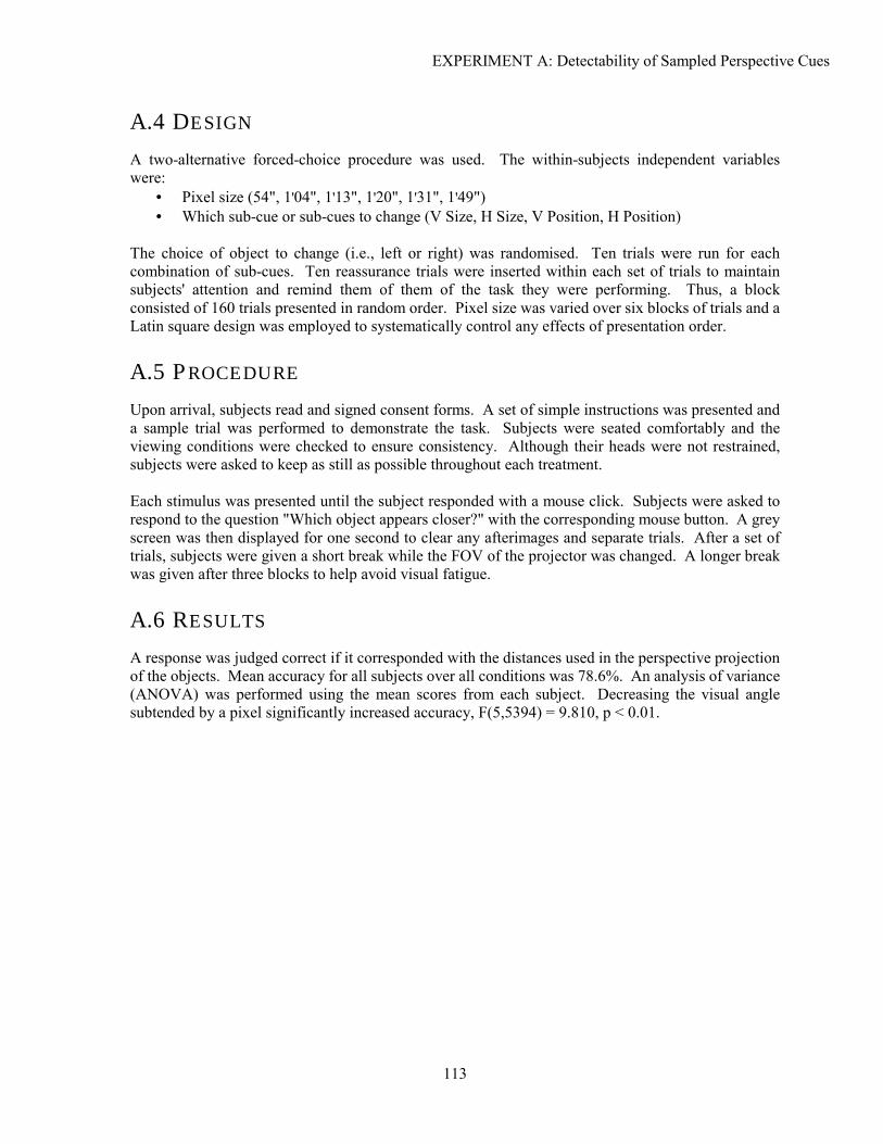
EXPERIMENT A: Detectability of Sampled Perspective Cues
113
A.4 DESIGN
A two-alternative forced-choice procedure was used. The within-subjects independent variables were:
• Pixel size (54", 1'04", 1'13", 1'20", 1'31", 1'49") • Which sub-cue or sub-cues to change (V Size, H Size, V Position, H Position)
The choice of object to change (i.e., left or right) was randomised. Ten trials were run for each combination of sub-cues. Ten reassurance trials were inserted within each set of trials to maintain subjects' attention and remind them of them of the task they were performing. Thus, a block consisted of 160 trials presented in random order. Pixel size was varied over six blocks of trials and a Latin square design was employed to systematically control any effects of presentation order.
A.5 PROCEDURE
Upon arrival, subjects read and signed consent forms. A set of simple instructions was presented and a sample trial was performed to demonstrate the task. Subjects were seated comfortably and the viewing conditions were checked to ensure consistency. Although their heads were not restrained, subjects were asked to keep as still as possible throughout each treatment. Each stimulus was presented until the subject responded with a mouse click. Subjects were asked to respond to the question "Which object appears closer?" with the corresponding mouse button. A grey screen was then displayed for one second to clear any afterimages and separate trials. After a set of trials, subjects were given a short break while the FOV of the projector was changed. A longer break was given after three blocks to help avoid visual fatigue.
A.6 RESULTS
A response was judged correct if it corresponded with the distances used in the perspective projection of the objects. Mean accuracy for all subjects over all conditions was 78.6%. An analysis of variance (ANOVA) was performed using the mean scores from each subject. Decreasing the visual angle subtended by a pixel significantly increased accuracy, F(5,5394) = 9.810, p < 0.01.
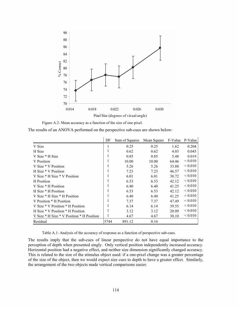
114
70
72
74
76
78
80
82
84
86
88
90
0.014 0.018 0.022 0.026 0.030
Pixel Size (degrees of visual angle)
% C
orre
ct
Figure A.2: Mean accuracy as a function of the size of one pixel.
The results of an ANOVA performed on the perspective sub-cues are shown below:
DF Sum of Squares Mean Square F-Value P-Value V Size 1 0.25 0.25 1.62 0.204 H Size 1 0.62 0.62 4.03 0.045 V Size * H Size 1 0.85 0.85 5.48 0.019 V Position 1 10.00 10.00 64.46 < 0.010 V Size * V Position 1 5.26 5.26 33.88 < 0.010 H Size * V Position 1 7.23 7.23 46.57 < 0.010 V Size * H Size * V Position 1 6.01 6.01 38.72 < 0.010 H Position 1 6.53 6.53 42.12 < 0.010 V Size * H Position 1 6.40 6.40 41.25 < 0.010 H Size * H Position 1 6.53 6.53 42.12 < 0.010 V Size * H Size * H Position 1 6.40 6.40 41.25 < 0.010 V Position * H Position 1 7.37 7.37 47.49 < 0.010 V Size * V Position * H Position 1 6.14 6.14 39.55 < 0.010 H Size * V Position * H Position 1 3.12 3.12 20.09 < 0.010 V Size * H Size * V Position * H Position 1 4.67 4.67 30.10 < 0.010 Residual 5744 891.12 0.16
Table A.1: Analysis of the accuracy of response as a function of perspective sub-cues.
The results imply that the sub-cues of linear perspective do not have equal importance to the perception of depth when presented singly. Only vertical position independently increased accuracy. Horizontal position had a negative effect, and neither size dimension significantly changed accuracy. This is related to the size of the stimulus object used: if a one-pixel change was a greater percentage of the size of the object, then we would expect size cues to depth to have a greater effect. Similarly, the arrangement of the two objects made vertical comparisons easier.

EXPERIMENT A: Detectability of Sampled Perspective Cues
115
With the exception of combined vertical and horizontal size, presenting combinations of sub-cues significantly reduced error. There was no significant interaction between pixel size and position or size. No effect was found due to subject or practice. The main results of the experiment can be summarised as:
• Decreasing pixel size reduced detectability of a fixed change in depth • Vertical position sub-cues significantly increased accuracy when presented individually; the
other sub-cues did not • Combining sub-cues increased the detectability of changes in perspective depth

116
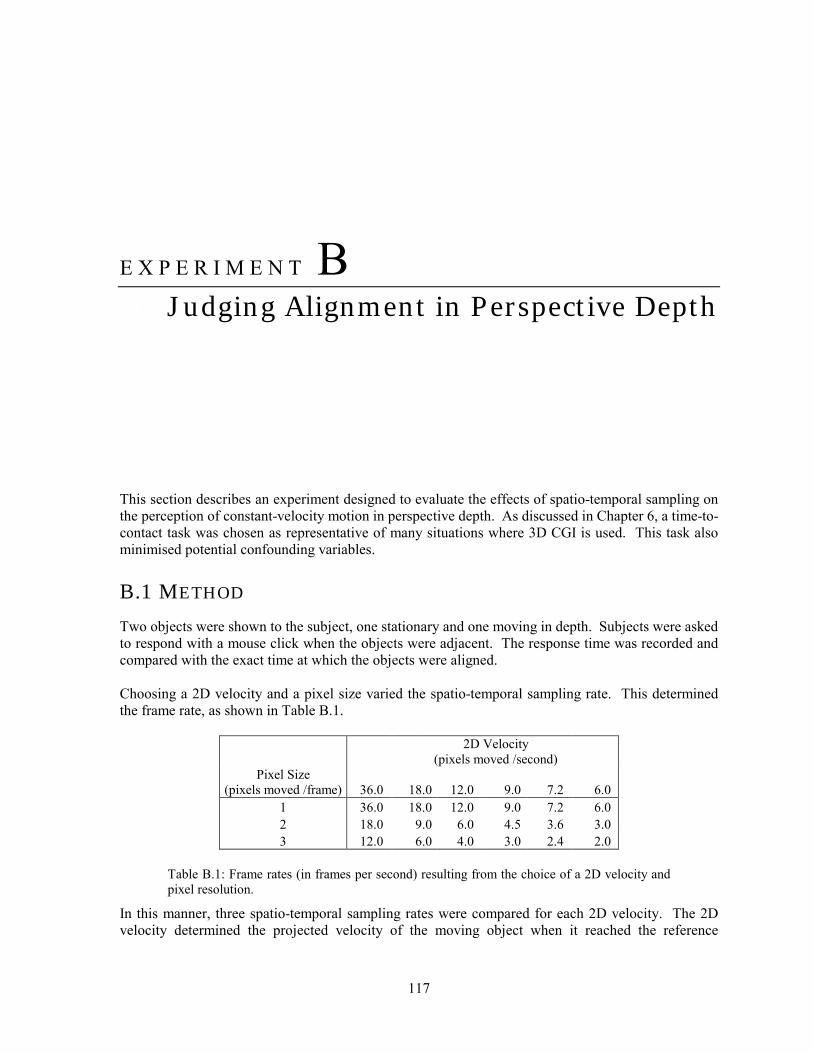
117
E X P E R I M E N T B B Judging Alignment in Perspective Depth
This section describes an experiment designed to evaluate the effects of spatio-temporal sampling on the perception of constant-velocity motion in perspective depth. As discussed in Chapter 6, a time-to-contact task was chosen as representative of many situations where 3D CGI is used. This task also minimised potential confounding variables.
B.1 METHOD
Two objects were shown to the subject, one stationary and one moving in depth. Subjects were asked to respond with a mouse click when the objects were adjacent. The response time was recorded and compared with the exact time at which the objects were aligned. Choosing a 2D velocity and a pixel size varied the spatio-temporal sampling rate. This determined the frame rate, as shown in Table B.1.
2D Velocity
(pixels moved /second) Pixel Size
(pixels moved /frame) 36.0 18.0 12.0 9.0 7.2 6.0 1 36.0 18.0 12.0 9.0 7.2 6.0 2 18.0 9.0 6.0 4.5 3.6 3.0 3 12.0 6.0 4.0 3.0 2.4 2.0
Table B.1: Frame rates (in frames per second) resulting from the choice of a 2D velocity and pixel resolution.
In this manner, three spatio-temporal sampling rates were compared for each 2D velocity. The 2D velocity determined the projected velocity of the moving object when it reached the reference
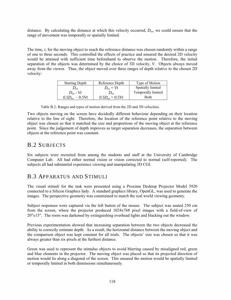
118
distance. By calculating the distance at which this velocity occurred, Dex, we could ensure that the range of movement was temporally or spatially limited. The time, t, for the moving object to reach the reference distance was chosen randomly within a range of one to three seconds. This controlled the effects of practice and ensured the desired 2D velocity would be attained with sufficient time beforehand to observe the motion. Therefore, the initial separation of the objects was determined by the choice of 3D velocity, V. Objects always moved away from the viewer. Thus, the object moved over three ranges of depth relative to the chosen 2D velocity:
Starting Depth Reference Depth Type of Motion Dex Dex + Vt Spatially limited
Dex - Vt Dex Temporally limited 0.5Dex � 0.5Vt 0.5Dex + 0.5Vt Both
Table B.2: Ranges and types of motion derived from the 2D and 3D velocities.
Two objects moving on the screen have decidedly different behaviour depending on their location relative to the line of sight. Therefore, the location of the reference point relative to the moving object was chosen so that it matched the size and proportions of the moving object at the reference point. Since the judgement of depth improves as target separation decreases, the separation between objects at the reference point was constant.
B.2 SUBJECTS
Six subjects were recruited from among the students and staff at the University of Cambridge Computer Lab. All had either normal vision or vision corrected to normal (self-reported). The subjects all had substantial experience viewing and manipulating 3D CGI.
B.3 APPARATUS AND STIMULI
The visual stimuli for the task were presented using a Proxima Desktop Projector Model 5920 connected to a Silicon Graphics Indy. A standard graphics library, OpenGL, was used to generate the images. The perspective geometry was constrained to match the real world viewing geometry. Subject responses were captured via the left button of the mouse. The subject was seated 250 cm from the screen, where the projector produced 1024x768 pixel images with a field-of-view of 20°x15°. The room was darkened by extinguishing overhead lights and blacking out the window. Previous experimentation showed that increasing separation between the two objects decreased the ability to correctly estimate depth. As a result, the horizontal distance between the moving object and the comparison object was kept constant for all trials. The objects� size was chosen so that it was always greater than six pixels at the furthest distance. Green was used to represent the stimulus objects to avoid blurring caused by misaligned red, green and blue elements in the projector. The moving object was placed so that its projected direction of motion would lie along a diagonal of the screen. This ensured the motion would be spatially limited or temporally limited in both dimensions simultaneously.
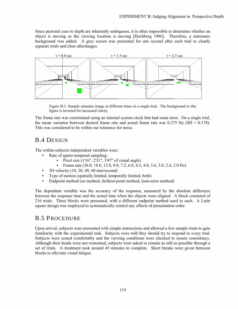
EXPERIMENT B: Judging Alignment in Perspective Depth
119
Since pictorial cues to depth are inherently ambiguous, it is often impossible to determine whether an object is moving or the viewing location is moving [Hochberg 1986]. Therefore, a stationary background was added. A grey screen was presented for one second after each trial to clearly separate trials and clear afterimages.
t = 0.0 sec t = 1.5 sec t = 2.5 sec
Figure B.1: Sample stimulus image at different times in a single trial. The background in this figure is inverted for increased clarity.
The frame rate was constrained using an internal system clock that had some error. On a single trial, the mean variation between desired frame rate and actual frame rate was 0.275 Hz (SD = 0.178). This was considered to be within our tolerance for noise.
B.4 DESIGN
The within-subjects independent variables were: • Rate of spatio-temporal sampling:
▪ Pixel size (1'16", 2'31", 3'47" of visual angle) ▪ Frame rate (36.0, 18.0, 12.0, 9.0, 7.2, 6.0, 4.5, 4.0, 3.6, 3.0, 2.4, 2.0 Hz)
• 3D velocity (10, 20, 40, 60 mm/second) • Type of motion (spatially limited, temporally limited, both) • Endpoint method (no method, furthest-point method, least-error method)
The dependent variable was the accuracy of the response, measured by the absolute difference between the response time and the actual time when the objects were aligned. A block consisted of 216 trials. Three blocks were presented, with a different endpoint method used in each. A Latin square design was employed to systematically control any effects of presentation order.
B.5 PROCEDURE
Upon arrival, subjects were presented with simple instructions and allowed a few sample trials to gain familiarity with the experimental task. Subjects were told they should try to respond to every trial. Subjects were seated comfortably and the viewing conditions were checked to ensure consistency. Although their heads were not restrained, subjects were asked to remain as still as possible through a set of trials. A treatment took around 45 minutes to complete. Short breaks were given between blocks to alleviate visual fatigue.
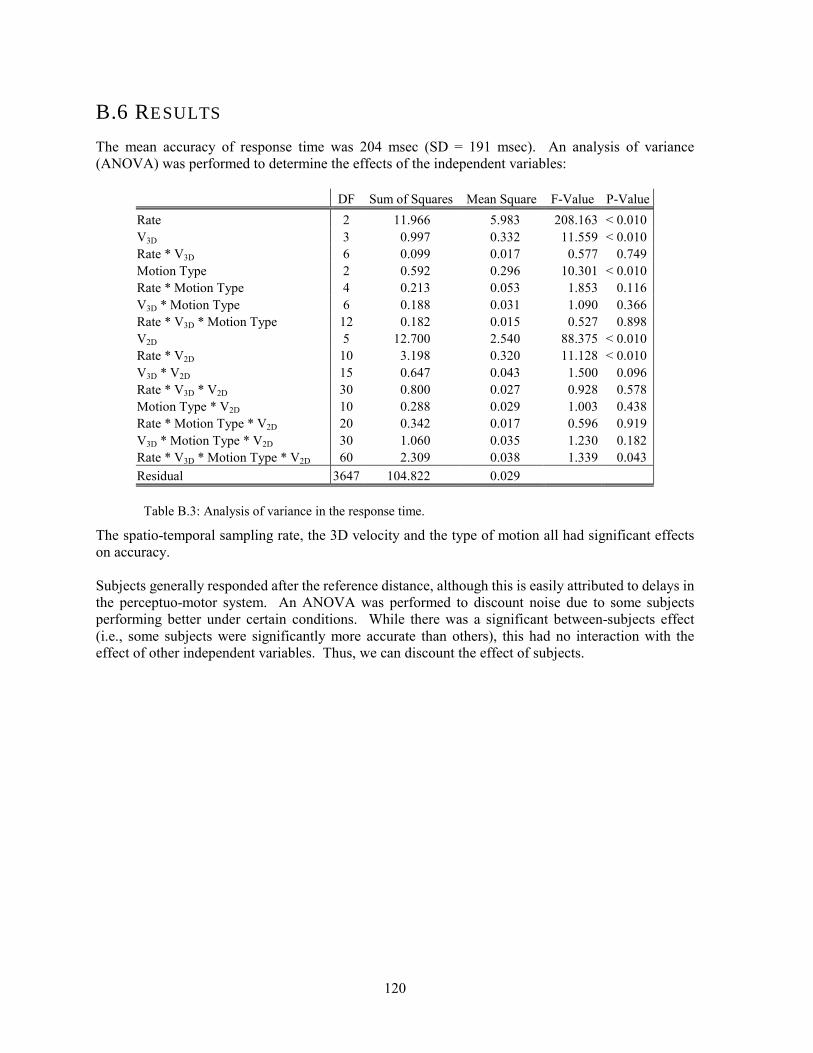
120
B.6 RESULTS
The mean accuracy of response time was 204 msec (SD = 191 msec). An analysis of variance (ANOVA) was performed to determine the effects of the independent variables:
DF Sum of Squares Mean Square F-Value P-Value Rate 2 11.966 5.983 208.163 < 0.010V3D 3 0.997 0.332 11.559 < 0.010Rate * V3D 6 0.099 0.017 0.577 0.749Motion Type 2 0.592 0.296 10.301 < 0.010Rate * Motion Type 4 0.213 0.053 1.853 0.116V3D * Motion Type 6 0.188 0.031 1.090 0.366Rate * V3D * Motion Type 12 0.182 0.015 0.527 0.898V2D 5 12.700 2.540 88.375 < 0.010Rate * V2D 10 3.198 0.320 11.128 < 0.010V3D * V2D 15 0.647 0.043 1.500 0.096Rate * V3D * V2D 30 0.800 0.027 0.928 0.578Motion Type * V2D 10 0.288 0.029 1.003 0.438Rate * Motion Type * V2D 20 0.342 0.017 0.596 0.919V3D * Motion Type * V2D 30 1.060 0.035 1.230 0.182Rate * V3D * Motion Type * V2D 60 2.309 0.038 1.339 0.043Residual 3647 104.822 0.029
Table B.3: Analysis of variance in the response time.
The spatio-temporal sampling rate, the 3D velocity and the type of motion all had significant effects on accuracy. Subjects generally responded after the reference distance, although this is easily attributed to delays in the perceptuo-motor system. An ANOVA was performed to discount noise due to some subjects performing better under certain conditions. While there was a significant between-subjects effect (i.e., some subjects were significantly more accurate than others), this had no interaction with the effect of other independent variables. Thus, we can discount the effect of subjects.
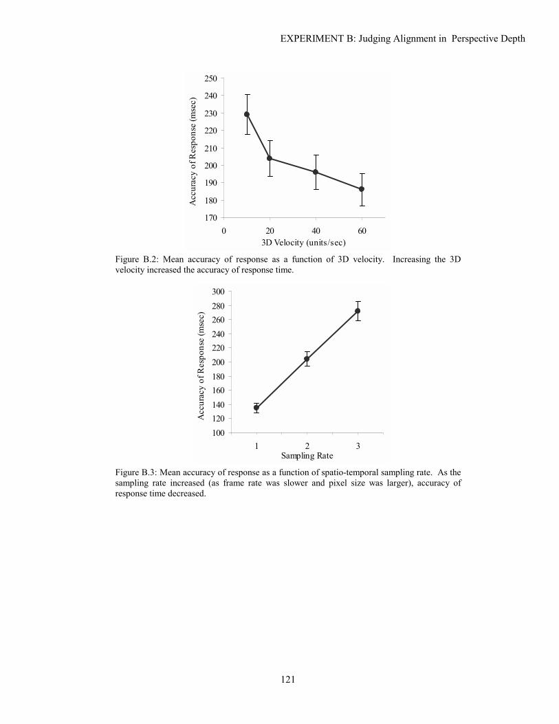
EXPERIMENT B: Judging Alignment in Perspective Depth
121
170
180
190
200
210
220
230
240
250
0 20 40 603D Velocity (units/sec)
Acc
urac
y of
Res
pons
e (m
sec)
Figure B.2: Mean accuracy of response as a function of 3D velocity. Increasing the 3D velocity increased the accuracy of response time.
100120140160180200220240260280300
1 2 3Sampling Rate
Acc
urac
y of
Res
pons
e (m
sec)
Figure B.3: Mean accuracy of response as a function of spatio-temporal sampling rate. As the sampling rate increased (as frame rate was slower and pixel size was larger), accuracy of response time decreased.
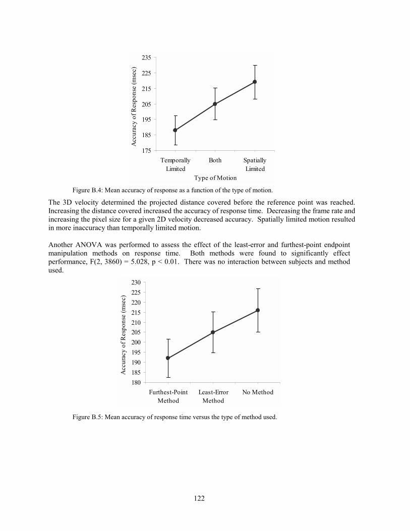
122
175
185
195
205
215
225
235
TemporallyLimited
Both SpatiallyLimited
Type of Motion
Acc
urac
y of
Res
pons
e (m
sec)
Figure B.4: Mean accuracy of response as a function of the type of motion.
The 3D velocity determined the projected distance covered before the reference point was reached. Increasing the distance covered increased the accuracy of response time. Decreasing the frame rate and increasing the pixel size for a given 2D velocity decreased accuracy. Spatially limited motion resulted in more inaccuracy than temporally limited motion. Another ANOVA was performed to assess the effect of the least-error and furthest-point endpoint manipulation methods on response time. Both methods were found to significantly effect performance, F(2, 3860) = 5.028, p < 0.01. There was no interaction between subjects and method used.
180185190195200205210215220225230
Furthest-PointMethod
Least-ErrorMethod
No Method
Acc
urac
y of
Res
pons
e (m
sec)
Figure B.5: Mean accuracy of response time versus the type of method used.

EXPERIMENT B: Judging Alignment in Perspective Depth
123
Sheffe�s post-hoc analysis method was used to find which methods were significantly different.
Mean Diff. Critical Diff. P-Value Normal vs. Furthest-Point Method 0.0238 0.184 0.007 Normal vs. Least-Error Method 0.0107 0.184 0.364 Furthest-Point Method vs. Least-Error Method -0.0131 0.183 0.216
Table B.4: Results of a Sheffe post-hoc analysis.
Only the difference between using no method and the furthest-point method was significant within a 5% confidence interval. This suggests that only the furthest-point method significantly improved performance. We can state the significant results as follows:
• Decreasing the spatio-temporal sampling rate (i.e., lowering the frame rate and increasing the pixel size) decreased accuracy.
• Decreasing the projected distance moved before the reference point was reached decreased accuracy.
• Spatially-limited motion was less accurate than temporally-limited motion. • Using an endpoint method significantly improved performance. • Post-hoc analysis showed that only the furthest-point manipulation showed a significant
improvement over using no method.

124
125
E X P E R I M E N T C C Interactive Alignment in Depth
This section describes an experiment to determine the effect of varying the spatial sampling rate in an interactive task. Furthermore, we want to establish the value of traditional antialiasing techniques for the same task.
C.1 METHOD
The task chosen was similar to the one used in other depth acuity experiments [Drascic & Milgram 1991; Graham 1951; Nagata 1993]. The subject used the mouse to move one object to match the depth of a stationary object. The movement of the mouse was in the same axis as the movement on the display (i.e., to and from the viewer). The spatial sampling rate was varied from typical values for desktop viewing to typical values for low to mid-range HMDs. Perspective geometry predicts that accuracy in 3D will decrease with increased distance from the viewer. Therefore, using only accuracy in depth as a measure may confound the experiment. Therefore, we sum the differences in the four perspective sub-cues (vertical and horizontal position and size) to obtain the projected or 2D accuracy. The antialiased cases were treated as having sub-pixel steps whose size depended on the rate of supersampling. This implies that accuracy in 2D will measure the ability to match the 2D size and position of the two objects.
C.2 SUBJECTS
Six subjects were recruited from among the students and staff at the University of Cambridge Computer Lab. All had either normal vision or vision corrected to normal (self-reported). The subjects all had substantial experience viewing and manipulating 3D CGI.
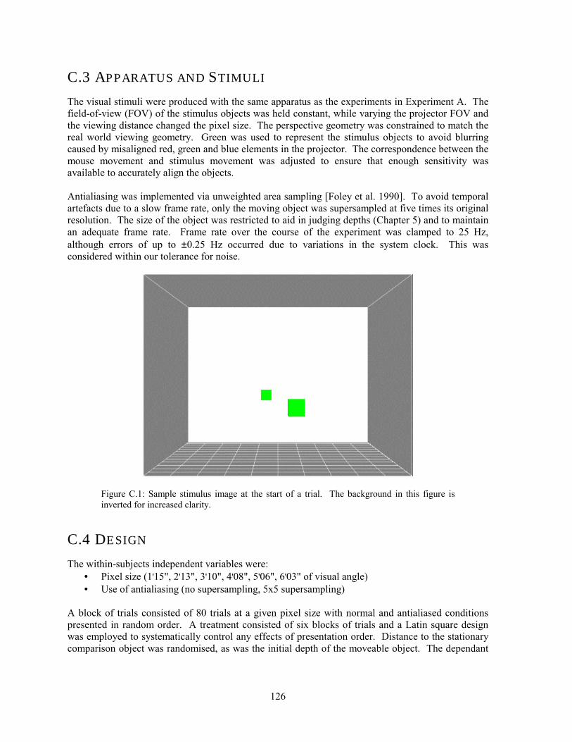
126
C.3 APPARATUS AND STIMULI
The visual stimuli were produced with the same apparatus as the experiments in Experiment A. The field-of-view (FOV) of the stimulus objects was held constant, while varying the projector FOV and the viewing distance changed the pixel size. The perspective geometry was constrained to match the real world viewing geometry. Green was used to represent the stimulus objects to avoid blurring caused by misaligned red, green and blue elements in the projector. The correspondence between the mouse movement and stimulus movement was adjusted to ensure that enough sensitivity was available to accurately align the objects. Antialiasing was implemented via unweighted area sampling [Foley et al. 1990]. To avoid temporal artefacts due to a slow frame rate, only the moving object was supersampled at five times its original resolution. The size of the object was restricted to aid in judging depths (Chapter 5) and to maintain an adequate frame rate. Frame rate over the course of the experiment was clamped to 25 Hz, although errors of up to ±0.25 Hz occurred due to variations in the system clock. This was considered within our tolerance for noise.
Figure C.1: Sample stimulus image at the start of a trial. The background in this figure is inverted for increased clarity.
C.4 DESIGN
The within-subjects independent variables were: • Pixel size (1'15", 2'13", 3'10", 4'08", 5'06", 6'03" of visual angle) • Use of antialiasing (no supersampling, 5x5 supersampling)
A block of trials consisted of 80 trials at a given pixel size with normal and antialiased conditions presented in random order. A treatment consisted of six blocks of trials and a Latin square design was employed to systematically control any effects of presentation order. Distance to the stationary comparison object was randomised, as was the initial depth of the moveable object. The dependant
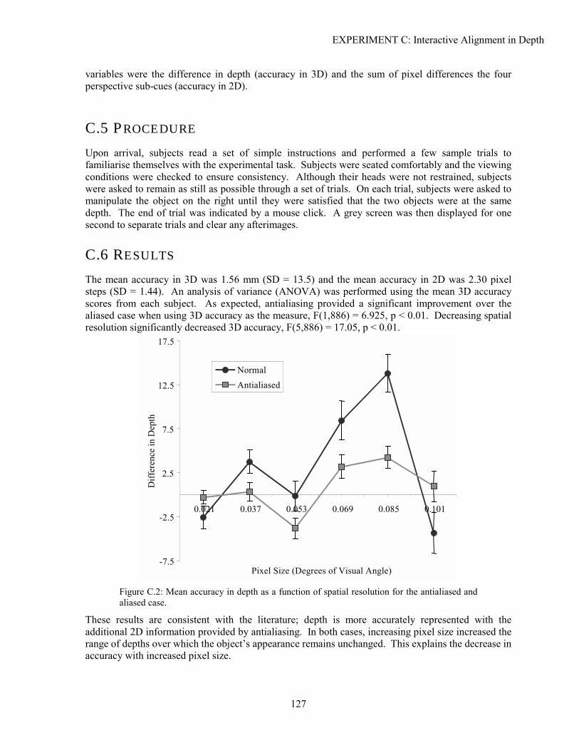
EXPERIMENT C: Interactive Alignment in Depth
127
variables were the difference in depth (accuracy in 3D) and the sum of pixel differences the four perspective sub-cues (accuracy in 2D).
C.5 PROCEDURE
Upon arrival, subjects read a set of simple instructions and performed a few sample trials to familiarise themselves with the experimental task. Subjects were seated comfortably and the viewing conditions were checked to ensure consistency. Although their heads were not restrained, subjects were asked to remain as still as possible through a set of trials. On each trial, subjects were asked to manipulate the object on the right until they were satisfied that the two objects were at the same depth. The end of trial was indicated by a mouse click. A grey screen was then displayed for one second to separate trials and clear any afterimages.
C.6 RESULTS
The mean accuracy in 3D was 1.56 mm (SD = 13.5) and the mean accuracy in 2D was 2.30 pixel steps (SD = 1.44). An analysis of variance (ANOVA) was performed using the mean 3D accuracy scores from each subject. As expected, antialiasing provided a significant improvement over the aliased case when using 3D accuracy as the measure, F(1,886) = 6.925, p < 0.01. Decreasing spatial resolution significantly decreased 3D accuracy, F(5,886) = 17.05, p < 0.01.
-7.5
-2.5
2.5
7.5
12.5
17.5
0.021 0.037 0.053 0.069 0.085 0.101
Pixel Size (Degrees of Visual Angle)
Diff
eren
ce in
Dep
th
Normal Antialiased
Figure C.2: Mean accuracy in depth as a function of spatial resolution for the antialiased and aliased case.
These results are consistent with the literature; depth is more accurately represented with the additional 2D information provided by antialiasing. In both cases, increasing pixel size increased the range of depths over which the object�s appearance remains unchanged. This explains the decrease in accuracy with increased pixel size.
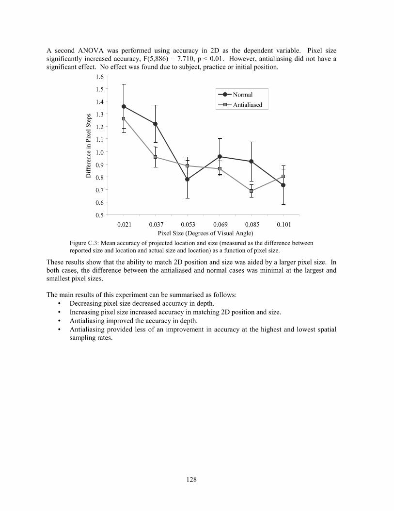
128
A second ANOVA was performed using accuracy in 2D as the dependent variable. Pixel size significantly increased accuracy, F(5,886) = 7.710, p < 0.01. However, antialiasing did not have a significant effect. No effect was found due to subject, practice or initial position.
0.5
0.6
0.7
0.8
0.9
1.0
1.1
1.2
1.3
1.4
1.5
1.6
0.021 0.037 0.053 0.069 0.085 0.101Pixel Size (Degrees of Visual Angle)
Diff
eren
ce in
Pix
el S
teps
Normal Antialiased
Figure C.3: Mean accuracy of projected location and size (measured as the difference between reported size and location and actual size and location) as a function of pixel size.
These results show that the ability to match 2D position and size was aided by a larger pixel size. In both cases, the difference between the antialiased and normal cases was minimal at the largest and smallest pixel sizes. The main results of this experiment can be summarised as follows:
• Decreasing pixel size decreased accuracy in depth. • Increasing pixel size increased accuracy in matching 2D position and size. • Antialiasing improved the accuracy in depth. • Antialiasing provided less of an improvement in accuracy at the highest and lowest spatial
sampling rates.
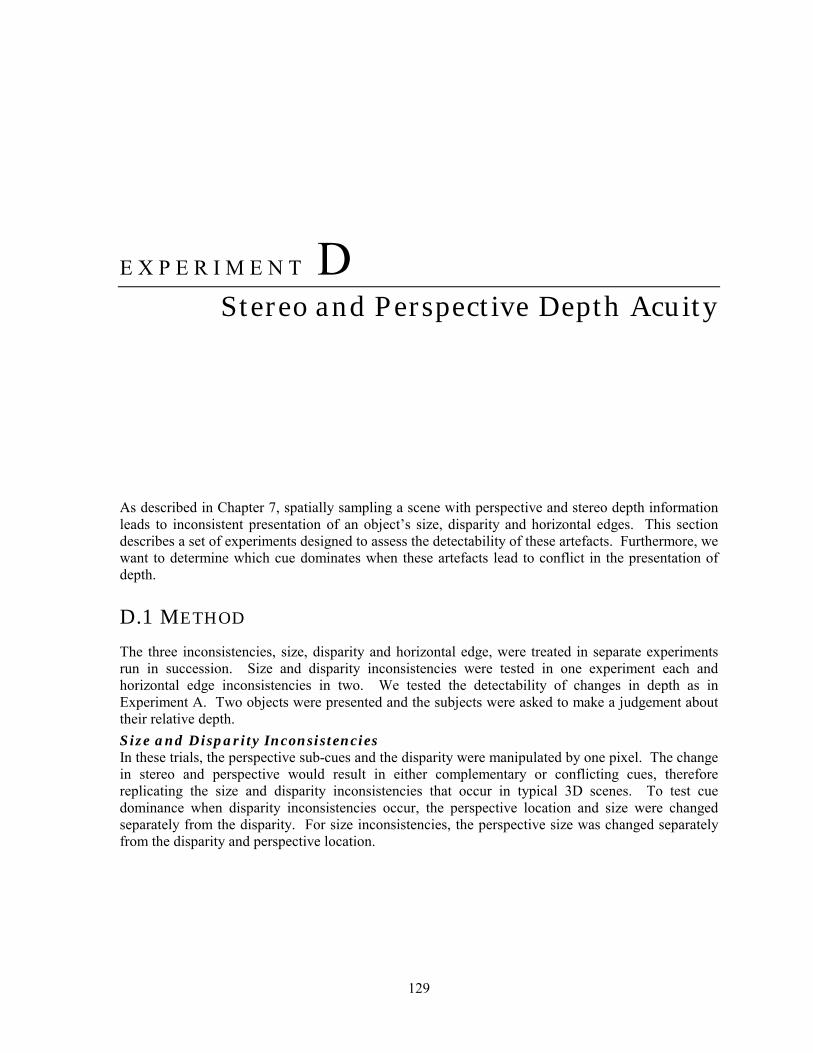
129
E X P E R I M E N T D D Stereo and Perspective Depth Acuity
As described in Chapter 7, spatially sampling a scene with perspective and stereo depth information leads to inconsistent presentation of an object�s size, disparity and horizontal edges. This section describes a set of experiments designed to assess the detectability of these artefacts. Furthermore, we want to determine which cue dominates when these artefacts lead to conflict in the presentation of depth.
D.1 METHOD
The three inconsistencies, size, disparity and horizontal edge, were treated in separate experiments run in succession. Size and disparity inconsistencies were tested in one experiment each and horizontal edge inconsistencies in two. We tested the detectability of changes in depth as in Experiment A. Two objects were presented and the subjects were asked to make a judgement about their relative depth. Size and Disparity Inconsistencies In these trials, the perspective sub-cues and the disparity were manipulated by one pixel. The change in stereo and perspective would result in either complementary or conflicting cues, therefore replicating the size and disparity inconsistencies that occur in typical 3D scenes. To test cue dominance when disparity inconsistencies occur, the perspective location and size were changed separately from the disparity. For size inconsistencies, the perspective size was changed separately from the disparity and perspective location.
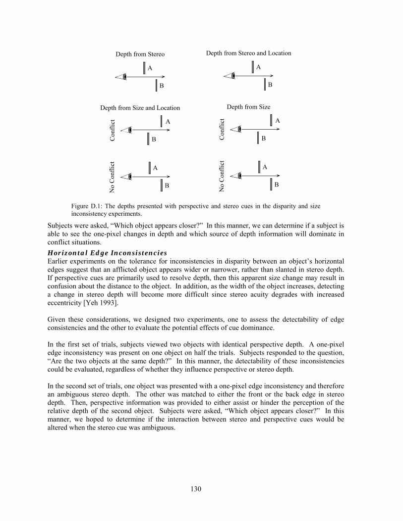
130
A
B
Depth from Stereo
Depth from Size and LocationC
onfli
ct A
B
A
B
No
Con
flict
A
B
Depth from Stereo and Location
Depth from Size
Con
flict A
B
A
B
No
Con
flict
Figure D.1: The depths presented with perspective and stereo cues in the disparity and size inconsistency experiments.
Subjects were asked, �Which object appears closer?� In this manner, we can determine if a subject is able to see the one-pixel changes in depth and which source of depth information will dominate in conflict situations. Horizontal Edge Inconsistencies Earlier experiments on the tolerance for inconsistencies in disparity between an object�s horizontal edges suggest that an afflicted object appears wider or narrower, rather than slanted in stereo depth. If perspective cues are primarily used to resolve depth, then this apparent size change may result in confusion about the distance to the object. In addition, as the width of the object increases, detecting a change in stereo depth will become more difficult since stereo acuity degrades with increased eccentricity [Yeh 1993]. Given these considerations, we designed two experiments, one to assess the detectability of edge consistencies and the other to evaluate the potential effects of cue dominance. In the first set of trials, subjects viewed two objects with identical perspective depth. A one-pixel edge inconsistency was present on one object on half the trials. Subjects responded to the question, �Are the two objects at the same depth?� In this manner, the detectability of these inconsistencies could be evaluated, regardless of whether they influence perspective or stereo depth. In the second set of trials, one object was presented with a one-pixel edge inconsistency and therefore an ambiguous stereo depth. The other was matched to either the front or the back edge in stereo depth. Then, perspective information was provided to either assist or hinder the perception of the relative depth of the second object. Subjects were asked, �Which object appears closer?� In this manner, we hoped to determine if the interaction between stereo and perspective cues would be altered when the stereo cue was ambiguous.
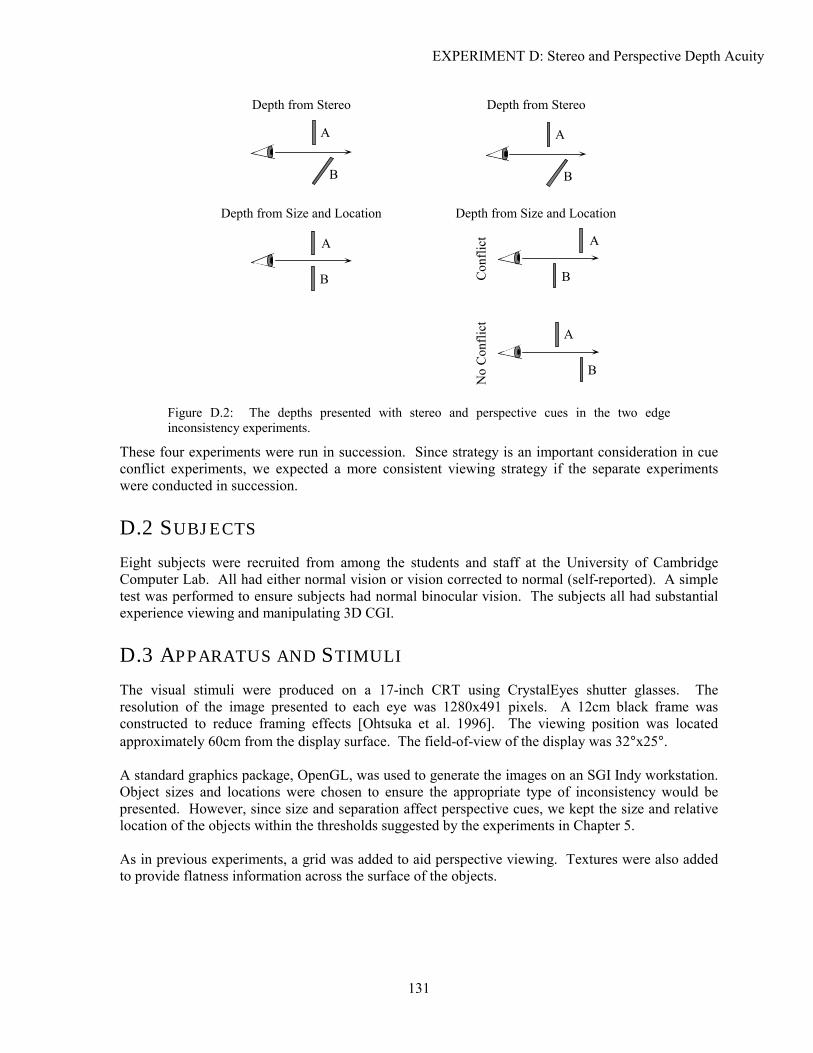
EXPERIMENT D: Stereo and Perspective Depth Acuity
131
Depth from Stereo
Depth from Size and Location
B
A
B
A
Depth from Stereo
Depth from Size and Location
Con
flict A
B
A
B
No
Con
flict
B
A
Figure D.2: The depths presented with stereo and perspective cues in the two edge inconsistency experiments.
These four experiments were run in succession. Since strategy is an important consideration in cue conflict experiments, we expected a more consistent viewing strategy if the separate experiments were conducted in succession.
D.2 SUBJECTS
Eight subjects were recruited from among the students and staff at the University of Cambridge Computer Lab. All had either normal vision or vision corrected to normal (self-reported). A simple test was performed to ensure subjects had normal binocular vision. The subjects all had substantial experience viewing and manipulating 3D CGI.
D.3 APPARATUS AND STIMULI
The visual stimuli were produced on a 17-inch CRT using CrystalEyes shutter glasses. The resolution of the image presented to each eye was 1280x491 pixels. A 12cm black frame was constructed to reduce framing effects [Ohtsuka et al. 1996]. The viewing position was located approximately 60cm from the display surface. The field-of-view of the display was 32°x25°. A standard graphics package, OpenGL, was used to generate the images on an SGI Indy workstation. Object sizes and locations were chosen to ensure the appropriate type of inconsistency would be presented. However, since size and separation affect perspective cues, we kept the size and relative location of the objects within the thresholds suggested by the experiments in Chapter 5. As in previous experiments, a grid was added to aid perspective viewing. Textures were also added to provide flatness information across the surface of the objects.
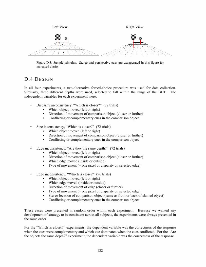
132
Left View Right View
Figure D.3: Sample stimulus. Stereo and perspective cues are exaggerated in this figure for increased clarity.
D.4 DESIGN
In all four experiments, a two-alternative forced-choice procedure was used for data collection. Similarly, three different depths were used, selected to fall within the range of the BDT. The independent variables for each experiment were:
• Disparity inconsistency, �Which is closer?� (72 trials) ▪ Which object moved (left or right) ▪ Direction of movement of comparison object (closer or further) ▪ Conflicting or complementary cues in the comparison object
• Size inconsistency, �Which is closer?� (72 trials)
▪ Which object moved (left or right) ▪ Direction of movement of comparison object (closer or further) ▪ Conflicting or complementary cues in the comparison object
• Edge inconsistency, �Are they the same depth?� (72 trials)
▪ Which object moved (left or right) ▪ Direction of movement of comparison object (closer or further) ▪ Which edge moved (inside or outside) ▪ Type of movement (± one pixel of disparity on selected edge)
• Edge inconsistency, �Which is closer?� (96 trials)
▪ Which object moved (left or right) ▪ Which edge moved (inside or outside) ▪ Direction of movement of edge (closer or further) ▪ Type of movement (± one pixel of disparity on selected edge) ▪ Stereo location of comparison object (same as front or back of slanted object) ▪ Conflicting or complementary cues in the comparison object
These cases were presented in random order within each experiment. Because we wanted any development of strategy to be consistent across all subjects, the experiments were always presented in the same order. For the �Which is closer?� experiments, the dependent variable was the correctness of the response when the cues were complementary and which cue dominated when the cues conflicted. For the �Are the objects the same depth?� experiment, the dependent variable was the correctness of the response.
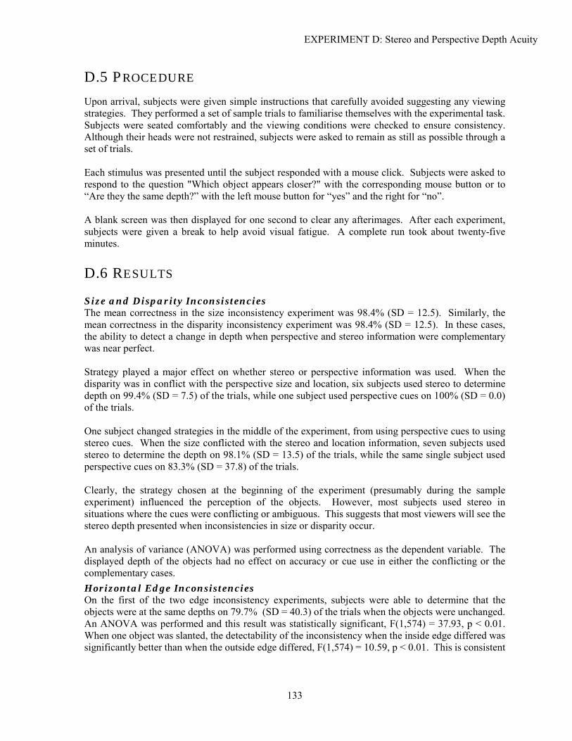
EXPERIMENT D: Stereo and Perspective Depth Acuity
133
D.5 PROCEDURE
Upon arrival, subjects were given simple instructions that carefully avoided suggesting any viewing strategies. They performed a set of sample trials to familiarise themselves with the experimental task. Subjects were seated comfortably and the viewing conditions were checked to ensure consistency. Although their heads were not restrained, subjects were asked to remain as still as possible through a set of trials. Each stimulus was presented until the subject responded with a mouse click. Subjects were asked to respond to the question "Which object appears closer?" with the corresponding mouse button or to �Are they the same depth?� with the left mouse button for �yes� and the right for �no�. A blank screen was then displayed for one second to clear any afterimages. After each experiment, subjects were given a break to help avoid visual fatigue. A complete run took about twenty-five minutes.
D.6 RESULTS
Size and Disparity Inconsistencies The mean correctness in the size inconsistency experiment was 98.4% (SD = 12.5). Similarly, the mean correctness in the disparity inconsistency experiment was 98.4% (SD = 12.5). In these cases, the ability to detect a change in depth when perspective and stereo information were complementary was near perfect. Strategy played a major effect on whether stereo or perspective information was used. When the disparity was in conflict with the perspective size and location, six subjects used stereo to determine depth on 99.4% (SD = 7.5) of the trials, while one subject used perspective cues on 100% (SD = 0.0) of the trials. One subject changed strategies in the middle of the experiment, from using perspective cues to using stereo cues. When the size conflicted with the stereo and location information, seven subjects used stereo to determine the depth on 98.1% (SD = 13.5) of the trials, while the same single subject used perspective cues on 83.3% (SD = 37.8) of the trials. Clearly, the strategy chosen at the beginning of the experiment (presumably during the sample experiment) influenced the perception of the objects. However, most subjects used stereo in situations where the cues were conflicting or ambiguous. This suggests that most viewers will see the stereo depth presented when inconsistencies in size or disparity occur. An analysis of variance (ANOVA) was performed using correctness as the dependent variable. The displayed depth of the objects had no effect on accuracy or cue use in either the conflicting or the complementary cases. Horizontal Edge Inconsistencies On the first of the two edge inconsistency experiments, subjects were able to determine that the objects were at the same depths on 79.7% (SD = 40.3) of the trials when the objects were unchanged. An ANOVA was performed and this result was statistically significant, F(1,574) = 37.93, p < 0.01. When one object was slanted, the detectability of the inconsistency when the inside edge differed was significantly better than when the outside edge differed, F(1,574) = 10.59, p < 0.01. This is consistent

134
with our expectation that the inner edge will dominate the comparison since stereo acuity decreases with increased eccentricity. The depth of the objects had no effect on accuracy. The second edge inconsistency experiment had no significant results. Subjects were either guessing on most cases or the effects of the various conditions were too subtle to show up in the statistical analysis. While subjects reported some visual fatigue and discomfort after all four experiments, they especially mentioned difficulties after the two edge inconsistency experiments. The main results of each experiment can be summarised as:
• Disparity inconsistency, �Which is closer?�: ▪ Complementary stereo and perspective cues resulted in near-perfect accuracy ▪ Stereo cues dominated perspective cues in conflict situations
• Size inconsistency, �Which is closer?�:
▪ Complementary stereo and perspective cues resulted in near-perfect accuracy ▪ Stereo cues dominated perspective cues in conflict situations
• Edge inconsistency, �Are they at the same depth?�:
▪ Complementary stereo and perspective cues improved accuracy ▪ Differences in the inner edges of the objects were more detectable than differences in
the outer edges of the objects ▪ Subjects reported visual discomfort
• Edge inconsistency, �Which is closer?�: ▪ No statistically significant results ▪ Subjects reported visual discomfort
135
E X P E R I M E N T E E Judging Alignment in Stereo and
Perspective Depth
This section describes an experiment designed to evaluate the effects of spatio-temporal sampling on the perception of constant-velocity motion in perspective and stereo depth. A time-to-contact (TTC) task was chosen to mirror the methodology used in Experiment B and Chapter 6. In addition, we tested the endpoint manipulation methods designed for use in stereo and perspective imagery.
E.1 METHOD
The TTC task used was the same as in Experiment B. Two objects were shown to the subject, one stationary and one moving in depth. Subjects were asked to respond with a mouse click when the two objects were adjacent. Accuracy was measured in two ways. Accuracy in time was the absolute difference between the time at which the objects were adjacent and the response time. Similarly, accuracy in depth was the absolute difference between the depth of the reference object and the depth at which a response was given. Unlike the previous TTC experiment (Experiment B), the pixel size and frame rate were varied independently. Given that the six points that define a stereo object experience ranges of spatially and temporally limited motion at different times, designing the experiment to independently investigate these types of motion was impossible. This also simplified the experiment and subsequent analyses. The binocular disparity threshold (BDT) limited the range in depth over which a movement occurred. Violating the BDT would introduce visual fatigue. The starting point of the moving object was chosen such that it would reach the reference point in one to two seconds after the beginning of the trial. The exact time was randomised to avoid training effects. All trials were conducted with the object moving away from the viewer. The object continued to move beyond the reference point for
136
two seconds before terminating the trial if no response was given. Fixing the amount of time meant that the location of the reference point, combined with the 3D velocity, would describe the number of steps in perspective and stereo depth that would be shown. Two endpoint manipulation methods were used, the furthest-point method and the midpoint method. These are described in detail in Chapter 7.
E.2 SUBJECTS
Six subjects were recruited from among the students and staff at the University of Cambridge Computer Lab. All had either normal vision or vision corrected to normal (self-reported). A simple test was performed to ensure subjects had normal binocular vision. The subjects all had substantial experience viewing and manipulating 3D CGI.
E.3 APPARATUS AND STIMULI
The visual stimuli were produced on a 17-inch CRT using CrystalEyes shutter glasses. The resolution of the image presented to each eye was 1280x491 pixels. A 12cm black frame was used to remove potential framing effects [Ohtsuka et al. 1996]. The viewing position was located approximately 50cm from the display surface. Given a BDT of ±1.5°, the maximum disparity displayed was ±8 pixels. The FOV of the display was 32°x25°. A standard graphics package, OpenGL, was used to generate the images on an SGI Indy workstation. Object locations were chosen so as present a typical perspective path that contains inconsistencies in both vertical and horizontal size. The horizontal location of the reference object was calculated so that the separation of the two objects at the depth of the reference object was the same over all trials. Similarly, the size of the reference object was adjusted to match the moving object at the reference distance. To avoid problems caused by phosphor persistence between the left and right views, the stimulus objects were coloured red. Informal experimentation demonstrated that red phosphors had a faster decay time than the green or blue phosphors on the CRT used. As in previous experiments, a surrounding box and grid were added to improve the overall sense of depth. The surround was constructed to avoid interference or overlap with the reference and target objects.
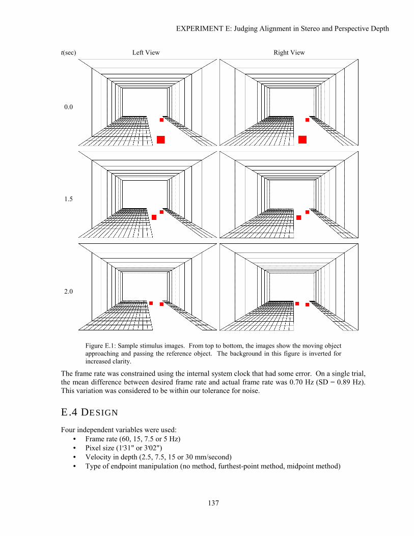
EXPERIMENT E: Judging Alignment in Stereo and Perspective Depth
137
t(sec) Left View Right View
0.0
1.5
2.0
Figure E.1: Sample stimulus images. From top to bottom, the images show the moving object approaching and passing the reference object. The background in this figure is inverted for increased clarity.
The frame rate was constrained using the internal system clock that had some error. On a single trial, the mean difference between desired frame rate and actual frame rate was 0.70 Hz (SD = 0.89 Hz). This variation was considered to be within our tolerance for noise.
E.4 DESIGN
Four independent variables were used: • Frame rate (60, 15, 7.5 or 5 Hz) • Pixel size (1'31" or 3'02") • Velocity in depth (2.5, 7.5, 15 or 30 mm/second) • Type of endpoint manipulation (no method, furthest-point method, midpoint method)
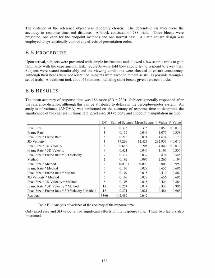
138
The distance of the reference object was randomly chosen. The dependent variables were the accuracy in response time and distance. A block consisted of 288 trials. Three blocks were presented, one each for the endpoint methods and one normal case. A Latin square design was employed to systematically control any effects of presentation order.
E.5 PROCEDURE
Upon arrival, subjects were presented with simple instructions and allowed a few sample trials to gain familiarity with the experimental task. Subjects were told they should try to respond to every trial. Subjects were seated comfortably and the viewing conditions were checked to ensure consistency. Although their heads were not restrained, subjects were asked to remain as still as possible through a set of trials. A treatment took about 45 minutes, including short breaks given between blocks.
E.6 RESULTS
The mean accuracy of response time was 186 msec (SD = 230). Subjects generally responded after the reference distance, although this can be attributed to delays in the perceptuo-motor system. An analysis of variance (ANOVA) was performed on the accuracy of response time to determine the significance of the changes in frame rate, pixel size, 3D velocity and endpoint manipulation method:
DF Sum of Squares Mean Square F-Value P-Value Pixel Size 1 0.375 0.375 8.850 < 0.010 Frame Rate 3 0.137 0.046 1.075 0.358 Pixel Size * Frame Rate 3 0.213 0.071 1.674 0.170 3D Velocity 3 37.269 12.423 292.956 < 0.010 Pixel Size * 3D Velocity 3 0.616 0.205 4.840 < 0.010 Frame Rate * 3D Velocity 9 0.421 0.047 1.103 0.357 Pixel Size * Frame Rate * 3D Velocity 9 0.334 0.037 0.874 0.548 Method 2 0.192 0.096 2.266 0.104 Pixel Size * Method 2 0.0003 0.0001 0.003 0.997 Frame Rate * Method 6 0.167 0.028 0.655 0.686 Pixel Size * Frame Rate * Method 6 0.107 0.018 0.419 0.867 3D Velocity * Method 6 0.167 0.028 0.656 0.685 Pixel Size * 3D Velocity * Method 6 0.108 0.018 0.424 0.864 Frame Rate * 3D Velocity * Method 18 0.254 0.014 0.333 0.996 Pixel Size * Frame Rate * 3D Velocity * Method 18 0.371 0.021 0.486 0.965 Residual 3360 142.482 0.042
Table E.1: Analysis of variance of the accuracy of the response time.
Only pixel size and 3D velocity had significant effects on the response time. These two factors also interacted.
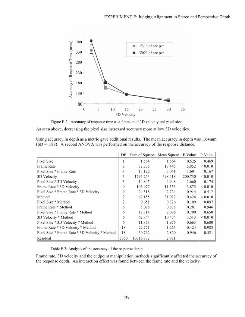
EXPERIMENT E: Judging Alignment in Stereo and Perspective Depth
139
80
130
180
230
280
330
380
0 5 10 15 20 25 30 35 3D Velocity ( / )
Acc
urac
y of
Res
pons
e Ti
me
(mse
c)
1'31" of arc per i l3'02" of arc per i l
Figure E.2: Accuracy of response time as a function of 3D velocity and pixel size.
As seen above, decreasing the pixel size increased accuracy more at low 3D velocities. Using accuracy in depth as a metric gave additional results. The mean accuracy in depth was 1.64mm (SD = 1.88). A second ANOVA was performed on the accuracy of the response distance: DF Sum of Squares Mean Square F-Value P-ValuePixel Size 1 1.564 1.564 0.525 0.469 Frame Rate 3 52.335 17.445 5.852 < 0.010 Pixel Size * Frame Rate 3 15.122 5.041 1.691 0.167 3D Velocity 3 1795.253 598.418 200.730 < 0.010 Pixel Size * 3D Velocity 3 14.845 4.948 1.660 0.174 Frame Rate * 3D Velocity 9 103.977 11.553 3.875 < 0.010 Pixel Size * Frame Rate * 3D Velocity 9 24.518 2.724 0.914 0.512 Method 2 62.155 31.077 10.424 < 0.010 Pixel Size * Method 2 0.651 0.326 0.109 0.897 Frame Rate * Method 6 5.028 0.838 0.281 0.946 Pixel Size * Frame Rate * Method 6 12.514 2.086 0.700 0.650 3D Velocity * Method 6 62.844 10.474 3.513 < 0.010 Pixel Size * 3D Velocity * Method 6 11.853 1.976 0.663 0.680 Frame Rate * 3D Velocity * Method 18 22.771 1.265 0.424 0.983 Pixel Size * Frame Rate * 3D Velocity * Method 18 50.762 2.820 0.946 0.521 Residual 3360 10016.872 2.981
Table E.2: Analysis of the accuracy of the response depth.
Frame rate, 3D velocity and the endpoint manipulation methods significantly affected the accuracy of the response depth. An interaction effect was found between the frame rate and the velocity.
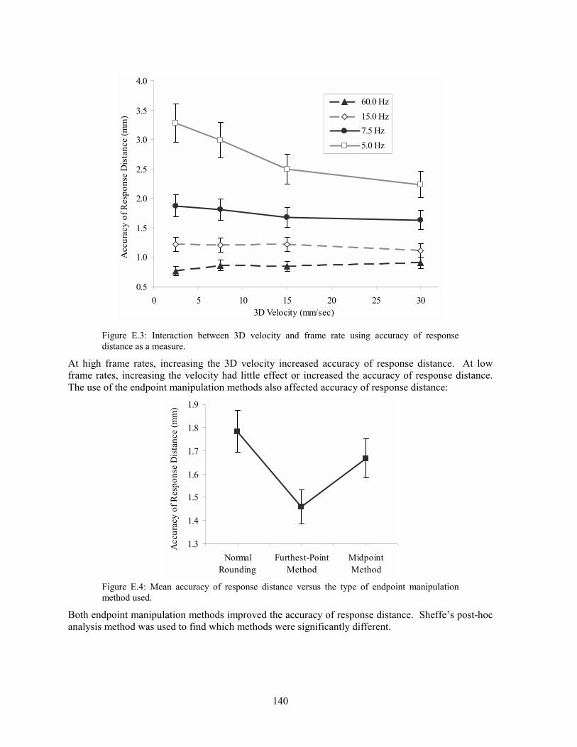
140
0.5
1.0
1.5
2.0
2.5
3.0
3.5
4.0
0 5 10 15 20 25 303D Velocity (mm/sec)
Acc
urac
y of
Res
pons
e D
ista
nce
(mm
)
60.0 Hz15.0 Hz7.5 Hz5.0 Hz
Figure E.3: Interaction between 3D velocity and frame rate using accuracy of response distance as a measure.
At high frame rates, increasing the 3D velocity increased accuracy of response distance. At low frame rates, increasing the velocity had little effect or increased the accuracy of response distance. The use of the endpoint manipulation methods also affected accuracy of response distance:
1.3
1.4
1.5
1.6
1.7
1.8
1.9
NormalRounding
Furthest-PointMethod
MidpointMethod
Acc
urac
y of
Res
pons
e D
ista
nce
(mm
)
Figure E.4: Mean accuracy of response distance versus the type of endpoint manipulation method used.
Both endpoint manipulation methods improved the accuracy of response distance. Sheffe�s post-hoc analysis method was used to find which methods were significantly different.
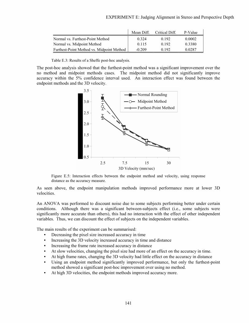
EXPERIMENT E: Judging Alignment in Stereo and Perspective Depth
141
Mean Diff. Critical Diff. P-Value Normal vs. Furthest-Point Method 0.324 0.192 0.0002 Normal vs. Midpoint Method 0.115 0.192 0.3380 Furthest-Point Method vs. Midpoint Method -0.209 0.192 0.0287
Table E.3: Results of a Sheffe post-hoc analysis.
The post-hoc analysis showed that the furthest-point method was a significant improvement over the no method and midpoint methods cases. The midpoint method did not significantly improve accuracy within the 5% confidence interval used. An interaction effect was found between the endpoint methods and the 3D velocity.
0.5
1.0
1.5
2.0
2.5
3.0
3.5
2.5 7.5 15 30 3D Velocity (mm/sec)
Normal Rounding
Midpoint Method Furthest-Point Method
Figure E.5: Interaction effects between the endpoint method and velocity, using response distance as the accuracy measure.
As seen above, the endpoint manipulation methods improved performance more at lower 3D velocities. An ANOVA was performed to discount noise due to some subjects performing better under certain conditions. Although there was a significant between-subjects effect (i.e., some subjects were significantly more accurate than others), this had no interaction with the effect of other independent variables. Thus, we can discount the effect of subjects on the independent variables. The main results of the experiment can be summarised:
• Decreasing the pixel size increased accuracy in time • Increasing the 3D velocity increased accuracy in time and distance • Increasing the frame rate increased accuracy in distance • At slow velocities, changing the pixel size had more of an effect on the accuracy in time. • At high frame rates, changing the 3D velocity had little effect on the accuracy in distance • Using an endpoint method significantly improved performance, but only the furthest-point
method showed a significant post-hoc improvement over using no method. • At high 3D velocities, the endpoint methods improved accuracy more.

142
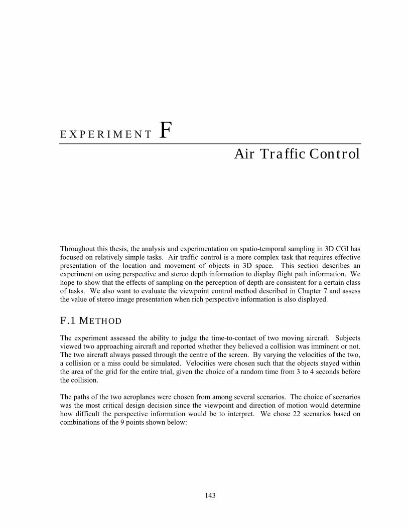
143
E X P E R I M E N T F F Air Traffic Control
Throughout this thesis, the analysis and experimentation on spatio-temporal sampling in 3D CGI has focused on relatively simple tasks. Air traffic control is a more complex task that requires effective presentation of the location and movement of objects in 3D space. This section describes an experiment on using perspective and stereo depth information to display flight path information. We hope to show that the effects of sampling on the perception of depth are consistent for a certain class of tasks. We also want to evaluate the viewpoint control method described in Chapter 7 and assess the value of stereo image presentation when rich perspective information is also displayed.
F.1 METHOD
The experiment assessed the ability to judge the time-to-contact of two moving aircraft. Subjects viewed two approaching aircraft and reported whether they believed a collision was imminent or not. The two aircraft always passed through the centre of the screen. By varying the velocities of the two, a collision or a miss could be simulated. Velocities were chosen such that the objects stayed within the area of the grid for the entire trial, given the choice of a random time from 3 to 4 seconds before the collision. The paths of the two aeroplanes were chosen from among several scenarios. The choice of scenarios was the most critical design decision since the viewpoint and direction of motion would determine how difficult the perspective information would be to interpret. We chose 22 scenarios based on combinations of the 9 points shown below:
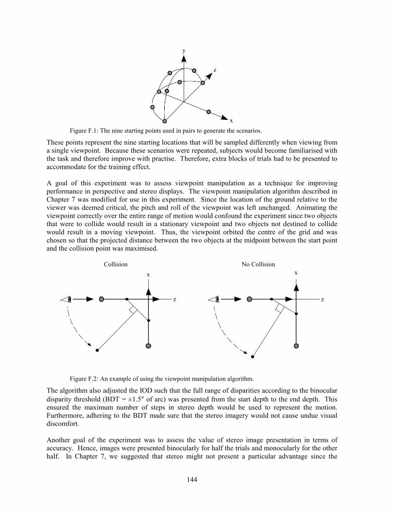
144
Figure F.1: The nine starting points used in pairs to generate the scenarios.
These points represent the nine starting locations that will be sampled differently when viewing from a single viewpoint. Because these scenarios were repeated, subjects would become familiarised with the task and therefore improve with practise. Therefore, extra blocks of trials had to be presented to accommodate for the training effect. A goal of this experiment was to assess viewpoint manipulation as a technique for improving performance in perspective and stereo displays. The viewpoint manipulation algorithm described in Chapter 7 was modified for use in this experiment. Since the location of the ground relative to the viewer was deemed critical, the pitch and roll of the viewpoint was left unchanged. Animating the viewpoint correctly over the entire range of motion would confound the experiment since two objects that were to collide would result in a stationary viewpoint and two objects not destined to collide would result in a moving viewpoint. Thus, the viewpoint orbited the centre of the grid and was chosen so that the projected distance between the two objects at the midpoint between the start point and the collision point was maximised. Collision No Collision
z
x
z
x
Figure F.2: An example of using the viewpoint manipulation algorithm.
The algorithm also adjusted the IOD such that the full range of disparities according to the binocular disparity threshold (BDT = ±1.5° of arc) was presented from the start depth to the end depth. This ensured the maximum number of steps in stereo depth would be used to represent the motion. Furthermore, adhering to the BDT made sure that the stereo imagery would not cause undue visual discomfort. Another goal of the experiment was to assess the value of stereo image presentation in terms of accuracy. Hence, images were presented binocularly for half the trials and monocularly for the other half. In Chapter 7, we suggested that stereo might not present a particular advantage since the
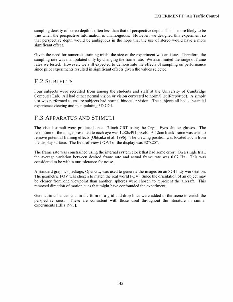
EXPERIMENT F: Air Traffic Control
145
sampling density of stereo depth is often less than that of perspective depth. This is more likely to be true when the perspective information is unambiguous. However, we designed this experiment so that perspective depth would be ambiguous in the hope that the use of stereo would have a more significant effect. Given the need for numerous training trials, the size of the experiment was an issue. Therefore, the sampling rate was manipulated only by changing the frame rate. We also limited the range of frame rates we tested. However, we still expected to demonstrate the effects of sampling on performance since pilot experiments resulted in significant effects given the values selected.
F.2 SUBJECTS
Four subjects were recruited from among the students and staff at the University of Cambridge Computer Lab. All had either normal vision or vision corrected to normal (self-reported). A simple test was performed to ensure subjects had normal binocular vision. The subjects all had substantial experience viewing and manipulating 3D CGI.
F.3 APPARATUS AND STIMULI
The visual stimuli were produced on a 17-inch CRT using the CrystalEyes shutter glasses. The resolution of the image presented to each eye was 1280x491 pixels. A 12cm black frame was used to remove potential framing effects [Ohtsuka et al. 1996]. The viewing position was located 50cm from the display surface. The field-of-view (FOV) of the display was 32°x25°. The frame rate was constrained using the internal system clock that had some error. On a single trial, the average variation between desired frame rate and actual frame rate was 0.07 Hz. This was considered to be within our tolerance for noise. A standard graphics package, OpenGL, was used to generate the images on an SGI Indy workstation. The geometric FOV was chosen to match the real world FOV. Since the orientation of an object may be clearer from one viewpoint than another, spheres were chosen to represent the aircraft. This removed direction of motion cues that might have confounded the experiment. Geometric enhancements in the form of a grid and drop lines were added to the scene to enrich the perspective cues. These are consistent with those used throughout the literature in similar experiments [Ellis 1993].
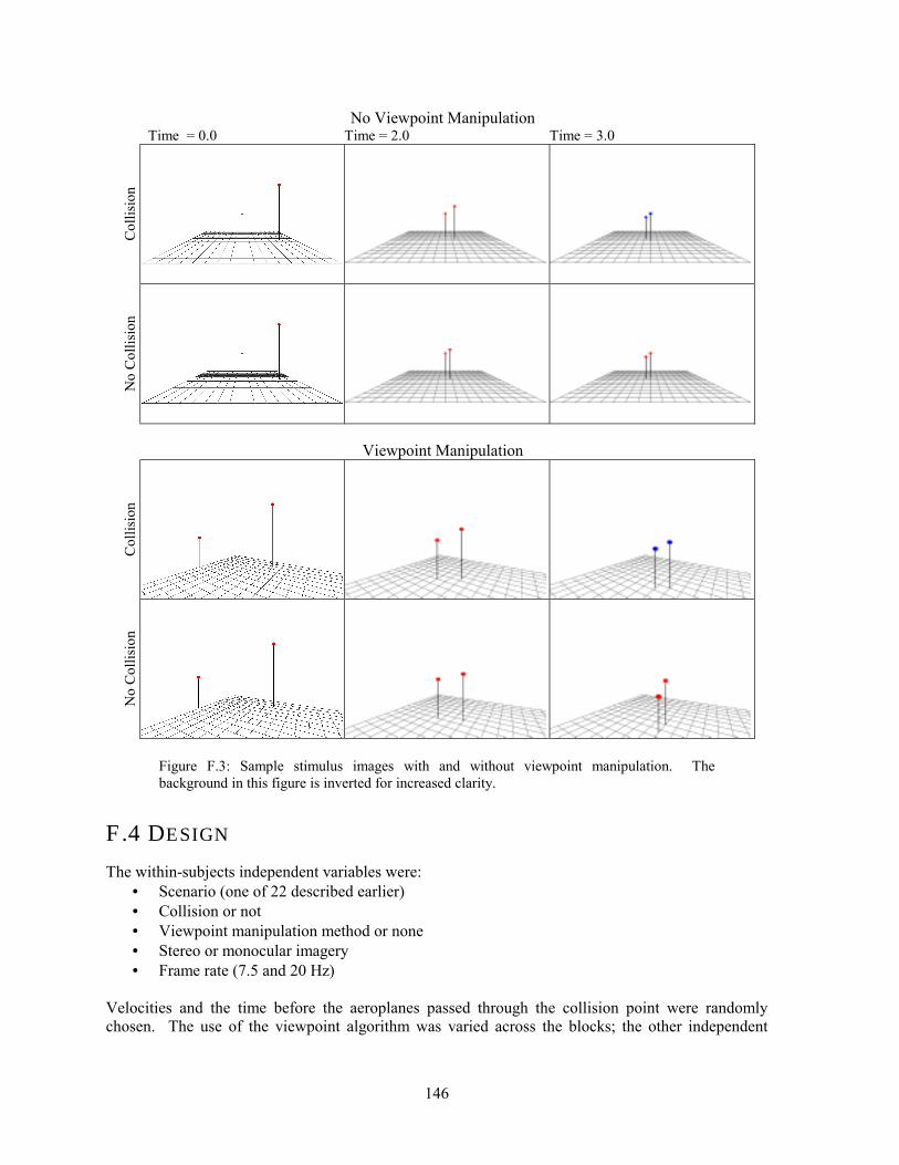
146
No Viewpoint Manipulation Time = 0.0 Time = 2.0 Time = 3.0
Col
lisio
n
No
Col
lisio
n
Viewpoint Manipulation
Col
lisio
n
No
Col
lisio
n
Figure F.3: Sample stimulus images with and without viewpoint manipulation. The background in this figure is inverted for increased clarity.
F.4 DESIGN
The within-subjects independent variables were: • Scenario (one of 22 described earlier) • Collision or not • Viewpoint manipulation method or none • Stereo or monocular imagery • Frame rate (7.5 and 20 Hz)
Velocities and the time before the aeroplanes passed through the collision point were randomly chosen. The use of the viewpoint algorithm was varied across the blocks; the other independent
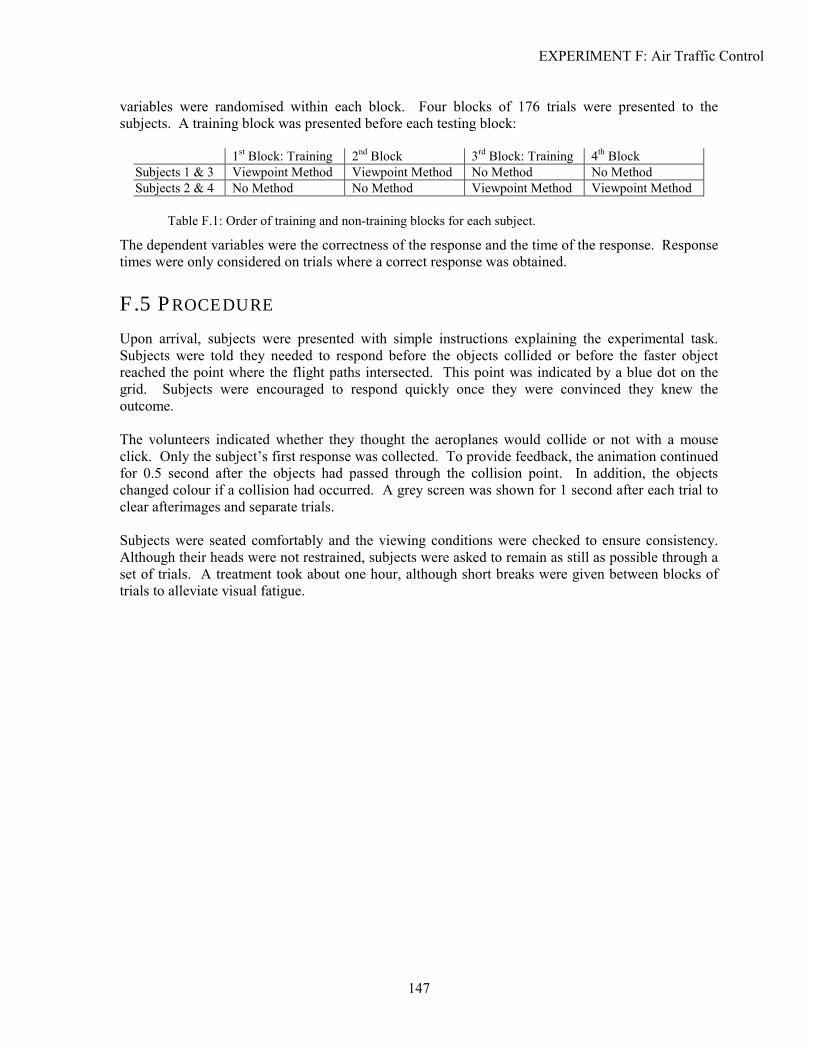
EXPERIMENT F: Air Traffic Control
147
variables were randomised within each block. Four blocks of 176 trials were presented to the subjects. A training block was presented before each testing block:
1st Block: Training 2nd Block 3rd Block: Training 4th Block Subjects 1 & 3 Viewpoint Method Viewpoint Method No Method No Method Subjects 2 & 4 No Method No Method Viewpoint Method Viewpoint Method
Table F.1: Order of training and non-training blocks for each subject.
The dependent variables were the correctness of the response and the time of the response. Response times were only considered on trials where a correct response was obtained.
F.5 PROCEDURE
Upon arrival, subjects were presented with simple instructions explaining the experimental task. Subjects were told they needed to respond before the objects collided or before the faster object reached the point where the flight paths intersected. This point was indicated by a blue dot on the grid. Subjects were encouraged to respond quickly once they were convinced they knew the outcome. The volunteers indicated whether they thought the aeroplanes would collide or not with a mouse click. Only the subject�s first response was collected. To provide feedback, the animation continued for 0.5 second after the objects had passed through the collision point. In addition, the objects changed colour if a collision had occurred. A grey screen was shown for 1 second after each trial to clear afterimages and separate trials. Subjects were seated comfortably and the viewing conditions were checked to ensure consistency. Although their heads were not restrained, subjects were asked to remain as still as possible through a set of trials. A treatment took about one hour, although short breaks were given between blocks of trials to alleviate visual fatigue.
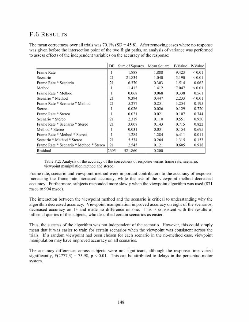
148
F.6 RESULTS
The mean correctness over all trials was 70.1% (SD = 45.8). After removing cases where no response was given before the intersection point of the two flight paths, an analysis of variance was performed to assess effects of the independent variables on the accuracy of the response:
DF Sum of Squares Mean Square F-Value P-Value Frame Rate 1 1.888 1.888 9.423 < 0.01 Scenario 21 21.834 1.040 5.190 < 0.01 Frame Rate * Scenario 21 6.370 0.303 1.514 0.062 Method 1 1.412 1.412 7.047 < 0.01 Frame Rate * Method 1 0.068 0.068 0.338 0.561 Scenario * Method 21 9.394 0.447 2.233 < 0.01 Frame Rate * Scenario * Method 21 5.277 0.251 1.254 0.195 Stereo 1 0.026 0.026 0.129 0.720 Frame Rate * Stereo 1 0.021 0.021 0.107 0.744 Scenario * Stereo 21 2.319 0.110 0.551 0.950 Frame Rate * Scenario * Stereo 21 3.008 0.143 0.715 0.822 Method * Stereo 1 0.031 0.031 0.154 0.695 Frame Rate * Method * Stereo 1 1.284 1.284 6.411 0.011 Scenario * Method * Stereo 21 5.534 0.264 1.315 0.153 Frame Rate * Scenario * Method * Stereo 21 2.545 0.121 0.605 0.918 Residual 2605 521.860 0.200
Table F.2: Analysis of the accuracy of the correctness of response versus frame rate, scenario, viewpoint manipulation method and stereo.
Frame rate, scenario and viewpoint method were important contributors to the accuracy of response. Increasing the frame rate increased accuracy, while the use of the viewpoint method decreased accuracy. Furthermore, subjects responded more slowly when the viewpoint algorithm was used (871 msec to 904 msec). The interaction between the viewpoint method and the scenario is critical to understanding why the algorithm decreased accuracy. Viewpoint manipulation improved accuracy on eight of the scenarios, decreased accuracy on 13 and made no difference on one. This is consistent with the results of informal queries of the subjects, who described certain scenarios as easier. Thus, the success of the algorithm was not independent of the scenario. However, this could simply mean that it was easier to train for certain scenarios when the viewpoint was consistent across the trials. If a random viewpoint had been chosen for each scenario in the no-method case, viewpoint manipulation may have improved accuracy on all scenarios. The accuracy differences across subjects were not significant, although the response time varied significantly, F(2777,3) = 75.98, p < 0.01. This can be attributed to delays in the perceptuo-motor system.

EXPERIMENT F: Air Traffic Control
149
The main results of the experiment can be summarised as: • Decreasing frame rate decreased accuracy • Using stereo imagery did not improve accuracy • Scenario significantly affected accuracy • Scenario significantly affected whether the viewpoint manipulation method used increased
accuracy

150
151
Bibliography Alfano, P. & Michel, G. 1990. �Restricting the Field of View: Perceptual and Performance Effects.�
Perceptual and Motor Skills, 70, pp. 35-45.
Allen, R., McDonald, D. & Singer, M. 1997. �Landmark Direction and Distance Estimation in Large Scale Virtual Environments.� in Proc. HFES 41st Annual Meeting, pp. 1213-1217.
Allison, D., Wills, B., Hodges, L. & Wineman, J. 1996. �Gorillas in the Bits.� GVU Technical Report 96-16. Atlanta, Georgia: Georgia Institute of Technology, Graphics, Visualization and Usability Center.
American National Standards Institute, 1988. American National Standard for Human Factors Engineering of Visual Display Terminal Workstations. Santa Monica, California: The Human Factors Society.
Baird, J. 1970. Psychophysical Analysis of Visual Space. London: Pergamon Press.
Barfield, W., Hendrix, C., Bjorneseth, O., Kaczmarek, K. & Lotens, W. 1995. �Comparison of Human Sensory Capabilities with Technical Specifications of Virtual Environment Equipment.� Presence, 4(4), pp. 329-356.
Barfield, W. & Kim, Y. 1991. �Computer Graphics Programming Principals as Factors in the Design of Perspective Displays.� in H. Bullinger (Ed.), Human Aspects in Computing: Design and Use of Interactive Systems and Work with Terminals, pp. 93-97. Amsterdam: Elsevier Science Publishers.
Barfield, W. & Rosenberg, C. 1995. �Judgements of Azimuth and Elevation as a Function of Monoscopic and Binocular Depth Cues Using a Perspective Display.� Human Factors, 37(1), pp. 173-181.
152
Barrette, R. 1992. �Wide Field-of-View Full-Colour High-Resolution Helmet-Mounted Display.� in Proc. SID International Symposium, pp. 69-72.
Bartschi, W. 1981. Linear Perspective. New York: Van Nostrand Reinhold.
Bevan, M. (Ed.). 1997. �Headmounted Displays.� VR News, 6(4), pp. 28-33.
Boff, K. & Lincoln, J. (Eds.). 1988. Engineering Data Compendium: Human Perception and Performance. Wright-Patterson AFB, Ohio: AAMRL.
Booth, K., Bryden, M., Cowan, W., Morgan, M. & Plante, B. 1987. �On the Parameters of Human Visual Performance: An Investigation of the Benefits of Antialiasing.� Computer Graphics & Animation, September 1987, pp. 34-41
Bos, P. 1993. �Performance Limits of Stereoscopic Viewing Systems Using Active and Passive Glasses.� in Proc. VRAIS ’93, pp. 371-376.
Brewster, D. 1856. The Stereoscope: Its History, Theory and Construction (Reprinted 1971). Hastings-on-Hudson, NY: Morgan & Morgan, Publishers.
Bridgeman, B. & Montegut, M. 1993. �Faster Flicker Rate Increases Reading Speed on CRTs.� in Proc. SPIE – Human Vision, Visual Processing and Digital Display IV, vol. 1913, pp. 134-145.
Bullimore, M., Howarth, P. & Fulton, E. 1998. �Assessment of Visual Performance.� in J. Wilson & E. Corlett E. (Eds.), Evaluation of Human Work: A Practical Ergonomics Methodology (2nd Edition), pp. 804-839. London: Taylor & Francis.
Buser, P. & Imbert, M. 1992. Vision. Cambridge, Massachusetts: The MIT Press.
Canfield, T., Disz, T., Paka, M., Stevens, R., Huang, M., Taylor, V. & Chen, J. 1996. �Towards Real-Time Interactive Virtual Prototyping of Mechanical Systems.� in Proc. High Performance Computing, pp. 339-345.
Castle, O. 1995. �Synthetic Image Generation for a Multiple-View Autostereo Display.� Technical Report 382. Cambridge, UK: University of Cambridge, Computer Laboratory.
Chen, J. & Wang, X. 1999. �Approximate Line Scan-Conversion and Antialiasing.� Computer Graphics Forum, 18(1), pp. 69-78.
Clapp, R. 1987. �Field of View, Resolution and Brightness Parameters for Eye Limited Displays.� Proc. SPIE – Imaging Sensors and Displays, vol. 765, pp. 10-18.
Costello, P. & Howarth, P. 1996. �The Visual Effects of Immersion in Four Virtual Environments.� Technical Report 9604. Loughborough, UK: Loughborough University, VISERG.
Crow, F. 1977. �The Aliasing Problem in Computer-Generated Shaded Images.� Comm. of the ACM, 20(11).
Crow, F. 1981. �A Comparison of Antialiasing Techniques.� Computer Graphics and Animation, January 1981, pp. 40-48.
Cruz-Neira, C., Sandin, D. & DeFanti, T. 1993. �Surround-Screen Projection-Based Virtual Reality: The Design and Implementation of the CAVE.� in Proc. SIGGRAPH ’93, pp. 135-142.
Cuqlock-Knopp, W. & Whitaker, L. 1993. �Spatial Ability and Land Navigation under Degraded Visual Conditions.� Human Factors, 35(3), pp. 511-520.
BIBLIOGRAPHY
153
Cutting, J. & Vishton, P. 1995. �Perceiving Layout and Knowing Distance: The Integration, Relative Potency and Contextual use of Different Information about Depth.� in W. Epstein & S. Rogers (Eds.), Perception of Space and Motion, pp. 69-118. New York: Academic Press.
Davis, E. & Hodges, L. 1995. �Human Stereopsis, Fusion and Stereoscopic Virtual Environments.� in W. Barfield & T. Furness (Eds.), Virtual Environments and Advanced Interface Design, pp. 145-174. Oxford: Oxford University Press.
Debons, A. 1968. �Introduction to Display Systems.� in H. Luxenberg & R. Kuehn (Eds.), Display Systems Engineering, pp. 1-23. New York: McGraw-Hill.
Deering, M. 1992. �High Resolution Virtual Reality.� in Proc. SIGGRAPH ’92, pp. 195-202.
Deering, M. 1993. �Explorations of Display Interfaces for Virtual Reality.� in Proc. VRAIS ’93, pp. 141-147.
Delucia, P. 1995. �Effects of Pictorial Relative Size and Ground-Intercept Information on Judgements about Potential Collisions in Perspective Displays.� Human Factors, 37(3), pp. 528-538.
Dodgson, N. 1992. �Image Resampling.� Technical Report 261. Cambridge, UK: University of Cambridge, Computer Laboratory.
Dodgson, N., Moore, J., Lang, S., Martin, G. & Canepa, P. 2000. �A 50" Time-Multiplexed Autostereoscopic Display.� in Proc. SPIE – Stereoscopic Displays & Applications XI, vol. 3957.
Dolezal, H. 1982. Living in a World Transformed. New York: Academic Press.
DiZio, P. & Lackner, J. 1992. �Spatial Orientation, Adaptation and Motion Sickness in Real and Virtual Environments.� Presence, 1(3), pp. 319-328.
Drascic, D. & Milgram, P. 1991. �Positioning Accuracy of a Virtual Stereographic Pointer in a Real Stereoscopic Video World.� in Proc. SPIE – Stereoscopic Displays and Applications II, vol. 1457, pp. 58-69.
Durlach, N. & Mavor, A. (Eds.). 1995. Virtual Reality: Scientific and Technical Challenges. Washington, D.C.: National Academy Press.
Edgar, G. & Bex, P. 1995. �Vision and Displays.� in K. Carr & R. England (Eds.), Simulated and Virtual Realities: Elements of Perception, pp. 85-101. London: Taylor & Francis.
Eggleston, R., William, J. & Aldrich, K. 1997. �Field of View Effects on a Direct Manipulation Task in a Virtual Environment.� in Proc. HFES 41st Annual Meeting 1997, pp. 1244-1248.
Ellis, S. 1993. �Pictorial Communication: Pictures and the Synthetic Universe.� in S. Ellis (Ed.), Pictorial Communication in Virtual and Real Environments, pp.22-40. London: Taylor & Francis.
Ellis, S. 1995. �Virtual Environments and Environmental Instruments.� in K. Carr & R. England (Eds.), Simulated and Virtual Realities: Elements of Perception, pp. 85-101. London: Taylor & Francis.
Ellis, S., Smith, S. & McGreevy, M. 1987. �Distortions of Perceived Visual Directions out of Pictures.� Perception & Psychophysics, 42(6), pp. 535-544.
Ellis, S., Tharp, G., Grunwald, A. & Smith, S. 1992. �Exocentric Judgements in Real and Virtual Spaces.� in Proc. SID International Symposium, pp. 837-840.
154
Erickson, R. 1978. "Line Criteria in Target Acquisition with Television.� Human Factors, 20, pp. 573-588.
Fahle, M. & Poggio, T. 1984. �Visual Hyperacuity: Spatiotemporal Interpolation in Human Vision.� in Proc. Image Understanding ’84, pp. 49-77.
Ferwerda, J. & Greenberg, D. 1988. �A Psychophysical Approach to Assessing the Quality of Antialiased Images.� Computer Graphics & Applications, September 1988, pp. 85-95.
Fiske, T., Silverstein, L., Penn, C. & Kelley, E. 1998. �Viewing Angle: A Matter of Perspective.� in Proc. SID International Symposium, pp. 937-940.
Fleischman, T. & Sola, K. 1999. �Usability: The Value-Added Characteristic.� Information Display, 15(8), pp. 12-15.
Foley, J., van Dam, A., Feiner, S. & Hughes, J. 1990. Computer Graphics: Principles and Practice (2nd Edition). New York: Addison Wesley Publishing.
Funkhauser, T., Teller, S., Sequin, C. & Khorramabadi, D. 1996. �The UC Berkeley System for Interactive Visualization of Large Architectural Models.� Presence, 5(1), pp. 13-44.
Furness, T. 1986. �The Super Cockpit and Human Factors Challenges.� Technical Report HITL-M-886-1. Seattle, Washington: University of Washington, Human Interface Technologies Laboratory.
Geise, W. 1946. �The Interrelationship of Visual Acuity at Different Distances.� Journal of Applied Psychology, 30, pp. 91-106.
Gibson, J. 1986. The Ecological Approach to Visual Perception. London: Lawrence Erlbaum Associates.
Gillam, B. 1980. �Geometrical Illusions.� Scientific American, 242(1), pp. 102-111.
Gillam, B. 1995. �The Perception of Spatial Layout from Static Optical Information.� in W. Epstein & S. Rogers (Eds.), Perception of Space and Motion, pp. 23-67. New York: Academic Press.
Glantz, K., Durlach, N., Barnett, R. & Aviles, W. 1997. �Virtual Reality and Psychotherapy: Opportunities and Challenges.� Presence, 6(1), pp. 87-105.
Glassner, A. 1995. Principles of Digital Image Synthesis. San Francisco: Morgan Kaufmann Publishers.
Goldstein, E. 1989. Sensation and Perception (3rd Edition). Belmont, California: Wadsworth Publishing.
Gombrich, E. 1969. Art and Illusion. Princeton, New Jersey: Princeton University Press.
Gonzalez, R. & Woods, R. 1993. Digital Image Processing. New York: Addison-Wesley Publishing.
Graham, C. 1951. �Visual Perception.� in S. Stevens (Ed.), Handbook of Experimental Psychology, pp. 868-920. New York: John Wiley & Sons.
Green, M. 1992. �The Perceptual Basis of Aliasing and Antialiasing.� in Proc. SPIE – Human Vision, Visual Processing and Digital Display III, vol. 1666, pp. 84-93.
Grunwald, A., Ellis, S. & Smith, S. 1988. �A Mathematical Model for Spatial Orientation from Pictorial Perspective Displays.� IEEE Trans. on Systems, Man and Cybernetics, 18(3), pp. 425-437.
BIBLIOGRAPHY
155
Gupta, R. 1995. Prototyping and Design for Assembly Analysis using Multimodal Virtual Environments. Doctoral dissertation, Massachusetts Institute of Technology.
Haber, R. 1980. �How We Perceive Depth from Flat Pictures.� American Scientist, 68, July-August, pp. 370-390.
Hagen, M., Jones, R. & Reed, E. 1978. "On a Neglected Variable in Theories of Pictorial Perception: Truncation of the Visual Field.� Perception & Psychophysics, 23(4), pp. 326-330.
Harrison, L. & McAllister, D. 1993. �Implementation Issues in Interactive Stereo Systems.� in D. McAllister (Ed.), Stereo Computer Graphics and Other True 3D Technologies, pp. 117-151. Princeton, New Jersey: Princeton University Press.
Hatada, T., Sakata, H. & Kusaka, H. 1980. "Psychophysical Analysis of the 'Sensation of Reality' Induced by a Visual Wide-Field Display.� SMPTE Journal, 89, August 1980, pp. 560-569.
Held, R. & Durlach, D. 1993. �Telepresence, Time Delay and Adaptation.� in S. Ellis (Ed.), Pictorial Communication in Real and Virtual Worlds, pp. 232-246. London: Taylor & Francis.
Hendrix, C. & Barfield, W. 1995. �Presence in Virtual Environments as a Function of Visual and Auditory Cues.� in Proc. VRAIS ‘95, pp. 74-82.
Hendrix, C. & Barfield, W. 1996. �Presence in Virtual Environments as a Function of Visual Display Parameters.� Presence, 5(3), pp. 274-289.
Hendrix, C. & Barfield, W. 1997. �Spatial Discrimination in Three-Dimensional Displays as a Function of Computer Graphics Eyepoint Elevation and Stereoscopic Viewing.� Human Factors, 39(4), pp. 602-617.
Henry, D. & Furness, T. 1993. �Spatial Perception in Virtual Environments: Evaluating an Architectural Application.� in Proc. VRAIS ’93, pp. 33-40.
Hettinger, L. & Riccio, G. 1992. �Visually Induced Motion Sickness in Virtual Environments.� Presence, 1(3), pp. 306-310.
Higgins, K., Wood, J. & Tait, A. 1998. �Vision and Driving: Selective Effect of Optical Blur on Different Driving Tasks.� Human Factors, 41(2), pp. 224-232.
Hochberg, J. 1986. �Representation of Motion and Space in Video and Cinematic Displays.� in K. Boff, L. Kaufman & J. Thomas (Eds.), Handbook of Perception and Human Performance, Vol. 1, pp. 22.1-22.64. New York: John Wiley & Sons.
Hodges, L. & Davis, E. 1993. �Geometric Considerations for Stereoscopic Virtual Environments.� Presence, 2(1), pp. 34-43.
Holway, A. & Boring, E. 1941. �Determinants of Apparent Visual Size with Distance Variant.� American Journal of Psychology, 54, pp. 21-37.
Holst, G. 1998. Sampling, Aliasing and Data Fidelity for Electronic Imaging Systems, Communications and Data Acquisition. Winter Park, Florida: JCD Publishing and Bellingham, Washington: SPIE Press.
Hone, G. & Davis, R. 1993. �Brightness and Depth on the Flat Screen: Cue Conflict in Simulator Displays.� in Proc. SPIE – Human Vision, Visual Processing and Digital Display IV, vol. 1913, pp. 518-528.
156
Hone, G. & Davis, R. 1995. �Brightness and Contrast as Cues to Depth in the Simulator Display: Cue Combination and Conflict Resolution.� in Proc. SPIE – Human Vision, Visual Processing and Digital Imagery VI, vol. 2411, pp. 240-249.
Hsu, J., Pizlo, Z., Babbs, C., Chelberg, D. & Delp, E. 1994. �Design of Studies to Test the Effectiveness of Stereo Imaging Truth or Dare: Is Stereo Viewing Really Better?� in Proc. SPIE – Stereoscopic Displays and Virtual Reality Systems, vol. 2177, pp. 211-222.
Ittleson, W. 1952. The Ames Demonstrations in Perception. Princeton, New Jersey: Princeton University Press.
Johnson, C. & Leibowitz, H. 1979. �Practice Effects for Visual Resolution in the Periphery.� Perception & Psychophysics, 25(5), pp. 439-442.
Johnson, J. 1958. �Analysis of Image Forming Systems.� in Proc. Image Intensifier Symposium, pp. 249-273.
Johnston, R., Bhoryrul, S., Way, L., Satava, R., McGovern, K., Fletcher, J., Rangel, S. & Loftin, R. 1996. �Assessing a Virtual Reality Surgical Skills Simulator.� Technical Report. Houston, Texas: University of Houston, Virtual Environment Training Laboratory.
Jones, N. & Watson, J. 1990. Digital Signal Processing. London: Peter Peregrinus on behalf of Institute for Electrical Engineers.
Kalawsky, R. 1993. The Science of Virtual Reality and Virtual Environments. New York: Addison-Wesley Publishing.
Kappé, B., Korteling, J. & Van de Grind, W. 1995. �Time-to-Contact Estimation in a Driving Simulator.� in Proc. SID International Symposium, pp. 297-300.
Kenyon, R. & Kneller E. 1992. "Human Performance and Field of View.� in Proc. SID International Symposium, pp. 290-293.
Kenyon, R. & Kneller E. 1993. "The Effects of Field of View Size on the Control of Roll Motion.� IEEE Trans. on Systems, Man and Cybernetics, 23(1), pp. 183-193.
Kim, W., Ellis, S., Tyler, M., Hannaford, B. & Stark, L. 1987. �Quantitative Evaluation of Perspective and Stereoscopic Displays in Three-Axis Manual Tracking Tasks.� IEEE Trans. on Systems, Man and Cybernetics, 17(1), pp. 61-72.
Kline, P. & Witmer, B. 1996. �Distance Perception in VEs: Effects of FOV and Surface Texture at Near Distances.� in Proc. HFES 40th Annual Meeting, pp. 1112-1116.
Korein, J. & Balder, N. 1983. �Temporal Anti-Aliasing in Computer Generated Animation.� Computer Graphics, 17(3), pp. 377-388.
Lampton, D., Knerr, B., Goldberg, S., Bliss, J., Moshell, J. & Blau, B. 1994. �The Virtual Environment Performance Assessment Battery: Development and Evaluation.� Presence, 3(2), pp. 145-147.
Lampton, D., McDonald, D., Singer, M. & Bliss, J. 1995. �Distance Estimation in Virtual Environments.� in Proc. HFES 39th Annual Meeting, pp. 1268-1272.
Lasko-Harvill, A., Blanchard, C., Lanier, J. & McGrew, D. 1995. �A Fully Immersive Cholecystectomy Simulation.� in Proc. Medicine Meets Virtual Reality III.
BIBLIOGRAPHY
157
Ledley, R. & Frye, R. 1994. �Processing of Stereo Image Pairs: Elimination of Depth Planes Using the �Cut-Plane� Procedure.� in Proc. SPIE – Stereoscopic Displays and Virtual Reality Systems, vol. 2177, pp. 66-77.
Levison, W., Pew, R. & Getty, D. 1994. �Application of Virtual Environments to the Training of Naval Personnel.� Technical Report 7988. Cambridge, Massachusetts: BBN Corp.
Li, B., Meyer, G. & Klassen, R. 1998. �A Comparison of Two Image Quality Models.� in Proc. SPIE – Human Vision and Electronic Imaging III, vol. 3299, pp. 98-109.
Lipton, L. 1991. The CrystalEyes Handbook. San Rafael, California: StereoGraphics Corporation.
Lipton, L. 1993. �Composition for Electrostereoscopic Displays.� in D. McAllister (Ed.), Stereo Computer Graphics and Other True 3D Technologies, pp. 11-25. Princeton, New Jersey: Princeton University Press.
Liu, A., Tharp, G. & Stark, L. 1992. �Depth Cue Interaction in Telepresence and Simulated Telemanipulation.� in Proc. SPIE – Human Vision, Visual Processing and Digital Display III, vol. 1666, pp. 541-547.
Loftin, R. & Kenney, P. 1995. �Training the Hubble Space Telescope Flight Team.� Computer Graphics & Applications, 15(5), pp. 31-37.
Marshall, J., Burbeck, C., Ariely, D., Rolland, J. & Martin, K. 1996. �Occlusion Edge Blur: A Cue to Relative Visual Depth.� Journal of the Optical Society of America A, 13, April 1996, pp. 681-688.
Matsunaga, K., Shidoji, K., Matsubara, K. 1999. �A Comparison of Operation Efficiency for the Insert Task when Using Stereoscopic Images with Additional Lines, Stereoscopic Images and a Manipulator with Force Feedback.� in Proc. SPIE – Stereoscopic Displays and Applications X, vol. 3639, pp. 50-56.
McCauley, M. & Sharkey, T. 1992. �Cybersickness: Perception of Self-Motion in Virtual Environments.� Presence, 1(3), pp. 311-317.
McGreevy, M. & Ellis, S. 1986. �The Effect of Perspective Geometry on Judged Direction in Spatial Information Instruments.� Human Factors, 28(4), pp. 439-456.
McKenna, M. & Zeltzer, D. 1992. �Three Dimensional Visual Display Systems for Virtual Environments.� Presence, 1(4), pp. 421-458.
Meehan, J. & Triggs, T. 1992. �Apparent Size and Distance in an Imaging Display.� Human Factors, 34(3), pp. 303-311.
Merritt, J., Cole, R. & Ikehara, C. 1992. �Interaction between Binocular and Monocular Depth Cues in Teleoperator Task Performance.� in Proc. SID International Symposium, pp. 841-844.
Miller, R. 1976. �The Human Task as Reference for System Interface Design.� in Proc. User-Oriented Design of Interactive Graphics, pp. 97-99.
Moore, J., Dodgson, N., Travis, A. & Lang, S. 1996. �Time-Multiplexed Colour Autostereoscopic Display.� in Proc. SPIE – Stereoscopic Displays and Applications VII, vol. 2653, pp 10-19.
Nagata, S. 1993. �How to Reinforce Perception of Depth in Single Two-Dimensional Pictures.� in S. Ellis (Ed.), Pictorial Communication in Virtual and Real Environments, pp. 527-545. London: Taylor & Francis.
158
Neale, D. 1996. �Spatial Perception in Desktop Virtual Environments.� in Proc. HFES 40th Annual Meeting, pp. 1117-1121.
Ohtsuka, S., Ishigure, Y., Kanatsugu, Y., Yoshida, T. & Usui, S. 1996. �Virtual Window: A Technique for Correcting Depth-Perception Distortion in Stereoscopic Displays.� in Proc. SID International Symposium, pp. 893-896.
Ojima, S. & Yano, S. 1995. "Evaluation of 2D and 3D Images Using Eye Movement, Head Movement and Body Sway.� in Proc. SPIE – Human Vision, Visual Processing and Digital Imagery VI, vol. 2411, pp. 262-270.
Omura, K., Shiwa, S. & Kishino, F. 1996. �3D Display with Accommodative Compensation Employing Real-Time Gaze Detection.� in Proc. SID International Symposium, pp. 889-892.
Okuyama, F. 1999. �Evaluation of Stereoscopic Display with Visual Function and Interview.� in Proc. SPIE – Stereoscopic Displays and Applications X, vol. 3639, pp. 28-35.
Panel on Impact of Video Viewing on Vision of Workers. 1983. Video Displays, Work and Vision. Washington, D.C.: National Academy Press.
Patterson, R., Bowd, C., Becker, S., Monaghan, M., Shorter, S. & Gilbert, J. 1996. �Stereoscopic Depth Discrimination in the Crossed and Uncrossed Directions with Brief vs. Extended Stimulus Exposure.� in Proc. SID International Symposium, pp. 973-975.
Patterson, R. & Martin, W. 1992. �Human Stereopsis.� Human Factors, 34(6), pp. 669-692.
Pausch, R., Crea, T. & Conway, M. 1992. �A Literature Survey for Virtual Environments: Military Flight Simulator Visual Systems and Simulator Sickness.� Presence, 1(3), pp. 344-363.
Pausch, R., Proffitt, D. & Williams, G. 1997. "Quantifying Immersion in Virtual Reality.� in Proc. SIGGRAPH ’97, pp. 13-18.
Pausch, R., Snoddy, J., Taylor, R., Watson, S. & Haseltine, E. 1996. �Disney�s Aladdin: First Steps Towards Storytelling Virtual Reality.� in Proc. SIGGRAPH ’96, pp. 193-203.
Perkins, D. 1973. �Compensating for Distortion in Viewing Pictures Obliquely.� Perception & Psychophysics, 14(1), pp. 13-18.
Perrone, J. & Wenderoth, P. 1993. �Visual Slant Underestimation.� in S. Ellis (Ed.), Pictorial Communication in Virtual and Real Environments, pp. 496-503. London: Taylor & Francis.
Peters, D. 1991. �Chasing the Eye: An Eye-Tracked Display for the Simulation Industry � The How and the Why.� in Proc. SID International Symposium, pp. 495-497.
Pfautz, J. 1996. Distortion of Depth Perception in a Virtual Environment Application. Master�s Dissertation, Massachusetts Institute of Technology.
Pfautz, J. & Robinson, P. 1999. �An Analysis of Perspective Geometry and Antialiasing.� in Proc. Eurographics UK 17th Annual Conference.
Piantanida, T., Boman, D., Larimer, J., Gille, J. & Reed, C. 1992. �Studies of the FOV/Resolution Tradeoff in VR Systems.� in Proc. SPIE – Human Vision, Visual Processing and Digital Display III, vol. 1666, pp. 448-456.
Pirenne, M. 1970. Optics, Painting and Photography, New York: Cambridge University Press.
Pizlo, Z. & Scheessele, M. 1998. �Perception of 3D Scenes from Pictures.� in Proc. SPIE – Human Vision and Electronic Imaging III, vol. 3299, pp. 410-423.
BIBLIOGRAPHY
159
Platt, J. 1960. �How We See Straight Lines.� Scientific American, June 1960, pp. 121-129.
Poynton, C. 1996. A Technical Introduction to Digital Video, New York: John Wiley & Sons.
Prothero, J. & Hoffman, H. 1995. "Widening the Field of View Increases the Sense of Presence in Immersive Virtual Environments.� Technical Report R-95-5. Seattle, Washington: University of Washington, Human Interface Technology Laboratory.
Reeves, B. & Nass, C. 1996. The Media Equation. Cambridge, UK: Cambridge University Press.
Richards, W. 1970. �Stereopsis and Stereoblindness,� in Exp. Brain Research, vol. 10, pp. 380-388.
Ridder, H. 1998. �Psychophysical Evaluation of Image Quality: From Judgement to Impression.� in Proc. SPIE – Human Vision and Electronic Imaging III, vol. 3299, pp. 252-263.
Robinett, W. & Rolland, J. 1992. �A Computational Model for the Stereoscopic Optics of a Head-Mounted Display.� Presence, 1(1), pp. 45-62.
Rogowitz, B. 1983. �The Human Visual System: A Guide for the Display Technologist.� in Proc. SID International Symposium, pp. 235-252.
Rogowitz, B. 1985. �A Psychophysical Approach to Image Quality.� in Proc. SPIE – Image Quality: An Overview, vol. 549, pp. 9-13.
Rolland, J., Gibson, W. & Ariely, D. 1995. �Towards Quantifying Depth and Size Perception in Virtual Environments.� Presence, 4(1), pp. 24-49.
Roscoe, S. 1984. �Judgements of Size and Distance with Imaging Displays.� Human Factors, 26(6), pp. 617-629.
Rosenberg, C. & Barfield, W. 1995. �Estimation of Spatial Distortion as a Function of Geometric Parameters of Perspective.� IEEE Trans. on Systems, Man and Cybernetics, 25(9), pp. 1323-1333.
Rosenberg, L. 1993. �The Effect of Interocular Distance upon Operator Performance Using Stereoscopic Displays to Perform Virtual Depth Tasks.� in Proc. VRAIS ’93, pp. 27-32.
Rosinski, R., Mulholland, T., Degelman, D. & Farber, J. 1980. �Picture Perception: An Analysis of Visual Compensation.� Perception & Psychophysics, 28(6), pp. 521-526.
Rushton, S. & Wann, J. 1993. �Problems in Perception and Action in Virtual Worlds.� in Proc. VR International ’93, pp. 43-54.
Schloerb, D. 1997. Adaptation of Perceived Depth Related to Changes of the Effective Interpupillary Distance in Computer-Graphics Stereoscopic Displays. Doctoral Dissertation, Massachusetts Institute of Technology.
Schreiber, W. & Troxel, D. 1985. �Transformation Between Continuous and Discrete Representations of Images: A Perceptual Approach.� IEEE Trans. on Pattern Analysis and Machine Intelligence, 7(2), pp. 178-186.
Sedgwick, H. 1980. �The Geometry of Spatial Layout in Pictorial Representation.� in M. Hagen (Ed.), The Perception of Pictures, Volume 1: Alberti’s Window: The Projective Model of Pictorial Information, pp. 34-90. London: Academic Press.
Sekuler, R., Anstis, S., Braddick, O., Brandt, T., Movshon, J. & Orban, G. 1990. �The Perception of Motion.� in L. Spillmann & J. Werner (Eds.), Visual Perception: The Neurophysiological Foundations, pp. 205-230. London: Academic Press.
160
Sheridan, T. 1992. Telerobotics, Automation and Human Supervisory Control. Cambridge, Massachusetts: The MIT Press.
Siegel, M., Tobinaga, Y. & Akiya, T. 1999. �Kinder, Gentler Stereo.� in Proc. SPIE – Stereoscopic Displays and Applications X, vol. 3839, pp. 18-27.
Smets, G. & Overbeeke, K. 1995. �Visual Resolution and Spatial Performance: The Trade-Off Between Resolution and Interactivity.� in Proc. VRAIS ‘95, pp. 67-73.
So, R. & Griffin, M. 1995 �Head-Coupled Virtual Environment with Display Lag.� in K. Carr & R. England (Eds.), Simulated and Virtual Realities: Elements of Perception, pp. 103-112. London: Taylor & Francis.
Sollenberger, R. & Milgram, P. 1993. �Effects of Stereoscopic and Rotational Displays in a Three-Dimensional Path-Tracing Task.� Human Factors, 35(3), pp. 483-499.
Stammers, R. & Shepard, A. 1998. �Task Analysis.� in J. Wilson & E. Corlett (Eds.), Evaluation of Human Work: A Practical Ergonomics Methodology (2nd Edition), pp. 144-168. London: Taylor & Francis.
Stanney, K., Mourant, R. & Kennedy, R. 1998. �Human Factors Issues in Virtual Environments: A Review of the Literature.� Presence, 7(4), pp. 327-351.
Stelmach, L., Tam, W. & Meegan, D. 1999. �Stereo Image Quality: Effects of Spatio-Temporal Resolution.� in Proc. SPIE – Stereoscopic Displays and Applications X, vol. 3639, pp. 4-11.
Strickland, D. 1996. �A Virtual Reality Application with Autistic Children.� Presence, 5(3), pp. 319-329.
Surdick, R., Davis, E., King, R., Corso, G., Shapiro, A., Hodges, L. & Elliot, K. 1994. �Relevant Cues for the Visual Perception of Depth: Is it where you see where it is?� in Proc. HFES 38th Annual Meeting, pp. 1305-1309.
Sutherland, I. 1965. �The Ultimate Display.� in Proc. IFIP Congress, vol. 2, pp. 506-508.
Swartz, M., Wallace, D. & Tkacz, S. 1992. �The Influence of Frame Rate and Resolution Reduction on Human Performance.� Proc. Human Factors Society 36th Annual Meeting, pp. 1440-1444.
Taylor, C., Pizlo, Z. & Allebach, J. 1998. �Perceptually Relevant Image Fidelity.� in Proc. SPIE – Human Vision and Electronic Imaging III, vol. 3299, pp.110-118.
Tiana, C., Pavel, M. & Ahumada, A. 1994. �Enhancing Displays by Blurring.� in Proc. SID International Symposium, pp. 118-121.
Toye, R. 1986. �The Effect of Viewing Position on the Perceived Layout of Space.� Perception & Psychophysics, 40(2), pp. 85-92.
Tresilian, J. 1991. �Empirical and Theoretical Issues in the Perception of Time to Contact.� Journal of Experimental Psychology: Human Perception & Performance, 17(3), pp. 865-876.
Tullis, T. 1983. �The Formatting of Alphanumeric Displays: A Review and Analysis.� Human Factors, 25(6), pp. 637-682.
Utsumi, A., Milgram, P., Takemura, H. & Kishino, F. 1994. �Investigation of Errors in Perception of Stereoscopically Presented Virtual Object Locations in Real Display Space.� in Proc. HFES 38th Annual Meeting, pp. 250-254.
BIBLIOGRAPHY
161
Virtual Environment and Teleoperator Research Consortium (VETREC). 1992. �Virtual Environment Technology for Training.� Technical Report 7661. Cambridge, Massachusetts: BBN Corp.
Wanger, L., Ferwerda, J & Greenberg, D. 1992. �Perceiving Spatial Relationships in Computer-Generated Images.� Computer Graphics & Applications, 12(3), pp. 44-58.
Wann, J. & Mon-Williams, M. 1996. �What Does Virtual Reality NEED?: Human Factors Issues in the Design of Three-Dimensional Computer Environments.� International Journal of Human-Computer Studies, 44, pp. 829-847.
Wann, J., Rushton, S. & Mon-Williams, M. 1995. �Natural Problems for Stereoscopic Depth Perception in Virtual Environments.� Vision Research, 35(19), pp. 2731-2736.
Watson, A., Ahumada, A., Jr., & Farrell, J. 1986. �Window of Visibility: A Psychophysical Theory of Fidelity in Time-Sampled Visual Motion Displays.� Journal of the Optical Society of America, 3(3), pp. 300-307.
Watt, A. 1989. Fundamentals of Three-Dimensional Computer Graphics. New York: Addison-Wesley Publishing.
Watt, A. & Watt, M. 1992. Advanced Animation and Rendering Techniques. New York: Addison-Wesley Publishing.
Wells, M. & Venturino, M. 1990. "Performance and Head Movements Using a Helmet-Mounted Display with Different Sized Fields-of-View.� Optical Engineering, 29(8), pp. 870-877.
Wheatstone, C. 1838. �Contributions to the Physiology of Vision: I. On Some Remarkable and Hitherto Unobserved, Phenomena of Binocular Vision.� Philosophical Transactions of the Royal Society, London, vol. 128, pp. 371-394.
Wilson, J. 1998. �A Framework and a Context for Ergonomics Methodology.� in J. Wilson & E. Corlett (Eds.), Evaluation of Human Work: A Practical Ergonomics Methodology (2nd Edition), pp. 1-40. London: Taylor & Francis.
Witmer, B. & Kline, P. 1998. �Judging Perceived and Traversed Distance in Virtual Environments.� Presence, 7(2), pp. 155-167.
Yeh, Y. 1993. �Visual and Perceptual Issues in Stereoscopic Colour Displays.� in D. McAllister (Ed.), Stereo Computer Graphics and Other True 3D Technologies, pp. 50-70. Princeton, New Jersey: Princeton University Press.
Yeh, Y. & Silverstein, L. 1992. �Spatial Judgements with Monoscopic and Stereoscopic Presentation of Perspective Displays.� Human Factors, 34(5), pp. 583-600.
Yoshida, A., Rolland, J. & Reif, J. 1995. �Design and Applications of a High-Resolution Insert Head-Mounted-Display.� in Proc. VRAIS ‘95, pp. 84-91.
Zeltzer, D., Aviles, W., Gupta, R., Lee, J., Nygren, E., Pfautz, J., Pioch, N. & Reid, B. 1994. �Virtual Environment Technology for Training: Core Testbed.� Annual Report. Cambridge, Massachusetts: Massachusetts Institute of Technology, Research Lab for Electronics.
Zhai, S, Milgram, P. & Rastogi, A. 1997. �Anisotropic Human Performance in Six Degree-of-Freedom Tracking: An Evaluation of Three-Dimensional Display and Control Interfaces.� IEEE Trans. On Systems, Man and Cybernetics—Part A: Systems and Humans, 27(24), pp. 518-528.

162
Ziefle, M. 1998. �Effects of Display Resolution on Visual Performance.� Human Factors, 40(4), pp. 554-568.
Zyda, M., Pratt, D., Falby, J., Lombardo, C. & Kelleher, K. 1994. �The Software Required for the Computer Generation of Virtual Environments.� Presence, 2(2), pp. 130-140.

BIBLIOGRAPHY
163

164