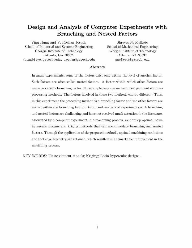
Design and Analysis of Computer Experiments with

Branching and Nested Factors

Ying Hung and V. Roshan JosephSchool of Industrial and Systems Engineering

Georgia Institute of TechnologyAtlanta, GA 30332

yhung@isye.gatech.edu, roshan@gatech.edu

Shreyes N. MelkoteSchool of Mechanical EngineeringGeorgia Institute of Technology

Atlanta, GA 30332smelkote@gatech.edu

Abstract

In many experiments, some of the factors exist only within the level of another factor.

Such factors are often called nested factors. A factor within which other factors are

nested is called a branching factor. For example, suppose we want to experiment with two

processing methods. The factors involved in these two methods can be different. Thus,

in this experiment the processing method is a branching factor and the other factors are

nested within the branching factor. Design and analysis of experiments with branching

and nested factors are challenging and have not received much attention in the literature.

Motivated by a computer experiment in a machining process, we develop optimal Latin

hypercube designs and kriging methods that can accommodate branching and nested

factors. Through the application of the proposed methods, optimal machining conditions

and tool edge geometry are attained, which resulted in a remarkable improvement in the

machining process.

KEY WORDS: Finite element models; Kriging; Latin hypercube designs.

1

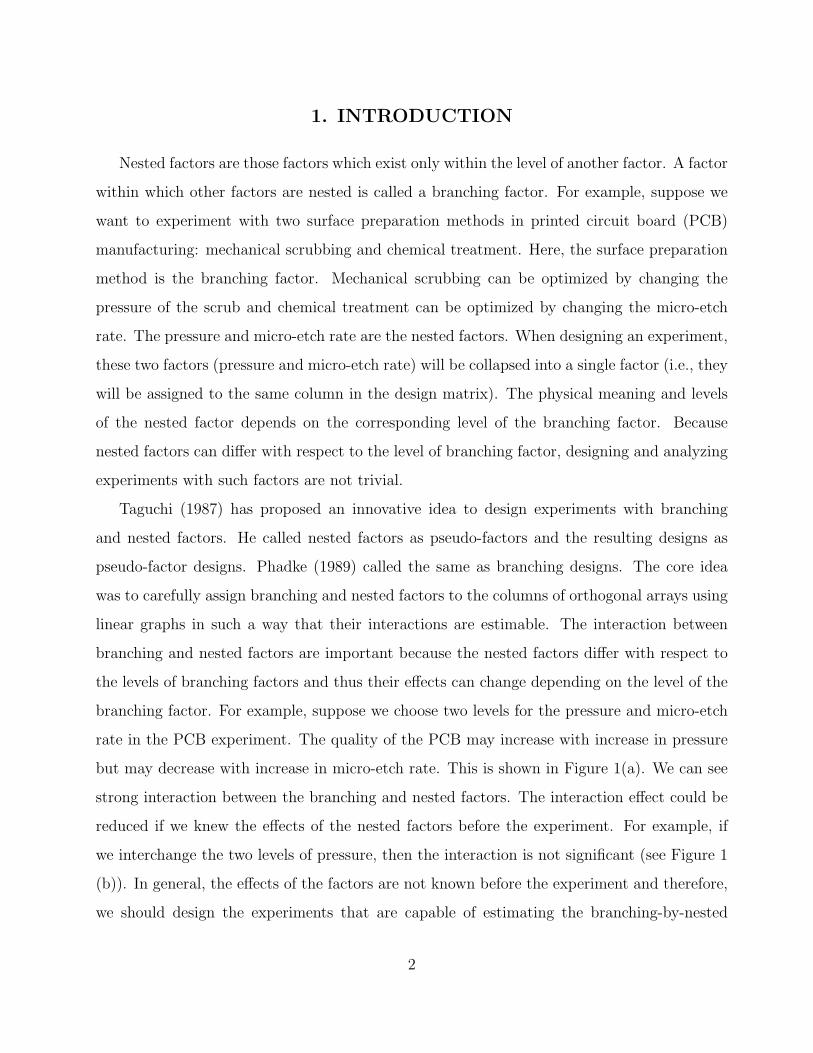
1. INTRODUCTION

Nested factors are those factors which exist only within the level of another factor. A factor

within which other factors are nested is called a branching factor. For example, suppose we

want to experiment with two surface preparation methods in printed circuit board (PCB)

manufacturing: mechanical scrubbing and chemical treatment. Here, the surface preparation

method is the branching factor. Mechanical scrubbing can be optimized by changing the

pressure of the scrub and chemical treatment can be optimized by changing the micro-etch

rate. The pressure and micro-etch rate are the nested factors. When designing an experiment,

these two factors (pressure and micro-etch rate) will be collapsed into a single factor (i.e., they

will be assigned to the same column in the design matrix). The physical meaning and levels

of the nested factor depends on the corresponding level of the branching factor. Because

nested factors can differ with respect to the level of branching factor, designing and analyzing

experiments with such factors are not trivial.

Taguchi (1987) has proposed an innovative idea to design experiments with branching

and nested factors. He called nested factors as pseudo-factors and the resulting designs as

pseudo-factor designs. Phadke (1989) called the same as branching designs. The core idea

was to carefully assign branching and nested factors to the columns of orthogonal arrays using

linear graphs in such a way that their interactions are estimable. The interaction between

branching and nested factors are important because the nested factors differ with respect to

the levels of branching factors and thus their effects can change depending on the level of the

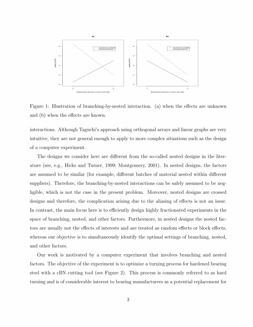
branching factor. For example, suppose we choose two levels for the pressure and micro-etch

rate in the PCB experiment. The quality of the PCB may increase with increase in pressure

but may decrease with increase in micro-etch rate. This is shown in Figure 1(a). We can see

strong interaction between the branching and nested factors. The interaction effect could be

reduced if we knew the effects of the nested factors before the experiment. For example, if

we interchange the two levels of pressure, then the interaction is not significant (see Figure 1

(b)). In general, the effects of the factors are not known before the experiment and therefore,

we should design the experiments that are capable of estimating the branching-by-nested

2

02

46

8

Nested factor (pressure or micro−etch rate)

qual

ity o

f PC

B

(a)

1 2

mechanical scrubbingchemical treatment

02

46

8

Nested factor (pressure or micro−etch rate)

qual

ity o

f PC

B

(b)

1 2

mechanical scrubbingchemical treatment

Figure 1: Illustration of branching-by-nested interaction. (a) when the effects are unknown

and (b) when the effects are known.

interactions. Although Taguchi’s approach using orthogonal arrays and linear graphs are very

intuitive, they are not general enough to apply to more complex situations such as the design

of a computer experiment.

The designs we consider here are different from the so-called nested designs in the liter-

ature (see, e.g., Hicks and Turner, 1999; Montgomery, 2001). In nested designs, the factors

are assumed to be similar (for example, different batches of material nested within different

suppliers). Therefore, the branching-by-nested interactions can be safely assumed to be neg-

ligible, which is not the case in the present problem. Moreover, nested designs are crossed

designs and therefore, the complication arising due to the aliasing of effects is not an issue.

In contrast, the main focus here is to efficiently design highly fractionated experiments in the

space of branching, nested, and other factors. Furthermore, in nested designs the nested fac-

tors are usually not the effects of interests and are treated as random effects or block effects,

whereas our objective is to simultaneously identify the optimal settings of branching, nested,

and other factors.

Our work is motivated by a computer experiment that involves branching and nested

factors. The objective of the experiment is to optimize a turning process for hardened bearing

steel with a cBN cutting tool (see Figure 2). This process is commonly referred to as hard

turning and is of considerable interest to bearing manufacturers as a potential replacement for

3

the grinding process. Since the material being machined is very hard (hardness in excess of 60

Rockwell C), the cutting tool is subjected to large forces, stresses, and temperatures during

the operation. In practice, the cutting edge of the tool is shaped such that it can withstand

the severe conditions. Two commonly employed cutting edge shapes, hone and chamfer, are

shown in Figure 3. Note that Figure 3 represent the idealized view of the instantaneous

cutting action in the cross section A-A indicated in Figure 2. These cutting edge shapes are

intended to strengthen the cutting edge to bear the large tool stresses generated in cutting.

The chamfer tool design can be changed using two factors: chamfer length and chamfer angle,

whereas the hone design is fixed. In other words, the two factors length and angle are nested

within the chamfer edge and there are no factors nested within hone edge. In our terminology,

the tool edge is a branching factor. Thus, when the branching factor takes the level chamfer,

there are two additional factors present in the experiment; but when the branching factor

takes the level hone, there are no factors. There are a few other factors that are common to

both of the tool edges such as the cutting edge radius, tool nose radius, and rake angle. The

machining parameters such as cutting speed, feed, and depth of cut are also factors that do

not depend on the type of tool edges. To distinguish them from the branching and nested

factors, we call them as shared factors. All of the factors involved in this experiment and their

allowable ranges are shown in Table 1. The experiments can be performed in computers using

a commercially available finite element software AdvantEdge.

Latin hypercube designs (LHDs) are commonly used in computer experiments (McKay,

Beckman, and Conover, 1979). A desirable property of a LHD is its one-dimensional balance,

i.e., when we project a N -point design onto any factor, there will be N different levels for that

factor. Clearly this cannot be satisfied for branching and nested factors. The branching factor

is usually a qualitative factor and therefore the number of levels of a branching factor is fixed

(it does not depend on the number of runs N). Moreover, the nested factors are different

for different levels of the branching factor. Therefore, we need a one-dimensional balance

for the nested factors within each level of the branching factor. As an example, consider an

experiment with one branching factor z1, one nested factor v1, and two shared factors x1 and

x2. Suppose that the branching factor has two levels and that we want to do the experiment

4

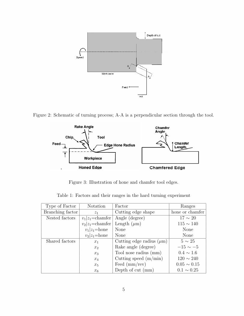
Figure 2: Schematic of turning process; A-A is a perpendicular section through the tool.

ERCNSM

High Performance Machining5

Copyright © ERC/NSM 2006. All rights reserved.

Introduction – Hard Turning Process

Tool Edge Preparation

Cubic Boron Nitride

Tungsten Carbide Figure 3: Illustration of hone and chamfer tool edges.

Table 1: Factors and their ranges in the hard turning experiment

Type of Factor Notation Factor RangesBranching factor z1 Cutting edge shape hone or chamferNested factors v1|z1=chamfer Angle (degree) 17 ∼ 20

v2|z1=chamfer Length (µm) 115 ∼ 140v1|z1=hone None Nonev2|z1=hone None None

Shared factors x1 Cutting edge radius (µm) 5 ∼ 25x2 Rake angle (degree) −15 ∼ −5x3 Tool nose radius (mm) 0.4 ∼ 1.6x4 Cutting speed (m/min) 120 ∼ 240x5 Feed (mm/rev) 0.05 ∼ 0.15x6 Depth of cut (mm) 0.1 ∼ 0.25

5

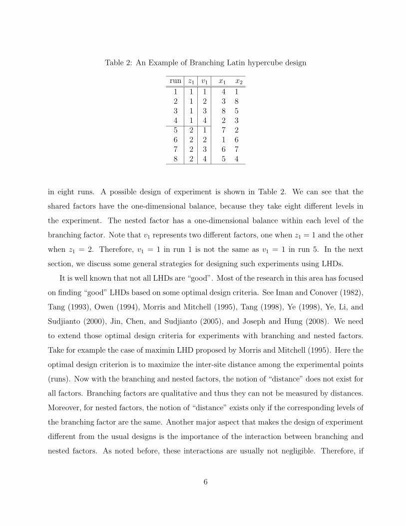
Table 2: An Example of Branching Latin hypercube design

run z1 v1 x1 x2

1 1 1 4 12 1 2 3 83 1 3 8 54 1 4 2 35 2 1 7 26 2 2 1 67 2 3 6 78 2 4 5 4

in eight runs. A possible design of experiment is shown in Table 2. We can see that the

shared factors have the one-dimensional balance, because they take eight different levels in

the experiment. The nested factor has a one-dimensional balance within each level of the

branching factor. Note that v1 represents two different factors, one when z1 = 1 and the other

when z1 = 2. Therefore, v1 = 1 in run 1 is not the same as v1 = 1 in run 5. In the next

section, we discuss some general strategies for designing such experiments using LHDs.

It is well known that not all LHDs are “good”. Most of the research in this area has focused

on finding “good” LHDs based on some optimal design criteria. See Iman and Conover (1982),

Tang (1993), Owen (1994), Morris and Mitchell (1995), Tang (1998), Ye (1998), Ye, Li, and

Sudjianto (2000), Jin, Chen, and Sudjianto (2005), and Joseph and Hung (2008). We need

to extend those optimal design criteria for experiments with branching and nested factors.

Take for example the case of maximin LHD proposed by Morris and Mitchell (1995). Here the

optimal design criterion is to maximize the inter-site distance among the experimental points

(runs). Now with the branching and nested factors, the notion of “distance” does not exist for

all factors. Branching factors are qualitative and thus they can not be measured by distances.

Moreover, for nested factors, the notion of “distance” exists only if the corresponding levels of

the branching factor are the same. Another major aspect that makes the design of experiment

different from the usual designs is the importance of the interaction between branching and

nested factors. As noted before, these interactions are usually not negligible. Therefore, if

6

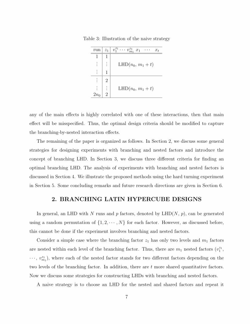
Table 3: Illustration of the naive strategy

run z1 vz11 · · · vz1

m1x1 · · · xt

1 1...

... LHD(n0, m1 + t)... 1... 2...

... LHD(n0, m1 + t)2n0 2

any of the main effects is highly correlated with one of these interactions, then that main

effect will be misspecified. Thus, the optimal design criteria should be modified to capture

the branching-by-nested interaction effects.

The remaining of the paper is organized as follows. In Section 2, we discuss some general

strategies for designing experiments with branching and nested factors and introduce the

concept of branching LHD. In Section 3, we discuss three different criteria for finding an

optimal branching LHD. The analysis of experiments with branching and nested factors is

discussed in Section 4. We illustrate the proposed methods using the hard turning experiment

in Section 5. Some concluding remarks and future research directions are given in Section 6.

2. BRANCHING LATIN HYPERCUBE DESIGNS

In general, an LHD with N runs and p factors, denoted by LHD(N , p), can be generated

using a random permutation of {1, 2, · · · , N} for each factor. However, as discussed before,

this cannot be done if the experiment involves branching and nested factors.

Consider a simple case where the branching factor z1 has only two levels and m1 factors

are nested within each level of the branching factor. Thus, there are m1 nested factors (vz11 ,

· · · , vz1m1

), where each of the nested factor stands for two different factors depending on the

two levels of the branching factor. In addition, there are t more shared quantitative factors.

Now we discuss some strategies for constructing LHDs with branching and nested factors.

A naive strategy is to choose an LHD for the nested and shared factors and repeat it

7

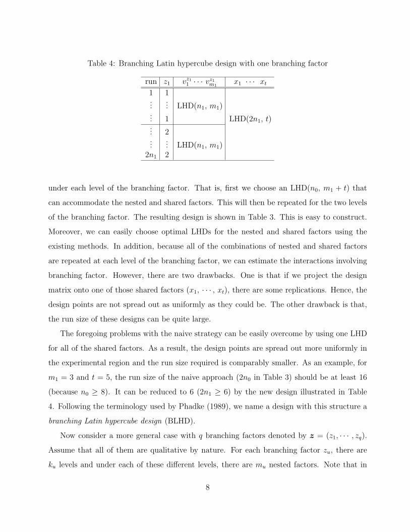
Table 4: Branching Latin hypercube design with one branching factor

run z1 vz11 · · · vz1

m1x1 · · · xt

1 1...

... LHD(n1, m1)... 1 LHD(2n1, t)... 2...

... LHD(n1, m1)2n1 2

under each level of the branching factor. That is, first we choose an LHD(n0, m1 + t) that

can accommodate the nested and shared factors. This will then be repeated for the two levels

of the branching factor. The resulting design is shown in Table 3. This is easy to construct.

Moreover, we can easily choose optimal LHDs for the nested and shared factors using the

existing methods. In addition, because all of the combinations of nested and shared factors

are repeated at each level of the branching factor, we can estimate the interactions involving

branching factor. However, there are two drawbacks. One is that if we project the design

matrix onto one of those shared factors (x1, · · · , xt), there are some replications. Hence, the

design points are not spread out as uniformly as they could be. The other drawback is that,

the run size of these designs can be quite large.

The foregoing problems with the naive strategy can be easily overcome by using one LHD

for all of the shared factors. As a result, the design points are spread out more uniformly in

the experimental region and the run size required is comparably smaller. As an example, for

m1 = 3 and t = 5, the run size of the naive approach (2n0 in Table 3) should be at least 16

(because n0 ≥ 8). It can be reduced to 6 (2n1 ≥ 6) by the new design illustrated in Table

4. Following the terminology used by Phadke (1989), we name a design with this structure a

branching Latin hypercube design (BLHD).

Now consider a more general case with q branching factors denoted by z = (z1, · · · , zq).

Assume that all of them are qualitative by nature. For each branching factor zu, there are

ku levels and under each of these different levels, there are mu nested factors. Note that in

8

general, the number of factors nested under each level of a branching factor can be different.

For example, in the hard turning experiment there are two factors nested under chamfer but

none under hone. However, for notational simplicity, we assume the number of nested factors

to be the same (for a given branching factor) and develop the construction of BLHD. Later

we explain how it can be extended to deal with unequal number of nested factors.

Denote the nested factors by vzu = (vzu1 , · · · , vzu

mu)′, 1 ≤ u ≤ q. Again note that, each

nested factor corresponds to different factors depending on the branching factor and its level.

That is why we use a superscript to denote the branching factor level. In addition to the

branching and nested factors, there are t shared quantitative factors x = (x1, · · · , xt)′. Let

v = ((vz1)′, · · · , (vzq)′)′, and w = (x′, z′,v′)′ represents all of the p factors involved in the

experiment, where p = t + q +∑q

u=1mu. A N -run BLHD can then be represented by W =

(w1, · · · ,wN)′. In general, it consists of three parts. The first part is a design for branching

factors. Because branching factors are qualitative factors, we can choose an orthogonal array

of appropriate size depending on the number of levels of each branching factor. The second

part consists of LHDs for the nested factors. Choose LHD(nu, mu) for the mu nested factors

under the branching factor zu, u = 1, 2, · · · , q. The third part is a LHD(N , t) for all of the

shared factors x. If there are ku levels for branching factor zu, where 1 ≤ u ≤ q, it is clear

that N = k1n1 = k2n2 = · · · = kqnq. Thus, we have one orthogonal array for the branching

factors, q LHDs for the nested factors, and one LHD for the shared factors. These designs

can be assembled to obtain a BLHD.

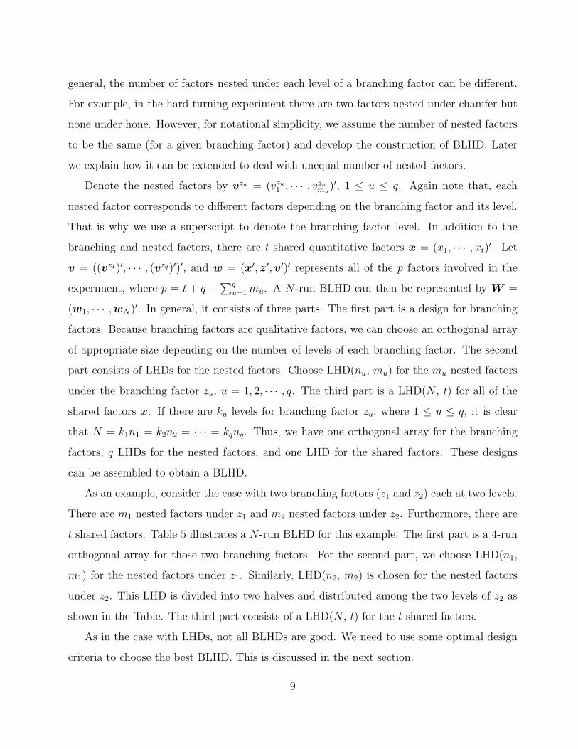
As an example, consider the case with two branching factors (z1 and z2) each at two levels.

There are m1 nested factors under z1 and m2 nested factors under z2. Furthermore, there are

t shared factors. Table 5 illustrates a N -run BLHD for this example. The first part is a 4-run

orthogonal array for those two branching factors. For the second part, we choose LHD(n1,

m1) for the nested factors under z1. Similarly, LHD(n2, m2) is chosen for the nested factors

under z2. This LHD is divided into two halves and distributed among the two levels of z2 as

shown in the Table. The third part consists of a LHD(N , t) for the t shared factors.

As in the case with LHDs, not all BLHDs are good. We need to use some optimal design

criteria to choose the best BLHD. This is discussed in the next section.

9

Table 5: Branching Latin hypercube design with two branching factors

run z1 vz11 · · · vz1

m1z2 vz2

1 · · · vz2m2

x1 · · · xt

1 1 LHD(n1, m1) 1 LHD(n2, m2) first half... 1 2 LHD(n2, m2) first half LHD(N , t)... 2 LHD(n1, m1) 1 LHD(n2, m2) second halfN 2 2 LHD(n2, m2) second half

3. OPTIMAL BRANCHING LATIN HYPERCUBE DESIGNS

As discussed in the introduction, there are several approaches for finding a good LHD.

We may think it is enough to use one of those approaches to generate q + 1 optimal LHDs

for the nested and shared factors and assemble them to obtain the BLHD. However, such an

assembly of optimal LHDs may not lead to an optimal BLHD. Moreover, we need to make

sure that in a BLHD, the correlation between the branching-by-nested interaction and any

other main effect is small. In this section, we propose three optimal design criteria for finding

good BLHDs.

3.1 Maximin BLHD

Morris and Mitchell (1995) proposed to find LHDs that maximize the minimum inter-site

distance. Let g and h be two design points (or sites or runs). Consider the distance measure

d(g,h) = {∑p

j=1 |gj − hj|ς}1/ς , in which ς = 1 and ς = 2 correspond to the rectangular and

Euclidean distance, respectively. For simplicity, rectangular distance (ς = 1) is considered

for the rest of the paper. For a given LHD, define a distance list (D1, D2, · · · , DM) in which

the elements are the distinct values of inter-site distances, sorted from the smallest to the

largest. Let Ji be the number of pairs of design points in the design separated by Di. Then a

design is called a maximin design if it sequentially maximizes Di’s and minimizes Ji’s in the

following order: D1, J1, D2, J2, · · · , DM , JM . A scalar-valued function which can be used to

rank competing designs in such a way that the maximin design receives the highest ranking

is given by

φλ = (M∑i=1

JiD−λi )1/λ =

(∑g 6=h

d(g,h)−λ

)1/λ

, (1)

10

where λ is a positive integer.

Extension of the maximin criterion to BLHDs is not straightforward. Different from LHDs

where all factors can be measured by distances, BLHDs have branching factors which have no

notion of distance and nested factors where definition of distance depend on the corresponding

branching factors. Because of different roles of factors, instead of calculating all the pairwise

distances over all factors, we need to consider branching and nested factors separately from

those of shared factors. First note that for BLHDs, not all factors are divided into same

number of levels as that in LHDs: there are ku levels for branching factor zu, nu levels for

nested factors vzu , and N levels for x. Therefore, before calculating the distances, the design

matrix should be scaled to (−1, 1).

Start with a simple case where q = 1 and m1 = 1. Thus, there are t + 2 factors in the

experiment. Assume that the last two factors are branching factor z1 and nested factor vz11 ,

respectively. We need to define two types of inter-site distances. The first type of distance

focuses on all of the shared factors. It is the distance projection onto the t-dimensional space

(x), which can be defined by dx(g,h) =∑t

j=1 |gj − hj|, where g = (g1, · · · gt+2) and h =

(h1, · · · , ht+2) are (t + 2)-dimensional design points. There are a total of (N2 ) distances. The

second type of distance takes into account of the branching and nested factors by considering

distances within each level of branching factors. The objective here is to spread out the design

points for each level of branching factors. To do so, for each level z1,i of the branching factor,

where 1 ≤ i ≤ k1, distances are calculated based on x and vz11 . Define the second type

of distance by dB(g,h) =∑t

l=1 |gl − hl| + |gt+2 − ht+2|. One can easily obtain dB(g,h) =

dv1(g,h) + dx(g,h), where dv1(g,h) = |gt+2 − ht+2|. The second type of inter-site distances

are calculated only for those within the same level of the branching factor (gt+1 = ht+1 = z1,i,

for some 1 ≤ i ≤ k1) and thus there are(

n1

2

)k1 of them.

Note that, the first type of distance measure consists of t dimensions, while the second

consists of t+1 dimensions. After standardizing with respect to their dimensions, the maximin

distance criterion can be extended to BLHDs by defining a distance list based on these (N2 ) +(

n1

2

)k1 standardized inter-site distances. Furthermore, as in (1), the scalar-valued function can

11

●

●

●

●

2 4 6 8

24

68

(a)

x1

x2

X

X

X

X

●

●

●

●

1 2 3 4

24

68

(b)

v1

x1

X

XX

X

●

●

●

●

1 2 3 4

24

68

(c)

v1

x2

X

X

X

X

Figure 4: Maximin BLHD. “X” stands for z1 = 1 and solid points stands for z1 = 2.

be defined as

φλ =

(∑g 6=h

[t

dx(g,h)

]λ

+

k1∑i=1

∑gt+1=ht+1=z1,i

[1 + t

dv1(g,h) + dx(g,h)

]λ)1/λ

, (2)

where∑

gt+1=ht+1=z1,idv1(g,h) is the sum of

(n1

2

)pairwise distances in which g and h have the

same level of branching factor and∑

g 6=h dx(g,h) =∑k1

i=1

∑gt+1=ht+1=z1,i

dx(g,h)+∑

gt+1 6=ht+1dx(g,h).

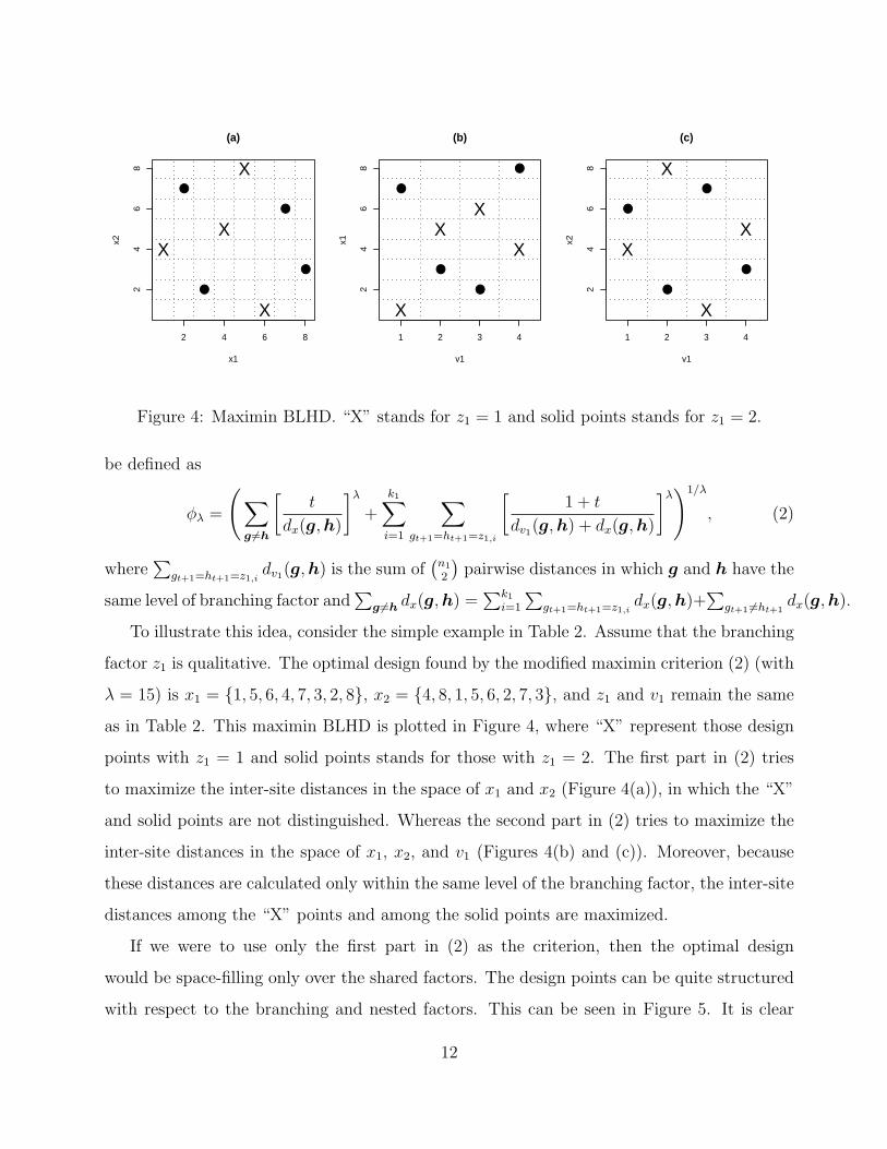
To illustrate this idea, consider the simple example in Table 2. Assume that the branching

factor z1 is qualitative. The optimal design found by the modified maximin criterion (2) (with

λ = 15) is x1 = {1, 5, 6, 4, 7, 3, 2, 8}, x2 = {4, 8, 1, 5, 6, 2, 7, 3}, and z1 and v1 remain the same

as in Table 2. This maximin BLHD is plotted in Figure 4, where “X” represent those design

points with z1 = 1 and solid points stands for those with z1 = 2. The first part in (2) tries

to maximize the inter-site distances in the space of x1 and x2 (Figure 4(a)), in which the “X”

and solid points are not distinguished. Whereas the second part in (2) tries to maximize the

inter-site distances in the space of x1, x2, and v1 (Figures 4(b) and (c)). Moreover, because

these distances are calculated only within the same level of the branching factor, the inter-site

distances among the “X” points and among the solid points are maximized.

If we were to use only the first part in (2) as the criterion, then the optimal design

would be space-filling only over the shared factors. The design points can be quite structured

with respect to the branching and nested factors. This can be seen in Figure 5. It is clear

12

●

●

●

●

2 4 6 8

24

68

(a)

x1

x2

X

X

X

X

●

●

●

●

1 2 3 4

24

68

(b)

v1

x1

XX

XX

●

●

●

●

1 2 3 4

24

68

(c)

v1

x2

X

X

X

X

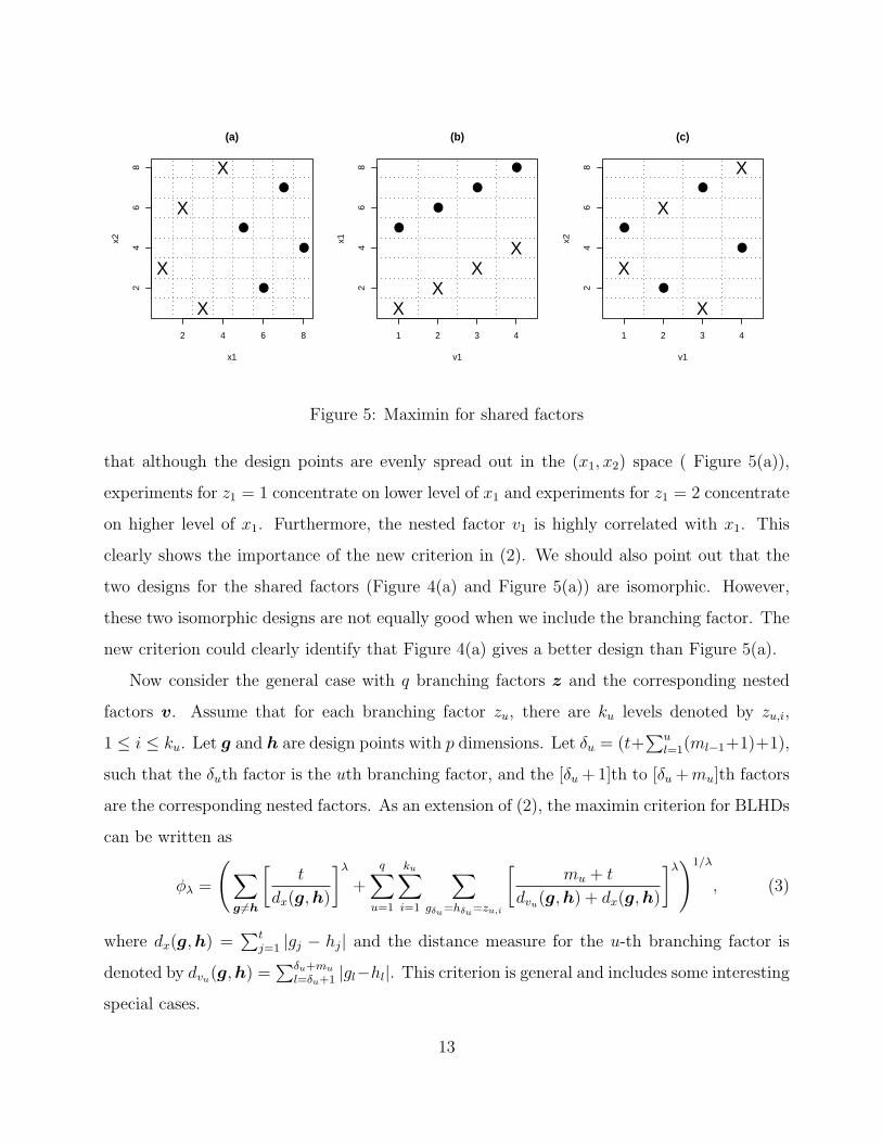
Figure 5: Maximin for shared factors

that although the design points are evenly spread out in the (x1, x2) space ( Figure 5(a)),

experiments for z1 = 1 concentrate on lower level of x1 and experiments for z1 = 2 concentrate

on higher level of x1. Furthermore, the nested factor v1 is highly correlated with x1. This

clearly shows the importance of the new criterion in (2). We should also point out that the

two designs for the shared factors (Figure 4(a) and Figure 5(a)) are isomorphic. However,

these two isomorphic designs are not equally good when we include the branching factor. The

new criterion could clearly identify that Figure 4(a) gives a better design than Figure 5(a).

Now consider the general case with q branching factors z and the corresponding nested

factors v. Assume that for each branching factor zu, there are ku levels denoted by zu,i,

1 ≤ i ≤ ku. Let g and h are design points with p dimensions. Let δu = (t+∑u

l=1(ml−1+1)+1),

such that the δuth factor is the uth branching factor, and the [δu + 1]th to [δu +mu]th factors

are the corresponding nested factors. As an extension of (2), the maximin criterion for BLHDs

can be written as

φλ =

(∑g 6=h

[t

dx(g,h)

]λ

+

q∑u=1

ku∑i=1

∑gδu=hδu=zu,i

[mu + t

dvu(g,h) + dx(g,h)

]λ)1/λ

, (3)

where dx(g,h) =∑t

j=1 |gj − hj| and the distance measure for the u-th branching factor is

denoted by dvu(g,h) =∑δu+mu

l=δu+1 |gl−hl|. This criterion is general and includes some interesting

special cases.

13

Case 1: If q = 0, and mu = 0 for all u, then this would lead to the standard LHD(N, t). Up

to a constant, the maximin criterion (3) would be the same as (1) proposed by Morris and

Mitchell (1995).

Case 2: If there is no nested factor corresponding to the branching factors, that is mu =

0, for all u, one can think about this as an experiment with q qualitative factors z and t

quantitative factors x. As a special case of (3), the maximin criterion for experimental design

with quantitative and qualitative factors can be written as

φλ =

(∑g 6=h

[t

dx(g,h)

]λ

+

q∑u=1

ku∑i=1

∑gδu=hδu=zu,i

[t

dx(g,h)

]λ)1/λ

(4)

Case 3: Another special case is that when t = 0. In this situation, experiments consist

branching factors and nested factors but no shared factors. Because dx(g,h) = 0, for all g

and h, (3) can be simplified to

φλ =

(q∑

u=1

ku∑i=1

∑gδu=hδu=zu,i

[mu

dv(g,h)

]λ)1/λ

.

3.2 Minimum Correlation BLHD

Apart from space-filling, another important issue regarding experimental designs is how to

construct them such that the significant factors can be correctly identified. For LHDs, it can

be achieved by minimizing the pairwise correlation among factors (Iman and Conover, 1982;

Owen, 1994; Tang, 1998). Owen (1994) proposed a performance measure ρ2 for evaluating

the goodness of an LHD with respect to pairwise correlations. For LHD(N , t),

ρ2 =

∑ti=2

∑i−1j=1 ρ

2ij

t(t− 1)/2, (5)

where ρij is the linear correlation between columns i and j.

Different from LHDs, orthogonality among main effects is not enough in BLHDs. In BL-

HDs, it is equally important to consider the branching-by-nested interactions. Therefore, we

propose a modified correlation criterion, which minimizes the correlations among the main

effects of all factors as well as those between main effect of a shared factor and a branching-

by-nested interaction effect. To do so, we first enlarge the BLHDs by including two-factor

14

●

●

●

●

2 4 6 8

24

68

(a)

x1

x2

X

X

X

X●

●

●

●

1 2 3 4

24

68

(b)

v1

x1

X

X

X

X

●

●

●

●

1 2 3 4

24

68

(c)

v1

x2

X

X

X

X

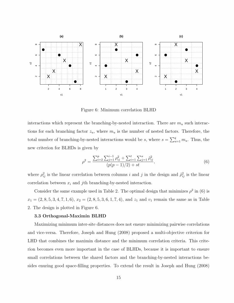
Figure 6: Minimum correlation BLHD

interactions which represent the branching-by-nested interaction. There are mu such interac-

tions for each branching factor zu, where mu is the number of nested factors. Therefore, the

total number of branching-by-nested interactions would be s, where s =∑q

u=1mu. Thus, the

new criterion for BLHDs is given by

ρ2 =

∑pi=2

∑i−1j=1 ρ

2ij +

∑ti=1

∑sj=1 ρ

2ij

(p(p− 1)/2) + st, (6)

where ρ2ij is the linear correlation between columns i and j in the design and ρ2

ij is the linear

correlation between xi and jth branching-by-nested interaction.

Consider the same example used in Table 2. The optimal design that minimizes ρ2 in (6) is

x1 = (2, 8, 5, 3, 4, 7, 1, 6), x2 = (2, 8, 5, 3, 6, 1, 7, 4), and z1 and v1 remain the same as in Table

2. The design is plotted in Figure 6.

3.3 Orthogonal-Maximin BLHD

Maximizing minimum inter-site distances does not ensure minimizing pairwise correlations

and vice-versa. Therefore, Joseph and Hung (2008) proposed a multi-objective criterion for

LHD that combines the maximin distance and the minimum correlation criteria. This crite-

rion becomes even more important in the case of BLHDs, because it is important to ensure

small correlations between the shared factors and the branching-by-nested interactions be-

sides enuring good space-filling properties. To extend the result in Joseph and Hung (2008)

15

to BLHD, we should scale φλ and ρ2 to the same range so that some meaningful weights can

be assigned in the multi-objective function. The following result gives the lower and upper

bounds for φλ, which can be used for scaling it to [0, 1]. Here we only consider the case of

a single branching factor. The result can be extended to include more than one branching

factor, but the expressions become more complicated.

Proposition 1. If there is only one branching factor, then

φλ,L ≤ φλ ≤ φλ,U ,

where

φλ,L = 3

[ k1∑i=1

∑gδ1

=hδ1=z1,i

21

p+1 (m1 + t)p

p+1 +∑

gδ16=hδ1

tp

p+1

] (λ+1)λ[t(N2 − 1) +

k1∑i=1

m1(n21 − 1)

]−1

,

and

φλ,U =N

2

[k1∑i=1

n1−1∑j=1

(n1 − j)(t+m1)λ

jλ(t+ k1m1)λ+

N−1∑j=1

N − j

jλ

]1/λ

.

Thus, the multi-objective criterion is to minimize

ψλ = wρ2 + (1− w)φλ − φλ,L

φλ,U − φλ,L

. (7)

We usually take w = .5 and call the design that minimizes this criterion as orthogonal-maximin

BLHD.

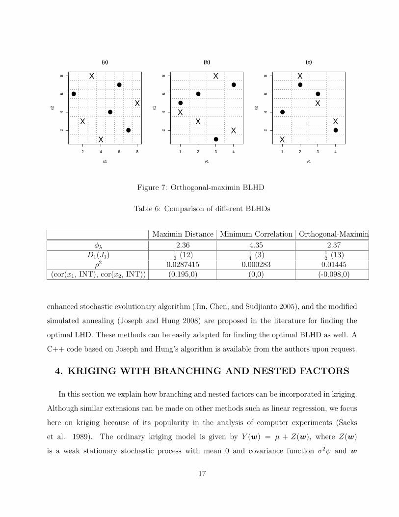
The design matrix in Table 2 is an orthogonal-maximin BLHD. It is plotted in Figure 7.

Comparisons of the optimal designs found by the forgoing three criteria are provided in Table

6. It can be seen that the correlation between the shared factor and the branching-by-nested

interaction (denoted by INT) is 0 in the case of minimum correlation design. However, the

points are much closer compared to the maximin BLHD. The orthogonal-maximin BLHD

provides a good compromise between them.

Because of the combinatorial nature of the optimization problem, finding the optimal

BLHD for large dimensions is a difficult task. Several methods such as simulated annealing

(Morris and Mitchell 1995), columnwise-pairwise algorithm (Ye, Li, and Sudjianto 2000),

16

●

●

●

●

2 4 6 8

24

68

(a)

x1

x2

X

X

X

X

●

●

●

●

1 2 3 4

24

68

(b)

v1

x1

XX

X

X

●

●

●

●

1 2 3 4

24

68

(c)

v1

x2

X

X

X

X

Figure 7: Orthogonal-maximin BLHD

Table 6: Comparison of different BLHDs

Maximin Distance Minimum Correlation Orthogonal-Maximin

φλ 2.36 4.35 2.37D1(J1)

12

(12) 14

(3) 12

(13)ρ2 0.0287415 0.000283 0.01445

(cor(x1, INT), cor(x2, INT)) (0.195,0) (0,0) (-0.098,0)

enhanced stochastic evolutionary algorithm (Jin, Chen, and Sudjianto 2005), and the modified

simulated annealing (Joseph and Hung 2008) are proposed in the literature for finding the

optimal LHD. These methods can be easily adapted for finding the optimal BLHD as well. A

C++ code based on Joseph and Hung’s algorithm is available from the authors upon request.

4. KRIGING WITH BRANCHING AND NESTED FACTORS

In this section we explain how branching and nested factors can be incorporated in kriging.

Although similar extensions can be made on other methods such as linear regression, we focus

here on kriging because of its popularity in the analysis of computer experiments (Sacks

et al. 1989). The ordinary kriging model is given by Y (w) = µ + Z(w), where Z(w)

is a weak stationary stochastic process with mean 0 and covariance function σ2ψ and w

17

∈ Rp. The correlation function is defined as cor{Y (w1), Y (w2)} = ψ(w1,w2). Usually, a

product correlation structure is assumed for the correlation function. Consider the example

in Table 2. The correlation function between two points w1 = (x11, x12, z11, vz1111 ) and w2 =

(x21, x22, z21, vz2121 ) can be described as a product of correlation functions of each factor (ψi).

In the usual cases, a common correlation function is chosen for each factor. However, this

cannot be done in the present problem because of the different types of factors.

For the shared factors, a Gaussian correlation function may be used (Santner et al. 2003):

ψi(x1i, x2i) = exp{−αi(x1i − x2i)2},

whereas for a branching factor, an isotropic correlation function may be used (Joseph and

Delaney 2007):

ξ1(z11, z21) = exp

{− θ1I[z11 6=z21]

}.

Here αi and θ1 are correlation parameters and IA is an indicator function which takes value 1

when A is true and 0 otherwise.

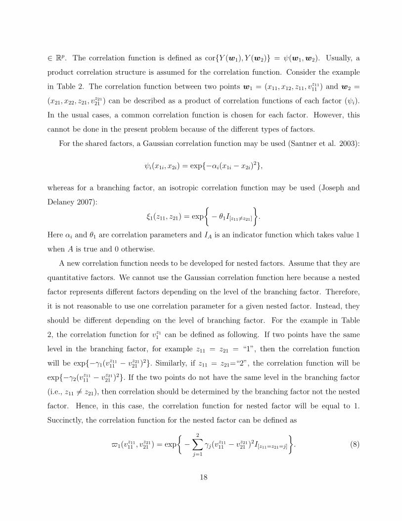
A new correlation function needs to be developed for nested factors. Assume that they are

quantitative factors. We cannot use the Gaussian correlation function here because a nested

factor represents different factors depending on the level of the branching factor. Therefore,

it is not reasonable to use one correlation parameter for a given nested factor. Instead, they

should be different depending on the level of branching factor. For the example in Table

2, the correlation function for vz11 can be defined as following. If two points have the same

level in the branching factor, for example z11 = z21 = “1”, then the correlation function

will be exp{−γ1(vz1111 − vz21

21 )2}. Similarly, if z11 = z21=“2”, the correlation function will be

exp{−γ2(vz1111 − vz21

21 )2}. If the two points do not have the same level in the branching factor

(i.e., z11 6= z21), then correlation should be determined by the branching factor not the nested

factor. Hence, in this case, the correlation function for nested factor will be equal to 1.

Succinctly, the correlation function for the nested factor can be defined as

$1(vz1111 , v

z2121 ) = exp

{−

2∑j=1

γj(vz1111 − vz21

21 )2I[z11=z21=j]

}. (8)

18

We can easily extend this to a more general situation. Let there are q branching fac-

tors z1, · · · , zq. For each branching factor zu, there are mu nested factors. Assume x1 =

(x11, · · ·x1t)′, z1 = (z11, · · · , z1q)

′, vzu1 = (vzu

11 , · · · , vzu1 mu

)′, and v1 = ((vz11 )′, · · · , (vzq

1 )′). Simi-

larly, x2 = (x21, · · ·x2t)′, z2 = (z21, · · · , z2q)

′, vzu2 = (vzu

21 , · · · , vzu2mu

)′, and v2 = ((vz12 )′, · · · , (vzq

2 )′).

Given any two design points w1 = (x1, z1,v1) and w2 = (x2, z2,v2), the correlation function

can be written as

cor(Y (w1), Y (w2)) =

( t∏i=1

ψi(x1,x2)

) q∏u=1

[ξu(z1, z2)

( mu∏j=1

$u(vz1u1j , v

z2u2j )

)], (9)

where ψi(x1,x2) = exp{−αi(x1i − x2i)2} is the correlation function for the shared factors,

ξu(z1, z2) = exp

{− θuI[z1u 6=z2u]

}is the correlation function for the branching factors, and

$u(vz1u1i , v

z2u2i ) = exp

{−

ku∑j=1

γuij(vz1u1i − vz2u

2i )2I[z1u=z2u=zu,j ]

}, (10)

is the correlation function for the nested factors. Note that zu,j, 1 ≤ j ≤ ku are the ku levels

for each branching factor zu. Thus, we obtain

cor(Y (w1), Y (w2)) = exp

{−∑t

i=1 αi(x1i − x2i)2

−∑q

u=1

[θuI[z1u 6=z2u] +

∑mu

i=1

∑ku

j=1 γuij(vz1u1i − vz2u

2i )2I[z1u=z2u=zu,j ]

]}.

(11)

Denote the correlation parameters by Θ = (α′,θ′,γ ′), whereα = (α1, · · · , αt)′, θ = (θ1, · · · , θq)

′,

and γ = (γ111, · · · γqmqkq)′. We can estimate these parameters from data and obtain the ordi-

nary kriging predictor. This will be explained with an example in the next section.

5. HARD TURNING EXPERIMENT

The objective of our experiment is to optimize a hard turning process with respect to cut-

ting forces. Hard turning is a metal cutting process that produces machined parts out of hard

materials with good dimensional accuracy, surface finish, and surface integrity. Minimizing

cutting forces will help reduce the power requirements, elastic distortion of the workpiece, and

tool wear; thus reducing the manufacturing cost and improving the quality of the machined

part.

19

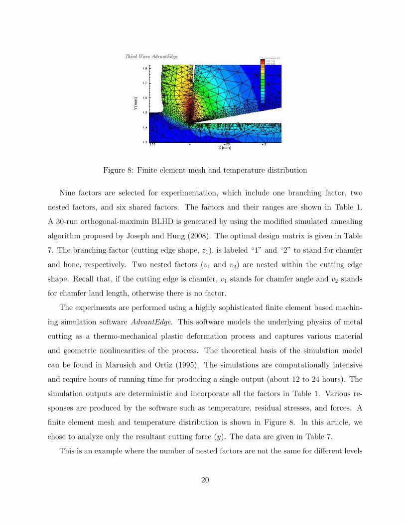
Figure 8: Finite element mesh and temperature distribution

Nine factors are selected for experimentation, which include one branching factor, two

nested factors, and six shared factors. The factors and their ranges are shown in Table 1.

A 30-run orthogonal-maximin BLHD is generated by using the modified simulated annealing

algorithm proposed by Joseph and Hung (2008). The optimal design matrix is given in Table

7. The branching factor (cutting edge shape, z1), is labeled “1” and “2” to stand for chamfer

and hone, respectively. Two nested factors (v1 and v2) are nested within the cutting edge

shape. Recall that, if the cutting edge is chamfer, v1 stands for chamfer angle and v2 stands

for chamfer land length, otherwise there is no factor.

The experiments are performed using a highly sophisticated finite element based machin-

ing simulation software AdvantEdge. This software models the underlying physics of metal

cutting as a thermo-mechanical plastic deformation process and captures various material

and geometric nonlinearities of the process. The theoretical basis of the simulation model

can be found in Marusich and Ortiz (1995). The simulations are computationally intensive

and require hours of running time for producing a single output (about 12 to 24 hours). The

simulation outputs are deterministic and incorporate all the factors in Table 1. Various re-

sponses are produced by the software such as temperature, residual stresses, and forces. A

finite element mesh and temperature distribution is shown in Figure 8. In this article, we

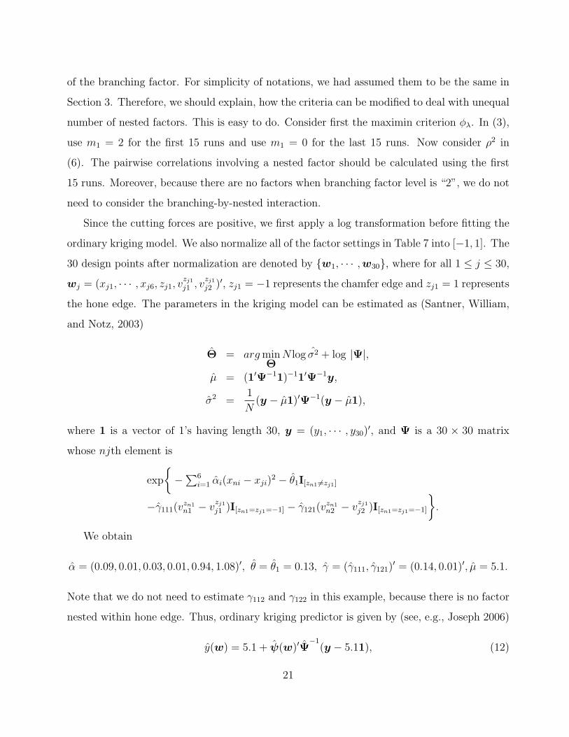
chose to analyze only the resultant cutting force (y). The data are given in Table 7.

This is an example where the number of nested factors are not the same for different levels

20

of the branching factor. For simplicity of notations, we had assumed them to be the same in

Section 3. Therefore, we should explain, how the criteria can be modified to deal with unequal

number of nested factors. This is easy to do. Consider first the maximin criterion φλ. In (3),

use m1 = 2 for the first 15 runs and use m1 = 0 for the last 15 runs. Now consider ρ2 in

(6). The pairwise correlations involving a nested factor should be calculated using the first

15 runs. Moreover, because there are no factors when branching factor level is “2”, we do not

need to consider the branching-by-nested interaction.

Since the cutting forces are positive, we first apply a log transformation before fitting the

ordinary kriging model. We also normalize all of the factor settings in Table 7 into [−1, 1]. The

30 design points after normalization are denoted by {w1, · · · ,w30}, where for all 1 ≤ j ≤ 30,

wj = (xj1, · · · , xj6, zj1, vzj1

j1 , vzj1

j2 )′, zj1 = −1 represents the chamfer edge and zj1 = 1 represents

the hone edge. The parameters in the kriging model can be estimated as (Santner, William,

and Notz, 2003)

Θ = argminΘ

N log σ2 + log |Ψ|,

µ = (1′Ψ−11)−11′Ψ−1y,

σ2 =1

N(y − µ1)′Ψ−1(y − µ1),

where 1 is a vector of 1’s having length 30, y = (y1, · · · , y30)′, and Ψ is a 30 × 30 matrix

whose njth element is

exp

{−∑6

i=1 αi(xni − xji)2 − θ1I[zn1 6=zj1]

−γ111(vzn1n1 − v

zj1

j1 )I[zn1=zj1=−1] − γ121(vzn1n2 − v

zj1

j2 )I[zn1=zj1=−1]

}.

We obtain

α = (0.09, 0.01, 0.03, 0.01, 0.94, 1.08)′, θ = θ1 = 0.13, γ = (γ111, γ121)′ = (0.14, 0.01)′, µ = 5.1.

Note that we do not need to estimate γ112 and γ122 in this example, because there is no factor

nested within hone edge. Thus, ordinary kriging predictor is given by (see, e.g., Joseph 2006)

y(w) = 5.1 + ψ(w)′Ψ−1

(y − 5.11), (12)

21

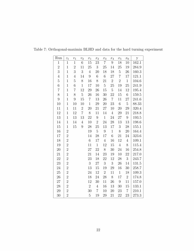
Table 7: Orthogonal-maximin BLHD and data for the hard turning experiment

Run z1 v1 v2 x1 x2 x3 x4 x5 x6 y1 1 1 6 15 23 7 9 18 10 162.12 1 2 11 25 3 25 14 25 19 284.93 1 3 3 4 20 18 18 5 26 160.34 1 4 14 9 6 6 27 7 17 121.15 1 5 8 16 8 21 2 2 1 104.66 1 6 1 17 10 5 25 19 25 241.97 1 7 12 29 26 15 5 14 12 195.48 1 8 5 26 16 30 22 15 6 159.59 1 9 15 7 13 26 7 11 27 241.610 1 10 10 1 29 20 23 6 5 88.3311 1 11 2 20 21 27 10 20 29 320.412 1 12 7 8 11 14 4 29 21 218.813 1 13 13 22 9 1 24 27 9 193.514 1 14 4 10 2 24 28 13 13 198.615 1 15 9 28 25 13 17 3 28 155.116 2 19 5 9 1 8 20 164.417 2 14 28 17 6 21 24 323.618 2 6 17 4 16 12 4 109.119 2 11 1 12 15 4 8 115.420 2 27 22 8 30 24 16 254.821 2 21 14 23 19 10 22 217.022 2 23 18 22 12 28 3 243.723 2 3 27 3 3 26 14 131.524 2 13 15 19 29 16 30 258.725 2 24 12 2 11 1 18 109.326 2 18 24 28 8 17 2 174.827 2 12 30 11 26 9 11 157.028 2 2 4 16 13 30 15 133.129 2 30 7 10 20 23 7 210.130 2 5 19 29 21 22 23 273.3

22

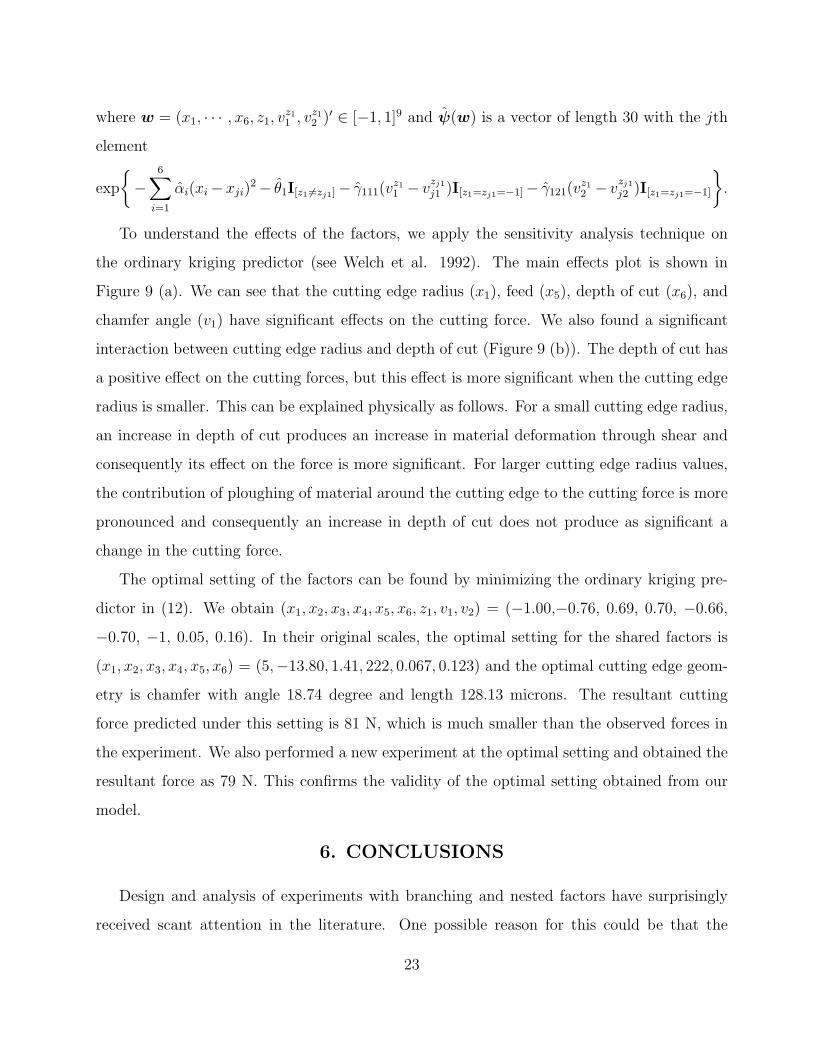
where w = (x1, · · · , x6, z1, vz11 , v

z12 )′ ∈ [−1, 1]9 and ψ(w) is a vector of length 30 with the jth

element

exp

{−

6∑i=1

αi(xi−xji)2− θ1I[z1 6=zj1]− γ111(v

z11 − vzj1

j1 )I[z1=zj1=−1]− γ121(vz12 − vzj1

j2 )I[z1=zj1=−1]

}.

To understand the effects of the factors, we apply the sensitivity analysis technique on

the ordinary kriging predictor (see Welch et al. 1992). The main effects plot is shown in

Figure 9 (a). We can see that the cutting edge radius (x1), feed (x5), depth of cut (x6), and

chamfer angle (v1) have significant effects on the cutting force. We also found a significant

interaction between cutting edge radius and depth of cut (Figure 9 (b)). The depth of cut has

a positive effect on the cutting forces, but this effect is more significant when the cutting edge

radius is smaller. This can be explained physically as follows. For a small cutting edge radius,

an increase in depth of cut produces an increase in material deformation through shear and

consequently its effect on the force is more significant. For larger cutting edge radius values,

the contribution of ploughing of material around the cutting edge to the cutting force is more

pronounced and consequently an increase in depth of cut does not produce as significant a

change in the cutting force.

The optimal setting of the factors can be found by minimizing the ordinary kriging pre-

dictor in (12). We obtain (x1, x2, x3, x4, x5, x6, z1, v1, v2) = (−1.00,−0.76, 0.69, 0.70, −0.66,

−0.70, −1, 0.05, 0.16). In their original scales, the optimal setting for the shared factors is

(x1, x2, x3, x4, x5, x6) = (5,−13.80, 1.41, 222, 0.067, 0.123) and the optimal cutting edge geom-

etry is chamfer with angle 18.74 degree and length 128.13 microns. The resultant cutting

force predicted under this setting is 81 N, which is much smaller than the observed forces in

the experiment. We also performed a new experiment at the optimal setting and obtained the

resultant force as 79 N. This confirms the validity of the optimal setting obtained from our

model.

6. CONCLUSIONS

Design and analysis of experiments with branching and nested factors have surprisingly

received scant attention in the literature. One possible reason for this could be that the

23

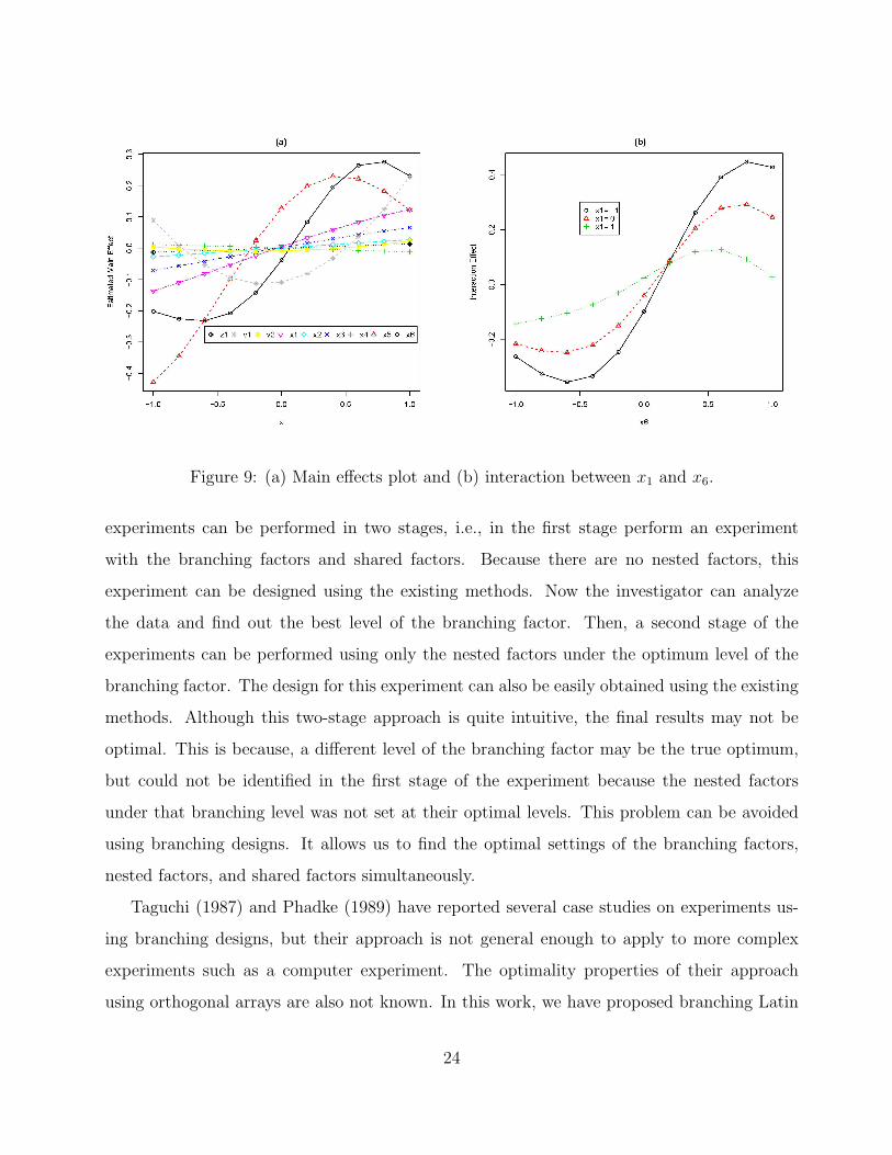
Figure 9: (a) Main effects plot and (b) interaction between x1 and x6.

experiments can be performed in two stages, i.e., in the first stage perform an experiment

with the branching factors and shared factors. Because there are no nested factors, this

experiment can be designed using the existing methods. Now the investigator can analyze

the data and find out the best level of the branching factor. Then, a second stage of the

experiments can be performed using only the nested factors under the optimum level of the

branching factor. The design for this experiment can also be easily obtained using the existing

methods. Although this two-stage approach is quite intuitive, the final results may not be

optimal. This is because, a different level of the branching factor may be the true optimum,

but could not be identified in the first stage of the experiment because the nested factors

under that branching level was not set at their optimal levels. This problem can be avoided

using branching designs. It allows us to find the optimal settings of the branching factors,

nested factors, and shared factors simultaneously.

Taguchi (1987) and Phadke (1989) have reported several case studies on experiments us-

ing branching designs, but their approach is not general enough to apply to more complex

experiments such as a computer experiment. The optimality properties of their approach

using orthogonal arrays are also not known. In this work, we have proposed branching Latin

24

hypercube designs that is suitable for a computer experiment when it involves branching and

nested factors. The optimal choice of such designs are also discussed. The approach was

successfully applied to the optimization of a machining process.

Although the primary focus was on Latin hypercube designs, some issues regarding the use

of orthogonal arrays and its applications in physical experiments are also important. Research

on these topics is currently ongoing and will be reported elsewhere.

ACKNOWLEDGMENTS

This research was supported by U. S. National Science Foundation grants CMMI-0654369

and CMMI-0620259. We are grateful to the Editor, an AE and four referees for their helpful

comments and suggestions.

APPENDIX: PROOF OF PROPOSITION 1

If there is one branching factor (q = 1), a BLHD will include k1 small LHD(n1, m1) for the

k1 levels of the branching factor and a LHD(N , t) for the shared factors. φλ can be written as

φλ =

(∑g 6=h

[t

dx(g,h)

]λ

+

k1∑i=1

∑gδ1

=hδ1z1,i

[m1 + t

dv1(g,h) + dx(g,h)

]λ)1/λ

As shown in Joseph and Hung (2008), for a given LHD(N,t), the average inter-site distance

(rectangular measure) is N(N2 − 1)t/6, which is a constant. With these constraints, finding

a lower bound for φλ can be formulated as a constraint minimization problem:

min φλ

subject to∑

gδ1=hδ1

=z1,idv1(g,h) =

m1n1(n21−1)

6, 1 ≤ i ≤ k1∑

g 6=h dx(g,h) = tN(N2−1)6

,(13)

where∑

gδ1=hδ1

=z1,idv1(g,h) is the sum of inter-site distances for those smaller LHD(n1,m1)

and∑

g 6=h dx(g,h) is the sum of inter-site distances for LHD(N ,t). Since

φλ ≥ φ∗λ =

( ∑gδ1

6=hδ1

[t

dx(g,h)

]λ

+

k1∑i=1

∑gδ1

=hδ1=z1,i

2

[m1 + t

dv1(g,h) + dx(g,h)

]λ)1/λ

,

25

the lower bound can be found by minimizing φ∗λ with the same constraints in (13). Hence, the

lower bound can be solved by using the Lagrange multiplier method. For the upper bound of

φλ, result for BLHD is a simple extension of that for LHD. Therefore, they can be proved by

the same argument used in Joseph and Hung (2008).

REFERENCES

Fang, K. T., Li, R., and Sudjianto, A. (2006). Design and Modeling for Computer Experi-

ments, CRC Press, New York.

Hicks, C. R. and Turner K. V. (1999). Fundamental Concepts in the Design of Experiments,

5th ed., Oxford: Oxford University Press, New York.

Iman, R. L. and Conover, W. J. (1982), “A Distribution-free Approach to Inducing Rank

Correlation Among Input Variables,” Communications in Statistics Part B–Simulation

and Computation, 11, 311-334.

Jin, R., Chen, W. and Sudjianto, A. (2005), “An Efficient Algorithm for Constructing Op-

timal Design of Computer Experiments,” Journal of Statistical Planning and Inference,

to appear.

Joseph, V. R. (2006), “Limit Kriging,” Technometrics, 48, 458-466.

Joseph, V. R. and Delaney, J. D. (2007), “Functional Induced Priors for the Analysis of

Experiments,” Technometrics, 49, 1-11.

Joseph, V. R. and Hung, Y. (2008), “Orthogonal-maximin Latin Hypercube Designs,” Sta-

tistica Sinica, to appear. (available at http://www.isye.gatech.edu/statistics/papers).

Marusich, T. D. and Ortiz, M. (1995), “Modeling and Simulation of High-Speed Machining,”

International Journal for Numerical Methods in Engineering, 38, 3675-3694.

McKay, M. D., Beckman, R. J. and Conover, W. J. (1979), “A Comparison of Three Methods

for Selecting Values of Input Variables in the Analysis of Output from a Computer

Code,” Technometrics, 21, 239-245.

26

Montgomery, D. C. (2004). Design and Analysis of Experiments, Wiley, New York.

Morris, M. D. and Mitchell, T. J. (1995), “Exploratory Designs for Computer Experiments,”

Journal of Statistical Planning and Inference, 43, 381-402.

Owen, A. B. (1994), “Controlling Correlations in Latin Hypercube Samples,” Journal of

American Statistical Association, 89, 1517-1522.

Phadke, M. S. (1989), Quality Engineering Using Robust Design, Englewood Cliffs, NJ:

Prentice Hall.

Sacks, J., Welch, W. J., Mitchell, T. J. and Wynn, H. P. (1989), “Design and Analysis of

Computer Experiments,” Statistical Science, 4, 409-423.

Santner, T. J., Williams, B. J., and Notz, W. I. (2003), The Design and Analysis of Computer

Experiments, Springer, New York.

Taguchi, G. (1987), Systems of Experimental Design, Vol.1 & Vol 2, White Plains, New York:

Unipub/Kraus International.

Tang, B. (1993), “Orthogonal Array-based Latin Hypercubes,” Journal of American Statis-

tical Association, 88, 1392-1397.

Tang, B. (1998), “Selecting Latin Hypercubes Using Correlation Criteria,” Statistica Sinica,

8, 965-978.

Welch, W. J., Buck, R. J., Sacks, J., Wynn, H. P., Mitchell, T. J., and Morris, M. D. (1992),

“Screening, Predicting, and Computer Experiments,” Technometrics, 34, 15-25.

Ye, K.Q. (1998), “Orthogonal Column Latin Hypercubes and their Application in Computer

Experiments,” Journal of American Statistical Association, 93, 1430-1439.

Ye, K. Q., Li, W. and Sudjianto, A. (2000), “Algorithmic Construction of Optimal Symmetric

Latin Hypercube Designs,” Journal of Statistical Planning and Inference, 90, 145-159.

27