Designing threshold networks with given structural and dynamical properties

Aric Hagberg and Pieter J. SwartMathematical Modeling and Analysis, Theoretical Division, Los Alamos National Laboratory, Los Alamos, New Mexico 87545, USA

Daniel A. SchultDepartment of Mathematics, Colgate University, Hamilton, New York 13346, USA

�Received 14 July 2006; published 29 November 2006�

The threshold model can be used to generate random networks of arbitrary size with given local propertiessuch as the degree distribution, clustering, and degree correlation. We summarize the properties of networkscreated using the threshold model and present an alternative deterministic construction. These networks arethreshold graphs and therefore contain a highly compressible layered structure and allow computation ofimportant network properties in linear time. We show how to construct arbitrarily large, sparse, thresholdnetworks with �approximately� any prescribed degree distribution or Laplacian spectrum. Control of the spec-trum allows careful study of the synchronization properties of threshold networks including the relationshipbetween heterogeneous degrees and resistance to synchrony.

DOI: 10.1103/PhysRevE.74.056116 PACS number�s�: 89.75.Hc, 89.75.Da, 89.75.Fb, 05.45.Xt

I. INTRODUCTION

Discovering and modeling the structure of biological, so-cial, and technological networks has been the subject of in-tense research in recent years. This activity has been fueledby the increasing availability of large experimental data setsand the discovery that real networks share common topologi-cal properties that are quite different from classic randomnetworks. The network structure, encoded in the links�edges� between nodes, is important for many applicationsincluding gene transcription regulation and protein interac-tion �1�, strategies for the control of epidemics �2,3�, under-standing network robustness against failures or deliberate at-tack �4�, and discovering communities in social systems �5�.Many real-world networks display an approximate power-law degree distribution p�k��k−�, typically with 2���3�6�, and also tend to have high clustering with low diameter,a structure labeled “the small world effect” �7�. The resultson modeling the structure of networks using these two de-scriptions and others are reviewed in Refs. �8–12�.

Global properties, such as the diameter and size of thelargest component, have dominated structural analysis of net-works. With the increasing availability of a wide array ofmore detailed experimental data sets and accompanying so-phisticated network models, attention has now focused ondistributions of local statistics such as degree �number ofedges at a node�, clustering �number of triangles�, anddegree-degree correlation �propensity for nodes of degree kto connect to nodes of similar degree�.

Most models for the creation of networks with a specificdegree distribution, clustering, or other statistical propertiesare growth models where nodes and edges are added to cre-ate the desired features in the limit of a large number ofnodes �6,12�. These models are in contrast to “static models”such as the classic Erdős-Rényi random graph �13� or theconfiguration model �8� and generalization to networks witha given expected degree sequence �14�, where a fixed num-ber of nodes, N, is specified and edges are connected be-tween them randomly. More recently, an interesting class of

static models has been developed that can generate networkswith statistical properties similar to growing network models�15–19�. These models assign a real variable xi to each nodei which is termed the “node weight,” “intrinsic fitness,” “hid-den variable,” or “propensity to form edges.” In generalform, such hidden variable models assign node weights ran-domly from a specified probability density function ��x� andthen assign edges between nodes i and j with another prob-ability given by a symmetric function f�xi ,xj�.

A preferential attachment method for building networkswith the addition of a node fitness parameter was presentedin Ref. �12�. A static model using node intrinsic fitness wasthen used to study data packet transport through scale-freenetworks �15� and the size of connected components in amodel with a discrete set of node fitness values �18�. Furtherstudies showed that scale-free networks could be constructedfrom node fitness models even if the distribution of nodeweights was not scale free �16,17�.

In the general setting of random networks constructedfrom hidden variables, one focus has been the derivation ofstatistical properties of the network in terms of the distribu-tion of node fitness and the probability of connected nodes�19,20�. Note that static models can always be put into anetwork growth framework if the node weights are assignedduring a growth process.

In this paper, we further analyze the threshold model stud-ied in Refs. �16,19,21�. The threshold model creates randomnetworks through specification of a density function ��x� forindependently assigned weights on nodes xi, i=1, . . . ,N, anda threshold value �. Once node weights xi have been as-signed, each possible edge �xi ,xj� �i� j� is created if xi+xj

��. Here we show that the threshold model creates networksthat exactly meet the definition of a threshold graph in thegraph theory context �22,23� and we call the resulting net-works “threshold networks.” These threshold networks dis-play many novel properties.

In Sec. II, we discuss the basic structure of threshold net-works. We summarize the predictions of distributions of net-work structure measures for the threshold model in the limit

PHYSICAL REVIEW E 74, 056116 �2006�

1539-3755/2006/74�5�/056116�10� ©2006 The American Physical Society056116-1

of large network size. We exploit their highly compressiblelayered structure to derive compact representations. We thenshow how to construct arbitrarily large, sparse, threshold net-works with �approximately� any prescribed degree distribu-tion. In Sec. III, we describe the fast computation of manyrelevant measures of network structure, including the La-placian spectrum and eigenvectors. This allows us to con-struct arbitrarily large, sparse, threshold networks with �ap-proximately� any prescribed Laplacian spectrum. We thenuse these tools to provide insights into the dynamics onthreshold networks, in particular when dynamic coupling isof diffusive type so that the Laplacian spectrum is relevant.Control of the spectrum allows careful study of diffusivedynamics and synchronization properties, including the rela-tionship between heterogeneous degrees and resistance tosynchrony. Section IV provides a summary and conclusions.

II. THRESHOLD NETWORKS

In this section we review some properties of thresholdnetworks and some previous results from studies of thethreshold model. We present a compact description of thresh-old networks and a deterministic algorithm for creatingthreshold networks with a chosen degree distribution.

A. Properties of threshold networks

Threshold networks have been studied extensively in thegraph-theoretic literature �24,25� with reviews in Refs.�23,26�. They belong to the chordal, cochordal, comparabil-ity, cocomparability, interval, split, and permutation graphclasses ��27�, p. 23�. In threshold networks, the neighbor-hoods of nodes are nested �i.e., include the neighbors of ev-ery lower-degree node�, and the graph can therefore be par-titioned into groups of identical nodes according to thisnesting. We use this partition to provide a compact notation,which we call the creation sequence, for storing and manipu-lating these networks.

The structure of a threshold network is uniquely deter-mined �modulo relabeling of nodes with the same degree� byits degree sequence �23,28�. It is worth noting that thresholdnetworks are not the only networks with this property. Alsonote that the degree sequence restricts the number of nodes,while the degree distribution would not.

Threshold networks include many common networks suchas the star �one hub connected to many points� and completegraph. They also include networks with a wide range ofproperties. For example, the density, or fraction of possibleedges present, for a connected threshold network ranges overall possible values from 2/N �stars� to 1 �complete graphs�.As we will show, for large N we can create a threshold net-work with any approximate degree distribution. In addition,threshold networks have the interesting property that the La-placian spectrum consists solely of integers �28�. The pri-mary restriction in terms of network properties seems to bethe extremely small diameter �when connected�, which is atmost 2. In addition, the threshold nature results in a nestedneighborhood structure. That is, the set of neighbors of eachnode is a subset of the neighbors of every higher degree

node. This rigid structure may seem unrealistic as a modelfor real networks. But they certainly occur as important sub-networks containing hubs of real networks: the prototypehub, the star, is a threshold network. Furthermore, networksthat are similar but not exactly threshold in nature may beapproximated in many situations by the threshold networksthey mimic. For example, models where the probability ofattachment between nodes depends in a smooth way on thesum or product of node weights can produce networks verysimilar in structure to threshold networks. Finally, networkproperties other than diameter can be engineered quite flex-ibly and quickly. This allows us to determine the impact ofthese network properties.

B. Threshold model

The threshold model generates a threshold network of Nnodes each with a weight chosen randomly from a distribu-tion ��x�. Edges are then formed for any pair of nodes �i , j�for which xi+xj �� for some threshold value �. The networkstructure is completely determined by the choice of ��x� and�. Without loss of generality we can take �=1, althoughsometimes it is easier to vary � rather than scale the weightsx.

The degree correlations and clustering of the thresholdmodel in the large-N limit were analyzed in Ref. �19�. Ma-suda et al. �21� demonstrated that many forms of the densityfunction lead to power-law degree distributions with expo-nent 2. We review these results here briefly.

Let the cumulative distribution function for weights beR�x�=�−�

x ��x�dx. Then the expected degree for a node withweight x is given by

E�k�x� = �N − 1��1 − R�� − x�� . �1�

Letting k̃=k / �N−1�, we obtain an approximation for the de-gree distribution P�k�,

P�k̃� = ��x�dx

dk̃=

��x���� − x�

=�„� − R−1�1 − k̃�…

�„R−1�1 − k̃�…. �2�

This distribution is computed for a number of forms of thedensity function. Two results are worth special attention.First, power-law distributions arise for large k �on the orderof N� when density functions decay more rapidly than powerlaw. Second, a power-law density with exponent a+1 yieldsa power-law degree distribution with exponent �a+1� /a.Thus to obtain a power-law degree distribution with specifiedexponent �, one should arrange ��x� to be power law withexponent

a + 1 =�

� − 1.

Unfortunately, finding the density function which pro-duces a given degree distribution involves solving the inte-gral equation

P„�N − 1��1 − R�� − x��…��� − x� = ��x� , �3�

with P�·� known and ��·� �and thus R�·�� unknown. Thisequation is nonlinear for most interesting distributions. Thus,

HAGBERG, SWART, AND SCHULT PHYSICAL REVIEW E 74, 056116 �2006�

056116-2

while we know how to generate certain specific power-lawdistributions, there is no formulation for general distribu-tions.

The threshold model thus joins the collection of randomnetwork generation methods that produce realizations which,in the limit of large networks, approach a desired degreedistribution. One distinct advantage of this model is that itprovides analytical insight, fast algorithms, and concreteconstruction without assuming any lattice or hierarchicalsymmetry.

C. Creation sequence

Threshold networks can be described very compactly bywhat we call a “creation sequence” S: a binary string thatprovides a recipe for construction by reading the sequencefrom the left and adding one node for each digit. There aretwo types of nodes: dominating nodes, denoted by a 1, andisolated nodes, denoted by a 0.

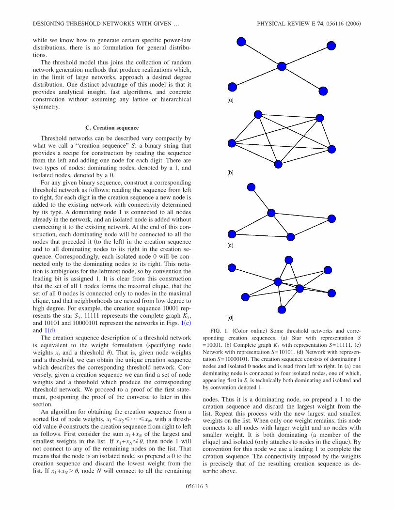
For any given binary sequence, construct a correspondingthreshold network as follows: reading the sequence from leftto right, for each digit in the creation sequence a new node isadded to the existing network with connectivity determinedby its type. A dominating node 1 is connected to all nodesalready in the network, and an isolated node is added withoutconnecting it to the existing network. At the end of this con-struction, each dominating node will be connected to all thenodes that preceded it �to the left� in the creation sequenceand to all dominating nodes to its right in the creation se-quence. Correspondingly, each isolated node 0 will be con-nected only to the dominating nodes to its right. This nota-tion is ambiguous for the leftmost node, so by convention theleading bit is assigned 1. It is clear from this constructionthat the set of all 1 nodes forms the maximal clique, that theset of all 0 nodes is connected only to nodes in the maximalclique, and that neighborhoods are nested from low degree tohigh degree. For example, the creation sequence 10001 rep-resents the star S5, 11111 represents the complete graph K5,and 10101 and 10000101 represent the networks in Figs. 1�c�and 1�d�.

The creation sequence description of a threshold networkis equivalent to the weight formulation �specifying nodeweights xi and a threshold ��. That is, given node weightsand a threshold, we can obtain the unique creation sequencewhich describes the corresponding threshold network. Con-versely, given a creation sequence we can find a set of nodeweights and a threshold which produce the correspondingthreshold network. We proceed to a proof of the first state-ment, postponing the proof of the converse to later in thissection.

An algorithm for obtaining the creation sequence from asorted list of node weights, x1�x2� ¯ �xN, with a thresh-old value � constructs the creation sequence from right to leftas follows. First consider the sum x1+xN of the largest andsmallest weights in the list. If x1+xN��, then node 1 willnot connect to any of the remaining nodes on the list. Thatmeans that the node is an isolated node, so prepend a 0 to thecreation sequence and discard the lowest weight from thelist. If x1+xN��, node N will connect to all the remaining

nodes. Thus it is a dominating node, so prepend a 1 to thecreation sequence and discard the largest weight from thelist. Repeat this process with the new largest and smallestweights on the list. When only one weight remains, this nodeconnects to all nodes with larger weight and no nodes withsmaller weight. It is both dominating �a member of theclique� and isolated �only attaches to nodes in the clique�. Byconvention for this node we use a leading 1 to complete thecreation sequence. The connectivity imposed by the weightsis precisely that of the resulting creation sequence as de-scribe above.

FIG. 1. �Color online� Some threshold networks and corre-sponding creation sequences. �a� Star with representation S=10001. �b� Complete graph K5 with representation S=11111. �c�Network with representation S=10101. �d� Network with represen-tation S=10000101. The creation sequence consists of dominating 1nodes and isolated 0 nodes and is read from left to right. In �a� onedominating node is connected to four isolated nodes, one of which,appearing first in S, is technically both dominating and isolated andby convention denoted 1.

DESIGNING THRESHOLD NETWORKS WITH GIVEN … PHYSICAL REVIEW E 74, 056116 �2006�

056116-3

In the absence of additional structure, networks are gen-erally incompressible; i.e., nearly all N-node graphs requireO�N2� bits in any lossless representation. The obvious binarynature of the creation sequence provides storage for thresh-old networks, which requires at most N bits. We will showthat this compact storage also facilitates computation ofmany network properties. The algorithms presented herework directly with creation sequences, so there is no over-head for retrieval. The transformation from node weights tocreation sequence involves sorting the weights and thusO�N ln N� time. Indeed calculating network properties �suchas the degree� also requires sorting the node weights. So it ismuch more efficient in storage and algorithmic speed to storenetwork connectivity in creation sequence form than vianode weights. Our algorithms assume the network is pre-scribed by a creation sequence.

Adjacent bits in S of the same type represent nodes iden-tical in connectivity. If node labeling is not needed, an evenmore compact representation C can be obtained by com-pressing run lengths of similar node types. This is done bycounting how many adjacent bits are the same starting fromthe left. The counts are then listed C= �D1 , I1 ,D2 , I2 , . . . ,Dn , In� where Dj is the number of domi-nating nodes in the jth group of 1’s and similarly Ij is thenumber of isolated nodes in the jth group of 0’s. Thus thecreation sequence S=11000110 has compact representationC= �2,3 ,2 ,1�. Note that the first number always representsdominating nodes. As examples, C= �1,3 ,1�, C= �5�, C= �1,1 ,1 ,1 ,1�, and C= �1,4 ,1 ,1 ,1� denote the four net-works in Fig. 1. For some network properties, the algorithmsare actually faster when exploiting a compact creation se-quence, allowing the computation of network properties ofmultimillion node dense or sparse threshold networks on amodern desktop computer.

The high compressibility of threshold networks derivesfrom two facts: �i� groups of adjacent nodes in the creationsequence with the same type are identical �up to node rela-beling�, and �ii� connectivity is fully determined by a se-quence of length �N. This observation motivates a visualframework �based on the proof of theorem 1.2.4 in Ref. �23��that more clearly exposes the underlying network structure.

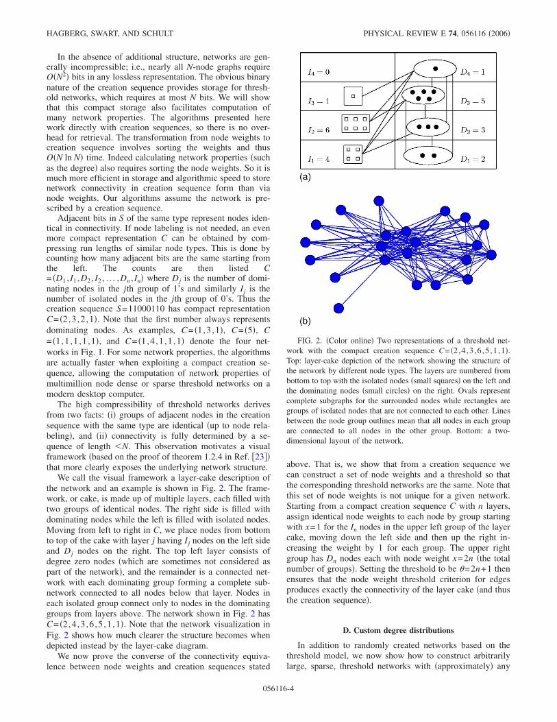
We call the visual framework a layer-cake description ofthe network and an example is shown in Fig. 2. The frame-work, or cake, is made up of multiple layers, each filled withtwo groups of identical nodes. The right side is filled withdominating nodes while the left is filled with isolated nodes.Moving from left to right in C, we place nodes from bottomto top of the cake with layer j having Ij nodes on the left sideand Dj nodes on the right. The top left layer consists ofdegree zero nodes �which are sometimes not considered aspart of the network�, and the remainder is a connected net-work with each dominating group forming a complete sub-network connected to all nodes below that layer. Nodes ineach isolated group connect only to nodes in the dominatinggroups from layers above. The network shown in Fig. 2 hasC= �2,4 ,3 ,6 ,5 ,1 ,1�. Note that the network visualization inFig. 2 shows how much clearer the structure becomes whendepicted instead by the layer-cake diagram.

We now prove the converse of the connectivity equiva-lence between node weights and creation sequences stated

above. That is, we show that from a creation sequence wecan construct a set of node weights and a threshold so thatthe corresponding threshold networks are the same. Note thatthis set of node weights is not unique for a given network.Starting from a compact creation sequence C with n layers,assign identical node weights to each node by group startingwith x=1 for the In nodes in the upper left group of the layercake, moving down the left side and then up the right in-creasing the weight by 1 for each group. The upper rightgroup has Dn nodes each with node weight x=2n �the totalnumber of groups�. Setting the threshold to be �=2n+1 thenensures that the node weight threshold criterion for edgesproduces exactly the connectivity of the layer cake �and thusthe creation sequence�.

D. Custom degree distributions

In addition to randomly created networks based on thethreshold model, we now show how to construct arbitrarilylarge, sparse, threshold networks with �approximately� any

FIG. 2. �Color online� Two representations of a threshold net-work with the compact creation sequence C= �2,4 ,3 ,6 ,5 ,1 ,1�.Top: layer-cake depiction of the network showing the structure ofthe network by different node types. The layers are numbered frombottom to top with the isolated nodes �small squares� on the left andthe dominating nodes �small circles� on the right. Ovals representcomplete subgraphs for the surrounded nodes while rectangles aregroups of isolated nodes that are not connected to each other. Linesbetween the node group outlines mean that all nodes in each groupare connected to all nodes in the other group. Bottom: a two-dimensional layout of the network.

HAGBERG, SWART, AND SCHULT PHYSICAL REVIEW E 74, 056116 �2006�

056116-4

prescribed degree distribution or Laplacian spectrum. A gen-eralization of this problem to vertex hidden variable modelswith scale-free degree distributions was studied in Ref. �17�.

Let pk be a discrete degree distribution that is normalizedso that �kpk=1. The goal is to construct a threshold networkwith approximately N nodes and with node degrees follow-ing the degree distribution pk. The maximum degree kmaxmust be less than N, and the number of nodes with degree kshould be nk= �Npk�. The construction strategy involves firstcreating a specific degree distribution realization nk fromthe discrete distribution. The resulting degree sequence neednot be graphical since our algorithm adjusts the number ofnodes and edges slightly to be able to build a threshold net-work.

We build a threshold network with approximately this dis-tribution by using isolated �0� nodes to fill out the degreedistribution and dominating �1� nodes to keep the networkconnected and distinguish between isolated nodes of differ-ing degrees. With this construction, we create N isolatednodes and kmax dominating nodes. While the number ofnodes is thus larger than N, for large sparse networks it isclose to N. Similarly, there will be a small number of nodes�the kmax dominating nodes� of very high degree. These willgenerally affect the connectivity of the network but they donot alter the degree distribution very much for large net-works.

As a simple example consider the degree distribution�1,2,3,5� which we will assume is chosen from a given pk.Starting at the highest degree k, we create nk isolated nodesfollowed by a single dominating node. The highest degree inthe distribution is 4 of which there are 5 nodes so the se-quence starts with 100001 �the first node in the creation se-quence is always 1, but it will be treated as an isolated nodefor this construction process�. Descending in degree with thesame algorithm we find the creation sequence S=100001000100101 or C= �1,4 ,1 ,3 ,1 ,2 ,1 ,1�. The corre-sponding threshold network has 15 nodes instead of 11, andthe degree distribution is �1,2,3,5,0,0,0,1,0,0,1,0,1,1�, whichhas 4 nodes of degree higher than 4 that do not exactly matchthe original degree distribution. While these few extra nodescertainly influence the connectivity or topology of the net-work, they do not significantly affect the degree distributionin the limit of large networks.

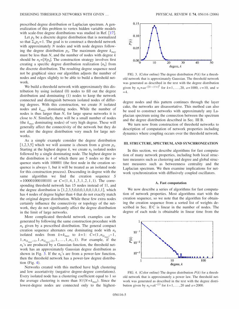
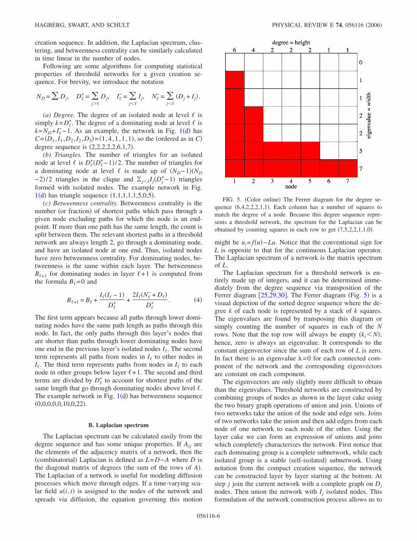
More complicated threshold network examples can begenerated by following the same construction procedure withnk given by a prescribed distribution. The general compactcreation sequence alternates one dominating node with nkisolated nodes from k=kmax to k=1: C= �1,n�kmax�−1,1 ,n�kmax−1� ,1 ,n�kmax−2� ,1 , . . . ,1 ,n1 ,1�. For example, if thenk’s are produced by a Gaussian function, the threshold net-work has an approximately Gaussian degree distribution asshown in Fig. 3. If the nk’s are from a power-law function,then the threshold network has a power-law degree distribu-tion �Fig. 4�.

Networks created with this method have high clusteringand low assortativity �negative degree-degree correlations�.Every isolated node has a clustering coefficient equal to 1 sothe average clustering is more than N / �N+kmax�. Since thelowest-degree nodes are connected only to the highest-

degree nodes and this pattern continues through the layercake, the networks are disassortative. This method can alsobe used to construct networks with approximately any La-placian spectrum using the connection between the spectrumand the degree distribution described in Sec. III B.

We turn now from construction of threshold networks todescription of computation of network properties includingdynamics where coupling occurs over the threshold network.

III. STRUCTURE, SPECTRUM, AND SYNCHRONIZATION

In this section, we describe algorithms for fast computa-tion of many network properties, including both local struc-ture measures such as clustering and degree and global struc-ture measures such as betweenness centrality and theLaplacian spectrum. We then examine implications for net-work synchronization with diffusively coupled oscillators.

A. Fast computation

We now describe a series of algorithms for fast computa-tion of network properties. Most algorithms start with thecreation sequence, so we note that the algorithm for obtain-ing the creation sequence from a sorted list of weights de-scribed in Sec. II C is linear in the number of nodes. Thedegree of each node is obtainable in linear time from the

FIG. 3. �Color online� The degree distribution P�k� for a thresh-old network that is approximately Gaussian. The threshold networkwas generated as described in the text with the degree distributiongiven by nk=ae−��k − c� / w�2

for k=1, . . . ,20, a=1000, c=10, and w=4.

FIG. 4. �Color online� The degree distribution P�k� for a thresh-old network that is approximately a power law. The threshold net-work was generated as described in the text with the degree distri-bution given by nk=ak−2.5 for k=1, . . . ,20 and a=2000.

DESIGNING THRESHOLD NETWORKS WITH GIVEN … PHYSICAL REVIEW E 74, 056116 �2006�

056116-5

creation sequence. In addition, the Laplacian spectrum, clus-tering, and betweenness centrality can be similarly calculatedin time linear in the number of nodes.

Following are some algorithms for computing statisticalproperties of threshold networks for a given creation se-quence. For brevity, we introduce the notation

ND = � Dj, D�+ = �

j��

Dj, I�− = �

j��

Ij, N�− = �

j��

�Dj + Ij� .

(a) Degree. The degree of an isolated node at level � issimply k=D�

+. The degree of a dominating node at level � isk=ND+ I�

−−1. As an example, the network in Fig. 1�d� hasC= �D1 , I1 ,D2 , I2 ,D3�= �1,4 ,1 ,1 ,1�, so the �ordered as in C�degree sequence is �2,2,2,2,2,6,1,7�.

(b) Triangles. The number of triangles for an isolatednode at level � is D�

+�D�+−1� /2. The number of triangles for

a dominating node at level � is made up of �ND−1��ND

−2� /2 triangles in the clique and � j��Ij�Dj+−1� triangles

formed with isolated nodes. The example network in Fig.1�d� has triangle sequence �1,1,1,1,1,5,0,5�.

(c) Betweenness centrality. Betweenness centrality is thenumber �or fraction� of shortest paths which pass through agiven node excluding paths for which the node is an end-point. If more than one path has the same length, the count issplit between them. The relevant shortest paths in a thresholdnetwork are always length 2, go through a dominating node,and have an isolated node at one end. Thus, isolated nodeshave zero betweenness centrality. For dominating nodes, be-tweenness is the same within each layer. The betweennessB�+1 for dominating nodes in layer �+1 is computed fromthe formula B1=0 and

B�+1 = B� +I��I� − 1�

D�+ +

2I��N�− + D��

D�+ . �4�

The first term appears because all paths through lower domi-nating nodes have the same path length as paths through thisnode. In fact, the only paths through this layer’s nodes thatare shorter than paths through lower dominating nodes haveone end in the previous layer’s isolated nodes I�. The secondterm represents all paths from nodes in I� to other nodes inI�. The third term represents paths from nodes in I� to eachnode in other groups below layer �+1. The second and thirdterms are divided by D�

+ to account for shortest paths of thesame length that go through dominating nodes above level �.The example network in Fig. 1�d� has betweenness sequence�0,0,0,0,0,10,0,22�.

B. Laplacian spectrum

The Laplacian spectrum can be calculated easily from thedegree sequence and has some unique properties. If Aij arethe elements of the adjacency matrix of a network, then the�combinatorial� Laplacian is defined as L=D−A where D isthe diagonal matrix of degrees �the sum of the rows of A�.The Laplacian of a network is useful for modeling diffusionprocesses which move through edges. If a time-varying sca-lar field u�i , t� is assigned to the nodes of the network andspreads via diffusion, the equation governing this motion

might be ut= f�u�−Lu. Notice that the conventional sign forL is opposite to that for the continuous Laplacian operator.The Laplacian spectrum of a network is the matrix spectrumof L.

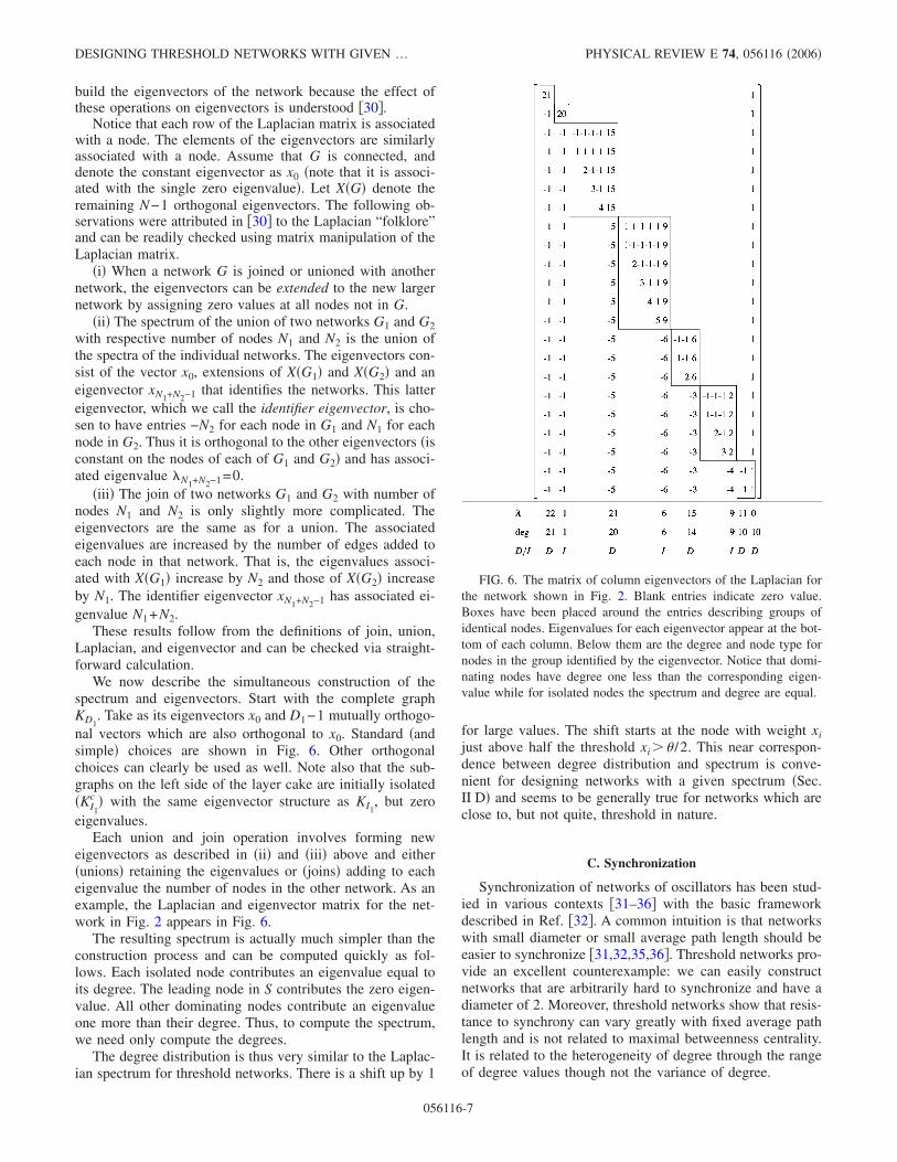
The Laplacian spectrum for a threshold network is en-tirely made up of integers, and it can be determined imme-diately from the degree sequence via transposition of theFerrer diagram �25,29,30�. The Ferrer diagram �Fig. 5� is avisual depiction of the sorted degree sequence where the de-gree k of each node is represented by a stack of k squares.The eigenvalues are found by transposing this diagram orsimply counting the number of squares in each of the Nrows. Note that the top row will always be empty �ki�N�;hence, zero is always an eigenvalue. It corresponds to theconstant eigenvector since the sum of each row of L is zero.In fact there is an eigenvalue �=0 for each connected com-ponent of the network and the corresponding eigenvectorsare constant on each component.

The eigenvectors are only slightly more difficult to obtainthan the eigenvalues. Threshold networks are constructed bycombining groups of nodes as shown in the layer cake usingthe two binary graph operations of union and join. Unions oftwo networks take the union of the node and edge sets. Joinsof two networks take the union and then add edges from eachnode of one network to each node of the other. Using thelayer cake we can form an expression of unions and joinswhich completely characterizes the network. First notice thateach dominating group is a complete subnetwork, while eachisolated group is a stable �self-isolated� subnetwork. Usingnotation from the compact creation sequence, the networkcan be constructed layer by layer starting at the bottom. Atstep j join the current network with a complete graph on Djnodes. Then union the network with Ij isolated nodes. Thisformulation of the network construction process allows us to

FIG. 5. �Color online� The Ferrer diagram for the degree se-quence �6,4,2,2,2,1,1�. Each column has a number of squares tomatch the degree of a node. Because this degree sequence repre-sents a threshold network, the spectrum for the Laplacian can beobtained by counting squares in each row to get �7,5,2,2,1,1,0�.

HAGBERG, SWART, AND SCHULT PHYSICAL REVIEW E 74, 056116 �2006�

056116-6

build the eigenvectors of the network because the effect ofthese operations on eigenvectors is understood �30�.

Notice that each row of the Laplacian matrix is associatedwith a node. The elements of the eigenvectors are similarlyassociated with a node. Assume that G is connected, anddenote the constant eigenvector as x0 �note that it is associ-ated with the single zero eigenvalue�. Let X�G� denote theremaining N−1 orthogonal eigenvectors. The following ob-servations were attributed in �30� to the Laplacian “folklore”and can be readily checked using matrix manipulation of theLaplacian matrix.

�i� When a network G is joined or unioned with anothernetwork, the eigenvectors can be extended to the new largernetwork by assigning zero values at all nodes not in G.

�ii� The spectrum of the union of two networks G1 and G2with respective number of nodes N1 and N2 is the union ofthe spectra of the individual networks. The eigenvectors con-sist of the vector x0, extensions of X�G1� and X�G2� and aneigenvector xN1+N2−1 that identifies the networks. This lattereigenvector, which we call the identifier eigenvector, is cho-sen to have entries −N2 for each node in G1 and N1 for eachnode in G2. Thus it is orthogonal to the other eigenvectors �isconstant on the nodes of each of G1 and G2� and has associ-ated eigenvalue �N1+N2−1=0.

�iii� The join of two networks G1 and G2 with number ofnodes N1 and N2 is only slightly more complicated. Theeigenvectors are the same as for a union. The associatedeigenvalues are increased by the number of edges added toeach node in that network. That is, the eigenvalues associ-ated with X�G1� increase by N2 and those of X�G2� increaseby N1. The identifier eigenvector xN1+N2−1 has associated ei-genvalue N1+N2.

These results follow from the definitions of join, union,Laplacian, and eigenvector and can be checked via straight-forward calculation.

We now describe the simultaneous construction of thespectrum and eigenvectors. Start with the complete graphKD1

. Take as its eigenvectors x0 and D1−1 mutually orthogo-nal vectors which are also orthogonal to x0. Standard �andsimple� choices are shown in Fig. 6. Other orthogonalchoices can clearly be used as well. Note also that the sub-graphs on the left side of the layer cake are initially isolated�KI1

c � with the same eigenvector structure as KI1, but zero

eigenvalues.Each union and join operation involves forming new

eigenvectors as described in �ii� and �iii� above and either�unions� retaining the eigenvalues or �joins� adding to eacheigenvalue the number of nodes in the other network. As anexample, the Laplacian and eigenvector matrix for the net-work in Fig. 2 appears in Fig. 6.

The resulting spectrum is actually much simpler than theconstruction process and can be computed quickly as fol-lows. Each isolated node contributes an eigenvalue equal toits degree. The leading node in S contributes the zero eigen-value. All other dominating nodes contribute an eigenvalueone more than their degree. Thus, to compute the spectrum,we need only compute the degrees.

The degree distribution is thus very similar to the Laplac-ian spectrum for threshold networks. There is a shift up by 1

for large values. The shift starts at the node with weight xijust above half the threshold xi�� /2. This near correspon-dence between degree distribution and spectrum is conve-nient for designing networks with a given spectrum �Sec.II D� and seems to be generally true for networks which areclose to, but not quite, threshold in nature.

C. Synchronization

Synchronization of networks of oscillators has been stud-ied in various contexts �31–36� with the basic frameworkdescribed in Ref. �32�. A common intuition is that networkswith small diameter or small average path length should beeasier to synchronize �31,32,35,36�. Threshold networks pro-vide an excellent counterexample: we can easily constructnetworks that are arbitrarily hard to synchronize and have adiameter of 2. Moreover, threshold networks show that resis-tance to synchrony can vary greatly with fixed average pathlength and is not related to maximal betweenness centrality.It is related to the heterogeneity of degree through the rangeof degree values though not the variance of degree.

FIG. 6. The matrix of column eigenvectors of the Laplacian forthe network shown in Fig. 2. Blank entries indicate zero value.Boxes have been placed around the entries describing groups ofidentical nodes. Eigenvalues for each eigenvector appear at the bot-tom of each column. Below them are the degree and node type fornodes in the group identified by the eigenvector. Notice that domi-nating nodes have degree one less than the corresponding eigen-value while for isolated nodes the spectrum and degree are equal.

DESIGNING THRESHOLD NETWORKS WITH GIVEN … PHYSICAL REVIEW E 74, 056116 �2006�

056116-7

Consider a system of N identical oscillators with statevector field u�t� where solutions with ui�t�=uj�t� for allnodes i and j are defined as synchronized. The system is saidto be synchronizable if a synchronized solution is linearlystable to nonuniform perturbations. A standard linear analy-sis near the synchronized solution shows that for generaloscillators with diffusive coupling the stability of the syn-chronized state is determined by the largest Lyapunov expo-nent ���, also called the master stability function�32,37,38�. If ��i��0 for each i2, the synchronized stateis linearly stable. �The eigenvalue �1=0 corresponds to spa-tially uniform perturbations.�

For many oscillatory systems the master equation is nega-tive only in a single interval ��1 ,�2� determined by the typeof oscillator and strength of coupling. This implies that thenetwork is synchronizable only when the ratio r��N /�2��2 /�1 �32�. Thus if �2 and �N are inside this interval—i.e.,r��2 /�1—then network synchronization is stable. Con-struction of a synchronizable network is easier for small r.To make a network resistant to synchronization, we designthe connectivity so that r, the resistance to synchrony, islarge.

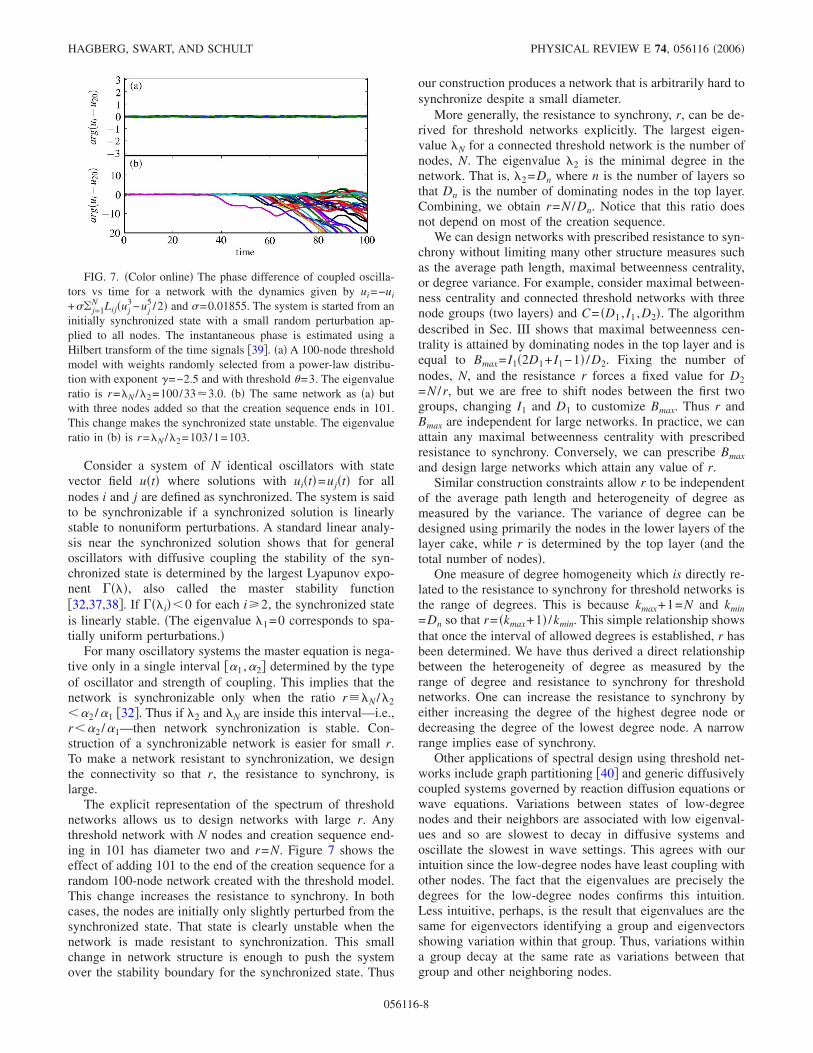
The explicit representation of the spectrum of thresholdnetworks allows us to design networks with large r. Anythreshold network with N nodes and creation sequence end-ing in 101 has diameter two and r=N. Figure 7 shows theeffect of adding 101 to the end of the creation sequence for arandom 100-node network created with the threshold model.This change increases the resistance to synchrony. In bothcases, the nodes are initially only slightly perturbed from thesynchronized state. That state is clearly unstable when thenetwork is made resistant to synchronization. This smallchange in network structure is enough to push the systemover the stability boundary for the synchronized state. Thus

our construction produces a network that is arbitrarily hard tosynchronize despite a small diameter.

More generally, the resistance to synchrony, r, can be de-rived for threshold networks explicitly. The largest eigen-value �N for a connected threshold network is the number ofnodes, N. The eigenvalue �2 is the minimal degree in thenetwork. That is, �2=Dn where n is the number of layers sothat Dn is the number of dominating nodes in the top layer.Combining, we obtain r=N /Dn. Notice that this ratio doesnot depend on most of the creation sequence.

We can design networks with prescribed resistance to syn-chrony without limiting many other structure measures suchas the average path length, maximal betweenness centrality,or degree variance. For example, consider maximal between-ness centrality and connected threshold networks with threenode groups �two layers� and C= �D1 , I1 ,D2�. The algorithmdescribed in Sec. III shows that maximal betweenness cen-trality is attained by dominating nodes in the top layer and isequal to Bmax= I1�2D1+ I1−1� /D2. Fixing the number ofnodes, N, and the resistance r forces a fixed value for D2=N /r, but we are free to shift nodes between the first twogroups, changing I1 and D1 to customize Bmax. Thus r andBmax are independent for large networks. In practice, we canattain any maximal betweenness centrality with prescribedresistance to synchrony. Conversely, we can prescribe Bmaxand design large networks which attain any value of r.

Similar construction constraints allow r to be independentof the average path length and heterogeneity of degree asmeasured by the variance. The variance of degree can bedesigned using primarily the nodes in the lower layers of thelayer cake, while r is determined by the top layer �and thetotal number of nodes�.

One measure of degree homogeneity which is directly re-lated to the resistance to synchrony for threshold networks isthe range of degrees. This is because kmax+1=N and kmin=Dn so that r= �kmax+1� /kmin. This simple relationship showsthat once the interval of allowed degrees is established, r hasbeen determined. We have thus derived a direct relationshipbetween the heterogeneity of degree as measured by therange of degree and resistance to synchrony for thresholdnetworks. One can increase the resistance to synchrony byeither increasing the degree of the highest degree node ordecreasing the degree of the lowest degree node. A narrowrange implies ease of synchrony.

Other applications of spectral design using threshold net-works include graph partitioning �40� and generic diffusivelycoupled systems governed by reaction diffusion equations orwave equations. Variations between states of low-degreenodes and their neighbors are associated with low eigenval-ues and so are slowest to decay in diffusive systems andoscillate the slowest in wave settings. This agrees with ourintuition since the low-degree nodes have least coupling withother nodes. The fact that the eigenvalues are precisely thedegrees for the low-degree nodes confirms this intuition.Less intuitive, perhaps, is the result that eigenvalues are thesame for eigenvectors identifying a group and eigenvectorsshowing variation within that group. Thus, variations withina group decay at the same rate as variations between thatgroup and other neighboring nodes.

FIG. 7. �Color online� The phase difference of coupled oscilla-tors vs time for a network with the dynamics given by ui=−ui

+�� j=1N Lij�uj

3−uj5 /2� and �=0.01855. The system is started from an

initially synchronized state with a small random perturbation ap-plied to all nodes. The instantaneous phase is estimated using aHilbert transform of the time signals �39�. �a� A 100-node thresholdmodel with weights randomly selected from a power-law distribu-tion with exponent �=−2.5 and with threshold �=3. The eigenvalueratio is r=�N /�2=100/33�3.0. �b� The same network as �a� butwith three nodes added so that the creation sequence ends in 101.This change makes the synchronized state unstable. The eigenvalueratio in �b� is r=�N /�2=103/1=103.

HAGBERG, SWART, AND SCHULT PHYSICAL REVIEW E 74, 056116 �2006�

056116-8

IV. SUMMARY

The threshold model for network creation is one of manymodels used to generate networks of arbitrary size with anapproximate local properties such as degree distribution,clustering, degree correlation, or spectrum. We summarizeprevious work on networks created by the threshold modeland present an alternative deterministic model for thresholdnetwork creation which approximates a prescribed degreedistribution or spectrum. In either case, the created thresholdnetworks are graph-theoretic threshold graphs, a fact that im-poses a very specific network structure. We use this structureto develop a methodology for compact storage and fast com-putation of many network properties. The degree distribu-tion, clustering, betweenness centrality, and Laplacian spec-trum can all be computed in linear time. In addition, theLaplacian spectrum and eigenvector structure are completelycharacterized, allowing these networks to be created withcustomized spectrum. Algorithms for the generation, storage,and structural analysis presented here are contained in theauthors’ open-source software package NetworkX �41�.

Building on this base, we have described some implica-tions for the study of synchronization of diffusively coupledoscillators. Diffusive spreading occurs most quickly throughhigh degree nodes, with spread around a clique being nofaster than spread to those outside the clique �42,43�. Syn-chronization is described in terms of the spectrum of thenetwork. Threshold networks provide constructive counter-examples to the notion that networks with small diameter areeasy to synchronize. We also derived the result for thresholdnetworks that resistance to synchrony is completely deter-mined by the minimum and maximum degrees in the net-work.

The existence of fast algorithms for structural analysissuggests that threshold networks are good candidates for net-work deconstruction. That is, rather than analyzing an entirenetwork at once, we might consider the important thresholdnetworks embedded in a larger network and how they areconnected. Storing and manipulating this reduced networkmay be more effective than working with the original net-work for some tasks. The network motif literature �see, e.g.,�1�� deconstructs large networks using subnetworks withsmall numbers of nodes. By identifying small structures thatoccur more often than expected they attempt to identifystructures with useful features in the network. Using thresh-old networks as the motif structures may have advantagesover small subnetworks because threshold networks are arbi-trarily large and yet are still computationally manageable.

Threshold networks are also good candidates for con-structing nonthreshold networks with specified structure. Thealgorithm might consist of creating many threshold networkswith desired properties and then connecting them in waysthat do not significantly alter those properties. The ability tocreate networks by connecting subnetworks with given struc-ture could provide great flexibility in network design.

ACKNOWLEDGMENTS

This work was carried out under the auspices of the Na-tional Nuclear Security Administration of the U.S. Depart-ment of Energy at Los Alamos National Laboratory underContract No. DE-AC52-06NA25396, partially supported bythe Laboratory Directed Research and Development Pro-gram, and the DOE Office of Science Advanced ScientificComputing Research �ASCR� Program in Applied Math-ematics Research.

�1� E. Yeger-Lotem, S. Sattath, N. Kashtan, S. Itzkovitz, R. Milo,R. Y. Pinter, U. Alon, and H. Margalit, Proc. Natl. Acad. Sci.U.S.A. 101, 5934 �2004�.

�2� M. E. J. Newman, Phys. Rev. E 66, 016128 �2002�.�3� S. Eubank, H. Guclu, V. S. A. Kumar, M. V. Marathe, A.

Srinivasan, Z. Toroczkai, and N. Wang, Nature �London� 429,180 �2004�.

�4� J. C. Doyle, D. L. Anderson, L. Li, S. Low, M. Roughan, S.Shalunov, R. Tanaka, and W. Willinger, Proc. Natl. Acad. Sci.U.S.A. 102, 14497 �2005�.

�5� M. Girvan and M. E. J. Newman, Proc. Natl. Acad. Sci. U.S.A.99, 7821 �2002�.

�6� A. L. Barabási and R. Albert, Science 286, 509 �1999�.�7� D. J. Watts and S. H. Strogatz, Nature �London� 393, 440

�1998�.�8� M. E. J. Newman, SIAM Rev. 45, 167 �2003�.�9� S. N. Dorogovtsev and J. F. F. Mendes, Adv. Phys. 51, 1079

�2002�.�10� R. Albert and A. L. Barabási, Rev. Mod. Phys. 74, 47 �2002�.�11� Complex Networks, edited by E. Ben-Naim, H. Frauenfelder,

and Z. Torozckai, Vol. 650 of Lecture Notes in Physics�Springer, Berlin, 2004�.

�12� G. Bianconi and A. L. Barabási, Europhys. Lett. 54, 436�2001�.

�13� B. Bollobás, Random Graphs, 2nd ed. �Cambridge UniversityPress, Cambridge, England, 2001�.

�14� F. R. K. Chung, L. Lu, and V. Vu, Internet Mathematics 1, 257�2004�.

�15� K.-I. Goh, B. Kahng, and D. Kim, Phys. Rev. Lett. 87, 278701�2001�.

�16� G. Caldarelli, A. Capocci, P. De Los Rios, and M. A. Muñoz,Phys. Rev. Lett. 89, 258702 �2002�.

�17� V. D. P. Servedio, G. Caldarelli, and P. Buttà, Phys. Rev. E 70,056126 �2004�.

�18� B. Söderberg, Phys. Rev. E 66, 066121 �2002�.�19� M. Boguña and R. Pastor-Satorras, Phys. Rev. E 68, 036112

�2003�.�20� M. Catanzaro and R. Pastor-Satorras, Eur. Phys. J. B 44, 241

�2005�.�21� N. Masuda, H. Miwa, and N. Konno, Phys. Rev. E 70, 036124

�2004�.�22� M. C. Golumbic, Algorithmic Graph Theory and Perfect

Graphs �Academic Press, New York, 1980�.�23� N. V. R. Mahadev and U. N. Peled, Threshold Graphs and

DESIGNING THRESHOLD NETWORKS WITH GIVEN … PHYSICAL REVIEW E 74, 056116 �2006�

056116-9

Related Topics, Vol. 56 of Annals of Discrete Mathematics�Elsevier, New York, 1995�.

�24� P. L. Hammer, T. Ibaraki, and B. Simeone, SIAM J. AlgebraicDiscrete Methods 2, 39 �1981�.

�25� R. Merris, Linear Algebr. Appl. 198, 143 �1994�.�26� R. Merris, Eur. J. Comb. 24, 413 �2003�.�27� M. Golumbic and A. Trenk, Tolerance Graphs �Cambridge

University Press, Cambridge, England, 2004�.�28� R. Merris, Linear Algebr. Appl. 199, 381 �1994�.�29� P. L. Hammer and A. K. Kelmans, Discrete Appl. Math. 65,

255 �1996�.�30� R. Merris, Linear Algebr. Appl. 278, 221 �1998�.�31� T. Nishikawa, A. E. Motter, Y. C. Lai, and F. C. Hoppensteadt,

Phys. Rev. Lett. 91, 014101 �2003�.�32� M. Barahona and L. M. Pecora, Phys. Rev. Lett. 89, 054101

�2002�.�33� H. Hong, B. J. Kim, M. Y. Choi, and H. Park, Phys. Rev. E 69,

067105 �2004�.�34� D. U. Hwang, M. Chavez, A. Amann, and S. Boccaletti, Phys.

Rev. Lett. 94, 138701 �2005�.�35� F. M. Atay, T. Biyikoğlu, and J. Jost, IEEE Trans. Circuits

Syst., I: Fundam. Theory Appl. 53, 92 �2006�.�36� A. E. Motter, C. Zhou, and J. Kurths, Phys. Rev. E 71, 016116

�2005�.�37� L. M. Pecora and T. L. Carroll, Phys. Rev. Lett. 80, 2109

�1998�.�38� K. S. Fink, G. Johnson, T. Carroll, D. Mar, and L. Pecora,

Phys. Rev. E 61, 5080 �2000�.�39� M. G. Rosenblum, A. S. Pikovsky, and J. Kurths, Phys. Rev.

Lett. 76, 1804 �1996�.�40� A. Arenas, A. Díaz-Guilera, and C. J. Pérez-Vicente, Phys.

Rev. Lett. 96, 114102 �2006�.�41� A. Hagberg, D. A. Schult, and P. J. Swart, https://

networkx.lanl.gov/.�42� M. Barthélemy, A. Barrat, R. Pastor-Satorras, and A. Vespig-

nani, Phys. Rev. Lett. 92, 178701 �2004�.�43� M. Barthélemy, A. Barrat, R. Pastor-Satorras, and A. Vespig-

nani, J. Theor. Biol. 235, 275 �2005�.

HAGBERG, SWART, AND SCHULT PHYSICAL REVIEW E 74, 056116 �2006�

056116-10