Embed Size (px)
Citation preview
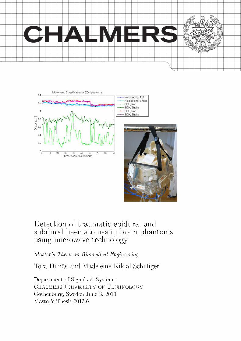
Detection of traumatic epidural andsubdural haematomas in brain phantomsusing microwave technology
Master's Thesis in Biomedical Engineering
Tora Dunås and Madeleine Kildal Schilliger
Department of Signals & Systems
Chalmers University of Technology
Gothenburg, Sweden June 3, 2013
Master's Thesis 2013:6
Abstract
Traumatic brain injury (TBI) is a worldwide problem with around 10 mil-lion serious incidences every year, whereof 22 000 in Sweden. The maincauses are road trac accidents, falls and violence. The most serious com-plication of a TBI is an intracranial haematoma, which is a bleeding insidethe cranium that rapidly can cause fatal complications in the form of is-chemia and increased intracranial pressure. A TBI is normally diagnosedat the hospital with computed tomography (CT). However, to be able togive faster and better medical care a portable diagnosis method is needed.
In this project, which is a cooperation between two engineering studentsand one medical student, the possibility to use microwave technology in theform of a microwave helmet (MWH) to detect intracranial bleedings was in-vestigated. A network analyser with a built in switch was used together witha MWH consisting of twelve antennas. The measurements were performedon phantoms in a human cranium. Two types of common TBI bleedings,epidural and subdural haematomas with the volumes 20, 40 and 60ml, weremodelled. Interfering factors that may aect the measurements were alsostudied. The measurement data were analysed with a singular value decom-position based classier. The analyses were focused on classifying phantomswith or without bleeding and with respect to type, volume and location ofthe bleeding.
Interferences such as a microwave radiation from an active mobile phoneor person close to the measurement setup did not signicantly aect themeasurements. The interference factors that had a visible eect on themeasurements were a person holding the measurement cables, presence ofa wig of human hair around the cranium and moving the phantoms duringthe measurements.
The thirteen phantoms that were constructed were not enough to beable to say if the MWH together with the classier can detect intracranialbleedings. Although some trends can be seen, for example manages theclassier to recognise the individual phantoms, which is an indication thatit will be able to recognise bleedings with a larger test set. The interfer-ence factors that had a visible eect need to be investigated further andcompensated for.
MWT seeems to be a promising technique to detect intracranial bleedins.However a larger data base is needed before it can be completely evaluated.
Sammanfattning
Traumatiska hjärnskador är ett stort problem världen över, med omkring10 miljoner allvarliga fall varje år, varav 20 000 bara i Sverige. De huvudsak-liga orsakerna är trakolyckor, fallolyckor och misshandel. En av de farligas-te komplikationerna av en traumatisk hjärnskada är en intrakraniell blöd-ning. Det är blödningar innanför kraniet som kan ge dödliga komplikationer,så som ischemi och ökat intrakraniellt tryck. Vanligtvis diagnosticeras entraumatisk hjärnskada med hjälp av en CT på sjukhuset, men för att kunnage snabbare och bättre medicinsk vård behövs en portabel diagnosmetod.
I detta projekt, som är ett samarbete mellan två ingenjörsstudenteroch en läkarstudent, undersöktes möjligheten att använda mikrovågstekniki form av en mikrovågshjälm för att diagnosticera intrakraniella blödning-ar. En nätverksanalysator med inbyggd switch användes tillsammans meden mikrovågshjälm bestående av tolv antenner för att utföra mätningarna.Mätningarna genomfördes på fantomer i ett mänskligt kranium. Två typerav vanliga blödningar vid traumatiska hjärnskador, epidural- och subdu-ralhematom med volymerna 20, 40 och 60ml, modellerades. Även störandefaktorer som kan påverka mätningarna undersöktes. Mätdatan analyseradesmed hjälp av en klassicerare baserad på singulärvärdesuppdelning. Analy-serna fokuserade på att klassicera fantomer med eller utan blödning, samtmed avseende på typ, volym och placering av blödningen.
Störningar av mikrovågsstrålning från en aktiv mobiltelefon eller personsom stod nära mätuppställningen gav ingen påverkan. Däremot påverkadestörningar i form av en person som håller i mätkablarna, förekomst av enperuk med mänskligt hår runt kraniet och skakning av fantomen undermätningarna.
De tretton fantomerna som gjordes var inte tillräckligt många för attkunna avgöra om mikrovågshjälmen tillsammans med klassiceraren kandetektera blödningar. Vissa trender kunde dock ses, till exempel kunde klas-siceraren känna igen individuella fantomer, vilket är en indikation på attden kommer kunna detektera blödningar med en större referensdatagrupp.Störningarna som hade en synlig påverkan behöver undersökas ytterligareoch kompenseras för.
Mikrovågsteknik verkar vara lovande för att detektera intrakraniellablödnignar, dock behövs en större databas för att fullständigt kunna ut-värdera tekniken.

ii
Preface
Medeld Diagnostics has developed a microwave based product called Stroke-nder R10 for diagnosing stroke patients and are right now in the clinicaltrials. This project investigates the Strokender further, to see if it also canbe used to diagnose traumatic intracranial bleedings.
This project has mostly been carried out at MedTech West at Sahlgren-ska University Hospital in Gothenburg. Measurements have been performedat Medeld Diagnostics and Chalmers University of Technology.
This project was a cooperation with medical student Philip Swahn,whom we would like to thank for his work with the phantoms.
We would also like to thank our supervisors Stefan Candefjord at MedTechWest and Stefan Kidborg at Medeld Diagnostics for their help, supportand great encouragement throughout the project.
Thanks to Medeld Diagnostics and Dag Jungenfelt, and especiallythanks to Gustav Mårtensson and Johan Klingstedt that has helped us a lotwith the measurement equipment. Thanks to MedTech West for providingus with a work place and nice work environment.
We would also like to thank Tora's examinator Andreas Fhager andHana Dobsicek Trefna at the Biomedical Electromagnetics research groupat Chalmers for help at the Microwave laboratory and with placement oforders, as well as Tomas McKelvey and Yinan Yu at the Signal Processingresearch group at Chalmers for providing the classier used for analysisof the data. Thank to Madeleine's examinator Mats Gustafsson, at thedepartment of Electrical and Information technology at Lund University,for his time.
We would also like to thank neurosurgeons Thomas Skoglund and JohanLjungqvist at Sahlgrenska University Hospital for advise on the clinicalaspects of the project.
Tora DunåsMadeleine Kildal Schilliger
Gothenburg, June 2013
iii

iv
Contents
1 Introduction 1
1.1 Aim . . . . . . . . . . . . . . . . . . . . . . . . . . . . . . . 2
1.1.1 Research questions 2
1.2 Delimitations . . . . . . . . . . . . . . . . . . . . . . . . . . . 2
1.3 Division of labor . . . . . . . . . . . . . . . . . . . . . . . . . 3
2 Theory 5
2.1 Anatomy of the brain . . . . . . . . . . . . . . . . . . . . . . 5
2.2 Traumatic brain injuries . . . . . . . . . . . . . . . . . . . . . 8
2.3 Diagnostic methods . . . . . . . . . . . . . . . . . . . . . . . 9
2.3.1 Computed tomography 11
2.3.2 Magnetic resonance imaging 12
2.3.3 Near infrared spectroscopy 12
2.3.4 Ultrasound 13
2.4 Microwave technology . . . . . . . . . . . . . . . . . . . . . . 13
2.4.1 Microwaves 13
2.4.2 Scattering parameters 20
2.4.3 Applications 21
2.4.4 Patch Antennas 22
2.4.5 Safety guidelines 23
2.5 Data analysis . . . . . . . . . . . . . . . . . . . . . . . . . . . 24
2.5.1 Singular value decomposition 24
2.5.2 Ttest 25
3 Method 27
3.1 Experimental setup . . . . . . . . . . . . . . . . . . . . . . . 27
3.1.1 Dielectric measurements 27
3.1.2 Microwave helmet measurements 27
3.2 Phantom construction . . . . . . . . . . . . . . . . . . . . . . 28
3.3 Dielectric measurements . . . . . . . . . . . . . . . . . . . . . 32
v
3.3.1 Phantoms 32
3.3.2 Coagulated blood measurements 33
3.4 Microwave helmet measurements . . . . . . . . . . . . . . . . 34
3.4.1 Ordinary measurements 35
3.4.2 Interfering factors 35
Person close and holding the cables 35
Phone 35
Hair 36
Movement 36
3.5 Data analysis . . . . . . . . . . . . . . . . . . . . . . . . . . . 36
3.5.1 Dielectric measurements 36
Phantoms 36
Liquid and solid phantoms 37
Coagulated blood measurements 37
3.5.2 Microwave helmet measurements 37
4 Result 41
4.1 Phantoms . . . . . . . . . . . . . . . . . . . . . . . . . . . . 41
4.2 Dielectric properties . . . . . . . . . . . . . . . . . . . . . . . 43
4.2.1 Phantoms 43
Contrast in bleeding phantoms 43
4.2.2 Grey matter and blood recipes 43
4.2.3 Liquid and solid phantoms 45
4.2.4 Coagulated blood measurements 48
4.3 Microwave helmet . . . . . . . . . . . . . . . . . . . . . . . . 50
4.4 Data analysis . . . . . . . . . . . . . . . . . . . . . . . . . . . 52
4.4.1 Non bleeding and bleeding phantoms 53
Classifying a phantom that is not in the trainingset 53
4.4.2 Epidural and subdural haematomas 53
4.4.3 Volume of bleedings 55
4.4.4 Left and right bleedings 55
4.4.5 Interfering factors 60
Person close 60
Holding the cables 60
Phone call 60
Hair 60
Movement 61
5 Discussion 67
5.1 Phantoms . . . . . . . . . . . . . . . . . . . . . . . . . . . . 67
5.2 Dielectric properties . . . . . . . . . . . . . . . . . . . . . . . 68
5.2.1 Phantoms 68
vi
Contrast in bleeding phantoms 69
5.2.2 Grey matter and blood recipes 70
5.2.3 Liquid and solid phantoms 70
5.2.4 Coagulated blood measurements 70
5.3 Microwave helmet . . . . . . . . . . . . . . . . . . . . . . . . 71
5.4 Data analysis . . . . . . . . . . . . . . . . . . . . . . . . . . . 71
5.4.1 Non bleeding and bleeding phantoms 73
5.4.2 Epidural and subdural haematomas 74
5.4.3 Volume of bleedings 75
5.4.4 Left and right bleedings 75
5.4.5 Interfering factors 76
Person close 76
Holding the cables 76
Phone call 76
Hair 76
Movement 77
5.5 Future work . . . . . . . . . . . . . . . . . . . . . . . . . . . 77
6 Conclusion 79
Bibliography 81
A Measurement protocol 85
A.1 Create phantom . . . . . . . . . . . . . . . . . . . . . . . . . 85
A.1.1 Blood phantom mass 85
A.1.2 Brain phantom mass 88
A.2 Calibration of dielectric probe (Chalmers) . . . . . . . . . . . . 90
A.3 Measure with dielectric probe (Chalmers) . . . . . . . . . . . . 93
A.4 Calibration of measurement equipment (Medeld Diagnostics) 94
A.5 Preparation for measurements . . . . . . . . . . . . . . . . . . 97
A.6 Measurements at Medeld Diagnostics . . . . . . . . . . . . . 100
A.6.1 Perform measurements 102
A.7 After measurements . . . . . . . . . . . . . . . . . . . . . . . 105
B List of phantoms 107
vii

viii
List of Figures
2.1 The main parts of the brain. . . . . . . . . . . . . . . . . . . 6
2.2 The dierent lobes of the brain. . . . . . . . . . . . . . . . . . 6
2.3 Grey and white matter in the brain. . . . . . . . . . . . . . . . 7
2.4 Schematic picture of a nerve cell. . . . . . . . . . . . . . . . . 7
2.5 The meninges and other layers that protect the brain. . . . . . 8
2.6 Three types of intracranial bleedings. . . . . . . . . . . . . . . 10
2.7 Position of the temporal bone. . . . . . . . . . . . . . . . . . 10
2.8 CT image of brain. . . . . . . . . . . . . . . . . . . . . . . . 12
2.9 Dielectric properties for dierent tissues. . . . . . . . . . . . . 16
2.10 Electromagnetic wave with normal and oblique incidence at a
material border. . . . . . . . . . . . . . . . . . . . . . . . . . 17
2.11 Illustration of phase shift. . . . . . . . . . . . . . . . . . . . . 19
2.12 Skin depth for dierent tissues. . . . . . . . . . . . . . . . . . 20
2.13 Illustration of the S-parameters. . . . . . . . . . . . . . . . . . 21
2.14 Microwave propagation. . . . . . . . . . . . . . . . . . . . . . 22
2.15 E-eld for a rectangular patch antenna. . . . . . . . . . . . . . 23
2.16 Triangular patch antenna. . . . . . . . . . . . . . . . . . . . . 24
3.1 Measurement setup for the dielectric probe. . . . . . . . . . . 28
3.2 Measurement setup at Medeld Diagnostics. . . . . . . . . . . 29
3.3 One of the patch antennas used in the microwave helmet. . . . 29
3.4 The microwave helmet. . . . . . . . . . . . . . . . . . . . . . 30
3.5 Placing a bleeding in the cranium. . . . . . . . . . . . . . . . 33
3.6 Location of epidural bleeding. . . . . . . . . . . . . . . . . . . 34
3.7 Schematic gures of the positions of the bleedings relative the
antennas in the microwave helmet. . . . . . . . . . . . . . . . 39
3.8 Dierent types of measurements with the microwave helmet. . 40
3.9 Cranium with wig for hair impact measurements. . . . . . . . 40
4.1 Examples of bleeding phantoms. . . . . . . . . . . . . . . . . 42
ix
4.2 Relative permittivity and conductivity for all phantoms. . . . . 44
4.3 Relative permittivity and conductivity for grey matter phantom
solutions. . . . . . . . . . . . . . . . . . . . . . . . . . . . . . 46
4.4 Relative permittivity and conductivity for blood phantom solutions. 47
4.5 Relative permittivity and conductivity for coagulated blood. . . 49
4.6 Reection and transmission coecients for all phantoms. . . . 51
4.7 Classication of non bleeding phantoms with all measurement
points. . . . . . . . . . . . . . . . . . . . . . . . . . . . . . . 52
4.8 Classication of non bleeding and bleeding phantoms. . . . . . 56
4.9 Classication of epidural and subdural haematomas. . . . . . . 57
4.10 Classication with respect to bleeding volumes. . . . . . . . . 58
4.11 Classication with respect to bleeding locations. . . . . . . . . 59
4.12 Classication of bleeding phantoms with a person close to the
microwave helmet. . . . . . . . . . . . . . . . . . . . . . . . . 62
4.13 Classication of bleeding phantoms with a person holding the
cables. . . . . . . . . . . . . . . . . . . . . . . . . . . . . . . 63
4.14 Classication of non bleeding phantoms with a calling mobile
phone. . . . . . . . . . . . . . . . . . . . . . . . . . . . . . . 64
4.15 Classication of EDH phantoms with hair. . . . . . . . . . . . 65
4.16 Classication of shaking epidural phantoms. . . . . . . . . . . 66
A.1 Preparation for EDH. . . . . . . . . . . . . . . . . . . . . . . 86
A.2 Preparation of cranium. . . . . . . . . . . . . . . . . . . . . . 86
A.3 Setup of dielectric probe. . . . . . . . . . . . . . . . . . . . . 91
A.4 Schematic polar plot for calibration. . . . . . . . . . . . . . . 92
A.5 Calibration kit. . . . . . . . . . . . . . . . . . . . . . . . . . . 95
A.6 The microwave helmet. . . . . . . . . . . . . . . . . . . . . . 98
A.7 Measurement setup at Medeld Diagnostics. . . . . . . . . . . 98
A.8 Test measurements at Medeld Diagnostics. . . . . . . . . . . 101
A.9 Dierent types of measurements with the microwave helmet. . 104
A.10 Cranium with wig for hair interfering measurements. . . . . . . 104
x
List of Tables
3.1 Recipes for the grey matter phantom masses. . . . . . . . . . 31
3.2 Recipes for blood phantom masses. . . . . . . . . . . . . . . . 32
4.1 List of phantoms. . . . . . . . . . . . . . . . . . . . . . . . . 41
4.2 Contrast in dielectric properties between grey matter and blood
phantom masses. . . . . . . . . . . . . . . . . . . . . . . . . 45
4.3 Dierence between solid and liquid phantom masses. . . . . . 45
4.4 Classication when leaving one phantom out of the training data. 54
4.5 Classication of phantoms with a person close to the microwave
helmet. . . . . . . . . . . . . . . . . . . . . . . . . . . . . . . 62
4.6 Classication of phantoms with a person holding the cables. . . 63
4.7 Classication of phantoms with calling mobile phone. . . . . . 64
4.8 Classication of phantoms with hair. . . . . . . . . . . . . . . 65
4.9 Classication of shaking phantoms. . . . . . . . . . . . . . . . 66
A.1 Recipe for blood phantom mass. . . . . . . . . . . . . . . . . 85
A.2 Recipe for grey matter phantom mass. . . . . . . . . . . . . . 88
B.1 Detailed list of reference phantoms. . . . . . . . . . . . . . . . 107
B.2 Detailed list of bleeding phantoms. . . . . . . . . . . . . . . . 108
xi

xii
Nomenclature
CSF Cerebrospinal Fluid
CT Computed Tomography
DAI Diuse Axonal Injury
EDH Epidural Haematoma
GCS Glasgow Coma Scale
ICH Intracerebral Haematoma
ICNIRP International Comission on Non-Ionizing Radiation Protection
ICP Intracranial Pressure
MRI Magnetic Resonance Imaging
MWH Microwave Helmet
MWT Microwave Technology
NIRS Near Infrared Spectroscopy
PNA Programmable Network Analyser
SAH Subarachnoid Haemorrhage
SAR Specic energy Absorption Rate
SDH Subdural Haematoma
SVD Singular Value Decomposition
TBI Traumatic Brain Injury
VNA Vector Network Analyser
xiii

xiv
Chapter1
Introduction
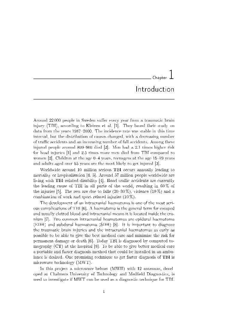
Around 22 000 people in Sweden suer every year from a traumatic braininjury (TBI), according to Kleiven et al. [1]. They based their study ondata from the years 19872000. The incidence rate was stable in this timeinterval, but the distribution of causes changed, with a decreasing numberof trac accidents and an increasing number of fall accidents. Among theseinjured people around 800900 died [2]. Men had a 2.1 times higher riskfor head injuries [1] and 2.5 times more men died from TBI compared towomen [2]. Children at the age 04 years, teenagers at the age 1519 yearsand adults aged over 65 years are the most likely to get injured [3].
Worldwide around 10 million serious TBI occurs annually leading tomortality or hospitalisation [4, 5]. Around 57 million people worldwide areliving with TBIrelated disability [4]. Road trac accidents are currentlythe leading cause of TBI in all parts of the world, resulting in 60% ofthe injuries [5]. The rest are due to falls (2030%), violence (10%) and acombination of work and sport related injuries (10%).
The development of an intracranial haematoma is one of the most seri-ous complications of TBI [6]. A haematoma is the general term for escapedand usually clotted blood and intracranial means it is located inside the cra-nium [7]. Two common intracranial heamatomas are epidural haematoma(EDH) and subdural haematoma (SDH) [8]. It is important to diagnosethe traumatic brain injuries and the intracranial haematomas as early aspossible to be able to give the best medical care and minimise the risk forpermanent damage or death [6]. Today TBI is diagnosed by computed to-mography (CT) at the hospital [8]. To be able to give better medical carea portable and faster diagnosis method that could be installed in an ambu-lance is desired. One promising technique to get faster diagnosis of TBI ismicrowave technology (MWT).
In this project a microwave helmet (MWH) with 12 antennas, devel-oped at Chalmers University of Technology and Medeld Diagnostics, isused to investigate if MWT can be used as a diagnostic technique for TBI.
1
2 Introduction
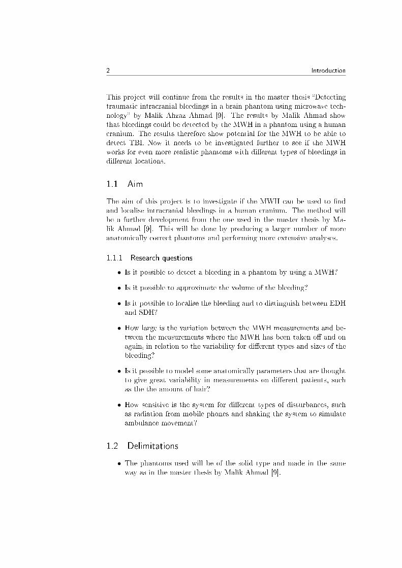
This project will continue from the results in the master thesis Detectingtraumatic intracranial bleedings in a brain phantom using microwave tech-nology by Malik Ahzaz Ahmad [9]. The results by Malik Ahmad showthat bleedings could be detected by the MWH in a phantom using a humancranium. The results therefore show potential for the MWH to be able todetect TBI. Now it needs to be investigated further to see if the MWHworks for even more realistic phantoms with dierent types of bleedings indierent locations.
1.1 Aim
The aim of this project is to investigate if the MWH can be used to ndand localise intracranial bleedings in a human cranium. The method willbe a further development from the one used in the master thesis by Ma-lik Ahmad [9]. This will be done by producing a larger number of moreanatomically correct phantoms and performing more extensive analyses.
1.1.1 Research questions
• Is it possible to detect a bleeding in a phantom by using a MWH?
• Is it possible to approximate the volume of the bleeding?
• Is it possible to localise the bleeding and to distinguish between EDHand SDH?
• How large is the variation between the MWH measurements and be-tween the measurements where the MWH has been taken o and onagain, in relation to the variability for dierent types and sizes of thebleeding?
• Is it possible to model some anatomically parameters that are thoughtto give great variability in measurements on dierent patients, suchas the the amount of hair?
• How sensitive is the system for dierent types of disturbances, suchas radiation from mobile phones and shaking the system to simulateambulance movement?
1.2 Delimitations
• The phantoms used will be of the solid type and made in the sameway as in the master thesis by Malik Ahmad [9].
Introduction 3
• The MWH provided by Medeld Diagnostics will be used for the mea-surements. No design changes will be done to the MWH.
• The analyses will be done with the provided in house classier and nofurther developments will be performed.
1.3 Division of labor
This master's thesis is part of a collaboration between two engineering stu-dents, Tora Dunås and Madeleine Kildal Schilliger, and one medical student,Philip Swahn. Philip Swahn has been responsible for the anatomical designof the phantoms, whereas Tora Dunås and Madeleine Kildal Schilliger havebeen responsible for the dielectric measurements, MWH measurements andthe data analysis.
All construction of the recipes and measurements have Tora Dunås andMadeleine Kildal Schilliger performed together. Tora Dunås has lookedmore at the raw data from the MWH measurements and Madeleine KildalSchilliger has looked more at the dielectric data. The classications havebeen divided between the two engineering students, but all the discussionshave been made together.

4 Introduction
Chapter2
Theory
2.1 Anatomy of the brain
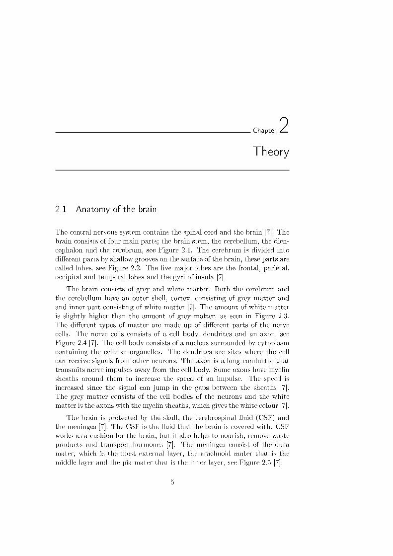
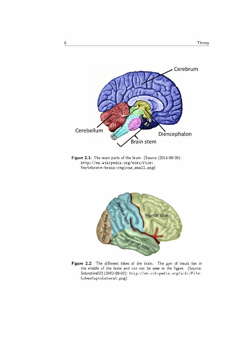
The central nervous system contains the spinal cord and the brain [7]. Thebrain consists of four main parts; the brain stem, the cerebellum, the dien-cephalon and the cerebrum, see Figure 2.1. The cerebrum is divided intodierent parts by shallow grooves on the surface of the brain, these parts arecalled lobes, see Figure 2.2. The ve major lobes are the frontal, parietal,occipital and temporal lobes and the gyri of insula [7].
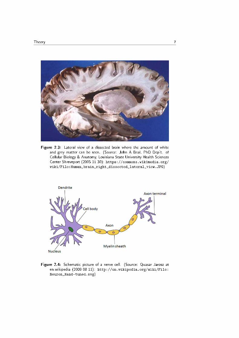
The brain consists of grey and white matter. Both the cerebrum andthe cerebellum have an outer shell, cortex, consisting of grey matter andand inner part consisting of white matter [7]. The amount of white matteris slightly higher than the amuont of grey matter, as seen in Figure 2.3.The dierent types of matter are made up of dierent parts of the nervecells. The nerve cells consists of a cell body, dendrites and an axon, seeFigure 2.4 [7]. The cell body consists of a nucleus surrounded by cytoplasmcontaining the cellular organelles. The dendrites are sites where the cellcan receive signals from other neurons. The axon is a long conductor thattransmits nerve impulses away from the cell body. Some axons have myelinsheaths around them to increase the speed of an impulse. The speed isincreased since the signal can jump in the gaps between the sheaths [7].The grey matter consists of the cell bodies of the neurons and the whitematter is the axons with the myelin sheaths, which gives the white colour [7].
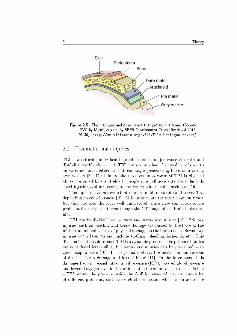
The brain is protected by the skull, the cerebrospinal uid (CSF) andthe meninges [7]. The CSF is the uid that the brain is covered with. CSFworks as a cushion for the brain, but it also helps to nourish, remove wasteproducts and transport hormones [7]. The meninges consist of the duramater, which is the most external layer, the arachnoid mater that is themiddle layer and the pia mater that is the inner layer, see Figure 2.5 [7].
5
6 Theory
Figure 2.1: The main parts of the brain. (Source (2011-09-30):http://en.wikipedia.org/wiki/File:
Vertebrate-brain-regions_small.png)
Figure 2.2: The dierent lobes of the brain. The gyri of insula lies inthe middle of the brain and can not be seen in the gure. (Source:Sebastian023 (2012-09-02): http://en.wikipedia.org/wiki/File:LobesCaptsLateral.png)
Theory 7
Figure 2.3: Lateral view of a dissected brain where the amount of whiteand grey matter can be seen. (Source: John A Beal, PhD Dep't. ofCellular Biology & Anatomy, Louisiana State University Health SciencesCenter Shreveport (2005-11-30): https://commons.wikimedia.org/wiki/File:Human_brain_right_dissected_lateral_view.JPG)
Figure 2.4: Schematic picture of a nerve cell. (Source: Quasar Jarosz aten.wikipedia (2009-08-11): http://en.wikipedia.org/wiki/File:
Neuron_Hand-tuned.svg)
8 Theory
Figure 2.5: The meninges and other layers that protect the brain. (Source:SVG by Mysid, original by SEER Development Team(Retrieved 2013-01-30): http://en.wikipedia.org/wiki/File:Meninges-en.svg)
2.2 Traumatic brain injuries
TBI is a critical public health problem and a major cause of death anddisability worldwide [5]. A TBI can occur when the head is subject toan external force, either as a direct hit, a penetrating force or a strongacceleration [8]. For infants, the most common cause of TBI is physicalabuse, for small kids and elderly people it is fall accidents, for older kidssport injuries, and for teenagers and young adults trac accidents [10].
The injuries can be divided into minor, mild, moderate and severe TBIdepending on consciousness [10]. Mild injuries are the most common types,but they are also the least well understood, since they can cause severeproblems for the patient even though the CT-image of the brain looks nor-mal.
TBI can be divided into primary and secondary injuries [10]. Primaryinjuries, such as bleeding and tissue damage are caused by the force at theinitial trauma and consist of physical damage on the brain tissue. Secondaryinjuries occur later on and include swelling, bleeding, ischemia, etc. Thisdivision is not absolute since TBI is a dynamic process. The primary injuriesare considered irreversible, but secondary injuries can be prevented withgood hospital care [10]. In the primary stage, the most common reasonsof death is brain damage and loss of blood [11]. In the later stage, it isdamages from increased intracranial pressure (ICP), lowered blood pressureand lowered oxygen level in the brain that is the main cause of death. Whena TBI occurs, the pressure inside the skull increases which can cause a lotof dierent problems, such as cerebral herniation, which is an acute life
Theory 9
threatening condition were the brain is pressed out through openings in thecranium [11].
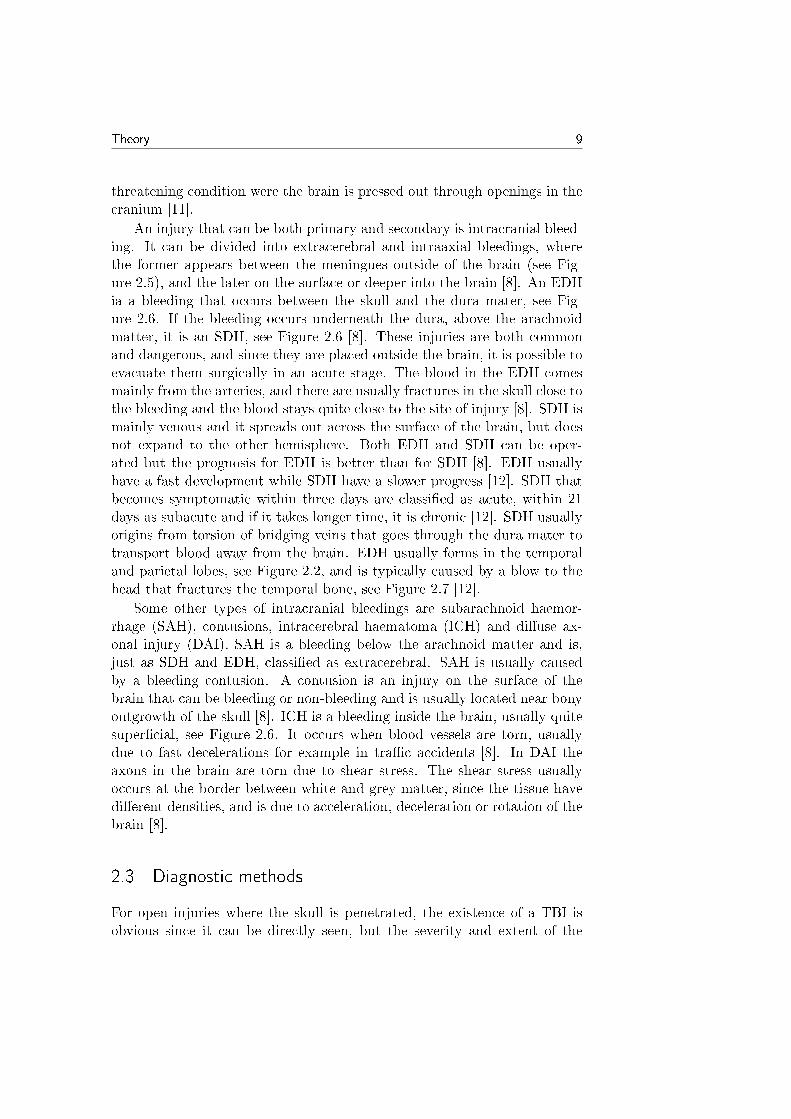
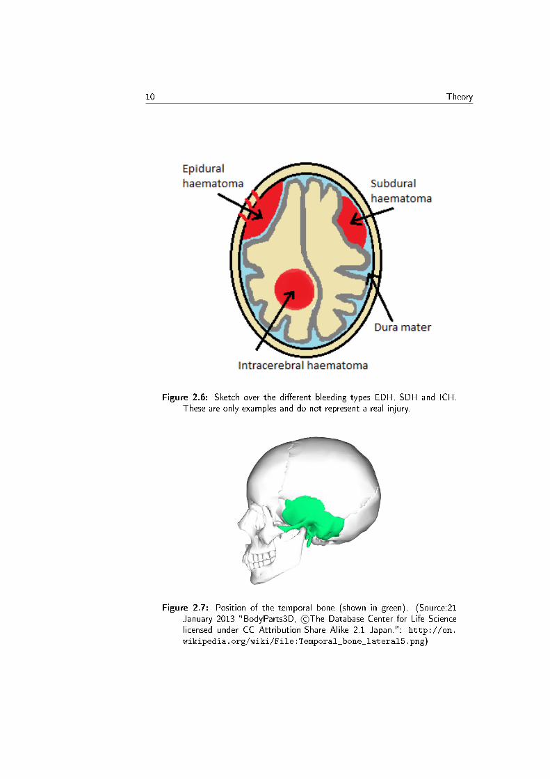
An injury that can be both primary and secondary is intracranial bleed-ing. It can be divided into extracerebral and intraaxial bleedings, wherethe former appears between the meningues outside of the brain (see Fig-ure 2.5), and the later on the surface or deeper into the brain [8]. An EDHia a bleeding that occurs between the skull and the dura mater, see Fig-ure 2.6. If the bleeding occurs underneath the dura, above the arachnoidmatter, it is an SDH, see Figure 2.6 [8]. These injuries are both commonand dangerous, and since they are placed outside the brain, it is possible toevacuate them surgically in an acute stage. The blood in the EDH comesmainly from the arteries, and there are usually fractures in the skull close tothe bleeding and the blood stays quite close to the site of injury [8]. SDH ismainly venous and it spreads out across the surface of the brain, but doesnot expand to the other hemisphere. Both EDH and SDH can be oper-ated but the prognosis for EDH is better than for SDH [8]. EDH usuallyhave a fast development while SDH have a slower progress [12]. SDH thatbecomes symptomatic within three days are classied as acute, within 21days as subacute and if it takes longer time, it is chronic [12]. SDH usuallyorigins from torsion of bridging veins that goes through the dura mater totransport blood away from the brain. EDH usually forms in the temporaland parietal lobes, see Figure 2.2, and is typically caused by a blow to thehead that fractures the temporal bone, see Figure 2.7 [12].
Some other types of intracranial bleedings are subarachnoid haemor-rhage (SAH), contusions, intracerebral haematoma (ICH) and diuse ax-onal injury (DAI). SAH is a bleeding below the arachnoid matter and is,just as SDH and EDH, classied as extracerebral. SAH is usually causedby a bleeding contusion. A contusion is an injury on the surface of thebrain that can be bleeding or non-bleeding and is usually located near bonyoutgrowth of the skull [8]. ICH is a bleeding inside the brain, usually quitesupercial, see Figure 2.6. It occurs when blood vessels are torn, usuallydue to fast decelerations for example in trac accidents [8]. In DAI theaxons in the brain are torn due to shear stress. The shear stress usuallyoccurs at the border between white and grey matter, since the tissue havedierent densities, and is due to acceleration, deceleration or rotation of thebrain [8].
2.3 Diagnostic methods
For open injuries where the skull is penetrated, the existence of a TBI isobvious since it can be directly seen, but the severity and extent of the
10 Theory
Figure 2.6: Sketch over the dierent bleeding types EDH, SDH and ICH.These are only examples and do not represent a real injury.
Figure 2.7: Position of the temporal bone (shown in green). (Source:21January 2013 "BodyParts3D, c©The Database Center for Life Sciencelicensed under CC Attribution-Share Alike 2.1 Japan.": http://en.
wikipedia.org/wiki/File:Temporal_bone_lateral5.png)
Theory 11
injury still needs to be determined. For closed injuries, the diagnosis mightbe harder. If no injury can be seen on the surface of the head, internaldamages might go unnoticed [10]. This is often the case for more severeinjuries where the damage is underestimated and time is lost by sendingthe patient to the wrong hospital or department [13].
One way to determine the severity of a brain injury is by the GlascowComa Scale (GCS) [8] where the motor response, verbal response and eyeopening response is graded on a scale and summed to get a total score [14].If the person is already intubated, or for some other reason not able to fullyinteract, it can be hard to obtain the GCS-score [8].
2.3.1 Computed tomography
To make a more detailed diagnosis, imaging of the brain is needed, this isdone with CT. To perform a CT is a standard procedure for head injuries,but it is always a consideration if it should be done or not. Some riskfactors that motivates the use of CT are if the patient is over 60 years old,have experienced amnesia, loss of consciousness or have an alcohol or drugproblem [8].
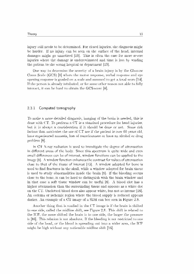
In CT X-ray radiation is used to investigate the degree of attenuationin dierent areas of the body. Since this spectrum is quite wide and evensmall dierences can be of interest, window functions can be applied to theimage [8]. A window function enhances the contrast for values of attenuationclose to that of the tissue of interest [15]. A window adapted for bone isused to nd fractures in the skull, while a window adapted for brain tissueis used to study abnormalities inside the brain [8]. If the bleeding occursclose to the bone, it can be hard to distinguish with the brain window andin that case a soft tissue window can be useful [8]. A blood clot has ahigher attenuation than the surrounding tissue and appears as a white doton the CT. Unclotted blood does also appear white, but not as intense [16].An oedema or ischemic region where the blood supply is reduced appearsdarker. An example of a CT image of a SDH can bee seen in Figure 2.8.
Another thing that is studied in the CT image is if the brain is shiftedto one side, called the midline shift, see Figure 2.8. This shift is related tothe ICP, the more shifted the brain is to one side, the larger the pressureis [16]. This relation is not absolute. If the bleeding is not restricted to oneside of the head, or the blood is spreading out into a wider area, the ICPmight be high without any noticeable midline shift [16].
12 Theory
Figure 2.8: CT scan showing the spread of a SDH (single arrows)and a midline shift (double arrows). (Source:2007-06-24 17:16Glitzy queen00 at Wikipedia: http://en.wikipedia.org/wiki/
File:Trauma_subdural_arrows.jpg)
2.3.2 Magnetic resonance imaging
If the CT does not give any clear result or the long term eects are of inter-est, magnetic resonance imaging (MRI) is used. It has a higher sensitivityand gives a more detailed picture [16]. MRI is also better at imaging in-juries in the inner parts of the brain. The reason it is not used in the acutecases is that it takes longer time than a CT and is usually not available onshort notice [16].
To see how the injury has aected the brain function of the patient,the physiology of the brain, such as the metabolism and blood ow, mustbe examined. This can be done in many ways, such as functional MRI,perfusion CT or proton emission tomography (PET) [16].
2.3.3 Near infrared spectroscopy
The Infrascanner is a new technology that is based on the near infraredspectroscopy (NIRS) technique [17]. Light with a wavelength of 808 nm isused to detect traumatic haematomas in the head [17]. The technique isbased on the principle that the higher concentration of haemoglobin in thehaematoma absorbs more light than the normal brain tissue. The absorp-tion of the dierent sides of the head are compared to each other. In normal
Theory 13
condition head is assumed to be symmetrical, so if there is a great enoughdierence it could indicate a haematoma [17]. The sensor device consists ofa NIRS diode laser and a detector that measures the reected light inten-sity [17]. The penetration depth is 23 cm and measurable width is around2 cm [17]. The exam lasts for 3min and four predened points at oppositepositions on each side of the head is examined using a handheld device.
2.3.4 Ultrasound
Ultrasound is normally not used in diagnosing TBI, since human bonesattenuates the sound waves too much [18]. Instead it can be used duringbrain surgery and the removal of deep seated haematomas [19]. In brainsurgery the problem with the bone is avoided, since parts of the craniumis removed during the surgery. It is possible to detect a midline shift withultrasound, by using transcranial colour-coded duplex sonography (TCCS)through the thinner temporal bone in the head, see Figure 2.7 [20].
2.4 Microwave technology
Another future technique that can be used to detect TBI is MWT. Thissection explains what MWT is, how it works, how it is used and somesafety guidelines that needs to be considered when using it.
2.4.1 Microwaves
Microwaves are electromagnetic radiation with a wavelength of between1mm and 1m in vacuum, which corresponds to a frequency of 300MHz to300GHz, the wavelength in air is practically the same [21]. Electromag-netic waves have one electric and one magnetic component, perpendicularto each other. The waves make up an electric and a magnetic eld, andthe propagation of these elds depends on the dielectric properties of themedium. This eld propagation can be described by Maxwell's equations,see Equation (2.1)(2.4) [21].
∇×E =−∂B∂t−M Faraday's Law of induction (2.1)
∇×H = J +∂D
∂tAmpere's Law (2.2)
∇ ·D = ρ Gauss's Law for electricity (2.3)
∇ ·B = 0 Gauss's Law for magnetism (2.4)
14 Theory
E and H are the electric and magnetic eld respectively, D and B theelectric and magnetic ux density, J and M the electric and magnetic cur-rent density and ρ the total charge density [21]. To relate these equationsto the properties of the material in which the eld propagates, these con-stitutive relations are needed
D = εE (2.5)
B = µH (2.6)
J = σE, (2.7)
where ε is the permittivity, µ the permeability and σ the conductivity ofthe material. These three properties are usually refered to as the dielectricproperties of the material. Equation (2.8) is the continuity equation thatfollows from Maxwells equation, this equation is particularly important fornon-linear materials [21].
∇ · J = −∂ρ∂t
(2.8)
When a dielectric material is exposed to an electric eld, the atomsand molecules of the material are polarised, creating a dipole moment thatincreases the electric ux [21]. For free space, Equation (2.5) looks likeD = ε0E where ε0 = 8.854 · 10−12 F m−1, for other media the permittivityis a complex number
ε = ε′ − jε′′, (2.9)
where the imaginary part accounts for heat loss due to damping of thevibrating dipole moments. The conductivity σ does also impact the materialloss [21]. If an ejωt time dependency is assumed, all time derivatives in theEquations (2.1), (2.2) and (2.8) can be replaced by jω, where ω is theangular frequency ω = 2πf rad s−1.
The conductivity of a material can be calculated from the imaginarypart of the permittivity and the angular frequency as
σ = ωε′′. (2.10)
The complex relative permittivity ε can be expressed as
ε =ε′ − jε′′
ε0= εr −
jε′′
ε0[21]. (2.11)
This can be calculated for dierent tissues from the 4-ColeCole dispersionmodel, see Equation (2.12), using the parameters from Gabriel et al. [22].
ε(ω) = ε∞ +
4∑n=1
∆εn
1 + (jωτn)(1−αn)+
σijωε0
(2.12)
Theory 15
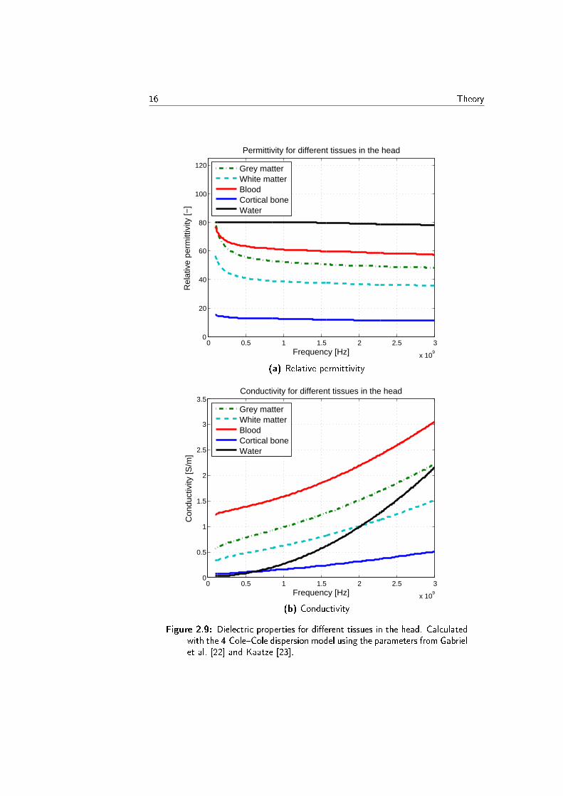
Where τ is the relaxation time of the material, ε∞ the permittivity at highfrequencies (ωτ 1), ∆εn = ε∞− εs the dierence between permittivity athigh and low frequencies (ωτ 1), α the broadening of the dispersion areaand σi the static ionic conductivity [22]. The conductivity σ of the materialcan then be calculated from the imaginary part of ε, using Equation (2.10).The dielectric properties for dierent tissues, calculated from the 4ColeCole dispersion model using the parameters from Gabriel et al. [22] andKaatze [23], can be seen in Figure 2.9.
The propagation of plane electromagnetic waves in lossless medium canbe described by the propagation constant k and the wave impedance η, seeEquations (2.13) and (2.14) where λ is the wavelength and v the speed ofthe wave [21].
k =2π
λ=ω
v= ω√εµ (2.13)
η =ωµ
k=
õ
ε(2.14)
When a plane electromagnetic wave is travelling through lossy medium,the conductivity comes into account and the propagation constant and waveimpedance becomes complex. The complex propagation constant is denotedγ and is dened by Equation (2.15). The wave impedance, η, is redenedby Equation (2.16) [21].
γ = jω√ε′µ
√1− j σ
ωε′(2.15)
η =jωµ
γ=
õ
ε− j σω(2.16)
The wave impedance, η, relates the electric and magnetic eld strengthsto each other. In free space the intrinsic impedance is denoted η0, seeEquation (2.17), where σ = 0 [21].
η0 =
√µ0ε0≈ 377Ω (2.17)
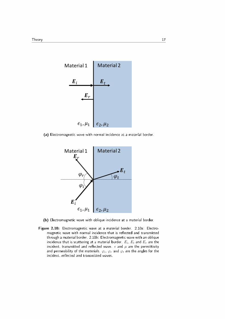
The case when an electromagnetic wave Ei comes in normal to a ma-terial border is illustrated in Figure 2.10a. Some part, Et, of the wave willpropagate into material 2, but some, Er, will be reected at the border andcontinue to travel in material 1, but in the backward direction [24]. In anobject with several material borders this phenomenon will happen at eachborder. The electromagnetic wave will scatter according to Snell's law if ithas an oblique incidence to the border, see Figure 2.10b and Equation (2.18)and (2.19).
16 Theory
0 0.5 1 1.5 2 2.5 3
x 109
0
20
40
60
80
100
120
Frequency [Hz]
Rel
ativ
e pe
rmitt
ivity
[−]
Permittivity for different tissues in the head
Grey matterWhite matterBloodCortical boneWater
(a) Relative permittivity
0 0.5 1 1.5 2 2.5 3
x 109
0
0.5
1
1.5
2
2.5
3
3.5
Frequency [Hz]
Con
duct
ivity
[S/m
]
Conductivity for different tissues in the head
Grey matterWhite matterBloodCortical boneWater
(b) Conductivity
Figure 2.9: Dielectric properties for dierent tissues in the head. Calculatedwith the 4-ColeCole dispersion model using the parameters from Gabrielet al. [22] and Kaatze [23].
Theory 17
𝑬𝑖
𝑬𝑟
𝑬𝑡
Material 1 Material 2
𝜖1 , 𝜇1 𝜖2, 𝜇2
(a) Electromagnetic wave with normal incidence at a material border.
Material 1 Material 2
𝜖1 , 𝜇1 𝜖2, 𝜇2
𝜑𝑖
𝜑𝑟 𝜑𝑡
𝑬𝑟
𝑬𝑡
𝑬𝑖
(b) Electromagnetic wave with oblique incidence at a material border.
Figure 2.10: Electromagnetic wave at a material border. 2.10a: Electro-magnetic wave with normal incidence that is reected and transmittedthrough a material border. 2.10b: Electromagnetic wave with an obliqueincidence that is scattering at a material border. Ei, Et and Er are theincident, transmitted and reected wave. ε and µ are the permittivityand permeability of the materials. ϕi, ϕr and ϕt are the angles for theincident, reected and transmitted waves.
18 Theory
ϕi = ϕr (2.18)
k1 sin(ϕi) = k2 sin(ϕt) (2.19)
Where ϕi, ϕr and ϕt are the angles for the incident, reected and trans-mitted waves. The propagation constants k1 and k2 are dened by Equa-tion (2.13) and are the constants for material 1 and material 2, respectively.
The amount of reection can be expressed with the reection coe-cient Γ. The reection coecient is the ratio between the incident and thereected wave, see Equation (2.20) [24].
Γ =ErEi
=η − η0η + η0
(2.20)
The return loss is the magnitude of the reection coecient expressedin dB, see Equation (2.21) [25]. The return loss is how many dB:s thatthe reected signal is below the incident signal. The return loss is alwaysdenoted as a positive number, so therefore an extra minus sign is added inEquation (2.21) [25].
Lossreturn = −20 · log10(|Γ|) (2.21)
The transmission T is how much of the signal that is transmitted throughthe medium and is calculated with Equation (2.22) [21].
T = 1 + Γ =2η
η + η0(2.22)
The magnitude of the transmitted voltage will be lower than the incidentvoltage for tissue, and the material will then exhibit insertion loss. Theinsertion loss is the magnitude of the transmission coecient expressed indB, see Equation (2.23) [25]. Also here a minus sign is added to the equationto get a positive dB-number on the loss.
Lossinsertion = −20 · log10(|T |) (2.23)
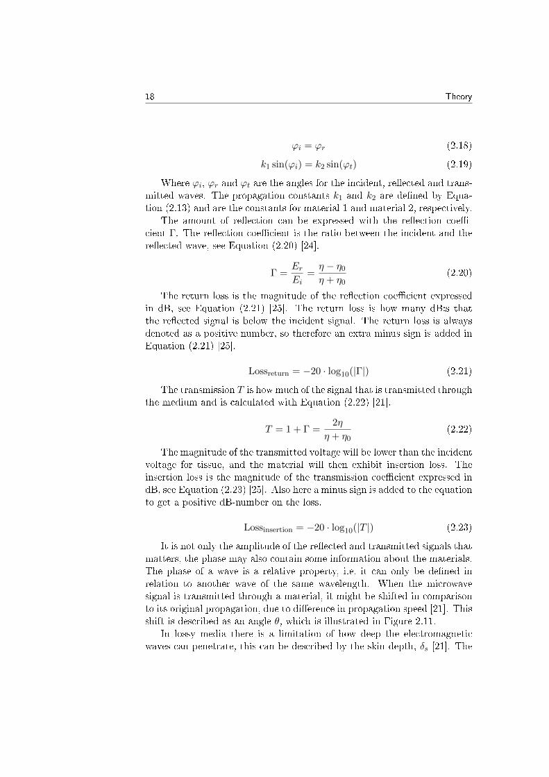
It is not only the amplitude of the reected and transmitted signals thatmatters, the phase may also contain some information about the materials.The phase of a wave is a relative property, i.e. it can only be dened inrelation to another wave of the same wavelength. When the microwavesignal is transmitted through a material, it might be shifted in comparisonto its original propagation, due to dierence in propagation speed [21]. Thisshift is described as an angle θ, which is illustrated in Figure 2.11.
In lossy media there is a limitation of how deep the electromagneticwaves can penetrate, this can be described by the skin depth, δs [21]. The
Theory 19
0 1 2 3 4 5 6 7−1
−0.8
−0.6
−0.4
−0.2
0
0.2
0.4
0.6
0.8
1Phase shift
Radians
Am
plitu
de
θ
Figure 2.11: Illustration of a π/2 phase shift.
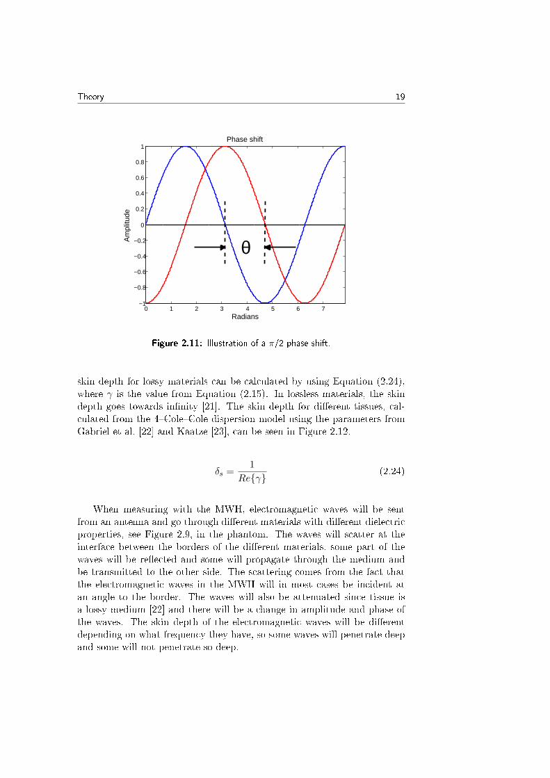
skin depth for lossy materials can be calculated by using Equation (2.24),where γ is the value from Equation (2.15). In lossless materials, the skindepth goes towards innity [21]. The skin depth for dierent tissues, cal-culated from the 4ColeCole dispersion model using the parameters fromGabriel et al. [22] and Kaatze [23], can be seen in Figure 2.12.
δs =1
Reγ(2.24)
When measuring with the MWH, electromagnetic waves will be sentfrom an antenna and go through dierent materials with dierent dielectricproperties, see Figure 2.9, in the phantom. The waves will scatter at theinterface between the borders of the dierent materials, some part of thewaves will be reected and some will propagate through the medium andbe transmitted to the other side. The scattering comes from the fact thatthe electromagnetic waves in the MWH will in most cases be incident atan angle to the border. The waves will also be attenuated since tissue isa lossy medium [22] and there will be a change in amplitude and phase ofthe waves. The skin depth of the electromagnetic waves will be dierentdepending on what frequency they have, so some waves will penetrate deepand some will not penetrate so deep.
20 Theory
0 0.5 1 1.5 2 2.5 3
x 109
0
0.05
0.1
0.15
0.2
0.25
0.3
0.35
0.4
Frequency (Hz)
Ski
n de
pth
[m]
Skin depth for different tissues in the head
Grey matterWhite matterBloodCortical boneWater
Figure 2.12: Skin depth for dierent tissues in the head. Calculated withthe 4ColeCole dispersion model using the parameters from Gabriel etal. [22] and Kaatze [23].
2.4.2 Scattering parameters
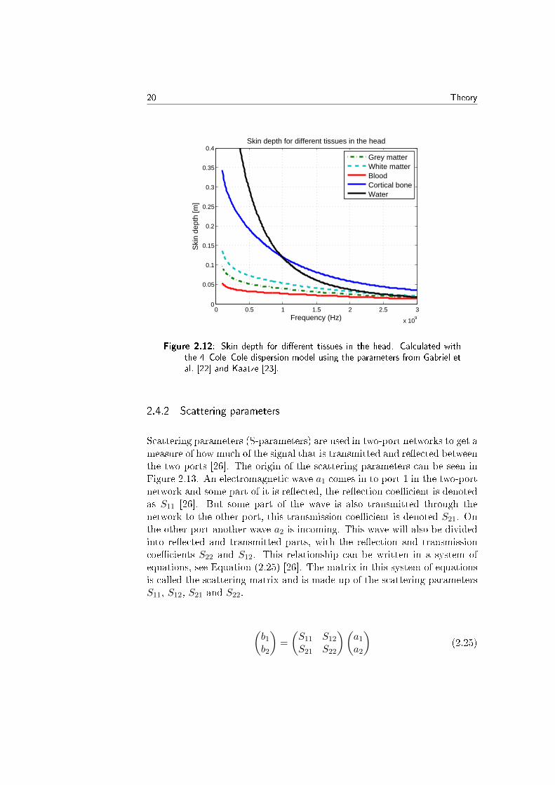
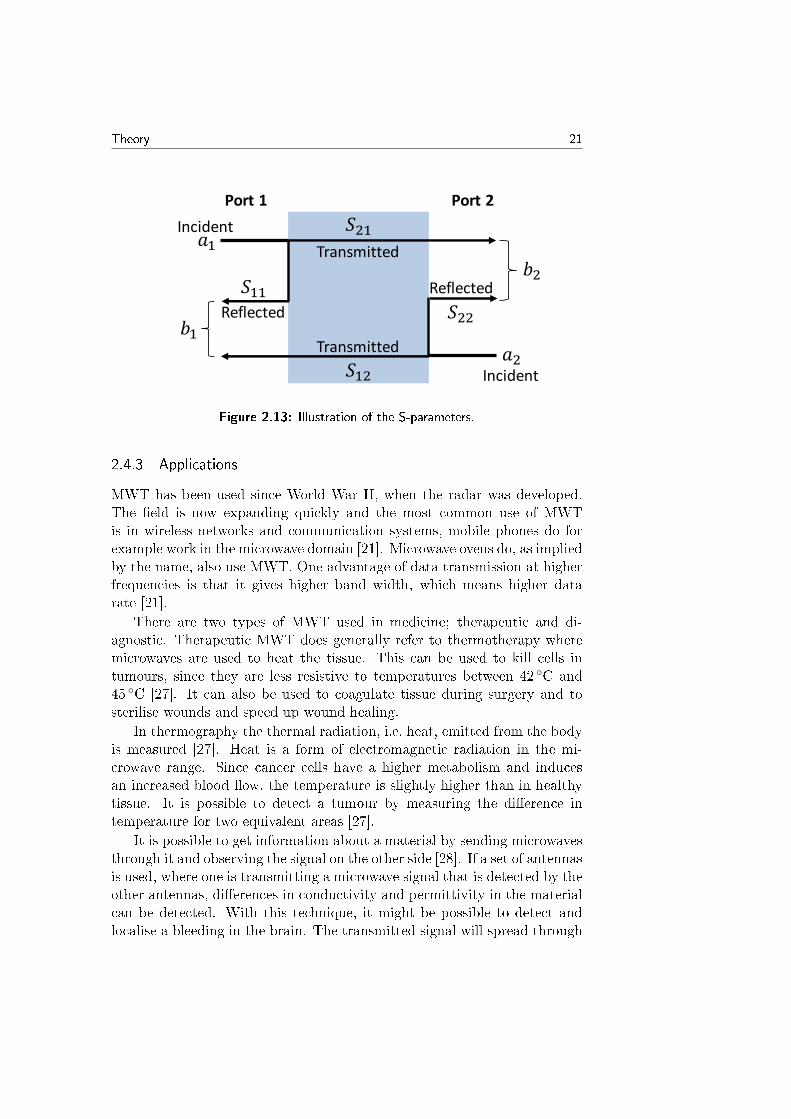
Scattering parameters (S-parameters) are used in two-port networks to get ameasure of how much of the signal that is transmitted and reected betweenthe two ports [26]. The origin of the scattering parameters can be seen inFigure 2.13. An electromagnetic wave a1 comes in to port 1 in the two-portnetwork and some part of it is reected, the reection coecient is denotedas S11 [26]. But some part of the wave is also transmitted through thenetwork to the other port, this transmission coecient is denoted S21. Onthe other port another wave a2 is incoming. This wave will also be dividedinto reected and transmitted parts, with the reection and transmissioncoecients S22 and S12. This relationship can be written in a system ofequations, see Equation (2.25) [26]. The matrix in this system of equationsis called the scattering matrix and is made up of the scattering parametersS11, S12, S21 and S22.
(b1b2
)=
(S11 S12S21 S22
)(a1a2
)(2.25)
Theory 21
𝑎1
𝑏1
𝑏2
𝑎2
𝑆11
𝑆21
𝑆12
𝑆22
Transmitted
Transmitted
Reflected
Reflected
Incident
Incident
Port 1 Port 2
Figure 2.13: Illustration of the S-parameters.
2.4.3 Applications
MWT has been used since World War II, when the radar was developed.The eld is now expanding quickly and the most common use of MWTis in wireless networks and communication systems, mobile phones do forexample work in the microwave domain [21]. Microwave ovens do, as impliedby the name, also use MWT. One advantage of data transmission at higherfrequencies is that it gives higher band width, which means higher datarate [21].
There are two types of MWT used in medicine; therapeutic and di-agnostic. Therapeutic MWT does generally refer to thermotherapy wheremicrowaves are used to heat the tissue. This can be used to kill cells intumours, since they are less resistive to temperatures between 42 C and45 C [27]. It can also be used to coagulate tissue during surgery and tosterilise wounds and speed up wound healing.
In thermography the thermal radiation, i.e. heat, emitted from the bodyis measured [27]. Heat is a form of electromagnetic radiation in the mi-crowave range. Since cancer cells have a higher metabolism and inducesan increased blood ow, the temperature is slightly higher than in healthytissue. It is possible to detect a tumour by measuring the dierence intemperature for two equivalent areas [27].
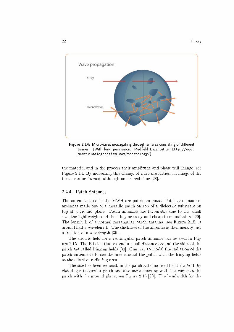
It is possible to get information about a material by sending microwavesthrough it and observing the signal on the other side [28]. If a set of antennasis used, where one is transmitting a microwave signal that is detected by theother antennas, dierences in conductivity and permittivity in the materialcan be detected. With this technique, it might be possible to detect andlocalise a bleeding in the brain. The transmitted signal will spread through
22 Theory
Figure 2.14: Microwaves propagating through an area consisting of dierenttissues. (With kind permission: Medeld Diagnostics, http://www.medfielddiagnostics.com/technology/)
the material and in the process their amplitude and phase will change, seeFigure 2.14. By measuring this change of wave properties, an image of thetissue can be formed, although not in real time [28].
2.4.4 Patch Antennas
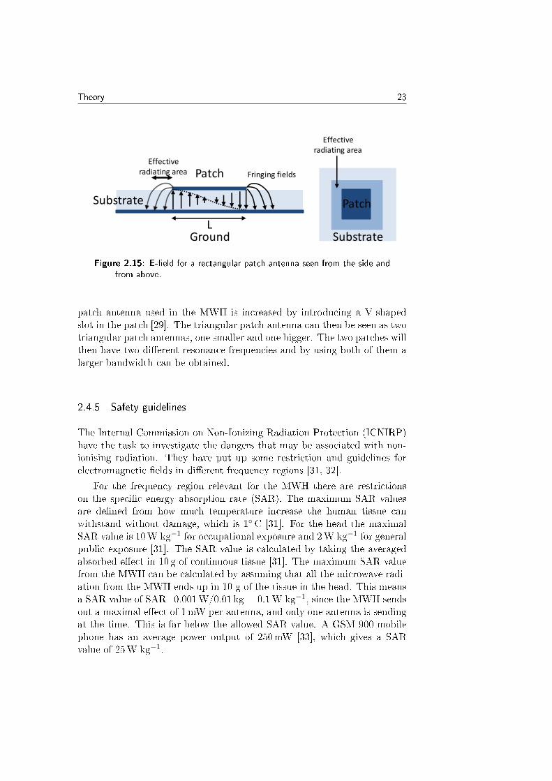
The antennas used in the MWH are patch antennas. Patch antennas areantennas made out of a metallic patch on top of a dielectric substrate ontop of a ground plane. Patch antennas are favourable due to the smallsize, the light weight and that they are easy and cheap to manufacture [29].The length L of a normal rectangular patch antenna, see Figure 2.15, isaround half a wavelength. The thickness of the antenna is then usually justa fraction of a wavelength [30].
The electric eld for a rectangular patch antenna can be seen in Fig-ure 2.15. The E-elds that extend a small distance around the sides of thepatch are called fringing elds [30]. One way to model the radiation of thepatch antenna is to see the area around the patch with the fringing eldsas the eective radiating area.
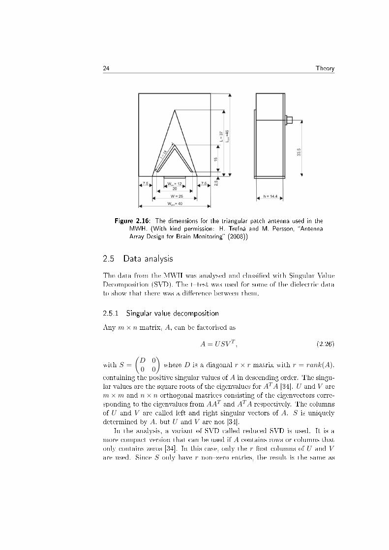
The size has been reduced, in the patch antenna used for the MWH, bychoosing a triangular patch and also use a shorting wall that connects thepatch with the ground plane, see Figure 2.16 [29]. The bandwidth for the
Theory 23
Patch
Substrate
Effective radiating area
Fringing fields Patch
Ground
Substrate
Effective radiating area
L
Figure 2.15: E-eld for a rectangular patch antenna seen from the side andfrom above.
patch antenna used in the MWH is increased by introducing a V-shapedslot in the patch [29]. The triangular patch antenna can then be seen as twotriangular patch antennas, one smaller and one bigger. The two patches willthen have two dierent resonance frequencies and by using both of them alarger bandwidth can be obtained.
2.4.5 Safety guidelines
The Internal Commission on Non-Ionizing Radiation Protection (ICNIRP)have the task to investigate the dangers that may be associated with non-ionising radiation. They have put up some restriction and guidelines forelectromagnetic elds in dierent frequency regions [31, 32].
For the frequency region relevant for the MWH there are restrictionson the specic energy absorption rate (SAR). The maximum SAR valuesare dened from how much temperature increase the human tissue canwithstand without damage, which is 1C [31]. For the head the maximalSAR value is 10W kg−1 for occupational exposure and 2W kg−1 for generalpublic exposure [31]. The SAR value is calculated by taking the averagedabsorbed eect in 10 g of continuous tissue [31]. The maximum SAR valuefrom the MWH can be calculated by assuming that all the microwave radi-ation from the MWH ends up in 10 g of the tissue in the head. This meansa SAR value of SAR=0.001W/0.01 kg = 0.1W kg−1, since the MWH sendsout a maximal eect of 1mW per antenna, and only one antenna is sendingat the time. This is far below the allowed SAR value. A GSM 900 mobilephone has an average power output of 250mW [33], which gives a SARvalue of 25W kg−1.
24 Theory
Figure 2.16: The dimensions for the triangular patch antenna used in theMWH. (With kind permission: H. Trefná and M. Persson, AntennaArray Design for Brain Monitoring (2008))
2.5 Data analysis
The data from the MWH was analysed and classied with Singular ValueDecomposition (SVD). The ttest was used for some of the dielectric datato show that there was a dierence between them.
2.5.1 Singular value decomposition
Any m× n matrix, A, can be factorised as
A = USV T , (2.26)
with S =
(D 00 0
)where D is a diagonal r × r matrix with r = rank(A),
containing the positive singular values of A in descending order. The singu-lar values are the square roots of the eigenvalues for ATA [34]. U and V arem×m and n× n orthogonal matrices consisting of the eigenvectors corre-sponding to the eigenvalues from AAT and ATA respectively. The columnsof U and V are called left and right singular vectors of A. S is uniquelydetermined by A, but U and V are not [34].
In the analysis, a variant of SVD called reduced SVD is used. It is amore compact version that can be used if A contains rows or columns thatonly contains zeros [34]. In this case, only the r rst columns of U and Vare used. Since S only have r nonzero entries, the result is the same as
Theory 25
for regular SVD, but can be written as A = UrDVTr where Ur and Vr are
the reduced matrices. SVD can be used to estimate the rank of a matrixby counting the number of nonzero singular values. Roundo errors fromthe row reduction shows up as extremely small singular values, so if thoseare removed, it is possible to get rid of the redundant information in thematrix [34].
2.5.2 Ttest
The ttest can be performed to see if two independent and normally dis-tributed samples dier from each other [35]. The two samples X and Yhave the means µX , µY and equal variances.
The statistic in Equation (2.27) follows a tdistribution with m + n −2 degrees of freedom, where m and n are the sample sizes of X and Yrespectively [35].
t =(X − Y )− (µX − µY )
sp
√1n + 1
m
(2.27)
The variance can be estimated with the pooled sample variance s2p that isdened in Equation (2.28) [35].
s2p =(n− 1)s2x + (m− 1)s2Y
m+ n− 2(2.28)
Where s2X and s2Y are the standard deviations for X and Y . The teststatistic for testing the null hypothesis H0 : µX = µY is
t =X − Y
sp
√1n + 1
m
. (2.29)
The probability of falsely rejecting the null hypothesis is dened as the pvalue. Therefore, the smaller the pvalue is, the more likely it is that thenull hypothesis could be rejected and that the two samples have unequalmeans [35].

26 Theory
Chapter3Method
This chapter explains in detail how the project was carried out, with thecreation of the phantoms, the MWH measurements, measurements of thedielectric properties of the phantoms and the data analyses of the MWHdata.
3.1 Experimental setup
3.1.1 Dielectric measurements
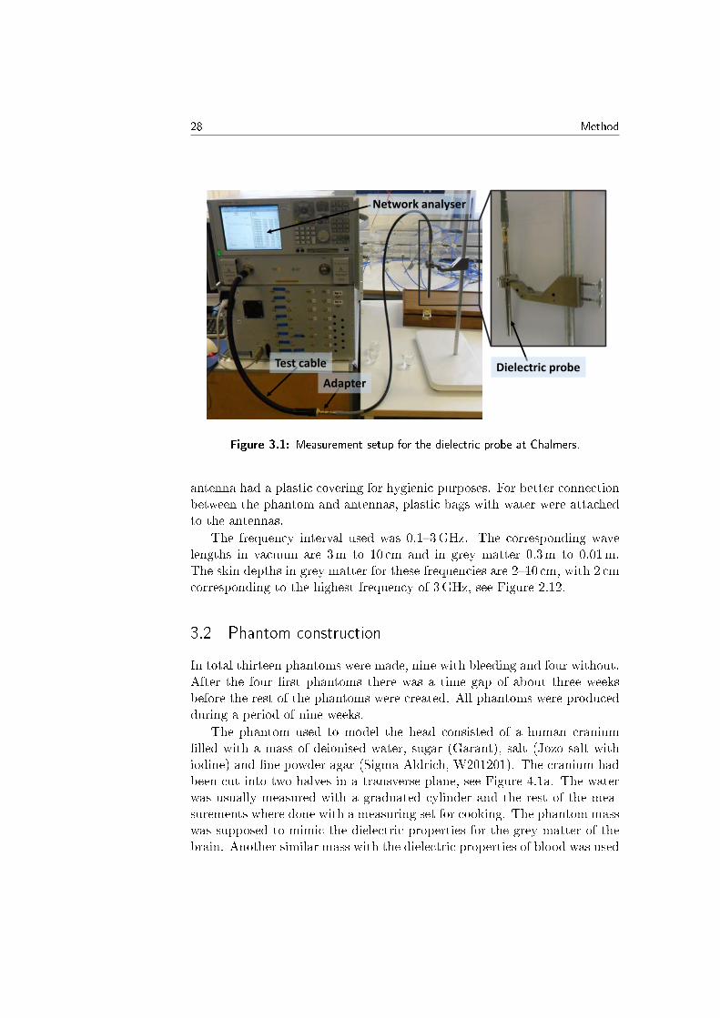
The measurements on the dielectric properties were performed in the Mi-crowave laboratory at the department Signal and Systems at Chalmers Uni-versity of Technology. A programmable network analyser (PNA Series Net-work Analyzer, 10MHz20GHz, Agilent Technologies E8362B) was usedto transmit and receive the microwave signals. A dielectric probe (Dielec-tric Probe Kit, Agilent Technologies 85070E) was connected to the PNAto measure the dielectric properties. The probe was connected to the PNAby using a test-cable (Test-Cable, Hochfrequenztechnik, Rosenberger) andan adapter (Adapter Kit, Precision 3.5mm, Agilent Technologies 83059K).The whole measurement setup is shown in Figure 3.1.
3.1.2 Microwave helmet measurements
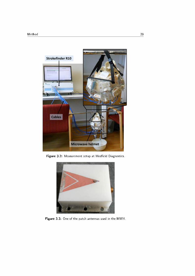
The measurements with the MWH were done in the laboratory at Med-eld Diagnostics. A Strokender R10 (Medeld Diagnostics) was used to-gether with a MWH to perform the measurements. The 12 ports at theStrokender were connected with cables to the 12 antennas on the MWH, seeFigure 3.2. The Strokender consists of a vector network analyser (VNA)and a mechanical switching box.
The MWH was a research prototype developed by Medeld Diagnosticsin collaboration with Chalmers. It consisted of 12 patch antennas, seeFigure 2.16 and 3.3, attached to a plastic helmet, see Figure 3.4. Each
27
28 Method
Dielectric probe Test cable
Network analyser
Adapter
Figure 3.1: Measurement setup for the dielectric probe at Chalmers.
antenna had a plastic covering for hygienic purposes. For better connectionbetween the phantom and antennas, plastic bags with water were attachedto the antennas.
The frequency interval used was 0.13GHz. The corresponding wavelengths in vacuum are 3m to 10 cm and in grey matter 0.3m to 0.01m.The skin depths in grey matter for these frequencies are 210 cm, with 2 cmcorresponding to the highest frequency of 3GHz, see Figure 2.12.
3.2 Phantom construction
In total thirteen phantoms were made, nine with bleeding and four without.After the four rst phantoms there was a time gap of about three weeksbefore the rest of the phantoms were created. All phantoms were producedduring a period of nine weeks.
The phantom used to model the head consisted of a human craniumlled with a mass of deionised water, sugar (Garant), salt (Jozo salt withiodine) and ne powder agar (Sigma-Aldrich, W201201). The cranium hadbeen cut into two halves in a transverse plane, see Figure 4.1a. The waterwas usually measured with a graduated cylinder and the rest of the mea-surements where done with a measuring set for cooking. The phantom masswas supposed to mimic the dielectric properties for the grey matter of thebrain. Another similar mass with the dielectric properties of blood was used
Method 29
Strokefinder R10
Cables
Microwave helmet
Figure 3.2: Measurement setup at Medeld Diagnostics.
Figure 3.3: One of the patch antennas used in the MWH.
30 Method
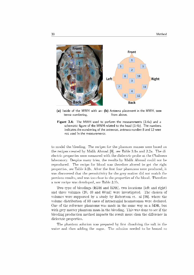
(a) Inside of the MWH with an-tenna numbering.
(b) Antenna placement in the MWH, seenfrom above.
Figure 3.4: The MWH used to perform the measurements (3.4a) and aschematic gure of the MWH related to the head (3.4b). The numbersindicates the numbering of the antennas, antenna number 8 and 12 werenot used in the measurements.
to model the bleeding. The recipes for the phantom masses were based onthe recipes created by Malik Ahmad [9], see Table 3.1a and 3.2a. The di-electric properties were measured with the dielectric probe at the Chalmerslaboratory. Despite many tries, the results by Malik Ahmad could not bereproduced. The recipe for blood was therefore altered to get the rightproperties, see Table 3.2b. After the rst four phantoms were produced, itwas discovered that the permittivity for the grey matter did not match theprevious results, and was too close to the properties of the blood. Thereforea new recipe was developed, see Table 3.1b.
Two type of bleedings (EDH and SDH), two locations (left and right)and three volumes (20, 40 and 60ml) were investigated. The choices ofvolumes were supported by a study by Robertson et. al [36], where thevolume distribution of 83 cases of intracranial heamatomas were declared.One of the reference phantoms was made in the same way as a SDH, butwith grey matter phantom mass in the bleeding. This was done to see if thebleeding production method impacts the result more than the dierence indielectric properties.
The phantom solution was prepared by rst dissolving the salt in thewater and then adding the sugar. The solution needed to be heated to
Method 31
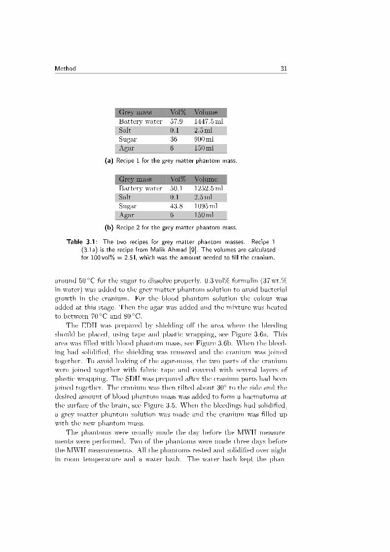
Grey mass Vol% VolumeBattery water 57.9 1447.5mlSalt 0.1 2.5mlSugar 36 900mlAgar 6 150ml
(a) Recipe 1 for the grey matter phantom mass.
Grey mass Vol% VolumeBattery water 50.1 1252.5mlSalt 0.1 2.5mlSugar 43.8 1095mlAgar 6 150ml
(b) Recipe 2 for the grey matter phantom mass.
Table 3.1: The two recipes for grey matter phantom masses. Recipe 1(3.1a) is the recipe from Malik Ahmad [9]. The volumes are calculatedfor 100 vol% = 2.5 l, which was the amount needed to ll the cranium.
around 50 C for the sugar to dissolve properly. 0.3 vol% formalin (37wt.%in water) was added to the grey matter phantom solution to avoid bacterialgrowth in the cranium. For the blood phantom solution the colour wasadded at this stage. Then the agar was added and the mixture was heatedto between 70 C and 80 C.
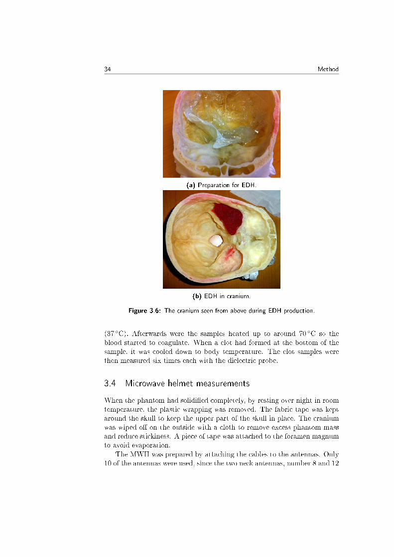
The EDH was prepared by shielding o the area where the bleedingshould be placed, using tape and plastic wrapping, see Figure 3.6a. Thisarea was lled with blood phantom mass, see Figure 3.6b. When the bleed-ing had solidied, the shielding was removed and the cranium was joinedtogether. To avoid leaking of the agar-mass, the two parts of the craniumwere joined together with fabric tape and covered with several layers ofplastic wrapping. The SDH was prepared after the cranium parts had beenjoined together. The cranium was then tilted about 30 to the side and thedesired amount of blood phantom mass was added to form a haematoma atthe surface of the brain, see Figure 3.5. When the bleedings had solidied,a grey matter phantom solution was made and the cranium was lled upwith the new phantom mass.
The phantoms were usually made the day before the MWH measure-ments were performed. Two of the phantoms were made three days beforethe MWH measurements. All the phantoms rested and solidied over nightin room temperature and a water bath. The water bath kept the phan-
32 Method
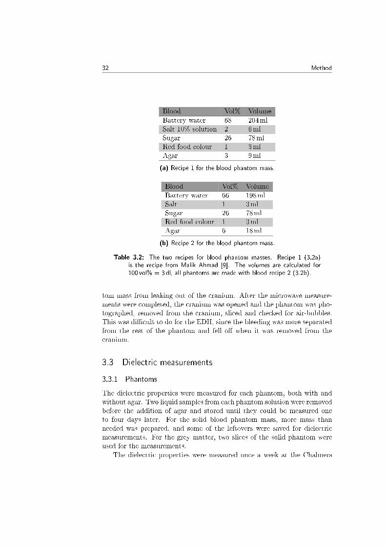
Blood Vol% VolumeBattery water 68 204mlSalt 10% solution 2 6mlSugar 26 78mlRed food colour 1 3mlAgar 3 9ml
(a) Recipe 1 for the blood phantom mass.
Blood Vol% VolumeBattery water 66 198mlSalt 1 3mlSugar 26 78mlRed food colour 1 3mlAgar 6 18ml
(b) Recipe 2 for the blood phantom mass.
Table 3.2: The two recipes for blood phantom masses. Recipe 1 (3.2a)is the recipe from Malik Ahmad [9]. The volumes are calculated for100 vol% = 3 dl, all phantoms are made with blood recipe 2 (3.2b).
tom mass from leaking out of the cranium. After the microwave measure-ments were completed, the cranium was opened and the phantom was pho-tographed, removed from the cranium, sliced and checked for air-bubbles.This was dicult to do for the EDH, since the bleeding was more separatedfrom the rest of the phantom and fell o when it was removed from thecranium.
3.3 Dielectric measurements
3.3.1 Phantoms
The dielectric properties were measured for each phantom, both with andwithout agar. Two liquid samples from each phantom solution were removedbefore the addition of agar and stored until they could be measured oneto four days later. For the solid blood phantom mass, more mass thanneeded was prepared, and some of the leftovers were saved for dielectricmeasurements. For the grey matter, two slices of the solid phantom wereused for the measurements.
The dielectric properties were measured once a week at the Chalmers
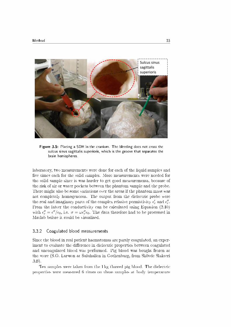
Method 33
Sulcus sinus sagittalis superioris
Figure 3.5: Placing a SDH in the cranium. The bleeding does not cross thesulcus sinus sagittalis superioris, which is the groove that separates thebrain hemispheres.
laboratory, two measurements were done for each of the liquid samples andve times each for the solid samples. More measurements were needed forthe solid sample since it was harder to get good measurements, because ofthe risk of air or water pockets between the phantom sample and the probe.There might also be some variations over the areas if the phantom mass wasnot completely homogeneous. The output from the dielectric probe werethe real and imaginary parts of the complex relative permittivity ε′r and ε
′′r .
From the latter the conductivity can be calculated using Equation (2.10)with ε′′r = ε′′/ε0, i.e. σ = ωε′′rε0. The data therefore had to be processed inMatlab before it could be visualised.
3.3.2 Coagulated blood measurements
Since the blood in real patient haematomas are partly coagulated, an exper-iment to evaluate the dierence in dielectric properties between coagulatedand uncoagulated blood was performed. Pig blood was bought frozen atthe store (S.O. Larsson at Saluhallen in Gothenburg, from Skövde SlakteriAB).
Ten samples were taken from the 1 kg thawed pig blood. The dielectricproperties were measured 6 times on these samples at body temperature
34 Method
(a) Preparation for EDH.
(b) EDH in cranium.
Figure 3.6: The cranium seen from above during EDH production.
(37 C). Afterwards were the samples heated up to around 70 C so theblood started to coagulate. When a clot had formed at the bottom of thesample, it was cooled down to body temperature. The clot samples werethen measured six times each with the dielectric probe.
3.4 Microwave helmet measurements
When the phantom had solidied completely, by resting over night in roomtemperature, the plastic wrapping was removed. The fabric tape was keptaround the skull to keep the upper part of the skull in place. The craniumwas wiped o on the outside with a cloth to remove excess phantom massand reduce stickiness. A piece of tape was attached to the foramen magnumto avoid evaporation.
The MWH was prepared by attaching the cables to the antennas. Only10 of the antennas were used, since the two neck antennas, number 8 and 12
Method 35
in Figure 3.4 and 3.2, did not get a good connection with the craniumsince it was quite small. The two ports that weren't used were terminatedwith a 50Ω load to avoid interference. Water bags were attached to theantennas to get a better connection between the antennas and the skull.The bags were partly lled with water and air bubbles were removed beforethe cranium was placed in the MWH. Afterwards more water was addeduntil the cranium was xated. The MWH with the phantom was hung ona metal rod between two chairs, see Figure 3.2.
The position of the MWH relative the bleedings can be seen in theschematic picture in Figure 3.7. The EDH were always placed at the samelocation by the temporal bone, SDH varied more in location and were some-times positioned more to the front and sometimes more to the back.
3.4.1 Ordinary measurements
30 measurements were performed in ten sets of three. After every thirdmeasurement the water bags were emptied, the cranium was lifted a fewcentimetres and the position was adjusted. The water bags were relledand the measurements continued. This was done to simulate the varia-tion in position of the MWH on the patients head and between dierentmeasurements on the same patient.
3.4.2 Interfering factors
Person close and holding the cables
The impact of a persons close to the measurement setup was investigatedby doing 30 measurements with a person standing close the MWH, see Fig-ure 3.8a. This is interesting to investigate for the possibility to use theMWH in an ambulance where the space is limited. Another 30 measure-ments were performed with a person holding the cables, see Figure 3.8b, andthen yet another 30 measurements were performed, where the person wasstanding more than 1m from the setup, as a reference to the other measure-ments. All these three types of measurements were randomised among eachother. These experiments were only performed for the rst four phantoms.
Phone
The impact of a mobile phone (HTC Wildre S) signal was also investi-gated. The mobile phone calls in the GSM network with a frequency around900MHz [21], which is in the frequency interval used for the MWH mea-surements. This was done by doing 30 measurements with a calling mobilephone close to the MWH, see Figure 3.8c. The mobile phone was calling
36 Method
another mobile phone in the same room that did not answer. As a referenceto these measurements, 30 measurements were performed with the mobilephone in ight mode close to the MWH. All these 60 measurements wereperformed in a randomised manner to minimise time dependent errors.
Hair
For the last nine phantoms, the impact of hair was investigated by putting awig with real human hair on the cranium. 30 measurements were performedin the same way as the ordinary measurements, with the cranium beingrepositioned after every three measurements. The position of the craniumwith the wig in the MWH can bee seen in see Figure 3.9.
Movement
The impact of movement was investigated by doing 30 measurements whenthe MWH was put into movement, by rocking it back and forth, and com-pare these to 30 measurements without movement, see Figure 3.8d. These60 measurements were performed in a randomised manner to minimise thetime dependent errors.
3.5 Data analysis
3.5.1 Dielectric measurements
The dielectric probe gave unstable results below 0.5GHz and those valuescan therefore not be trusted. All the ttests and mean value calculationsare therefore done in the frequency interval 0.53GHz.
Phantoms
The mean values from all the measurements (liquid and solid for both greymatter and blood phantom samples) for each phantom sample were rstcalculated. After this the mean values for the relative permittivity and con-ductivity from all the phantom samples were calculated. Reference valuesfor grey matter and blood were calculated in Matlab by using the 4-Cole-Cole dispersion model, see Equation (2.12), together with the parametersfor grey matter and blood from Gabriel et al. [22].
The dierence in dielectric properties between the grey matter and theblood phantom masses were calculated for all the bleeding phantoms indi-vidually. This was dened as the contrast in the phantom. The contrastwas calculated for each phantom individually and then the mean value andstandard deviation (SD) was calculated for all the phantoms together.
Method 37
Liquid and solid phantoms
A ttest, see Section 2.5.2, was performed to see if the mean values of thedielectric properties for the liquid phantom solutions diered from the solidphantom masses. The data was preprocessed by integrating each measure-ment over the whole frequency region, with the Matlab function trapz. Bydoing this one value could be obtained for each measurement. To be ableto perform the ttest the data had to be normally distributed, which wastested for all the group of values with the Matlab function lillietest.The data in the two groups also had to have the same variance, which wastested with the Matlab function vartest2. The only data that was nor-mally distributed was grey matter phantom mass with recipe 2, thereforethe ttest was only performed on this group. The pvalue was calculatedwith the Matlab function ttest2. The values for the frequencies below0.5GHz were not used, since the dielectric probe wasn't reliable in thatfrequency region.
Coagulated blood measurements
A ttest was performed in the same way as for the liquid and solid phan-tom samples, using the data for the coagulated and uncoagulated blood.The mean value from all the uncoagulated blood measurements were rstcalculated for each sample. After this the mean values for the relative per-mittivity and conductivity from all the samples were calculated. The sameprocedure was used for the measurements on the coagulated blood samples.Since the shape of the curves were equal in all groups (in the frequencyinterval 0.53GHz), the dierence in mean value could be calculated. Thismean value was calculated by taking the mean over these frequencies forone group and divide by the mean over these frequencies for another group,which gave a value for the oset between the two groups.
3.5.2 Microwave helmet measurements
For data analysis an in-house classier, made by Professor Tomas McK-elvey and Yinan Yu at Chalmers University of Technology, was used. Thephantoms were divided into groups depending on location, type and size ofbleeding, and each property was analysed independently. The measurementdata for each group of phantoms formed a data sets. The data sets werepresented as a 2Dmatrix where each column corresponded to one measure-ment, containing all other variables, which can be as many as 30 000. Thedata were preprocessed by taking the natural logarithm and the 2norm ofthe raw data.
38 Method
The classier uses SVD, see Section 2.5.1, to calculate a subspace U, seeEquation (2.26), for each data set. The distance from the data point thatshould be classied to each subspace is calculated using the 2norm. Theclassier returns a scalar describing which subspace is closest, a vector withthe distances to each subspace and the matrix describing the subspaces.
The data from the group of phantoms that should be classied is dividedinto a training set and a test set. The training set is used to create thesubspace of the class, and the test set is the data that is classied. Thedata from the other groups of phantoms are used to create the subspacesof the other classes, one for each class. When the rst test set has beenclassied, a new test set is formed from the training data. The rest of thetraining data, together with the previous test set forms the new trainingset and a new subspace is calculated. This is called cross-validation, inthis case, kfold cross-validation is used. This means that the dataset israndomly divided into k number of subsets. One of these subsets are usedas the test set while the rest is used as the training set, this is repeated forall k subsets. In all results presented, vefold crossvalidation is used.
The ordinary measurements were done in groups of three were the phan-tom was moved in between. Care was taken in the analysis that measure-ments from the same three measurement groups were in the same test sets,since they were so alike.
Method 39
Front
10
11
12
1
8
9
Back
Right Left
SDH EDH 2
3
5
7
4
6
(a) Seen from above.
Front Back
SDH
EDH
1
2
5
6
3
4
7
8
(b) Seen from the left side.
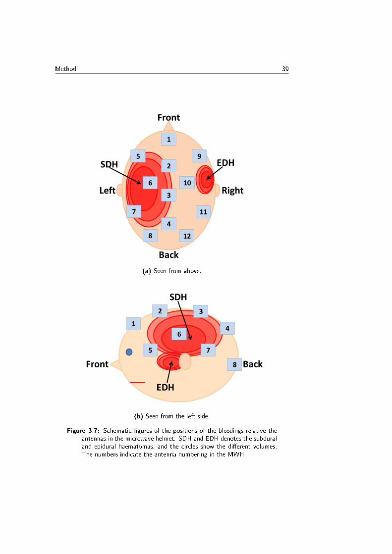
Figure 3.7: Schematic gures of the positions of the bleedings relative theantennas in the microwave helmet. SDH and EDH denotes the subduraland epidural haematomas, and the circles show the dierent volumes.The numbers indicate the antenna numbering in the MWH.
40 Method
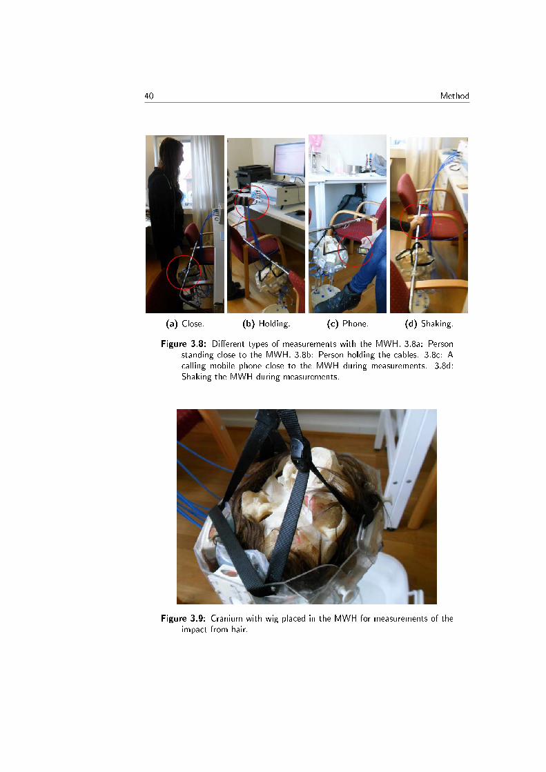
(a) Close. (b) Holding. (c) Phone. (d) Shaking.
Figure 3.8: Dierent types of measurements with the MWH. 3.8a: Personstanding close to the MWH. 3.8b: Person holding the cables. 3.8c: Acalling mobile phone close to the MWH during measurements. 3.8d:Shaking the MWH during measurements.
Figure 3.9: Cranium with wig placed in the MWH for measurements of theimpact from hair.
Chapter4Result
4.1 Phantoms
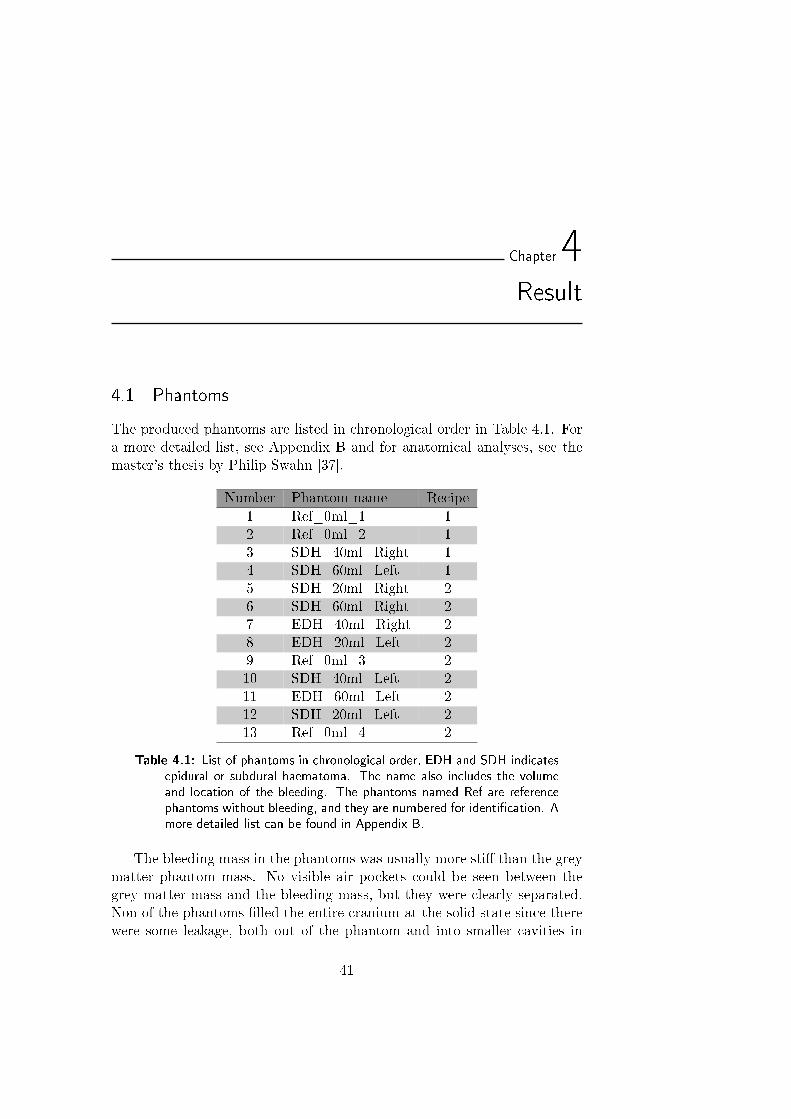
The produced phantoms are listed in chronological order in Table 4.1. Fora more detailed list, see Appendix B and for anatomical analyses, see themaster's thesis by Philip Swahn [37].
Number Phantom name Recipe1 Ref_0ml_1 12 Ref_0ml_2 13 SDH_40ml_Right 14 SDH_60ml_Left 15 SDH_20ml_Right 26 SDH_60ml_Right 27 EDH_40ml_Right 28 EDH_20ml_Left 29 Ref_0ml_3 210 SDH_40ml_Left 211 EDH_60ml_Left 212 SDH_20ml_Left 213 Ref_0ml_4 2
Table 4.1: List of phantoms in chronological order, EDH and SDH indicatesepidural or subdural haematoma. The name also includes the volumeand location of the bleeding. The phantoms named Ref are referencephantoms without bleeding, and they are numbered for identication. Amore detailed list can be found in Appendix B.
The bleeding mass in the phantoms was usually more sti than the greymatter phantom mass. No visible air pockets could be seen between thegrey matter mass and the bleeding mass, but they were clearly separated.Non of the phantoms lled the entire cranium at the solid state since therewere some leakage, both out of the phantom and into smaller cavities in
41
42 Result
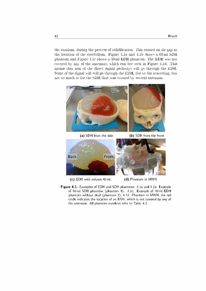
the cranium, during the process of solidication. This caused an air gap atthe location of the cerebellum. Figure 4.1a and 4.1b shows a 60ml SDHphantom and Figure 4.1c shows a 40ml EDH phantom. The EDH was notcovered by any of the antennas, which can bee seen in Figure 4.1d. Thismeans that non of the direct signal pathways will go through the EDH.Some of the signal will still go through the EDH, due to the scattering, butnot as much as for the SDH that was covered by several antennas.
(a) SDH from the side. (b) SDH from the front.
(c) EDH with volume 40ml. (d) Phantom in MWH.
Figure 4.1: Examples of EDH and SDH phantoms. 4.1a and 4.1b: Exampleof 60ml SDH phantom (phantom 4). 4.1c: Example of 40ml EDHphantom without skull (phantom 7), 4.1d: Phantom in MWH, the redcircle indicates the location of an EDH, which is not covered by any ofthe antennas. All phantom numbers refer to Table 4.1.
Result 43
4.2 Dielectric properties
4.2.1 Phantoms
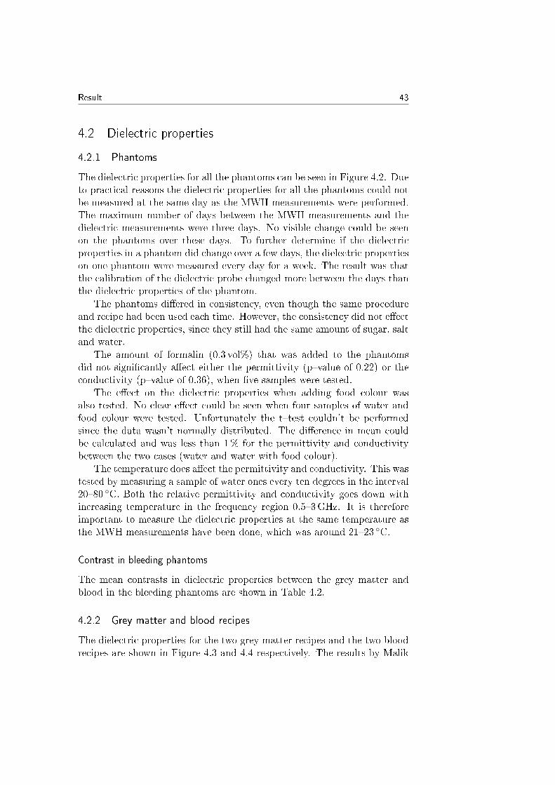
The dielectric properties for all the phantoms can be seen in Figure 4.2. Dueto practical reasons the dielectric properties for all the phantoms could notbe measured at the same day as the MWH measurements were performed.The maximum number of days between the MWH measurements and thedielectric measurements were three days. No visible change could be seenon the phantoms over these days. To further determine if the dielectricproperties in a phantom did change over a few days, the dielectric propertieson one phantom were measured every day for a week. The result was thatthe calibration of the dielectric probe changed more between the days thanthe dielectric properties of the phantom.
The phantoms diered in consistency, even though the same procedureand recipe had been used each time. However, the consistency did not eectthe dielectric properties, since they still had the same amount of sugar, saltand water.
The amount of formalin (0.3 vol%) that was added to the phantomsdid not signicantly aect either the permittivity (pvalue of 0.22) or theconductivity (pvalue of 0.36), when ve samples were tested.
The eect on the dielectric properties when adding food colour wasalso tested. No clear eect could be seen when four samples of water andfood colour were tested. Unfortunately the ttest couldn't be performedsince the data wasn't normally distributed. The dierence in mean couldbe calculated and was less than 1% for the permittivity and conductivitybetween the two cases (water and water with food colour).
The temperature does aect the permittivity and conductivity. This wastested by measuring a sample of water ones every ten degrees in the interval2080 C. Both the relative permittivity and conductivity goes down withincreasing temperature in the frequency region 0.53GHz. It is thereforeimportant to measure the dielectric properties at the same temperature asthe MWH measurements have been done, which was around 2123 C.
Contrast in bleeding phantoms
The mean contrasts in dielectric properties between the grey matter andblood in the bleeding phantoms are shown in Table 4.2.
4.2.2 Grey matter and blood recipes
The dielectric properties for the two grey matter recipes and the two bloodrecipes are shown in Figure 4.3 and 4.4 respectively. The results by Malik
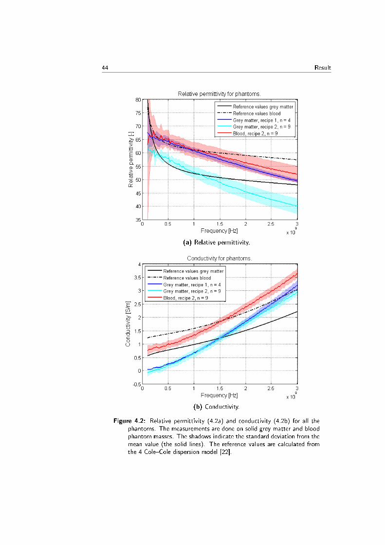
44 Result
(a) Relative permittivity.
(b) Conductivity.
Figure 4.2: Relative permittivity (4.2a) and conductivity (4.2b) for all thephantoms. The measurements are done on solid grey matter and bloodphantom masses. The shadows indicate the standard deviation from themean value (the solid lines). The reference values are calculated fromthe 4-ColeCole dispersion model [22].
Result 45
Relative contrast(mean ± SD) [%]
Reference values 15Phantoms, 6 ± 3grey matter recipe 1, n = 2Phantoms, 17 ± 6grey matter recipe 2, n = 7
(a) Relative Permittivity
Relative contrast(mean ± SD) [%]
Reference values 33Phantoms, 37 ± 1grey matter recipe 1, n = 2Phantoms, 34 ± 4grey matter recipe 2, n = 7
(b) Conductivity
Table 4.2: Relative contrast in dielectric properties between solid grey matterand blood phantom masses. All recipes can be found in Table 3.1a, 3.1band 3.2b. The reference values are calculated from the 4-ColeColedispersion model [22].
Ahmad [9] are also shown in the gures.
4.2.3 Liquid and solid phantoms
The permittivity of the solid phantoms that contains agar are signicantlydierent from the ones without agar (p<0.05). The permittivity for thesolid phantom are 6% lower than the permittivity of the liquid phantoms,see Table 4.3. The conductivity for the solution is not signicantly aectedby the agar.
t-test Mean valuepvalue dierence [%]
Relative Permittivity, n = 9 0.02 6 ± 1Conductivity, n = 9 0.78 -
Table 4.3: Dierence in relative permittivity and conductivity between solidand liquid phantom masses in the frequency interval 0.53GHz.
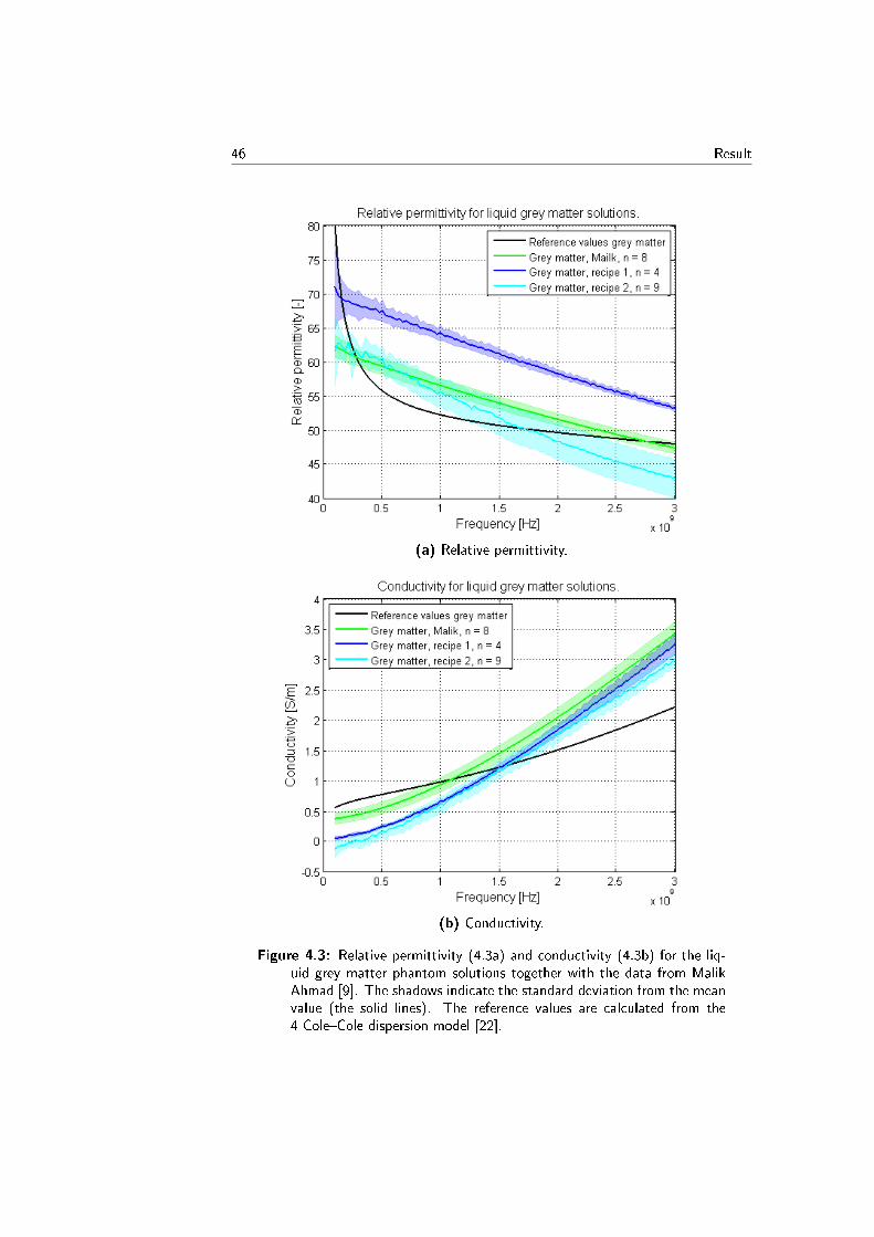
46 Result
(a) Relative permittivity.
(b) Conductivity.
Figure 4.3: Relative permittivity (4.3a) and conductivity (4.3b) for the liq-uid grey matter phantom solutions together with the data from MalikAhmad [9]. The shadows indicate the standard deviation from the meanvalue (the solid lines). The reference values are calculated from the4-ColeCole dispersion model [22].
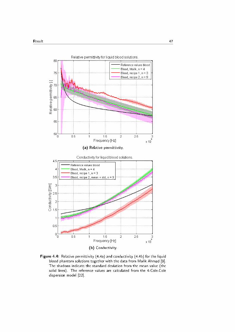
Result 47
(a) Relative permittivity.
(b) Conductivity.
Figure 4.4: Relative permittivity (4.4a) and conductivity (4.4b) for the liquidblood phantom solutions together with the data from Malik Ahmad [9].The shadows indicate the standard deviation from the mean value (thesolid lines). The reference values are calculated from the 4-Cole-Coledispersion model [22].

48 Result
4.2.4 Coagulated blood measurements
Measurements on relative permittivity and conductivity were performed onpig blood to see the impact of coagulation, see Figure 4.5. The permittiv-ity for uncoagulated blood and coagulated blood diered (p<0.05). Themean value for the permittivity was 2% lower for coagulated 37 C bloodthan for uncoagulated 37C blood and the standard deviation was 2%.The conductivity for the uncoagulated and coagulated blood did not diersignicantly.
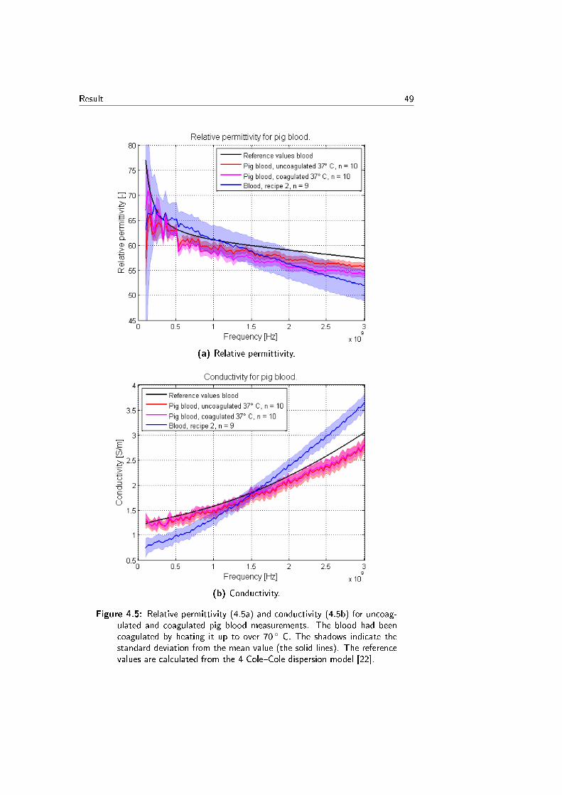
Result 49
(a) Relative permittivity.
(b) Conductivity.
Figure 4.5: Relative permittivity (4.5a) and conductivity (4.5b) for uncoag-ulated and coagulated pig blood measurements. The blood had beencoagulated by heating it up to over 70 C. The shadows indicate thestandard deviation from the mean value (the solid lines). The referencevalues are calculated from the 4-ColeCole dispersion model [22].
50 Result
4.3 Microwave helmet
The MWH that was used for the measurements works best between 0.51.7GHz. Below 0.5GHz, the transmission is very low, as seen in Figure 4.6aand 4.6b. Above 1.7GHz, the transmission is divided into two groups oflines, see Figure 4.6b. These groups are seen for all transmission coecientsand originates from dierent calibrations where some internal changes haveoccurred in between. This dierence is due to bad isolation in some of theswitches, witch causes the transmission to takes place inside the machinerather than between the antennas. Therefore the analyses are performed inthe interval previously mentioned.
There were some problems with bad cable connections and noisy sig-nals. Both cables and ports were swapped to try to get the best signals.Two of the antennas on the MWH (8 and 12) were not connected to theStrokender R10 and are therefore not included in the analyses. Anotherantenna (number 1) had to be excluded because of some problems with badconnection and very high reection.
Due to some unexpected problems with the equipment, the data fromphantom 5 and phantom 6 in Table 4.1 could not be used due to artefactsin data. The transmission signal for these measurements were about 40 dBhigher than usual, resulting in positive values. The same thing occurred forthe movement data from phantom 4.
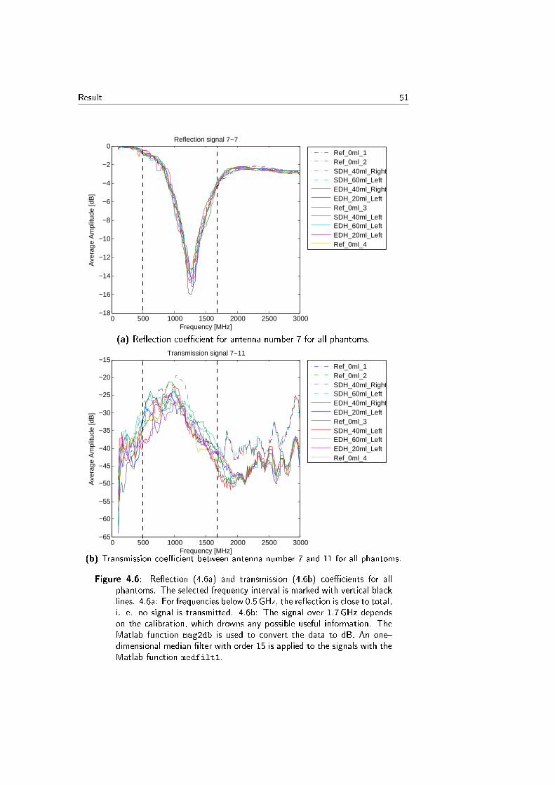
Result 51
0 500 1000 1500 2000 2500 3000−18
−16
−14
−12
−10
−8
−6
−4
−2
0
Frequency [MHz]
Ave
rage
Am
plitu
de [d
B]
Reflection signal 7−7
Ref_0ml_1Ref_0ml_2SDH_40ml_RightSDH_60ml_LeftEDH_40ml_RightEDH_20ml_LeftRef_0ml_3SDH_40ml_LeftEDH_60ml_LeftEDH_20ml_LeftRef_0ml_4
(a) Reection coecient for antenna number 7 for all phantoms.
0 500 1000 1500 2000 2500 3000−65
−60
−55
−50
−45
−40
−35
−30
−25
−20
−15
Frequency [MHz]
Ave
rage
Am
plitu
de [d
B]
Transmission signal 7−11
Ref_0ml_1Ref_0ml_2SDH_40ml_RightSDH_60ml_LeftEDH_40ml_RightEDH_20ml_LeftRef_0ml_3SDH_40ml_LeftEDH_60ml_LeftEDH_20ml_LeftRef_0ml_4
(b) Transmission coecient between antenna number 7 and 11 for all phantoms.
Figure 4.6: Reection (4.6a) and transmission (4.6b) coecients for allphantoms. The selected frequency interval is marked with vertical blacklines. 4.6a: For frequencies below 0.5GHz, the reection is close to total,i. e. no signal is transmitted. 4.6b: The signal over 1.7 GHz dependson the calibration, which drowns any possible useful information. TheMatlab function mag2db is used to convert the data to dB. An onedimensional median lter with order 15 is applied to the signals with theMatlab function medfilt1.
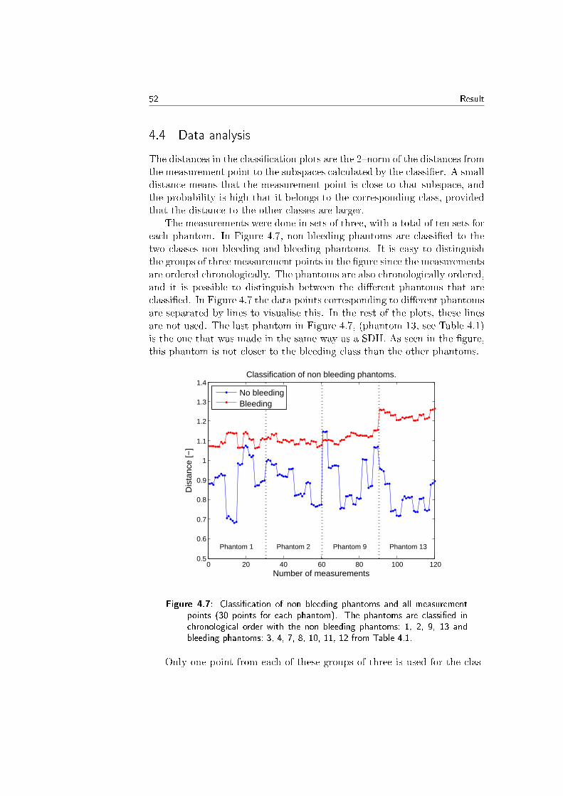
52 Result
4.4 Data analysis
The distances in the classication plots are the 2norm of the distances fromthe measurement point to the subspaces calculated by the classier. A smalldistance means that the measurement point is close to that subspace, andthe probability is high that it belongs to the corresponding class, providedthat the distance to the other classes are larger.
The measurements were done in sets of three, with a total of ten sets foreach phantom. In Figure 4.7, non bleeding phantoms are classied to thetwo classes non bleeding and bleeding phantoms. It is easy to distinguishthe groups of three measurement points in the gure since the measurementsare ordered chronologically. The phantoms are also chronologically ordered,and it is possible to distinguish between the dierent phantoms that areclassied. In Figure 4.7 the data points corresponding to dierent phantomsare separated by lines to visualise this. In the rest of the plots, these linesare not used. The last phantom in Figure 4.7, (phantom 13, see Table 4.1)is the one that was made in the same way as a SDH. As seen in the gure,this phantom is not closer to the bleeding class than the other phantoms.
0 20 40 60 80 100 1200.5
0.6
0.7
0.8
0.9
1
1.1
1.2
1.3
1.4Classification of non bleeding phantoms.
Number of measurements
Dis
tanc
e [−
]
No bleedingBleeding
Phantom 1 Phantom 2 Phantom 9 Phantom 13
Figure 4.7: Classication of non bleeding phantoms and all measurementpoints (30 points for each phantom). The phantoms are classied inchronological order with the non bleeding phantoms: 1, 2, 9, 13 andbleeding phantoms: 3, 4, 7, 8, 10, 11, 12 from Table 4.1.
Only one point from each of these groups of three is used for the clas-
Result 53
sications, in all cases except for the interference data. This means a totalof ten points per phantom, where the phantom orders are specied in thecaption. All the classications are done with data from the frequency re-gion 0.51.7GHz.
4.4.1 Non bleeding and bleeding phantoms
Figure 4.8 shows the classication results of non bleeding and bleeding phan-toms. Four non bleeding phantoms are used in the non bleeding class andseven bleeding phantoms are used in the bleeding class. It can be seen thatthe classication is 100 % correct in the bleeding case and almost 100 % inthe non bleeding case. There are bigger variations between the distances be-longing to the same phantom than between the dierent phantoms. Thesestrong results were only obtained when data from the classied phantomswere included in the training data.
Classifying a phantom that is not in the trainingset
Table 4.4a shows the result from the classication of one phantom at thetime that is completely left out of the training set. The phantoms wereclassied to two classes; non bleeding and bleeding phantoms. The num-ber of phantoms were the same in each class. If the size was uneven, thesmallest distance was obtained to the class with the largest number of phan-toms. The bleeding phantoms that were used were the phantoms with thepermittivity contrast closest to the reference values calculated from the 4-ColeCole dispersion model (see Equation (2.12)), using the parametersfrom Gabriel et al. [22].
The results show that the classier manages to classify the non bleedingphantoms with grey matter recipe 1 to the non bleeding phantom class andalmost all the bleeding phantoms with grey matter recipe 2 to the bleedingclass. But it does not manage to classify the non bleeding phantoms withthe grey matter recipe 2 correct or the bleeding phantoms with grey matterrecipe 1. When the same analysis were done in the frequency intervals100300MHz and 2.53GHz where the information content of the signalshould be much lower, similar results were obtained, but the distances weredierent.
4.4.2 Epidural and subdural haematomas
Figure 4.9 shows the classication results of non bleeding, EDH and SDHphantoms. The classier manages to classify all the phantoms 100 % cor-rect. Only the phantoms made with grey matter recipe 2 were used forthese analysis. It is possible to see some trends here. In Figure 4.9a, the
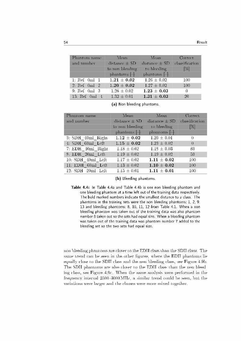
54 Result
Phantom name Mean Mean Correctand number distance ± SD distance ± SD classication
to non bleeding to bleeding [%]phantoms [] phantoms []
1: Ref_0ml_1 1.21 ± 0.02 1.26 ± 0.02 1002: Ref_0ml_2 1.20 ± 0.02 1.27 ± 0.02 1009: Ref_0ml_3 1.28 ± 0.02 1.23 ± 0.03 013: Ref_0ml_4 1.32 ± 0.01 1.31 ± 0.03 20
(a) Non bleeding phantoms.
Phantom name Mean Mean Correctand number distance ± SD distance ± SD classication
to non bleeding to bleeding [%]phantoms [] phantoms []
3: SDH_40ml_Right 1.12 ± 0.02 1.20 ± 0.01 04: SDH_60ml_Left 1.15 ± 0.02 1.23 ± 0.02 07: EDH_40ml_Right 1.18 ± 0.02 1.18 ± 0.03 808: EDH_20ml_Left 1.19 ± 0.02 1.19 ± 0.02 5010: SDH_40ml_Left 1.17 ± 0.02 1.11 ± 0.02 10011: EDH_60ml_Left 1.13 ± 0.02 1.10 ± 0.02 10012: SDH_20ml_Left 1.15 ± 0.01 1.11 ± 0.01 100
(b) Bleeding phantoms.
Table 4.4: In Table 4.4a and Table 4.4b is one non bleeding phantom andone bleeding phantom at a time left out of the training data respectively.The bold marked numbers indicate the smallest distance to a class. Thephantoms in the training sets were the non bleeding phantoms: 1, 2, 9,13 and bleeding phantoms: 8, 10, 11, 12 from Table 4.1. When a nonbleeding phantom was taken out of the training data was also phantomnumber 8 taken out so the sets had equal size. When a bleeding phantomwas taken out of the training data was phantom number 7 added to thebleeding set so the two sets had equal size.
non bleeding phantoms are closer to the EDH class than the SDH class. Thesame trend can be seen in the other gures, where the EDH phantoms lieequally close to the SDH class and the non bleeding class, see Figure 4.9b.The SDH phantoms are also closer to the EDH class than the non bleed-ing class, see Figure 4.9c. When the same analysis were performed in thefrequency interval 25003000MHz, a similar trend could be seen, but thevariations were larger and the classes were more mixed together.
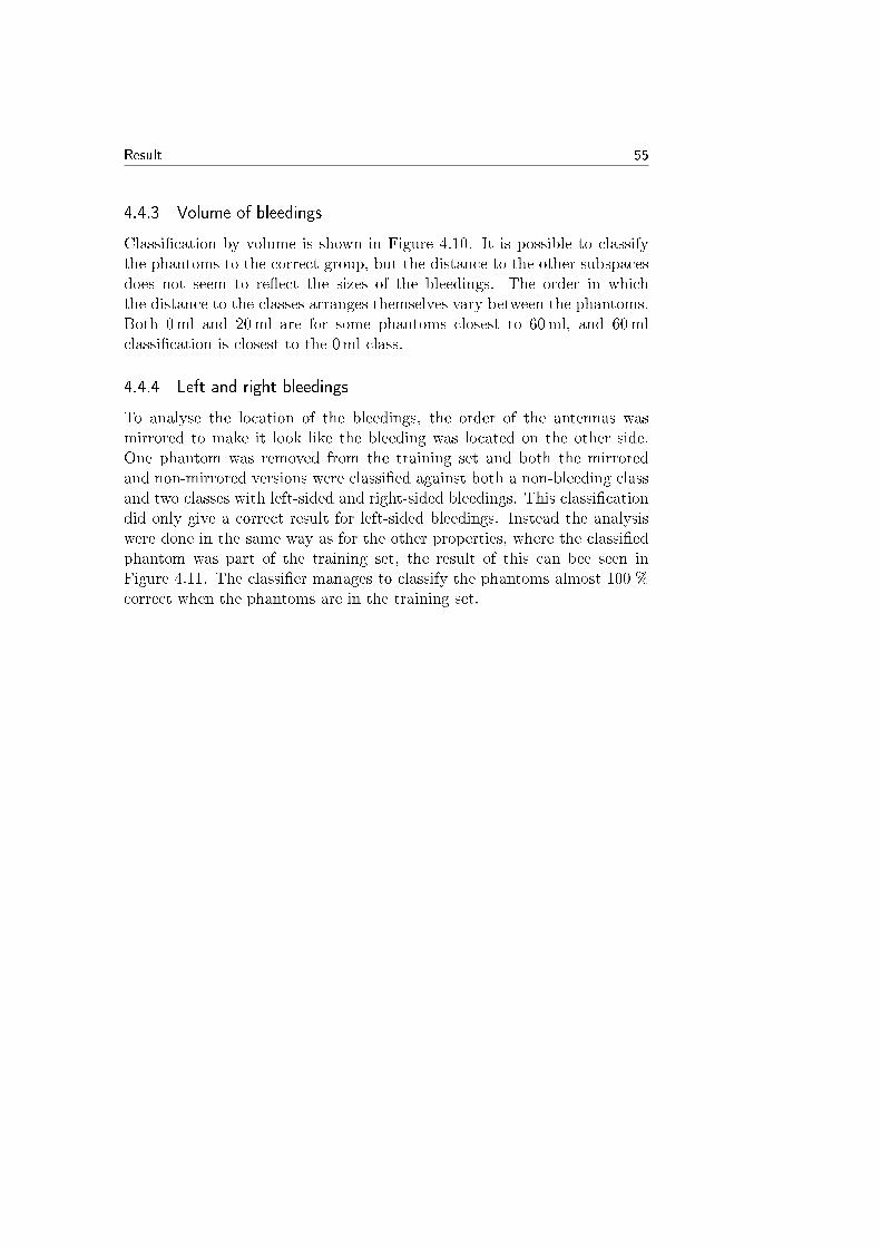
Result 55
4.4.3 Volume of bleedings
Classication by volume is shown in Figure 4.10. It is possible to classifythe phantoms to the correct group, but the distance to the other subspacesdoes not seem to reect the sizes of the bleedings. The order in whichthe distance to the classes arranges themselves vary between the phantoms.Both 0ml and 20ml are for some phantoms closest to 60ml, and 60mlclassication is closest to the 0ml class.
4.4.4 Left and right bleedings
To analyse the location of the bleedings, the order of the antennas wasmirrored to make it look like the bleeding was located on the other side.One phantom was removed from the training set and both the mirroredand non-mirrored versions were classied against both a non-bleeding classand two classes with left-sided and right-sided bleedings. This classicationdid only give a correct result for left-sided bleedings. Instead the analysiswere done in the same way as for the other properties, where the classiedphantom was part of the training set, the result of this can bee seen inFigure 4.11. The classier manages to classify the phantoms almost 100 %correct when the phantoms are in the training set.
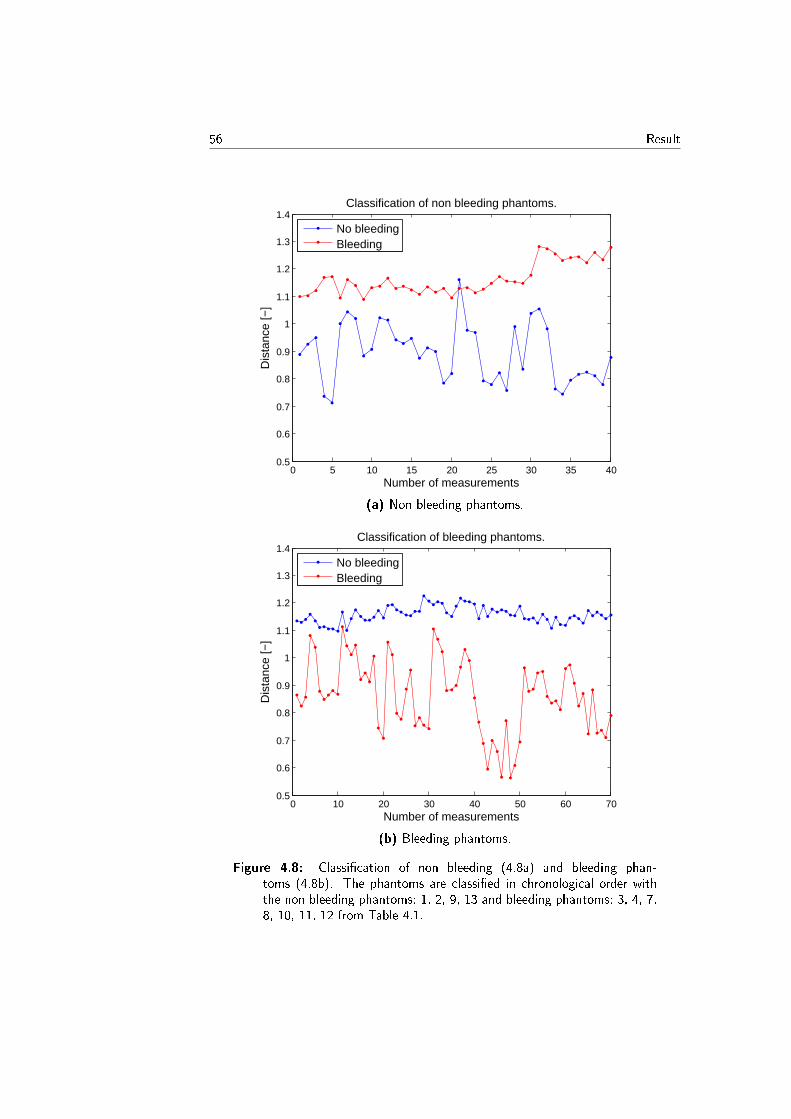
56 Result
0 5 10 15 20 25 30 35 400.5
0.6
0.7
0.8
0.9
1
1.1
1.2
1.3
1.4Classification of non bleeding phantoms.
Number of measurements
Dis
tanc
e [−
]
No bleedingBleeding
(a) Non bleeding phantoms.
0 10 20 30 40 50 60 700.5
0.6
0.7
0.8
0.9
1
1.1
1.2
1.3
1.4Classification of bleeding phantoms.
Number of measurements
Dis
tanc
e [−
]
No bleedingBleeding
(b) Bleeding phantoms.
Figure 4.8: Classication of non bleeding (4.8a) and bleeding phan-toms (4.8b). The phantoms are classied in chronological order withthe non bleeding phantoms: 1, 2, 9, 13 and bleeding phantoms: 3, 4, 7,8, 10, 11, 12 from Table 4.1.
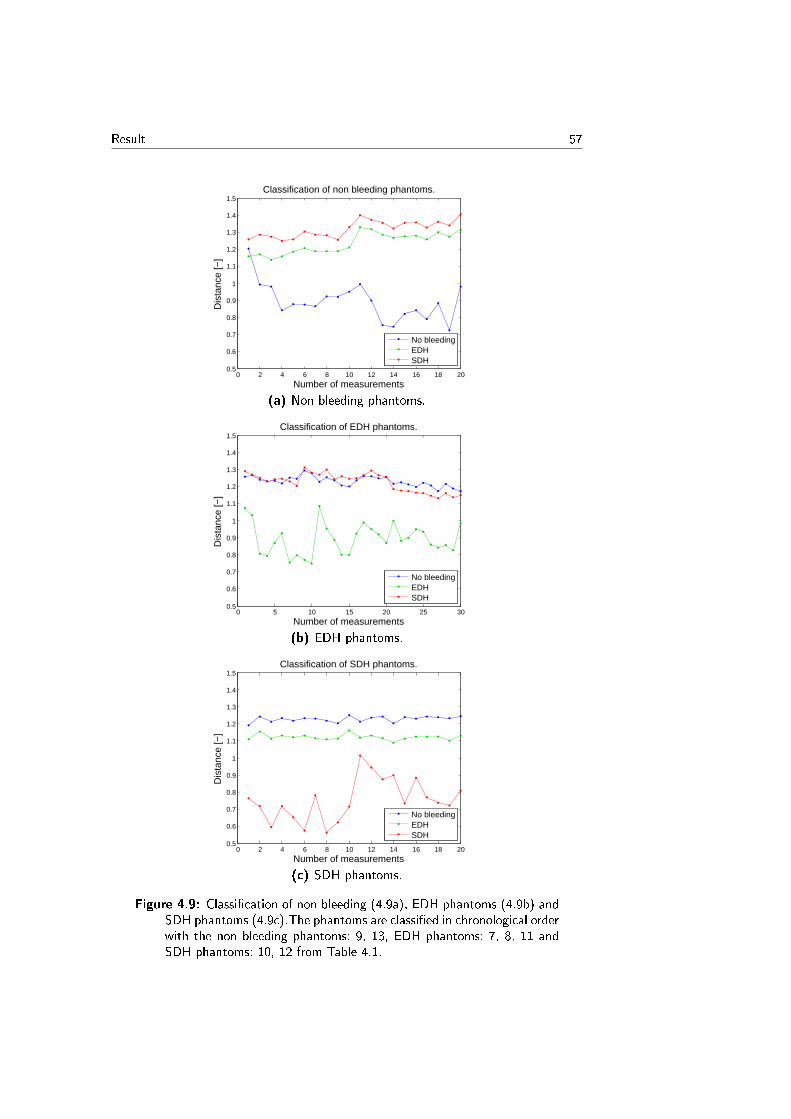
Result 57
0 2 4 6 8 10 12 14 16 18 200.5
0.6
0.7
0.8
0.9
1
1.1
1.2
1.3
1.4
1.5Classification of non bleeding phantoms.
Number of measurements
Dis
tanc
e [−
]
No bleedingEDHSDH
(a) Non bleeding phantoms.
0 5 10 15 20 25 300.5
0.6
0.7
0.8
0.9
1
1.1
1.2
1.3
1.4
1.5Classification of EDH phantoms.
Number of measurements
Dis
tanc
e [−
]
No bleedingEDHSDH
(b) EDH phantoms.
0 2 4 6 8 10 12 14 16 18 200.5
0.6
0.7
0.8
0.9
1
1.1
1.2
1.3
1.4
1.5Classification of SDH phantoms.
Number of measurements
Dis
tanc
e [−
]
No bleedingEDHSDH
(c) SDH phantoms.
Figure 4.9: Classication of non bleeding (4.9a), EDH phantoms (4.9b) andSDH phantoms (4.9c).The phantoms are classied in chronological orderwith the non bleeding phantoms: 9, 13, EDH phantoms: 7, 8, 11 andSDH phantoms: 10, 12 from Table 4.1.
58 Result
0 5 10 15 20 25 30 35 400.5
0.6
0.7
0.8
0.9
1
1.1
1.2
1.3
1.4Classification of 0 ml bleeding phantoms
Number of measurements
Dis
tanc
e [−
]
0 ml20 ml40 ml60 ml
(a) Classication of non bleeding (0ml)phantoms.
0 2 4 6 8 10 12 14 16 18 200.5
0.6
0.7
0.8
0.9
1
1.1
1.2
1.3
1.4Classification of 20 ml bleeding phantoms
Number of measurementsD
ista
nce
[−]
0 ml20 ml40 ml60 ml
(b) Classication of 20ml bleeding phan-toms.
0 5 10 15 20 25 300.5
0.6
0.7
0.8
0.9
1
1.1
1.2
1.3
1.4Classification of 40 ml bleeding phantoms
Number of measurements
Dis
tanc
e [−
]
0 ml
20 ml
40 ml
60 ml
(c) Classication of 40ml bleeding phan-toms.
0 2 4 6 8 10 12 14 16 18 200.5
0.6
0.7
0.8
0.9
1
1.1
1.2
1.3
1.4Classification of 60 ml bleeding phantoms
Number of measurements
Dis
tanc
e [−
]
0 ml20 ml40 ml60 ml
(d) Classication of 60ml bleeding phan-toms.
Figure 4.10: Classication with respect to volume. The phantoms are classi-ed in chronological order with the non bleeding (0ml) phantoms: 1, 2,9, 13, 20ml: phantoms 8, 12, 40ml: phantoms 3, 7, 10 and 60ml phan-toms: 4, 11 from Table 4.1.
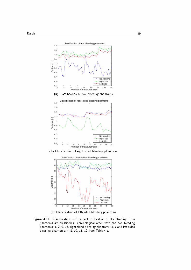
Result 59
0 5 10 15 20 25 30 35 400.5
0.6
0.7
0.8
0.9
1
1.1
1.2
1.3
1.4Classification of non bleeding phantoms
Number of measurements
Dis
tanc
e [−
]
No bleedingRight sideLeft side
(a) Classication of non bleeding phantoms.
0 2 4 6 8 10 12 14 16 18 200.5
0.6
0.7
0.8
0.9
1
1.1
1.2
1.3
1.4Classification of right−sided bleeding phantoms
Number of measurements
Dis
tanc
e [−
]
No bleedingRight sideLeft side
(b) Classication of right-sided bleeding phantoms.
0 5 10 15 20 25 30 35 40 45 500.5
0.6
0.7
0.8
0.9
1
1.1
1.2
1.3Classification of left−sided bleeding phantoms
Number of measurements
Dis
tanc
e [−
]
No bleedingRight sideLeft side
(c) Classication of left-sided bleeding phantoms.
Figure 4.11: Classication with respect to location of the bleeding. Thephantoms are classied in chronological order with the non bleedingphantoms: 1, 2, 9, 13, right sided bleeding phantoms: 3, 7 and left sidedbleeding phantoms: 4, 8, 10, 11, 12 from Table 4.1.
60 Result
4.4.5 Interfering factors
Person close
Figure 4.12 shows the classication of bleeding phantoms with interferencefrom a person close to the measurement setup. Table 4.5 shows a summaryof the classications of bleeding and non bleeding phantom classes with thisinterference. There is no clear dierence between the reference and when aperson is standing close to the measurement setup.
Holding the cables
Figure 4.13 shows the classication of bleeding phantoms with interferencefrom a person holding the cables during the measurements. Table 4.6 showsa summary of the classication of bleeding and non bleeding phantom classeswith this interference. There is a dierence between the mean values for thereference and the interference data, where the interference data lies closer tothe other subspaces. The standard deviation is also larger for the referencevalues.
Phone call
Figure 4.14 shows an example of the interference from a calling mobilephone close to the phantom during the measurements. The example is fromclassication of non bleeding phantoms to the three classes; no bleeding,EDH and SDH phantoms. Table 4.7 presents a summary of the classicationof the interference from a calling mobile phone. The mean distances areapproximately the same for the reference values as for the calling phonevalues.
Hair
Figure 4.15 shows the interference from hair around the phantoms duringmeasurements. The example is from classication of SDH phantoms tothe three classes; no bleeding, EDH and SDH phantoms. The referencevalues in this classication are the ordinary measurements. Just like inthe ordinary measurements, the phantoms were repositioned between themeasurements, which gives an extra variability. Table 4.8 shows a summaryof the interference from hair on the phantoms. The classication of thephantoms with hair was closer to the other subspaces than the referenceand the classier did not manage to classify all the phantoms correctly.
Result 61
Movement
Figure 4.16 shows an example of how shaking the phantoms during mea-surements aects the classication. The example is from the classicationof the EDH phantoms to the three classes; non bleeding, EDH and SDHphantoms. A summary of the eect of movement on the classication isshown in Table 4.9. All the shaking values lie generally closer to the otherclasses than the reference values, but the classication is still made correctlyin all the cases. Another interesting thing that can be seen, is that the stan-dard deviation is smaller for the shaking phantom values than the referencevalues. The raw data from the movement experiments were studied andcompared to the reference data and no obvious dierences could be found.
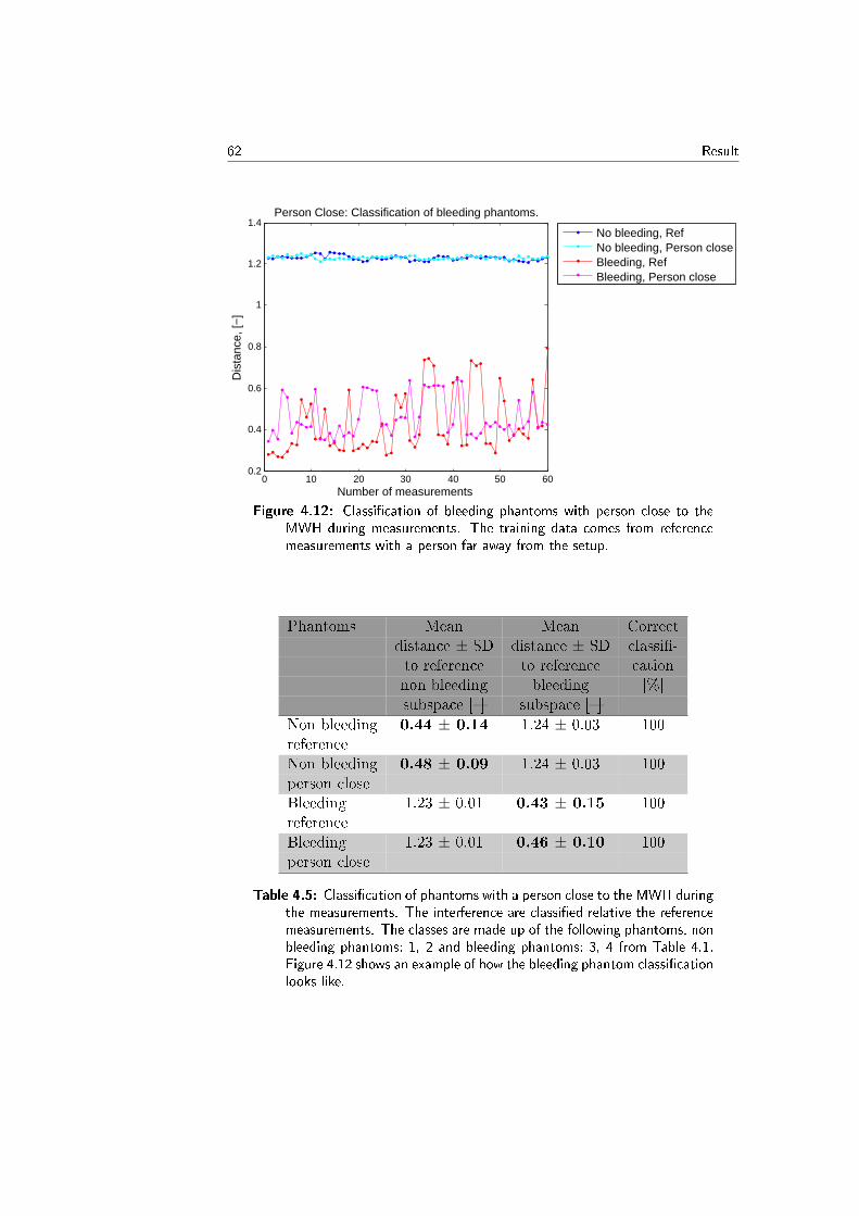
62 Result
0 10 20 30 40 50 600.2
0.4
0.6
0.8
1
1.2
1.4Person Close: Classification of bleeding phantoms.
Number of measurements
Dis
tanc
e, [−
]
No bleeding, RefNo bleeding, Person closeBleeding, RefBleeding, Person close
Figure 4.12: Classication of bleeding phantoms with person close to theMWH during measurements. The training data comes from referencemeasurements with a person far away from the setup.
Phantoms Mean Mean Correctdistance ± SD distance ± SD classi-to reference to reference cationnon bleeding bleeding [%]subspace [] subspace []
Non bleeding 0.44 ± 0.14 1.24 ± 0.03 100referenceNon bleeding 0.48 ± 0.09 1.24 ± 0.03 100person closeBleeding 1.23 ± 0.01 0.43 ± 0.15 100referenceBleeding 1.23 ± 0.01 0.46 ± 0.10 100person close
Table 4.5: Classication of phantoms with a person close to the MWH duringthe measurements. The interference are classied relative the referencemeasurements. The classes are made up of the following phantoms, nonbleeding phantoms: 1, 2 and bleeding phantoms: 3, 4 from Table 4.1.Figure 4.12 shows an example of how the bleeding phantom classicationlooks like.
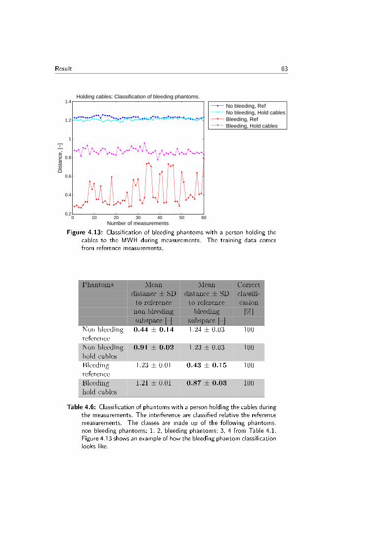
Result 63
0 10 20 30 40 50 600.2
0.4
0.6
0.8
1
1.2
1.4Holding cables: Classification of bleeding phantoms.
Number of measurements
Dis
tanc
e, [−
]
No bleeding, RefNo bleeding, Hold cablesBleeding, RefBleeding, Hold cables
Figure 4.13: Classication of bleeding phantoms with a person holding thecables to the MWH during measurements. The training data comesfrom reference measurements.
Phantoms Mean Mean Correctdistance ± SD distance ± SD classi-to reference to reference cationnon bleeding bleeding [%]subspace [] subspace []
Non bleeding 0.44 ± 0.14 1.24 ± 0.03 100referenceNon bleeding 0.91 ± 0.02 1.23 ± 0.03 100hold cablesBleeding 1.23 ± 0.01 0.43 ± 0.15 100referenceBleeding 1.21 ± 0.01 0.87 ± 0.03 100hold cables
Table 4.6: Classication of phantoms with a person holding the cables duringthe measurements. The interference are classied relative the referencemeasurements. The classes are made up of the following phantoms,non bleeding phantoms: 1, 2, bleeding phantoms: 3, 4 from Table 4.1.Figure 4.13 shows an example of how the bleeding phantom classicationlooks like.
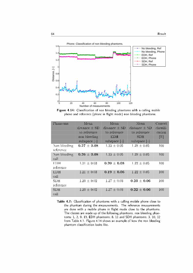
64 Result
0 20 40 60 80 100 1200
0.2
0.4
0.6
0.8
1
1.2
1.4
1.6Phone: Classification of non bleeding phantoms.
Number of measurements
Dis
tanc
e, [−
]
No bleeding, RefNo bleeding, PhoneEDH, RefEDH, PhoneSDH, RefSDH, Phone
Figure 4.14: Classication of non bleeding phantoms with a calling mobilephone and reference (phone in ight mode) non bleeding phantoms.
Phantoms Mean Mean Mean Correctdistance ± SD distance ± SD distance ± SD classi-to reference to reference to reference cationnon bleeding EDH SDH [%]subspace [] subspace [] subspace []
Non bleeding 0.27 ± 0.08 1.35 ± 0.05 1.28 ± 0.05 100referenceNon bleeding 0.26 ± 0.08 1.35 ± 0.05 1.28 ± 0.05 100callEDH 1.21 ± 0.03 0.20 ± 0.08 1.22 ± 0.05 100referenceEDH 1.21 ± 0.03 0.19 ± 0.06 1.22 ± 0.05 100callSDH 1.20 ± 0.02 1.27 ± 0.03 0.23 ± 0.06 100referenceSDH 1.20 ± 0.02 1.27 ± 0.03 0.22 ± 0.06 100call
Table 4.7: Classication of phantoms with a calling mobile phone close tothe phantom during the measurements. The reference measurementsare done with a mobile phone in ight mode close to the phantoms.The classes are made up of the following phantoms, non bleeding phan-toms: 1, 2, 9, 13, EDH phantoms: 8, 11 and SDH phantoms: 3, 10, 12from Table 4.1. Figure 4.14 shows an example of how the non bleedingphantom classication looks like.
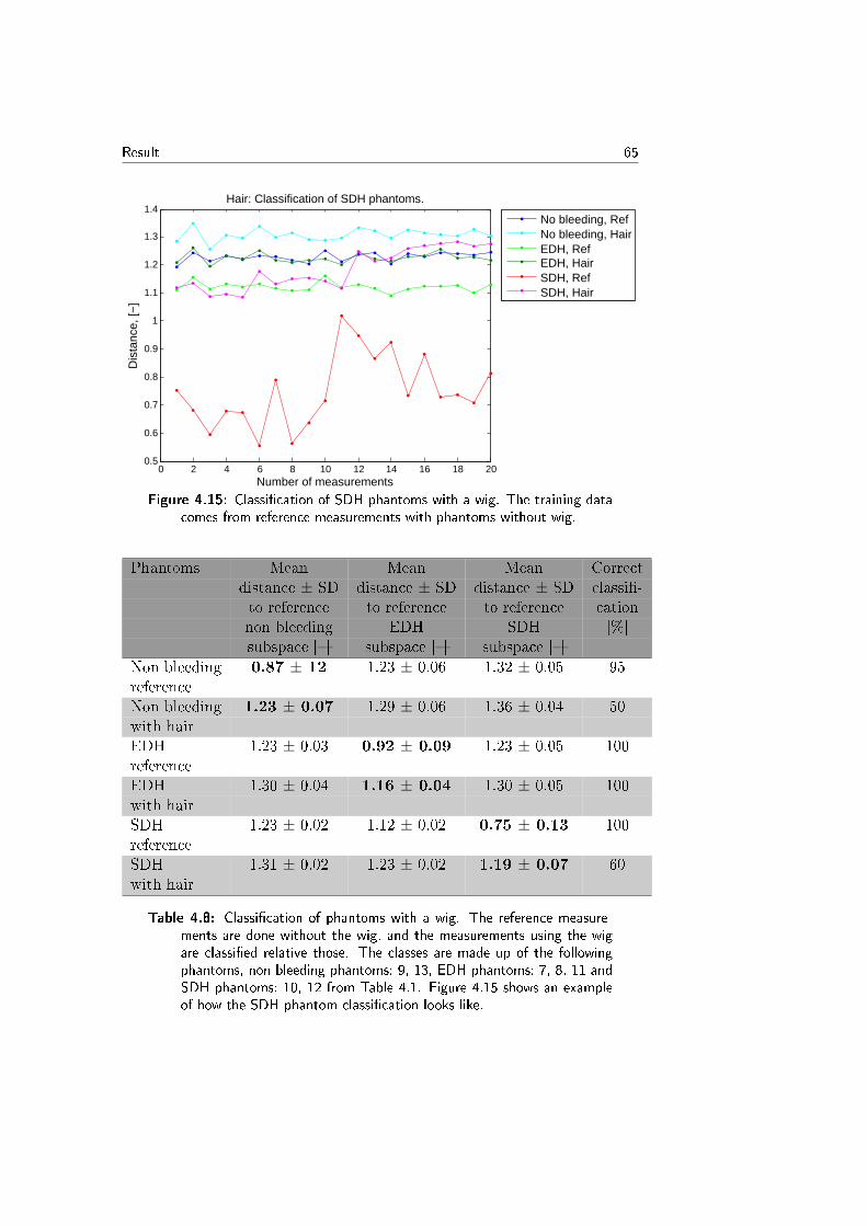
Result 65
0 2 4 6 8 10 12 14 16 18 200.5
0.6
0.7
0.8
0.9
1
1.1
1.2
1.3
1.4Hair: Classification of SDH phantoms.
Number of measurements
Dis
tanc
e, [−
]
No bleeding, RefNo bleeding, HairEDH, RefEDH, HairSDH, RefSDH, Hair
Figure 4.15: Classication of SDH phantoms with a wig. The training datacomes from reference measurements with phantoms without wig.
Phantoms Mean Mean Mean Correctdistance ± SD distance ± SD distance ± SD classi-to reference to reference to reference cationnon bleeding EDH SDH [%]subspace [] subspace [] subspace []
Non bleeding 0.87 ± 12 1.23 ± 0.06 1.32 ± 0.05 95referenceNon bleeding 1.23 ± 0.07 1.29 ± 0.06 1.36 ± 0.04 50with hairEDH 1.23 ± 0.03 0.92 ± 0.09 1.23 ± 0.05 100referenceEDH 1.30 ± 0.04 1.16 ± 0.04 1.30 ± 0.05 100with hairSDH 1.23 ± 0.02 1.12 ± 0.02 0.75 ± 0.13 100referenceSDH 1.31 ± 0.02 1.23 ± 0.02 1.19 ± 0.07 60with hair
Table 4.8: Classication of phantoms with a wig. The reference measure-ments are done without the wig, and the measurements using the wigare classied relative those. The classes are made up of the followingphantoms, non bleeding phantoms: 9, 13, EDH phantoms: 7, 8, 11 andSDH phantoms: 10, 12 from Table 4.1. Figure 4.15 shows an exampleof how the SDH phantom classication looks like.
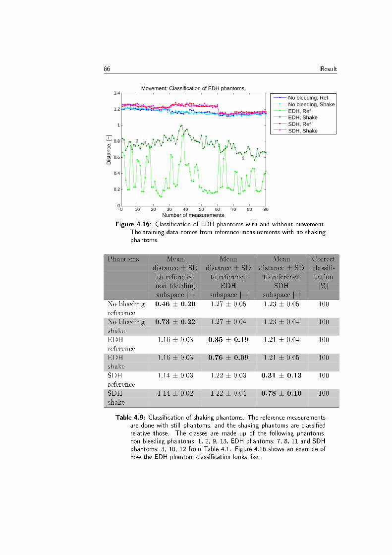
66 Result
0 10 20 30 40 50 60 70 80 900
0.2
0.4
0.6
0.8
1
1.2
1.4Movement: Classification of EDH phantoms.
Number of measurements
Dis
tanc
e, [−
]
No bleeding, RefNo bleeding, ShakeEDH, RefEDH, ShakeSDH, RefSDH, Shake
Figure 4.16: Classication of EDH phantoms with and without movement.The training data comes from reference measurements with no shakingphantoms.
Phantoms Mean Mean Mean Correctdistance ± SD distance ± SD distance ± SD classi-to reference to reference to reference cationnon bleeding EDH SDH [%]subspace [] subspace [] subspace []
No bleeding 0.46 ± 0.20 1.27 ± 0.05 1.23 ± 0.05 100referenceNo bleeding 0.73 ± 0.22 1.27 ± 0.04 1.23 ± 0.04 100shakeEDH 1.16 ± 0.03 0.35 ± 0.19 1.21 ± 0.04 100referenceEDH 1.16 ± 0.03 0.76 ± 0.09 1.21 ± 0.05 100shakeSDH 1.14 ± 0.03 1.22 ± 0.03 0.31 ± 0.13 100referenceSDH 1.14 ± 0.02 1.22 ± 0.04 0.78 ± 0.10 100shake
Table 4.9: Classication of shaking phantoms. The reference measurementsare done with still phantoms, and the shaking phantoms are classiedrelative those. The classes are made up of the following phantoms,non bleeding phantoms: 1, 2, 9, 13, EDH phantoms: 7, 8, 11 and SDHphantoms: 3, 10, 12 from Table 4.1. Figure 4.16 shows an example ofhow the EDH phantom classication looks like.
Chapter5
Discussion
5.1 Phantoms
Two types of bleedings were modelled, EDH and SDH. They were chosensince they are both common, dangerous and extracerebral, which makethem operable in an acute stage. The brain consists of both white and greymatter, surrounded by CSF and meninges. The phantoms on the otherhand consisted only of grey matter. To add extra layers, such as whitematter or meninges, would be both complicated and add an extra factorof variation between the phantoms. The anatomy of the brain is similarbetween dierent persons and not all layers have to be included, since theywill contribute in a similar way for all the patients. Grey matter was selectedeven though the amount of white matter in the brain is higher. The reason isthat the dierence in permittivity between blood and grey matter is smallerthan the dierence between blood and white matter. The MWH seemsto detect symmetry dierences in the brain, rather than borders betweenmaterials. So if a bleeding placed in grey matter can be detected, it canalso be detected in white matter.
Several ways to produce the bleedings were tested, the ones that werenally selected were recommended by neurosurgeons Thomas Skoglund andJohan Ljungqvist at Sahlgrenska University Hospital. These methods werechosen since the phantoms were easy to construct and reproduce and theneurosurgeons thought they looked realistic.
Even if the phantoms were produced in the same way, the consistencydiered between them. Some were very soft and collapsed when they wereremoved from the cranium and others were very solid. This has to do withthe temperature of the mass. The temperature was monitored with a simplethermometer and it was hard to keep an even temperature throughout themass. The consistency was evaluated by eye, and the speed with which itsolidied depended on how much and for how long the mixture was heated.The bleeding was usually more solid than the rest of the brain. The rea-
67
68 Discussion
son was that a smaller amount of phantom mass heats up and cools downquicker, due to higher surface to volume ratio. The consistency aects howeasy it is to measure the dielectric properties, but is not thought to af-fect the dielectric properties much. Even if there would be an eect fromthe consistency, it would be smaller than the change in dielectric propertiesbetween liquid and solid phantom mass, which for the permittivity was 6%.
The EDH does usually spread out more and have a larger area in thereal cases than they did in the phantoms. It can be hard for the MWHto detect the EDH in the phantoms, since no antenna was covering it, seeFigure 4.1d. It could therefore be interesting to change the design of theMWH to also cover the temporal bone where the EDH often is positioned.This would probably make it easier to detect the EDH.
After the rst set of phantoms were nished, some discolouration on thecranium was noticed. A yeast infection was suspected due to the high sugarcontent of the mass and insucient drying of the cranium. The craniumwas put in a formaline bath and carefully cleaned. From then on formalinewas put into the phantom mass to avoid further bacterial growth. Thecondition of the cranium was changed during the period of measurements.There were some cracks when the project started, but both the number andsize increased during the measurement period and the thin cartilage in forexample the nose was lost during the cleaning. Non of this should aectthe results signicantly, since the cartilage in the face was so thin and noantenna was placed there. A human cranium contains a lot of small naturalcavities which made it hard to remove all excess phantom mass. There wastherefore a risk that old dried phantom mass was still present when the nextphantom was produced. The amount was very small and would thereforehave no inuence on the measurements.
The air gap in the phantoms at the location of the cerebellum wasinevitable. The same thing appeared for all phantoms and the antennasclose to this region were not used during the measurements, so this shouldnot be a big problem.
5.2 Dielectric properties
5.2.1 Phantoms
It was hard to create recipes for grey matter and blood that had exactly theright relative permittivity and conductivity over the whole frequency range,see Figure 4.2. The shape of the permittivity and conductivity curves arenot the same as for the reference values, which means that a certain tar-get frequency had to be chosen where the reference values were matched.This was due to the chosen phantom recipes that can not fully replicate
Discussion 69
the dielectric properties for grey matter and blood in the whole frequencyrange. In the curves the mean value for blood and grey matter phantommass are the same as the reference values at 1GHz for the relative per-mittivity and 1.5GHz for the conductivity. How much the electromagneticwaves scatter, reect and transmit through the phantom has to do with thedierence in dielectric properties between the grey matter and the bloodphantom masses. Even though the slope of the curves are not the same asthe references, the dierence between the means of blood and grey matteris approximately the same for the permittivity and conductivity. Thereforeit can be assumed that the recipes works as models for grey matter andblood.
The variations between the phantoms are probably due to the fact thatit is not exactly the same amount of each ingredient in every phantom, eventhough care was taken to be as precise as possible. If it would have beenpossible to measure the dielectric properties during the phantom makingcould more even results be obtained. Another change that was noticed dur-ing the measurements were the dierences in the calibration of the dielectricprobe. A new calibration was done every day, but the water measurementsdiered each day, even though it had the same temperature. This mayhave aected the dielectric property measurements with a few percent. Thenumber of days between the creation of the phantoms and the dielectricmeasurements may also have aected the properties. The eect is probablynot be that big, due to the fact that the phantom mass samples were cov-ered in plastic wrapping and stored in the refrigerator until the day of thedielectric measurements.
In some of the dielectric graphs the conductivity goes below zero, seeFigure 4.2. This is due to the uncertainties for the dielectric probe mea-surements at frequencies below 0.5GHz.
The small amount of food colour and formalin used in the phantommasses do not aect the dielectric properties and can therefore be replacedwith deionised water in the recipes. The food colour was practical to useto be able to see where the bleeding was located in the phantom.
Contrast in bleeding phantoms
The mean contrast in relative permittivity between the grey matter andblood phantom masses in the bleeding phantoms, see Table 4.2a, are alittle bit higher than for the reference values. There is a quite big standarddeviation, so some phantoms have a dierence in permittivity that may beharder to see than what it actually is in a real brain, especially the case withthe bleeding phantoms done with grey matter recipe 1. These dierencesmay also make the classication harder, because the MWH data will dier
70 Discussion
between dierent phantoms.
5.2.2 Grey matter and blood recipes
Dierences between the grey matter and blood phantom solution resultsfrom recipe 1, and the results from Malik Ahmad [9] in Figure 4.3 and 4.4,may be due to method dierences. Malik Ahmad had for example thepossibility to measure the dielectric properties during the construction ofthe phantom solutions.
5.2.3 Liquid and solid phantoms
The results for liquid and solid phantom masses makes it possible to createnew recipes from liquid solutions. If six percent agar is added the per-mittivity will decrease with six percent and no eect will be seen on theconductivity, see Table 4.3. Only the phantoms with grey matter recipe 2could be used for these calculations, since the other phantom groups werenot normally distributed over all frequency points. If these other phantoms,22 in a total, were taken into account for the calculations of the mean valuechange, the result become the same. This indicates that the results arecorrect. Another indication that the results are valid is that experimentswhere agar was added to water gave the same result.
5.2.4 Coagulated blood measurements
The haematoma usually consists of clotted blood. Since the dielectric prop-erties for blood from Gabriel et al. [22] are given for liquid 37 C blood,it is interesting to see if the dielectric properties are the same for coagu-lated blood. It is very hard to mimic the coagulation process in the bodyand therefore the pig blood was coagulated by heat. These results, see Fig-ure 4.5, can only be used as an indication for how the coagulation will aectthe dielectric properties and more extended experiments have to be madeto get certain results. The coagulated blood was shown to the neurosur-geons Thomas Skoglund and Johan Ljungqvist at Sahlgrenska UniversityHospital. They said it had similar consistency as blood in a haematomain the brain. In this result the eect of the coagulation is small and thedierences between the blood mass phantoms and the reference values forblood are larger than the eect of the coagulated blood is.
The information from the store was that no additives or special treat-ment procedures had been performed except freezing. However, the neuro-surgeon Johan Ljungqvist thought that the pig blood may have been treatedin some way, since it did not coagulate naturally. This could also be part ofthe explanation why the pig blood had lower permittivity and conductivity
Discussion 71
than the reference values. Other reasons may be temperature variations inthe pig blood samples, dierences in method or dierences in the dielectricprobes used.
5.3 Microwave helmet
There were some problems with the measurement equipment. Several ofthe antennas gave weak or shaky signals, the error often built up duringthe measurements and the severity could not be seen until afterwards. Thisproblem was present for most of the phantoms and on the same antennas,but worsened during the progress of the project. At one point, somethinghappened inside the network analyser which made the old calibration lesuseless. What happened was that the isolation in one of the mechanicalswitches was changed, causing a large part of the signal to go directly fromthe transmitting port to the receiving port without going through the phan-tom. When the system was recalibrated, this leakage was compensated for,but the original problem was still present. Two phantoms were measuredbefore this problem was discovered. The data from the deviant phantomswere normalised after recalibration, but they did still dier to much fromthe rest of the data to be able to use. Unfortunately the bleedings of bothphantoms were placed on the right side, which means that only two rightsided bleedings were left. It is hard to say if this change aected the classi-cation since each phantom was measured only on one day. The dierencesbetween the rst group of phantoms done with grey matter recipe 1, andthe second group done with recipe 2, may be due to either the dierencesin dielectric properties or the change in the measurement equipment.
The skin depth in grey matter for the frequencies used in these measure-ments are only a few centimetres, see Figure 2.12. This means that a majorpart of the signal is lost before it reaches the antennas on the opposite side ofthe head. This might make it harder to nd a bleeding deeper in the brain.However, if the MWH is compared to the Infrascanner, which uses a muchshorter wavelength (808 nm), the skin depth of the MWH is much longer.Another problem with the Infrascanner is that a lot of practice is neededto perform the measurement, since the measurement sequence is done byhand. Only a few places on the head are measured, so if the bleeding islocated somewhere else, or deeper into the brain, it would go unnoticed.
5.4 Data analysis
When analyses were done for frequencies outside the chosen interval, similarresults were obtained. This is of course not good, since it indicates that the
72 Discussion
classier focuses on things outside the phantoms. Since the classier atthis point only seems to recognise the individual phantoms, rather than thebleedings, this was not really a surprising result. The interval is limitedsince the dierences outside the frequency interval come from uninterestingfactors.
The analysis in this project were done with an in-house classier, nochanges have been made to it and no extensive preprocessing of the datahave been performed. There might be better ways to nd the sought pat-terns in the data, but since this project focused on the phantoms, there wasno time to develop a new method of classication.
The ordinary measurements were performed in groups of three, wherethe variation between the groups were much larger than within the groups,see Figure 4.7. This means that there is a greater variation between howthe phantom was placed in the MWH and how the water bags were lled,than between the individual MWH measurements. The variation was cal-culated as the ratio between the mean of the standard deviation for all thephantoms and the mean of the standard deviation for each group of threemeasurements. It is not possible to compare them directly, since the num-ber of measurements is much higher for the phantoms than for the smallergroups. The distance from one measurement point to the class it belongsto depends on the data in the training set and is therefore a very imprecisemeasurement from the beginning. To take the standard deviation of thesevalues makes it even more imprecise since the class it is compared to is notthe same for all points, due to the vefold crossvalidation. It is thereforedicult to evaluate this eect, but illustrates how the measurements arerelated.
Several kvalues for the crossvalidation were tested, generally largervalues gave better results, since more of the data was put into the trainingset. However, a relatively small kvalue was chosen to avoid the risk ofovertraining the classier.
One of the reference phantoms was made as a SDH, but with the samebatch of grey matter phantom mass for both the bleeding and the greymatter phantom parts. The distance from this phantom to the bleeding classis actually larger than for the other phantoms, see phantom 13 in Figure 4.7.This is probably due to the low permittivity for this phantom comparedto the other reference phantoms, see Table B.1, and it indicates that thedierence in dielectric properties is more important than the constructionprocess.
The reason that only one measurement was used from each group ofthree for the analysis was that it might be easier for the classier to seeother, less obvious trends when this groupofthree trend is removed. Sincethe dierence between the groups are much larger than within the group,
Discussion 73
not much of the information are lost in this process. In the case when allthree measurements were used, they were put in the same training set. Thereason for this was that if one of them were in the training set and anotherone in the test set, the classier may recognise these similarities instead ofthe properties of the bleeding.
5.4.1 Non bleeding and bleeding phantoms
The classier manages to classify almost 100% correct when some of themeasurement points from the phantoms that were classied were part of thetraining data, see Figure 4.8. The classier does not manage to classify allthe phantoms correctly when leaving one phantom out of the training data,see Table 4.4. This indicates that the classier manages to recognise indi-vidual phantoms, but it is not possible to tell if it can detect the bleedings.It also means that the measurements for each phantom are more similar toeach other than dierent phantoms in the same class. This depends on thedierences between the phantoms, such as the contrast in permittivity andconductivity between the bleeding and the grey matter, recipe, calibration,the dielectric properties for the phantom, the location of the bleeding andthe connections between the antennas and the cables etc.
It is also possible to see that the rst bleeding phantoms, phantomsnumber 3 and 4, lie closer to the non bleeding phantom set than the phan-toms made with grey matter recipe 2, see Figure 4.8a. This can also beseen in the non bleeding phantom classication in Figure 4.8b, where thetwo rst phantoms, phantom number 1 and 2, lie closer to the non bleedingphantom class than for the other phantoms. This may either be due to therecipe changes that were made between these groups of phantoms or thenew calibration. It is hard to know which one of these factors that are themain contributor to the change. In the non bleeding phantom class were50% old phantoms made with recipe 1 and the old calibration, compared to30% of the phantoms in the bleeding class. This may make it easier to clas-sify the old phantoms to the non bleeding class and phantoms with recipe 2to the bleeding class. This argument is also supported by the results whereone phantom is left out of the training set, see Table 4.4.
The classication for leave one phantom out is almost the same in thelow and high frequency regions as in the chosen interval. This can bepartly explained by the possibility that the classier dier the phantommeasurements between the old and the new phantoms. In between whichboth the recipe and calibration of the equipment was changed, as well asthe hardware problem that occurred. Classes with even sizes had to be usedin the case where one phantom at the time was left out of the training data.If the classes were not even in size, the classier always gave the smallest
74 Discussion
distance to the class with the largest number of phantoms. The classicationbecame the same for uneven and even class sizes if the classication was donewith measurement points from phantoms in the training data. This indicatethat the classication keeps information in the subspace that is specic forthe individual phantoms and not just the group of phantoms. Therefore it isnot that important to have even class data size when classifying phantomsthat are also in the training data.
There are too few phantoms made, to be able to say if the classiermanages to classify bleedings and non bleedings correctly. More phantomswould have to be made, especially phantoms that have equal size and lo-cation of the bleeding, since it is very hard for the classier to nd thecommon factor between the phantoms when they dier so much from eachother. That is also one of the problems in the real case with real patientswhere the intracranial bleedings are all dierent from each other. Largetraining data sets are therefore needed to achieve high detection accuracy.This also means that phantoms made in this project are realistic, since theyare not exactly the same.
Some analysis of the raw data were performed, where the mean phaseand amplitude of the signal between two antennas were plotted. This wasdone for all phantoms and a couple of antenna pairs. The signals frombleeding and non bleeding phantoms were compared, but no obvious trendscould be seen. This was a very simple analysis, and there might still be alot of information in the phase, but it can not be seen with bare eye in theseanalysis.
5.4.2 Epidural and subdural haematomas
For EDH and SDH, only the phantoms made with grey matter recipe 2 wereused, which removes the largest uncertainty factors. The classication ofthe non bleeding phantoms lie closer to the EDH class than the SDH class,see Figure 4.9. This may be due to the shape and location of the EDH inthe phantom. In EDH, the bleeding had a smaller area and was not coveredby any antennas, see Figure 4.1d and Figur 3.7, which can make the EDHphantoms look less like a bleeding phantom than the SDH phantoms.
This is the only case where it was possible to remove the old phantomsand still have enough data in all classes. Both volume and location had oneclass containing only one old and one new phantom. If the old one had beenremoved, only one phantom would have been left in the class. For bleedingand non bleeding, it would be possible to remove the old phantoms, but thenthe bleeding class would be more than twice the size of the non bleedingclass, which might eect the possibility to make an adequate classication.In the EDH and SDH case, as well as for volume and location, the number
Discussion 75
of phantoms in each subset was too small to leave a phantom out of thetraining set.
5.4.3 Volume of bleedings
As in the other cases it was possible to make a correct classication if datafrom the classied phantom was part of the training set, but there was notrend in the distances to the other subspaces. In many cases there was noobvious order in which the other subsets should arrange themselves, but inthis case there was. A non bleeding phantom should optimally be closest tothe subspace of the smallest bleeding, and furthest from the largest one. Ifthis had been the case, it might have been possible to estimate the size of thebleeding even if no bleeding of the same size is present in the training set. Inthe real world, bleedings do not come in discrete sizes, they have dierentsizes, forms and locations. It is therefore good that there are variationsbetween the phantoms, also inside the classes, but to get a full span of theclass, the number of phantoms needs to be much larger, with more replicasof each type of bleeding.
5.4.4 Left and right bleedings
When the data was reversed to resemble bleedings on the other side of thehead, the classier found a much larger dierence between if the data hadbeen reversed or not, than between the two locations of the bleeding. Thereason for this is probably that the antennas and their connections havedierent characteristics. The classier did therefore recognise if the datahad been modied.
Since both the phantoms that had to be removed due to hardware prob-lems had the bleeding on the right side, and the number of right sidedbleedings were lower to begin with, only two of the seven bleedings wereplaced on the right side. Since most of the bleedings were placed on the leftside, it contained mostly unreversed data, while the right class consistedmostly of reversed data. Therefore all reversed data was classied to theright sided class, and the unreversed to the left sided. Even if it is desirableto see a dierence between right and left sided bleedings, the dierence tothe non bleeding phantom class should be larger, but this can not be seenin the results, see Figure 4.11.
76 Discussion
5.4.5 Interfering factors
Person close
There was no impact on the measurements when a person was standingclose to the measurement setup, see Figure 4.12 and Table 4.5. This corre-sponds well to the expectation since there still was no direct contact withthe measurement setup. This result means that this part would not be aproblem in an ambulance.
Holding the cables
There was a change in the results when a person was holding the cablesduring the measurements, but there were still no problem with the classi-cation, see Figure 4.13 and Table 4.6. This is probably due to the fact thatthe cables are not well enough isolated and the ground is then changed.This change in the ground makes the measurement signals dier from thereference. The standard deviation for the reference data is higher than forthe interference data. This might have to do with the fact that the datathat is sent in to the classier is logarithmised. The classication was alsodone without logarithming the data, which gave a slightly larger standarddeviation, but did not completely explain the dierence in standard devia-tion.
Phone call
It can be seen that there is no eect from a calling mobile phone close to themeasurement setup, see Figure 4.14 and Table 4.7. Therefore no care mustbe taken to turn o the patients phone before performing the measurements.
Hair
The hair measurements were performed in another way, due to practicalreasons. The results can therefore not be compared to the other interferingresults. In these experiments, the phantoms were moved between the mea-surements and classied against the ordinary measurements done a coupleof hours before. This means that there are at least two interferences thatare shown in this graph; the movement and the hair. There is also a possibletime interference. However a comparison between reference measurementsdone in the morning and in the afternoon indicate that the time factorshould not have a large impact. All these interferences may together makeit hard to classify all the phantoms correctly. It can be seen in Figure 4.15and Table 4.8 that it is harder to classify the hair phantoms than the regularphantoms.
Discussion 77
It is interesting to test this eect further and maybe with dierent thick-ness of the hair. The hair probably makes it harder to get a good connectionbetween the MWH and the phantom, since it is easier to get air pockets.The results indicate that the hair can make it harder to classify phantoms.
Movement
It can be seen in the results that the movement has an eect on the classi-cation, see Figure 4.16 and Table 4.9. The classication of the movementmeasurements gets closer to the other subspaces than the reference measure-ments. These results are done without changing position of the phantomsbetween the measurements, so together with that eect it may build uptogether and be hard to classify the phantoms.
The inuence of the movement was tested by rocking the MWH andphantom back and forth. The shaking in an actual ambulance is probablysmaller than the tested movement. A damping mechanism could be usedin the future to reduce the eect even further. The results only show thatthere is an eect but it does not say if the eect is so big that it can disguisea bleeding. Figure 4.16 indicates that it is still possible to make a correctclassication.
5.5 Future work
There are a lot of things that needs to be further investigated with theMWH technique.
• Designing more realistic phantoms with white matter, meningues andblood vessels.
• Adapting recipes so the dielectric properties come closer to the refer-ence values over the whole frequency range.
• Look more carefully at the phase of the raw data and see if any usefulinformation is hidden there.
• Analyse dierent combination of antennas to focus more on deviationsfrom the symmetry of the brain.
• Evaluate the obtained data with another classier.
• Make a larger number of phantoms to get a larger database for betterclassications.
• Make phantoms with dierent cranium sizes and forms.

78 Discussion
• Test how dierent thickness and amount of hair aects the measure-ments.
• Do more extensive tests on the movement interference.
Chapter6Conclusion
It was not possible to obtain the correct dielectric properties over the wholefrequency range, and hard to repeat the results, even though the samerecipes were used. Despite this, the contrasts in the phantoms were gen-erally close to the real dierences, which indicates that the phantoms werestill a valid model.
The methods to produce the EDH and SDH phantoms were ne sincethey were easy to reproduce and gave realistic looking bleedings. Thesemethods can therefore be used in the future to produce more phantoms.
The best thing would have been if all the phantoms had been measuredon the same day in a randomised manner. This could not be done, sinceonly one cranium was available.
The amount of data from the MWH measurements was very large, witheach measurement containing over 30 000 variables. It is therefore not thatsimple to nd the relevant trends in the data, and a lot of eort needs tobe put into the analysis.
It was possible to classify a phantom that was in the training set, butharder if the phantom was not in the training set. This indicates that theclassier can identify the individual phantoms. To be able to nd the largertrends, such as the presence and type of bleedings, a lot more phantomsand a lot more measurements needs to be done. The trend that can be seenin the analysis for EDH and SDH is very positive, since it corresponds wellto the expectations.
In the analysis of the interfering factors, it can be seen that hair, move-ment and holding the cables have impact on the classication, while juststanding close to the device or using a mobile phone does not. On the otherhand it is not clear if these impacts are large enough to disguise a bleeding,since the classications in almost all cases were successful.
Overall MWT seems to be a promising technique for detecting intracra-nial bleedings, however a much larger set of measurement data needs to beobtained before it could be completely evaluated.
79

80 Conclusion
Bibliography
[1] S. Kleiven, P. M. Peloso, and H. Holst, The epidemiology of headinjuries in Sweden from 1987 to 2000, Injury Control and Safety Pro-
motion, vol. 10(3), pp. 173180, Sep 2003.
[2] T. Sundstrøm, S. Sollid, T. Wentzel-Larsen, and K. Wester, Headinjury mortality in the nordic countries, Journal of Neurotrauma, vol.24(1), pp. 147153, Jan 2007.
[3] M. Faul, L. Xu, M. M. Wald, and V. G. Coronado, Traumatic braininjury in the united states, U.S. Department of Health and Human
Services, pp. 174, March 2010.
[4] J. A. Langlois, W. Rutland-Brown, and M. M. Wald, The epidemi-ology and impact of traumatic brain injury, J Head Trauma Rehabil,vol. 21(5), pp. 375378, 2006.
[5] A. A. Hyder, C. A. Wunderlich, P. Puvanachandra, G. Gururaj, andO. C. Kobusingye, The impact of traumatic brain injuries: A globalperspective, NeuroRehabilitation, vol. 22, pp. 341353, 2007.
[6] R. M. Bullock, R. Chesnut, J. Ghajar, D. Gordon, R. Hartl, D. W.Newell, F. Servadei, B. C. Walters, and J. E. Wilberger, Surgicalmanagement of traumatic brain injury, Neurosurgery, vol. 3, pp. S21S23, 2006.
[7] E. N. Marieb, J. Mallatt, and P. B. Wilhelm, Human Anatomy, 5th ed.,S. Beauparlant, Ed. Pearson International Edition, 2008.
[8] Y. Toyama, T. Kobayashi, Y. Nishiyama, K. Satoh, M. Ohkawa, andK. Seki, CT for acute stage of closed head injury, Radiation medicine,vol. 23(5), pp. 309316, 2005.
81
82 Bibliography
[9] A. A. Malik, Detecting traumatic intracranial bleedings in a brainphantom using microwave technology, Master's thesis, Chalmers Uni-versity of Technology, 2012.
[10] A. D. Gean and N. J. Fischbein, Head trauma, Neuroimaging Clinicsof North America, vol. 20, pp. 527556, 2010.
[11] B.-M. Bellander, S. Sollid, C. Kock-Jensen, N. Juul, V. Eskesen,T. Sundstrøm, K. Wester, and B. Romner, Prehospital handläggn-ing av patienter med svår skallskada, Läkartidningen, vol. 105, pp.2425, 2008.
[12] J. M. Hardman and A. Manoukian, Pathology of head trauma, Neu-roimaging Clinics of North America, vol. 12, pp. 175187, 2002.
[13] B. Haas, D. Gomez, B. Zagorski, T. A. Stukel, G. D. Rubenfeld, andA. B. Nathens, Survival of the ttest: The hidden cost of undertriageof major trauma, Journal of the American College of Surgeons, vol.211, no. 6, pp. 804811, Dec 2010.
[14] B. Jennett, Assessment of the severity of head injury, Journal of
Neurology, Neurosurgery and Psychiatry, vol. 39, pp. 647655, 1976.
[15] J. L. Prince and J. M. Links, Medical imaging signals and systems,M. J. Horton, Ed. Pearson Prentice Hall, 2006.
[16] J. P. Coles, Imaging after brain injury, British Journal of Anaesthe-
sia, vol. 99(1), pp. 4960, Jul 2007.
[17] J. Leon-Carrion, J. M. Dominguez-Roldan, U. Leon-Dominguez, andF. Murillo-Cabezas, The infrascanner, a handheld device for screeningin situ for the presence of brain haematomas, Brain Injury, vol. 24(10),pp. 11931201, Sep 2010.
[18] K. Hynynen and F. A. Jolesz, Demonstration of potential noninva-sive ultrasound brain theraphy through an intact skull, Ultrasound in
Medicine and Biology, vol. 24(2), pp. 275283, 1998.
[19] G. Unsgaard, A. Gronningsaeter, S. Ommedal, and T. A. N. Hernes,Brain operations guided by real-time two-dimensional ultrasound:New possibilities as a result of improved image quality, Neurosurgery,vol. 51, pp. 402412, 2002.
[20] T. Gerriets, E. Stolz, S. König, S. Babacan, I. Fiss, M. Jauss, andM. Kaps, Sonographic monitoring of midline shift in space-occupyingstroke, Stroke, vol. 32, pp. 442447, 2001.
Bibliography 83
[21] D. M. Pozar, Microwave Engineering, 4th ed., A. Melhorn, Ed. JohnWiley & Sons, Inc., 2012.
[22] S. Gabriel, R. W. Lau, and C. Gabriel, The dielectric properties ofbiological tissues iii. parametric models for the dielectric spectrum oftissues, Physics in Medicine and Biology, vol. 41(11), pp. 22712293,1996.
[23] U. Kaatze, Complex permittivity and of water and as a function andof frequency and temperature, Journal of Chemical and Engineering
Data, vol. 34, no. 4, pp. 371374, 1989.
[24] S. J. Orfanidis, Ch 5: Reection and transmission, in ElectromagneticWaves and Antennas, 2008, pp. 152158.
[25] A. Technologies, Agilent network analyzer basics, pp. 15, 17, 2224,August 2004. [Online]. Available: http://cp.literature.agilent.com/litweb/pdf/5965-7917E.pdf
[26] S. J. Orfanidis, Ch 13: S-parameters, in Electromagnetic Waves and
Antennas, 2008, pp. 525530.
[27] J. Lantis II, K. Carr, R. Grabowy, R. Connolly, and S. Schwaitzberg,Microwave applications in clinical medicine, Surgical Endoscopy, vol.12(2), pp. 170176, 1997.
[28] S. Y. Semenov and D. R. Coreld, Microwave tomography for brainimaging: Feasibility assessment for stroke detection, International
Journal of Antennas and Propagation, pp. 18, 2008.
[29] H. Trefná and M. Persson, Antenna array design for brain monitoring,pp. 14, 2008.
[30] S. J. Orfanidis, Ch 18: Aperture antennas, in Electromagnetic Waves
and Antennas, 2008, pp. 743748.
[31] ICNIRP, ICNIRP guidelines, for limiting exposure to time-varyingelectric, magnetic and electromagnetic elds (up to 300 GHz), HealthPhysics, vol. 74(4), pp. 494522, 1998.
[32] ICNIRP, ICNIRP statement on the "guidelines for limiting exposureto time-varying electric, magnetic and electromagnetic elds (up to 300GHz)", Health Physics, vol. 97(3), pp. 257258, 2009.
[33] D. L. Hamblin, A. W. Wood, R. J. Croft, and C. Stough, Examiningthe eects of electromagnetic elds emitted by gsm mobile phones on
84 Bibliography
human event-related ppotential and performance during an auditorytask, Clinical Neurophysiology, vol. 115, pp. 171178, 2004.
[34] D. C. Lay, Linear Algebra and Its Applications, 3rd ed. Tobin, Greg,2006.
[35] J. A. Rice, Mathematical Statistics and Data Analysis, 3rd ed.,C. Crockett, Ed. Thomson Brooks/Cole, 2007.
[36] C. S. Robertson, E. L. Zager, R. K. Narayan, N. Handly, A. Sharma,D. F. Hanley, H. Garza, E. Maloney-Wilensky, J. M. Plaum, C. H.Koenig, A. Johnson, and T. Morgan, Clinical evaluation of aportable near-infrared device for detection of traumatic intracranialhematomas, Journal of Neurotrauma, vol. 27, no. 9, pp. 15971604,Sep 2010.
[37] P. Swahn, Creating realistic phantoms of intracranial bleedings to eval-uate detection accuracy with microwave technology, Master's thesis,University of Gothenburg, 2013.
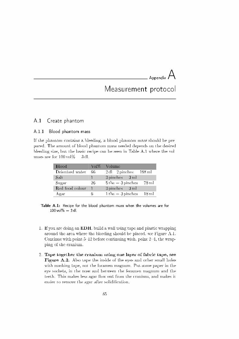
AppendixA
Measurement protocol
A.1 Create phantom
A.1.1 Blood phantom mass
If the phantom contains a bleeding, a blood phantom mass should be pre-pared. The amount of blood phantom mass needed depends on the desiredbleeding size, but the basic recipe can be seen in Table A.1 where the vol-umes are for 100 vol% = 3dl.
Blood Vol% VolumeDeionised water 66 2 dl - 2 pinches = 198mlSalt 1 3 pinches = 3mlSugar 26 5 tbs + 3pinches = 78mlRed food colour 1 3 pinches = 3mlAgar 6 1 tbs + 3 pinches = 18ml
Table A.1: Recipe for the blood phantom mass when the volumes are for100 vol% = 3 dl.
1. If you are doing an EDH, build a wall using tape and plastic wrappingaround the area where the bleeding should be placed, see Figure A.1.Continue with point 512 before continuing with, point 24, the wrap-ping of the cranium.
2. Tape together the cranium using one layer of fabric tape, seeFigure A.2. Also tape the inside of the eyes and other small holeswith masking tape, not the foramen magnum. Put some paper in theeye sockets, in the nose and between the foramen magnum and theteeth. This makes less agar ow out from the cranium, and makes iteasier to remove the agar after solidication.
85
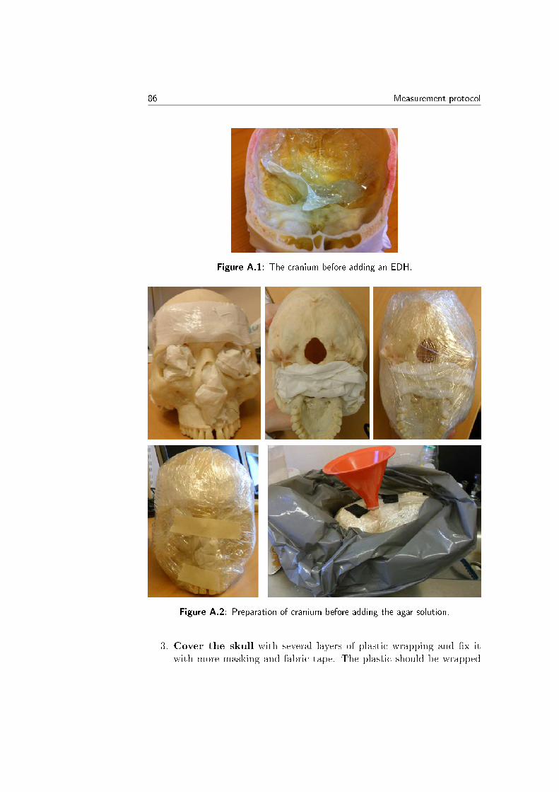
86 Measurement protocol
Figure A.1: The cranium before adding an EDH.
Figure A.2: Preparation of cranium before adding the agar solution.
3. Cover the skull with several layers of plastic wrapping and x itwith more masking and fabric tape. The plastic should be wrapped
Measurement protocol 87
several times around the skull in dierent angles so nothing can comeout, see Figure A.2.
4. Put the plastic-wrapped cranium in a plastic bag in a bowl. Thiswill make it easier to make a water-bath with the water close to thehead, see Figure A.2.
5. Mix sugar, salt, food colour and deionised water in a pot.Mix the salt in a small amount of deionised water rst (otherwise itmay not dissolve completely). Add sugar, food colour and the rest ofthe water, let the sugar dissolve completely in the water, this can bedone by heating the liquid. Avoid air-bubbles!
6. Remove 6 cl of the water-sugar-salt-colour mixture and put it in twoshot glasses and measure the dielectric properties. Put the glassesin the refrigerator if it is not possible to measure the dielectric prop-erties immediately. Mark the glasses with name and date and coverit with plastic wrapping.
7. Add the agar. Since 6 cl have been removed the new agar amountwhere the volumes are for 100 vol% = 3dl is 13.5ml (2 tsp + 3.5 pinches)!This volume is calculated from the fact that the total solution volumeis not 3 dl, but around 2.4 dl (since sugar is dissolved). Stir the mix-ture and avoid air-bubbles!
8. Heat the liquid to 70 C, keep the temperature between 70-80 Cfor ve minutes, otherwise it will not solidify properly [9].
9. Let the agar mass rest for 5-10minutes until it starts to thicken,evaluate the consistency by eye.
10. Connect the syringe with the tube.
11. Suck up the blood phantom mass with the syringe, try to avoid airbubbles and boiling due to suppression. Remove air bubbles by turn-ing the syringe upside down and push the air out.
12. If you are doing an EDH, ll the shielded area with the desiredamount of blood mass, let it solidify and remove the wall. Continuewith point 24 and afterwards with 1416.
13. If you are doing an SDH, place the cranium in the plastic bowl at anangle and place the bleeding at the side of the head using the tube,make sure the bleeding stays on one side of the midline.
14. Clean the syringe and tube immediately to avoid clogging.
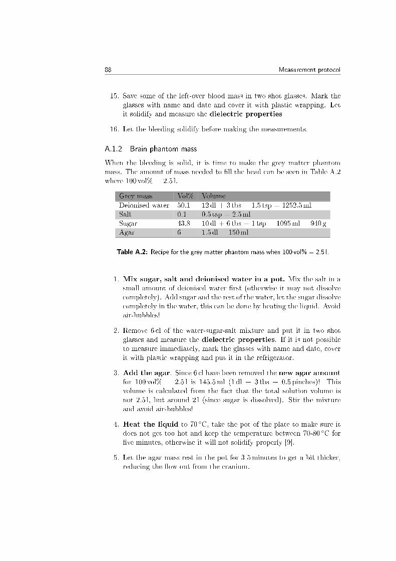
88 Measurement protocol
15. Save some of the left-over blood mass in two shot glasses. Mark theglasses with name and date and cover it with plastic wrapping. Letit solidify and measure the dielectric properties
16. Let the bleeding solidify before making the measurements.
A.1.2 Brain phantom mass
When the bleeding is solid, it is time to make the grey matter phantommass. The amount of mass needed to ll the head can be seen in Table A.2where 100 vol% = 2.5 l.
Grey mass Vol% VolumeDeionised water 50.1 12 dl + 3 tbs + 1.5 tsp = 1252.5mlSalt 0.1 0.5 tsp = 2.5mlSugar 43.8 10 dl + 6 tbs + 1 tsp = 1095ml = 940 gAgar 6 1.5 dl = 150ml
Table A.2: Recipe for the grey matter phantom mass when 100 vol% = 2.5 l.
1. Mix sugar, salt and deionised water in a pot. Mix the salt in asmall amount of deionised water rst (otherwise it may not dissolvecompletely). Add sugar and the rest of the water, let the sugar dissolvecompletely in the water, this can be done by heating the liquid. Avoidair-bubbles!
2. Remove 6 cl of the water-sugar-salt mixture and put it in two shotglasses and measure the dielectric properties. If it is not possibleto measure immediately, mark the glasses with name and date, coverit with plastic wrapping and put it in the refrigerator.
3. Add the agar. Since 6 cl have been removed the new agar amountfor 100 vol% = 2.5 l is 145.5ml (1 dl + 3 tbs + 0.5 pinches)! Thisvolume is calculated from the fact that the total solution volume isnot 2.5 l, but around 2 l (since sugar is dissolved). Stir the mixtureand avoid air-bubbles!
4. Heat the liquid to 70 C, take the pot of the plate to make sure itdoes not get too hot and keep the temperature between 70-80 C forve minutes, otherwise it will not solidify properly [9].
5. Let the agar mass rest in the pot for 3-5minutes to get a bit thicker,reducing the ow out from the cranium.

Measurement protocol 89
6. Fill the head with the agar mass through the foramen magnum,using a funnel. Be careful not to destroy any bleeding, don't turn thecranium back up until it is partly lled. Make sure the cranium isproperly lled and add some extra solution if needed.
7. Clean the funnel and other equipment to avoid clogging.
8. Fill the bowl (outside of the plastic bag) with cold water and let themass solidify, change the water from time to time to keep it cold. Thewater will also make the leakage from the phantom smaller.
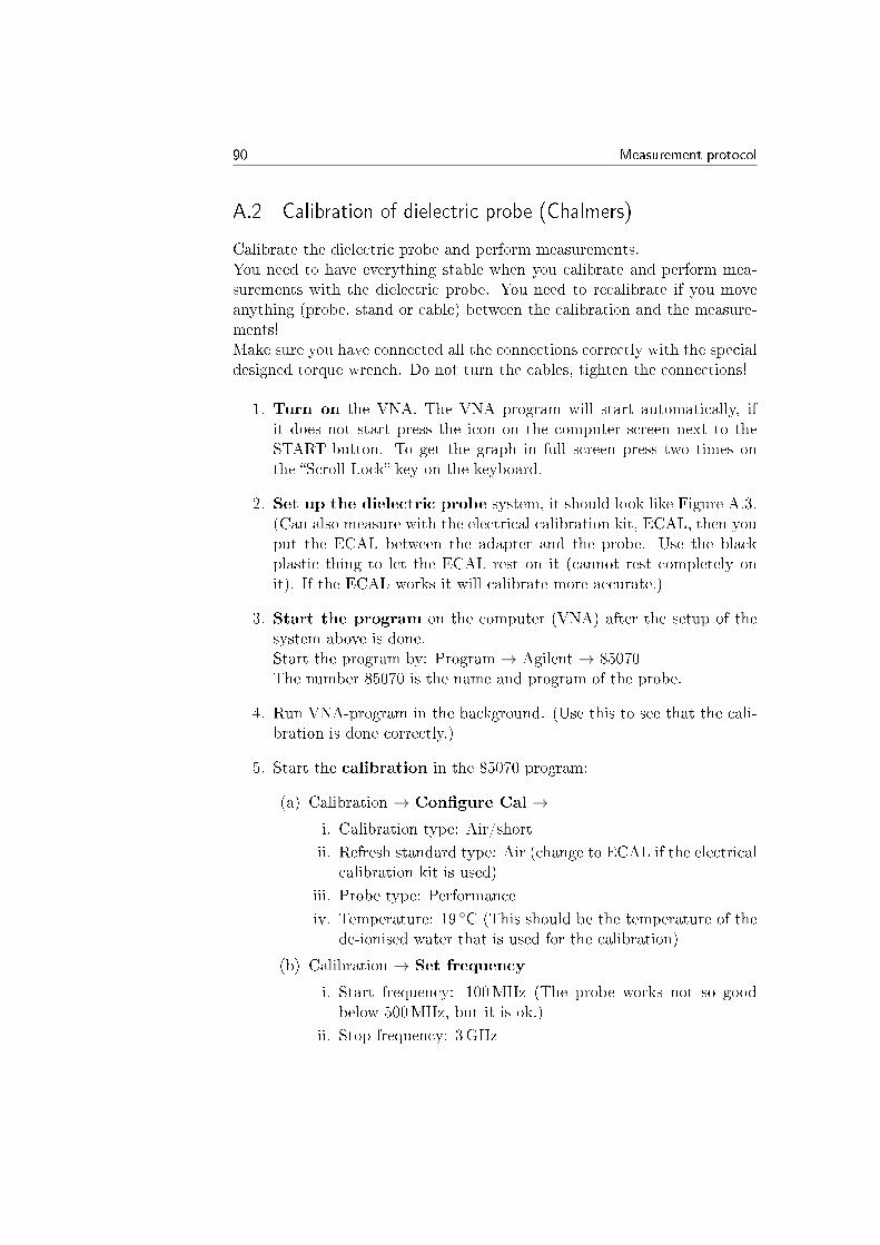
90 Measurement protocol
A.2 Calibration of dielectric probe (Chalmers)
Calibrate the dielectric probe and perform measurements.You need to have everything stable when you calibrate and perform mea-surements with the dielectric probe. You need to recalibrate if you moveanything (probe, stand or cable) between the calibration and the measure-ments!Make sure you have connected all the connections correctly with the specialdesigned torque wrench. Do not turn the cables, tighten the connections!
1. Turn on the VNA. The VNA program will start automatically, ifit does not start press the icon on the computer screen next to theSTART-button. To get the graph in full screen press two times onthe Scroll Lock-key on the keyboard.
2. Set up the dielectric probe system, it should look like Figure A.3.(Can also measure with the electrical calibration kit, ECAL, then youput the ECAL between the adapter and the probe. Use the blackplastic thing to let the ECAL rest on it (cannot rest completely onit). If the ECAL works it will calibrate more accurate.)
3. Start the program on the computer (VNA) after the setup of thesystem above is done.Start the program by: Program → Agilent → 85070The number 85070 is the name and program of the probe.
4. Run VNA-program in the background. (Use this to see that the cali-bration is done correctly.)
5. Start the calibration in the 85070 program:
(a) Calibration → Congure Cal →i. Calibration type: Air/short
ii. Refresh standard type: Air (change to ECAL if the electricalcalibration kit is used)
iii. Probe type: Performance
iv. Temperature: 19 C (This should be the temperature of thede-ionised water that is used for the calibration)
(b) Calibration → Set frequency
i. Start frequency: 100MHz (The probe works not so goodbelow 500MHz, but it is ok.)
ii. Stop frequency: 3GHz
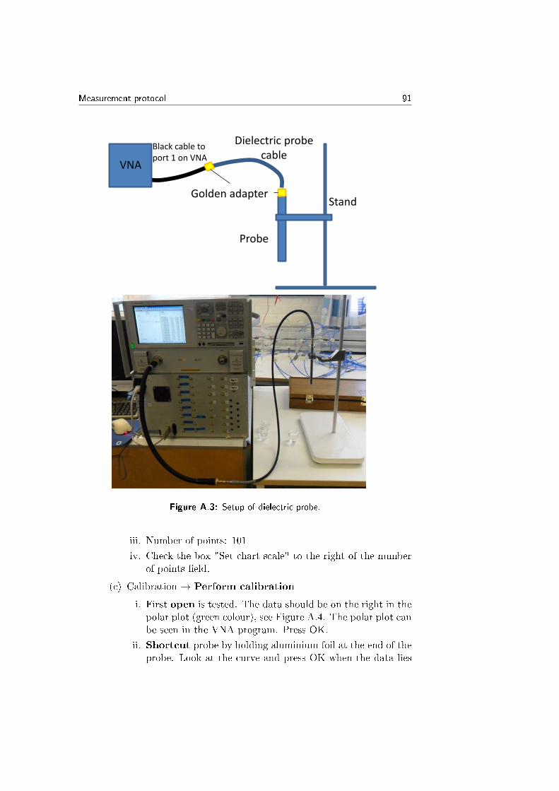
Measurement protocol 91
VNA
Probe
Golden adapter
Dielectric probe cable
Black cable to port 1 on VNA
Stand
Figure A.3: Setup of dielectric probe.
iii. Number of points: 101
iv. Check the box "Set chart scale" to the right of the numberof points eld.
(c) Calibration → Perform calibration
i. First open is tested. The data should be on the right in thepolar plot (green colour), see Figure A.4. The polar plot canbe seen in the VNA program. Press OK.
ii. Shortcut probe by holding aluminium foil at the end of theprobe. Look at the curve and press OK when the data lies
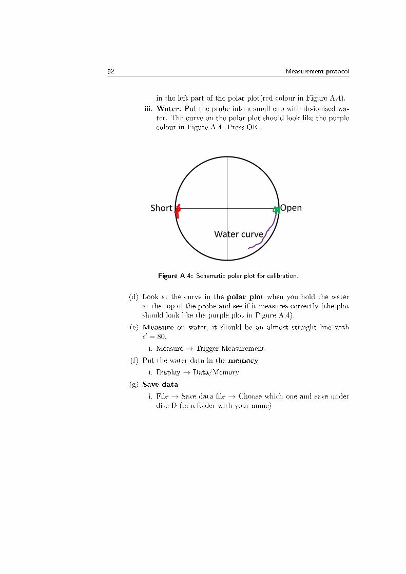
92 Measurement protocol
in the left part of the polar plot(red colour in Figure A.4).
iii. Water: Put the probe into a small cup with de-ionised wa-ter. The curve on the polar plot should look like the purplecolour in Figure A.4. Press OK.
Open Short
Water curve
Figure A.4: Schematic polar plot for calibration.
(d) Look at the curve in the polar plot when you hold the waterat the top of the probe and see if it measures correctly (the plotshould look like the purple plot in Figure A.4).
(e) Measure on water, it should be an almost straight line withε′ = 80.
i. Measure → Trigger Measurement
(f) Put the water data in the memory
i. Display → Data/Memory
(g) Save data
i. File → Save data le → Choose which one and save underdisc D (in a folder with your name)
Measurement protocol 93
A.3 Measure with dielectric probe (Chalmers)
1. To perform measurements use
(a) Measure → trigger measurement
(b) Make sure you save the measurements.
(c) The data can be placed on a USB-stick afterwards. (USB-connectionboth on the front and the back of the VNA)
(d) Make sure you have no bubbles on the probe when you measure.
(e) Measure deionised in between your measurements to see thatit still looks okay. The relative permittivity of the deionised watershould look like a relatively at line at 80 over all the frequencies.Also use this to clean the probe.
(f) Measure liquid phantom solution: Stir the sample beforemeasuring to make sure it is homogeneous. Make two measure-ments per sample (there should be two samples), if they dier,clean the probe, stir the sample and try again.
(g) Measure solid phantom mass: Press the dielectric probe intothe solid phantom mass. If there is a layer of liquid on thetop, remove it with a paper towel. Avoid to get air pockets inbetween the probe and the phantom mass. Press the sample tothe probe and perform 5 measurements per slice (there shouldbe two slices).
2. You will get the permittivity with real and imaginary parts. Theconductivity, σ, can then be calculated from the imaginary part ofthe permittivity, ε′′, see Equation (A.1).
σ = ωε0ε′′ (A.1)
Where ω is the angular frequency and ε0 = 8.854 · 10−12 F/m.
3. Put the measured data on a USB-stick and analyse it in Matlab tosee if it looks good compared to the desired data (the permittivityand conductivity of the real tissue) from Gabriel et al. [22].
4. At the end:
(a) Measure water to see that you still have the same water-curve.
(b) Clean the probe with battery water and paper so it is clean forother to use it afterwards.
94 Measurement protocol
A.4 Calibration of measurement equipment (Medeld Diag-nostics)
How to calibrate VNA with cables to be able to measure with the MWH.
1. Turn on the VNA, the button is at the front left corner, behindthe switch box, wait at least 1 hour before starting to measure. It ispossible to have the VNA turned on for up to a week, but it will gointo sleep-mode if it hasn't been used for a while.
2. Programs that should be started on the computer:
(a) Switch GUI: It is a LabVIEW-le that lies on the desktop. Setthe switches in the Switch GUI so the two cables and correspond-ing ports are connected.
i. Green line = transmitting antenna
ii. Blue line = receiving antenna
(b) NI-VNA: Under the Start-menu, START → NI-VNA (secondon the top in the menu). If it does not start, right click on it andstart as an administrator.
3. Connect all the cables with the ports. Use the special designedtorque wrench, this wrench should be used for all connections every-time they need to be tightened.
4. Load an old calibration le in the NI-VNA so you get the rightsettings. File→ Recal setup→ C→ VNA→ 20110816 (this is a goodle for us to load). You only need to load the le for one connection.
5. Use a through (adapter) to connect the two cables that are goingto be calibrated. It will show in the NI-VNA program when the twocables are connected. If the transmission S21 lies on 0 dB it meansthat it is correctly connected in the Switch GUI. (You do not need totake away the through yet.)
6. Press on Frequency to the right in the NI-VNA, and see that thecorrect frequencies are set.
7. Change Power on the top left to 0 dB. (Medeld Diagnostics havepermission to use 0 dBm (1mW)).
8. Perform calibration in the NI-VNA with the calibration kit, seeFigure A.5.
Calibration → Calibrate → Manual cal → choose 1 path → 2 port.
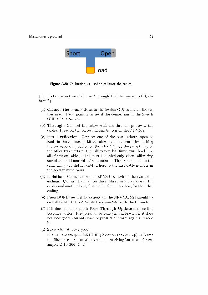
Measurement protocol 95
Short Open
Load
Figure A.5: Calibration kit used to calibrate the cables.
(If reection is not needed: use Through Update instead of Cali-brate.)
(a) Change the connections in the Switch GUI to match the ca-bles used. Redo point 5 to see if the connection in the SwitchGUI is done correct.
(b) Through: Connect the cables with the through, put away thecables. Press on the corresponding button on the NI-VNA.
(c) Port 1 reection: Connect one of the parts (short, open orload) in the calibration kit to cable 1 and calibrate (by pushingthe corresponding button on the NI-VNA), do the same thing forthe other two parts in the calibration kit, nish with load. Doall of this on cable 1. This part is needed only when calibratingone of the bold marked pairs in point 9. Then you should do thesame thing you did for cable 1 here to the rst cable number inthe bold marked pairs.
(d) Isolation: Connect one load of 50Ω to each of the two cableendings. Can use the load on the calibration kit for one of thecables and another load, that can be found in a box, for the otherending.
(e) Press DONE, see if it looks good on the NI-VNA. S21 should beon 0 dB when the two cables are connected with the through.
(f) If it does not look good: Press Through Update and see if itbecomes better. It is possible to redo the calibration if it doesnot look good, you only have to press Calibrate again and redoit.
(g) Save when it looks good:
File→ Save setup→ EXJOBB (folder on the desktop)→ Namethe le: date_transmittingAntenna_receivingAntenna. For ex-ample: 20130204_1_2
96 Measurement protocol
9. Calibrate the rest of the cables: Redo step 8 for all the cablecombinations; 12, 13, 14, ..., 23, 24, 25, ..., 34, 35, 36, ...121, the last one is to get the reection for cable 12. The reectionpart needs to be calibrated for the bold marked pairs, but not theother pairs since they use the reection value from the bold pairs. Tocalibrate the non-bold pairs, Through Update is used instead ofCalibrate.
(a) Switch connections in the Switch GUI and connect the cableswith the through.
(b) Do the through update in the NI-VNA, press done and save thedata as above.
10. If only one cable (x) needs to be calibrated, load the calibrationle (12), do a Throug Update for cable 1x, load the calibration le23, do a Throug Update for 2x and continue to (x-1)x where theentire procedure needs to be done, continue with x(x+1) and theentire procedure again, continue with Through Update for the rest ofthe cables but do not change calibration le.
11. When the calibrations is done: place all the calibration les in afolder marked with today's date, for example: 20130204. The date-folder should be placed in C:\VNA.
Measurement protocol 97
A.5 Preparation for measurements
The things that have to bee done before the measurements can be started.
1. Take away the plastic wrapping and the agar solution that has solid-ied outside the cranium. Try to lift in both cranium parts to avoidthat they fall apart. Take away the tape that isn't needed in the eyesand over the other holes, just leave the tape that keeps the craniumtogether. Wipe o the cranium with a wet cloth before the measure-ment so it isn't so sticky. Do not turn the cranium over, there is arisk that the phantom will loosen from the cranium and air will comein between the cranium and the phantom.
2. If the upper part of the cranium is loose, add some tape around thecranium to keep it together.
3. Put tape over foramen magnum so the water does not evaporate.
4. Fill up the water bags in the MWH with some water (all the bagsneed to have some water in them so they don't stick together). Re-move the air bubbles in the bags (it is not possible to remove all theair from the water bags).
5. Connect the cables to the antennas on the MWH before the craniumis placed in it. It is important which port is connected to whichantenna! Follow Figure A.6. Use the special designed torque wrenchto connect the cables.
(a) Port 3 does not work, so this port needs to be terminated witha 50Ω load.
(b) Antenna 3 can instead be connected to port 12. The data fromport 12 is normally not used since the connection between theantennas in the neck and the cranium are so bad.
(c) Cable 8 needs to be terminated with a 50Ω load, since antenna8 is one of the neck antennas that have bad connection with thecranium.
6. Carefully place the cranium in the MWH.
7. Hang the MWH on a metal rod between two chairs and place abucket with water under it, see Figure A.7. The cables have to laystill and not be stretched. It is possible to touch and move the cablesafter the calibration is done.
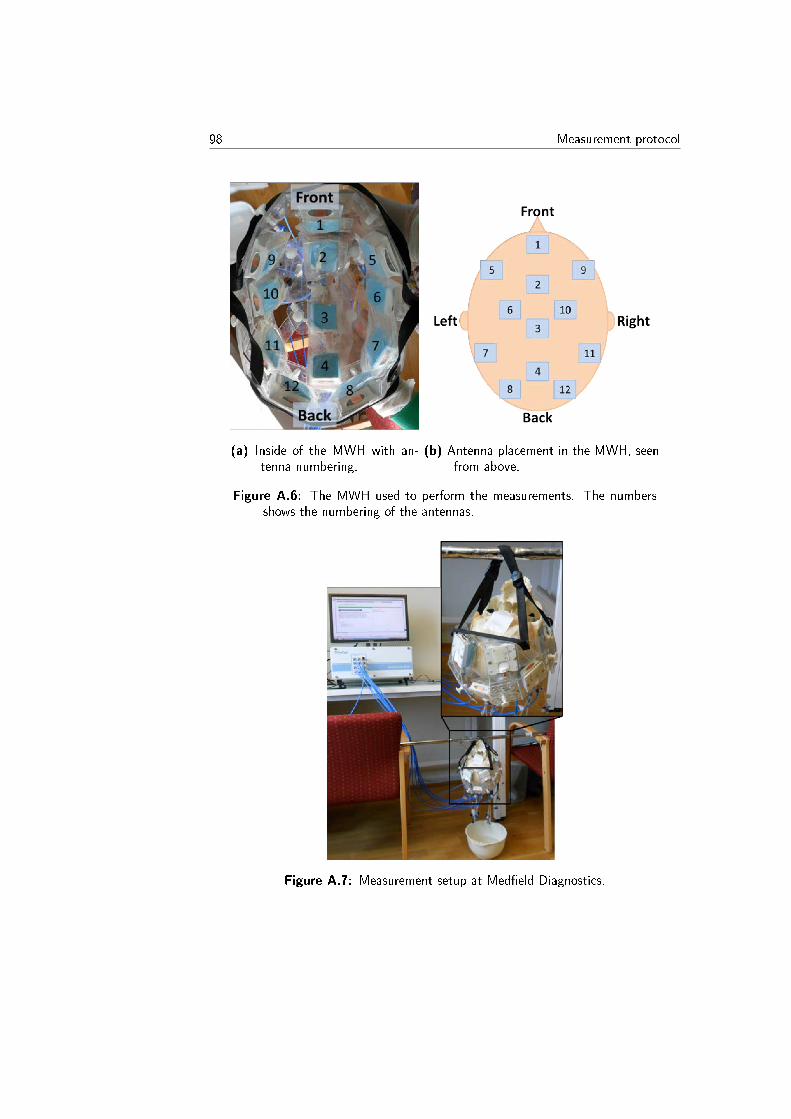
98 Measurement protocol
(a) Inside of the MWH with an-tenna numbering.
(b) Antenna placement in the MWH, seenfrom above.
Figure A.6: The MWH used to perform the measurements. The numbersshows the numbering of the antennas.
Figure A.7: Measurement setup at Medeld Diagnostics.

Measurement protocol 99
8. Fill up the water bags with water. All the bags should have ap-proximately equal size and the cranium should lie stable in the MWH.Make sure that all the taps on the water bags are shut.
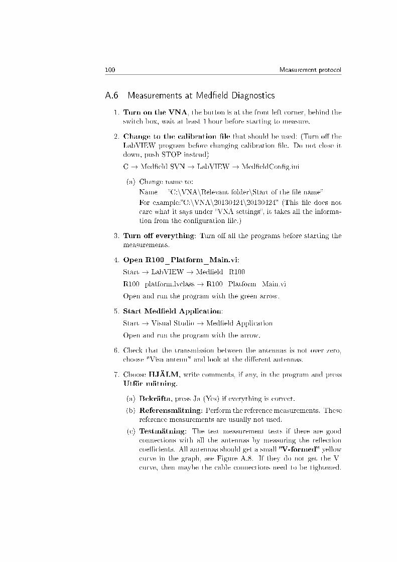
100 Measurement protocol
A.6 Measurements at Medeld Diagnostics
1. Turn on the VNA, the button is at the front left corner, behind theswitch box, wait at least 1 hour before starting to measure.
2. Change to the calibration le that should be used: (Turn o theLabVIEW program before changing calibration le. Do not close itdown, push STOP instead)
C → Medeld SVN → LabVIEW → MedeldCong.ini
(a) Change name to:
Name = C:\VNA\Relevant folder\Start of the le name
For example:C:\VNA\20130424\20130424 (This le does notcare what it says under VNA settings, it takes all the informa-tion from the conguration le.)
3. Turn o everything: Turn o all the programs before starting themeasurements.
4. Open R100_Platform_Main.vi:
Start → LabVIEW → Medeld_R100
R100_platform.lvclass → R100_Platform_Main.vi
Open and run the program with the green arrow.
5. Start Medeld Application:
Start → Visual Studio → Medeld Application
Open and run the program with the arrow.
6. Check that the transmission between the antennas is not over zero,choose "Visa antenn" and look at the dierent antennas.
7. Choose HJÄLM, write comments, if any, in the program and pressUtför mätning.
(a) Bekräfta, press Ja (Yes) if everything is correct.
(b) Referensmätning: Perform the reference measurements. Thesereference measurements are usually not used.
(c) Testmätning: The test measurement tests if there are goodconnections with all the antennas by measuring the reectioncoecients. All antennas should get a small V-formed yellowcurve in the graph, see Figure A.8. If they do not get the V-curve, then maybe the cable connections need to be tightened.
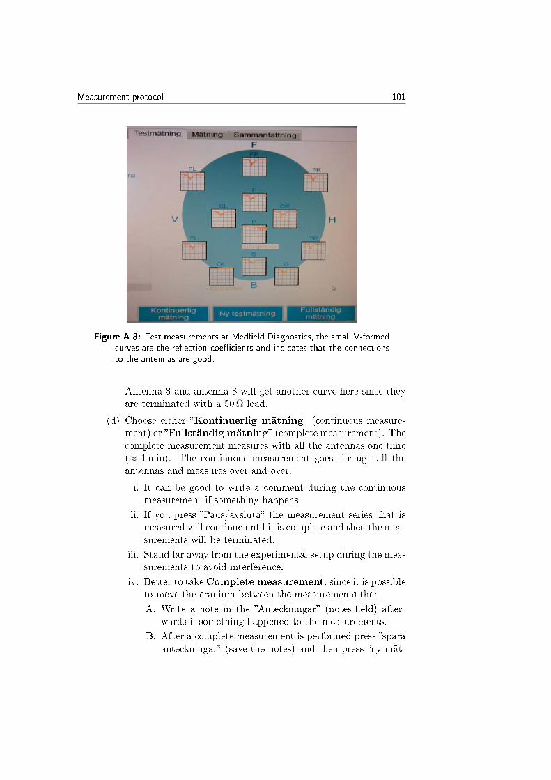
Measurement protocol 101
Figure A.8: Test measurements at Medeld Diagnostics, the small V-formedcurves are the reection coecients and indicates that the connectionsto the antennas are good.
Antenna 3 and antenna 8 will get another curve here since theyare terminated with a 50Ω load.
(d) Choose either Kontinuerlig mätning (continuous measure-ment) or Fullständig mätning (complete measurement). Thecomplete measurement measures with all the antennas one time(≈ 1min). The continuous measurement goes through all theantennas and measures over and over.
i. It can be good to write a comment during the continuousmeasurement if something happens.
ii. If you press Paus/avsluta the measurement series that ismeasured will continue until it is complete and then the mea-surements will be terminated.
iii. Stand far away from the experimental setup during the mea-surements to avoid interference.
iv. Better to takeComplete measurement, since it is possibleto move the cranium between the measurements then.
A. Write a note in the Anteckningar (notes-eld) after-wards if something happened to the measurements.
B. After a complete measurement is performed press sparaanteckningar (save the notes) and then press ny mät-
102 Measurement protocol
ning (new measurement).
C. Check out how the graphs for the antennas look. Writedown if something looks weird.
8. End the measurements:
Avsluta→ Spara Anteckningar→ Avsluta mätande→ Spara resultat
There is a short cut (2013-Shortcut) on the desktop to where the lesare saved. The data is saved in a le with the date.
9. Open one of the les in Notepad and check if all values are below one.
10. Do all the measurements, see section A.6.1.
11. Put all the data on a USB-stick. There is a USB-port on the key-board.
12. Turn o the VNA in the same way as a normal computer.
13. Analyse the data in Matlab and see if it looks good.
A.6.1 Perform measurements
1. Do the following measurements on every phantom:
(a) Ordinary measurement: 3 x 10 measurements (lift the cra-nium a few cm from the MWH and put it back again betweenevery 3 measurements).
(b) Hair measurements: 3 x 10 measurements (lift the cranium afew cm from the MWH and put it back again between every 3measurements). Take the cranium from the MWH and put thewig on it and put it back into the MWH, see Figure A.10.
(c) Interference of persons: total 90 measurement, randomised.Write a note in the note eld for every measurement that sayswhich type of measurement it is (close, touching or reference).Write a note in the measurement notes document in what orderthe measurements come.
i. Person close: 30 measurements (measure when a personstands close to the setup), see Figure A.9a.
ii. Holding the cables: 30 measurements (measure when aperson grips the cables 10 cm from the switch box), see Fig-ure A.9b.
iii. Reference: 30 measurements (measure when all personsstand >1 m from the setup).
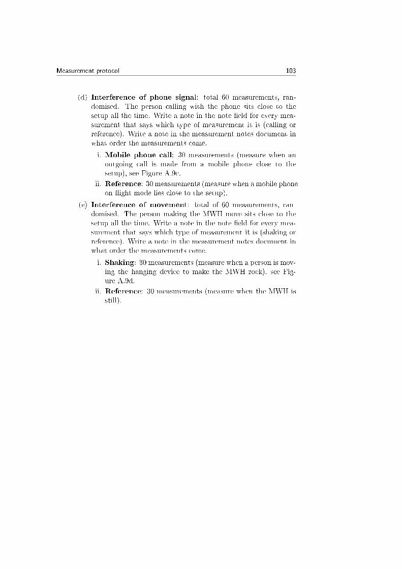
Measurement protocol 103
(d) Interference of phone signal: total 60 measurements, ran-domised. The person calling with the phone sits close to thesetup all the time. Write a note in the note eld for every mea-surement that says which type of measurement it is (calling orreference). Write a note in the measurement notes document inwhat order the measurements come.
i. Mobile phone call: 30 measurements (measure when anoutgoing call is made from a mobile phone close to thesetup), see Figure A.9c.
ii. Reference: 30 measurements (measure when a mobile phoneon ight mode lies close to the setup).
(e) Interference of movement: total of 60 measurements, ran-domised. The person making the MWH move sits close to thesetup all the time. Write a note in the note eld for every mea-surement that says which type of measurement it is (shaking orreference). Write a note in the measurement notes document inwhat order the measurements come.
i. Shaking: 30 measurements (measure when a person is mov-ing the hanging device to make the MWH rock), see Fig-ure A.9d.
ii. Reference: 30 measurements (measure when the MWH isstill).
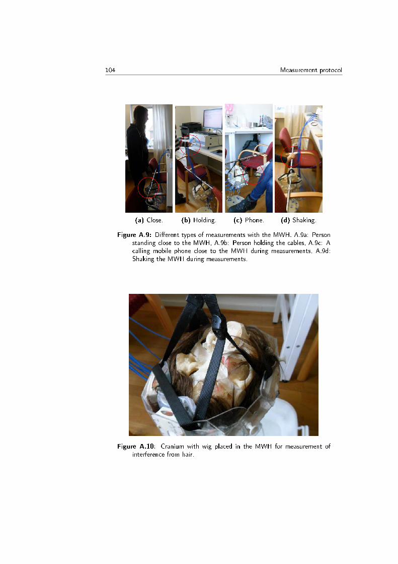
104 Measurement protocol
(a) Close. (b) Holding. (c) Phone. (d) Shaking.
Figure A.9: Dierent types of measurements with the MWH. A.9a: Personstanding close to the MWH, A.9b: Person holding the cables, A.9c: Acalling mobile phone close to the MWH during measurements, A.9d:Shaking the MWH during measurements.
Figure A.10: Cranium with wig placed in the MWH for measurement ofinterference from hair.
Measurement protocol 105
A.7 After measurements
1. Empty the waterbags in the MWH and remove the cranium.
2. Remove the tape and wipe the skull with some wet paper if it is sticky.
3. Remove the upper part of the skull.
4. Take photos of the phantom together with a ruler and a note with thedate and bleeding volume/type.
5. Turn the skull upside down and shake until the phantom falls out,take some more photos.
6. Slice the phantom into 1-2 cm thick slices, make two thicker (>2 cm)slices, one from the front and one from the back of the phantom,without any bleeding. Wrap it carefully in plastic wrapping and markwith date and bleeding type. Save for dielectric measurements.
7. Check the phantom for air bubbles.
8. Take some more pictures of the slices where the shape of the bleedingcan be seen. Take the pictures of the phantom together with a rulerand a note with the date and bleeding volume/type.

106 Measurement protocol
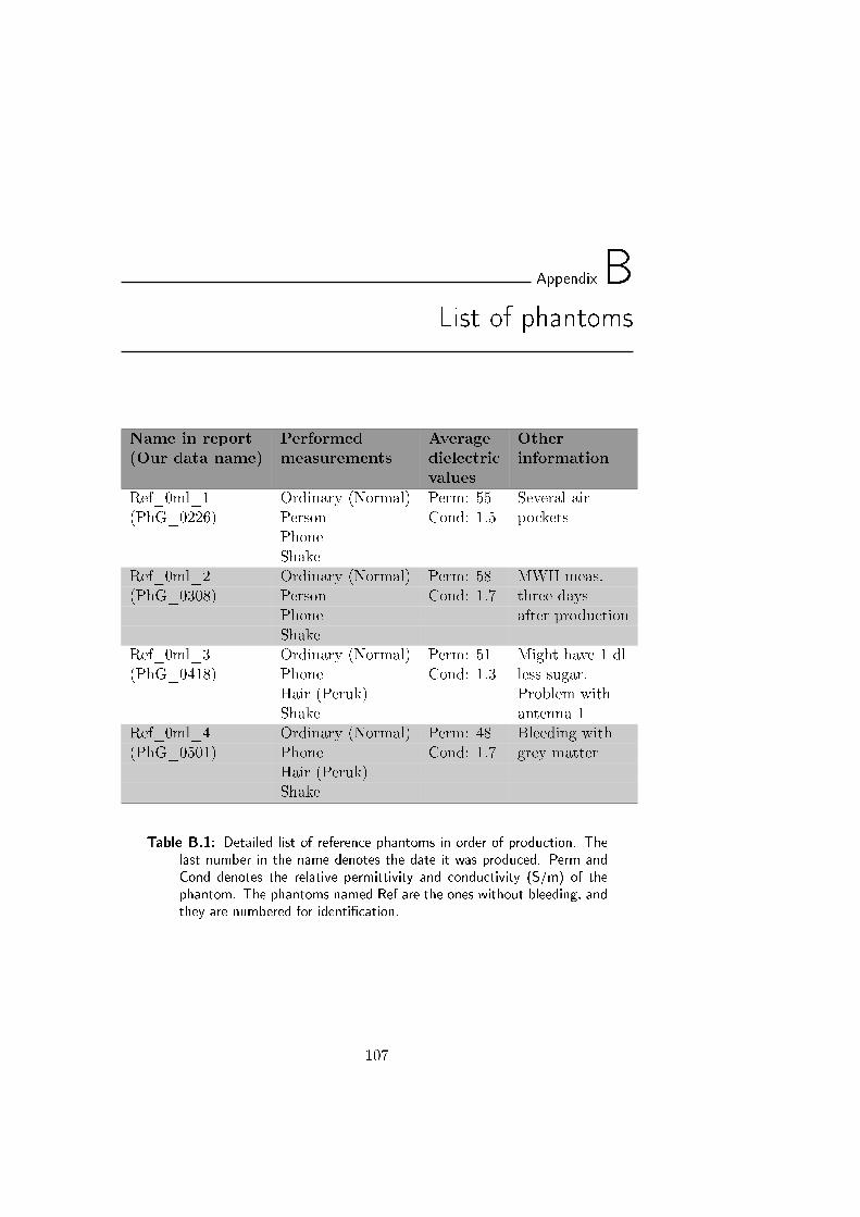
AppendixBList of phantoms
Name in report Performed Average Other(Our data name) measurements dielectric information
valuesRef_0ml_1 Ordinary (Normal) Perm: 55 Several air(PhG_0226) Person Cond: 1.5 pockets
PhoneShake
Ref_0ml_2 Ordinary (Normal) Perm: 58 MWH meas.(PhG_0308) Person Cond: 1.7 three days
Phone after productionShake
Ref_0ml_3 Ordinary (Normal) Perm: 51 Might have 1 dl(PhG_0418) Phone Cond: 1.3 less sugar.
Hair (Peruk) Problem withShake antenna 1
Ref_0ml_4 Ordinary (Normal) Perm: 48 Bleeding with(PhG_0501) Phone Cond: 1.7 grey matter
Hair (Peruk)Shake
Table B.1: Detailed list of reference phantoms in order of production. Thelast number in the name denotes the date it was produced. Perm andCond denotes the relative permittivity and conductivity (S/m) of thephantom. The phantoms named Ref are the ones without bleeding, andthey are numbered for identication.
107
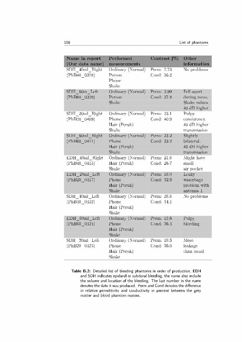
108 List of phantoms
Name in report Performed Contrast [%] Other(Our data name) measurements informationSDH_40ml_Right Ordinary (Normal) Perm: 7.73 No problems(PhB40_0318) Person Cond: 36.2
PhoneShake
SDH_60m_Left Ordinary (Normal) Perm: 3.99 Fell apart(PhB60_0320) Person Cond: 37.8 during meas.
Shake Shake values40 dB higher
SDH_20ml_Right Ordinary (Normal) Perm: 23.1 Pulpy(PhB20_0409) Phone Cond: 40.9 consistency.
Hair (Peruk) 40 dB higherShake transmission
SDH_60ml_Right Ordinary (Normal) Perm: 23.2 Slightly(PhB60_0411) Phone Cond: 33.2 bilateral.
Hair (Peruk) 40 dB higherShake transmission
EDH_40ml_Right Ordinary (Normal) Perm: 21.8 Might have(PhB40_0415) Hair (Peruk) Cond: 26.7 small
Shake air pocketEDH_20ml_Left Ordinary (Normal) Perm: 10.0 Leaky(PhB20_0417) Phone Cond: 32.9 waterbags
Hair (Peruk) problem withShake antenna 1
SDH_40ml_Left Ordinary (Normal) Perm: 20.8 No problems(PhB40_0422) Phone Cond: 34.1
Hair (Peruk)Shake
EDH_60ml_Left Ordinary (Normal) Perm: 12.6 Pulpy(PhB60_0424) Phone Cond: 36.4 bleeding
Hair (Peruk)Shake
SDH_20ml_Left Ordinary (Normal) Perm: 10.3 More(PhB20_0425) Phone Cond: 36.0 leakage
Hair (Peruk) than usualShake
Table B.2: Detailed list of bleeding phantoms in order of production, EDHand SDH indicates epidural or subdural bleeding, the name also includethe volume and location of the bleeding. The last number in the namedenotes the date it was produced. Perm and Cond denotes the dierencein relative permittivity and conductivity in percent between the greymatter and blood phantom masses.