Developing predictable and flexible distributed real-time systems

Control Engineering Practice 6 (1998) 67—81

Developing predictable and flexible distributed real-time systems

Juan Manuel Adan-Coello!, Maurıcio F. Magalha8 es", Krithi Ramamritham#,*

! Instituto de Informatica, PUC-Campinas, Campinas, SP-Brazil, [email protected]"DCA/FEEC-ºNICAMP, Campinas, SP-Brazil [email protected]

#Dept. of Comp. Science, ºniv. of Massachusetts, Amherst, MA-ºSA [email protected]

Received 15 September 1997; accepted 11 November 1997

Abstract

Predictability is considered the most distinguishing characteristic of real-time systems. Besides that, adaptability is also a veryimportant attribute because RT systems are usually designed for long life cycles, during which they will have to cope with change. Thispaper presents the STER real-time software development environment, designed to support the production of predictable, and yetflexible, distributed real-time systems. Flexibility is one of the main concerns of STER’s programming model, based on theconstruction of reusable software modules. Modules can be reused with different timing constraints without having to be recoded,since the specification of their timing constraints is decoupled from their implementation. Predictable temporal behavior isobtained by an integrated allocation and scheduling strategy that involves off-line and online schedulers. The off-line scheduler triesto satisfy timing, precedence and allocation constraints of periodic hard real-time tasks, and to give the necessary leeway for thedynamic scheduling of aperiodic tasks. The paper shows how distributed programs are translated to scheduling graphs, and givesthe results of some experiments conducted to evaluate the performance of the off-line algorithm. ( 1998 Elsevier Science ¸td. Allrights reserved.

Keywords: Real-time systems; predictability; configuration language; task graphs; scheduling

1. Introduction

Real-time systems should be predictable in meetingtheir application timing requirements, and easy to adaptto the changes that are likely to occur during theirlifetime (Stankovic, 1988; Le Lann, 1990; Burns and Wel-lings, 1990a). To meet these requirements, a real-timesoftware development environment should integrate flex-ible programming languages that support the specifica-tion of real-time constraints, with scheduling algorithmsthat will determine when, and where, the components ofa program should execute.

Some languages specifically designed to satisfy theneeds of real-time applications, such as Pearl (DIN, 1979)and Ada (DOD, 1980), have been extensively used. Theselanguages are well structured and, with adequate envir-onmental support, cope with most of the problems facedin the development of large-scale systems. However, in

*Corresponding author. E-mail: [email protected].

spite of being specifically designed for programming em-bedded real-time systems, they do not adequatelysupport the specification of the applications’ timingrequirements and, as a consequence, they do not producepredictable systems (Halang and Stoyenko, 1990; Burnsand Wellings, 1990b).

To address the lack of support for predictability ob-served in commercial real-time languages, some researchlanguages have been proposed. Real-time Euclid (Klin-german and Stoyenko, 1986), for example, permits usersto specify the timing requirements of a program, andanalyze it to check if the specified requirements can bemet. Real-time Euclid, however, does not offer adequatesupport for aperiodic tasks, nor for the distribution ofprograms.

Other research languages, like Flex (Kenny and Lin,1991), Real-Time Concurrent C (Gehani and Rama-mritham, 1991), and RTC##(Ishikawa et al., 1992)also permit one to specify programs’ timing constraints,but, in various degrees, have a limited capacity toguarantee that hard real-time constraints will be metunder all circumstances, or provide insufficient support

0967-0661/98/$19.00 ( 1998 Elsevier Science Ltd. All rights reservedPII S 0 9 6 7 - 0 6 6 1 ( 9 7 ) 1 0 0 4 8 - X

for component reuse, distribution, or the specification ofprecedence relations.

Flex provides tools to try to achieve statistical confi-dence in the program’s performance, based on experi-ments, but, as pointed out by Niehaus (1994) it is notclear ‘‘... how to choose testing data that will produceworst case, or at least representative behavior’’. Real-Time Concurrent C is implemented under the Unix sys-tem, which limits the timing guarantees that can beprovided. RTC##extends the C##language anduses the rate monotonic schedulability analysis (Liu andLayland, 1973) and the priority inheritance protocols(Sha et al., 1990) to try to guarantee programs’ timingbehavior. The language construct bound permits theworst-case execution time of object’s functions to beasserted, but it is not clear how to precisely determine it.The schedulability analysis assumes that all methodscalling sequences to objects can be determined statis-tically but, again, it is not clear if that is enough toguarantee hard real-time constraints.

In these languages, component reuse would not be aneasy task because the specification of timing constraintsis mixed in with the remaining program code. This makesit difficult to reuse a module whose functionality isneeded in different applications, but with different timing(periodicity/aperiodicity, deadlines) and precedenceconstraints.

As mentioned above, besides specifying the programtiming constraints, it is necessary to guarantee that theseconstraints will be met at run-time. This problem is fairlysimple when the corresponding programming model isalso simple. For example, when a program is composedonly of independent periodic tasks, the rate monotonicor the earliest deadline first scheduling algorithms (Liuand Layland, 1973) can be successfully used. As theprogramming model becomes more elaborate, as isnecessitated by more complex applications, schedulingturns into a computationally intractable problem(Blazewicz et al., 1983), that demands the use of heuristicalgorithms.

The application of heuristic algorithms requires themapping of programming model representations toscheduling algorithm representations, usually some kindof directed graph. Niehaus (1991), for example, developeda method of translating program representations usingprocesses to a run-time representation using groups ofnonpreemptable tasks to represent a process. Thismethod is part of a broad effort to provide a program-ming environment for hard real-time systems (Niehaus,1994), developed as part of the Spring Project (Stankovicand Ramamritham, 1991).

The objective of this paper is to present the STERreal-time software development environment, which sup-ports the production of predictable, and yet flexible,distributed real-time systems. Predictable temporal be-havior is obtained by the integration of programming

language constructs that specify applications’ timing,precedence and resource requirements with an allocationand scheduling strategy that tries to satisfy these require-ments. Flexibility is obtained by a programming modelcentered on the construction of reusable softwaremodules.

The paper is structured as follows. Section 2 outlinesSTER’s programming model and languages, focusing onthe aspects that are more relevant to the programming ofdistributed predictable systems. Section 3 discusses theallocation and scheduling strategy that tries to meetapplications’ timing and resource requirements, focusingon the mapping of programs to scheduling graphs, andon the off-line algorithm that uses this representation toallocate and schedule programs. Section 4 discusses someexperiments that were conducted to evaluate the perfor-mance of the scheduling algorithm. Finally, in Section 5,some concluding remarks are made.

2. STER’s programming model

In order to offer the flexibility required to adapt a sys-tem to changes, STER’s programming model supportsthe construction of applications using reusable com-ponents (Adan and Magalha8 es, 1992a, 1992b), that is,software modules that can be employed in differentapplications, running on different hardware architectures(centralized or distributed), with different timingconstraints.

STER’s programming model clearly divides the con-struction of an application into two integrated steps: 1)the development of reusable objects, called modules, and2) the configuration of distributed applications usingavailable modules. This modular approach simplifies thereconfiguration of programs when necessary to adapt tothe changing needs of applications, due to changing func-tional or performance requirements, expansions or hard-ware modifications, or for fault tolerance.

The development of software modules and the config-uration of application programs in STER is done by theModules Programming Language (MPL) and the Mod-ules Configuration Language (MCL), respectively. Atprogram configuration time, modules’ communicationports are linked to establish communication channelsand implicitly define precedence relations, and the mod-ules’ timing and allocation constraints are defined. Bothlanguages will be introduced in this section by informallydiscussing some pieces of code. A comprehensive descrip-tion of both languages’ syntax and semantics can befound in (Adan-Coello, 1993).

2.1. Maximum execution times of modules

To search for a schedule that meets timing constraints,it is not only necessary to know the modules’ constraints,

68 J.M. Ada& n-Coello et al./Control Engineering Practice 6 (1998) 67—81

but also their maximum execution times. This impliesthat language constructs and mechanisms that are typi-cally non-deterministic, such as iterative commands, dy-namic memory allocation and recursive calls, should notbe allowed, or should be supported with some restric-tions that permit their maximum execution times to becomputed (off-line). For this reason, in STER, real-timemodules cannot be recursive, nor request dynamic mem-ory allocation. Iterations can only be done using thebounded commands LOOP, WHILE, REPEAT andFOR, with a clause AFTER specifying the maximumnumber of permitted iterations. For example, the follow-ing WHILE command,

...WHILE (SexpressionT) DO

c1;AFTER 10 TIMES

Nc2;END;

c3;...

specifies that procedure c1 may not be executed morethan 10 times. After this number of iterations, if Sexpres-sionT is still evaluated true, procedure c2 will be executedand the execution of the module will continue with thenext statement after the WHILE; in this example, in theline where procedure c3 is called.

2.2. Module cooperation

Modules can cooperate by direct or indirect interac-tion. Direct interaction occurs when modules explicitlyexchange messages. These messages can carry data fromthe sending module to the destination module, establisha precedence relation (enabling messages) of the sendingmodule over the destination module, or accomplish bothfunctions. Indirect interaction occurs when modulesshare a resource, using the services of special modulescalled servers.

A client-server interaction consists of the sending ofa request message from a client module to a servermodule, followed by a response message, sent back fromthe server to the client.

Servers are executed in mutual exclusion. A server willnot accept new service requests while working on a pre-viously accepted request. This guarantees the exclusiveaccess of only one client at a time to the resourcemanaged by the server.

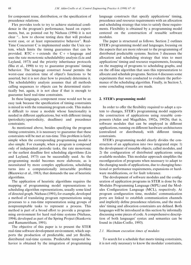
Fig. 1 shows the definition of a server module named S.The identifiers TRReq, TRRep and TWReq are definedin the definition unit DefUnitA. Definition units containdefinitions of constants, types, procedures and functionsshared by several modules. As modules are compiledindependently, this avoids the redundancy of common

Fig. 1. A server module.

definitions, and enables the implementation of the auto-matic control of versions, allowing, for example, auto-matic recompiling of all modules that share an entitywhose definition has been modified.

Server S has two bi-directional entry ports, ReadP andWriteP, defined in the clause entryport. The server willuse ReadP to receive service request messages of typeTRReq, and to reply with messages of type TRRep. In thesame way, through WriteP, the server will receive mess-age requests of type TWReq, and reply with messages ofthe predefined type signal. Messages of type signal carryno data; they are used to signfy the occurrence of a pre-defined event, in the current example the completion ofa write operation. The clause enabled—by any specifiesthat module S will be enabled to execute when a messageis received either at port ReadP or at port WriteP. Thearrival of an enabling message is a necessary but notsufficient condition to make the module ready for execu-tion. This will also depend on decisions taken by thesystem scheduler, aimed at meeting the timing con-straints of client modules, as will be discussed later in thissection and in Section 3.

The clause message, in Fig. 1, is used to declare themessages employed by server S to communicate with itsclients. The main difference between a message anda normal variable is that the former can be sent throughcommunication ports, and the latter cannot.

The body of server S consists of a prioritized selectcommand (pselect). A select command may have several

J.M. Ada& n-Coello et al./Control Engineering Practice 6 (1998) 67—81 69

parts, but at run-time only one of them will be chosenfor execution. In the example, the select statement inserver S has two parts. If the first is executed, MReadReqis received from port ReadP, some action (representedby ‘‘...’’) is performed and message MReadRep is repliedto the module that originated the message MReadReq.The second part is similar to the first, and is related tothe reception of message MWriteReq and the transmis-sion of Msignal through port WriteP. When the pselectis executed, the server will be blocked until a messagearrives at one of its enabling ports, unless thereare already messages available at those ports. If thereare messages queued in only one port, the message atthe head of the port queue is read, the actions specifiedin the corresponding receive clause are executed, anda reply message is sent to the client that originatedthat message. If there are messages in both ports, pselectwill give priority to the port in its first clause, in thiscase associated with port ReadP. A pselect can includemore than two parts; in that case, parts will have de-scending priorities. A server could also use a randomselect command (rselect), which does not give priority toany part.

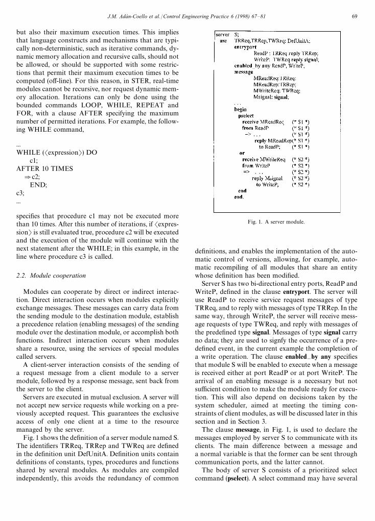
Sometimes a client might require the server to executeseveral services in mutual exclusion. A typical example isa read-modify-update transaction on a database. To copewith these situations, a client module can request exclus-ive access to the server for a given sequence of services,using the lock command. Fig. 2 shows an example ofa module, named B, which performs a lock. After themessage MReadReq (sent inside the lock) is delivered, thedestination server will only accept request messages sentby module B, until the lock is released (by the delivery ofthe message MWriteReq).

A lock command always starts with a send statement.The message that is sent by this statement carries a flagthat signals to the server (and to the scheduler) that thelock is being closed. In the same way, a lock always endswith a message sent to signal that the lock is beingreleased. Between the messages that close and open thelock, asynchronous and synchronous messages can besent by the module that requested the lock to severalserver modules, but only the server connected to the portaddressed by the locking message is accessed in mutualexclusion. Nested transactions are disallowed. It is notpossible to embed one lock inside another. As will bediscussed in Section 3, the system scheduler will ensurethat a locked server will only receive requests from theclient that closed the lock.

2.3. Timing and precedence exception handling

STER’s run-time support can handle three types ofexceptions related to the scheduling of modules: 1) en-abling message fault, 2) non-guaranteed module and 3)missed deadline. An ‘‘enabling message fault’’ exception

Fig. 2. A client performing a lock.

is raised if at a module’s scheduled start time its enablingmessages have not yet arrived. This type of exception canbe originated by errors on predecessor modules (themodules that generate the enabling messages) or, in thecase of remote predecessors, by the faulty operation ofthe nodes where predecessor modules are allocated orby the communication sub-system. A ‘‘non-guaranteedmodule’’ exception is raised when it is not possible toguarantee that a dynamically scheduled aperiodic mod-ule will meet its deadline. Finally, a missed deadlineexception is raised when it is detected that a module hasalready missed its deadline.

STER provides a two-level exception-handling mecha-nism consisting of (1) a module exception-handling leveland (2) a system exception-handling level. At the modulelevel a handler for each predefined type of exception canbe defined, and at the system level it is possible to definethe actual policy to follow when exceptions are raised. Atthe system level it is possible to (1) command the execu-tion of the handler provided by the module, (2) skip thecurrent execution instance of the module and (3) kill themodule instance. Details about the language constructsrelated to exception handling can be found elsewhere(Adan-Coello, 1993).

2.4. Program configuration

A configuration program specifies the modules thatconstitute an application, modules’ port connections,


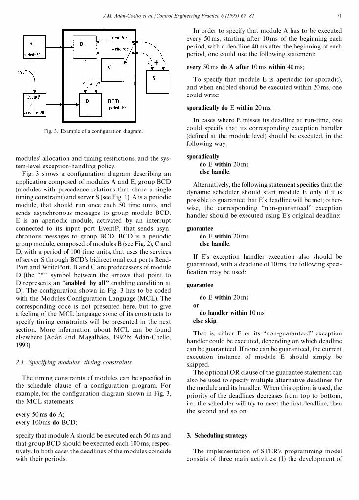
Fig. 3. Example of a configuration diagram.

modules’ allocation and timing restrictions, and the sys-tem-level exception-handling policy.

Fig. 3 shows a configuration diagram describing anapplication composed of modules A and E; group BCD(modules with precedence relations that share a singletiming constraint) and server S (see Fig. 1). A is a periodicmodule, that should run once each 50 time units, andsends asynchronous messages to group module BCD.E is an aperiodic module, activated by an interruptconnected to its input port EventP, that sends asyn-chronous messages to group BCD. BCD is a periodicgroup module, composed of modules B (see Fig. 2), C andD, with a period of 100 time units, that uses the servicesof server S through BCD’s bidirectional exit ports Read-Port and WritePort. B and C are predecessors of moduleD (the ‘‘*’’ symbol between the arrows that point toD represents an ‘‘enabled—by all’’ enabling condition atD). The configuration shown in Fig. 3 has to be codedwith the Modules Configuration Language (MCL). Thecorresponding code is not presented here, but to givea feeling of the MCL language some of its constructs tospecify timing constraints will be presented in the nextsection. More information about MCL can be foundelsewhere (Adan and Magalha8 es, 1992b; Adan-Coello,1993).

2.5. Specifying modules+ timing constraints

The timing constraints of modules can be specified inthe schedule clause of a configuration program. Forexample, for the configuration diagram shown in Fig. 3,the MCL statements:

every 50ms do A;every 100ms do BCD;

specify that module A should be executed each 50ms andthat group BCD should be executed each 100ms, respec-tively. In both cases the deadlines of the modules coincidewith their periods.

In order to specify that module A has to be executedevery 50ms, starting after 10ms of the beginning eachperiod, with a deadline 40ms after the beginning of eachperiod, one could use the following statement:

every 50ms do A after 10 ms within 40ms;

To specify that module E is aperiodic (or sporadic),and when enabled should be executed within 20ms, onecould write:

sporadically do E within 20ms.

In cases where E misses its deadline at run-time, onecould specify that its corresponding exception handler(defined at the module level) should be executed, in thefollowing way:

sporadicallydo E within 20mselse handle.

Alternatively, the following statement specifies that thedynamic scheduler should start module E only if it ispossible to guarantee that E’s deadline will be met; other-wise, the corresponding ‘‘non-guaranteed’’ exceptionhandler should be executed using E’s original deadline:

guaranteedo E within 20mselse handle.

If E’s exception handler execution also should beguaranteed, with a deadline of 10ms, the following speci-fication may be used:

guarantee

do E within 20msor

do handler within 10 mselse skip.

That is, either E or its ‘‘non-guaranteed’’ exceptionhandler could be executed, depending on which deadlinecan be guaranteed. If none can be guaranteed, the currentexecution instance of module E should simply beskipped.

The optional OR clause of the guarantee statement canalso be used to specify multiple alternative deadlines forthe module and its handler. When this option is used, thepriority of the deadlines decreases from top to bottom,i.e., the scheduler will try to meet the first deadline, thenthe second and so on.

3. Scheduling strategy

The implementation of STER’s programming modelconsists of three main activities: (1) the development of


language processors for the MPL and MCL languages,(2) the development of scheduling disciplines to guaran-tee modules’ timing constraints, and (3) the implementa-tion of the program run-time support.

The development of language processors for theMPL and MCL languages is similar in many respectsto the implementation of other concurrent program-ming languages, but, in addition to these commonaspects, the language processors should extract fromthe source code the information necessary to search forfeasible program schedules. This information shouldidentify scheduling blocks, with their respective execu-tion times, and their timing, allocation and precedenceconstraints.

Using the information provided by the language trans-lators, allocation and scheduling disciplines can try toguarantee that hard real-time constraints will always bemet, while soft real-time constraints will be met most ofthe time, and give an acceptable service time for nonreal-time modules.

The scheduling of most complex task models, such asthe one resulting from STER’s programming model, is anNP-hard problem (Blazewicz et al., 1983), implying thatthe search for a feasible schedule for hard real-time mod-ules should be made off-line.

The run-time support involves typical services of oper-ating systems and communication protocols. At the oper-ating-system level it is necessary to dispatch schedulingsegments for execution, according to the static schedule,and dynamically schedule soft and non-real-time mod-ules. Communication protocols are mainly concernedwith guaranteeing deterministic message transmissiontimes.

Of the above aspects, attention will be centered here onthe scheduling strategy, because of its pervasive role inthe implementation of STER.

Section 2 showed that STER programs can includeperiodic hard real-time modules, aperiodic soft real-timemodules and non-real-time modules. To meet the timingconstraints of these categories of modules a schedulingstrategy structured into three levels was adopted (Adanand Magalha8 es, 1992c): 1) off-line scheduling of hard-real-time periodic modules, 2) time-driven dynamicscheduling of soft real-time (SRT) aperiodic modules, and3) dynamic scheduling of non-real-time modules, usingidle intervals of time (i.e., when there are no real-timemodules scheduled).

As the focus of this paper is on meeting hard real-timeconstraints, the discussion will concentrate on aspects oflevel one, that is, the off-line scheduling algorithm.

3.1. Scheduling graphs

Modules are the smallest entities of a program atprogram configuration time, but, for program schedul-ing, some modules can be further divided into smaller

entities. These entities, called scheduling segments, arethe pieces of sequential code that will be scheduled forexecution.

To implement STER’s scheduling strategy, the in-formation that identifies scheduling segments will beextracted from the code of each program, with the re-spective precedence, allocation and timing constraints,and will be used to construct a scheduling graph.

This section will provide a general outlook on howto map STER programs to scheduling graphs. Detailsof the process of translating real-time programs tographs representing scheduling models similar to theone used here can be found elsewhere (Niehaus, 1991,1994).

In a scheduling graph, nodes represent the schedulingsegments of a program and arcs their precedence rela-tions. Nodes and arcs have costs attached. The costs ofnodes represent the computation times required to ex-ecute the corresponding segments, and the costs of arcsrepresent the time needed to transfer messages betweencommunicating scheduling segments. Both costs arehighly dependent on the architecture of the hardware andsoftware of the computers and communication media onwhich programs will run.

The generation of scheduling graphs is done in twophases, performed at module and configuration process-ing times. When a module is compiled, its schedulingsubgraph is generated, and when a configuration pro-gram is processed, module subgraphs are combined toproduce the program scheduling graph.

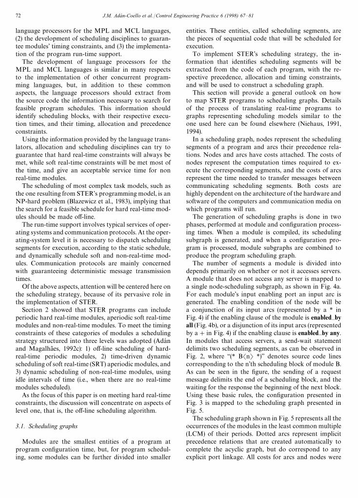
The number of segments a module is divided intodepends primarily on whether or not it accesses servers.A module that does not access any server is mapped toa single node-scheduling subgraph, as shown in Fig. 4a.For each module’s input enabling port an input arc isgenerated. The enabling condition of the node will bea conjunction of its input arcs (represented by a * inFig. 4) if the enabling clause of the module is enabled—byall (Fig. 4b), or a disjunction of its input arcs (representedby a#in Fig. 4) if the enabling clause is enabled—by any.In modules that access servers, a send-wait statementdelimits two scheduling segments, as can be observed inFig. 2, where ‘‘(* BSnT *)’’ denotes source code linescorresponding to the n’th scheduling block of module B.As can be seen in the figure, the sending of a requestmessage delimits the end of a scheduling block, and thewaiting for the response the beginning of the next block.Using these basic rules, the configuration presented inFig. 3 is mapped to the scheduling graph presented inFig. 5.

The scheduling graph shown in Fig. 5 represents all theoccurrences of the modules in the least common multiple(LCM) of their periods. Dotted arcs represent implicitprecedence relations that are created automatically tocomplete the acyclic graph, but do correspond to anyexplicit port linkage. All costs for arcs and nodes were


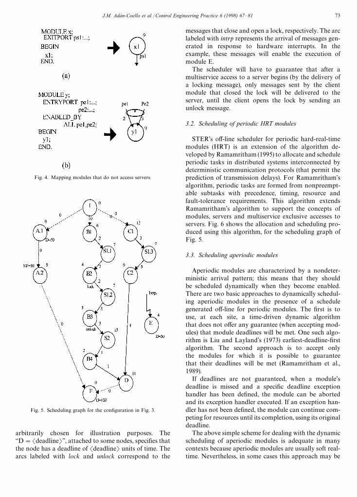
Fig. 4. Mapping modules that do not access servers.

Fig. 5. Scheduling graph for the configuration in Fig. 3.

arbitrarily chosen for illustration purposes. The‘‘D"SdeadlineT’’, attached to some nodes, specifies thatthe node has a deadline of SdeadlineT units of time. Thearcs labeled with lock and unlock correspond to the

messages that close and open a lock, respectively. The arclabeled with intrp represents the arrival of messages gen-erated in response to hardware interrupts. In theexample, these messages will enable the execution ofmodule E.

The scheduler will have to guarantee that after amultiservice access to a server begins (by the delivery ofa locking message), only messages sent by the clientmodule that closed the lock will be delivered to theserver, until the client opens the lock by sending anunlock message.

3.2. Scheduling of periodic HRT modules

STER’s off-line scheduler for periodic hard-real-timemodules (HRT) is an extension of the algorithm de-veloped by Ramamritham (1995) to allocate and scheduleperiodic tasks in distributed systems interconnected bydeterministic communication protocols (that permit theprediction of transmission delays). For Ramamritham’salgorithm, periodic tasks are formed from nonpreempt-able subtasks with precedence, timing, resource andfault-tolerance requirements. This algorithm extendsRamamritham’s algorithm to support the concepts ofmodules, servers and multiservice exclusive accesses toservers. Fig. 6 shows the allocation and scheduling pro-duced using this algorithm, for the scheduling graph ofFig. 5.

3.3. Scheduling aperiodic modules

Aperiodic modules are characterized by a nondeter-ministic arrival pattern; this means that they shouldbe scheduled dynamically when they become enabled.There are two basic approaches to dynamically schedul-ing aperiodic modules in the presence of a schedulegenerated off-line for periodic modules. The first is touse, at each site, a time-driven dynamic algorithmthat does not offer any guarantee (when accepting mod-ules) that module deadlines will be met. One such algo-rithm is Liu and Layland’s (1973) earliest-deadline-firstalgorithm. The second approach is to accept onlythe modules for which it is possible to guaranteethat their deadlines will be met (Ramamritham et al.,1989).

If deadlines are not guaranteed, when a module’sdeadline is missed and a specific deadline exceptionhandler has been defined, the module can be abortedand its exception handler executed. If an exception han-dler has not been defined, the module can continue com-peting for resources until its completion, using its originaldeadline.

The above simple scheme for dealing with the dynamicscheduling of aperiodic modules is adequate in manycontexts because aperiodic modules are usually soft real-time. Nevertheless, in some cases this approach may be


Fig. 6. Allocation and scheduling for the graph of Fig. 5.

inadequate, or even unacceptable. It is inadequate,for example, when after missing its deadline a modulecannot make any additional effective contribution to thesystem. In such a case, executing the module until itfinishes, and sometimes even running its exception han-dler, counts only as overhead. The scheme is not accept-able, for example, when a client module is accessinga server. In that case, the module cannot continue ‘‘us-ing’’ the server after its scheduled time because this canproduce a ripple effect that may cause guaranteed peri-odic modules that also need the server also to miss theirdeadlines. In addition, it may not be possible to releasethe server immediately because it could be absolutelynecessary to bring it back to a consistent state beforedoing that.

Independent of whether aperiodic modules are sched-uled using a simple dynamic algorithm, like the ear-liest deadline first, or using a more elaborateone that includes the notion of guaranteed execution,the schedulability of aperiodic modules arrivingat a given node of a distributed system will be greatlyinfluenced by the allocation and schedule producedoff-line for periodic modules. In particular, if the load-ing of the sites in a distributed system is not well bal-anced, modules arriving at heavily loaded nodes mayhave a reduced probability of meeting their deadlines.Moreover, if the off-line schedule defines exactly whenthe modules should start their execution, deadlines ofaperiodic modules may be missed in situations whereboth periodic and aperiodic deadlines could be met, justby adjusting the scheduled start times of the periodicmodules.

The objective of scheduling algorithms for periodicmodules, such as the one presented earlier in this section,is to meet modules’ deadlines, respecting precedence andresource constraints. The schedules they produce areseldom well balanced in the space and time dimensions;that is, the load is not fairly distributed across the sites(nodes), nor along the scheduling interval (the LCM ofthe modules’ periods).

To increase the probability that a dynamic schedulerwill have to find a feasible schedule for aperiodic mod-ules, some strategies have been developed to improve thesystem load balance, in the time and space dimensions,

and to introduce some leeway for the start of each sche-duling segment.

3.4. Balancing the load in the space and time dimensions

To provide for dynamic arrivals it is desirable to bal-ance the load, not only across individual sites, but alsoalong the time axis. Two heuristic strategies have beendeveloped, that can improve the load balance character-istics of static scheduling algorithms: the Maximum LoadStrategy (MLS), and the Gap Factor Strategy (GFS)(Ramamritham et al., 1993). These strategies were addedto the algorithm described previously in this section.

The MLS strategy limits the load that can be imposedon each site. The percentage of the total load that can beallocated to each site is defined by the parameter Max-Load. When it is not possible to find a schedule fora given MaxLoad, a new one is tried. This new value isobtained by adding the parameter MaxLoadInc to Max-Load. This procedure is repeated until the module set issuccessfully scheduled or MaxLoad reaches 100%, whichis equivalent to permitting that the total load be allo-cated to a single site.

The GFS strategy introduces gaps, i.e., idle times, aftereach scheduled segment, decreasing the number of seg-ments that can be allocated to a site and forcing thealgorithm to try to distribute the segments over thesystem. This should improve the system load in the spaceand time domains.

The percentage of the computation time that should beleft idle after each scheduled segment is given by theparameter GapFactor. For instance, if GapFactor isequal to 20% and a segment with computation time 50has been scheduled, the static scheduler should keep thesite idle for, at least, 10 time units.

Each time the algorithm fails to find a schedule fora given GapFactor, it is decreased by the value of theparameter GapFactorDec. This process is repeated untilthe module set is successfully scheduled, or GapFactorreaches zero.

The effects of different limits on the load as well assegment execution time dependent idle times werestudied via simulation. The main results of this study arediscussed in Section 4.


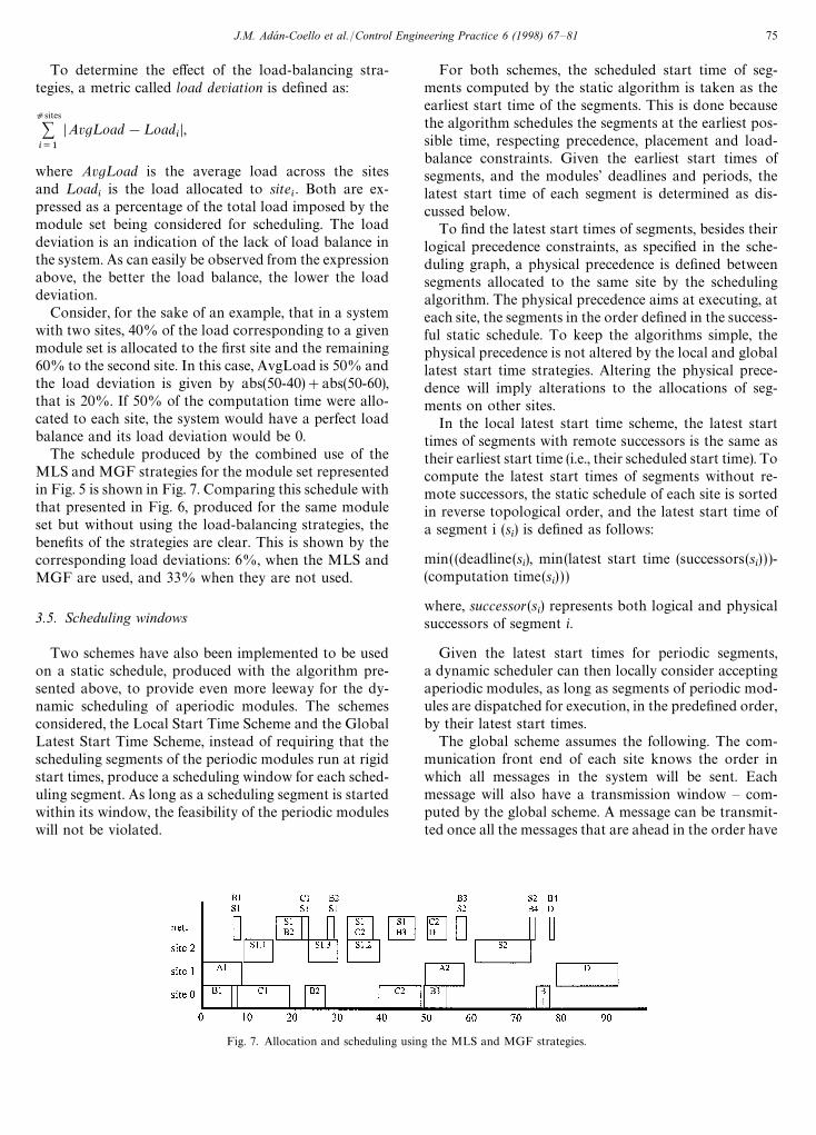
Fig. 7. Allocation and scheduling using the MLS and MGF strategies.

To determine the effect of the load-balancing stra-tegies, a metric called load deviation is defined as:

dsites

+i/1

DAvg¸oad!¸oadiD,

where Avg¸oad is the average load across the sitesand ¸oad

iis the load allocated to site

i. Both are ex-

pressed as a percentage of the total load imposed by themodule set being considered for scheduling. The loaddeviation is an indication of the lack of load balance inthe system. As can easily be observed from the expressionabove, the better the load balance, the lower the loaddeviation.

Consider, for the sake of an example, that in a systemwith two sites, 40% of the load corresponding to a givenmodule set is allocated to the first site and the remaining60% to the second site. In this case, AvgLoad is 50% andthe load deviation is given by abs(50-40)#abs(50-60),that is 20%. If 50% of the computation time were allo-cated to each site, the system would have a perfect loadbalance and its load deviation would be 0.

The schedule produced by the combined use of theMLS and MGF strategies for the module set representedin Fig. 5 is shown in Fig. 7. Comparing this schedule withthat presented in Fig. 6, produced for the same moduleset but without using the load-balancing strategies, thebenefits of the strategies are clear. This is shown by thecorresponding load deviations: 6%, when the MLS andMGF are used, and 33% when they are not used.

3.5. Scheduling windows

Two schemes have also been implemented to be usedon a static schedule, produced with the algorithm pre-sented above, to provide even more leeway for the dy-namic scheduling of aperiodic modules. The schemesconsidered, the Local Start Time Scheme and the GlobalLatest Start Time Scheme, instead of requiring that thescheduling segments of the periodic modules run at rigidstart times, produce a scheduling window for each sched-uling segment. As long as a scheduling segment is startedwithin its window, the feasibility of the periodic moduleswill not be violated.

For both schemes, the scheduled start time of seg-ments computed by the static algorithm is taken as theearliest start time of the segments. This is done becausethe algorithm schedules the segments at the earliest pos-sible time, respecting precedence, placement and load-balance constraints. Given the earliest start times ofsegments, and the modules’ deadlines and periods, thelatest start time of each segment is determined as dis-cussed below.

To find the latest start times of segments, besides theirlogical precedence constraints, as specified in the sche-duling graph, a physical precedence is defined betweensegments allocated to the same site by the schedulingalgorithm. The physical precedence aims at executing, ateach site, the segments in the order defined in the success-ful static schedule. To keep the algorithms simple, thephysical precedence is not altered by the local and globallatest start time strategies. Altering the physical prece-dence will imply alterations to the allocations of seg-ments on other sites.

In the local latest start time scheme, the latest starttimes of segments with remote successors is the same astheir earliest start time (i.e., their scheduled start time). Tocompute the latest start times of segments without re-mote successors, the static schedule of each site is sortedin reverse topological order, and the latest start time ofa segment i (s

i) is defined as follows:

min((deadline(si), min(latest start time (successors(s

i)) )-

(computation time(si) ) )

where, successor(si) represents both logical and physical

successors of segment i.

Given the latest start times for periodic segments,a dynamic scheduler can then locally consider acceptingaperiodic modules, as long as segments of periodic mod-ules are dispatched for execution, in the predefined order,by their latest start times.

The global scheme assumes the following. The com-munication front end of each site knows the order inwhich all messages in the system will be sent. Eachmessage will also have a transmission window — com-puted by the global scheme. A message can be transmit-ted once all the messages that are ahead in the order have


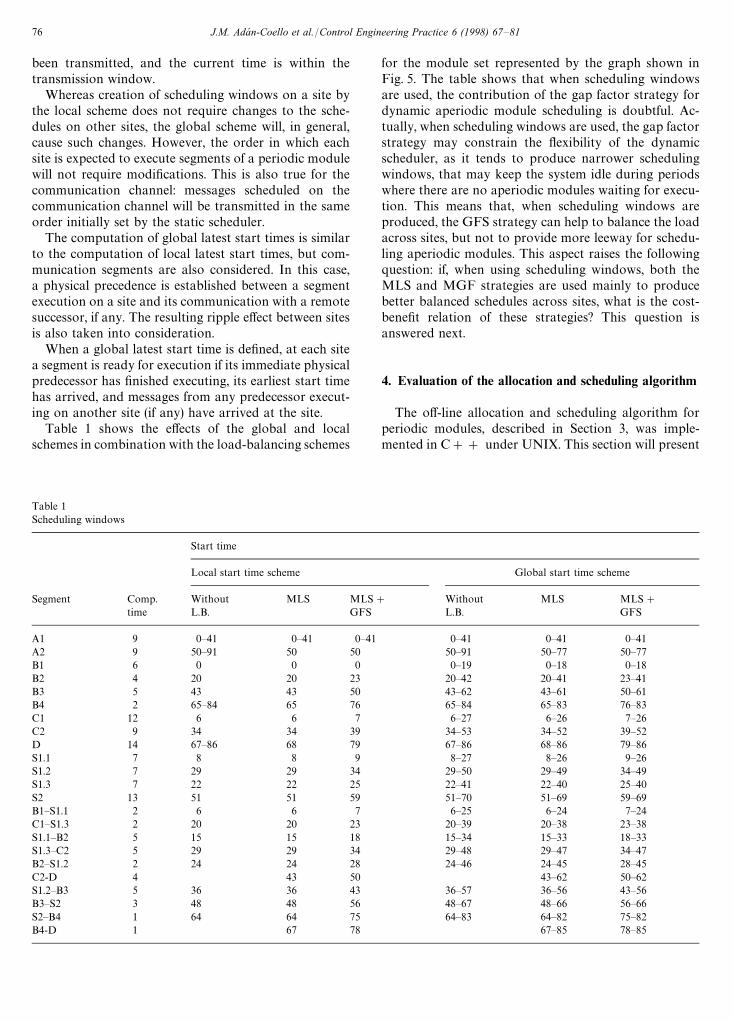
Table 1Scheduling windows

Start time

Local start time scheme Global start time scheme

Segment Comp. Without MLS MLS# Without MLS MLS#time L.B. GFS L.B. GFS

A1 9 0—41 0—41 0—41 0—41 0—41 0—41A2 9 50—91 50 50 50—91 50—77 50—77B1 6 0 0 0 0—19 0—18 0—18B2 4 20 20 23 20—42 20—41 23—41B3 5 43 43 50 43—62 43—61 50—61B4 2 65—84 65 76 65—84 65—83 76—83C1 12 6 6 7 6—27 6—26 7—26C2 9 34 34 39 34—53 34—52 39—52D 14 67—86 68 79 67—86 68—86 79—86S1.1 7 8 8 9 8—27 8—26 9—26S1.2 7 29 29 34 29—50 29—49 34—49S1.3 7 22 22 25 22—41 22—40 25—40S2 13 51 51 59 51—70 51—69 59—69B1—S1.1 2 6 6 7 6—25 6—24 7—24C1—S1.3 2 20 20 23 20—39 20—38 23—38S1.1—B2 5 15 15 18 15—34 15—33 18—33S1.3—C2 5 29 29 34 29—48 29—47 34—47B2—S1.2 2 24 24 28 24—46 24—45 28—45C2-D 4 43 50 43—62 50—62S1.2—B3 5 36 36 43 36—57 36—56 43—56B3—S2 3 48 48 56 48—67 48—66 56—66S2—B4 1 64 64 75 64—83 64—82 75—82B4-D 1 67 78 67—85 78—85

been transmitted, and the current time is within thetransmission window.

Whereas creation of scheduling windows on a site bythe local scheme does not require changes to the sche-dules on other sites, the global scheme will, in general,cause such changes. However, the order in which eachsite is expected to execute segments of a periodic modulewill not require modifications. This is also true for thecommunication channel: messages scheduled on thecommunication channel will be transmitted in the sameorder initially set by the static scheduler.

The computation of global latest start times is similarto the computation of local latest start times, but com-munication segments are also considered. In this case,a physical precedence is established between a segmentexecution on a site and its communication with a remotesuccessor, if any. The resulting ripple effect between sitesis also taken into consideration.

When a global latest start time is defined, at each sitea segment is ready for execution if its immediate physicalpredecessor has finished executing, its earliest start timehas arrived, and messages from any predecessor execut-ing on another site (if any) have arrived at the site.

Table 1 shows the effects of the global and localschemes in combination with the load-balancing schemes

for the module set represented by the graph shown inFig. 5. The table shows that when scheduling windowsare used, the contribution of the gap factor strategy fordynamic aperiodic module scheduling is doubtful. Ac-tually, when scheduling windows are used, the gap factorstrategy may constrain the flexibility of the dynamicscheduler, as it tends to produce narrower schedulingwindows, that may keep the system idle during periodswhere there are no aperiodic modules waiting for execu-tion. This means that, when scheduling windows areproduced, the GFS strategy can help to balance the loadacross sites, but not to provide more leeway for schedu-ling aperiodic modules. This aspect raises the followingquestion: if, when using scheduling windows, both theMLS and MGF strategies are used mainly to producebetter balanced schedules across sites, what is the cost-benefit relation of these strategies? This question isanswered next.

4. Evaluation of the allocation and scheduling algorithm

The off-line allocation and scheduling algorithm forperiodic modules, described in Section 3, was imple-mented in C## under UNIX. This section will present


and discuss the results of some representative experi-ments, conducted to evaluate this implementation.

4.1. Test case generation

The test cases used in the experiments were producedin two steps. The first mainly followed the proceduredescribed in Ramamritham (1995) to produce schedulinggraphs representing sets of modules without servers. Inthe second step, a filter program was used to add servers,and accesses to servers, to these scheduling graphs.

The graphs generated in the first step represent peri-odic module sets with the following characteristics. Seg-ments (nodes of the scheduling graph) have their execu-tion times uniformly distributed between 50 (t—exec—min)and 100 (t—exec—max) time units. The communicationcosts, CC, of each pair of communicating segments (withprecedence relations) is given by:

(50 * CR)4CC4(100 * CR).

In the experiments described in this section, the CR(Communication Ratio) is equal to 0.1. To determine theperiod P of the module with the lowest period of each testcase the following formula was used:

P"C * module—size * laxity— factor

where C is the average computation time of a segment,i.e., 75, module—size is the number of segments beinggenerated, and laxity— factor is a parameter that reflectsthe computational load imposed by the module in eachof its periodic activations. The above formula impliesthat, given the computational requirements of a module,the larger the laxity—factor, the larger the period of themodule and, consequently, the easier it would be to finda feasible schedule for it.

The results presented in this paper correspond to testcases with laxity—factors varying from 0.9 to 1.6, andthree periodic modules, composed of one segment (mod-ule—size"1), two segments (module—size"2) and threesegments (module—size"3), respectively. The period ofthe first module, determined using the above formula, isP, the period of the second module is 2P and the periodof the third module is 3P. Thus, for each test case, thealgorithm will search for a scheduling interval of length6P, which corresponds to the least common multiple ofthe periods of the three modules. This means that thescheduling interval will include 6 occurrences of the firstmodule, 3 occurrences of the second module and 2 occur-rences of the third module. Thus, the correspondingscheduling graph will have 20 nodes—18 representing thesegments and 2 representing the initial and final nodes ofthe graph.

The graphs generated in the first pass of the test-casegeneration process do not include accesses to servers. In

the second pass, some nodes of those graphs are trans-formed into single service accesses (SSA) and multipleservice accesses (MSA) to servers. In an SSA, a clientmodule requests a single service to a server. In an MSAa client requests two or more services to a server.

The percentage of nodes from the original graphtransformed into single service accesses to servers (SSA)and into multiple service accesses to servers (MSA) isgiven by the parameters single service access ratio(SSAR) and multiple service access ratio (MSAR), respec-tively. Due to space limitations, this paper will discussonly experiments where 10% of the nodes of the graphsproduced in step 1 of the test-case-generation process aretransformed into SSAs (SSAR"0.1) to a single server(S"1).

When a single service access is introduced, a nodeof the original graph is transformed into three newnodes, connected by two arcs. The first node repres-ents the client’s segment of code that requests the ser-vice, the second node represents the server’s segment ofcode that provides the service and sends a reply messageto the client, and the third node the client’s segment ofcode that waits for the reply message. Two arcs repres-enting the transmission of the request and reply messagesconnect these nodes. Using this procedure, for an SSARof 0.1, the graphs composed of 20 nodes without SSA,generated in the first pass of test cases generation, aretransformed into graphs with 24 nodes, in the secondpass.

Each node generated to represent an SSA will havea computation time equal to one third of the cost of theoriginal node, and the arcs connecting the new nodes willhave a cost of one third of the cost of an arc of theoriginal graph. This procedure keeps the laxity of the newgraph constant, because communication costs are nottaken into account in calculating the periods of themodules, although they increase the communicationload between the nodes by SSAR*0.66 (6.6% for anSSAR of 0.1).

4.2. Performance of the algorithm without theload-balancing strategies

The performance of the algorithm was studied whenusing three different heuristics to construct commun-ication graphs: 1) the heuristic discussed in Sec-tion 3, here denoted as the client—server heuristic (C—S), 2)the node—node heuristic (N—N), and 3) the randomheuristic.

As discussed before, in the C—S heuristic a pair ofcommunicating client—server modules will be allocatedto the same site if the sum of the computation times oftheir interacting scheduling segments, divided by theircommunication costs, is lower than the current commun-ication factor (CF). In the N—N and random heuristics,allocation decisions are taken for pairs of communicating


scheduling segments, and not for pairs of communicatingmodules. When the N—N heuristic is used, two com-municating nodes are placed in the same site if the sum oftheir computation times, divided by their communicationcost, is lower than CF (the communication factor). Whenthe random heuristic is used, the decision to allocate, ornot, a pair of communicating nodes to the same site istaken at random.

As the N—N and the random heuristic take allocationdecisions for pairs of scheduling segments and not forpairs of modules, it is possible that they will allocatescheduling segments of the same module (client or server)to different sites, which is incorrect, as the schedulingsegments of a module instance share a single addressspace. When this happens, these mappings are discardedduring the mapping validity-check phase of the schedu-ling algorithm.

4.2.1. Single service accesses to a serverFig. 8 shows the success rate of the algorithm, in

percentage of module sets successfully scheduled, whensearching for a feasible schedule for test cases where10% of the segments perform SSA to a single server(SSAR"0.1 and S"1) and the communication ratio(CR) between segments is equal to 0.1. Each point inFig. 8, as well in the subsequent plots, is the result ofrunning the algorithm for 100 different periodic mod-ule sets, with the above characteristics and same laxityfactor.

Fig. 8 clearly shows that the allocation decisions basedon the execution and communication costs of the seg-ments (heuristics N—N and C—S) are better than thosetaken at random.

When backtracks are not used, the client—server heu-ristic has, most of the time, a better performance than thenode—node heuristic. In some cases, for instance, fora laxity factor of 1.1, the success rate of the algorithmusing the client—server heuristic is more than 20% higherthan the success rate when the node—node heuristic isused.

For the C—S and N—N strategies, Fig. 8 also shows thatperforming a limited number of backtracks (up to 100)increases the success rate of the algorithm even more. Insome cases (laxity factor 1.2, for example), there is a new,significant increase, of the order of 20%. On the otherhand, the use of backtracks makes the difference betweenthe success ratios accomplished using either of the heuris-tics insignificant.

In the case of the random heuristic, the use of back-tracks substantially increases (90% in some cases) thesuccess ratio of the algorithm, compared to the resultsobtained with the same heuristics without backtracks.This result shows the large number of inconsistent sche-duling decisions that are taken when the algorithm deci-des whether or not to allocate scheduling segments tothe same node at random, without taking into account

Fig. 8. Success rate for S"1, SSAR"0.1 and CR"0.1.

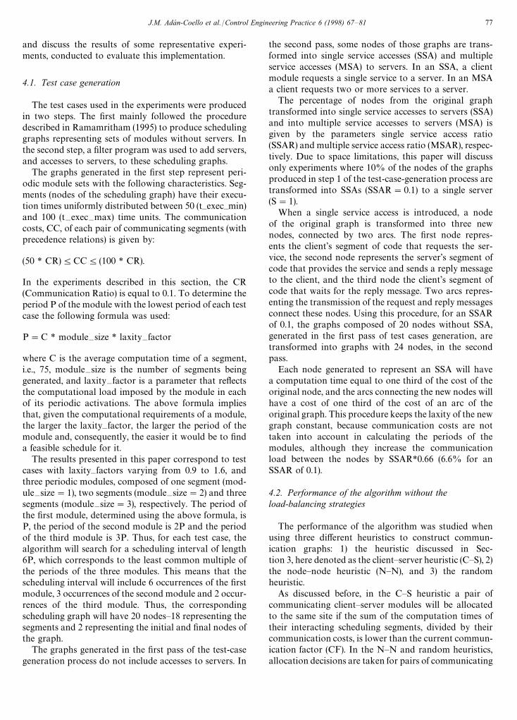
Fig. 9. Costs of scheduling for success.

segments, computation and communication times andmodule boundaries.

Fig. 9 shows the costs, in number of search pointsvisited, of finding feasible schedules for each of the com-pared heuristics. It can be seen that the C—S heuristic haslower costs than the N—N heuristic for all laxity factors.Additionally, for most cases, the cost of the C—S heuristicwith backtracks is equivalent to the cost of the N—Nheuristic without backtracks. The cost of the randomheuristic is comparable to the cost of the client—serverheuristic; however, as shown in Fig. 8, its success rate isconsiderably lower.

Fig. 10 shows the costs of the heuristics when thealgorithm could not find a feasible schedule. As can beobserved, when backtracks are not used, the C—S heuris-tic presents a cost slightly lower than the cost of the N—Nheuristic, indicating that, with the C—S heuristic, the


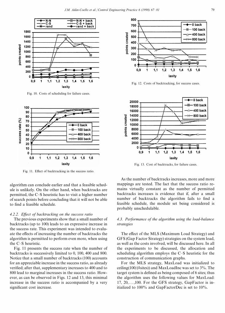
Fig. 10. Costs of scheduling for failure cases.

Fig. 11. Effect of backtracking in the success ratio.

algorithm can conclude earlier and that a feasible sched-ule is unlikely. On the other hand, when backtracks arepermitted, the C—S heuristic has to visit a higher numberof search points before concluding that it will not be ableto find a feasible schedule.

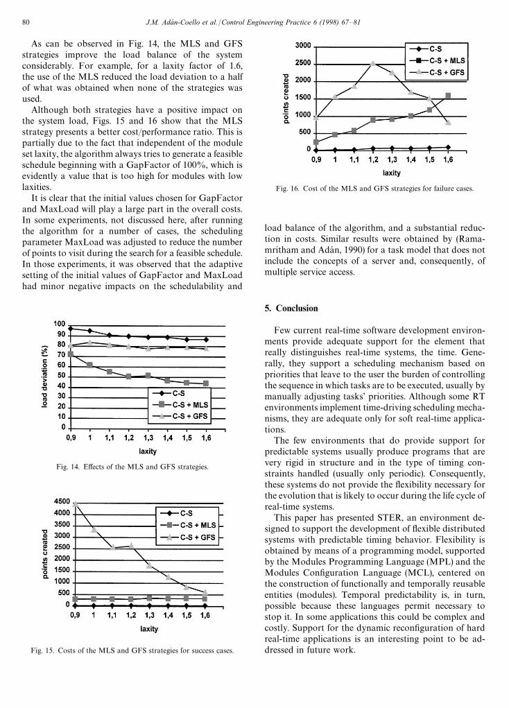
4.2.2. Effect of backtracking on the success ratioThe previous experiments show that a small number of

backtracks (up to 100) leads to an expressive increase inthe success rate. This experiment was intended to evalu-ate the effects of increasing the number of backtracks thealgorithm is permitted to perform even more, when usingthe C—S heuristic.

Fig. 11 presents the success rate when the number ofbacktracks is successively limited to 0, 100, 400 and 800.Notice that a small number of backtracks (100) accountsfor an appreciable increase in the success ratio, as alreadyverified; after that, supplementary increases to 400 and to800 lead to marginal increases in the success ratio. How-ever, as can be observed in Figs. 12 and 13, this minimalincrease in the success ratio is accompanied by a verysignificant cost increase.

Fig. 12. Costs of backtracking, for success cases.

Fig. 13. Cost of backtracks, for failure cases.

As the number of backtracks increases, more and moremappings are tested. The fact that the success ratio re-mains virtually constant as the number of permittedbacktracks increases is evidence that if, after a smallnumber of backtracks the algorithm fails to find afeasible schedule, the module set being considered isprobably unschedulable.

4.3. Performance of the algorithm using the load-balancestrategies

The effect of the MLS (Maximum Load Strategy) andGFS (Gap Factor Strategy) strategies on the system load,as well as the costs involved, will be discussed here. In allthe experiments to be discussed, the allocation andscheduling algorithm employs the C—S heuristic for theconstruction of communication graphs.

For the MLS strategy, MaxLoad was initialized toceiling(100/(Asites)) and MaxLoadInc was set to 3%. Thetarget system is defined as being composed of 6 sites; thusthe algorithm uses the following values for MaxLoad:17, 20, . . . ,100. For the GFS strategy, GapFactor is in-itialized to 100% and GapFactorDec is set to 10%.


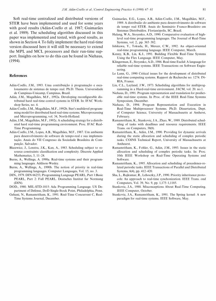
As can be observed in Fig. 14, the MLS and GFSstrategies improve the load balance of the systemconsiderably. For example, for a laxity factor of 1.6,the use of the MLS reduced the load deviation to a halfof what was obtained when none of the strategies wasused.

Although both strategies have a positive impact onthe system load, Figs. 15 and 16 show that the MLSstrategy presents a better cost/performance ratio. This ispartially due to the fact that independent of the moduleset laxity, the algorithm always tries to generate a feasibleschedule beginning with a GapFactor of 100%, which isevidently a value that is too high for modules with lowlaxities.

It is clear that the initial values chosen for GapFactorand MaxLoad will play a large part in the overall costs.In some experiments, not discussed here, after runningthe algorithm for a number of cases, the schedulingparameter MaxLoad was adjusted to reduce the numberof points to visit during the search for a feasible schedule.In those experiments, it was observed that the adaptivesetting of the initial values of GapFactor and MaxLoadhad minor negative impacts on the schedulability and

Fig. 14. Effects of the MLS and GFS strategies.

Fig. 15. Costs of the MLS and GFS strategies for success cases.

Fig. 16. Cost of the MLS and GFS strategies for failure cases.

load balance of the algorithm, and a substantial reduc-tion in costs. Similar results were obtained by (Rama-mritham and Adan, 1990) for a task model that does notinclude the concepts of a server and, consequently, ofmultiple service access.

5. Conclusion

Few current real-time software development environ-ments provide adequate support for the element thatreally distinguishes real-time systems, the time. Gene-rally, they support a scheduling mechanism based onpriorities that leave to the user the burden of controllingthe sequence in which tasks are to be executed, usually bymanually adjusting tasks’ priorities. Although some RTenvironments implement time-driving scheduling mecha-nisms, they are adequate only for soft real-time applica-tions.

The few environments that do provide support forpredictable systems usually produce programs that arevery rigid in structure and in the type of timing con-straints handled (usually only periodic). Consequently,these systems do not provide the flexibility necessary forthe evolution that is likely to occur during the life cycle ofreal-time systems.

This paper has presented STER, an environment de-signed to support the development of flexible distributedsystems with predictable timing behavior. Flexibility isobtained by means of a programming model, supportedby the Modules Programming Language (MPL) and theModules Configuration Language (MCL), centered onthe construction of functionally and temporally reusableentities (modules). Temporal predictability is, in turn,possible because these languages permit necessary tostop it. In some applications this could be complex andcostly. Support for the dynamic reconfiguration of hardreal-time applications is an interesting point to be ad-dressed in future work.


Soft real-time centralized and distributed versions ofSTER have been implemented and used for some yearswith good results (Adan-Coello et al. 1987; Guimara8 eset al. 1989). The scheduling algorithm discussed in thispaper was implemented and tested, with good results, asshown in Section 4. To fully implement the hard real-timeversion discussed here it will still be necessary to extendthe MPL and MCL processors and their run-time sup-port. Insights on how to do this can be found in Niehaus,(1994).

References

Adan-Coello, J.M., 1993. Uma contribuiia8 o a programaia8 o e esca-lonamento de sistemas de tempo real. Ph.D. Thesis. Universidadede Campinas-Unicamp, Campinas, Brazil.

Adan, J.M., Magalha8 es, M.F., 1992a. Developing reconfigurable dis-tributed hard real-time control systems in STER. In: IFAC Work-shop Series, no. 4.

Adan-Coello, J.M., Magalha8 es, M.F., 1992b. Ster’s multilevel program-ming model for distributed hard real-time systems. Microprocessingand Microprogramming, vol. 34, North-Holland.

Adan, J.M., Magalha8 es, M.F., 1992c. A scheduling strategy for a distrib-uted hard real-time programming environment. Proc. IFAC Real-Time Programming.

Adan-Coello, J.M., Lopes, A.B., Magalha8 es, M.F., 1987. Um ambientepara desenvolvimento de software de tempo-real e sua implemen-taia8 o. Anais do VII Congresso da Sociedade Brasileira de Com-putia8 o. Salvador.

Blazewicz, J., Lenstra, J.K., Kan, A., 1983. Scheduling subject to re-source constraints: classification and complexity. Discrete AppliedMathematics, 5, 11—24.

Burns, A., Wellings, A. 1990a. Real-time systems and their program-ming languages. Addison-Wesley.

Burns, A., Wellings, A., 1990b. The notion of priority in real-timeprogramming languages. Computer Languages, Vol. 15, no. 3.

DIN., 1979. DIN 66253, Programming Language PEARL, Part 1:BasicPEARL, Part 2: Full PEARL. Deutsches Institut fur Normung(DIN).

DOD., 1980. MIL-STD-1815: Ada Programming Language. US De-partment of Defense, DoD Single-Stock Point, Philadelphia, Penn.

Gehani, N., Ramamritham, K., 1991. Real-Time Concurrent C, Real-Time Systems Journal, December.

Guimara8 es, E.G., Lopes, A.B., Adan-Coello, J.M., Magalha8 es, M.F.,1989. A distribuia8 o do ambiente para desenvolvimento de softwarede tempo real STER. Anais do Semina& rio Franco-Brasileiro emSistemas Distribui&dos. Florianopolis, SC, Brazil.

Halang, W.A., Stoyenko, A.D., 1990. Comparative evaluation of high-level real-time programming languages. The Journal of Real-TimeSystems, vol. 2., pp. 365—382.

Ishikawa, Y., Tokuda, H., Mercer, C.W., 1992. An object-orientedreal-time programming language. IEEE Computer, March.

Kenny, K.B., Lin, K.J., 1991. Building Flexible Real-Time SystemsUsing the Flex Language. IEEE Computer, May.

Klingerman, E., Stoyenko, A.D., 1986. Real-time Euclid: A language forreliable real-time systems. IEEE Transactions on Software Engin-eering.

Le Lann, G., 1990 Critical issues for the development of distributedreal-time computing systems. Rapport de Recherche no. 1274. IN-RIA, France.

Liu, C.L., Layland, J.W., 1973. Scheduling algorithms for multiprog-ramming in a Hard-real-time environment. JACM, vol. 20. no.1.

Niehaus, D., 1991. Program representation and translation for predict-able real-time systems. In Proc. of the IEEE Real-Time SystemsSymposium, December.

Niehaus, D., 1994. Program Representation and Execution inReal-Time Multiprocessor Systems. Ph.D. Dissertation, Dept.of Computer Science, University of Massachusetts at Amherst,February.

Ramamritham, K., Stankovic, J.A., Zhao, W., 1989. Distributed sched-uling of tasks with deadlines and resource requirements. IEEETrans. on Computers, 38(8).

Ramamritham, K., Adan, J.M., 1990. Providing for dynamic arrivalsduring the static allocation and scheduling of complex periodictasks. COINS Technical Report, University of Massachusetts atAmhearst.

Ramamritham, K., Fohler, G., Adan, J.M., 1993. Issues in the staticallocation and scheduling of complex periodic tasks. In: Proc.10th IEEE Workshop on Real-Time Operating Systems andSoftware.

Ramamritham, K., 1995. Allocation and scheduling of precedence-re-lated periodic tasks. IEEE Transactions of Parallel and DistributedSystems, 6(4), pp. 412—420.

Sha, L., Rajkumar, R., Lehoczky, J.P., 1990. Priority inheritance proto-cols: An approach to real-time synchonization. IEEE Trans. ondComputers, Vol. 39, No. 9, pp. 1,175—1,1185.

Stankovic, J.A., 1988. Misconceptions About Real-Time Computing.IEEE Computer, October.

Stankovic, J.A., Ramamritham, K., 1991. The Spring kernel: A newparadigm for real-time systems. IEEE Software, May.


Documents

Developing predictable and flexible distributed real-time systems