Diagonalization of Matrices

By: Abdurazak Mudesir

Diagonalization of Matrices

• Motivation• Eigenvalue decomposition• Singular-value decomposition• Discrete Fourier transform • Applications : FEXT cancellation

Wireless applications

Motivation

•Image Compression

•Noise Filtering

And more…..

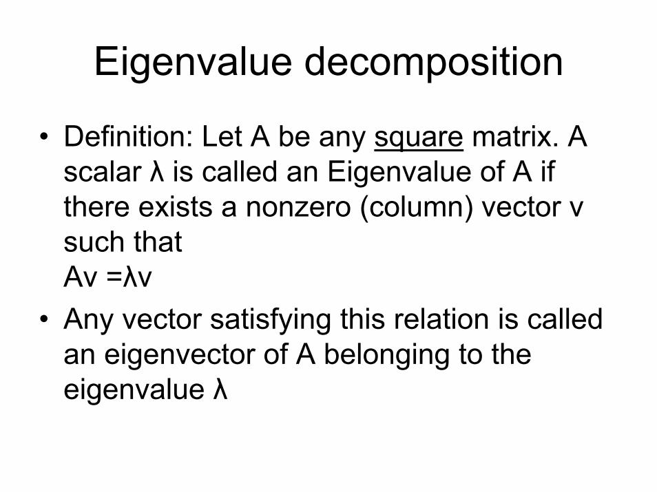
Eigenvalue decomposition

• Definition: Let A be any square matrix. A scalar λ is called an Eigenvalue of A if there exists a nonzero (column) vector v such that Av =λv

• Any vector satisfying this relation is called an eigenvector of A belonging to the eigenvalue λ

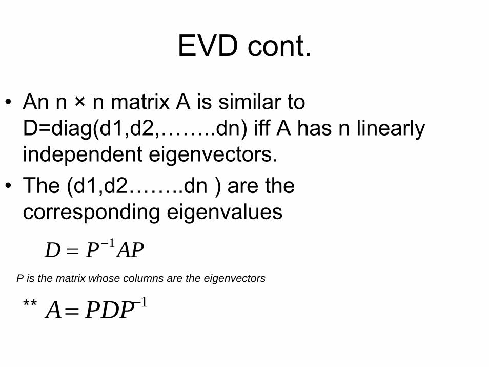
EVD cont.

• An n × n matrix A is similar to D=diag(d1,d2,……..dn) iff A has n linearly independent eigenvectors.

• The (d1,d2……..dn ) are the corresponding eigenvalues

P is the matrix whose columns are the eigenvectors

**

APPD 1−=

1−= PDPA

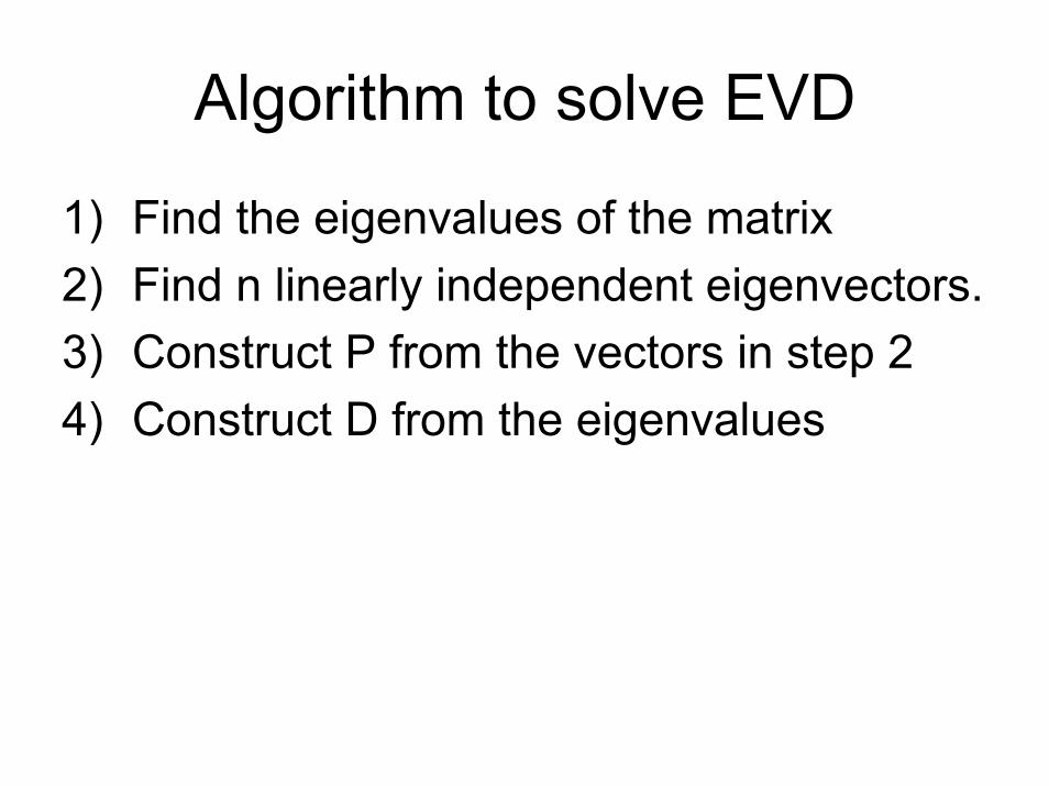
Algorithm to solve EVD

1) Find the eigenvalues of the matrix2) Find n linearly independent eigenvectors.3) Construct P from the vectors in step 24) Construct D from the eigenvalues

Example:

Singular-value decomposition

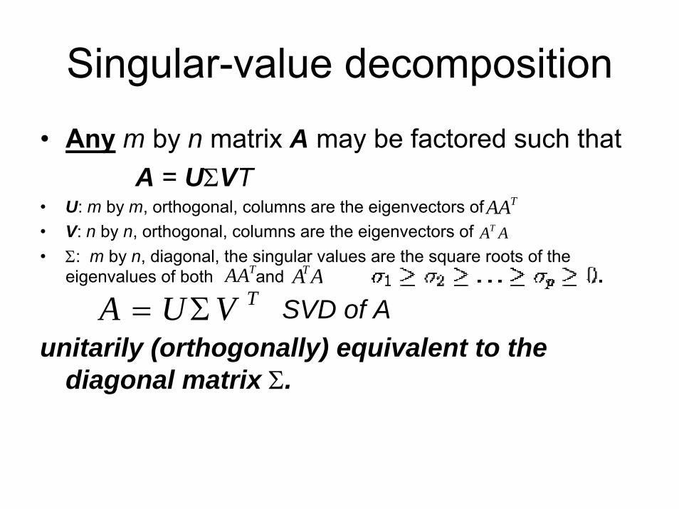
• Any m by n matrix A may be factored such that A = UΣVT

• U: m by m, orthogonal, columns are the eigenvectors of • V: n by n, orthogonal, columns are the eigenvectors of • Σ: m by n, diagonal, the singular values are the square roots of the

eigenvalues of both and

SVD of Aunitarily (orthogonally) equivalent to the

diagonal matrix Σ.

TAAAAT

TAA AAT

TVUA Σ=

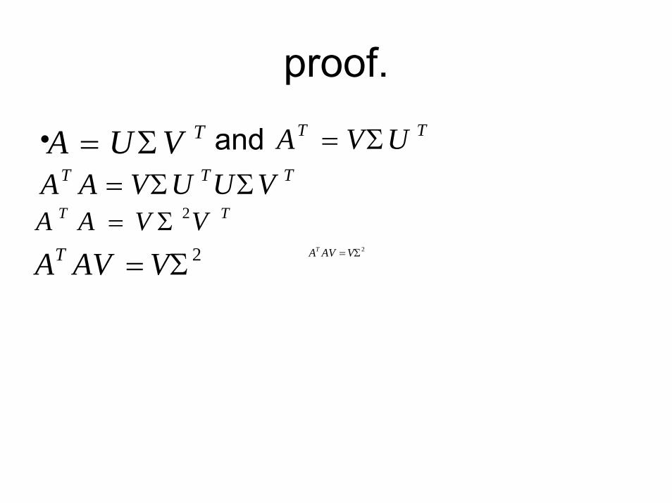
proof.

• andTVUA Σ=

2Σ=VAVAT

TT UVA Σ=TTT VUUVAA ΣΣ=

TT VVAA 2Σ=2Σ= VAVAT

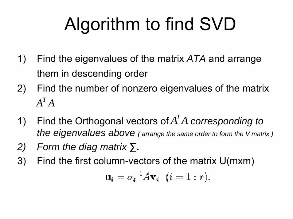
Algorithm to find SVD

1) Find the eigenvalues of the matrix ATA and arrange them in descending order

2) Find the number of nonzero eigenvalues of the matrix

1) Find the Orthogonal vectors of corresponding to the eigenvalues above ( arrange the same order to form the V matrix.)

2) Form the diag matrix ∑.3) Find the first column-vectors of the matrix U(mxm)

AAT

AAT

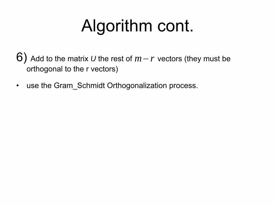
Algorithm cont.

6) Add to the matrix U the rest of vectors (they must be orthogonal to the r vectors)

• use the Gram_Schmidt Orthogonalization process.

rm−

Examples

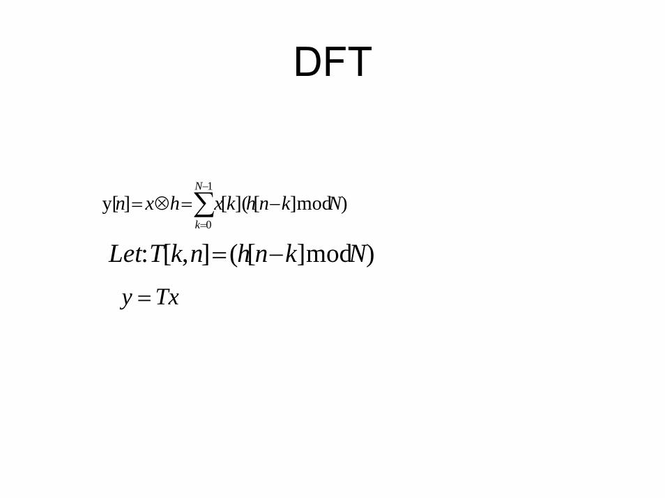
DFT

)mod][]([]y[1

0

NknhkxhxnN

k∑−

=

−=⊗=

)mod][(],[: NknhnkTLet −=

Txy =

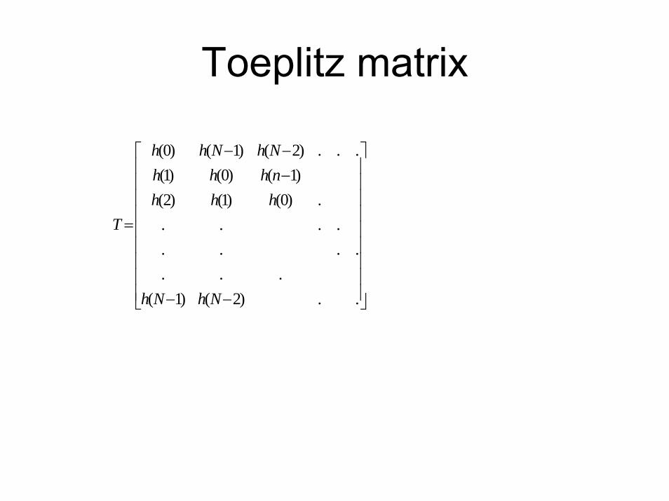
Toeplitz matrix

⎥⎥⎥⎥⎥⎥⎥⎥⎥

⎦

⎤

⎢⎢⎢⎢⎢⎢⎢⎢⎢

⎣

⎡

−−

−−−

=

..)2()1(...

........

.)0()1()2()1()0()1(

...)2()1()0(

NhNh

hhhnhhhNhNhh

T

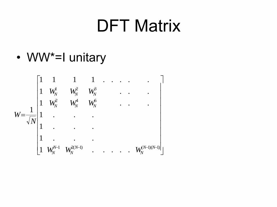
DFT Matrix

• WW*=I unitary

⎥⎥⎥⎥⎥⎥⎥⎥⎥

⎦

⎤

⎢⎢⎢⎢⎢⎢⎢⎢⎢

⎣

⎡

=

−−−− )1)(1()1(21

642

321

.....1...1...1...1

...1

...1

.....1111

1

NNN

NN

NN

NNN

NNN

WWW

WWWWWW

NW

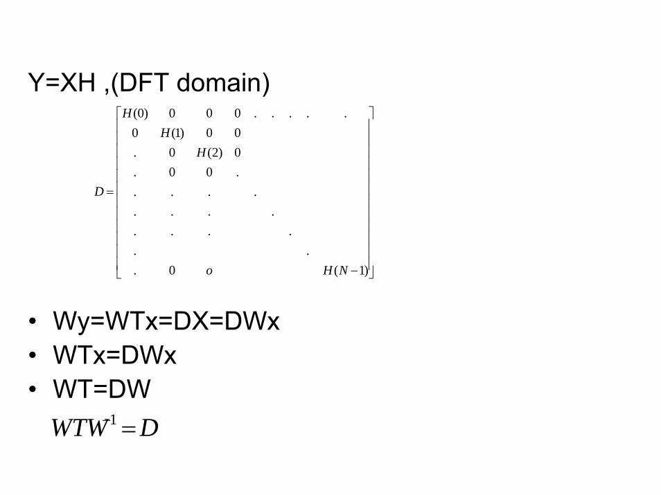
Y=XH ,(DFT domain)

• Wy=WTx=DX=DWx• WTx=DWx• WT=DW

⎥⎥⎥⎥⎥⎥⎥⎥⎥⎥⎥⎥

⎦

⎤

⎢⎢⎢⎢⎢⎢⎢⎢⎢⎢⎢⎢

⎣

⎡

−

=

)1(0...

........

.....00.0)2(0.00)1(0

.....000)0(

NHo

HH

H

D

DWTW =−1

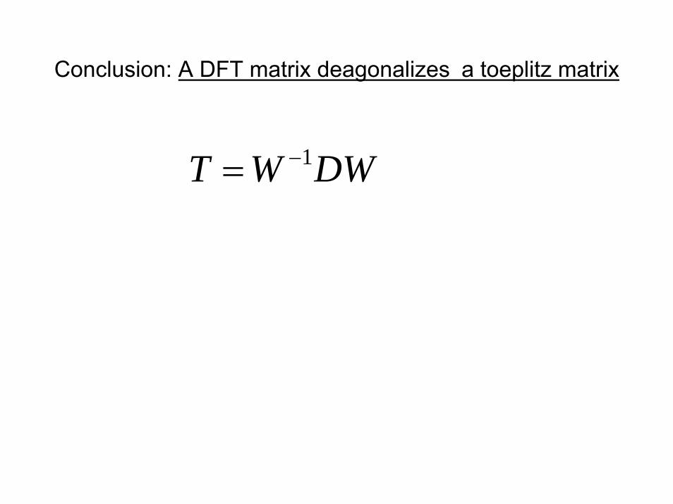
Conclusion: A DFT matrix deagonalizes a toeplitz matrix

DWWT 1−=

Applications:

• FEXT cancellation.The Next slides are taken from prof Henkel’s

presentation.

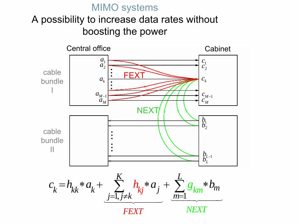
MIMO systemsA possibility to increase data rates without

boosting the power

1a2a

1−MaMa

1c2c

1−McMc

1b2b

1−LbLb

...

CabinetCentral office

FEXT

NEXT

ka kc.........

cablebundle

I

cablebundle

II

11,kj

FEXT

K Lmjk kk k

mj jk

Nk

m

EXT

c bha a gh== ≠

= ∗ + ∗ + ∗∑ ∑14442444314444244443

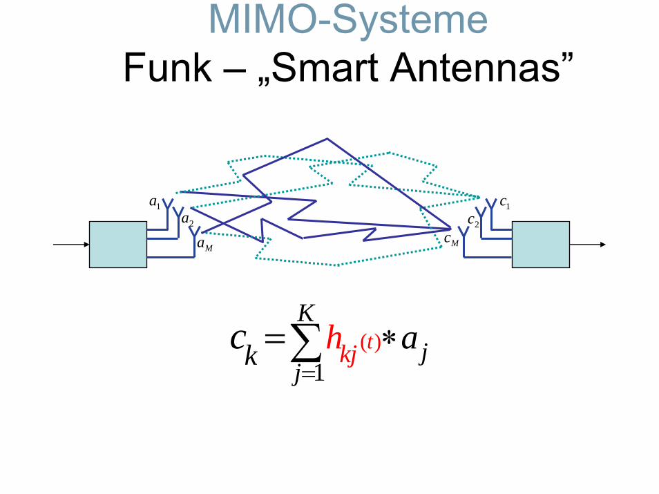
MIMO-SystemeFunk – „Smart Antennas”

1a2a

Ma

1c2c

Mc

( )1

tkjK

jjk h ac=

∗=∑

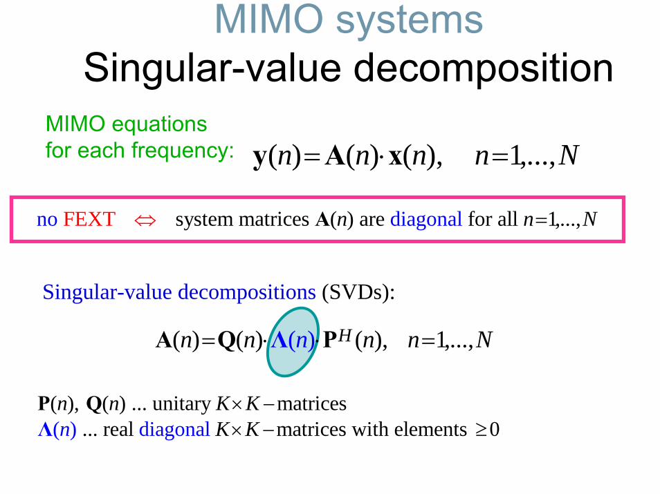
MIMO systemsSingular-value decomposition

MIMO equationsfor each frequency: ( ) ( ) ( ), 1,...,n n n n N= ⋅ =y A x

system matrices ( )no diagonalare for aFEX ll , .,T 1..n n N=⇔ A

Singular-value decompositions (SVDs):

( ) ( ) ( ), 1,( ) ...,Hn n n nn N= ⋅ ⋅ =ΛA Q P

( ), ( ) ... unitary matrices ... ( ) diagonalreal matrices with elements 0n

n n K KK K× −× − ≥

P QΛ

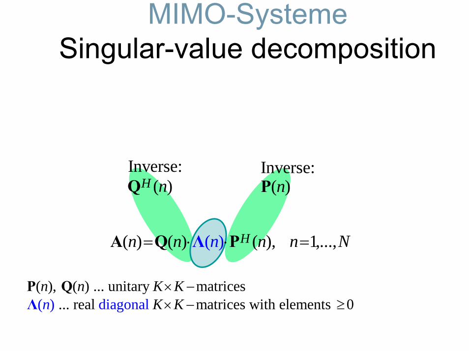
MIMO-SystemeSingular-value decomposition

( ) ( ) ( ), 1,( ) ...,Hn n n nn N= ⋅ ⋅ =Λ P

Inverse: ( )nP

Inverse: ( )H nQ

A Q

( ), ( ) ... unitary matrices ... ( ) diagonalreal matrices with elements 0n

n n K KK K× −× − ≥

P QΛ

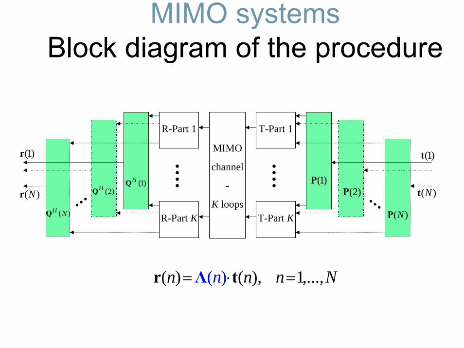
MIMO systemsBlock diagram of the procedure

T-Part 1

T-Part KR-Part K

R-Part 1

MIMO

channel

-

K loops

(1)P(2)P

( )NP

(1)HQ

(1)t

( )Nt

(1)r

( )Nr (2)HQ

( )H NQ

( ) ( ), ( 1,...,)nn n n N= ⋅ =Λr t

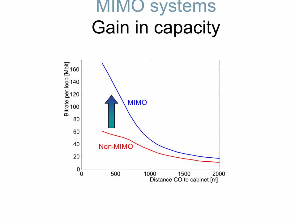
MIMO systemsGain in capacity

0 500 1000 1500 20000

20

40

60

80

100

120

140

160

Distance CO to cabinet [m]

Bitr

ate

per l

oop

[Mbi

t]

MIMO

Non-MIMO

Reference:• http://www.coastal.edu/~jbernick/• http://www.cs.ut.ee/~toomas_l/linalg/lin2/node14.html• http://web.mit.edu/be.400/www/SVD/Singular_Value_Decomposition.htm• http://www.cs.utk.edu/~dongarra/etemplates/node43.html