Embed Size (px)
Citation preview
Principles of Communication Prof. V. Venkata Rao
Indian Institute of Technology Madras
6.1
CHAPTER 6 CHAPTER 6
Digital Transmission of Analog Signals: PCM, DPCM and DM
6.1 Introduction Quite a few of the information bearing signals, such as speech, music,
video, etc., are analog in nature; that is, they are functions of the continuous
variable t and for any t t1= , their value can lie anywhere in the interval, say
A− to A . Also, these signals are of the baseband variety. If there is a channel
that can support baseband transmission, we can easily set up a baseband
communication system. In such a system, the transmitter could be as simple as
just a power amplifier so that the signal that is transmitted could be received at
the destination with some minimum power level, even after being subject to
attenuation during propagation on the channel. In such a situation, even the
receiver could have a very simple structure; an appropriate filter (to eliminate the
out of band spectral components) followed by an amplifier.
If a baseband channel is not available but have access to a passband
channel, (such as ionospheric channel, satellite channel etc.) an appropriate CW
modulation scheme discussed earlier could be used to shift the baseband
spectrum to the passband of the given channel.
Interesting enough, it is possible to transmit the analog information in a
digital format. Though there are many ways of doing it, in this chapter, we shall
explore three such techniques, which have found widespread acceptance. These
are: Pulse Code Modulation (PCM), Differential Pulse Code Modulation (DPCM)
Principles of Communication Prof. V. Venkata Rao
Indian Institute of Technology Madras
6.2
and Delta Modulation (DM). Before we get into the details of these techniques, let
us summarize the benefits of digital transmission. For simplicity, we shall assume
that information is being transmitted by a sequence of binary pulses.
i) During the course of propagation on the channel, a transmitted pulse
becomes gradually distorted due to the non-ideal transmission
characteristic of the channel. Also, various unwanted signals (usually
termed interference and noise) will cause further deterioration of the
information bearing pulse. However, as there are only two types of signals
that are being transmitted, it is possible for us to identify (with a very high
probability) a given transmitted pulse at some appropriate intermediate
point on the channel and regenerate a clean pulse. In this way, we will be
completely eliminating the effect of distortion and noise till the point of
regeneration. (In long-haul PCM telephony, regeneration is done every few
kilometers, with the help of regenerative repeaters.) Clearly, such an
operation is not possible if the transmitted signal was analog because there
is nothing like a reference waveform that can be regenerated.
ii) Storing the messages in digital form and forwarding or redirecting them at a
later point in time is quite simple.
iii) Coding the message sequence to take care of the channel noise,
encrypting for secure communication can easily be accomplished in the
digital domain.
iv) Mixing the signals is easy. All signals look alike after conversion to digital
form independent of the source (or language!). Hence they can easily be
multiplexed (and demultiplexed)
6.2 The PCM system Two basic operations in the conversion of analog signal into the digital is
time discretization and amplitude discretization. In the context of PCM, the former
is accomplished with the sampling operation and the latter by means of
quantization. In addition, PCM involves another step, namely, conversion of
Principles of Communication Prof. V. Venkata Rao
Indian Institute of Technology Madras
6.3
quantized amplitudes into a sequence of simpler pulse patterns (usually binary),
generally called as code words. (The word code in pulse code modulation refers
to the fact that every quantized sample is converted to an R -bit code word.)
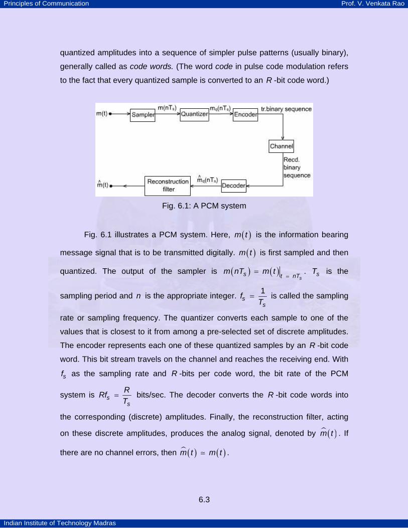
Fig. 6.1: A PCM system
Fig. 6.1 illustrates a PCM system. Here, ( )m t is the information bearing
message signal that is to be transmitted digitally. ( )m t is first sampled and then
quantized. The output of the sampler is ( ) ( )s
s t nTm nT m t
== . sT is the
sampling period and n is the appropriate integer. ss
fT1
= is called the sampling
rate or sampling frequency. The quantizer converts each sample to one of the
values that is closest to it from among a pre-selected set of discrete amplitudes.
The encoder represents each one of these quantized samples by an R -bit code
word. This bit stream travels on the channel and reaches the receiving end. With
sf as the sampling rate and R -bits per code word, the bit rate of the PCM
system is ss
RRfT
= bits/sec. The decoder converts the R -bit code words into
the corresponding (discrete) amplitudes. Finally, the reconstruction filter, acting
on these discrete amplitudes, produces the analog signal, denoted by ( )m t . If
there are no channel errors, then ( ) ( )m t m t .
Principles of Communication Prof. V. Venkata Rao
Indian Institute of Technology Madras
6.4
6.3 Sampling We shall now develop the sampling theorem for lowpass signals.
Theoretical basis of sampling is the Nyquist sampling theorem which is stated
below.
Let a signal ( )x t be band limited to W Hz; that is, ( )X f 0= for f W> .
Let ( ) ( )s
s t nTx nT x t n,
== − ∞ < < ∞ represent the samples of ( )x t at
uniform intervals of sT seconds. If sTW1
2≤ , then it is possible to reconstruct
( )x t exactly from the set of samples, ( ){ }sx nT .
In other words, the sequence of samples ( ){ }sx nT can provide the
complete time behavior of ( )x t . Let ss
fT1
= . Then sf W2= is the minimum
sampling rate for ( )x t . This minimum sampling rate is called the Nyquist rate.
Note: If ( )x t is a sinusoidal signal with frequency f0 , then sf f02> . sf f02= is
not adequate because if the two samples per cycle are at the zero crossings of
the tone, then all the samples will be zero!
We shall consider three cases of sampling, namely, i) ideal impulse
sampling, ii) sampling with rectangular pulses and iii) flat-topped sampling.
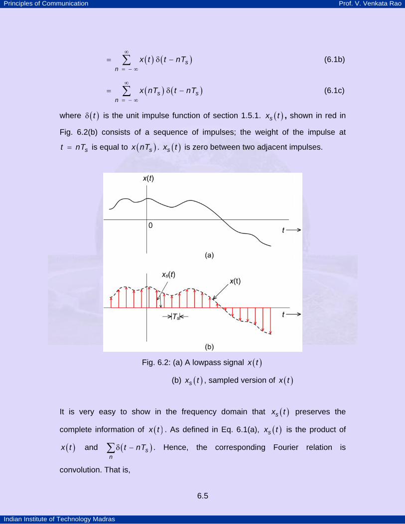
6.3.1 Ideal impulse sampling Consider an arbitrary lowpass signal ( )x t shown in Fig. 6.2(a). Let
( ) ( ) ( )s sn
x t x t t nT∞
= − ∞
⎡ ⎤= δ −⎢ ⎥
⎢ ⎥⎣ ⎦∑ (6.1a)
Principles of Communication Prof. V. Venkata Rao
Indian Institute of Technology Madras
6.5
( ) ( )sn
x t t nT∞
= − ∞= δ −∑ (6.1b)
( ) ( )s sn
x nT t nT∞
= − ∞= δ −∑ (6.1c)
where ( )tδ is the unit impulse function of section 1.5.1. ( )sx t , shown in red in
Fig. 6.2(b) consists of a sequence of impulses; the weight of the impulse at
st nT= is equal to ( )sx nT . ( )sx t is zero between two adjacent impulses.
Fig. 6.2: (a) A lowpass signal ( )x t
(b) ( )sx t , sampled version of ( )x t
It is very easy to show in the frequency domain that ( )sx t preserves the
complete information of ( )x t . As defined in Eq. 6.1(a), ( )sx t is the product of
( )x t and ( )sn
t nTδ −∑ . Hence, the corresponding Fourier relation is
convolution. That is,
Principles of Communication Prof. V. Venkata Rao
Indian Institute of Technology Madras
6.6
( ) ( )ss sn
nX f X f fT T1 ∞
= − ∞
⎡ ⎤⎛ ⎞= ∗ δ −⎢ ⎥⎜ ⎟
⎢ ⎥⎝ ⎠⎣ ⎦∑ (6.2a)
s sn
nX fT T1 ∞
= − ∞
⎛ ⎞= −⎜ ⎟
⎝ ⎠∑ (6.2b)
( )ss n
X f n fT1 ∞
= − ∞= −∑ (6.2c)
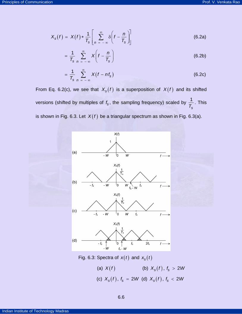
From Eq. 6.2(c), we see that ( )sX f is a superposition of ( )X f and its shifted
versions (shifted by multiples of sf , the sampling frequency) scaled by sT1 . This
is shown in Fig. 6.3. Let ( )X f be a triangular spectrum as shown in Fig. 6.3(a).
Fig. 6.3: Spectra of ( )x t and ( )sx t
(a) ( )X f (b) ( )sX f , sf W2>
(c) ( )sX f , sf W2= (d) ( )sX f , sf W2<
Principles of Communication Prof. V. Venkata Rao
Indian Institute of Technology Madras
6.7
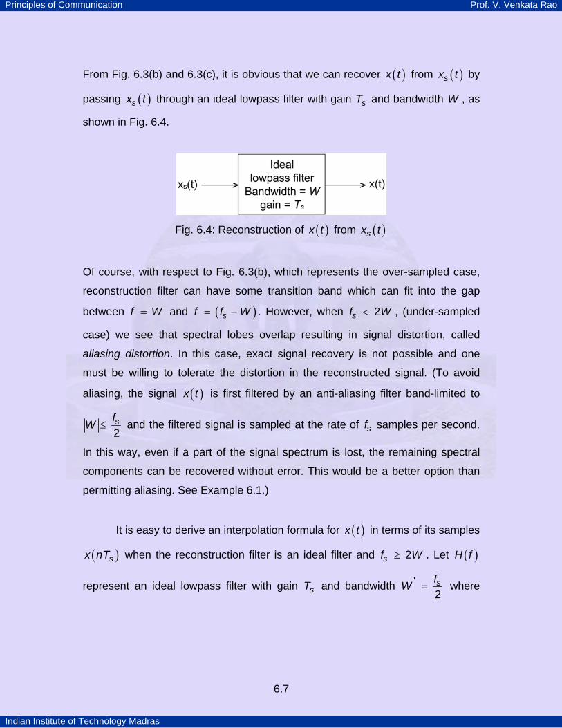
From Fig. 6.3(b) and 6.3(c), it is obvious that we can recover ( )x t from ( )sx t by
passing ( )sx t through an ideal lowpass filter with gain sT and bandwidth W , as
shown in Fig. 6.4.
Fig. 6.4: Reconstruction of ( )x t from ( )sx t
Of course, with respect to Fig. 6.3(b), which represents the over-sampled case,
reconstruction filter can have some transition band which can fit into the gap
between f W= and ( )sf f W= − . However, when sf W2< , (under-sampled
case) we see that spectral lobes overlap resulting in signal distortion, called
aliasing distortion. In this case, exact signal recovery is not possible and one
must be willing to tolerate the distortion in the reconstructed signal. (To avoid
aliasing, the signal ( )x t is first filtered by an anti-aliasing filter band-limited to
sfW2
≤ and the filtered signal is sampled at the rate of sf samples per second.
In this way, even if a part of the signal spectrum is lost, the remaining spectral
components can be recovered without error. This would be a better option than
permitting aliasing. See Example 6.1.)
It is easy to derive an interpolation formula for ( )x t in terms of its samples
( )sx nT when the reconstruction filter is an ideal filter and sf W2≥ . Let ( )H f
represent an ideal lowpass filter with gain sT and bandwidth sfW '2
= where
Principles of Communication Prof. V. Venkata Rao
Indian Institute of Technology Madras
6.8
ss
fW f W2
≤ ≤ − . Then, ( )h t the impulse response of the ideal lowpass filter
is, ( ) ( )sh t T W c W t' '2 sin 2= . As ( ) ( ) ( )sx t x t h t= ∗ and sW T'2 1= , we have
( ) ( ) ( )s sn
x t x nT c W t nT'sin 2∞
= − ∞
⎡ ⎤= −⎢ ⎥⎣ ⎦∑ (6.3a)
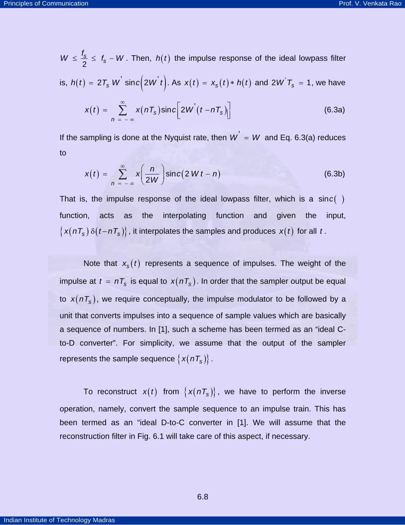
If the sampling is done at the Nyquist rate, then W W' = and Eq. 6.3(a) reduces
to
( ) ( )n
nx t x c W t nW
sin 22
∞
= − ∞
⎛ ⎞= −⎜ ⎟
⎝ ⎠∑ (6.3b)
That is, the impulse response of the ideal lowpass filter, which is a ( )csin
function, acts as the interpolating function and given the input,
( ) ( ){ }s sx nT t nTδ − , it interpolates the samples and produces ( )x t for all t .
Note that ( )sx t represents a sequence of impulses. The weight of the
impulse at st nT= is equal to ( )sx nT . In order that the sampler output be equal
to ( )sx nT , we require conceptually, the impulse modulator to be followed by a
unit that converts impulses into a sequence of sample values which are basically
a sequence of numbers. In [1], such a scheme has been termed as an “ideal C-
to-D converter”. For simplicity, we assume that the output of the sampler
represents the sample sequence ( ){ }sx nT .
To reconstruct ( )x t from ( ){ }sx nT , we have to perform the inverse
operation, namely, convert the sample sequence to an impulse train. This has
been termed as an “ideal D-to-C converter in [1]. We will assume that the
reconstruction filter in Fig. 6.1 will take care of this aspect, if necessary.
Principles of Communication Prof. V. Venkata Rao
Indian Institute of Technology Madras
6.9
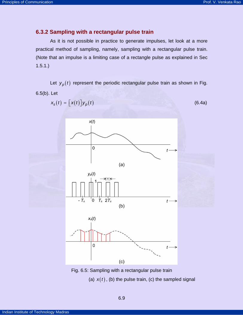
6.3.2 Sampling with a rectangular pulse train As it is not possible in practice to generate impulses, let look at a more
practical method of sampling, namely, sampling with a rectangular pulse train.
(Note that an impulse is a limiting case of a rectangle pulse as explained in Sec
1.5.1.)
Let ( )py t represent the periodic rectangular pulse train as shown in Fig.
6.5(b). Let
( ) ( ) ( )s px t x t y t⎡ ⎤= ⎣ ⎦ (6.4a)
Fig. 6.5: Sampling with a rectangular pulse train
(a) ( )x t , (b) the pulse train, (c) the sampled signal
Principles of Communication Prof. V. Venkata Rao
Indian Institute of Technology Madras
6.10
Then, ( ) ( ) ( )s pX f X f Y f= ∗ (6.4b)
But, from exercise 1.1, we have
( ) ( ) ( )p s ssn
Y f c n f f n fT
sin∞
= − ∞
⎛ ⎞τ= τ δ −⎜ ⎟
⎝ ⎠∑
Hence,
( ) ( ) ( )s s ss n
X f c n f X f n fT
sin∞
= − ∞
τ= τ −∑ (6.5)
( ) ( ) ( )s ss s s
c X f f X f c X f fT T T
sin sin⎡ ⎤⎛ ⎞ ⎛ ⎞τ τ τ
= ⋅⋅ + + + + − + ⋅⋅⎢ ⎥⎜ ⎟ ⎜ ⎟⎢ ⎥⎝ ⎠ ⎝ ⎠⎣ ⎦
As s
ncT
sin⎛ ⎞τ⎜ ⎟⎝ ⎠
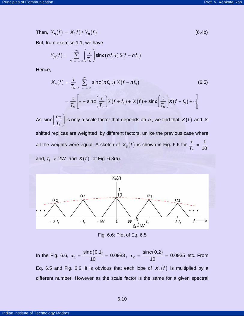
is only a scale factor that depends on n , we find that ( )X f and its
shifted replicas are weighted by different factors, unlike the previous case where
all the weights were equal. A sketch of ( )sX f is shown in Fig. 6.6 for sT
110
τ=
and, sf W2> and ( )X f of Fig. 6.3(a).
Fig. 6.6: Plot of Eq. 6.5
In the Fig. 6.6, ( )c1
sin 0.10.0983
10α = = , ( )c
2sin 0.2
0.093510
α = = etc. From
Eq. 6.5 and Fig. 6.6, it is obvious that each lobe of ( )sX f is multiplied by a
different number. However as the scale factor is the same for a given spectral
Principles of Communication Prof. V. Venkata Rao
Indian Institute of Technology Madras
6.11
lobe of ( )sX f , there is no distortion. Hence ( )x t can be recovered from ( )sx t of
Eq. 6.4(a).
From Fig. 6.5(c), we see that during the time interval τ , when ( )py t 1= ,
( )sx t follows the shape of ( )x t . Hence, this method of sampling is also called
exact scanning.
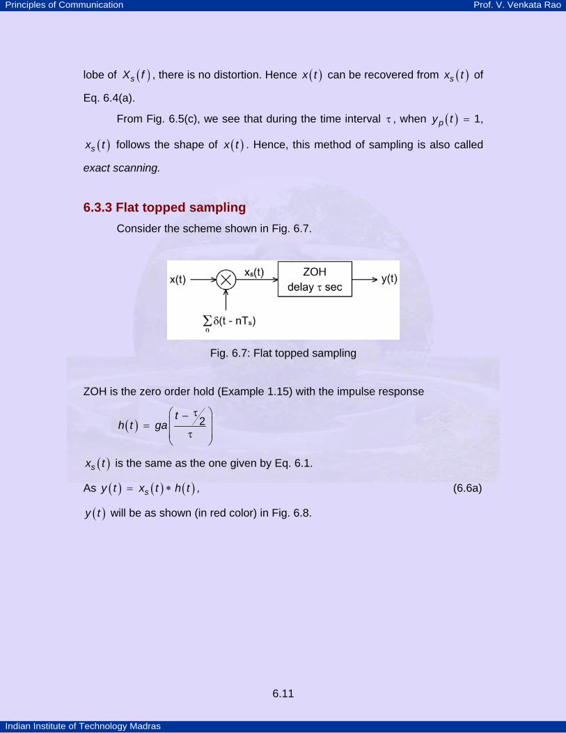
6.3.3 Flat topped sampling Consider the scheme shown in Fig. 6.7.
Fig. 6.7: Flat topped sampling
ZOH is the zero order hold (Example 1.15) with the impulse response
( )t
h t ga 2τ⎛ ⎞−
⎜ ⎟=τ⎜ ⎟
⎝ ⎠
( )sx t is the same as the one given by Eq. 6.1.
As ( ) ( ) ( )sy t x t h t= ∗ , (6.6a)
( )y t will be as shown (in red color) in Fig. 6.8.
Principles of Communication Prof. V. Venkata Rao
Indian Institute of Technology Madras
6.12
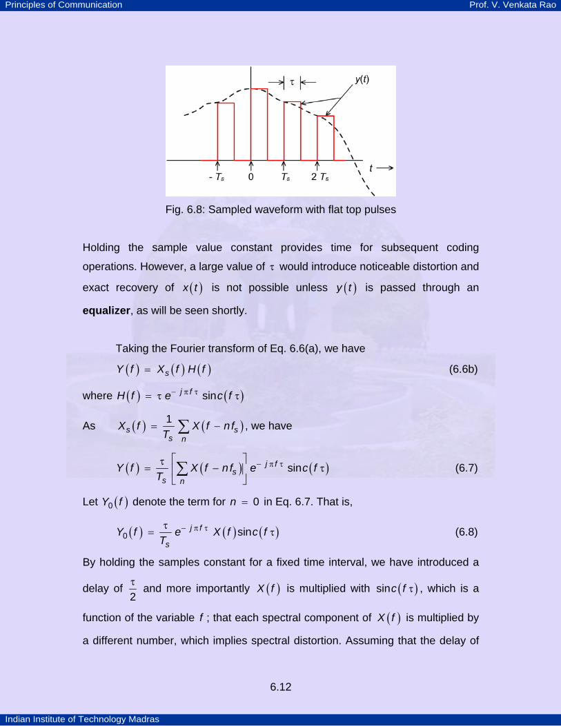
Fig. 6.8: Sampled waveform with flat top pulses
Holding the sample value constant provides time for subsequent coding
operations. However, a large value of τ would introduce noticeable distortion and
exact recovery of ( )x t is not possible unless ( )y t is passed through an
equalizer, as will be seen shortly.
Taking the Fourier transform of Eq. 6.6(a), we have
( ) ( ) ( )sY f X f H f= (6.6b)
where ( ) ( )j fH f e c fsin− π τ= τ τ
As ( ) ( )s ss n
X f X f n fT1
= −∑ , we have
( ) ( ) ( )j fs
s nY f X f n f e c f
Tsin− π τ⎡ ⎤τ
= − τ⎢ ⎥⎣ ⎦∑ (6.7)
Let ( )Y f0 denote the term for n 0= in Eq. 6.7. That is,
( ) ( ) ( )j f
sY f e X f c f
T0 sin− π ττ= τ (6.8)
By holding the samples constant for a fixed time interval, we have introduced a
delay of 2τ and more importantly ( )X f is multiplied with ( )c fsin τ , which is a
function of the variable f ; that each spectral component of ( )X f is multiplied by
a different number, which implies spectral distortion. Assuming that the delay of
Principles of Communication Prof. V. Venkata Rao
Indian Institute of Technology Madras
6.13
2τ is not serious, we have to equalize the amplitude distortion caused and this
can be achieved by multiplying ( )Y f0 by ( )H f1 . Of course, if
sT0.1τ
< , then the
amplitude distortion may not be significant. The distortion caused by holding the
pulses constant is referred to as the aperture effect.
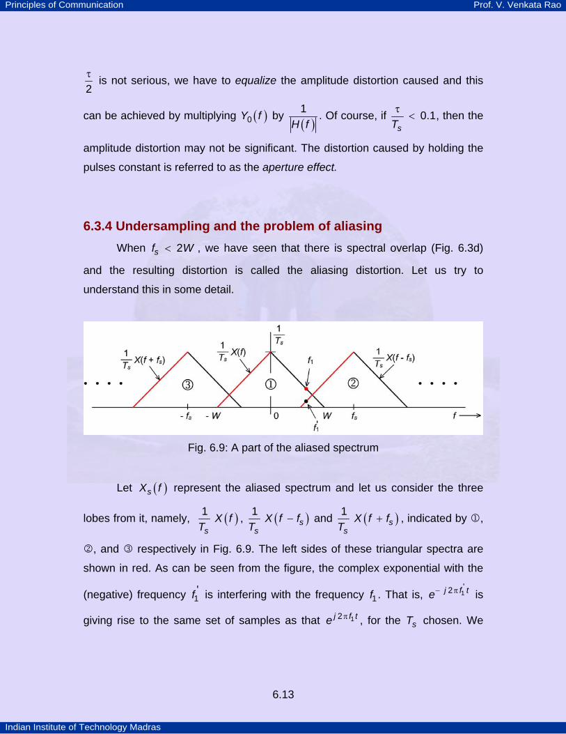
6.3.4 Undersampling and the problem of aliasing When sf W2< , we have seen that there is spectral overlap (Fig. 6.3d)
and the resulting distortion is called the aliasing distortion. Let us try to
understand this in some detail.
Fig. 6.9: A part of the aliased spectrum
Let ( )sX f represent the aliased spectrum and let us consider the three
lobes from it, namely, ( )s
X fT1 , ( )s
sX f f
T1
− and ( )ss
X f fT1
+ , indicated by 1,
2, and 3 respectively in Fig. 6.9. The left sides of these triangular spectra are
shown in red. As can be seen from the figure, the complex exponential with the
(negative) frequency f1' is interfering with the frequency f1. That is, j f te 1
'2− π is
giving rise to the same set of samples as that j f te 12π , for the sT chosen. We
Principles of Communication Prof. V. Venkata Rao
Indian Institute of Technology Madras
6.14
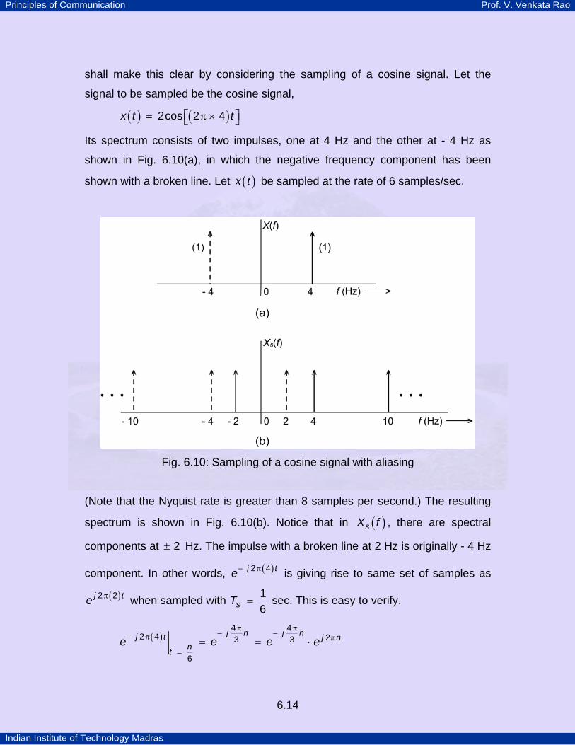
shall make this clear by considering the sampling of a cosine signal. Let the
signal to be sampled be the cosine signal,
( ) ( )x t t2cos 2 4⎡ ⎤= π ×⎣ ⎦
Its spectrum consists of two impulses, one at 4 Hz and the other at - 4 Hz as
shown in Fig. 6.10(a), in which the negative frequency component has been
shown with a broken line. Let ( )x t be sampled at the rate of 6 samples/sec.
Fig. 6.10: Sampling of a cosine signal with aliasing
(Note that the Nyquist rate is greater than 8 samples per second.) The resulting
spectrum is shown in Fig. 6.10(b). Notice that in ( )sX f , there are spectral
components at 2± Hz. The impulse with a broken line at 2 Hz is originally - 4 Hz
component. In other words, ( )j te 2 4− π is giving rise to same set of samples as
( )j te 2 2π when sampled with sT 16
= sec. This is easy to verify.
( ) j n j nj t j nnt
e e e e4 4
2 4 23 3
6
π π− −− π π
== = ⋅
Principles of Communication Prof. V. Venkata Rao
Indian Institute of Technology Madras
6.15
( )j n j tnt
e e2
2 23
6
ππ
== =
Similarly, the set of values obtained from j te 8π for st nT= is the same as those
from j te 4− π (Notice that in Fig. 6.10(b), there is a solid line at f 2= − ). In other
words, a 4 Hz cosine signal becomes an alias of 2 Hz cosine signal. If there were
to be a 2 Hz component in ( )X f , the 4 Hz will interfere with the 2 Hz component
and thereby leading to distortion due to under sampling. In fact, a frequency
component at f f2= is the alias of another lower frequency component at f f1=
if sf k f f2 1= ± , where k is an integer. Hence, with sf 6= , we find that the 4 Hz
component is an alias the of 2 Hz component, because 4 = 6 - 2. Similarly,
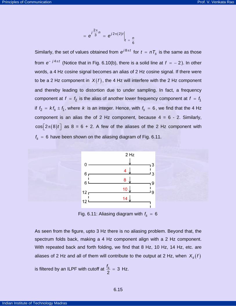
( ) tcos 2 8⎡ ⎤π⎣ ⎦ as 8 = 6 + 2. A few of the aliases of the 2 Hz component with
sf 6= have been shown on the aliasing diagram of Fig. 6.11.
Fig. 6.11: Aliasing diagram with sf 6=
As seen from the figure, upto 3 Hz there is no aliasing problem. Beyond that, the
spectrum folds back, making a 4 Hz component align with a 2 Hz component.
With repeated back and forth folding, we find that 8 Hz, 10 Hz, 14 Hz, etc. are
aliases of 2 Hz and all of them will contribute to the output at 2 Hz, when ( )sX f
is filtered by an ILPF with cutoff at sf 32
= Hz.
Principles of Communication Prof. V. Venkata Rao
Indian Institute of Technology Madras
6.16
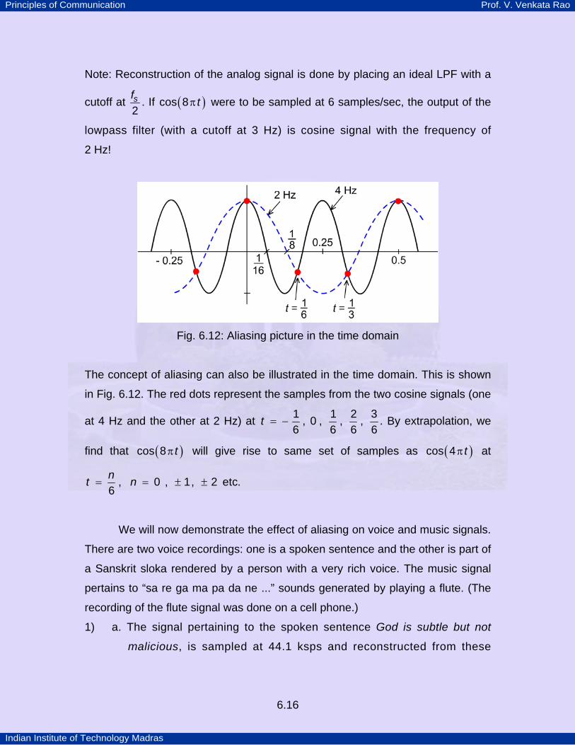
Note: Reconstruction of the analog signal is done by placing an ideal LPF with a
cutoff at sf2
. If ( )tcos 8π were to be sampled at 6 samples/sec, the output of the
lowpass filter (with a cutoff at 3 Hz) is cosine signal with the frequency of
2 Hz!
Fig. 6.12: Aliasing picture in the time domain
The concept of aliasing can also be illustrated in the time domain. This is shown
in Fig. 6.12. The red dots represent the samples from the two cosine signals (one
at 4 Hz and the other at 2 Hz) at t 1 1 2 3, 0 , , ,6 6 6 6
= − . By extrapolation, we
find that ( )tcos 8π will give rise to same set of samples as ( )tcos 4π at
nt n, 0 , 1, 2 etc.6
= = ± ±
We will now demonstrate the effect of aliasing on voice and music signals.
There are two voice recordings: one is a spoken sentence and the other is part of
a Sanskrit sloka rendered by a person with a very rich voice. The music signal
pertains to “sa re ga ma pa da ne ...” sounds generated by playing a flute. (The
recording of the flute signal was done on a cell phone.)
1) a. The signal pertaining to the spoken sentence God is subtle but not
malicious, is sampled at 44.1 ksps and reconstructed from these
Principles of Communication Prof. V. Venkata Rao
Indian Institute of Technology Madras
6.17
samples.
b. The reconstructed signal after down sampling by a factor of 8.
2) a. Last line of a Sanskrit sloka. Sampling rate 44.1 ksps.
b. Reconstructed signal after down sampling by a factor of 8.
c. Reconstructed signal after down sampling by a factor of 12.
3) a. Flute music sampled at 8 ksps.
b. Reconstructed signal after down sampling by a factor of 2.
0 1000 2000 3000 4000 5000 60000
100
200
300
400
500
600
frequency (Hz)
mag
nitu
de
Magnitude spectrum of original version
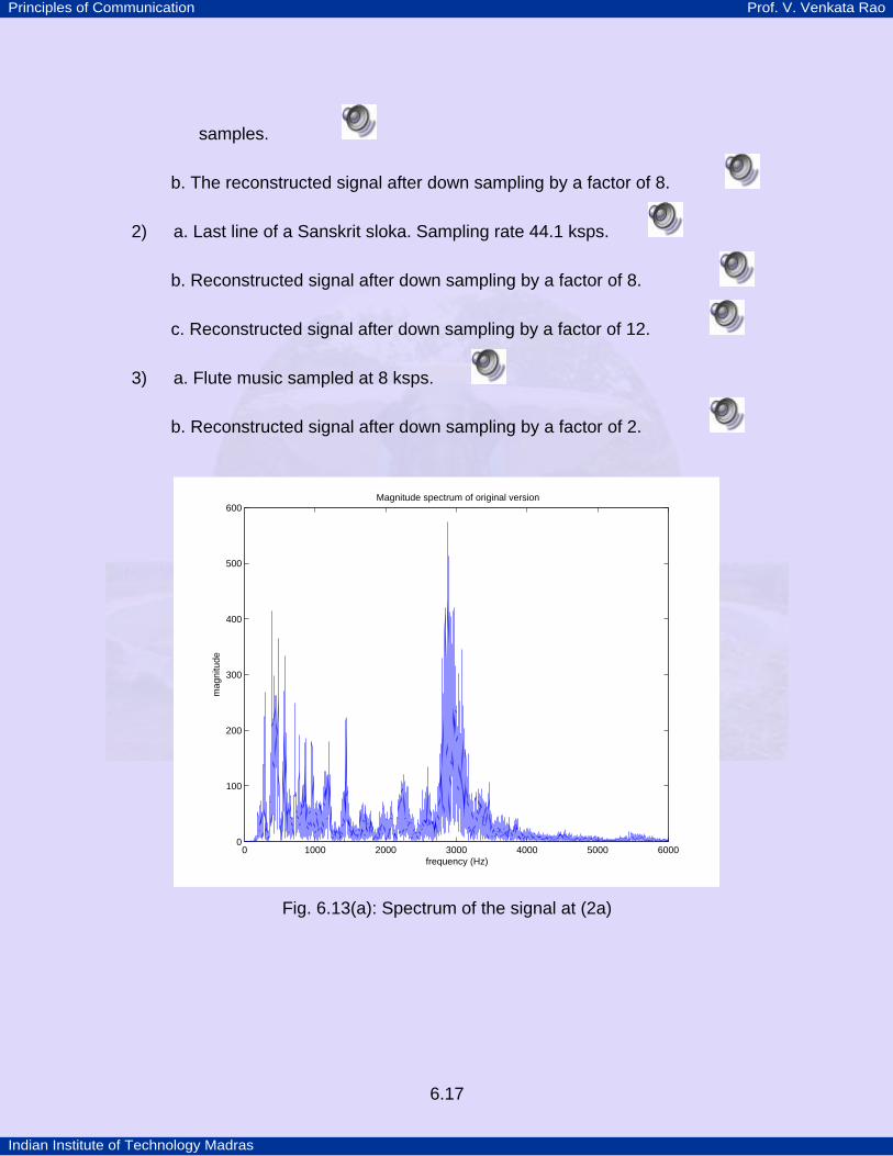
Fig. 6.13(a): Spectrum of the signal at (2a)
Principles of Communication Prof. V. Venkata Rao
Indian Institute of Technology Madras
6.18
0 500 1000 1500 2000 25000
20
40
60
80
100
120
140
160
180
200
frequency (Hz)
mag
nitu
de
Magnitude spectrum of aliased version (downsampling factor = 8)
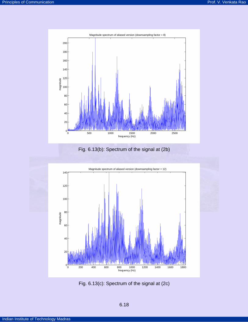
Fig. 6.13(b): Spectrum of the signal at (2b)
0 200 400 600 800 1000 1200 1400 1600 18000
20
40
60
80
100
120
140
frequency (Hz)
mag
nitu
de
Magnitude spectrum of aliased version (downsampling factor = 12)
Fig. 6.13(c): Spectrum of the signal at (2c)
Principles of Communication Prof. V. Venkata Rao
Indian Institute of Technology Madras
6.19
With respect to 1b, we find that there is noticeable distortion when the word
malicious is being uttered. As this word gives rise to spectral components at the
higher end of the voice spectrum, fold back of the spectrum results in severe
aliasing. Some distortion is to be found elsewhere in the sentence.
Aliasing effect is quite evident in the voice outputs 2(b) and (c). (It is much
more visible in 2(c).) We have also generated the spectral plots corresponding to
the signals at 2(a), (b) and (c). These are shown in Fig. 6.13(a), (b) and (c). From
Fig. 6.13(a), we see that the voice spectrum extends all the way upto 6 kHz with
strong spectral components in the ranges 200 Hz to 1500 Hz and 2700 Hz to
3300 Hz. (Sampling frequency used is 44.1 kHz.)
Fig. 6.13(b) corresponds to the down sampled (by a factor of 8) version of
(a); that is, sampling frequency is about 5500 samples/sec. Spectral components
above 2750 Hz will get folded over. Because of this, we find strong spectral
components in the range 2500-2750 Hz.
Fig. 6.13(c) corresponds to a sampling rate of 3600 samples/sec. Now
spectrum fold over takes place with respect to 1800 Hz and this can be easily
seen in Fig. 6.13(c).
As it is difficult to get rid of aliasing once it sets in, it is better to pass the
signal through an anti-aliasing filter with cutoff at sf2
and then sample the output
of the filter at the rate of sf samples per second. This way, we are sure that all
the spectral components upto sff2
≤ will be preserved in the sampling process.
Example 6.1 illustrates that the reconstruction mean square error is less than or
equal to the error resulting from sampling without the anti-aliasing filter.
Principles of Communication Prof. V. Venkata Rao
Indian Institute of Technology Madras
6.20
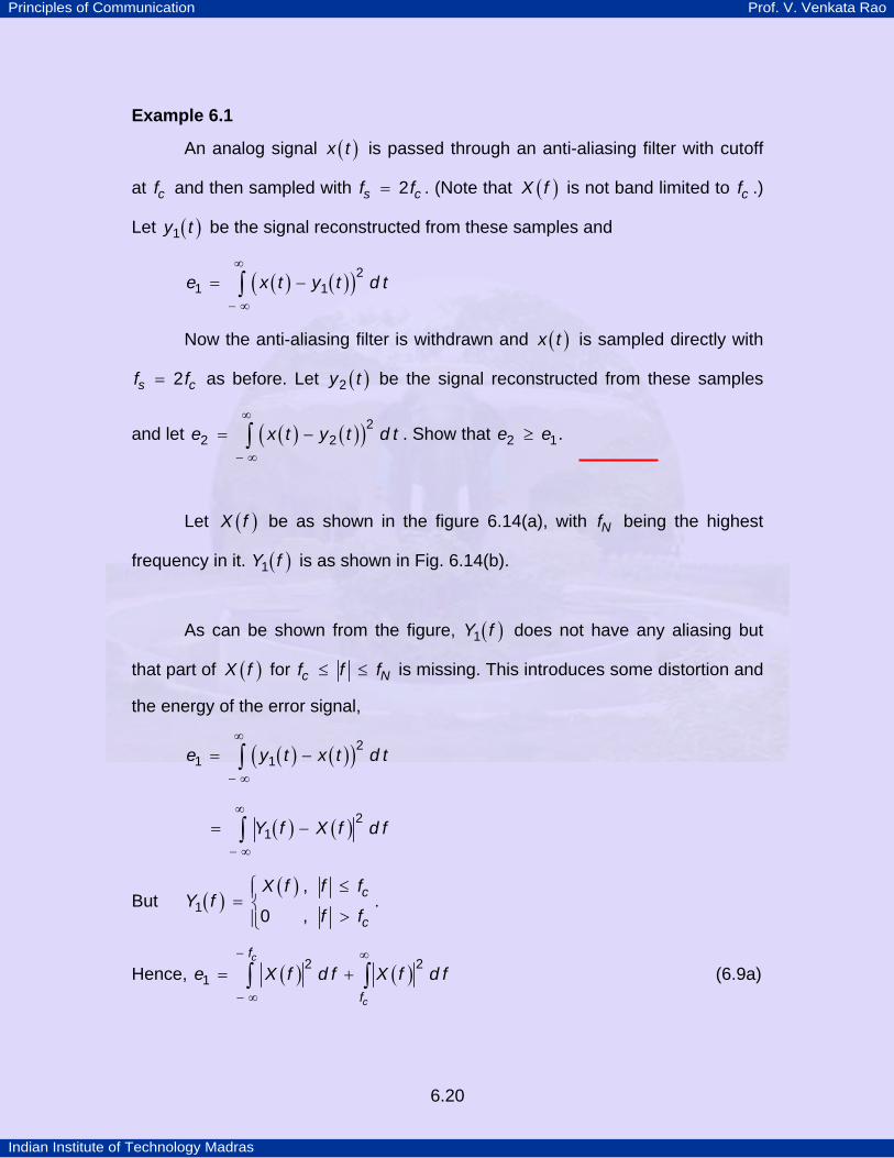
Example 6.1
An analog signal ( )x t is passed through an anti-aliasing filter with cutoff
at cf and then sampled with s cf f2= . (Note that ( )X f is not band limited to cf .)
Let ( )y t1 be the signal reconstructed from these samples and
( ) ( )( )e x t y t d t21 1
∞
− ∞
= −∫
Now the anti-aliasing filter is withdrawn and ( )x t is sampled directly with
s cf f2= as before. Let ( )y t2 be the signal reconstructed from these samples
and let ( ) ( )( )e x t y t d t22 2
∞
− ∞
= −∫ . Show that e e2 1≥ .
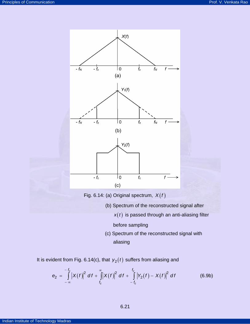
Let ( )X f be as shown in the figure 6.14(a), with Nf being the highest
frequency in it. ( )Y f1 is as shown in Fig. 6.14(b).
As can be shown from the figure, ( )Y f1 does not have any aliasing but
that part of ( )X f for c Nf f f≤ ≤ is missing. This introduces some distortion and
the energy of the error signal,
( ) ( )( )e y t x t d t21 1
∞
− ∞
= −∫
( ) ( )Y f X f d f21
∞
− ∞
= −∫
But ( )( ) c
c
X f f fY f
f f1,
0 ,
⎧ ≤⎪= ⎨>⎪⎩
.
Hence, ( ) ( )c
c
f
f
e X f d f X f d f2 21
− ∞
− ∞
= +∫ ∫ (6.9a)
Principles of Communication Prof. V. Venkata Rao
Indian Institute of Technology Madras
6.21
Fig. 6.14: (a) Original spectrum, ( )X f
(b) Spectrum of the reconstructed signal after
( )x t is passed through an anti-aliasing filter
before sampling
(c) Spectrum of the reconstructed signal with
aliasing
It is evident from Fig. 6.14(c), that ( )y t2 suffers from aliasing and
( ) ( ) ( ) ( )c c
c c
f f
f f
e X f d f X f d f Y f X f d f2 2 22 2
− ∞
− ∞ −
= + + −∫ ∫ ∫ (6.9b)
Principles of Communication Prof. V. Venkata Rao
Indian Institute of Technology Madras
6.22
But ( ) ( )Y f X f2 ≠ for cf f≤ . Comparing Eqs. 6.9(a) and (b), we find that Eq.
6.9(b) has an extra term which is greater or equal to zero. Hence e e2 1≥ .
Example 6.2 Find the Nyquist sampling rate for the signal
( ) ( ) ( )x t c t c t2sin 200 sin 1000= .
( )c tsin 200 has a rectangular spectrum in the interval f 100≤ Hz and
( ) ( ) ( )c t c t c t2sin 1000 sin 1000 sin 1000⎡ ⎤ ⎡ ⎤= ⎣ ⎦ ⎣ ⎦ has a triangular spectrum in the
frequency range f 1000≤ Hz. Hence ( )X f has spectrum confined to the range
f 1100≤ Hz. This implies the Nyquist rate is 2200 samples/sec.
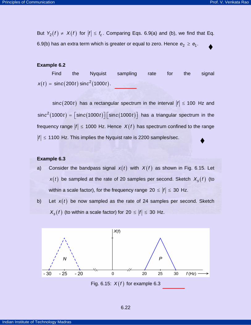
Example 6.3
a) Consider the bandpass signal ( )x t with ( )X f as shown in Fig. 6.15. Let
( )x t be sampled at the rate of 20 samples per second. Sketch ( )sX f (to
within a scale factor), for the frequency range f20 30≤ ≤ Hz.
b) Let ( )x t be now sampled as the rate of 24 samples per second. Sketch
( )sX f (to within a scale factor) for f20 30≤ ≤ Hz.
Fig. 6.15: ( )X f for example 6.3

Principles of Communication Prof. V. Venkata Rao
Indian Institute of Technology Madras
6.23
a) Let P denote ( )X f for f 0≥ and let N denote ( )X f for f 0< . (N is
shown with a broken line.) Consider the right shifts of ( )X f in multiples of
20 Hz, which is the sampling frequency. Then P will be shifted away from
the frequency interval of interest. We have to only check whether shifted N
can contribute to spectrum in the interval f20 30≤ ≤ . It is easy to see
that this will not happen. This implies, in ( )sX f , spectrum has the same
shape as ( )X f for f20 30≤ ≤ . This is also true for the left shifts of ( )X f .
That is, for f20 30≤ ≤ , ( )sX f , to within a scale factor, is the same as
( )X f .
b) Let sf 24= . Consider again right shifts. When N is shifted to the right by
sf2 48= , it will occupy the interval ( )30 48 18− + = to ( )20 48 28− + = .
That is, we have the situation shown in Fig. 6.16.
Fig. 6.16: The two lobes contributing to the spectrum for f20 30≤ ≤
Principles of Communication Prof. V. Venkata Rao
Indian Institute of Technology Madras
6.24
Let the sum of (a) and (b) be denoted by ( )Y f . Then, ( )Y f is as shown in Fig.
6.17.
Fig. 6.17: Spectrum for f20 30≤ ≤ when sf 24=
For f30 20− ≤ ≤ − , ( )Y f is the mirror image of the spectrum shown in Fig.
6.17. Notice that for the bandpass signal, increasing sf has resulted in the
distortion of the original spectrum.
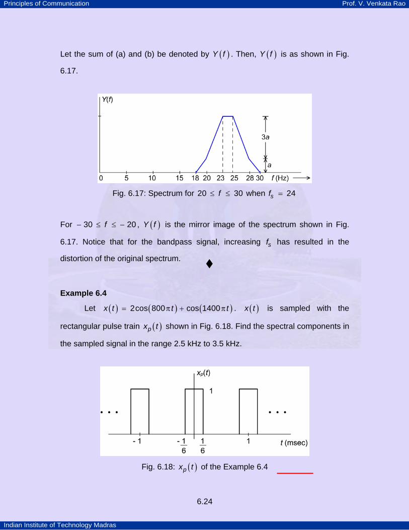
Example 6.4
Let ( ) ( ) ( )x t t t2cos 800 cos 1400= π + π . ( )x t is sampled with the
rectangular pulse train ( )px t shown in Fig. 6.18. Find the spectral components in
the sampled signal in the range 2.5 kHz to 3.5 kHz.
Fig. 6.18: ( )px t of the Example 6.4
Principles of Communication Prof. V. Venkata Rao
Indian Institute of Technology Madras
6.25
( )X f has spectral components at 400± Hz and 700± Hz. The impulses
in ( )pX f occur at 1± kHz, 2± kHz, 4± kHz, 5± kHz, etc. (Note the absence
of spectral lines in ( )pX f at f 3= ± kHz, 6± kHz, etc.) Convolution of ( )X f
with the impulses in ( )pX f at 2 kHz will give rise to spectral components at 2.4
kHz and 2.7 kHz. Similarly, we will have spectral components at ( )4 0.4 3.6− =
kHz and ( )4 0.7 3.3− = kHz. Hence, in the range 2.5 kHz to 3.5 kHz, sampled
spectrum will have two components, namely, at 2.7 kHz and 3.3 kHz.
Exercise 6.1
A sinusoidal signal ( ) ( )x t A t3cos 2 10⎡ ⎤= π ×⎣ ⎦ is sampled with a
uniform impulse train at the rate of 1500 samples per second. The sampled
signal is passed through an ideal lowpass filter with a cutoff at 750 Hz. By
sketching the appropriate spectra, show that the output is a sinusoid at 500
Hz. What would be the output if the cutoff frequency of the LPF is 950 Hz?
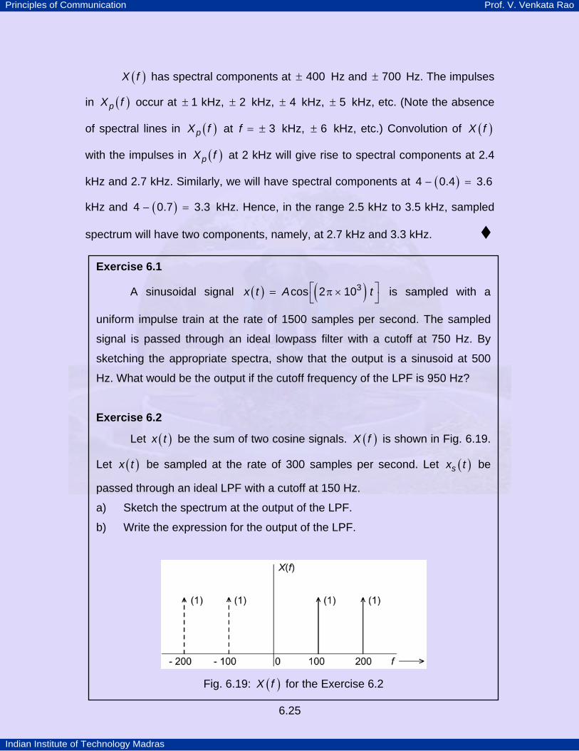
Exercise 6.2
Let ( )x t be the sum of two cosine signals. ( )X f is shown in Fig. 6.19.
Let ( )x t be sampled at the rate of 300 samples per second. Let ( )sx t be
passed through an ideal LPF with a cutoff at 150 Hz.
a) Sketch the spectrum at the output of the LPF.
b) Write the expression for the output of the LPF.
Fig. 6.19: ( )X f for the Exercise 6.2
Principles of Communication Prof. V. Venkata Rao
Indian Institute of Technology Madras
6.26
6.4 Quantization 6.4.1 Uniform quantization An analog signal, even it is limited in its peak-to-peak excursion, can in
general assume any value within this permitted range. If such a signal is
sampled, say at uniform time intervals, the number of different values the
samples can assume is unlimited. Any human sensor (such as ear or eye) as the
ultimate receiver can only detect finite intensity differences. If the receiver is not
able to distinguish between two sample amplitudes, say v1 and v2 such that
v v1 2 2∆
− < , then we can have a set of discrete amplitude levels separated by
∆ and the original signal with continuous amplitudes, may be approximated by a
signal constructed of discrete amplitudes selected on a minimum error basis from
an available set. This ensures that the magnitude of the error between the actual
sample and its approximation is within 2∆ and this difference is irrelevant from the
receiver point of view. The realistic assumption that a signal ( )m t is (essentially)
limited in its peak-to-peak variations and any two adjacent (discrete) amplitude
levels are separated by ∆ will result in a finite number (say L ) of discrete amplitudes for the signal.
The process of conversion of analog samples of a signal into a set of
discrete (digital) values is called quantization. Note however, that quantization is
inherently information lossy. For a given peak-to-peak range of the analog signal,
smaller the value of ∆ , larger is the number of discrete amplitudes and hence,
finer is the quantization. Sometimes one may resort to somewhat coarse
quantization, which can result in some noticeable distortion; this may, however
be acceptable to the end receiver.
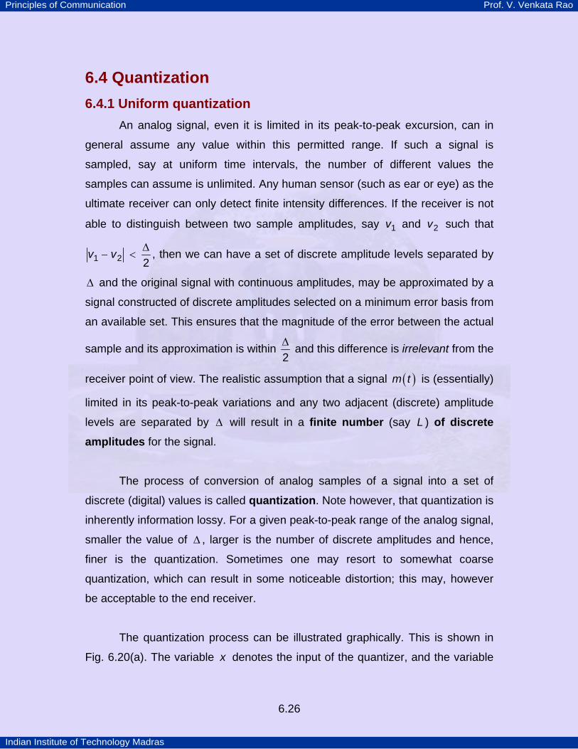
The quantization process can be illustrated graphically. This is shown in
Fig. 6.20(a). The variable x denotes the input of the quantizer, and the variable
Principles of Communication Prof. V. Venkata Rao
Indian Institute of Technology Madras
6.27
y represents the output. As can be seen from the figure, the quantization
process implies that a straight line relation between the input and output (broken
line through the origin) of a linear continuous system is replaced by a staircase
characteristic.
The difference between two adjacent discrete values, ∆ , is called the step
size of the quantizer. The error signal, that is, difference between the input and
the quantizer output has been shown in Fig. 6.20(b). We see from the figure that
the magnitude of the error is always less than or equal to 2∆ . (We are assuming
that the input to the quantizer is confined to the range 7 7to2 2∆ ∆⎛ ⎞−⎜ ⎟
⎝ ⎠.
Fig. 6.20: (a) Quantizer characteristic of a uniform quantizer (b) Error signal
Principles of Communication Prof. V. Venkata Rao
Indian Institute of Technology Madras
6.28
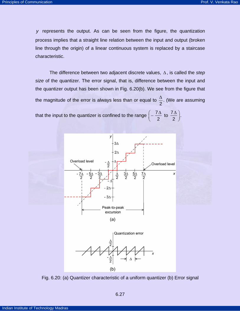
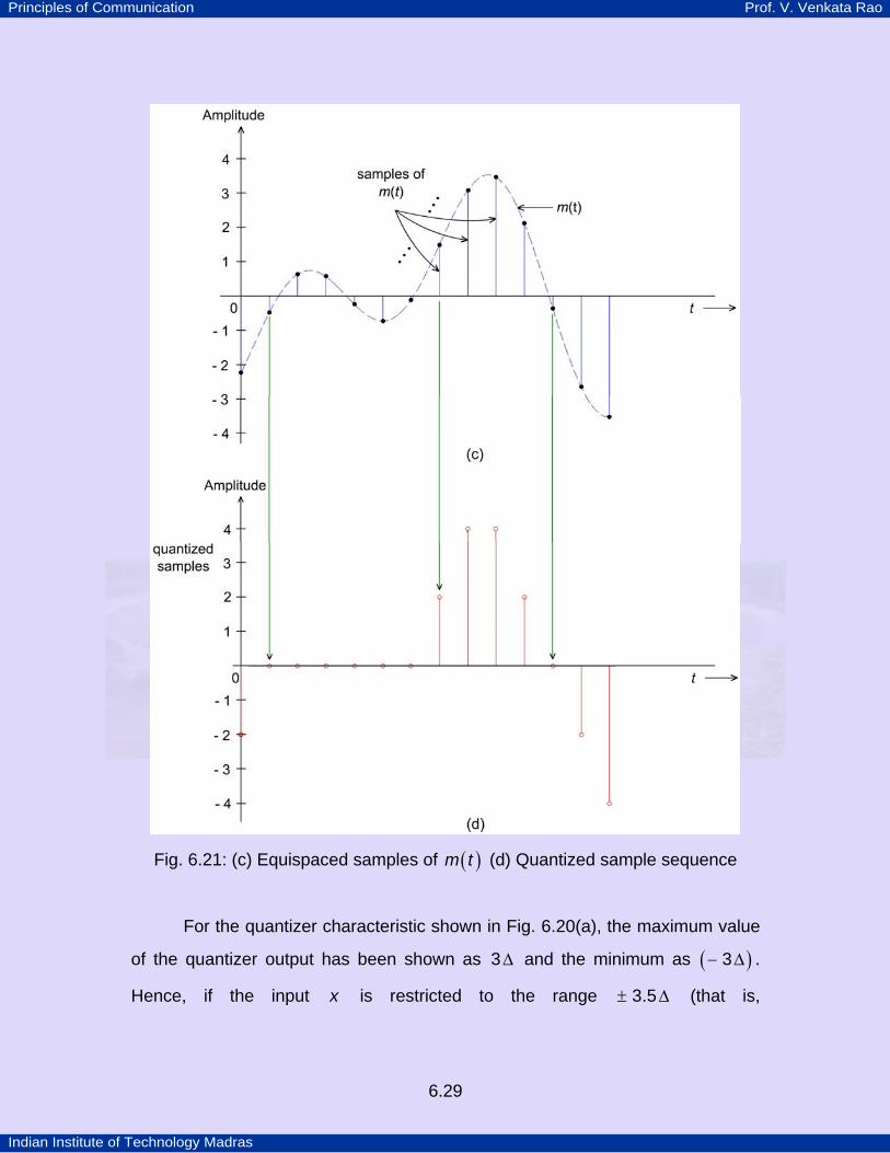
Let the signal ( )m t , shown in Fig. 6.21(a), be the input to a quantizer with
the quantization levels at 0, 2 and 4± ± . Then, ( )qm t , the quantizer output is
the waveform shown in red. Fig. 6.21(b) shows the error signal
( ) ( ) ( )qe t m t m t= − as a function of time. Because of the noise like appearance
of ( )e t , it is a common practice to refer to it as the quantization noise. If the input
to the quantizer is the set of (equispaced) samples of ( )m t , shown in Fig.
6.21(c), then the quantizer output is the sample sequence shown at (d).
Fig. 6.21: (a) An analog signal and its quantized version (b) The error signal
Principles of Communication Prof. V. Venkata Rao
Indian Institute of Technology Madras
6.29
Fig. 6.21: (c) Equispaced samples of ( )m t (d) Quantized sample sequence
For the quantizer characteristic shown in Fig. 6.20(a), the maximum value
of the quantizer output has been shown as 3∆ and the minimum as ( )3− ∆ .
Hence, if the input x is restricted to the range 3.5± ∆ (that is,
Principles of Communication Prof. V. Venkata Rao
Indian Institute of Technology Madras
6.30
∆ ⎞= − ≤ ⎟⎠
x xmax min72
, the quantization error magnitude is less than or equal to
2∆ . Hence, (for the quantizer shown), 3.5± ∆ is treated as the overload level.
The quantizer output of Fig. 6.20(a) can assume values of the form iH∆ ⋅
where iH 0, 1, 2,± = ⋅ ⋅ ⋅ . A quantizer having this input-output relation is said to
be of the mid-tread type, because the origin lies in the middle of a tread of a
staircase like graph.
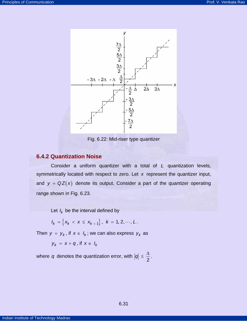
A quantizer whose output levels are given by iH2∆ , where
iH 1, 3, 5,± = ⋅ ⋅ ⋅ is referred to as the mid-riser type. In this case, the origin lies
in the middle of the rising part of the staircase characteristic as shown in Fig.
6.22. Note that overload level has not been indicated in the figure. The difference
in performance of these two quantizer types will be brought out in the next sub-
section in the context of idle-channel noise. The two quantizer types described
above, fall under the category of uniform quantizers because the step size ∆ of
the quantizer is constant. A non-uniform quantizer is characterized by a variable
step size. This topic is taken up in the sub-section 6.4.3.
Principles of Communication Prof. V. Venkata Rao
Indian Institute of Technology Madras
6.31
Fig. 6.22: Mid-riser type quantizer
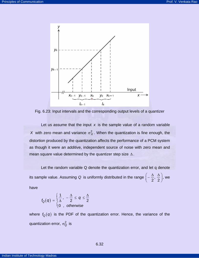
6.4.2 Quantization Noise Consider a uniform quantizer with a total of L quantization levels,
symmetrically located with respect to zero. Let x represent the quantizer input,
and ( )y Q Z x= denote its output. Consider a part of the quantizer operating
range shown in Fig. 6.23.
Let kI be the interval defined by
{ }k k kI x x x k L1 , 1, 2, ,+= < ≤ = ⋅ ⋅ ⋅ .
Then ky y= , if kx I∈ ; we can also express ky as
ky x q= + , if kx I∈
where q denotes the quantization error, with q2∆
≤ .
Principles of Communication Prof. V. Venkata Rao
Indian Institute of Technology Madras
6.32
Fig. 6.23: Input intervals and the corresponding output levels of a quantizer
Let us assume that the input x is the sample value of a random variable
X with zero mean and variance X2σ . When the quantization is fine enough, the
distortion produced by the quantization affects the performance of a PCM system
as though it were an additive, independent source of noise with zero mean and
mean square value determined by the quantizer step size ∆ .
Let the random variable Q denote the quantization error, and let q denote
its sample value. Assuming Q is uniformly distributed in the range ,2 2∆ ∆⎛ ⎞−⎜ ⎟
⎝ ⎠, we
have
f qotherwise
1 ,2 2
0 ,
∆ ∆⎧ − ≤ ≤⎪= ∆⎨⎪⎩
where ( )Qf q is the PDF of the quantization error. Hence, the variance of the
quantization error, Q2σ is
Principles of Communication Prof. V. Venkata Rao
Indian Institute of Technology Madras
6.33
Q
22
12∆
σ = (6.10)
The reconstructed signal at the receiver output, can be treated as the sum of the
original signal and quantization noise. We may therefore define an output signal-
to-quantization noise ratio ( ) qSNR 0, as
( ) X Xq
QSNR
2 2
2 20,12σ σ
= =σ ∆
(6.11a)
As can be expected, Eq. 6.11(a) states the result “for a given Xσ , smaller the
value of the step size ∆ , larger is the ( ) qSNR 0, ”. Note that Q2σ is independent of
the input PDF provided overload does not occur. ( ) qSNR 0, is usually specified in
dB.
( ) ( ) ( )q qSNR SNR100, 0,in dB 10 log ⎡ ⎤= ⎣ ⎦ (6.11b)
Idle Channel Noise Idle channel noise is the coding noise measured at the receiver output with zero
input to the transmitter. (In telephony, zero input condition arises, for example,
during a silence in speech or when the microphone of the handset is covered
either for some consultation or deliberation). The average power of this form of
noise depends on the type of quantizer used. In a quantizer of the mid-riser type,
zero input amplitude is coded into one of two innermost representation levels,
2∆
± . Assuming that these two levels are equiprobable, the idle channel noise for
mid-riser quantizer has a zero mean with the mean squared value
2 2 21 1
2 2 2 2 4∆ ∆ ∆⎛ ⎞ ⎛ ⎞+ − =⎜ ⎟ ⎜ ⎟
⎝ ⎠ ⎝ ⎠
On the other hand, in a quantizer of the mid-tread type, the output is zero for zero
input and the ideal channel noise is correspondingly zero. Another difference
between the mid-tread and mid-riser quantizer is that, the number of quantization
levels is odd in the case of the former where as it is even for the latter. But for
Principles of Communication Prof. V. Venkata Rao
Indian Institute of Technology Madras
6.34
these minor differences, the performance of the two types of quantizers is
essentially the same.
Example 6.5
Let a baseband signal ( )x t be modeled as the sample function of a zero
mean Gaussian random process ( )X t . ( )x t is the input to a quantizer with the
overload level set at X4± σ , where Xσ is the variance of the input process (In
other words, we assume that the ( ) XP x t 4 0⎡ ⎤≥ σ⎣ ⎦ ). If the quantizer output
is coded with R -bit sequence, find an expression for the ( ) qSNR 0, .
With R -bits per code word, the number of quantization levels, RL 2= .
For calculating the step size ∆ , we shall take ( )x x tmax max= as X4 σ .
Step size X XR
xL Lmax2 8 8
2σ σ
∆ = = =
( ) X Xq
QSNR
2 2
2 20,
12
σ σ= =
σ ∆
( ) R
X
X
2 2
2
12 2
64
σ=
σ
R23 216
= ⋅
( ) ( )qSNR R0, in dB 6.02 7.2= − (6.12)
This formula states that each bit in the code word of a PCM system contributes 6
dB to the signal-to-noise ratio. Remember that this formula is valid, provided,
i) The quantization error is uniformly distributed.
ii) The quantization is fine enough (say n 6≥ ) to prevent signal correlated
patterns in the error waveform.
Principles of Communication Prof. V. Venkata Rao
Indian Institute of Technology Madras
6.35
iii) The quantizer is aligned with the input amplitude range (from X4− σ to
X4σ ) and the probability of overload is negligible.
Example 6.6
Let ( )x t be modeled as the sample function of a zero mean stationary
process ( )X t with a uniform PDF, in the range ( )a a,− . Let us find the
( ) qSNR 0, assuming an R -bit code word per sample.
Now the signal ( )x t has only a finite support; that is, x amax = . Its
variance, Xa2
23
σ = .
Step size Ra2
2∆ =
( )Ra 12− −=
Hence, ( ) ( )− −
σ= =
⎛ ⎞∆⎜ ⎟⎜ ⎟⎝ ⎠
Mq R
a
SNRa
22
0, 2 12 23
212 12
= R22
( ) ( )qSNR R0, in dB 6.02= (6.13a)
Even in this case, we find the 6 dB per bit behavior of the ( ) qSNR 0, .
Example 6.7
Let ( )m t , a sinusoidal signal with the peak value of A be the input to a
uniform quantizer. Let us calculate the ( ) qSNR 0, assuming R -bit code word per
sample.
Principles of Communication Prof. V. Venkata Rao
Indian Institute of Technology Madras
6.36
Step size RA2
2∆ =
Signal power A2
2=
( )R
qASNR
A
2 2
20,2 12
2 4=
( )R23 22
=
( ) ( )qSNR R0, in dB 6.02 1.8= + (6.13b)
We now make a general statement that ( ) qSNR 0, of a PCM system using a
uniform quantizer can be taken as R6 + α , where R is the number of bits/code
word and α is a constant that depends on the ratio rms Xxx xmax max
⎛ ⎞ ⎛ ⎞σ=⎜ ⎟ ⎜ ⎟
⎝ ⎠ ⎝ ⎠, as shown
below.
Rxmax22
∆ =
Q Rx22
2 max212 2 3
∆σ = =
×
( ) RX Xq
QSNR
x
222
20,max
3 2⎛ ⎞σ σ
= = ⋅⎜ ⎟⎜ ⎟σ ⎝ ⎠
( ) XqSNR R
x10 100,max
10 log 4.77 6.02 20 log⎛ ⎞σ
= + + ⎜ ⎟⎝ ⎠
R6.02= + α (6.14a)
where Xx10
max4.77 20 log
⎛ ⎞σα = + ⎜ ⎟
⎝ ⎠ (6.14b)
Principles of Communication Prof. V. Venkata Rao
Indian Institute of Technology Madras
6.37
Example 6.8
Let ( )m t be a real bandpass signal with a non-zero spectrum (for f 0> )
only in the range Lf to Hf , with H Lf f≥ . Then, it can be shown that, the minimum
sampling frequency1 to avoid aliasing is,
( )L
Hs
L
ffBf B
f kB
min
122
1
⎛ ⎞+⎜ ⎟⎝ ⎠= =
⎢ ⎥ ⎢ ⎥⎣ ⎦+ ⎢ ⎥⎣ ⎦
(6.15)
Where H LB f f= − , HfkB
= and x⎢ ⎥⎣ ⎦ denotes the integer part of x . Let ( )m t be
a bandpass signal with Lf 3= MHz and Hf 5= MHz. This signal is to be sent
using PCM on a channel whose capacity is limited to 7 Mbps. Assume that the
samples of ( )m t are uniformly distributed in the range - 2 V to 2 V.
a) Show that the minimum sampling rate as given by Eq. 6.15 is adequate to
avoid aliasing.
b) How many (uniform) quantization levels are possible and what are these
levels so that the error is uniform with in 2∆
± .
c) Determine the ( ) qSNR 0, (in dB) that can be achieved.
a) Eq. 6.15 gives ( )sf min as
( )sf6
min
3122 2 10312
+= × ×
⎢ ⎥+ ⎢ ⎥⎣ ⎦
65 10= × samples/sec
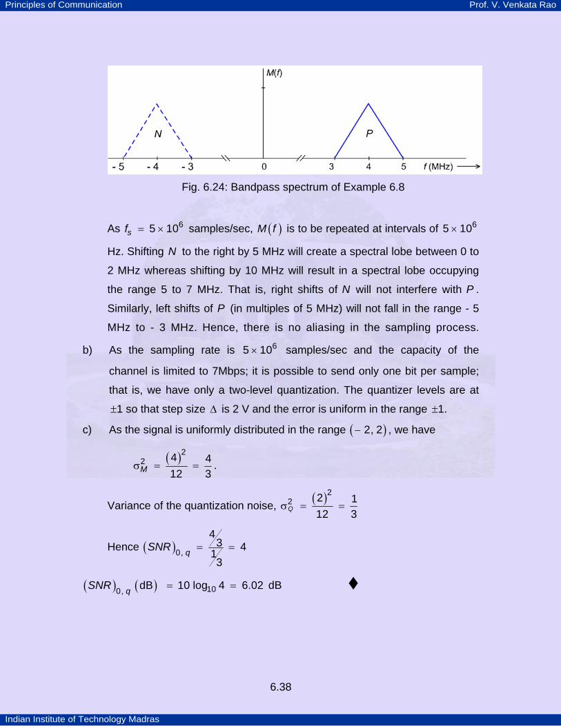
Let ( )M f , the spectrum of ( )m t be as shown in Fig. 6.24.
1 Note that a sampling frequency ( )s sf f min> could result in aliasing (see Example 6.3) unless
s Hf f2≥ , in which case the sampling of a bandpass signal reduces to that of sampling a lowpass signal.
Principles of Communication Prof. V. Venkata Rao
Indian Institute of Technology Madras
6.38
Fig. 6.24: Bandpass spectrum of Example 6.8
As sf65 10= × samples/sec, ( )M f is to be repeated at intervals of 65 10×
Hz. Shifting N to the right by 5 MHz will create a spectral lobe between 0 to
2 MHz whereas shifting by 10 MHz will result in a spectral lobe occupying
the range 5 to 7 MHz. That is, right shifts of N will not interfere with P .
Similarly, left shifts of P (in multiples of 5 MHz) will not fall in the range - 5
MHz to - 3 MHz. Hence, there is no aliasing in the sampling process.
b) As the sampling rate is 65 10× samples/sec and the capacity of the
channel is limited to 7Mbps; it is possible to send only one bit per sample;
that is, we have only a two-level quantization. The quantizer levels are at
1± so that step size ∆ is 2 V and the error is uniform in the range 1± .
c) As the signal is uniformly distributed in the range ( )2, 2− , we have
( )M
22 4 4
12 3σ = = .
Variance of the quantization noise, ( )Q
22 2 1
12 3σ = =
Hence ( ) qSNR 0,
43 413
= =
( ) ( ) = =qSNR 100, dB 10 log 4 6.02 dB
Principles of Communication Prof. V. Venkata Rao
Indian Institute of Technology Madras
6.39
When the assumption that quantization noise is uniformly distributed
between 2∆
± , is not valid, then we have to take a more basic approach in
calculating the noise variance. This is illustrated with the help of Example 6.9.
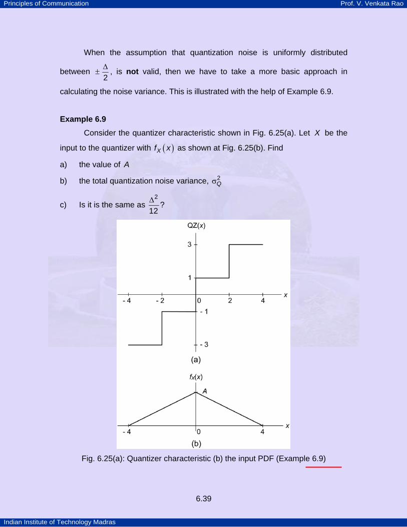
Example 6.9 Consider the quantizer characteristic shown in Fig. 6.25(a). Let X be the
input to the quantizer with ( )Xf x as shown at Fig. 6.25(b). Find
a) the value of A
b) the total quantization noise variance, Q2σ
c) Is it is the same as 2
12∆ ?
Fig. 6.25(a): Quantizer characteristic (b) the input PDF (Example 6.9)

Principles of Communication Prof. V. Venkata Rao
Indian Institute of Technology Madras
6.40
a) As ( )Xf x d x4
41
−
=∫ , A 14
=
b) ( )Xx x
f xotherwise
1 1 , 44 16
0 ,
⎧ − ≤⎪= ⎨⎪⎩
Let us calculate the variance of the quantization noise for x 0≥ . Total
variance is twice this value. For x 0> , let
( ) ( ) ( ) ( )Q X Xx f x d x x f x d x2 4
2 22
0 2
' 1 3σ = − + −∫ ∫
Carrying out the calculations, we have
Q2 1'
6σ = and hence, Q
2 13
σ =
c) As 2 4 1
12 12 3∆
= = , in this case we have Q2σ the same as
2
12∆ .
Exercise 6.3 The input to the quantizer of Example 6.9 (Fig. 6.25(a)) is a random
variable with the PDF,
( )x
XAe xf x
otherwise, 4
0 ,
−⎧ ≤⎪= ⎨⎪⎩
Find the answers to (a), (b) and (c) of Example 6.9.
Answers: Q
22 0.037
12∆
σ = ≠ .
Exercise 6.4 A random variable X , which is uniformly distributed in the range 0 to
1 is quantized as follows:
( )QZ x x0 , 0 0.3= ≤ ≤
( )QZ x x0.7 , 0.3 1= < ≤
Show that the root-mean square value of the quantization is 0.198.
Principles of Communication Prof. V. Venkata Rao
Indian Institute of Technology Madras
6.41
6.4.3 Non-uniform quantization and companding In certain applications, such as PCM telephony, it is preferable to use a
non-uniform quantizer, where in the step size ∆ is not a constant. The reason is
as follows. The range of voltages covered by voice signals (say between the
peaks of a loud talk and between the peaks of a fairly weak talk), is of the order
of 1000 to 1. For a uniform quantizer we have seen that ( ) XqSNR
2
20,12 σ
=∆
,
where ∆ is a constant. Hence ( ) qSNR 0, is decided by signal power. For a
person with a loud tone, if the system can provide an ( ) qSNR 0, of the order of
40 dB, it may not be able to provide even 10 dB ( ) qSNR 0, for a person with a
soft voice. As a given quantizer would have to cater to various speakers, (in a
commercial setup, there is no dedicated CODEC1 for a given speaker), uniform
quantization is not the proper method. A non-uniform quantizer with the feature
that step size increases as the separation from the origin of the input -output
characteristic is increased, would provide a much better alternative. This is
because larger signal amplitudes are subjected to coarser quantization and the
weaker passages are subjected to fine quantization. By choosing the
quantization characteristic properly, it would be possible to obtain an acceptable
( ) qSNR 0, over a wide range of input signal variation. In other words, such a
1 CODEC stands for COder-DECoder combination
Exercise 6.5
A signal ( )m t with amplitude variations in the range pm− to pm is to
be sent using PCM with a uniform quantizer. The quantization error should be
less than or equal to 0.1 percent of the peak value pm . If the signal is band
limited to 5 kHz, find the minimum bit rate required by this scheme.
Ans: 510 bps
Principles of Communication Prof. V. Venkata Rao
Indian Institute of Technology Madras
6.42
quantizer favors weak passages (which need more protection) at the expense of
loud ones.
The use of a non-uniform quantizer is equivalent to passing the baseband
signal through a compressor and then applying the compressed signal to a
uniform quantizer. In order to restore the signal samples to their correct relative
level, we must of course use a device in the receiver with a characteristic
complimentary to the compressor. Such a device is called an expander. A non-
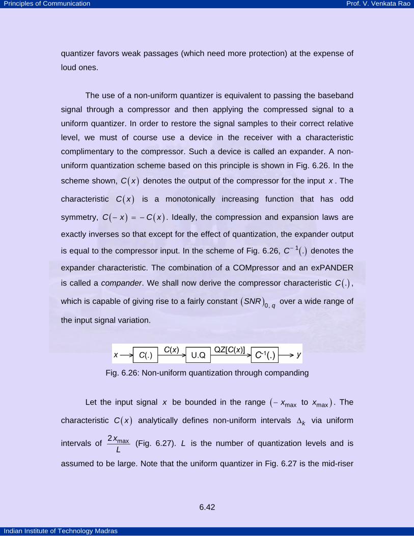
uniform quantization scheme based on this principle is shown in Fig. 6.26. In the
scheme shown, ( )C x denotes the output of the compressor for the input x . The
characteristic ( )C x is a monotonically increasing function that has odd
symmetry, ( ) ( )C x C x− = − . Ideally, the compression and expansion laws are
exactly inverses so that except for the effect of quantization, the expander output
is equal to the compressor input. In the scheme of Fig. 6.26, ( )C 1 .− denotes the
expander characteristic. The combination of a COMpressor and an exPANDER
is called a compander. We shall now derive the compressor characteristic ( )C . ,
which is capable of giving rise to a fairly constant ( ) qSNR 0, over a wide range of
the input signal variation.
Fig. 6.26: Non-uniform quantization through companding
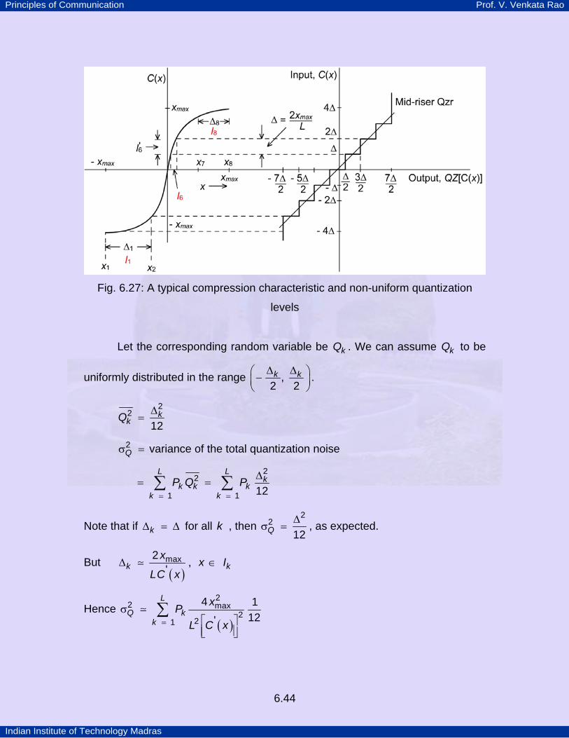
Let the input signal x be bounded in the range ( )x xmax maxto− . The
characteristic ( )C x analytically defines non-uniform intervals k∆ via uniform
intervals of xLmax2 (Fig. 6.27). L is the number of quantization levels and is
assumed to be large. Note that the uniform quantizer in Fig. 6.27 is the mid-riser
Principles of Communication Prof. V. Venkata Rao
Indian Institute of Technology Madras
6.43
variety. When x I6∈ , ( )C x I6'∈ and the input to the UQ will be in the range
( ), 2∆ ∆ . Then the quantizer output is 32∆ . When kx I∈ , the compressor
characteristic ( )C x , may be approximated by a straight line segment with a
slope equal to k
xL
max2∆
, where k∆ is the width of the interval kI . That is,
( ) ( )k
k
d C x xC x x Id x L
max2' ,= ∈∆
As ( )C x' is maximum at the origin, the equivalent step size is smallest at
x 0= and k∆ is the largest at x xmax= . If L is large, the input PDF ( )Xf x can
be treated to be approximately constant in any interval kI k L, 1, ,= ⋅ ⋅ ⋅ . Note
that we are assuming that the input is bounded in practice to a value xmax , even
if the PDF should have a long tail. We also assume that ( )Xf x is symmetric; that
is ( ) ( )X Xf x f x= − . Let ( ) ( )X X kf x f yconstant = , kx I∈ , where
k kk
x xy 1
2+ +
=
and k k k klength of I x x1+∆ = = −
Then, [ ] ( )k
k
x
k k Xx
P P x I f x d x1+
= ∈ = ∫ , and, L
kk
P1
1=
=∑
Let kq denote the quantization error when kx I∈ .
That is, ( )k kq QZ x x x I,= − ∈
k ky x x I,= − ∈
Principles of Communication Prof. V. Venkata Rao
Indian Institute of Technology Madras
6.44
Fig. 6.27: A typical compression characteristic and non-uniform quantization
levels
Let the corresponding random variable be kQ . We can assume kQ to be
uniformly distributed in the range k k,2 2∆ ∆⎛ ⎞−⎜ ⎟
⎝ ⎠.
kkQ
22
12∆
=
Q2σ = variance of the total quantization noise
L L
kk k k
k kP Q P
22
1 1 12= =
∆= =∑ ∑
Note that if k∆ = ∆ for all k , then Q
22
12∆
σ = , as expected.
But ( )
k kx x I
LC xmax2 ,'∆ ∈
Hence ( )
L
Q kk
xPL C x
22 max
221
4 112'=
σ⎡ ⎤⎢ ⎥⎣ ⎦
∑
Principles of Communication Prof. V. Venkata Rao
Indian Institute of Technology Madras
6.45
( )L
kk
x P C xL
2 2max
21
'3
−
=
⎡ ⎤⎢ ⎥⎣ ⎦∑
( ) ( )k
k
xL
Xk x
x f x C x d xL
12 2max
21
'3
+ −
=
⎡ ⎤⎢ ⎥⎣ ⎦∑ ∫
( ) ( )x
Xx
x f x C x d xL
max
max
2 2max
2'
3
−
−
⎡ ⎤⎢ ⎥⎣ ⎦∫ (6.16a)
This approximate formula for Q2σ is referred to as Bennet’s formula.
( )( )
( ) ( )
XX
xqQ
Xx
x f x d xLSNR
xf x C x d x
max
max
22 2
2 20, 2max
3
'
∞
− ∞
−
−
σ=
σ ⎡ ⎤⎢ ⎥⎣ ⎦
∫
∫
( )
( ) ( )
x
Xx
x
Xx
x f x d xL
xf x C x d x
max
max
max
max
22
2 2max
3
'
−
−
−
⎡ ⎤⎢ ⎥⎣ ⎦
∫
∫ (6.16b)
From the above approximation, we see that it is possible for us to have a
constant ( ) qSNR 0, i.e. independent of X2σ , provided
( )C xK x1' = where K is a constant, or ( )C x K x
22 2' −⎛ ⎞⎡ ⎤ =⎜ ⎟⎢ ⎥⎣ ⎦⎝ ⎠
Then, ( ) qLSNR
K x
2
2 20,max
3=
As ( )C xK x1' = , we have
( ) xC xK
ln= + α , with x 0> and α being a constant. (Note that
ex xln log= .)
Principles of Communication Prof. V. Venkata Rao
Indian Institute of Technology Madras
6.46
The constant α is arrived at by using the condition, when x xmax= ,
( )C x xmax= . Therefore, xxKmax
maxln
α = − .
Hence, ( ) xxC x xK K
maxmax
lnln= + −
x x xK x max
max
1 ln , 0⎛ ⎞
= + >⎜ ⎟⎝ ⎠
As ( ) ( )C x C x− = − we have
( ) ( )xC x x x
K x maxmax
1 ln sgn⎛ ⎞⎛ ⎞
= +⎜ ⎟⎜ ⎟⎜ ⎟⎝ ⎠⎝ ⎠, (6.17)
where, ( ) xx
x1, 0
sgn1, 0
>⎧= ⎨− <⎩
As the non-uniform quantizer with the above ( )C x results in a constant
( ) qSNR 0, , it is also called “robust quantization”.
The above ( )C x is not realizable because ( )x
C x0
lim→
→ ∞ . We want
( )x
C x0
lim 0→
→ . That is, we have to modify the theoretical companding law. We
discuss two schemes, both being linear at the origin.
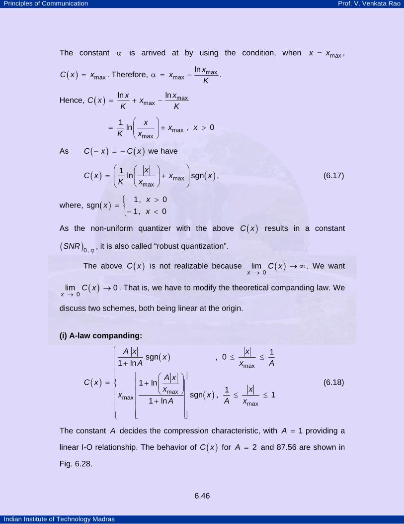
(i) A-law companding:
( )
( )
( )
A x xx
A x A
A xC xx x
x xA A x
max
maxmax
max
1sgn , 01 ln
1 ln1sgn , 1
1 ln
⎧≤ ≤⎪ +⎪
⎪ ⎡ ⎤⎛ ⎞⎪= +⎨ ⎢ ⎥⎜ ⎟⎪ ⎝ ⎠⎢ ⎥ ≤ ≤⎪ ⎢ ⎥+⎪ ⎢ ⎥⎪ ⎢ ⎥⎣ ⎦⎩
(6.18)
The constant A decides the compression characteristic, with A 1= providing a
linear I-O relationship. The behavior of ( )C x for A 2= and 87.56 are shown in
Fig. 6.28.
Principles of Communication Prof. V. Venkata Rao
Indian Institute of Technology Madras
6.47
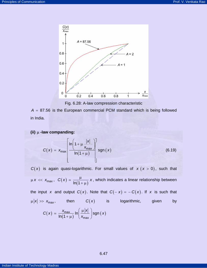
Fig. 6.28: A-law compression characteristic
A 87.56= is the European commercial PCM standard which is being followed
in India.
(ii) µ -law companding:
( ) ( ) ( )
xx
C x x xmaxmax
ln 1sgn
ln 1
⎡ ⎤⎛ ⎞+ µ⎢ ⎥⎜ ⎟
⎝ ⎠⎢ ⎥= ⎢ ⎥+ µ⎢ ⎥⎢ ⎥⎣ ⎦
(6.19)
( )C x is again quasi-logarithmic. For small values of ( )x x 0> , such that
x xmaxµ << , ( ) ( )C x x
ln 1µ+ µ
, which indicates a linear relationship between
the input x and output ( )C x . Note that ( ) ( )C x C x− = − . If x is such that
x xmaxµ >> , then ( )C x is logarithmic, given by
( ) ( ) ( )xxC x xx
max
maxln sgn
ln 1⎛ ⎞µ⎜ ⎟+ µ ⎝ ⎠

Principles of Communication Prof. V. Venkata Rao
Indian Institute of Technology Madras
6.48
µ is a constant, whose value decides the curvature of ( )C x ; 0µ = corresponds
to no compression and as the value of µ increases, signal compression
increases, as shown in Fig. 6.29.
Fig. 6.29: µ -law compression characteristic
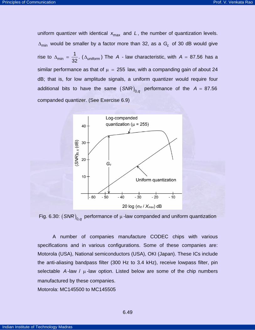
255µ = is the north American standard for PCM voice telephony. Fig. 6.30
compares the performance of the 8-bit µ -law companded PCM with that of an 8
bit uniform quantizer; input is assumed to have the bounded Laplacian PDF
which is typical of speech signals. The ( ) qSNR 0, for the uniform quantizer is
based on Eq. 6.14. As can be seen from this figure, companding results in a
nearly constant signal-to-quantization noise ratio (within 3 dB of the maximum
value of 38 dB) even when the mean square value of the input changes by about
30 dB (a factor of 310 ). cG is the companding gain which is indicative of the
improvement in SNR for small signals as compared to the uniform quantizer. In
Fig. 6.30, cG has been shown to be about 33 dB. This implies that the smallest
step size, min∆ is about 32 times smaller than the step size of a corresponding
Principles of Communication Prof. V. Venkata Rao
Indian Institute of Technology Madras
6.49
uniform quantizer with identical xmax and L , the number of quantization levels.
min∆ would be smaller by a factor more than 32, as a cG of 30 dB would give
rise to min1
32∆ = . ( uniform∆ ) The A - law characteristic, with A 87.56= has a
similar performance as that of 255µ = law, with a companding gain of about 24
dB; that is, for low amplitude signals, a uniform quantizer would require four
additional bits to have the same ( ) qSNR 0, performance of the A 87.56=
companded quantizer. (See Exercise 6.9)
Fig. 6.30: ( ) qSNR 0, performance of µ -law companded and uniform quantization
A number of companies manufacture CODEC chips with various
specifications and in various configurations. Some of these companies are:
Motorola (USA), National semiconductors (USA), OKI (Japan). These ICs include
the anti-aliasing bandpass filter (300 Hz to 3.4 kHz), receive lowpass filter, pin
selectable A -law / µ -law option. Listed below are some of the chip numbers
manufactured by these companies.
Motorola: MC145500 to MC145505

Principles of Communication Prof. V. Venkata Rao
Indian Institute of Technology Madras
6.50
National: TP3070, TP3071 and TP3070-X
OKI: MSM7578H / 7578V / 7579
Details about these ICs can be downloaded from their respective websites.
Example 6.10
A random variable X with the density function ( )Xf x shown in Fig. 6.31 is
given as input to a non-uniform quantizer with the levels q1± , q2± and q3± .
Fig. 6.31: Input PDF of Example 6.10
q1, q2 and q3 are such that
( ) ( ) ( )qq q
X X Xq q q
f x d x f x d x f x d x32 1
3 2 2
16
− −
− −
= = ⋅ ⋅ ⋅ = =∫ ∫ ∫ (6.20)
a) Find q1, q2 and q3 .
b) Suggest a compressor characteristic that should precede a uniform
quantizer such that Eq. 6.20 is satisfied. Is this unique?
a) ( ) ( )q q
X Xq
f x d x f x d x1 1
1 0
126
−
= =∫ ∫
Hence, ( )q
x d x1
0
1112
− =∫
Principles of Communication Prof. V. Venkata Rao
Indian Institute of Technology Madras
6.51
Solving, we obtain q1 0.087=
Similarly we have equations
( )q
Xf x d x2
0.087
16
=∫ (6.21a)
( )q
Xq
f x d x3
2
16
=∫ (6.21b)
From Eq. 6.21(a), we get q2 0.292= and solving Eq. 6.21(b) for q3 yields
q3 0.591= .
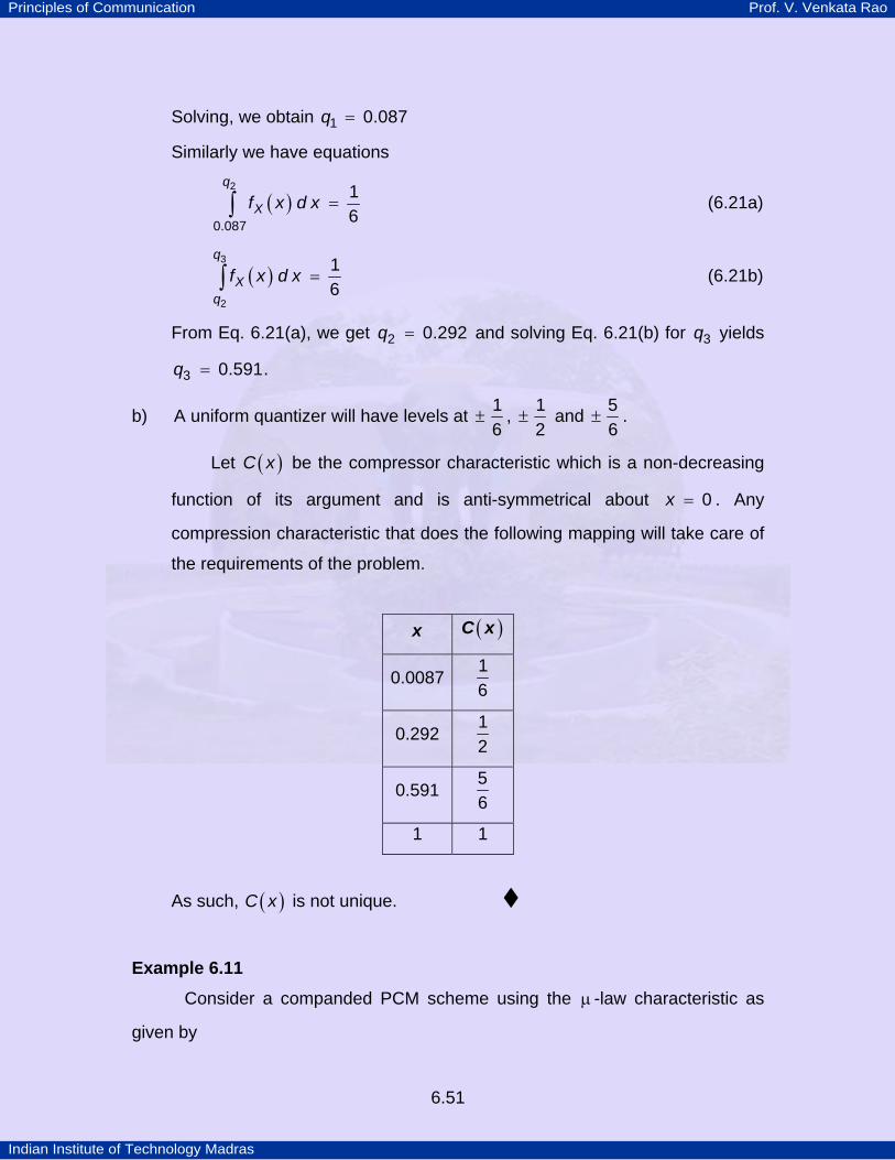
b) A uniform quantizer will have levels at 16
± , 12
± and 56
± .
Let ( )C x be the compressor characteristic which is a non-decreasing
function of its argument and is anti-symmetrical about x 0= . Any
compression characteristic that does the following mapping will take care of
the requirements of the problem.
x ( )C x
0.008716
0.292 12
0.591 56
1 1
As such, ( )C x is not unique.
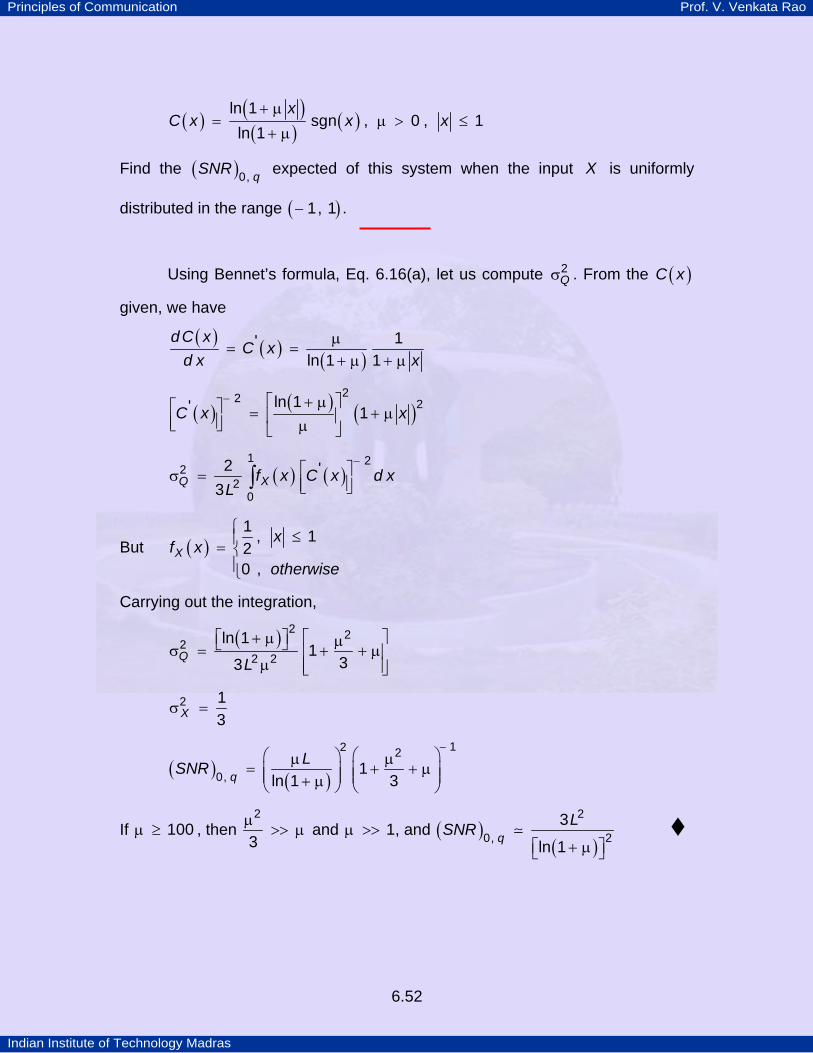
Example 6.11 Consider a companded PCM scheme using the µ -law characteristic as
given by
Principles of Communication Prof. V. Venkata Rao
Indian Institute of Technology Madras
6.52
( ) ( )( ) ( )
xC x x x
ln 1sgn , 0 , 1
ln 1+ µ
= µ > ≤+ µ
Find the ( ) qSNR 0, expected of this system when the input X is uniformly
distributed in the range ( )1, 1− .
Using Bennet’s formula, Eq. 6.16(a), let us compute Q2σ . From the ( )C x
given, we have
( ) ( ) ( )dC x
C xd x x
1'ln 1 1
µ= =
+ µ + µ
( ) ( ) ( )C x x22 2ln 1' 1
− ⎡ ⎤+ µ⎡ ⎤ = + µ⎢ ⎥⎢ ⎥⎣ ⎦ µ⎣ ⎦
( ) ( )Q Xf x C x d xL
1 22
20
2 '3
−⎡ ⎤σ = ⎢ ⎥⎣ ⎦∫
But ( )Xx
f xotherwise
1 , 120 ,
⎧ ≤⎪= ⎨⎪⎩
Carrying out the integration,
( )
Q L
2 22
2 2ln 1
133
⎡ ⎤⎡ ⎤+ µ µ⎣ ⎦σ = + + µ⎢ ⎥µ ⎢ ⎥⎣ ⎦
X2 1
3σ =
( ) ( )qLSNR
12 2
0, 1ln 1 3
−⎛ ⎞⎛ ⎞µ µ
= + + µ⎜ ⎟⎜ ⎟⎜ ⎟ ⎜ ⎟+ µ⎝ ⎠ ⎝ ⎠
If 100µ ≥ , then 2
3µ
>> µ and 1µ >> , and ( )( )q
LSNR2
20,3
ln 1⎡ ⎤+ µ⎣ ⎦
Principles of Communication Prof. V. Venkata Rao
Indian Institute of Technology Madras
6.53
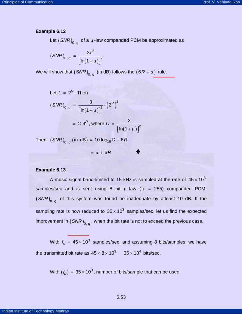
Example 6.12
Let ( ) qSNR 0, of a µ -law companded PCM be approximated as
( )( )q
LSNR2
20,3
ln 1⎡ ⎤+ µ⎣ ⎦
We will show that ( ) qSNR 0, (in dB) follows the ( )R6 + α rule.
Let RL 2= . Then
( )( )
( )RqSNR
2
20,3 2
ln 1⋅
⎡ ⎤+ µ⎣ ⎦
RC 4 , where ( )
C 23
ln 1=
⎡ ⎤+ µ⎣ ⎦
Then ( ) ( )qSNR C R100, in dB 10 log 6= +
R6= α +
Example 6.13
A music signal band-limited to 15 kHz is sampled at the rate of 345 10×
samples/sec and is sent using 8 bit µ -law (µ = 255) companded PCM.
( ) qSNR 0, of this system was found be inadequate by atleast 10 dB. If the
sampling rate is now reduced to 335 10× samples/sec, let us find the expected
improvement in ( ) qSNR 0, , when the bit rate is not to exceed the previous case.
With sf345 10= × samples/sec, and assuming 8 bits/samples, we have
the transmitted bit rate as 3 445 8 10 36 10× × = × bits/sec.
With ( )sf335 10= × , number of bits/sample that can be used

Principles of Communication Prof. V. Venkata Rao
Indian Institute of Technology Madras
6.54
R4
336 10 10.2835 10
×= =
×
As R has to be an integer, it can be taken as 10. As R has increased by two
bits, we can expect 12 dB improvement in SNR.
Exercise 6.6 Consider the three level quantizer (mid-tread type) shown in Fig. 6.32.
The input to the quantizer is a random variable X with the PDF ( )Xf x give by
( )X
xf x
x
1 , 141 , 1 38
⎧ ≤⎪⎪= ⎨⎪ < ≤⎪⎩
Fig, 6.32: Quantizer characteristic for the Exercise 6.5
a) Find the value of A such that all the quantizer output levels are
equiprobable. (Note that A has to be less than 1, because with A 1= ,
we have ( )P QZ x 102
⎡ ⎤= =⎣ ⎦ )
b) Show that the variance of the quantization noise for the range x A≤ ,
is 481
.

Principles of Communication Prof. V. Venkata Rao
Indian Institute of Technology Madras
6.55
Exercise 6.7
Let the input to µ -law compander be the sample function ( )jx t of a random
process ( ) ( )mX t f tcos 2= π + Θ where Θ is uniformly distributed in the
range ( )0, 2π . Find the ( ) qSNR 0, expected of the scheme.
Note that samples of ( )jx t will have the PDF,
( )X
xf x x
otherwise
2
1 , 110 ,
⎧ ≤⎪= π −⎨⎪⎩
Answer: ( ) ( )qLSNR
12 2
0,3 12 ln 1 2
−⎡ ⎤⎛ ⎞µ µ 4µ
= + +⎜ ⎟ ⎢ ⎥⎜ ⎟+ µ π⎢ ⎥⎝ ⎠ ⎣ ⎦
Note that if 2
12µ
>> µ >> , we have ( )( )q
LSNR2
20,3
ln 1⎡ ⎤+ µ⎣ ⎦
Exercise 6.8
Show that for values of x such that A x xmax>> , ( ) qSNR 0, of the
A-law PCM is given by
( ) qSNR R0, 6= + α
where [ ]A104.77 20 log 1 lnα = − +
Exercise 6.9
Let ( )C x denote the compression characteristic. Then ( )x
d C xd x 0→
is called the companding gain, cG . Show that
a) cG (A-law) with A 87.56= is 15.71 (and hence cG1020 log 24 dB)
b) cG (µ -law) with 255µ = is 46.02 (and hence cG1020 log 33 dB.)
Principles of Communication Prof. V. Venkata Rao
Indian Institute of Technology Madras
6.56
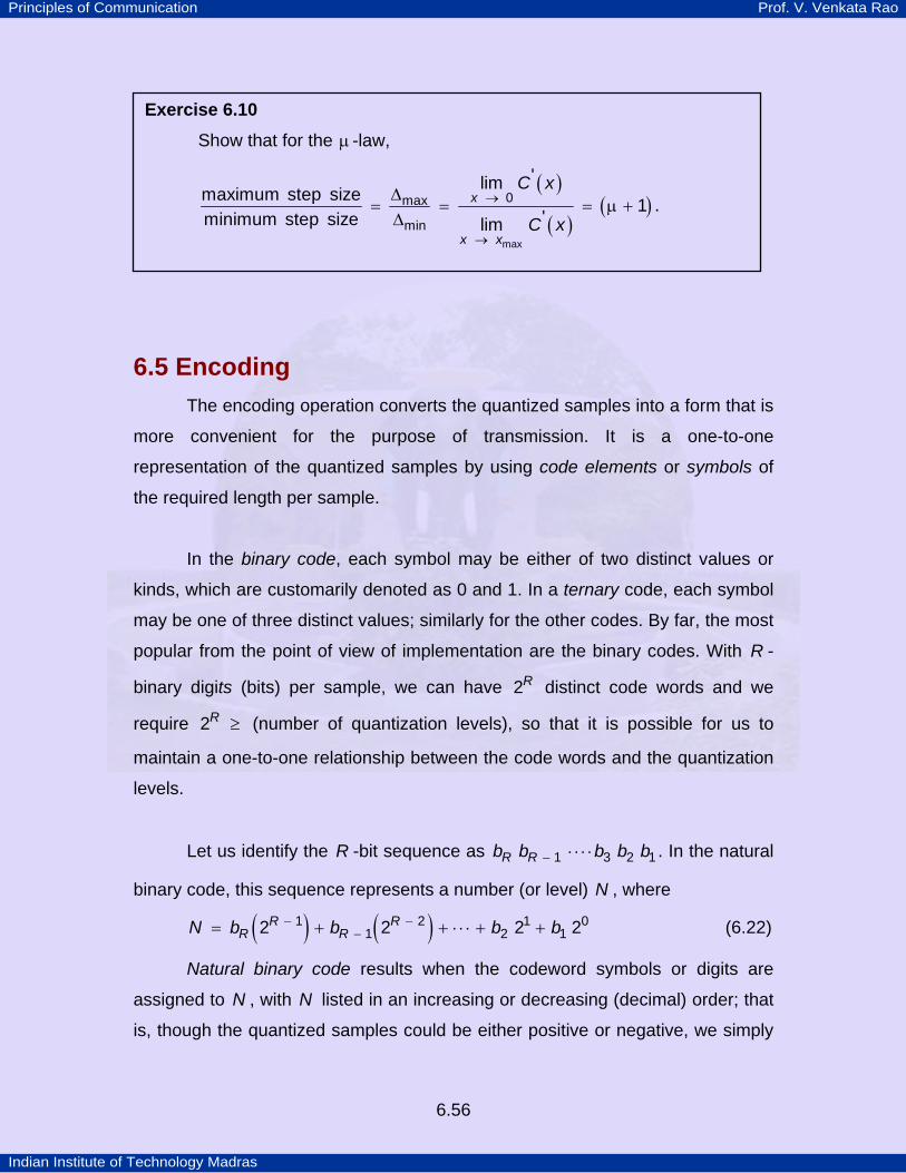
6.5 Encoding The encoding operation converts the quantized samples into a form that is
more convenient for the purpose of transmission. It is a one-to-one
representation of the quantized samples by using code elements or symbols of
the required length per sample.
In the binary code, each symbol may be either of two distinct values or
kinds, which are customarily denoted as 0 and 1. In a ternary code, each symbol
may be one of three distinct values; similarly for the other codes. By far, the most
popular from the point of view of implementation are the binary codes. With R -
binary digits (bits) per sample, we can have R2 distinct code words and we
require R2 ≥ (number of quantization levels), so that it is possible for us to
maintain a one-to-one relationship between the code words and the quantization
levels.
Let us identify the R -bit sequence as R Rb b b b b1 3 2 1− ⋅ ⋅ ⋅ ⋅ . In the natural
binary code, this sequence represents a number (or level) N , where
( ) ( )R RR RN b b b b1 2 1 0
1 2 12 2 2 2− −−= + + ⋅ ⋅ ⋅ + + (6.22)
Natural binary code results when the codeword symbols or digits are
assigned to N , with N listed in an increasing or decreasing (decimal) order; that
is, though the quantized samples could be either positive or negative, we simply
Exercise 6.10 Show that for the µ -law,
( )
( )( )x
x x
C x
C xmax
0max
min
'limmaximum step size 1'minimum step size lim→
→
∆= = = µ +
∆.
Principles of Communication Prof. V. Venkata Rao
Indian Institute of Technology Madras
6.57
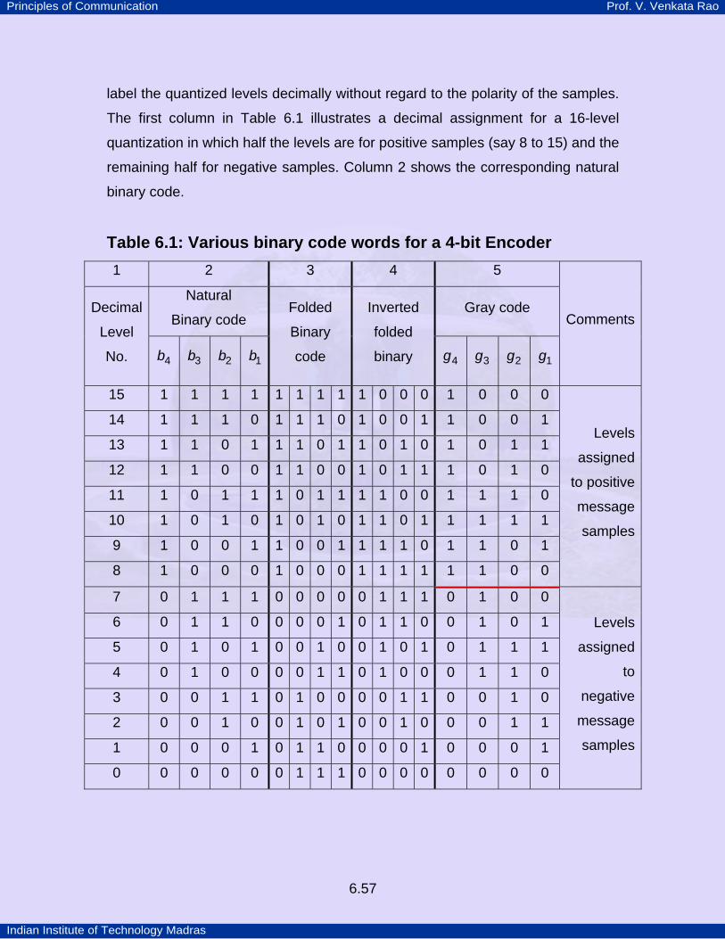
label the quantized levels decimally without regard to the polarity of the samples.
The first column in Table 6.1 illustrates a decimal assignment for a 16-level
quantization in which half the levels are for positive samples (say 8 to 15) and the
remaining half for negative samples. Column 2 shows the corresponding natural
binary code.
Table 6.1: Various binary code words for a 4-bit Encoder 1 2 3 4 5
Natural
Binary code Gray code Decimal
Level
No. b4 b3 b2 b1
Folded
Binary
code
Inverted
folded
binary g4 g3 g2 g1
Comments
15 1 1 1 1 1 1 1 1 1 0 0 0 1 0 0 0
14 1 1 1 0 1 1 1 0 1 0 0 1 1 0 0 1
13 1 1 0 1 1 1 0 1 1 0 1 0 1 0 1 1
12 1 1 0 0 1 1 0 0 1 0 1 1 1 0 1 0
11 1 0 1 1 1 0 1 1 1 1 0 0 1 1 1 0
10 1 0 1 0 1 0 1 0 1 1 0 1 1 1 1 1
9 1 0 0 1 1 0 0 1 1 1 1 0 1 1 0 1
8 1 0 0 0 1 0 0 0 1 1 1 1 1 1 0 0
Levels
assigned
to positive
message
samples
7 0 1 1 1 0 0 0 0 0 1 1 1 0 1 0 0
6 0 1 1 0 0 0 0 1 0 1 1 0 0 1 0 1
5 0 1 0 1 0 0 1 0 0 1 0 1 0 1 1 1
4 0 1 0 0 0 0 1 1 0 1 0 0 0 1 1 0
3 0 0 1 1 0 1 0 0 0 0 1 1 0 0 1 0
2 0 0 1 0 0 1 0 1 0 0 1 0 0 0 1 1
1 0 0 0 1 0 1 1 0 0 0 0 1 0 0 0 1
0 0 0 0 0 0 1 1 1 0 0 0 0 0 0 0 0
Levels
assigned
to
negative
message
samples
Principles of Communication Prof. V. Venkata Rao
Indian Institute of Technology Madras
6.58
The other codes shown in the table are derived from the natural binary
code. The folded binary code (also called the sign-magnitude representation)
assigns the first (left most) digit to the sign and the remaining digits are used to
code the magnitude as shown in the third column of the table. This code is
superior to the natural code in masking transmission errors when encoding
speech. If only the amplitude digits of a folded binary code are complemented
(1's changed to 0's and 0's to 1's), an inverted folded binary code results; this
code has the advantage of higher density of 1's for small amplitude signals,
which are most probable for voice messages. (The higher density of 1's relieves
some system timing errors but does lead to some increase in cross talk in
multiplexed systems).
With natural binary encoding, a number of codeword digits can change
even when a change of only one quantization level occurs. For example, with
reference to Table 6.1, a change from level 7 to 8 entails every bit changing in
the 4-bit code illustrated. In some applications, this behavior is undesirable and a
code is desired for which only one digit changes when any transition occurs
between adjacent levels. The Gray Code has this property, if we consider the
extreme levels as adjacent. The digits of the Gray code, denoted by kg , can be
derived from those of the natural binary code by
Rk
k k
b k Rg
b b k R1
,,+
=⎧⎪= ⎨ ⊕ <⎪⎩
where ⊕ denotes modulo-2 addition of binary digits.
(0 0 0; 0 1 1 0 1 and 1 1 0⊕ = ⊕ = ⊕ = ⊕ = ; note that, if we exclude the sign
bit, the remaining three bits are mirror images with respect to red line in the
table.)
The reverse behavior of the Gray code does not hold. That is, a change in
anyone of code digits does not necessarily result in a change of only one code
level. For example, a change in digit g4 from 0 when the code is 0001 (level 1) to
Principles of Communication Prof. V. Venkata Rao
Indian Institute of Technology Madras
6.59
1 will result in 1001 (the code word for level 14), a change spanning almost the
full quantizer range.
6.6 Electrical Waveform Representation of Binary Sequences For the purposes of transmission, the symbols 0 and 1 should be
converted to electrical waveforms. A number of waveform representations have
been developed and are being currently used, each representation having its
own specific applications. We shall now briefly describe a few of these
representations that are considered to be the most basic and are being widely
used. This representation is also called as line coding or transmission coding.
The resulting waveforms are called line codes or transmission codes for the
reason that they are used for transmission on a telephone line.
In the Unipolar format (also known as On-Off signaling), symbol 1
represented by transmitting a pulse, where as symbol 0 is represented by
switching off the pulse. When the pulse occupies the full duration of a symbol,
the unipolar format is said to be of the nonreturn-to-zero (NRZ) type. When it
occupies only a fraction (usually one-half) of the symbol duration, it is said to be
of the return-to-zero (RZ) type. The unipolar format contains a DC component
that is often undesirable.
In the polar format, a positive pulse is transmitted for symbol 1 and a
negative pulse for symbol 0. It can be of the NRZ or RZ type. Unlike the unipolar
waveform, a polar waveform has no dc component, provided that 0's and 1's in
the input data occur in equal proportion.
In the bipolar format (also known as pseudo ternary signaling or Alternate
Mark Inversion, AMI), positive and negative pulses are used alternatively for the
Principles of Communication Prof. V. Venkata Rao
Indian Institute of Technology Madras
6.60
transmission of 1's (with the alternation taking place at every occurrence of a 1)
and no pulses for the transmission of 0‘s. Again it can be of the NRZ or RZ type.
Note that in this representation there are three levels: +1, 0, -1. An attractive
feature of the bipolar format is the absence of a DC component, even if the input
binary data contains large strings of 1's or 0's. The absence of DC permits
transformer coupling during the course of long distance transmission. Also, the
bipolar format eliminates ambiguity that may arise because of polarity inversion
during the course of transmission. Because of these features, bipolar format is
used in the commercial PCM telephony. (Note that, some authors use the word
bipolar to mean polar)
In the Manchester format (also known as biphase or split phase signaling),
symbol 1 is represented by transmitting a positive pulse for one-half of the
symbol duration, followed by a negative pulse for the remaining half of the
symbol duration; for symbol 0, these two pulses are transmitted in the reverse
order. Clearly, this format has no DC component; moreover, it has a built in
synchronization capability because there is a predictable transition during each
bit interval. The disadvantage of the Manchester format is that it requires twice
the bandwidth when compared to the NRZ unipolar, polar and bipolar formats.
Fig. 6.33 illustrates some of the waveform formats described above. Duration of
each bit has been taken as bT sec and the levels as 0 or a± .

Principles of Communication Prof. V. Venkata Rao
Indian Institute of Technology Madras
6.61
Fig. 6.33: Binary data waveform formats
NRZ: (a) on-off (b) polar (c) bipolar
(d) Manchester format
6.7 Bandwidth requirements of PCM In Appendix A6.1, it has been shown that if
( ) ( )k dk
X t A p t kT T∞
= − ∞= − −∑ ,
then, the power spectral density of the process is,
Principles of Communication Prof. V. Venkata Rao
Indian Institute of Technology Madras
6.62
( ) ( ) ( ) j n f TX A
nS f P f R n e
T2 21 ∞
π
= − ∞= ∑
By using this result, let us estimate the bandwidth required to transmit the
waveforms using any one of the signaling formats discussed in Sec. 6.6
6.7.1 Unipolar Format In this case, kA 's represent an on-off sequence. Let us assume that 0's
and 1's of the binary sequence to be transmitted are equally likely and '0' is
represented by level 0 and '1' is represented by level 'a'. Then,
( ) ( )k kP A P A a 102
= = = =
Let us compute ( )A k k nR n E A A +⎡ ⎤= ⎣ ⎦ . For n 0= , we have ( )A kR E A20 ⎡ ⎤= ⎣ ⎦ .
That is,
( ) ( ) ( ) ( ) ( )A k kR P A a P A a2 20 0 0= = + =
a2
2=
Next consider the product k k nA A n, 0+ ≠ . This product has four possible
values, namely, 0, 0, 0 and a2 . Assuming that successive symbols in the binary
sequence are statistically independent, these four values occur with equal
probability resulting in,
k k nE A A a23 104 4+
⎛ ⎞ ⎛ ⎞⎡ ⎤ = ⋅ +⎜ ⎟ ⎜ ⎟⎣ ⎦ ⎝ ⎠ ⎝ ⎠
a n2
, 04
= ≠
Hence,
( )A
a nR n
a n
2
2
, 02
, 04
⎧=⎪⎪= ⎨
⎪ ≠⎪⎩
Principles of Communication Prof. V. Venkata Rao
Indian Institute of Technology Madras
6.63
Let ( )p t be rectangular pulse of unit amplitude and duration bT sec. Then, ( )P f
is ( ) ( )b bP f T c f Tsin=
and ( )XS f can be written as
( ) ( ) ( ) [ ]b bX b b b
n
a T a TS f c f T c f T j n f T2 2
2 2sin sin exp 24 4
∞
= − ∞
⎛ ⎞= + π⎜ ⎟⎜ ⎟⎝ ⎠
∑
But from Poisson's formula,
[ ]bb bn m
mj n f T fT T1exp 2
∞ ∞
= − ∞ = − ∞
⎛ ⎞π = δ −⎜ ⎟
⎝ ⎠∑ ∑
Noting that ( )bc f Tsin has nulls at ( )Xb
nf n S fT
, 1, 2, ,= = ± ± ⋅ ⋅ ⋅ can be
simplified to
( ) ( ) ( )bX b
a T aS f c f T f2 2
2sin4 4
= + δ (6.23a)
If the duration of ( )p t is less than bT , then we have unipolar RZ sequence. If
( )p t is of duration bT2
seconds, then ( )XS f reduces to
( ) b bX
b bm
a T f T mS f c fT T
22 1sin 1
16 2
∞
= − ∞
⎡ ⎤⎛ ⎞⎛ ⎞= + δ −⎢ ⎥⎜ ⎟⎜ ⎟⎝ ⎠ ⎢ ⎥⎝ ⎠⎣ ⎦
∑ (6.23b)
From equation 6.23(b) it follows that unipolar RZ signaling has discrete spectral
components at b b
fT T1 30, ,= ± etc. A plot of Eq. 6.23(b) is shown in Fig. 6.34(a).
6.7.2 Polar Format
Assuming, [ ] [ ]k kP A a P A a 12
= + = = − = and 0's and 1's of the binary
data sequence are statistically independent; it is easy to show,
( )Aa nR n
n
2 , 00 , 0
⎧ =⎪= ⎨≠⎪⎩
Principles of Communication Prof. V. Venkata Rao
Indian Institute of Technology Madras
6.64
With ( )p t being a rectangular pulse of duration bT sec. (NRZ case), we have
( ) ( )X b bS f a T c f T2 2sin= (6.24a)
The PSD for the case when ( )p t is duration of bT2
(RZ case), is given by
( ) b bX
T f TS f a c2 2sin4 2
⎛ ⎞= ⎜ ⎟⎝ ⎠
(6.24b)
6.7.3 Bipolar Format Bipolar format has three levels: a, 0 and ( )a− . Assuming that 1's and 0's
are equally likely, we have [ ] [ ]k kP A a P A a 14
= = = − = and
[ ]kP A 102
= = . We shall now compute the autocorrelation function of a bipolar
sequence.
( ) ( ) ( ) ( ) ( )AR a a a a1 1 10 0 04 4 2
= ⋅ + − − + ⋅
a2
2=
To compute ( )AR 1 , we have to consider the four two bit sequences, namely, 00,
01, 10, 11. As the binary ‘0’ is represented by zero volts, we have only one non-
zero product, corresponding to the binary sequence (11). As each one of these
two bit sequences occur with a probability 14
, we have
( )AaR
21
4= −
To compute ( )AR n , for n 2≥ , again we have to take into account only those
binary n-tuples which have ‘1’ in the first and last position, which will result in the
product a2± . It is not difficult to see that, in these product terms, there are as
many terms with a2− as there are with a2 which implies that the sum of the
product terms would be zero. (For example, if we take the binary 3-tuples, only

Principles of Communication Prof. V. Venkata Rao
Indian Institute of Technology Madras
6.65
101 and 111 will result in a non-zero product quantity. 101 will yield a2−
whereas 111 will result in a2 ). Therefore ( )AR n 0= for n 2≥ . That is, for the
bipolar format,
( )A
a n
aR n n
otherwise
2
2
, 02
, 14
0 ,
⎧=⎪
⎪⎪⎪= − = ±⎨⎪⎪⎪⎪⎩
For the NRZ case, with a rectangular ( )p t , we obtain
( ) ( ) ( )X b b bS f a T c f T f T2 2 2sin sin= π (6.25a)
Similarly for the return-to-zero case, we have
( ) ( )b bX b
a T f TS f c f T2
2 2sin sin4 2
⎛ ⎞= π⎜ ⎟⎝ ⎠
(6.25b)
6.7.4 Manchester Format If the input binary data consists of independent equally likely symbols,
( )AR n for the Manchester format is the same as that of the polar format. The
pulse ( )p t for the Manchester format is a doublet of unit amplitude and duration
bT . Hence,
( ) b bb
f T f TP f jT csin sin2 2
π⎛ ⎞ ⎛ ⎞= ⎜ ⎟ ⎜ ⎟⎝ ⎠ ⎝ ⎠
and ( ) b bX b
f T f TS f a T c2 2 2sin sin2 2
π⎛ ⎞ ⎛ ⎞= ⎜ ⎟ ⎜ ⎟⎝ ⎠ ⎝ ⎠
(6.26)
Plots of Eq. 6.24(b), 6.25(b) and 6.26 are shown in Fig. 6.34(b).
From Fig. 6.34(a), we see that most of the power of the unipolar return- to-
zero signal is in a bandwidth of bT2 (of course, for the NRZ case, it would be
bT1 ).
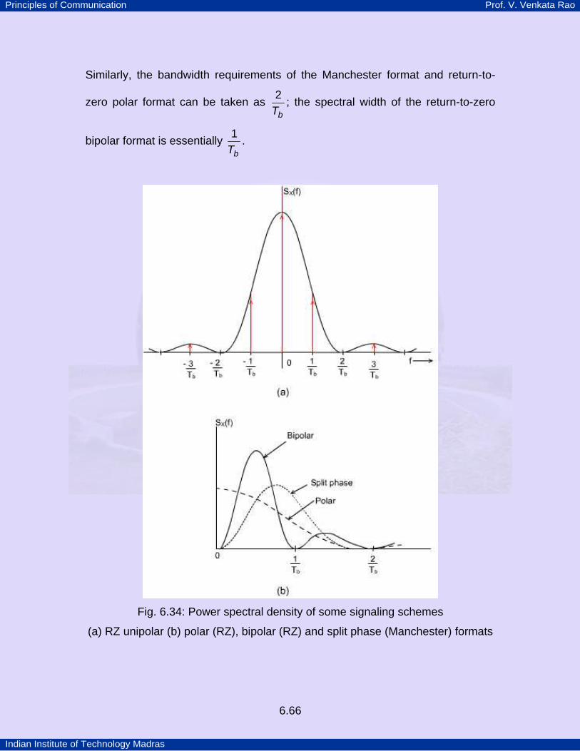
Principles of Communication Prof. V. Venkata Rao
Indian Institute of Technology Madras
6.66
Similarly, the bandwidth requirements of the Manchester format and return-to-
zero polar format can be taken as bT2 ; the spectral width of the return-to-zero
bipolar format is essentially bT1 .
Fig. 6.34: Power spectral density of some signaling schemes
(a) RZ unipolar (b) polar (RZ), bipolar (RZ) and split phase (Manchester) formats
Principles of Communication Prof. V. Venkata Rao
Indian Institute of Technology Madras
6.67
Bipolar signaling has several advantages:
1) The spectrum has a D.C. null; hence it is possible to transformer-couple
such a signal
2) Its transmission bandwidth is not excessive
3) It has single error detection capability because an isolated error, whether it
causes the deletion or erection of a pulse will violate the pulse alternation
property of the bipolar format
4) It is insensitive to polarity inversion during the course of transmission
5) If a return-to-zero bipolar pulse is rectified, we get an on-off signal that has
a discrete component at the clock frequency. This feature can be used to
regenerate the clock at the receiving end. (See Example 6.15.)
For these reasons, bipolar signaling is used in the PCM voice telephony.
Now let us look at the bandwidth requirement of a PCM system. Consider
the case of a speech signal. In the commercial PCM telephony, this signal is
sampled at 8 kHz and each sample is converted to an 8 bit sequence which
implies a bit rate of 64 kbps. Assuming bipolar signaling, we require a bandwidth
of 64 kHz which is an order of magnitude larger than analog baseband
transmission whose bandwidth requirement is just about 4 kHz!
Example 6.14 A PCM voice communication system uses bipolar return-to-zero pulses for
transmission. The signal to be transmitted has a bandwidth of 3.5 kHz with the
peak-to-peak and RMS values of 4 V and 0.2 V respectively. If the channel
bandwidth is limited to 50 kHz, let us find the maximum ( ) ( )qSNR 0, in dB that
can be expected out of this system.
Assuming that the bandwidth requirements of return-to-zero bipolar pulse
as bT1 , it would be possible for us to send upto 50,000 pulses per second on this
channel. As the bit rate is the product of sampling rate and the number of
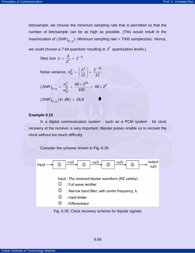
Principles of Communication Prof. V. Venkata Rao
Indian Institute of Technology Madras
6.68
bits/sample, we choose the minimum sampling rate that is permitted so that the
number of bits/sample can be as high as possible. (This would result in the
maximization of ( ) qSNR 0, ). Minimum sampling rate = 7000 samples/sec. Hence,
we could choose a 7-bit quantizer resulting in 72 quantization levels.)
Step size 57
4 22
−∆ = =
Noise variance, Q
2 102 2
12 12
−⎛ ⎞∆σ = =⎜ ⎟⎜ ⎟
⎝ ⎠
( ) xq
QSNR
2 108
20,48 2 48 2
100σ ×
= = = ×σ
( ) ( )qSNR 0, in dB 26.8=
Example 6.15 In a digital communication system - such as a PCM system - bit clock
recovery at the receiver is very important. Bipolar pulses enable us to recover the
clock without too much difficulty.
Consider the scheme shown in Fig. 6.35.
Fig. 6.35: Clock recovery scheme for bipolar signals
Principles of Communication Prof. V. Venkata Rao
Indian Institute of Technology Madras
6.69
The bit rate of the bipolar waveform is 510 bps. Let us find the output of
the system when
(a) f0 100= kHz (b) f0 200= kHz
a) ( )v t1 , output of the full wave rectifier, is a RZ, on-off waveform. From Eq.
6.23(b), we know that this waveform process has a discrete spectral
component at b
fT1
= which is 100 kHz in this case. This component will be
selected by the tuned filter; hence ( )v t2 is a sinusoidal signal with
frequency 100 kHz. The output of the hard limiter, ( )v t3 , is a square wave
at 100 kHz. Differentiation of this result in a sequence of positive and
negative going impulses with two positive (or negative) impulses being
separated by 510− sec. This can be used as the clock for the receiver.
b) When the centre frequency of the tuned filter is 200 kHz, the output ( )v t2 is
zero as there is no discrete component at 200 kHz in ( )v t1 .
Principles of Communication Prof. V. Venkata Rao
Indian Institute of Technology Madras
6.70
6.8 Differential Pulse Code Modulation (DPCM) DPCM can be treated as a variation of PCM; it also involves the three
basic steps of PCM, namely, sampling, quantization and coding. But, in the case
of DPCM, what is quantized is the difference between the actual sample and its
predicted value, as explained below.
Exercise 6.11
Let a random process ( )X t be given by
( ) ( )k b dk
X t B p t kT T∞
= − ∞= − −∑
It is given that k k kB A A 1−= + where kA ’s are discrete random variables
with ( )k Ak nA A R n± = . kA a= if the input binary symbol is ‘1’ and
kA a= − if the input symbol is ‘0’. 1’s and 0’s are equally likely and are
statistically independent. bT is the bit duration and dT is a random delay with
a uniform distribution in the range b bT T,2 2
⎛ ⎞−⎜ ⎟⎝ ⎠
. kA ’s are independent of dT .
Show that
a) ( )k Bk n
a n
B B R n a notherwise
2
2
2 , 0
, 10 ,
±
⎧ =⎪⎪= = = ±⎨⎪⎪⎩
b) ( ) ( )bX b b
f TS f a T c f T2 2 2sin cos2
⎛ ⎞= π⎜ ⎟⎝ ⎠
when ( )p t is a unit amplitude
rectangular pulse of duration bT2
⎛ ⎞⎜ ⎟⎝ ⎠
seconds.
Principles of Communication Prof. V. Venkata Rao
Indian Institute of Technology Madras
6.71
Let ( )x t represent the analog signal that is to be DPCM coded, and let it
be sampled with a period sT . The sampling frequency ss
fT1
= is such that there
is no aliasing in the sampling process. Let ( ) ( )st nT
x n x t=
= . As sT is a fixed
quantity, which is known apriori, it is the integer n that carries the time
information of the signal ( )x t . Quite a few real world signals such as speech
signals, biomedical signals (ECG, EEG, etc.), telemetry signals (temperature
inside a space craft, atmospheric pressure, etc.) do exhibit sample-to-sample
correlation. This implies that ( )x n and ( )x n 1+ (or ( )x n and ( )x n 1− ) do not
differ significantly. In fact, given a set of previous M samples, say ( )x n 1 ,−
( ) ( )x n x n M2 , ,− ⋅ ⋅ ⋅ − , it may be possible for us to predict (or estimate) ( )x n to
within a small percentage error. Let ( )x n denote the predicted value of ( )x n and
let ( ) ( ) ( )e n x n x n= − (6.27)
In DPCM, it is the error sequence ( )e n that is quantized, coded and sent on the
channel. At the receiver, samples are reconstructed using the quantized version
of the error sequence. If there are no transmission errors, the reconstructed
sample sequence ( )y n will follow the sequence ( )x n to within the limits of
quantization error.
From the point of view of calculating the ( ) qSNR 0, , we can treat ( )e n to
be a specific value of the random variable ( )nE . Similarly, we will assume that
( )x n and ( )x n represent specific values of the random variable ( )X n and
( )X n . Hence
( ) ( ) ( )n X n X n= −E (6.28)
Principles of Communication Prof. V. Venkata Rao
Indian Institute of Technology Madras
6.72
The rationale behind quantizing the sequence ( )nE is the following: if the
assumption that ( )X n sequence is correlated is true in practice, then the
variance of ( )nE would be less that ( )X n . As such, for a given number of
quantization levels, the quantization step size ε∆ to discretize ( )nE would be
smaller than x∆ , the step size required to quantize ( )X n . This implies that
x2 2
12 12ε∆ ∆< and there would be net improvement in the overall signal-to-
quantization noise ratio. In other words, for a given signal-to-quantization ratio,
DPCM requires fewer bits/input sample than what is required by PCM.
We shall now look at a few prediction schemes and show that the variance
of the error sequence, 2εσ , is less than x
2σ , the variance of the sequence ( )X n .
Case i) ( )X n is a scaled version of ( )X n 1− .
Let ( ) ( )X n X n1 1= α − , (6.29)
where 1α is a constant. Then,
( ) ( ) ( )n X n X n= −E
( ) ( )X n X n1 1= − α −
( ) ( ) ( ){ }E n E X n X n 22 21 1ε
⎡ ⎤ ⎡ ⎤= σ = − α −⎣ ⎦⎣ ⎦E
( ) ( ) ( ) ( )E X n X n X n X n2 2 2 21 11 2 1ε
⎡ ⎤σ = + α − − α −⎣ ⎦
But, ( ) ( ) t nTX n X t
== and if ( )X t is zero mean, WSS process, then
( ) ( ) xE X n E X n2 2 21⎡ ⎤ ⎡ ⎤= − = σ⎣ ⎦ ⎣ ⎦ . Therefore,
( ) ( )
xx
E X n X n2 2 21 1 2
11 2ε
⎧ ⎫⎡ ⎤−⎪ ⎪⎣ ⎦σ = σ + α − α⎨ ⎬σ⎪ ⎪⎩ ⎭
Principles of Communication Prof. V. Venkata Rao
Indian Institute of Technology Madras
6.73
Let 1ρ denote the adjacent sample correlation coefficient; that is,
( ) ( )
x
E X n X n1 2
1⎡ ⎤−⎣ ⎦ρ =σ
.
Hence, x2 2 2
1 1 11 2ε⎡ ⎤σ = σ + α − α ρ⎣ ⎦ (6.30)
Let us find the value of 1α that minimizes 2εσ . Differentiating Eq. 6.30 with
respect to 1α and setting the result to zero, we will end up with the result,
1 1α = ρ (6.31a)
Using this value in Eq. 6.30, gives us the result
( )x2 2 2
11εσ = σ − ρ (6.31b)
If 1ρ is 0.8, then x2 20.36εσ = σ , which is about a third of the input signal
variance.
Case ii) Let us generalize the predictor of Eq. 6.29. Let
( ) ( ) ( ) ( )MX n X n X n X n M1 21 2= α − + α − + ⋅ ⋅ ⋅ + α −
( )M
ii
X n i1=
= α −∑ (6.32)
where 1α to Mα are constants.
Eq. 6.32 expresses ( )X n in terms weighted linear combination of past M input
samples and represents the I-O relation of a linear predictor of order M . 1α to
Mα are called Linear Predictor Coefficients (LPCs).
We would like to choose M1 2, , ,α α ⋅ ⋅ ⋅ α such that
Principles of Communication Prof. V. Venkata Rao
Indian Institute of Technology Madras
6.74
( ) ( ) ( )M
ii
E n E X n X n i2
2
1=
⎧ ⎫⎡ ⎤⎪ ⎪⎡ ⎤ = − α −⎢ ⎥⎨ ⎬⎣ ⎦ ⎢ ⎥⎪ ⎪⎣ ⎦⎩ ⎭∑E is minimized. To obtain the
optimum ( )M1 2, , ,= α α ⋅ ⋅ ⋅ αα , let us introduce some notation. Let
n i n jE X X− −⎡ ⎤⎣ ⎦ be denoted by ( )xr j i− and let
( ) ( ) ( )( ) ( ) ( )
( ) ( ) ( )
x x x
x x x
X
x x x
r r r Mr r r M
R
r M r M r
0 1 11 0 2
1 2 0
⎡ ⎤⋅ ⋅ ⋅ −⎢ ⎥⋅ ⋅ ⋅ −⎢ ⎥⎢ ⎥⋅
= ⎢ ⎥⋅⎢ ⎥
⎢ ⎥⋅⎢ ⎥
− − ⋅ ⋅ ⋅⎢ ⎥⎣ ⎦
( )( )
( )
x
x
X
x
rr
r M
12
⎡ ⎤⎢ ⎥⎢ ⎥⎢ ⎥⋅
= ⎢ ⎥⋅⎢ ⎥
⎢ ⎥⋅⎢ ⎥⎢ ⎥⎣ ⎦
t
Then, it has been shown that (see Haykin [2], Jayant and Noll [3]), the optimum
predictor vector
( ) ( )T TMopt 1 2, , ,= α α ⋅ ⋅ ⋅ αα , where the superscript T denotes the
transpose, is given by
( )T XXopt R 1−=α t (6.33)
and ( ) ( ) ( )M
X i Xi
r r i2min 1
0ε=
σ = − α∑ (6.34a)
M
X i ii
2
11
=
⎡ ⎤= σ − α ρ⎢ ⎥
⎢ ⎥⎣ ⎦∑ (6.34b)
where ( )( )
Xj
X
r jr 0
ρ = (6.34c)
Principles of Communication Prof. V. Venkata Rao
Indian Institute of Technology Madras
6.75
Let us look at some special cases of Eq. 6.33 and 6.34.
i) First order predictor ( )M 1=
Then, α is the scalar 1α and
( )( )
x
x
rr1 1
10
α = = ρ
and ( ) ( ) ( )x xr r21min
0 1εσ = − α
( ) ( )( )
xx
x
rr
r11
0 10
⎛ ⎞= − ρ⎜ ⎟⎜ ⎟
⎝ ⎠
( )x2 2
11= σ − ρ
which are the same as given by Eq. 6.31.
ii) Second order predictor ( )M 2=
Topt
1
2
α⎛ ⎞= ⎜ ⎟α⎝ ⎠
α is obtained from
( ) ( )( ) ( )
( )( )
x x x
x x x
r r rr r r
1
2
0 1 11 0 2
⎡ ⎤ ⎡ ⎤α⎡ ⎤=⎢ ⎥ ⎢ ⎥⎢ ⎥α⎣ ⎦⎣ ⎦ ⎣ ⎦
Solving for 1α and 2α , we obtain
1 1 21 2
11ρ − ρ ρ
α =− ρ
(6.35a)
2
2 12 2
11ρ − ρ
α =− ρ
(6.35b)
where ( )( )
x
x
rr2
20
ρ =
( )2minεσ is obtained by using 6.35(a) and 6.35(b) in Eq. 6.34.
The block diagram of a DPCM transmitter is shown in Fig. 6.36(a) and the
corresponding receiver is shown in Fig. 6.36(b).
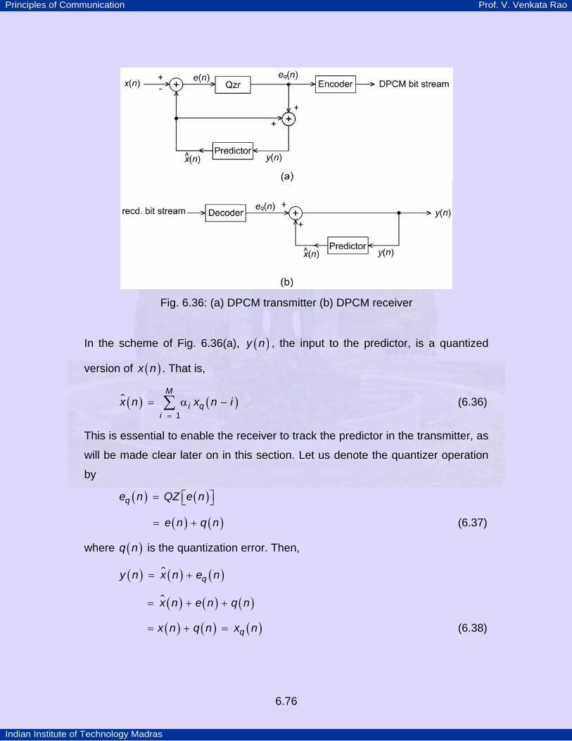
Principles of Communication Prof. V. Venkata Rao
Indian Institute of Technology Madras
6.76
Fig. 6.36: (a) DPCM transmitter (b) DPCM receiver
In the scheme of Fig. 6.36(a), ( )y n , the input to the predictor, is a quantized
version of ( )x n . That is,
( ) ( )M
i qi
x n x n i1=
= α −∑ (6.36)
This is essential to enable the receiver to track the predictor in the transmitter, as
will be made clear later on in this section. Let us denote the quantizer operation
by
( ) ( )qe n QZ e n⎡ ⎤= ⎣ ⎦
( ) ( )e n q n= + (6.37)
where ( )q n is the quantization error. Then,
( ) ( ) ( )qy n x n e n= +
( ) ( ) ( )x n e n q n= + +
( ) ( ) ( )qx n q n x n= + = (6.38)
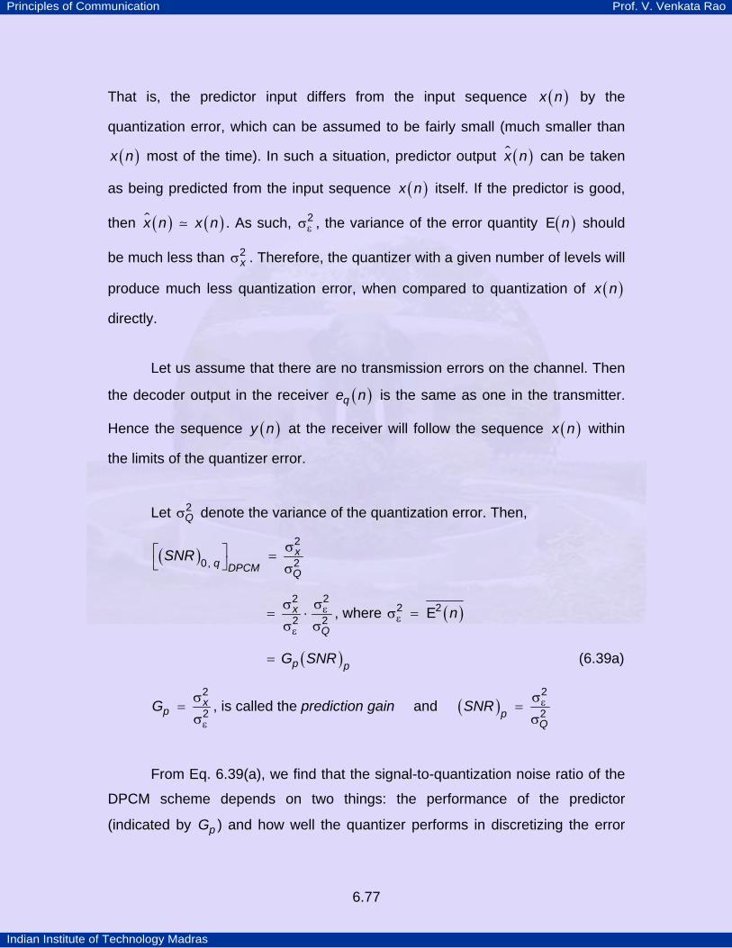
Principles of Communication Prof. V. Venkata Rao
Indian Institute of Technology Madras
6.77
That is, the predictor input differs from the input sequence ( )x n by the
quantization error, which can be assumed to be fairly small (much smaller than
( )x n most of the time). In such a situation, predictor output ( )x n can be taken
as being predicted from the input sequence ( )x n itself. If the predictor is good,
then ( ) ( )x n x n . As such, 2εσ , the variance of the error quantity ( )nE should
be much less than x2σ . Therefore, the quantizer with a given number of levels will
produce much less quantization error, when compared to quantization of ( )x n
directly.
Let us assume that there are no transmission errors on the channel. Then
the decoder output in the receiver ( )qe n is the same as one in the transmitter.
Hence the sequence ( )y n at the receiver will follow the sequence ( )x n within
the limits of the quantizer error.
Let Q2σ denote the variance of the quantization error. Then,
( ) xq DPCM Q
SNR2
20,σ⎡ ⎤ =
⎣ ⎦ σ
x
Q
22
2 2ε
ε
σσ= ⋅
σ σ, where ( )n2 2
εσ = E
( )p pG SNR= (6.39a)
xpG
2
2ε
σ=
σ, is called the prediction gain and ( )p
QSNR
2
2εσ=
σ
From Eq. 6.39(a), we find that the signal-to-quantization noise ratio of the
DPCM scheme depends on two things: the performance of the predictor
(indicated by pG ) and how well the quantizer performs in discretizing the error
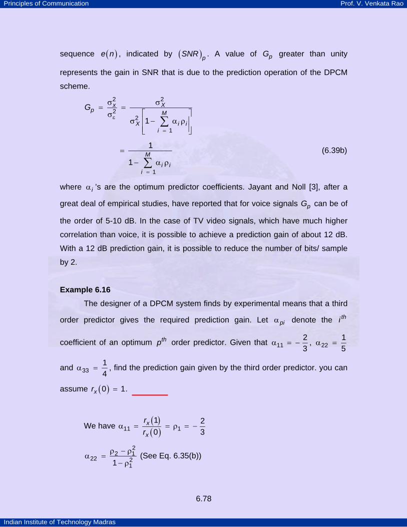
Principles of Communication Prof. V. Venkata Rao
Indian Institute of Technology Madras
6.78
sequence ( )e n , indicated by ( )pSNR . A value of pG greater than unity
represents the gain in SNR that is due to the prediction operation of the DPCM
scheme.
x Xp M
X i ii
G2 2
22
11ε
=
σ σ= =
⎡ ⎤σσ − α ρ⎢ ⎥
⎢ ⎥⎣ ⎦∑
M
i ii 1
1
1=
=− α ρ∑
(6.39b)
where iα ’s are the optimum predictor coefficients. Jayant and Noll [3], after a
great deal of empirical studies, have reported that for voice signals pG can be of
the order of 5-10 dB. In the case of TV video signals, which have much higher
correlation than voice, it is possible to achieve a prediction gain of about 12 dB.
With a 12 dB prediction gain, it is possible to reduce the number of bits/ sample
by 2.
Example 6.16 The designer of a DPCM system finds by experimental means that a third
order predictor gives the required prediction gain. Let piα denote the thi
coefficient of an optimum thp order predictor. Given that 1123
α = − , 2215
α =
and 3314
α = , find the prediction gain given by the third order predictor. you can
assume ( )xr 0 1= .
We have ( )( )
x
x
rr11 1
1 20 3
α = = ρ = −
2
2 122 2
11ρ − ρ
α =− ρ
(See Eq. 6.35(b))
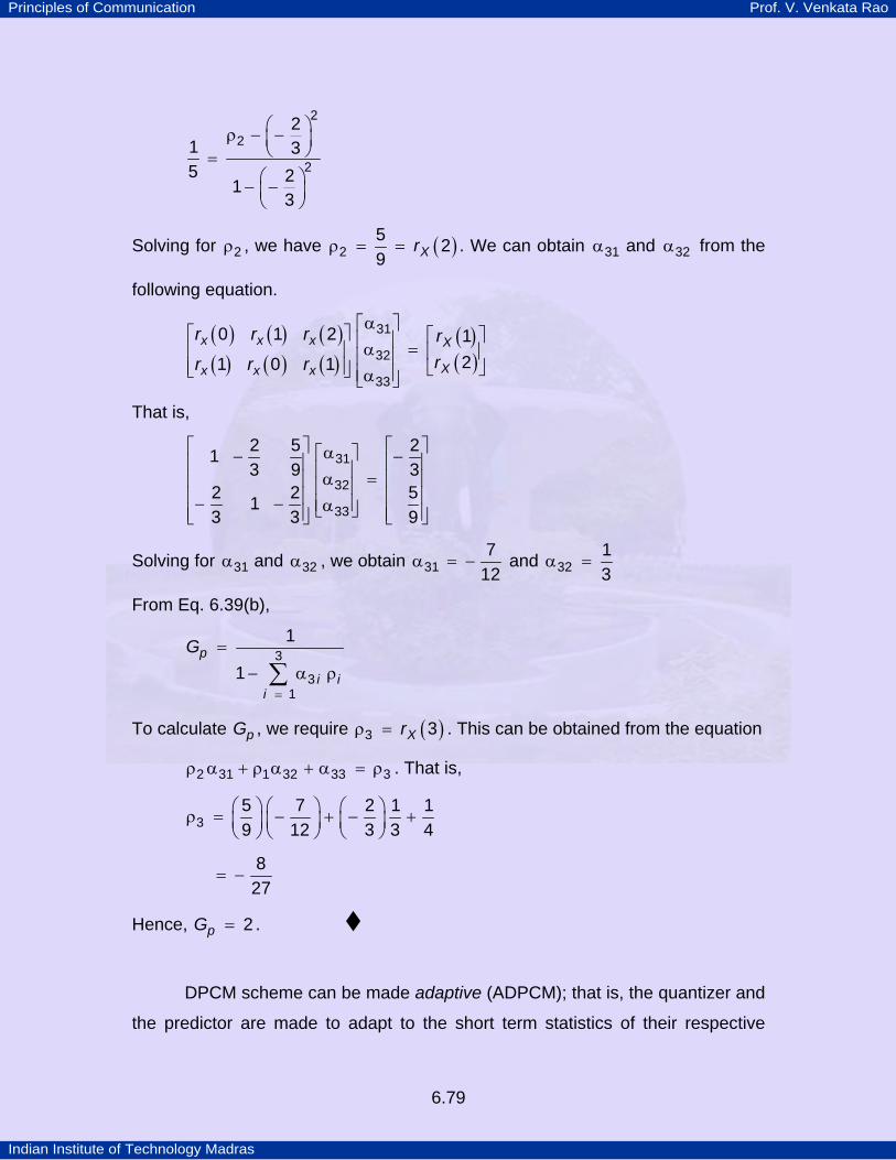
Principles of Communication Prof. V. Venkata Rao
Indian Institute of Technology Madras
6.79
2
2
2
21 35 21
3
⎛ ⎞ρ − −⎜ ⎟⎝ ⎠=⎛ ⎞− −⎜ ⎟⎝ ⎠
Solving for 2ρ , we have ( )Xr25 29
ρ = = . We can obtain 31α and 32α from the
following equation.
( ) ( ) ( )( ) ( ) ( )
( )( )
x x x X
Xx x x
r r r rrr r r
31
32
33
0 1 2 121 0 1
α⎡ ⎤⎡ ⎤ ⎡ ⎤⎢ ⎥α =⎢ ⎥ ⎢ ⎥⎢ ⎥⎢ ⎥ ⎣ ⎦⎣ ⎦ ⎢ ⎥α⎣ ⎦
That is,
31
32
33
2 5 213 9 3
2 2 513 3 9
⎡ ⎤ ⎡ ⎤α⎡ ⎤− −⎢ ⎥ ⎢ ⎥⎢ ⎥α =⎢ ⎥ ⎢ ⎥⎢ ⎥⎢ ⎥ ⎢ ⎥− − ⎢ ⎥α⎣ ⎦⎢ ⎥ ⎢ ⎥⎣ ⎦ ⎣ ⎦
Solving for 31α and 32α , we obtain 317
12α = − and 32
13
α =
From Eq. 6.39(b),
p
i ii
G 3
31
1
1=
=− α ρ∑
To calculate pG , we require ( )Xr3 3ρ = . This can be obtained from the equation
2 31 1 32 33 3ρ α + ρ α + α = ρ . That is,
35 7 2 1 19 12 3 3 4
⎛ ⎞ ⎛ ⎞ ⎛ ⎞ρ = − + − +⎜ ⎟ ⎜ ⎟ ⎜ ⎟⎝ ⎠ ⎝ ⎠ ⎝ ⎠
827
= −
Hence, pG 2= .
DPCM scheme can be made adaptive (ADPCM); that is, the quantizer and
the predictor are made to adapt to the short term statistics of their respective
Principles of Communication Prof. V. Venkata Rao
Indian Institute of Technology Madras
6.80
inputs. Evidently, we can expect better performance from a ADPCM than a
scheme that is fixed. 32 kbps (8 kHz sampling, 4 bits/sample coding) ADPCM
coders for speech have been developed whose performance is quite comparable
with that of 64 kbps companded PCM. Also 64 kbps DPCM has been developed
for encoding audio signals with a bandwidth of 7 kHz. This coder uses a
sampling rate of 16 kHz and a quantizer with 16 levels. Details can be found in
Benevuto et al [4] and Decina and Modena [5].
At the start of the section, we had mentioned that DPCM is a special case
of PCM. If we want, we could treat PCM to be a special case of DPCM where the
predictor output is always zero!
6.9 Delta Modulation
Delta modulation, like DPCM is a predictive waveform coding technique
and can be considered as a special case of DPCM. It uses the simplest possible
quantizer, namely a two level (one bit) quantizer. The price paid for achieving the
simplicity of the quantizer is the increased sampling rate (much higher than the
Nyquist rate) and the possibility of slope-overload distortion in the waveform
reconstruction, as explained in greater detail later on in this section.
In DM, the analog signal is highly over-sampled in order to increase the
adjacent sample correlation. The implication of this is that there is very little
change in two adjacent samples, thereby enabling us to use a simple one bit
quantizer, which like in DPCM, acts on the difference (prediction error) signals.
In its original form, the DM coder approximates an input time function by a
series of linear segments of constant slope. Such a coder is therefore referred to
as a Linear (or non-adaptive) Delta Modulator (LDM). Subsequent developments
have resulted in delta modulators where the slope of the approximating function
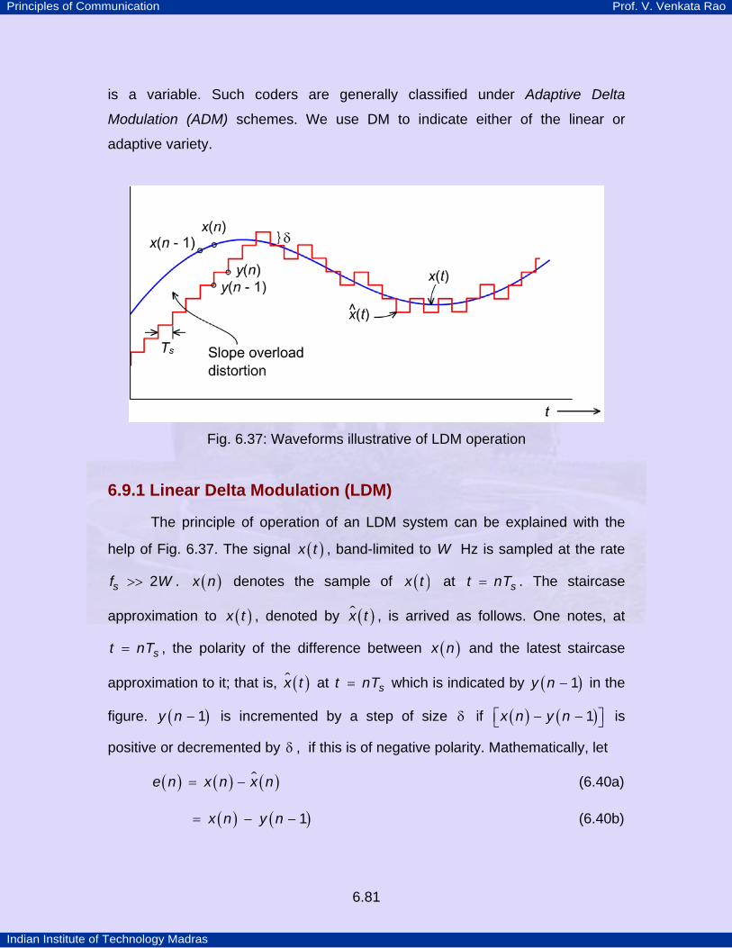
Principles of Communication Prof. V. Venkata Rao
Indian Institute of Technology Madras
6.81
is a variable. Such coders are generally classified under Adaptive Delta
Modulation (ADM) schemes. We use DM to indicate either of the linear or
adaptive variety.
Fig. 6.37: Waveforms illustrative of LDM operation
6.9.1 Linear Delta Modulation (LDM)
The principle of operation of an LDM system can be explained with the
help of Fig. 6.37. The signal ( )x t , band-limited to W Hz is sampled at the rate
sf W2>> . ( )x n denotes the sample of ( )x t at st nT= . The staircase
approximation to ( )x t , denoted by ( )x t , is arrived as follows. One notes, at
st nT= , the polarity of the difference between ( )x n and the latest staircase
approximation to it; that is, ( )x t at st nT= which is indicated by ( )y n 1− in the
figure. ( )y n 1− is incremented by a step of size δ if ( ) ( )x n y n 1⎡ ⎤− −⎣ ⎦ is
positive or decremented by δ , if this is of negative polarity. Mathematically, let
( ) ( ) ( )e n x n x n= − (6.40a)
( ) ( )x n y n 1= − − (6.40b)
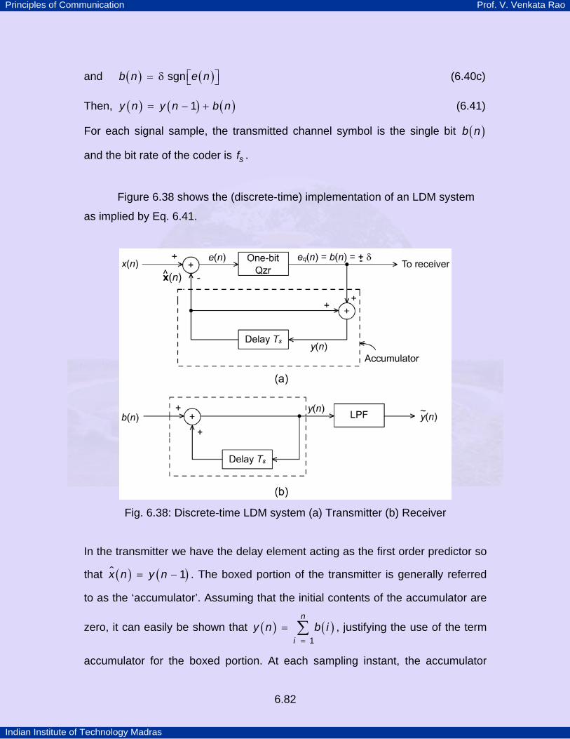
Principles of Communication Prof. V. Venkata Rao
Indian Institute of Technology Madras
6.82
and ( ) ( )b n e nsgn ⎡ ⎤= δ ⎣ ⎦ (6.40c)
Then, ( ) ( ) ( )y n y n b n1= − + (6.41)
For each signal sample, the transmitted channel symbol is the single bit ( )b n
and the bit rate of the coder is sf .
Figure 6.38 shows the (discrete-time) implementation of an LDM system
as implied by Eq. 6.41.
Fig. 6.38: Discrete-time LDM system (a) Transmitter (b) Receiver
In the transmitter we have the delay element acting as the first order predictor so
that ( ) ( )x n y n 1= − . The boxed portion of the transmitter is generally referred
to as the ‘accumulator’. Assuming that the initial contents of the accumulator are
zero, it can easily be shown that ( ) ( )n
iy n b i
1== ∑ , justifying the use of the term
accumulator for the boxed portion. At each sampling instant, the accumulator
Principles of Communication Prof. V. Venkata Rao
Indian Institute of Technology Madras
6.83
increments the approximation to the input signal by ± δ , depending on the output
of the quantizer. (Note that the quantizer step size is 2∆ = δ ). In the receiver,
the sequence ( )y n is reconstructed by passing the incoming sequence of
positive and negative pulses through an accumulator in a manner similar to that
used in the transmitter. The sequence ( )y n is passed through a discrete time
LPF resulting in ( )y n . This lowpass filtering operation is quite essential in the
case of DM because it improves the ( ) qSNR 0, of a DM scheme as explained
later.
Figure 6.39 shows a single integration DM coder-decoder system in an
‘analog implementation’ notation that is very common in the DM literature. Note
that the coder input is ( )x t , a function of the continuous parameter t , and that
the sampling clock appears after the two level quantizer. The outputs
corresponding to ( )x n and ( )y n of Fig. 6.38 have not been indicated in Fig.
6.39(a). These quantities ( )x n and ( )y n , are realized at the output of the
integrator just before and just after each clock operation. The time-continuous
notation in Fig. 6.39 is very relevant for implementation, though for analytical
reasons, the use of discrete time notation may be preferred.
Figure 6.39 also depicts the waveforms involved at various stages of the
LDM coder. These illustrations are self explanatory.
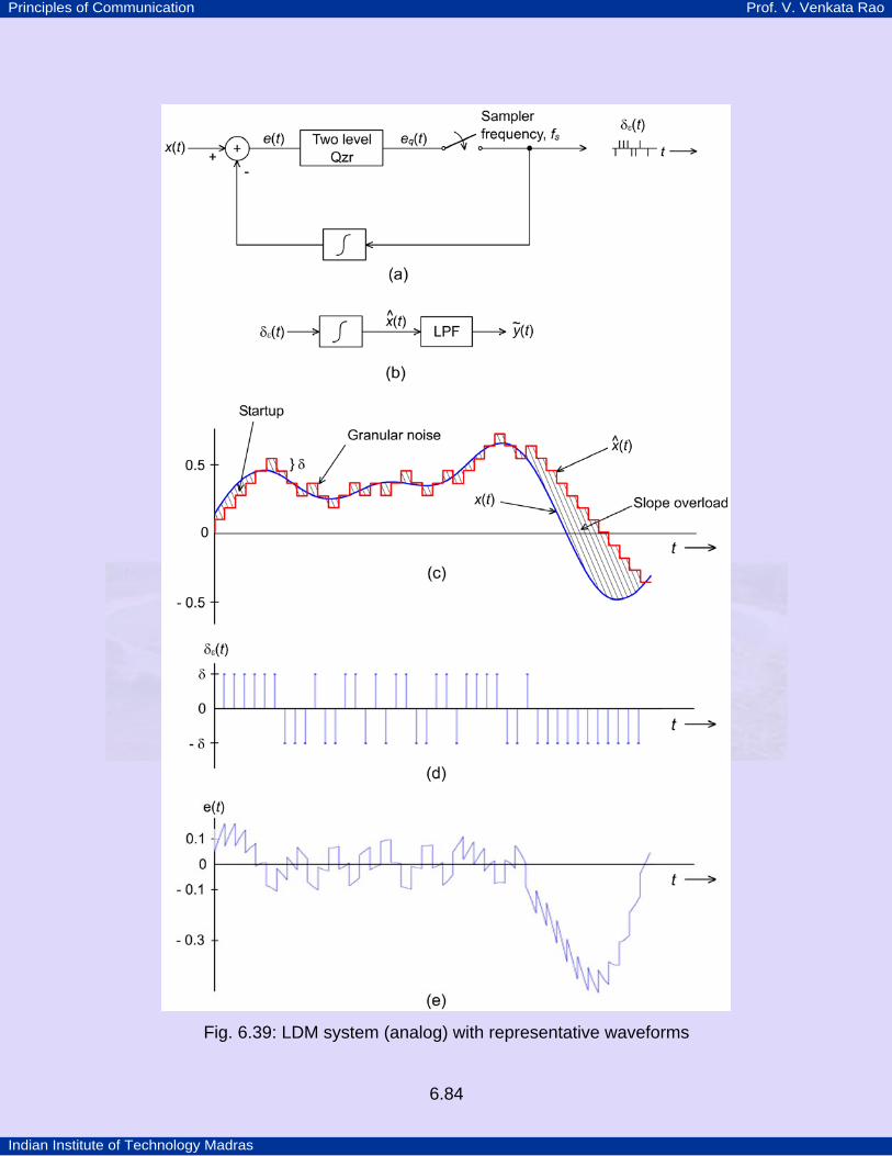
Principles of Communication Prof. V. Venkata Rao
Indian Institute of Technology Madras
6.84
Fig. 6.39: LDM system (analog) with representative waveforms
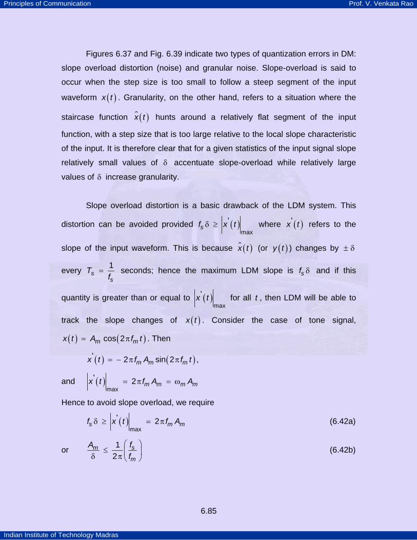
Principles of Communication Prof. V. Venkata Rao
Indian Institute of Technology Madras
6.85
Figures 6.37 and Fig. 6.39 indicate two types of quantization errors in DM:
slope overload distortion (noise) and granular noise. Slope-overload is said to
occur when the step size is too small to follow a steep segment of the input
waveform ( )x t . Granularity, on the other hand, refers to a situation where the
staircase function ( )x t hunts around a relatively flat segment of the input
function, with a step size that is too large relative to the local slope characteristic
of the input. It is therefore clear that for a given statistics of the input signal slope
relatively small values of δ accentuate slope-overload while relatively large
values of δ increase granularity.
Slope overload distortion is a basic drawback of the LDM system. This
distortion can be avoided provided ( )sf x tmax
'δ ≥ where ( )x t' refers to the
slope of the input waveform. This is because ( )x t (or ( )y t ) changes by ± δ
every ss
Tf1
= seconds; hence the maximum LDM slope is sf δ and if this
quantity is greater than or equal to ( )x tmax
' for all t , then LDM will be able to
track the slope changes of ( )x t . Consider the case of tone signal,
( ) ( )m mx t A f tcos 2= π . Then
( ) ( )m m mx t f A f t' 2 sin 2= − π π ,
and ( ) m m m mx t f A Amax
' 2= π = ω
Hence to avoid slope overload, we require
( )s m mf x t f Amax
' 2δ ≥ = π (6.42a)
or sm
m
fAf
12
⎛ ⎞≤ ⎜ ⎟δ π ⎝ ⎠
(6.42b)
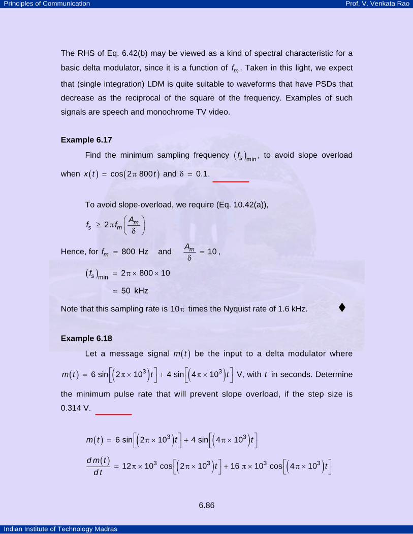
Principles of Communication Prof. V. Venkata Rao
Indian Institute of Technology Madras
6.86
The RHS of Eq. 6.42(b) may be viewed as a kind of spectral characteristic for a
basic delta modulator, since it is a function of mf . Taken in this light, we expect
that (single integration) LDM is quite suitable to waveforms that have PSDs that
decrease as the reciprocal of the square of the frequency. Examples of such
signals are speech and monochrome TV video.
Example 6.17
Find the minimum sampling frequency ( )sf min , to avoid slope overload
when ( ) ( )x t tcos 2 800= π and 0.1δ = .
To avoid slope-overload, we require (Eq. 10.42(a)),
ms m
Af f2 ⎛ ⎞≥ π ⎜ ⎟δ⎝ ⎠
Hence, for mf 800= Hz and mA 10=δ
,
( )sf min 2 800 10= π × ×
50 kHz
Note that this sampling rate is 10π times the Nyquist rate of 1.6 kHz.
Example 6.18
Let a message signal ( )m t be the input to a delta modulator where
( ) ( ) ( )m t t t3 36 sin 2 10 4 sin 4 10⎡ ⎤ ⎡ ⎤= π × + π ×⎣ ⎦ ⎣ ⎦
V, with t in seconds. Determine
the minimum pulse rate that will prevent slope overload, if the step size is
0.314 V.
( ) ( ) ( )m t t t3 36 sin 2 10 4 sin 4 10⎡ ⎤ ⎡ ⎤= π × + π ×⎣ ⎦ ⎣ ⎦
( ) ( ) ( )d m tt t
d t3 3 3 312 10 cos 2 10 16 10 cos 4 10⎡ ⎤ ⎡ ⎤= π × π × + π × π ×
⎣ ⎦ ⎣ ⎦
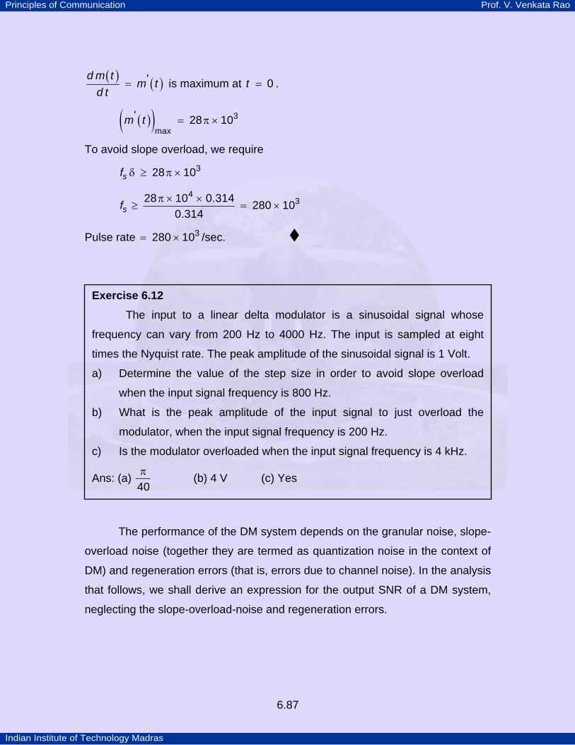
Principles of Communication Prof. V. Venkata Rao
Indian Institute of Technology Madras
6.87
( ) ( )d m tm t
d t'= is maximum at t 0= .
( )( )m t 3
max
' 28 10= π ×
To avoid slope overload, we require
sf328 10δ ≥ π ×
sf4
328 10 0.314 280 100.314
π × ×≥ = ×
Pulse rate 3280 10= × /sec.
The performance of the DM system depends on the granular noise, slope-
overload noise (together they are termed as quantization noise in the context of
DM) and regeneration errors (that is, errors due to channel noise). In the analysis
that follows, we shall derive an expression for the output SNR of a DM system,
neglecting the slope-overload-noise and regeneration errors.
Exercise 6.12 The input to a linear delta modulator is a sinusoidal signal whose
frequency can vary from 200 Hz to 4000 Hz. The input is sampled at eight
times the Nyquist rate. The peak amplitude of the sinusoidal signal is 1 Volt.
a) Determine the value of the step size in order to avoid slope overload
when the input signal frequency is 800 Hz.
b) What is the peak amplitude of the input signal to just overload the
modulator, when the input signal frequency is 200 Hz.
c) Is the modulator overloaded when the input signal frequency is 4 kHz.
Ans: (a) 40π (b) 4 V (c) Yes
Principles of Communication Prof. V. Venkata Rao
Indian Institute of Technology Madras
6.88
For negligible slope-overload, we require ( ) ( ) ( )e t x t x t= − ≤ δ . Let
( )tE denote the random process of which ( )e t is a sample function. We will
assume that ( )tE is zero mean WSS process and the samples of ( )E t are
uniformly distributed in the range ( ),− δ δ . Then 2εσ , the variance of ( )tE is,
22
3εδ
σ = . Experimental results confirm that the PSD of ( )tE is essentially flat for
ss
f fT1
≤ = . That is,
( )s s
S ff f
2 2
2 6ε
εσ δ
= = , for sf f≤
Lowpass filtering the output of the accumulator in the receiver rejects the out-of-
band noise components (remember that in DM, sf W2>> ), giving the output
granular noise component, gN , as
( )W
gW
N S f d fε−
= ∫
s
Wf
2
3δ
= (6.43a)
and ( ) sXg
fSNRW
220,3
= σδ
(6.43b)
where ( )X X t2 2σ =
Recall that in order to avoid slope-overload, δ and sf must satisfy Eq. 6.42.
Principles of Communication Prof. V. Venkata Rao
Indian Institute of Technology Madras
6.89
Now, if the PSD of ( )X t is ( )XS f , then the PSD of ( )d X td t
is ( ) ( )Xf S f22π .
Hence the mean square signal slope can be put in the form
( ) ( ) ( )Xd X t
f S f d fd t
222
∞
− ∞
⎡ ⎤= π⎢ ⎥
⎣ ⎦∫
( )X rmsB 22= πσ
where rmsB , the RMS bandwidth of the lowpass process ( )X t , is defined as
( )rms Xx
B f S f d f
12
21 ∞
− ∞
⎡ ⎤⎢ ⎥=
σ ⎢ ⎥⎣ ⎦∫ (6.44)
We now introduce the so called slope loading factor
s
X rms
fB2δ
ξ =πσ
(6.45)
which is the ratio of maximum DM slope to the RMS signal slope. For any given
signal ( )x t , the parameters xσ and rmsB are fixed. Hence, given the sampling
frequency, ξ is a function of only δ . A reasonably large value of ξ ensures
negligible slope-overload. Expressing δ in terms of ξ and using this value in Eq.
6.43(b), we obtain
Exercise 6.13
The input to an LDM scheme is the sinusoidal signal ( )m mA f tcos 2⎡ ⎤π⎣ ⎦ .
The scheme uses a sampling frequency of sf and the step size δ is such that it
is the minimum value required to avoid slope overload. Show that the ( ) gSNR 0,
expected of such a system, at the output of the final lowpass filter with cutoff at
mf , is
( ) sg
m
fSNRf
3
20,3
8⎛ ⎞
= ⎜ ⎟π ⎝ ⎠
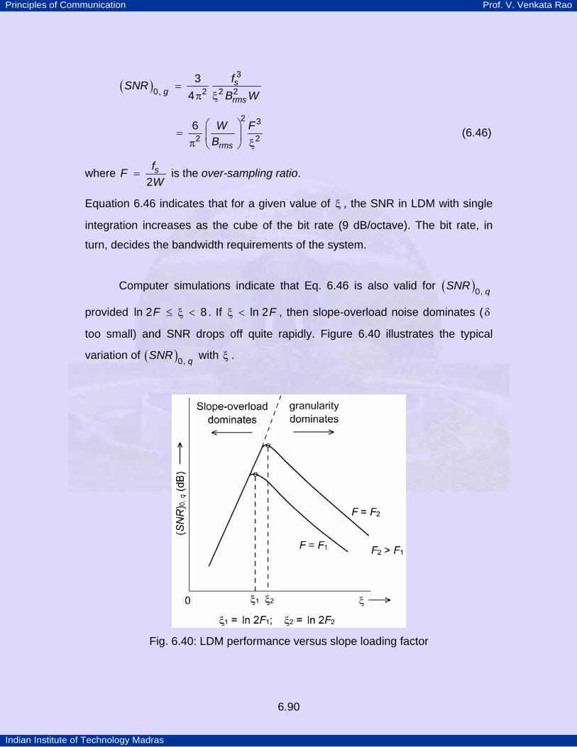
Principles of Communication Prof. V. Venkata Rao
Indian Institute of Technology Madras
6.90
( ) sg
rms
fSNRB W
3
2 2 20,3
4=
π ξ
rms
W FB
2 3
2 26 ⎛ ⎞
= ⎜ ⎟π ξ⎝ ⎠
(6.46)
where sfFW2
= is the over-sampling ratio.
Equation 6.46 indicates that for a given value of ξ , the SNR in LDM with single
integration increases as the cube of the bit rate (9 dB/octave). The bit rate, in
turn, decides the bandwidth requirements of the system.
Computer simulations indicate that Eq. 6.46 is also valid for ( ) qSNR 0,
provided Fln 2 8≤ ξ < . If Fln 2ξ < , then slope-overload noise dominates (δ
too small) and SNR drops off quite rapidly. Figure 6.40 illustrates the typical
variation of ( ) qSNR 0, with ξ .
Fig. 6.40: LDM performance versus slope loading factor
Principles of Communication Prof. V. Venkata Rao
Indian Institute of Technology Madras
6.91
For a specified value of F , DM performance is maximized by taking the
empirically determined optimum slope loading factor,
opt Fln 2ξ
The maximum value of ( ) ( )g qSNR SNR0, 0, is then given by Eq. 6.46 with
optξ = ξ . Note that as the over sampling ratio is fixed for each curve, ξ is
dependent only on δ . Hence, when optξ < ξ , δ is not large enough to prevent
slope overload. Similarly, as the value of ξ increases away from optξ , the size of
δ increases which implies an increase in the granular noise level.
Example 10.20
A signal ( )x t with X2 1σ = has the spectral density ( )XS f given by
( )X
fS f
f
1 , 125 Hz500
1 , 125 375 Hz1000
⎧ ≤⎪⎪= ⎨⎪ < <⎪⎩
( )x t is over sampled by a factor of 10 and the samples are applied to DM coder.
Find optδ , the optimum value of δ .
We will take opt ln20 3ξ = = . From Eq. 6.45,
rms optopt
s
Bf
2π ξδ = .
We need to compute rmsB .
rmsB f d f f d f125 375
2 2 2
0 125
1 12500 1000
⎡ ⎤= ⋅ + ⋅⎢ ⎥
⎢ ⎥⎣ ⎦∫ ∫
f f125 2753 3
0 125
1 1250 3 500 3
⎡ ⎤ ⎡ ⎤= +⎢ ⎥ ⎢ ⎥
⎢ ⎥ ⎢ ⎥⎣ ⎦ ⎣ ⎦
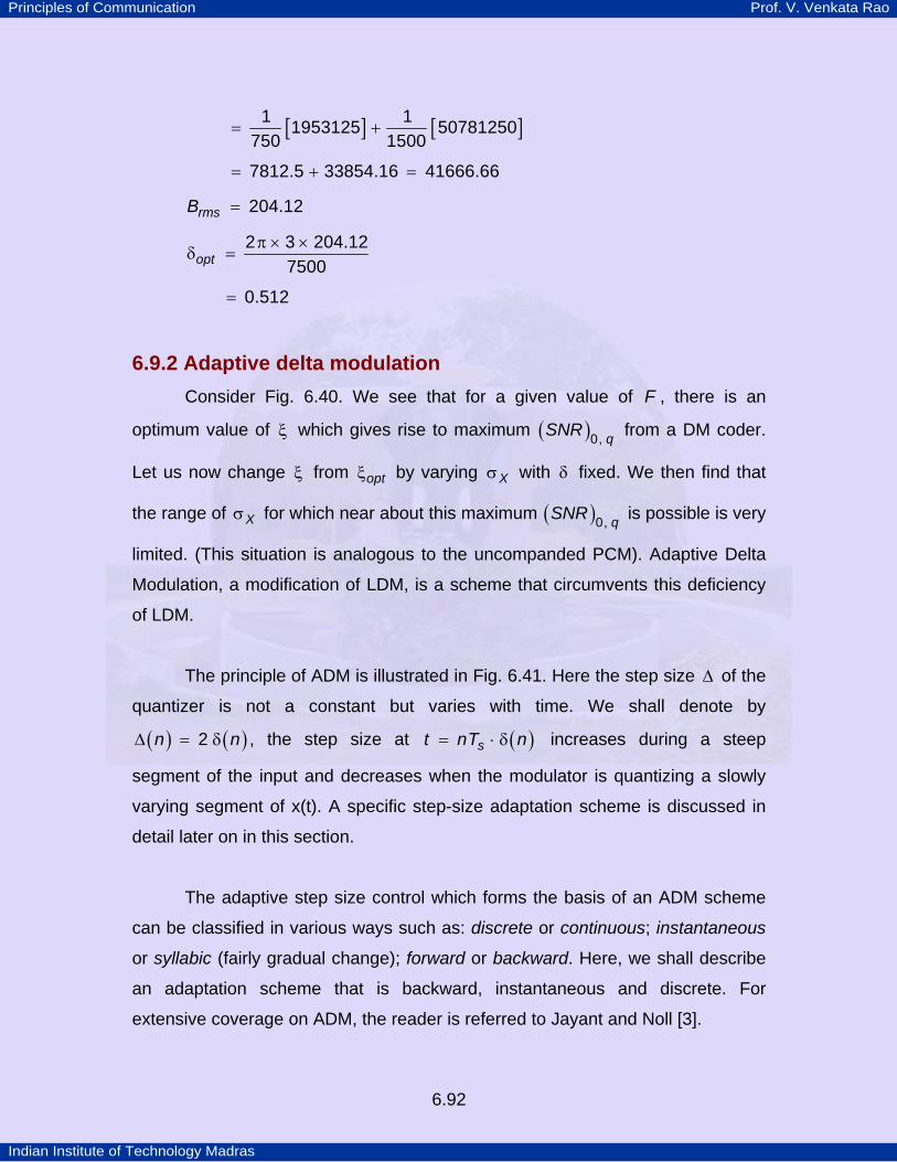
Principles of Communication Prof. V. Venkata Rao
Indian Institute of Technology Madras
6.92
[ ] [ ]1 11953125 50781250750 1500
= +
7812.5 33854.16 41666.66= + =
rmsB 204.12=
opt2 3 204.12
7500π × ×
δ =
0.512=
6.9.2 Adaptive delta modulation Consider Fig. 6.40. We see that for a given value of F , there is an
optimum value of ξ which gives rise to maximum ( ) qSNR 0, from a DM coder.
Let us now change ξ from optξ by varying Xσ with δ fixed. We then find that
the range of Xσ for which near about this maximum ( ) qSNR 0, is possible is very
limited. (This situation is analogous to the uncompanded PCM). Adaptive Delta
Modulation, a modification of LDM, is a scheme that circumvents this deficiency
of LDM.
The principle of ADM is illustrated in Fig. 6.41. Here the step size ∆ of the
quantizer is not a constant but varies with time. We shall denote by
( ) ( )n n2∆ = δ , the step size at ( )st nT n= ⋅ δ increases during a steep
segment of the input and decreases when the modulator is quantizing a slowly
varying segment of x(t). A specific step-size adaptation scheme is discussed in
detail later on in this section.
The adaptive step size control which forms the basis of an ADM scheme
can be classified in various ways such as: discrete or continuous; instantaneous
or syllabic (fairly gradual change); forward or backward. Here, we shall describe
an adaptation scheme that is backward, instantaneous and discrete. For
extensive coverage on ADM, the reader is referred to Jayant and Noll [3].
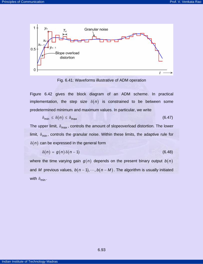
Principles of Communication Prof. V. Venkata Rao
Indian Institute of Technology Madras
6.93
Fig. 6.41: Waveforms illustrative of ADM operation
Figure 6.42 gives the block diagram of an ADM scheme. In practical
implementation, the step size ( )nδ is constrained to be between some
predetermined minimum and maximum values. In particular, we write
( )nmin maxδ ≤ δ ≤ δ (6.47)
The upper limit, maxδ , controls the amount of slopeoverload distortion. The lower
limit, minδ , controls the granular noise. Within these limits, the adaptive rule for
( )nδ can be expressed in the general form
( ) ( ) ( )n g n n 1δ = δ − (6.48)
where the time varying gain ( )g n depends on the present binary output ( )b n
and M previous values, ( ) ( )b n b n M1 , ,− ⋅ ⋅ ⋅ − . The algorithm is usually initiated
with minδ .
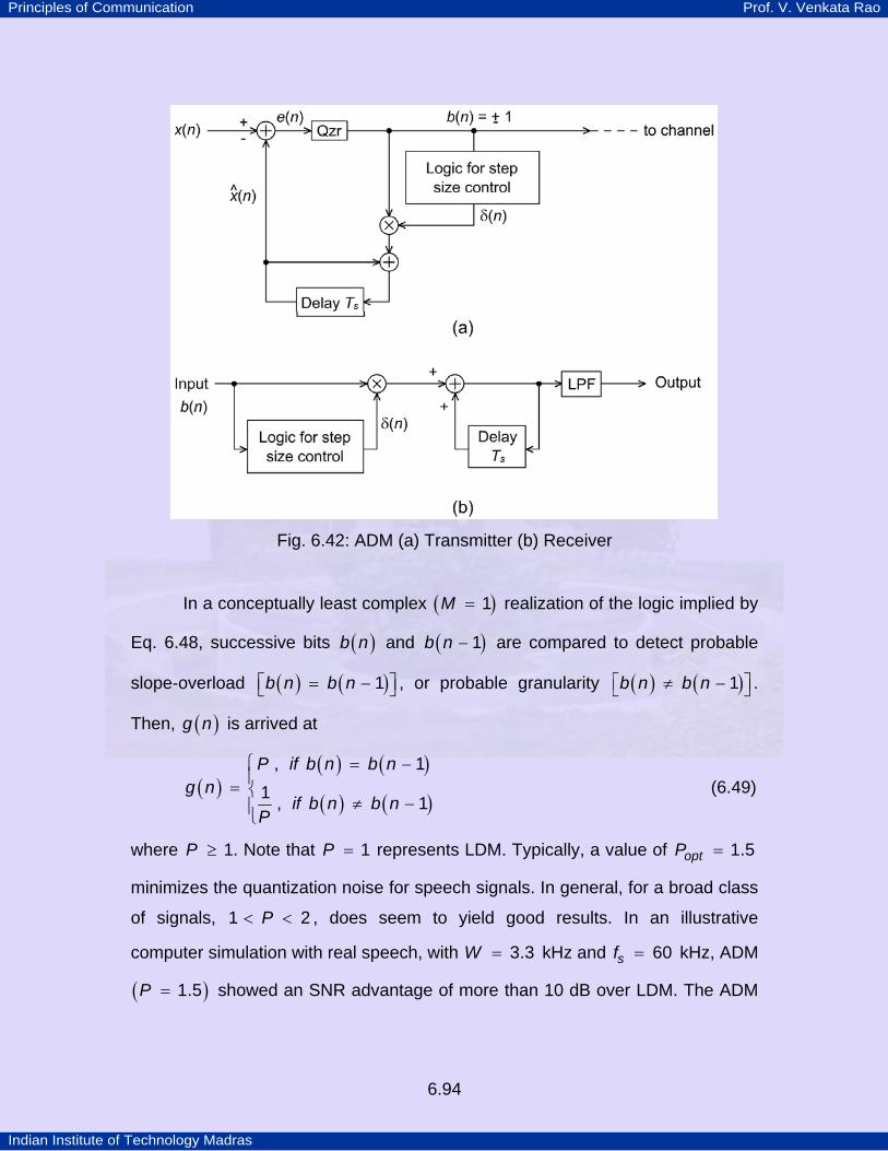
Principles of Communication Prof. V. Venkata Rao
Indian Institute of Technology Madras
6.94
Fig. 6.42: ADM (a) Transmitter (b) Receiver
In a conceptually least complex ( )M 1= realization of the logic implied by
Eq. 6.48, successive bits ( )b n and ( )b n 1− are compared to detect probable
slope-overload ( ) ( )b n b n 1⎡ ⎤= −⎣ ⎦ , or probable granularity ( ) ( )b n b n 1⎡ ⎤≠ −⎣ ⎦ .
Then, ( )g n is arrived at
( )( ) ( )
( ) ( )
P if b n b ng n
if b n b nP
, 11 , 1
⎧ = −⎪= ⎨
≠ −⎪⎩
(6.49)
where P 1≥ . Note that P 1= represents LDM. Typically, a value of optP 1.5=
minimizes the quantization noise for speech signals. In general, for a broad class
of signals, P1 2< < , does seem to yield good results. In an illustrative
computer simulation with real speech, with W 3.3= kHz and sf 60= kHz, ADM
( )P 1.5= showed an SNR advantage of more than 10 dB over LDM. The ADM
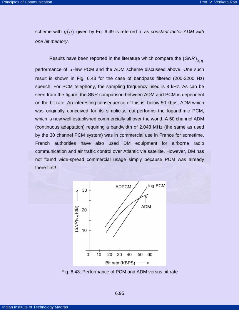
Principles of Communication Prof. V. Venkata Rao
Indian Institute of Technology Madras
6.95
scheme with ( )g n given by Eq. 6.49 is referred to as constant factor ADM with
one bit memory.
Results have been reported in the literature which compare the ( ) qSNR 0,
performance of µ -law PCM and the ADM scheme discussed above. One such
result is shown in Fig. 6.43 for the case of bandpass filtered (200-3200 Hz)
speech. For PCM telephony, the sampling frequency used is 8 kHz. As can be
seen from the figure, the SNR comparison between ADM and PCM is dependent
on the bit rate. An interesting consequence of this is, below 50 kbps, ADM which
was originally conceived for its simplicity, out-performs the logarithmic PCM,
which is now well established commercially all over the world. A 60 channel ADM
(continuous adaptation) requiring a bandwidth of 2.048 MHz (the same as used
by the 30 channel PCM system) was in commercial use in France for sometime.
French authorities have also used DM equipment for airborne radio
communication and air traffic control over Atlantic via satellite. However, DM has
not found wide-spread commercial usage simply because PCM was already
there first!
Fig. 6.43: Performance of PCM and ADM versus bit rate
Principles of Communication Prof. V. Venkata Rao
Indian Institute of Technology Madras
6.96
Instantaneously adapting delta modulators (such as the scheme described
above) are more vulnerable to channel noise than the slowly adapting or linear
coders. Therefore, although instantaneously adapting delta modulators are very
simple and efficient (SNR-wise) in a relatively noise-free environments (say, bit
error probability 410−< ), a number of syllabically adaptive delta modulators
have been designed for use over noisy channels and these coders are
particularly attractive for low-bit-rate ( 20< k bits/sec) applications. For details on
syllabic adaptation, the reader is referred to [3].
Principles of Communication Prof. V. Venkata Rao
Indian Institute of Technology Madras
6.97
Appendix A6.1 PSD of a waveform process with discrete amplitudes A sequence of symbols are transmitted using some basic pulse ( )p t . Let
the resulting waveform process be denoted by ( )X t , given by
( ) ( )k dk
X t A p t kT T∞
= − ∞= − −∑ (A6.1)
kA ’s are discrete random variables, and dT 1 is a random variable uniformly
distributed in the interval T T,2 2
⎛ ⎞−⎜ ⎟⎝ ⎠
. kA ’s are independent of dT . T is the
symbol duration. (For the case of binary transmission, we use bT instead of T ;
bit rate bT1
= .) We shall assume that the autocorrelation of the discrete
amplitude sequence is a function of only the time difference. That is,
( )k k n A k k nE A A R n E A A+ −⎡ ⎤ ⎡ ⎤= =⎣ ⎦ ⎣ ⎦ (A6.2)
With these assumptions, we shall derive an expression for the
autocorrelation of the process ( )X t
( ) ( ) ( )XR t t E X t + X t, ⎡ ⎤+ τ = τ⎣ ⎦
( ) ( )k j d dk j
E A A p t kT T p t jT T∞ ∞
= − ∞ = − ∞
⎡ ⎤= + τ − − − −⎢ ⎥
⎢ ⎥⎣ ⎦∑ ∑
Let j k n= + for some n . Then,
( ) ( ) ( )+
−
⎡ ⎤⎢ ⎥
+ τ = α β⎢ ⎥⎢ ⎥⎢ ⎥⎣ ⎦
∑∑ ∫
T
X k k dnk n T
R t t A A p p d tT
2
2
1,
where ( )dt kT tα = + τ − − and ( )dt jT tβ = − − .
1 For an alternative derivative for the PSD, without the random delay dT in ( )X t , see [6].
Principles of Communication Prof. V. Venkata Rao
Indian Institute of Technology Madras
6.98
(Note that kA ’s are independent of dT ; hence the expectation with respect to dT
can be separated from k jA A )
( ) ( ) ( ) ( )
T
X A dn k T
R t t R n p p d tT
2
2
1,−
⎡ ⎤⎢ ⎥
+ τ = α β⎢ ⎥⎢ ⎥⎢ ⎥⎣ ⎦
∑ ∑ ∫
Let dt kT t u− − = ; then, dd u d t= −
( ) ( ) ( ) ( )t k T
X An k
t k T
R t t R n p u p u nT d uT
12
12
1,
⎛ ⎞− +⎜ ⎟⎝ ⎠
⎛ ⎞− −⎜ ⎟⎝ ⎠
+ τ = − + τ −∑ ∑ ∫
( ) ( ) ( )t k T
An k
t k T
R n p u p u nT d uT
12
12
1⎛ ⎞− −⎜ ⎟⎝ ⎠
⎛ ⎞− +⎜ ⎟⎝ ⎠
= + τ −∑ ∑ ∫
( ) ( ) ( )An
R n p u p u nT d uT1 ∞
− ∞
= + τ −∑ ∫
Let ( )pr τ be the autocorrelation of the pulse ( )p t ; that is,
( ) ( ) ( )pr p u p u d u∞
− ∞
τ = + τ∫ .
Then, ( ) ( ) ( )X A pn
R t t R n r nTT1,+ τ = τ +∑ (A6.3)
As the RHS of Eq. A6.3 is only a function of τ , we have,
( ) ( ) ( )X A pn
R R n r nTT1 ∞
= − ∞τ = τ +∑ (A6.4)
As ( ) ( )pr P f 2τ ←⎯→ , Fourier transform of A6.4 results in the equation
( ) ( ) ( ) j n f TX A
nS f P f R n e
T2 21 ∞
π
= − ∞= ∑
where ( )XS f is the power spectral density of the process.
Principles of Communication Prof. V. Venkata Rao
Indian Institute of Technology Madras
6.99
References
1) A. V. Oppenheim, R. W. Schafer and J. R. Buck, Discrete-Time signal
processing, (2nd ed.), Pearson Education, 2000
2) Simon Haykin, Communication Systems, (4th ed.) John Wiley, 2001
3) N. S. Jayant and P. Noll, Digital Coding of Waveforms: Principles and
applications to speech and video, Prentice Hall, 1984
4) Benevuto et al, The 32 kbps coding standard, AT & T technical journal, vol.
65, no.5, pp12-22, Sept-Oct, 1986
5) M. Decina and G. Modena, CCITT standards on digital speech processing,
IEEE journal on selected areas of communication, Vol. 6, Feb. 1988, pp
227-234
6) Leon W. Couch, II, Digital and analog communication systems, Pearson
Education Asia, 2001