Available online at www.sciencedirect.com

www.elsevier.com/locate/solener

Solar Energy 86 (2012) 2771–2782

Direct beam and hemispherical terrestrial solar spectraldistributions derived from broadband hourly solar radiation data

Daryl R. Myers ⇑,1

National Renewable Energy Laboratory, Electricity, Resources, and Buildings System Integration Center, 1617 Cole Blvd., Golden, CO 80401, USA

Received 14 December 2011; received in revised form 9 June 2012; accepted 15 June 2012Available online 13 July 2012

Communicated by: Associate Editor Frank Vignola

Abstract

Multiple junction and thin film photovoltaic (PV) technologies respond differently to varying terrestrial spectral distributions of solarenergy. PV device and system designers are concerned with the impact of spectral variation on PV specific technologies. Spectral distri-bution data are generally very rare, expensive, and difficult to obtain. We modified an existing empirical spectral conversion model toconvert hourly broadband global (total hemispherical) horizontal and direct normal solar radiation to representative spectral distribu-tions. Hourly average total hemispherical and direct normal beam solar radiation, such as provided in Typical Meteorological Year(TMY) data, are spectral model input data. Default or prescribed atmospheric aerosols and water vapor are possible inputs. Individualhourly and monthly and annual average spectral distributions are computed for a specified tilted surface. The spectral range is from300 nm to 1800 nm. The model is a modified version of the Nann and Riordan SEDES2 model. Measured hemispherical spectral dis-tributions for a wide variety of conditions at the Solar Radiation Research Laboratory at the National Renewable Energy Laboratory,Golden, Co. and Florida Solar Energy Center (Cocoa, FL) show that reasonable spectral accuracy of about ±10% is obtainable withexceptions for weather events such as snow. Differing cloud climatology and variable albedo and aerosol optical depth atmospheric con-ditions can lead to spectral model differences of 30–40%.� 2012 Elsevier Ltd. All rights reserved.

Keywords: Spectral distribution; Broadband irradiance; Spectral model; Conversion; TMY; Photovoltaic

1. Introduction

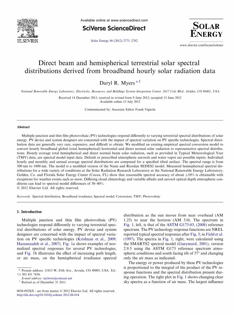
Multiple junction and thin film photovoltaic (PV)technologies respond differently to varying terrestrial spec-tral distributions of solar energy. PV device and systemdesigners are concerned with the impact of spectral varia-tion on PV specific technologies (Krishnan et al., 2009;Hassanzadeh et al., 2007). Fig. 1a shows examples of nor-malized spectral responses for several PV technologies,and Fig. 1b illustrates the effect of increasing path length,or air mass, on the hemispherical irradiance spectral

0038-092X/$ - see front matter � 2012 Elsevier Ltd. All rights reserved.

http://dx.doi.org/10.1016/j.solener.2012.06.014

⇑ Present address: 11815 W, 85th Ave., Arvada, CO 80005, USA. Tel.:+1 303 431 7650.

E-mail address: mybow@comcast.net1 Retired as of December 31 2011.

distribution as the sun moves from near overhead (AM1.25) to near the horizon (AM 5.0). The spectrum inFig. 1, left, is that of the ASTM G173-03, (2008) referencespectrum. The PV technology response functions are NRELreported typical spectral responses after Fig. 3; in Field et al.(1997). The spectra in Fig. 1, right, were calculated usingthe SMARTS2 spectral model (Gueymard, 2001), version2.9.5 using the ASTM G173 reference spectrum atmo-spheric conditions and south facing tilt of 37� and changingonly the air mass as indicated.

The energy or power produced by these PV technologiesis proportional to the integral of the product of the PV re-sponse functions and the spectral distribution present dur-ing operation. The right plot in Fig. 1 shows changing clearsky spectra as a function of air mass. The largest influence

Fig. 1. (Left) variety of PV technology spectral response curves (a-si = amorphous Silicon; Ga = Gallium; Ar = Arsenide; Cu = Copper; In = Indium;Se2 = Diselenide; P = Phosphide; Ge = Germanium; a-Si/aiSi/aiSi:GE = doped triple junction. (Right) influence of changing air mass on modeled clearsky hemispherical total spectral distributions on a tilted surface.

Fig. 2. (Left) measured global hemispherical spectral irradiance distributions on a 40� tilted south facing surface near noon on a clear (April 6), partlycloudy (April 5), and overcast (April 9) day. (Right) relative differences between spectral distributions when they are normalized by peak values. Note“cloud enhancement” of 600–1100 nm region for partly cloudy day (April 5) and overcast day (April 9) above 900 nm.

2772 D.R. Myers / Solar Energy 86 (2012) 2771–2782

on spectral distributions aside from equivalent clear skyconditions is the presence or absence of clouds. Cloud typeand density modify the clear sky spectral distribution,sometimes in a marked fashion. Fig. 2 shows plots of clearand cloudy spectra at nearly identical times near noon(11:50 and 11:55 AM) on 3 days (April 5, 6, and 9th,2008) close together in time. The left plot is of the measuredspectral irradiance, the right of the spectral irradiance nor-malized to the peak value. The measurements in Fig. 2 weremade using a Li-Cor model Li-1800 portable spectrometermounted on a 40� south facing tilt at the National Renew-able Energy Laboratory (NREL) Solar RadiationResearch Laboratory (SRRL) located near Golden, Colo-rado, USA, at 39.74� N, 105.18� W, elevation 1829 m.The spectroradiometer is calibrated routinely every

6 months against a National Institute of Standards andTechnology (NIST) spectral irradiance standard lamp. Ex-pected measurement uncertainty in the measured data is15% for wavelengths <400 nm, 5% for wavelengths from400 nm to 1000 nm, and 10% for wavelengths >1000 nm.(Riordan et al., 1989; Riordan and Myers, 1990; Myers,1989). Data is available on-line through the NREL Mea-surement and Instrumentation Data Center (MIDC) Base-line Measurement System (BMS) “Spectral Data” link atthe following URL: http://www.nrel.gov/midc/srrl_bms(last accessed 9 June 2012). Since spectral distribution mea-surements are relatively expensive and labor intensive, theyare rare and difficult to come by. Model solar spectral dis-tributions derived from widely available broadband datacould provide some insight into PV technology impacts.

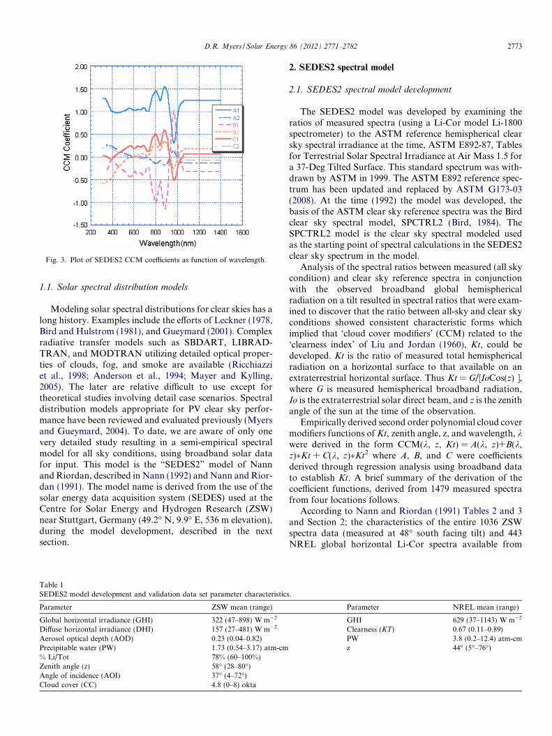
Fig. 3. Plot of SEDES2 CCM coefficients as function of wavelength.

D.R. Myers / Solar Energy 86 (2012) 2771–2782 2773

1.1. Solar spectral distribution models

Modeling solar spectral distributions for clear skies has along history. Examples include the efforts of Leckner (1978,Bird and Hulstrom (1981), and Gueymard (2001). Complexradiative transfer models such as SBDART, LIBRAD-TRAN, and MODTRAN utilizing detailed optical proper-ties of clouds, fog, and smoke are available (Ricchiazziet al., 1998; Anderson et al., 1994; Mayer and Kylling,2005). The later are relative difficult to use except fortheoretical studies involving detail case scenarios. Spectraldistribution models appropriate for PV clear sky perfor-mance have been reviewed and evaluated previously (Myersand Gueymard, 2004). To date, we are aware of only onevery detailed study resulting in a semi-empirical spectralmodel for all sky conditions, using broadband solar datafor input. This model is the “SEDES2” model of Nannand Riordan, described in Nann (1992) and Nann and Rior-dan (1991). The model name is derived from the use of thesolar energy data acquisition system (SEDES) used at theCentre for Solar Energy and Hydrogen Research (ZSW)near Stuttgart, Germany (49.2� N, 9.9� E, 536 m elevation),during the model development, described in the nextsection.

Table 1SEDES2 model development and validation data set parameter characteristics

Parameter ZSW mean (range)

Global horizontal irradiance (GHI) 322 (47–898) W m�2

Diffuse horizontal irradiance (DHI) 157 (27–481) W m�2

Aerosol optical depth (AOD) 0.23 (0.04–0.82)Precipitable water (PW) 1.73 (0.54–3.17) atm-cm% Li/Tot 78% (60–100%)Zenith angle (z) 58� (28–80�)Angle of incidence (AOI) 37� (4–72�)Cloud cover (CC) 4.8 (0–8) okta

2. SEDES2 spectral model

2.1. SEDES2 spectral model development

The SEDES2 model was developed by examining theratios of measured spectra (using a Li-Cor model Li-1800spectrometer) to the ASTM reference hemispherical clearsky spectral irradiance at the time, ASTM E892-87, Tablesfor Terrestrial Solar Spectral Irradiance at Air Mass 1.5 fora 37-Deg Tilted Surface. This standard spectrum was with-drawn by ASTM in 1999. The ASTM E892 reference spec-trum has been updated and replaced by ASTM G173-03(2008). At the time (1992) the model was developed, thebasis of the ASTM clear sky reference spectra was the Birdclear sky spectral model, SPCTRL2 (Bird, 1984). TheSPCTRL2 model is the clear sky spectral modeled usedas the starting point of spectral calculations in the SEDES2clear sky spectrum in the model.

Analysis of the spectral ratios between measured (all skycondition) and clear sky reference spectra in conjunctionwith the observed broadband global hemisphericalradiation on a tilt resulted in spectral ratios that were exam-ined to discover that the ratio between all-sky and clear skyconditions showed consistent characteristic forms whichimplied that ‘cloud cover modifiers’ (CCM) related to the‘clearness index’ of Liu and Jordan (1960), Kt, could bedeveloped. Kt is the ratio of measured total hemisphericalradiation on a horizontal surface to that available on anextraterrestrial horizontal surface. Thus Kt = G/[IoCos(z) ],where G is measured hemispherical broadband radiation,Io is the extraterrestrial solar direct beam, and z is the zenithangle of the sun at the time of the observation.

Empirically derived second order polynomial cloud covermodifiers functions of Kt, zenith angle, z, and wavelength, kwere derived in the form CCM(k, z, Kt) = A(k, z)+B(k,z)�Kt + C(k, z)�Kt2 where A, B, and C were coefficientsderived through regression analysis using broadband datato establish Kt. A brief summary of the derivation of thecoefficient functions, derived from 1479 measured spectrafrom four locations follows.

According to Nann and Riordan (1991) Tables 2 and 3and Section 2; the characteristics of the entire 1036 ZSWspectra data (measured at 48� south facing tilt) and 443NREL global horizontal Li-Cor spectra available from

.

Parameter NREL mean (range)

GHI 629 (37–1143) W m�2

Clearness (KT) 0.67 (0.11–0.89)PW 3.8 (0.2–12.4) atm-cmz 44� (5�–76�)

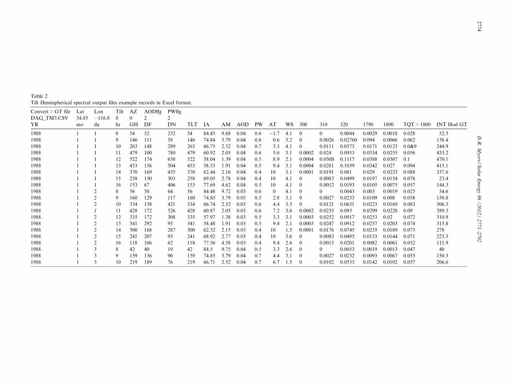
Table 2Tilt Hemispherical spectral output files example records in Excel format.

Convert > GT file Lat Lon Tilt AZ AODflg PWflgDAG_TM3.CSV 34.85 �116.8 0 0 2 2YR mo da hr GH DF DN TLT IA AM AOD PW AT WS 300 310 320 1790 1800 TQT > 1800 INT Hod GT

1988 1 1 8 54 32 232 54 84.45 9.68 0.04 0.6 �1.7 4.1 0 0 0.0044 0.0029 0.0018 0.028 52.51988 1 1 9 146 111 58 146 74.84 3.79 0.04 0.6 0.6 5.2 0 0.0026 0.02760 0.094 0.0066 0.062 138.41988 1 1 10 263 148 289 263 66.75 2.52 0.04 0.7 3.3 4.1 0 0.0111 0.0573 0.0171 0.0123 0.0&9 244.91988 1 1 11 479 100 780 479 60.92 2.05 0.04 0.6 5.6 3.1 0.0002 0.024 0.0953 0.0334 0.0255 0.056 433.21988 1 1 12 522 174 658 522 58.04 1.39 0.04 0.5 8.9 2.1 0.0004 0.030S 0.1117 0.0388 0.0307 0.1 470.11988 1 1 13 453 156 504 453 58.53 1.91 0.04 0.5 9.4 3.1 0.0004 0.0281 0.1039 0.0342 0.027 0.094 415.11988 1 1 14 370 169 435 370 62.44 2.16 0.04 0.4 10 3.1 0.0001 0.0191 0.081 0.029 0.0233 0.088 337.61988 1 1 15 258 150 303 258 69.05 2.78 0.04 0.4 10 4.1 0 0.0083 0.0499 0.0197 0.0154 0.076 23.41988 1 1 16 153 67 406 153 77.69 4.62 0.04 0.5 10 4.1 0 0.0012 0.0193 0.0105 0.0075 0.057 144.31988 1 2 8 56 50 64 56 84.48 9.72 0.03 0.6 0 4.1 0 0 0.0043 0.003 0.0019 0.025 54.61988 1 2 9 160 129 117 160 74.S5 3.79 0.03 0.5 2.8 3.1 0 0.0027 0.0233 0.0109 0.008 0.058 150.81988 1 2 10 334 158 421 334 66.74 2.52 0.03 0.6 4.4 3.5 0 0.0121 0.0631 0.0223 0.0169 0.083 306.31988 1 1 11 428 172 526 428 60.87 2.05 0.03 0.6 7.2 3.6 0.0002 0.0233 0.093 0.0299 0.0228 0.09 389.31988 1 2 12 335 172 308 335 57.97 1.38 0.03 0.5 3.3 3.1 0.0003 0.0252 0.0917 0.0253 0.02 0.072 310.91988 1 2 13 341 292 95 341 58.48 1.91 0.03 0.5 9.4 2.1 0.0003 0.0247 0.0912 0.0257 0.0203 0.074 315.81988 1 2 14 300 168 287 300 62.32 2.15 0.03 0.4 10 1.5 0.0001 0.0176 0.0745 0.0235 0.0189 0.073 2781988 1 2 15 241 207 95 241 68.92 2.77 0.03 0.4 10 3.6 0 0.00S3 0.0495 0.0133 0.0144 0.071 223.31988 1 2 16 118 106 62 118 77.56 4.58 0.03 0.4 9.4 2.6 0 0.0013 0.0201 0.0082 0.0061 0.052 111.91988 1 3 8 42 40 19 42 84.5 9.75 0.04 0.5 3.3 2.6 0 0 0.0053 0.0019 0.0013 0.047 401988 1 3 9 159 136 90 159 74.85 3.79 0.04 0.7 4.4 3.1 0 0.0027 0.0232 0.0093 0.0067 0.055 150.31988 1 3 10 219 189 76 219 66.71 2.52 0.04 0.7 6.7 1.5 0 0.0102 0.0533 0.0142 0.0102 0.057 206.6

2774D

.R.

My

ers/S

ola

rE

nerg

y8

6(

20

12

)2

77

1–

27

82

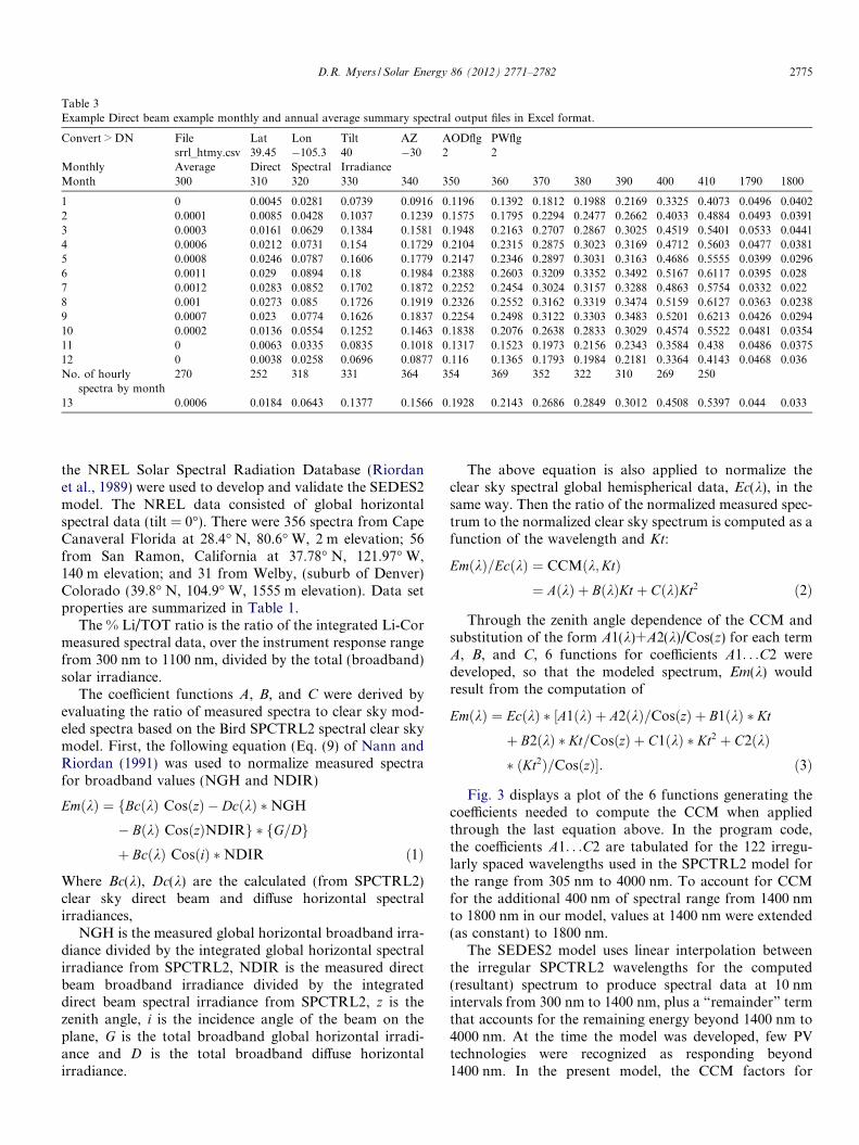
Table 3Example Direct beam example monthly and annual average summary spectral output files in Excel format.

Convert > DN File Lat Lon Tilt AZ AODflg PWflgsrrl_htmy.csv 39.45 �105.3 40 �30 2 2

Monthly Average Direct Spectral IrradianceMonth 300 310 320 330 340 350 360 370 380 390 400 410 1790 1800

1 0 0.0045 0.0281 0.0739 0.0916 0.1196 0.1392 0.1812 0.1988 0.2169 0.3325 0.4073 0.0496 0.04022 0.0001 0.0085 0.0428 0.1037 0.1239 0.1575 0.1795 0.2294 0.2477 0.2662 0.4033 0.4884 0.0493 0.03913 0.0003 0.0161 0.0629 0.1384 0.1581 0.1948 0.2163 0.2707 0.2867 0.3025 0.4519 0.5401 0.0533 0.04414 0.0006 0.0212 0.0731 0.154 0.1729 0.2104 0.2315 0.2875 0.3023 0.3169 0.4712 0.5603 0.0477 0.03815 0.0008 0.0246 0.0787 0.1606 0.1779 0.2147 0.2346 0.2897 0.3031 0.3163 0.4686 0.5555 0.0399 0.02966 0.0011 0.029 0.0894 0.18 0.1984 0.2388 0.2603 0.3209 0.3352 0.3492 0.5167 0.6117 0.0395 0.0287 0.0012 0.0283 0.0852 0.1702 0.1872 0.2252 0.2454 0.3024 0.3157 0.3288 0.4863 0.5754 0.0332 0.0228 0.001 0.0273 0.085 0.1726 0.1919 0.2326 0.2552 0.3162 0.3319 0.3474 0.5159 0.6127 0.0363 0.02389 0.0007 0.023 0.0774 0.1626 0.1837 0.2254 0.2498 0.3122 0.3303 0.3483 0.5201 0.6213 0.0426 0.029410 0.0002 0.0136 0.0554 0.1252 0.1463 0.1838 0.2076 0.2638 0.2833 0.3029 0.4574 0.5522 0.0481 0.035411 0 0.0063 0.0335 0.0835 0.1018 0.1317 0.1523 0.1973 0.2156 0.2343 0.3584 0.438 0.0486 0.037512 0 0.0038 0.0258 0.0696 0.0877 0.116 0.1365 0.1793 0.1984 0.2181 0.3364 0.4143 0.0468 0.036No. of hourly

spectra by month270 252 318 331 364 354 369 352 322 310 269 250

13 0.0006 0.0184 0.0643 0.1377 0.1566 0.1928 0.2143 0.2686 0.2849 0.3012 0.4508 0.5397 0.044 0.033

D.R. Myers / Solar Energy 86 (2012) 2771–2782 2775

the NREL Solar Spectral Radiation Database (Riordanet al., 1989) were used to develop and validate the SEDES2model. The NREL data consisted of global horizontalspectral data (tilt = 0�). There were 356 spectra from CapeCanaveral Florida at 28.4� N, 80.6� W, 2 m elevation; 56from San Ramon, California at 37.78� N, 121.97� W,140 m elevation; and 31 from Welby, (suburb of Denver)Colorado (39.8� N, 104.9� W, 1555 m elevation). Data setproperties are summarized in Table 1.

The % Li/TOT ratio is the ratio of the integrated Li-Cormeasured spectral data, over the instrument response rangefrom 300 nm to 1100 nm, divided by the total (broadband)solar irradiance.

The coefficient functions A, B, and C were derived byevaluating the ratio of measured spectra to clear sky mod-eled spectra based on the Bird SPCTRL2 spectral clear skymodel. First, the following equation (Eq. (9) of Nann andRiordan (1991) was used to normalize measured spectrafor broadband values (NGH and NDIR)

EmðkÞ ¼ fBcðkÞ CosðzÞ � DcðkÞ �NGH

� BðkÞ CosðzÞNDIRg � fG=Dgþ BcðkÞ CosðiÞ �NDIR ð1Þ

Where Bc(k), Dc(k) are the calculated (from SPCTRL2)clear sky direct beam and diffuse horizontal spectralirradiances,

NGH is the measured global horizontal broadband irra-diance divided by the integrated global horizontal spectralirradiance from SPCTRL2, NDIR is the measured directbeam broadband irradiance divided by the integrateddirect beam spectral irradiance from SPCTRL2, z is thezenith angle, i is the incidence angle of the beam on theplane, G is the total broadband global horizontal irradi-ance and D is the total broadband diffuse horizontalirradiance.

The above equation is also applied to normalize theclear sky spectral global hemispherical data, Ec(k), in thesame way. Then the ratio of the normalized measured spec-trum to the normalized clear sky spectrum is computed as afunction of the wavelength and Kt:

EmðkÞ=EcðkÞ ¼ CCMðk;KtÞ¼ AðkÞ þ BðkÞKt þ CðkÞKt2 ð2Þ

Through the zenith angle dependence of the CCM andsubstitution of the form A1(k)+A2(k)/Cos(z) for each termA, B, and C, 6 functions for coefficients A1. . .C2 weredeveloped, so that the modeled spectrum, Em(k) wouldresult from the computation of

EmðkÞ ¼ EcðkÞ � ½A1ðkÞ þ A2ðkÞ=CosðzÞ þ B1ðkÞ � Kt

þ B2ðkÞ � Kt=CosðzÞ þ C1ðkÞ � Kt2 þ C2ðkÞ� ðKt2Þ=CosðzÞ�: ð3Þ

Fig. 3 displays a plot of the 6 functions generating thecoefficients needed to compute the CCM when appliedthrough the last equation above. In the program code,the coefficients A1. . .C2 are tabulated for the 122 irregu-larly spaced wavelengths used in the SPCTRL2 model forthe range from 305 nm to 4000 nm. To account for CCMfor the additional 400 nm of spectral range from 1400 nmto 1800 nm in our model, values at 1400 nm were extended(as constant) to 1800 nm.

The SEDES2 model uses linear interpolation betweenthe irregular SPCTRL2 wavelengths for the computed(resultant) spectrum to produce spectral data at 10 nmintervals from 300 nm to 1400 nm, plus a “remainder” termthat accounts for the remaining energy beyond 1400 nm to4000 nm. At the time the model was developed, few PVtechnologies were recognized as responding beyond1400 nm. In the present model, the CCM factors for

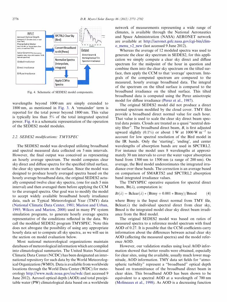
Fig. 4. Schematic of SEDES2 model components.

2776 D.R. Myers / Solar Energy 86 (2012) 2771–2782

wavelengths beyond 1000 nm are simply extended to1800 nm, as mentioned in Fig. 3. A ‘remainder’ term isreported for the total power beyond 1800 nm. This valueis typically less than 5% of the total integrated spectralpower. Fig. 4 is a schematic representation of the operationof the SEDES2 model modules.

2.2. SEDES2 modifications: TMYSPEC

The SEDES2 model was developed utilizing broadbandand spectral measured data collected on 5 min intervals.However, the final output was conceived as representingan hourly average spectrum. The model computes clearsky direct and diffuse spectra for the specified tilted surface,the clear sky spectrum on the surface. Since the model wasdesigned to produce hourly averaged spectra based on thehourly average broadband data, the original SEDES2 actu-ally computed twelve clear sky spectra, (one for each 5 mininterval) and then averaged them before applying the CCMto the averaged spectra. Our goal was to modify the modelto accept widely available broadband hourly irradiancedata, such as Typical Meteorological Year (TMY) data(National Climatic Data Center, 1981; Marion and Urban,1995; Wilcox and Marion, 2008) used in many PV systemsimulation programs, to generate hourly average spectrarepresentative of the conditions reflected in the data. Wecall the modified SEDES2 program TMYSPEC. Note thisdoes not abrogate the possibility of using any appropriatehourly data set to compute all sky spectra, as we will see inthe section on model evaluation below.

Most national meteorological organizations maintaindatabases of meteorological information which are compiledinto climatological summaries. The United States NationalClimatic Data Center (NCDC) has been designated an inter-national repository for such data by the World Meteorolog-ical Organization (WMO). Data is available from worldwidelocations through the World Data Center (WDC) for mete-orology http://www.ncdc.noaa.gov/oa/wdc (last accessed 9June 2012). Aerosol optical depth (AOD) and total precipi-table water (PW) climatological data based on a worldwide

network of measurements representing a wide range ofclimates, is available through the National Aeronauticsand Space Administration (NASA) AERONET networkare available at http://aeronet.gsfc.nasa.gov/cgi-bin/clim-o_menu_v2_new (last accessed 9 June 2012).

Whereas the average of 12 modeled spectra was used togenerate the clear sky spectrum in SEDES2, for this appli-cation we simply compute a clear sky direct and diffusespectrum for the midpoint of the hour in question andcombine them into the clear sky spectrum on the tilted sur-face, then apply the CCM to that ‘average’ spectrum. Inte-grals of the computed spectrum are compared to themeasured, hourly average broadband data. The integralof the spectrum on the tilted surface is compared to thebroadband irradiance on the tilted surface. This tiltedbroadband data is computed using the Perez anisotropicmodel for diffuse irradiance (Perez et al., 1987).

The original SEDES2 model did not produce a directnormal spectrum modified by the cloud cover. TMY filesprovide a broadband direct normal value for each hour.That value is used to scale the clear sky direct beam spec-tral data points. Clouds are treated as a quasi “neutral den-sity filter”. The broadband direct beam, B, is first adjustedupward slightly (0.1%) or about 1 W at 1000 W m�2 toaccount for low spectral resolution of the Bird model inthe IR bands. Only the ‘starting’, ‘ending’, and centerwavelengths of absorption bands are used in SPCTRL2.For instance the model uses 8 wavelengths at approxi-mately 30 nm intervals to cover the water vapor absorptionband from 1300 nm to 1500 nm (a range of 200 nm). Onaverage, the Bird model underestimates the integrated irra-diance over these bands. The correction is an average basedon comparison of SMARTS2 and SPCTRL2 absorptionband integrated irradiance values.

The TMYSPEC operative equation for spectral directbeam, Bt(k), computation is:

BtðkÞ ¼ BclearðkÞ � ðBtmyþ 0:001 � BtmyÞ=Bmod ð4Þ

where Btmy is the Input direct normal from TMY file,Bclear(k) the individual spectral direct from clear sky,Bmod is the integrated model clear sky direct beam irradi-ance from the Bird model.

The original SEDES2 model was based on ratios ofmeasured spectra to a reference model spectrum with fixedAOD of 0.27. It is possible that the CCM coefficients carryinformation about the differences between actual clear skyAOD (affecting the measured spectra) and the model refer-ence AOD.

However, our validation studies using local AOD infor-mation showed that better results were obtained, especiallyfor clear sites, using the available, usually much lower mag-nitude, AOD information. TMY data set fields for “atmo-spheric turbidity” represent a “broadband” optical depthbased on transmittance of the broadband direct beam inclear skies. This broadband AOD has been shown to beequivalent to a spectral AOD at a wavelength of 700 nm(Molineaux et al., 1998). As AOD is a decreasing function

D.R. Myers / Solar Energy 86 (2012) 2771–2782 2777

of wavelength, the user has an option to correct the TMYAOD upwards to represent a spectral AOD at 500 nm(which is utilized by the SPCTRL2 model). If actual500 nm AOD data is available, it can read directly intothe model. Similarly, TMY data sets also provide total pre-cipitable water content. There are options for using eitherof these data, or if not available in a measured data set,water vapor estimated from relative humidity, temperature,and/or dewpoint temperature are computed.

Originally, SEDES2 utilized solar time to compute thesolar geometry. The broadband and spectral data for devel-oping and validating the model used solar time. Since mostcurrent TMY and other solar radiation data collection uselocal standard time (note: the original 1952–1978 SOL-MET/ERSATZ (National Climatic Data Center, 1978)and original TMY (National Climatic Data Center, 1981)data set used solar time, TMY2 (Marion and Urban,1995) and TMY3 (Wilcox and Marion, 2008) use standardtime). The present model uses local standard time, and theMichalsky, 1988 solar position subroutine SOLPOS (Wil-cox and Marion, 2008) to compute solar geometry.

The broadband data (global, direct, and diffuse irradi-ances) as well as meteorological data (relative humidity,temperature, etc.) are all hourly averaged data. The valueof the data is assumed to represent the average of the pre-ceding hour, and time associated with that data point isassumed to be the midpoint (half hour) of the precedinghour. Thus “11:00” data represents the hourly average ofdata from 10:00 AM to 11:00 AM, and is assumed to occurat 10:30 AM.

The model spectral resolution at each wavelength is thatof the SPCTRL2 model, which has never been definitivelyestablished, though it is sometimes quoted as “approxi-mately 20 cm�1” (0.5 nm in the ultraviolet and visible, and2 nm in the infrared). This is because the model was partlyvalidated against a Monte Carlo radiative transfer code withthis spectral resolution. The SPCTRL2 model wavelengthmodel step size is limited to the (varying) spectral step sizeof the SPCTRL2 model (e.g., 5 nm from 305 nm to350 nm, 10 nm for 350 nm to 550, then irregular spacingthereafter to capture spectral absorption features in a‘coarse’ way. The SEDES2 model linearly interpolates themodeled spectral data (derived from SPCTRL2 wavelengthsand algorithms) into uniform steps of 10 nm from 300 nm to1800 nm. The NREL measured spectral data is at 2 nmwavelength intervals with a 6 nm spectral passband. Thereis no effective way to smooth the lower resolution (10 nm)model data to the higher resolution (2 nm) of the measureddata. The measured data at the 10 nm incremental valuesbetween 300 nm and 1100 nm is used in this analysis.

3. TMYSPEC operational model

3.1. TMYSPEC user input

The SEDES2 model was originally written in the FOR-TRAN programming language, and the modifications to

produce the TMYSPEC version were done in FORTRANas well. Modifications made for operational considerations,not mentioned above, include:

User specified location (latitude, longitude, time zone,altitude).

User specified tilt and azimuth orientations for the col-lector surface.User specified input file and output file names.Choice of default, climatological, or input file values for

aerosol optical depth and precipitable water vapor.

The first element required to run the model is a suitableinput file. A comma separated, free format string of vari-ables is required for each (hourly) record. If the user electsto read the AOD and total water vapor from TMY datasets, the input record is of the form (the prescribed orderof the parameters is required, and is the order in whichTMY2 and TMY3 variables appear in their respectivefiles):

Year, month, day of year, hour, global horizontal, directbeam, diffuse horizontal, ambient temperature, dew pointtemperature, relative humidity, station barometric pres-sure, wind speed, precipitable water, broadband aerosoloptical depth.

Irradiance units are watts per square meter (W m�2),temperatures are in degrees Celsius (�C) multiplied by 10,Relative humidity in percent, and pressure is in millibars.

If either dewpoint or relative humidity (but not both)are missing from an input file (say if actual measuredhourly average data is used to build an input file), totalwater is computed from the non-missing parameter andtemperature. If desired, ‘climatological’ or long term meanvalues of aerosol optical depth can be used in conjunctionwith measured data.

TMY2 values of AOD are multiplied by 1000; (e.g.,AOD 0.02 is reported as “20”), wind speed is reported intenths of meters per second (1 m/s is reported as “10”).TMY3 values for these data are in ‘standard’ format, andneed to be adjusted by these factors when building theinput file for the model. Global horizontal radiation isalways required, but if one of the other radiation compo-nents is missing, it will be computed from the two avail-able. Missing values are designated as ‘9999’.

An example data record line of input data would be“1984, 1, 1, 11, 185, 90, 149, �39, �106, 60, 836, 30, 34,3”. The elements are, in order, year, month, day, hour (end-ing), global horizontal irradiance, direct beam irradiance,diffuse horizontal irradiance, all in W m�2; dewpoint tem-perature (�C � 10), ambient temperature (�C � 10), relativehumidity (percent), station pressure (mB), wind speed (10thsof m/s), total precipitable water vapor (atm-mm), and aero-sol optical depth multiplied by 1000. These values are just asextracted from a TMY2 data file.

Any measured data set with these components couldalso be used, but reformatted into the format matching

2778 D.R. Myers / Solar Energy 86 (2012) 2771–2782

the above TMY2 fields, as discussed in the evaluationsection.

Once the input data file has been assembled, the execut-able application is run, which requests the following usersupplied inputs:

Latitude, longitude, (decimal degrees).Site elevation (meters) and time zone (� for W, + for E).Tilt angle of surface, (degrees) from horizontal.Azimuth of surface normal (degrees): (S = 0�, E = +90�,W = �90�).Choice of (1) use default 0.27 aerosol optical depth, (2)read aerosol optical depth from file, or (3) enter constant(climatological) value for aerosol optical depth.Choice of (1) compute (from relative humidity or dew-point) or (2) read water vapor data.

The user then enters the input file path and file name andseparate output file names for the global tilted and directnormal spectral data and monthly average spectral data.

The input files do not have to be serially complete or anentire year of 8760 h. A yearly file of daylight hours, amonthly file of daylight hours, or just a few hours of datacan be used for the computation. The computations areperformed on a record by record basis. The processing ofone record of input data results in one record of outputdata being written (if all internal data quality and modellimits checks are passed).

3.2. TMYSPEC output

The model computations are performed, and the hourlyspectral distributions (with the same time stamp as the inputdata) are written to the user specified output files. The globaland direct output file consists of a header with labels.

Converted (input) file name, latitude, longitude, speci-fied tilt and azimuth, AOD flag (1 = default, 2 = read fromfile, or 3 = constant climatological value), total watervapor flag (1 = compute from RH or temperatures,2 = read from file). The broadband values from the inputfile as well as the modeled tilted broadband data arereported. The next record contains the labels for the broad-band radiation data, geometrical parameters, and the mod-eled plane of array spectrum in the format.

Year, month, day, hour, global, diffuse, direct, tilt irra-diance, incidence angle, relative air mass, AOD, watervapor, ambient dry bulb temperature, wind speed, 300,310, . . ., 1790, 1800 > 1800, an estimate of the spectral inte-gral beyond 1800 nm, and the total integrated modeledspectral data.

The records following echo the time stamp, input irradi-ance, modeled irradiance on the tilt, incidence angle of thedirect beam on the plane, incidence angle, etc. followed by151 values of the spectral irradiance from 300 to 1800 nmin ten nanometer increments. A final value representingthe ‘remainder’ of the integrated spectral irradiance beyond1800 nm is the last field in the record. Units of the output

spectra are watts per square meter per nanometer(W m�2 nm�1). Table 2 is a compressed, summarizedversion of the output files with appropriate abbreviationsfor the headings of the output fields mentioned above:

Two other output files for the monthly average hourlyglobal (hemispherical) and direct beam spectral irradianceare automatically generated. These contain the simplearithmetic average of all computed hourly spectra withineach month for the 300–1800 nm range, in 10 nm intervals.For input files of smaller subsets of data, the ‘average’ dataare computed based on the month data field and the num-ber of modeled spectra generated in each month. Forinstance, if only 10 h of measured broadband data for asingle day were available, the model would compute the10 “hourly average” spectra and the average of the tenspectra would be computed as the ‘monthly average’. Anentire year of measured broadband data, with relative highsample sizes, is needed to get ‘accurate’ monthly averagespectra. The number of hourly spectra modeled for eachmonth is reported. The last records in these files are theannual (yearly) average spectra. In this way, monthly andannual average spectra are available for evaluating spectralinfluences on PV technologies. Table 3 is condensed versionof the monthly average output file.

4. TMYSPEC model evaluations and validation

To validate and evaluate the model performance, mea-sured spectra are needed. We obtained three sets of solarradiation, meteorological, and spectral data. Measuredhemispherical spectra on latitude tilt (40� and on a horizon-tal are available at the National Renewable Energy Labo-ratory, Solar Radiation Research Laboratory (SRRL) inGolden, Co. (Latitude 39.78� N, Longitude �105.17� W,altitude 1800 m). The spectroradiometer, a Li-Cor modelLi-1800, reports data in the spectral range from 300 nmto 1100 nm. The spectral and broadband data are accessi-ble through the NREL Measurement and InstrumentationData Center (MIDC) website at http://www.nrel.gov/midc/srrl_bms (last accessed 9 June 2012).

A second source of both broadband and spectral mea-sured data is the NREL Spectral Solar Radiation Data Base(Riordan et al., 1989; Riordan and Myers, 1990), availableon line at http://rredc.nrel.gov/solar/old_data/spectra (lastaccessed 9 June 2012). That data base contains over 3000measured spectra from three sites, as described in Section2.1 above. The data set uses the same model Li-1800 spec-trometer as presently deployed at latitude (40�) tilt at NREL.

4.1. NREL SRRL validation study

We selected NREL SRRL broadband and spectral mea-sured data from 2005, when the spectroradiometer wasmeasuring 40� tilted hemispherical spectra. The SRRLbroadband data were recorded at 1 min intervals and thespectra were recorded every 5 min. MIDC online toolswere used to integrate the broadband data to hourly data.

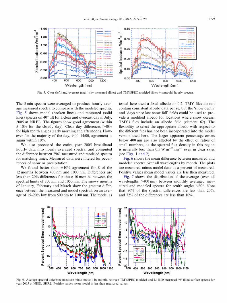
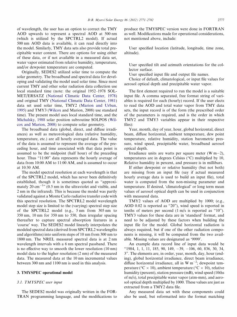
Fig. 5. Clear (left) and overcast (right) sky measured (lines) and TMYSPEC modeled (lines + symbols) hourly spectra.

D.R. Myers / Solar Energy 86 (2012) 2771–2782 2779

The 5 min spectra were averaged to produce hourly aver-age measured spectra to compare with the modeled spectra.Fig. 5 shows model (broken lines) and measured (solidlines) spectra on 40� tilt for a clear and overcast day in July,2005 at NREL. The figures show good agreement (within5–10% for the cloudy day). Clear day differences >40%for high zenith angles (early morning and afternoon). How-ever for the majority of the day, 9:00–14:00, agreement isagain within 10%.

We also processed the entire year 2005 broadbandhourly data into hourly averaged spectra, and computedthe difference between 2961 measured and modeled spectrafor matching times. Measured data were filtered for occur-rences of snow or precipitation.

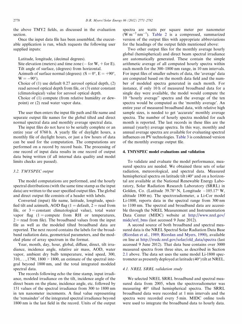
We found better than ±10% agreement for 8 of the12 months between 400 nm and 1000 nm. Differences areless than 20% differences for those 10 months between thespectral limits of 350 nm and 1050 nm. The snowy monthsof January, February and March show the greatest differ-ence between the measured and model spectral, on an aver-age of 15–20% low from 500 nm to 1100 nm. The model as

Fig. 6. Average spectral difference (measure minus model), by month, betweenyear 2005 at NREL SRRL. Positive values mean model is less than measured

tested here used a fixed albedo or 0.2. TMY files do notcontain consistent albedo data per se, but the ‘snow depth’and ‘days since last snow fall’ fields could be used to pro-vide a modified albedo for locations where snow occurs.TMY3 files include an albedo field (element 62). Theflexibility to select the appropriate albedo with respect tothe different files has not been incorporated into the modelversion used here. The larger apparent percentage errorsbelow 400 nm are also affected by the effect of ratios ofsmall numbers, as the spectral flux density in this regionis generally less than 0.5 W m�2 nm�1 even in clear skies(see Figs. 1 and 2).

Fig. 6 shows the mean difference between measured andmodeled spectra over all wavelengths by month. The plotsare measured minus model data as a percent of measured.Positive values mean model values are less then measured.

Fig. 7 shows the distribution of the average (over allwavelengths >400 nm) between monthly averaged mea-sured and modeled spectra for zenith angles <60�. Notethat 90% of the spectral differences are less than 20%,and 72% of the differences are less than 10%.

TMYSPEC modeled and Li-1800 measured 40� tilted surface spectra forvalues.

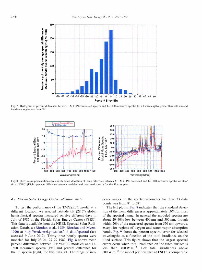
Fig. 7. Histogram of percent differences between TMYSPEC modeled spectra and Li-1800 measured spectra for all wavelengths greater than 400 nm andincidence angles less than 60�.

Fig. 8. (Left) mean percent difference and standard deviation of mean difference between 33 TMYSPEC modeled and Li-1800 measured spectra on 28.6�tilt at FSEC. (Right) percent difference between modeled and measured spectra for the 33 examples.

2780 D.R. Myers / Solar Energy 86 (2012) 2771–2782

4.2. Florida Solar Energy Center validation study

To test the performance of the TMYSPEC model at adifferent location, we selected latitude tilt (28.6�) globalhemispherical spectra measured on five different days inJuly of 1987 at the Florida Solar Energy Center (FSEC).This data is available from the NREL Spectral Solar Radi-ation Database (Riordan et al., 1989; Riordan and Myers,1990) at http://rredc.nrel.gov/solar/old_data/spectral (lastaccessed 9 June 2012). Thirty-three hourly spectra weremodeled for July 23–24, 27–29 1987. Fig. 8 shows meanpercent differences between TMYSPEC modeled and Li-1800 measured spectra (left) and percent difference forthe 33 spectra (right) for this data set. The range of inci-

dence angles on the spectroradiometer for these 33 datapoints was from 8� to 68�.

The left plot in Fig. 8 indicates that the standard devia-tion of the mean differences is approximately 10% for mostof the spectral range. In general the modeled spectra areabout 20–40% low between 400 nm and 500 nm, thoughwithin 20% of the measured spectra from 550 nm upwards,except for regions of oxygen and water vapor absorptionbands. Fig. 9 shows the percent spectral error for selectedwavelengths as a function of the total irradiance on thetilted surface. This figure shows that the largest spectralerrors occur when total irradiance on the tilted surface isless than 400 W m�2. For total irradiances above600 W m�2 the model performance at FSEC is comparable

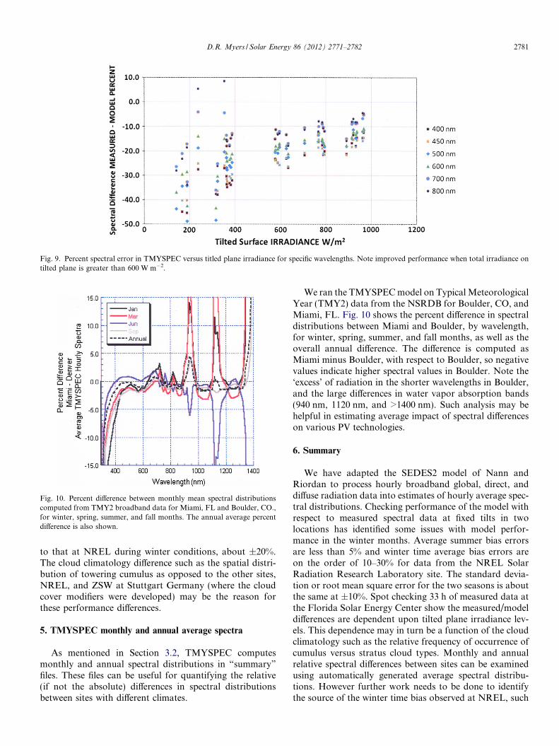
Fig. 9. Percent spectral error in TMYSPEC versus titled plane irradiance for specific wavelengths. Note improved performance when total irradiance ontilted plane is greater than 600 W m�2.

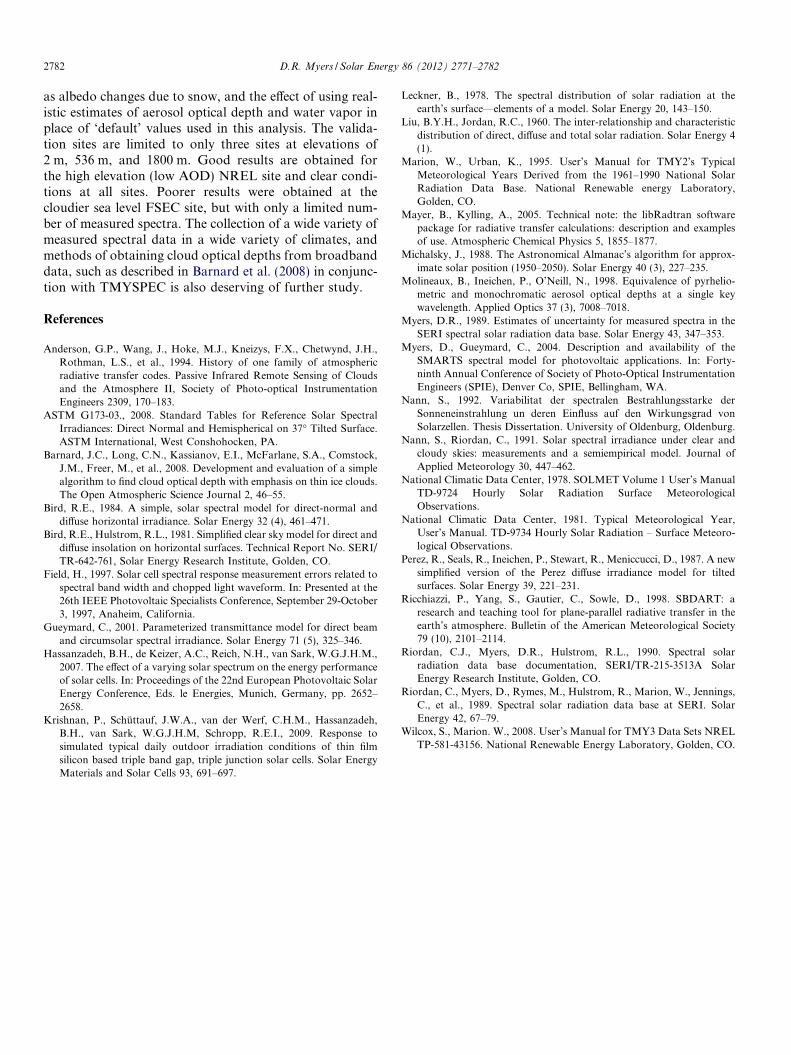
Fig. 10. Percent difference between monthly mean spectral distributionscomputed from TMY2 broadband data for Miami, FL and Boulder, CO.,for winter, spring, summer, and fall months. The annual average percentdifference is also shown.

D.R. Myers / Solar Energy 86 (2012) 2771–2782 2781

to that at NREL during winter conditions, about ±20%.The cloud climatology difference such as the spatial distri-bution of towering cumulus as opposed to the other sites,NREL, and ZSW at Stuttgart Germany (where the cloudcover modifiers were developed) may be the reason forthese performance differences.

5. TMYSPEC monthly and annual average spectra

As mentioned in Section 3.2, TMYSPEC computesmonthly and annual spectral distributions in “summary”

files. These files can be useful for quantifying the relative(if not the absolute) differences in spectral distributionsbetween sites with different climates.

We ran the TMYSPEC model on Typical MeteorologicalYear (TMY2) data from the NSRDB for Boulder, CO, andMiami, FL. Fig. 10 shows the percent difference in spectraldistributions between Miami and Boulder, by wavelength,for winter, spring, summer, and fall months, as well as theoverall annual difference. The difference is computed asMiami minus Boulder, with respect to Boulder, so negativevalues indicate higher spectral values in Boulder. Note the‘excess’ of radiation in the shorter wavelengths in Boulder,and the large differences in water vapor absorption bands(940 nm, 1120 nm, and >1400 nm). Such analysis may behelpful in estimating average impact of spectral differenceson various PV technologies.

6. Summary

We have adapted the SEDES2 model of Nann andRiordan to process hourly broadband global, direct, anddiffuse radiation data into estimates of hourly average spec-tral distributions. Checking performance of the model withrespect to measured spectral data at fixed tilts in twolocations has identified some issues with model perfor-mance in the winter months. Average summer bias errorsare less than 5% and winter time average bias errors areon the order of 10–30% for data from the NREL SolarRadiation Research Laboratory site. The standard devia-tion or root mean square error for the two seasons is aboutthe same at ±10%. Spot checking 33 h of measured data atthe Florida Solar Energy Center show the measured/modeldifferences are dependent upon tilted plane irradiance lev-els. This dependence may in turn be a function of the cloudclimatology such as the relative frequency of occurrence ofcumulus versus stratus cloud types. Monthly and annualrelative spectral differences between sites can be examinedusing automatically generated average spectral distribu-tions. However further work needs to be done to identifythe source of the winter time bias observed at NREL, such

2782 D.R. Myers / Solar Energy 86 (2012) 2771–2782

as albedo changes due to snow, and the effect of using real-istic estimates of aerosol optical depth and water vapor inplace of ‘default’ values used in this analysis. The valida-tion sites are limited to only three sites at elevations of2 m, 536 m, and 1800 m. Good results are obtained forthe high elevation (low AOD) NREL site and clear condi-tions at all sites. Poorer results were obtained at thecloudier sea level FSEC site, but with only a limited num-ber of measured spectra. The collection of a wide variety ofmeasured spectral data in a wide variety of climates, andmethods of obtaining cloud optical depths from broadbanddata, such as described in Barnard et al. (2008) in conjunc-tion with TMYSPEC is also deserving of further study.

References

Anderson, G.P., Wang, J., Hoke, M.J., Kneizys, F.X., Chetwynd, J.H.,Rothman, L.S., et al., 1994. History of one family of atmosphericradiative transfer codes. Passive Infrared Remote Sensing of Cloudsand the Atmosphere II, Society of Photo-optical InstrumentationEngineers 2309, 170–183.

ASTM G173-03., 2008. Standard Tables for Reference Solar SpectralIrradiances: Direct Normal and Hemispherical on 37� Tilted Surface.ASTM International, West Conshohocken, PA.

Barnard, J.C., Long, C.N., Kassianov, E.I., McFarlane, S.A., Comstock,J.M., Freer, M., et al., 2008. Development and evaluation of a simplealgorithm to find cloud optical depth with emphasis on thin ice clouds.The Open Atmospheric Science Journal 2, 46–55.

Bird, R.E., 1984. A simple, solar spectral model for direct-normal anddiffuse horizontal irradiance. Solar Energy 32 (4), 461–471.

Bird, R.E., Hulstrom, R.L., 1981. Simplified clear sky model for direct anddiffuse insolation on horizontal surfaces. Technical Report No. SERI/TR-642-761, Solar Energy Research Institute, Golden, CO.

Field, H., 1997. Solar cell spectral response measurement errors related tospectral band width and chopped light waveform. In: Presented at the26th IEEE Photovoltaic Specialists Conference, September 29-October3, 1997, Anaheim, California.

Gueymard, C., 2001. Parameterized transmittance model for direct beamand circumsolar spectral irradiance. Solar Energy 71 (5), 325–346.

Hassanzadeh, B.H., de Keizer, A.C., Reich, N.H., van Sark, W.G.J.H.M.,2007. The effect of a varying solar spectrum on the energy performanceof solar cells. In: Proceedings of the 22nd European Photovoltaic SolarEnergy Conference, Eds. le Energies, Munich, Germany, pp. 2652–2658.

Krishnan, P., Schuttauf, J.W.A., van der Werf, C.H.M., Hassanzadeh,B.H., van Sark, W.G.J.H.M, Schropp, R.E.I., 2009. Response tosimulated typical daily outdoor irradiation conditions of thin filmsilicon based triple band gap, triple junction solar cells. Solar EnergyMaterials and Solar Cells 93, 691–697.

Leckner, B., 1978. The spectral distribution of solar radiation at theearth’s surface—elements of a model. Solar Energy 20, 143–150.

Liu, B.Y.H., Jordan, R.C., 1960. The inter-relationship and characteristicdistribution of direct, diffuse and total solar radiation. Solar Energy 4(1).

Marion, W., Urban, K., 1995. User’s Manual for TMY2’s TypicalMeteorological Years Derived from the 1961–1990 National SolarRadiation Data Base. National Renewable energy Laboratory,Golden, CO.

Mayer, B., Kylling, A., 2005. Technical note: the libRadtran softwarepackage for radiative transfer calculations: description and examplesof use. Atmospheric Chemical Physics 5, 1855–1877.

Michalsky, J., 1988. The Astronomical Almanac’s algorithm for approx-imate solar position (1950–2050). Solar Energy 40 (3), 227–235.

Molineaux, B., Ineichen, P., O’Neill, N., 1998. Equivalence of pyrhelio-metric and monochromatic aerosol optical depths at a single keywavelength. Applied Optics 37 (3), 7008–7018.

Myers, D.R., 1989. Estimates of uncertainty for measured spectra in theSERI spectral solar radiation data base. Solar Energy 43, 347–353.

Myers, D., Gueymard, C., 2004. Description and availability of theSMARTS spectral model for photovoltaic applications. In: Forty-ninth Annual Conference of Society of Photo-Optical InstrumentationEngineers (SPIE), Denver Co, SPIE, Bellingham, WA.

Nann, S., 1992. Variabilitat der spectralen Bestrahlungsstarke derSonneneinstrahlung un deren Einfluss auf den Wirkungsgrad vonSolarzellen. Thesis Dissertation. University of Oldenburg, Oldenburg.

Nann, S., Riordan, C., 1991. Solar spectral irradiance under clear andcloudy skies: measurements and a semiempirical model. Journal ofApplied Meteorology 30, 447–462.

National Climatic Data Center, 1978. SOLMET Volume 1 User’s ManualTD-9724 Hourly Solar Radiation Surface MeteorologicalObservations.

National Climatic Data Center, 1981. Typical Meteorological Year,User’s Manual. TD-9734 Hourly Solar Radiation – Surface Meteoro-logical Observations.

Perez, R., Seals, R., Ineichen, P., Stewart, R., Meniccucci, D., 1987. A newsimplified version of the Perez diffuse irradiance model for tiltedsurfaces. Solar Energy 39, 221–231.

Ricchiazzi, P., Yang, S., Gautier, C., Sowle, D., 1998. SBDART: aresearch and teaching tool for plane-parallel radiative transfer in theearth’s atmosphere. Bulletin of the American Meteorological Society79 (10), 2101–2114.

Riordan, C.J., Myers, D.R., Hulstrom, R.L., 1990. Spectral solarradiation data base documentation, SERI/TR-215-3513A SolarEnergy Research Institute, Golden, CO.

Riordan, C., Myers, D., Rymes, M., Hulstrom, R., Marion, W., Jennings,C., et al., 1989. Spectral solar radiation data base at SERI. SolarEnergy 42, 67–79.

Wilcox, S., Marion. W., 2008. User’s Manual for TMY3 Data Sets NRELTP-581-43156. National Renewable Energy Laboratory, Golden, CO.