Embed Size (px)
Citation preview
Direct Visibility of Point SetsSagi Katz∗
Technion – Israel Inst. of TechnologyAyellet Tal†
Technion – Israel Inst. of TechnologyRonen Basri‡
Weizmann Inst. of Science
Abstract
This paper proposes a simple and fast operator, the “Hidden” PointRemoval operator, which determines the visible points in a pointcloud, as viewed from a given viewpoint. Visibility is determinedwithout reconstructing a surface or estimating normals. It is shownthat extracting the points that reside on the convex hull of a trans-formed point cloud, amounts to determining the visible points. Thisoperator is general – it can be applied to point clouds at various di-mensions, on both sparse and dense point clouds, and on viewpointsinternal as well as external to the cloud. It is demonstrated that theoperator is useful in visualizing point clouds, in view-dependentreconstruction and in shadow casting.
Keywords: Point-based graphics, visibility, visualizing point sets
1 Introduction
In the last decade, an alternative to meshes, in the form of a point-based representation (a point cloud), has gained increasing popular-ity [Rusinkiewicz and Levoy 2000; Pauly and Gross 2001; Zwickeret al. 2002; Alexa et al. 2003; Fleishman et al. 2003; Alexa et al.2004; Kobbelt and Botsch 2004]. Point clouds are 3D positions,possibly associated with additional information, such as colors andnormals, and can be considered a sampling of a continuous surface.This representation is extremely simple and flexible. Moreover, itoffers the additional advantage of avoiding connectivity informa-tion and topological consistency.
This paper investigates visibility of point clouds. One way to com-pute visibility of a point cloud is to reconstruct the surface [Hoppeet al. 1992; Bernardini et al. 1999; Curless and Levoy 1996; Carret al. 2001; Amenta et al. 2001; Amenta et al. 2002; Amenta andKil 2004; Fleishman et al. 2005] and determine visibility on the re-constructed triangular mesh. Reconstruction, however, is a difficultproblem, both theoretically and implementation-wise, which oftenrequires additional information, such as normals and sufficientlydense input.
The key question that this paper attempts to answer is how the visi-bility information can be directly extracted from a point cloud. Ev-idently, points cannot occlude one another (unless they accidentallyfall along the same ray from the viewpoint), and therefore no pointis actually hidden. However, once a surface is reconstructed fromthe points, it is certainly possible to determine which of the points
∗e-mail: [email protected]†e-mail: [email protected]‡e-mail: [email protected]
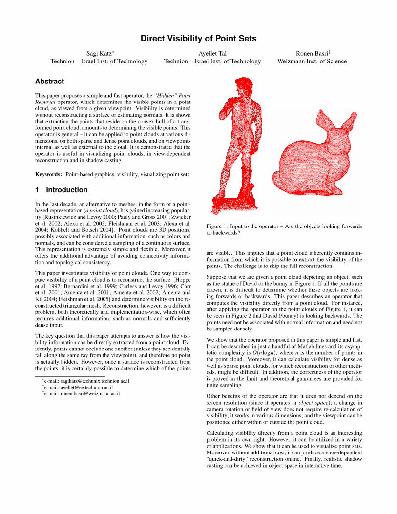
Figure 1: Input to the operator – Are the objects looking forwardsor backwards?
are visible. This implies that a point cloud inherently contains in-formation from which it is possible to extract the visibility of thepoints. The challenge is to skip the full reconstruction.
Suppose that we are given a point cloud depicting an object, suchas the statue of David or the bunny in Figure 1. If all the points aredrawn, it is difficult to determine whether these objects are look-ing forwards or backwards. This paper describes an operator thatcomputes the visibility directly from a point cloud. For instance,after applying the operator on the point clouds of Figure 1, it canbe seen in Figure 2 that David (/bunny) is looking backwards. Thepoints need not be associated with normal information and need notbe sampled densely.
We show that the operator proposed in this paper is simple and fast.It can be described in just a handful of Matlab lines and its asymp-totic complexity is O(n logn), where n is the number of points inthe point cloud. Moreover, it can calculate visibility for dense aswell as sparse point clouds, for which reconstruction or other meth-ods, might be difficult. In addition, the correctness of the operatoris proved in the limit and theoretical guarantees are provided forfinite sampling.
Other benefits of the operator are that it does not depend on thescreen resolution (since it operates in object space); a change incamera rotation or field of view does not require re-calculation ofvisibility; it works in various dimensions; and the viewpoint can bepositioned either within or outside the point cloud.
Calculating visibility directly from a point cloud is an interestingproblem in its own right. However, it can be utilized in a varietyof applications. We show that it can be used to visualize point sets.Moreover, without additional cost, it can produce a view-dependent“quick-and-dirty” reconstruction online. Finally, realistic shadowcasting can be achieved in object space in interactive time.
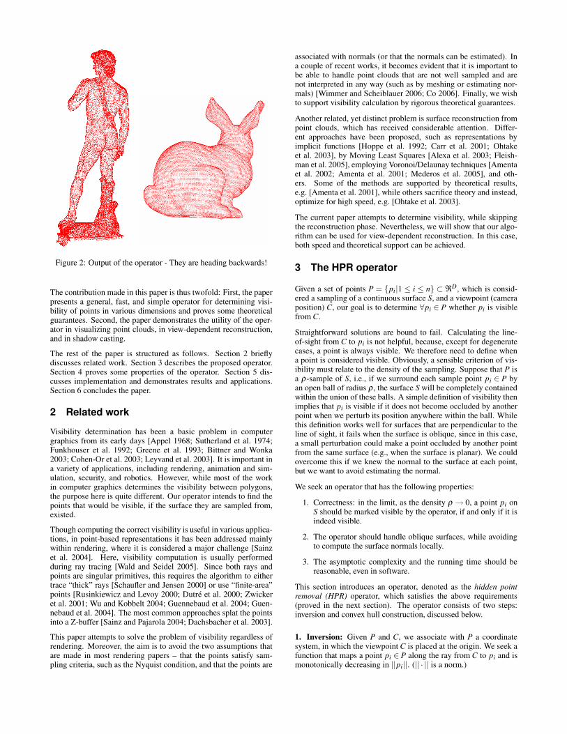
Figure 2: Output of the operator - They are heading backwards!
The contribution made in this paper is thus twofold: First, the paperpresents a general, fast, and simple operator for determining visi-bility of points in various dimensions and proves some theoreticalguarantees. Second, the paper demonstrates the utility of the oper-ator in visualizing point clouds, in view-dependent reconstruction,and in shadow casting.
The rest of the paper is structured as follows. Section 2 brieflydiscusses related work. Section 3 describes the proposed operator.Section 4 proves some properties of the operator. Section 5 dis-cusses implementation and demonstrates results and applications.Section 6 concludes the paper.
2 Related workVisibility determination has been a basic problem in computergraphics from its early days [Appel 1968; Sutherland et al. 1974;Funkhouser et al. 1992; Greene et al. 1993; Bittner and Wonka2003; Cohen-Or et al. 2003; Leyvand et al. 2003]. It is important ina variety of applications, including rendering, animation and sim-ulation, security, and robotics. However, while most of the workin computer graphics determines the visibility between polygons,the purpose here is quite different. Our operator intends to find thepoints that would be visible, if the surface they are sampled from,existed.
Though computing the correct visibility is useful in various applica-tions, in point-based representations it has been addressed mainlywithin rendering, where it is considered a major challenge [Sainzet al. 2004]. Here, visibility computation is usually performedduring ray tracing [Wald and Seidel 2005]. Since both rays andpoints are singular primitives, this requires the algorithm to eithertrace “thick” rays [Schaufler and Jensen 2000] or use “finite-area”points [Rusinkiewicz and Levoy 2000; Dutre et al. 2000; Zwickeret al. 2001; Wu and Kobbelt 2004; Guennebaud et al. 2004; Guen-nebaud et al. 2004]. The most common approaches splat the pointsinto a Z-buffer [Sainz and Pajarola 2004; Dachsbacher et al. 2003].
This paper attempts to solve the problem of visibility regardless ofrendering. Moreover, the aim is to avoid the two assumptions thatare made in most rendering papers – that the points satisfy sam-pling criteria, such as the Nyquist condition, and that the points are
associated with normals (or that the normals can be estimated). Ina couple of recent works, it becomes evident that it is important tobe able to handle point clouds that are not well sampled and arenot interpreted in any way (such as by meshing or estimating nor-mals) [Wimmer and Scheiblauer 2006; Co 2006]. Finally, we wishto support visibility calculation by rigorous theoretical guarantees.
Another related, yet distinct problem is surface reconstruction frompoint clouds, which has received considerable attention. Differ-ent approaches have been proposed, such as representations byimplicit functions [Hoppe et al. 1992; Carr et al. 2001; Ohtakeet al. 2003], by Moving Least Squares [Alexa et al. 2003; Fleish-man et al. 2005], employing Voronoi/Delaunay techniques [Amentaet al. 2002; Amenta et al. 2001; Mederos et al. 2005], and oth-ers. Some of the methods are supported by theoretical results,e.g. [Amenta et al. 2001], while others sacrifice theory and instead,optimize for high speed, e.g. [Ohtake et al. 2003].
The current paper attempts to determine visibility, while skippingthe reconstruction phase. Nevertheless, we will show that our algo-rithm can be used for view-dependent reconstruction. In this case,both speed and theoretical support can be achieved.
3 The HPR operator
Given a set of points P = {pi|1 ≤ i ≤ n} ⊂ ℜD, which is consid-ered a sampling of a continuous surface S, and a viewpoint (cameraposition) C, our goal is to determine ∀pi ∈ P whether pi is visiblefrom C.
Straightforward solutions are bound to fail. Calculating the line-of-sight from C to pi is not helpful, because, except for degeneratecases, a point is always visible. We therefore need to define whena point is considered visible. Obviously, a sensible criterion of vis-ibility must relate to the density of the sampling. Suppose that P isa ρ-sample of S, i.e., if we surround each sample point pi ∈ P byan open ball of radius ρ , the surface S will be completely containedwithin the union of these balls. A simple definition of visibility thenimplies that pi is visible if it does not become occluded by anotherpoint when we perturb its position anywhere within the ball. Whilethis definition works well for surfaces that are perpendicular to theline of sight, it fails when the surface is oblique, since in this case,a small perturbation could make a point occluded by another pointfrom the same surface (e.g., when the surface is planar). We couldovercome this if we knew the normal to the surface at each point,but we want to avoid estimating the normal.
We seek an operator that has the following properties:
1. Correctness: in the limit, as the density ρ → 0, a point pi onS should be marked visible by the operator, if and only if it isindeed visible.
2. The operator should handle oblique surfaces, while avoidingto compute the surface normals locally.
3. The asymptotic complexity and the running time should bereasonable, even in software.
This section introduces an operator, denoted as the hidden pointremoval (HPR) operator, which satisfies the above requirements(proved in the next section). The operator consists of two steps:inversion and convex hull construction, discussed below.
1. Inversion: Given P and C, we associate with P a coordinatesystem, in which the viewpoint C is placed at the origin. We seek afunction that maps a point pi ∈ P along the ray from C to pi and ismonotonically decreasing in ||pi||. (|| · || is a norm.)
There are various ways to perform inversion. Here, we focus onspherical flipping, which was first presented in [Katz et al. 2005] ina different context. Consider a D-dimensional sphere with radius R,centered at the origin (C), and constrained to include all the pointsin P. Spherical flipping reflects a point pi ∈ P with respect to thesphere by applying the following equation:
pi = f (pi) = pi +2(R−||pi||)pi
||pi||. (1)
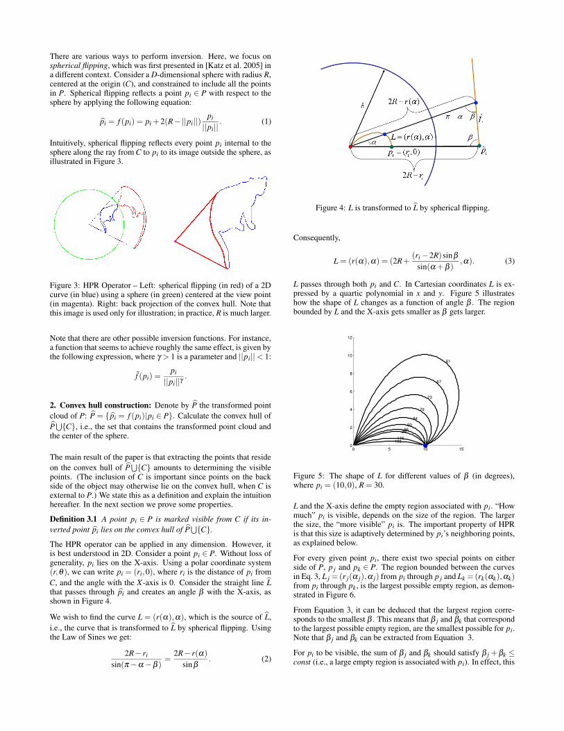
Intuitively, spherical flipping reflects every point pi internal to thesphere along the ray from C to pi to its image outside the sphere, asillustrated in Figure 3.
Figure 3: HPR Operator – Left: spherical flipping (in red) of a 2Dcurve (in blue) using a sphere (in green) centered at the view point(in magenta). Right: back projection of the convex hull. Note thatthis image is used only for illustration; in practice, R is much larger.
Note that there are other possible inversion functions. For instance,a function that seems to achieve roughly the same effect, is given bythe following expression, where γ > 1 is a parameter and ||pi||< 1:
f (pi) =pi
||pi||γ.
2. Convex hull construction: Denote by P the transformed pointcloud of P: P = { pi = f (pi)|pi ∈ P}. Calculate the convex hull ofP⋃{C}, i.e., the set that contains the transformed point cloud and
the center of the sphere.
The main result of the paper is that extracting the points that resideon the convex hull of P
⋃{C} amounts to determining the visible
points. (The inclusion of C is important since points on the backside of the object may otherwise lie on the convex hull, when C isexternal to P.) We state this as a definition and explain the intuitionhereafter. In the next section we prove some properties.
Definition 3.1 A point pi ∈ P is marked visible from C if its in-verted point pi lies on the convex hull of P
⋃{C}.
The HPR operator can be applied in any dimension. However, itis best understood in 2D. Consider a point pi ∈ P. Without loss ofgenerality, pi lies on the X-axis. Using a polar coordinate system(r,θ), we can write pi = (ri,0), where ri is the distance of pi fromC, and the angle with the X-axis is 0. Consider the straight line Lthat passes through pi and creates an angle β with the X-axis, asshown in Figure 4.
We wish to find the curve L = (r(α),α), which is the source of L,i.e., the curve that is transformed to L by spherical flipping. Usingthe Law of Sines we get:
2R− risin(π −α −β )
=2R− r(α)
sinβ. (2)
Figure 4: L is transformed to L by spherical flipping.
Consequently,
L = (r(α),α) = (2R+(ri −2R)sinβ
sin(α +β ),α). (3)
L passes through both pi and C. In Cartesian coordinates L is ex-pressed by a quartic polynomial in x and y. Figure 5 illustrateshow the shape of L changes as a function of angle β . The regionbounded by L and the X-axis gets smaller as β gets larger.
0 5 10 150
2
4
6
8
10
12
61
67
73
79
8490
9699116
133
Figure 5: The shape of L for different values of β (in degrees),where pi = (10,0), R = 30.
L and the X-axis define the empty region associated with pi. “Howmuch” pi is visible, depends on the size of the region. The largerthe size, the “more visible” pi is. The important property of HPRis that this size is adaptively determined by pi’s neighboring points,as explained below.
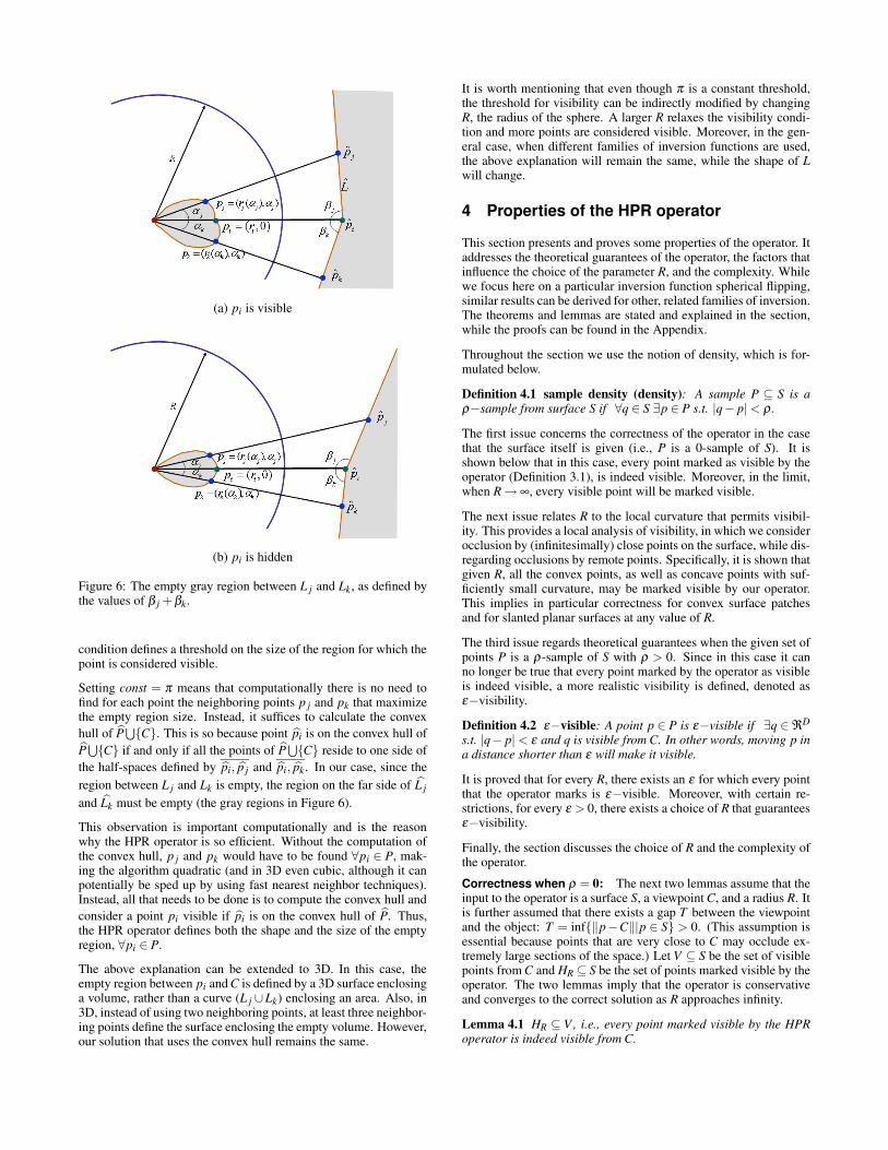
For every given point pi, there exist two special points on eitherside of P, p j and pk ∈ P. The region bounded between the curvesin Eq. 3, L j = (r j(α j),α j) from pi through p j and Lk = (rk(αk),αk)from pi through pk, is the largest possible empty region, as demon-strated in Figure 6.
From Equation 3, it can be deduced that the largest region corre-sponds to the smallest β . This means that β j and βk that correspondto the largest possible empty region, are the smallest possible for pi.Note that β j and βk can be extracted from Equation 3.
For pi to be visible, the sum of β j and βk should satisfy β j + βk ≤const (i.e., a large empty region is associated with pi). In effect, this
(a) pi is visible
(b) pi is hidden
Figure 6: The empty gray region between L j and Lk, as defined bythe values of β j +βk.
condition defines a threshold on the size of the region for which thepoint is considered visible.
Setting const = π means that computationally there is no need tofind for each point the neighboring points p j and pk that maximizethe empty region size. Instead, it suffices to calculate the convexhull of P
⋃{C}. This is so because point pi is on the convex hull of
P⋃{C} if and only if all the points of P
⋃{C} reside to one side of
the half-spaces defined by pi, p j and pi, pk. In our case, since theregion between L j and Lk is empty, the region on the far side of L jand Lk must be empty (the gray regions in Figure 6).
This observation is important computationally and is the reasonwhy the HPR operator is so efficient. Without the computation ofthe convex hull, p j and pk would have to be found ∀pi ∈ P, mak-ing the algorithm quadratic (and in 3D even cubic, although it canpotentially be sped up by using fast nearest neighbor techniques).Instead, all that needs to be done is to compute the convex hull andconsider a point pi visible if pi is on the convex hull of P. Thus,the HPR operator defines both the shape and the size of the emptyregion, ∀pi ∈ P.
The above explanation can be extended to 3D. In this case, theempty region between pi and C is defined by a 3D surface enclosinga volume, rather than a curve (L j ∪Lk) enclosing an area. Also, in3D, instead of using two neighboring points, at least three neighbor-ing points define the surface enclosing the empty volume. However,our solution that uses the convex hull remains the same.
It is worth mentioning that even though π is a constant threshold,the threshold for visibility can be indirectly modified by changingR, the radius of the sphere. A larger R relaxes the visibility condi-tion and more points are considered visible. Moreover, in the gen-eral case, when different families of inversion functions are used,the above explanation will remain the same, while the shape of Lwill change.
4 Properties of the HPR operator
This section presents and proves some properties of the operator. Itaddresses the theoretical guarantees of the operator, the factors thatinfluence the choice of the parameter R, and the complexity. Whilewe focus here on a particular inversion function spherical flipping,similar results can be derived for other, related families of inversion.The theorems and lemmas are stated and explained in the section,while the proofs can be found in the Appendix.
Throughout the section we use the notion of density, which is for-mulated below.
Definition 4.1 sample density (density): A sample P ⊆ S is aρ−sample from surface S if ∀q ∈ S ∃p ∈ P s.t. |q− p| < ρ .
The first issue concerns the correctness of the operator in the casethat the surface itself is given (i.e., P is a 0-sample of S). It isshown below that in this case, every point marked as visible by theoperator (Definition 3.1), is indeed visible. Moreover, in the limit,when R → ∞, every visible point will be marked visible.
The next issue relates R to the local curvature that permits visibil-ity. This provides a local analysis of visibility, in which we considerocclusion by (infinitesimally) close points on the surface, while dis-regarding occlusions by remote points. Specifically, it is shown thatgiven R, all the convex points, as well as concave points with suf-ficiently small curvature, may be marked visible by our operator.This implies in particular correctness for convex surface patchesand for slanted planar surfaces at any value of R.
The third issue regards theoretical guarantees when the given set ofpoints P is a ρ-sample of S with ρ > 0. Since in this case it canno longer be true that every point marked by the operator as visibleis indeed visible, a more realistic visibility is defined, denoted asε−visibility.
Definition 4.2 ε−visible: A point p ∈ P is ε−visible if ∃q ∈ ℜD
s.t. |q− p| < ε and q is visible from C. In other words, moving p ina distance shorter than ε will make it visible.
It is proved that for every R, there exists an ε for which every pointthat the operator marks is ε−visible. Moreover, with certain re-strictions, for every ε > 0, there exists a choice of R that guaranteesε−visibility.
Finally, the section discusses the choice of R and the complexity ofthe operator.Correctness when ρ = 0: The next two lemmas assume that theinput to the operator is a surface S, a viewpoint C, and a radius R. Itis further assumed that there exists a gap T between the viewpointand the object: T = inf{‖p−C‖|p ∈ S} > 0. (This assumption isessential because points that are very close to C may occlude ex-tremely large sections of the space.) Let V ⊆ S be the set of visiblepoints from C and HR ⊆ S be the set of points marked visible by theoperator. The two lemmas imply that the operator is conservativeand converges to the correct solution as R approaches infinity.
Lemma 4.1 HR ⊆ V , i.e., every point marked visible by the HPRoperator is indeed visible from C.
Lemma 4.2 limR−→∞ HR = V , i.e., assuming T > 0, when R → ∞,the set of visible points marked by HPR is equal to the set of visiblepoints.R and the local curvature: For a finite value of R, we can furtheranalyze which points will be marked visible by the HPR operator,by considering the influence of the curvature on the results. We startagain with the intuition. It is straightforward to see that obliqueplanar surfaces are correctly handled by the HPR operator, sincespherical flipping maps such surfaces to convex structures. Han-dling concave sections of a surface, in contrast, is affected by thelocal curvature. Below, we provide a derivation of the permissiblecurvature as a function of the radius R, the distance r from the pointp to the viewpoint C, and the orientation of the convex hull throughp, β (Figure 4). The derivation is general, yet a particularly simpleexpression is obtained when the tangent to a point is perpendicularto the line of sight from this point.
Lemma 4.3 Let S be an infinitesimal surface patch around p. Thenp ∈ HR if and only if the curvature k at p satisfies:
k <4R(2R− r)cot2 β +2Rr(
4Rr−4R2 +(r−2R)2
sin2 β
)3/2 .
In the case that β = π/2, which corresponds to the case that thetangent to the surface at p is perpendicular to the line of sight,k < 2R
r2 .
This implies in particular that convex shapes and slanted planes arecorrectly handled for any choice of R, and that points on concavesections of a surface are handled correctly as long as the curvature issufficiently low (except when remote sections of the surface happento fall close to the line of sight through those points). Note thatin higher dimensions all sectional curvatures must not exceed thebound, i.e., this bound is on the maximal curvature. The case thata patch is perpendicular to the line of sight also demonstrates thatthe permissible curvature grows with R. Thus, as R increases, morepoints become visible, until all (truly visible) points become visibleby the HPR operator.Theoretical guarantees ρ > 0: In the rest of the section, it isassumed that the given set of points P is a ρ-sample of S with ρ >0. Recall that a point is ε−visible, if moving it by ε will make itvisible. Using this definition, it is possible to extend the correctnesslemmas stated above to the more practical case of the given data.
Assuming that the sample is sufficiently dense, we show that forevery R, there exists an ε , such that every point marked visible bythe operator is ε−visible. Moreover, for sufficiently large ε , thereexists R, such that every point marked visible by the operator isε-visible.
Let Vε ⊆ P be the set of ε-visible points from C (points visible in S).As before, we assume that the distance of S to C is at least T > 0.
Theorem 4.4 Assume that the sample is sufficiently dense, then forevery R, there exists ε > 0 such that HR ⊆Vε .
Theorem 4.5 Assume that the sample is sufficiently dense, then forsufficiently large ε > 0, there exists R > 0 such that HR ⊆Vε .
The proofs of these theorems imply that for a constant value of R,as ρ decreases, a smaller value of ε is obtained.Choosing R: The proofs of the above theorems show the rela-tion between the density ρ , R, and ε-visibility. In particular, thesefactors are essential for choosing a suitable R.
As R increases, more points pass the threshold of the convex hulland hence are marked visible. For instance, as R → ∞, ri in Eq. 3
becomes negligible, β j,βk → π/2, and all the points are markedvisible. This is so because they are transformed by spherical flip-ping to a sphere with an infinite radius and thus reside on the convexhull. Therefore, a large R is suitable for dense point clouds, while asmall R is suitable for sparse clouds.
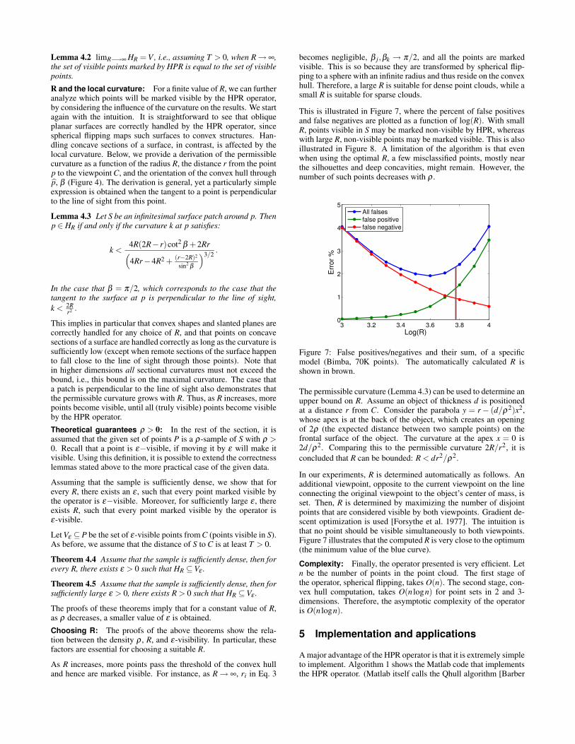
This is illustrated in Figure 7, where the percent of false positivesand false negatives are plotted as a function of log(R). With smallR, points visible in S may be marked non-visible by HPR, whereaswith large R, non-visible points may be marked visible. This is alsoillustrated in Figure 8. A limitation of the algorithm is that evenwhen using the optimal R, a few misclassified points, mostly nearthe silhouettes and deep concavities, might remain. However, thenumber of such points decreases with ρ .
3 3.2 3.4 3.6 3.8 40
1
2
3
4
5
Erro
r %Log(R)
All falsesfalse positivefalse negative
Figure 7: False positives/negatives and their sum, of a specificmodel (Bimba, 70K points). The automatically calculated R isshown in brown.
The permissible curvature (Lemma 4.3) can be used to determine anupper bound on R. Assume an object of thickness d is positionedat a distance r from C. Consider the parabola y = r − (d/ρ2)x2,whose apex is at the back of the object, which creates an openingof 2ρ (the expected distance between two sample points) on thefrontal surface of the object. The curvature at the apex x = 0 is2d/ρ2. Comparing this to the permissible curvature 2R/r2, it isconcluded that R can be bounded: R < dr2/ρ2.
In our experiments, R is determined automatically as follows. Anadditional viewpoint, opposite to the current viewpoint on the lineconnecting the original viewpoint to the object’s center of mass, isset. Then, R is determined by maximizing the number of disjointpoints that are considered visible by both viewpoints. Gradient de-scent optimization is used [Forsythe et al. 1977]. The intuition isthat no point should be visible simultaneously to both viewpoints.Figure 7 illustrates that the computed R is very close to the optimum(the minimum value of the blue curve).Complexity: Finally, the operator presented is very efficient. Letn be the number of points in the point cloud. The first stage ofthe operator, spherical flipping, takes O(n). The second stage, con-vex hull computation, takes O(n logn) for point sets in 2 and 3-dimensions. Therefore, the asymptotic complexity of the operatoris O(n logn).
5 Implementation and applications
A major advantage of the HPR operator is that it is extremely simpleto implement. Algorithm 1 shows the Matlab code that implementsthe HPR operator. (Matlab itself calls the Qhull algorithm [Barber
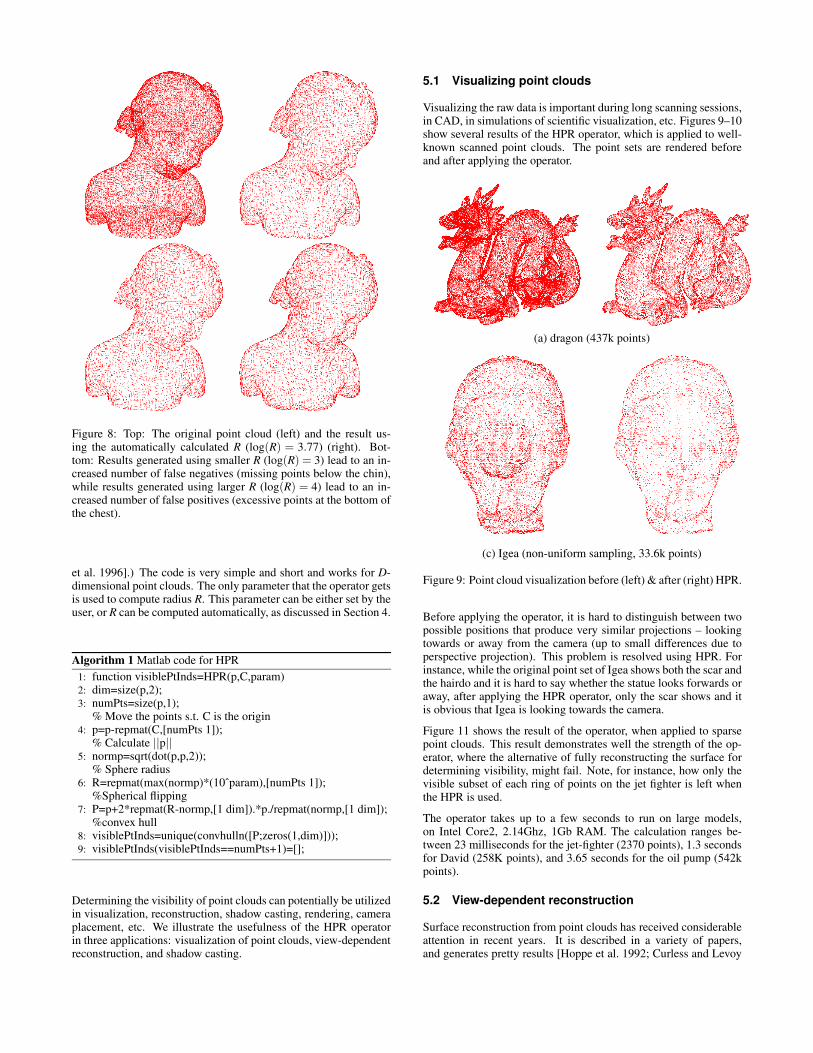
Figure 8: Top: The original point cloud (left) and the result us-ing the automatically calculated R (log(R) = 3.77) (right). Bot-tom: Results generated using smaller R (log(R) = 3) lead to an in-creased number of false negatives (missing points below the chin),while results generated using larger R (log(R) = 4) lead to an in-creased number of false positives (excessive points at the bottom ofthe chest).
et al. 1996].) The code is very simple and short and works for D-dimensional point clouds. The only parameter that the operator getsis used to compute radius R. This parameter can be either set by theuser, or R can be computed automatically, as discussed in Section 4.
Algorithm 1 Matlab code for HPR1: function visiblePtInds=HPR(p,C,param)2: dim=size(p,2);3: numPts=size(p,1);
% Move the points s.t. C is the origin4: p=p-repmat(C,[numPts 1]);
% Calculate ||p||5: normp=sqrt(dot(p,p,2));
% Sphere radius6: R=repmat(max(normp)*(10ˆparam),[numPts 1]);
%Spherical flipping7: P=p+2*repmat(R-normp,[1 dim]).*p./repmat(normp,[1 dim]);
%convex hull8: visiblePtInds=unique(convhulln([P;zeros(1,dim)]));9: visiblePtInds(visiblePtInds==numPts+1)=[];
Determining the visibility of point clouds can potentially be utilizedin visualization, reconstruction, shadow casting, rendering, cameraplacement, etc. We illustrate the usefulness of the HPR operatorin three applications: visualization of point clouds, view-dependentreconstruction, and shadow casting.
5.1 Visualizing point clouds
Visualizing the raw data is important during long scanning sessions,in CAD, in simulations of scientific visualization, etc. Figures 9–10show several results of the HPR operator, which is applied to well-known scanned point clouds. The point sets are rendered beforeand after applying the operator.
(a) dragon (437k points)
(c) Igea (non-uniform sampling, 33.6k points)
Figure 9: Point cloud visualization before (left) & after (right) HPR.
Before applying the operator, it is hard to distinguish between twopossible positions that produce very similar projections – lookingtowards or away from the camera (up to small differences due toperspective projection). This problem is resolved using HPR. Forinstance, while the original point set of Igea shows both the scar andthe hairdo and it is hard to say whether the statue looks forwards oraway, after applying the HPR operator, only the scar shows and itis obvious that Igea is looking towards the camera.
Figure 11 shows the result of the operator, when applied to sparsepoint clouds. This result demonstrates well the strength of the op-erator, where the alternative of fully reconstructing the surface fordetermining visibility, might fail. Note, for instance, how only thevisible subset of each ring of points on the jet fighter is left whenthe HPR is used.
The operator takes up to a few seconds to run on large models,on Intel Core2, 2.14Ghz, 1Gb RAM. The calculation ranges be-tween 23 milliseconds for the jet-fighter (2370 points), 1.3 secondsfor David (258K points), and 3.65 seconds for the oil pump (542kpoints).
5.2 View-dependent reconstruction
Surface reconstruction from point clouds has received considerableattention in recent years. It is described in a variety of papers,and generates pretty results [Hoppe et al. 1992; Curless and Levoy
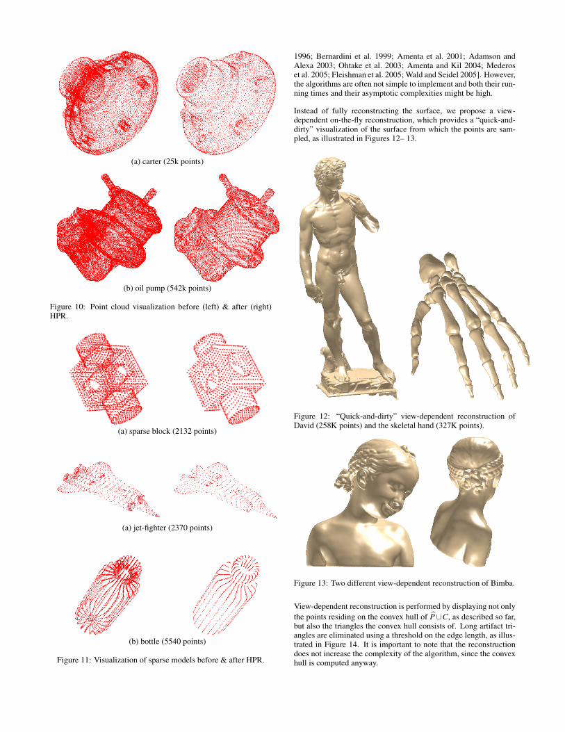
(a) carter (25k points)
(b) oil pump (542k points)
Figure 10: Point cloud visualization before (left) & after (right)HPR.
(a) sparse block (2132 points)
(a) jet-fighter (2370 points)
(b) bottle (5540 points)
Figure 11: Visualization of sparse models before & after HPR.
1996; Bernardini et al. 1999; Amenta et al. 2001; Adamson andAlexa 2003; Ohtake et al. 2003; Amenta and Kil 2004; Mederoset al. 2005; Fleishman et al. 2005; Wald and Seidel 2005]. However,the algorithms are often not simple to implement and both their run-ning times and their asymptotic complexities might be high.
Instead of fully reconstructing the surface, we propose a view-dependent on-the-fly reconstruction, which provides a “quick-and-dirty” visualization of the surface from which the points are sam-pled, as illustrated in Figures 12– 13.
Figure 12: “Quick-and-dirty” view-dependent reconstruction ofDavid (258K points) and the skeletal hand (327K points).
Figure 13: Two different view-dependent reconstruction of Bimba.
View-dependent reconstruction is performed by displaying not onlythe points residing on the convex hull of P∪C, as described so far,but also the triangles the convex hull consists of. Long artifact tri-angles are eliminated using a threshold on the edge length, as illus-trated in Figure 14. It is important to note that the reconstructiondoes not increase the complexity of the algorithm, since the convexhull is computed anyway.
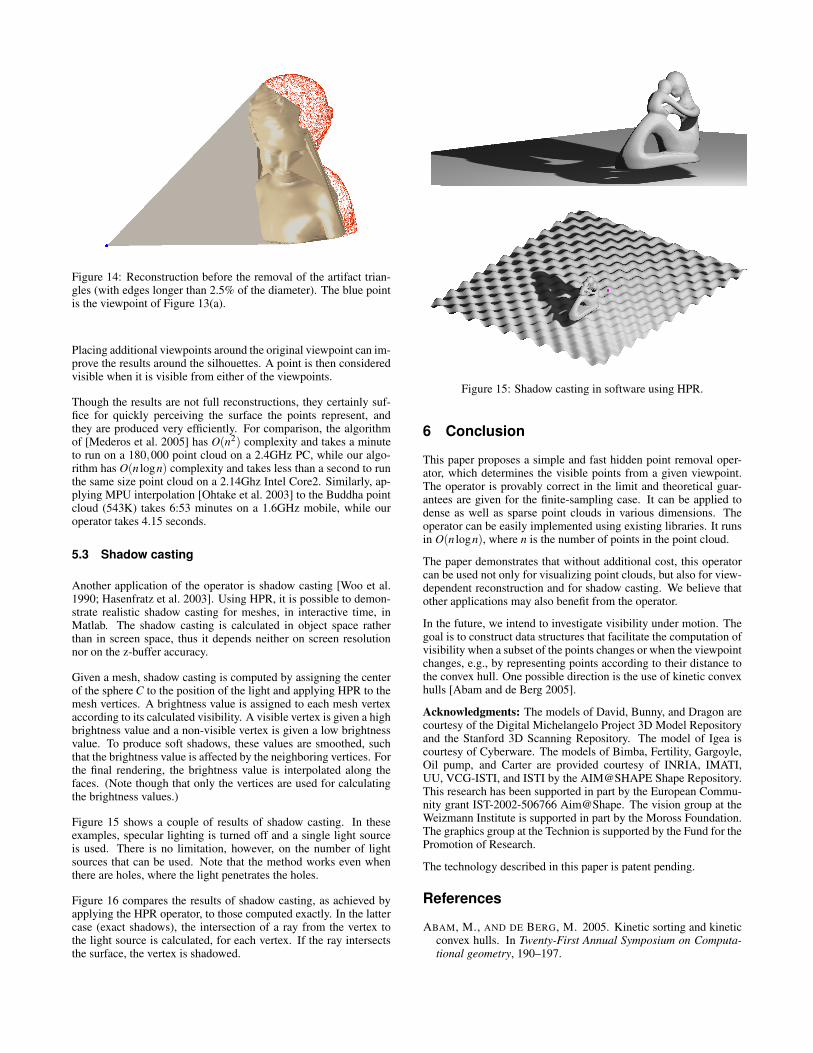
Figure 14: Reconstruction before the removal of the artifact trian-gles (with edges longer than 2.5% of the diameter). The blue pointis the viewpoint of Figure 13(a).
Placing additional viewpoints around the original viewpoint can im-prove the results around the silhouettes. A point is then consideredvisible when it is visible from either of the viewpoints.
Though the results are not full reconstructions, they certainly suf-fice for quickly perceiving the surface the points represent, andthey are produced very efficiently. For comparison, the algorithmof [Mederos et al. 2005] has O(n2) complexity and takes a minuteto run on a 180,000 point cloud on a 2.4GHz PC, while our algo-rithm has O(n logn) complexity and takes less than a second to runthe same size point cloud on a 2.14Ghz Intel Core2. Similarly, ap-plying MPU interpolation [Ohtake et al. 2003] to the Buddha pointcloud (543K) takes 6:53 minutes on a 1.6GHz mobile, while ouroperator takes 4.15 seconds.
5.3 Shadow casting
Another application of the operator is shadow casting [Woo et al.1990; Hasenfratz et al. 2003]. Using HPR, it is possible to demon-strate realistic shadow casting for meshes, in interactive time, inMatlab. The shadow casting is calculated in object space ratherthan in screen space, thus it depends neither on screen resolutionnor on the z-buffer accuracy.
Given a mesh, shadow casting is computed by assigning the centerof the sphere C to the position of the light and applying HPR to themesh vertices. A brightness value is assigned to each mesh vertexaccording to its calculated visibility. A visible vertex is given a highbrightness value and a non-visible vertex is given a low brightnessvalue. To produce soft shadows, these values are smoothed, suchthat the brightness value is affected by the neighboring vertices. Forthe final rendering, the brightness value is interpolated along thefaces. (Note though that only the vertices are used for calculatingthe brightness values.)
Figure 15 shows a couple of results of shadow casting. In theseexamples, specular lighting is turned off and a single light sourceis used. There is no limitation, however, on the number of lightsources that can be used. Note that the method works even whenthere are holes, where the light penetrates the holes.
Figure 16 compares the results of shadow casting, as achieved byapplying the HPR operator, to those computed exactly. In the lattercase (exact shadows), the intersection of a ray from the vertex tothe light source is calculated, for each vertex. If the ray intersectsthe surface, the vertex is shadowed.
Figure 15: Shadow casting in software using HPR.
6 Conclusion
This paper proposes a simple and fast hidden point removal oper-ator, which determines the visible points from a given viewpoint.The operator is provably correct in the limit and theoretical guar-antees are given for the finite-sampling case. It can be applied todense as well as sparse point clouds in various dimensions. Theoperator can be easily implemented using existing libraries. It runsin O(n logn), where n is the number of points in the point cloud.
The paper demonstrates that without additional cost, this operatorcan be used not only for visualizing point clouds, but also for view-dependent reconstruction and for shadow casting. We believe thatother applications may also benefit from the operator.
In the future, we intend to investigate visibility under motion. Thegoal is to construct data structures that facilitate the computation ofvisibility when a subset of the points changes or when the viewpointchanges, e.g., by representing points according to their distance tothe convex hull. One possible direction is the use of kinetic convexhulls [Abam and de Berg 2005].
Acknowledgments: The models of David, Bunny, and Dragon arecourtesy of the Digital Michelangelo Project 3D Model Repositoryand the Stanford 3D Scanning Repository. The model of Igea iscourtesy of Cyberware. The models of Bimba, Fertility, Gargoyle,Oil pump, and Carter are provided courtesy of INRIA, IMATI,UU, VCG-ISTI, and ISTI by the AIM@SHAPE Shape Repository.This research has been supported in part by the European Commu-nity grant IST-2002-506766 Aim@Shape. The vision group at theWeizmann Institute is supported in part by the Moross Foundation.The graphics group at the Technion is supported by the Fund for thePromotion of Research.
The technology described in this paper is patent pending.
References
ABAM, M., AND DE BERG, M. 2005. Kinetic sorting and kineticconvex hulls. In Twenty-First Annual Symposium on Computa-tional geometry, 190–197.
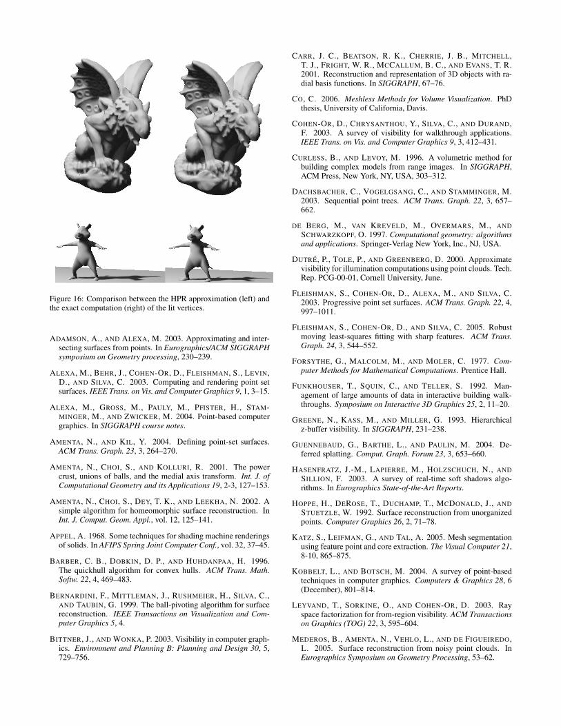
Figure 16: Comparison between the HPR approximation (left) andthe exact computation (right) of the lit vertices.
ADAMSON, A., AND ALEXA, M. 2003. Approximating and inter-secting surfaces from points. In Eurographics/ACM SIGGRAPHsymposium on Geometry processing, 230–239.
ALEXA, M., BEHR, J., COHEN-OR, D., FLEISHMAN, S., LEVIN,D., AND SILVA, C. 2003. Computing and rendering point setsurfaces. IEEE Trans. on Vis. and Computer Graphics 9, 1, 3–15.
ALEXA, M., GROSS, M., PAULY, M., PFISTER, H., STAM-MINGER, M., AND ZWICKER, M. 2004. Point-based computergraphics. In SIGGRAPH course notes.
AMENTA, N., AND KIL, Y. 2004. Defining point-set surfaces.ACM Trans. Graph. 23, 3, 264–270.
AMENTA, N., CHOI, S., AND KOLLURI, R. 2001. The powercrust, unions of balls, and the medial axis transform. Int. J. ofComputational Geometry and its Applications 19, 2-3, 127–153.
AMENTA, N., CHOI, S., DEY, T. K., AND LEEKHA, N. 2002. Asimple algorithm for homeomorphic surface reconstruction. InInt. J. Comput. Geom. Appl., vol. 12, 125–141.
APPEL, A. 1968. Some techniques for shading machine renderingsof solids. In AFIPS Spring Joint Computer Conf., vol. 32, 37–45.
BARBER, C. B., DOBKIN, D. P., AND HUHDANPAA, H. 1996.The quickhull algorithm for convex hulls. ACM Trans. Math.Softw. 22, 4, 469–483.
BERNARDINI, F., MITTLEMAN, J., RUSHMEIER, H., SILVA, C.,AND TAUBIN, G. 1999. The ball-pivoting algorithm for surfacereconstruction. IEEE Transactions on Visualization and Com-puter Graphics 5, 4.
BITTNER, J., AND WONKA, P. 2003. Visibility in computer graph-ics. Environment and Planning B: Planning and Design 30, 5,729–756.
CARR, J. C., BEATSON, R. K., CHERRIE, J. B., MITCHELL,T. J., FRIGHT, W. R., MCCALLUM, B. C., AND EVANS, T. R.2001. Reconstruction and representation of 3D objects with ra-dial basis functions. In SIGGRAPH, 67–76.
CO, C. 2006. Meshless Methods for Volume Visualization. PhDthesis, University of California, Davis.
COHEN-OR, D., CHRYSANTHOU, Y., SILVA, C., AND DURAND,F. 2003. A survey of visibility for walkthrough applications.IEEE Trans. on Vis. and Computer Graphics 9, 3, 412–431.
CURLESS, B., AND LEVOY, M. 1996. A volumetric method forbuilding complex models from range images. In SIGGRAPH,ACM Press, New York, NY, USA, 303–312.
DACHSBACHER, C., VOGELGSANG, C., AND STAMMINGER, M.2003. Sequential point trees. ACM Trans. Graph. 22, 3, 657–662.
DE BERG, M., VAN KREVELD, M., OVERMARS, M., ANDSCHWARZKOPF, O. 1997. Computational geometry: algorithmsand applications. Springer-Verlag New York, Inc., NJ, USA.
DUTRE, P., TOLE, P., AND GREENBERG, D. 2000. Approximatevisibility for illumination computations using point clouds. Tech.Rep. PCG-00-01, Cornell University, June.
FLEISHMAN, S., COHEN-OR, D., ALEXA, M., AND SILVA, C.2003. Progressive point set surfaces. ACM Trans. Graph. 22, 4,997–1011.
FLEISHMAN, S., COHEN-OR, D., AND SILVA, C. 2005. Robustmoving least-squares fitting with sharp features. ACM Trans.Graph. 24, 3, 544–552.
FORSYTHE, G., MALCOLM, M., AND MOLER, C. 1977. Com-puter Methods for Mathematical Computations. Prentice Hall.
FUNKHOUSER, T., SQUIN, C., AND TELLER, S. 1992. Man-agement of large amounts of data in interactive building walk-throughs. Symposium on Interactive 3D Graphics 25, 2, 11–20.
GREENE, N., KASS, M., AND MILLER, G. 1993. Hierarchicalz-buffer visibility. In SIGGRAPH, 231–238.
GUENNEBAUD, G., BARTHE, L., AND PAULIN, M. 2004. De-ferred splatting. Comput. Graph. Forum 23, 3, 653–660.
HASENFRATZ, J.-M., LAPIERRE, M., HOLZSCHUCH, N., ANDSILLION, F. 2003. A survey of real-time soft shadows algo-rithms. In Eurographics State-of-the-Art Reports.
HOPPE, H., DEROSE, T., DUCHAMP, T., MCDONALD, J., ANDSTUETZLE, W. 1992. Surface reconstruction from unorganizedpoints. Computer Graphics 26, 2, 71–78.
KATZ, S., LEIFMAN, G., AND TAL, A. 2005. Mesh segmentationusing feature point and core extraction. The Visual Computer 21,8-10, 865–875.
KOBBELT, L., AND BOTSCH, M. 2004. A survey of point-basedtechniques in computer graphics. Computers & Graphics 28, 6(December), 801–814.
LEYVAND, T., SORKINE, O., AND COHEN-OR, D. 2003. Rayspace factorization for from-region visibility. ACM Transactionson Graphics (TOG) 22, 3, 595–604.
MEDEROS, B., AMENTA, N., VEHLO, L., AND DE FIGUEIREDO,L. 2005. Surface reconstruction from noisy point clouds. InEurographics Symposium on Geometry Processing, 53–62.
OHTAKE, Y., BELYAEV, A., ALEXA, M., TURK, G., AND SEI-DEL, H.-P. 2003. Multi-level partition of unity implicits. ACMTrans. Graph. 22, 3, 463–470.
PAULY, M., AND GROSS, M. 2001. Spectral processing of point-sampled geometry. In SIGGRAPH, 379–386.
RUSINKIEWICZ, S., AND LEVOY, M. 2000. Qsplat: A multireso-lution point rendering system for large meshes. In SIGGRAPH,343–352.
SAINZ, M., AND PAJAROLA, R. 2004. Point-based renderingtechniques. Computers & Graphics 28, 6, 869–879.
SAINZ, M., PAJAROLA, R., AND LARIO, R. 2004. Pointsreloaded: Point-based rendering revisited. In Symposium onPoint-Based Graphics, 121–128.
SCHAUFLER, G., AND JENSEN, H. 2000. Ray tracing point sam-pled geometry. In Eurographics Workshop on Rendering Tech-niques, 319–328.
SUTHERLAND, E., SPROULL, R., AND SCHUMACKER, R. 1974.A characterization of ten hidden-surface algorithms. ACM Com-put. Surv. 6, 1, 1–55.
WALD, I., AND SEIDEL, H.-P. 2005. Interactive ray tracingof point-based models. In Eurographics Symposium on Point-Based Graphics, 1–8.
WIMMER, M., AND SCHEIBLAUER, C. 2006. Instant points: Fastrendering of unprocessed point clouds. In Proceedings Sympo-sium on Point-Based Graphics 2006, 129–136.
WOO, A., POULIN, P., AND FOURNIER, A. 1990. A survey ofshadow algorithms. IEEE Comput. Graph. Appl. 10, 6, 13–32.
WU, J., AND KOBBELT, L. 2004. Optimized sub-sampling ofpoint sets for surface splatting. Computer Graphics Forum 23,643–652.
ZWICKER, M., PFISTER, H., VAN BAAR, J., AND GROSS, M.2001. Surface splatting. In SIGGRAPH, 371–378.
ZWICKER, M., PAULY, M., KNOLL, O., AND GROSS, M. 2002.Pointshop 3D: an interactive system for point-based surface edit-ing. ACM Trans. Graph. 21, 3, 322–329.
A Proofs of the operator’s properties
This appendix provides the proofs of the properties of the operator.
Lemma 4.1 HR ⊆ V , i.e., every point marked visible by the HPRoperator is indeed visible from C.
Proof: Let p ∈ HR. Suppose, by way of contradiction, that p 6∈ V .Then, the ray from C to p passes through some point p′ ∈ S thathides p. After inversion, p′ will be farther away than p from C onthis ray, since flipping is strictly monotonically decreasing alongeach ray from C. Thus, p is internal to the convex hull. 2
Lemma 4.2 limR−→∞ HR = V , i.e., assuming T = inf{‖p−C‖|p ∈S} > 0, when R → ∞, the set of visible points marked by HPR isequal to the set of visible points.
Proof: One side of the equality was proved in Lemma 4.1. To provethe other side, we will show that if p ∈ V , then p ∈ limR−→∞ HR.Without loss of generality, let p = (r,0) (in spherical coordinates),i.e., p lies on the X−axis. Recall that we assume that ∀q = (rq,θ)∈S, r,rq ≥ T .
Then, applying spherical flipping to p and another arbitrary pointq∈ S, we get f (p) = (2R−r,0) and f (q) = (2R−rq,θ), (θ 6= 0). Toshow that p ∈ limR−→∞ HR, we will show that there exists R0 suchthat ∀R > R0, f (q) is on one side of a line through f (p), ∀q ∈ S.The line we choose is x = 2R− r, which is parallel to the y−axis.
Now, the x coordinate of f (q) is qx = (2R − rq)cosθ , but sincerq > T , then qx < (2R − T )cosθ . For sufficiently large R thisquantity satisfies (2R − T )cosθ < 2R − r. This happens when2R(1− cosθ) > r−T cosθ , i.e., R > r−T cosθ
2(1−cosθ), which holds since
both the numerator and the denominator are positive. 2
Lemma 4.3 Let S be an infinitesimal surface patch around p. Thenp ∈ HR if and only if the curvature k at p satisfies:
k <4R(2R− r)cot2 β +2Rr(
4Rr−4R2 +(r−2R)2
sin2 β
)3/2 .
In the case that β = π/2, which corresponds to the case that thetangent to the surface at p is perpendicular to the line of sight,k < 2R/r2.
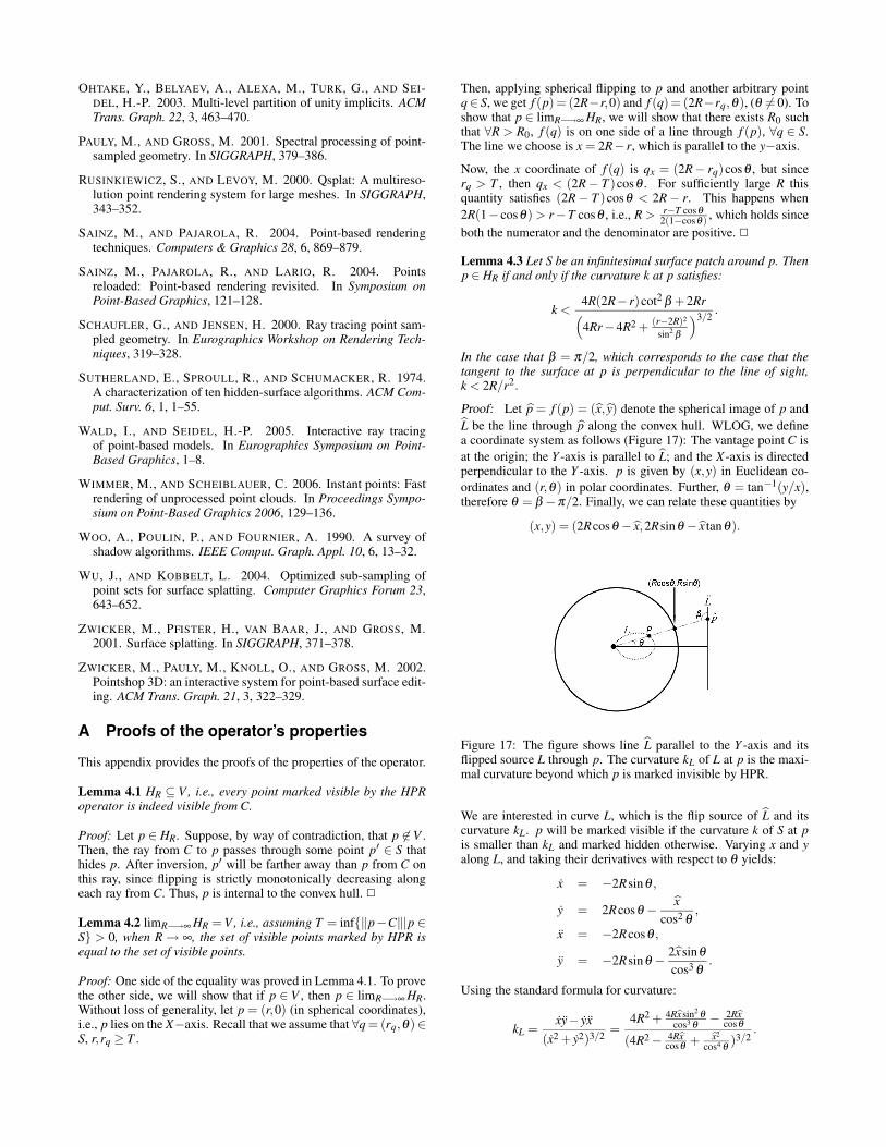
Proof: Let p = f (p) = (x, y) denote the spherical image of p andL be the line through p along the convex hull. WLOG, we definea coordinate system as follows (Figure 17): The vantage point C isat the origin; the Y -axis is parallel to L; and the X-axis is directedperpendicular to the Y -axis. p is given by (x,y) in Euclidean co-ordinates and (r,θ) in polar coordinates. Further, θ = tan−1(y/x),therefore θ = β −π/2. Finally, we can relate these quantities by
(x,y) = (2Rcosθ − x,2Rsinθ − x tanθ).
Figure 17: The figure shows line L parallel to the Y -axis and itsflipped source L through p. The curvature kL of L at p is the maxi-mal curvature beyond which p is marked invisible by HPR.
We are interested in curve L, which is the flip source of L and itscurvature kL. p will be marked visible if the curvature k of S at pis smaller than kL and marked hidden otherwise. Varying x and yalong L, and taking their derivatives with respect to θ yields:
x = −2Rsinθ ,
y = 2Rcosθ −x
cos2 θ,
x = −2Rcosθ ,
y = −2Rsinθ −2xsinθcos3 θ
.
Using the standard formula for curvature:
kL =xy− yx
(x2 + y2)3/2 =4R2 + 4Rxsin2 θ
cos3 θ − 2Rxcosθ
(4R2 − 4Rxcosθ + x2
cos4 θ )3/2.
Expressing this in terms of r and β , using the identities
β =π2 +θ ,
x = r cosθ = r sinβ ,
y = r sinθ = −r cosβ ,
x = 2Rcosθ − x = (2R− r)sinβ ,
we obtain
kL =4R(2R− r)cot2 β +2Rr(
4Rr−4R2 +(r−2R)2
sin2 β
)3/2 .
In the special case that β = π/2 this simplifies to kL = 2Rr2 . 2
Theorem 4.4 Assume that the sample is sufficiently dense, then forevery R, there exists ε > 0 such that HR ⊆Vε .
Proof: To prove the theorem, we should find ε > 0 for which if apoint p /∈ Vε , then p /∈ HR. Denote the distance from p to C by r,and assume that the sample is sufficiently dense with
ρ <T2
√rR (1− r
4R ).
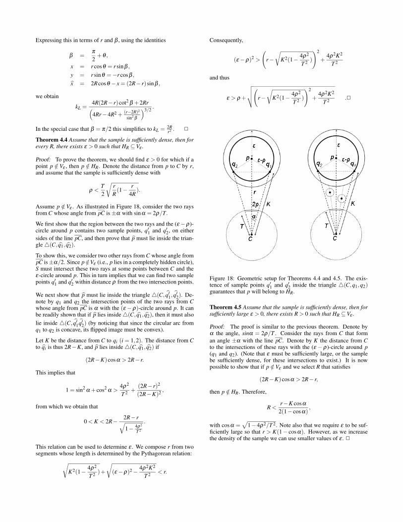
Assume p /∈ Vε . As illustrated in Figure 18, consider the two raysfrom C whose angle from pC is ±α with sinα = 2ρ/T.
We first show that the region between the two rays and the (ε −ρ)-circle around p contains two sample points, q′1 and q′2, on eithersides of the line pC, and then prove that p must lie inside the trian-gle 4(C, q1, q2).
To show this, we consider two other rays from C whose angle frompC is ±α/2. Since p /∈Vε (i.e., p lies in a completely hidden circle),S must intersect these two rays at some points between C and theε-circle around p. This in turn implies that we can find two samplepoints q′1 and q′2 within distance ρ from the two intersection points.
We next show that p must lie inside the triangle 4(C, q′1, q′2). De-note by q1 and q2 the intersection points of the two rays from Cwhose angle from pC is α with the (ε −ρ)-circle around p. It canbe readily shown that if p lies inside 4(C, q1, q2), then it must alsolie inside 4(C, q′1q′2) (by noticing that since the circular arc fromq1 to q2 is concave, its flipped image must be convex).
Let K be the distance from C to qi (i = 1,2). The distance from Cto qi is thus 2R−K, and p lies inside 4(C, q1, q2) if
(2R−K)cosα > 2R− r.
This implies that
1 = sin2 α + cos2 α >4ρ2
T 2 +(2R− r)2
(2R−K)2 ,
from which we obtain that
0 < K < 2R−2R− r√1− 4ρ2
T 2
.
This relation can be used to determine ε . We compose r from twosegments whose length is determined by the Pythagorean relation:
√K2(1− 4ρ2
T 2 )+
√(ε −ρ)2 −
4ρ2K2
T 2 < r.
Consequently,
(ε −ρ)2 >
(r−√
K2(1− 4ρ2
T 2 )
)2
+4ρ2K2
T 2
and thus
ε > ρ +
√√√√(
r−√
K2(1− 4ρ2
T 2 )
)2
+4ρ2K2
T 2 .2
Figure 18: Geometric setup for Theorems 4.4 and 4.5. The exis-tence of sample points q′1 and q′2 inside the triangle 4(C,q1,q2)guarantees that p will belong to HR.
Theorem 4.5 Assume that the sample is sufficiently dense, then forsufficiently large ε > 0, there exists R > 0 such that HR ⊆Vε .
Proof: The proof is similar to the previous theorem. Denote byα the angle, sinα = 2ρ/T . Consider the rays from C that forman angle ±α with the line pC. Denote by K the distance from Cto the intersections of these rays with the (ε − ρ)-circle around p(q1 and q2). (Note that ε must be sufficiently large, or the samplebe sufficiently dense, for these intersections to exist.) It is nowpossible to show that if p /∈Vε and we select R that satisfies
(2R−K)cosα > 2R− r,
then p /∈ HR. Therefore,
R <r−K cosα
2(1− cosα),
with cosα =√
1−4ρ2/T 2. Note also that we require ε to be suf-ficiently large so that r > K(1− cosα). However, as we increasethe density of the sample we can use smaller values of ε . 2