Directly measuring single-molecule heterogeneityusing force spectroscopyMichael Hinczewskia,1, Changbong Hyeonb, and D. Thirumalaic

aDepartment of Physics, Case Western Reserve University, Cleveland, OH 44106; bKorea Institute for Advanced Study, Seoul 02455, Korea; and cBiophysicsProgram, Institute For Physical Science and Technology, University of Maryland, College Park, MD 20742

Edited by Ken A. Dill, Stony Brook University, Stony Brook, NY, and approved May 10, 2016 (received for review September 16, 2015)

One of the most intriguing results of single-molecule experimentson proteins and nucleic acids is the discovery of functional heteroge-neity: the observation that complex cellular machines exhibit multiple,biologically active conformations. The structural differences betweenthese conformations may be subtle, but each distinct state can beremarkably long-lived, with interconversions between states occurringonly at macroscopic timescales, fractions of a second or longer.Althoughwe now have proof of functional heterogeneity in a handfulof systems—enzymes, motors, adhesion complexes—identifying andmeasuring it remains a formidable challenge. Here, we show thatevidence of this phenomenon is more widespread than previouslyknown, encoded in data collected from some of the most well-estab-lished single-molecule techniques: atomic force microscopy or opticaltweezer pulling experiments. We present a theoretical procedure foranalyzing distributions of rupture/unfolding forces recorded at differ-ent pulling speeds. This results in a single parameter, quantifying thedegree of heterogeneity, and also leads to bounds on the equilibrationand conformational interconversion timescales. Surveying 10 pub-lished datasets, we find heterogeneity in 5 of them, all with intercon-version rates slower than 10 s−1. Moreover, we identify two systemswhere additional data at realizable pulling velocities is likely to find atheoretically predicted, but so far unobserved crossover regime be-tween heterogeneous and nonheterogeneous behavior. The signifi-cance of this regime is that it will allow far more precise estimatesof the slow conformational switching times, one of the least under-stood aspects of functional heterogeneity.

biomolecule heterogeneity | atomic force microscope | optical tweezers |rupture force distribution | dynamic disorder

One of the great problems in modern biology is to understandhow the intrinsic diversity of cellular behaviors is shaped by

factors outside of the genome. The causes of this heterogeneityare spread across multiple scales, from noise in biochemical reactionnetworks through epigenetic mechanisms like DNAmethylation andhistone modification (1). It might be natural to expect heterogeneityat the cellular level because of the bewildering array of time andlength scales associated with the molecules of life that govern cellfunction. Surprisingly, even at the level of individual biomolecules,diversity in functional properties like rates of enzymatic catalysis(2–5) or receptor–ligand binding (6, 7) can occur. This diversityarises from the presence of many distinct functional states in thefree-energy landscape, which correspond to long-lived active con-formations of the biomolecule. Although the reigning paradigm inproteins and nucleic acids has been a single, folded native structure,well separated in free energy from any other conformations, pos-sibilities about rugged landscapes with multiple native states havebeen explored for a long time (8–15). However, only with the rev-olutionary advances in single-molecule experimental techniques inrecent years have we been able to gather direct evidence of func-tional heterogeneity, in systems ranging from protein enzymes (2–4)and nucleic acids (5, 16, 17), to molecular motors (18) and celladhesion complexes (6, 7). As research inevitably moves towardlarger macromolecular systems, the examples of functional hetero-geneity will only multiply. We thus need to develop theories that candeduce aspects of the hidden kinetic network of states underlying

the single-molecule experimental data (19), allowing us to quantifythe nature and extent of the heterogeneity.The focus in this study is single-molecule force spectroscopy,

conducted either by atomic force microscopy (AFM) or opticaltweezers, which constitutes an extensive experimental literatureover the last two decades. Our contention is that evidence of het-erogeneity is widespread in this literature, but has gone largely un-noticed, because researchers [with a few exceptions, as discussedbelow (20–23)] did not recognize the markers in their data that in-dicated heterogeneous behavior. To remedy this situation, we in-troduce a universal approach to analyzing distributions of rupture/unfolding forces collected in pulling experiments, which yields asingle nondimensional parameter Δ≥ 0. The magnitude of Δ char-acterizes the extent of the disorder in the underlying ensemble, theruggedness of the free-energy landscape. Moreover, our methodprovides a way of estimating bounds on key timescales, describingboth the fast local equilibration in each well (distinct system state) ofour rugged landscape, and the slow interconversion between thevarious wells. After verifying the validity of our approach using syn-thetic data generated from a heterogeneous model system, we survey10 experimental datasets, comprising a diverse set of biomolecularsystems from simple DNA oligomers to large complexes of proteinsand nucleic acids. The largest values ofΔ in our survey, indicating thestrongest heterogeneity, come from systems involving nucleic acidsalone or protein/nucleic acid interactions, supporting the hypothesisthat nucleic acid free-energy landscapes are generally more ruggedthan those involving only proteins (24). Our theory thus provides apowerful new analytical tool, for the first time (to our knowledge)allowing a broad comparison of functional heterogeneity amongdifferent biomolecules through a common experimental protocol.

Significance

The relationship between structure and function is the heart ofmodern cell biology. Technological innovations in manipulatingsingle molecules of proteins, DNA/RNA, and their complexes, arebeginning to reveal the surprising intricacies of this relationship.In certain cases, the same molecule randomly switches betweenvarious long-lived structures, each with different functional prop-erties. We present a theory to extract the extent and dynamics ofthese structural fluctuations from single-molecule experimentaldata. We find large heterogeneity in DNA and RNA complexes,supporting the notion that energy landscapes involving nucleicacids are rugged. Our work shows that functional heterogeneityis far more common than previously thought and suggests ex-perimental approaches for estimating the timescales of thesefluctuations with unprecedented accuracy.

Author contributions: M.H., C.H., and D.T. designed research, performed research, ana-lyzed data, and wrote the paper.

The authors declare no conflict of interest.

This article is a PNAS Direct Submission.1To whom correspondence should be addressed. Email: mxh605@case.edu.

This article contains supporting information online at www.pnas.org/lookup/suppl/doi:10.1073/pnas.1518389113/-/DCSupplemental.

www.pnas.org/cgi/doi/10.1073/pnas.1518389113 PNAS Early Edition | 1 of 10

BIOPH

YSICSAND

COMPU

TATIONALBIOLO

GY

PNASPL

US

TheoryForce Spectroscopy for a Pure, Adiabatic System.As a starting point,consider a generic free-energy landscape for a biomolecular sys-tem with a single functional state (Fig. 1A) subject to an increasingtime-dependent external force f ðtÞ. For a molecular complex, thefunctional basin of attraction in the landscape would correspondto an ensemble of bound conformations with similar energies,which we label N. For the case of single-molecule folding, thiswould be the unique native ensemble. The force is applied throughan experimental apparatus like an AFM or optical tweezer, typi-cally connected to the biomolecule through protein or nucleic acidlinkers of known stiffness. The apparatus is pulled at a constantvelocity v, leading to a force ramp with slope df=dt=ωsðf Þv, whereωsðf Þ is the effective stiffness of the setup (linkers plus the AFMcantilever or optical trap). This ωsðf Þ may in general depend onthe force, particularly for the AFM setup, where the cantilever

stiffness is often comparable to or greater than that of the mo-lecular construct. So we also define a characteristic stiffness ωs,which we set to the mean ωsðf Þ over the range of forces probed inthe experiment (although the precise value of ωs is not important).This allows us to introduce a characteristic force loading rate rproportional to the velocity, r=ωsv.If at time t= 0 the system starts in N, the force ramp tilts the

landscape along the extension coordinate. If we model the con-formational dynamics of the system as diffusion within this land-scape, the tilting eventually leads to a transition out of N, associatedwith unbinding of the complex or unfolding of the molecule (anensemble of states we call U). We let ΣrðtÞ be the survival proba-bility for loading rate r, in other words, the probability that thetransition to U has not occurred by time t. The distribution of firstrupture times is then −dΣr=dt, and the mean rupture rate kðrÞ is justthe inverse of the average rupture time:

kðrÞ=� Z ∞

0dt  t�−dΣr

dt

��−1=� Z ∞

0dt  ΣrðtÞ

�−1, [1]

where we have used integration by parts and assumed that rupturealways occurs if we wait long enough, Σrð∞Þ= 0.The behavior of ΣrðtÞ at different r depends on how kðrÞ

compares to two other intrinsic rates. The first is the equilibrationrate keq in the N well, or how quickly the system samples the con-figurations of the functional ensemble. For a single, smooth wellwith mean curvature ω0 and a diffusion constant D, this rate is onthe order of keq ∼ βω0D, where β= 1=kBT. The second is a criticalrate kcðrÞ= r=fc, which describes how quickly the force reaches acritical force scale for rupture fc ∼G‡=x‡. Here, G‡ is the energyscale of the barrier that needs to be overcome for the N-to-Utransition at zero force, and x‡ is the extension difference betweenthe N well minimum and the transition state. For f J fc, the land-scape is tilted sufficiently that the barrier becomes insignificant,and rupture occurs quickly (on a diffusion-limited timescale). IfkcðrÞ � kðrÞ � keq, the system is in the adiabatic regime. The forceramp is sufficiently slow that rupture occurs before the critical forceis reached, and equilibration is fast enough that the system canreach quasiequilibrium at the instantaneous value of the force f ðtÞat all times t before the rupture.If the adiabatic condition is satisfied, the survival probability

ΣrðtÞ obeys the kinetic equation dΣrðtÞ=dt=−kðf ðtÞÞΣrðtÞ, wherekðf Þ is the rupture rate at constant force f. Because f ðtÞ is amonotonically increasing function of t, we can change variablesfrom t to f ðtÞ (25), and solve for Σrðf Þ, the probability that thesystem does not rupture before the force value f is reached:

Σrðf Þ= exp�−1r

Z f

0df ′

ωskðf ′Þωsðf ′Þ

�. [2]

Interestingly, the integral inside the exponential is independentof the loading rate r. Hence, for a system pulled from a single nativeensemble, we can calculate the following quantity from experi-mental trajectories at different r:

Ωr ðf Þ≡ − r   log  Σrðf Þ, [3]

and the results should collapse onto a single master curve for all r inthe adiabatic regime. When r is sufficiently large that kðrÞ< kcðrÞ orkðrÞ> keq, the assumption of quasiequilibrium on a slowly changingenergy landscape breaks down, and Eq. 2 no longer holds. For thisfast, nonadiabatic case (26, 27), we should find that Ωrðf Þ varieswith r, as we will explore later in more detail.

Force Spectroscopy for a Heterogeneous, Adiabatic System. In a pio-neering series of studies, Raible and collaborators (20–22) analyzedforce ramp experiments for the regulatory protein ExpG unbinding

free

ener

gy

end-to-endextension

conformationaldegrees offreedom

single functional state

A

N U

B

heterogeneousfunctional states

UN

N

N

f

f

f

f

Fig. 1. (A) Schematic biomolecular free-energy landscape with a singlefunctional state, N, corresponding to an ensemble of folded/bound confor-mations. Under an adiabatically increasing external force fðtÞ, there is aninstantaneous rupture rate kðfðtÞÞ describing transitions between N and theunfolded/unbound ensemble U. (B) Schematic free-energy landscape of aheterogeneous system with multiple functional states. Each functional en-semble Nα will have a state-dependent adiabatic rupture rate kðf , αÞ. As-suming the states are roughly equally probable in equilibrium, there will bea single overall rate ki for interconversion between the various states.

2 of 10 | www.pnas.org/cgi/doi/10.1073/pnas.1518389113 Hinczewski et al.

from a DNA fragment. Plotting Ωrðf Þ (the data reproduced in Fig.6D), they did not find any collapse, as might be surmised fromEq. 3. This was not an artifact due to nonadiabaticity [violation ofthe inequality kcðrÞ � kðrÞ � keq], because the absence of collapsebecomes even more pronounced at small loading rates, further intothe adiabatic territory where collapse should be observed. Theycorrectly inferred that the cause of this divergence is heterogeneityin the ensemble of states in the protein–DNA complex.To understand the behavior of Ωrðf Þ in a heterogeneous system,

let us consider the effects of a force ramp on a biomolecular free-energy landscape with multiple functional states (Fig. 1B). Our goalis to use Ωrðf Þ, derived from experimental pulling trajectories, toquantify the extent of the heterogeneity and extract informationabout the underlying conformational dynamics. The functional statesare distinct basins of attraction in the landscape, corresponding todistinct functional ensembles which we label Nα for state α. We as-sume the minimum energy in each well and their overall dimensionsare comparable, so that the equilibrium probabilities peqα of thevarious states are of the same order. In this case, if α≠ α′, thetransition rates kα→α′ and kα′→α are also similar from detailed bal-ance, kα→α′=kα′→α = peqα′ =p

eqα ∼Oð1Þ. Hence, we can introduce an

overall scale for the interconversion rate between the different states,ki, such that kα→α′ ∼OðkiÞ for any α≠ α′. Thus, we now have twointrinsic timescales: keq for equilibration within a single Nα, and kifor transitions between distinct Nα values, where typically ki � keqmust be true in order to observe clear heterogeneity.The experimental setup is the same as above, with a loading rate

r, and a corresponding mean rupture rate kðrÞ for reaching the Uensemble. We can identify three dynamical regimes, based on themagnitude of ki. In the first regime, interconversion is slow, withki � kðrÞ. In the second regime, ki is comparable to kðrÞ. In fact, aswe will discuss later in more detail, we will be particularly interestedin the crossover scenario where ki ≥ kðrÞ for some subset of the rvalues in the experiment, but ki < kðrÞ for the remainder. If thissecond regime is identified in an experiment, it provides a way toestimate the scale of ki. Finally, in the third regime, the barriersbetween the Nα basins of attraction are small, such that ki � kðrÞ,and the system can sample all of the states before rupture. Quali-tatively, this scenario is indistinguishable from the case of a systemwith a single native basin of attraction, with ki taking the role of keqas the rate scale for overall equilibration in the landscape. Becausethe first regime is simpler to treat mathematically than the secondregime, we will initially focus on a theory to describe the first regimeand identify its signatures in experimental data. Assessing thevalidity of this theory in experiments will turn out to be a usefulcriterion for distinguishing between the first, second, and third re-gimes, and thus putting bounds on ki. This by-product of our theoryis of considerable importance because it is a priori very difficult toestimate ki.To begin, consider adiabatic pulling where ki is the slowest

rate in the system, ki � kcðrÞ � kðrÞ � keq. On the timescale ofpulling and rupture, the system is effectively trapped in a het-erogeneous array of states: if we start a pulling trajectory in stateα, the system will remain in that state until rupture. The rupturerate at constant force, kðf , αÞ will in general depend on the state,and the ensemble of molecules from which we pull will becharacterized by a set of initial state probabilities pα. If ki is ex-tremely small, such that the system cannot interconvert even onthe macroscopic timescales of experimental preparation, pα maybe different from peqα , because we are not guaranteed to drawfrom an equilibrium distribution across the entire landscape.This distinction is not important for the analysis below. In fact,our approach also works when ki = 0, corresponding to thequenched disorder limit, as seen for example in an ensemble ofmolecules with covalent chemical differences.The analog of Eq. 2 for the survival probability Σrðf Þ during adi-

abatic pulling in a heterogeneous system with small ki is as follows:

Σrðf Þ=�exp�−1r

Z f

0df ′

ωskðf ′, αÞωsðf ′Þ

��, [4]

where the brackets denote an average over the initial ensemble ofstates, hOðαÞi≡PαpαOðαÞ for any quantity OðαÞ. The associatedΩrðf Þ from Eq. 3 can be expressed through a cumulant expansion interms of the integrand Iðf , αÞ≡ R f0 df ′ωskðf ′, αÞ=ωsðf ′Þ as follows:

Ωrðf Þ=−X∞n=1

ð−1Þn κnðf Þn!rn−1

,

κnðf Þ≡ ∂n∂λn   log

�eλIðf , αÞ

λ=0.

[5]

The first two cumulants are κ1ðf Þ= hIðf , αÞi and κ2ðf Þ= hI2ðf , αÞi−hIðf , αÞi2. In the absence of heterogeneity, all cumulants κnðf Þ withn> 1 are exactly zero. For a small degree of heterogeneity, or equiv-alently for sufficiently fast loading rates r, the main contribution tothe expansion is from the n= 1 and n= 2 terms. For the case offast r, we assume that we are still within the adiabatic regime,where kcðrÞ � kðrÞ, which turns out to be valid even for the largestloading rates in the experimental studies discussed below. In thisscenario, where the n> 2 contributions are negligible, Ωrðf Þ can beapproximated as follows:

Ωrðf Þ≈ rΔðf Þ log

�1+

κ1ðf ÞΔðf Þr

�, [6]

where Δðf Þ≡ κ2ðf Þ=κ21ðf Þ≥ 0 is a dimensionless measure of theensemble heterogeneity. For a pure system, Δðf Þ→ 0, givingΩrðf Þ→ κ1ðf Þ, independent of r. Eq. 6 agrees with the expansion inEq. 5 up to order n= 2, and also has the nice property that itsatisfies the inequality Ωrðf Þ≤ κ1ðf Þ, just like the exact form. Thelatter inequality follows from the definition of Σrðf Þ in Eq. 4 andJensen’s inequality, Σrðf Þ≥ expð−κ1ðf Þ=rÞ.Implementing the Model on Experimental Data. So far, the discussionhas been completely general, but to fit Eq. 6 to experimental datawe need specific forms for Δðf Þ and κ1ðf Þ. The minimal physicallysensible approximation, with the smallest number of unknown pa-rameters, supplements Eq. 6 with the following assumptions:

Δðf Þ=Δ, κ1ðf Þ= k0βx‡

�eβfx

‡

− 1�. [7]

The constants Δ, k0, and x‡ are fitting parameters. This presumesthat Δðf Þ changes little over the range of forces in the data, andκ1ðf Þ has the same mathematical form as in a pure Bell modelwith an escape rate kðf Þ= k0eβfx

‡

and ωsðf Þ=ωs, where k0 is theescape rate at zero force and x‡ is the distance to the transitionstate. For a heterogeneous system, the parameters k0 and x‡ nolonger have this simple interpretation, but we can still treat themas effective Bell values, averaged over the ensemble, with Δmeasuring the overall scale of the heterogeneity. Eq. 6, togetherwith the three-parameter approximation of Eq. 7, provides re-markably accurate fits to all of the heterogeneous experimentaldatasets we have encountered in the literature. As will be seenbelow, it is capable of simultaneously fitting Ωrðf Þ data for load-ing rates r spanning nearly two orders of magnitude.Although we focus on Ωrðf Þ as the main experimental quantity

of interest, Eqs. 6 and 7 can also be used to derive a closed formexpression for the probability distribution of rupture forces,prðf Þ=−dΣrðf Þ=df =−ðd=df Þexpð−Ωrðf Þ=rÞ, at loading rate r:

prðf Þ= k0eβ fx‡

r

1+

Δk0 eβ fx

‡ − 1�

βrx‡

!−Δ+1Δ

. [8]

In the limit of no heterogeneity, Δ→ 0, this distribution reducesto the one predicted for a Bell model under a constant loading

Hinczewski et al. PNAS Early Edition | 3 of 10

BIOPH

YSICSAND

COMPU

TATIONALBIOLO

GY

PNASPL

US

rate (25). The theoretical form for prðf Þ also allows us to carry out arelative likelihood analysis on the experimental data, to verify that Δis indeed a robust indicator of heterogeneity. As detailed in Support-ing Information, 6. Relative Likelihood Analysis of Heterogeneous vs.Pure Model Fitting for Experimental Data, we found that experimen-tal distributions prðf Þ corresponding to systems with nonzero Δwere far more likely to be described by the heterogeneous theory inEq. 8 than a pure model with the same number of parameters. We

surmise that if analysis of experimental data using our theory indicatesthatΔ ≠ 0 then it is highly probable that a multiple state description isneeded, thus dismissing a one-dimensional pure state description.To verify that our analysis and conclusions would not change

substantially even if the assumptions of the minimal model wererelaxed, we have also tested two generalized versions of themodel: one using the Dudko–Hummer–Szabo (28) instead of theBell form for the escape rate in κ1ðf Þ, and the other allowing Δðf Þ

i

Free

ene

rgy U(x)

x0

x0

interconversion rate ki

extent of disorder

A B

C D

ff

f

ff

f

f

c

eq

i

i

i

f

c

x

0xx

x

eq

eq

x

c

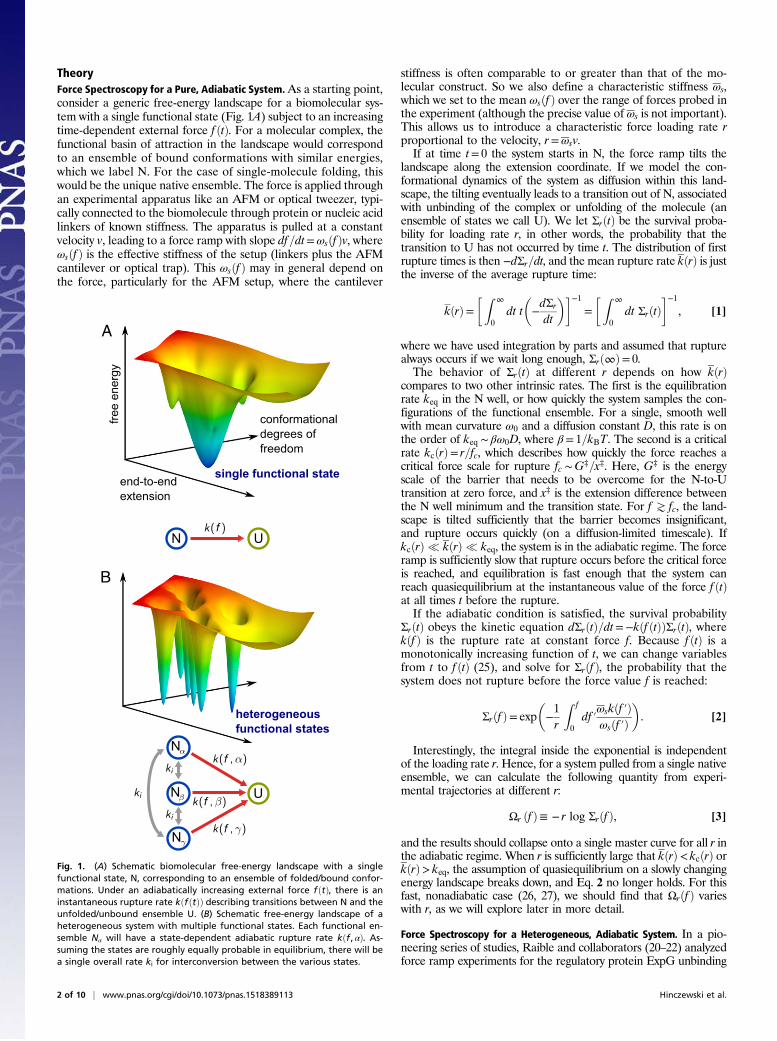
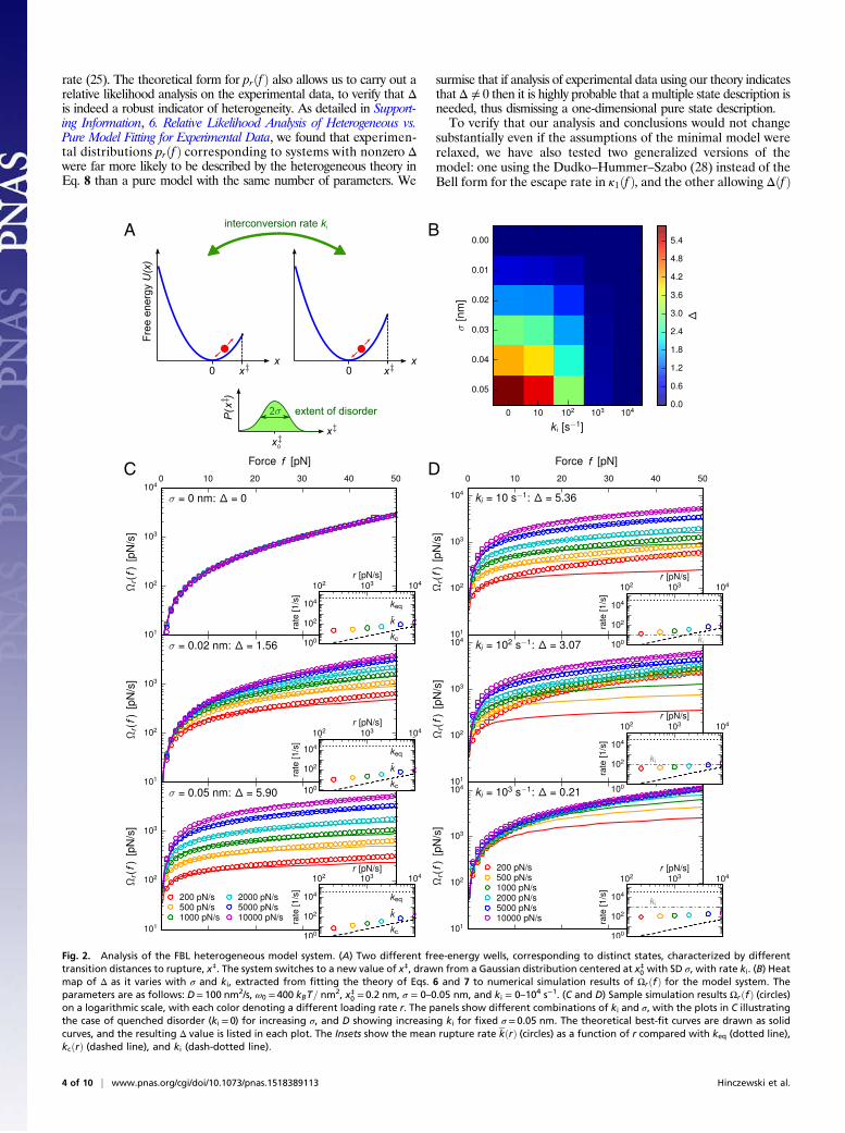
Fig. 2. Analysis of the FBL heterogeneous model system. (A) Two different free-energy wells, corresponding to distinct states, characterized by differenttransition distances to rupture, x‡. The system switches to a new value of x‡, drawn from a Gaussian distribution centered at x‡0 with SD σ, with rate ki. (B) Heatmap of Δ as it varies with σ and ki, extracted from fitting the theory of Eqs. 6 and 7 to numerical simulation results of ΩrðfÞ for the model system. Theparameters are as follows: D= 100 nm2/s, ω0 = 400 kBT= nm

2, x‡0 = 0.2 nm, σ = 0–0.05 nm, and ki = 0–104 s−1. (C and D) Sample simulation results ΩrðfÞ (circles)on a logarithmic scale, with each color denoting a different loading rate r. The panels show different combinations of ki and σ, with the plots in C illustratingthe case of quenched disorder (ki = 0) for increasing σ, and D showing increasing ki for fixed σ = 0.05 nm. The theoretical best-fit curves are drawn as solidcurves, and the resulting Δ value is listed in each plot. The Insets show the mean rupture rate kðrÞ (circles) as a function of r compared with keq (dotted line),kcðrÞ (dashed line), and ki (dash-dotted line).

4 of 10 | www.pnas.org/cgi/doi/10.1073/pnas.1518389113 Hinczewski et al.

to vary linearly with f across the force range. Both extensionshave four instead of three fitting parameters, but the heteroge-neity results for the experimental systems we analyzed arecompletely consistent with those obtained using the minimal model(see Supporting Information, 1. Testing the Assumptions of the Ωr(f)Model with Respect to Possible Generalizations, for details). Theseresults demonstrate that, if the need arises in future experimentalcontexts, the theory leading to Eq. 6 is quite general, and can betailored by choosing suitable expressions for κ1ðf Þ and Δðf Þ that gobeyond the minimal model of Eq. 7.The theory described up to now applies only to the first dynamical

regime, where ki � kðrÞ. However, the cases where ki is larger thansome or all of the kðrÞ, and the theory partially or completely fails,turn out to be very informative as well. To understand these points,it is easier to discuss the theory in the context of a concrete physicalmodel for heterogeneity, which we introduce in the next section.

Results and DiscussionFluctuating Barrier Location Model. Before turning to experimentaldata, we verify that the Δ parameter extracted from the fitting ofΩrðf Þ curves using Eqs. 6 and 7 is a meaningful measure of hetero-geneity. To do this, we will generate synthetic rupture data from aheterogeneous model system. The fluctuating barrier location (FBL)model, illustrated in Fig. 2A, consists of a reaction coordinate xwhose dynamics are described by diffusion with constant D along aparabolic free energy UðxÞ= ð1=2Þω0x2 for x≤ x‡. Rupture occurs ifx exceeds the transition distance x‡. To mimic dynamic heterogeneity,the value of x‡ changes at random intervals, governed by a Poissonprocess with an interconversion rate ki. At every switching event, anew value of x‡ is drawn from a Gaussian probability distributionPðx‡Þ= expð−ðx‡ − x‡0Þ2=2σ2Þ=

ffiffiffiffiffiffiffiffiffiffi2πσ2

pcentered at x‡0 with SD σ, and

diffusion continues if x is less than the transition distance. At timet= 0, when the applied force ramp f ðtÞ= rt begins, we assume theinitial ensemble of systems all start at x= 0 with x‡ values distributedaccording to Pðx‡Þ. Survival probabilities Σrðf Þ are computed fromnumerical simulations of the diffusive process, with about 3× 104rupture events collected for each parameter set (see SupportingInformation, 2. Heterogeneous Model Simulation Details, for ad-ditional details). The simplicity of the model, where one pa-rameter, σ, controls the degree of heterogeneity, and another, ki,the interconversion dynamics, allows us to explore the behaviorof Σrðf Þ, and hence Ωrðf Þ, over a broad range of disorder andintrinsic timescales.The circles in Fig. 2 C and D show simulation results for Ωrðf Þ

between f = 0–50 pN, plotted on a logarithmic scale, with eachcolor denoting a different ramp rate in the range r = 200–10,000pN/s. The model parameters areD= 100 nm2/s, ω0 = 400 kBT=nm2,x‡0 = 0.2 nm, σ = 0–0.05 nm, ki = 0–104 s−1, which give a variety ofΩrðf Þ curves of comparable magnitude over similar force scalesto the experimental data discussed below. Fig. 2C shows resultsfor quenched disorder (ki = 0) at different σ, whereas Fig. 2Dshows results for varying ki at fixed σ = 0.05 nm. For a givenchoice of ki and σ, we fit the analytical form of Eqs. 6 and 7 si-multaneously to the six Ωrðf Þ curves at different r, with the best-fit model plotted as solid lines in Fig. 2 C and D. This fittingyields values for Δ, k0, and x‡ in each case. The variation of Δwith σ and ki is plotted as a heat map in Fig. 2B.Let us first consider the quenched disorder results (Fig. 2C and

the left column of Fig. 2B). By definition, because ki = 0, the sys-tem ensemble is permanently frozen in a heterogeneous array ofdifferent states with different values of x‡. Moreover, the adiabaticassumptions also hold, as can be seen in the Insets to Fig. 2C. Theseshow the mean rupture rate kðrÞ for different r (circles) comparedwith keq (dotted line) and kcðrÞ (dashed line). For all of the r valuesanalyzed, kcðrÞ< kðrÞ � keq, so adiabaticity should approximatelyhold. Thus, the assumptions leading to Eqs. 6 and 7 are valid, andindeed the analytical form provides an excellent fit to the simulationdata. Although the theory is by construction most accurate in the

limit of fast (but still adiabatic) r, it still quantitatively describes theresults for r spanning two orders of magnitude. Only small discrep-ancies start to appear at the slowest loading rates. For the puresystem limit (σ = 0), the best-fit value of Δ is also zero, with all of theΩrðf Þ curves collapsing on one another. Δ progressively increaseswith σ, growing roughly proportional to the width of the disorderdistribution. The greater the heterogeneity, the more pronouncedthe separation between the Ωrðf Þ curves at various r.The results in Fig. 2D are obtained by keeping the extent of

heterogeneity fixed at a large level (σ = 0.05 nm) and allows in-terconversion, increasing ki from 10 to 103 s−1. So long as kðrÞ � ki,the system is unlikely to interconvert on the timescale of rupture,and we see distinct, noncollapsed Ωrðf Þ curves. However, as ki in-creases and overtakes kðrÞ, starting from the smallest values ofr where kðrÞ has the smallest magnitude, the Ωrðf Þ curves begin tocollapse on one another. This leads to increasing discrepanciesbetween the data and the theoretical fit, because the assumptionsjustifying the theory break down when kðrÞ< ki. Eventually, once kiis greater than all of the kðrÞ, there is total collapse of the Ωrðf Þcurves (Fig. 2D, Bottom). Frequent interconversion between thedifferent states of the system before rupture averages out the het-erogeneity, making the results indistinguishable from a pure system.In this limit, the ensemble of functional states acts effectively like asingle functional basin of attraction, with multiple distinct pathwaysto rupture. Although multiple pathways between a pair of states canbe considered to be another manifestation of heterogeneity, theyare not in themselves sufficient to lead to noncollapse of the Ωrðf Þcurves, as we discuss in more detail in Supporting Information, 3.Heterogeneity in Rupture Pathways vs. Heterogeneity in FunctionalStates. To see anything but complete collapse of the Ωrðf Þ curves inthe adiabatic regime requires a small enough interconversion rateki, slower than the mean rupture rates kðrÞ for at least some subsetof the r values.

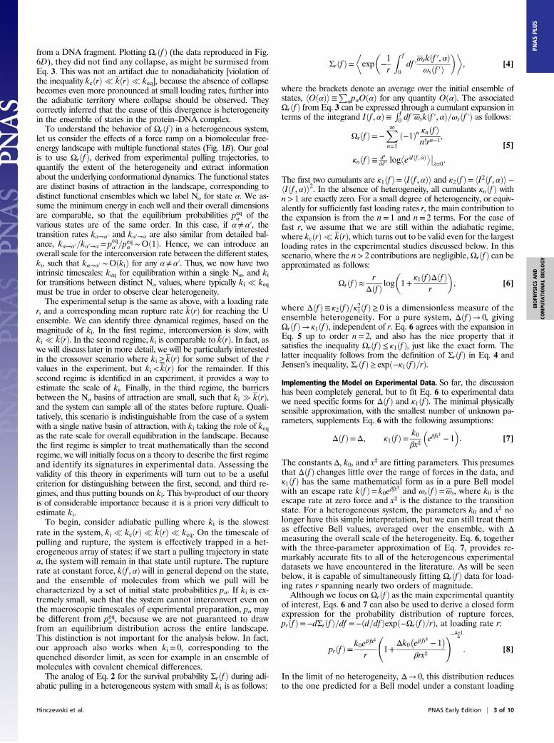
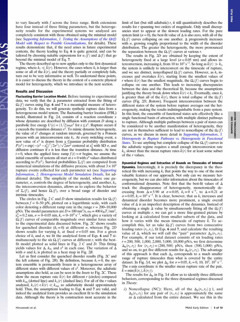
Dynamical Regimes and Extraction of Bounds on Timescales of InternalDynamics. Interestingly, it is precisely the discrepancy in the theo-retical fits with increasing ki that points the way to one of the mostvaluable features of our approach. Not only can we measure het-erogeneity, but we can also infer information about the timescales ofconformational dynamics. Note first that the best-fit values of Δtrack the disappearance of heterogeneity, monotonically de-creasing from Δ= 5.90 at σ = 0.05, ki = 0 s−1, to Δ= 0.21 atσ = 0.05, ki = 103 s−1. It is clear, however, that as ki increases anddynamical disorder becomes more prominent, a single overallvalue of Δ is an imperfect description of the dynamics. Instead ofobtaining a single Δ value by simultaneously fitting all the Ωrðf Þcurves at multiple r, we can get a more fine-grained picture bylooking at Δ calculated from smaller subsets of the data, andhow it varies with the mean timescale of rupture k. To ac-complish this, let us take Ωrðf Þ curves from two consecutiveloading rates ðr1, r2Þ, fit Eqs. 6 and 7, and calculate the resultingvalue of Δ, which we will call the “pair” parameter Δpðr1, r2Þ.For example, if our total dataset consists of six loading ratesr= 200, 500, 1,000, 2,000, 5,000, 10,000 pN/s, we first determineΔpðr1, r2Þ for ðr1, r2Þ= ð200, 500Þ pN/s, then ð500, 1,000Þ pN/s,and so on, to get five different results for Δpðr1, r2Þ. The advantageof this approach is that each Δp corresponds to a much smallerrange of rupture timescales than what is covered by the entiredataset. In Fig. 3A, we plot Δp for σ = 0.05, ki = 0, 10, 102, 103 s−1.The x-axis coordinate is the smaller mean rupture rate of the pair,k=minðkðr1Þ, kðr2ÞÞ.The results for Δp in Fig. 3A allow us to identify three different

behaviors, corresponding to the three dynamical regimes discussedin Theory:

i) Noncollapse (NC): Here, all of the Δpðr1, r2Þ≥ 1, andΔpðr1, r2Þ for any pair of ðr1, r2Þ is approximately the sameas Δ calculated from the entire dataset. We see this in the

Hinczewski et al. PNAS Early Edition | 5 of 10

BIOPH

YSICSAND

COMPU

TATIONALBIOLO

GY

PNASPL

US

ki = 0 s−1 case in Fig. 3A, where for comparison the value ofΔ over the whole set is marked by a horizontal dashed line.The corresponding Ωrðf Þ curves are in Fig. 2C, Bottom. Theagreement between Δpðr1, r2Þ and Δ is a consistency checkfor the theory, and implies that the underlying assumptionsare valid, namely ki < kðrÞ< keq for all r in the dataset. From this,we can conclude that the minimum value of kðrÞ among all ofthe loading rates r used in the experiment gives us an upperbound on ki. Similarly the maximum value of kðrÞ over allr gives a lower bound on keq. For ki = 10 s−1 in Fig. 3A, wesee what happens as ki approaches the timescale of kðrÞ. Weare still in the NC regime, because Δp ≥ 1 and ki (verticaldotted line) is smaller than any of the kðrÞ. However, ki isnow sufficiently close to kðr= 200  pN=sÞ that Δpð200, 500Þ(the leftmost point) is smaller than the rest of the Δp, whichlie at faster rupture timescales relatively unaffected by ki.

ii) Partial collapse (PC): Δpðr1, r2Þ≥ 1 for the largest values ofðr1, r2Þ, but for small loading rates Δpðr1, r2Þ � 1. This occursin the ki = 102 s−1 results in Fig. 3A. In this regime, the systemis adiabatic, keq > kðrÞ, but now ki falls between the smallestand largest values of kðrÞ. In the ki = 102 s−1 case, the var-iation in Δp is a reflection of the degree of overlap in theΩrðf Þ curves (Fig. 2D, Middle). The ðr1, r2Þ= ð5,000, 10,000ÞpN/s pair (blue and purple Ωrðf Þ circles) are clearly sepa-rated, corresponding to Δp ≥ 1 and the fact that ki K kðr1Þ,kðr2Þ. The ð200,  500Þ pN/s pair (red and orange circles) arenearly overlapping, corresponding to Δp � 1, and ki > kðr1Þ,kðr2Þ. The PC regime thus provides the best case scenario fordirectly estimating ki from the data, because we can boundki from above and below, and we know ki will roughly co-incide with the k where Δpðr1, r2Þ∼ 1.

iii) Total collapse (TC): Δpðr1, r2Þ � 1 for the all ðr1, r2Þ in thedataset. This is illustrated by the ki = 1,000 s−1 case in Fig.3A, corresponding to the Ωrðf Þ curves in Fig. 2D, Bottom. Δpvalues close to zero translate into near total overlap of theΩrðf Þresults. This regime requires adiabaticity, keq > kðrÞ, and if thereis any heterogeneity in the system, the interconversion betweenstates has to be fast, ki > kðrÞ. Thus, the maximum value of kðrÞover all r gives a lower bound on both ki and keq.

To summarize, we can use the magnitude of the heterogeneityparameters (Δ or Δp depending on whether we look at the whole

dataset or pairs of ramp rates) to make specific inferences aboutthe nature of the biomolecular free-energy landscape. Δ � 1(large disorder) in an experimental dataset implies the followingfacts: there is an ensemble of folded/intact states in the system,these states have substantially different force-dependent rates ofrupture, and the system will only rarely switch from one state toanother before rupture occurs. A small but finite Δ in the range0 � ΔK 1 (low disorder) indicates that heterogeneity is stillpresent, but one or both of the following are true: the inter-conversion rate ki is comparable to the mean rupture rates, soheterogeneity is partially averaged out due to transitions be-tween states, or the differences in rupture rate functions betweenstates are small. Finding Δ≈ 0 (no disorder) indicates that eitherthere is no heterogeneity (a single native state) or that ki is solarge that the ensemble of native states behaves effectively likea single state.

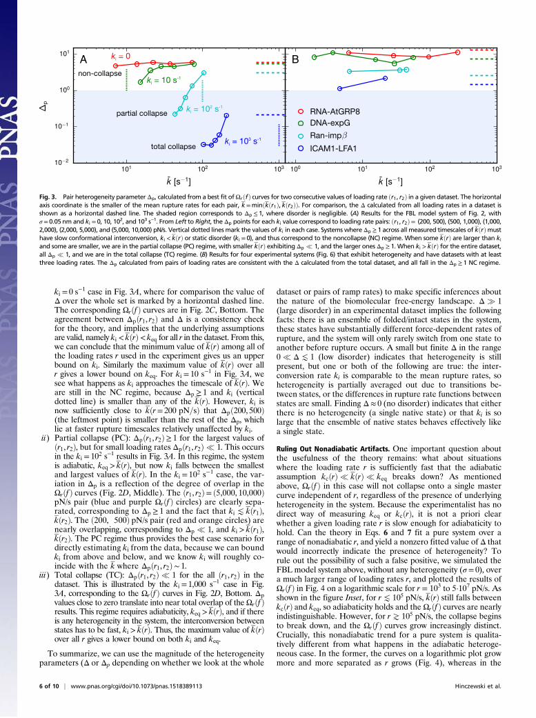
Ruling Out Nonadiabatic Artifacts. One important question aboutthe usefulness of the theory remains: what about situationswhere the loading rate r is sufficiently fast that the adiabaticassumption kcðrÞ � kðrÞ � keq breaks down? As mentionedabove, Ωrðf Þ in this case will not collapse onto a single mastercurve independent of r, regardless of the presence of underlyingheterogeneity in the system. Because the experimentalist has nodirect way of measuring keq or kcðrÞ, it is not a priori clearwhether a given loading rate r is slow enough for adiabaticity tohold. Can the theory in Eqs. 6 and 7 fit a pure system over arange of nonadiabatic r, and yield a nonzero fitted value of Δ thatwould incorrectly indicate the presence of heterogeneity? Torule out the possibility of such a false positive, we simulated theFBL model system above, without any heterogeneity (σ = 0), overa much larger range of loading rates r, and plotted the results ofΩrðf Þ in Fig. 4 on a logarithmic scale for r = 103 to 5·107 pN/s. Asshown in the figure Inset, for rK 105 pN/s, kðrÞ still falls betweenkcðrÞ and keq, so adiabaticity holds and the Ωrðf Þ curves are nearlyindistinguishable. However, for rJ 105 pN/s, the collapse beginsto break down, and the Ωrðf Þ curves grow increasingly distinct.Crucially, this nonadiabatic trend for a pure system is qualita-tively different from what happens in the adiabatic heteroge-neous case. In the former, the curves on a logarithmic plot growmore and more separated as r grows (Fig. 4), whereas in the

p

A Bnon-collapse

partial collapse

total collapse

ki = 0

ki = 10 s-1

ki = 102 s-1

ki = 103 s-1

RNA-AtGRP8DNA-expG

Ran-imp

ICAM1-LFA1

Fig. 3. Pair heterogeneity parameterΔp, calculated from a best fit ofΩrðfÞ curves for two consecutive values of loading rate ðr1, r2Þ in a given dataset. The horizontalaxis coordinate is the smaller of the mean rupture rates for each pair, k=minðkðr1Þ, kðr2ÞÞ. For comparison, the Δ calculated from all loading rates in a dataset isshown as a horizontal dashed line. The shaded region corresponds to Δp ≤ 1, where disorder is negligible. (A) Results for the FBL model system of Fig. 2, withσ= 0.05 nm and ki = 0, 10, 102, and 103 s−1. From Left to Right, theΔp points for each ki value correspond to loading rate pairs: ðr1, r2Þ= (200, 500), (500, 1,000), (1,000,2,000), (2,000, 5,000), and (5,000, 10,000) pN/s. Vertical dotted lines mark the values of ki in each case. Systems where Δp ≥ 1 across all measured timescales of kðrÞmusthave slow conformational interconversion, ki < kðrÞ or static disorder (ki = 0), and thus correspond to the noncollapse (NC) regime. When some kðrÞ are larger than kiand some are smaller, we are in the partial collapse (PC) regime, with smaller kðrÞ exhibiting Δp � 1, and the larger ones Δp ≥ 1. When ki > kðrÞ for the entire dataset,all Δp � 1, and we are in the total collapse (TC) regime. (B) Results for four experimental systems (Fig. 6) that exhibit heterogeneity and have datasets with at leastthree loading rates. The Δp calculated from pairs of loading rates are consistent with the Δ calculated from the total dataset, and all fall in the Δp ≥ 1 NC regime.

6 of 10 | www.pnas.org/cgi/doi/10.1073/pnas.1518389113 Hinczewski et al.

latter situation the Ωrðf Þ curves get closer together with in-creasing r (Fig. 2C). Thus, a theory like Eqs. 6 and 7, whereconvergence at large r is present [Ωrðf Þ→ κ1ðf Þ as r increases],would not fit the nonadiabatic Ωrðf Þ data, preventing a falsepositive. Indeed, for the model system used in our simulations,an expression for Σrðf Þ in the nonadiabatic r→∞ limit can beanalytically derived (details are in Supporting Information) froman integral equation approach (26):

Σrðf Þ→ 12

0B@1+ erf

264βDx‡0ω

20 − rðe−γ + γ − 1Þ

Dffiffiffiffiffiffiffiffiffiffiffiffiffiffiffiffiffiffiffiffiffiffiffiffiffiffiffiffiffi2βω3

0ð1− e−2γÞq

3751CA, [9]

where γ ≡ βDfω0=r. The corresponding analytical form forΩrðf Þ=−r logΣrðf Þ is plotted in Fig. 4 as solid curves for thetwo largest values of r, comparing well with the simulated results.From Eq. 9, we can explicitly see that, for a fixed f, Σrðf Þ→ 1 andΩrðf Þ→ 0 as r→∞, so that the Ωrðf Þ curves on a logarithmic plotlike Fig. 4 are pushed increasingly downward, the opposite trend ofthe theory in Eqs. 6 and 7. Thus, in general, we should be able todistinguish datasets corresponding to pure, nonadiabatic Ωrðf Þ fromheterogeneous, adiabatic ones, and false positives can be avoided.

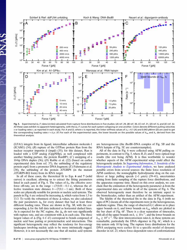
Analysis of Experimental Data. As a demonstration of the wide ap-plicability of our method, we have analyzed 10 earlier datasets frombiomolecular force ramp experiments, spanning a range of scalesfrom strand separation in DNA oligomers up to the unbinding oflarge receptor–ligand complexes. Five of these systems (Fig. 5)showed TC of the Ωrðf Þ curves, within experimental error bars,whereas the other five showed NC, and hence heterogeneity (Fig.6). Let us consider each of these two groups in more detail.

Systems Exhibiting TC. The five experimental studies exhibiting TCin Fig. 5 are as follows: (A) Schlierf and Rief (29), the unfolding ofIg-like domain 4 (ddFLN4) from Dictyostelium discoideum F-actincross-linker filamin; (B) Koch and Wang (30), the unbinding of acomplex between the restriction enzyme BsoBI and DNA; (C)Neuert et al. (31), the unbinding of the steroid digoxigenin from ananti-digoxigenin antibody; (D) Kim et al. (6), the unbinding of thevonWillebrand factor A1 domain from the glycoprotein Ib α subunit(GPIbα); and (E) Manosas et al. (32), unzipping of an RNA hairpin.In the hairpin case, the collapse of the Ωrðf Þ curves is consistent withcollapse seen in other dynamical quantities extracted from the data

at different loading rates, for example, the rupture rate kðf Þ or theeffective barrier height at a given force (32, 33). In all of the aboveexperiments, the data are originally gathered as time traces of theapplied force. The rupture or unfolding event in each trace is iden-tified as a large drop in the force when using AFM (or a large in-crease in the end-to-end distance using optical tweezers), a signatureeasily detected due to its high signal-to-noise ratio. The value of theforce immediately before the drop is then recorded. From hundredsof such traces, the experimentalists construct the distribution offorces pvðf Þ or prðf Þ at which the system unfolds/ruptures for a fixedpulling velocity v or loading rate r. In those cases (A and D) wheredata are reported in terms of v rather than r, mean values of thelinker stiffness ωs are used to get corresponding loading ratesr=ωsv (see the figure legend for values). The distribution prðf Þ isrelated to Σrðf Þ through prðf Þ=−dΣrðf Þ=df . By integrating prðf Þ, weobtain Σrðf Þ and hence Ωrðf Þ. We can also calculate the meanrupture force f ðrÞ= R∞0 df   fprðf Þ and thus the mean rupture ratekðrÞ= r=f ðrÞ. The largest value of kðrÞ among all of the r for a givenexperiment is shown in the bar chart of Fig. 5F. As mentionedabove in discussing the TC scenario, the maximum observed valueof kðrÞ provides a lower bound for both keq and ki.The local equilibration rate keq defines an intrinsic timescale

whether or not the system is heterogeneous, but the slower in-terconversion rate ki exists as a distinct timescale only whenthere is a heterogeneous ensemble of states with sufficientlylarge energy barriers between them. Observing collapse of Ωrðf Þover a range of r does not absolutely rule out heterogeneity, butit does constrain the possible values of ki. The two systems in Fig.5 with the strongest constraints on ki (the largest lower bounds)are A and C, where any ki (or keq) must be > Oð102   s−1Þ. This isnot surprising, because A is a single, compact protein domain,and C is a tight antibody complex. For these systems, wherespecificity of the interactions stabilizing the functional state is ofa prime importance, significant heterogeneity is unlikely, be-cause it would require at least two conformational states in-volving substantially different sets of interactions. For the moregeneral category of enzyme–substrate or receptor–ligand com-plexes (which encompasses systems B and D in Fig. 5 and all butone of the systems in Fig. 6), specificity may not always be themost important factor. Conformational heterogeneity amongbound complexes could play crucial biological roles, as a part ofenzymatic regulation or signaling.System D of Fig. 5 presents an intriguing case, because force

ramp experiments on the A1–GPIbα complex show evidence of twobound conformational states: a weaker bound state, from which thesystem is more likely to rupture at small forces (K 10 pN), and amore strongly bound state, predominating at larger forces (6). Theinterconversion rates between the states could not be measured, butbased on fitting the ramp data to a two-state model are estimatedto be on the order of ∼Oð1  s−1Þ. However, the four experimentalpulling velocities are so slow that the mean rupture rate at thehighest velocity (v= 40 nm/s) is only 0.16 s−1. Hence, if the twostates do exist, they get averaged out over the timescale of rupture,leading to a set of Ωrðf Þ curves that are collapsed. We can thusmake a prediction for this particular system—assuming the two-state picture is reasonable and that both states are populated in theensemble of complexes at the start of the force ramp. If the mea-surements were extended to velocities significantly above 40 nm/s,where rupture could occur on average before interconversion, theexpanded dataset should exhibit PC of the Ωrðf Þ curves. As in Fig.2D, Middle, in the heterogeneous model system, the values of kðrÞwhere PC occurs would roughly coincide with the interconversionrate ki. This would be one way of directly estimating the scale of kifrom experiment.

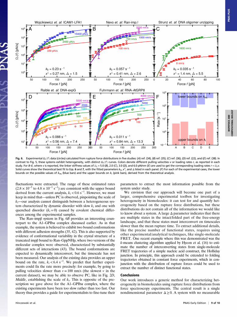
Heterogeneous Systems. In contrast to Fig. 5, the five experimentalstudies of Fig. 6 all show clear NC and thus evidence of heteroge-neity: (A) unbinding of the leukocyte function-associated antigen-1

Fig. 4. Simulation results (circles) of ΩrðfÞ for the FBL model system of Fig. 2,with no disorder (σ = 0) over a range of loading rates r extending into thenonadiabatic regime. Each color is a different value of r. The solid curves for thetwo largest r are plots of the analytical expression in Eq. 9, derived for the modelsystem in the r→∞ limit. The Inset shows themean rupture rate kðrÞ (circles) as afunction of r compared with keq (dotted line) and kcðrÞ (dashed line).

Hinczewski et al. PNAS Early Edition | 7 of 10

BIOPH

YSICSAND

COMPU

TATIONALBIOLO

GY

PNASPL

US

(LFA1) integrin from its ligand, intercellular adhesion molecule-1(ICAM1) (34); (B) rupture of the GTPase protein Ran from thenuclear receptor importin β (impβ) (35); for this dataset, Ran isloaded with a GTP analog (GppNHp), as well complexed withanother binding partner, the protein RanBP1; (C) unzipping of a10-bp DNA duplex (36); (D) Raible et al. (22) (based on earlierexperimental data from ref. 37), the unbinding of the regulatoryprotein expG from a promoter DNA fragment; (E) Fuhrmann et al.(38), the unbinding of the protein ATGRP8 (in the mutantATGRP8-RQ form) from its RNA target.In all of these cases, the theoretical fit to Eqs. 6 and 7 (solid

curves) is excellent, allowing us to extract the fitting parameterslisted in each panel of Fig. 6. The values of k0, the effective zero-force off-rate, are in the range ∼Oð0.01− 0.1  sÞ, whereas the ef-fective transition state distance b∼Oð0.1− 1  nmÞ. Both of thesescales are physically sensible for protein or nucleic acid systems. Thepanels in Fig. 6 are ordered by increasingΔ, which varies from 1.5 to13.3. To verify the robustness of these Δ values, we also calculatedthe pair parameters Δp for every dataset that had at least threedifferent loading rates. These are shown in Fig. 3B, with the cor-responding Δ for the full data indicated as horizontal dashed lines.As is expected for the NC regime, the Δp do not vary significantlywith rupture rate, and are consistent with Δ in each case. The threelargest values of Δ (Fig. 6 C–E) correspond to bonds composed ofnucleic acid base pairing or protein/nucleic acid interactions. Thissignificant heterogeneity may reflect the tendency for free-energylandscapes involving nucleic acids to be more intrinsically rugged.However, it is not necessarily the case that all nucleic acid systems

are heterogeneous (the BsoBI–DNA complex of Fig. 5B and theRNA hairpin of Fig. 5E are counterexamples).All of the data in Fig. 6 were collected using AFM pulling ex-

periments, in contrast to Fig. 5, where B,D, and E were optical-trapresults (the rest being AFM). It is thus worthwhile to wonderwhether aspects of the AFM experimental setup could affect theheterogeneity analysis. In Supporting Information, 5. Sensitivity of theHeterogeneity Analysis to Experimental Artifacts, we have analyzedpossible errors from several sources: the finite force resolution ofAFM cantilever, the nonnegligible hydrodynamic drag on the can-tilever at large pulling speeds (>1 μm/s) (39–41), uncertaintiesarising from finite sampling of the rupture force distributions, andthe apparatus response time. Based on this error analysis, we con-clude that the estimation of the heterogeneity parameterΔ from theexperimental data are reliable in all of the systems of Fig. 6. Theobserved heterogeneity must therefore be an intrinsic aspect tothe biomolecules, rather than an artifact of the AFM experiment.The fidelity of the theoretical fits to the data in Fig. 6 (with no

signs of PC) means all of the experiments were in the heterogeneous,adiabatic regime. Thus, the range of observed kðrÞ allows us to placeupper bounds on ki and lower bounds on keq, which are plotted inthe bar chart of Fig. 6F. There is a clear separation of timescales,with all of the upper bounds on ki K 10 s−1, and the lower bounds onkeq J 102 s−1. The slow interconversion rates ki in these systems areremarkable, particularly the DNA oligomer in Fig. 6C, which is atiny system only 10 bp long. The rupture force distributions for theDNA unzipping were earlier fit to a specific model of dynamicdisorder in ref. 23, where force-dependent rates of conformational

A

D E F

B C

Fig. 5. Experimental ΩrðfÞ data (circles) calculated from rupture force distributions in five studies: (A) ref. 29, (B) ref. 30, (C) ref. 31, (D) ref. 6, and (E) ref. 32.All these cases exhibit no apparent heterogeneity, with the ΩrðfÞ curves for each system collapsing on one another. Colors denote different pulling velocitiesv or loading rates r, as reported in each study. For A and D, where v is reported, the linker stiffness values of ωs = 4.1 (A) and 0.043 pN/nm (D) are used to getthe corresponding loading rates r =ωsv. (F) For each of the experimental cases, the lower bounds on the possible values of keq and ki, derived from thetheoretical analysis.

8 of 10 | www.pnas.org/cgi/doi/10.1073/pnas.1518389113 Hinczewski et al.

fluctuations were extracted. The range of these estimated rates(2.8 × 10−5 to 4.8 × 10−1 s−1) are consistent with the upper boundderived from the current analysis, ki < 0.6 s−1. However, we mustkeep in mind that—unless PC is observed, pinpointing the scale ofki—our analysis cannot distinguish between a heterogeneous sys-tem characterized by dynamic disorder with slow ki and one withquenched disorder (ki = 0) caused by covalent chemical differ-ences among the experimental samples.The Ran–impβ system in Fig. 6B provides an interesting coun-

terpart to the A1–GPIbα complex discussed earlier. As in thatexample, the system is believed to exhibit two bound conformationswith different adhesion strengths (35, 42). This is also supported byevidence of conformational variability in the crystal structure of atruncated impβ bound to Ran–GppNHp, where two versions of themolecular complex were observed, characterized by substantiallydifferent sets of interactions (43). The bound conformations areexpected to dynamically interconvert, but the timescale has notbeen measured. Our analysis of the existing data provides an upperbound on the rate, ki < 6.4 s−1. We predict that further experi-ments could fix the rate more precisely: for example, by going topulling velocities slower than v= 100 nm/s (the slowest v in thecurrent dataset), we may be able to observe PC, like in Fig. 2D,Middle, establishing the scale of ki. This is opposite of the pre-scription we gave above for the A1–GPIbα complex, where theexisting experiments have been too slow rather than too fast. Ourtheory thus provides a guide for experimentalists to fine-tune their

parameters to extract the most information possible from thesystem under study.We envision that our approach will become one part of a

larger, comprehensive experimental toolbox for investigatingheterogeneity in biomolecules: it can test for and quantify het-erogeneity based on the rupture force distributions, but thesedistributions do not contain all of the information we would liketo know about a system. A large Δ parameter indicates that thereare multiple states in the intact/folded part of the free-energylandscape, and that these states must interconvert on timescalesslower than the mean rupture time. To extract additional details,like the precise number of functional states, requires usingother experimental/analytical techniques, like single-moleculeFRET. One recent example where this was demonstrated was thek-means clustering algorithm applied by Hyeon et al. (16) to esti-mate the number of interconverting states from single-moleculeFRET trajectories of a simple nucleic acid construct, the Hollidayjunction. In principle, this approach could be extended to foldingtrajectories obtained in constant force experiments, which in con-junction with the distribution of rupture forces could be used toextract the number of distinct functional states.

ConclusionsOur work introduces a generic method for characterizing het-erogeneity in biomolecules using rupture force distributions fromforce spectroscopy experiments. The central result is a singlenondimensional parameter Δ≥ 0. A system with no measurable

A

D E F

B C

Fig. 6. ExperimentalΩrðfÞ data (circles) calculated from rupture force distributions in five studies: (A) ref. (34), (B) ref. (35), (C) ref. (36), (D) ref. (22), and (E) ref. (38). Incontrast to Fig. 5, these systems exhibit heterogeneity, with distinct ΩrðfÞ curves. Colors denote different pulling velocities v or loading rates r, as reported in eachstudy. For B–E, where v is reported, the linker stiffness values of ωs = 5.0 (B), 2.0 (C), 3.0 (D), and 6.0 pN/nm (E) are used to get the corresponding loading rates r =ωsv.Solid curves show the theoretical best fit to Eqs. 6 and 7, with the fitted parameters k0, x‡, and Δ listed in each panel. (F) For each of the experimental cases, the lowerbounds on the possible values of keq (blue bars) and the upper bounds on ki (pink bars), derived from the theoretical analysis.

Hinczewski et al. PNAS Early Edition | 9 of 10

BIOPH

YSICSAND

COMPU

TATIONALBIOLO

GY

PNASPL

US

heterogeneity on the timescale of the pulling experiment hasΔ= 0. When Δ> 0, its magnitude characterizes the degree of thedisorder. Both in the presence and absence of heterogeneity, themethod yields bounds on the local equilibration rate keq within asystem state, and (if heterogeneity is present) the rate of in-terconversion ki between states. The practical value of our ap-proach is demonstrated by analyzing ten previous experiments,allowing us to classify a broad range of biomolecular systems.The five cases where heterogeneity was observed are all the morestriking given the persistence of their conformational states, withupper bounds on ki K 10 s−1.Our theory leads to a proposal for future experimental studies:

searching for a range of pulling speeds where the data exhibits theproperty of partial collapse, allowing for a more accurate de-termination of ki. This PC scenario did not occur among thedatasets we considered, although in two cases (the protein com-plexes A1–GPIbα and Ran–impβ) we predict that extending the

range of pulling velocities would very likely result in PC. Theglobal energy landscapes of multidomain protein and nucleic acidsystems are essential guides to their biological function, but arequite difficult to map out in the laboratory. This is particularly truefor systems where the ruggedness of the landscape creates a hostof long-lived, functional states. The approach described heresuggests new ways in which single-molecule pulling experimentscan be used to obtain information about internal dynamics ofsystems with functionally heterogeneous states. Our theory shouldshed light on both the static and dynamic aspects of such landscapes,the first step toward a comprehensive structural understanding ofthese biomolecular shape-shifters.

ACKNOWLEDGMENTS. This work was initiated when M.H. and D.T. werevisiting scholars at Korea Institute for Advanced Study in 2013. We aregrateful for the support from the National Science Foundation Award CHE16-36424 (to D.T.).

1. Altschuler SJ, Wu LF (2010) Cellular heterogeneity: Do differences make a difference?Cell 141(4):559–563.

2. Lu HP, Xun L, Xie XS (1998) Single-molecule enzymatic dynamics. Science 282(5395):1877–1882.

3. van Oijen AM, et al. (2003) Single-molecule kinetics of λ exonuclease reveal basedependence and dynamic disorder. Science 301(5637):1235–1238.

4. English BP, et al. (2006) Ever-fluctuating single enzyme molecules: Michaelis-Mentenequation revisited. Nat Chem Biol 2(2):87–94.

5. Solomatin SV, Greenfeld M, Chu S, Herschlag D (2010) Multiple native states revealpersistent ruggedness of an RNA folding landscape. Nature 463(7281):681–684.

6. Kim J, Zhang CZ, Zhang X, Springer TA (2010) A mechanically stabilized receptor-ligand flex-bond important in the vasculature. Nature 466(7309):992–995.

7. Buckley CD, et al. (2014) Cell adhesion. The minimal cadherin-catenin complex bindsto actin filaments under force. Science 346(6209):1254211.

8. Austin RH, Beeson KW, Eisenstein L, Frauenfelder H, Gunsalus IC (1975) Dynamics ofligand binding to myoglobin. Biochemistry 14(24):5355–5373.

9. Frieden C (1979) Slow transitions and hysteretic behavior in enzymes. Annu RevBiochem 48:471–489.

10. Schmid FX, Blaschek H (1981) A native-like intermediate on the ribonuclease Afolding pathway. 2. Comparison of its properties to native ribonuclease A. Eur JBiochem 114(1):111–117.

11. Agmon N, Hopfield JJ (1983) Transient kinetics of chemical reactions with boundeddiffusion perpendicular to the reaction coordinate: Intramolecular processes withslow conformational changes. J Chem Phys 78(11):6947–6959.

12. Frauenfelder H, Parak F, Young RD (1988) Conformational substates in proteins. AnnuRev Biophys Biophys Chem 17(1):451–479.

13. Honeycutt JD, Thirumalai D (1990) Metastability of the folded states of globularproteins. Proc Natl Acad Sci USA 87(9):3526–3529.

14. Zwanzig R (1990) Rate processes with dynamical disorder. Acc Chem Res 23(5):148–152.

15. Zwanzig R (1992) Dynamical disorder: Passage through a fluctuating bottleneck.J Chem Phys 97(5):3587–3589.

16. Hyeon C, Lee J, Yoon J, Hohng S, Thirumalai D (2012) Hidden complexity in theisomerization dynamics of Holliday junctions. Nat Chem 4(11):907–914.

17. Kowerko D, et al. (2015) Cation-induced kinetic heterogeneity of the intron-exonrecognition in single group II introns. Proc Natl Acad Sci USA 112(11):3403–3408.

18. Liu B, Baskin RJ, Kowalczykowski SC (2013) DNA unwinding heterogeneity by RecBCDresults from static molecules able to equilibrate. Nature 500(7463):482–485.

19. Pressé S, Lee J, Dill KA (2013) Extracting conformational memory from single-mole-cule kinetic data. J Phys Chem B 117(2):495–502.

20. Raible M, Evstigneev M, Reimann P, Bartels FW, Ros R (2004) Theoretical analysis ofdynamic force spectroscopy experiments on ligand-receptor complexes. J Biotechnol112(1-2):13–23.

21. Raible M, Reimann P (2006) Single-molecule force spectroscopy: Heterogeneity ofchemical bonds. EPL 73(4):628–634.

22. Raible M, et al. (2006) Theoretical analysis of single-molecule force spectroscopy ex-periments: Heterogeneity of chemical bonds. Biophys J 90(11):3851–3864.

23. Hyeon C, Hinczewski M, Thirumalai D (2014) Evidence of disorder in biological mol-ecules from single molecule pulling experiments. Phys Rev Lett 112(13):138101.

24. Thirumalai D, Hyeon C (2005) RNA and protein folding: Common themes and varia-tions. Biochemistry 44(13):4957–4970.

25. Evans E, Ritchie K (1997) Dynamic strength of molecular adhesion bonds. Biophys J72(4):1541–1555.

26. Hu Z, Cheng L, Berne BJ (2010) First passage time distribution in stochastic processeswith moving and static absorbing boundaries with application to biological ruptureexperiments. J Chem Phys 133(3):034105.

27. Bullerjahn JT, Sturm S, Kroy K (2014) Theory of rapid force spectroscopy. Nat Commun5:4463.

28. Dudko OK, Hummer G, Szabo A (2006) Intrinsic rates and activation free energiesfrom single-molecule pulling experiments. Phys Rev Lett 96(10):108101.

29. Schlierf M, Rief M (2006) Single-molecule unfolding force distributions reveal a fun-nel-shaped energy landscape. Biophys J 90(4):L33–L35.

30. Koch SJ, Wang MD (2003) Dynamic force spectroscopy of protein-DNA interactions byunzipping DNA. Phys Rev Lett 91(2):028103.

31. Neuert G, Albrecht C, Pamir E, Gaub HE (2006) Dynamic force spectroscopy of thedigoxigenin-antibody complex. FEBS Lett 580(2):505–509.

32. Manosas M, Collin D, Ritort F (2006) Force-dependent fragility in RNA hairpins. PhysRev Lett 96(21):218301.

33. Bizarro CV, Alemany A, Ritort F (2012) Non-specific binding of Na+ and Mg2+ to RNAdetermined by force spectroscopy methods. Nucleic Acids Res 40(14):6922–6935.

34. Wojcikiewicz EP, Abdulreda MH, Zhang X, Moy VT (2006) Force spectroscopy of LFA-1and its ligands, ICAM-1 and ICAM-2. Biomacromolecules 7(11):3188–3195.

35. Nevo R, Brumfeld V, Elbaum M, Hinterdorfer P, Reich Z (2004) Direct discriminationbetween models of protein activation by single-molecule force measurements. Biophys J87(4):2630–2634.

36. Strunz T, Oroszlan K, Schäfer R, Güntherodt HJ (1999) Dynamic force spectroscopy ofsingle DNA molecules. Proc Natl Acad Sci USA 96(20):11277–11282.

37. Bartels FW, Baumgarth B, Anselmetti D, Ros R, Becker A (2003) Specific binding of theregulatory protein ExpG to promoter regions of the galactoglucan biosynthesis genecluster of Sinorhizobium meliloti—a combined molecular biology and force spec-troscopy investigation. J Struct Biol 143(2):145–152.

38. Fuhrmann A, Schoening JC, Anselmetti D, Staiger D, Ros R (2009) Quantitative analysisof single-molecule RNA-protein interaction. Biophys J 96(12):5030–5039.

39. Alcaraz J, et al. (2002) Correction of microrheological measurements of soft sampleswith atomic force microscopy for the hydrodynamic drag on the cantilever. Langmuir18(3):716–721.

40. Janovjak H, Struckmeier J, Müller DJ (2005) Hydrodynamic effects in fast AFM single-molecule force measurements. Eur Biophys J 34(1):91–96.

41. Liu R, Roman M, Yang G (2010) Correction of the viscous drag induced errors inmacromolecular manipulation experiments using atomic force microscope. Rev SciInstrum 81(6):063703.

42. Nevo R, et al. (2003) A molecular switch between alternative conformational states inthe complex of Ran and importin β1. Nat Struct Biol 10(7):553–557.

43. Vetter IR, Nowak C, Nishimoto T, Kuhlmann J, Wittinghofer A (1999) Structure of aRan-binding domain complexed with Ran bound to a GTP analogue: Implications fornuclear transport. Nature 398(6722):39–46.

44. Ermak DL, McCammon JA (1978) Brownian dynamics with hydrodynamic interactions.J Chem Phys 69(4):1352–1360.

45. Van Kampen NG (2007) Stochastic Processes in Physics and Chemistry (Elsevier, Amsterdam).46. Neuman KC, Nagy A (2008) Single-molecule force spectroscopy: Optical tweezers,

magnetic tweezers and atomic force microscopy. Nat Methods 5(6):491–505.47. Viani MB, et al. (1999) Small cantilevers for force spectroscopy of single molecules.

J Appl Phys 86(4):2258–2262.

10 of 10 | www.pnas.org/cgi/doi/10.1073/pnas.1518389113 Hinczewski et al.

Supporting InformationHinczewski et al. 10.1073/pnas.15183891131. Testing the Assumptions of the Ωr(f) Model with Respectto Possible GeneralizationsThe general form for Ωrðf Þ introduced in Eq. 6 of the main text:

Ωrðf Þ≈ rΔðf Þ log

�1+

κ1ðf ÞΔðf Þr

�, [S1]

depends on the functions Δðf Þ and κ1ðf Þ. For the analysis of theexperimental data, we chose a minimal model for these twofunctions, shown in Eq. 7:

Δðf Þ=Δ, κ1ðf Þ= k0βx‡

�eβ fx

‡

− 1�. [S2]

This assumes Δðf Þ is constant across the force range of the ex-periment, and κ1ðf Þ takes the same mathematical form as in thecase of a pure Bell model, κ1ðf Þ=

R f0 df ′kðf ′Þ, where kðf Þ= k0eβfx

‡

.The result is a three-parameter model (depending on Δ, k0, x‡)that is able to simultaneously fit Ωrðf Þ data for loading ratesacross two to three orders of magnitude for a large number ofunrelated biological systems.However, it is worthwhile to ask whether the general conclu-

sions that we draw from the experimental fitting would changesubstantially if the above assumptions were relaxed, and we usedmore complicated forms for Δðf Þ and κ1ðf Þ. Here, we will ex-amine two generalizations of the minimal model (in each addinganother fitting parameter) and verify that our characterization ofheterogeneity in the experimental systems is indeed robust.

i. Dudko–Hummer–Szabo Model for k(f ). The most widely used gen-eralization of the Bell model was introduced by Dudko, Hummer,and Szabo (DHS) (28). In this approach, the escape rate kðf Þ iscalculated from Kramers theory for particular choices of the un-derlying 1D free-energy profile, leading to the following:

kDHSðf Þ= k0

�1−

νfx‡

G‡

�1ν−1

eβG‡

�1−ð1−νfx‡=G‡Þ1=ν

�, [S3]

which introduces two extra parameters: G‡, the height of the free-energy barrier at zero force, and ν, characterizing the shape of the1D free-energy profile, in addition to x‡ (the transition state dis-tance) and k0 (the rate at zero force). The constant ν is usuallychosen to be either 2/3 or 1/2, corresponding to linear-cubic or cusp-like free-energy profiles, respectively. We use ν= 2=3 in the analysisbelow, although the results were similar for ν= 1=2. With the es-cape rate kDHSðf Þ, the generalized form for κ1ðf Þ=

R f0 df ′kDHSðf ′Þ

becomes the following:

κ1ðf Þ= k0βx‡

�eβG

‡

�1−ð1−νfx‡=G‡Þ1=ν

�− 1�. [S4]

Substituting this for κ1ðf Þ in Eq. S2, with ν fixed at 2/3, we have afour-parameter model for Ωrðf Þ, depending on Δ, k0, x‡, and G‡.In the limit of G‡ →∞, the DHS model reduces to the original

Bell form, and hence the results for Ωrðf Þ are the same as in theminimal model. For G‡ <∞, the DHS form introduces small cor-rections, shown in Fig. S1, particularly at larger forces where theincrease in Ωrðf Þ is not as rapid as in the Bell version. Note that, infitting to experimental data, the parameter G‡ cannot be madesmaller than fmaxνx‡, where fmax is the largest force value that ap-pears in the dataset. The DHS model is not mathematically defined

for G‡ below that cutoff. Fig. S2 shows three sets of experimentalresults for Ωrðf Þ from Fig. 6 of the main text, comparing the min-imal model fits (solid curves) to the best fit using the more complexDHS model (dashed curves). These three systems yieldedG‡ valuesin the range of 16–53 kBT. (The other two experimental systemsfrom Fig. 6 did not exhibit any improved fitting using the DHSmodel, because the best-fit G‡ was large enough that the resultswere numerically indistinguishable from the minimal Bell model.)The DHS fits for Ωrðf Þ in Fig. S2 are very close to the minimalmodel fits, and the extracted Δ values from the two approachesdiffer by only 5–20%, a discrepancy comparable to the uncertaintyin Δ due to finite sampling of the rupture force distribution(ii. Finite Sampling). Thus, at least for the datasets we have lookedat, the Bell approximation is justifiable and does not affect ourheterogeneity analysis in terms of Δ in a significant way.

ii. Linearly Varying Δ(f ). The second generalization of the minimalmodel that we consider is relaxing the assumption that Δðf Þ isconstant across the measured force range. At lowest order, wecan allow Δðf Þ to be a linear function of f, Δðf Þ=Δ0 + f=f0, whereΔ0 and f0 are constants. This leads to a four-parameter model forΩrðf Þ, depending on Δ0, f0, k0, and x‡. Fig. S3 shows Ωrðf Þ for allfive experimental systems from Fig. 6 of the main text and comparesthe best-fit results for the constant vs. linear Δðf Þ models. Theshapes of theΩrðf Þ curves from the two approaches are very similar.To compare the predicted heterogeneity from the two models, wecalculated the average Δ of the linear Δðf Þ best-fit function acrossthe range of experimentally measured forces in each case. Thedifference between Δ and the best-fit value for Δ in the minimalmodel was less than 20% in all of the systems. This confirms thatassuming constant Δðf Þ in the minimal model gives a reasonableestimate of the average of Δðf Þ over the experimental force range.Thus, both generalizations of the minimal model lead to

quantitatively similar results for heterogeneity in the experi-mental data. Following the Occam’s razor principle, we thus haveconfined our analysis in the main text to the three-parameter modelfor Ωrðf Þ, which has the added benefit of a simpler interpretation.However, it is conceivable that future datasets might require one orboth of these extensions for reasonable fitting, due to specific detailsof the biological system. The generality of Eq. S1 easily accom-modates these extensions and more, allowing us to incorporatecomplex parametrizations of Δðf Þ and κ1ðf Þ if necessary.2. Heterogeneous Model Simulation DetailsThe heterogeneousmodel in themain text describes diffusion along areaction coordinate x characterized by a diffusivity D and a freeenergy at zero force UðxÞ= ð1=2Þω0x2. If the system undergoespulling at a constant force ramp rate r, the potential becomes timedependent, Uðx, tÞ= ð1=2Þω0x2 − rtx. Each simulation trajectory isgenerated using Brownian dynamics (44) on this potential, withparameters r = 200–10,000 pN/s,D= 100 nm2/s, ω0 = 400 kBT= nm2,x‡0 = 0.2 nm. The simulation time step is Δt= 0.1 μs. The system isinitialized at x= 0 and x‡ = x‡0, and run until rupture occurs, x≥ x‡. Atevery time step, along with the Brownian dynamics update of x, wealso include the possibility of conformational interconversion as aPoisson process: a random number η between 0 and 1 is chosen; ifη> expð−kiΔtÞ, a new value of x‡ is drawn from the Gaussian dis-tribution Pðx‡Þ= expð−ðx‡ − x‡0Þ2=2σ2Þ=

ffiffiffiffiffiffiffiffiffiffi2πσ2

p. The ranges of dis-

tribution widths and interconversion rates are σ = 0–0.05 nm,ki = 0–104 s−1. The rupture event at the end of a trajectory occurs ata particular time t, corresponding to a force f = rt. By collectingabout 3× 104 trajectories for each value of r, we get a rupture force

Hinczewski et al. www.pnas.org/cgi/content/short/1518389113 1 of 7

distribution prðf Þ. The survival probability Σrðf Þ is the cumulativedistribution Σrðf Þ= 1−

R f0 df ′  pðf ′Þ, from which we can then cal-

culate Ωrðf Þ=−r logΣrðf Þ.3. Heterogeneity in Rupture Pathways vs. Heterogeneity inFunctional StatesThe heterogeneity discussed in themain text refers to the presence ofmultiple, distinct functional states Nα, each characterized by a cer-tain rupture rate at constant force, kðf , αÞ. However, biomoleculescan also exhibit another kind of heterogeneity, where a native basinof attraction has multiple dynamic pathways by which the systemcan unfold or rupture to reach state U. In fact, the two kinds ofheterogeneity can in principle exist in the same system. Fig. S4Adepicts a simple model that is heterogeneous in the second sense(although not the first): a single native state, N, has three rupturepathways, labeled α, β, and γ, with corresponding rate functions~kðf , αÞ, ~kðf , βÞ, and ~kðf , γÞ. At a certain force f, this is equivalent to atotal rate of transitioning from N to U given by kðf Þ= ~kðf ,αÞ+~kðf , βÞ+ ~kðf , αÞ. Assuming adiabaticity under a force ramp f ðtÞ, thesurvival probability ΣrðtÞ obeys the kinetic equation dΣrðtÞ=dt=−kðf ðtÞÞΣrðtÞ, and the same arguments apply as for the puresystem in the main text, leading to collapse of the Ωrðf Þ curves.We verify this numerically for the model system, solving theassociated master equation. We show the Ωrðf Þ results in Fig.S4A for particular choices of ~k described in the legend.It is instructive to compare this multiple-pathway, single–

native-state system to the functionally heterogeneous system shownin Fig. S4B. Here, there are three native states Nα, Nβ, and Nγ,with corresponding rupture rate functions kðf , αÞ, kðf , βÞ, andkðf , γÞ. In the limit ki � kðrÞ, where the rate of interconversionbetween the states is much faster than the rate of transitioning toU, the ensemble of native states gets averaged out, acting as effectivelya single state with net rupture rate kðf Þ= pαkðf ,αÞ+ pβkðf , βÞ+pγkðf , γÞ. Here, pα is the stationary probability of the system beingin state α. Because the interconversion rate is identical betweenall pairs of states, pα = pβ = pγ = 1=3. If we choose rate functionssuch that kðf , αÞ= 3~kðf , αÞ, and similarly for β and γ, we shouldfind that the Ωrðf Þ curves collapse to the same result as in thefirst, multiple-pathway system. This is indeed what the numericalresults in Fig. S4B show.In contrast, if ki � kðrÞ, functional heterogeneity will manifest

itself in the Ωrðf Þ curves, and we get the noncollapse of Fig. S4C.Thus, noncollapse is a signature of a particular kind of hetero-geneity: multiple native states with slow rates of interconversionbetween them (i.e., due to high barriers separating the states).Such a system will by definition have many pathways to rupture(at least one from each native state), but the existence of mul-tiple pathways is not by itself sufficient to trigger noncollapse.The argument above has interesting implications for analyzing

distributions of forces at which biomolecules fold (rather thanunfold/rupture). These correspond to transitions starting in theunfolded ensemble, which should usually behave as a single state,having sufficiently fast interconversion times due to small energybarriers between unfolded configurations. Even if there weremultiple pathways to fold to a single (or many) native states, theΩrðf Þ calculated from the survival probability Σrðf Þ of the un-folded state should exhibit collapse, assuming adiabaticity holds.However, it is conceivable that the unfolded state ensemble in

certain cases could be heterogeneous, partitioning into multiplestates that do not interconvert readily. In this scenario, therefolding force distributions when analyzed using our theorywould manifest heterogeneity. If this were the case, then ourframework offers an ideal way of investigating the nature ofunbound complexes or unfolded states of proteins and RNA.These issues await future experiments.

4. Derivation of Nonadiabatic Survival ProbabilityThe derivation of Eq. 9 in the main text, the nonadiabatic limit ofthe survival probability Σrðf Þ for the heterogeneous model, followsfrom an approach outlined by Hu et al. (26). This is closely relatedto the renewal method for calculating first-passage time distribu-tions (45). We are interested in ΣrðtÞ, the probability that the sys-tem has never reached x= x‡ > 0 at time t, given the initialcondition x= 0 at t= 0. This yields Σrðf Þ after the change of vari-ables from t to f ðtÞ= rt. In the model accounting for heterogeneitydescribed in the main text, the value of b changes randomly with aninterconversion rate ki. However, here we focus only on the casewith no disorder, where x‡ is fixed at a value of x‡0.The survival probability ΣrðtÞ can be expressed as an integral:

ΣrðtÞ=Z x‡0

−∞dx  Pðx, tÞ, [S5]

where Pðx, tÞ is the probability that the system is at x at time t,having never reached x= x‡0 at any time before t. The initial conditionis Pðx, 0Þ= δðxÞ. Because of the x= x‡0 condition, Pðx, tÞ is difficult tocalculate directly, but it is related to the simpler Green’s functionGðx, tjx′, t′Þ defined in the absence of any condition. Gðx, tjx′, t′Þ isjust the probability of the system being at x at time t, given that itwas at x′ at time t′≤ t, and assuming that diffusion is allowed in theUðx, tÞ= ð1=2Þω0x2 − rtx potential across the entire range −∞<x<∞. The Green’s function satisfies the Fokker–Planck equation:

∂G∂t

=D∂∂x

he−βUðx, tÞ ∂

∂xeβUðx, tÞG

i, [S6]

with initial condition Gðx, t′jx′, t′Þ= δðx− x′Þ. The connection be-tween P and G arises from by noting that Gðx, tj0,0Þ can bedecomposed into two parts: (i) a contribution Pðx, tÞ from thosetrajectories that never reach x‡0 at any time before t; (ii) a con-tribution from those trajectories that reach x‡0 for the first time atsome t′≤ t, and then diffuse from x‡0 to x in the time t− t′. Thedistribution of first passage times to x‡0 is just −dΣrðtÞ=dt, and theprobability of getting from x‡0 to x is Gðx, tjx‡0, t′Þ. Putting every-thing together, we have the following:

Gðx, tj0,0Þ=Pðx, tÞ−Z t

0dt′G

x, tjx‡0, t′

dΣrðt′Þdt′

. [S7]

Solving Eq. S7 for Pðx, tÞ, and then integrating x from −∞ to x‡0,gives the following integral equation for ΣrðtÞ (26):

ΣrðtÞ=Z x‡0

−∞dx  Pðx, tÞ=

Z x‡0

−∞dx Gðx, tj0,0Þ

+Z t

0dt′

dΣrðt′Þdt′

Z x‡0

−∞dx G

x, tjx‡0, t′

.

[S8]

To make further progress, we note that the solution to Eq. S6 forour choice of Uðx, tÞ is as follows:

Gðx, tjx′, t′Þ= 1ffiffiffiffiffiffiffiffiffiffiffiffiffiffiffiffiffiffiffiffiffi2πσðt− t′Þp exp

−ðx− μðx′, t− t′ÞÞ2

2σðt− t′Þ

!,

σðtÞ≡ 1− e−2βDω0t

βω0, μðx, tÞ≡ rðβDω0t− 1Þ+ e−βDω0t

r+ βDω2

0x

βDω20

,

[S9]

for t≥ t′. This describes a Gaussian function with time-dependentmean μ and variance σ. In the limit r→∞ the mean μ rapidly

Hinczewski et al. www.pnas.org/cgi/content/short/1518389113 2 of 7

increases with t, and the character of the dynamics becomesmore ballistic than diffusive. As a result the contribution ii de-scribed above, from those trajectories that diffuse backward fromx‡0 to some x≤ x‡0, becomes negligible. Thus, Gðx, tj0,0Þ≈Pðx, tÞfor r→∞, and we can approximate Eq. S8 as follows:

ΣrðtÞ≈Z x‡0

−∞dx Gðx, tj0,0Þ

=1ffiffiffiffiffiffiffiffiffiffiffiffiffi

2πσðtÞp Z x‡0

−∞dx  exp

−ðx− μð0, tÞÞ2

2σðtÞ

!

=12

1+ erf

"x‡0 − μð0, tÞffiffiffiffiffiffiffiffiffiffi

2σðtÞp#!

.

[S10]

Plugging in the values of μð0, tÞ and σðtÞ from Eq. S9, and makingthe change of variables f = rt, gives the approximate expressionfor Σrðf Þ in Eq. 9 of the main text.

5. Sensitivity of the Heterogeneity Analysis to ExperimentalArtifactsAll five sets of experimental data that exhibited heterogeneity inFig. 6 of the main text were collected using AFM pulling ex-periments. (In contrast, three of the collapsed datasets in Fig. 5were from optical tweezer studies, whereas the other two usedAFM.) Thus, it is important to check whether any aspects of theAFM experimental apparatus or procedure could influence theanalysis of heterogeneity. We will consider three separate issues:cantilever force resolution and drag, noise due to finite samplingof the rupture distributions, and apparatus response time. We willfocus on the AFM case, because this is most relevant to theexisting data, but the discussion can easily be generalized tooptical tweezers.

i. Cantilever Force Resolution and Drag. AFM cantilevers typicallyhave spring constants ωc ∼Oð10  pN=nmÞ. Thermal fluctuationsof the cantilever limit the resolution at which forces can bemeasured to δf ∼

ffiffiffiffiffiffiffiffiffiffiffiffiffiffiωckBT

p, where for example δf ∼ 6 pN when

ωc = 10 pN/nm (46). [Low-pass filtering of the data can in prin-ciple improve the force resolution (46, 47), but is not necessarilyhelpful for experiments involving steep force ramps, wheremaximum temporal resolution is necessary to pinpoint the rup-ture force.] The cantilever is also subject to viscous drag, withfriction coefficient γðhÞ that in general depends on the geometryof the cantilever and its height h from the surface. Experimentalmeasurements of this drag are often fit well by a phenomeno-logical scaled spherical model, γðhÞ= 6πηa2eff=ðh+ heffÞ, whereη= 0.89 mPa·s is the viscosity of the surrounding water at roomtemperature, and aeff and heff are parameters with dimensions oflength (39, 40). We will choose typical experimental values ofaeff = 25 μm and heff = 5 μm, and assume that the rupture mea-surements are all conducted at h � heff, so in our analysis thedrag coefficient is approximately constant, with a value γ ≈ 2 pN · s/μm(which matches the measured drag coefficient in ref. 34).An unloaded (postrupture) cantilever moving at fast pulling

speeds of v> 1 μm/s (or ramp rates r> 104 pN/s for ωc = 10 pN/nm)away from the surface will feel drag forces fdrag = γv> 2 pN. Be-cause in experiments the magnitude of the rupture force is definedas the difference in the prerupture and postrupture force levels,the drag creates a velocity-dependent artifact. The magnitude of theerror in the measured rupture force depends also on velocity ofthe cantilever tip prerupture, and hence the stiffness of the sample:the softer the sample, the smaller the velocity difference of the tipprerupture and postrupture, and the smaller the error (39, 40, 41).However, in typical biomolecule rupture experiments, the sample atthe point of rupture is maximally extended, with large stiffness, and

the tip velocity is much slower than the pulling velocity. In the limitwhere tip velocity immediately prerupture is zero, the error reachesits maximal value: the measured rupture force is approximately γvsmaller than the actual one due to the drag offset postrupture. Thisunderestimation has been observed in fast AFM pulling experi-ments on the I27 domain of titin (40, 41).To see the effects of cantilever artifacts on the heterogeneity

analysis, we compared two different numerical approaches for theFBL model: (i) the approach described in the main text and2. Heterogeneous Model Simulation Details (with results in Fig. 2of the main text). The simulations have an idealized force rampf ðtÞ= rt at fixed r with no cantilever artifacts. The rupture force ina simulation trajectory is just recorded as rtrup, where trup is thetime of rupture. (ii) An analogous approach, using the Hamil-tonian Uðx, tÞ= ð1=2Þω0x2 + ð1=2ÞωcðxcðtÞ− xÞ2. Here, xcðtÞmimicsthe experimentally controlled position of the clamped end of thecantilever, with the tip end point assumed to be at x, and hencesubject to thermal fluctuations. The cantilever stiffness is set toωc = 10 pN/nm. To achieve an average ramp rate of r, the positionxcðtÞ= vt, with the velocity chosen to be v= r=ωc. The rupture forcefor a simulation trajectory is recorded as ωcðvtrup − xrupÞ− γv, wherexrup is the value of x at rupture, and the γv offset reflects the worse-case scenario for drag-induced error.Fig. S5 shows the numerical results for Ωrðf Þ in the quenched

disorder limit (ki = 0) using the two approaches, with solid curvesrepresenting case i, and circles, case ii. Fig. S5 A–C correspond todifferent levels of disorder: σ = 0, 0.02, 0.05 nm, and in each panelthe range of ramp rates is r = 200–10,000 pN/s, comparable to therates used in the experimental observations of heterogeneity (Fig.6 of the main text). The two numerical approaches converge as fincreases but show clear discrepancies in the low force regime(K 10 pN), a consequence of the cantilever artifacts. Despitethese artifacts, the extracted heterogeneity parameters Δ from thetwo approaches are similar. In A (σ = 0 nm, no heterogeneity), weare close to total collapse even in the presence of artifacts, with aΔ value near zero. In B and C (σ = 0.02 and 0.05 nm), the Δ valuesof the second approach differ from the first one by less than 16%due to the artifacts. In all these cases, there are sufficient datapoints at larger forces (f J 10 pN) to mitigate the cantilever ef-fects, and give a robust estimation of Δ. We note that all of theexperimental datasets in Fig. 6 of the main text entirely fall in thislarger force regime, and thus should yield reliable values for Δ,even without correcting for drag artifacts. [Although in at leastone of the studies, corresponding to Fig. 6A, the researchers ex-plicitly corrected for cantilever drag in measurements at pullingspeeds of v> 1 μm/s (34).]

ii. Finite Sampling. Because Ωrðf Þ depends on the survival proba-bility distribution Σrðf Þ, the analysis of heterogeneity is sensitiveto sampling noise in this distribution. In typical experiments, thenumber of rupture events recorded at each r is ∼Oð102Þ, andthus it is useful to determine the uncertainty in the best-fit valuesof Δ due to the finite sampling of the distribution. To do this, weinvestigated every heterogeneous experimental system in Fig. 6of the main text, and carried out the following procedure: theminimal model best-fit theoretical result for Ωrðf Þ was used todetermine an analytical form for the survival probability distri-bution Σrðf Þ= expð−Ωrðf Þ=rÞ at each experimental value of r. Wethen generated 1,000 synthetic experimental datasets, drawingNev values of the rupture force f from the cumulative distribution1−Σrðf Þ at every r through inverse transform sampling. Thevalue of Nev is listed for each experimental system in Table S1and is based on the number of rupture events per pulling speedmeasured in that particular study. For each of the 1,000 syntheticdatasets, the best-fit value of Δ was extracted, and from the re-sulting distribution of Δ values, we calculated 95% confidenceintervals (also listed in Table S1). The confidence intervals all liewithin roughly 30% of the original best-fit value of Δ in each

Hinczewski et al. www.pnas.org/cgi/content/short/1518389113 3 of 7

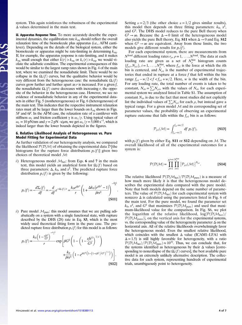
system. This again reinforces the robustness of the experimentalΔ values determined in the main text.

iii. Apparatus Response Time. To more accurately describe the exper-imental dynamics, the equilibration rate keq should reflect the overallrelaxation time of the biomolecule plus apparatus (i.e., AFM canti-lever). Depending on the details of the biological system, either thebiomolecule or apparatus might be rate-limiting in determining keq.If, for example, the apparatus response is rate-limiting, and it makeskeq small enough that either kðrÞ> keq or kcðrÞ> keq, we would vi-olate the adiabatic condition. The experimental consequences of thiswould be similar to the largest ramp rates shown in Fig. 4 of the maintext, where we examined the nonadiabatic limit. There would be nocollapse in the Ωrðf Þ curves, but the qualitative behavior would bevery different from the heterogeneous case: the nonadiabatic Ωrðf Þcurves grow further and further apart as r is increased. For a given f,the nonadiabatic Ωrðf Þ curve decreases with increasing r, the oppo-site of the behavior in the heterogeneous case. However, we see noevidence of nonadiabatic behavior in any of the experimental data-sets in either Fig. 5 (nonheterogeneous) or Fig. 6 (heterogeneous) ofthe main text. This indicates that the respective instrument relaxationrates must all be larger than the lower bounds on keq shown in Figs.5F and 6F. In the AFM case, the relaxation rate of a cantilever withstiffness ωc and friction coefficient γ is ωc=γ. Using typical values ofωc = 10 pN/nm and γ = 2 pN · s/μm, we get ωc=γ = 5,000 s−1, which isindeed larger than the lower bounds depicted in the figures.

6. Relative Likelihood Analysis of Heterogeneous vs. PureModel Fitting for Experimental DataAs further validation of our heterogeneity analysis, we comparedthe likelihood PðDjMÞ of obtaining the experimental data D [thehistograms for the rupture force distributions prðf Þ] given twochoices of theoretical model M:

i) Heterogeneous model Mhet: from Eqs. 6 and 7 in the maintext, this model yields an analytical form for Ωrðf Þ based onthree parameters: Δ, k0, and x‡. The predicted rupture forcedistribution prðf Þ is given by the following:

prðf Þ=−dΣrðf Þdf

=−ddf

e−Ωrðf Þ=r =k0eβfx

‡

r

1+

Δk0eβfx

‡ − 1

βrx‡

!−Δ+1Δ

.

[S11]

i) Pure model Mpure: this model assumes that we are pulling adi-abatically on a system with a single functional state, with rupturedescribed by the DHS (28) rate in Eq. S3, which is the mostwidely used theoretical fitting form in the pure case. The pre-dicted rupture force distribution prðf Þ for this model is as follows:

prðf Þ=k0�1− νfx‡

G‡

�−ν−1ν

rexp

"βG‡

1−�1−

νfx‡

G‡

�1=ν!

+k0βrx‡

�1− eβG

‡

1−ð1−νfx‡=G‡Þ1=ν

�#.

[S12]

Setting ν= 2=3 (the other choice ν= 1=2 gives similar results),this model then depends on three fitting parameters: k0, x‡,and G‡. The DHS model reduces to the pure Bell theory whenG‡ →∞. Because the Δ→ 0 limit of the heterogeneous modelalso yields the pure Bell theory, Eq. S11 when Δ→ 0 and Eq. S12when G‡ →∞ are equivalent. Away from those limits, the twomodels give different results for prðf Þ.For each experimental system, there are measurements from

N load different loading rates rρ, ρ= 1, . . . ,N load. The data at eachloading rate are given as a set of Nhist

ρ histogram countsffρ,i,Nρ,ig, i= 1, . . . ,Nhist

ρ , where fρ,i is the force at which the ithbin is centered, and Nρ,i is the number of experimental trajec-tories that ended in rupture at a force f that fell within the binrange fρ,i −w=2< f < fρ,i +w=2. Here, w is the width of the bin.For any loading rate, the total number of events is taken to beconstant, Nev =

PiNρ,i, with the values of Nev for each experi-

mental system we analyzed listed in Table S1. The assumption ofconstant Nev is due to the fact that most studies did not explicitlylist the individual values of

PiNρ,i for each ρ, but instead gave a

typical range. For a given model M and its corresponding set ofparameter values, the probability of observing an experimentalrupture outcome that falls within the fρ,i bin is as follows:

Pρ,iðMÞ=Z fρ,i+w=2

fρ,i−w=2df   prðf Þ, [S13]

with prðf Þ given by either Eq. S11 or S12 depending on M. Theoverall likelihood of all of the experimental outcomes for asystem is:

PðDjMÞ=YN load

ρ=1

YNhistρ

i=1

�Pρ,iðMÞ�Nρ,i . [S14]

The relative likelihood PðDjMhetÞ=PðDjMpureÞ is a measure ofhow much more likely it is that the heterogeneous model de-scribes the experimental data compared with the pure model.Note that both models depend on the same number of parame-ters. The value of PðDjMhetÞ for each experimental system withnonzero Δ is calculated using the parameters listed in Fig. 6 ofthe main text. For the pure model, we found the parameter setk0, x‡, and G‡ that maximizes PðDjMpureÞ and used that maxi-mum-likelihood value for the comparison. In Fig. S6, we plotthe logarithm of the relative likelihood, log½PðDjMhetÞ=PðDjMpureÞ�, on the vertical axis for the experimental systems,vs. the corresponding value of the heterogeneity parameterΔ on thehorizontal axis. All of the relative likelihoods overwhelmingly favorthe heterogeneous model. Even the smallest relative likelihood,which coincides with the smallest Δ value (ICAM1–LFA1 withΔ= 1.5) is still highly favorable for heterogeneity, with a ratioPðDjMhetÞ=PðDjMpureÞ≈ 1032. Thus, we can conclude that, forthe systems identified as heterogeneous by their Δ values [corre-sponding to noncollapse of theΩrðf Þ curves], the best available puremodel is an extremely unlikely alternative description. The collec-tive data for each system, representing hundreds of experimentaltrials, unambiguously point to heterogeneity.

Hinczewski et al. www.pnas.org/cgi/content/short/1518389113 4 of 7

Fig. S1. ΩrðfÞ curves of the FBL model for r =100, 1,000, and 1,000 pN/s using the DHS form for κ1ðfÞ (Eq. S4). The parameters are Δ= 5, k0 = 0.1 s−1, x‡ = 0.3 nm,and various values for G‡, ranging from ∞ (red curves, corresponding to the Bell limit) down to 15 kBT (purple curves).

Fig. S2. Experimental ΩrðfÞ data (circles) calculated from rupture force distributions in three studies: (A) ref. 34, (B) ref. 35, and (C) ref. 22. Colors denotedifferent pulling velocities v or loading rates r, as reported in each study. For B and C, where v is reported, the linker stiffness values of ωs = 5.0 (B) and 3.0 (C)are used to get the corresponding loading rates r =ωsv. Solid curves show the theoretical best fit for the minimal three-parameter model (Eqs. S1 and S2) withthe extracted value of Δ indicated in the panels. The dashed curves are the best fits from the four-parameter DHS model [κ1ðfÞ replaced by Eq. S4] with thevalues for G‡ and Δ listed at the bottom of the panels.

Hinczewski et al. www.pnas.org/cgi/content/short/1518389113 5 of 7

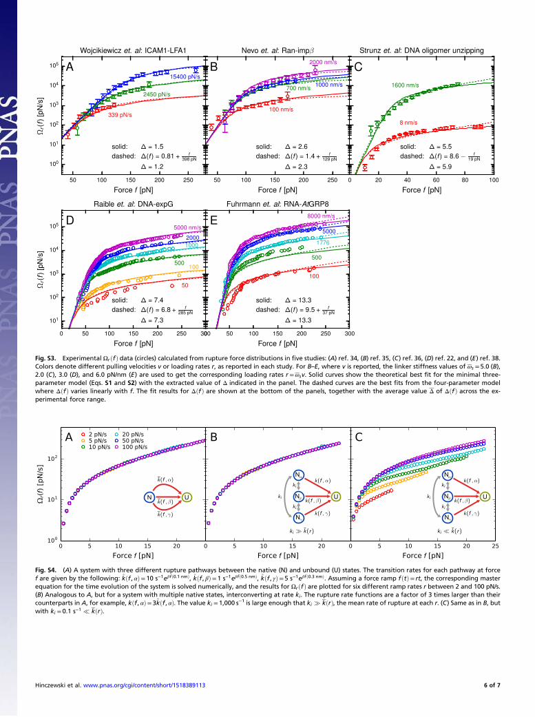
Fig. S3. Experimental ΩrðfÞ data (circles) calculated from rupture force distributions in five studies: (A) ref. 34, (B) ref. 35, (C) ref. 36, (D) ref. 22, and (E) ref. 38.Colors denote different pulling velocities v or loading rates r, as reported in each study. For B–E, where v is reported, the linker stiffness values of ωs =5.0 (B),2.0 (C), 3.0 (D), and 6.0 pN/nm (E) are used to get the corresponding loading rates r =ωsv. Solid curves show the theoretical best fit for the minimal three-parameter model (Eqs. S1 and S2) with the extracted value of Δ indicated in the panel. The dashed curves are the best fits from the four-parameter modelwhere ΔðfÞ varies linearly with f. The fit results for ΔðfÞ are shown at the bottom of the panels, together with the average value Δ of ΔðfÞ across the ex-perimental force range.

UN

N

N

f

f

f

UN

N

N

f

f

f

UN

f

f

f

~

~

~

Fig. S4. (A) A system with three different rupture pathways between the native (N) and unbound (U) states. The transition rates for each pathway at forcef are given by the following: ~kðf , αÞ= 10  s−1eβfð0.1  nmÞ, ~kðf , βÞ=1  s−1eβfð0.5  nmÞ, ~kðf , γÞ= 5  s−1eβfð0.3  nmÞ. Assuming a force ramp fðtÞ= rt, the corresponding masterequation for the time evolution of the system is solved numerically, and the results for ΩrðfÞ are plotted for six different ramp rates r between 2 and 100 pN/s.(B) Analogous to A, but for a system with multiple native states, interconverting at rate ki. The rupture rate functions are a factor of 3 times larger than theircounterparts in A, for example, kðf , αÞ= 3~kðf , αÞ. The value ki = 1,000 s−1 is large enough that ki � kðrÞ, the mean rate of rupture at each r. (C) Same as in B, butwith ki =0.1  s−1 � kðrÞ.

Hinczewski et al. www.pnas.org/cgi/content/short/1518389113 6 of 7

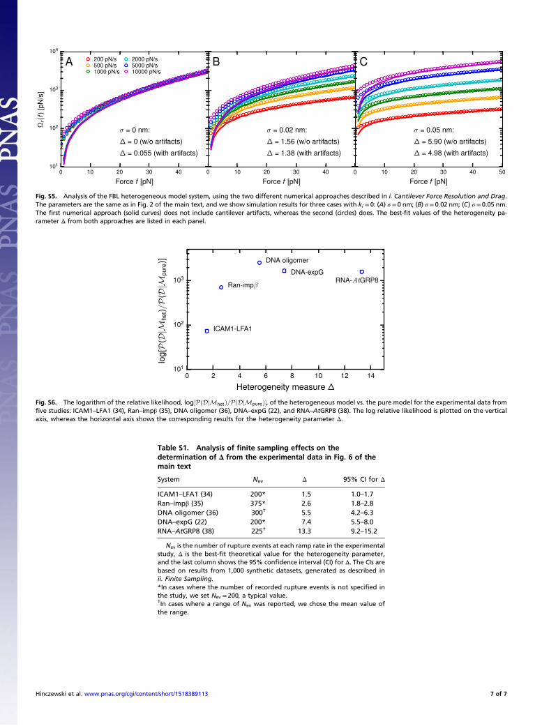
Fig. S5. Analysis of the FBL heterogeneous model system, using the two different numerical approaches described in i. Cantilever Force Resolution and Drag.The parameters are the same as in Fig. 2 of the main text, and we show simulation results for three cases with ki = 0: (A) σ = 0 nm; (B) σ = 0.02 nm; (C) σ = 0.05 nm.The first numerical approach (solid curves) does not include cantilever artifacts, whereas the second (circles) does. The best-fit values of the heterogeneity pa-rameter Δ from both approaches are listed in each panel.

Fig. S6. The logarithm of the relative likelihood, log½PðDjMhetÞ=PðDjMpureÞ�, of the heterogeneous model vs. the pure model for the experimental data fromfive studies: ICAM1–LFA1 (34), Ran–impβ (35), DNA oligomer (36), DNA–expG (22), and RNA–AtGRP8 (38). The log relative likelihood is plotted on the verticalaxis, whereas the horizontal axis shows the corresponding results for the heterogeneity parameter Δ.

Table S1. Analysis of finite sampling effects on thedetermination of Δ from the experimental data in Fig. 6 of themain text

System Nev Δ 95% CI for Δ

ICAM1–LFA1 (34) 200* 1.5 1.0–1.7Ran–impβ (35) 375* 2.6 1.8–2.8DNA oligomer (36) 300† 5.5 4.2–6.3DNA–expG (22) 200* 7.4 5.5–8.0RNA–AtGRP8 (38) 225† 13.3 9.2–15.2

Nev is the number of rupture events at each ramp rate in the experimentalstudy, Δ is the best-fit theoretical value for the heterogeneity parameter,and the last column shows the 95% confidence interval (CI) for Δ. The CIs arebased on results from 1,000 synthetic datasets, generated as described inii. Finite Sampling.*In cases where the number of recorded rupture events is not specified inthe study, we set Nev = 200, a typical value.†In cases where a range of Nev was reported, we chose the mean value ofthe range.

Hinczewski et al. www.pnas.org/cgi/content/short/1518389113 7 of 7