Disciplined Convex-Concave Programming

Xinyue Shen Steven Diamond Yuantao Gu Stephen Boyd

April 12, 2016

Abstract

In this paper we introduce disciplined convex-concave programming (DCCP), whichcombines the ideas of disciplined convex programming (DCP) with convex-concave pro-gramming (CCP). Convex-concave programming is an organized heuristic for solvingnonconvex problems that involve objective and constraint functions that are a sum ofa convex and a concave term. DCP is a structured way to define convex optimizationproblems, based on a family of basic convex and concave functions and a few rulesfor combining them. Problems expressed using DCP can be automatically convertedto standard form and solved by a generic solver; widely used implementations includeYALMIP, CVX, CVXPY, and Convex.jl. In this paper we propose a framework that com-bines the two ideas, and includes two improvements over previously published workon convex-concave programming, specifically the handling of domains of the functions,and the issue of nondifferentiability on the boundary of the domains. We describe aPython implementation called DCCP, which extends CVXPY, and give examples.

1 Disciplined convex-concave programming

1.1 Difference of convex programming

Difference of convex (DC) programming problems have the form

minimize f0(x)− g0(x)subject to fi(x)− gi(x) ≤ 0, i = 1, . . . ,m,

(1)

where x ∈ Rn is the optimization variable, and the functions fi : Rn → R and gi : Rn → Rfor i = 0, . . . ,m are convex. The DC problem (1) can also include equality constraints ofthe form pi(x) = qi(x), where pi and qi are convex; we simply express these as the pair ofinequality constraints

pi(x)− qi(x) ≤ 0, qi(x)− pi(x) ≤ 0,

which have the difference of convex form in (1). When the functions gi are all affine, theproblem (1) is a convex optimization problem, and easily solved [BV04].

1

arX

iv:1

604.

0263

9v1

[m

ath.

OC

] 1

0 A

pr 2

016

The broad class of DC functions includes all C2 functions [Har59], so the DC problem(1) is very general. A special case is Boolean linear programs, which can represent manyproblems, such as the traveling salesman problem, that are widely believed to be hard tosolve [Kar72]. DC programs arise in many applications in fields such as signal processing[LOX15], machine learning [ALNT08], computer vision [LZOX15], and statistics [THA+14].

DC problems can be solved globally by methods such as branch and bound [Agi66, LW66],which can be slow in practice. Good overviews of solving DC programs globally can be foundin [HPT95, HT99] and the references therein. A locally optimal (approximate) solution canbe found instead through the many techniques of general nonlinear optimization [NW06].

The convex-concave procedure (CCP) [YR03] is another heuristic algorithm for findinga local optimum of (1), which leverages our ability to efficiently solve convex optimizationproblems. In its basic form, it replaces concave terms with a convex upper bound, andthen solves the resulting convex problem, which is a restriction of the original DC problem.Basic CCP can thus be viewed as an instance of majorization minimization (MM) algorithms[LHY00], in which a minimization problem is approximated by an easier to solve upper boundcreated around the current point (a step called majorization) and then minimized. ManyMM extensions have been developed over the years and more can be found in [LR87, Lan04,MK07]. CCP can also be viewed as a version of DCA [TS86] which instead of explicitlystating the linearization, finds it by solving a dual problem. More information on DCA canbe found at [An15] and the references therein.

A recent overview of CCP, with some extensions, can be found in [LB15], where the issueof infeasibility is handled (heuristically) by an increasing penalty on constraint violations.The method we present in this paper is an extension of the penalty CCP method introducedin [LB15], given as algorithm 1.1 below.

Algorithm 1.1 Penalty CCP.

given an initial point x0, τ0 > 0, τmax > 0, and µ > 1.k := 0.

repeat1. Convexify. Form gi(x;xk) = gi(xk) +∇gi(xk)T (x− xk) for i = 0, . . . ,m.2. Solve. Set the value of xk+1 to a solution of

minimize f0(x)− g0(x;xk) + τk∑m

i=1 sisubject to fi(x)− gi(x;xk) ≤ si, i = 1, . . . ,m

si ≥ 0, i = 1, . . . ,m.3. Update τ . τk+1 := min(µτk, τmax).4. Update iteration. k := k + 1.

until stopping criterion is satisfied.

See [LB15] for discussion of a few variations on the penalty CCP algorithm, such as notusing slack variables for constraints that are convex, i.e., the case when gi is affine. Here itis assumed that gi are differentiable, and have full domain (i.e., Rn). The first condition is

2

not critical; we can replace ∇gi(xk) with a subgradient of gi at xk, if it is not differentiable.The linearization with a subgradient instead of the gradient is still a lower bound on gi.

In some practical applications, the second assumption, that gi have full domain, does nothold, in which case the penalty CCP algorithm can fail, by arriving at a point xk not in thedomain of gi, so the convexification step fails. This is one of the issues we will address inthis paper.

1.2 Disciplined convex programming

Disciplined convex programming (DCP) is a methodology introduced by Grant et al. [GBY06]that imposes a set of conventions that must be followed when constructing (or specifying ordefining) convex programs. Conforming problems are called disciplined convex programs.

The conventions of DCP restrict the set of functions that can appear in a problem andthe way functions can be composed. Every function in a disciplined convex program mustcome from a set of atomic functions with known curvature and graph implementation, orrepresentation as partial optimization over a cone program [GB08, NN92]. Every compositionof functions f(g1(x), . . . , gk(x)), where f : Rp → R→ R is convex and g1, . . . , gp : Rn → R,must satisfy the following composition rule, which ensures the composition is convex. Letf : Rp → R→ R ∪ ∞ be the extended-value extension of f [BV04, Chap. 3]. One of thefollowing conditions must hold for each i = 1, . . . , p:

• gi is convex and f is nondecreasing in argument i on the range of (g1(x), . . . , gp(x)).

• gi is concave and f is nonincreasing in argument i on the range of (g1(x), . . . , gp(x)).

• gi is affine.

The composition rule for concave functions is analogous. These rules allow us to certifythe curvature (i.e., convexity or concavity) of functions described as compositions using thebasic atomic functions.

A DCP problem has the specific form

minimize/maximize o(x)subject to li(x) ∼ ri(x), i = 1, . . . ,m,

(2)

where o (the objective), li (lefthand sides), and ri (righthand sides) are expressions (functionsof the variable x) with curvature known from the DCP rules, and ∼ denotes one of therelational operators =, ≤, or ≥. In DCP this problem must be convex, which imposesconditions on the curvature of the expressions, listed below.

• For a minimization problem, o must be convex; for a maximization problem, o mustbe concave.

• When the relational operator is =, li and ri must both be affine.

• When the relational operator is ≤, li must be convex, and ri must be concave.

3

• When the relational operator is ≥, li must be concave, and ri must be convex.

Functions that are affine (i.e., are both convex and concave) can match either curvaturerequirement; for example, we can minimize or maximize an affine expression.

A disciplined convex program can be transformed into an equivalent cone program byreplacing each function with its graph implementation. The convex optimization modelingsystems YALMIP [Lof04], CVX [CVX12], CVXPY [DB16], and Convex.jl [UMZ+14] use DCPto verify problem convexity and automatically convert convex programs into cone programs,which can then be solved using generic solvers.

1.3 Disciplined convex-concave programming

We refer to a problem as a disciplined convex-concave program if it has the form (2), witho, li, and ri all having known DCP-verified curvature, but the DCP curvature conditionsfor the objective and constraints need not hold. Such problems include DCP as a specialcase, but it includes many other nonconvex problems as well. In a DCCP problem we can,for example, maximize a convex function, subject to nonaffine equality constraints, andnonconvex inequality constraints between convex and concave expressions.

The general DC program (1) and the DCCP standard form (2) are equivalent. To express(1) as (2), we express it as

minimize f0(x)− tsubject to t = g0(x)

fi(x) ≤ gi(x), i = 1, . . . ,m,

where x is the original optimization variable, and t is a new optimization variable. Theobjective here is convex, we have one (nonconvex) equality constraint, and the constraintsare all nonconvex (except for some special cases when fi or gi is affine) It is straighforwardto express the DCCP problem (2) in the form (1), by identifying the functions oi, li, and rias ±fi or ±gi depending on their curvatures.

DCCP problems are an ideal standard form for DC programming because the linearizedproblem in algorithm 1.1 is a DCP program whenever the original problem is DCCP. Thelinearized problem can thus be automatically converted into a cone program and solved usinggeneric solvers.

2 Domain and subdifferentiability

In this section we delve deeper into an issue that is ‘assumed away’ in the standard treatmentsand discussions of DC programming, specifically, how to handle the case when the functionsgi do not have full domain. (The functions fi can have non-full domains, but this is handledautomatically by the conversion into a cone program.)

4

An example. Suppose the domain of gi is Di, for i = 0, . . . ,m. If Di 6= Rn, simplydefining the linearization gi(x; z) as the first order Taylor expansion of gi at the point z canlead to failure. The following simple problem gives an example:

minimize√x

subject to x ≥ −1,

where x ∈ R is the optimization variable. The objective has domain R+, and the solutionis evidently x? = 0. The linearized problem in the first iteration of CCP is

minimize x0 + 12√x0

(x− x0)

subject to x ≥ −1,

which has solution x1 = −1. The DCCP algorithm will fail in the first step of the nextiteration, since the original objective function is not defined at x1 = −1.

If we add the domain constraint directly into the linearized problem, we obtain x1 = 0,but the first step of the next iteration also fails here, in a different way. While x1 is in thedomain of the objective function, the objective is not differentiable (or superdifferentiable)at x1, so the linearization does not exist. This phenomenon of non-subdifferentiability ornon-superdifferentiability can only occur at a point on the boundary of the domain.

2.1 Linearization with domain

Suppose that the intersection of domains of all gi in problem (1) is D = ∩mi=0Di. The correctway to handle the domain is to define the linearization of gi at point z to be

gi(x; z) = gi(z) +∇gi(z)T (x− z)− Ii(x), (3)

where the indicator function is

Ii(x) =

0 x ∈ Di

∞ x /∈ Di,

so any feasible point for the linearized problem is in the domain D.Since gi is convex, Di is a convex set and Ii is a convex function. Therefore the ‘lin-

earization’ (3) is a concave function; it follows that if we replace the standard linearizationin algorithm 1.1 with the domain-restricted linearization (3), the linearized problem is stillconvex.

2.2 Domain in DCCP

Recall that we defined DCCP problems to ensure that the linearized problem in algorithm1.1 is a DCP problem. It is not obvious that if we replace the standard linearization withequation (3) the linearized problem is still a DCP problem. In this section we prove thatthe linearized DCCP problem still satisfies the rules of DCP, or equivalently that each Ii(x)has a known graph implementation or satisfies the DCP composition rule.

5

If gi is an atomic function, then we assume that

Di = ∩pi=1x | Aix+ bi ∈ Ki,

for some cone constraints K1, . . . ,Kp. The assumption is reasonable since gi itself can berepresented as partial optimization over a cone program. The graph implementation of Ii(x)is simply

minimize 0subject to Aix+ bi ∈ Ki, i = 1, . . . , p.

The other possibility is that gi is a composition of atomic functions. Since the originalproblem is DCCP, we may assume that gi(x) = f(h1(x), . . . , hp(x)) for some convex atomicfunction f : Rp → R and DCP compliant h1, . . . , hp : Rn → R such that f(h1(x), . . . , hp(x))satisfies the DCP composition rule. Then we have

Ii(x) = If (h1(x), . . . , hp(x)) +

p∑j=1

Ihj(x),

where If is the indicator function for the domain of f and Ih1 , . . . , Ihp are defined similarly.Since f is convex, If is convex. Moreover, If (h1(x), . . . , hp(x)) satisfies the DCP compo-

sition rule. To see why, observe that for i = 1, . . . , p, if hi is convex then by assumption theextended-value extension f is nondecreasing in argument i on the range of (h1(x), . . . , hp(x)).It follows that If is nondecreasing in argument i on the range of (h1(x), . . . , hp(x)). Similarly,if hi is concave then If is nonincreasing in argument i on the range of (h1(x), . . . , hp(x)).

An inductive argument shows that Ih1 , . . . , Ihp are convex and satisfy the DCP rules. Weconclude that Ii satisfies the DCP composition rule.

2.3 Sub-differentiability on boundary

When D 6= Rn, a solution to the linearized problem xk at iteration k can be on the boundaryof the closure of D. It is possible (as our simple example above shows) that the convexfunction gi is not subdifferentiable at xk, which means the linearization does not exist andthe algorithm fails. This pathology can and does occur in practical problems.

In order to handle this, at each iteration, when the subgradient ∇gi(xk) for any functiongi does not exist, we simply take a damped step,

xk = αxk + (1− α)xk−1,

where 0 < α < 1. If x0 is in the interior of the domain, then xk will be in the interior for allk ≥ 0, and ∇gi(xk) will be guaranteed to exist. The algorithm can (and does, for our simpleexample) converge to a point on the boundary of the the domain, but each iterate is in theinterior of the domain, which is enough to guarantee that the linearization exists.

6

3 Initialization

As a heuristic method, the result of algorithm 1.1 generally depends on the initialization, andthe initial values of variables should be in the interior of the domain. In many applicationsthere is a natural way to carry out this initialization; here we discuss a generic method(attempting) to do it. Note that in general the problem of finding x0 ∈ D can be very hard,so we do not expect to have a generic method that always works.

One simple and effective method is to generate random points zj for j = 1, . . . , kini, withentries drawn from from i.i.d. standard Gaussian distributions. We then project these pointsonto D, i.e., solve the problems

minimize ‖x− zj‖2

subject to x ∈ D,

for j = 1, . . . , kini, denoting the solutions as xjini. These points are on the boundary of Dwhen zj 6∈ D. We then take

x0 =1

kini

kini∑j=1

xjini.

Forming the average is a heuristic for finding x0 in the interior of D; but it is still possiblethat x0 is on the boundary, in which case it is an unacceptable starting point. As a genericpractical method, however, this approach seems to work very well.

4 Implementation

The proposed methods described above have been implemented as the Python package DCCP,which extends the package CVXPY. New methods were added to CVXPY to return the domain ofa DCP expression (as a list of constraints), and gradients (or subgradients or supergradients)were added to the atoms. The linearization, damping, and initialization are handled by thepackage DCCP. Users can form any DCCP problem of the form (2), with each expressioncomposed of functions in the CVXPY library.

When the solve(method = ’dccp’) method is called on a problem object, DCCP firstverifies that the problem satisfies the DCCP rules. The package then splits each non-affineequality constraint li = ri into li ≤ ri and li ≥ ri. The curvature of the objective andthe left and righthand sides of each constraint is checked, and if needed, linearized. Inthe linearization the function value and gradient are CVXPYparameters, which are constantswhose value can change without reconstructing the problem. For each constraint in which theleft or righthand side is linearized, a slack variable is introduced, and added to the objective.For any expression that is linearized, the domain of the original expression is added into theconstraints.

Algorithm 1.1 is next applied to the convexified problem. If a valid initial value of avariable is given by the user, it is used; otherwise the generic method described above isused. In each iteration the parameters in the linearizations (which are function and gradient

7

values) are updated based on the current value of the variables. If a gradient (or super- orsubgradient) w.r.t. any variable does not exist, damping is applied to all the variables. Theconvexified problem at each iteration is solved using CVXPY.

Some useful functions and attributes in the DCCP package are below.

• Function is_dccp(problem) returns a boolean indicating if an optimization problemis DCCP.

• Attribute expression.gradient returns a dictionary of the gradients of a DCP ex-pression w.r.t. its variables at the points specified by variable.value. (This attributeis also in the core CVXPY package.)

• Function linearize(expression) returns the linearization (3) of a DCP expression.

• Attribute expression.domain returns a list of constraints describing the domain of aDCP expression. (This attribute is also in the core CVXPY package.)

• Function convexify(constraint) returns the transformed constraint (without slackvariables) satisfying DCP of a DCCP constraint.

• Method problem.solve(method = ’dccp’) carries out the proposed penalty CCP al-gorithm, and returns the value of the transformed cost function, the value of the weightµk, and the maximum value of slack variables at each iteration k. An optional parame-ter is used to set the number of times to run CCP, using the randomized initialization.

8

10 5 0 5 10

10

5

0

5

10

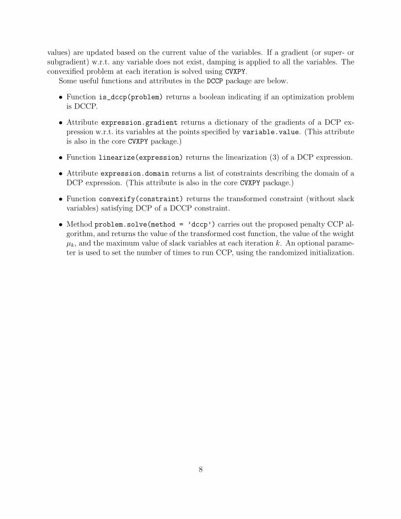
Figure 1: Circle packing.

5 Examples

In this section we describe some simple examples, show how they can be expressed usingDCCP, and give the results. In each case we run the default solve method, with no tuning oradjustment of algorithm parameters.

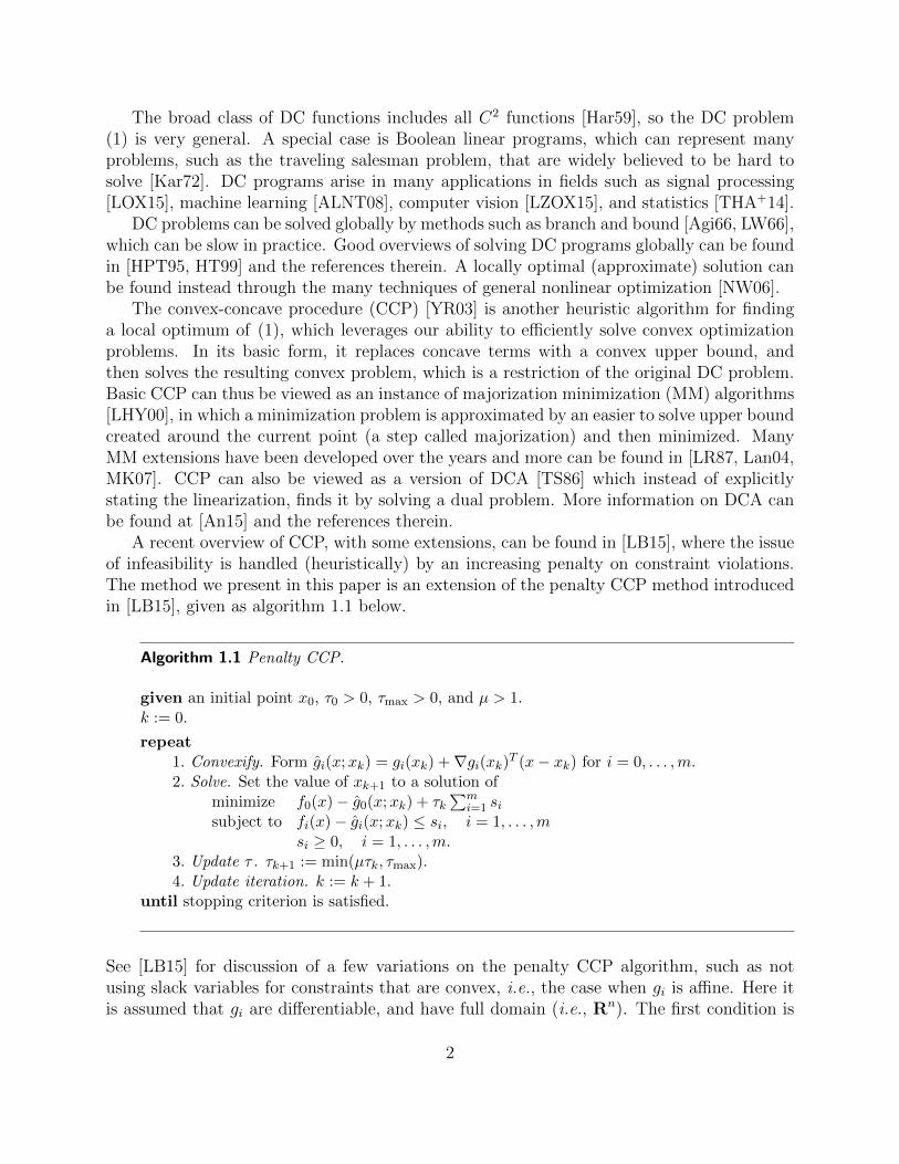
5.1 Circle packing

The aim is to arrange n circles in R2 with given radii ri for i = 1, . . . , n, so that they do notoverlap and are contained in the smallest possible square [Spe13]. The optimization problemcan be formulated as

minimize maxi=1,...,n(‖ci‖∞ + ri)subject to ‖ci − cj‖2 ≥ ri + rj, 1 ≤ i < j ≤ n,

where the variables are the centers of the circles ci ∈ R2, i = 1, . . . , n, and ri, i = 1, . . . , n,are given data. If l is the value of the objective function, the circles are contained in thesquare [−l, l]× [−l, l].

This problem can be specified in DCCP (and solved, in the last line) as follows.

c = Variable(n,2)

constr = []

for i in range(n-1):

for j in range(i+1,n):

constr += [norm(c[i,:]-c[j,:]) >= r[i]+r[j]]

prob = Problem(Minimize(max_entries(row_norm(c,’inf’)+r)), constr)

prob.solve(method = ’dccp’)

The result obtained for an instance of the problem, with n = 14 circles, is shown infigure 1. The fraction of the square covered by circles is 0.73.

9

0 2 4 6 8 10 12 14 16 18

n/σ2

0

5

10

15

20

25

bit

err

or

rate

dccpglobal optimal

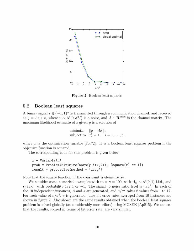
Figure 2: Boolean least squares.

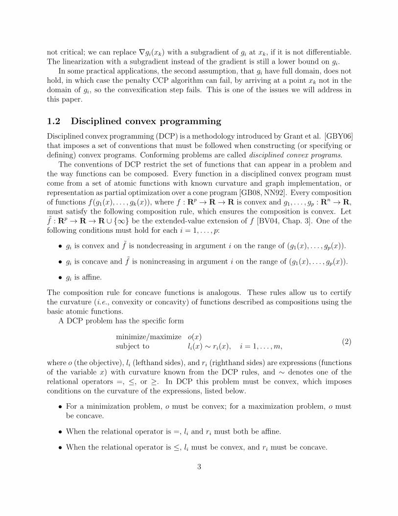
5.2 Boolean least squares

A binary signal s ∈ −1, 1n is transmitted through a communication channel, and receivedas y = As + v, where v ∼ N (0, σ2I) is a noise, and A ∈ Rm×n is the channel matrix. Themaximum likelihood estimate of s given y is a solution of

minimize ‖y − Ax‖2

subject to x2i = 1, i = 1, . . . , n,

where x is the optimization variable [For72]. It is a boolean least squares problem if theobjective function is squared.

The corresponding code for this problem is given below.

x = Variable(n)

prob = Problem(Minimize(norm(y-A*x,2)), [square(x) == 1])

result = prob.solve(method = ’dccp’)

Note that the square function in the constraint is elementwise.We consider some numerical examples with m = n = 100, with Aij ∼ N (0, 1) i.i.d., and

si i.i.d. with probability 1/2 1 or −1. The signal to noise ratio level is n/σ2. In each ofthe 10 independent instances, A and s are generated, and n/σ2 takes 8 values from 1 to 17.For each value of n/σ2, v is generated. The bit error rates averaged from 10 instances areshown in figure 2. Also shown are the same results obtained when the boolean least squaresproblem is solved globally (at considerably more effort) using MOSEK [ApS15]. We can seethat the results, judged in terms of bit error rate, are very similar.

10

0 2 4 6 8 100

2

4

6

8

10

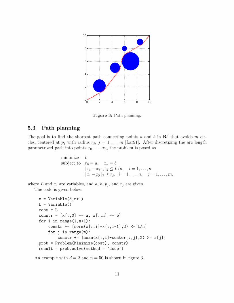
Figure 3: Path planning.

5.3 Path planning

The goal is to find the shortest path connecting points a and b in Rd that avoids m cir-cles, centered at pj with radius rj, j = 1, . . . ,m [Lat91]. After discretizing the arc lengthparametrized path into points x0, . . . , xn, the problem is posed as

minimize Lsubject to x0 = a, xn = b

‖xi − xi−1‖2 ≤ L/n, i = 1, . . . , n‖xi − pj‖2 ≥ rj, i = 1, . . . , n, j = 1, . . . ,m,

where L and xi are variables, and a, b, pj, and rj are given.The code is given below.

x = Variable(d,n+1)

L = Variable()

cost = L

constr = [x[:,0] == a, x[:,n] == b]

for i in range(1,n+1):

constr += [norm(x[:,i]-x[:,i-1],2) <= L/n]

for j in range(m):

constr += [norm(x[:,i]-center[:,j],2) >= r[j]]

prob = Problem(Minimize(cost), constr)

result = prob.solve(method = ’dccp’)

An example with d = 2 and n = 50 is shown in figure 3.

11

5.4 Control with collision avoidance

We have n linear dynamic systems, given by

xit+1 = Aixit +Biuit, yit = Cixit, i = 1, . . . , n,

where t = 0, 1, . . . denotes (discrete) time, xit are the states, and yit are the outputs. At eachtime t for t = 0, . . . , T the n outputs yit are required to keep a distance of at least dmin fromeach other [MWCD99]. The initial states xi0 and ending states xin are given by xiinit and xiend,and the inputs are limited by ‖uit‖∞ ≤ fmax. We will minimize a sum of the `1 norms of theinputs, an approximation of fuel use. (Of course we can have any convex state and inputconstraints, and any convex objective.) This gives the problem

minimize∑n

i=1

∑T−1t=0 ‖uit‖1

subject to xi0 = xiinit, xiT = xiend, i = 1, . . . , nxit+1 = Aixit +Biuit, t = 0, . . . , T − 1, i = 1, . . . , n

‖yit − yjt‖2 ≥ dmin, t = 0, . . . , T, 1 ≤ i < j ≤ n

yit = Cixit, ‖uit‖∞ ≤ fmax, t = 0, . . . , T − 1, i = 1, . . . , n,

where xit, yit, and uit are variables.

The code can be written as follows.

constr = []

cost = 0

for i in range(n):

for t in range(T):

u[i] += [Variable(d)]

constr += [norm(u[i][-1],’inf’) <= f_max]

cost += norm(u[i][-1],1)

y[i] += [Variable(d)]

x[i] += [Variable(2*d)]

constr += [y[i][-1] == C[i]*x[i][-1]]

for i in range(n):

constr += [x[i][0] == x_ini[i]]

constr += [x[i][-1] == x_end[i]]

for t in range(T-1):

constr += [x[i][t+1] == A[i]*x[i][t] + B[i]*u[i][t]]

for t in range(T):

for i in range(n-1):

for j in range(i+1,n):

constr += [norm(y[i][t] - y[j][t],2) >= d_min]

prob = Problem(Minimize(cost), constr)

prob.solve(method = ’dccp’)

12

1.0 1.5 2.0 2.5 3.0 3.5 4.02.0

2.5

3.0

3.5

4.0

4.5

5.0

5.5

6.0

1.0 1.5 2.0 2.5 3.0 3.5 4.02.0

2.5

3.0

3.5

4.0

4.5

5.0

5.5

6.0

0 20 40 60 80 100t

0.0

0.5

1.0

1.5

2.0

2.5

||y0 t−y

1 t|| 2

with avoidancewithout avoidance

Figure 4: Optimal control with collision avoidance. Left : Output trajectory with-out collision avoidance. Middle: Output trajectory with collision avoidance. Right :Distance between outputs versus time.

We consider an instance with n = 2, with outputs (positions) yit ∈ R2, dmin = 0.6,fmax = 0.5, T = 100. The linear dynamic system matrices are

Ai =

1 0 0.1 00 1 0 0.10 0 0.95 00 0 0 0.95

, Bi =

0 00 0

0.1 00 0.1

, Ci =

[1 0 0 00 1 0 0

].

The results are in figure 4, where the black arrows in the first two figures show initial andfinal states (position and velocity), and the black dashed line in the third figure shows dmin.

13

30 34 38 42 46 50cardinality

50

56

62

68

74

80

num

ber

of

measu

rem

ents

probability of recovery

0.00

0.15

0.30

0.45

0.60

0.75

0.90

30 34 38 42 46 50cardinality

50

56

62

68

74

80

num

ber

of

measu

rem

ents

probability of recovery

0.00

0.15

0.30

0.45

0.60

0.75

0.90

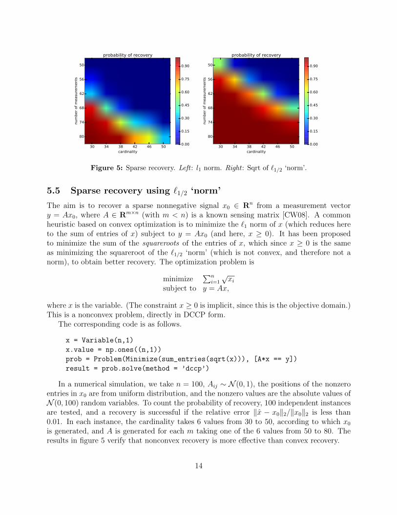
Figure 5: Sparse recovery. Left : l1 norm. Right : Sqrt of `1/2 ‘norm’.

5.5 Sparse recovery using `1/2 ‘norm’

The aim is to recover a sparse nonnegative signal x0 ∈ Rn from a measurement vectory = Ax0, where A ∈ Rm×n (with m < n) is a known sensing matrix [CW08]. A commonheuristic based on convex optimization is to minimize the `1 norm of x (which reduces hereto the sum of entries of x) subject to y = Ax0 (and here, x ≥ 0). It has been proposedto minimize the sum of the squareroots of the entries of x, which since x ≥ 0 is the sameas minimizing the squareroot of the `1/2 ‘norm’ (which is not convex, and therefore not anorm), to obtain better recovery. The optimization problem is

minimize∑n

i=1

√xi

subject to y = Ax,

where x is the variable. (The constraint x ≥ 0 is implicit, since this is the objective domain.)This is a nonconvex problem, directly in DCCP form.

The corresponding code is as follows.

x = Variable(n,1)

x.value = np.ones((n,1))

prob = Problem(Minimize(sum_entries(sqrt(x))), [A*x == y])

result = prob.solve(method = ’dccp’)

In a numerical simulation, we take n = 100, Aij ∼ N (0, 1), the positions of the nonzeroentries in x0 are from uniform distribution, and the nonzero values are the absolute values ofN (0, 100) random variables. To count the probability of recovery, 100 independent instancesare tested, and a recovery is successful if the relative error ‖x − x0‖2/‖x0‖2 is less than0.01. In each instance, the cardinality takes 6 values from 30 to 50, according to which x0

is generated, and A is generated for each m taking one of the 6 values from 50 to 80. Theresults in figure 5 verify that nonconvex recovery is more effective than convex recovery.

14

0 20 40 60 80 100 120 1401.0

0.5

0.0

0.5

1.0

1.5

2.0

phase of the original signalphase of the recovered signal

0 20 40 60 80 100 1200.0

0.2

0.4

0.6

0.8

1.0

1.2

1.4

1.6

1.8

amplitude of the original signalamplitude of the recovered signal

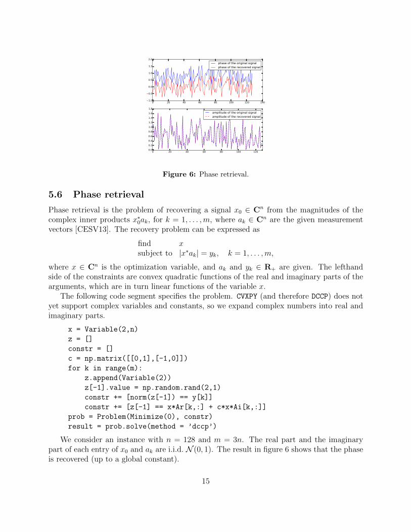
Figure 6: Phase retrieval.

5.6 Phase retrieval

Phase retrieval is the problem of recovering a signal x0 ∈ Cn from the magnitudes of thecomplex inner products x∗0ak, for k = 1, . . . ,m, where ak ∈ Cn are the given measurementvectors [CESV13]. The recovery problem can be expressed as

find xsubject to |x∗ak| = yk, k = 1, . . . ,m,

where x ∈ Cn is the optimization variable, and ak and yk ∈ R+ are given. The lefthandside of the constraints are convex quadratic functions of the real and imaginary parts of thearguments, which are in turn linear functions of the variable x.

The following code segment specifies the problem. CVXPY (and therefore DCCP) does notyet support complex variables and constants, so we expand complex numbers into real andimaginary parts.

x = Variable(2,n)

z = []

constr = []

c = np.matrix([[0,1],[-1,0]])

for k in range(m):

z.append(Variable(2))

z[-1].value = np.random.rand(2,1)

constr += [norm(z[-1]) == y[k]]

constr += [z[-1] == x*Ar[k,:] + c*x*Ai[k,:]]

prob = Problem(Minimize(0), constr)

result = prob.solve(method = ’dccp’)

We consider an instance with n = 128 and m = 3n. The real part and the imaginarypart of each entry of x0 and ak are i.i.d. N (0, 1). The result in figure 6 shows that the phaseis recovered (up to a global constant).

15

5.7 Magnitude filter design

A filter is characterized by its impulse response hknk=1. Its frequency response H : [0, π]→C is defined as

H(ω) =n∑

k=1

hke−iωk,

where i =√−1. In magnitude filter design, the goal is to find impulse response coefficients

that meet certain specifications on the magnitude of the frequency response [WBV99]. Wewill consider a typical lowpass filter design problem, which can be expressed as

minimize Ustop

subject to Lpass ≤ |H(πl/N)| ≤ Upass, l = 0, . . . , lpass − 1|H(πl/N)| ≤ Upass, l = lpass, . . . , lstop − 1|H(πl/N)| ≤ Ustop, l = lstop, . . . , N,

where h ∈ Rn and Ustop ∈ R are the optimization variables. The passband magnitude limitsLpass and Upass are given.

The code can be written as follows.

omega = np.linspace(0,np.pi,N)

h = Variable(n)

U_stop = Variable()

constr = []

for l in range(len(omega)):

if l < l_pass:

constr += [norm(expo[l]*h,2) >= L_pass]

if l < l_stop:

constr += [norm(expo[l]*h,2) <= U_pass]

else:

constr += [norm(expo[l]*h,2) <= U_stop]

prob = Problem(Minimize(U_stop), constr)

result = prob.solve(method = ’dccp’)

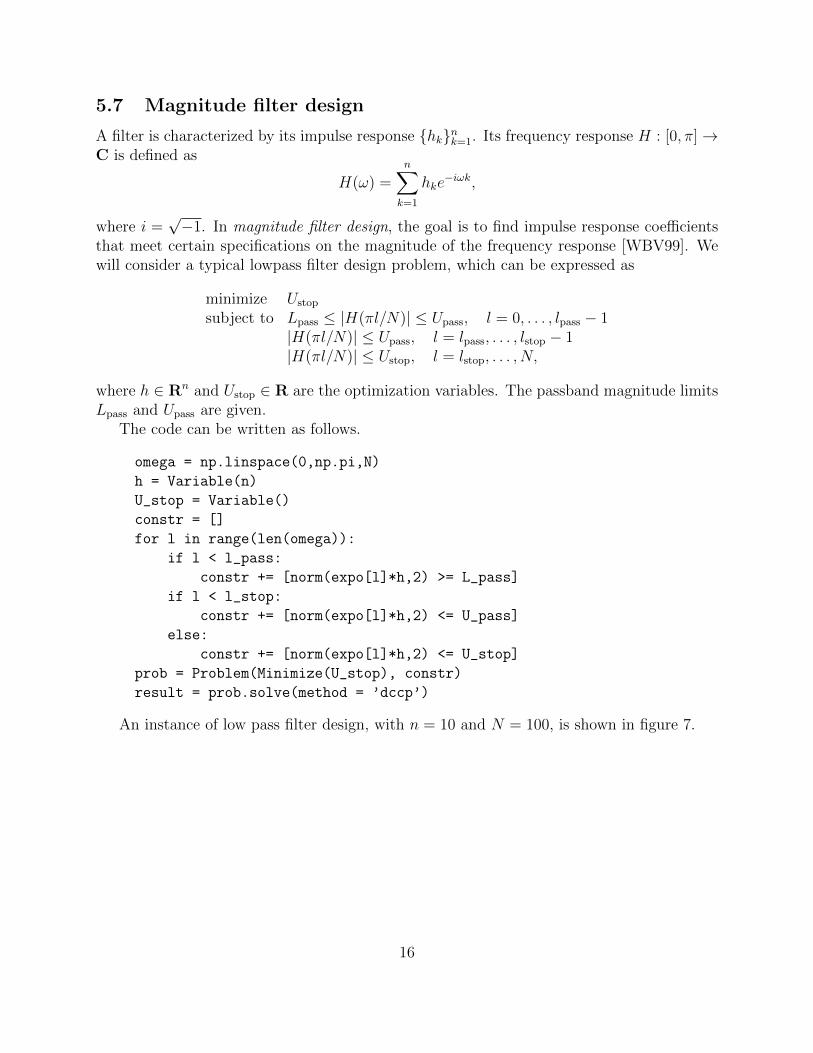
An instance of low pass filter design, with n = 10 and N = 100, is shown in figure 7.

16

0.0 0.5 1.0 1.5 2.0 2.5 3.0 3.5frequency

0.0

0.2

0.4

0.6

0.8

1.0

1.2

am

plit

ude

Figure 7: Low pass filter design. The frequency response magnitude upper andlower limits are shown.

17

0 20 40 60 80 100

card(x)

100

101

102

||Ax|| 2/σ

min

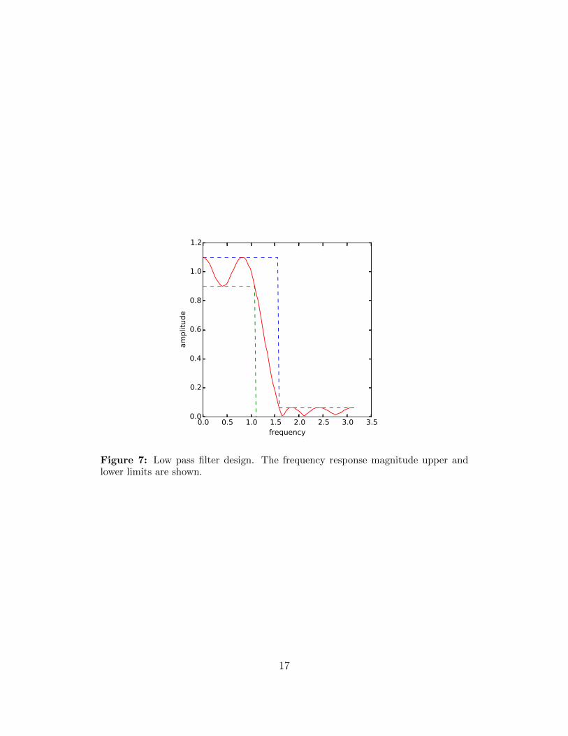
Figure 8: Sparse singular vectors.

5.8 Sparse singular vectors

The left singular vectors associated with the smallest and largest singular values of a matrixA (globally) minimize and maximize ‖Ax‖2 subject to ‖x‖2 = 1. Here we seek sparse vectors,with ‖x‖2 = 1, which make ‖Ax‖2 large or small [WTH09]. To induce sparsity in x, we limitthe `1-norm of x. (We could also limit a nonconvex sparsifier, as above in sparse recovery.)This leads to the problems

minimize/maximize ‖Ax‖2

subject to ‖x‖2 = 1, ‖x‖1 ≤ µ,

where x ∈ Rn is the variable and µ ≥ 0 controls the sparsification, to find x that is sparse,satisfies ‖x‖2 = 1, and makes ‖Ax‖2 small or large. We call such a vector, with some abuseof notation, a sparse singular vector. Since ‖x‖2 = 1, we know 1 ≤ ‖x‖1 ≤

√n, so the range

of µ can be set as [1,√n].

The code (for minimization) is the following.

x = Variable(n)

prob = Problem(Minimize(norm(A*x)), [norm(x) == 1, norm(x,1) <= mu])

prob.solve(method = ’dccp’)

We consider an instance for minimization with a random matrix A ∈ R100×100 with i.i.d.entries Aij ∼ N (0, 1), with (positive) smallest singular value σmin. The parameter µ is sweptfrom 1 to 10 with increment 0.2, and for each value of µ the result of solving the problemabove is shown as a red dot in figure 8. The most left point in the figure corresponds to‖x‖1 ≤ 1, which gives cardinality 1. (In this instance it achieves the globally optimal value,which is the smallest of the norm of the columns of A.)

18

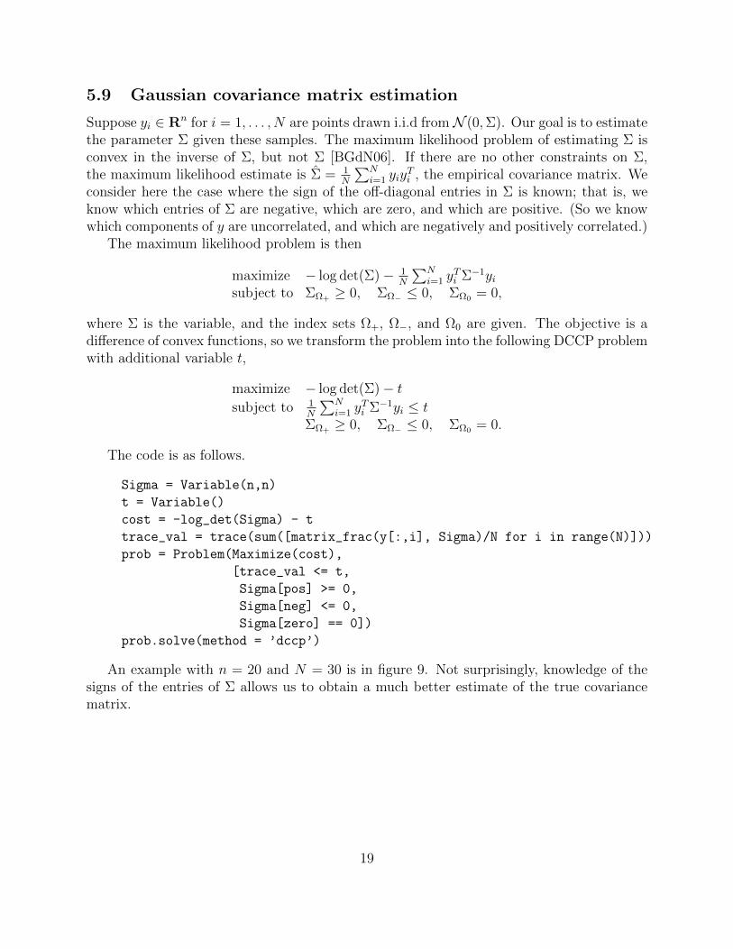
5.9 Gaussian covariance matrix estimation

Suppose yi ∈ Rn for i = 1, . . . , N are points drawn i.i.d fromN (0,Σ). Our goal is to estimatethe parameter Σ given these samples. The maximum likelihood problem of estimating Σ isconvex in the inverse of Σ, but not Σ [BGdN06]. If there are no other constraints on Σ,the maximum likelihood estimate is Σ = 1

N

∑Ni=1 yiy

Ti , the empirical covariance matrix. We

consider here the case where the sign of the off-diagonal entries in Σ is known; that is, weknow which entries of Σ are negative, which are zero, and which are positive. (So we knowwhich components of y are uncorrelated, and which are negatively and positively correlated.)

The maximum likelihood problem is then

maximize − log det(Σ)− 1N

∑Ni=1 y

Ti Σ−1yi

subject to ΣΩ+ ≥ 0, ΣΩ− ≤ 0, ΣΩ0 = 0,

where Σ is the variable, and the index sets Ω+, Ω−, and Ω0 are given. The objective is adifference of convex functions, so we transform the problem into the following DCCP problemwith additional variable t,

maximize − log det(Σ)− tsubject to 1

N

∑Ni=1 y

Ti Σ−1yi ≤ t

ΣΩ+ ≥ 0, ΣΩ− ≤ 0, ΣΩ0 = 0.

The code is as follows.

Sigma = Variable(n,n)

t = Variable()

cost = -log_det(Sigma) - t

trace_val = trace(sum([matrix_frac(y[:,i], Sigma)/N for i in range(N)]))

prob = Problem(Maximize(cost),

[trace_val <= t,

Sigma[pos] >= 0,

Sigma[neg] <= 0,

Sigma[zero] == 0])

prob.solve(method = ’dccp’)

An example with n = 20 and N = 30 is in figure 9. Not surprisingly, knowledge of thesigns of the entries of Σ allows us to obtain a much better estimate of the true covariancematrix.

19

0 5 10 15

0

5

10

15

optimize over Σ with signs

0.25

0.00

0.25

0.50

0.75

1.00

1.25

1.50

0 5 10 15

0

5

10

15

empirical covariance

0.50

0.25

0.00

0.25

0.50

0.75

1.00

1.25

1.50

0 5 10 15

0

5

10

15

true covariance

0.15

0.00

0.15

0.30

0.45

0.60

0.75

0.90

Figure 9: Gaussian covariance matrix estimation.

20

Acknowledgments

This material is based upon work supported by the National Science Foundation GraduateResearch Fellowship under Grant No. DGE-114747, by the DARPA X-DATA and SIMPLEXprograms, and by the CSC State Scholarship Fund.

References

[Agi66] N. Agin. Optimum seeking with branch and bound. Management Science,13:176–185, 1966.

[ALNT08] L. T. H. An, H. M. Le, V. V. Nguyen, and P. D. Tao. A DC programmingapproach for feature selection in support vector machines learning. Advances inData Analysis and Classification, 2(3):259–278, 2008.

[An15] L. T. H. An. DC programming and DCA: local and global approaches - theory,algorithms and applications. http://lita.sciences.univ-metz.fr/~lethi/

DCA.html, 2015.

[ApS15] MOSEK ApS. The MOSEK Python optimizer API manual. Version 7.1 (Revi-sion 49)., 2015.

[BGdN06] O. Banerjee, L. E. Ghaoui, A. d’Aspremont, and G. Natsoulis. Convex opti-mization techniques for fitting sparse gaussian graphical models. In Proceedingsof the 23rd International Conference on Machine Learning, ICML ’06, pages89–96, 2006.

[BV04] S. Boyd and L. Vandenberghe. Convex Optimization. Cambridge UniversityPress, Cambridge, 2004.

[CESV13] E. J. Candes, Y. C. Eldar, T. Strohmer, and V. Voroninski. Phase retrieval viamatrix completion. SIAM Journal on Imaging Sciences, 6(1):199–225, 2013.

[CVX12] CVX Research, Inc. CVX: Matlab software for disciplined convex programming,version 2.0. http://cvxr.com.cvx, August 2012.

[CW08] E. J. Candes and M. B. Wakin. An introduction to compressive sampling. IEEESignal Processing Magazine, 25(2):21–30, 2008.

[DB16] S. Diamond and S. Boyd. CVXPY: A Python-embedded modeling language forconvex optimization. To appear, Journal of Machine Learning Research, 2016.

[For72] G. Forney. Maximum-likelihood sequence estimation of digital sequences inthe presence of intersymbol interference. IEEE Transactions on InformationTheory, 18(3):363–378, 1972.

21

[GB08] M. Grant and S. Boyd. Graph implementation for nonsmooth convex programs.In V. Blondel, S. Boyd, and H. Kimura, editors, Recent Advances in Learningand Control, Lecture Notes in Control and Information Sciences. Springer-VerlagLimited, 2008. http://stanford.edu/~boyd/graph_dcp.html.

[GBY06] M. Grant, S. Boyd, and Y. Ye. Disciplined convex programming. In L. Libertiand N. Maculan, editors, Global Optimization: From Theory to Implementation,Nonconvex Optimization and its Applications, pages 155–210. Springer, 2006.

[Har59] P. Hartman. On functions representable as a difference of convex functions.Pacific Journal of Math, 9(3):707–713, 1959.

[HPT95] R. Horst, P. M. Pardalos, and N. V. Thoai. Introduction to Global Optimization.Kluwer Academic Publishers, Dordrecht, Netherlands, 1995.

[HT99] R. Horst and N. V. Thoai. DC programming: overview. Journal of OptimizationTheory and Applications, 103(1):1–43, 1999.

[Kar72] R. M. Karp. Reducibility among combinatorial problems. In R. E. Miller andJ. W. Thatcher, editors, Complexity of Computer Computation, pages 85–104.Plenum, 1972.

[Lan04] K. Lange. Optimization. Springer Texts in Statistics. Springer, New York, NewYork, 2004.

[Lat91] J. C. Latombe. Robot Motion Planning. Kluwer Academic Publishers, 1991.

[LB15] T. Lipp and S. Boyd. Variations and extension of the convex–concave procedure.Optimization and Engineering, pages 1–25, 2015.

[LHY00] K. Lange, D. R. Hunter, and I. Yang. Optimization transfer using surrogateobjective functions. Journal of Computational and Graphical Statistics, 9(1):1–20, 2000.

[Lof04] J. Lofberg. YALMIP: A toolbox for modeling and optimization in MATLAB. InProceedings of the IEEE International Symposium on Computed Aided ControlSystems Design, pages 294–289, September 2004.

[LOX15] Y. Lou, S. Osher, and J. Xin. Computational aspects of constrained L1-L2minimization for compressive sensing, volume 359 of Advances in IntelligentSystems and Computing, pages 169–180. 2015.

[LR87] R. J. A. Little and D. B. Rubin. Statistical Analysis with Missing Data. JohnWiley & Sons, New York, New York, 1987.

[LW66] E. L. Lawler and D. E. Wood. Branch-and-bound methods: a survey. OperationsResearch, 14:699–719, 1966.

22

[LZOX15] Y. Lou, T. Zeng, S. Osher, and J. Xin. A weighted difference of anisotropic andisotropic total variation model for image processing. SIAM Journal on ImagingSciences, 8(3):1798–1823, 2015.

[MK07] G. McLachlan and T. Krishnan. The EM algorithm and extensions. John Wiley& Sons, 2007.

[MWCD99] A. Miele, T. Wang, C. S. Chao, and J. B. Dabney. Optimal control of a shipfor collision avoidance maneuvers. Journal of Optimization Theory and Appli-cations, 103(3):495–519, 1999.

[NN92] Y. Nesterov and A. Nemirovsky. Conic formulation of a convex programmingproblem and duality. Optimization Methods and Software, 1(2):95–115, 1992.

[NW06] J. Nocedal and S. J. Wright. Numerical Optimization. Springer, 2006.

[Spe13] E. Specht. Packomania. http://www.packomania.com/, October 2013.

[THA+14] J. Thai, T. Hunter, A. K. Akametalu, C. J. Tomlin, and A. M. Bayen. Inversecovariance estimation from data with missing values using the concave-convexprocedure. In Decision and Control (CDC), 2014 IEEE 53rd Annual Conferenceon, pages 5736–5742. IEEE, 2014.

[TS86] P. D. Tao and E. B. Souad. Algorithms for solving a class of nonconvex optimiza-tion problems. Methods of subgradients. In J.-B. Hiriart-Urruty, editor, FER-MAT Days 85: Mathematics for Optimization, pages 249–271. Elsevier ScincePublishers B. V., 1986.

[UMZ+14] M. Udell, K. Mohan, D. Zeng, J. Hong, S. Diamond, and S. Boyd. Convexoptimization in Julia. In Proceedings of the Workshop for High PerformanceTechnical Computing in Dynamic Languages, pages 18–28, 2014.

[WBV99] S. P. Wu, S. Boyd, and L. Vandenberghe. Applied and Computational Control,Signals, and Circuits: Volume 1, chapter FIR Filter Design via Spectral Factor-ization and Convex Optimization, pages 215–245. Birkhauser Boston, 1999.

[WTH09] D. M. Witten, R. Tibshirani, and T. Hastie. A penalized matrix decomposi-tion, with applications to sparse principal components and canonical correlationanalysis. Biostatistics, 2009.

[YR03] A. L. Yuille and A. Rangarajan. The concave-convex procedure. Neural Com-putation, 15(4):915–936, 2003.

23