Embed Size (px)
Citation preview
Jan S HesthavenBrown [email protected]
Discontinuous Galerkin methodsLecture 3
x
y
-1 -0.5 0 0.5 1-1
-0.75
-0.5
-0.25
0
0.25
0.5
0.75
1
1.203
1.142
1.081
1.019
0.958
0.896
0.835
0.774
0.712
0.651
0.590
0.528
0.467
0.405
0.344
0.283
0.221
0.160
0.099
0.037
x
y
-1 -0.5 0 0.5 1-1
-0.75
-0.5
-0.25
0
0.25
0.5
0.75
1
-0.0028
-0.0072
-0.0117
-0.0162
-0.0207
-0.0252
-0.0297
-0.0342
-0.0387
-0.0432
-0.0477
-0.0522
-0.0567
-0.0612
-0.0657
-0.0702
-0.0747
-0.0791
-0.0836
-0.0881
x
y
-0.03 -0.02 -0.01 0 0.01 0.02 0.03
-0.03
-0.02
-0.01
0
0.01
0.02
x
y
-1 -0.5 0 0.5 1-1
-0.75
-0.5
-0.25
0
0.25
0.5
0.75
1
10
9
8
7
6
x
y
-0.03 -0.02 -0.01 0 0.01 0.02 0.03
-0.03
-0.02
-0.01
0
0.01
0.02
x
y
-1 -0.5 0 0.5 1-1
-0.75
-0.5
-0.25
0
0.25
0.5
0.75
1
1.95E-06
1.70E-06
1.45E-06
1.20E-06
9.45E-07
6.94E-07
4.43E-07
1.92E-07
-5.90E-08
-3.10E-07
-5.61E-07
-8.12E-07
-1.06E-06
-1.31E-06
-1.57E-06
Darmstadt International Workshop, October 2004 – p.79
8.4 Scattering about a vertical cylinder in a finite-width channel 147
8.4 Scattering about a vertical cylinder in a finite-width channel
Figure 8.12: Scattering of waves about acylinder in a finite-width channel.
A numerical study is carried out to bothtest the consistency of the imposed bound-ary conditions and investigate how the geo-metric representation of the the domain maya!ect the computed solution. In a numeri-cal model based on the linear Pade (2,2) ro-tational velocity version we set up a test foropen-channel flow. We seek to model the scat-tering of an incident wave field which is prop-agating toward a bottom-mounted rigid cylin-der positioned in the middle of a finite-widthchannel.
Due to the symmetry, the solution is mathe-matically equivalent to the solution of an infi-nite row of cylinders positioned perpendicularto the wave propagation direction. For example, see Linton and Evans (1993) and Linton(2005). The domain can be represented by a channel with a cylinder in the middle or alter-natively on a half-sized domain with rigid walls at the symmetry lines of the solution. Thelatter approach reduces the domain to the smallest size, which is convenient computationallyand this approach is therefore used.
To consider how the geometric representation of the domain may a!ect the resulting wavefield and the maximum wave run up at the cylinder surface boundary, we consider threedi!erent unstructured grids. The grids shown in Figures 8.13 a)-b) have comparable spatialresolution away from the cylinder surface, such that the significant di!erences between thegrid lies in the spatial resolution (measured by the size and number of elements) in the imme-diate neighborhood of the cylinder surface and the representation (or rather approximation)of the circular cylinder surface. Thus the grid in Figure 8.13 a) is defined using curvilinearelements for the accurate representation of the cylinder boundary (thus the representationwill no longer be polygonal but curved at the boundary). For the straight-sides represen-tation of the cylinder surface we use both the coarse grid in 8.13 a) and the locally refinedgrid in 8.13 b).
In each case, a combined wave generation and wave absorption zone is introduced in theregion !5.0 " x/L " !3.5 in the western end of the channel. A sponge layer is positionedat the eastern end in the region 3.0 " x/L " 5.0. The incident wave field consist ofplane waves propagating parallel to the channel walls. The wave length is set to L = 1m,the cylinder radius is a quarter of the width of the channel, a = 0.5 m, and hence thedimensionless radius is ka = !. The angular wave frequency " is determined from the linearBoussinesq dispersion relation given in Eq. (2.66). In all tests the time increment is chosen
RMMC 2008

A brief overview of what’s to come
• Lecture 1: Introduction, Motivation, History
• Lecture 2: Basic elements of DG-FEM
• Lecture 3: Linear systems and some theory
• Lecture 4: A bit more theory and discrete stability
• Lecture 5: Attention to implementations
• Lecture 6: Nonlinear problems and properties
• Lecture 7: Problems with discontinuities and shocks
• Lecture 8: Higher order/Global problems
Lecture 3
• Let’s briefly recall what we know
• Constructing fluxes for linear systems
• The local basis and Legendre polynomials
• Approximation theory on the interval
Let us recall
We already know a lot about the basic DG-FEM
• Stability is provided by carefully choosing the numerical flux.• Accuracy appear to be given by the local solution representation.• We can utilize major advances on monotone schemes to design fluxes.• The scheme generalizes with very few changes to very general problems -- multidimensional systems of conservation laws.
At least in principle -- but what can we actually prove ?
But first a bit more on fluxes
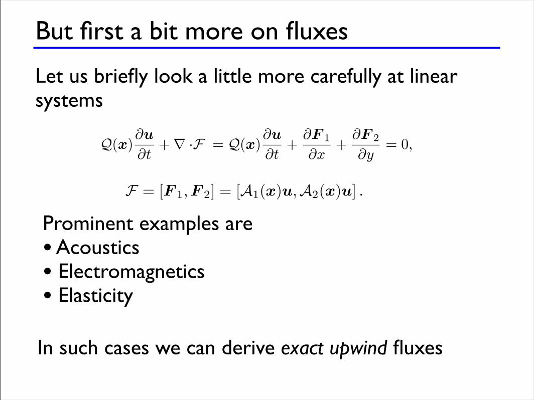
Let us briefly look a little more carefully at linearsystems
34 2 The key ideas
The final extension of the formulation to multidimensional systems is entirelystraightforward; that is, we assume that the solution, u(x, t), is approximatedby a multidimensional piecewise polynomial, uh. Proceeding as above, werecover the weak formulation
!
Dk
"!uk
h
!t"k
h ! fkh(uk
h) ·""kh
#dx = !
!
!Dkn · f!"k
h dx, (2.17)
and the strong form!
Dk
"!uk
h
!t+ " · fk
h(ukh)
#"k
h dx =!
!Dkn ·
$fk
h(ukh) ! f!
%"k
h dx. (2.18)
for all locally defined test functions, "kh # Vk
h. Naturally, ukh and the test func-
tions, "kh, are now multidimensional functions of x # Rd. The semi-discrete
formulation then follows immediately by expressing the local test functions asin Eq. (2.13).
The definition of the numerical fluxes follows the path discussed in theabove, e.g., the Lax-Friedrichs flux along the normal, n, is
f! = {{fh(uh)}} +C
2[[uh]].
Alternatives are possible, but this flux generally leads to both e!cient, ac-curate, and robust methods. The constant in the Lax-Friedrichs flux is givenas
C = maxu
&&&&#"
n · !f
!u
#&&&& ,
where #(·) indicates the eigenvalue of the matrix.
2.4 Interlude on linear hyperbolic problems
For linear systems, the construction of the upwind numerical flux is partic-ularly simple and we will discuss this in a bit more detail. Important appli-cation areas include Maxwell’s equations and the equations of acoustics andelasticity.
To illustrate the basic approach, let us consider the two-dimensionalsystem
Q(x)!u
!t+ " ·F = Q(x)
!u
!t+
!F 1
!x+
!F 2
!y= 0, (2.19)
where the flux is assumed to be given as
F = [F 1,F 2] = [A1(x)u,A2(x)u] .
Furthermore, we will make the natural assumption that Q(x) is invertible andsymmetric for all x # $. To formulate the numerical flux, we will need an
Prominent examples are• Acoustics• Electromagnetics• Elasticity
In such cases we can derive exact upwind fluxes
Linear systems and fluxes
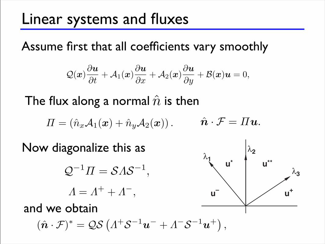
Assume first that all coefficients vary smoothly
The flux along a normal is then
2.4 Interlude on linear hyperbolic problems 35
approximation of n · F utilizing information from both sides of the interface.Exactly how this information is combined should follow the dynamics of theequations.
Let us first assume that Q(x) and Ai(x) vary smoothly throughout !. Inthis case, we can rewrite Eq. (2.19) as
Q(x)"u
"t+ A1(x)
"u
"x+ A2(x)
"u
"y+ B(x)u = 0,
where B collects all low-order terms; for example, it vanishes if Ai is constant.Since we are interested in the formulation of a flux along the normal, n, wewill consider the operator
# = (nxA1(x) + nyA2(x)) .
Note in particular thatn · F = #u.
The dynamics of the linear system can be understood by considering Q!1#.Let us assume that Q!1# can be diagonalized as
Q!1# = S$S!1,
where the diagonal matrix, $, has purely real entries; that is, Eq. (2.19) is astrongly hyperbolic system [142]. We express this as
$ = $+ + $!,
corresponding to the elements of $ that have positive and negative signs, re-spectively. Thus, the nonzero elements of $! correspond to those elementsof the characteristic vector S!1u where the direction of propagation is op-posite to the normal (i.e., they are incoming components). In contrast, thoseelements corresponding to $+ reflect components propagating along n (i.e.,they are leaving through the boundary). The basic picture is illustrated inFig. 2.3, where we, for completeness, also illustrate a %2 = 0 eigenvalue (i.e.,a nonpropagating mode).
With this basic understanding, it is clear that a numerical upwind flux canbe obtained as
(n · F)" = QS!$+S!1u! + $!S!1u+
",
by simply combining the information from the two sides of the shared edge inthe appropriate manner.
As intuitive as this approach is, it hinges on the assumption that Q!1 and# vary smoothly with x throughout !. Unfortunately, this is not the casefor many types of application (e.g., electromagnetic or acoustic problems withpiecewise smooth materials).
n
2.4 Interlude on linear hyperbolic problems 35
approximation of n · F utilizing information from both sides of the interface.Exactly how this information is combined should follow the dynamics of theequations.
Let us first assume that Q(x) and Ai(x) vary smoothly throughout !. Inthis case, we can rewrite Eq. (2.19) as
Q(x)"u
"t+ A1(x)
"u
"x+ A2(x)
"u
"y+ B(x)u = 0,
where B collects all low-order terms; for example, it vanishes if Ai is constant.Since we are interested in the formulation of a flux along the normal, n, wewill consider the operator
# = (nxA1(x) + nyA2(x)) .
Note in particular thatn · F = #u.
The dynamics of the linear system can be understood by considering Q!1#.Let us assume that Q!1# can be diagonalized as
Q!1# = S$S!1,
where the diagonal matrix, $, has purely real entries; that is, Eq. (2.19) is astrongly hyperbolic system [142]. We express this as
$ = $+ + $!,
corresponding to the elements of $ that have positive and negative signs, re-spectively. Thus, the nonzero elements of $! correspond to those elementsof the characteristic vector S!1u where the direction of propagation is op-posite to the normal (i.e., they are incoming components). In contrast, thoseelements corresponding to $+ reflect components propagating along n (i.e.,they are leaving through the boundary). The basic picture is illustrated inFig. 2.3, where we, for completeness, also illustrate a %2 = 0 eigenvalue (i.e.,a nonpropagating mode).
With this basic understanding, it is clear that a numerical upwind flux canbe obtained as
(n · F)" = QS!$+S!1u! + $!S!1u+
",
by simply combining the information from the two sides of the shared edge inthe appropriate manner.
As intuitive as this approach is, it hinges on the assumption that Q!1 and# vary smoothly with x throughout !. Unfortunately, this is not the casefor many types of application (e.g., electromagnetic or acoustic problems withpiecewise smooth materials).
Now diagonalize this as
36 2 The key ideas
u–
u* u**
u+
!1!2
!3
Fig. 2.3. Sketch of the characteristic wave speeds of a three-wave system at aboundary between two states, u! and u+. The two intermediate states, u" and u"",are used to derive the upwind flux. In this case, !1 < 0, !2 = 0, and !3 > 0.
To derive the proper numerical upwind flux for such cases, we need tobe more careful. One should keep in mind that the much simpler local Lax-Friedrichs flux also works in this case, albeit most likely leading to moredissipation than if the upwind flux is used.
For simplicity, we assume that we have only three entries in !, given as
"1 = !", "2 = 0, "3 = ",
with " > 0; that is, the wave corresponding to "1 is entering the domain, thewave corresponding to "3 is leaving, and "2 corresponds to a stationary waveas illustrated in Fig. 2.3.
Following the well-developed theory or Riemann solvers [218, 303], weknow that
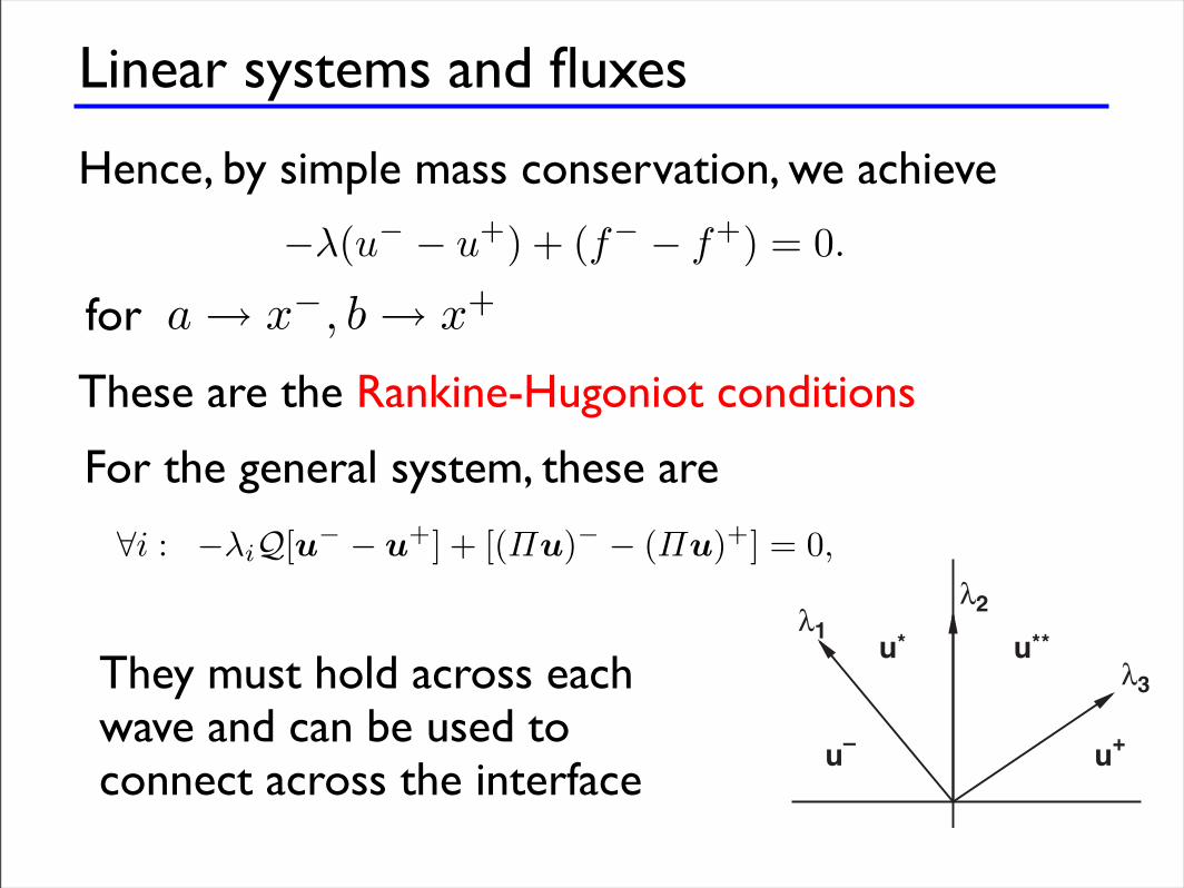
"i : !"iQ[u! ! u+] + [(#u)! ! (#u)+] = 0, (2.20)must hold across each wave. This is also known as the Rankine-Hugoniotcondition and is a simple consequence of conservation of u across the point ofdiscontinuity. To appreciate this, consider the scalar wave equation
$u
$t+ "
$u
$x= 0, x # [a, b].
Integrating over the interval, we have
d
dt
! b
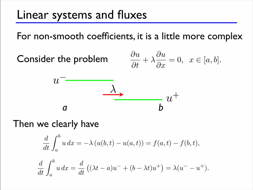
au dx = !" (u(b, t) ! u(a, t)) = f(a, t) ! f(b, t),
since f = "u. On the other hand, since the wave is propagating at a constantspeed, ", we also have
d
dt
! b
au dx =
d
dt
"("t ! a)u! + (b ! "t)u+
#= "(u! ! u+).
Taking a $ x! and b $ x+, we recover the jump conditions
!"(u! ! u+) + (f! ! f+) = 0.
The generalization to Eq. (2.20) is now straightforward.
and we obtain
Linear systems and fluxes
For non-smooth coefficients, it is a little more complex
Consider the problem
36 2 The key ideas
u–
u* u**
u+
!1!2
!3
Fig. 2.3. Sketch of the characteristic wave speeds of a three-wave system at aboundary between two states, u! and u+. The two intermediate states, u" and u"",are used to derive the upwind flux. In this case, !1 < 0, !2 = 0, and !3 > 0.
To derive the proper numerical upwind flux for such cases, we need tobe more careful. One should keep in mind that the much simpler local Lax-Friedrichs flux also works in this case, albeit most likely leading to moredissipation than if the upwind flux is used.
For simplicity, we assume that we have only three entries in !, given as
"1 = !", "2 = 0, "3 = ",
with " > 0; that is, the wave corresponding to "1 is entering the domain, thewave corresponding to "3 is leaving, and "2 corresponds to a stationary waveas illustrated in Fig. 2.3.
Following the well-developed theory or Riemann solvers [218, 303], weknow that
"i : !"iQ[u! ! u+] + [(#u)! ! (#u)+] = 0, (2.20)must hold across each wave. This is also known as the Rankine-Hugoniotcondition and is a simple consequence of conservation of u across the point ofdiscontinuity. To appreciate this, consider the scalar wave equation
$u
$t+ "
$u
$x= 0, x # [a, b].
Integrating over the interval, we have
d
dt
! b
au dx = !" (u(b, t) ! u(a, t)) = f(a, t) ! f(b, t),
since f = "u. On the other hand, since the wave is propagating at a constantspeed, ", we also have
d
dt
! b
au dx =
d
dt
"("t ! a)u! + (b ! "t)u+
#= "(u! ! u+).
Taking a $ x! and b $ x+, we recover the jump conditions
!"(u! ! u+) + (f! ! f+) = 0.
The generalization to Eq. (2.20) is now straightforward.
a b
u!
u+!
Then we clearly have
36 2 The key ideas
u–
u* u**
u+
!1!2
!3
Fig. 2.3. Sketch of the characteristic wave speeds of a three-wave system at aboundary between two states, u! and u+. The two intermediate states, u" and u"",are used to derive the upwind flux. In this case, !1 < 0, !2 = 0, and !3 > 0.
To derive the proper numerical upwind flux for such cases, we need tobe more careful. One should keep in mind that the much simpler local Lax-Friedrichs flux also works in this case, albeit most likely leading to moredissipation than if the upwind flux is used.
For simplicity, we assume that we have only three entries in !, given as
"1 = !", "2 = 0, "3 = ",
with " > 0; that is, the wave corresponding to "1 is entering the domain, thewave corresponding to "3 is leaving, and "2 corresponds to a stationary waveas illustrated in Fig. 2.3.
Following the well-developed theory or Riemann solvers [218, 303], weknow that
"i : !"iQ[u! ! u+] + [(#u)! ! (#u)+] = 0, (2.20)must hold across each wave. This is also known as the Rankine-Hugoniotcondition and is a simple consequence of conservation of u across the point ofdiscontinuity. To appreciate this, consider the scalar wave equation
$u
$t+ "
$u
$x= 0, x # [a, b].
Integrating over the interval, we have
d
dt
! b
au dx = !" (u(b, t) ! u(a, t)) = f(a, t) ! f(b, t),
since f = "u. On the other hand, since the wave is propagating at a constantspeed, ", we also have
d
dt
! b
au dx =
d
dt
"("t ! a)u! + (b ! "t)u+
#= "(u! ! u+).
Taking a $ x! and b $ x+, we recover the jump conditions
!"(u! ! u+) + (f! ! f+) = 0.
The generalization to Eq. (2.20) is now straightforward.
Linear systems and fluxes
Hence, by simple mass conservation, we achieve
36 2 The key ideas
u–
u* u**
u+
!1!2
!3
Fig. 2.3. Sketch of the characteristic wave speeds of a three-wave system at aboundary between two states, u! and u+. The two intermediate states, u" and u"",are used to derive the upwind flux. In this case, !1 < 0, !2 = 0, and !3 > 0.
To derive the proper numerical upwind flux for such cases, we need tobe more careful. One should keep in mind that the much simpler local Lax-Friedrichs flux also works in this case, albeit most likely leading to moredissipation than if the upwind flux is used.
For simplicity, we assume that we have only three entries in !, given as
"1 = !", "2 = 0, "3 = ",
with " > 0; that is, the wave corresponding to "1 is entering the domain, thewave corresponding to "3 is leaving, and "2 corresponds to a stationary waveas illustrated in Fig. 2.3.
Following the well-developed theory or Riemann solvers [218, 303], weknow that
"i : !"iQ[u! ! u+] + [(#u)! ! (#u)+] = 0, (2.20)must hold across each wave. This is also known as the Rankine-Hugoniotcondition and is a simple consequence of conservation of u across the point ofdiscontinuity. To appreciate this, consider the scalar wave equation
$u
$t+ "
$u
$x= 0, x # [a, b].
Integrating over the interval, we have
d
dt
! b
au dx = !" (u(b, t) ! u(a, t)) = f(a, t) ! f(b, t),
since f = "u. On the other hand, since the wave is propagating at a constantspeed, ", we also have
d
dt
! b
au dx =
d
dt
"("t ! a)u! + (b ! "t)u+
#= "(u! ! u+).
Taking a $ x! and b $ x+, we recover the jump conditions
!"(u! ! u+) + (f! ! f+) = 0.
The generalization to Eq. (2.20) is now straightforward.for a! x!, b! x+
These are the Rankine-Hugoniot conditions
36 2 The key ideas
u–
u* u**
u+
!1!2
!3
Fig. 2.3. Sketch of the characteristic wave speeds of a three-wave system at aboundary between two states, u! and u+. The two intermediate states, u" and u"",are used to derive the upwind flux. In this case, !1 < 0, !2 = 0, and !3 > 0.
To derive the proper numerical upwind flux for such cases, we need tobe more careful. One should keep in mind that the much simpler local Lax-Friedrichs flux also works in this case, albeit most likely leading to moredissipation than if the upwind flux is used.
For simplicity, we assume that we have only three entries in !, given as
"1 = !", "2 = 0, "3 = ",
with " > 0; that is, the wave corresponding to "1 is entering the domain, thewave corresponding to "3 is leaving, and "2 corresponds to a stationary waveas illustrated in Fig. 2.3.
Following the well-developed theory or Riemann solvers [218, 303], weknow that
"i : !"iQ[u! ! u+] + [(#u)! ! (#u)+] = 0, (2.20)must hold across each wave. This is also known as the Rankine-Hugoniotcondition and is a simple consequence of conservation of u across the point ofdiscontinuity. To appreciate this, consider the scalar wave equation
$u
$t+ "
$u
$x= 0, x # [a, b].
Integrating over the interval, we have
d
dt
! b
au dx = !" (u(b, t) ! u(a, t)) = f(a, t) ! f(b, t),
since f = "u. On the other hand, since the wave is propagating at a constantspeed, ", we also have
d
dt
! b
au dx =
d
dt
"("t ! a)u! + (b ! "t)u+
#= "(u! ! u+).
Taking a $ x! and b $ x+, we recover the jump conditions
!"(u! ! u+) + (f! ! f+) = 0.
The generalization to Eq. (2.20) is now straightforward.
For the general system, these are
36 2 The key ideas
u–
u* u**
u+
!1!2
!3
Fig. 2.3. Sketch of the characteristic wave speeds of a three-wave system at aboundary between two states, u! and u+. The two intermediate states, u" and u"",are used to derive the upwind flux. In this case, !1 < 0, !2 = 0, and !3 > 0.
To derive the proper numerical upwind flux for such cases, we need tobe more careful. One should keep in mind that the much simpler local Lax-Friedrichs flux also works in this case, albeit most likely leading to moredissipation than if the upwind flux is used.
For simplicity, we assume that we have only three entries in !, given as
"1 = !", "2 = 0, "3 = ",
with " > 0; that is, the wave corresponding to "1 is entering the domain, thewave corresponding to "3 is leaving, and "2 corresponds to a stationary waveas illustrated in Fig. 2.3.
Following the well-developed theory or Riemann solvers [218, 303], weknow that
"i : !"iQ[u! ! u+] + [(#u)! ! (#u)+] = 0, (2.20)must hold across each wave. This is also known as the Rankine-Hugoniotcondition and is a simple consequence of conservation of u across the point ofdiscontinuity. To appreciate this, consider the scalar wave equation
$u
$t+ "
$u
$x= 0, x # [a, b].
Integrating over the interval, we have
d
dt
! b
au dx = !" (u(b, t) ! u(a, t)) = f(a, t) ! f(b, t),
since f = "u. On the other hand, since the wave is propagating at a constantspeed, ", we also have
d
dt
! b
au dx =
d
dt
"("t ! a)u! + (b ! "t)u+
#= "(u! ! u+).
Taking a $ x! and b $ x+, we recover the jump conditions
!"(u! ! u+) + (f! ! f+) = 0.
The generalization to Eq. (2.20) is now straightforward.
They must hold across eachwave and can be used toconnect across the interface
Linear systems and fluxes
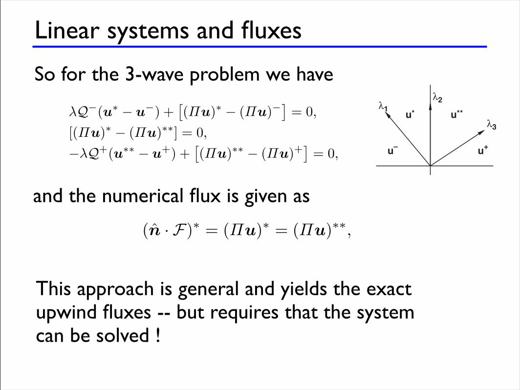
So for the 3-wave problem we have36 2 The key ideas
u–
u* u**
u+
!1!2
!3
Fig. 2.3. Sketch of the characteristic wave speeds of a three-wave system at aboundary between two states, u! and u+. The two intermediate states, u" and u"",are used to derive the upwind flux. In this case, !1 < 0, !2 = 0, and !3 > 0.
To derive the proper numerical upwind flux for such cases, we need tobe more careful. One should keep in mind that the much simpler local Lax-Friedrichs flux also works in this case, albeit most likely leading to moredissipation than if the upwind flux is used.
For simplicity, we assume that we have only three entries in !, given as
"1 = !", "2 = 0, "3 = ",
with " > 0; that is, the wave corresponding to "1 is entering the domain, thewave corresponding to "3 is leaving, and "2 corresponds to a stationary waveas illustrated in Fig. 2.3.
Following the well-developed theory or Riemann solvers [218, 303], weknow that
"i : !"iQ[u! ! u+] + [(#u)! ! (#u)+] = 0, (2.20)must hold across each wave. This is also known as the Rankine-Hugoniotcondition and is a simple consequence of conservation of u across the point ofdiscontinuity. To appreciate this, consider the scalar wave equation
$u
$t+ "
$u
$x= 0, x # [a, b].
Integrating over the interval, we have
d
dt
! b
au dx = !" (u(b, t) ! u(a, t)) = f(a, t) ! f(b, t),
since f = "u. On the other hand, since the wave is propagating at a constantspeed, ", we also have
d
dt
! b
au dx =
d
dt
"("t ! a)u! + (b ! "t)u+
#= "(u! ! u+).
Taking a $ x! and b $ x+, we recover the jump conditions
!"(u! ! u+) + (f! ! f+) = 0.
The generalization to Eq. (2.20) is now straightforward.
and the numerical flux is given as
2.4 Interlude on linear hyperbolic problems 37
Returning to the problem in Fig. 2.3, we have the system of equations
!Q!(u" ! u!) +!("u)" ! ("u)!
"= 0,
[("u)" ! ("u)""] = 0,!!Q+(u"" ! u+) +
!("u)"" ! ("u)+
"= 0,
where (u",u"") represents the intermediate states.The numerical flux can then be obtained by realizing that
(n · F)" = ("u)" = ("u)"",
which one can attempt to express using (u!,u+) through the jump conditionsabove. This leads to an upwind flux for the general discontinuous case.
To appreciate this approach, we consider a few examples.
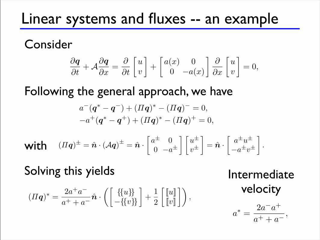
Example 2.5. Consider first the linear hyperbolic problem
#q
#t+ A#q
#x=
#
#t
#uv
$+
#a(x) 0
0 !a(x)
$#
#x
#uv
$= 0,
with a(x) being piecewise constant. For this simple equation, it is clear thatu(x, t) propagates right while v(x, t) propagates left and we could use this toform a simple upwind flux.
However, let us proceed using the Riemann jump conditions. If we intro-duce a± as the values of a(x) on two sides of the interface, we recover theconditions
a!(q" ! q!) + ("q)" ! ("q)! = 0,
!a+(q" ! q+) + ("q)" ! ("q)+ = 0,
where q" refers to the intermediate state, ("q)" is the numerical flux alongn, and
("q)± = n · (Aq)± = n ·#
a± 00 !a±
$ #u±
v±
$= n ·
#a±u±
!a±v±
$.
A bit of manipulation yields
("q)" =1
a+ + a!%a+("q)! + a!("q)+ + a+a!(q! ! q+)
&,
which simplifies as
("q)" =2a+a!
a+ + a! n ·'#
{{u}}!{{v}}
$+
12
#[[u]][[v]]
$(,
and the numerical flux (Aq)" follows directly from the definition of ("q)"We observe that if a(x) is smooth (i.e., a! = a+) then the numerical flux is
2.4 Interlude on linear hyperbolic problems 37
Returning to the problem in Fig. 2.3, we have the system of equations
!Q!(u" ! u!) +!("u)" ! ("u)!
"= 0,
[("u)" ! ("u)""] = 0,!!Q+(u"" ! u+) +
!("u)"" ! ("u)+
"= 0,
where (u",u"") represents the intermediate states.The numerical flux can then be obtained by realizing that
(n · F)" = ("u)" = ("u)"",
which one can attempt to express using (u!,u+) through the jump conditionsabove. This leads to an upwind flux for the general discontinuous case.
To appreciate this approach, we consider a few examples.
Example 2.5. Consider first the linear hyperbolic problem
#q
#t+ A#q
#x=
#
#t
#uv
$+
#a(x) 0
0 !a(x)
$#
#x
#uv
$= 0,
with a(x) being piecewise constant. For this simple equation, it is clear thatu(x, t) propagates right while v(x, t) propagates left and we could use this toform a simple upwind flux.
However, let us proceed using the Riemann jump conditions. If we intro-duce a± as the values of a(x) on two sides of the interface, we recover theconditions
a!(q" ! q!) + ("q)" ! ("q)! = 0,
!a+(q" ! q+) + ("q)" ! ("q)+ = 0,
where q" refers to the intermediate state, ("q)" is the numerical flux alongn, and
("q)± = n · (Aq)± = n ·#
a± 00 !a±
$ #u±
v±
$= n ·
#a±u±
!a±v±
$.
A bit of manipulation yields
("q)" =1
a+ + a!%a+("q)! + a!("q)+ + a+a!(q! ! q+)
&,
which simplifies as
("q)" =2a+a!
a+ + a! n ·'#
{{u}}!{{v}}
$+
12
#[[u]][[v]]
$(,
and the numerical flux (Aq)" follows directly from the definition of ("q)"We observe that if a(x) is smooth (i.e., a! = a+) then the numerical flux is
This approach is general and yields the exactupwind fluxes -- but requires that the system can be solved !
Linear systems and fluxes -- an example
Consider
2.4 Interlude on linear hyperbolic problems 37
Returning to the problem in Fig. 2.3, we have the system of equations
!Q!(u" ! u!) +!("u)" ! ("u)!
"= 0,
[("u)" ! ("u)""] = 0,!!Q+(u"" ! u+) +
!("u)"" ! ("u)+
"= 0,
where (u",u"") represents the intermediate states.The numerical flux can then be obtained by realizing that
(n · F)" = ("u)" = ("u)"",
which one can attempt to express using (u!,u+) through the jump conditionsabove. This leads to an upwind flux for the general discontinuous case.
To appreciate this approach, we consider a few examples.
Example 2.5. Consider first the linear hyperbolic problem
#q
#t+ A#q
#x=
#
#t
#uv
$+
#a(x) 0
0 !a(x)
$#
#x
#uv
$= 0,
with a(x) being piecewise constant. For this simple equation, it is clear thatu(x, t) propagates right while v(x, t) propagates left and we could use this toform a simple upwind flux.
However, let us proceed using the Riemann jump conditions. If we intro-duce a± as the values of a(x) on two sides of the interface, we recover theconditions
a!(q" ! q!) + ("q)" ! ("q)! = 0,
!a+(q" ! q+) + ("q)" ! ("q)+ = 0,
where q" refers to the intermediate state, ("q)" is the numerical flux alongn, and
("q)± = n · (Aq)± = n ·#
a± 00 !a±
$ #u±
v±
$= n ·
#a±u±
!a±v±
$.
A bit of manipulation yields
("q)" =1
a+ + a!%a+("q)! + a!("q)+ + a+a!(q! ! q+)
&,
which simplifies as
("q)" =2a+a!
a+ + a! n ·'#
{{u}}!{{v}}
$+
12
#[[u]][[v]]
$(,
and the numerical flux (Aq)" follows directly from the definition of ("q)"We observe that if a(x) is smooth (i.e., a! = a+) then the numerical flux is
38 2 The key ideas
simply upwinding. Furthermore, for the general case, the above is equivalentto defining an intermediate wave speed, a!, as
a! =2a"a+
a+ + a" ,
which is the harmonic average.
Let us also consider a slightly more complicated problem, originating inelectromagnetics.
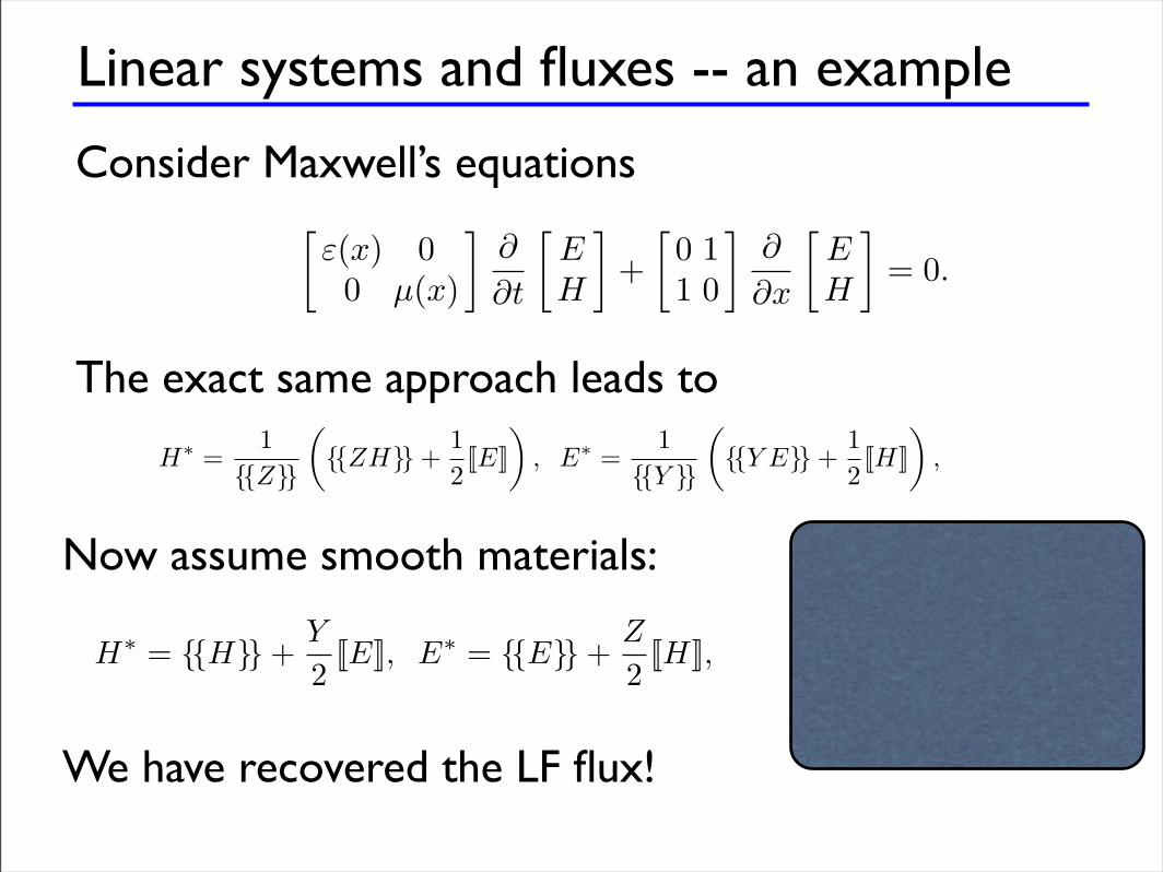
Example 2.6. Consider the one-dimensional Maxwell’s equations!
!(x) 00 µ(x)
""
"t
!EH
"+
!0 11 0
""
"x
!EH
"= 0. (2.21)
Here (E,H) = (E(x, t),H(x, t)) represent the electric and magnetic field,respectively, while ! and µ are the electric and magnetic material properties,known as permittivity and permeability, respectively.
To simplify the notation, let us write this as
Q"q
"t+ A"q
"x= 0,
whereQ =
!!(x) 00 µ(x)
", A =
!0 11 0
", q =
!EH
",
reflect the spatially varying material coe!cients, the one-dimensional rotationoperator, and the vector of state variables, respectively.
The flux is given as Aq and the eigenvalues of Q"1A are ±(!µ)"1/2, reflect-ing the two counter-propagating light waves propagating at the local speed oflight, c = (!µ)"1/2.
Proceeding by using the Riemann conditions, we obtain
c"Q"(q! ! q") + (#q)! ! (#q)" = 0,
!c+Q+(q! ! q+) + (#q)! ! (#q)+ = 0,
where q! refers to the intermediate state, (Aq)! is the numerical flux, and
(#q)± = n · (Aq)± = n ·!
H±
E±
".
Simple manipulations yield
(c+Q++c"Q")(#q)! = c+Q+(#q)"+c"Q"(#q)++c"c+Q"Q+#q" ! q+
$,
Following the general approach, we have
with
Solving this yields Intermediate velocity
Linear systems and fluxes -- an example
Consider Maxwell’s equations
38 2 The key ideas
simply upwinding. Furthermore, for the general case, the above is equivalentto defining an intermediate wave speed, a!, as
a! =2a"a+
a+ + a" ,
which is the harmonic average.
Let us also consider a slightly more complicated problem, originating inelectromagnetics.
Example 2.6. Consider the one-dimensional Maxwell’s equations!
!(x) 00 µ(x)
""
"t
!EH
"+
!0 11 0
""
"x
!EH
"= 0. (2.21)
Here (E,H) = (E(x, t),H(x, t)) represent the electric and magnetic field,respectively, while ! and µ are the electric and magnetic material properties,known as permittivity and permeability, respectively.
To simplify the notation, let us write this as
Q"q
"t+ A"q
"x= 0,
whereQ =
!!(x) 00 µ(x)
", A =
!0 11 0
", q =
!EH
",
reflect the spatially varying material coe!cients, the one-dimensional rotationoperator, and the vector of state variables, respectively.
The flux is given as Aq and the eigenvalues of Q"1A are ±(!µ)"1/2, reflect-ing the two counter-propagating light waves propagating at the local speed oflight, c = (!µ)"1/2.
Proceeding by using the Riemann conditions, we obtain
c"Q"(q! ! q") + (#q)! ! (#q)" = 0,
!c+Q+(q! ! q+) + (#q)! ! (#q)+ = 0,
where q! refers to the intermediate state, (Aq)! is the numerical flux, and
(#q)± = n · (Aq)± = n ·!
H±
E±
".
Simple manipulations yield
(c+Q++c"Q")(#q)! = c+Q+(#q)"+c"Q"(#q)++c"c+Q"Q+#q" ! q+
$,
2.5 Exercises 39
or
H! =1
{{Z}}
!{{ZH}} +
12[[E]]
", E! =
1{{Y }}
!{{Y E}} +
12[[H]]
",
where
Z± =
#µ±
!±= (Y ±)"1,
represents the impedance of the medium.If we again consider the simplest case of a continuous medium, things
simplify considerably as
H! = {{H}} +Y
2[[E]], E! = {{E}} +
Z
2[[H]],
which we recognize as the Lax-Friedrichs flux since
Y
!=
Z
µ=
1!
!µ= c
is the speed of light (i.e., the fastest wave speed in the system).
2.5 Exercises
1. Consider the scalar problem
"u
"t= #
"2u
"x2, x " [#1, 1].
a) Use an energy method to determine how many boundary conditionsare needed and suggest di!erent combinations.
b) Does the problem preserve energy in a periodic domain?
2. Consider the scalar problem
"u
"t=
"3u
"x3, x " [#1, 1].
a) Use an energy method to determine how many boundary conditionsare needed and suggest di!erent combinations.
b) Does the problem preserve energy in a periodic domain?
3. Show that for the linear scalar problem, the local Lax-Friedrichs, theglobal Lax-Friedrichs, and the upwind flux are all the same.
The exact same approach leads to
Now assume smooth materials:
We have recovered the LF flux!
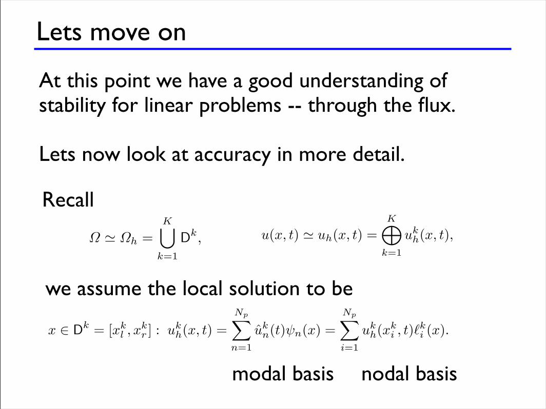
Lets move on
At this point we have a good understanding ofstability for linear problems -- through the flux.
Lets now look at accuracy in more detail.
16 2 The key ideas
where u can be both a scalar and a vector. In a similar fashion we also define the jumps along anormal, n, as
[[u]] = n!u! + n+u+, [[u]] = n! · u! + n+ · u+.
Note that it is defined di!erently depending on whether u is a scalar or a vector, u.
2.2 Basic elements of the schemes
In the following, we introduce the key ideas behind the family of discontinuous element methodsthat are the main topic of this text. Before getting into generalizations and abstract ideas, let usdevelop a basic understanding of the schemes through a simple example.
2.2.1 The first schemes
Consider the linear scalar wave equation
!u
!t+
!f(u)!x
= 0, x ! [L,R] = ", (2.1)
where the linear flux is given as f(u) = au. This is subject to the appropriate initial conditions
u(x, 0) = u0(x).
Boundary conditions are given when the boundary is an inflow boundary, that is
u(L, t) = g(t) if a " 0,u(R, t) = g(t) if a # 0.
We approximate " by K nonoverlapping elements, x ! [xkl , xk
r ] = Dk, as illustrated in Fig. 2.1. Oneach of these elements we express the local solution as a polynomial of order N
x ! Dk : ukh(x, t) =
Np!
n=1
ukn(t)#n(x) =
Np!
i=1
ukh(xk
i , t)$ki (x).
Here, we have introduced two complementary expressions for the local solution. In the first one,known as the modal form, we use a local polynomial basis, #n(x). A simple example of this couldbe #n(x) = xn!1. In the alternative form, known as the nodal representation, we introduce Np =N + 1 local grid points, xk
i ! Dk, and express the polynomial through the associated interpolatingLagrange polynomial, $k
i (x). The connection between these two forms is through the definition ofthe expansion coe"cients, uk
n. We return to a discussion of these choices in much more detail later;for now it su"ces to assume that we have chosen one of these representations.
The global solution u(x, t) is then assumed to be approximated by the piecewise N -th orderpolynomial approximation uh(x, t),
u(x, t) $ uh(x, t) =K"
k=1
ukh(x, t),
2
The key ideas
2.1 Briefly on notation
While we initially strive to stay away from complex notation a few funda-mentals are needed. We consider problems posed on the physical domain !with boundary "! and assume that this domain is well approximated bythe computational domain !h. This is a space filling triangulation composedof a collection of K geometry-conforming nonoverlapping elements, Dk. Theshape of these elements can be arbitrary although we will mostly considercases where they are d-dimensional simplexes.
We define the local inner product and L2(Dk) norm
(u, v)Dk =!
Dkuv dx, !u!2
Dk = (u, u)Dk ,
as well as the global broken inner product and norm
(u, v)!,h =K"
k=1
(u, v)Dk , !u!2!,h = (u, u)!,h .
Here, (!, h) reflects that ! is only approximated by the union of Dk, that is
! " !h =K#
k=1
Dk,
although we will not distinguish the two domains unless needed.Generally, one has local information as well as information from the neigh-
boring element along an intersection between two elements. Often we will referto the union of these intersections in an element as the trace of the element.For the methods we discuss here, we will have two or more solutions or bound-ary conditions at the same physical location along the trace of the element.
Recall
we assume the local solution to be
3
Making it work in one dimension
As simple as the formulations in the last chapter appear, there is often aleap between mathematical formulations and an actual implementation of thealgorithms. This is particularly true when one considers important issues suchas e!ciency, flexibility, and robustness of the resulting methods.
In this chapter we address these issues by first discussing details such asthe form of the local basis and, subsequently, how one implements the nodalDG-FEMs in a flexible way. To keep things simple, we continue the emphasison one-dimensional linear problems, although this results in a few apparentlyunnecessarily complex constructions. We ask the reader to bear with us, asthis slightly more general approach will pay o" when we begin to considermore complex nonlinear and/or higher-dimensional problems.
3.1 Legendre polynomials and nodal elements
In Chapter 2 we started out by assuming that one can represent the globalsolution as a the direct sum of local piecewise polynomial solution as
u(x, t) ! uh(x, t) =K!
k=1
ukh(xk, t).
The careful reader will note that this notation is a bit careless, as we do notaddress what exactly happens at the overlapping interfaces. However, a morecareful definition does not add anything essential at this point and we will usethis notation to reflect that the global solution is obtained by combining theK local solutions as defined by the scheme.
The local solutions are assumed to be of the form
x " Dk = [xkl , xk
r ] : ukh(x, t) =
Np"
n=1
ukn(t)!n(x) =
Np"
i=1
ukh(xk
i , t)"ki (x).
modal basis nodal basis
Local approximation
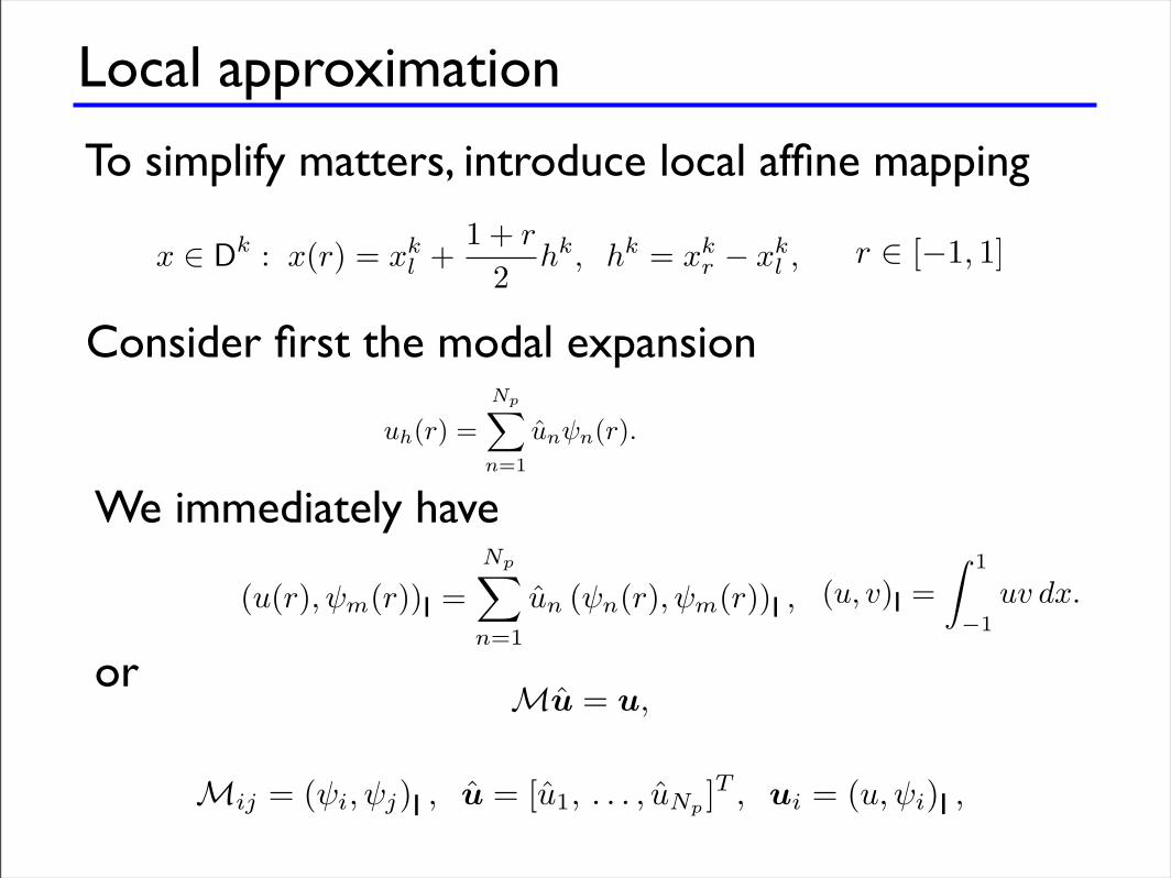
To simplify matters, introduce local affine mapping
44 3 Making it work in one dimension
We did not, however, discuss the specifics of this representation, as this is lessimportant from a theoretical point of view. The results in Example 2.4 clearlyillustrate, however, that the accuracy of the method is closely linked to theorder of the local polynomial representation and some care is warranted whenchoosing this.
Let us begin by introducing the a!ne mapping
x ! Dk : x(r) = xkl +
1 + r
2hk, hk = xk
r " xkl , (3.1)
with the reference variable r ! I = ["1, 1]. We consider local polynomialrepresentations of the form
x ! Dk : ukh(x(r), t) =
Np!
n=1
ukn(t)!n(r) =
Np!
i=1
ukh(xk
i , t)"ki (r).
Let us first discuss the local modal expansion,
uh(r) =Np!
n=1
un!n(r).
where we have dropped the superscripts for element k and the explicit timedependence, t, for clarity of notation.
As a first choice, one could consider !n(r) = rn!1 (i.e., the simple mono-mial basis). This leaves only the question of how to recover un. A natural wayis by an L2-projection; that is by requiring that
(u(r),!m(r))I =Np!
n=1
un (!n(r),!m(r))I ,
for each of the Np basis functions !n. We have introduced the inner producton the interval I as
(u, v)I =" 1
!1uv dx.
This yieldsMu = u,
whereMij = (!i,!j)I , u = [u1, . . . , uNp ]T , ui = (u,!i)I ,
leading to Np equations for the Np unknown expansion coe!cients, ui. How-ever, note that
Mij =1
i + j " 1#1 + ("1)i+j
$, (3.2)
which resembles a Hilbert matrix, known to be very poorly conditioned. If wecompute the condition number, #(M), for M for increasing order of approx-imation, N , we observe in Table 3.1 the very rapidly deteriorating condition-ing of M. The reason for this is evident in Eq. (3.2), where the coe!cient
r ! ["1, 1]
Consider first the modal expansion
44 3 Making it work in one dimension
We did not, however, discuss the specifics of this representation, as this is lessimportant from a theoretical point of view. The results in Example 2.4 clearlyillustrate, however, that the accuracy of the method is closely linked to theorder of the local polynomial representation and some care is warranted whenchoosing this.
Let us begin by introducing the a!ne mapping
x ! Dk : x(r) = xkl +
1 + r
2hk, hk = xk
r " xkl , (3.1)
with the reference variable r ! I = ["1, 1]. We consider local polynomialrepresentations of the form
x ! Dk : ukh(x(r), t) =
Np!
n=1
ukn(t)!n(r) =
Np!
i=1
ukh(xk
i , t)"ki (r).
Let us first discuss the local modal expansion,
uh(r) =Np!
n=1
un!n(r).
where we have dropped the superscripts for element k and the explicit timedependence, t, for clarity of notation.
As a first choice, one could consider !n(r) = rn!1 (i.e., the simple mono-mial basis). This leaves only the question of how to recover un. A natural wayis by an L2-projection; that is by requiring that
(u(r),!m(r))I =Np!
n=1
un (!n(r),!m(r))I ,
for each of the Np basis functions !n. We have introduced the inner producton the interval I as
(u, v)I =" 1
!1uv dx.
This yieldsMu = u,
whereMij = (!i,!j)I , u = [u1, . . . , uNp ]T , ui = (u,!i)I ,
leading to Np equations for the Np unknown expansion coe!cients, ui. How-ever, note that
Mij =1
i + j " 1#1 + ("1)i+j
$, (3.2)
which resembles a Hilbert matrix, known to be very poorly conditioned. If wecompute the condition number, #(M), for M for increasing order of approx-imation, N , we observe in Table 3.1 the very rapidly deteriorating condition-ing of M. The reason for this is evident in Eq. (3.2), where the coe!cient
We immediately have
or
Local approximation
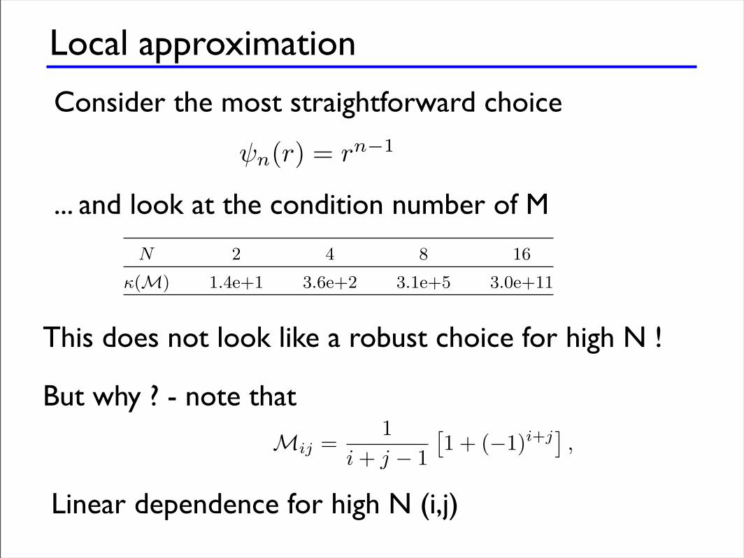
Consider the most straightforward choice
!n(r) = rn!13.1 Legendre polynomials and nodal elements 45
Table 3.1. Condition number of M based on the monomial basis for increasingvalue of N .
N 2 4 8 16
!(M) 1.4e+1 3.6e+2 3.1e+5 3.0e+11
(i + j ! 1)!1 implies an increasing close to linear dependence of the basis as(i, j) increases, resulting in the ill-conditioning. The impact of this is that,even at moderately high order (e.g., N > 10), one cannot accurately computeu and therefore not a good polynomial representation, uh.
A natural solution to this problem is to seek an orthonormal basis asa more suitable and computationally stable approach. We can simply takethe monomial basis, rn, and recover an orthonormal basis from this throughan L2-based Gram-Schmidt orthogonalization approach. This results in theorthonormal basis [296]
!n(r) = Pn!1(r) =Pn!1(r)"
"n!1,
where Pn(r) are the classic Legendre polynomials of order n and
"n =2
2n + 1
is the normalization. An easy way to compute this new basis is through therecurrence
rPn(r) = anPn!1(r) + an+1Pn+1(r),
an =
!n2
(2n + 1)(2n ! 1),
with
!1(r) = P0(r) =1"2, !2(r) = P1(r) =
"32r.
Appendix A discusses how to implement these recurrences and a number ofother useful manipulations of Pn(r), which is a special example of the muchlarger family of normalized Jacobi polynomials [159, 296].
To evaluate Pn(r) we use the library routine JacobiP.m as
>> P =JacobiP(r,0,0,n);
Using this basis, the mass matrix, M, is the identity and the problem ofconditioning is resolved. It leaves open the question of how to compute un,which is given as
un = (u,!n)I = (u, Pn!1)I.
... and look at the condition number of M
This does not look like a robust choice for high N !
But why ? - note that
44 3 Making it work in one dimension
We did not, however, discuss the specifics of this representation, as this is lessimportant from a theoretical point of view. The results in Example 2.4 clearlyillustrate, however, that the accuracy of the method is closely linked to theorder of the local polynomial representation and some care is warranted whenchoosing this.
Let us begin by introducing the a!ne mapping
x ! Dk : x(r) = xkl +
1 + r
2hk, hk = xk
r " xkl , (3.1)
with the reference variable r ! I = ["1, 1]. We consider local polynomialrepresentations of the form
x ! Dk : ukh(x(r), t) =
Np!
n=1
ukn(t)!n(r) =
Np!
i=1
ukh(xk
i , t)"ki (r).
Let us first discuss the local modal expansion,
uh(r) =Np!
n=1
un!n(r).
where we have dropped the superscripts for element k and the explicit timedependence, t, for clarity of notation.
As a first choice, one could consider !n(r) = rn!1 (i.e., the simple mono-mial basis). This leaves only the question of how to recover un. A natural wayis by an L2-projection; that is by requiring that
(u(r),!m(r))I =Np!
n=1
un (!n(r),!m(r))I ,
for each of the Np basis functions !n. We have introduced the inner producton the interval I as
(u, v)I =" 1
!1uv dx.
This yieldsMu = u,
whereMij = (!i,!j)I , u = [u1, . . . , uNp ]T , ui = (u,!i)I ,
leading to Np equations for the Np unknown expansion coe!cients, ui. How-ever, note that
Mij =1
i + j " 1#1 + ("1)i+j
$, (3.2)
which resembles a Hilbert matrix, known to be very poorly conditioned. If wecompute the condition number, #(M), for M for increasing order of approx-imation, N , we observe in Table 3.1 the very rapidly deteriorating condition-ing of M. The reason for this is evident in Eq. (3.2), where the coe!cient
Linear dependence for high N (i,j)
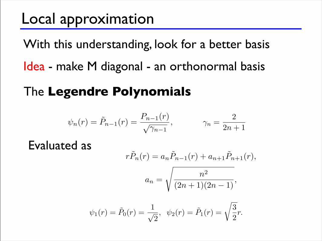
Local approximation
With this understanding, look for a better basis
Idea - make M diagonal - an orthonormal basis
3.1 Legendre polynomials and nodal elements 45
Table 3.1. Condition number of M based on the monomial basis for increasingvalue of N .
N 2 4 8 16
!(M) 1.4e+1 3.6e+2 3.1e+5 3.0e+11
(i + j ! 1)!1 implies an increasing close to linear dependence of the basis as(i, j) increases, resulting in the ill-conditioning. The impact of this is that,even at moderately high order (e.g., N > 10), one cannot accurately computeu and therefore not a good polynomial representation, uh.
A natural solution to this problem is to seek an orthonormal basis asa more suitable and computationally stable approach. We can simply takethe monomial basis, rn, and recover an orthonormal basis from this throughan L2-based Gram-Schmidt orthogonalization approach. This results in theorthonormal basis [296]
!n(r) = Pn!1(r) =Pn!1(r)"
"n!1,
where Pn(r) are the classic Legendre polynomials of order n and
"n =2
2n + 1
is the normalization. An easy way to compute this new basis is through therecurrence
rPn(r) = anPn!1(r) + an+1Pn+1(r),
an =
!n2
(2n + 1)(2n ! 1),
with
!1(r) = P0(r) =1"2, !2(r) = P1(r) =
"32r.
Appendix A discusses how to implement these recurrences and a number ofother useful manipulations of Pn(r), which is a special example of the muchlarger family of normalized Jacobi polynomials [159, 296].
To evaluate Pn(r) we use the library routine JacobiP.m as
>> P =JacobiP(r,0,0,n);
Using this basis, the mass matrix, M, is the identity and the problem ofconditioning is resolved. It leaves open the question of how to compute un,which is given as
un = (u,!n)I = (u, Pn!1)I.
The Legendre Polynomials
Evaluated as
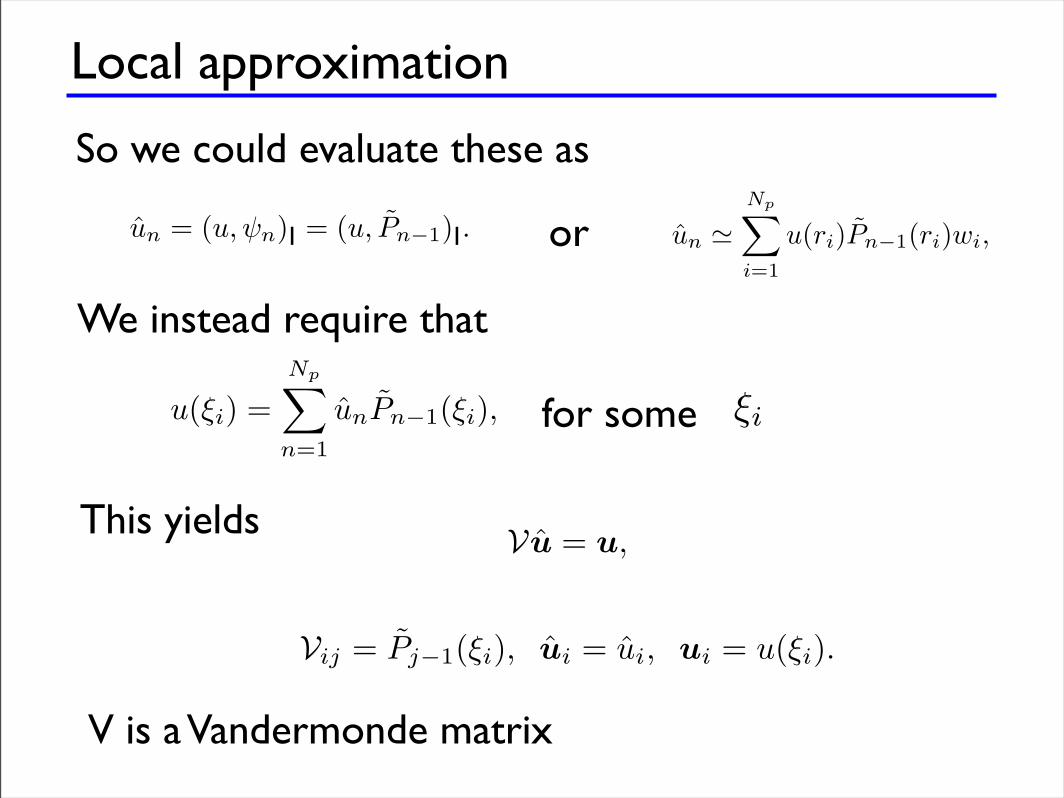
Local approximation
So we could evaluate these as
3.1 Legendre polynomials and nodal elements 45
Table 3.1. Condition number of M based on the monomial basis for increasingvalue of N .
N 2 4 8 16
!(M) 1.4e+1 3.6e+2 3.1e+5 3.0e+11
(i + j ! 1)!1 implies an increasing close to linear dependence of the basis as(i, j) increases, resulting in the ill-conditioning. The impact of this is that,even at moderately high order (e.g., N > 10), one cannot accurately computeu and therefore not a good polynomial representation, uh.
A natural solution to this problem is to seek an orthonormal basis asa more suitable and computationally stable approach. We can simply takethe monomial basis, rn, and recover an orthonormal basis from this throughan L2-based Gram-Schmidt orthogonalization approach. This results in theorthonormal basis [296]
!n(r) = Pn!1(r) =Pn!1(r)"
"n!1,
where Pn(r) are the classic Legendre polynomials of order n and
"n =2
2n + 1
is the normalization. An easy way to compute this new basis is through therecurrence
rPn(r) = anPn!1(r) + an+1Pn+1(r),
an =
!n2
(2n + 1)(2n ! 1),
with
!1(r) = P0(r) =1"2, !2(r) = P1(r) =
"32r.
Appendix A discusses how to implement these recurrences and a number ofother useful manipulations of Pn(r), which is a special example of the muchlarger family of normalized Jacobi polynomials [159, 296].
To evaluate Pn(r) we use the library routine JacobiP.m as
>> P =JacobiP(r,0,0,n);
Using this basis, the mass matrix, M, is the identity and the problem ofconditioning is resolved. It leaves open the question of how to compute un,which is given as
un = (u,!n)I = (u, Pn!1)I.
46 3 Making it work in one dimension
For a general function u, the evaluation of this inner product is nontrivial. Theonly practical way is to approximate the integral with a sum. In particular,one can use a Gaussian quadrature of the form
un !Np!
i=1
u(ri)Pn!1(ri)wi,
where ri are the quadrature points and wi are the quadrature weights. Animportant property of such quadratures is that they are exact, provided u isa polynomial of order 2Np " 1 [90]. The weights and nodes for the Gaussianquadrature can be computed using JacobiGQ.m, as discussed in Appendix A.To compute the Np = N +1 nodes and weights (r,w) for an (2N +1)-th-orderaccurate quadrature, one executes the command
>> [r,w] =JacobiGQ(0,0,N);
For the purpose of later generalizations, we consider a slightly di!erent ap-proach and define un such that the approximation is interpolatory; that is
u(!i) =Np!
n=1
unPn!1(!i),
where !i represents a set of Np distinct grid points. Note that these need notbe associated with any quadrature points. We can now write
Vu = u,
whereVij = Pj!1(!i), ui = ui, ui = u(!i).
This matrix, V, is recognized as a generalized Vandermonde matrix and willplay a pivotal role in all of the subsequent developments of the scheme. Thismatrix establishes the connection between the modes, u, and the nodal values,u, and we will benefit from making sure that it is well conditioned.
Since we have already determined that Pn is the optimal basis, we are leftwith the need to choose the grid points !i to define the Vandermonde matrix.There is significant freedom in this choice, so let us try to develop a bit ofintuition for a reasonable criteria.
We first recognize that if
u(r) ! uh(r) =Np!
n=1
unPn!1(r),
is an interpolant (i.e., u(!i) = uh(!i) at the grid points, !i), then we can writeit as
u(r) ! uh(r) =Np!
i=1
u(!i)"i(r).
or
We instead require that
for some !i
This yields
V is a Vandermonde matrix
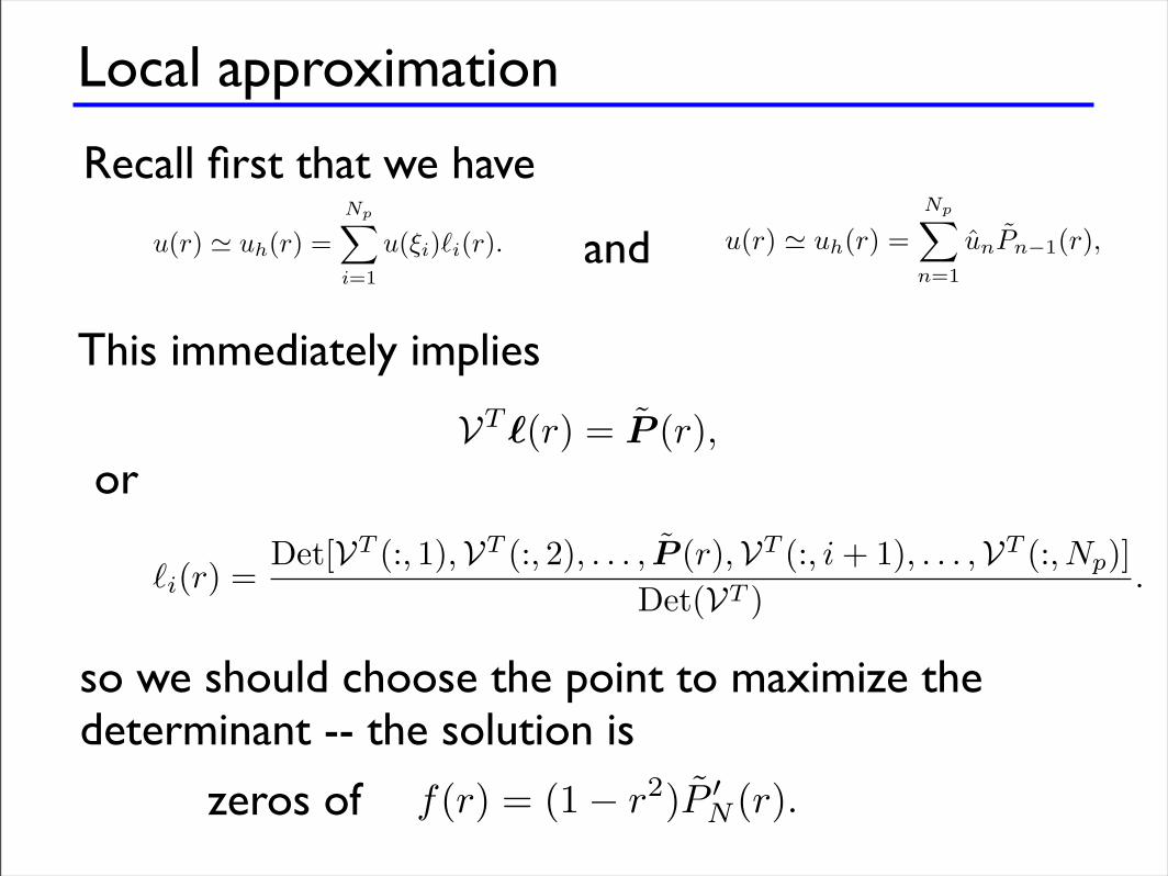
Local approximation
Recall first that we have
46 3 Making it work in one dimension
For a general function u, the evaluation of this inner product is nontrivial. Theonly practical way is to approximate the integral with a sum. In particular,one can use a Gaussian quadrature of the form
un !Np!
i=1
u(ri)Pn!1(ri)wi,
where ri are the quadrature points and wi are the quadrature weights. Animportant property of such quadratures is that they are exact, provided u isa polynomial of order 2Np " 1 [90]. The weights and nodes for the Gaussianquadrature can be computed using JacobiGQ.m, as discussed in Appendix A.To compute the Np = N +1 nodes and weights (r,w) for an (2N +1)-th-orderaccurate quadrature, one executes the command
>> [r,w] =JacobiGQ(0,0,N);
For the purpose of later generalizations, we consider a slightly di!erent ap-proach and define un such that the approximation is interpolatory; that is
u(!i) =Np!
n=1
unPn!1(!i),
where !i represents a set of Np distinct grid points. Note that these need notbe associated with any quadrature points. We can now write
Vu = u,
whereVij = Pj!1(!i), ui = ui, ui = u(!i).
This matrix, V, is recognized as a generalized Vandermonde matrix and willplay a pivotal role in all of the subsequent developments of the scheme. Thismatrix establishes the connection between the modes, u, and the nodal values,u, and we will benefit from making sure that it is well conditioned.
Since we have already determined that Pn is the optimal basis, we are leftwith the need to choose the grid points !i to define the Vandermonde matrix.There is significant freedom in this choice, so let us try to develop a bit ofintuition for a reasonable criteria.
We first recognize that if
u(r) ! uh(r) =Np!
n=1
unPn!1(r),
is an interpolant (i.e., u(!i) = uh(!i) at the grid points, !i), then we can writeit as
u(r) ! uh(r) =Np!
i=1
u(!i)"i(r).
3.1 Legendre polynomials and nodal elements 47
Here,
!i(r) =Np!
j=1j !=i
r ! "j
"i ! "j,
is the interpolating Lagrange polynomial with the property !i(rj) = #ij . It iswell known that !i(r) exists and is unique as long as the "i’s are distinct.
If we define the Lebesque constant
$ = maxr
Np"
i=1
|!i(r)|,
we realize that
"u!uh"! = "u!u"+u"!uh"! # "u!u""!+"u"!uh"! # (1+$)"u!u""!,
where " ·" ! is the usual maximum norm and u" represents the best approx-imating polynomial of order N . Hence, the Lebesque constant indicates howfar away the interpolation may be from the best possible polynomial repre-sentation u". Note that $ is determined solely by the grid points, "i. To getan optimal approximation, we should therefore aim to identify those points,"i, that minimize the Lebesque constant.
To appreciate how this relates to the conditioning of V, recognize that asa consequence of uniqueness of the polynomial interpolation, we have
VT !(r) = P (r),
where ! = [!1(r), . . . , !Np(r)]T and P (r) = [P0(r), . . . , PN (r)]T . We are inter-ested in the particular solution, !, which minimizes the Lebesque constant. Ifwe recall Cramer’s rule for solving linear systems of equations
!i(r) =Det[VT (:, 1),VT (:, 2), . . . , P (r),VT (:, i + 1), . . . ,VT (:, Np)]
Det(VT ).
It suggests that it is reasonable to seek "i such that the denominator (i.e., thedeterminant of V), is maximized.
For this one dimensional case, the solution to this problem is known in arelatively simple form as the Np zeros of [151, 159]
f(r) = (1 ! r2)P #N (r).
These are closely related to the normalized Legendre polynomials and areknown as the Legendre-Gauss-Lobatto (LGL) quadrature points. Using thelibrary routine JacobiGL.m in Appendix A, these nodes can be computed as
>> [r] = JacobiGL(0,0,N);
and
This immediately implies
or
so we should choose the point to maximize the determinant -- the solution is
zeros of
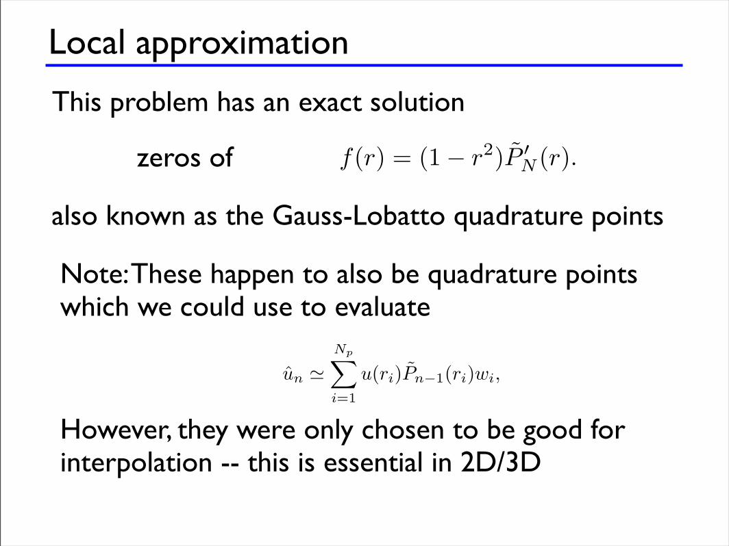
Local approximation
This problem has an exact solution
3.1 Legendre polynomials and nodal elements 47
Here,
!i(r) =Np!
j=1j !=i
r ! "j
"i ! "j,
is the interpolating Lagrange polynomial with the property !i(rj) = #ij . It iswell known that !i(r) exists and is unique as long as the "i’s are distinct.
If we define the Lebesque constant
$ = maxr
Np"
i=1
|!i(r)|,
we realize that
"u!uh"! = "u!u"+u"!uh"! # "u!u""!+"u"!uh"! # (1+$)"u!u""!,
where " ·" ! is the usual maximum norm and u" represents the best approx-imating polynomial of order N . Hence, the Lebesque constant indicates howfar away the interpolation may be from the best possible polynomial repre-sentation u". Note that $ is determined solely by the grid points, "i. To getan optimal approximation, we should therefore aim to identify those points,"i, that minimize the Lebesque constant.
To appreciate how this relates to the conditioning of V, recognize that asa consequence of uniqueness of the polynomial interpolation, we have
VT !(r) = P (r),
where ! = [!1(r), . . . , !Np(r)]T and P (r) = [P0(r), . . . , PN (r)]T . We are inter-ested in the particular solution, !, which minimizes the Lebesque constant. Ifwe recall Cramer’s rule for solving linear systems of equations
!i(r) =Det[VT (:, 1),VT (:, 2), . . . , P (r),VT (:, i + 1), . . . ,VT (:, Np)]
Det(VT ).
It suggests that it is reasonable to seek "i such that the denominator (i.e., thedeterminant of V), is maximized.
For this one dimensional case, the solution to this problem is known in arelatively simple form as the Np zeros of [151, 159]
f(r) = (1 ! r2)P #N (r).
These are closely related to the normalized Legendre polynomials and areknown as the Legendre-Gauss-Lobatto (LGL) quadrature points. Using thelibrary routine JacobiGL.m in Appendix A, these nodes can be computed as
>> [r] = JacobiGL(0,0,N);
zeros of
also known as the Gauss-Lobatto quadrature points
Note: These happen to also be quadrature pointswhich we could use to evaluate
46 3 Making it work in one dimension
For a general function u, the evaluation of this inner product is nontrivial. Theonly practical way is to approximate the integral with a sum. In particular,one can use a Gaussian quadrature of the form
un !Np!
i=1
u(ri)Pn!1(ri)wi,
where ri are the quadrature points and wi are the quadrature weights. Animportant property of such quadratures is that they are exact, provided u isa polynomial of order 2Np " 1 [90]. The weights and nodes for the Gaussianquadrature can be computed using JacobiGQ.m, as discussed in Appendix A.To compute the Np = N +1 nodes and weights (r,w) for an (2N +1)-th-orderaccurate quadrature, one executes the command
>> [r,w] =JacobiGQ(0,0,N);
For the purpose of later generalizations, we consider a slightly di!erent ap-proach and define un such that the approximation is interpolatory; that is
u(!i) =Np!
n=1
unPn!1(!i),
where !i represents a set of Np distinct grid points. Note that these need notbe associated with any quadrature points. We can now write
Vu = u,
whereVij = Pj!1(!i), ui = ui, ui = u(!i).
This matrix, V, is recognized as a generalized Vandermonde matrix and willplay a pivotal role in all of the subsequent developments of the scheme. Thismatrix establishes the connection between the modes, u, and the nodal values,u, and we will benefit from making sure that it is well conditioned.
Since we have already determined that Pn is the optimal basis, we are leftwith the need to choose the grid points !i to define the Vandermonde matrix.There is significant freedom in this choice, so let us try to develop a bit ofintuition for a reasonable criteria.
We first recognize that if
u(r) ! uh(r) =Np!
n=1
unPn!1(r),
is an interpolant (i.e., u(!i) = uh(!i) at the grid points, !i), then we can writeit as
u(r) ! uh(r) =Np!
i=1
u(!i)"i(r).
However, they were only chosen to be good forinterpolation -- this is essential in 2D/3D
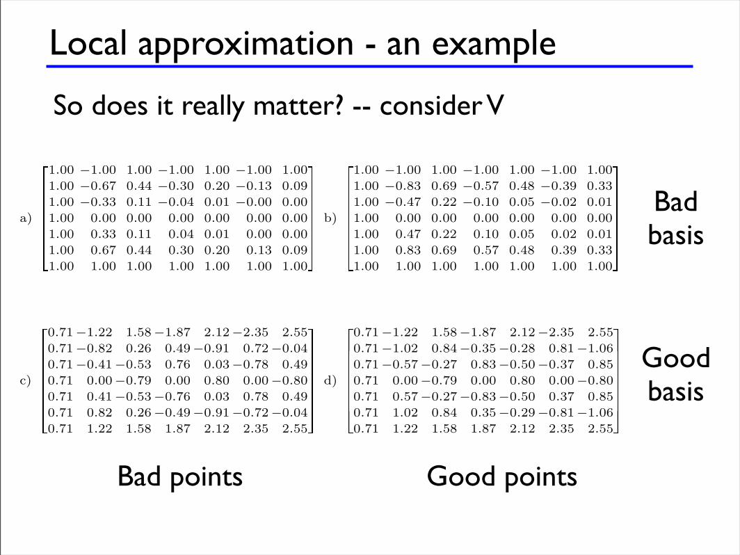
Local approximation - an example
So does it really matter? -- consider V
48 3 Making it work in one dimension
To illustrate the importance of choosing these points correctly, consider thefollowing example.
Example 3.1. We first compare the growth of the determinant of V as a func-tion of N , using either the LGL points or the equidistant points
!i = !1 +2(i ! 1)
N, i " [1, Np].
In Fig. 3.1 we show the entries of V for di!erent choices of the basis, "n(r), andthe interpolation points, !i. For Fig. 3.1a and Fig. 3.1b, both relying on themonomial basis, we see indications that the last columns are almost linearlydependent and that the situation is worse in the case of the equidistant points.In Fig. 3.1b the situation is slightly improved through the use of the LGL gridpoints.
In Fig. 3.2 we further illustrate this by computing the determinant of theVandermonde matrix V, highlighting a significant qualitative di!erence in thebehavior for the two sets of nodes as N increases. For the LGL nodes, thedeterminant continues to increase in size with N , reflecting a well-behavedinterpolation where #i(r) takes small values in between the nodes. For theequidistant nodes, the situation is entirely di!erent.
While the determinant has comparable values for small values of N , thedeterminant for the equidistant nodes begins to decay exponentially fast onceN exceeds 16, caused by the close to linear dependence of the last columns
a)
1.00 !1.00 1.00 !1.00 1.00 !1.00 1.001.00 !0.67 0.44 !0.30 0.20 !0.13 0.091.00 !0.33 0.11 !0.04 0.01 !0.00 0.001.00 0.00 0.00 0.00 0.00 0.00 0.001.00 0.33 0.11 0.04 0.01 0.00 0.001.00 0.67 0.44 0.30 0.20 0.13 0.091.00 1.00 1.00 1.00 1.00 1.00 1.00
b)
1.00 !1.00 1.00 !1.00 1.00 !1.00 1.001.00 !0.83 0.69 !0.57 0.48 !0.39 0.331.00 !0.47 0.22 !0.10 0.05 !0.02 0.011.00 0.00 0.00 0.00 0.00 0.00 0.001.00 0.47 0.22 0.10 0.05 0.02 0.011.00 0.83 0.69 0.57 0.48 0.39 0.331.00 1.00 1.00 1.00 1.00 1.00 1.00
c)
0.71!1.22 1.58!1.87 2.12!2.35 2.550.71!0.82 0.26 0.49!0.91 0.72!0.040.71!0.41!0.53 0.76 0.03!0.78 0.490.71 0.00!0.79 0.00 0.80 0.00!0.800.71 0.41!0.53!0.76 0.03 0.78 0.490.71 0.82 0.26!0.49!0.91!0.72!0.040.71 1.22 1.58 1.87 2.12 2.35 2.55
d)
0.71!1.22 1.58!1.87 2.12!2.35 2.550.71!1.02 0.84!0.35!0.28 0.81!1.060.71!0.57!0.27 0.83!0.50!0.37 0.850.71 0.00!0.79 0.00 0.80 0.00!0.800.71 0.57!0.27!0.83!0.50 0.37 0.850.71 1.02 0.84 0.35!0.29!0.81!1.060.71 1.22 1.58 1.87 2.12 2.35 2.55
Fig. 3.1. Entries of V for N = 6 and di!erent choices of the basis, !n(r), andevaluation points, "i. For (a) and (c) we use equidistant points and (b) and (d) arebased on LGL points. Furthermore, (a) and (b) are based on V computed using asimple monomial basis, !n(r) = rn!1, while (c) and (d) are based on the orthonormalbasis, !n(r) = Pn!1(r).
Bad points Good points
Badbasis
Goodbasis
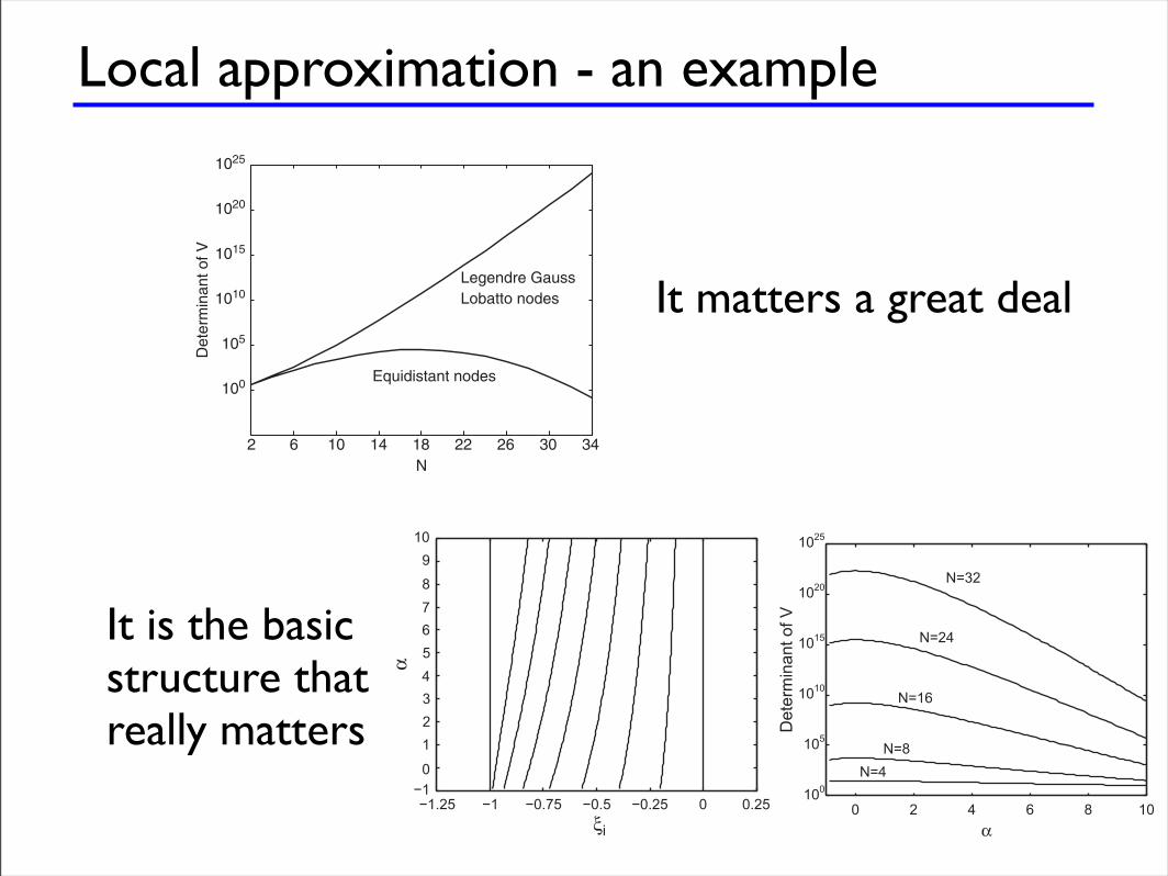
Local approximation - an example3.1 Legendre polynomials and nodal elements 49
2 6 10 14 18 22 26 30 34
100
105
1010
1015
1020
1025
N
Det
erm
inan
t of V
Legendre GaussLobatto nodes
Equidistant nodes
Fig. 3.2. Growth of the determinant of the Vandermonde matrix, V, when computedbased on LGL nodes and the simple equidistant nodes.
in V. For the interpolation, this manifests itself as the well-known Rungephenomenon [90] for interpolation at equidistant grids. The rapid decay ofthe determinant enables an exponentially fast growth of !i(r) between thegrid points, resulting in a very poorly behaved interpolation. This is alsoreflected in the corresponding Lebesque constant, which grows like 2Np forthe equidistant nodes while it grows like logNp in the optimal case of theLGL nodes (see [151, 307] and references therein).
The main lesson here is that it is generally not a good idea to use equidis-tant grid points when representing the local interpolating polynomial solution.This point is particularly important when the interest is in the developmentof methods performing robustly at higher values of N .
One can ask, however, whether there is anything special about the LGLpoints, beyond the fact that they maximize the Vandermonde determinant.In particular, can one find other families of points with the similar propertythat the Vandermonde determinant continues to grow with the order of ap-proximation.
To investigate this, we compute the determinant of V for fixed valuesof N but with points which are Gauss-Lobatto points for the symmetricJacobi polynomials P (!,!)
n (r) (see Appendix A). A special case of these arethe Legendre polynomials obtained with " = 0.
In Fig. 3.3 we show the spatial variation of the nodes for N = 16 as well asthe variation of the Vandermonde determinant as a function of " for di!erentvalues of N . While this confirms that " = 0 maximizes the determinantfor all N , we also see that there is a broad range of values of " where thequantitative behavior is identical to that obtained with the LGL nodes. Onlywhen " becomes significantly larger than zero do we begin to see a significant
50 3 Making it work in one dimension
!1.25 !1 !0.75 !0.5 !0.25 0 0.25!1
0123456789
10
!i
"
0 2 4 6 8 10100
105
1010
1015
1020
1025
"
Det
erm
inan
t of V
N=4N=8
N=16
N=24
N=32
Fig. 3.3. On the left is shown the location of the left half of the Jacobi-Gauss-Lobatto nodes for N = 16 as a function of !, the type of the polynomial. Note that! = 0 corresponds to the LGL nodes. On the right is shown the behavior of theVandermonde determinant as a function of ! for di!erent values of N , confirmingthe optimality of the LGL nodes but also showing robustness of the interpolationto this choice.
decay in the value of the determinant, indicating possible problems in theinterpolation. Considering the corresponding nodal distribution in Fig. 3.3for these values of !, this is perhaps not surprising.
This highlights that it is the overall structure of the nodes rather thanthe details of the individual node position that is important; for example, onecould optimize these nodal sets for various applications.
To summarize matters, we have local approximations of the form
u(r) ! uh(r) =Np!
n=1
unPn!1(r) =Np!
i=1
u(ri)"i(r), (3.3)
where #i = ri are the Legendre-Gauss-Lobatto quadrature points. A centralcomponent of this construction is the Vandermonde matrix, V, which estab-lishes the connections
u = Vu, VT !(r) = P (r), Vij = Pj(ri).
By carefully choosing the orthonormal Legendre basis, Pn(r), and the nodalpoints, ri, we have ensured that V is a well-conditioned object and that theresulting interpolation is well behaved. A script for initializing V is given inVandermonde1D.m.
It matters a great deal
It is the basicstructure that really matters
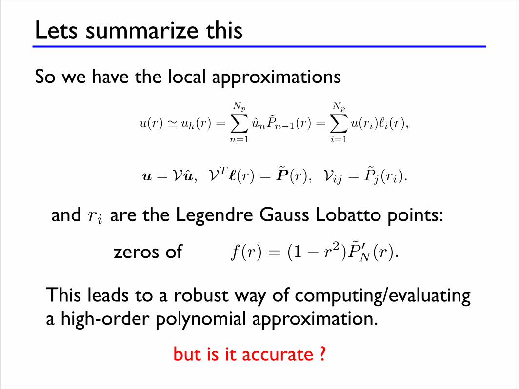
Lets summarize this
So we have the local approximations
50 3 Making it work in one dimension
!1.25 !1 !0.75 !0.5 !0.25 0 0.25!1
0123456789
10
!i
"
0 2 4 6 8 10100
105
1010
1015
1020
1025
"
Det
erm
inan
t of V
N=4N=8
N=16
N=24
N=32
Fig. 3.3. On the left is shown the location of the left half of the Jacobi-Gauss-Lobatto nodes for N = 16 as a function of !, the type of the polynomial. Note that! = 0 corresponds to the LGL nodes. On the right is shown the behavior of theVandermonde determinant as a function of ! for di!erent values of N , confirmingthe optimality of the LGL nodes but also showing robustness of the interpolationto this choice.
decay in the value of the determinant, indicating possible problems in theinterpolation. Considering the corresponding nodal distribution in Fig. 3.3for these values of !, this is perhaps not surprising.
This highlights that it is the overall structure of the nodes rather thanthe details of the individual node position that is important; for example, onecould optimize these nodal sets for various applications.
To summarize matters, we have local approximations of the form
u(r) ! uh(r) =Np!
n=1
unPn!1(r) =Np!
i=1
u(ri)"i(r), (3.3)
where #i = ri are the Legendre-Gauss-Lobatto quadrature points. A centralcomponent of this construction is the Vandermonde matrix, V, which estab-lishes the connections
u = Vu, VT !(r) = P (r), Vij = Pj(ri).
By carefully choosing the orthonormal Legendre basis, Pn(r), and the nodalpoints, ri, we have ensured that V is a well-conditioned object and that theresulting interpolation is well behaved. A script for initializing V is given inVandermonde1D.m.
and are the Legendre Gauss Lobatto points: ri
3.1 Legendre polynomials and nodal elements 47
Here,
!i(r) =Np!
j=1j !=i
r ! "j
"i ! "j,
is the interpolating Lagrange polynomial with the property !i(rj) = #ij . It iswell known that !i(r) exists and is unique as long as the "i’s are distinct.
If we define the Lebesque constant
$ = maxr
Np"
i=1
|!i(r)|,
we realize that
"u!uh"! = "u!u"+u"!uh"! # "u!u""!+"u"!uh"! # (1+$)"u!u""!,
where " ·" ! is the usual maximum norm and u" represents the best approx-imating polynomial of order N . Hence, the Lebesque constant indicates howfar away the interpolation may be from the best possible polynomial repre-sentation u". Note that $ is determined solely by the grid points, "i. To getan optimal approximation, we should therefore aim to identify those points,"i, that minimize the Lebesque constant.
To appreciate how this relates to the conditioning of V, recognize that asa consequence of uniqueness of the polynomial interpolation, we have
VT !(r) = P (r),
where ! = [!1(r), . . . , !Np(r)]T and P (r) = [P0(r), . . . , PN (r)]T . We are inter-ested in the particular solution, !, which minimizes the Lebesque constant. Ifwe recall Cramer’s rule for solving linear systems of equations
!i(r) =Det[VT (:, 1),VT (:, 2), . . . , P (r),VT (:, i + 1), . . . ,VT (:, Np)]
Det(VT ).
It suggests that it is reasonable to seek "i such that the denominator (i.e., thedeterminant of V), is maximized.
For this one dimensional case, the solution to this problem is known in arelatively simple form as the Np zeros of [151, 159]
f(r) = (1 ! r2)P #N (r).
These are closely related to the normalized Legendre polynomials and areknown as the Legendre-Gauss-Lobatto (LGL) quadrature points. Using thelibrary routine JacobiGL.m in Appendix A, these nodes can be computed as
>> [r] = JacobiGL(0,0,N);
zeros of
This leads to a robust way of computing/evaluating a high-order polynomial approximation.
but is it accurate ?
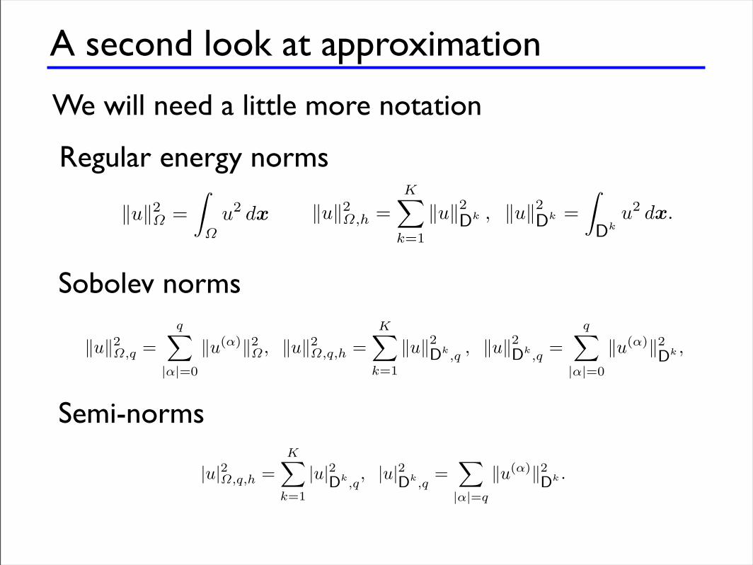
A second look at approximation
We will need a little more notation
Regular energy norms
4
Insight through theory
While the last chapters have focused on basic ideas and their implementa-tion as a computational method, further insight into the performance of themethod can be gained by revisiting some issues in more detail. To keep thingsrelatively simple, we focus on the properties of the scheme for one-dimensionallinear problems. However, as we will see later, many of the results obtainedhere carry over to multidimensional problems and even nonlinear problemswith just a few modifications.
4.1 A bit more notation
Before we embark on a more rigorous discussion, we need to introduce someadditional notation. In particular, both global norms, defined on !, and bro-ken norms, defined over !h as sums of K elements Dk, need to be introduced.
For the solution, u(x, t), we define the global L2-norm over the domain! ! Rd as
"u"2! =
!
!u2 dx
as well as the broken norms
"u"2!,h =
K"
k=1
"u"2Dk , "u"2
Dk =!
Dku2 dx.
In a similar way, we define the associated Sobolev norms
"u"2!,q =
q"
|"|=0
"u(")"2! , "u"2
!,q,h =K"
k=1
"u"2Dk
,q, "u"2
Dk,q
=q"
|"|=0
"u(")"2Dk ,
where " is a multi-index of length d. For the one-dimensional case, mostoften considered in this chapter, this norm is simply the L2-norm of the q-th
Sobolev norms
Semi-norms
76 4 Insight through theory
derivative. We will also define the space of functions, u ! Hq(!), as thosefunctions for which "u"!,q or "u"!,q,h is bounded.
Finally, we will need the semi-norms
|u|2!,q,h =K!
k=1
|u|2Dk,q
, |u|2Dk,q
=!
|"|=q
"u(")"2Dk .
4.2 Briefly on convergence
Let us consider the one-dimensional hyperbolic system
"u
"t+ A"u
"x= 0,
where A is diagonizable and we assume that appropriate boundary conditionsare available to ensure well-posedness; that is, there exists constants C and #such that
"u(t)"! # C exp(#t)"u(0)"! .
Let us assume that the solution is being approximated by an N -th-orderpiecewise polynomial, uh, which satisfies the semidiscrete scheme
duh
dt+ Lhuh = 0.
Here, Lh represents the discrete approximation of A"x. Inserting the exactsolution, u, into the semidiscrete form yields
du
dt+ Lhu = T (u(x, t)),
where T (u) is the truncation error, or the error by which the exact solutionfails to satisfy the discrete approximation.
If we now introduce the error
!(x, t) = u(x, t) $ uh(x, t),
it is natural to seek convergence in the sense that
%t ! [0, T ] : limdof!"
"!(t)"!,h & 0.
We have introduced the notion of degrees of freedom (dof) to reflect thatconvergence can be achieved either by decreasing the cell size, h, by increasingthe order of the approximation, N , or by doing both simultaneously, knownas hp-convergence.
Proving convergence directly is, however, complicated due to the need toprove it for all time. Fortunately, there is shortcut. Consider the error equation
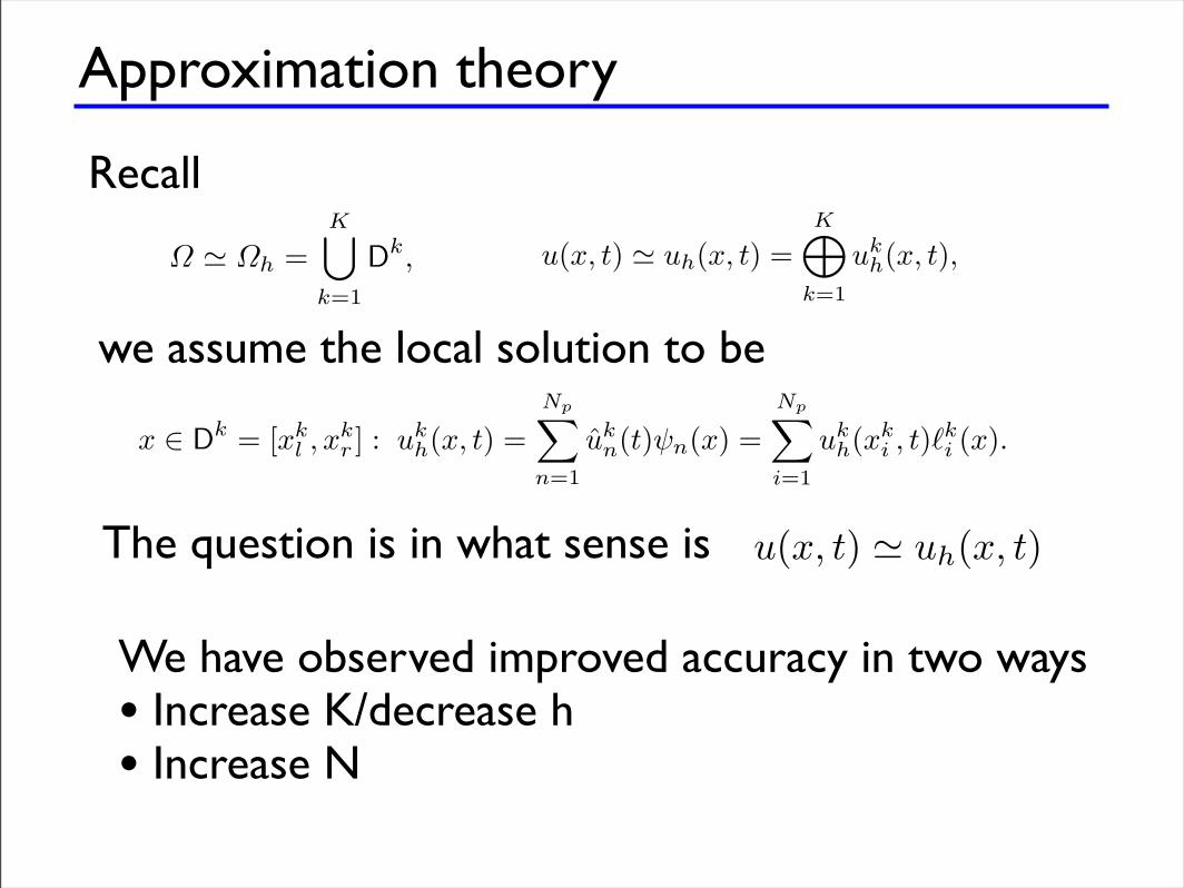
Approximation theory
16 2 The key ideas
where u can be both a scalar and a vector. In a similar fashion we also define the jumps along anormal, n, as
[[u]] = n!u! + n+u+, [[u]] = n! · u! + n+ · u+.
Note that it is defined di!erently depending on whether u is a scalar or a vector, u.
2.2 Basic elements of the schemes
In the following, we introduce the key ideas behind the family of discontinuous element methodsthat are the main topic of this text. Before getting into generalizations and abstract ideas, let usdevelop a basic understanding of the schemes through a simple example.
2.2.1 The first schemes
Consider the linear scalar wave equation
!u
!t+
!f(u)!x
= 0, x ! [L,R] = ", (2.1)
where the linear flux is given as f(u) = au. This is subject to the appropriate initial conditions
u(x, 0) = u0(x).
Boundary conditions are given when the boundary is an inflow boundary, that is
u(L, t) = g(t) if a " 0,u(R, t) = g(t) if a # 0.
We approximate " by K nonoverlapping elements, x ! [xkl , xk
r ] = Dk, as illustrated in Fig. 2.1. Oneach of these elements we express the local solution as a polynomial of order N
x ! Dk : ukh(x, t) =
Np!
n=1
ukn(t)#n(x) =
Np!
i=1
ukh(xk
i , t)$ki (x).
Here, we have introduced two complementary expressions for the local solution. In the first one,known as the modal form, we use a local polynomial basis, #n(x). A simple example of this couldbe #n(x) = xn!1. In the alternative form, known as the nodal representation, we introduce Np =N + 1 local grid points, xk
i ! Dk, and express the polynomial through the associated interpolatingLagrange polynomial, $k
i (x). The connection between these two forms is through the definition ofthe expansion coe"cients, uk
n. We return to a discussion of these choices in much more detail later;for now it su"ces to assume that we have chosen one of these representations.
The global solution u(x, t) is then assumed to be approximated by the piecewise N -th orderpolynomial approximation uh(x, t),
u(x, t) $ uh(x, t) =K"
k=1
ukh(x, t),
2
The key ideas
2.1 Briefly on notation
While we initially strive to stay away from complex notation a few funda-mentals are needed. We consider problems posed on the physical domain !with boundary "! and assume that this domain is well approximated bythe computational domain !h. This is a space filling triangulation composedof a collection of K geometry-conforming nonoverlapping elements, Dk. Theshape of these elements can be arbitrary although we will mostly considercases where they are d-dimensional simplexes.
We define the local inner product and L2(Dk) norm
(u, v)Dk =!
Dkuv dx, !u!2
Dk = (u, u)Dk ,
as well as the global broken inner product and norm
(u, v)!,h =K"
k=1
(u, v)Dk , !u!2!,h = (u, u)!,h .
Here, (!, h) reflects that ! is only approximated by the union of Dk, that is
! " !h =K#
k=1
Dk,
although we will not distinguish the two domains unless needed.Generally, one has local information as well as information from the neigh-
boring element along an intersection between two elements. Often we will referto the union of these intersections in an element as the trace of the element.For the methods we discuss here, we will have two or more solutions or bound-ary conditions at the same physical location along the trace of the element.
Recall
we assume the local solution to be
3
Making it work in one dimension
As simple as the formulations in the last chapter appear, there is often aleap between mathematical formulations and an actual implementation of thealgorithms. This is particularly true when one considers important issues suchas e!ciency, flexibility, and robustness of the resulting methods.
In this chapter we address these issues by first discussing details such asthe form of the local basis and, subsequently, how one implements the nodalDG-FEMs in a flexible way. To keep things simple, we continue the emphasison one-dimensional linear problems, although this results in a few apparentlyunnecessarily complex constructions. We ask the reader to bear with us, asthis slightly more general approach will pay o" when we begin to considermore complex nonlinear and/or higher-dimensional problems.
3.1 Legendre polynomials and nodal elements
In Chapter 2 we started out by assuming that one can represent the globalsolution as a the direct sum of local piecewise polynomial solution as
u(x, t) ! uh(x, t) =K!
k=1
ukh(xk, t).
The careful reader will note that this notation is a bit careless, as we do notaddress what exactly happens at the overlapping interfaces. However, a morecareful definition does not add anything essential at this point and we will usethis notation to reflect that the global solution is obtained by combining theK local solutions as defined by the scheme.
The local solutions are assumed to be of the form
x " Dk = [xkl , xk
r ] : ukh(x, t) =
Np"
n=1
ukn(t)!n(x) =
Np"
i=1
ukh(xk
i , t)"ki (x).
The question is in what sense is
16 2 The key ideas
where u can be both a scalar and a vector. In a similar fashion we also define the jumps along anormal, n, as
[[u]] = n!u! + n+u+, [[u]] = n! · u! + n+ · u+.
Note that it is defined di!erently depending on whether u is a scalar or a vector, u.
2.2 Basic elements of the schemes
In the following, we introduce the key ideas behind the family of discontinuous element methodsthat are the main topic of this text. Before getting into generalizations and abstract ideas, let usdevelop a basic understanding of the schemes through a simple example.
2.2.1 The first schemes
Consider the linear scalar wave equation
!u
!t+
!f(u)!x
= 0, x ! [L,R] = ", (2.1)
where the linear flux is given as f(u) = au. This is subject to the appropriate initial conditions
u(x, 0) = u0(x).
Boundary conditions are given when the boundary is an inflow boundary, that is
u(L, t) = g(t) if a " 0,u(R, t) = g(t) if a # 0.
We approximate " by K nonoverlapping elements, x ! [xkl , xk
r ] = Dk, as illustrated in Fig. 2.1. Oneach of these elements we express the local solution as a polynomial of order N
x ! Dk : ukh(x, t) =
Np!
n=1
ukn(t)#n(x) =
Np!
i=1
ukh(xk
i , t)$ki (x).
Here, we have introduced two complementary expressions for the local solution. In the first one,known as the modal form, we use a local polynomial basis, #n(x). A simple example of this couldbe #n(x) = xn!1. In the alternative form, known as the nodal representation, we introduce Np =N + 1 local grid points, xk
i ! Dk, and express the polynomial through the associated interpolatingLagrange polynomial, $k
i (x). The connection between these two forms is through the definition ofthe expansion coe"cients, uk
n. We return to a discussion of these choices in much more detail later;for now it su"ces to assume that we have chosen one of these representations.
The global solution u(x, t) is then assumed to be approximated by the piecewise N -th orderpolynomial approximation uh(x, t),
u(x, t) $ uh(x, t) =K"
k=1
ukh(x, t),
We have observed improved accuracy in two ways• Increase K/decrease h• Increase N
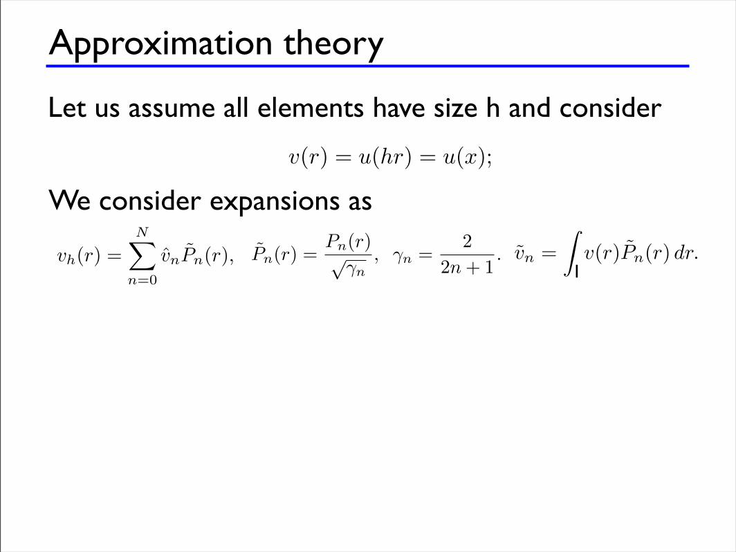
Approximation theory
Let us assume all elements have size h and consider
78 4 Insight through theory
where
x ! Dk : ukh(x) =
Np!
n=1
ukn!n(x) =
Np!
i=1
ukh(xi)"k
i (x),
how well and in what sense can we expect uh to approximate u?As observed experimentally, we have two ways to improve the quality
of uh as an approximation of u: One can keep the order, N , of the localapproximation fixed and increase the number of elements, K, known as h-refinement. Alternatively, one can keep K fixed and increase N , known asorder or p-refinement. While both lead to a better approximation, they achievethis in di!erent ways and it is important to understand when to use whichpath to achieve convergence.
Let us first estimate what can be expected under order refinement. Forsimplicity, we assume that all elements have length h (i.e., Dk = xk + r
2hwhere xk = 1
2 (xkr +xk
l ) represents the cell center and r ! ["1, 1] is the referencecoordinate).
We begin by considering the standard interval and introduce the new vari-able
v(r) = u(hr) = u(x);
that is, v is defined on the standard interval, I = ["1, 1], and xk = 0, x !["h, h]. We discussed in Chapter 3 the advantage of using a local orthonormalbasis – in this case, the normalized Legendre polynomials
Pn(r) =Pn(r)#
#n, #n =
22n + 1
.
Here, Pn(r) are the classic Legendre polynomials of order n. A key propertyof these polynomials is that they satisfy a singular Sturm-Liouville problem
d
dr(1 " r2)
d
drPn + n(n + 1)Pn = 0. (4.2)
Let us consider the basic question of how well
vh(r) =N!
n=0
vnPn(r),
represents v ! L2(I). Note, that for simplicity of the notation and to conformwith standard notation, we now have the sum running from 0 to N ratherthan from 1 to N + 1 = Np, as used previously.
Prior to discussing interpolation, used throughout this text, we considerthe properties of the projection where we utilize the orthonomality of Pn(r)to find vn as
vn ="
Iv(r)Pn(r) dr.
We consider expansions as
78 4 Insight through theory
where
x ! Dk : ukh(x) =
Np!
n=1
ukn!n(x) =
Np!
i=1
ukh(xi)"k
i (x),
how well and in what sense can we expect uh to approximate u?As observed experimentally, we have two ways to improve the quality
of uh as an approximation of u: One can keep the order, N , of the localapproximation fixed and increase the number of elements, K, known as h-refinement. Alternatively, one can keep K fixed and increase N , known asorder or p-refinement. While both lead to a better approximation, they achievethis in di!erent ways and it is important to understand when to use whichpath to achieve convergence.
Let us first estimate what can be expected under order refinement. Forsimplicity, we assume that all elements have length h (i.e., Dk = xk + r
2hwhere xk = 1
2 (xkr +xk
l ) represents the cell center and r ! ["1, 1] is the referencecoordinate).
We begin by considering the standard interval and introduce the new vari-able
v(r) = u(hr) = u(x);
that is, v is defined on the standard interval, I = ["1, 1], and xk = 0, x !["h, h]. We discussed in Chapter 3 the advantage of using a local orthonormalbasis – in this case, the normalized Legendre polynomials
Pn(r) =Pn(r)#
#n, #n =
22n + 1
.
Here, Pn(r) are the classic Legendre polynomials of order n. A key propertyof these polynomials is that they satisfy a singular Sturm-Liouville problem
d
dr(1 " r2)
d
drPn + n(n + 1)Pn = 0. (4.2)
Let us consider the basic question of how well
vh(r) =N!
n=0
vnPn(r),
represents v ! L2(I). Note, that for simplicity of the notation and to conformwith standard notation, we now have the sum running from 0 to N ratherthan from 1 to N + 1 = Np, as used previously.
Prior to discussing interpolation, used throughout this text, we considerthe properties of the projection where we utilize the orthonomality of Pn(r)to find vn as
vn ="
Iv(r)Pn(r) dr.
Approximation theory
Let us assume all elements have size h and consider
78 4 Insight through theory
where
x ! Dk : ukh(x) =
Np!
n=1
ukn!n(x) =
Np!
i=1
ukh(xi)"k
i (x),
how well and in what sense can we expect uh to approximate u?As observed experimentally, we have two ways to improve the quality
of uh as an approximation of u: One can keep the order, N , of the localapproximation fixed and increase the number of elements, K, known as h-refinement. Alternatively, one can keep K fixed and increase N , known asorder or p-refinement. While both lead to a better approximation, they achievethis in di!erent ways and it is important to understand when to use whichpath to achieve convergence.
Let us first estimate what can be expected under order refinement. Forsimplicity, we assume that all elements have length h (i.e., Dk = xk + r
2hwhere xk = 1
2 (xkr +xk
l ) represents the cell center and r ! ["1, 1] is the referencecoordinate).
We begin by considering the standard interval and introduce the new vari-able
v(r) = u(hr) = u(x);
that is, v is defined on the standard interval, I = ["1, 1], and xk = 0, x !["h, h]. We discussed in Chapter 3 the advantage of using a local orthonormalbasis – in this case, the normalized Legendre polynomials
Pn(r) =Pn(r)#
#n, #n =
22n + 1
.
Here, Pn(r) are the classic Legendre polynomials of order n. A key propertyof these polynomials is that they satisfy a singular Sturm-Liouville problem
d
dr(1 " r2)
d
drPn + n(n + 1)Pn = 0. (4.2)
Let us consider the basic question of how well
vh(r) =N!
n=0
vnPn(r),
represents v ! L2(I). Note, that for simplicity of the notation and to conformwith standard notation, we now have the sum running from 0 to N ratherthan from 1 to N + 1 = Np, as used previously.
Prior to discussing interpolation, used throughout this text, we considerthe properties of the projection where we utilize the orthonomality of Pn(r)to find vn as
vn ="
Iv(r)Pn(r) dr.
78 4 Insight through theory
where
x ! Dk : ukh(x) =
Np!
n=1
ukn!n(x) =
Np!
i=1
ukh(xi)"k
i (x),
how well and in what sense can we expect uh to approximate u?As observed experimentally, we have two ways to improve the quality
of uh as an approximation of u: One can keep the order, N , of the localapproximation fixed and increase the number of elements, K, known as h-refinement. Alternatively, one can keep K fixed and increase N , known asorder or p-refinement. While both lead to a better approximation, they achievethis in di!erent ways and it is important to understand when to use whichpath to achieve convergence.
Let us first estimate what can be expected under order refinement. Forsimplicity, we assume that all elements have length h (i.e., Dk = xk + r
2hwhere xk = 1
2 (xkr +xk
l ) represents the cell center and r ! ["1, 1] is the referencecoordinate).
We begin by considering the standard interval and introduce the new vari-able
v(r) = u(hr) = u(x);
that is, v is defined on the standard interval, I = ["1, 1], and xk = 0, x !["h, h]. We discussed in Chapter 3 the advantage of using a local orthonormalbasis – in this case, the normalized Legendre polynomials
Pn(r) =Pn(r)#
#n, #n =
22n + 1
.
Here, Pn(r) are the classic Legendre polynomials of order n. A key propertyof these polynomials is that they satisfy a singular Sturm-Liouville problem
d
dr(1 " r2)
d
drPn + n(n + 1)Pn = 0. (4.2)
Let us consider the basic question of how well
vh(r) =N!
n=0
vnPn(r),
represents v ! L2(I). Note, that for simplicity of the notation and to conformwith standard notation, we now have the sum running from 0 to N ratherthan from 1 to N + 1 = Np, as used previously.
Prior to discussing interpolation, used throughout this text, we considerthe properties of the projection where we utilize the orthonomality of Pn(r)to find vn as
vn ="
Iv(r)Pn(r) dr.
78 4 Insight through theory
where
x ! Dk : ukh(x) =
Np!
n=1
ukn!n(x) =
Np!
i=1
ukh(xi)"k
i (x),
how well and in what sense can we expect uh to approximate u?As observed experimentally, we have two ways to improve the quality
of uh as an approximation of u: One can keep the order, N , of the localapproximation fixed and increase the number of elements, K, known as h-refinement. Alternatively, one can keep K fixed and increase N , known asorder or p-refinement. While both lead to a better approximation, they achievethis in di!erent ways and it is important to understand when to use whichpath to achieve convergence.
Let us first estimate what can be expected under order refinement. Forsimplicity, we assume that all elements have length h (i.e., Dk = xk + r
2hwhere xk = 1
2 (xkr +xk
l ) represents the cell center and r ! ["1, 1] is the referencecoordinate).
We begin by considering the standard interval and introduce the new vari-able
v(r) = u(hr) = u(x);
that is, v is defined on the standard interval, I = ["1, 1], and xk = 0, x !["h, h]. We discussed in Chapter 3 the advantage of using a local orthonormalbasis – in this case, the normalized Legendre polynomials
Pn(r) =Pn(r)#
#n, #n =
22n + 1
.
Here, Pn(r) are the classic Legendre polynomials of order n. A key propertyof these polynomials is that they satisfy a singular Sturm-Liouville problem
d
dr(1 " r2)
d
drPn + n(n + 1)Pn = 0. (4.2)
Let us consider the basic question of how well
vh(r) =N!
n=0
vnPn(r),
represents v ! L2(I). Note, that for simplicity of the notation and to conformwith standard notation, we now have the sum running from 0 to N ratherthan from 1 to N + 1 = Np, as used previously.
Prior to discussing interpolation, used throughout this text, we considerthe properties of the projection where we utilize the orthonomality of Pn(r)to find vn as
vn ="
Iv(r)Pn(r) dr.
4.3 Approximations by orthogonal polynomials and consistency 79
An immediate consequence of the orthonormality of the basis is that
!v " vh!2I =
!!
n=N+1
|vn|2,
recognized as Parseval’s identity. A basic result for this approximation errorfollows directly.
Theorem 4.1. Assume that v # Hp(I) and that vh represents a polynomialprojection of order N . Then
!v " vh!I,q $ N!"p|v|I,p,
where! =
"32q, 0 $ q $ 12q " 1
2 , q % 1
and 0 $ q $ p.
Proof. We will just sketch the proof; the details can be found in [43]. Com-bining the definition of vn and Eq. (4.2), we recover
|vn| $#
1n(n + 1)
$p %
Iv(2p)(r)Pn(r) dr,
by integration by parts 2p times. Combining this with Parseval’s identityyields the required estimate in L2:
!v " vh!I,0 $ N"p|v|I,p,
for v # Hp(I), p % 0.An intuitive understanding of the bound in the higher norms can be ob-
tained by recalling the classic inverse inequality [43, 296]&&&&&
dPn(r)dr
&&&&&I,0
$ n2&&&Pn(r)
&&&I,0
;
that is, one should generally expect to lose two orders of convergence foreach derivative, as reflected in the theorem. The more delicate estimate inthe theorem relies on careful estimates of the behavior of the polynomials andproperties of Sobolev spaces. We will not repeat the arguments here but referto [43] for the details. !
Note in particular that a consequence of this result is that if the localsolution is smooth (i.e., v # Hp(I) for p large), convergence is very fast andexponential for an analytic function [297]. Thus, we recover the trademark ofa classic spectral method [159] where the error decays exponentially fast withincreasing N .
We will need a slightly refined estimate to get an improved insight intothe convergence. For this, we need the following lemma [280].
We consider expansions as
78 4 Insight through theory
where
x ! Dk : ukh(x) =
Np!
n=1
ukn!n(x) =
Np!
i=1
ukh(xi)"k
i (x),
how well and in what sense can we expect uh to approximate u?As observed experimentally, we have two ways to improve the quality
of uh as an approximation of u: One can keep the order, N , of the localapproximation fixed and increase the number of elements, K, known as h-refinement. Alternatively, one can keep K fixed and increase N , known asorder or p-refinement. While both lead to a better approximation, they achievethis in di!erent ways and it is important to understand when to use whichpath to achieve convergence.
Let us first estimate what can be expected under order refinement. Forsimplicity, we assume that all elements have length h (i.e., Dk = xk + r
2hwhere xk = 1
2 (xkr +xk
l ) represents the cell center and r ! ["1, 1] is the referencecoordinate).
We begin by considering the standard interval and introduce the new vari-able
v(r) = u(hr) = u(x);
that is, v is defined on the standard interval, I = ["1, 1], and xk = 0, x !["h, h]. We discussed in Chapter 3 the advantage of using a local orthonormalbasis – in this case, the normalized Legendre polynomials
Pn(r) =Pn(r)#
#n, #n =
22n + 1
.
Here, Pn(r) are the classic Legendre polynomials of order n. A key propertyof these polynomials is that they satisfy a singular Sturm-Liouville problem
d
dr(1 " r2)
d
drPn + n(n + 1)Pn = 0. (4.2)
Let us consider the basic question of how well
vh(r) =N!
n=0
vnPn(r),
represents v ! L2(I). Note, that for simplicity of the notation and to conformwith standard notation, we now have the sum running from 0 to N ratherthan from 1 to N + 1 = Np, as used previously.
Prior to discussing interpolation, used throughout this text, we considerthe properties of the projection where we utilize the orthonomality of Pn(r)to find vn as
vn ="
Iv(r)Pn(r) dr.
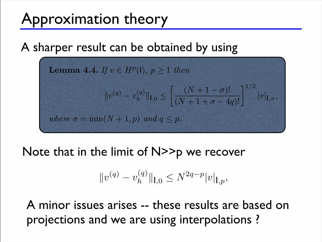
Approximation theory
A sharper result can be obtained by using
80 4 Insight through theory
Lemma 4.2. Assume that for v ! Hp(I), p " 0,
v(r) =N!
n=0
vnPn(r).
Then " 1
!1|v(q)|2(1 # r2)qdr =
!
n"q
|vn|2(n + q)!(n # q)!
$ |v|2I,q,
for 0 $ q $ p.
The proof relies on properties of the orthogonal polynomials and the detailscan be found in [280]. With this one can establish the result:
Lemma 4.3. If v ! Hp(I), p " 1, then
%v # vh%I,0 $#(N + 1 # !)!(N + 1 + !)!
$1/2
|v|I,!,
where ! = min(N + 1, p).
Proof. Through Parseval’s identity we have
%v # vh%2I,0 =
#!
n=N+1
|vn|2 =#!
n=N+1
|vn|2(n # !)!(n + !)!
(n + !)!(n # !)!
.
Provided ! $ N + 1, we have
%v # vh%2I,0 $ (N + 1 # !)!
(N + 1 + !)!
#!
n=N+1
|vn|2(n + !)!(n # !)!
,
which, combined with Lemma 4.2 and ! = min(N + 1, p), gives the result. !
A generalization of this is the following result.
Lemma 4.4. If v ! Hp(I), p " 1 then
%v(q) # v(q)h %I,0 $
#(N + 1 # !)!
(N + 1 + ! # 4q)!
$1/2
|v|I,!,
where ! = min(N + 1, p) and q $ p.
The proof follows the one above and is omitted. Note that in the limit ofN & p, the Stirling formula gives
%v(q) # v(q)h %I,0 $ N2q!p|v|I,p,
in agreement with Theorem 4.1.
Note that in the limit of N>>p we recover
A minor issues arises -- these results are based on projections and we are using interpolations ?
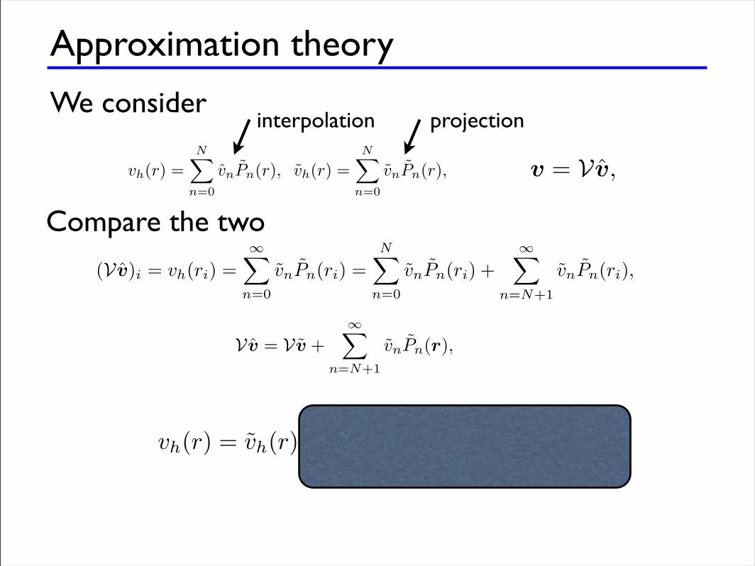
Approximation theory
We consider
4.3 Approximations by orthogonal polynomials and consistency 81
The above estimates are all related to projections. However, as we dis-cussed in Chapter 3, we are often concerned with the interpolations of vwhere
v = Vv,
is based on N + 1 points. The di!erence may be minor, but it is essential toappreciate it. Consider
vh(r) =N!
n=0
vnPn(r), vh(r) =N!
n=0
vnPn(r),
where vh(x) is the usual approximation based on interpolation and vh(r) refersto the approximation based on projection.
By the interpolation property we have
(Vv)i = vh(ri) =!!
n=0
vnPn(ri) =N!
n=0
vnPn(ri) +!!
n=N+1
vnPn(ri),
from which we recover
Vv = Vv +!!
n=N+1
vnPn(r), r = (r0, . . . , rN )T .
This implies
vh(r) = vh(r) + PT(r)V"1
!!
n=N+1
vnPn(r).
Now, consider the additional term on the right-hand side,
PT(r)V"1
!!
n=N+1
vnPn(r) =!!
n=N+1
vn
"P
T(r)V"1Pn(r)
#,
which is allowed provided v ! Hp(I), p > 1/2 [280]. Since
PT(r)V"1Pn(r) =
N!
l=0
plPl(r), Vp = Pn(r),
we can interpret the additional term as those high-order modes (recall n > N)that look like lower order modes on the grid. It is exactly this phenomenonthat is known as aliasing and which is the fundamental di!erence between aninterpolation and a projection.
The final statement, the proof of which is technical and given in [27], yieldsthe following
interpolation projection
Compare the two
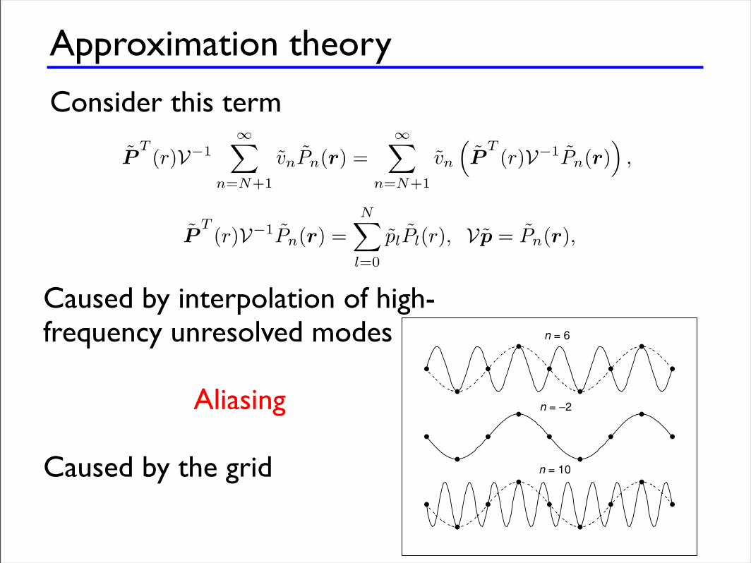
Approximation theory
Consider this term
4.3 Approximations by orthogonal polynomials and consistency 81
The above estimates are all related to projections. However, as we dis-cussed in Chapter 3, we are often concerned with the interpolations of vwhere
v = Vv,
is based on N + 1 points. The di!erence may be minor, but it is essential toappreciate it. Consider
vh(r) =N!
n=0
vnPn(r), vh(r) =N!
n=0
vnPn(r),
where vh(x) is the usual approximation based on interpolation and vh(r) refersto the approximation based on projection.
By the interpolation property we have
(Vv)i = vh(ri) =!!
n=0
vnPn(ri) =N!
n=0
vnPn(ri) +!!
n=N+1
vnPn(ri),
from which we recover
Vv = Vv +!!
n=N+1
vnPn(r), r = (r0, . . . , rN )T .
This implies
vh(r) = vh(r) + PT(r)V"1
!!
n=N+1
vnPn(r).
Now, consider the additional term on the right-hand side,
PT(r)V"1
!!
n=N+1
vnPn(r) =!!
n=N+1
vn
"P
T(r)V"1Pn(r)
#,
which is allowed provided v ! Hp(I), p > 1/2 [280]. Since
PT(r)V"1Pn(r) =
N!
l=0
plPl(r), Vp = Pn(r),
we can interpret the additional term as those high-order modes (recall n > N)that look like lower order modes on the grid. It is exactly this phenomenonthat is known as aliasing and which is the fundamental di!erence between aninterpolation and a projection.
The final statement, the proof of which is technical and given in [27], yieldsthe following
P1: FQF/GQE P2: FQF/GQE QC: FQF/GQE T1: FQF
CUUK702-Hesthaven June 6, 2006 18:54
2.2 Discrete trigonometric polynomials 31
n = 6
n = !2
n = 10
Figure 2.7 Illustration of aliasing. The three waves, n = 6, n = !2 and n = !10are all interpreted as a n = !2 wave on an 8-point grid. Consequently, the n = !2appears as more energetic after the discrete Fourier transform than in the originalsignal.
computationally different ways to approximate the derivative of a function. Inthe following subsections, we assume that our function u and all its derivativesare continuous and periodic on [0, 2! ].
Using expansion coefficients Given the values of the function u(x) at thepoints x j , differentiating the basis functions in the interpolant yields
ddx
IN u(x) =!
|n|"N/2
inuneinx , (2.17)
where
un = 1Ncn
N!1!
j=0
u(x j )e!inx j ,
are the coefficients of the interpolant IN u(x) given in Equations (2.8)–(2.9).Higher order derivatives can be obtained simply by further differentiating thebasis functions.
Note that, unlike in the case of the continuous approximation, the derivativeof the interpolant is not the interpolant of the derivative, i.e.,
INdudx
#= INd
dxIN u, (2.18)
unless u(x) $ BN .
Caused by interpolation of high-frequency unresolved modes
Aliasing
Caused by the grid
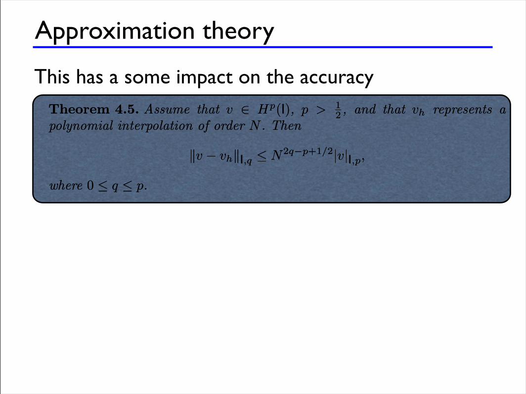
Approximation theory
This has a some impact on the accuracy82 4 Insight through theory
Theorem 4.5. Assume that v ! Hp(I), p > 12 , and that vh represents a
polynomial interpolation of order N . Then
"v # vh"I,q $ N2q!p+1/2|v|I,p,
where 0 $ q $ p.
Note in particular that the order of convergence can be up to one orderlower due to the aliasing errors, but not worse than that.
Example 4.6. Let us revisit Example 3.2 where we considered the error whencomputing the discrete derivative. Using Theorem 4.5, we get a crude estimateas
"v" #Drvh"I,0 $ "v # vh"I,1 $ N5/2!p|v|I,p.
For the first example, that is,
v(r) = exp(sin(!r)),
this confirms the exponential convergence since v(r) is analytic.However, for the second problem,
v(0)(r) =!# cos(!r), #1 $ r < 0
cos(!r), 0 $ r $ 1,dv(i+1)
dr= v(i), i = 0, 1, 2, 3 . . . ,
the situation is di!erent. Note that v(i) ! Hi(I). In this case, the computationsindicate
"(v(i))r #Drv(i)h "I,0 $ CN1/2!i,
which is considerably better than indicated by the general result. An improvedestimate, valid only for interpolation of Gauss-Lobatto grid points, is [27]
"v" #Drvh"I,0 $ N1!p|v|I,p,
and is much closer to the observed behavior but suboptimal. This is, however,a sharp result for the general case, reflecting that special cases may showbetter results.
We return to the behavior for the general element of length h to recoverthe estimates for u(x) rather than v(r). We have the following bound:
Theorem 4.7. Assume that u ! Hp(Dk) and that uh represents a piecewisepolynomial approximation of order N . Then
"u # uh"!,q,h $ Ch"!q|u|!,",h,
for 0 $ q $ ", and " = min(N + 1, p).
82 4 Insight through theory
Theorem 4.5. Assume that v ! Hp(I), p > 12 , and that vh represents a
polynomial interpolation of order N . Then
"v # vh"I,q $ N2q!p+1/2|v|I,p,
where 0 $ q $ p.
Note in particular that the order of convergence can be up to one orderlower due to the aliasing errors, but not worse than that.
Example 4.6. Let us revisit Example 3.2 where we considered the error whencomputing the discrete derivative. Using Theorem 4.5, we get a crude estimateas
"v" #Drvh"I,0 $ "v # vh"I,1 $ N5/2!p|v|I,p.
For the first example, that is,
v(r) = exp(sin(!r)),
this confirms the exponential convergence since v(r) is analytic.However, for the second problem,
v(0)(r) =!# cos(!r), #1 $ r < 0
cos(!r), 0 $ r $ 1,dv(i+1)
dr= v(i), i = 0, 1, 2, 3 . . . ,
the situation is di!erent. Note that v(i) ! Hi(I). In this case, the computationsindicate
"(v(i))r #Drv(i)h "I,0 $ CN1/2!i,
which is considerably better than indicated by the general result. An improvedestimate, valid only for interpolation of Gauss-Lobatto grid points, is [27]
"v" #Drvh"I,0 $ N1!p|v|I,p,
and is much closer to the observed behavior but suboptimal. This is, however,a sharp result for the general case, reflecting that special cases may showbetter results.
We return to the behavior for the general element of length h to recoverthe estimates for u(x) rather than v(r). We have the following bound:
Theorem 4.7. Assume that u ! Hp(Dk) and that uh represents a piecewisepolynomial approximation of order N . Then
"u # uh"!,q,h $ Ch"!q|u|!,",h,
for 0 $ q $ ", and " = min(N + 1, p).
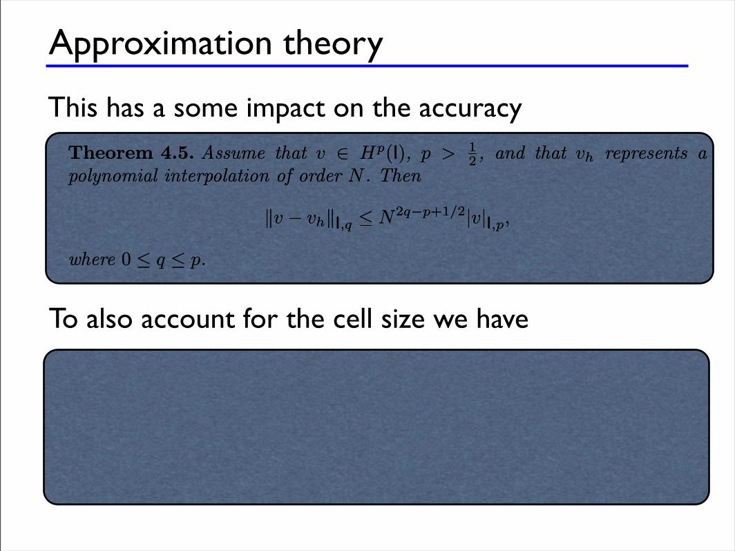
Approximation theory
This has a some impact on the accuracy82 4 Insight through theory
Theorem 4.5. Assume that v ! Hp(I), p > 12 , and that vh represents a
polynomial interpolation of order N . Then
"v # vh"I,q $ N2q!p+1/2|v|I,p,
where 0 $ q $ p.
Note in particular that the order of convergence can be up to one orderlower due to the aliasing errors, but not worse than that.
Example 4.6. Let us revisit Example 3.2 where we considered the error whencomputing the discrete derivative. Using Theorem 4.5, we get a crude estimateas
"v" #Drvh"I,0 $ "v # vh"I,1 $ N5/2!p|v|I,p.
For the first example, that is,
v(r) = exp(sin(!r)),
this confirms the exponential convergence since v(r) is analytic.However, for the second problem,
v(0)(r) =!# cos(!r), #1 $ r < 0
cos(!r), 0 $ r $ 1,dv(i+1)
dr= v(i), i = 0, 1, 2, 3 . . . ,
the situation is di!erent. Note that v(i) ! Hi(I). In this case, the computationsindicate
"(v(i))r #Drv(i)h "I,0 $ CN1/2!i,
which is considerably better than indicated by the general result. An improvedestimate, valid only for interpolation of Gauss-Lobatto grid points, is [27]
"v" #Drvh"I,0 $ N1!p|v|I,p,
and is much closer to the observed behavior but suboptimal. This is, however,a sharp result for the general case, reflecting that special cases may showbetter results.
We return to the behavior for the general element of length h to recoverthe estimates for u(x) rather than v(r). We have the following bound:
Theorem 4.7. Assume that u ! Hp(Dk) and that uh represents a piecewisepolynomial approximation of order N . Then
"u # uh"!,q,h $ Ch"!q|u|!,",h,
for 0 $ q $ ", and " = min(N + 1, p).
To also account for the cell size we have
82 4 Insight through theory
Theorem 4.5. Assume that v ! Hp(I), p > 12 , and that vh represents a
polynomial interpolation of order N . Then
"v # vh"I,q $ N2q!p+1/2|v|I,p,
where 0 $ q $ p.
Note in particular that the order of convergence can be up to one orderlower due to the aliasing errors, but not worse than that.
Example 4.6. Let us revisit Example 3.2 where we considered the error whencomputing the discrete derivative. Using Theorem 4.5, we get a crude estimateas
"v" #Drvh"I,0 $ "v # vh"I,1 $ N5/2!p|v|I,p.
For the first example, that is,
v(r) = exp(sin(!r)),
this confirms the exponential convergence since v(r) is analytic.However, for the second problem,
v(0)(r) =!# cos(!r), #1 $ r < 0
cos(!r), 0 $ r $ 1,dv(i+1)
dr= v(i), i = 0, 1, 2, 3 . . . ,
the situation is di!erent. Note that v(i) ! Hi(I). In this case, the computationsindicate
"(v(i))r #Drv(i)h "I,0 $ CN1/2!i,
which is considerably better than indicated by the general result. An improvedestimate, valid only for interpolation of Gauss-Lobatto grid points, is [27]
"v" #Drvh"I,0 $ N1!p|v|I,p,
and is much closer to the observed behavior but suboptimal. This is, however,a sharp result for the general case, reflecting that special cases may showbetter results.
We return to the behavior for the general element of length h to recoverthe estimates for u(x) rather than v(r). We have the following bound:
Theorem 4.7. Assume that u ! Hp(Dk) and that uh represents a piecewisepolynomial approximation of order N . Then
"u # uh"!,q,h $ Ch"!q|u|!,",h,
for 0 $ q $ ", and " = min(N + 1, p).
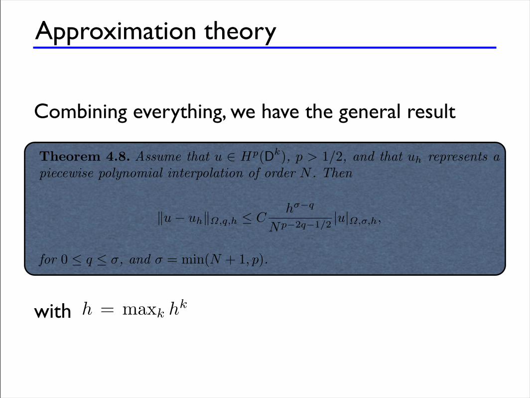
Approximation theory
Combining everything, we have the general result
4.4 Stability 83
Proof. Introduce the new variable
v(r) = u(hr) = u(x).
Then
|v|2I,q =!
I
"v(q)
#2dr =
!
Dkh2q!1
"u(q)
#2dx = h2q!1|u|2Dk
,q.
Similarly fashion, we have
!u!2Dk
,q=
q$
p=0
|u|2Dk,p
=q$
p=0
h1!2p|v|2I,p " h1!2q!v!2I,q.
We combine these estimates to obtain
!u # uh!2Dk
,q" h1!2q!v # vh!2
I,q " h1!2q|v|2I,! = h2!!2q|u|2Dk,!
,
where we have used Lemma 4.4 and defined ! = min(N +1, p). Summing overall elements yields the result. !
For a more general grid where the element length is variable, it is natural touse h = maxk hk (i.e., the maximum interval length). Combining this withTheorem 4.7 yields the main approximation result:
Theorem 4.8. Assume that u $ Hp(Dk), p > 1/2, and that uh represents apiecewise polynomial interpolation of order N . Then
!u # uh!",q,h " Ch!!q
Np!2q!1/2|u|",!,h,
for 0 " q " !, and ! = min(N + 1, p).
This result gives the essence of the approximation properties; that is, it showsclearly under which conditions on u we can expect consistency and whatconvergence rate to expect depending on the regularity of u and the norm inwhich the error is measured.
4.4 Stability
Stability is, in many ways, harder to deal with than consistency. In Chapter2 we established stability for the simple scalar problem
"u
"t+ a
"u
"x= 0,
with
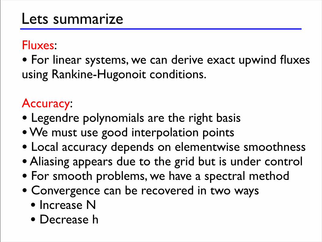
Lets summarize
Fluxes:• For linear systems, we can derive exact upwind fluxes using Rankine-Hugonoit conditions.
Accuracy:• Legendre polynomials are the right basis• We must use good interpolation points• Local accuracy depends on elementwise smoothness• Aliasing appears due to the grid but is under control• For smooth problems, we have a spectral method• Convergence can be recovered in two ways• Increase N• Decrease h