Embed Size (px)
Citation preview
Discrete Structures - CM0246Introduction
Andrés Sicard-Ramírez
Universidad EAFIT
Semester 2014-2
Administrative Information
Course CoordinatorAndrés Sicard Ramírez
Head of the Department of Mathematical SciencesCarlos Mario Vélez Sánchez
Course web pagehttp://www1.eafit.edu.co/asr/courses/discrete-structures-CM0246/
Exams, textbook, etc.See course web page.
Introduction 2/9
Discrete Structures
Definition of ‘discrete’Adjective. Individually separate and distinct. Late Middle English. FromLatin discretus ‘separate’.†
Adjetivo. Separado, distinto.‡
DescriptionAbstract mathematical structures used to represent discrete objects (separ-ated from each other) and relationships between these objects.
ExamplesSets, relations, graphs, trees, finite-state machines, among others.
†From http://www.oxforddictionaries.com .‡From http://www.rae.es/drae .
Introduction 3/9
Discrete Structures
Definition of ‘discrete’Adjective. Individually separate and distinct. Late Middle English. FromLatin discretus ‘separate’.†
Adjetivo. Separado, distinto.‡
DescriptionAbstract mathematical structures used to represent discrete objects (separ-ated from each other) and relationships between these objects.
ExamplesSets, relations, graphs, trees, finite-state machines, among others.
†From http://www.oxforddictionaries.com .‡From http://www.rae.es/drae .
Introduction 4/9
Discrete Structures
Applications
Algorithm designAutomata theoryBio-informaticsComplexity theoryComputabilityCryptography
Formal languagesGenetic algorithmsMathematical modellingNetwork flowsSimulations
Introduction 5/9
Course Outline
Functions, infinite sets, and mathematical and structural induction
Relations (representation, equivalence relations)
Ordering relations (partial orders, lexicographical orders, Hassediagrams, notable elements, lattices, Boolean algebras)
Graphs (classification, representation, Euler and Hamilton paths,shortest-path problems, planar graphs, graph coloring)
Introduction 6/9
Course Outline
Functions, infinite sets, and mathematical and structural induction
Relations (representation, equivalence relations)
Ordering relations (partial orders, lexicographical orders, Hassediagrams, notable elements, lattices, Boolean algebras)
Graphs (classification, representation, Euler and Hamilton paths,shortest-path problems, planar graphs, graph coloring)
Introduction 7/9
Course Outline
Functions, infinite sets, and mathematical and structural induction
Relations (representation, equivalence relations)
Ordering relations (partial orders, lexicographical orders, Hassediagrams, notable elements, lattices, Boolean algebras)
Graphs (classification, representation, Euler and Hamilton paths,shortest-path problems, planar graphs, graph coloring)
Introduction 8/9
Course Outline
Functions, infinite sets, and mathematical and structural induction
Relations (representation, equivalence relations)
Ordering relations (partial orders, lexicographical orders, Hassediagrams, notable elements, lattices, Boolean algebras)
Graphs (classification, representation, Euler and Hamilton paths,shortest-path problems, planar graphs, graph coloring)
Introduction 9/9
Discrete Structures - CM0246Functions
Andrés Sicard-Ramírez
Universidad EAFIT
Semester 2014-2
Preliminaries
ConventionIf an element of a set is listed more than once it doesn’t matter.
Example{1, 3, 3, 3, 5, 5, 5, 5} = {1, 3, 5}.
Functions 2/60
Preliminaries
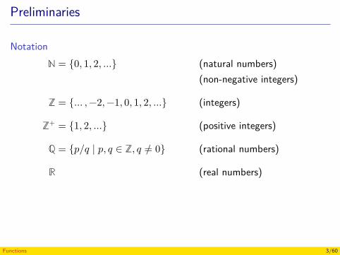
Notationℕ = {0, 1, 2, …} (natural numbers)
(non-negative integers)
ℤ = {… , −2, −1, 0, 1, 2, …} (integers)
ℤ+ = {1, 2, …} (positive integers)
ℚ = {𝑝/𝑞 ∣ 𝑝, 𝑞 ∈ ℤ, 𝑞 ≠ 0} (rational numbers)
ℝ (real numbers)
Functions 3/60
Functions
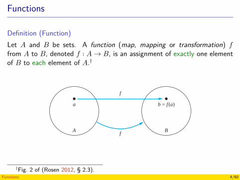
Definition (Function)Let 𝐴 and 𝐵 be sets. A function (map, mapping or transformation) 𝑓from 𝐴 to 𝐵, denoted 𝑓 ∶ 𝐴 → 𝐵, is an assignment of exactly one elementof 𝐵 to each element of 𝐴.†
2.3 Functions 139
Adams
Chou
Goodfriend
Rodriguez
Stevens
A
B
C
D
F
FIGURE 1 Assignment of Grades in a Discrete Mathematics Class.
which are functions defined in terms of themselves, are used throughout computer science; theywill be studied in Chapter 5. This section reviews the basic concepts involving functions neededin discrete mathematics.
DEFINITION 1 Let A and B be nonempty sets. A function f from A to B is an assignment of exactly oneelement of B to each element of A. We write f (a) = b if b is the unique element of B
assigned by the function f to the element a of A. If f is a function from A to B, we writef : A→ B.
Remark: Functions are sometimes also called mappings or transformations.
Functions are specified in many different ways. Sometimes we explicitly state the assign-ments, as in Figure 1. Often we give a formula, such as f (x) = x + 1, to define a function.Other times we use a computer program to specify a function.
A function f : A→ B can also be defined in terms of a relation from A to B. Recall fromSection 2.1 that a relation from A to B is just a subset of A× B. A relation from A to B thatcontains one, and only one, ordered pair (a, b) for every element a ∈ A, defines a function f
from A to B. This function is defined by the assignment f (a) = b, where (a, b) is the uniqueordered pair in the relation that has a as its first element.
DEFINITION 2 If f is a function from A to B, we say that A is the domain of f and B is the codomain of f.
If f (a) = b, we say that b is the image of a and a is a preimage of b. The range, or image,of f is the set of all images of elements of A. Also, if f is a function from A to B, we saythat f maps A to B.
Figure 2 represents a function f from A to B.When we define a function we specify its domain, its codomain, and the mapping of elements
of the domain to elements in the codomain. Two functions are equal when they have the samedomain, have the same codomain, and map each element of their common domain to the sameelement in their common codomain. Note that if we change either the domain or the codomain
A B
a b = f (a)
f
f
FIGURE 2 The Function f Maps A to B.
†Fig. 2 of (Rosen 2012, § 2.3).Functions 4/60
Functions
Specification of functionsExplicitly
FormulaProgramming languages
(Advance) questionAre all the functions define using a programming language really functions?
Functions 5/60
Functions
Specification of functionsExplicitlyFormula
Programming languages
(Advance) questionAre all the functions define using a programming language really functions?
Functions 6/60
Functions
Specification of functionsExplicitlyFormulaProgramming languages
(Advance) questionAre all the functions define using a programming language really functions?
Functions 7/60
Functions
Specification of functionsExplicitlyFormulaProgramming languages
(Advance) questionAre all the functions define using a programming language really functions?
Functions 8/60
Functions
Definitions (Domain, codomain, image, preimage and range)Let 𝑓 be a function from 𝐴 to 𝐵:Domain of 𝑓 : 𝐴Codomain of 𝑓 : 𝐵
If 𝑓(𝑎) = 𝑏:𝑏 is the image of 𝑎𝑎 is a preimage of 𝑏The range or image of 𝑓 : Set of all images of elements of 𝐴If 𝑆 is a subset of 𝐴: 𝑓(𝑆) = {𝑓() ∣ 𝑠 ∈ 𝑆}
Functions 9/60
Functions
Definitions (Domain, codomain, image, preimage and range)Let 𝑓 be a function from 𝐴 to 𝐵:Domain of 𝑓 : 𝐴Codomain of 𝑓 : 𝐵If 𝑓(𝑎) = 𝑏:𝑏 is the image of 𝑎𝑎 is a preimage of 𝑏The range or image of 𝑓 : Set of all images of elements of 𝐴
If 𝑆 is a subset of 𝐴: 𝑓(𝑆) = {𝑓() ∣ 𝑠 ∈ 𝑆}
Functions 10/60
Functions
Definitions (Domain, codomain, image, preimage and range)Let 𝑓 be a function from 𝐴 to 𝐵:Domain of 𝑓 : 𝐴Codomain of 𝑓 : 𝐵If 𝑓(𝑎) = 𝑏:𝑏 is the image of 𝑎𝑎 is a preimage of 𝑏The range or image of 𝑓 : Set of all images of elements of 𝐴If 𝑆 is a subset of 𝐴: 𝑓(𝑆) = {𝑓() ∣ 𝑠 ∈ 𝑆}
Functions 11/60
Functions
ExampleSee slides § 2.3, p. 2 for the 6th ed. of Rosen’s textbook.
Exercise (Rosen (2004), Problem 3, p. 99)Determine whether 𝑓 is a function from the set of all bit strings to the setof integers if
𝑓(𝑠) is the number of 1 bits in 𝑠𝑓(𝑠) is the position of a 0 bit in 𝑠𝑓(𝑠) is the smallest integer 𝑖 such that the 𝑖th bit of 𝑠 is 1 and𝑓(𝑠) = 0 when 𝑠 is the empty string
Functions 12/60
Functions
ExampleSee slides § 2.3, p. 2 for the 6th ed. of Rosen’s textbook.
Exercise (Rosen (2004), Problem 3, p. 99)Determine whether 𝑓 is a function from the set of all bit strings to the setof integers if
𝑓(𝑠) is the number of 1 bits in 𝑠
𝑓(𝑠) is the position of a 0 bit in 𝑠𝑓(𝑠) is the smallest integer 𝑖 such that the 𝑖th bit of 𝑠 is 1 and𝑓(𝑠) = 0 when 𝑠 is the empty string
Functions 13/60
Functions
ExampleSee slides § 2.3, p. 2 for the 6th ed. of Rosen’s textbook.
Exercise (Rosen (2004), Problem 3, p. 99)Determine whether 𝑓 is a function from the set of all bit strings to the setof integers if
𝑓(𝑠) is the number of 1 bits in 𝑠𝑓(𝑠) is the position of a 0 bit in 𝑠
𝑓(𝑠) is the smallest integer 𝑖 such that the 𝑖th bit of 𝑠 is 1 and𝑓(𝑠) = 0 when 𝑠 is the empty string
Functions 14/60
Functions
ExampleSee slides § 2.3, p. 2 for the 6th ed. of Rosen’s textbook.
Exercise (Rosen (2004), Problem 3, p. 99)Determine whether 𝑓 is a function from the set of all bit strings to the setof integers if
𝑓(𝑠) is the number of 1 bits in 𝑠𝑓(𝑠) is the position of a 0 bit in 𝑠𝑓(𝑠) is the smallest integer 𝑖 such that the 𝑖th bit of 𝑠 is 1 and𝑓(𝑠) = 0 when 𝑠 is the empty string
Functions 15/60
Functions
Definition (Cartesian product)Let 𝐴 and 𝐵 be sets. The Cartesian product of 𝐴 and 𝐵 is
𝐴 × 𝐵 = {(𝑎, 𝑏) ∣ 𝑎 ∈ 𝐴 ∧ 𝑏 ∈ 𝐵}.ExampleLet 𝐴 = {𝑎, 𝑏} and 𝐵 = {1, 2}. Then
𝐴 × 𝐵 = {(𝑎, 1), (𝑎, 2), (𝑏, 1), (𝑏, 2)}.
Definition (Relation)A subset 𝑅 of the Cartesian product 𝐴 × 𝐵 is called a relation from theset 𝐴 to the set 𝐵.
Functions 16/60
Functions
Definition (Cartesian product)Let 𝐴 and 𝐵 be sets. The Cartesian product of 𝐴 and 𝐵 is
𝐴 × 𝐵 = {(𝑎, 𝑏) ∣ 𝑎 ∈ 𝐴 ∧ 𝑏 ∈ 𝐵}.ExampleLet 𝐴 = {𝑎, 𝑏} and 𝐵 = {1, 2}. Then
𝐴 × 𝐵 = {(𝑎, 1), (𝑎, 2), (𝑏, 1), (𝑏, 2)}.
Definition (Relation)A subset 𝑅 of the Cartesian product 𝐴 × 𝐵 is called a relation from theset 𝐴 to the set 𝐵.
Functions 17/60
Functions
Definition (Function)Let 𝐴 and 𝐵 be sets. A function 𝑓 from 𝐴 to 𝐵 is a relation of 𝐴 to 𝐵(i.e. subset of 𝐴 × 𝐵) such that
∀𝑥 [𝑥 ∈ 𝐴 → ∃𝑦 [𝑦 ∈ 𝐵 ∧ (𝑥, 𝑦) ∈ 𝑓]]
and
∀𝑥∀𝑦∀𝑦′ {[(𝑥, 𝑦) ∈ 𝑓 ∧ (𝑥, 𝑦′) ∈ 𝑓] → 𝑦 = 𝑦′}.RemarkIn some theories different to set theory, the concept of function is aprimitive concept.
Functions 18/60
Injective Functions
Definition (Injective function)Let 𝑓 ∶ 𝐴 → 𝐵. The function 𝑓 is an injunction (or one-to-one),if and only if,𝑓(𝑎) = 𝑓(𝑎′) implies that 𝑎 = 𝑎′ for all 𝑎, 𝑎′ ∈ 𝐴.
ExamplesWhiteboard.
Functions 19/60
Injective Functions
Definition (Injective function)Let 𝑓 ∶ 𝐴 → 𝐵. The function 𝑓 is an injunction (or one-to-one),if and only if,𝑓(𝑎) = 𝑓(𝑎′) implies that 𝑎 = 𝑎′ for all 𝑎, 𝑎′ ∈ 𝐴.
ExamplesWhiteboard.
Functions 20/60
Injective Functions
Definition (Injective function)Let 𝑓 ∶ 𝐴 → 𝐵. The function 𝑓 is an injunction, if and only if,
∀𝑥∀𝑥′ (𝑓(𝑥) = 𝑓(𝑥′) → 𝑥 = 𝑥′)or equivalent
∀𝑥∀𝑥′ [𝑥 ≠ 𝑥′ → 𝑓(𝑥) ≠ 𝑓(𝑥′)] (contrapositive)
where 𝐴 is the domain of quantification.
Functions 21/60
Injective Functions
Is a function (non)-injective?Let 𝑓 ∶ 𝐴 → 𝐵.
To show that 𝑓 is injectiveShow that if 𝑓(𝑥) = 𝑓(𝑥′) for arbitrary 𝑥, 𝑥′ ∈ 𝐴 then 𝑥 = 𝑥′.
To show that 𝑓 is not injectiveFind particular elements 𝑥, 𝑥′ ∈ 𝐴 such that 𝑥 ≠ 𝑥′ and𝑓(𝑥) = 𝑓(𝑥′).
ExerciseIs the function 𝑓 ∶ ℤ → ℤ, where 𝑓(𝑥) = 𝑥2 injective?
Functions 22/60
Injective Functions
Is a function (non)-injective?Let 𝑓 ∶ 𝐴 → 𝐵.
To show that 𝑓 is injectiveShow that if 𝑓(𝑥) = 𝑓(𝑥′) for arbitrary 𝑥, 𝑥′ ∈ 𝐴 then 𝑥 = 𝑥′.To show that 𝑓 is not injectiveFind particular elements 𝑥, 𝑥′ ∈ 𝐴 such that 𝑥 ≠ 𝑥′ and𝑓(𝑥) = 𝑓(𝑥′).
ExerciseIs the function 𝑓 ∶ ℤ → ℤ, where 𝑓(𝑥) = 𝑥2 injective?
Functions 23/60
Injective Functions
Is a function (non)-injective?Let 𝑓 ∶ 𝐴 → 𝐵.
To show that 𝑓 is injectiveShow that if 𝑓(𝑥) = 𝑓(𝑥′) for arbitrary 𝑥, 𝑥′ ∈ 𝐴 then 𝑥 = 𝑥′.To show that 𝑓 is not injectiveFind particular elements 𝑥, 𝑥′ ∈ 𝐴 such that 𝑥 ≠ 𝑥′ and𝑓(𝑥) = 𝑓(𝑥′).
ExerciseIs the function 𝑓 ∶ ℤ → ℤ, where 𝑓(𝑥) = 𝑥2 injective?
Functions 24/60
Surjective Functions
Definition (Surjective function)Let 𝑓 ∶ 𝐴 → 𝐵. The function 𝑓 is a surjection (or onto),if and only if,for every element 𝑏 ∈ 𝐵 there is an element 𝑎 ∈ 𝐴 with 𝑓(𝑎) = 𝑏.
ExamplesWhiteboard.
Functions 25/60
Surjective Functions
Definition (Surjective function)Let 𝑓 ∶ 𝐴 → 𝐵. The function 𝑓 is a surjection (or onto),if and only if,for every element 𝑏 ∈ 𝐵 there is an element 𝑎 ∈ 𝐴 with 𝑓(𝑎) = 𝑏.
ExamplesWhiteboard.
Functions 26/60
Surjective Functions
Definition (Surjective function)Let 𝑓 ∶ 𝐴 → 𝐵. The function 𝑓 is a surjection, if and only if,
∀𝑦∃𝑥 (𝑓(𝑥) = 𝑦),
where 𝐴 is the domain of quantification for 𝑥 and 𝐵 is the domain ofquantification for 𝑦.
Functions 27/60
Surjective Functions
Is a function (non)-surjective?Let 𝑓 ∶ 𝐴 → 𝐵.
To show that 𝑓 is surjectiveConsider an arbitrary element 𝑦 ∈ 𝐵 and find an element 𝑥 ∈ 𝐴 suchthat 𝑓(𝑥) = 𝑦.
To show that 𝑓 is not surjectiveFind a particular 𝑦 ∈ 𝐵 such that 𝑓(𝑥) ≠ 𝑦 for all 𝑥 ∈ 𝐴.
ExerciseIs the function 𝑓 ∶ ℤ → ℤ, where 𝑓(𝑥) = 𝑥 + 1 surjective?
Functions 28/60
Surjective Functions
Is a function (non)-surjective?Let 𝑓 ∶ 𝐴 → 𝐵.
To show that 𝑓 is surjectiveConsider an arbitrary element 𝑦 ∈ 𝐵 and find an element 𝑥 ∈ 𝐴 suchthat 𝑓(𝑥) = 𝑦.To show that 𝑓 is not surjectiveFind a particular 𝑦 ∈ 𝐵 such that 𝑓(𝑥) ≠ 𝑦 for all 𝑥 ∈ 𝐴.
ExerciseIs the function 𝑓 ∶ ℤ → ℤ, where 𝑓(𝑥) = 𝑥 + 1 surjective?
Functions 29/60
Surjective Functions
Is a function (non)-surjective?Let 𝑓 ∶ 𝐴 → 𝐵.
To show that 𝑓 is surjectiveConsider an arbitrary element 𝑦 ∈ 𝐵 and find an element 𝑥 ∈ 𝐴 suchthat 𝑓(𝑥) = 𝑦.To show that 𝑓 is not surjectiveFind a particular 𝑦 ∈ 𝐵 such that 𝑓(𝑥) ≠ 𝑦 for all 𝑥 ∈ 𝐴.
ExerciseIs the function 𝑓 ∶ ℤ → ℤ, where 𝑓(𝑥) = 𝑥 + 1 surjective?
Functions 30/60
Bijective Functions
Definition (Bijective function)A function 𝑓 is a bijection (or one-to-one correspondence),if and only if,it is both injective and surjective.
Example (The identity function)Let 𝐴 be a set. The identity function 𝜄𝐴 ∶ 𝐴 → 𝐴 where 𝜄𝐴(𝑎) = 𝑎 isbijective.
Functions 31/60
Bijective Functions
Definition (Bijective function)A function 𝑓 is a bijection (or one-to-one correspondence),if and only if,it is both injective and surjective.
Example (The identity function)Let 𝐴 be a set. The identity function 𝜄𝐴 ∶ 𝐴 → 𝐴 where 𝜄𝐴(𝑎) = 𝑎 isbijective.
Functions 32/60
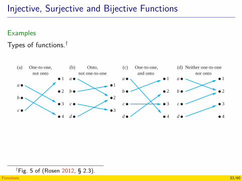
Injective, Surjective and Bijective Functions
ExamplesTypes of functions.†144 2 / Basic Structures: Sets, Functions, Sequences, Sums, and Matrices
a
b
c
1
2
3
4
a
b
c
d
1
2
3
a
b
c
d
1
2
3
4
a
b
c
d
1
2
3
4
a
b
c
1
2
3
4
One-to-one,not onto
Onto,not one-to-one
One-to-one,and onto
Neither one-to-onenor onto
Not a function(a) (b) (c) (d) (e)
FIGURE 5 Examples of Different Types of Correspondences.
Solution: This function is onto, because for every integer y there is an integer x such thatf (x) = y. To see this, note that f (x) = y if and only if x + 1 = y, which holds if and only ifx = y − 1. ▲
EXAMPLE 15 Consider the function f in Example 11 that assigns jobs to workers. The function f is onto iffor every job there is a worker assigned this job. The function f is not onto when there is atleast one job that has no worker assigned it. ▲
DEFINITION 8 The function f is a one-to-one correspondence, or a bijection, if it is both one-to-one andonto. We also say that such a function is bijective.
Examples 16 and 17 illustrate the concept of a bijection.
EXAMPLE 16 Let f be the function from {a, b, c, d} to {1, 2, 3, 4} with f (a) = 4, f (b) = 2, f (c) = 1, andf (d) = 3. Is f a bijection?
Solution: The function f is one-to-one and onto. It is one-to-one because no two values inthe domain are assigned the same function value. It is onto because all four elements of thecodomain are images of elements in the domain. Hence, f is a bijection. ▲
Figure 5 displays four functions where the first is one-to-one but not onto, the second is ontobut not one-to-one, the third is both one-to-one and onto, and the fourth is neither one-to-onenor onto. The fifth correspondence in Figure 5 is not a function, because it sends an element totwo different elements.
Suppose that f is a function from a set A to itself. If A is finite, then f is one-to-one if andonly if it is onto. (This follows from the result in Exercise 72.) This is not necessarily the caseif A is infinite (as will be shown in Section 2.5).
EXAMPLE 17 Let A be a set. The identity function on A is the function ιA : A→ A, where
ιA(x) = x
for all x ∈ A. In other words, the identity function ιA is the function that assigns each elementto itself. The function ιA is one-to-one and onto, so it is a bijection. (Note that ι is the Greekletter iota.) ▲
For future reference, we summarize what needs be to shown to establish whether a functionis one-to-one and whether it is onto. It is instructive to review Examples 8–17 in light of thissummary.
†Fig. 5 of (Rosen 2012, § 2.3).Functions 33/60
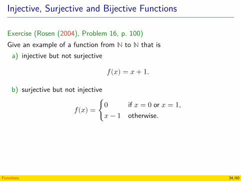
Injective, Surjective and Bijective Functions
Exercise (Rosen (2004), Problem 16, p. 100)Give an example of a function from ℕ to ℕ that is
a) injective but not surjective
𝑓(𝑥) = 𝑥 + 1.
b) surjective but not injective
𝑓(𝑥) = {0 if 𝑥 = 0 or 𝑥 = 1,𝑥 − 1 otherwise.
Functions 34/60
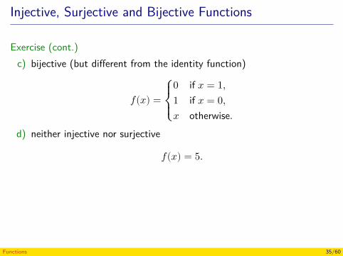
Injective, Surjective and Bijective Functions
Exercise (cont.)c) bijective (but different from the identity function)
𝑓(𝑥) =⎧{⎨{⎩
0 if 𝑥 = 1,1 if 𝑥 = 0,𝑥 otherwise.
d) neither injective nor surjective
𝑓(𝑥) = 5.
Functions 35/60
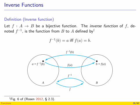
Inverse Functions
Definition (Inverse function)Let 𝑓 ∶ 𝐴 → 𝐵 be a bijective function. The inverse function of 𝑓 , de-noted 𝑓−1, is the function from 𝐵 to 𝐴 defined by†
𝑓−1(𝑏) = 𝑎 iff 𝑓(𝑎) = 𝑏.
2.3 Functions 145
Suppose that f : A→ B.
To show that f is injective Show that if f (x) = f (y) for arbitrary x, y ∈ A with x �= y,then x = y.
To show that f is not injective Find particular elements x, y ∈ A such that x �= y andf (x) = f (y).
To show that f is surjective Consider an arbitrary element y ∈ B and find an element x ∈ A
such that f (x) = y.
To show that f is not surjective Find a particular y ∈ B such that f (x) �= y for all x ∈ A.
Inverse Functions and Compositions of Functions
Now consider a one-to-one correspondence f from the set A to the set B. Because f is an ontofunction, every element of B is the image of some element in A. Furthermore, because f is alsoa one-to-one function, every element of B is the image of a unique element of A. Consequently,we can define a new function from B to A that reverses the correspondence given by f . Thisleads to Definition 9.
DEFINITION 9 Let f be a one-to-one correspondence from the set A to the set B. The inverse function off is the function that assigns to an element b belonging to B the unique element a in A
such that f (a) = b. The inverse function of f is denoted by f−1. Hence, f−1(b) = a whenf (a) = b.
Remark: Be sure not to confuse the function f−1 with the function 1/f , which is the functionthat assigns to each x in the domain the value 1/f (x). Notice that the latter makes sense onlywhen f (x) is a non-zero real number.
Figure 6 illustrates the concept of an inverse function.If a function f is not a one-to-one correspondence, we cannot define an inverse function of
f . When f is not a one-to-one correspondence, either it is not one-to-one or it is not onto. Iff is not one-to-one, some element b in the codomain is the image of more than one element inthe domain. If f is not onto, for some element b in the codomain, no element a in the domainexists for which f (a) = b. Consequently, if f is not a one-to-one correspondence, we cannotassign to each element b in the codomain a unique element a in the domain such that f (a) = b
(because for some b there is either more than one such a or no such a).A one-to-one correspondence is called invertible because we can define an inverse of this
function. A function is not invertible if it is not a one-to-one correspondence, because theinverse of such a function does not exist.
f
A B
a = f –1(b) b = f (a)f (a)
f –1(b)
f –1
FIGURE 6 The Function f −1 Is the Inverse of Function f .†Fig. 6 of (Rosen 2012, § 2.3).Functions 36/60
Inverse Functions
ExampleLet 𝑓 ∶ ℤ → ℤ, where 𝑓(𝑥) = 𝑥 + 1. Find 𝑓−1.
RemarkIf a function 𝑓 is not bijective, we cannot define 𝑓−1. Why?
Functions 37/60
Inverse Functions
ExampleLet 𝑓 ∶ ℤ → ℤ, where 𝑓(𝑥) = 𝑥 + 1. Find 𝑓−1.
RemarkIf a function 𝑓 is not bijective, we cannot define 𝑓−1. Why?
Functions 38/60
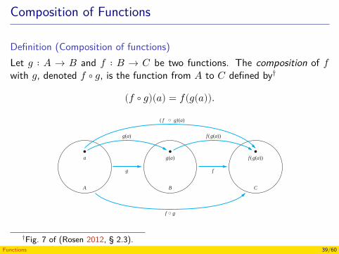
Composition of Functions
Definition (Composition of functions)Let 𝑔 ∶ 𝐴 → 𝐵 and 𝑓 ∶ 𝐵 → 𝐶 be two functions. The composition of 𝑓with 𝑔, denoted 𝑓 ∘ 𝑔, is the function from 𝐴 to 𝐶 defined by†
(𝑓 ∘ 𝑔)(𝑎) = 𝑓(𝑔(𝑎)). 2.3 Functions 147
A B
a g(a)
g(a)
C
f (g(a))
f (g(a))
g f
( f g)(a)
f g
FIGURE 7 The Composition of the Functions f and g.
EXAMPLE 22 Let g be the function from the set {a, b, c} to itself such that g(a) = b, g(b) = c, and g(c) = a.Let f be the function from the set {a, b, c} to the set {1, 2, 3} such that f (a) = 3, f (b) = 2, andf (c) = 1. What is the composition of f and g, and what is the composition of g and f ?
Solution: The composition f ◦ g is defined by (f ◦ g)(a) = f (g(a)) = f (b) = 2,(f ◦ g) (b) = f (g(b)) = f (c) = 1, and (f ◦ g)(c) = f (g(c)) = f (a) = 3.
Note that g ◦ f is not defined, because the range of f is not a subset of the domain of g. ▲EXAMPLE 23 Let f and g be the functions from the set of integers to the set of integers defined by
f (x) = 2x + 3 and g(x) = 3x + 2. What is the composition of f and g? What is the com-position of g and f ?
Solution: Both the compositions f ◦ g and g ◦ f are defined. Moreover,
(f ◦ g)(x) = f (g(x)) = f (3x + 2) = 2(3x + 2)+ 3 = 6x + 7
and
(g ◦ f )(x) = g(f (x)) = g(2x + 3) = 3(2x + 3)+ 2 = 6x + 11. ▲
Remark: Note that even though f ◦ g and g ◦ f are defined for the functions f and g inExample 23, f ◦ g and g ◦ f are not equal. In other words, the commutative law does not holdfor the composition of functions.
When the composition of a function and its inverse is formed, in either order, an identityfunction is obtained. To see this, suppose that f is a one-to-one correspondence from the set A
to the set B. Then the inverse function f−1 exists and is a one-to-one correspondence from B
to A. The inverse function reverses the correspondence of the original function, so f−1(b) = a
when f (a) = b, and f (a) = b when f−1(b) = a. Hence,
(f−1 ◦ f )(a) = f−1(f (a)) = f−1(b) = a,
and
(f ◦ f−1)(b) = f (f−1(b)) = f (a) = b.
Consequently f−1 ◦ f = ιA and f ◦ f−1 = ιB , where ιA and ιB are the identity functions onthe sets A and B, respectively. That is, (f−1)−1 = f .
†Fig. 7 of (Rosen 2012, § 2.3).Functions 39/60
Composition of Functions
ExampleSee slides § 2.3, p. 8 for the 6th ed. of Rosen’s textbook.
RemarkLet 𝑓 and 𝑔 be functions. The composition 𝑓 ∘ 𝑔 cannot be defined unlessthe range of 𝑔 is a subset of the domain of 𝑓 .
Functions 40/60
Composition of Functions
ExampleSee slides § 2.3, p. 8 for the 6th ed. of Rosen’s textbook.
RemarkLet 𝑓 and 𝑔 be functions. The composition 𝑓 ∘ 𝑔 cannot be defined unlessthe range of 𝑔 is a subset of the domain of 𝑓 .
Functions 41/60
Composition of Functions
ExampleLet 𝑓 ∶ 𝐴 → 𝐵 a bijective function such that 𝑓(𝑎) = 𝑏.The function 𝑓 ∘ 𝑓−1 ∶ 𝐵 → 𝐵 is defined by
(𝑓 ∘ 𝑓−1)(𝑏) = 𝑓(𝑓−1(𝑏)) (by def. of composition)= 𝑓(𝑎) (by def. of inverse function)= 𝑏 (by def. of inverse function)
that is, 𝑓 ∘ 𝑓−1 = 𝜄𝐵.
Functions 42/60
Composition of Functions
In general, the composition of function is not commutative.
ExampleLet 𝑓, 𝑔 ∶ ℕ → ℕ be functions, where 𝑓(𝑥) = 𝑥2 and 𝑔(𝑥) = 2𝑥 + 1. Showthat 𝑓 ∘ 𝑔 ≠ 𝑔 ∘ 𝑓 .
Functions 43/60
Composition of Functions
In general, the composition of function is not commutative.
ExampleLet 𝑓, 𝑔 ∶ ℕ → ℕ be functions, where 𝑓(𝑥) = 𝑥2 and 𝑔(𝑥) = 2𝑥 + 1. Showthat 𝑓 ∘ 𝑔 ≠ 𝑔 ∘ 𝑓 .
Functions 44/60
Composition of Functions
Example (Rosen (2004), Problem 25(b), p. 100)Let 𝑔 ∶ 𝐴 → 𝐵 and 𝑓 ∶ 𝐵 → 𝐶 be two functions. Show that if both 𝑓 and𝑔 are surjective functions, then 𝑓 ∘ 𝑔 is also surjective.
Functions 45/60
Composition of Functions
Example (cont.)
Proof.1. Let 𝑐 ∈ 𝐶.
2. 𝑓(𝑏) = 𝑐, for some 𝑏 ∈ 𝐵 (𝑓 is surjective by hypothesis)3. 𝑔(𝑎) = 𝑏, for some 𝑎 ∈ 𝐴 (𝑔 is surjective by hypothesis)4. Then
(𝑓 ∘ 𝑔)(𝑎) = 𝑓(𝑔(𝑎)) (by def. of composition)= 𝑓(𝑏) (by 3)= 𝑐 (by 2)
5. That is, for all 𝑐 ∈ 𝐶, exists 𝑎 ∈ 𝐴 such (𝑓 ∘ 𝑔)(𝑎) = 𝑐.6. 𝑓 ∘ 𝑔 is surjective (by def. of composition).
Functions 46/60
Composition of Functions
Example (cont.)
Proof.1. Let 𝑐 ∈ 𝐶.2. 𝑓(𝑏) = 𝑐, for some 𝑏 ∈ 𝐵 (𝑓 is surjective by hypothesis)
3. 𝑔(𝑎) = 𝑏, for some 𝑎 ∈ 𝐴 (𝑔 is surjective by hypothesis)4. Then
(𝑓 ∘ 𝑔)(𝑎) = 𝑓(𝑔(𝑎)) (by def. of composition)= 𝑓(𝑏) (by 3)= 𝑐 (by 2)
5. That is, for all 𝑐 ∈ 𝐶, exists 𝑎 ∈ 𝐴 such (𝑓 ∘ 𝑔)(𝑎) = 𝑐.6. 𝑓 ∘ 𝑔 is surjective (by def. of composition).
Functions 47/60
Composition of Functions
Example (cont.)
Proof.1. Let 𝑐 ∈ 𝐶.2. 𝑓(𝑏) = 𝑐, for some 𝑏 ∈ 𝐵 (𝑓 is surjective by hypothesis)3. 𝑔(𝑎) = 𝑏, for some 𝑎 ∈ 𝐴 (𝑔 is surjective by hypothesis)
4. Then(𝑓 ∘ 𝑔)(𝑎) = 𝑓(𝑔(𝑎)) (by def. of composition)
= 𝑓(𝑏) (by 3)= 𝑐 (by 2)
5. That is, for all 𝑐 ∈ 𝐶, exists 𝑎 ∈ 𝐴 such (𝑓 ∘ 𝑔)(𝑎) = 𝑐.6. 𝑓 ∘ 𝑔 is surjective (by def. of composition).
Functions 48/60
Composition of Functions
Example (cont.)
Proof.1. Let 𝑐 ∈ 𝐶.2. 𝑓(𝑏) = 𝑐, for some 𝑏 ∈ 𝐵 (𝑓 is surjective by hypothesis)3. 𝑔(𝑎) = 𝑏, for some 𝑎 ∈ 𝐴 (𝑔 is surjective by hypothesis)4. Then
(𝑓 ∘ 𝑔)(𝑎) = 𝑓(𝑔(𝑎)) (by def. of composition)= 𝑓(𝑏) (by 3)= 𝑐 (by 2)
5. That is, for all 𝑐 ∈ 𝐶, exists 𝑎 ∈ 𝐴 such (𝑓 ∘ 𝑔)(𝑎) = 𝑐.6. 𝑓 ∘ 𝑔 is surjective (by def. of composition).
Functions 49/60
Composition of Functions
Example (cont.)
Proof.1. Let 𝑐 ∈ 𝐶.2. 𝑓(𝑏) = 𝑐, for some 𝑏 ∈ 𝐵 (𝑓 is surjective by hypothesis)3. 𝑔(𝑎) = 𝑏, for some 𝑎 ∈ 𝐴 (𝑔 is surjective by hypothesis)4. Then
(𝑓 ∘ 𝑔)(𝑎) = 𝑓(𝑔(𝑎)) (by def. of composition)= 𝑓(𝑏) (by 3)= 𝑐 (by 2)
5. That is, for all 𝑐 ∈ 𝐶, exists 𝑎 ∈ 𝐴 such (𝑓 ∘ 𝑔)(𝑎) = 𝑐.
6. 𝑓 ∘ 𝑔 is surjective (by def. of composition).
Functions 50/60
Composition of Functions
Example (cont.)
Proof.1. Let 𝑐 ∈ 𝐶.2. 𝑓(𝑏) = 𝑐, for some 𝑏 ∈ 𝐵 (𝑓 is surjective by hypothesis)3. 𝑔(𝑎) = 𝑏, for some 𝑎 ∈ 𝐴 (𝑔 is surjective by hypothesis)4. Then
(𝑓 ∘ 𝑔)(𝑎) = 𝑓(𝑔(𝑎)) (by def. of composition)= 𝑓(𝑏) (by 3)= 𝑐 (by 2)
5. That is, for all 𝑐 ∈ 𝐶, exists 𝑎 ∈ 𝐴 such (𝑓 ∘ 𝑔)(𝑎) = 𝑐.6. 𝑓 ∘ 𝑔 is surjective (by def. of composition).
Functions 51/60
Composition of Functions
Exercise (Rosen (2004), Problem 26, p. 101)If 𝑓 and 𝑓 ∘ 𝑔 are injections, does it follow that 𝑔 is injective? Justify youranswer.
The function 𝑔 must be injective. (Proof in the next slide)
Functions 52/60
Composition of Functions
Exercise (Rosen (2004), Problem 26, p. 101)If 𝑓 and 𝑓 ∘ 𝑔 are injections, does it follow that 𝑔 is injective? Justify youranswer.The function 𝑔 must be injective. (Proof in the next slide)
Functions 53/60
Composition of Functions
Exercise (cont.)
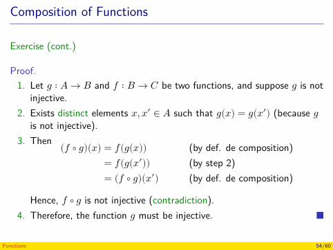
Proof.1. Let 𝑔 ∶ 𝐴 → 𝐵 and 𝑓 ∶ 𝐵 → 𝐶 be two functions, and suppose 𝑔 is not
injective.2. Exists distinct elements 𝑥, 𝑥′ ∈ 𝐴 such that 𝑔(𝑥) = 𝑔(𝑥′) (because 𝑔
is not injective).3. Then (𝑓 ∘ 𝑔)(𝑥) = 𝑓(𝑔(𝑥)) (by def. de composition)
= 𝑓(𝑔(𝑥′)) (by step 2)= (𝑓 ∘ 𝑔)(𝑥′) (by def. de composition)
Hence, 𝑓 ∘ 𝑔 is not injective (contradiction).4. Therefore, the function 𝑔 must be injective.
Functions 54/60
The Graphs of Functions
Definition (Graph of a function)Let 𝑓 ∶ 𝐴 → 𝐵. The graph of 𝑓 is the set
{(𝑎, 𝑏) ∣ 𝑎 ∈ 𝐴 and 𝑓(𝑎) = 𝑏}.
ExamplesWhiteboard
RemarksGraphs of functions and polymorphic functionsGraphs of functions and programsPartial and total functions
Functions 55/60

The Graphs of Functions
Definition (Graph of a function)Let 𝑓 ∶ 𝐴 → 𝐵. The graph of 𝑓 is the set
{(𝑎, 𝑏) ∣ 𝑎 ∈ 𝐴 and 𝑓(𝑎) = 𝑏}.ExamplesWhiteboard
RemarksGraphs of functions and polymorphic functionsGraphs of functions and programsPartial and total functions
Functions 56/60
The Graphs of Functions
Definition (Graph of a function)Let 𝑓 ∶ 𝐴 → 𝐵. The graph of 𝑓 is the set
{(𝑎, 𝑏) ∣ 𝑎 ∈ 𝐴 and 𝑓(𝑎) = 𝑏}.ExamplesWhiteboard
RemarksGraphs of functions and polymorphic functions
Graphs of functions and programsPartial and total functions
Functions 57/60
The Graphs of Functions
Definition (Graph of a function)Let 𝑓 ∶ 𝐴 → 𝐵. The graph of 𝑓 is the set
{(𝑎, 𝑏) ∣ 𝑎 ∈ 𝐴 and 𝑓(𝑎) = 𝑏}.ExamplesWhiteboard
RemarksGraphs of functions and polymorphic functionsGraphs of functions and programs
Partial and total functions
Functions 58/60
The Graphs of Functions
Definition (Graph of a function)Let 𝑓 ∶ 𝐴 → 𝐵. The graph of 𝑓 is the set
{(𝑎, 𝑏) ∣ 𝑎 ∈ 𝐴 and 𝑓(𝑎) = 𝑏}.ExamplesWhiteboard
RemarksGraphs of functions and polymorphic functionsGraphs of functions and programsPartial and total functions
Functions 59/60
References
Rosen, K. H. (2004). Matemática Discreta y sus Aplicaciones. 5th ed.McGraw-Hill (cit. on pp. 12–15, 34, 45, 52, 53).— (2012). Discrete Mathematics and Its Applications. 7th ed.McGraw-Hill (cit. on pp. 4, 33, 36, 39).
Functions 60/60
Discrete Structures - CM0246Cardinality
Andrés Sicard-Ramírez
Universidad EAFIT
Semester 2014-2
Cardinality
Definition (Cardinality (finite sets))Let 𝐴 be a set. The number of (distinct) elements in 𝐴, denoted |𝐴|, iscalled the cardinality of 𝐴.
Definition (Cardinality (finite and infinite sets))The sets 𝐴 and 𝐵 have the same cardinality,if and only,there is a bijection from 𝐴 to 𝐵.
Injunction, surjection or bijection?Draw figures in the whiteboard.
Cardinality 2/26
Cardinality
Definition (Cardinality (finite sets))Let 𝐴 be a set. The number of (distinct) elements in 𝐴, denoted |𝐴|, iscalled the cardinality of 𝐴.
Definition (Cardinality (finite and infinite sets))The sets 𝐴 and 𝐵 have the same cardinality,if and only,there is a bijection from 𝐴 to 𝐵.
Injunction, surjection or bijection?Draw figures in the whiteboard.
Cardinality 3/26
Cardinality
Definition (Cardinality (finite sets))Let 𝐴 be a set. The number of (distinct) elements in 𝐴, denoted |𝐴|, iscalled the cardinality of 𝐴.
Definition (Cardinality (finite and infinite sets))The sets 𝐴 and 𝐵 have the same cardinality,if and only,there is a bijection from 𝐴 to 𝐵.
Injunction, surjection or bijection?Draw figures in the whiteboard.
Cardinality 4/26
Cardinality
Examples|ℤ+| = |ℕ|
|ℕ| = |Even|, where Even is the set defined by Even = {2𝑛 ∣ 𝑛 ∈ ℕ}.
|ℕ| = |Even|, where 𝑀𝑘 is the set of the non-negative multiples of𝑘 ∈ ℤ+, i.e. 𝑀𝑘 = {𝑛𝑘 ∣ 𝑛 ∈ ℕ}.
|[0, 1]| = |[𝑎, 𝑏]|, where 𝑎, 𝑏 ∈ ℝ and 𝑎 < 𝑏.
Cardinality 5/26
Cardinality
Examples|ℤ+| = |ℕ|
|ℕ| = |Even|, where Even is the set defined by Even = {2𝑛 ∣ 𝑛 ∈ ℕ}.
|ℕ| = |Even|, where 𝑀𝑘 is the set of the non-negative multiples of𝑘 ∈ ℤ+, i.e. 𝑀𝑘 = {𝑛𝑘 ∣ 𝑛 ∈ ℕ}.
|[0, 1]| = |[𝑎, 𝑏]|, where 𝑎, 𝑏 ∈ ℝ and 𝑎 < 𝑏.
Cardinality 6/26
Cardinality
Examples|ℤ+| = |ℕ|
|ℕ| = |Even|, where Even is the set defined by Even = {2𝑛 ∣ 𝑛 ∈ ℕ}.
|ℕ| = |Even|, where 𝑀𝑘 is the set of the non-negative multiples of𝑘 ∈ ℤ+, i.e. 𝑀𝑘 = {𝑛𝑘 ∣ 𝑛 ∈ ℕ}.
|[0, 1]| = |[𝑎, 𝑏]|, where 𝑎, 𝑏 ∈ ℝ and 𝑎 < 𝑏.
Cardinality 7/26
Cardinality
Examples|ℤ+| = |ℕ|
|ℕ| = |Even|, where Even is the set defined by Even = {2𝑛 ∣ 𝑛 ∈ ℕ}.
|ℕ| = |Even|, where 𝑀𝑘 is the set of the non-negative multiples of𝑘 ∈ ℤ+, i.e. 𝑀𝑘 = {𝑛𝑘 ∣ 𝑛 ∈ ℕ}.
|[0, 1]| = |[𝑎, 𝑏]|, where 𝑎, 𝑏 ∈ ℝ and 𝑎 < 𝑏.
Cardinality 8/26
Cardinality
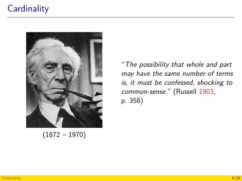
(1872 – 1970)
“The possibility that whole and partmay have the same number of termsis, it must be confessed, shocking tocommon-sense.” (Russell 1903,p. 358)
Cardinality 9/26
Cardinality
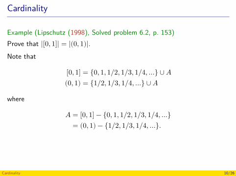
Example (Lipschutz (1998), Solved problem 6.2, p. 153)Prove that |[0, 1]| = |(0, 1)|.Note that
[0, 1] = {0, 1, 1/2, 1/3, 1/4, …} ∪ 𝐴(0, 1) = {1/2, 1/3, 1/4, …} ∪ 𝐴
where
𝐴 = [0, 1] − {0, 1, 1/2, 1/3, 1/4, …}= (0, 1) − {1/2, 1/3, 1/4, …}.
Cardinality 10/26
Cardinality
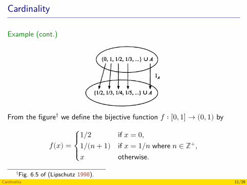
Example (cont.)
From the figure† we define the bijective function 𝑓 ∶ [0, 1] → (0, 1) by
𝑓(𝑥) =⎧{⎨{⎩
1/2 if 𝑥 = 0,1/(𝑛 + 1) if 𝑥 = 1/𝑛 where 𝑛 ∈ ℤ+,𝑥 otherwise.
†Fig. 6.5 of (Lipschutz 1998).Cardinality 11/26
Cardinality
ExerciseLet 𝐴 and 𝐵 be sets. Show |𝐴 × 𝐵| = |𝐵 × 𝐴|.
Cardinality 12/26
Enumerable and Non-Enumerable Sets
Has all the infinite sets the same cardinality?
Definition (Enumerable set)A set that is either finite or has the same cardinality as the set of positiveintegers is called enumerable (or countable).
Definition (Non-enumerable set)A set that is not enumerable countable is called non-enumerable (or un-countable).
ExamplesWhiteboard
Cardinality 13/26
Enumerable and Non-Enumerable Sets
Has all the infinite sets the same cardinality?
Definition (Enumerable set)A set that is either finite or has the same cardinality as the set of positiveintegers is called enumerable (or countable).
Definition (Non-enumerable set)A set that is not enumerable countable is called non-enumerable (or un-countable).
ExamplesWhiteboard
Cardinality 14/26
Enumerable and Non-Enumerable Sets
Has all the infinite sets the same cardinality?
Definition (Enumerable set)A set that is either finite or has the same cardinality as the set of positiveintegers is called enumerable (or countable).
Definition (Non-enumerable set)A set that is not enumerable countable is called non-enumerable (or un-countable).
ExamplesWhiteboard
Cardinality 15/26
Enumerable and Non-Enumerable Sets
Has all the infinite sets the same cardinality?
Definition (Enumerable set)A set that is either finite or has the same cardinality as the set of positiveintegers is called enumerable (or countable).
Definition (Non-enumerable set)A set that is not enumerable countable is called non-enumerable (or un-countable).
ExamplesWhiteboard
Cardinality 16/26
Enumerable and Non-Enumerable Sets
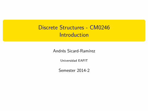
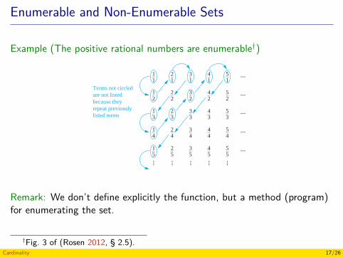
Example (The positive rational numbers are enumerable†) 2.5 Cardinality of Sets 173
11
12
13
14
15
21
22
23
24
25
31
32
3
3
3
4
35
41
42
43
44
45
51
52
53
54
55
...
...
...
...
...
...............
Terms not circledare not listedbecause theyrepeat previouslylisted terms
FIGURE 3 The Positive Rational Numbers Are Countable.
arrange the positive rational numbers by listing those with denominator q = 1 in the first row,those with denominator q = 2 in the second row, and so on, as displayed in Figure 3.
The key to listing the rational numbers in a sequence is to first list the positive rationalnumbers p/q with p + q = 2, followed by those with p + q = 3, followed by those withp + q = 4, and so on, following the path shown in Figure 3. Whenever we encounter a numberp/q that is already listed, we do not list it again. For example, when we come to 2/2 = 1 wedo not list it because we have already listed 1/1 = 1. The initial terms in the list of positiverational numbers we have constructed are 1, 1/2, 2, 3, 1/3, 1/4, 2/3, 3/2, 4, 5, and so on. Thesenumbers are shown circled; the uncircled numbers in the list are those we leave out becausethey are already listed. Because all positive rational numbers are listed once, as the reader canverify, we have shown that the set of positive rational numbers is countable. ▲
An Uncountable SetNot all infinite sets havethe same size! We have seen that the set of positive rational numbers is a countable set. Do we have a promising
candidate for an uncountable set? The first place we might look is the set of real numbers. InExample 5 we use an important proof method, introduced in 1879 by Georg Cantor and knownas the Cantor diagonalization argument, to prove that the set of real numbers is not countable.This proof method is used extensively in mathematical logic and in the theory of computation.
EXAMPLE 5 Show that the set of real numbers is an uncountable set.
Solution: To show that the set of real numbers is uncountable, we suppose that the set of realnumbers is countable and arrive at a contradiction. Then, the subset of all real numbers thatfall between 0 and 1 would also be countable (because any subset of a countable set is alsocountable; see Exercise 16). Under this assumption, the real numbers between 0 and 1 can belisted in some order, say, r1, r2, r3, . . . . Let the decimal representation of these real numbers be
r1 = 0.d11d12d13d14 . . .
r2 = 0.d21d22d23d24 . . .
r3 = 0.d31d32d33d34 . . .
r4 = 0.d41d42d43d44 . . .
...
where dij ∈ {0, 1, 2, 3, 4, 5, 6, 7, 8, 9}. (For example, if r1 = 0.23794102 . . . , we have d11 =2, d12 = 3, d13 = 7, and so on.) Then, form a new real number with decimal expansion
Remark: We don’t define explicitly the function, but a method (program)for enumerating the set.
†Fig. 3 of (Rosen 2012, § 2.5).Cardinality 17/26
Enumerable and Non-Enumerable Sets
TheoremThe interval (0, 1) is non-enumerable.Proof (next slide).
Cardinality 18/26
Enumerable and Non-Enumerable Sets
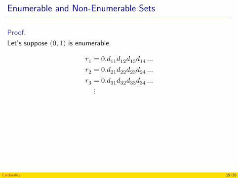
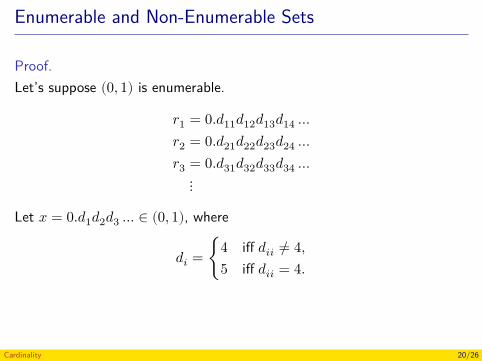
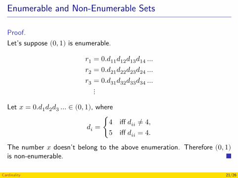
Proof.Let’s suppose (0, 1) is enumerable.
𝑟1 = 0.𝑑11𝑑12𝑑13𝑑14 …𝑟2 = 0.𝑑21𝑑22𝑑23𝑑24 …𝑟3 = 0.𝑑31𝑑32𝑑33𝑑34 …
⋮
Let 𝑥 = 0.𝑑1𝑑2𝑑3 … ∈ (0, 1), where
𝑑𝑖 = {4 iff 𝑑𝑖𝑖 ≠ 4,5 iff 𝑑𝑖𝑖 = 4.
The number 𝑥 doesn’t belong to the above enumeration. Therefore (0, 1)is non-enumerable.
Cardinality 19/26
Enumerable and Non-Enumerable Sets
Proof.Let’s suppose (0, 1) is enumerable.
𝑟1 = 0.𝑑11𝑑12𝑑13𝑑14 …𝑟2 = 0.𝑑21𝑑22𝑑23𝑑24 …𝑟3 = 0.𝑑31𝑑32𝑑33𝑑34 …
⋮
Let 𝑥 = 0.𝑑1𝑑2𝑑3 … ∈ (0, 1), where
𝑑𝑖 = {4 iff 𝑑𝑖𝑖 ≠ 4,5 iff 𝑑𝑖𝑖 = 4.
The number 𝑥 doesn’t belong to the above enumeration. Therefore (0, 1)is non-enumerable.
Cardinality 20/26
Enumerable and Non-Enumerable Sets
Proof.Let’s suppose (0, 1) is enumerable.
𝑟1 = 0.𝑑11𝑑12𝑑13𝑑14 …𝑟2 = 0.𝑑21𝑑22𝑑23𝑑24 …𝑟3 = 0.𝑑31𝑑32𝑑33𝑑34 …
⋮
Let 𝑥 = 0.𝑑1𝑑2𝑑3 … ∈ (0, 1), where
𝑑𝑖 = {4 iff 𝑑𝑖𝑖 ≠ 4,5 iff 𝑑𝑖𝑖 = 4.
The number 𝑥 doesn’t belong to the above enumeration. Therefore (0, 1)is non-enumerable.
Cardinality 21/26
Enumerable and Non-Enumerable Sets
TheoremLet 𝐴 and 𝐵 be sets such 𝐴 ⊆ 𝐵. If 𝐴 is non-enumerable then 𝐵 isnon-enumerable.
Cardinality 22/26
Enumerable and Non-Enumerable Sets
TheoremThe set of the real numbers is non-enumerable.
Proof.The interval (0, 1) is a non-enumerable subset of ℝ. Therefore (using aprevious theorem), ℝ is non-enumerable.
Comment about the continuum hypothesis
Cardinality 23/26
Enumerable and Non-Enumerable Sets
TheoremThe set of the real numbers is non-enumerable.Proof.The interval (0, 1) is a non-enumerable subset of ℝ. Therefore (using aprevious theorem), ℝ is non-enumerable.
Comment about the continuum hypothesis
Cardinality 24/26
Enumerable and Non-Enumerable Sets
TheoremThe set of the real numbers is non-enumerable.Proof.The interval (0, 1) is a non-enumerable subset of ℝ. Therefore (using aprevious theorem), ℝ is non-enumerable.
Comment about the continuum hypothesis
Cardinality 25/26
References
Lipschutz, S. (1998). Schaum’s Outline of Theory and Problems of SetTheory and Related Topics. 2nd ed. McGraw-Hill (cit. on pp. 10, 11).Rosen, K. H. (2012). Discrete Mathematics and Its Applications. 7th ed.McGraw-Hill (cit. on p. 17).Russell, B. (1903). The Principles of Mathematics. W. W. Norton &Company, Inc (cit. on p. 9).
Cardinality 26/26
Discrete Structures - CM0246Mathematical Induction
Andrés Sicard-Ramírez
Universidad EAFIT
Semester 2014-2
Motivation
ExampleConjecture a formula for the sum of the first 𝑛 positive odd integers.
ProblemLet 𝑃(𝑛) be a propositional function. How can we proof that 𝑃(𝑛) is truefor all 𝑛 ∈ ℤ+?
Mathematical Induction 2/39
Motivation
ExampleConjecture a formula for the sum of the first 𝑛 positive odd integers.
ProblemLet 𝑃(𝑛) be a propositional function. How can we proof that 𝑃(𝑛) is truefor all 𝑛 ∈ ℤ+?
Mathematical Induction 3/39
Principle of Mathematical Induction
Definition (Principle of mathematical induction)Let 𝑃(𝑛) be a propositional function.To prove that 𝑃(𝑛) is true for all 𝑛 ∈ ℤ+, we must make two proofs:
Basis step: Prove 𝑃(1)
Inductive step: Prove 𝑃(𝑘) → 𝑃(𝑘 + 1) for all 𝑘 ∈ ℤ+
𝑃 (𝑘) is called the inductive hypothesis.
Mathematical Induction 4/39
Principle of Mathematical Induction
Definition (Principle of mathematical induction)Let 𝑃(𝑛) be a propositional function.To prove that 𝑃(𝑛) is true for all 𝑛 ∈ ℤ+, we must make two proofs:
Basis step: Prove 𝑃(1)Inductive step: Prove 𝑃(𝑘) → 𝑃 (𝑘 + 1) for all 𝑘 ∈ ℤ+
𝑃(𝑘) is called the inductive hypothesis.
Mathematical Induction 5/39
Principle of Mathematical Induction
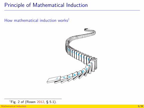
How mathematical induction works†314 5 / Induction and Recursion
FIGURE 2 Illustrating How Mathematical Induction Works Using Dominoes.
WAYS TO REMEMBER HOW MATHEMATICAL INDUCTION WORKS Thinking ofthe infinite ladder and the rules for reaching steps can help you remember how mathematicalinduction works. Note that statements (1) and (2) for the infinite ladder are exactly the basisstep and inductive step, respectively, of the proof that P(n) is true for all positive integers n,where P(n) is the statement that we can reach the nth rung of the ladder. Consequently, we caninvoke mathematical induction to conclude that we can reach every rung.
Another way to illustrate the principle of mathematical induction is to consider an infiniterow of dominoes, labeled 1, 2, 3, . . . , n, . . . , where each domino is standing up. Let P(n) bethe proposition that domino n is knocked over. If the first domino is knocked over—i.e., if P(1)
is true—and if, whenever the kth domino is knocked over, it also knocks the (k + 1)st dominoover—i.e., if P(k)→ P(k + 1) is true for all positive integers k—then all the dominoes areknocked over. This is illustrated in Figure 2.
Why Mathematical Induction is Valid
Why is mathematical induction a valid proof technique? The reason comes from the well-ordering property, listed in Appendix 1, as an axiom for the set of positive integers, whichstates that every nonempty subset of the set of positive integers has a least element. So, supposewe know that P(1) is true and that the proposition P(k)→P(k + 1) is true for all positiveintegers k. To show that P(n) must be true for all positive integers n, assume that there is atleast one positive integer for which P(n) is false. Then the set S of positive integers for whichP(n) is false is nonempty. Thus, by the well-ordering property, S has a least element, whichwill be denoted by m. We know that m cannot be 1, because P(1) is true. Because m is positiveand greater than 1, m− 1 is a positive integer. Furthermore, because m− 1 is less than m, it isnot in S, so P(m− 1) must be true. Because the conditional statement P(m− 1)→P(m) isalso true, it must be the case that P(m) is true. This contradicts the choice of m. Hence, P(n)
must be true for every positive integer n.
The Good and the Bad of Mathematical Induction
An important point needs to be made about mathematical induction before we commence astudy of its use. The good thing about mathematical induction is that it can be used to prove
†Fig. 2 of (Rosen 2012, § 5.1).Mathematical Induction 6/39
Principle of Mathematical Induction
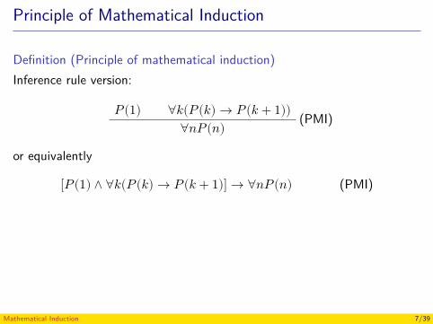
Definition (Principle of mathematical induction)Inference rule version:
𝑃(1) ∀𝑘(𝑃(𝑘) → 𝑃(𝑘 + 1)) (PMI)∀𝑛𝑃 (𝑛)
or equivalently
[𝑃 (1) ∧ ∀𝑘(𝑃(𝑘) → 𝑃 (𝑘 + 1)] → ∀𝑛𝑃(𝑛) (PMI)
Mathematical Induction 7/39
Principle of Mathematical Induction
Methodology for using the principle of mathematical induction
1. State the propositional function 𝑃(𝑛).2. Prove the basis step, i.e. 𝑃(1).3. Prove the induction step, i.e. ∀𝑘(𝑃(𝑘) → 𝑃(𝑘 + 1)).
Remark: In this proof you need to use the inductive hypothesis 𝑃(𝑛).4. Conclude ∀𝑛𝑃(𝑛) by the principle of mathematical induction.
Mathematical Induction 8/39
Principle of Mathematical Induction
Methodology for using the principle of mathematical induction1. State the propositional function 𝑃(𝑛).
2. Prove the basis step, i.e. 𝑃(1).3. Prove the induction step, i.e. ∀𝑘(𝑃(𝑘) → 𝑃(𝑘 + 1)).
Remark: In this proof you need to use the inductive hypothesis 𝑃(𝑛).4. Conclude ∀𝑛𝑃(𝑛) by the principle of mathematical induction.
Mathematical Induction 9/39
Principle of Mathematical Induction
Methodology for using the principle of mathematical induction1. State the propositional function 𝑃(𝑛).2. Prove the basis step, i.e. 𝑃(1).
3. Prove the induction step, i.e. ∀𝑘(𝑃(𝑘) → 𝑃(𝑘 + 1)).Remark: In this proof you need to use the inductive hypothesis 𝑃(𝑛).
4. Conclude ∀𝑛𝑃(𝑛) by the principle of mathematical induction.
Mathematical Induction 10/39
Principle of Mathematical Induction
Methodology for using the principle of mathematical induction1. State the propositional function 𝑃(𝑛).2. Prove the basis step, i.e. 𝑃(1).3. Prove the induction step, i.e. ∀𝑘(𝑃(𝑘) → 𝑃(𝑘 + 1)).
Remark: In this proof you need to use the inductive hypothesis 𝑃(𝑛).
4. Conclude ∀𝑛𝑃(𝑛) by the principle of mathematical induction.
Mathematical Induction 11/39
Principle of Mathematical Induction
Methodology for using the principle of mathematical induction1. State the propositional function 𝑃(𝑛).2. Prove the basis step, i.e. 𝑃(1).3. Prove the induction step, i.e. ∀𝑘(𝑃(𝑘) → 𝑃(𝑘 + 1)).
Remark: In this proof you need to use the inductive hypothesis 𝑃(𝑛).4. Conclude ∀𝑛𝑃(𝑛) by the principle of mathematical induction.
Mathematical Induction 12/39
Principle of Mathematical Induction
ExampleProve that the sum of the first 𝑛 odd positive integers is 𝑛2.†
Whiteboard.
†Historical remark. From 1575, it could be the first property proved using thePMI (Gunderson 2011, § 1.8).
Mathematical Induction 13/39
Principle of Mathematical Induction
ExerciseProve that if 𝑛 ∈ ℤ+, then
1 + 2 + 3 + ⋯ + 𝑛 = 𝑛(𝑛 + 1)/2.
Mathematical Induction 14/39
Principle of Mathematical Induction
Exercise (cont.)
Proof.1. 𝑃(𝑛): 1 + 2 + 3 + ⋯ + 𝑛 = 𝑛(𝑛 + 1)/2.
2. Basis step 𝑃(1): 1 = 1(1 + 1)/2.3. Inductive step:
Inductive hypothesis 𝑃(𝑘): 1 + 2 + 3 + ⋯ + 𝑘 = 𝑘(𝑘 + 1)/2.Let’s prove 𝑃(𝑘 + 1):
1 + 2 + 3 + ⋯ + 𝑘 + (𝑘 + 1) = 𝑘(𝑘 + 1)/2 + (𝑘 + 1) (by IH)= (𝑘 + 1)(𝑘/2 + 1) (by arithmetic)= (𝑘 + 1)(𝑘 + 2)/2 (by arithmetic)
4. ∀𝑛𝑃(𝑛) by the principle of induction mathematical.
Mathematical Induction 15/39
Principle of Mathematical Induction
Exercise (cont.)
Proof.1. 𝑃(𝑛): 1 + 2 + 3 + ⋯ + 𝑛 = 𝑛(𝑛 + 1)/2.2. Basis step 𝑃(1): 1 = 1(1 + 1)/2.
3. Inductive step:Inductive hypothesis 𝑃(𝑘): 1 + 2 + 3 + ⋯ + 𝑘 = 𝑘(𝑘 + 1)/2.Let’s prove 𝑃(𝑘 + 1):
1 + 2 + 3 + ⋯ + 𝑘 + (𝑘 + 1) = 𝑘(𝑘 + 1)/2 + (𝑘 + 1) (by IH)= (𝑘 + 1)(𝑘/2 + 1) (by arithmetic)= (𝑘 + 1)(𝑘 + 2)/2 (by arithmetic)
4. ∀𝑛𝑃(𝑛) by the principle of induction mathematical.
Mathematical Induction 16/39
Principle of Mathematical Induction
Exercise (cont.)
Proof.1. 𝑃(𝑛): 1 + 2 + 3 + ⋯ + 𝑛 = 𝑛(𝑛 + 1)/2.2. Basis step 𝑃(1): 1 = 1(1 + 1)/2.3. Inductive step:
Inductive hypothesis 𝑃(𝑘): 1 + 2 + 3 + ⋯ + 𝑘 = 𝑘(𝑘 + 1)/2.Let’s prove 𝑃(𝑘 + 1):
1 + 2 + 3 + ⋯ + 𝑘 + (𝑘 + 1) = 𝑘(𝑘 + 1)/2 + (𝑘 + 1) (by IH)= (𝑘 + 1)(𝑘/2 + 1) (by arithmetic)= (𝑘 + 1)(𝑘 + 2)/2 (by arithmetic)
4. ∀𝑛𝑃(𝑛) by the principle of induction mathematical.
Mathematical Induction 17/39
Principle of Mathematical Induction
Exercise (cont.)
Proof.1. 𝑃(𝑛): 1 + 2 + 3 + ⋯ + 𝑛 = 𝑛(𝑛 + 1)/2.2. Basis step 𝑃(1): 1 = 1(1 + 1)/2.3. Inductive step:
Inductive hypothesis 𝑃(𝑘): 1 + 2 + 3 + ⋯ + 𝑘 = 𝑘(𝑘 + 1)/2.Let’s prove 𝑃(𝑘 + 1):
1 + 2 + 3 + ⋯ + 𝑘 + (𝑘 + 1) = 𝑘(𝑘 + 1)/2 + (𝑘 + 1) (by IH)= (𝑘 + 1)(𝑘/2 + 1) (by arithmetic)= (𝑘 + 1)(𝑘 + 2)/2 (by arithmetic)
4. ∀𝑛𝑃(𝑛) by the principle of induction mathematical.
Mathematical Induction 18/39
Principle of Mathematical Induction
ExerciseProve that if 𝑛 ∈ ℕ, then
20 + 21 + 22 + ⋯ + 2𝑛 = 2𝑛+1 − 1
Mathematical Induction 19/39
Principle of Mathematical Induction
Exercise (cont.)
Proof.1. 𝑃(𝑛): 20 + 21 + 22 + ⋯ + 2𝑛 = 2𝑛+1 − 1
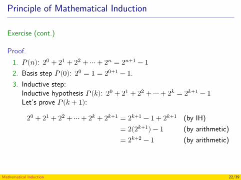
2. Basis step 𝑃(0): 20 = 1 = 20+1 − 1.3. Inductive step:
Inductive hypothesis 𝑃(𝑘): 20 + 21 + 22 + ⋯ + 2𝑘 = 2𝑘+1 − 1Let’s prove 𝑃(𝑘 + 1):
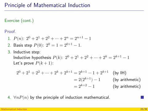
20 + 21 + 22 + ⋯ + 2𝑘 + 2𝑘+1 = 2𝑘+1 − 1 + 2𝑘+1 (by IH)= 2(2𝑘+1) − 1 (by arithmetic)= 2𝑘+2 − 1 (by arithmetic)
4. ∀𝑛𝑃(𝑛) by the principle of induction mathematical.
Mathematical Induction 20/39
Principle of Mathematical Induction
Exercise (cont.)
Proof.1. 𝑃(𝑛): 20 + 21 + 22 + ⋯ + 2𝑛 = 2𝑛+1 − 12. Basis step 𝑃(0): 20 = 1 = 20+1 − 1.
3. Inductive step:Inductive hypothesis 𝑃(𝑘): 20 + 21 + 22 + ⋯ + 2𝑘 = 2𝑘+1 − 1Let’s prove 𝑃(𝑘 + 1):
20 + 21 + 22 + ⋯ + 2𝑘 + 2𝑘+1 = 2𝑘+1 − 1 + 2𝑘+1 (by IH)= 2(2𝑘+1) − 1 (by arithmetic)= 2𝑘+2 − 1 (by arithmetic)
4. ∀𝑛𝑃(𝑛) by the principle of induction mathematical.
Mathematical Induction 21/39
Principle of Mathematical Induction
Exercise (cont.)
Proof.1. 𝑃(𝑛): 20 + 21 + 22 + ⋯ + 2𝑛 = 2𝑛+1 − 12. Basis step 𝑃(0): 20 = 1 = 20+1 − 1.3. Inductive step:
Inductive hypothesis 𝑃(𝑘): 20 + 21 + 22 + ⋯ + 2𝑘 = 2𝑘+1 − 1Let’s prove 𝑃(𝑘 + 1):
20 + 21 + 22 + ⋯ + 2𝑘 + 2𝑘+1 = 2𝑘+1 − 1 + 2𝑘+1 (by IH)= 2(2𝑘+1) − 1 (by arithmetic)= 2𝑘+2 − 1 (by arithmetic)
4. ∀𝑛𝑃(𝑛) by the principle of induction mathematical.
Mathematical Induction 22/39
Principle of Mathematical Induction
Exercise (cont.)
Proof.1. 𝑃(𝑛): 20 + 21 + 22 + ⋯ + 2𝑛 = 2𝑛+1 − 12. Basis step 𝑃(0): 20 = 1 = 20+1 − 1.3. Inductive step:
Inductive hypothesis 𝑃(𝑘): 20 + 21 + 22 + ⋯ + 2𝑘 = 2𝑘+1 − 1Let’s prove 𝑃(𝑘 + 1):
20 + 21 + 22 + ⋯ + 2𝑘 + 2𝑘+1 = 2𝑘+1 − 1 + 2𝑘+1 (by IH)= 2(2𝑘+1) − 1 (by arithmetic)= 2𝑘+2 − 1 (by arithmetic)
4. ∀𝑛𝑃(𝑛) by the principle of induction mathematical.
Mathematical Induction 23/39
Strong Induction
Definition (Strong (or course-of-values) induction)Let 𝑃(𝑛) be a propositional function.To prove that 𝑃(𝑛) is true for all 𝑛 ∈ ℤ+, we must make two proofs:
Basis step: Prove 𝑃(1)
Inductive step: Prove [𝑃 (1) ∧ 𝑃(2) ∧ ⋯ ∧ 𝑃(𝑘)] → 𝑃(𝑘 + 1) for all𝑘 ∈ ℤ+
The (strong) inductive hypothesis is given by
𝑃(𝑗) is true for 𝑗 = 1, 2, … , 𝑘.
Mathematical Induction 24/39
Strong Induction
Definition (Strong (or course-of-values) induction)Let 𝑃(𝑛) be a propositional function.To prove that 𝑃(𝑛) is true for all 𝑛 ∈ ℤ+, we must make two proofs:
Basis step: Prove 𝑃(1)Inductive step: Prove [𝑃 (1) ∧ 𝑃 (2) ∧ ⋯ ∧ 𝑃(𝑘)] → 𝑃(𝑘 + 1) for all𝑘 ∈ ℤ+
The (strong) inductive hypothesis is given by
𝑃(𝑗) is true for 𝑗 = 1, 2, … , 𝑘.
Mathematical Induction 25/39
Strong Induction
Definition (Strong (or course-of-values) induction)Let 𝑃(𝑛) be a propositional function.To prove that 𝑃(𝑛) is true for all 𝑛 ∈ ℤ+, we must make two proofs:
Basis step: Prove 𝑃(1)Inductive step: Prove [𝑃 (1) ∧ 𝑃 (2) ∧ ⋯ ∧ 𝑃(𝑘)] → 𝑃(𝑘 + 1) for all𝑘 ∈ ℤ+
The (strong) inductive hypothesis is given by
𝑃(𝑗) is true for 𝑗 = 1, 2, … , 𝑘.
Mathematical Induction 26/39
Strong Induction
Definition (Strong induction)Inference rule version:
𝑃 (1) ∀𝑘[(𝑃 (1) ∧ 𝑃(2) ∧ ⋯ ∧ 𝑃(𝑘)) → 𝑃(𝑘 + 1)] (strong induction)∀𝑛𝑃 (𝑛)
Mathematical Induction 27/39
Strong Induction
Example (A part of the fundamental theorem of arithmetic)Prove that if 𝑛 is an integer greater than 1, either is prime itself or is theproduct of prime numbers.
Mathematical Induction 28/39
Strong Induction
Example (cont.)
Proof.1. 𝑃(𝑛): 𝑛 is prime itself or it is the product of prime numbers.
2. Basis step 𝑃(2): 2 is a prime number.3. Inductive step:
Inductive hypothesis: 𝑃(𝑗) is true for 𝑗 = 1, 2, … , 𝑘.Let’s prove that 𝑘 + 1 satisfies the property:3.1 If 𝑘 + 1 is a prime number then it satisfies the property.3.2 If 𝑘 + 1 is a composite number:
𝑘 + 1 = 𝑎𝑏 where 2 ≤ 𝑎 ≤ 𝑏 < 𝑘 + 1. Since 𝑃(𝑎) and 𝑃(𝑏) bythe inductive hypothesis, then 𝑃(𝑘 + 1).
4. 𝑃 (𝑛) is true for all integer 𝑛 greater than 1 by strong induction.
Mathematical Induction 29/39
Strong Induction
Example (cont.)
Proof.1. 𝑃(𝑛): 𝑛 is prime itself or it is the product of prime numbers.2. Basis step 𝑃(2): 2 is a prime number.
3. Inductive step:Inductive hypothesis: 𝑃(𝑗) is true for 𝑗 = 1, 2, … , 𝑘.Let’s prove that 𝑘 + 1 satisfies the property:3.1 If 𝑘 + 1 is a prime number then it satisfies the property.3.2 If 𝑘 + 1 is a composite number:
𝑘 + 1 = 𝑎𝑏 where 2 ≤ 𝑎 ≤ 𝑏 < 𝑘 + 1. Since 𝑃(𝑎) and 𝑃(𝑏) bythe inductive hypothesis, then 𝑃(𝑘 + 1).
4. 𝑃 (𝑛) is true for all integer 𝑛 greater than 1 by strong induction.
Mathematical Induction 30/39
Strong Induction
Example (cont.)
Proof.1. 𝑃(𝑛): 𝑛 is prime itself or it is the product of prime numbers.2. Basis step 𝑃(2): 2 is a prime number.3. Inductive step:
Inductive hypothesis: 𝑃(𝑗) is true for 𝑗 = 1, 2, … , 𝑘.
Let’s prove that 𝑘 + 1 satisfies the property:3.1 If 𝑘 + 1 is a prime number then it satisfies the property.3.2 If 𝑘 + 1 is a composite number:
𝑘 + 1 = 𝑎𝑏 where 2 ≤ 𝑎 ≤ 𝑏 < 𝑘 + 1. Since 𝑃(𝑎) and 𝑃(𝑏) bythe inductive hypothesis, then 𝑃(𝑘 + 1).
4. 𝑃 (𝑛) is true for all integer 𝑛 greater than 1 by strong induction.
Mathematical Induction 31/39
Strong Induction
Example (cont.)
Proof.1. 𝑃(𝑛): 𝑛 is prime itself or it is the product of prime numbers.2. Basis step 𝑃(2): 2 is a prime number.3. Inductive step:
Inductive hypothesis: 𝑃(𝑗) is true for 𝑗 = 1, 2, … , 𝑘.Let’s prove that 𝑘 + 1 satisfies the property:
3.1 If 𝑘 + 1 is a prime number then it satisfies the property.3.2 If 𝑘 + 1 is a composite number:
𝑘 + 1 = 𝑎𝑏 where 2 ≤ 𝑎 ≤ 𝑏 < 𝑘 + 1. Since 𝑃(𝑎) and 𝑃(𝑏) bythe inductive hypothesis, then 𝑃(𝑘 + 1).
4. 𝑃 (𝑛) is true for all integer 𝑛 greater than 1 by strong induction.
Mathematical Induction 32/39
Strong Induction
Example (cont.)
Proof.1. 𝑃(𝑛): 𝑛 is prime itself or it is the product of prime numbers.2. Basis step 𝑃(2): 2 is a prime number.3. Inductive step:
Inductive hypothesis: 𝑃(𝑗) is true for 𝑗 = 1, 2, … , 𝑘.Let’s prove that 𝑘 + 1 satisfies the property:3.1 If 𝑘 + 1 is a prime number then it satisfies the property.
3.2 If 𝑘 + 1 is a composite number:𝑘 + 1 = 𝑎𝑏 where 2 ≤ 𝑎 ≤ 𝑏 < 𝑘 + 1. Since 𝑃(𝑎) and 𝑃(𝑏) bythe inductive hypothesis, then 𝑃(𝑘 + 1).
4. 𝑃 (𝑛) is true for all integer 𝑛 greater than 1 by strong induction.
Mathematical Induction 33/39
Strong Induction
Example (cont.)
Proof.1. 𝑃(𝑛): 𝑛 is prime itself or it is the product of prime numbers.2. Basis step 𝑃(2): 2 is a prime number.3. Inductive step:
Inductive hypothesis: 𝑃(𝑗) is true for 𝑗 = 1, 2, … , 𝑘.Let’s prove that 𝑘 + 1 satisfies the property:3.1 If 𝑘 + 1 is a prime number then it satisfies the property.3.2 If 𝑘 + 1 is a composite number:
𝑘 + 1 = 𝑎𝑏 where 2 ≤ 𝑎 ≤ 𝑏 < 𝑘 + 1. Since 𝑃(𝑎) and 𝑃(𝑏) bythe inductive hypothesis, then 𝑃(𝑘 + 1).
4. 𝑃 (𝑛) is true for all integer 𝑛 greater than 1 by strong induction.
Mathematical Induction 34/39
Strong Induction
Example (cont.)
Proof.1. 𝑃(𝑛): 𝑛 is prime itself or it is the product of prime numbers.2. Basis step 𝑃(2): 2 is a prime number.3. Inductive step:
Inductive hypothesis: 𝑃(𝑗) is true for 𝑗 = 1, 2, … , 𝑘.Let’s prove that 𝑘 + 1 satisfies the property:3.1 If 𝑘 + 1 is a prime number then it satisfies the property.3.2 If 𝑘 + 1 is a composite number:
𝑘 + 1 = 𝑎𝑏 where 2 ≤ 𝑎 ≤ 𝑏 < 𝑘 + 1. Since 𝑃(𝑎) and 𝑃(𝑏) bythe inductive hypothesis, then 𝑃(𝑘 + 1).
4. 𝑃(𝑛) is true for all integer 𝑛 greater than 1 by strong induction.
Mathematical Induction 35/39

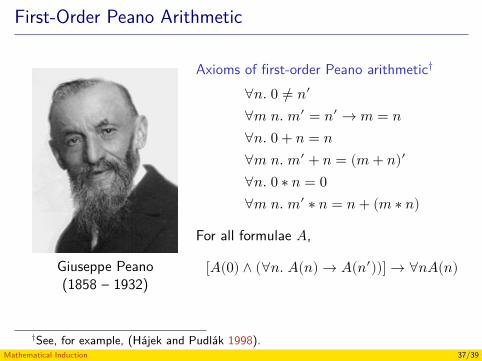
First-Order Peano Arithmetic
Giuseppe Peano(1858 – 1932)
Axioms of first-order Peano arithmetic†
∀𝑛. 0 ≠ 𝑛′
∀𝑚 𝑛. 𝑚′ = 𝑛′ → 𝑚 = 𝑛∀𝑛. 0 + 𝑛 = 𝑛∀𝑚 𝑛. 𝑚′ + 𝑛 = (𝑚 + 𝑛)′
∀𝑛. 0 ∗ 𝑛 = 0∀𝑚 𝑛. 𝑚′ ∗ 𝑛 = 𝑛 + (𝑚 ∗ 𝑛)
For all formulae 𝐴,
[𝐴(0) ∧ (∀𝑛. 𝐴(𝑛) → 𝐴(𝑛′))] → ∀𝑛𝐴(𝑛)
†See, for example, (Hájek and Pudlák 1998).Mathematical Induction 36/39
First-Order Peano Arithmetic
Giuseppe Peano(1858 – 1932)
Axioms of first-order Peano arithmetic†
∀𝑛. 0 ≠ 𝑛′
∀𝑚 𝑛. 𝑚′ = 𝑛′ → 𝑚 = 𝑛∀𝑛. 0 + 𝑛 = 𝑛∀𝑚 𝑛. 𝑚′ + 𝑛 = (𝑚 + 𝑛)′
∀𝑛. 0 ∗ 𝑛 = 0∀𝑚 𝑛. 𝑚′ ∗ 𝑛 = 𝑛 + (𝑚 ∗ 𝑛)
For all formulae 𝐴,
[𝐴(0) ∧ (∀𝑛. 𝐴(𝑛) → 𝐴(𝑛′))] → ∀𝑛𝐴(𝑛)
†See, for example, (Hájek and Pudlák 1998).Mathematical Induction 37/39
First-Order Peano Arithmetic
TheoremThe principle of mathematical induction and strong induction are equival-ent.†
†See, for example, (Gunderson 2011).Mathematical Induction 38/39
References
Gunderson, D. S. (2011). Handbook of Mathematical Induction. Chapman& Hall (cit. on pp. 13, 38).Hájek, P. and Pudlák, P. (1998). Metamathematics of First-OrderArithmetic. 2nd printing. Springer (cit. on pp. 36, 37).Rosen, K. H. (2012). Discrete Mathematics and Its Applications. 7th ed.McGraw-Hill (cit. on p. 6).
Mathematical Induction 39/39
Discrete Structures - CM0246Recursive Definitions and Structural Induction
Andrés Sicard-Ramírez
Universidad EAFIT
Semester 2014-2
Introduction
SubjectsRecursively defined functions from the natural numbers
Inductively defined sets and structuresRecursively defined functions from inductively defined sets andstructuresStructural induction
Terminological noteWe talk about ‘recursively’ defined functions and ‘inductively’ definedsets/structures. Both terms are used interchangeably in the textbook.
Recursive Definitions and Structural Induction 2/52
Introduction
SubjectsRecursively defined functions from the natural numbersInductively defined sets and structures
Recursively defined functions from inductively defined sets andstructuresStructural induction
Terminological noteWe talk about ‘recursively’ defined functions and ‘inductively’ definedsets/structures. Both terms are used interchangeably in the textbook.
Recursive Definitions and Structural Induction 3/52
Introduction
SubjectsRecursively defined functions from the natural numbersInductively defined sets and structuresRecursively defined functions from inductively defined sets andstructures
Structural induction
Terminological noteWe talk about ‘recursively’ defined functions and ‘inductively’ definedsets/structures. Both terms are used interchangeably in the textbook.
Recursive Definitions and Structural Induction 4/52
Introduction
SubjectsRecursively defined functions from the natural numbersInductively defined sets and structuresRecursively defined functions from inductively defined sets andstructuresStructural induction
Terminological noteWe talk about ‘recursively’ defined functions and ‘inductively’ definedsets/structures. Both terms are used interchangeably in the textbook.
Recursive Definitions and Structural Induction 5/52
Introduction
SubjectsRecursively defined functions from the natural numbersInductively defined sets and structuresRecursively defined functions from inductively defined sets andstructuresStructural induction
Terminological noteWe talk about ‘recursively’ defined functions and ‘inductively’ definedsets/structures. Both terms are used interchangeably in the textbook.
Recursive Definitions and Structural Induction 6/52
Introduction
Recursion“Sometimes it is difficult to define an object explicitly. However, it maybe easy to define this object in terms of itself. This process is called recur-sion.” (Rosen 2012, 7th ed. p. 344)
Recursive Definitions and Structural Induction 7/52
Recursively Defined Functions from the Natural Numbers
Recursively defined functions from the natural numbersLet 𝐴 be a set. A function 𝑓 ∶ ℕ → 𝐴 is recursively defined if:
Basis step: We define the function on 𝑓(0).
Recursive step: We give a rule for 𝑓(𝑛) from the value of 𝑓 on smallernatural numbers.
Recursive Definitions and Structural Induction 8/52
Recursively Defined Functions from the Natural Numbers
Recursively defined functions from the natural numbersLet 𝐴 be a set. A function 𝑓 ∶ ℕ → 𝐴 is recursively defined if:
Basis step: We define the function on 𝑓(0).Recursive step: We give a rule for 𝑓(𝑛) from the value of 𝑓 on smallernatural numbers.
Recursive Definitions and Structural Induction 9/52
Recursively Defined Functions from the Natural Numbers
Example𝑓 ∶ ℕ → ℕ𝑓(0) = 3,
𝑓(𝑛 + 1) = 2𝑓(𝑛) + 3.
Example (The factorial function)! ∶ ℕ → ℕ
0! = 1,(𝑛 + 1)! = (𝑛 + 1)𝑛!.
Recursive Definitions and Structural Induction 10/52
Recursively Defined Functions from the Natural Numbers
Example𝑓 ∶ ℕ → ℕ𝑓(0) = 3,
𝑓(𝑛 + 1) = 2𝑓(𝑛) + 3.
Example (The factorial function)! ∶ ℕ → ℕ
0! = 1,(𝑛 + 1)! = (𝑛 + 1)𝑛!.
Recursive Definitions and Structural Induction 11/52
Recursively Defined Functions from the Natural Numbers
ExerciseGive a recursive definition of ∑𝑛
𝑘=0 𝑎𝑘.
0∑𝑘=0
𝑎𝑘 = 𝑎0,
𝑛+1∑𝑘=0
𝑎𝑘 = (𝑛
∑𝑘=0
𝑎𝑘) + 𝑎𝑛+1.
Recursive Definitions and Structural Induction 12/52
Recursively Defined Functions from the Natural Numbers
ExerciseGive a recursive definition of ∑𝑛
𝑘=0 𝑎𝑘.0
∑𝑘=0
𝑎𝑘 = 𝑎0,
𝑛+1∑𝑘=0
𝑎𝑘 = (𝑛
∑𝑘=0
𝑎𝑘) + 𝑎𝑛+1.
Recursive Definitions and Structural Induction 13/52
Recursively Defined Functions from the Natural Numbers
Let 𝐴 be a set. A function 𝑓 ∶ ℕ → 𝐴 is well defined if for every nat-ural number, the value of the function at this number is determined in anunambiguous way.
Example (Rosen (2004), Problem 56, p. 254)Use mathematical induction to prove that a function 𝑓 defined byspecifying 𝑓(0) and a rule for obtaining 𝑓(𝑛 + 1) from 𝑓(𝑛) is well defined.
SchemeThe function 𝑓 ∶ ℕ → 𝐴 is defined by
𝑓(0) = 𝑐 ∈ 𝐴,𝑓(𝑛 + 1) = 𝑒[𝑓(𝑛)].
ProofProof by mathematical induction (see whiteboard).
Recursive Definitions and Structural Induction 14/52
Recursively Defined Functions from the Natural Numbers
Let 𝐴 be a set. A function 𝑓 ∶ ℕ → 𝐴 is well defined if for every nat-ural number, the value of the function at this number is determined in anunambiguous way.
Example (Rosen (2004), Problem 56, p. 254)Use mathematical induction to prove that a function 𝑓 defined byspecifying 𝑓(0) and a rule for obtaining 𝑓(𝑛 + 1) from 𝑓(𝑛) is well defined.
SchemeThe function 𝑓 ∶ ℕ → 𝐴 is defined by
𝑓(0) = 𝑐 ∈ 𝐴,𝑓(𝑛 + 1) = 𝑒[𝑓(𝑛)].
ProofProof by mathematical induction (see whiteboard).
Recursive Definitions and Structural Induction 15/52
Recursively Defined Functions from the Natural Numbers
Let 𝐴 be a set. A function 𝑓 ∶ ℕ → 𝐴 is well defined if for every nat-ural number, the value of the function at this number is determined in anunambiguous way.
Example (Rosen (2004), Problem 56, p. 254)Use mathematical induction to prove that a function 𝑓 defined byspecifying 𝑓(0) and a rule for obtaining 𝑓(𝑛 + 1) from 𝑓(𝑛) is well defined.
SchemeThe function 𝑓 ∶ ℕ → 𝐴 is defined by
𝑓(0) = 𝑐 ∈ 𝐴,𝑓(𝑛 + 1) = 𝑒[𝑓(𝑛)].
ProofProof by mathematical induction (see whiteboard).
Recursive Definitions and Structural Induction 16/52
Recursively Defined Functions from the Natural Numbers
Let 𝐴 be a set. A function 𝑓 ∶ ℕ → 𝐴 is well defined if for every nat-ural number, the value of the function at this number is determined in anunambiguous way.
Example (Rosen (2004), Problem 56, p. 254)Use mathematical induction to prove that a function 𝑓 defined byspecifying 𝑓(0) and a rule for obtaining 𝑓(𝑛 + 1) from 𝑓(𝑛) is well defined.
SchemeThe function 𝑓 ∶ ℕ → 𝐴 is defined by
𝑓(0) = 𝑐 ∈ 𝐴,𝑓(𝑛 + 1) = 𝑒[𝑓(𝑛)].
ProofProof by mathematical induction (see whiteboard).
Recursive Definitions and Structural Induction 17/52
Recursively Defined Functions from the Natural Numbers
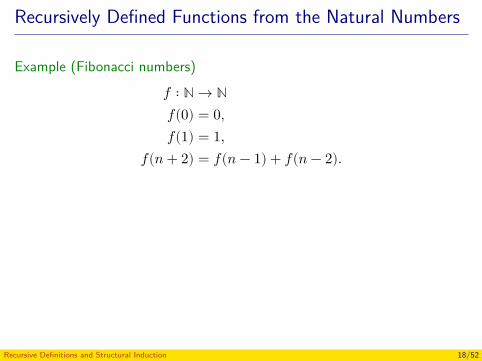
Example (Fibonacci numbers)𝑓 ∶ ℕ → ℕ𝑓(0) = 0,𝑓(1) = 1,
𝑓(𝑛 + 2) = 𝑓(𝑛 − 1) + 𝑓(𝑛 − 2).
Recursive Definitions and Structural Induction 18/52
Subjects
Recursively defined functions from the natural numbersInductively defined sets and structuresRecursively defined functions from inductively defined sets andstructuresStructural induction
Recursive Definitions and Structural Induction 19/52
Inductively Defined Sets and Structures
Example (The natural numbers)See whiteboard.
Definition (Alphabet)Finite, non-empty set of symbols.
ExamplesΣ1 = {0, 1},Σ2 = {𝑎, 𝑏, … , 𝑧},Σ3 = {𝑥 ∣ 𝑥 is an Unicode codepoint }.
Recursive Definitions and Structural Induction 20/52
Inductively Defined Sets and Structures
Example (The natural numbers)See whiteboard.
Definition (Alphabet)Finite, non-empty set of symbols.
ExamplesΣ1 = {0, 1},Σ2 = {𝑎, 𝑏, … , 𝑧},Σ3 = {𝑥 ∣ 𝑥 is an Unicode codepoint }.
Recursive Definitions and Structural Induction 21/52
Inductively Defined Sets and Structures
Definition (String)Finite sequence of symbols of an alphabet. The empty string is denoted 𝜆.
ExamplesSee whiteboard.
Example (Inductive definition of strings)See whiteboard.Remark: See the correction to the textbook definition in course’s website.
Recursive Definitions and Structural Induction 22/52
Inductively Defined Sets and Structures
Definition (String)Finite sequence of symbols of an alphabet. The empty string is denoted 𝜆.
ExamplesSee whiteboard.
Example (Inductive definition of strings)See whiteboard.
Remark: See the correction to the textbook definition in course’s website.
Recursive Definitions and Structural Induction 23/52
Inductively Defined Sets and Structures
Definition (String)Finite sequence of symbols of an alphabet. The empty string is denoted 𝜆.
ExamplesSee whiteboard.
Example (Inductive definition of strings)See whiteboard.Remark: See the correction to the textbook definition in course’s website.
Recursive Definitions and Structural Induction 24/52
Inductively Defined Sets and Structures
Example (Well-formed propositional logic formulae)Basis step: T, F and 𝑝 (propositional variable) are well-formedformulae.Inductive step: If 𝐸 and 𝐹 are well-formed formulae, then (¬𝐸), and(𝐸 ∗ 𝐹) with ∗ ∈ {∧, ∨, →}, are well-formed formulae.
Recursive Definitions and Structural Induction 25/52
Inductively Defined Sets and Structures
Inductively defined sets and structuresA set/structure is inductively defined if:
Basis step: We define an initial collection of elements in theset/structure.
Inductive step: We give rules for forming new elements in theset/structure from those already known to be in the set/structure.Exclusion rule: We specific that all the elements in the set/structureare those elements specified in the basis step or generated byapplications of the inductive step.
RemarkThe exclusion rule is tacitly assumed in the slides.
Recursive Definitions and Structural Induction 26/52
Inductively Defined Sets and Structures
Inductively defined sets and structuresA set/structure is inductively defined if:
Basis step: We define an initial collection of elements in theset/structure.Inductive step: We give rules for forming new elements in theset/structure from those already known to be in the set/structure.
Exclusion rule: We specific that all the elements in the set/structureare those elements specified in the basis step or generated byapplications of the inductive step.
RemarkThe exclusion rule is tacitly assumed in the slides.
Recursive Definitions and Structural Induction 27/52
Inductively Defined Sets and Structures
Inductively defined sets and structuresA set/structure is inductively defined if:
Basis step: We define an initial collection of elements in theset/structure.Inductive step: We give rules for forming new elements in theset/structure from those already known to be in the set/structure.Exclusion rule: We specific that all the elements in the set/structureare those elements specified in the basis step or generated byapplications of the inductive step.
RemarkThe exclusion rule is tacitly assumed in the slides.
Recursive Definitions and Structural Induction 28/52
Inductively Defined Sets and Structures
Inductively defined sets and structuresA set/structure is inductively defined if:
Basis step: We define an initial collection of elements in theset/structure.Inductive step: We give rules for forming new elements in theset/structure from those already known to be in the set/structure.Exclusion rule: We specific that all the elements in the set/structureare those elements specified in the basis step or generated byapplications of the inductive step.
RemarkThe exclusion rule is tacitly assumed in the slides.
Recursive Definitions and Structural Induction 29/52
Subjects
Recursively defined functions from the natural numbersInductively defined sets and structuresRecursively defined functions from inductively defined sets andstructuresStructural induction
Recursive Definitions and Structural Induction 30/52
Recursively Defined Functions from Inductively DefinedSets and Structures
Example (Concatenation of strings)See whiteboard.
Example (Length of strings)See whiteboard.
Recursive Definitions and Structural Induction 31/52
Recursively Defined Functions from Inductively DefinedSets and Structures
Example (Concatenation of strings)See whiteboard.
Example (Length of strings)See whiteboard.
Recursive Definitions and Structural Induction 32/52
Recursively Defined Functions from Inductively DefinedSets and Structures
Recursively defined functions from inductively defined sets and structuresA function from an inductively defined set/structure is recursively defined if:
Basis step: We define the function on the initial collection ofelements in the set/structure.
Recursive step: We give rules for defining the value of the function ona new element from those values of the function on the elements ofthe new element.
RemarkNote that the exclusion rule is not used in the definition of recursivefunctions.
Recursive Definitions and Structural Induction 33/52
Recursively Defined Functions from Inductively DefinedSets and Structures
Recursively defined functions from inductively defined sets and structuresA function from an inductively defined set/structure is recursively defined if:
Basis step: We define the function on the initial collection ofelements in the set/structure.Recursive step: We give rules for defining the value of the function ona new element from those values of the function on the elements ofthe new element.
RemarkNote that the exclusion rule is not used in the definition of recursivefunctions.
Recursive Definitions and Structural Induction 34/52
Recursively Defined Functions from Inductively DefinedSets and Structures
Recursively defined functions from inductively defined sets and structuresA function from an inductively defined set/structure is recursively defined if:
Basis step: We define the function on the initial collection ofelements in the set/structure.Recursive step: We give rules for defining the value of the function ona new element from those values of the function on the elements ofthe new element.
RemarkNote that the exclusion rule is not used in the definition of recursivefunctions.
Recursive Definitions and Structural Induction 35/52
Subjects
Recursively defined functions from the natural numbersInductively defined sets and structuresRecursively defined functions from inductively defined sets andstructuresStructural induction
Recursive Definitions and Structural Induction 36/52
Structural Induction
Structural induction is used for proving properties on inductively definedsets/structures.
Recursive Definitions and Structural Induction 37/52
Structural Induction
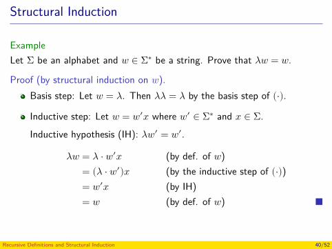
ExampleLet Σ be an alphabet and 𝑤 ∈ Σ∗ be a string. Prove that 𝜆𝑤 = 𝑤.
Proof (by structural induction on 𝑤).Basis step: Let 𝑤 = 𝜆. Then 𝜆𝜆 = 𝜆 by the basis step of (·).
Inductive step: Let 𝑤 = 𝑤′𝑥 where 𝑤′ ∈ Σ∗ and 𝑥 ∈ Σ.Inductive hypothesis (IH): 𝜆𝑤′ = 𝑤′.
𝜆𝑤 = 𝜆 · 𝑤′𝑥 (by def. of 𝑤)= (𝜆 · 𝑤′)𝑥 (by the inductive step of (·))= 𝑤′𝑥 (by IH)= 𝑤 (by def. of 𝑤)
Recursive Definitions and Structural Induction 38/52
Structural Induction
ExampleLet Σ be an alphabet and 𝑤 ∈ Σ∗ be a string. Prove that 𝜆𝑤 = 𝑤.
Proof (by structural induction on 𝑤).Basis step: Let 𝑤 = 𝜆. Then 𝜆𝜆 = 𝜆 by the basis step of (·).
Inductive step: Let 𝑤 = 𝑤′𝑥 where 𝑤′ ∈ Σ∗ and 𝑥 ∈ Σ.Inductive hypothesis (IH): 𝜆𝑤′ = 𝑤′.
𝜆𝑤 = 𝜆 · 𝑤′𝑥 (by def. of 𝑤)= (𝜆 · 𝑤′)𝑥 (by the inductive step of (·))= 𝑤′𝑥 (by IH)= 𝑤 (by def. of 𝑤)
Recursive Definitions and Structural Induction 39/52
Structural Induction
ExampleLet Σ be an alphabet and 𝑤 ∈ Σ∗ be a string. Prove that 𝜆𝑤 = 𝑤.
Proof (by structural induction on 𝑤).Basis step: Let 𝑤 = 𝜆. Then 𝜆𝜆 = 𝜆 by the basis step of (·).
Inductive step: Let 𝑤 = 𝑤′𝑥 where 𝑤′ ∈ Σ∗ and 𝑥 ∈ Σ.Inductive hypothesis (IH): 𝜆𝑤′ = 𝑤′.
𝜆𝑤 = 𝜆 · 𝑤′𝑥 (by def. of 𝑤)= (𝜆 · 𝑤′)𝑥 (by the inductive step of (·))= 𝑤′𝑥 (by IH)= 𝑤 (by def. of 𝑤)
Recursive Definitions and Structural Induction 40/52
Structural Induction
ExampleLet Σ be an alphabet and 𝑤, 𝑤′ ∈ Σ∗ be two strings. Prove that𝑙(𝑤𝑤′) = 𝑙(𝑤) + 𝑙(𝑤′).
Recursive Definitions and Structural Induction 41/52
Structural Induction
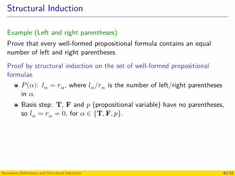
Example (Left and right parentheses)Prove that every well-formed propositional formula contains an equalnumber of left and right parentheses.
Proof by structural induction on the set of well-formed propositionalformulae
𝑃(𝛼): 𝑙𝛼 = 𝑟𝛼, where 𝑙𝛼/𝑟𝛼 is the number of left/right parenthesesin 𝛼.Basis step: T, F and 𝑝 (propositional variable) have no parentheses,so 𝑙𝛼 = 𝑟𝛼 = 0, for 𝛼 ∈ {T, F, 𝑝}.
Recursive Definitions and Structural Induction 42/52
Structural Induction
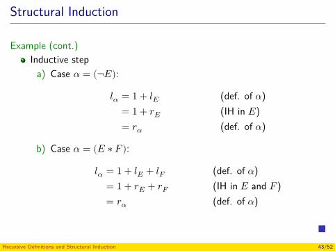
Example (cont.)Inductive step
a) Case 𝛼 = (¬𝐸):
𝑙𝛼 = 1 + 𝑙𝐸 (def. of 𝛼)= 1 + 𝑟𝐸 (IH in 𝐸)= 𝑟𝛼 (def. of 𝛼)
b) Case 𝛼 = (𝐸 ∗ 𝐹):
𝑙𝛼 = 1 + 𝑙𝐸 + 𝑙𝐹 (def. of 𝛼)= 1 + 𝑟𝐸 + 𝑟𝐹 (IH in 𝐸 and 𝐹 )= 𝑟𝛼 (def. of 𝛼)
Recursive Definitions and Structural Induction 43/52
Structural Induction
Structural inductionLet 𝑃 be a propositional function on an inductively defined set/structure.To prove that 𝑃 is true for all the elements on the set/structure, we mustmake two proofs:
Basis step: Prove 𝑃 for all elements specified in the basis step of theinductive definition of the set/structure.
Inductive step: Prove that if 𝑃 is true for each of the elements usedto construct new elements in the inductive step of the definition, theresult holds for these new elements.
Recursive Definitions and Structural Induction 44/52
Structural Induction
Structural inductionLet 𝑃 be a propositional function on an inductively defined set/structure.To prove that 𝑃 is true for all the elements on the set/structure, we mustmake two proofs:
Basis step: Prove 𝑃 for all elements specified in the basis step of theinductive definition of the set/structure.Inductive step: Prove that if 𝑃 is true for each of the elements usedto construct new elements in the inductive step of the definition, theresult holds for these new elements.
Recursive Definitions and Structural Induction 45/52
Structural Induction
Exercise (Rosen (2004), Problem 27(c), p. 252)Let 𝑆 be the subset of the set of ordered pairs of integers inductivelydefined by
Basis step: (0, 0) ∈ 𝑆.Inductive step: If (𝑎, 𝑏) ∈ 𝑆, then
a) (𝑎, 𝑏 + 1) ∈ 𝑆,b) (𝑎 + 1, 𝑏 + 1) ∈ 𝑆 andc) (𝑎 + 2, 𝑏 + 1) ∈ 𝑆.
Use structural induction to show that 𝑎 ≤ 2𝑏 whenever (𝑎, 𝑏) ∈ 𝑆.
Recursive Definitions and Structural Induction 46/52
Structural Induction
Exercise (cont.)
Proof by structural induction on 𝑆𝑃((𝑎, 𝑏)): If (𝑎, 𝑏) ∈ 𝑆 then 𝑎 ≤ 2𝑏.
Basis step 𝑃((0, 0)): 0 ≤ 2 · 0Inductive step:
a) 𝑃((𝑎, 𝑏 + 1)):𝑎 ≤ 2𝑏 (IH 𝑃((𝑎, 𝑏)))
≤ 2𝑏 + 2 (arithmetic)≤ 2(𝑏 + 1) (arithmetic)
Recursive Definitions and Structural Induction 47/52
Structural Induction
Exercise (cont.)
Proof by structural induction on 𝑆𝑃((𝑎, 𝑏)): If (𝑎, 𝑏) ∈ 𝑆 then 𝑎 ≤ 2𝑏.Basis step 𝑃((0, 0)): 0 ≤ 2 · 0
Inductive step:a) 𝑃((𝑎, 𝑏 + 1)):
𝑎 ≤ 2𝑏 (IH 𝑃((𝑎, 𝑏)))≤ 2𝑏 + 2 (arithmetic)≤ 2(𝑏 + 1) (arithmetic)
Recursive Definitions and Structural Induction 48/52
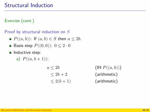
Structural Induction
Exercise (cont.)
Proof by structural induction on 𝑆𝑃((𝑎, 𝑏)): If (𝑎, 𝑏) ∈ 𝑆 then 𝑎 ≤ 2𝑏.Basis step 𝑃((0, 0)): 0 ≤ 2 · 0Inductive step:
a) 𝑃((𝑎, 𝑏 + 1)):𝑎 ≤ 2𝑏 (IH 𝑃((𝑎, 𝑏)))
≤ 2𝑏 + 2 (arithmetic)≤ 2(𝑏 + 1) (arithmetic)
Recursive Definitions and Structural Induction 49/52
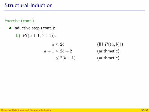
Structural Induction
Exercise (cont.)Inductive step (cont.):
b) 𝑃((𝑎 + 1, 𝑏 + 1)):𝑎 ≤ 2𝑏 (IH 𝑃((𝑎, 𝑏)))
𝑎 + 1 ≤ 2𝑏 + 2 (arithmetic)≤ 2(𝑏 + 1) (arithmetic)
c) 𝑃((𝑎 + 2, 𝑏 + 1)):𝑎 ≤ 2𝑏 (IH 𝑃((𝑎, 𝑏)))
𝑎 + 2 ≤ 2𝑏 + 2 (arithmetic)≤ 2(𝑏 + 1) (arithmetic)
Recursive Definitions and Structural Induction 50/52
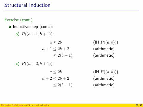
Structural Induction
Exercise (cont.)Inductive step (cont.):
b) 𝑃((𝑎 + 1, 𝑏 + 1)):𝑎 ≤ 2𝑏 (IH 𝑃((𝑎, 𝑏)))
𝑎 + 1 ≤ 2𝑏 + 2 (arithmetic)≤ 2(𝑏 + 1) (arithmetic)
c) 𝑃((𝑎 + 2, 𝑏 + 1)):𝑎 ≤ 2𝑏 (IH 𝑃((𝑎, 𝑏)))
𝑎 + 2 ≤ 2𝑏 + 2 (arithmetic)≤ 2(𝑏 + 1) (arithmetic)
Recursive Definitions and Structural Induction 51/52
References
Rosen, K. H. (2004). Matemática Discreta y sus Aplicaciones. 5th ed.McGraw-Hill (cit. on pp. 14–17, 46).— (2012). Discrete Mathematics and Its Applications. 7th ed.McGraw-Hill (cit. on p. 7).
Recursive Definitions and Structural Induction 52/52
Discrete Structures - CM0246Relations and Their Properties
Andrés Sicard-Ramírez
Universidad EAFIT
Semester 2014-2
Relations
Recall the definition of Cartesian productLet 𝐴 and 𝐵 be sets. The Cartesian product of 𝐴 and 𝐵 is
𝐴 × 𝐵 = {(𝑎, 𝑏) ∣ 𝑎 ∈ 𝐴 ∧ 𝑏 ∈ 𝐵}.ExampleLet 𝐴 = {𝑎, 𝑏} and 𝐵 = {1, 2}. Then
𝐴 × 𝐵 = {(𝑎, 1), (𝑎, 2), (𝑏, 1), (𝑏, 2)}.
Relations and Their Properties 2/36
Relations
Definition (Binary relation)Let 𝐴 and 𝐵 be sets. A binary relation from 𝐴 to 𝐵 is a subset of 𝐴 × 𝐵.
Examples (Trivial relations)𝑅 = ∅ and 𝑅 = 𝐴 × 𝐵 are relations from 𝐴 to 𝐵.
ExamplesSee whiteboard.
Notation(𝑎, 𝑏) ∈ 𝑅 and 𝑎𝑅𝑏. The slides for the 6th ed. of Rosen’s textbook use< 𝑎, 𝑏 >.
Relations and functionsThe functions are relations with additional constraints.
Relations and Their Properties 3/36
Relations
Definition (Binary relation)Let 𝐴 and 𝐵 be sets. A binary relation from 𝐴 to 𝐵 is a subset of 𝐴 × 𝐵.
Examples (Trivial relations)𝑅 = ∅ and 𝑅 = 𝐴 × 𝐵 are relations from 𝐴 to 𝐵.
ExamplesSee whiteboard.
Notation(𝑎, 𝑏) ∈ 𝑅 and 𝑎𝑅𝑏. The slides for the 6th ed. of Rosen’s textbook use< 𝑎, 𝑏 >.
Relations and functionsThe functions are relations with additional constraints.
Relations and Their Properties 4/36
Relations
Definition (Binary relation)Let 𝐴 and 𝐵 be sets. A binary relation from 𝐴 to 𝐵 is a subset of 𝐴 × 𝐵.
Examples (Trivial relations)𝑅 = ∅ and 𝑅 = 𝐴 × 𝐵 are relations from 𝐴 to 𝐵.
ExamplesSee whiteboard.
Notation(𝑎, 𝑏) ∈ 𝑅 and 𝑎𝑅𝑏. The slides for the 6th ed. of Rosen’s textbook use< 𝑎, 𝑏 >.
Relations and functionsThe functions are relations with additional constraints.
Relations and Their Properties 5/36
Relations
Definition (Binary relation)Let 𝐴 and 𝐵 be sets. A binary relation from 𝐴 to 𝐵 is a subset of 𝐴 × 𝐵.
Examples (Trivial relations)𝑅 = ∅ and 𝑅 = 𝐴 × 𝐵 are relations from 𝐴 to 𝐵.
ExamplesSee whiteboard.
Notation(𝑎, 𝑏) ∈ 𝑅 and 𝑎𝑅𝑏. The slides for the 6th ed. of Rosen’s textbook use< 𝑎, 𝑏 >.
Relations and functionsThe functions are relations with additional constraints.
Relations and Their Properties 6/36
Relations
Definition (Binary relation)Let 𝐴 and 𝐵 be sets. A binary relation from 𝐴 to 𝐵 is a subset of 𝐴 × 𝐵.
Examples (Trivial relations)𝑅 = ∅ and 𝑅 = 𝐴 × 𝐵 are relations from 𝐴 to 𝐵.
ExamplesSee whiteboard.
Notation(𝑎, 𝑏) ∈ 𝑅 and 𝑎𝑅𝑏. The slides for the 6th ed. of Rosen’s textbook use< 𝑎, 𝑏 >.
Relations and functionsThe functions are relations with additional constraints.
Relations and Their Properties 7/36
Relations
Definition (Relation on a set)A relation on a set 𝐴 is a relation from 𝐴 to 𝐴.
ExampleSome relations on ℤ:
𝑅1 = {(𝑎, 𝑏) ∣ 𝑎 ≤ 𝑏},𝑅2 = {(𝑎, 𝑏) ∣ 𝑎 > 𝑏},𝑅3 = {(𝑎, 𝑏) ∣ 𝑎 = 𝑏 ∨ 𝑎 = −𝑏},𝑅4 = {(𝑎, 𝑏) ∣ 𝑎 = 𝑏},𝑅5 = {(𝑎, 𝑏) ∣ 𝑎 = 𝑏 + 1},𝑅6 = {(𝑎, 𝑏) ∣ 𝑎 + 𝑏 ≤ 3}.
Relations and Their Properties 8/36

Relations
Definition (Relation on a set)A relation on a set 𝐴 is a relation from 𝐴 to 𝐴.
ExampleSome relations on ℤ:
𝑅1 = {(𝑎, 𝑏) ∣ 𝑎 ≤ 𝑏},𝑅2 = {(𝑎, 𝑏) ∣ 𝑎 > 𝑏},𝑅3 = {(𝑎, 𝑏) ∣ 𝑎 = 𝑏 ∨ 𝑎 = −𝑏},𝑅4 = {(𝑎, 𝑏) ∣ 𝑎 = 𝑏},𝑅5 = {(𝑎, 𝑏) ∣ 𝑎 = 𝑏 + 1},𝑅6 = {(𝑎, 𝑏) ∣ 𝑎 + 𝑏 ≤ 3}.
Relations and Their Properties 9/36
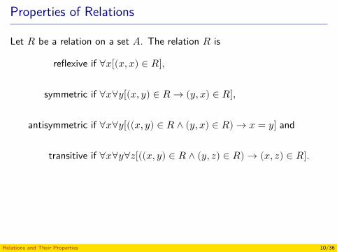
Properties of Relations
Let 𝑅 be a relation on a set 𝐴. The relation 𝑅 is
reflexive if ∀𝑥[(𝑥, 𝑥) ∈ 𝑅],
symmetric if ∀𝑥∀𝑦[(𝑥, 𝑦) ∈ 𝑅 → (𝑦, 𝑥) ∈ 𝑅],
antisymmetric if ∀𝑥∀𝑦[((𝑥, 𝑦) ∈ 𝑅 ∧ (𝑦, 𝑥) ∈ 𝑅) → 𝑥 = 𝑦] and
transitive if ∀𝑥∀𝑦∀𝑧[((𝑥, 𝑦) ∈ 𝑅 ∧ (𝑦, 𝑧) ∈ 𝑅) → (𝑥, 𝑧) ∈ 𝑅].
Relations and Their Properties 10/36
Properties of Relations
ExamplesSee slides § 8.1, p. 5 for the 6th ed. of Rosen’s textbook.
Relations and Their Properties 11/36
Combing Relations
See slides § 8.1, pp. 6-8 for the 6th ed. of Rosen’s textbook.
Relations and Their Properties 12/36
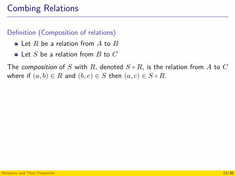
Combing Relations
Definition (Composition of relations)Let 𝑅 be a relation from 𝐴 to 𝐵Let 𝑆 be a relation from 𝐵 to 𝐶
The composition of 𝑆 with 𝑅, denoted 𝑆 ∘ 𝑅, is the relation from 𝐴 to 𝐶where if (𝑎, 𝑏) ∈ 𝑅 and (𝑏, 𝑐) ∈ 𝑆 then (𝑎, 𝑐) ∈ 𝑆 ∘ 𝑅.
Relations and Their Properties 13/36
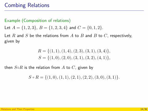
Combing Relations
Example (Composition of relations)Let 𝐴 = {1, 2, 3}, 𝐵 = {1, 2, 3, 4} and 𝐶 = {0, 1, 2}.Let 𝑅 and 𝑆 be the relations from 𝐴 to 𝐵 and 𝐵 to 𝐶, respectively,given by
𝑅 = {(1, 1), (1, 4), (2, 3), (3, 1), (3, 4)},𝑆 = {(1, 0), (2, 0), (3, 1), (3, 2), (4, 1)},
then 𝑆◦𝑅 is the relation from 𝐴 to 𝐶, given by
𝑆 ∘ 𝑅 = {(1, 0), (1, 1), (2, 1), (2, 2), (3, 0), (3, 1)}.
Relations and Their Properties 14/36
Combing Relations
Exercise (Rosen (2004), Problem 31, p. 448)Let 𝑅 be the relation on the set of people consisting of pairs (𝑎, 𝑏),where 𝑎 is a parent of 𝑏. Let 𝑆 be the relation on the set of peopleconsisting of pairs (𝑎, 𝑏), where 𝑎 and 𝑏 are siblings (brothers or sisters).
What are 𝑆◦𝑅 and 𝑅◦𝑆?(𝑎, 𝑏) ∈ 𝑆 ∘ 𝑅 if exists 𝑐 such (𝑎, 𝑐) ∈ 𝑅 (𝑎 is parent of 𝑐) and(𝑐, 𝑏) ∈ 𝑆 (𝑐 is sibling of 𝑏), that is
𝑆 ∘ 𝑅 = {(𝑎, 𝑏) ∣ 𝑎 is a parent of 𝑏 and 𝑏 has a sibling}.
(𝑎, 𝑏) ∈ 𝑅 ∘ 𝑆 if exists 𝑐 such (𝑎, 𝑐) ∈ 𝑆 (𝑎 is sibling of 𝑐) and(𝑐, 𝑏) ∈ 𝑅 (𝑐 is parent of 𝑏), that is
𝑅 ∘ 𝑆 = {(𝑎, 𝑏) ∣ 𝑎 is an aunt or uncle of 𝑏}.
Relations and Their Properties 15/36
Combing Relations
Exercise (Rosen (2004), Problem 31, p. 448)Let 𝑅 be the relation on the set of people consisting of pairs (𝑎, 𝑏),where 𝑎 is a parent of 𝑏. Let 𝑆 be the relation on the set of peopleconsisting of pairs (𝑎, 𝑏), where 𝑎 and 𝑏 are siblings (brothers or sisters).What are 𝑆◦𝑅 and 𝑅◦𝑆?
(𝑎, 𝑏) ∈ 𝑆 ∘ 𝑅 if exists 𝑐 such (𝑎, 𝑐) ∈ 𝑅 (𝑎 is parent of 𝑐) and(𝑐, 𝑏) ∈ 𝑆 (𝑐 is sibling of 𝑏), that is
𝑆 ∘ 𝑅 = {(𝑎, 𝑏) ∣ 𝑎 is a parent of 𝑏 and 𝑏 has a sibling}.
(𝑎, 𝑏) ∈ 𝑅 ∘ 𝑆 if exists 𝑐 such (𝑎, 𝑐) ∈ 𝑆 (𝑎 is sibling of 𝑐) and(𝑐, 𝑏) ∈ 𝑅 (𝑐 is parent of 𝑏), that is
𝑅 ∘ 𝑆 = {(𝑎, 𝑏) ∣ 𝑎 is an aunt or uncle of 𝑏}.
Relations and Their Properties 16/36
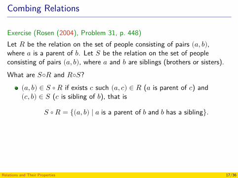
Combing Relations
Exercise (Rosen (2004), Problem 31, p. 448)Let 𝑅 be the relation on the set of people consisting of pairs (𝑎, 𝑏),where 𝑎 is a parent of 𝑏. Let 𝑆 be the relation on the set of peopleconsisting of pairs (𝑎, 𝑏), where 𝑎 and 𝑏 are siblings (brothers or sisters).What are 𝑆◦𝑅 and 𝑅◦𝑆?
(𝑎, 𝑏) ∈ 𝑆 ∘ 𝑅 if exists 𝑐 such (𝑎, 𝑐) ∈ 𝑅 (𝑎 is parent of 𝑐) and(𝑐, 𝑏) ∈ 𝑆 (𝑐 is sibling of 𝑏), that is
𝑆 ∘ 𝑅 = {(𝑎, 𝑏) ∣ 𝑎 is a parent of 𝑏 and 𝑏 has a sibling}.
(𝑎, 𝑏) ∈ 𝑅 ∘ 𝑆 if exists 𝑐 such (𝑎, 𝑐) ∈ 𝑆 (𝑎 is sibling of 𝑐) and(𝑐, 𝑏) ∈ 𝑅 (𝑐 is parent of 𝑏), that is
𝑅 ∘ 𝑆 = {(𝑎, 𝑏) ∣ 𝑎 is an aunt or uncle of 𝑏}.
Relations and Their Properties 17/36
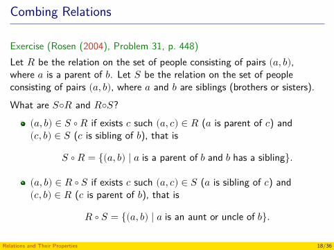
Combing Relations
Exercise (Rosen (2004), Problem 31, p. 448)Let 𝑅 be the relation on the set of people consisting of pairs (𝑎, 𝑏),where 𝑎 is a parent of 𝑏. Let 𝑆 be the relation on the set of peopleconsisting of pairs (𝑎, 𝑏), where 𝑎 and 𝑏 are siblings (brothers or sisters).What are 𝑆◦𝑅 and 𝑅◦𝑆?
(𝑎, 𝑏) ∈ 𝑆 ∘ 𝑅 if exists 𝑐 such (𝑎, 𝑐) ∈ 𝑅 (𝑎 is parent of 𝑐) and(𝑐, 𝑏) ∈ 𝑆 (𝑐 is sibling of 𝑏), that is
𝑆 ∘ 𝑅 = {(𝑎, 𝑏) ∣ 𝑎 is a parent of 𝑏 and 𝑏 has a sibling}.
(𝑎, 𝑏) ∈ 𝑅 ∘ 𝑆 if exists 𝑐 such (𝑎, 𝑐) ∈ 𝑆 (𝑎 is sibling of 𝑐) and(𝑐, 𝑏) ∈ 𝑅 (𝑐 is parent of 𝑏), that is
𝑅 ∘ 𝑆 = {(𝑎, 𝑏) ∣ 𝑎 is an aunt or uncle of 𝑏}.
Relations and Their Properties 18/36
Combing Relations
Definition (Powers of a relation)Let 𝑅 be a relation on the set 𝐴. The powers 𝑅𝑛, for 𝑛 ∈ ℤ+ are definedrecursively by
𝑅1 = 𝑅,𝑅𝑛+1 = 𝑅𝑛 ∘ 𝑅.
ExampleSee slides § 8.1, pp. 9-10 for the 6th ed. of Rosen’s textbook.
Relations and Their Properties 19/36
Combing Relations
Definition (Powers of a relation)Let 𝑅 be a relation on the set 𝐴. The powers 𝑅𝑛, for 𝑛 ∈ ℤ+ are definedrecursively by
𝑅1 = 𝑅,𝑅𝑛+1 = 𝑅𝑛 ∘ 𝑅.
ExampleSee slides § 8.1, pp. 9-10 for the 6th ed. of Rosen’s textbook.
Relations and Their Properties 20/36
Combing Relations
Theorem (Theorem 1, Rosen (5th ed.), p. 446)Let 𝑅 be a relation on a set 𝐴. The relation 𝑅 is transitive iff 𝑅𝑛 ⊆ 𝑅 for𝑛 ∈ ℤ+.
Relations and Their Properties 21/36
Combing Relations
Theorem (cont.)
Proof of ⇒ (if 𝑅 is transitive implies 𝑅𝑛 ⊆ 𝑅 for 𝑛 ∈ ℤ+).By induction on 𝑛 ∈ ℤ+.
1. 𝑃 (𝑛): if 𝑅 is transitive implies 𝑅𝑛 ⊆ 𝑅.2. Basis step 𝑃(1): 𝑅1 = 𝑅 ⊆ 𝑅3. Inductive step:
Inductive hypothesis 𝑃(𝑘): if 𝑅 is transitive implies 𝑅𝑘 ⊆ 𝑅Let’s prove 𝑃(𝑘 + 1):3.1 Let (𝑎, 𝑏) ∈ 𝑅𝑘+1.3.2 Exists 𝑥 ∈ 𝐴 such (𝑎, 𝑥) ∈ 𝑅𝑘 and (𝑥, 𝑏) ∈ 𝑅 (definition of ∘).3.3 (𝑎, 𝑥) ∈ 𝑅 (IH).3.4 If (𝑎, 𝑥) ∈ 𝑅 and (𝑥, 𝑏) ∈ 𝑅 then (𝑎, 𝑏) ∈ 𝑅 (𝑅 is transitive).3.5 𝑅𝑘+1 ⊆ 𝑅.
Relations and Their Properties 22/36
Combing Relations
Theorem (cont.)
Proof of ⇒ (if 𝑅 is transitive implies 𝑅𝑛 ⊆ 𝑅 for 𝑛 ∈ ℤ+).By induction on 𝑛 ∈ ℤ+.
1. 𝑃(𝑛): if 𝑅 is transitive implies 𝑅𝑛 ⊆ 𝑅.
2. Basis step 𝑃(1): 𝑅1 = 𝑅 ⊆ 𝑅3. Inductive step:
Inductive hypothesis 𝑃(𝑘): if 𝑅 is transitive implies 𝑅𝑘 ⊆ 𝑅Let’s prove 𝑃(𝑘 + 1):3.1 Let (𝑎, 𝑏) ∈ 𝑅𝑘+1.3.2 Exists 𝑥 ∈ 𝐴 such (𝑎, 𝑥) ∈ 𝑅𝑘 and (𝑥, 𝑏) ∈ 𝑅 (definition of ∘).3.3 (𝑎, 𝑥) ∈ 𝑅 (IH).3.4 If (𝑎, 𝑥) ∈ 𝑅 and (𝑥, 𝑏) ∈ 𝑅 then (𝑎, 𝑏) ∈ 𝑅 (𝑅 is transitive).3.5 𝑅𝑘+1 ⊆ 𝑅.
Relations and Their Properties 23/36
Combing Relations
Theorem (cont.)
Proof of ⇒ (if 𝑅 is transitive implies 𝑅𝑛 ⊆ 𝑅 for 𝑛 ∈ ℤ+).By induction on 𝑛 ∈ ℤ+.
1. 𝑃(𝑛): if 𝑅 is transitive implies 𝑅𝑛 ⊆ 𝑅.2. Basis step 𝑃(1): 𝑅1 = 𝑅 ⊆ 𝑅
3. Inductive step:Inductive hypothesis 𝑃(𝑘): if 𝑅 is transitive implies 𝑅𝑘 ⊆ 𝑅Let’s prove 𝑃(𝑘 + 1):3.1 Let (𝑎, 𝑏) ∈ 𝑅𝑘+1.3.2 Exists 𝑥 ∈ 𝐴 such (𝑎, 𝑥) ∈ 𝑅𝑘 and (𝑥, 𝑏) ∈ 𝑅 (definition of ∘).3.3 (𝑎, 𝑥) ∈ 𝑅 (IH).3.4 If (𝑎, 𝑥) ∈ 𝑅 and (𝑥, 𝑏) ∈ 𝑅 then (𝑎, 𝑏) ∈ 𝑅 (𝑅 is transitive).3.5 𝑅𝑘+1 ⊆ 𝑅.
Relations and Their Properties 24/36
Combing Relations
Theorem (cont.)
Proof of ⇒ (if 𝑅 is transitive implies 𝑅𝑛 ⊆ 𝑅 for 𝑛 ∈ ℤ+).By induction on 𝑛 ∈ ℤ+.
1. 𝑃(𝑛): if 𝑅 is transitive implies 𝑅𝑛 ⊆ 𝑅.2. Basis step 𝑃(1): 𝑅1 = 𝑅 ⊆ 𝑅3. Inductive step:
Inductive hypothesis 𝑃(𝑘): if 𝑅 is transitive implies 𝑅𝑘 ⊆ 𝑅
Let’s prove 𝑃(𝑘 + 1):3.1 Let (𝑎, 𝑏) ∈ 𝑅𝑘+1.3.2 Exists 𝑥 ∈ 𝐴 such (𝑎, 𝑥) ∈ 𝑅𝑘 and (𝑥, 𝑏) ∈ 𝑅 (definition of ∘).3.3 (𝑎, 𝑥) ∈ 𝑅 (IH).3.4 If (𝑎, 𝑥) ∈ 𝑅 and (𝑥, 𝑏) ∈ 𝑅 then (𝑎, 𝑏) ∈ 𝑅 (𝑅 is transitive).3.5 𝑅𝑘+1 ⊆ 𝑅.
Relations and Their Properties 25/36
Combing Relations
Theorem (cont.)
Proof of ⇒ (if 𝑅 is transitive implies 𝑅𝑛 ⊆ 𝑅 for 𝑛 ∈ ℤ+).By induction on 𝑛 ∈ ℤ+.
1. 𝑃(𝑛): if 𝑅 is transitive implies 𝑅𝑛 ⊆ 𝑅.2. Basis step 𝑃(1): 𝑅1 = 𝑅 ⊆ 𝑅3. Inductive step:
Inductive hypothesis 𝑃(𝑘): if 𝑅 is transitive implies 𝑅𝑘 ⊆ 𝑅Let’s prove 𝑃(𝑘 + 1):
3.1 Let (𝑎, 𝑏) ∈ 𝑅𝑘+1.3.2 Exists 𝑥 ∈ 𝐴 such (𝑎, 𝑥) ∈ 𝑅𝑘 and (𝑥, 𝑏) ∈ 𝑅 (definition of ∘).3.3 (𝑎, 𝑥) ∈ 𝑅 (IH).3.4 If (𝑎, 𝑥) ∈ 𝑅 and (𝑥, 𝑏) ∈ 𝑅 then (𝑎, 𝑏) ∈ 𝑅 (𝑅 is transitive).3.5 𝑅𝑘+1 ⊆ 𝑅.
Relations and Their Properties 26/36
Combing Relations
Theorem (cont.)
Proof of ⇒ (if 𝑅 is transitive implies 𝑅𝑛 ⊆ 𝑅 for 𝑛 ∈ ℤ+).By induction on 𝑛 ∈ ℤ+.
1. 𝑃(𝑛): if 𝑅 is transitive implies 𝑅𝑛 ⊆ 𝑅.2. Basis step 𝑃(1): 𝑅1 = 𝑅 ⊆ 𝑅3. Inductive step:
Inductive hypothesis 𝑃(𝑘): if 𝑅 is transitive implies 𝑅𝑘 ⊆ 𝑅Let’s prove 𝑃(𝑘 + 1):3.1 Let (𝑎, 𝑏) ∈ 𝑅𝑘+1.
3.2 Exists 𝑥 ∈ 𝐴 such (𝑎, 𝑥) ∈ 𝑅𝑘 and (𝑥, 𝑏) ∈ 𝑅 (definition of ∘).3.3 (𝑎, 𝑥) ∈ 𝑅 (IH).3.4 If (𝑎, 𝑥) ∈ 𝑅 and (𝑥, 𝑏) ∈ 𝑅 then (𝑎, 𝑏) ∈ 𝑅 (𝑅 is transitive).3.5 𝑅𝑘+1 ⊆ 𝑅.
Relations and Their Properties 27/36
Combing Relations
Theorem (cont.)
Proof of ⇒ (if 𝑅 is transitive implies 𝑅𝑛 ⊆ 𝑅 for 𝑛 ∈ ℤ+).By induction on 𝑛 ∈ ℤ+.
1. 𝑃(𝑛): if 𝑅 is transitive implies 𝑅𝑛 ⊆ 𝑅.2. Basis step 𝑃(1): 𝑅1 = 𝑅 ⊆ 𝑅3. Inductive step:
Inductive hypothesis 𝑃(𝑘): if 𝑅 is transitive implies 𝑅𝑘 ⊆ 𝑅Let’s prove 𝑃(𝑘 + 1):3.1 Let (𝑎, 𝑏) ∈ 𝑅𝑘+1.3.2 Exists 𝑥 ∈ 𝐴 such (𝑎, 𝑥) ∈ 𝑅𝑘 and (𝑥, 𝑏) ∈ 𝑅 (definition of ∘).
3.3 (𝑎, 𝑥) ∈ 𝑅 (IH).3.4 If (𝑎, 𝑥) ∈ 𝑅 and (𝑥, 𝑏) ∈ 𝑅 then (𝑎, 𝑏) ∈ 𝑅 (𝑅 is transitive).3.5 𝑅𝑘+1 ⊆ 𝑅.
Relations and Their Properties 28/36
Combing Relations
Theorem (cont.)
Proof of ⇒ (if 𝑅 is transitive implies 𝑅𝑛 ⊆ 𝑅 for 𝑛 ∈ ℤ+).By induction on 𝑛 ∈ ℤ+.
1. 𝑃(𝑛): if 𝑅 is transitive implies 𝑅𝑛 ⊆ 𝑅.2. Basis step 𝑃(1): 𝑅1 = 𝑅 ⊆ 𝑅3. Inductive step:
Inductive hypothesis 𝑃(𝑘): if 𝑅 is transitive implies 𝑅𝑘 ⊆ 𝑅Let’s prove 𝑃(𝑘 + 1):3.1 Let (𝑎, 𝑏) ∈ 𝑅𝑘+1.3.2 Exists 𝑥 ∈ 𝐴 such (𝑎, 𝑥) ∈ 𝑅𝑘 and (𝑥, 𝑏) ∈ 𝑅 (definition of ∘).3.3 (𝑎, 𝑥) ∈ 𝑅 (IH).
3.4 If (𝑎, 𝑥) ∈ 𝑅 and (𝑥, 𝑏) ∈ 𝑅 then (𝑎, 𝑏) ∈ 𝑅 (𝑅 is transitive).3.5 𝑅𝑘+1 ⊆ 𝑅.
Relations and Their Properties 29/36
Combing Relations
Theorem (cont.)
Proof of ⇒ (if 𝑅 is transitive implies 𝑅𝑛 ⊆ 𝑅 for 𝑛 ∈ ℤ+).By induction on 𝑛 ∈ ℤ+.
1. 𝑃(𝑛): if 𝑅 is transitive implies 𝑅𝑛 ⊆ 𝑅.2. Basis step 𝑃(1): 𝑅1 = 𝑅 ⊆ 𝑅3. Inductive step:
Inductive hypothesis 𝑃(𝑘): if 𝑅 is transitive implies 𝑅𝑘 ⊆ 𝑅Let’s prove 𝑃(𝑘 + 1):3.1 Let (𝑎, 𝑏) ∈ 𝑅𝑘+1.3.2 Exists 𝑥 ∈ 𝐴 such (𝑎, 𝑥) ∈ 𝑅𝑘 and (𝑥, 𝑏) ∈ 𝑅 (definition of ∘).3.3 (𝑎, 𝑥) ∈ 𝑅 (IH).3.4 If (𝑎, 𝑥) ∈ 𝑅 and (𝑥, 𝑏) ∈ 𝑅 then (𝑎, 𝑏) ∈ 𝑅 (𝑅 is transitive).
3.5 𝑅𝑘+1 ⊆ 𝑅.
Relations and Their Properties 30/36
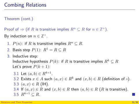
Combing Relations
Theorem (cont.)
Proof of ⇒ (if 𝑅 is transitive implies 𝑅𝑛 ⊆ 𝑅 for 𝑛 ∈ ℤ+).By induction on 𝑛 ∈ ℤ+.
1. 𝑃(𝑛): if 𝑅 is transitive implies 𝑅𝑛 ⊆ 𝑅.2. Basis step 𝑃(1): 𝑅1 = 𝑅 ⊆ 𝑅3. Inductive step:
Inductive hypothesis 𝑃(𝑘): if 𝑅 is transitive implies 𝑅𝑘 ⊆ 𝑅Let’s prove 𝑃(𝑘 + 1):3.1 Let (𝑎, 𝑏) ∈ 𝑅𝑘+1.3.2 Exists 𝑥 ∈ 𝐴 such (𝑎, 𝑥) ∈ 𝑅𝑘 and (𝑥, 𝑏) ∈ 𝑅 (definition of ∘).3.3 (𝑎, 𝑥) ∈ 𝑅 (IH).3.4 If (𝑎, 𝑥) ∈ 𝑅 and (𝑥, 𝑏) ∈ 𝑅 then (𝑎, 𝑏) ∈ 𝑅 (𝑅 is transitive).3.5 𝑅𝑘+1 ⊆ 𝑅.
Relations and Their Properties 31/36
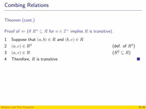
Combing Relations
Theorem (cont.)
Proof of ⇐ (if 𝑅𝑛 ⊆ 𝑅 for 𝑛 ∈ ℤ+ implies 𝑅 is transitive).
1 Suppose that (𝑎, 𝑏) ∈ 𝑅 and (𝑏, 𝑐) ∈ 𝑅2 (𝑎, 𝑐) ∈ 𝑅2 (def. of 𝑅2)3 (𝑎, 𝑐) ∈ 𝑅 (𝑅2 ⊆ 𝑅)4 Therefore, 𝑅 is transitive
Relations and Their Properties 32/36
Inverse and Complementary Relations
Let 𝑅 be a relation from 𝐴 to 𝐵.
Definition (Inverse relation)The inverse relation from 𝐵 to 𝐴, denoted by 𝑅−1, is the set of orderedpairs
𝑅−1 = {(𝑏, 𝑎) ∣ (𝑎, 𝑏) ∈ 𝑅}.
Definition (Complementary relation)The complementary relation from 𝐴 to 𝐵, denoted by 𝑅, is the set ofordered pairs
𝑅 = {(𝑎, 𝑏) ∣ (𝑎, 𝑏) ∉ 𝑅}.
Relations and Their Properties 33/36
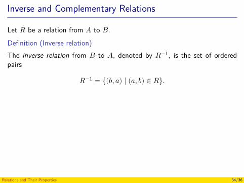
Inverse and Complementary Relations
Let 𝑅 be a relation from 𝐴 to 𝐵.Definition (Inverse relation)The inverse relation from 𝐵 to 𝐴, denoted by 𝑅−1, is the set of orderedpairs
𝑅−1 = {(𝑏, 𝑎) ∣ (𝑎, 𝑏) ∈ 𝑅}.
Definition (Complementary relation)The complementary relation from 𝐴 to 𝐵, denoted by 𝑅, is the set ofordered pairs
𝑅 = {(𝑎, 𝑏) ∣ (𝑎, 𝑏) ∉ 𝑅}.
Relations and Their Properties 34/36
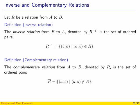
Inverse and Complementary Relations
Let 𝑅 be a relation from 𝐴 to 𝐵.Definition (Inverse relation)The inverse relation from 𝐵 to 𝐴, denoted by 𝑅−1, is the set of orderedpairs
𝑅−1 = {(𝑏, 𝑎) ∣ (𝑎, 𝑏) ∈ 𝑅}.
Definition (Complementary relation)The complementary relation from 𝐴 to 𝐵, denoted by 𝑅, is the set ofordered pairs
𝑅 = {(𝑎, 𝑏) ∣ (𝑎, 𝑏) ∉ 𝑅}.
Relations and Their Properties 35/36
References
Rosen, K. H. (2004). Matemática Discreta y sus Aplicaciones. 5th ed.McGraw-Hill (cit. on pp. 15–18).
Relations and Their Properties 36/36
Discrete Structures - CM0246Representing Relations
Andrés Sicard-Ramírez
Universidad EAFIT
Semester 2014-2
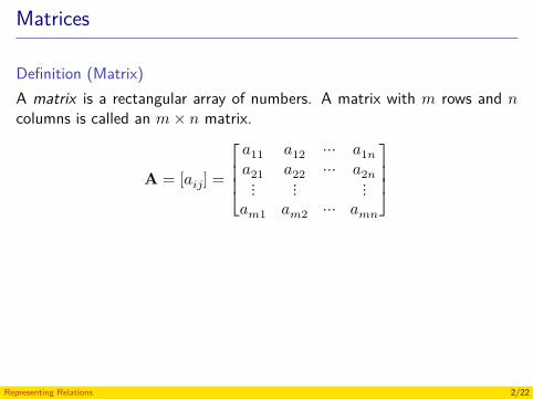
Matrices
Definition (Matrix)A matrix is a rectangular array of numbers. A matrix with 𝑚 rows and 𝑛columns is called an 𝑚 × 𝑛 matrix.
A = [𝑎𝑖𝑗] =⎡⎢⎢⎣
𝑎11 𝑎12 ⋯ 𝑎1𝑛𝑎21 𝑎22 ⋯ 𝑎2𝑛
⋮ ⋮ ⋮𝑎𝑚1 𝑎𝑚2 ⋯ 𝑎𝑚𝑛
⎤⎥⎥⎦
Representing Relations 2/22
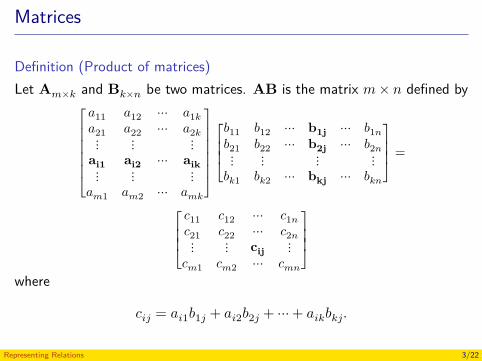
Matrices
Definition (Product of matrices)Let A𝑚×𝑘 and B𝑘×𝑛 be two matrices. AB is the matrix 𝑚 × 𝑛 defined by
⎡⎢⎢⎢⎢⎣
𝑎11 𝑎12 ⋯ 𝑎1𝑘𝑎21 𝑎22 ⋯ 𝑎2𝑘
⋮ ⋮ ⋮ai1 ai2 ⋯ aik⋮ ⋮ ⋮
𝑎𝑚1 𝑎𝑚2 ⋯ 𝑎𝑚𝑘
⎤⎥⎥⎥⎥⎦
⎡⎢⎢⎣
𝑏11 𝑏12 ⋯ b1j ⋯ 𝑏1𝑛𝑏21 𝑏22 ⋯ b2j ⋯ 𝑏2𝑛⋮ ⋮ ⋮ ⋮
𝑏𝑘1 𝑏𝑘2 ⋯ bkj ⋯ 𝑏𝑘𝑛
⎤⎥⎥⎦
=
⎡⎢⎢⎣
𝑐11 𝑐12 ⋯ 𝑐1𝑛𝑐21 𝑐22 ⋯ 𝑐2𝑛⋮ ⋮ cij ⋮
𝑐𝑚1 𝑐𝑚2 ⋯ 𝑐𝑚𝑛
⎤⎥⎥⎦
where
𝑐𝑖𝑗 = 𝑎𝑖1𝑏1𝑗 + 𝑎𝑖2𝑏2𝑗 + ⋯ + 𝑎𝑖𝑘𝑏𝑘𝑗.
Representing Relations 3/22
Matrices
Definition (Transpose of a matrix)Let A = [𝑎𝑖𝑗] be a 𝑚 × 𝑛 matrix. The transpose of A, denoted by A𝑡, isthe 𝑛 × 𝑚 matrix obtained by interchanging the rows and columns of A.
Representing Relations 4/22
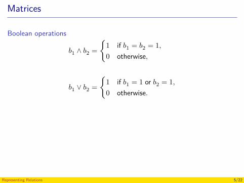
Matrices
Boolean operations
𝑏1 ∧ 𝑏2 = {1 if 𝑏1 = 𝑏2 = 1,0 otherwise,
𝑏1 ∨ 𝑏2 = {1 if 𝑏1 = 1 or 𝑏2 = 1,0 otherwise.
Representing Relations 5/22
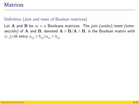
Matrices
Definition (Join and meet of Boolean matrices)Let A and B be 𝑚 × 𝑛 Booleans matrices. The join (unión)/meet (inter-sección) of A and B, denoted A ∨ B/A ∧ B, is the Boolean matrix with(𝑖, 𝑗)-th entry 𝑎𝑖𝑗 ∨ 𝑏𝑖𝑗/𝑎𝑖𝑗 ∧ 𝑏𝑖𝑗.
Example
A = [1 0 10 1 0] , B = [0 1 0
1 1 0] ,
A ∨ B = [1 ∨ 0 0 ∨ 1 1 ∨ 00 ∨ 1 1 ∨ 1 0 ∨ 0] = [1 1 1
1 1 0] ,
A ∧ B = [1 ∧ 0 0 ∧ 1 1 ∧ 00 ∧ 1 1 ∧ 1 0 ∧ 0] = [0 0 0
0 1 0] .
Representing Relations 6/22
Matrices
Definition (Join and meet of Boolean matrices)Let A and B be 𝑚 × 𝑛 Booleans matrices. The join (unión)/meet (inter-sección) of A and B, denoted A ∨ B/A ∧ B, is the Boolean matrix with(𝑖, 𝑗)-th entry 𝑎𝑖𝑗 ∨ 𝑏𝑖𝑗/𝑎𝑖𝑗 ∧ 𝑏𝑖𝑗.
Example
A = [1 0 10 1 0] , B = [0 1 0
1 1 0] ,
A ∨ B = [1 ∨ 0 0 ∨ 1 1 ∨ 00 ∨ 1 1 ∨ 1 0 ∨ 0] = [1 1 1
1 1 0] ,
A ∧ B = [1 ∧ 0 0 ∧ 1 1 ∧ 00 ∧ 1 1 ∧ 1 0 ∧ 0] = [0 0 0
0 1 0] .
Representing Relations 7/22
Matrices
Definition (Join and meet of Boolean matrices)Let A and B be 𝑚 × 𝑛 Booleans matrices. The join (unión)/meet (inter-sección) of A and B, denoted A ∨ B/A ∧ B, is the Boolean matrix with(𝑖, 𝑗)-th entry 𝑎𝑖𝑗 ∨ 𝑏𝑖𝑗/𝑎𝑖𝑗 ∧ 𝑏𝑖𝑗.
Example
A = [1 0 10 1 0] , B = [0 1 0
1 1 0] ,
A ∨ B = [1 ∨ 0 0 ∨ 1 1 ∨ 00 ∨ 1 1 ∨ 1 0 ∨ 0] = [1 1 1
1 1 0] ,
A ∧ B = [1 ∧ 0 0 ∧ 1 1 ∧ 00 ∧ 1 1 ∧ 1 0 ∧ 0] = [0 0 0
0 1 0] .
Representing Relations 8/22
Matrices
Definition (Join and meet of Boolean matrices)Let A and B be 𝑚 × 𝑛 Booleans matrices. The join (unión)/meet (inter-sección) of A and B, denoted A ∨ B/A ∧ B, is the Boolean matrix with(𝑖, 𝑗)-th entry 𝑎𝑖𝑗 ∨ 𝑏𝑖𝑗/𝑎𝑖𝑗 ∧ 𝑏𝑖𝑗.
Example
A = [1 0 10 1 0] , B = [0 1 0
1 1 0] ,
A ∨ B = [1 ∨ 0 0 ∨ 1 1 ∨ 00 ∨ 1 1 ∨ 1 0 ∨ 0] = [1 1 1
1 1 0] ,
A ∧ B = [1 ∧ 0 0 ∧ 1 1 ∧ 00 ∧ 1 1 ∧ 1 0 ∧ 0] = [0 0 0
0 1 0] .
Representing Relations 9/22
Matrices
Definition (Product of Boolean matrices)Let A𝑚×𝑘 and B𝑘×𝑛 be two Boolean matrices. The Boolean product of Aand B, denoted A ⊙ B, is the Boolean matrix 𝑚 × 𝑛 with (𝑖, 𝑗)-th entry
𝑐𝑖𝑗 = (𝑎𝑖1 ∧ 𝑏1𝑗) ∨ (𝑎𝑖2 ∧ 𝑏2𝑗) ∨ ⋯ ∨ (𝑎𝑖𝑘 ∧ 𝑏𝑘𝑗).
Representing Relations 10/22
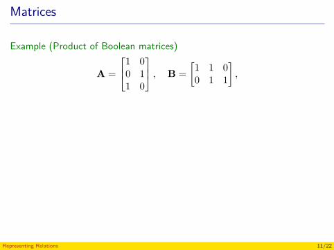
Matrices
Example (Product of Boolean matrices)
A = ⎡⎢⎣
1 00 11 0
⎤⎥⎦
, B = [1 1 00 1 1] ,
A ⊙ B = ⎡⎢⎣
(1 ∧ 1) ∨ (0 ∧ 0) (1 ∧ 1) ∨ (0 ∧ 1) (1 ∧ 0) ∨ (0 ∧ 1)(0 ∧ 1) ∨ (1 ∧ 0) (0 ∧ 1) ∨ (1 ∧ 1) (0 ∧ 0) ∨ (1 ∧ 1)(1 ∧ 1) ∨ (0 ∧ 0) (1 ∧ 1) ∨ (0 ∧ 1) (1 ∧ 0) ∨ (0 ∧ 1)
⎤⎥⎦
= ⎡⎢⎣
1 ∨ 0 1 ∨ 0 0 ∨ 00 ∨ 0 0 ∨ 1 0 ∨ 11 ∨ 0 1 ∨ 0 0 ∨ 0
⎤⎥⎦
= ⎡⎢⎣
1 1 00 1 11 1 0
⎤⎥⎦
.
Representing Relations 11/22
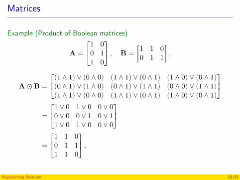
Matrices
Example (Product of Boolean matrices)
A = ⎡⎢⎣
1 00 11 0
⎤⎥⎦
, B = [1 1 00 1 1] ,
A ⊙ B = ⎡⎢⎣
(1 ∧ 1) ∨ (0 ∧ 0) (1 ∧ 1) ∨ (0 ∧ 1) (1 ∧ 0) ∨ (0 ∧ 1)(0 ∧ 1) ∨ (1 ∧ 0) (0 ∧ 1) ∨ (1 ∧ 1) (0 ∧ 0) ∨ (1 ∧ 1)(1 ∧ 1) ∨ (0 ∧ 0) (1 ∧ 1) ∨ (0 ∧ 1) (1 ∧ 0) ∨ (0 ∧ 1)
⎤⎥⎦
= ⎡⎢⎣
1 ∨ 0 1 ∨ 0 0 ∨ 00 ∨ 0 0 ∨ 1 0 ∨ 11 ∨ 0 1 ∨ 0 0 ∨ 0
⎤⎥⎦
= ⎡⎢⎣
1 1 00 1 11 1 0
⎤⎥⎦
.
Representing Relations 12/22
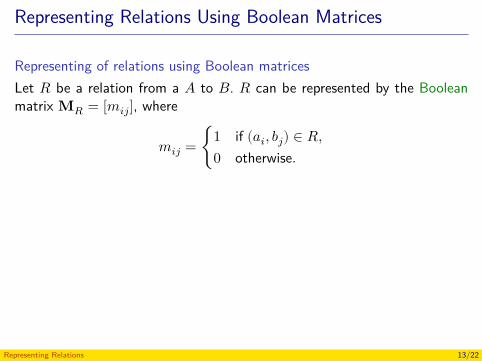
Representing Relations Using Boolean Matrices
Representing of relations using Boolean matricesLet 𝑅 be a relation from a 𝐴 to 𝐵. 𝑅 can be represented by the Booleanmatrix M𝑅 = [𝑚𝑖𝑗], where
𝑚𝑖𝑗 = {1 if (𝑎𝑖, 𝑏𝑗) ∈ 𝑅,0 otherwise.
ExamplesWhiteboard.
Representing Relations 13/22
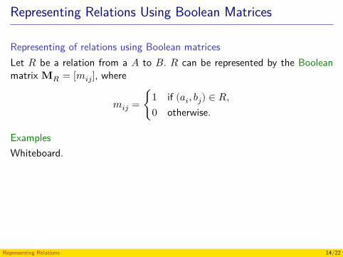
Representing Relations Using Boolean Matrices
Representing of relations using Boolean matricesLet 𝑅 be a relation from a 𝐴 to 𝐵. 𝑅 can be represented by the Booleanmatrix M𝑅 = [𝑚𝑖𝑗], where
𝑚𝑖𝑗 = {1 if (𝑎𝑖, 𝑏𝑗) ∈ 𝑅,0 otherwise.
ExamplesWhiteboard.
Representing Relations 14/22
Representing Relations Using Boolean Matrices
Properties of relations from their Boolean matrix representationSee slides § 8.3 for the 6th ed. of Rosen’s textbook.
Representing Relations 15/22
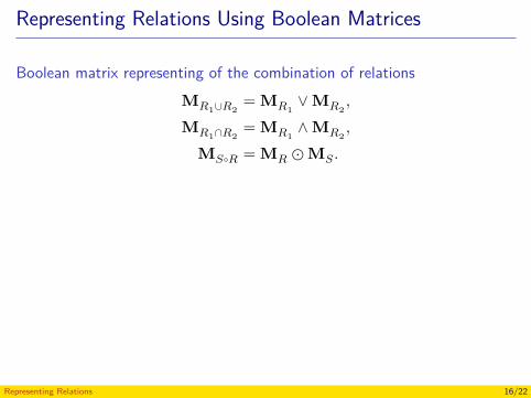
Representing Relations Using Boolean Matrices
Boolean matrix representing of the combination of relationsM𝑅1∪𝑅2
= M𝑅1∨ M𝑅2
,M𝑅1∩𝑅2
= M𝑅1∧ M𝑅2
,M𝑆∘𝑅 = M𝑅 ⊙ M𝑆.
Representing Relations 16/22
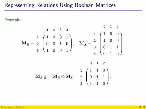
Representing Relations Using Boolean Matrices
Example
M𝑅 = ⎛⎜⎜⎜⎝
1 2 3 4
1 1 0 0 12 0 0 1 03 1 0 0 1
⎞⎟⎟⎟⎠
, M𝑆 =⎛⎜⎜⎜⎜⎜⎜⎝
0 1 2
1 1 0 02 1 0 03 0 1 14 0 1 0
⎞⎟⎟⎟⎟⎟⎟⎠
,
M𝑆∘𝑅 = M𝑅 ⊙ M𝑆 = ⎛⎜⎜⎜⎝
0 1 2
1 1 1 02 0 1 13 1 1 0
⎞⎟⎟⎟⎠
.
Representing Relations 17/22
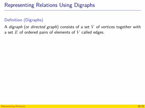
Representing Relations Using Digraphs
Definition (Digraphs)A digraph (or directed graph) consists of a set 𝑉 of vertices together witha set 𝐸 of ordered pairs of elements of 𝑉 called edges.
Representing relations using digraphsThe relation 𝑅 on a set 𝐴 is represented by a digraph where 𝑉 = 𝐴 and(𝑎, 𝑏) is an edge if (𝑎, 𝑏) ∈ 𝑅.
Representing Relations 18/22
Representing Relations Using Digraphs
Definition (Digraphs)A digraph (or directed graph) consists of a set 𝑉 of vertices together witha set 𝐸 of ordered pairs of elements of 𝑉 called edges.
Representing relations using digraphsThe relation 𝑅 on a set 𝐴 is represented by a digraph where 𝑉 = 𝐴 and(𝑎, 𝑏) is an edge if (𝑎, 𝑏) ∈ 𝑅.
Representing Relations 19/22
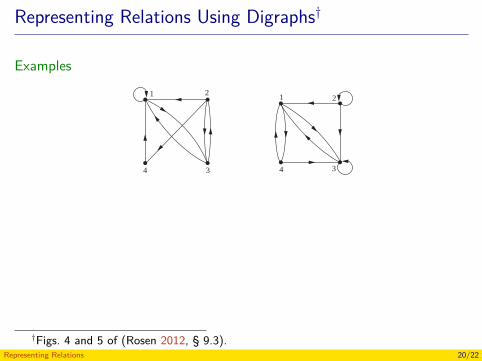
Representing Relations Using Digraphs†
Examples
9.3 Representing Relations 595
EXAMPLE 8 The directed graph of the relation
R = {(1, 1), (1, 3), (2, 1), (2, 3), (2, 4), (3, 1), (3, 2), (4, 1)}
on the set {1, 2, 3, 4} is shown in Figure 4. ▲
EXAMPLE 9 What are the ordered pairs in the relation R represented by the directed graph shown in Figure 5?
Solution: The ordered pairs (x, y) in the relation are
R = {(1, 3), (1, 4), (2, 1), (2, 2), (2, 3), (3, 1), (3, 3), (4, 1), (4, 3)}.
Each of these pairs corresponds to an edge of the directed graph, with (2, 2) and (3, 3) corre-sponding to loops. ▲
The directed graph representing a relation can be used to determine whether the relationWe will study directedgraphs extensively inChapter 10.
has various properties. For instance, a relation is reflexive if and only if there is a loop at everyvertex of the directed graph, so that every ordered pair of the form (x, x) occurs in the relation.A relation is symmetric if and only if for every edge between distinct vertices in its digraphthere is an edge in the opposite direction, so that (y, x) is in the relation whenever (x, y) isin the relation. Similarly, a relation is antisymmetric if and only if there are never two edgesin opposite directions between distinct vertices. Finally, a relation is transitive if and only ifwhenever there is an edge from a vertex x to a vertex y and an edge from a vertex y to avertex z, there is an edge from x to z (completing a triangle where each side is a directed edgewith the correct direction).
Remark: Note that a symmetric relation can be represented by an undirected graph, which is agraph where edges do not have directions. We will study undirected graphs in Chapter 10.
EXAMPLE 10 Determine whether the relations for the directed graphs shown in Figure 6 are reflexive, sym-metric, antisymmetric, and/or transitive.
Solution: Because there are loops at every vertex of the directed graph of R, it is reflexive. R isneither symmetric nor antisymmetric because there is an edge from a to b but not one from b toa, but there are edges in both directions connecting b and c. Finally, R is not transitive becausethere is an edge from a to b and an edge from b to c, but no edge from a to c.
1
4 3
2
FIGURE 4 TheDirected Graphof the Relation R.
21
4 3
FIGURE 5 TheDirected Graphof the Relation R.
a
b c
(a) Directed graph of R
b
(b) Directed graph of S
c
a
d
FIGURE 6 The Directed Graphs of theRelations R and S.
†Figs. 4 and 5 of (Rosen 2012, § 9.3).Representing Relations 20/22
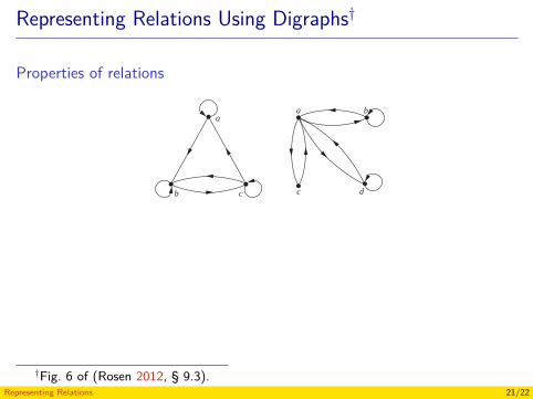
Representing Relations Using Digraphs†
Properties of relations
9.3 Representing Relations 595
EXAMPLE 8 The directed graph of the relation
R = {(1, 1), (1, 3), (2, 1), (2, 3), (2, 4), (3, 1), (3, 2), (4, 1)}
on the set {1, 2, 3, 4} is shown in Figure 4. ▲
EXAMPLE 9 What are the ordered pairs in the relation R represented by the directed graph shown in Figure 5?
Solution: The ordered pairs (x, y) in the relation are
R = {(1, 3), (1, 4), (2, 1), (2, 2), (2, 3), (3, 1), (3, 3), (4, 1), (4, 3)}.
Each of these pairs corresponds to an edge of the directed graph, with (2, 2) and (3, 3) corre-sponding to loops. ▲
The directed graph representing a relation can be used to determine whether the relationWe will study directedgraphs extensively inChapter 10.
has various properties. For instance, a relation is reflexive if and only if there is a loop at everyvertex of the directed graph, so that every ordered pair of the form (x, x) occurs in the relation.A relation is symmetric if and only if for every edge between distinct vertices in its digraphthere is an edge in the opposite direction, so that (y, x) is in the relation whenever (x, y) isin the relation. Similarly, a relation is antisymmetric if and only if there are never two edgesin opposite directions between distinct vertices. Finally, a relation is transitive if and only ifwhenever there is an edge from a vertex x to a vertex y and an edge from a vertex y to avertex z, there is an edge from x to z (completing a triangle where each side is a directed edgewith the correct direction).
Remark: Note that a symmetric relation can be represented by an undirected graph, which is agraph where edges do not have directions. We will study undirected graphs in Chapter 10.
EXAMPLE 10 Determine whether the relations for the directed graphs shown in Figure 6 are reflexive, sym-metric, antisymmetric, and/or transitive.
Solution: Because there are loops at every vertex of the directed graph of R, it is reflexive. R isneither symmetric nor antisymmetric because there is an edge from a to b but not one from b toa, but there are edges in both directions connecting b and c. Finally, R is not transitive becausethere is an edge from a to b and an edge from b to c, but no edge from a to c.
1
4 3
2
FIGURE 4 TheDirected Graphof the Relation R.
21
4 3
FIGURE 5 TheDirected Graphof the Relation R.
a
b c
(a) Directed graph of R
b
(b) Directed graph of S
c
a
d
FIGURE 6 The Directed Graphs of theRelations R and S.
†Fig. 6 of (Rosen 2012, § 9.3).Representing Relations 21/22

References
Rosen, K. H. (2012). Discrete Mathematics and Its Applications. 7th ed.McGraw-Hill (cit. on pp. 20, 21).
Representing Relations 22/22
Discrete Structures - CM0246Equivalence Relations
Andrés Sicard-Ramírez
Universidad EAFIT
Semester 2014-2
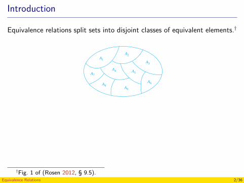
Introduction
Equivalence relations split sets into disjoint classes of equivalent elements.†9.5 Equivalence Relations 613
A1
A7
A4
A2
A3
A6
A5
A9
A8
FIGURE 1 A Partition of a Set.
and
⋃
i∈IAi = S.
(Here the notation⋃
i∈I Ai represents the union of the sets Ai for all i ∈ I .) Figure 1 illustratesthe concept of a partition of a set.
EXAMPLE 12 Suppose that S = {1, 2, 3, 4, 5, 6}. The collection of sets A1 = {1, 2, 3}, A2 = {4, 5}, andA3 = {6} forms a partition of S, because these sets are disjoint and their union is S. ▲
We have seen that the equivalence classes of an equivalence relation on a set form a partitionof the set. The subsets in this partition are the equivalence classes. Conversely, every partitionof a set can be used to form an equivalence relation. Two elements are equivalent with respectto this relation if and only if they are in the same subset of the partition.
To see this, assume that {Ai | i ∈ I } is a partition on S. Let R be the relation on S consistingof the pairs (x, y), where x and y belong to the same subset Ai in the partition. To show that R
is an equivalence relation we must show that R is reflexive, symmetric, and transitive.We see that (a, a) ∈ R for every a ∈ S, because a is in the same subset as itself. Hence, R
is reflexive. If (a, b) ∈ R, then b and a are in the same subset of the partition, so that (b, a) ∈ R
as well. Hence, R is symmetric. If (a, b) ∈ R and (b, c) ∈ R, then a and b are in the samesubset X in the partition, and b and c are in the same subset Y of the partition. Because the subsetsof the partition are disjoint and b belongs to X and Y , it follows that X = Y . Consequently, a
and c belong to the same subset of the partition, so (a, c) ∈ R. Thus, R is transitive.It follows that R is an equivalence relation. The equivalence classes of R consist of subsets
of S containing related elements, and by the definition of R, these are the subsets of the partition.Theorem 2 summarizes the connections we have established between equivalence relations andpartitions.
THEOREM 2 Let R be an equivalence relation on a set S. Then the equivalence classes of R form a partitionof S. Conversely, given a partition {Ai | i ∈ I } of the set S, there is an equivalence relationR that has the sets Ai , i ∈ I , as its equivalence classes.
Example 13 shows how to construct an equivalence relation from a partition.
EXAMPLE 13 List the ordered pairs in the equivalence relation R produced by the partition A1 = {1, 2, 3},A2 = {4, 5}, and A3 = {6} of S = {1, 2, 3, 4, 5, 6}, given in Example 12.
†Fig. 1 of (Rosen 2012, § 9.5).Equivalence Relations 2/36
Equivalence Relations
Definition (Equivalence relation)A relation on a set 𝐴 is an equivalence relation if it is reflexive, symmetricand transitive.
Example (Words of the same length)
Σ = {𝑎, 𝑏, … , 𝑧},Σ∗ = {𝑤 ∣ 𝑤 is a word on Σ},
𝑅 = {(𝑤, 𝑤′) ∣ 𝑙(𝑤) = 𝑙(𝑤′)} ⊆ Σ∗ × Σ∗.
Equivalence Relations 3/36
Equivalence Relations
Definition (Equivalence relation)A relation on a set 𝐴 is an equivalence relation if it is reflexive, symmetricand transitive.
Example (Words of the same length)
Σ = {𝑎, 𝑏, … , 𝑧},Σ∗ = {𝑤 ∣ 𝑤 is a word on Σ},
𝑅 = {(𝑤, 𝑤′) ∣ 𝑙(𝑤) = 𝑙(𝑤′)} ⊆ Σ∗ × Σ∗.
Equivalence Relations 4/36
Equivalence Relations
ExerciseLet 𝐴 = {𝑎, 𝑒, 𝑖, 𝑜, 𝑢}. Is the equality relation on 𝐴 an equivalencerelation?
ExerciseLet 𝐴 ≠ ∅ be a set. Are the relations ∅ and 𝐴 × 𝐴 equivalence relations?
Example
FUN = {𝑓 ∣ 𝑓 ∶ {0, 1} → {0, 1}},
𝑅 = {(𝑓, 𝑔) ∣ 𝑓(1) = 𝑔(1)} ⊆ FUN × FUN.
Equivalence Relations 5/36
Equivalence Relations
ExerciseLet 𝐴 = {𝑎, 𝑒, 𝑖, 𝑜, 𝑢}. Is the equality relation on 𝐴 an equivalencerelation?
ExerciseLet 𝐴 ≠ ∅ be a set. Are the relations ∅ and 𝐴 × 𝐴 equivalence relations?
Example
FUN = {𝑓 ∣ 𝑓 ∶ {0, 1} → {0, 1}},
𝑅 = {(𝑓, 𝑔) ∣ 𝑓(1) = 𝑔(1)} ⊆ FUN × FUN.
Equivalence Relations 6/36
Equivalence Relations
ExerciseLet 𝐴 = {𝑎, 𝑒, 𝑖, 𝑜, 𝑢}. Is the equality relation on 𝐴 an equivalencerelation?
ExerciseLet 𝐴 ≠ ∅ be a set. Are the relations ∅ and 𝐴 × 𝐴 equivalence relations?
Example
FUN = {𝑓 ∣ 𝑓 ∶ {0, 1} → {0, 1}},
𝑅 = {(𝑓, 𝑔) ∣ 𝑓(1) = 𝑔(1)} ⊆ FUN × FUN.
Equivalence Relations 7/36
Equivalence Relations
ExerciseLet 𝐴 be a unitary set. It is possible to define an equivalence relationon 𝐴?
ExerciseDefine an equivalence relation on a finite/infinite set.
Equivalence Relations 8/36
Equivalence Relations
ExerciseLet 𝐴 be a unitary set. It is possible to define an equivalence relationon 𝐴?
ExerciseDefine an equivalence relation on a finite/infinite set.
Equivalence Relations 9/36
Equivalence Relations
Definition (Congruence relation)Let 𝑚 and 𝑛 be integers and let 𝑑 be a positive integer. The number 𝑚is congruent to 𝑛 modulo 𝑑, denoted by 𝑚 ≡ 𝑛 (mod 𝑑) if, and only if,𝑑 ∣ (𝑚 − 𝑛).
ExampleThe congruence relation is an equivalence relation.
Equivalence Relations 10/36
Equivalence Relations
Definition (Congruence relation)Let 𝑚 and 𝑛 be integers and let 𝑑 be a positive integer. The number 𝑚is congruent to 𝑛 modulo 𝑑, denoted by 𝑚 ≡ 𝑛 (mod 𝑑) if, and only if,𝑑 ∣ (𝑚 − 𝑛).
ExampleThe congruence relation is an equivalence relation.
Equivalence Relations 11/36
Equivalence Classes
Definition (Equivalence class)Let 𝑅 be an equivalence relation on a set 𝐴. The equivalence class of 𝑎 ∈ 𝐴with respect to 𝑅 is defined by
[𝑎]𝑅 = {𝑠 ∣ (𝑎, 𝑠) ∈ 𝑅}.
Notation: We remove the subscript 𝑅 if the relation 𝑅 is clear in thecontext.Example (Words of the same length)
[𝜆] = {𝜆},[𝑎] = {𝑎, 𝑏, … , 𝑧} = [𝑘],
[𝑎𝑎] = {𝑎𝑎, 𝑎𝑏, … , 𝑎𝑧, 𝑏𝑎, 𝑏𝑏, … , 𝑏𝑧, … 𝑧𝑎, … 𝑧𝑧},[ℎ𝑔𝑏𝑗] = {𝑤 ∣ 𝑙(𝑤) = 4}.
Equivalence Relations 12/36
Equivalence Classes
Definition (Equivalence class)Let 𝑅 be an equivalence relation on a set 𝐴. The equivalence class of 𝑎 ∈ 𝐴with respect to 𝑅 is defined by
[𝑎]𝑅 = {𝑠 ∣ (𝑎, 𝑠) ∈ 𝑅}.Notation: We remove the subscript 𝑅 if the relation 𝑅 is clear in thecontext.
Example (Words of the same length)
[𝜆] = {𝜆},[𝑎] = {𝑎, 𝑏, … , 𝑧} = [𝑘],
[𝑎𝑎] = {𝑎𝑎, 𝑎𝑏, … , 𝑎𝑧, 𝑏𝑎, 𝑏𝑏, … , 𝑏𝑧, … 𝑧𝑎, … 𝑧𝑧},[ℎ𝑔𝑏𝑗] = {𝑤 ∣ 𝑙(𝑤) = 4}.
Equivalence Relations 13/36
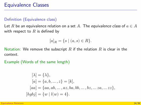
Equivalence Classes
Definition (Equivalence class)Let 𝑅 be an equivalence relation on a set 𝐴. The equivalence class of 𝑎 ∈ 𝐴with respect to 𝑅 is defined by
[𝑎]𝑅 = {𝑠 ∣ (𝑎, 𝑠) ∈ 𝑅}.Notation: We remove the subscript 𝑅 if the relation 𝑅 is clear in thecontext.Example (Words of the same length)
[𝜆] = {𝜆},[𝑎] = {𝑎, 𝑏, … , 𝑧} = [𝑘],
[𝑎𝑎] = {𝑎𝑎, 𝑎𝑏, … , 𝑎𝑧, 𝑏𝑎, 𝑏𝑏, … , 𝑏𝑧, … 𝑧𝑎, … 𝑧𝑧},[ℎ𝑔𝑏𝑗] = {𝑤 ∣ 𝑙(𝑤) = 4}.
Equivalence Relations 14/36
Equivalence Classes
Example (Equality relation)
Example (Cartesian product)
Equivalence Relations 15/36
Equivalence Classes
Example (Equality relation)
Example (Cartesian product)
Equivalence Relations 16/36
Equivalence Relations
TheoremLet 𝑅 be an equivalence relation on a set 𝐴. For all 𝑎, 𝑏 ∈ 𝐴,
𝑎𝑅𝑏 ⇒ [𝑎] = [𝑏].
Proof.i) 𝑎𝑅𝑏 ⇒ [𝑎] ⊆ [𝑏]1 𝑎𝑅𝑏2 Let 𝑐 ∈ [𝑎]3 𝑎𝑅𝑐 (def. of [𝑎])4 𝑏𝑅𝑎 (𝑅 is symmetric)5 𝑏𝑅𝑐 (𝑅 is transitive)6 𝑐 ∈ [𝑏] (def. of [𝑏])7 Therefore [𝑎] ⊆ [𝑏]
Equivalence Relations 17/36

Equivalence Relations
TheoremLet 𝑅 be an equivalence relation on a set 𝐴. For all 𝑎, 𝑏 ∈ 𝐴,
𝑎𝑅𝑏 ⇒ [𝑎] = [𝑏].
Proof.i) 𝑎𝑅𝑏 ⇒ [𝑎] ⊆ [𝑏]
1 𝑎𝑅𝑏2 Let 𝑐 ∈ [𝑎]3 𝑎𝑅𝑐 (def. of [𝑎])4 𝑏𝑅𝑎 (𝑅 is symmetric)5 𝑏𝑅𝑐 (𝑅 is transitive)6 𝑐 ∈ [𝑏] (def. of [𝑏])7 Therefore [𝑎] ⊆ [𝑏]
Equivalence Relations 18/36
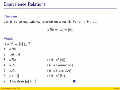
Equivalence Relations
TheoremLet 𝑅 be an equivalence relation on a set 𝐴. For all 𝑎, 𝑏 ∈ 𝐴,
𝑎𝑅𝑏 ⇒ [𝑎] = [𝑏].
Proof.i) 𝑎𝑅𝑏 ⇒ [𝑎] ⊆ [𝑏]1 𝑎𝑅𝑏2 Let 𝑐 ∈ [𝑎]3 𝑎𝑅𝑐 (def. of [𝑎])4 𝑏𝑅𝑎 (𝑅 is symmetric)5 𝑏𝑅𝑐 (𝑅 is transitive)6 𝑐 ∈ [𝑏] (def. of [𝑏])7 Therefore [𝑎] ⊆ [𝑏]
Equivalence Relations 19/36
Equivalence Relations
TheoremLet 𝑅 be an equivalence relation on a set 𝐴. For all 𝑎, 𝑏 ∈ 𝐴,
𝑎𝑅𝑏 ⇒ [𝑎] = [𝑏].
Proof.ii) 𝑎𝑅𝑏 ⇒ [𝑏] ⊆ [𝑎]1 𝑎𝑅𝑏2 Let 𝑐 ∈ [𝑏]3 𝑏𝑅𝑐 (def. of [𝑏])4 𝑎𝑅𝑐 (𝑅 is transitive)5 𝑐 ∈ [𝑎] (def. of [𝑎])6 Therefore [𝑏] ⊆ [𝑎]
Equivalence Relations 20/36
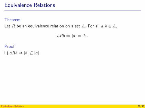
Equivalence Relations
TheoremLet 𝑅 be an equivalence relation on a set 𝐴. For all 𝑎, 𝑏 ∈ 𝐴,
𝑎𝑅𝑏 ⇒ [𝑎] = [𝑏].
Proof.ii) 𝑎𝑅𝑏 ⇒ [𝑏] ⊆ [𝑎]
1 𝑎𝑅𝑏2 Let 𝑐 ∈ [𝑏]3 𝑏𝑅𝑐 (def. of [𝑏])4 𝑎𝑅𝑐 (𝑅 is transitive)5 𝑐 ∈ [𝑎] (def. of [𝑎])6 Therefore [𝑏] ⊆ [𝑎]
Equivalence Relations 21/36
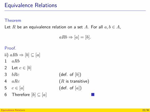
Equivalence Relations
TheoremLet 𝑅 be an equivalence relation on a set 𝐴. For all 𝑎, 𝑏 ∈ 𝐴,
𝑎𝑅𝑏 ⇒ [𝑎] = [𝑏].
Proof.ii) 𝑎𝑅𝑏 ⇒ [𝑏] ⊆ [𝑎]1 𝑎𝑅𝑏2 Let 𝑐 ∈ [𝑏]3 𝑏𝑅𝑐 (def. of [𝑏])4 𝑎𝑅𝑐 (𝑅 is transitive)5 𝑐 ∈ [𝑎] (def. of [𝑎])6 Therefore [𝑏] ⊆ [𝑎]
Equivalence Relations 22/36
Equivalence Relations
TheoremLet 𝑅 be an equivalence relation on a set 𝐴. For all 𝑎, 𝑏 ∈ 𝐴,
[𝑎] = [𝑏] ⇒ [𝑎] ∩ [𝑏] ≠ ∅.
Proof.1 [𝑎] = [𝑏]2 [𝑎] = {𝑎, …} (𝑅 is reflexive)3 Therefore [𝑎] ∩ [𝑏] ≠ ∅
Equivalence Relations 23/36
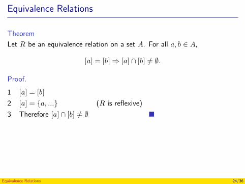
Equivalence Relations
TheoremLet 𝑅 be an equivalence relation on a set 𝐴. For all 𝑎, 𝑏 ∈ 𝐴,
[𝑎] = [𝑏] ⇒ [𝑎] ∩ [𝑏] ≠ ∅.
Proof.1 [𝑎] = [𝑏]2 [𝑎] = {𝑎, …} (𝑅 is reflexive)3 Therefore [𝑎] ∩ [𝑏] ≠ ∅
Equivalence Relations 24/36
Equivalence Relations
TheoremLet 𝑅 be an equivalence relation on a set 𝐴. For all 𝑎, 𝑏 ∈ 𝐴,
[𝑎] ∩ [𝑏] ≠ ∅ ⇒ 𝑎𝑅𝑏.
Proof.1 [𝑎] ∩ [𝑏] ≠ ∅2 Let 𝑐 such that 𝑐 ∈ [𝑎] and 𝑐 ∈ [𝑏]3 𝑎𝑅𝑐 y 𝑏𝑅𝑐 (def. of [𝑎] and [𝑏])4 𝑐𝑅𝑏 (𝑅 is symmetric)5 Therefore 𝑎𝑅𝑏 (𝑅 is transitive)
Equivalence Relations 25/36
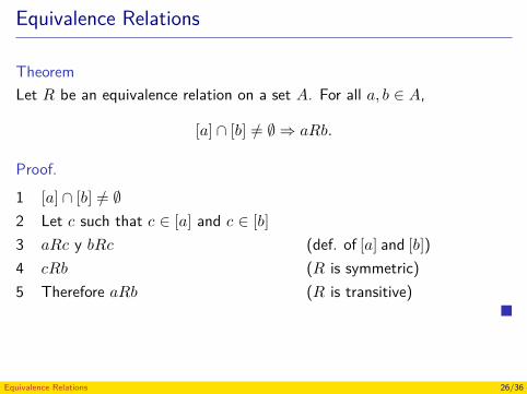
Equivalence Relations
TheoremLet 𝑅 be an equivalence relation on a set 𝐴. For all 𝑎, 𝑏 ∈ 𝐴,
[𝑎] ∩ [𝑏] ≠ ∅ ⇒ 𝑎𝑅𝑏.
Proof.1 [𝑎] ∩ [𝑏] ≠ ∅2 Let 𝑐 such that 𝑐 ∈ [𝑎] and 𝑐 ∈ [𝑏]3 𝑎𝑅𝑐 y 𝑏𝑅𝑐 (def. of [𝑎] and [𝑏])4 𝑐𝑅𝑏 (𝑅 is symmetric)5 Therefore 𝑎𝑅𝑏 (𝑅 is transitive)
Equivalence Relations 26/36
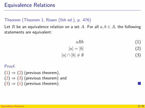
Equivalence Relations
Theorem (Theorem 1, Rosen (5th ed.), p. 476)Let 𝑅 be an equivalence relation on a set 𝐴. For all 𝑎, 𝑏 ∈ 𝐴, the followingstatements are equivalent:
𝑎𝑅𝑏 (1)[𝑎] = [𝑏] (2)
[𝑎] ∩ [𝑏] ≠ ∅ (3)
Proof.(1) ⇒ (2) (previous theorem),(2) ⇒ (3) (previous theorem) and(3) ⇒ (1) (previous theorem).
Equivalence Relations 27/36
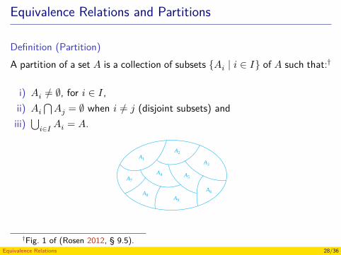
Equivalence Relations and Partitions
Definition (Partition)A partition of a set 𝐴 is a collection of subsets {𝐴𝑖 ∣ 𝑖 ∈ 𝐼} of 𝐴 such that:†
i) 𝐴𝑖 ≠ ∅, for 𝑖 ∈ 𝐼 ,ii) 𝐴𝑖 ⋂ 𝐴𝑗 = ∅ when 𝑖 ≠ 𝑗 (disjoint subsets) andiii) ⋃𝑖∈𝐼 𝐴𝑖 = 𝐴. 9.5 Equivalence Relations 613
A1
A7
A4
A2
A3
A6
A5
A9
A8
FIGURE 1 A Partition of a Set.
and
⋃
i∈IAi = S.
(Here the notation⋃
i∈I Ai represents the union of the sets Ai for all i ∈ I .) Figure 1 illustratesthe concept of a partition of a set.
EXAMPLE 12 Suppose that S = {1, 2, 3, 4, 5, 6}. The collection of sets A1 = {1, 2, 3}, A2 = {4, 5}, andA3 = {6} forms a partition of S, because these sets are disjoint and their union is S. ▲
We have seen that the equivalence classes of an equivalence relation on a set form a partitionof the set. The subsets in this partition are the equivalence classes. Conversely, every partitionof a set can be used to form an equivalence relation. Two elements are equivalent with respectto this relation if and only if they are in the same subset of the partition.
To see this, assume that {Ai | i ∈ I } is a partition on S. Let R be the relation on S consistingof the pairs (x, y), where x and y belong to the same subset Ai in the partition. To show that R
is an equivalence relation we must show that R is reflexive, symmetric, and transitive.We see that (a, a) ∈ R for every a ∈ S, because a is in the same subset as itself. Hence, R
is reflexive. If (a, b) ∈ R, then b and a are in the same subset of the partition, so that (b, a) ∈ R
as well. Hence, R is symmetric. If (a, b) ∈ R and (b, c) ∈ R, then a and b are in the samesubset X in the partition, and b and c are in the same subset Y of the partition. Because the subsetsof the partition are disjoint and b belongs to X and Y , it follows that X = Y . Consequently, a
and c belong to the same subset of the partition, so (a, c) ∈ R. Thus, R is transitive.It follows that R is an equivalence relation. The equivalence classes of R consist of subsets
of S containing related elements, and by the definition of R, these are the subsets of the partition.Theorem 2 summarizes the connections we have established between equivalence relations andpartitions.
THEOREM 2 Let R be an equivalence relation on a set S. Then the equivalence classes of R form a partitionof S. Conversely, given a partition {Ai | i ∈ I } of the set S, there is an equivalence relationR that has the sets Ai , i ∈ I , as its equivalence classes.
Example 13 shows how to construct an equivalence relation from a partition.
EXAMPLE 13 List the ordered pairs in the equivalence relation R produced by the partition A1 = {1, 2, 3},A2 = {4, 5}, and A3 = {6} of S = {1, 2, 3, 4, 5, 6}, given in Example 12.
†Fig. 1 of (Rosen 2012, § 9.5).Equivalence Relations 28/36
Equivalence Relations and Partitions
Theorem (Theorem 2, Rosen (5th ed.), p. 477)Let 𝑅 be an equivalence relation on a set 𝐴. Then the equivalence classesof 𝑅 form a partition of 𝐴.
Proof.The collection of subsets is given by
{𝐴[𝑎]𝑅 ∣ [𝑎]𝑅 is an equivalence class respect to 𝑅}.
Using the above collection, the conditions i), ii) and iii) are satisfied.
Equivalence Relations 29/36
Equivalence Relations and Partitions
Theorem (Theorem 2, Rosen (5th ed.), p. 477)Given a partition {𝐴𝑖 ∣ 𝑖 ∈ 𝐼} of a set 𝐴, there is an equivalence relation 𝑅that has the sets 𝐴𝑖 as its equivalence classes.
ExampleGiven a partition to build the equivalence relation associated.
Equivalence Relations 30/36
Equivalence Relations and Partitions
Theorem (Theorem 2, Rosen (5th ed.), p. 477)Given a partition {𝐴𝑖 ∣ 𝑖 ∈ 𝐼} of a set 𝐴, there is an equivalence relation 𝑅that has the sets 𝐴𝑖 as its equivalence classes.
ExampleGiven a partition to build the equivalence relation associated.
Equivalence Relations 31/36
Equivalence Relations and Partitions
Proof.Let 𝑅 be the relation defined by
𝑅 = {(𝑎, 𝑏) ∣ 𝑎, 𝑏 ∈ 𝐴𝑖}.
𝑅 is a relation of equivalence:
Reflexivity and symmetryDirect from the definition of 𝑅.
Equivalence Relations 32/36
Equivalence Relations and Partitions
Proof.Let 𝑅 be the relation defined by
𝑅 = {(𝑎, 𝑏) ∣ 𝑎, 𝑏 ∈ 𝐴𝑖}.
𝑅 is a relation of equivalence:Reflexivity and symmetryDirect from the definition of 𝑅.
Equivalence Relations 33/36
Equivalence Relations and Partitions
Proof (cont.)
𝑅 = {(𝑎, 𝑏) ∣ 𝑎, 𝑏 ∈ 𝐴𝑖}.
Transitivity1 𝑎𝑅𝑏 and 𝑏𝑅𝑐2 Exists 𝑋 ∈ {𝐴𝑖 ∣ 𝑖 ∈ 𝐼} such 𝑎, 𝑏 ∈ 𝑋 (def. of 𝑅)3 Exists 𝑌 ∈ {𝐴𝑖 ∣ 𝑖 ∈ 𝐼} such 𝑏, 𝑐 ∈ 𝑌 (def. of 𝑅)4 𝑋 = 𝑌 (𝑏 ∈ 𝑋 and 𝑏 ∈ 𝑌 and
the 𝐴𝑖s are disjoints)5 𝑎𝑅𝑐 (𝑎, 𝑐 ∈ 𝑋 and def. of 𝑅)
Now, [𝑎]𝑅 = {𝑠 ∣ (𝑎, 𝑠) ∈ 𝑅} and by the definition of the relation 𝑅, theseequivalence classes correspond to the sets 𝐴𝑖.
Equivalence Relations 34/36
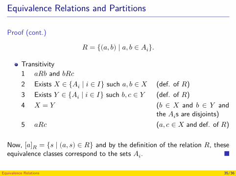
Equivalence Relations and Partitions
Proof (cont.)
𝑅 = {(𝑎, 𝑏) ∣ 𝑎, 𝑏 ∈ 𝐴𝑖}.
Transitivity1 𝑎𝑅𝑏 and 𝑏𝑅𝑐2 Exists 𝑋 ∈ {𝐴𝑖 ∣ 𝑖 ∈ 𝐼} such 𝑎, 𝑏 ∈ 𝑋 (def. of 𝑅)3 Exists 𝑌 ∈ {𝐴𝑖 ∣ 𝑖 ∈ 𝐼} such 𝑏, 𝑐 ∈ 𝑌 (def. of 𝑅)4 𝑋 = 𝑌 (𝑏 ∈ 𝑋 and 𝑏 ∈ 𝑌 and
the 𝐴𝑖s are disjoints)5 𝑎𝑅𝑐 (𝑎, 𝑐 ∈ 𝑋 and def. of 𝑅)
Now, [𝑎]𝑅 = {𝑠 ∣ (𝑎, 𝑠) ∈ 𝑅} and by the definition of the relation 𝑅, theseequivalence classes correspond to the sets 𝐴𝑖.
Equivalence Relations 35/36
References
Rosen, K. H. (2012). Discrete Mathematics and Its Applications. 7th ed.McGraw-Hill (cit. on pp. 2, 28).
Equivalence Relations 36/36
Discrete Structures - CM0246Partial Orders
Andrés Sicard-Ramírez
Universidad EAFIT
Semester 2014-2
Introduction
We can use relations to order some or all the elements of a set.
ExamplesThe words in a dictionary(𝑎, 𝑏) if 𝑎 comes before 𝑏 in the dictionary.Academic genealogical descent(𝑎, 𝑏) if 𝑎 was the supervisor of the thesis of 𝑏.Schedule projects(𝑎, 𝑏) if 𝑎 is a task that must be completed before the task 𝑏 begins.
Partial Orders 2/67
Introduction
We can use relations to order some or all the elements of a set.Examples
The words in a dictionary(𝑎, 𝑏) if 𝑎 comes before 𝑏 in the dictionary.
Academic genealogical descent(𝑎, 𝑏) if 𝑎 was the supervisor of the thesis of 𝑏.Schedule projects(𝑎, 𝑏) if 𝑎 is a task that must be completed before the task 𝑏 begins.
Partial Orders 3/67
Introduction
We can use relations to order some or all the elements of a set.Examples
The words in a dictionary(𝑎, 𝑏) if 𝑎 comes before 𝑏 in the dictionary.Academic genealogical descent(𝑎, 𝑏) if 𝑎 was the supervisor of the thesis of 𝑏.
Schedule projects(𝑎, 𝑏) if 𝑎 is a task that must be completed before the task 𝑏 begins.
Partial Orders 4/67
Introduction
We can use relations to order some or all the elements of a set.Examples
The words in a dictionary(𝑎, 𝑏) if 𝑎 comes before 𝑏 in the dictionary.Academic genealogical descent(𝑎, 𝑏) if 𝑎 was the supervisor of the thesis of 𝑏.Schedule projects(𝑎, 𝑏) if 𝑎 is a task that must be completed before the task 𝑏 begins.
Partial Orders 5/67
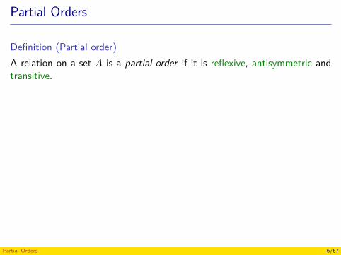
Partial Orders
Definition (Partial order)A relation on a set 𝐴 is a partial order if it is reflexive, antisymmetric andtransitive.
Definition (Poset)Let 𝑅 be a partial order on a set 𝐴, then (𝐴, 𝑅) is called a partially orderset (or poset).
Examples(ℤ, ≤) is a poset.(𝑃 (𝐴), ⊆) is a poset.
Partial Orders 6/67
Partial Orders
Definition (Partial order)A relation on a set 𝐴 is a partial order if it is reflexive, antisymmetric andtransitive.
Definition (Poset)Let 𝑅 be a partial order on a set 𝐴, then (𝐴, 𝑅) is called a partially orderset (or poset).
Examples(ℤ, ≤) is a poset.(𝑃 (𝐴), ⊆) is a poset.
Partial Orders 7/67
Partial Orders
Definition (Partial order)A relation on a set 𝐴 is a partial order if it is reflexive, antisymmetric andtransitive.
Definition (Poset)Let 𝑅 be a partial order on a set 𝐴, then (𝐴, 𝑅) is called a partially orderset (or poset).
Examples(ℤ, ≤) is a poset.
(𝑃 (𝐴), ⊆) is a poset.
Partial Orders 8/67
Partial Orders
Definition (Partial order)A relation on a set 𝐴 is a partial order if it is reflexive, antisymmetric andtransitive.
Definition (Poset)Let 𝑅 be a partial order on a set 𝐴, then (𝐴, 𝑅) is called a partially orderset (or poset).
Examples(ℤ, ≤) is a poset.(𝑃 (𝐴), ⊆) is a poset.
Partial Orders 9/67
Partial Orders
Definition (Divisibility relation)Let 𝑎, 𝑏 ∈ ℤ with 𝑎 ≠ 0. The divisibility relation, denoted by |, is defined by
𝑎 ∣ 𝑏 def= ∃𝑐 (𝑏 = 𝑎𝑐).
If 𝑎 ∣ 𝑏, we say that 𝑎 divides 𝑏.
ExamplesWhiteboard
Examples(ℤ+, ∣) is a poset.Is (ℕ, ∣) a poset?
Partial Orders 10/67
Partial Orders
Definition (Divisibility relation)Let 𝑎, 𝑏 ∈ ℤ with 𝑎 ≠ 0. The divisibility relation, denoted by |, is defined by
𝑎 ∣ 𝑏 def= ∃𝑐 (𝑏 = 𝑎𝑐).
If 𝑎 ∣ 𝑏, we say that 𝑎 divides 𝑏.
ExamplesWhiteboard
Examples(ℤ+, ∣) is a poset.Is (ℕ, ∣) a poset?
Partial Orders 11/67
Partial Orders
Definition (Divisibility relation)Let 𝑎, 𝑏 ∈ ℤ with 𝑎 ≠ 0. The divisibility relation, denoted by |, is defined by
𝑎 ∣ 𝑏 def= ∃𝑐 (𝑏 = 𝑎𝑐).
If 𝑎 ∣ 𝑏, we say that 𝑎 divides 𝑏.
ExamplesWhiteboard
Examples(ℤ+, ∣) is a poset.
Is (ℕ, ∣) a poset?
Partial Orders 12/67
Partial Orders
Definition (Divisibility relation)Let 𝑎, 𝑏 ∈ ℤ with 𝑎 ≠ 0. The divisibility relation, denoted by |, is defined by
𝑎 ∣ 𝑏 def= ∃𝑐 (𝑏 = 𝑎𝑐).
If 𝑎 ∣ 𝑏, we say that 𝑎 divides 𝑏.
ExamplesWhiteboard
Examples(ℤ+, ∣) is a poset.Is (ℕ, ∣) a poset?
Partial Orders 13/67
Partial Orders
Exercise (Rosen (2004), Problem 6, p. 492)Let (𝐴, 𝑅) be a poset. Prove that (𝑆, 𝑅−1) is also a poset, where 𝑅−1 isthe inverse of 𝑅. The poset (𝑆, 𝑅−1) is called the dual of (𝑆, 𝑅).
Partial Orders 14/67
Partial Orders
Notation≼: Denotes an arbitrary partial order
𝑎 ≺ 𝑏 def= 𝑎 ≼ 𝑏 ∧ 𝑎 ≠ 𝑏(𝐴, ≼): Denotes an arbitrary poset
Partial Orders 15/67
Comparable Elements
Definition (Comparable elements)Let (𝐴, ≼) be a poset. The elements 𝑎, 𝑏 ∈ 𝐴 are called comparable if either𝑎 ≼ 𝑏 or 𝑏 ≼ 𝑎.
ExamplesWhiteboard
Partial Orders 16/67
Comparable Elements
Definition (Comparable elements)Let (𝐴, ≼) be a poset. The elements 𝑎, 𝑏 ∈ 𝐴 are called comparable if either𝑎 ≼ 𝑏 or 𝑏 ≼ 𝑎.
ExamplesWhiteboard
Partial Orders 17/67
Total Orders
Definition (Totally order set, total order)If (𝐴, ≼) is a poset and every two elements of 𝐴 are comparable, 𝐴 is calleda totally ordered set (or linearly ordered set). The relation ≼ is called atotal order (or a linear order).
Examples(ℤ, ≤) is a totally order set.(ℤ+, ∣) is a not totally order set.Is (𝑃 (𝐴), ⊆) a totally order set?
Partial Orders 18/67
Total Orders
Definition (Totally order set, total order)If (𝐴, ≼) is a poset and every two elements of 𝐴 are comparable, 𝐴 is calleda totally ordered set (or linearly ordered set). The relation ≼ is called atotal order (or a linear order).
Examples(ℤ, ≤) is a totally order set.
(ℤ+, ∣) is a not totally order set.Is (𝑃 (𝐴), ⊆) a totally order set?
Partial Orders 19/67
Total Orders
Definition (Totally order set, total order)If (𝐴, ≼) is a poset and every two elements of 𝐴 are comparable, 𝐴 is calleda totally ordered set (or linearly ordered set). The relation ≼ is called atotal order (or a linear order).
Examples(ℤ, ≤) is a totally order set.(ℤ+, ∣) is a not totally order set.
Is (𝑃 (𝐴), ⊆) a totally order set?
Partial Orders 20/67
Total Orders
Definition (Totally order set, total order)If (𝐴, ≼) is a poset and every two elements of 𝐴 are comparable, 𝐴 is calleda totally ordered set (or linearly ordered set). The relation ≼ is called atotal order (or a linear order).
Examples(ℤ, ≤) is a totally order set.(ℤ+, ∣) is a not totally order set.Is (𝑃 (𝐴), ⊆) a totally order set?
Partial Orders 21/67
Well-Ordered Sets
Definition (Least element)An element 𝑎 ∈ 𝐴 is the least element (mínimo) of a poset (𝐴, ≼) if 𝑎 ≼ 𝑏for all 𝑏 ∈ 𝐴.
Definition (Well-ordered set)Let (𝐴, ≼) be a totally order set. (𝐴, ≼) is a well-ordered set if everynonempty subset of 𝐴 has a least element.
Examples(ℕ, ≤) is a well-ordered set.(ℕ, ≥) is not a well-ordered set.Is (ℤ, ≤) a well-ordered set?
Partial Orders 22/67
Well-Ordered Sets
Definition (Least element)An element 𝑎 ∈ 𝐴 is the least element (mínimo) of a poset (𝐴, ≼) if 𝑎 ≼ 𝑏for all 𝑏 ∈ 𝐴.
Definition (Well-ordered set)Let (𝐴, ≼) be a totally order set. (𝐴, ≼) is a well-ordered set if everynonempty subset of 𝐴 has a least element.
Examples(ℕ, ≤) is a well-ordered set.(ℕ, ≥) is not a well-ordered set.Is (ℤ, ≤) a well-ordered set?
Partial Orders 23/67
Well-Ordered Sets
Definition (Least element)An element 𝑎 ∈ 𝐴 is the least element (mínimo) of a poset (𝐴, ≼) if 𝑎 ≼ 𝑏for all 𝑏 ∈ 𝐴.
Definition (Well-ordered set)Let (𝐴, ≼) be a totally order set. (𝐴, ≼) is a well-ordered set if everynonempty subset of 𝐴 has a least element.
Examples(ℕ, ≤) is a well-ordered set.
(ℕ, ≥) is not a well-ordered set.Is (ℤ, ≤) a well-ordered set?
Partial Orders 24/67
Well-Ordered Sets
Definition (Least element)An element 𝑎 ∈ 𝐴 is the least element (mínimo) of a poset (𝐴, ≼) if 𝑎 ≼ 𝑏for all 𝑏 ∈ 𝐴.
Definition (Well-ordered set)Let (𝐴, ≼) be a totally order set. (𝐴, ≼) is a well-ordered set if everynonempty subset of 𝐴 has a least element.
Examples(ℕ, ≤) is a well-ordered set.(ℕ, ≥) is not a well-ordered set.
Is (ℤ, ≤) a well-ordered set?
Partial Orders 25/67
Well-Ordered Sets
Definition (Least element)An element 𝑎 ∈ 𝐴 is the least element (mínimo) of a poset (𝐴, ≼) if 𝑎 ≼ 𝑏for all 𝑏 ∈ 𝐴.
Definition (Well-ordered set)Let (𝐴, ≼) be a totally order set. (𝐴, ≼) is a well-ordered set if everynonempty subset of 𝐴 has a least element.
Examples(ℕ, ≤) is a well-ordered set.(ℕ, ≥) is not a well-ordered set.Is (ℤ, ≤) a well-ordered set?
Partial Orders 26/67
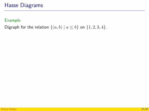
Hasse Diagrams
ExampleDigraph for the relation {(𝑎, 𝑏) ∣ 𝑎 ≤ 𝑏} on {1, 2, 3, 4}.
Partial Orders 27/67
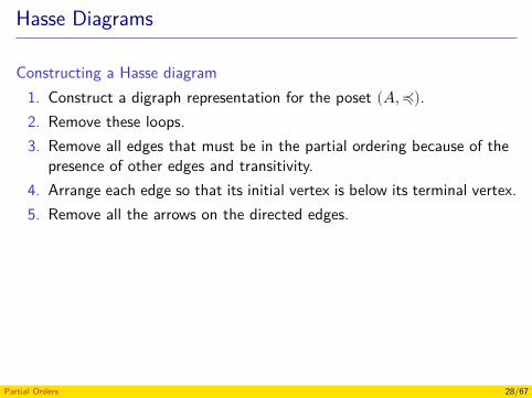
Hasse Diagrams
Constructing a Hasse diagram1. Construct a digraph representation for the poset (𝐴, ≼).2. Remove these loops.3. Remove all edges that must be in the partial ordering because of the
presence of other edges and transitivity.4. Arrange each edge so that its initial vertex is below its terminal vertex.5. Remove all the arrows on the directed edges.
Partial Orders 28/67
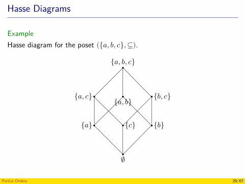
Hasse Diagrams
ExampleHasse diagram for the poset ({𝑎, 𝑏, 𝑐}, ⊆).
∅
{𝑐}{𝑎} {𝑏}
{𝑎, 𝑐} {𝑎, 𝑏} {𝑏, 𝑐}
{𝑎, 𝑏, 𝑐}
Partial Orders 29/67
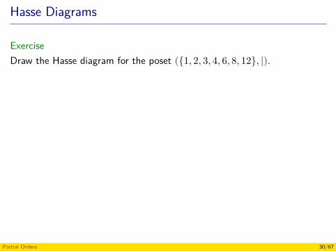
Hasse Diagrams
ExerciseDraw the Hasse diagram for the poset ({1, 2, 3, 4, 6, 8, 12}, ∣).
1
2 3
4 6
8 12
Partial Orders 30/67
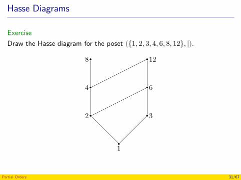
Hasse Diagrams
ExerciseDraw the Hasse diagram for the poset ({1, 2, 3, 4, 6, 8, 12}, ∣).
1
2 3
4 6
8 12
Partial Orders 31/67
Lexicographic Ordering
ExampleLet ≼ be relation on ℤ × ℤ defined by
(𝑎1, 𝑎2) ≼ (𝑏1, 𝑏2) def= 𝑎1 < 𝑏1 or (𝑎1 = 𝑏1 and 𝑎2 ≤ 𝑏2).
Is (3, 100) ≼ (4, 4)?
Is (3, 5) ≼ (3, 4)?
Is (ℤ × ℤ, ≼) a poset?
Is (ℤ × ℤ, ≼) a totally order set?
Partial Orders 32/67
Lexicographic Ordering
ExampleLet ≼ be relation on ℤ × ℤ defined by
(𝑎1, 𝑎2) ≼ (𝑏1, 𝑏2) def= 𝑎1 < 𝑏1 or (𝑎1 = 𝑏1 and 𝑎2 ≤ 𝑏2).
Is (3, 100) ≼ (4, 4)?
Is (3, 5) ≼ (3, 4)?
Is (ℤ × ℤ, ≼) a poset?
Is (ℤ × ℤ, ≼) a totally order set?
Partial Orders 33/67
Lexicographic Ordering
ExampleLet ≼ be relation on ℤ × ℤ defined by
(𝑎1, 𝑎2) ≼ (𝑏1, 𝑏2) def= 𝑎1 < 𝑏1 or (𝑎1 = 𝑏1 and 𝑎2 ≤ 𝑏2).
Is (3, 100) ≼ (4, 4)?
Is (3, 5) ≼ (3, 4)?
Is (ℤ × ℤ, ≼) a poset?
Is (ℤ × ℤ, ≼) a totally order set?
Partial Orders 34/67
Lexicographic Ordering
ExampleLet ≼ be relation on ℤ × ℤ defined by
(𝑎1, 𝑎2) ≼ (𝑏1, 𝑏2) def= 𝑎1 < 𝑏1 or (𝑎1 = 𝑏1 and 𝑎2 ≤ 𝑏2).
Is (3, 100) ≼ (4, 4)?
Is (3, 5) ≼ (3, 4)?
Is (ℤ × ℤ, ≼) a poset?
Is (ℤ × ℤ, ≼) a totally order set?
Partial Orders 35/67
Lexicographic Ordering
ExampleLet ≼ be relation on ℤ × ℤ defined by
(𝑎1, 𝑎2) ≼ (𝑏1, 𝑏2) def= 𝑎1 < 𝑏1 or (𝑎1 = 𝑏1 and 𝑎2 ≤ 𝑏2).
Is (3, 100) ≼ (4, 4)?
Is (3, 5) ≼ (3, 4)?
Is (ℤ × ℤ, ≼) a poset?
Is (ℤ × ℤ, ≼) a totally order set?
Partial Orders 36/67
Lexicographic Ordering
Definition (Lexicographic ordering of two posets)Let (𝐴1, ≼1) and (𝐴2, ≼2) be two posets. The lexicographic ordering ≼ on𝐴1 × 𝐴2 is defined by:
(𝑎1, 𝑎2) ≼ (𝑏1, 𝑏2) def= 𝑎1 ≺1 𝑏1 or (𝑎1 = 𝑏1 and 𝑎2 ≼2 𝑏2).
ExamplesPrevious exampleWhiteboard
Partial Orders 37/67
Lexicographic Ordering
Definition (Lexicographic ordering of two posets)Let (𝐴1, ≼1) and (𝐴2, ≼2) be two posets. The lexicographic ordering ≼ on𝐴1 × 𝐴2 is defined by:
(𝑎1, 𝑎2) ≼ (𝑏1, 𝑏2) def= 𝑎1 ≺1 𝑏1 or (𝑎1 = 𝑏1 and 𝑎2 ≼2 𝑏2).Examples
Previous example
Whiteboard
Partial Orders 38/67
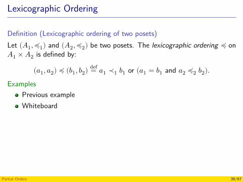
Lexicographic Ordering
Definition (Lexicographic ordering of two posets)Let (𝐴1, ≼1) and (𝐴2, ≼2) be two posets. The lexicographic ordering ≼ on𝐴1 × 𝐴2 is defined by:
(𝑎1, 𝑎2) ≼ (𝑏1, 𝑏2) def= 𝑎1 ≺1 𝑏1 or (𝑎1 = 𝑏1 and 𝑎2 ≼2 𝑏2).Examples
Previous exampleWhiteboard
Partial Orders 39/67
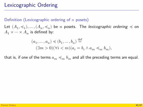
Lexicographic Ordering
Definition (Lexicographic ordering of 𝑛 posets)Let (𝐴1, ≼1), … , (𝐴𝑛, ≼𝑛) be 𝑛 posets. The lexicographic ordering ≼ on𝐴1 × ⋯ × 𝐴𝑛 is defined by:
(𝑎1, … , 𝑎𝑛) ≼ (𝑏1, … , 𝑏𝑛) def=(∃𝑚 > 0)(∀𝑖 < 𝑚)(𝑎𝑖 = 𝑏𝑖 ∧ 𝑎𝑚 ≼𝑚 𝑏𝑚),
that is, if one of the terms 𝑎𝑚 ≼𝑚 𝑏𝑚 and all the preceding terms are equal.
Partial Orders 40/67
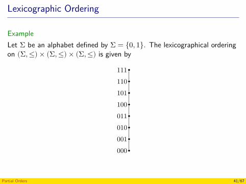
Lexicographic Ordering
ExampleLet Σ be an alphabet defined by Σ = {0, 1}. The lexicographical orderingon (Σ, ≤) × (Σ, ≤) × (Σ, ≤) is given by
000001010011100101110111
Partial Orders 41/67
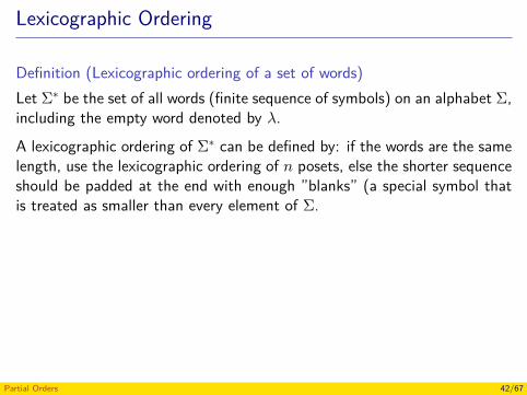
Lexicographic Ordering
Definition (Lexicographic ordering of a set of words)Let Σ∗ be the set of all words (finite sequence of symbols) on an alphabet Σ,including the empty word denoted by 𝜆.A lexicographic ordering of Σ∗ can be defined by: if the words are the samelength, use the lexicographic ordering of 𝑛 posets, else the shorter sequenceshould be padded at the end with enough ”blanks” (a special symbol thatis treated as smaller than every element of Σ.
Partial Orders 42/67
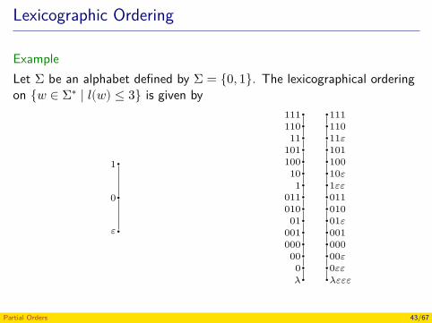
Lexicographic Ordering
ExampleLet Σ be an alphabet defined by Σ = {0, 1}. The lexicographical orderingon {𝑤 ∈ Σ∗ ∣ 𝑙(𝑤) ≤ 3} is given by
𝜀
0
1
𝜆0
00000001
01010011
110
100101
11110111
𝜆𝜀𝜀𝜀0𝜀𝜀00𝜀00000101𝜀0100111𝜀𝜀10𝜀10010111𝜀110111
Partial Orders 43/67
Product Order
Definition (Product order of two posets)Let (𝐴, ≼𝐴) and (𝐵, ≼𝐵) be two posets. The product order ≼ on 𝐴 × 𝐵 isdefined by:
(𝑎1, 𝑏1) ≼ (𝑎2, 𝑏2) def= 𝑎1 ≼𝐴 𝑎2 and 𝑏1 ≼𝐵 𝑏2.
ExampleWhiteboard.
Partial Orders 44/67
Product Order
Definition (Product order of two posets)Let (𝐴, ≼𝐴) and (𝐵, ≼𝐵) be two posets. The product order ≼ on 𝐴 × 𝐵 isdefined by:
(𝑎1, 𝑏1) ≼ (𝑎2, 𝑏2) def= 𝑎1 ≼𝐴 𝑎2 and 𝑏1 ≼𝐵 𝑏2.
ExampleWhiteboard.
Partial Orders 45/67
Product Order
Exercise (Rosen (2004), Problem 33, p. 494)Prove that the product order of two posets is a poset.
Proof.Let (𝐴, ≼𝐴) and (𝐵, ≼𝐵) be two posets. We need to prove that (𝐴×𝐵, ≼)is a poset, where ≼ is the product order on 𝐴 × 𝐵.
Reflexivity: (𝑎, 𝑏) ≼ (𝑎, 𝑏), for all 𝑎 ∈ 𝐴 and 𝑏 ∈ 𝐵. Whiteboard.
Antisymmetry: If (𝑎1, 𝑏1) ≼ (𝑎2, 𝑏2) and (𝑎2, 𝑏2) ≼ (𝑎1, 𝑏1) then(𝑎1, 𝑏1) = (𝑎2, 𝑏2), for all 𝑎1, 𝑎2 ∈ 𝐴 and 𝑏1, 𝑏2 ∈ 𝐵. Whiteboard.
Transitivity: If (𝑎1, 𝑏1) ≼ (𝑎2, 𝑏2) and (𝑎2, 𝑏2) ≼ (𝑎3, 𝑏3) then(𝑎1, 𝑏1) ≼ (𝑎3, 𝑏3), for all 𝑎1, 𝑎2, 𝑎3 ∈ 𝐴 and 𝑏1, 𝑏2, 𝑏3 ∈ 𝐵.Whiteboard.
Partial Orders 46/67
Product Order
Exercise (Rosen (2004), Problem 33, p. 494)Prove that the product order of two posets is a poset.
Proof.Let (𝐴, ≼𝐴) and (𝐵, ≼𝐵) be two posets. We need to prove that (𝐴×𝐵, ≼)is a poset, where ≼ is the product order on 𝐴 × 𝐵.
Reflexivity: (𝑎, 𝑏) ≼ (𝑎, 𝑏), for all 𝑎 ∈ 𝐴 and 𝑏 ∈ 𝐵. Whiteboard.
Antisymmetry: If (𝑎1, 𝑏1) ≼ (𝑎2, 𝑏2) and (𝑎2, 𝑏2) ≼ (𝑎1, 𝑏1) then(𝑎1, 𝑏1) = (𝑎2, 𝑏2), for all 𝑎1, 𝑎2 ∈ 𝐴 and 𝑏1, 𝑏2 ∈ 𝐵. Whiteboard.
Transitivity: If (𝑎1, 𝑏1) ≼ (𝑎2, 𝑏2) and (𝑎2, 𝑏2) ≼ (𝑎3, 𝑏3) then(𝑎1, 𝑏1) ≼ (𝑎3, 𝑏3), for all 𝑎1, 𝑎2, 𝑎3 ∈ 𝐴 and 𝑏1, 𝑏2, 𝑏3 ∈ 𝐵.Whiteboard.
Partial Orders 47/67
Product Order
Exercise (Rosen (2004), Problem 33, p. 494)Prove that the product order of two posets is a poset.
Proof.Let (𝐴, ≼𝐴) and (𝐵, ≼𝐵) be two posets. We need to prove that (𝐴×𝐵, ≼)is a poset, where ≼ is the product order on 𝐴 × 𝐵.
Reflexivity: (𝑎, 𝑏) ≼ (𝑎, 𝑏), for all 𝑎 ∈ 𝐴 and 𝑏 ∈ 𝐵. Whiteboard.
Antisymmetry: If (𝑎1, 𝑏1) ≼ (𝑎2, 𝑏2) and (𝑎2, 𝑏2) ≼ (𝑎1, 𝑏1) then(𝑎1, 𝑏1) = (𝑎2, 𝑏2), for all 𝑎1, 𝑎2 ∈ 𝐴 and 𝑏1, 𝑏2 ∈ 𝐵. Whiteboard.
Transitivity: If (𝑎1, 𝑏1) ≼ (𝑎2, 𝑏2) and (𝑎2, 𝑏2) ≼ (𝑎3, 𝑏3) then(𝑎1, 𝑏1) ≼ (𝑎3, 𝑏3), for all 𝑎1, 𝑎2, 𝑎3 ∈ 𝐴 and 𝑏1, 𝑏2, 𝑏3 ∈ 𝐵.Whiteboard.
Partial Orders 48/67
Product Order
Exercise (Rosen (2004), Problem 33, p. 494)Prove that the product order of two posets is a poset.
Proof.Let (𝐴, ≼𝐴) and (𝐵, ≼𝐵) be two posets. We need to prove that (𝐴×𝐵, ≼)is a poset, where ≼ is the product order on 𝐴 × 𝐵.
Reflexivity: (𝑎, 𝑏) ≼ (𝑎, 𝑏), for all 𝑎 ∈ 𝐴 and 𝑏 ∈ 𝐵. Whiteboard.
Antisymmetry: If (𝑎1, 𝑏1) ≼ (𝑎2, 𝑏2) and (𝑎2, 𝑏2) ≼ (𝑎1, 𝑏1) then(𝑎1, 𝑏1) = (𝑎2, 𝑏2), for all 𝑎1, 𝑎2 ∈ 𝐴 and 𝑏1, 𝑏2 ∈ 𝐵. Whiteboard.
Transitivity: If (𝑎1, 𝑏1) ≼ (𝑎2, 𝑏2) and (𝑎2, 𝑏2) ≼ (𝑎3, 𝑏3) then(𝑎1, 𝑏1) ≼ (𝑎3, 𝑏3), for all 𝑎1, 𝑎2, 𝑎3 ∈ 𝐴 and 𝑏1, 𝑏2, 𝑏3 ∈ 𝐵.Whiteboard.
Partial Orders 49/67
Product Order
Exercise (Rosen (2004), Problem 33, p. 494)Prove that the product order of two posets is a poset.
Proof.Let (𝐴, ≼𝐴) and (𝐵, ≼𝐵) be two posets. We need to prove that (𝐴×𝐵, ≼)is a poset, where ≼ is the product order on 𝐴 × 𝐵.
Reflexivity: (𝑎, 𝑏) ≼ (𝑎, 𝑏), for all 𝑎 ∈ 𝐴 and 𝑏 ∈ 𝐵. Whiteboard.
Antisymmetry: If (𝑎1, 𝑏1) ≼ (𝑎2, 𝑏2) and (𝑎2, 𝑏2) ≼ (𝑎1, 𝑏1) then(𝑎1, 𝑏1) = (𝑎2, 𝑏2), for all 𝑎1, 𝑎2 ∈ 𝐴 and 𝑏1, 𝑏2 ∈ 𝐵. Whiteboard.
Transitivity: If (𝑎1, 𝑏1) ≼ (𝑎2, 𝑏2) and (𝑎2, 𝑏2) ≼ (𝑎3, 𝑏3) then(𝑎1, 𝑏1) ≼ (𝑎3, 𝑏3), for all 𝑎1, 𝑎2, 𝑎3 ∈ 𝐴 and 𝑏1, 𝑏2, 𝑏3 ∈ 𝐵.Whiteboard.
Partial Orders 50/67
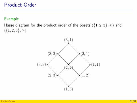
Product Order
ExampleHasse diagram for the product order of the posets ({1, 2, 3}, ≤) and({1, 2, 3}, ≥).
(1, 3)
(2, 3) (1, 2)(2, 2)(3, 3) (1, 1)
(3, 2) (2, 1)
(3, 1)
Partial Orders 51/67
Notable Elements
Let (𝐴, ≼) be a poset.
Definition (Greatest element)An element 𝑎 ∈ 𝐴 is the greatest element (máximo) of (𝐴, ≼) if 𝑏 ≼ 𝑎 forall 𝑏 ∈ 𝐴.
Definition (Least element)An element 𝑎 ∈ 𝐴 is the least element (mínimo) if 𝑎 ≼ 𝑏 for all 𝑏 ∈ 𝐴.
Definition (Maximal elements)An element 𝑎 ∈ 𝐴 is a maximal of (𝐴, ≼) if there is no 𝑏 ∈ 𝐴 such 𝑎 ≺ 𝑏.
Definition (Minimal elements)An element 𝑎 ∈ 𝐴 is a minimal (𝐴, ≼) if there is no 𝑏 ∈ 𝐴 such 𝑏 ≺ 𝑎.
Partial Orders 52/67
Notable Elements
Let (𝐴, ≼) be a poset.
Definition (Greatest element)An element 𝑎 ∈ 𝐴 is the greatest element (máximo) of (𝐴, ≼) if 𝑏 ≼ 𝑎 forall 𝑏 ∈ 𝐴.
Definition (Least element)An element 𝑎 ∈ 𝐴 is the least element (mínimo) if 𝑎 ≼ 𝑏 for all 𝑏 ∈ 𝐴.
Definition (Maximal elements)An element 𝑎 ∈ 𝐴 is a maximal of (𝐴, ≼) if there is no 𝑏 ∈ 𝐴 such 𝑎 ≺ 𝑏.
Definition (Minimal elements)An element 𝑎 ∈ 𝐴 is a minimal (𝐴, ≼) if there is no 𝑏 ∈ 𝐴 such 𝑏 ≺ 𝑎.
Partial Orders 53/67
Notable Elements
Let (𝐴, ≼) be a poset.
Definition (Greatest element)An element 𝑎 ∈ 𝐴 is the greatest element (máximo) of (𝐴, ≼) if 𝑏 ≼ 𝑎 forall 𝑏 ∈ 𝐴.
Definition (Least element)An element 𝑎 ∈ 𝐴 is the least element (mínimo) if 𝑎 ≼ 𝑏 for all 𝑏 ∈ 𝐴.
Definition (Maximal elements)An element 𝑎 ∈ 𝐴 is a maximal of (𝐴, ≼) if there is no 𝑏 ∈ 𝐴 such 𝑎 ≺ 𝑏.
Definition (Minimal elements)An element 𝑎 ∈ 𝐴 is a minimal (𝐴, ≼) if there is no 𝑏 ∈ 𝐴 such 𝑏 ≺ 𝑎.
Partial Orders 54/67
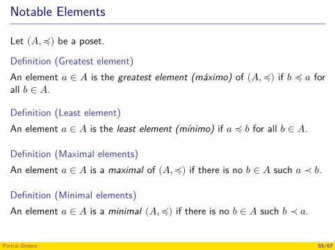
Notable Elements
Let (𝐴, ≼) be a poset.
Definition (Greatest element)An element 𝑎 ∈ 𝐴 is the greatest element (máximo) of (𝐴, ≼) if 𝑏 ≼ 𝑎 forall 𝑏 ∈ 𝐴.
Definition (Least element)An element 𝑎 ∈ 𝐴 is the least element (mínimo) if 𝑎 ≼ 𝑏 for all 𝑏 ∈ 𝐴.
Definition (Maximal elements)An element 𝑎 ∈ 𝐴 is a maximal of (𝐴, ≼) if there is no 𝑏 ∈ 𝐴 such 𝑎 ≺ 𝑏.
Definition (Minimal elements)An element 𝑎 ∈ 𝐴 is a minimal (𝐴, ≼) if there is no 𝑏 ∈ 𝐴 such 𝑏 ≺ 𝑎.
Partial Orders 55/67
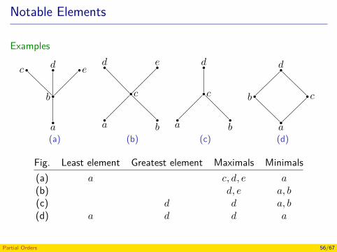
Notable Elements
Examples
𝑎
𝑏
𝑑𝑐 𝑒
(a)𝑎 𝑏
𝑐
𝑑 𝑒
(b)𝑎 𝑏
𝑐
𝑑
(c)𝑎
𝑏 𝑐
𝑑
(d)
Fig. Least element Greatest element Maximals Minimals(a) 𝑎 𝑐, 𝑑, 𝑒 𝑎(b) 𝑑, 𝑒 𝑎, 𝑏(c) 𝑑 𝑑 𝑎, 𝑏(d) 𝑎 𝑑 𝑑 𝑎
Partial Orders 56/67
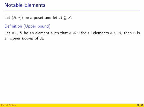
Notable Elements
Let (𝑆, ≼) be a poset and let 𝐴 ⊆ 𝑆.
Definition (Upper bound)Let 𝑢 ∈ 𝑆 be an element such that 𝑎 ≼ 𝑢 for all elements 𝑎 ∈ 𝐴, then 𝑢 isan upper bound of 𝐴.
Definition (Lower bound)Let 𝑙 ∈ 𝑆 be an element such 𝑙 ≼ 𝑎 for all elements 𝑎 ∈ 𝐴, then 𝑙 is a lowerbound of 𝐴.
Examples (Using intervals of real numbers)Whiteboard.
Partial Orders 57/67
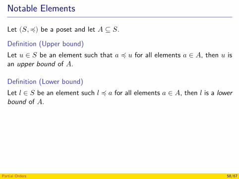
Notable Elements
Let (𝑆, ≼) be a poset and let 𝐴 ⊆ 𝑆.
Definition (Upper bound)Let 𝑢 ∈ 𝑆 be an element such that 𝑎 ≼ 𝑢 for all elements 𝑎 ∈ 𝐴, then 𝑢 isan upper bound of 𝐴.
Definition (Lower bound)Let 𝑙 ∈ 𝑆 be an element such 𝑙 ≼ 𝑎 for all elements 𝑎 ∈ 𝐴, then 𝑙 is a lowerbound of 𝐴.
Examples (Using intervals of real numbers)Whiteboard.
Partial Orders 58/67
Notable Elements
Let (𝑆, ≼) be a poset and let 𝐴 ⊆ 𝑆.
Definition (Upper bound)Let 𝑢 ∈ 𝑆 be an element such that 𝑎 ≼ 𝑢 for all elements 𝑎 ∈ 𝐴, then 𝑢 isan upper bound of 𝐴.
Definition (Lower bound)Let 𝑙 ∈ 𝑆 be an element such 𝑙 ≼ 𝑎 for all elements 𝑎 ∈ 𝐴, then 𝑙 is a lowerbound of 𝐴.
Examples (Using intervals of real numbers)Whiteboard.
Partial Orders 59/67
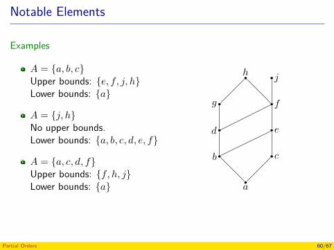
Notable Elements
Examples
𝐴 = {𝑎, 𝑏, 𝑐}Upper bounds: {𝑒, 𝑓, 𝑗, ℎ}Lower bounds: {𝑎}
𝐴 = {𝑗, ℎ}No upper bounds.Lower bounds: {𝑎, 𝑏, 𝑐, 𝑑, 𝑒, 𝑓}
𝐴 = {𝑎, 𝑐, 𝑑, 𝑓}Upper bounds: {𝑓, ℎ, 𝑗}Lower bounds: {𝑎} 𝑎
𝑏 𝑐
𝑑 𝑒
𝑓𝑔
ℎ 𝑗
Partial Orders 60/67
Notable Elements
Definition (Supremum)An element 𝑥 is the supremum (or the least upper bound) of the subset 𝐴,denoted by sup(𝐴), if 𝑥 is an upper bound that is less than every otherupper bound of 𝐴.
Definition (Infimum)An element 𝑦 is the infimum (or the greatest lower bound) of the subset 𝐴,denoted by inf(𝐴), if 𝑦 is an lower bound that is greater than every otherlower bound of 𝐴.
Examples (Using intervals of real numbers)Whiteboard.
Partial Orders 61/67
Notable Elements
Definition (Supremum)An element 𝑥 is the supremum (or the least upper bound) of the subset 𝐴,denoted by sup(𝐴), if 𝑥 is an upper bound that is less than every otherupper bound of 𝐴.
Definition (Infimum)An element 𝑦 is the infimum (or the greatest lower bound) of the subset 𝐴,denoted by inf(𝐴), if 𝑦 is an lower bound that is greater than every otherlower bound of 𝐴.
Examples (Using intervals of real numbers)Whiteboard.
Partial Orders 62/67
Notable Elements
Definition (Supremum)An element 𝑥 is the supremum (or the least upper bound) of the subset 𝐴,denoted by sup(𝐴), if 𝑥 is an upper bound that is less than every otherupper bound of 𝐴.
Definition (Infimum)An element 𝑦 is the infimum (or the greatest lower bound) of the subset 𝐴,denoted by inf(𝐴), if 𝑦 is an lower bound that is greater than every otherlower bound of 𝐴.
Examples (Using intervals of real numbers)Whiteboard.
Partial Orders 63/67
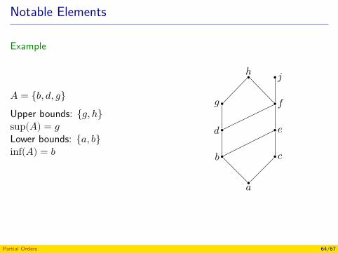
Notable Elements
Example
𝐴 = {𝑏, 𝑑, 𝑔}Upper bounds: {𝑔, ℎ}sup(𝐴) = 𝑔Lower bounds: {𝑎, 𝑏}inf(𝐴) = 𝑏
𝑎
𝑏 𝑐
𝑑 𝑒
𝑓𝑔
ℎ 𝑗
Partial Orders 64/67
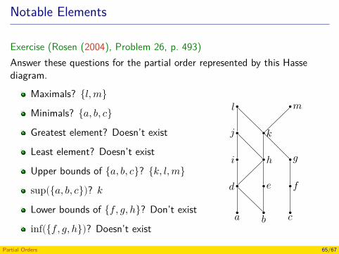
Notable Elements
Exercise (Rosen (2004), Problem 26, p. 493)Answer these questions for the partial order represented by this Hassediagram.
Maximals? {𝑙, 𝑚}Minimals? {𝑎, 𝑏, 𝑐}Greatest element? Doesn’t exist
Least element? Doesn’t exist
Upper bounds of {𝑎, 𝑏, 𝑐}? {𝑘, 𝑙, 𝑚}sup({𝑎, 𝑏, 𝑐})? 𝑘Lower bounds of {𝑓, 𝑔, ℎ}? Don’t exist
inf({𝑓, 𝑔, ℎ})? Doesn’t exist𝑎 𝑏 𝑐
𝑑 𝑒 𝑓
𝑖 ℎ 𝑔
𝑗 𝑘
𝑙 𝑚
Partial Orders 65/67
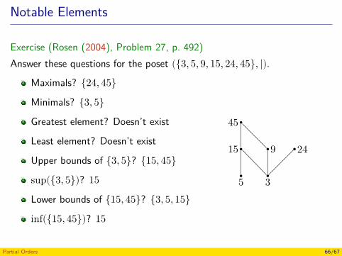
Notable Elements
Exercise (Rosen (2004), Problem 27, p. 492)Answer these questions for the poset ({3, 5, 9, 15, 24, 45}, |).
Maximals? {24, 45}Minimals? {3, 5}Greatest element? Doesn’t exist
Least element? Doesn’t exist
Upper bounds of {3, 5}? {15, 45}sup({3, 5})? 15Lower bounds of {15, 45}? {3, 5, 15}inf({15, 45})? 15
5 3
15 9 24
45
Partial Orders 66/67
References
Rosen, K. H. (2004). Matemática Discreta y sus Aplicaciones. 5th ed.McGraw-Hill (cit. on pp. 14, 46–50, 65, 66).
Partial Orders 67/67
Discrete Structures - CM0246Lattices
Andrés Sicard-Ramírez
Universidad EAFIT
Semester 2014-2
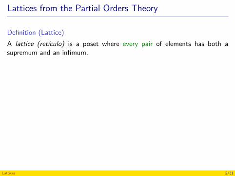
Lattices from the Partial Orders Theory
Definition (Lattice)A lattice (retículo) is a poset where every pair of elements has both asupremum and an infimum.
ExampleThe following poset is a lattice.
𝑎
𝑏𝑐
𝑑
𝑒
𝑓
Lattices 2/31
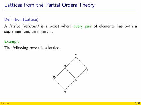
Lattices from the Partial Orders Theory
Definition (Lattice)A lattice (retículo) is a poset where every pair of elements has both asupremum and an infimum.
ExampleThe following poset is a lattice.
𝑎
𝑏𝑐
𝑑
𝑒
𝑓
Lattices 3/31
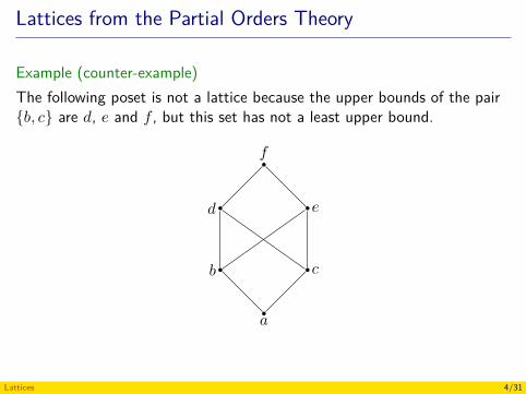
Lattices from the Partial Orders Theory
Example (counter-example)The following poset is not a lattice because the upper bounds of the pair{𝑏, 𝑐} are 𝑑, 𝑒 and 𝑓 , but this set has not a least upper bound.
𝑎
𝑏 𝑐
𝑑 𝑒
𝑓
Lattices 4/31
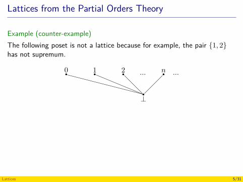
Lattices from the Partial Orders Theory
Example (counter-example)The following poset is not a lattice because for example, the pair {1, 2}has not supremum.
⊥
2 …10 𝑛 …
Lattices 5/31
Lattices from the Partial Orders Theory
Examples(ℤ+, ∣) is a lattice where the supremum is the least common multipleand the infimum is the greatest common divisor.
Let 𝐴 be a set. Is (𝑃 (𝐴), ⊆) a lattice?
Lattices 6/31
Lattices from the Partial Orders Theory
Examples(ℤ+, ∣) is a lattice where the supremum is the least common multipleand the infimum is the greatest common divisor.Let 𝐴 be a set. Is (𝑃 (𝐴), ⊆) a lattice?
Lattices 7/31
Algebraic Structures
Definition (Algebraic structure)An algebraic structure on a set 𝐴 ≠ 0 is essentially a collection of 𝑛-aryoperations on 𝐴 (Cohn 1981, p. 41).
Example (Semigroup)A semigroup (𝑆, ∗) is a set 𝑆 with an associative binary operation∗ ∶ 𝑆 × 𝑆 → 𝑆.
Example (Monoid)A monoid (𝑀, ∗, 𝜀) is a semigroup (𝑀, ∗) with an element 𝜀 ∈ 𝑀 which isan unit for ∗, i.e. (∀𝑥)(𝑥 ∗ 𝜀 = 𝜀 ∗ 𝑥 = 𝑥).
Lattices 8/31
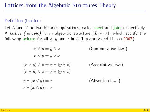
Lattices from the Algebraic Structures Theory
Definition (Lattice)Let ∧ and ∨ be two binaries operations, called meet and join, respectively.A lattice (retículo) is an algebraic structure (𝐿, ∧, ∨), which satisfy thefollowing axioms for all 𝑥, 𝑦 and 𝑧 in 𝐿 (Lipschutz and Lipson 2007):
𝑥 ∧ 𝑦 = 𝑦 ∧ 𝑥 (Commutative laws)𝑥 ∨ 𝑦 = 𝑦 ∨ 𝑥
(𝑥 ∧ 𝑦) ∧ 𝑧 = 𝑥 ∧ (𝑦 ∧ 𝑧) (Associative laws)(𝑥 ∨ 𝑦) ∨ 𝑧 = 𝑥 ∨ (𝑦 ∨ 𝑧)
𝑥 ∧ (𝑥 ∨ 𝑦) = 𝑥 (Absortion laws)𝑥 ∨ (𝑥 ∧ 𝑦) = 𝑥
Lattices 9/31
Lattices from the Algebraic Structures Theory
ExampleLet 𝐴 be a set. (𝑃 (𝐴), ∩, ∪) is a lattice.
Lattices 10/31
Lattices from the Algebraic Structures Theory
Definition (Dual)The dual of any statement in a lattice (𝐿, ∧, ∨) is the statement obtainedby interchanging ∧ and ∨.
ExampleThe dual of 𝑥 ∧ (𝑦 ∨ 𝑥) = 𝑥 ∨ 𝑥 is 𝑥 ∨ (𝑦 ∧ 𝑥) = 𝑥 ∧ 𝑥.
Theorem (Principle of duality)The dual of any theorem in a lattice is also an theorem (Lipschutz andLipson 2007).
Proof.The dual of every axiom in a lattice is also an axiom. Hence, the dualtheorem can be proved by using the dual of each step of the proof of theoriginal theorem.
Lattices 11/31
Lattices from the Algebraic Structures Theory
Definition (Dual)The dual of any statement in a lattice (𝐿, ∧, ∨) is the statement obtainedby interchanging ∧ and ∨.
ExampleThe dual of 𝑥 ∧ (𝑦 ∨ 𝑥) = 𝑥 ∨ 𝑥 is 𝑥 ∨ (𝑦 ∧ 𝑥) = 𝑥 ∧ 𝑥.
Theorem (Principle of duality)The dual of any theorem in a lattice is also an theorem (Lipschutz andLipson 2007).
Proof.The dual of every axiom in a lattice is also an axiom. Hence, the dualtheorem can be proved by using the dual of each step of the proof of theoriginal theorem.
Lattices 12/31
Lattices from the Algebraic Structures Theory
Definition (Dual)The dual of any statement in a lattice (𝐿, ∧, ∨) is the statement obtainedby interchanging ∧ and ∨.
ExampleThe dual of 𝑥 ∧ (𝑦 ∨ 𝑥) = 𝑥 ∨ 𝑥 is 𝑥 ∨ (𝑦 ∧ 𝑥) = 𝑥 ∧ 𝑥.
Theorem (Principle of duality)The dual of any theorem in a lattice is also an theorem (Lipschutz andLipson 2007).
Proof.The dual of every axiom in a lattice is also an axiom. Hence, the dualtheorem can be proved by using the dual of each step of the proof of theoriginal theorem.
Lattices 13/31
Lattices from the Algebraic Structures Theory
Definition (Dual)The dual of any statement in a lattice (𝐿, ∧, ∨) is the statement obtainedby interchanging ∧ and ∨.
ExampleThe dual of 𝑥 ∧ (𝑦 ∨ 𝑥) = 𝑥 ∨ 𝑥 is 𝑥 ∨ (𝑦 ∧ 𝑥) = 𝑥 ∧ 𝑥.
Theorem (Principle of duality)The dual of any theorem in a lattice is also an theorem (Lipschutz andLipson 2007).
Proof.The dual of every axiom in a lattice is also an axiom. Hence, the dualtheorem can be proved by using the dual of each step of the proof of theoriginal theorem.
Lattices 14/31
Lattices from the Algebraic Structures Theory
ExampleLet (𝐿, ∧, ∨) be a lattice. Prove the idempotent laws
𝑥 ∧ 𝑥 = 𝑥, (1)𝑥 ∨ 𝑥 = 𝑥. (2)
Proof of (1).𝑥 ∧ 𝑥 = 𝑥 ∧ (𝑥 ∨ (𝑥 ∧ 𝑦)) (second absortion law)
= 𝑥 (first absortion law)
Proof of (2).By principle of duality on (1).
Lattices 15/31
Lattices from the Algebraic Structures Theory
ExampleLet (𝐿, ∧, ∨) be a lattice. Prove the idempotent laws
𝑥 ∧ 𝑥 = 𝑥, (1)𝑥 ∨ 𝑥 = 𝑥. (2)
Proof of (1).𝑥 ∧ 𝑥 = 𝑥 ∧ (𝑥 ∨ (𝑥 ∧ 𝑦)) (second absortion law)
= 𝑥 (first absortion law)
Proof of (2).By principle of duality on (1).
Lattices 16/31
Lattices from the Algebraic Structures Theory
ExampleLet (𝐿, ∧, ∨) be a lattice. Prove the idempotent laws
𝑥 ∧ 𝑥 = 𝑥, (1)𝑥 ∨ 𝑥 = 𝑥. (2)
Proof of (1).𝑥 ∧ 𝑥 = 𝑥 ∧ (𝑥 ∨ (𝑥 ∧ 𝑦)) (second absortion law)
= 𝑥 (first absortion law)
Proof of (2).By principle of duality on (1).
Lattices 17/31
Lattices from the Algebraic Structures Theory
Exercise (Rosen (2004), Problem 40, p. 500)Prove that if 𝑥 and 𝑦 are elements of a lattice (𝐿, ∧, ∨) then 𝑥 ∨ 𝑦 = 𝑦, ifand only if, 𝑥 ∧ 𝑦 = 𝑥.
Proof →.Let’s suppose 𝑥 ∨ 𝑦 = 𝑦. Then
𝑥 = 𝑥 ∧ (𝑥 ∨ 𝑦) (first absortion law)= 𝑥 ∧ 𝑦 (hypothesis)
Lattices 18/31
Lattices from the Algebraic Structures Theory
Exercise (Rosen (2004), Problem 40, p. 500)Prove that if 𝑥 and 𝑦 are elements of a lattice (𝐿, ∧, ∨) then 𝑥 ∨ 𝑦 = 𝑦, ifand only if, 𝑥 ∧ 𝑦 = 𝑥.
Proof →.Let’s suppose 𝑥 ∨ 𝑦 = 𝑦. Then
𝑥 = 𝑥 ∧ (𝑥 ∨ 𝑦) (first absortion law)= 𝑥 ∧ 𝑦 (hypothesis)
Lattices 19/31
Lattices from the Algebraic Structures Theory
Exercise (cont.)
Proof ←.Let’s suppose 𝑥 ∧ 𝑦 = 𝑥. Then
𝑦 = 𝑦 ∨ (𝑦 ∧ 𝑥) (second absortion law)= 𝑦 ∨ (𝑥 ∧ 𝑦) (commutative law)= 𝑦 ∨ 𝑥 (hypothesis)= 𝑥 ∨ 𝑦 (commutative law)
Lattices 20/31
Equivalence of the Definitions
TheoremLet (𝐿, ∧, ∨) be a lattice. Then (𝐿, ≼) is a partial order, where the relation ≼is defined by (Lipschutz and Lipson 2007):
𝑥 ≼ 𝑦 def= 𝑥 ∧ 𝑦 = 𝑥.
Proof.1. The relation ≼ is reflexive
𝑥 ∧ 𝑥 = 𝑥 (idempotency), for all 𝑥 ∈ 𝐿. Therefore 𝑥 ≼ 𝑥, for all𝑥 ∈ 𝐿.
Lattices 21/31
Equivalence of the Definitions
TheoremLet (𝐿, ∧, ∨) be a lattice. Then (𝐿, ≼) is a partial order, where the relation ≼is defined by (Lipschutz and Lipson 2007):
𝑥 ≼ 𝑦 def= 𝑥 ∧ 𝑦 = 𝑥.Proof.
1. The relation ≼ is reflexive𝑥 ∧ 𝑥 = 𝑥 (idempotency), for all 𝑥 ∈ 𝐿. Therefore 𝑥 ≼ 𝑥, for all𝑥 ∈ 𝐿.
Lattices 22/31
Equivalence of the Definitions
Proof (cont.)2. The relation ≼ is antisymmetric
Suppose 𝑥 ≼ 𝑦 and 𝑦 ≼ 𝑥, then 𝑥 ∧ 𝑦 = 𝑥 and 𝑦 ∧ 𝑥 = 𝑦. Therefore
𝑥 = 𝑥 ∧ 𝑦 (hypothesis)= 𝑦 ∧ 𝑥 (commutative law)= 𝑦 (hypothesis)
That is, ≼ is antisymmetric.
Lattices 23/31
Equivalence of the Definitions
Proof (cont.)3. The relation ≼ is transitive
Suppose 𝑥 ≼ 𝑦 and 𝑦 ≼ 𝑧, then 𝑥 ∧ 𝑦 = 𝑥 and 𝑦 ∧ 𝑧 = 𝑦. Therefore
𝑥 ∧ 𝑧 = (𝑥 ∧ 𝑦) ∧ 𝑧 (hypothesis)= 𝑥 ∧ (𝑦 ∧ 𝑧) (associativity law)= 𝑥 ∧ 𝑦 (hypothesis)= 𝑥 (hypothesis)
That is, 𝑥 ≼ 𝑧.
Lattices 24/31
Equivalence of the Definitions
RemarkLet (𝐿, ∧, ∨) be a lattice and let be (𝐿, ≼) the order partial induced by(𝐿, ∧, ∨). It is possible prove that (𝐿, ≼) is a lattice.
Lattices 25/31
Equivalence of the Definitions
Theorem (Rosen (2004), Problem 39, p. 500)Let (𝐿, ≼) be a lattice. Then (𝐿, ∧, ∨) is a lattice, where
𝑥 ∧ 𝑦 def= inf(𝑥, 𝑦),𝑥 ∨ 𝑦 def= sup(𝑥, 𝑦),
Proof.1. Commutative laws for ∧ and ∨ (Rosen’s solution).
Because inf(𝑥, 𝑦) = inf(𝑦, 𝑥) and sup(𝑥, 𝑦) = sup(𝑦, 𝑥), it followsthat 𝑥 ∧ 𝑦 = 𝑦 ∧ 𝑥 and 𝑥 ∨ 𝑦 = 𝑦 ∨ 𝑥.
Lattices 26/31
Equivalence of the Definitions
Theorem (Rosen (2004), Problem 39, p. 500)Let (𝐿, ≼) be a lattice. Then (𝐿, ∧, ∨) is a lattice, where
𝑥 ∧ 𝑦 def= inf(𝑥, 𝑦),𝑥 ∨ 𝑦 def= sup(𝑥, 𝑦),
Proof.1. Commutative laws for ∧ and ∨ (Rosen’s solution).
Because inf(𝑥, 𝑦) = inf(𝑦, 𝑥) and sup(𝑥, 𝑦) = sup(𝑦, 𝑥), it followsthat 𝑥 ∧ 𝑦 = 𝑦 ∧ 𝑥 and 𝑥 ∨ 𝑦 = 𝑦 ∨ 𝑥.
Lattices 27/31
Equivalence of the Definitions
Proof (cont.)2. Associative laws for ∧ and ∨ (Rosen’s solution).
Using the definition, (𝑥 ∧ 𝑦) ∧ 𝑧 is a lower bound of 𝑥, 𝑦 and 𝑧 thatis greater than every other lower bound. Because 𝑥, 𝑦 and 𝑧 playinterchangeable roles, 𝑥 ∧ (𝑦 ∧ 𝑧) is the same element.
Similarly, (𝑥 ∨ 𝑦) ∨ 𝑧 is an upper bound of 𝑥, 𝑦 and 𝑧 that is less thanevery other upper bound. Because 𝑥, 𝑦 and 𝑧 play interchangeableroles, 𝑥 ∨ (𝑦 ∨ 𝑧) is the same element.
Lattices 28/31
Equivalence of the Definitions
Proof (cont.)2. Associative laws for ∧ and ∨ (Rosen’s solution).
Using the definition, (𝑥 ∧ 𝑦) ∧ 𝑧 is a lower bound of 𝑥, 𝑦 and 𝑧 thatis greater than every other lower bound. Because 𝑥, 𝑦 and 𝑧 playinterchangeable roles, 𝑥 ∧ (𝑦 ∧ 𝑧) is the same element.
Similarly, (𝑥 ∨ 𝑦) ∨ 𝑧 is an upper bound of 𝑥, 𝑦 and 𝑧 that is less thanevery other upper bound. Because 𝑥, 𝑦 and 𝑧 play interchangeableroles, 𝑥 ∨ (𝑦 ∨ 𝑧) is the same element.
Lattices 29/31
Equivalence of the Definitions
Proof (cont.)3. Absortion laws for ∧ and ∨ (Rosen’s solution).
To show that 𝑥 ∧ (𝑥 ∨ 𝑦) = 𝑥 it is sufficient to show that 𝑥 is thegreatest lower bound of 𝑥, and 𝑥 ∨ 𝑦. Note that 𝑥 is a lower boundof 𝑥, and because 𝑥 ∨ 𝑦 is by definition greater than 𝑥, 𝑥 is a lowerbound for it as well. Therefore, 𝑥 is a lower bound. But any lowerbound of 𝑥 has to be less than 𝑥, so 𝑥 is the greatest lower bound.
The second statement is the dual of the first; we omit its proof.
Lattices 30/31
References
Cohn, P. M. (1981). Universal Algebra. Revised edition. D. ReidelPublishing Company (cit. on p. 8).Lipschutz, S. and Lipson, M. L. (2007). Schaum’s Outline of DiscreteMathematics. 3rd ed. McGraw-Hill (cit. on pp. 9, 11–14, 21, 22).Rosen, K. H. (2004). Matemática Discreta y sus Aplicaciones. 5th ed.McGraw-Hill (cit. on pp. 18, 19, 26, 27).
Lattices 31/31
Discrete Structures - CM0246Boolean Algebras
Andrés Sicard-Ramírez
Universidad EAFIT
Semester 2014-2
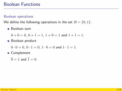
Boolean Functions
Boolean operationsWe define the following operations in the set 𝐵 = {0, 1}:
Boolean sum0 + 0 = 0, 0 + 1 = 1, 1 + 0 = 1 and 1 + 1 = 1.Boolean product0 · 0 = 0, 0 · 1 = 0, 1 · 0 = 0 and 1 · 1 = 1.Complement0 = 1 and 1 = 0.
Precedence (highest to lowest): Complement, Boolean product and Booleansum.
ExamplesWhiteboard.
Boolean Algebras 2/29
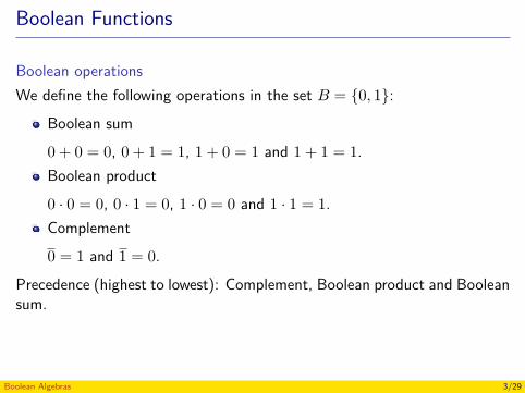
Boolean Functions
Boolean operationsWe define the following operations in the set 𝐵 = {0, 1}:
Boolean sum0 + 0 = 0, 0 + 1 = 1, 1 + 0 = 1 and 1 + 1 = 1.Boolean product0 · 0 = 0, 0 · 1 = 0, 1 · 0 = 0 and 1 · 1 = 1.Complement0 = 1 and 1 = 0.
Precedence (highest to lowest): Complement, Boolean product and Booleansum.
ExamplesWhiteboard.
Boolean Algebras 3/29
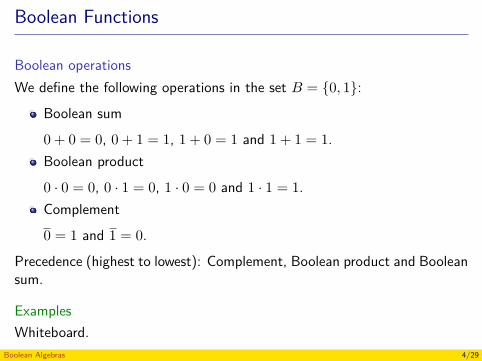
Boolean Functions
Boolean operationsWe define the following operations in the set 𝐵 = {0, 1}:
Boolean sum0 + 0 = 0, 0 + 1 = 1, 1 + 0 = 1 and 1 + 1 = 1.Boolean product0 · 0 = 0, 0 · 1 = 0, 1 · 0 = 0 and 1 · 1 = 1.Complement0 = 1 and 1 = 0.
Precedence (highest to lowest): Complement, Boolean product and Booleansum.
ExamplesWhiteboard.
Boolean Algebras 4/29
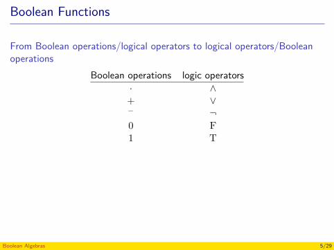
Boolean Functions
From Boolean operations/logical operators to logical operators/Booleanoperations
Boolean operations logic operators· ∧+ ∨− ¬0 F1 T
Examples (From equality/logical equivalence to logicalequivalence/equality)Whiteboard.
Boolean Algebras 5/29
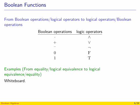
Boolean Functions
From Boolean operations/logical operators to logical operators/Booleanoperations
Boolean operations logic operators· ∧+ ∨− ¬0 F1 T
Examples (From equality/logical equivalence to logicalequivalence/equality)Whiteboard.
Boolean Algebras 6/29
Boolean Functions
Definition (Boolean function)Let 𝐵 = {0, 1}. A function from 𝐵𝑛 to 𝐵 is called a Boolean function ofdegree 𝑛.
ExamplesWhiteboard.
Boolean Algebras 7/29
Boolean Functions
Definition (Boolean function)Let 𝐵 = {0, 1}. A function from 𝐵𝑛 to 𝐵 is called a Boolean function ofdegree 𝑛.
ExamplesWhiteboard.
Boolean Algebras 8/29
Boolean Functions
Theorem (Rosen (2004), Example 5, p. 280)If |𝐴| = 𝑚 and |𝐵| = 𝑛 then |{𝑓 ∶ 𝐴 → 𝐵}| = 𝑛𝑚.
ExampleThere are 16 Boolean functions of degree 2.
Boolean Algebras 9/29
Boolean Functions
Theorem (Rosen (2004), Example 5, p. 280)If |𝐴| = 𝑚 and |𝐵| = 𝑛 then |{𝑓 ∶ 𝐴 → 𝐵}| = 𝑛𝑚.
ExampleThere are 16 Boolean functions of degree 2.
Boolean Algebras 10/29
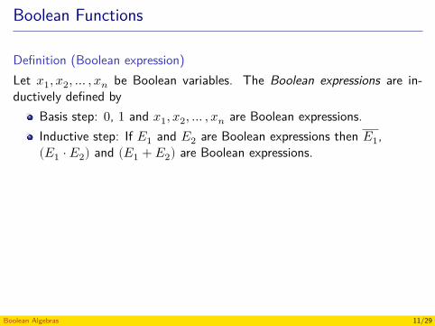
Boolean Functions
Definition (Boolean expression)Let 𝑥1, 𝑥2, … , 𝑥𝑛 be Boolean variables. The Boolean expressions are in-ductively defined by
Basis step: 0, 1 and 𝑥1, 𝑥2, … , 𝑥𝑛 are Boolean expressions.Inductive step: If 𝐸1 and 𝐸2 are Boolean expressions then 𝐸1,(𝐸1 · 𝐸2) and (𝐸1 + 𝐸2) are Boolean expressions.
Each Boolean expression represents a Boolean function.
ExamplesWhiteboard.
Boolean Algebras 11/29
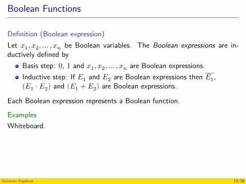
Boolean Functions
Definition (Boolean expression)Let 𝑥1, 𝑥2, … , 𝑥𝑛 be Boolean variables. The Boolean expressions are in-ductively defined by
Basis step: 0, 1 and 𝑥1, 𝑥2, … , 𝑥𝑛 are Boolean expressions.Inductive step: If 𝐸1 and 𝐸2 are Boolean expressions then 𝐸1,(𝐸1 · 𝐸2) and (𝐸1 + 𝐸2) are Boolean expressions.
Each Boolean expression represents a Boolean function.
ExamplesWhiteboard.
Boolean Algebras 12/29
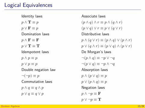
Logical Equivalences
Identity laws𝑝 ∧ T ≡ 𝑝𝑝 ∨ F ≡ 𝑝Domination laws𝑝 ∧ F ≡ F𝑝 ∨ T ≡ TIdempotent laws𝑝 ∧ 𝑝 ≡ 𝑝𝑝 ∨ 𝑝 ≡ 𝑝Double negation law¬(¬𝑝) ≡ 𝑝Commutative laws𝑝 ∧ 𝑞 ≡ 𝑞 ∧ 𝑝𝑝 ∨ 𝑞 ≡ 𝑞 ∨ 𝑝
Associate laws(𝑝 ∧ 𝑞) ∧ 𝑟 ≡ 𝑝 ∧ (𝑞 ∧ 𝑟)(𝑝 ∨ 𝑞) ∨ 𝑟 ≡ 𝑝 ∨ (𝑞 ∨ 𝑟)Distributive laws𝑝 ∧ (𝑞 ∨ 𝑟) ≡ (𝑝 ∧ 𝑞) ∨ (𝑝 ∧ 𝑟)𝑝 ∨ (𝑞 ∧ 𝑟) ≡ (𝑝 ∨ 𝑞) ∧ (𝑝 ∨ 𝑟)De Morgan’s laws¬(𝑝 ∧ 𝑞) ≡ ¬𝑝 ∨ ¬𝑞¬(𝑝 ∨ 𝑞) ≡ ¬𝑝 ∧ ¬𝑞Absorption laws𝑝 ∧ (𝑝 ∨ 𝑞) ≡ 𝑝𝑝 ∨ (𝑝 ∧ 𝑞) ≡ 𝑝Negation laws𝑝 ∧ ¬𝑝 ≡ F𝑝 ∨ ¬𝑝 ≡ T
Boolean Algebras 13/29
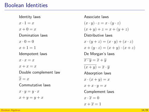
Boolean Identities
Identity laws𝑥 · 1 = 𝑥𝑥 + 0 = 𝑥Domination laws𝑥 · 0 = 0𝑥 + 1 = 1Idempotent laws𝑥 · 𝑥 = 𝑥𝑥 + 𝑥 = 𝑥Double complement law𝑥 = 𝑥Commutative laws𝑥 · 𝑦 = 𝑦 · 𝑥𝑥 + 𝑦 = 𝑦 + 𝑥
Associate laws(𝑥 · 𝑦) · 𝑧 = 𝑥 · (𝑦 · 𝑧)(𝑥 + 𝑦) + 𝑧 = 𝑥 + (𝑦 + 𝑧)Distributive laws𝑥 · (𝑦 + 𝑧) = (𝑥 · 𝑦) + (𝑥 · 𝑧)𝑥 + (𝑦 · 𝑧) = (𝑥 + 𝑦) · (𝑥 + 𝑧)De Morgan’s laws𝑥 · 𝑦 = 𝑥 + 𝑦(𝑥 + 𝑦) = 𝑥 · 𝑦Absorption laws𝑥 · (𝑥 + 𝑦) = 𝑥𝑥 + 𝑥 · 𝑦 = 𝑥Complement laws𝑥 · 𝑥 = 0𝑥 + 𝑥 = 1
Boolean Algebras 14/29
Boolean Identities
Each Boolean identity can be proved using a table.
ExamplesWhiteboard.
Boolean Algebras 15/29
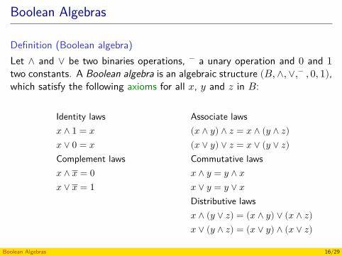
Boolean Algebras
Definition (Boolean algebra)Let ∧ and ∨ be two binaries operations, − a unary operation and 0 and 1two constants. A Boolean algebra is an algebraic structure (𝐵, ∧, ∨,− , 0, 1),which satisfy the following axioms for all 𝑥, 𝑦 and 𝑧 in 𝐵:
Identity laws𝑥 ∧ 1 = 𝑥𝑥 ∨ 0 = 𝑥Complement laws𝑥 ∧ 𝑥 = 0𝑥 ∨ 𝑥 = 1
Associate laws(𝑥 ∧ 𝑦) ∧ 𝑧 = 𝑥 ∧ (𝑦 ∧ 𝑧)(𝑥 ∨ 𝑦) ∨ 𝑧 = 𝑥 ∨ (𝑦 ∨ 𝑧)Commutative laws𝑥 ∧ 𝑦 = 𝑦 ∧ 𝑥𝑥 ∨ 𝑦 = 𝑦 ∨ 𝑥Distributive laws𝑥 ∧ (𝑦 ∨ 𝑧) = (𝑥 ∧ 𝑦) ∨ (𝑥 ∧ 𝑧)𝑥 ∨ (𝑦 ∧ 𝑧) = (𝑥 ∨ 𝑦) ∧ (𝑥 ∨ 𝑧)
Boolean Algebras 16/29
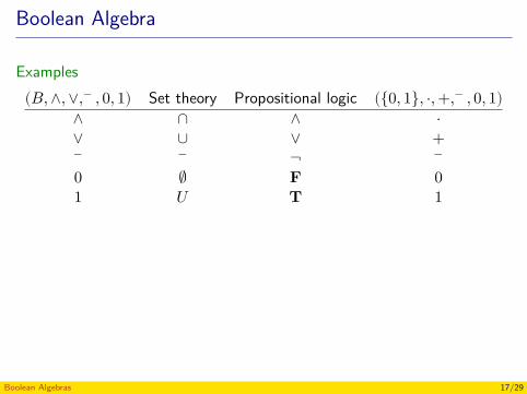
Boolean Algebra
Examples(𝐵, ∧, ∨,− , 0, 1) Set theory Propositional logic ({0, 1}, ·, +,− , 0, 1)
∧ ∩ ∧ ·∨ ∪ ∨ +− − ¬ −
0 ∅ F 01 𝑈 T 1
Boolean Algebras 17/29
Boolean Algebra
Definition (Dual)The dual of any statement in a Boolean algebra (𝐵, ∧, ∨,− , 0, 1) is thestatement obtained by interchanging ∧ and ∨, and interchanging 0 and 1.
ExampleThe dual of 𝑥 ∧ (𝑦 ∨ 0) is 𝑥 ∨ (𝑦 ∧ 1)
Theorem (Principle of duality. Rosen (2004), Problem 38, p. 660)The dual of any theorem in a Boolean algebra is also an theorem.
Proof.Similar to the proof of the principle of duality for lattices.
Boolean Algebras 18/29
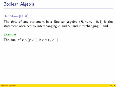
Boolean Algebra
Definition (Dual)The dual of any statement in a Boolean algebra (𝐵, ∧, ∨,− , 0, 1) is thestatement obtained by interchanging ∧ and ∨, and interchanging 0 and 1.
ExampleThe dual of 𝑥 ∧ (𝑦 ∨ 0) is 𝑥 ∨ (𝑦 ∧ 1)
Theorem (Principle of duality. Rosen (2004), Problem 38, p. 660)The dual of any theorem in a Boolean algebra is also an theorem.
Proof.Similar to the proof of the principle of duality for lattices.
Boolean Algebras 19/29
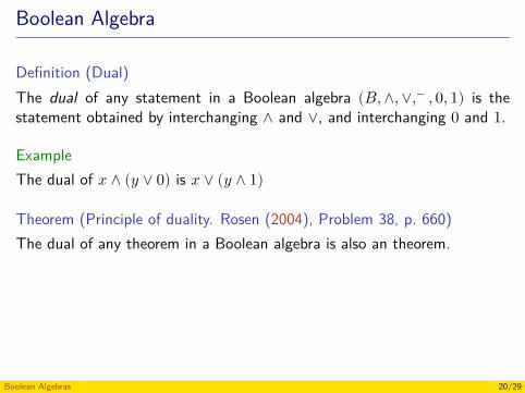
Boolean Algebra
Definition (Dual)The dual of any statement in a Boolean algebra (𝐵, ∧, ∨,− , 0, 1) is thestatement obtained by interchanging ∧ and ∨, and interchanging 0 and 1.
ExampleThe dual of 𝑥 ∧ (𝑦 ∨ 0) is 𝑥 ∨ (𝑦 ∧ 1)
Theorem (Principle of duality. Rosen (2004), Problem 38, p. 660)The dual of any theorem in a Boolean algebra is also an theorem.
Proof.Similar to the proof of the principle of duality for lattices.
Boolean Algebras 20/29
Boolean Algebra
Definition (Dual)The dual of any statement in a Boolean algebra (𝐵, ∧, ∨,− , 0, 1) is thestatement obtained by interchanging ∧ and ∨, and interchanging 0 and 1.
ExampleThe dual of 𝑥 ∧ (𝑦 ∨ 0) is 𝑥 ∨ (𝑦 ∧ 1)
Theorem (Principle of duality. Rosen (2004), Problem 38, p. 660)The dual of any theorem in a Boolean algebra is also an theorem.
Proof.Similar to the proof of the principle of duality for lattices.
Boolean Algebras 21/29
Boolean Algebra
Example (Rosen (2004), Problem 31, p. 660)Let 𝔹 = (𝐵, ∧, ∨,− , 0, 1) be a Boolean algebra. To prove that 𝔹 satisfythe idempotent laws 𝑥 ∨ 𝑥 = 𝑥 and 𝑥 ∧ 𝑥 = 𝑥, for every element 𝑥.
Proof.𝑥 ∨ 𝑥 = (𝑥 ∨ 𝑥) ∧ 1
= (𝑥 ∨ 𝑥) ∧ (𝑥 ∨ 𝑥)= 𝑥 ∨ (𝑥 ∧ 𝑥)= 𝑥 ∨ 0= 𝑥
(identity law)(complement law)(distributive law)
(complement law)(identity law)
𝑥 ∧ 𝑥 = (𝑥 ∧ 𝑥) ∨ 0= (𝑥 ∧ 𝑥) ∨ (𝑥 ∧ 𝑥)= 𝑥 ∧ (𝑥 ∨ 𝑥)= 𝑥 ∧ 1= 𝑥
Remark: 𝑥 ∧ 𝑥 = 𝑥/𝑥 ∨ 𝑥 = 𝑥 also follows from 𝑥 ∨ 𝑥 = 𝑥/𝑥 ∧ 𝑥 = 𝑥 bythe principle of duality.
Boolean Algebras 22/29
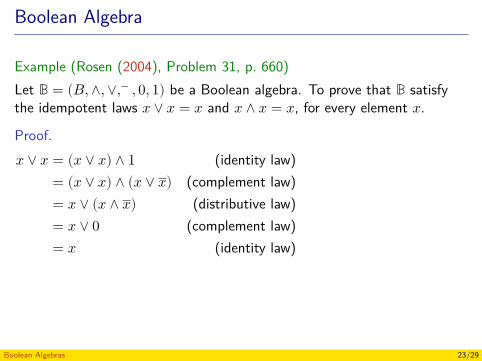
Boolean Algebra
Example (Rosen (2004), Problem 31, p. 660)Let 𝔹 = (𝐵, ∧, ∨,− , 0, 1) be a Boolean algebra. To prove that 𝔹 satisfythe idempotent laws 𝑥 ∨ 𝑥 = 𝑥 and 𝑥 ∧ 𝑥 = 𝑥, for every element 𝑥.
Proof.𝑥 ∨ 𝑥 = (𝑥 ∨ 𝑥) ∧ 1
= (𝑥 ∨ 𝑥) ∧ (𝑥 ∨ 𝑥)= 𝑥 ∨ (𝑥 ∧ 𝑥)= 𝑥 ∨ 0= 𝑥
(identity law)(complement law)(distributive law)
(complement law)(identity law)
𝑥 ∧ 𝑥 = (𝑥 ∧ 𝑥) ∨ 0= (𝑥 ∧ 𝑥) ∨ (𝑥 ∧ 𝑥)= 𝑥 ∧ (𝑥 ∨ 𝑥)= 𝑥 ∧ 1= 𝑥
Remark: 𝑥 ∧ 𝑥 = 𝑥/𝑥 ∨ 𝑥 = 𝑥 also follows from 𝑥 ∨ 𝑥 = 𝑥/𝑥 ∧ 𝑥 = 𝑥 bythe principle of duality.
Boolean Algebras 23/29
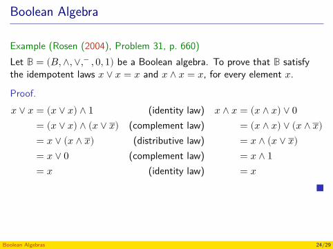
Boolean Algebra
Example (Rosen (2004), Problem 31, p. 660)Let 𝔹 = (𝐵, ∧, ∨,− , 0, 1) be a Boolean algebra. To prove that 𝔹 satisfythe idempotent laws 𝑥 ∨ 𝑥 = 𝑥 and 𝑥 ∧ 𝑥 = 𝑥, for every element 𝑥.
Proof.𝑥 ∨ 𝑥 = (𝑥 ∨ 𝑥) ∧ 1
= (𝑥 ∨ 𝑥) ∧ (𝑥 ∨ 𝑥)= 𝑥 ∨ (𝑥 ∧ 𝑥)= 𝑥 ∨ 0= 𝑥
(identity law)(complement law)(distributive law)
(complement law)(identity law)
𝑥 ∧ 𝑥 = (𝑥 ∧ 𝑥) ∨ 0= (𝑥 ∧ 𝑥) ∨ (𝑥 ∧ 𝑥)= 𝑥 ∧ (𝑥 ∨ 𝑥)= 𝑥 ∧ 1= 𝑥
Remark: 𝑥 ∧ 𝑥 = 𝑥/𝑥 ∨ 𝑥 = 𝑥 also follows from 𝑥 ∨ 𝑥 = 𝑥/𝑥 ∧ 𝑥 = 𝑥 bythe principle of duality.
Boolean Algebras 24/29
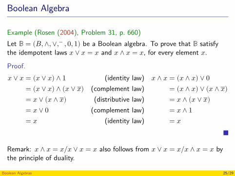
Boolean Algebra
Example (Rosen (2004), Problem 31, p. 660)Let 𝔹 = (𝐵, ∧, ∨,− , 0, 1) be a Boolean algebra. To prove that 𝔹 satisfythe idempotent laws 𝑥 ∨ 𝑥 = 𝑥 and 𝑥 ∧ 𝑥 = 𝑥, for every element 𝑥.
Proof.𝑥 ∨ 𝑥 = (𝑥 ∨ 𝑥) ∧ 1
= (𝑥 ∨ 𝑥) ∧ (𝑥 ∨ 𝑥)= 𝑥 ∨ (𝑥 ∧ 𝑥)= 𝑥 ∨ 0= 𝑥
(identity law)(complement law)(distributive law)
(complement law)(identity law)
𝑥 ∧ 𝑥 = (𝑥 ∧ 𝑥) ∨ 0= (𝑥 ∧ 𝑥) ∨ (𝑥 ∧ 𝑥)= 𝑥 ∧ (𝑥 ∨ 𝑥)= 𝑥 ∧ 1= 𝑥
Remark: 𝑥 ∧ 𝑥 = 𝑥/𝑥 ∨ 𝑥 = 𝑥 also follows from 𝑥 ∨ 𝑥 = 𝑥/𝑥 ∧ 𝑥 = 𝑥 bythe principle of duality.
Boolean Algebras 25/29
Boolean Algebra
Example (Rosen (2004), Problem 34, p. 660)Let 𝔹 = (𝐵, ∧, ∨,− , 0, 1) be a Boolean algebra. To prove that 𝔹 satisfythe double complement law, i.e. ∀𝑥(𝑥 = 𝑥).
HintFrom the complement laws, we have
𝑥 ∧ 𝑥 = 0,𝑥 ∨ 𝑥 = 1.
Boolean Algebras 26/29
Boolean Algebra
Example (Rosen (2004), Problem 34, p. 660)Let 𝔹 = (𝐵, ∧, ∨,− , 0, 1) be a Boolean algebra. To prove that 𝔹 satisfythe double complement law, i.e. ∀𝑥(𝑥 = 𝑥).
HintFrom the complement laws, we have
𝑥 ∧ 𝑥 = 0,𝑥 ∨ 𝑥 = 1.
Boolean Algebras 27/29
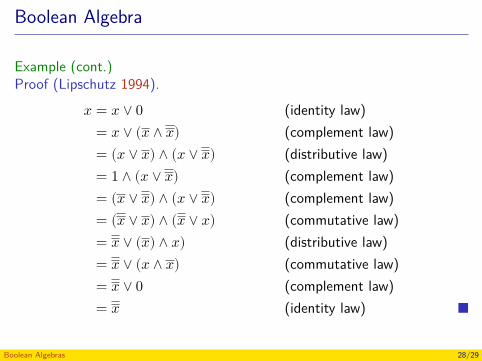
Boolean Algebra
Example (cont.)Proof (Lipschutz 1994).
𝑥 = 𝑥 ∨ 0 (identity law)= 𝑥 ∨ (𝑥 ∧ 𝑥) (complement law)= (𝑥 ∨ 𝑥) ∧ (𝑥 ∨ 𝑥) (distributive law)= 1 ∧ (𝑥 ∨ 𝑥) (complement law)= (𝑥 ∨ 𝑥) ∧ (𝑥 ∨ 𝑥) (complement law)= (𝑥 ∨ 𝑥) ∧ (𝑥 ∨ 𝑥) (commutative law)= 𝑥 ∨ (𝑥) ∧ 𝑥) (distributive law)= 𝑥 ∨ (𝑥 ∧ 𝑥) (commutative law)= 𝑥 ∨ 0 (complement law)= 𝑥 (identity law)
Boolean Algebras 28/29
References
Lipschutz, S. (1994). Teoría de Conjuntos y Temas Afines. Serie Schaum.McGraw-Hill (cit. on p. 28).Rosen, K. H. (2004). Matemática Discreta y sus Aplicaciones. 5th ed.McGraw-Hill (cit. on pp. 9, 10, 18–27).
Boolean Algebras 29/29
Discrete Structures - CM0246Representing Graphs and Graph Isomorphism
Andrés Sicard-Ramírez
Universidad EAFIT
Semester 2014-2
Graphs
Graphs are discrete structures consisting of vertices and edges thatconnect these vertices.
We need different kinds of graphs for solving problems using graph models.
Example (Computer networks)A computer networkA computer network with multiple links between data centers (paralleledges)A computer network with diagnostic links (loops)A computer network with one-way links (edges with direction)A computer network with multiple one-way links (parallel edges withdirection)
Representing Graphs and Graph Isomorphism 2/63
Graphs
Graphs are discrete structures consisting of vertices and edges thatconnect these vertices.We need different kinds of graphs for solving problems using graph models.
Example (Computer networks)A computer networkA computer network with multiple links between data centers (paralleledges)A computer network with diagnostic links (loops)A computer network with one-way links (edges with direction)A computer network with multiple one-way links (parallel edges withdirection)
Representing Graphs and Graph Isomorphism 3/63
Graphs
Graphs are discrete structures consisting of vertices and edges thatconnect these vertices.We need different kinds of graphs for solving problems using graph models.
Example (Computer networks)
A computer networkA computer network with multiple links between data centers (paralleledges)A computer network with diagnostic links (loops)A computer network with one-way links (edges with direction)A computer network with multiple one-way links (parallel edges withdirection)
Representing Graphs and Graph Isomorphism 4/63
Graphs
Graphs are discrete structures consisting of vertices and edges thatconnect these vertices.We need different kinds of graphs for solving problems using graph models.
Example (Computer networks)A computer network
A computer network with multiple links between data centers (paralleledges)A computer network with diagnostic links (loops)A computer network with one-way links (edges with direction)A computer network with multiple one-way links (parallel edges withdirection)
Representing Graphs and Graph Isomorphism 5/63
Graphs
Graphs are discrete structures consisting of vertices and edges thatconnect these vertices.We need different kinds of graphs for solving problems using graph models.
Example (Computer networks)A computer networkA computer network with multiple links between data centers (paralleledges)
A computer network with diagnostic links (loops)A computer network with one-way links (edges with direction)A computer network with multiple one-way links (parallel edges withdirection)
Representing Graphs and Graph Isomorphism 6/63
Graphs
Graphs are discrete structures consisting of vertices and edges thatconnect these vertices.We need different kinds of graphs for solving problems using graph models.
Example (Computer networks)A computer networkA computer network with multiple links between data centers (paralleledges)A computer network with diagnostic links (loops)
A computer network with one-way links (edges with direction)A computer network with multiple one-way links (parallel edges withdirection)
Representing Graphs and Graph Isomorphism 7/63
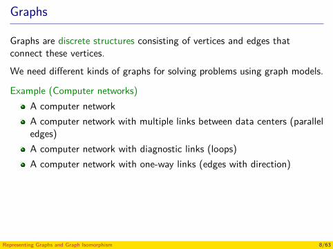
Graphs
Graphs are discrete structures consisting of vertices and edges thatconnect these vertices.We need different kinds of graphs for solving problems using graph models.
Example (Computer networks)A computer networkA computer network with multiple links between data centers (paralleledges)A computer network with diagnostic links (loops)A computer network with one-way links (edges with direction)
A computer network with multiple one-way links (parallel edges withdirection)
Representing Graphs and Graph Isomorphism 8/63
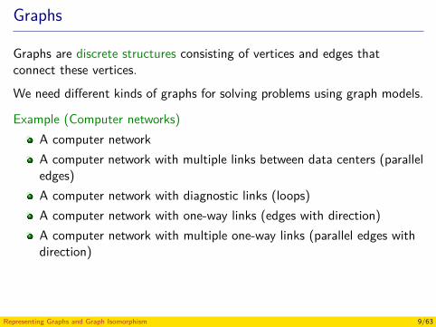
Graphs
Graphs are discrete structures consisting of vertices and edges thatconnect these vertices.We need different kinds of graphs for solving problems using graph models.
Example (Computer networks)A computer networkA computer network with multiple links between data centers (paralleledges)A computer network with diagnostic links (loops)A computer network with one-way links (edges with direction)A computer network with multiple one-way links (parallel edges withdirection)
Representing Graphs and Graph Isomorphism 9/63
Simple Graphs
Remark: In all the definitions related to graphs, the set of vertices isnon-empty. Moreover, we shall assume that this set is finite.
Definition (Simple graph)A simple graph 𝐺 = (𝑉 , 𝐸) consist of 𝑉 , a set of vertices, and 𝐸, a set ofunordered pairs of distinct elements of 𝑉 called edges.
Remark: In a simple graph there is no parallel edges nor loops.
ExamplesWhiteboard.
Representing Graphs and Graph Isomorphism 10/63
Simple Graphs
Remark: In all the definitions related to graphs, the set of vertices isnon-empty. Moreover, we shall assume that this set is finite.
Definition (Simple graph)A simple graph 𝐺 = (𝑉 , 𝐸) consist of 𝑉 , a set of vertices, and 𝐸, a set ofunordered pairs of distinct elements of 𝑉 called edges.
Remark: In a simple graph there is no parallel edges nor loops.
ExamplesWhiteboard.
Representing Graphs and Graph Isomorphism 11/63
Simple Graphs
Remark: In all the definitions related to graphs, the set of vertices isnon-empty. Moreover, we shall assume that this set is finite.
Definition (Simple graph)A simple graph 𝐺 = (𝑉 , 𝐸) consist of 𝑉 , a set of vertices, and 𝐸, a set ofunordered pairs of distinct elements of 𝑉 called edges.
Remark: In a simple graph there is no parallel edges nor loops.
ExamplesWhiteboard.
Representing Graphs and Graph Isomorphism 12/63
Simple Graphs
Remark: In all the definitions related to graphs, the set of vertices isnon-empty. Moreover, we shall assume that this set is finite.
Definition (Simple graph)A simple graph 𝐺 = (𝑉 , 𝐸) consist of 𝑉 , a set of vertices, and 𝐸, a set ofunordered pairs of distinct elements of 𝑉 called edges.
Remark: In a simple graph there is no parallel edges nor loops.
ExamplesWhiteboard.
Representing Graphs and Graph Isomorphism 13/63
Multigraphs
Definition (Multigraph)A multigraph 𝐺 = (𝑉 , 𝐸) consist of set 𝑉 of vertices, a set 𝐸 of edges anda function
𝑓 ∶ 𝐸 → {{𝑢, 𝑣} ∣ 𝑢, 𝑣 ∈ 𝑉 , 𝑢 ≠ 𝑣}.
The edges 𝑒𝑖 and 𝑒𝑗 are called parallel edges if 𝑓(𝑒𝑖) = 𝑓(𝑒𝑗).
Remark: In a multigraph there is no loops.
ExamplesWhiteboard.
Representing Graphs and Graph Isomorphism 14/63
Multigraphs
Definition (Multigraph)A multigraph 𝐺 = (𝑉 , 𝐸) consist of set 𝑉 of vertices, a set 𝐸 of edges anda function
𝑓 ∶ 𝐸 → {{𝑢, 𝑣} ∣ 𝑢, 𝑣 ∈ 𝑉 , 𝑢 ≠ 𝑣}.
The edges 𝑒𝑖 and 𝑒𝑗 are called parallel edges if 𝑓(𝑒𝑖) = 𝑓(𝑒𝑗).
Remark: In a multigraph there is no loops.
ExamplesWhiteboard.
Representing Graphs and Graph Isomorphism 15/63
Multigraphs
Definition (Multigraph)A multigraph 𝐺 = (𝑉 , 𝐸) consist of set 𝑉 of vertices, a set 𝐸 of edges anda function
𝑓 ∶ 𝐸 → {{𝑢, 𝑣} ∣ 𝑢, 𝑣 ∈ 𝑉 , 𝑢 ≠ 𝑣}.
The edges 𝑒𝑖 and 𝑒𝑗 are called parallel edges if 𝑓(𝑒𝑖) = 𝑓(𝑒𝑗).
Remark: In a multigraph there is no loops.
ExamplesWhiteboard.
Representing Graphs and Graph Isomorphism 16/63
Multigraphs
Definition (Multigraph)A multigraph 𝐺 = (𝑉 , 𝐸) consist of set 𝑉 of vertices, a set 𝐸 of edges anda function
𝑓 ∶ 𝐸 → {{𝑢, 𝑣} ∣ 𝑢, 𝑣 ∈ 𝑉 , 𝑢 ≠ 𝑣}.
The edges 𝑒𝑖 and 𝑒𝑗 are called parallel edges if 𝑓(𝑒𝑖) = 𝑓(𝑒𝑗).
Remark: In a multigraph there is no loops.
ExamplesWhiteboard.
Representing Graphs and Graph Isomorphism 17/63
Directed Graphs
Definition (Direct graph)A direct graph 𝐺 = (𝑉 , 𝐸) consist of a set of vertices 𝑉 and a set ofedges 𝐸 that are ordered pairs of elements of 𝑉 .
ExamplesWhiteboard.
Representing Graphs and Graph Isomorphism 18/63
Directed Graphs
Definition (Direct graph)A direct graph 𝐺 = (𝑉 , 𝐸) consist of a set of vertices 𝑉 and a set ofedges 𝐸 that are ordered pairs of elements of 𝑉 .
ExamplesWhiteboard.
Representing Graphs and Graph Isomorphism 19/63
Adjacent Vertices and Incident edges
Definitions (Adjacent vertices and incident edges in an undirected graph)Two vertices 𝑢 and 𝑣 in an undirected graph 𝐺 are called adjacent in 𝐺 if{𝑢, 𝑣} is an edge of 𝐺. If 𝑒 = {𝑢, 𝑣}, the edge 𝑒 is called incident with thevertices 𝑢 and 𝑣.
ExamplesWhiteboard.
Representing Graphs and Graph Isomorphism 20/63
Adjacent Vertices and Incident edges
Definitions (Adjacent vertices and incident edges in an undirected graph)Two vertices 𝑢 and 𝑣 in an undirected graph 𝐺 are called adjacent in 𝐺 if{𝑢, 𝑣} is an edge of 𝐺. If 𝑒 = {𝑢, 𝑣}, the edge 𝑒 is called incident with thevertices 𝑢 and 𝑣.
ExamplesWhiteboard.
Representing Graphs and Graph Isomorphism 21/63
Degrees of the Vertices
Definition (Degree of a vertex in an undirected graph)The degree of a vertex 𝑣 in an undirected graph, denoted 𝛿(𝑣), is the numberof edges incident with it, except that a loop at a vertex contributes twiceto the degree of that vertex.
ExerciseFind the degree of each vertex in the following graph:
𝑎 𝑏 𝑐
𝑑𝑒
Solution: 𝛿(𝑎) = 4, 𝛿(𝑏) = 𝛿(𝑒) = 6, 𝛿(𝑐) = 1 and 𝛿(𝑑) = 5.
Representing Graphs and Graph Isomorphism 22/63
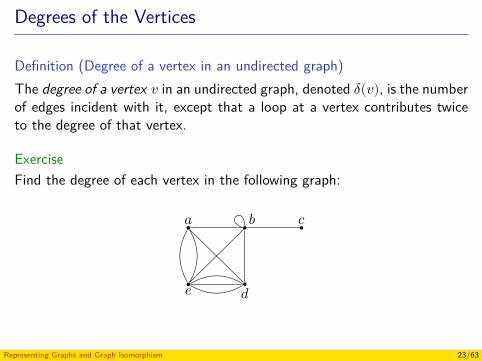
Degrees of the Vertices
Definition (Degree of a vertex in an undirected graph)The degree of a vertex 𝑣 in an undirected graph, denoted 𝛿(𝑣), is the numberof edges incident with it, except that a loop at a vertex contributes twiceto the degree of that vertex.
ExerciseFind the degree of each vertex in the following graph:
𝑎 𝑏 𝑐
𝑑𝑒
Solution: 𝛿(𝑎) = 4, 𝛿(𝑏) = 𝛿(𝑒) = 6, 𝛿(𝑐) = 1 and 𝛿(𝑑) = 5.
Representing Graphs and Graph Isomorphism 23/63
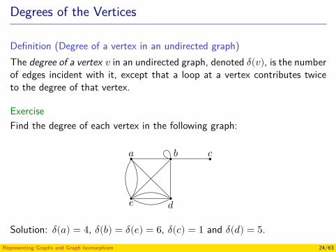
Degrees of the Vertices
Definition (Degree of a vertex in an undirected graph)The degree of a vertex 𝑣 in an undirected graph, denoted 𝛿(𝑣), is the numberof edges incident with it, except that a loop at a vertex contributes twiceto the degree of that vertex.
ExerciseFind the degree of each vertex in the following graph:
𝑎 𝑏 𝑐
𝑑𝑒
Solution: 𝛿(𝑎) = 4, 𝛿(𝑏) = 𝛿(𝑒) = 6, 𝛿(𝑐) = 1 and 𝛿(𝑑) = 5.Representing Graphs and Graph Isomorphism 24/63
Vertex Degrees
Theorem (The handshaking theorem. Rosen (2004), Theorem 1, p. 511)Let 𝐺 = (𝑉 , 𝐸) be an undirected graph with 𝑒 edges, then
2𝑒 = ∑𝑣∈𝑉
𝛿(𝑣).
Proof.Each edge contributes two to the sum of the degrees of the vertices becausean edge is incident with exactly two (possibly equal) vertices. This meansthat the sum of the degrees of the vertices is twice the number of edges.
Representing Graphs and Graph Isomorphism 25/63
Vertex Degrees
Theorem (The handshaking theorem. Rosen (2004), Theorem 1, p. 511)Let 𝐺 = (𝑉 , 𝐸) be an undirected graph with 𝑒 edges, then
2𝑒 = ∑𝑣∈𝑉
𝛿(𝑣).
Proof.Each edge contributes two to the sum of the degrees of the vertices becausean edge is incident with exactly two (possibly equal) vertices. This meansthat the sum of the degrees of the vertices is twice the number of edges.
Representing Graphs and Graph Isomorphism 26/63
Representing Graphs
Adjacency matricesIncidence matrices
Representing Graphs and Graph Isomorphism 27/63
Adjacency Matrices
Definition (Adjacency matrix for simple graphs)Let 𝐺 = (𝑉 , 𝐸) be a simple graph.
The vertices of 𝐺 are listed arbitrarily as 𝑣1, 𝑣2, … , 𝑣𝑛.The adjacency matrix A𝐺 = [𝑎𝑖𝑗] of 𝐺 is a 𝑛 × 𝑛 matrix, where
𝑎𝑖𝑗 = {1 if {𝑣𝑖, 𝑣𝑗} is an edge of 𝐺,0 otherwise.
Remark: The matrix A𝐺 is Boolean, symmetric and it has zeros in thediagonal.
ExamplesWhiteboard.
Representing Graphs and Graph Isomorphism 28/63
Adjacency Matrices
Definition (Adjacency matrix for simple graphs)Let 𝐺 = (𝑉 , 𝐸) be a simple graph.The vertices of 𝐺 are listed arbitrarily as 𝑣1, 𝑣2, … , 𝑣𝑛.
The adjacency matrix A𝐺 = [𝑎𝑖𝑗] of 𝐺 is a 𝑛 × 𝑛 matrix, where
𝑎𝑖𝑗 = {1 if {𝑣𝑖, 𝑣𝑗} is an edge of 𝐺,0 otherwise.
Remark: The matrix A𝐺 is Boolean, symmetric and it has zeros in thediagonal.
ExamplesWhiteboard.
Representing Graphs and Graph Isomorphism 29/63
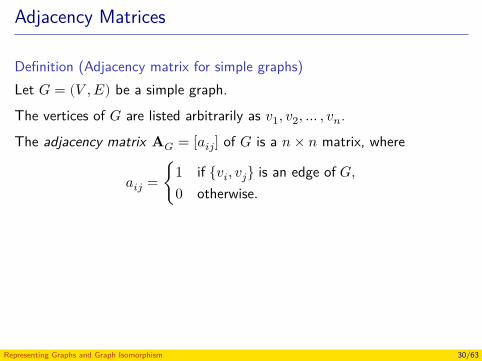
Adjacency Matrices
Definition (Adjacency matrix for simple graphs)Let 𝐺 = (𝑉 , 𝐸) be a simple graph.The vertices of 𝐺 are listed arbitrarily as 𝑣1, 𝑣2, … , 𝑣𝑛.The adjacency matrix A𝐺 = [𝑎𝑖𝑗] of 𝐺 is a 𝑛 × 𝑛 matrix, where
𝑎𝑖𝑗 = {1 if {𝑣𝑖, 𝑣𝑗} is an edge of 𝐺,0 otherwise.
Remark: The matrix A𝐺 is Boolean, symmetric and it has zeros in thediagonal.
ExamplesWhiteboard.
Representing Graphs and Graph Isomorphism 30/63
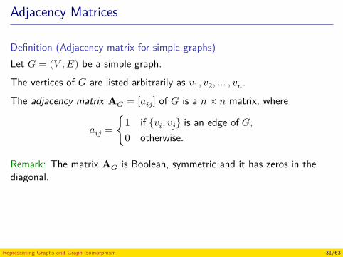
Adjacency Matrices
Definition (Adjacency matrix for simple graphs)Let 𝐺 = (𝑉 , 𝐸) be a simple graph.The vertices of 𝐺 are listed arbitrarily as 𝑣1, 𝑣2, … , 𝑣𝑛.The adjacency matrix A𝐺 = [𝑎𝑖𝑗] of 𝐺 is a 𝑛 × 𝑛 matrix, where
𝑎𝑖𝑗 = {1 if {𝑣𝑖, 𝑣𝑗} is an edge of 𝐺,0 otherwise.
Remark: The matrix A𝐺 is Boolean, symmetric and it has zeros in thediagonal.
ExamplesWhiteboard.
Representing Graphs and Graph Isomorphism 31/63
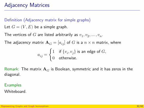
Adjacency Matrices
Definition (Adjacency matrix for simple graphs)Let 𝐺 = (𝑉 , 𝐸) be a simple graph.The vertices of 𝐺 are listed arbitrarily as 𝑣1, 𝑣2, … , 𝑣𝑛.The adjacency matrix A𝐺 = [𝑎𝑖𝑗] of 𝐺 is a 𝑛 × 𝑛 matrix, where
𝑎𝑖𝑗 = {1 if {𝑣𝑖, 𝑣𝑗} is an edge of 𝐺,0 otherwise.
Remark: The matrix A𝐺 is Boolean, symmetric and it has zeros in thediagonal.
ExamplesWhiteboard.
Representing Graphs and Graph Isomorphism 32/63
Adjacency Matrices
Adjacency matrices for undirected graphs with loops and parallel edgesIn this case, the (𝑖, 𝑗)-entry represents the number of edges that are associ-ated to {𝑣𝑖, 𝑣𝑗}.
Remark: The matrix is symmetric.
ExamplesWhiteboard.
Representing Graphs and Graph Isomorphism 33/63
Adjacency Matrices
Adjacency matrices for undirected graphs with loops and parallel edgesIn this case, the (𝑖, 𝑗)-entry represents the number of edges that are associ-ated to {𝑣𝑖, 𝑣𝑗}.
Remark: The matrix is symmetric.
ExamplesWhiteboard.
Representing Graphs and Graph Isomorphism 34/63
Adjacency Matrices
Adjacency matrices for undirected graphs with loops and parallel edgesIn this case, the (𝑖, 𝑗)-entry represents the number of edges that are associ-ated to {𝑣𝑖, 𝑣𝑗}.
Remark: The matrix is symmetric.
ExamplesWhiteboard.
Representing Graphs and Graph Isomorphism 35/63
Adjacency Matrices
Definition (Adjacency matrix for directed graphs)Let 𝐺 = (𝑉 , 𝐸) be a direct graph where the vertices of 𝐺 are listed arbitrarilyas 𝑣1, 𝑣2, … , 𝑣𝑛.
The adjacency matrix A𝐺 is defined by
𝑎𝑖𝑗 = {1 if (𝑣𝑖, 𝑣𝑗) is an edge of 𝐺,0 otherwise.
ExamplesWhiteboard.
Representing Graphs and Graph Isomorphism 36/63
Adjacency Matrices
Definition (Adjacency matrix for directed graphs)Let 𝐺 = (𝑉 , 𝐸) be a direct graph where the vertices of 𝐺 are listed arbitrarilyas 𝑣1, 𝑣2, … , 𝑣𝑛.The adjacency matrix A𝐺 is defined by
𝑎𝑖𝑗 = {1 if (𝑣𝑖, 𝑣𝑗) is an edge of 𝐺,0 otherwise.
ExamplesWhiteboard.
Representing Graphs and Graph Isomorphism 37/63
Adjacency Matrices
Definition (Adjacency matrix for directed graphs)Let 𝐺 = (𝑉 , 𝐸) be a direct graph where the vertices of 𝐺 are listed arbitrarilyas 𝑣1, 𝑣2, … , 𝑣𝑛.The adjacency matrix A𝐺 is defined by
𝑎𝑖𝑗 = {1 if (𝑣𝑖, 𝑣𝑗) is an edge of 𝐺,0 otherwise.
ExamplesWhiteboard.
Representing Graphs and Graph Isomorphism 38/63
Incidence Matrices
Definition (Incidence matrix)Let 𝐺 = (𝑉 , 𝐸) be an undirected graph.
Suppose 𝑣1, 𝑣2, … , 𝑣𝑛 are the vertices and 𝑒1, 𝑒2, … , 𝑒𝑚 are the edges.The incidence matrix M𝐺 = [𝑚𝑖𝑗] of 𝐺 is a 𝑛 × 𝑚 Boolean matrix, where
𝑚𝑖𝑗 = {1 when 𝑒𝑗 is incident with 𝑣𝑖,0 otherwise.
ExamplesWhiteboard.
Representing Graphs and Graph Isomorphism 39/63
Incidence Matrices
Definition (Incidence matrix)Let 𝐺 = (𝑉 , 𝐸) be an undirected graph.Suppose 𝑣1, 𝑣2, … , 𝑣𝑛 are the vertices and 𝑒1, 𝑒2, … , 𝑒𝑚 are the edges.
The incidence matrix M𝐺 = [𝑚𝑖𝑗] of 𝐺 is a 𝑛 × 𝑚 Boolean matrix, where
𝑚𝑖𝑗 = {1 when 𝑒𝑗 is incident with 𝑣𝑖,0 otherwise.
ExamplesWhiteboard.
Representing Graphs and Graph Isomorphism 40/63
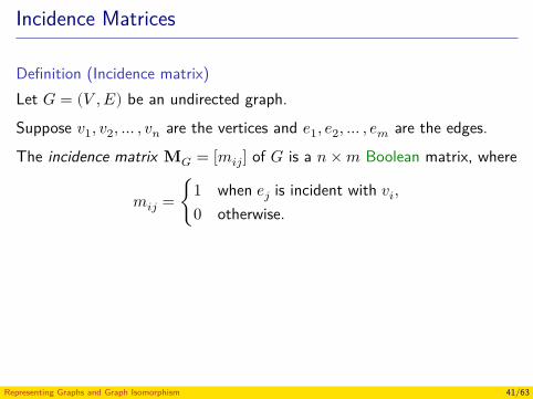
Incidence Matrices
Definition (Incidence matrix)Let 𝐺 = (𝑉 , 𝐸) be an undirected graph.Suppose 𝑣1, 𝑣2, … , 𝑣𝑛 are the vertices and 𝑒1, 𝑒2, … , 𝑒𝑚 are the edges.The incidence matrix M𝐺 = [𝑚𝑖𝑗] of 𝐺 is a 𝑛 × 𝑚 Boolean matrix, where
𝑚𝑖𝑗 = {1 when 𝑒𝑗 is incident with 𝑣𝑖,0 otherwise.
ExamplesWhiteboard.
Representing Graphs and Graph Isomorphism 41/63
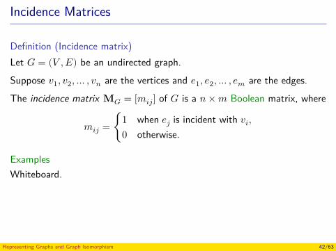
Incidence Matrices
Definition (Incidence matrix)Let 𝐺 = (𝑉 , 𝐸) be an undirected graph.Suppose 𝑣1, 𝑣2, … , 𝑣𝑛 are the vertices and 𝑒1, 𝑒2, … , 𝑒𝑚 are the edges.The incidence matrix M𝐺 = [𝑚𝑖𝑗] of 𝐺 is a 𝑛 × 𝑚 Boolean matrix, where
𝑚𝑖𝑗 = {1 when 𝑒𝑗 is incident with 𝑣𝑖,0 otherwise.
ExamplesWhiteboard.
Representing Graphs and Graph Isomorphism 42/63
Isomorphism of Graphs
Definition (Isomorphic simple graphs)The simple graphs 𝐺1 = (𝑉1, 𝐸1) and 𝐺2 = (𝑉2, 𝐸2) are isomorphic if thereexists a bijective function 𝑓 from 𝑉1 to 𝑉2 with the property that 𝑢 and 𝑣are adjacent in 𝐺1, if and only if, 𝑓(𝑢) and 𝑓(𝑣) are adjacent in 𝐺2, forall 𝑢 and 𝑣 in 𝑉1.
Representing Graphs and Graph Isomorphism 43/63
Isomorphism of Graphs
Definition (Isomorphic simple graphs)The simple graphs 𝐺1 = (𝑉1, 𝐸1) and 𝐺2 = (𝑉2, 𝐸2) are isomorphic if thereexists a bijective function 𝑓 from 𝑉1 to 𝑉2 with the property that 𝑢 and 𝑣are adjacent in 𝐺1, if and only if, 𝑓(𝑢) and 𝑓(𝑣) are adjacent in 𝐺2, forall 𝑢 and 𝑣 in 𝑉1.
Representing Graphs and Graph Isomorphism 44/63
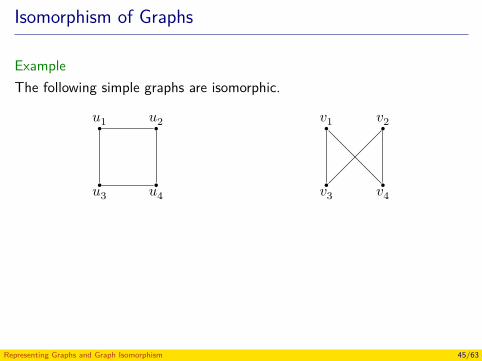
Isomorphism of Graphs
ExampleThe following simple graphs are isomorphic.
𝑢1 𝑢2
𝑢3 𝑢4
𝑣1 𝑣2
𝑣3 𝑣4
The bijective function 𝑓 preserves adjacency.
𝑓 ∶ {𝑢1, 𝑢2, 𝑢3, 𝑢4} → {𝑣1, 𝑣2, 𝑣3, 𝑣4}𝑓(𝑢1) = 𝑣1, 𝑓(𝑢2) = 𝑣4, 𝑓(𝑢3) = 𝑣3 and 𝑓(𝑢4) = 𝑣2.
Representing Graphs and Graph Isomorphism 45/63
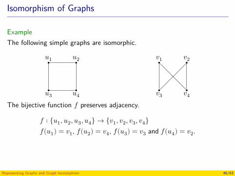
Isomorphism of Graphs
ExampleThe following simple graphs are isomorphic.
𝑢1 𝑢2
𝑢3 𝑢4
𝑣1 𝑣2
𝑣3 𝑣4
The bijective function 𝑓 preserves adjacency.
𝑓 ∶ {𝑢1, 𝑢2, 𝑢3, 𝑢4} → {𝑣1, 𝑣2, 𝑣3, 𝑣4}𝑓(𝑢1) = 𝑣1, 𝑓(𝑢2) = 𝑣4, 𝑓(𝑢3) = 𝑣3 and 𝑓(𝑢4) = 𝑣2.
Representing Graphs and Graph Isomorphism 46/63
Isomorphism of Graphs
Remark: Determining whether two simple graphs are isomorphic is oftendifficult because if |𝐴| = |𝐵| = 𝑛 then
|{𝑓 ∶ 𝐴 → 𝐵 ∣ 𝑓 is a bijection}| = 𝑛!.
Definition (Graph invariant property)A property preserved by isomorphism of graphs is called a graph invariantproperty.
ExamplesThe number of vertices, the number of edges and the degrees of the verticesare graph invariant properties.
Representing Graphs and Graph Isomorphism 47/63
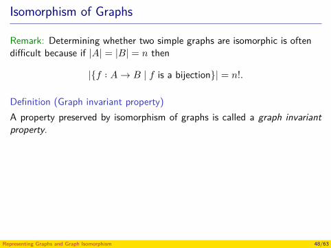
Isomorphism of Graphs
Remark: Determining whether two simple graphs are isomorphic is oftendifficult because if |𝐴| = |𝐵| = 𝑛 then
|{𝑓 ∶ 𝐴 → 𝐵 ∣ 𝑓 is a bijection}| = 𝑛!.
Definition (Graph invariant property)A property preserved by isomorphism of graphs is called a graph invariantproperty.
ExamplesThe number of vertices, the number of edges and the degrees of the verticesare graph invariant properties.
Representing Graphs and Graph Isomorphism 48/63
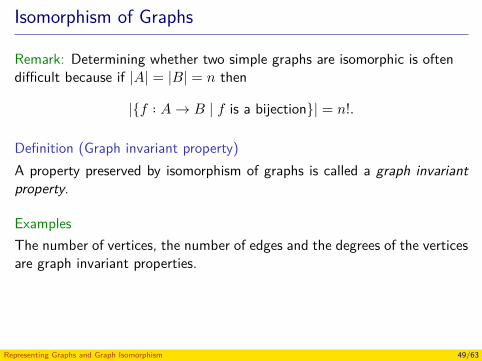
Isomorphism of Graphs
Remark: Determining whether two simple graphs are isomorphic is oftendifficult because if |𝐴| = |𝐵| = 𝑛 then
|{𝑓 ∶ 𝐴 → 𝐵 ∣ 𝑓 is a bijection}| = 𝑛!.
Definition (Graph invariant property)A property preserved by isomorphism of graphs is called a graph invariantproperty.
ExamplesThe number of vertices, the number of edges and the degrees of the verticesare graph invariant properties.
Representing Graphs and Graph Isomorphism 49/63
Isomorphism of Graphs
Remark: We can prove that two graphs are not isomorphic if we can find agraph invariant property that only one of the two graphs has.
ExampleAre the following graphs isomorphic?
𝑎
𝑏
𝑐
𝑑𝑒𝐺
𝑎
𝑏
𝑐
𝑑𝑒𝐻
No. The graph 𝐻 has a vertice of degree 1 but the graph 𝐺 have novertices of degree 1.
Representing Graphs and Graph Isomorphism 50/63
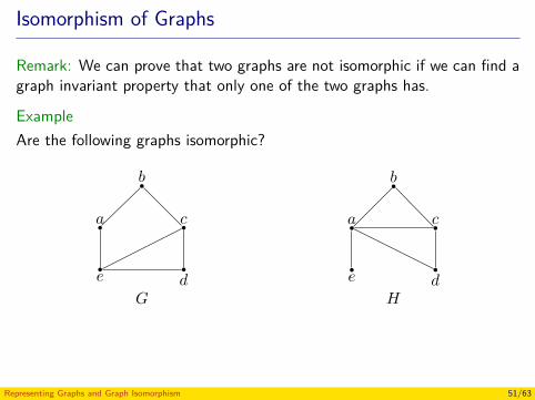
Isomorphism of Graphs
Remark: We can prove that two graphs are not isomorphic if we can find agraph invariant property that only one of the two graphs has.
ExampleAre the following graphs isomorphic?
𝑎
𝑏
𝑐
𝑑𝑒𝐺
𝑎
𝑏
𝑐
𝑑𝑒𝐻
No. The graph 𝐻 has a vertice of degree 1 but the graph 𝐺 have novertices of degree 1.
Representing Graphs and Graph Isomorphism 51/63
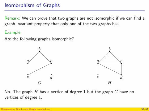
Isomorphism of Graphs
Remark: We can prove that two graphs are not isomorphic if we can find agraph invariant property that only one of the two graphs has.
ExampleAre the following graphs isomorphic?
𝑎
𝑏
𝑐
𝑑𝑒𝐺
𝑎
𝑏
𝑐
𝑑𝑒𝐻
No. The graph 𝐻 has a vertice of degree 1 but the graph 𝐺 have novertices of degree 1.
Representing Graphs and Graph Isomorphism 52/63
Isomorphism of Graphs
Definition (Complementary graph)The complementary graph 𝐺 of a simple graph 𝐺 has the same verticesas 𝐺. Two (different) vertices are adjacent in 𝐺 if and only if they are notadjacent in 𝐺.
ExamplesWhiteboard.
Representing Graphs and Graph Isomorphism 53/63
Isomorphism of Graphs
Definition (Self-complementary graph)A simple graph 𝐺 is called self-complementary if 𝐺 and 𝐺 are isomorphic.
Exercise (Rosen (2004), Problem 50, p. 529)Is the given graphself-complementary?
𝑎 𝑏
𝑑 𝑐
Yes! The complementary graph is given by thefigure.
𝑐 𝑑
𝑎 𝑏
The isomorphism is 𝑓(𝑎) = 𝑐, 𝑓(𝑏) = 𝑑,𝑓(𝑐) = 𝑏 and 𝑓(𝑑) = 𝑎.
Representing Graphs and Graph Isomorphism 54/63
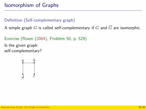
Isomorphism of Graphs
Definition (Self-complementary graph)A simple graph 𝐺 is called self-complementary if 𝐺 and 𝐺 are isomorphic.
Exercise (Rosen (2004), Problem 50, p. 529)Is the given graphself-complementary?
𝑎 𝑏
𝑑 𝑐
Yes! The complementary graph is given by thefigure.
𝑐 𝑑
𝑎 𝑏
The isomorphism is 𝑓(𝑎) = 𝑐, 𝑓(𝑏) = 𝑑,𝑓(𝑐) = 𝑏 and 𝑓(𝑑) = 𝑎.
Representing Graphs and Graph Isomorphism 55/63
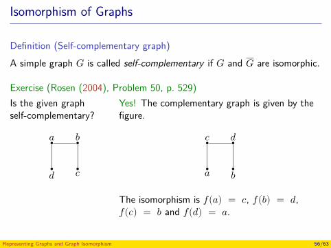
Isomorphism of Graphs
Definition (Self-complementary graph)A simple graph 𝐺 is called self-complementary if 𝐺 and 𝐺 are isomorphic.
Exercise (Rosen (2004), Problem 50, p. 529)Is the given graphself-complementary?
𝑎 𝑏
𝑑 𝑐
Yes! The complementary graph is given by thefigure.
𝑐 𝑑
𝑎 𝑏
The isomorphism is 𝑓(𝑎) = 𝑐, 𝑓(𝑏) = 𝑑,𝑓(𝑐) = 𝑏 and 𝑓(𝑑) = 𝑎.
Representing Graphs and Graph Isomorphism 56/63
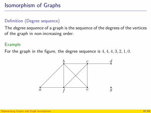
Isomorphism of Graphs
Definition (Degree sequence)The degree sequence of a graph is the sequence of the degrees of the verticesof the graph in non-increasing order.
ExampleFor the graph in the figure, the degree sequence is 4, 4, 4, 3, 2, 1, 0.
𝑎 𝑓
𝑏
𝑒
𝑐
𝑔
𝑑
Representing Graphs and Graph Isomorphism 57/63
Isomorphism of Graphs
Exercise (Rosen (2004), Problem 69, p. 530)A counter-example for a purported isomorphism test is a pair of non-isomorphic graphs that the test fails to show that they are not isomorphic.Find a counter-example for the test that checks the degree sequence in twographs to make sure they agree.
Representing Graphs and Graph Isomorphism 58/63
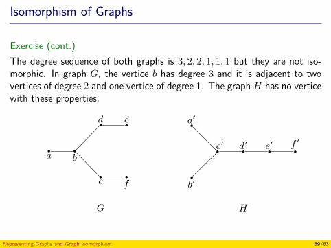
Isomorphism of Graphs
Exercise (cont.)The degree sequence of both graphs is 3, 2, 2, 1, 1, 1 but they are not iso-morphic. In graph 𝐺, the vertice 𝑏 has degree 3 and it is adjacent to twovertices of degree 2 and one vertice of degree 1. The graph 𝐻 has no verticewith these properties.
𝑎 𝑏
𝑑 𝑐
𝑐 𝑓
𝐺
𝑎′
𝑏′
𝑐′ 𝑑′ 𝑒′ 𝑓 ′
𝐻
Representing Graphs and Graph Isomorphism 59/63
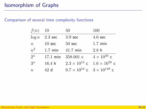
Isomorphism of Graphs
Comparison of several time complexity functions
𝑓(𝑛) 10 50 100log 𝑛 2.3 sec 3.9 sec 4.6 sec𝑛 10 sec 50 sec 1.7 min𝑛2 1.7 min 41.7 min 2.8 h2𝑛 17.1 min 358.001 c 4 × 10²⁰ c3𝑛 16.4 h 2.3 × 10¹⁴ c 1.6 × 1038 c𝑛 42 d 9.7 × 1054 c 3 × 10148 c
Representing Graphs and Graph Isomorphism 60/63
Isomorphism of Graphs
Algorithms for graph isomorphismThe best algorithm known has time complexity of 2𝑂(√𝑛 log 𝑛), where 𝑛 isthe number of vertices (Johnson 2005).
10 100 1000 100002
√𝑛 log 𝑛 27.8 sec 33.4 d 3.3 × 10¹⁵ c 7.3 × 1081 c
Representing Graphs and Graph Isomorphism 61/63
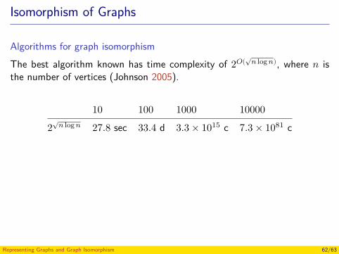
Isomorphism of Graphs
Algorithms for graph isomorphismThe best algorithm known has time complexity of 2𝑂(√𝑛 log 𝑛), where 𝑛 isthe number of vertices (Johnson 2005).
10 100 1000 100002
√𝑛 log 𝑛 27.8 sec 33.4 d 3.3 × 10¹⁵ c 7.3 × 1081 c
Representing Graphs and Graph Isomorphism 62/63
References
Johnson, D. S. (2005). The NP-Completeness Column. ACM Transactionson Algorithms 1.1, pp. 160–176. doi: 10.1145/1077464.1077476 (cit. onpp. 61, 62).Rosen, K. H. (2004). Matemática Discreta y sus Aplicaciones. 5th ed.McGraw-Hill (cit. on pp. 25, 26, 54–56, 58).
Representing Graphs and Graph Isomorphism 63/63
Discrete Structures - CM0246Euler and Hamilton Paths
Andrés Sicard-Ramírez
Universidad EAFIT
Semester 2014-2
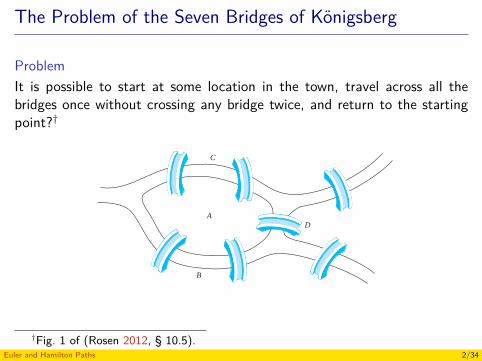
The Problem of the Seven Bridges of Königsberg
ProblemIt is possible to start at some location in the town, travel across all thebridges once without crossing any bridge twice, and return to the startingpoint?†
10.5 Euler and Hamilton Paths 693
∗65. Use a graph model and a path in your graph, as in Exer-cise 64, to solve the jealous husbands problem. Twomarried couples, each a husband and a wife, want tocross a river. They can only use a boat that can carryone or two people from one shore to the other shore.Each husband is extremely jealous and is not willingto leave his wife with the other husband, either in theboat or on shore. How can these four people reach theopposite shore?
66. Suppose that you have a three-gallon jug and a five-gallonjug. You may fill either jug with water, you may emptyeither jug, and you may transfer water from either juginto the other jug. Use a path in a directed graph toshow that you can end up with a jug containing exactlyone gallon. [Hint: Use an ordered pair (a, b) to indicatehow much water is in each jug. Represent these orderedpairs by vertices. Add an edge for each allowable opera-tion with the jugs.]
10.5 Euler and Hamilton Paths
Introduction
Can we travel along the edges of a graph starting at a vertex and returning to it by traversingeach edge of the graph exactly once? Similarly, can we travel along the edges of a graph startingat a vertex and returning to it while visiting each vertex of the graph exactly once? Althoughthese questions seem to be similar, the first question, which asks whether a graph has an Eulercircuit, can be easily answered simply by examining the degrees of the vertices of the graph,while the second question, which asks whether a graph has a Hamilton circuit, is quite difficultto solve for most graphs. In this section we will study these questions and discuss the difficultyof solving them. Although both questions have many practical applications in many differentareas, both arose in old puzzles. We will learn about these old puzzles as well as modernpractical applications.
Euler Paths and Circuits
The town of Königsberg, Prussia (now called Kaliningrad and part of the Russian republic),was divided into four sections by the branches of the Pregel River. These four sections includedthe two regions on the banks of the Pregel, Kneiphof Island, and the region between the twobranches of the Pregel. In the eighteenth century seven bridges connected these regions. Figure 1depicts these regions and bridges.
Only five bridges connectKaliningrad today. Ofthese, just two remainfrom Euler’s day.
The townspeople took long walks through town on Sundays. They wondered whether it waspossible to start at some location in the town, travel across all the bridges once without crossingany bridge twice, and return to the starting point.
The Swiss mathematician Leonhard Euler solved this problem. His solution, publishedin 1736, may be the first use of graph theory. (For a translation of Euler’s original paper see[BiLlWi99].) Euler studied this problem using the multigraph obtained when the four regionsare represented by vertices and the bridges by edges. This multigraph is shown in Figure 2.
C
A
B
D
FIGURE 1 The Seven Bridges of Königsberg.
A
C
B
D
FIGURE 2 Multigraph Modelof the Town of Königsberg.
†Fig. 1 of (Rosen 2012, § 10.5).Euler and Hamilton Paths 2/34
Paths
Definition (Path)Let 𝑛 be a non-negative integer and 𝐺 an undirected graph. A path oflength 𝑛 from 𝑢 to 𝑣 in 𝐺 is a sequence of 𝑛 edges 𝑒1, 𝑒2, … , 𝑒𝑛 of 𝐺 suchthat 𝑓(𝑒1) = {𝑥0, 𝑥1}, 𝑓(𝑒2) = {𝑥1, 𝑥2}, …, 𝑓(𝑒𝑛) = {𝑥𝑛−1, 𝑥𝑛}, where𝑥0 = 𝑢 and 𝑥𝑛 = 𝑣.
ExamplesWhiteboard.
Euler and Hamilton Paths 3/34
Paths
Definition (Circuit)A path is a circuit if 𝑢 = 𝑣 (it begins and ends at the same vertex) and haslength greater than zero.
ExamplesWhiteboard.
Definition (Simple path/circuit)A path/circuit is simple if it does not contain the same edge more thanonce.
ExamplesWhiteboard.
Euler and Hamilton Paths 4/34
Paths
Definition (Circuit)A path is a circuit if 𝑢 = 𝑣 (it begins and ends at the same vertex) and haslength greater than zero.
ExamplesWhiteboard.
Definition (Simple path/circuit)A path/circuit is simple if it does not contain the same edge more thanonce.
ExamplesWhiteboard.
Euler and Hamilton Paths 5/34
Connectedness
Definition (Connected undirected graph)An undirected graph is called connected (conexo) if there is a path betweenevery pair of distinct vertices of the graph.
ExamplesWhiteboard.
Euler and Hamilton Paths 6/34
Connectedness
Definition (Connected undirected graph)An undirected graph is called connected (conexo) if there is a path betweenevery pair of distinct vertices of the graph.
ExamplesWhiteboard.
Euler and Hamilton Paths 7/34
Euler Paths
Definition (Euler path)An Euler path in a graph 𝐺 is a simple path containing every edge of 𝐺.
ExerciseFind an Euler path in the following graph:
𝑎 𝑏
𝑐 𝑑 𝑒
An Euler path is 𝑎, 𝑐, 𝑑, 𝑒, 𝑏, 𝑑, 𝑎, 𝑏.
Euler and Hamilton Paths 8/34
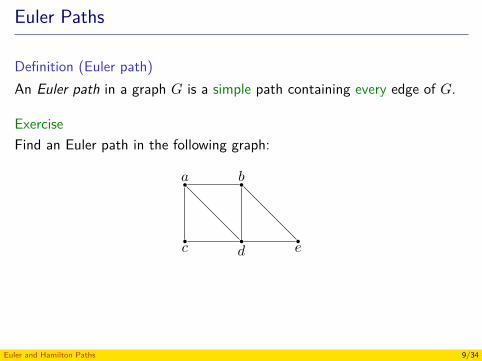
Euler Paths
Definition (Euler path)An Euler path in a graph 𝐺 is a simple path containing every edge of 𝐺.
ExerciseFind an Euler path in the following graph:
𝑎 𝑏
𝑐 𝑑 𝑒
An Euler path is 𝑎, 𝑐, 𝑑, 𝑒, 𝑏, 𝑑, 𝑎, 𝑏.
Euler and Hamilton Paths 9/34
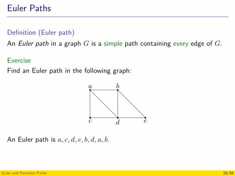
Euler Paths
Definition (Euler path)An Euler path in a graph 𝐺 is a simple path containing every edge of 𝐺.
ExerciseFind an Euler path in the following graph:
𝑎 𝑏
𝑐 𝑑 𝑒
An Euler path is 𝑎, 𝑐, 𝑑, 𝑒, 𝑏, 𝑑, 𝑎, 𝑏.
Euler and Hamilton Paths 10/34
Euler Circuits
Definition (Euler circuit)An Euler circuit in a graph 𝐺 is a simple circuit containing every edge of 𝐺.
ExerciseFind an Euler circuit in the following graph:
𝑎 𝑏
𝑒
𝑑 𝑐
An Euler circuit is 𝑎, 𝑒, 𝑐, 𝑑, 𝑒, 𝑏, 𝑎.
Euler and Hamilton Paths 11/34
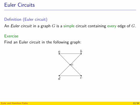
Euler Circuits
Definition (Euler circuit)An Euler circuit in a graph 𝐺 is a simple circuit containing every edge of 𝐺.
ExerciseFind an Euler circuit in the following graph:
𝑎 𝑏
𝑒
𝑑 𝑐
An Euler circuit is 𝑎, 𝑒, 𝑐, 𝑑, 𝑒, 𝑏, 𝑎.
Euler and Hamilton Paths 12/34
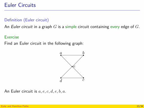
Euler Circuits
Definition (Euler circuit)An Euler circuit in a graph 𝐺 is a simple circuit containing every edge of 𝐺.
ExerciseFind an Euler circuit in the following graph:
𝑎 𝑏
𝑒
𝑑 𝑐
An Euler circuit is 𝑎, 𝑒, 𝑐, 𝑑, 𝑒, 𝑏, 𝑎.
Euler and Hamilton Paths 13/34
Euler Paths and Circuits
Theorem (Rosen (2004), Theorem 1, p. 543)A connected multigraph with at least two vertices has an Euler circuit, ifand only if, each of its vertices has even degree.
Euler and Hamilton Paths 14/34
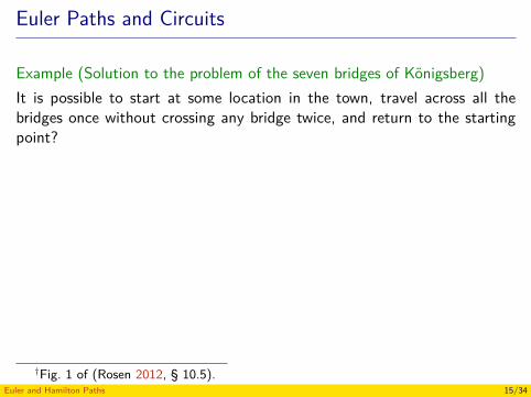
Euler Paths and Circuits
Example (Solution to the problem of the seven bridges of Königsberg)It is possible to start at some location in the town, travel across all thebridges once without crossing any bridge twice, and return to the startingpoint?
No, it is not possible, because the multigraph representing the bridges has(four) vertices of odd degree.†
10.5 Euler and Hamilton Paths 693
∗65. Use a graph model and a path in your graph, as in Exer-cise 64, to solve the jealous husbands problem. Twomarried couples, each a husband and a wife, want tocross a river. They can only use a boat that can carryone or two people from one shore to the other shore.Each husband is extremely jealous and is not willingto leave his wife with the other husband, either in theboat or on shore. How can these four people reach theopposite shore?
66. Suppose that you have a three-gallon jug and a five-gallonjug. You may fill either jug with water, you may emptyeither jug, and you may transfer water from either juginto the other jug. Use a path in a directed graph toshow that you can end up with a jug containing exactlyone gallon. [Hint: Use an ordered pair (a, b) to indicatehow much water is in each jug. Represent these orderedpairs by vertices. Add an edge for each allowable opera-tion with the jugs.]
10.5 Euler and Hamilton Paths
Introduction
Can we travel along the edges of a graph starting at a vertex and returning to it by traversingeach edge of the graph exactly once? Similarly, can we travel along the edges of a graph startingat a vertex and returning to it while visiting each vertex of the graph exactly once? Althoughthese questions seem to be similar, the first question, which asks whether a graph has an Eulercircuit, can be easily answered simply by examining the degrees of the vertices of the graph,while the second question, which asks whether a graph has a Hamilton circuit, is quite difficultto solve for most graphs. In this section we will study these questions and discuss the difficultyof solving them. Although both questions have many practical applications in many differentareas, both arose in old puzzles. We will learn about these old puzzles as well as modernpractical applications.
Euler Paths and Circuits
The town of Königsberg, Prussia (now called Kaliningrad and part of the Russian republic),was divided into four sections by the branches of the Pregel River. These four sections includedthe two regions on the banks of the Pregel, Kneiphof Island, and the region between the twobranches of the Pregel. In the eighteenth century seven bridges connected these regions. Figure 1depicts these regions and bridges.
Only five bridges connectKaliningrad today. Ofthese, just two remainfrom Euler’s day.
The townspeople took long walks through town on Sundays. They wondered whether it waspossible to start at some location in the town, travel across all the bridges once without crossingany bridge twice, and return to the starting point.
The Swiss mathematician Leonhard Euler solved this problem. His solution, publishedin 1736, may be the first use of graph theory. (For a translation of Euler’s original paper see[BiLlWi99].) Euler studied this problem using the multigraph obtained when the four regionsare represented by vertices and the bridges by edges. This multigraph is shown in Figure 2.
C
A
B
D
FIGURE 1 The Seven Bridges of Königsberg.
A
C
B
D
FIGURE 2 Multigraph Modelof the Town of Königsberg.
𝐶
𝐴
𝐵
𝐷
†Fig. 1 of (Rosen 2012, § 10.5).Euler and Hamilton Paths 15/34
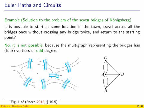
Euler Paths and Circuits
Example (Solution to the problem of the seven bridges of Königsberg)It is possible to start at some location in the town, travel across all thebridges once without crossing any bridge twice, and return to the startingpoint?No, it is not possible, because the multigraph representing the bridges has(four) vertices of odd degree.†
10.5 Euler and Hamilton Paths 693
∗65. Use a graph model and a path in your graph, as in Exer-cise 64, to solve the jealous husbands problem. Twomarried couples, each a husband and a wife, want tocross a river. They can only use a boat that can carryone or two people from one shore to the other shore.Each husband is extremely jealous and is not willingto leave his wife with the other husband, either in theboat or on shore. How can these four people reach theopposite shore?
66. Suppose that you have a three-gallon jug and a five-gallonjug. You may fill either jug with water, you may emptyeither jug, and you may transfer water from either juginto the other jug. Use a path in a directed graph toshow that you can end up with a jug containing exactlyone gallon. [Hint: Use an ordered pair (a, b) to indicatehow much water is in each jug. Represent these orderedpairs by vertices. Add an edge for each allowable opera-tion with the jugs.]
10.5 Euler and Hamilton Paths
Introduction
Can we travel along the edges of a graph starting at a vertex and returning to it by traversingeach edge of the graph exactly once? Similarly, can we travel along the edges of a graph startingat a vertex and returning to it while visiting each vertex of the graph exactly once? Althoughthese questions seem to be similar, the first question, which asks whether a graph has an Eulercircuit, can be easily answered simply by examining the degrees of the vertices of the graph,while the second question, which asks whether a graph has a Hamilton circuit, is quite difficultto solve for most graphs. In this section we will study these questions and discuss the difficultyof solving them. Although both questions have many practical applications in many differentareas, both arose in old puzzles. We will learn about these old puzzles as well as modernpractical applications.
Euler Paths and Circuits
The town of Königsberg, Prussia (now called Kaliningrad and part of the Russian republic),was divided into four sections by the branches of the Pregel River. These four sections includedthe two regions on the banks of the Pregel, Kneiphof Island, and the region between the twobranches of the Pregel. In the eighteenth century seven bridges connected these regions. Figure 1depicts these regions and bridges.
Only five bridges connectKaliningrad today. Ofthese, just two remainfrom Euler’s day.
The townspeople took long walks through town on Sundays. They wondered whether it waspossible to start at some location in the town, travel across all the bridges once without crossingany bridge twice, and return to the starting point.
The Swiss mathematician Leonhard Euler solved this problem. His solution, publishedin 1736, may be the first use of graph theory. (For a translation of Euler’s original paper see[BiLlWi99].) Euler studied this problem using the multigraph obtained when the four regionsare represented by vertices and the bridges by edges. This multigraph is shown in Figure 2.
C
A
B
D
FIGURE 1 The Seven Bridges of Königsberg.
A
C
B
D
FIGURE 2 Multigraph Modelof the Town of Königsberg.
𝐶
𝐴
𝐵
𝐷
†Fig. 1 of (Rosen 2012, § 10.5).Euler and Hamilton Paths 16/34
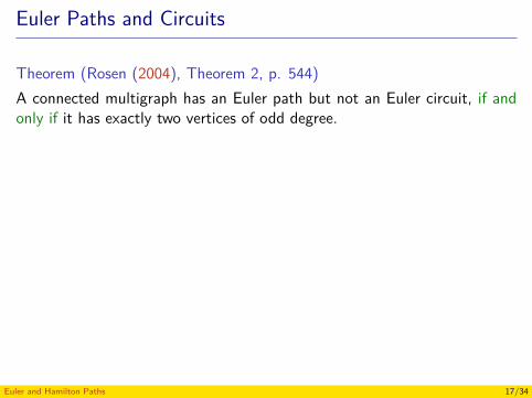
Euler Paths and Circuits
Theorem (Rosen (2004), Theorem 2, p. 544)A connected multigraph has an Euler path but not an Euler circuit, if andonly if it has exactly two vertices of odd degree.
ExerciseHas the following graph an Euler path? If so, find it.
𝑎
𝑏 𝑐 𝑑
𝑔 𝑓 𝑒
The only vertices with degree odd are 𝑏 and 𝑑, so the graph has an Eulerpath. An Euler path is: 𝑏, 𝑎, 𝑔, 𝑓, 𝑒, 𝑑, 𝑐, 𝑔, 𝑏, 𝑐, 𝑓, 𝑑.
Euler and Hamilton Paths 17/34
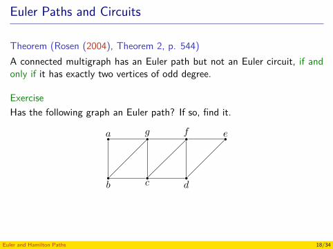
Euler Paths and Circuits
Theorem (Rosen (2004), Theorem 2, p. 544)A connected multigraph has an Euler path but not an Euler circuit, if andonly if it has exactly two vertices of odd degree.
ExerciseHas the following graph an Euler path? If so, find it.
𝑎
𝑏 𝑐 𝑑
𝑔 𝑓 𝑒
The only vertices with degree odd are 𝑏 and 𝑑, so the graph has an Eulerpath. An Euler path is: 𝑏, 𝑎, 𝑔, 𝑓, 𝑒, 𝑑, 𝑐, 𝑔, 𝑏, 𝑐, 𝑓, 𝑑.
Euler and Hamilton Paths 18/34
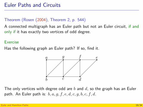
Euler Paths and Circuits
Theorem (Rosen (2004), Theorem 2, p. 544)A connected multigraph has an Euler path but not an Euler circuit, if andonly if it has exactly two vertices of odd degree.
ExerciseHas the following graph an Euler path? If so, find it.
𝑎
𝑏 𝑐 𝑑
𝑔 𝑓 𝑒
The only vertices with degree odd are 𝑏 and 𝑑, so the graph has an Eulerpath. An Euler path is: 𝑏, 𝑎, 𝑔, 𝑓, 𝑒, 𝑑, 𝑐, 𝑔, 𝑏, 𝑐, 𝑓, 𝑑.
Euler and Hamilton Paths 19/34
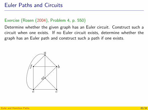
Euler Paths and Circuits
Exercise (Rosen (2004), Problem 4, p. 550)Determine whether the given graph has an Euler circuit. Construct such acircuit when one exists. If no Euler circuit exists, determine whether thegraph has an Euler path and construct such a path if one exists.
𝑎
𝑓 𝑏
𝑑
𝑒 𝑐
The graph has no an Eulercircuit because it has at least avertice of odd degree(𝛿(𝑓) = 3).The graph has an Euler pathbecause the only two vertices ofodd degree are 𝑓 and 𝑐.Euler path:𝑓, 𝑎, 𝑒, 𝑓, 𝑏, 𝑎, 𝑑, 𝑒, 𝑐, 𝑑, 𝑏, 𝑐.
Euler and Hamilton Paths 20/34
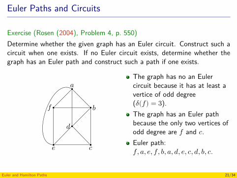
Euler Paths and Circuits
Exercise (Rosen (2004), Problem 4, p. 550)Determine whether the given graph has an Euler circuit. Construct such acircuit when one exists. If no Euler circuit exists, determine whether thegraph has an Euler path and construct such a path if one exists.
𝑎
𝑓 𝑏
𝑑
𝑒 𝑐
The graph has no an Eulercircuit because it has at least avertice of odd degree(𝛿(𝑓) = 3).The graph has an Euler pathbecause the only two vertices ofodd degree are 𝑓 and 𝑐.Euler path:𝑓, 𝑎, 𝑒, 𝑓, 𝑏, 𝑎, 𝑑, 𝑒, 𝑐, 𝑑, 𝑏, 𝑐.
Euler and Hamilton Paths 21/34
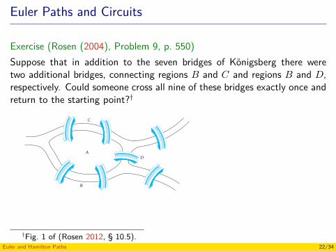
Euler Paths and Circuits
Exercise (Rosen (2004), Problem 9, p. 550)Suppose that in addition to the seven bridges of Königsberg there weretwo additional bridges, connecting regions 𝐵 and 𝐶 and regions 𝐵 and 𝐷,respectively. Could someone cross all nine of these bridges exactly once andreturn to the starting point?†
10.5 Euler and Hamilton Paths 693
∗65. Use a graph model and a path in your graph, as in Exer-cise 64, to solve the jealous husbands problem. Twomarried couples, each a husband and a wife, want tocross a river. They can only use a boat that can carryone or two people from one shore to the other shore.Each husband is extremely jealous and is not willingto leave his wife with the other husband, either in theboat or on shore. How can these four people reach theopposite shore?
66. Suppose that you have a three-gallon jug and a five-gallonjug. You may fill either jug with water, you may emptyeither jug, and you may transfer water from either juginto the other jug. Use a path in a directed graph toshow that you can end up with a jug containing exactlyone gallon. [Hint: Use an ordered pair (a, b) to indicatehow much water is in each jug. Represent these orderedpairs by vertices. Add an edge for each allowable opera-tion with the jugs.]
10.5 Euler and Hamilton Paths
Introduction
Can we travel along the edges of a graph starting at a vertex and returning to it by traversingeach edge of the graph exactly once? Similarly, can we travel along the edges of a graph startingat a vertex and returning to it while visiting each vertex of the graph exactly once? Althoughthese questions seem to be similar, the first question, which asks whether a graph has an Eulercircuit, can be easily answered simply by examining the degrees of the vertices of the graph,while the second question, which asks whether a graph has a Hamilton circuit, is quite difficultto solve for most graphs. In this section we will study these questions and discuss the difficultyof solving them. Although both questions have many practical applications in many differentareas, both arose in old puzzles. We will learn about these old puzzles as well as modernpractical applications.
Euler Paths and Circuits
The town of Königsberg, Prussia (now called Kaliningrad and part of the Russian republic),was divided into four sections by the branches of the Pregel River. These four sections includedthe two regions on the banks of the Pregel, Kneiphof Island, and the region between the twobranches of the Pregel. In the eighteenth century seven bridges connected these regions. Figure 1depicts these regions and bridges.
Only five bridges connectKaliningrad today. Ofthese, just two remainfrom Euler’s day.
The townspeople took long walks through town on Sundays. They wondered whether it waspossible to start at some location in the town, travel across all the bridges once without crossingany bridge twice, and return to the starting point.
The Swiss mathematician Leonhard Euler solved this problem. His solution, publishedin 1736, may be the first use of graph theory. (For a translation of Euler’s original paper see[BiLlWi99].) Euler studied this problem using the multigraph obtained when the four regionsare represented by vertices and the bridges by edges. This multigraph is shown in Figure 2.
C
A
B
D
FIGURE 1 The Seven Bridges of Königsberg.
A
C
B
D
FIGURE 2 Multigraph Modelof the Town of Königsberg.
𝐶
𝐴
𝐵
𝐷
The problem asks for building an Euler circuit. It it not possible because thegraph representing the problem has vertices of odd degree (e.g. 𝛿(𝐴) = 5).
†Fig. 1 of (Rosen 2012, § 10.5).Euler and Hamilton Paths 22/34
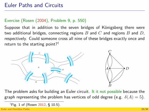
Euler Paths and Circuits
Exercise (Rosen (2004), Problem 9, p. 550)Suppose that in addition to the seven bridges of Königsberg there weretwo additional bridges, connecting regions 𝐵 and 𝐶 and regions 𝐵 and 𝐷,respectively. Could someone cross all nine of these bridges exactly once andreturn to the starting point?†
10.5 Euler and Hamilton Paths 693
∗65. Use a graph model and a path in your graph, as in Exer-cise 64, to solve the jealous husbands problem. Twomarried couples, each a husband and a wife, want tocross a river. They can only use a boat that can carryone or two people from one shore to the other shore.Each husband is extremely jealous and is not willingto leave his wife with the other husband, either in theboat or on shore. How can these four people reach theopposite shore?
66. Suppose that you have a three-gallon jug and a five-gallonjug. You may fill either jug with water, you may emptyeither jug, and you may transfer water from either juginto the other jug. Use a path in a directed graph toshow that you can end up with a jug containing exactlyone gallon. [Hint: Use an ordered pair (a, b) to indicatehow much water is in each jug. Represent these orderedpairs by vertices. Add an edge for each allowable opera-tion with the jugs.]
10.5 Euler and Hamilton Paths
Introduction
Can we travel along the edges of a graph starting at a vertex and returning to it by traversingeach edge of the graph exactly once? Similarly, can we travel along the edges of a graph startingat a vertex and returning to it while visiting each vertex of the graph exactly once? Althoughthese questions seem to be similar, the first question, which asks whether a graph has an Eulercircuit, can be easily answered simply by examining the degrees of the vertices of the graph,while the second question, which asks whether a graph has a Hamilton circuit, is quite difficultto solve for most graphs. In this section we will study these questions and discuss the difficultyof solving them. Although both questions have many practical applications in many differentareas, both arose in old puzzles. We will learn about these old puzzles as well as modernpractical applications.
Euler Paths and Circuits
The town of Königsberg, Prussia (now called Kaliningrad and part of the Russian republic),was divided into four sections by the branches of the Pregel River. These four sections includedthe two regions on the banks of the Pregel, Kneiphof Island, and the region between the twobranches of the Pregel. In the eighteenth century seven bridges connected these regions. Figure 1depicts these regions and bridges.
Only five bridges connectKaliningrad today. Ofthese, just two remainfrom Euler’s day.
The townspeople took long walks through town on Sundays. They wondered whether it waspossible to start at some location in the town, travel across all the bridges once without crossingany bridge twice, and return to the starting point.
The Swiss mathematician Leonhard Euler solved this problem. His solution, publishedin 1736, may be the first use of graph theory. (For a translation of Euler’s original paper see[BiLlWi99].) Euler studied this problem using the multigraph obtained when the four regionsare represented by vertices and the bridges by edges. This multigraph is shown in Figure 2.
C
A
B
D
FIGURE 1 The Seven Bridges of Königsberg.
A
C
B
D
FIGURE 2 Multigraph Modelof the Town of Königsberg.
𝐶
𝐴
𝐵
𝐷
The problem asks for building an Euler circuit. It it not possible because thegraph representing the problem has vertices of odd degree (e.g. 𝛿(𝐴) = 5).
†Fig. 1 of (Rosen 2012, § 10.5).Euler and Hamilton Paths 23/34
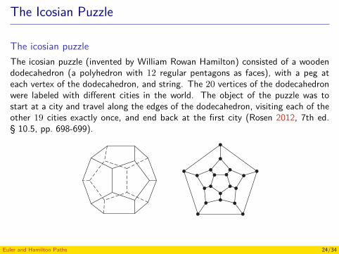
The Icosian Puzzle
The icosian puzzleThe icosian puzzle (invented by William Rowan Hamilton) consisted of a woodendodecahedron (a polyhedron with 12 regular pentagons as faces), with a peg ateach vertex of the dodecahedron, and string. The 20 vertices of the dodecahedronwere labeled with different cities in the world. The object of the puzzle was tostart at a city and travel along the edges of the dodecahedron, visiting each of theother 19 cities exactly once, and end back at the first city (Rosen 2012, 7th ed.§ 10.5, pp. 698-699).
10.5 Euler and Hamilton Paths 699
(a) (b)
FIGURE 8 Hamilton’s “A Voyage Round theWorld” Puzzle.
FIGURE 9 A Solution tothe “A Voyage Round theWorld” Puzzle.
Because the author cannot supply each reader with a wooden solid with pegs and string, wewill consider the equivalent question: Is there a circuit in the graph shown in Figure 8(b) thatpasses through each vertex exactly once? This solves the puzzle because this graph is isomorphicto the graph consisting of the vertices and edges of the dodecahedron. A solution of Hamilton’spuzzle is shown in Figure 9.
EXAMPLE 5 Which of the simple graphs in Figure 10 have a Hamilton circuit or, if not, a Hamilton path?
Solution: G1 has a Hamilton circuit: a, b, c, d, e, a. There is no Hamilton circuit in G2 (this canbe seen by noting that any circuit containing every vertex must contain the edge {a, b} twice),but G2 does have a Hamilton path, namely, a, b, c, d. G3 has neither a Hamilton circuit nor aHamilton path, because any path containing all vertices must contain one of the edges {a, b},{e, f }, and {c, d} more than once. ▲
a b
e c
d
G1
a b
d c
G2
a b
d c
G3
g
e f
FIGURE 10 Three Simple Graphs.
CONDITIONS FOR THE EXISTENCE OF HAMILTON CIRCUITS Is there a simple wayto determine whether a graph has a Hamilton circuit or path? At first, it might seem that thereshould be an easy way to determine this, because there is a simple way to answer the similarquestion of whether a graph has an Euler circuit. Surprisingly, there are no known simplenecessary and sufficient criteria for the existence of Hamilton circuits. However, many theoremsare known that give sufficient conditions for the existence of Hamilton circuits. Also, certainproperties can be used to show that a graph has no Hamilton circuit. For instance, a graph with avertex of degree one cannot have a Hamilton circuit, because in a Hamilton circuit, each vertexis incident with two edges in the circuit. Moreover, if a vertex in the graph has degree two, thenboth edges that are incident with this vertex must be part of any Hamilton circuit. Also, notethat when a Hamilton circuit is being constructed and this circuit has passed through a vertex,then all remaining edges incident with this vertex, other than the two used in the circuit, can beremoved from consideration. Furthermore, a Hamilton circuit cannot contain a smaller circuitwithin it.
Euler and Hamilton Paths 24/34
Hamilton Paths
Definition (Hamilton path)A simple path in a graph 𝐺 that passes through every vertex exactly onceis called a Hamilton path.
ExerciseFind a Hamilton path in the following graph:
𝑎 𝑏
𝑐𝑑
A Hamilton path is 𝑎, 𝑏, 𝑐, 𝑑.
Euler and Hamilton Paths 25/34
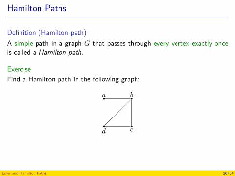
Hamilton Paths
Definition (Hamilton path)A simple path in a graph 𝐺 that passes through every vertex exactly onceis called a Hamilton path.
ExerciseFind a Hamilton path in the following graph:
𝑎 𝑏
𝑐𝑑
A Hamilton path is 𝑎, 𝑏, 𝑐, 𝑑.
Euler and Hamilton Paths 26/34
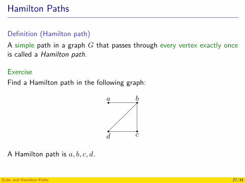
Hamilton Paths
Definition (Hamilton path)A simple path in a graph 𝐺 that passes through every vertex exactly onceis called a Hamilton path.
ExerciseFind a Hamilton path in the following graph:
𝑎 𝑏
𝑐𝑑
A Hamilton path is 𝑎, 𝑏, 𝑐, 𝑑.
Euler and Hamilton Paths 27/34
Hamilton Circuits
Definition (Hamilton circuit)A simple circuit in a graph 𝐺 that passes through every vertex exactly onceis called a Hamilton circuit.
ExerciseFind a Hamilton circuit in the following graph:
𝑎 𝑏
𝑐𝑒
𝑑
A Hamilton circuit is 𝑎, 𝑏, 𝑐, 𝑑, 𝑒, 𝑎.
Euler and Hamilton Paths 28/34
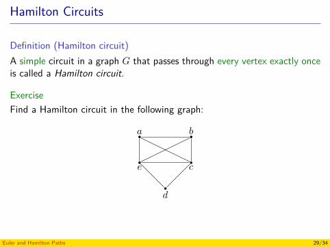
Hamilton Circuits
Definition (Hamilton circuit)A simple circuit in a graph 𝐺 that passes through every vertex exactly onceis called a Hamilton circuit.
ExerciseFind a Hamilton circuit in the following graph:
𝑎 𝑏
𝑐𝑒
𝑑
A Hamilton circuit is 𝑎, 𝑏, 𝑐, 𝑑, 𝑒, 𝑎.
Euler and Hamilton Paths 29/34
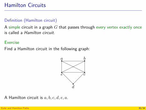
Hamilton Circuits
Definition (Hamilton circuit)A simple circuit in a graph 𝐺 that passes through every vertex exactly onceis called a Hamilton circuit.
ExerciseFind a Hamilton circuit in the following graph:
𝑎 𝑏
𝑐𝑒
𝑑
A Hamilton circuit is 𝑎, 𝑏, 𝑐, 𝑑, 𝑒, 𝑎.
Euler and Hamilton Paths 30/34
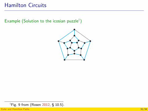
Hamilton Circuits
Example (Solution to the icosian puzzle†)10.5 Euler and Hamilton Paths 699
(a) (b)
FIGURE 8 Hamilton’s “A Voyage Round theWorld” Puzzle.
FIGURE 9 A Solution tothe “A Voyage Round theWorld” Puzzle.
Because the author cannot supply each reader with a wooden solid with pegs and string, wewill consider the equivalent question: Is there a circuit in the graph shown in Figure 8(b) thatpasses through each vertex exactly once? This solves the puzzle because this graph is isomorphicto the graph consisting of the vertices and edges of the dodecahedron. A solution of Hamilton’spuzzle is shown in Figure 9.
EXAMPLE 5 Which of the simple graphs in Figure 10 have a Hamilton circuit or, if not, a Hamilton path?
Solution: G1 has a Hamilton circuit: a, b, c, d, e, a. There is no Hamilton circuit in G2 (this canbe seen by noting that any circuit containing every vertex must contain the edge {a, b} twice),but G2 does have a Hamilton path, namely, a, b, c, d. G3 has neither a Hamilton circuit nor aHamilton path, because any path containing all vertices must contain one of the edges {a, b},{e, f }, and {c, d} more than once. ▲
a b
e c
d
G1
a b
d c
G2
a b
d c
G3
g
e f
FIGURE 10 Three Simple Graphs.
CONDITIONS FOR THE EXISTENCE OF HAMILTON CIRCUITS Is there a simple wayto determine whether a graph has a Hamilton circuit or path? At first, it might seem that thereshould be an easy way to determine this, because there is a simple way to answer the similarquestion of whether a graph has an Euler circuit. Surprisingly, there are no known simplenecessary and sufficient criteria for the existence of Hamilton circuits. However, many theoremsare known that give sufficient conditions for the existence of Hamilton circuits. Also, certainproperties can be used to show that a graph has no Hamilton circuit. For instance, a graph with avertex of degree one cannot have a Hamilton circuit, because in a Hamilton circuit, each vertexis incident with two edges in the circuit. Moreover, if a vertex in the graph has degree two, thenboth edges that are incident with this vertex must be part of any Hamilton circuit. Also, notethat when a Hamilton circuit is being constructed and this circuit has passed through a vertex,then all remaining edges incident with this vertex, other than the two used in the circuit, can beremoved from consideration. Furthermore, a Hamilton circuit cannot contain a smaller circuitwithin it.
†Fig. 9 from (Rosen 2012, § 10.5).Euler and Hamilton Paths 31/34
Hamilton Circuits
Theorem (Dirac’s Theorem (Rosen (2004), Theorem 3, p. 548))If 𝐺 is a simple graph with 𝑛 vertices with 𝑛 ≥ 3 such that the degree ofevery vertex in 𝐺 is at least 𝑛/2, then 𝐺 has a Hamilton circuit.
Theorem (Ore’s Theorem (Rosen (2004), Theorem 4, p. 548))If 𝐺 is a simple graph with 𝑛 vertices with 𝑛 ≥ 3 such that 𝛿(𝑢) + 𝛿(𝑣) ≥ 𝑛for every pair of non-adjacent vertices 𝑢 and 𝑣 in 𝐺, then 𝐺 has a Hamiltoncircuit.
Euler and Hamilton Paths 32/34
Hamilton Circuits
Theorem (Dirac’s Theorem (Rosen (2004), Theorem 3, p. 548))If 𝐺 is a simple graph with 𝑛 vertices with 𝑛 ≥ 3 such that the degree ofevery vertex in 𝐺 is at least 𝑛/2, then 𝐺 has a Hamilton circuit.
Theorem (Ore’s Theorem (Rosen (2004), Theorem 4, p. 548))If 𝐺 is a simple graph with 𝑛 vertices with 𝑛 ≥ 3 such that 𝛿(𝑢) + 𝛿(𝑣) ≥ 𝑛for every pair of non-adjacent vertices 𝑢 and 𝑣 in 𝐺, then 𝐺 has a Hamiltoncircuit.
Euler and Hamilton Paths 33/34
References
Rosen, K. H. (2004). Matemática Discreta y sus Aplicaciones. 5th ed.McGraw-Hill (cit. on pp. 14, 17–23, 32, 33).— (2012). Discrete Mathematics and Its Applications. 7th ed.McGraw-Hill (cit. on pp. 2, 15, 16, 22–24, 31).
Euler and Hamilton Paths 34/34