DISTINGUISHING THE EFFECTS OF THE RED QUEEN …€¦ · 172 Journal of Vertebrate Paleontology 21(1):172–185, March 2001 q 2001 by the Society of Vertebrate Paleontology DISTINGUISHING

172

Journal of Vertebrate Paleontology 21(1):172–185, March 2001q 2001 by the Society of Vertebrate Paleontology

DISTINGUISHING THE EFFECTS OF THE RED QUEEN AND COURT JESTER ON MIOCENEMAMMAL EVOLUTION IN THE NORTHERN ROCKY MOUNTAINS

ANTHONY D. BARNOSKYMuseum of Paleontology and Department of Integrative Biology, University of California,

Berkeley, California 94720

ABSTRACT—Red Queen hypotheses maintain that biotic interactions are the most important drivers of evolutionarychange, whereas Court Jester hypotheses regard physical-environmental perturbations, such as climate change, as mostimportant. Tests for the biotic effects of climate change that are conducted on too large a geographic scale can falselyreject the Court Jester because climate is so complex its manifestation is in opposite directions in different geographicareas. Consequently, faunal responses vary from place to place, and lumping of data from different climate zonesaverages out any local faunal responses. Likewise, tests that are conducted at inappropriate temporal scales will not beeffective at distinguishing between the Red Queen and Court Jester.

A test at a temporal and geographic scale that takes the above considerations into account suggests a biotic responseof mammals to a climatic warming event in the northern Rocky Mountains 18.5–14.0 Ma (the late-Early Mioceneclimatic optimum). During the environmental perturbation, mammalian species richness possibly increased, faunalturnover was pronounced, and taxa adapted to warm, arid environments became more abundant in numbers of speciesand density of individuals. The data are consistent with environmental change—the Court Jester—driving evolutionarychange at sub-continental spatial scales and temporal scales that exceed typical Milankovitch oscillations. The RedQueen may be active at smaller temporal and geographic scales.

INTRODUCTION

Mammal species and communities have turned over on arepeated basis, witnessed by our ability to recognize at least 39subdivisions of the Cenozoic based solely on composition offossil mammal assemblages (Woodburne and Swisher, 1995). Arich literature debates whether this march of morphology andspecies compositions through time, so well documented notonly for mammals but throughout the fossil record, is morestrongly influenced by interactions among species (Red Queenhypotheses), or by random perturbations to the physical envi-ronment such as climate change, tectonic events, or even bolideimpacts that change the ground rules for the biota (Court Jesterhypotheses).

Macroevolutionary (Van Valen, 1973) and microevolutionary(Bell, 1982) versions of Red Queen hypotheses, named afterLewis Carroll’s Red Queen (originally printed 1871, reprinted1960 and in several other editions), have been widely discussedin the scientific literature (Lively, 1996). Red Queen hypothesesgenerally state that biotic interactions are more important thanphysical-environmental change in driving evolutionary change(see for example McCune, 1982; Kitchell and Hoffman 1991;Pearson, 1992; Vrba, 1993; Alroy, 1996, 1998; Clay and Kover,1996; Ebert and Hamilton, 1996; Lively, 1996; Rosenzweig,1996; Lythgoe and Read, 1998; Martin and Fairbanks; 1999; toname but a few).

A class of alternative ideas, here termed Court Jester hy-potheses, share the basic tenet that changes in the physical en-vironment rather than biotic interactions themselves are the ini-tiators of major changes in organisms and ecosystems. Some ofthe more prominent ideas are listed in Table 1. Court Jesterhypotheses imply that events random in respect to the biotaoccasionally change the rules on the biotic playing field. Ac-celerated biotic response (relative to background rates) is theresult.

ANALYTICAL CONTEXT

The purpose of this paper is to explore why it is so difficultto sort between the relative importance of biotic versus abiotic

triggers to evolution, to discuss some scaling issues relevant tothe problem, and to present new data on Miocene mammals tohelp decipher the roles of the Red Queen and Court Jester inevolution. Mammals have fared no better than evidence fromany other taxonomic group as a system in which to test therelative influence of the Red Queen and Court Jester. For ex-ample, Van Valen (1973), Alroy (1996, 1998), Prothero andHeaton (1996), and Prothero (1999) all have presented evidencethat environmental changes, notably climate change, did littleto influence faunal turnover patterns in North America in var-ious parts of the Cenozoic. Martin and Fairbanks (1999:44)used Plio–Pleistocene mammalian turnover patterns as supportfor a ‘‘weak’’ Red Queen. Yet Vrba (1985, 1992, 1993, 1995),Janis (1989, 1993, 1997), Janis and Wilhelm (1993), Webb etal. (1995), Webb and Opdyke (1995), and Barry et al. (1995)just as cogently cited certain groups of mammals in which as-pects of evolutionary change correspond well with aspects ofenvironmental change, notably climate and vegetation.

Why has the relative influence of the Red Queen and CourtJester proven so difficult to sort out, even when examined usingsimilar kinds of data (fossil mammals) and at the same hierar-chical level of biology (macroevolutionary patterns)? At facevalue, the procedure for recognizing the Red Queen’s or CourtJester’s manifestation with these kinds of data is straightfor-ward: (1) postulate an aspect of environmental change thatmight influence evolutionary patterns; (2) specify how the en-vironmental change would be expected to influence evolutionin the taxa of interest, based on reasonable knowledge or in-ferences about life history traits; (3) document and date faunalpatterns; (4) document the timing of the specified environmen-tal change; (5) using appropriate techniques, determine whetherthe timing of the environmental change corresponds (or doesnot correspond) to appropriate aspects of the faunal patterns.Straightforward as this approach sounds, it is fraught with allthe pitfalls inherent in working with paleontological data, andwith potential methodological vagaries that can render gener-alizations nearly impossible. The paleontological-data problemsinclude: uneven distribution of requisite fossils through time orspace; insufficient information to adequately interpret paleoen-

173BARNOSKY—RED QUEEN VS. COURT JESTER

TABLE 1. Examples of Court Jester hypotheses.

Hypothesis General tenet and study system

Stationary modelStenseth and Maynard Smith(1984)

This model essentially arose out of a mathematical formulation that demonstrates that ecosystems areexpected to approach one of two evolutionary modes. One of these is the Stationary Model: ‘‘evolu-tionary stasis, with zero rate of evolution and no extinction or speciation; evolutionary change occursonly in response to changes in the physical environment’’ (italics mine) (Stenseth and MaynardSmith, 1984:870). The other plausible condition is the Red Queen model: ‘‘a steady state of change(even in a constant physical environment) characterized by continuing evolutionary change, extinc-tion, and speciation.’’ (Stenseth and Maynard Smith, 1984:870). Thus, Stenseth and Maynard Smithdemonstrated that both models are plausible from a mathematical perspective. Their formulation tookinto account Van Valen’s (1973) Red Queen hypothesis, MacArthur and Wilson’s (1967) theory ofisland biogeography, and the concepts of species packing and limiting similarity (MacArthur andLevins, 1964; May and MacArthur, 1972). The study system was theoretical.

Habitat theory(Vrba, 1992)

Changes in the physical environment (such as temperature, rainfall, substrate, food, and vegetation cov-er) in the habitat of a species drive evolutionary change. Seven hypotheses were presented about howspecies relate to their habitats, and biotic effects of (1) cyclic (Milankovitch-scale) climate change,(2) topographic diversity, (3) latitudinal distribution of speciation and extinction rates during times ofclimatic stability and (4) climatic cooling, (5) pulsed response of species to physical perturbations, (6)unusually long or intense climatic changes, and (7) how environmental variance affects generalist andspecialist species. The model was based primarily on studies of fossil mammals and macroevolution-ary theory.

Turnover-pulse hypothesis(Vrba, 1985, 1992, 1993, 1995)

The extreme version holds that initiation of lineage turnover (which includes speciation, extinction, im-migration, and emigration) ‘‘. . . is exclusively physical . . . . Speciation does not occur unless forcedby the physical environment . . . most lineage turnover in the history of life has occurred in pulses,nearly synchronous across diverse groups of organisms, and in predictable synchrony with changes inthe physical environment. Most of these turnover-pulses are small peaks involving few lineages and/or restricted geographic areas. Some of them are massive and of global extent’’ (Vrba, 1993:428).‘‘. . . not every lineage undergoes speciation or extinction even during extreme changes in the globalenvironment. . . . Such differences between lineages may be causally influenced by intrinsic biologicalfactors . . .’’ (Vrba 1993:431). The model derives primarily from studies of fossil mammals and mac-roevolutionary theory and was listed as one of the hypotheses (Hypothesis 5) in the Habitat Theory.

Traffic light model(Vrba, 1995)

Climatic changes open and close habitat corridors analogous to a biased traffic light that allows moretraffic to move in one direction than another. Faunal turnover is therefore expected to be more dra-matic in areas that are more frequently opened by a ‘‘green light’’ (Vrba, 1995:27-29). The modelwas based on studies of fossil mammals, Pleistocene climate change in Eurasia and Africa, and eco-logical theory.

Relay model(Vrba, 1995)

In response to climate change, ‘‘Lineages in contrasting habitat categories have new species starting up(by speciation) at displaced times and old species ending (by extinction) at differing times, rather likerunners in a relay race’’ (Vrba, 1995:29). The model was based on studies of fossil mammals, Pleis-tocene climate change in Eurasia and Africa, and ecological theory.

Tiers of time(Gould, 1985; Bennett, 1990,1997)

Based on observations of patterns in the fossil record, Gould (1985) hypothesized that evolutionary pro-cesses occur on at least three different scales. The first tier of time is the ecological scale (roughlytens to thousands of years), within which microevolutionary processes (mutation, recombination, se-lection, drift) and ecological interactions between individuals and populations (competition, predator-prey, parasite-host, etc.) take place. The second tier of time is the geological scale (millions of years),during which macroevolutionary processes such as species sorting occur. Evolution at this scale mayor may not be related to physical-environmental changes. The third tier is represented by geologicallyinfrequent catastrophes such as bolide impacts that dramatically change the physical environment andreset the ground rules for the biota. These events are separated by tens to hundreds of millions ofyears. Bennett (1990, 1997) added another tier, the cyclic climate changes caused by the Milankov-itch orbital variations on the scale of ten thousand to hundreds of thousands of years. Bennett (1990,1997) and Vrba (1992:8, 1993:422; 1995:27) noted that the most common response of species at thistier is to shift geographic ranges.

Coordinated stasis(Brett and Baird, 1995)

‘‘Long-ranging associations of species or biofacies display very minor or no morphological change inmost lineages of macrofossils . . . overall patterns of species richness, rank abundance, and guildstructure are relatively constant for a particular biofacies’’ (Brett and Baird, 1995:307) ‘‘. . . In con-trast, during geologically brief intervals—probably no more than a half million years in duration—major faunal changes occurred in many biofacies more or less simultaneously . . . There seems to besome relationship with major low stands of sea level . . . .’’ (Brett and Baird, 1995:308). ‘‘. . . itseems likely that without the episodic perturbations [to the physical environment in the form of sealevel changes] and collapse of stable ecosystems there would have been little movement in the histo-ry of life’’ (Brett and Baird, 1995:310). The model is based on empirical study of Silurian to MiddleDevonian marine invertebrate macrofossils.

Coevolutionary disequilibrium(Graham and Lundelius, 1984)

Ecosystems develop complex interactions among species during times of environmental stability. Pertur-bations such as climate change remove keystone species and result in individualistic response of oth-er species, causing ecosystems to significantly restructure. The model was developed from studies ofthe extinction patterns of late Pleistocene mammals, in an effort to ascribe a mechanism to that ex-tinction event.

vironmental changes; insufficient ability to reliably date envi-ronmental changes and/or faunal patterns; insufficient knowl-edge to predict how specified environmental changes might beexpected to influence extinct (or even extant) taxa. In effect,these and other ‘‘data problems’’ affect steps 3, 4, and 5 enu-

merated above. Methodological vagaries tend to affect steps 1,2, and 3, but can be minimized by specifying the kind of en-vironmental change with as much precision as possible, thetemporal and geographic scale over which the environmentalchange acts, the aspect of the biotic pattern (i.e., morphology,

174 JOURNAL OF VERTEBRATE PALEONTOLOGY, VOL. 21, NO. 1, 2001

diversity, speciation rate, extinction rate, etc.) that is hypothe-sized to respond (or not respond), and the mechanism thatwould link biotic response to the environmental change.

SCALING ISSUES

Climate proxy data are available in many forms through thegeological record, and for that reason most studies that examinethe interplay between environmental perturbations and mam-malian faunal patterns focus on climate as the forcing function.Climate change is a complex phenomenon. To understand itseffect on faunal patterns, the attribute(s) of climate postulatedto affect the biota must be specified, a relevant geographic scalemust be identified (as explained below), and the scale at whichthe biota is analyzed must be commensurate with the geograph-ic scale and specified climatic attributes. In most previous stud-ies, the global temperature curve indicated by oxygen- and/orcarbon-istotope stratigraphies is compared to continental-leveldiversity patterns of terrestrial, non-volant mammals in NorthAmerica or world-wide (Janis, 1993; Webb and Opdyke, 1995;Alroy, 1996, 1998; Prothero and Heaton, 1996; Prothero, 1999),or to diversity or phylogenetic patterns of selected groups withcontinent-wide distributions, most often large ungulates (Vrba,1985, 1992, 1993, 1995; MacFadden and Hulbert, 1988; Janis,1989; Janis and Wilhelm, 1993; Webb et al., 1995; Janis, 1997).These broad-scale studies have contributed a tremendousamount of useful information, even though they offer differentconclusions about the role of physical perturbations in spurringfaunal change, ranging from very little importance (Alroy,1996, 1998; Prothero and Heaton, 1996; Prothero, 1999) to verygreat importance (Janis, 1989; Janis and Wilhelm, 1993; VanValkenburgh and Janis, 1993; Vrba, 1993, 1995; Webb et al.,1995; Janis, 1997). The contradictory conclusions result in partfrom examining different scales of data, for example, focusingon certain orders of mammals or biogeographic provinces inone case and on all mammals and all provinces in another.Likewise, the climatic attributes and taxonomic attributes thatare being compared in the various studies sometimes differ. Forexample, in some cases the correspondence between the globaltemperature curve and extinction and/or origination rates mightbe compared (Alroy, 1996, 1998), whereas in others the attri-butes of interest are immigration rates in response to climatechange (Webb and Opdyke, 1995), or the response of morpho-logical features such as digestive or locomoter adapations toparticular climatic events (Janis, 1989; Janis and Wilhelm,1993; Van Valkenburgh and Janis, 1993; Webb et al., 1995;Vrba, 1995; Janis, 1997). Particular attributes of climate changeand how they mechanistically might influence faunal changeare treated at the level of generalities in some studies (Janis,1989; Janis and Wilhelm, 1993; Webb et al., 1995; Alroy, 1996,1998; Prothero and Heaton, 1996; Prothero, 1999), whereasthey are more precisely specified in others (Vrba, 1993, 1995).Finally, yet other studies examine faunal change through par-ticular, geographically restricted sequences, and compare thetiming of change to varyingly-resolved local or global climatesignals (Barnosky, 1993; Barry et al., 1995; Martin and Fair-banks, 1999).

Given that scaling and specificity constraints govern inter-pretations, what is the ‘right’ scale at which to study the relativeimportance of the Red Queen and the Court Jester? For studiesthat focus on interpreting the effects of climate change, thefollowing considerations are important.

Climate Dynamics and Geographic Scale

A mean change in global temperature does not imply that allparts of the globe, or even one continent, change climatic at-tributes in the same direction and to the same degree. For ex-ample, Atmospheric General Circulation Models suggest that

with a doubling of atmospheric CO2, aridity (measured as pre-cipitation-evapotranspiration) and mean annual temperaturewould increase in some parts of the North America, while de-creasing or changing little in other parts of the continent(Houghton et al., 1990). Such geographic variability means thatdetectable changes in a given climatic indicator assessed fromthe geologic record—such as global mean temperature—wouldbe expected to affect the biota quite differently in different re-gions of a continent. Therefore, comparing changes in globalmean temperature to changes in continental diversity patterns,for example, represents a mismatch in scale, even though bothscales are ‘‘large’’. The expected result of such a comparisonwould be no evidence that climate change influences biotic pat-terns for the following reason. The set of taxa in one geographicregion (for example, the Rocky Mountains) might experienceand respond to an increase in mean temperature, while analo-gous taxa in a different climatic and biogeographic province(for example, in the eastern U.S.). simultaneously experienceand respond to a decrease in mean temperature. Because thelocal climatic effect is in opposite directions, the net biotic re-sponse would be expected to be in opposite directions. Multiplythis effect by many taxa and many geographic areas, and the‘‘average’’ biotic response to climate looks like no response,even though in each geographic area there may be a clear effect.On the other hand, if the geographic scale drops to the levelthat encompasses only one direction of climatic response (e.g.,a discrete ‘‘climate zone’’ such as the northern Rocky Moun-tains, or Colorado Plateau, or southeastern U.S.), the effect ofspace-averaging biotic responses becomes less of a problem.Vrba (1993:431) implicitly recognized such potential scalingproblems in her elaboration of the Turnover-Pulse hypothesis:‘‘. . . geographic factors may determine that global coolingcauses extensive environmental changes in most localities,moderate changes in others, and none in some areas.’’

Evolutionary and Ecological Theory

A large body of evolutionary literature equates probability ofspeciation with size of geographic range (see, for example, ref-erences in Rosensweig, 1995). Basically, the larger the geo-graphic range of a species, the more likely it will be to cast offnew species given enough time because it is more likely thatpopulations will become isolated. Isolation can occur throughdispersal at the periphery of a range; larger geographic rangeshave larger peripheries, thus increasing the probability of iso-lates. Isolation can also occur from vicariance events; largerranges have a greater probability of being ‘‘cut’’ by a vicarianceevent simply because there is more area onto which to ‘‘vicar-iance knife’’ can fall (Rosensweig, 1995). Thus, climate changemight be expected to increase speciation rates by either en-couraging dispersal at peripheries of species ranges, or actingas a vicariance knife that fragments species ranges. An exampleof the latter would be the Great Basin, where mountaintops nowcontain ‘‘island faunas’’ that were more widespread during fulland late-glacial times (Grayson, 1987; Macdonald and Brown,1992).

Climate change causes vicariance events because some limitson a species’ geographic range are defined by climatic param-eters (e.g., Begon et al., 1990; Kareiva et al., 1993; Brown andLomolino, 1998; Schneider and Root, 1998; Graham, 1999).These can be direct limiters, such as the metabolic cost of sur-viving through a cold winter or the inability to conserve enoughmoisture to survive in desert environments (Brown and Lom-olino, 1998). Or, climate can limit ranges through an interme-diary, such as limiting the vegetation that a mammal speciesneeds for either food or shelter (for example, the associationbetween sagebrush voles and clumps of sagebrush documentedby Carroll and Genoways, 1980). By either pathway, a change


in an important climatic parameter would be expected to influ-ence geographic range boundaries of some species. An increasein speciation rate might be detectable if there was a markedincrease in range size; conversely, a decrease in speciation rateand/or increase in extinction rate would be expected if geo-graphic range shrank past a critical limit. Increases in immigra-tion rates might also be expected, as might increased extirpa-tion, depending on the nature of the climate change.

Given this logic, climate change could reasonably be ex-pected to produce a detectable change in faunal turnover, whichcombines speciation, extinction, immigration, and extirpation.However, in order to detect such changes (and in the best casesto sort between them), the geographic area of interest must belarge enough to encompass much of the geographic ranges ofthe species under consideration. Typically, geographic rangesof most mammal species are subcontinental in extent (excep-tions are ecological generalists in larger body-size classes,which can extend across much of a continent) (Hall, 1981).Coupling this constraint with the observation that a given cli-matic forcing produces changes of different direction on dif-ferent parts of the continent, it follows that the optimal geo-graphic scale on which to study the effects of climate changeis a scale small enough to encompass only one major climatezone, but large enough to encompass a variety of species rang-es. Examples of areas that fit this criterion would be the PacificNorthwest, the Great Basin, the Northern Rocky Mountains, theCentral Rocky Mountains, the Northern Great Plains, the South-ern Great Plains, and other areas of such magnitude.

Ecological theory also predicts that as certain climatic param-eters change, they might give some species a competitive ad-vantage over other species, resulting in individuals of the com-petitively favored species to become more abundant. Therefore,changes in relative abundance of individuals within species,and, scaling up, of species within higher taxa (i.e., perissodac-tyls vs. artiodactyls, or arvicolines vs. sciurids), is also an ex-pected response to climate change.

Competitive interactions can also lead to phenotypic change(e.g., character displacement), with or without speciation.Hence, if new climatic regimes bring closely related taxa intosympatry, phenotypic changes within populations may be evi-dent. Further contributing to the potential for phenotypic changeis ecophenotypic response. For example, as nutritional qualityincreases with a longer growing season, populations of speciesas diverse as pocket gophers (Patton and Brylski, 1987; Hadly,1997) and big-horn sheep (Guthrie, 1984) demostrate clearlydetectable morphological manifestations.

Temporal Scale

Just as an individual must be able to withstand daily andseasonal variations in weather throughout its life span if it isgoing to survive and reproduce, a species must be able to with-stand ‘‘normal’’ climatic variation that occurs over its lifespanif it is going to remain extant. The median life span of a mam-malian species through the Cenozoic is about 1.5 million years(Alroy, 1996). Climate clearly varies considerably on a finerscale than that, most notably exemplified in the approximately58C mean global temperature fluctuations that occur on a100,000 year cycle as a result of the Milankovitch orbital var-iations (Hays et al., 1976; Imbrie et al., 1993; Schneider andRoot, 1998).

Milankovitch orbital variations are most clearly manifestedfor the Quaternary probably because the orbital parameterscombined in a complex way with continental position, eleva-tion, and geochemical feedbacks to finally produce clear glacialand interglacial cycles (Raymo and Ruddiman, 1992). However,the same orbital parameters very likely were effecting climatechanges throughout the Cenozoic, albeit without the dramatic

effects of advancing and retreating continental ice sheets. If so,at a minimum, the ‘‘typical’’ mammalian species must havesurvived at least 10 to 15 Milankovitch cycles. In order for thatto happen, a certain amount of resiliency with respect to this‘‘normal’’ climate change must be built into a typical mam-malian species. At the very least, the typical species must beable to track environmental change by migrating, as Vrba(1995) clearly recognized.

How does this resiliency get ‘‘built in’’? Assume, as thepunctuated equilibrium model does (Eldredge and Gould, 1972;Gould, 1982; Gould and Eldredge, 1993), that the speciationevent occurs within the first one tenth of a species lifespan. Ifone favors gradualist models as the primary mode of speciation,the following argument is even more robust. That means thatspeciation takes place within about 150,000 years in a typicalmammalian species. Within that 150,000 years, the probabilityis high (indeed, almost 100%) that at least one Milankovitchoscillation event will be spanned. If the species is not resilientto that event, it becomes extinct. If the newly formed speciesis resilient to the first Milankovitch event it encounters, it alsowill be resilient to all following events of similar or lesser mag-nitude and of about equal or longer frequency. Because theseare the species that survive much longer than 150,000 years,they make up most of our fossil sample. This is because thechance of preservation is a function of the length of time thespecies survives to be sampled, holding abundance and all othertaphonomic factors equal. Thus, it is unlikely that most mam-mal species in the fossil record will demonstrate an evolution-ary response to climatic changes on the order of Milankovitch-cycle events.

This is not a new argument. Gould (1985), Bennett (1990,1997), and Vrba (1992, 1993, 1995) noted that species mustexperience out of the ordinary perturbations to their physicalenvironment to show an evolutionary response. The point isthat in order to test for a clear biotic response to climate changethat includes evolution and extinction, the most meaningful re-sults will be found by focusing on climatic changes that aremore pronounced than the typical Milankovitch-scale event.

TESTING THE RED QUEEN AND THE COURT JESTER

In order to test the importance of the Red Queen and CourtJester at the theoretically constrained scale discussed above, thisstudy examines the effect of a specific climate change—globalwarming—at a temporal scale that exceeds the typical Milan-kovitch cycle. Response of mammals is examined in a restrictedgeographic area—the Northern Rocky Mountains (Fig. 1).

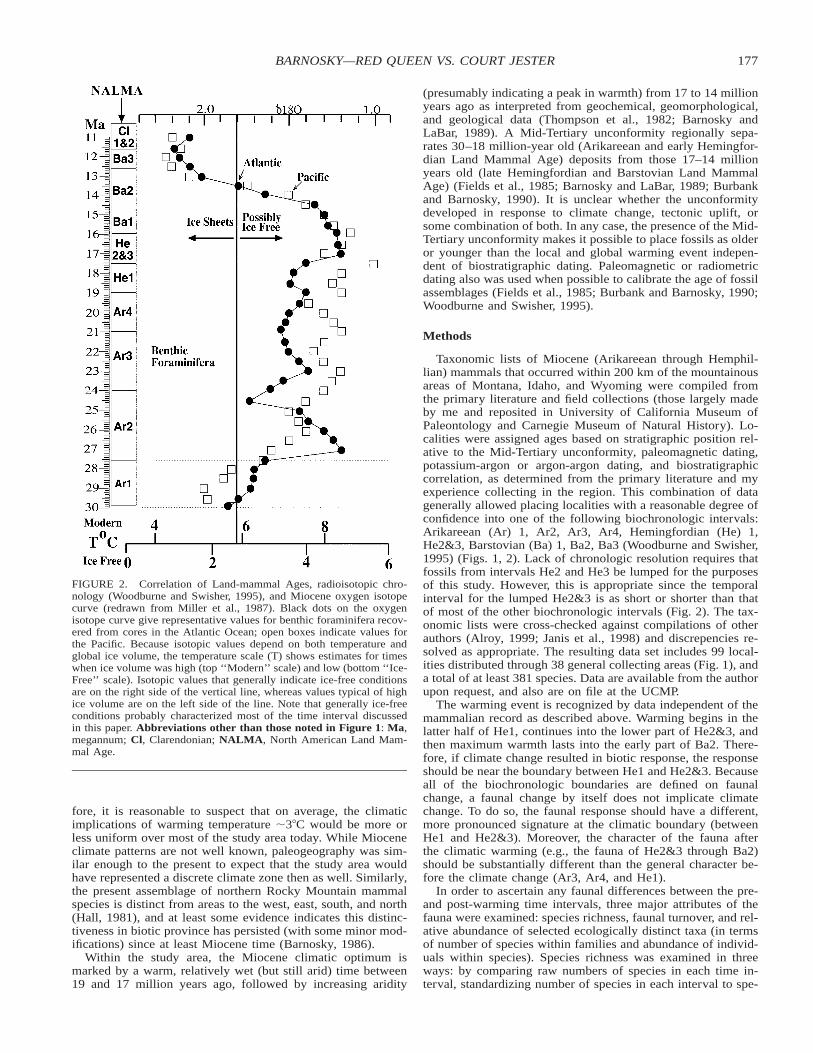
The global warming event took place in the late-Early Mio-cene, from 18.5 to 17 million years ago. The Atlantic d18Ocurve (Miller et al., 1987) (Fig. 2) demonstrates the Miocenewas relatively cool from about 24 to 18.5 Ma, when this late-Early Miocene climatic optimum (Flower and Kennett, 1994;Flower, 1999) began. Although the Pacific d18O curve is lessclear in demonstrating the warming event because sampling andcorrelation is not as good, it also documents warming at 17.5Ma (Fig. 2). Estimates for the increase in global temperatureduring this time range from 1–58C, with 3–48C the most com-mon (Buchardt, 1978; Woodruff et al., 1981; Miller et al., 1987;Zubukov and Borzenkova, 1990; Wright et al., 1992; Janis,1993; Wolfe, 1994; Schoell et al., 1994) (Fig. 2). Peak warmthlasted about 2.5 million years (17–14.5 Ma). Thus, the Mioceneglobal warming event was of different character than typicalMilankovitch warming events, in that the warming trend wassustained over a much longer time (1.5 million years vs. at mosta few thousand years), and resulted in a warm period that lastedon the order of millions rather than tens of thousands of years.It is very likely that typical Milankovitch oscillations continuedthrough the late-Early Miocene climatic optimum; for example,


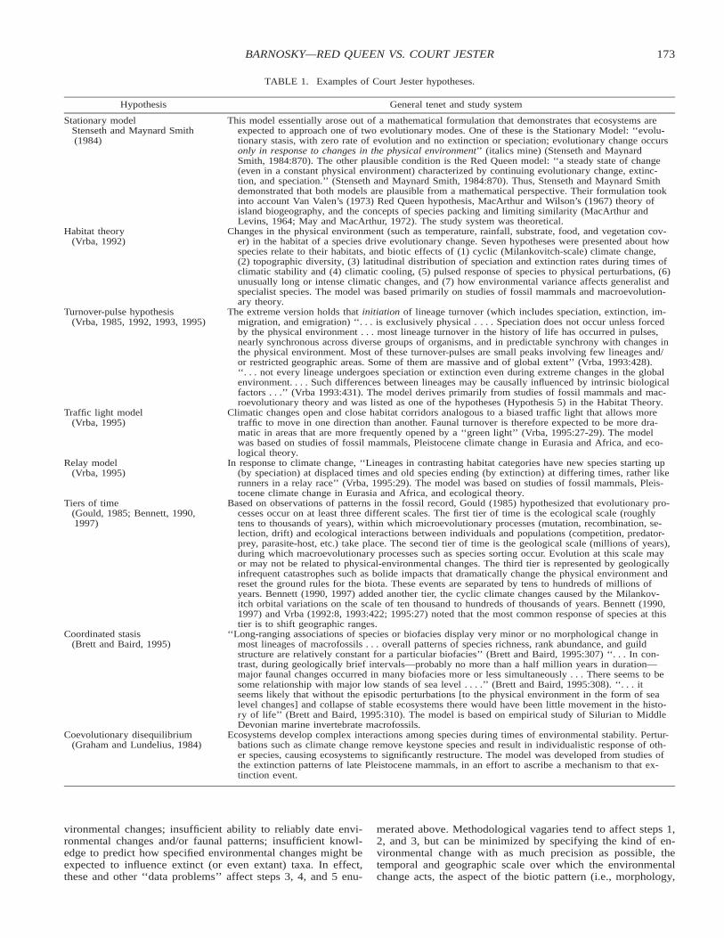
FIGURE 1. Geographic and temporal distribution of the collections that provided the data for this study. Numbers show where collecting areasoccur (some collecting areas are represented by the same number if they are geographically too close to separate on these small maps). Somecollecting areas contain multiple localities. A ‘‘locality’’ is here considered a restricted stratigraphic horizon or outcrop that has produced abundantspecimens. Abbreviations: Ar, Arikareean; He, Hemingfordian; Ba, Barstovian; Cl, Clarendonian; locs, localities. See Figure 2 for correlationof the biochronologic units with the radiometric timescale. Names of collecting areas are as follows (when a collecting area contains multiplelocalities, the number of localities is given in parentheses): 1, Canyon Ferry; 2, Tavenner Ranch (in general equates to Middle/Upper CabbagePatch); 3, Lower Cabbage Patch (11 locs.) and Middle/Upper Cabbage Patch including Tavenner Ranch (25 locs.); 4, Flint Creek; 5, JohnsonGulch; 6, North Boulder; 7, McKanna Spring; 8, Fort Logan (Ar1), Spring Creek 1 (University of Washington Burke Museum [UW] loc. A5867-1, Ar2), Spring Creek 2 (UW loc. A5867-2, Ba1); 9, Anceney; 10, Hepburn’s Mesa (9 locs.); 11, Upper Railroad Canyon, Mollie Gulch; 12,Peterson Creek (3 Ar2, 1 potentially Ar3 locs.); 13, Barstovian Colter faunas (North Pilgrim 2, Cunningham Hill, Two Ocean Lake); 14, Arikareeanand Hemingfordian Colter faunas (East Pilgrim 5 [He1], East Pilgrim 11 and Saunders Locality [Ar4], Emerald Lake [Ar2]); 15, Split Rock (12locs.); 16, Darton’s Bluff; 17, Devil’s Gate; 18, Lower Van Tassel; 19, Raw Hide Buttes; 20, Little Muddy Creek; 21, Willow Creek; 22, RoyalValley; 23, Keeline; 2, Lay Ranch (Ar4) and Jay Em (He1); 25, Bear Creek Mt. East; 26, Lower Sixty-six Mt.; 27, Upper Sixty-six Mt.; 28,Sixteen Mile District; 29, Joe’s Quarry; 30, Tremain; 31, Horse Creek; 32, Trail Creek; 33, Woodin; 34, Blacktail Deer Creek; 35, GrasshopperCreek. See Table 2 for a summary of numbers of collecting areas and numbers of localities per time interval. Physiographic base map is modifiedfrom Sterner (1995).

between 18.5 and 17.0 million years, the average warming rateof 28C/Ma embedded at least three cold excursions (Woodruffet al., 1981).

The spatial scale in this study is defined by the Rocky Moun-tain region of Wyoming, Montana, and Idaho (Fig. 1). Today,

this area of the Northern Rockies typically is recognized asfalling largely within one major climate zone (the Highlandzone [Brown and Lomolino, 1998]) and is characterized by rea-sonably similar mean temperature and precipitation in Januaryand July (World Meteorological Organization, 1979). There-


FIGURE 2. Correlation of Land-mammal Ages, radioisotopic chro-nology (Woodburne and Swisher, 1995), and Miocene oxygen isotopecurve (redrawn from Miller et al., 1987). Black dots on the oxygenisotope curve give representative values for benthic foraminifera recov-ered from cores in the Atlantic Ocean; open boxes indicate values forthe Pacific. Because isotopic values depend on both temperature andglobal ice volume, the temperature scale (T) shows estimates for timeswhen ice volume was high (top ‘‘Modern’’ scale) and low (bottom ‘‘Ice-Free’’ scale). Isotopic values that generally indicate ice-free conditionsare on the right side of the vertical line, whereas values typical of highice volume are on the left side of the line. Note that generally ice-freeconditions probably characterized most of the time interval discussedin this paper. Abbreviations other than those noted in Figure 1: Ma,megannum; Cl, Clarendonian; NALMA, North American Land Mam-mal Age.

fore, it is reasonable to suspect that on average, the climaticimplications of warming temperature ;38C would be more orless uniform over most of the study area today. While Mioceneclimate patterns are not well known, paleogeography was sim-ilar enough to the present to expect that the study area wouldhave represented a discrete climate zone then as well. Similarly,the present assemblage of northern Rocky Mountain mammalspecies is distinct from areas to the west, east, south, and north(Hall, 1981), and at least some evidence indicates this distinc-tiveness in biotic province has persisted (with some minor mod-ifications) since at least Miocene time (Barnosky, 1986).

Within the study area, the Miocene climatic optimum ismarked by a warm, relatively wet (but still arid) time between19 and 17 million years ago, followed by increasing aridity

(presumably indicating a peak in warmth) from 17 to 14 millionyears ago as interpreted from geochemical, geomorphological,and geological data (Thompson et al., 1982; Barnosky andLaBar, 1989). A Mid-Tertiary unconformity regionally sepa-rates 30–18 million-year old (Arikareean and early Hemingfor-dian Land Mammal Age) deposits from those 17–14 millionyears old (late Hemingfordian and Barstovian Land MammalAge) (Fields et al., 1985; Barnosky and LaBar, 1989; Burbankand Barnosky, 1990). It is unclear whether the unconformitydeveloped in response to climate change, tectonic uplift, orsome combination of both. In any case, the presence of the Mid-Tertiary unconformity makes it possible to place fossils as olderor younger than the local and global warming event indepen-dent of biostratigraphic dating. Paleomagnetic or radiometricdating also was used when possible to calibrate the age of fossilassemblages (Fields et al., 1985; Burbank and Barnosky, 1990;Woodburne and Swisher, 1995).

Methods

Taxonomic lists of Miocene (Arikareean through Hemphil-lian) mammals that occurred within 200 km of the mountainousareas of Montana, Idaho, and Wyoming were compiled fromthe primary literature and field collections (those largely madeby me and reposited in University of California Museum ofPaleontology and Carnegie Museum of Natural History). Lo-calities were assigned ages based on stratigraphic position rel-ative to the Mid-Tertiary unconformity, paleomagnetic dating,potassium-argon or argon-argon dating, and biostratigraphiccorrelation, as determined from the primary literature and myexperience collecting in the region. This combination of datagenerally allowed placing localities with a reasonable degree ofconfidence into one of the following biochronologic intervals:Arikareean (Ar) 1, Ar2, Ar3, Ar4, Hemingfordian (He) 1,He2&3, Barstovian (Ba) 1, Ba2, Ba3 (Woodburne and Swisher,1995) (Figs. 1, 2). Lack of chronologic resolution requires thatfossils from intervals He2 and He3 be lumped for the purposesof this study. However, this is appropriate since the temporalinterval for the lumped He2&3 is as short or shorter than thatof most of the other biochronologic intervals (Fig. 2). The tax-onomic lists were cross-checked against compilations of otherauthors (Alroy, 1999; Janis et al., 1998) and discrepencies re-solved as appropriate. The resulting data set includes 99 local-ities distributed through 38 general collecting areas (Fig. 1), anda total of at least 381 species. Data are available from the authorupon request, and also are on file at the UCMP.

The warming event is recognized by data independent of themammalian record as described above. Warming begins in thelatter half of He1, continues into the lower part of He2&3, andthen maximum warmth lasts into the early part of Ba2. There-fore, if climate change resulted in biotic response, the responseshould be near the boundary between He1 and He2&3. Becauseall of the biochronologic boundaries are defined on faunalchange, a faunal change by itself does not implicate climatechange. To do so, the faunal response should have a different,more pronounced signature at the climatic boundary (betweenHe1 and He2&3). Moreover, the character of the fauna afterthe climatic warming (e.g., the fauna of He2&3 through Ba2)should be substantially different than the general character be-fore the climate change (Ar3, Ar4, and He1).

In order to ascertain any faunal differences between the pre-and post-warming time intervals, three major attributes of thefauna were examined: species richness, faunal turnover, and rel-ative abundance of selected ecologically distinct taxa (in termsof number of species within families and abundance of individ-uals within species). Species richness was examined in threeways: by comparing raw numbers of species in each time in-terval, standardizing number of species in each interval to spe-


TABLE 2. Species richness and Survival Index (SI) per time interval. Maximum total of species considers indeterminate species as separatespecies; minimum total of species considers indeterminate species as belonging to one of the other species identified for a given genus. Speciesper million years and SI are calculated using the minimum total species. The SI shows the proportion of species that extend from the giveninterval into the next higher interval (see Methods section for further explanation). Adding species for Mountain and Adjacent Plains data doesnot exactly equal the Total Data set because of the effects of combining indeterminate species when considering data sets separately.

Biochronologic unit Ar1 Ar2 Ar3 Ar4 He1 He2&3 Ba1 Ba2 Ba3

Duration of interval (106 yrs.) 2.2 3.6 3 2 1.5 1.5 1.2 3.2 1

Total data setMaximum total speciesMinimum total speciesNumber of species per million yearsSpecies surviving to next intervalSurvival index (SI)Total localitiesTotal general collecting areas

53442019

0.4314

4

867821.7

60.08

379

454515

80.1855

242311.510

0.4365

232214.70044

534630.7

70.15

131

353226.7

90.2855

847021.9

10.01

133

191919——

22

Mountain data set onlyMaximum total speciesMinimum total speciesNumber of species per million yearsSpecies surviving to next intervalSurvival index (SI)Total localitiesTotal general collecting areas

494018.217

0.4313

3

555415

30.06

326

1919

6.33310.0533

44210.2532

885.30022

534631

40.09

131

303025

90.3044

847021.9

00

133

777

——

11

Adjacent plains data set onlyMaximum total speciesMinimum total speciesNumber of species per million yearsSpecies surviving to next intervalSurvival index (SI)Total localitiesTotal general collecting areas

441.80011

3333

9.1720.0653

2727

990.2222

212010

80.4033

171711——22

00———00

554.2——11

00———00

121212——

11

cies per million years (the quotient of how many species arepresent in each interval, divided by the length of the interval),and by employing regression, bootstrap and rarefaction analysesto identify the relationship between numbers of identified spec-imens (NISP) and numbers of identified species (Colwell andCoddington, 1994; Colwell, 1997). Taxonomy follows assign-ment of authors who reported specimens from the sites listedin Figure 1; in general, the species reflect a morphological spe-cies concept. As a crude index of faunal turnover, a survivalindex (SI) was determined as SI 5 (Survivors/Species Pool),where ‘Survivors’ is the number of species surviving across aninterval boundary (i.e., from Ar3 into Ar4), and ‘Species Pool’is the number of species found in the lower interval (Ar3 inthis example). SI basically measures the proportion of speciesthat persist across temporal intervals: the higher the SI, themore species persist from one interval into the next. Statisticswere calculated using Stratview 5.0, Microsoft Excel, andEstimateS 5 (Colwell, 1997).

Results

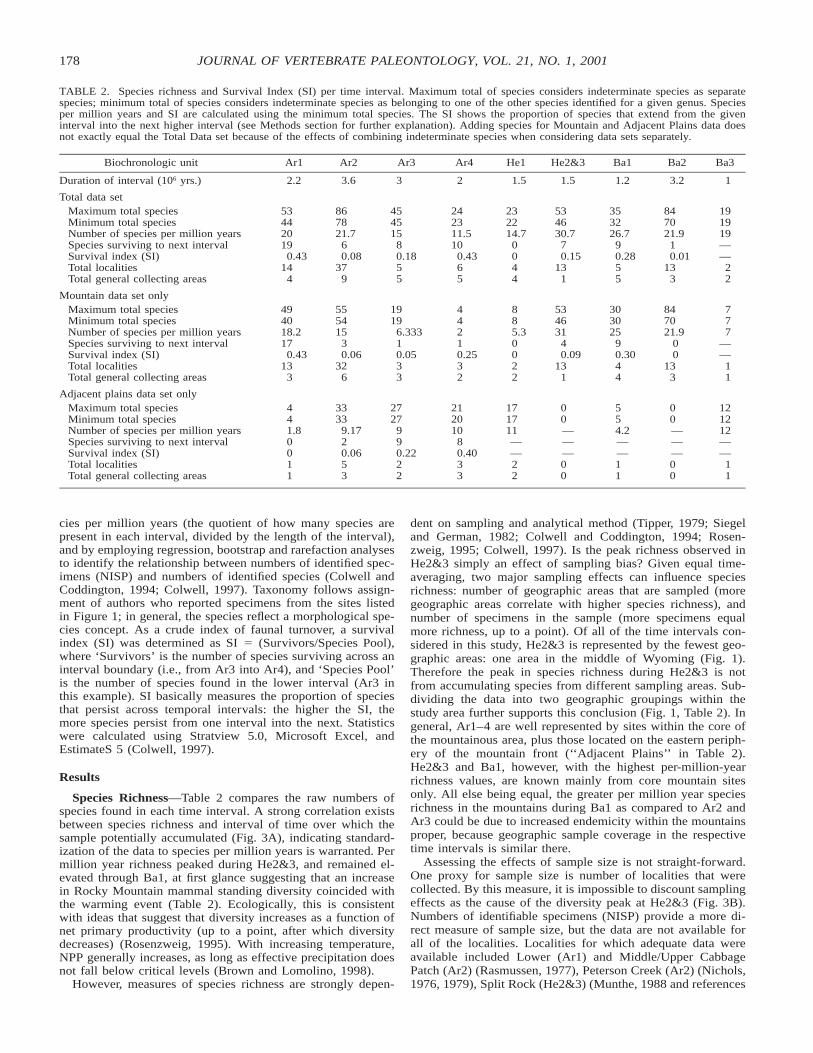
Species Richness—Table 2 compares the raw numbers ofspecies found in each time interval. A strong correlation existsbetween species richness and interval of time over which thesample potentially accumulated (Fig. 3A), indicating standard-ization of the data to species per million years is warranted. Permillion year richness peaked during He2&3, and remained el-evated through Ba1, at first glance suggesting that an increasein Rocky Mountain mammal standing diversity coincided withthe warming event (Table 2). Ecologically, this is consistentwith ideas that suggest that diversity increases as a function ofnet primary productivity (up to a point, after which diversitydecreases) (Rosenzweig, 1995). With increasing temperature,NPP generally increases, as long as effective precipitation doesnot fall below critical levels (Brown and Lomolino, 1998).

However, measures of species richness are strongly depen-

dent on sampling and analytical method (Tipper, 1979; Siegeland German, 1982; Colwell and Coddington, 1994; Rosen-zweig, 1995; Colwell, 1997). Is the peak richness observed inHe2&3 simply an effect of sampling bias? Given equal time-averaging, two major sampling effects can influence speciesrichness: number of geographic areas that are sampled (moregeographic areas correlate with higher species richness), andnumber of specimens in the sample (more specimens equalmore richness, up to a point). Of all of the time intervals con-sidered in this study, He2&3 is represented by the fewest geo-graphic areas: one area in the middle of Wyoming (Fig. 1).Therefore the peak in species richness during He2&3 is notfrom accumulating species from different sampling areas. Sub-dividing the data into two geographic groupings within thestudy area further supports this conclusion (Fig. 1, Table 2). Ingeneral, Ar1–4 are well represented by sites within the core ofthe mountainous area, plus those located on the eastern periph-ery of the mountain front (‘‘Adjacent Plains’’ in Table 2).He2&3 and Ba1, however, with the highest per-million-yearrichness values, are known mainly from core mountain sitesonly. All else being equal, the greater per million year speciesrichness in the mountains during Ba1 as compared to Ar2 andAr3 could be due to increased endemicity within the mountainsproper, because geographic sample coverage in the respectivetime intervals is similar there.

Assessing the effects of sample size is not straight-forward.One proxy for sample size is number of localities that werecollected. By this measure, it is impossible to discount samplingeffects as the cause of the diversity peak at He2&3 (Fig. 3B).Numbers of identifiable specimens (NISP) provide a more di-rect measure of sample size, but the data are not available forall of the localities. Localities for which adequate data wereavailable included Lower (Ar1) and Middle/Upper CabbagePatch (Ar2) (Rasmussen, 1977), Peterson Creek (Ar2) (Nichols,1976, 1979), Split Rock (He2&3) (Munthe, 1988 and references


FIGURE 3. Species richness as a function of (A) the maximum time potentially spanned by the samples; (B) the number of localities (on a logscale) at which specimens were collected; and (C and D) the number of identified specimens (NISP) in pooled numbers of samples. The bootstrap(C) and rarefaction (D) curves are statistical estimators of species richness (Coleman, 1997) constructed by selecting a single sample from aspecified collecting area, computing richness estimators, then selecting a second sample, adding it to the first, recomputing estimators for thepooled sample, and so on until all samples in the matrix are included. The process was repeated 50 times, with sample order randomized eachtime. Note that the relative position of curves from the different localities closely corresponds to the NISP of the pooled samples and the numberof samples composing the pool, with higher NISP and fewer samples equating with higher, steeper curves. Mean NISP per sample is as follows.Ba2, Hepburn’s Mesa, 149.7; Colter 70.3. He2&3, Split Rock, 94.9. Ar1, Lower Cabbage Patch, 23.5; Ar2, Middle/Upper Cabbage Patch, 17.7.Peterson Creek, 16.8. Abbreviations: CF, Barstovian Colter faunas; HM, Hepburn’s Mesa; LCP, Lower Cabbage Patch; MUCP, Middle/UpperCabbage Patch; PC, Peterson Creek; SR, Split Rock.

therein, plus UCMP specimen database), Colter faunas (Ba2)(Barnosky, 1986), Hepburn’s Mesa (Ba2) (Burbank and Bar-nosky, 1990, plus unpublished Carnegie Museum collections),and Anceney (Ba2) (Sutton, 1977; Sutton and Korth, 1995)(Fig. 4). For these localities NISP was considered an estimateof number of individuals and used in algorithms of Colwell(1997) to calculate rarefaction and bootstrap estimates of spe-cies richness for Ar1, Ar2, He2&3, and Ba2. In interpreting thecurves (Figs. 3C, D, 5A, B), it is important to note that NISPclearly overestimates the numbers of individuals sampled andtherefore affects the shape of the curves. However, this bias isconstant for all of the localities. Although it would not be validto compare these curves to those produced from accuratelysampling individuals from a modern fauna, the curves do pro-vide interesting estimates of species accumulation for the re-spective paleontological samples. The major trends in Figure3C and D suggest that the He2&3 localities are more speciesrich than the Ar1 or Ar2 ones, and that the Ba2 faunas areprobably the most species rich (i.e., steeper species accumula-

tion curves and higher y-intercepts). Sampling biases preventthese curves from being taken at face value, however. The rel-atively low Coleman rarefaction estimate for the Ba2 Colterfaunas (Fig. 3D) probably is because the localities includemainly screen-washing sites; thus large-bodied species are notwell represented in the sample. Likewise, the low rarefactionvalue for Peterson Creek (Fig. 3D) probably reflects that onlysurface collecting built the sample. For all other localities, acombination of screen-washing and surface collecting was usedto collect the samples, so collection bias probably is not a prob-lem in comparing them. But these results may be very stronglybiased by unequal sample sizes and sample numbers. The rel-ative position and shape of the curves strongly corresponds withtotal number of specimens (NISP) in the pooled samples (Fig.3C, D).

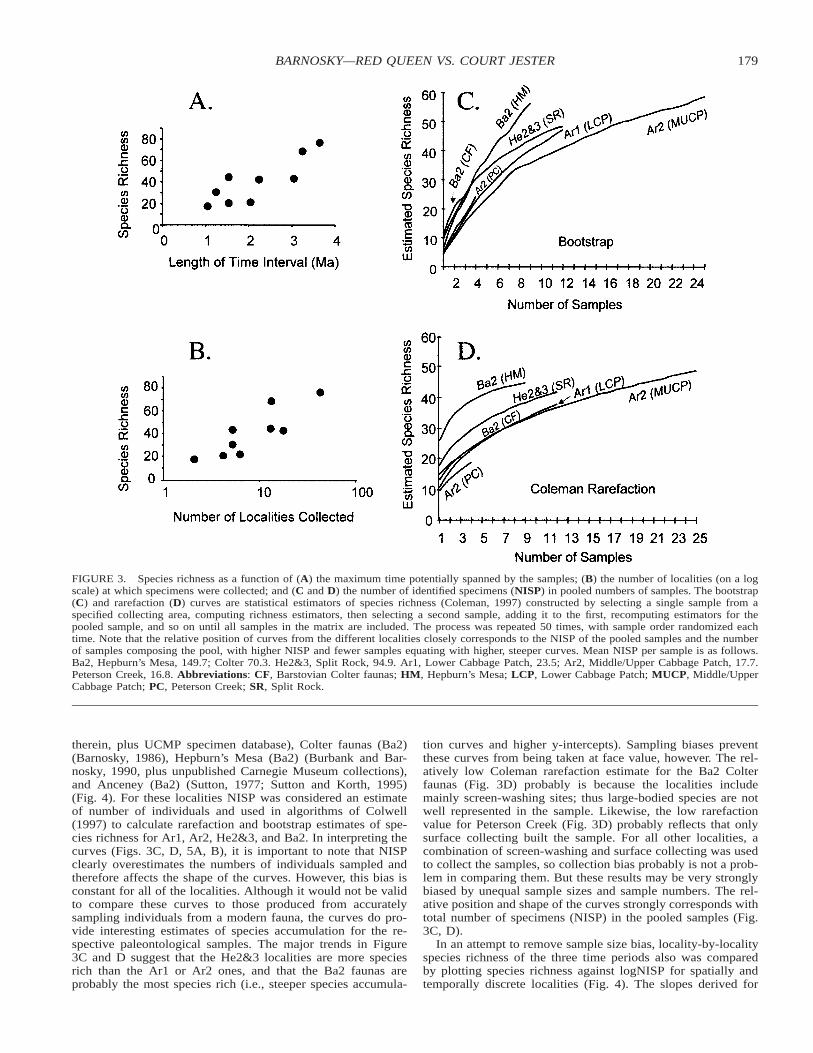
In an attempt to remove sample size bias, locality-by-localityspecies richness of the three time periods also was comparedby plotting species richness against logNISP for spatially andtemporally discrete localities (Fig. 4). The slopes derived for


FIGURE 4. Species richness as a function of the log of the numberof identifiable specimens (logNISP). A, Middle/Upper Cabbage Patchplus Peterson Creek (Ar2) compared to Split Rock (He2&3) localitiesthat contain comparable numbers of specimens (i.e., NISP,200). B,Middle/Upper Cabbage Patch plus Peterson Creek (Ar2) compared toHepburn’s Mesa plus Barstovian Colter localities (Ba2) that containcomparable numbers of specimens (i.e., NISP,200). C, Split Rock (He2&3) compared to Ba2 localities (Hepburn’s Mesa, Barstovian Colter,Anceney) including very large samples (NISP approaching 1,400). Theslopes for the Split Rock and Barstovian regression lines in panel C aresignificantly steeper than the slope for Middle/Upper Cabbage Patchplus Peterson Creek lines in panels A and B. The Split Rock line shownin panel A also is significantly steeper than the Cabbage Patch plusPeterson Creek line. However, when the analysis is confined toNISP,200, the slope of the Barstovian line does not differ significantlyfrom that of the Middle/Upper Cabbage Patch plus Peterson Creek sam-ple as shown in panel B. Regressions for Lower Cabbage Patch (Ar1)samples are not shown, but do not differ significantly from the Ar2samples. Equations for the illustrated regression lines are as follows.Ar2 Richness (Middle/Upper Cabbage Patch plus Peterson Creek) inpanels A and B 5 20.446 1 7.326(log NISP), R2 5 0.836. He2&3Richness (Split Rock) in panel A 5 27.37 1 14.265(log NISP), R2 50.897; in panel C, He2&3 Richness 5 22.595 1 9.616(log NISP), R2

5 0.694. Ba2 Richness (Hepburn’s Mesa plus Barstovian Colter) inpanel B 5 21.208 1 7.043(log NISP), R2 5 0.877; in panel C, Ba2Richness (Hepburn’s Mesa, Barstovian Colter, plus Ancencey) 525.168 1 11.678(log NISP), R2 5 0.882.

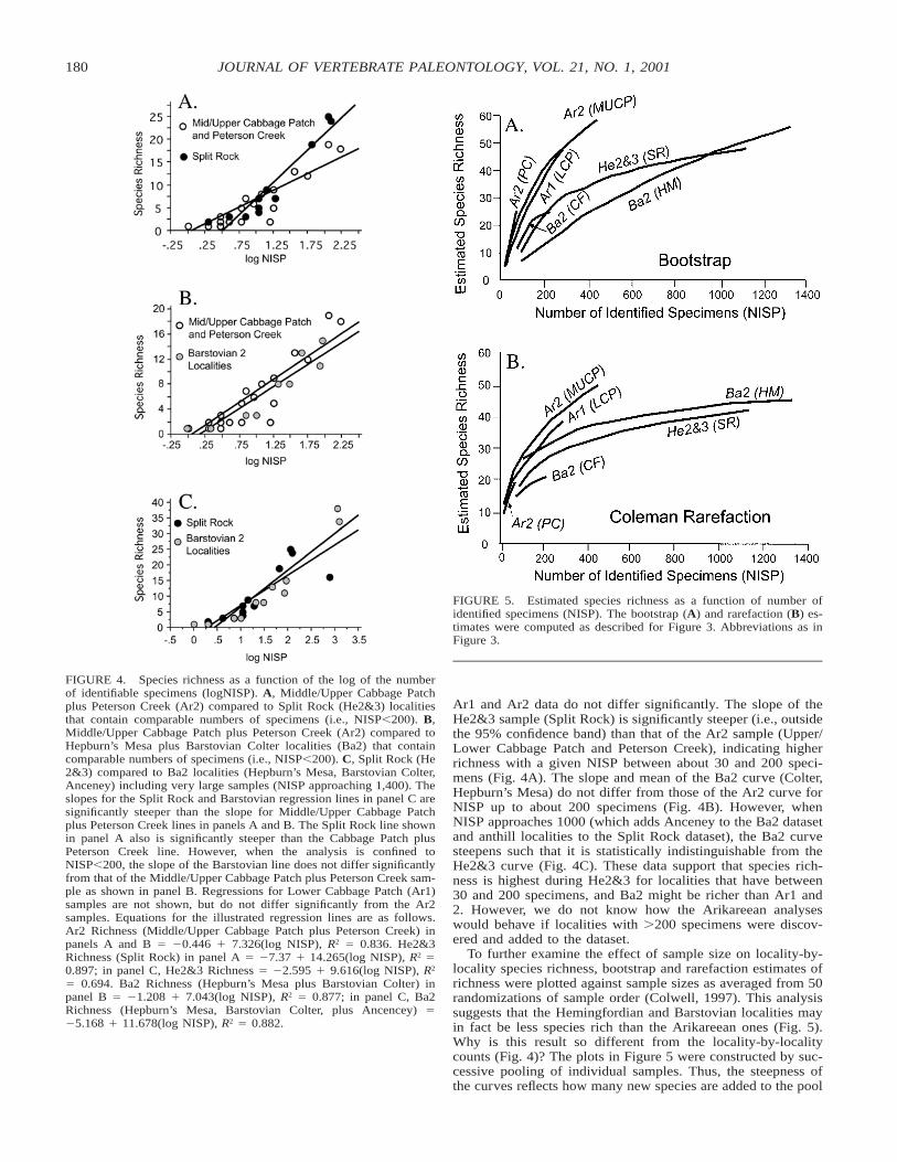
FIGURE 5. Estimated species richness as a function of number ofidentified specimens (NISP). The bootstrap (A) and rarefaction (B) es-timates were computed as described for Figure 3. Abbreviations as inFigure 3.

Ar1 and Ar2 data do not differ significantly. The slope of theHe2&3 sample (Split Rock) is significantly steeper (i.e., outsidethe 95% confidence band) than that of the Ar2 sample (Upper/Lower Cabbage Patch and Peterson Creek), indicating higherrichness with a given NISP between about 30 and 200 speci-mens (Fig. 4A). The slope and mean of the Ba2 curve (Colter,Hepburn’s Mesa) do not differ from those of the Ar2 curve forNISP up to about 200 specimens (Fig. 4B). However, whenNISP approaches 1000 (which adds Anceney to the Ba2 datasetand anthill localities to the Split Rock dataset), the Ba2 curvesteepens such that it is statistically indistinguishable from theHe2&3 curve (Fig. 4C). These data support that species rich-ness is highest during He2&3 for localities that have between30 and 200 specimens, and Ba2 might be richer than Ar1 and2. However, we do not know how the Arikareean analyseswould behave if localities with .200 specimens were discov-ered and added to the dataset.

To further examine the effect of sample size on locality-by-locality species richness, bootstrap and rarefaction estimates ofrichness were plotted against sample sizes as averaged from 50randomizations of sample order (Colwell, 1997). This analysissuggests that the Hemingfordian and Barstovian localities mayin fact be less species rich than the Arikareean ones (Fig. 5).Why is this result so different from the locality-by-localitycounts (Fig. 4)? The plots in Figure 5 were constructed by suc-cessive pooling of individual samples. Thus, the steepness ofthe curves reflects how many new species are added to the pool


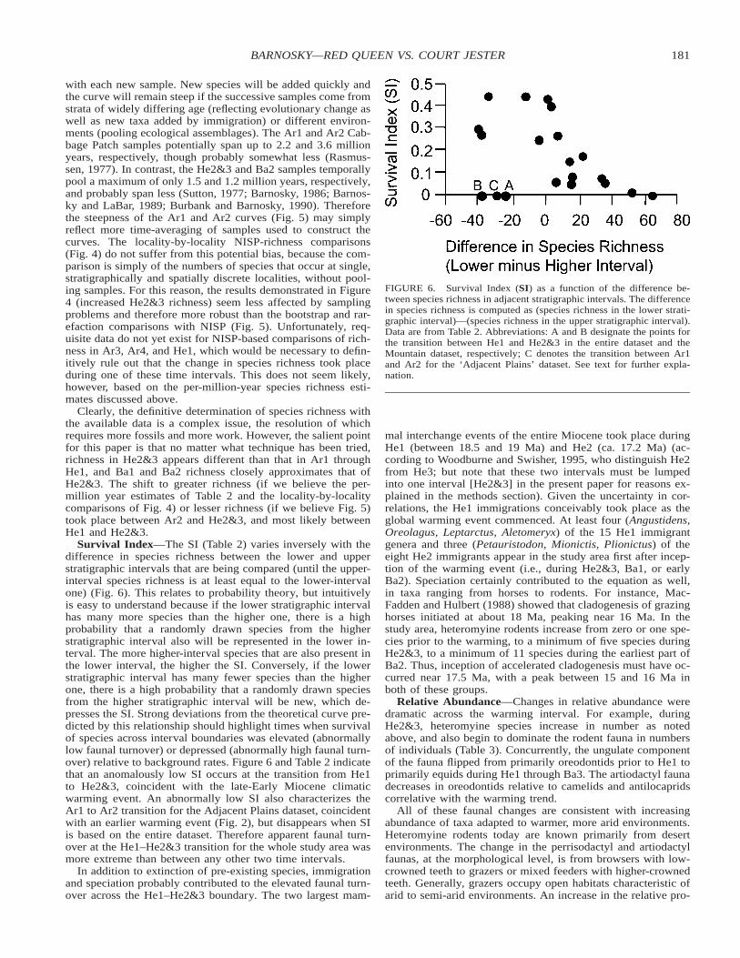
FIGURE 6. Survival Index (SI) as a function of the difference be-tween species richness in adjacent stratigraphic intervals. The differencein species richness is computed as (species richness in the lower strati-graphic interval)—(species richness in the upper stratigraphic interval).Data are from Table 2. Abbreviations: A and B designate the points forthe transition between He1 and He2&3 in the entire dataset and theMountain dataset, respectively; C denotes the transition between Ar1and Ar2 for the ‘Adjacent Plains’ dataset. See text for further expla-nation.

with each new sample. New species will be added quickly andthe curve will remain steep if the successive samples come fromstrata of widely differing age (reflecting evolutionary change aswell as new taxa added by immigration) or different environ-ments (pooling ecological assemblages). The Ar1 and Ar2 Cab-bage Patch samples potentially span up to 2.2 and 3.6 millionyears, respectively, though probably somewhat less (Rasmus-sen, 1977). In contrast, the He2&3 and Ba2 samples temporallypool a maximum of only 1.5 and 1.2 million years, respectively,and probably span less (Sutton, 1977; Barnosky, 1986; Barnos-ky and LaBar, 1989; Burbank and Barnosky, 1990). Thereforethe steepness of the Ar1 and Ar2 curves (Fig. 5) may simplyreflect more time-averaging of samples used to construct thecurves. The locality-by-locality NISP-richness comparisons(Fig. 4) do not suffer from this potential bias, because the com-parison is simply of the numbers of species that occur at single,stratigraphically and spatially discrete localities, without pool-ing samples. For this reason, the results demonstrated in Figure4 (increased He2&3 richness) seem less affected by samplingproblems and therefore more robust than the bootstrap and rar-efaction comparisons with NISP (Fig. 5). Unfortunately, req-uisite data do not yet exist for NISP-based comparisons of rich-ness in Ar3, Ar4, and He1, which would be necessary to defin-itively rule out that the change in species richness took placeduring one of these time intervals. This does not seem likely,however, based on the per-million-year species richness esti-mates discussed above.

Clearly, the definitive determination of species richness withthe available data is a complex issue, the resolution of whichrequires more fossils and more work. However, the salient pointfor this paper is that no matter what technique has been tried,richness in He2&3 appears different than that in Ar1 throughHe1, and Ba1 and Ba2 richness closely approximates that ofHe2&3. The shift to greater richness (if we believe the per-million year estimates of Table 2 and the locality-by-localitycomparisons of Fig. 4) or lesser richness (if we believe Fig. 5)took place between Ar2 and He2&3, and most likely betweenHe1 and He2&3.

Survival Index—The SI (Table 2) varies inversely with thedifference in species richness between the lower and upperstratigraphic intervals that are being compared (until the upper-interval species richness is at least equal to the lower-intervalone) (Fig. 6). This relates to probability theory, but intuitivelyis easy to understand because if the lower stratigraphic intervalhas many more species than the higher one, there is a highprobability that a randomly drawn species from the higherstratigraphic interval also will be represented in the lower in-terval. The more higher-interval species that are also present inthe lower interval, the higher the SI. Conversely, if the lowerstratigraphic interval has many fewer species than the higherone, there is a high probability that a randomly drawn speciesfrom the higher stratigraphic interval will be new, which de-presses the SI. Strong deviations from the theoretical curve pre-dicted by this relationship should highlight times when survivalof species across interval boundaries was elevated (abnormallylow faunal turnover) or depressed (abnormally high faunal turn-over) relative to background rates. Figure 6 and Table 2 indicatethat an anomalously low SI occurs at the transition from He1to He2&3, coincident with the late-Early Miocene climaticwarming event. An abnormally low SI also characterizes theAr1 to Ar2 transition for the Adjacent Plains dataset, coincidentwith an earlier warming event (Fig. 2), but disappears when SIis based on the entire dataset. Therefore apparent faunal turn-over at the He1–He2&3 transition for the whole study area wasmore extreme than between any other two time intervals.

In addition to extinction of pre-existing species, immigrationand speciation probably contributed to the elevated faunal turn-over across the He1–He2&3 boundary. The two largest mam-

mal interchange events of the entire Miocene took place duringHe1 (between 18.5 and 19 Ma) and He2 (ca. 17.2 Ma) (ac-cording to Woodburne and Swisher, 1995, who distinguish He2from He3; but note that these two intervals must be lumpedinto one interval [He2&3] in the present paper for reasons ex-plained in the methods section). Given the uncertainty in cor-relations, the He1 immigrations conceivably took place as theglobal warming event commenced. At least four (Angustidens,Oreolagus, Leptarctus, Aletomeryx) of the 15 He1 immigrantgenera and three (Petauristodon, Mionictis, Plionictus) of theeight He2 immigrants appear in the study area first after incep-tion of the warming event (i.e., during He2&3, Ba1, or earlyBa2). Speciation certainly contributed to the equation as well,in taxa ranging from horses to rodents. For instance, Mac-Fadden and Hulbert (1988) showed that cladogenesis of grazinghorses initiated at about 18 Ma, peaking near 16 Ma. In thestudy area, heteromyine rodents increase from zero or one spe-cies prior to the warming, to a minimum of five species duringHe2&3, to a minimum of 11 species during the earliest part ofBa2. Thus, inception of accelerated cladogenesis must have oc-curred near 17.5 Ma, with a peak between 15 and 16 Ma inboth of these groups.

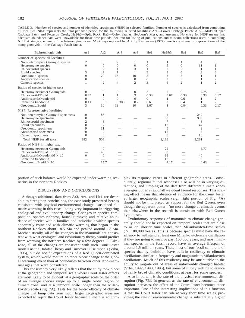
Relative Abundance—Changes in relative abundance weredramatic across the warming interval. For example, duringHe2&3, heteromyine species increase in number as notedabove, and also begin to dominate the rodent fauna in numbersof individuals (Table 3). Concurrently, the ungulate componentof the fauna flipped from primarily oreodontids prior to He1 toprimarily equids during He1 through Ba3. The artiodactyl faunadecreases in oreodontids relative to camelids and antilocapridscorrelative with the warming trend.

All of these faunal changes are consistent with increasingabundance of taxa adapted to warmer, more arid environments.Heteromyine rodents today are known primarily from desertenvironments. The change in the perrisodactyl and artiodactylfaunas, at the morphological level, is from browsers with low-crowned teeth to grazers or mixed feeders with higher-crownedteeth. Generally, grazers occupy open habitats characteristic ofarid to semi-arid environments. An increase in the relative pro-


TABLE 3. Number of species and number of identified specimens (NISP) in selected families. Number of species is calculated from combiningall localities. NISP represents the total per time period for the following selected localities: Ar1—Lower Cabbage Patch; AR2—Middle/UpperCabbage Patch and Peterson Creek; He2&3—Split Rock; Ba2—Colter faunas, Hepburn’s Mesa, and Anceney. No entry for NISP means thatadequate abundance data were unavailable for those time periods. See text for listing of publications and museum collections used in compilingNISP. A single specimen of the heteromyine rodent Mookomys reported for Ar2 by Rasmussen (1977) here is considered to represent one of themany geomyids in the Cabbage Patch fauna.

Bichronologic unit Ar1 Ar2 Ar3 Ar4 He1 He2&3 Ba1 Ba2 Ba3

Number of species: all localitiesNon-heteromyine Geomyid speciesHeteromyine speciesRhinocerotid speciesEquid speciesOreodontid speciesAntilocaprid speciesCamelid species

2013901

8022

2002

2011

1304

1031

1002

1013503

1523336

1026532

411

13111

0116122

Ratios of species in higher taxaHeteromyines/other GeomyoidsRhinocerotid/EquidAntilocaprid/OreodontidCamelid/OreodontidOreodontid/Equid

00.3300.113

0100.1

10

0100.308

13

0300.2

10

30.3300.61.67

50.67121

00.330.60.40.84

2.750.33110.33

—0.17220.17

NISP: Representative localitiesNon-heteromyine Geomyid specimensHeteromyine specimensRhinocerotid specimensEquid specimensOreodontid specimensAntilocaprid specimensCamelid specimens

0020900

183037

1100

———————

———————

———————

488

712

518

8

———————

249939

347

28

18

———————

Total NISP for all taxa 282 509 1,139 2,261 —

Ratios of NISP in higher taxaHeteromyines/other GeomyoidsRhinocerotid/Equid 3 100Antilocaprid/Oreodontid 3 10Camelid/OreodontidOreodontid/Equid 3 10

——0——

043

0—15.7

—————

—————

—————

22583616

4.17

—————

3.776

4090

0.43

—————

portion of such habitats would be expected under warming sce-narios in the northern Rockies.

DISCUSSION AND CONCLUSIONS

Although additional data from Ar3, Ar4, and He1 are desir-able to strengthen conclusions, the case study presented here isconsistent with physical-environmental change—sustained cli-matic warming in this case—being very important in triggeringecological and evolutionary change. Changes in species com-position, species richness, faunal turnover, and relative abun-dance of species within families and individuals within speciesapparently coincided with climatic warming that began in thenorthern Rockies about 18.5 Ma and peaked around 17 Ma.Mechanistically, all of the changes in the mammals are consis-tent with what ecological and evolutionary theory would predictfrom warming the northern Rockies by a few degrees C. Like-wise, all of the changes are consistent with such Court Jestermodels as the Habitat Theory and Turnover Pulse models (Vrba,1995), but do not fit expectations of a Red Queen-dominatedsystem, which would require no more biotic change at the glob-al warming event than at boundaries between other land-mam-mal ages that were considered.

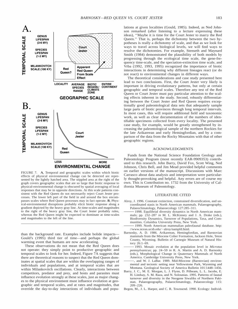
This consistency very likely reflects that the study took placeat the geographic and temporal scale where Court Jester effectsare most likely to be evident: at a geographic scale on the orderof an average species range up to a single biotic region orclimate zone, and at a temporal scale longer than the Milan-kovitch scale (Fig. 7A). Tests for the biotic efficacy of climatechange that lump data from much larger geographic areas areexpected to reject the Court Jester because climate is so com-

plex its response varies in different geographic areas. Conse-quently, regional faunal responses also will be in varying di-rections, and lumping of the data from different climate zonesaverages out any regionally-evident faunal responses. This scal-ing effect means that absence of evidence for the Court Jesterat larger geographic scales (e.g., right portion of Fig. 7A)should not be interpreted as support for the Red Queen, eventhough the apparent pattern (no more change at climatic eventsthan elsewhere in the record) is consistent with Red Queenhypotheses.

Evolutionary responses of mammals to climate change gen-erally should not be expected on temporal scales that are closeto or on shorter time scales than Milankovitch-time scales(#;100,000 years). This is because species must have the re-siliency to withstand at least one Milankovitch-scale oscillationif they are going to survive past 100,000 years, and most mam-mal species in the fossil record have an average lifespan ofaround 1.5 million years. Thus, most of our fossil sample is ofspecies that by definition have built-in resiliency to climaticoscillations similar in frequency and magnitude to Milankovitchoscillations. Much of this resiliency may be attributable to theability to migrate out of areas of unfavorably changed habitat(Vrba, 1992, 1993, 1995), but some of it may well be toleranceof fairly broad climatic conditions, at least for some species.

Also important is the rate of the physical-environmental dis-ruption (Fig. 7B). In general, as the rate of environmental dis-ruption increases, the effect of the Court Jester becomes moreimportant. One of the interesting implications of this functionis that the Court Jester can rule at very short time scales, pro-viding the rate of environmental change is substantially higher


FIGURE 7. A, Temporal and geographic scales within which bioticeffects of physical environmental change can be detected are repre-sented by the lightly hatched area. The stippled area at the right of thegraph covers geographic scales that are so large that biotic response tophysical-environmental change is obscured by spatial averaging of localresponses that may be in opposite directions. At this scale patterns con-sistent with the Red Queen do not necessarily reject Court Jester pro-cesses. The lower left part of the field in and around the box encom-passes scales where Red Queen processes may in fact operate. B, Phys-ical-environmental disruptions probably elicit biotic response along agradient depicted by the heavy gray line. At time-scales and magnitudesto the right of the heavy gray line, the Court Jester probably rules,whereas the Red Queen might be expected to dominate at time-scalesand magnitudes to the left of the line.

than the background rate. Examples include bolide impacts—Gould’s (1995) third tier of time—and perhaps the globalwarming event that humans are now accelerating.

These observations do not mean that the Red Queen doesnot operate: they simply point to productive geographic andtemporal scales to look for her. Indeed, Figure 7A suggests thatthere are theoretical reasons to suspect that the Red Queen dom-inates at spatial scales that are within the overlapping ranges ofindividuals and populations, and at temporal scales that arewithin Milankovitch oscillations. Clearly, interactions betweencompetitors, predator and prey, and hosts and parasites mustinfluence evolution strongly at these scales, just as major chang-es to the physical environment must influence evolution at geo-graphic and temporal scales, and at rates and magnitudes, thatoverride the day-to-day interactions of individuals and popu-

lations at given localities (Gould, 1985). Indeed, as Ned John-son remarked (after listening to a lecture expressing theseideas), ‘‘Maybe it is time for the Court Jester to marry the RedQueen.’’ That is, perhaps the dichotomy between the two hy-potheses is really a dichotomy of scale, and that as we look forways to travel across biological levels, we will find ways toresolve the dichotomies. For example, Stenseth and MaynardSmith (1984) demonstrated the plausibility of both models byprogressing through the ecological time scale, the gene-fre-quency time-scale, and the speciation-extinction time scale, andVrba (1992, 1993, 1995) recognized the importance of bioticinteractions in determining why different lineages react (or donot react) to environmental changes in different ways.

The theoretical considerations and case study presented herelead to two conclusions. First, the Court Jester very likely isimportant in driving evolutionary patterns, but only at certaingeographic and temporal scales. Therefore any test of the RedQueen or Court Jester must pay particular attention to the scal-ing effects inherent in the study. Second, robustly differentiat-ing between the Court Jester and Red Queen requires excep-tionally good paleontological data sets that adequately samplelarge parts of biotic provinces through long temporal intervals.In most cases, this will require additional field and taxonomicwork, as well as clear documentation of the numbers of iden-tifiable specimens collected from every locality. The presentedcase study, for example, would be greatly strengthened by in-creasing the paleontological sample of the northern Rockies forthe late Arikareean and early Hemingfordian, and by a com-parison of the data from the Rocky Mountains with that of othergeographic regions.

ACKNOWLEDGMENTS

Funds from the National Science Foundation Geology andPaleontology Program (most recently EAR-9909353) contrib-uted to this research. John Barry, David Fox, Scott Wing, NedJohnson, Chris Bell, and Jim Mead provided helpful commentson earlier versions of the manuscript. Discussions with MarcCarrasco about data analysis and interpretation were particular-ly thought-provoking and helpful. Any errors are of course myown. This is Contribution no. 1732 from the University of Cal-ifornia Museum of Paleontology.

LITERATURE CITED

Alroy, J. 1996. Constant extinction, constrained diversification, and un-coordinated stasis in North American mammals. Palaeogeography,Palaeoclimatology, Palaeoecology 127:285–311.

1998. Equilibrial diversity dynamics in North American mam-mals; pp. 232–287 in M. L. McKinney and J. A. Drake (eds.),Biodiversity Dynamics, Turnover of Populations, Taxa, and Com-munities. Columbia University Press, New York.

1999. North American mammalian paleofaunal database. http://www.nceas.ucsb.edu/;alroy/nampfd.html.

Barnosky, A. D. 1986. Arikareean, Hemingfordian, and Barstovianmammals from the Miocene Colter Formation, Jackson Hole, TetonCounty, Wyoming. Bulletin of Carnegie Museum of Natural His-tory 26:1–69.

1993. Mosaic evolution at the population level in Microtuspennsylvanicus; pp. 24–59 in R. A. Martin and A. D. Barnosky(eds.), Morphological Change in Quaternary Mammals of NorthAmerica. Cambridge University Press, New York.

, and W. J. LaBar. 1989. Mid-Miocene (Barstovian) environ-mental and tectonic setting near Yellowstone Park, Wyoming andMontana. Geological Society of America Bulletin 101:1448–1456.

Barry, J. C., M. E. Morgan, L. J. Flynn, D. Pilbeam, L. L. Jacobs, E.H. Lindsay, S. M. Raza, and N. Solounias. 1995. Patterns of faunalturnover and diversity in the Neogene Siwaliks of Northern Paki-stan. Palaeogeography, Palaeoclimatology, Palaeoecology 115:209–226.

Begon, M., J. L. Harper, and C. R. Townsend. 1990. Ecology: Individ-


uals, Populations, and Communities, 2nd ed. Blackwell ScientificPublications, Boston, 945 pp.

Bell, G. 1982. The Masterpiece Of Nature: The Evolution and Geneticsof Sexuality. University of California Press, Berkeley, 635 pp.

Bennett, K. D. 1990. Milankovitch cycles and their effects on speciesin ecological and evolutionary time. Paleobiology 16:11–21.

1997. Ecology and Evolution, The Pace of Life. CambridgeUniversity Press, Cambridge, England, 241 pp.

Brett, C. E., and G. C. Baird. 1995. Coordinated stasis and evolutionaryecology of Silurian to Middle Devonian faunas in the AppalachianBasin; pp. 285–315 in D. H. Erwin and R. L. Anstey (eds.), NewApproaches to Speciation in the Fossil Record. Columbia Univer-sity Press, New York.

Brown, J. H., and M. V. Lomolino. 1998. Biogeography, Second Edi-tion. Sinauer Associates, Sunderland, Massachusetts, 691 pp.

Burbank, D. W., and A. D. Barnosky. 1990. The magnetochronology ofBarstovian mammals in southwestern Montana and implications forthe initiation of Neogene crustal extension in the northern RockyMountains. Geological Society of America Bulletin 102:1093–1104.

Buchardt, B. 1978. Oxygen isotope palaeotemperatures from the Tertia-ry period in the North Sea Area. Nature 275:121–123.

Carroll, L. 1960 (reprinted). The Annotated Alice: Alice’s Adventuresin Wonderland and Through the Looking-Glass, illustrated by J.Tenniel, with an Introduction and Notes by M. Gardner. The NewAmerican Library, New York, 345 pp.

Carroll, L. E., and H. H. Genoways. 1980. Lemmiscus curtatus. Mam-malian Species 124:1–6.

Clay, K., and P. X. Kover. 1996. The Red Queen hypothesis and plant/pathogen interactions. Annual Review of Phytopathology 34:29–50.

Colwell, R. K. 1997. EstimateS: Statistical estimation of species rich-ness and shared species from samples. Version 5. User’s Guide andapplication. http://viceroy.eeb.uconn.edu/estimates.

, and J. A. Coddington. 1994. Estimating terrestrial biodiversitythrough extrapolation. Philosophical Transactions of the Royal So-ciety of London B 345:108–118.

Ebert, D., and W. D. Hamilton. 1996. Sex against virulence: the coevo-lution of parasitic diseases. Trends in Ecology and Evolution 11:79–82.

Eldredge, N., and S. J. Gould. 1972. Punctuated equilibria: an alterna-tive to phyletic gradualism; pp. 82–115 in T. J. M. Schopf (ed.),Models in Paleobiology. W. H. Freeman, San Francisco.

Fields, R. W., D. L Rasmussen, A. R. Tabrum, and R. Nichols. 1985.Cenozoic rocks of the intermontane basins of western Montana andeastern Idaho; pp. 9–36 in R. S. Flores and S. S. Kaplan (eds.),Cenozoic Paleogeography of the West-Central United States. So-ciety of Economic, Paleontology, and Mineralogy, Rocky MountainSection, Symposium 3.

Flower, B. P. 1999. Warming without high CO2? Nature 399:313–314., and Kennett, J. P. 1994. The middle Miocene climatic transi-

tion: East Antarctic ice sheet development, deep ocean circulationand global carbon cycling. Palaeogeography, Palaeoclimatololgy,Palaeoecology 108:537–555.

Gould, S. J. 1982. The meaning of punctuated equilibrium and its rolein validating a hierarchical approach to macroevolution; pp. 83–104 in R. Milkman (ed.), Perspectives on Evolution. Sinauer As-sociates Sunderland, Massachusetts.

1985. The paradox of the 1st tier: an agenda for paleobiology.Paleobiology 11:2–12.

, and N. Eldredge, 1993. Punctuated equilibria comes of age.Nature 366:223–227.

Graham, A. 1999. Late Cretaceous and Cenozoic History of NorthAmerican Vegetation: North of Mexico. Oxford University Press,New York, 350 pp.

Graham, R. W., and E. L. Lundelieus, Jr. 1984. Coevolutionary dis-equilibrium and Pleistocene extinctions; pp. 223–249 in P. S. Mar-tin and R. G. Klein (eds.), Quaternary Extinctions, a PrehistoricRevolution. University of Arizona Press, Tucson.

Grayson, D. K. 1987. The biogeographic history of small mammals inthe Great Basin: Observations on the last 20000 years. Journal ofMammalogy 68:359–375.

Guthrie, R. D. 1984. Alaskan megabucks, megabulls, and megarams:the issue of Pleistocene gigantism; pp. 482–510 in H. H. Genowaysand M. R. Dawson (eds.), Contributions in Quaternary Vertebrate

Paleontology: a Volume in Memorial to John E. Guilday. CarnegieMuseum of Natural History Special Publication 8, Pittsburgh,Pennsylvania.

Hadly, E. A. 1997. Evolutionary and ecological response of pocketgophers (Thomomys talpoides) to late-Holocene climatic change.Biological Journal of the Linnean Society 60:277–296.

Hall, E. R. 1981. The Mammals of North America, 2nd ed. John Wileyand Sons, New York, 2 volumes, 1175 pp.

Hays, J. D., J. Imbrie, and N. J. Shackleton. 1976. Variations in theearth’s orbit: pacemaker of the ice ages. Science 194:1121–1132.

Houghton, J. T, G. J. Jenkins, and J. J. Ephraums (eds.). 1990. Climatechange: the IPCC Scientific Assessment. Cambridge UniversityPress, Cambridge, England, 364 pp.

Imbrie, J., A. Berger, and N. J. Shackleton. 1993. Role of orbital forc-ing: a two-million-year perspective; pp. 263–267 in J. A. Eddy andH. Oeschger (eds.), Global Changes in the Perspective of the Past.John Wiley and Sons, New York.

Janis, C. M. 1989. A climatic explanation for patterns of evolutionarydiversity in ungulate mammals. Palaeontology 32:463–481.

1993. Tertiary mammal evolution in the context of changingclimates, vegetation, and tectonic events. Annual Review of Ecol-ogy and Systematics 24:467–500.

1997. Ungulate teeth, diets, and climatic changes at the Eocene/Oligocene boundary. Zoology 100:203–220.

, and P. B.Wilhelm. 1993. Were there mammalian pursuit pred-ators in the Tertiary? Dances with wolf avatars. Journal of Mam-malian Evolution 1:103–125.

, K. M. Scott, and L. L. Jacobs (eds.). 1998. Evolution of Ter-tiary Mammals of North America, Vol. 1. Cambridge UniversityPress, New York.

Kareiva, P. M., J. G. Kingsolver, and R. B. Huey (eds.). 1993. BioticInteractions and Global Change. Sinauer Associates, Sunderland,Massachusetts, 559 pp.

Kitchell, J. A., and A. Hoffman. 1991. Rates of species-level originationand extinction: functions of age, diversity, and history. Acta Pa-laeontologica Polonica 36:39–68.

Lively, C. M. 1996. Host-parasite coevolution and sex. Bioscience 46:107–114.

Lythgoe, K. A., and A. F. Read. 1998. Catching the Red Queen? Theadvice of the rose. Trends in Ecology and Evolution 13:473–474.

MacArthur, R. H., and R. Levins. 1964. Competition, habitat selection,and character displacement in a patchy environment. Proceedingsof the National Academy of Science 51:1207–1210.

, and E. O. Wilson. 1967. The Theory of Island Biogeography.Princeton University Press, Princeton.

MacDonald, K. A., and J. H. Brown. 1992. Using montane mammalsto model extinctions due to climate change. Conservation Biology6:409–415.

MacFadden, B., and R. Hulbert, Jr. 1988. Explosive speciation at thebase of the adaptive radiation of Miocene grazing horses. Nature336:466–468.

Martin, R. A., and K. B. Fairbanks. 1999. Cohesion and survivorshipof a rodent community during the past 4 million years in south-western Kansas. Evolutionary Ecology Research 1:21–48.

May, R. M., and R. H. MacArthur. 1972. Niche overlap as a functionof environmental variability. Proceedings of the National Academyof Science 69:1109–1113.

McCune, A. R. 1982. On the fallacy of constant extinction rates. Evo-lution 36:610–614.

Miller, K. G., R. G. Fairbanks, and G. S. Mountain. 1987. Tertiaryoxygen isotope synthesis, sea level history, and continental marginerosion. Paleoceanography 2:1–19.

Munthe, J. 1988. Miocene mammals of the Split Rock area, GraniteMountains Basin, Central Wyoming. University of California Pub-lications in Geological Sciences 126:1–136.

Nichols, R. 1976. Early Miocene mammals from the Lemhi Valley ofIdaho. Tebiwa 18:9–48.

1979. Additional early Miocene mammals from the Lemhi Val-ley of Idaho. Miscellaneous Papers of the Idaho State UniversityMuseum of Natural History 17:1–12.

Patton, J. L., and P. V. Brylski. 1987. Pocket gophers in alfalfa fields:causes and consequences of habitat-related body size variation.American Naturalist 130:493–506.

Pearson, P. N. 1992. Survivorship analysis of fossil taxa when real-time


extinction rates vary: The Paleogene planktonic foraminifera. Pa-leobiology 18:115–131.

Prothero, D. R. 1999. Does climatic change drive mammalian evolu-tion? GSA Today 9:1–7.

, and T. H. Heaton. 1996. Faunal stability during the early Oli-gocene climatic crash. Palaeogeography, Palaeoclimatology, Pa-laeoecology 127:239–256.

Rasmussen, D. L. 1977. Geology and mammalian paleontology of theOligo–Miocene Cabbage Patch Formation, central-western Mon-tana. Ph.D. dissertation, University of Kansas, Lawrence, 775 pp.

Raymo, M. E., and W. F. Ruddiman. 1992. Tectonic forcing of lateCenozoic climate. Nature 359:117–122.

Rosenzweig, M. L. 1995. Species Diversity in Space and Time. Cam-bridge University Press, Cambridge, England, 436 pp.

1996. And now for something completely different: geneticgames and Red Queens. Evolutionary Ecology 10:327.

Schneider, S. H., and T. L. Root. 1998. Climate Change; pp. 89–116 inM. J. Mac, P. A. Opler, C. E. Puckett Haecker and P. D. Doran(eds.), Status and Trends of the Nation’s Biological Resources. U.S.Geological Survey, Reston, Virginia.

Schoell, M., S. Schouten, J. S. Sinninghe Damste, J. W de Leeuw, andR. E Summons. 1994. A molecular organic carbon isotope recordof Miocene climatic changes. Science 263:1122–1125.

Siegel, A. F., and R. Z. German. 1982. Rarefaction and taxonomic di-versity. Biometrics 38:235–241.

Stenseth, N. C., and J. Maynard Smith. 1984. Coevolution in ecosys-tems: Red Queen evolution or stasis? Evolution 38:870–880.

Sterner, R. 1995. Untitled. http://fermi.jhuapl.edu/states/us/uspcolor.gif.Sutton, J. F. 1977. Mammals of the Anceney local fauna (late Miocene)

of Montana. Ph.D. dissertation, Texas Tech University, Lubbock,257 pp.

, and W. W. Korth. 1995. Rodents (Mammalia) from the Barsto-vian (Miocene) Anceney local fauna, Montana. Annals of CarnegieMuseum 64:267–314.

Thompson, G. T., R. W. Fields, and D. Alt. 1982. Land-based evidenceof Tertiary climatic variations, northern Rockies. Geology 10:413–417.

Tipper, J. C. 1979. Rarefaction and rarefiction—the use and abuse of amethod in paleoecology. Paleobiology 5:423–434.

Van Valen, L. 1973. A new evolutionary law. Evolutionary Theory 1:1–30.

Van Valkenburgh, B., and C. M. Janis. 1993. Historical diversity pat-terns in North American large herbivores and carnivores; pp. 330–

340 in R. E. Ricklefs and D. Schluter (eds.), Species Diversity inEcological Communities. University of Chicago Press, Chicago.

Vrba, E. S. 1985. Environment and evolution: alternative causes of thetemporal distribution of evolutionary events. South African Journalof Science 81:229–236.

1992. Mammals as a key to evolutionary theory. Journal ofMammalogy 73:1–28.

1993. Turnover-pulses, the Red Queen, and related topics.American Journal of Science 293-A:418–452.

1995. On the connections between paleoclimate and evolution;pp. 24–45 in E. S. Vrba, G. H. Denton, T. C. Partridge, and L. H.Burckle (eds.), Paleoclimate and Evolution, with Emphasis on Hu-man Origins. Yale University Press, New Haven.

Webb, S. D., R. C. Hulbert, Jr., and W. D. Lambert. 1995. Climaticimplications of large-herbivore distributions in the Miocene ofNorth America; pp. 91–108 in E. S. Vrba, G. H. Denton, T. C.Partridge, and L. H. Burckle (eds.), Paleoclimate and Evolution,with Emphasis on Human Origins. Yale University Press, New Ha-ven.

, and N. D. Opdyke. 1995. Global climatic influence on Ceno-zoic land mammal faunas; pp. 184–208 in J. P. Kennett and S. M.Stanley (eds.), Effects of Past Global Change on Life. NationalAcademy of Sciences, Washington, D.C.

Woodburne, M. O., and C. C. Swisher, III. 1995. Land mammal high-resolution geochronology, intercontinental overland dispersals, sealevel, climate, and vicariance; pp. 336–364 in W. A. Berggren, D.V. Kent, M.-P. Aubry, and J. Hardenbol (eds.), Geochronology,Time Scales and Global Stratigraphic Correlation. Society of Sed-imentary Geology Special Publication 54.

Woodruff, F., S. M Savin, and R. G. Douglas. 1981. Miocene stableisotope record: a detailed deep Pacific Ocean study and its paleo-climatic implications. Science 212:665–668.

World Meteorological Organization. 1979. Climatic Atlas of North andCentral America (technical supervisor, F. Steinhauser). World Me-teorological Organization, Geneva.

Wolfe, J. A. 1994. Tertiary climatic changes at middle latitudes of west-ern North America. Palaeogeography, Palaeoclimatology, Palaeoe-cology 108:195–205.

Wright, J. D., K. G. Miller, and R. G. Fairbanks. 1992. Early and middleMiocene stable isotopes: implications for deepwater circulation andclimate. Paleoceanography 7:357–389.

Zubakov, V. A., and I. I. Borzenkova. 1990. Global Palaeoclimate ofthe Late Cenozoic. Elsevier, Amsterdam, 456 pp.

Received 10 April 2000; accepted 1 October 2000.

Documents

DISTINGUISHING THE EFFECTS OF THE RED QUEEN …€¦ · 172 Journal of Vertebrate Paleontology 21(1):172–185, March 2001 q 2001 by the Society of Vertebrate Paleontology DISTINGUISHING