Distributed Clock Skew and Offset Estimation in Wireless Sensor

IEEE TRANSACTIONS ON WIRELESS COMMUNICATIONS, ACCEPTED FOR PUBLICATION 1

Distributed Clock Skew and Offset Estimation inWireless Sensor Networks: Asynchronous

Algorithm and Convergence AnalysisJian Du and Yik-Chung Wu

Abstract—In this paper, we propose a fully distributed algo-rithm for joint clock skew and offset estimation in wireless sensornetworks based on belief propagation. In the proposed algorithm,each node can estimate its clock skew and offset in a completelydistributed and asynchronous way: some nodes may update theirestimates more frequently than others using outdated messagefrom neighboring nodes. In addition, the proposed algorithmis robust to random packet loss. Such algorithm does notrequire any centralized information processing or coordination,and is scalable with network size. The proposed algorithmrepresents a unified framework that encompasses both classesof synchronous and asynchronous algorithms for network-wideclock synchronization. It is shown analytically that the proposedasynchronous algorithm converges to the optimal estimates withestimation mean-square-error at each node approaching thecentralized Cramer-Rao bound under any network topology.Simulation results further show that the convergence speed isfaster than that corresponding to a synchronous algorithm.

Index Terms—Clock synchronization, wireless sensor network,factor graph, asynchronous algorithm.

I. INTRODUCTION

W IRELESS sensor networks (WSNs) have been widelyused in environmental and emergency monitoring [1],

[2], event detection [3] and object tracking [4]. To performdistributed information processing in WSNs, a common clockacross the network is usually required to guarantee the nodesact in a collaborative and synchronized fashion. Unfortunately,clock oscillator in each sensor node has its own imperfectionand both clock skew (frequency difference) and clock offset(phase difference) are present. Therefore, time synchronization[5] appears as one of the most important research challengesin the design of WSNs.

Existing time synchronization algorithms can be categorizedinto two main classes. One is pairwise synchronization [6]–[17] where protocols are primarily designed to synchronizetwo nodes. The other is network-wide synchronization whereprotocols are designed to synchronize a large number ofnodes in the network [18]–[30]. Network-wide clock syn-chronization is much more challenging due to limited radio

Manuscript received March 28, 2013; revised June 25 and August 13, 2013;accepted August 25, 2013. The associate editor coordinating the review of thispaper and approving it for publication was A. Vosoughi.

Part of this manuscript appeared at the 2013 IEEE International Conferenceon Acoustics, Speech, and Signal Processing [30].

The authors are with the Department of Electrical and Electronic Engi-neering, The University of Hong Kong, Pokfulam Road, Hong Kong (e-mail:{dujian, ycwu}@eee.hku.hk).

Digital Object Identifier 10.1109/TWC.2013.100213.130553

range. Nodes in a sensor network cannot directly communicatewith every other node, but they have to do it via multi-hop.Traditionally, network-wide clock synchronization in WSNsrelies on spanning tree or clustered-based structure. Undersuch structures, synchronization is achieved through layer-by-layer pairwise synchronization. Such protocols, like time-synchronization protocol for sensor network (TPSN) [18] andpairwise broadcast synchronization (PBS) [19], suffer largeoverhead in building and maintaining the tree or clusterstructure, and are vulnerable to sudden node failures.

Without global structure or special nodes, by exchangingpulses emitted by oscillators, sensors are synchronized totransmit and receive at the same time in [20]–[22]. However,these algorithms cannot provide a precise clock reading atthe sensor node. On the other hand, fully distributed synchro-nization based on averaged consensus algorithms have beenproposed in [23]–[28]. Unfortunately, as shown in [26], [29],consensus protocol is not optimal and the performance willdeteriorate when message delay exists. Besides, as average-consensus based algorithm seeks to reach global average inthe whole network, it has slow convergence [27] (in orderof hundreds of iterations before convergence). More recently,[29] pioneered the fully distributed network-wide clock offsetestimation algorithm based on belief propagation (BP), andfound that its performance is superior to consensus algorithms.However, ignoring the effect of clock skew would significantlyincrease the re-synchronization frequency. Moreover, [29]considers a parallel implementation with message exchangecarried out in a synchronous fashion. Notwithstanding, inmany practical scenarios, the inter-sensor message exchangeis asynchronous since random data packet losses may occur,and different nodes may update at different frequencies. Atpresent, it is not clear the impact of these disturbance factorson the performance of synchronization algorithms.

This work advances the state-of-the-art distributed synchro-nization in the following ways: 1) The distributed algorithmis fairly general and can cope with both clock skews aswell as offsets over the whole network in parallel. 2) Itrepresents a unified framework that encompasses both classesof synchronous [29], [30] and asynchronous algorithms. 3)The convergence of the proposed method under asynchronousenvironments is formally proved. The convergence result is de-rived for vector variable case, in which the Perron-Frobenioustheorem used in [29] is not applicable. 4) With the adoptionof a different message passing rule from [29], the mean-

1536-1276/13$31.00 c© 2013 IEEE

This article has been accepted for inclusion in a future issue of this journal. Content is final as presented, with the exception of pagination.

2 IEEE TRANSACTIONS ON WIRELESS COMMUNICATIONS, ACCEPTED FOR PUBLICATION

square error (MSE) performance of the derived algorithm isshown to approach the centralized Cramer-Rao bound (CRB)asymptotically. Simulations show that the convergence speedof asynchronous algorithm is faster than its synchronouscounterpart.

The rest of this paper is organized as follows. The systemmodel is presented in Section II. A fully distributed asyn-chronous clock skew and offset estimation algorithm based onBP is derived in Section III. The convergence of the proposedasynchronous algorithm is analyzed in Section IV. Simulationresults are given in Section V and, finally, conclusions aredrawn in Section VI.

Notations: Boldface uppercase and lowercase letters areused for matrices and vectors, respectively. Superscript Tdenotes transpose. The symbol IN represents the N × Nidentity matrix. Notation N (x|μ,R) stands for the probabilitydensity function (pdf) of a Gaussian random vector x withmean μ and covariance matrix R. The symbol ∝ representsthe linear scalar relationship between two real valued functionsand |V| denotes the cardinality of set V . For two matrices Xand Y , X � Y means that X − Y is a positive definitematrix, and X � Y means that X − Y is a positive semi-definite matrix.

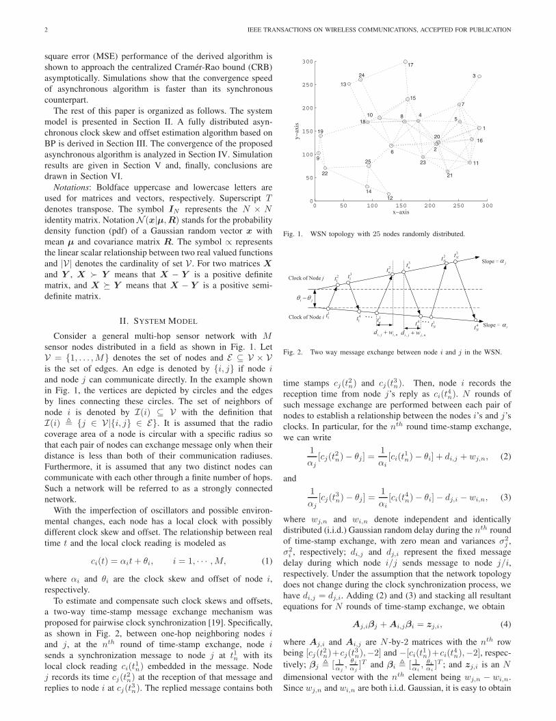
II. SYSTEM MODEL

Consider a general multi-hop sensor network with Msensor nodes distributed in a field as shown in Fig. 1. LetV = {1, . . . ,M} denotes the set of nodes and E ⊆ V × Vis the set of edges. An edge is denoted by {i, j} if node iand node j can communicate directly. In the example shownin Fig. 1, the vertices are depicted by circles and the edgesby lines connecting these circles. The set of neighbors ofnode i is denoted by I(i) ⊆ V with the definition thatI(i) � {j ∈ V|{i, j} ∈ E}. It is assumed that the radiocoverage area of a node is circular with a specific radius sothat each pair of nodes can exchange message only when theirdistance is less than both of their communication radiuses.Furthermore, it is assumed that any two distinct nodes cancommunicate with each other through a finite number of hops.Such a network will be referred to as a strongly connectednetwork.

With the imperfection of oscillators and possible environ-mental changes, each node has a local clock with possiblydifferent clock skew and offset. The relationship between realtime t and the local clock reading is modeled as

ci(t) = αit+ θi, i = 1, · · · ,M, (1)

where αi and θi are the clock skew and offset of node i,respectively.

To estimate and compensate such clock skews and offsets,a two-way time-stamp message exchange mechanism wasproposed for pairwise clock synchronization [19]. Specifically,as shown in Fig. 2, between one-hop neighboring nodes iand j, at the nth round of time-stamp exchange, node isends a synchronization message to node j at t1n with itslocal clock reading ci(t

1n) embedded in the message. Node

j records its time cj(t2n) at the reception of that message and

replies to node i at cj(t3n). The replied message contains both

0 50 100 150 200 250 3000

50

100

150

200

250

300

1

2

3

45

6

7

8

9

10

11

12

13

14

15

16

17

18

1920

2122

23

24

x−axis

y−ax

is

25

Fig. 1. WSN topology with 25 nodes randomly distributed.

Clock of Node j

i j

, ,i j j nd w, ,i j i nd w

11t

21t

31t

41t

2nt

3nt

2Nt

3Nt

1Nt 4

Nt1nt 4

ntClock of Node i

Slope i

Slope j

Fig. 2. Two way message exchange between node i and j in the WSN.

time stamps cj(t2n) and cj(t

3n). Then, node i records the

reception time from node j’s reply as ci(t4n). N rounds of

such message exchange are performed between each pair ofnodes to establish a relationship between the nodes i’s and j’sclocks. In particular, for the nth round time-stamp exchange,we can write

1

αj[cj(t

2n)− θj ] =

1

αi[ci(t

1n)− θi] + di,j + wj,n, (2)

and

1

αj[cj(t

3n)− θj ] =

1

αi[ci(t

4n)− θi]− dj,i − wi,n, (3)

where wj,n and wi,n denote independent and identicallydistributed (i.i.d.) Gaussian random delay during the nth roundof time-stamp exchange, with zero mean and variances σ2

j ,σ2i , respectively; di,j and dj,i represent the fixed message

delay during which node i/j sends message to node j/i,respectively. Under the assumption that the network topologydoes not change during the clock synchronization process, wehave di,j = dj,i. Adding (2) and (3) and stacking all resultantequations for N rounds of time-stamp exchange, we obtain

Aj,iβj +Ai,jβi = zj,i, (4)

where Aj,i and Ai,j are N -by-2 matrices with the nth rowbeing [cj(t

2n)+cj(t

3n),−2] and −[ci(t

1n)+ci(t

4n),−2], respec-

tively; βj � [ 1αj

,θjαj

]T and βi � [ 1αi, θiαi]T ; and zj,i is an N

dimensional vector with the nth element being wj,n − wi,n.Since wj,n and wi,n are both i.i.d. Gaussian, it is easy to obtain


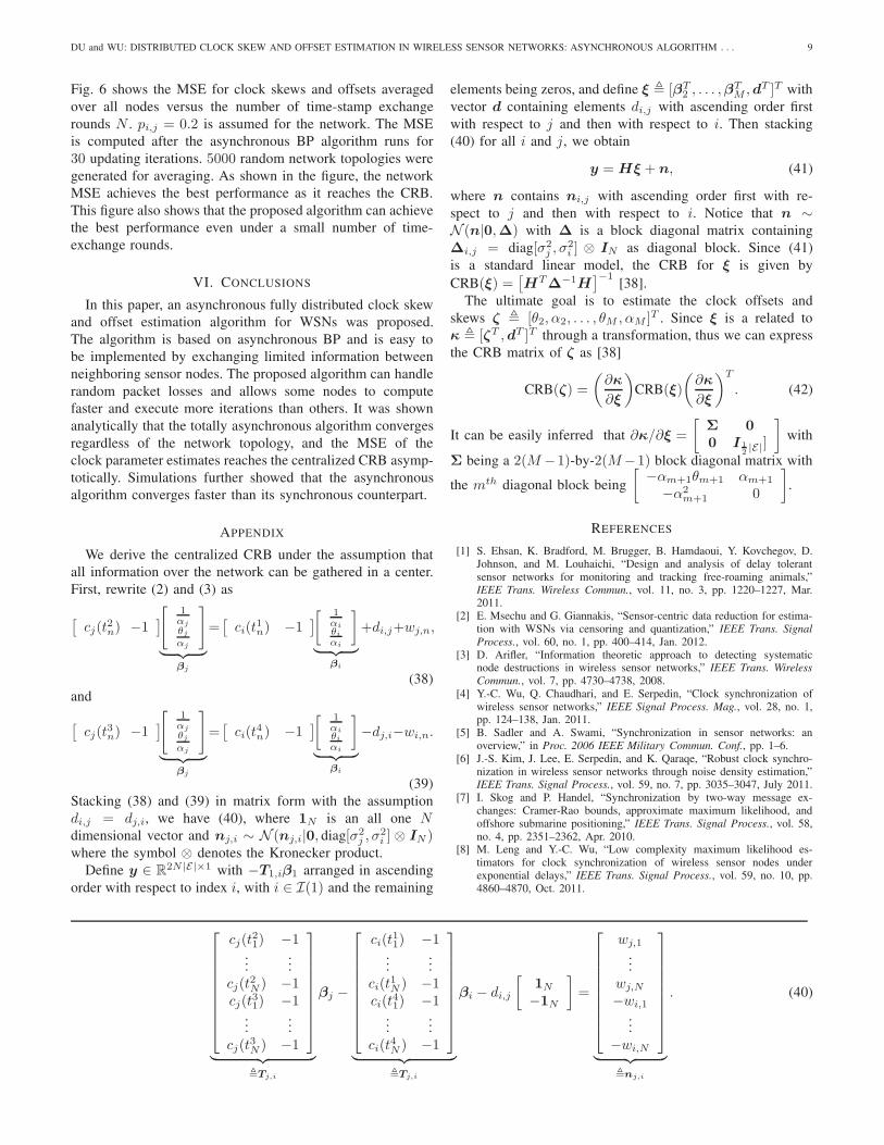
DU and WU: DISTRIBUTED CLOCK SKEW AND OFFSET ESTIMATION IN WIRELESS SENSOR NETWORKS: ASYNCHRONOUS ALGORITHM . . . 3

zj,i ∼ N (zj,i|0, σ2i,jIN ), where σ2

i,j = σ2i + σ2

j . The goal isto establish global synchronization (i.e., estimate αi and θi ineach node) based on the local observations Aj,i and Ai,j .

III. ASYNCHRONOUS DISTRIBUTED ESTIMATION

In this section, the asynchronous distributed clock parameterestimation algorithm is derived based on BP. In the following,message exchange means BP message passing since two-waytime-stamp exchange has been completed.

A. BP Framework

For the reason that the established clock relationships duringtwo-way time-stamp exchanges involve interaction betweenneighboring nodes, the optimal clock estimate at each noderequires the marginalization of joint posterior distribution ofall βi, which is

gi(βi) ∝∫

...

∫ M∏i=1

p(βi)∏

{i,j}∈Ep(Ai,j ,Aj,i|βi,βj)

dβ1...dβi−1dβi+1dβM ,

(5)

where p(βi) is the prior distribution of βi;p(Ai,j ,Aj,i|βi,βj) = N (Aj,iβj |Ai,jβi, σ

2i,jIN ) is the

likelihood function obtained from (4). Node 1 is assumedto be the reference node with p(β1) = δ(β1 − [1, 0]T ), andits parameters need not to be estimated. The computationof gi(βi) in (5) needs to gather all information in a centralprocessing unit. Besides, for the arbitrary network topology,the corresponding |V| and |E| can be very large leading tothe computationally demanding integration (5).

Although the joint posterior distribution of β1, . . . ,βM

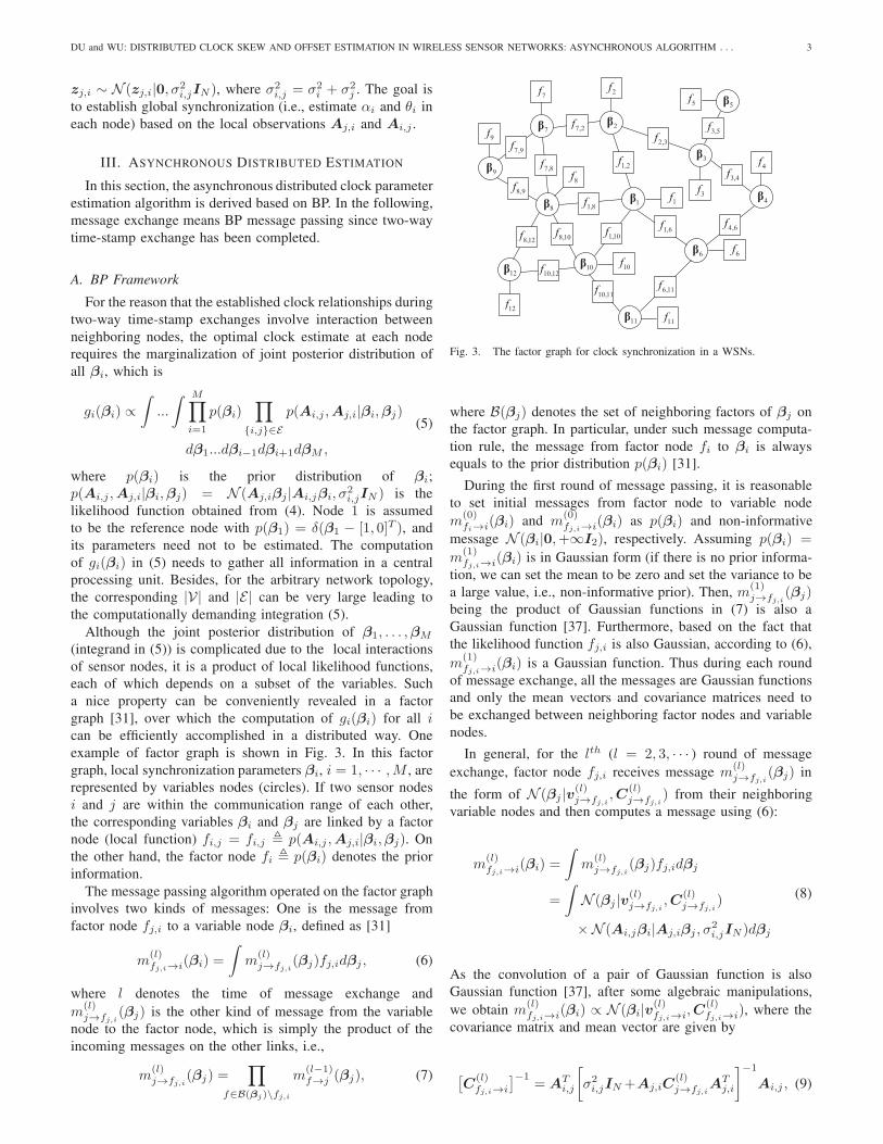
(integrand in (5)) is complicated due to the local interactionsof sensor nodes, it is a product of local likelihood functions,each of which depends on a subset of the variables. Sucha nice property can be conveniently revealed in a factorgraph [31], over which the computation of gi(βi) for all ican be efficiently accomplished in a distributed way. Oneexample of factor graph is shown in Fig. 3. In this factorgraph, local synchronization parameters βi, i = 1, · · · ,M , arerepresented by variables nodes (circles). If two sensor nodesi and j are within the communication range of each other,the corresponding variables βi and βj are linked by a factornode (local function) fi,j = fi,j � p(Ai,j ,Aj,i|βi,βj). Onthe other hand, the factor node fi � p(βi) denotes the priorinformation.

The message passing algorithm operated on the factor graphinvolves two kinds of messages: One is the message fromfactor node fj,i to a variable node βi, defined as [31]

m(l)fj,i→i(βi) =

∫m

(l)j→fj,i

(βj)fj,idβj , (6)

where l denotes the time of message exchange andm

(l)j→fj,i

(βj) is the other kind of message from the variablenode to the factor node, which is simply the product of theincoming messages on the other links, i.e.,

m(l)j→fj,i

(βj) =∏

f∈B(βj)\fj,im

(l−1)f→j (βj), (7)

1

6

5

2

1f

3

4

2,3f

1,2f3,4f

1,6f 4,6f

3,5f7

10

8

9

11

1,10f8,10f

1,8f

10,11f 6,11f

8,9f7,8f

7,9f7,2f

12 10,12f

8,12f

5f

4f

2f7f

9f

6f

11f

10f

12f

8f3f

Fig. 3. The factor graph for clock synchronization in a WSNs.

where B(βj) denotes the set of neighboring factors of βj onthe factor graph. In particular, under such message computa-tion rule, the message from factor node fi to βi is alwaysequals to the prior distribution p(βi) [31].

During the first round of message passing, it is reasonableto set initial messages from factor node to variable nodem

(0)fi→i(βi) and m

(0)fj,i→i(βi) as p(βi) and non-informative

message N (βi|0,+∞I2), respectively. Assuming p(βi) =

m(1)fj,i→i(βi) is in Gaussian form (if there is no prior informa-

tion, we can set the mean to be zero and set the variance to bea large value, i.e., non-informative prior). Then, m(1)

j→fj,i(βj)

being the product of Gaussian functions in (7) is also aGaussian function [37]. Furthermore, based on the fact thatthe likelihood function fj,i is also Gaussian, according to (6),m

(1)fj,i→i(βi) is a Gaussian function. Thus during each round

of message exchange, all the messages are Gaussian functionsand only the mean vectors and covariance matrices need tobe exchanged between neighboring factor nodes and variablenodes.

In general, for the lth (l = 2, 3, · · · ) round of messageexchange, factor node fj,i receives message m

(l)j→fj,i

(βj) in

the form of N (βj |v(l)j→fj,i

,C(l)j→fj,i

) from their neighboringvariable nodes and then computes a message using (6):

m(l)fj,i→i(βi) =

∫m

(l)j→fj,i

(βj)fj,idβj

=

∫N (βj |v(l)

j→fj,i,C

(l)j→fj,i

)

×N (Ai,jβi|Aj,iβj , σ2i,jIN )dβj

(8)

As the convolution of a pair of Gaussian function is alsoGaussian function [37], after some algebraic manipulations,we obtain m

(l)fj,i→i(βi) ∝ N (βi|v(l)

fj,i→i,C(l)fj,i→i), where the

covariance matrix and mean vector are given by

[C

(l)fj,i→i

]−1= AT

i,j

[σ2i,jIN +Aj,iC

(l)j→fj,i

ATj,i

]−1

Ai,j , (9)



and

v(l)fj,i→i =C

(l)fj,i→iA

Ti,jAj,i

{AT

j,iAj,i + σ2i,j

[C

(l)j→fj,i

]−1}−1

× [C

(l)j→fj,i

]−1v(l)j→fj,i

.

(10)

On the other hand, using (7), the message passed from thevariable node to the factor node is given by the product ofGaussian distributions, which is

m(l)j→fj,i

(βj) =∏

f∈B(βj)\fj,im

(l−1)f→j (βj)

∝ N (βj |v(l)j→fj,i

,C(l)j→fj,i

),

(11)

where [C

(l)j→fj,i

]−1 =∑

f∈B(βj)\fj,i

[C

(l−1)f→j

]−1(12)

and

v(l)j→fj,i

= C(l)j→fj,i

∑f∈B(βj)\fj,i

[C

(l−1)f→j

]−1v(l−1)f→j .(13)

Furthermore, during each round of message passing, eachnode can compute the belief for βi as the product of all theincoming messages from neighboring factor nodes, which isgiven by

b(l)(βi) =∏

f∈B(βi)

m(l−1)f→i (βi). (14)

According to (9), (10) and (14), we can easily obtain (15) atthe bottom of this page. Finally, the estimate of βi in the lth

iteration is (16).

B. Asynchronous Message Update

In practical WSNs, there is neither factor nodes norvariable nodes. These two kinds of messages m

(l)j→fj,i

(βj)

and m(l)fj,i→i(βi) are computed locally at node j, and only

m(l)fj,i→i(βi) is sent from node j to node i during each round of

message exchange of BP. Let m(l)j→i(βi) = N (βi|γ(l)

j→i,Γ(l)j→i)

represent the physical message from node j to node i. Putting(12) and (13) into (9) and (10), we have (17) and (18), whereΓj and γj are the covariance matrix and mean vector of priordistribution of βj , respectively, and they will never changeduring the updating process.

As shown in (17) and (18), from the perspective of node j,the outgoing message covariance Γ

(l)j→i and mean vector γ(l)

j→i

computed by node j at time l depends on the incoming mes-sage covariance Γ

(l−1)k→j and γ

(l−1)k→j from node j’s neighbour

(i.e., k ∈ I(j) \ i) at time l− 1. However, in many situations,the inter-sensor message exchange is possibly asynchronousdue to random data packet dropouts, and different nodes mayupdate their messages at different frequencies. If every nodeis allowed to update its belief only after receiving updatedmessages from all its neighbors, the convergence speed ofthe distributed algorithm would be slow. Thus, some nodesshould be allowed to update their beliefs more frequentlythan others, as long as they receive some of the updates fromtheir neighboring nodes within a predetermined time period.It means that when node j computes Γ

(l)j→i, it may only have

Γ(s)k→j computed by node k ∈ I(j)\i with s ≤ l−1. In order to

capture these asynchronous properties of message exchanges,we introduce the totally asynchronous model [32] as follows.

Let the message covariance matrices and mean vectors

available to node j at time l are Γ(τk

j (l−1))

k→j and γ(τk

j (l−1))

k→j ,where 0 � τkj (l − 1) � l − 1. Without loss of generality,we assume that node j computes its outgoing messagesto its neighboring nodes according to a discrete time setLj ⊆ {0, 1, 2, . . .}. According to (17) and (18), the asyn-chronous message covariance and mean evolution are definedas (19) and (20) at the bottom of the next page. We assumeliml→∞ τkj (l) = ∞ for all {k, j} ∈ E , which guaranteesthat old information is eventually purged out of the network,and that each node eventually exchanges messages with itsneighboring nodes.

The asynchronous iterative algorithm is summarized as

b(l)(βi) ∼ N (βi|[ ∑f∈B(βi)

[C

(l−1)f→i

]−1]−1 ∑f∈B(βi)

[C

(l−1)f→i

]−1v(l−1)f→i ,

[ ∑f∈B(βi)

[C

(l−1)f→i

]−1]−1). (15)

β(l)i =

∫βib

(l)(βi)dβi =[ ∑f∈B(βi)

[C

(l−1)f→i

]−1]−1 ∑f∈B(βi)

[C

(l−1)f→i

]−1v(l−1)f→i . (16)

[Γ(l)j→i

]−1= AT

i,j

[σ2i,jIN +Aj,i

[Γ−1j +

∑k∈I(j)\i

[Γ(l−1)k→j

]−1]−1

ATj,i

]−1

Ai,j . (17)

γ(l)j→i = Γ

(l)j→iA

Ti,j

[σ2i,jIN +Aj,i

[Γ−1j +

∑k∈I(j)\i

[Γ(l−1)k→j

]−1]−1

ATj,i

]−1

(18)

×Aj,i

[Γ−1j +

∑k∈I(j)\i

[Γ(l−1)k→j

]−1]−1[

Γ−1j γj +

∑k∈I(j)\i

[Γ(l−1)k→j

]−1γ(l−1)k→j

],



follows. The algorithm is started by setting the messagesfrom node j to node i as m

(0)j→i(βi) = N (βi;0,+∞I2)

1. Each node i computes its outgoing message according to(19) and (20) at independent time l ∈ Li with its available[Γ(τ j

i (l−1))j→i

]−1and γ

(τ ji (l−1))

j→i . The corresponding belief ofnode i at time l is computed as

b(l)(βi) ∼ N (βi|μ(l)

i ,P(l)i

), (21)

where the belief covariance matrix is

P(l)i =

[Γ−1i +

∑j∈I(i)

[Γ(τ j

i (l−1))j→i

]−1]−1

, (22)

and mean vector is

μ(l)i = P

(l)i

[Γ−1i γi +

∑j∈I(i)

[Γ(τ j

i (l−1))j→i

]−1γ(τ j

i (l−1))j→i

]. (23)

The iterative computation terminates when (21) convergesor the maximum number of iterations is reached. Then eachsensor computes its clock skew and offset according to

αi = 1/μ(l)i (1), θi = μ

(l)i (2)/μ

(l)i (1), (24)

where μ(l)i (k) denotes the kth element of μ(l)

i .

IV. ASYNCHRONOUS BP CONVERGENCE ANALYSIS

It is important to note that the BP message updates (8) and(11) are specially designed for the computation of marginalfunctions (e.g., gi(βi) in (5)) on cycle-free FG and it isknown that the beliefs will converge to the exact marginalfunctions. On the other hand, the BP algorithm may be appliedto FG with cycles, but since messages will be passed multipletimes on a given edge, no convergence can be guaranteed[34]. Although some of the most exciting applications ofBP algorithm like the decoding of turbo codes and low-density parity-check codes [31] do not exhibit divergence inthe simulations even under loopy FG, there are still manyapplications where BP do diverge. General sufficient conditionfor convergence of loopy FGs is available in [35] but itrequires the knowledge of the joint posterior distribution of

1Since the message updating using (19) and (20) only involves inverse ofcovariance matrix, in practice, we can set the inverse of the initial covariancematrix as 0.

all unknown variables as shown in the integrand of (5),and is difficult to verify for large-scale dynamic networks.Reference [29] proved the convergence of BP in the contextof distributed clock offset synchronization, by exploiting thePerron-Frobenius theorem in the context of matrices withnonnegative elements. However, in the vector variable case(both clock skew and offset), the BP message covariancematrices contain negative elements, and the analysis in [29] isnot applicable. Besides, the effect of asynchronous message-update was not addressed in [29]. In the following, we willprove the convergence of asynchronous vector BP messagesin distributed clock synchronization.

Defining the operator Fj→i(·) corresponding to the updateof the message covariance in (19), the following properties arefirst established.

Lemma 1. The updating operator Fj→i(·) satisfies thefollowing properties:Property i): Fj→i(0) = 0.Property ii): Fj→i(X) � 0, if X � 0.Property iii): Fj→i(X) � Fj→i(Y ), if X � Y � 0.Proof : Property i) is apparent according to (19). The proof ofproperty ii) is given as follows. Let X � 0, it is obviousthat X−1 � 0, which means yTX−1y ≥ 0 for any y.Putting y = AT

j,ix, we have xTAj,iX−1AT

j,ix ≥ 0. Assum of positive definite and positive semi-definite matricesis positive definite, we have

[σ2i,jIN +Aj,iX

−1ATj,i

]−1 � 0.Since Ai,j is of full column rank, we obtain AT

i,j

[σ2i,jIN +

Aj,iX−1AT

j,i

]−1Ai,j � 0. Thus, property ii) is proved.

For the proof of property iii), let X � Y � 0, thenwe have Y −1 − X−1 � 0 [39], which means yT (Y −1 −X−1)y ≥ 0 for any y. Let y = AT

j,ix, we havexTAj,iY

−1ATj,ix ≥ xTAj,iX

−1ATj,ix. Hence, we have[

σ2i,jIN + Aj,iX

−1ATj,i

]−1 � [σ2i,jIN + Aj,iY

−1ATj,i

]−1.

Due to the fact that Ai,j is of full column rank, wehave AT

i,j

[σ2i,jIN + Aj,iX

−1ATj,i

]−1Ai,j � AT

i,j

[σ2i,jIN +

Aj,iY−1AT

j,i

]−1Ai,j , which is equivalent to Fj→i(X) �

Fj→i(Y ). �To consider the updates of all message covariance matri-

ces, we introduce the following definitions. Let Ξ(τ(l−1)) �[[Γ

(τ1k(l−1))

1→k ]−1; . . . ; [Γ(τ j

i (l−1))j→i ]−1; . . . ; [Γ

(τrM (l−1))

r→M ]−1;Γ−11 ;

. . . ;Γ−1M

]be the collection of all available message covariance

[Γ(l)j→i

]−1=

⎧⎪⎪⎪⎪⎪⎨⎪⎪⎪⎪⎪⎩

ATi,j

[σ2i,jIN +Aj,i

[Γ−1j +

∑k∈I(j)\i

[Γ(τk

j (l−1))

k→j

]−1]−1

ATj,i

]−1

Ai,j

︸︷︷︸�Fj→i

(Γ−1

j +∑

k∈I(j)\i[Γ

(τkj

(l−1))

k→j

]−1), l ∈ Lj ,

[Γ(l−1)j→i

]−1, otherwise.

(19)

γ(l)j→i =

⎧⎪⎪⎪⎪⎪⎨⎪⎪⎪⎪⎪⎩

Γ(l)j→iA

Ti,j

[σ2i,jIN+Aj,i

[Γ−1j +

∑k∈I(j)\i

[Γ(τk

j (l−1))

k→j

]−1]−1

ATj,i

]−1

Aj,i

×[Γ−1j +

∑k∈I(j)\i

[Γ(τk

j (l−1))

k→j

]−1]−1[

Γ−1j γj+

∑k∈I(j)\i

[Γ(τk

j (l−1))

k→j

]−1γ(τk

j (l−1))

k→j

], l ∈ Lj ,

γ(l−1)j→i , otherwise.

(20)



(including prior covariance) matrices in the network at timel, and Ξ(l) �

[[Γ

(l)1→k]

−1; . . . ; [Γ(l)j→i]

−1; . . . ; [Γ(l)r→M ]−1

]be

the collection of all outgoing message covariances in thenetwork at time l. Define Ξ(l) �b 0 if its component[Γ

(l)j→i]

−1 � 0; and Ξ(l) �b Ξ(l−1) if their corresponding

components satisfy [Γ(l)j→i]

−1 � [Γ(l−1)j→i ]−1. The same defi-

nitions apply to Ξ(τ(l)). Furthermore, we define the functionF � (F1→k, . . . ,Fj→i, . . . ,Fr→M ) which satisfies Ξ(l+1) =F(Ξ(τ(l))). Then we have the following lemma.

Lemma 2. Ξ(l) and Ξ(τ(l−1)) satisfy the following proper-ties:Property iv): If Ξ(l) �b Ξ(l−1), then Ξ(τ(l)) �b Ξ(τ(l−1)).Property v): If Ξ(τ(l)) �b Ξ(τ(l−1)), then F(Ξ(τ(l))) �b

F(Ξ(τ(l−1))) or equivalently Ξ(l+1) �b Ξ(l).Proof : The proofs of properties iv) and v) rest on the basicdefinitions that [Γ

(l)j→i]

−1 represents the message covariance

matrix sends from node j to node i at time l, and [Γ(τ(l))j→i ]−1

represents message covariance matrix received by node i attime l. If [Γ

(l)j→i]

−1 � [Γ(l−1)j→i ]−1, it is obvious that the

received covariance will satisfy [Γ(τ(l))j→i ]−1 � [Γ

(τ(l−1))j→i ]−1.

Since Ξ(l) and Ξ(τ(l)) contain [Γ(l)j→i]

−1 and [Γ(τ(l))j→i ]−1 as

components respectively, property iv) is obvious. On the otherhand, property v) is apparent since each of the correspondingcomponents in Ξ(τ(l)) and Ξ(τ(l−1)) satisfies property i) oriii) in Lemma 1. �

Now we present the convergence property of the covariancematrix in the local beliefs.

Theorem 1. For the totally asynchronous clock synchro-nization algorithm, the covariance matrix P

(l)i of belief

b(l)i (βi) at each node converges to a positive definite matrix

regardless of network topology.Proof : Initially, all messages are non-informative, that is,Γτ(−1)j→i = Γ

(0)j→i = ∞I2. From (19), properties i)

and ii), we obtain that[Γ(l)j→i

]−1 � 0 only if Γ−1j +∑

k∈I(j)\i[Γ(τk

j (l−1))

k→j

]−1 � 0. Therefore, the first batch

of nodes having outgoing covariance[Γ(l)j→i

]−1 � 0 musthave Γ−1

j � 0, i.e., informative prior. Let the first messageupdating event in the network occurs at time s. We haveΞ(s) �b Ξ(s−1). Applying property iv), we further obtainΞτ(s) �b Ξτ(s−1).

Suppose Ξ(τ(l)) �b Ξ(τ(l−1)) for l ≥ s, according toproperty v), Ξ(l+1) �b Ξ(l). Thus Ξ(τ(l+1)) �b Ξ(τ(l)) forl ≥ s due to property iv). Hence, by induction the updating

relationship of Ξ(τ(l)) is

. . . �b Ξ(τ(l)) . . . �b Ξ(τ(s)) �b 0. (25)

Focusing on node i, we obtain

. . . � Γ−1i +

∑

j∈I(i)

[Γ

(τji(l))

j→i

]−1. . . � Γ−1

i +∑

j∈I(i)

[Γ

(τji(s))

j→i

]−1.

(26)Since a strongly connected network is considered, there

must be one of [Γ(τ j

i (l′−1))

j→i ]−1 � 0 for some l′ ≥ s,and therefore (26) is lower bounded by the all-zero matrix.

Furthermore, since ∞I2 � Γ−1j +

∑k∈I(j)\i

[Γ(τk

j (l−1))

k→j

]−1,

according to property iii), Fj→i

(∞I2) � Fj→i

(Γ−1j +∑

k∈I(j)\i[Γ(τk

j (l−1))

k→j

]−1). Using the definition of Fj→i(·)

in (19), this is equivalent to 1σ2i,jAT

i,jAi,j � [Γ(τ j

i (l))j→i

]−1.

Therefore, we can add an upper bound to (26) and obtain (27).Then, applying matrix inverse to (27) and using the definitionof P (l)

i in (22) results in

P(l′)i � P

(l′+1)i � . . . � [

Γ−1i +

∑j∈I(i)

1

σ2i,j

ATi,jAi,j

]−1 � 0,

(28)where the inequality relationship is due to the fact that ifX,Y � 0 and X � Y , then Y −1 � X−1 [39]. Conse-quently, such non-increasing positive definite matrix sequenceP

(l)i in (28) converges to a positive definite matrix [40]. �The importance of Theorem 1 is that the covariance matrices

of belief always converge regardless of network topology aslong as informative prior exists. Next, we show the conver-gence of belief mean vectors.

Theorem 2. For the totally asynchronous clock synchro-nization algorithm, the mean vector μ(l)

i of the belief b(l)(βi)converges to a constant vector regardless of the networktopology.Proof : From (25) in the proof of Theorem 1, we can readily

see that Γ(τk

j (l))

k→j satisfies: . . . � [Γ(τk

j (l))

k→j ]−1 � . . . �[Γ

(τkj (s))

k→j ]−1 � 0. If there is a path from any node withinformative prior to node k, according to property ii), there

must be a time instant l′ after which . . . � [Γ(τk

j (l′+1))

k→j ]−1 �. . . � [Γ

(τkj (l′))

k→j ]−1 � 0. Hence Γ(τk

j (l′))k→j is convergent [40].

On the other hand, if there is no path from any node with

informative prior to node k, we have . . . = [Γ(τk

j (l))

k→j ]−1 =

. . . = [Γ(τk

j (0))

k→j ]−1 = 0. Either case implies Γ(τk

j (l))

k→j converges

Γ−1i +

∑j∈I(i)

1

σ2i,j

ATi,jAi,j � . . . � Γ−1

i +∑

j∈I(i)

[Γ(τ j

i (l′+1))

j→i

]−1 � Γ−1i +

∑j∈I(i)

[Γ(τ j

i (l′))

j→i

]−1 � 0. (27)

γ(l)j→i =

⎧⎪⎪⎪⎪⎪⎨⎪⎪⎪⎪⎪⎩

Γ(∗)j→iA

Ti,j

[σ2i,jIN +Aj,i

[Γ−1j +

∑k∈I(j)\i

[Γ(∗)k→j

]−1]−1

ATj,i

]−1

Aj,i

×[Γ−1j +

∑k∈I(j)\i

[Γ(∗)k→j

]−1]−1[

Γ−1j γj +

∑k∈I(j)\i

[Γ(∗)k→j

]−1γ(τk

j (l−1))

k→j

], l ∈ Lj ,

γ(l−1)j→i , otherwise.

(29)



to a matrix Γ(∗)k→j . From (19), if Γ

(τkj (l))

k→j converges, we have

Γ(l)j→i also converges to a fixed matrix Γ

(∗)j→i. Then, (20) can

be rewritten as (29). Without loss of generality, define γ(l)

as a vector containing all γj and outgoing message meanγ(l)j→i with ascending index first on j and then on i (γj can

be interpreted as γj→j for the ordering), and γ(l−1) is thevector constituted by available message means with the sameordering. It should be noticed that the order of γ(l)

j→i arrangedin γ(l) can be arbitrary as long as it does not change after theorder is fixed. Then, (29) can be expressed as

γ(l) = Q(l)γ(l−1), (30)

where the specific structure of Q(l) depends on the messagessent and received at time l. Notice that Q(l) is time-varyingdue to asynchronous updating. The convergence condition forthe asynchronous system (30) turns out to be related to thesystem matrix of the corresponding synchronous system [32,p. 434], [33, p. 14]. Consider Lj = {0, 1, 2, . . .} for allj = 1, 2, . . . ,M , the asynchronous system (30) becomes asynchronous one:

γ(l) = Qγ(l−1), (31)

where Q is now independent of iteration number l. The neces-sary and sufficient convergence condition for the asynchronousiteration (30) is ρ(|Q|) < 1 [32, p. 434], where |Q| denotesthe matrix whose elements are the absolute values of those inQ. Next, we prove that ρ(|Q|) < 1.

First, construct the new linear iteration as

x(r) = Qx(r−1), (32)

where Q = |Q|, x(r) is a vector with the same structure asγ(r) and x(0) = γ(0). Since there is always a positive valueη, satisfying η >

∑i�=j |[Q]i,j | for all i, we have ηI + Q is

strictly diagonally dominant and then ηI + Q is nonsingular[41]. Hence, the arbitrary initial value x(0) can be expressedin terms of the eigenvectors of ηI+ Q as x(0) =

∑Dd=1 cdqd,

where D is the dimension of matrix Q and q1, q2,· · · , qD arethe eigenvectors of ηI+ Q. Since the eigenvectors of ηI+ Qare the same as those of Q, and the eigenvalues of ηI + Qare η + λd (1 � d � D), where λd is the eigenvalue of Q,we have

x(r) = Qrx(0) =

D∑d=1

cdλrdqd. (33)

Without loss of generality, suppose λd are arranged in de-scending order as

|λ1| ≥ |λ2| ≥ · · · ≥ |λD|. (34)

Let the eigenvalue with the largest magnitude has a multiplic-ity of d0. Then λd/λ1 < 1 for d > d0 and (λd/λ1)

r = 0 if ris large enough. We then obtain

limr→∞x(r) = λr

1

d0∑d=1

cdqd. (35)

On the other hand, putting j = 1 into (19), and notingΓ−11 = ∞I2, we obtain [Γ

(l)1→i]

−1 = 1σ2i,1

ATi,1Ai,1, for

l ∈ Li. But since this outgoing covariance from the reference

node is independent of time l, we can combine the twocases in (19). Substituting this result into (20), we haveγ(l)1→i =

1σ2i,1

[AT

i,1Ai,1

]−1AT

i,1A1,iβ1, which shows that γ(l)1→i

is also independent of time l. Consequently, according to(31), γ

(l)1→i = [Q]1:2,1:Dγ(l−1) and [Q]1:2,1:D = [I2,0].

Hence, |[Q]1:2,1:D|x(0) = x(0)1→i = x

(1)1→i. In general, we

also have x(r)1→i = x

(0)1→i for all r. Therefore, we can put

x(r)(mi) = γ(l)1→i � ξc being a constant into (35) to obtain

λr1 = ξc

∑d0d=1 cdqd(mi)

for r large enough. Substituting it back

into (35) yields

limr→∞x(r) =

ξc∑d0

d=1 cdqd∑d0

d=1 cdqd(mi). (36)

It is obvious that x(r) does not change when r is large enough,and therefore, x(r) in (32) converges. Hence, the spectrumradius ρ(Q) = ρ(|Q|) < 1 [42], and according to [32, p.434], the asynchronous version of the iteration given by (30)converges. Finally, with μ

(l)i defined in (23), since P

(l)i , Γ(l)

j→i

and γ(l)j→i converge, we can draw the conclusion that the vector

sequence {μ(1)i ,μ

(2)i , . . .} converges. �

Theorems 1 and 2 reveal that the BP messages converge.Next, we address how good is the clock parametersestimate (24) based on the converged message meanμ∗

i = liml→+∞ μ(l)i . Since the prior p(βi) and likelihood

function p(Ai,j ,Aj,i|βi,βj) are both Gaussian distributionand it is known that if Gaussian BP (synchronous orasynchronous) converges, the means of the beliefscomputed by BP equal the means of the marginalposterior distribution [35], [36], i.e., μ∗

i = βMMSEi �∫ · · · ∫ βip

(β1,β2, . . . ,βM |{Ai,j}{i,j}∈E

)dβ2 · · · dβM .

Stacking βMMSEi into a block vector βMMSE =

[(βMMSE2 )T , . . . , (βMMSE

M )T ]T gives

βMMSE =

∫...

∫[βT

2 , . . . ,βTM ]T

× p(β1,β2, . . . ,βM |{Ai,j}{i,j}∈E

)dβ2 . . . dβM .

(37)

It is obvious that μ∗ =[(μ∗

2)T , . . . , (μ∗

M )T]T

equals thecentralized joint MMSE estimator βMMSE. In case of non-informative prior, βMMSE is the mean of the joint likelihoodfunction. Since the mean and maximum of a Gaussian distri-bution are the same, μ∗ equals the centralized joint maximumlikelihood (ML) estimator under non-informative prior.

Theorem 3. Under non-informative prior of βi, theMSE of the estimator [ 1

μ∗2(1)

,μ∗

2(2)μ∗

2(1), . . . , 1

μ∗M (1) ,

μ∗M (2)

μ∗M (1) ]

T ob-tained from the converged BP message mean vectors μ∗

i

asymptotically approaches the centralized CRB of ζ =[θ2, α2, . . . , θM , αM ]T , where the CRB is given by (42) inthe Appendix.Proof : As discussed after (37), under non-informativeprior, μ∗ equals the centralized joint ML estimatorof [βT

2 , . . . ,βTM ]T . Due to βi = [ 1

αi, θiαi]T and

from the invariance property of ML estimator [38],[ 1μ∗

2(1),μ∗

2(2)μ∗

2(1), . . . , 1

μ∗M (1) ,

μ∗M (2)

μ∗M (1) ]

T is the ML estimator

of ζ = [θ2, α2, . . . , θM , αM ]T , with the corresponding MSE



0 5 10 15 20 25 30 35 40 45 50 5510

−8

10−7

10−6

10−5

10−4

10−3

Updating time

MSE

of

cloc

k sk

ew

Synchronous BP pi, j

= 0.99

Asynchronous BP pi, j

= 0.2


= 0.99

Centralized CRB

Node index = 5

Node index = 19

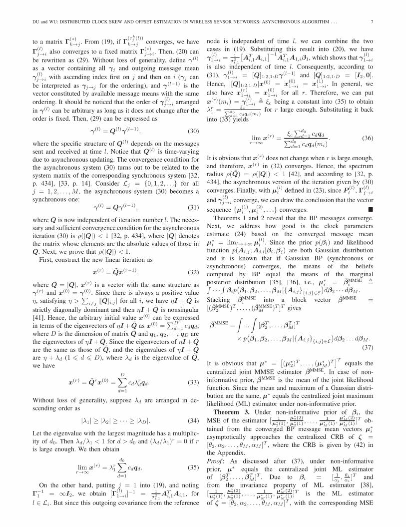
Fig. 4. Convergence performance of estimated clock skew at two nodes.

asymptotically approaches the centralized CRB of ζ derivedin (42) in the Appendix. �

Synchronous message updating, i.e., L1 = . . . = LM andτkj (l−1) = l−1, is obviously a special case of (19) and (20).Hence, Theorem 1, Theorem 2 and Theorem 3 also apply tothe synchronous BP.

V. SIMULATION RESULTS

This section presents numerical results to assess the per-formance of the proposed algorithm. Simulation results ofestimation mean-square-error (MSE) are presented for randomnetworks with 25 nodes randomly located in an area ofsize [0, 300] × [0, 300]. Each node can only communicatewith the sensor nodes that are within its radio range, whichis assumed to be 90. In each simulation, clock skews αi

and clock offsets θi are uniformly distributed in the range[−0.945, 1.055] and [−5.5, 5.5], respectively. The fixed delaydi,j is uniformly distributed in [8, 12] and variance of randomdelay σ2

i = 0.05 is assumed to be identical for all nodes.5000 Monte-carlo simulation trials were performed to obtainthe average performance of each point in all the figurespresented in this section. Without loss of generality, Node1 is selected as the reference node with β1 = [1, 0]T , andp(β1) = δ(β1− [1, 0]T ). For the other nodes, non-informativeprior is assumed p(βi) = N (βi;0,+∞I2). The probabilityof node i successfully pass a message to its direct neighboringnode j is pi,j for {i, j} ∈ E . With pi,j �= 1, we can emulatean asynchronous network. To serve as a reference of thedistributed estimation performance, the CRB for centralizedestimation is derived in the Appendix.

Fig. 4 shows the MSE of the clock skew estimations innodes 19 and 5 as a function of updating time {0, 1, 2, . . .}for the topology of WSN shown in Fig. 1. The number oftime-stamp exchange rounds is N = 20 at the beginning.Synchronous schedule, asynchronous schedule and centralizedCRB are plotted for comparison. The synchronous algorithmcan only be updated when each node has successfully receivedupdated messages from all its neighboring nodes. It can beseen from the figure that for both synchronous and asyn-chronous algorithms, MSEs touch the corresponding CRBs,

0 5 10 15 20 25 30 35 40 45 50 5510- 4

10- 3

10- 2

10- 1

100

101

102

Updating time

MSE

of c

lock

offs

et

Synchronous BP pi, j= 0.99Asynchronous BP pi, j=0.2Asynchronous BP pi, j= 0.99Centralized CRB

Node index = 5

Node index = 19

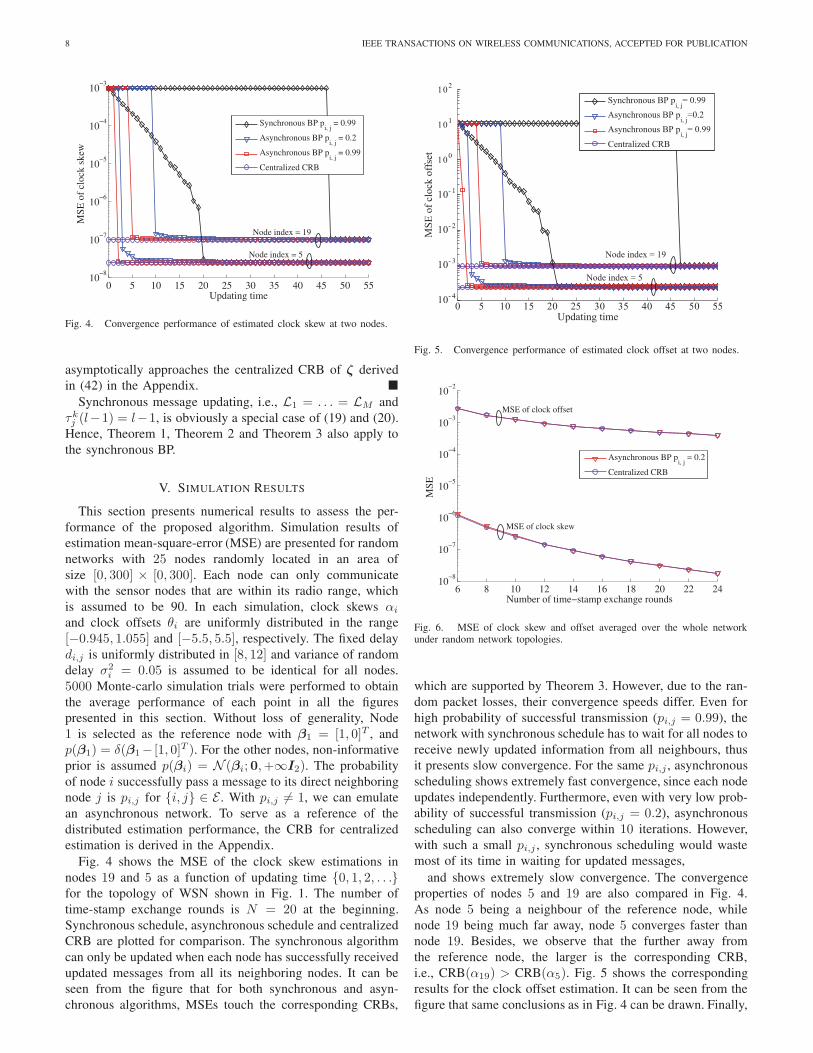
Fig. 5. Convergence performance of estimated clock offset at two nodes.

6 8 10 12 14 16 18 20 22 2410

−8

10−7

10−6

10−5

10−4

10−3

10−2

Number of time−stamp exchange round

MSE


= 0.2

Centralized CRB

MSE of clock skew

MSE of clock offset

s

Fig. 6. MSE of clock skew and offset averaged over the whole networkunder random network topologies.

which are supported by Theorem 3. However, due to the ran-dom packet losses, their convergence speeds differ. Even forhigh probability of successful transmission (pi,j = 0.99), thenetwork with synchronous schedule has to wait for all nodes toreceive newly updated information from all neighbours, thusit presents slow convergence. For the same pi,j , asynchronousscheduling shows extremely fast convergence, since each nodeupdates independently. Furthermore, even with very low prob-ability of successful transmission (pi,j = 0.2), asynchronousscheduling can also converge within 10 iterations. However,with such a small pi,j , synchronous scheduling would wastemost of its time in waiting for updated messages,

and shows extremely slow convergence. The convergenceproperties of nodes 5 and 19 are also compared in Fig. 4.As node 5 being a neighbour of the reference node, whilenode 19 being much far away, node 5 converges faster thannode 19. Besides, we observe that the further away fromthe reference node, the larger is the corresponding CRB,i.e., CRB(α19) > CRB(α5). Fig. 5 shows the correspondingresults for the clock offset estimation. It can be seen from thefigure that same conclusions as in Fig. 4 can be drawn. Finally,


Documents

Distributed Clock Skew and Offset Estimation in Wireless Sensor