Diversification, Cost Structure, and the Risk Premium of

Multinational Corporations∗

Jose L. Fillat†

Federal Reserve Bank of Boston

Stefania Garetto‡

Boston University

Lindsay Oldenski§

Georgetown University

August 13, 2013

Abstract

This paper investigates theoretically and empirically the relationship between the geographicstructure of a multinational corporation and its risk premium. We use a structural model to iden-tify two main channels through which the countries in which a U.S.-based multinational operatesaffect the firm’s exposure to risk. On the one hand, multinational activity offers diversificationpotential, implying that the risk premium should be higher for firms operating in countries whereshocks are more correlated with those of the US. On the other hand, there is cash flow risk arisingfrom hysteresis and potential losses induced by fixed and sunk costs associated with entering andoperating in a new country. This implies that the risk should be greater for firms operating incountries that are more costly to enter. To identify these channels empirically, we merge Compus-tat/CRSP data on stock returns with the Bureau of Economic Analysis data on the operations ofmultinational corporations. Our empirical results confirm the predictions of the theory and delivera decomposition of firm-level risk premia into individual host countries contributions.Keywords: Multinational firms, diversification, risk premium, stock returns.JEL Classification: F14, F23, G12.

∗The statistical analysis of firm-level data on U.S. multinational companies was conducted at the Bureau of EconomicAnalysis, U.S. Department of Commerce under arrangements that maintain legal confidentiality requirements. The viewsexpressed are those of the authors and do not reflect official positions of the U.S. Department of Commerce. The authorswould like to thank William Zeile and Raymond Mataloni for assistance with the BEA data. We are also grateful toMaggie Chen, Simon Gilchrist, Eduardo Morales, Marc Muendler, Alan Spearot, and seminar participants at Columbia,EITI 2013 (Bangkok), SED 2013 (Seoul), SCIEA 2013, and WAITS 2013 for their helpful comments.

†Federal Reserve Bank of Boston, 600 Atlantic Avenue, Boston MA 02210. E-mail: Jose.Fillat@bos.frb.org. Theviews expressed in this paper are those of the authors and do not necessarily reflect those of the Federal Reserve Bankof Boston or Federal Reserve System.

‡Department of Economics, Boston University, 270 Bay State Road, Boston, MA 02215. E-mail: garettos@bu.edu.§Georgetown University, Intercultural Center 515, 37th and O Streets, NW Washington DC, 20057. E-mail:

lo36@georgetown.edu.

1

1 Introduction

In this paper we investigate the role of geography as a driver of risk. To do so, we analyze how the

geographical structure of a multinational corporation (henceforth, MNC) impacts its risk premium in

the stock market. Multinational corporations account for about half of the firms publicly listed in the

U.S., and have assets, operations, and sales in many countries. The pervasiveness of MNCs’ activities

implies that misunderstanding their exposure to risk can have costly implications for both investors

and policy makers.

Theoretically, the decisions of firms about which countries to enter affect the risk premium via two

channels: operating an affiliate in a foreign country induces diversification and reduces risk exposure,

but fixed operating costs and sunk entry costs generate leverage that increases risk exposure. In

equilibrium, risk averse agents require a risk premium that is higher the higher the risk exposure of

their investments.

Empirically, we focus on differences in risk premia across firms that differ in their geographical

structure. To do so, we exploit a rich firm-level dataset on MNCs with detailed information about

firms’ foreign operations, accounting, and financial markets data. We find that firms operating in

countries that co-move more with the US and in countries with higher fixed and sunk entry costs

exhibit systematically higher risk premia.

The theoretical underpinning of our analysis is a streamlined, multi-country version of the model

developed by Fillat and Garetto (2012), which links firms’ international activities with their stock

market returns.1 In the model, multinational activity offers diversification potential: if the business

cycles of two countries are not perfectly correlated, multinational sales diversify away the risk arising

from country-specific fluctuations and reduce firms’ returns in equilibrium. This mechanism, referred

to as the “diversification channel”, implies that, in equilibrium, MNCs should exhibit lower returns

than non-multinational firms – all else equal. Within multinationals, returns should be higher for

those firms operating in countries whose business cycles are more correlated with the US. Moreover,

the model introduces another channel of risk, arising from hysteresis and potential losses induced by

1Stock returns in excess of the risk-free rate define the risk premium of a firm.

2

sunk entry costs and fixed operating costs, which make firms leveraged. Firms open affiliates abroad

when prospects of growth make foreign operations profitable, but they must bear sunk entry costs to

open an affiliate, and fixed costs of production. If the host country is hit by a negative shock, the

affiliate may incur losses. The parent may find optimal not to exit the foreign market and bear those

losses for a while, in order not to forego the sunk cost it paid to enter. The higher the fixed and sunk

costs of production, the higher the potential losses and the longer the time for which a firm is willing

to bear them. These potential losses are perceived as a cash flow risk by the investors. This second

mechanism, that we refer to as the “fixed and sunk cost channel”, implies that MNCs with affiliates in

countries where entry is more costly and fixed operating costs are higher should exhibit higher stock

returns than MNCs with affiliates located in countries that are more easily and cheaply accessible.

Our empirical analysis exploits a rich firm-level dataset obtained by merging accounting and finan-

cial data from Compustat/CRSP with the Bureau of Economic Analysis (BEA) data on the operations

of multinational corporations. The data display a large amount of variation across MNCs in terms

of number, characteristics, and location of foreign affiliates, allowing us to study the cross-section of

returns of MNCs and to relate it to firm- and country-level characteristics.

We start with a reduced form specification whose goal is to explore the statistical relationship

between measures of diversification, entry costs, and returns. We use the correlations between the

GDP growth rates of the US and foreign affiliates’ host countries as our measure of diversification.

We proxy entry costs with country level data on the cost of starting a business from the World Bank’s

Doing Business database. The results of our regression analysis are consistent with the predictions of

the model: GDP growth correlations and entry costs in the countries in which firms have affiliates are

positively correlated with the returns that firms offer in the stock market.

Since the geographical structure of a firm is endogenous, we account for the impact that potential

activities in countries other than the ones currently served have on the returns of the firm (the option

value). To control for the contribution of the option value to stock returns, we follow a two-stage

approach. In the first stage, we estimate the probability that each firm will have an affiliate in each

country using standard predictors of FDI activity. In the second stage, we estimate the impact of

3

the characteristics of countries in which the firm has affiliates on annual returns, also controlling for

characteristics of the countries where the firm does not have any affiliates.

The results of the reduced form analysis are useful to illustrate the importance of GDP growth

correlations and sunk costs for the firms’ returns, but the estimated parameters do not have a structural

interpretation. For this reason, we also run regressions based on the structural equation that the model

delivers. The results of the structural specification allow us to decompose firm-level risk premia along

two dimensions. First, we compute the contribution of each host country to the risk premium. Second,

we can separate the contribution of option value versus assets in place in explaining stock returns.

The question of understanding why and how average stock returns vary across firms based on cer-

tain characteristics is central to the asset pricing literature.2 Nonetheless, very little empirical work

has been done on the returns of multinational corporations. Early research examined the returns of

MNCs to assess whether firms’ foreign activities provide diversification benefits to their stockholders.

Support for this “diversification hypothesis” is scarce: Jacquillat and Solnik (1978) regressed the re-

turns of multinationals from nine countries on a set of market indices and found that multinational

returns tended to covary most with the firm’s home market, hence not providing any evidence in sup-

port of diversification. Senchack and Beedles (1980) compared the risk, returns and betas of portfolios

of multinationals with portfolios of domestic and international equities and found that multinationals

did not deliver diversification benefits. Using a different methodology based on mean-variance span-

ning tests, Rowland and Tesar (2004) also found limited evidence of diversification benefits for MNCs.

More recently, using a sample of manufacturing firms from Compustat, Fillat and Garetto (2012) have

shown that the stock market returns of multinational corporations are systematically higher than the

stock market returns of non-multinational firms, also against what would be predicted by the diversi-

fication hypothesis. The structural model in Fillat and Garetto (2012) sheds light on this “puzzle” by

introducing another channel, the fixed and sunk cost channel, that increases the risk to which MNCs

are exposes compared to non-multinational firms and can potentially explain MNCs’ higher returns

2An extensive literature in finance has been investigating cross-sectional differences in stock returns across firms, assets,or portfolios, identifying several variables driving returns differentials. Fama and French (1996) provide comprehensiveevidence about returns differentials across portfolios formed according to particular characteristics like size and book-to-market.

4

and the lack of evidence of diversification.

This paper aims to deepen our understanding of the operations of multinational corporations

by examining the relationship between their geographical structure and their stock market returns.

As such, our analysis is related to an extensive literature on foreign direct investment, which has

documented important differences across firms in their choice of geographic locations,3 and to empirical

research using the BEA data on the operations of multinational corporations, starting with Kravis and

Lipsey (1982) and Brainard (1997), and more recently Yeaple (2003), Helpman, Melitz, and Yeaple

(2004), and Yeaple (2009). We contribute to this literature by providing more information on the

operations of MNCs from a financial markets perspective.4 The theoretical framework at the basis of

our empirical specifications builds on the literature on investment under uncertainty, particularly on

the real option value framework developed by Dixit (1989) and Dixit and Pindyck (1994) as applied

to the heterogeneous firms framework by Fillat and Garetto (2012).

Our work is also related to a strand of literature in corporate finance that studies the linkages

between international activity and stock market variables. Denis, Denis, and Yost (2002) find that

multinational corporations trade at a discount, and Baker, Foley, and Wurgler (2009) link empirically

market valuations, returns, and FDI activity. Our analysis departs from these contributions by taking

into account the full geographic structure of the firm as a determinant of stock returns, and by starting

from the predictions of a structural model to identify the economic forces that link MNCs’ structure

and stock returns in the data.

The rest of the paper is organized as follows. Section 2 lays out the theoretical model at the basis

of our empirical specification. Section 3 describes the financial data and the data on the operations

of multinational corporations. Section 4 presents our baseline empirical specification and results, and

Section 5 concludes. The derivation of the model and several robustness exercises are relegated to the

Appendix.

3See Helpman, Melitz, and Yeaple (2004), and more recently Yeaple (2009), Chen and Moore (2010), or Alfaro andChen (2013).

4Branstetter, Fisman, and Foley (2006) also merge the BEA data on the operations of US multinationals withCompustat data to examine the effect of IPR reforms on technology transfer within multinational corporations.

5

2 The Returns of Multinational Corporations

The model we develop in this section is designed to illustrate how the stock returns of multinational

corporations depend on a set of variables related to their international activities across countries. At

the aggregate level, the model is specified as an endowment economy, consistently with consumption-

based asset pricing models. We take aggregate consumption as given, and focus on modeling the

production side of the economy, where firms’ valuations are affected by firm-level and country-level

characteristics. Firms’ valuations and the covariance of their profits with the agents’ stochastic dis-

count factor drive the returns.

The model is a multi-country extension of the framework developed in Fillat and Garetto (2012).5

The economy is composed by N+1 countries: a Home country, that we denote by h, and N potentially

asymmetric foreign countries, that we denote by j = 1, ...N . Time is continuous. Each country is hit

by aggregate shocks to its GDP growth rate, which are described by the following geometric Brownian

motions:

dYiYi

= µidt+ σidzi, for i = h, j and j = 1, ...N (1)

where µi ≥ 0, σi > 0. Yi denotes the GDP level in country i and dzi is the increment of a standard

Wiener process. GDP growth processes may be correlated across countries: let ρj ∈ [−1, 1] denote

the correlation between the GDP growth of the Home country and the one of country j.

International markets are incomplete: aggregate consumption in each country is equal to the GDP

level Yi, and there is no possibility of consumption smoothing over time. We assume complete home

bias in the asset markets, in the sense that firms are owned by agents in country h, who discount cash

5While the framework in Fillat and Garetto (2012) distinguishes entry in foreign markets according to whether ithappens via export or FDI, in this paper we disregard the decision to export and focus on the choice of becoming amultinational corporation.

6

flows with the following discount factor Mh:6

dMh

Mh= −rhdt− γσhdzh (2)

where rh denotes the risk-free rate in the Home country and γ denotes risk-aversion.7

Let V denote the value of a multinational firm. The value of a firm depends on both firm-

specific characteristics, like productivity, size, employment, etc., and on country-specific characteris-

tics, like the GDP growth processes of the countries where it operates, entry costs, and other oper-

ating costs. For this reason, we write V = V(a, Y , X), where a denotes firm-specific characteristics,

Y = (Yh, Y1, ...YN ) denotes a vector whose entries are the realizations of the GDP described by (1),

and X = (Xh, X1, ...XN ) denotes a vector whose entries are other country-specific characteristics af-

fecting firm value. Consistently with the literature on selection into export and multinational activity

and with the empirical evidence on firms’ international dynamics, fixed operating costs of production

and sunk costs of entry into a market are particularly relevant among the variables entering the vector

X.8

We assume that firms’ activities are independent across countries, i.e. each firm makes entry

and production decisions country-by-country.9 Since the decision of setting up a foreign affiliate is

endogenous and affected by uncertainty through the country-specific GDP growth shocks, we must

consider the fact that a firm’s valuation is affected both by its assets currently in place in various

countries, and by the possibility of entering new countries (its option value).10 For these reasons we

6The model does not allow for any possibility of international portfolio diversification, but features perfect homebias in equity portfolios. This assumption is not at odds with the data: Tesar and Werner (1998) provide evidenceof an extreme home bias in equity portfolios: about 90% of U.S. equity was invested in the U.S. stock market in themid-1990s. Atkeson and Bayoumi (1993), Sorensen and Yosha (1998), and Crucini (1999) present evidence supportingthe assumption of international market incompleteness.

7The process for the stochastic discount factorMh can be derived from agents having CRRA preferences over aggregateconsumption Yi.

8Helpman, Melitz, and Yeaple (2004) model selection into multinational activity as motivated by the interaction ofhigh productivity and fixed costs. The importance of fixed costs for multinational production is documented in theempirical work of Brainard (1997). Roberts and Tybout (1997) and Das, Roberts, and Tybout (2007) show the empiricalrelevance of sunk costs for entry in foreign markets.

9The model does not accommodate the possibility of bridge multinational production, whereby foreign affiliates of amultinational corporation export to third countries.

10Dixit (1989) provides a seminal treatment of the option value of entry in a model of investment under uncertaintyand sunk costs.

7

write the value of the firm as:

V(a, Y , X) = Vh(a, Yh, Xh) +∑j∈A

Vj(a, Yj , Xj) +∑j ∈A

V oj (a, Yj , Xj) (3)

where Vh(a, Yh, Xh) denotes the firm’s value of domestic sales, Vj(a, Yj , Xj) denotes the value of the

firm’s affiliate sales in country j if the firm has an affiliate there, and V oj (a, Yj , Xj) denotes the option

value of the firm’s affiliate sales in country j if the firm does not have an affiliate there. A denotes

the set of countries where the firm has affiliates (A ⊆ {1, 2, ...N}).

Given that we do not observe exit in our sample, we assume that all firms sell in the Home

country. Conversely, firms’ entry and exit into foreign markets are endogenous and observable. For

these reasons, over a generic time interval ∆t we can express the components of a firm’s value function

as:

Vh(a, Yh, Xh) = πh(a, Yh, Xh)M∆t+ E[M∆t · Vh(a, Y ′h, Xh|Yh)] (4)

Vj(a, Yj , Xj) = max{πj(a, Yj , Xj)M∆t+ E[M∆t · Vj(a, Y ′

j , Xj |Yj)] ; V oj (a, Yj , Xj)

}(5)

V oj (a, Yj , Xj) = max

{E[M∆t · V o

j (a, Y′j , Xj |Yj)] ; Vj(a, Yj , Xj)− Fj

}(6)

where πi(a, Yi, Xi) denotes the flow profits of the firm in country i (for i = h, j and j = 1, ...N), Fj

denotes the sunk entry cost that a firm has to cover to open an affiliate in country j, and the terms in

expectations indicate the firm’s continuation value in the event in which its status in a country does

not change (i.e. it does not enter or exit the country).

We show in the Appendix that, in the continuation regions, the three value functions above satisfy

the following no-arbitrage conditions:

πh − rhVh + (µh − γσ2h)YhVh′Y dt+

1

2σ2hY

2h Vh

′′Y = 0 (7)

πj − rhVj + (µj − γρjσhσj)YjVj′Y dt+

1

2σ2jY

2j Vj

′′Y = 0 (8)

−rhV oj + (µj − γρjσhσj)YjV

oj′Ydt+

1

2σ2jY

2j V

oj′′Y

= 0. (9)

8

By combining equations (7)-(9) one can obtain the following expression for a multinational’s ex-

pected returns:11

E(retf ) ≡

πh +∑j∈A

πj + E(dV)

V= rh + γ

σ2hYhVh′Y

V+

∑j∈A

σhσjρjYjVj

′Y

V+

∑j ∈A

σhσjρjYjV

oj′Y

V

.

(10)

Equation (10) summarizes the implications of the model for the dependence of returns (and hence

of the risk premium E(Rf )− rh) on country-specific variables, and is the theoretical foundation of our

empirical specifications. The risk aversion, γ, represents the price of risk for the representative agent,

or how much does she need to be rewarded for additional risk incurred by the firms. The terms in the

parenthesis capture the three sources of risk that a firm is exposed to: domestic risk, risk from the

countries where the firm has an affiliate, and risk from the countries where the firm has the option

of opening an affiliate, respectively. The first term of the expression describes the contribution of

domestic activities to the returns, and is common to all firms in our sample. The last term captures

the option value, which we will address empirically by constructing a proxy in a two-stage model. We

now focus on the second term, which we refer to as “assets in place”. This term captures the exposure

of multinational firms to the risk that emerges from having affiliates in foreign countries, and generates

three testable implications.

First, equation (10) indicates that expected returns should be higher the higher the correlations ρj

between the Home country’s GDP growth rate and the GDP growth rates of the host countries. This

prediction summarizes the effect of diversification on returns in the model: when the GDP growth

rates of two countries are highly correlated, foreign activities provide a relatively small amount of

diversification. As a result, MNCs with affiliates in countries whose GDP growth rates are highly

correlated with the US GDP growth rate are less diversified (and more risky) than MNCs with affiliates

in countries whose GDP growth rates are not strongly correlated with that of the US. Riskier firms

command higher returns in equilibrium.

11Details of the calculations are relegated to the Appendix.

9

Second, the fact that a firm has activities in a foreign country indicates that the firm paid an

entry cost to establish an affiliate there and is bearing fixed operating costs. These costs, which are

independent on firm size, affect a firm’s value but not its derivative V ′. In other words, the elasticity of

the value function is increasing in the fixed and sunk costs of production, and equation (10) indicates

that expected returns should be higher the higher the fixed and sunk costs of production in the host

countries where it operates. The economic intuition behind this prediction is the following: due to

sunk entry costs and fixed costs of production, if a host country is hit by a negative shock, the foreign

affiliate of a multinational firm may incur losses. The parent may find optimal not to exit the foreign

market and bear those losses for a while, in order not to forego the sunk cost it payed to enter. The

extent and duration of these losses are positively correlated with the size of fixed and sunk costs.

Investors perceive as a risk the possibility of losses, and this cash flow risk must be rewarded by a

higher stock return in equilibrium.

Third, the extensive margin of the number of countries in which a firm operates (the cardinality of

A) also matters for the returns. The effect of the number of countries on the returns is ambiguous: on

the one hand, operating in more markets may induce more diversification, and then command lower

returns in equilibrium. On the other hand, operating in more markets entails paying more fixed and

sunk costs, and then a higher risk induced by potential losses. It is a quantitative question to determine

which effect is stronger empirically. However, once one controls for country characteristics like the

GDP growth correlations and the fixed and sunk costs mentioned above, the number of countries with

affiliates should act as a pure extensive margin and increase the firm’s riskiness and hence its returns.

The analysis in Section 4 tests the empirical validity of these predictions.

3 Data

To test the predictions of the model outlined in Section 2, we need information on multinational

companies’ operations across countries and their stock returns. We also need country-level data on

GDP growth correlations and on fixed and sunk costs of production.

10

The Bureau of Economic Analysis collects firm-level data on US multinational companies’ oper-

ations in its annual surveys of US direct investment abroad. All US headquartered firms that have

at least one foreign affiliate and meet a minimum size threshold are required by law to respond to

these surveys. The data include detailed information on the firms’ operations both in the US and at

their foreign affiliates. Our empirical analysis uses information from the BEA data on the countries in

which each firm has operations. We also use data on the sales by each foreign affiliate, as well as total

global sales by the MNCs to control for the scale of operations in each location and by each firm. The

BEA surveys cover both manufacturing and service industries, classified according to BEA versions

of 3-digit SIC codes. We include firms in all industries and use data from 1987 through 2009.

Stock market returns data are obtained from the Center for Research in Security Prices (CRSP),

which includes information on all firms that are publicly traded in the US stock market.12 We match

the firm level stock return data from CRSP with the firm level data on multinational operations from

the BEA to obtain a set of publicly traded US-headquartered multinational firms. To ensure that

outlier firms are not biasing our results, we drop observations that fall into the highest or lowest 5

percent in terms of their annual stock market returns. The result is a sample of more than 3200

multinational firms operating in 118 countries and 148 industries over the 23 year period.

The model emphasizes two channels that link firms’ foreign activities with their stock market

returns. To measure the diversification channel, we construct a firm-level measure, ρft, of the extent

to which GDP growth in each host country of firm f is correlated with GDP growth in the home

country (the US). We begin with data on real GDP growth rates by country from the IMF. We

assume that expected GDP growth is constant. We then take the correlation between annual US

GDP growth and annual GDP growth in each country over our sample period (1987-2009), resulting

in a time-invariant GDP growth correlation measure for each country ρj . We use these correlations

together with information on firm f ’s affiliate sales to construct our firm-level measure as a weighted

average of the GDP growth correlations for the countries in which the firm has foreign affiliates, where

the share of sales by the affiliates in each country are used as weights:13

12The CRSP population includes NYSE, AMEX, and NASDAQ. We identify firm-level returns with the returns of thefirm’s common equity. Stock market expected returns in excess of the risk free rate are the empirical counterpart of therisk premium.

13We construct this measure using the correlations rather than the covariances of US GDP growth with the host

11

ρft =∑j∈Af

sfjtρj (11)

where ρj is the country-level GDP growth correlation and sfjt is the share of sales by foreign affiliates

of firm f that were produced in country j in year t.

To measure the fixed and sunk cost channel, we use country level data on the cost of starting

a business from the World Bank’s Doing Business database. Doing Business records the costs and

procedures officially required, or commonly done in practice, for an entrepreneur to start up and

formally operate an industrial or commercial business. The information used to construct these data

comes from official laws, regulations and publicly available information on business entry, and the

data are verified in consultation with local incorporation lawyers, notaries and government officials.

The database includes information on various aspects of the cost of starting a business, including

initial capital requirements, license and registration fees, number of start up procedures that must

be undertaken, and the amount of time these procedures usually require. Our primary specification

uses the paid in minimum capital requirement. Doing Business defines this as “the amount that the

entrepreneur needs to deposit in a bank or with a notary before registration and up to 3 months

following incorporation, recorded as a percentage of the economy’s income per capita.” We convert

this measure to a US dollar value by multiplying by income per capita. For robustness checks we also

use licensing fees, the number of procedures required to start a business, and the number of days these

procedures take to complete.14 We use these variables to construct a firm-level measure of sunk costs.

As with the GDP growth correlations, the firm-level sunk cost variable is a weighted average of the

doing business measures for the countries in which the firm has foreign affiliates, where the share of

sales by the affiliates in each country are used as weights:

Pft =∑j∈Af

sfjtPj (12)

countries. This choice is motivated by the convenience of having a unit-free measure that we can compare with theextreme cases of perfect diversification (ρft = 0) and no diversification (ρft=1). Appendix B reports robustness testusing the covariances rather than the correlations.

14Results of these robustness checks are relegated to Appendix B.

12

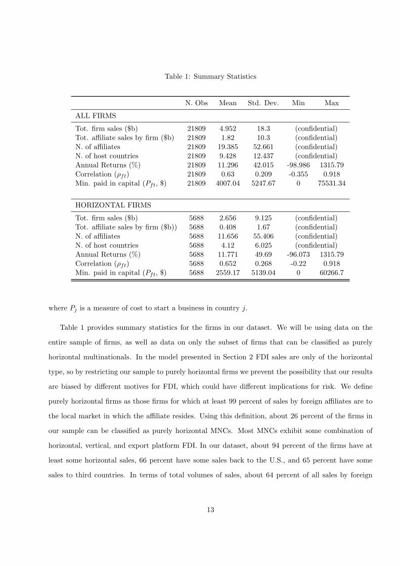
Table 1: Summary Statistics

N. Obs Mean Std. Dev. Min Max

ALL FIRMS

Tot. firm sales ($b) 21809 4.952 18.3 (confidential)Tot. affiliate sales by firm ($b) 21809 1.82 10.3 (confidential)N. of affiliates 21809 19.385 52.661 (confidential)N. of host countries 21809 9.428 12.437 (confidential)Annual Returns (%) 21809 11.296 42.015 -98.986 1315.79Correlation (ρft) 21809 0.63 0.209 -0.355 0.918Min. paid in capital (Pft, $) 21809 4007.04 5247.67 0 75531.34

HORIZONTAL FIRMS

Tot. firm sales ($b) 5688 2.656 9.125 (confidential)Tot. affiliate sales by firm ($b)) 5688 0.408 1.67 (confidential)N. of affiliates 5688 11.656 55.406 (confidential)N. of host countries 5688 4.12 6.025 (confidential)Annual Returns (%) 5688 11.771 49.69 -96.073 1315.79Correlation (ρft) 5688 0.652 0.268 -0.22 0.918Min. paid in capital (Pft, $) 5688 2559.17 5139.04 0 60266.7

where Pj is a measure of cost to start a business in country j.

Table 1 provides summary statistics for the firms in our dataset. We will be using data on the

entire sample of firms, as well as data on only the subset of firms that can be classified as purely

horizontal multinationals. In the model presented in Section 2 FDI sales are only of the horizontal

type, so by restricting our sample to purely horizontal firms we prevent the possibility that our results

are biased by different motives for FDI, which could have different implications for risk. We define

purely horizontal firms as those firms for which at least 99 percent of sales by foreign affiliates are to

the local market in which the affiliate resides. Using this definition, about 26 percent of the firms in

our sample can be classified as purely horizontal MNCs. Most MNCs exhibit some combination of

horizontal, vertical, and export platform FDI. In our dataset, about 94 percent of the firms have at

least some horizontal sales, 66 percent have some sales back to the U.S., and 65 percent have some

sales to third countries. In terms of total volumes of sales, about 64 percent of all sales by foreign

13

affiliates are horizontal, about 10 percent are vertical, and about 26 percent are export platform.

We report summary statistics for this subset of horizontal firms as well as for the full sample of

firms in Table 1. The average firm in our sample has about 19 foreign affiliates located in 9 different

countries with total global sales of 5.0 billion and an 11.3 percent annual stock market return. The

average correlation between the GDP growth in the U.S. and in the host countries is about 0.63. The

purely horizontal firms have an average of 12 affiliates in 4 countries with global sales of about 2.7

billion and an 11.7 percent annual stock market return. The average GDP shock correlations are

similar for both sets of firms, however sunk costs are lower for the purely horizontal firms. This is

consistent with a proximity-concentration model of FDI, in which high entry costs are a deterrent to

horizontal FDI.

4 The Role of Diversification and Cost Structure: Empirical Results

4.1 Reduced-Form Analysis

We test here the predictions of the model described in Section 2. The goal of the reduced form

specification is to establish a statistical relationship between firm-level stock returns and the relevant

explanatory variables that are suggested by the model: GDP growth correlations across countries and

fixed and sunk costs of production. Our baseline specification is given by:

retft = α+ β1ρft + β2Pft + β3Xft + δk + δt + εft (13)

where Retft is the annual stock return of firm f in year t, ρft is the weighted correlation of GDP

growth between the U.S. and the countries in which firm f has affiliates, and Pft is the weighted cost of

capital required to start a business in the countries in which firm f has affiliates. Xft is a vector of firm

level controls, including the total sales of the firm, the number of countries in which it has affiliates,

the market beta of the individual firm to capture its exposure to the domestic uncertainty,15 and

15The market beta of the individual firm is obtained by regressing firm-level returns on the aggregate return on themarket portfolio. One time-series regression for each firm delivers each firm’s beta.

14

gravity variables like GDP and distance from the host countries. Because the industry in which a firm

operates is likely to impact returns, we also include fixed effects δk for each firm’s primary industry.

We include year fixed effects δt to interpret our results as cross-sectional. εft is an orthogonal error

term.

In the model, GDP shocks in host countries impact US MNCs through local demand, which should

have a greater effect on firms that rely more heavily on sales to the local market, rather than sales back

to the US or to third countries (the model presented in Section 2 is primarily a model of horizontal,

rather than vertical, FDI). For this reason, our reduced form estimates focus on firms that are purely

horizontal in structure. We classify a firm as a purely horizontal MNC if at least 99 percent of sales

by the foreign affiliates of that firm are to local market in which each affiliate is located.

Table 2 shows the results. We begin by adding the two variables ρft and Pft separately. Column

I shows the result of regressing returns on the correlations variable. As predicted, the coefficient on

the variable measuring how correlated shocks are between the U.S. and the countries in which a firm

operates, ρft, is positive and significant. This implies that stock returns are higher (lower) for MNCs

with affiliates in countries where GDP growth is more (less) positively correlated with growth in the

US. Quantitatively, the interpretation is as follows: ceteris paribus, a firm that has affiliates only in a

host country whose GDP growth is perfectly correlated with the US has a risk premium 5.5% higher

than a firm with affiliates only in a host country whose GDP growth is uncorrelated with the US.

This result is consistent with the fact that more highly correlated shocks imply greater risk, and thus

higher returns are necessary to compensate for this risk.

Column II of Table 2 show the results of regressing returns on our proxy for the entry costs. As

predicted, the coefficient on the measure of sunk costs, Pft, is positive and significant. In particular,

each additional $1,000 of minimum paid in capital required in each country of destination is associated

with an increase in returns of 0.4%. This additional capital requirement, which proxies sunk and fixed

operating costs, increases the risk of experiencing negative cash-flows, and higher returns are necessary

to compensate for this risk. Since the average minimum paid in capital requirement in our sample is

$2,559, on average, the risk premium associated with entry costs is about 1.02%.

15

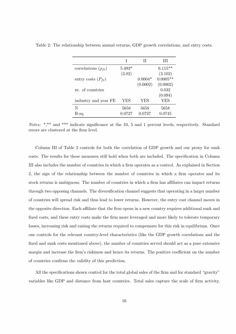
Table 2: The relationship between annual returns, GDP growth correlations, and entry costs.

I II III

correlations (ρft) 5.493* 6.115**(3.02) (3.102)

entry costs (Pft) 0.0004* 0.0005**(0.0002) (0.0002)

nr. of countries 0.032(0.094)

industry and year FE YES YES YES

N 5658 5658 5658R-sq 0.0727 0.0737 0.0745

Notes: *,** and *** indicate significance at the 10, 5 and 1 percent levels, respectively. Standarderrors are clustered at the firm level.

Column III of Table 2 controls for both the correlation of GDP growth and our proxy for sunk

costs. The results for these measures still hold when both are included. The specification in Column

III also includes the number of countries in which a firm operates as a control. As explained in Section

2, the sign of the relationship between the number of countries in which a firm operates and its

stock returns is ambiguous. The number of countries in which a firm has affiliates can impact returns

through two opposing channels. The diversification channel suggests that operating in a larger number

of countries will spread risk and thus lead to lower returns. However, the entry cost channel moves in

the opposite direction. Each affiliate that the firm opens in a new country requires additional sunk and

fixed costs, and these entry costs make the firm more leveraged and more likely to tolerate temporary

losses, increasing risk and raising the returns required to compensate for this risk in equilibrium. Once

one controls for the relevant country-level characteristics (like the GDP growth correlations and the

fixed and sunk costs mentioned above), the number of countries served should act as a pure extensive

margin and increase the firm’s riskiness and hence its returns. The positive coefficient on the number

of countries confirms the validity of this prediction.

All the specifications shown control for the total global sales of the firm and for standard “gravity”

variables like GDP and distance from host countries. Total sales capture the scale of firm activity,

16

and have also been shown to be highly correlated with other factors, such as productivity, that may

affect returns. Gravity variables don’t have significant effects on returns.16

Our results confirm the importance of cross-country GDP growth correlations and entry costs into

the host countries for the stock returns of US multinationals. These results provide a “first pass”

of a theory built on those fundamentals, but disregard the fact that – according to equation (10) –

GDP growth correlations and entry costs in the countries in which the firm does not have affiliates

also matter, through the option value term. The two-stage model that we present in the next section

controls for the components of the option value term by building a proxy based on the estimated

probabilities that firms open affiliates in given countries.

4.2 Two-Stage Model

In this section we augment our reduced form specification to include a proxy for the option value

component of returns. Equation (10) shows that GDP growth correlations and entry costs matter not

only for the value of assets in place, in the countries in which firms have affiliates, but also for the

option value of entering new countries.

The difficulty in measuring the contribution of the effect of these variables on returns through the

option value is that we cannot construct firm-level measures like (11) and (12) since firms do not have

sales in these countries. In order to proxy for the contribution of correlations and entry costs to the

option value of the firm, we use a two-stage approach. In the first stage, we estimate the probability

that each firm will have an affiliate in each country using standard predictors of FDI activity. In the

second stage, we estimate the impact of the characteristics of countries in which the firm does have

affiliates on annual returns, controlling for characteristics of the countries where the firm does not

have any affiliates. We use the predicted probabilities of entering each country from the first stage as

weights in constructing these characteristics.

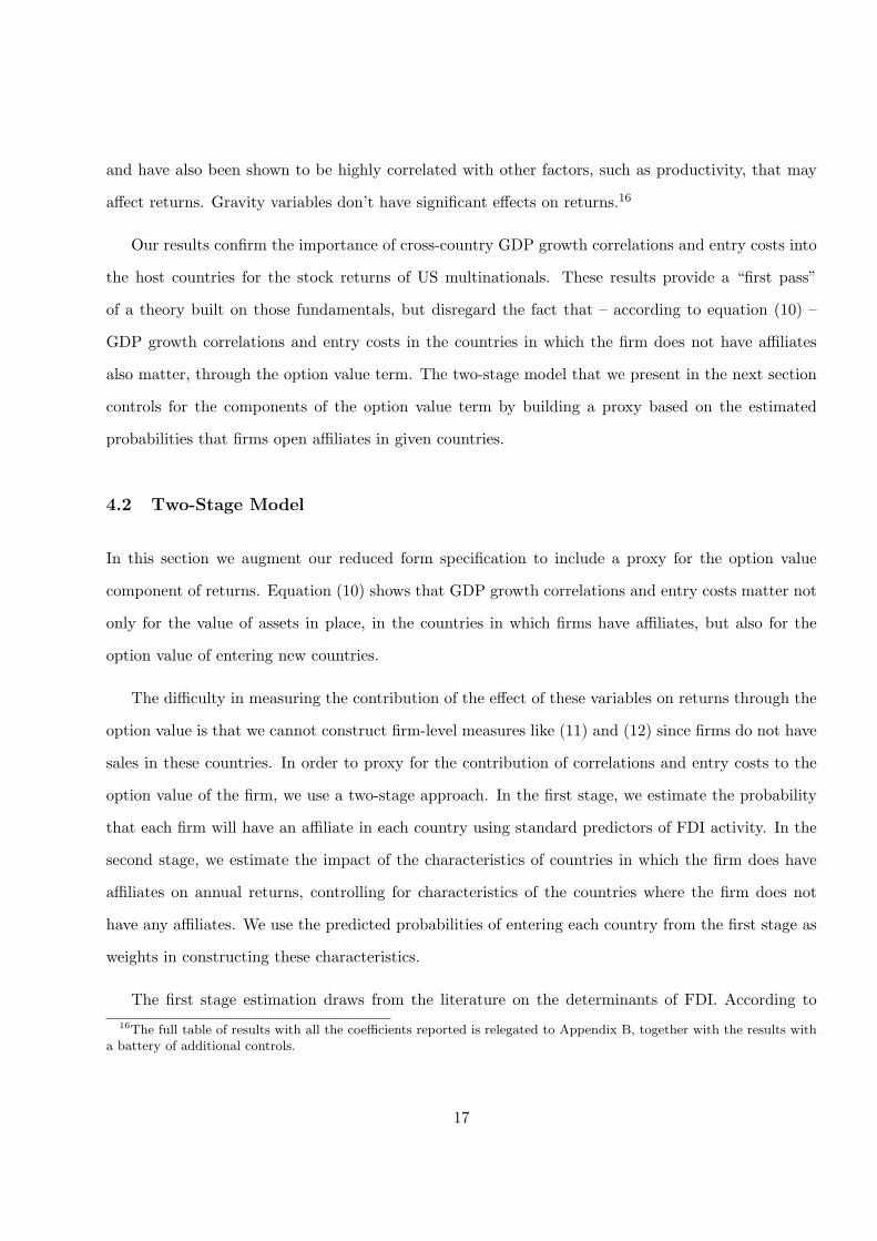
The first stage estimation draws from the literature on the determinants of FDI. According to

16The full table of results with all the coefficients reported is relegated to Appendix B, together with the results witha battery of additional controls.

17

the knowledge capital model developed by Carr, Markusen, and Maskus (2001) and Markusen and

Maskus (2002), the volume of FDI activity between two countries depends on the sum of the GDPs

of the countries, the squared difference in their GDPs, the difference in skilled labor endowments, and

trade costs. The proximity-concentration model developed by Brainard (1997) and Helpman, Melitz,

and Yeaple (2004) suggests that a firm’s decision to engage in FDI is a function of proximity, which

we proxy with distance, and market size, measured by the sum of US GDP and the GDP of the host

country.

When considering the likelihood of entering a new country, it is important to also consider where

the firm already has foreign affiliates. Work by Ekholm, Forslid, and Markusen (2007) and Mrazova

and Neary (2011) has demonstrated the importance of export platform FDI, that is, firms choosing

to use one foreign affiliate to serve multiple countries rather than locating an affiliate in each country.

This would suggest that, under certain conditions, already having an affiliate in the same region may

reduce a firm’s incentives to enter a neighboring country. On the other hand, Chen (2011) emphasizes

the interdependence of location choices across affiliates of the same MNC. She finds that the impact

of already having a nearby affiliate can be negative (in the case of export platform FDI) or positive,

as is the case when firms ship components between affiliates and thus benefit from proximity.

We control for the presence of other affiliates in the region in our first stage probit regression by

including a dummy variable that equals one if the firm had an affiliate in the region in year t − 1.

To avoid placing strong restrictions on what constitutes a region, we define regions broadly as either

Europe, Asia, NAFTA, South America, Africa, and the Middle East. The estimating equation is:

Afjt = α+ β1Wjt + β2Regionfj,t−1 + δt + εfjt (14)

where Afjt is a dummy variable that equals 1 if firm f has an affiliate in country j in time t. Wjt

is a vector of the knowledge capital and proximity-concentration variables described above, including

ln(dist)j , ln(sumgdp)jt, ln(gdpdif2)jt, ln(skilldif)jt, and ln(tradecost)jt. Regionfj,t−1 is a dummy

variable that equals one if firm f had an affiliate in the region in which country j is located in time

t− 1. We estimate equation (14) using both the full sample and the sample of only purely horizontal

18

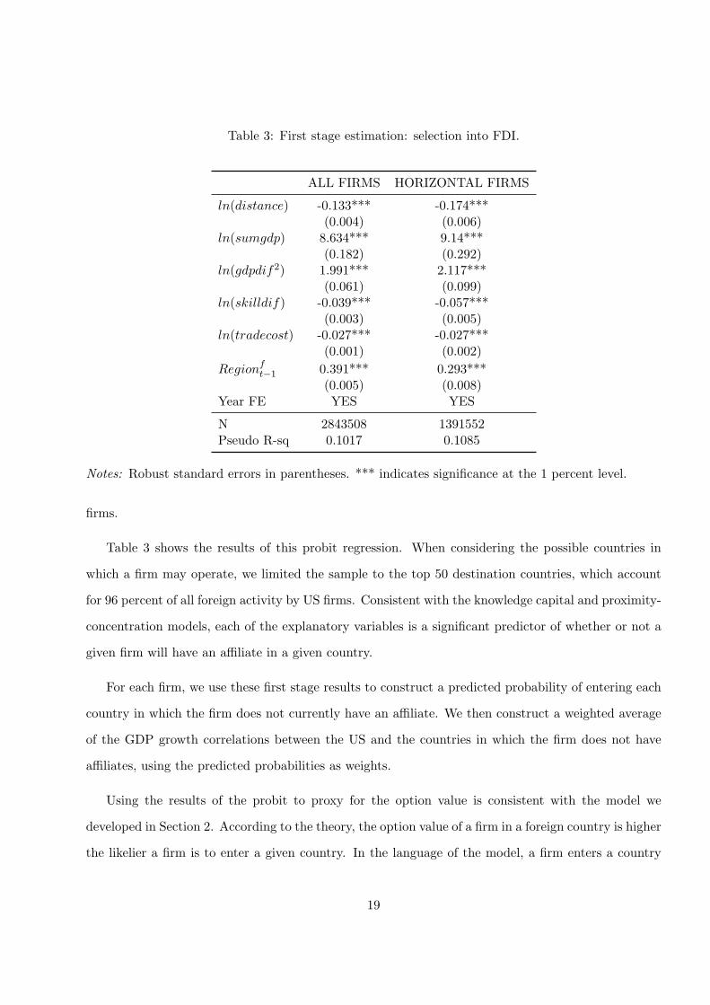
Table 3: First stage estimation: selection into FDI.

ALL FIRMS HORIZONTAL FIRMS

ln(distance) -0.133*** -0.174***(0.004) (0.006)

ln(sumgdp) 8.634*** 9.14***(0.182) (0.292)

ln(gdpdif2) 1.991*** 2.117***(0.061) (0.099)

ln(skilldif) -0.039*** -0.057***(0.003) (0.005)

ln(tradecost) -0.027*** -0.027***(0.001) (0.002)

Regionft−1 0.391*** 0.293***(0.005) (0.008)

Year FE YES YES

N 2843508 1391552Pseudo R-sq 0.1017 0.1085

Notes: Robust standard errors in parentheses. *** indicates significance at the 1 percent level.

firms.

Table 3 shows the results of this probit regression. When considering the possible countries in

which a firm may operate, we limited the sample to the top 50 destination countries, which account

for 96 percent of all foreign activity by US firms. Consistent with the knowledge capital and proximity-

concentration models, each of the explanatory variables is a significant predictor of whether or not a

given firm will have an affiliate in a given country.

For each firm, we use these first stage results to construct a predicted probability of entering each

country in which the firm does not currently have an affiliate. We then construct a weighted average

of the GDP growth correlations between the US and the countries in which the firm does not have

affiliates, using the predicted probabilities as weights.

Using the results of the probit to proxy for the option value is consistent with the model we

developed in Section 2. According to the theory, the option value of a firm in a foreign country is higher

the likelier a firm is to enter a given country. In the language of the model, a firm enters a country

19

Table 4: Summary statistics by affiliate presence.

Correlation Entry cost ($)

ALL FIRMS

Countries with affiliates 0.630 4007.04Countries without affiliates 0.456 6645.29

HORIZONTAL FIRMS

Countries with affiliates 0.652 2559.17Countries without affiliates 0.495 6605.01

when its expected profits in that country are above some threshold (that one can derive explicitly given

functional forms for preferences and technologies). The estimated probability of entering a country

that results from the probit can then be interpreted as a measure of how close a firm is to the entry

threshold and hence of how important the option value of entering that country is.

The weighted correlation of GDP growth between the US and countries in which the firm does not

currently have affiliates is calculated as

ρoft =

∑j ∈A

probfjtρj∑j ∈A

probfjt(15)

where probfjt is the predicted probability that firm f has an affiliate in country j in time t from the

first stage and ρj is the correlation of GDP growth between the US and country j. We construct a

similar measure for the cost of capital required to start a business in the countries in which the firm

does not currently have affiliates.

Table 4 shows the weighted average GDP growth correlations and cost of capital required to start a

business for the countries in which a firm does and does not have affiliates. For the average horizontal

firm in our sample, the GDP growth correlation for countries in which the firm has affiliates is 0.652.

The weighted correlation of shocks for countries in which they do not have affiliates is 0.495. These

numbers suggest that US MNCs don’t choose their affiliates’ host countries to diversify away risk.

20

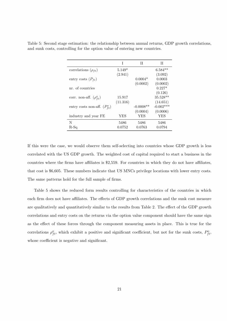
Table 5: Second stage estimation: the relationship between annual returns, GDP growth correlations,and sunk costs, controlling for the option value of entering new countries.

I II II

correlations (ρft) 5.149* 6.584**(2.941) (3.092)

entry costs (Pft) 0.0004* 0.0003(0.0002) (0.0002)

nr. of countries 0.227*(0.126)

corr. non-aff. (ρoft) 15.917 35.528**

(11.316) (14.651)entry costs non-aff. (P o

ft) -0.0008** -0.002***

(0.0004) (0.0006)industry and year FE YES YES YES

N 5486 5486 5486R-Sq 0.0752 0.0763 0.0794

If this were the case, we would observe them self-selecting into countries whose GDP growth is less

correlated with the US GDP growth. The weighted cost of capital required to start a business in the

countries where the firms have affiliates is $2,559. For countries in which they do not have affiliates,

that cost is $6,605. These numbers indicate that US MNCs privilege locations with lower entry costs.

The same patterns hold for the full sample of firms.

Table 5 shows the reduced form results controlling for characteristics of the countries in which

each firm does not have affiliates. The effects of GDP growth correlations and the sunk cost measure

are qualitatively and quantitatively similar to the results from Table 2. The effect of the GDP growth

correlations and entry costs on the returns via the option value component should have the same sign

as the effect of these forces through the component measuring assets in place. This is true for the

correlations ρoft, which exhibit a positive and significant coefficient, but not for the sunk costs, P oft,

whose coefficient is negative and significant.

21

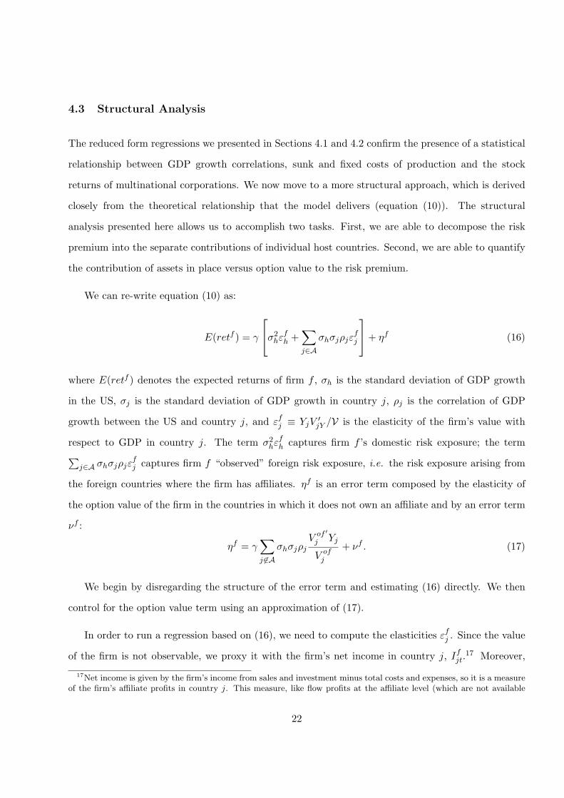
4.3 Structural Analysis

The reduced form regressions we presented in Sections 4.1 and 4.2 confirm the presence of a statistical

relationship between GDP growth correlations, sunk and fixed costs of production and the stock

returns of multinational corporations. We now move to a more structural approach, which is derived

closely from the theoretical relationship that the model delivers (equation (10)). The structural

analysis presented here allows us to accomplish two tasks. First, we are able to decompose the risk

premium into the separate contributions of individual host countries. Second, we are able to quantify

the contribution of assets in place versus option value to the risk premium.

We can re-write equation (10) as:

E(retf ) = γ

σ2hεfh +∑j∈A

σhσjρjεfj

+ ηf (16)

where E(retf ) denotes the expected returns of firm f , σh is the standard deviation of GDP growth

in the US, σj is the standard deviation of GDP growth in country j, ρj is the correlation of GDP

growth between the US and country j, and εfj ≡ YjV′jY /V is the elasticity of the firm’s value with

respect to GDP in country j. The term σ2hεfh captures firm f ’s domestic risk exposure; the term∑

j∈A σhσjρjεfj captures firm f “observed” foreign risk exposure, i.e. the risk exposure arising from

the foreign countries where the firm has affiliates. ηf is an error term composed by the elasticity of

the option value of the firm in the countries in which it does not own an affiliate and by an error term

νf :

ηf = γ∑j ∈A

σhσjρjV of ′

j Yj

V ofj

+ νf . (17)

We begin by disregarding the structure of the error term and estimating (16) directly. We then

control for the option value term using an approximation of (17).

In order to run a regression based on (16), we need to compute the elasticities εfj . Since the value

of the firm is not observable, we proxy it with the firm’s net income in country j, Ifjt.17 Moreover,

17Net income is given by the firm’s income from sales and investment minus total costs and expenses, so it is a measureof the firm’s affiliate profits in country j. This measure, like flow profits at the affiliate level (which are not available

22

since income is an imperfect measure of the value of the firm, we assume that the true elasticity εfj is

given by the approximated elasticity εfj times a country-specific unobserved component ζj :

εfj ≡ ζj εfj . (18)

The approximated elasticity εfj is estimated by running one time series regression of log-income on

log-GDP for each firm f and host country j.18

Estimating the elasticity, εfj , using actual data on the responsiveness of each firm’s income to local

GDP shocks also helps us avoid potential complications resulting from differences between horizontal,

vertical, and export platform FDI. GDP growth shocks in host countries impact US MNCs through

local demand, which should have a greater effect on firms that rely more heavily on sales to the

local market. For our reduced form approach, we addressed the distinction between horizontal versus

vertical sales by only including purely horizontal firms in our analysis. However, this distinction is not

an issue in our structural estimation. Here we are able to directly identify the responsiveness of the

net income of each firm to fluctuations in the local market using our estimates of εfj . By estimating

this elasticity directly at the firm level, we pick up any differences in responsiveness to local GDP

across firms that may result from being primarily horizontal or vertical in structure.

We also prefer to avoid making a strong distinction between horizontal versus vertical FDI in

our empirical estimates because most firms do not fall cleanly into one of those two categories. The

majority of US MNCs engage in some combination of both horizontal and vertical FDI, and thus our

model should apply to all of these firms. Moreover, most of the sales by US MNCs are horizontal.

For example, in our sample, 64 percent of sales by foreign affiliates of US firms are to the market in

which the affiliate is located and 94 percent of the firms have at least some sales to the local markets

in which their affiliates are located. Thus for our full sample of firms, almost all of them have at least

from the BEA data), is not a perfect measure of the value of the firm because it disregards the option value of assetsin place. Alternatively, CRSP contains data on profits and market capitalization at the firm level. This measure isalso problematic as we only have information on the firm total market capitalization and total profits, not by individualaffiliate or country of operation, hence the variation of εfj across countries only comes from variation in Yjt. To construct

εfj , we also need to take a stand on the status of MNCs that enter or exit countries during the sample period. In ourbaseline specification, we consider the effect on the returns of those assets that are in place for at least two years ofsample period.

18We estimate εfh in the same way, regressing the log of each firm’s domestic net income on the log of US GDP.

23

some sales to the local market, and for most affiliates these local sales make up the majority of their

total sales. The structural estimates that follow make use of the full sample of firms, rather than

focusing on firms that only have horizontal sales.

We present the results in two parts. First, we allow the risk premium to vary by country. We run

regression (16) for the entire sample of firms having affiliates in the top 50 countries. The results of

the full sample structural estimation allow us to decompose the risk premium into the contributions

of each individual host country. Next, we aggregate the risk premium across countries to give an

estimate of the total effect of MNC risk. Each of these sets of results is further decomposed into the

contributions of assets in place and option value.

4.3.1 Decomposition of Risk Premium by Country

In this section we estimate

E(retf ) = ψhσ2hε

fh +

∑j∈A

ψjσhσjρj εfj + ηf (19)

allowing the risk premium coefficients, ψj ≡ γζj , to vary by country. We do this by introducing a

separate variable for each of the 50 top host countries, j, in our sample which takes a value of σhσjρj εfj

if firm f has an affiliate in country j and equals zero if firm f does not have an affiliate in country j.

The results of this specification, which we refer to as specification I, are reported in Table 6. In the

left panel we report the estimated coefficients ψj , while in the right panel we report the corresponding

risk premium ψjσhσjρjεfj . For clarity of exposition, Table 6 only reports the risk premium for ψj

coefficients that are either statistically significant or that correspond to a country that is an especially

important FDI destination for US firms, such as the UK, Mexico, and China. We report the full set

of results for all countries in Appendix C.1.

As Table 6 shows, 16 of the ψj coefficients are statistically significant at least at the ten percent

level. Of these 16 significant coefficients, 14 are positive and (with the exception of Indonesia) asso-

ciated with a positive risk premium, indicating that the corresponding host countries are a source of

24

risk to MNCs with affiliates there.

The country-specific risk premia vary in a an intuitive way. The countries with the highest risk

premia in Table 6 are Greece, Malaysia, India, Singapore, and China. Most European countries and

Canada have relatively low risk premia, indicating that the effect of low sunk costs outweighs the

one of high co-movement with the US. Two of the coefficients are negative, but these are for Poland

and Israel, which are both countries that have very strong political ties to the US and thus may be

perceived by investors as being less risky.

Each country-specific risk premium can be interpreted as the additional annual return required

to induce investors to hold shares of firms with affiliates in that country. For example, firms with

affiliates in Greece have annual returns that are, on average, 0.67 percentage points higher than those

of firms that do not have affiliates in Greece. For firms that have affiliates in the UK, the additional

annual return is only 0.06 percentage points.

The country-specific risk premia reported here are for the average firm in our sample. However,

firms are very heterogeneous in terms of their responsiveness to shocks. This heterogeneity enters

through εfj , the elasticity of the firm’s value with respect to changes in host country GDP. Thus the

positive values for the ψ coefficients indicate that firms whose values are more responsive to changes

in destination countries’ GDP tend to be riskier and to exhibit higher returns.

As mentioned above, the results of specification I do not take into account the structure of the

error term given by equation (17). This results in biased estimates of the risk premia. To address this

concern, in specification II we report the results of the following regression:

E(retf ) = ψhσ2hε

fh +

∑j∈A

ψjσhσjρj εfj +

∑j ∈A

ψojσhσjρjZ

fj + νf (20)

where Zfj ≡ probfj ε

fh is a proxy for the option value of firm f in j.

Recall from equation (10) that the option value term is expressed as∑

j ∈A σhσjρjYjV

oj

′Y

V . σh, σj

and ρj can be observed directly for each country in which the firm does not have an affiliate. The

elasticity of the firm’s value with respect to GDP in country j,YjV

oj

′Y

V , is not observable for countries

25

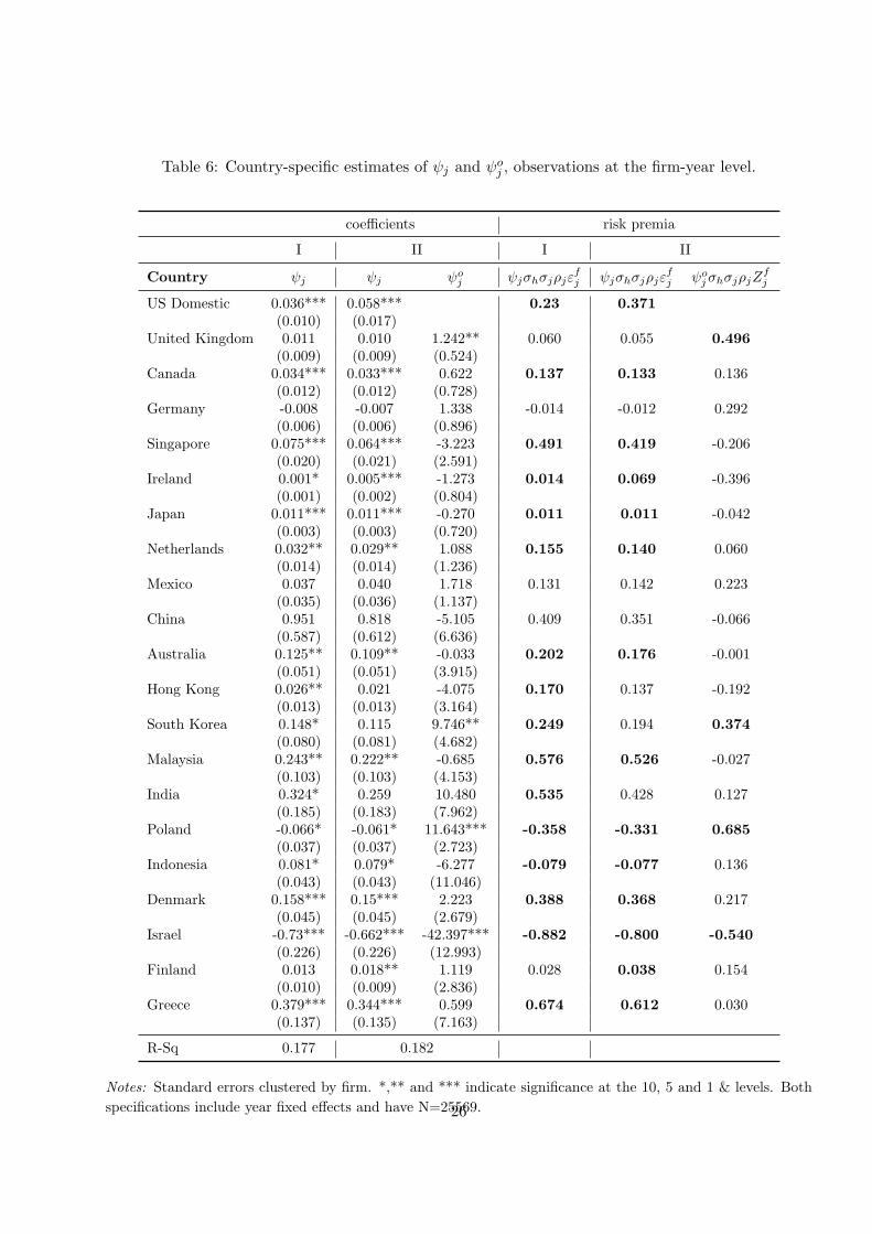
Table 6: Country-specific estimates of ψj and ψoj , observations at the firm-year level.

coefficients risk premia

I II I II

Country ψj ψj ψoj ψjσhσjρjε

fj ψjσhσjρjε

fj ψo

jσhσjρjZfj

US Domestic 0.036*** 0.058*** 0.23 0.371(0.010) (0.017)

United Kingdom 0.011 0.010 1.242** 0.060 0.055 0.496(0.009) (0.009) (0.524)

Canada 0.034*** 0.033*** 0.622 0.137 0.133 0.136(0.012) (0.012) (0.728)

Germany -0.008 -0.007 1.338 -0.014 -0.012 0.292(0.006) (0.006) (0.896)

Singapore 0.075*** 0.064*** -3.223 0.491 0.419 -0.206(0.020) (0.021) (2.591)

Ireland 0.001* 0.005*** -1.273 0.014 0.069 -0.396(0.001) (0.002) (0.804)

Japan 0.011*** 0.011*** -0.270 0.011 0.011 -0.042(0.003) (0.003) (0.720)

Netherlands 0.032** 0.029** 1.088 0.155 0.140 0.060(0.014) (0.014) (1.236)

Mexico 0.037 0.040 1.718 0.131 0.142 0.223(0.035) (0.036) (1.137)

China 0.951 0.818 -5.105 0.409 0.351 -0.066(0.587) (0.612) (6.636)

Australia 0.125** 0.109** -0.033 0.202 0.176 -0.001(0.051) (0.051) (3.915)

Hong Kong 0.026** 0.021 -4.075 0.170 0.137 -0.192(0.013) (0.013) (3.164)

South Korea 0.148* 0.115 9.746** 0.249 0.194 0.374(0.080) (0.081) (4.682)

Malaysia 0.243** 0.222** -0.685 0.576 0.526 -0.027(0.103) (0.103) (4.153)

India 0.324* 0.259 10.480 0.535 0.428 0.127(0.185) (0.183) (7.962)

Poland -0.066* -0.061* 11.643*** -0.358 -0.331 0.685(0.037) (0.037) (2.723)

Indonesia 0.081* 0.079* -6.277 -0.079 -0.077 0.136(0.043) (0.043) (11.046)

Denmark 0.158*** 0.15*** 2.223 0.388 0.368 0.217(0.045) (0.045) (2.679)

Israel -0.73*** -0.662*** -42.397*** -0.882 -0.800 -0.540(0.226) (0.226) (12.993)

Finland 0.013 0.018** 1.119 0.028 0.038 0.154(0.010) (0.009) (2.836)

Greece 0.379*** 0.344*** 0.599 0.674 0.612 0.030(0.137) (0.135) (7.163)

R-Sq 0.177 0.182

Notes: Standard errors clustered by firm. *,** and *** indicate significance at the 10, 5 and 1 & levels. Both

specifications include year fixed effects and have N=25569.26

in which the firm does not have an affiliate. We proxy this elasticity using εfh, the firm’s elasticity

of domestic net income with respect to GDP fluctuations in the US This measure captures the firm-

specific component of elasticity, but does not suffer from bias due to selection into affiliate countries,

as it is a purely domestic measure. probfj is the predicted probability that firm f will enter country j,

as described in Section 4.2. As long as this proxy is a good one, controlling for the option value term

corrects the omitted variable bias in the estimated coefficients on assets in place, ψj . Moreover, the

difference between the R2 in the two specifications quantifies how much more of the variance of the

risk premium is explained by explicitly taking into account the option value of entering new countries

using the approximation described above.19

For 12 of the 16 countries that had a positive risk premium in specification I, adding the control

for the option value decreases the estimated risk premium. This suggests that attempting to estimate

the risk premium without controlling for the option value term overestimates the risk premium.

In addition to their role in resolving the omitted variable bias, the option value terms are also

informative themselves. In the entire sample of top 50 countries, there are 12 for which the ψoj

coefficient on the option value is significant; of those, 7 display a positive coefficient, indicating that

the mere possibility of entering those countries is a source of risk to the firm. The coefficients on the

option value terms vary much more widely than the coefficients on the the assets in place. This is not

surprising, as the approximated firm-level elasticities for the option value countries are not as good

of an approximation of the true elasticity as in the case of assets in place. The corresponding risk

premia, ψσhσjρjεfj , are still reasonable in magnitude, ranging from -0.540 to 0.685.

4.3.2 Aggregate Risk Premium

The results presented in Table 6 shed light on country-specific sources of risk. However, we are also

interested in their aggregation to the overall risk premia of multinational firms, most of which have

affiliates in more than one country.

19Appendix C reports the results of an alternative methodology to control for the country-specific component of theoption value.

27

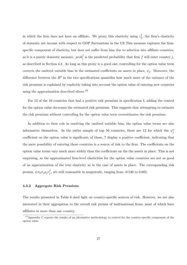
Table 7: Structural model: the relationship between annual returns and the elasticity of affiliate valueto GDP, controlling for the option value of entering new countries.

Country-specificrisk premia

Aggregate ψestimates

I II I II

Risk premium:- from domestic sales: 0.23 0.371 0.256 0.403- from foreign sales: 3.647 3.265 0.056 0.056- from option value: 0.488 -0.237

Prob > F :F-test for joint significance 0.000 0.000H0: ψj = ψk, ∀j = k 0.000 0.000H0: ψ

oj = ψo

k, ∀j = k 0.000

Notes: Dependent variable is annual stock market returns. Aggregate estimates include year fixedeffects. *,** and *** indicate significance at the 10, 5 and 1 percent levels, respectively. Robuststandard errors are in parentheses.

To estimate the aggregate risk premium we sum the country-specific risk premia reported in Ta-

ble 6, which were estimated using equation (19). Alternatively, one could argue that cross-country

heterogeneity across the estimated coefficients ψj may not be important quantitatively, and estimate

a unique coefficient ψ that is common across host countries. This would amount to run the following

regression:

E(retf ) = ψhσ2hε

fh + ψ

∑j∈A

σhσjρj εfj + ψo

∑j ∈A

σhσjρjZfj + νf (21)

The results of these two approaches are reported in Table 7.

The left panel of Table 7 shows the aggregate risk premium obtained by summing the country-

specific risk premia estimated using equation (19). The aggregate risk premium from foreign assets

in place is large, at 3.6 percentage points. By summing over the risk premia for all countries, we are

constructing an estimate of what the risk premium would be for a firm that has affiliates in all of

the top 50 FDI host countries. This implies that a firm with affiliates in every country in our sample

would have, on average, expected annual returns that are 3.6 percent higher than those of a purely

domestic firm.

28

As was the case for most of the individual country risk premia, the aggregate risk premium from

assets in place falls slightly when the option value term is included. The aggregate risk premium of

the option value implies that if a firm did not have affiliates in any of the countries in our sample, the

option to enter those countries in the future would increase expected returns by 0.488 percent for the

average firm.

As mentioned above, the aggregate results give the risk premium for an average firm with affiliates

in all of the countries in the sample. However, it is also possible to use the country-specific results

from Table 6 to estimate the expected risk premium for a typical firm with any combination of

foreign affiliates. For example, suppose that a firm only has affiliates in Canada, Singapore, and

Ireland. The expected contribution of these assets in place to the firm’s risk premium would be

0.133+0.419+0.069 = 0.621. The contribution to the risk premium from the option value of entering

countries in which the firm does not currently have affiliates would be the sum∑

j ∈A ψojσhσjρjZ

fj

where j ∈ A includes all countries except for Canada, Singapore, and Ireland. This is a value of 0.954.

Adding in the risk premium for domestic US assets, the total risk premium for the average firm with

affiliates in Canada, Singapore, and Ireland would be 0.371 + 0.621 + 0.954 = 1.946, so the expected

returns would be about 2 percentage points higher than the returns of a purely domestic firm.

Finally, the F-tests reported in Table 7 show that all the ψj parameters are significantly different

from each other. Since we defined ψj ≡ γζj , this result confirms the importance of across-country

heterogeneity in the unobserved component of the elasticity of firms’ value with respect to GDP.

The right panel of Table 7 shows the results of estimating equation (21) with one coefficient ψ that

is common across host countries. This approach gives a positive and significant estimate for ψ,20 and

the corresponding risk premium for foreign assets in place implies that, on average, having foreign

affiliates adds 0.056 percentage points to the expected returns of the firms in our sample.

The estimated aggregate risk premium of 0.056 is relatively small. However, this is not surprising.

Since in equation (21) we sums the values of σhσjρj εfj for each country, we are implicitly assuming

independence across explanatory variables. Ignoring the covariance structure of risk exposures across

20The values of the estimated parameters ψ and ψo are reported in Appendix C.

29

counties augments the strength of the diversification channel, as would be the case if shocks across

countries were uncorrelated. A similar argument applies to the risk premium coming from the option

value, which is negative in this specification. When we assume independence across countries, the

diversification channel is much more important, and thus the option to further diversify by entering

more countries reduces the risk premium of a firm. Similarly, the larger estimate obtained aggregating

country-specific risk premia is partly due to the fact that we account for the covariance structure of

the explanatory variables, giving a more realistic treatment of the diversification channel. Finally,

when we sum over the right-hand-side variables for each country in equation (21), the magnitude of

the aggregate is driven by countries that have a greater number of non-zero observations. Thus it is

not surprising that the risk premium of 0.056 that we obtain from this aggregation is quantitatively

similar to the risk premium of the UK reported in Table 6, as the UK is one of the largest host

countries for US MNCs.

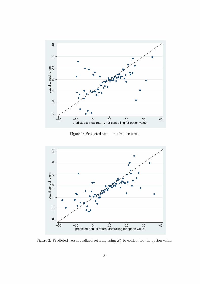
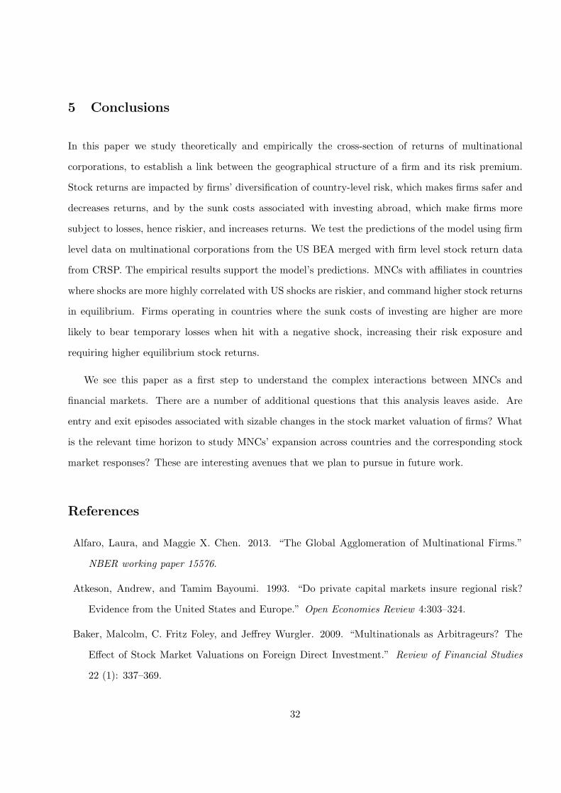
4.3.3 Goodness of Fit

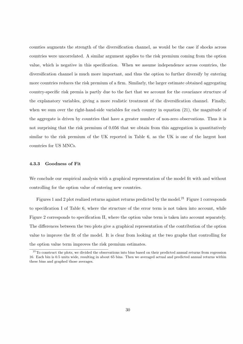
We conclude our empirical analysis with a graphical representation of the model fit with and without

controlling for the option value of entering new countries.

Figures 1 and 2 plot realized returns against returns predicted by the model.21 Figure 1 corresponds

to specification I of Table 6, where the structure of the error term is not taken into account, while

Figure 2 corresponds to specification II, where the option value term is taken into account separately.

The differences between the two plots give a graphical representation of the contribution of the option

value to improve the fit of the model. It is clear from looking at the two graphs that controlling for

the option value term improves the risk premium estimates.

21To construct the plots, we divided the observations into bins based on their predicted annual returns from regression16. Each bin is 0.5 units wide, resulting in about 65 bins. Then we averaged actual and predicted annual returns withinthese bins and graphed those averages.

30

−20

−10

010

2030

40ac

tual

ann

ual r

etur

n

−20 −10 0 10 20 30 40predicted annual return, not controlling for option value

Figure 1: Predicted versus realized returns.

−20

−10

010

2030

40ac

tual

ann

ual r

etur

n

−20 −10 0 10 20 30 40predicted annual return, controlling for option value

Figure 2: Predicted versus realized returns, using Zfj to control for the option value.

31

5 Conclusions

In this paper we study theoretically and empirically the cross-section of returns of multinational

corporations, to establish a link between the geographical structure of a firm and its risk premium.

Stock returns are impacted by firms’ diversification of country-level risk, which makes firms safer and

decreases returns, and by the sunk costs associated with investing abroad, which make firms more

subject to losses, hence riskier, and increases returns. We test the predictions of the model using firm

level data on multinational corporations from the US BEA merged with firm level stock return data

from CRSP. The empirical results support the model’s predictions. MNCs with affiliates in countries

where shocks are more highly correlated with US shocks are riskier, and command higher stock returns

in equilibrium. Firms operating in countries where the sunk costs of investing are higher are more

likely to bear temporary losses when hit with a negative shock, increasing their risk exposure and

requiring higher equilibrium stock returns.

We see this paper as a first step to understand the complex interactions between MNCs and

financial markets. There are a number of additional questions that this analysis leaves aside. Are

entry and exit episodes associated with sizable changes in the stock market valuation of firms? What

is the relevant time horizon to study MNCs’ expansion across countries and the corresponding stock

market responses? These are interesting avenues that we plan to pursue in future work.

References

Alfaro, Laura, and Maggie X. Chen. 2013. “The Global Agglomeration of Multinational Firms.”

NBER working paper 15576.

Atkeson, Andrew, and Tamim Bayoumi. 1993. “Do private capital markets insure regional risk?

Evidence from the United States and Europe.” Open Economies Review 4:303–324.

Baker, Malcolm, C. Fritz Foley, and Jeffrey Wurgler. 2009. “Multinationals as Arbitrageurs? The

Effect of Stock Market Valuations on Foreign Direct Investment.” Review of Financial Studies

22 (1): 337–369.

32

Brainard, S. Lael. 1997. “An Empirical Assessment of the Proximity-Concentration Trade-off between

Multinational Sales and Trade.” The American Economic Review 87 (4): 520–544.

Branstetter, Lee G., Raymond Fisman, and C. Fritz Foley. 2006. “Do Stronger Intellectual Property

Rights Increase International Technology Transfer? Empirical Evidence from U.S. Firm-Level

Panel Data.” Quarterly Journal of Economics 121 (1): 321349.

Carr, David L, James R. Markusen, and Keith E. Maskus. 2001. “Testing the knowledge-capital

model of the multinational enterprise.” American Economic Review 91 (3): 995–1001.

Chen, Maggie X. 2011. “Interdependence in Multinational Production Networks.” Canadian Journal

of Economics 44 (3): 930–956.

Chen, Maggie X., and Michael Moore. 2010. “Location Decision of Heterogeneous Multinational

Firms.” Journal of International Economics 80 (2): 188–199.

Crucini, Mario. 1999. “On international and national dimensions of risk sharing.” Review of Eco-

nomics and Statistics 8 (1): 73–84.

Das, Sanghamitra, Mark J. Roberts, and James R. Tybout. 2007. “Market Entry Costs, Producer

Heterogeneity, and Export Dynamics.” Econometrica 75 (3): 837–873.

Denis, David J., Diane K. Denis, and Keven Yost. 2002. “Global Diversification, Industrial Diversi-

fication, and Firm Value.” The Journal of Finance 57 (5): 1951–1979.

Dixit, Avinash K. 1989. “Entry and Exit Decisions under Uncertainty.” Journal of Political Economy

97 (3): 620–638.

Dixit, Avinash K., and Robert S. Pindyck. 1994. Investment under Uncertainty. Princeton, NJ:

Princeton University Press.

Ekholm, Karolina, Rikard Forslid, and James R. Markusen. 2007. “Export-Platform Foreign Direct

Investment.” Journal of the European Economic Association 5 (4): 776–795.

Fama, Eugene F., and Kenneth R. French. 1996. “Multifactor Explanations of Asset Pricing Anoma-

lies.” Journal of Finance 51 (1): 55–84.

Fillat, Jose L., and Stefania Garetto. 2012. “Risk, Returns, and Multinational Production.” Mimeo,

Boston University.

33

Helpman, Elhanan, Marc J. Melitz, and Stephen R. Yeaple. 2004. “Exports Versus FDI with

Heterogeneous Firms.” The American Economic Review 94 (1): 300–316.

Jacquillat, Bertrand, and Bruno Solnik. 1978. “Multinationals are poor tools for international

diversification.” Journal of Portfolio Management 4 (2): 812.

Kravis, Irving B., and Robert E. Lipsey. 1982. “The location of overseas production and production

for export by U.S. multinational firms.” Journal of International Economics 12 (3-4): 201–223.

Markusen, James R., and Keith E. Maskus. 2002. “Discriminating among alternative theories of the

multinational enterprise.” Review of International Economics 10:694–707.

Mrazova, Monika, and J. Peter Neary. 2011. “Firm Selection into Export-Platform Foreign Direct

Investment.” Working paper.

Roberts, Mark J., and James R. Tybout. 1997. “The Decision to Export in Colombia: An Empirical

Model of Entry with Sunk Costs.” The American Economic Review 87 (4): 545–564.

Rowland, Patrick F., and Linda L. Tesar. 2004. “Multinationals and the gains from international

diversification.” Review of Economic Dynamics 7:798–826.

Senchack, Andrew J., and William L. Beedles. 1980. “Is indirect international diversification desir-

able?” Journal of Portfolio Management 6 (2): 49–57.

Sorensen, Bent E., and Oved Yosha. 1998. “International risk sharing and European monetary

unification.” Journal of International Economics 45:211–238.

Tesar, Linda L., and Ingrid Werner. 1998. “The internationalization of securities markets since the

1987 crash.” In R. Litan and A. Santomero (eds.) , Brookings-Wharton Papers on Financial

Services. Washington: The Brookings Institution.

Yeaple, Stephen. 2003. “The Complex Integration Strategies of Multinational Firms and Cross-

Country Dependencies in the Structure of Foreign Direct Investment.” Journal of International

Economics 60 (2): 293–314.

. 2009. “Firm Heterogeneity and the Structure of U.S. Multinational Activity: An Empirical

Analysis.” Journal of International Economics 78 (2): 206–215.

34

Appendix

A Derivation of the Model

We present here the derivation of the results of Section 2. In the continuation region, each one of the

three value functions of a firm (Vh, Vj , and Voj ) satisfies:

π(a, Y,X)M∆t+E[M∆t · V (a, Y ′, X|Y )]− V (a, Y,X) = 0. (B.1)

For ∆t→ 0:

π(a, Y,X)Mdt+E[d(M · V (a, Y,X))] = 0. (B.2)

The term in the expectation can be written as:

E[d(M · V )] = E[dM · V +M · dV + dM · dV ]

= M · V · E[dM

M+dV

V+dM

M· dVV

]= M · V

[−rdt+ E

(dV

V

)+ E

(dM

M· dVV

)]= Mdt

[−rV + E

(dV

dt

)+ E

(dM

M· dVdt

)](B.3)

where the dependence of V on (a, Y,X) has been suppressed to ease the notation. Plugging (B.3) into

(B.2):

π − rV + E

(dV

dt

)+ E

(dM

M· dVdt

)= 0. (B.4)

By applying Ito’s Lemma and using the expressions for the Brownian motions ruling the evolution

of Y , we can derive expressions for some of the terms in (B.4):

dV = V ′Y dY +

1

2σ2Y 2V ′′

Y dt = V ′Y [µY dt+ σY dz] +

1

2σ2Y 2V ′′

Y dt

E[dV ] = µY V ′Y dt+

1

2σ2Y 2V ′′

Y dt .

35

Using these results and the equation describing the evolution of M , we can rewrite (B.4) for the

three value functions as:

πhdt− rhVhdt+ µhYhVh′Y dt+

1

2σ2hY

2h Vh

′′Y dt+ E

[(−rhdt− γσhdzh) ·

(µhYhVh

′Y dt+ σhYhVh

′Y dzh +

1

2σ2hY

2h Vh

′′Y dt

)]= 0.

πjdt− rhVjdt+ µjYjVj′Y dt+

1

2σ2jY

2j Vj

′′Y dt+ E

[(−rhdt− γσhdzh) ·

(µjYjVj

′Y dt+ σjYjVj

′Y dzj +

1

2σ2jY

2j Vj

′′Y dt

)]= 0.

−rhV oj dt+ µjYjV

oj′Ydt+

1

2σ2jY

2j V

oj′′Ydt+ E

[(−rhdt− γσhdzh) ·

(µjYjV

oj′Ydt+ σjYjV

oj′Ydzj +

1

2σ2jY

2j V

oj′′Ydt

)]= 0.

The terms in expectations can be reduced to:

E

[(−rhdt− γσhdzh) ·

(µhYhVh

′Y dt+ σhYhVh

′Y dzh +

1

2σ2hY

2h Vh

′′Y dt

)]= −γσ2hY Vh′Y dt

E

[(−rhdt− γσhdzh) ·

(µjYjVj

′Y dt+ σjYjVj

′Y dzj +

1

2σ2jY

2j Vj

′′Y dt

)]= −γρjσhσjY Vj ′Y dt

E

[(−rhdt− γσhdzh) ·

(µjYjV

oj′Ydt+ σjYjV

oj′Ydzj +

1

2σ2jY

2j V

oj′′Ydt

)]= −γρjσhσjY V o

j′Ydt.

So we obtain:

πh − rhVh + (µh − γσ2h)YhVh′Y +

1

2σ2hY

2h Vh

′′Y = 0 (B.5)

πj − rhVj + (µj − γρjσhσj)YjVj′Y +

1

2σ2jY

2j Vj

′′Y = 0 (B.6)

−rhV oj + (µj − γρjσhσj)YjV

oj′Y+

1

2σ2jY

2j V

oj′′Y

= 0. (B.7)

Combining the three equations and adding and subtracting the term µhYhVh′Y +

∑j∈A

µjYjVj′Y +

36

∑j ∈A

µjYjVoj′Y:

πh − rhVh − γσ2hYhVh′Y + µhYhVh

′Y +

1

2σ2hY

2h Vh

′′Y︸ ︷︷ ︸

E(dVh)

+...

∑j∈A

πj − rhVj − γρjσhσjYjVj′Y + µjYjVj

′Y +

1

2σ2jY

2j Vj

′′Y︸ ︷︷ ︸

E(dVj)

+...

+∑j ∈A

−rhV oj − γρjσhσj)YjV

oj′Y+ µjYjV

oj′Y+

1

2σ2jY

2j V

oj′′Y︸ ︷︷ ︸

E(dV oj )

= 0. (B.8)

Since E(dVh) +∑j∈A

E(dVj) +∑j ∈A

E(dV oj ) = E(dV):

πh +∑j∈A

πj + E(dV) = rhVh + γσ2hYhVh′Y +

∑j∈A

(rhVj + γρjσhσjYjVj

′Y

)+

∑j ∈A

(rhV

oj + γρjσhσjYjV

oj′Y

)

πh +∑j∈A

πj + E(dV)

V= rh +

γσh

σhYhVh′Y +∑j∈A

γρjσjYjVj′Y +

∑j ∈A

γρjσjYjVoj′Y

V

. (B.9)

B Robustness: Reduced Form Estimates

In this section, we include a number of robustness tests to ensure that our empirical results are not

sensitive to changes in variable definitions or controls. We begin by controlling for a variety of factors

that may impact stock returns including total firm sales, market capitalization, leverage, and the

book to market ratio of the firm. We then replace our measure of country-specific entry costs with

two alternative measures from the World Bank’s Doing Business Database: the number of procedures

required to start a business and the average number of days required to start a business. Finally, we

measure the co-movement of GDP shocks in the US and the host country using the covariance, rather

than the correlation, of these shocks. We run all of these robustness tests for both the single-stage

and the two-stage regressions. Table B.1 provides summary statistics for the variables we use in the

37

Table B.1: Summary Statistics of Robustness Controls.

N. Obs Mean Std. Dev. Min Max

ALL FIRMS

Firm beta 21809 0.921 1.128 -12.487 23.552Market cap. ($b) 21809 5.439 20.508 0.0006 511.887Leverage 21809 0.047 1.701 -122.097 206.254Book-to-market 21809 0.906 7.456 -906.639 66.022Nr. of days 21809 15.181 12.235 0 195Nr. of procedures 21809 5.319 2.578 0 17Covariance 21809 2.718 1.099 -6.585 8.096

HORIZONTAL FIRMS

Firm beta 5688 0.928 1.256 -5.94 23.552Market cap. ($b) 5688 2.754 10.486 0.001 267.336Leverage 5688 0.074 2.743 -5.937 206.254Book-to-market 5688 0.762 6.786 -479.385 30.3Nr. of days 5688 12.054 12.257 0 149Nr. of procedures 5688 4.314 3.073 0 17Covariance 5688 2.725 1.205 -2.105 8.096

robustness checks.

B.1 Reduced Form Estimation

Table B.2 reports the reduced form estimates controlling for potential determinants of annual stock

returns. Total firm sales and market cap are conceptually similar, as they each proxy for firm size, and

so we do not include both of these variables in the same specification. The same applies to leverage

and book to market. Our results are robust to the inclusion of these measures. The coefficients on

GDP shock correlations and entry costs are all positive and significant regardless of which combination

of the firm-level controls are included.

Tables B.3 and B.4 use alternate measures of country-level entry costs from the World Bank’s

Doing Business Database. Table B.3 reports the results using the number of days necessary to start

a business. In Table B.4 we report the results using the number of required procedures. Consistently

38

with the predictions of the model, both of these measures are positively and significantly related to

annual returns.

Table B.5 reports the results using the covariance of GDP shocks in the US and the host country,

rather than the correlation of these shocks. As with the correlation measure, countries that exhibit

a higher covariance of shocks are relatively more risky and are thus associated with higher annual

returns. We also ran the regressions reported in Table B.5 using the alternate measures of entry costs

described above. The signs and significance of the covariance and entry cost measures are robust to

all of these specifications.

Table B.2: The relationship between annual returns, GDP growth correlations, and entry costs: ro-bustness.

I II III IV V VI

correlations (ρft) 6.115** 6.106** 6.152** 6.142** 6.132** 6.124**(3.102) (3.102) (3.102) (3.102) (3.104) (3.104)

entry costs (Pft) 0.0005** 0.0005** 0.0005** 0.0005** 0.0005** 0.0005**(0.0002) (0.0002) (0.0002) (0.0002) (0.0002) (0.0002)

nr. of countries 0.0323 -0.035 0.034 -0.033 0.034 -0.034(0.094) (0.094) (0.094) (0.094) (0.094) (0.094)

beta 4.288 4.241 4.278 4.231 4.31 4.263(2.625) (2.622) (2.626) (2.623) (2.629) (2.626)

GDP -0.002 -0.002 -0.002 -0.002 -0.002 -0.002(0.001) (0.001) (0.001) (0.001) (0.001) (0.001)

distance -0.00001 0.00003 -0.00002 -0.00003 -0.00001 0.00003(0.0002) (0.0002) (0.0002) (0.0002) (0.0002) (0.0002)

global sales 3.03e-08 2.99e-08 3.08e-08(4.51e-08) (5.28e-08) (4.52e-08)

market cap. 0.0002** 0.0002* 0.0002*(0.0001) (0.0001) (0.0001)

leverage -0.393*** -0.39***(0.042) (0.042)

book-to-market 0.071 0.073(0.075) (0.074)

industry and year FE YES YES YES YES YES YES

N 5658 5658 5658 5658 5658 5658R-sq 0.0745 0.0765 0.0749 0.077 0.0746 0.0766

Notes: *,** and *** indicate significance at the 10, 5 and 1 percent levels, respectively. Standarderrors are clustered at the firm level.

39

Table B.3: The relationship between annual returns, GDP growth correlations, and entry costs: ro-bustness. Entry costs measured as the number of days necessary to start a business.

I II III IV V VI

correlations (ρft) 7.082** 6.997** 7.113** 7.027** 7.095** 7.01**(3.354) (3.351) (3.354) (3.351) (3.356) (3.353)

entry costs (Pft) 0.141* 0.132* 0.141* 0.132* 0.14* 0.132*(0.074) (0.074) (0.074) (0.074) (0.074) (0.073)

nr. of countries 0.052 -0.011 0.055 -0.009 0.054 -0.009(0.092) (0.091) (0.092) (0.091) (0.092) (0.091)

beta 4.298 4.251 4.288 4.242 4.319 4.273(2.634) (2.632) (2.636) (2.633) (2.638) (2.635)

GDP -0.002 -0.002* -0.002 -0.002* -0.002 -0.002*(0.001) (0.001) (0.001) (0.001) (0.001) (0.001)

distance 6.73e-06 0.00005 5.37e-06 0.00005 6.74e-06 -0.00005(0.0002) (0.0002) (0.0002) (0.0002) (0.0002) (0.0002)

global sales 3.76e-08 3.73e-08 3.81e-08(4.78e-08) (4.79e-08) (4.79e-08)

market cap. 0.0002* 0.0002* 0.0002*(0.0001) (0.0001) (0.0001)

leverage -0.38*** -0.377***(0.041) (0.041)

book-to-market 0.069 0.071(0.075) (0.073)

industry and year FE YES YES YES YES YES YES

N 5658 5658 5658 5658 5658 5658R-sq 0.0737 0.0757 0.0741 0.0747 0.0737 0.0737

Notes: *,** and *** indicate significance at the 10, 5 and 1 percent levels, respectively. Standarderrors are clustered at the firm level.

40

Table B.4: The relationship between annual returns, GDP growth correlations, and entry costs: ro-bustness. Entry costs measured as the number of procedures necessary to start a business.

I II III IV V VI

correlations (ρft) 7.397** 7.331** 7.431** 7.365** 7.41** 7.344**(3.428) (3.427) (3.428) (3.427) (3.43) (3.429)

entry costs (Pft) 0.958** 0.921** 0.959** 0.922** 0.956** 0.919**(0.434) (0.431) (0.434) (0.431) (0.434) (0.431)

nr. of countries 0.043 -0.021 0.045 -0.019 0.044 -0.019(0.092) (0.091) (0.092) (0.091) (0.092) (0.092)

beta 4.293 4.247 4.284 4.238 4.314 4.269(2.629) (2.627) (2.63) (2.628) (2.633) (2.63)

GDP -0.003* -0.003** -0.003* -0.003** -0.003* -0.003**(0.001) (0.001) (0.001) (0.001) (0.001) (0.001)

distance -0.0003 -0.0002 -0.0003 -0.0002 -0.0003 -0.0002(0.0003) (0.0003) (0.0003) (0.0003) (0.0003) (0.0003)

global sales 3.67e-08 3.64e-08 3.71e-08(5.09e-08) (5.09e-08) (5.1e-08)

market cap. 0.0002* 0.0002* 0.0002*(0.0001) (0.0001) (0.0001)

leverage -0.382*** -0.379***(0.04) (0.039)

book-to-market 0.068 0.07(0.075) (0.074)

industry and year FE YES YES YES YES YES YES

N 5658 5658 5658 5658 5658 5658R-sq 0.0743 0.0751 0.0748 0.0768 0.0744 0.0764

Notes: *,** and *** indicate significance at the 10, 5 and 1 percent levels, respectively. Standarderrors are clustered at the firm level.

41

Table B.5: The relationship between annual returns, GDP growth covariances, and entry costs.

I II III IV V VI

covariances 1.7** 1.716** 1.705*** 1.721** 1.698** 1.714**(0.664) (0.674) (0.664) (0.674) (0.664) (0.674)

entry costs (Pft) 0.0005** 0.0005** 0.0005** 0.0005** 0.0005** 0.0005**(0.0002) (0.0002) (0.0002) (0.0002) (0.0002) (0.0002)

nr. of countries 0.035 -0.033 0.036 -0.031 0.036 -0.032(0.094) (0.094) (0.094) (0.094) (0.094) (0.094)

beta 4.253 4.206 4.242 4.196 4.273 4.227(2.614) (2.611) (2.615) (2.612) (2.618) (2.615)

GDP -0.002 -0.002* -0.002 -0.002* -0.002 -0.002*(0.001) (0.001) (0.001) (0.001) (0.001) (0.001)

distance -0.00003 -0.00001 -0.00003 8.7e-06 -0.00003 -0.00001(0.0002) (0.0002) (0.0002) (0.0002) (0.0002) (0.0002)

global sales 3.1e-08 3.07e-08 3.15e-08(4.64e-08) (4.64e-08) (4.65e-08)

market cap. 0.0002* 0.0002* 0.0002*(0.0001) (0.0001) (0.0001)

leverage -0.393*** -0.39***(0.042) (0.042)

book-to-market 0.069 0.07(0.076) (0.074)

industry and year FE YES YES YES YES YES YES

N 5658 5658 5658 5658 5658 5658R-sq 0.075 0.0772 0.0755 0.0776 0.0751 0.074

Notes: *,** and *** indicate significance at the 10, 5 and 1 percent levels, respectively. Standarderrors are clustered at the firm level.

42

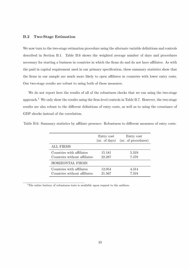
B.2 Two-Stage Estimation

We now turn to the two-stage estimation procedure using the alternate variable definitions and controls

described in Section B.1. Table B.6 shows the weighted average number of days and procedures

necessary for starting a business in countries in which the firms do and do not have affiliates. As with

the paid in capital requirement used in our primary specification, these summary statistics show that

the firms in our sample are much more likely to open affiliates in countries with lower entry costs.

Our two-stage results are robust to using both of these measures.

We do not report here the results of all of the robustness checks that we ran using the two-stage

approach.1 We only show the results using the firm-level controls in Table B.7. However, the two-stage

results are also robust to the different definitions of entry costs, as well as to using the covariance of

GDP shocks instead of the correlation.

Table B.6: Summary statistics by affiliate presence: Robustness to different measures of entry costs.

Entry cost Entry cost(nr. of days) (nr. of procedures)

ALL FIRMS

Countries with affiliates 15.181 5.319Countries without affiliates 22.287 7.478

HORIZONTAL FIRMS

Countries with affiliates 12.054 4.314Countries without affiliates 21.567 7.318

1The entire battery of robustness tests is available upon request to the authors.

43

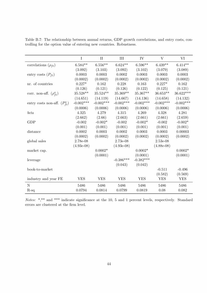
Table B.7: The relationship between annual returns, GDP growth correlations, and entry costs, con-trolling for the option value of entering new countries. Robustness.

I II III IV V VI

correlations (ρft) 6.584** 6.556** 6.624** 6.596** 6.439** 6.414**(3.092) (3.103) (3.092) (3.102) (3.079) (3.089)

entry costs (Pft) 0.0003 0.0003 0.0002 0.0003 0.0003 0.0003(0.0002) (0.0002) (0.0002) (0.0002) (0.0002) (0.0002)

nr. of countries 0.227* 0.162 0.228 0.163 0.227* 0.162(0.126) (0.121) (0.126) (0.122) (0.125) (0.121)

corr. non-aff. (ρoft) 35.528** 35.524** 35.369** 35.367** 36.653** 36.622***

(14.651) (14.119) (14.667) (14.136) (14.658) (14.132)entry costs non-aff. (P o

ft) -0.002*** -0.002*** -0.002*** -0.002*** -0.002*** -0.002***

(0.0006) (0.0006) (0.0006) (0.0006) (0.0006) (0.0006)beta 4.325 4.279 4.315 4.269 4.328 4.281

(2.662) (2.66) (2.663) (2.661) (2.661) (2.659)GDP -0.002 -0.002* -0.002 -0.002* -0.002 -0.002*

(0.001) (0.001) (0.001) (0.001) (0.001) (0.001)distance 0.0002 0.0003 0.0002 0.0003 0.0003 0.00003

(0.0002) (0.0002) (0.0002) (0.0002) (0.0002) (0.0002)global sales 2.78e-08 2.73e-08 2.53e-08

(4.93e-08) (4.93e-08) (4.88e-08)market cap. 0.0002* 0.0002* 0.0002*

(0.0001) (0.0001) (0.0001)leverage -0.386*** -0.382***

(0.043) (0.042)book-to-market -0.511 -0.496

(0.582) (0.569)industry and year FE YES YES YES YES YES YES

N 5486 5486 5486 5486 5486 5486R-sq 0.0794 0.0814 0.0799 0.0819 0.08 0.082

Notes: *,** and *** indicate significance at the 10, 5 and 1 percent levels, respectively. Standarderrors are clustered at the firm level.

44

C Robustness: Structural Analysis

C.1 Risk Premium by Country

Table C.1 shows the full set of country-level results described in Section 4.3.1.

Table C.1: Country-specific estimates of ψj and ψoj , observations at the firm-year level.

coefficients risk premia

ψj ψj ψoj ψσhσjρjε

fj ψσhσjρjε

fj ψo

jσhσjρjZfj

Country I II I II

US Domestic 0.036*** 0.058*** 0.23 0.371(0.010) (0.017)

United Kingdom 0.011 0.010 1.242** 0.060 0.055 0.496(0.009) (0.009) (0.524)

Canada 0.034*** 0.033*** 0.622 0.137 0.133 0.136(0.012) (0.012) (0.728)

Germany -0.008 -0.007 1.338 -0.014 -0.012 0.292(0.006) (0.006) (0.896)

Singapore 0.075*** 0.064*** -3.223 0.491 0.419 -0.206(0.020) (0.021) (2.591)

Switzerland 0.031 0.021 -0.258 0.048 0.033 -0.014(0.027) (0.027) (2.960)

Ireland 0.001* 0.005*** -1.273 0.014 0.069 -0.396(0.001) (0.002) (0.804)

Japan 0.011*** 0.011*** -0.270 0.011 0.011 -0.042(0.003) (0.003) (0.720)

Netherlands 0.032** 0.029** 1.088 0.155 0.140 0.060(0.014) (0.014) (1.236)

France -0.010 -0.007 -1.366 -0.022 -0.015 -0.301(0.012) (0.013) (1.185)

Mexico 0.037 0.040 1.718 0.131 0.142 0.223(0.035) (0.036) (1.137)

China 0.951 0.818 -5.105 0.409 0.351 -0.066(0.587) (0.612) (6.636)

Brazil -0.018 -0.018 -8.398 -0.009 -0.009 -0.12(0.038) (0.038)

Australia 0.125** 0.109** -0.033 0.202 0.176 -0.001(0.051) (0.051) (3.915)

45

coefficients risk premia

ψj ψj ψoj ψσhσjρjε

fj ψσhσjρjε

fj ψo

jσhσjρjZfj

Country I II I II

Belgium 0.017 0.017 4.449** 0.030 0.030 0.461(0.031) (0.031) (2.242)

Italy 0.032 0.033 -0.426 0.087 0.090 -0.079(0.024) (0.025) (1.070)

Hong Kong 0.026** 0.021 -4.075 0.170 0.137 -0.192(0.013) (0.013) (3.164)

Spain -0.004 -0.006 -1.189 0.001 0.001 -0.151(0.009) (0.010) (1.898)

South Korea 0.148* 0.115 9.746** 0.249 0.194 0.374(0.080) (0.081) (4.682)

Norway -0.069 -0.037 -9.849 -0.105 -0.056 -0.610(0.127) (0.126) (5.591)

Malaysia 0.243** 0.222** -0.685 0.576 0.526 -0.027(0.103) (0.103) (4.153)

India 0.324* 0.259 10.480 0.535 0.428 0.127(0.185) (0.183) (7.962)

Sweden 0.015 0.008 0.889 0.071 0.038(0.025) (0.025) (2.088)

Thailand 0.032 -0.019 -18.164** 0.063 -0.037 -0.434(0.043) (0.040) (8.884)

Argentina 0.02 0.021 96.846** -0.014 -0.014 -0.445(0.028) (0.027) (43.707)

Poland -0.066* -0.061* 11.643*** -0.358 -0.331 0.685(0.037) (0.037) (2.723)

Luxembourg 0.004 0.004 0.059 0.059(0.006) (0.005)

Russia -0.018 -0.020 -12.414** 0.030 0.030 -0.627(0.015) (0.015) (5.196)

Chile 0.069 0.087 5.520 0.075 0.095 0.143(0.090) (0.090) (8.400)

Indonesia 0.081* 0.079* -6.277 -0.079 -0.077 0.136(0.043) (0.043) (11.046)

Austria 0.004 0.006 -6.542 0.006 0.008 -0.433(0.018) (0.018) (5.317)

Venezuela -1.063 -1.146 10.765 0.128 0.138 -0.022(1.060) (1.060) (127.628)

South Africa -0.060 -0.045 18.842 -0.071 -0.053 0.284(0.078) (0.076) (12.540)

Turkey 0.057 0.061 14.127*** 0.052 0.056 1.100(0.078) (0.077) (4.859)

46

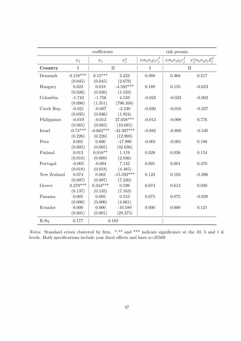
coefficients risk premia

ψj ψj ψoj ψσhσjρjε

fj ψσhσjρjε

fj ψo

jσhσjρjZfj

Country I II I II

Denmark 0.158*** 0.15*** 2.223 0.388 0.368 0.217(0.045) (0.045) (2.679)

Hungary 0.022 0.018 -4.592*** 0.189 0.155 -0.623(0.026) (0.026) (1.533)

Colombia -1.743 -1.756 4.533 -0.023 -0.023 -0.002(0.090) (1.351) (796.356)

Czech Rep. -0.021 -0.007 -2.240 -0.030 -0.010 -0.337(0.035) (0.036) (1.824)

Philippines -0.019 -0.012 37.058*** -0.013 -0.008 0.776(0.085) (0.085) (10.085)

Israel -0.73*** -0.662*** -42.397*** -0.882 -0.800 -0.540(0.226) (0.226) (12.993)

Peru 0.001 0.000 -17.990 -0.001 -0.001 0.186(0.005) (0.005) (32.638)

Finland 0.013 0.018** 1.119 0.028 0.038 0.154(0.010) (0.009) (2.836)

Portugal -0.005 -0.004 7.142 0.001 0.001 0.470(0.018) (0.018) (4.485)

New Zealand 0.074 0.062 -15.592*** 0.123 0.103 -0.396(0.097) (0.097) (7.220)

Greece 0.379*** 0.344*** 0.599 0.674 0.612 0.030(0.137) (0.135) (7.163)

Panama 0.005 0.005 0.553 0.075 0.075 -0.028(0.006) (0.006) (4.861)

Ecuador 0.000 0.000 -10.589 0.000 0.000 0.121(0.001) (0.001) (29.375)

R-Sq 0.177 0.182

Notes: Standard errors clustered by firm. *,** and *** indicate significance at the 10, 5 and 1 &levels. Both specifications include year fixed effects and have n=25569

47

C.2 Risk Premium of Single Host Country Firms

Section 4.3 describes the method we used to approximate the option value of entering countries in

which a firm currently does not have affiliates. Including this measure improves the fit of the model

and provides reasonable estimates of the contribution of the option value to a firm’s risk premium.

However, because we do not directly observe the option value, this is still just an approximation.

In this section, we test the robustness of our results by estimating the risk premium for a small

subset of firms in a way that controls for the option value but does not require us to approximate

it. We do this by limiting our sample to firms that operate in an identical set of countries. In this

way, the option value term is shut down, and all of the variation comes from differences in the firm’s

assets in place. To implement this, we examine the returns of the sub-sample of firms with affiliates

operating in only one country. There are 13 countries in the sample that are the sole foreign affiliate

location for 10 or more US MNCs. We separately estimate equation (16) for the set of firms that

operate exclusively in each of these countries. The single-country version of equation (16) is:

E(retfj ) = ψhσ2hε

fh + ψjσhσjρj ε

fj + ηf (C.1)

where E(retfj ) are the returns of a firm j that has affiliates in country j only and ψi ≡ γζi, for i = h, j

and j = 1, ...N . Notice that the single host country estimates - by keeping the set of host countries

constant - automatically control for the country-specific component of the option value of entering

new countries.

The country-specific estimates of the parameter ψj convey information on the riskiness of individual

countries that host affiliate activities. The results are reported in Table C.2. Each row of Table C.2

gives the estimated values of ψj for firms whose foreign operations take place exclusively in the country

listed in the first column. Of the 12 estimated ψj coefficients presented in Table C.2, 11 are positive. 4

of the 12 coefficients are statistically significant at the 5 percent level, and all 4 of these significant ψj

coefficients are positive. Positive values of ψj indicate that the corresponding countries are a source

of risk to the firm. Like in our baseline results, a positive value of ψj indicates that foreign operations

are a source of risk to the firm, while negative values of ψj indicate that the host country generates a

48

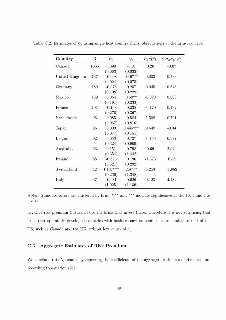
Table C.2: Estimates of ψj using single host country firms, observations at the firm-year level.

Country N ψh ψj ψhσ2hε

fh ψjσhσjρj ε

fj

Canada 1665 0.098 -0.01 0.26 -0.07(0.063) (0.033)

United Kingdom 737 -0.008 0.167** 0.003 0.733(0.024) (0.075)

Germany 189 -0.076 0.257 0.045 0.548(0.108) (0.229)

Mexico 139 0.064 0.59** -0.023 0.863(0.191) (0.233)

France 107 -0.168 0.238 -0.179 0.132(0.276) (0.367)

Netherlands 96 0.085 0.584 1.508 0.791(0.067) (0.816)

Japan 95 0.099 0.445*** 0.649 -0.34(0.077) (0.151)

Belgium 92 0.053 0.727 -0.153 0.387(0.324) (0.909)

Australia 63 0.151 0.798 0.69 2.644(0.354) (1.442)

Ireland 68 -0.693 0.196 -1.376 0.86(0.521) (0.292)

Switzerland 42 1.137*** 2.877* 5.253 -1.982(0.236) (1.348)

Italy 37 -0.031 0.626 0.123 4.182(1.025) (1.136)

Notes: Standard errors are clustered by firm. *,** and *** indicate significance at the 10, 5 and 1 &levels.

negative risk premium (insurance) to the firms that invest there. Therefore it is not surprising that

firms that operate in developed countries with business environments that are similar to that of the

US, such as Canada and the UK, exhibit low values of ψj .

C.3 Aggregate Estimates of Risk Premium

We conclude this Appendix by reporting the coefficients of the aggregate estimates of risk premium

according to equation (21).

49

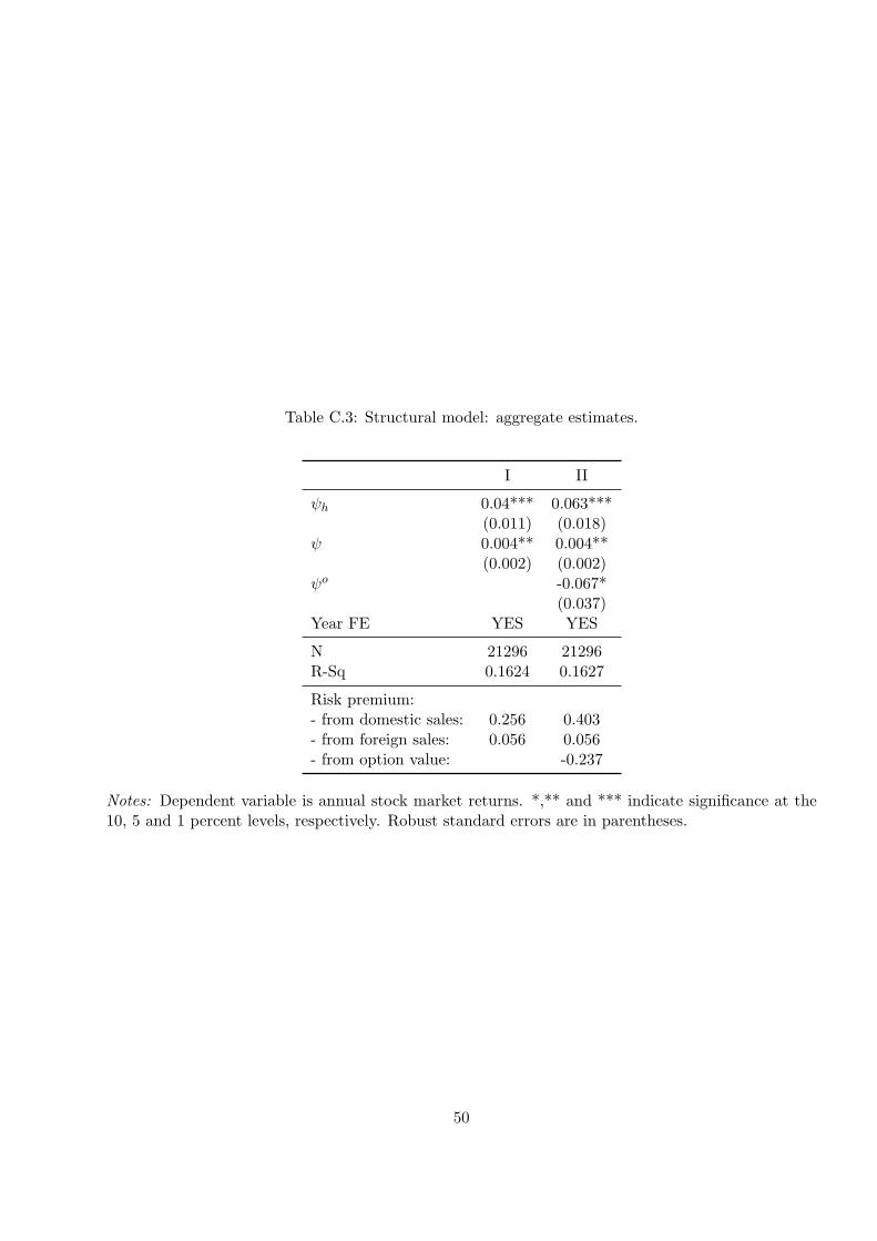
Table C.3: Structural model: aggregate estimates.

I II

ψh 0.04*** 0.063***(0.011) (0.018)

ψ 0.004** 0.004**(0.002) (0.002)

ψo -0.067*(0.037)

Year FE YES YES

N 21296 21296R-Sq 0.1624 0.1627

Risk premium:- from domestic sales: 0.256 0.403- from foreign sales: 0.056 0.056- from option value: -0.237

Notes: Dependent variable is annual stock market returns. *,** and *** indicate significance at the10, 5 and 1 percent levels, respectively. Robust standard errors are in parentheses.

50