Embed Size (px)
Citation preview
Journal of Financial Economics 14 (1985) 473-489. North-Holland
DIVIDEND YIELDS AND STOCK RETURNS Implications of Abnormal January Returns
Donald B. KEIM*
University of Pennsylvania, Philadelphia, PA I91 04 USA
Received January 1983, final version received March 1985
This study examines the empirical relation between stock returns and (long-run) dividend yields. The findings show that much of the phenomenon is due to a nonlinear relation between dividend yields and returns in January. Regression coefficients on dividend yields, which some models predict should be non-zero due to differential taxation of dividends and capital gains, exhibit a significant January seasonal, even when controlling for size. This finding is significant since there are no provisions in the after-tax asset pricing models that predict the tax differential is more important in January than in other months.
1. Introduction
Asset pricing anomalies are a subject of considerable recent attention in financial economics. The relation between dividend yields and common stock returns has received particularly close scrutiny. Much of this research has been conducted as tests of an after-tax Capital Asset Pricing Model (CAPM), which predicts that a positive relation between dividend yields and returns is induced by the disparity in the tax rates for dividend yields and capital gains.’ These empirical tests have documented a positive yield effect with both short-run [e.g., Litzenberger and Ramaswamy (1979)] and long-run [e.g., Blume (1980)] definitions of dividend yields. In a recent paper, Miller and Scholes (1982) argue that yield-related effects associated with short-term definitions of div-
*I would like to thank my dissertation committee - Eugene Fama (Chairman), Robert Hamada, Robert Holthausen, Richard Leftwich, Merton Miller, and Myron Scholes - as well as Marshall Blume, Wayne Ferson, Bruce Grundy, Bob Korajnyk, Paul Schultz, Rob Stambaugh, participants of the Berkeley-Stanford Finance Workshop, and especially Allan Kleidon, the referee, for valuable comments and discussions. An earlier version of this paper was presented at the Small Firm Effect Conference at the University of Southern California in April 1982. I gratefully acknowledge the comments of my discussant, Fischer Black, and of the conference participants. Any remaining errors are my responsibility.
‘See Brennan (1970) and Litzenberger and Ramaswamy (1979). Miller and Scholes (1978) argue that the effective marginal tax rate on dividends is no larger than the tax rate on capital gains. Several studies [e.g., Blume (1980) and Gordon and Bradford (1980)] find a significant relation between dividend yields and returns but do not attribute the relation to taxes.
0304-405X/85/$3.3Ool985, Elsevier Science Publishers B.V. (North-Holland)
414 D. B. Kern,, Dividend yields and the January sire effect
idend yield are due to information biases and not taxes. The purpose here is to examine whether yield effects that are estimated with long-run definitions of
dividend yield are indeed tax effects or whether they are related to anomalous effects documented recently in the literature [e.g., the size effect found by Banz (1981) and Reinganum (1981)].
The first half of this paper focuses on the relation between raw returns and dividend yields and confirms earlier results [Blume (1980)] by finding a non-linear relation between long-run yields and returns. The results indicate, however, that this yield effect occurs predominantly in January. When January observations are excluded the yield-return relation is no longer significant.
The second half of the paper examines the seasonal behavior of dividend yield coefficients. A necessary result of differential marginal taxation of dividends and capital gains is a non-zero coefficient in a regression of returns
on dividend yields. Although a formal test of an after-tax pricing model is not conducted here, the tests below find a positive yield coefficient that exhibits a significant January seasonal. This evidence is not entirely consistent with a
simple tax-related model [e.g., Brennan (1970), Litzenberger and Ramaswamy (1979)] as the sole explanation of the phenomenon.
An alternative explanation is that the January yield effect may be a mani- festation of the significant relation in January between returns and market value of equity (size) documented in Keim (1983b). I investigate, therefore, the marginal explanatory power of dividend yields in January while controlling for size. Inclusion of size in the regressions results in attenuation of the yield coefficient in both January and non-January months, but a significant relation between returns and dividend yields still remains. Further, estimates of the yield coefficient remain significantly larger in January than in the other
months. Section 2 contains a brief summary of the arguments concerning the effects
of dividends and taxes on stock returns. In section 3 I reproduce the non-linear relation between returns and long-run dividend yields and document a January seasonal in this relation. Section 4 reports that estimates of dividend yield coefficients exhibit a significant January seasonal, and also reports similar tests that control for market value of equity. Section 5 contains a brief summary
and conclusions.
2. Dividends and taxes
Higher marginal tax rates of dividend income versus capital gains should make taxable investors prefer a dollar of pre-tax capital gain to a dollar of dividends. Under such conditions, Brennan (1970) and Litzenberger and Ramaswamy (1979) formulate an after-tax CAPM which takes the following
D. B. Keim, Dividend yields and rhe Junuq see effecr 475
general form:
E(R,)-r,=a,+a,P,+a,(d,-r,), (1)
where E( R,) is the before-tax expected rate of return on asset i, j3, and d, are the systematic risk and dividend yield for asset i, respectively, and rF is the risk-free rate of interest. The coefficient on the yield variable, u2, is interpreted as an implicit tax bracket and is independent of the level of the dividend
yield d. Miller and Scholes (1978) argue that the tax code has provisions that permit
investors to transform dividend income into capital gains. If the marginal investors are using these or other effective shelters, the coefficient a, in (1) may not be different from zero even though the tax law appears to penalize dividends. Furthermore, as Black and Scholes (1974) point out, the potential tax effect may be offset by supply adjustments and the need to preserve
adequate diversification, A large body of empirical research is devoted to understanding the relation
between dividend yields and stock returns. The studies can be broadly clas- sified into two groups: those that use long-run estimates of dividend yield and those that use short-run estimates. * The rationale for the use of a short-run
definition of dividend yield, such as that used by Litzenberger and Ramaswamy (1979) is the tax-induced cum-ex return differential investigated by Elton and
Gruber (1970). This difference is necessary for indifference at the beginning of the ex-month, on the part of current shareholders, between (1) continuing to hold the shares and paying full tax on the forthcoming dividend and (2) selling the shares cum dividend and paying tax on the implicit dividend at the capital gains tax rate. Miller and Scholes (1982) argue that if short-term traders or tax-exempt institutions (who both have the same tax rates on both dividends and capital gains) dominate the equilibrium, then any tax-induced return differential will be eliminated.3 Miller and Scholes (1982, p. 1139) recognize that a yield effect might exist, nevertheless, since ‘transactions costs.. . may well keep the ex-dividend price from falling by the full amount of the dividend’. The empirical tests conducted by Miller and Scholes suggest that yield-related effects documented with certain short-term yields are a result of information effects and not the tax differential.
Blume (1980) documents a positive value for u2 in (1) using a long-run measure of yield. The purpose here is to examine whether yield effects that are estimated with long-run definitions of dividend yields are solely tax effects or
whether they are related to anomalous effects like the size effect.
‘Miller and Scholes (1982) are the first to make this distinction. See the discussion in Miller and Scholes (1982) and the references cited therein.
‘See Kalay (1982) for a similar argument.
416 D. B. Keim, Dividend yields and the January size efse
3. The relation between dividend yields and stock returns
3.1. The data
The data are from the monthly files of New York Stock Exchange (NYSE) stocks maintained by the Center for Research in Security Prices (CRSP) at the University of Chicago. The criteria employed in selecting sample firms in a particular month are that the firm is listed on the NYSE and had returns on the CRSP monthly file for the previous sixty months. Thus, every month firms enter or leave the sample due to mergers, bankruptcies, delistings and new listings. The number of firms which meet this requirement range from 429 in January 1931 to 1289 in December 1978.
3.2. Results
To analyze the relation between returns and dividend yields of NYSE firms, I employ the following procedure. In each month I divide the sample securities into six groups of increasing dividend yield (one group containing all zero- dividend firms, the other five representing the quintiles of the positive-yield firms), where dividend yield in month t is defined as the sum of the dividends paid in the previous twelve months divided by the stock price in month t- 13:4
I then compute portfolio returns by combining the returns for the securities in each portfolio with equal weights. This procedure is repeated month-by-month, resulting in a time series of portfolio returns for the period January 1931 to December 1978.
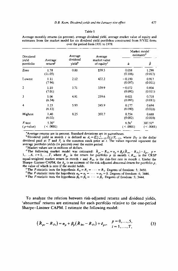
Table 1 reports mean returns for each dividend yield portfolio, along with average dividend yields and average market values of equity for each portfolio. The average returns of the dividend yield portfolios display a non-linear relation with average yields that is consistent with the results of Blume (1980) and Litzenberger and Ramaswamy (1980). Zero dividend securities have, on average, the largest returns, while returns for dividend paying stocks tend to increase as dividend yield increases. The hypothesis that average returns are equal across portfolios is easily rejected (F = 5.30).
‘In Keim (1983a) I replicated much of the analysis in this paper with a dividend yield variable that used P,_, (rather than P,_,3) in the denominator; the results there are quantitatively and qualitatively the same as those reported here.
D. B. Keim, Dividend yields und the Junuq size effect 471
Table 1
Average monthly returns (in percent), average dividend yield, average market value of equity and estimates from the market model for six dividend yield portfolios constructed from NYSE firms
over the period from 1931 to 1978.
Dividend yield portfolio
Average return=
Average dividend
yieldb
Average market value
of equityC
Zero
Lowest
2
3
4
Highest
F-test (p-value)
1.78 (11.05)
1.11 (7.94)
1.10 (7.01)
1.06 (6.34)
1.23 (6.12)
1.40 (6.02)
5.30’ (< .OOOl)
2.12
3.71
4.81
5.93
8.25
$59.5
422.2
339.9
259.6
245.9
202.7
Market model. estimatesd
& P
0.058 1.298 (0.106) (0.013)
-0.190 0.917 (0.097) (0.011)
- 0.072 0.804 (0.092) (0.011)
- 0.021 0.718 (0.093) (0.011)
0.177 0.694 (0.090) (0.011)
0.354 0.688 (0.082) (0.010)
6.56’ 307.519 ( < .cQOl) (< .OOOl)
‘Average returns are in percent. Standard deviations are in parentheses. bDividend yield in month t is defined as d, = c’-l _ T-r 13 I D )/P,_ 13, where D, is the dollar
dividend paid at T and P, is the common stock price at t. The values reported represent the average portfolio yields (in percent) over the entire period.
‘Market values are in millions of dollars. dThe following market model was estimated: A,, - R, = ap + /?,(k,,,, - R,) + Sp,, P=
l,..., 6, f=l,..., T, where R,, is the return for portfolio p in month t, R,, is the CRSP
equal-weighted market return in month t and R, is the risk-free rate in month I. Under the Sharpe-Lintner CAPM, the & the value of which is zero if t R
is an estimate of the risk-adjusted abnormal ietum for portfolio p, e model holds.
‘The F-statistic tests the hypothesis R,, = R, = = R,. Degrees of freedom: 5; 3450. ‘The F-statistic tests the hypothesis a0 = 0~~ = . = ns = 0. Degrees of freedom: 6; 3444. &The F-statistic tests the hypothesis & = 8, = . = &. Degrees of freedom: 5; 3444.
To analyze the relation between risk-adjusted returns and dividend yields, ‘abnormal’ returns are estimated for each portfolio relative to the one-period Sharpe-Lintner CAPM. I estimate the following model:
(3)
478 D. B. Keim, Dividend yields and the January sire effect
where ii,, = rate of return for portfolio p in month t, A,, = rate of return for CRSP equal-weighted market return in month t, *and RF, is the riskless rate of interest in month t. The Sharpe-Lintner CAPM implies 0~~ = 0. If there is a dividend yield effect relative to the Sharpe-Lintner model, then estimates of (Y~ will be systematically related to average portfolio dividend yields.
Columns 5 and 6 of table 1 show estimates of (Ye and /3,, for the period 1931 to 1978. The results indicate a non-linear relation between risk-adjusted returns and dividend yield. To test the hypothesis that abnormal returns are jointly equal to zero across portfolios, I test that (Ye = 0~~ = 0~~ = LYE = (Ye = 0~~ = 0. The F-statistic, reported at the bottom of column 5, easily rejects the hypothesis (F = 6.56). The hypothesis is also rejected in each of three subperi- ods examined (1931-1945,1946-1962,1963-1978) but not reported here.
3.3. The relation between yields and size
The differences in abnormal returns across dividend yield portfolios may be related to systematic differences in market capitalization among the portfolios. The average market capitalization of the zero dividend portfolio is $59.5 million (table 1). In contrast, the average market value of firms with the lowest (but positive) yield is $422.2 million. Furthermore, positive dividend yields and market values are inversely related. A relation between firm size and dividend yield suggests that the long-run yield effect may be another mani- festation of the relation between returns and size-related variables.
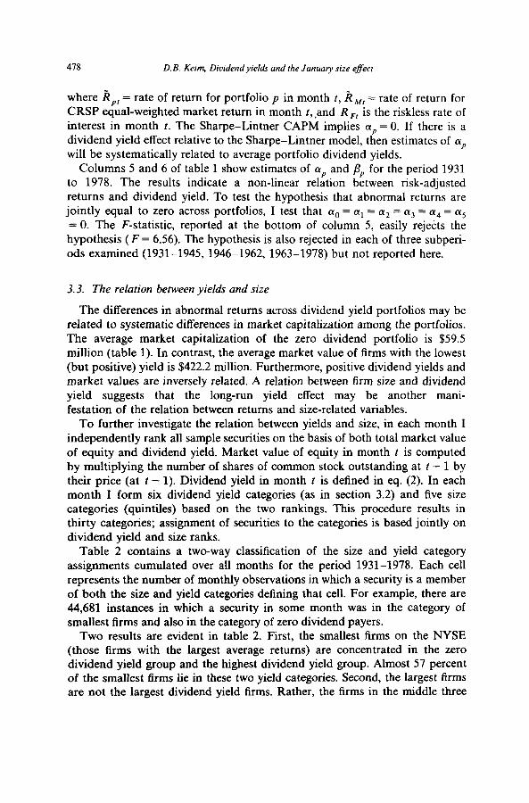
To further investigate the relation between yields and size, in each month I independently rank all sample securities on the basis of both total market value of equity and dividend yield. Market value of equity in month t is computed by multiplying the number of shares of common stock outstanding at t - 1 by their price (at t - 1). Dividend yield in month t is defined in eq. (2). In each month I form six dividend yield categories (as in section 3.2) and five size categories (quintiles) based on the two rankings. This procedure results in thirty categories; assignment of securities to the categories is based jointly on dividend yield and size ranks.
Table 2 contains a two-way classification of the size and yield category assignments cumulated over all months for the period 1931-1978. Each cell represents the number of monthly observations in which a security is a member of both the size and yield categories defining that cell. For example, there are 44,681 instances in which a security in some month was in the category of smallest firms and also in the category of zero dividend payers.
Two results are evident in table 2. First, the smallest firms on the NYSE (those firms with the largest average returns) are concentrated in the zero dividend yield group and the highest dividend yield group. Almost 57 percent of the smallest firms he in these two yield categories. Second, the largest firms are not the largest dividend yield firms. Rather, the firms in the middle three
D.B. Kelm. Diurdendylelds und the Junuuty sire eflecl 479
Table 2
Two-way classification of the number of NYSE securities assigned to the size and yield portfolios for every month over the period from 1931 to 1978.a
Size
portfoliob
Smallest 2 3 4 Largest
Zero
44681 22936 14103
9654 4968
Dividend yield portfolio’
Lowest 2 3 4 Highest
9081 8771 9356 10931 15026 11676 12857 14271 16184 19565 14279 15045 16549 18586 18933 17660 19096 19038 17140 14911 26081 22386 19007 15413 10364
‘The cell values are the total number of monthly observations in which a security was a member of both the size and yield portfolios defining that cell. For example, there were 44,681 instances in which a security in some month was in the portfolio of smallest companies and also in the portfolio of zero-dividend payers.
‘Size is measured by the market value of common equity. ‘Dividend yield in month t is defined as the sum of the dividends paid in the previous twelve
months divided by the stock price in month r - 13.
size categories have historically had larger yields. Almost 69 percent of the largest firms (those firms that, on average, have the lowest returns) lie in the three lowest non-zero yield groups.
The implication is clear. The high average returns of the zero and highest yield groups may simply reflect the high returns of small firms that are concentrated in those categories. On the other hand, the largest NYSE firms are distributed among the lower end of the non-zero yield firms. The low returns of the lower, non-zero yield group, therefore, may reflect the low average returns of larger firms. The peaks and troughs of the non-linear long-run yield function may be due to the location of small and large firms within the dividend yield continuum.
3.4. Seasonality and the relation between yields and returns
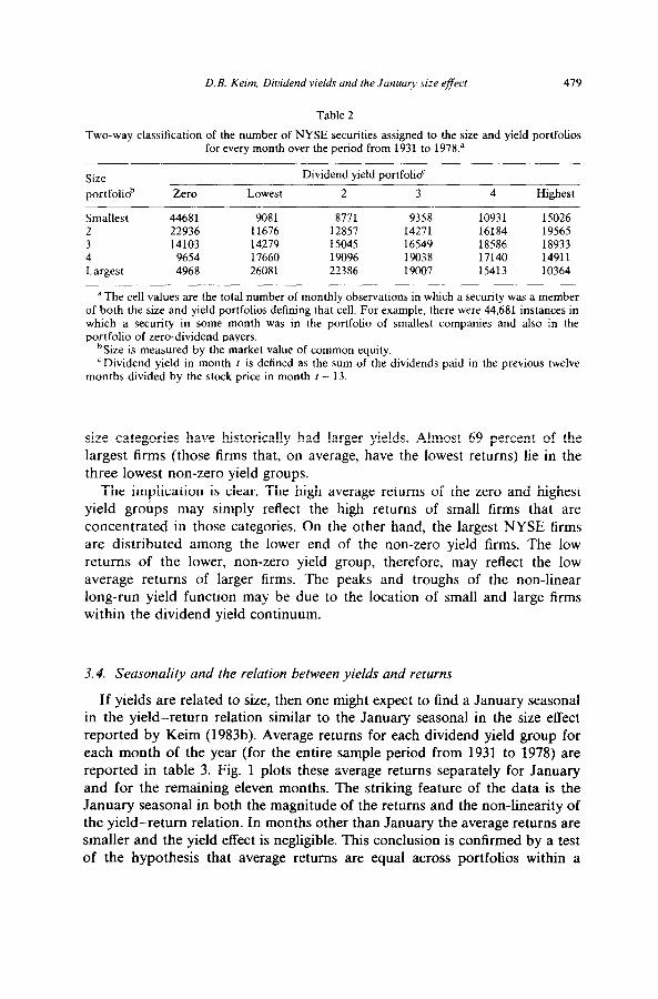
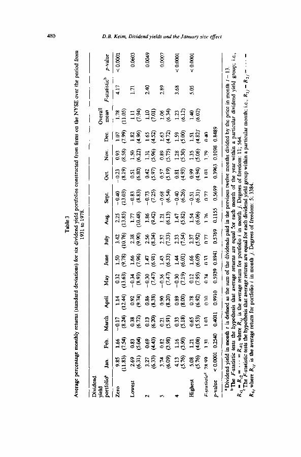
If yields are related to size, then one might expect to find a January seasonal in the yield-return relation similar to the January seasonal in the size effect reported by Keim (1983b). Average returns for each dividend yield group for each month of the year (for the entire sample period from 1931 to 1978) are reported in table 3. Fig. 1 plots these average returns separately for January and for the remaining eleven months. The striking feature of the data is the January seasonal in both the magnitude of the returns and the non-linearity of the yield-return relation. In months other than January the average returns are smaller and the yield effect is negligible. This conclusion is confirmed by a test of the hypothesis that average returns are equal across portfolios within a
Tab
le 3
Ave
rage
pe
rcen
tage
m
onth
ly r
etur
ns
(sta
ndar
d de
viat
ions
) fo
r si
x di
vide
nd
yiel
d po
rtfo
lios
cons
truc
ted
from
fir
ms
on t
he N
YSE
ove
r th
e pe
riod
fr
om
1931
to 1
978.
Div
iden
d yi
eld
Ove
rall
port
folid
Ja
n.
Feb.
M
arch
A
pril
May
Ju
ne
July
A
ug.
Sept
. O
ct.
Nov
. D
ec.
mea
n F-
stat
istic
b p-
valu
e P PJ
Zer
o 9.
85
1.66
-0
.17
1.14
0.
32
1.50
3.
42
2.25
-0
.40
- 0.
23
0.93
1.
07
1.78
4.
17
< 0
.000
1 3 _,
(1
1.83
) (7
.54)
(8
.24)
(1
2.44
) (1
3.63
) (9
.78)
(1
0.76
) (1
3.85
) (1
3.03
) (8
.19)
(8
.58)
(7
.99)
(1
1.05
) 3
Low
est
2.69
0.
83
0.38
0.
92
-0.3
4 1.
66
2.38
1.
77
-0.8
3 0.
51
1.50
1.
82
1.11
1.
71
(6.3
1)
(5.0
4)
(6.7
2)
(9.7
4)
(8.9
3)
(7.9
6)
(9.9
0)
(10.
48)
(8.8
3)
(6.8
0)
(6.2
2)
(4.9
6)
(7.9
4)
0.06
03
$ 3 2
3.27
0.
69
0.13
0.
86
- 0.
30
1.47
2.
56
1.86
-
0.73
0.
42
1.31
1.
65
1.10
2.
40
(6.3
3)
(4.4
3)
(6.2
0)
(8.3
8)
(7.4
7)
(6.9
1)
(8.3
4)
(9.4
2)
(7.2
5)
(5.9
7)
(5.9
6)
(4.5
2)
(7.0
1)
0.00
49
$ ;i;.
3 3.
74
0.82
0.
21
0.90
-0
.36
1.43
2.
32
1.21
-
0.68
0.
57
0.89
1.
63
l.c.6
2.
89
B
(6.0
9)
(3.9
8)
(5.9
1)
(8.2
0)
(7.4
7)
(6.3
3)
(7.3
3)
(6.1
3)
0.00
07
~ (6
.54)
(5
.19)
(5
.75)
(4
.72)
(6
.34)
&
4
4.13
1.
16
0.33
0.
89
- 0.
30
1.44
2.
33
1.47
-0
.40
0.81
1.
28
1.59
1.
23
3.68
<
0.0
001
3
(5.7
6)
(3.9
0)
(5.1
8)
(8.0
0)
(7.1
9)
(6.0
1)
(7.5
4)
(5.8
2)
(6.2
6)
(4.9
3)
(5.3
0)
(5.0
0)
(6.1
2)
: : H
ighe
st
5.08
1.
21
0.65
0.
78
0.12
1.
66
2.37
1.
54
-0.5
1 0.
99
1.35
1.
51
1.40
5.
05
< 0
.000
1 (5
.76)
(4
.08)
(5
.53)
(6
.92)
(7
.95)
(6
.09)
(5
.92)
(6
.06)
(6
.31)
(4
.94)
(5
.06)
(4
.82)
’ (6
.02)
5 h
F-st
atis
tic’
28.9
9 1.
31
1.03
0.
10
0.74
0.
33
0.77
1.
76
0.77
1.
03
1.79
0.
40
;;-
p-va
lue
< 0
.000
1 0.
2540
0.
4011
0.
9910
0.
5939
0.
8941
0.
5769
0.
1155
0.
5699
0.
3963
0.
1098
0.
8489
4 $
‘Div
iden
d yi
eld
in m
onth
r
is d
efin
ed
as t
he s
um o
f th
e di
vide
nds
paid
in
the
prev
ious
tw
elve
mon
ths
divi
ded
by t
he p
rice
in
mon
th
t -
13.
bThe
F-
stat
istic
te
sts
the
hypo
thes
is
that
av
erag
e re
turn
s ar
e eq
ual
for
each
m
onth
of
th
e ye
ar
with
in
a pa
rtic
ular
di
vide
nd
yiel
d gr
oup;
i.e
., R
il =
Ri2
=
. .
. =
Ri1
2 w
here
Ri
is t
he a
vera
ge r
etur
n fo
r po
rtfo
lio
i in
mon
th
j. D
egre
es o
f fr
eedo
m:
11;
564.
‘T
he
Fsta
tistic
te
sts
the
hypo
tfre
sis
that
ave
rage
ret
urns
ar
e eq
ual
for
each
div
iden
d yi
eld
grou
p w
ithin
a p
artic
ular
m
onth
; i.e
., R
,, =
RZ
, =
.
=
RY
whe
re
R,j
is t
he a
vera
ge r
etur
n fo
r po
rtfo
lio
i in
mon
th
j. D
egre
es o
f fr
eedo
m:
5; 3
384.
D. B. Keim. Diuidendyielak and the January size e&r 481
10.0
9.0
8.0
C 7.0
S G 6.0 a
is 5.0 C-0
Ci 4.c 0
t a 3.0
2.0
1.0
I-
,-
l-
l-
l-
l-
,-
February to December
Dividend Yield Portfolio
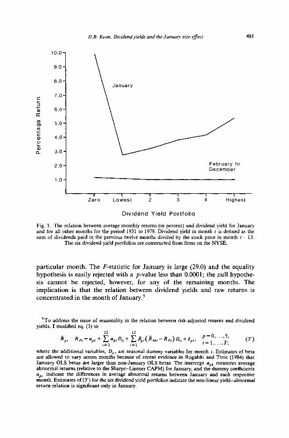
Fig. 1. The relation between average monthly returns (in percent) and dividend yield for January and for all other months for the period 1931 to 1978. Dividend yield in month I is defined as the sum of dividends paid in the previous twelve months divided by the stock price in month f - 13.
The six dividend yield portfolios are constructed from firms on the NYSE.
particular month. The F-statistic for January is large (29.0) and the equality hypothesis is easily rejected with a p-value less than 0.0001; the null hypothe- sis cannot be rejected, however, for any of the remaining months. The implication is that the relation between dividend yields and raw returns is concentrated in the month of January.S
5To address the issue of seasonality in the relation between risk-adjusted returns and dividend yields, I modified eq. (3) to
where the additional variables, D,,, are seasonal dummy variables for month i. Estimates of beta are allowed to vary across months because of recent evidence in Rogalski and Tinic (1984) that January OLS betas are huger than non-January OLS betas. The intercept apI measures average abnormal returns (relative to the Sharpe-Lintner CAPM) for January, and the dummy coefficients ap, indicate the differences in average abnormal returns between January and each respective month. Estimates of (3’) for the six dividend yield portfolios indicate the non-linear yield-abnormal return relation is significant only in January.
482 D. B. Keim, Dividend yields and the Januav size effect
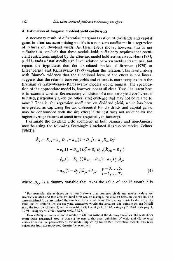
4. Estimation of long-run dividend yield coefficients
A necessary result of differential marginal taxation of dividends and capital gains in after-tax asset pricing models is a non-zero coefficient in a regression of returns on dividend yields. As Hess (1983) shows, however, this is not sufficient to conclude that these models hold; sufficiency requires that coeffi- cient restrictions implied by the after-tax model hold across assets. Hess (1983, p. 553) finds a ‘statistically significant relation between yields and returns’, but rejects the hypothesis that the tax-related models of Brennan (1970) or Litzenberger and Ramaswamy (1979) explain the relation. This result, along with Blume’s evidence that the functional form of the effect is not linear, suggests that the relation between yields and returns is more complex than the Brennan or Litzenberger-Ramaswamy models would suggest. The specifica- tion of the appropriate model is, however, not at all clear. Thus, the intent here is to examine whether the necessary condition of a non-zero yield coefficient is
fulfilled, particularly given the other (size) evidence that may not be related to taxes.6 That is, the regression coefficient on dividend yield, which has been interpreted as capturing the tax differential for dividends and capital gains, may be confounded with the size effect if the test does not account for the higher average returns of small firms (especially in January).
I estimate the dividend yield coefficient in both January and non-January months using the following Seemingly Unrelated Regression model [Zellner
(1962)]:7
+%r(l - D,.,)~p, + q7,Y p=O ‘6, >...,
t=l,...,T,
where Dj I is a dummy variable that takes the value of one if month t is
6For example, the evidence in section 3 shows that non-zero yields and market values are inversely related and that zero-dividend firms are, on average, the smallest firms on the NYSE. The zero-dividend firms are indeed the smallest of the small firms. The average market value of equity (millions of dollars) for the six yield categories within the smallest size quintile on the NYSE (i.e., the top row of table 2) are: zero yield, 8.29; lowest yield, 13.42; category 2, 16.64; category 3, 17.98; category 4, 17.05; highest yield, 14.13.
‘Hess (1983) estimates a model similar to (4). but without the dummy variables. His tests differ from those presented here in that (1) he uses a short-run definition of yield and (2) he tests restrictions on the parameters of the model implied by tax-related theoretical models. His tests reject the four tax-motivated theories he examines.
D. B. Kerm, Dividend yields and the January size effect 483
January and is zero otherwise, J,, is the average dividend yield of the securities in portfolio p for time t, where single security yield is defined in eq. (2) and Dpz takes the value of one if d, = 0 and is zero otherwise. This last variable accounts for the non-linearity found by Blume (1980). Estimation of a2 with the SUR model avoids the errors-in-the-variable problem associated with the use of estimates of p in other approaches [e.g., Fama and MacBeth (1973)] and also accounts for cross-equation (i.e., cross-portfolio) correlation in
the residuals when estimating the parameters.a Prior to 1936 dividend income was excluded from the normal tax on
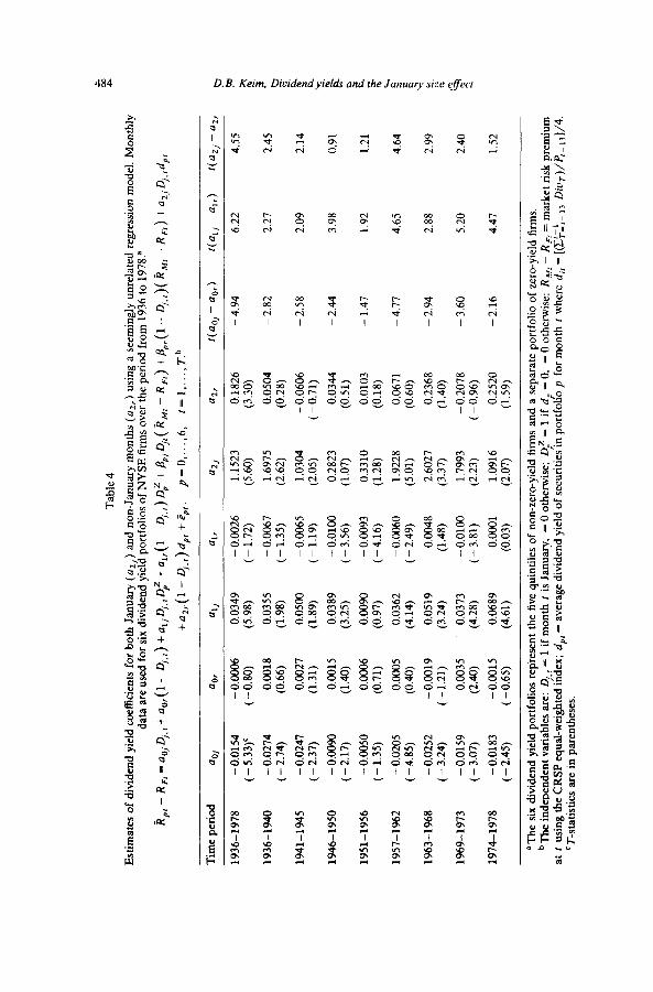
individual income. Thus, most tests of after-tax models have been conducted over the post-1936 period [e.g., Litzenberger and Ramaswamy (1979)]. For comparative purposes, eq. (4) is estimated for the 1936-1978 period. Results for the overall period and eight subperiods are reported in table 4. For the overall period the yield coefficient is positive and significant in both January (t = 5.60) and non-January months (t = 3.30), although the subperiod results indicate substantial variation in the magnitude of the coefficients through time.’ More importantly, the January yield coefficient is significantly larger than the non-January coefficient in the overall period and many of the subperiods. Previous tests of after-tax models have implicitly assumed that the
tax effects associated with the models are constant throughout the year. The test reported in the rightmost column of table 4 clearly rejects the hypothesis that a2, = azr (i.e., constant tax effect) for the overall period (t = 4.55) and many of the subperiods. Further, the January coefficient is too large to be interpreted as a marginal tax bracket (115% for the entire period), although the
non-January coefficient is in a plausible range for a tax effect (18%) and is similar in magnitude to yield coefficients reported elsewhere for similar time periods [cf. table 1 in Litzenberger and Ramaswamy (1979)].
Although these results should not be viewed as a formal test of the after-tax model, the results clearly suggest rejection of a model which does not predict a January seasonal in the relation between returns and yields. At a minimum, the significant January seasonal in the a, estimates suggests that the observed relation between long-run dividend yields and stock returns may not be solely attributable to differences in the tax rates for dividends and capital gains.
‘See Gibbons (1980) for an extensive discussion of the econometric problems associated with the cross-sectional regression approach. I have also conducted the tests of this section (and section 4.1) with the Fama-MacBeth approach. With regard to the dividend yield coefficient, those results are qualitatively the same as those reported here.
‘The behavior of the non-January yield coefficients appears to mirror, period-by-period, the behavior of the non-January size effect. In particular, non-January estimates of uz are insignificant but negative (implying an inverted yield effect) in the 1969-1973 subperiod when the non-January size effect reversed itself [Brown, Kleidon and Marsh (1983)]. Grundy (1982) has independently documented this phenomenon.
Tab
le
4
Est
imat
es
of
divi
dend
yi
eld
coef
fici
ents
fo
r bo
th
Janu
ary
(a*,
) an
d no
n-Ja
nuar
y m
onth
s (a
,,)
usin
g a
seem
ingl
y un
rela
ted
regr
essi
on
mod
el.
Mon
thly
da
ta
are
use
d fo
r si
x di
vide
nd
yiel
d po
rtfo
lios
of N
YS
E
firm
s ov
er
the
peri
od
from
19
36
to 1
978.
=
~pr-
~~,=
oo,~
,.r+
~o,(
l-~,
.r)+
~,,~
,.,~,
Z+
~,,(
l-~,
.,~~,
Z+
8,,~
,,(~,
,-~~
,)+
Bpr
(l-~
,.~)(
~~,-
~~,)
+~~
,~,.,
~p,
+ns,
(l-D
,,,)d
,,+$,
p=
O
,.._,
6,
r=
l,__.
, T
.b
Tim
e pe
riod
oo
j ao
r %
U
lr
(121
a2,
t(a0,
- 00,)
ICal
, -
a,,)
l(a2,
- a2
r
1936
-197
8 -
0.01
54
-0.0
006
0.03
49
- 0.
0026
1.
1523
0.
1826
-4
.94
6.22
4.
55
(-
5.33
)’
( -
0.80
) (5
.98)
(-
1.72
) (5
.60)
(3
.30)
1936
-194
0 -
0.02
74
0.00
18
0.03
55
- 0.
0067
1.
6975
0.
0504
-
2.82
2.
27
2.45
(-
2.
74)
(0.6
6)
(1.9
8)
(-1.
35)
(2.6
2)
(0.2
8)
1941
-194
5 -
0.02
47
0.00
27
0.05
00
- 0.
0065
1.
0304
-
0.06
06
- 2.
58
2.09
2.
14
(-
2.37
) (1
.31)
(1
.89)
(-
1.19
) (2
.05)
(-
0.71
)
1946
-195
0 -
0.00
90
0.00
15
0.03
89
- 0.
0100
0.
2823
0.
0344
-
2.44
3.
98
0.91
(-
2.17
) (1
.40)
(3
.25)
(-
3.
56)
(1.0
7)
(0.5
1)
1951
-195
6 -
0.00
50
0.00
06
0.00
90
- 0.
0093
0.
3310
0.
0103
-
1.47
1.
92
1.21
(-
1.35
) (0
.71)
(0
.97)
(-
4.16
) (1
.28)
(0
.18)
1957
-196
2 -
0.02
05
0.00
05
0.03
62
- 0.
0060
1.
9228
0.
0671
-4
.77
4.65
4.
64
(-.4
.85)
(0
.40)
(4
.14)
(-
2.
49)
(5.0
1)
(0.6
0)
1963
-196
8 -
0.02
52
- 0.
0019
0.
0519
0.
0048
2.
6027
0.
2368
-
2.94
2.
88
2.99
(
- 3.
24)
(-
1.21
) (3
.24)
(1
.48)
(3
.37)
(1
.40)
1969
-197
3 -
0.01
59
0.00
35
0.03
73
- 0.
0100
1.
7993
-
0.20
78
-3.6
0 5.
20
2.40
(-
3.
07)
(2.4
0)
(4.2
8)
(-
3.81
) (2
.23)
(
- 0.
96)
1974
-197
8 -
0.01
83
- 0.
0015
0.
0689
O
.ooo
l 1.
0916
0.
2520
-2
.16
4.47
1.
52
( -
2.45
) (
- 0.
65)
(4.6
1)
(0.0
3)
(2.0
7)
(1.5
9)
‘The
si
x di
vide
nd
yiel
d po
rtfo
lios
repr
esen
t th
e fi
ve q
uint
iles
of
non-
zero
-yie
ld
firm
s an
d a
sepa
rate
po
rtfo
lio
of z
ero-
yiel
d fi
rms.
bT
he
inde
pend
ent
vari
able
s ar
e:
Dj,,
= 1
if
mon
th
t is
Jan
uary
, =
0 ot
herw
ise;
D
pT =
1
if
dj,
= 0,
=
0 ot
herw
ise;
R
,, -
R,
= m
arke
t ri
sk
prem
ium
at
r
usin
g th
e C
RSP
eq
ual-
wei
ghte
d in
dex;
dp
, =
aver
age
divi
dend
yi
eld
of s
ecur
ities
m
por
tfoh
o p
for
mon
th
I w
here
d,
, =
[G’,;‘
,_
13
Diu,
)/P,
_ ,3
]/4.
‘T-s
tatis
tics
are
in p
aren
thes
es.
--
_....
I ~
---
-I
_ -
-.--
. _
,..
D. B. Keim, Dividend yields and the Junuuty size effect 485
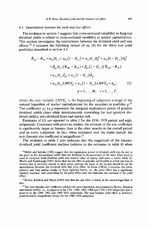
4.1. Interrelation between the yield and size effects
The evidence in section 3 suggests that cross-sectional variability in long-run dividend yields is related to cross-sectional variability in market capitalization. This section investigates the interrelation between the dividend yield and size
effects. lo I estimate the following variant of eq. (4) for the thirty size-yield portfolios described in section 3.3:
+PpjDj.tCiiMt -RF,) +Ppr(l -Dj.t)(~~t-R~t)
+az,Dj,t’pt + a,,(’ - D,,t)‘pt
+a3jDj,fLMVEp + a,,(1 - D,,,) LMVE, + fiP,, (5)
p=l ,..., 30, t=l,..., T,
where the new variable LMVE, is the beginning-of-subperiod average of the natural logarithm of market capitalizations for the securities in portfolio p.” The coefficient a2 (a3) represents the marginal explanatory power of positive dividend yields (size) while simultaneously controlling for size (positive div-
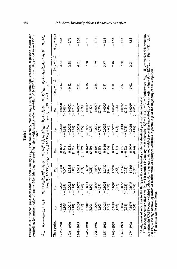
idend yields), zero dividend firms and market risk. Estimates of (5) are reported in table 5 for the 1936-1978 period and eight
subperiods. Consistent with previous studies, the estimate of the size coefficient is significantly larger in January than in the other months in the overall pe.riod and in every subperiod. In fact, when estimated over the entire period, the non-January size coefficient is insignificant.”
The evidence in table 5 also indicates that the magnitude of the January dividend yield coefficient declines (relative to the estimates in table 4) when
‘“Miller and Scholes (1982) suggest that the explanatory power of dividend yield may be due to the price in the denominator rather than the dividend in the numerator of the ratio. Since price is used to compute both dividend yield and market value of equity, and since a recent study by Blume and Stambaugh (1983) shows that the size effect is partially attributable to a bid-ask bias in returns that is inversely related to share price, perhaps the focus of the section should be on the interrelation between the dividend yield and price effect. In Keim (1983a). I examine this latter relation and find similar results to those reported below; i.e., the price effect has a significant January seasonal, and controlling for the price effect does not eliminate the seasonal in the yield effect.
“Brown, Kleidon and Marsh (1983) find that the size effect is linear in the natural logarithm of size.
“The non-January size coefficient exhibits the non-stationarity documented by Brown, Kleidon and Marsh (1983): os, is negative in the 1931-1945, 1963-1968 and 1974-1978 subperiods and is positive in the 1946-1962 and 1969-1973 subperiods. The non-January yield effect is, however, predominantly insignificant except for the 1946-1956 subperiod.
Tab
le 5
Est
imat
es
of
divi
dend
yi
eld
coef
fici
ents
fo
r bo
th
Janu
ary
(a,
) an
d no
n-Ja
nuar
y m
onth
s (a
,,)
usin
g a
seem
ingl
y un
rela
ted
regr
essi
on
mod
el
and
cont
rolli
ng
for
mar
ket
valu
e of
equ
ity.
M
onth
ly
data
ar
e us
ed fo
r th
irty
yi
eld-
mar
ket
valu
e po
rtfo
lios
of N
YSE
fi
rms
over
th
e pe
riod
fr
om
1936
to
1978
.”
Rpr
-
RF{
“‘01
j,t
D fa
ol(l-D
,.r)+
a~jD
j,~D~
‘+a~
,(l
-D,.r
)‘,Z+
B~Dj
.,(R,
,-R,)+
~~
,(l
-D,.r
#~
M,-
RFr
)+a2
,~.,d
,,+u,
,(l
-D,.,
)d,,
+u,
~D~~
,LM
~‘E
,+u,
,(~-
D~,
,)L
M~‘
E~~
+~~
~,,
p=l,.
..,
30,
t=l,.
..,
T.b
Tim
e pe
riod
'11
al,
U2J
=2,
a3j
=3r
tea,,
- Qlr)
t(a2,
-a,,)
'(03,
-a,,)
1936
-197
8
1936
-194
0
1941
-194
5
1946
-195
0
1951
-195
6
1957
-196
2
1963
-196
8
1969
-197
3
1974
-197
8
0.00
66
(1.8
0)’
- 0.
0079
(-
1.10
)
0.01
54
(1.3
8)
0.03
86
(6.3
0)
0.00
92
(1.6
0)
0.01
24
(2.3
5)
0.01
87
(1.9
5)
0.01
40
(2.1
2)
0.02
75
(4.5
4)
- 0.
0026
0.
7241
0.
1682
(-
2.
65)
(4.5
0)
(3.7
4)
- 0.
0018
1.
1833
0.
1388
(-
0.89
) (3
.05)
(1
.21)
- 0.
0076
1.
3711
-
0.07
22
(-3.
27)
(4.7
4)
(-
1.39
)
- 0.
0014
0.
6036
0.
1617
(-
1.00
) (3
.23)
(3
.50)
- 0.
0058
0.
4879
0.
1031
(-
4.19
) (2
.46)
(2
.28)
- 0.
0033
1.
1482
-
2.33
) (4
.60)
0.00
03
1.36
84
(0.1
5)
(2.5
8)
- 0.
0055
1.
2069
-
2.81
) (2
.13)
- 0.
0038
1.
1106
(-
2.57
) (3
.30)
-0.0
044
( - 6
.68)
- 0.
0052
(-
2.88
)
- 0.
0051
(-
3.99
)
- 0.
0053
(-
4.27
)
- 0.
0019
(-
1.73
)
- o.
oooo
2.
42
3.33
-
6.45
(-
0.06
)
- 0.
0001
-
0.82
2.
58
- 2.
71
(-0.
27)
- 0.
0007
2.
02
4.91
-
3.33
(-
2.76
)
0.00
12
6.36
2.
30
- 5.
11
(4.3
2)
0.00
07
2.54
1.
89
- 2.
32
(2.7
0)
0.14
10
- 0.
0085
0.
0005
2.
87
3.87
-
7.53
(1
.95)
( -
7.4
0)
(1.4
8)
0.17
53
- 0.
0075
-
0.00
12
1.88
2.
20
- 3.
52
(1.5
1)
(-
4.25
) (-
3.18
)
- 0.
0791
-
0.00
81
0.00
12
2.82
2.
20
- 5.
17
(-
0.52
) ( -
4.7
3)
(2.2
4)
0.09
09
- 0.
0101
-
0.00
19
5.02
2.
91
- 3.
85
(0.9
4)
(-4.
88)
(-4.
05)
BA
ssig
nmen
t of
sec
uriti
es t
o th
e th
irty
por
tfol
ios
is b
ased
joi
ntly
on
div
iden
d yi
eld
and
mar
ket
valu
e.
bath
e in
depe
nden
t va
riab
les
are:
Dj,,
= 1
if m
onth
t
is J
anua
ry,
= 0
oth
erw
ise;
D
pz =
1 if
dp
= 0
, =
0 o
ther
wis
e;
R,,,
, -
R,
= m
arke
t ri
sk p
rem
ium
at
t
usin
g th
e C
RSP
equ
al-w
eigh
ted
Inde
x; d
% , =
ave
rage
div
iden
d yi
eld
of s
ecur
ities
m p
ortf
oho
p fo
r m
onth
t
whe
re d
,, =
[(X
l>:‘,
_ 13
Div
T)/
4_
,,]/4
; L
MV
E,
=, a
yera
ge n
atur
al l
ogar
ithm
of
mar
et
val
ue o
f eq
uity
of
secu
ritie
s in
por
tfol
io
p at
the
beg
inni
ng
of t
he s
ubpe
riod
. ‘T
-sta
ttsnc
s ar
e in
par
enth
eses
.
__ ,
--
.I .-
-.
--
- -
- _
_ . .
. .
D. B. Kelm, Diuidendyrelds md the Jutwq sue effecr 487
estimated simultaneously with size: the January yield coefficient declines by 37.2% to 0.72 and the non-January coefficient declines by 7.9% to 0.17 when
estimated for the entire period. The attenuation of the yield coefficient suggests that dividend yields and size are related to the same asset pricing factor. The yield coefficient remains significant, though, in January and non-January months, even after controlling for size. However, the January coefficient is still significantly larger than the estimate for the other months and is not within the range for a plausible tax bracket when estimated over the entire period (it exceeds 100% in six of eight subperiods).
Finally, the findings above rely on tests that assume stationarity of the parameters and a large sample size. For example, the test for the overall period requires stationarity of the yield (and size) coefficients over the entire period; likewise, the subperiod tests assume a large sample size. To the extent that these assumptions are violated, the results should be interpreted cautiously.
5. Conclusions
Using ‘long-run’ estimates of expected dividend yield, this paper finds that much of the relation between yields and stock returns is due to a significant non-linear relation between dividend yields and returns in the month of January. Estimates of regression coefficients on dividend yields are also signifi- cantly larger in January than in the other months and are too large to be
interpreted as tax brackets associated with after-tax asset pricing models. There is, however, substantial attenuation of both the January and non-January coefficients when the test controls for market value of equity, although both the January and non-January estimates remain significant. A formal test of an after-tax asset pricing model is not conducted here, but the finding of a positive yield coefficient that exhibits a January seasonal is not entirely consistent with the implicit assumptions of previous tests of such models. At a minimum, the results suggest the observed relation between long-run dividend yields and stock returns may not be solely attributable to differences in marginal tax rates for dividends and capital gains.
An obvious question concerns the robustness of the results. The opening paragraph of this paper refers to the variety of potential definitions of dividend yield and the sensitivity of the estimated yield effect to these definitions. Results based on the Fama-MacBeth (1973) methodology (and reported in earlier versions of this paper) illustrate precisely this point. Fama-MacBeth
coefficients on short-term dividend yields as defined by Litzenberger and Ramaswamy (1979) are insignificant in January and significantly positive in non-January months, whereas the coefficients on yield as defined by Miller and Scholes (1982, table 2A, panel 3) are significantly positive in January and significantly negative in non-January months. These coefficients are estimated with single security data and are subject to the estimation problems discussed
488 D. B. Keim, Dividend yields and the January size effect
in section 4. Although many of those problems are avoided with the SUR model, the subperiod SUR systems in section 4.1 require estimation of a fairly large covariance matrix with relatively few observations (less than two observa- tions per parameter). Thus, tests that rely on this estimated covariance matrix may be sensitive to problems similar to those discussed (in a somewhat
different context) by Stambaugh (1982) Shanken (1985) and Ma&inlay (1984). The results presented here suggest, nevertheless, that further work may be necessary to examine (1) the generality of the seasonal in the yield coefficient and (2) whether a positive yield coefficient is in fact a tax-related or some other (e.g., size) phenomenon.
References
Banz, R., 1981, The relationship between return and market value of common stocks, Journal of Financial Economics 9, 3-18.
Black, F. and M. Scholes, 1974, The effects of dividend yield and dividend policy on common stock prices and returns, Journal of Financial Economics 1, l-22.
Blume, M., 1980, Stock returns and dividend yields: Some more evidence, Review of Economics and Statistics 62, 567-577.
Blume, M. and R. Stambaugh, 1983, Biases in computed returns: An application to the size effect, Journal of Financial Economics 12, 387404.
Brennan, M.J., 1970, Taxes, market valuation and corporate financial policy, National Tax Journal 23,417-427.
Brown, P., A. Kleidon and T. Marsh, 1983, New evidence on the nature of size-related anomalies in stock prices, Journal of Financial Economics 12, 33-56.
Elton, E. and M. Gruber, 1970, Marginal stockholder tax rates and the clientele effect, Review of Economics and Statistics 52, 68-74.
Fama, E.F. and J.D. MacBeth, 1973, Risk, return and equilibrium: Empirical tests, Journal of Political Economy 81, 607-636.
Gibbons, M., 1980, Econometric methods for testing a class of financial models: An application of the nonlinear multivariate regression model, Ph.D. dissertation (Department of Economics, University of Chicago, Chicago, IL).
Gordon, R.H. and D.F. Bradford, 1980, Taxation and the stock market valuation of capital gains and dividends: Theory and empirical results, Journal of Public Economics 14,109-136.
Grundy, B., 1982, The interrelation of the size and yield effects, Unpublished mimeo. (University of Chicago, Chicago, IL).
Hess, P.J., 1983, Test for tax effects in the pricing of financial assets, Journal of Business 56, 537-554.
Kalay, A., 1982, The ex-dividend day behavior of stock prices: A reexamination of the clientele effect, Journal of Finance 37,1059-1070.
Keim, D.B., 1983a, The interrelation between dividend yields, equity values and stock returns: Implications of abnormal January returns, Unpublished Ph.D. dissertation (University of Chicago, Chicago, IL).
Keim, D.B., 1983b, Size-related anomalies and stock market seasonality: Further empirical evidence, Journal of Financial Economics 12, 13-32.
Litzenberger, R.H. and K. Ramaswamy, 1979, The effects of personal taxes and dividends on capital asset prices: Theory and market equilibrium, Journal of Financial Economics 7, 163-195.
Litxenberger, R.H. and K. Ramaswamy, 1980, Dividends, short selling restrictions, tax-induced investor clienteles and market equilibrium, Journal of Finance 35, 469-482.
Ma&inlay, A.C., 1984, An analysis of multivariate financial tests, Unpublished manuscript, Jan. (University of Chicago, Chicago, IL).

D. B. Keim, Dividendyrelds and the Junucm, size effect 489
Miller, M.H. and M.S. Scholes, 1978, Dividends and taxes, Journal of Financial Economics 6, 333-364.
Miller, M.H. and M.S. Scholes, 1982, Dividends and taxes: Some empirical evidence, Journal of Political Economy 90, 1118- 1141.
Reinganum, M.R., 1981, Misspecitication of capital asset pricing: Empirical anomalies based on earnings yields and market values, Journal of Financial Economics 9, 19-46.
Rogalski. R. and S. Tinic. 1984, The January effect: Anomaly or risk mismeasurement?, Unpub- lished manuscript, Jan. (Dartmouth College, Hanover, NH).
Shanken, J., 1985, Multivariate tests of the zero-beta CAPM, Journal of Financial Economics 14. this issue.
Stambaugh, R.F., 1982, On the exclusion of assets from tests of the two-parameter model: A sensitivity analysis, Journal of Financial Economics 10, 237-268.
Zellner, A., 1962, An efficient method of estimating seemingly unrelated regressions and tests for aggregation bias, Journal of the American Statistical Association 57, 348-368.