9368 2021

October 2021

Do Carbon Offsets Offset Carbon? Raphael Calel, Jonathan Colmer, Antoine Dechezleprêtre, Matthieu Glachant

Impressum:

CESifo Working Papers ISSN 2364-1428 (electronic version) Publisher and distributor: Munich Society for the Promotion of Economic Research - CESifo GmbH The international platform of Ludwigs-Maximilians University’s Center for Economic Studies and the ifo Institute Poschingerstr. 5, 81679 Munich, Germany Telephone +49 (0)89 2180-2740, Telefax +49 (0)89 2180-17845, email office@cesifo.de Editor: Clemens Fuest https://www.cesifo.org/en/wp An electronic version of the paper may be downloaded · from the SSRN website: www.SSRN.com · from the RePEc website: www.RePEc.org · from the CESifo website: https://www.cesifo.org/en/wp

CESifo Working Paper No. 9368

Do Carbon Offsets Offset Carbon?

Abstract

We develop and implement a new method for identifying wasted subsidies, and use it to provide systematic evidence on the misallocation of carbon offsets in the Clean Development Mechanism—the world’s largest carbon offset program. Using newly constructed data on the locations and characteristics of 1,350 wind farms in India—a context where it was believed, ex ante, that the Clean Development Mechanism could significantly increase development above baseline projections—we estimate that at least 52% of approved carbon offsets were allocated to projects that would very likely have been built anyway. In addition to wasting scarce resources, we estimate that the sale of these offsets to regulated polluters has substantially increased global carbon dioxide emissions. JEL-Codes: H230, H430, L940, Q420, Q540. Keywords: carbon offsets, infra-marginal support, subsidies, investment, wind power, misallocation.

Raphael Calel* Georgetown University / Washington DC / USA

raphael.calel@georgetown.edu

Jonathan Colmer University of Virginia / Charlottesville / USA

jonathan.colmer@virginia.edu

Antoine Dechezleprêtre London School of Economics / United Kingdom

A.Dechezlepretre@lse.ac.uk

Matthieu Glachant MINES ParisTech / France

matthieu.glachant@mines-paristech.fr

*corresponding author

Do Carbon Offsets Offset Carbon?∗

Raphael Calel Jonathan Colmer

Georgetown University University of Virginia

Antoince Dechezlepretre Matthieu Glachant

London School of Economics MINES ParisTech

1 Introduction

Carbon offsets have become a popular tool in global efforts to mitigate climate change. These

programs work by offering regulated polluters the opportunity to increase their own emissions if

they subsidize equivalent emission reductions in unregulated markets. In theory, this allows the

same total emissions abatement to be achieved at lower cost. The world’s largest carbon offset

program—the Clean Development Mechanism (CDM)—has supported more than $90 billion of

renewable energy investments in developing countries, equivalent to 13% of their total renewable

energy investments (Kossoy et al., 2015).

A key unanswered question is whether these carbon offsets resulted in additional emissions

reductions in unregulated markets. If carbon offsets are awarded to projects that would have been

developed without the subsidy, they do not represent emissions savings. This results in an inefficient

allocation of scarce climate change mitigation resources and a net increase in global emissions.

∗This Version: October 2021. Corresponding and Lead Author: raphael.calel@georgetown.edu. We thank Jishnu Das, DaveDonaldson, Seema Jayachandran, Molly Lipscomb, David Popp, David Rapson, Lutz Sager, Joseph Shapiro, Jay Shimshack,Sandip Sukhtankar, Alex Teytelboym, and John Van Reenen for helpful thoughts, comments, and discussions. We are gratefulto seminar participants at American University, the University of Oslo, and the University of Virginia for their commentsand suggestions. Nathan Lado, Eric LaRose, Anna Schroder, and Alex Watkins provided invaluable research assistance. Thisproject was supported by the ESRC Centre for Climate Change Economics and Policy, the Grantham Foundation. All errorsand omissions are our own.

1

Researchers have struggled to quantify such misallocation due to the difficulty of identifying a

credible counterfactual.

In this paper we propose a new approach to identifying projects that would have been built

without a subsidy, and use it to provide systematic evidence on carbon offset misallocation in the

CDM. Our approach identifies a subset of all infra-marginal projects, which we refer to as Blatantly

Infra-marginal Projects (BLIMPs). BLIMPs are not just infra-marginal, but blatantly so, in the

sense that there exist other projects that are strictly less profitable, yet were built without the same

subsidies. The number of BLIMPs provides a lower bound on the degree of subsidy misallocation.

Our approach does not require us to estimate the net benefits of each project. This would require

strong assumptions and be incredibly data intensive. Instead, we derive sufficient conditions for

identifying project dominance based on observable characteristics. We determine that, conditional

on being built in the same state and year, a subsidized wind farm strictly dominates an unsubsidized

farm if it has a higher capacity, and is built in a windier location, and is built closer to a connection

point. In this setting, these three conditions are sufficient to define a BLIMP.

As an illustration, consider the case of the 91.8 megawatt CDM-supported wind farm built

in Jangi, Gujarat, in 2011. We observe that an unsubsidized wind farm was completed during

the same year, just 10 miles away in Surajbari. The unsubsidized project had a capacity of only

7.5 megawatt, was estimated to deliver about 5% less power per installed megawatt because of

less favorable wind resources, and was located 3 miles further away from the nearest electrical

substation. These two wind farms were built in the same state and year, and were therefore subject

to the same policies and market conditions, yet the CDM-supported project was both bigger and

better located. We show that the existence of the less profitable unsubsidized project at Surajbari

is a sufficient condition for identifying the larger CDM-supported wind project as a BLIMP.

To understand how prevalent this phenomenon is, we apply our framework to a new data set

of 1,350 wind power projects in India—a context where it was believed, ex ante, that the CDM

could significantly increase development above baseline projections (Purohit and Michaelowa, 2007).

We independently geo-locate all of the Indian wind power projects identified by Bloomberg New

Energy Finance at the village-level (BNEF, 2013), and then cross-reference them with individual

CDM applications from the UN Environment Program’s CDM Pipeline database (UNEP DTU,

2021). For each project-site, we forecast power output using the hourly distribution of wind speeds

and weather conditions from the European Centre for Medium-Range Weather Forecasts’ global

reanalysis data set (Munoz Sabater, 2019). We also estimate the cost of connecting each wind

farm to the electrical grid by using detailed grid-infrastructure data from Burlig et al. (2020). This

provides a comprehensive database covering 1,350 Indian wind farms built between 1992 and 2013,

of which 472 were registered to receive carbon offsets under the CDM.

Out of the 472 CDM-registered Indian wind farms in our data, we identify 265 BLIMPs. For

each of these 265 projects, we can point to at least one unsubsidized wind farm built in the same

state and year that is strictly less profitable. These projects account for 52% of carbon offsets

approved for Indian wind projects. Under the assumption that these credits were later used by

2

regulated entities to augment their emissions quotas, global emissions will have increased by 28

million tonnes of carbon dioxide emissions, equivalent to keeping a one-gigawatt coal plant running

for nearly 5 years.1 The misallocation is so severe that we find that the random assignment of

subsidies through a lottery would have resulted in fewer offsets being allocated to BLIMPs.

Our findings are robust to a broad range of sensitivity tests. For instance, our results remain

qualitatively similar even if we systematically deflate the power output and inflate the connection

costs of CDM projects by as much as 20%. This addresses concerns that unobserved systematic

differences between CDM and non-CDM projects could be driving our results. These differences

could arise from measurement error in our data or from differential barriers to entry, such as credit

or political economy constraints. We show that a confounding explanation would have to be almost

perfectly correlated with a project being marginal and the CDM’s observed decisions in order to

undo our findings. Even if we assume that all BLIMPs are partially infra-marginal, i.e., that they

would have been built in the absence of the subsidy, but to a smaller capacity, the CDM’s allocation

of carbon offsets still only performs on par with the lottery assignment mechanism.

Do carbon offsets offset carbon? Our analysis suggests that in many cases they don’t. Carbon

offsets are frequently given to BLIMPs, which means that they do not generate the emissions

reductions needed to offset the emissions increases that they enable. It is still possible, however,

that the remaining CDM-supported wind farms have offset more than their share of emissions. To

counterbalance the increase in emissions from subsidizing BLIMPs, we would have to assume that

the CDM-supported wind farms that are not BLIMPs reduced India’s carbon emissions by 2.12

tonnes per offset. This is equivalent to assuming that all non-BLIMPs are marginal and collectively

responsible for the realization of half of India’s non-CDM wind power capacity.2 This theoretical

possibility doesn’t undermine our finding that the CDM has subsidized a large number of infra-

marginal projects. If our estimates are valid for the CDM as a whole, and we do not assume

any indirect emissions reductions, the program will have approved enough offsets to increase global

emissions by 6.1 billion tonnes of carbon dioxide, the equivalent of operating roughly 20 one-gigawatt

coal plants for their entire 50-year lifespan.

These findings contribute most directly to our understanding of carbon offset programs. Carbon

offsetting is an increasingly important policy tool. A growing number of countries and organizations

are now committing themselves to achieving “net zero” carbon emissions (Black et al., 2021),

and international negotiations are underway to develop and implement a successor to the CDM

(Michaelowa et al., 2019). It is critical to carefully consider the design of these programs going

forward to ensure that carbon offsets actually offset carbon. Previous work has already identified

particular industrial processes that should not be subsidized with carbon offsets (Wara, 2007a,b;

Schneider, 2011; Schneider and Kollmuss, 2015), but our results identify a significant misallocation

1For scale, the average conventional coal plant in the US in 2019 had a capacity of 808 MW, according to figuresreported by the US Energy Information Administration.

2Infra-marginal projects may also result in agglomeration effects, crowding in non-CDM capacity due to economiesof scale. However, any crowding in that arises from infra-marginal CDM projects is also infra-marginal. Theseagglomeration effects would have arisen absent CDM support.

3

of resources even for the type of projects that the CDM was made to support. Our study suggests

that, despite good intentions, the CDM may actually have increased emissions. In this regard, our

paper connects to a large literature documenting how well-intentioned policies can have unintended

consequences (Davis, 2008; Oliva, 2015; Holland et al., 2016; Agan and Starr, 2017; Parker and

Vadheim, 2017; Bharadwaj et al., 2019; Taylor, 2019; Doleac and Hansen, 2020; Filmer et al.,

2021).

Our paper also contributes to the study of a broader class of policies that leverage the logic

of offsetting. This includes everything from Corporate Average Fuel Economy standards (Kwoka,

1983; Anderson and Sallee, 2011; Ito and Sallee, 2018) to Renewable Portfolio Standards (Cullen,

2013; Gowrisankaran et al., 2016; Carley et al., 2018) to key provisions of the Clean Air Act (Shapiro

and Walker, 2020). Compared with the traditional approach of using tax revenue to subsidize

emissions-saving activities, these policies work by getting the private sector to cross-subsidize those

activities directly without the funds passing through the public treasury. While this approach has

some appeal, our findings highlight a very real downside. Unlike a traditional subsidy program,

the consequence of misallocating offsets isn’t just to create an inefficient transfer. It also generates

external costs by underwriting an increase in global emissions. When choosing between offset-style

regulation and the more traditional subsidy model, the potential external costs from misallocation

should be an important consideration.

We also contribute to a broader literature that seeks to identify the existence and magni-

tude of infra-marginal support in subsidy programs. The empirical challenge in identifying infra-

marginal carbon offsets is similar to the problem that researchers have faced when trying to deter-

mine whether new technologies would have been adopted without rebates (Chandra et al., 2010;

Boomhower and Davis, 2014), whether firms would have invested in additional innovation without

special tax credits or grants (Hall and Van Reenen, 2000; Bloom et al., 2002; Dechezlepretre et al.,

2016; Howell, 2017; Azoulay et al., 2019; Pless, 2021), or whether firms or workers would have

moved in the absence of discretionary incentives (Moretti and Wilson, 2014; Slattery, 2019; Mast,

2020; Slattery and Zidar, 2020). In certain cases, researchers have managed to find and exploit

discontinuities in rules that have allowed for causal identification. However, this is not the norm.

We have explored opportunities to apply these research designs in the context of carbon offsets

and are not aware of any successful applications. Our framework offers a different approach to

systematically evaluating grant-based subsidy programs.

To apply our framework three conditions must be met. First, one needs a context in which some

activity is not subsidized (these activities are infra-marginal by definition). Second, one needs to

establish which conditions are sufficient for project dominance. Third, one needs data to evaluate

these conditions. We believe that our framework could be applied to grant-based agricultural

subsidies, small-business grants, innovation grants, concessionary financing programs, and to other

grant-based subsidy programs aimed at supporting renewable energy technologies, such as solar

power and production of biofuels.

4

2 Institutional Background

In this section, we provide relevant institutional details about the CDM, discuss how marginal and

infra-marginal projects are distinguished in practice through the registration process, and provide

background information on the Indian wind power sector.

2.1 The Clean Development Mechanism

The Clean Development Mechanism (CDM) is the largest pollution offset program in the world.

It was established as part of the Kyoto Protocol in 1997. Under this program, industrialised

countries that had committed to reducing emissions domestically were permitted to meet some of

their obligation by developing or financing equivalent emission reductions projects in developing

countries. This additional flexibility ostensibly achieves the same global emissions reduction at a

lower cost. In practice, the exchange of financing and emissions would be accomplished by the UN

issuing Certified Emission Reduction (CER) credits to approved projects in developing countries,

each CER signifying one avoided tonne of carbon dioxide. Those credits could then be sold to

regulated firms in developed countries and counted towards their country’s Kyoto target.

From a project developer’s perspective, the CDM is much like any other subsidy program.

Although developers don’t receive money directly from the UN, they do receive valuable CERs

that can be exchanged for money on the open market, including through the sale of carbon offset

futures. It is the promise of this extra money that was intended to lure developers to build more

renewable energy projects than they otherwise would have.

The CDM has been an extremely popular program. By 2030, it is expected that the CDM will

have issued up to 11.8 billion credits, equivalent in magnitude to the total emissions of the United

States and Europe in 2019. China (6.55 billion), India (1.32 billion), and Brazil (0.7 billion) account

for over 70% of these credits. Over half of all CERs finance just two types of projects: hydro power

(27%) and wind power (24%), the latter being the focus of our study. It has been estimated that

the CDM has supported over $90 billion of renewable energy investment in developing countries, or

roughly 13% of their total renewable energy investment (Kossoy et al., 2015). Although the CDM

is now no longer accepting new applications, the Paris Agreement promises to expand the program

under a new name: the Sustainable Development Mechanism.

To register under the CDM, a project had to go through two stages of evaluation. First, project

developers would initiate the process by writing a Project Design Document (PDD) describing

the project and proposing a demonstration of “additionality.” In this context, “additionality”

means that the project is expected to reduce emissions below the business-as-usual trajectory. A

Designated National Authority (DNA)—in India, the Ministry of Environment and Forests—then

evaluates whether the project, as described in the PDD, meets the CDM requirements, which

include “additionality.” Second, the CDM Executive Board, which supervises the CDM globally,

decides whether or not to register valid projects submitted by the DNA. If a project is approved, the

developer starts receiving CERs as soon as it starts delivering emissions reductions—a hydroelectric

5

dam or a wind farm, for instance, would start receiving its approved allotment of CERs as soon as

a third-party verifies that it has begun generating electricity.

It is critical that CDM projects are in fact marginal, since they receive CER credits that are

used to relax someone else’s emissions quota. If CDM projects are marginal, the CERs represent

emissions reductions that offset emissions that are generated elsewhere, reducing abatement costs

without compromising progress towards meeting global emissions reduction targets. However, if

projects are infra-marginal, global emissions increase. The regulatory problem is the same as any

subsidy program—the regulator’s objective is to avoid supporting infra-marginal projects.

The CDM Executive Board applies a set of standardized methodologies to determine whether or

not a project is marginal. For renewable energy projects, the principle is straightforward. Calculate

the project’s internal rate of return with and without the extra revenue that would come from selling

CER credits. If the internal rate of return with CER revenue exceeds a benchmark rate, but the

rate without CER revenue does not, the project is judged to be marginal. The CER revenue is

estimated by multiplying the electricity that would be generated by a “business as usual” emissions

factor. Most projects use a factor equal to the generation-weighted average carbon dioxide emissions

per unit of net electricity generation from all generating power plants serving the same regional

grid (tCO2/MWh). The assumption is that the new project would replace an equivalent amount

of “business as usual” generation capacity, avoiding the associated emissions.

This approach to assessing the “additionality” of projects has a number of problems. First, it is

difficult to objectively estimate or evaluate internal rates of return. In practice the PDDs frequently

rely on subjective arguments or neglect to provide the underlying data used in their calculations

(Schneider, 2009). Even when detailed information is available and analysis has been performed, the

results are not verifiable by the authorities in charge of CDM registration (Michaelowa and Purohit,

2007). Second, even if all the information was correct and verifiable, the methodology itself builds

in incredibly strong assumptions about the growth of renewable power (or more accurately, the

lack of growth) in the absence of CER credits.

This raises clear issues of accountability and regulatory governance. However, the absence of

evidence that projects are marginal that previous studies have pointed to is not the same as pro-

viding evidence that they are infra-marginal. The most notable direct evidence of infra-marginal

projects concerns the potent greenhouse gas HFC-23, which is a by-product in the production of

some refrigerants. Wara (2007b,a), Schneider (2011), and Schneider and Kollmuss (2015) persua-

sively show that Chinese and Russian refrigerant factories were running over-time just to produce

more of this by-product, since the destruction of this highly potent greenhouse gas allowed them

to claim CERs that were much more valuable than the refrigerant being manufactured. Once the

problematic projects were identified, regulators could easily ban polluters from using these specific

credits for compliance purposes.

6

1995 2000 2005 2010

0

1

2

3

Newly installedcapacity (GW)

0

5

10

15

20

25

CER price ($/tCO2)

CER price($/tCO2)

CDM

Non-CDM

Kyoto ProtocolProject registrationbegins

Kyoto Protocolcommitment period

1995 2000 2005 2010

0

5

10

15

20

Cumulative installedcapacity (GW)

CDM

Non-CDM

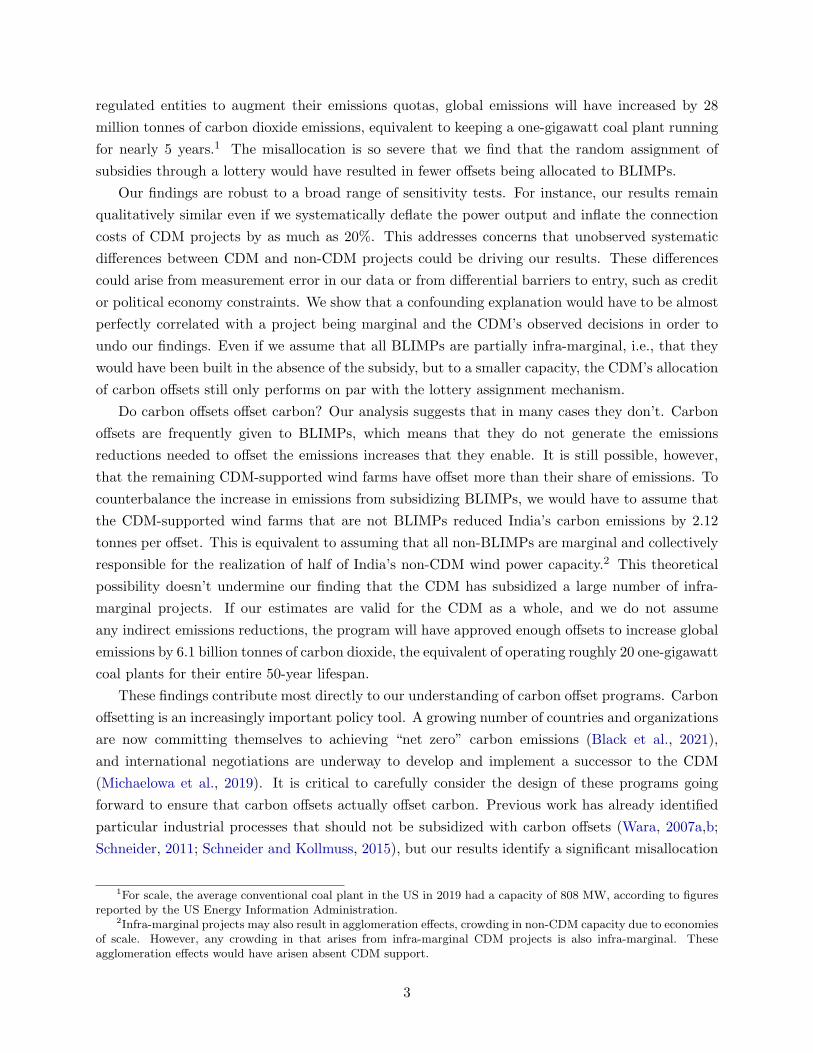
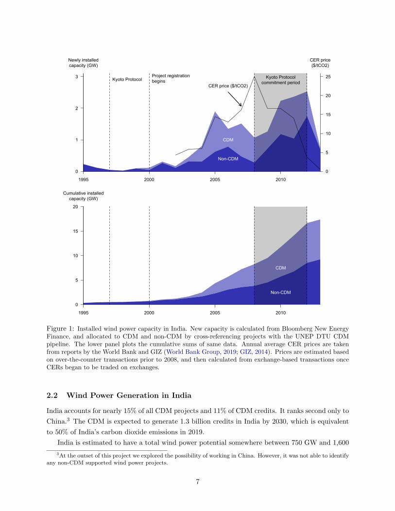
Figure 1: Installed wind power capacity in India. New capacity is calculated from Bloomberg New EnergyFinance, and allocated to CDM and non-CDM by cross-referencing projects with the UNEP DTU CDMpipeline. The lower panel plots the cumulative sums of same data. Annual average CER prices are takenfrom reports by the World Bank and GIZ (World Bank Group, 2019; GIZ, 2014). Prices are estimated basedon over-the-counter transactions prior to 2008, and then calculated from exchange-based transactions onceCERs began to be traded on exchanges.

2.2 Wind Power Generation in India

India accounts for nearly 15% of all CDM projects and 11% of CDM credits. It ranks second only to

China.3 The CDM is expected to generate 1.3 billion credits in India by 2030, which is equivalent

to 50% of India’s carbon dioxide emissions in 2019.

India is estimated to have a total wind power potential somewhere between 750 GW and 1,600

3At the outset of this project we explored the possibility of working in China. However, it was not able to identifyany non-CDM supported wind power projects.

7

GW, with much of this potential concentrated in Southern and Western parts of the country

(Phadke, 2012). At the turn of the century, however, India had almost no wind power, and neither

was it building new wind farms. The main barrier to wind farm construction was believed to be the

high up-front capital costs (Jagadeesh, 2000). Consequently, ex ante evaluations of the Indian wind

power sector concluded that there was huge potential for the CDM to finance the construction of

additional capacity and maximize the utilization of this untapped wind power potential (Purohit

and Michaelowa, 2007).

Figure 1 plots the construction of new wind power capacity in India based on the Bloomberg’s

New Energy Finance database (see appendix A for details). Within a few years of the CDM

coming online in 2000, wind farm construction accelerated and CDM-registered projects began to

account for a substantial proportion of new capacity (Figure 1, top panel). The price of CERs had

reached about $10 by this point, and it remained high until the final year of the Kyoto Protocol’s

commitment period. Over this whole period, India experienced more than a 20-fold expansion of its

installed wind power capacity, and today India has the 4th largest installed wind power capacity

in the world (Lee et al., 2021). Notably, nearly half of the capacity added between 2000 and

2013 belongs to projects that were registered to receive credits under the CDM (Figure 1, bottom

panel). We calculate that these projects were expected to collectively generate roughly 50 million

CERs over their lifetime. Our analysis will provide insight into the extent to which CDM subsidies

actually contributed to the explosive growth of India’s wind power capacity.

By studying the Indian wind power sector, we are consciously selecting a context where the

CDM was expected to perform particularly well. This stacks the deck in favor of finding that the

CDM Executive Board has been successful in supporting projects that would not have been built

otherwise. This is an important difference from earlier studies, which have looked for examples of

“non-additionality” mainly in places where they are most likely to be found, such as the case of

HFC-23 (Wara, 2007b,a; Schneider, 2011; Schneider and Kollmuss, 2015). Finding that HFC-23

projects are infra-marginal is mainly helpful in highlighting a specific type of project that should

not be subsidized. By searching for infra-marginal projects in a setting where we least expect to

find them, we are providing something closer to an upper bound on the CDM’s overall success in

identifying and supporting marginal projects.

3 Conceptual Framework

3.1 Marginal and Infra-marginal Projects

Following Berry (1992), we consider a simple two-stage game for each market—entry followed by

service provision. In the first stage, each potential entrant n = 1, . . . , N makes a choice whether or

not to enter market k. In the second stage, entrants make investments that determine post-entry

payoffs.

Solving backwards, we define a payoff function V (s, x) for potential market entrants, where

s ≥ 0 is a subsidy and x is a vector of other payoff determinants. The essential features of V (s, x)

8

are that it is monotonically increasing in s, and that V depends monotonically on the entry decisions

of other potential entrants.

Given the payoff function, potential entrants decide whether or not to enter the market. There

is a reservation payoff, R, such that entry occurs if V ≥ R.

Under these conditions, one can rank potential projects according to their payoffs in the absence

of subsidies,

V (s = 0, x1) ≥ · · · ≥ V (s = 0, xi) ≥ R > V (s = 0, xi+1) ≥ · · · ≥ V (s = 0, xN ). (1)

where the subscript indicates the rank order. We assume that V is such that this ranking is

preserved for all values of s. Increasing s will only have the effect of shifting some projects from the

right side to the left side of R without otherwise disturbing their ranking. Hence, for some subsidy

s > 0, it will be the case that

V (s, x1) ≥ · · · ≥ V (s, xj) ≥ R > V (s, xj+1) ≥ · · · ≥ V (s, xN ) (2)

where j ≥ i. Potential entrants with an index above j (to the right of R in equation 2) will not

enter either with or without the subsidy, so we need not consider them any further. Potential

entrants with an index between i and j will enter only with a subsidy, which means the subsidy

is affecting their decision at the margin. We refer to these as “marginal projects” for convenience,

which in this setting is equivalent to calling them “additional.” Potential entrants with an index

below i will enter with or without a subsidy, which means the subsidy is infra-marginal to their

entry decision. We refer to them as infra-marginal projects, which in this setting is equivalent to

calling them “non-additional.”

3.2 Blatantly Infra-marginal Projects

The typical approach for determining whether or not a project n is infra-marginal is to attempt

to estimate V (0, xn), V (s, xn), and R, and then check whether V (s, xn) ≥ R > V (0, xn). This

approach faces several challenges, not least of which is the fundamentally unobservable nature of

V (0, xn) once a subsidy has been awarded.

Fortunately, one does not need to estimate V (0, xn), V (s, xn), and R to determine whether a

project is infra-marginal (i.e. whether n ≤ i). A sufficient condition for identifying a project as

infra-marginal is that there exists some project m > n that is not receiving a subsidy. Because no

projects m > i would enter the market without a subsidy, the existence of an unsubsidised project

m is sufficient to infer that n must be less than i.

If one can identify and measure the variables in x (or proxies thereof), and can further identify

some subset of these variables that produce monotonic changes in V , which we’ll denote x ∈ x,

then for each project n, one can determine whether or not there exists another project m such that:

1. m did not receive a subsidy (s = 0),

9

2. xm ≤ xn for each variable in x (where, for convenience, the variables in x are ordered so that

higher values produce larger values of V ), and

3. xm = xn for each variable not in x.

If a project m exists that satisfies the first condition, it must be true that the value of V was

large enough to justify entry even in the absence of the subsidy, which can be stated formally as

V (s = 0, xm) ≥ R, or equivalently, m < i. If project m satisfies the second and third conditions

as well, we know that V (s = 0, xn) ≥ V (s = 0, xm) (or m < n). Transitivity implies that

V (s = 0, xn) ≥ R (or n < i), which means that project n would have been built in the absence of

a subsidy, too.

If project n is marginal, no other project satisfying all three conditions will exist. If project

n is infra-marginal, then a project m satisfying all three conditions may exist. The existence of

a project m is therefore a sufficient condition to infer that n is infra-marginal. To distinguish

these infra-marginal projects from the rest, we refer to them as blatantly infra-marginal projects,

or BLIMPs for short.

While infra-marginality is unobservable, being a BLIMP is fundamentally observable, defined

by the relation between two observed projects. We note, however, that BLIMP-ness is an inherently

conservative indicator of infra-marginality. An application of the definition of a BLIMP is likely to

identify only a subset of infra-marginal projects, even when a researcher or regulator is in possession

of a complete list of projects.

If our list of projects is incomplete, the measure only becomes more conservative. Consider

starting with a complete list of projects and then dropping one. If this project is itself a BLIMP,

we’ve reduced the number of BLIMPs by one. If this project is not a BLIMP, its presence could

have served to identify other projects as BLIMPs. Any projects that we do not observe will tend

to reduce the number of BLIMPs.

This conceptual approach imposes very mild conditions on the payoff function. It therefore

lends itself to many different applications. For any given application, it is necessary to specify

the payoff function with enough precision that the researcher can determine what variables are

contained in x and in x. We now turn our attention to operationalizing the concept of a BLIMP

in the context of wind power generation.

4 BLIMPs in India’s Wind Power Sector

In this section we map the preceding framework onto India’s wind power sector to develop an

operational definition of a BLIMP in this context. We will discuss the functional form of the payoff

function and how we measure the variables that enter into it.

10

4.1 An Operational Definition of a BLIMP

The following equation describes what we consider a reasonable description of the net present value

from building a wind farm, i, in state `, in year y.

Vn`y =

T∑t=y

(p`yt + snt)(cn × fn)(1− l(dn))− vyt(cn)− τ`yt(1 + r)(t−y)

− Fy(cn, dn) (3)

The first term gives us the net present value of the stream of operating profits. Each kWh of

electricity fetches a price of electricity, p`yt, that may differ across states `, across vintages, y, and

across time t, as well as a per-kWh subsidy, snt, that varies across projects and time. Total annual

revenue can then be calculated by multiplying the revenue per kWh by the annual power output,

which can be written as the product of generation capacity, cn, and the capacity factor, fn (the

power output per unit of capacity). Total output then needs to be multiplied by a factor that takes

account of transmission losses, l. Transmission losses increase as a function of the distance to the

where the wind farm connects to the grid, dn. The operating profit in year t is what is left over

after subtracting maintenance costs, vyt, and taxes, τ`yt. Two projects built in the same year, y,

with the same capacity, will have the same maintenance cost schedule. If they are built in the same

state they will face the same tax schedule as well. Finally, the stream of profits is discounted at an

annual rate of r, which is common to all projects.

The second term of equation 3 represents the up-front cost of construction, Fy, which depends

on the generation capacity, cn, and distance between the wind farm and its closest connection point

to the grid, dn.

As we indicate with our subscripts in equation 3, and will discuss in greater depth shortly, most

of the variables vary across, but not within, states and vintages. Aside from the subsidy rate,

only three variables vary across wind farms built in the same state and year, and we will argue

that V is monotonic in all three: V is an increasing function of generation capacity (cn) and the

capacity factor (fn), and a decreasing function of the connection distance (dn). This gives rise to

the following operational definition of a BLIMP in the context of India’s wind power sector.

Definition 1 For a CDM-registered wind farm n and an unregistered wind farm m that are built

in the same state and year, n is a BLIMP if:

1. it is larger (cn ≥ cm), and

2. it is built in a windier location (fn ≥ fm), and

3. it is built closer to a connection point (dn ≤ dm).

Although equation 3 is helpful as motivation, our empirical analysis does not require us to

estimate the value function. We only rely on the milder conditions stated in Definition 1, which are

compatible with a larger set of alternative payoff functions. The remainder of this section is devoted

to motivating the functional form assumptions contained in this definition and to describing how

we measure each of the variables.

11

4.2 Payoffs Increase in Capacity

Generation capacity is easy to observe and measure, but its mapping to payoffs is more complicated.

Each MW of capacity yields cn × fn kWh of power output in year t, which are then sold at a fixed

price of p`yt. In India, as in many other places, the price of wind power is agreed in advance through

standardized power purchase agreements. Throughout the period of our study these prices were set

by state-wide feed-in-tariffs. This means that all wind farms built in the same state and year will

earn the same price per unit of electricity (Kathuria et al., 2015). These factors suggest constant

marginal revenue from each additional MW of capacity.

Marginal revenue could be increasing or decreasing, however, depending on what subsidies

are on offer, snt. The only relevant domestic program in this period is India’s Generation-based

incentive—a nation-wide program that supplements state-level feed-in-tariffs with an extra INR

0.5 per kWh of power. The only eligibility criteria is that the wind farm has at least 5 MW

built capacity. The Generation-based incentive therefore results in increasing marginal revenue for

projects exceeding 5 MW of capacity. Given that the GBI is available to all projects above 5MW,

we have no reason to believe that it disproportionately serves non-CDM projects. We explore the

the consequences of this assumption in sensitivity analyses.

The only other subsidy to consider is the CDM, which provides registered wind farms with

carbon offsets in proportion to their power output. The price of offsets varies over time in response

to global demand and supply, but since individual wind farms are price takers in the global offset

market, two CDM-projects that are built in the same year will receive the same subsidy-per-

kWh over the lifetime of the project. Non-CDM projects do not receive the subsidy. Unlike the

Generation-based incentive, eligibility for the CDM is not determined by a capacity threshold. This

is why Definition 1 starts by specifying that one wind farm is registered and the other one isn’t.

For such a pair, we can say that the larger CDM-project will have a higher subsidy rate than the

smaller non-CDM project.

While the marginal revenue from an additional MW of wind farm is constant, or even increasing,

the marginal cost of building and operating an additional MW of wind farm tends to decline as a

function of capacity. The up-front capital cost of a wind power project, Fy, accounts for as much

as 85% of the lifetime costs (Blanco, 2009). It can be broken down into four categories: turbine

cost, construction cost, grid connection cost, and planning cost.

The bulk of the up-front investment is the cost of acquiring turbines (65-75%) and for construc-

tion (10-15%) (Blanco, 2009). Both of these costs scale more-or-less proportionately with wind farm

capacity, which means we should expect a close positive linear association between project costs,

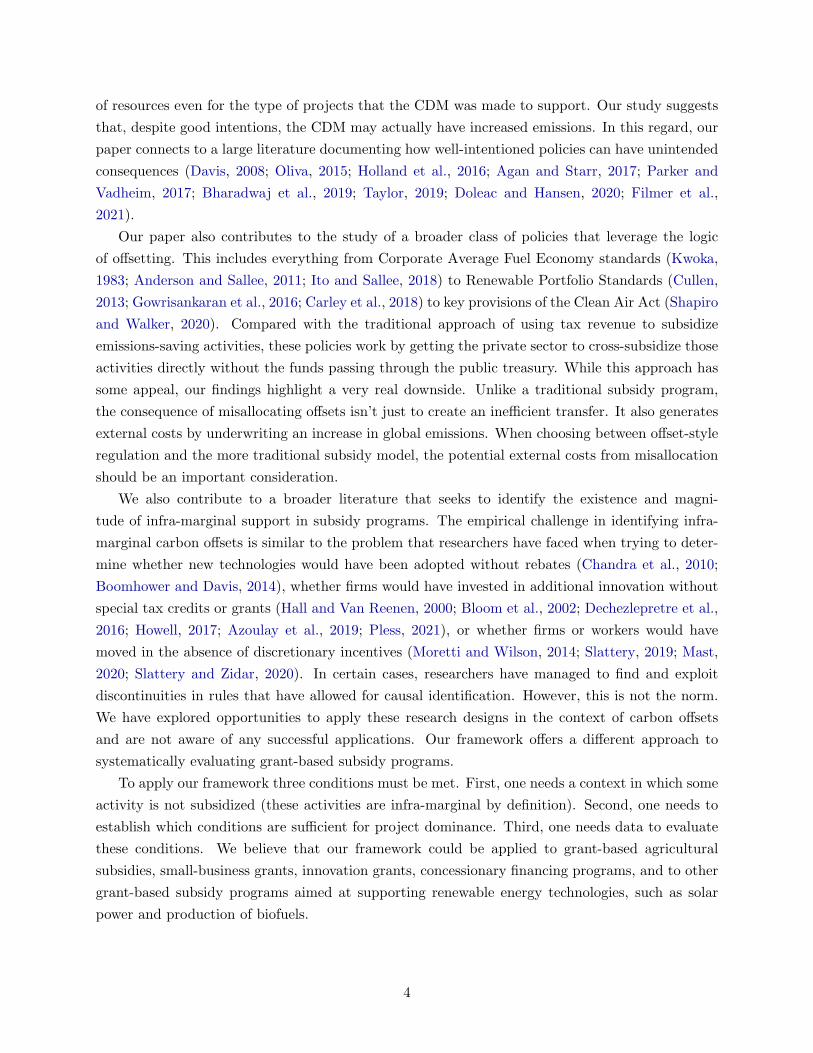
Fy, and capacity, cn. This prediction appears to be supported by our data. From the Bloomberg

New Energy Finance project database, we observe both the built capacity and the total up-front

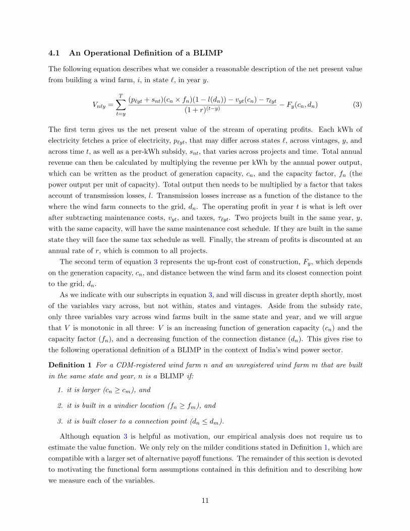
cost for ≈ 30% of wind power projects. Figure 2 shows that, for this sample, these two variables

display a strong positive linear association.

Planning costs are primarily made up of fixed fees that apply to projects of any size, which

implies that the function Fy will have a positive intercept. Indeed, studies of European wind

12

Capacity (MW)

1 10 100

1

10

100

1,000

10,000

Project cost(million INR)

β = 49.23(SE = 0.58)

Figure 2: Capacity and project costs. Source: Bloomberg New Energy Finance

developments suggest that these costs make up about 8-10% of up-front investment (Blanco, 2009).

If we regress project costs on capacity and distance for the subset where all three are observed, the

intercept is ≈ INR 20 million, which corresponds to nearly 8% of project costs on average. The

combination of a fixed up-front cost and a constant cost per MW means that the average cost per

MW is declining in the scale of the project.

Maintenance costs, vyt, and taxes, τ`yt, could in principle undo some of the benefits of scale,

but in practice they do not. Similar to prices, maintenance costs are contracted at the time

of construction, and they tend to follow an industry-standard schedule. A typical maintenance

contract charges a flat fee per MW of built capacity, which subsequently increases by some fixed

percentage with each passing year. Therefore, if we are comparing two wind farms of the same size,

built in the same year, they will have the same maintenance cost over the lifetime of the project.

When it comes to taxes, wind farms pay the same state and national taxes in India as any other

enterprise, with the exception of the Accelerated Depreciation Benefit. Starting in 1994, wind farm

developers were permitted to apply a 100% rate of depreciation to their newly built projects. The

rate was lowered to 80% in 2002, then to 0% in 2012, before returning to 80% in 2014. This means

that wind farm developers in India would have paid almost no taxes on their developments during

our period of study. To the extent that wind farm developments are subject to different tax regimes,

these will differ primarily by vintage. We have found no evidence that there were any state tax

policies that disproportionately increased the cost of building larger wind farms.

To summarize, power output is an increasing function of generation capacity, and to some

extent, so is the revenue per kWh. Because of planning costs, larger wind farms will have a lower

13

average up-front cost per MW. Maintenance and taxes do not increase fast enough, as a function of

capacity, to undo the benefits of scale. Taken together, these facts support the presumption that, at

least among wind farms built in a particular state and year, the payoffs to wind farm development

are an increasing function of generation capacity. Developers are incentivized to build the largest

projects that they are able to. In practice, the most important constraints on size appear to be the

availability of land and capital.

4.3 Payoffs Increase in the Capacity Factor

For a wind farm of a given capacity, cn, the amount of power that it generates depends on its

capacity factor, fn. The capacity factor is the ratio of actual-to-maximum output, and is sometimes

also referred to as the plant load factor. If a 1 MW wind turbine produced at maximum capacity

it would generate 1 MWh of power in one hour, or 8,766 MWh in a year (1 MW × 8,766 hours).

Since the wind doesn’t blow constantly, however, turbines will generate much less power in practice,

typically between 10% to 20% of maximal output. For all intents and purposes, the capacity factor

measures the windiness of the site on which you put your turbine, but it does so in relation to the

optimal wind profile of the turbine.

There is no real cost to building in a windier location, so it is straightforward to see that the

payoff is an increasing function of the capacity factor. The challenge, in this case, is that neither

we nor the developers know in advance how much the wind will blow at a particular site. To assess

the value of a potential wind farm we both have to estimate the capacity factor.

We have already calculated the denominator for a 1 MW capacity factor—simply multiplying

the maximal power output by the number of hours in a year—and the same can be done for turbines

of any rated capacity, c. To estimate the numerator, the actual power output, we need to know the

turbine’s power curve:

P (ρ, w) =

0 if w < w or w ≥ w

min(12ρAw

3C(w), c)

if w ≤ w < w(4)

where the power output P is given as a function of the wind speed, w, and air density, ρ. The

swept area, A, the cut-in speed, w, cut-out speed, w, power coefficient, C, and rated capacity, c,

are all features of the turbine itself.4

Like many economists working in countries where the quality and quantity of historical weather

data is limited, we have opted to use reanalysis data to estimate wind resources at each project-site

(Auffhammer et al., 2013). We use the ERA5-Land database produced by the European Centre

for Medium-Range Weather Forecasts (Munoz Sabater, 2019). It uses a global circulation model to

interpolate meteorological variables in observationally sparse regions, yielding data that are more

uniform in quality and realism than observations alone, and that is closer to reality than any model

could provide on its own. ERA5-Land includes a complete set of hourly observations going back

4See appendix B for a lengthier description of power curves.

14

to 1981, at a spatial resolution of roughly 9 km over land.5

Wind speed (m/s)

0 10 20 30 40

0

200

400

600

800

1000

Power output (kW)

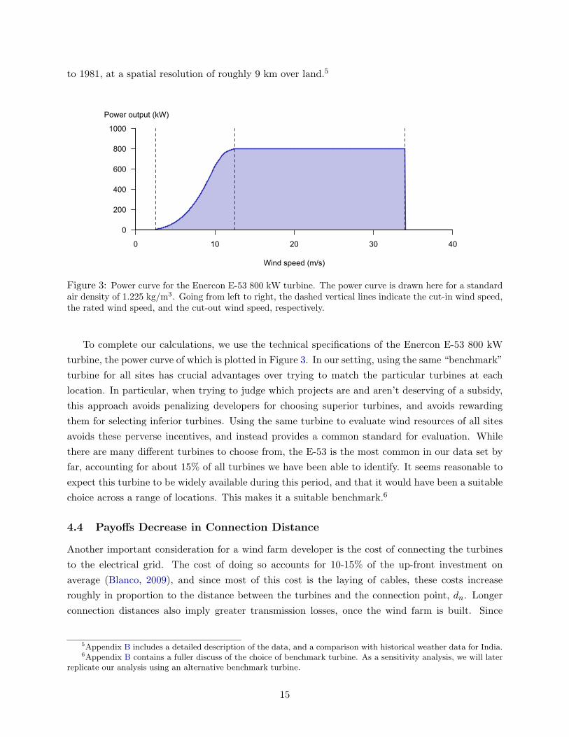
Figure 3: Power curve for the Enercon E-53 800 kW turbine. The power curve is drawn here for a standardair density of 1.225 kg/m3. Going from left to right, the dashed vertical lines indicate the cut-in wind speed,the rated wind speed, and the cut-out wind speed, respectively.

To complete our calculations, we use the technical specifications of the Enercon E-53 800 kW

turbine, the power curve of which is plotted in Figure 3. In our setting, using the same “benchmark”

turbine for all sites has crucial advantages over trying to match the particular turbines at each

location. In particular, when trying to judge which projects are and aren’t deserving of a subsidy,

this approach avoids penalizing developers for choosing superior turbines, and avoids rewarding

them for selecting inferior turbines. Using the same turbine to evaluate wind resources of all sites

avoids these perverse incentives, and instead provides a common standard for evaluation. While

there are many different turbines to choose from, the E-53 is the most common in our data set by

far, accounting for about 15% of all turbines we have been able to identify. It seems reasonable to

expect this turbine to be widely available during this period, and that it would have been a suitable

choice across a range of locations. This makes it a suitable benchmark.6

4.4 Payoffs Decrease in Connection Distance

Another important consideration for a wind farm developer is the cost of connecting the turbines

to the electrical grid. The cost of doing so accounts for 10-15% of the up-front investment on

average (Blanco, 2009), and since most of this cost is the laying of cables, these costs increase

roughly in proportion to the distance between the turbines and the connection point, dn. Longer

connection distances also imply greater transmission losses, once the wind farm is built. Since

5Appendix B includes a detailed description of the data, and a comparison with historical weather data for India.6Appendix B contains a fuller discuss of the choice of benchmark turbine. As a sensitivity analysis, we will later

replicate our analysis using an alternative benchmark turbine.

15

greater remoteness, in and of itself, provides no particular benefit, it is easy to see that the payoff

is a decreasing function of connection distance.

We do not observe the connection distance directly and so need to estimate it. To do this, we

need the geographical coordinates of the electrical substations as well as of turbines themselves.

The coordinates of electrical substations were collected by Burlig et al. (2020), while the coordinates

of the turbines were found using a combination of information found in the Bloomberg New Energy

Finance database, the UNFCCC’s CDM project database, and extensive online research, including

press releases, news reports, and documents published by the Indian government. Rather than

pinpointing turbines individually, we record the coordinates of the village in which the turbines

are located. This was partly out of practical necessity, but also means that our findings cannot be

driven by arbitrarily small differences in location. Any variation in location that we might have

been able to generate at the sub-village level would likely have contained more noise than signal.7

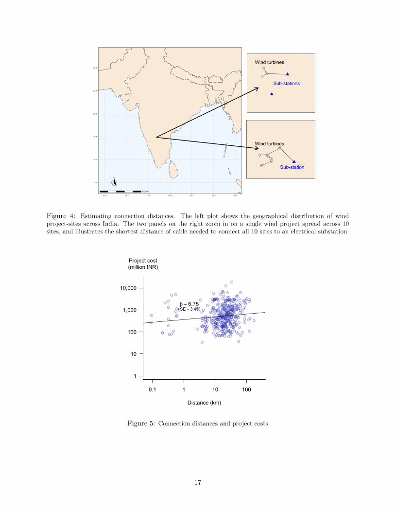
Under the assumption that wind farm developers will do their best to minimize connection

costs, we calculate the minimum distance to connect each project to the electrical grid, using a

modified minimum spanning tree algorithm.8 Figure 4 illustrates the results for one multi-site wind

power project that is spread across ten villages.

This approach may underestimate connection distances, since it does not take into account

topographical obstacles. The magnitude of any bias will tend to scale with the connection distance.

As a result, this type of measurement error will not distort the ordering of connection distances,

and therefore does not affect our empirical analysis.

Classical measurement error is not expected to affect our analysis. This is because it would be

just as likely to lead to an erroneous BLIMP inference as an erroneous non-BLIMP inference. In

our setting, a problem would arise only if our estimation method systematically underestimated

the distance for CDM projects relative to non-CDM projects, or vice versa. This might occur,

for example, if CDM projects are disproportionately built in places where topographical features

increase the the real connection distance relative to the distance measured as the crow flies. In

sensitivity analysis, we how sensitive our findings are to this possibility by deliberately inflating

the distances for CDM projects relative to non-CDM projects.

Figure 5 shows that the estimated connection distance is positively associated with project costs

for the sub-sample where both are observed. The association is comparatively weak, consistent with

the premise that distance to the grid affects only a small portion of overall project costs.

7Appendix A provides additional details about how the raw data was processed.8To avoid inflating the distances for wind farms spread across widely dispersed sites, we modified the standard

algorithm. Instead of trying to connect all points in one step, we first connect the electrical substations to each other.Only then do we extend the graph to include the wind farm sites. This means that the total connection distance willinclude the edges that connect each cluster of turbines to its nearest substation, but avoids any edges that would benecessary to connect distant clusters. See appendix C for a more detailed description of the algorithm.

16

1000 km

N

5°N

10°N

15°N

20°N

25°N

30°N

65°E 70°E 75°E 80°E 85°E 90°E 95°E

Sub-stations

Wind turbines

Sub-station

Wind turbines

Figure 4: Estimating connection distances. The left plot shows the geographical distribution of windproject-sites across India. The two panels on the right zoom in on a single wind project spread across 10sites, and illustrates the shortest distance of cable needed to connect all 10 sites to an electrical substation.

Distance (km)

0.1 1 10 100

1

10

100

1,000

10,000

Project cost(million INR)

β = 6.75(SE = 3.45)

Figure 5: Connection distances and project costs

17

4.5 All Else Equal

We have argued that, all else equal, the developer’s payoff is increasing in generation capacity and

capacity factor, and decreasing in connection distance. But what things need to be held constant?

The most important factor is the electricity price, p`yt. Electricity prices do vary across states

and time, but they do not vary across wind farms built in the same state and year. The same goes

for maintenance and tax schedules, τ`yt and vyt.

The final piece of equation 3 is the discount rate r. If we wanted to determine the real payoff

to any particular wind farm developer, we would need to know the rate of interest at which they

are able to access capital. However, our objective is somewhat different, in that we are trying to

determine whether the a project is worth subsidizing or not. Obviously, we do not want to subsidize

wind farms simply because their developers are risky borrowers. The relevant quantity is not the

market rate of interest, but the social discount rate.

The way that the UN Executive Board evaluates applications is by setting V equal to zero and

then working out whether the implied internal rate of return r exceeds some common threshold

value or not. This is equivalent to letting r equal the social discount rate and working out whether

V exceeds some common reservation payoff. For the purpose of evaluating projects for carbon

offsets we should apply a common discount rate to all projects. Since electricity prices and taxes

only vary across states and years, and there is no additional variation coming from the discount

rate, the “other things equal”-condition will be met so long as we are comparing wind farms built

in the same state and year. In sensitivity analysis we impose more restrictive comparison groups.

5 How Many BLIMPs is Too Many?

The ideal number of BLIMPs receiving subsidies is clearly zero. BLIMPs are only a subset of infra-

marginal projects, and they are a conservative indicator of infra-marginality. A program could in

principle subsidize many infra-marginal projects without subsidizing any BLIMPs. The number

of BLIMPs therefore provides a conservative lower bound on the total number of infra-marginal

projects. On some level the existence of any BLIMPs is a sign of something having gone wrong in

the CDM’s decision making process.

The total number of BLIMPs, however, can provide a useful indication of the degree of mis-

allocation. To give this number a meaningful interpretation we require an alternative allocation

mechanism of known quality that can serve as a benchmark. We can then compare the realized

number of BLIMPs in the CDM’s allocation to the number of BLIMPs that would have received

support in counterfactual allocation scenarios.

We argue that a lottery is a useful benchmark mechanism. A lottery provides a floor for

performance. In expectation, a lottery would allocate subsidies in a way that is uncorrelated with

whether a project is marginal or infra-marginal.

By repeating the lottery many times, we can obtain a distribution of the number of BLIMPs

that a lottery would subsidize. Each time the lottery is repeated, we let the CDM Executive Board

18

randomly select a fixed number of wind farms for registration in each year, equal to the number

they actually registered. Some iterations will, by chance, register a lot of small wind farms in

remote and windless locations (i.e. few BLIMPs). Other times chance alone will result in a large

number of BLIMPs. This distribution gives us a scale. The quality of the realized CDM allocation

can be measured by the probability that the lottery results in fewer subsidised BLIMPs. A small

probability means the real program has performed much better than a lottery, while a large enough

probability implies that the real program is indistinguishable from a lottery. One would hope that

no real-world program would produce more subsidised BLIMPs than a lottery.

Unlike the real CDM, however, the lottery can only select project from among those that were

actually built, since those are the only projects in our database. This gives the CDM a built-in

advantage. If there are any potential projects that weren’t built on account of lacking support

from the CDM, they would be invisible to us and to the lottery. The larger we imagine this set of

potential projects to be, the more we will tend to over-represent the performance of the CDM.

6 Results

6.1 Main Results

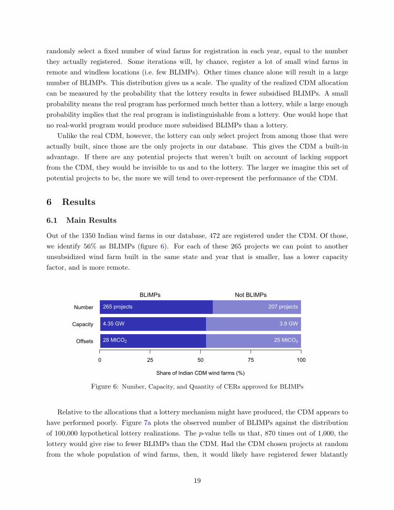
Out of the 1350 Indian wind farms in our database, 472 are registered under the CDM. Of those,

we identify 56% as BLIMPs (figure 6). For each of these 265 projects we can point to another

unsubsidized wind farm built in the same state and year that is smaller, has a lower capacity

factor, and is more remote.

Share of Indian CDM wind farms (%)

Offsets

Capacity

Number

0 25 50 75 100

BLIMPs Not BLIMPs

265 projects 207 projects

4.35 GW 3.9 GW

28 MtCO2 25 MtCO2

Figure 6: Number, Capacity, and Quantity of CERs approved for BLIMPs

Relative to the allocations that a lottery mechanism might have produced, the CDM appears to

have performed poorly. Figure 7a plots the observed number of BLIMPs against the distribution

of 100,000 hypothetical lottery realizations. The p-value tells us that, 870 times out of 1,000, the

lottery would give rise to fewer BLIMPs than the CDM. Had the CDM chosen projects at random

from the whole population of wind farms, then, it would likely have registered fewer blatantly

19

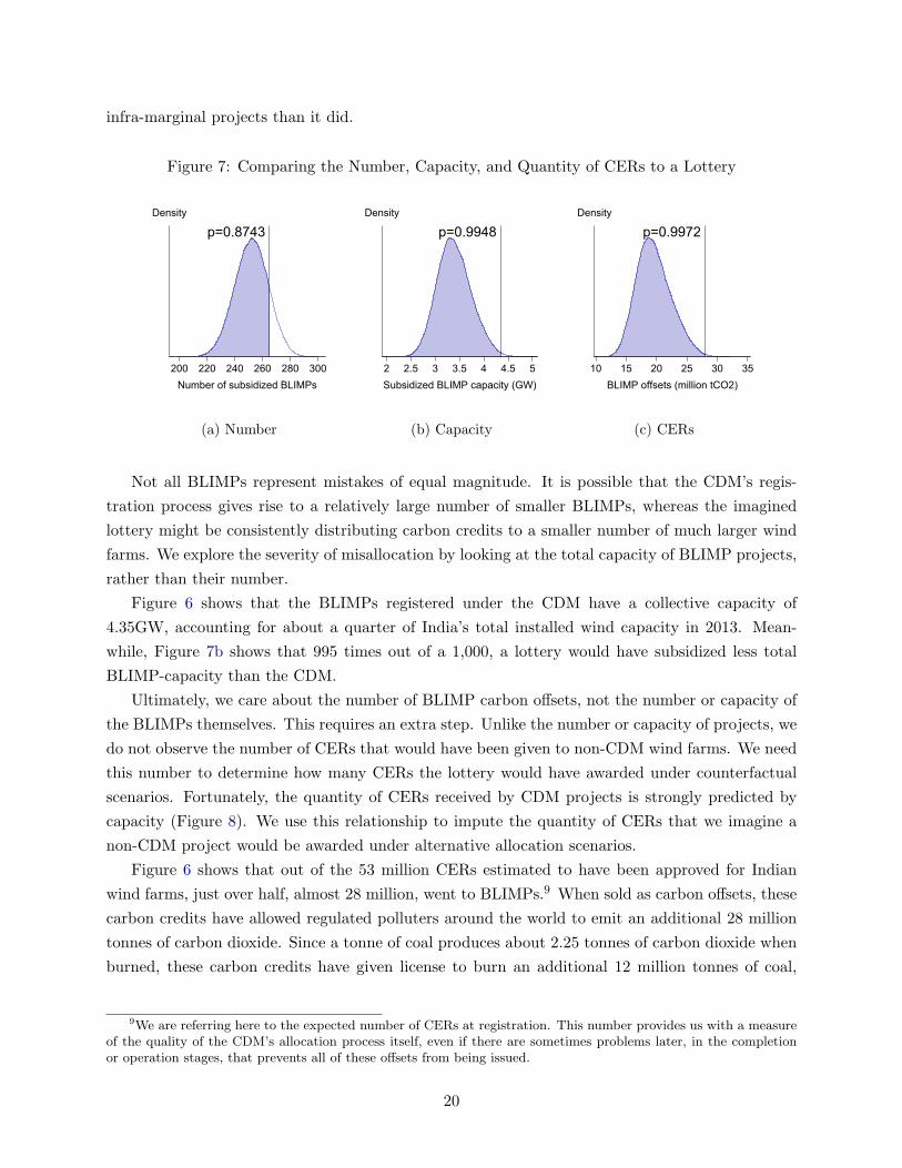
infra-marginal projects than it did.

Figure 7: Comparing the Number, Capacity, and Quantity of CERs to a Lottery

200 220 240 260 280 300Number of subsidized BLIMPs

p=0.8743Density

(a) Number

2 2.5 3 3.5 4 4.5 5Subsidized BLIMP capacity (GW)

Density

p=0.9948

(b) Capacity

10 15 20 25 30 35BLIMP offsets (million tCO2)

Density

p=0.9972

(c) CERs

Not all BLIMPs represent mistakes of equal magnitude. It is possible that the CDM’s regis-

tration process gives rise to a relatively large number of smaller BLIMPs, whereas the imagined

lottery might be consistently distributing carbon credits to a smaller number of much larger wind

farms. We explore the severity of misallocation by looking at the total capacity of BLIMP projects,

rather than their number.

Figure 6 shows that the BLIMPs registered under the CDM have a collective capacity of

4.35GW, accounting for about a quarter of India’s total installed wind capacity in 2013. Mean-

while, Figure 7b shows that 995 times out of a 1,000, a lottery would have subsidized less total

BLIMP-capacity than the CDM.

Ultimately, we care about the number of BLIMP carbon offsets, not the number or capacity of

the BLIMPs themselves. This requires an extra step. Unlike the number or capacity of projects, we

do not observe the number of CERs that would have been given to non-CDM wind farms. We need

this number to determine how many CERs the lottery would have awarded under counterfactual

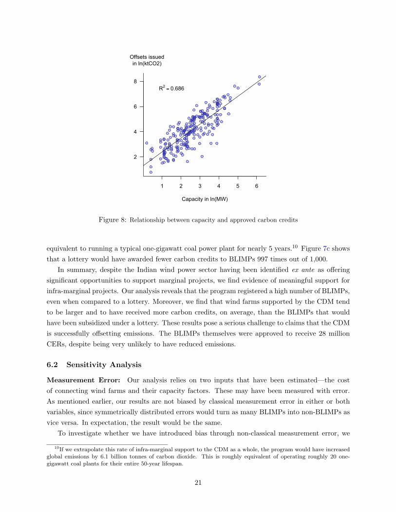
scenarios. Fortunately, the quantity of CERs received by CDM projects is strongly predicted by

capacity (Figure 8). We use this relationship to impute the quantity of CERs that we imagine a

non-CDM project would be awarded under alternative allocation scenarios.

Figure 6 shows that out of the 53 million CERs estimated to have been approved for Indian

wind farms, just over half, almost 28 million, went to BLIMPs.9 When sold as carbon offsets, these

carbon credits have allowed regulated polluters around the world to emit an additional 28 million

tonnes of carbon dioxide. Since a tonne of coal produces about 2.25 tonnes of carbon dioxide when

burned, these carbon credits have given license to burn an additional 12 million tonnes of coal,

9We are referring here to the expected number of CERs at registration. This number provides us with a measureof the quality of the CDM’s allocation process itself, even if there are sometimes problems later, in the completionor operation stages, that prevents all of these offsets from being issued.

20

1 2 3 4 5 6

Capacity in ln(MW)

2

4

6

8

Offsets issuedin ln(ktCO2)

R2 = 0.686

Figure 8: Relationship between capacity and approved carbon credits

equivalent to running a typical one-gigawatt coal power plant for nearly 5 years.10 Figure 7c shows

that a lottery would have awarded fewer carbon credits to BLIMPs 997 times out of 1,000.

In summary, despite the Indian wind power sector having been identified ex ante as offering

significant opportunities to support marginal projects, we find evidence of meaningful support for

infra-marginal projects. Our analysis reveals that the program registered a high number of BLIMPs,

even when compared to a lottery. Moreover, we find that wind farms supported by the CDM tend

to be larger and to have received more carbon credits, on average, than the BLIMPs that would

have been subsidized under a lottery. These results pose a serious challenge to claims that the CDM

is successfully offsetting emissions. The BLIMPs themselves were approved to receive 28 million

CERs, despite being very unlikely to have reduced emissions.

6.2 Sensitivity Analysis

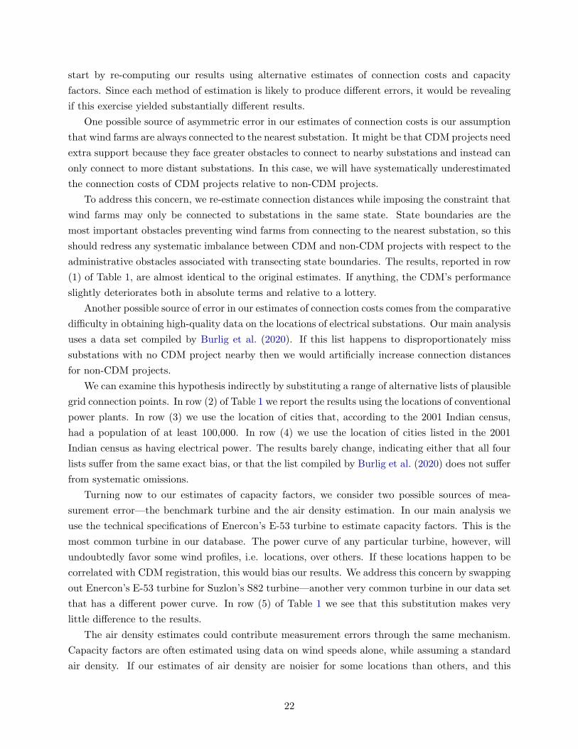
Measurement Error: Our analysis relies on two inputs that have been estimated—the cost

of connecting wind farms and their capacity factors. These may have been measured with error.

As mentioned earlier, our results are not biased by classical measurement error in either or both

variables, since symmetrically distributed errors would turn as many BLIMPs into non-BLIMPs as

vice versa. In expectation, the result would be the same.

To investigate whether we have introduced bias through non-classical measurement error, we

10If we extrapolate this rate of infra-marginal support to the CDM as a whole, the program would have increasedglobal emissions by 6.1 billion tonnes of carbon dioxide. This is roughly equivalent of operating roughly 20 one-gigawatt coal plants for their entire 50-year lifespan.

21

start by re-computing our results using alternative estimates of connection costs and capacity

factors. Since each method of estimation is likely to produce different errors, it would be revealing

if this exercise yielded substantially different results.

One possible source of asymmetric error in our estimates of connection costs is our assumption

that wind farms are always connected to the nearest substation. It might be that CDM projects need

extra support because they face greater obstacles to connect to nearby substations and instead can

only connect to more distant substations. In this case, we will have systematically underestimated

the connection costs of CDM projects relative to non-CDM projects.

To address this concern, we re-estimate connection distances while imposing the constraint that

wind farms may only be connected to substations in the same state. State boundaries are the

most important obstacles preventing wind farms from connecting to the nearest substation, so this

should redress any systematic imbalance between CDM and non-CDM projects with respect to the

administrative obstacles associated with transecting state boundaries. The results, reported in row

(1) of Table 1, are almost identical to the original estimates. If anything, the CDM’s performance

slightly deteriorates both in absolute terms and relative to a lottery.

Another possible source of error in our estimates of connection costs comes from the comparative

difficulty in obtaining high-quality data on the locations of electrical substations. Our main analysis

uses a data set compiled by Burlig et al. (2020). If this list happens to disproportionately miss

substations with no CDM project nearby then we would artificially increase connection distances

for non-CDM projects.

We can examine this hypothesis indirectly by substituting a range of alternative lists of plausible

grid connection points. In row (2) of Table 1 we report the results using the locations of conventional

power plants. In row (3) we use the location of cities that, according to the 2001 Indian census,

had a population of at least 100,000. In row (4) we use the location of cities listed in the 2001

Indian census as having electrical power. The results barely change, indicating either that all four

lists suffer from the same exact bias, or that the list compiled by Burlig et al. (2020) does not suffer

from systematic omissions.

Turning now to our estimates of capacity factors, we consider two possible sources of mea-

surement error—the benchmark turbine and the air density estimation. In our main analysis we

use the technical specifications of Enercon’s E-53 turbine to estimate capacity factors. This is the

most common turbine in our database. The power curve of any particular turbine, however, will

undoubtedly favor some wind profiles, i.e. locations, over others. If these locations happen to be

correlated with CDM registration, this would bias our results. We address this concern by swapping

out Enercon’s E-53 turbine for Suzlon’s S82 turbine—another very common turbine in our data set

that has a different power curve. In row (5) of Table 1 we see that this substitution makes very

little difference to the results.

The air density estimates could contribute measurement errors through the same mechanism.

Capacity factors are often estimated using data on wind speeds alone, while assuming a standard

air density. If our estimates of air density are noisier for some locations than others, and this

22

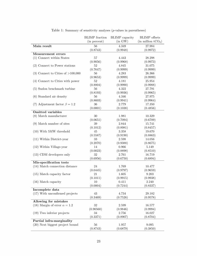
Table 1: Summary of sensitivity analyses (p-values in parentheses)

BLIMP fraction BLIMP capacity BLIMP offsets(in percent) (in GW) (in million tCO2)

Main result 56 4.349 27.984(0.8743) (0.9948) (0.9972)

Measurement errors(1) Connect within States 57 4.443 28.298

(0.9056) (0.9968) (0.9973)(2) Connect to Power stations 52 4.845 31.075

(0.7647) (0.9999) (0.9999)(3) Connect to Cities of >100,000 56 4.283 26.366

(0.9653) (0.9999) (0.9999)(4) Connect to Cities with power 52 4.181 25.954

(0.8804) (0.9990) (0.9988)(5) Suzlon benchmark turbine 56 4.322 27.791

(0.8193) (0.9936) (0.9965)(6) Standard air density 56 4.346 27.975

(0.8603) (0.9941) (0.9964)(7) Adjustment factor β = 1.2 36 2.779 17.350

(0.0001) (0.1038) (0.4856)Omitted variables(8) Match manufacturer 30 1.981 10.329

(0.0651) (0.7094) (0.6709)(9) Match number of sites 39 2.844 15.741

(0.1012) (0.8981) (0.8457)(10) With 5MW threshold 45 3.358 19.670

(0.5587) (0.9190) (0.8863)(11) Within District-year 33 2.598 14.056

(0.2070) (0.9388) (0.8675)(12) Within Village-year 14 0.966 5.149

(0.0023) (0.8898) (0.8510)(13) CDM developers only 32 2.761 16.719

(0.6956) (0.6750) (0.6894)Mis-specification tests(14) Match connection distance 24 1.769 10.477

(0.0445) (0.9797) (0.9659)(15) Match capacity factor 21 1.605 9.203

(0.1011) (0.9915) (0.9938)(16) Match capacity 10 0.411 2.240

(0.0004) (0.7244) (0.8337)Incomplete data(17) With unconfirmed projects 43 4.734 29.182

(0.3469) (0.7526) (0.9578)Allowing for mistakes(18) Margin of error α = 1.2 32 2.599 16.577

(0.90560) (0.9846) (0.9994)(19) Two inferior projects 34 2.756 16.027

(0.3371) (0.8907) (0.8704)Partial infra-marginality(20) Next biggest project bound 56 1.957 9.095

(0.8743) (0.6879) (0.3850)

23

pattern correlates with CDM registration, it could affect our results. However, row (6) of Table 1

shows that using a common air density measure has no meaningful effect on our findings.

It is possible that there are other sources of systematic measurement error that we haven’t

thought about. How much measurement error would be necessary to qualitatively alter our find-

ings? If connection costs are systematically underestimated, or capacity factors systematically

overestimated, for non-CDM projects compared to CDM projects, we would need to correct for

this adjustment factor before concluding that a CDM project is a BLIMP. To explore this we im-

pose the assumption that CDM projects are actually β ≥ 1 times more remote, and only 1/β times

as windy as our estimates indicate. As we increase β, CDM projects look less and less desirable as

investment opportunities, compared to non-CDM projects.

1.0 1.2 1.4 1.6 1.8 2.0

Adjustment factor (β)

BLIMP offsets(million CERs)

0

5

10

15

20

25

30Error in connection costError in capacity factorError in both

1.0 1.2 1.4 1.6 1.8 2.0

Adjustment factor (β)

Pr(Lottery allocatesfewer CERs to BLIMPs

than does CDM)

0.0

0.2

0.4

0.6

0.8

1.0

Figure 9: Sensitivity to asymmetric measurement error in connection costs and capacity factors

Row (7) of Table 1 shows the results for β = 1.2.11 At this value, the number of BLIMPs

drops sharply, however, the BLIMPs that remain still account for a large number of carbon offsets.

Figure 9 (left panel) provides a graphical representation of all β values between 1 and 2. The right

panel of 9 shows, that the CDM only performs on par with lottery assignment when CDM projects

are handicapped by a 20% penalty in both connection costs and capacity factors.

Omitted Variables: Factors other than capacity, capacity factors, and connection costs could,

conceivably, produce systematic differences in profitability even among wind farms built in the same

state and year. If any of those factors are correlated with capacity, capacity factors, or connection

costs, our results would be biased.

One possible omitted variable is the turbine manufacturer. To the extent that turbine manufac-

11This value, applied only to CDM projects, inflates connection distances by 20% and reduces capacity factors by20%.

24

turers differ in their pricing, quality, technical specifications, ability to supply large developments,

maintenance costs, etc., we could imagine that the choice of manufacturer affects both the prof-

itability of a wind farm and features like its capacity or capacity factor. In row (8) of Table 1, we

therefore require projects to use turbines from the same manufacturer in order to allow one of them

to be classified as a BLIMP. Unsurprisingly, BLIMPs are much rarer occurrences if we require that

wind farms are built in the same year, in the same state, and use turbines from the same man-

ufacturer. However, taking into account that the same difficulty extends to counterfactual CDM

assignments, we see that the CDM still performs quite poorly compared to a lottery (except for

the number of BLIMPs).

Another potential omitted variable is the number of sites a project is spread across. The number

of sites could affect the cost to build and to connect a wind farm. Row (9) matches projects on

state, vintage, and number of sites. As before, this makes it harder to identify BLIMPs, but in

relative terms, the CDM still performs poorly when compared to a lottery.

Another possibility is that projects above 5MW are somehow different than projects below

5MW. As discussed, the Generation-Based Incentive specifically supports wind farm developments

that exceed 5MW in capacity. If the policy is in place to compensate for some unobserved cost of

scale, such as the loss of support from local governments then our results may be biased. In row (10)

we match wind farms on the year of construction, the state, and on whether it exceeded the 5MW

capacity threshold. This improves outcomes for the CDM, but a lottery would still outperform the

CDM most of the time.

Arguments about omitted policy variables can be extended down to the district-level, and in

the limit, down to the village-level. Perhaps there is systematic variation in policies (or factor

prices) between districts or villages within the same state, which affect costs. In rows (11) and

(12) we match wind farms built in the same districts and the same villages. It now becomes much

more difficult to find comparable wind farms and to spot BLIMPs. Matching at the village-year

level has the side-effect of also eliminating variation in connection distances and capacity factors, so

BLIMPs are only identified based on size differences. Even so, measured either in BLIMP capacity

or offsets, the CDM still performs poorly relative to a lottery.

It is also possible that differences in project developer are more important than a feature of

the wind farm, or a function of its location. Project developers may differ systematically in their

engagement with local stakeholders, in their adherence to local regulations, and in their ability to

develop wind projects more broadly. The CDM may quite reasonably support only projects put

forward by reputable developers. If smaller, more remote wind farms are all built by less reputable

developers. If so, our results may be driven by the fact reputation is only observed by the CDM.

Row (13) shows that the CDM’s performance relative to a lottery improves when we limit our

sample to projects built by developers with at least one CDM-registered wind farm. However, even

within this restricted sample, the lottery outperforms the CDM ≈ 700 times out of 1,000. While

there might be some merit in the “developer quality”-hypothesis, it explains at best a small part

of the CDM’s apparently poor performance.

25

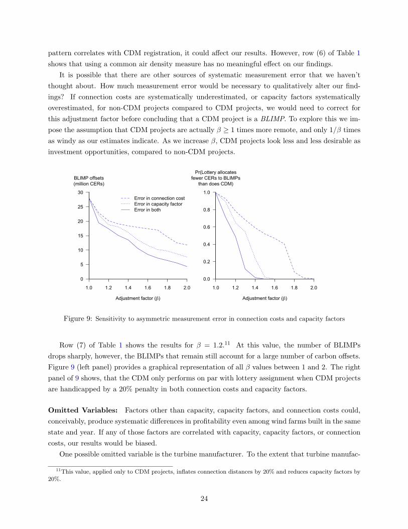
To address omitted variable concerns more generally, we investigate how much omissions is re-

quired to alter our conclusions. If the CDM observes some factors, hidden from us, that support the

project’s claim of being marginal, then their approval should provide a signal to us that the project

is more likely to be marginal. Introducing an omitted variable is therefore equivalent to putting

more faith in the CDM’s decisions. Rather that determining counterfactual CDM assignments

through a lottery where every project has an equal probability of being selected, we should perhaps

give the real CDM projects a Γ > 1 times greater chance of being selected. As Γ rises, the lottery

assignments will conform more and more closely to the actual CDM assignment. This makes the

CDM look better and better.12 How much faith, short of deferring to the CDM unquestioningly, is

required to materially alter our conclusion?

2 4 6 8 10

Strength of omitted variable (Γ)

Pr(Lottery allocatesfewer CERs to BLIMPs

than does CDM)

0

0.5

0.6

0.7

0.8

0.9

1

Figure 10: Sensitivity to generic omitted variable

Figure 10 shows what happens to the p-value as we increase Γ from 1, the value implicit in our

main results, all the way up to 10, at which point CDM projects have a ten-fold higher probability

of being selected.13 Increasing Γ in this way does reduce the p-value, but even when we put more

faith in the CDM’s decisions, a lottery still assigns fewer CERs to BLIMPs 70% of the time. For an

omitted variable to explain the CDM’s assignment, it would have to be almost perfectly correlated

with a project being marginal and the CDM’s observed decisions.

Mis-specification Tests: While the general framework we introduce in this paper is flexible

enough to accommodate a wide range of payoff functions, our empirical application relies on having

a detailed understanding of the factors that determine the profitability of wind farms in India.

12Although our interpretation of Γ differs somewhat from Rosenbaum (1987), our sensitivity analysis with respectto a generic omitted variable here is formally equivalent to his.

13Note that Γ has no effect our ability to spot BLIMPs, so the number of BLIMPs, the BLIMP capacity, and thequantity of BLIMP offsets all remain constant as we increase Γ.

26

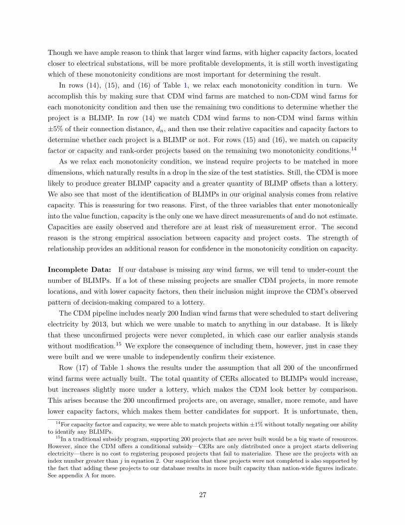
Though we have ample reason to think that larger wind farms, with higher capacity factors, located

closer to electrical substations, will be more profitable developments, it is still worth investigating

which of these monotonicity conditions are most important for determining the result.

In rows (14), (15), and (16) of Table 1, we relax each monotonicity condition in turn. We

accomplish this by making sure that CDM wind farms are matched to non-CDM wind farms for

each monotonicity condition and then use the remaining two conditions to determine whether the

project is a BLIMP. In row (14) we match CDM wind farms to non-CDM wind farms within

±5% of their connection distance, dn, and then use their relative capacities and capacity factors to

determine whether each project is a BLIMP or not. For rows (15) and (16), we match on capacity

factor or capacity and rank-order projects based on the remaining two monotonicity conditions.14

As we relax each monotonicity condition, we instead require projects to be matched in more

dimensions, which naturally results in a drop in the size of the test statistics. Still, the CDM is more

likely to produce greater BLIMP capacity and a greater quantity of BLIMP offsets than a lottery.

We also see that most of the identification of BLIMPs in our original analysis comes from relative

capacity. This is reassuring for two reasons. First, of the three variables that enter monotonically

into the value function, capacity is the only one we have direct measurements of and do not estimate.

Capacities are easily observed and therefore are at least risk of measurement error. The second

reason is the strong empirical association between capacity and project costs. The strength of

relationship provides an additional reason for confidence in the monotonicity condition on capacity.

Incomplete Data: If our database is missing any wind farms, we will tend to under-count the

number of BLIMPs. If a lot of these missing projects are smaller CDM projects, in more remote

locations, and with lower capacity factors, then their inclusion might improve the CDM’s observed

pattern of decision-making compared to a lottery.

The CDM pipeline includes nearly 200 Indian wind farms that were scheduled to start delivering

electricity by 2013, but which we were unable to match to anything in our database. It is likely

that these unconfirmed projects were never completed, in which case our earlier analysis stands

without modification.15 We explore the consequence of including them, however, just in case they

were built and we were unable to independently confirm their existence.

Row (17) of Table 1 shows the results under the assumption that all 200 of the unconfirmed

wind farms were actually built. The total quantity of CERs allocated to BLIMPs would increase,

but increases slightly more under a lottery, which makes the CDM look better by comparison.

This arises because the 200 unconfirmed projects are, on average, smaller, more remote, and have

lower capacity factors, which makes them better candidates for support. It is unfortunate, then,

14For capacity factor and capacity, we were able to match projects within ±1% without totally negating our abilityto identify any BLIMPs.

15In a traditional subsidy program, supporting 200 projects that are never built would be a big waste of resources.However, since the CDM offers a conditional subsidy—CERs are only distributed once a project starts deliveringelectricity—there is no cost to registering proposed projects that fail to materialize. These are the projects with anindex number greater than j in equation 2. Our suspicion that these projects were not completed is also supported bythe fact that adding these projects to our database results in more built capacity than nation-wide figures indicate.See appendix A for more.

27

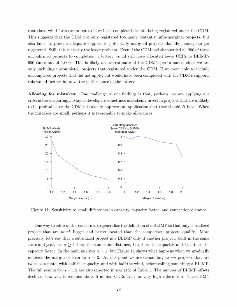
that these wind farms seem not to have been completed despite being registered under the CDM.

This suggests that the CDM not only registered too many blatantly infra-marginal projects, but

also failed to provide adequate support to potentially marginal projects that did manage to get

registered. Still, this is clearly the lesser problem. Even if the CDM had shepherded all 200 of these

unconfirmed projects to completion, a lottery would still have allocated fewer CERs to BLIMPs

950 times out of 1,000. This is likely an overestimate of the CDM’s performance, since we are

only including uncompleted projects that registered under the CDM. If we were able to include

uncompleted projects that did not apply, but would have been completed with the CDM’s support,

this would further improve the performance of the lottery.

Allowing for mistakes: One challenge to our findings is that, perhaps, we are applying our

criteria too unsparingly. Maybe developers sometimes mistakenly invest in projects that are unlikely

to be profitable, or the CDM mistakenly approves an application that they shouldn’t have. When

the mistakes are small, perhaps it is reasonable to make allowances.

1.0 1.2 1.4 1.6 1.8 2.0

Margin of error (α)

BLIMP offsets(million CERs)

0

5

10

15

20

25

30

1.0 1.2 1.4 1.6 1.8 2.0

Margin of error (α)

Pr(Lottery allocatesfewer CERs to BLIMPs

than does CDM)

0

0.5

0.6

0.7

0.8

0.9

1

Figure 11: Sensitivity to small differences in capacity, capacity factor, and connection distance

One way to address this concern is to generalize the definition of a BLIMP so that only subsidized

project that are much bigger and better located than the comparison projects qualify. More

precisely, let’s say that a subsidized project is a BLIMP only if another project, built in the same

state and year, has α ≥ 1 times the connection distance, 1/α times the capacity, and 1/α times the

capacity factor. In the main analysis α = 1, but Figure 11 shows what happens when we gradually

increase the margin of error to α = 2. At this point we are demanding to see projects that are

twice as remote, with half the capacity, and with half the wind, before calling something a BLIMP.

The full results for α = 1.2 are also reported in row (18) of Table 1. The number of BLIMP offsets

declines, however, it remains above 5 million CERs even for very high values of α. The CDM’s

28

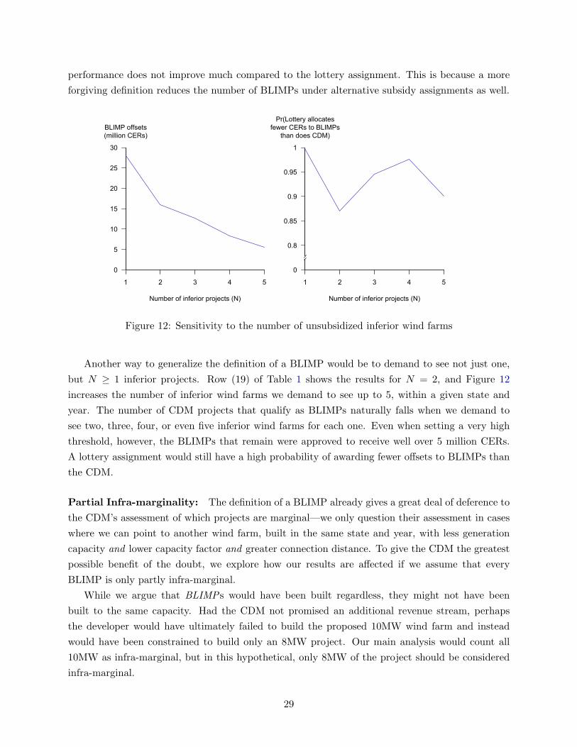
performance does not improve much compared to the lottery assignment. This is because a more

forgiving definition reduces the number of BLIMPs under alternative subsidy assignments as well.

1 2 3 4 5

Number of inferior projects (N)

BLIMP offsets(million CERs)

0

5

10

15

20

25

30

1 2 3 4 5

Number of inferior projects (N)

Pr(Lottery allocatesfewer CERs to BLIMPs

than does CDM)

0

0.8

0.85

0.9

0.95

1

Figure 12: Sensitivity to the number of unsubsidized inferior wind farms

Another way to generalize the definition of a BLIMP would be to demand to see not just one,

but N ≥ 1 inferior projects. Row (19) of Table 1 shows the results for N = 2, and Figure 12

increases the number of inferior wind farms we demand to see up to 5, within a given state and

year. The number of CDM projects that qualify as BLIMPs naturally falls when we demand to

see two, three, four, or even five inferior wind farms for each one. Even when setting a very high

threshold, however, the BLIMPs that remain were approved to receive well over 5 million CERs.

A lottery assignment would still have a high probability of awarding fewer offsets to BLIMPs than

the CDM.

Partial Infra-marginality: The definition of a BLIMP already gives a great deal of deference to

the CDM’s assessment of which projects are marginal—we only question their assessment in cases

where we can point to another wind farm, built in the same state and year, with less generation

capacity and lower capacity factor and greater connection distance. To give the CDM the greatest

possible benefit of the doubt, we explore how our results are affected if we assume that every

BLIMP is only partly infra-marginal.

While we argue that BLIMPs would have been built regardless, they might not have been

built to the same capacity. Had the CDM not promised an additional revenue stream, perhaps

the developer would have ultimately failed to build the proposed 10MW wind farm and instead

would have been constrained to build only an 8MW project. Our main analysis would count all

10MW as infra-marginal, but in this hypothetical, only 8MW of the project should be considered

infra-marginal.

29

To operationalize this idea, we use the next biggest inferior non-CDM project to bound from

below the counterfactual capacity of BLIMPs. The next biggest non-CDM project shows what

capacity each BLIMP could have been built to, at least, without CDM support. This approach

yields a lower bound on infra-marginal capacity, by imposing the assumption that every BLIMP is

only partly infra-marginal.

Row (20) of Table 1 shows the results of this exercise. Since we have built in the assumption

that every BLIMP is partly infra-marginal, the blatantly infra-marginal capacity is much lower—

about half of the number in our main results. The number of carbon credits allocated to support

this infra-marginal wind capacity is also lower, about a third of our main finding. This should

be thought of as a conservative lower bound on infra-marginality. At this lower bound the CDM

performs on par with the lottery allocation mechanism.

7 Conclusion

The last decade has seen billions of carbon offsets issued to project developers around the world,

providing opportunities for regulatory compliance at lower cost. However, when offset programs

support projects that would have been developed anyway, they not only waste the limited resources

available to mitigate climate change, but also contribute to climate change by increasing global

emissions. In the context of the CDM—the world’s largest carbon offset program—we estimate

that at least 52% of approved carbon offsets were allocated to projects that would very likely have

been built anyway. This is a substantial misallocation of resources.

When the CDM was created, India’s wind power sector was identified as a context where there

was huge potential for supporting marginal projects and increasing development beyond baseline

projections. Yet, we estimate that the CDM has approved at least 28 million tonnes-worth of

carbon offsets to infra-marginal projects. If we extrapolate this rate of infra-marginal support to

the CDM as a whole, we calculate that the program may have increased global carbon dioxide

emissions by 6.1 billion tonnes, equivalent to running 20 one-gigawatt coal power plants for their

entire 50-year lifespan.

We also find that the allocation of offsets to Indian wind power projects compares unfavor-

ably with a lottery, indicating that there is substantial room for improvement in the design and

implementation of the project selection mechanism. Having a process that accurately screens out

projects that do not require subsidies is essential to safeguarding the integrity of offset programs.

Why is the CDM failing to screen out these projects? We cannot answer this question defini-

tively, though we observe that the vast majority of Indian wind power projects whose applications

made it to the UN Executive Board were approved. Of the 666 CDM applications submitted for

Indian wind farms, including the nearly 200 that we could not link to any real projects, 98% were

approved. Even though we have identified hundreds of CDM applications that perhaps should have

been denied, final approval appears to be almost automatic.

In practice, most of the screening is accomplished earlier in the process through some combina-

30

tion of India’s Ministry of Environment and Forests, which decides which applications to forward to

the UN for final approval, and through self-selection on the part of the developers themselves. We

do not have data on submissions to the Ministry, but two observations suggest that self-selection

might be an important factor. First, our sensitivity analysis revealed that the CDM favors the

larger and better located wind farms even among the subset of projects belonging to develop-

ers with at least one CDM-project. Second, for developers that submit applications for multiple

projects, direct inspection reveals that the application documents are often nearly identical. Both

of these facts are consistent with there being substantial costs of applying, and developers choosing

not to submit applications for smaller projects that would be less likely to generate enough carbon

offsets to recoup the cost.

We acknowledge that our analysis only explores the direct effect of the CDM. It is possible

that, despite increasing emissions, the transfer of wealth from developed to developing countries

increased welfare. It is also possible that any marginal support provided by the CDM may have

had an indirect effect on establishing the wind power sector in India. Non-BLIMPs may have offset

more than one tonne of carbon dioxide per credit if their existence resulted in the entry of non-CDM

projects. To compensate for the emissions increases due to BLIMPs, we calculate that each offset

awarded to a non-BLIMP would, on average, have to generate an emissions reduction of 2.12 tonnes.

This is equivalent to assuming that all non-BLIMPs are marginal and collectively responsible for

the realization of half of India’s non-CDM wind power capacity. This theoretical possibility does

not undermine our finding that the CDM appears to have substantially misallocated resources. If

anything, the possibility that marginal support could deliver indirect emissions reductions implies

an even greater opportunity cost to subsidizing infra-marginal projects.

References

Agan, A. and Starr, S. (2017). Ban the box, criminal records, and racial discrimination: A field

experiment. Quarterly Journal of Economics, 133(1):191–235.

Anderson, S. T. and Sallee, J. M. (2011). Using loopholes to reveal the marginal cost of regulation:

The case of fuel-economy standards. American Economic Review, 101(4):1375–1409.

Auffhammer, M., Hsiang, S. M., Schlenker, W., and Sobel, A. (2013). Using weather data and cli-

mate model output in economic analyses of climate change. Review of Environmental Economics

and Policy, 7(2):181–198.

Azoulay, P., Graff Zivin, J., Li, D., and Sampat, B. (2019). Public r&d investments and private-

sector patenting: Evidence from nih funding rules. Review of Economic Studies, 86(1):117–152.

Berry, S. T. (1992). Estimation of a model of entry in the airline industry. Econometrica, 60(4):889–

917.

31

Bharadwaj, P., Lakdawala, L. K., and Li, N. (2019). Perverse Consequences of Well Intentioned

Regulation: Evidence from India’s Child Labor Ban. Journal of the European Economic Associ-

ation, 18(3):1158–1195.

Black, R., Cullen, K., Fay, B., Hale, T., Lang, J., Mahmood, S., and Smith, S. (2021). Taking

stock: A global assessment of net zero targets. Technical report, Energy & Climate Intelligence

Unit and Oxford Net Zero.

Blanco, M. I. (2009). The economics of wind energy. Renewable and Sustainable Energy Reviews,

13(6):1372–1382.

Bloom, N., Griffith, R., and Van Reenen, J. (2002). Do r&d tax credits work? evidence from a

panel of countries 1979-1997. Journal of Public Economics, 85(1):1–31.

BNEF (2013). Bloomberg new energy finance. (Last accessed May 2013).

Boomhower, J. and Davis, L. (2014). A credible approach for measuring inframarginal participation

in energy efficiency programs. Journal of Public Economics, 113:67–79.

Burlig, F., Jha, A., and Preonas, L. (2020). Transmission constraints and electricity trade in india.

Mimeo.

Carley, S., Davies, L. L., Spence, D. B., and Zirogiannis, N. (2018). Empirical evaluation of the

stringency and design of renewable portfolio standards. Nature Energy, 3(9):754–763.

Carta, J. A., Velazquez, S., and Cabrera, P. (2013). A review of measure-correlate-predict (mcp)

methods used to estimate long-term wind characteristics at a target site. Renewable and Sus-

tainable Energy Reviews, 27:362–400.

Chandra, A., Gulati, S., and Kandlikar, M. (2010). Green drivers or free riders? an analysis of tax

rebates for hybrid vehicles. Journal of Environmental Economics and Management, 60(2):78–93.

Cullen, J. (2013). Measuring the environmental benefits of wind-generated electricity. American

Economic Journal: Economic Policy, 5(4):107–33.

Davis, L. W. (2008). The effect of driving restrictions on air quality in mexico city. Journal of

Political Economy, 116(1):38–81.

Dechezlepretre, A., Einio, E., Martin, R., Nguyen, K., and Van Reenen, J. (2016). Do tax incentives

for research increase firm innovation? an rd design for r&d. NBER Working Paper 22405.

Doleac, J. and Hansen, B. (2020). The unintended consequences of “ban the box”: Statistical

discrimination and employment outcomes when criminal histories are hidden. Journal of Labor

Economics, 38(2):321–374.

Filmer, D., Friedman, J., Kandpal, E., and Onishi, J. (2021). Cash Transfers, Food Prices, and

Nutrition Impacts on Ineligible Children. The Review of Economics and Statistics, pages 1–45.

32

GIZ (2014). Carbon market roadmap for india: Looking back on cdm and looking ahead. Technical

report, Deutsche Gesellschaft fur Internationale Zusammenarbeit (GIZ).

Gowrisankaran, G., Reynolds, S. S., and Samano, M. (2016). Intermittency and the value of

renewable energy. Journal of Political Economy, 124(4):1187–1234.

Hall, B. and Van Reenen, J. (2000). How effective are fiscal incentives for r&d? a review of the

evidence. Research Policy, 29(4):449–469.

Holland, S. P., Mansur, E. T., Muller, N. Z., and Yates, A. J. (2016). Are there environmental

benefits from driving electric vehicles? the importance of local factors. American Economic

Review, 106(12):3700–3729.

Howell, S. (2017). Financing innovation: Evidence from r&d grants. American Economic Review,

107(4):1136–1164.

Ito, K. and Sallee, J. M. (2018). The Economics of Attribute-Based Regulation: Theory and

Evidence from Fuel Economy Standards. The Review of Economics and Statistics, 100(2):319–

336.

Jagadeesh, A. (2000). Wind energy development in tamil nadu and andhra pradesh, india institu-

tional dynamics and barriers – a case study. Energy Policy, 28(3):157–168.

Kathuria, V., Ray, P., and Bhangaonkar, R. (2015). Fdi (foreign direct investment) in wind energy

sector in india: Testing the effectiveness of state policies using panel data. Energy, 80:190–202.

Kossoy, A., Peszko, G., Oppermann, K., Prytz, N., Klein, N., Blok, K., Lam, L., Wong, L., and

Borkent, B. (2015). State and trends of carbon pricing 2015. Technical report, World Bank.

Kwoka, John E., J. (1983). The Limits of Market-Oriented Regulatory Techniques: The Case of

Automotive Fuel Economy*. The Quarterly Journal of Economics, 98(4):695–704.

Lakshmanan, N., Gomathinayagam, S., Harikrishna, P., Abraham, A., and Ganapathi, S. C. (2009).

Basic wind speed map of india with long-term hourly wind data. Current Science, 96(7):911–922.

Lee, J., Zhao, F., Dutton, A., Backwell, B., Fiestas, R., Qiao, L., Balachandran, N., Lim, S., Liang,

W., Clarke, E., Lathigara, A., and Younger, D. R. (2021). Global wind report 2021. Technical

report, Global Wind Energy Council.

Mast, E. (2020). Race to the bottom? local tax break competition and business location. American

Economic Journal: Applied Economics, 12(1):288–317.

Meiyappan, P., Roy, P., Soliman, A., Li, T., Mondal, P., Wang, S., and Jain, A. K. (2018). India

village-level geospatial socio-economic data set: 1991, 2001. Palisades, NY: NASA Socioeconomic

Data and Applications Center (SEDAC) (Last accessed September 2020 extraction).

33

Michaelowa, A. and Purohit, P. (2007). Additionality determination of indian cdm projects: Can

indian cdm project developers outwit the cdm executive board? Technical report, Climate

Strategies.

Michaelowa, A., Shishlov, I., and Brescia, D. (2019). Evolution of international carbon markets:

lessons for the paris agreement. WIREs Climate Change, 10(6):e613.

Monahan, A. H., He, Y., McFarlane, N., and Dai, A. (2011). The probability distribution of land

surface wind speeds. Journal of Climate, 24(15):3892 – 3909.

Moretti, E. and Wilson, D. (2014). State incentives for innovation, star scientists and jobs: Evidence

from biotech. Journal of Urban Economics, 79(20-38).

Munoz Sabater, J. (2019). ERA5-Land hourly data from 1981 to present. Technical report, Coper-

nicus Climate Change Service (C3S) Climate Data Store (CDS).

Oliva, P. (2015). Environmental regulations and corruption: Automobile emissions in mexico city.

Journal of Political Economy, 123(3):686–724.

Parker, D. P. and Vadheim, B. (2017). Resource cursed or policy cursed? us regulation of conflict

minerals and violence in the congo. Journal of the Association of Environmental and Resource

Economists, 4(1):1–49.

Phadke, A. (2012). Reassessing wind potential estimates for india: Economic and policy implica-

tions. Lawrence Berkeley National Laboratory Report.

Picard, A., Davis, R. S., Glaser, M., and Fujii, K. (2008). Revised formula for the density of moist

air (CIPM-2007). Metrologia, 45(2):149–155.

Pless, J. (2021). Are ‘complementary policies’ substitutes? evidence from r&d subsidies in the uk.

Unpublished Working Paper.

Purohit, P. and Michaelowa, A. (2007). Potential of wind power projects under the clean develop-

ment mechanism in india. Carbon Balance and Management, 2(1):8.

Rosenbaum, P. R. (1987). Sensitivity analysis for certain permutation inferences in matched ob-

servational studies. Biometrika, 74(1):13–26.

Schneider, L. (2009). Assessing the additionality of cdm projects: practical experiences and lessons

learned. Climate Policy, 9(3):242–254.

Schneider, L. (2011). Perverse incentives under the cdm: an evaluation of hfc-23 destruction

projects. Climate Policy, 11(2):851–864.

Schneider, L. and Kollmuss, A. (2015). Perverse effects of carbon markets on hfc-23 and sf6

abatement projects in russia. Nature Climate Change, 5(12):1061–1063.

34

Shapiro, J. S. and Walker, R. (2020). Is air pollution regulation too stringent? Mimeo.

Slattery, C. (2019). Bidding for firms: Subsidy competition in the u.s. Unpublished Working Paper.

Slattery, C. and Zidar, O. (2020). Evaluating state and local business incentives. Journal of

Economic Perspectives, 34(2):90–118.

Smith, A., Lott, N., and Vose, R. (2011). The integrated surface database: Recent developments

and partnerships. Bulletin of the American Meteorological Society, 92(6):704 – 708.

Taylor, R. L. (2019). Bag leakage: The effect of disposable carryout bag regulations on unregulated

bags. Journal of Environmental Economics and Management, 93:254–271.

UNEP DTU (2021). Cdm pipeline database. (Last accessed May 2021).

Wara, M. (2007a). Is the global carbon market working? Nature, 445(7128):595–596.

Wara, M. (2007b). Measuring the clean development mechanism’s performance and potential.

UCLA Law Review, 55:1759.

World Bank Group (2019). State and trends of carbon pricing 2019. Technical report, World Bank.

35

Online Appendices – Not for Publication

Contents

A Data overview 1

A.1 Bloomberg New Energy Finance . . . . . . . . . . . . . . . . . . . . . . . . . . . . . 1

A.2 UNFCCC CDM database and UNEP DTU CDM Pipeline . . . . . . . . . . . . . . . 2

A.3 2001 Indian Village Census . . . . . . . . . . . . . . . . . . . . . . . . . . . . . . . . 2

A.4 ERA5-Land . . . . . . . . . . . . . . . . . . . . . . . . . . . . . . . . . . . . . . . . . 2

B Estimating capacity factors 2

C Estimating connection distances 6

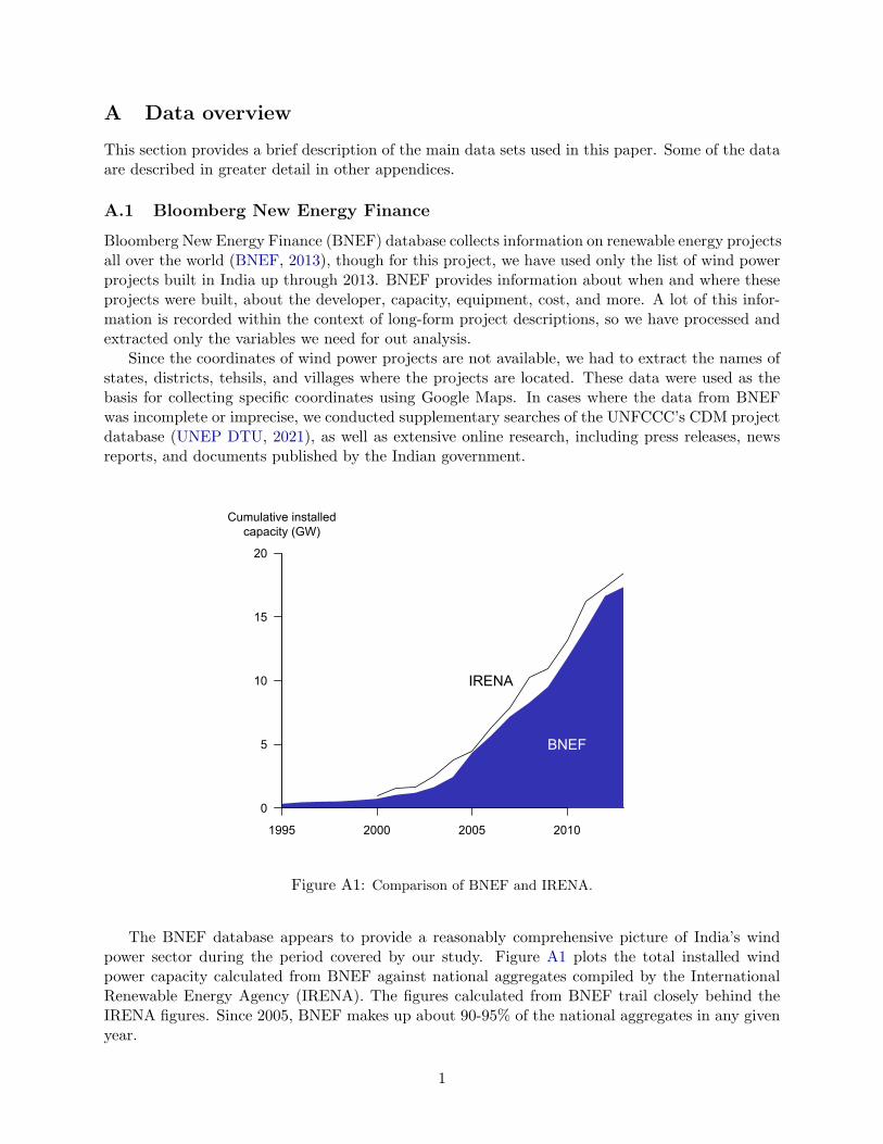
A Data overview

This section provides a brief description of the main data sets used in this paper. Some of the dataare described in greater detail in other appendices.

A.1 Bloomberg New Energy Finance

Bloomberg New Energy Finance (BNEF) database collects information on renewable energy projectsall over the world (BNEF, 2013), though for this project, we have used only the list of wind powerprojects built in India up through 2013. BNEF provides information about when and where theseprojects were built, about the developer, capacity, equipment, cost, and more. A lot of this infor-mation is recorded within the context of long-form project descriptions, so we have processed andextracted only the variables we need for out analysis.

Since the coordinates of wind power projects are not available, we had to extract the names ofstates, districts, tehsils, and villages where the projects are located. These data were used as thebasis for collecting specific coordinates using Google Maps. In cases where the data from BNEFwas incomplete or imprecise, we conducted supplementary searches of the UNFCCC’s CDM projectdatabase (UNEP DTU, 2021), as well as extensive online research, including press releases, newsreports, and documents published by the Indian government.

1995 2000 2005 2010

0

5

10

15

20

Cumulative installedcapacity (GW)

BNEF

IRENA

Figure A1: Comparison of BNEF and IRENA.

The BNEF database appears to provide a reasonably comprehensive picture of India’s windpower sector during the period covered by our study. Figure A1 plots the total installed windpower capacity calculated from BNEF against national aggregates compiled by the InternationalRenewable Energy Agency (IRENA). The figures calculated from BNEF trail closely behind theIRENA figures. Since 2005, BNEF makes up about 90-95% of the national aggregates in any givenyear.

1

A.2 UNFCCC CDM database and UNEP DTU CDM Pipeline

The UN Framework Convention on Climate Change (UNFCCC) provides an online database ofall CDM project applications. The United Nations Environment Program (UNEP), in partnershipwith the Technical University of Denmark (DTU), provides a processed version of this database,called the CDM pipeline (UNEP DTU, 2021), which includes many key details of the proposedprojects, as well as the status of the applications.

We have relied primarily on the UNEP DTU CDM pipeline for this project. To link these datato the BNEF database, we cross-referenced details about the location, timing, and characteristicsof projects. In cases where matches were difficult to identify, we took the extra step of reading theProject Design Documents in the UNFCCC CDM database to see if we could find any additionaldetails that could be cross-referenced. Even after this secondary search, however, we were unableto match up almost 200 Indian’s wind farms in the CDM pipeline. The most likely explanation forthis failure is that the projects were registered under the CDM but never completed. In fact, werewe to assume that all of these projects were completed and add them to the BNEF data (as we doas part of a robustness check), the total installed capacity in some years exceeds the nation-widefigures collected by IRENA.

A.3 2001 Indian Village Census

The 2001 Indian Village Census (Meiyappan et al., 2018) provides a map that divides the countryinto states, districts, tehsils, and villages, and in addition, provides basic information about eachgeographical unit and sub-unit, including population and access to electricity.

We use these data for two purposes. The first is to harmonize administrative units—we usethe census map to assign coordinates to specific villages, districts, and states. This resolves someinconsistencies in the BNEF database (e.g. villages close to borders are sometimes assigned to onestate when mentioned in the context of one project, and then to another state when mentioned againfor another project). This also allows us to be consistent in how we assign electrical substations tostates, for the purposes of calculating connection distances using only in-state substations.

The second way we use the census data is to extract lists of cities with a population in excessof 100,000, and a list of cities with access to power. The coordinates of these cities are used assubstitutes for electrical substations, as part of our sensitivity analyses.

A.4 ERA5-Land

The European Centre for Medium-Range Weather Forecasts provides a range of gridded dataproducts, including ERA5-Land (Munoz Sabater, 2019). It uses the global circulation model H-TESSEL to interpolate meteorological data to provide greater coverage of observationally sparseregions, yielding data that are more uniform in quality and realism than observations alone, andthat is closer to reality than any model could provide on its own. ERA5-Land is discussed in greaterdetail in appendix B, where we describe how we use these data to estimate capacity factors.

B Estimating capacity factors

The kinetic power of the wind, P , that passes through a hoop with an area of A square meters isgiven by the following equation.

P =1

2ρAw3 (5)

2

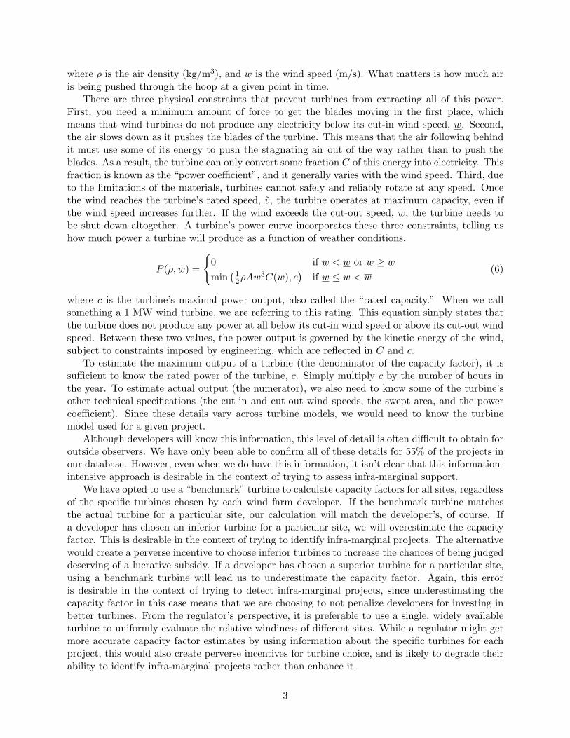
where ρ is the air density (kg/m3), and w is the wind speed (m/s). What matters is how much airis being pushed through the hoop at a given point in time.

There are three physical constraints that prevent turbines from extracting all of this power.First, you need a minimum amount of force to get the blades moving in the first place, whichmeans that wind turbines do not produce any electricity below its cut-in wind speed, w. Second,the air slows down as it pushes the blades of the turbine. This means that the air following behindit must use some of its energy to push the stagnating air out of the way rather than to push theblades. As a result, the turbine can only convert some fraction C of this energy into electricity. Thisfraction is known as the “power coefficient”, and it generally varies with the wind speed. Third, dueto the limitations of the materials, turbines cannot safely and reliably rotate at any speed. Oncethe wind reaches the turbine’s rated speed, v, the turbine operates at maximum capacity, even ifthe wind speed increases further. If the wind exceeds the cut-out speed, w, the turbine needs tobe shut down altogether. A turbine’s power curve incorporates these three constraints, telling ushow much power a turbine will produce as a function of weather conditions.

P (ρ, w) =

{0 if w < w or w ≥ wmin

(12ρAw

3C(w), c)

if w ≤ w < w(6)

where c is the turbine’s maximal power output, also called the “rated capacity.” When we callsomething a 1 MW wind turbine, we are referring to this rating. This equation simply states thatthe turbine does not produce any power at all below its cut-in wind speed or above its cut-out windspeed. Between these two values, the power output is governed by the kinetic energy of the wind,subject to constraints imposed by engineering, which are reflected in C and c.

To estimate the maximum output of a turbine (the denominator of the capacity factor), it issufficient to know the rated power of the turbine, c. Simply multiply c by the number of hours inthe year. To estimate actual output (the numerator), we also need to know some of the turbine’sother technical specifications (the cut-in and cut-out wind speeds, the swept area, and the powercoefficient). Since these details vary across turbine models, we would need to know the turbinemodel used for a given project.

Although developers will know this information, this level of detail is often difficult to obtain foroutside observers. We have only been able to confirm all of these details for 55% of the projects inour database. However, even when we do have this information, it isn’t clear that this information-intensive approach is desirable in the context of trying to assess infra-marginal support.

We have opted to use a “benchmark” turbine to calculate capacity factors for all sites, regardlessof the specific turbines chosen by each wind farm developer. If the benchmark turbine matchesthe actual turbine for a particular site, our calculation will match the developer’s, of course. Ifa developer has chosen an inferior turbine for a particular site, we will overestimate the capacityfactor. This is desirable in the context of trying to identify infra-marginal projects. The alternativewould create a perverse incentive to choose inferior turbines to increase the chances of being judgeddeserving of a lucrative subsidy. If a developer has chosen a superior turbine for a particular site,using a benchmark turbine will lead us to underestimate the capacity factor. Again, this erroris desirable in the context of trying to detect infra-marginal projects, since underestimating thecapacity factor in this case means that we are choosing to not penalize developers for investing inbetter turbines. From the regulator’s perspective, it is preferable to use a single, widely availableturbine to uniformly evaluate the relative windiness of different sites. While a regulator might getmore accurate capacity factor estimates by using information about the specific turbines for eachproject, this would also create perverse incentives for turbine choice, and is likely to degrade theirability to identify infra-marginal projects rather than enhance it.

3

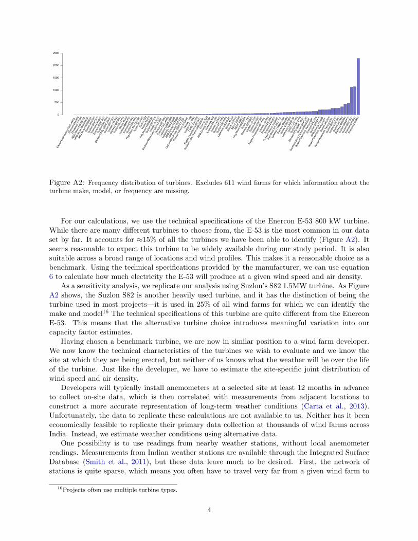
Elec

on E

ngin

eerin

g T6

00-4

8DS

Ener

con

E54/

800

Gho

dawa

t G16

50

NEG

Mico

n NM

48/7

50

NEG

Mico

n NM

72/1

650

NEG

Mico

n NM

950/

54

Suzlo

n S3

0/35

0

Suzlo

n S6

4/15

00

Ener

con

E33/

330

Ener

con

S82/

1500

Suzlo

n S6

6/15

00

Shrir

am E

PCy

SEPC

250

T

Suzlo

n S6

0/10

00

Vest

as V

39-5

00

Gam

esa

G50

/850

Suzlo

n S8

2/21

00Ve

stas

NM

44

Vest

as N

M48

/750

Ener

con

E30/

300

Suzlo

n S8

8/15

00

Neg

Mico

n NM

72/1

650

Suzlo

n E3

3/35

0Su

zlon

S82

Vest

as N

M54

Neg

Mico

n NM

48/7

50

Suzlo

n S5

2/15

00

Vest

as V

27/2

25

Sout

hern

Win

d Fa

rm G

WP4

7-75

0

Vens

ys V

82/1

650

Elec

on T

600-

48DS

Leitw

ind

LW80

/180

0

Leitw

ind

LTW

77-1

500

RRB

Ener

gy V

47-6

00

RRB

Ener

gy V

27-2

25

Glo

bal W

ind

Powe

r GW

P47-

750

Pion

eer W

inco

n P7

50/4

9Ve

stas

V10

0

Vest

as V

70/1

650

CWEL

C30

/250

Rege

n Po

werte

ch V

82/1

500

Sout

hern

Win

d Fa

rm G

WL2

25/4

0En

erco

n E4

8

RRB

Ener

gy V

39-5

00Ke

ners

ys K

82

Ener

con

E30/

230

Vest

as V

47/5

00

Suzlo

n S7

0/12

50

Suzlo

n S8

2/16

50

Lage

rway

LW

250-

27Ve

stas

NM

48

Suzlo

n 95

/210

0NE

PC 2

25/4

0NE

PC 2

50/3

1

Neg

Mico

n NM

950/

54En

erco

n E5

3

Gam

esa

G97

/200

0

Vest

as V

27-2

25

Suzlo

n S9

7/35

0

Vest

as V

66/1

650

Rege

n Po

werte

ch V

87/1

500

Vest

as V

39/5

00

Ener

con

E40/

650

Ener

con

E43/

800

Pion

eer W

inco

n P2

50/2

9

Inox

Win

d W

T 20

00 D

F

Leitw

ind

LTW

80-1

500

Gam

esa

G52

/850

Vest

as V

100/

1800

Lage

rway

LW

250-

30

CWEL

C-3

0/25

0

Suzlo

n S9

7/21

00

Shrir

am E

PC S

EPC

250T

Suzlo

n S6

4/12

50

Sout

hern

Win

d Fa

rms

GW

L225

/40

Rege

n Po

werte

ch V

ensy

s V8

7

Ener

con

E40/

600

Suzlo

n S9

5/21

00

RRB

Ener

gy P

S-60

0

Rege

n Po

werte

ch V

ensy

s V7

7Su

zlon

S52/

600

Rege

n Po

werte

ch V

ensy

s V8

2

Suzlo

n S6

6/12

50

Vest

as V

82/1

650

Suzlo

n S3

3/35

0

Gam

esa

G58

/850

Suzlo

n S8

8/21

00

Suzlo

n S8

2/15

00

Ener

con

E48/

800

Ener

con

E53/

800

0

500

1000

1500

2000

2500

Figure A2: Frequency distribution of turbines. Excludes 611 wind farms for which information about theturbine make, model, or frequency are missing.

For our calculations, we use the technical specifications of the Enercon E-53 800 kW turbine.While there are many different turbines to choose from, the E-53 is the most common in our dataset by far. It accounts for ≈15% of all the turbines we have been able to identify (Figure A2). Itseems reasonable to expect this turbine to be widely available during our study period. It is alsosuitable across a broad range of locations and wind profiles. This makes it a reasonable choice as abenchmark. Using the technical specifications provided by the manufacturer, we can use equation6 to calculate how much electricity the E-53 will produce at a given wind speed and air density.

As a sensitivity analysis, we replicate our analysis using Suzlon’s S82 1.5MW turbine. As FigureA2 shows, the Suzlon S82 is another heavily used turbine, and it has the distinction of being theturbine used in most projects—it is used in 25% of all wind farms for which we can identify themake and model16 The technical specifications of this turbine are quite different from the EnerconE-53. This means that the alternative turbine choice introduces meaningful variation into ourcapacity factor estimates.

Having chosen a benchmark turbine, we are now in similar position to a wind farm developer.We now know the technical characteristics of the turbines we wish to evaluate and we know thesite at which they are being erected, but neither of us knows what the weather will be over the lifeof the turbine. Just like the developer, we have to estimate the site-specific joint distribution ofwind speed and air density.

Developers will typically install anemometers at a selected site at least 12 months in advanceto collect on-site data, which is then correlated with measurements from adjacent locations toconstruct a more accurate representation of long-term weather conditions (Carta et al., 2013).Unfortunately, the data to replicate these calculations are not available to us. Neither has it beeneconomically feasible to replicate their primary data collection at thousands of wind farms acrossIndia. Instead, we estimate weather conditions using alternative data.

One possibility is to use readings from nearby weather stations, without local anemometerreadings. Measurements from Indian weather stations are available through the Integrated SurfaceDatabase (Smith et al., 2011), but these data leave much to be desired. First, the network ofstations is quite sparse, which means you often have to travel very far from a given wind farm to

16Projects often use multiple turbine types.

4

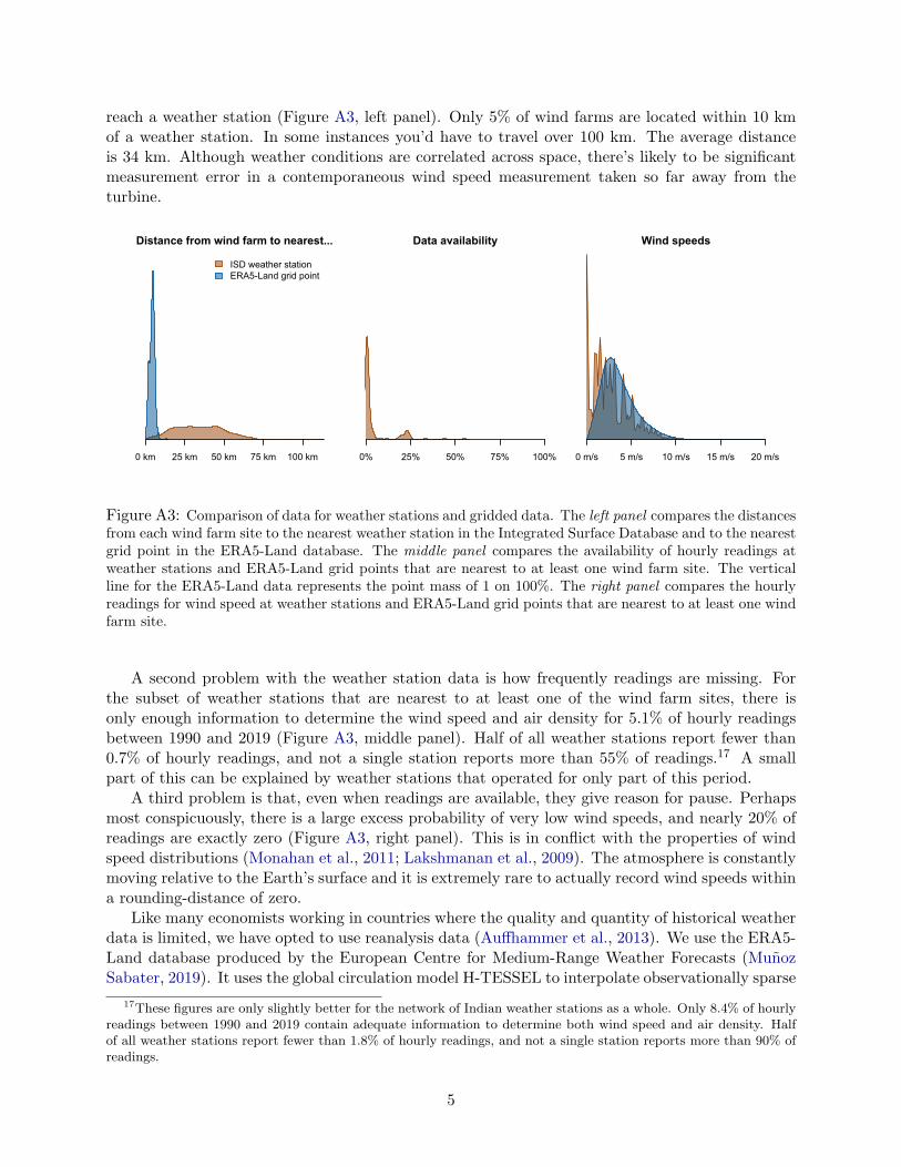
reach a weather station (Figure A3, left panel). Only 5% of wind farms are located within 10 kmof a weather station. In some instances you’d have to travel over 100 km. The average distanceis 34 km. Although weather conditions are correlated across space, there’s likely to be significantmeasurement error in a contemporaneous wind speed measurement taken so far away from theturbine.

Distance from wind farm to nearest...

0 km 25 km 50 km 75 km 100 km

ISD weather stationERA5-Land grid point

Data availability

0% 25% 50% 75% 100%

Wind speeds

0 m/s 5 m/s 10 m/s 15 m/s 20 m/s

Figure A3: Comparison of data for weather stations and gridded data. The left panel compares the distancesfrom each wind farm site to the nearest weather station in the Integrated Surface Database and to the nearestgrid point in the ERA5-Land database. The middle panel compares the availability of hourly readings atweather stations and ERA5-Land grid points that are nearest to at least one wind farm site. The verticalline for the ERA5-Land data represents the point mass of 1 on 100%. The right panel compares the hourlyreadings for wind speed at weather stations and ERA5-Land grid points that are nearest to at least one windfarm site.

A second problem with the weather station data is how frequently readings are missing. Forthe subset of weather stations that are nearest to at least one of the wind farm sites, there isonly enough information to determine the wind speed and air density for 5.1% of hourly readingsbetween 1990 and 2019 (Figure A3, middle panel). Half of all weather stations report fewer than0.7% of hourly readings, and not a single station reports more than 55% of readings.17 A smallpart of this can be explained by weather stations that operated for only part of this period.

A third problem is that, even when readings are available, they give reason for pause. Perhapsmost conspicuously, there is a large excess probability of very low wind speeds, and nearly 20% ofreadings are exactly zero (Figure A3, right panel). This is in conflict with the properties of windspeed distributions (Monahan et al., 2011; Lakshmanan et al., 2009). The atmosphere is constantlymoving relative to the Earth’s surface and it is extremely rare to actually record wind speeds withina rounding-distance of zero.

Like many economists working in countries where the quality and quantity of historical weatherdata is limited, we have opted to use reanalysis data (Auffhammer et al., 2013). We use the ERA5-Land database produced by the European Centre for Medium-Range Weather Forecasts (MunozSabater, 2019). It uses the global circulation model H-TESSEL to interpolate observationally sparse

17These figures are only slightly better for the network of Indian weather stations as a whole. Only 8.4% of hourlyreadings between 1990 and 2019 contain adequate information to determine both wind speed and air density. Halfof all weather stations report fewer than 1.8% of hourly readings, and not a single station reports more than 90% ofreadings.

5

regions, yielding data that are more uniform in quality and realism than observations alone, andthat is closer to reality than any model could provide on its own.

ERA5-Land includes a complete set of hourly observations going back to 1981, at a spatialresolution of roughly 9 km over land. At this spatial resolution, the average distance from one ofthe wind farm sites in our data set to the nearest ERA5-Land grid point is 4.3 km (Figure A3, leftpanel). A small fraction of wind farms are sited along irregular coastlines, which limits the numberof available grid points over land. Although we would generally expect a grid point no farther thanroughly 6 km from any wind farm site, a few cases do exceed the Pythagorean limit. The farthestone is 13.4 km away from a wind farm site.

Reassuringly, weather conditions are so highly correlated at this spatial scale that it would makelittle difference whether we calculated capacity factors using the time-series from the nearest gridpoint or from the next nearest grid point in ERA5-Land (Spearman correlation = 0.996). Thisreanalysis data set appears to provide the best available estimates of weather conditions in thevicinity of the Indian wind farms we are studying.

From the ERA5-Land database we use the u and v components of wind to calculate wind speeds,and the mean temperature, dew point temperature, and surface pressure to calculate air densities(following Picard et al., 2008). Using our chosen turbine specification, we then obtain the poweroutput from equation 6 and compare the cumulative output at each site to the maximal output.

Auffhammer et al. (2013) warn that the precise timing of deviations of weather variables fromtheir means is somewhat idiosyncratic across alternative gridded data products. We do not relyon timing to calculate capacity factors. We use the full-time series at each location to estimate alocation-specific distribution of wind speed and air density. That distribution is our best guess forwhat a wind farm developer would have estimated at any point during this period.

Finally,while turbines like the E-53 have a hub height of at least 50 meters, ERA5-Land inter-polates wind at a height of 10 meters and the other variables at 2 meters, the heights at whichmost measurement instruments are placed. Since wind speeds increase monotonically with height,capacity factors also increase with height, which means that we will slightly underestimate the truecapacity factors. In particular, the so-called “wind profile power law” states that, under neutralstability conditions, the ratio of wind speeds at heights k and l is related to the ratio of k and l

by the following equation, vkvl

=(kl

) 17 . From this relationship we can deduce that the wind speed

at 50 meters height is roughly 1.26 times faster than at 10 meters. Air density, by contrast, fallsmonotonically as you ascend, though the change is very small when close to the surface. Since airdensity enters linearly rather than cubically in the power function, the rising wind speed dominates.

This means that, were a wind farm developer to use the same data and methods as we haveto forecast capacity factors, they would have to multiply the estimate by some height-adjustmentfactor to get a more accurate forecast. Our analysis relies only on the ordering of capacity factorsacross sites, which would not be affected by a monotonic transformation. As such, this extraadjustment provides no additional value.

C Estimating connection distances

Connection distances are estimated by computing the smallest length of cable that would be neededto connect wind farm sites to electrical substations. The geographical coordinates of electricalsubstations were collected, and generously provided, by Fiona Burlig. The coordinates of theturbines were found using a combination of information found in the Bloomberg’s New EnergyFinance database, the UNFCCC’s CDM project database, as well as extensive online research,including press releases, news reports, and documents published by the Indian government. We

6

recorded the coordinates of the village in which the turbines are located, rather than pinpointingindividual turbines. This was partly out of practical necessity, but also means that our findingscannot be driven by arbitrarily small differences in location. Any variation in location that wemight have been able to generate at the sub-village level would likely have contained more noisethan signal.

We calculate the connection distance using a modified minimum spanning tree (MST) algorithm.A standard MST algorithm considers only one type of node, and will search for a set of edges thatconnects all of the nodes together, yet whose combined length is as small as possible. This approachwould yield strange results, however, for multi-site wind farms, sometimes with sites spread acrosslarge distances. In these situations, developers may not wish to connect all sites to each other, butinstead exercise the option of connecting different clusters of sites to different electrical substations.To avoid inflating the connection distances for wind farms spread across multiple sites, we neededto modify the standard algorithm.

The modified MST algorithm has three steps.

1. Connect the entire network of electrical substations to each other (by any method) and recordthe total edge length.

2. Append the wind farm sites for each project as unconnected nodes in the network, and thenuse a standard MST algorithm to add the set of edges of shortest length that creates a graphwithout any unconnected nodes. Record the total edge length of the augmented graph.

3. Subtract the total edge length in step 1 from the total edge length in step 2 to retrieve theminimum length of cable needed for every wind farm site to be connected, either directly orindirectly, to at least one electrical substation.

As part of our robustness checks, we further modify this algorithm to permit only connectionsto electrical substations located in the same state as the wind farm site. This is accomplished byrunning the above algorithm separately for the electrical substations and wind farm sites locatedin each state, and then summing the results across states. In other robustness checks, we use theabove algorithm as stated, with the only difference that we swap out the electrical substations forpower stations or cities.

7