DO RURAL BANKS MATTER? EVIDENCE FROM THE INDIAN SOCIAL BANKING EXPERIMENT

Robin Burgess

London School of Economics and Political Science

and

Rohini Pande Yale University

Contents: 1. Introduction 2. Data and Program Description 3. Identification Strategy 4. Effects on Rural Development 5. Discussion References Data Appendix Tables 1 – 11 Figures 1 - 9

The Suntory Centre Suntory and Toyota International Centres for Economics and Related Disciplines London School of Economics and Political Science Discussion Paper Houghton Street No. DEDPS/40 London WC2A 2AE August 2003 Tel.: 020-7955 6674 We thank Esther Duflo for very helpful and detailed comments. We have benefited from comments and suggestions from Josh Angrist, Abhijit Banerjee, Tim Besley, Richard Blundell, Bronwen Burgess, Anne Case, Ken Chay, Dom Leggett, Jonathan Murdoch, Atif Mian, Andrew Newman, Debraj Ray, Mark Rosenzweig, Ken Sokoloff, Duncan Thomas, Robert Townsend, and seminar participants at the Bureau for Research in Economic Analysis of Development (BREAD) 2002 Meeting, Caltech, Cornell, Harvard, IMF, LSE, Michigan, MIT, NYU, Princeton, Southampton, Stanford, Stockholm, UBC, UCLA, UCSD, World Bank and Yale. Juan de Laiglesia, Mattia Romani, Gaurav Shah, Heideeflower Stoller and Grace Wong provided exceptional research assistance.

Abstract

Lack of access to finance is often cited as a key reason why poor people remain poor. This paper uses data on the Indian rural branch expansion program to provide empirial evidence on this issue. Between 1977 and 1990, the Indian Central Bank mandated that a commercial bank can open a branch in a location with one or more bank branches only if it opens four in locations with no bank branches. We show that between 1977 and 1990 this rule caused banks to open relatively more rural branches in Indian states with lower initial financial development. The reverse is true outside this period. We exploit this fact to identify the impact of opening a rural bank on poverty and output. Our estimates suggest that the Indian rural branch expansion program significantly lowered rural poverty, and increased non-agricultural output. Keywords: Finance and development; rural banking; bank licensing; credit constraints; structural change; diversification; redistribution; poverty, growth. JEL Nos.: E5, G2, H1, H4, I3, N2, O0, O1, O2, O4. © The authors. All rights reserved. Short sections of text, not to exceed two paragraphs, may be quoted without explicit permission provided that full credit, including notice, is given to the source.

Contact address: Dr Robin Burgess, STICERD, London School of Economics and Political Science, Houghton Street, London WC2A 2AE, UK. Email: r.burgess@lse.ac.uk

1 Introduction

A key objective in development economics is to work out ways to lift people out ofpoverty. Access to finance has been seen as a critical factor in enabling people totransform their production and employment activities and to exit poverty (Banerjeeand Newman 1993; Aghion and Bolton 1997; Banerjee, 2001). Countries with betterdeveloped financial systems, it is argued, should be better able to exploit growth op-portunities (Schumpeter, 1934; Gerschenkron 1962; Greenwood and Jovanovic, 1990;Bencivenga and Smith, 1991). Financial development may also enhance financialstability with positive implications for economic performance (Bernanke and Gertler,1990). While these arguments have often provided the theoretical justification forwidespread government intervention in the banking sector, evidence on the successof such interventions in reducing poverty remains limited.1 In this paper we use dataon the Indian rural bank branch expansion program — the largest ever attempted ina developing country — to provide such evidence.

The Indian branch expansion program was representative of a whole host of state-led rural finance programs that spread across the developing world in the post-colonialperiod. This trend was not restricted to low income countries — in the United States,for example, the Community Reinvestment Act of 1977 requires a bank to meet thecredit needs of its entire community, including low income neighborhoods (Zinman2002). In most cases such financial interventions went hand in hand with governmentoversight of the banking sector, often aided by government ownership of banks.2

However, it is now widely believed that state control of the banking sector impliedthat political, not economic, considerations determined the flow of credit across sec-tors and individuals. Political imperatives also implied that widespread loan defaulton the part of borrowers was permitted, and made the banking sector more suscepti-ble to elite capture (La Porta, Lopez-De-Silanes and Shleifer, 2003; Sapienza, 2003).Some go as far as to claim that elite capture, combined with the imposition of interestrate ceilings in the formal sector, led to financial dualism wherein formal subsidizedfunds are concentrated in the hands of the powerful few and terms in the informalmarkets (on which the poor depend) worsened (see Adams et al 1984; Bravermanand Guasch 1986; Hoff and Stiglitz, 1998). In sum, it is believed that formal sub-sidized credit was ineffective in reaching the poor, and may even have underminedrural development and increased rural poverty.

However, the evidence in support of such claims remains thin. By virtue of theirvintage social banking episodes, though numerous and large in scale, have largelyescaped serious evaluation. And this is despite the fact that, even today, state provi-sion remains the dominant source for formal finance in the rural areas of developing

1Cross country data shows that banking expansion and economic growth are positively correlated(King and Levine, 1993; Levine and Zervos, 1998; Rajan and Zingales, 1998). However, the fact thatcountries (or regions) with greater growth potential attract more banks renders a causal interpretationproblematic. In addition, the absence of comparable cross-country poverty data across time makesworking out the distributional impact of banking expansion problematic.

2La Porta, Lopez-De-Silanes and Shleifer (2002) report that, in the average country, 42 percentof the equity of the ten largest banks remained government owned in 1995.

countries (Besley 1995). This paper seeks to address this lacuna in the literature.India is an appropriate place for such an evaluation, both because of the size andscope of the social banking experiment and also because it is home to close to a thirdof the world’s poor, the bulk of whom are located in rural areas (Deaton and Dreze,2002).

Between bank nationalization in 1969 and the onset of financial liberalization in1990 bank branches were opened in over 30,000 rural locations which had no priorpresence of commercial banks (henceforth, unbanked locations).3 Alongside, theshare of bank credit and savings which was accounted for by rural branches rose from1.5 and 3 percent respectively to 15 percent each. The branch expansion programwas an integral part of India’s social banking experiment which sought to improve theaccess of the rural poor to cheap formal credit. The preamble to the Bank CompanyAcquisition Act of 1969 — the piece of legislation which empowered the state tonationalize commercial banks — makes the intentions of the Indian government plain.

“The Banking system touches the lives of millions and has to be inspiredby a larger social purpose and has to subserve national priorities and ob-jectives such as rapid growth of agriculture, small industries and exports,raising of employment levels, encouragement of new entrepreneurs anddevelopment of backward areas. For this purpose it is necessary for thegovernment to take direct responsibility for the extension and diversifica-tion of banking services and for the working of a substantial part of thebanking system”.

Key to the rural branch expansion endeavor was the imposition of the 1:4 licenserule in 1977. This rule stated that a bank could open a branch in a location withone or more branches (now on, a banked location) only if it opened four in unbankedlocations. This rule was abandoned in 1990. States with lower initial financial de-velopment (as measured by the number of bank branches per capita in 1961) had ahigher incidence of unbanked locations. We use a panel data-set for the sixteen ma-jor Indian states (1961-2000), and show that, between 1977 and 1990, the 1:4 licenserule caused financially less developed states to attract more rural branches than theirmore financially developed counterparts. The reverse was true outside this period.

We show that an identical temporal and geographic pattern exists for rural poverty— rural poverty reductions were more rapid in states with lower financial developmentbetween 1977 and 1990. The opposite was true outside this period. In contrast, po-litical and policy variables which may have reduced poverty in India over this perioddid not show trend breaks in their relationship with initial financial development in1977 or 1990. This allows us to use the trend breaks in 1977 and 1990 in the rela-tionship between a state’s initial financial development and rural branch expansionas instruments for the number of rural locations banked in a state. Our instrumentalvariable estimates suggest that a one percent increase in the number of rural bankedlocations reduced rural poverty by 0.36 percent and increased total output by 0.55

3Locations here refer to villages, towns and cities as defined by the Indian census.

2

percent. The output effects are solely accounted for by increases in non-primary sec-tor output — a finding which suggests that increased financial intermediation in ruralIndia aided output and employment diversification out of agriculture.

The rapid increase in the Indian rural branch network and rural credit and sav-ings share after bank nationalization in 1969, and the subsequent slowdown post1990, has been widely documented (Nair 2000). However, evidence on the impact ofthe social banking program on poverty remains limited. Our findings on output lineup with Binswanger, Khandker and Rozensweig (1993) and Binswanger and Khand-ker (1995). These papers use Indian district-level data, and find that rural branchexpansion increased non-agricultural but not agricultural growth.4 Our results arealso consistent with the simulations by Townsend and Ueda (2001) based on Thaidata which show that increased participation in the formal financial sector enhancesgrowth. By exploiting the policy induced reversal in the relationship between ini-tial branch placement we are able to control for endogenous bank branch placementand to identify the impact of rural branch expansion on poverty. Our identificationstrategy is related to a number of recent program evaluation studies which exploitpolicy-induced trend breaks in the variables of interest for identification purposes —important related examples include Duflo (2001) and Almond, Chay and Greenstone(2002).

The paper is organized as follows. Section 2 describes the data we use, and theprogram we study. Section 3 contains our identification strategy, and Section 4 theempirical analysis. Section 5 discusses the policy implications of our findings.

2 Data and Program Description

2.1 Data

We use a panel data-set for the sixteen major Indian states over the period 1961-2000.We start in 1961 as it is the year of the census which preceded bank nationalization.Also, our poverty and output series begin around this year. Table 1 gives the meansand standard deviations for our main variables and the Data Appendix informationon variable definitions and data sources.5

We use a branch level data-set which records, for every bank branch opened since1805, the date it was opened, whether it was situated in a rural location and thenumber of branches already existing in that location to construct three measures offinancial development (Reserve Bank of India, 2000).6 The number of bank branchesper 100,000 persons in a state in 1961 is our measure of initial financial development.

4Eastwood and Kohli (1999) use firm level data and find that the branch expansion program anddirected lending program enhanced small scale industrial activity in India. Our findings are also inline with Dehejia and Lleras-Muney (2002) who find that financial development was associated withmanufacturing growth in US states between 1900 and 1940.

5The sixteen states in our sample cover over 95% of the Indian population. For some variablesthe data span fewer years; details are in the Data Appendix.

6We always use the census definition of a rural location — that is, a location with a population ofless than 10,000 persons. This is the same definition used to distinguish rural from urban poverty.

3

If a branch is the first to be opened in a rural location we classify it as havingopened in a rural unbanked location. In our sample states between 1961 and 2000 thenumber of rural locations so banked increased from 116 to 30,428. The total numberof branches opened in rural unbanked locations per 100,000 persons is our ‘socialbanking’ measure. A branch opening in a census location with at least one bank isclassified as opening in a banked location. Our third measure of financial developmentis the number of branches opened in already banked locations per 100,000 persons.Figure 1 charts the evolution of (cumulative) branch openings in banked, unbankedand rural unbanked locations.

Every bank branch in our sample is a distinct physical entity which undertakesboth deposit-taking and lending activities.7 Deposit taking is relatively straightfor-ward, with the interest rate and other terms and conditions laid down by the Indiancentral bank. In the area of lending, bank branch officials enjoy discretion in choosingborrowers, subject to satisfying directed lending targets for the so-called ‘priority’ sec-tors of agriculture, entrepreneurs and small scale industry. The Indian central bankmandates that every bank branch satisfy a credit-deposit ratio of 60 percent withinits geographical area of operation — this is to ensure that lending activities are notconcentrated in urban locales.

In 2000, the Indian rural banking sector accounted for the rupee equivalent of26,768 million dollars as deposits and 10,834 million dollars as loans outstanding.In terms of population reached, the rural sector accounted for 125 million savingsaccounts and 25 million borrowing accounts.8 Figure 2 shows the dramatic expansionin rural savings and credit over our sample period; the figure plots the state-wiseshares of total bank credit and savings accounted for by rural banks. Finally, interms of lending portfolio the average rural bank lent 38.6 percent to agriculture, 27.5percent to industry, 13.9 percent to trade and 9 percent as personal loans (ReserveBank of India, 2000).

In Table 2, we use Indian household survey data to decompose rural householddebt by source for ten year intervals between 1951 and 1991. In 1951, four years afterindependence, the informal credit sector accounted for the bulk of rural lending, withmoneylenders contributing close to 70 percent of the total. In contrast, less thanone percent of rural household debt came from commercial banks. These banks wereconfined to urban areas and geared towards the financing of trade and commerceactivities (Reserve Bank of India, 1954).9 By 1971 lending by commercial bankscontributed only 3 percent to rural household debt. However, by 1991 this figure

7The average bank branch is staffed by one officer, two clerks, one of whom also acts as thecashier, and one security guard.

8If we assume every savings account is held by a different person and the rural population consistedof 700 million persons in 2000, then roughly one in every five or six rural persons had a savings accountby 2000.

9These findings were published the 1951 All-India Credit Survey Report (Reserve Bank of India,1954). It concluded that financial backwardness was a root cause of rural poverty, and that commer-cial banks needed to be harnessed to enhance formal credit in rural areas — both to enable poor, ruralhouseholds to adopt new technologies and production processes, and to displace ‘evil’ moneylenderswho exploited their monopoly power to charge high rates of interest. These conclusions guided Indianrural banking policy for the next four decades.

4

had risen ten fold to 29 percent. Over the same time period the moneylender shareof rural household debt more than halved from 35 to 15.7 percent. Thus over thisperiod, arguably due to the large scale expansion of commercial banks into ruralIndia, commercial banks transited from being the smallest to the largest lender inrural areas. Our focus is on identifying the economic implications of this change inrural India.

India is unique amongst developing countries in having carried out household ex-penditure surveys on a regular basis since the 1950s. This allows us to construct aconsistent and comparable series of rural and urban poverty measures across our pe-riod.10 We use the head count ratio which measures the proportion of the populationbelow the Indian poverty line. Poverty incidence in India is high — over the 1961-2000period 48 percent of the rural and 40 percent of the urban population are classifiedas poor. Figure 3 shows the evolution of poverty across Indian states between 1961and 1990. Up to the early 1970s there are sharp year-to-year fluctuations followed bya downward trend in both the rural and urban series between 1973 and 1990. Imme-diately after 1990, as India entered a period of economic liberalization, the patternbecomes less clear with considerable debate over the net direction (Deaton 2001). Themost recent figures suggests that the post 1990 trend is overall downward. What iseven more striking, however, are the differences in poverty trajectories across states.A key objective of this paper is to examine whether the pattern of branch expansioninto rural unbanked areas altered these rural poverty trajectories. Over this periodreal male agricultural wages, an important inverse correlate of rural poverty, doubled.Given the controversy surrounding the more recent poverty figures using agriculturalwages as an alternative dependent variable provides a useful robustness check.

Separate output estimates for the rural and urban sectors of an Indian state areunavailable. For this reason, we focus on the sector-wise evolution of state out-put. The primary sector which includes agriculture, forestry, fisheries and mining ismainly rural. The secondary sector consists of construction, registered and unregis-tered manufacturing, and electricity, water and gas output. Of these, constructionand registered manufacturing are mainly located in the urban sector, while unregis-tered manufacturing (which consists of small businesses which employ less than tenpersons with power, or twenty without) and electricity, water and gas output havea substantial rural presence. The tertiary sector consists of various service sectorssuch as trade and transportation which occur in both rural and urban areas. In1961 the primary sector contributed the most to total state output; however, sincethe mid 1970s the growth rates in the non-primary sector exceeded those in theprimary sector (see Figure 4). We examine the links, if any, between rural branchexpansion and sector-wise increases in economic activity. Evidence both from theeconomic history and economic development literatures suggests the process of struc-tural change, where the secondary and tertiary sectors become the main contributorsto total output, is typically associated with poverty reduction (see Chenery, Robinson

10We are grateful to Gaurav Datt and Martin Ravallion for providing us these state-level povertyfigures (see Ozler, Datt and Ravallion (1996)). Gaurav Datt was kind enough to provide us withcomparable updates which allowed us to extend the series from 1994-2000.

5

and Syrquin, 1986; Dehejia and Lleras-Muney, 2002; Burgess and Venables, 2003).We also examine whether the fraction of non-agricultural laborers in the rural laborforce is affected.

2.2 The Program

In 1969 the fourteen largest Indian commercial banks were nationalized, at whichpoint they came under the direct control of the Indian central bank and were formallyincorporated into the planning architecture of the country (Balachandran, 1998).Bank nationalization was intended to allow the state to target financial backwardnessas a means of promoting social objectives. A central aim was to reduce and equalizethe average population per bank branch across Indian states.

To achieve this the Indian central bank adopted an area approach whereby un-banked locations — census locations with no prior presence of commercial banks —were targeted (Desai 1987). At any point in time, the central bank sought to fillunbanked locations with populations exceeding a specific number. Unbanked loca-tions in states whose population per bank branch exceeded the national average hadpriority. Over time, as unbanked locations were filled, the population target waslowered. The priority status assigned to financially less developed states, combinedwith a common definition for unbanked locations across Indian states, meant thatmore unbanked locations were targeted in financially backward states.

In every Indian district a commercial bank was designated as the Lead Bank andmade responsible for identifying unbanked locations (based on the criteria set by thecentral bank). Every three years new (district-wise) lists of unbanked locations weredrawn up by the central bank (in consultation with Lead Banks and state developmentauthorities) and made available to commercial banks working in a district. The LeadBank was responsible for coordinating branch expansion into these locations withother commercial banks working in the district.11

The Indian central bank, however, still needed to coerce commercial banks toexpand into unbanked, rural locations. In particular, in states where unbanked loca-tions were remote and/or unprofitable. Under the Banking Regulation Act of 1949commercial banks have to obtain a license from the central bank in order to open anew branch. On January 1, 1977 the Indian central bank announced that to qualifyto open a branch in an already banked location a commercial bank must open fourin unbanked locations.12 In 1990 the licensing procedure was frozen, and in 1991formally repealed. At this point it was deemed that future branch expansion shoulddepend on “need, business potential and financial viability of location” (Governmentof India, 1991).

Branch level data shows that the 1:4 rule was binding — the annual ratio of bankbranches opened in unbanked locations to total branches opened stands at, or around,

11The district is the administrative unit below a state. An alternative would be undertake theanalysis at the district level. However, annual poverty and output estimates are only available atthe state level.12Up to this point banks had enjoyed some latitude as regards branch placement as the central

bank emphasized the banking of towns and the need to satisfy pent up urban demand.

6

0.8 for every year between 1977 and 1990, and falls to zero thereafter. This effectis also visible in Figure 1 which shows that from about 1975 onwards, increases inthe number of locations banked are due to increases in the number of rural locationsbanked. Between 1977 and 1990 branch expansion into rural unbanked locationsaccelerated while that of already banked locations fell. After 1990 branch expansion inunbanked locations came to a halt, while that in already banked locations increased.To date, a bank cannot close a rural branch if it is the only branch servicing thelocation. The 1990 rural branch network is therefore, in effect, frozen.13

The typical commercial bank in India operates in districts in both financiallydeveloped and backward states (either as a Lead Bank or collaborator). The cen-tral bank prioritized branch expansion in financially backward states, and this wasreflected in the unbanked location lists. Therefore, compliance with the 1:4 rule im-plied that banks opened more branches in unbanked locations in financially backwardstates. Figure 5 shows the equalization and reduction in population per bank branchacross Indian states over this period. Between 1961 and 2000 the average populationper bank branch fell tenfold from 139,790 to 14,681. There is some, albeit limited,evidence of convergence in population per bank branch across Indian states priorto nationalization. Convergence, however, is much stronger between 1970 and 1990,with the post-1976 convergence driven by differential rates of rural branch expansionacross Indian states. By 1990, all states were at or below the national target of 17,000persons per bank branch. Interestingly, after the removal of placement restrictionsin 1990 and an increase in branch building in already banked locations there is someevidence that population per bank branch began to increase and diverge across In-dian states with more backward states seeing larger increases (see inset panel, Figure5).

This period also saw the central bank affect the credit policies of commercialbanks. Since 1968, the central bank has mandated that a certain fraction of everybank’s lending had to be to individuals or firms who are in the ‘priority’ sector. Thissector includes agriculture, entrepreneurs and small scale industries.14 These loanswere intended to encourage new productive activities, and were also disbursed viarural bank branches. However, unlike rural branch expansion, the incidence of thesecredit policies does not vary with a state’s initial financial development.

3 Identification Strategy

In this section we demonstrate that the bulk of rural branch expansion in India waspolicy-driven and significantly increased the flows of bank credit and savings to ruralareas. The first fact allows for a credible evaluation of the branch expansion program,and the second implies we can interpret our results as informative of the economic

13Additional credit needs of the rural population post 1990 are supposed to be met through othermeans, principally microfinance (Ramachandran and Swaminathan, 2001).14These targets were ratcheted up over time — they started at 33 percent of total bank lending and

have stood at 40 percent since 1985.

7

impact of state-led financial intermediation.15

The 1:4 license rule sought to coerce commercial banks to open more branchesin rural unbanked locations in less financially developed states. The underlying as-sumption was that financially developed states offered more profitable locations forbanks and therefore, in the absence of such a rule, would attract more branches. Thissuggests that if the rule had any bite its imposition in 1977 and subsequent removalin 1990 should have altered the relationship between initial financial development ofa state and subsequent rural branch expansion. To examine this possibility we run afixed effects regression of the form:

BRit = αi + βt +2000Xt=1961

(Bi61 ×Dk)γk +2000Xt=1961

(Xi61 ×Dk)δk + ²it (1)

αi and βt are state and year effects respectively. BRit , the number of branches opened

in rural unbanked locations per capita, is our social banking measure and Bi61, thenumber of bank branches per capita in state i in 1961, our measure of initial financialdevelopment.16 Dk is a dummy which equals one where k = t. The coefficientset γk captures the year-wise effect of initial financial development on rural branchexpansion. As other initial conditions in a state may also have a time-varying effecton branch expansion we include a vector of control variables (Xi61) as additionalcovariates. This vector includes log real state income per capita, population densityand the number of rural locations per capita, all measured in 1961. These controlsalso enter the regression interacted with year dummies.

Figure 6 graphs the γk coefficients for two specifications. The dots on the solidline are the coefficients from a specification without the Xi61 controls, and the dotson the broken line are from a specification with the Xi61 controls. In both cases 1961is the control year, and the 1961 dummy is omitted.17 γk summarizes the effect ofbetween-state variation in initial financial development on the cumulative number ofbranches opened in rural unbanked locations as of year t. As our dependent variableis a cumulative variable, a comparison of the coefficients for any two adjacent years(γk and γk+1) is informative of the relationship between initial financial developmentand the growth in rural branch openings.

Over this period the number of rural banked locations trend upwards in everystate. However, two clear reversals in the relationship between a state’s initial fi-nancial development and the number of rural banked locations stand out in Figure6 — one in 1977 and one in 1990. Between 1961 and 1977 the γk coefficients increasewith time — that is, financially more developed states witness higher growth of ruralbanked locations. As banks enjoyed considerable leeway regarding where to locate

15Our focus on the economic impact of bank branches sidesteps many of the endogeneity problemsassociated with a direct study of the impact of credit flows. In a similar vein Jayarathne and Strahan(1996) use information on when a U.S. state relaxed branching restrictions to examine how financialmarkets affect economic growth16Both variables are normalized by 1961 population. The results are also robust to, instead,

normalizing the banking variables by land area (as in Binswanger, Khandker and Rosenzwieg 1993).17We chose 1961 as it is the census year preceding bank nationalization. Our results are robust to

choosing any alternative year as the control year.

8

this suggests that financially more developed states offered banks greater profit op-portunities. This relationship is reversed in 1977 precisely when the 1:4 license rulewas imposed. Moreover, the reversal is not temporary. Between 1977 and 1990 theγk coefficients decrease with time — that is, financially less developed states witnessedhigher growth of rural banked locations. After 1990 rural branch expansion into ruralunbanked locations ended, and is reflected in the lack of over time variation in thesize of the γk coefficients. Overall, the precise correspondence in the timing of thesetrend reversals and license regime shifts provides strong prima facie evidence thatthe pattern of rural branch expansion across Indian states was policy driven.

We include the vector of economic controls, Xi61, as additional controls to checkthat convergence in economic activity (as proxied for by income, population density ornumber of rural locations) across Indian states is not driving the observed relationshipbetween rural branch expansion and initial financial development. The broken linegraph in Figure 6 shows that this is not the case. If we graph out the δk coefficients forthe interaction between initial state income and year dummies we find the relationshipbetween initial state income and rural branch expansion is throughout positive (i.e.the graph is upward sloping). That is, controlling for initial financial development,banks open more branches in states with higher initial state income.18

Further evidence that economic convergence does not underlie the trend reversalsin Figure 6 comes from data on branch openings in already banked locations. The 1:4license rule linked branch expansion in already banked locations to that in unbankedlocations. Banks, however, were free to decide branch placement in already bankedlocations. If the relationship between initial financial development and bank prof-itability remained unchanged during this period, then the imposition and subsequentremoval of the 1:4 license rule should have affected the rate of branch expansion inalready banked locations but not its distribution across states. To check this werun regression (1) where the outcome variable is the cumulative number of branchesopened in banked locations per capita. Figure 7 graphs out the γk coefficients on theinteraction between initial financial development of a state (Bi61) and year dummies(Dk). This relationship, though affected by license regime shifts in 1977 and 1990,is positive throughout. This mirrors what was happening with branch openings inrural unbanked locations pre-1977 but is in strict contrast to what was happeningbetween 1977 and 1990.

In Figure 8 we examine the relationship between rural bank credit and initial fi-nancial development. That is, we report the γk coefficients from regression (1) wherethe dependent variable is the share of bank credit disbursed by rural branches.19 Weobserve a pattern that mirrors that for rural unbanked locations (Figure 6). Disburse-ments via rural banks are higher in more financially developed states until around1975 when there is a trend reversal. Between 1976 and 1989 we see more backwardstates experiencing a greater share of credit being disbursed via rural banks. After1989 the relationship between rural credit share and initial financial development

18For obvious reasons, this relationship is much more muted between 1977 and 1990 if we excludethe interaction between initial financial development and year dummies from this regression.19Data on credit and savings flows from rural banks is only available from 1969.

9

reverts to being broadly positive. A similar pattern exists for the rural savings share.The most likely explanation for the negative relationship between credit and savingflows and initial financial development between mid 1970s and 1990 is the highergrowth of rural branches in financially backward states. These findings put us onstronger grounds in interpreting the economic effects of rural banks as coming, atleast in part, through improved financial intermediation in rural areas.

The key trend reversals in the relationship between rural branch expansion andinitial financial intermediation occur in 1977 and 1990, with only very limited vari-ation in this relationship in other years (Figure 6). The variation in Figure 6 can,therefore, be summarized by a linear trend break model:

BRit = αi + βt + (Bi61 × [t− 61])γ1 + (Bi61 × [t− 76]× P77)γ2 + (2)

(Bi61 × [t− 89]× P90)γ3 + (Bi61 × P77)γ4 + (Bi61 × P90)γ5 + ²it.

The first coefficient of interest, γ1, measures the trend relationship between initialfinancial development (Bi61) and rural branch expansion. To check for trend reversalsin this relationship we include two further interaction terms — first, an interaction ofBi61 with dummy variable which equals one post 1976 (P77) and a post 1976 timetrend (t−76), and second, an interaction of Bi61 with a dummy variable which equalsone post 1990 (P90) and a post 1989 time trend (t−89). To allow for intercept changeswe also include the interactions of Bi61 with P77 and P90 respectively. Finally, wealways include the set of additional controls Xi61, entered in the regression in thesame way as Bi61. A standard concern with difference in difference estimation usingpanel data is serial correlation. Therefore in all regressions we cluster our standarderrors by state. This procedure gives us an estimator of the variance covariancematrix which is consistent in the presence of any correlation pattern within statesover time (Bertrand, Duflo and Mullainathan, 2002).20

Column (1) in Table 3 reports the trend break model results for branch expansioninto rural unbanked locations. Both the 1977 and 1990 trend reversals are statisticallysignificant which lines up with the pattern observed in Figure 6. It is useful tointerpret the reported coefficients with reference to the states at the 25th and 75thpercentile of the initial financial development distribution — Madhya Pradesh andTamil Nadu respectively. The initial financial development of these two states differby one point. The coefficient γ1, given in the first row, tells us that between 1961and 1976, relative to Madhya Pradesh, 0.08 additional rural locations per capita werebanked in Tamil Nadu. The second row, which reports γ2, shows that this positivetrend was reversed between 1977 and 1990 with 0.16 fewer rural locations receivinga branch in Tamil Nadu annually relative to Madhya Pradesh.21 Finally, the thirdrow, which reports γ3, tells us that after 1989 no rural branch expansion occurredand hence, Tamil Nadu and Madhya Pradesh were equally likely to receive rural

20As Bertrand et al (2002) demonstrate for the US rejection rates using this method do increaseabove 5 percent when the number of states falls below 20. As we only have 16 states in India thesignificance levels we obtain using this method should be treated as conservative.21This is given by γ1 + γ2. F -test 1 shows that γ1 + γ2 is significantly different from zero.

10

branches.22 In contrast, and in line with Figure 7, the results for branch expansioninto banked locations shown in column (2) do not show any trend reversals.

Columns (3) and (4) consider the relationship between the shares of bank creditand savings disbursed by rural branches and initial financial development.23 Priorto 1977 both variables are uncorrelated with initial financial development. However,between 1977 and 1990 both are significantly negatively correlated with initial finan-cial development. Rural credit share exhibits a second trend reversal in 1990 withrural credit and initial financial development unrelated after 1990. Rural savings,however, remain negatively related with initial financial development post 1990. Incolumn (5) we find no evidence of trend reversals in the case of the share of banklending going to priority sectors. This makes sense as priority sector targets wereset at the bank-level, and remained independent of the state-wise distribution of acommercial bank’s rural and urban branches. In a similar vein in column (6) we seeno trend breaks in the relationship between the share of formal credit disbursed byrural credit cooperatives and initial financial development.24 The fact that the trendbreaks are only observed for variables which were directly affected by licensing ruleincreases our confidence that the observed trend reversals are policy-driven.

4 Effects on Rural Development

The exposure of an Indian state to the rural branch expansion program was jointlydetermined by its initial financial development and the license regime shifts in 1977and 1990. Between 1977 and 1990 initial financial development and rural branchexpansion were negatively correlated, with the reverse true outside this time-period.We exploit this fact to provide two types of evidence on the link between ruraldevelopment and rural branch expansion. In section 4.1 we check whether ruraldevelopment outcomes also exhibit trend breaks in 1977 and 1990 in their relationshipwith initial financial development, and in section 4.2 we use these trend breaks asinstruments for rural branch expansion.

4.1 Reduced Form Evidence

Basic Results

We start by examining the relationship between initial financial development andpoverty outcomes. The bold line in Figure 9 traces out the γk coefficients for aregression (of the form in equation (1)) where rural poverty is the dependent variable,and the dotted line the γk coefficients from a regression where urban poverty is thedependent variable. Each γk summarizes the effect of between state variation ininitial financial development on poverty in year t. The pattern across years thustells how poverty rose or fell in relation to the financial development of a state. In

22γ1+ γ2+γ3 equals zero. F -test 2 shows that γ1+ γ2+ γ3 does not differ significantly from zero.23These data are only available from 1969.24Credit cooperatives were the other main source of formal credit in rural areas across the 1961-

2000 period.

11

interpreting these coefficients it is useful to remember that over our sample periodboth rural and urban poverty series trend downwards (Figure 3). Figure 9 showsthat between 1970 and 1978 both rural and urban poverty correlate negatively withfinancial development. That is poverty falls more rapidly in states with higher initialfinancial development. After this the two series diverge. The urban poverty seriesflattens out in 1978 with the γk coefficients close to zero until 1990. In contrast,the rural poverty series continues its downward trend until the early 1980s afterwhich rural poverty reductions are more pronounced in less developed states until1990.25 After 1990 both series return to being negatively correlated with financialdevelopment as they were pre-1978. The plot for rural poverty in Figure 9 is thus theinverse of that for rural branch expansion in Figure 6. Backward states, in contrast,did not experience more rapid urban poverty reduction between 1977 and 1990. Thismatches up with the fact that branch expansion into urban locales which tended tobe already banked was higher in financially developed states throughout the period(Figure 7).

In Table 4 we summarize these, and other, findings for poverty outcomes usingour basic trend break model (see equation (2)). In column (1) we observe that ruralpoverty reduction is more rapid in financially developed states both before 1977 andafter 1990. This trend is, however, reversed between 1977 and 1990. Comparing thestates at the 25th (Madhya Pradesh) and 75th percentile (Tamil Nadu) of the initialfinancial development distribution these coefficients imply that annual reductions inthe rural head count ratio were 0.77 percent higher in Tamil Nadu than MadhyaPradesh before 1977. However, between 1977 and 1990 this trend was reversed withMadhya Pradesh experiencing a 1.15 percent more rural poverty reduction per yearrelative to Tamil Nadu. There is then a second reversal in 1990 when rural branchexpansion is discontinued. After this year the more developed state (Tamil Nadu)experiences 1.15 percent more rural poverty reduction per year relative to the morebackward state (Madhya Pradesh). These results strongly suggest that more rapidexpansion of rural bank branches into more financially backward states during the1977-1990 period is affecting poverty reduction in these states relative to what washappening in more financially developed states.

Consistent with the fact that we are evaluating a rural program, column (2) showsthat initial financial development and urban poverty reductions are unrelated. Ruralpoverty tends to lie above urban poverty in India (see Figure 3). The results incolumns (1) and (2) imply that results for the difference between rural and urbanpoverty will mirror those for rural poverty. The closing of the gap between rural andurban poverty will be more rapid in more financially developed states pre-1977 andpost-1990. In contrast between 1977 and 1990 it will be more backward states thatare experiencing more rapid closing of their rural-urban poverty gaps. The resultsfor aggregate poverty in column (3) also mirror those for rural poverty in column (1)and tell us that changes in rural poverty drive the aggregate pattern.

25We would expect there to be a lag between the opening of rural branches and their exertingany effect on rural poverty. This may explain why trend breaks in poverty lead those in branchexpansion.

12

In column (4) we see that the results for real daily male agricultural wages mirrorthose for rural poverty. Relative to financially developed states, agricultural wages infinancially backward states grew more quickly only between 1977 and 1990. Column(4) serves as a robustness check on our poverty results, and points to an impor-tant route through which rural branch expansion may have reduced poverty. As arobustness check we show in column (5) that real wages for workers in registeredmanufacturing — which is mainly located in the urban sector — do not exhibit breaksin 1977 and 1990.

Table 5 considers different components of state output. Column (1) tells us thatthe relationship between state output per capita and initial financial developmentexhibited trend reversals in 1977 and 1990. Evaluated at the sample mean, andcomparing states at the 25th and 75th percentile of the initial financial developmentdistribution, the point estimates imply that, prior to 1977 annual increases in totaloutput were 18.5 Rupees per capita lower in Madhya Pradesh than Tamil Nadu. Be-tween 1977 and 1990, this trend was exactly reversed. Post 1990 the pattern is bothreversed and magnified. In columns (2) and (3) we see that this pattern is not sharedby primary sector output, or within this sector agricultural output.26 In column (4)we see that non-primary sector output drove the growth in total output, with thelatter also exhibiting trend breaks in 1977 and 1990. Columns (5)-(8) focus in on thedifferent components of the secondary sector. Initial financial development is uncor-related with construction output and registered manufacturing output. Both theseactivities are concentrated in the urban sector. In contrast, column (7) shows thatunregistered manufacturing and initial financial development are positively correlateduntil 1977, negatively between 1977 and 1990 and positively thereafter. The smallbusinesses which make up unregistered manufacturing are important contributors tonon-agricultural output in the rural sector (Visaria and Basant, 1994). Electricity,water and gas output is also negatively correlated with initial financial developmentafter 1977 — this, possibly, also reflects the increase in rural non-agricultural activities.In column (9) we examine tertiary sector output. Between 1977 and 1990 tertiarysector output is lower in financially developed states. The opposite is true outsidethis period. Consistent with the thesis that the branch expansion program increasedrural non-primary sector output, in column (10) we observe that while before 1977financially developed states witnessed faster growth in the share of non-agriculturallaborers in total unskilled rural labor, this trend is reversed between 1977 and 1987.27

Robustness

We interpret the observed trend breaks in the rural development outcomes and initialfinancial development relationship as reflecting the economic effects of rural branchexpansion. We have provided evidence that these changes were caused by the 1:4license rule, not by a reversal in the relationship between an Indian state’s initialfinancial development and potential for economic growth after 1977. A different

26We have checked that the results are unaffected if we instead use agricultural output per hectareas our dependent variable27As our data series ends in 1987 we cannot check for a 1990 trend break in employment

13

source of potential omitted variable bias is poverty alleviation policies pursued bystate governments. In our estimation framework this is a cause of concern if keypolitical and policy variables which have the potential to influence rural developmentexhibited trend reversals in their relationship with initial financial development atthe same points as rural branch expansion. Table 6 examines this possibility.

The Congress party which had been the dominant party in Indian politics sinceindependence suffered a major electoral setback in 1977.28 A first concern is thatthe extent of state-wise ousting of Congress may have been systematically related toboth the state’s initial financial development and the subsequent choice of state-levelpublic policies. Column (1), Table 6, however, finds no evidence of trend breaksin the relationship between the fraction of Congress legislators and initial financialdevelopment in 1977 or 1990. A second concern is that the 1977 political shockrealigned political interests between the center and states with possible implicationsfor resource flows. More backward states, for example, may have received more federalresources post-1977 as a result of this reconfiguration.29 However, in column (2) wefind no evidence of trend breaks in the relationship between center-state alignment, asmeasured by whether the same party is in power in both places, and initial financialdevelopment.

The remainder of Table 6 considers an array of state-level anti-poverty policies.In the first few decades after independence land reform as a program for ushering ina just social order was an important item on almost every state government’s policyagenda (Besley and Burgess, 2000; Banerjee, Gertler and Ghatak, 2002). Using statepanel data 1958-1992 Besley and Burgess (2000) show that this land reform measurereduced rural poverty. We, however, in column (3) we find no evidence of trendbreaks in the relationship the cumulative number of land reform acts passed by astate government bears to initial financial development. In column (4) we examinethe relationship between the extent of public food distribution in a state and its initialfinancial development.30 The use of this program as a major poverty alleviationpolicy increased in the 1970s, with its incidence showing substantial variation acrossstates (Besley and Burgess, 2002). However, again, we see no evidence of trendbreaks. Finally, in columns (5) and (6) we directly consider the shares of governmentspending going to sectors which have the potential to impact rural development —spending on education and health , and other development spending. We find noevidence of trend breaks for these variables.

These findings suggest that our identification strategy is reasonable and that ruralbranch expansion affected rural, but not urban, outcomes. We now turn to a morestructural analysis of the impact of rural branches on rural development outcomes.

28This setback was linked to Indira Gandhi’s decision to invoke a State of Emergency in 1975 asa means of remaining in power — a decision which tainted herself and her party. The proportion ofCongress seats in state assemblies fell from 0.56 in 1976 to 0.25 in 1978.29Dasgupta, Dhillon and Dutta [2001] show that state governments who were politically aligned

with central government received greater transfers between 1968 and 1997.30The Indian public food distribution system seeks to enhance the real incomes of poor households,

and protect them against food shocks.

14

4.2 Instrumental Variables Evidence

It is useful to start with the OLS results for the relationship between rural bankbranch expansion and rural poverty.31 Column (1), Table 7 reports the results forrural head count ratio. The coefficient on the number of branches opened in ruralunbanked locations is positive and significant. The positive relationship persists, butis statistically insignificant, once we include the interaction between a state’s initialfinancial development and a time trend, and the vector of state initial conditions asadditional covariates, column (2).32 Naively interpreted, these OLS results suggestthat rural branch expansion increased rural poverty. However, an alternative ‘pro-gram’ based explanation is that the OLS estimate reflects the fact that poorer, lessdeveloped states attracted more rural branches between 1977 and 1990.

To take account of endogenous branch placement we use deviations in the trendrelationship between initial financial development and rural branch expansion whichwere induced by license regime shifts in 1977 and 1990 as instruments for branchopenings in rural unbanked locations. This is equivalent to a difference in differenceestimator where we control for the systematic variation in branch expansion acrossstates and time by including state and year fixed effects and a time trend interactedwith initial financial development, and only consider the interaction between initialfinancial development and whether a state is in a treatment or control period asexogenous. Here, we have two ‘control’ periods (1961-1976 and 1990-2000) and one‘treatment’ period (1977-1989).

The first stage regression is as in column (1), Table 3, and the second stageregression takes the form:

yit = αi+βt+λBRit + η1([t− 61]×Bi61)+ η2(P77×Bi61) + η3(P90×Bi61) +uit (3)

where P77 × [t − 76] × Bi61 and P90 × [t − 89] × Bi61 are instruments for BRit . Thisstrategy assumes that the instruments affect rural development only via their effect onrural branch expansion. Table 6 showed that a range of political and policy variableswhich might affect rural development were orthogonal to our instruments. We alsoreport over-identification tests of the validity of this assumption (Sargan (1958)).

Columns (3) - (5) of Table 7 report IV estimates for poverty outcomes. The pointestimate on rural branches in column (3) imply that one additional bank branch per100,000 persons reduces rural poverty by 4.7 percent.33 Evaluated at the sampleaverage, our results implies that rural branch expansion in India can explain a 15percent reduction in the head count ratio. This finding lines up with the reducedform evidence but is in strict contrast with the OLS results. In column (4) we findno evidence that rural branch expansion affected urban poverty. This increases our

31The OLS regression is of the form yit = αi+βt+λBRit + εit, where yit is the outcome of interest

and BRit is the cumulative number of branches opened in rural unbanked locations per capita.

32The coefficient on initial financial development time trend interaction term shows that ruralpoverty was throughout lower in more financially developed states.33The point estimate for the marginal effect of rural banks on poverty is -4.74, while the sample

means for rural poverty and rural banked locations is 48.1 and 3.7 respectively. This gives an elasticityof rural poverty to rural branch expansion evaluated at the sample means of -0.36

15

confidence that we are identifying the poverty impact of banking rural locations.Also given that our explanatory variable is a cumulative stock and that rural andurban poverty trend downwards this finding reduces concerns that we are capturinga trend effect.34 Column (5) summarizes the overall poverty impact of the ruralbranch expansion program. Opening a bank branch in one additional rural locationper 100,000 persons lowers aggregate head count ratio by 4 percentage points.

In columns (6)-(8) we check whether our results for rural head count ratio arerobust to alternative specifications. First, we check the robustness of our resultsto using a single control period. In column (6) we restrict the sample to the pre-treatment (1961-1976) and treatment period (1977-1989) and use a single instrument— P77 × [t − 76]× Bi61. In column (7) we, instead, restrict the sample to the treat-ment and post-treatment periods (1977-2000). Here, our instrument for rural branchexpansion is P90 × [t− 89]×Bi61. In both cases rural branch openings reduce ruralpoverty; however, the magnitude is larger in the second case. A possible interpre-tation is that during the control period 1990-2000 financial liberalization exertedindependent effects on rural poverty. Second, we check the sensitivity of our findingsto sample restrictions. We are using poverty estimates constructed by Ozler, Dattand Ravallion (1996) from Indian National Sample Survey household-level data. Foryears in which the survey was not conducted, the authors use weighted interpolationto construct poverty measures. In column (8) we show that our results for rural headcount ratio are robust to restricting the regression only to years in which NSS surveyswere conducted.

The operation of casual agricultural labor as a ‘last resort’ employment optionunderlines its link with poverty and a range of studies suggest that agricultural wagesare an important and independent marker of rural welfare (Dreze and Mukherjee,1991; Deaton and Dreze, 2002). In column (9) we see that opening a bank branchin an additional rural location increases agricultural wages. This may in part reflecta tightening of the agricultural labor market due to access to banks leading to risein non-agricultural activities. Through this mechanism agricultural laborers maybenefit from rural branch expansion even if they do not directly transact with ruralbanks. Given the debates surrounding the accuracy of the Indian poverty figures forthe 1990s (see Deaton 2001; Deaton and Dreze 2002) it is also comforting to see theimpact of rural branch expansion being felt on an independently collected, separatemeasure of welfare. In contrast, we find no evidence that factory wages are affectedby rural branch expansion, column (10).

A key mechanism through which we may expect rural branch expansion to af-fect rural poverty is economic growth and diversification. Table 8 examines differentelements of state domestic product in India. Rural branch expansion increases logstate income per capita, column (1) and this occurs through effects on non-primarysector output. Columns (2) and (3) show that rural branch expansion exerts nodirect effect on the primary sector output, or, within it, agricultural output.35 In

34Consistent with this we also find that rural branch expansion reduces the gap between rural andurban poverty — a variable which exhibits no clear trend over the period (see Figure 3).35The absence of an effect in the agricultural sector is striking as raising agricultural productivity

16

contrast, opening a bank branch in an additional rural location significantly raisessecondary sector output — the effects in this sector are driven by unregistered man-ufacturing and electricity, water and gas. The estimated elasticities suggest a oneto one correspondence between bank branch expansion and increases in unregisteredmanufacturing/electricity, water and gas output. The fact that we are finding sig-nificant effects for unregistered manufacturing which has a significant rural presencebut not for registered manufacturing which is predominately urban is important. Incolumn (9) we find a similar effect for the tertiary or services sector. Finally, ruralbranch expansion and the share of rural labor employed in non agricultural activitiesare positively associated. This is consistent with the thesis that a movement of laborout of agriculture contributed to the increase in agricultural wages. The relationship,however, is statistically insignificant once we cluster standard errors at the state-level.Taken together, these results suggest the rural poverty results we observe may be inpart be accounted for by rural banking facilitating structural change in the ruraleconomy.

Robustness

We conclude our empirical analysis with two types of robustness checks on our results.First, we show that increases in the share of rural credit and savings affect povertyand output outcomes in a manner similar to rural banks. This is evidence that thepoverty and output impact of rural branch expansion was linked to increased financialintermediation in rural India. Second, we check the robustness of our findings toincluding as co-variates an array of time-varying policy and political variables whichare known to affect poverty.

In Table 3 we saw that rural credit and rural saving shares exhibit trend reversalsin their relationship with initial financial development in 1977 and, in the case of ruralcredit, in 1990 as well. This suggests that we can replicate the above IV procedure,where we, instead, measure financial intermediation by rural credit or savings share.The results are in Table 9. Columns (1)-(4) tell us that increases in rural creditand saving shares reduces rural, but not urban, poverty. A one percentage pointincrease in the share of credit disbursed by rural branches reduces rural poverty by1.49 percent, while a one percentage point increase in rural saving reduces poverty by2.2 percent. Columns (5)-(10) consider output variables. Columns (5) and (6) showthat increases in rural credit and savings are associated with increases in total output.In columns (9) and (10) we see that these results are driven by increases increase inthe rural credit and savings share leading to increase in non-primary output. Incontrast, columns (7) and (8) show that primary output is unaffected.

In Table 10, we revisit the role of time-varying political and policy variables indriving poverty reductions in rural India. For expositional ease, we only presentresults for rural and urban head count ratio — however, all other results are alsorobust to the inclusion of these controls. In column (1) we include a cumulative

was a central objective of the program. Our results are, however, in line with previous findings formIndia (Binswanger et al, 1993, 1995). These authors find a very small, and mostly insignificant, effectof branch expansion on gross crop output.

17

index of land reform acts passed by a state as an explanatory variable. In line withprevious studies, we find increases in land reform reduces rural poverty. However, theeffect of branch expansion on rural poverty is robust to this change in specification.In column (2) we add two state-level expenditure measures - spending on healthand education, and other development spending. The latter category includes statespending on agriculture, rural development, irrigation, public works and communitydevelopment programs. Both types of spending are important elements of a state’spoverty reduction efforts. We, however, find that rural head count ratio is negativelycorrelated only with other development spending. We continue to find a negativerelationship between rural branch expansion and rural poverty. And rural bankscontinue to exert a negative influence on rural poverty. In column (3) we directlycontrol for the political make-up of state legislatures. Political parties in India differwith respect to both their commitment to redistribution, and the groups in whosefavor they redistribute. We find the political make-up of state legislature does notaffect the poverty outcomes and with the full set of additional controls included theeffect of rural banks on rural poverty remains robust. Finally, in columns (4)-(6) wecarry out the same exercise for urban head count ratio and find no impact of ruralbank branches, land reform, development spending or political composition on urbanpoverty.

5 Discussion

A central question in the literature on finance and development is whether specificinterventions can be identified which are capable of reducing poverty and promotinggrowth. Despite the existence of a large cross-country literature on finance and devel-opment, and a large theoretical and case study literature which suggests that creditmarket imperfections may constrain development we remain largely in the dark onthe issue of whether and how to intervene. This paper uses data from the Indiansocial banking experiment program to shed some light on this issue. State led bankbranch expansions have been an important means of expanding access to finance inlow income countries in the post colonial period. Despite their importance, these pro-grams have rarely been evaluated but are often condemned. An important criticismis that elite capture has rendered the bulk of state-led credit programs ineffective.This, in turn, has led to calls to replace banks with microfinance operations.

To address this lacuna in the literature we exploit the policy-driven nature of theIndian rural branch expansion program to evaluate its impact on rural poverty. Ourcentral finding is that this program significantly reduced rural poverty, while leavingurban poverty unaffected. Moreover the magnitudes of the effects we find are large.Over our sample period aggregate poverty in India peaked in 1967 when 61 percentof the population was beneath the poverty line. This number fell to 31 percent by2000. Evaluated at the sample mean, the coefficients in Tables 7 tell us that ruralbranch expansion can explain roughly half of this fall in rural poverty. This suggeststhat lack of access to finance may be an important reason why poor people stay poor.Our findings also go some way towards counteracting the widespread pessimism which

18

surround state intervention in rural credit markets. Though we make no claim as tothe transferability of our results to other settings these are, nonetheless, importantresults which suggest a need to reconsider rural banking as a mechanism for attackingpoverty.

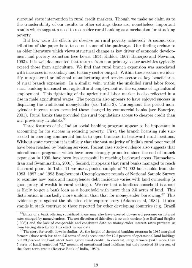
But how were the effects we observe on rural poverty achieved? A second con-tribution of the paper is to tease out some of the pathways. Our findings relate toan older literature which views structural change as key driver of economic develop-ment and poverty reduction (see Lewis, 1954; Kaldor, 1967; Banerjee and Newman,1993). It is well documented that returns from non-primary sector activities typicallyexceed those from agriculture. We find that rural branch expansion was associatedwith increases in secondary and tertiary sector output. Within these sectors we iden-tify unregistered or informal manufacturing and service sector as key beneficiariesof rural branch expansion. In a similar vein, within the unskilled rural labor force,rural banking increased non-agricultural employment at the expense of agriculturalemployment. This tightening of the agricultural labor market is also reflected in arise in male agricultural wages. The program also appears to have enjoyed success indisplacing the traditional moneylender (see Table 2). Throughout this period mon-eylender interest rates exceeded those charged by commercial banks (see Banerjee,2001). Rural banks thus provided the rural populations access to cheaper credit thanwas previously available.36

Three features of the Indian social banking program appear to be important inaccounting for its success in reducing poverty. First, the branch licensing rule suc-ceeded in coercing commercial banks to open branches in backward rural locations.Without state coercion it is unlikely that the vast majority of India’s rural poor wouldhave been reached by banking services. Recent case study evidence also suggests thatmicrofinance programs, which have been strongly promoted since the end of branchexpansion in 1990, have been less successful in reaching backward areas (Ramachan-dran and Swaminathan, 2001). Second, it appears that rural banks managed to reachthe rural poor. In Table 11 we use a pooled sample of 74,992 households from the1983, 1987 and 1993 Employment/Unemployment rounds of National Sample Surveyto examine how bank and moneylender debt incidence varies with land ownership (agood proxy of wealth in rural settings). We see that a landless household is aboutas likely to get a bank loan as a household with more than 2.5 acres of land. Thisdistribution is markedly more uniform than that for moneylender borrowing.37 Thisevidence goes against the oft cited elite capture story (Adams et al, 1984). It alsostands in stark contrast to those reported for other developing countries (e.g. Brazil

36Entry of a bank offering subsidized loans may also have exerted downward pressure on interestrates charged by moneylenders. The net direction of this effect is ex ante unclear (see Hoff and Stiglitz(1998)) and the lack of comparable and consistent data on moneylender interest rates prevents usfrom testing directly for this effect in our data.37The story for credit flows is similar. At the height of the social banking program in 1985 marginal

farmers (those with less than 2.5 acres of land) accounted for 12.2 percent of operational land holdingsbut 33 percent for bank short term agricultural credit. In contrast, large farmers (with more than5 acres of land) controlled 73.7 percent of operational land holdings but only received 38 percent ofthe short term credit (Reserve Bank of India, 1989).

19

and Costa Rica — see Besley 1995). It is also worth noting that microfinance programsin Bangladesh has often faced problems getting through to the poorest (Morduch,1999). Third, commercial banks offered opportunities for households to save (Ta-ble 9). Savings accounts likely provided households with the means of accumulatingcapital which could be used to invest in various productive activities. Microfinanceoperations, in contrast, tend not to offer this option with the focus being on shortterm loans with frequent repayment.

It is, however, premature to conclude that social banking is the optimal policyresponse to the problem of widespread rural poverty. The branch expansion programended in 1990 because of the heavy toll it exacted on the balance sheets of com-mercial banks. A key cause was high loan default rates — the average default ratefor commercial banks during the 1980s stood at 42 percent (as a share of all loansdue for repayment). Default rates were very similar across types of borrower — afinding consistent with poor monitoring of borrowers at all levels, and the fact thatlarge scale loan defaults were very often politically condoned (Reserve Bank of India,1989). Another factor contributing to high program costs was rural interest ratesubsidies — during the 1980s the average interest rate on loans from rural brancheswas 11 percent as against 14 percent in urban branches.

From a policy design viewpoint, the fact that rural branches were a vehicle forcostly redistribution of resources to rural areas is, in itself, not a damning criticism ofthe program. It is well-known that, in the presence of informational asymmetries, itmay be optimal for a government that wishes to target resources to particular groupsof citizens to undertake costly redistribution in order to best screen amongst citizens(Besley and Coate, 1992). It is clear that the Indian government sought to use thesocial banking program to redistribute resources to the rural poor. This suggests thatthe relevant policy question is, whether, in the class of costly redistributive programs,the social banking program was the most cost-effective.

The cost effectiveness comparison with microfinance is especially germane sincethe widespread perception that development banks are both costly and ineffectivehas led to widespread calls that they be replaced by microfinance operations. This istrue both for India post-1990 and more broadly for low income countries as a whole(Morduch, 1999).38 Unfortunately, lack of comparable data on microfinance schemesin India makes a direct comparison infeasible. We can, however, get a ‘back of theenvelope’ feel for the cost-benefit ratio for our program and compare this to ratiosfor microfinance programs in Bangladesh reported in Morduch (1999). Whilst notwishing to read too much into this exercise — due to the assumptions involved in thecalculation and the problems of comparison across counties — it is, nonetheless, ofinterest to see whether our ratio lies in the ballpark of the microfinance ratios.

Our cost figures come from an evaluation of the program carried out by the Indiancentral bank in 1986 (Reserve Bank of India, 1989). For each 100 rupees of working

38The Indian central bank task force on microfinance (1997) stated, ‘To achieve a process of changeleading to empowerment of 7.5 million poor households, and more particularly of the women fromthese households, through strong and viable people’s structures like Self help groups and micro-finance institutions which draw strength and support from the banking system with the messagethat banking with the poor is a profitable business opportunity for both the poor and the banks’.

20

funds the average rural branch received 11.5 rupees as interest on loans, paid 7.3rupees as interest on deposits and had variable costs of 4.8 rupees (these includemanpower and other expenses). The average rural branch, therefore, made a lossof 0.6 rupees per 100 rupees of working funds. The revenue position of a branch,however, was significantly worsened by the fact only 58 percent of loans were repaid.This increases the loss to 5.4 rupees per 100 rupees. We use our total deposits andtotal advances figures to compute the real loss per bank branch per capita in 1986(498.13 rupees). To calculate benefits we take the coefficient (0.08) — which we obtainfrom regressing rural banks per capita on log state income per capita in column (1) ofTable 8 — and multiply it by the real state output per capita in 1986 (1020.2 rupees)to get a real benefit figure in 1986 of 183.45 per bank branch per capita. Dividingcosts by benefits gives a cost benefit ratio of 2.72. That is it costs 2.72 rupees togenerate an additional rupee of state income via the social banking program.

This figure exceeds the cost benefit ratio of 0.91 that Khandker (1998) reports forimprovements in household expenditure via borrowing by women from the GrameenBank and of 1.48 for borrowing by men. Our figure of 2.72 is, however, in the ballparkof the ratios of 3.53 and 2.59 for borrowing from BRAC, the second largest microfi-nance lender in Bangladesh, by women and men, respectively (Khandker, 1998). Andthis is the case even when the default rate is at 42 percent. If we assume no defaultthen our cost benefit ratio at 0.31 is well below even the Grameen ratios. If we takea default rate of 7.8 percent which is the average that Morduch (1999) reports forthe Grameen Bank over the 1985-1996 period then our ratio rises to 0.75 which isclose to the Grameen ratio for women. These comparisons, though rough, do bringout the fact that a key advantage of microfinance lies in its superior ability to enforcerepayment of loans.39

This simple comparison, however, also suggests that no easy ranking of microfi-nance and social banking as regards cost effectiveness is possible. Both confer sig-nificant benefits as measured in terms of increased expenditure or income. However,both types of schemes also incur significant subsidies. The demonstrated advantageof microfinance in terms of repayment needs to be balanced against disadvantagesin terms of reaching the poorest individuals and localities.40 One clear thing thatwe do learn from this paper is that coercion is needed to expand formal credit intobackward rural areas and to force banks to lend to poorer individuals. And heregovernment may have some advantages in terms of coordination, legal powers and re-sources. There is also the issue of whether providing a savings function is important.The fact that a number of microfinance operations are evolving into banks whichoffer this service suggests that it may be.

In 1998 India accounted for a third of the people in the developing world livingbelow the dollar a day poverty line. That the rural branch expansion managed to

39It is also clear that there is scope for banks to increase lending rates as a means of reducing costsas even microfinance operations charge higher nominal rates than those on offer from rural banks.The problem with this strategy as Morduch (1999) points out is that one runs the risk of excludingthe poor.40Reaching the poorest in rural areas who are often involved in subsistence agriculture and who

cannot make frequent repayments, for example, is problematic.

21

make a significant dent on the numbers in poverty during the 1961-2000 period is thekey finding of this paper. It suggests that expanding access to finance in poor, ruralsettings can generate significant social returns. It also points to the need to identifyingspecific interventions which facilitate the adoption of new production activities andlead to structural change, growth and poverty. Our analysis is limited to a specificpolicy episode. Whether rural branch expansion would be effective in other settingsand whether resources would be better spent on other types of programs remain openquestions. Nonetheless it does appear to be an opportune moment to reexaminewhether rural banks can be harnessed to attack rural poverty.

23

References

[1] Adams, Dale, Graham, Douglas and J.D. Von Pischke, [1984], “UnderminingRural Development with Cheap Credit” (Boulder: Westview Press).

[2] Aghion, P. and P. Bolton [1997], “A Theory of Trickle-Down Growth and De-velopment”, Review of Economic Studies 64(2): 151-72

[3] Almond, Douglas, Kenneth Chay and Michael Greenstone [2002], “Civil Rights,The War on Poverty and Black-White Convergence in Infant Mortality in RuralMississipi”, mimeo, University of Chicago.

[4] Balachandran, Gopal, [1998], “The Reserve Bank of India, 1951-1967 ” (Mumbai:Reserve Bank of India; New York : Oxford University Press).

[5] Banerjee, Abhijit, [2001], “Contracting Constraints, Credit Markets and Eco-nomic Development” mimeo MIT.

[6] Banerjee, Abhijit V., Gertler, Paul J. and Maitreesh Ghatak, [2002], “Empow-erment and Efficiency: Tenancy Reform in West Bengal”, Journal of PoliticalEconomy , 110(2), 239-80.

[7] Banerjee, Abhijit and Andrew Newman, [1993], “Occupational Choice and theProcess of Development”, Journal of Political Economy, 101, 274-298.

[8] Bencivenga, Valerie and Bruce D. Smith, [1991], “Financial Intermediation andEndogenous Growth” Review of Economic Studies 58, 195-209.

[9] Bernanke, Ben and Mark Gertler, [1990], “Financial Fragility and EconomicPerformance”, Quarterly Journal of Economics, 105.

[10] Bertrand, Marianne, Esther Duflo, and Sendhil Mullainathan, [2002], “HowMuch Should We Trust Differences in Differences Estimates”, NBER WorkingPaper No. 8841.

[11] Besley, Timothy, [1995], “Saving, Credit and Insurance,” in Jere Behrman andT.N. Srinivasan (ed) Handbook of Development Economics, Vol. IIIa Amster-dam: North Holland.

[12] Besley, Timothy and Robin Burgess, [2000], “Land Reform, Poverty and Growth:Evidence from India”, Quarterly Journal of Economics, 115 (2), 389-430.

[13] Besley, Timothy and Robin Burgess, [2002], “The Political Economy of Govern-ment Responsiveness: Theory and Evidence from India”, Quarterly Journal ofEconomics, 117 (4).

[14] Besley, Timothy and Stephen Coate, [1992], “Workfare versus Welfare: IncentiveArguments for Work Requirements in Poverty Alleviation Programs” AmericanEconomic Review, 82, (1) 249-261.

23

[15] Binswanger, Hans, and Khandker, Shahidur, [1995], “The impact of formal fi-nance on the rural economy of India ,” Journal of Development studies32(2):234-262.

[16] Binswanger, Hans, Khandker, Shahidur and Mark Rozenzweig, [1993], “HowAgriculture and Financial Institutions Affect Agricultural Output and Invest-ment in India,” Journal of Development Economics.

[17] Braverman, A and JL Guasch [1986], “Rural Credit Markets and Institutionsin Developing Countries: Lessons for Policy Analysis from Practice and ModernTheory,” World Development, 14.

[18] Burgess, Robin and Anthony Venables [2003], “Towards a Microeconomics ofGrowth”. Forthcoming Annual World Bank Conference on Development Eco-nomics.

[19] Chenery, Hollis B., Moshe Syrquin and and Sherman Robinson [1986] “Indus-trialization and Growth: A Comparative Study” (Oxford: Oxford UniversityPress)

[20] Dasgupta, Sugato, Amrita Dhillon and Bhaskar Dutta [2001], “The PoliticalEconomy of Centre-State resource Transfer in India,” mimeo, Warwick.

[21] Deaton, Angus [2001]: “Adjusted Indian Poverty Estimates 1999-2000” mimeo,Princeton.

[22] Deaton, Angus and Jean Dreze [2002]: “Poverty and Inequality in India: ARe-examination” Economic and Political Weekly, September 7.

[23] Dehejia, Rajeev and Adriana Lleras-Muney, [2002] “Why Does Financial De-velopment Matter? The United States from 1900 to 1940”, mimeo ColumbiaUniversity

[24] Desai, Vasant, [1987], “Indian banking : Nature and Problems ” (Bombay :Himalaya Pub. House).

[25] Dreze, J. and Mukherjee, A. [1991]: “Labour Contracts in Rural India: The-ory and Evidence” in S. Chakravarty (ed) The Balance between Industry andAgriculture in Economic Development (New York)

[26] Duflo, Esther [2001], “Schooling and Labor Market Consequences of School Con-struction in Indonesia: Evidence from an Unusual Policy Experiment” AmericanEconomic Review..

[27] Eastwood, Robert and Renu Kohli [1999], “Directed Credit and Investment inSmall-Scale Industry in India: Evidence from Firm-Level Data, 1965-1978” Jour-nal of Development Studies, 35 (4)

[28] Government of India [1991], “Report of the Committee on the Financial Sector”chairman M. Narsimhan, Ministry of Finance, Delhi .

24

[29] Gerschenkron, Alexander [1962], Economic Backwardness in Historical Perspec-tive Harvard University Press, Cambridge.

[30] Greenwood, J. and B. Jovanovic, [1990], “Financial Development, Growth andthe Distribution of Income” Journal of Political Economy, 98(5), 1076-1107.

[31] Hoff, Karla and Joseph Stiglitz, [1998], “Moneylenders and Bankers: Price In-creasing Subsidies in a Monopolistically Competitive Market” Journal of Devel-opment Economics 55: 485-518.

[32] Jayaratne, Jith and Philip E. Strahan, [1996], “The Finance-Growth Nexus:Evidence from Bank Branch Deregulation” Quarterly Journal of Economics,111(3), 639-70.

[33] Kaldor, Nicholas [1967], “Strategic Factors in Economic Development” (Ithaca:Cornell University Press)

[34] Khandker, Shahidur R. [1998] “Fighting poverty with microcredit : experiencein Bangladesh”, New York, Oxford University Press.

[35] King, Robert and Levine, Ross [1993]: “Finance and Growth: Schumpeter mightbe Right” Quarterly Journal of Economics, CVIII, no. 3 August, 717-738.

[36] La Porta, Rafael, Florencio Lopez de Silanes and Andrei Shleifer, [2002], “Gov-ernment Ownership of Banks” Journal of Finance, February.

[37] Levine, Ross and Sara Zervos, [1998], “Stock Markets, Banks, and EconomicGrowth” American Economic Review, 88(3), 537-58.

[38] Lewis, W.A., [1954], “Economic Development with Unlimited Supplies ofLabour” The Manchester School of Economic and Social Studies 22, 139-191.

[39] Morduch, Jonathan [1999],” The Microfinance Promise”, Journal of EconomicLiterature, Vol. XXXVII, 1569-1614

[40] Nair, Tara , [2000], “Rural Financial Intermediation and Commercial Banks:Review of Recent Trends” Economic and Political Weekly, January 29.

[41] Ozler, B. Datt, G. and Ravallion, M., [1996], “A Data Base on Poverty andGrowth in India” mimeo, World Bank.

[42] Rajan, Raghuram G. and Luigi Zingales, [1998] “Financial Dependence andGrowth”, American Economic Review 88(3), 559-86.

[43] Reserve Bank of India, [1954], ‘All-India rural credit survey: report’, Report ofthe Committee of Direction of the All India Rural Credit Survey, Mumbai.

[44] Ramachandran, V.K. and Madhura Swaminathan, [2001], “Does Informal CreditProvide Security? Rural Banking Policy in India” mimeo International LabourOffice, Geneva.

25

[45] Reserve Bank of India, [1989], ‘A Review of the Agricultural Credit System inIndia’, Report of the Agricultural Credit Review Committee, Mumbai

[46] Reserve Bank of India, [1997], Basic Statistical Returns for Commercial Banks,Mumbai.

[47] Reserve Bank of India, [1998], Banking Statistics 1972-1995, Mumbai.

[48] Reserve Bank of India, [2000], Directory of Commercial Bank Offices in India(Volume 1), Mumbai.

[49] Sapienza, Paola, [2003], “The Effects of Government Ownership on Bank Lend-ing” Journal of Financial Economics forthcoming.

[50] Sargan, John Denis, [1958], “The Estimation of Economic Relationships UsingInstrumental Variables” Econometrica XXVI , 393-415

[51] Schumpeter, Joseph, [1934], The Theory of Economic Development: An Inquiryinto Profits, Capital, Interest, and the Business Cycle (Cambridge: HarvardUniversity Press)

[52] Townsend, Robert M. and Kenichi Ueda [2001], “Transitional Growth with In-creasing Inequality and Financial Deepening” mimeo University of Chicago.

[53] Visaria, Pravin and Rakesh Basant, [1994], “Non-Agricultural Employment inIndia: Trends and Prospects” (New Delhi, Sage Publications).

[54] Zinman, Jonathan [2002], “The Efficacy and Efficiency of Credit Market Inter-ventions: Evidence from the Community Reinvestment Act”, mimeo, MIT.

27

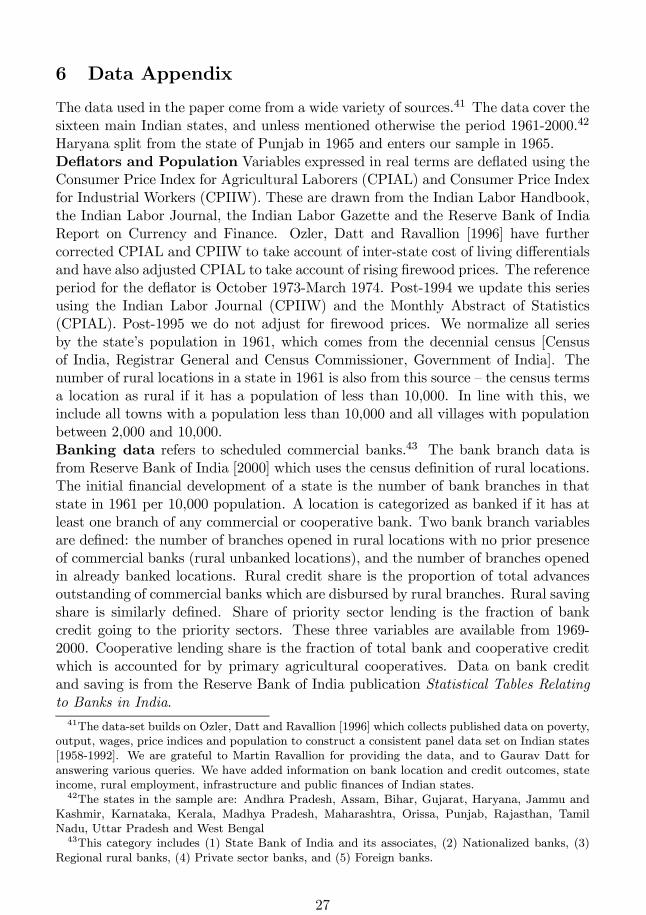
6 Data Appendix

The data used in the paper come from a wide variety of sources.41 The data cover thesixteen main Indian states, and unless mentioned otherwise the period 1961-2000.42

Haryana split from the state of Punjab in 1965 and enters our sample in 1965.Deflators and Population Variables expressed in real terms are deflated using theConsumer Price Index for Agricultural Laborers (CPIAL) and Consumer Price Indexfor Industrial Workers (CPIIW). These are drawn from the Indian Labor Handbook,the Indian Labor Journal, the Indian Labor Gazette and the Reserve Bank of IndiaReport on Currency and Finance. Ozler, Datt and Ravallion [1996] have furthercorrected CPIAL and CPIIW to take account of inter-state cost of living differentialsand have also adjusted CPIAL to take account of rising firewood prices. The referenceperiod for the deflator is October 1973-March 1974. Post-1994 we update this seriesusing the Indian Labor Journal (CPIIW) and the Monthly Abstract of Statistics(CPIAL). Post-1995 we do not adjust for firewood prices. We normalize all seriesby the state’s population in 1961, which comes from the decennial census [Censusof India, Registrar General and Census Commissioner, Government of India]. Thenumber of rural locations in a state in 1961 is also from this source — the census termsa location as rural if it has a population of less than 10,000. In line with this, weinclude all towns with a population less than 10,000 and all villages with populationbetween 2,000 and 10,000.Banking data refers to scheduled commercial banks.43 The bank branch data isfrom Reserve Bank of India [2000] which uses the census definition of rural locations.The initial financial development of a state is the number of bank branches in thatstate in 1961 per 10,000 population. A location is categorized as banked if it has atleast one branch of any commercial or cooperative bank. Two bank branch variablesare defined: the number of branches opened in rural locations with no prior presenceof commercial banks (rural unbanked locations), and the number of branches openedin already banked locations. Rural credit share is the proportion of total advancesoutstanding of commercial banks which are disbursed by rural branches. Rural savingshare is similarly defined. Share of priority sector lending is the fraction of bankcredit going to the priority sectors. These three variables are available from 1969-2000. Cooperative lending share is the fraction of total bank and cooperative creditwhich is accounted for by primary agricultural cooperatives. Data on bank creditand saving is from the Reserve Bank of India publication Statistical Tables Relatingto Banks in India.41The data-set builds on Ozler, Datt and Ravallion [1996] which collects published data on poverty,

output, wages, price indices and population to construct a consistent panel data set on Indian states[1958-1992]. We are grateful to Martin Ravallion for providing the data, and to Gaurav Datt foranswering various queries. We have added information on bank location and credit outcomes, stateincome, rural employment, infrastructure and public finances of Indian states.42The states in the sample are: Andhra Pradesh, Assam, Bihar, Gujarat, Haryana, Jammu and

Kashmir, Karnataka, Kerala, Madhya Pradesh, Maharashtra, Orissa, Punjab, Rajasthan, TamilNadu, Uttar Pradesh and West Bengal43This category includes (1) State Bank of India and its associates, (2) Nationalized banks, (3)

Regional rural banks, (4) Private sector banks, and (5) Foreign banks.

27

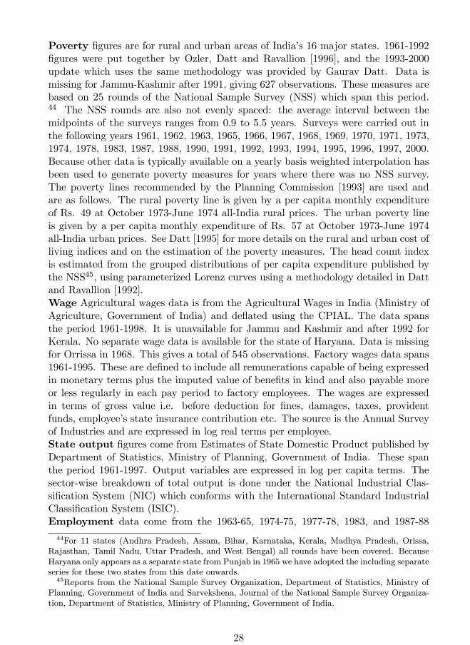
Poverty figures are for rural and urban areas of India’s 16 major states. 1961-1992figures were put together by Ozler, Datt and Ravallion [1996], and the 1993-2000update which uses the same methodology was provided by Gaurav Datt. Data ismissing for Jammu-Kashmir after 1991, giving 627 observations. These measures arebased on 25 rounds of the National Sample Survey (NSS) which span this period.44 The NSS rounds are also not evenly spaced: the average interval between themidpoints of the surveys ranges from 0.9 to 5.5 years. Surveys were carried out inthe following years 1961, 1962, 1963, 1965, 1966, 1967, 1968, 1969, 1970, 1971, 1973,1974, 1978, 1983, 1987, 1988, 1990, 1991, 1992, 1993, 1994, 1995, 1996, 1997, 2000.Because other data is typically available on a yearly basis weighted interpolation hasbeen used to generate poverty measures for years where there was no NSS survey.The poverty lines recommended by the Planning Commission [1993] are used andare as follows. The rural poverty line is given by a per capita monthly expenditureof Rs. 49 at October 1973-June 1974 all-India rural prices. The urban poverty lineis given by a per capita monthly expenditure of Rs. 57 at October 1973-June 1974all-India urban prices. See Datt [1995] for more details on the rural and urban cost ofliving indices and on the estimation of the poverty measures. The head count indexis estimated from the grouped distributions of per capita expenditure published bythe NSS45, using parameterized Lorenz curves using a methodology detailed in Dattand Ravallion [1992].Wage Agricultural wages data is from the Agricultural Wages in India (Ministry ofAgriculture, Government of India) and deflated using the CPIAL. The data spansthe period 1961-1998. It is unavailable for Jammu and Kashmir and after 1992 forKerala. No separate wage data is available for the state of Haryana. Data is missingfor Orrissa in 1968. This gives a total of 545 observations. Factory wages data spans1961-1995. These are defined to include all remunerations capable of being expressedin monetary terms plus the imputed value of benefits in kind and also payable moreor less regularly in each pay period to factory employees. The wages are expressedin terms of gross value i.e. before deduction for fines, damages, taxes, providentfunds, employee’s state insurance contribution etc. The source is the Annual Surveyof Industries and are expressed in log real terms per employee.State output figures come from Estimates of State Domestic Product published byDepartment of Statistics, Ministry of Planning, Government of India. These spanthe period 1961-1997. Output variables are expressed in log per capita terms. Thesector-wise breakdown of total output is done under the National Industrial Clas-sification System (NIC) which conforms with the International Standard IndustrialClassification System (ISIC).Employment data come from the 1963-65, 1974-75, 1977-78, 1983, and 1987-88

44For 11 states (Andhra Pradesh, Assam, Bihar, Karnataka, Kerala, Madhya Pradesh, Orissa,Rajasthan, Tamil Nadu, Uttar Pradesh, and West Bengal) all rounds have been covered. BecauseHaryana only appears as a separate state from Punjab in 1965 we have adopted the including separateseries for these two states from this date onwards.45Reports from the National Sample Survey Organization, Department of Statistics, Ministry of

Planning, Government of India and Sarvekshena, Journal of the National Sample Survey Organiza-tion, Department of Statistics, Ministry of Planning, Government of India.

28

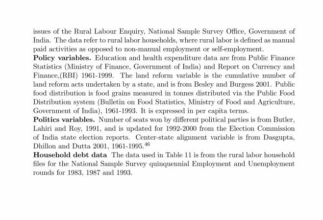
issues of the Rural Labour Enquiry, National Sample Survey Office, Government ofIndia. The data refer to rural labor households, where rural labor is defined as manualpaid activities as opposed to non-manual employment or self-employment.Policy variables. Education and health expenditure data are from Public FinanceStatistics (Ministry of Finance, Government of India) and Report on Currency andFinance,(RBI) 1961-1999. The land reform variable is the cumulative number ofland reform acts undertaken by a state, and is from Besley and Burgess 2001. Publicfood distribution is food grains measured in tonnes distributed via the Public FoodDistribution system (Bulletin on Food Statistics, Ministry of Food and Agriculture,Government of India), 1961-1993. It is expressed in per capita terms.Politics variables. Number of seats won by different political parties is from Butler,Lahiri and Roy, 1991, and is updated for 1992-2000 from the Election Commissionof India state election reports. Center-state alignment variable is from Dasgupta,Dhillon and Dutta 2001, 1961-1995.46

Household debt data The data used in Table 11 is from the rural labor householdfiles for the National Sample Survey quinquennial Employment and Unemploymentrounds for 1983, 1987 and 1993.

46State political configurations are held constant between elections.

30

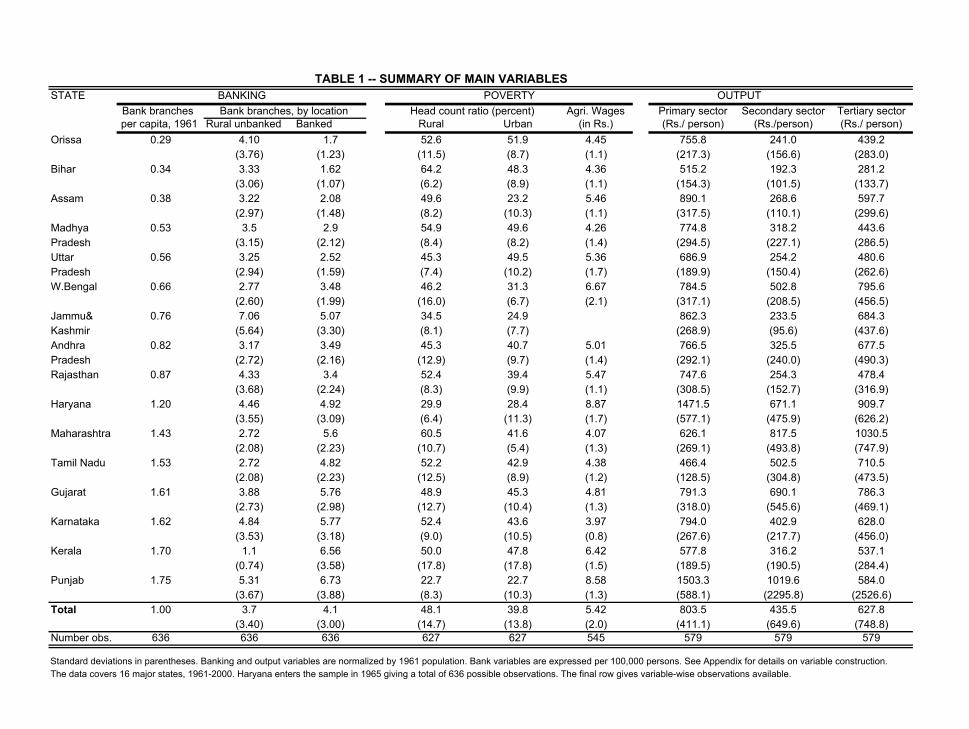
STATEBank branches Agri. Wages Primary sector Secondary sector Tertiary sectorper capita, 1961 Rural unbanked Banked Rural Urban (in Rs.) (Rs./ person) (Rs./person) (Rs./ person)

Orissa 0.29 4.10 1.7 52.6 51.9 4.45 755.8 241.0 439.2(3.76) (1.23) (11.5) (8.7) (1.1) (217.3) (156.6) (283.0)

Bihar 0.34 3.33 1.62 64.2 48.3 4.36 515.2 192.3 281.2(3.06) (1.07) (6.2) (8.9) (1.1) (154.3) (101.5) (133.7)

Assam 0.38 3.22 2.08 49.6 23.2 5.46 890.1 268.6 597.7(2.97) (1.48) (8.2) (10.3) (1.1) (317.5) (110.1) (299.6)

Madhya 0.53 3.5 2.9 54.9 49.6 4.26 774.8 318.2 443.6Pradesh (3.15) (2.12) (8.4) (8.2) (1.4) (294.5) (227.1) (286.5)Uttar 0.56 3.25 2.52 45.3 49.5 5.36 686.9 254.2 480.6Pradesh (2.94) (1.59) (7.4) (10.2) (1.7) (189.9) (150.4) (262.6)W.Bengal 0.66 2.77 3.48 46.2 31.3 6.67 784.5 502.8 795.6

(2.60) (1.99) (16.0) (6.7) (2.1) (317.1) (208.5) (456.5)Jammu& 0.76 7.06 5.07 34.5 24.9 862.3 233.5 684.3Kashmir (5.64) (3.30) (8.1) (7.7) (268.9) (95.6) (437.6)Andhra 0.82 3.17 3.49 45.3 40.7 5.01 766.5 325.5 677.5Pradesh (2.72) (2.16) (12.9) (9.7) (1.4) (292.1) (240.0) (490.3)Rajasthan 0.87 4.33 3.4 52.4 39.4 5.47 747.6 254.3 478.4

(3.68) (2.24) (8.3) (9.9) (1.1) (308.5) (152.7) (316.9)Haryana 1.20 4.46 4.92 29.9 28.4 8.87 1471.5 671.1 909.7

(3.55) (3.09) (6.4) (11.3) (1.7) (577.1) (475.9) (626.2)Maharashtra 1.43 2.72 5.6 60.5 41.6 4.07 626.1 817.5 1030.5

(2.08) (2.23) (10.7) (5.4) (1.3) (269.1) (493.8) (747.9)Tamil Nadu 1.53 2.72 4.82 52.2 42.9 4.38 466.4 502.5 710.5

(2.08) (2.23) (12.5) (8.9) (1.2) (128.5) (304.8) (473.5)Gujarat 1.61 3.88 5.76 48.9 45.3 4.81 791.3 690.1 786.3

(2.73) (2.98) (12.7) (10.4) (1.3) (318.0) (545.6) (469.1)Karnataka 1.62 4.84 5.77 52.4 43.6 3.97 794.0 402.9 628.0

(3.53) (3.18) (9.0) (10.5) (0.8) (267.6) (217.7) (456.0)Kerala 1.70 1.1 6.56 50.0 47.8 6.42 577.8 316.2 537.1

(0.74) (3.58) (17.8) (17.8) (1.5) (189.5) (190.5) (284.4)Punjab 1.75 5.31 6.73 22.7 22.7 8.58 1503.3 1019.6 584.0

(3.67) (3.88) (8.3) (10.3) (1.3) (588.1) (2295.8) (2526.6)Total 1.00 3.7 4.1 48.1 39.8 5.42 803.5 435.5 627.8

(3.40) (3.00) (14.7) (13.8) (2.0) (411.1) (649.6) (748.8)Number obs. 636 636 636 627 627 545 579 579 579

The data covers 16 major states, 1961-2000. Haryana enters the sample in 1965 giving a total of 636 possible observations. The final row gives variable-wise observations available.

TABLE 1 -- SUMMARY OF MAIN VARIABLESOUTPUT

Bank branches, by location BANKING POVERTY

Standard deviations in parentheses. Banking and output variables are normalized by 1961 population. Bank variables are expressed per 100,000 persons. See Appendix for details on variable construction.

Head count ratio (percent)

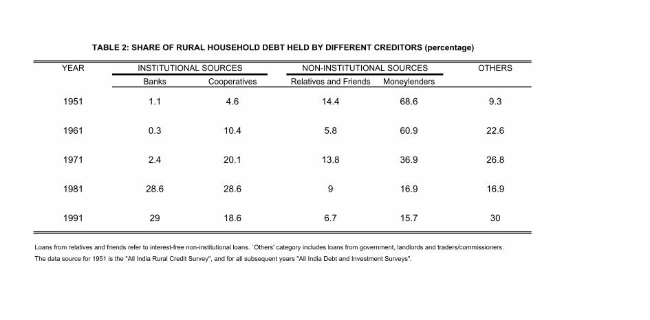
YEAR OTHERSBanks Cooperatives Relatives and Friends Moneylenders

1951 1.1 4.6 14.4 68.6 9.3

1961 0.3 10.4 5.8 60.9 22.6

1971 2.4 20.1 13.8 36.9 26.8

1981 28.6 28.6 9 16.9 16.9

1991 29 18.6 6.7 15.7 30

Loans from relatives and friends refer to interest-free non-institutional loans. `Others' category includes loans from government, landlords and traders/commissioners.

The data source for 1951 is the "All India Rural Credit Survey", and for all subsequent years "All India Debt and Investment Surveys".

TABLE 2: SHARE OF RURAL HOUSEHOLD DEBT HELD BY DIFFERENT CREDITORS (percentage)

INSTITUTIONAL SOURCES NON-INSTITUTIONAL SOURCES

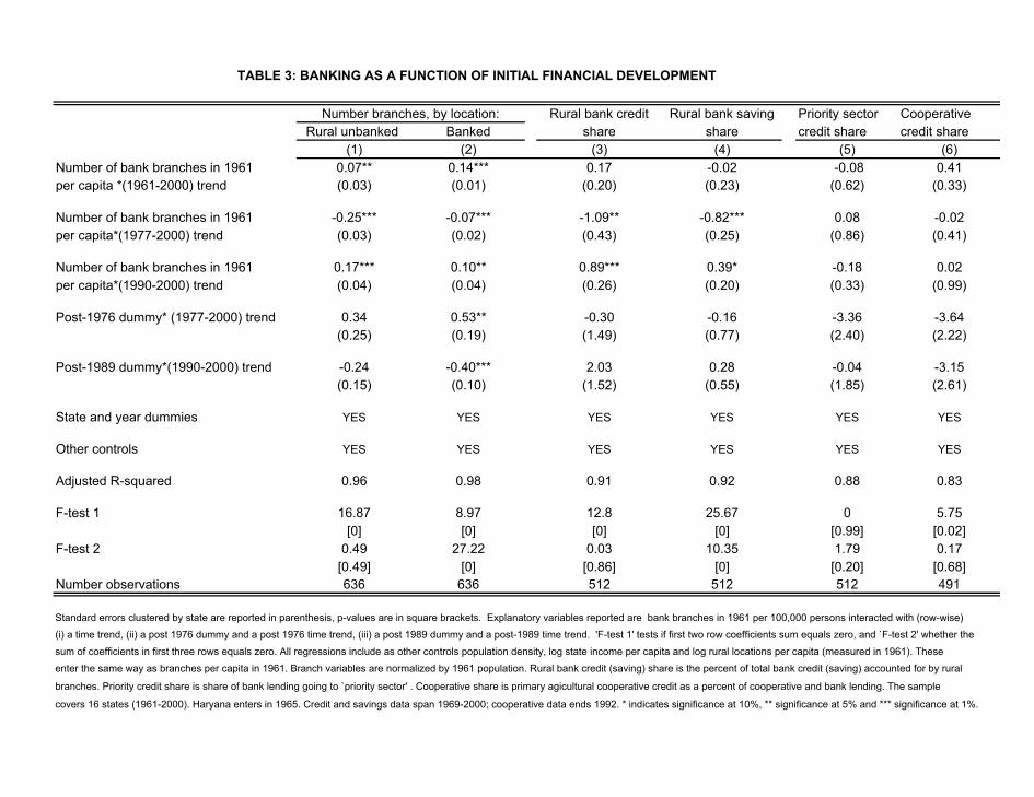
Rural bank credit Rural bank saving Priority sector CooperativeRural unbanked Banked share share credit share credit share

(1) (2) (3) (4) (5) (6)Number of bank branches in 1961 0.07** 0.14*** 0.17 -0.02 -0.08 0.41per capita *(1961-2000) trend (0.03) (0.01) (0.20) (0.23) (0.62) (0.33)

Number of bank branches in 1961 -0.25*** -0.07*** -1.09** -0.82*** 0.08 -0.02per capita*(1977-2000) trend (0.03) (0.02) (0.43) (0.25) (0.86) (0.41)

Number of bank branches in 1961 0.17*** 0.10** 0.89*** 0.39* -0.18 0.02per capita*(1990-2000) trend (0.04) (0.04) (0.26) (0.20) (0.33) (0.99)

Post-1976 dummy* (1977-2000) trend 0.34 0.53** -0.30 -0.16 -3.36 -3.64(0.25) (0.19) (1.49) (0.77) (2.40) (2.22)

Post-1989 dummy*(1990-2000) trend -0.24 -0.40*** 2.03 0.28 -0.04 -3.15 (0.15) (0.10) (1.52) (0.55) (1.85) (2.61)

State and year dummies YES YES YES YES YES YES

Other controls YES YES YES YES YES YES

Adjusted R-squared 0.96 0.98 0.91 0.92 0.88 0.83

F-test 1 16.87 8.97 12.8 25.67 0 5.75[0] [0] [0] [0] [0.99] [0.02]

F-test 2 0.49 27.22 0.03 10.35 1.79 0.17[0.49] [0] [0.86] [0] [0.20] [0.68]

Number observations 636 636 512 512 512 491

TABLE 3: BANKING AS A FUNCTION OF INITIAL FINANCIAL DEVELOPMENT

Number branches, by location:

Standard errors clustered by state are reported in parenthesis, p-values are in square brackets. Explanatory variables reported are bank branches in 1961 per 100,000 persons interacted with (row-wise)

branches. Priority credit share is share of bank lending going to `priority sector' . Cooperative share is primary agicultural cooperative credit as a percent of cooperative and bank lending. The sample

covers 16 states (1961-2000). Haryana enters in 1965. Credit and savings data span 1969-2000; cooperative data ends 1992. * indicates significance at 10%, ** significance at 5% and *** significance at 1%.

(i) a time trend, (ii) a post 1976 dummy and a post 1976 time trend, (iii) a post 1989 dummy and a post-1989 time trend. 'F-test 1' tests if first two row coefficients sum equals zero, and `F-test 2' whether thesum of coefficients in first three rows equals zero. All regressions include as other controls population density, log state income per capita and log rural locations per capita (measured in 1961). These enter the same way as branches per capita in 1961. Branch variables are normalized by 1961 population. Rural bank credit (saving) share is the percent of total bank credit (saving) accounted for by rural

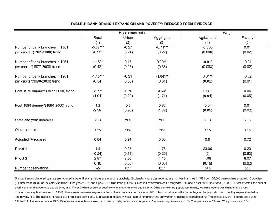
Rural Urban Aggregate Agricultural Factory(1) (2) (3) (4) (5)

Number of bank branches in 1961 -0.77*** -0.27 -0.71*** -0.003 0.01per capita *(1961-2000) trend (0.23) (0.24) (0.22) (0.006) (0.02)

Number of bank branches in 1961 1.15** 0.15 0.99*** -0.01* -0.01per capita*(1977-2000) trend (0.42) (0.26) (0.33) (0.008) (0.02)

Number of bank branches in 1961 -1.15*** -0.31 -1.04*** 0.04** -0.02per capita*(1990-2000) trend (0.34) (0.38) (0.31) (0.02) (0.01)

Post-1976 dummy* (1977-2000) trend -3.77* -2.76 -3.53** 0.08* 0.04(1.94) (2.29) (1.71) (0.04) (0.05)

Post-1989 dummy*(1990-2000) trend 1.2 0.5 0.62 -0.04 0.01(2.39) (0.96) (1.82) (0.05) (0.02)

State and year dummies YES YES YES YES YES

Other controls YES YES YES YES YES

Adjusted R-squared 0.84 0.91 0.88 0.9 0.72

F-test 1 1.5 0.37 1.76 23.95 0.23[0.24] [0.55] [0.20] [0] [0.63]

F-test 2 2.97 3.95 4.15 1.88 6.07[0.10] [0.06] [0.05] [0.19] [0.02]

Number observations 627 627 627 545 553

1961-2000. Haryana enters in 1965. Differences in sample size are due to missing data, details are in Appendix. * indicates significance at 10%, ** significance at 5% and *** significance at 1%.

TABLE 4: BANK BRANCH EXPANSION AND POVERTY: REDUCED FORM EVIDENCE

the poverty line. The agricultural wage is log real male daily agricultural wage, and factory wage log real remunerations per worker in registered manufacturing. The sample covers 16 states and spans

Head count ratio

Standard errors clustered by state are reported in parenthesis, p-values are in square brackets. Explanatory variables reported are number branches in 1961 per 100,000 persons interacted with (row-wise)(i) a time trend (t), (ii) an indicator variable=1 if the year>1976, and a post 1976 time trend (t-1976), (iii) an indicator variable=1 if the year>1989 and a post-1989 time trend (t-1989). 'F-test 1' tests if the sum ofcoefficients for first two rows equals zero, and `F-test 2' whether sum of coefficients in first three rows equals zero. Other controls are population density, log state income per capita and log rurallocations per capita (measured in 1961). These enter the same way as number of bank branches per capita in 1961. Head count ratio is the percentage of the population with monthly expenditure below

Wage

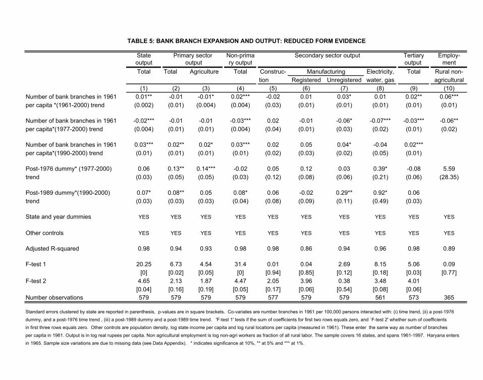
State Non-prima Tertiary Employ-output ry output output mentTotal Total Agriculture Total Construc- Electricity, Total Rural non-

tion Registered Unregistered water, gas agricultural(1) (2) (3) (4) (5) (6) (7) (8) (9) (10)

Number of bank branches in 1961 0.01** -0.01 -0.01* 0.02*** -0.02 0.01 0.03* 0.01 0.02** 0.06***per capita *(1961-2000) trend (0.002) (0.01) (0.004) (0.004) (0.03) (0.01) (0.01) (0.01) (0.01) (0.01)

Number of bank branches in 1961 -0.02*** -0.01 -0.01 -0.03*** 0.02 -0.01 -0.06* -0.07*** -0.03*** -0.06**per capita*(1977-2000) trend (0.004) (0.01) (0.01) (0.004) (0.04) (0.01) (0.03) (0.02) (0.01) (0.02)

Number of bank branches in 1961 0.03*** 0.02** 0.02* 0.03*** 0.02 0.05 0.04* -0.04 0.02***per capita*(1990-2000) trend (0.01) (0.01) (0.01) (0.01) (0.02) (0.03) (0.02) (0.05) (0.01)

Post-1976 dummy* (1977-2000) 0.06 0.13** 0.14*** -0.02 0.05 0.12 0.03 0.39* -0.08 5.59trend (0.03) (0.05) (0.05) (0.03) (0.12) (0.08) (0.06) (0.21) (0.06) (28.35)

Post-1989 dummy*(1990-2000) 0.07* 0.08** 0.05 0.08* 0.06 -0.02 0.29** 0.92* 0.06trend (0.03) (0.03) (0.03) (0.04) (0.08) (0.09) (0.11) (0.49) (0.03)

State and year dummies YES YES YES YES YES YES YES YES YES YES

Other controls YES YES YES YES YES YES YES YES YES YES

Adjusted R-squared 0.98 0.94 0.93 0.98 0.98 0.86 0.94 0.96 0.98 0.89

F-test 1 20.25 6.73 4.54 31.4 0.01 0.04 2.69 8.15 5.06 0.09[0] [0.02] [0.05] [0] [0.94] [0.85] [0.12] [0.18] [0.03] [0.77]

F-test 2 4.65 2.13 1.87 4.47 2.05 3.96 0.38 3.48 4.01[0.04] [0.16] [0.19] [0.05] [0.17] [0.06] [0.54] [0.08] [0.06]

Number observations 579 579 579 579 577 579 579 561 573 365

in 1965. Sample size variations are due to missing data (see Data Appendix). * indicates significance at 10%, ** at 5% and *** at 1%.

Standard errors clustered by state are reported in parenthesis, p-values are in square brackets. Co-variates are number branches in 1961 per 100,000 persons interacted with: (i) time trend, (ii) a post-1976dummy, and a post-1976 time trend , (iii) a post-1989 dummy and a post-1989 time trend. 'F-test 1' tests if the sum of coefficients for first two rows equals zero, and `F-test 2' whether sum of coefficientsin first three rows equals zero. Other controls are population density, log state income per capita and log rural locations per capita (measured in 1961). These enter the same way as number of branches

TABLE 5: BANK BRANCH EXPANSION AND OUTPUT: REDUCED FORM EVIDENCE

per capita in 1961. Output is in log real rupees per capita. Non agricultural employment is log non-agri workers as fraction of all rural labor. The sample covers 16 states, and spans 1961-1997. Haryana enters

Secondary sector outputPrimary sector

Manufacturingoutput

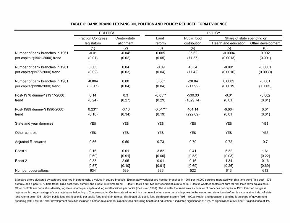
Fraction Congress Center-state Land Public foodlegislators alignment reform distribution Health and education Other development

(1) (2) (3) (4) (5) (6)Number of bank branches in 1961 -0.01 -0.04* 0.005 35.62 -0.0004 0.002per capita *(1961-2000) trend (0.01) (0.02) (0.05) (71.37) (0.0013) (0.001)

Number of bank branches in 1961 0.005 0.04 -0.09 45.54 -0.001 -0.0001per capita*(1977-2000) trend (0.02) (0.03) (0.04) (77.42) (0.0016) (0.0030)

Number of bank branches in 1961 -0.004 0.08 0.08* -20.04 0.0002 -0.001per capita*(1990-2000) trend (0.017) (0.04) (0.04) (217.92) (0.0019) ( 0.005)

Post-1976 dummy* (1977-2000) 0.14 0.3 -0.85** -530.33 -0.01 -0.002trend (0.24) (0.27) (0.29) (1029.74) (0.01) (0.01)

Post-1989 dummy*(1990-2000) 0.23** -0.10 -0.54*** 464.14 -0.004 0.01trend (0.10) (0.34) (0.19) (292.69) (0.01) (0.01)

State and year dummies YES YES YES YES YES YES

Other controls YES YES YES YES YES YES

Adjusted R-squared 0.56 0.59 0.73 0.79 0.72 0.7

F-test 1 0.16 0.01 3.82 0.41 5.32 1.61[0.69] [0.91] [0.06] [0.53] [0.03] [0.22]

F-test 2 0.33 2.95 0.01 0.16 1.34 0.16[0.57] [0.10] [0.91] [0.69] [0.26] [0.69]

Number observations 634 539 636 522 613 613

land reform acts (1961-2000); public food distribution is per capita food grains (in tonnes) distributed via public food distribution system (1961-1993). Health and education spending is as share of governmentspending (1961-1999). Other development activities includes all other development expenditures excluding health and education. * indicates significance at 10%, ** significance at 5% and *** significance at 1%.

dummy, and a post-1976 time trend, (iii) a post-1989 dummy and a post-1989 time trend. 'F-test 1' tests if first two row coefficient sum to zero, `F-test 2' whether coefficient sum for first three rows equals zero. Other controls are population density, log state income per capita and log rural locations per capita (measured 1961). These enter the same way as number of branches per capita in 1961. Fraction congress legislators is the percentage of state legislators belonging to Congress party. Center-state alignment is a dummy=1 when same party is in power in the center and state. Land reform is a cumulative index of state

TABLE 6: BANK BRANCH EXPANSION, POLITICS AND POLICY: REDUCED FORM EVIDENCE

Standard errors clustered by state are reported in parenthesis, p-values in square brackets. Explanatory variables are number branches in 1961 per 10,000 persons interacted with (i) a time trend (ii) a post-1976

POLITICS POLICYShare of state spending on

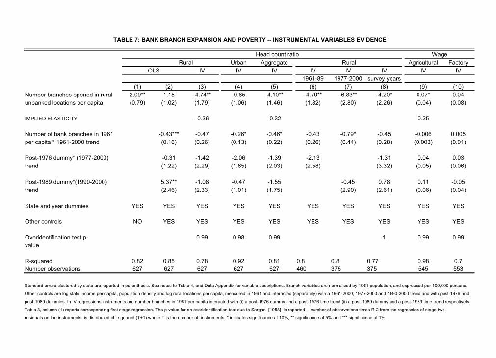
Urban Aggregate Agricultural FactoryIV IV IV IV IV IV IV IV

1961-89 1977-2000 survey years(1) (2) (3) (4) (5) (6) (7) (8) (9) (10)

Number branches opened in rural 2.09** 1.15 -4.74** -0.65 -4.10** -4.70** -6.83** -4.20* 0.07* 0.04unbanked locations per capita (0.79) (1.02) (1.79) (1.06) (1.46) (1.82) (2.80) (2.26) (0.04) (0.08)

IMPLIED ELASTICITY -0.36 -0.32 0.25

Number of bank branches in 1961 -0.43*** -0.47 -0.26* -0.46* -0.43 -0.79* -0.45 -0.006 0.005per capita * 1961-2000 trend (0.16) (0.26) (0.13) (0.22) (0.26) (0.44) (0.28) (0.003) (0.01)

Post-1976 dummy* (1977-2000) -0.31 -1.42 -2.06 -1.39 -2.13 -1.31 0.04 0.03trend (1.22) (2.29) (1.65) (2.03) (2.58) (3.32) (0.05) (0.06)

Post-1989 dummy*(1990-2000) 5.37** -1.08 -0.47 -1.55 -0.45 0.78 0.11 -0.05trend (2.46) (2.33) (1.01) (1.75) (2.90) (2.61) (0.06) (0.04)

State and year dummies YES YES YES YES YES YES YES YES YES YES

Other controls NO YES YES YES YES YES YES YES YES YES

Overidentification test p- 0.99 0.98 0.99 1 0.99 0.99value

R-squared 0.82 0.85 0.78 0.92 0.81 0.8 0.8 0.77 0.98 0.7Number observations 627 627 627 627 627 460 375 375 545 553

Standard errors clustered by state are reported in parenthesis. See notes to Table 4, and Data Appendix for variable descriptions. Branch variables are normalized by 1961 population, and expressed per 100,000 persons.

Other controls are log state income per capita, population density and log rural locations per capita, measured in 1961 and interacted (separately) with a 1961-2000; 1977-2000 and 1990-2000 trend and with post-1976 and

post-1989 dummies. In IV regressions instruments are number branches in 1961 per capita interacted with (i) a post-1976 dummy and a post-1976 time trend (ii) a post-1989 dummy and a post-1989 time trend respectively.

Table 3, column (1) reports corresponding first stage regression. The p-value for an overidentification test due to Sargan [1958] is reported -- number of observations times R-2 from the regression of stage two

residuals on the instruments is distributed chi-squared (T+1) where T is the number of instruments. * indicates significance at 10%, ** significance at 5% and *** significance at 1%

OLS

TABLE 7: BANK BRANCH EXPANSION AND POVERTY -- INSTRUMENTAL VARIABLES EVIDENCE

WageRural

Head count ratioRural

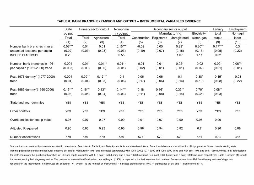
State Non-prima Tertiary Employmentoutput ry output Electricity, total Non-agriTotal Total Agriculture Total Construction Registered Unregistered water, gas output labor(1) (2) (3) (4) (5) (6) (7) (8) (9) (10)

Number bank branches in rural 0.08*** 0.04 0.01 0.15*** -0.09 0.05 0.29* 0.30** 0.17*** 0.3unbanked locations per capita (0.02) (0.03) (0.03) (0.03) (0.19) (0.07) (0.15) (0.13) (0.05) (0.22)IMPLIED ELASTICITY 0.29 0.55 1.07 1.11 0.62

Number bank branches in 1961 0.004 -0.01* -0.01** 0.01** -0.01 0.01 0.02* -0.02 0.02* 0.06***per capita * (1961-2000) trend (0.003) (0.00) (0.00) (0.01) (0.02) (0.01) (0.01) (0.02) (0.01) (0.01)

Post-1976 dummy* (1977-2000) 0.004 0.09** 0.12*** -0.1 0.06 0.06 -0.1 0.38* -0.15* -0.03trend (0.04) (0.04) (0.03) (0.06) (0.17) (0.06) (0.14) (0.19) (0.08) (0.22)

Post-1989 dummy*(1990-2000) 0.15*** 0.16*** 0.13** 0.14*** 0.18 0.16* 0.33** 0.70* 0.08**trend (0.03) (0.05) (0.04) (0.03) (0.11) (0.08) (0.14) (0.35) (0.03)

State and year dummies YES YES YES YES YES YES YES YES YES YES

Other controls YES YES YES YES YES YES YES YES YES YES

Overidentification test p-value 0.98 0.97 0.97 0.99 0.91 0.97 0.99 0.98 0.99

Adjusted R-squared 0.96 0.93 0.93 0.96 0.98 0.94 0.82 0.7 0.96 0.88

Number observations 579 579 579 579 577 579 579 561 573 365

Standard errors clustered by state are reported in parenthesis. See notes to Table 4, and Data Appendix for variable descriptions. Branch variables are normalized by 1961 population. Other controls are log state

income, population density and log rural locations per capita, measured in 1961 and interacted (separately) with 1961-2000; 1977-2000 and 1990-2000 trend and with post-1976 and post-1989 dummies. In IV regressions

the instruments are the number of branches in 1961 per capita interacted with (i) a post-1976 dummy and a post-1976 time trend (ii) a post-1989 dummy and a post-1989 time trend respectively. Table 3, column (1) reports

the corresponding first stage regression. The p-value for an overidentification test due to Sargan [1958] is reported -- the test assumes that number of observations times R-2 from the regression of stage two

residuals on the instruments is distributed chi-squared (T+1) where T is the number of instruments. * indicates significance at 10%, ** significance at 5% and *** significance at 1%

TABLE 8: BANK BRANCH EXPANSION AND OUTPUT -- INSTRUMENTAL VARIABLES EVIDENCE

Primary sector output Secondary sector outputManufacturing

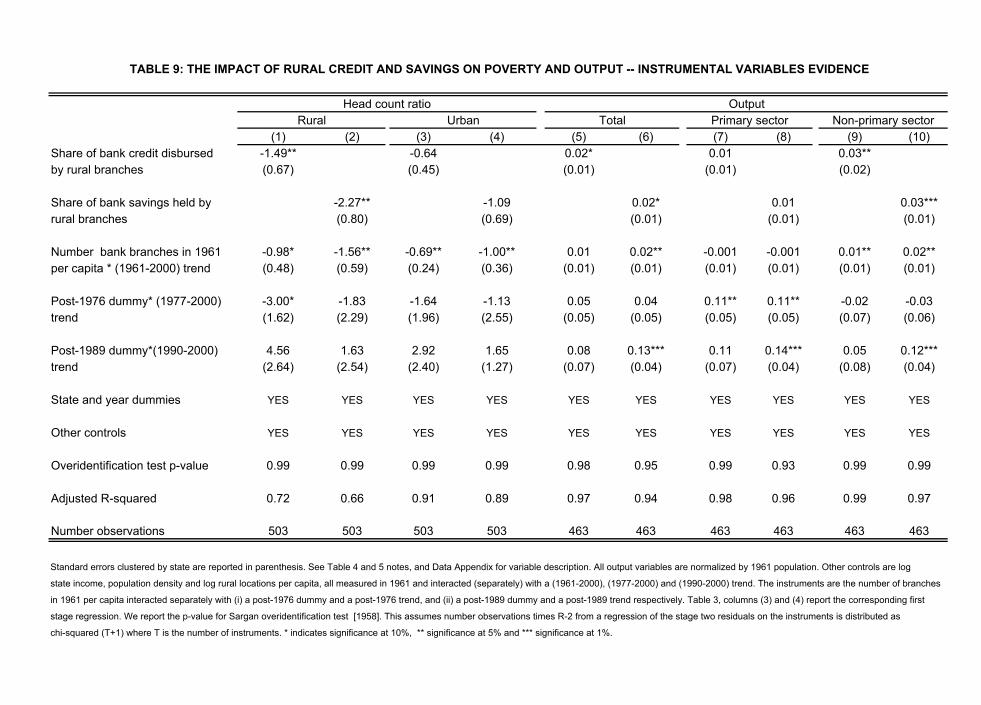
(1) (2) (3) (4) (5) (6) (7) (8) (9) (10)Share of bank credit disbursed -1.49** -0.64 0.02* 0.01 0.03**by rural branches (0.67) (0.45) (0.01) (0.01) (0.02)

Share of bank savings held by -2.27** -1.09 0.02* 0.01 0.03***rural branches (0.80) (0.69) (0.01) (0.01) (0.01)

Number bank branches in 1961 -0.98* -1.56** -0.69** -1.00** 0.01 0.02** -0.001 -0.001 0.01** 0.02**per capita * (1961-2000) trend (0.48) (0.59) (0.24) (0.36) (0.01) (0.01) (0.01) (0.01) (0.01) (0.01)

Post-1976 dummy* (1977-2000) -3.00* -1.83 -1.64 -1.13 0.05 0.04 0.11** 0.11** -0.02 -0.03trend (1.62) (2.29) (1.96) (2.55) (0.05) (0.05) (0.05) (0.05) (0.07) (0.06)

Post-1989 dummy*(1990-2000) 4.56 1.63 2.92 1.65 0.08 0.13*** 0.11 0.14*** 0.05 0.12***trend (2.64) (2.54) (2.40) (1.27) (0.07) (0.04) (0.07) (0.04) (0.08) (0.04)

State and year dummies YES YES YES YES YES YES YES YES YES YES

Other controls YES YES YES YES YES YES YES YES YES YES

Overidentification test p-value 0.99 0.99 0.99 0.99 0.98 0.95 0.99 0.93 0.99 0.99

Adjusted R-squared 0.72 0.66 0.91 0.89 0.97 0.94 0.98 0.96 0.99 0.97

Number observations 503 503 503 503 463 463 463 463 463 463

Standard errors clustered by state are reported in parenthesis. See Table 4 and 5 notes, and Data Appendix for variable description. All output variables are normalized by 1961 population. Other controls are log

state income, population density and log rural locations per capita, all measured in 1961 and interacted (separately) with a (1961-2000), (1977-2000) and (1990-2000) trend. The instruments are the number of branches

in 1961 per capita interacted separately with (i) a post-1976 dummy and a post-1976 trend, and (ii) a post-1989 dummy and a post-1989 trend respectively. Table 3, columns (3) and (4) report the corresponding first

stage regression. We report the p-value for Sargan overidentification test [1958]. This assumes number observations times R-2 from a regression of the stage two residuals on the instruments is distributed as

chi-squared (T+1) where T is the number of instruments. * indicates significance at 10%, ** significance at 5% and *** significance at 1%.

OutputNon-primary sector

Head count ratio

TABLE 9: THE IMPACT OF RURAL CREDIT AND SAVINGS ON POVERTY AND OUTPUT -- INSTRUMENTAL VARIABLES EVIDENCE

Rural Urban Total Primary sector

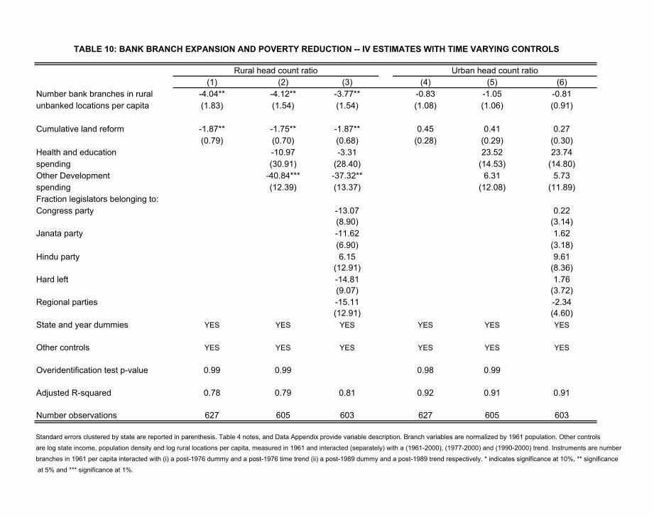
(1) (2) (3) (4) (5) (6)Number bank branches in rural -4.04** -4.12** -3.77** -0.83 -1.05 -0.81unbanked locations per capita (1.83) (1.54) (1.54) (1.08) (1.06) (0.91)

Cumulative land reform -1.87** -1.75** -1.87** 0.45 0.41 0.27(0.79) (0.70) (0.68) (0.28) (0.29) (0.30)

Health and education -10.97 -3.31 23.52 23.74spending (30.91) (28.40) (14.53) (14.80)Other Development -40.84*** -37.32** 6.31 5.73spending (12.39) (13.37) (12.08) (11.89)Fraction legislators belonging to:Congress party -13.07 0.22

(8.90) (3.14)Janata party -11.62 1.62

(6.90) (3.18)Hindu party 6.15 9.61

(12.91) (8.36)Hard left -14.81 1.76

(9.07) (3.72)Regional parties -15.11 -2.34

(12.91) (4.60)State and year dummies YES YES YES YES YES YES

Other controls YES YES YES YES YES YES

Overidentification test p-value 0.99 0.99 0.98 0.99

Adjusted R-squared 0.78 0.79 0.81 0.92 0.91 0.91

Number observations 627 605 603 627 605 603

Standard errors clustered by state are reported in parenthesis. Table 4 notes, and Data Appendix provide variable description. Branch variables are normalized by 1961 population. Other controlsare log state income, population density and log rural locations per capita, measured in 1961 and interacted (separately) with a (1961-2000), (1977-2000) and (1990-2000) trend. Instruments are numberbranches in 1961 per capita interacted with (i) a post-1976 dummy and a post-1976 time trend (ii) a post-1989 dummy and a post-1989 trend respectively. * indicates significance at 10%, ** significance at 5% and *** significance at 1%.

TABLE 10: BANK BRANCH EXPANSION AND POVERTY REDUCTION -- IV ESTIMATES WITH TIME VARYING CONTROLS

Urban head count ratioRural head count ratio

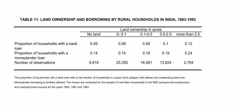
No land 0- 0.1 0.1-0.5 0.5-2.5 more than 2.5

Proportion of households with a bank 0.09 0.08 0.09 0.1 0.12loanProportion of households with a 0.14 0.15 0.18 0.19 0.24moneylender loanNumber of observations 9,619 25,350 16,581 13,824 2,764

The proportion of households with a bank loan refer to the fraction of households in a given land category with atleast one outstanding bank loan.

Moneylender borrowing is similarly defined. The means are computed for the sample of rural labor households in the NSS quinquennial employment

and unemployment surveys for the years 1983, 1987 and 1993.

Land ownership in acres

TABLE 11: LAND OWNERSHIP AND BORROWING BY RURAL HOUSEHOLDS IN INDIA, 1983-1993

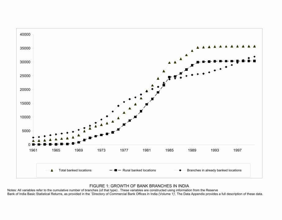
0

5000

10000

15000

20000

25000

30000

35000

40000

1961 1965 1969 1973 1977 1981 1985 1989 1993 1997

Total banked locations Rural banked locations Branches in already banked locations

FIGURE 1: GROWTH OF BANK BRANCHES IN INDIA Notes: All variables refer to the cumulative number of branches (of that type) . These variables are constructed using information from the Reserve Bank of India Basic Statistical Returns, as provided in the `Directory of Commercial Bank Offices in India (Volume 1)', The Data Appendix provides a full description of these data.

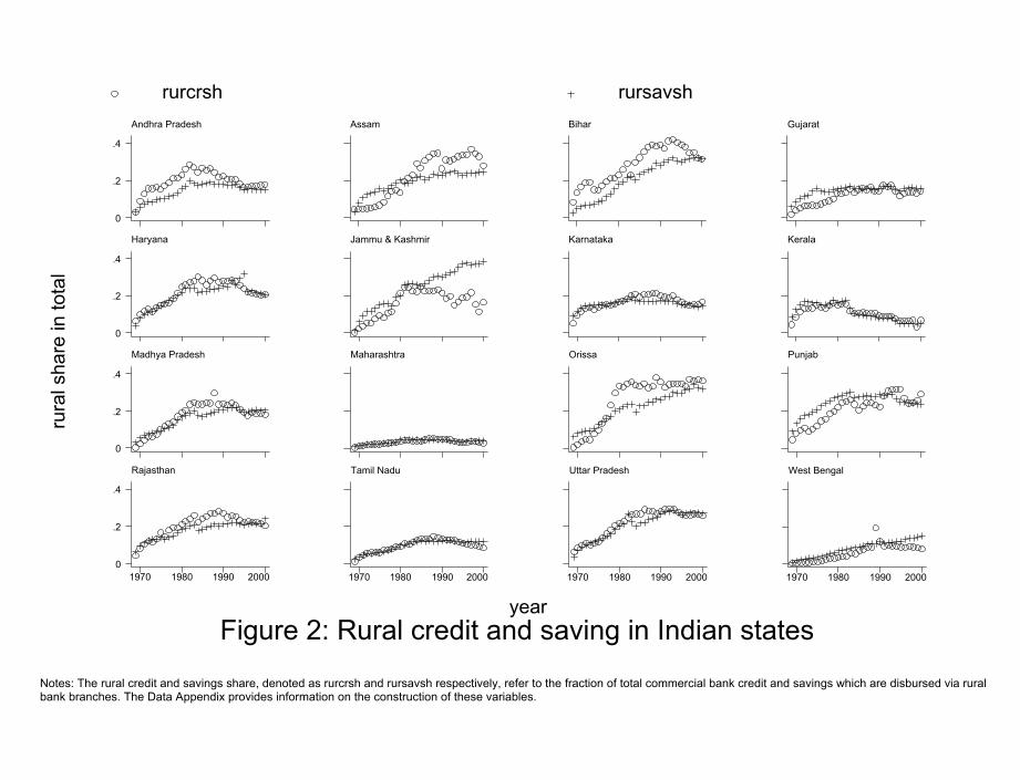
rura

l sha

re in

tota

l

Figure 2: Rural credit and saving in Indian statesyear

rurcrsh rursavshAndhra Pradesh

0

.2

.4

Assam Bihar Gujarat

Haryana

0

.2

.4

Jammu & Kashmir Karnataka Kerala

Madhya Pradesh

0

.2

.4

Maharashtra Orissa Punjab

Rajasthan

1970 1980 1990 20000

.2

.4

Tamil Nadu

1970 1980 1990 2000

Uttar Pradesh

1970 1980 1990 2000

West Bengal

1970 1980 1990 2000

Notes: The rural credit and savings share, denoted as rurcrsh and rursavsh respectively, refer to the fraction of total commercial bank credit and savings which are disbursed via rural bank branches. The Data Appendix provides information on the construction of these variables.

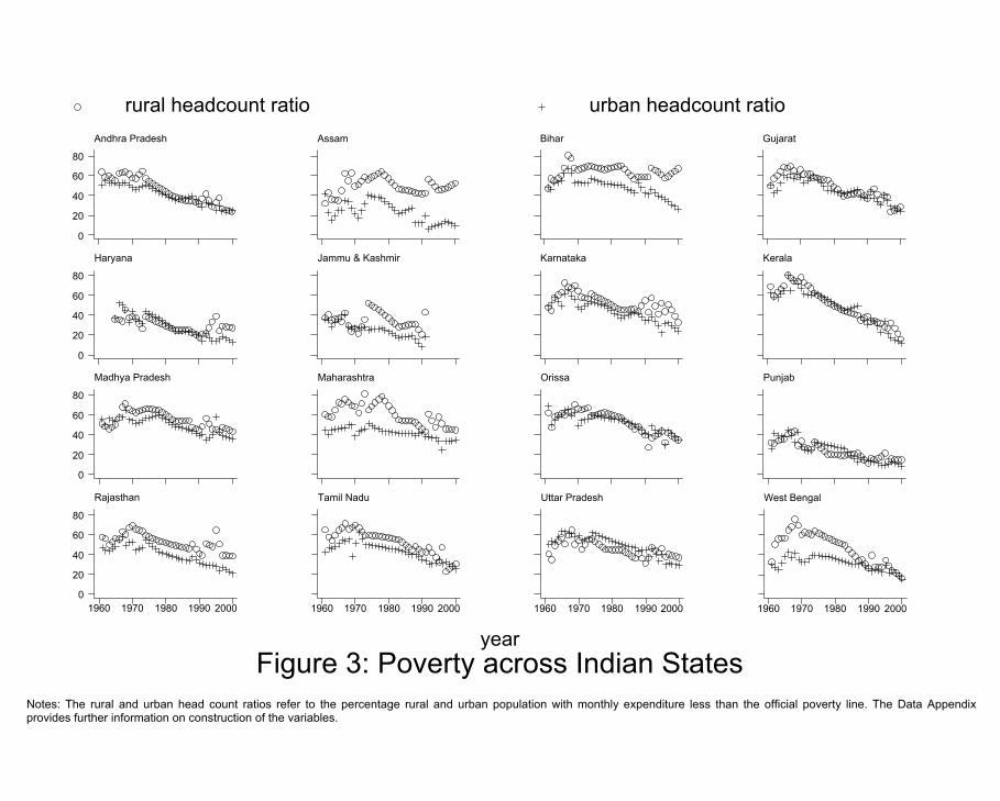
Figure 3: Poverty across Indian Statesyear

rural headcount ratio urban headcount ratioAndhra Pradesh

0

20

40

60

80

Assam Bihar Gujarat

Haryana

0

20

40

60

80

Jammu & Kashmir Karnataka Kerala

Madhya Pradesh

0

20

40

60

80

Maharashtra Orissa Punjab

Rajasthan

1960 1970 1980 1990 20000

20

40

60

80

Tamil Nadu

1960 1970 1980 1990 2000

Uttar Pradesh

1960 1970 1980 1990 2000

West Bengal

1960 1970 1980 1990 2000

Notes: The rural and urban head count ratios refer to the percentage rural and urban population with monthly expenditure less than the official poverty line. The Data Appendix provides further information on construction of the variables.

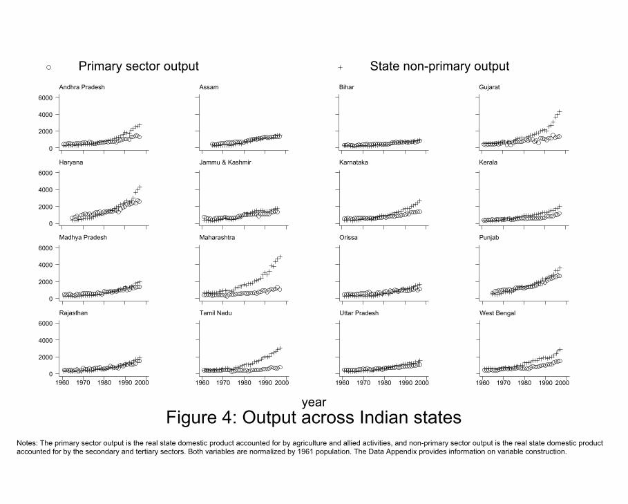
Figure 4: Output across Indian statesyear

Primary sector output State non-primary outputAndhra Pradesh

0

2000

4000

6000Assam Bihar Gujarat

Haryana

0

2000

4000

6000Jammu & Kashmir Karnataka Kerala

Madhya Pradesh

0

2000

4000

6000Maharashtra Orissa Punjab

Rajasthan

1960 1970 1980 1990 20000

2000

4000

6000Tamil Nadu

1960 1970 1980 1990 2000

Uttar Pradesh

1960 1970 1980 1990 2000

West Bengal

1960 1970 1980 1990 2000

Notes: The primary sector output is the real state domestic product accounted for by agriculture and allied activities, and non-primary sector output is the real state domestic product accounted for by the secondary and tertiary sectors. Both variables are normalized by 1961 population. The Data Appendix provides information on variable construction.

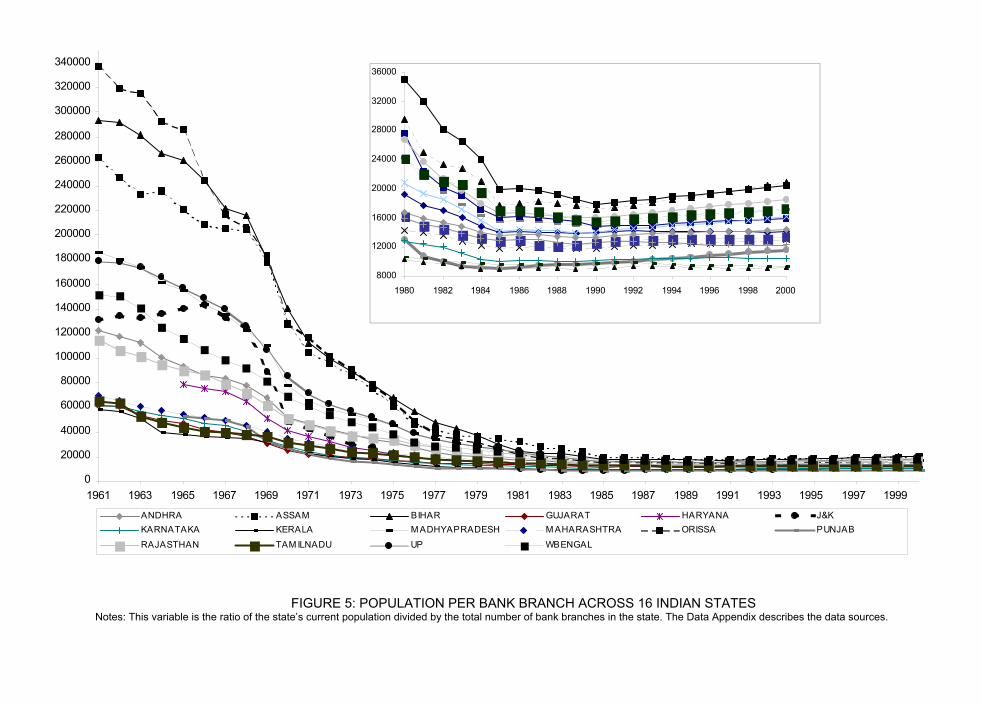
0

20000

40000

60000

80000

100000

120000

140000

160000

180000

200000

220000

240000

260000

280000

300000

320000

340000

1961 1963 1965 1967 1969 1971 1973 1975 1977 1979 1981 1983 1985 1987 1989 1991 1993 1995 1997 1999

ANDHRA ASSAM BIHAR GUJARAT HARYANA J&KKARNATAKA KERALA M ADHYAPRADESH M AHARASHTRA ORISSA PUNJABRAJASTHAN TAM ILNADU UP WBENGAL

8000

12000

16000

20000

24000

28000

32000

36000

1980 1982 1984 1986 1988 1990 1992 1994 1996 1998 2000

FIGURE 5: POPULATION PER BANK BRANCH ACROSS 16 INDIAN STATES

Notes: This variable is the ratio of the state’s current population divided by the total number of bank branches in the state. The Data Appendix describes the data sources.

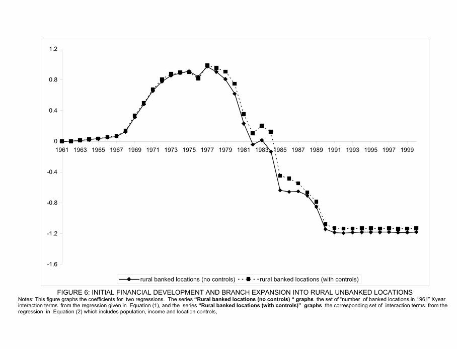
-1.6

-1.2

-0.8

-0.4

0

0.4

0.8

1.2

1961 1963 1965 1967 1969 1971 1973 1975 1977 1979 1981 1983 1985 1987 1989 1991 1993 1995 1997 1999

rural banked locations (no controls) rural banked locations (with controls)

FIGURE 6: INITIAL FINANCIAL DEVELOPMENT AND BRANCH EXPANSION INTO RURAL UNBANKED LOCATIONS Notes: This figure graphs the coefficients for two regressions. The series “Rural banked locations (no controls) “ graphs the set of “number of banked locations in 1961” Xyear interaction terms from the regression given in Equation (1), and the series “Rural banked locations (with controls)” graphs the corresponding set of interaction terms from the regression in Equation (2) which includes population, income and location controls,

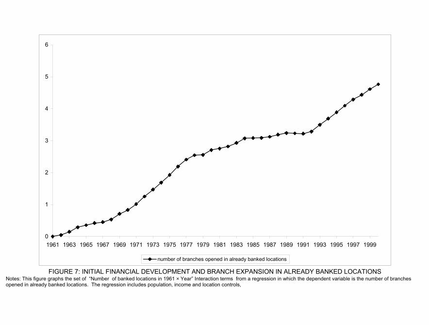
0

1

2

3

4

5

6

1961 1963 1965 1967 1969 1971 1973 1975 1977 1979 1981 1983 1985 1987 1989 1991 1993 1995 1997 1999

number of branches opened in already banked locations

FIGURE 7: INITIAL FINANCIAL DEVELOPMENT AND BRANCH EXPANSION IN ALREADY BANKED LOCATIONS Notes: This figure graphs the set of “Number of banked locations in 1961 × Year” Interaction terms from a regression in which the dependent variable is the number of branches opened in already banked locations. The regression includes population, income and location controls,

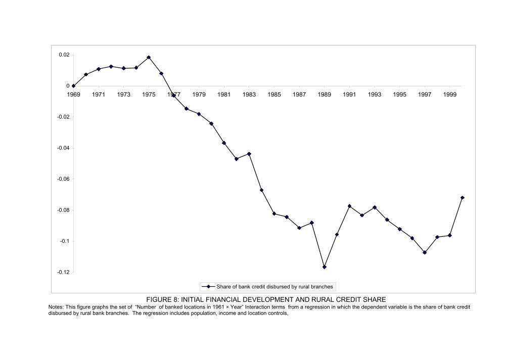
-0.12

-0.1

-0.08

-0.06

-0.04

-0.02

0

0.02

1969 1971 1973 1975 1977 1979 1981 1983 1985 1987 1989 1991 1993 1995 1997 1999

Share of bank credit disbursed by rural branches

FIGURE 8: INITIAL FINANCIAL DEVELOPMENT AND RURAL CREDIT SHARE Notes: This figure graphs the set of “Number of banked locations in 1961 × Year” Interaction terms from a regression in which the dependent variable is the share of bank credit disbursed by rural bank branches. The regression includes population, income and location controls,

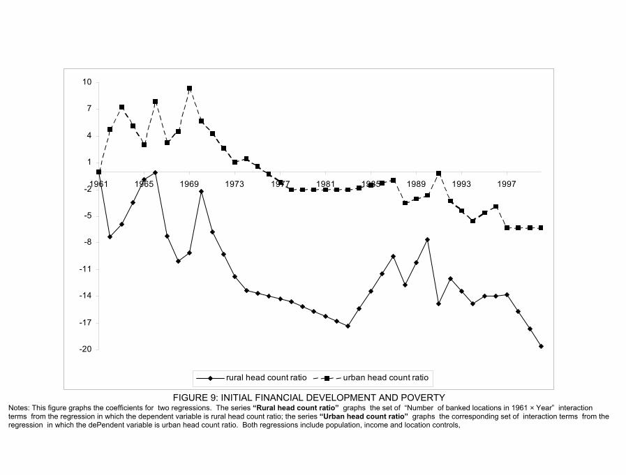
-20

-17

-14

-11

-8

-5

-2

1

4

7

10

1961 1965 1969 1973 1977 1981 1985 1989 1993 1997

rural head count ratio urban head count ratio

FIGURE 9: INITIAL FINANCIAL DEVELOPMENT AND POVERTY Notes: This figure graphs the coefficients for two regressions. The series “Rural head count ratio” graphs the set of “Number of banked locations in 1961 × Year” interaction terms from the regression in which the dependent variable is rural head count ratio; the series “Urban head count ratio” graphs the corresponding set of interaction terms from the regression in which the dePendent variable is urban head count ratio. Both regressions include population, income and location controls,