Do Social Networks Solve Information Problems for Peer-to-Peer

Lending? Evidence from Prosper.com∗

Seth Freedman

University of Maryland

Ginger Zhe Jin

University of Maryland & NBER

November 19, 2008

Warning: This is an academic study using Prosper data from June 1, 2006 through July

31, 2008. Readers should not use it as an investment guide. Because none of the Prosper loans

have reached their regular maturity, the loan performance reported in this paper is up to data

availability as of August 1, 2008 (our data download date). Consequently, the estimated rate of

return entails a number of assumptions. Any conclusion drawn from our study is subject to the

validity of these assumptions.

JEL: D45, D53, D8, L81∗Seth Freedman, Department of Economics, University of Maryland, College Park. Phone: 301-405-3266,

Email: freedman-s@econ.umd.edu. Ginger Zhe Jin, Department of Economics, University of Maryland, College

Park. Phone: 301-405-3484, Fax: 301-405-3542, Email: jin@econ.umd.edu. We received constructive comments

from Larry Ausubel, Robert Hampshire, John Haltiwanger, Anton Korinek, Haim Mendelson and Phillip Leslie.

Special thanks to Chris Larsen, Kirk Inglis, Nancy Satoda, Reagan Murray, Anurag Malik, and other Prosper

personnel for providing us detailed information about prosper.com, to Jim Bruene for helping us understand the

lending industry in general, and to Adam Weyeneth and other prosper lenders for sharing with us their experience

on prosper.com. We are grateful to the UMD Department of Economics, the Kauffman Foundation, and the Net

Institute (www.netinst.org) for their generous financial support. An earlier draft has been circulated under the

title “Dynamic Learning and Selection.” In comparison, this draft has updated the data from December 2007

to July 2008 and corrected several mistakes in the data work. All the remaining errors are our own. All rights

reserved.

1

Abstract

This paper studies peer-to-peer (p2p) lending on the Internet. Prosper.com, the first

p2p lending website in the US, matches individual lenders and borrowers for unsecured

consumer loans. Using transaction data from June 1, 2006 to July 31, 2008, we examine

what information problems exist on Prosper and whether social networks help alleviate the

information problems.

As we expect, data identifies three information problems on Prosper.com. First, Prosper

lenders face extra adverse selection because they observe categories of credit grades rather

than the actual credit scores. This selection is partially offset when Prosper posts more

detailed credit information on the website. Second, many Prosper lenders have made mistakes

in loan selection but they learn vigorously over time. Third, as Stiglitz and Weiss (1981)

predict, a higher interest rate can imply lower rate of return because higher interest attracts

lower quality borrowers.

Micro-finance theories argue that social networks may identify good risks either because

friends and colleagues observe the intrinsic type of borrowers ex ante or because the moni-

toring within social networks provides a stronger incentive to pay off loans ex post. We find

evidence both for and against this argument. For example, loans with friend endorsements

and friend bids have fewer missed payments and yield significantly higher rates of return

than other loans. On the other hand, the estimated returns of group loans are significantly

lower than those of non-group loans. That being said, the return gap between group and

non-group loans is closing over time. This convergence is partially due to lender learning

and partially due to Prosper eliminating group leader rewards which motivated leaders to

fund lower quality loans in order to earn the rewards.

1 Introduction

The idea of using the Internet as a platform for peer-to-peer (p2p) transactions has extended

to job search, dating, social networks, and other every day interaction. A relatively new exam-

ple is finance. The past three years have witnessed 12 new consumer lending websites opening

around the world, all aiming to link individual borrowers with individual lenders without finan-

cial institutions as an intermediary. What kind of credit risks are listed and funded on these

platforms? On what grounds will p2p lending differ from and compete with traditional banks?

How do individual borrowers and lenders behave in p2p lending? Will P2P lending define the

future of consumer finance, or is it a fad to wane over time? Answers to these questions are not

only important for the long-run viability of p2p platforms, but will deepen the understanding of

social interactions and help reshape policies that target the functionality of financial markets.

This paper is the first attempt to address these questions using transaction level data from

Prosper.com.1 As the first P2P lending website in the US2, Prosper.com has attracted 750,000

members and originated loans of over 160 million dollars in 2.5 years. Aside from operation

style3, Prosper.com differs from a traditional lending market in two ways.

First, although Prosper lenders face a traditional information imperfection in assessing bor-

rower risk, anonymous online interaction presents new challenges that do not apply to traditional

banks. For instance, Prosper only posts a categorical credit grade for each borrower, so the lender

never observes the borrowers exact credit score. Furthermore, individual lenders, by definition

smaller and less professional than financial institutions, may not have the expertise to predict

and screen risks. Even if they can, most loans are funded by multiple lenders (for the purpose

of risk diversification), and therefore each individual lender may lack the incentive to gather

information before funding and monitor performance after funding.4

1Hampshire (2008) has studied lender perception of group variables on Prosper, but he focuses on group listings

only and does not analyze loan performance.2Zopa.com (of UK) is the first peer-to-peer lending website world wide.3Prosper.com automates the borrower-lender match via real-time auctions. With sufficient scale, this format

may generate significant savings in operation costs, implying lower interest rates for individual borrowers and

better returns for individual lenders. Unfortunately, we do not have sufficient data to measure the cost difference.4In the recent subprime mortgage crisis, a similar argument may apply to those traditional lenders that initiate

high risk loans, repackage them in securities, and spread the risk to the rest of the market. In this sense, it is

unclear whether p2p lenders have more or less incentives to care about the loan performance as compared to

traditional lenders.

1

The second difference between p2p and traditional lending is the formers ability to utilize

social networks. Prosper.com encourages borrowers and lenders to form online groups and estab-

lish friendships with other members. It allows group leaders and friends to offer endorsements

for a specific listing and highlights bids from group members, endorsing group leaders, and en-

dorsing friends. Like other micro-finance approaches, it is hoped that p2p lending can better

utilize the social ties among its individual members. Coupled with the potential for the Internet

to facilitate information flow among borrowers and lenders, the “soft” information conveyed via

social networks may compensate for the lack of “hard” information on Prosper. However, unlike

group lending in the Grameen Bank (Yunus 2003), the social networks permitted on Prosper do

not impose joint liability within the network. That being said, social networks, especially those

with offline ties, may still identify good risks if friends and colleagues observe the intrinsic type

of borrowers ex ante or the monitoring within social networks provides a stronger incentive to

pay back ex post (Stiglitz 1990, Arnott and Stiglitz 1991, Besley, Coate and Loury 1993, Besley

and Coate 1995). Whether these features hold in reality is an empirical question.

Aware of these issues, Prosper.com has implemented a series of policies to minimize its

disadvantage in information access and strengthen its advantage in social networks. The first

and foremost policy is information transparency: before listing a loan request, Prosper.com

authenticates the identity of each borrower (by checking her social security number), extracts

the borrower’s credit history from a third party credit bureau (Experian), and posts credit grades

and historical credit information in the borrower’s listing.5 In addition, Prosper.com posts all

of the up-to-date Prosper activities, from listing to loan performance, on its website.6 In theory,

every potential lender can look at the complete collection of prosper “books” before lending. As

detailed in Section 2, both the extent of transparency and the nature of Prosper networks have

evolved over time.

Using transaction data from June 1, 2006 to July 31, 2008, we present evidence of three

information problems on Prosper: first, Prosper lenders face extra adverse selection because

they observe categories of credit grades rather than the actual credit scores. We show that,

although the overall Prosper market has moved towards better credit grades, over time there

are more listings and more loans towards the lower end of each grade. This selection is partially

offset by increasing interest rates in these intervals when Prosper begins to post more detailed5If a borrower defaults, she is not allowed to borrow any more from Prosper.com and the default is reported

to the credit bureau.6In fact, the transparency policy has spawned a number of user-generated websites that summarize the Prosper

statistics in real time.

2

credit information on the website. Second, many Prosper lenders make mistakes in loan selection

and therefore have a negative rate of return on their portfolios, but they learn vigorously and

the learning speeds up over time. Third, as Stiglitz and Weiss (1981) predict (for traditional

lending), a higher interest rate may imply a lower (financial) rate of return because higher

interest attracts lower quality borrowers. We show that, the estimated internal rate of return

(IRR) is a non-monotone function of interest rate reaching a peak when the interest rate is 8-9%

and then decreasing until the interest rate is above 28%.

While abundant evidence points to information problems on Propser.com, a key question

is whether social networks help alleviate the problems. We find evidence that social networks

do help identify quality borrowers when a borrower’s listing is endorsed by her friend and this

friend bids on the listing. In fact, loans with friend endorsement and friend bids tend to have

less missed payments and yield significantly higher rates of return than other loans. This result

suggests that the market may under-estimate the positive signaling effect of friend endorsement

plus bid. In contrast, loans with friend endorsement but no bid generate a lower rate of return

than the loans without endorsements, implying that the market does not discount the negative

signal of friend endorsement alone to the full extent.

On average Prosper groups do not succeed in identifying high quality borrowers. The esti-

mated rate of return is significantly lower for group loans; however, the gap has been closing

over time. This convergence is partially due to lender learning and partially due to Prosper

eliminating group leader rewards which motivated leaders to fund lower quality loans in order

to earn the rewards.

Additionally, there is a large amount of heterogeneity among group loans: we observe better

performance and higher returns if a group borrower is endorsed by the group leader but receives

no bid from the leader, if the group borrower belongs to a group that is small and less borrower-

concentrated, if the loan attracts a greater percent of funding from its own group members, and

if the group is formed based on alumni or other tangible connections. Overall, these results

suggest that Prosper groups have the potential to clear some information hurdles if the group

is designed with the correct incentives.

Our work contributes to a number of literatures. As Stiglitz and Weiss (1981) point out,

the information asymmetry between lenders and borrowers leads to credit rationing. While

many papers using offline data have found evidence of credit rationing (e.g. Jaffee 1971, Cox

and Japelli 1990, Berger and Udell 1992, Voridis 1993) and liquidity constraints (e.g. Souleles

3

1999, Parker 1999, Gross and Souleles 2002, Adam, Einov and Levin 2007), we have a rare

opportunity to directly test the non-monotonic relationship between rate of return and interest

rate. As the loan performance unravels and Prosper lenders learn from mistakes, we observe a

dynamic evolution toward credit rationing based on the “hard” information in the borrower’s

credit profile.

Our paper also relates to the literature of informal lending and micro-finance. Previous

researchers have argued that informal lenders and micro-finance institutions have an information

advantage over traditional banks because they utilize borrowers’ social networks to ensure good

risks (e.g. La Ferrara 2003, Udry 1994, Hoff and Stiglitz 1990). We show evidence both for and

against this argument. It seems some social networks permitted on Prosper can clear information

hurdles if they face the right incentives. If well understood by the market, “soft” information

provided by social networks could contribute to an alleviation of credit rationing.

Finally, as a fresh example of an online marketplace, the experience of Prosper highlights

the role that information and social relationships can play in the rise of e-commerce. Unlike

previous studies that document the segmentation between online and offline markets (Jin and

Kato 2007, Hendal, Nevo and Ortalo-Magne 2008), we show that Prosper is converging with the

traditional market except for the positive signals contained in some social network variables.

The rest of the paper is organized as follows. Section 2 describes the background of Pros-

per.com and its major competitors in traditional lending. Section 3 describes the data, defines

the sample, and provides a simple summary of the Prosper population over time. Section 4

presents evidence for three types of information problems. Section 5 lists the potential roles of

social networks and tests them in the data. A short conclusion is offered in Section 6.

2 Background

After two years of development, Prosper officially opened to the public on February 13, 2006.

The launch attracted significant media coverage including features in Business Week, the Wall

Street Journal, and ABC’s World News Tonight. As of August 1, 2008, Prosper had registered

750,000 members and originated 26,273 loans that total over 164 million US dollars. The quick

expansion of Prosper has coincided with a number of similar new p2p lending sites in the US.7

7The best known examples are Kiva.org (incorporated November 05), Smava (launched in February 2007),

Lending Club (open May 24, 2007 as part of Facebook), MyC4 (launched in May 2007), Globefunder (launched

4

In this section we describe the specifics of the Prosper market place, policy changes that have

occurred since its inception, and the parameters of Prosper’s social networks. Finally we discuss

Prosper’s competition from traditional credit markets and the changes in the macroeconomic

environment that coincide with our study period.

2.1 Market Setup

All Prosper loans are fixed rate, unsecured, three-year, and fully amortized with simple interest.

Loan can range from $1,000 to $25,000. There is no penalty for early payment. As of today, the

loans are not tradable in any financial market8, which means a lender that funds a loan is tied

up with the loan until full payment or default. Upon default Prosper hires collection agencies

and any money retrieved in collections is returned to the loan’s lenders.

Before listing on Prosper, a potential borrower must file a short application so that Prosper

can authenticate the applicant’s social security number, driver’s license, and address. Prosper

also pulls the borrower’s credit history from Experian, which includes the borrower’s credit score

and historical credit information such as total number of delinquencies, current delinquencies,

inquiries in the last six months, etc.9 If the credit score falls into an allowable range, the

borrower may post an eBay-style listing specifying the maximum interest rate she is willing to

pay, the requested loan amount, the duration of the auction (3-10 days)10, and whether she

wants to close the listing immediately after it is fully funded (called autofunding). In the listing,

the borrower may also describe herself, the purpose of the loan, the city of residence, how she

intends to repay the loan, and any other information (including an image) that she feels may

help fund the loan. In the same listing, Prosper will post the borrower’s credit grade (computed

based on credit score), home ownership status, debt-to-income ratio, and other credit history

information.11

Like borrowers, a potential lender must provide a social security number and bank informa-

tion for Prosper to verify identity. Lenders can browse listing pages which include all of the

in Oct. 2, 2007), and Zopa US (us.zopa.com, open December 4, 2007).8In October of 2008, Prosper began the process of registering with the appropriate securities authorities in

order to offer a secondary market.9The credit score reported uses the Experian ScorePLUS model, which is different from a FICO score, because

it intends to better predict risks for new accounts.10As of April 15, 2008 all listings have a duration of 7 days.11The debt information is available from the credit bureau, but income is self-reported. Therefore, the debt-to-

income ratio reported in the listing is not fully objective.

5

information described above, plus information about bids placed, the percent funded, and the

listings current prevailing interest rate. To view historical market data a lender can download

a snapshot of all Prosper records from Prosper.com, use a Prosper tool to query desired statis-

tics, or visit a third party website that summarizes the data. Interviews conducted at the 2008

Prosper Days Conference suggest that there is enormous heterogeneity in lender awareness of

the data, ability to process the data, and intent to track the data over time.

The auction process is similar to proxy bidding on eBay. A lender bids on a listing by

specifying the lowest interest rate he will accept (so long as it is below the borrower’s specified

maximum rate) and the amount of dollars he would like to contribute (any amount above $50).

Most lenders bid a small amount on each loan in order to diversify their Prosper portfolio. A

listing is fully funded if the total amount bid exceeds the borrower’s request. If the borrower

chooses the autofunding option, the auction will end immediately and the borrower’s maximum

interest rate applies. Otherwise, the listing remains open and new bids will compete down the

interest rate. Lenders with the lowest specified minimum interest rate will fund the loan and

the prevailing rate is set as the minimum interest rate specified by the first lender excluded from

funding the loan. We will refer to the resulting interest rate as the contract rate.

Prosper charges fees to both borrowers and lenders. These fees have changed over time,

but in general borrowers pay a closing fee when their loan originates ranging from 1% to 3%

depending on credit grade (there is no fee for posting a listing). If a borrower’s monthly payment

is 15 days late, a late fee is charged to the borrower and transferred to lenders in the full amount.

Prosper does not acquire anything in this process. Lenders are charged an annual servicing fee

based on the current outstanding loan principal12. The lender fee has ranged from 0.5% to 1%

depending on credit grade.

In legal terms, Prosper loans are first issued by Prosper and then sold to individual lenders.

Prior to April 15, 2008, Prosper was subject to state usury laws which specify the maximum

interest rate a lender could charge. The binding law was that of the borrower’s state of residence,

and within each state regulations depended on whether Prosper held a consumer loan license

in that state. The interest rate caps varied from 6% to 36% across states. On April 15, 2008,

Prosper became a partner of WebBank, a Utah-chartered industrial bank, which allows the site

to circumvent most state usury laws. Following this partnership, the interest rate cap became a

universal Prosper implemented 36% (except for Texas and South Dakota).12This fee is accrued the same way that regular interest is accrued on the loan.

6

2.2 Information Policies

Prosper has continually changed the information that it provides lenders. The policy changes

are listed in Table 1 and highlighted here. Originally, the only credit information posted on

Prosper was debt-to-income ratio and credit grade. Credit grades are reported in categories,

where grade AA is defined as 760 or above, A as 720-759, B as 680-719, C as 640-679, D as

600-639, E as 540-599, HR as less than 540, and NC if no credit score is available. The numerical

credit score is never available to lenders. On April 19, 2006, Prosper started to post whether

the borrower has a verified bank account at the time of listing and whether the borrower owns

a home.

On May 30, 2006 further credit history information about delinquencies, credit lines, public

records, and credit inquires were reported followed by even more detailed credit information,

self reported income, employment and occupation on February 12, 2007. On this date, lenders

were also allowed to begin asking borrowers questions and the borrowers had the option to post

the Q&A on the listing page. Additionally, Prosper tightened the definition of credit grade E

from 540-599 to 560-599 and grade HR from less than 540 to 520-559 eliminating borrowers who

do not have a credit score (NC) or have a score below 520 from borrowing on the site. The

February 12, 2007 policy changes are likely to particularly impact risk selection on Prosper as

we discuss in Section 4.

The next information change occurred on October 30, 2007, when Prosper began to display

a Prosper-estimated rate of return on the bidding page (bidder guidance). Before the change,

a lender had to visit a separate page to look for the historical performance of similar loans.

Prosper also introduced portfolio plans on October 30, 2007, which allow lenders to specify a

criterion regarding what types of listings they would like to fund and Prosper will place their

bids automatically. These portfolio plans simplified the previously existing standing orders.

2.3 Social Networks on Prosper

A unique feature of Prosper is its use of social networking through groups and friends. A

non-borrowing individual may set up a group on Prosper and become a group leader. The

group leader is responsible for setting up the group web page, recruiting new borrowers into

the group, coaching the borrower members to construct a Prosper listing, and monitoring the

performance of the listings and loans within the group. The group leader does not have any

7

legal responsibility. Rather, the group leader is supposed to foster a “community” environment

within the group so that the group members feel social pressure to pay the loan on time. Group

leaders can also provide an “endorsement” on a member’s listing and bids by group leaders

and group members are highlighted on the listing page. Since October 19, 2006, Prosper has

posted star ratings (one to five) in order to measure how well groups perform against expected

(Experian historical) default rates.13

Prosper groups were initiated as a tool to expand the market, and thus Prosper initially

rewarded a group leader roughly $12 when a group member had a loan funded (Mendelson

2006). Given the fact that borrowing is immediate but payment does not occur until at least

one month later, the group leader reward may have created a perverse incentive to recruit

borrowers without careful screening of credit risk. To the extent that the group leader knows

the borrower in other contexts (e.g. colleagues, college alumni, military affiliation), she could

collect credit-related information via emails, interviews, house visits, employment checks, and

other labor-intensive means.14 However, when a group gets very large (some with over 10,000

members), it becomes difficult if not impossible to closely monitor each loan. The imbalance

between member recruiting and performance monitoring prompted Prosper to discontinue the

group leader reward on September 12, 2007. We will consider these changing incentives when

analyzing the role of groups in the Prosper marketplace.

Starting February 12, 2007, Prosper members could begin to invite their offline friends to

join the website. The inviting friend receives a reward when the new member funds ($25) or

borrows her first loan ($50). Existing Prosper members can become friends as well if they know

each other’s email address but the monetary reward does not apply. Friends can also provide

endorsements on each other’s listings and a bid by a friend is highlighted on the listing page.

Beginning February 23, 2008 lenders could begin including aspects such as friend endorsements

and bids from friends as criteria in their listing searches.

2.4 Who Competes With Prosper in the Traditional Market?

The main competitors Prosper face in the traditional market are credit card issuers. Up to

our observation date (August 1, 2008), 36% of all previous Prosper listings have mentioned

credit card consolidation, which is higher than the mention of business (23%), mortgage (14%),13Groups must have at least 15 loan cycles billed before they are rated, otherwise they are “not yet rated.”14Group leaders do not have access to the borrower’s credit report prior to listing.

8

education (21%), and family purposes (18%) such as weddings.15

According to the Federal Reserve, the total consumer credit outstanding (excluding mort-

gages) was valued at $2.54 trillion in February 2008.16 Within this category, $0.95 trillion was

revolving debts primarily borrowed in the form of credit cards. The rest ($1.58 trillion) were

non-revolving debts including loans for cars, mobile homes, education, boats, trailers, vacations,

etc. By definition, credit card borrowing is not secured by any tangible asset. In contrast,

a large proportion of the non-revolving debt is collateralized by the goods purchased via the

loan, and therefore carries a lower interest rate than credit cards.17 Commercial banks also

issue unsecured personal loans, at an average interest rate of 11.40%. Most Prosper loans carry

an interest rate much higher than the average rate of credit cards, but since we do not know

the credit grade composition of credit card accounts, we are not able to make the comparison

conditional on the same observable attributes. We will revisit this issue in Section 4.

Roughly 6% of Prosper listings mention that the Prosper loan, if funded, will be used to

pay off payday loans in the offline market. Compared to the APR of 528% that Caskey(2005)

reports for payday loans, one may argue Prosper could provide a much better alternative to

payday loans, given the 3-year duration of Prosper loans and the interest rate cap no higher

than 36%. However, lenders must consider the credit risk they face on Prosper. If a payday

lender must charge an annual interest rate of 500% to survive competition (Skiba and Tobachman

2007), it is unclear why Prosper lenders would be willing to support this pool of borrowers with

a much lower interest rate.

2.5 Changes in Macro Environments

The years 2007 and 2008 have witnessed dramatic changes in consumer lending as shown in

Figure 1. Before the subprime mortgage crisis began to grab headlines in August 2007, the

financial market was relatively calm with stable monetary policy. Starting August 9, 2007, the

major indices such as the London Interbank Offered Rate (LIBOR), jumbo mortgage spread, and

the yields of asset-backed commercial paper (ABCP) have all shown abrupt change and increased1569% of listings mention cars, but this is likely a result of borrowers listing their car payments as a monthly

expense.16Source: Federal Reserve G.19 Statistical Release as of April 7, 2008. Based on the Quinquennial Finance

Company Survey 2005, see more details at http://www.federalreserve.gov/releases/g19/ (accessed at April 9,

2008).17e.g. 7.27% for 4-year new-car loans vs. 13.71% for credit card accounts that have assessed interest.

9

volatility. The Senior Loan Officer Survey (conducted quarterly by the Federal Reserve) also

reveals progressive tightening of credit standards on a wide variety of loans, including prime

and subprime mortgages, commercial & industrial loans, and credit cards. In response, the Fed

funds rate has fallen from 5.41% (August 9, 2007) to 2.04% (August 1, 2008). It is clear that

the macro environment changes are primarily driven by the subprime mortgage crisis, and the

crisis spills over to other types of lending and investment.

Given the drastic changes in the macro environment during our study period, our analysis

controls for a number of macroeconomic variables. At the daily level we include the bank prime

rate, which tracks the Fed funds rate with a 0.99 correlation, the TED spread (the difference

between 3-month LIBOR and 3-month Treasury bills), the yield difference between corporate

bonds rated AAA and BAA, and S&P 500 closing quotes. According to Greenlaw et al. (2008),

the middle two are the strongest indicators of the subprime mortgage crisis. Additionally, we

include the unemployment rate reported by the Bureau of Labor Statistics (BLS) by state

and month, the housing price index reported by the Office of Federal Housing and Enterprise

Oversight (OFHEO) by state and quarter, and the quarterly percentage of senior loan officers

that have eased or tightened credit standards for consumer loans, and the foreclosure rate

reported by Realtytrac.com by state and month.

In addition, we control for a number of daily Prosper-specific market characteristics, includ-

ing the total value of active loan requests by credit grade, the total dollar amount of submitted

bids by credit grade, and the percentage of funded loans that have ever been late by credit

grade. The first two variables intend to capture the overall traffic on Prosper, which may vary

by media coverage, word of mouth, or the mood of borrowers and lenders. The percent ever late

intends to capture the ex-post performance of the Prosper market as a whole, so as to track the

performance evolution that lenders may observe on Prosper over time. Because the financial

turmoil observed in the macro environment is rooted in the subprime mortgage crisis, we control

for the interaction of the OFHEO foreclosure rate and the borrower’s home owner status and

consumer loan easing and tightening with whether the borrower has a credit grade of E or HR.

It is worth noting that most of the time-series variables, except for those specific to day, state

or credit grade, will be absorbed in year-week fixed effects. Whenever possible, we estimate

specifications with and without these fixed effects for robustness.

10

3 Data

In addition to macroeconomic indicators described above, our study utilizes data publicly avail-

able for download from Prosper’s website and a private data set provided to us by Prosper.

The main data set is downloaded on August 1, 2008. This data set includes all of the

information available to borrowers and lenders on the website since Prosper’s inception. For each

listing it contains the credit variables extracted from Experian credit reports, the description

and image information that the borrower posts, and a list of auction parameters chosen by the

borrower. For those listings that become loans, we observe the full payment history up to the

download date. For each Prosper member we observe their group affiliation and their network

of friends.18 Finally, we observe data on all Prosper bids allowing us to construct each lender’s

portfolio on any given day.

We also utilize a private data set obtained from Prosper that includes the number of listings,

number of loans, average contact interest rate, percent late at 6 months, and percent late at 12

months by state, month and credit score interval. These credit score intervals are finer than the

publicly posted credit grades. For comparison, it also includes Experian data on historical loan

performance in these finer credit intervals for offline consumer loans.

Our sample includes listings that began on or after June 1, 2006 and end on or before July

31, 2008 and the loans that originate from this set of listings. We exclude the few loans that

were suspects of identity theft and as a result repurchased by Prosper. Table 2 summarizes

listings and loans by quarter for this sample. This sample includes 293,808 listings and 25,008

loans for $158.27 million. This implies an average funding rate of 8.51%, though this has varied

over time ranging from 6.32% to 10.14%. Average listing size and average loan size have both

increased through the first half of 2007 and have decreased since. Comparing listings and loans,

the average listing requests $7,592 and the average loan is worth $6,329. This difference is

preliminary evidence of credit rationing. It appears that lenders are wary of listings requesting

larger loans and view this as a signal of higher risk. The average listing lists a maximum borrower

rate of 19.19% while the average contract rate is 17.90%.19

18The data dump reflects information about groups and friends as of the download date. Because these char-

acteristics can change over time, we use monthly downloads beginning in January 2007 to identify these charac-

teristics at the closest possible date to the actual listing.19The sharp increase in borrower maximum rates between the first and second quarters of 2008 reflects the

April 2008 removal of state specific interest rate caps.

11

In terms of social networks, Table 2 suggests that being a group member and having a friend

endorsement increases the likelihood of funding. Both variables have larger representation in

loans than in listings. However, it is striking that the proportion of listings and loans with group

affiliation has decreased drastically from 60% and 70% to 7.5% and 10%, respectively. When

friend and group leader endorsements became available, the percent of listings and loans with

endorsements initially grew but have decreased since the middle of 2007. The only exception is

the percent with friend endorsements plus bids. These patterns call into question the importance

and effectiveness of social networks which we will explore in detail in Section 5.

Table 2 also summarizes the percent of default as observed on August 1, 2008. We define

a loan as in “default” if it is four or more months late or labeled default by Prosper due to

bankruptcy.20 About 30% of loans originating in 2006 have defaulted by August 1, 2008, which

makes it clear that lenders observe negative performance in their portfolios and the overall

market. Note that the proportion of loans in the 2007 and 2008 cohorts that have defaulted are

much lower than in the earlier cohorts as a result of the life cycle of loans.

4 Information Problems

This section presents evidence for three information problems on Prosper.com: (1) adverse selec-

tion due to less credit information on Prosper; (2) lender misinterpretation of listing attributes

because they do not have expertise in consumer lending; and (3) a non-monotone relationship

between rate of return and interest rate because lenders have imperfect information about bor-

rower risk (Stiglitz and Weiss 1981). The last problem is common to all lending, but the first

two are likely unique to p2p lending.

4.1 Adverse selection due to less information on Prosper

The most compelling example for the information difference between traditional and Prosper

lenders is that traditional lenders observe a borrower’s actual credit score but Prosper lenders

only observe a credit grade. Consider two borrowers, one with a credit score of 601 and the other20Once a loan is four months late, Prosper considers it eligible for debt sale, and once it is sold it is considered

to be in default. However, because debt buyers only purchase packages of loans, a four month late loan will not

be considered “default” immediately. Loans can thus be labeled “4+ months late” for long periods of time. Our

default definition overcomes this mechanical ambiguity.

12

639. Traditional lenders observe the exact scores and treat the two differently. But since Prosper

categorizes both as credit grade D, they look identical to Prosper lenders if the other observable

information is the same. According to Akerlof (1970), this will drive the D- borrowers towards

Prosper more often than those with a grade of D+, because Prosper lenders cannot price these

categories differentially. Using the confidential data from Prosper, we observe the distribution

of D- and D+ and its evolution over time.

More specifically, we focus on summary statistics by census division, month, and “half grade.”

Except for the ends of the score distribution (300-900), most half grades are defined as a 20-

point interval of credit scores, for instance, 600-619 (referred to as D-) and 620-639 (D+). In

total, we have 20 half grades, which is much more detailed than the 8 credit grades posted

on Prosper.com.21 Not only does this data allow us to identify adverse selection in the whole

sample of Prosper, we can also test whether such adverse selection is alleviated when Prosper

reveals more detailed credit information or exacerbated when traditional lenders tighten credit

in general.

Table 3 presents the funding rate, interest rate, the percent late, and the percent 3-months

late or worse (as of August 1, 2008) by the 8 credit grades observable to Prosper lenders. As

expected, a better grade means a higher funding rate, lower interest rate, and better loan perfor-

mance. The last two columns attempt to compare Prosper loan performance to all the Experian

accounts that have a new credit line approved in September 2003. Since the performance of

Experian accounts are observed as of September 2005, we summarize the observed 2-year per-

formance for the Prosper loans that were originated in July 2006. While the time horizon of

Prosper and Experian loans are not exactly the same, it is clear that Prosper loans perform

much worse than the traditional Experian accounts.22 One potential explanation is that Pros-

per loan composition is worse than the Experian accounts within each credit grade because

Prosper attracts more borrowers towards the lower end of the grade.

To better reflect the composition difference, Figure 2 compares the c.d.f. of Prosper listings,

Prosper loans, the Experian population, and Experian new accounts across the 20 half grades. By

Experian population, we mean all the accounts that have a score by the Experian ScorexPLUS21The precise definition of the 20 half grades are 300-479, 480-499, 500-519, 520-539 (HR-), 540-559 (HR+),

560-579 (E-), 580-599 (E+), 600-619 (D-), 620-639 (D+), 640-659 (C-), 660-679 (C+), 680-699 (B-), 700-719

(B+), 720-739 (A-), 740-759 (A+), 760-779 (AA-), 780-799 (AA+), 800-819, 820-839, 840-900.22According to the Federal Researve, the credit card charge-off rate has increased from 4.3% in the third quarter

of 2005 to 5.5% in the second quarter of 2008. If we had grade-specific performance data in 2008, the comparison

between traditional and Prosper loans would be less stark.

13

model in December 2003.23 This comparison imperfect because a person may have a record in

Experian but does not demand credit. The Experian new accounts are defined as above, where

the credit could be secured (such as a mortgage) or unsecured (such as a credit card). Even

though the Prosper vs. Experian comparison is imperfect,24 there is no doubt that Propser

listings have much greater concentration on lower credit intervals. Prosper lenders are able to

select better risks from the listing pool, but the overall distribution of Prosper loans is still worse

than that of Experian accounts.

Figures 3 and 4 present the p.d.f. of Prosper listings and Prosper loans by the 20 half

grades and across time. The loan distribution is also compared with the p.d.f. of Experian new

accounts as defined above. Not surprisingly, Prosper attracts listings towards the lowest end of

the credit score distribution (Figure 3) while the traditional lenders tend to focus on the highest

end (Figure 4). These two facts are probably linked – because traditional lenders cannot satisfy

the credit demand of near or subprime risk (due to credit rationing), these risks find Prosper an

attractive alternative.

More interestingly, the Prosper loan distribution is much jumpier than the Experian accounts.

As Figure 4 shows we see a higher frequency at D- than D+, C- than C+, etc. in the Prosper loans

(but not in the Experian accounts), suggesting adverse selection with more Prosper borrowers

appearing in the lower half of each grade. Of course, this evidence is only suggestive because

loans reflect both borrower selection and lender decisions. Given the fact that the Prosper listing

distribution leans toward the very low tail of credit scores, the decline of listing frequency from

the lower end to higher end of each grade could be due to adverse selection or the skewness

itself. Note that the jumpiness of Prosper loans does not disappear over time. The listing and

loan distributions are both moving towards the right, which could be due to the credit crunch in

traditional lending (which forces near prime and prime risks to seek credit on Prosper), Prosper

revealing more information hence discouraging subprime risks, or Prosper lenders learning to

avoid subprime risks.

The imperfect comparison of Experian accounts and the Prosper population motivates us to

explore the discontinuity of credit grade definitions in a more sophisticated way. For a “half-23“Redeveloped Experian/Fair, Issac Risk Model” (December 2003) accessed at

www.chasecredit.com/news/expficov2.pdf on September 5, 200824Given the stability of credit markets before the subprime crisis and the credit crunch after August 2007, the

Experian distribution is likely to overestimate the traditional credit access in 2006-2008 and therefore constitutes

a conservative comparison group against Prosper.

14

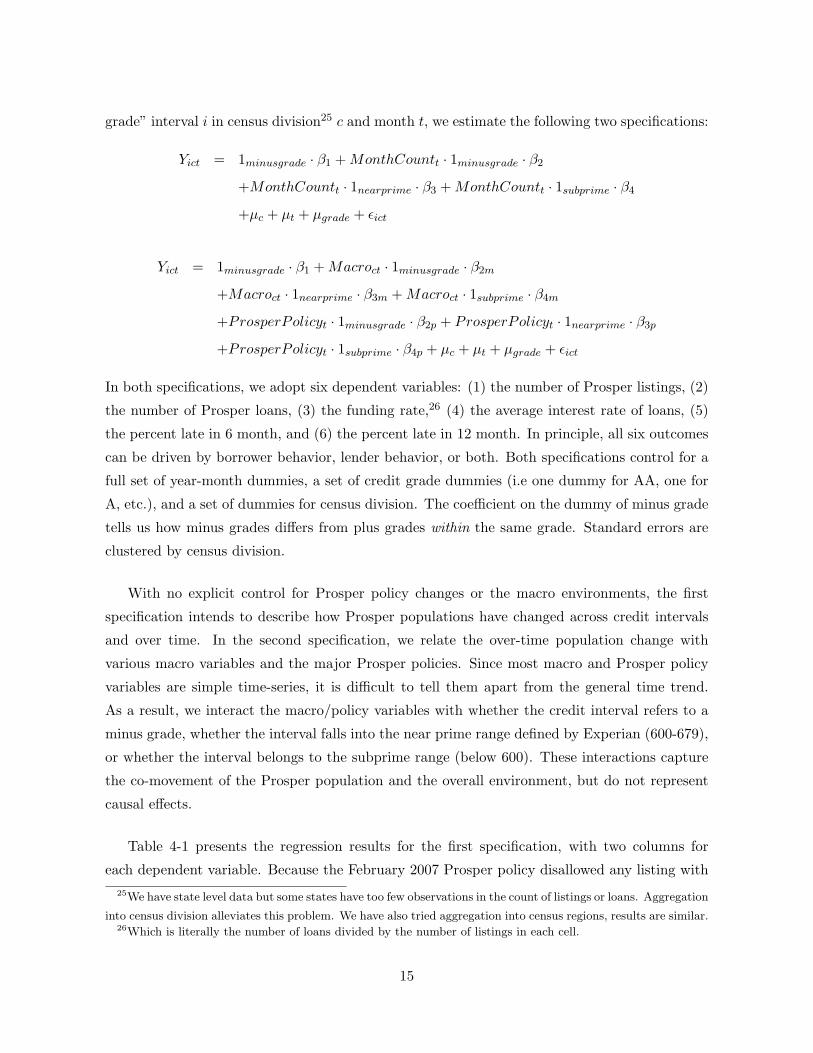
grade” interval i in census division25 c and month t, we estimate the following two specifications:

Yict = 1minusgrade · β1 + MonthCountt · 1minusgrade · β2

+MonthCountt · 1nearprime · β3 + MonthCountt · 1subprime · β4

+µc + µt + µgrade + εict

Yict = 1minusgrade · β1 + Macroct · 1minusgrade · β2m

+Macroct · 1nearprime · β3m + Macroct · 1subprime · β4m

+ProsperPolicyt · 1minusgrade · β2p + ProsperPolicyt · 1nearprime · β3p

+ProsperPolicyt · 1subprime · β4p + µc + µt + µgrade + εict

In both specifications, we adopt six dependent variables: (1) the number of Prosper listings, (2)

the number of Prosper loans, (3) the funding rate,26 (4) the average interest rate of loans, (5)

the percent late in 6 month, and (6) the percent late in 12 month. In principle, all six outcomes

can be driven by borrower behavior, lender behavior, or both. Both specifications control for a

full set of year-month dummies, a set of credit grade dummies (i.e one dummy for AA, one for

A, etc.), and a set of dummies for census division. The coefficient on the dummy of minus grade

tells us how minus grades differs from plus grades within the same grade. Standard errors are

clustered by census division.

With no explicit control for Prosper policy changes or the macro environments, the first

specification intends to describe how Prosper populations have changed across credit intervals

and over time. In the second specification, we relate the over-time population change with

various macro variables and the major Prosper policies. Since most macro and Prosper policy

variables are simple time-series, it is difficult to tell them apart from the general time trend.

As a result, we interact the macro/policy variables with whether the credit interval refers to a

minus grade, whether the interval falls into the near prime range defined by Experian (600-679),

or whether the interval belongs to the subprime range (below 600). These interactions capture

the co-movement of the Prosper population and the overall environment, but do not represent

causal effects.

Table 4-1 presents the regression results for the first specification, with two columns for

each dependent variable. Because the February 2007 Prosper policy disallowed any listing with25We have state level data but some states have too few observations in the count of listings or loans. Aggregation

into census division alleviates this problem. We have also tried aggregation into census regions, results are similar.26Which is literally the number of loans divided by the number of listings in each cell.

15

credit score below 520, to facilitate comparison the regression sample excludes credit scores

below 520.27 The odd numbered columns suggest significant adverse selection: compared to

plus grades, minus grades have on average 11 more listings and 2 more loans per division-grade-

month. Both numbers imply a significant density towards minus grades as there are only 30

listings and 6 loans in each division-month-interval on average. As the theory predicts, the

minus grade loans perform significantly worse. The fact that Prosper lenders do not observe

credit scores explains why the funding rate is no different between minus and plus grades after

we control for the fixed effects of month, grade and division. However conditional on funding,

lenders charge 0.4 percentage point higher interest rates on the minus grades, which suggests

that they may have some clue as to which loans are minus grades and which are not. The even

numbered columns include the interactions of month count (since June 2006) with minus grade,

near prime, and subprime. Over time we observe more near and subprime listings relative to

prime, but less subprime loans. Note this is slightly different from what is seen in Figures 3 and

4, because these regressions describe the absolute number of listings and loans in each interval

as opposed to the relative distribution. While the overall risk composition has improved, the

adverse selection towards minus grades increases through time at a speed of 0.55 more minus

grade listings and 0.18 more minus grade loans per month.

Table 4-2 replaces the month count interactions with those that involve macro variables and

Prosper policy changes. While we have included all the major macro variables (bank prime rate,

state-specific unemployment rate, and state-specific foreclosure rate) in the interactions, we only

report those of bank prime rates because they are most related to the credit crunch.28 As shown

in column 1, changes in the listing population is clearly correlated with the macro environment.

However, when we include the interaction of Prosper policies (column 3), the coefficients of the

bank prime rate interactions have all switched sign from negative to positive. Thus, it is unclear

whether the credit crunch has contributed to more or fewer non-prime borrowers (relative to

prime).

The coefficients on the policy interactions are much more stable: data suggests that, for both

the number of loans and listings, the concentration towards minus grades has increased after

Feburary 2007 and April 2008. Interestingly, Prosper lenders do not demand a higher interest

rate on a minus grade loan until February 2007. We suspect this occurs because the extra27Results using all the “half-grade” intervals are very similar to the presented results except for the chop-off of

the scores below 520 after February 2007.28The correlation between bank prime rate and the fraction of banks that reported credit tightening of consumer

loans is -0.92.

16

credit information that Prosper provided since February 2007 has helped lenders distinguish

risks within a grade. One may argue that Prosper introduced friend endorsement in February

2007 as well and that could contribute to lenders charging higher interest rates. We cannot

test this explicitly because the half-grade data is aggregated. But as shown in Table 2, friend

endorsements account for only 20-30% of the Prosper population and these percentages are

declining sharply over time. These facts do not explain why the increased interest rate for the

minus grade loans appears abruptly in Feburary 2007 and stays stable afterwards. Turning

to the interaction of Prosper policies and sub prime, the results suggest that Prosper policies,

especially the bidder guidance introduced in October 2007, may have helped lenders better

understand the true meaning of sub prime and therefore motivate them to shift towards better

grades. This result will be further confirmed in Section 4.3.

Above all, we argue that the crude definition of credit grade has resulted in adverse selection

towards the lower end of each grade. While the macro environment and the Prosper policies

may have contributed to the shift towards better grades, the adverse selection towards minus

grades has increased over time. The market is aware of the problem, as the adverse selection is

partially offset by higher interest rates when Prosper began posting more credit information in

February 2007.

4.2 Funding rate, interest rate and loan performance

The second information problem is probably specific to p2p lending: because most individual

lenders are amateurs in consumer lending, they may not understand the true risk underlying a

specific attribute. If the misunderstanding exists in a systematic way, we may observe a listing

attribute that signals higher default but has a higher funding probability or a lower interest rate.

However, mismatch alone does not necessarily imply lender mistakes, especially if some lenders

have charity motives towards the listing attribute or other incentives.29

To detect mismatch, we run three descriptive regressions that correlate observable listing29A third explanation is omitted variables that lenders observe but we do not. Examples include the attrac-

tiveness of the image or the way in which the borrower answers a lender question privately. But for the omitted

variables to explain the mismatch, they must be correlated with the observables in a systematic way and overturn

the initial signal embodied in the observable attributes. For instance, if most low grade borrowers are more

responsive to lender questions and this attitude dominates the effect of credit grade on default risk, that may

explain the mismatch. But we believe such events are unlikely and no data allow us to justify it one way or the

other.

17

attributes to the probability of being funded (1funded), the interest rate if funded (InterestRate),

and whether the loan is default or late as of August 1, 2008 (1defaultorlate). In all three, we include

year-week fixed effects (FEyw) to control for the changing environment on and off Prosper. In

the third equation, we also control for a full set of monthly loan age dummies (FEa) to control

for the life cycle of loan performance. Table 5 summarizes the listing attributes we use in these

regressions. The funding rate and performance regressions are estimated by probits and the

interest rate regression is estimated by OLS.

1funded,i = f1(ListingAttributesi,macro, FEyw) + e1it

InterestRatei = f2(ListingAttributes, macro, FEyw) + e2it

1defaultorlate,it = f3(ListingAttributes, macroFEyw, FEa) + e3it.

According to the regression results reported in Table 6, the consistency between funding rate,

interest rate and loan performance holds for most but not all listing attributes. For example,

the probability of being default or late increases by credit grade, and in response, interest rate

increases and the funding probability decreases. Similarly, lenders understand that the more a

borrower requests to borrow, the higher the risk of misperformance, and therefore deserves a

lower funding probability and a higher interest rate.30

The consistency between interest rate and loan performance is easier to interpret because

they are based on the same sample of Prosper loans. For instance, conditional on being funded,

a listing with an image on average enjoys a lower interest rate (0.1 percentage points) than

a seemingly equivalent listing without an image. However, the two listings do not show any

significant difference in loan performance. These two findings imply that the expected rate of

return is lower for listings with an image.31 The impact of an image on the funding rate is harder

to interpret. While having an image increases the funding rate, one explanation is that having an

image is meaningless but lenders misinterpret it as a positive signal. Another possibility is that

loans without an image are better in other attributes (in a non-linear way) and the borrowers of

these loans feel it is unnecessary to post an image. As a result, loans with and without images

perform the same but the listings that do not get funded due to lack of an image could perform

worse than the funded loans.

We observe both consistency and inconsistency for the social network variables. Compared

with others, borrowers that belong to a group are 0.4 percentage points more likely to get30Loan size is a typical method of credit rationing.31Ravina (2007) and Pope and Sydnor (2008) present more details on the impact of the race, gender, age and

beauty contents of the images in Prosper listings.

18

funded, enjoy a 0.4 percentage point lower interest rate, but are 0.5 percentage points more

likely (though statistically insignificant) to be default or late. Similar inconsistency occurs for

a group loan that receives an endorsement and bid from the group leader. These results imply

that group loans, especially those that receive an endorsement and bid from the group leader,

may generate lower returns than the non-group loans. How much lower the rate of return is and

why lenders are willing to support lower-return loans are the questions we will examine next.

In comparison, having a friend endorsing and bidding on the listing shows more consistency:

it has a large effect on the funding rate (9.6 percentage points), and conditional on being

funded, the interest rate is 0.7 percentage points lower and the probability of default or late is

4.1 percentage points lower. Whether the favorable interest rate has over- or under-compensated

the better loan performance is an empirical question.

4.3 Expected Rate of Return

To better understand loan performance, we follow two principles to compute the internal rate of

return (IRR) that a sophisticated lender should expect from a Prosper loan: the lender considers

all the information at the time of listing, and he projects the risk of late and default throughout

the 36-month loan life. We define IRR as the annual discount factor that equalizes the loan

amount to the present value of all the predicted monthly payments. We believe this method

reflects the rate of return that a lender expects to earn at the start of the loan if he can perfectly

predict the statistical distribution of loan performance. The step-by-step algorithm is described

in the Appendix.

Our method is more comprehensive than the ones used by Prosper and LendingStats.32

Specifically, when we predict misperformance in a specific month, we regress observed loan-

month performance on all listing attributes posted online, their interactions with each credit

grade, and a set of loan age dummies (in months). This method utilizes more listing information

than Prosper’s grade-specific predictions.33 Unlike LendingStats, we consider the fact that every32LendingStats is a popular independent website that tracks Prosper activities in real time.33For a given portfolio, Prosper assumes that roll rates from one loan status to another are revealed in the

historical performance of each grade. For example, a 1-month-late AA loan has a 42% probability of becoming

2-months late, and a 2-months-late AA loan has a 71% probability of becoming 3-months-late. Prosper also

makes assumptions on the probability of early payment-in-full (3.5% for AA, 0.5% for HR) and the probability

of loss recovery if default. These assumptions enter the calculation of monthly returns. Annualizing this figure

and averaging it across the whole life of the loan results in an overall rate of return.

19

loan has a positive risk at the time of origination even if ex post it is paid in full.34 In this sense,

we capture the return expected at the time of origination, not the return that is realized ex post.

We use three dummies to measure loan performance: default, default or late, and missed

payment. Located between the most optimistic (default) and the most pessimistic (default or

late), the dummy of missed payment is defined as one if the loan’s payment history indicates that

the borrower has missed the payment in a specific month. If the borrower misses the payment

at month t but makes it up in a later month, we count it as not missing the payment. To reflect

the actual cash flow as much as possible, we treat loans that are paid off early in two ways. One

counts these loans as on-time in all months following the early pay off, and the other counts the

early pay off as a bulk of cash flow in the actual month of payment and zero afterwards. In the

present value framework, the former effectively assumes that the early payoff is reinvested in a

loan that is always on time, while the latter assumes that the early payoff is reinvested into a

loan that is identical to the loan under study. For both versions, we predict the probability of

missed payment and early payoff for each loan and each month using the full history from June

1, 2006 to July 31, 2008. Since Prosper added new credit information in February 2007, our

full-sample prediction only uses the variables that are always available.35

Because all Prosper loans are three years, the majority of them are still ongoing at our

observation date unless they were paid early or have already defaulted. As a result, we do not

have information for loan performance in months 25-36 if we use the full sample to predict risk.

Instead of using arbitrary roll over rates, we report two sets of IRR estimates: one assumes that

the cumulative misperformance remains constant after month 24 (referred to as “flat IRR”),

and the other assumes that the misperformance rate will follow a linear projection after month

24 (“linear IRR”).36 Our prediction regressions suggest that misperformance does not have a

statistically significant increase after month 18. While this concavity may be driven by fewer

observations towards the later loan life, the raw Prosper performance depicted in Figure 5 does

confirm that misperformance is more likely to occur in the earlier part of the loan life, as typically34Compared to Prosper, LendingStats uses more pessimistic roll rate assumptions but puts more emphasis on

actual performance than predicted performance. In particular, it takes the current status of a loan as given, and

does not project its future risk until it is late. In that case, it is assumed that a 1-month-late loan will default

with a 50% probability and loans that are more than 1 month late will default for sure.35As a robustness check, we rerun the prediction regression for the post-Feb-2007 sample only. For this sample,

including or excluding the new credit information makes very little difference (less than 0.2%) in the final IRR

estimates. From this we conclude that not using the new credit information does not bias our IRR estimates.36More specifically, linear projection for the full sample means that the predicted misperformance rate at month

x (where x ≥ 25) is equal to [predicted risk at month 24 + (x-24)*(predicted risk at month 24-predicted risk at

month 23)].

20

observed in the industry. Based on this observation, we believe the truth is somewhere between

the flat and linear IRRs. More details of the potential bias in our IRR calculation are discussed

in the Appendix.

Table 7 summarizes 12 IRR estimates for each loan depending on which performance measure

we use, how we treat early payoffs, and whether we assume a flat or linear projection in the

unobserved loan life. Because the performance prediction is probabilistic and the present value

function may be non-smooth37, we cannot achieve convergence for every IRR estimate. As

reported in Table 7, each of the 12 IRR estimates has a convergence rate close to or above

90%. In the simplest version where we measure performance by default and treat early payoff

as on-time payments, the convergence rate is higher than 97%.

Conditional on the converged IRRs, the average estimates are consistent with expectation.

Treating early payoff as an early cash flow yields a lower rate of return because the reinvestment

of the early payoff faces a positive risk of misperformance. Additionally, flat IRRs are 2-3

percentage points higher than linear IRRs because the latter is more pessimistic about the

unobserved loan life. Within flat IRRs, the average return based on missed payments (IRR2,

-0.45%) is bounded between those based on default (IRR1, 3.02%) and default or late (IRR3,

-0.99%). For comparison, the average annual yields of 3-year Treasury Bill and S&P 500 are

3.97% and -0.66% in the same period (June 1, 2006 to July 31, 2008). As shown below, the

seemingly low average IRRs of Prosper loans masks the fact that IRRs of newer loans are

significantly higher (and positive) than the reported average because lenders have learned over

time.

In all 12 IRR estimates, we find large heterogeneity across loans, ranging from nearly -60%

to +34%. To describe how the IRRs differ across different types of loans, the tables and figures

discussed below utilize IRR2, which is computed based on the risk of missed payment, counts

early payoff as early cash flows, and assumes a flat projection into the unobserved loan life. Using

the other IRR estimates generates very similar comparisons across loans, which suggests that

the relatively low convergence rate on IRR2 does not imply significant bias in the understanding

of loan heterogeneity.38

The first IRR heterogeneity we explore is testing an important prediction from Stiglitz and37Due to the fact that Prosper does not charge lender service fees if the borrower makes no payment38We also check that the difference in the reported IRR averages are not driven by the different samples of

converged loans.

21

Weiss (1981): because lenders have imperfect information about borrower risk (due to either

adverse selection or moral hazard), the willingness to pay for a higher interest rate may signal

higher risk. This implies that a higher interest rate may yield lower financial returns because

it attracts worse risk. As a result, Stiglitz and Weiss argue that there exists a non-monotonic

relationship between rate of return and interest rate and this non-monotonicity motivates credit

rationing. To test this prediction, Figure 6 plots IRR2 against the contract rate.39 The curve

suggests that IRR2 first increases and then decreases after the interest rate reaches 8-9%. The

final uptick suggests that an increase of interest rate does not fully compensate the increased

risk until 30-31%. According to the 5 and 95 percentiles shown in the same figure, we have more

noise at the two ends due to smaller numbers of observations. Over all, Figure 6 confirms the

argument that higher interest rates may attract riskier borrowers leading to lower IRRs.

Figure 7 presents the kernel density of IRR2 by credit grade. On average, grades AA-A have

the highest average rate of return (3.89%) as compared to the other categories (1.54% B-D and

-8.35% E-HR). AA-A also has a tighter distribution and less variability than B-D and E-HR. As

one would expect, E-HR has the longest left tail and the lowest return on average. The negative

IRRs suggest that some lenders are not experienced enough to foresee a negative return, or they

have specific incentives to fund lower-quality loans. As shown below, both explanations hold to

some extent.

Turning to social loans, we compare the kernel density of IRR2 by group status in Figure

8 and endorsement status in Figure 9. As shown in Figure 8, group loans perform worse than

the non-group loans. This result is against the intuition that group members may have better

“soft” information to signal a “good type” all else equal. In contrast, friend endorsements show

a different pattern. On average, loans that have friend endorsements and friend bids perform

better than the loans without friend endorsements. However, loans with friend endorsements

only perform worse. Combined with the descriptive regressions reported in Table 6, this suggests

that friend endorsements may not provide any positive signal about borrower risk until the

endorsing friend is willing to certify the “soft” information with a bid of their own. Section 5

will revisit this argument and present evidence in greater detail.

Figure 10 plots the average IRR2, contract rate, and the predicted risk of missed payment as

a function of loan origination month. It is clear that the estimated IRR2 increases steadily over

time, which is attributed to a significant decline in missed payments and a relatively smaller

decline in interest rate. These trends are consistent with the fact that the market is moving39Interest rates are rounded by percentage points in Figure 6.

22

towards better credit grades over time, partly a result of lender learning as shown below. The

two vertical lines drawn on this picture represent Prosper information policies in February 2007

and October 2007. While we do not know whether the policy changes have a causal effect on

the increase of IRR2, they definitely coincide with the trend towards improving returns: the

average IRR2s before February 2007, between February and October 2007, and after October

2007 are -3.63%, -1.60%, and 2.13% respectively.

4.4 Lender Learning

As we have shown in the previous section, some lenders have chosen loans whose observables

predict poor performance. We are interested in understanding whether these choices are caused

by lenders making mistakes or lenders choosing risky loans as a form of charity or due to other

incentives. Assuming a lender’s charity preference remains fixed over his life as a Prosper lender,

if we observe that lenders learn, we can infer that at least a portion of these choices resulted

from “mistakes.”

To identify the extent to which lenders learn from their own mistakes, we estimate a series

of regressions describing how a lender’s behavior changes in response to late or default loans in

his portfolio. We estimate three types of regressions at the lender-week level. These regressions

describe a particular behavior of lender i in week t as a function of lender i’s age at time t and

characteristics and performance of the lender’s portfolio up through week t − 1. The outcome

behaviors that we look at are whether or not a lender funds at least one loan in a given week,

and conditional on funding a loan in a given week, the investment amount and the portion of

new loans in various categories. The following three equations describe these regressions:

FundedALoanit = g1(LenderAgeit, PortCharit−1, PortLateit−1) + µ1i + γ1t + ε1it

AmountFundedit = g2(LenderAgeit, PortCharit−1, PortLateit−1) + µ2i + γ2t + ε2it

PortCompit = g3(LenderAgeit, PortCharit−1, AtoAALateit−1, BtoDLateit−1,

EtoHRLateit−1, NCLateit−1) + µ3i + γ3t + ε3it

The FundedALoan regression is a linear probability model40 of an indicator that a lender funded

at least one loan in a given week. The other two equations only include the sample of lenders

who funded at least one loan in week t. In the AmountFunded equation, AmountFundedit is40Because we will use a large number of fixed effects, we choose a linear probability model over a probit model

for this set of regressions

23

the dollar amount invested by an active lender in week t. The PortComp Equation is estimated

for various PortCompit variables which specify the percentage of an active lender’s investment

in AA to A, B to D, and E to HR loans in week t.

LenderAgeit includes indicators of lender i being in his first month and second through sixth

month on Prosper at week t.41 PortCharit−1 includes lender i’s portfolio HHI and portfolio size

through the previous week. PortLateit−1 reflects the percentage of lender i’s portfolio that has

ever been late as of the previous week. AtoAALateit−1, BtoDLateit−1, EtoHRLateit−1 are the

percentage of lender i’s portfolio through the previous week that has ever been late in each of

the three respective credit grade categories42.

γjt is a set of year-week fixed effects allowing us to control for changes in the macro environ-

ment and the Prosper market.43 µji is a set of lender fixed effects. With these fixed effects the

coefficients on the ever late variables are identified by within lender changes in portfolio perfor-

mance and investment decisions. In other words, we can interpret these coefficients as within

lender learning from the performance of their past investments. In all of the results presented

here, we cluster standard errors at the lender level.

The results of these regressions are reported in Table 8. The first two columns show a very

pronounced age profile as lenders are less likely to invest and invest less when active as they

age. The sample mean probability of funding a loan in a week is 0.382, so the coefficient on the

month 1 indicator of 0.350 in column 1 implies that lenders are 92% more likely to fund a loan

in a week in their first month on Prosper as compared to weeks in months 7 and higher. Lenders

also show strong responses to poorly performing loans in their portfolios. On average, a ten

percentage point increase in the proportion of their portfolio that has ever been late decreases

their probability of funding a loan by 2.5 percentage points and decreases the amount they invest

in an active week by $78.

The next 3 columns display the coefficients from the different versions of the PortComp

regressions. Controlling for the performance of lenders’ portfolios in each grade category, lenders

are more likely to fund AA to A and E to HR loans in their first month on Prosper than in later

months. As lenders age, they move away from these two extremes and toward B to D loans.41We count a lender as joining Prosper when he funds his first loan42We have also tried specifications using the percent of a lender’s portfolio (in total or in various categories)

that is currently late or in default and the results are very similar.43Results of identical regressions with controls for macro variables and Prosper supply, demand, and market

performance instead of week fixed effects are very similar.

24

As lenders observe late loans, they tend to decrease their funding of loans in the grade with

the adverse shock and increase their funding of higher quality grades.44 These results indicate

strong evidence of learning. The high late and default rates of E and HR loans have driven

lenders away from these loans and toward higher credit grades as lenders have learned about

the dangers of investing in these lower credit grades.45

To further explore details of lender learning we run similar regressions as above but interact

the ever late variables with dummies indicating different Prosper policy regimes. In results

not shown here we find that the magnitude of these coefficients increase over time. We cannot

identify if this change is attributable to Prosper’s information policies or a natural acceleration

of learning over time, but in general, Prosper lenders learn more strongly from their “mistakes.”

We also directly test whether lenders shift toward loans with higher rates of return in response

to late loans in their portfolio. Figure 11 plots the average lender’s IRR2 for loans he funds in

a given week by lender cohort. As lender’s age, they clearly fund loans with a higher rate of

return. Interestingly, new cohorts pick up the market trend, perhaps responding to information

that was not available when older lenders joined Prosper. In the final column of Table 8 we

present results of a regression as above with IRR2 as the dependent variable and the percent

of the lender’s portfolio that has ever been late as the key explanatory variable. As lenders see

more late loans in their portfolios, subsequent loans that they fund do in fact have a higher

rate of return. The coefficient implies that when the average lender sees a ten percentage point

increase in the portion of his portfolio that has been late, his newly funded loan will have a 1.69

percentage point higher rate of return.

Lenders clearly respond to the realization of bad outcomes in their portfolios by adjusting the

characteristics of loans they choose to fund. The presence of this learning suggests lenders fund

observably risky loans partially as a result of not fully understanding the relationship between

observable characteristics and loan performance.44Note that when lenders observe late AA to A loans, they do show slight substitution towards the lower credit

grade loans.45In results not shown here, coefficients from regressions describing the propensity to fund loans in other

categories including autofunded loans and loans of various sizes as a function of late loans in these categories

show similar patterns.

25

5 Analysis specific to social networks

This section focuses on social networks on Prosper.com. We first describe four potential roles

of social networks and then look for evidence for or against each explanation.

5.1 Potential roles of social networks

First, having a social tie may be a good signal of on-time payment. For example, kins, friends and

colleagues who are familiar with the borrower in their daily lives may have private information

as to whether the borrower has good repayment prospects in the future even if she has a poor

or no credit history. If so, the soft information conveyed in friend endorsements could alleviate

adverse selection. Alternatively, kins, friends and colleagues may have the opportunity to closely

monitor the borrower after the loan is approved, which could mitigate moral hazard (Arnott and

Stiglitz 1991). Members of a social network may also impose social sanctions on the borrower,

thus reducing the incentive to default (Besley and Coate 1995). In the cases such as alumni

connections, even if alumni do not know each other in person, an alumni group that verifies

the alumni status could serve as a credible signal of the borrower’s education. To the extent

that higher education represents better risk, belonging to an alumni group could have a positive

signaling effect. All of these channels can ensure a higher probability of repayment all else

equal. Since Prosper broadcasts social ties to all lenders, the signaling effect of social ties should

imply a higher funding rate and equal financial return. More specifically, because we can only

compare loan performance among the funded listings, the selective and competitive funding

process implies that a loan with social ties may have better performance and lower interest rate

than a non-social loan, or worse performance and a higher interest rate. Either way, the financial

return should be equal if lenders understand the signaling effect of social networks correctly.

The separating equilibrium described above will not occur unless the social ties lead to

incentives to gather and/or reveal the true type of borrowers, and the bad type cannot mimic

the good type. Both conditions do not necessarily hold on Prosper. Group leaders are expected

to do the leg work for a listing of a group member but the financial return is no more than a

small group leader reward ($12 per new loan) plus the interest if the leader funds a portion of the

loan. Since group leaders do not co-sign the loan and there is a natural lag between funding and

repayment, the group leader reward could provide a perverse incentive for group leaders to recruit

as many borrowers as possible, endorse/bid on the groups listings to ensure funding, but engage

26

in no leg work at all.46 Even if the group leader completes the leg work, the information gathered

is broadcast only via a group leader endorsement. As a result, the mechanism encourages free-

riding and diminishes the incentives to gather new information. These arguments suggest that

group affiliation and group leader endorsements do not necessarily certify good risks unless the

group leader has a cost advantage in information access and imposes stringent screening before

inviting a new borrower to join the group. This could happen if the group is based on close

off-line ties, which we test below. Similar logic applies to friend endorsements: if it is easy for

a bad borrower to obtain favorable endorsements from a dishonest friend, friend endorsement

cannot separate good types from bad types and therefore loses its signaling value.

The second role of social networks lies in the potential to facilitate within-network charity.

Sociologists have argued that network members may do favors to each other due to reciprocity, or

make charity giving in a single direction because the giver enjoys non-financial returns from the

giving process (see the survey article of Portes 1998). The non-financial returns may be approval

and status within the network, future benefits from the network as a whole, or satisfaction of

helping people within the same network. In short, the charity role of networks implies that

social loans should have a higher funding rate but lower financial returns.

One unique feature of within-network charity is the distinction between insiders and out-

siders. In the simplest case where everyone that should belong to the network is in the network

(e.g. every Harvard alumni that joins Prosper is in the Harvard alumni group), we should observe

all the social loans being funded inside the network. To the extent that a Harvard graduate may

not join the Harvard group but still has a charity motive for any listing from the Harvard group,

he may fund the listing despite the low financial return. This implies that social loans may

be funded by both insiders and outsiders, but so long as the network affiliation reflects charity

motives, we should observe lower financial returns as the amount of inside funding increases.

The third possibility is that social networks represent meaningless cheap talk. If every

borrower can have some social ties with little cost, the pooling means that social networks will

not convey any information. In theory, cheap talk may still be informative if the message sender

has full incentives to reveal the truth (Farrell and Rabin 1996). This condition is unlikely to hold

on Prosper: if lenders are more willing to lend to borrowers with certain social ties, both good

and bad borrowers would like to have those ties. In other words, assuming lenders interpret the

cheap talk correctly, social loans should have the same funding rate and same financial return46To give credit to Prosper, it held back part of the $12 group leader reward until the loan had some payment

history.

27

as non-social loans.

The last possibility is lenders misinterpret social ties as a signal of good risk when it is

actually not. In this case, we could have a misalignment in funding rate and financial returns:

the misinterpretation may lead to a higher funding rate on social loans, but these loans yield

lower financial returns. On this front, the prediction is similar to that of within-network charity.

However, the two explanations can be distinguished if mistaken lenders learn over time. All of

the predictions discussed above are summarized in Table 9.

5.2 Data summary on social networks

Table 10 presents a detailed summary of social variables. As we saw in Table 5, 28.8% of listings

have some group affiliation, 19.1% have friends, 3.2% have an endorsement from a group leader

(2.2% with a leader bid), and 3.2% receives friend endorsement (1% with a friend bid). All these

fractions have increased substantially in the loan sample, indicating that social loans are more

likely to be funded than the listings that have no group affiliation or friend ties.

Conditional on a borrower being in a group, on average the borrower belongs to a group

with 1800 members in which 1083 (or 63%) are borrowers. More specifically, borrowers’ group

membership is almost evenly distributed between groups with 1-100, 101-500, 501-1000 and

above 1000 borrower members. But because larger groups have a larger number of borrowers,

they contribute more to the average. In terms of group types, 2.3% of group borrowers belong to

an alumni group, 1.9% to a military group, 1.7% to a group with employment, local or personal

connections (in combination referred to as other connection), and 2.5% to a loose connection

such as common religion or common ethnicity. All the other group borrowers are not classified.

Since alumni groups account for 9% of the group count, this implies that most alumni groups

are smaller than an average group. The same observation is true for military group and other

connections, but not for the groups with loose connections. Only 34.1% of borrowers belong

to groups that require borrower review (by the group leader) before listing. After Prosper

introduced group ratings in October 2006, we observe 41.4% of group members belonging to low

rated groups (1-3 stars), 32.3% to high rated groups (4-5 stars), and 26.1% to the groups that

do not have sufficient data to be rated at the time of listing (referred to as unrated).

The rest of Table 10 documents the extent to which social loans are funded within the

borrower’s network. For an average group borrower (whose listing gets funded), 3.2% (or $130.8)

28

comes from the group leader and 1.7% (or $95.7) of the loan amount comes from other members

of the group. For an average borrower that has any endorsement and is funded at the end of

the listing auction, the endorsing friends contribute to an average 12.7% (or $775) of the loan

amount. In comparison, endorsing group leaders contribute to an average 6.8% (or $323). These

numbers suggest that while social ties contribute positively to the final funding of social loans,

most funding comes from stranger lenders.

Table 11 reports what types of borrowers are more likely to have social ties. Given the

importance of credit grade in summarizing borrower risk, we present the grade composition

conditional on group borrowers, endorsed borrowers, and the whole Prosper market. At the

listing level, it is clear that group borrowers are more likely to have lower credit grades, especially

E and HR. This observation does not hold at the loan level though group affiliation does help

funding within each credit grade at or below D. For the endorsed loans, we focus on the borrower

population after February 12, 2007 because friends are not allowed to make endorsement until

then. Unlike group listings, the grade composition of endorsed listings is very similar to that

of the whole market. Judging from the grade composition, friend endorsement seems to help

funding in grades at or below D, a phenomenon similar to that of group loans.

5.3 IRR analysis by social variables

According to Table 9, the key difference among the four potential roles of social networks lies in

the effect of social ties on the funding rate and the financial rate of return. Based on both the

summary statistics in Table 11 and the regression results of the funding equation in Table 6 (the

latter controls for other listing attributes), we have no doubt that having a social tie increases

the funding rate. This fact excludes the cheap talk explanation of social networks if we assume

lenders have interpreted the meaning of social ties correctly. For the other three explanations –

signaling good risk, within-network charity/other incentives, and lender misinterpretation – we

turn to analyze the estimated IRR2 as a proxy for the financial rate of return.

Conditional on the funded loans that have a valid estimate of IRR2, Table 12 reports regres-

sions of the estimated IRR2 on different functions of social variables. Because the calculation of

IRR2 has already taken into account all the observable listing attributes, the contracted interest

rate, and the predicted loan performance at each loan age, this regression does not control for

listing attributes other than social variables. In this sense, it already accounts for the selection

of social ties by observable attributes. To isolate the social variables from time trends due to

29

lender learning or changes in the macro environment, we control for year-week fixed effect (µyw)

based on loan origination date.

IRR2 = f4(socialvariables) + µyw + ε4

Column 1 confirms the results of Figure 8 that group loans have a lower IRR2 than non-

group loans. In particular, an average group loan (with no endorsement) yields a statistically

significant 2.9 percentage point lower return than the non-group loans, which is a large difference

considering the average IRR2 is -0.45%. The distinction between endorsed and non-endorsed

loans is more complicated: having an endorsement but no bid from a group leader implies a 3.1

percentage point higher IRR2, but group leader endorsement plus bid does not make a difference

(as compared to the group loans that have no endorsement). In contrast, friend endorsements

plus bid implies a 4.2 percentage point higher IRR2, but friend endorsement with no bid means

2.7 percentage points lower, both compared to loans with no friend endorsement.

These significant coefficients reject the most stringent form of the signaling effect: if these

social variables are valuable signals and lenders understand their meanings to the full extent,

we should not observe significant rate of return heterogeneity across different types of social

loans. One possible explanation for the positive coefficients of leader endorsements without bids

and friend endorsements with bids is that these social variables provide positive signals but

lenders under estimate these signals. Similarly, the negative coefficients for group loans, group

leader endorsements with bids, and friend endorsements without bids may imply that they are

negative signals but lenders do not account for it fully in the interest rate. We will examine

these possibilities in Table 13 when we look at the impact of social variables on interest rate

and loan performance separately. But before doing that, we would like to check basic evidence

for the remaining stories, that is, charity motives/other incentives or lender misinterpretation.

If charity is the main explanation we expect to see that group members do not learn from

lower returns within their own group. We also expect that returns will be lower if a higher

portion of the loan is funded within the borrowers network. Figure 12 plots IRR2 for group and

non-group loans and shows that the IRR gap has partially closed as the IRR of group loans has

increased more than the IRR of non-group loans. We also know from Table 2 that the fraction

of loans to group members has fallen drastically. Together this suggests that group loans were

perceived as unattractive due to the lower IRR and became less prevalent in the listing and loan

population over time. In results not shown here, we run learning regressions similar to section

4.4 and it is clear that group lenders substitute away from own group loans when they observe

late own group loans in their portfolios suggesting within group charity is not a large factor.

30

Turning to friend endorsements without bids, Figure 13 shows that the IRR of these loans

remains lower through time. As we saw in Table 2, the population of friend endorsed listings

and loans without bids has decreased and the population of friend endorsed listings and loans

with bids has increased over time. In learning regressions not reported, lenders show expected

substitution patterns between these two categories and loans with no friend endorsements. These

results indicate that the market has reacted to the performance of these types of loans on the

funding margin, but interest rates have not adjusted accordingly.

To test how the IRR varies as a function of the amount of in network funding, Column 2 of

Table 12 includes the percentage of funding that comes from the group leader, group members

and friends. These results show that returns are higher when a larger portion of the loan is

funded group members and friends, but returns are lower when a larger portion is funded by

the group leader. Because of this discrepancy we cannot yet rule out charity or other incentives

for group loans.

Because of the nature of group incentives early on and the changing incentives when group

leader rewards are eliminated, we statistically test how the IRR gap between group and non-

group loans and the effect of the funding portion by group leaders has changed since group

ratings were removed. These results are presented in Columns 3 and 4 of Table 12. The initial

gap between group and non-group loans was a statistically significant 3.0 percentage points,

increased slightly when ratings were adopted, but decreased by 0.8 percentage points after

leader rewards were eliminated. Column 4 shows that when we let the effect of the portion of

funds from the group leader change after the elimination of leader rewards, the negative impact

is largely driven by the period with group leader rewards.

One explanation is that before the removal of rewards, group leaders may have been mo-

tivated to endorse and bid on a group members listing in order to earn group leader rewards.

The ex post performance indicates that group leader endorsement plus bid constituted a signal

of worse risk. But to the extent that the market does not fully understand the true meaning

of this signal, group leader endorsement plus bid could increase the funding probability and be

profitable for the leader. After the removal of rewards, group leader manipulation may have

decreased as seen in the drastic decrease in the number of listings with group leader endorsement

plus bid (4.1% in the third quarter of 2007 to 0.84% in the fourth quarter of 2007).

While it appears that lenders have misinterpreted group loans as a positive signal on average,

it is possible that certain types of group loans do provide signals of lower risk. Table 13 adds

31

variables that describe group size, percentage of a group made up of borrowers, group rating,

whether a group is based on alumni, military, other or loose connections, and whether the group

requires review before listing to the regressions discussed above. The “group loan” dummy is

dropped because we include a complete list of dummies for group ratings that includes no rating

before rating was introduced, unrated due to insufficient data, low rating, and high rating. If we

believe lenders correctly interpret the meaning of different ratings, there should not be any rate

of return difference by rating categories - with sufficient competition, interest rates will fully

adjust. This prediction is confirmed in the regression: high rating does not imply higher rate

of return than low or no ratings. If anything, the coefficients suggest the opposite relationship.

While the worst performance seems to come from the unrated groups, the group rating dummies

suggest that group loans are universally worse than the non-group loans.

Compared to groups with 1000 or more borrowers, smaller the groups and groups with

fewer members that are borrowers have a higher rate of return. Compared to the unclassified

groups, we find IRR2 is significantly higher in alumni groups or groups with employment, local

or personal connections. In contrast, military groups have significantly lower IRR2s.

To ensure the connection between positive rate of return and positive signaling effect, we

need to decompose the heterogeneity of IRR2 by interest rate and loan performance. Columns

2 and 3 of Table 13 replace the dependent variable with these two measures. All of the factors

that associate with higher IRR2 – endorsement plus bid from friends, endorsement but no bid

from group leader, percent funds from group members, percent funds from friends, small and

less borrower-concentrated groups, and groups based on alumni and other tangible connections –

show less likelihood of missed payment and lower interest rate. In an unreported table, we show

that these relationships continue to hold if we control for the other observable listing attributes.

Over all, these results suggest that some social variables have a positive signaling effect for

“good” risk and the market tends to under-estimate this effect and not fully adjust interest

rates. Similarly, factors that correlate with worse performance – such as group affiliation, friend

endorsement without bid, group leader endorsement plus bid – are not fully compensated in the

interest rate and therefore generate significantly lower IRR2s. We present evidence that some of

the negative signaling effect of group affiliation is due to the perverse incentives of group leader

rewards. Once Prosper removes the leader rewards the percent of funds from the group leader

is less of a negative signal. This phenomenon, combined with strong learning of group lenders

suggests that charity is not a big factor contributing to the lower returns of group loans.

32

6 Conclusion

The most fundamental question facing p2p lending is how it differs from and competes with

traditional banks. We show that the basic information problem faced by traditional banks –

that higher interest rate tends to attract worse borrowers – also exists in p2p lending. This

implies that p2p lenders should exercise similar credit rationing if they do not have other hard

information and pursue financial returns like traditional banks. This prediction has already been

confirmed in the data: the market of Prosper.com has evolved towards better credit grades,

which effectively rations credit to the lower grades. The evolution also suggests that most of the

Prosper market will compete head to head with traditional banks in the near future.

We identify two more information problems that are unique to p2p lending: Prosper lenders

face increased adverse selection because they do not observe the actual credit score, and many

lenders have made mistakes in their loan selection. The latter is gradually improved by lender

learning, and the former is partially offset by lenders charging higher interest rates on minus

grade loans when Prosper posts more detailed credit information on the website. One way to

further reduce the adverse selection would be for Prosper to post the actual credit score on

each listing, or at least allow borrowers to voluntarily post a certified score. According to the

unraveling theory (Grossman 1981, Milgrom 1981), these two methods should yield the same

results because borrowers would have full incentive to disclose a score that they know privately

with zero cost.47

One dimension that p2p lending could differ from traditional banks is by utilizing social

networks. Our results suggest that some social network variables may convey “soft” information

about borrower risk and therefore has a potential to compensate the lack of “hard” information

on Prosper.com. In this sense social networks utilized in p2p lending could alleviate credit

rationing, if they are implemented with the right incentives. That being said, our data suggest

that the market does not fully understand the signaling effect of social networks, resulting in

significantly higher returns for loans with the positive signals and lower returns for loans with

the negative signals.

Overall, the past two years have seen substantial changes in the nature of p2p lending.

Although the estimated rate of return to Prosper loans is still on average lower than alternative

investment vehicles such as CDs and T-bills, both the degree of lender learning and the distinctive47The theory could break down if there is serious concern about privacy or identity theft based on the credit

score.

33

effects of social networks point towards an optimistic future. Whether p2p lending leads to

welfare enhancements or simply to a redistribution of wealth is a question to be answered in the

future.

7 Appendix: IRR algorithm and potential bias

For each loan funded in our sample period, we use the following algorithm to compute the

expected internal rate of return (IRR):

• Given a loan amount and the interest rate of the loan, calculate the amortized monthly

payment (MonthlyPay) and the proportion that goes into the payment of principal

(MonthlyPrincipalPay). Specifically, we define MonthlyPay = [(InterestRate/12) ∗LoanSize∗(1+InterestRate/12)36]/[(1+InsterestRate/12)36−1]. MonthlyPrincipalPayt =

(MonthlyPay − InterestRate ∗ LoanSize/12) ∗ (1 + InterestRate/12)(t−1).

• Regress the observed monthly performance of each loan (which includes four dummies

that indicates default, default or late, miss payment and paid off)48 on an exhaustive set

of loan age dummies plus all the listing variables available since June 1, 2006. To be

comprehensive, we also interact all the listing variables with each credit grade. These four

prediction regressions yield the predicted probability of the four outcomes by loan-month

for each loan that was originated on Prosper between June 1, 2006 and July 31, 2008.

Because we do not observe any loans older than 24 months we have to make assumptions

about the performance in months 25 through 36. In one version we assume that the

cumulative misperformance remains constant after month 24 (referred to as “flat IRR”).

The other version assumes that the misperformance rate will follow a linear projection after

month 24 (“linear IRR”). In this version the predicted misperformance rate at month x

(where x ≥ 25) is equal to [predicted risk at month 24 + (x-24)*(predicted risk at month

24-predicted risk at month 23)]. In both versions, we assume no new early payoff occurs

after month 24.

• For loan i at month t, define PrincipalRemainit as the remaining principal after consid-

ering the possibility of misperformance or early payoff in that month. This is calculated

iteratively. In the first month of the loan, PrincipalRemaini1 = LoanSize. For the other48If a loan is defaulted at month t, it is counted as default in all months after t.

34

months, PrincipalRemainit = PrincipalRemainit−1−MonthlyPay∗(1−Probit(nopay)−Probit(paidoff)).

• For loan i and month t, define NetMonthlyReturnit as the difference between the expected

payment and lender service fees, where the expected monthly payment is set equal to

PrincipalRemain ∗ (1 + InterestRate/12) ∗Prob(paidoffinthismonth) + MonthlyPay ∗(1 − Probit(nopay) − Probit(paidoff)) and the monthly lender service fee is set equal to

LenderFee/12 ∗ PrincipalRemainit.

• Solve for the IRR that equalizes LoanSize to the sum of the present value of NetMonthlyReturn

from month 1 to month 36, while using IRR as the discount factor.

The algorithm described above are subject to potential bias in both directions. On the one

hand, our IRR estimates may be downward biased because we try to be conservative in the

calculation of cash flows. Specifically, we assume away any loss recovery from default loans, and

we do not account for the late fees that a lender may receive from a late-but-non-defaulting

borrower. When we count early payoff as a bulk cash flow that arrives in the paid-off month, it

effectively assumes that the paid off amount is reinvested in a loan that is identical to the loan

under study. This assumption may be conservative because lenders may learn to fund better

loans over time.

On the other hand, our IRR estimates may have overestimated the return of investment

because we do not consider any cost that lenders may incur in processing Prosper information.

The time that lenders spend on screening listings and digesting Prosper history could be long

and stressful. Lastly, our IRR estimates are based on the average loan performance observed

from June 1, 2006 to July 31, 2008, a period that stretches from the end of a boom to the

beginning of a recession. If the recession prolongs and worsens over time, the reported IRR will

overestimate the actual rate of return.

8 References

Adam, William; Liran Einav and Jonathan Levin (2007): ”Liquidity Constraints and Imperfect

Information in Subprime Lending” American Economic Review forthcoming.

Akerlof, George A. (1970): ”The Market for ’Lemons’: Quality Uncertainty and the Market

Mechanism” Quarterly Journal of Economics 84(3): 488-500.

35

Arnott, Richard and Joseph E. Stiglitz (1991) ”Moral Hazard and Nonmarket Institutions:

Dysfunctional Crowding Out or Peer Monitoring?” The American Economic Review March

1991, 179-190.

Berger, Allen N. and Gregory F. Udell (1992): ”Some Evidence on the Empirical Significance

of Credit Rationing” The Journal of Political Economy 100(5): 1047-1077.

Besley, Timothy; Stephen Coate and Glenn Loury (1993) ”The Economics of Rotating Savings

and Credit Associations” The American Economic Review September 1993, 792-810.

Besley, Timothy and Stephen Coate (1995) ”Group Lending, Repayment Incentives and Social

Collateral” Journal of Development Economics Vol. 46, 1-18.

Caskey, John P. (2005): ”Fringe Banking and the Rise of Payday Lending”, Chapter 2 of Credit

Markets for the Poor, Russell Sage Foundation, New York.

Cox, Donald and Tullio Japelli (1990) ”Credit Rationing and Private Transfers: Evidence from

Survey Data” The Review of Economics and Statistics 72(3): 445-454.

Farrell, Joseph and Matthew Rabin (1996) ”Cheap Talk” Journal of Economic Perspectives

Summer 1996, 10:3, 103-118.

Greenlaw, David; Jan Hatzius; Anil Kashyap, Hyun Song Shin (2008) : “Leveraged Losses:

Lessons from the Mortgage Market Meltdown”, mimeo, accessed at

http://www.chicagogsb.edu/usmpf/docs/usmpf2008confdraft.pdf.

Gross, David B. and Nicholas S. Souleles (2002) ”Do Liquidity Constraints and Interest Rates

Matter for Consumer Behavior: Evidence from Credit Card Data” Quarterly Journal of

Economics 117(1): 149-185.

Grossman, S. (1981) The informational Role of Warranties and Private Disclosure about Prod-

uct Quality, Journal of Law and Economics Vol. 24 (1981), pp. 461-489.

Hampshire, Robert (2008) ”Group Reputation Effects in Peer-to-Peer Lending Markets: An

Empirical Analysis from a Principle-Agent Perspective” mimeo.

Hendal, Igal; Aviv Nevo and Francois Ortalo-Magne (2008) ”The Relative Performance of Real

Estate Marketing Platforms: MLS versus FSBOMadison.com” mimeo.

Hoff, Karla and Joseph E. Stiglitz ”Introduction: Imperfect Information and Rural Credit

Markets – Puzzles and Policy Perspectives” the World Bank Economic Review 4(3): 235-

250.

36

Jaffee, Dwight M. (1971) Credit Rationing and the Commercial Loan Market New York: Wiley.

Jin, Ginger Z. and Andrew Kato (2007) ”Dividing Online and Offline: A Case Study” Review

of Economic Studies July 2007.

La Ferrara, Eliana (2003) ”Kin Groups and Reciprocity: A Model of Credit Transactions in

Ghaha” American Economic Review 93(5): 1730-1751.

Madajewicz, Malgosia (2005) ”Can Microcredit Reduce Poverty? The Effect of the Loan Con-

tract on Loan Size” Chapter 9 of Credit Markets for the Poor, Russell Sage Foundation,

New York.

Mendelson, Haim (2006) ”Prosper.com: A People-to-People Lending Marketplace” mimeo.

Milgrom, Paul (1981) Good News and Bad News: Representation Theorems and Applications,

The Bell Journal of Economics Vol. 12 (1981), pp. 380-391.

Parker, Jonathan A. (1999) ”The Reaction of Household Consumption to Predictable Changes

in Social Security Taxes” American Economic Review 89(4): 959-973.

Pope, Devin and Justin R. Sydnor (2008) ”What’s in a Picture? Evidence of Discrimination

from Prosper.com” mimeo.

Portes, Alejandro (1998) ”Social Capital: Its Origins and Applications in Modern Sociology”

Annual Reviews of Sociology 24: 1-24.

Ravina, Enrichetta ”Love & Loans: The Effect of Beauty and Personal Characteristics in Credit

Markets”, Available at SSRN: http://ssrn.com/abstract=972801.

Skiba, Paige and Jeremy Tobacman (2007) ”Profitability of Payday Loans” Working paper

available at http://www.law.vanderbilt.edu/faculty/faculty-personal-sites/paige-skiba/index.aspx.

Souleles, Nicholas S. (1999) ”The Response of Household Consumption to Income Tax Refunds”

American Economic Review 89(4): 947-958.

Stiglitz, Joseph E. (1990) ”Peer Monitoring and Credit Markets” The World Bank Economic

Review 4:3 351-366.

Stiglitz, Joseph E. and Andrew Weiss (1981): ”Credit Rationing in Markets with Imperfect

Information” American Economic Review 71(3): 393-410.

Udry, Cristopher (1994): ”Risk and Insurance in a Rural Credit Market: An Empirical Inves-

tigation in Northern Nigeria” Review of Economic Studies July 1994, 61(3): 495-526.

37

Voridis, Hercules (1993): ”Ceilings on Interest Rates and Investment: The Example of Greece”

The Review of Economics and Statistics 75(2): 276-283.

Yunus, Muhammad (2003): BANKER TO THE POOR: Micro-Lending and the Battle Against

World Poverty PublicAffairs, New York, 2003. ISBN 978-1-58648-198-8.

38

Table 1: Evolution of Prosper Policies Date initiated Policy Always History updated online every day, Allow groups May 30, 2006 Reveal more credit info, home ownership status, and bank account status Oct. 19, 2006 Start group rating based on past loan performance

Disallow borrowers with score<520 Feb. 12, 2007 Reveal more credit info (e.g. amount delinquent) Feb. 12, 2007 Allow friend endorsements Sept. 12, 2007 Eliminate group leader rewards ($4/new borrower) Oct. 30, 2007 Add bidder guidance Feb. 23, 2008 Allow search by friend bids and endorsements Apr. 15, 2008 Raise interest rate cap to 36% except for TX (10%) and SD (N/A)

Note: Gray rows indicate social network policies. White rows indicate information and other policies.

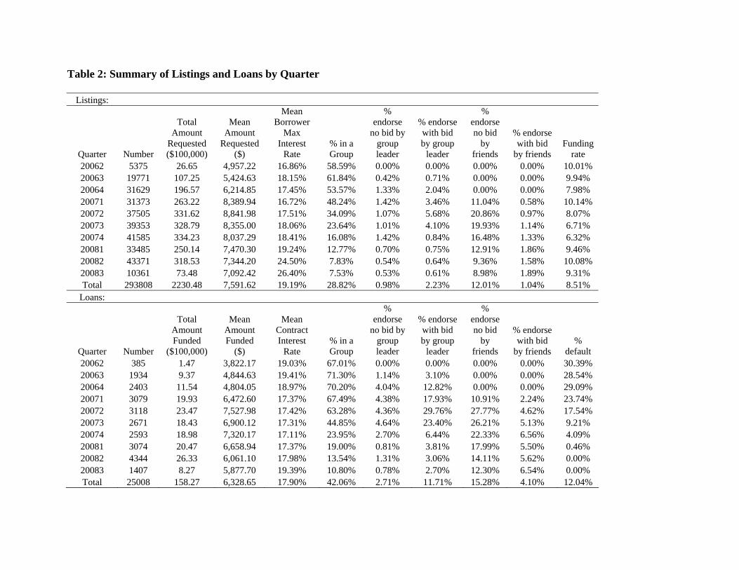
Table 2: Summary of Listings and Loans by Quarter

Listings:

Quarter Number

Total Amount

Requested ($100,000)

Mean Amount

Requested ($)

Mean Borrower

Max Interest

Rate % in a Group

% endorse

no bid by group leader

% endorse with bid by group

leader

% endorse no bid

by friends

% endorse with bid

by friends Funding

rate 20062 5375 26.65 4,957.22 16.86% 58.59% 0.00% 0.00% 0.00% 0.00% 10.01% 20063 19771 107.25 5,424.63 18.15% 61.84% 0.42% 0.71% 0.00% 0.00% 9.94% 20064 31629 196.57 6,214.85 17.45% 53.57% 1.33% 2.04% 0.00% 0.00% 7.98% 20071 31373 263.22 8,389.94 16.72% 48.24% 1.42% 3.46% 11.04% 0.58% 10.14% 20072 37505 331.62 8,841.98 17.51% 34.09% 1.07% 5.68% 20.86% 0.97% 8.07% 20073 39353 328.79 8,355.00 18.06% 23.64% 1.01% 4.10% 19.93% 1.14% 6.71% 20074 41585 334.23 8,037.29 18.41% 16.08% 1.42% 0.84% 16.48% 1.33% 6.32% 20081 33485 250.14 7,470.30 19.24% 12.77% 0.70% 0.75% 12.91% 1.86% 9.46% 20082 43371 318.53 7,344.20 24.50% 7.83% 0.54% 0.64% 9.36% 1.58% 10.08% 20083 10361 73.48 7,092.42 26.40% 7.53% 0.53% 0.61% 8.98% 1.89% 9.31% Total 293808 2230.48 7,591.62 19.19% 28.82% 0.98% 2.23% 12.01% 1.04% 8.51%

Loans:

Quarter Number

Total Amount Funded

($100,000)

Mean Amount Funded

($)

Mean Contract Interest

Rate % in a Group

% endorse

no bid by group leader

% endorse with bid by group

leader

% endorse no bid

by friends

% endorse with bid

by friends %

default 20062 385 1.47 3,822.17 19.03% 67.01% 0.00% 0.00% 0.00% 0.00% 30.39% 20063 1934 9.37 4,844.63 19.41% 71.30% 1.14% 3.10% 0.00% 0.00% 28.54% 20064 2403 11.54 4,804.05 18.97% 70.20% 4.04% 12.82% 0.00% 0.00% 29.09% 20071 3079 19.93 6,472.60 17.37% 67.49% 4.38% 17.93% 10.91% 2.24% 23.74% 20072 3118 23.47 7,527.98 17.42% 63.28% 4.36% 29.76% 27.77% 4.62% 17.54% 20073 2671 18.43 6,900.12 17.31% 44.85% 4.64% 23.40% 26.21% 5.13% 9.21% 20074 2593 18.98 7,320.17 17.11% 23.95% 2.70% 6.44% 22.33% 6.56% 4.09% 20081 3074 20.47 6,658.94 17.37% 19.00% 0.81% 3.81% 17.99% 5.50% 0.46% 20082 4344 26.33 6,061.10 17.98% 13.54% 1.31% 3.06% 14.11% 5.62% 0.00% 20083 1407 8.27 5,877.70 19.39% 10.80% 0.78% 2.70% 12.30% 6.54% 0.00% Total 25008 158.27 6,328.65 17.90% 42.06% 2.71% 11.71% 15.28% 4.10% 12.04%

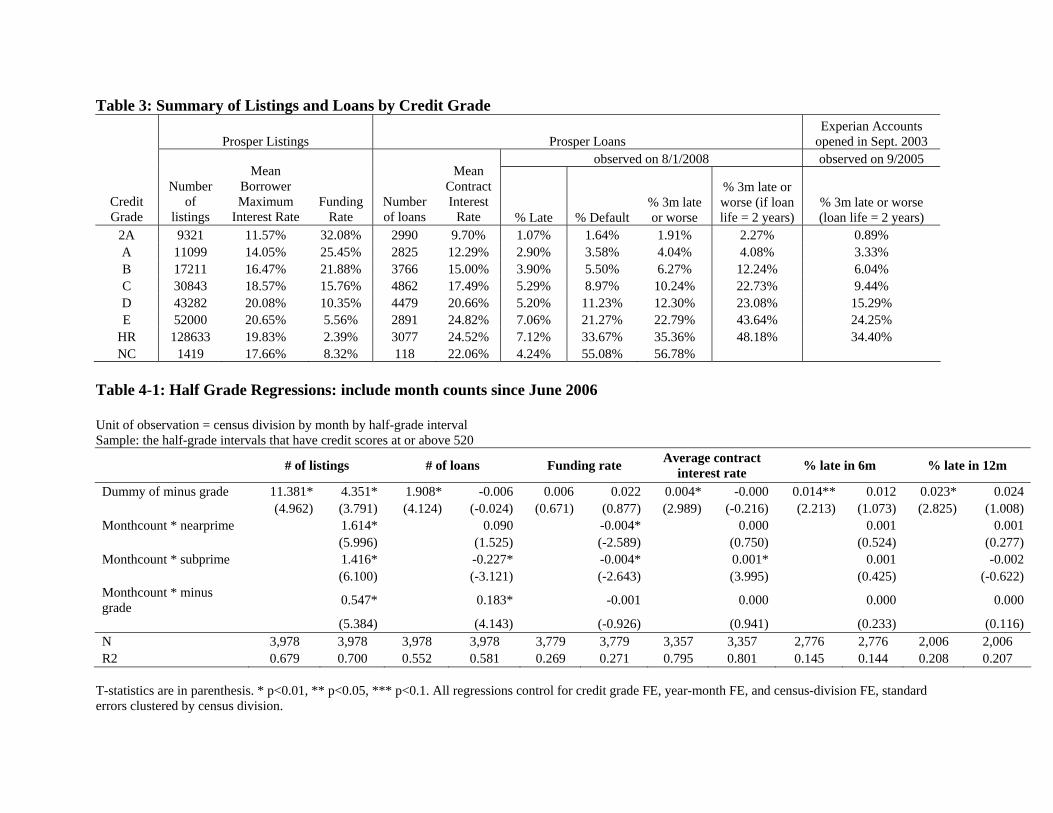
Table 3: Summary of Listings and Loans by Credit Grade

Prosper Listings Prosper Loans Experian Accounts

opened in Sept. 2003 observed on 8/1/2008 observed on 9/2005

Credit Grade

Number of

listings

Mean Borrower Maximum

Interest Rate Funding

Rate Number of loans

Mean Contract Interest

Rate % Late % Default % 3m late or worse

% 3m late or worse (if loan life = 2 years)

% 3m late or worse (loan life = 2 years)

2A 9321 11.57% 32.08% 2990 9.70% 1.07% 1.64% 1.91% 2.27% 0.89% A 11099 14.05% 25.45% 2825 12.29% 2.90% 3.58% 4.04% 4.08% 3.33% B 17211 16.47% 21.88% 3766 15.00% 3.90% 5.50% 6.27% 12.24% 6.04% C 30843 18.57% 15.76% 4862 17.49% 5.29% 8.97% 10.24% 22.73% 9.44% D 43282 20.08% 10.35% 4479 20.66% 5.20% 11.23% 12.30% 23.08% 15.29% E 52000 20.65% 5.56% 2891 24.82% 7.06% 21.27% 22.79% 43.64% 24.25%

HR 128633 19.83% 2.39% 3077 24.52% 7.12% 33.67% 35.36% 48.18% 34.40% NC 1419 17.66% 8.32% 118 22.06% 4.24% 55.08% 56.78%

Table 4-1: Half Grade Regressions: include month counts since June 2006 Unit of observation = census division by month by half-grade interval Sample: the half-grade intervals that have credit scores at or above 520

# of listings # of loans Funding rate Average contract interest rate % late in 6m % late in 12m

Dummy of minus grade 11.381* 4.351* 1.908* -0.006 0.006 0.022 0.004* -0.000 0.014** 0.012 0.023* 0.024 (4.962) (3.791) (4.124) (-0.024) (0.671) (0.877) (2.989) (-0.216) (2.213) (1.073) (2.825) (1.008) Monthcount * nearprime 1.614* 0.090 -0.004* 0.000 0.001 0.001 (5.996) (1.525) (-2.589) (0.750) (0.524) (0.277) Monthcount * subprime 1.416* -0.227* -0.004* 0.001* 0.001 -0.002 (6.100) (-3.121) (-2.643) (3.995) (0.425) (-0.622) Monthcount * minus grade 0.547* 0.183* -0.001 0.000 0.000 0.000

(5.384) (4.143) (-0.926) (0.941) (0.233) (0.116) N 3,978 3,978 3,978 3,978 3,779 3,779 3,357 3,357 2,776 2,776 2,006 2,006 R2 0.679 0.700 0.552 0.581 0.269 0.271 0.795 0.801 0.145 0.144 0.208 0.207

T-statistics are in parenthesis. * p<0.01, ** p<0.05, *** p<0.1. All regressions control for credit grade FE, year-month FE, and census-division FE, standard errors clustered by census division.

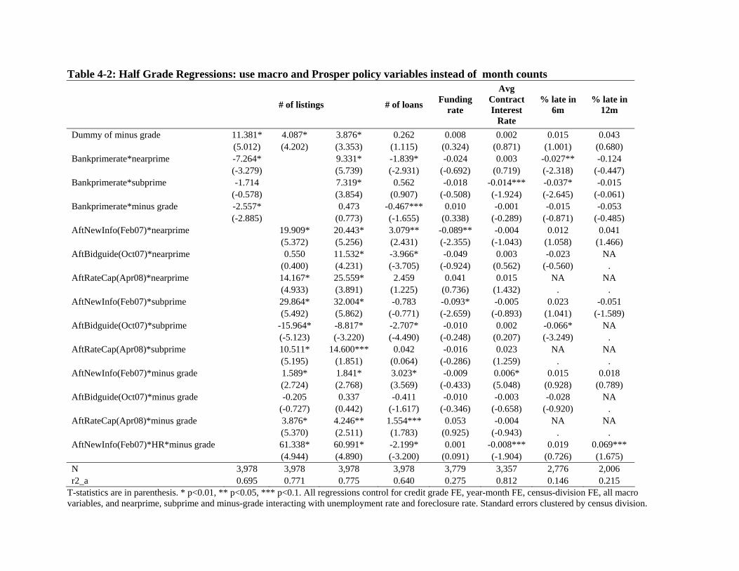
Table 4-2: Half Grade Regressions: use macro and Prosper policy variables instead of month counts

# of listings # of loans Funding rate

Avg Contract Interest

Rate

% late in 6m

% late in 12m

Dummy of minus grade 11.381* 4.087* 3.876* 0.262 0.008 0.002 0.015 0.043 (5.012) (4.202) (3.353) (1.115) (0.324) (0.871) (1.001) (0.680) Bankprimerate*nearprime -7.264* 9.331* -1.839* -0.024 0.003 -0.027** -0.124 (-3.279) (5.739) (-2.931) (-0.692) (0.719) (-2.318) (-0.447) Bankprimerate*subprime -1.714 7.319* 0.562 -0.018 -0.014*** -0.037* -0.015 (-0.578) (3.854) (0.907) (-0.508) (-1.924) (-2.645) (-0.061) Bankprimerate*minus grade -2.557* 0.473 -0.467*** 0.010 -0.001 -0.015 -0.053 (-2.885) (0.773) (-1.655) (0.338) (-0.289) (-0.871) (-0.485) AftNewInfo(Feb07)*nearprime 19.909* 20.443* 3.079** -0.089** -0.004 0.012 0.041 (5.372) (5.256) (2.431) (-2.355) (-1.043) (1.058) (1.466) AftBidguide(Oct07)*nearprime 0.550 11.532* -3.966* -0.049 0.003 -0.023 NA (0.400) (4.231) (-3.705) (-0.924) (0.562) (-0.560) . AftRateCap(Apr08)*nearprime 14.167* 25.559* 2.459 0.041 0.015 NA NA (4.933) (3.891) (1.225) (0.736) (1.432) . . AftNewInfo(Feb07)*subprime 29.864* 32.004* -0.783 -0.093* -0.005 0.023 -0.051 (5.492) (5.862) (-0.771) (-2.659) (-0.893) (1.041) (-1.589) AftBidguide(Oct07)*subprime -15.964* -8.817* -2.707* -0.010 0.002 -0.066* NA (-5.123) (-3.220) (-4.490) (-0.248) (0.207) (-3.249) . AftRateCap(Apr08)*subprime 10.511* 14.600*** 0.042 -0.016 0.023 NA NA (5.195) (1.851) (0.064) (-0.286) (1.259) . . AftNewInfo(Feb07)*minus grade 1.589* 1.841* 3.023* -0.009 0.006* 0.015 0.018 (2.724) (2.768) (3.569) (-0.433) (5.048) (0.928) (0.789) AftBidguide(Oct07)*minus grade -0.205 0.337 -0.411 -0.010 -0.003 -0.028 NA (-0.727) (0.442) (-1.617) (-0.346) (-0.658) (-0.920) . AftRateCap(Apr08)*minus grade 3.876* 4.246** 1.554*** 0.053 -0.004 NA NA (5.370) (2.511) (1.783) (0.925) (-0.943) . . AftNewInfo(Feb07)*HR*minus grade 61.338* 60.991* -2.199* 0.001 -0.008*** 0.019 0.069*** (4.944) (4.890) (-3.200) (0.091) (-1.904) (0.726) (1.675) N 3,978 3,978 3,978 3,978 3,779 3,357 2,776 2,006 r2_a 0.695 0.771 0.775 0.640 0.275 0.812 0.146 0.215

T-statistics are in parenthesis. * p<0.01, ** p<0.05, *** p<0.1. All regressions control for credit grade FE, year-month FE, census-division FE, all macro variables, and nearprime, subprime and minus-grade interacting with unemployment rate and foreclosure rate. Standard errors clustered by census division.

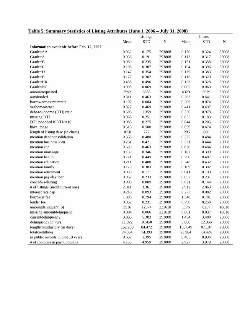
Table 5: Summary Statistics of Listing Attributes (June 1, 2006 – July 31, 2008) Listings Loans Mean STD N Mean STD N Information available before Feb. 12, 2007 Grade=AA 0.032 0.175 293808 0.120 0.324 25008 Grade=A 0.038 0.191 293808 0.113 0.317 25008 Grade=B 0.059 0.235 293808 0.151 0.358 25008 Grade=C 0.105 0.307 293808 0.194 0.396 25008 Grade=D 0.147 0.354 293808 0.179 0.383 25008 Grade=E 0.177 0.382 293808 0.116 0.320 25008 Grade=HR 0.438 0.496 293808 0.123 0.328 25008 Grade=NC 0.005 0.069 293808 0.005 0.069 25008 amountrequested 7592 6388 293808 6329 5679 25008 autofunded 0.311 0.463 293808 0.263 0.441 25008 borrowermaximumrate 0.192 0.084 293808 0.209 0.074 25008 yeshomeowner 0.327 0.469 293808 0.441 0.497 25008 debt-to-income (DTI) ratio 0.505 1.359 293808 0.330 0.978 25008 missing DTI 0.068 0.251 293808 0.035 0.183 25008 DTI topcoded if DTI>=10 0.083 0.275 293808 0.044 0.205 25008 have image 0.515 0.500 293808 0.659 0.474 25008 length of listing desc (in chars) 1058 772 293808 1295 866 25008 mention debt consolidation 0.358 0.480 293808 0.375 0.484 25008 mention business loan 0.231 0.421 293808 0.271 0.444 25008 mention car 0.689 0.463 293808 0.626 0.484 25008 mention mortgage 0.139 0.346 293808 0.187 0.390 25008 mention health 0.721 0.449 293808 0.790 0.407 25008 mention education 0.211 0.408 293808 0.248 0.432 25008 mention family 0.179 0.383 293808 0.189 0.392 25008 mention retirement 0.030 0.171 293808 0.041 0.199 25008 mention pay-day loan 0.057 0.233 293808 0.057 0.231 25008 concede relisting 0.008 0.089 293808 0.021 0.144 25008 # of listings (incld current one) 2.811 3.361 293808 2.912 2.863 25008 interest rate cap 0.243 0.093 293808 0.273 0.082 25008 borrower fee 1.800 0.794 293808 1.548 0.781 25008 lender fee 0.852 0.231 293808 0.790 0.258 25008 amountdelinquent ($) 3516 12374 221618 1176 6257 18618 missing amountdelinquent 0.004 0.066 221618 0.001 0.037 18618 currentdelinquency 3.833 5.303 293808 1.454 3.400 25008 delinquency in 7yrs 11.022 16.450 293808 5.800 12.356 25008 lengthcredithistory (in days) 152.208 84.472 293808 158.049 87.107 25008 totalcreditlines 24.354 14.393 293808 23.964 14.424 25008 in public records in past 10 years 0.657 1.395 293808 0.405 0.936 25008 # of inquiries in past 6 months 4.153 4.959 293808 2.927 3.979 25008

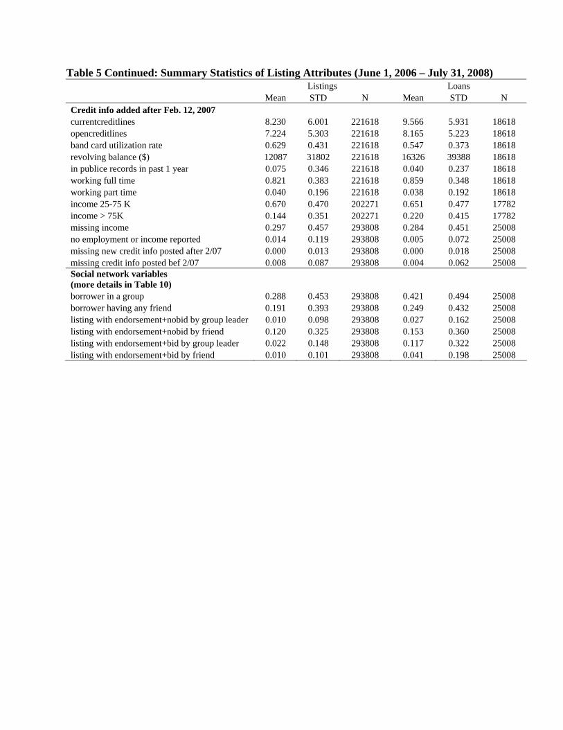
Table 5 Continued: Summary Statistics of Listing Attributes (June 1, 2006 – July 31, 2008) Listings Loans Mean STD N Mean STD N Credit info added after Feb. 12, 2007 currentcreditlines 8.230 6.001 221618 9.566 5.931 18618 opencreditlines 7.224 5.303 221618 8.165 5.223 18618 band card utilization rate 0.629 0.431 221618 0.547 0.373 18618 revolving balance ($) 12087 31802 221618 16326 39388 18618 in publice records in past 1 year 0.075 0.346 221618 0.040 0.237 18618 working full time 0.821 0.383 221618 0.859 0.348 18618 working part time 0.040 0.196 221618 0.038 0.192 18618 income 25-75 K 0.670 0.470 202271 0.651 0.477 17782 income > 75K 0.144 0.351 202271 0.220 0.415 17782 missing income 0.297 0.457 293808 0.284 0.451 25008 no employment or income reported 0.014 0.119 293808 0.005 0.072 25008 missing new credit info posted after 2/07 0.000 0.013 293808 0.000 0.018 25008 missing credit info posted bef 2/07 0.008 0.087 293808 0.004 0.062 25008 Social network variables (more details in Table 10) borrower in a group 0.288 0.453 293808 0.421 0.494 25008 borrower having any friend 0.191 0.393 293808 0.249 0.432 25008 listing with endorsement+nobid by group leader 0.010 0.098 293808 0.027 0.162 25008 listing with endorsement+nobid by friend 0.120 0.325 293808 0.153 0.360 25008 listing with endorsement+bid by group leader 0.022 0.148 293808 0.117 0.322 25008 listing with endorsement+bid by friend 0.010 0.101 293808 0.041 0.198 25008

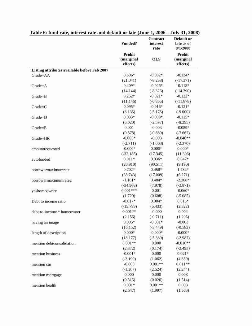
Table 6: fund rate, interest rate and default or late (June 1, 2006 – July 31, 2008)

Funded?

Contract interest

rate

Default or late as of 8/1/2008

Probit (marginal

effects) OLS

Probit (marginal

effects) Listing attributes available before Feb 2007 Grade=AA 0.696* -0.032* -0.134* (21.041) (-8.258) (-17.371) Grade=A 0.409* -0.026* -0.118* (14.144) (-8.326) (-14.290) Grade=B 0.252* -0.021* -0.122* (11.146) (-6.855) (-11.878) Grade=C 0.095* -0.016* -0.121* (8.135) (-5.175) (-9.000) Grade=D 0.033* -0.008* -0.115* (6.020) (-2.597) (-9.295) Grade=E 0.001 -0.003 -0.089* (0.578) (-0.889) (-7.667) Grade=HR -0.005* -0.003 -0.048** (-2.711) (-1.068) (-2.370) amountrequested -0.000* 0.000* 0.000* (-32.188) (17.345) (11.306) autofunded 0.011* 0.036* 0.047* (20.910) (90.511) (9.190) borrowermaximumrate 0.702* 0.458* 1.732* (38.743) (17.009) (6.271) borrowermaximumrate2 -1.161* 0.484* -2.308* (-34.968) (7.978) (-3.871) yeshomeowner 0.001*** 0.001 -0.060* (1.729) (0.608) (-5.085) Debt to income ratio -0.017* 0.004* 0.015* (-15.799) (5.433) (2.822) debt-to-income * homeowner 0.001** -0.000 0.004 (2.156) (-0.711) (1.205) having an image 0.005* -0.001* -0.003 (16.152) (-3.449) (-0.582) length of description 0.000* -0.000* -0.000* (18.177) (-5.380) (-2.987) mention debtconsolidation 0.001** 0.000 -0.010** (2.372) (0.174) (-2.493) mention business -0.001* 0.000 0.021* (-3.199) (1.062) (4.359) mention car -0.000 0.001** 0.011** (-1.207) (2.524) (2.244) mention mortgage 0.000 0.000 0.008 (0.315) (0.026) (1.514) mention health 0.001* 0.001** 0.008 (2.647) (1.997) (1.563)

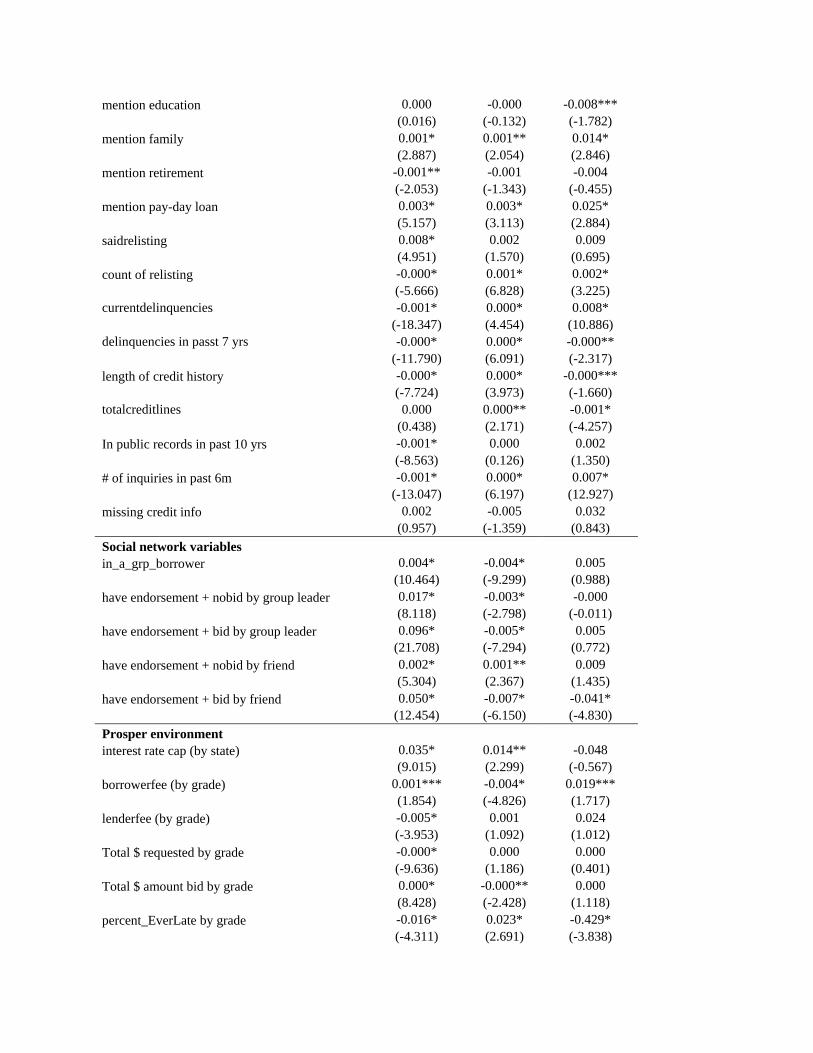
mention education 0.000 -0.000 -0.008*** (0.016) (-0.132) (-1.782) mention family 0.001* 0.001** 0.014* (2.887) (2.054) (2.846) mention retirement -0.001** -0.001 -0.004 (-2.053) (-1.343) (-0.455) mention pay-day loan 0.003* 0.003* 0.025* (5.157) (3.113) (2.884) saidrelisting 0.008* 0.002 0.009 (4.951) (1.570) (0.695) count of relisting -0.000* 0.001* 0.002* (-5.666) (6.828) (3.225) currentdelinquencies -0.001* 0.000* 0.008* (-18.347) (4.454) (10.886) delinquencies in passt 7 yrs -0.000* 0.000* -0.000** (-11.790) (6.091) (-2.317) length of credit history -0.000* 0.000* -0.000*** (-7.724) (3.973) (-1.660) totalcreditlines 0.000 0.000** -0.001* (0.438) (2.171) (-4.257) In public records in past 10 yrs -0.001* 0.000 0.002 (-8.563) (0.126) (1.350) # of inquiries in past 6m -0.001* 0.000* 0.007* (-13.047) (6.197) (12.927) missing credit info 0.002 -0.005 0.032 (0.957) (-1.359) (0.843) Social network variables in_a_grp_borrower 0.004* -0.004* 0.005 (10.464) (-9.299) (0.988) have endorsement + nobid by group leader 0.017* -0.003* -0.000 (8.118) (-2.798) (-0.011) have endorsement + bid by group leader 0.096* -0.005* 0.005 (21.708) (-7.294) (0.772) have endorsement + nobid by friend 0.002* 0.001** 0.009 (5.304) (2.367) (1.435) have endorsement + bid by friend 0.050* -0.007* -0.041* (12.454) (-6.150) (-4.830) Prosper environment interest rate cap (by state) 0.035* 0.014** -0.048 (9.015) (2.299) (-0.567) borrowerfee (by grade) 0.001*** -0.004* 0.019*** (1.854) (-4.826) (1.717) lenderfee (by grade) -0.005* 0.001 0.024 (-3.953) (1.092) (1.012) Total $ requested by grade -0.000* 0.000 0.000 (-9.636) (1.186) (0.401) Total $ amount bid by grade 0.000* -0.000** 0.000 (8.428) (-2.428) (1.118) percent_EverLate by grade -0.016* 0.023* -0.429* (-4.311) (2.691) (-3.838)

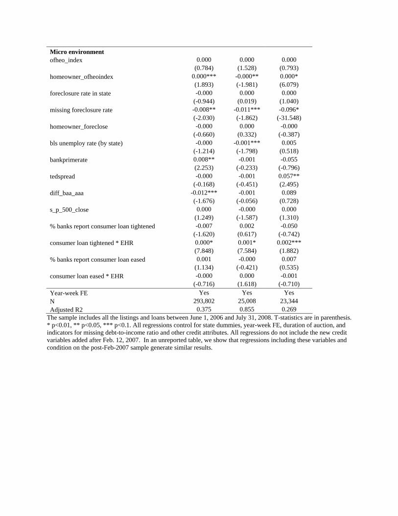
Micro environment ofheo_index 0.000 0.000 0.000 (0.784) (1.528) (0.793) homeowner_ofheoindex 0.000*** -0.000** 0.000* (1.893) (-1.981) (6.079) foreclosure rate in state -0.000 0.000 0.000 (-0.944) (0.019) (1.040) missing foreclosure rate -0.008** -0.011*** -0.096* (-2.030) (-1.862) (-31.548) homeowner_foreclose -0.000 0.000 -0.000 (-0.660) (0.332) (-0.387) bls unemploy rate (by state) -0.000 -0.001*** 0.005 (-1.214) (-1.798) (0.518) bankprimerate 0.008** -0.001 -0.055 (2.253) (-0.233) (-0.796) tedspread -0.000 -0.001 0.057** (-0.168) (-0.451) (2.495) diff_baa_aaa -0.012*** -0.001 0.089 (-1.676) (-0.056) (0.728) s_p_500_close 0.000 -0.000 0.000 (1.249) (-1.587) (1.310) % banks report consumer loan tightened -0.007 0.002 -0.050 (-1.620) (0.617) (-0.742) consumer loan tightened * EHR 0.000* 0.001* 0.002*** (7.848) (7.584) (1.882) % banks report consumer loan eased 0.001 -0.000 0.007 (1.134) (-0.421) (0.535) consumer loan eased * EHR -0.000 0.000 -0.001 (-0.716) (1.618) (-0.710) Year-week FE Yes Yes Yes N 293,802 25,008 23,344 Adjusted R2 0.375 0.855 0.269

The sample includes all the listings and loans between June 1, 2006 and July 31, 2008. T-statistics are in parenthesis. * p<0.01, ** p<0.05, *** p<0.1. All regressions control for state dummies, year-week FE, duration of auction, and indicators for missing debt-to-income ratio and other credit attributes. All regressions do not include the new credit variables added after Feb. 12, 2007. In an unreported table, we show that regressions including these variables and condition on the post-Feb-2007 sample generate similar results.

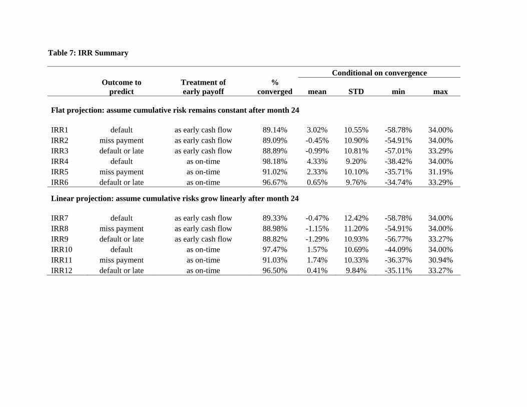
Table 7: IRR Summary Conditional on convergence

Outcome to

predict Treatment of early payoff

% converged mean STD min max

Flat projection: assume cumulative risk remains constant after month 24 IRR1 default as early cash flow 89.14% 3.02% 10.55% -58.78% 34.00% IRR2 miss payment as early cash flow 89.09% -0.45% 10.90% -54.91% 34.00% IRR3 default or late as early cash flow 88.89% -0.99% 10.81% -57.01% 33.29% IRR4 default as on-time 98.18% 4.33% 9.20% -38.42% 34.00% IRR5 miss payment as on-time 91.02% 2.33% 10.10% -35.71% 31.19% IRR6 default or late as on-time 96.67% 0.65% 9.76% -34.74% 33.29%

Linear projection: assume cumulative risks grow linearly after month 24 IRR7 default as early cash flow 89.33% -0.47% 12.42% -58.78% 34.00% IRR8 miss payment as early cash flow 88.98% -1.15% 11.20% -54.91% 34.00% IRR9 default or late as early cash flow 88.82% -1.29% 10.93% -56.77% 33.27% IRR10 default as on-time 97.47% 1.57% 10.69% -44.09% 34.00% IRR11 miss payment as on-time 91.03% 1.74% 10.33% -36.37% 30.94% IRR12 default or late as on-time 96.50% 0.41% 9.84% -35.11% 33.27%

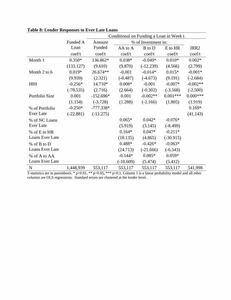
Table 8: Lender Responses to Ever Late Loans Conditional on Funding a Loan in Week t % of Investment in:

Funded A Loan

Amount Funded AA to A B to D E to HR IRR2

coef/t coef/t coef/t coef/t coef/t coef/t Month 1 0.350* 136.862* 0.038* -0.049* 0.010* 0.002* (133.127) (9.610) (9.870) (-12.239) (4.566) (2.799) Month 2 to 6 0.019* 26.674** -0.001 -0.014* 0.015* -0.001* (9.939) (2.321) (-0.487) (-4.673) (9.191) (-2.684) HHI -0.256* 14.710* 0.008* -0.001 -0.007* -0.002** (-78.535) (2.716) (2.664) (-0.302) (-3.568) (-2.500) Portfolio Size 0.001 -152.696* 0.001 -0.002** 0.001*** 0.000*** (1.154) (-3.728) (1.288) (-2.166) (1.805) (1.919)

-0.250* -777.338* 0.169* % of Portfolio Ever Late (-22.881) (-11.275) (41.143)

0.065* 0.042* -0.076* % of NC Loans Ever Late (5.919) (3.145) (-8.499)

0.164* 0.047* -0.211* % of E to HR Loans Ever Late (18.135) (4.865) (-30.915)

0.488* -0.426* -0.063* % of B to D Loans Ever Late (24.713) (-21.666) (-6.543)

-0.144* 0.085* 0.059* % of A to AA Loans Ever Late (-10.609) (5.474) (5.412) N 1,448,939 553,117 553,117 553,117 553,117 541,998

T-statistics are in parenthesis. * p<0.01, ** p<0.05, *** p<0.1. Column 1 is a linear probability model and all other columns are OLS regressions. Standard errors are clustered at the lender level.

Table 9: Potential roles of Social Networks on Prosper.com Predictions

Potential roles of social network Funding rate

IRR conditional on funded

Others

Signal good risk + 0

Within-network charity + - (1) Lower IRR if more funds come from within-network (2) No or less learning over time, especially for listings within the network

Cheap talk (interpreted correctly) 0 0

Lender misinterpretation + - Learn over time

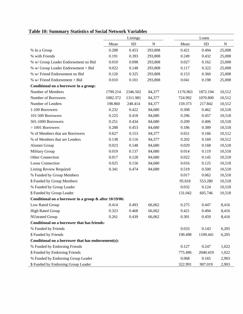
Table 10: Summary Statistics of Social Network Variables Listings Loans Mean SD N Mean SD N % In a Group 0.288 0.453 293,808 0.421 0.494 25,008 % with Friends 0.191 0.393 293,808 0.249 0.432 25,008 % w/ Group Leader Endorsement no Bid 0.010 0.098 293,808 0.027 0.162 25,008 % w/ Group Leader Endorsement + Bid 0.022 0.148 293,808 0.117 0.322 25,008 % w/ Friend Endorsement no Bid 0.120 0.325 293,808 0.153 0.360 25,008 % w/ Friend Endorsement + Bid 0.010 0.101 293,808 0.041 0.198 25,008 Conditional on a borrower in a group: Number of Members 1799.214 2346.502 84,377 1176.963 1872.194 10,512 Number of Borrowers 1082.372 1311.981 84,377 724.992 1070.800 10,512 Number of Lenders 198.860 248.414 84,377 159.373 217.842 10,512 1-100 Borrowers 0.232 0.422 84,680 0.308 0.462 10,518 101-500 Borrowers 0.225 0.418 84,680 0.296 0.457 10,518 501-1000 Borrowers 0.251 0.434 84,680 0.209 0.406 10,518 > 1001 Borrowers 0.288 0.453 84,680 0.186 0.389 10,518 % of Members that are Borrowers 0.627 0.153 84,377 0.651 0.166 10,512 % of Members that are Lenders 0.138 0.116 84,377 0.202 0.169 10,512 Alumni Group 0.023 0.148 84,680 0.029 0.168 10,518 Military Group 0.019 0.137 84,680 0.014 0.119 10,518 Other Connection 0.017 0.128 84,680 0.022 0.145 10,518 Loose Connection 0.025 0.156 84,680 0.016 0.125 10,518 Listing Review Required 0.341 0.474 84,680 0.519 0.500 10,518 % Funded by Group Members 0.017 0.062 10,518 $ Funded by Group Members 95.818 553.280 10,518 % Funded by Group Leader 0.032 0.124 10,518 $ Funded by Group Leader 131.042 605.746 10,518 Conditional on a borrower in a group & after 10/19/06: Low Rated Group 0.414 0.493 66,062 0.275 0.447 8,416 High Rated Group 0.323 0.468 66,062 0.421 0.494 8,416 NUnrated Group 0.261 0.439 66,062 0.301 0.459 8,416 Conditional on a borrower that has friends: % Funded by Friends 0.033 0.143 6,205 $ Funded by Friends 190.498 1109.441 6,205 Conditional on a borrower that has endorsement(s): % Funded by Endorsing Friends 0.127 0.247 1,022 $ Funded by Endorsing Friends 775.496 2040.419 1,022 % Funded by Endorsing Group Leader 0.068 0.165 2,903 $ Funded by Endorsing Group Leader 322.991 907.019 2,903

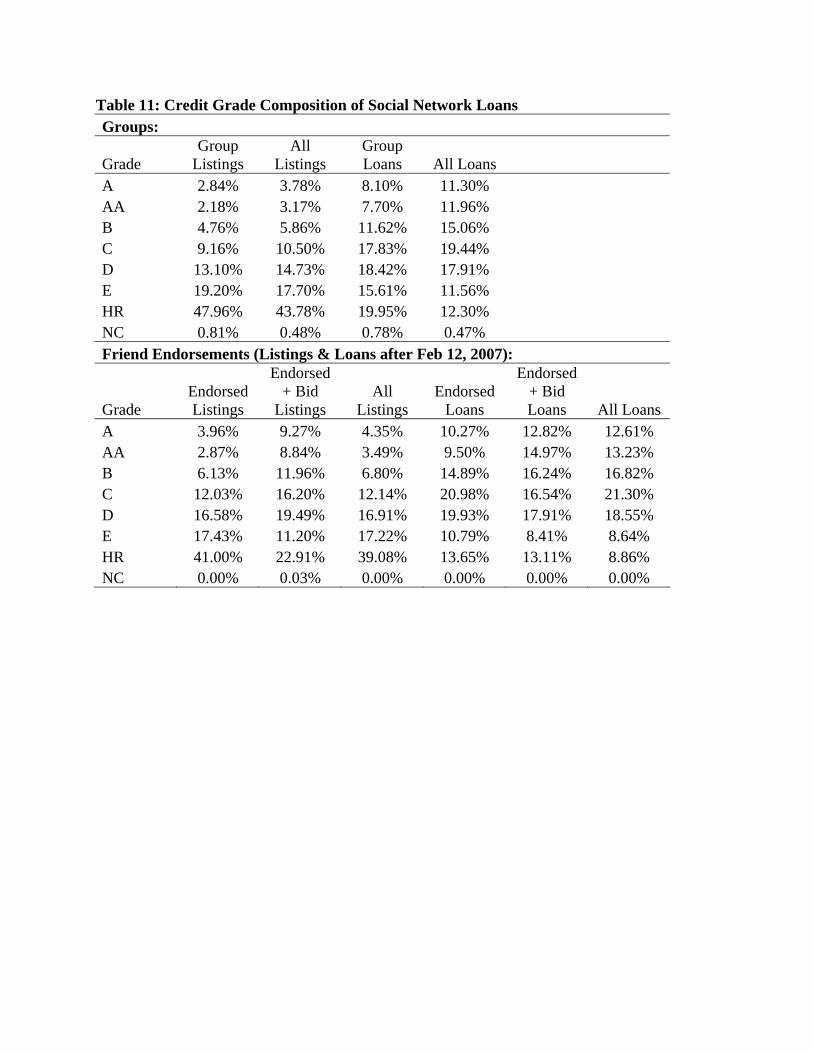
Table 11: Credit Grade Composition of Social Network Loans Groups:

Grade Group

Listings All

Listings Group Loans All Loans

A 2.84% 3.78% 8.10% 11.30% AA 2.18% 3.17% 7.70% 11.96% B 4.76% 5.86% 11.62% 15.06% C 9.16% 10.50% 17.83% 19.44% D 13.10% 14.73% 18.42% 17.91% E 19.20% 17.70% 15.61% 11.56% HR 47.96% 43.78% 19.95% 12.30% NC 0.81% 0.48% 0.78% 0.47% Friend Endorsements (Listings & Loans after Feb 12, 2007):

Grade Endorsed Listings

Endorsed + Bid

Listings All

Listings Endorsed

Loans

Endorsed + Bid Loans All Loans

A 3.96% 9.27% 4.35% 10.27% 12.82% 12.61% AA 2.87% 8.84% 3.49% 9.50% 14.97% 13.23% B 6.13% 11.96% 6.80% 14.89% 16.24% 16.82% C 12.03% 16.20% 12.14% 20.98% 16.54% 21.30% D 16.58% 19.49% 16.91% 19.93% 17.91% 18.55% E 17.43% 11.20% 17.22% 10.79% 8.41% 8.64% HR 41.00% 22.91% 39.08% 13.65% 13.11% 8.86% NC 0.00% 0.03% 0.00% 0.00% 0.00% 0.00%

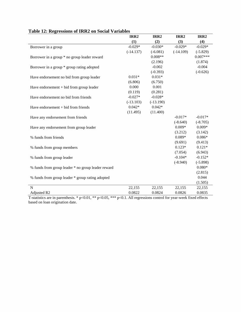
Table 12: Regressions of IRR2 on Social Variables IRR2 IRR2 IRR2 IRR2 (1) (2) (3) (4) Borrower in a group -0.029* -0.030* -0.029* -0.029* (-14.137) (-6.081) (-14.109) (-5.829) Borrower in a group * no group leader reward 0.008** 0.007*** (2.196) (1.874) Borrower in a group * group rating adopted -0.002 -0.004 (-0.393) (-0.626) Have endorsement no bid from group leader 0.031* 0.031* (6.806) (6.750) Have endorsement + bid from group leader 0.000 0.001 (0.119) (0.281) Have endorsement no bid from friends -0.027* -0.028* (-13.103) (-13.190) Have endorsement + bid from friends 0.042* 0.042* (11.495) (11.400) Have any endorsement from friends -0.017* -0.017* (-8.640) (-8.705) Have any endorsement from group leader 0.009* 0.009* (3.212) (3.142) % funds from friends 0.089* 0.086* (9.691) (9.413) % funds from group members 0.123* 0.121* (7.054) (6.943) % funds from group leader -0.104* -0.152* (-8.940) (-5.898) % funds from group leader * no group leader reward 0.080* (2.815) % funds from group leader * group rating adopted 0.044 (1.505) N 22,155 22,155 22,155 22,155 Adjusted R2 0.0822 0.0824 0.0826 0.0835

T-statistics are in parenthesis. * p<0.01, ** p<0.05, *** p<0.1. All regressions control for year-week fixed effects based on loan origination date.

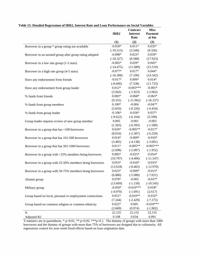
Table 13: Detailed Regressions of IRR2, Interest Rate and Loan Performance on Social Variables

IRR2

Contract Interest

Rate

Miss Payment

at 6m (1) (2) (3) Borrower in a group * group rating not available -0.059* 0.011* 0.035* (-10.313) (3.546) (9.326) Borrower in an unrated group after group rating adopted -0.098* 0.023* 0.059* (-18.327) (8.588) (17.023) Borrower in a low rate group (1-3 stars) -0.065* 0.029* 0.045* (-14.475) (11.689) (15.519) Borrower in a high rate group (4-5 stars) -0.077* 0.017* 0.044* (-16.308) (7.100) (14.342) Have any endorsement from friends -0.017* 0.009* 0.014* (-8.690) (7.538) (11.733) Have any endorsement from group leader 0.012* -0.003*** -0.005* (3.942) (-1.923) (-2.662) % funds from friends 0.083* -0.068* -0.063* (9.331) (-11.962) (-16.337) % funds from group members 0.100* -0.004 -0.047* (5.810) (-0.326) (-4.454) % funds from group leader -0.106* -0.036* 0.037* (-9.622) (-6.164) (5.590) Group leader requires review of new group member 0.005 -0.001 -0.003 (1.565) (-0.393) (-1.580) Borrower in a group that has <100 borrowers 0.034* -0.005** -0.017* (8.016) (-2.387) (-6.259) Borrower in a group that has 101-500 borrowers 0.014* -0.009* -0.010* (3.405) (-4.138) (-3.681) Borrower in a group that has 501-1000 borrowers 0.011* -0.005** -0.005*** (2.698) (-2.087) (-1.952) Borrower in a group with <25% members being borrowers 0.085* -0.025* -0.054* (10.797) (-4.406) (-11.547) Borrower in a group with 25-50% members being borrowers 0.053* -0.018* -0.033* (13.618) (-8.402) (-12.970) Borrower in a group with 50-75% members being borrowers 0.023* -0.009* -0.015* (6.886) (-5.080) (-7.021) Alumni group 0.078* -0.005 -0.037* (13.669) (-1.158) (-10.545) Military group -0.050* -0.010*** 0.018* (-4.970) (-1.691) (2.617) Group based on local, personal or employment connections 0.051* -0.010** -0.032* (7.244) (-2.429) (-7.373) Group based on common religion or common ethnicity 0.022* 0.005 -0.010*** (2.669) (0.974) (-1.902) N 22,155 22,155 22,155 Adjusted R2 0.108 0.034 0.091

T-statistics are in parenthesis. * p<0.01, ** p<0.05, ***p<0.1. The dummy of groups with more than 1000 borrowers and the dummy of groups with more than 75% of borrowers are dropped due to colinearity. All regressions control for year-week fixed effects based on loan origination date.

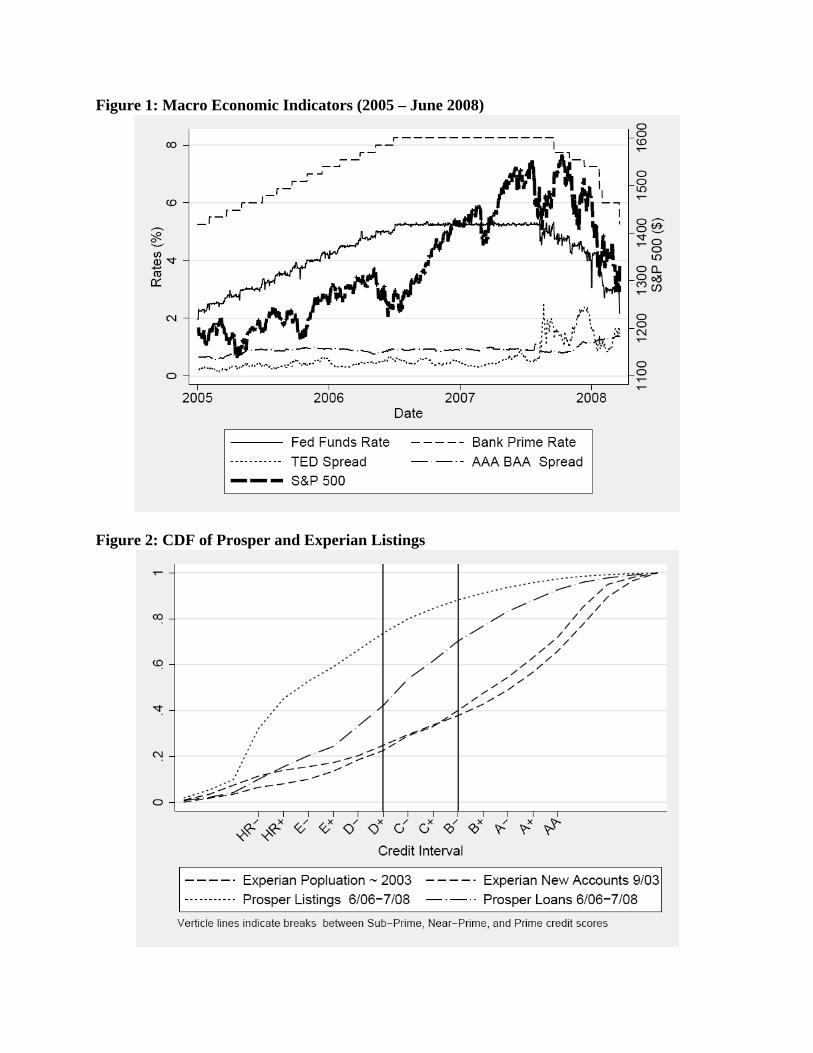
Figure 1: Macro Economic Indicators (2005 – June 2008)

Figure 2: CDF of Prosper and Experian Listings

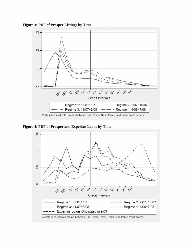
Figure 3: PDF of Prosper Listings by Time

Figure 4: PDF of Prosper and Experian Loans by Time

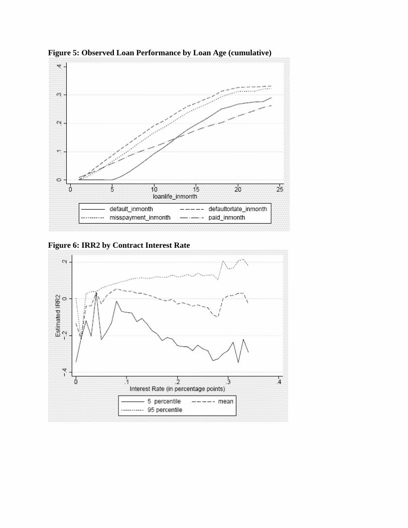
Figure 5: Observed Loan Performance by Loan Age (cumulative)

Figure 6: IRR2 by Contract Interest Rate

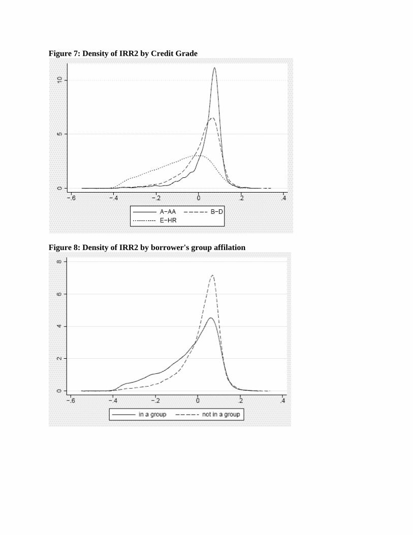
Figure 7: Density of IRR2 by Credit Grade

Figure 8: Density of IRR2 by borrower's group affilation

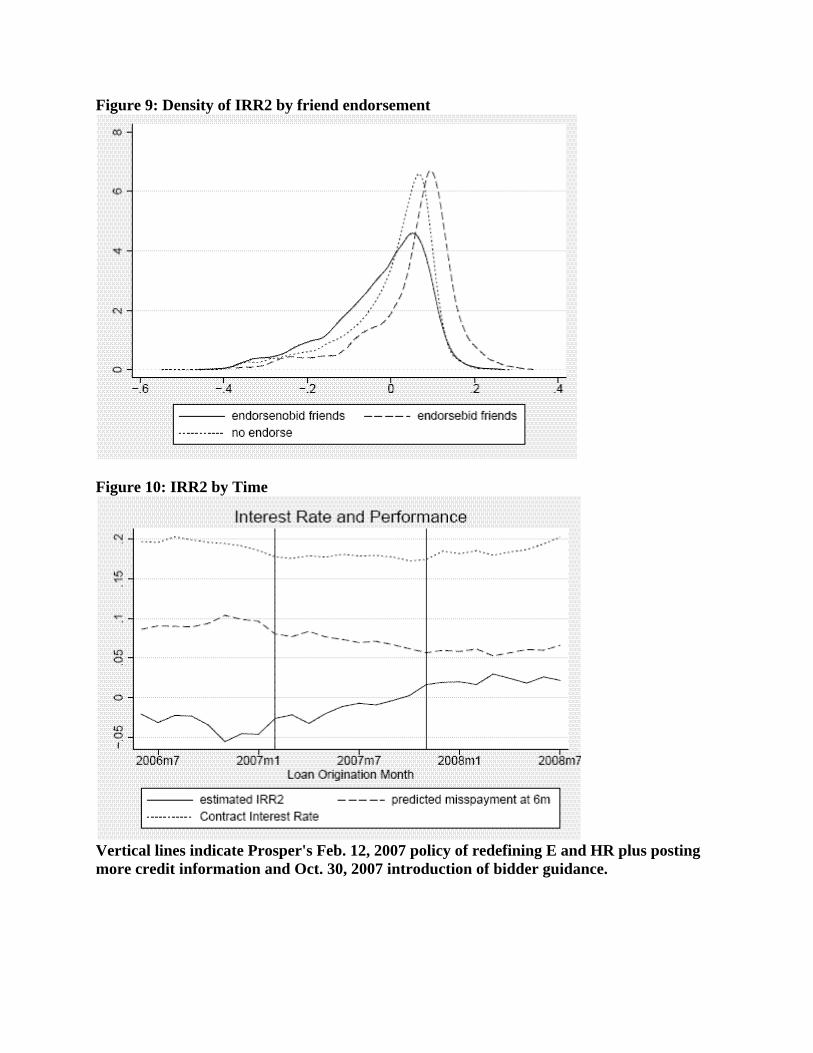
Figure 9: Density of IRR2 by friend endorsement

Figure 10: IRR2 by Time

Vertical lines indicate Prosper's Feb. 12, 2007 policy of redefining E and HR plus posting more credit information and Oct. 30, 2007 introduction of bidder guidance.

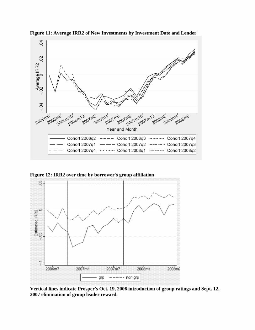
Figure 11: Average IRR2 of New Investments by Investment Date and Lender

Figure 12: IRR2 over time by borrower's group affiliation

Vertical lines indicate Prosper's Oct. 19, 2006 introduction of group ratings and Sept. 12, 2007 elimination of group leader reward.

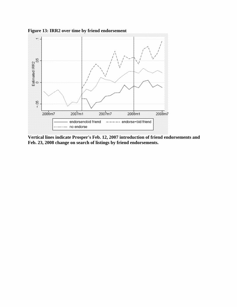
Figure 13: IRR2 over time by friend endorsement

Vertical lines indicate Prosper's Feb. 12, 2007 introduction of friend endorsements and Feb. 23, 2008 change on search of listings by friend endorsements.