Document title: We appreciate your feedback · We appreciate your feedback Please click on the icon to take a 5’ online survey and provide your feedback about this document Share

Document title:

Publishing date: 06/10/2017

We appreciate your feedback

Please click on the icon to take a 5’ online surveyand provide your feedback about this document

Share this document

https://www.acer.europa.eu/Lists/Survey/NewForm.aspx?documentid=ACER-2017-46983&Source=https%3a%2f%2fwww.acer.europa.eu

https://twitter.com/intent/tweet?url=https%3a%2f%2fwww.acer.europa.eu%2f%2fOfficial_documents%2fActs_of_the_Agency%2fPublication%2fACER+Market+Monitoring+Report+2016+-+ELECTRICITY.pdf&text=

http://www.facebook.com/share.php?u=https%3a%2f%2fwww.acer.europa.eu%2f%2fOfficial_documents%2fActs_of_the_Agency%2fPublication%2fACER+Market+Monitoring+Report+2016+-+ELECTRICITY.pdf&t=

http://www.linkedin.com/shareArticle?mini=true&url=https%3a%2f%2fwww.acer.europa.eu%2f%2fOfficial_documents%2fActs_of_the_Agency%2fPublication%2fACER+Market+Monitoring+Report+2016+-+ELECTRICITY.pdf&title=&ro=false&summary=&source=

https://plus.google.com/share?url=https%3a%2f%2fwww.acer.europa.eu%2f%2fOfficial_documents%2fActs_of_the_Agency%2fPublication%2fACER+Market+Monitoring+Report+2016+-+ELECTRICITY.pdf&t=

ACER/CEER

Annual Report on the Results of Monitoring the Internal Electricity and Gas Marketsin 2016Electricity Wholesale Markets Volume

October 2017

Legal notice

The joint publication of the Agency for the Cooperation of Energy Regulators and the Council of European Energy Regulators is protected by copyright. The Agency for the Cooperation of Energy Regulators and the Council of European Energy Regulators accept no responsibility or liability for any consequences arising from the use of the data contained in this document.

© Agency for the Cooperation of Energy Regulators and the Council of European Energy Regulators, 2017Reproduction is authorised provided the source is acknowledged.

3

A C E R / C E E R A N N U A L R E P O R T O N T H E R E S U L T S O F M O N I T O R I N G T H E I N T E R N A L E L E C T R I C I T Y M A R K E T S I N 2 0 1 6

ACER/CEER

Annual Report on the Results of Monitoring the Internal Electricity and Gas Markets in 2016Electricity Wholesale Markets Volume

October 2017

The support of the Energy Community Secretariat in coordinating the collection and in analysing the information related to the Energy Community Contracting Parties is gratefully acknowledged.

CEER

Mr Andrew EbrillT +32 (0)2 788 73 35E [email protected]

ACER

Mr David MerinoT +386 (0)8 2053 417E [email protected]

Cours Saint-Michel 30a, box F1040 BrusselsBelgium

Trg republike 3 1000 Ljubljana Slovenia

If you have any queries relating to this report, please contact:

4


ContentsExecutive Summary . . . . . . . . . . . . . . . . . . . . . . . . . . . . . . . . . . . . . . . . . . . . . . . . . . . . . . . . . . . . . . . . . . . . . . . . . . . . . . . . . . . . . . . . 5

Recommendations . . . . . . . . . . . . . . . . . . . . . . . . . . . . . . . . . . . . . . . . . . . . . . . . . . . . . . . . . . . . . . . . . . . . . . . . . . . . . . . . . . . . . . . . . 12

1 Introduction . . . . . . . . . . . . . . . . . . . . . . . . . . . . . . . . . . . . . . . . . . . . . . . . . . . . . . . . . . . . . . . . . . . . . . . . . . . . . . . . . . . . . . . . . 14

2 Key developments in 2016 . . . . . . . . . . . . . . . . . . . . . . . . . . . . . . . . . . . . . . . . . . . . . . . . . . . . . . . . . . . . . . . . . . . . . . . . . . 152.1 Evolution of electricity wholesale prices . . . . . . . . . . . . . . . . . . . . . . . . . . . . . . . . . . . . . . . . . . . . . . . . . . . . . . . . . . 152.2 Price convergence . . . . . . . . . . . . . . . . . . . . . . . . . . . . . . . . . . . . . . . . . . . . . . . . . . . . . . . . . . . . . . . . . . . . . . . . . . . . . . . 18

3 Available cross-zonal capacity . . . . . . . . . . . . . . . . . . . . . . . . . . . . . . . . . . . . . . . . . . . . . . . . . . . . . . . . . . . . . . . . . . . . . . . 213.1 Methodological improvements . . . . . . . . . . . . . . . . . . . . . . . . . . . . . . . . . . . . . . . . . . . . . . . . . . . . . . . . . . . . . . . . . . . . 213.2 Amount of cross-zonal capacity made available to the market . . . . . . . . . . . . . . . . . . . . . . . . . . . . . . . . . . . . 24

3.2.1 Evolution of commercial cross-zonal capacity . . . . . . . . . . . . . . . . . . . . . . . . . . . . . . . . . . . . . . . . . . . . . . . . . 243.2.2 Ratio between commercial and benchmark cross-zonal capacity . . . . . . . . . . . . . . . . . . . . . . . . . . . . . . 27

3.3 Factors impacting commercial cross-zonal capacity . . . . . . . . . . . . . . . . . . . . . . . . . . . . . . . . . . . . . . . . . . . . . . . 303.3.1 Level of coordination . . . . . . . . . . . . . . . . . . . . . . . . . . . . . . . . . . . . . . . . . . . . . . . . . . . . . . . . . . . . . . . . . . . . . . . . . 313.3.2 Discrimination between internal and cross-zonal exchanges . . . . . . . . . . . . . . . . . . . . . . . . . . . . . . . . . . 35

3.4 Remedial actions . . . . . . . . . . . . . . . . . . . . . . . . . . . . . . . . . . . . . . . . . . . . . . . . . . . . . . . . . . . . . . . . . . . . . . . . . . . . . . . . 38

4 Efficientuseofavailablecross-zonalcapacity . . . . . . . . . . . . . . . . . . . . . . . . . . . . . . . . . . . . . . . . . . . . . . . . . . . . . . . 404.1 Forward markets . . . . . . . . . . . . . . . . . . . . . . . . . . . . . . . . . . . . . . . . . . . . . . . . . . . . . . . . . . . . . . . . . . . . . . . . . . . . . . . . . 404.2 Day-ahead markets . . . . . . . . . . . . . . . . . . . . . . . . . . . . . . . . . . . . . . . . . . . . . . . . . . . . . . . . . . . . . . . . . . . . . . . . . . . . . . 42

4.2.1 Progress in day-ahead market coupling . . . . . . . . . . . . . . . . . . . . . . . . . . . . . . . . . . . . . . . . . . . . . . . . . . . . . . 424.2.2 Grosswelfarebenefitofbetteruseoftheexistingnetwork . . . . . . . . . . . . . . . . . . . . . . . . . . . . . . . . . . . . . 44

4.3 Intraday markets . . . . . . . . . . . . . . . . . . . . . . . . . . . . . . . . . . . . . . . . . . . . . . . . . . . . . . . . . . . . . . . . . . . . . . . . . . . . . . . . . 464.3.1 Evolution of intraday market liquidity . . . . . . . . . . . . . . . . . . . . . . . . . . . . . . . . . . . . . . . . . . . . . . . . . . . . . . . . . . 464.3.2 Intraday use of cross-zonal capacity . . . . . . . . . . . . . . . . . . . . . . . . . . . . . . . . . . . . . . . . . . . . . . . . . . . . . . . . . . 48

4.4 Balancing markets . . . . . . . . . . . . . . . . . . . . . . . . . . . . . . . . . . . . . . . . . . . . . . . . . . . . . . . . . . . . . . . . . . . . . . . . . . . . . . . 494.4.1 Balancing (capacity and energy) and imbalance prices . . . . . . . . . . . . . . . . . . . . . . . . . . . . . . . . . . . . . . . . 494.4.2 Cross-zonal exchange of balancing services . . . . . . . . . . . . . . . . . . . . . . . . . . . . . . . . . . . . . . . . . . . . . . . . . . 53

5 Capacity mechanisms and generation adequacy . . . . . . . . . . . . . . . . . . . . . . . . . . . . . . . . . . . . . . . . . . . . . . . . . . . . . 555.1 Situation in capacity mechanisms . . . . . . . . . . . . . . . . . . . . . . . . . . . . . . . . . . . . . . . . . . . . . . . . . . . . . . . . . . . . . . . . 555.2 Treatment of interconnectors in adequacy assessments . . . . . . . . . . . . . . . . . . . . . . . . . . . . . . . . . . . . . . . . . . 56

Annex1:Additionalfiguresandtables . . . . . . . . . . . . . . . . . . . . . . . . . . . . . . . . . . . . . . . . . . . . . . . . . . . . . . . . . . . . . . . . . . . . . . 61Annex 2: Methodology for calculating the benchmark capacity for CNTC and FB CC methods . . . . . . . . . . . . . . 67Annex3:Adaptedscoringmethodologyfortheleveloffulfilmentofcapacitycalculationrequirements . . . . . . . . 70Annex4:Unscheduledflows . . . . . . . . . . . . . . . . . . . . . . . . . . . . . . . . . . . . . . . . . . . . . . . . . . . . . . . . . . . . . . . . . . . . . . . . . . . . . . . 72

5


Executive Summary Key developments in 2016

1 The downward trend in wholesale electricity prices observed in previous years continued in 2016. In parallel, pricespikesoccurredsignificantlymorefrequentlythaninpreviousyears,with1,195occurrencesinEuropein2016,whichisaroundfivetimestheaverageovertheprecedingfouryears.Thesespikeswereobservedmoreoften in the Member States (MSs) with the tightest adequacy margins, such as Belgium, Finland, France and GreatBritain.Althoughthesespikesmayreflectefficientpriceformationattimesofscarcity,theyalsohighlighttheimportanceofaddressingsecurityofsupplyefficientlyandinacoordinatedmanner.

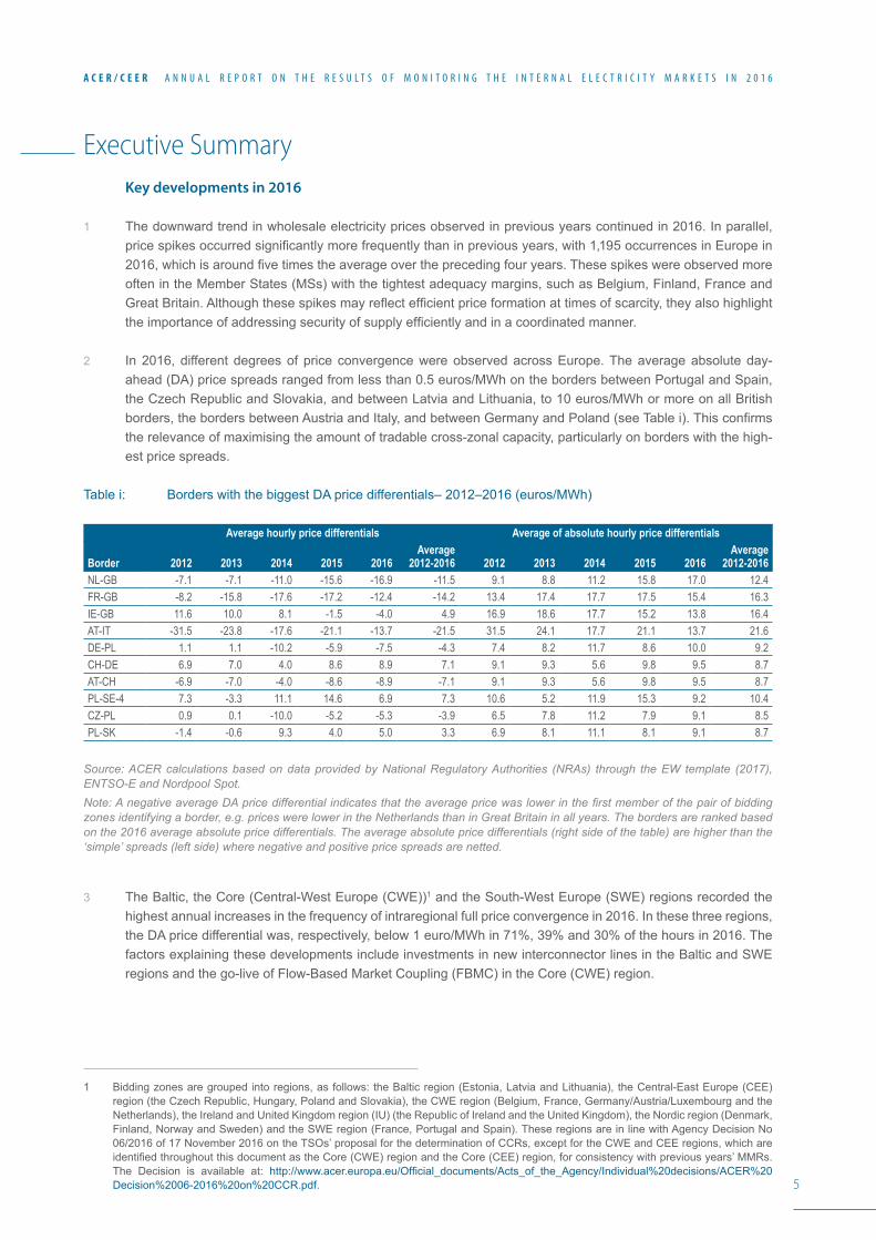
2 In 2016, different degrees of price convergence were observed across Europe. The average absolute day-ahead (DA) price spreads ranged from less than 0.5 euros/MWh on the borders between Portugal and Spain, the Czech Republic and Slovakia, and between Latvia and Lithuania, to 10 euros/MWh or more on all British borders,thebordersbetweenAustriaandItaly,andbetweenGermanyandPoland(seeTablei).Thisconfirmsthe relevance of maximising the amount of tradable cross-zonal capacity, particularly on borders with the high-est price spreads.

Table i: Borders with the biggest DA price differentials– 2012–2016 (euros/MWh)

Average hourly price differentials Average of absolute hourly price differentials

Border 2012 2013 2014 2015 2016Average

2012-2016 2012 2013 2014 2015 2016Average

2012-2016NL-GB -7.1 -7.1 -11.0 -15.6 -16.9 -11.5 9.1 8.8 11.2 15.8 17.0 12.4FR-GB -8.2 -15.8 -17.6 -17.2 -12.4 -14.2 13.4 17.4 17.7 17.5 15.4 16.3IE-GB 11.6 10.0 8.1 -1.5 -4.0 4.9 16.9 18.6 17.7 15.2 13.8 16.4AT-IT -31.5 -23.8 -17.6 -21.1 -13.7 -21.5 31.5 24.1 17.7 21.1 13.7 21.6DE-PL 1.1 1.1 -10.2 -5.9 -7.5 -4.3 7.4 8.2 11.7 8.6 10.0 9.2CH-DE 6.9 7.0 4.0 8.6 8.9 7.1 9.1 9.3 5.6 9.8 9.5 8.7AT-CH -6.9 -7.0 -4.0 -8.6 -8.9 -7.1 9.1 9.3 5.6 9.8 9.5 8.7PL-SE-4 7.3 -3.3 11.1 14.6 6.9 7.3 10.6 5.2 11.9 15.3 9.2 10.4CZ-PL 0.9 0.1 -10.0 -5.2 -5.3 -3.9 6.5 7.8 11.2 7.9 9.1 8.5PL-SK -1.4 -0.6 9.3 4.0 5.0 3.3 6.9 8.1 11.1 8.1 9.1 8.7

Source: ACER calculations based on data provided by National Regulatory Authorities (NRAs) through the EW template (2017), ENTSO-E and Nordpool Spot.Note: A negative average DA price differential indicates that the average price was lower in the first member of the pair of bidding zones identifying a border, e.g. prices were lower in the Netherlands than in Great Britain in all years. The borders are ranked based on the 2016 average absolute price differentials. The average absolute price differentials (right side of the table) are higher than the ‘simple’ spreads (left side) where negative and positive price spreads are netted.

3 The Baltic, the Core (Central-West Europe (CWE))1 and the South-West Europe (SWE) regions recorded the highest annual increases in the frequency of intraregional full price convergence in 2016. In these three regions, theDApricedifferentialwas,respectively,below1euro/MWhin71%,39%and30%ofthehoursin2016.Thefactors explaining these developments include investments in new interconnector lines in the Baltic and SWE regions and the go-live of Flow-Based Market Coupling (FBMC) in the Core (CWE) region.

1 Bidding zones are grouped into regions, as follows: the Baltic region (Estonia, Latvia and Lithuania), the Central-East Europe (CEE) region (the Czech Republic, Hungary, Poland and Slovakia), the CWE region (Belgium, France, Germany/Austria/Luxembourg and the Netherlands), the Ireland and United Kingdom region (IU) (the Republic of Ireland and the United Kingdom), the Nordic region (Denmark, Finland, Norway and Sweden) and the SWE region (France, Portugal and Spain). These regions are in line with Agency Decision No 06/2016 of 17 November 2016 on the TSOs’ proposal for the determination of CCRs, except for the CWE and CEE regions, which are identifiedthroughoutthisdocumentastheCore(CWE)regionandtheCore(CEE)region,forconsistencywithpreviousyears’MMRs.The Decision is available at: http://www.acer.europa.eu/Official_documents/Acts_of_the_Agency/Individual%20decisions/ACER%20Decision%2006-2016%20on%20CCR.pdf.

6


4 While FBMC does indeed contribute to increasing price convergence, recent experience in the Core (CWE) regionillustratesthatFBMCaloneisnotsufficienttodeliveranintegratedelectricitymarket.Fullpriceconver-gencedroppedinthisregionfrom48%inthefirstthreequartersof2016to11%inthelastquarter,duetohighDApricesinFranceandBelgium.ThesehighDApricesweremainlytheresultofasignificantnumberofnuclearreactorsbeingoffline inthesecountries,combinedwithasignificantreduction inthelevelof tradablecross-zonal capacity during the second semester of 2016.

Available cross-border capacity

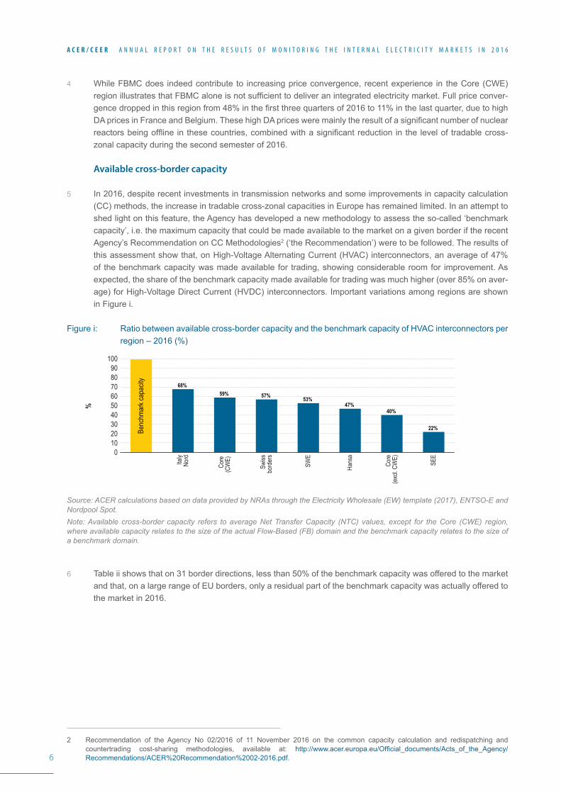
5 In 2016, despite recent investments in transmission networks and some improvements in capacity calculation (CC) methods, the increase in tradable cross-zonal capacities in Europe has remained limited. In an attempt to shed light on this feature, the Agency has developed a new methodology to assess the so-called ‘benchmark capacity’, i.e. the maximum capacity that could be made available to the market on a given border if the recent Agency’s Recommendation on CC Methodologies2 (‘the Recommendation’) were to be followed. The results of this assessment show that, on High-Voltage Alternating Current (HVAC) interconnectors, an average of 47% of the benchmark capacity was made available for trading, showing considerable room for improvement. As expected, the share of the benchmark capacity made available for trading was much higher (over 85% on aver-age) for High-Voltage Direct Current (HVDC) interconnectors. Important variations among regions are shown in Figure i.

Figure i: Ratio between available cross-border capacity and the benchmark capacity of HVAC interconnectors per region – 2016 (%)

Source: ACER calculations based on data provided by NRAs through the Electricity Wholesale (EW) template (2017), ENTSO-E and Nordpool Spot.Note: Available cross-border capacity refers to average Net Transfer Capacity (NTC) values, except for the Core (CWE) region, where available capacity relates to the size of the actual Flow-Based (FB) domain and the benchmark capacity relates to the size of a benchmark domain.

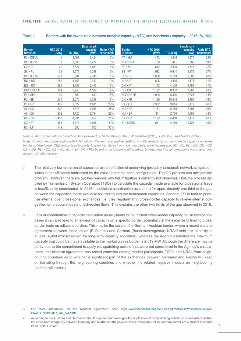
6 Table ii shows that on 31 border directions, less than 50% of the benchmark capacity was offered to the market and that, on a large range of EU borders, only a residual part of the benchmark capacity was actually offered to the market in 2016.

2 Recommendation of the Agency No 02/2016 of 11 November 2016 on the common capacity calculation and redispatching and countertrading cost-sharing methodologies, available at: http://www.acer.europa.eu/Official_documents/Acts_of_the_Agency/Recommendations/ACER%20Recommendation%2002-2016.pdf.

%

100

20

60

40

8090

10

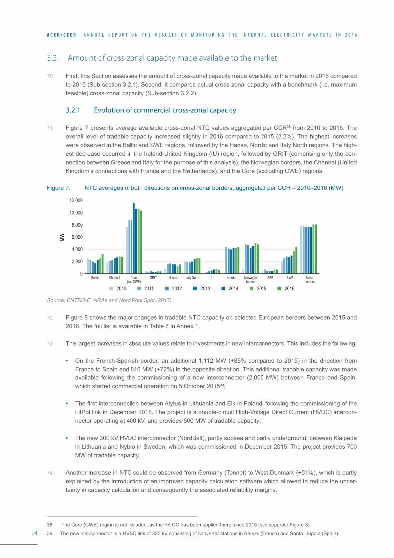
50

30

70

0

SWE

SEE

Core

(CW

E)

Core

(exc

l. CW

E)

Swiss

bord

ers

Italy

Nord

Hans

a

68% 59% 57% 53%

47% 40%

22% Benc

hmar

k cap

acity

7


Table ii: Borders with the lowest ratio between tradable capacity (NTC) and benchmark capacity – 2016 (%, MW)

Border- Direction

NTC 2016 (MW) TC [MW]

Benchmark capacity

(MW)Ratio NTC/benchmark

Border- Direction

NTC 2016 (MW) TC [MW]

Benchmark capacity

(MW)Ratio NTC/benchmark

PL > DE/LU 1 3,095 2,424 0% AT > HU 472 3,115 1,474 32%DE/LU > PL 9 3,095 2,424 0% NORD > AT 100 421 306 33%CZ > PL 22 3,527 1,881 1% AT > SI 642 2,505 1,743 37%SK > PL 21 2,075 1,386 2% ES > PT 1,932 9,614 5,179 37%DE/LU > CZ 278 5,564 2,745 10% HR > HU 1,000 5,159 2,503 40%RO > BG 250 4,156 2,443 10% HU > AT 605 3,115 1,474 41%BG > RO 281 4,156 2,443 12% CH > AT 1,152 4,120 2,794 41%DK1 > DE/LU 194 3,748 1,582 12% IT > CH 1,722 8,332 3,987 43%PL > SE4 99 600 600 16% NORD > FR 1,020 5,336 2,324 44%PL > SK 231 2,075 1,386 17% CH > FR 1,125 10,545 2,461 46%PL > CZ 406 3,527 1,881 22% PT > ES 2,382 9,614 5,179 46%AT > CZ 527 3,576 1,908 28% HU > HR 1,164 5,159 2,503 46%AT > CH 802 4,120 2,794 29% HU > SK 811 2,736 1,689 48%DE > CH 1,467 11,991 5,059 29% SK > CZ 1,192 4,480 2,477 48%CZ > AT 561 3,576 1,908 29% SI > NORD 551 2,150 1,126 49%PL > LT 149 500 500 30%

Source: ACER calculations based on data provided by NRAs through the EW template (2017), ENTSO-E and Nordpool Spot.Note: To improve comparability with NTC values, the technical profiles setting simultaneous limits on commercial capacity on some borders of the former CEE region (see footnote 1) were translated into maximum bilateral exchanges (i.e. DE > PL, PL > DE, DE > CZ, CZ > DE, PL > CZ, CZ > PL, PL > SK, SK > PL) based on actual price differentials by ensuring that all constraints were taken into account simultaneously.

7 Therelativelylowcross-zonalcapacitiesareareflectionofunderlying(probablystructural)networkcongestion,whichisnotefficientlyaddressedbytheexistingbiddingzoneconfiguration.TheCCprocesscanmitigatethisproblem. However, there are two key reasons why this mitigation is currently not observed. First, the process ap-plied by Transmission System Operators (TSOs) to calculate the capacity made available for cross-zonal trade isinsufficientlycoordinated.In2016,insufficientcoordinationaccountedforapproximatelyonethirdofthegapbetween the capacities made available for trading and the benchmark capacities. Second, TSOs tend to priori-tise internal over cross-zonal exchanges, i.e. they regularly limit cross-border capacity to relieve internal con-gestionortoaccommodateunscheduledflows.Thisexplainstheothertwothirdsofthegapobservedin2016.

8 Lackofcoordinationincapacitycalculationusuallyleadstoinsufficientcross-bordercapacity,butinexceptionalcasesitcanalsoleadtoanexcessofcapacityonaspecificborder,potentiallyattheexpenseoflimitingcross-border trade on adjacent borders. This may be the case on the German-Austrian border, where a recent bilateral agreement between the Austrian (E-Control) and German (Bundesnetzagentur) NRAs3 sets this capacity to atleast4,900MW(reservedforlong-termcapacityallocation),whereastheAgencyestimatesthemaximumcapacitythatcouldbemadeavailabletothemarketonthisborderis2,519MW.Althoughthedifferencemaybepartly due to the commitment to apply redispatching actions that were not considered in the Agency’s calcula-tions4, the bilateral agreement has raised concerns among market participants, TSOs and NRAs from neigh-bouringcountriesastowhetherasignificantpartof theexchangesbetweenGermanyandAustriawillkeepon transiting through the neighbouring countries and whether the related negative impacts on neighbouring markets will remain.

3 For more information on the bilateral agreement, see: https://www.bundesnetzagentur.de/SharedDocs/Pressemitteilungen/EN/2017/15052017_DE_AU.html.

4 According to the Austrian and German NRAs, the agreement envisages the application of redispatching actions, in cases where neither thecross-bordercapacitybetweenGermanyandAustrianorthephysicalflowsacrossthePolish-Germanborderaresufficienttoensuretradeupto4.9GW.

8


9 Analysing the extent to which internal exchanges are prioritised requires access to detailed information. The Flow-based (FB) method increases the transparency of the CC process and allows such an analysis to be performed. For example, in the Core (CWE) region where FB applies, the data made available to the Agency leads to the conclusion that in case of congestion in the CWE region (more than 60% of the hours in 2016), the available cross-zonal capacity is more often constrained by internal lines (72% of the occurrences in 2016) than cross-zonal lines (28%). Moreover, 77% of the congestions relate to lines located in Germany (including cross-border lines), of which 62% are related to internal lines in the Amprion’s area.

10 Moreover, in 2016 the average proportion of capacity made available for cross-zonal trade in internal-to-bidding zone lines in the Core (CWE) region was only 12% of their maximum capacity, whereas the remaining 88% was ‘consumed’byflowsresultingfrominternalexchanges.

11 More generally, TSOs tend to use cross-zonal capacity as an adjustment variable to address various internal-to-bidding-zone issues, which could be resolved without a reduction of cross-zonal capacity. For example, on the Lithuanian and Swedish borders with Poland, cross-zonal capacities were often reduced in 2016 by the PolishTSO toguaranteesufficientbalancing reserves in thePolish system.Althoughbalancing capacity isindeed needed to ensure operational security, the reduction of cross-zonal capacity is not necessarily needed to achieve this objective.

12 In 2016, the volume of remedial actions (countertrading or redispatching) that TSOs applied to guarantee ad-equatelevelsofcross-bordercapacityinEuropewaslowerthanin2015,andremainedinsufficienttoaddressthediscriminationofcross-zonalexchangesinEurope.Thisconfirmsthelackofcorrectandadequateincen-tives for TSOs to take remedial actions, the latter preferring to limit ex-ante cross-zonal capacities in order to limit the costs of such actions.

13 Thegrosswelfarebenefitsofapplying theAgency’sRecommendation to theCore (CWE) regionwereesti-matedatmorethan150millioneurosperyearin2016,anamountthatiscomparabletothebenefitsfromtheimplementationoftheFBMCitself.ThegrosswelfarebenefitsfromapplyingtheRecommendationtothewholeof Europe are estimated to total several billion euros per year. Although these estimates do not account for the costsincurredbyTSOsinmakingthiscross-bordercapacityavailabletothemarket,additionalbenefitscanbeexpected from enlarging the amount of available cross-zonal capacity in the long term. This includes stronger incentives for reinforcing the internal networks5, stronger incentives to coordinate both TSOs’ action and national energypoliciesand,finally,strongerincentivestoconsiderthebiddingzonereconfigurationasacrucialandpossiblymoreefficienttooltofostermarketintegrationinthemediumterm.

14 AnimportantfinalremarkregardingCCisthattransparencyin2016remainedanissuebothformarketpartici-pantsandfortheAgency.Marketparticipantsareaffectedbecausetheyhavedifficultiespredictinghowmuchcapacity will be available for trade. The Agency is impacted because it has to devote disproportionate effort to obtainthenecessaryinformation,ratherthanfocusingonfulfillingitsmonitoringmission.Itoftenhastorelyonvoluntary data collection involving TSOs, NRAs and ENTSO-E6.

Efficient use of available cross-zonal capacity

15 In general, the liquidity of forward markets in Europe remained low in 2016, with the main exceptions being Ger-many/Austria/Luxembourg, followed by the United Kingdom, France and the Nordic region. The highest growth in the same period was recorded in the French forward market.

16 In the context of a limited number of liquid forward markets in Europe, cross-zonal access to these markets be-comes particularly important. Without prejudice to the NRAs’ competence to decide on this matter, the Agency will monitor the extent to which the implementation of the Forward Capacity Allocation (FCA) Regulation helps providemarketparticipantswithsufficienthedgingopportunities.

5 Whenthisproducespositivenetbenefits.

6 Forinstance,theAgencyneededadisproportionateeffortandmorethansixmonthsinordertoobtainthefinalconsentofCore(CWE)TSOs and NRAs to access the FB data, while the latter are already accessible to all Core (CWE) NRAs.

9


17 Thanks to the DA market coupling of two thirds of the European borders, covering 22 European countries7 by theendof2016,thelevelofefficiencyintheuseoftheinterconnectorsinthistimeframeincreasedfromap-proximately60%in2010to86%in2016.Theanalysisshowsthattheoveralllevelofefficiencyintheuseofthe interconnectors slightly increased between 2015 and 2016 due to the extension of market coupling to the Austrian-Slovenian border as of 22 July 2016.

18 Over thepastsevenyears, thankstomarketcoupling, theEUhasreapedsignificantefficiencygains–andthereforewelfaregains–tothebenefitofconsumers.Furthermore,thefinalisationofmarketcouplingimple-mentation, as required by the Capacity Allocation and Congestion Management (CACM) Regulation, on all remaining European borders that still applied explicit DA auctions by the end of 2016 would render a social wel-farebenefitofmorethan200millioneurosperyear.Amongthenon-coupledregions,thelargestsocialwelfaregains could be obtained on the British borders with Ireland and Northern Ireland and on the Swiss borders with Italy and France.

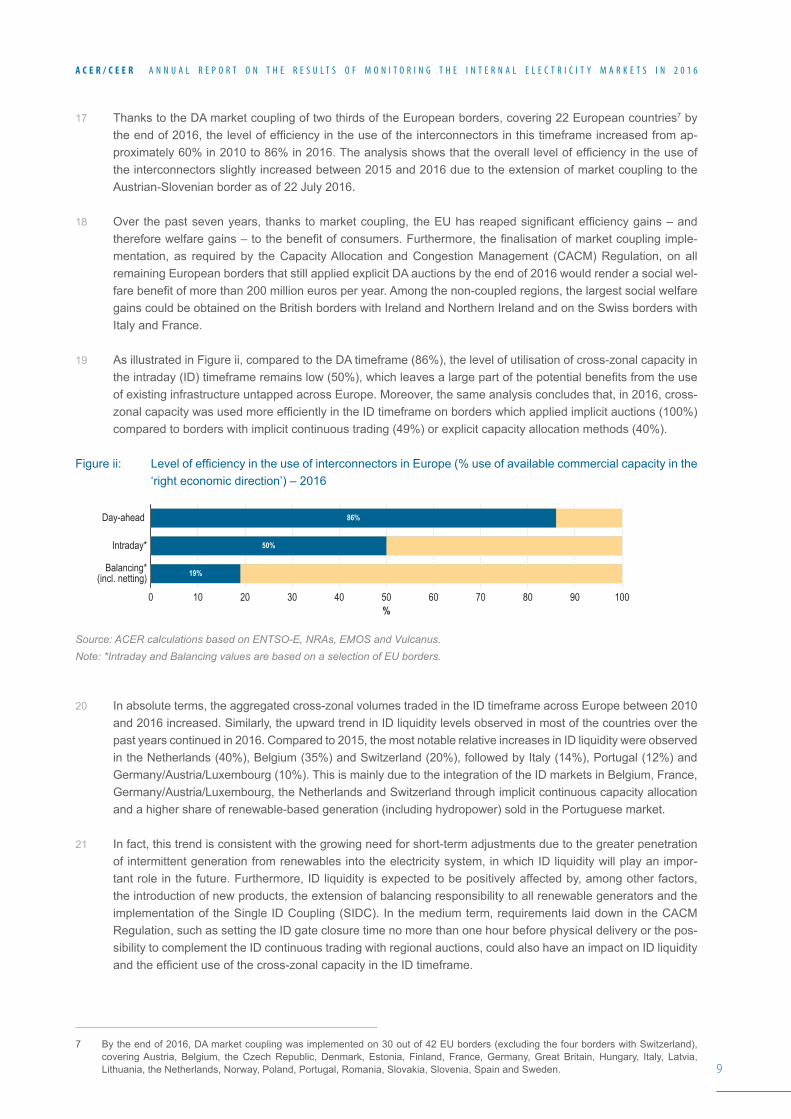
19 As illustrated in Figure ii, compared to the DA timeframe (86%), the level of utilisation of cross-zonal capacity in theintraday(ID)timeframeremainslow(50%),whichleavesalargepartofthepotentialbenefitsfromtheuseof existing infrastructure untapped across Europe. Moreover, the same analysis concludes that, in 2016, cross-zonalcapacitywasusedmoreefficientlyintheIDtimeframeonborderswhichappliedimplicitauctions(100%)comparedtoborderswithimplicitcontinuoustrading(49%)orexplicitcapacityallocationmethods(40%).

Figureii: LevelofefficiencyintheuseofinterconnectorsinEurope(%useofavailablecommercialcapacityinthe‘right economic direction’) – 2016

Source: ACER calculations based on ENTSO-E, NRAs, EMOS and Vulcanus.Note: *Intraday and Balancing values are based on a selection of EU borders.

20 In absolute terms, the aggregated cross-zonal volumes traded in the ID timeframe across Europe between 2010 and 2016 increased. Similarly, the upward trend in ID liquidity levels observed in most of the countries over the past years continued in 2016. Compared to 2015, the most notable relative increases in ID liquidity were observed in the Netherlands (40%), Belgium (35%) and Switzerland (20%), followed by Italy (14%), Portugal (12%) and Germany/Austria/Luxembourg (10%). This is mainly due to the integration of the ID markets in Belgium, France, Germany/Austria/Luxembourg, the Netherlands and Switzerland through implicit continuous capacity allocation and a higher share of renewable-based generation (including hydropower) sold in the Portuguese market.

21 In fact, this trend is consistent with the growing need for short-term adjustments due to the greater penetration of intermittent generation from renewables into the electricity system, in which ID liquidity will play an impor-tant role in the future. Furthermore, ID liquidity is expected to be positively affected by, among other factors, the introduction of new products, the extension of balancing responsibility to all renewable generators and the implementation of the Single ID Coupling (SIDC). In the medium term, requirements laid down in the CACM Regulation, such as setting the ID gate closure time no more than one hour before physical delivery or the pos-sibility to complement the ID continuous trading with regional auctions, could also have an impact on ID liquidity andtheefficientuseofthecross-zonalcapacityintheIDtimeframe.

7 By the end of 2016, DA market coupling was implemented on 30 out of 42 EU borders (excluding the four borders with Switzerland), covering Austria, Belgium, the Czech Republic, Denmark, Estonia, Finland, France, Germany, Great Britain, Hungary, Italy, Latvia, Lithuania, the Netherlands, Norway, Poland, Portugal, Romania, Slovakia, Slovenia, Spain and Sweden.

Balancing*(incl. netting)

Day-ahead

Intraday*

40%

100700 10 60 90805020 30

86%

50%

19%

10


22 In 2016, despite some improvements, large disparities in balancing energy and balancing capacity prices per-sisted inEurope.Thesedisparities, togetherwithasignificantamountofunusedcross-bordercapacity(seeFigure ii), suggest considerable potential for further cross-border exchanges of balancing services in Europe. In2016,theoverallcross-borderexchangeofbalancingservicesincreasedsignificantly(almostdoubled)com-pared to 2015, although it continued to be limited when compared to its maximum potential.

23 In some countries, such as Austria, the overall costs of balancing show a decreasing trend following the intro-duction of improvements in recent years. These improvements include regulatory measures aimed at enabling the participation of a wider range of technologies in balancing, the increasing cross-border exchange of balanc-ingservicesandthewidergeographicalscopeofprojectsaimedatexchangingtheseservices.Thisconfirmsthe importance of rapidly and effectively implementing the recently adopted Regulation establishing an electric-ity Balancing Guideline.

Capacity mechanisms and adequacy assessments

24 In 2016, a patchwork of different Capacity Mechanisms (CMs) remained throughout Europe in 2016. There are several key changes compared to what was presented in last year’s Market Monitoring Report. First, Latvia is now shown as having an operational mechanism which resembles the German planned network reserves mechanism8, and could be considered as a CM. Second, the transitional capacity payments designed in Greece for the period from May 2016 to April 2017 were approved by the European Commission. Additionally, Poland decidedtoextendtheoperationofstrategicreservesuntiltheendof2019,whileinSpain,oneoftheexistingtypes of capacity payments no longer applies to new capacity as of 1 January 2016. Furthermore, in Germany, the plan to implement a capacity reserves mechanism has been postponed until the end of 2018 (envisaged startofthefirstcontractingperiod),whiletheformalapprovalofthismechanismisstillpending.

25 The starting point in the process of determining whether to implement a CM should be an assessment of the resource adequacy situation. Given the increasing interdependence of national electricity systems, a robust ad-equacy assessment needs to carefully consider the contribution of interconnectors to adequacy, because such a contribution may be a determining factor when deciding to implement a CM.

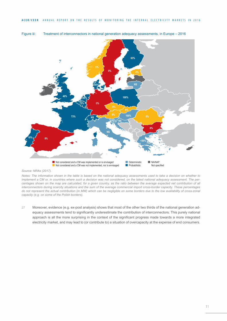
26 However, more than one third of the national adequacy assessments used as a basis to decide on the implemen-tation of a CM consider the contribution of interconnectors to be equal to zero MW of capacity (see Figure iii).

8 Although the mechanism is in place since 2005, the update on the existence of a CM in Latvia is based on the most recent information received from the Latvian NRA, which was previously not made available to the Agency.

11


Figure iii: Treatment of interconnectors in national generation adequacy assessments, in Europe – 2016

Source: NRAs (2017).Notes: The information shown in the table is based on the national adequacy assessments used to take a decision on whether to implement a CM or, in countries where such a decision was not considered, on the latest national adequacy assessment. The per-centages shown on the map are calculated, for a given country, as the ratio between the average expected net contribution of all interconnectors during scarcity situations and the sum of the average commercial import cross-border capacity. These percentages do not represent the actual contribution (in MW) which can be negligible on some borders due to the low availability of cross-zonal capacity (e.g. on some of the Polish borders).

27 Moreover, evidence (e.g. ex-post analysis) shows that most of the other two thirds of the national generation ad-equacyassessmentstendtosignificantlyunderestimatethecontributionofinterconnectors.Thispurelynationalapproachisallthemoresurprisinginthecontextofthesignificantprogressmadetowardsamoreintegratedelectricity market, and may lead to (or contribute to) a situation of overcapacity at the expense of end consumers.

Not considered and a CM was implemented or is envisaged Not considered and a CM was not implemented, nor is envisaged

DeterministicProbabilistic

NA/NAPNot specified

40%

0%0%

0%0%

0%0%

0%

0%

0%

63%

0%

100%

100%100%

100%100%

NSNS

NSNS100%100%100%100%

<30%<30%

72%72%

73%73%

10%10%

NSNS

NS

12


Recommendations28 Electricity markets are facing emerging unprecedented challenges as they adapt to meet global decarbonisation

targets while safeguarding security of supply and ensuring affordability. In this context, the timely and effective implementation of all the Regulations establishing Network Codes and Guidelines shall remain an utmost prior-ity. The Agency is strongly convinced that implementing the following list of policy recommendations would also help to address both existing and emerging challenges, with the ultimate goal of ensuring a well-functioning Internal Electricity Market.

29 These recommendations are grouped into three distinct categories: 1) recommendations on how to increase the limited amount of cross-zonal capacity made available for trading throughout Europe, without which any market integration project is meaningless; 2) recommendations on how to make use of existing cross-zonal capacity madeavailablefortradingmoreefficientlyinthedifferenttimeframesand3)recommendationsonhowtoad-dressadequacyconcernsinanefficientmanner.

30 Thefirstgroupofrecommendations isaimedat increasingthe limitedamountofcross-zonalcapacitymadeavailablefortrading,whichiscurrentlyoneofthemostsignificantlimitingfactorsforintegratingelectricitymar-kets in Europe. This requires, among other things, ensuring the equal treatment of internal-to-bidding-zones and cross-zonal exchanges, increasing the level of TSOs’ coordination, and improving the level of transparency in capacity calculation.

31 In order to ensure the equal treatment of internal and cross-zonal exchanges, the Agency recommends a pro-found paradigm shift in the way cross-border capacities are currently considered: instead of using these capaci-ties as the main adjustment variables in the overall network security equation, the level of cross-border capacity made available to the market should become a clear priority. In this respect, the following is recommended:

a) Asafirststep, theAgencyrecommendsthat thethreehigh-levelprinciplesproposedintheAgency’sRecommendation No 02/2016 be followed by TSOs and NRAs when developing, approving, implement-ing and monitoring capacity calculation methodologies. In the context of this Recommendation, the ar-gument that available cross-border capacity needs to be reduced due to operational security reasons should be used by TSOs only in exceptional situations, i.e. when no other remedies are available (in-steadofarecurrentandvaguejustification)and,inanycase,suchreductionsneedtobethoroughlyandtransparently substantiated.

b) Wheretheuseofremedialactionsisnotsufficienttoensureanappropriatelevelofcross-bordercapaci-ties,theAgencyrecommendsthatareconfigurationofbiddingzonesbeappliedasamatterofurgency.

c) As the required paradigm shift will require strong political support from Member States, these could consider setting a binding target for the availability of existing and future cross-border capacity, e.g. by definingaminimumshareofphysicalcross-zonalcapacitywhichshouldbemadeavailableforcross-zonal trade at, for example, the regional level.

32 In order to improve the level of TSO coordination, the following is recommended:

a) NRAs and TSOs should ensure the effective and rapid implementation of all legal provisions related to TSO coordination (for instance, as introduced by the Regulation establishing a System Operation Guideline9 for the Regional Security Centres or potentially for Regional Operation Centres in the future10).

b) NRAs and TSOs should ensure the effective and rapid implementation of FB capacity calculation, as required by the CACM Regulation.

9 See the provisional final version of the System Operation Guideline at https://ec.europa.eu/energy/sites/ener/files/documents/SystemOperationGuideline%20final%28provisional%2904052016.pdf.

10 See more in the EC’s ‘Clean Energy for All Europeans’ legislative proposal, which is available at: https://ec.europa.eu/energy/en/news/commission-proposes-new-rules-consumer-centred-clean-energy-transition.

13


33 In order to increase the transparency of capacity calculation, the following is recommended:

a) NRAs and/or the EC should request from TSOs the publication of all data generated for cross-zonal capacity calculation in a timely and user-friendly manner. This could be done on a voluntary basis or by amending the existing Regulation (e.g. the so-called ‘Transparency Regulation’11).

b) The EC and the European Legislators should consider providing the Agency with stronger data collection powersinordertofulfilitsmonitoringtasks.

34 The second group of recommendations is aimed at ensuring that existing cross-zonal capacity made available fortradingisusedmoreefficientlyinthedifferenttimeframes.Forthis,theAgencyrecommendsthefollowing:

a) NRAs and TSOs should implement DA market coupling on the 16 European borders (including the Swiss borders) that were still uncoupled at the end of 2016.

b) When developing and approving a cross-zonal ID capacity pricing methodology12, TSOs and NRAs should take into account that ID auctions are not only a possible tool to price capacity, but also a way to increasethelevelofefficientinterconnectoruseintheIDtimeframe.

c) In order to support and foster ID liquidity, NRAs and TSOs should ensure full balancing responsibility for all technologies13andshouldenforcecost-reflectivebalancingcharges.

d) TSOs should optimise the procurement of balancing capacity.

e) TSOs should increase the exchange of balancing resources.

f) In general, effective and rapid implementation of the Regulation establishing an EB Guideline is needed.

35 Thethirdgroupofrecommendationsisintendedtoaddressadequacyconcernsinanefficientmanner.Inthisfield,theAgencyrecommendsthefollowing:

a) Before implementing a CM, MSs should exhaust all possible no-regret measures, including the removal of price caps, ensuring the equal treatment of generation technologies regarding balance responsibili-ties, increasing demand-side participation, removing undue limitations on cross-zonal trade and remov-inganyotherbarriertoefficientpriceformationinthewholesaleelectricitymarkets.

b) MSs, the EC and NRAs should seek ways to strengthen the role of European adequacy assessments. In particular, the estimated contribution of interconnectors when considering the implementation of a CM should be based on regional or pan-European assessments, as they have a clear potential to provide better results than fragmented national assessments.

11 Commission Regulation (EU) No 543/2013 of 14 June 2013 on the submission and publication of data in electricity markets and amending AnnexItoRegulation(EC)No714/2009oftheEuropeanParliamentandoftheCouncil.

12 On 14 August 2017, an all TSOs’ common proposal for a single methodology for pricing intraday cross-zonal capacity was submitted to all NRAs.

13 Except pilot projects for the purpose of research and development.

14


1 Introduction36 The Market Monitoring Report (MMR), which is in its sixth edition, consists of four volumes, respectively on:

Electricity Wholesale Markets, Gas Wholesale Markets, Electricity and Gas Retail Markets, and Consumer Pro-tection and Empowerment.

37 The goal of the Electricity Wholesale Markets Volume is to present the results of the monitoring of the perfor-mance of the internal electricity market in the European Union14(EU),whichdependsontheefficientuseoftheEuropean electricity network and the good performance of electricity wholesale markets in all timeframes. When electricitywholesalemarketsareintegratedviasufficientinterconnectorcapacity,thencompetitionwillworktothebenefitofallconsumersandimproveenergysystemadequacyandsupplysecurityinthelongrun.

38 The Regulation establishing a Capacity Allocation and Congestion Management (CACM) Guideline15 that is cur-rently being implemented provides for clear objectives to deliver an integrated internal electricity market in the following areas: (i) full coordination and optimisation of Capacity Calculations (CCs) performed by Transmission SystemOperators(TSO)withinregions;(ii)definitionofappropriatebiddingzones,includingregularmonitoringandreviewingoftheefficiencyofbiddingzoneconfiguration;andiii)theuseofFlow-Based(FB)CCmethodsinhighly meshed networks. These processes are intended to optimise the utilisation of the existing infrastructure and to provide the market with more possibilities to exchange energy, enabling the cheapest supply to meet demand with the greatest willingness to pay in Europe, subject to the capacity of the existing network.

39 The recently adopted Regulations establishing Guidelines on Forward Capacity Allocation (FCA)16 and on Bal-ancing17 will also play a crucial role in the further integration of the Internal Energy Market (IEM). The former establishes a framework for calculating and allocating interconnection capacity, and for cross-zonal trading, in forward markets, while the latter sets rules on the operation of balancing markets, i.e. those markets that TSOs use to procure energy and capacity to keep the system in balance in real time. Moreover, it aims to increase the opportunitiesforcross-zonaltradingandtheefficiencyofbalancingmarkets.

40 Although implementing the provisions included in the above-mentioned Guidelines remains a key priority for the Agency for the Cooperation of Energy Regulators (‘the Agency’ or ‘ACER’), the document should also be read in the context of the ongoing discussions regarding the European Commission’s (EC) legislative proposal ‘Clean Energy for All Europeans’18 on new rules for a consumer centred clean energy transition.

41 The volume is organised as follows. Chapter 2 presents the key developments in electricity wholesale markets in the EU in 2016. Chapter 3 assesses the level of cross-zonal capacities made available for trade and the performance of the CC processes, with a focus on the comparative treatment of internal-to-bidding zones as opposed to cross-zonal exchanges. The performance of forward, Day-ahead (DA), Intraday (ID) and balancing markets, and particularly the use of cross-zonal capacity across these timeframes, is presented in Chapter 4. The document ends with a presentation of the situation of Capacity Mechanisms (CMs) and on the treatment of interconnectors in the national adequacy assessments (Chapter 5).

14 The Norwegian and Swiss markets are also analysed throughout in several Chapters of this report, but for simplicity, the scope of the analysis is referred to as the ‘EU’ or ‘Europe’.

15 Commission Regulation (EU) 2015/1222 of 24 July 2015, available at: http://eur-lex.europa.eu/legal-content/EN/TXT/PDF/?uri=CELEX:32015R1222&from=EN.

16 CommissionRegulation(EU)2016/1719of26September2016,availableat:http://eur-lex.europa.eu/legal-content/EN/TXT/PDF/?uri=CELEX:32016R1719&from=EN.

17 SeetheprovisionalfinalversionoftheElectricityBalancingGuidelineathttps://ec.europa.eu/energy/sites/ener/files/documents/informal_service_level_ebgl_16-03-2017_final.pdf.

18 TheCommission’s ‘CleanEnergy forAllEuropeans’ legislativeproposalcoversenergyefficiency, renewableeneragy, thedesignofthe electricity market, security of electricity supply and governance rules for the Energy Union, and is available at: https://ec.europa.eu/energy/en/news/commission-proposes-new-rules-consumer-centred-clean-energy-transition.

15


2 Key developments in 201642 This Chapter reports on prices in European electricity wholesale markets in 2016 (Section 2.1), including an

analysis of the evolution of the level of price convergence (Section 2.2).

2.1 Evolution of electricity wholesale prices

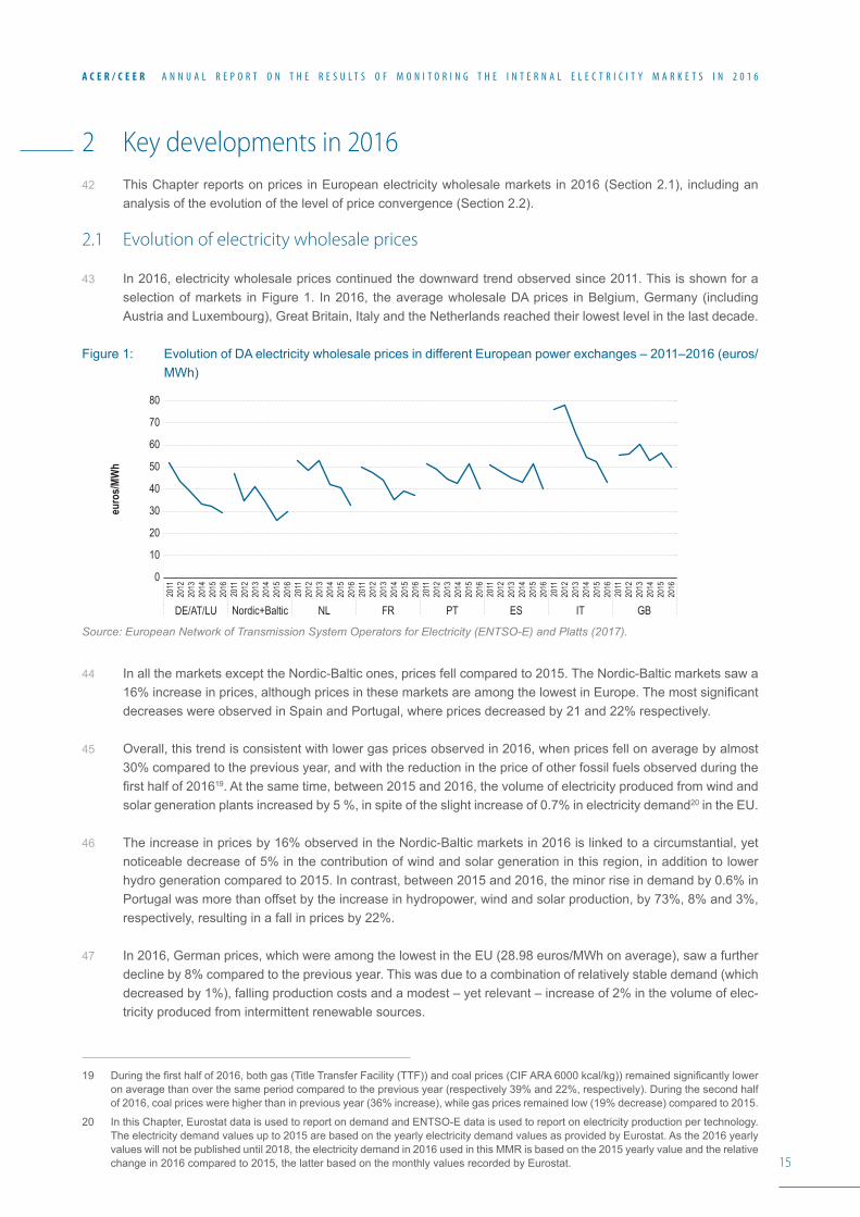
43 In 2016, electricity wholesale prices continued the downward trend observed since 2011. This is shown for a selection of markets in Figure 1. In 2016, the average wholesale DA prices in Belgium, Germany (including Austria and Luxembourg), Great Britain, Italy and the Netherlands reached their lowest level in the last decade.

Figure 1: Evolution of DA electricity wholesale prices in different European power exchanges – 2011–2016 (euros/MWh)

Source: European Network of Transmission System Operators for Electricity (ENTSO-E) and Platts (2017).

44 In all the markets except the Nordic-Baltic ones, prices fell compared to 2015. The Nordic-Baltic markets saw a 16%increaseinprices,althoughpricesinthesemarketsareamongthelowestinEurope.Themostsignificantdecreases were observed in Spain and Portugal, where prices decreased by 21 and 22% respectively.

45 Overall, this trend is consistent with lower gas prices observed in 2016, when prices fell on average by almost 30% compared to the previous year, and with the reduction in the price of other fossil fuels observed during the firsthalfof201619. At the same time, between 2015 and 2016, the volume of electricity produced from wind and solar generation plants increased by 5 %, in spite of the slight increase of 0.7% in electricity demand20 in the EU.

46 The increase in prices by 16% observed in the Nordic-Baltic markets in 2016 is linked to a circumstantial, yet noticeable decrease of 5% in the contribution of wind and solar generation in this region, in addition to lower hydro generation compared to 2015. In contrast, between 2015 and 2016, the minor rise in demand by 0.6% in Portugal was more than offset by the increase in hydropower, wind and solar production, by 73%, 8% and 3%, respectively, resulting in a fall in prices by 22%.

47 In2016,Germanprices,whichwereamongthelowestintheEU(28.98euros/MWhonaverage),sawafurtherdecline by 8% compared to the previous year. This was due to a combination of relatively stable demand (which decreased by 1%), falling production costs and a modest – yet relevant – increase of 2% in the volume of elec-tricity produced from intermittent renewable sources.

19 Duringthefirsthalfof2016,bothgas(TitleTransferFacility(TTF))andcoalprices(CIFARA6000kcal/kg))remainedsignificantlyloweronaveragethanoverthesameperiodcomparedtothepreviousyear(respectively39%and22%,respectively).Duringthesecondhalfof2016,coalpriceswerehigherthaninpreviousyear(36%increase),whilegaspricesremainedlow(19%decrease)comparedto2015.

20 In this Chapter, Eurostat data is used to report on demand and ENTSO-E data is used to report on electricity production per technology. The electricity demand values up to 2015 are based on the yearly electricity demand values as provided by Eurostat. As the 2016 yearly values will not be published until 2018, the electricity demand in 2016 used in this MMR is based on the 2015 yearly value and the relative change in 2016 compared to 2015, the latter based on the monthly values recorded by Eurostat.

euro

s/MW

h

DE/AT/LU Nordic+Baltic NL FR PT ES IT GB

2011

2012

2013

2014

2015

2016

2011

2012

2013

2014

2015

2016

2011

2012

2013

2014

2015

2016

2011

2012

2013

2014

2015

2016

2011

2012

2013

2014

2015

2016

2011

2012

2013

2014

2015

2016

2011

2012

2013

2014

2015

2016

2011

2012

2013

2014

2015

2016

80

70

40

60

50

30

20

0

10

16


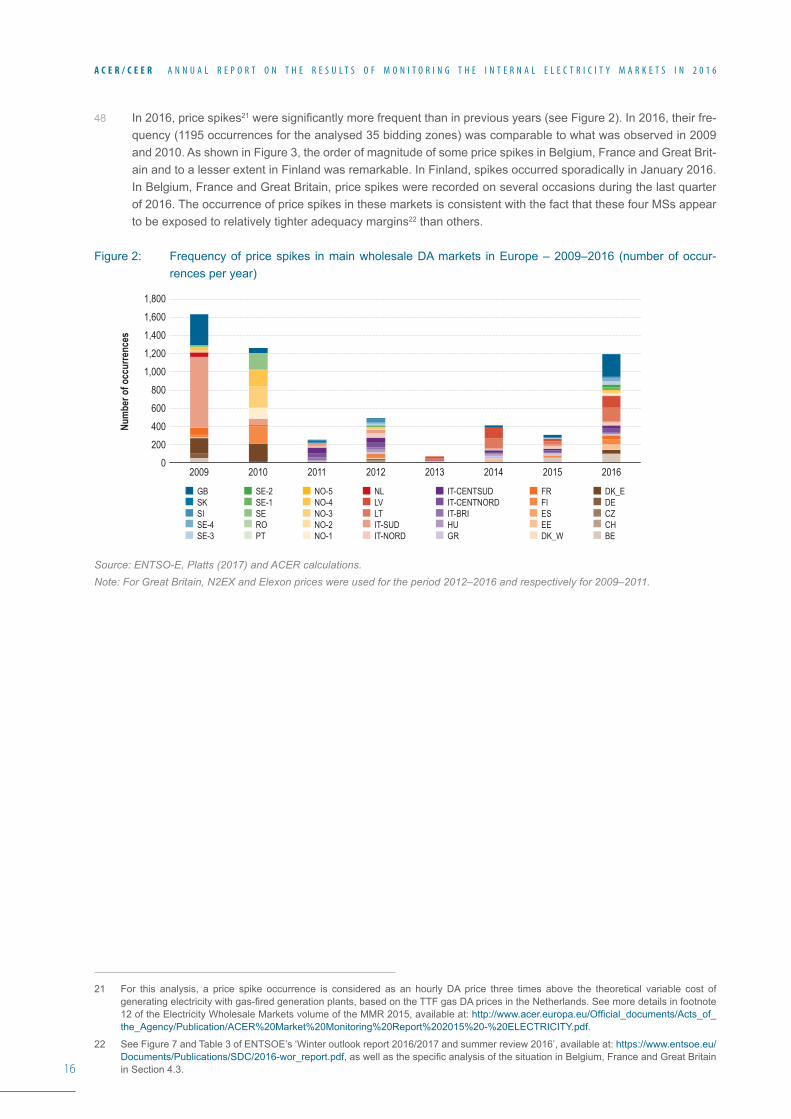
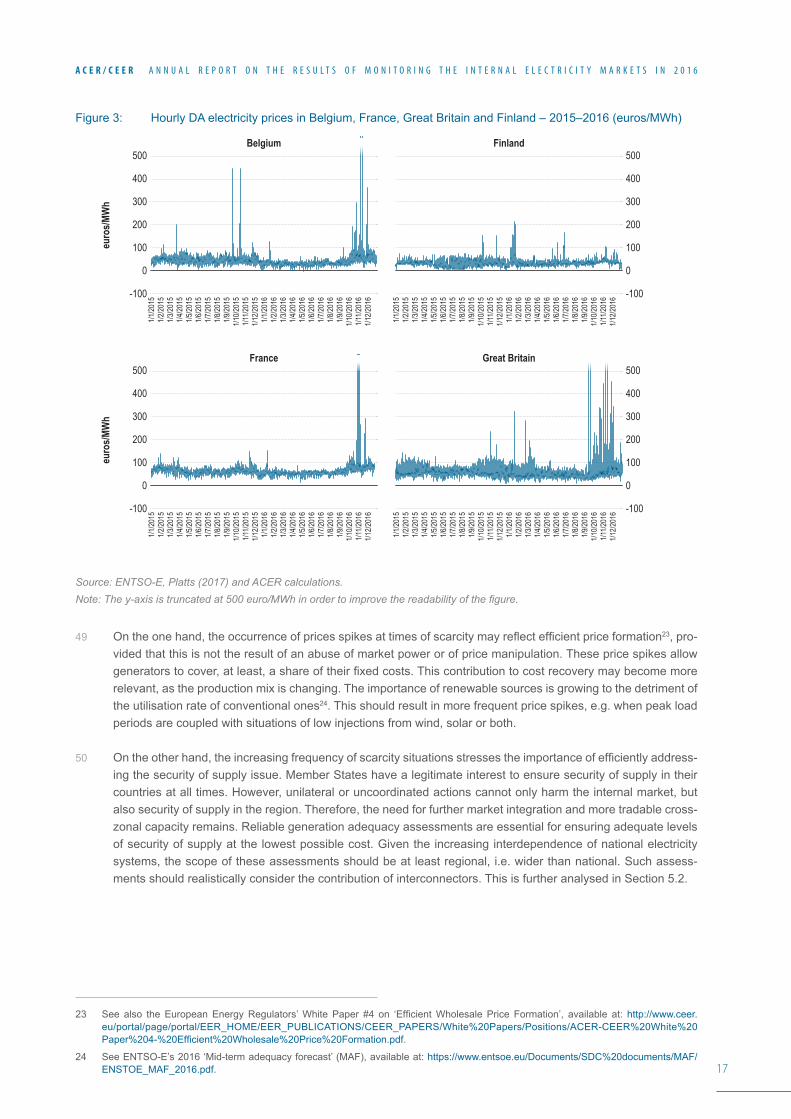
48 In 2016, price spikes21weresignificantlymorefrequentthaninpreviousyears(seeFigure2).In2016,theirfre-quency(1195occurrencesfortheanalysed35biddingzones)wascomparabletowhatwasobservedin2009and 2010. As shown in Figure 3, the order of magnitude of some price spikes in Belgium, France and Great Brit-ain and to a lesser extent in Finland was remarkable. In Finland, spikes occurred sporadically in January 2016. In Belgium, France and Great Britain, price spikes were recorded on several occasions during the last quarter of 2016. The occurrence of price spikes in these markets is consistent with the fact that these four MSs appear to be exposed to relatively tighter adequacy margins22 than others.

Figure2: Frequencyofpricespikes inmainwholesaleDAmarkets inEurope–2009–2016 (numberofoccur-rences per year)

Source: ENTSO-E, Platts (2017) and ACER calculations.Note: For Great Britain, N2EX and Elexon prices were used for the period 2012–2016 and respectively for 2009–2011.

21 For this analysis, a price spike occurrence is considered as an hourly DA price three times above the theoretical variable cost of generatingelectricitywithgas-firedgenerationplants,basedontheTTFgasDApricesintheNetherlands.Seemoredetailsinfootnote12 of the Electricity Wholesale Markets volume of the MMR 2015, available at: http://www.acer.europa.eu/Official_documents/Acts_of_the_Agency/Publication/ACER%20Market%20Monitoring%20Report%202015%20-%20ELECTRICITY.pdf.

22 See Figure 7 and Table 3 of ENTSOE’s ‘Winter outlook report 2016/2017 and summer review 2016’, available at: https://www.entsoe.eu/Documents/Publications/SDC/2016-wor_report.pdf,aswellasthespecificanalysisofthesituationinBelgium,FranceandGreatBritainin Section 4.3.

Num

ber o

f occ

urre

nces

1,800

1,400

1,000

600

200

1,600

1,200

800

400

02009 2010 2011 2012 2013 2014 2015 2016

GBSKSISE-4SE-3

SE-2SE-1SEROPT

NO-5NO-4NO-3NO-2NO-1

NLLVLTIT-SUDIT-NORD

IT-CENTSUDIT-CENTNORDIT-BRIHUGR

FRFIESEEDK_W

DK_EDECZCHBE

17


Figure 3: Hourly DA electricity prices in Belgium, France, Great Britain and Finland – 2015–2016 (euros/MWh)

Source: ENTSO-E, Platts (2017) and ACER calculations.Note: The y-axis is truncated at 500 euro/MWh in order to improve the readability of the figure.

49 Ontheonehand,theoccurrenceofpricesspikesattimesofscarcitymayreflectefficientpriceformation23, pro-vided that this is not the result of an abuse of market power or of price manipulation. These price spikes allow generatorstocover,atleast,ashareoftheirfixedcosts.Thiscontributiontocostrecoverymaybecomemorerelevant, as the production mix is changing. The importance of renewable sources is growing to the detriment of the utilisation rate of conventional ones24. This should result in more frequent price spikes, e.g. when peak load periods are coupled with situations of low injections from wind, solar or both.

50 Ontheotherhand,theincreasingfrequencyofscarcitysituationsstressestheimportanceofefficientlyaddress-ing the security of supply issue. Member States have a legitimate interest to ensure security of supply in their countries at all times. However, unilateral or uncoordinated actions cannot only harm the internal market, but also security of supply in the region. Therefore, the need for further market integration and more tradable cross-zonal capacity remains. Reliable generation adequacy assessments are essential for ensuring adequate levels of security of supply at the lowest possible cost. Given the increasing interdependence of national electricity systems, the scope of these assessments should be at least regional, i.e. wider than national. Such assess-ments should realistically consider the contribution of interconnectors. This is further analysed in Section 5.2.

23 See also theEuropeanEnergyRegulators’WhitePaper #4 on ‘EfficientWholesalePrice Formation’, available at:http://www.ceer.eu/portal/page/portal/EER_HOME/EER_PUBLICATIONS/CEER_PAPERS/White%20Papers/Positions/ACER-CEER%20White%20Paper%204-%20Efficient%20Wholesale%20Price%20Formation.pdf.

24 See ENTSO-E’s 2016 ‘Mid-term adequacy forecast’ (MAF), available at: https://www.entsoe.eu/Documents/SDC%20documents/MAF/ENSTOE_MAF_2016.pdf.

euro

s/MW

h

500

400

300

100

200

0

-100

1/1/20

151/2

/2015

1/3/20

151/4

/2015

1/5/20

151/6

/2015

1/7/20

151/8

/2015

1/9/20

151/1

0/201

51/1

1/201

51/1

2/201

51/1

/2016

1/2/20

161/3

/2016

1/4/20

161/5

/2016

1/6/20

161/7

/2016

1/8/20

161/9

/2016

1/10/2

016

1/11/2

016

1/12/2

016

1/1/20

151/2

/2015

1/3/20

151/4

/2015

1/5/20

151/6

/2015

1/7/20

151/8

/2015

1/9/20

151/1

0/201

51/1

1/201

51/1

2/201

51/1

/2016

1/2/20

161/3

/2016

1/4/20

161/5

/2016

1/6/20

161/7

/2016

1/8/20

161/9

/2016

1/10/2

016

1/11/2

016

1/12/2

016

1/1/20

151/2

/2015

1/3/20

151/4

/2015

1/5/20

151/6

/2015

1/7/20

151/8

/2015

1/9/20

151/1

0/201

51/1

1/201

51/1

2/201

51/1

/2016

1/2/20

161/3

/2016

1/4/20

161/5

/2016

1/6/20

161/7

/2016

1/8/20

161/9

/2016

1/10/2

016

1/11/2

016

1/12/2

016

1/1/20

151/2

/2015

1/3/20

151/4

/2015

1/5/20

151/6

/2015

1/7/20

151/8

/2015

1/9/20

151/1

0/201

51/1

1/201

51/1

2/201

51/1

/2016

1/2/20

161/3

/2016

1/4/20

161/5

/2016

1/6/20

161/7

/2016

1/8/20

161/9

/2016

1/10/2

016

1/11/2

016

1/12/2

016

euro

s/MW

h

500

400

300

100

200

0

-100

Belgium

France

Finland

Great Britain500

400

300

100

200

0

-100

500

400

300

100

200

0

-100

18


2.2 Price convergence

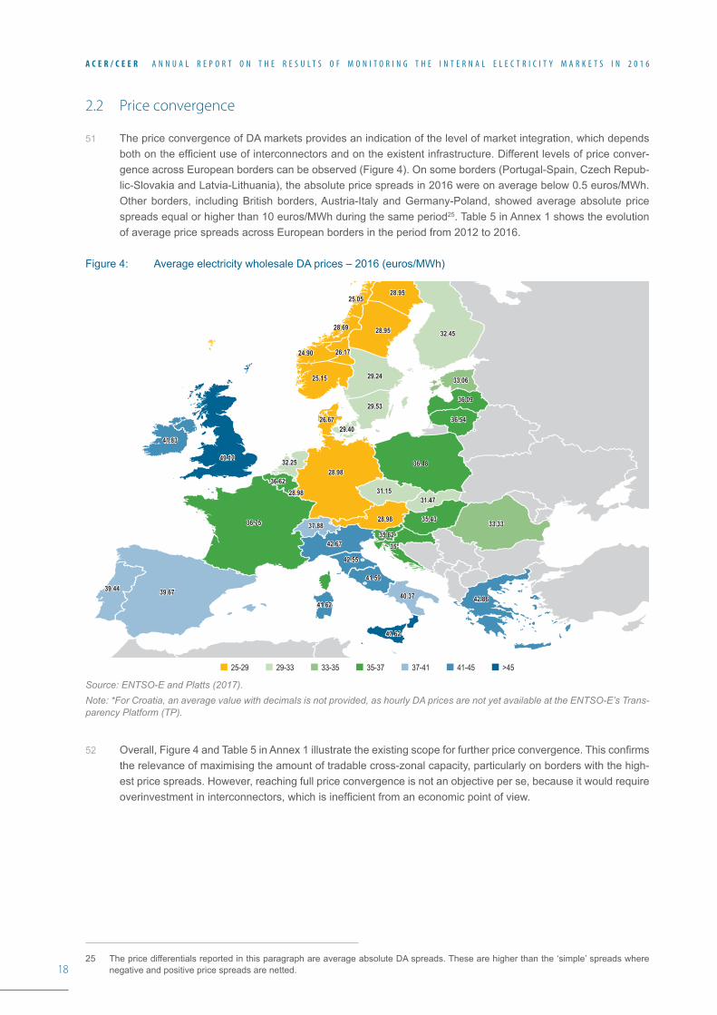
51 The price convergence of DA markets provides an indication of the level of market integration, which depends bothontheefficientuseofinterconnectorsandontheexistentinfrastructure.Differentlevelsofpriceconver-gence across European borders can be observed (Figure 4). On some borders (Portugal-Spain, Czech Repub-lic-Slovakia and Latvia-Lithuania), the absolute price spreads in 2016 were on average below 0.5 euros/MWh. Other borders, including British borders, Austria-Italy and Germany-Poland, showed average absolute price spreads equal or higher than 10 euros/MWh during the same period25. Table 5 in Annex 1 shows the evolution of average price spreads across European borders in the period from 2012 to 2016.

Figure 4: Average electricity wholesale DA prices – 2016 (euros/MWh)

Source: ENTSO-E and Platts (2017).Note: *For Croatia, an average value with decimals is not provided, as hourly DA prices are not yet available at the ENTSO-E’s Trans-parency Platform (TP).

52 Overall,Figure4andTable5inAnnex1illustratetheexistingscopeforfurtherpriceconvergence.Thisconfirmsthe relevance of maximising the amount of tradable cross-zonal capacity, particularly on borders with the high-est price spreads. However, reaching full price convergence is not an objective per se, because it would require overinvestmentininterconnectors,whichisinefficientfromaneconomicpointofview.

25 The price differentials reported in this paragraph are average absolute DA spreads. These are higher than the ‘simple’ spreads where negative and positive price spreads are netted.

>4541-4537-4135-3733-3529-3325-29

25.0525.05

28.6928.69

28.9828.98

28.9828.98

28.9828.98

28.9528.95

28.9528.95

29.2429.24

29.4029.40

32.4532.45

32.2532.25

3 36.62

36.7536.75

39.6739.6741.6241.62

47.6247.62

41.5941.59

31.1531.1531.4731.47

42.5542.55

42.6742.67

37.8837.8835.6235.62

36.4836.48

36.5436.54

36.0936.09

33.0633.06

35.4335.43 33.3333.33

35*35*

40.3740.37 42.8642.8639.4439.44

49.1249.12

41.8341.83

29.5329.53

24.9024.90 26.1726.17

26.6726.67

25.1525.15

19


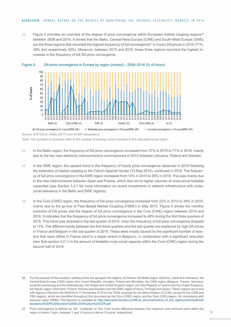
53 Figure 5 provides an overview of the degree of price convergence within European market coupling regions26 between 2008 and 2016. It shows that the Baltic, Central-West Europe (CWE) and South-West Europe (SWE) are the three regions that recorded the highest frequency of full convergence27 in hourly DA prices in 2016 (71%, 39%andrespectively30%).Moreover,between2015and2016,thesethreeregionsrecordedthehighestin-creases in the frequency of full DA price convergence.

Figure 5: DA price convergence in Europe by region (ranked) – 2008–2016 (% of hours)

Source: ENTSO-E, Platts (2017) and ACER calculations.Note: The numbers in brackets refer to the number of bidding zones included in the calculations per region.

54 In the Baltic region, the frequency of DA price convergence increased from 37% in 2015 to 71% in 2016, mainly due to the two new electricity interconnectors commissioned in 2015 between Lithuania, Poland and Sweden.

55 In the SWE region, the upward trend in the frequency of hourly price convergence observed in 2015 following the extension of market coupling to the French-Spanish border (13 May 2014), continued in 2016. The frequen-cy of full price convergence in the SWE region increased from 14% in 2015 to 30% in 2016. This was mainly due to the new interconnector between Spain and France, which also led to higher volumes of cross-zonal tradable capacities (see Section 3.2.1 for more information on recent investments in network infrastructure with cross-zonal relevance in the Baltic and SWE regions).

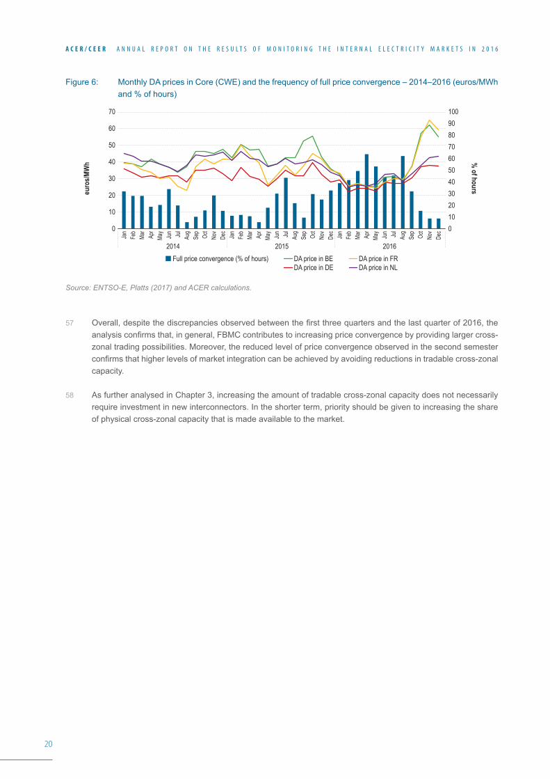
56 IntheCore(CWE)region,thefrequencyoffullpriceconvergenceincreasedfrom22%in2015to39%in2016,mainly due to the go-live of Flow-Based Market Coupling (FBMC) in May 2015. Figure 6 shows the monthly evolution of DA prices and the degree of full price convergence in the Core (CWE) region between 2014 and 2016.Itindicatesthatthefrequencyoffullpriceconvergenceincreasedto48%duringthefirstthreequartersof2016. This trend was reversed in the last quarter of 2016, when the frequency of full price convergence dropped to11%.ThedifferenttrendsbetweenthefirstthreequartersandthelastquarterareexplainedbyhighDApricesinFranceandBelgiuminthelastquarterof2016.Theseweremostlycausedbythesignificantnumberofreac-torsthatwereofflineinFrance(andtoalesserextentinBelgium),incombinationwithasignificantreduction(see Sub-section 3.2.1) in the amount of tradable cross-zonal capacity within the Core (CWE) region during the second half of 2016.

26 For the purpose of this analysis, bidding zones are grouped into regions, as follows: the Baltic region (Estonia, Latvia and Lithuania), the Central-East Europe (CEE) region (the Czech Republic, Hungary, Poland and Slovakia), the CWE region (Belgium, France, Germany/Austria/Luxembourg and the Netherlands), the Ireland and United Kingdom region (IU) (the Republic of Ireland and the United Kingdom), the Nordic region (Denmark, Finland, Norway and Sweden) and the SWE region (France, Portugal and Spain). These regions are in line with Agency’s Decision No 06/2016 of 17 November 2016 on the TSOs’ proposal for the determination of CCRs, except for the CWE and CEEregions,whichareidentifiedthroughoutthisdocumentastheCore(CWE)regionandtheCore(CEE)region,forconsistencywithprevious years’ MMRs. The Decision is available at: http://www.acer.europa.eu/Official_documents/Acts_of_the_Agency/Individual%20decisions/ACER%20Decision%2006-2016%20on%20CCR.pdf.

27 Priceconvergenceisdefinedas‘full’,‘moderate’or‘low’ifthehourlydifferencebetweenthemaximumandminimumpricewithintheregion is below 1 euro, between 1 and 10 euros or above 10 euros, respectively.

% o

f hou

rs

100

30405060708090

2010

0

Full price convergence (0-1 euros/MWh diff.) Moderate price convergence (1-10 euros/MWh diff.) Low price convergence (>10 euros/MWh diff.)

Baltic (3) Core (CWE) (4) SWE (3) Nordic (12) Core (CEE) (4) IU (2)

2011

2012

2013

2014

2015

2016

2008

2009

2010

2011

2012

2013

2014

2015

2016

2008

2009

2010

2011

2012

2013

2014

2015

2016

2008

2009

2010

2011

2012

2013

2014

2015

2016

2010

2011

2012

2013

2014

2015

2016

2008

2009

2010

2011

2012

2013

2014

2015

2016

20


Figure 6: Monthly DA prices in Core (CWE) and the frequency of full price convergence – 2014–2016 (euros/MWh and % of hours)

Source: ENTSO-E, Platts (2017) and ACER calculations.

57 Overall,despitethediscrepanciesobservedbetweenthefirstthreequartersandthelastquarterof2016,theanalysisconfirmsthat,ingeneral,FBMCcontributestoincreasingpriceconvergencebyprovidinglargercross-zonal trading possibilities. Moreover, the reduced level of price convergence observed in the second semester confirmsthathigherlevelsofmarketintegrationcanbeachievedbyavoidingreductionsintradablecross-zonalcapacity.

58 As further analysed in Chapter 3, increasing the amount of tradable cross-zonal capacity does not necessarily require investment in new interconnectors. In the shorter term, priority should be given to increasing the share of physical cross-zonal capacity that is made available to the market.

euro

s/MW

h % of hours

70

60

50

40

30

10

20

0

100

708090

60504030

1020

0

Jan

Feb

Mar

Apr

May

Jun Jul

Aug

Sep

Oct

Nov

Dec

Jan

Feb

Mar

Apr

May

Jun Jul

Aug

Sep

Oct

Nov

Dec

Jan

Feb

Mar

Apr

May

Jun Jul

Aug

Sep

Oct

Nov

Dec

20152014 2016Full price convergence (% of hours) DA price in BE

DA price in DEDA price in FRDA price in NL

21


3 Available cross-zonal capacity59 Theoptimisationofcross-zonalcapacityisanessentialprerequisiteforanefficientIEM.First,thisChapterintro-

duces a number of improvements in the methodologies used to monitor available cross-zonal capacity (Section 3.1). Second, it provides an overview of the volumes of tradable28 (i.e. available for trade) cross-zonal capacity in the EU, including the relation between these volumes and the physical capacity of interconnectors (Section 3.2). Third, it assesses the reasons for the large gap between physical and tradable capacity on most EU borders and provides recommendations on how to reduce this gap (Section 3.3).

3.1 Methodological improvements

60 The Agency already examined the relationship between physical and tradable capacity on EU borders in the last year MMR29. However, this edition of the MMR makes use of a number of data items which have been madeavailabletotheAgencyforthefirsttime.Itintroducesanumberofnewmethodologieswhichhavebeendeveloped to assess the issue of CC.

61 ThefirstnoveltyrelatestoaRecommendation30 recently issued by the Agency (hereinafter ‘the Recommenda-tion’). This Recommendation builds, inter alia, on the following two provisions:

a) Article16(3)oftheRegulation(EC)No714/200931: “The maximum capacity of the interconnections and/orthetransmissionnetworksaffectingcross-zonalflowsshallbemadeavailabletomarketparticipants,complying with safety standards of secure network operation” and Point 1.7 of Annex I to the same regu-lation: “TSOs shall not limit interconnection capacity in order to solve congestion inside their own control area […].”);

b) Article 21(I)(b)(ii) of the CACM Regulation32,whichspecifiesthatCCandallocationmethodologiesmustbe based on “rules for avoiding undue discrimination between internal and cross-zonal exchanges”.

62 The Recommendation establishes two high-level CC principles33. First, limitations on internal network elements should not be considered in cross-zonal CC methods. Second, the capacity of the cross-zonal network elements considered in the common CC methodologies should not be reduced in order to accommodate Loop Flows (LFs). TSOs and National Regulatory Authorities (NRAs) are expected to follow these high-level principles when developing, approving, implementing and monitoring their CC methodologies. However, the Recommendation allowsfordeviationsfromtheseprinciplesiftheyareproperlyjustified(fromanoperationalsecurityandsocio-economical point of view at the EU level) and do not unduly discriminate against cross-zonal exchanges.

63 Based on this Recommendation, this edition of the MMR introduces the concept of ‘benchmark’ capacity, which isdefinedasthecapacitythatcouldbemadeavailabletothemarketifthetwohigh-levelprinciplesunderlyingthe Recommendation were strictly followed. The calculated benchmark capacities are presented in Sub-section 3.2.2.Asdeviationsfromthehigh-levelprinciplesareacceptablesubjecttoadequatejustifications,asoutlinedabove, the monitoring of CC should not only focus on the deviations from the benchmark capacities but also on the proportion of capacity of Critical Network Elements (CNEs) that is made available for cross-border ex-changes and the proportion reserved for internal exchanges. The combined analysis of these elements allow an assessment of the extent to which internal exchanges are prioritised (Sub-section 3.3.2).

28 Throughout this Chapter, tradable cross-zonal capacity is also referred to as commercial cross-zonal capacity, available cross-zonal capacity or simply commercial or available capacity.

29 The MMR 2015 is available at http://www.acer.europa.eu/en/electricity/Market%20monitoring/Pages/Current-edition.aspx.

30 Recommendation of the Agency No 02/2016 of 11 November 2016 on the common capacity calculation and redispatching and countertrading cost-sharing methodologies, available at: http://www.acer.europa.eu/Official_documents/Acts_of_the_Agency/Recommendations/ACER%20Recommendation%2002-2016.pdf.

31 Regulation(EC)No714/2009oftheEuropeanParliamentandoftheCouncilof13July2009onconditionsforaccesstothenetworkforcross-zonal exchanges in electricity and repealing Regulation (EC) No 1228/2003, available at: http://eur-lex.europa.eu/legal-content/EN/TXT/PDF/?uri=CELEX:32009R0714&from=EN.

32 See footnote 15.

33 Additionally, the Recommendation includes a third principle related to redispatching and countertrading cost-sharing methodologies.

22


64 The second novelty refers to the availability of new data, enabling the Agency to enhance its analysis on CC. In2017,twosetsofdatawereprovidedtotheAgencyforthefirsttime.First,TSOsprovidedinformationontheCommon Grid Model (CGM)34 for continental Europe. The Agency used this information to estimate the bench-mark capacities. Second, the Core (CWE) region TSOs provided via ENTSO-E detailed information on the most relevant data items used in the Flow-Based Capacity Calculation (FB CC) process in the Core (CWE) region. This data included, inter alia,hourlyinformationontheforecastedphysicalflowsoninternalandcross-zonaltransmissionlinesintheCore(CWE)regionresultingfrominternalexchanges.Theseforecastedphysicalflowsareusedtodefinetheconstraintsdeterminingthetradablecross-zonalcapacityinaFBcontext.

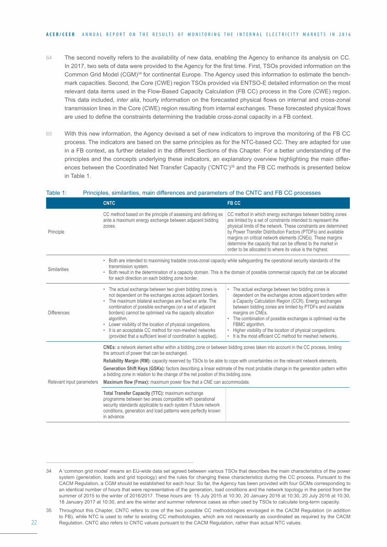
65 With this new information, the Agency devised a set of new indicators to improve the monitoring of the FB CC process. The indicators are based on the same principles as for the NTC-based CC. They are adapted for use in a FB context, as further detailed in the different Sections of this Chapter. For a better understanding of the principles and the concepts underlying these indicators, an explanatory overview highlighting the main differ-ences between the Coordinated Net Transfer Capacity (‘CNTC’)35 and the FB CC methods is presented below in Table 1.

Table 1: Principles, similarities, main differences and parameters of the CNTC and FB CC processes

CNTC FB CC

Principle

CC method based on the principle of assessing and defining ex ante a maximum energy exchange between adjacent bidding zones.

CC method in which energy exchanges between bidding zones are limited by a set of constraints intended to represent the physical limits of the network. These constraints are determined by Power Transfer Distribution Factors (PTDFs) and available margins on critical network elements (CNEs). These margins determine the capacity that can be offered to the market in order to be allocated to where its value is the highest.

Similarities• Both are intended to maximising tradable cross-zonal capacity while safeguarding the operational security standards of the

transmission system. • Both result in the determination of a capacity domain. This is the domain of possible commercial capacity that can be allocated

for each direction on each bidding zone border.

Differences

• The actual exchange between two given bidding zones is not dependent on the exchanges across adjacent borders.

• The maximum bilateral exchanges are fixed ex ante. The combination of possible exchanges (on a set of adjacent borders) cannot be optimised via the capacity allocation algorithm.

• Lower visibility of the location of physical congestions.• It is an acceptable CC method for non-meshed networks

(provided that a sufficient level of coordination is applied).

• The actual exchange between two bidding zones is dependent on the exchanges across adjacent borders within a Capacity Calculation Region (CCR). Energy exchanges between bidding zones are limited by PTDFs and available margins on CNEs.

• The combination of possible exchanges is optimised via the FBMC algorithm.

• Higher visibility of the location of physical congestions.• It is the most efficient CC method for meshed networks.

Relevant input parameters

CNEs: a network element either within a bidding zone or between bidding zones taken into account in the CC process, limiting the amount of power that can be exchanged.Reliability Margin (RM): capacity reserved by TSOs to be able to cope with uncertainties on the relevant network elements.Generation Shift Keys (GSKs): factors describing a linear estimate of the most probable change in the generation pattern within a bidding zone in relation to the change of the net position of this bidding zone.Maximum flow (Fmax): maximum power flow that a CNE can accommodate.

Total Transfer Capacity (TTC): maximum exchange programme between two areas compatible with operational security standards applicable to each system if future network conditions, generation and load patterns were perfectly known in advance.

34 A ‘common grid model’ means an EU-wide data set agreed between various TSOs that describes the main characteristics of the power system (generation, loads and grid topology) and the rules for changing these characteristics during the CC process. Pursuant to the CACM Regulation, a CGM should be established for each hour. So far, the Agency has been provided with four GCMs corresponding to an identical number of hours that were representative of the generation, load conditions and the network topology in the period from the summer of 2015 to the winter of 2016/2017. These hours are: 15 July 2015 at 10:30, 20 January 2016 at 10:30, 20 July 2016 at 10:30, 18 January 2017 at 10:30, and are the winter and summer reference cases as often used by TSOs to calculate long-term capacity.

35 Throughout this Chapter, CNTC refers to one of the two possible CC methodologies envisaged in the CACM Regulation (in addition to FB), while NTC is used to refer to existing CC methodologies, which are not necessarily as coordinated as required by the CACM Regulation. CNTC also refers to CNTC values pursuant to the CACM Regulation, rather than actual NTC values.

23


CNTC FB CC

Relevant output parameters

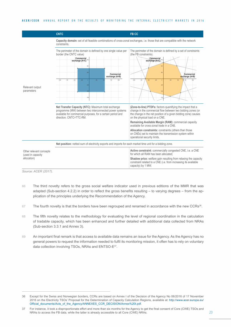
Capacity domain: set of all feasible combinations of cross-zonal exchanges, i.e. those that are compatible with the network constraints.

The perimeter of the domain is defined by one single value per border (the CNTC value)

The perimeter of the domain is defined by a set of constraints (the FB constraints).

Net Transfer Capacity (NTC): Maximum total exchange programme (MW) between two interconnected power systems available for commercial purposes, for a certain period and direction. CNTC=TTC-RM.

(Zone-to-line) PTDFs: factors quantifying the impact that a change in the commercial flow between two bidding zones (or the change in the net position of a given bidding zone) causes on the physical load on a CNE.Remaining Available Margin (RAM): commercial capacity available for cross-zonal trade in a CNE.Allocation constraints: constraints (others than those on CNEs) set to maintain the transmission system within operational security limits.

Other relevant concepts (used in capacity allocation)

Net position: netted sum of electricity exports and imports for each market time unit for a bidding zone.

Active constraint: commercially congested CNE, i.e. a CNE for which all RAM has been allocated; Shadow price: welfare gain resulting from relaxing the capacity constraint related to a CNE (i.e. from increasing its available capacity) by 1 MW.

Source: ACER (2017).

66 The third novelty refers to the gross social welfare indicator used in previous editions of the MMR that was adapted(Sub-section4.2.2)inordertoreflectthegrossbenefitsresulting–tovaryingdegrees–fromtheap-plication of the principles underlying the Recommendation of the Agency.

67 The fourth novelty is that the borders have been regrouped and renamed in accordance with the new CCRs36.

68 Thefifthnoveltyrelatestothemethodologyforevaluatingthelevelofregionalcoordinationinthecalculationof tradable capacity, which has been enhanced and further detailed with additional data collected from NRAs (Sub-section 3.3.1 and Annex 3).

69 AnimportantfinalremarkisthataccesstoavailabledataremainsanissuefortheAgency.AstheAgencyhasnogeneralpowerstorequesttheinformationneededtofulfilitsmonitoringmission,itoftenhastorelyonvoluntarydata collection involving TSOs, NRAs and ENTSO-E37.

36 Except for the Swiss and Norwegian borders, CCRs are based on Annex I of the Decision of the Agency No 06/2016 of 17 November 2016 on the Electricity TSOs’ Proposal for the Determination of Capacity Calculation Regions, available at: http://www.acer.europa.eu/Official_documents/Acts_of_the_Agency/ANNEXES_CCR_DECISION/Annex%20I.pdf.

37 Forinstance,ittookadisproportionateeffortandmorethansixmonthsfortheAgencytogetthefinalconsentofCore(CWE)TSOsandNRAs to access the FB data, while the latter is already accessible to all Core (CWE) NRAs.

Commercialexchange (A>C)

-500

-500

500

500

-750

-750

750

750

-250

-250

250

250

0-1000 1000

Commercialexchange (A>B)

Commercialexchange (A>C)

-500

-500

500

500

-750

-750

750

750

-250

-250

250

250

0-1000 1000

Commercialexchange (A>B)

24


3.2 Amount of cross-zonal capacity made available to the market

70 First, this Section assesses the amount of cross-zonal capacity made available to the market in 2016 compared to 2015 (Sub-section 3.2.1). Second, it compares actual cross-zonal capacity with a benchmark (i.e. maximum feasible) cross-zonal capacity (Sub-section 3.2.2).

3.2.1 Evolution of commercial cross-zonal capacity

71 Figure 7 presents average available cross-zonal NTC values aggregated per CCR38 from 2010 to 2016. The overall level of tradable capacity increased slightly in 2016 compared to 2015 (2.2%). The highest increases were observed in the Baltic and SWE regions, followed by the Hansa, Nordic and Italy North regions. The high-est decrease occurred in the Ireland-United Kingdom (IU) region, followed by GRIT (comprising only the con-nection between Greece and Italy for the purpose of this analysis), the Norwegian borders, the Channel (United Kingdom’s connections with France and the Netherlands), and the Core (excluding CWE) regions.

Figure 7: NTC averages of both directions on cross-zonal borders, aggregated per CCR – 2010–2016 (MW)

Source: ENTSO-E, NRAs and Nord Pool Spot (2017).

72 Figure 8 shows the major changes in tradable NTC capacity on selected European borders between 2015 and 2016. The full list is available in Table 7 in Annex 1.

73 The largest increases in absolute values relate to investments in new interconnectors. This includes the following:

• On the French-Spanish border, an additional 1,112 MW (+85% compared to 2015) in the direction from France to Spain and 810 MW (+72%) in the opposite direction. This additional tradable capacity was made available following the commissioning of a new interconnector (2,000 MW) between France and Spain, which started commercial operation on 5 October 201539;

• ThefirstinterconnectionbetweenAlytusinLithuaniaandElkinPoland,followingthecommissioningoftheLitPol link in December 2015. The project is a double-circuit High-Voltage Direct Current (HVDC) intercon-nector operating at 400 kV, and provides 500 MW of tradable capacity;

• The new 300 kV HVDC interconnector (NordBalt), partly subsea and partly underground, between Klaipeda in Lithuania and Nybro in Sweden, which was commissioned in December 2015. The project provides 700 MW of tradable capacity.

74 Another increase in NTC could be observed from Germany (Tennet) to West Denmark (+51%), which is partly explained by the introduction of an improved capacity calculation software which allowed to reduce the uncer-tainty in capacity calculation and consequently the associated reliability margins.

38 The Core (CWE) region is not included, as the FB CC has been applied there since 2015 (see separate Figure 3).

39 The new interconnector is a HVDC link of 320 kV consisting of converter stations in Baixas (France) and Santa Llogaia (Spain).

MW

Baltic Channel Core(exl. CWE)

GRIT Hansa Italy North IU Nordic Norwegianborders

SEE SWE Swissborders

12,000

8,000

10,000

4,000

6,000

2,000

0

20112010 2012 2013 2014 2015 2016

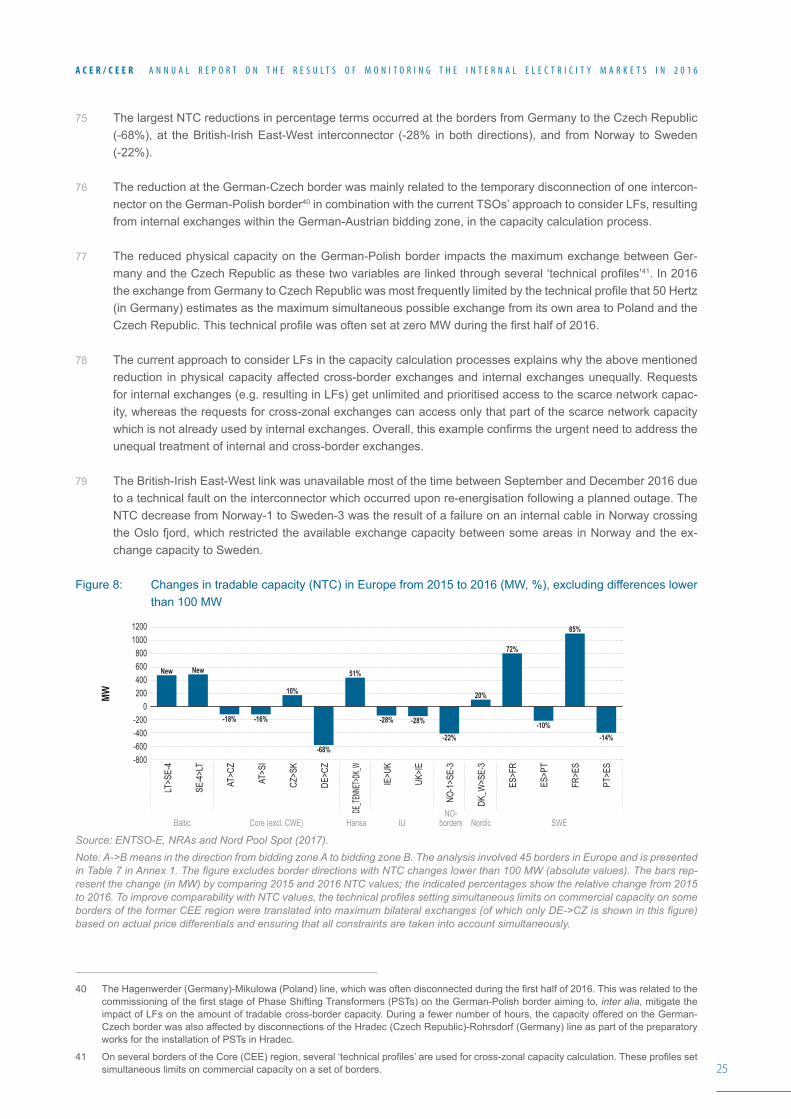
25


75 The largest NTC reductions in percentage terms occurred at the borders from Germany to the Czech Republic (-68%), at the British-Irish East-West interconnector (-28% in both directions), and from Norway to Sweden (-22%).

76 The reduction at the German-Czech border was mainly related to the temporary disconnection of one intercon-nector on the German-Polish border40 in combination with the current TSOs’ approach to consider LFs, resulting from internal exchanges within the German-Austrian bidding zone, in the capacity calculation process.

77 The reduced physical capacity on the German-Polish border impacts the maximum exchange between Ger-manyandtheCzechRepublicasthesetwovariablesarelinkedthroughseveral‘technicalprofiles’41. In 2016 theexchangefromGermanytoCzechRepublicwasmostfrequentlylimitedbythetechnicalprofilethat50Hertz(in Germany) estimates as the maximum simultaneous possible exchange from its own area to Poland and the CzechRepublic.ThistechnicalprofilewasoftensetatzeroMWduringthefirsthalfof2016.

78 The current approach to consider LFs in the capacity calculation processes explains why the above mentioned reduction in physical capacity affected cross-border exchanges and internal exchanges unequally. Requests for internal exchanges (e.g. resulting in LFs) get unlimited and prioritised access to the scarce network capac-ity, whereas the requests for cross-zonal exchanges can access only that part of the scarce network capacity whichisnotalreadyusedbyinternalexchanges.Overall,thisexampleconfirmstheurgentneedtoaddresstheunequal treatment of internal and cross-border exchanges.

79 The British-Irish East-West link was unavailable most of the time between September and December 2016 due to a technical fault on the interconnector which occurred upon re-energisation following a planned outage. The NTC decrease from Norway-1 to Sweden-3 was the result of a failure on an internal cable in Norway crossing the Oslo fjord, which restricted the available exchange capacity between some areas in Norway and the ex-change capacity to Sweden.

Figure 8: Changes in tradable capacity (NTC) in Europe from 2015 to 2016 (MW, %), excluding differences lower than 100 MW

Source: ENTSO-E, NRAs and Nord Pool Spot (2017).Note: A->B means in the direction from bidding zone A to bidding zone B. The analysis involved 45 borders in Europe and is presented in Table 7 in Annex 1. The figure excludes border directions with NTC changes lower than 100 MW (absolute values). The bars rep-resent the change (in MW) by comparing 2015 and 2016 NTC values; the indicated percentages show the relative change from 2015 to 2016. To improve comparability with NTC values, the technical profiles setting simultaneous limits on commercial capacity on some borders of the former CEE region were translated into maximum bilateral exchanges (of which only DE->CZ is shown in this figure) based on actual price differentials and ensuring that all constraints are taken into account simultaneously.

40 TheHagenwerder(Germany)-Mikulowa(Poland)line,whichwasoftendisconnectedduringthefirsthalfof2016.ThiswasrelatedtothecommissioningofthefirststageofPhaseShiftingTransformers(PSTs)ontheGerman-Polishborderaimingto,inter alia, mitigate the impact of LFs on the amount of tradable cross-border capacity. During a fewer number of hours, the capacity offered on the German-Czech border was also affected by disconnections of the Hradec (Czech Republic)-Rohrsdorf (Germany) line as part of the preparatory works for the installation of PSTs in Hradec.

41 OnseveralbordersoftheCore(CEE)region,several‘technicalprofiles’areusedforcross-zonalcapacitycalculation.Theseprofilessetsimultaneous limits on commercial capacity on a set of borders.

MW

1200

400

800600

1000

2000

-400-200

-600-800

LT>S

E-4

SE-4

>LT

AT>C

Z

AT>S

I

CZ>S

K

DE>C

Z

DE_TE

NNET

>DK_W

IE>U

K

UK>IE

NO-1

>SE-

3

DK_W

>SE-

3

ES>F

R

ES>P

T

FR>E

S

PT>E

S

Baltic Core (excl. CWE) Hansa IUNO-

borders Nordic SWE

New New

-18% -16%

10%

-68%

51%

-28% -28%

-22%

20%

72%

-10%

85%

-14%

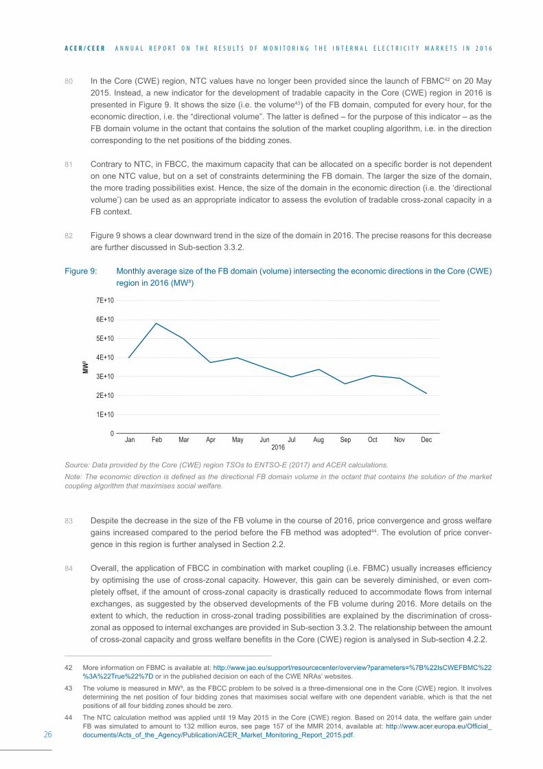
26


80 In the Core (CWE) region, NTC values have no longer been provided since the launch of FBMC42 on 20 May 2015. Instead, a new indicator for the development of tradable capacity in the Core (CWE) region in 2016 is presentedinFigure9.Itshowsthesize(i.e.thevolume43) of the FB domain, computed for every hour, for the economicdirection,i.e.the“directionalvolume”.Thelatterisdefined–forthepurposeofthisindicator–astheFB domain volume in the octant that contains the solution of the market coupling algorithm, i.e. in the direction corresponding to the net positions of the bidding zones.

81 ContrarytoNTC,inFBCC,themaximumcapacitythatcanbeallocatedonaspecificborderisnotdependenton one NTC value, but on a set of constraints determining the FB domain. The larger the size of the domain, the more trading possibilities exist. Hence, the size of the domain in the economic direction (i.e. the ‘directional volume’) can be used as an appropriate indicator to assess the evolution of tradable cross-zonal capacity in a FB context.

82 Figure9showsacleardownwardtrendinthesizeofthedomainin2016.Theprecisereasonsforthisdecreaseare further discussed in Sub-section 3.3.2.

Figure9: MonthlyaveragesizeoftheFBdomain(volume)intersectingtheeconomicdirectionsintheCore(CWE)region in 2016 (MW³)

Source: Data provided by the Core (CWE) region TSOs to ENTSO-E (2017) and ACER calculations.Note: The economic direction is defined as the directional FB domain volume in the octant that contains the solution of the market coupling algorithm that maximises social welfare.

83 Despite the decrease in the size of the FB volume in the course of 2016, price convergence and gross welfare gains increased compared to the period before the FB method was adopted44. The evolution of price conver-gence in this region is further analysed in Section 2.2.

84 Overall,theapplicationofFBCCincombinationwithmarketcoupling(i.e.FBMC)usuallyincreasesefficiencyby optimising the use of cross-zonal capacity. However, this gain can be severely diminished, or even com-pletelyoffset,iftheamountofcross-zonalcapacityisdrasticallyreducedtoaccommodateflowsfrominternalexchanges, as suggested by the observed developments of the FB volume during 2016. More details on the extent to which, the reduction in cross-zonal trading possibilities are explained by the discrimination of cross-zonal as opposed to internal exchanges are provided in Sub-section 3.3.2. The relationship between the amount ofcross-zonalcapacityandgrosswelfarebenefitsintheCore(CWE)regionisanalysedinSub-section4.2.2.

42 More information on FBMC is available at: http://www.jao.eu/support/resourcecenter/overview?parameters=%7B%22IsCWEFBMC%22%3A%22True%22%7D or in the published decision on each of the CWE NRAs’ websites.

43 The volume is measured in MW³, as the FBCC problem to be solved is a three-dimensional one in the Core (CWE) region. It involves determining the net position of four bidding zones that maximises social welfare with one dependent variable, which is that the net positions of all four bidding zones should be zero.

44 TheNTCcalculationmethodwasapplieduntil19May2015intheCore(CWE)region.Basedon2014data,thewelfaregainunderFB was simulated to amount to 132 million euros, see page 157 of the MMR 2014, available at: http://www.acer.europa.eu/Official_documents/Acts_of_the_Agency/Publication/ACER_Market_Monitoring_Report_2015.pdf.

AT-CH, 5.46

MW3

5E+10

4E+10

7E+10

6E+10

1E+10

2E+10

3E+10

0Jan

2016Mar May Jul Sep NovFeb Apr Jun Aug Oct Dec

27


3.2.2 Ratio between commercial and benchmark cross-zonal capacity

85 This Sub-section analyses the potential scope for increasing the available cross-zonal capacity. The underly-ingassumptioninanalysingthispotential isthatinanefficientzonalmarketdesign(i.e. ifthebiddingzonesareproperlydefinedaccordingtophysicalconstraints)theonlyfactorlimitingtradebetweentwobiddingzonesis the capacity of the network elements on the bidding zone borders (i.e. the interconnection lines)45. This as-sumption is equivalent to the principles underlying the Agency’s Recommendation on Capacity Calculation Methodologies.

86 Therefore the ratio between actual commercial cross-zonal capacity and the maximum capacity that could be made available to the market (hereinafter referred to as benchmark capacity) indicates the potential scope for increasing the available cross-zonal capacity.

87 Inordertoassignabenchmarkcapacityvaluetoaspecificborder,adistinctionbetweenHVDCinterconnectorsand High-Voltage Alternating Current (HVAC) interconnectors needs to be made. In the case of HVDC intercon-nectors, the benchmark capacity is assumed to be equal to the thermal capacity of the interconnector46. In the case of HVAC interconnectors, several elements limiting the capacity that can be offered to the market need to be considered.

88 Thefirstoftheseelementsisthesecuritycriteria(i.e.N-1)47. The second is the uncertainty of CC (i.e. a RM). Finally,theelectricityexchangeonaspecificborderwillcreateanunevendistributionofphysicalflowsonthevariousinterconnectorsofthatspecificborder.Therefore,thecapacityonaspecificbordercouldbefurtherlim-itedtothemaximumexchangeatwhichoneinterconnectorisbeingcongestedfirst,whileothersmightbenot.In order to account for these elements, the Agency has developed a calculation methodology which is described in Annex 2. The results of the calculations can be considered as realistic targets for HVAC interconnectors, although due to the assumptions, the following caveats need to be made.

89 First, the benchmark capacities could be higher if data not currently available to the Agency on all non-costly remedial actions (e.g. the setting of PSTs and various topological measures) and on all available redispatching and countertrading possibilities were considered in the calculations. Second, the results could be affected by the useofmorespecificGSKs48. Third, the commercial capacity is based on average actual observed values (NTC orFBvolumes)irrespectiveofwhethersomereductionswerecausedbysomejustifiedreasons(e.g.plannedmaintenance).

90 Figure 10 shows the different elements that are considered in the methodology used to calculate benchmark capacities.

45 This implies that remedial actions should be applied to avoid that cross-border trade is limited by the (residual) LFs or internal congestions thatwillalwaysexistinaclose-to-optimalbiddingzoneconfiguration.

46 As HVDC interconnectors are virtually unaffected by the factors that impact available cross-zonal capacity on HVAC interconnectors.

47 N-1 security criterion is used to provide protection from cascading failures in the interconnected grids.

48 For the calculations, GSKs proportional to the generation output modelled within a CGM were used. Two exceptions were France and SwitzerlandwheretheuseofproportionalGSKswouldleadtoaspecificcongestiononsomeinterconnectorsduetotheproximityoffew large nuclear power plants to the border. In order to avoid this, GSKs with equal participation of generation nodes with the largest generation were used.

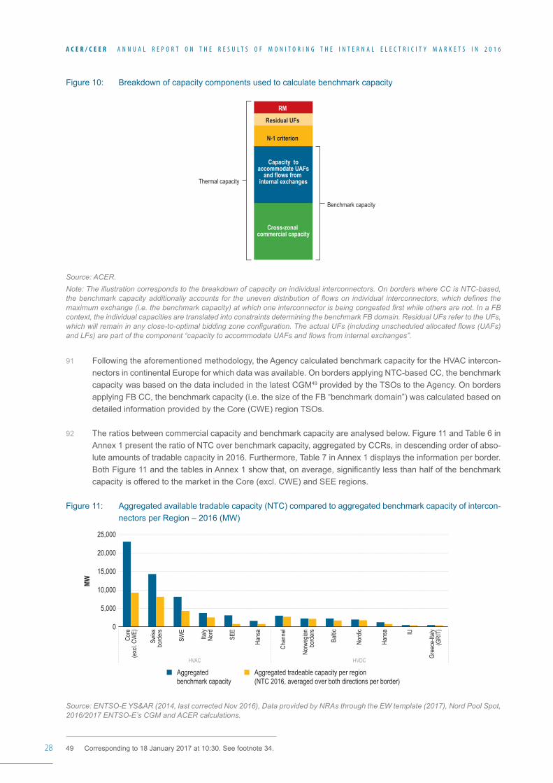
28


Figure 10: Breakdown of capacity components used to calculate benchmark capacity

Source: ACER.Note: The illustration corresponds to the breakdown of capacity on individual interconnectors. On borders where CC is NTC-based, the benchmark capacity additionally accounts for the uneven distribution of flows on individual interconnectors, which defines the maximum exchange (i.e. the benchmark capacity) at which one interconnector is being congested first while others are not. In a FB context, the individual capacities are translated into constraints determining the benchmark FB domain. Residual UFs refer to the UFs, which will remain in any close-to-optimal bidding zone configuration. The actual UFs (including unscheduled allocated flows (UAFs) and LFs) are part of the component “capacity to accommodate UAFs and flows from internal exchanges”.

91 Following the aforementioned methodology, the Agency calculated benchmark capacity for the HVAC intercon-nectors in continental Europe for which data was available. On borders applying NTC-based CC, the benchmark capacity was based on the data included in the latest CGM49 provided by the TSOs to the Agency. On borders applying FB CC, the benchmark capacity (i.e. the size of the FB “benchmark domain”) was calculated based on detailed information provided by the Core (CWE) region TSOs.

92 The ratios between commercial capacity and benchmark capacity are analysed below. Figure 11 and Table 6 in Annex 1 present the ratio of NTC over benchmark capacity, aggregated by CCRs, in descending order of abso-lute amounts of tradable capacity in 2016. Furthermore, Table 7 in Annex 1 displays the information per border. BothFigure11andthetablesinAnnex1showthat,onaverage,significantlylessthanhalfofthebenchmarkcapacity is offered to the market in the Core (excl. CWE) and SEE regions.

Figure 11: Aggregated available tradable capacity (NTC) compared to aggregated benchmark capacity of intercon-nectors per Region – 2016 (MW)

Source: ENTSO-E YS&AR (2014, last corrected Nov 2016), Data provided by NRAs through the EW template (2017), Nord Pool Spot, 2016/2017 ENTSO-E’s CGM and ACER calculations.

49 Corresponding to 18 January 2017 at 10:30. See footnote 34.

Benchmark capacity

Thermal capacity

N-1 criterion

Cross-zonal commercial capacity

RM

Residual UFs

Capacity toaccommodate UAFs

and flows from internal exchanges

MW

25,000

5,000

15,000

10,000

20,000

0

Aggregated benchmark capacity

Aggregated tradeable capacity per region(NTC 2016, averaged over both directions per border)

Chan

nel

Baltic

Nord

ic

SWE

SEE

Core

(exc

l. CW

E)

Swiss

bord

ers

Norw

egian

bord

ers

Italy

Nord

Hans

a

Hans

a IU

Gree

ce-It

aly(G

RIT)

HVAC HVDC

29


Note: Out of 51 borders, 35 borders are included in the analysis (see Table 7 in Annex 1). The following borders are excluded from the analysis for the following various reasons: the DE_TENNET-SE-4 border because this is a merchant line not included in the CCR, the Nordic, Norwegian and Baltic borders because they were not part of the CGM provided to the Agency and the four Core (CWE) region borders because FBCC is applied in Core (CWE). The values for the thermal capacity of interconnectors were taken from ENTSO-E YS&AR, and – where updated information was available via the ‘EW template’ or via the available CGMs – from NRAs or from TSOs, respectively. Tradable capacities are calculated as average NTC values per border in both directions, whereas benchmark capacity is calculated according to the methodology described in Annex 2.

93 Figure 11 shows that HVDC interconnectors have higher ratios, with an average of 85%, whereas on HVAC interconnectors an average of only 47% of benchmark capacity is available for trading.

94 Two of the main reasons for this higher percentage for HVDC interconnectors are that i) these interconnectors are not impacted by UFs50 and that ii) these interconnectors are usually not considered in the N-1 assessment. The lowest ratios for HVDC interconnectors were observed on the border from Poland to Sweden-4 (Hansa region) and from Poland to Lithuania.

95 According to the Polish NRA, these reduced values are partly related to operational security issues, including theneedtoguaranteesufficientupwardordownwardreservesforbalancingthePolishsysteminrealtime.ThePolish system is centrally dispatched and the reserves are procured after the closure of the day-ahead market and as close-to-real-time as possible. In the view of the Polish NRA this is an essential feature of the Polish market design and there is a need to restrict the cross-border capacity through capacity allocation constraints, to avoid a situation where there are not enough balancing reserves in the Polish system close-to-real time.

96 However, in the Agency’s view, the argument that TSOs are forced to reduce cross-zonal capacity (and thereby discriminate between internal and cross-zonal trade) in order to ensure secure operation of the network is a false dichotomy. This is because TSOs have at their disposal several remedies by which both the non-discrimi-nationaswellassecurenetworkoperationcouldbeefficientlymaintained.Forinstance,thebalancingcapacitycan be procured ahead of real time, before the day-ahead capacity calculation without systematically reducing cross-zonal capacity. Moreover, although balancing capacity is indeed needed to ensure operational security, the reduction of cross-zonal capacity is not inherently needed to achieve this objective.

97 By contrast, the very low ratio of NTC over benchmark capacity on several HVAC cables continued to be cor-related with the presence of UFs. For example, on the border from Germany to Poland, 76% of the benchmark capacity is used to accommodate UFs51. This is of particular concern in light of the observed average price dif-ferential between Germany and Poland (7.5 euros/MWh) which is among the largest average price differentials recorded on European borders in 2016 (as seen in Table 5 in Annex 1).

98 On HVAC interconnectors, relatively low ratios are observed in both meshed (average 46%) and non-meshed networks (i.e. on the Spanish borders with France and Portugal and on the border between Germany and Den-mark 1 with an average 52%). However, individual results per border vary, as can be seen in Table 7 in Annex 1. The lowest values are observed on the borders of Germany to Poland (0%), the Czech Republic to Poland (1%) Slovakia to Poland (2%), Germany to the Czech Republic (10%), on the Bulgarian-Romanian border (aver-age 11% considering both directions) and on the border of West Denmark to Germany (12%). An improvement on the West Denmark to Germany border is expected after the joint declaration between the ministries and the regulators of the respective MSs issued on 14 June 2017 that aims gradually to increase the minimum available cross-zonal capacity on this border for both directions up to 1100 MW in 2020.

99 At the other end, relatively high ratios (on average around 80%) can be observed on the Northern Italian borders (directions to Italy).

50 SeeFigure36oncapacitylossesduetoUFs.MoreinformationonthedifferenttypesofUFs,ontheunderlyingdefinitionsandontheirmagnitude can be found in Annex 4.

51 Calculated by combining information on benchmark capacity from Table 7 and on UFs from Figure 36.

30


100 Finally, on the German-Austrian border, no ratio was calculated, as there was no CC on this border in 2016. However, the recent agreement52 between the Austrian (E-Control) and German (Bundesnetzagentur) NRAs set thiscapacitytoatleast4,900MW(reservedforlong-termcapacityallocation).Thisappearstobeinconsistentwith the calculations of the Agency, which estimate the maximum capacity that could be made available to the marketonthisborderat2,519MW53.Anexplanationforthissignificantdifferenceisthatthe4,900MWstemsfrom a bilateral agreement rather than from a coordinated process with neighbouring TSOs. The difference can also be partly explained by the fact that the agreement envisages the application of redispatching actions54 which have not been considered in the Agency’s calculations. The Agency believes that the parties involved in the bilateral agreement should clarify the extent to which the envisaged redispatching actions will relieve capaci-ty for trade on adjacent borders. In fact, the bilateral agreement has raised concerns among market participants, TSOsandNRAsfromtheneighbouringcountriesastowhetherasignificantpartoftheexchangesbetweenGermany and Austria will keep on transiting through the neighbouring countries55 and whether the related nega-tive impacts on neighbouring markets will remain.

101 The examples listed in this Sub-section illustrate the wide disparities in the performance of CC methods from one border to another. Moreover, the good performance on some borders suggests that the benchmark capaci-tiesareachievabletargetsandemphasisesthatthecommercialcross-zonalcapacityinEuropecouldbesignifi-cantly improved through enhanced CC methods.

102 For FB CC, an equivalent method was applied (see Annex 2). It allows the calculation of a ratio between the volume of the actual FB domain and the volume of a FB ‘benchmark domain’56. The result of this calculation fortheCore(CWE)regionindicatedaratioof59%57,whichsuggestssignificantscopeforincreasingavailablecross-zonal capacity in the region.

103 Tosumup,onmostEUborders,actualNTCvalues(orthesizeoftheFBdomain)aresignificantlylowerthanwhat would be expected from the benchmark capacities (or respectively, the benchmark FB domain), which are considered by the Agency as realistic targets58. There is a large scope for improvement, because commercial capacity can potentially be doubled through improved CC methodologies.

104 The reasons for the relatively low values of commercial capacity are explained in the next Section.

3.3 Factors impacting commercial cross-zonal capacity

105 Therelativelylowcross-zonalcapacitiesareareflectionofunderlying(probablystructural)networkcongestion,whichisnotefficientlyaddressedbytheexistingbiddingzoneconfiguration,neitherbytheapplicationofreme-dial actions (e.g. redispatching or countertrading). The CC process can mitigate this problem. However, there are two key reasons why this mitigation is currently not observed. First, the process applied by TSOs to calculate thecapacitymadeavailableforcross-zonaltradeisinsufficientlycoordinated,anaspectwhichisanalysedinSub-section 3.3.1. Second, TSOs treat internal and cross-zonal exchanges unequally, which is explained in Sub-section 3.3.2.

106 As concluded in the previous Section, the gap between the commercial and the maximum possible (benchmark)

52 See more information at https://www.bundesnetzagentur.de/SharedDocs/Pressemitteilungen/EN/2017/15052017_DE_AU.html.

53 This value is consistent with available publications on this matter, e.g. see the paper “Splitting price zones: The impact of the German-Austrian: breakup on European energy objectives” at https://www.ihs.ac.at/fileadmin/public/2016_Files/Documents/2017-02_Blume-Werry_Splitting_price_zones%40EuropeanEnergy_Journal.pdf.

54 According to the Austrian and German NRAs, the agreement envisages the application of redispatching actions, in cases where neither thecross-bordercapacitybetweenGermanyandAustrianorthephysicalflowsacrossthePolish-Germanborderaresufficienttoensuretradeupto4.9GW.

55 BasedonpreviousAgency’sestimationsonaverage,about59%ofthephysicalflowsresultingfromtheDE-ATcross-zonalexchangesarenotrealisedthroughtheDE-ATborder,butareflowingasLFsthroughotherborders.Seeparagraph56oftheAgency’sDecisiononthe TSOs’ Proposal for determining Capacity Calculation Regions (see also footnote 36).

56 Seemoreinformationonbenchmarkcapacityand‘benchmarkdomain’inparagraph(91)andinAnnex2.

57 In order to improve comparability with the NTC ratios (based on values in MW), the cubic root of the FB volume was used for the FB ratio. For consistency with previous Sections, the directional volume (see paragraph (80) was used).

58 Asmentionedabove,thisispartlyconfirmedbythefactthattheactualavailablecommercialcapacityonsomebordersisindeedcloseto 100% of the benchmark value.

31


capacity is on average 15% and 53% of the benchmark capacity for HVDC and HVAC interconnectors, respec-tively. Although it is not currently possible to disentangle accurately the relative proportion of this gap that can be attributed to the two above-mentioned reasons, Sub-sections 3.3.1 and 3.3.2, provide some insight into the extent to which these two aspects (lack of coordination and discrimination of exchanges) are indeed affecting actual commercial capacity.

3.3.1 Level of coordination

107 Coordination between TSOs is essential for the well-functioning of the IEM, as their actions and the electricity exchangeswithinandbetweencontrolareascansignificantlyinfluencephysicalflowsandoperationalsecurityin other areas. In this respect, the CACM Regulation requires better coordination in the CC process among the TSOswithinandbetweenCCRs.Oneoftheconsequencesofinsufficientcoordinationisthepresenceofflowsresulting from non-coordinated capacity allocation on other borders (UAFs)59. They reduce the amount of trad-able capacity.

108 This Sub-section presents the results of the following analyses. First, it provides an update on the implementa-tion status of the CACM Regulation provisions related to the TSO coordination in CC processes. To this end, the evaluation and scoring methodology applied last year has been enhanced with additional data that the Agency collected from NRAs. A detailed description of the methodology is presented in Annex 3. Second, based on the assessed capacity losses due to UAFs, it provides an estimate of the scope for improving cross-zonal capacity by means of better coordination.

109 To assess the level of TSO cooperation in CC, NRAs had to report via a new questionnaire – among other things – the following key information for each border and CC timeframe60:

• whichofthepredefinedcoordinationmethodologies61 is applied;

• whether a common grid model is used for the CC; and

• which of the relevant input parameters62 are (re)assessed in the CC process.

110 The NRA’s response for each border and timeframe was matched by the Agency with the response from the other side of the same border. Congruent answers were evaluated and scored as provided. When the informa-tion reported by two NRAs for the same border was different, only the lower level of coordination reported and the consistently reported parameters were further considered in the assessment and respective scoring63. This approach was chosen because it is assumed that the coordination on a given border is only as strong as its weakest part.

111 The results of the enriched CC coordination assessment for 2016 is presented per border in Table 2 and aggre-gatedattheregionallevelinFigure12.Thenotesbelowthetabledefinethedifferentcoordinationlevels,andlist the (re)assessed CC parameters and the key explanations on the applied scoring methodology.

59 More information on UAFs and LFs and on their magnitude can be found in Annex 4.

60 Rangingfromyear-ahead(Y),month-ahead(M),DAtoID.

61 See notes below Table 2.

62 Relevant parameters are: a) RM, b) operational security limits (mostly CNEs) and contingencies (i.e. outages) relevant to CC, c) allocation constraints (e.g. import/export limits, losses, etc.), d) generation shift keys, (e) remedial actions.

63 In three cases, exceptions from the general rule applied. These are explained in the description of the methodology in Annex 3.

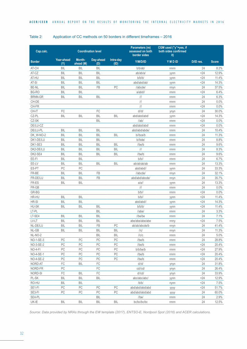
32


Table 2: Application of CC methods on 50 borders in different timeframes – 2016

Cap.calc. Coordination levelParameters (re)

assessed on both border sides

CGM used (”y”=yes, if both sides confirmed

it)

Border Year-ahead (Y)

Month-ahead (M)

Day-ahead (D)

Intra-day (ID) Y/M/D/ID Y M D ID D/ID res. Score

AT-CH BIL BIL BIL b/b/ab/ nnnn 24 8.2%AT-CZ BIL BIL BIL ab/ab/a/ yynn <24 12.9%AT-HU BIL BIL BIL b/b/b/ yynn <24 11.4%AT-SI BIL BIL BIL abd/abd/ab/ yynn <24 14.3%BE-NL BIL BIL FB PC //abcde/ nnyn 24 37.5%BG-RO BIL BIL a/abd// nnnn <24 6.4%BRNN-GR BIL BIL BIL /// nnnn 24 6.3%CH-DE /// nnnn 24 0.0%CH-FR /// nnnn <24 0.0%CH-IT FC FC d//d/ ynyn 24 30.0%CZ-PL BIL BIL BIL BIL abd/abd/abd/ yynn <24 14.3%CZ-SK BIL //ab/ nnnn <24 0.0%DE/LU-CZ abd/abd/abd/ nnnn <24 0.0%DE/LU-PL BIL BIL BIL abd/abd/abde/ nnnn 24 10.4%DK_W-NO-2 BIL BIL BIL BIL b//bce/b nnnn 24 11.3%DK1-DE/LU BIL BIL BIL b//bde/ nnnn 24 8.8%DK1-SE3 BIL BIL BIL BIL //be/b nnnn 24 9.6%DK2-DE/LU BIL BIL BIL BIL /// nnnn 24 8.3%DK2-SE4 BIL BIL BIL BIL //be/b nnnn 24 9.6%EE-FI BIL BIL b/b// nnnn 24 6.7%EE-LV BIL BIL BIL BIL ab/ab/ab/ab nnnn 24 13.3%ES-PT PC PC abd/abd// yynn 24 33.3%FR-BE BIL BIL FB //abcde/ nnyn 24 32.1%FR-DE/LU BIL BIL FB abd/abd/abcde/ nnyn 24 35.7%FR-ES BIL BIL a/a// yynn 24 13.3%FR-GB /// nnnn 24 0.0%GR-BG b/b// nnnn <24 0.0%HR-HU BIL BIL b/b// yynn <24 11.4%HR-SI BIL BIL abd/abd// yynn <24 14.3%HU-SK BIL BIL BIL b/b/b/ yynn <24 11.4%LT-PL BIL //abe/ nnnn 24 3.3%LT-SE4 BIL BIL BIL //be/be nnnn 24 7.1%LV-LT BIL BIL BIL abe/abe/abe/abe nnny <24 7.5%NL-DE/LU BIL BIL FB PC ab/ab/abcde/b nnyn 24 41.4%NL-GB BIL BIL BIL BIL //c/ nnyn 24 11.3%NL-NO-2 BIL BIL //c/c nnnn 24 5.0%NO-1-SE-3 PC PC PC PC //be/b nnnn 24 28.8%NO-3-SE-2 PC PC PC PC //be/b nnnn <24 20.4%NO-4-FI PC PC PC PC b/b/be/b nnnn <24 27.9%NO-4-SE-1 PC PC PC PC //be/b nnnn <24 20.4%NO-4-SE-2 PC PC PC PC //be/b nnnn <24 20.4%NORD-AT FC BIL FC d//d/ ynyn 24 31.8%NORD-FR PC FC cd//cd/ ynyn 24 26.4%NORD-SI FC BIL FC d//cd/ ynyn 24 33.9%PL-SK BIL BIL BIL abc/abc/abc/ yynn <24 12.9%RO-HU BIL BIL /b/b/ nynn <24 7.5%SE1-FI PC PC PC PC abd/abd/abd/abd yyyy <24 51.7%SE3-FI PC PC PC PC abd/abd/abd/abd yyyy 24 60.0%SE4-PL BIL //be/ nnnn 24 2.9%UK-IE BIL BIL BIL BIL bc/bc/bc/bc nnnn 24 12.5%

Source: Data provided by NRAs through the EW template (2017), ENTSO-E, Nordpool Spot (2016) and ACER calculations.

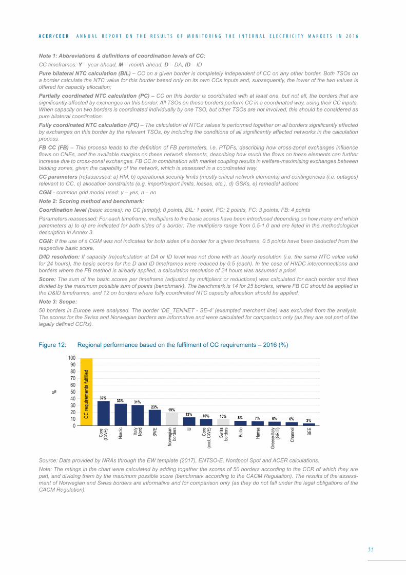
33


Note 1: Abbreviations & definitions of coordination levels of CC:CC timeframes: Y – year-ahead, M – month-ahead, D – DA, ID – ID Pure bilateral NTC calculation (BIL) – CC on a given border is completely independent of CC on any other border. Both TSOs on a border calculate the NTC value for this border based only on its own CCs inputs and, subsequently, the lower of the two values is offered for capacity allocation;Partially coordinated NTC calculation (PC) – CC on this border is coordinated with at least one, but not all, the borders that are significantly affected by exchanges on this border. All TSOs on these borders perform CC in a coordinated way, using their CC inputs. When capacity on two borders is coordinated individually by one TSO, but other TSOs are not involved, this should be considered as pure bilateral coordination. Fully coordinated NTC calculation (FC) – The calculation of NTCs values is performed together on all borders significantly affected by exchanges on this border by the relevant TSOs, by including the conditions of all significantly affected networks in the calculation process.FB CC (FB) – This process leads to the definition of FB parameters, i.e. PTDFs, describing how cross-zonal exchanges influence flows on CNEs, and the available margins on these network elements, describing how much the flows on these elements can further increase due to cross-zonal exchanges. FB CC in combination with market coupling results in welfare-maximising exchanges between bidding zones, given the capability of the network, which is assessed in a coordinated way.CC parameters (re)assessed: a) RM, b) operational security limits (mostly critical network elements) and contingencies (i.e. outages) relevant to CC, c) allocation constraints (e.g. import/export limits, losses, etc.), d) GSKs, e) remedial actionsCGM - common grid model used: y – yes, n – noNote 2: Scoring method and benchmark:Coordination level (basic scores): no CC [empty]: 0 points, BIL: 1 point, PC: 2 points, FC: 3 points, FB: 4 points Parameters reassessed: For each timeframe, multipliers to the basic scores have been introduced depending on how many and which parameters a) to d) are indicated for both sides of a border. The multipliers range from 0.5-1.0 and are listed in the methodological description in Annex 3.CGM: If the use of a CGM was not indicated for both sides of a border for a given timeframe, 0.5 points have been deducted from the respective basic score.D/ID resolution: If capacity (re)calculation at DA or ID level was not done with an hourly resolution (i.e. the same NTC value valid for 24 hours), the basic scores for the D and ID timeframes were reduced by 0.5 (each). In the case of HVDC interconnections and borders where the FB method is already applied, a calculation resolution of 24 hours was assumed a priori.Score: The sum of the basic scores per timeframe (adjusted by multipliers or reductions) was calculated for each border and then divided by the maximum possible sum of points (benchmark). The benchmark is 14 for 25 borders, where FB CC should be applied in the D&ID timeframes, and 12 on borders where fully coordinated NTC capacity allocation should be applied. Note 3: Scope:50 borders in Europe were analysed. The border ‘DE_TENNET - SE-4’ (exempted merchant line) was excluded from the analysis. The scores for the Swiss and Norwegian borders are informative and were calculated for comparison only (as they are not part of the legally defined CCRs).

Figure12: RegionalperformancebasedonthefulfilmentofCCrequirements–2016(%)

Source: Data provided by NRAs through the EW template (2017), ENTSO-E, Nordpool Spot and ACER calculations.Note: The ratings in the chart were calculated by adding together the scores of 50 borders according to the CCR of which they are part, and dividing them by the maximum possible score (benchmark according to the CACM Regulation). The results of the assess-ment of Norwegian and Swiss borders are informative and for comparison only (as they do not fall under the legal obligations of the CACM Regulation).

%

100

20

60

40

8090

10

50

30

70

0

Chan

nel

Baltic

Nord

ic

SWE

SEE

Core

(CW

E)

Core

(exc

l. CW

E)

Swiss

bord

ers

Norw

egian

bord

ers

Italy

Nord

Hans

aIU

Gree

ce-It

aly(G

RIT)

37% 33% 31% 23% 19%

13% 10% 10% 8% 7% 6% 6% 3%

CC re

quire

ments

fulfil

led

34


112 The assessment of the individual and regional results of the current implementation analysis suggests generally low fulfilmentoftheCCcoordinationrequirementsoftheCACMRegulationandshowsawidedifferenceinperformancebetween regions. The regions with the best performance are the Core (CWE), Nordic and Italy North regions. For the Core (CWE) region, this is mainly explained by the application of the FB method and the common grid model for the DA timeframe, while for the Nordic region it can be explained by the relatively good performance of the Finnish-Swedish border in all timeframes. For the Italy North region, this is mainly due to the relatively high level of coordinationreportedfortheDAandyear-aheadtimeframes.TheSEEregionshowsthelowestleveloffulfilment.

113 Becauseofthesignificantmethodologicalchanges,includingthenewdefinitionofCCR,adirectcomparisonofthe individual scores per border or per region with the scores of previous years would not be meaningful. The additional information requested for the analysis64 and the fact that the lower level of coordination was used in the caseofincongruentanswersonspecificborderspartlyexplainsthegenerallylowerscoresforindividualborders.

114 An important caveat underlying the assessment of the level of coordination is that the related obligations stem-ming from the CACM Regulation and the FCA Guideline65 do not yet apply66. Therefore, the assessment should be understood as an indication of the room for improvement at this early stage of implementation. In addition, thefollowingmainissuesthatarecurrentlyleadingtothelowfulfilmentonmanybordersstillstandout.First,on many borders, TSOs reported that no CC was performed: out of the 50 borders assessed, this applied to 28 EU borders (+4 non-EU) for the ID timeframe, 10 EU borders (+2 non-EU) for DA, 7 EU borders (+4 non-EU) for month-ahead and 6 EU borders (+3 non-EU) for year-ahead. Second, either a bilateral or partly coordinated CC method is still applied on many borders67. There are still only very few exceptions where a fully coordinated NTC CC (Italy North region) or FB (Core (CWE) region) are implemented. These two exceptions apply to at least the DA timeframe.

115 As a result, the degree of coordination in CC has not yet reached the level required by the CACM Regulation68. Therefore,significanteffortsarestilltobemadebyTSOsandNRAstoimprovethecoordinationofCC.

116 Improved coordination will contribute to increasing the amount of tradable capacity. In particular, as concluded in preceding MMRs, more coordination, e.g. through the introduction of FB CC, should result in a reduction in the amount of UAFs. UAFs, together with LFs, tend to decrease the amount of tradable capacity.

117 GiventheimpactofUAFsandLFsonmarketefficiencyandintegration,theAgencyhasbeenmonitoringsuchflowssince2012.AnupdatedanalysisoftheamountofthesetwotypesofUFsandtheassociatedcapacitylosses is presented in Annex 4.

118 TheanalysisshowsthatUAFsdecreasedfrom104.6TWhin2015to96.2TWhin2016.Followingtheimple-mentation of the improvements required by the CACM Regulation, this decrease is expected to consolidate in the coming years. In theory, where FB applies, UAFs should disappear. However, this is not yet seen in the Core (CWE)regionfortworeasons.First,someexchangesscheduledontheCore(CWE)bordersphysicallyflowthrough borders outside the Core (CWE) region. The opposite is also true, i.e. some exchanges scheduled on bordersoutsidetheCore(CWE)regionphysicallyflowthroughCore(CWE)borders.Second,themethodologyapplied to estimate AFs (which are necessary to calculate UAFs) is still subject to improvements69.

119 Finally, the potential increase in tradable cross-zonal capacity expected from improved coordination can be estimated to an average 16% of benchmark capacity or to an average of 35% when compared to the currently offered commercial capacity (average NTC) in 2016. This is derived from the actual capacity losses due to UAFs on the borders analysed for 2016 (see Annex 4) when compared with the respective benchmark capacities.

64 E.g. on the application of a CGM and the kind of parameters (re)assessed in the different calculation processes.

65 See footnotes 15 and 16.

66 Althoughsimilarobligations,withalessdetailedlegalandgovernanceframework,werealreadyrequiredbyRegulation(EC)No714/2009.

67 For example, 22 EU borders (+8 non-EU) for the DA timeframe.

68 Requirements in CACM Regulation and similar requirements applicable since 2006, following Regulation (EC) No 1228/2003, Annex I. Oncetheserequirementsarefulfilled,allbordersshouldscore100%accordingtothescoringmethodologydescribedinthisSub-section.

69 This includes the use of more CGMs, which should ideally be one per market time unit and an improved methodology for calculating GSKs that are input parameters for estimating UAFs.

35


3.3.2 Discrimination between internal and cross-zonal exchanges

3.3.2.1 The issue of discrimination

120 Electricity wholesale markets in Europe are structured in bidding zones within which any consumer may con-tract electricity with any generator without limitations. Therefore, to ensure operational security, TSOs limit exchangesbetweenbiddingzonesthroughtheCCandallocationprocess.Regulation(EC)No714/2009and,in particular, the CACM Regulation require that CC and allocation should not result in undue discrimination be-tweendifferenttypesofflows.ThisisalsothepurposeoftheAgency’sRecommendationonCapacityCalcula-tion Methodologies (see Section 3.1). In practice, this means that the capacity of the network elements should not be disproportionally allocated to support internal exchanges to the detriment of cross-zonal exchanges. Of-fering less cross-zonal capacity for cross-zonal trade due to unequal treatment of electricity exchanges reduces marketefficiencyandhencereducessocialwelfare.

121 The prioritisation of internal exchanges may take the form of i) LFs impacting interconnections, as well as ii) reductions of capacity available for cross-zonal exchanges in order to relieve congestion on internal lines. The issue of LFs, and more generally, of UFs was analysed in previous editions of the MMR. An update on the vol-umes of LFs and the associated capacity losses on interconnectors is presented in Annex 4.

122 As explained at the beginning of Section 3.3, the gap between the commercial and the maximum (benchmark) capacityislargelytheconsequenceofasuboptimalbiddingzoneconfiguration.Whereasinthemid-termthereconfigurationofbiddingzonesispossiblythemostefficienttooltoaddressthisissue,intheshort-termCCmay contribute to alleviate the gap. However, this relevant gap persists on most European borders, which can bemainlyexplainedbyeitherflowsresulting fromnon-coordinatedcapacityallocationonotherborders(i.e.UAFs) or by the prioritisation of internal exchanges.

123 As concluded in Sub-section 3.3.1, a proportion of this gap (approximately one third70) can be addressed by improved coordination in CC. Based on this, there are grounds to conclude that the largest proportion of this gap (approximately two thirds), which is on average 53% of the benchmark capacity on HVAC interconnectors, is explained by the prioritisation of internal exchanges. The individual ratios between commercial and benchmark capacity included in the last column of Table 7 in Annex 1 and the ratios between available commercial capacity andmaximumflow(Fmax)intheCore(CWE)regionprovideanindicationoftheborderswherethisprioritisa-tion is the highest.

124 In addition, the Agency could access detailed data on FB CC in the Core (CWE) region. This allowed further analysis of the issue of discrimination in this region. This analysis is included in Sub-section 3.3.2.2 below and concludes for instance, that the constraints associated with internal lines in Amprion’s area in Germany strongly limit cross-zonal exchanges within the Core (CWE) region.

125 In other regions, where CC is NTC-based, discussions are ongoing between ENTSO-E and the Agency on how to provide data with a level of detail similar to the FB case.

3.3.2.2 Analysis of the level of discrimination of cross-zonal exchanges on individual network constraints in the Core (CWE) region

126 This Sub-section analyses the frequency and extent to which discrimination of cross-zonal exchanges on indi-vidual CNEs affect the availability of cross-zonal capacity in the Core (CWE) region71.

70 Seeparagraph (119)concluding thatapproximately16%of thebenchmarkcapacitycouldbeadded to thecommercial capacitybyimproved coordination in CC. This is roughly one third of the gap between the commercial and benchmark capacity.

71 The analysis in this Sub-section is limited to the DA timeframe. However, given the fact that most of the cross-border capacity allocated in the long-term timeframe is not nominated on the borders of the region (i.e. the share of long-term nominated capacity represents only between 0% and 6% of all nominations depending on the border) and that the cross-border capacity available for the closer-to-real-time timeframes is a small share of the overall offered cross-border capacity, the conclusions of this Sub-section can be considered as valid for all timeframes taken together.

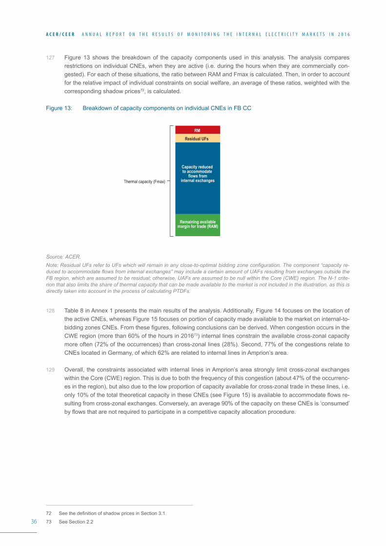
36


127 Figure 13 shows the breakdown of the capacity components used in this analysis. The analysis compares restrictions on individual CNEs, when they are active (i.e. during the hours when they are commercially con-gested). For each of these situations, the ratio between RAM and Fmax is calculated. Then, in order to account for the relative impact of individual constraints on social welfare, an average of these ratios, weighted with the corresponding shadow prices72, is calculated.

Figure 13: Breakdown of capacity components on individual CNEs in FB CC

Source: ACER.Note: Residual UFs refer to UFs which will remain in any close-to-optimal bidding zone configuration. The component “capacity re-duced to accommodate flows from internal exchanges” may include a certain amount of UAFs resulting from exchanges outside the FB region, which are assumed to be residual; otherwise, UAFs are assumed to be null within the Core (CWE) region. The N-1 crite-rion that also limits the share of thermal capacity that can be made available to the market is not included in the illustration, as this is directly taken into account in the process of calculating PTDFs.

128 Table 8 in Annex 1 presents the main results of the analysis. Additionally, Figure 14 focuses on the location of the active CNEs, whereas Figure 15 focuses on portion of capacity made available to the market on internal-to-biddingzonesCNEs.Fromthesefigures,followingconclusionscanbederived.WhencongestionoccursintheCWE region (more than 60% of the hours in 201673) internal lines constrain the available cross-zonal capacity more often (72% of the occurrences) than cross-zonal lines (28%). Second, 77% of the congestions relate to CNEs located in Germany, of which 62% are related to internal lines in Amprion’s area.

129 Overall, the constraints associated with internal lines in Amprion’s area strongly limit cross-zonal exchanges within the Core (CWE) region. This is due to both the frequency of this congestion (about 47% of the occurrenc-es in the region), but also due to the low proportion of capacity available for cross-zonal trade in these lines, i.e. only10%ofthetotaltheoreticalcapacityintheseCNEs(seeFigure15)isavailabletoaccommodateflowsre-sultingfromcross-zonalexchanges.Conversely,anaverage90%ofthecapacityontheseCNEsis‘consumed’byflowsthatarenotrequiredtoparticipateinacompetitivecapacityallocationprocedure.

72 SeethedefinitionofshadowpricesinSection3.1.

73 See Section 2.2

Thermal capacity (Fmax)

Remaining availablemargin for trade (RAM)

Capacity reduced to accommodate

flows frominternal exchanges

RM

Residual UFs

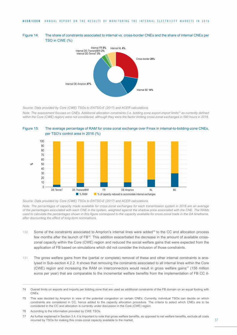
37


Figure 14: The share of constraints associated to internal vs. cross-border CNEs and the share of internal CNEs per TSO in CWE (%)

Source: Data provided by Core (CWE) TSOs to ENTSO-E (2017) and ACER calculations.Note: The assessment focuses on CNEs. Additional allocation constraints (i.e. bidding zone export-import limits74 as currently defined within the Core (CWE) region) were not considered, although they were the factor limiting cross-zonal exchanges in 590 hours in 2016.

Figure 15: The average percentage of RAM for cross-zonal exchange over Fmax in internal-to-bidding-zone CNEs, per TSO’s control area in 2016 (%)

Source: Data provided by Core (CWE) TSOs to ENTSO-E (2017) and ACER calculations.Note: The percentages of capacity made available for cross-zonal exchanges for each transmission system in 2016 are an average of the percentages associated with each CNE in the system, weighted against the shadow price associated with the CNE. The RAMs used to calculate the percentages shown in this figure correspond to the capacity available for cross-zonal trade in the DA timeframe, after discounting the effect of long-term nominations.

130 Some of the constraints associated to Amprion’s internal lines were added75 to the CC and allocation process few months after the launch of FB76. This addition exacerbated the decrease in the amount of available cross-zonal capacity within the Core (CWE) region and reduced the social welfare gains that were expected from the application of FB based on simulations which did not consider the inclusion of those constraints.

131 The gross welfare gains from the (partial or complete) removal of these and other internal constraints is ana-lysed in Sub-section 4.2.2. It shows that removing the constraints associated to all internal lines within the Core (CWE) region and increasing the RAM on interconnectors would result in gross welfare gains77 (156 million eurosperyear)thatarecomparabletotheincrementalwelfarebenefitsfromtheimplementationofFBCCit-

74 Overall limits on exports and imports per bidding zone that are used as additional constraints of the FB domain on an equal footing with CNEs.

75 This was decided by Amprion in view of the potential congestion on certain CNEs. Currently, individual TSOs can decide on which constraints are considered in CC, hence added to the capacity allocation procedure. The criteria to select which CNEs are to be considered in the CC and allocation is currently under discussion in the Core (CWE) region.

76 According to the information provided by CWE TSOs.

77 AsfurtherexplainedinSection3.4,itisimportanttonotethatgrosswelfarebenefits,asopposedtonetwelfarebenefits,excludeallcostsincurred by TSOs for making this cross-zonal capacity available to the market.

Cross-border 28%

Internal BE 14%

Internal DE-Amprion 47%

Internal DE-TenneT 3%Internal DE-TransnetBW 2%

Internal NL 6%Internal FR 0%

%

100

708090

40

6050

302010

0DE-TenneT

% of capacity reduced to accomodate internal exchanges% RAMDE-TransnetBW FR DE-Amprion NL BE

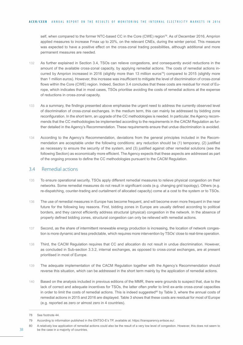
38


self, when compared to the former NTC-based CC in the Core (CWE) region78. As of December 2016, Amprion applied measures to increase Fmax up to 20%, on the relevant CNEs, during the winter period. This measure was expected to have a positive effect on the cross-zonal trading possibilities, although additional and more permanent measures are needed.

132 As further explained in Section 3.4, TSOs can relieve congestions, and consequently avoid reductions in the amount of the available cross-zonal capacity, by applying remedial actions. The costs of remedial actions in-curred by Amprion increased in 2016 (slightly more than 13 million euros79) compared to 2015 (slightly more than1millioneuros).However,thisincreasewasinsufficienttomitigatethelevelofdiscriminationofcross-zonalflowswithintheCore(CWE)region.Indeed,Section3.4concludesthatthesecostsareresidualformostofEu-rope, which indicates that in most cases, TSOs prioritise avoiding the costs of remedial actions at the expense of reductions in cross-zonal capacity.

133 Asasummary,thefindingspresentedaboveemphasisetheurgentneedtoaddressthecurrentlyobservedlevelof discrimination of cross-zonal exchanges. In the medium term, this can mainly be addressed by bidding zone reconfiguration.Intheshortterm,anupgradeoftheCCmethodologiesisneeded.Inparticular,theAgencyrecom-mends that the CC methodologies be implemented according to the requirements in the CACM Regulation as fur-ther detailed in the Agency’s Recommendation. These requirements ensure that undue discrimination is avoided.

134 According to the Agency’s Recommendation, deviations from the general principles included in the Recom-mendationareacceptableunderthefollowingconditions:anyreductionshouldbe(1)temporary,(2)justifiedasnecessarytoensurethesecurityofthesystem,and(3)justifiedagainstotherremedialsolutions(seethefollowingSection)aseconomicallymoreefficient.TheAgencyexpectsthattheseaspectsareaddressedaspartoftheongoingprocesstodefinetheCCmethodologiespursuanttotheCACMRegulation.

3.4 Remedial actions

135 To ensure operational security, TSOs apply different remedial measures to relieve physical congestion on their networks.Someremedialmeasuresdonotresultinsignificantcosts(e.g.changinggridtopology).Others(e.g.re-dispatching, counter-trading and curtailment of allocated capacity) come at a cost to the system or to TSOs.

136 The use of remedial measures in Europe has become frequent, and will become even more frequent in the near futurefor thefollowingkeyreasons.First,biddingzones inEuropeareusuallydefinedaccordingtopoliticalborders,andtheycannotefficientlyaddressstructural(physical)congestioninthenetwork.Intheabsenceofproperlydefinedbiddingzones,structuralcongestioncanonlyberelievedwithremedialactions.

137 Second, as the share of intermittent renewable energy production is increasing, the location of network conges-tion is more dynamic and less predictable, which requires more intervention by TSOs’ close to real-time operation.

138 Third, the CACM Regulation requires that CC and allocation do not result in undue discrimination. However, as concluded in Sub-section 3.3.2, internal exchanges, as opposed to cross-zonal exchanges, are at present prioritised in most of Europe.

139 The adequate implementation of the CACM Regulation together with the Agency’s Recommendation should reverse this situation, which can be addressed in the short term mainly by the application of remedial actions.

140 Based on the analysis included in previous editions of the MMR, there were grounds to suspect that, due to the lack of correct and adequate incentives for TSOs, the latter often prefer to limit ex-ante cross-zonal capacities in order to limit the costs of remedial actions. This is indeed suggested80 by Table 3, where the annual costs of remedial actions in 2015 and 2016 are displayed. Table 3 shows that these costs are residual for most of Europe (e.g. reported as zero or almost zero in 4 countries).

78 See footnote 44.

79 According to information published in the ENTSO-E’s TP, available at: https://transparency.entsoe.eu/.

80 A relatively low application of remedial actions could also be the result of a very low level of congestion. However, this does not seem to be the case in a majority of countries.

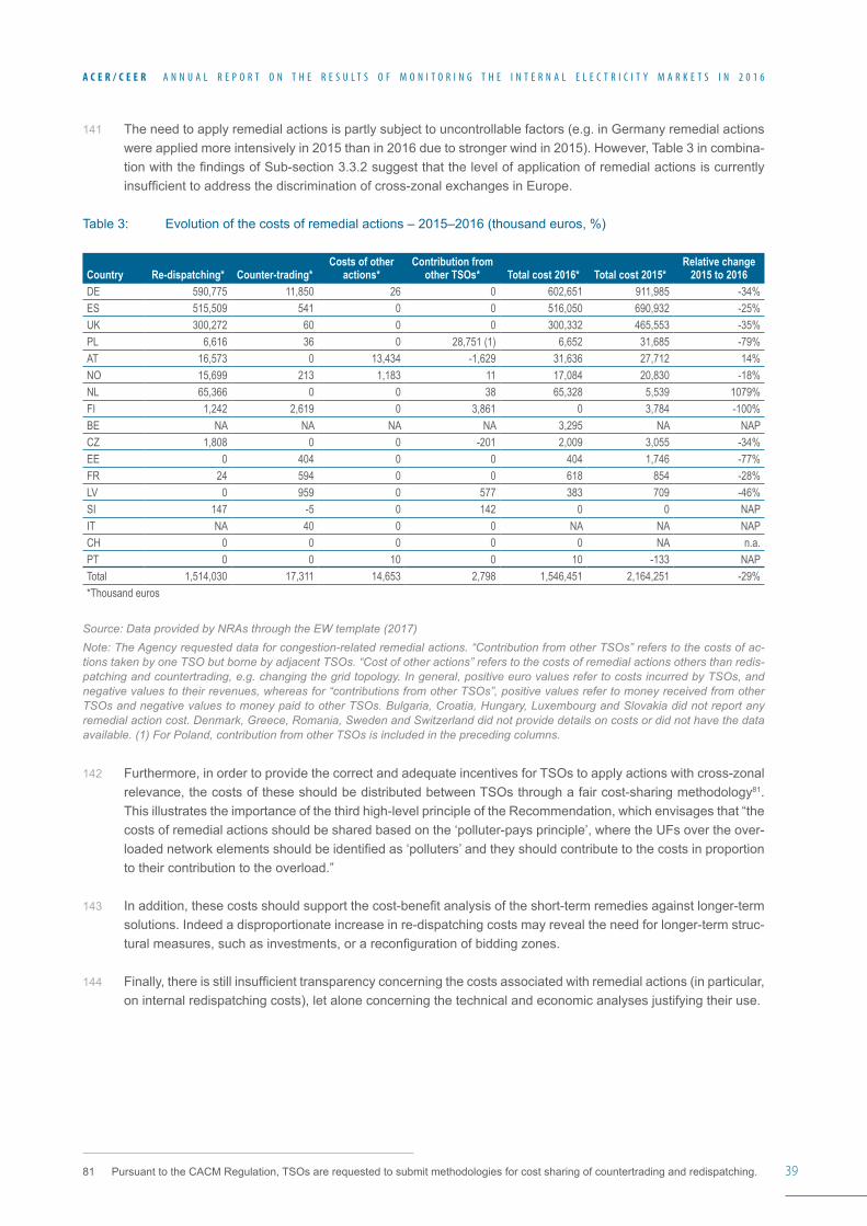
39


141 The need to apply remedial actions is partly subject to uncontrollable factors (e.g. in Germany remedial actions were applied more intensively in 2015 than in 2016 due to stronger wind in 2015). However, Table 3 in combina-tionwiththefindingsofSub-section3.3.2suggestthatthelevelofapplicationofremedialactionsiscurrentlyinsufficienttoaddressthediscriminationofcross-zonalexchangesinEurope.

Table 3: Evolution of the costs of remedial actions – 2015–2016 (thousand euros, %)

Country Re-dispatching* Counter-trading*Costs of other

actions*Contribution from

other TSOs* Total cost 2016* Total cost 2015*Relative change

2015 to 2016DE 590,775 11,850 26 0 602,651 911,985 -34%ES 515,509 541 0 0 516,050 690,932 -25%UK 300,272 60 0 0 300,332 465,553 -35%PL 6,616 36 0 28,751 (1) 6,652 31,685 -79%AT 16,573 0 13,434 -1,629 31,636 27,712 14%NO 15,699 213 1,183 11 17,084 20,830 -18%NL 65,366 0 0 38 65,328 5,539 1079%FI 1,242 2,619 0 3,861 0 3,784 -100%BE NA NA NA NA 3,295 NA NAPCZ 1,808 0 0 -201 2,009 3,055 -34%EE 0 404 0 0 404 1,746 -77%FR 24 594 0 0 618 854 -28%LV 0 959 0 577 383 709 -46%SI 147 -5 0 142 0 0 NAPIT NA 40 0 0 NA NA NAPCH 0 0 0 0 0 NA n.a.PT 0 0 10 0 10 -133 NAPTotal 1,514,030 17,311 14,653 2,798 1,546,451 2,164,251 -29%*Thousand euros

Source: Data provided by NRAs through the EW template (2017)Note: The Agency requested data for congestion-related remedial actions. “Contribution from other TSOs” refers to the costs of ac-tions taken by one TSO but borne by adjacent TSOs. “Cost of other actions” refers to the costs of remedial actions others than redis-patching and countertrading, e.g. changing the grid topology. In general, positive euro values refer to costs incurred by TSOs, and negative values to their revenues, whereas for “contributions from other TSOs”, positive values refer to money received from other TSOs and negative values to money paid to other TSOs. Bulgaria, Croatia, Hungary, Luxembourg and Slovakia did not report any remedial action cost. Denmark, Greece, Romania, Sweden and Switzerland did not provide details on costs or did not have the data available. (1) For Poland, contribution from other TSOs is included in the preceding columns.

142 Furthermore, in order to provide the correct and adequate incentives for TSOs to apply actions with cross-zonal relevance, the costs of these should be distributed between TSOs through a fair cost-sharing methodology81. This illustrates the importance of the third high-level principle of the Recommendation, which envisages that “the costs of remedial actions should be shared based on the ‘polluter-pays principle’, where the UFs over the over-loadednetworkelementsshouldbeidentifiedas‘polluters’andtheyshouldcontributetothecostsinproportionto their contribution to the overload.”

143 Inaddition,thesecostsshouldsupportthecost-benefitanalysisoftheshort-termremediesagainstlonger-termsolutions. Indeed a disproportionate increase in re-dispatching costs may reveal the need for longer-term struc-turalmeasures,suchasinvestments,orareconfigurationofbiddingzones.

144 Finally,thereisstillinsufficienttransparencyconcerningthecostsassociatedwithremedialactions(inparticular,on internal redispatching costs), let alone concerning the technical and economic analyses justifying their use.

81 Pursuant to the CACM Regulation, TSOs are requested to submit methodologies for cost sharing of countertrading and redispatching.

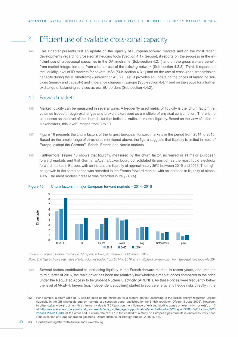
40


4 Efficient use of available cross-zonal capacity 145 ThisChapterpresentsfirstanupdateon the liquidityofEuropean forwardmarketsandon themost recent

developments regarding cross-zonal hedging tools (Section 4.1). Second, it reports on the progress in the ef-ficientuseofcross-zonalcapacitiesintheDAtimeframe(Sub-section4.2.1)andonthegrosswelfarebenefitfrom market integration and from a better use of the existing network (Sub-section 4.2.2). Third, it reports on the liquidity level of ID markets for several MSs (Sub-section 4.3.1) and on the use of cross-zonal transmission capacity during the ID timeframe (Sub-section 4.3.2). Last, it provides an update on the prices of balancing ser-vices (energy and capacity) and imbalance charges in Europe (Sub-section 4.4.1) and on the scope for a further exchange of balancing services across EU borders (Sub-section 4.4.2).

4.1 Forward markets

146 Market liquidity can be measured in several ways. A frequently used metric of liquidity is the ‘churn factor’, i.e. volumes traded through exchanges and brokers expressed as a multiple of physical consumption. There is no consensusonthelevelofthechurnfactorthatindicatessufficientmarketliquidity.Basedontheviewofdifferentstakeholders, this level82 ranges from 3 to 10.

147 Figure 16 presents the churn factors of the largest European forward markets in the period from 2014 to 2016. Basedontheamplerangeofthresholdsmentionedabove,thefiguresuggeststhatliquidityislimitedinmostofEurope, except the German83, British, French and Nordic markets.

148 Furthermore, Figure 16 shows that liquidity, measured by the churn factor, increased in all major European forward markets and that Germany/Austria/Luxembourg consolidated its position as the most liquid electricity forward market in Europe, with an increase in liquidity of approximately 35% between 2015 and 2016. The high-est growth in the same period was recorded in the French forward market, with an increase in liquidity of almost 40%. The most modest increase was recorded in Italy (+3%).

Figure 16: Churn factors in major European forward markets – 2014–2016

Source: European Power Trading 2017 report, © Prospex Research Ltd, March 2017.Note: The figure shows estimates of total volumes traded from 2014 to 2016 as a multiple of consumption from Eurostat (see footnote 20).

149 Several factors contributed to increasing liquidity in the French forward market. In recent years, and until the third quarter of 2016, the main driver has been the relatively low wholesale market prices compared to the price under the Regulated Access to Incumbent Nuclear Electricity (ARENH). As these prices were frequently below the level of ARENH, buyers (e.g. independent suppliers) started to source energy and hedge risks directly in the

82 For example, a churn ratio of 10 can be seen as the minimum for a mature market, according to the British energy regulator, Ofgem (LiquidityintheGBwholesaleenergymarkets,adiscussionpaperpublishedbytheBritishregulator,Ofgem,8June2009).However,inotherstakeholders’opinion,thisminimumvalueis3(‘Reportontheinfluenceofexistingbiddingzonesonelectricitymarkets’,p.13at http://www.acer.europa.eu/official_documents/acts_of_the_agency/publication/acer%20market%20report%20on%20bidding%20zones%202014.pdf). At the other end, a churn rate of 1.77 in the context of a study on European gas markets is quoted as ‘very poor’ (The evolution of European traded gas hubs, Oxford Institute for Energy Studies, 2015, p. 45).

83 Considered together with Austria and Luxembourg.

Chur

n fa

ctor

9

78

4

65

3210

DE/AT/LU201620152014

UK France Nordic Italy Netherlands Spain

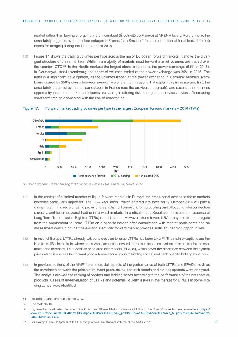
41


market rather than buying energy from the incumbent (Électricité de France) at ARENH levels. Furthermore, the uncertainty triggered by the nuclear outages in France (see Section 2.2) created additional (or at least different) needs for hedging during the last quarter of 2016.

150 Figure 17 shows the trading volumes per type across the major European forward markets. It shows the diver-gent structure of these markets. While in a majority of markets most forward market volumes are traded over the counter (OTC)84, in the Nordic markets the largest share is traded at the power exchange (53% in 2016). In Germany/Austria/Luxembourg, the share of volumes traded at the power exchange was 35% in 2016. The latterisasignificantdevelopment,asthevolumestradedatthepowerexchangeinGermany/Austria/Luxem-bourgsoaredby259%overafive-yearperiod.Twoofthemainreasonsthatexplainthisincreaseare,first,theuncertainty triggered by the nuclear outages in France (see the previous paragraph), and second, the business opportunity that some market participants are seeing in offering risk management services in view of increasing short-term trading associated with the rise of renewables.

Figure 17: Forward market trading volumes per type in the largest European forward markets – 2016 (TWh)

Source: European Power Trading 2017 report, © Prospex Research Ltd, March 2017.

151 In the context of a limited number of liquid forward markets in Europe, the cross-zonal access to these markets becomes particularly important. The FCA Regulation85 which entered into force on 17 October 2016 will play a crucial role in this regard, as its provisions establish a framework for calculating and allocating interconnection capacity, and for cross-zonal trading in forward markets. In particular, this Regulation foresees the issuance of Long-Term Transmission Rights (LTTRs) on all borders. However, the relevant NRAs may decide to derogate fromtherequirementtoissueLTTRsonaspecificborder,afterconsultationwithmarketparticipantsandanassessmentconcludingthattheexistingelectricityforwardmarketprovidessufficienthedgingopportunities.

152 In most of Europe, LTTRs already exist or a decision to issue LTTRs has been taken86. The main exceptions are the Nordic and Baltic markets, where cross-zonal access to forward markets is based on system price contracts and con-tracts for differences, i.e. electricity price area differentials (EPADs), which cover the difference between the system price(whichisusedastheforwardpricereferenceforagroupofbiddingzones)andeachspecificbiddingzoneprice.

153 In previous editions of the MMR87, some crucial aspects of the performance of both LTTRs and EPADs, such as the correlation between the prices of relevant products, ex-post risk premia and bid-ask spreads were analysed. The analysis allowed the ranking of borders and bidding zones according to the performance of their respective products. Cases of undervaluation of LTTRs and potential liquidity issues in the market for EPADs in some bid-dingzoneswereidentified.

84 Including cleared and non-cleared OTC.

85 See footnote 16.

86 E.g. see the coordinated decision of the Czech and Slovak NRAs to introduce LTTRs on the Czech-Slovak borders, available at: https://www.eru.cz/documents/10540/3221065/Spole%C4%8Dn%C3%A9_prohl%C3%A1%C5%A1en%C3%AD_AJ.pdf/cd5db5f2-aac2-4db2-9db3-837812271c39.

87 For example, see Chapter 6 of the Electricity Wholesale Markets volume of the MMR 2015.

DE/AT/LU

France

Nordics

UK

Italy

Spain

Netherlands

2000TWh

500035000 500 3000 4500400025001000 1500

Power exchange forward OTC clearing Non-cleared OTC

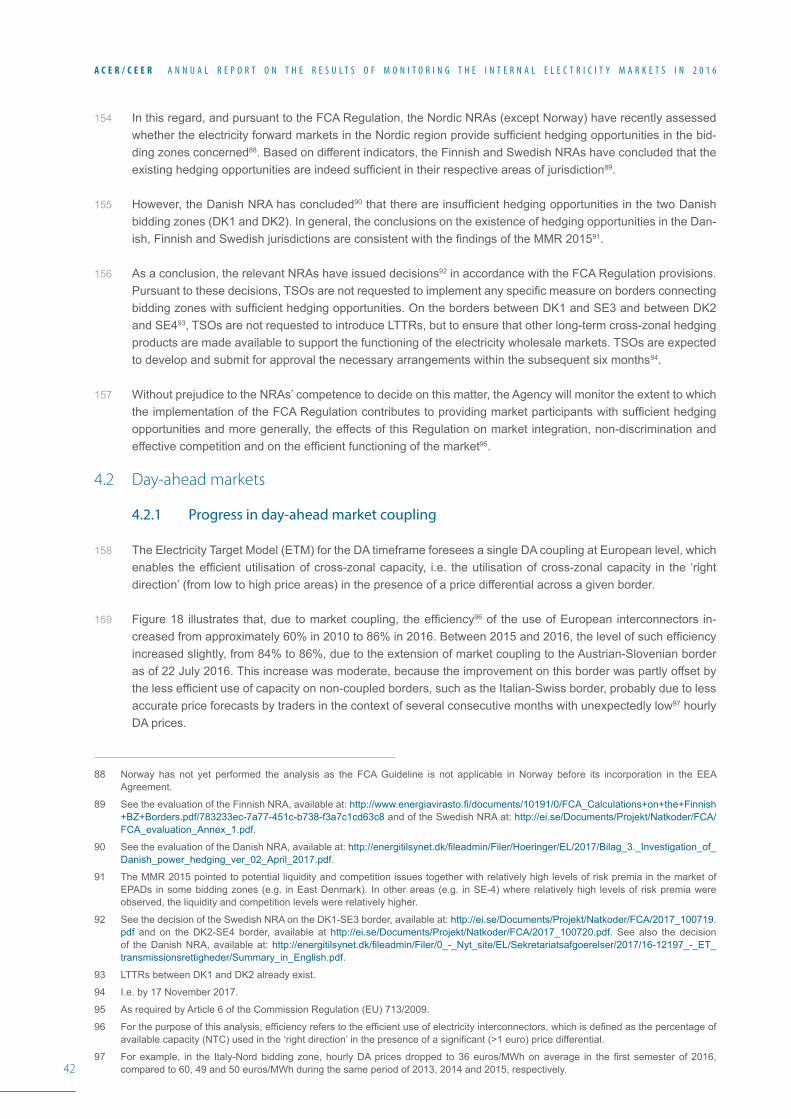
42


154 In this regard, and pursuant to the FCA Regulation, the Nordic NRAs (except Norway) have recently assessed whethertheelectricityforwardmarketsintheNordicregionprovidesufficienthedgingopportunitiesinthebid-ding zones concerned88. Based on different indicators, the Finnish and Swedish NRAs have concluded that the existinghedgingopportunitiesareindeedsufficientintheirrespectiveareasofjurisdiction89.

155 However, the Danish NRA has concluded90thatthereareinsufficienthedgingopportunitiesinthetwoDanishbidding zones (DK1 and DK2). In general, the conclusions on the existence of hedging opportunities in the Dan-ish,FinnishandSwedishjurisdictionsareconsistentwiththefindingsoftheMMR201591.

156 As a conclusion, the relevant NRAs have issued decisions92 in accordance with the FCA Regulation provisions. Pursuanttothesedecisions,TSOsarenotrequestedtoimplementanyspecificmeasureonbordersconnectingbiddingzoneswithsufficienthedgingopportunities.OnthebordersbetweenDK1andSE3andbetweenDK2and SE493, TSOs are not requested to introduce LTTRs, but to ensure that other long-term cross-zonal hedging products are made available to support the functioning of the electricity wholesale markets. TSOs are expected to develop and submit for approval the necessary arrangements within the subsequent six months94.

157 Without prejudice to the NRAs’ competence to decide on this matter, the Agency will monitor the extent to which theimplementationoftheFCARegulationcontributestoprovidingmarketparticipantswithsufficienthedgingopportunities and more generally, the effects of this Regulation on market integration, non-discrimination and effectivecompetitionandontheefficientfunctioningofthemarket95.

4.2 Day-ahead markets

4.2.1 Progress in day-ahead market coupling

158 The Electricity Target Model (ETM) for the DA timeframe foresees a single DA coupling at European level, which enablestheefficientutilisationofcross-zonalcapacity, i.e. theutilisationofcross-zonalcapacity in the ‘rightdirection’ (from low to high price areas) in the presence of a price differential across a given border.

159 Figure18 illustratesthat,duetomarketcoupling, theefficiency96 of the use of European interconnectors in-creasedfromapproximately60%in2010to86%in2016.Between2015and2016,thelevelofsuchefficiencyincreased slightly, from 84% to 86%, due to the extension of market coupling to the Austrian-Slovenian border as of 22 July 2016. This increase was moderate, because the improvement on this border was partly offset by thelessefficientuseofcapacityonnon-coupledborders,suchastheItalian-Swissborder,probablyduetolessaccurate price forecasts by traders in the context of several consecutive months with unexpectedly low97 hourly DA prices.

88 Norway has not yet performed the analysis as the FCA Guideline is not applicable in Norway before its incorporation in the EEA Agreement.

89 See the evaluation of the Finnish NRA, available at: http://www.energiavirasto.fi/documents/10191/0/FCA_Calculations+on+the+Finnish+BZ+Borders.pdf/783233ec-7a77-451c-b738-f3a7c1cd63c8 and of the Swedish NRA at: http://ei.se/Documents/Projekt/Natkoder/FCA/FCA_evaluation_Annex_1.pdf.

90 See the evaluation of the Danish NRA, available at: http://energitilsynet.dk/fileadmin/Filer/Hoeringer/EL/2017/Bilag_3._Investigation_of_Danish_power_hedging_ver_02_April_2017.pdf.

91 The MMR 2015 pointed to potential liquidity and competition issues together with relatively high levels of risk premia in the market of EPADs in some bidding zones (e.g. in East Denmark). In other areas (e.g. in SE-4) where relatively high levels of risk premia were observed, the liquidity and competition levels were relatively higher.

92 See the decision of the Swedish NRA on the DK1-SE3 border, available at: http://ei.se/Documents/Projekt/Natkoder/FCA/2017_100719.pdf and on the DK2-SE4 border, available at http://ei.se/Documents/Projekt/Natkoder/FCA/2017_100720.pdf. See also the decision of the Danish NRA, available at: http://energitilsynet.dk/fileadmin/Filer/0_-_Nyt_site/EL/Sekretariatsafgoerelser/2017/16-12197_-_ET_transmissionsrettigheder/Summary_in_English.pdf.

93 LTTRs between DK1 and DK2 already exist.

94 I.e. by 17 November 2017.

95 AsrequiredbyArticle6oftheCommissionRegulation(EU)713/2009.

96 Forthepurposeofthisanalysis,efficiencyreferstotheefficientuseofelectricityinterconnectors,whichisdefinedasthepercentageofavailablecapacity(NTC)usedinthe‘rightdirection’inthepresenceofasignificant(>1euro)pricedifferential.

97 Forexample, in the Italy-Nordbiddingzone,hourlyDApricesdropped to36euros/MWhonaverage in thefirst semesterof2016,comparedto60,49and50euros/MWhduringthesameperiodof2013,2014and2015,respectively.

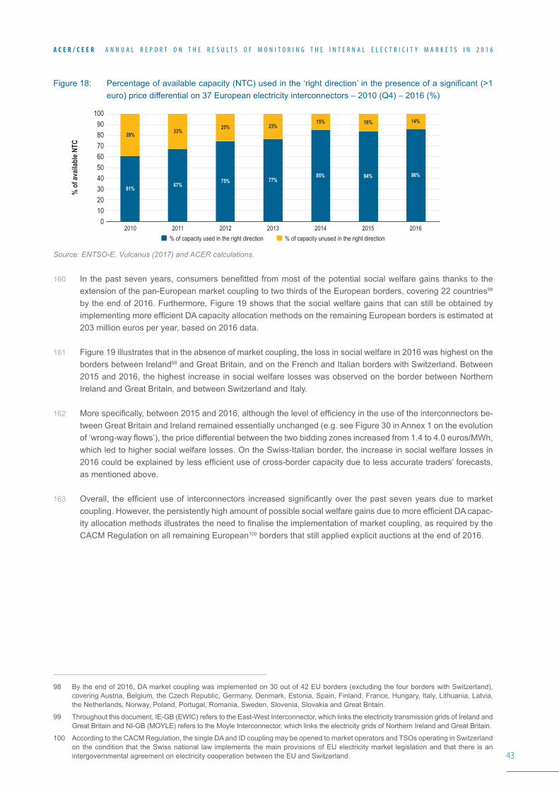
43


Figure18: Percentageofavailablecapacity(NTC)usedinthe‘rightdirection’inthepresenceofasignificant(>1euro) price differential on 37 European electricity interconnectors – 2010 (Q4) – 2016 (%)

Source: ENTSO-E, Vulcanus (2017) and ACER calculations.

160 In thepastsevenyears,consumersbenefitted frommostof thepotentialsocialwelfaregains thanks to theextension of the pan-European market coupling to two thirds of the European borders, covering 22 countries98 bytheendof2016.Furthermore,Figure19showsthatthesocialwelfaregainsthatcanstillbeobtainedbyimplementingmoreefficientDAcapacityallocationmethodsontheremainingEuropeanbordersisestimatedat203 million euros per year, based on 2016 data.

161 Figure19illustratesthatintheabsenceofmarketcoupling,thelossinsocialwelfarein2016washighestontheborders between Ireland99 and Great Britain, and on the French and Italian borders with Switzerland. Between 2015 and 2016, the highest increase in social welfare losses was observed on the border between Northern Ireland and Great Britain, and between Switzerland and Italy.

162 Morespecifically,between2015and2016,althoughthelevelofefficiencyintheuseoftheinterconnectorsbe-tween Great Britain and Ireland remained essentially unchanged (e.g. see Figure 30 in Annex 1 on the evolution of‘wrong-wayflows’),thepricedifferentialbetweenthetwobiddingzonesincreasedfrom1.4to4.0euros/MWh,which led to higher social welfare losses. On the Swiss-Italian border, the increase in social welfare losses in 2016couldbeexplainedbylessefficientuseofcross-bordercapacityduetolessaccuratetraders’forecasts,as mentioned above.

163 Overall, theefficientuseof interconnectors increasedsignificantlyover thepastsevenyearsdue tomarketcoupling.However,thepersistentlyhighamountofpossiblesocialwelfaregainsduetomoreefficientDAcapac-ityallocationmethodsillustratestheneedtofinalisetheimplementationofmarketcoupling,asrequiredbytheCACM Regulation on all remaining European100 borders that still applied explicit auctions at the end of 2016.

98 By the end of 2016, DA market coupling was implemented on 30 out of 42 EU borders (excluding the four borders with Switzerland), covering Austria, Belgium, the Czech Republic, Germany, Denmark, Estonia, Spain, Finland, France, Hungary, Italy, Lithuania, Latvia, the Netherlands, Norway, Poland, Portugal, Romania, Sweden, Slovenia, Slovakia and Great Britain.

99 Throughout this document, IE-GB (EWIC) refers to the East-West Interconnector, which links the electricity transmission grids of Ireland and GreatBritainandNI-GB(MOYLE)referstotheMoyleInterconnector,whichlinkstheelectricitygridsofNorthernIrelandandGreatBritain.

100 According to the CACM Regulation, the single DA and ID coupling may be opened to market operators and TSOs operating in Switzerland on the condition that the Swiss national law implements the main provisions of EU electricity market legislation and that there is an intergovernmental agreement on electricity cooperation between the EU and Switzerland.

% o

f ava

ilabl

e NTC

100

708090

40

6050

302010

02010

% of capacity unused in the right direction% of capacity used in the right direction

61% 67% 75% 77%85% 84% 86%

39% 33% 25% 23%15% 16% 14%

2011 2012 2013 2014 2015 2016

44


Figure19: Estimated‘socialwelfarelosses’intheabsenceofmarketcoupling,perborder–2015–2016(millioneuros)

Source: ENTSO-E, NRAs, Vulcanus (2017) and ACER calculations.Note: Only non-coupled borders are shown. The borders within the Core (CEE) region with ‘multilateral’ technical profiles are not included in this figure, because the methodology applied to the other borders, based on NTC values, is not applicable to these Core (CEE) borders for this calculation. Figure 30 in the Annex shows that cross-zonal capacity was underutilised in 2016 on those borders (DE/LU-CZ, DE/LU-PL, PL-SK), as they were affected by ‘wrong-way flows’.

4.2.2 Gross welfare benefit of better use of the existing network

164 Market integrationisexpectedtodeliverseveralbenefits.Oneoftheseisenhancedeconomicefficiency,al-lowing the lowest cost producer to serve demand in neighbouring areas. This Sub-section shows the extent to whichthisbenefithasbeenachieved,usingthesameindicatorintroducedinprecedingeditionsoftheMMR,the‘grosswelfarebenefits’101 indicator.

165 For the purpose of this Chapter, several European Power Exchanges102 were asked to perform a simulation in ordertoestimatethesegrosswelfarebenefitsfor2016.Thealgorithmusedforthesimulationsoriginatesfromthe Price Coupling of Regions (PCR) Project (Euphemia), which is used for clearing the single European DA price coupling of power regions.

166 On the basis of a set of assumptions103, twodifferent analyseswere carried out.The firstwas intended toestimatetheorderofmagnitudeoftheoverallbenefitsofmarketintegrationinEuropein2016,whilethesec-ondanalysisaimedtoestimatethegrosswelfarebenefitsfromincreasingcross-bordercapacitybyacertainamount, in accordance with the Recommendation of the Agency on CC and redispatching and countertrading cost-sharing methodologies (see Section 3.1).

167 ThegeographicalscopeofthefirstanalysiswastheMulti-RegionalCoupling(MRC)region,comprising35bor-ders.Thisanalysisincludedthecomputationofgrosswelfarebenefitsin2016fortwoscenarios:

• Historicalscenario:thegrosswelfarebenefitin2016calculatedonthebasisofdetailedhistoricalinformationsuch as network constraints, the exchange participants’ order books (that is, supply offers and demand bids) and available cross-border capacity. For the latter, the relevant Available Transfer Capacity (ATC) and FB constraints104 were used as a proxy for capacity effectively made available.

101 Grosswelfare benefit includes, first, the ʻconsumers’ and ʻproducers’ surplus gained by consumers and producerswho participatein power exchanges (welfare is measured as the difference between the prices bid into the market and the matched prices obtained multiplied by the quantity), and second, congestion rents.The first componentmeasures themonetary gain (saving) that could beobtained by consumers (producers) because they are able to purchase (sell) electricity at a price that is less than the higher (lower) price they would be willing to pay (offer) as a result of changes in cross-border transmission capacity. The second component corresponds to price differences between interconnected markets multiplied by hourly aggregated nominations between these markets. It is important tonotethatgrosswelfarebenefits,asopposedtonetwelfarebenefits,excludeallcostsincurredbyTSOsformakingthiscross-bordercapacity available to the market.

102 EPEX SPOT, Nord Pool, GME, OMIE, OTE, OPCOM and TGE.

103 Due to the assumptions, several caveats need to be made, which are the same as mentioned in the MMR 2014, paragraph 503.

104 ATC was used for borders where CC is CNTC-based, and FB constraints for the borders within the Core (CWE) region where CC is FB.

Millio

n eu

ros

80

70

40

60

50

30

20

10

0IE-GB (EWIC)

2015 2016NI-GB (MOYLE) CH-FR CH-IT CH-DE AT-CZ AT-CH AT-HU DE/LU-CZ (TenneT)

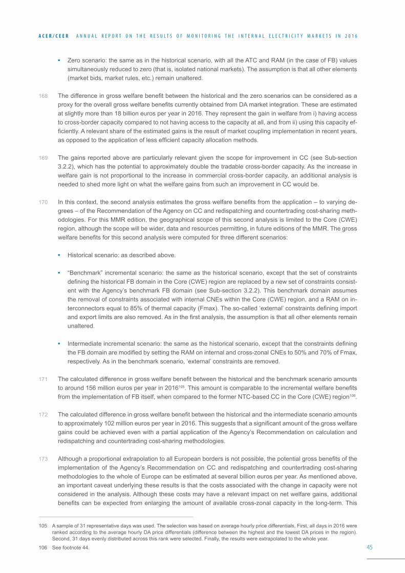
45


• Zero scenario: the same as in the historical scenario, with all the ATC and RAM (in the case of FB) values simultaneously reduced to zero (that is, isolated national markets). The assumption is that all other elements (market bids, market rules, etc.) remain unaltered.

168 ThedifferenceingrosswelfarebenefitbetweenthehistoricalandthezeroscenarioscanbeconsideredasaproxyfortheoverallgrosswelfarebenefitscurrentlyobtainedfromDAmarketintegration.Theseareestimatedat slightly more than 18 billion euros per year in 2016. They represent the gain in welfare from i) having access to cross-border capacity compared to not having access to the capacity at all, and from ii) using this capacity ef-ficiently.Arelevantshareoftheestimatedgainsistheresultofmarketcouplingimplementationinrecentyears,asopposedtotheapplicationoflessefficientcapacityallocationmethods.

169 The gains reported above are particularly relevant given the scope for improvement in CC (see Sub-section 3.2.2), which has the potential to approximately double the tradable cross-border capacity. As the increase in welfare gain is not proportional to the increase in commercial cross-border capacity, an additional analysis is needed to shed more light on what the welfare gains from such an improvement in CC would be.

170 Inthiscontext,thesecondanalysisestimatesthegrosswelfarebenefitsfromtheapplication–tovaryingde-grees – of the Recommendation of the Agency on CC and redispatching and countertrading cost-sharing meth-odologies. For this MMR edition, the geographical scope of this second analysis is limited to the Core (CWE) region, although the scope will be wider, data and resources permitting, in future editions of the MMR. The gross welfarebenefitsforthissecondanalysiswerecomputedforthreedifferentscenarios:

• Historical scenario: as described above.

• “Benchmark” incremental scenario: the same as the historical scenario, except that the set of constraints definingthehistoricalFBdomainintheCore(CWE)regionarereplacedbyanewsetofconstraintsconsist-ent with the Agency’s benchmark FB domain (see Sub-section 3.2.2). This benchmark domain assumes the removal of constraints associated with internal CNEs within the Core (CWE) region, and a RAM on in-terconnectorsequalto85%ofthermalcapacity(Fmax).Theso-called‘external’constraintsdefiningimportandexportlimitsarealsoremoved.Asinthefirstanalysis,theassumptionisthatallotherelementsremainunaltered.

• Intermediateincrementalscenario:thesameasthehistoricalscenario,exceptthattheconstraintsdefiningtheFBdomainaremodifiedbysettingtheRAMoninternalandcross-zonalCNEsto50%and70%ofFmax,respectively. As in the benchmark scenario, ‘external’ constraints are removed.

171 Thecalculateddifferenceingrosswelfarebenefitbetweenthehistoricalandthebenchmarkscenarioamountsto around 156 million euros per year in 2016105.Thisamountiscomparabletotheincrementalwelfarebenefitsfrom the implementation of FB itself, when compared to the former NTC-based CC in the Core (CWE) region106.

172 Thecalculateddifferenceingrosswelfarebenefitbetweenthehistoricalandtheintermediatescenarioamountstoapproximately102millioneurosperyearin2016.Thissuggeststhatasignificantamountofthegrosswelfaregains could be achieved even with a partial application of the Agency’s Recommendation on calculation and redispatching and countertrading cost-sharing methodologies.

173 AlthoughaproportionalextrapolationtoallEuropeanbordersisnotpossible,thepotentialgrossbenefitsoftheimplementation of the Agency’s Recommendation on CC and redispatching and countertrading cost-sharing methodologies to the whole of Europe can be estimated at several billion euros per year. As mentioned above, an important caveat underlying these results is that the costs associated with the change in capacity were not considered in the analysis. Although these costs may have a relevant impact on net welfare gains, additional benefitscanbeexpectedfromenlargingtheamountofavailablecross-zonalcapacity in the long-term.This

105 A sample of 31 representative days was used. The selection was based on average hourly price differentials, First, all days in 2016 were ranked according to the average hourly DA price differentials (difference between the highest and the lowest DA prices in the region). Second, 31 days evenly distributed across this rank were selected. Finally, the results were extrapolated to the whole year.

106 See footnote 44.

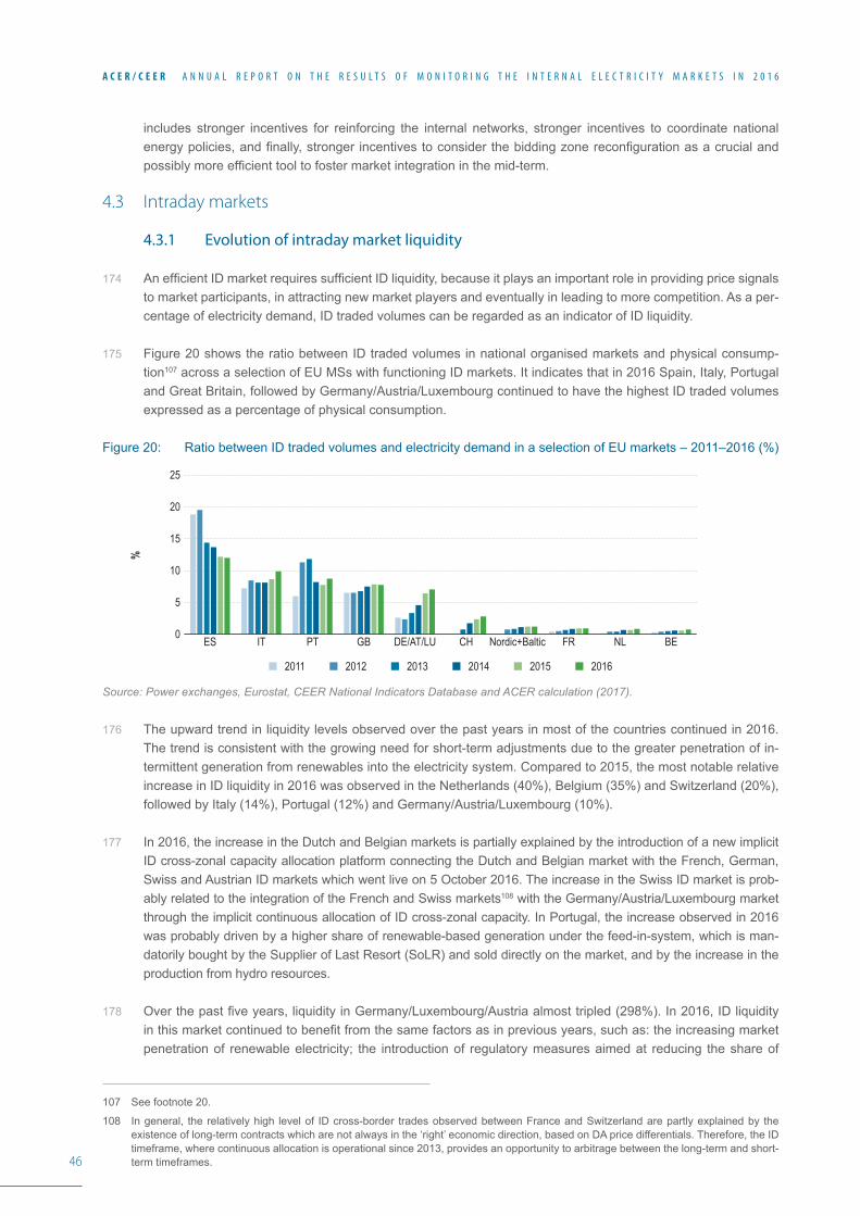
46


includes stronger incentives for reinforcing the internal networks, stronger incentives to coordinate national energypolicies,andfinally,strongerincentivestoconsiderthebiddingzonereconfigurationasacrucialandpossiblymoreefficienttooltofostermarketintegrationinthemid-term.

4.3 Intraday markets

4.3.1 Evolution of intraday market liquidity

174 AnefficientIDmarketrequiressufficientIDliquidity,becauseitplaysanimportantroleinprovidingpricesignalsto market participants, in attracting new market players and eventually in leading to more competition. As a per-centage of electricity demand, ID traded volumes can be regarded as an indicator of ID liquidity.

175 Figure 20 shows the ratio between ID traded volumes in national organised markets and physical consump-tion107 across a selection of EU MSs with functioning ID markets. It indicates that in 2016 Spain, Italy, Portugal and Great Britain, followed by Germany/Austria/Luxembourg continued to have the highest ID traded volumes expressed as a percentage of physical consumption.

Figure 20: Ratio between ID traded volumes and electricity demand in a selection of EU markets – 2011–2016 (%)

Source: Power exchanges, Eurostat, CEER National Indicators Database and ACER calculation (2017).

176 The upward trend in liquidity levels observed over the past years in most of the countries continued in 2016. The trend is consistent with the growing need for short-term adjustments due to the greater penetration of in-termittent generation from renewables into the electricity system. Compared to 2015, the most notable relative increase in ID liquidity in 2016 was observed in the Netherlands (40%), Belgium (35%) and Switzerland (20%), followed by Italy (14%), Portugal (12%) and Germany/Austria/Luxembourg (10%).

177 In 2016, the increase in the Dutch and Belgian markets is partially explained by the introduction of a new implicit ID cross-zonal capacity allocation platform connecting the Dutch and Belgian market with the French, German, Swiss and Austrian ID markets which went live on 5 October 2016. The increase in the Swiss ID market is prob-ably related to the integration of the French and Swiss markets108 with the Germany/Austria/Luxembourg market through the implicit continuous allocation of ID cross-zonal capacity. In Portugal, the increase observed in 2016 was probably driven by a higher share of renewable-based generation under the feed-in-system, which is man-datorily bought by the Supplier of Last Resort (SoLR) and sold directly on the market, and by the increase in the production from hydro resources.

178 Overthepastfiveyears,liquidityinGermany/Luxembourg/Austriaalmosttripled(298%).In2016,IDliquidityinthismarketcontinuedtobenefitfromthesamefactorsasinpreviousyears,suchas:theincreasingmarketpenetration of renewable electricity; the introduction of regulatory measures aimed at reducing the share of


108 In general, the relatively high level of ID cross-border trades observed between France and Switzerland are partly explained by the existence of long-term contracts which are not always in the ‘right’ economic direction, based on DA price differentials. Therefore, the ID timeframe, where continuous allocation is operational since 2013, provides an opportunity to arbitrage between the long-term and short-term timeframes.

%

ES IT PT GB DE/AT/LU CH Nordic+Baltic FR NL BE

25

15

20

5

10

0

2011 2012 2013 2014 2015 2016

47


renewable electricity generators exempt from balancing responsibility (around 43% of installed German renew-able capacity by the end of 2015), and measures aimed at avoiding imbalance prices being set below incurred cost; the launch of 15-minute products ID auctions; and the extension of the trading of 15-minute contracts to the continuous ID market in Austria.

179 In the near future, several factors are expected to have a positive effect on ID liquidity across the EU.

180 First, new ID products were recently introduced or are planned to be introduced in a number of markets and borders. This includes the launch of 30-minute products continuous ID trading in France, Germany and Switzer-land on 30 March 2017 and the plan to introduce 15-minute products auctions in the Netherlands and 30-minute productsauctionsinFrance.TheeffectofthesedevelopmentsonliquidityisnotyetreflectedinFigure20,asthe latter captures annual increases only up to 2016.

181 Second, the extension of balancing responsibility to renewable electricity generators is expected to further increase ID liquidity. As of 31 December 2016, renewable generation was not treated in the same way as conventional generation regarding balancing responsibility in at least 10 MSs109. The Agency advocates110 the integration of electricity from renewables in the wholesale market, which implies the removal of derogations to balancing responsibility and market-based principles applied to curtailments or redispatching.

182 Third, the implementation of a single ID coupling (SIDC) with implicit continuous cross-zonal capacity allocation, as laid down in the CACM Regulation, is expected to increase liquidity, because participants will have access to a larger portfolio of bids and offers to meet their balancing needs. The implementation of the SIDC through the cross-border ID (XBID) project111 is planned for 2018.

183 Fourth, the requirement laid down in the CACM Regulation to set the ID cross-zonal Gate Closure Time (GCT) to at most one hour112 before real time is also expected to have a positive effect on liquidity. In general, setting CGTs closer to real time, when more accurate information on the supply-demand balance is available, should lead to higher liquidity levels and reduce the need for more costly balancing services.

184 National ID GCTs are also expected to be set at most one hour before real time. Currently, various GCTs are being applied throughout national markets, ranging from 30 minutes before the beginning of physical delivery in Germany, Austria and France to 60 minutes in Great Britain and Switzerland or more, which is the case in Spain (135minutes),Portugal(135minutes)andItaly(195-540minutes).AnimportantcaveatregardingthesettingofGCTs closer to physical delivery time is that this measure should not jeopardise operational security or hamper the integration of balancing markets, which might occur if they are set too close to real time. Irrespective of this caveat, the scope for harmonising ID GCTs across Europe is evident.

185 Finally, some other aspects of the CACM Regulation potentially affecting ID liquidity are left to agreement at the regional level. This includes the possibility that continuous trading between and within bidding zones of the SIDC is complemented by regional113 ID auctions. This is subject to several conditions, including, inter alia, the absence of an adverse impact on the liquidity of the SIDC and the absence of undue discrimination between market participants from adjacent regions.

186 Without prejudice to the NRAs’ competence to decide on these matters, the Agency will monitor the extent to which the implementation of the different provisions of the CACM Regulation affect ID liquidity and, in particular, whether they limit the access of market players to ID trading opportunities beyond the physical constraints of the network.

109 Austria, Croatia, Cyprus, France, Germany, Greece, Italy, Lithuania, Malta and Portugal.

110 For further information, see the ACER/CEER White Paper #1 on ‘Renewables in the Wholesale Market Relevant to European Commission’s Clean Energy Proposals’ of 11 May 2017, available at: http://www.acer.europa.eu/Official_documents/Position_Papers/Position%20papers/WP%20ACER%2001%2017.pdf.SeealsotheEuropeanEnergyRegulators’WhitePaper#4on‘EfficientWholesalePrice formation’.

111 Nominated electricity market operators (NEMOs) proposed to NRAs in the ‘All NEMO proposal for the Market Coupling Operator (MCO) Plan’ that the delivery of the ID market coupling should be based on the XBID commercial solution.

112 Article59(3)oftheCACMRegulation.

113 Inthefirstsemesterof2017,twoinitiativeshaveundergonepublicconsultationsfortheintroductionofregionalauctions(oneintheIberian market and the other in Italy).

48


4.3.2 Intraday use of cross-zonal capacity

187 Figure 21 shows the absolute sum of net ID nominations for a selection of EU borders over the past seven years. In spite of a slight decrease of approximately 1% between 2015 and 2016, Figure 21 shows an upward trend in traded cross-zonal volumes in the ID timeframe between 2010 and 2016. As shown in Figure 31 in Annex 1, in 2016themostsignificantprogresscomparedtothepreviousyearwasrecordedontheborderbetweenSpainand France, where volumes more than doubled (increased by 118%), probably thanks to the new interconnector between these two MSs (see Sub-section 3.2.1).

Figure 21: Level of ID cross-zonal trade per year (absolute sum of net ID nominations for a selection of EU borders) – 2010–2016 (GWh)

Source: ENTSO-E, NRAs, Vulcanus (2017) and ACER calculations.Note: This figure contains data for those borders for which data was consistently available for the period analysed, i.e. AT-DE, AT-SI, BE-FR, BE-NL, CH-DE, CH-FR, CH-IT, CZ-SK, CZ-DE, DE-FR, DE-NL, DE-PL, ES-FR, ES-PT and FR-IT.

188 Figure22showsthelevelofutilisationofcross-zonalcapacityintheIDtimeframewhenithasavalue(>1euro/MWh),foraselectionofborders.First, thisFigure illustratesthatthe levelofefficiency114 in the utilisation of cross-zonal capacity in the ID timeframe (on average 50% for the borders analysed) was relatively low in 2016, comparedtothelevelofefficiencyintheDAtimeframe(86%,asshowninFigure18).Second,Figure22con-firms thatcross-zonalcapacitywasusedmoreefficiently in2016 in the ID timeframeonborderswhere thecapacitywasallocatedbyusingimplicitallocationmethods(61%ofefficiency)asopposedtoexplicitorotherallocation methods (40%).

189 Furthermore,Figure22suggeststhatimplicitauctions(100%efficiencyfortheSpanish-Portugueseborder)per-formbetterthanimplicitcontinuoustrade(onaverage49%efficiencyfortheFrench-German,Dutch-NorwegianandFrench-Swissborders)intermsofefficientutilisationofIDcross-zonalcapacity115.

190 In conclusion, the level of utilisation of cross-zonal capacity in the ID timeframe remains low, which leaves a largepartofthepotentialbenefitsfrominfrastructureinvestmentsuntapped.However,despitesignificantdelaysexperienced in the implementation of the SIDC, mainly caused by technical and decision-making issues among theprojectpartiesinvolvedintheXBIDproject,theforthcominggo-liveoftheSIDCinfirstquarterof2018isexpectedfurthertoincreasetheefficientuseofthecross-zonalcapacityintheIDtimeframe.

114 For the purpose of this analysis, the most representative prices are provided by the closest-to-real-time trades, since they are considered bettertorevealthevalueofcross-zonalcapacityatthetimewhenfinalcross-zonalnominationsaredetermined.WhereIDmarketsareauction-based, the closest-to-real-time trades can be valued at the price of the last auction for every delivery hour. Where ID markets are based on continuous trading, the weighted average ID prices can be used as a proxy for the value of the closest-to-real-time trades. See more details in Sub-section 3.3.1 on ‘Utilisation of cross-zonal capacity in the ID and balancing timeframes’ of the MMR 2013.

115 ThismeansthatthefinalnetIDnominationsonbordersfeaturingimplicitcontinuousallocationofcapacityarenotalwaysalignedwiththe close-to-real-time value of cross-zonal capacity, which can be derived from the close-to-real time ID price differentials.

GWh

2010 2011 2012 2013 2014 2015 2016

30,000

25,000

15,000

20,000

5,000

10,000

0

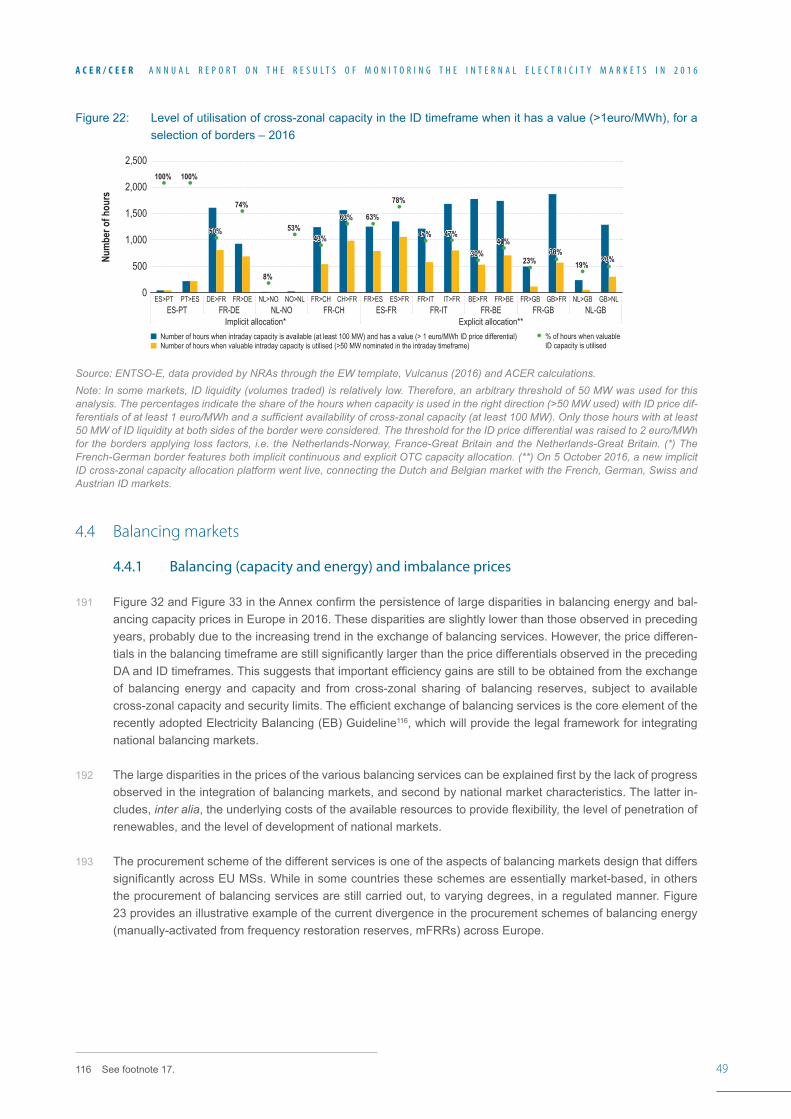
49


Figure22: Levelofutilisationofcross-zonalcapacityintheIDtimeframewhenithasavalue(>1euro/MWh),foraselection of borders – 2016

Source: ENTSO-E, data provided by NRAs through the EW template, Vulcanus (2016) and ACER calculations.Note: In some markets, ID liquidity (volumes traded) is relatively low. Therefore, an arbitrary threshold of 50 MW was used for this analysis. The percentages indicate the share of the hours when capacity is used in the right direction (>50 MW used) with ID price dif-ferentials of at least 1 euro/MWh and a sufficient availability of cross-zonal capacity (at least 100 MW). Only those hours with at least 50 MW of ID liquidity at both sides of the border were considered. The threshold for the ID price differential was raised to 2 euro/MWh for the borders applying loss factors, i.e. the Netherlands-Norway, France-Great Britain and the Netherlands-Great Britain. (*) The French-German border features both implicit continuous and explicit OTC capacity allocation. (**) On 5 October 2016, a new implicit ID cross-zonal capacity allocation platform went live, connecting the Dutch and Belgian market with the French, German, Swiss and Austrian ID markets.

4.4 Balancing markets

4.4.1 Balancing (capacity and energy) and imbalance prices

191 Figure32andFigure33intheAnnexconfirmthepersistenceoflargedisparitiesinbalancingenergyandbal-ancing capacity prices in Europe in 2016. These disparities are slightly lower than those observed in preceding years, probably due to the increasing trend in the exchange of balancing services. However, the price differen-tialsinthebalancingtimeframearestillsignificantlylargerthanthepricedifferentialsobservedintheprecedingDAandIDtimeframes.Thissuggeststhatimportantefficiencygainsarestilltobeobtainedfromtheexchangeof balancing energy and capacity and from cross-zonal sharing of balancing reserves, subject to available cross-zonalcapacityandsecuritylimits.Theefficientexchangeofbalancingservicesisthecoreelementoftherecently adopted Electricity Balancing (EB) Guideline116, which will provide the legal framework for integrating national balancing markets.

192 Thelargedisparitiesinthepricesofthevariousbalancingservicescanbeexplainedfirstbythelackofprogressobserved in the integration of balancing markets, and second by national market characteristics. The latter in-cludes, inter alia,theunderlyingcostsoftheavailableresourcestoprovideflexibility,thelevelofpenetrationofrenewables, and the level of development of national markets.

193 The procurement scheme of the different services is one of the aspects of balancing markets design that differs significantlyacrossEUMSs.Whileinsomecountriestheseschemesareessentiallymarket-based,inothersthe procurement of balancing services are still carried out, to varying degrees, in a regulated manner. Figure 23 provides an illustrative example of the current divergence in the procurement schemes of balancing energy (manually-activated from frequency restoration reserves, mFRRs) across Europe.


Num

ber o

f hou

rs

2,500

2,000

1,500

1,000

500

0ES>PT

ES-PT FR-DEImplicit allocation* Explicit allocation**

NL-NO FR-CH ES-FR FR-ITPT>ES DE>FR FR>DE NL>NO NO>NL FR>CH CH>FR FR>ES ES>FR FR>IT IT>FR

FR-BE FR-GB NL-GBBE>FR FR>BE FR>GB GB>FR NL>GB GB>NL

Number of hours when intraday capacity is available (at least 100 MW) and has a value (> 1 euro/MWh ID price differential)Number of hours when valuable intraday capacity is utilised (>50 MW nominated in the intraday timeframe)

% of hours when valuable ID capacity is utilised

100% 100% 100% 100%

50% 50%

74% 74%

8% 8%

53% 53% 43% 43%

63% 63% 63% 63%

78% 78%

47% 47% 47% 47%

30% 30% 41% 41%

23% 23% 30% 30%

19% 19% 23% 23%

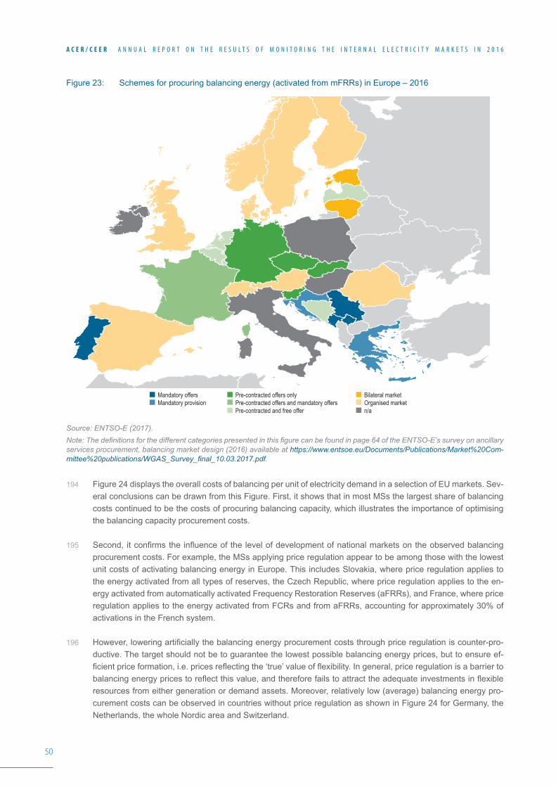
50


Figure 23: Schemes for procuring balancing energy (activated from mFRRs) in Europe – 2016

Source: ENTSO-E (2017).Note: The definitions for the different categories presented in this figure can be found in page 64 of the ENTSO-E’s survey on ancillary services procurement, balancing market design (2016) available at https://www.entsoe.eu/Documents/Publications/Market%20Com-mittee%20publications/WGAS_Survey_final_10.03.2017.pdf.

194 Figure 24 displays the overall costs of balancing per unit of electricity demand in a selection of EU markets. Sev-eral conclusions can be drawn from this Figure. First, it shows that in most MSs the largest share of balancing costs continued to be the costs of procuring balancing capacity, which illustrates the importance of optimising the balancing capacity procurement costs.

195 Second, itconfirmstheinfluenceofthelevelofdevelopmentofnationalmarketsontheobservedbalancingprocurement costs. For example, the MSs applying price regulation appear to be among those with the lowest unit costs of activating balancing energy in Europe. This includes Slovakia, where price regulation applies to the energy activated from all types of reserves, the Czech Republic, where price regulation applies to the en-ergy activated from automatically activated Frequency Restoration Reserves (aFRRs), and France, where price regulation applies to the energy activated from FCRs and from aFRRs, accounting for approximately 30% of activations in the French system.

196 However,loweringartificiallythebalancingenergyprocurementcoststhroughpriceregulationiscounter-pro-ductive. The target should not be to guarantee the lowest possible balancing energy prices, but to ensure ef-ficientpriceformation,i.e.pricesreflectingthe‘true’valueofflexibility.Ingeneral,priceregulationisabarriertobalancingenergypricestoreflectthisvalue,andthereforefailstoattracttheadequateinvestmentsinflexibleresources from either generation or demand assets. Moreover, relatively low (average) balancing energy pro-curement costs can be observed in countries without price regulation as shown in Figure 24 for Germany, the Netherlands, the whole Nordic area and Switzerland.

Mandatory offersMandatory provision

Pre-contracted offers onlyPre-contracted offers and mandatory offersPre-contracted and free offer

Bilateral marketOrganised marketn/a

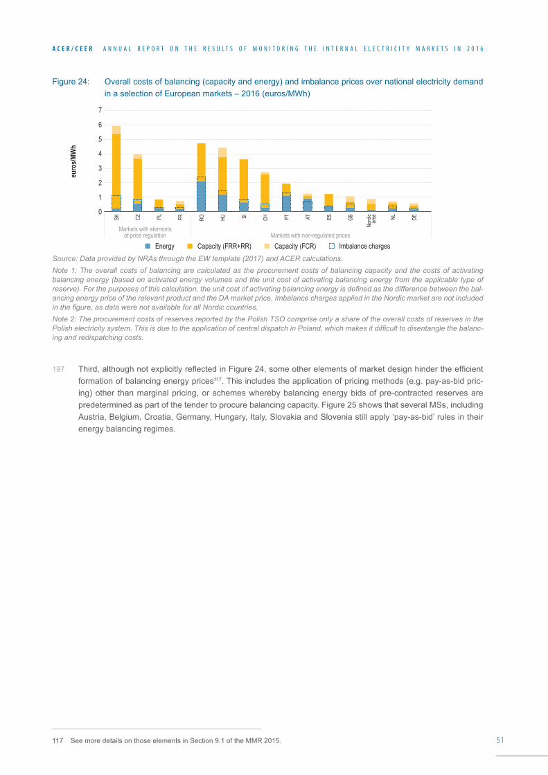
51


Figure 24: Overall costs of balancing (capacity and energy) and imbalance prices over national electricity demand in a selection of European markets – 2016 (euros/MWh)

Source: Data provided by NRAs through the EW template (2017) and ACER calculations.Note 1: The overall costs of balancing are calculated as the procurement costs of balancing capacity and the costs of activating balancing energy (based on activated energy volumes and the unit cost of activating balancing energy from the applicable type of reserve). For the purposes of this calculation, the unit cost of activating balancing energy is defined as the difference between the bal-ancing energy price of the relevant product and the DA market price. Imbalance charges applied in the Nordic market are not included in the figure, as data were not available for all Nordic countries.Note 2: The procurement costs of reserves reported by the Polish TSO comprise only a share of the overall costs of reserves in the Polish electricity system. This is due to the application of central dispatch in Poland, which makes it difficult to disentangle the balanc-ing and redispatching costs.

197 Third,althoughnotexplicitlyreflectedinFigure24,someotherelementsofmarketdesignhindertheefficientformation of balancing energy prices117. This includes the application of pricing methods (e.g. pay-as-bid pric-ing) other than marginal pricing, or schemes whereby balancing energy bids of pre-contracted reserves are predetermined as part of the tender to procure balancing capacity. Figure 25 shows that several MSs, including Austria, Belgium, Croatia, Germany, Hungary, Italy, Slovakia and Slovenia still apply ‘pay-as-bid’ rules in their energy balancing regimes.

117 SeemoredetailsonthoseelementsinSection9.1oftheMMR2015.

euro

s/MW

h

SK CZ PL FR RO HU SI CH PT AT ES GB NL DE

4

7

5

6

3

2

1

0

Energy Capacity (FRR+RR) Capacity (FCR) Imbalance charges

Nord

icar

ea

Markets with elementsof price regulation Markets with non-regulated prices

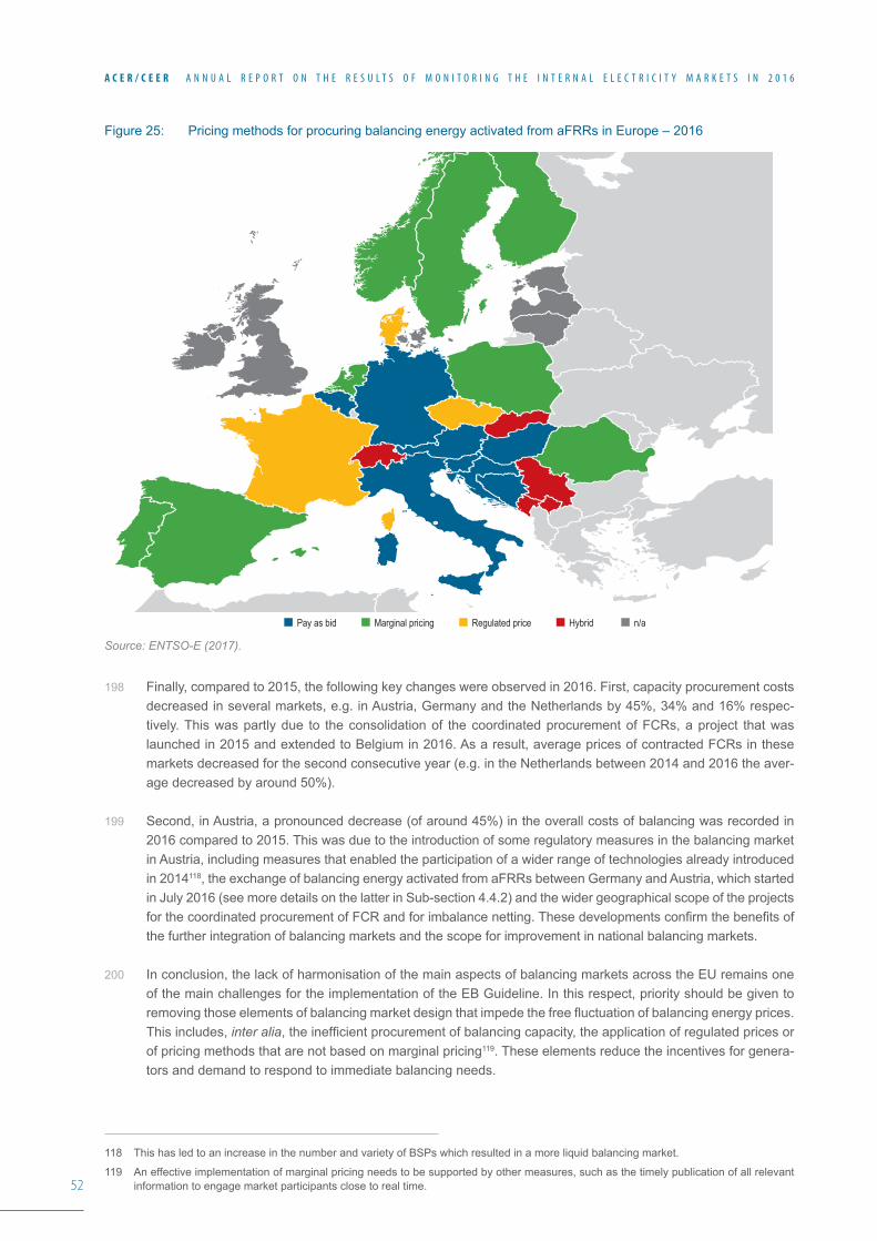
52


Figure 25: Pricing methods for procuring balancing energy activated from aFRRs in Europe – 2016

Source: ENTSO-E (2017).

198 Finally, compared to 2015, the following key changes were observed in 2016. First, capacity procurement costs decreased in several markets, e.g. in Austria, Germany and the Netherlands by 45%, 34% and 16% respec-tively. This was partly due to the consolidation of the coordinated procurement of FCRs, a project that was launched in 2015 and extended to Belgium in 2016. As a result, average prices of contracted FCRs in these markets decreased for the second consecutive year (e.g. in the Netherlands between 2014 and 2016 the aver-age decreased by around 50%).

199 Second, in Austria, a pronounced decrease (of around 45%) in the overall costs of balancing was recorded in 2016 compared to 2015. This was due to the introduction of some regulatory measures in the balancing market in Austria, including measures that enabled the participation of a wider range of technologies already introduced in 2014118, the exchange of balancing energy activated from aFRRs between Germany and Austria, which started in July 2016 (see more details on the latter in Sub-section 4.4.2) and the wider geographical scope of the projects forthecoordinatedprocurementofFCRandforimbalancenetting.Thesedevelopmentsconfirmthebenefitsofthe further integration of balancing markets and the scope for improvement in national balancing markets.

200 In conclusion, the lack of harmonisation of the main aspects of balancing markets across the EU remains one of the main challenges for the implementation of the EB Guideline. In this respect, priority should be given to removingthoseelementsofbalancingmarketdesignthatimpedethefreefluctuationofbalancingenergyprices.This includes, inter alia,theinefficientprocurementofbalancingcapacity,theapplicationofregulatedpricesorof pricing methods that are not based on marginal pricing119. These elements reduce the incentives for genera-tors and demand to respond to immediate balancing needs.

118 This has led to an increase in the number and variety of BSPs which resulted in a more liquid balancing market.

119 An effective implementation of marginal pricing needs to be supported by other measures, such as the timely publication of all relevant information to engage market participants close to real time.

Pay as bid Marginal pricing Regulated price Hybrid n/a

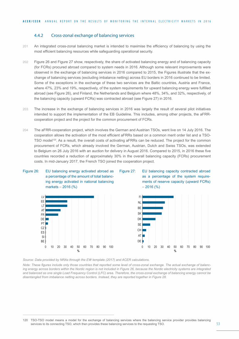
53


4.4.2 Cross-zonal exchange of balancing services

201 Anintegratedcross-zonalbalancingmarket is intendedtomaximisetheefficiencyofbalancingbyusingthemostefficientbalancingresourceswhilesafeguardingoperationalsecurity.

202 Figure 26 and Figure 27 show, respectively, the share of activated balancing energy and of balancing capacity (for FCRs) procured abroad compared to system needs in 2016. Although some relevant improvements were observed in the exchange of balancing services in 2016 compared to 2015, the Figures illustrate that the ex-change of balancing services (excluding imbalance netting) across EU borders in 2016 continued to be limited. Some of the exceptions in the exchange of these two services are the Baltic countries, Austria and France, where47%,23%and19%,respectively,ofthesystemrequirementsforupwardbalancingenergywerefulfilledabroad (see Figure 26), and Finland, the Netherlands and Belgium where 48%, 34%, and 32%, respectively, of the balancing capacity (upward FCRs) was contracted abroad (see Figure 27) in 2016.

203 The increase in the exchange of balancing services in 2016 was largely the result of several pilot initiatives intended to support the implementation of the EB Guideline. This includes, among other projects, the aFRR-cooperation project and the project for the common procurement of FCRs.

204 The aFRR-cooperation project, which involves the German and Austrian TSOs, went live on 14 July 2016. The cooperationallowstheactivationofthemostefficientaFRRsbasedonacommonmeritorderlistandaTSO-TSO model120. As a result, the overall costs of activating aFRRs can be reduced. The project for the common procurement of FCRs, which already involved the German, Austrian, Dutch and Swiss TSOs, was extended toBelgiumon26July2016withanauctionfordeliveryinAugust2016.Comparedto2015,in2016thesefivecountries recorded a reduction of approximately 30% in the overall balancing capacity (FCRs) procurement costs. In mid-January 2017, the French TSO joined the cooperation project.

Figure 26: EU balancing energy activated abroad as a percentage of the amount of total balanc-ing energy activated in national balancing markets – 2016 (%)

Figure 27: EU balancing capacity contracted abroad as a percentage of the system require-ments of reserve capacity (upward FCRs) – 2016 (%)

Source: Data provided by NRAs through the EW template (2017) and ACER calculations.Note: These figures include only those countries that reported some level of cross-zonal exchange. The actual exchange of balanc-ing energy across borders within the Nordic region is not included in Figure 26, because the Nordic electricity systems are integrated and balanced as one single Load Frequency Control (LFC) area. Therefore, the cross-zonal exchange of balancing energy cannot be disentangled from imbalance netting across borders. Instead, they are reported together in Figure 28.

120 TSO-TSO model means a model for the exchange of balancing services where the balancing service provider provides balancing services to its connecting TSO, which then provides these balancing services to the requesting TSO.

LVEELTATFRDEPTCZESSI

BE40

%100700 10 60 90805020 30 40

%100700 10 60 90805020 30

FINLBESKDKSECHATDE

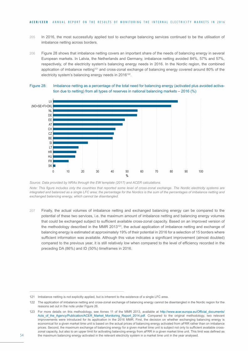
54


205 In 2016, the most successfully applied tool to exchange balancing services continued to be the utilisation of imbalance netting across borders.

206 Figure 28 shows that imbalance netting covers an important share of the needs of balancing energy in several European markets. In Latvia, the Netherlands and Germany, imbalance netting avoided 84%, 57% and 57%, respectively, of the electricity system’s balancing energy needs in 2016. In the Nordic region, the combined application of imbalance netting121 and cross-zonal exchange of balancing energy covered around 80% of the electricity system’s balancing energy needs in 2016122.

Figure 28: Imbalance netting as a percentage of the total need for balancing energy (activated plus avoided activa-tion due to netting) from all types of reserves in national balancing markets – 2016 (%)

Source: Data provided by NRAs through the EW template (2017) and ACER calculations.Note: This figure includes only the countries that reported some level of cross-zonal exchange. The Nordic electricity systems are integrated and balanced as a single LFC area; the percentage for the Nordics is the sum of the percentages of imbalance netting and exchanged balancing energy, which cannot be disentangled.

207 Finally, the actual volumes of imbalance netting and exchanged balancing energy can be compared to the potential of these two services, i.e. the maximum amount of imbalance netting and balancing energy volumes thatcouldbeexchangedsubjecttosufficientavailablecross-zonalcapacity.Basedonanimprovedversionofthe methodology described in the MMR 2013123, the actual application of imbalance netting and exchange of balancingenergyisestimatedatapproximately19%oftheirpotentialin2016foraselectionof15borderswheresufficientinformationwasavailable.Althoughthisvalueindicatesasignificantimprovement(almostdoubled)comparedtothepreviousyear,itisstillrelativelylowwhencomparedtothelevelofefficiencyrecordedinthepreceding DA (86%) and ID (50%) timeframes in 2016.

121 Imbalance netting is not explicitly applied, but is inherent to the existence of a single LFC area.

122 The application of imbalance netting and cross-zonal exchange of balancing energy cannot be disentangled in the Nordic region for the reasons set out in the note under Figure 26.

123 For more details on this methodology, see Annex 11 of the MMR 2013, available at http://www.acer.europa.eu/Official_documents/Acts_of_the_Agency/Publication/ACER_Market_Monitoring_Report_2014.pdf. Compared to the original methodology, two relevant improvements were introduced for its application in the 2016 MMR. First, the decision on whether exchanging balancing energy is economical for a given market time unit is based on the actual prices of balancing energy activated from aFRR rather than on imbalance prices.Second,themaximumexchangeofbalancingenergyforagivenmarkettimeunitissubjectnotonlytosufficientavailablecross-zonalcapacity,butalsotoanupperlimitforactivatingbalancingenergyfromaFRRinagivenmarkettimeunit.Thislimitwasdefinedasthe maximum balancing energy activated in the relevant electricity system in a market time unit in the year analysed.

LV(NO+SE+FI+DK)

NLDEEEATCHCZBESILT

HRHUFRSK

40%

100700 10 60 90805020 30

55


5 Capacity mechanisms and generation adequacy208 ThisChapterfirstpresentsanupdateonthesituationofCMsinEurope(Section5.1)and,second,areport

on how the contribution of interconnectors is taken into account in national generation adequacy assessments (Section 5.2).

5.1 Situation in capacity mechanisms

209 Figure29presentstheupdatedsituationofthedifferenttypesofCMs124 and their stage of implementation in Eu-rope by the end of 2016125.Theupdateincludessomekeychangescomparedtolastyear.First,thefigureshowsthat Latvia has had a scheme since 2005 which resembles the German planned network reserves mechanism126 and could be considered as a CM. Second, in Greece, capacity payments considered as a transitional measure for the period from May 2016 to April 2017 were approved by the European Commission. Third, in Germany, the plan to implement a capacity reserves mechanism has been postponed until the end of 2018 (envisaged start of thefirstcontractingperiod).However,theformalapprovalofthismechanismisstillpending.Fourth,inPolanditwasdecidedthattheoperationofstrategicreserveswouldbeextendeduntiltheendof2019.Polandcurrentlyconsiders to implement a market-wide capacity mechanism similar to the British capacity market. Fifth, in Spain, one of the existing types of capacity payments no longer applies to new capacity (as of 1 January 2016). Finally, inFrance,thefirstauctionofcapacityguarantees,fordeliveryin2017,tookplaceon15December2016,whileinGreatBritainthefirstdeliveryofcapacityacquiredintheCMisexpectedon1October2017127.

124 AvarietyofCMshavebeenproposed.Theycanbeclassifiedaccordingtowhethertheyarevolume-basedorprice-based.Volume-basedCMs can be further grouped in targeted and market-wide categories. For the taxonomy of the main CMs, see http://europa.eu/rapid/press-release_MEMO-15-4892_en.htm.

125 The update is based on information provided by NRAs and the European Commission’s report (DG Competition) of the sector inquiry intocapacitymechanismspublishedinNovember2016.Thereportdrawsconclusionsastowhencapacitymechanismsarejustifiedinterventions in themarketandsetsoutwhich typesof capacitymechanismsareappropriate inwhichsituation.Thefinal report isavailable at http://ec.europa.eu/competition/sectors/energy/capacity_mechanisms_final_report_en.pdf.

126 Based on the most recent information received from the Latvian NRA.

127 The production of the Electricity Wholesale Markets Volume was completed before this date.

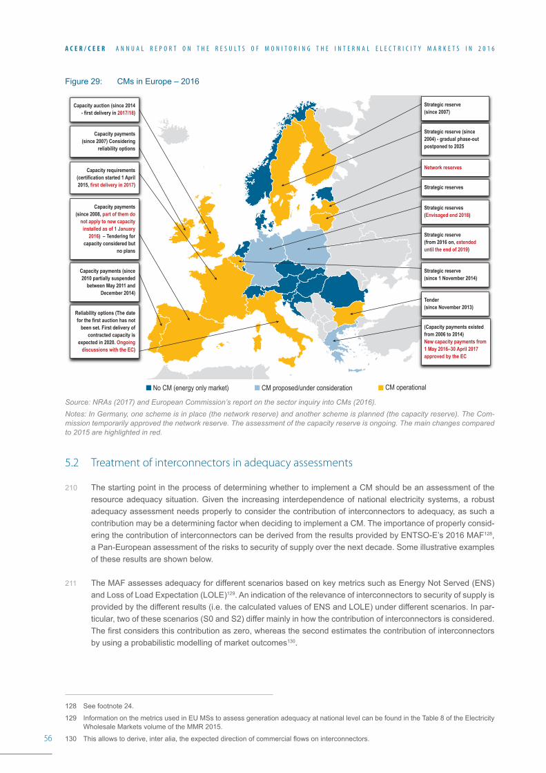
56


Figure29: CMsinEurope–2016

Source: NRAs (2017) and European Commission’s report on the sector inquiry into CMs (2016). Notes: In Germany, one scheme is in place (the network reserve) and another scheme is planned (the capacity reserve). The Com-mission temporarily approved the network reserve. The assessment of the capacity reserve is ongoing. The main changes compared to 2015 are highlighted in red.

5.2 Treatment of interconnectors in adequacy assessments

210 The starting point in the process of determining whether to implement a CM should be an assessment of the resource adequacy situation. Given the increasing interdependence of national electricity systems, a robust adequacy assessment needs properly to consider the contribution of interconnectors to adequacy, as such a contribution may be a determining factor when deciding to implement a CM. The importance of properly consid-ering the contribution of interconnectors can be derived from the results provided by ENTSO-E’s 2016 MAF128, a Pan-European assessment of the risks to security of supply over the next decade. Some illustrative examples of these results are shown below.

211 The MAF assesses adequacy for different scenarios based on key metrics such as Energy Not Served (ENS) and Loss of Load Expectation (LOLE)129. An indication of the relevance of interconnectors to security of supply is provided by the different results (i.e. the calculated values of ENS and LOLE) under different scenarios. In par-ticular, two of these scenarios (S0 and S2) differ mainly in how the contribution of interconnectors is considered. Thefirstconsidersthiscontributionaszero,whereasthesecondestimatesthecontributionofinterconnectorsby using a probabilistic modelling of market outcomes130.


129 Information on the metrics used in EU MSs to assess generation adequacy at national level can be found in the Table 8 of the Electricity Wholesale Markets volume of the MMR 2015.

130 Thisallowstoderive,interalia,theexpecteddirectionofcommercialflowsoninterconnectors.

CM proposed/under consideration CM operationalNo CM (energy only market)

Strategic reserve (since 2007)

Strategic reserve (since 2004) - gradual phase-out postponed to 2025

Strategic reserve (from 2016 on, extended until the end of 2019)

(Capacity payments existed from 2006 to 2014)New capacity payments from 1 May 2016–30 April 2017 approved by the EC

Strategic reserves (Envisaged end 2018)

Strategic reserves

Network reserves

Tender (since November 2013)

Reliability options (The date for the first auction has not

been set. First delivery of contracted capacity is

expected in 2020. Ongoing discussions with the EC)

Strategic reserve (since 1 November 2014)

Capacity auction (since 2014 - first delivery in 2017/18)

Capacity payments (since 2010 partially suspended

between May 2011 and December 2014)

Capacity payments (since 2008, part of them do

not apply to new capacity installed as of 1 January

2016) – Tendering for capacity considered but

no plans

Capacity payments (since 2007) Considering

reliability options

Capacity requirements (certification started 1 April 2015, first delivery in 2017)

57


212 By comparing the security of supply levels in these two scenarios, it can be derived that the outcome of the ad-equacy assessments (i.e. the values obtained for ENS and LOLE) are highly sensitive to the approach followed in considering the contribution of interconnectors to adequacy. This is the case even in countries where the ratio of cross-zonal capacity to national demand is relatively low. For example, in Italy, Germany, Bulgaria, and Greece, the LOLE assessed without interconnector capacity (scenario S0) would be 588, 3, 15, and 11 hours/year, respectively, for the year 2020. All these values (except in Germany) are above the most frequently used reliability standards (LOLE between 3 and 8)131, which would lead to the conclusion that these countries might132 face a security of supply issue in 2020.

213 By contrast, when the contribution of interconnectors is considered (scenario S2), the LOLE is assessed to be 0.2, 0, 0.1 and 0 hours/year, respectively, for the same year. These results, together with the fact that most na-tional adequacy assessments ignore or at best underestimate the contribution of interconnectors133,confirmthekey importance of correctly estimating the contribution of interconnectors to adequacy.

214 In this regard, several countries have started or intend to use probabilistic techniques similar to the ones used in the MAF in their national adequacy assessments. However, the underlying assumptions used in these assess-ments are often more conservative. The current situation of national adequacy assessments with respect to the treatment of interconnectors is provided below.

215 Table 4 shows that in ten countries the contribution of interconnectors is not considered, or is assessed to be non-existent134 in the scenario used to take a decision on whether to implement a CM. In these countries, the conceptofsecurityofsupplyistreatedasnational‘self-sufficiency’.SuchanapproachmightbeduetoMSsdistrusting that interconnectors will be available at times of scarcity. For example, curtailments in cross-border electricityflowsorexplicitexportbanswereimposedinafewEUMemberStates(e.g.inGreeceandinBulgaria)during the January cold spell with the aim of ‘protecting domestic consumers’. This lack of cross-border coop-erationisinconflictwiththelegalprovisionsaimingtoavoiddiscriminationbetweeninternalandcross-borderflows.

216 It is worth highlighting that out of these ten countries, three (Bulgaria, Spain and Sweden) have already imple-mented a CM, one (Germany) has already taken the decision to introduce a CM, while in the other six (Austria, the Czech Republic, Estonia, Norway, Romania and Slovakia) the national generation capacity is considered to provide ‘adequate’ security of supply levels. The latter can be considered as a de-facto situation of overcapacity.

217 In15othercountriesthecontributionof interconnectorstoadequacyisquantified.However,consideringthecontributionofinterconnectorsisnotsufficienttoremovetheriskofovercapacity.Arobustmethodologyshouldincludeprobabilisticmodellingtechniquesandavoidinsufficientlygroundedconservativeassumptions135. Based on this, Table 4 suggests that, even in countries that consider the contribution of interconnectors to adequacy, thereisasignificantroomforimprovementinthemethodologiesusedtoquantifythiscontribution,asfurtherdetailed below.

131 Seefootnote129.

132 With a probability above the desired levels of security of supply.

133 As further elaborated below.

134 I.e. the contribution of interconnectors is considered, but is assessed to be equal to zero MW of capacity. This is the case in Spain, for instance.

135 Examples of such assumptions are provided below.

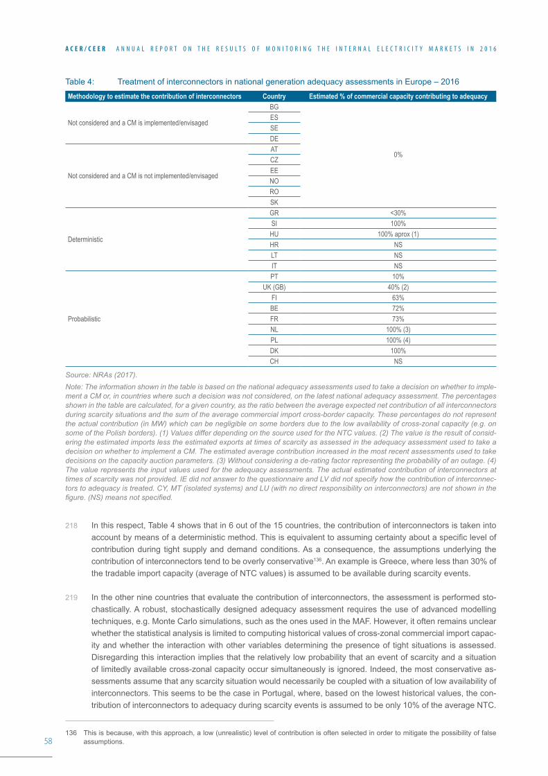
58


Table 4: Treatment of interconnectors in national generation adequacy assessments in Europe – 2016

Methodology to estimate the contribution of interconnectors Country Estimated % of commercial capacity contributing to adequacy

Not considered and a CM is implemented/envisaged

BG

0%

ESSEDE

Not considered and a CM is not implemented/envisaged

ATCZEENOROSK

Deterministic

GR <30%SI 100%HU 100% aprox (1)HR NSLT NSIT NS

Probabilistic

PT 10%UK (GB) 40% (2)

FI 63%BE 72%FR 73%NL 100% (3)PL 100% (4)DK 100%CH NS

Source: NRAs (2017).Note: The information shown in the table is based on the national adequacy assessments used to take a decision on whether to imple-ment a CM or, in countries where such a decision was not considered, on the latest national adequacy assessment. The percentages shown in the table are calculated, for a given country, as the ratio between the average expected net contribution of all interconnectors during scarcity situations and the sum of the average commercial import cross-border capacity. These percentages do not represent the actual contribution (in MW) which can be negligible on some borders due to the low availability of cross-zonal capacity (e.g. on some of the Polish borders). (1) Values differ depending on the source used for the NTC values. (2) The value is the result of consid-ering the estimated imports less the estimated exports at times of scarcity as assessed in the adequacy assessment used to take a decision on whether to implement a CM. The estimated average contribution increased in the most recent assessments used to take decisions on the capacity auction parameters. (3) Without considering a de-rating factor representing the probability of an outage. (4) The value represents the input values used for the adequacy assessments. The actual estimated contribution of interconnectors at times of scarcity was not provided. IE did not answer to the questionnaire and LV did not specify how the contribution of interconnec-tors to adequacy is treated. CY, MT (isolated systems) and LU (with no direct responsibility on interconnectors) are not shown in the figure. (NS) means not specified.

218 In this respect, Table 4 shows that in 6 out of the 15 countries, the contribution of interconnectors is taken into accountbymeansofadeterministicmethod.Thisisequivalenttoassumingcertaintyaboutaspecificlevelofcontribution during tight supply and demand conditions. As a consequence, the assumptions underlying the contribution of interconnectors tend to be overly conservative136. An example is Greece, where less than 30% of the tradable import capacity (average of NTC values) is assumed to be available during scarcity events.

219 In the other nine countries that evaluate the contribution of interconnectors, the assessment is performed sto-chastically. A robust, stochastically designed adequacy assessment requires the use of advanced modelling techniques, e.g. Monte Carlo simulations, such as the ones used in the MAF. However, it often remains unclear whether the statistical analysis is limited to computing historical values of cross-zonal commercial import capac-ity and whether the interaction with other variables determining the presence of tight situations is assessed. Disregarding this interaction implies that the relatively low probability that an event of scarcity and a situation of limitedly available cross-zonal capacity occur simultaneously is ignored. Indeed, the most conservative as-sessments assume that any scarcity situation would necessarily be coupled with a situation of low availability of interconnectors. This seems to be the case in Portugal, where, based on the lowest historical values, the con-tribution of interconnectors to adequacy during scarcity events is assumed to be only 10% of the average NTC.

136 This is because, with this approach, a low (unrealistic) level of contribution is often selected in order to mitigate the possibility of false assumptions.

59


220 Even in countries that perform relatively advanced adequacy assessments, some assumptions on the contribu-tion of interconnectors appear to be excessively prudent. For example, in Great Britain, one of the assumptions included in the adequacy assessment used to determine whether to implement a CM considered that full exports over the interconnectors to Ireland could be expected at times of stress in Great Britain137. Although an available analysis had preliminarily suggested that imports from Ireland to Great Britain at times of stress would be pos-sible138, the revised (more conservative than the initial) assumption was considered as ‘reasonable’.

221 By contrast, during six of the eight highest price spike events139 observed in Great Britain in 2016 (in fact, among the highest price spikes recorded in Europe in recent years), the interconnector capacity was used (on average more than 0.2 GW) in the direction from Ireland to Great Britain140. In the other two occasions, the interconnector was unavailable and, consequently, no exports to Ireland during these events were observed. This suggests that assuming with certainty full exports to Ireland at times of stress in Great Britain is – to say the least – an overly conservative assumption. In quantitative terms, the revised hypothesis was equivalent to increasing the needs for adequacy in Great Britain by around 1 GW141.

222 It should be emphasised that, since the introduction of the CM in Great Britain, there has been a focus on im-provingthemethodologiesandmodellingontheexpectedinterconnectorflowswhichhasledtoasignificantincrease in the expected contribution of imports to security of supply at times of stress. While the “net contribu-tion” assumed in the adequacy assessment used to determine whether to implement a CM considered an aver-age 40% contribution from all interconnectors (see Table 4), the estimated contribution increased to an average higher than 60% in the most recent evaluations of capacity auction parameters142. The experience in Great Britain underlines the importance of having a robust methodology and strong base on which to take decisions, asevidenceshowsthattheseassumptionscanhaveasignificanteffectontheadequacymetrics(suchLOLEand ENS)143 in European markets.

223 Another conclusion that can be derived from Table 4 is that the estimates of the contribution of interconnectors to adequacy are at best based on average historical values of available cross-zonal capacity (i.e. average NTC values). Given that these values are the outcome of conservative CC processes (see Sub-section 3.2.2 on the ratio between commercial and physical cross-zonal capacity), the estimates used for adequacy assessments may end up being disproportionately conservative.

224 Based on Table 4 and the additional details provided above, there are grounds to conclude that most national adequacy assessments ignore, or at best tend to underestimate, the ‘true’ contribution of interconnectors to se-curity of supply. This purely national approach is all the more surprising in the context of a move towards a more integrated IEM. This may lead to (or contribute to) a situation of overcapacity at the expense of end consumers.

225 Instead, a number of improvements in the process of estimating the contribution of interconnectors should be introduced. First, the methodology and assumptions used to assess the contribution of interconnectors should be more transparent. Second, estimates should be based on the expected availability of interconnectors during stress situations, not on annual or seasonal averages, as these may not be adequate proxies.

137 This assumption was based on “historical exports to Ireland”, and the fact that “market coupling with Ireland is yet to be implemented”. For more information, see para 1.11, available at https://www.gov.uk/government/uploads/system/uploads/attachment_data/file/354677/CM_-_revised_IA_and_front_page__September_2014__pdf_-_Adobe_Acrobat.pdf.

138 For instance, this study shows that for the ‘baseline scenario’, the Irish-British interconnector would be used on average in the direction from Ireland to Great Britain in times of stress, with a utilisation rate ranging between 0% and 53%, depending on the level of tightness assumed in Ireland.

139 15September2016-hour21 (1174.92euros/MWh),19September2016-hour21 (1127.04euros/MWh),15September2016-hour22(939.7euros/MWh),7November2016-hour19(894.7euros/MWh),19September2016-hour20(880.5euros/MWh),19September2016-hour22(876.98euros/MWh),8November2016-hour19(870.2euros/MWh)and14November2016-hour19(810.6euros/MWh).

140 Analysis based on DA prices and DA nominations.

141 The assumptions imply that the British generation capacity should serve not only domestic consumption, but also provide an additional 0.75 GW for exports to Ireland in times of stress. This is in addition to a certain amount of possible imports from Ireland that are ‘ignored’ (see footnote 138).

142 For example, see the decision on the capacity auction parameters for the auctions planned in January and February 2018 available at https://www.gov.uk/government/uploads/system/uploads/attachment_data/file/625657/170705_SoS_to_National_Grid.pdf.

143 E.g. see paragraphs 171 to 174.

60


226 Third,estimatesof thecontributionof interconnectorsfor thepurposeofassessingadequacyshouldbenefitfrom the most advanced CC methods, i.e. they should be FB, rather than NTC-based (at least in meshed net-works) and they should consider the Agency’s principles of non-discrimination to the maximum extent possible.

227 An illustration of the potential of adequately applied FB methods is provided by the fact that, in 2016, the amount of energy imported during a given hour to France and Belgium (i.e. their joint net position) from Germany and the Netherlands reached a maximum of 8,328 MW, which is about twice the equivalent value (i.e. the sum of the highest recorded import NTC values) observed before FBMC was implemented (4,501 MW in 2014). At the same time, both countries faced several moderate stress events in 2016, resulting in the highest price spreads observed within the Core (CWE) region in recent years.

228 However, during those events, net imports to Belgium and France were still less than half the above-mentioned 2016 maximum. As shown in Sub-section 3.2.1, the relatively low level of imports was largely the result of the limited amount of tradable cross-zonal capacity in the Core (CWE) region in the second half of 2016. The ap-plication of the high-level principles of the Agency’s Recommendation which are intended to avoid undue dis-criminationinCCwouldprobablyhaveallowedthemaximisationoftheCore(CWE)regionflowstothesetwocountries during those events, hence maximising welfare within the Core (CWE) region, while ensuring security of supply in Belgium and France at a lower cost.

229 Fourth, more operational coordination as envisaged in the CACM Regulation and the System Operation Guide-lineshouldbeputinplaceassoonaspossible.TheseGuidelineswillenabletheapplicationofthemostefficientCCtechniquesandthemostefficientremedialactionsinthecaseofasupplyshortage,basedonregionalratherthan country-level calculations.

230 Finally, the geographical scope of adequacy assessments should also be at least regional, i.e. wider than na-tional.Overall,thesuggestedimprovementswilldefinitelycontributetoachievingthedesiredlevelsofsecurityof supply at a lower cost for end consumers.

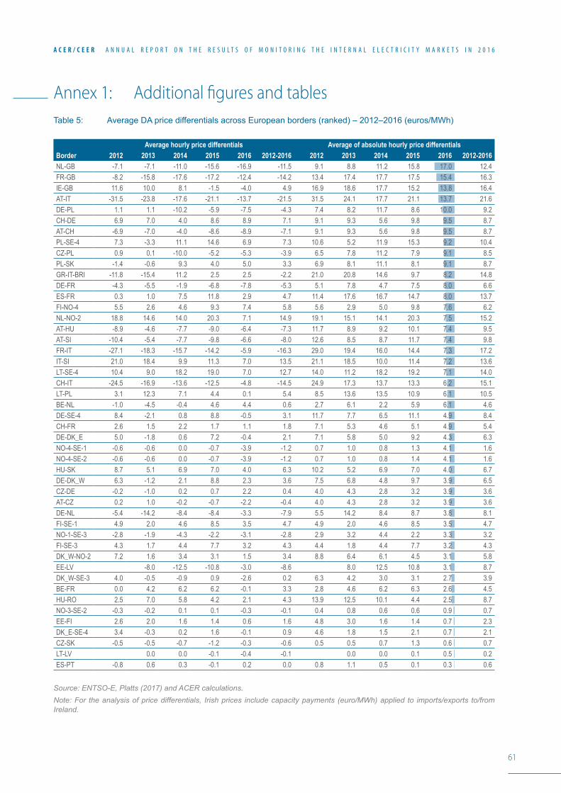
61


Annex 1: Additional figures and tablesTable 5: Average DA price differentials across European borders (ranked) – 2012–2016 (euros/MWh)

Average hourly price differentials Average of absolute hourly price differentialsBorder 2012 2013 2014 2015 2016 2012-2016 2012 2013 2014 2015 2016 2012-2016NL-GB -7.1 -7.1 -11.0 -15.6 -16.9 -11.5 9.1 8.8 11.2 15.8 17.0 12.4FR-GB -8.2 -15.8 -17.6 -17.2 -12.4 -14.2 13.4 17.4 17.7 17.5 15.4 16.3IE-GB 11.6 10.0 8.1 -1.5 -4.0 4.9 16.9 18.6 17.7 15.2 13.8 16.4AT-IT -31.5 -23.8 -17.6 -21.1 -13.7 -21.5 31.5 24.1 17.7 21.1 13.7 21.6DE-PL 1.1 1.1 -10.2 -5.9 -7.5 -4.3 7.4 8.2 11.7 8.6 10.0 9.2CH-DE 6.9 7.0 4.0 8.6 8.9 7.1 9.1 9.3 5.6 9.8 9.5 8.7AT-CH -6.9 -7.0 -4.0 -8.6 -8.9 -7.1 9.1 9.3 5.6 9.8 9.5 8.7PL-SE-4 7.3 -3.3 11.1 14.6 6.9 7.3 10.6 5.2 11.9 15.3 9.2 10.4CZ-PL 0.9 0.1 -10.0 -5.2 -5.3 -3.9 6.5 7.8 11.2 7.9 9.1 8.5PL-SK -1.4 -0.6 9.3 4.0 5.0 3.3 6.9 8.1 11.1 8.1 9.1 8.7GR-IT-BRI -11.8 -15.4 11.2 2.5 2.5 -2.2 21.0 20.8 14.6 9.7 8.2 14.8DE-FR -4.3 -5.5 -1.9 -6.8 -7.8 -5.3 5.1 7.8 4.7 7.5 8.0 6.6ES-FR 0.3 1.0 7.5 11.8 2.9 4.7 11.4 17.6 16.7 14.7 8.0 13.7FI-NO-4 5.5 2.6 4.6 9.3 7.4 5.8 5.6 2.9 5.0 9.8 7.6 6.2NL-NO-2 18.8 14.6 14.0 20.3 7.1 14.9 19.1 15.1 14.1 20.3 7.5 15.2AT-HU -8.9 -4.6 -7.7 -9.0 -6.4 -7.3 11.7 8.9 9.2 10.1 7.4 9.5AT-SI -10.4 -5.4 -7.7 -9.8 -6.6 -8.0 12.6 8.5 8.7 11.7 7.4 9.8FR-IT -27.1 -18.3 -15.7 -14.2 -5.9 -16.3 29.0 19.4 16.0 14.4 7.3 17.2IT-SI 21.0 18.4 9.9 11.3 7.0 13.5 21.1 18.5 10.0 11.4 7.2 13.6LT-SE-4 10.4 9.0 18.2 19.0 7.0 12.7 14.0 11.2 18.2 19.2 7.1 14.0CH-IT -24.5 -16.9 -13.6 -12.5 -4.8 -14.5 24.9 17.3 13.7 13.3 6.2 15.1LT-PL 3.1 12.3 7.1 4.4 0.1 5.4 8.5 13.6 13.5 10.9 6.1 10.5BE-NL -1.0 -4.5 -0.4 4.6 4.4 0.6 2.7 6.1 2.2 5.9 6.1 4.6DE-SE-4 8.4 -2.1 0.8 8.8 -0.5 3.1 11.7 7.7 6.5 11.1 4.9 8.4CH-FR 2.6 1.5 2.2 1.7 1.1 1.8 7.1 5.3 4.6 5.1 4.9 5.4DE-DK_E 5.0 -1.8 0.6 7.2 -0.4 2.1 7.1 5.8 5.0 9.2 4.3 6.3NO-4-SE-1 -0.6 -0.6 0.0 -0.7 -3.9 -1.2 0.7 1.0 0.8 1.3 4.1 1.6NO-4-SE-2 -0.6 -0.6 0.0 -0.7 -3.9 -1.2 0.7 1.0 0.8 1.4 4.1 1.6HU-SK 8.7 5.1 6.9 7.0 4.0 6.3 10.2 5.2 6.9 7.0 4.0 6.7DE-DK_W 6.3 -1.2 2.1 8.8 2.3 3.6 7.5 6.8 4.8 9.7 3.9 6.5CZ-DE -0.2 -1.0 0.2 0.7 2.2 0.4 4.0 4.3 2.8 3.2 3.9 3.6AT-CZ 0.2 1.0 -0.2 -0.7 -2.2 -0.4 4.0 4.3 2.8 3.2 3.9 3.6DE-NL -5.4 -14.2 -8.4 -8.4 -3.3 -7.9 5.5 14.2 8.4 8.7 3.8 8.1FI-SE-1 4.9 2.0 4.6 8.5 3.5 4.7 4.9 2.0 4.6 8.5 3.5 4.7NO-1-SE-3 -2.8 -1.9 -4.3 -2.2 -3.1 -2.8 2.9 3.2 4.4 2.2 3.3 3.2FI-SE-3 4.3 1.7 4.4 7.7 3.2 4.3 4.4 1.8 4.4 7.7 3.2 4.3DK_W-NO-2 7.2 1.6 3.4 3.1 1.5 3.4 8.8 6.4 6.1 4.5 3.1 5.8EE-LV -8.0 -12.5 -10.8 -3.0 -8.6 8.0 12.5 10.8 3.1 8.7DK_W-SE-3 4.0 -0.5 -0.9 0.9 -2.6 0.2 6.3 4.2 3.0 3.1 2.7 3.9BE-FR 0.0 4.2 6.2 6.2 -0.1 3.3 2.8 4.6 6.2 6.3 2.6 4.5HU-RO 2.5 7.0 5.8 4.2 2.1 4.3 13.9 12.5 10.1 4.4 2.5 8.7NO-3-SE-2 -0.3 -0.2 0.1 0.1 -0.3 -0.1 0.4 0.8 0.6 0.6 0.9 0.7EE-FI 2.6 2.0 1.6 1.4 0.6 1.6 4.8 3.0 1.6 1.4 0.7 2.3DK_E-SE-4 3.4 -0.3 0.2 1.6 -0.1 0.9 4.6 1.8 1.5 2.1 0.7 2.1CZ-SK -0.5 -0.5 -0.7 -1.2 -0.3 -0.6 0.5 0.5 0.7 1.3 0.6 0.7LT-LV 0.0 0.0 -0.1 -0.4 -0.1 0.0 0.0 0.1 0.5 0.2ES-PT -0.8 0.6 0.3 -0.1 0.2 0.0 0.8 1.1 0.5 0.1 0.3 0.6

Source: ENTSO-E, Platts (2017) and ACER calculations.Note: For the analysis of price differentials, Irish prices include capacity payments (euro/MWh) applied to imports/exports to/from Ireland.

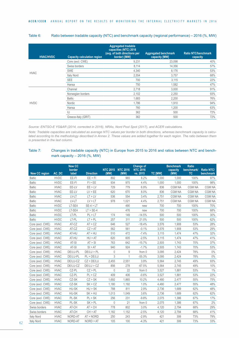
62


Table 6: Ratio between tradable capacity (NTC) and benchmark capacity (regional performance) – 2016 (%, MW)

HVAC/HVDC Capacity calculation region

Aggregated tradable capacities (NTC) 2016

(avg. of both directions per border) [MW]

Aggregated benchmark capacity [MW]

Ratio NTC/benchmark capacity

HVAC

Core (excl. CWE) 9,231 23,098 40%Swiss borders 8,114 14,356 57%SWE 4,340 8,176 53%Italy Nord 2,554 3,757 68%SEE 700 3,115 22%Hansa 750 1,582 47%

HVDC

Channel 2,718 3,000 91%Norwegian borders 2,102 2,250 93%Baltic 1,683 2,200 76%Nordic 1,786 1,910 94%Hansa 760 1,200 63%IU 362 500 72%Greece-Italy (GRIT) 362 500 72%

Source: ENTSO-E YS&AR (2014, corrected in 2016), NRAs, Nord Pool Spot (2017), and ACER calculations.Note: Tradable capacities are calculated as average NTC values per border in both directions, whereas benchmark capacity is calcu-lated according to the methodology described in Annex 2. These values are added together for each region. The ratio between them is presented in the last column.

Table 7: Changes in tradable capacity (NTC) in Europe from 2015 to 2016 and ratios between NTC and bench-mark capacity – 2016 (%, MW)

New CC region AC_DC

New CC border label Direction

NTC 2015 (MW)

NTC 2016 (MW)

Change of NTC 2016 vs. 2015 TC [MW]

Benchmark capacity

(MW)

Ratio benchmark/

TCRatio NTC/benchmark

Baltic HVDC EE-FI EE > FI 892 965 8.2% 1,000 1,000 100% 97%Baltic HVDC EE-FI FI > EE 934 975 4.4% 1,000 1,000 100% 98%Baltic HVAC EE-LV EE > LV 729 779 6.9% 836 CGM NA CGM NA CGM NABaltic HVAC EE-LV LV > EE 620 670 8.0% 836 CGM NA CGM NA CGM NABaltic HVAC LV-LT LT > LV 536 554 3.4% 2,751 CGM NA CGM NA CGM NABaltic HVAC LV-LT LV > LT 978 1,021 4.4% 2,751 CGM NA CGM NA CGM NABaltic HVDC LT-SE4 SE-4 > LT 490 new 700 700 100% 70%Baltic HVDC LT-SE4 LT > SE-4 476 new 700 700 100% 68%Baltic HVDC LT-PL PL > LT 174 149 -14.5% 500 500 100% 30%Baltic HVDC LT-PL LT > PL 257 311 21.0% 500 500 100% 62%Core (excl. CWE) HVAC AT-CZ AT > CZ 646 527 -18.4% 3,576 1,908 53% 28%Core (excl. CWE) HVAC AT-CZ CZ > AT 562 561 -0.1% 3,576 1,908 53% 29%Core (excl. CWE) HVAC AT-HU AT > HU 510 472 -7.4% 3,115 1,474 47% 32%Core (excl. CWE) HVAC AT-HU HU > AT 620 605 -2.5% 3,115 1,474 47% 41%Core (excl. CWE) HVAC AT-SI AT > SI 763 642 -15.7% 2,505 1,743 70% 37%Core (excl. CWE) HVAC AT-SI SI > AT 940 924 -1.7% 2,505 1,743 70% 53%Core (excl. CWE) HVAC DE/LU-PL DE/LU > PL 0 9 from 0 3,095 2,424 78% 0%Core (excl. CWE) HVAC DE/LU-PL PL > DE/LU 3 1 -55.3% 3,095 2,424 78% 0%Core (excl. CWE) HVAC DE/LU-CZ CZ > DE/LU 2,455 2,551 3.9% 5,564 2,745 49% 93%Core (excl. CWE) HVAC DE/LU-CZ DE/LU > CZ 856 278 -67.5% 5,564 2,745 49% 10%Core (excl. CWE) HVAC CZ-PL CZ > PL 0 22 from 0 3,527 1,881 53% 1%Core (excl. CWE) HVAC CZ-PL PL > CZ 409 406 -0.6% 3,527 1,881 53% 22%Core (excl. CWE) HVAC CZ-SK CZ > SK 1,692 1,865 10.2% 4,480 2,477 55% 75%Core (excl. CWE) HVAC CZ-SK SK > CZ 1,180 1,192 1.0% 4,480 2,477 55% 48%Core (excl. CWE) HVAC HU-SK HU > SK 788 811 2.9% 2,736 1,689 62% 48%Core (excl. CWE) HVAC HU-SK SK > HU 1,013 1,049 3.6% 2,736 1,689 62% 62%Core (excl. CWE) HVAC PL-SK PL > SK 256 231 -9.8% 2,075 1,386 67% 17%Core (excl. CWE) HVAC PL-SK SK > PL 0 21 from 0 2,075 1,386 67% 2%Swiss borders HVAC AT-CH AT > CH 778 802 3.0% 4,120 2,794 68% 29%Swiss borders HVAC AT-CH CH > AT 1,182 1,152 -2.5% 4,120 2,794 68% 41%Italy Nord HVAC NORD-AT AT > NORD 250 243 -2.9% 421 306 73% 79%Italy Nord HVAC NORD-AT NORD > AT 105 100 -4.3% 421 306 73% 33%

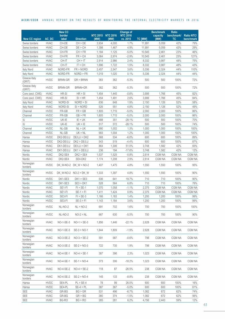
63


New CC region AC_DC


NTC 2015 (MW)

NTC 2016 (MW)


Benchmark capacity

(MW)

Ratio benchmark/


Swiss borders HVAC CH-DE CH > DE 3,934 4,000 1.7% 11,991 5,059 42% 79%Swiss borders HVAC CH-DE DE > CH 1,398 1,467 4.9% 11,991 5,059 42% 29%Swiss borders HVAC CH-FR CH > FR 1,184 1,125 -5.0% 10,545 2,461 23% 46%Swiss borders HVAC CH-FR FR > CH 3,064 2,974 -2.9% 10,545 2,461 23% 121%Swiss borders HVAC CH-IT CH > IT 2,914 2,986 2.4% 8,332 3,987 48% 75%Swiss borders HVAC CH-IT IT > CH 1,696 1,722 1.5% 8,332 3,987 48% 43%Italy Nord HVAC NORD-FR FR > NORD 2,457 2,547 3.6% 5,336 2,324 44% 110%Italy Nord HVAC NORD-FR NORD > FR 1,019 1,020 0.1% 5,336 2,324 44% 44%Greece-Italy (GRIT) HVDC BRNN-GR GR > BRNN 383 362 -5.3% 500 500 100% 72%

Greece-Italy (GRIT) HVDC BRNN-GR BRNN>GR 382 362 -5.3% 500 500 100% 72%

Core (excl. CWE) HVAC HR-SI HR > SI 1,454 1,445 -0.6% 3,906 1,766 45% 82%Core (excl. CWE) HVAC HR-SI SI > HR 1,454 1,491 2.6% 3,906 1,766 45% 84%Italy Nord HVAC NORD-SI NORD > SI 636 648 1.9% 2,150 1,126 52% 58%Italy Nord HVAC NORD-SI SI > NORD 526 551 4.8% 2,150 1,126 52% 49%Channel HVDC FR-GB FR > GB 1,805 1,715 -5.0% 2,000 2,000 100% 86%Channel HVDC FR-GB GB > FR 1,805 1,715 -5.0% 2,000 2,000 100% 86%IU HVDC UK-IE IE > UK 488 351 -28.1% 500 500 100% 70%IU HVDC UK-IE UK > IE 517 372 -28.1% 500 500 100% 74%Channel HVDC NL-GB NL > UK 990 1,002 1.3% 1,000 1,000 100% 100%Channel HVDC NL-GB UK > NL 993 1,004 1.2% 1,000 1,000 100% 100%Hansa HVDC DK2-DE/LU DE/LU > DK2 568 534 -6.0% 600 600 100% 89%Hansa HVDC DK2-DE/LU DK2 > DE/LU 543 519 -4.4% 600 600 100% 87%Hansa HVAC DK1-DE/LU DE/LU > DK1 864 1,306 51.0% 3,748 1,582 42% 83%Hansa HVAC DK1-DE/LU DK1 > DE/LU 236 194 -17.6% 3,748 1,582 42% 12%Nordic HVAC DK2-SE4 DK2 > SE4 1,537 1,525 -0.8% 2,614 CGM NA CGM NA CGM NANordic HVAC DK2-SE4 SE4-DK2 1,174 1,208 2.9% 2,614 CGM NA CGM NA CGM NANorwegian borders HVDC DK_W-NO-2 DK_W > NO-2 1,407 1,475 4.8% 1,550 1,550 100% 95%

Norwegian borders HVDC DK_W-NO-2 NO-2 > DK_W 1,333 1,397 4.8% 1,550 1,550 100% 90%

Nordic HVDC DK1-SE3 DK1 > SE3 536 641 19.7% 710 710 100% 90%Nordic HVDC DK1-SE3 SE3 > DK1 528 564 6.8% 710 710 100% 79%Nordic HVAC SE1-FI FI > SE-1 1,070 1,058 -1.1% 2,375 CGM NA CGM NA CGM NANordic HVAC SE1-FI SE-1 > FI 1,411 1,424 0.9% 2,375 CGM NA CGM NA CGM NANordic HVDC SE3-FI FI > SE-3 1,166 1,183 1.4% 1,200 1,200 100% 99%Nordic HVDC SE3-FI SE-3 > FI 1,143 1,184 3.6% 1,200 1,200 100% 99%Norwegian borders HVDC NL-NO-2 NL > NO-2 691 702 1.6% 700 700 100% 100%

Norwegian borders HVDC NL-NO-2 NO-2 > NL 667 630 -5.5% 700 700 100% 90%

Norwegian borders HVAC NO-1-SE-3 NO-1 > SE-3 1,856 1,446 -22.1% 2,628 CGM NA CGM NA CGM NA

Norwegian borders HVAC NO-1-SE-3 SE-3 > NO-1 1,844 1,809 -1.9% 2,628 CGM NA CGM NA CGM NA

Norwegian borders HVAC NO-3-SE-2 NO-3 > SE-2 591 587 -0.6% 798 CGM NA CGM NA CGM NA

Norwegian borders HVAC NO-3-SE-2 SE-2 > NO-3 722 735 1.9% 798 CGM NA CGM NA CGM NA

Norwegian borders HVAC NO-4-SE-1 NO-4 > SE-1 387 396 2.3% 1,023 CGM NA CGM NA CGM NA

Norwegian borders HVAC NO-4-SE-1 SE-1 > NO-4 373 306 -18.2% 1,023 CGM NA CGM NA CGM NA

Norwegian borders HVAC NO-4-SE-2 NO-4 > SE-2 118 87 -26.5% 238 CGM NA CGM NA CGM NA

Norwegian borders HVAC NO-4-SE-2 SE-2 > NO-4 145 133 -8.8% 238 CGM NA CGM NA CGM NA

Hansa HVDC SE4-PL PL > SE-4 78 99 26.0% 600 600 100% 16%Hansa HVDC SE4-PL SE-4 > PL 387 367 -5.0% 600 600 100% 61%SEE HVAC GR-BG BG > GR 531 496 -6.7% 1,082 672 62% 74%SEE HVAC GR-BG GR > BG 380 374 -1.5% 1,082 672 62% 56%SEE HVAC BG-RO BG > RO 265 281 6.2% 4,156 2,443 59% 12%

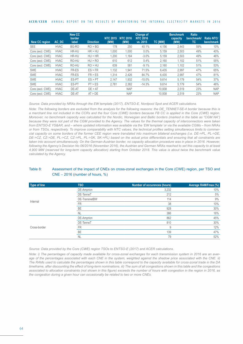
64


New CC region AC_DC


NTC 2015 (MW)

NTC 2016 (MW)


Benchmark capacity

(MW)

Ratio benchmark/


SEE HVAC BG-RO RO > BG 178 250 40.1% 4,156 2,443 59% 10%Core (excl. CWE) HVAC HR-HU HR > HU 1,000 1,000 0.0% 5,159 2,503 49% 40%Core (excl. CWE) HVAC HR-HU HU > HR 1,200 1,164 -3.0% 5,159 2,503 49% 46%Core (excl. CWE) HVAC RO-HU HU > RO 610 612 0.4% 2,160 1,102 51% 55%Core (excl. CWE) HVAC RO-HU RO > HU 639 581 -9.1% 2,160 1,102 51% 53%SWE HVAC FR-ES ES > FR 1,132 1,941 71.5% 6,435 2,997 47% 65%SWE HVAC FR-ES FR > ES 1,314 2,426 84.7% 6,435 2,997 47% 81%SWE HVAC ES-PT ES > PT 2,147 1,932 -10.0% 9,614 5,179 54% 37%SWE HVAC ES-PT PT > ES 2,781 2,382 -14.3% 9,614 5,179 54% 46%Core (excl. CWE) HVAC DE-AT DE > AT NAP 10,938 2,519 23% NAPCore (excl. CWE) HVAC DE-AT AT > DE NAP 10,938 2,519 23% NAP

Source: Data provided by NRAs through the EW template (2017), ENTSO-E, Nordpool Spot and ACER calculations.Note: The following borders are excluded from the analysis for the following reasons: the DE_TENNET-SE-4 border because this is a merchant line not included in the CCRs and the four Core (CWE) borders because FB CC is applied in the Core (CWE) region. Moreover, no benchmark capacity was calculated for the Nordic, Norwegian and Baltic borders (marked in the table as “CGM NA”) because they were not part of the CGM provided to the Agency. The values for the thermal capacity of interconnectors were taken from ENTSO-E YS&AR, and – where updated information was available via the ‘EW template’ or via the available CGMs – from NRAs or from TSOs, respectively. To improve comparability with NTC values, the technical profiles setting simultaneous limits to commer-cial capacity on some borders of the former CEE region were translated into maximum bilateral exchanges (i.e. DE->PL, PL->DE, DE->CZ, CZ->DE, PL->CZ, CZ->PL, PL->SK, SK->PL) based on the actual price differentials and ensuring that all constraints are taken into account simultaneously. On the German-Austrian border, no capacity allocation procedure was in place in 2016. However, following the Agency’s Decision No 06/2016 (November 2016), the Austrian and German NRAs reached to set this capacity to at least 4,900 MW (reserved for long-term capacity allocation) starting from October 2018. This value is about twice the benchmark value calculated by the Agency.

Table 8: Assessment of the impact of CNEs on cross-zonal exchanges in the Core (CWE) region, per TSO and CNE – 2016 (number of hours, %)

Type of line TSO Number of occurences (hours) Average RAM/Fmax (%)

Internal

DE-Amprion 3,232 10%DE-TenneT 212 5%DE-TransnetBW 114 9%FR 38 10%BE 928 30%NL 386 16%

Cross-border

DE-Amprion 862 45%DE-TenneT 810 30%FR 9 12%BE 139 47%NL 79 52%

Source: Data provided by the Core (CWE) region TSOs to ENTSO-E (2017) and ACER calculations.Note: i) The percentages of capacity made available for cross-zonal exchanges for each transmission system in 2016 are an aver-age of the percentages associated with each CNE in the system, weighted against the shadow price associated with the CNE. ii) The RAMs used to calculate the percentages shown in this table correspond to the capacity available for cross-zonal trade in the DA timeframe, after discounting the effect of long-term nominations. iii) The sum of all congestions shown in this table and the congestions associated to allocation constraints (not shown in this figure) exceeds the number of hours with congestion in the region in 2016, as the congestion during a given hour can occasionally be related to two or more CNEs.

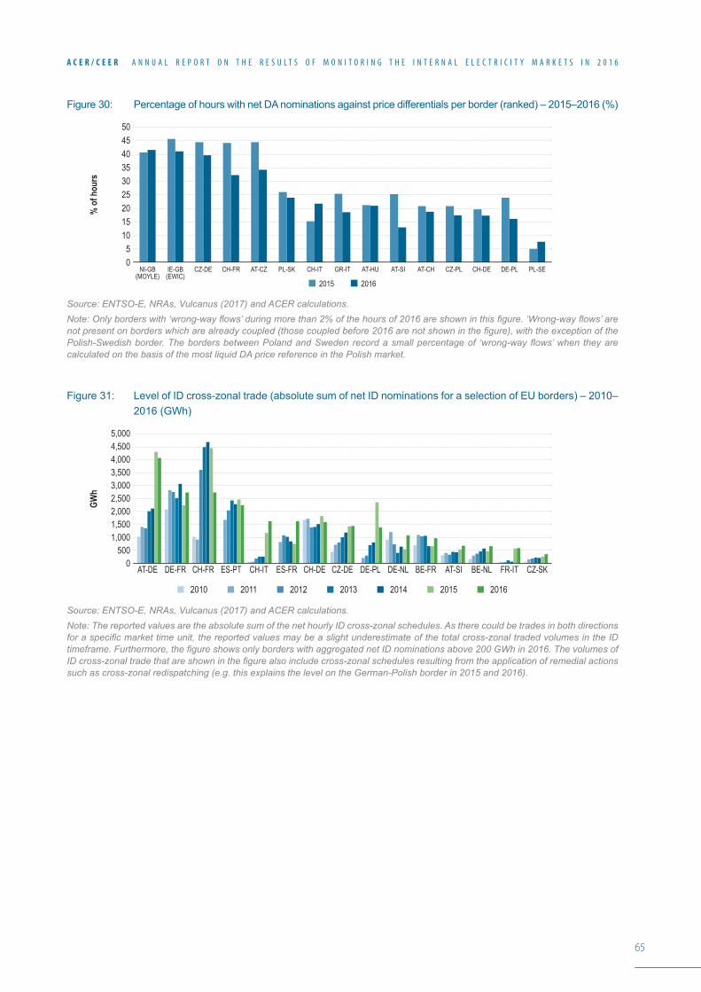
65


Figure 30: Percentage of hours with net DA nominations against price differentials per border (ranked) – 2015–2016 (%)

Source: ENTSO-E, NRAs, Vulcanus (2017) and ACER calculations.Note: Only borders with ‘wrong-way flows’ during more than 2% of the hours of 2016 are shown in this figure. ‘Wrong-way flows’ are not present on borders which are already coupled (those coupled before 2016 are not shown in the figure), with the exception of the Polish-Swedish border. The borders between Poland and Sweden record a small percentage of ‘wrong-way flows’ when they are calculated on the basis of the most liquid DA price reference in the Polish market.

Figure 31: Level of ID cross-zonal trade (absolute sum of net ID nominations for a selection of EU borders) – 2010–2016 (GWh)

Source: ENTSO-E, NRAs, Vulcanus (2017) and ACER calculations.Note: The reported values are the absolute sum of the net hourly ID cross-zonal schedules. As there could be trades in both directions for a specific market time unit, the reported values may be a slight underestimate of the total cross-zonal traded volumes in the ID timeframe. Furthermore, the figure shows only borders with aggregated net ID nominations above 200 GWh in 2016. The volumes of ID cross-zonal trade that are shown in the figure also include cross-zonal schedules resulting from the application of remedial actions such as cross-zonal redispatching (e.g. this explains the level on the German-Polish border in 2015 and 2016).

% o

f hou

rs

50

354045

20

3025

1510

50

IE-GB(EWIC)

2015 2016

NI-GB(MOYLE)

CH-FR PL-SK CH-IT GR-ITCZ-DE CH-DE DE-PL PL-SEAT-CZ CZ-PLAT-CHAT-HU AT-SI

GWh

AT-DE AT-SIDE-FR CH-FR ES-PT CH-IT FR-ITES-FR BE-FRCH-DE CZ-DE CZ-SKDE-PL DE-NL BE-NL

5,000

4,0004,500

3,500

2,500

1,500

500

2,000

3,000

1,000

0

20112010 2012 2013 2014 2015 2016

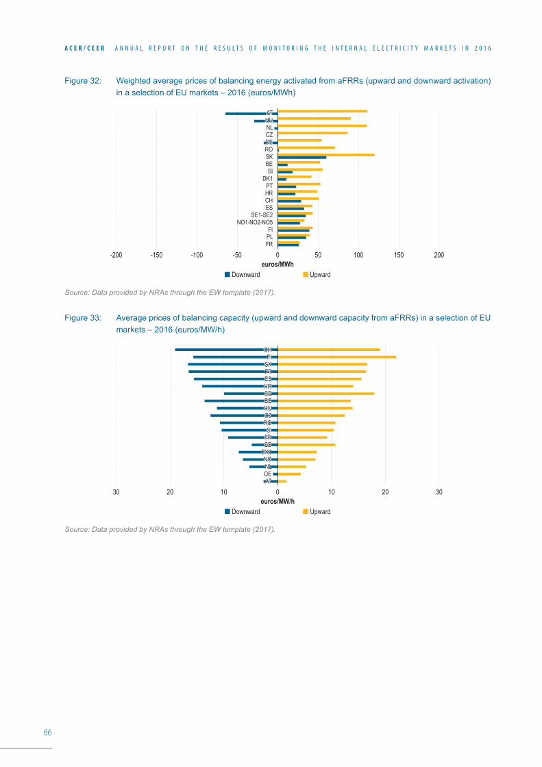
66


Figure 32: Weighted average prices of balancing energy activated from aFRRs (upward and downward activation) in a selection of EU markets – 2016 (euros/MWh)

Source: Data provided by NRAs through the EW template (2017).

Figure 33: Average prices of balancing capacity (upward and downward capacity from aFRRs) in a selection of EU markets – 2016 (euros/MW/h)

Source: Data provided by NRAs through the EW template (2017).

0euros/MWh

200150-200 -150 10050-100 -50

Downward Upward

ATHUNLCZDEROSKBESI

DK1PTHRCHES

SE1-SE2NO1-NO2-NO5

FIPLFR

ATHUNLCZDEROSKBESI

DK1PTHRCHES

SE1-SE2NO1-NO2-NO5

FIPLFR

0euros/MW/h

302030 1020 10

Downward Upward

CHFI

SKPTESHRSEBEHUCZROSI

FRGB

DK1NONLDEAT

CHFI

SKPTESHRSEBEHUCZROSI

FRGB

DK1NONLDEAT

67


Annex 2: Methodology for calculating the benchmark capacity for CNTC and FB CC methods

The Agency intends to monitor the gap between the level of cross-zonal capacity that is currently made available to the market and the capacity (hereinafter benchmark capacity) that could be made available if the recent Agency’s Recom-mendation on Capacity Calculation Methodologies144 is followed with no (or very limited) deviations. This annex de-scribes the assumptions and process applied to calculate the benchmark capacity both for CNTC and FB CC methods. It is therefore assumed that the CC methodologies envisaged in the CACM Regulation are applied.

The Agency’s Recommendation assumes that the delimitation of bidding zones addresses all structural physical con-gestion and that the remaining congestion within bidding zones is addressed via remedial actions. Hence, the bench-mark capacity can be calculated assuming that i) cross-zonal capacity is only limited by cross-zonal network elements and that ii) the full capacity of these network elements is fully available for cross-zonal exchanges. This is without preju-dice to the possibility of applying the deviations to the Agency’s Recommendation by which internal congestion and LFs could be taken into account in cross-zonal CC, if this can be proved to be needed to ensure operational security and socio-economicefficiencyattheEUlevelandcanbedoneinnon-discriminatorymanner.

In order for the benchmark capacity to be a realistic target, the following basic assumptions are adopted:

a) It is assumed that the thermal capacity of all individual cross-zonal network elements is reduced by 15% to cope withuncertainty(RM)andwitharesidualamountofUFsthatwouldremaininany“close-to-ideal”configurationof bidding zones

b) The methodology for calculating benchmark capacity respects the N-1 security criterion.

These two assumptions take into consideration only the thermal limits of network elements; however, other operational security limits (e.g. voltage stability, dynamic stability), which under some circumstances145 may additionally decrease the level of cross-zonal capacity, are not considered.

1. Benchmark capacity in the context of calculating the CNTC

The methodology for calculating benchmark capacity in a CNTC context must allow a comparison between the cur-rently available capacity (actual NTC value) and the benchmark CNTC values on a border-per-border basis. The benchmark should correspond to a maximum CNTC capacity. Furthermore, it entails that the values of benchmark capacity on different borders must be simultaneously feasible146.

ThisrequirementisdifficulttoachieveinhighlymeshednetworksasintheCNTCmethodthephysicalflowsonnet-workelementsarefundamentallydefinedbyasetofnetpositionsofbiddingzones,whereasCNTCvaluesareonlyanindirect attempt to limit the net positions via limitations of exchanges on individual borders. In the case of small bidding zonesinhighlymeshednetworks,calculatingasetofCNTCsthataresimultaneouslyfeasibleisparticularlydifficult.Theproposedmethodologyprovidesacertaindegreeofsimultaneitybutitdoesnotguaranteefullefficiency(whichwouldnotbenotbeefficient)asfurtherexplainedbelow.

1.1 The problem of the interdependency of CNTC values in meshed networks

Inmeshednetworks,CNTCvaluesareinterdependent.Thecapacityallocatedononeborderwillcreatephysicalflowson the other borders. CC on one border must take account of the part of the physical capacity on that border that will be ‘consumed’ by cross-zonal capacity on other borders, i.e. the share of the physical capacity on that border necessary to provide commercial cross-zonal capacity on other borders.


145 ThefrequencyoftheseoccurrencesmaydifferlargelyperborderandshouldbejustifiedbytherespectiveTSOsonanad-hocbasis.

146 By contrast, in FBCC methods, the equivalent values (maximum bilateral exchanges) are not simultaneously feasible.

68


To that end, TSOs split the physical capacities of network elements into quantities reserved for each border. This split is based on a number of assumptions, more or less arbitrary, that this methodology does not intend to reproduce.

Instead, in order to ensure the simultaneity of CNTC values, the Agency proposes the following assumption: the CNTC valueonaspecificborderisequaltothemaximumphysicalflowthatthisbordercanaccommodate147. This assump-tion provides certain degree of simultaneity of CNTC values, but it does not guarantee full simultaneity. Achieving full simultaneitywouldmeanthatifacertaincriticalnetworkelementis,forexample,significantlyimpactedbyfivebiddingzone borders, it would not become overloaded in case of maximum exchanges on these borders (i.e. equal to CNTC values) in the direction with a positive impact (i.e. PTDF) on this critical network element. Because the likelihood of such anevent(i.e.maximumexchangesonfiveborders/directionsthesametime)isverysmall,strivingforfullsimultaneityinCNTCcapacitycalculationwouldnotbeefficientasitwouldleadtoverylowcross-bordercapacities.

1.2 Proposed steps for calculating CNTC values

The calculation of benchmark capacity takes account of cross-zonal network elements only, as internal elements should notbeallowedtoreducepossibilitiesforcross-zonaltrade.Hence,thecalculationofCNTCvaluesonaspecificborderessentiallytranslatesintocalculatingthephysicalflowsonthecross-zonalnetworkelementsonthatborderwhichdonot exceed the 85% of the maximum capacity of these interconnectors in contingency148 (i.e. respecting the N-1 cri-terion).Furthermore,thebenchmarkcapacitymethodologyaccountsfortheunevendistributionofflowsonindividualinterconnectors,whichdefinesthemaximumexchange(i.e.thebenchmarkcapacity)atwhichoneinterconnectorisbeingcongestedfirstwhileothersarenot.ThenthemaximumCNTCcorrespondstothesumofthecalculatedphysicalflowsonallcross-zonalnetworkelementswhenthefirstofthesecross-zonalnetworkelementsreachescongestion.

Based on these principles, the benchmark CNTC capacity is calculated using the following process:

a) Define the contingency list for cross-zonal network elements on a border. The starting point is to identify thosenetworkelementsthat–inthecaseofcontingency–havethemostsignificantimpactontheincreaseofphysicalflowsonthecross-zonalnetworkelements.ThisresultsinalistofCNECO(CNE,criticaloutage)pairs.In these pairs, CNEs consist of cross-zonal network elements on the border in question. Associated critical outagesconsistofanyothernetworkelementwhichintheeventofcontingencyisfoundtosignificantlyimpactflowsonCNEs.Additionally,CNEswithoutcontingencyshouldbeaddedtothelist.Finally,whencompletingthelist, the following should be considered:• in non-meshed networks (e.g. on the Spain to France or Germany to West Denmark borders), the list may

include cross-zonal network elements on the border in question. This is because the increase of physical flowincaseofaninterconnectoroutagecannotbeaccommodatedwithintheremaining15%ofthephysicalcapacity of the interconnectors on other borders. Therefore it has to be accommodated by the interconnec-tors on the given border; and

• in meshed networks, the contingency of cross-zonal network elements is not considered. It is assumed that theflowincreaseduetosuchcontingencycanbeaccommodatedwithinthe15%149 of physical capacity of other interconnectors in the region.

147 Explanation/justification:TSOscalculateasetofCNTCvaluesforeachborderinaspecificCCR(originalCNTCvalues)andapplyrules–determined to some extent on an arbitrary basis – in order to split the capacities among borders to address the interdependency problem.These CNTC values are then allocated via the market coupling algorithm that provides a market outcome, i.e. a set of net positions (per biddingzone)andasetofflowsonthebordersoftheregions.Theactualphysicalflowsarenotnecessarilyequaltothecommercialflowsontheborders.If–insteadoftheoriginalCNTCvalues–alternativeCNTCvaluesequaltothesetofflowscreatedbytheoriginalCNTCvalueswereprovidedtothemarketcouplingalgorithm,themarketoutcomeandtheresultingflowsontheborderwouldnotchange.Thisisexplainedby the fact that the trading possibilities (sum of CNTC values) of a given bidding zone would remain unaffected, although the distribution of capacities across the borders of that bidding zone within the region would be different. This means that instead of arbitrary CNTC values,theassumptiondescribedabovecreatesalternativeCNTCvalueswithamorejustifiedcriterion(i.e.toalignthecommercialandthe physical reality).

148 Contingencymeans the identifiedandpossibleoralreadyoccurred fault ofanelement, includingnotonly the transmissionsystemelements,butalsosignificantgridusersanddistributionnetworkelementsifrelevantforthetransmissionsystemoperationalsecurity.

149 I.e. within the 15% margin foreseen to cope with uncertainty and residual UFs. This assumption might slightly underestimate the impact of the N-1 criterion on certain borders where the outage of one interconnector line could not be accommodated within the 15% margin definedabove.

69


b) Define PTDFs: This requires a calculation of the PTDF values for the elements in the CNECO list corresponding to an exchange on the border.

c) Define maximum exchange:Thisistheexchange(Mex)ontheborderwhichcreatesaphysicalflowequalto85%ofthethermalcapacity(Fmax)forone(thefirsttoreachthislimit)CNECO.Thisiscalculatedas:

Mex = min(85%*Fmax/PTDFCNECO).

d) Calculate CNTC values:thisisthesumofphysicalflowsthatthemaximumexchange(Mex)causesonthecross-zonal network elements without contingency.

This is calculated as the sum CNTCi = Sum(MeX*PTDFCNE)j, where j refers to the individual lines on a border i.

Asafinalresult,thecalculatedCNTCvalueensuresthat:a) Noneoftheflowsoncross-zonalnetworkelementsexceeds85%Fmaxintheeventofcontingency;andb) NTC values on different borders in a given CCR are simultaneous.

2. Benchmark capacity in the context of flow-based capacity calculation

The initial assumption for calculating benchmark capacity in a FB context is that the actual FB parameters provide the best framework for calculating the theoretical maximum capacity. These include the PTDFs and the technical charac-teristicsofCNEs.Inparticular,thesecharacteristicsincludeinformationonthemaximumpossibleflowinCNEs(Fmax).

InFB,thereisnosinglevaluelimitingbilateralcross-zonalexchanges.Thereisasetofconstraintsdefiningadomainof possible net positions compatible with the physical limits of the network. Therefore, the calculation of benchmark capacity is equivalent to building a new theoretical domain whereby:

a) Only cross-zonal network elements are considered as CNEs, whereas internal CNEs and allocation constraints are not considered; and

b) All the physical capacity in CNEs is offered to the market.

This process is consistent with the calculation of benchmark capacity under CNTC. Both the issues of contingency and uncertainty are treated as follows:

a) Contingency (N-1 criterion) is accounted for, as PTDFs in CNECOs do already account for this aspect; andb) Reliability and residual UFs can be treated in the same way as in CNTC, i.e. by considering a RM (e.g.

15% of Fmax) which is deducted from the Fmax when setting the remaining available capacity (RAM).

For FB CC, the size of the FB domain (i.e. its ‘volume’) based on the assumptions listed above, can be considered as the benchmark capacity, since this volume represents all the simultaneous possibilities of cross-zonal exchanges within a region. Then, the volume of this benchmark FB domain can be compared to the volume of the actual FB domain.

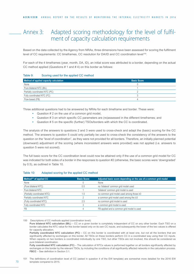
70


Annex 3: Adapted scoring methodology for the level of fulfil-ment of capacity calculation requirements

BasedonthedatacollectedbytheAgencyfromNRAs,threedimensionshavebeenassessedforscoringthefulfilmentlevel of CC requirements: CC timeframes, CC resolution for DA/ID and CC coordination level150.

For each of the 4 timeframes (year, month, DA, ID), an initial score was attributed to a border, depending on the actual CC method applied (Questions # 1 and # 4) on this border as follows:

Table9: ScoringusedfortheappliedCCmethod

Method of applied capacity calculation Basic ScoreNone 0Pure bilateral NTC (BIL) 1Partially coordinated NTC (PC) 2Fully coordinated NTC (FC) 3Flow-based (FB) 4

Three additional questions had to be answered by NRAs for each timeframe and border. These were: • Question # 2 on the use of a common grid model,• Question#3onwhichspecificCCparametersare(re)assessedinthedifferenttimeframes;and• Question#5onthespecific(further)TSOs/borderswithwhichtheCCiscoordinated.

The analysis of the answers to questions 2 and 3 were used to cross-check and adapt the (basic) scoring for the CC method. The answers to question 5 could only partially be used to cross-check the consistency of the answers to the question on the “level of coordination”, as they were not provided for all borders. Therefore, an initially planned potential (downward) adjustment of the scoring (where inconsistent answers were provided) was not applied (i.e. answers to question 5 were not scored).

The full basic score for the CC coordination level could now be attained only if the use of a common grid model for CC was indicated for both sides of a border in the responses to question #2 (otherwise, the basic scores were ‘downgraded’ by 0.5), as outlined in Table 10.

Table 10: Adapted scoring for the applied CC method

Method151 of applied CC Basic Score Adjusted basic score depending on the use of a common grid modelNone 0 None(Pure bilateral NTC) 0.5 no ‘bilateral’ common grid model usedPure bilateral NTC 1 ‘bilateral’ common grid model is used(Partially coordinated NTC) 1.5 no common grid model used among those ≥3Partially coordinated NTC 2 a common grid model used among the ≥3(Fully coordinated NTC) 2.5 no common grid model is usedFully coordinated NTC 3 a common grid model is usedFB 4 FB applied and a common grid model is used

150 Descriptions of CC methods applied (coordination level):Pure bilateral NTC calculation (BIL) – CC on a given border is completely independent of CC on any other border. Each TSO on a border calculates the NTC value for this border based only on its own CC inputs, and subsequently the lower of the two values is offered for capacity allocation;Partially coordinated NTC calculation (PC) – CC on this border is coordinated with at least one, but not all the borders that are significantlyaffectedbyexchangesonthisborder.AllTSOsonthesebordersperformCCinacoordinatedwayusingtheirCCinputs.When capacity on two borders is coordinated individually by one TSO, but other TSOs are not involved, this should be considered as pure bilateral coordination. Fully coordinated NTC calculation (FC)–ThecalculationofNTCsvaluesisperformedtogetheronallborderssignificantlyaffectedbyexchangesonthisborderbytherelevantTSOs,byincludingtheconditionsofallsignificantlyaffectednetworksinthecalculationprocess.FBCC–SeedefinitioninSection3.1.

151 Thedefinitionsofcoordination levelofCC(asked inquestion4of theEWtemplate)aresomewhatmoredetailed for the2016EWtemplate compared to 2015.

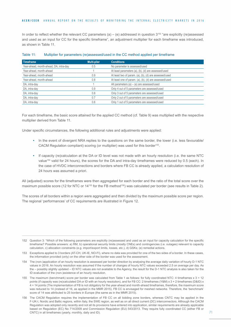
71


InordertoreflectwhethertherelevantCCparameters(a)–(e)addressedinquestion3152 “are explicitly (re)assessed andusedasaninputforCCforthespecifictimeframe”,anadjustmentmultiplierforeachtimeframewasintroduced,as shown in Table 11.

Table 11: Multiplier for parameters (re)assessed/used in the CC method applied per timeframe

Timeframe Multi-plier ConditionsYear-ahead, month-ahead, DA, intra-day 0.5 No parameter is assessed/usedYear-ahead, month-ahead 1 At least parameters (a), (b), (d) are assessed/usedYear-ahead, month-ahead 0.9 At least two of param. (a), (b), (d) are assessed/usedYear-ahead, month-ahead 0.8 At least one of param. (a), (b), (d) are assessed/usedDA, intra-day 1 All parameters (a) – (e) are assessed/usedDA, intra-day 0.9 Only 4 out of 5 parameters are assessed/usedDA, intra-day 0.8 Only 3 out of 5 parameters are assessed/usedDA, intra-day 0.7 Only 2 out of 5 parameters are assessed/usedDA, intra-day 0.6 Only 1 out of 5 parameters are assessed/used

Foreachtimeframe,thebasicscoreattainedfortheappliedCCmethod(cf.Table9)wasmultipliedwiththerespectivemultiplier derived from Table 11.

Underspecificcircumstances,thefollowingadditionalrulesandadjustmentswereapplied:

• In the event of divergent NRA replies to the questions on the same border, the lower (i.e. less favourable/CACM Regulation compliant) scoring (or multiplier) was used for this border153.

• If capacity (re)calculation at the DA or ID level was not made with an hourly resolution (i.e. the same NTC value154 valid for 24 hours), the scores for the DA and intra-day timeframes were reduced by 0.5 (each). In the case of HVDC interconnections and borders where FB CC is already applied, a calculation resolution of 24 hours was assumed a priori.

All (adjusted) scores for the timeframes were then aggregated for each border and the ratio of the total score over the maximum possible score (12 for NTC or 14155 for the FB method156) was calculated per border (see results in Table 2).

The scores of all borders within a region were aggregated and then divided by the maximum possible score per region. The regional ‘performances’ of CC requirements are illustrated in Figure 12.

152 Question3:“Whichofthefollowingparametersareexplicitly(re)assessedandusedasaninputforcapacitycalculationforthespecifictimeframe? Possible answers: a) RM, b) operational security limits (mostly CNEs) and contingencies (i.e. outages) relevant to capacity calculation, c) allocation constraints (e.g. import/export limits, losses, etc.), d) GSKs; (e) remedial actions.

153 Exceptions applied to 3 borders (AT-CH, UK-IE, NO-FI), where no data was provided for one of the two sides of a border. In these cases, the information provided (only) on the other side of the border was used for the assessment.

154 The (non-)application of an hourly resolution is assessed per border direction by analysing the average daily variation of hourly D-1 NTC values in 2016. An hourly resolution was assumed if the number of changes of hourly NTC values exceeded 2.5 on average per day. As the – possibly slightly updated – ID NTC values are not available to the Agency, the result for the D-1 NTC analysis is also taken for the ID evaluation of the (non-)existence of an hourly resolution.

155 The maximum (benchmark) score per border was calculated from Table 1 as follows: for fully coordinated NTC: 4 timeframes x 3 = 12 points(ifcapacitywas(re)calculatedDAorIDwithanhourlyresolution),andforFBCC:2timeframes(Y&M)x3+2timeframes(D&ID)x4 = 14 points (The implementation of FB is not obligatory for the year-ahead and month-ahead timeframes, therefore, the maximum score was reduced to 14 (instead of 16, as applied in the MMR 2015). FB CC is envisaged for meshed networks. Therefore, the ‘benchmark’ score of 14 was attributed to 25 borders in Europe (the same as in the MMR 2015).

156 The CACM Regulation requires the implementation of FB CC on all bidding zone borders, whereas CNTC may be applied in the F-UK-I, Nordic and Baltic regions, within Italy, the SWE region, as well as on all direct current (DC) interconnectors. Although the CACM Regulation was adopted only recently and not all its provisions have entered into application, similar requirements are already applicable basedonRegulation(EC)No714/2009andCommissionRegulation(EU)543/2013.TheyrequirefullycoordinatedCC(eitherFBorCNTC) in all timeframes (yearly, monthly, daily and ID).

72


Annex 4: Unscheduled flowsAs shown in previous editions of the MMRs157, UFs present a challenge to the further integration of the IEM. Their per-sistencereducestradablecross-zonalcapacity,marketefficiencyandnetworksecurity.

ThedefinitionsoftheflowsusedinthisAnnexareprovidedintheMMR2014.Briefly,UFsarecomprisedofUAFs,mostofwhichstemfromaninsufficientcoordinationinCCandallocationprocessandLFs,whichoriginatefromelectricityexchanges inside other bidding zones.

The data on the AFs used in the analysis of this Annex were provided to the Agency by ENTSO-E. AFs were calculated onanhourlybasis,usingsomesimplifications158, although several improvements compared to previous years were introduced159.Becauseofthesimplificationsused,theobtainedAFsdatacanbeconsideredonlyasaproxyforthetotalamount of AFs (and indirectly LFs and UAFs) observed on each border.

The Agency has been monitoring the evolution of UFs in Europe (i.e. on the borders in the former CEE, CSE and CWE regions160)since2012.Theyhaveincreasedfrom129.6TWhin2012to155.5TWhin2015,a20%increase.In2016,they decreased to 134.2 TWh, a 13.7% decrease compared to 2015, but still 3.6% higher than in 2012.

The main factor contributing to this decrease in 2016 appears to have been the reduction in commercial exchanges be-tweenGermanyandAustriaby11.2%from2015to2016,whichwereidentifiedbytheAgencyasoneimportantcauseof UFs on borders of the Core (CEE) region161.InadditionthespecificdecreaseontheGerman-Polishbordermaybetheconsequenceofthereductioninphysicalcapacity(andconsequentlyphysicalflows)betweenGermanyandPolanddue to a temporary disconnection of the Vierraden-Krajnik interconnector.

Figure 34162 shows the evolution of the aggregated sum of UFs volumes in the former three regions in 2014 and 2016163. ThehighestdecreasecanbeobservedintheCore(CWE)region,wherevolumesdecreasedby25.9%or11.5TWhin2016.Thesevolumesarethelowestsince2012,withanoveralldecreaseof22.5%or9.6TWhovertheperiod.Asimilar conclusion can be drawn for the former CEE, with a decrease of 13.6% or 10.2 TWh in 2016. However, the level of UFs remained 28%% or 14 TWh higher in this region than in 2012. The level of UFs in the CSE region remained stable, with a slight increase of 1.2% or 0.42 TWh in 2016.

157 See Chapter 5, in particular Section 5.1, of the Electricity Wholesale Markets volume of MMR 2015.

158 For more details on the assumptions used, see footnote 44 of the Electricity Wholesale Markets volume of the MMR 2015.

159 For example, six different sets of PTDFs based on the GCMs of six representative days in 2016 were used in this MMR edition, as opposed to three in previous ones. This could be further improved, e.g. by using one GCM per market time unit.

160 Following the Agency’s Decision on the TSOs’ Proposal for determining Capacity Calculation Regions (see footnote 36), the German-AustrianbordershouldbeallocatedtothenewCoreregion.AstheformerCWEandCEEregionsareidentifiedthroughoutthisdocumentas the Core (CWE) region and respectively the Core (CEE) region, for consistency with previous MMR editions, this border was included intheCore(CEE)region.TheformerCSEregioncomprisesthenew‘ItalyNorth’andtheSwissbordersasidentifiedinthisAnnex.

161 See page 12 of the Agency’s Decision on the TSOs’ Proposal for determining Capacity Calculation Regions (see also footnote 36).

162 The German-Austrian border, included in Figure 34, has not been included in the subsequent analysis in this Chapter, as UFs within the same bidding zone cannot be divided into LFs and UAFs. The border between Italy and Greece is a part of the former CSE region. However, since they are connected through a DC cable, this border is not relevant to the UFs analysis.

163 For a comparison with previous years, see the MMR 2012 (p. 100), MMR 2013 (p. 150), MMR 2014 (p. 165), available at http://nra.acer.europa.eu/en/Electricity/Market%20monitoring/Pages/Reports.aspxandMMR2015,ElectricityWholesaleMarketsvolume(p.29).

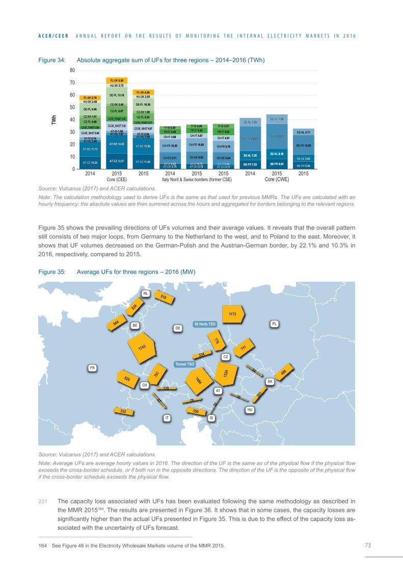
73


Figure 34: Absolute aggregate sum of UFs for three regions – 2014–2016 (TWh)

Source: Vulcanus (2017) and ACER calculations.Note: The calculation methodology used to derive UFs is the same as that used for previous MMRs. The UFs are calculated with an hourly frequency; the absolute values are then summed across the hours and aggregated for borders belonging to the relevant regions.

Figure 35 shows the prevailing directions of UFs volumes and their average values. It reveals that the overall pattern still consists of two major loops, from Germany to the Netherland to the west, and to Poland to the east. Moreover, it shows that UF volumes decreased on the German-Polish and the Austrian-German border, by 22.1% and 10.3% in 2016, respectively, compared to 2015.

Figure 35: Average UFs for three regions – 2016 (MW)

Source: Vulcanus (2017) and ACER calculations.Note: Average UFs are average hourly values in 2016. The direction of the UF is the same as of the physical flow if the physical flow exceeds the cross-border schedule, or if both run in the opposite directions. The direction of the UF is the opposite of the physical flow if the cross-border schedule exceeds the physical flow.

231 The capacity loss associated with UFs has been evaluated following the same methodology as described in the MMR 2015164. The results are presented in Figure 36. It shows that in some cases, the capacity losses are significantlyhigherthantheactualUFspresentedinFigure35.Thisisduetotheeffectofthecapacitylossas-sociated with the uncertainty of UFs forecast.

164 See Figure 48 in the Electricity Wholesale Markets volume of the MMR 2015.

TWh

60

50

80

70

10

20

30

40

02014

Core (CEE) Italy Nord & Swiss borders (former CSE) Core (CWE)20152015 2014 20152015 2014 20152015

BE-FR 7.33BE-FR 7.33

BE-NL 7.25BE-NL 7.25

DE-FR 19.91DE-FR 19.91

DE-NL 7.20DE-NL 7.20



DE-FR 20.27DE-FR 20.27




DE-FR 15.68DE-FR 15.68


AT-CH 3.79AT-CH 3.79AT-IT 0.55AT-IT 0.55

CH-DE 9.31CH-DE 9.31

CH-FR 10.50CH-FR 10.50

CH-IT 3.88CH-IT 3.88FR-IT 4.46FR-IT 4.46IT-SI 2.30IT-SI 2.30



CH-FR 10.80CH-FR 10.80

CH-IT 3.87CH-IT 3.87FR-IT 4.68FR-IT 4.68IT-SI 2.48IT-SI 2.48



CH-FR 9.19CH-FR 9.19

CH-IT 4.61CH-IT 4.61

FR-IT 5.63FR-IT 5.63

IT-SI 3.51IT-SI 3.51

AT-CZ 10.28AT-CZ 10.28

AT-DE 11.73AT-DE 11.73

AT-HU 1.84AT-HU 1.84AT-SI 2.14AT-SI 2.14

CZ-DE_50HZT 6.40CZ-DE_50HZT 6.40

CZ-DE_TENNET 2.66CZ-DE_TENNET 2.66

CZ-PL 6.69CZ-PL 6.69CZ-SK 1.91CZ-SK 1.91

DE-PL 9.96DE-PL 9.96

HU-SK 2.49HU-SK 2.49PL-SK 3.70PL-SK 3.70

AT-CZ 12.87AT-CZ 12.87

AT-DE 14.89AT-DE 14.89

AT-HU 1.97AT-HU 1.97AT-SI 1.58AT-SI 1.58

CZ-DE_50HZT 7.51CZ-DE_50HZT 7.51

CZ-DE_TENNET 3.93CZ-DE_TENNET 3.93

CZ-PL 8.67CZ-PL 8.67

CZ-SK 2.08CZ-SK 2.08

DE-PL 13.18DE-PL 13.18

HU-SK 2.72HU-SK 2.72PL-SK 5.30PL-SK 5.30

AT-CZ 11.64 AT-CZ 11.64

AT-DE 13.86 AT-DE 13.86

AT-HU 1.85 AT-HU 1.85 AT-SI 2.04 AT-SI 2.04

CZ-DE_50HZT 6.97 CZ-DE_50HZT 6.97

CZ-DE_TENNET 2.71 CZ-DE_TENNET 2.71

CZ-PL 6.24 CZ-PL 6.24 CZ-SK 1.99 CZ-SK 1.99

DE-PL 10.30 DE-PL 10.30

HU-SK 2.55 HU-SK 2.55 PL-SK 4.38 PL-SK 4.38

NLNL

CZCZ

ATAT

SISI

FRFR

CHCH

DEDE50 Hertz TSO50 Hertz TSO

Tennet TSOTennet TSO

PLPL

SKSK

HUHU

ITIT

BEBE

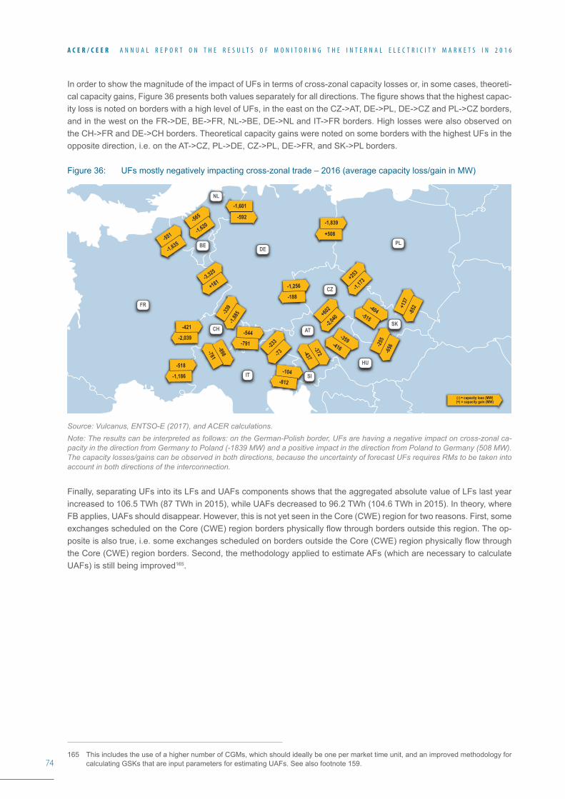
74


In order to show the magnitude of the impact of UFs in terms of cross-zonal capacity losses or, in some cases, theoreti-calcapacitygains,Figure36presentsbothvaluesseparatelyforalldirections.Thefigureshowsthatthehighestcapac-itylossisnotedonborderswithahighlevelofUFs,intheeastontheCZ->AT,DE->PL,DE->CZandPL->CZborders,andinthewestontheFR->DE,BE->FR,NL->BE,DE->NLandIT->FRborders.HighlosseswerealsoobservedontheCH->FRandDE->CHborders.TheoreticalcapacitygainswerenotedonsomeborderswiththehighestUFsintheoppositedirection,i.e.ontheAT->CZ,PL->DE,CZ->PL,DE->FR,andSK->PLborders.

Figure 36: UFs mostly negatively impacting cross-zonal trade – 2016 (average capacity loss/gain in MW)

Source: Vulcanus, ENTSO-E (2017), and ACER calculations.Note: The results can be interpreted as follows: on the German-Polish border, UFs are having a negative impact on cross-zonal ca-pacity in the direction from Germany to Poland (-1839 MW) and a positive impact in the direction from Poland to Germany (508 MW). The capacity losses/gains can be observed in both directions, because the uncertainty of forecast UFs requires RMs to be taken into account in both directions of the interconnection.

Finally, separating UFs into its LFs and UAFs components shows that the aggregated absolute value of LFs last year increasedto106.5TWh(87TWhin2015),whileUAFsdecreasedto96.2TWh(104.6TWhin2015).Intheory,whereFB applies, UAFs should disappear. However, this is not yet seen in the Core (CWE) region for two reasons. First, some exchangesscheduledontheCore(CWE)regionbordersphysicallyflowthroughbordersoutsidethisregion.Theop-positeisalsotrue,i.e.someexchangesscheduledonbordersoutsidetheCore(CWE)regionphysicallyflowthroughthe Core (CWE) region borders. Second, the methodology applied to estimate AFs (which are necessary to calculate UAFs) is still being improved165.

165 This includes the use of a higher number of CGMs, which should ideally be one per market time unit, and an improved methodology for calculatingGSKsthatareinputparametersforestimatingUAFs.Seealsofootnote159.

NLNL

CZCZ

ATAT

SISI

FRFR

CHCH

DEDEPLPL

SKSK

HUHU

ITIT

BEBE-551

-1,635

-1,839

+508

(-) = capacity loss (MW)(+) = capacity gain (MW)

-565

-1,620

-3,325

+181

-339

-1,88

5

-544

-791

-1,256

-188

-233

-73

+602

-2,040

+253

-1,173

+137

-852

-255

-656-372-437

-104-812

-404-515

-359-416

-421

-2,039

-518

-1,186

-898-781

-1,601

-592

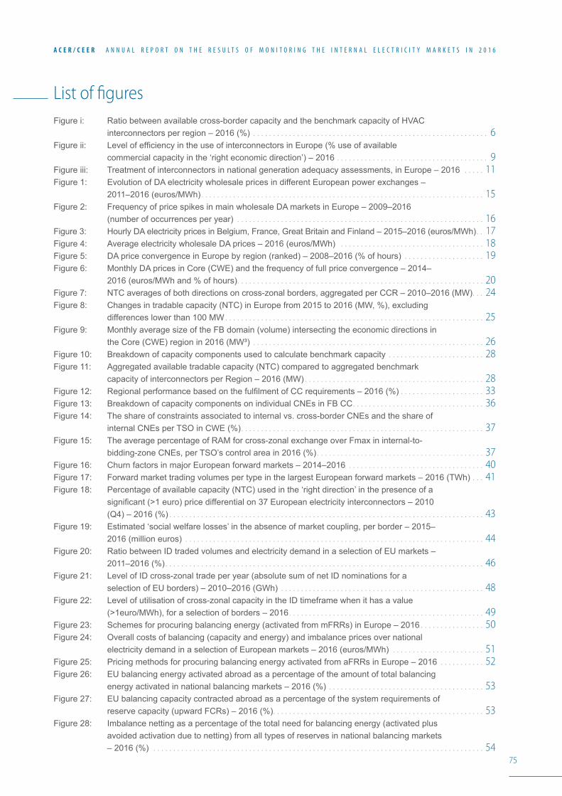
75


List of figuresFigure i: Ratio between available cross-border capacity and the benchmark capacity of HVAC

interconnectors per region – 2016 (%) . . . . . . . . . . . . . . . . . . . . . . . . . . . . . . . . . . . . . . . . . . . . . . . . . . . . . . . . . . . 6Figureii: LevelofefficiencyintheuseofinterconnectorsinEurope(%useofavailable

commercial capacity in the ‘right economic direction’) – 2016 . . . . . . . . . . . . . . . . . . . . . . . . . . . . . . . . . . . . . . 9Figure iii: Treatment of interconnectors in national generation adequacy assessments, in Europe – 2016 . . . . . 11Figure 1: Evolution of DA electricity wholesale prices in different European power exchanges –

2011–2016 (euros/MWh) . . . . . . . . . . . . . . . . . . . . . . . . . . . . . . . . . . . . . . . . . . . . . . . . . . . . . . . . . . . . . . . . . . . . . . . 15Figure2: FrequencyofpricespikesinmainwholesaleDAmarketsinEurope–2009–2016

(number of occurrences per year) . . . . . . . . . . . . . . . . . . . . . . . . . . . . . . . . . . . . . . . . . . . . . . . . . . . . . . . . . . . . . . 16Figure 3: Hourly DA electricity prices in Belgium, France, Great Britain and Finland – 2015–2016 (euros/MWh) . . 17Figure 4: Average electricity wholesale DA prices – 2016 (euros/MWh) . . . . . . . . . . . . . . . . . . . . . . . . . . . . . . . . . . . . 18Figure 5: DA price convergence in Europe by region (ranked) – 2008–2016 (% of hours) . . . . . . . . . . . . . . . . . . . . 19Figure 6: Monthly DA prices in Core (CWE) and the frequency of full price convergence – 2014–

2016 (euros/MWh and % of hours). . . . . . . . . . . . . . . . . . . . . . . . . . . . . . . . . . . . . . . . . . . . . . . . . . . . . . . . . . . . . . 20Figure 7: NTC averages of both directions on cross-zonal borders, aggregated per CCR – 2010–2016 (MW) . . . 24Figure 8: Changes in tradable capacity (NTC) in Europe from 2015 to 2016 (MW, %), excluding

differences lower than 100 MW . . . . . . . . . . . . . . . . . . . . . . . . . . . . . . . . . . . . . . . . . . . . . . . . . . . . . . . . . . . . . . . . . 25Figure9: MonthlyaveragesizeoftheFBdomain(volume)intersectingtheeconomicdirectionsin

the Core (CWE) region in 2016 (MW³) . . . . . . . . . . . . . . . . . . . . . . . . . . . . . . . . . . . . . . . . . . . . . . . . . . . . . . . . . . 26Figure 10: Breakdown of capacity components used to calculate benchmark capacity . . . . . . . . . . . . . . . . . . . . . . . . 28Figure 11: Aggregated available tradable capacity (NTC) compared to aggregated benchmark

capacity of interconnectors per Region – 2016 (MW) . . . . . . . . . . . . . . . . . . . . . . . . . . . . . . . . . . . . . . . . . . . . . 28Figure12: RegionalperformancebasedonthefulfilmentofCCrequirements–2016(%) . . . . . . . . . . . . . . . . . . . . . 33Figure 13: Breakdown of capacity components on individual CNEs in FB CC . . . . . . . . . . . . . . . . . . . . . . . . . . . . . . . . . 36Figure 14: The share of constraints associated to internal vs. cross-border CNEs and the share of

internal CNEs per TSO in CWE (%) . . . . . . . . . . . . . . . . . . . . . . . . . . . . . . . . . . . . . . . . . . . . . . . . . . . . . . . . . . . . . 37Figure 15: The average percentage of RAM for cross-zonal exchange over Fmax in internal-to-

bidding-zone CNEs, per TSO’s control area in 2016 (%) . . . . . . . . . . . . . . . . . . . . . . . . . . . . . . . . . . . . . . . . . . 37Figure 16: Churn factors in major European forward markets – 2014–2016 . . . . . . . . . . . . . . . . . . . . . . . . . . . . . . . . . . 40Figure 17: Forward market trading volumes per type in the largest European forward markets – 2016 (TWh) . . . 41Figure 18: Percentage of available capacity (NTC) used in the ‘right direction’ in the presence of a

significant(>1euro)pricedifferentialon37Europeanelectricityinterconnectors–2010(Q4) – 2016 (%) . . . . . . . . . . . . . . . . . . . . . . . . . . . . . . . . . . . . . . . . . . . . . . . . . . . . . . . . . . . . . . . . . . . . . . . . . . . . . . . 43

Figure19: Estimated‘socialwelfarelosses’intheabsenceofmarketcoupling,perborder–2015–2016 (million euros) . . . . . . . . . . . . . . . . . . . . . . . . . . . . . . . . . . . . . . . . . . . . . . . . . . . . . . . . . . . . . . . . . . . . . . . . . . . 44

Figure 20: Ratio between ID traded volumes and electricity demand in a selection of EU markets – 2011–2016 (%) . . . . . . . . . . . . . . . . . . . . . . . . . . . . . . . . . . . . . . . . . . . . . . . . . . . . . . . . . . . . . . . . . . . . . . . . . . . . . . . . 46

Figure 21: Level of ID cross-zonal trade per year (absolute sum of net ID nominations for a selection of EU borders) – 2010–2016 (GWh) . . . . . . . . . . . . . . . . . . . . . . . . . . . . . . . . . . . . . . . . . . . . . . . . . . . 48

Figure 22: Level of utilisation of cross-zonal capacity in the ID timeframe when it has a value (>1euro/MWh),foraselectionofborders–2016 . . . . . . . . . . . . . . . . . . . . . . . . . . . . . . . . . . . . . . . . . . . . . . . . . 49

Figure 23: Schemes for procuring balancing energy (activated from mFRRs) in Europe – 2016 . . . . . . . . . . . . . . . . 50Figure 24: Overall costs of balancing (capacity and energy) and imbalance prices over national

electricity demand in a selection of European markets – 2016 (euros/MWh) . . . . . . . . . . . . . . . . . . . . . . . 51Figure 25: Pricing methods for procuring balancing energy activated from aFRRs in Europe – 2016 . . . . . . . . . . . 52Figure 26: EU balancing energy activated abroad as a percentage of the amount of total balancing

energy activated in national balancing markets – 2016 (%) . . . . . . . . . . . . . . . . . . . . . . . . . . . . . . . . . . . . . . . 53Figure 27: EU balancing capacity contracted abroad as a percentage of the system requirements of

reserve capacity (upward FCRs) – 2016 (%). . . . . . . . . . . . . . . . . . . . . . . . . . . . . . . . . . . . . . . . . . . . . . . . . . . . . 53Figure 28: Imbalance netting as a percentage of the total need for balancing energy (activated plus

avoided activation due to netting) from all types of reserves in national balancing markets – 2016 (%) . . . . . . . . . . . . . . . . . . . . . . . . . . . . . . . . . . . . . . . . . . . . . . . . . . . . . . . . . . . . . . . . . . . . . . . . . . . . . . . . . . . 54

76


Figure29: CMsinEurope–2016 . . . . . . . . . . . . . . . . . . . . . . . . . . . . . . . . . . . . . . . . . . . . . . . . . . . . . . . . . . . . . . . . . . . . . . . . . 56Figure 30: Percentage of hours with net DA nominations against price differentials per border

(ranked) – 2015–2016 (%) . . . . . . . . . . . . . . . . . . . . . . . . . . . . . . . . . . . . . . . . . . . . . . . . . . . . . . . . . . . . . . . . . . . . . 65Figure 31: Level of ID cross-zonal trade (absolute sum of net ID nominations for a selection of EU

borders) – 2010–2016 (GWh) . . . . . . . . . . . . . . . . . . . . . . . . . . . . . . . . . . . . . . . . . . . . . . . . . . . . . . . . . . . . . . . . . . 65Figure 32: Weighted average prices of balancing energy activated from aFRRs (upward and

downward activation) in a selection of EU markets – 2016 (euros/MWh) . . . . . . . . . . . . . . . . . . . . . . . . . . . 66Figure 33: Average prices of balancing capacity (upward and downward capacity from aFRRs) in a

selection of EU markets – 2016 (euros/MW/h) . . . . . . . . . . . . . . . . . . . . . . . . . . . . . . . . . . . . . . . . . . . . . . . . . . 66Figure 34: Absolute aggregate sum of UFs for three regions – 2014–2016 (TWh) . . . . . . . . . . . . . . . . . . . . . . . . . . . . 73Figure 35: Average UFs for three regions – 2016 (MW) . . . . . . . . . . . . . . . . . . . . . . . . . . . . . . . . . . . . . . . . . . . . . . . . . . . . 73Figure 36: UFs mostly negatively impacting cross-zonal trade – 2016 (average capacity loss/gain in MW) . . . . . . 74

List of tablesTable i: Borders with the biggest DA price differentials– 2012–2016 (euros/MWh) . . . . . . . . . . . . . . . . . . . . . . . . . . 5Table ii: Borders with the lowest ratio between tradable capacity (NTC) and benchmark capacity

– 2016 (%, MW) . . . . . . . . . . . . . . . . . . . . . . . . . . . . . . . . . . . . . . . . . . . . . . . . . . . . . . . . . . . . . . . . . . . . . . . . . . . . . . . . 7Table 1: Principles, similarities, main differences and parameters of the CNTC and FB CC processes . . . . . . . . 22Table 2: Application of CC methods on 50 borders in different timeframes – 2016 . . . . . . . . . . . . . . . . . . . . . . . . . . 32Table 3: Evolution of the costs of remedial actions – 2015–2016 (thousand euros, %) . . . . . . . . . . . . . . . . . . . . . . 39Table 4: Treatment of interconnectors in national generation adequacy assessments in Europe – 2016 . . . . . . 58Table 5: Average DA price differentials across European borders (ranked) – 2012–2016 (euros/MWh) . . . . . . . 61Table 6: Ratio between tradable capacity (NTC) and benchmark capacity (regional performance)

– 2016 (%, MW) . . . . . . . . . . . . . . . . . . . . . . . . . . . . . . . . . . . . . . . . . . . . . . . . . . . . . . . . . . . . . . . . . . . . . . . . . . . . . . . 62Table 7: Changes in tradable capacity (NTC) in Europe from 2015 to 2016 and ratios between

NTC and benchmark capacity – 2016 (%, MW) . . . . . . . . . . . . . . . . . . . . . . . . . . . . . . . . . . . . . . . . . . . . . . . . . . 62Table 8: Assessment of the impact of CNEs on cross-zonal exchanges in the Core (CWE) region,

per TSO and CNE – 2016 (number of hours, %) . . . . . . . . . . . . . . . . . . . . . . . . . . . . . . . . . . . . . . . . . . . . . . . . . 64Table9: ScoringusedfortheappliedCCmethod . . . . . . . . . . . . . . . . . . . . . . . . . . . . . . . . . . . . . . . . . . . . . . . . . . . . . . . . 70Table 10: Adapted scoring for the applied CC method . . . . . . . . . . . . . . . . . . . . . . . . . . . . . . . . . . . . . . . . . . . . . . . . . . . . . 70Table 11: Multiplier for parameters (re)assessed/used in the CC method applied per timeframe . . . . . . . . . . . . . . . 71

Document title:

Publishing date: 06/10/2017

We appreciate your feedback

Please click on the icon to take a 5’ online surveyand provide your feedback about this document

Share this document

https://www.acer.europa.eu/Lists/Survey/NewForm.aspx?documentid=ACER-2017-46983&Source=https%3a%2f%2fwww.acer.europa.eu

https://twitter.com/intent/tweet?url=https%3a%2f%2fwww.acer.europa.eu%2f%2fOfficial_documents%2fActs_of_the_Agency%2fPublication%2fACER+Market+Monitoring+Report+2016+-+ELECTRICITY.pdf&text=

http://www.facebook.com/share.php?u=https%3a%2f%2fwww.acer.europa.eu%2f%2fOfficial_documents%2fActs_of_the_Agency%2fPublication%2fACER+Market+Monitoring+Report+2016+-+ELECTRICITY.pdf&t=

http://www.linkedin.com/shareArticle?mini=true&url=https%3a%2f%2fwww.acer.europa.eu%2f%2fOfficial_documents%2fActs_of_the_Agency%2fPublication%2fACER+Market+Monitoring+Report+2016+-+ELECTRICITY.pdf&title=&ro=false&summary=&source=

https://plus.google.com/share?url=https%3a%2f%2fwww.acer.europa.eu%2f%2fOfficial_documents%2fActs_of_the_Agency%2fPublication%2fACER+Market+Monitoring+Report+2016+-+ELECTRICITY.pdf&t=