Does Religion Make You Healthier and Longer Lived?Evidence for Germany

Bruce Headey • Gerhard Hoehne • Gert G. Wagner

Accepted: 16 December 2013� Springer Science+Business Media Dordrecht 2013

Abstract Researchers in the US have consistently reported substantial—not just statis-

tically significant—links between religious belief and practice, and improved health and

longevity. In this paper we report evidence for Germany, using data from the long-running,

nationally representative German Socio-Economic Panel (SOEP 1984). The SOEP dataset

includes multiple measures of health, plus many ‘controls’ which it is appropriate to use in

assessing links between religious practice, health and longevity. These controls include

personality traits known to be associated with better health (notably conscientiousness),

and also the age of death of parents of the survey respondents. Initial results suggested that

religious practice (church attendance) may be linked only to subjective (self-rated) mea-

sures of health, not to more objective measures. It seemed possible that results in some

previous research could be due to what may be termed satisfaction bias or positivity bias;

the known tendency of religious people to report higher than average satisfaction with

almost all aspects of life. Further investigation indicated that relationships between church

attendance and subjective measures of health were weaker, when a control for satisfaction

bias was in place. However, there was countervailing evidence that the subjective measures

in SOEP may actually be more not less valid than the objective measures; they are better

not worse predictors of mortality. It was also clear that religious belief and church

attendance are associated with health-protective behaviors and attitudes, including taking

more exercise, not smoking and higher life satisfaction. At the end of the paper we estimate

B. Headey (&)Melbourne Institute, University of Melbourne, Parkville 3052, Australiae-mail: brucewh@unimelb.edu.au; b.headey@unimelb.edu.au

B. Headey � G. G. WagnerGerman Institute for Economic Research (DIW), Berlin, Germany

G. Hoehne � G. G. WagnerBerlin University of Technology, Berlin, Germany

G. G. WagnerMax Planck Institute for Human Development, Berlin, Germany

123

Soc Indic ResDOI 10.1007/s11205-013-0546-x

a structural equation model which maps links between religious practice, these protective

behaviors and attitudes, and improved health outcomes.

Keywords Subjective and objective health measures � Church attendance �Satisfaction bias � German Socio-Economic Panel (SOEP)

1 Introduction

Obviously, social scientists have nothing useful to say about the truth or falsity of the

world’s religions. But social scientists certainly have had a great deal to say about the

benefits which religion may confer on its adherents. In particular, it has been claimed that

Christian belief and practice are strongly linked to better health and longer life. Because

most of the available evidence comes from the United States, it is worthwhile examining

whether similar results hold for Germany, another Western country in which most people

who practise religion are Protestant or Catholic Christians. In Germany about 17 % (21 %

in the West, 8 % in the East) of the population report that they attend a religious service at

least once a month, compared with about 35 % in the United States.

Evidence comes from the nationally representative, long-running German Socio-Eco-

nomic Panel Survey (SOEP) in which respondents have been interviewed annually since

1984 (Frick et al. 2007). The questionnaire includes a fairly comprehensive set of health

measures. We use five of these measures, described in the Methods section. Here we note

that the measures can be classified as ranging from relatively subjective (e.g. health sat-

isfaction reported on a 0–10 scale) to relatively objective (e.g. grip strength measured by

squeezing a dynamometer). Our initial results showed that links between religious practice

and health differed systematically according to the subjectivity–objectivity of the measures

deployed. The more subjective the measure, the stronger the evidence seemed that reli-

gious practice benefits health. But the more objective the measure, the less convincing was

the evidence.

These first results drove the investigation in new directions. However, it must imme-

diately be pointed out that we do not assume that measurement objectivity can be equated

with measurement validity. Objective measures are nearly always more reliable (consis-

tent, repeatable) than subjective measures, but there is no reason to assume that they are

more (or less) valid as ‘true’ indicators of health. Measurement validity will be discussed

more fully in the ‘‘Methods’’ and ‘‘Results’’ sections. Here we just flag the issue that

religious practice is more strongly linked to subjective than objective indicators of health.

There has to be a reason for this difference. One hypothesis is that religious people may

have a tendency to report relatively high levels of satisfaction with their lives-as-a-whole,

and with virtually all specific aspects of life, including health (Campbell et al. 1976;

Argyle 2001). They may tend to overrate their health, compared to ratings that professional

observers (e.g. a team of physicians) would give. This tendency (if it exists) might be

termed satisfaction bias or positivity bias.

We find some initial evidence to support a hypothesis of satisfaction bias. But, again

unexpectedly, we also find strong countervailing evidence that the subjective measures in

SOEP are more not less valid than the objective measures. The strong evidence is that the

subjective measures are better predictors of mortality than the objective ones. Eventually,

by a rather tortuous route, we reach the conclusion that religious people are healthier and

B. Headey et al.

123

longer lived than less religious and non-religious people. They have attitudes and behaviors

(one could say a lifestyle) which promotes longevity. Relative to the population average,

religious people are more likely to marry and less likely to divorce. They smoke less, take

more exercise, are more socially active and volunteer more (partly through their church).

Their higher than average life satisfaction also contributes to longevity. Towards the end of

the paper we estimate a structural equation model which summarises linkages between

church attendance, exercise, smoking, life satisfaction and health. Church attendance is

shown to improve health primarily via a healthier lifestyle and increased life satisfaction.

There appear to be two-way causal links between health and life satisfaction; good health

enhances life satisfaction and vice versa.

As well as providing a comprehensive set of health measures, SOEP includes a wide

range of variables that it is desirable to take into account in assessing links between religious

practice and health. These include both health risk and protective factors. Among the risk

factors are smoking and risk-taking, including health risk-taking. Among the protective

factors are getting married and staying married, social networks and participation, and the

personality trait of conscientiousness (Friedman and Martin 2011). For many respondents

information is available about the age at which their father and mother died. It is desirable to

control for these variables in assessing the impact of religiosity on longevity, although

previous research has found that it is only in very long-lived families that there are sig-

nificant associations between the death ages of successive generations (Gudmundsson et al.

2000; Lach et al. 2006). More technically, the panel design makes it possible to undertake

fixed-effects panel regression analyses in which the effects on health of all time-invariant

factors are automatically controlled. These include family background, genetic effects,

intelligence and personality traits (assuming these are time invariant).

1.1 Previous Research

The claim that the religious are especially healthy and long lived has a long history. Biblical

scholars used to claim that Abraham lived to be 175 and Moses to 120. More plausibly,

Schnall et al. (2010), analysing data from the longitudinal US National Institute of Health’s

Women’s Health Initiative (N = 95,000), reported that women over fifty were 20 % less

likely to die in any given year if they attended a religious service every week, and 15 % less

likely to die if they were less frequent attenders. These findings held, even controlling for

baseline measures of health (physician assessments). Strawbridge et al. (1997) conducted a

28-year follow-up study and found that regular church-goers were significantly more likely

to be still alive, even after this long period. During the course of the study, religious

individuals were more likely than average to take up regular exercise, stop smoking,

improve their social networks and stay married; all factors associated with longevity.

Strawbridge et al. (1997) found that religion benefited the health of women more than

men. By contrast, Maselko and Kubzansky (2006), analysing data from the US General

Social Survey, found that religious activity benefited the health of men more than women,

although both genders gained. Hall (2006) reported that church-goers live 2–3 years longer

than non church-goers, partly because churches provide effective social networks. He

found that church networks were about as beneficial as regular exercise and cholesterol-

reducing drugs in promoting these extra years of life.

The Handbook of Health and Religion (Koenig et al. 2012) and The Handbook of

Mental Health and Religion (Koenig 1998) report that positive associations have been

found between religious practice and better physical and mental health in several hundred

studies, nearly all of which were conducted in the US and based on cross-sectional data.

Evidence for Germany

123

Research which explores possible mechanisms promoting better health among churchgoers

is particularly interesting. A Norwegian study (Sørensen et al. 2011) found that attending

church services directly lowers blood pressure and that the more often a person goes to

church, the lower blood pressure falls. Maselko (2006) found that churchgoers have better

lung health than non-attenders, noting that lung health is a valid measure of general

physical health and that smoking, which greatly affects lung health, is less prevalent among

churchgoers than non-attenders.

The most astonishing claim about the health benefits of religion was made in the Byrd

study (1988) conducted at a large hospital in San Francisco. This appeared to show that the

incidence of complications following a heart attack among patients who had a group of

believers praying for them was significantly lower than the incidence for a control group, who

did not receive intercessory prayer. However, a recent large scale investigation, sponsored by

the Templeton Foundation, failed to replicate this finding and, in fact, found that patients who

were prayed for suffered more complications. The difference between the prayer group and

the control groups was small but statistically significant (Benson et al. 2006).

All the American studies reviewed so far have claimed direct positive associations

between religious practice, health and longevity. The US study to which our German results

are closest is Friedman and Martin’s (2011) reanalysis of data related to longevity in the

eight-decade long Terman Study of the Gifted. Friedman and Martin analysed a wide range

of factors affecting longevity; their study was not focussed primarily on religion. However,

they did find that church attendance was one of many ‘lifestyle’ variables associated with

longevity. Good social networks, the personality trait of conscientiousness, volunteering,

community consciousness, high career achievement (see also Marmot et al. 1978, 1991)

and, for men, avoiding marital break-up were also found to be protective health factors.

1.2 Health and Longevity Hypotheses

We began this research with the following hypotheses:

1. Regular Christian religious practice (attendance at church services) is associated with

better health.

2. Regular religious practice is associated with increased longevity.

3.1–3.2 Regular religious practice is more beneficial for women than men in relation to

(i) health and (ii) longevity.

The finding that the strength of the apparent link between religious practice and health

depends partly on the subjectivity–objectivity of health measures only emerged in the

course of our research. Similarly, we did not envisage that subjective measures of health

might prove to be more valid, at least as predictors of mortality, than more objective

measures. Precisely because some main findings emerged in the course of the investiga-

tion, rather than being envisaged as hypotheses, it will be particularly important in future

work to check results and see if they replicate.

2 Methods

2.1 The German Socio-Economic Panel (SOEP): Annual Interviews Since 1984

The German (SOEP) panel began in 1984 in West Germany with a sample of 12,541

respondents (Frick et al. 2007). Interviews have been conducted annually ever since.

B. Headey et al.

123

Everyone in the household aged 16 and over is interviewed. The cross-sectional repre-

sentativeness of the panel is maintained by interviewing ‘split-offs’ and their new families.

So when a young person leaves home (‘splits off’) to marry and set up a new family, the

entire new family becomes part of the panel. The sample was extended to East Germany in

1990, shortly after the Berlin Wall came down, and since then has been boosted by the

addition of new immigrant samples, a special sample of the rich, and recruitment of new

respondents partly to increase numbers in ‘policy groups’. There are now over 60,000

respondents on file, including a few grandchildren, as well as children of the original

respondents. The main topics covered in the annual questionnaire are family, income and

labour force dynamics.

2.2 Measures

2.2.1 Religious Practice: Church Attendance

The main measure of religious practice available in SOEP is attendance at religious ser-

vices or activities (church attendance) reported in four categories: every week, every

month, seldom or never. The question was first asked in 1990 and has been asked on

thirteen occasions since. Attendance has declined steadily. In 1990 27.5 % attended reli-

gious services either weekly or at least monthly. By 2009 (latest date available) regular

attendance had dropped to 17.5 %.

On just three occasions (1994, 1998 and 1999) respondents have been asked about the

‘importance’ of religion in their lives, responding on a scale running from 1 (not at all

important) to 4 (very important). This question is probably intended to tap the spiritual

dimension of religion; the extent to which it provides a sense of purpose and meaning to

life. In 1999 11.1 % said that religion was ‘very important’ to them. Information is also

available about which Christian denomination respondents belong to. In Germany about

34 % are Protestant (Evangelisch), 29 % are Roman Catholic, and 2.5 % belong to other

Christian denominations.1 In SOEP about 3 % report belonging to other religions, with

most being Moslems. 31 % report ‘no denomination’.

Because our focus is on the effects of Christian religious practice on health, we exclude

those who practise religions other than Christianity. Our sample/panel therefore comprises

Christians, plus those who report no denomination.

We have imputed values for church attendance in years since 1990 in which the

question was not asked. This was done by averaging results for the nearest year before, and

the nearest year after any year with missing data.

The church attendance measure used here is almost identical to measures used in most

US surveys which report evidence on religious practice and health. It may be noted that

social scientists generally prefer behavioral measures of religiosity rather than less reliable

attitudinal measures intended to assess beliefs or the spiritual dimensions of religion. In

SOEP the behavioral church attendance measure has a Spearman rank order correlation of

0.65 with the ‘importance of religion’ measure. This is a very high correlation for two

items measured on 4-point response scales, so essentially both measures are identifying the

same people as ‘religious’.

Preliminary analysis indicated that relationships between church attendance and health

measures are not linear, or at least not clearly so. The main break appeared to be between

‘high’ attenders who attend every week or every month, and those who attend seldom or

1 These figures are for 2007; the latest year in which denomination was asked in SOEP.

Evidence for Germany

123

never. Accordingly, for inclusion in regression analyses, we constructed a dichotomous

variable, church attendance, scored 1 for high attenders and 0 for seldom and non-

attenders.

2.2.2 Health Measures Rank Ordered from Subjective to Objective

The five health measures used in this article can be ranked in a common sense way from

most subjective to most objective. Perhaps the most subjective is health satisfaction, which

has been asked every year in SOEP and is measured on a single item 0–10 scale, on which

zero is labelled ‘very dissatisfied’ and 10 is labelled ‘very satisfied’. The next most (or

perhaps equally) subjective measure is based on asking respondents to rate their current

state of health on a 1–5 scale ranging from ‘very good’ to ‘bad’. This question has been

asked annually since 1992. It correlates satisfactorily with physician ratings of health

(Schwarze et al. 2000). Somewhat less subjective is the physical health measure (pcs)

based on the SF12 health survey, which has been included in SOEP in alternate years since

2002. The SF12 is a short form of the internationally widely used Medical Outcomes Study

SF36 survey (Ware et al. 2000). The twelve items cover physical and mental health issues.

The data are factor analysed to yield physical (pcs) and mental health (mcs) summary

scales.2 The pcs is partly based on the 1–5 self-report item described earlier, plus other

items focussed on physical problems in the past 4 weeks (e.g. ‘‘During the past 4 weeks,

how much did pain interfere with your normal work…?’’ and ‘‘Does your health now limit

you in these activities…moving a table? Pushing a vacuum cleaner? Climbing several

flights of stairs?’’ Scores on the pcs scale are standardized to range from 0 to 100.

A somewhat more objective measure, although open to recall bias, is reported number

of doctor visits (general practitioners and all other types of medical doctor) in the last

3 months.3 Answers are multiplied by four to provide annual estimates. The doctor visits

question has been asked every year in SOEP. In a typical year about a third of the

population reports no visits, the mean is about ten, and over 20 % are estimated to have

made more than twelve visits.

Clearly, the most objective measure currently included in SOEP is grip strength,

measured in SOEP in 2006 and 2008.4 Grip strength is assessed by squeezing a dyna-

mometer. Respondents squeeze twice each with their left and right hands, with results for

each hand being averaged. Current grip strength of the dominant hand, measured in

kilograms, has been shown to be well correlated with physician ratings of health (Bo-

hannon 2001, 2008). Furthermore, change in grip strength is claimed to be a fairly accurate

predictor of death, especially for older people (Metter et al. 2002; Rantanen et al. 2000;

Ambrasat et al. 2011).

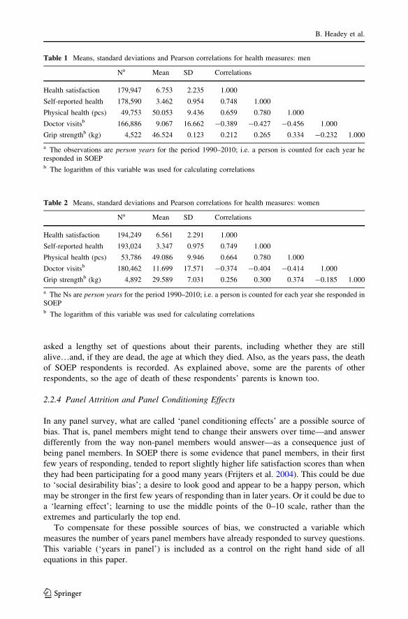
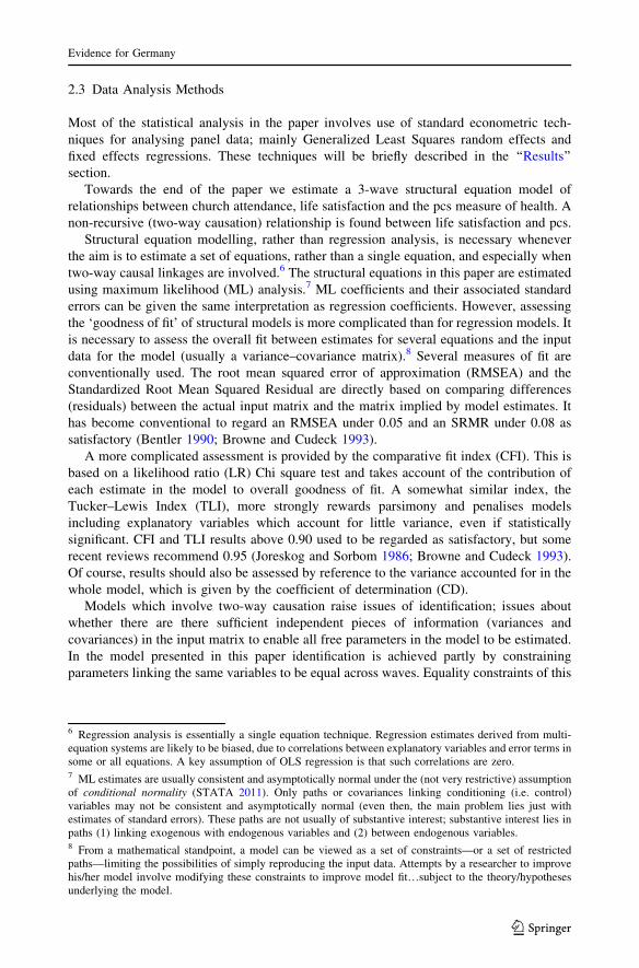
Tables 1 (men) and 2 (women) report the means and standard deviations of the health

measures, plus correlations among them.

The summary statistics in Tables 1 and 2 indicate that men report slightly better health

than women and go to the doctor less. These are standard results found in surveys in all

Western countries. The correlations among the measures are all moderate to high. The

measure which has the highest average correlation with the other items in the set is the pcs

2 Pcs and mcs stand for physical component summary and mental component summary.3 The longer ago a doctor visit occurred, the more likely it is that it will be forgotten and not reported,especially if the health problem was minor. Recall over a 3-month period is likely to be subject to a smalldegree of downward bias (Ayhan and Isiksal 2004).4 Data have also been collected in 2010 and 2012 but are not yet available.

B. Headey et al.

123

physical health index, which may be taken as an indication of its convergent validity; a

point to which we will return later.5

The remaining health outcome used in this article is mortality (1 = dead 0 = still

alive). Plainly, this is an unimpeachably objective measure. The obvious way to measure

the effects of church attendance on longevity might seem to be to relate it to age of death

(controlling for other factors). But this is not the approach usually taken by health

researchers, because it yields a biased sample in which the dead are included but those who

survive are right censored. The usual approach, followed here, is to ‘predict’ mortality

some years ahead on the basis of explanatory variables of interest, plus standard controls.

Here we predict mortality by church attendance, taking account of gender, age and many

other controls described below.

2.2.3 Personality Traits and Other Variables Included in Equations Primarily as Controls

We now describe a range of variables included in our equations mainly as ‘controls’ in order

to estimate the net effects of church attendance on health and longevity.

In 2005 and again in 2009 a short version of the Big Five Personality Domains (Costa

and McCrae 1991) was included in SOEP. The traits in the Big Five are neuroticism,

extroversion, openness, agreeableness and conscientiousness. The data managers report

that the short version has proved satisfactorily reliable and valid, and has yielded trait

measures which correlate highly with longer versions of the NEO (Gerlitz and Schupp

2005).

The Big Five personality traits are estimated to be about 30–50 % genetic (Lucas 2008),

so it makes sense to regard them as causally antecedent to measures of religiosity and

health. Traits are usually assumed to be stable in adulthood, so in the case of panel

members who provided trait measures in both 2005 and 2009, the average of their two

scores was taken. If only one measure was available that was used. Our working

assumption of trait stability is not entirely correct. Even if traits are 50 % genetic, that still

leaves 50 % of the variance to be explained by environmental effects. It is thought that

ratings on traits can be changed to some degree by life experiences like having a stable

marriage or an absorbing job (Roberts et al. 2006; Scollon and Diener 2006).

It is well known that neuroticism is quite strongly related to subjective measures of

health; neurotic individuals are almost by definition hypochondriacal (Costa and McCrae

1991). Conscientiousness is usually found to be positively related to health (Costa and

McCrae 1991).

Other variables included in equations primarily as controls are: gender, age (also age-

squared), marital/partnership status (1 = partnered 0 = not partnered), years of education,

household net income, unemployed (1 = unemployed 0 = employed or not in the labour

force), age of death of father and age of death of mother. There are straightforward

justifications for all of these controls. Women generally report somewhat worse health than

men, although they live longer. Age: health declines with slowly with age, and then sharply

in old age (hence the need for a quadratic term). Years of education and household net

income are included because both are positively associated with health. Being unemployed

is quite strongly associated with ill-health. Age of father’s death and age of mother’s death

are valuable inclusions as indicators of genetic ‘healthiness’. In SOEP new respondents are

5 However, the correlation of pcs with self-reported health cannot be considered in this context because theself-reported health measure (a single item) is included in the pcs index. It remains the case that pcs has thehighest mean correlation with the other 3 items.

Evidence for Germany

123

asked a lengthy set of questions about their parents, including whether they are still

alive…and, if they are dead, the age at which they died. Also, as the years pass, the death

of SOEP respondents is recorded. As explained above, some are the parents of other

respondents, so the age of death of these respondents’ parents is known too.

2.2.4 Panel Attrition and Panel Conditioning Effects

In any panel survey, what are called ‘panel conditioning effects’ are a possible source of

bias. That is, panel members might tend to change their answers over time—and answer

differently from the way non-panel members would answer—as a consequence just of

being panel members. In SOEP there is some evidence that panel members, in their first

few years of responding, tended to report slightly higher life satisfaction scores than when

they had been participating for a good many years (Frijters et al. 2004). This could be due

to ‘social desirability bias’; a desire to look good and appear to be a happy person, which

may be stronger in the first few years of responding than in later years. Or it could be due to

a ‘learning effect’; learning to use the middle points of the 0–10 scale, rather than the

extremes and particularly the top end.

To compensate for these possible sources of bias, we constructed a variable which

measures the number of years panel members have already responded to survey questions.

This variable (‘years in panel’) is included as a control on the right hand side of all

equations in this paper.

Table 1 Means, standard deviations and Pearson correlations for health measures: men

Na Mean SD Correlations

Health satisfaction 179,947 6.753 2.235 1.000

Self-reported health 178,590 3.462 0.954 0.748 1.000

Physical health (pcs) 49,753 50.053 9.436 0.659 0.780 1.000

Doctor visitsb 166,886 9.067 16.662 -0.389 -0.427 -0.456 1.000

Grip strengthb (kg) 4,522 46.524 0.123 0.212 0.265 0.334 -0.232 1.000

a The observations are person years for the period 1990–2010; i.e. a person is counted for each year heresponded in SOEPb The logarithm of this variable was used for calculating correlations

Table 2 Means, standard deviations and Pearson correlations for health measures: women

Na Mean SD Correlations

Health satisfaction 194,249 6.561 2.291 1.000

Self-reported health 193,024 3.347 0.975 0.749 1.000

Physical health (pcs) 53,786 49.086 9.946 0.664 0.780 1.000

Doctor visitsb 180,462 11.699 17.571 -0.374 -0.404 -0.414 1.000

Grip strengthb (kg) 4,892 29.589 7.031 0.256 0.300 0.374 -0.185 1.000

a The Ns are person years for the period 1990–2010; i.e. a person is counted for each year she responded inSOEPb The logarithm of this variable was used for calculating correlations

B. Headey et al.

123

2.3 Data Analysis Methods

Most of the statistical analysis in the paper involves use of standard econometric tech-

niques for analysing panel data; mainly Generalized Least Squares random effects and

fixed effects regressions. These techniques will be briefly described in the ‘‘Results’’

section.

Towards the end of the paper we estimate a 3-wave structural equation model of

relationships between church attendance, life satisfaction and the pcs measure of health. A

non-recursive (two-way causation) relationship is found between life satisfaction and pcs.

Structural equation modelling, rather than regression analysis, is necessary whenever

the aim is to estimate a set of equations, rather than a single equation, and especially when

two-way causal linkages are involved.6 The structural equations in this paper are estimated

using maximum likelihood (ML) analysis.7 ML coefficients and their associated standard

errors can be given the same interpretation as regression coefficients. However, assessing

the ‘goodness of fit’ of structural models is more complicated than for regression models. It

is necessary to assess the overall fit between estimates for several equations and the input

data for the model (usually a variance–covariance matrix).8 Several measures of fit are

conventionally used. The root mean squared error of approximation (RMSEA) and the

Standardized Root Mean Squared Residual are directly based on comparing differences

(residuals) between the actual input matrix and the matrix implied by model estimates. It

has become conventional to regard an RMSEA under 0.05 and an SRMR under 0.08 as

satisfactory (Bentler 1990; Browne and Cudeck 1993).

A more complicated assessment is provided by the comparative fit index (CFI). This is

based on a likelihood ratio (LR) Chi square test and takes account of the contribution of

each estimate in the model to overall goodness of fit. A somewhat similar index, the

Tucker–Lewis Index (TLI), more strongly rewards parsimony and penalises models

including explanatory variables which account for little variance, even if statistically

significant. CFI and TLI results above 0.90 used to be regarded as satisfactory, but some

recent reviews recommend 0.95 (Joreskog and Sorbom 1986; Browne and Cudeck 1993).

Of course, results should also be assessed by reference to the variance accounted for in the

whole model, which is given by the coefficient of determination (CD).

Models which involve two-way causation raise issues of identification; issues about

whether there are there sufficient independent pieces of information (variances and

covariances) in the input matrix to enable all free parameters in the model to be estimated.

In the model presented in this paper identification is achieved partly by constraining

parameters linking the same variables to be equal across waves. Equality constraints of this

6 Regression analysis is essentially a single equation technique. Regression estimates derived from multi-equation systems are likely to be biased, due to correlations between explanatory variables and error terms insome or all equations. A key assumption of OLS regression is that such correlations are zero.7 ML estimates are usually consistent and asymptotically normal under the (not very restrictive) assumptionof conditional normality (STATA 2011). Only paths or covariances linking conditioning (i.e. control)variables may not be consistent and asymptotically normal (even then, the main problem lies just withestimates of standard errors). These paths are not usually of substantive interest; substantive interest lies inpaths (1) linking exogenous with endogenous variables and (2) between endogenous variables.8 From a mathematical standpoint, a model can be viewed as a set of constraints—or a set of restrictedpaths—limiting the possibilities of simply reproducing the input data. Attempts by a researcher to improvehis/her model involve modifying these constraints to improve model fit…subject to the theory/hypothesesunderlying the model.

Evidence for Germany

123

kind are reasonably plausible for panel data in which the observed covariances are

approximately equal within and across waves (Kessler and Greenberg 1981; Finkel 1995).

Models involving two-way causation can be highly unstable; that is, small changes in

model specification can produce large and non-credible changes in results. In view of this,

Bentler and Freeman (1983) developed a test of model stability, which is used here.

We used the new STATA module for structural equation modelling to generate the

results reported here (STATA, Release 12, 2011). This package offers a range of esti-

mators, including maximum likelihood, and includes the tests of goodness of fit described

above. It also includes checks for model identification.

Statistics textbooks usually assert that regression analysis and structural equation

modelling both require the assumption that the endogenous variables of main interest

(church attendance, health measures and life satisfaction) are measured on an interval or

ratio scale. In fact, our main endogenous variables are only measured on ordinal (rank

order) scales. In recent years, it has become quite common to treat ordinal-level variables

as interval-level, provided that their distributions are not seriously skewed.9 The argument

for this approach is that interval-level techniques are more flexible, better understood by

most readers, and generally enable stronger causal inferences than nominal and ordinal-

level statistics.

3 Results: Effects of Religion Practice on Health and Longevity

3.1 Links Between Church Attendance and Health Measures

Our estimates of the effects of church attendance on health are mostly based on generalized

least squares (GLS) random effects (RE) or fixed effects (FE) longitudinal (panel)

regressions. Each method has advantages and disadvantages. An advantage of the RE

regressions is that they take account of both cross-sectional, between-person differences

and also longitudinal within-person changes in associations between church attendance and

health. A wide range of other variables can be included in equations—mostly as ‘con-

trols’—and their effects estimated. The main disadvantage of RE analysis is that, as with

ordinary least squares regression, it is assumed that there are no omitted variables which

are significantly associated with both the outcome variable (a health measure) and

explanatory variables. This assumption is usually dubious and cannot be checked. If it is

not correct, regression estimates of the effects of explanatory variables are likely to be

biased (omitted variables bias).

FE analysis is entirely based on within-person changes over time (within-person

regression), so that variables which vary between persons, but do not change within-person

(e.g. gender, personality traits) are automatically ‘controlled’ and just drop out of the

analysis. Because one major source of omitted variables bias is removed, FE estimates

allow for stronger causal inferences about the effects of explanatory variables on outcomes

of interest.10 A disadvantage is that information about the effects of variables which are

fixed within-person is lost. Further, a consequence of discarding between-person variance

is that estimates usually have much larger standard errors than would be the case if

between-person variance had been retained.

9 The pcs health measure (0–100 scale) and life satisfaction (0–10 scale) both have quasi-normaldistributions.10 However, omitted variables which vary within-person over time can still bias coefficients.

B. Headey et al.

123

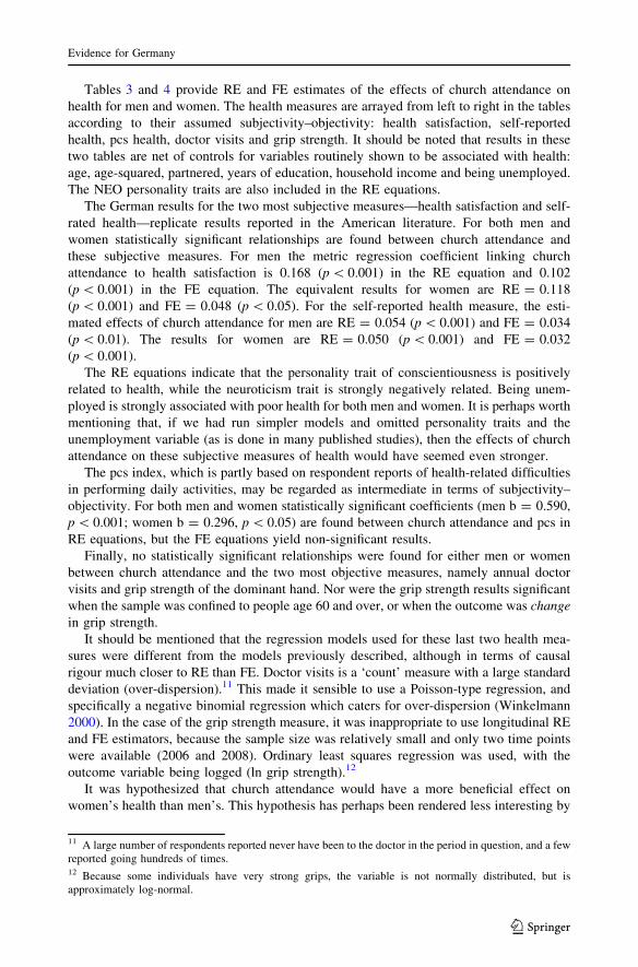
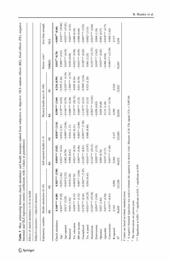
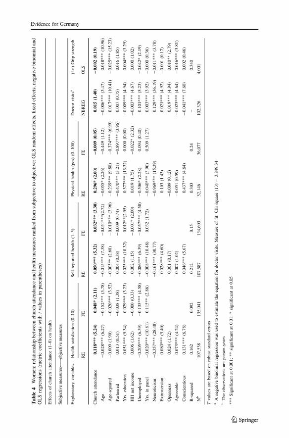
Tables 3 and 4 provide RE and FE estimates of the effects of church attendance on

health for men and women. The health measures are arrayed from left to right in the tables

according to their assumed subjectivity–objectivity: health satisfaction, self-reported

health, pcs health, doctor visits and grip strength. It should be noted that results in these

two tables are net of controls for variables routinely shown to be associated with health:

age, age-squared, partnered, years of education, household income and being unemployed.

The NEO personality traits are also included in the RE equations.

The German results for the two most subjective measures—health satisfaction and self-

rated health—replicate results reported in the American literature. For both men and

women statistically significant relationships are found between church attendance and

these subjective measures. For men the metric regression coefficient linking church

attendance to health satisfaction is 0.168 (p \ 0.001) in the RE equation and 0.102

(p \ 0.001) in the FE equation. The equivalent results for women are RE = 0.118

(p \ 0.001) and FE = 0.048 (p \ 0.05). For the self-reported health measure, the esti-

mated effects of church attendance for men are RE = 0.054 (p \ 0.001) and FE = 0.034

(p \ 0.01). The results for women are RE = 0.050 (p \ 0.001) and FE = 0.032

(p \ 0.001).

The RE equations indicate that the personality trait of conscientiousness is positively

related to health, while the neuroticism trait is strongly negatively related. Being unem-

ployed is strongly associated with poor health for both men and women. It is perhaps worth

mentioning that, if we had run simpler models and omitted personality traits and the

unemployment variable (as is done in many published studies), then the effects of church

attendance on these subjective measures of health would have seemed even stronger.

The pcs index, which is partly based on respondent reports of health-related difficulties

in performing daily activities, may be regarded as intermediate in terms of subjectivity–

objectivity. For both men and women statistically significant coefficients (men b = 0.590,

p \ 0.001; women b = 0.296, p \ 0.05) are found between church attendance and pcs in

RE equations, but the FE equations yield non-significant results.

Finally, no statistically significant relationships were found for either men or women

between church attendance and the two most objective measures, namely annual doctor

visits and grip strength of the dominant hand. Nor were the grip strength results significant

when the sample was confined to people age 60 and over, or when the outcome was change

in grip strength.

It should be mentioned that the regression models used for these last two health mea-

sures were different from the models previously described, although in terms of causal

rigour much closer to RE than FE. Doctor visits is a ‘count’ measure with a large standard

deviation (over-dispersion).11 This made it sensible to use a Poisson-type regression, and

specifically a negative binomial regression which caters for over-dispersion (Winkelmann

2000). In the case of the grip strength measure, it was inappropriate to use longitudinal RE

and FE estimators, because the sample size was relatively small and only two time points

were available (2006 and 2008). Ordinary least squares regression was used, with the

outcome variable being logged (ln grip strength).12

It was hypothesized that church attendance would have a more beneficial effect on

women’s health than men’s. This hypothesis has perhaps been rendered less interesting by

11 A large number of respondents reported never have been to the doctor in the period in question, and a fewreported going hundreds of times.12 Because some individuals have very strong grips, the variable is not normally distributed, but isapproximately log-normal.

Evidence for Germany

123

Ta

ble

3M

en:

rela

tionsh

ipbet

wee

nch

urc

hat

tendan

cean

dhea

lth

mea

sure

sra

nked

from

subje

ctiv

eto

obje

ctiv

e:G

LS

random

effe

cts

(RE

),fi

xed

effe

cts

(FE

),neg

ativ

eb

ino

mia

lan

dO

LS

reg

ress

ion

s(m

etri

cco

effi

cien

tsw

ith

tv

alu

esin

par

enth

eses

)

Eff

ects

of

churc

hat

tendan

ce(1

–0)

on

hea

lth

Subje

ctiv

em

easu

res !

obje

ctiv

em

easu

res

Expla

nat

ory

var

iable

sH

ealt

hsa

tisf

acti

on

(0–10)

Sel

f-re

port

edhea

lth

(1–5)

Physi

cal

hea

lth

(pcs

)(0

–100)

Doct

or

vis

itsa

(Ln)

Gri

pst

rength

RE

FE

RE

FE

RE

FE

NB

RE

GO

LS

Churc

hat

tendan

ce0.1

68***

(6.8

0)

0.1

02***

(3.9

8)

0.0

54***

(5.0

2)

0.0

34**

(3.1

4)

0.5

90***

(3.6

0)

0.2

16

(0.9

9)

0.0

11

ns

(0.7

0)

20.0

01

ns

(0.4

6)

Age

-0.0

47***

(9.2

0)

-0.0

70

(1.8

4)

-0.0

21***

(9.4

4)

-0.0

34

(1.8

1)

-0.1

30***

(4.9

2)

-0.5

95

(1.4

6)

0.0

06**

(2.6

3)

0.0

16***

(10.8

6)

Age-

squar

ed0.0

11*

(2.2

0)

-0.0

16*(2

.52)

0.0

02

(0.7

0)

-0.0

09**

(2.9

6)

-0.1

46***

(5.5

9)

-0.2

45***

(4.3

4)

0.0

15***

(6.5

4)

-0.0

23***

(15.8

1)

Par

tner

ed0.0

43

(1.5

4)

0.0

37(1

.20)

0.0

08

(0.6

3)

0.0

16

(1.1

7)

-0.6

88***

(4.4

8)

-1.0

94***

(4.7

5)

0.0

10

(0.6

8)

0.0

43***

(5.4

7)

Yrs

.ed

uca

tion

0.0

36***

(6.3

2)

-0.0

07(0

.70)

0.0

21***

(8.5

5)

-0.0

01

(0.3

1)

0.5

39***

(20.3

3)

0.0

29

(0.3

6)

-0.0

22***

(9.9

8)

-0.0

00

(0.1

0)

HH

net

inco

me

0.0

18***

(5.3

2)

0.0

07**

(2.8

0)

0.0

07***

(5.0

6)

0.0

03**

(2.8

0)

0.0

68***

(3.3

2)

0.0

11

(0.7

0)

-0.0

11***

(6.9

5)

-0.0

00

(0.4

0)

Unem

plo

yed

-0.2

78***

(8.2

6)

-0.2

26***

(7.4

5)

-0.1

20***

(8.8

1)

-0.0

93***

(7.5

8)

-1.1

16***

(4.5

3)

-0.5

89*

(2.2

4)

0.1

50***

(6.0

2)

-0.0

67***

(3.9

3)

Yrs

.in

pan

el-

0.0

31***

(16.2

5)

0.0

16

(0.4

3)

-0.0

14***

(15.9

7)

0.0

08

(0.4

0)

-0.0

52***

(5.1

5)

0.5

23

(1.2

8)

0.0

01

(1.2

5)

-0.0

02*

(3.1

3)

Neu

roti

cism

-0.3

45***

(25.3

0)

-0.1

44***

(25.4

1)

-0.9

01***

(13.8

1)

0.1

53***

(31.5

7)

-0.0

13***

(4.0

4)

Extr

over

sion

0.0

54***

(3.6

9)

0.0

20***

(3.3

2)

-0.0

58

(0.8

3)

0.0

19***

(3.6

2)

0.0

04

(1.3

4)

Open

nes

s0.0

27

(1.8

2)

0.0

05

(0.7

6)

0.0

29

(0.4

0)

0.0

32***

(6.0

2)

-0.0

01

(0.1

7)

Agre

eable

0.0

77***

(4.5

8)

0.0

15*

(2.1

7)

0.1

21

(1.4

9)

-0.0

06

(0.9

4)

-0.0

18***

(4.7

7)

Consc

ienti

ous

0.1

54***

(8.6

3)

0.0

57***

(7.4

0)

0.5

13***

(5.7

9)

-0.0

83***

(12.5

9)

0.0

04

(1.0

2)

R-s

quar

ed0.1

63

0.0

90

0.2

04

0.1

47

0.2

90

0.2

10

–0.3

17

Nb

96,8

49

123,2

98

96,8

32

122,8

05

28,8

56

32,8

52

92,0

97

3,6

58

Tval

ues

are

bas

edon

robust

stan

dar

der

rors

aA

neg

ativ

ebin

om

ial

regre

ssio

nw

asuse

dto

esti

mat

eth

eeq

uat

ion

for

doct

or

vis

its.

Mea

sure

of

fit:

Chi

squar

e(1

3)

=5,0

97.6

0b

The

obse

rvat

ions

are

per

son-y

ears

***

Sig

nifi

cant

at0.0

01;

**

signifi

cant

at0.0

1;

*si

gnifi

cant

at0.0

5

B. Headey et al.

123

Ta

ble

4W

om

en:

rela

tionsh

ipbet

wee

nch

urc

hat

tendan

cean

dhea

lth

mea

sure

sra

nked

from

subje

ctiv

eto

obje

ctiv

e:G

LS

random

effe

cts,

fixed

effe

cts,

neg

ativ

eb

ino

mia

lan

dO

LS

regre

ssio

ns

(met

ric

coef

fici

ents

wit

ht

val

ues

inp

aren

thes

es)

Eff

ects

of

churc

hat

tendan

ce(1

–0)

on

hea

lth

Subje

ctiv

em

easu

res !

obje

ctiv

em

easu

res

Expla

nat

ory

var

iable

sH

ealt

hsa

tisf

acti

on

(0–10)

Sel

f-re

port

edhea

lth

(1–5)

Physi

cal

hea

lth

(pcs

)(0

–100)

Doct

or

vis

itsa

(Ln)

Gri

pst

rength

RE

FE

RE

FE

RE

FE

NB

RE

GO

LS

Churc

hat

tendan

ce0.1

18***

(5.2

4)

0.0

48*

(2.1

1)

0.0

50***

(5.3

2)

0.0

32***

(3.3

0)

0.2

96*

(2.0

0)

20.0

09

(0.0

5)

0.0

15

(1.4

0)

20.0

02

(0.1

9)

Age

-0.0

28***

(6.2

7)

-0.1

52***

(3.7

8)

-0.0

15***

(7.3

8)

-0.0

51***(2

.72)

-0.0

55*

(2.2

6)

-0.4

49

(1.1

2)

-0.0

06***

(3.4

7)

0.0

18***

(10.9

6)

Age-

squar

ed-

0.0

09

(1.9

0)

-0.0

20***

(3.5

2)

-0.0

05**

(2.6

8)

-0.0

10***

(3.9

6)

-0.2

39***

(9.8

8)

-0.3

74***

(6.9

9)

0.0

17***

(10.4

1)

-0.0

25***

(15.2

3)

Par

tner

ed0.0

13

(0.5

1)

-0.0

38

(1.3

8)

0.0

04

(0.3

8)

-0.0

09

(0.7

4)

-0.4

70***

(3.2

1)

-0.8

97***

(3.9

6)

0.0

07

(0.7

5)

0.0

16

(1.8

5)

Yrs

.ed

uca

tion

0.0

51***

(9.3

4)

0.0

29***

(3.2

3)

0.0

25***

(10.3

2)

0.0

12**(2

.95)

0.3

77***

(13.3

2)

0.0

00

(0.0

0)

-0.0

09***

(4.9

4)

0.0

04***

(3.2

9)

HH

net

inco

me

0.0

06

(1.6

2)

-0.0

00

(0.3

3)

0.0

02

(1.1

5)

-0.0

01*

(2.0

0)

0.0

19

(1.7

5)

-0.0

22*

(2.3

2)

-0.0

03***

(4.6

7)

0.0

00

(1.0

2)

Unem

plo

yed

-0.2

05***

(6.3

9)

-0.1

35***

(4.5

8)

-0.0

86***

(6.3

9)

-0.0

57***

(4.5

8)

-0.5

06*

(2.2

8)

0.0

94

(0.4

0)

0.1

01***

(5.2

3)

-0.0

42*

(2.1

9)

Yrs

.in

pan

el-

0.0

20***

(10.8

1)

0.1

15**

(2.8

6)

-0.0

08***

(10.4

8)

0.0

32

(1.7

2)

-0.0

40***

(3.9

0)

0.5

09

(1.2

7)

0.0

03***

(3.9

2)

-0.0

00

(0.3

6)

Neu

roti

cism

-0.3

57***

(28.4

8)

-0.1

61***

(30.7

7)

-0.9

69***

(15.3

9)

0.1

29***

(36.1

9)

-0.0

11***

(3.7

8)

Extr

over

sion

0.0

80***

(5.4

0)

0.0

28***

(4.6

0)

0.1

03

(1.4

3)

0.0

21***

(4.9

2)

-0.0

01

(0.1

7)

Open

nes

s0.0

24

(1.7

2)

0.0

01

(0.1

7)

-0.0

09

(0.1

2)

0.0

19***

(4.9

4)

0.0

10**

(2.7

9)

Agre

eable

0.0

73***

(4.2

4)

0.0

07

(1.0

2)

-0.0

51

(0.5

9)

-0.0

23***

(4.6

4)

-0.0

16***

(3.8

1)

Consc

ienti

ous

0.1

31***

(6.7

8)

0.0

46***

(5.6

7)

0.4

37***

(4.6

4)

-0.0

41***

(7.6

0)

0.0

02

(0.4

6)

R-s

quar

ed0.1

62

0.0

92

0.2

12

0.1

50.3

03

0.2

4–

0.3

40

Nb

107,5

38

135,0

41

107,5

87

134,6

03

32,1

46

36,0

77

102,3

26

4,0

01

Tval

ues

are

bas

edon

robust

stan

dar

der

rors

aA

neg

ativ

ebin

om

ial

regre

ssio

nw

asuse

dto

esti

mat

eth

eeq

uat

ion

for

doct

or

vis

its.

Mea

sure

of

fit:

Chi

squar

e(1

3)

=3,8

49.3

4b

The

obse

rvat

ions

are

per

son-y

ears

***

Sig

nifi

cant

at0.0

01;

**

signifi

cant

at0.0

1;

*si

gnifi

cant

at0.0

5

Evidence for Germany

123

finding that the apparent strength of all effects depends heavily on which measures are

used. However, if we focus just on the three more subjective measures in Tables 3 and 4,

the evidence could be read as indicating that, if anything, men benefit somewhat more than

women.13 We will find similar pro-male evidence in a later section on mortality. The

thorny issue of whether the church attendance-health link is mainly an artefact of sub-

jective measurement is covered in the next section.

3.1.1 Is the Link Between Church Attendance and Health Measures Partly Due

to Satisfaction Bias/Positivity Bias? Issues of Measurement Validity

In this section we present evidence which suggests that the apparent link between church

attendance and better health might be due to satisfaction bias/positivity bias. This evidence

will be more or less contradicted later, but first let us see where the trail leads us.

It is certainly the case that religious people report that they are relatively satisfied with

everything under the sun (Andrews and Withey 1976; Campbell et al. 1976; Argyle 2001).

In SOEP there are positive correlations between church attendance and such miscellaneous

items as job satisfaction, leisure satisfaction, satisfaction with one’s school grades (years

ago), satisfaction with local public transport, and satisfaction with the introduction of the

Euro. It may be, of course, that religious people really are more satisfied with everything—

we come back to this possibility later—but it is also possible that what may be termed

satisfaction bias or positivity bias, is wholly or partly responsible for apparent links

between church attendance and subjective measures of health.

Our first approach to assessing this issue is to construct a composite measure of sat-

isfaction from four survey items which have been included in SOEP in most survey years:

job satisfaction, leisure satisfaction, satisfaction with household income, and satisfaction

with your household work. These items are all measured on the same 0–10 scale as life

satisfaction; the composite measure was constructed simply by averaging respondents’

scores. The Pearson correlation between this composite satisfaction measure and church

attendance is 0.078 (p \ 0.001). Its correlations with the subjective health measures are all

substantial: 0.446 with health satisfaction, 0.320 with self-reported health, and 0.207 with

the pcs health index. Correlations with the more objective measures of health are in the

expected direction but not statistically significant: -0.028 with (ln)doctor visits and 0.011

with (ln)grip strength of the dominant hand. Notice that these correlations decline

monotonically, moving from the most subjective to the most objective measures of health.

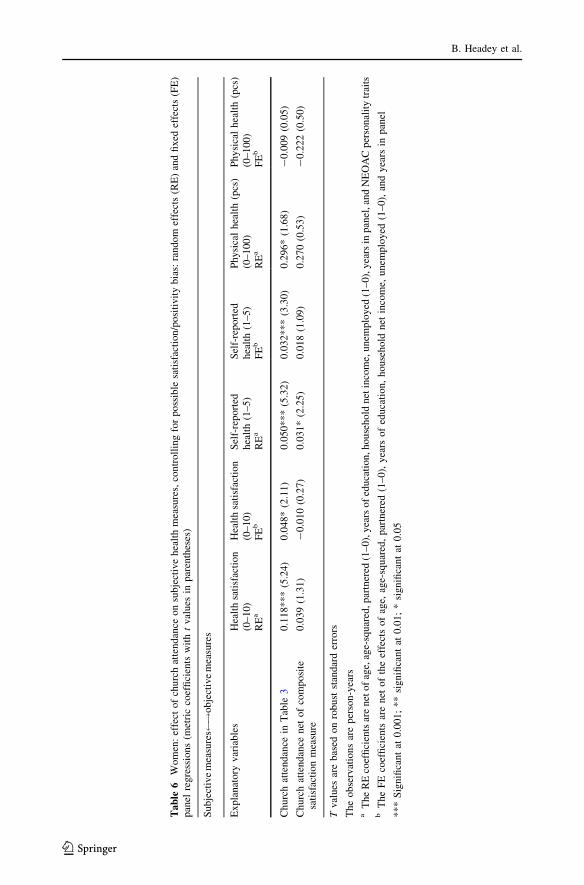
The next step is to see what happens to the associations reported in Tables 3 (men) and

4 (women) between church attendance and the subjective health measures, when we add

the composite satisfaction measure as a ‘control’. The original estimates (which were net

of demographic, socio-economic and personality trait controls) and the revised estimates

with the extra control are compared in Tables 5 and 6.

The evidence in these two tables could be read as indicating that the link between

church attendance and subjective health measures is in large part due to satisfaction/

positivity bias. Most of the relationships initially estimated to be statistically significant in

Tables 3 and 4 turn out to be non-significant, when the composite satisfaction measure is

added to equations as an extra ‘control’. In the men’s equations five out of six coefficients

for the effects of church attendance were initially estimated to be statistically significant, at

13 Again using the subjective measures, no differences in the church attendance-health link were foundbetween Protestants and Catholics. Nor did church attendance appear to benefit older people, or specificallyolder widows, more than younger people.

B. Headey et al.

123

Ta

ble

5M

en:

effe

cto

fch

urc

hat

ten

dan

ceo

nsu

bje

ctiv

eh

ealt

hm

easu

res,

con

tro

llin

gfo

rp

oss

ible

sati

sfac

tio

n/p

osi

tiv

ity

bia

s:ra

nd

om

effe

cts

(RE

)an

dfi

xed

effe

cts

(FE

)p

anel

regre

ssio

ns

(met

ric

coef

fici

ents

wit

ht

val

ues

inp

aren

thes

es)

Su

bje

ctiv

em

easu

res !

ob

ject

ive

mea

sure

s

Expla

nat

ory

var

iable

sH

ealt

hsa

tisf

acti

on

(0–

10)

Hea

lth

sati

sfac

tio

n(0

–1

0)

Sel

f-re

port

edh

ealt

h(1

–5

)S

elf-

rep

ort

edh

ealt

h(1

–5

)P

hysi

cal

hea

lth

(pcs

)(0

–1

00

)P

hy

sica

lh

ealt

h(p

cs)

(0–

100

)R

Ea

FE

bR

Ea

FE

bR

Ea

FE

b

Ch

urc

hat

ten

dan

cein

Tab

le3

0.1

68

**

*(6

.80

)0

.102

**

*(3

.98

)0

.054

**

*(5

.02

)0

.034

**

(3.1

4)

0.5

90

**

*(3

.60

)0

.216

(0.9

9)

Ch

urc

hat

ten

dan

cen

eto

fco

mp

osi

tesa

tisf

acti

on

mea

sure

0.1

03

**

(2.8

5)

0.0

36

(0.7

7)

0.0

24

(1.4

6)

-0

.021

(1.0

7)

0.6

04

*(2

.26

)-

0.4

71

(1.9

4)

Tv

alues

are

bas

edo

nro

bu

stst

andar

der

rors

Th

eo

bse

rvat

ion

sar

ep

erso

n-y

ears

aT

he

RE

coef

fici

ents

are

net

of

age,

age-

squ

ared

,p

artn

ered

(1–

0),

yea

rso

fed

uca

tio

n,

ho

use

ho

ldn

etin

com

e,u

nem

plo

yed

(1–

0),

yea

rsin

pan

el,

and

the

NE

OA

Cp

erso

nal

ity

trai

tsb

The

FE

coef

fici

ents

are

net

of

the

effe

cts

of

age,

age-

squar

ed,

par

tner

ed(1

–0),

yea

rso

fed

uca

tion,

house

hold

net

inco

me,

unem

plo

yed

(1–0),

and

yea

rsin

pan

el

**

*S

ign

ifica

nt

at0

.00

1;

**

sig

nifi

can

tat

0.0

1;

*S

ign

ifica

nt

at0

.05

Evidence for Germany

123

Ta

ble

6W

om

en:

effe

ctof

churc

hat

tendan

ceon

subje

ctiv

ehea

lth

mea

sure

s,co

ntr

oll

ing

for

poss

ible

sati

sfac

tion/p

osi

tivit

ybia

s:ra

ndom

effe

cts

(RE

)an

dfi

xed

effe

cts

(FE

)pan

elre

gre

ssio

ns

(met

ric

coef

fici

ents

wit

ht

val

ues

inp

aren

thes

es)

Su

bje

ctiv

em

easu

res !

ob

ject

ive

mea

sure

s

Expla

nat

ory

var

iable

sH

ealt

hsa

tisf

acti

on

(0–

10)

Hea

lth

sati

sfac

tio

n(0

–1

0)

Sel

f-re

port

edh

ealt

h(1

–5

)S

elf-

rep

ort

edh

ealt

h(1

–5

)P

hysi

cal

hea

lth

(pcs

)(0

–1

00

)P

hy

sica

lh

ealt

h(p

cs)

(0–

100

)R

Ea

FE

bR

Ea

FE

bR

Ea

FE

b

Ch

urc

hat

ten

dan

cein

Tab

le3

0.1

18

**

*(5

.24

)0

.048

*(2

.11

)0

.050

**

*(5

.32

)0

.032

**

*(3

.30

)0

.29

6*

(1.6

8)

-0

.00

9(0

.05

)

Ch

urc

hat

ten

dan

cen

eto

fco

mp

osi

tesa

tisf

acti

on

mea

sure

0.0

39

(1.3

1)

-0

.010

(0.2

7)

0.0

31

*(2

.25

)0

.018

(1.0

9)

0.2

70

(0.5

3)

-0

.22

2(0

.50

)

Tv

alues

are

bas

edo

nro

bu

stst

andar

der

rors

Th

eo

bse

rvat

ion

sar

ep

erso

n-y

ears

aT

he

RE

coef

fici

ents

are

net

of

age,

age-

squ

ared

,p

artn

ered

(1–

0),

yea

rso

fed

uca

tio

n,h

ou

seh

old

net

inco

me,

un

emp

loy

ed(1

–0

),y

ears

inp

anel

,an

dN

EO

AC

per

son

alit

ytr

aits

bT

he

FE

coef

fici

ents

are

net

of

the

effe

cts

of

age,

age-

squar

ed,

par

tner

ed(1

–0),

yea

rso

fed

uca

tion,

house

hold

net

inco

me,

unem

plo

yed

(1–0),

and

yea

rsin

pan

el

**

*S

ign

ifica

nt

at0

.00

1;

**

sig

nifi

can

tat

0.0

1;

*si

gn

ifica

nt

at0

.05

B. Headey et al.

123

least at the 0.01 level. Of these just one remains significant at the 0.01 level, and another at

the 0.05 level. In the women’s equations only one out of an initial five coefficients remains

significant, and that only at the 0.05 level.

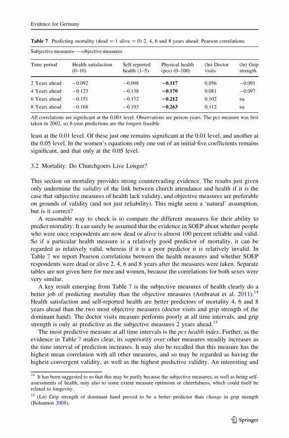
3.2 Mortality: Do Churchgoers Live Longer?

This section on mortality provides strong countervailing evidence. The results just given

only undermine the validity of the link between church attendance and health if it is the

case that subjective measures of health lack validity, and objective measures are preferable

on grounds of validity (and not just reliability). This might seem a ‘natural’ assumption,

but is it correct?

A reasonable way to check is to compare the different measures for their ability to

predict mortality. It can surely be assumed that the evidence in SOEP about whether people

who were once respondents are now dead or alive is almost 100 percent reliable and valid.

So if a particular health measure is a relatively good predictor of mortality, it can be

regarded as relatively valid, whereas if it is a poor predictor it is relatively invalid. In

Table 7 we report Pearson correlations between the health measures and whether SOEP

respondents were dead or alive 2, 4, 6 and 8 years after the measures were taken. Separate

tables are not given here for men and women, because the correlations for both sexes were

very similar.

A key result emerging from Table 7 is the subjective measures of health clearly do a

better job of predicting mortality than the objective measures (Ambrasat et al. 2011).14

Health satisfaction and self-reported health are better predictors of mortality 4, 6 and 8

years ahead than the two most objective measures (doctor visits and grip strength of the

dominant hand). The doctor visits measure performs poorly at all time intervals, and grip

strength is only as predictive as the subjective measures 2 years ahead.15

The most predictive measure at all time intervals is the pcs health index. Further, as the

evidence in Table 7 makes clear, its superiority over other measures steadily increases as

the time interval of prediction increases. It may also be recalled that this measure has the

highest mean correlation with all other measures, and so may be regarded as having the

highest convergent validity, as well as the highest predictive validity. An interesting and

Table 7 Predicting mortality (dead = 1 alive = 0) 2, 4, 6 and 8 years ahead: Pearson correlations

Subjective measures !objective measures

Time period Health satisfaction(0–10)

Self-reportedhealth (1–5)

Physical health(pcs) (0–100)

(ln) Doctorvisits

(ln) Gripstrength

2 Years ahead -0.092 -0.098 20.117 0.056 -0.091

4 Years ahead -0.123 -0.138 20.170 0.081 -0.097

6 Years ahead -0.151 -0.172 20.212 0.102 na

8 Years ahead -0.168 -0.193 20.263 0.112 na

All correlations are significant at the 0.001 level. Observations are person-years. The pcs measure was firsttaken in 2002, so 8-year predictions are the longest feasible

14 It has been suggested to us that this may be partly because the subjective measures, as well as being self-assessments of health, may also to some extent measure optimism or cheerfulness, which could itself berelated to longevity.15 (Ln) Grip strength of dominant hand proved to be a better predictor than change in grip strength(Bohannon 2008).

Evidence for Germany

123

perhaps critical feature of the pcs measure is that it is intermediate in the range from

subjective to objective. Recall that it combines self-rated health on a 1–5 scale with other

items measuring the difficulty a person experiences in performing routine tasks of daily

living.

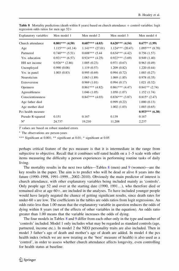
The mortality results in the next two tables—Tables 8 (men) and 9 (women)—are the

key results in the paper. The aim is to predict who will be dead or alive 8 years into the

future (1990–1998, 1991–1999…2002–2010). Obviously the main predictor of interest is

church attendance, with other explanatory variables being included mainly as ‘controls’.

Only people age 52 and over at the starting date (1990, 1991…), who therefore died or

remained alive at age 60?, are included in the analyses. To have included younger people

would have largely negated the chance of getting significant results, since death rates for

under-60 s are low. The coefficients in the tables are odds ratios from logit regressions. An

odds ratio less than 1.00 mean that the explanatory variable in question reduces the odds of

dying within 8 years (net of the effects of other variables in the equation). An odds ratio

greater than 1.00 means that the variable increases the odds of dying.

The four models in Tables 8 and 9 differ from each other only in the type and number of

‘controls’ included. Model 1 only includes what may be regarded as standard controls (age,

partnered, income etc.). In model 2 the NEO personality traits are also included. Then in

model 3 father’s age of death and mother’s age of death are added. In model 4 the pcs

health index (which we are now treating as the ‘best’ measure of health) is also used as a

‘control’, in order to assess whether church attendance affects longevity, even controlling

for health status at baseline.

Table 8 Mortality predictions (death within 8 years) based on church attendance ? control variables: logitregression odds ratios for men age 52?

Explanatory variables Men model 1 Men model 2 Men model 3 Men model 4

Church attendance 0.801*** (4.50) 0.687*** (4.03) 0.620*** (4.54) 0.677* (1.99)

Age 1.115*** (41.14) 1.141*** (27.01) 1.124*** (20.47) 1.095*** (8.70)

Partnered 0.740*** (5.51) 0.608*** (5.44 0.634*** (4.42) 0.756 (1.57)

Yrs. education 0.921*** (6.57) 0.924*** (4.25) 0.922*** (3.69) 0.949 (1.40)

HH net income 0.926** (2.86) 1.005 (0.23) 0.971 (0.67) 0.963 (0.49)

Unemployed 0.990 (0.08) 1.119 (0.57) 1.209 (0.82) 1.220 (0.44)

Yrs. in panel 1.003 (0.83) 0.995 (0.69) 0.994 (0.72) 1.003 (0.27)

Neuroticism 1.063 (1.89) 1.069 (1.85) 0.978 (0.35)

Extroversion 0.969 (1.01) 0.994 (0.17) 1.021 (0.32)

Openness 0.861*** (4.82) 0.861*** (4.47) 0.841** (2.74)

Agreeableness 1.046 (1.05) 1.050 (1.07) 1.152 (1.74)

Conscientiousness 0.847*** (4.03) 0.836*** (3.87) 0.815* (2.47)

Age father died 0.999 (0.22) 1.000 (0.13)

Age mother died 1.002 (1.03) 1.003 (0.65)

Pcs health measure 0.953*** (6.38)

Pseudo R-squared 0.151 0.167 0.139 0.167

Na 24,737 19,210 11,208 2,237

T values are based on robust standard errorsa The observations are person-years

*** Significant at 0.001; ** significant at 0.01; * significant at 0.05

B. Headey et al.

123

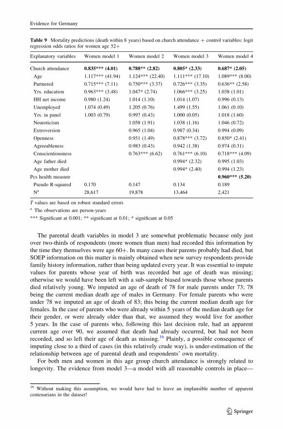
The parental death variables in model 3 are somewhat problematic because only just

over two-thirds of respondents (more women than men) had recorded this information by

the time they themselves were age 60?. In many cases their parents probably had died, but

SOEP information on this matter is mainly obtained when new survey respondents provide

family history information, rather than being updated every year. It was essential to impute

values for parents whose year of birth was recorded but age of death was missing;

otherwise we would have been left with a sub-sample biased towards those whose parents

died relatively young. We imputed an age of death of 78 for male parents under 73; 78

being the current median death age of males in Germany. For female parents who were

under 78 we imputed an age of death of 83; this being the current median death age for

females. In the case of parents who were already within 5 years of the median death age for

their gender, or were already older than that, we assumed they would live for another

5 years. In the case of parents who, following this last decision rule, had an apparent

current age over 90, we assumed that death had already occurred, but had not been

recorded, and so left their age of death as missing.16 Plainly, a possible consequence of

imputing close to a third of cases (in this relatively crude way), is under-estimation of the

relationship between age of parental death and respondents’ own mortality.

For both men and women in this age group church attendance is strongly related to

longevity. The evidence from model 3—a model with all reasonable controls in place—

Table 9 Mortality predictions (death within 8 years) based on church attendance ? control variables: logitregression odds ratios for women age 52?

Explanatory variables Women model 1 Women model 2 Women model 3 Women model 4

Church attendance 0.835*** (4.01) 0.788** (2.82) 0.805* (2.33) 0.687* (2.05)

Age 1.117*** (41.94) 1.124*** (22.40) 1.111*** (17.10) 1.089*** (8.00)

Partnered 0.715*** (7.11) 0.750*** (3.37) 0.726*** (3.35) 0.636** (2.58)

Yrs. education 0.963*** (3.48) 1.047* (2.74) 1.066*** (3.25) 1.038 (1.01)

HH net income 0.980 (1.24) 1.014 (1.10) 1.014 (1.07) 0.996 (0.13)

Unemployed 1.074 (0.49) 1.205 (0.76) 1.499 (1.55) 1.061 (0.10)

Yrs. in panel 1.003 (0.79) 0.997 (0.43) 1.000 (0.05) 1.018 (1.60)

Neuroticism 1.058 (1.91) 1.038 (1.16) 1.046 (0.72)

Extroversion 0.965 (1.04) 0.987 (0.34) 0.994 (0.09)

Openness 0.951 (1.49) 0.878*** (3.72) 0.850* (2.41)

Agreeableness 0.983 (0.43) 0.942 (1.38) 0.974 (0.31)

Conscientiousness 0.763*** (6.62) 0.761*** (6.10) 0.718*** (4.09)

Age father died 0.994* (2.32) 0.995 (1.03)

Age mother died 0.994* (2.40) 0.994 (1.23)

Pcs health measure 0.960*** (5.20)

Pseudo R-squared 0.170 0.147 0.134 0.189

Na 28,617 19,878 13,464 2,421

T values are based on robust standard errorsa The observations are person-years

*** Significant at 0.001; ** significant at 0.01; * significant at 0.05

16 Without making this assumption, we would have had to leave an implausible number of apparentcentenarians in the dataset!

Evidence for Germany

123

indicates that the odds of men dying within 8 years are 38 % lower (odds ratio = 0.620,

p \ 0.001) if they attend church regularly rather than seldom or never. For women church

attendance reduces mortality by just under 20 % (odds ratio = 0.805, p \ 0.05).

The evidence in Tables 8 and 9 confirms previous research in showing that longevity is

related to being partnered (odds ratio for men in model 3 = 0.634, p \ 0. 001; for women

odds ratio = 0.726, p \ 0.001) and is also increased by rating high on the personality trait

of conscientiousness (men’s odds ratio in model 3 = 0.836, p \ 0.001; women’s

ratio = 0.761, p \ 0.001) (Strawbridge et al. 1997; Friedman and Martin 2011; Koenig

et al. 2012).

In this dataset the age at which their parents died appears to be associated with women’s

but not men’s mortality rates.17 For every extra year their father lived, women’s odds of

dying within the next 8 years are reduced by about half of one percent, with a similar

margin for every extra year their mother lived. As noted above, it is possible that inter-

generational longevity links would have appeared stronger if more complete data were

available on age of parental death (but see Lach et al. 2006 for not dissimilar results in a

large Israeli study).

The results for model 4—the final column in these tables—are astonishing. Here we

control for health status at baseline.18 It transpires that church attendance has a statistically

significant effect on mortality, even controlling for pcs 8 years before. The odds of

churchgoing men and women dying within 8 years are nearly one-third lower (men’s odds

ratio 0.677, p \ 0.05; women’s odds ratio 0.687, p \ 0.05) than the odds for individuals

who are non-churchgoers but otherwise have the same health status (and the same age,

education, income and personality traits) at baseline.

The wheel has come full circle. In the previous section we reviewed evidence that lent

itself to the interpretation that the apparent link between church attendance and health is

due to satisfaction/positivity bias in the more subjective measures of health. But then

countervailing evidence made it clear that the subjective measures, and even more the

intermediate pcs measure, are in one key respect—ability to predict mortality—more valid

than the objective measures. Finally, evidence on mortality showed that church attendance

significantly reduces the probability of dying, even controlling for health status at baseline.

4 Church Attendance is Linked to Better Health Indirectly Via Health ProtectiveAttitudes and Behaviors: A Structural Equation Model

Plainly, it is improbable that attending church could by itself make individuals healthier

and longer lived.19 There must be intermediate causal ‘‘mechanisms’’—intermediate

17 Age of father’s death (but not age of mother’s death) appears significantly related to men’s own longevityin alternative equations in which personality traits are omitted. Further, the results linking women’s lon-gevity to parental longevity are strengthened if traits are omitted. It may be noted that personality traits werenot included as controls in the Israeli and Icelandic studies cited in the ‘‘Introduction’’, which showedstatistically significant but weak intergenerational longevity linkages.18 In this table only the coefficients for church attendance and the pcs health measure are of interest. Theother variables are worth inclusion as ‘controls’, but their coefficients are somewhat misleading because thecausal ordering is inappropriate. For example, the variables measuring age, partnership status and years ofeducation should be regarded as causally antecedent to the pcs health measure. See Table 5 for preferableestimates.19 Note, however, the Norwegian study referenced above which indicated that attending religious serviceslowers blood pressure (Sorensen et al. 2011).

B. Headey et al.

123

links—between church attendance and health which account for health benefits. In this

section we offer a structural equation model which estimates the effects of some of these

causal mechanisms. The mechanisms include non-smoking, taking regular exercise and

enjoying higher than average life satisfaction, all of which are associated with both church

attendance and religious belief. There are likely to be other more intangible mechanisms,

which for lack of evidence in SOEP, we cannot investigate here. These may include the

spiritual comfort and sense of purpose and meaning in life which religion can provide.

First some bivariate and partial correlations which show associations between church

attendance and a range of health protective (and risk-avoiding) attitudes and behaviors. In

the SOEP dataset the correlation between church attendance and smoking (1 = smoker

0 = non-smoker) is -0.173 (p \ 0.001). Correlations with being risk averse and health

risk averse are, respectively, 0.079 (p \ 0.001) and 0.084 (p \ 0.001). Controlling for

gender and age, the partial correlation between church attendance and being partnered

which, as we have seen, is quite strongly related to better health, is 0.108 (p \ 0.001).

Churchgoers are somewhat less likely to become separated or divorced; the partial cor-

relation, controlling for gender and age is -0.030 (p \ 0.001). Churchgoers also take more

exercise (partial correlation = 0.044, p \ 0.001) and have higher rates of social engage-

ment/participation (partial correlation = 0.085, p \ 0.001). Both these behaviors are

associated with better health; the partial correlation of the pcs index with exercise (again

controlling for gender and age) is 0.044 (p \ 0.001) and with social participation it is 0.085

(p \ 0.001).

Religious individuals mostly come from religious families. In the SOEP data the

bivariate correlation between respondents’ own level of church attendance and fathers’

attendance is 0.580 (p \ 0.001); with mothers’ attendance it is 0.571 (p \ 0.001). To a

considerable extent, parents inculcate not only religious belief and practice, but also the

health-protective and health risk-avoidance attitudes and behaviors just reviewed. There

are positive associations in the German data between parent and ‘child’ levels of smoking,

risk aversion, exercise and social participation (Headey et al. 2013).

More important for health and longevity than any of the attitudes or behaviors con-

sidered so far is life satisfaction/happiness. It has been shown that church attendance is

quite strongly associated with higher than average life satisfaction (Myers 2013; Clark and

Lelkes 2009). The link holds in the German dataset even in fixed effects models (Headey

et al. 2010). Furthermore, it is well established that life satisfaction is associated with better

health and longevity (Deeg and van Zonneveld 1989; Diener et al. 1999; Argyle 2001;

Ambrasat et al. 2011). Just by way of illustration: in the SOEP data the correlation of life

satisfaction with 8-year mortality is -0.120 (p \ 0.001). So, if life satisfaction had been

included in Table 8 as a quasi-health measure, it would have performed better than doctor

visits and, presumably, grip strength (Ambrasat et al. 2011).20

The structural equation model in Fig. 1 shows links from church attendance to exercise

and (not) smoking, and then through to life satisfaction and our preferred measure of

health, the pcs index. It is a 3-wave panel model of a somewhat unusual kind. It covers the

years 2002–2010 with variables being grouped as contemporaneous, 2-year lagged and

4-year lagged. So the years covered are 2002–2004–2006, then 2004–2006–2008 and

finally 2006–2008–2010. The reason for the 2-year lags is that the pcs measure was only

taken biennially in these particular years. It was thought preferable to run a 3-wave model,

rather than the maximum possible 5-wave model, in order to obtain more reliable results

20 The grip strength measure was first taken in 2006, so it is not possible to make an 8-year prediction.However, grip strength performs less well than life satisfaction for 2- and 4-year predictions.

Evidence for Germany

123

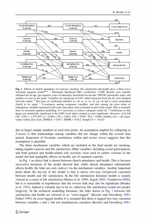
due to larger sample numbers at each time point. An assumption implied by collapsing to

3-waves is that relationships among variables did not change within the overall time

period. Inspection of bivariate correlations within and across waves suggests that this

assumption is plausible.

The three mechanism variables which are included in the final model are smoking,

taking regular exercise and life satisfaction. Other variables, including social participation,

and both general and health-related risk aversion, were tried in earlier versions of the

model but had negligible effects on health, net of standard controls.

In Fig. 1 no direct link is drawn between church attendance and health. This is because

successive iterations of the model showed that, while church attendance substantially

affects health, the links are only indirect via the mechanism variables. Another important

point about the lay-out of the model is that it shows two-way (reciprocal) causation

between health and life satisfaction. In the life satisfaction literature health is usually

viewed as a cause of life satisfaction (Diener et al. 1999; Argyle 2001; Veenhoven 2009),

but it is reasonable to hypothesize that the reverse link may also be significant (Headey

et al. 1991). Indeed it virtually has to be so, otherwise life satisfaction would not predict

longevity. In the technical modelling literature, the links drawn in Fig. 1 between life

satisfaction and health are referred to as ‘‘cross-lagged’’ (Kessler and Greenberg 1981;

Finkel 1995). In cross-lagged models it is assumed that there is lagged two-way causation

between variables x and y, but not simultaneous causation (Kessler and Greenberg 1981;

Fig. 1 Effects of church attendance on exercise, smoking, life satisfaction and health (pcs): a three-wavestructural equation modelabcd. a Maximum likelihood (ML) coefficients *1,000. Results were initiallyobtained net od age, age-squared, years of education, household net income, NEOAC personality traits, andnumber of years in the panel. Variables not significant at 0.05, which detracted from the fit, were droppedfrom the model. b The pairs of coefficients labelled =a, =b, =c, d, =e, =f, =g, =h and =i were constrained(fixed) to be equal. c Covariances among exogenous variables, and also among the error terms ofendogenous variables measured at the same time point, were estimated as part of the model. This is routinelydone in structural equation modelling. It is necessary to achieve adequate model fit. d Coefficients in thisfigure are statistically significant at the 0.001 level unless marked ns (not significant). Measures of fit LRChi2 (229) = 1,575.303 (p \ 0.001); CD = 0.601; CFI = 0.993, TLI = 0.998; stability test = all eigen-values within unit circle; RMSEA = 0.017, SRMR = 0.012; Sample N = 19,423

B. Headey et al.

123

Finkel 1995). It can be shown by calculus that a cross-lagged model is mathematically

justified if the variables implicated in the two-way causation are assumed to influence each

other more or less continuously (Coleman 1968; Tuma and Hannan 1984; Finkel 1995).

This seems plausible in regard to health and life satisfaction.

In this model we make use of a concept of causation due to Nobel Laureate, Clive

Granger. Granger (1969) proposed that x can be regarded as a cause of y if any lagged

values of x remain statistically significant in equations which include multiple lagged

values of y. The intuitions behind what is usually termed ‘‘Granger-causation’’ are that (1)

causes must precede effects in time and (2) if spikes in values of time series variable x are

associated with subsequent spikes in time series y, despite taking account of multiple

lagged values of y, then there is prima facie evidence that x is a cause of y.21 In our model

the estimated links between explanatory variables (e.g. church attendance) lagged by two

waves are net of outcome variables (e.g. smoking) lagged by both two and four waves.22

Not everyone shares Granger’s view of causation. Some specialists in panel data

modelling take the view that, if researchers believe that causal effects are more or less

simultaneous (or occur at time intervals that are closer to simultaneous than the time

between panel waves), then it is better to omit cross-lagged links and instead include

simultaneous links (Kessler and Greenberg 1981).23 An argument in favour of this

approach is that, although coefficients obtained from a cross-lagged model will have the

right sign, they are likely to be biased downwards if simultaneous causation is more or less

what is occurring. Here we rely primarily on a Granger-style model, but we also estimated

a simultaneous causation model and will mention a few results from it.24

A further point of both substantive and methodological importance is that the Fig. 1

model contains nine pairs of equality constraints (pairs of coefficients fixed equal to each

other), marked =a, =b, =c, =d, =e, =f, =g, =h and =i. These coefficients are estimates of

the nine most interesting links in the model: links between church attendance and the

lifestyle mechanism variables, and between life satisfaction and pcs health. It is a rea-

sonable supposition that these links should be stable. That is, one would expect links

between consecutive waves of data to be the same. By imposing these equality constraints,

and then later relaxing them one by one, we can provide sensitivity tests of whether the

links really are stable; stable when nested within the overall model (Kessler and Greenberg

1981; Finkel 1995).25

The Fig. 1 model proves to be a very satisfactory fit to the data. The Comparative Fit

Index (CFI) is 0.993 and the Tucker–Lewis index (TLI) is 0.988; both well above the ‘good

fit’ threshold of 0.95. The RMSEA is 0.017 (a good fit is generally taken to be below 0.05)

21 Initially, Granger’s reasoning only applied to pairs of variables and took no account of possible 3rd, 4thetc confounding variables which might be associated with both x and y. However, the approach was laterextended to relationships involving multiple variables by using vector autoregression.22 In practice, when 6- and 8-year lags were included, these ML models began to show symptoms ofmulticollinearity. This was another reason for preferring 3-wave panel models to models with 4 or 5 waves.23 It can be technically feasible to estimate 3? wave models which include both lagged and simultaneouslinks. However, it is difficult to achieve identification for such models, so few examples are found in theliterature.24 The simultaneous causation model included 2-year lagged links between the same variable at differenttime points, but not 4-year (Granger-style) lags.25 The sensitivity tests are all the more stringent because two lags of the ‘‘mechanism’’ variables areincluded in estimates of links between church attendance lagged by 2 years and contemporaneous (time t)‘‘mechanisms’’.

Evidence for Germany

123

and the SRMR is 0.012 (under 0.08 is usually regarded as a good fit).26 The coefficient of

determination (CD) for the whole model is 0.601 (p \ 0.001) and the model satisfies the

Bentler and Freeman (1983) stability criterion with all eigenvalues falling within the unit

circle.

Results for men and women were so similar that separate models were unnecessary.

A key result is that religious practice/church attendance improves pcs health indirectly

through the mechanisms of taking more exercise (b = 0.051 p \ 0.001), being less likely

to smoke (b = -0.015, p \ 0.001) and enjoying greater life satisfaction (b = 0.165,

p \ 0.001). While the effect of life satisfaction is substantial, it might seem that the effects

of exercise and (not) smoking are quite small. However, it should be recalled that these

estimates have survived the rigorous test imposed by Granger-causation.27 The effect sizes

are still significant at the 0.001 level despite inclusion of lagged versions of dependent

variables (which of course have very strong associations, shown in Fig. 1, with ‘them-

selves’ at time t). Similarly, the two-way causal links between life satisfaction and pcs

health remain significant in this Granger framework. The coefficient for the effect of life

satisfaction on health is 0.349 (p \ 0.001) and the reverse link from pcs health to life

satisfaction is 0.016 (p \ 0.001).

The finding that links between church attendance and pcs health are indirect does not

mean that they are insubstantial. The total effect of church attendance on health is the sum

of its indirect effects via the mechanisms (Sobel 1987). Estimates of total effects are

routinely provided by structural equation modelling programs and are often the chief point

of interest in social science research (rather than more routinely reported direct effects).

Our best estimate of the total effect of church attendance on health is 0.172 (p \ 0.001),

which comes from the alternative simultaneous causation model rather than the Granger-

style model in Fig. 1.28

Most of this effect is transmitted via enhanced life satisfaction, which in the simulta-

neous model has a very strong direct effect on pcs (b = 0.726, p \ 0.001).

As explained above, equality constraints were imposed on the nine inter-wave pairs of

coefficients in Fig. 1 linking church attendance, exercise, smoking, life satisfaction and

health. Pairs of equality constraints can be removed (one pair at a time) to check whether

the link in question is stable over time, and to check whether the overall fit of the model is

improved (Kessler and Greenberg 1981; Finkel 1995). When these sensitivity tests were

undertaken, and results assessed by Lagrange multiplier tests (Kline 2005), it transpired

that seven of the nine equalities were well justified. However, by small margins (just

significant at the 0.05 level), the equality constraints on the links between church atten-

dance and life satisfaction, and between smoking and health, were diagnosed as not jus-

tified; the overall model fit would be slightly better if they were removed and each

26 Our alternative simultaneous causation model is also a good fit: CFI = 0.993; TLI = 0.985;RMSEA = 0.020; SRMR = 0.013 and CD = 0.627 (p \ 0.001).27 In our alternative simultaneous equation model the coefficients (bs) for links between church attendanceand exercise, smoking and life satisfaction are a bit larger: exercise b = 0.066 (p \ 0.001), smoking b =-0.019 (p \ 0.001) and life satisfaction b = 0.196 (p \ 0.001).28 The reason for preferring the simultaneous model at this juncture is largely technical. In the simultaneousmodel it is possible to obtain estimates of the total effect of contemporaneous church attendance on pcs(given in the text), as well as church attendance lagged by 2 years and 4 years. In the Fig. 1 model, solelybecause of the Granger-style specification, there are neither direct nor indirect links between pcs andcontemporaneous church attendance, or church attendance lagged by 2 years. The only available estimate isbetween pcs and church attendance lagged by 4 years. This estimate is 0.075 (p \ 0.001) which, given the4-year lag, seems certain to be downwardly biased.

B. Headey et al.

123

parameter estimated separately. On theoretical grounds we decided to leave all equality

constraints in place, taking the view that (1) these repeated links between successive waves

of data are expected to be the same and (2) the overall fit of the model is excellent, so

improving it by margins that are barely statistically significant is not a major consideration.

As would be expected, the same causal mechanisms that affect health also affect

mortality. Logit regressions (sample restricted to age 52?) similar to those in Tables 8 and

9 indicate that exercise, smoking and life satisfaction mediate the relationship between

church attendance and 8-year mortality. When exercise, smoking and life satisfaction are

added as explanatory variables to model 3 in Tables 8 and 9, they have quite strong direct

effects on the odds of dying within 8 years. Church attendance ceases to have a statistically

significant direct effect, but it is clear from all the evidence assembled that it must have

substantial indirect effects on mortality.

5 Discussion

We have found somewhat different results for Germany compared with the US American

researchers have mostly reported strong direct links between church attendance, health and

longevity. In the German case we initially reported that such direct links appeared to hold

only in very simple models—models with minimal demographic and socio-economic

controls—and models in which health outcomes were assessed by subjective measures.

Fixed effects models for the intermediate pcs index, and for the two most objective health

measures, suggested that links to church attendance were not statistically significant. It

seemed that links between church attendance and subjective measures were at least partly

due to a general tendency among religious people to report greater satisfaction with vir-

tually all aspects of life (Andrews and Withey 1976; Campbell et al. 1976; Argyle 2001).

This interim assessment was then thrown into question by finding that the subjective

measures, and even more the intermediate pcs index, were actually better predictors of

mortality than the objective measures. So, using the pcs index as our preferred outcome

measure, we investigated a range of causal mechanisms which might account for links

between religious practice and better health. Our final structural equation panel model can

be read as indicating that church attendance improves health and mortality indirectly, in

part via the mechanisms of regular exercise, not smoking and enhanced life satisfaction.

This is a similar conclusion to that reached in Friedman and Martin’s (2011) magisterial

study of longevity in the US.

Contrary to hypothesis, we found no evidence that women’s health and mortality

benefits more than men’s from religious practice. There was little difference between the

sexes, but the mortality results in particular (Tables 8, 9) tended to favour religious men.

The most striking result in the paper is that both male and female churchgoers have

significantly better 8-year survival rates, even controlling for health status (pcs index) at

baseline.

Most of our results were not hypothesized in advance of data analysis. Instead they

emerged from following unexpected trails of evidence. This being so, it will be especially

important to see if results replicate in future research and other countries. In this paper we

have unavoidably focussed on church attendance as the main measure of religiosity. In

future work, it will be desirable to investigate the potential health benefits of differing

religious beliefs and the more spiritual dimensions of religion. Christian religious belief

and practice appear to be linked to improved health and mortality; is the same true for other

religions?

Evidence for Germany

123

Acknowledgments We are grateful for comments and suggestions from Ruud Muffels of Tilburg Uni-versity and Stephen Headey of Monash University.

References

Ambrasat, J., Schupp, J., & Wagner, G. G. (2011). Comparing the predictive power of subjective andobjective health indicators: Changes in hand grip strength and overall satisfaction with life as pre-dictors of mortality. SOEP papers on Multidisciplinary Panel Data Research from DIW Berlin No. 398.

Andrews, F. M., & Withey, S. B. (1976). Social indicators of well-being. New York: Plenum.Argyle, M. (2001). The psychology of happiness (2nd ed.). London: Taylor and Francis.Ayhan, H. O., & Isiksal, S. (2004). Memory recall errors in retrospective surveys: A review check record

study. Quality & Quantity, 38, 475–493.Benson, H., Dusek, J. A., Sherwood, J. B., et al. (2006). Study of the therapeutic effects of intercessory

prayer (STEP) in cardiac bypass patients: A multicenter randomized trial of uncertainty and certaintyof receiving intercessory prayer. American Heart Journal, 151(4), 934–942.

Bentler, P. M. (1990). Comparative fit indices in structural models. Psychological Bulletin, 107, 238–246.Bentler, P. M., & Freeman, E. H. (1983). Tests for stability in linear structural equation systems, Psy-

chometrika, 48, 143–145.Bentler, P. M., & Raykov, T. (2000). On measures of explained variance in non-recursive structural equation

models. Journal of Applied Psychology, 85, 125–131.Bohannon, R. W. (2001). Dynamometer measurements of hand-grip strength predict multiple outcomes.

Perceptual and Motor Skills, 93, 323–328.Bohannon, R. W. (2008). Hand-grip dynamometry predicts future outcomes in aging adults. Journal of

Geriatric Physical Therapy, 31, 3–10.Browne, M. W., & Cudeck, R. (1993). Alternative ways of assessing model fit. In J. S. Bollen & K. A. Long

(Eds.), Testing structural equation models. Newbury Park, CA: Sage.Byrd, R. C. (1988). Positive therapeutic effects of intercessory prayer in a coronary care unit population.

Southern Medical Journal, 81(7), 826–829.Campbell, A., Converse, P. E., & Rodgers, W. R. (1976). The quality of American Life. New York: Sage.Clark, A. E., & Lelkes, O. (2009). Let us pray: Religious interactions in life satisfaction. PSE Working

Papers, halshs-00566120, HAL.Coleman, J. S. (1968). The mathematical study of change. In H. Blalock & A. Blalock (Eds.), Methodology

in social research (pp. 428–478). New York: McGraw Hill.Costa, P. T., & McCrae, R. R. (1991). NEO PI-R. Odessa, FL: PAR.Deeg, D., & van Zonneveld (1989). Does happiness lengthen life? In R. Veenhoven (Ed.), How harmful is

happiness?, Chap. 5. Rotterdam: Erasmus University Press.Diener, E., Suh, E. M., Lucas, R. E., & Smith, H. L. (1999). Subjective well-being: Three decades of

progress. Psychological Bulletin, 25, 276–302.Finkel, S. E. (1995). Causal analysis with panel data. Thousand Oaks, CA: Sage.Frick, J. R., Schupp, J., & Wagner, G. G. (2007). Enhancing the power of the German Socio-Economic

Panel Study (SOEP)—evolution, scope and enhancements. Schmollers Jahrbuch, 127, 139–169.Friedman, H. S., & Martin, L. R. (2011). The longevity project: Surprising discoveries for health and long

life from the landmark eight-decade study. Harmondsworth: Penguin.Frijters, P., Haisken-DeNew, J. P., & Shields, M. A. (2004). Money does matter! Evidence from increasing

real incomes and life satisfaction in East Germany following reunification. American EconomicReview, 94, 730–741.

Gerlitz, J. -Y., & Schupp, J. (2005). Zur Erhebung der Big-Five-basierten Persoenlichkeitsmerkmale imSOEP. www.diw.de/deutsche/produkte/publikationen/researchnotes/docs/papers/rn4.pdf.

Granger, C. W. J. (1969). Investigating causal relations by econometric models and cross-spectral methods.Econometrica, 37(3), 424–438.

Gudmundsson, H., et al. (2000). Inheritance of human longevity in Iceland. European Journal of HumanGenetics, 10, 743–749.

Hall, D. E. (2006). Religious attendance: More cost-effective than Lipitor? The Journal of the AmericanBoard of Family Medicine, 19, 103–109.

Headey, B. W., Muffels, R. J. A., & Wagner, G. G. (2013). Parents transmit happiness along with associatedvalues and behaviors to their children: A lifelong happiness dividend? Social Indicators Research,.doi:10.1007/s/11205-013-0326-7.

B. Headey et al.

123

Headey, B. W., Schupp, J., Tucci, I., & Wagner, G. G. (2010). Authentic happiness theory supported byimpact of religion on life satisfaction: A longitudinal analysis with data for Germany. Journal ofPositive Psychology, 5, 73–82.

Headey, B. W., Veenhoven, R., & Wearing, A. J. (1991). Top-down versus bottom-up theories of subjectivewell-being. Social Indicators Research, 24, 81–90.

Joreskog, K. G, & Sorbom, D. (1986). LISREL VI: Analysis of linear structural relationships by the methodof maximum likelihood. Mooresville, IN: Scientific Software.

Kessler, R. C., & Greenberg, D. F. (1981). Linear panel analysis. New York: Academic Press.Kline, R. B. (2005). Principles and practice of structural equation modelling. New York: Guilford Press.Koenig, H. G. (1998). Handbook of religion and mental health. New York: Academic Press.Koenig, H. G., King, D., & Carson, V. (2012). Handbook of religion and health. New York: Oxford

University Press.Lach, S., Riton, Y., & Simhon, A. (2006). Longevity across generations. Discussion Paper No. 4.06.

Maurice Falk Institute for Economic Research in Israel, Hebrew University of Jerusalem.Lucas, R. E. (2008). Personality and subjective well-being. In M. Eid & R. J. Larsen (Eds.), The science of

subjective well-being (pp. 171–194). New York: Guilford Press.Marmot, M. G., Davey Smith, G., Stansfield, S., et al. (1991). Health inequalities among British Civil

Servants: The Whitehall II study. Lancet, 337(8754), 1387–1393.Marmot, M. G., Rose, G., Shipley, M., & Hamilton, P. J. (1978). Employment grade and coronary heart

disease in British civil servants. Journal of Epidemiology and Community, 32(4), 244–249.Maselko, J. (2006). Senior citizens who attend religious services may prolong lung health. www.

seniorjournal.com, 1 Nov 2006 [cached].Maselko, J., & Kubzansky, L. (2006). Gender differences in religious practices, spiritual experiences and

health: Results from the General Social Survey. Social Science and Medicine, 32(3), 245–253.Metter, E. J., Talbot, L. A., Schrager, M., et al. (2002). Skeletal muscle strength as a predictor of all-cause

mortality in healthy men. Journal of Gerontological and Biological Sciences Medical Sciences, 57(10),B359–B365.

Myers, D. G. (2013). Religious engagement and well-being. In S. A. David, I. Boniwell, & A. Conley Ayers(Eds.), The Oxford handbook of happiness (pp. 88–100). Oxford: Oxford University Press.

Rantanen, T., Harris, T., Leveille, S. G., Visser, M., Foley, D., Masaki, K., et al. (2000). Muscle strength andbody mass index as long-term predictors of mortality in initially healthy men. Journal of Gerontology:Medical Sciences, 55A, M168–M173.

Roberts, B. W., Walton, K., & Viechtbauer, W. (2006). Patterns of mean-level change in personality traitsacross the life course: A meta-analysis of longitudinal studies. Psychological Bulletin, 132, 3–27.

Schnall, E., Wassertheil-Smoller, S., Swencionis, C., Zemon, V., et al. (2010). The relationship betweenreligion and cardiovascular outcomes and all-cause mortality in the women’s health initiative obser-vational study. Psychology and Health, 25, 249–263.

Schwarze, J., Andersen, H., & Silke, A. (2000). Self-rated health and changes in self-rated health aspredictors of mortality—first evidence from the German panel data. DIW Discussion Paper No. 203.Berlin, DIW.

Scollon, C. N., & Diener, E. (2006). Love, work and changes in extroversion and neuroticism over time.Journal of Personality and Social Psychology, 91, 1152–1165.

Sobel, M. E. (1987). Direct and indirect effects in linear structural equation models. Sociological Methodsand Research, 16, 155–176.

Sørensen, T., Danbolt, L. J., Lien, L., Koenig, H. G., & Holmen, J. (2011). The relationship betweenreligious attendance and blood pressure: The Hunt Study, Norway. The International Journal ofPsychiatry in Medicine, 42(1), 13–28.

STATA. (2011). Structural equation modeling reference manual. College Station, TX: STATA Press.Strawbridge, W. J., Cohen, R. D., Shema, S. J., & Kaplan, G. A. (1997). Frequent attendance at religious

services and mortality over 28 years. American Journal of Public Health, 87(6), 957–961.Tuma, N., & Hannan, M. (1984). Social dynamics. New York: Academic Press.Veenhoven (2009). World database of happiness. Rotterdam: Erasmus University Press. http://

worlddatabaseofhappiness.eur.nl/. Accessed 6 August 2013.Ware, J. E., Snow, K., & Kosinski, M. (2000). SF-36 health survey: Manual and interpretation guide.

Lincoln, RI: QualityMetric Inc.Winkelmann, R. (2000). Seemingly unrelated negative binomial regression. Oxford Bulletin of Economics

and Statistics, 62, 553–560.

Evidence for Germany

123