Embed Size (px)
Citation preview
COMMITTEE OF ASTIN
Hans BÜHLMANN Honorary Chairman
David G. HARTMAN [email protected]
Jean H. LEMAIRE Vice Chairman (IAA-Delegate)[email protected]
Henk J. KRIEK [email protected]
Nino SAVELLI Treasurer
Paul EMBRECHTS Editor
MembersChris D. DAYKIN Yasuhide FUJII Christian HIPP
Tor EIVIND HOYLAND Edward J. LEVAY Charles LEVI
W. James MACGINNITIE (IAA-Delegate) Harry H. PANJER
COMMITTEE OF AFIR
Jean BERTHON ChairmanAlf GULDBERG Vice ChairmanMike BARKER SecretaryBill CHINERY Treasurer
MembersPeter ALBRECHT Arnaud CLEMENT-GRANDCOURT Eric THORLACIUS
Carla ANGELA Tor EIVIND HOYLAND David WILKIE
Robert CLARKSON Catherine PRIME (IAA nominee)
None of the COMMITTEES OF ASTIN or AFIR, or PEETERS s.a. are responsible for statements made oropinions expressed in the articles, criticisms and discussions published in ASTIN BULLETIN.
AS
TIN
BU
LL
ET
INP
EE
TE
RS
Volum
e 33,No.2
Novem
ber 2003
�� ������ �� ��� ���� ��� ���� �������� �� ���������������� ��������� �����������
EDITORS:
Andrew Cairns
Paul Embrechts
CO-EDITORS:
Stephen Philbrick
John Ryan
EDITORIAL BOARD:
David Dickson
Alois Gisler
Marc Goovaerts
Mary Hardy
Christian Hipp
Jean Lemaire
Gary Parker
Jukka Rantala
Robert Reitano
Uwe Schmock
René Schnieper
Gary Venter
Shaun Wang
ISSN 0515-0361
Volume 33, No 2 November 2003
CONTENTS
EDITORIAL 113
DISCUSSION ARTICLES
K.K. AASE, S.-A. PERSSONNew Econ for Life Actuaries 117
H. BÜHLMANNComment on the Discussion Article by Aase and Persson 123
ARTICLES
P. BOYLE, M. HARDYGuaranteed Annuity Options 125
H. BÜHLMANN, E. PLATENA Discrete Time Benchmark Approach for Insurance and Finance 153
M.J. GOOVAERTS, R. KAAS, J. DHAENE, Q. TANGA Unified Approach to Generate Risk Measures 173
C. HIPP, M. VOGTOptimal Dynamic XL Reinsurance 193
F. LINDSKOG, A.J. MCNEILCommon Poisson Shock Models: Applications to Insurance andCredit Risk Modelling 209
A.J. MATAAsymptotic Dependence of Reinsurance Aggregate Claim Amounts 239
R. NORBERGThe Markov Chain Market 265
M.I. OWADALLYPension Funding and the Actuarial Assumption Concerning Investment Returns 289
G. TAYLORChain Ladder Bias 313
M.V. WÜTHRICHClaims Reserving Using Tweedie’s Compound Poisson Model 331
PEETERS
continued on next page
WORKSHOP
T. ALBRECHTInterest-rate Changes and the Value of a Non-life Insurance Company 347
V. BRAZAUSKAS, R. SERFLINGFavorable Estimators for Fitting Pareto Models: A Study UsingGoodness-of-fit Measures with Actual Data 365
F. DE JONG, J. WIELHOUWERThe Valuation and Hedging of Variable Rate Savings Accounts 383
J.P. NIELSEN, S. SPERLICHPrediction of Stock Returns: A New Way to Look at It 399
S. PITREBOIS, M. DENUIT, J.-F. WALHINSetting a Bonus-Malus Scale in the Presence of Other Rating Factors:Taylor’s Work Revisited 419
BOOK REVIEW
H. WATERSRob Kaas et al., ‘Modern Actuarial Risk Theory’ 437
D. WILKIEMary Hardy, ‘Investment Guarantees: Modelling and Risk Managementfor Equity-linked Life Insurance’ 439
MISCELLANEOUS
Report on the XXXIV International ASTIN Colloquium 449
Report on the International AFIR Colloquium 2003 453
International Conference on “Dependence Modelling: Statistical Theoryand Applications to Finance and Insurance”, Quebec City, 2004 455
XXXV International ASTIN Colloquium, Bergen, 2004 456
3rd Conference in Actuarial Science and Finance, Samos, 2004 457
Job Advertisements 459
EDITORIAL POLICY
ASTIN BULLETIN started in 1958 as a journal providing an outlet for actuarial studies in non-lifeinsurance. Since then a well-established non-life methodology has resulted, which is also applicable toother fields of insurance. For that reason ASTIN BULLETIN has always published papers written fromany quantitative point of view – whether actuarial, econometric, engineering, mathematical, statistical,etc. – attacking theoretical and applied problems in any field faced with elements of insurance and risk.Since the foundation of the AFIR section of IAA, i.e. since 1988, ASTIN BULLETIN has opened itseditorial policy to include any papers dealing with financial risk.
We especially welcome papers opening up new areas of interest to the international actuarial profession.
ASTIN BULLETIN appears twice a year (May and November).
Details concerning submission of manuscripts are given on the inside back cover.
MEMBERSHIP
ASTIN and AFIR are sections of the International Actuarial Association (IAA). Membership is openautomatically to all IAA members and under certain conditions to non-members also. Applicationsfor membership can be made through the National Correspondent or, in the case of countries notrepresented by a national correspondent, through a member of the Committee of ASTIN.
Members of ASTIN and AFIR receive ASTIN BULLETIN as part of their annual subscription.
SUBSCRIPTION AND BACK ISSUES
Subscription price: 80 Euro.
Payments should be sent to Peeters, Bondgenotenlaan 153, B-3000 Leuven, Belgium.
To place your order or make an inquiry please contact: Peeters, Journals Department, Bondgenoten-laan 153, B-3000 Leuven, Belgium or e-mail: [email protected]
Orders are regarded as binding and payments are not refundable.
Subscriptions are accepted and entered by the volume. Claims cannot be made 4 months after publicationor date of order, whichever is later.
INDEX TO VOLUMES 1-27
The Cumulative Index to Volumes 1-27 is also published for ASTIN by Peeters at the above address andis available for the price of 80 Euro.
Copyright © 2003 PEETERS
EDITORIAL
The Combination of Theory and Practice as well as Finance and Insuranceis a successful formula
Astin meetings are held in high regard and affection by the attendees; both aca-demics and practitioners. There is a history of regular attendance, which indi-cates the value the participants place on the meetings. The Astin Bulletin hasan excellent reputation in the insurance industry and its articles are regularlycited and continuously referred to by other journals. However there is a schoolof thought that it is all too theoretical and is therefore of limited interest tothe practising actuary. As a practising actuary, I have not found this to be thecase and without fail find practical ideas and applications from each Astinmeeting I attend and also each edition of the Astin Bulletin I read.
THE IMPORTANCE OF THEORYActuaries need to have a sound theoretical base to undertake their work. Thisis particularly true of the general insurance and investment fields. It is very easy,in both these areas, to believe that one is undertaking sound analyses while actu-ally making serious mistakes or performing sub-optimally if one is not up todate with all the theoretical developments. It is important in this context torealise that ‘You don’t know what you don’t know’. Unfortunately this is alltoo common among actuaries who pride themselves on their practicality.
DFA is a case in point. It is regarded as a very practical subject, but it issurprising the number of DFA practitioners who have not kept up with recentdevelopments. The use of copulas to handle tail dependency rather than naivelyassuming independence, has a major impact on capital allocation. This theoryis not new, though the ability to use it computationally is a phenomenon ofthe reduction in the cost of computing power. Consequently, it has recentlybecome much more useful to the practitioner. There have been a number ofAstin papers that have analysed the application of copulas further and alsoadapted them to modern computing technology including covering many of thepractical issues of choosing which copula to use.
Some of the developments in the theory of risk measures are also veryrelevant to capital allocation and DFA. The theory can seem very abstract butthe use of non-coherent risk measures can dramatically distort the results andcause wrong decisions to be made. A good example is the use of Var as a riskmeasure. It is widely used in the banking world for market risk and wherework on capital allocation preceded that in the insurance industry. Consequentlythere is a temptation in diversified financial groups to use Var as a capital allo-cation tool for insurance risks. When that is done, it is usually with disastrousresults as there will often be an understatement of the capital requirementsfor the insurance risks. Without understanding the theoretical reasons as to why

this occurs is a recipe for disaster. Var works for banks for market risk becausethe risks are largely symmetrical. Under these circumstances Var will orderrisks in the same way as a number of coherent risk measures. However this isnot the case with skew risks, especially if there are tail dependencies. This isusually the situation for insurance companies and also for operational risk.Some very large financial institutions have made some serious mistakes as aresult of not being aware of the relevant theory. For the individual actuary thereis the real risk of a career ending in tears by not being up to speed with thetheory. There are also very serious implications for the profession as a whole.
Another development is pricing methodology. The work by Wang, Panjeret al is of major importance in providing consistent ways of pricing acrossmarkets and perhaps even more practically for measuring the relative attrac-tiveness of different markets or of measuring the underwriting cycle. A majorpractical problem is how to maintain consistency within an organisation. TheWang transform provides an approach that allows practical and readily imple-mentable methodology to solve an insurance company management problemthat would otherwise be an extremely complex organisational issue.
Often the practical actuary can utilise what superficially seem to be verytheoretical papers. For example, practising actuaries are not usually interestedin probabilities of ruin and hence may be tempted to dismiss the many papersdealing with approximations to it to be merely of interest to the academics.However these formulae also provide an approximation to the claim frequencyon an excess of loss contract. Simple appreciation of this fact allows thepractising actuary to utilise the work in this area and thus streamline thepricing. I have found judicial reading of such articles to be a fruitful source ofideas.
ASTIN WELCOMES PRACTICAL PAPERSThe Astin Bulletin would welcome more papers by practising actuaries. Indeedthis would create a virtuous circle of creating more interest in the applicationof theoretical developments which in turn would encourage more academicwork in this area and also more practising actuaries to participate in Astin.
It would also encourage academicians to solve problems that were com-plex but for which practically important. Assumptions that are mathematicallyconvenient or elegant are not helpful to the practitioner. Solutions to problemsthat are very complex are invaluable. The academics can identify fruitful areasfor them to research by understanding where the problems lie for the practi-tioner. In any event, actuarial science is an applied science and therefore by defi-nition must have its roots in the real world and produce relevant applications.
However it is important that Astin does not let its academic standardsslip, especially in the Bulletin. It is important that it has a high reputation foracademic rigour not only to maintain its reputation and attract academics topublish articles. The two are not incompatible and also demonstrate to thepractitioner the importance of correct theory. However the discussions at meet-ings cover many more of the practical aspects. This is not surprising and aforum for transmitting these to a wider audience would be of value to thewhole profession.
114 EDITORIAL
CONVERGENCE OF FINANCIAL MARKETSThe Astin Bulletin now incorporates the Journal of the Afir Section of the IAA.This is not just an administrative convenience or a consequence of banking andinsurance converging. It is also of immense use to the practising and acade-mic actuary alike as it allows ideas in one area to be more easily utilised in theother. Furthermore an analysis of the different techniques provides someinsights into the differences of the two areas. For example, much of the pricingmethodology in general insurance is based on the assumption that the risk willbe held on the balance sheet of the insurer and not traded( there is no realmarket place or natural short sellers for most insurance risks). However thebanking approach assumes a market based approach and the correspondingpricing methodologies. This requires markets to exist and the ability to diversifyrisk. This is not possible if the risks are too large for the number of partici-pants in the market place. Hence the ‘insurance pricing models’ will be requiredwith corresponding charges for risk. However for something that can be readilydiversified, then it is likely that a market based risk charge can apply. This alsohas implications for the relative pricing of reinsurance versus insurance.
Diversification by risk and also by risk class is something that the actuarycan learn from the different approaches. Financial risks usually have significantcorrelations and/or tail dependencies that diversification is used to mitigate.However this is often not the case between physical risks. Thus earthquakerisk is only correlated across zones and not world wide whereas there are worldwide correlations on credit risks and hence the problems that some insurers raninto in recent years when they did not realise this.
Another area is risk. Many insurance company actuaries (and indeed manynor-actuaries) intuitively believe that high risk should be handled by highdiscount rates. They do not understand that this gives the wrong answers andthe need for risk neutral probabilities, martingales etc. This is an issue not justof theory but of being exposed to different techniques. It is also an area whereincorrect methodology gives rise to wrong decisions and is heavily biasedtowards long term projects.
THE FUTUREI believe that the combination of academic and practitioner, of finance andinsurance is a powerful one. Provided we can all co-operate and communicatetogether the future is bright and that we will all benefit from each other andthat the sum of the parts is much greater than the whole. Failure to keep up withmodern developments even if they seem abstruse, mathematically complicatedand difficult to apply in practice is not a sign of a lack of practicality but moreof a high risk strategy to both the individual and the profession.
EDITORIAL 115

NEW ECON FOR LIFE ACTUARIES
BY
KNUT K. AASE AND SVEIN-ARNE PERSSON*
ABSTRACT
In an editorial in ASTIN BULLETIN, Hans Bühlmann (2002) suggests it is timeto change the teaching of life insurance theory towards the real life challengesof that industry. The following note is a response to this editorial. In Bergen wehave partially taught the NUMAT, or the NUMeraire based Actuarial Teach-ing since the beginning of the 90’s at the Norwegian School of Economics andBusiness Administration (NHH). In this short note we point out that theremay be some practical problems when these principles are to be implemented.
1. ACTUARIAL MATHEMATICS VS FINANCIAL ECONOMICS
As recognized by Bühlmann the model used in Life Insurance Mathematics isbuilt on the two elements: (i) mortality, and (ii) time value of money. This is,however, not sufficient to comprise a consistent pricing theory of a financialproduct, such as a private life insurance contract, a pension or an annuity.It is rather remarkable that mathematicians have, for more that 200 years,arrogantly (or more precisely, ignorantly) disregarded any economic principlesin pricing such products (or any other insurance products for that matter).It should not come as a surprise that it is rather natural to use the economictheory of contracts to study — insurance contracts.
Financial pricing of life insurance contracts often starts by assuming theexistence of a market of zero coupon bonds. The market price at time zero B0(t)of a default free unit discount bond maturing at the future time t is typicallygiven by the formula
( ) ,B t E e ( )Q r s ds0
t0= -#
% / (1)
where r(t) is the spot interest rate process, and Q is a risk adjusted probabilitymeasure equivalent to the originally given probability P. Standard referencessuch as Heath, Jarrow, and Morton (1992) or Duffie (2001) show that mostpopular term structure models lead to this representation of the market priceof a unit disount bond.
1 In addition to the response from Hans Bühlmann, the authors appreciate the comments from EditorAndrew Cairns.
ASTIN BULLETIN, Vol. 33, No. 2, 2003, pp. 117-122
Without going into further technical details regarding such models, let usconsider some standard actuarial formulae for the most common life insurancecontracts. We consider first the two building blocks for life and pension insur-ance regarding one life: pure endowment insurance and whole life insurance.We start with the former, stating that “one unit’’ is to be paid to the insuredif he is alive at time t. Let t px be the probability that a person of age x shallstill be alive after time t. That is, if Tx represents the remaining life time of anx year old representative insurance customer at the time of initiation of aninsurance contract, then t px =P(Tx > t). In the traditional framework, the singlepremium for a pure endowment insurance is
x ,E e p e( )t
dst x
td m dx st
0= =- + -+# (2)
where d is the “force of interest’’, or technical interest rate, and mx is the deathrate of an x year old insurance buyer. On the other hand, the above formulareads in the new language
( ),E p B tt xM
t x 0= (3)
provided the mortality risk is “diversifiable’’, or uncorrelated with the finan-cial risk and “unsystematic’’. The superscript M will be used to indicate markedbased valuation. Notice that the difference between (2) and (3) is how we valuethe “unit’’ at the inception of the contract.
The simplest way to show relation (3) is as follows: Let I(Tx > t) denote theindicator function of the event (Tx > t), i.e., I(Tx > t) = 1 if Tx > t and zero other-wise. Observe that E(I(Tx > t)) = t px.
By financial theory the market value of the above contract is
x,E E e I( )
( > )t xr s ds
T tM Q t
0= -#% /
where EQ{·} denotes the expectation under an equivalent martingale measure Q.The expectation under the measure Q can alternatively be written
x x,E e I E e Iz( )
( > )( )
( > )r s ds
T t tr s ds
T tQ t t
0 0=- -# #% %/ /
where zt is the “density’’ process, i.e., ep z ( )t t
r s dst
= -0
# is a state price. Underthe stipulated conditions the state price depends only on market variables, inthis case the interest rate process, and is thus independent of the random vari-able Tx. By this independence we get:
x x,E e I E e E I E e pz z( )
( > )( )
( > )( )
tr s ds
T t tr s ds
T tr s ds
t xQt t t
0 0 0= =- - -# # #` j% % %/ / /
the first equality follows from independence, the second from from propertiesof the probability measure Q. The result finally follows from expression (1).
118 KNUT K. AASE AND SVEIN-ARNE PERSSON
Turning to the other building block in life insurance, the whole life insurancecontract, here “a unit’’ is payable upon death. The single premium is denotedby Ax, and is given by the formula
p e dtdA 1x t xtd
0= -
3-# (4)
in the traditional approach, while in the new approach it is given by
( )p B t dtA 1x t xM
00= +
3 �# (5)
where B�0(t) = ( )( )t
B t0
2
2. Here the difference between (4) and (5) stems from how
we compute time changes in the present value of the “unit’’ in the two differentmodels. Again it is the difference in how we value the “unit’’ in a dynamicfinancial market based framework that matters.
From these two contracts all the other standard contracts could easily bedeveloped. One example which we use below is term insurance, i.e., “a unit” ispayable upon death, but only if death occurs before a given horizon T. The sin-gle premium A :x T
1eof the term insurance contract can be expressed as
,A e pA: :x T x TT
T xd= -1
e e(6)
where p e dtdA 1:x T t xtT d= - -
0e# , is the single premium of the endowment insur-
ance. In the new language this formula becomes
( ) ,A B T pA:,
:x T x T T xM M1
0= -e e (7)
where 0( )p B t dtA 1:x T t xTM = +
0e�# .
This approach would also be the starting point for valuing guarantees, andother financial derivatives that exist in this industry today. Other numerairesthan the zero cupon bond would have to be considered as the contracts maybe related to different portfolios of financial primitives.
The principles described above were indeed included in an elementary text-book in insurance mathematics (see1 Aase (1996)) already in the beginningof the 90’s. At NHH this could be easily done, in the Humboltian tradition,since our program does not have any formal ties, or strings attached to theactuarial profession, and could e.g., ignore any legal aspects or accountingstandards2.
NEW ECON FOR LIFE ACTUARIES 119
1 This book is based on lecture notes from 1993.2 Some universities have, in our view, a too close connection to the professional industry, which in
some cases may actually hamper the natural development of the field.
POSSIBLE PROBLEMS WITH THE NEW APPROACH
There are several scientific papers on the issues raised above3, but our aim isnot to give a complete account of these here. We would, however, like to pointout a few difficulties with the new approach.
First, the above price B0(t) could, according to Bühlmann (2002), “be readin today’s newspaper’’. A quick look at the existing markets for bonds revealsthat this is not possible, not even in highly liquid markets such as the UK Mar-ket, see e.g., Davis and Mataix-Pastor (2003). On the contrary, there is a seri-ous “missing markets’’ problem, meaning that the complete term structurefor maturities longer than 1 year must typically be extracted from only a smallnumber (maybe not more than two or three) of bond prices.
The above formulae require, on the other hand, the functions B0(t) to begiven for all t, and moreover, this should be possible at every instant, e.g., atevery day, as time goes.
Even if this difficulty could be partially overcome technically, by smooth-ing the yield curve (see e.g., Adams and van Deventer (1994) or Cairns (1998)),the issuer of the insurance products would face a second problem, this time ofa pedagogical nature: Identical and long term insurance contracts may obtaindiscernible different single premia on consecutive days, or even within the sameday. This difference would thus be due to daily (or intra-daily!) fluctuations inthe financial market, ceteris paribus. None of these issues arise in the traditionalapproach, which is based on a so-called technical interest rate, completely sep-arated from real world financial market conditions.
Let us illustrate the latter problem here. We use term structure data for theNorwegian market4 from the first Friday of each month in 2002. Daily obser-vations of the 1 year, 3 year, 5 year, and 10 year interest rates were available.These observations were interpolated to obtain the 2 year, 4 year, and the 6-9year interest rates. Single premiums for a 10 year pure endowment and 10 yearterm insurance were calculated using the Norwegian N 1963 mortality table.The benefit is normalized to 100.
Table 1 only reports monthly changes in single premiums, and thus, doesnot illustrate the potential problem of daily or even intra-daily price fluctua-tions. However, Table 1 does indicate that monthly price changes may varyfrom 0.47% to 3.44% for pure endowment single premiums. Actually, the aver-age monthly change in the pure endowment single premium is 1.6%. For terminsurance the monthly changes in single premiums are less, from 0.02%to 1.87%, with an average (over the 3 age groups) of the mean montly pricechange of 0.92%.
The volatility of a financial asset is the (annualized) square root of theinstantaneous variance of the logarithmic return. We estimated the volatilities
120 KNUT K. AASE AND SVEIN-ARNE PERSSON
3 The authors have been involved e.g., in the following articles: See Persson (1998); Bacinello andPersson (2002) for pricing of life insurance under stochastic interest rates, Persson and Aase (1997);Miltersen and Persson (1999, 2003) for guarantees in life insurance, Miltersen and Persson (1999)also briefly discuss different numeraires.
4 Found at www.norges-bank.no.
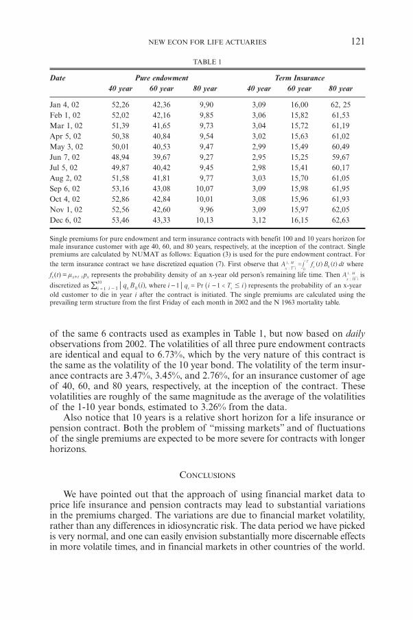
of the same 6 contracts used as examples in Table 1, but now based on dailyobservations from 2002. The volatilities of all three pure endowment contractsare identical and equal to 6.73%, which by the very nature of this contract isthe same as the volatility of the 10 year bond. The volatility of the term insur-ance contracts are 3.47%, 3.45%, and 2.76%, for an insurance customer of ageof 40, 60, and 80 years, respectively, at the inception of the contract. Thesevolatilities are roughly of the same magnitude as the average of the volatilitiesof the 1-10 year bonds, estimated to 3.26% from the data.
Also notice that 10 years is a relative short horizon for a life insurance orpension contract. Both the problem of “missing markets” and of fluctuationsof the single premiums are expected to be more severe for contracts with longerhorizons.
CONCLUSIONS
We have pointed out that the approach of using financial market data toprice life insurance and pension contracts may lead to substantial variationsin the premiums charged. The variations are due to financial market volatility,rather than any differences in idiosyncratic risk. The data period we have pickedis very normal, and one can easily envision substantially more discernable effectsin more volatile times, and in financial markets in other countries of the world.
NEW ECON FOR LIFE ACTUARIES 121
TABLE 1
Date Pure endowment Term Insurance40 year 60 year 80 year 40 year 60 year 80 year
Jan 4, 02 52,26 42,36 9,90 3,09 16,00 62, 25Feb 1, 02 52,02 42,16 9,85 3,06 15,82 61,53Mar 1, 02 51,39 41,65 9,73 3,04 15,72 61,19Apr 5, 02 50,38 40,84 9,54 3,02 15,63 61,02May 3, 02 50,01 40,53 9,47 2,99 15,49 60,49Jun 7, 02 48,94 39,67 9,27 2,95 15,25 59,67Jul 5, 02 49,87 40,42 9,45 2,98 15,41 60,17Aug 2, 02 51,58 41,81 9,77 3,03 15,70 61,05Sep 6, 02 53,16 43,08 10,07 3,09 15,98 61,95Oct 4, 02 52,86 42,84 10,01 3,08 15,96 61,93Nov 1, 02 52,56 42,60 9,96 3,09 15,97 62,05Dec 6, 02 53,46 43,33 10,13 3,12 16,15 62,63
Single premiums for pure endowment and term insurance contracts with benefit 100 and 10 years horizon formale insurance customer with age 40, 60, and 80 years, respectively, at the inception of the contract. Singlepremiums are calculated by NUMAT as follows: Equation (3) is used for the pure endowment contract. Forthe term insurance contract we have discretized equation (7). First observe that ( ) ( )A f t B t dt
:x T x
T
00
=, M1
e# where
fx(t) = mx+t t px represents the probability density of an x-year old person’s remaining life time. Then A:x 10
, M1
eis
discretized as i 1=
( )q B ix 0
10
i 1-! , where <Pri q i T i1 1
x x#- = -^ h represents the probability of an x-year
old customer to die in year i after the contract is initiated. The single premiums are calculated using theprevailing term structure from the first Friday of each month in 2002 and the N 1963 mortality table.
REFERENCES
AASE, K.K. (1996) Anvendt sannsynlighetsteori: Forsikringsmatematikk (in Norwegian) (English:Applied probability theory: Insurance mathematics). Cappelen Akademisk Forlag, Oslo, Norge.
ADAMS K. and VAN DEVENTER D. (1994) Fitting yield curves and forward rate curves with maxi-mum smoothness. Journal of Fixed Income, 52-62.
BACINELLO A. and PERSSON, S.-A. (2002) Design and pricing of equity-linked life insuranceunder stochastic interest rates. The Journal of Risk Finance 3(2), 6-21.
BÜHLMANN, H. (2002) New math for life actuaries. ASTIN Bulletin 32(2), 209-211.CAIRNS, A.J.G. (1998) Descriptive bond-yield and forward rate models for the british government
securities’ market. British Actuarial Journal 4(2), 265-321.DAVIS, M. and MATAIX-PASTOR, V. (2003) Finite-dimensional models of the yield curve. Working
paper, Department of Mathematics, Imperial College, London SW7 2BZ, England.DUFFIE, D. (2001) Dynamic Asset Pricing Theory. Princeton University Press, Princeton, New Jer-
sey, USA, 3rd edition.HEATH, D., JARROW, R. and MORTON, A.J. (1992) Bond pricing and the term structure of inter-
est rates: A new methodology for contingent claims valuation. Econometrica, 60(1) 77-105.MILTERSEN, K.R. and PERSSON, S.-A. (1999) Pricing rate of return guarantees in a Heath-Jarrow-
Morton framework. Insurance: Mathematics and Economics 25, 307-325.MILTERSEN, K.R. and PERSSON, S.-A. (2003) Guaranteed investment contracts: Distributed and
undistributed excess return. Scandinavian Actuarial Journal. Forthcoming.PERSSON, S.-A. (1998) Stochastic interest rate in life insurance: The principle of equivalence revis-
ited. Scandinavian Actuarial Journal, 97-112.PERSSON, S.-A. and AASE, K. (1997) Valuation of the minimum guaranteed return embedded in
life insurance contracts. Journal of Risk and Insurance 64, 599-617.
KNUT K. AASE and SVEIN-ARNE PERSSON
Norwegian School of Economics and Business Administration5045 BergenNorway
122 KNUT K. AASE AND SVEIN-ARNE PERSSON

COMMENT ON THE DISCUSSION ARTICLE BY AASE AND PERSSON
I applaud the article as it is exactly the type of reaction to my editorial inAstin Bulletin 32(2) that I hoped to provoke. Of course Aase and Persson’scontribution is much more academic in style than mine which is more journa-listic.
To my understanding there are three important messages on which everyreader of their article should reflect.
Message 1: The kind of NUMeraire based Actuarial Teaching (NUMAT)which I have advocated has been offered since the beginning of the 90tiesat the Norwegian School of Economics and Business Administration inBergen and there exists even an elementary textbook [1] covering that subject(unfortunately only in Norwegian language).
Message 2: The structure of Zero Coupon Prices needed is not so easy to getas my editorial suggested (“You can look it up in the Financial Part ofyour daily newspaper’’). Of course my wording was a tribute to the jour-nalistic style. To talk as a scientist I would like to mention that in a recentDiploma Thesis at ETH [2] we have interpolated from LIBOR ForwardShort Rates and from SWAP Rates to get the Zero Coupon Prices. Obvi-ously in any real world implementation there is the necessity for modellingthe market prices and the daily newspaper does not suffice.
Message 3: Prices calculated by NUMAT are indeed volatile! This lessonshould be learned by every actuary. It means that the products sold by LifeInsurers have substantially varying market value.
As hinted in my editorial I would see the practical role of NUMAT for cal-culating Embedded Value rather than for calculating Premiums. I take againan example from the above mentioned Diploma Thesis:
Take an Endowment Policy (x = 50, n = 5, sum insured 50 000 CHF). Accord-ing to the Swiss Table EKM 95 the yearly premium amounts to 9375.21 CHF.The value of the initial reserve by NUMAT amounts to
– CHF 2325.45 based on the Zero Coupon Structure of May 2000,– CHF 11.67 based on the Zero Coupon Structure of November 2002.
As the classical initial net reserve is nil you get the Economic Value by changingthe sign. Hence your pretty Embedded Value in May 2000 has disappeared inNovember 2002.
This is again a lesson to be learned by everybody who boosts with the“wonderful Embedded Value’’ in her/his Life Portfolio! Embedded Value isextremely volatile and needs to be monitored continuously.
ASTIN BULLETIN, Vol. 33, No. 2, 2003, pp. 123-124
The last message is my own:
Message 4: I hope to hear from other colleagues that they are already offeringNumeraire based Actuarial Teaching. So far the signal from Bergen is theonly one that I have received. Clearly, there are research papers wherethe economic value of insurance products is discussed and explicitly cal-culated. The point which I tried to make in my editorial was however:NUMAT should be part of the educational curriculum of every actuary.We academics are challenged to get the fundamental way of thinking overto the profession!
REFERENCES
[1] K.K. AASE. Anvendt sannsynlighetsteorie: Forsikring Matematik, Carrelen AkademiskForlag, Oslo, Norge 1996.
[2] G. BAUMGARTNER. Fair Value für Lebensversicherungen. Diploma Thesis, ETH Zürich, 2003.
HANS BÜHLMANN
ETH Zürich
124 HANS BUHLMANN
GUARANTEED ANNUITY OPTIONS
BY
PHELIM BOYLE AND MARY HARDY1
ABSTRACT
Under a guaranteed annuity option, an insurer guarantees to convert a poli-cyholder’s accumulated funds to a life annuity at a fixed rate when the policymatures. If the annuity rates provided under the guarantee are more beneficialto the policyholder than the prevailing rates in the market the insurer has tomake up the difference. Such guarantees are common in many US tax shelteredinsurance products. These guarantees were popular in UK retirement savingscontracts issued in the 1970’s and 1980’s when long-term interest rates werehigh. At that time, the options were very far out of the money and insurancecompanies apparently assumed that interest rates would remain high and thusthat the guarantees would never become active. In the 1990’s, as long-terminterest rates began to fall, the value of these guarantees rose. Because of theway the guarantee was written, two other factors influenced the cost of theseguarantees. First, strong stock market performance meant that the amounts towhich the guarantee applied increased significantly. Second, the mortalityassumption implicit in the guarantee did not anticipate the improvement inmortality which actually occurred.
The emerging liabilities under these guarantees threatened the solvency ofsome companies and led to the closure of Equitable Life (UK) to new business.In this paper we explore the pricing and risk management of these guarantees.
1. INTRODUCTION
1.1. An introduction to guaranteed annuity options
Insurance companies often include very long-term guarantees in their productswhich, in some circumstances, can turn out to be very valuable. Historicallythese options, issued deeply out of the money, have been viewed by some insur-ers as having negligible value. However for a very long dated option, with aterm of perhaps 30 to 40 years, there can be significant fluctuations in economicvariables, and an apparently negligible liability can become very substantial.The case of guaranteed annuity options (GAOs) in the UK provides a dramaticillustration of this phenomenon.
1 Both authors acknowledge the support of the National Science and Engineering Research Councilof Canada.
ASTIN BULLETIN, Vol. 33, No. 2, 2003, pp. 125-152
Guaranteed annuity options have proved to be a significant risk man-agement challenge for several UK insurance companies. Bolton et al (1997)describe the origin and nature of these guarantees. They also discuss the fac-tors which caused the liabilities associated with these guarantees to increase sodramatically in recent years. These factors include a decline in long-term inter-est rates and improvements in mortality. For many contracts the liability isalso related to equity performance and in the UK common stocks performedvery well during the last two decades of the twentieth century.
Under a guaranteed annuity the insurance company guarantees to convertthe maturing policy proceeds into a life annuity at a fixed rate. Typically, thesepolicies mature when the policyholder reaches a certain age. In the UK the mostpopular guaranteed rate for males, aged sixty five, was £111 annuity per annumper £1000 of cash value, or an annuity:cash value ratio of 1:9 and we use thisrate in our illustrations. If the prevailing annuity rates at maturity provide anannual payment that exceeds £111 per £1000, a rational policyholder would optfor the prevailing market rate. On the other hand, if the prevailing annuityrates at maturity produce a lower amount than £111 per £1000, a rational pol-icyholder would take the guaranteed annuity rate. As interest rates rise theannuity amount purchased by a lump sum of £1000 increases and as interestrates fall the annuity amount available per £1000 falls. Hence the guarantee cor-responds to a put option on interest rates. In Sections two, three and four wediscuss the option pricing approach to the valuation of GAOs.
These guarantees began to be included in some UK pension policies in the1950’s and became very popular in the 1970’s and 1980’s. In the UK the inclu-sion of these guarantees was discontinued by the end of the 1980’s but, giventhe long-term nature of this business, these guarantees still affect a significantnumber of contracts. Long-term interest rates in many countries were quite highin 1970’s and 1980’s and the UK was no exception. During these two decadesthe average UK long-term interest rate was around 11% p.a. The interest rateimplicit in the guaranteed annuity options depends on the mortality assump-tion but based on the mortality basis used in the original calculations thebreak-even interest rate was in the region of 5%-6% p.a. When these optionswere granted, they were very far out of the money and the insurance companiesapparently assumed that interest rates would never fall to these low levels again2
and thus that the guarantees would never become active. As we now know thispresumption was incorrect and interest rates did fall in the 1990’s.
The guaranteed annuity conversion rate is a function of the assumed inter-est rate and the assumed mortality rate. Bolton et al note that when many ofthese guarantees were written, it was considered appropriate to use a mortalitytable with no explicit allowance for future improvement such as a(55). Thisis a mortality table designed to be appropriate for immediate life annuitiespurchased in 1955, but was still in vogue in the 1970s. However, there was adramatic improvement in the mortality of the class of lives on which theseguarantees were written during the period 1970-2000. This improvement meant
126 PHELIM BOYLE AND MARY HARDY
2 Although interest rates were of this order for part of the 1960s.
that the break-even interest rate at which the guarantee kicked in rose. Forexample, for a 13-year annuity-certain, a lump sum of 1000 is equivalent to anannual payment of 111 p.a. at 5.70%. If we extend the term of the annuity tosixteen years the interest rate rises to 7.72%. Hence, if mortality rates improveso that policyholders live longer, the interest rate at which the guaranteebecomes effective will increase. In Section 2 we will relate these break-even ratesto appropriate UK life annuity rates.
1.2. A typical contract
To show the nature of the GAO put option we use standard actuarial nota-tion, adapted slightly. Assume we have a single premium equity-linked policy.The contract is assumed to mature at T, say, at which date the policyholder isassumed to be age 65. The premium is invested in an account with marketvalue S(t) at time t, where S(t) is a random process. The market cost of a lifeannuity of £1 p.a. for a life age 65 is also a random process. Let a65(t) denotethis market price.
The policy offers a guaranteed conversion rate of g = 9. This rate deter-mines the guaranteed minimum annuity payment per unit of maturity pro-ceeds of the contract; that is, £1 of the lump sum maturity value must purchasea minimum of £1/g of annuity.
At maturity the proceeds of the policy are S(T); if the guarantee is exercisedthis will be applied to purchase an annuity of S(T)/g, at a cost of (S(T)/g) a65(T).The excess of the annuity cost over the cash proceeds must be met by the insurer,and will be
( )( ) ( )g
S Ta T S T65 -
If a65(T) < 9 the guarantee will not be exercised and the cash proceeds will beannuitized without additional cost.
So, assuming the policyholder survives to maturity, the value of the guaran-tee at maturity is
( )( )
,maxS T ga T
1 065 -d n= G (1)
The market annuity rate a65(t) will depend on the prevailing long-term inter-est rates, the mortality assumptions used and the expense assumption. We willignore expenses and use the current long-term government bond yield as a proxyfor the interest rate assumption. We see that the option will be in-the-moneywhenever the current annuity factor exceeds the guaranteed factor, which isg = 9 in the examples used in this paper.
We see from equation (1) that, for a maturing policy, the size of the optionliability will be proportional to S(T): the amount of proceeds to which theguarantee applies. The size of S(T) will depend on the nature of the contract
GUARANTEED ANNUITY OPTIONS 127
and also on the investment returns attributed to the policy. The procedure bywhich the investment returns are determined depends on the terms of thepolicy. Under a traditional UK with profits contract profits are assigned usingreversionary bonuses and terminal bonuses. Reversionary bonuses are assignedon a regular basis as guaranteed additions to the basic maturity value and arenot distributed until maturity. Terminal bonuses are declared when the policymatures such that together with the reversionary bonuses, the investment expe-rience over the term of the contract is (more or less) fully reflected. The sizeof the reversionary bonuses depends both on the investment performance ofthe underlying investments and the smoothing convention used in setting thebonus level. The terminal bonus is not guaranteed but during periods of goodinvestment performance it can be quite significant, sometimes of the sameorder as the basic maturity sum assured. Bolton et al (1997) estimate that withprofits policies account for eighty percent of the total liabilities for contractswhich include a guaranteed annuity option. The remaining contracts whichincorporate a guaranteed annuity option were mostly unit-linked policies.
In contrast to with profits contracts, the investment gains and losses undera unit-linked (equity-linked) contract are distributed directly to the policyholder’saccount. Contracts of this nature are more transparent than with profits poli-cies and they have become very popular in many countries in recent years. Undera unit-linked contract the size of the option liability, if the guarantee is oper-ative, will depend directly on the investment performance of the assets in whichthe funds are invested. In the UK there is a strong tradition of investing inequities and during the twenty year period from 1980 until 2000 the rate ofgrowth on the major UK stock market index was a staggering 18% per annum.
In this paper we consider unit-linked policies rather than with profits. Unit-linked contracts are generally well defined with little insurer discretion. Withprofits policies would be essentially identical to unit-linked if there were nosmoothing, and assuming the asset proceeds are passed through to the policy-holder, subject to reasonable and similar expense deductions. However, thediscretionary element of smoothing, as well as the opaque nature of the invest-ment policy for some with profits policies make it more difficult to analysethese contracts in general. However, the methods proposed for unit-linked con-tracts can be adapted for with profits given suitably well defined bonus and assetallocation strategies.
1.3. Principal factors in the GAO cost
Three principal factors contributed to the growth of the guaranteed annuityoption liabilities in the UK over the last few decades. First, there was a largedecline in long-term interest rates over the period. Second, there was a signif-icant improvement in longevity that was not factored into the initial actuarialcalculations. Third, the strong equity performance during the period servedto increase further the magnitude of the liabilities. It would appear that theseevents were not considered when the guarantees were initially granted. Theresponsibility for long-term financial solvency of insurance companies rests
128 PHELIM BOYLE AND MARY HARDY
with the actuarial profession. It will be instructive to examine what possiblerisk management strategies could have been or should have been employed todeal with this situation. It is clear now with the benefit of hindsight that it wasimprudent to grant such long-term open ended guarantees of this type.
There are three main methods of dealing with the type of risks associatedwith writing financial guarantees. First, there is the traditional actuarial reser-ving method whereby the insurer sets aside additional capital to ensure that theliabilities under the guarantee will be covered with a high probability. Theliabilities are estimated using a stochastic simulation approach. The basic ideais to simulate the future using a stochastic model3 of investment returns. Thesesimulations can be used to estimate the distribution of the cost of the guaran-tee. From this distribution one can compute the amount of initial reserveso that the provision will be adequate, say, 99% of the time. The second approachis to reinsure the liability with another financial institution such as a reinsur-ance company or an investment bank. In this case the insurance company paysa fee to the financial institution and in return the institution agrees to meet theliability under the guarantee. The third approach is for the insurance companyto set up a replicating portfolio of traded securities and adjust (or dynamicallyhedge) this portfolio over time so that at maturity the market value of theportfolio corresponds to the liability under the guaranteed annuity option.
Implementations of these three different risk management strategies havebeen described in the literature. Yang (2001) and Wilkie, Waters and Yang(2003) describe the actuarial approach based on the Wilkie model. Dunbar(1999) provides an illustration of the second approach. The insurance company,Scottish Widows offset its guaranteed annuity liabilities by purchasing a struc-tured product from Morgan Stanley. Pelsser (2003) analyzes a hedging strategybased on the purchase of long dated receiver swaptions. This is described morefully in Section 8.
In this paper we will discuss a number of the issues surrounding the valua-tion and risk management of these guarantees. We will also discuss the degreeto which different risk management approaches would have been possible from1980 onwards.
1.4. Outline of the paper
The layout of the rest of the paper is as follows. Section two provides back-ground detail on the guaranteed annuity options and the relevant institutionalframework. We examine the evolution of the economic and demographic vari-ables which affect the value of the guarantee. In particular we provide a timeseries of the values of the guarantee at maturity for a representative contract.In Section three we use an option pricing approach to obtain the market priceof the guarantee. Section Four documents the time series of market values ofthe guarantee. Using a simple one-factor model it is possible to estimate the
GUARANTEED ANNUITY OPTIONS 129
3 One such model, the Wilkie Model was available in the UK actuarial literature as early as 1980. SeeMGWP(1980).
market value of the option. Section five examines a number of the concep-tual and practical issues involved in dynamic hedging the interest rate risk.Sections six and seven explore the issues involved in hedging the equity risk andthe mortality risk. One suggestion for dealing with these guarantees involvesthe insurer purchasing long dated receiver swaptions. We describe this approachin Section eight. Section nine comments on the lessons to be learned from thisepisode.
2. MATURITY VALUE OF THE GUARANTEE
In this section we document the evolution of the emerging liability under theguaranteed annuity option. Specifically we examine the magnitude of the guar-antee for a newly maturing policy over the last two decades. In these calcula-tions the policy proceeds at maturity are assumed to be held constant at £100,so the cost reported is the cost % of the policy maturity cash value. We assumethe annuity purchased with the policy proceeds is payable annually in arrearto a life age 65 at maturity, and has a five year guarantee period.
We consider three different mortality tables to determine the GAO cost.
• The a(55) mortality table represents the mortality assumptions being usedin the 1970’s to price immediate annuities. As previously mentioned, it wascalculated to be appropriate to lives purchasing immediate annuities in 1955.
• The PMA80(C10) table from this series is based on UK experience for theperiod 1979-1982 and is projected to 2010 to reflect mortality improvements.The PMA80 series became available in 1990.
• The PMA92 series was published in 1998 and the table we use, the PMA92(C20) table, is based on UK experience for the period 1991-1994, projectedto 2020 to reflect mortality improvements.
The improvement from the a(55) table to the PMA92(C20) provides an upperbound on the mortality improvement over the period since the last namedtable only appeared at the end of the period and includes a significant pro-jection for future mortality improvements. Wilkie Waters and Yang (2003) givea detailed account of the year by year relevant UK male mortality experiencefor the period 1984 to 2001.
The increase in longevity is quite dramatic over the period covered by thesethree tables. The expectation of life for a male aged 65 is 14.3 years using a(55)mortality, 16.9 years under the PMA80(C10) table and 19.8 years under thePMA92(C20) table. Thus the expected future lifetime of a male aged 65increased by 2.6 years from the a(55) table to the PMA80(C10) table. Moredramatically the expected future lifetime of a male aged 65 increased by overfive years from the a(55) table to the PMA92(C20) table.
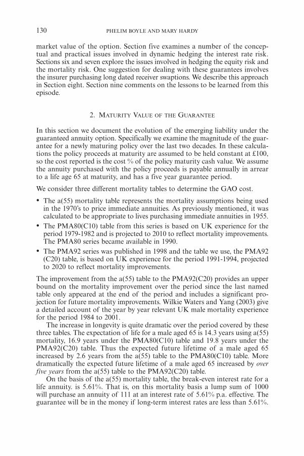
On the basis of the a(55) mortality table, the break-even interest rate for alife annuity. is 5.61%. That is, on this mortality basis a lump sum of 1000will purchase an annuity of 111 at an interest rate of 5.61% p.a. effective. Theguarantee will be in the money if long-term interest rates are less than 5.61%.
130 PHELIM BOYLE AND MARY HARDY
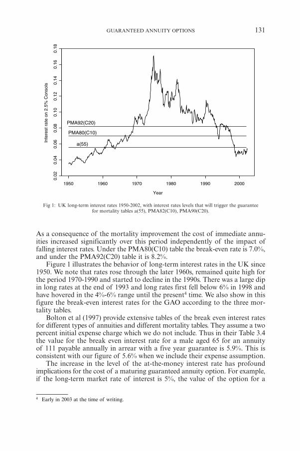
Fig 1: UK long-term interest rates 1950-2002, with interest rates levels that will trigger the guaranteefor mortality tables a(55), PMA82(C10), PMA90(C20).
As a consequence of the mortality improvement the cost of immediate annu-ities increased significantly over this period independently of the impact offalling interest rates. Under the PMA80(C10) table the break-even rate is 7.0%,and under the PMA92(C20) table it is 8.2%.
Figure 1 illustrates the behavior of long-term interest rates in the UK since1950. We note that rates rose through the later 1960s, remained quite high forthe period 1970-1990 and started to decline in the 1990s. There was a large dipin long rates at the end of 1993 and long rates first fell below 6% in 1998 andhave hovered in the 4%-6% range until the present4 time. We also show in thisfigure the break-even interest rates for the GAO according to the three mor-tality tables.
Bolton et al (1997) provide extensive tables of the break even interest ratesfor different types of annuities and different mortality tables. They assume a twopercent initial expense charge which we do not include. Thus in their Table 3.4the value for the break even interest rate for a male aged 65 for an annuityof 111 payable annually in arrear with a five year guarantee is 5.9%. This isconsistent with our figure of 5.6% when we include their expense assumption.
The increase in the level of the at-the-money interest rate has profoundimplications for the cost of a maturing guaranteed annuity option. For example,if the long-term market rate of interest is 5%, the value of the option for a
GUARANTEED ANNUITY OPTIONS 131
4 Early in 2003 at the time of writing.
Fig 2: Value of maturing guarantee per 100 proceeds based on PMA92(C20), PMA80(C10),and a(55) mortality.
maturing policy with £100 maturity proceeds, based on a(55) is £4.45; basedon PMA80(C10) it would be £16.53 and the corresponding value based onPMA92(C20) is £29.52. Note that we do not need any type of option formulato perform these calculations; we apply equation (1), with S(T) fixed at 100,and a65(T) calculated using the appropriate mortality and an interest rate of 5%per year. Figure 2 shows the magnitude of the option liability for our bench-mark contract under the three mortality assumptions using historical interestrates. Since the long-term interest rate is the main determinant of the annuitycost, we have used the yield on 2.5% consols, which are government bonds,generally considered irredeemable5.
There is no liability on maturing contracts until the 1990’s. Also note thatthe mortality assumption has a profound impact on the size of the liability.
We have already noted that during the period 1980-2000, UK equitiesperformed extremely well. This resulted in increased levels of bonus to thewith profits polices. For many contracts this meant that the volume of proceedsto which the guarantee applied also increased, thereby increasing the liabilityunder the guarantee. In the case of unit-linked polices the gains are passeddirectly to the policyholder, apart from the various expenses. If we assumethat a unit-linked contract earned the market rate of 18% minus 300 basispoints this still leaves a return of 15%. At this growth rate an initial single
132 PHELIM BOYLE AND MARY HARDY
5 In fact they may be redeemed at any time at the discretion of the Exchequer.
premium of £100 will accumulate to £1636.7 after twenty years. This growthwould be proportionately reflected in the cost of the guarantee.
To summarize, we have discussed the evolution of the value of the liability fora sequence of maturing contracts. This analysis indicates how the three factors:
• The fall in long-term interest rates
• The improvement in mortality
• The strong equity performance
served to increase the cost of the guarantee. Note that our analysis in thissection did not require any stochastic analysis or option pricing formula. Wesimply computed the value of the option at maturity each year of the period.In the next section we discuss the evaluation of these options prior to maturity.
3. DERIVATION OF AN OPTION FORMULA
3.1. Introduction
The guaranteed annuity option is similar to a call option on a coupon bond;the annuity payments and survival probabilities can be incorporated in thenotional coupons.
First we develop the option formula without assuming a specific model forinterest rates. Then, we will apply the Hull-White (1990) interest rate model(also known as extended Vasicek, from the Vasicek (1977) model) to calculateprices for the options.
We assume that the mortality risk is independent of the financial risk andthat it is therefore diversifiable. In this case it is well documented (see, forexample, Boyle and Schwartz (1977)) that it is appropriate to use determinis-tic mortality for valuing options dependent on survival or death.
3.2. The numeraire approach
Using stochastic interest rates, the price at some future date t of a zero couponbond with unit maturity value, maturing at T is a random variable which wedenote D(t,T ). The term structure of interest rates at t is therefore describedby the function {D(t,T )}T > t. This term structure is assumed to be known attime t.
So, the actuarial value at T of an immediate annuity payable to a life agedxr at T, contingent on survival, is
( ) ( , )a T p D T T jxr j xrj
J
1
= +=
! (2)
where j pxr represents the appropriate survival probability. For an annuity withan initial guarantee period of, say five years, we set the first five values of j pxr
GUARANTEED ANNUITY OPTIONS 133
to 1.0. The limiting age of the mortality table is denoted by w and we set J =(w – xr). Note that in valuing the annuity at T, the term structure is known,and there are no random variables in this expression.
Now, to value this expression at time t < T, we use a ‘numeraire’ approach.In the absence of arbitrage any market price deflated by a suitable numeraireis a martingale. We can use any traded asset which has a price that is alwaysstrictly positive as numeraire. Here we use the zero coupon bond which maturesat time T as the numeraire and we denote the associated probability measureby the symbol QT. This is often called the ‘forward measure’. If interest ratesare constant, it is the same as the risk neutral measure in the standard Black-Scholes framework. See Björk (1998) for more details.
Suppose V(s) is the market value at s of some payoff occurring at some timeT+ j, j ≥ 0. We use D(s,T) as the numeraire, where s ≤ T. The martingale resultmeans that Xs = ( , )
( )D s T
V s is a martingale under QT, so that EQT [Xs |Ft] =Xt for anys such that t ≤ s ≤ T. Here |Ft indicates that we are taking expectation of therandom process at time t + k given all the relevant information at t. In par-ticular at t we know all values of D(t,s), s ≥ t.
Applying this to take expectation of the ratio ( , )( )
D s TV s at T, and using the fact
that D(T,T) = 1.0, we have:
( , )( )
( , )( )
( )D t TV t
E D T TV T
E V TF FQ t Q tT T= =< 7F A (3)
( ) ( , ) ( )V t D t T E V T FQ tT& = 7 A (4)
Equation (4) provides a valuation formula at t for any payoff V(T). The dis-tribution QT depends on the assumption made for interest rates, and we willdiscuss this later.
Now for the GAO we know from equation (1) that the payoff at maturity is6
( )( ) ( )
V T gS T a T gxr=
-+
^ h
This is required for each policyholder surviving to time T, so to value at t < Twe multiply by the appropriate survival probability.
Then if G(t) is the value of this benefit at t, and letting x = xr – (T – t) we have:
( ) ( , ) ( )G t p D t T E V T FT t x Q tT= - 7 A (5)
( ) ( , )( ) ( )
G t p D t T E gS T a T g
FT t x Qxr
tT& =
--
+^ h
R
T
SSS
V
X
WWW
(6)
134 PHELIM BOYLE AND MARY HARDY
6 We use (X)+ = max(X,0).
Initially we assume that S(T) is independent of interest rates. This is a very strongassumption but it simplifies the analysis. Later we allow for correlation betweenequity returns and interest rates.
We have then:
( )( , ) ( )
( )
( )( )
G t gp D t T E S T
E a T g
gp S T
E a T g
F
F
T t x QQ xr t
T t xQ xr t
T
T
T
= -
= -
- +
- +
^
^
h
h
69
69
@C
@C
The last line follows from the numeraire martingale result, equation (4), becausereplacing V(T) with S(T) in that equation gives
( , )( )
( )D t TS t
E S T FQ tT= 7 A
Inserting the expression for axr(T) from (2) we have
( ) ( , )E a T g E p D T T j gF FQ xr t Q j xrj
J
t1
T T- = + -
+
=
+
!^ fh p
R
T
SSS
9
V
X
WWW
C
The expression inside the expectation on the right hand side corresponds to acall option on a coupon paying bond where the ‘coupon’ payment at time (T+ j)is j pxr. This ‘coupon bond’ has value at time, T :
( , ).p D T T jj xrj
J
1
+=
!
The market value at time, t of this coupon bond is
( ) ( , ).P t p D t T jj xrj
J
1
= +=
!
So P(t) is the value of a deferred annuity, but without allowance for mortalityduring deferment. With this notation our call option has a value at time, T of(P(T ) – g)+. The numeraire approach is described more fully in Björk (1998).
3.3. Using Jamshidian’s method for coupon bond options
Jamshidian (1989) showed that if the interest rate follows a one-factor process,then the market price of the option on the coupon bond with strike price gis equal to the price of a portfolio of options on the individual zero coupon
GUARANTEED ANNUITY OPTIONS 135
bonds with strike prices Kj, where {Kj} are equal to the notional zero couponbond prices to give an annuity axr(T) with market price g at T. That is, let r*
Tdenote the value of the short rate for which
( , )p D T T j gj xrj
J
1
+ ==
*! (7)
where we use the asterisk to signify that each zero coupon bond is evaluatedusing short rate r*
T7. Then set
j ( , ).K D T T j= +*
Then the call option with strike g on the coupon bond P(t) can be valued as
j( ), , ( , ), , ,C P t g t p C D t T j K tj xrj
J
1
= +=
!6 8@ B
where C [D(t,T+j), Kj , t] is the price at time t of a call option on the zero couponbond with maturity (T+ j) and strike price Kj.
We can use the call option C[P(t), g, t] to obtain an explicit expression forthe GAO value at t, G(t). Recall that
( )( )
( ) .G t gp S T
E P T g FT t xQ tT
= -- +^ h8 B
From the numeraire valuation equation we have
( , )( ), ,
( )D t TC P t g t
E P T g FQ tT= - +
^ h6
8@
B
Pulling all the pieces together we have
j( )
( )( , )
( , ), ,.G t g
p S tD t T
p C D t T j K tT t x j xrj
J1
=+
- =! 8 B
(8)
3.4. Applying the Hull-White interest rate model
Jamshidian’s result requires a one-factor interest rate model. We use a versionof the Hull-White (1990) model. This model is also known as extended Vasicek,from the Vasicek (1977) model.
The short rate of interest at t is assumed to follow the process:
t( ) ( ) ( )dr t t r t dt dWk q s= - +^ h (9)
136 PHELIM BOYLE AND MARY HARDY
7 In a one-factor model, setting the short rate determines the entire term structure.
where q (t) is a deterministic function determined by the initial term structureof interest rates. Using the function q (t) enables us to match the model termstructure and the market term structure at the start of the projection.
Björk (1998) gives the formula for the term structure at t, using the marketterm structure at initial date t = 0, as:
*( , ) ( , )( , )
( , ) ( , ) ( , ) ( ) ( , ) ( )expD t T D tD T
B t T f t B t T e B t T r tks
00
04
1 tk2
2 2= - - --( 2 (10)
where f *(0,t) is the t-year continuously compounded forward rate at t = 0, and
( , )B t T ek1
1 ( )T tk= - - -# -
This formula can be used to identify the strike price sequence {Kj} from equa-tion (7), and also used to value the option for given values of r(t).
The explicit formula for each individual bond option under the Hull-Whitemodel is
j j( , ), , ( , ) ( ) ( , ) ( ) ,C D t T J K t D t T j N h j K D t T N h j1 2+ = + -^ ^h h8 B
where
j
j
( ) ( )( )
,
( ) ( )( )
,
log
log
h j jj
h j jj
ss
ss
2
2
( , )( , )
( , )( , )
P
D t T KD t T j
P
P
D t T KD t T j
P
1
2
= +
= -
+
+
and
( ) .j e es s k k2
1 1( )
P
T t jk k2
=- -- - -
_ i
The parameters k and s characterize the dynamics of the short rate of interestunder the Hull-White process.
4. VALUATION OF THE GUARANTEED ANNUITY OPTION
In this section we will derive the historical time series of market values for theguarantee based on the formula derived in the last section. It would have beenhelpful if the UK insurance companies had computed these market valuesat regular intervals since they would have highlighted the emergence of theliability under the guaranteed annuity option. The technology for pricing inter-est rate options was in its infancy in 1980 but by 1990 the models we use werein the public domain. An estimate of the market value of the guarantee can
GUARANTEED ANNUITY OPTIONS 137
be derived from the one-factor stochastic interest rate model. We will use themodel to estimate the value of the guarantees for the period 1980-2002.
In the previous section we derived a formula for the market price of theguaranteed annuity option using the Hull-White model. A similar formula hasalso been derived by Ballotta and Haberman (2002). They start from the HeathJarrow Morton model and then restrict the volatility dynamics of the forwardrate process to derive tractable formulae.
We used the following parameter estimates to compute the market valuesof the guaranteed annuity option
138 PHELIM BOYLE AND MARY HARDY
These parameters are broadly comparable with estimates that have beenobtained in the literature based on UK data for this time period. See Nowman(1997) and Yu and Phillips (2001).
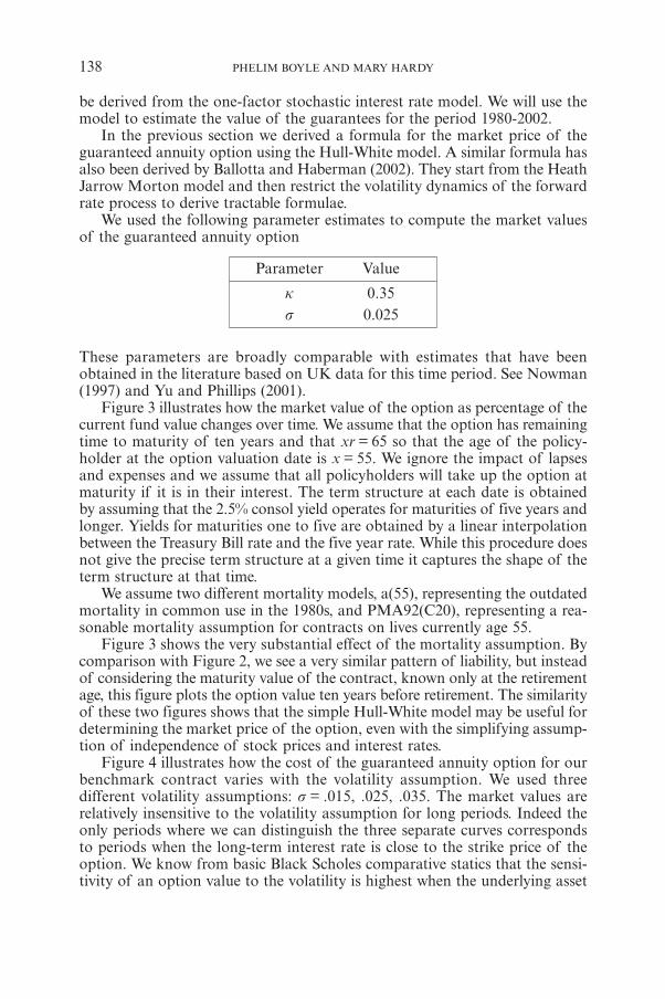
Figure 3 illustrates how the market value of the option as percentage of thecurrent fund value changes over time. We assume that the option has remainingtime to maturity of ten years and that xr = 65 so that the age of the policy-holder at the option valuation date is x = 55. We ignore the impact of lapsesand expenses and we assume that all policyholders will take up the option atmaturity if it is in their interest. The term structure at each date is obtainedby assuming that the 2.5% consol yield operates for maturities of five years andlonger. Yields for maturities one to five are obtained by a linear interpolationbetween the Treasury Bill rate and the five year rate. While this procedure doesnot give the precise term structure at a given time it captures the shape of theterm structure at that time.
We assume two different mortality models, a(55), representing the outdatedmortality in common use in the 1980s, and PMA92(C20), representing a rea-sonable mortality assumption for contracts on lives currently age 55.
Figure 3 shows the very substantial effect of the mortality assumption. Bycomparison with Figure 2, we see a very similar pattern of liability, but insteadof considering the maturity value of the contract, known only at the retirementage, this figure plots the option value ten years before retirement. The similarityof these two figures shows that the simple Hull-White model may be useful fordetermining the market price of the option, even with the simplifying assump-tion of independence of stock prices and interest rates.
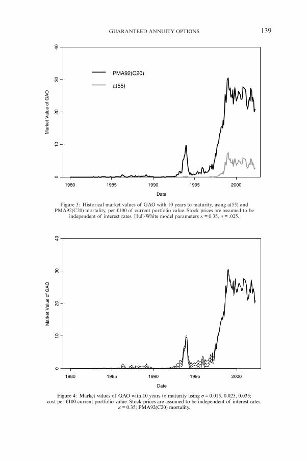
Figure 4 illustrates how the cost of the guaranteed annuity option for ourbenchmark contract varies with the volatility assumption. We used threedifferent volatility assumptions: s = .015, .025, .035. The market values arerelatively insensitive to the volatility assumption for long periods. Indeed theonly periods where we can distinguish the three separate curves correspondsto periods when the long-term interest rate is close to the strike price of theoption. We know from basic Black Scholes comparative statics that the sensi-tivity of an option value to the volatility is highest when the underlying asset
Parameter Value
k 0.35s 0.025
GUARANTEED ANNUITY OPTIONS 139
Figure 3: Historical market values of GAO with 10 years to maturity, using a(55) andPMA92(C20) mortality, per £100 of current portfolio value. Stock prices are assumed to be
independent of interest rates. Hull-White model parameters k = 0.35, s = .025.
Figure 4: Market values of GAO with 10 years to maturity using s = 0.015, 0.025, 0.035;cost per £100 current portfolio value. Stock prices are assumed to be independent of interest rates.
k = 0.35; PMA92(C20) mortality.
price is close to the strike price. If the option is very far out of the money ordeeply in the money the price of the option is relatively insensitive to the volatil-ity assumption. This same intuition is at work here.
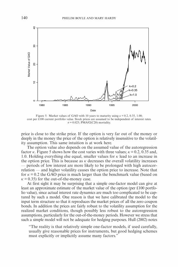
The option value also depends on the assumed value of the autoregressionfactor k. Figure 5 shows how the cost varies with three values; k = 0.2, 0.35 and,1.0. Holding everything else equal, smaller values for k lead to an increase inthe option price. This is because as k decreases the overall volatility increases— periods of low interest are more likely to be prolonged with high autocor-relation — and higher volatility causes the option price to increase. Note thatfor k = 0.2 the GAO price is much larger than the benchmark value (based onk = 0.35) for the out-of-the-money case.
At first sight it may be surprising that a simple one-factor model can give atleast an approximate estimate of the market value of the option (per £100 portfo-lio value), since actual interest rate dynamics are much too complicated to be cap-tured by such a model. One reason is that we have calibrated the model to theinput term structure so that it reproduces the market prices of all the zero couponbonds. In addition the prices are fairly robust to the volatility assumption for therealized market conditions, though possibly less robust to the autoregressionassumptions, particularly for the out-of-the-money periods. However we stress thatsuch a simple model will not be adequate for hedging purposes. Hull (2002) notes
“The reality is that relatively simple one-factor models, if used carefully,usually give reasonable prices for instruments, but good hedging schemesmust explicitly or implicitly assume many factors.”
140 PHELIM BOYLE AND MARY HARDY
Figure 5: Market values of GAO with 10 years to maturity using k = 0.2, 0.35, 1.00;cost per £100 current portfolio value. Stock prices are assumed to be independent of interest rates.
s = 0.025; PMA92(C20) mortality.
5. HEDGING
In this section we discuss some of the issues involved in hedging the guaran-teed annuity risk using traded securities. Although the full fledged guaranteedannuity option depends on three stochastic variables — interest rates, stockprices and mortality — here we just discuss the interest rate risk.
The hedging of long-term interest rate options is a difficult task. In orderto implement an effective hedging strategy we require a robust and reliablemodel of interest rate dynamics over the long-term. The search for such amodel remains an area of active research and, despite some useful progress,there appears to be no consensus on such a model. For a survey of some ofthe recent work in modelling term structure dynamics see Dai and Singleton(2003). Note that for risk management and hedging purposes we require amodel that provides a good description of the actual movements in yield curvesover time. In other words we need a model that describes interest rate move-ments under the real world measure. For pricing we only needed the Q-mea-sure, with parameters determined from the current market structure.
We begin by reviewing the relationship between pricing and hedging in anideal setting. Consider the standard no arbitrage pricing model, where thereis a perfect frictionless market with continuous trading. If the market is com-plete, then any payoff can be hedged with traded securities. Since there is noarbitrage the current price of the derivative must be equal to the current priceof the replicating portfolio. If an institution sells this derivative then it cantake the premium (price) and set up the replicating portfolio. As time passesit can dynamically adjust the position, so that at maturity the value of thereplicating portfolio is exactly equal to the payoff on the derivative. In an idealworld where the model assumptions are fulfilled, it should be possible toconduct this replication program without needing any additional funds. Theinitial price should be exactly sufficient.
In the real world the assumptions of these models are never exactly fulfilled.For example
• The asset price dynamics will not be correctly specified.• It will not be feasible to rebalance the replicating portfolio on a continuous
basis. Instead it has to be rebalanced at discrete intervals.• There are transaction costs on trading.
The impact of these deviations from the idealized assumptions has beenexplored in the Black Scholes Merton world. We discuss these three possibledeviations in turn.
If the process that generates the market prices deviates from the modelimplicit in the pricing formula there will be additional hedging errors. This isbecause the portfolio weights that would be required to replicate the payoffunder the true model will be different from the portfolio weights computedunder the assumed model. This point has been explored in the case of equityderivatives by several authors including Bakshi, Cao and Chen (1997, 2000),Chernov et al (2001) and Jiang and Oomen (2002), and in the case of equity-linked life insurance by Hardy (2003).
GUARANTEED ANNUITY OPTIONS 141

With discrete rebalancing, Boyle and Emanuel (1980) showed that if theportfolio is rebalanced at discrete intervals, there will be a hedging error whichtends to zero as the rebalancing becomes more frequent. In the presence oftransaction costs the frequency of rebalancing involves a trade-off betweenthe size of the hedging error and the trading costs.
However in practice we may emphasize pricing at the expense of hedgingby calibrating an incorrect model to give the accurate market price of a deriv-ative. For example, quoted swaption and cap prices are universally based onthe simple Black model. The Black model volatility that makes the marketprice equal to the model price has become a standard measure for conveyingthe price. However the Black model does not provide realistic dynamics forinterest rates and so it is unsuitable for hedging and risk management applica-tions. In the same way stock option prices when the asset price dynamics followa process with stochastic volatility can still be quoted in terms of the BlackScholes implied volatility. We can always find the value of the Black Scholesvolatility that reproduces the market price of the option even when the truedynamics include stochastic volatility. However as shown by Melino andTurnbull (1995) the use of the simple Black Scholes model, in the presence ofstochastic volatility, may lead to large and costly hedging errors, especially forlong dated options.
In the case of stochastic interest rates, several studies have shown that it is pos-sible to have a simple model that does a reasonable job of pricing interest ratederivatives even though the model is inadequate for hedging purposes. Canabarro(1995) uses a two factor simulated economy to show that, although one-factormodels produce accurate prices for interest rate derivatives, these models lead topoor hedging performance. Gupta and Subrahmanyam (2001) use actual pricedata to show that, while a one-factor model is adequate for pricing caps andfloors, a two factor model performs better in hedging these types of derivatives.
Litterman and Scheinkman (1991) demonstrated that most of the varia-tion in interest rates could be explained by three stochastic factors. Dai andSingleton (2000) examine three factor models of the so called affine class. Theclassical Cox Ingersoll Ross (1985) model and the Vasicek model are the bestknown examples of the affine class. These models have the attractive propertythat bond prices become exponentials of affine functions and are easy toevaluate. Dai and Singleton find reasonable empirical support for some ver-sions of the three factor affine model using swap market data for the periodApril 1987 to August 1996.
In the context of guaranteed annuity options we require an interest ratemodel that describes interest rate behavior over a longer time span. Ahn,Dittmar and Gallant (2002) provide support for quadratic term structure models.They are known as quadratic models because the short term rate of interest isa quadratic function of the underlying state variables. Their empirical tests useUS bond data for the period 1946-1991 and they conclude that the quadraticthree factor model
“...provides a fairly good description of term structure dynamics and cap-tures these dynamics better than the preferred affine term structure modelof Dai and Singleton.’’
142 PHELIM BOYLE AND MARY HARDY
Bansal and Zhou (2002) show that the affine models are also dominated bytheir proposed regime switching model. Their empirical test is based on USinterest rate data for the period 1964-1995. Even a casual inspection of the datasuggests the existence of different regimes. They conclude that standard mod-els, including the affine models with up to three factors, are sharply rejectedby the data. Regime switching models have been extensively used by Hardy(2003) to model equity returns in the context of pricing and risk managementof equity indexed annuities.
The interest rate exposure in a guaranteed annuity option is similar to thatunder a long dated swaption. Hence it is instructive to examine some recentresults on hedging swaptions. This is a topic of current interest as evidencedby papers by Andersen and Andreasen (2002), Fan, Gupta and Ritchken (2001),Driessen, Klaasen and Melenberg (2002), and Longstaff, Santa-Clara andSchwartz (2001). The main conclusion of these papers is that multi-factormodels are necessary for good hedging results. However it should be notedthat the empirical tests in these papers tend to use relatively short observationperiods — around three to five years being typical. Swaption data is unavail-able for long periods since the instruments first were created in the late 1980’s.Hence these models are being tested over the 1995-2000 period when interestrates were fairly stable. If the swaption data were available over longer periods,it seems likely that a regime switching interest rate model would be requiredto do an adequate hedging job.
In Section 6 we consider the GAO hedge using highly simplified assump-tions for equities and interest rates.
6. THE EQUITY RISK
We have already shown in equation (1) that the size of the payoff on the UKguaranteed annuity option is proportional to the amount of the maturity pro-ceeds. This amount will depend on the stock market performance over the lifeof the contract. For unit-linked policies the maturity amount depends directlyon the performance of the underlying fund. In the case of with profits con-tracts the policy proceeds depend on the bonuses declared by the insurancecompany and the size of these bonuses is directly related to stock marketperformance. In general the stock market returns are passed through to thepolicyholders in reversionary and terminal bonuses. In this section we discusshow the inclusion of equity risk impacts the pricing and risk management ofthe guaranteed annuity options.
We have seen in Section 3 that under some strong assumptions about thejoint dynamics of interest rates we can obtain simple pricing formula. Specif-ically if we assume that equity returns are independent of interest rates, andthat interest rates are governed by a one-factor Hull-White model, we canobtain a simple valuation formula for the price of the guaranteed annuityoption. The formula can be modified to handle the case when there is corre-lation between stocks and bonds. Ballotta and Haberman have also derived aformula under these assumptions.
GUARANTEED ANNUITY OPTIONS 143
We can illustrate the key issues involved in pricing and hedging when theequity risk is included by considering a simpler contract than the guaranteedannuity option. This contract has the following payoff at time T
j, ( ) , ,maxP T T j S T D T T j K 0+ = + -^ ^`h h j
It corresponds to an option on the zero coupon bond which matures at time(T+ j) and where the payoff is directly related to the value of the referenceindex. This contract includes no mortality risk here and there is just one zerocoupon bond at maturity rather than a linear combination of zero couponbonds. However this simpler contract captures the key dependencies of theguaranteed annuity option. The full guaranteed annuity option with correla-tion can then be determined, using D(t,T) as numeraire, and the forward mea-sure QT as the equivalent martingale measure:
( ) , ,V t D t T p E P T T jT j t x Qj
J
1T
= ++ -=
!] ^g h6 @
We can derive a closed form expression for each term in V(t) if, for example,we assume that under the forward measure QT the random variables S(T) andD(T,T+ j) have a bivariate lognormal distribution.
For simplicity we treat the period from t to T as a single time step, with vari-ance-covariance matrix for log S(T) |Ft and log D(T,T+ j) |Ft :
S
D
.s
rs s
rs s
sD S
D S2
2=
j!
R
T
SSSS
V
X
WWWW
Note that the values of r and sD would both vary with j .Assume also that under the forward measure QT the means of log S(T) /S(t) |Ft and log D(T,T+ j) / D(t,T+ j) |Ft are mS and mD respectively.From the martingale numeraire property, we know that
,,
,,
E D T TD T T j
D t TD t T j
FQ tT
+=
+
]
^
]
^
g
h
g
h< F
and from the lognormal distribution we know
, ,E D T T j D t T j eF /Q t
m s 2T
D D2
+ = + +^ ^h h7 A
so that
( , )e D t T1/m s 2D D
2
=+
Similarly, ( , )e D t T1/m s 2S S
2
=+
144 PHELIM BOYLE AND MARY HARDY
This is analogous to the risk-free property in a standard Black-Scholes frame-work, that all assets have the same expected accrual under the Q-measure.
Using properties of the bivariate lognormal distribution (see, for example,chapter four of Boyle et al (1998)), we have
j
j
D
D
,
( ) ,
( , )( )
( , ),
E P T T j
S t e D t T j e N h K N h
D t TS t
D t TD t T j
e N h K N h
F
/ /
Q t
m s m s r s s
r s s
2 23 4
3 4
T
S S D D S
S
2 2
+ =
+ -
=+
-
+ + +
^
^ ^ ^
^^ ^
h
h h h
hh h
7 A
%
(
/
2
(11)
where j
D
Dlog
h srs s s
2( , )( , )
D t T KD t T j
D S3 =
++
+
and h4 = h3 – sD
So the option price at t for the annuity payment at T + j is
jxD( ) ( , )
,S t D t T
D t T je N h K N hP
r s s3 4T j t
S+
-+ -
^^ ^
hh h( 2 (12)
Formula (12) incorporates both equity risk and interest rate risk. The fact thatthe option is proportional to the equity S(t) arises because it is a form of quantooption, where the payoff is essentially in units of stock rather than in cash.Wilkie et al (2003) discuss this quanto feature. The moneyness of the option isentirely related to the interest rate risk. Once the option is in the money, thenevery extra £ of stock accumulation increases the cost of the GAO proportion-ately. This leads to perverse incentives for the insurer acting as fund manager.
We see that the option price is an increasing function of the correlationcoefficients r. Indeed the price is quite sensitive to the values of r and for plau-sible parameter values the option price with r = 0 is roughly double that usingr = –1, and is around one-half the price using r = 1, for all j. Correlations arenotoriously difficult to forecast and so we conclude that when the equity riskis assumed to be correlated with the interest rate risk, pricing the optionbecomes more difficult. Of course this modifies our earlier conclusions aboutthe effectiveness of a one-factor model in pricing the guaranteed annuityoption. Our earlier model assumed that the stock price movements were inde-pendent of interest rate movements.
It is now well established in the empirical literature that equity prices donot follow a simple lognormal process. There is mounting evidence that sometype of stochastic volatility model does a better job of modelling equity returns.Hardy (2003) provides evidence that regime switching model does a good jobof fitting the empirical distribution of monthly stock returns. Andersen Ben-zoni and Lund (2002) demonstrate that both stochastic volatility and jumpcomponents are present in the S&P daily index returns. Several authors8 have
GUARANTEED ANNUITY OPTIONS 145
8 See Bakshi, Cao and Chen (1997, 2000).
shown that these models may produce significant pricing deviations from thelognormal Black Scholes option prices. This deviation depends to some extenton the moneyness and the term of the option. It will be less critical for shorter,in-the-money options which are not very sensitive to the volatility.
When we turn to hedging matters become worse. There are two reasons.First we require a good model of the joint dynamics of bonds and equities thatwill be robust over long time periods. There appears to be no obvious modelthat would fulfill these requirements. The lognormal assumption for the zerocoupon bond prices is a particular problem when, in practice, these prices arehighly auto-correlated. Second even if we are willing to adopt the pricing modelin (12) the resulting hedging implementation leads to some practical problems.
To hedge the option based on this simple model we would need to investin three securities. The first is an investment in the underlying equity indexequal to the current market value of the option. We denote the number ofunits invested in the index by H1(t) where
j
D
( ) ( , ),
H t D t TD t T j e
N h K N hrs s
1 3 4
S
=+
-J
L
KK^
^ ^
N
P
OOh
h h
The second consists of an investment of H2(t) units of the zero coupon bondwhich matures at time (T+ j), where
D
2 ( ) ( ) ( , )H t S t D t Te N h
rs s
3
S= ^ h
The third consists of an investment of H3(t) units of the zero coupon bondwhich matures at time (T), where
D
( ) ( )( , )
,H t S t
D t TD t T j e
N hrs s
3 2 3
S
= -+^
^h
h
Note that the value of the initial hedge is
H1(t)S(t) + H2(t)D (t,T+ j) + H3(t)D(t,T) = S(t)H1(t),
which is equal to the initial price of the option since the last two terms on theleft hand side cancel one another.
Suppose the hedge is to be rebalanced at time (t + h). Just before rebalancingthe value of the hedge portfolio is
H1(t)S(t + h) + H2(t)D(t+h,T+ j) + H3(t)D(t+h,T )
where S(t+h), D(t+h, T+j), D(t+h,T) denote the market prices at time (t + h)of the three hedge assets. The new hedging weights Hi (t+h), i = 1,2,3 are com-puted based on these new asset prices and the value of the revised hedge is
146 PHELIM BOYLE AND MARY HARDY
H1(t+h)S(t+h) + H2(t+h)D(t+h,T+ j) + H3(t+h)D(t+h,T).
If the value of the hedge portfolio after rebalancing increases funds need tobe added. If the value of the hedge portfolio after rebalancing goes down fundscan be withdrawn. In an idealized world the hedge would be self financing.However in practice hedging is done discretely, there are transactions costsand the market movements can deviate significantly from those implied by themodel. These slippages can lead to considerable hedging errors. Some numer-ical examples using a similar approach are given in Hardy (2003).
7. THE MORTALITY RISK
We noted earlier that there was a dramatic improvement in annuitants mor-tality over the relevant period. This improvement was not anticipated whenthe contracts were designed. The effect of this improvement was to increasethe value of the interest rate guarantee by raising the threshold interest rate atwhich the guarantee became effective. The structure of the guaranteed annuityoption means that the policyholder’s option is with respect to two randomvariables: future interest rates and future mortality rates. To isolate the mor-tality option, suppose that all interest rates are deterministic but that futuremortality rates are uncertain. In this case the option to convert the maturityproceeds into a life annuity is an option on future mortality rates. If, on matu-rity, the mortality rates have improved9 above the level assumed in the contractthe policyholder will obtain a higher annuity under the guarantee. On the otherhand if life expectancies are lower than those assumed in the contract the guar-antee is of no value since policyholder will obtain a higher annuity in the openmarket. When interest rates are stochastic the mortality option interacts withthe interest rate option as we saw in Section Two.
Milevsky and Promsilow (2001) have recently analyzed the twin impacts ofstochastic mortality and stochastic interest rates in their discussion of guar-anteed purchase rates under variable annuities in the United States. They modelthe mortality option by modeling the traditional actuarial force of mortalityas a random variable. The expectation of this random variable corresponds tothe classical actuarial force of mortality. They show that, under some assump-tions, the mortality option can — in principle — be hedged by the insurancecompany selling more life insurance. The intuition here is that if people livelonger the losses on the option to annuitize will be offset by profits on the lifepolicies sold.
There may be some practical difficulties in implementing this. First, it maynot be possible to sell the insurance policies to the same type of policyholderswho hold the GAO contracts. Secondly, to implement the mortality hedgingstrategy the insurer requires a good estimate of the distribution of future mor-tality. Harking back to the UK case it would have been most unlikely for any
GUARANTEED ANNUITY OPTIONS 147
9 When we write about mortality rates improving we mean that people are living longer.
insurer in the 1970’s to predict accurately the distribution of future mortalityrates. If the insurer has a sufficiently accurate estimate of the distribution of thefuture mortality rates to conduct an effective hedging strategy, then it shouldbe able to project future mortality improvements to minimize the mortalityrisk under the guarantee.
The mortality risk exposure facing insurers under the guaranteed annuityoptions could have been eliminated at inception by a different contract design.Instead of guaranteeing to pay a fixed annual amount the insurer could haveguaranteed to use a certain pre specified interest rate in conjunction with theprevailing mortality assumption (in use at the time of retirement). Under thisrevised contract design there is no additional liability incurred if mortalityimproves and annuities become more expensive. This adjustment would havesignificantly reduced the liabilities under the guaranteed annuity options.
8. HEDGING WITH SWAPTIONS
Swaps have became enormously important financial instruments for manag-ing interest rate risks. They are often more suitable than bonds for hedginginterest rate risk because the swap market is more liquid. Furthermore, whileit can be difficult to short a bond, the same exposure can easily be arrangedin the swap market by entering a payer swap. Options to enter swap contractsare known as swaptions and there is now a very liquid market in long datedswaptions, where the option maturities can extend for ten years and the ensu-ing swap can last for periods up to thirty years. Pelsser (2003) shows that longdated receiver swaptions are natural vehicles for dealing with the interest raterisk under guaranteed annuity options. In this section we discuss the feasibilityof using this approach.
Upon maturity, the owner of the swaption will only exercise it if the optionis in the money. Suppose the swaption gives its owner the option to entera receiver swap when the swaption matures. The counter party that enters(or is long) a receiver swap agrees to pay the floating interest rate (e.g. Liboror Euribor) and in return receive the fixed rate: known as the swap rate. If afirm owns a receiver swaption with a strike price of 7% it will compare themarket swap rate with the strike rate when the swaption reaches maturity.For example if the market swap rate at maturity is 5% then the firm shouldoptimally exercise the swaption because the guaranteed rate of 7% provides abetter deal. It is preferable to receive fixed rate coupons of 7% than the marketrate of 5%. By entering a receiver swaption an institution protects itself againstthe risk that interest rates will have fallen when the swaption matures. This isexactly the type of interest rate risk exposure in the guaranteed annuity option.
Pelsser shows how to incorporate mortality risk to replicate the expectedpayoff under the guaranteed annuity option. He assumes, as we do, that themortality risk is independent of the financial risk and that the force of mor-tality (hazard rate) is deterministic. He derives an expression for the price ofthe guaranteed annuity option as a portfolio of long dated receiver swaptions.The advantage of his approach is that the swaptions incorporate the right type
148 PHELIM BOYLE AND MARY HARDY
of interest rate options. Pelsser calls this approach the static hedge since thereis no need for dynamic hedging. This is an advantage given the difficulty ofhedging long-term interest rate options with more basic securities such asbonds and swaps. However the swaption approach still has problems in deal-ing with the stock price risk and the risk of increasing longevity.
The presence of equity risk means that the number of swaptions has to beadjusted in line with index movements. During a period of rising equity returnsan insurer would have to keep purchasing these swaptions and this wouldbecome very expensive as the swaptions began to move into the money. In thesecircumstances the liability under the guarantee is open ended. The swaptionsolution does not deal with the equity risk.
9. LESSONS
We have discussed the three major types of risks in the guaranteed annuityoption and examined the pricing and the feasibility of hedging the riskunder these contracts. In this section we will explore the extent to which theapproaches discussed in his paper could or should have been applied. We alsosuggest that this episode has implications for the eduction and training ofthe actuarial profession particulary in connection with its exposure to ideas inmodern financial economics.
It is worth emphasizing that when these guarantees were being written, theUK actuarial profession was still using deterministic methods to value liabilities.In particular valuation and premium calculations were based on a single deter-ministic interest rate. These methods were enshrined in the educational syllabusand rooted in current practice. Such methods are incapable of dealing adequatelywith options.
The relevant UK actuarial textbook used at the time, Fisher and Young (1965)in discussing guaranteed annuity options stated:
“If, when the maturity date arrives, the guaranteed annuity rate is not asgood as the office’s own rates or a better purchase can be made elsewherethe option will not be exercised. The office cannot possibly gain from thetransaction and should, therefore, at least in theory, guarantee only thelowest rate that seem likely in the foreseeable future.
However no guidance was provided as to what level this rate should be. Fisherand Young did suggest that conservative assumptions should be used and thatallowance should be made for future improvements in mortality.
“The option may not be exercised until a future date ranging perhaps from5 to 50 years hence, and since it will be relatively easy to compare the yieldunder the option with the then current yields it is likely to be exercisedagainst the office. The mortality and interest rate assumptions should beconservative.’’
The standard actuarial toolkit in use at the time was incapable of assessing therisks under this type of guarantee. However the guarantees were granted and
GUARANTEED ANNUITY OPTIONS 149
they gave rise to a serious risk management problem that jeopardized the sol-vency of a number of UK companies. For many companies, the first time thatthe guaranteed annuity option for maturing contract became in-the-moneywas in October 1993. In December 1993, Equitable Life announced that itwould cut the terminal bonuses in the case of policyholders who opted for theguarantee. This meant that the guaranteed annuity option policyholders whoexercised their guarantee ended up paying for their own guarantee. The affectedpolicyholders argued that Equitable’s action made a mockery of their guarantee.The validity of this controversial approach became the subject of a protractedlegal dispute. Eventually, in July 2000 the House of Lords settled the matter.It ruled against the Equitable and decreed that the practice of cutting theterminal bonuses to pay for the guarantee was disallowed. Equitable facedan immediate liability of 1.4 billion pounds to cover its current liability for theguaranteed annuity options and in December 2000 was forced to close its doorsto new business. The oldest life insurance company in the world was felled bythe guaranteed annuity option.
This entire episode should provide salutary lessons for the actuarial pro-fession. It is now clear that the profession could have benefited from greaterexposure to the paradigms of modern financial economics, to the differencebetween diversifiable and non-diversifiable risk, and to the application of sto-chastic simulation in asset-liability management would have enabled insurersto predict, monitor and manage the exposure under the guarantee.
10. ACKNOWLEDGMENTS
The authors thank Myung Chon, Antoon Pelsser and two anonymous refereesfor many very helpful comments.
11. REFERENCES
AHN, D-H., DITTMAR, R.F. and GALLANT, A.R. (2002) Quadratic term structure models: theoryand evidence. Review of Financial Studies 15, 243-288.
ANDERSEN, L. and ANDREASEN, J. (2001) “Factor dependence in bermudan swaptions: fact orfiction?’’ Journal of Financial Economics 62 3-37.
ANDERSEN, T.G., BENZONI, L. and LUND, J. (2002) An empirical investigation of continuous-timeequity return models. Journal of Finance, 1239-1284.
BAKSHI, G., CAO, C. and CHEN, Z. (1997) Empirical performance of alternative option pricingmodels. Journal of Finance 52, 2003-2049.
BAKSHI, G., CAO, C. and CHEN, Z. (2000) Pricing and hedging long-term options. Journal ofEconometrics 94, 277-318.
BALLOTTA, L. and HABERMAN, S. (2002) Valuation of guaranteed annuity options. Working Paper,Department of Actuarial Science and Statistics, City University, London, UK.
BANSAL, R. and ZHOU, H. (2002) Term structure of interest rates with regime shifts. Journal ofFinance 57, 1997-2043.
BJÖRK, T. (1998) Arbitrage theory in continuous time. Oxford University Press.BOLTON, M.J., CARR, D.H., COLLIS, P.A. et al (1997) Reserving for annuity guarantees. Report
of the Annuity Guarantees Working Party, Institute of Actuaries, London, UK.
150 PHELIM BOYLE AND MARY HARDY
BOYLE, P.P. and EMANUEL, D. (1980) Discretely adjusted option hedges. Journal of FinancialEconomics 8, 259-282.
BOYLE, P.P. and SCHWARTZ, E.S. (1977) Equilibrium prices of guarantees under equity-linkedcontracts, Journal of Risk and Insurance 44, 4, 639-660.
BOYLE, P.P., COX, S., DUFRESNE, D., GERBER, H., MUELLER, H., PEDERSEN, H., PLISKA, S.,SHERRIS, M., SHIU, E. and TAN, K.S. (1998) Financial Economics. The Actuarial Foundation,Chicago, USA.
CANNABERO, E. (1995) Where do one-factor interest rate models fail? Journal of Fixed Income 5,31-52.
CHERNOF, M., GALLANT, A.R., GHYSELS, E. and TAUCHEN, G. (2001) Alternative models forstock price dynamics. Working Paper, University of North Carolina.
COX, J.C., INGERSOLL, J.E. and ROSS, S.A. (1985) A theory of the term structure of interest rates.Econometrica 53, 385-467.
DAI, Q. and SINGLETON, K. (2000) Specification analysis of affine term structure models. Jour-nal of Finance 55, 1943-1978.
DAI, Q. and SINGLETON, K. (2003) Term structure dynamics in theory and reality. Review ofFinancial Studies, forthcoming.
DRIESSEN, J., KLAASSEN, P. and MELENBERG, B. (2003) The performance of multi-factor termstructure models for pricing and hedging caps and swaptions, Journal of Financial and Quan-titative Analysis, forthcoming.
DUNBAR, N. (1999) Sterling Swaptions under New Scrutiny. Risk, December 33-35.FAN, R., GUPTA, A. and RITCHKEN, P. (2001) On the performance of multi-factor term structure
models for pricing caps and swaptions, Working Paper Case Western University, WeatherheadSchool of Management.
FISHER, H.F. and YOUNG, J. (1965) Actuarial Practice of Life Assurance, Cambridge UniversityPress.
GUPTA, A. and SUBRAHMANYAM, M.G. (2001) An Examination of the Static and DynamicPerformance of Interest Rate Option Pricing Models in the Dollar Cap-Floor Markets. Work-ing Paper, Case Western Reserve University, Weatherhead School of Management.
HARDY, M.R. (2003) Investment Guarantees: Modeling and Risk Management for Equity-LinkedLife Insurance, Wiley.
HULL, J. (2002) Options Futures and Other Derivatives, Prentice Hall.HULL, J. and WHITE A. (1990) “Pricing Interest Rate Derivative Securities”, Review of Financial
Studies 3(4), 573-592.JAMSHIDIAN, F. (1989) “An Exact Bond Option Formula”, Journal of Finance 44(1), 205-209.JIANG, G.J. and OOMEN, R.C.A. (2002) Hedging Derivatives Risk, Working Paper, University of
Arizona.LITTERMAN, T. and SCHEINKMAN, J. (1991) Common factors affecting bond returns. Journal of
Fixed Income 1, 62-74.LONGSTAFF, F., SANTA-CLARA, P. and SCHWARTZ, E. (2001) Throwing Away a Billion Dollars. Jour-
nal of Financial Economics 63, 39-66.Maturity Guarantees Working Party (MGWP) (1980) Report of the Maturity Guarantees Work-
ing Party. Journal of the Institute of Actuaries 107, 102-212.MELINO A. and S. Turnbull, M. (1995) Mis-specification and the Pricing and Hedging of long-
term Foreign Currency Options. Journal of International Money and Finance 14.3, 373-393.MILEVSKY, M.A., and PROMISLOW, S.D. (2001) Mortality derivatives and the option to annuitize.
Insurance: Mathematics and Economics 29(3), 299-316.NOWMAN, K.B. (1997) Gaussian Estimation of Single-Factor Continuous Time Models of the
Term Structure of Interest Rates. Journal of Finance 52, 1695-1706.PELSSER, A. (2003) Pricing and Hedging Guaranteed Annuity Options via Static Option Repli-
cation. Insurance: Mathematics and Economics, forthcoming.VASICEK, O.A. (1977) “An Equilibrium Characterization of the Term Structure”. Journal of Finan-
cial Economics 5, 177-188.WILKIE, A.D., WATERS, H.R. and YANG, S. (2003) Reserving, Pricing and Hedging for Policies
with Guaranteed Annuity Options. Paper presented to the Faculty of Actuaries, Edinburgh,January 2003. British Actuarial Journal, forthcoming.
GUARANTEED ANNUITY OPTIONS 151

YANG, S. (2001) Reserving, Pricing and Hedging for Guaranteed Annuity Options. Phd Thesis,Department of Actuarial Mathematics and Statistics, Heriot Watt University, Edinburgh.
YU, J. and PHILLIPS, P. (2001) A Gaussian Approach for Continuous Time Models of the ShortTerm Interest Rates. The Econometrics Journal 4(2), 211-225.
PHELIM BOYLE
Centre for Advanced Studies in FinanceSchool of AccountancyUniversity of WaterlooWaterloo, OntarioCanada N2L 3G1
MARY HARDY
Statistics and Actuarial ScienceUniversity of WaterlooWaterloo, OntarioCanada N2L 3G1
152 PHELIM BOYLE AND MARY HARDY
A DISCRETE TIME BENCHMARK APPROACH FOR INSURANCE AND FINANCE
HANS BÜHLMANN1 AND ECKHARD PLATEN2
ABSTRACT
This paper proposes a consistent approach to discrete time valuation in insuranceand finance. This approach uses the growth optimal portfolio as reference unitor benchmark. When used as benchmark, it is shown that all benchmarkedprice processes are supermartingales. Benchmarked fair price processes arecharacterized as martingales. No measure transformation is needed for the fairpricing of insurance policies and derivatives. The standard actuarial pricing ruleis obtained as a particular case of fair pricing when the contingent claim is inde-pendent from the growth optimal portfolio.
1991 Mathematics Subject Classification: primary 90A12; secondary 60G30,62P20.JEL Classification: G10, G13
KEYWORDS AND PHRASES
Financial and insurance market model, benchmark approach, growth optimalportfolio, numeraire portfolio, fair pricing, actuarial pricing, unit linkedinsurance.
1. INTRODUCTION
There exists a stream of literature that exploits the concept of a growth optimalportfolio (GOP), originally developed by Kelly (1956) and later extended anddiscussed, for instance, in Long (1990), Artzner (1997), Bajeux-Besnainou &Portait (1997), Karatzas & Shreve (1998), Kramkov & Schachermayer (1999),Korn (2001) and Goll & Kallsen (2002). Under certain assumptions the GOPcoincides with the numeraire portfolio, which makes prices, when expressed inunits of this particular portfolio, into martingales under the given probability
1 Department of Mathematics, Eidgenössische Technische Hochschule, 8092 Zürich, Switzerland.2 University of Technology Sydney, School of Finance & Economics and Department of Mathematical
Sciences, PO Box 123, Broadway, NSW, 2007, Australia.
ASTIN BULLETIN, Vol. 33, No. 2, 2003, pp. 153-172
measure. In Kramkov & Schachermayer (1999) and Platen (2001, 2002) it wasdemonstrated that prices when benchmarked by the GOP can become super-martingales. The notion of a numeraire portfolio was recently extended byBecherer (2001), taking into account benchmarked prices that are supermartin-gales when an equivalent local martingale measure exists. In standard caseswith an equivalent martingale measure the numeraire portfolio has been shownto coincide with the inverse of the deflator or state price density, see Consta-tinides (1992), Duffie (1996) or Rogers (1997). Furthermore, in Bühlmann(1992, 1995) and Bühlmann et al. (1998) the deflator has been suggested for themodeling of financial and insurance markets. Similarly, in Platen (2001, 2002,2004) a financial market has been constructed by characterization of the GOPas benchmark portfolio.
Within this paper we follow a discrete time benchmark approach, where wecharacterize key features of a financial and insurance market via the GOP.We do not assume the existence of an equivalent martingale measure. The con-cept of fair pricing is introduced, where fair prices of insurance policies andderivatives are obtained via conditional expectations with respect to the realworld probability measure. This provides a consistent basis for pricing that iswidely applicable in insurance but also in derivative pricing. Examples of adiscrete time market will be given that illustrate some key features of the bench-mark approach.
2. DISCRETE TIME MARKET
Let us consider a discrete time market that is modeled on a given probabilityspace ( , , )PAX . Asset prices are assumed to change their values only at thegiven discrete times
< < < <t t t0 n0 1 f 3#
for fixed n ∈ {0, 1, …}. The information available at time t in this market isdescribed by Ati
. In this paper we consider d + 1 primary securities, d ∈ {1,2,…},which generate interest, dividend, coupon or other payments as income or loss,incurred from holding the respective asset. We denote by S (j)
i the nonnegativevalue at time ti of a primary security account. This account holds only units ofthe j th security and all income is reinvested into this account. The 0th primarysecurity account is the domestic savings account. According to the abovedescription, the domestic savings account S(0) is then a roll-over short termbond account, where the interest payments are reinvested at each time step.If the j th primary security is a share, then S (j)
i is the value at time ti of suchshares including accrued dividends. Thus, the quantity S (j)
i represents the j thcum-dividend share price at time ti. We assume that
>S 0ij] g (2.1)
almost surely for all { , , , }j d0 1 f! .
154 HANS BÜHLMANN AND ECKHARD PLATEN
Now, we introduce the growth ratio h( )i
j1+
of the j th primary security accountat time ti 1+ in the form
>for
otherwise
h S
SS 0
0i
j
ij
ij
ij
1
1
=+
+] ]
]
]g g
g
g
Z
[
\
]]
]]
(2.2)
for { , , , }i n0 1 1f! - and { , , , }j d0 1 f! . Note that the return of S( )j at time ti 1+ equals h 1( )
i
j
1-
+. In our context the concept of a growth ratio will be more
convenient than that of a return. We assume that i 1+h( )j is A t i 1+-measurable and
almost surely finite. The growth rate of the domestic savings account S(0) shallbe strictly positive, that is
>h 0( )i 10+
(2.3)
almost surely for all { , , , }i n0 1 1f! - with 0S 1( )0 = . We can express the priceof the j th primary security account at time ti, that is usually the j th cum-dividend share price S (j)
i , in the form
S S h( ) ( ) ( )i
j jl
j
l
i
01
==
% (2.4)
for { , , , }i n0 1 f! and { , , , }j d0 1 f! . Note that due to assumptions (2.1) and(2.3) we have for the savings account
>S 0( )i0 (2.5)
for all { , , , }i n0 1 f! .In the given discrete time market it is possible to form self-financing port-
folios containing the above primary security accounts, where the changesin the value of the portfolio are only due to changes in primary securityaccounts. Since we will only consider self-financing portfolios we omit in thefollowing the word “self-financing”. For the characterization of a strictly positiveportfolio at time ti it is sufficient to describe the proportion i ( , )3 3! -r( )j ofits value that at this time is invested in the j th primary security account,
{ , , , }j d0 1 f! . Obviously, the proportions add to one, that is
1( )ij
j
d
0
=r=
! (2.6)
for all { , , , }i d0 1 f! . The vector process , , ,( ) ( ) ( )
i i i i
d0 1 f= =r r r r r` j$ , i ∈, , ,n0 1 f! +, denotes the corresponding process of proportions. We assume
that ir is Ati-measurable, which means that the proportions at a given time donot depend on any future events. The value of the corresponding portfolio at
A DISCRETE TIME BENCHMARK APPROACH 155
time ti is denoted by iS ( )r and we write , , , ,S S i n0 1( ) ( )i f!=r r
!$ +.. Obviously,we obtain the growth ratio hl
( )r of this portfolio at time tl in the form
h h( ) ( ) ( )l l
jlj
j
d
10
= r-
=
r ! (2.7)
for { , , , }l n1 2 f! , where its value at time ti is given by the expression
S S h( ) ( ) ( )i l
l
i
01
==
r r r% (2.8)
for { , , , }i n0 1 f! .
3. DISCRETE TIME MARKET OF FINITE GROWTH
Let us denote by V the set of all strictly positive portfolio processes S( )r . This means, for a portfolio process S V( ) !r it holds ( , )h 0( )
i 1 3!+r almost surely for
all { , , , }i n0 1 1f! - . Due to (2.5) V is not empty. We define for a given port-folio process S V( ) !r with corresponding process of proportions r its growthrate gi
( )r at time ti by the conditional expectation
logg E h A( ) ( )i i t1 i=
+r r
`a j k (3.1)
for all { , , , }i n0 1 1f! - . This allows us to introduce the optimal growth rate gi
at time ti as the supremum
supg g( )i
Si
V( )=
!
r
r
(3.2)
for all { , , , }i n0 1 1f! - .If the optimal growth rate could reach an infinite value, then the corre-
sponding portfolio would have unlimited growth. We exclude such unrealisticbehaviour by introducing the following natural condition.
Assumption 3.1 We assume that the given discrete time market is of finite growth,that is
< ,max g{ , , , }i n i0 1 1
3f! -
(3.3)
almost surely.
Furthermore, it is natural to assume that our discrete time market is such thata portfolio exists, which attains the optimal growth rate.
156 HANS BÜHLMANN AND ECKHARD PLATEN
Assumption 3.2 There exists a portfolio S V( ) !r with corresponding process ofproportions r and
,S 1( )0
=r (3.4)
such that
g g( )i i
=r (3.5)
and
<Eh
hA( )
( )
i
it
1
1i 3
+
+r
rJ
L
KK
N
P
OO
(3.6)
for all { , , , }i n0 1 1f! - and S V( ) !r . Such a portfolio is called a growth opti-mal portfolio (GOP).
Without conditions (3.3) and (3.5) there is no basis for considering GOPs.Also condition (3.6) is a very natural condition, which only assumes theintegrability of ratios of growth rates and thus allows to form conditionalexpectations. There is an extremely wide range of models that satisfy theAssumptions 3.1 and 3.2. These cover most established discrete time modelsused in insurance and finance.
From the viewpoint of an investor, a growth optimal portfolio (GOP), canbe interpreted as a best performing portfolio because there is no other strictlypositive portfolio that in the long term can outperform its optimal growthrate. The GOP has also another remarkable property, which we derive in thefollowing. Let us study the situation that an investor puts almost all of his wealth in a GOP S( )r and invests a vanishing small proportion ,0
21!i b l into
an alternative portfolio S V( ) !r . We call the resulting portfolio the interpo-lated portfolio V V!r, ,i r . It exhibits by (2.7) at time ti 1+ the growth ratio
( )hV
Vh h1, ,
, ,
, ,( ) ( )
ii
ii i1
11 1
= = + -i i+
++ +
i r ri r r
i r rr r (3.7)
with corresponding growth rate
logg E h A, , , ,i i t1 i=
+i r r i r r
`a j k (3.8)
for { , , , }i n0 1 1f! - . To study the rate of change in the growth rate of theinterpolated portfolio let us define its derivative in the direction of the alter-native portfolio S V( )!r at time ti, that is the limit
limg
g g1, ,
, , ( )ii i
002
2= -
i i"= +
+
i r r
ii
i r r r` j (3.9)
A DISCRETE TIME BENCHMARK APPROACH 157
for { , , , }i n0 1 1f! - . We prove in Appendix A the following fundamentalidentity, which will give us access to the understanding of the central role ofthe GOP in pricing.
Theorem 3.3 For a portfolio S V( ) !r and { , , }i n0 1 1f! - the derivative of thegrowth rate of the interpolated portfolio at time ti equals
.g
Eh
hA 1
, ,
( )
( )i
i
it
0 1
1i2
2= -
i= + +
+i r r
i
r
rJ
L
KKK
N
P
OOO
(3.10)
One observes that from (3.9), (3.5) and (3.2), we must have by the optimalityproperty of the GOP that
,g 0, ,qq 0i2 #
= +
r r (3.11)
which leads by the identity (3.10) directly to the following important result.
Corollary 3.4 A portfolio process S V( ) !r is growth optimal if and only if allportfolios S V( ) !r , when expressed in units of S( )r , are ( , )PA -supermartingales,that is
Eh
hA 1( )
( )
i
it
1
1i #
+
+r
rJ
L
KKK
N
P
OOO
(3.12)
for all { , , , }i n0 1 1f! - .
Corollary 3.4 reveals a fundamental property of the GOP. It says, all nonnega-tive securities, when expressed in units of the GOP are supermartingales. Notethat we did not make any major assumptions on the given discrete timemarket. Under the additional assumption on the existence of an equivalentlocal martingale measure, a similar result has been obtained for semimartin-gale markets in Becherer (2001). Corollary 3.4 is proved without the explicitassumption on the existence of an equivalent risk neutral measure. The sim-ple and direct proof of Theorem 3.3 in the Appendix avoids the technicalmachinery employed in Becherer (2001). In addition, our approach is con-structive and the fundamental equation (3.10) can be used to establish furtheridentities or inequalities in risk management.
Let us consider two nonnegative portfolios that are both growth optimal,see (3.5). According to Corollary 3.4 the first portfolio, when expressed inunits of the second, must be a supermartingale. Additionally, by the sameargument the second, expressed in units of the first, must be also a super-martingale. This can only be true if both processes are identical, which yieldsthe following result.
Corollary 3.5 The value process of the GOP is unique.
158 HANS BÜHLMANN AND ECKHARD PLATEN
Note that the stated uniqueness of the GOP does not imply that its proportionsr have to be unique.
4. FAIR PORTFOLIOS
In what follows we call prices, which are expressed in units of the GOP, bench-marked prices and their growth ratios benchmarked growth ratios. The condi-tion (3.6) guarantees the integrability of benchmarked growth ratios and prices The benchmarked price S ( )
ir at time ti of a portfolio S( )r is defined by the rela-
tion
S
SS ( )
( )
( )
ii
i=rr
r
(4.1)
for all { , , , }i n0 1 f! . By Corollary 3.4, the benchmarked price of a strictlypositive portfolio S V( ) !r is a supermartingale, which means by (3.12), (4.1),and (2.8) that
,ES S A( ) ( )i k ti$r r
a k (4.2)
for all { , ,..., }k n0 1! and { , ,..., }i k0 1! .In common actuarial and financial valuations in competitive, liquid mar-
kets a price is typically chosen such that seller and buyer have no systematicadvantage or disadvantage. The problem of such a description is hidden inthe fact that one must specify the reference unit or numeraire and the corre-sponding probability measure that both buyers and sellers use to calculatetheir expected payoff. If one chooses the real world measure as obvious prob-ability measure, then one needs still to determine the reference unit. We knowfrom Long (1990) that under certain conditions benchmarked prices are mar-tingales. In markets with a corresponding equivalent risk neutral martingalemeasure this price corresponds to the risk neutral price. For this reason wechoose in our more general setting the GOP as numeraire. By using the realworld probability measure to form expectations and the GOP as numeraire itfollows from Corollary 3.4, as shown in (4.2), that any strictly positive port-folio price, when expressed in units of the GOP, must be a supermartingale.This could give an advantage to the seller of the portfolio S( )r if the equalityin (4.2) is a strict one. Its expected future benchmarked payoff is in such acase less than its present value. The only situation when buyers and sellersare equally treated is when the benchmarked price process S( )rt is an ( , )PA -martingale, that means
ES S A( ) ( )k k ti=r r
a k (4.3)
for all { , , , }k n0 1 f! and { , , , }i k0 1 f! . Equation (4.3) means that the actualbenchmarked price S ( )r
i is the best forecast of its future benchmarked values.
A DISCRETE TIME BENCHMARK APPROACH 159
Equivalently to (4.3) we have by (2.8) for the corresponding portfolio processS( )r that
Eh
hA 1( )
( )
i
it
1
1i =
+
+r
rJ
L
KKK
N
P
OOO
(4.4)
for all { , , , }i n0 1 1f! - . This leads us naturally to the concept of fair pricing,see also Platen (2002):
Definition 4.1 We call a value process { , { , , , }}V V k n0 1k g!= fair if its bench-
marked value kkV
S
V( )k
= rt forms an ( , )PA -martingale.
By Definition 4.1 and application of Theorem 3.3 we directly obtain the fol-lowing interesting characterization of fair prices.
Corollary 4.2 A given portfolio process S( )r is fair if and only if
g0
, ,i
02
2=
i= +
i r r
i
(4.5)
for all { , , , }i n0 1 1f! - .
Intuitively, Corollary 4.2 expresses the fact that a portfolio is fair if the maxi-mum that the growth rate of the corresponding interpolated portfolio attains,is a genuine maximum. This typically means that the GOP proportions mustsatisfy the usual first order conditions in the direction of the portfolio. Thiswill happen if S( )r is in the interior of V as in this case the derivative at zeromay be taken from both sides.
5. A TWO ASSET EXAMPLE
To illustrate key features of the given discrete time benchmark approach, letus consider a simple example of a market with two primary security accounts.The two primary securities are the domestic currency, which is assumed topay zero interest, and a stock that pays zero dividends. The savings account attime ti is here simply the constant S 1=( )0
i for { , , , }i n0 1 f! . The stock priceSi
( )1 at time ti is given by the expression
,S S h( ) ( ) ( )i l
l
i1
01 1
1
==
% (5.1)
for { , , , }i n0 1 f! . Here the growth ratio l ( , )h 0( )1 3! at time tl is assumedto be a random variable that can reach values, which are arbitrarily close
160 HANS BÜHLMANN AND ECKHARD PLATEN
close to 0 and 3. Since the GOP has always to be strictly positive we musthave
[ , ]0 1( )i1 !r (5.2)
for all { , , , }i n0 1 f! . By (2.6) the GOP proportions ( )i0r and ( )
i1r are such that
1( ) ( )i i0 1= -r r (5.3)
for all { , , , }i n0 1 f! . Obviously, the set V of strictly positive, portfolios S( )r
is then characterized by those portfolios with proportion i [ , ]0 1!r( )1 for all { , , , }i n0 1 f! . The growth rate g( )
ir at time ti for a portfolio S V( ) !r is accor-
ding to (3.1) given by the expression
logg E h A1 1( ) ( ) ( )i i i t
11
1i= + -r
+r
`aa jk k (5.4)
for all { , , , }i n0 1 1f! - . Let us now compute the optimal growth rate of this market, see (3.1). The first derivative of gi
( )r with respect to ir( )1 is
gE
h
hA
1 1
1( )
( )
( ) ( )
( )
i
i
i i
it1 1
11
11
i2
2=
+ -
-
r r+
+r J
L
KKK `
N
P
OOOj
(5.5)
and the second derivative has the form
gE
h
hA
1 1
1
( )
( )
( ) ( )
( )
i
i
i i
it
1 2
2
11
1 2
11 2
i
2
2= -
+ -
-
r r+
+r
J
L
KKK` `a
`N
P
OOOj jk
j(5.6)
for { , , , }i n0 1 1f! - . We note that the second derivative is always negative,which indicates that the growth rate has at most one maximum. However, thismaximum may refer to a proportion that does not belong to the interval [ , ].0 1To clarify such a situation we compute with (5.5) the values
gE h A 1( )
( )( )
i
ii t1
0
11
( )i
i
12
2= -
r=
+
r
r
a k (5.7)
and
gE
hA1
1( )
( )
( )i
i
i
t1
1 11
( )i
i
12
2= -
r= +
r
r
J
L
KK
N
P
OO (5.8)
for { , , , }i n0 1 1f! - . Due to (5.6) the first derivative g
( )
( )
i
i12
2
r
r
is decreasing for( )i1r increasing. If
A DISCRETE TIME BENCHMARK APPROACH 161
E h A 1( )i t11
i $+
m`c j m (5.9)
for both 1=m and 1= -m , then (5.7) and (5.8) are of opposite sign and hencethere exists some
i[ , ]0 1( )1 !r such that
g0( )
( )
i
i1
( ) ( )i i1 12
2=
r=
r
r r
(5.10)
for { , , , }i n0 1 1f! - . Otherwise, if condition (5.9) is violated, then the opti-mal proportion is to be chosen at one of the boundary points. In this case thederivative (5.5) will not be zero at the optimal proportion and we obtain nota genuine maximum for the optimal proportion.
To check whether particular primary securities and portfolios are fair wenow specify in our example the distribution of the growth ratios. Let us considerthe case when the growth ratio hi
( )1 is independent of the past and lognormallydistributed such that
,log h D DN( )i1 2+ n v` _j i (5.11)
with mean Dn , variance > 0D2v and time step size >t t 0D i i1= -+ .
1. At first, we clarify when the derivative g
( )
( )
i
i12
2
r
r
can become zero for [ , ]0 1( )i1 !r .
Because of
expE h A2
D( )i t11
2
i = +mn v+
m`c dj m n) 3 (5.12)
for 1=m and 1= -m , (5.10) can only hold for | |2
2
#n v . In this case it is also possible to show for 0D " that the optimal proportion ( )
i
1r for theGOP reaches asymptotically the value
,lim21( )
i1
20D
= +rvn
"
with limits
limEh
hA 1( )
( )
i
it
1
10
0D i ="
+
+r
J
L
KKK
N
P
OOO
and
limEh
hA 1( )
( )
i
it
1
11
0D i ="
+
+r
J
L
KKK
N
P
OOO
162 HANS BÜHLMANN AND ECKHARD PLATEN
and it follows for all strictly positive portfolios S V( ) !r that
g0
, ,i
02
2=
i=
i r r
i
for { , , , }i n0 1 1f! - . Thus by Corollary 4.2 all portfolios S V( ) !r are fairif the absolute mean to variance ratio is less than
21, that is
| |sm
21
2 # . Thismeans, for all strictly positive benchmarked portfolios the expected log-return of S( )1 is not allowed to be greater than half of its squared variance.
2. In the case <sm
21
2 - , when the stock significantly underperforms, then the
situation is different. The optimal proportion is
0( )i1 =r
for all { , , , }i n0 1 1f! - . For the GOP this requires to hold all investmentsin the savings account. Here we get
< ,expEh
hA
21D( )
( )
i
it
1
11
2
i = +n v
+
+r
J
L
KKK
de
N
P
OOO
n o
which shows that the benchmarked stock price process SSS ( )
( )
( )1
1
= r is a strict supermartingale and not a martingale. Thus S( )1 is not fair according to Defi-nition 4.1. Alternatively, we can check by Corollary 4.2 whether S( )1 isfair. For the portfolio p with all wealth invested in stock, that is pi =
, ( , )p p 0 1( ) ( )i i0 1 =` j , we obtain the derivative of the corresponding interpolated
portfolio in the form
< ,expg
21 0D
, ,i
0
2
2
2= + -
in v
= +
i r r
i
de n o
which shows by Corollary 4.1 that S( )1 is not fair. On the other hand S ( )0
is clearly a martingale and thus fair.
3. For >sm
21
2 the stock is performing extremely well. The optimal propotionis
1( )i1 =r
for { , , , }i n0 1 1f! - . This means, for sufficiently large mean of the logarithmof the growth ratio of the stock one has to hold for the GOP all investmentsin the stock. In this case we get
A DISCRETE TIME BENCHMARK APPROACH 163
< ,expEh
hA
21D( )
( )
i
it
1
10
2
i = - +n v
+
+r
J
L
KKK
de
N
P
OOO
n o
which says that the benchmarked domestic savings account SSS ( )
( )
( )0
0
= r is a
strict supermartingale. This means that S ( )0 is not a martingale and thusby Definition 4.1 not fair. However, note that S 1( )1 = is a martingale.For , ( , )1 0( ) ( )
i i i0 1= =r r r` j we have then
< .expg
D2
1 0
, ,i
0
2
2
2= - + -
in v
= +
i r r
i
de n o
This confirms also by Corollary 4.2 that S( )0 is not fair.
This example demonstrates that benchmarked prices are not always martingales.However, these benchmarked prices become martingales if the correspondingderivative of the growth rate of the interpolated portfolio in the direction ofthe security is zero, as follows from Corollary 4.2. Furthermore, the given log-normal example indicates that discrete time markets with securities, where themean to variance ratio of the excess log-return over the risk free rate exceedsone half, may not be fair.
6. FAIR PRICING OF CONTINGENT CLAIMS
Now, let us consider a contingent claim Hi, which is an Ati-measurable, possiblynegative payoff, expressed in units of the domestic currency and has to be paidat a maturity date ti, { , , , }i n1 2 f! . Note that the claim Hi is not only contin-gent on the information provided by the observed primary security accountsS ( j)
l up until time ti, { , , , }j d0 1 f! , , , ,l i0 1 f! ! +, but as well on additionalinformation contained in Ati as, for instance, the occurrence of defaults or insuredevents. Following our previous discussion and Definition 4.1 we obtain directlythe following formula for the fair price of a contingent claim.
Corollarly 6.1 The fair price kU ( )Hi at time tk for the contingent claim Hi satis-fies the fair pricing formula
ki
ik ,U S E
S
HA( ) ( )
( )H
ti
k= rr
J
L
KK
N
P
OO (6.1)
for { , , , }.k i0 1 f!
Obviously, by (4.10) all fair contingent claim prices have a corresponding bench-marked fair price of the type
164 HANS BÜHLMANN AND ECKHARD PLATEN
S
UU( )
( )
( )
kH
k
kH
i
i
= r (6.2)
for all { , , , }k i0 1 f! , { , , , }i n0 1 f! , where the process k ,UU( ) ( )H Hi i= $ k ∈{ , , , }i0 1 f , forms an ( , )PA -martingale according to Definition 4.1. The argu-ment can be easily extended to sums of contingent claims with A -adapted matu-rity dates. Note that all fair portfolios and fair contingent claim prices form aprice system, where benchmarked prices are ( , )PA -martingales.
If there exists only one equivalent risk neutral martingale measure, then thepricing formula (6.1) is the standard risk neutral pricing formula, used in finance,see Platen (2001, 2002, 2004). However note, in this paper we do not assumethe existence of such an equivalent risk neutral martingale measure and con-sider a more general framework.
Formally, one can extend (6.1) also for assessing the accumulated value forcashflows that occurred in the past, that is for { , , }.k i i1 2 f! + + Then weobtain
US
HS( )
( )( )
kH
i
ik
i = rr (6.3)
for { , , }i 0 1 g! and { , , }k i i1 2 f! + + . In (6.3) we express the with earningsaccumulated tk-value of the payment Hi made at time ti. This interpretation isimportant for insurance accounting as will be discussed below.
An important case arises when a contingent claim Hi with maturity tiis independent of the value iS( )r of the GOP. Then by using (6.1) its fair priceat time tk is obtained by the formula
,U E H PA( )kH
i t kii
k= ^ h (6.4)
where
P ES
SA( )
( )
ki
i
ktk= r
rJ
L
KKK
N
P
OOO
(6.5)
is the fair value at time tk of the zero coupon bond with maturity ti for k ∈{ , , , }i0 1 f , { , , , }i n0 1 f! . The formula (6.4) reflects the classical actuarialpricing formula that has been applied by actuaries for centuries to projectfuture cashflows into present values, though with an “artificial” not financialmarket oriented understanding of Pi
k. Thus it turns out that the actuarialpricing approach is in this particular case generalized by the fair pricing con-cept that we introduced above through Definition 4.1. Note, in this case theknowledge of the particular dynamics of the GOP is not necessary sincethe zero coupon bond Pi
k carries the relevant information needed from theGOP.
A DISCRETE TIME BENCHMARK APPROACH 165
7. FAIR PRICING OF SEQUENCES OF CASHFLOWS
For the pricing of an insurance policy the actuarial task is the valuation of asequence of cashflows X0, X1,…,Xn, which are paid at the times t0, t1,…, tn,respectively. After each payment, its value is invested by the insurance companyin a strictly positive portfolio, characterized by a process of proportions p. Herewe choose an arbitrary process of proportions p, representing the investmentportfolio of the insurance company. The benchmarked fair price Q0 at time t0 forthe above sequence of cashflows is according to (6.2) given by the expression
.ES
XQ A( )
k
kt
k
n
00
0=
=r!
J
L
KK
N
P
OO (7.1)
It follows that the benchmarked fair value Qi at time ti for { , , , }i n0 1 1f! - ofthis sequence of cashflows equals the sum
Q C Ri i i= + (7.2)
for { , , , }i n0 1 f! . Here we obtain
,S
X hC 1( )
( )i
ik l
l k
i
k
i
1
1
0
=+
=
-
=r
r%! (7.3)
which expresses the benchmarked value of the already accumulated payments.Furthermore,
ES
XR A( )i
k
kt
k
n
1 1i=
= +r!
J
L
KK
N
P
OO (7.4)
is the benchmarked fair price at time ti for the remaining payments, which iscalled the prospective reserve, see Bühlmann 95. It is easy to check that theprocess , { , , , }i nQ Q 0 1i f!= # - forms an ( , )PA -martingale for all choices of pby the insurance company. When expressed in units of the domestic currency,we have at time ti for the above sequence of cashflows the fair value
Q S Q( )i i i= r (7.5)
for all { , , , }i n0 1 f! .The above result is important, for instance, for the fair pricing of life
insurance policies. Each insurance carrier can choose its own process of pro-portions p to invest the payments that arise. However, the GOP, which isneeded to value the prospective reserve, must be the same for all insurancecompanies in the same market. Above we clarified the role of the GOP forpricing the prospective reserve. We point out that the above analysis says noth-ing about the performance and riskiness of different investment strategies that
166 HANS BÜHLMANN AND ECKHARD PLATEN
the insurance carrier can choose. The growth rate for the investment portfoliobecomes optimal, if the proportions of the GOP are used. If the insurance com-pany aims to maximize the growth rate of its investments, then the fair pricingof an insurance policy and the optimization of the investment portfolio bothinvolve the GOP.
8. UNIT LINKED INSURANCE CONTRACTS
In the insurance context we look again at the cashflows n, , ,X X X0 1 f butassume a specific form for these random variables. Intuitively, they stand nowfor unit linked claims and premiums. Hence they can be of either sign. The cash-flow at time ti is of the form
X D S( )i i i= r (8.1)
for { , , , }i n1 2 f! . The payments are linked to some strictly positive referenceportfolio S V( ) !r with given proportions p. The insurance contract specifiesthe reference portfolio S( )r and the random variables Di, which are contingenton the occurrence of insured events during the period ( , ]t ti i1- , for instance,death, disablement or accidents.
The standard actuarial technique treats such contracts by using the refer-ence portfolio process S( )r as numeraire and then deals with the unit linked ran-dom variables , , ,D D Dn0 1 f at interest rate zero. It is reasonable to assumethat these random variables are A -adapted and independent of the referenceportfolio process S( )r .
The standard actuarial value iW ( )r of the payment stream at time ti is deter-mined by the accumulated payments iC ( )r and the properly defined liability orprospective reserve ri. The standard actuarial methodology assumes that theinsurer invests all accumulated payments in the reference portfolio S( )r . Thenone obtains for iW ( )r , when expressed in units of the domestic currency, theexpression
W C r( ) ( )i i
p p= + i (8.2)
with accumulated payments
C S D( ) ( )i i k
k
i
1
==
r r ! (8.3)
and the liability or actuarial prospective reserve
|r S E D A( )i i k t
k i
n
1i=
= +
r !e o (8.4)
for { , , , }i n0 1 f! . Observe the difference between iW ( )r and Qi as defined in(7.5). Hence the standard actuarial pricing and fair pricing will, in general,
A DISCRETE TIME BENCHMARK APPROACH 167
lead to different results. As we have seen previously in (6.4) this is to beexpected when the cashflows are not independent of the GOP.
The benchmarked value ii
iS
WW ( )
( )
( )
=rr
r
at time ti for the cashflows of this unit
linked insurance contract is then by (8.2) of the form
ii
iS
C rW ( )
( )
( )i
=+rr
r
(8.5)
for { , , , }i n0 1 f! . On the other hand, the benchmarked fair value Q( )ri at time
ti of the cashflows of this contract is according to (7.1) - (7.5) given by the expres-sion
i
iS
C RQ( )
( )
( )
ii
=+rr
r
(8.6)
with fair prospective reserve
R S ES
D SA( )
( )
( )
i ik
k kt
k i
n
1i=
= +
rr
r
!J
L
KK
N
P
OO
(8.7)
for { , , , }i n0 1 f! . Under the natural condition of nonnegative fair prospectivereserves one can prove that the benchmarked fair prospective reserve is less orequal the actuarial prospective reserve. The proof of the following inequality
relies on the supermartingale property ofS
S( )
( )
k
kr
r
, { , , , }k n0 1 f! and is shown in Appendix B.
Lemma 8.1 If
E D A 0k tk m
n
1m $
= +
!e o (8.8)
for all { , , , }m n0 1 1f! - , then
R ri # i (8.9)
for all { , , , }i m0 1 1f! - .
As by (8.4) we have
,r S E D A( )m m k t
k m
n
1m=
= +
r !e o
168 HANS BÜHLMANN AND ECKHARD PLATEN
the condition (8.8) of the lemma means that the insurance contract defines acashflow whose actuarial prospective reserve never becomes negative. This isusually observed as a practical constraint, since insurance products that allowfor negative reserves have many defects. From (8.5) and (8.6) we immediatelyhave under condition (8.8) the inequality
WQ( ) ( )i i#r r
for { , , , }i n0 1 f! . Reverting to property (8.9) we observe that there is, in gen-eral, a nonnegative difference
r R 0i i $- (8.10)
between the actuarial and the fair prospective reserve. This difference is aconsequence of the classical actuarial price calculation leading to the prospec-tive reserve ri in (8.4). Of course, the actuarial and the fair prospective reservecoincide if one uses the GOP as reference portfolio.
CONCLUSION
We have shown that the growth optimal portfolio plays a central role for pric-ing in finance and insurance markets. The concept of fair contingent claimpricing has been introduced. Fair price processes, when measured in units ofthe growth optimal portfolio, form martingales. For contingent claims that areindependent of the growth optimal portfolio fair prices also coincide with theclassical actuarial prices, however, in general, this is not the case.
ACKNOWLEDGEMENT
The second author likes to express his gratitude to ETH Zurich for its kind hos-pitality during several visits. Both authors thank Freddy Delbaen, WalterSchachermayer, Martin Schweizer and Albert Shiryaev for valuable suggestionsfor improvements of this work. The paper has gone through different versions.The referees have been very helpful to identify its weak spots.
A DISCRETE TIME BENCHMARK APPROACH 169

A. APPENDIX
Proof of Theorem 3.3
For ,021!i b l and S V( ) !r we consider the interpolated portfolio V V, , !i r r ,
that is with growth ratio
>h 0, ,i 1+i r r (A.1)
given in (3.7) for { , , , }i n0 1 1f! - . One can then show, using ( )log x x 1# -and (3.7), that
logGh
h
h
h
h
h1 11 1, ,
( )
, ,
( )
, ,
( )
( )
ii
i
i
i
i
i1
1
1
1
1
1
1#= - = -i i+
+
+
+
+
+
+i r rr
i r r
r
i r r
r
rJ
L
KK
J
L
KK
N
P
OO
N
P
OO (A.2)
and
.Gh
h
h
h h11, ,
, ,
( )
, ,
( ) ( )
ii
i
i
i i1
1
1
1
1 1$ - - =-
i++
+
+
+ +i r ri r r
r
i r r
r rJ
L
KK
N
P
OO
(A.3)
We obtain in (A.3) for h h 0( ) ( )i i1 1
$-+ +
r r because of >h 0, ,i 1+
i r r the inequality
G 0, ,i 1
$+i r r (A.4)
and for <h h 0( ) ( )i i1 1-+ +
r r from (A.3) because of ,021!i b l, h 0( )
i 1$
+
r , and >h 0, ,i 1+
i r r
that
.Gh
h
h
h1
11
12, ,
, ,
( )
( )
( )ii
i
i
i1
1
1
1
1
$ $ $- = -
- +
--
-
i ii+
+
+
+
+
i r ri r r
r
r
r (A.5)
Summarizing (A.2)-(A.5) we have for { , , , }i n0 1 1f! - and S V( ) !r the upperand lower bounds
,Gh
h2 1, ,
( )
( )
ii
i1
1
1# #- -+
+
+i r rr
r
(A.6)
where by (3.6)
< .Eh
h( )
( )
i
i
1
1 3+
+r
rJ
L
KK
N
P
OO
(A.7)
170 HANS BÜHLMANN AND ECKHARD PLATEN
Then by using (A.6) and (A.7) it follows by the Dominated Convergence Theo-rem that
lim
lim
log
gE G
E G
Eh
h
Eh
h
A
A
A
A 1
, ,, ,
, ,
( )
, ,
( )
( )
ii t
i t
i
it
i
it
00 1
0 1
1
1
0
1
1
i
i
i
i
2
2
22
=
=
=
= -
i
i
"
"
=+ +
+ +
+
+
=
+
+
i r r
ii
i r r
i
i r r
r
i r r
i
r
r
J
L
KK
J
L
KKK
J
L
KKK
`
b
N
P
OO
N
P
OOO
N
P
OOO
j
l
(A.8)
for { , , , }i n0 1 1f! - and S V( ) !r . This proves equation (3.10). ¡
B. APPENDIX
Proof of Lemma 8.1
We have
ES
D SE
S
D SA A( )
( )
( )( )
( )( )
k
k kt
k i
n
k n
k k nt
k i
n
1 1
1
1n n1 1
#/
/
= + -
-
= +r
r
r
r
- -! !
J
L
KK
J
L
KKK
N
P
OO
N
P
OOO
if ( | )E D A 0n tn 1$
-,
ES
D SE
S
D SA A
( )( )
( )( )
( )( )
( )( )
k n
k k nt
k i
n
k n
k k nt
k i
n
1
1
1 2
2
1n n2 2
#/
/
/
/
-
-
= + -
-
= +r
r
r
r
- -! !
J
L
KKK
J
L
KKK
N
P
OOO
N
P
OOO
if ( | )E D D A 0n n t1 n 2$+ - -
h
i
ES
D SE
S
D S
S
r
A A( )
( )( )
( )
( )
( )
( )
k i
k k it
k i
n
k i
k k it
k i
n
1
1
1 1i i#
=
/
/
/
/
+
+
= + = +r
r
r
r
ri
! !J
L
KKK
J
L
KK
N
P
OOO
N
P
OO
A DISCRETE TIME BENCHMARK APPROACH 171
if E(Dn + Dn –1 +…+ Di +1 | Ati) ≥ 0, for i ∈ {0,1,…,n – 1}. Taking conditional
expectation with respect to Ati, the inequalities above become a chain, whose
first member equals iSR
( )ri , and the last member becomes
iSr( )ri .
This proves (8.9). ¡
REFERENCES
ARTZNER, P. (1997) On the numeraire portfolio. In Mathematics of Derivative Securities, pp. 53-58. Cambridge University Press.
BAJEUX-BESNAINOU, I. and PORTAIT, R. (1997) The numeraire portfolio: A new perspective onfinancial theory. The European Journal of Finance 3, 291-309.
BECHERER, D. (2001) The numeraire portfolio for unbounded semimartingales. Finance Stoch.5, 327-341.
BÜHLMANN, H. (1992) Stochastic discounting. Insurance: Mathematics and Economics 11, 113-127.
BÜHLMANN, H. (1995) Life insurance with stochastic interest rates. In G. Ottaviani (Ed.), Finan-cial Risk and Insurance, pp. 1-24. Springer.
BÜHLMANN, H., DELBAEN, F., EMBRECHTS, P. and SHIRYAEV, A. (1998) On Esscher transformsin discrete finance models. ASTIN Bulletin 28(2), 171-186.
CONSTATINIDES, G.M. (1992) A theory of the nominal structure of interest rates. Rev. FinancialStudies 5, 531-552.
DUFFIE, D. (1996) Dynamic Asset Pricing Theory (2nd ed.). Princeton, University Press.GOLL, T. and KALLSEN, J. (2003) A complete explicit solution to the log-optimal portfolio problem.
Adv. in Appl. Probab. 13(2), 774-799.HEATH, D. and PLATEN, E. (2002) Pricing and hedging of index derivatives under an alternative
asset price model with endogenous stochastic volatility. In J. Yong (Ed.), Recent Develop-ments in Mathematical Finance, pp. 117-126. World Scientific.
KARATZAS, I. and SHREVE, S.E. (1998) Methods of Mathematical Finance, Volume 39 of Appl.Math. Springer.
KELLY, J.R. (1956) A new interpretation of information rate. Bell Syst. Techn. J. 35, 917-926.KORN, R. (2001) Value preserving strategies and a general framework for local approaches to
optimal portfolios. Math. Finance 10(2), 227-241.KRAMKOV, D.O. and SCHACHERMAYER, W. (1999) The asymptotic elasticity of utility functions
and optimal investment in incomplete markets. Ann. Appl. Probab. 9, 904-950.LONG, J.B. (1990) The numeraire portfolio. J. Financial Economics 26, 29-69.PLATEN, E. (2001) A minimal financial market model. In Trends in Mathematics, pp. 293-301.
Birkhäuser.PLATEN, E. (2002) Arbitrage in continuous complete markets. Adv. in Appl. Probab. 34(3), 540-
558.PLATEN, E. (2004). A class of complete benchmark models with intensity based jumps to appear
in J. Appl. Probab. 4(1).ROGERS, L.C.G. (1997) The potential approach to the term structure of interest rates and their
exchange rates. Math. Finance 7, 157-176.
172 HANS BÜHLMANN AND ECKHARD PLATEN
A UNIFIED APPROACH TO GENERATE RISK MEASURES
BY
MARC J. GOOVAERTS1,2, ROB KAAS2, JAN DHAENE1,2, QIHE TANG2
ABSTRACT
The paper derives many existing risk measures and premium principles by min-imizing a Markov bound for the tail probability. Our approach involves twoexogenous functions v(S) and �(S,p) and another exogenous parameter � ≤ 1.Minimizing a general Markov bound leads to the following unifying equation:
, .z �S v SE Ep =] ]g g6 6@ @
For any random variable, the risk measure p is the solution to the unifyingequation. By varying the functions � and v, the paper derives the mean valueprinciple, the zero-utility premium principle, the Swiss premium principle,Tail VaR, Yaari’s dual theory of risk, mixture of Esscher principles and more.The paper also discusses combining two risks with super-additive properties andsub-additive properties. In addition, we recall some of the important charac-terization theorems of these risk measures.
KEYWORDS
Insurance premium principle, Risk measure, Markov inequality
1. INTRODUCTION
In the economic and actuarial financial literature the concept of insurancepremium principles (risk measures) has been studied from different angles.An insurance premium principle is a mapping from the set of risks to the reals,cf. e.g. Gerber (1979). The reason to study insurance premium principles is thewell-known fact in the actuarial field that if the premium income equals theexpectation of the claim size or less, ruin is certain. In order to keep the ruinprobability restricted one considers a risk characteristic or a risk measure forcalculating premiums that includes a safety loading. This concept is essentialfor the economics of actuarial evaluations. Several types of insurance premiumprinciples have been studied and characterized by means of axioms as in
1 CRIS, Catholic University of Leuven2 Department of Quantitative Economics, University of Amsterdam.
ASTIN BULLETIN, Vol. 33, No. 2, 2003, pp. 173-191
Goovaerts et al. (1984). On the other hand, desirable properties for premiumsrelevant from an economic point of view have been considered. An insurancepremium principle is often considered as the “price’’ of a risk (or of a tail riskin reinsurance), as the value of a stochastic reserve, or as an indication of themaximal probable loss. This gives the relation to ordering of risks that isrecently developed in the actuarial literature. In Artzner (1999), see also Artzneret al. (1999), a risk measure is also defined as a mapping from the set of r.v.’sto the reals. It could be argued that a risk measure is a broader concept thanan insurance premium calculation principle. Indeed, for a risk X, the proba-bility �(X) = Pr[X > 1.10E[X]] is a risk measure, but this is not a premiumcalculation principle because tacitly it is assumed that premiums are expressedin monetary units. However, assuming homogeneity for a risk measure, hence�(aX) = a�(X) for all real a > 0 and all risks X, implies that �(X) allows chang-ing the monetary units. On the other hand, because the parameters appearing inthe insurance premium principles may depend on monetary units, the class ofinsurance premiums contains the risk measures that are homogeneous as a spe-cial case. In addition, let X be a risk variable with finite expectation and let u bean initial surplus. Defining a transformed random variable describing risk as
�Y X u X XE 2= + -^ h6 @
also allows risk measures to depend on other monetary quantities. Conse-quently it is difficult to give a distinction between insurance premium principlesand homogeneous risk measures. Different sets of axioms lead to differentrisk measures. The choice of the relevant axioms of course depends on theeconomics of the situations for which it is used. Desirable properties might bedifferent for actual calculation of premiums, for reinsurance premiums, or forallocation, and so on.
In this paper we present a unified approach to some important classes ofpremium principles as well as risk measures, based on the Markov inequalityfor tail probabilities. We prove that most well-known insurance premiumprinciples can be derived in this way. In addition, we will refer to some of theimportant characterization theorems of these risk measures.
Basic material on utility theory and insurance goes back to Borch (1968,1974), using the utility concept of von Neumann and Morgenstern (1944).The foundation of premium principles was laid by Bühlmann (1970) who intro-duced the zero-utility premium, Gerber (1979) and comprehensively by Goo-vaerts et al. (1984). The utility concept, the mean-value premium principleas well as the expected value principle can be deduced from certain axioms.An early source is Hardy et al. (1952). The Swiss premium calculation princi-ple was introduced by Gerber (1974) and De Vijlder and Goovaerts (1979).A multiplicative equivalent of the utility framework has led to the Orlicz princi-ple as introduced by Haezendonck and Goovaerts (1982). A characterizationfor additive premiums has been introduced by Gerber and Goovaerts (1981),and led to the so-called mixture of Esscher premium principles. More recently,Wang (1996) introduced in the actuarial literature the distortion functions intothe framework of risk measures, using Yaari’s (1987) dual theory of choice
174 MARC J. GOOVAERTS, ROB KAAS, JAN DHAENE AND QIHE TANG
under risk. This approach can also be introduced in an axiomatic way. Artzner(1999) restricted the class of Orlicz premium principles by adding the require-ment of translation invariance to its axioms, weakened by Jarrow (2002).This has mathematical consequences that are sometimes contrary to practicalinsurance applications. In the 1980’s the practical significance of the basicaxioms has been discussed; see Goovaerts et al. (1984). On the same groundsArtzner (1999) provided an argumentation for selecting a set of desirable axioms.In Goovaerts et al. (2003) it is argued that there are no sets of axioms gener-ally valid for all types of risky situations. There is a difference in desirableproperties when one considers a risk measure for allocation of capital, a riskmeasure for regulating purposes or a risk measure for premiums. There is aparallel with mathematical statistics, where characteristics of distributions mayhave quite different meanings and uses, like e.g. the mean to measure centraltendency, the variance to measure spread, the skewness to reflect asymmetryand the peakedness to measure the thickness of the tails. In an actuarialcontext, risk measures might have different properties than in other economiccontexts. For instance, if we cannot assume that there are two different rein-surers willing to cover both halves of a risk separately, the risk measure (pre-mium) for the entire risk should be larger than twice the original risk measure.
This paper aims to introduce many different risk measures (premium prin-ciples) now available, each with their desirable properties, within a unifiedframework based on the Markov inequality. To give an idea how this isachieved, we give a simple illustration.
Example 1.1. The exponential premium is derived as the solution to the utilityequilibrium equation
,e eE E( ) ( )w X wb b p- = -- - - -8 8B B (1.1)
where w is the initial capital and u(x) = – e –bx is the utility attached to wealth level x.This is equivalent to
,eE 1( )Xb p =- -8 B (1.2)
hence we get the explicit solution
.log eEp b1 Xb= 8 B (1.3)
Taking Y = ebX and y = ebp and applying Pr[Y > y] ≤ y1E[Y ] (Markov inequality),
we get the following inequality for the survival probabilities with X:
> .Pr Xe
eEp 1 Xbp
b#6 8@ B (1.4)
For this Markov bound to be non-trivial, the r.h.s. of (1.4) must be at most 1.It equals 1 when p is equal to the exponential(b) premium with X. This procedureleads to an equation which gives the premium for X from a Markov bound.
A UNIFIED APPROACH TO GENERATE RISK MEASURES 175
Two more things must be noted. First, for fixed p, we write the bound in (1.4)as f (b) = E[eb(X – p)]. Since f �(b) = E[(X – p)2eb(X – p)] > 0 the function f (b) isconvex in some relevant b-region. The risk aversion b0 for which this bound f (b)is minimal has f�(b0) = 0, hence p = E[Xeb0X] / E[eb0X], which is the Esscher pre-mium for X with parameter b0. This way, also the Esscher premium has been linkedto a Markov bound. The r.h.s. of (1.4) equals 1 for b = 0 as well, and is less thanor equal to 1 for b in the interval [0,b1], where b1 is the risk aversion for whichthe exponential premium equals p. Second, if p = b
1 logE[e bX] holds, we have thefollowing exponential upper bound for tail probabilities: for any k > 0,
> .Pr X ke
e eEp 1( )k
X kb p
b b#+ =+-
6 8@ B (1.5)
Using variations of the Markov bound above, the various equations that gen-erate various premium principles (or risk measures) can be derived. Section 2presents a method to do this, Section 3 applies this method to many suchprinciples, and discusses their axiomatic foundations as well as some otherproperties; Section 4 concludes.
2. GENERATING MARKOVIAN RISK MEASURES
Throughout this paper, we denote the cumulative distribution function (cdf) ofa random variable S by FS. For any non-negative and non-decreasing functionv (s) satisfying
< ,v SE 3+] g6 @ (2.1)
we define an associated r.v. S* having a cdf with differential
SS( ) ( )
( ) ( ), < < .F s v S
v s F ssd E
d3 3= - +*
6 @(2.2)
It is easy to prove that
> > , < < .Pr PrS Sp p p3 3# - +*6 8@ B (2.3)
For any Lebesgue measurable bivariate function � (�, �) satisfying
, ,z s Ip ( > )s p$] g (2.4)
we have the following inequalities:
> , .Pr zS SE I Ep p( > )S p #= ** *_ i8 8 8B B B (2.5)
Then it follows from (2.3) that
> ( )( , ) ( )
.Prz
S v SS v S
EE
pp
#66
6@
@
@[GMI]
176 MARC J. GOOVAERTS, ROB KAAS, JAN DHAENE AND QIHE TANG
This is a generalized version of the Markov inequality, which has S ≥ 0 withprobability 1 and p ≥ 0, �(s,p) = s /p and v (s) / 1. Therefore, we denote it bythe acronym [GMI]. Similar discussions can be found in Runnenburg andGoovaerts (1985), where the functions v(�) and �(�,�) are specified as v(�) / 1and �(s,p) = f(s) /f(p), respectively, for some non-negative and non-decreasingfunction f (�).
For the inequality [GMI] to make sense, the bivariate function �(s,p) givenin (2.4) and the r.v. S should satisfy
, ( ) <z S v SE p 3+] g6 @ (2.6)
for all relevant p. Note that if (2.6) holds for some – ∞ < p < +∞ then (2.1) doesas well. By assuming (2.6), it is clear that the family of r.v.’s S considered inthe inequality [GMI] is restricted, in the sense that the right tail of S can notbe arbitrarily heavy. For the given functions �(�,�) and v(�) as above, we intro-duce below a family of all admissible r.v.’s that satisfy (2.6):
: ( , ) ( ) < .argz� S S v SE for all l ep p,z v 3= +6 @# - (2.7)
Sometimes we are interested in the case that there exists a minimal value p (�)M such
that [GMI] gives a bound
M> ( ),
.Prz
�S v SS v SE
Ep
p1
M# # #^ ]h g
76
7A
@
A(2.8)
Note that (2.8) produces an upper bound for the �-quantile q�(S) of S.For each 0 ≤ � ≤ 1, the restriction (2.4) on �(�,�) allows us further to introducea subfamily of ��,v as follows:
: ( ),
.argz
�� S v SS v S
EE
for all l ep
p, ,z �v #=] ]g g
6
6
@
@) 3 (2.9)
If in (2.4) the function �(s,p) is strictly smaller than 1 for at least one point(s,p), then it is not difficult to prove that there are some values of 0 ≤ � < 1such that the subfamilies ��,v,� are not empty. We also note that ��,v,� increasesin � ≥ 0.
Hereafter, for a real function f(�) defined on an interval D and a constant bin the range of the function f (�), we write an equation f (p) = b with the under-standing that its root is the minimal value of p satisfying the inequalitiesf (p) ≤ b and max{f (x) | x ∈ (p – e, p + e) � D} ≥ b for any e > 0. With this con-vention, the minimal value p (�)
M such that the second inequality in (2.8) holdsis simply the solution of the equation
( ),
.z
�v SS v SE
E pM=
^ ]h g
6
7
@
A[UE�]
A UNIFIED APPROACH TO GENERATE RISK MEASURES 177
When � = 1, we call
( ),zv S
S v SE
E p1
M=
^ ]h g
6
7
@
A[UE]
the unifying equation, or [UE] in acronym. This equation will act as the uni-fying form to generate many well-known risk measures. The equation [UE]gives the minimal percentile for which the upper bound for the tail probabil-ity of S still makes sense. It will turn out that these minimal percentiles cor-respond to several well-known premium principles (risk measures). It is clearthat the solution of the equation [UE] is not smaller than the minimal valueof the r.v. S.
Definition 2.1. Let S be an admissible r.v. from the family ��,v,� for some 0 ≤� ≤ 1, where � = �(�,�) and v = v(�) are two given measurable functions with �satisfying (2.4) and v non-negative and non-decreasing. The solution p (�)
M of theequation [UE�] is called a Markovian risk measure of the r.v. S at level �.
Remark 2.1. About the actuarial meaning of the ingredients �(�,�), v (�) and �in Definition 2.1 we remark that � represents a confidence bound, which in prac-tical situations is determined by the regulator or the management of an insurancecompany. In principle the actuarial risk measures considered are intended tobe approximations (on the safe side) for the VaR of order �, and to have somedesirable actuarial properties such as additivity, subadditivity, or superadditivity,according to actuarial applications for calculating solvency margins, for RBCcalculations, as well as for the top-down approach of premiums calculations. Thefunctions �(�,�) and v (�) are introduced to derive bounds for the VaR, so thatthese bounds have some desirable properties for applications. In addition, becausea risk measure provides an upper bound for the VaR, it might be interesting todetermine the minimal value of the risk measure attached by the different choicesof �(�,�) and v (�).
Remark 2.2. Clearly, given the ingredients �(�,�), v(�) and �, the Markovian riskmeasure p (�)
M (S) involves only the distribution of the admissible r.v. S. A Markovianrisk measure provides an upper bound for the VaR at the same level. By selectingappropriate functions � the Markovian risk measures can reflect desirable proper-ties when adding r.v.’s in addition to their dependence structure.
Remark 2.3. Let X1 and X2 be two admissible r.v.’s, with Markovian risk mea-sures p (�)
M (X1) and p (�)M (X2). Then we have
> ( ) , > ( ) .Pr Pr� �X X X Xp p( ) ( )� �M M1 1 2 2# #8 8B B (2.10)
We can obtain from the equation [UE�] that
2 2> ( ) ( )Pr �X X X Xp p( ) ( )� �M M1 1 #+ +8 B (2.11)
178 MARC J. GOOVAERTS, ROB KAAS, JAN DHAENE AND QIHE TANG
• in case X1 and X2 are independent when the risk measure p (�)M involved is sub-
additive for sums of independent risks;• in case X1 and X2 are comonotonic when the risk measure p (�)
M involved is sub-additive for sums of comonotonic risks;
• for any X1 and X2, regardless of their dependence structure, in case a sub-additive risk measure p (�)
M is applied.
3. SOME MARKOVIAN RISK MEASURES
In what follows we will provide a list of important insurance premium principles(or risk measures) and show how they can be derived from the equation [UE].We will also list a set of basic underlying axioms. In practice, for different sit-uations different sets of axioms are needed.
3.1. The mean value principle
The mean value principle has been characterized by Hardy et al. (1952);see also Goovaerts et al. (1984), Chapter 2.8, in the framework of insurancepremiums.
Definition 3.1. Let S be a risk variable. For a given non-decreasing and non-negative function f (�) such that E[ f (S)] converges, the mean value risk measurep = pf is the root of the equation f (p) = E[ f (S)] .
Clearly, we can obtain the mean value risk measure by choosing in the equation[UE] the functions �(s,p) = f(s) / f(p) and v(�)/ 1. As verified in Goovaerts et al.(1984), p. 57-61, this principle can be characterized by the following axioms(necessary and sufficient conditions):
A1.1. p(c) = c for any degenerate risk c ;A1.2. Pr[X ≤ Y] = 1 ( p(X) ≤ p(Y);A1.3. If p(X) = p(X�), Y is a r.v. and I is a Bernoulli variable independent of
the vector {X, X�,Y}, then p(IX+(1– I )Y) = p(IX�+ (1– I )Y).
Remark 3.1. This last axiom can be expressed in terms of distribution functionsby assuming that mixing FY with FX or with FX� leads to the same risk measure,as long as the mixing weights are the same.
Remark 3.2. Under the condition that E[ f(S)] converges one obtains as an upperbound for the survival probability
>( ) ( )
.Pr S u f uf S
f ufE
p p pp
#++
=+] ]g g
66
@@
(3.1)
Specifically, when E[e�S] < ∞ for some � > 0 one obtains e–�u as an upper boundfor the probability Pr[S >p + u], see the example in Section 1. In case p� is theroot of E[ f (S)] = �f (p), by the inequality [GMI] one gets Pr[S ≥ p�] ≤ �.
A UNIFIED APPROACH TO GENERATE RISK MEASURES 179
3.2. The zero-utility premium principle
The zero-utility premium principle was introduced by Bühlmann (1970).
Definition 3.2. Let u(�) be a non-decreasing utility function. The zero-utility pre-mium p(S) is the solution of u (0) = E[u (p – S )].
We assume that either the risk or the utility function is bounded from above.Because u(�) and u(�) + c define the same ordering in expected utility, the utilityis determined such that u(x) → 0 as x → + ∞. To obtain the zero-utility premiumprinciple, one chooses in the equation [UE] the functions �(s,p) = u (p – s) /u (0) and v(�) / 1.
In order to relate the utility to the VaR one should proceed as follows. Bythe inequality [GMI], we get
> ,Pr �S uu S
Epp
0��#
-
- -=
]
^
g
h7 =A G (3.2)
where p� is the solution of the equation E[u(p – S )] = �u(0). The resultobtained here requires that the utility function u (�) is bounded from below.However, this restriction can be weakened by considering limits for translatedutility functions.
Let the symbol )eu represent the weak order with respect to the zero-utilitypremium principle, that is, X )eu Y means that X is preferable to Y. We writeX +eu Y if both X )eu Y and Y )eu X. It is well-known that the preferences of adecision maker between risks can be described by means of comparing expectedutility as a measure of the risk if they fulfill the following five axioms whichare due to von Neumann and Morgenstern (1944) (combining Denuit et al.(1999) and Wang and Young (1998)):
A2.1. If FX = FY then X+euY;
A2.2. The order )eu is reflexive, transitive and complete;
A2.3. If Xn )eu Y and FXn→ FX then X )eu Y;
A2.4. If FX ≥ FY then X )eu Y;
A2.5. If X )eu Y and if the distribution functions of X�p and Y �p are given byFX �p(x) = pFX (x) + (1 – p)FZ(x) and FY�p(x) = pFY(x) + (1 – p)FZ(x) whereFZ is an arbitrary distribution function, then X�p )eu Y�p for any p ∈ [0,1].
From these axioms, the existence of a utility function u (�) can be proven, withthe property that X )eu Y if and only if E[u (–X )] ≥ E[u (–Y)].
3.3. The Swiss premium calculation principle
The Swiss premium principle was introduced by Gerber (1974) to put the meanvalue principle and the zero-utility principle in a unified framework.
180 MARC J. GOOVAERTS, ROB KAAS, JAN DHAENE AND QIHE TANG
Definition 3.3. Let w(�) be a non-negative and non-decreasing function on � and0 ≤ z ≤ 1 be a parameter. Then the Swiss premium principle p = p(S) is the rootof the equation
.w S z w zE p p1- = -] ]^g g h6 @ (3.3)
This equation is the special case of [UE] with �(s,p) = w(s – zp) / w((1 – z)p) andv (�) / 1. It is clear that z = 0 provides us with the mean value premium, whilez = 1 gives the zero-utility premium. Recall that by the inequality [GMI], theroot p� of the equation E[w(S – zp)] = �w((1 – z)p) determines an upper boundfor the VaR�.
Remark 3.3. Because one still may choose w(�), it can be arranged to havesupplementary properties for the risk measures. Indeed if we assume that w(�) isconvex, we have
( ( ) ( ).X Y X Yp pcx# # (3.4)
See for instance Dhaene et al. (2002a, b) for the definition of ≤ cx (convex order).For two random pairs (S1, S2) and (S“ 1, S“ 2) with the same marginal distributions,we call (S1, S2) more related than (S“ 1, S“ 2) if the probability Pr[S1 ≤ x, S2 ≤ y] thatS1 and S2 are both small is larger than that for S“ 1 and S“ 2, for all x and y; seee.g. Kaas et al. (2001), Chapter 10.6. In this case one gets from (3.4)
p(S“ 1+S“ 2) ≤ p(S1+S2). (3.5)
The risk measure of the sum of a pair of r.v.’s with the same marginal distribu-tions depends on the dependence structure, and in this case increases with thedegree of dependence between the terms of the sum.
Remark 3.4. Gerber (1974) proves the following characterization: Let w(�) be strictlyincreasing and continuous, then the Swiss premium calculation principle generatedby w(�) is additive for independent risks if and only if w(�) is exponential or linear.
3.4. The Orlicz premium principle
The Orlicz principle was introduced by Haezendonck and Goovaerts (1982)as a multiplicative equivalent of the zero-utility principle. To introduce thispremium principle, they used the concept of a Young function c, which is amapping from �+
0 into �+0 that can be written as an integral of the form
( ) ( ) , ,x f t t xdc 0x
0$= # (3.6)
where f is a left-continuous, non-decreasing on �+0 satisfying f (0) = 0 and
limx→+∞ f(x) = +∞. It is seen that a Young function c is absolutely continuous,convex and strictly increasing, and has c�(0) = 0. We say that c is normalizedif c(1) = 1.
A UNIFIED APPROACH TO GENERATE RISK MEASURES 181
Definition 3.4. Let c be a normalized Young function. The root of the equation
E[c (S /p)] = 1 (3.7)
is called the Orlicz premium principle of the risk S.
The unified approach follows from the equation [UE] with �(s,p) replaced byc(s /p) and v (s) / 1. The Orlicz premium satisfies the following properties:
A4.1. Pr[X ≤ Y ] = 1 ( p(X ) ≤ p(Y );A4.2. p(X ) = 1 when X / 1;A4.3. p(aX) = ap(X) for any a > 0 and any risk X;A4.4. p(X +Y) ≤ p(X ) + p(Y).
Remark 3.5. A4.3 above says that the Orlicz premium principle is positivelyhomogenous. In the literature, positive homogeneity is often confused with cur-rency independence. As an example, we look at the standard deviation principlep1(X) = E[X] + � �� [X] and the variance principle p2(X) = E[X] + b � Var [X],where � and b are two positive constants, � is dimension-free but the dimensionof 1/b is money. Clearly p1(X) is positive homogenous but p2(X) is not. But itstands to reason that when applying a premium principle, if the currency ischanged, so should all constants having dimension money. So going from BFr toEuro, where 1 Euro . 40 BFr, the value of b in p2(X) should be adjusted by thesame factor. In this way both p1(X) and p2(X) are independent of the monetaryunit.
Remark 3.6. These properties remain exactly the same for risks that may alsobe negative, such as those used in the definition of coherent risk measures byArtzner (1999). Indeed if p(–1) = –1 and one extends these properties to r.v.’ssupported on the whole line �, then
p(X + a – a) ≤ p(X + a) – a. (3.8)
Hence p(X + a) ≥ p(X) + a and consequently p(X+ a) = p(X) + a.
The interested reader is referred to Haezendonck and Goovaerts (1982).If in addition translation invariance is imposed for non-negative risks, it turnsout that the only coherent risk measure for non-negative risks within the classof Orlicz principles is an expectation p(X) = E[X].
Remark 3.7. The Orlicz principle can also be generalized to cope with VaR�.Actually, from the inequality [GMI], the solution p� of the equation E[c(S/p)]= � gives Pr[S >p�] ≤ �.
3.5. More general risk measures derived from Markov bounds
For this section, we confine to risks with the same mean. We consider moregeneral risk measures derived from Markov bounds, applied to sums of pairs
182 MARC J. GOOVAERTS, ROB KAAS, JAN DHAENE AND QIHE TANG
of r.v.’s, which may or may not be independent. The generalization consistsin the fact that we consider the dependence structure to some extent in therisk premium, letting the premium for the sum X +Y depend both on the dis-tribution of the sum X +Y and on the distribution of the sum Xc +Yc of thecomonotonic (maximally dependent) copies of the r.v.’s X and Y. Because of this,we denote the premium for the sum X +Y by p(X,Y) rather than by p(X +Y ).When the r.v.’s X and Y are comonotonic, however, there is no difference inunderstanding between the two symbols p(X,Y ) and p(X +Y ).
Taking p(X) simply equal to p(X,0), we consider the following properties:
A5.1. p(aX) = ap(X) for any a > 0;A5.2. p(X + b) = p(X)+ b for any b ∈ �;A5.3a. p(X,Y) ≤ p(X) + p(Y);A5.3b. p(X,Y) ≥ p(X) + p(Y);A5.3c. p(X,Y) = p(X) + p(Y).
Remark 3.8. A5.3a describes the subadditivity property, which is realistic only incase diversification of risks is possible. However, this is rarely the case in insur-ance. Subadditivity gives rise to easy mathematics because distance functionscan be used. The superadditivity property for a risk measure (that is not Artznercoherent) is redundant in the following practical situation of capital allocationor solvency assessment. Suppose that two companies with risks X1 and X2 mergeand form a company with risk X1 + X2. Let d1, d2 and d denote the allocated capi-tals or solvency margins. Then, with probability 1,
(X1+X2 – d1 – d2)+ ≤ (X1 – d1)++ (X2 – d2)+. (3.9)
This inequality expresses the fact that, with probability 1, the residual risk of themerged company is smaller than the risk of the split company. In case d ≥ d1 + d2,one gets, also with probability 1,
(X1+X2 – d )+ ≤ (X1 – d1)++ (X2 – d2)+. (3.10)
Hence in case one calculates the capitals d1, d2 and d by means of a risk measureit should be superadditive (or additive) to describe the economics in the right way.Subadditivity is only based on the idea that it is easier to convince the shareholdersof a conglomerate in failure to provide additional capital than the shareholdersof some of the subsidiaries. Recent cases indicate that for companies in a finan-cial distress situation splitting is the only way out.
Remark 3.9. It should also be noted that subadditivity cannot be used as anargument for a merger of companies to be efficient. The preservation (3.9) of theinequality of risks with probability one expresses this fact; indeed
p((X1+X2 – d1 – d2)+) ≤ p((X1 – d1)++ (X2 – d2)+) (3.11)
expresses the efficiency of a merger. It has nothing to do with the subadditivity.A capital d < d1 + d2, for instance derived by a subadditive risk measure, can only
A UNIFIED APPROACH TO GENERATE RISK MEASURES 183
be considered if the dependence structure allows it. For instance if d is determinedas the minimal root of the equation
p((X1+X2 – d )+) = p((X1 – d1)++ (X2 – d2)+), (3.12)
d obviously depends on the dependence between X1 and X2. Note that in (X1 – d1)+ +(X2 – d2)+, the two terms are dependent. Taking this dependence into account, therisk measure providing the capitals d, d1 and d2 will not always be subadditive,nor always superadditive, but may instead exhibit behavior similar to the VaR, seeEmbrechts et al. (2002).
Let c(�) be a non-decreasing, non-negative, and convex function on � satisfyinglimx→+∞ c(x) = +∞. For fixed 0 < p < 1, we get, by choosing v(�) = 1, the equality
X Y
X Y
+
+ +, , ( ) ( )
( )z X Y
F p
X Y F pp c c
p11
1
1
c c
c c
$=-
+ --
-J
L
KK]_ N
P
OOg
i(3.13)
and by solving [UE] for p, the following risk measure for the sum of two r.v.’s:
X Y
X Y
+
+ +
( , ) ( )
( )( )
X Y F p
X Y F pE c
pc 11
1
c c
c c
-
+ -=-
-J
L
KK
_ N
P
OO
iR
T
SSS
V
X
WWW
(3.14)
for some parameter 0 < p < 1. Hereafter, the pth quantile of a r.v. X with d.f.FX is, as usual, defined by
X X( ) ( ) , , .inf �F p x F x p p 0 11 ! $ !=-6 @" , (3.15)
It is easily seen that there exists a unique constant a(p) > 0 such that
X Y+ +
( )( )
( ).a pX Y F p
E c c 1
1c c+ -
=
-J
L
KK
_ N
P
OO
iR
T
SSS
V
X
WWW
(3.16)
Thus p(X,Y) = F –1Xc+Yc (p) + a(p). Especially, letting Y be degenerate at 0 we get
p(X) > F –1X (p).
Now we check that A5.1, A5.2 and A5.3a are satisfied by p (subadditivecase). In fact, the proofs for the first two axioms are trivial. As for A5.3a , wederive
X Y
X Y
+
+ +
( ) ( ) ( )
( )
X Y F p
X Y F pE c
p p 1
1
c c
c c
+ -
+ -
-
-J
L
KKK
`N
P
OOO
jR
T
SSS
V
X
WWW
184 MARC J. GOOVAERTS, ROB KAAS, JAN DHAENE AND QIHE TANG
X
X
X
X
X
X
X
X
X
X
X
X
X Y
X Y
+
+
+ +
( ) ( ) ( ) ( )
( ) ( )
( ) ( ) ( ) ( )
( ) ( )
( ) ( )
( )
( ) ( ) ( ) ( )
( ) ( )
( ) ( )
( )
( ) ( ) ( ) ( )
( ) ( )
( ) ( )
( )
( ) ( ) ( ) ( )
( ) ( )
( ) ( )
( )
( )
( , ) ( )
( ).
X Y F p F p
X F p Y F p
X Y F p F p
X F p
X F p
X F p
X Y F p F p
Y F p
Y F p
Y F p
X Y F p F p
X F p
X F p
X F p
X Y F p F p
Y F p
Y F p
Y F p
X Y F p
X Y F p
E
E
E
E
E
cp p
cp p
p
p
p p
p
p
p p
pc
p
p p
pc
p
c
cp
1
Y
Y
Y
Y
Y
Y
Y
Y
Y
Y
Y
Y
1 1
1 1
1 1
1
1
1
1 1
1
1
1
1 1
1
1
1
1 1
1
1
1
1
1
c c
c c
$
$
$
$
#
#
+ - -
- + -
=+ - -
-
-
-
++ - -
-
-
-
+ - -
-
-
-
++ - -
-
-
-
=
-
+ -=
- -
- -
- -
-
-
-
- -
-
-
-
- -
-
-
-
- -
-
-
-
-
-
J
L
KKK
J
L
KK
J
L
KK
J
L
KK
J
L
KKK
` `
`
N
P
OOO
N
P
OO
N
P
OO
N
P
OO
N
P
OOO
j j
j
R
T
SSS
R
T
SSS
R
T
SSS
R
T
SSS
R
T
SSS
V
X
WWW
V
X
WWW
V
X
WWW
V
X
WWW
V
X
WWW (3.17)
This proves A5.3a .
Remark 3.10. If the function c(�) above is restricted to satisfy c(1) = c�(1), thenit can be proven that the risk measure
X X +( ) ( ) ( )X F p X F pEpl
1 1= + -- -` j: D (3.18)
gives the lowest generalized Orlicz measure. In fact, since c is convex on � andsatisfies c(1) = c�(1), we have
c ((x)+) ≥ c (1) · (x)+ for any x ∈ �. (3.19)
Let p(X) be a generalized Orlicz risk measure of the risk X, that is, p(X) is thesolution of the equation
X
X +
( ) ( )
( )( ).
X F p
X F pE c
pc 11
1
-
-=-
-J
L
KKK
`N
P
OOO
jR
T
SSSS
V
X
WWWW
(3.20)
A UNIFIED APPROACH TO GENERATE RISK MEASURES 185
By (3.19) and recalling that p(X) > F –1X (p), we have
X
X
X
X+ +( )( ) ( )
( )( )
( ) ( )
( ),
X F p
X F p
X F p
X F pE Ec c
pc
p1 11
1
1
1
$$=-
-
-
-
-
-
-
-J
L
KKK
` `N
P
OOO
j jR
T
SSSS
R
T
SSS
V
X
WWWW
V
X
WWW
(3.21)
which implies that
X X +( ) ( ) ( ) ( ).X F p X F p XEp pl
1 1$ + - =- -` j9 C (3.22)
Remark 3.11. Now we consider the risk measure
X
X +
( ) ( )
( )
X F p
X F ppE c
p11
1
-
-= --
-J
L
KKK
`N
P
OOO
jR
T
SSSS
V
X
WWWW
(3.23)
for some parameter 0 < p < 1. Similarly as in Remark 3.12, if the function c(�)is restricted to satisfy c(1) = c�(1), we obtain the lowest risk measure as
X X X+( ) ( ) ( ) > ( ) .X F p p X F p X X F pE Ep
111 1 1= +-
- =- - -` j9 8C B (3.24)
Remark 3.12. Another choice is to consider the root of the equation
( ) ( ) ,�X XX X
E EE
c c p11
$-
-=d n
6
6=
@
@G (3.25)
defining, in general terms, a risk measure for the deviation from the expectation.As a special case when c(t) / t2I(t ≥0) one gets
( ) .�
X XX
Eps
= +66
@@
(3.26)
Note that both (3.24) and (3.26) produce an upper bound for the �-quantile q�(X)of X.
Remark 3.13. For a risk variable X, one could consider a risk measure pc(X) whichis additive, and define another risk measure �(X), where the deviation a (X) =�(X) – pc(X) is determined by
( )( )
( ).a XX X
E cp
c 1c-=e o> H (3.27)
Here the role of pc(X) is to measure central tendency while a(X) measures thedeviation of the risk variable X from pc(X). If pc(X) is positively homogenous,
186 MARC J. GOOVAERTS, ROB KAAS, JAN DHAENE AND QIHE TANG
translation invariant and additive, then �(X) is positively homogenous and trans-lation invariant. The measure �(X) may be subadditive or superadditive, dependingon the convexity or concavity of the function c(�).
3.6. Yaari’s dual theory of choice under risk
Yaari (1987) introduced the dual theory of choice under risk. It was used byWang (1996), who introduced distortion functions in the actuarial literature.A distortion function is defined as a non-decreasing function g : [0,1] $ [0,1]such that g (0) = 0 and g (1) = 1.
Definition 3.5. Let S be a non-negative r.v. with d.f. FS, and g (�) be a distortionfunction defined as above. The distortion risk measure associated with the dis-tortion function g is defined by
( ) .g F x xdp 1 S0
= -3+
# ^ h (3.28)
Choosing the function �(�,�) in the equation [UE] such that �(s,p) = s /p andusing the left-hand derivative g�– (1– FS(s)) instead of v (s), using integration byparts we get the desired unifying approach. The choice of v (�), which at firstglance may look artificial, is very natural if one wants to have E[v(S)] = 1.
This risk measure can be characterized by the following axioms:
A6.1. Pr[X ≤ Y] = 1 ( p(X) ≤ p(Y);A6.2. If risks X and Y are comonotonic then p(X +Y) = p(X) + p(Y);A6.3. p(1) = 1.
Remark 3.14. It is clear that this principle results in large upper bounds because
X ( ).Pr X u u
X g F XuEp p p
p1$$ #+ +
-= +
-�^ h
R
T
SSSS
6
V
X
WWWW
@ (3.29)
It is also clear that the set of risks for which p is finite contains all risks withfinite mean.
3.7. Mixtures of Esscher principles
The mixture of Esscher principles was introduced by Gerber and Goovaerts(1981). It is defined as follows:
Definition 3.6. For a bounded r.v. S, we say a principle p = p(S) is a mixture ofEsscher principles if it is of the form
( ) ( ) ( ) ( ) ( ) ( ) ( ),z z zS F t F t Fdp 1F 3 3 3 3= - - + + - + +3
3
-
+# ^ h (3.30)
A UNIFIED APPROACH TO GENERATE RISK MEASURES 187
where F is a non-decreasing function satisfying 0 ≤ F(t) ≤ 1 and � is of the form
( ) ( ) , .logz z �t t t e tdd ES
tS != = 8 B (3.31)
Actually we can regard F as a possibly defective cdf with mass at both – ∞ and+ ∞. Since the variable S is bounded, �(– ∞) = min[S] and �(+ ∞) = max[S].In addition, �S(t) is the Esscher premium of S with parameter t ∈ �.
In the special case where the function F is zero outside the interval [0, ∞],the mixture of Esscher principles is a mixture of premiums with a non-negativesafety loading coefficient. We show that in this case the mixture of Esscher pre-miums can also be derived from the Markov inequality. Actually,
( ) ( ) ( ) ( ) ( ) ( ) ( ).z z zS t F t F t F td dp 1,F
0 03 3= + - + + =
3
3
+
+# #^ h
5 ?(3.32)
It can be shown that the mixture of Esscher principles is translation invari-ant. Hence in what follows, we simply assume, without loss of generality, thatmin[S] ≥ 0 because otherwise a translation on S can be used. We notice that,for any t ∈ [0,+∞],
( ) .z te
SeS
E
EEtS
tS
$=8
86
B
B@ (3.33)
The inequality (3.33) can, for instance, be deduced from the fact that the variablesS and etS are comonotonic, hence positively correlated. Since we have assumedthat min[S] ≥ 0, now we choose in [GMI] the functions v (�) / 1 and �(s,p) =s /p, then we obtain that
> , ( ) ( ),Pr z zS S S t F tE E dp p p p1 1
,0# # #
3+#] g6 6 65
@ @ @?
(3.34)
where the last step in (3.34) is due to the inequality (3.33) and the fact thatF([0,+∞]) = 1. Letting the r.h.s. of (3.34) be equal to 1, we immediately obtain (3.32).
We now verify another result: the tail probability Pr[S > p + u] decreases expo-nentially fast in u ∈ [0,+∞). The proof is not difficult. Actually, since the riskvariable S is bounded, it holds for any � > 0 that
> .Pr exp exp� �S u u SEp p $#+ - +] g6 6@ @" !, + (3.35)
Hence, in order to get the announced result, it suffices to prove that, for some� > 0,
( ) ( ) ,exp exp exp z� � �S t F tE dp,0
# =3+
#65
@?
! ! (+ + 2
188 MARC J. GOOVAERTS, ROB KAAS, JAN DHAENE AND QIHE TANG
or equivalently to prove that, for some � > 0,
( ) ( ).log exp z� �S t F tE d,0
#3+
#65
@?
! + (3.36)
In the trivial case where the risk S is degenerate, both sides of (3.36) are equalfor any � > 0. If F is not degenerate, the Esscher premium � (t) is strictlyincreasing in t ∈ [0,+∞], and we can find some �0 > 0 such that
( ) ( ) ( )z z� t F td,0
#3+
#5 ?
(3.37)
holds for any � ∈ [0, �0]. Thus in any case we obtain that (3.36) holds for any� ∈ [0, �0]. We summarize:
Remark 3.15. For the mixture of Esscher premiums p defined above, if F is con-centrated on [0,+∞], then
>Pr exp �S u up 0#+ -6 @ " , (3.38)
holds for any u ≥ 0, where the constant �0 > 0 is the solution of the equation
( ) ( ) ( ).z z� t F td,0
=3+
#5 ?
(3.39)
The mixture of Esscher premiums is characterized by the following axioms; seeGerber and Goovaerts (1981):
A7.1. �X1(t) ≤ �X2
(t) ∀t ∈ � ( pF (X1) ≤ pF (X2);
A7.2. It holds for any two independent risks X1 and X2 that
.X X X Xp p pF F F1 2 1 2+ = +^ ^ ^h h h (3.40)
Hence this risk measure is additive for independent risks. When the function Fin (3.32) is non-zero only on the interval [0,∞], the premium contains a positivesafety loading.
4. CONCLUSIONS
This paper shows how many of the usual premium calculation principles (orrisk measures) can be deduced from a generalized Markov inequality. All riskmeasures provide information concerning the VaR, as well as the asymptoticbehavior of Pr[S > p + u]. Therefore, the effect of using a risk measure andrequiring additional properties is equivalent to making a selection of admis-sible risks. Notice that when using a risk measure, additional requirements areusually needed about convergence of certain integrals. In this way, the set ofadmissible risks is restricted, e.g. the one having finite mean, finite variance,finite moment generating function and so on.
A UNIFIED APPROACH TO GENERATE RISK MEASURES 189
REFERENCES
ARTZNER, Ph. (1999) Application of coherent risk measures to capital requirements in insur-ance. North American Actuarial Journal 3(2), 11-25.
ARTZNER, P., DELBAEN, F., EBER, J.-M. and HEATH, D. (1999) Coherent measures of risk. Mathe-matical Finance 9, 203-228.
BORCH, K. (1968) The economics of uncertainty. Princeton University Press, Princeton.BORCH, K. (1974) The mathematical theory of insurance. Lexington Books, Toronto.BÜHLMANN, H. (1970) Mathematical Methods in Risk Theory. Springer-Verlag, Berlin.DENUIT, M., DHAENE, J. and VAN WOUWE, M. (1999) The economics of insurance: a review and
some recent developments. Mitt. Schweiz. Aktuarver. 2, 137-175.DE VIJLDER, F. and GOOVAERTS, M.J. (1979) An invariance property of the Swiss premium cal-
culation principle. Mitt. Verein. Schweiz. Versicherungsmath. 79(2), 105-120.DHAENE, J., DENUIT, M., GOOVAERTS, M.J., KAAS, R. and VYNCKE, D. (2002a) The concept of
comonotonicity in actuarial science and finance: theory. Insurance Math. Econom. 31(1),3-33.
DHAENE, J., DENUIT, M., GOOVAERTS, M.J., KAAS, R. and VYNCKE, D. (2002b) The concept ofcomonotonicity in actuarial science and finance: application. Insurance Math. Econom. 31(2),133-161.
EMBRECHTS, P., MCNEIL, A.J. and STRAUMANN, D. (2002) Correlation and dependence in riskmanagement: properties and pitfalls. Risk management: value at risk and beyond, 176-223.Cambridge Univ. Press, Cambridge.
GERBER, H.U. (1974) On additive premium calculation principles. ASTIN Bulletin 7, 215-222.GERBER, H.U. (1979) An Introduction to Mathematical Risk Theory. Huebner Foundation Mono-
graph 8, distributed by Richard D. Irwin, Inc., Homewood, Illinois.GERBER, H.U. and GOOVAERTS, M.J. (1981) On the representation of additive principles of pre-
mium calculation. Scand. Actuar. J. 4, 221-227.GOOVAERTS, M.J., DE VIJLDER, F. and HAEZENDONCK, J. (1984) Insurance Premiums. North-Hol-
land Publishing Co., Amsterdam.GOOVAERTS, M.J., KAAS, R. and DHAENE, J. (2003) Economic capital allocation derived from risk
measures, North American Actuarial Journal 7(2), 44-59.HAEZENDONCK, J. and GOOVAERTS, M.J. (1982) A new premium calculation principle based on
Orlicz norms. Insurance Math. Econom. 1(1), 41-53.HARDY, G.H., LITTLEWOOD, J.E. and PÓLYA, G. (1952) Inequalities. 2nd ed. Cambridge Univer-
sity Press.JARROW, R. (2002) Put option premiums and coherent risk measures. Math. Finance 12(2), 135-
142.KAAS, R., GOOVAERTS, M.J., DHAENE, J. and DENUIT, M. (2001) Modern Actuarial Risk Theory.
Dordrecht: Kluwer Acad. Publ.RUNNENBURG, J.Th. and GOOVAERTS, M.J. (1985) Bounds on compound distributions and stop-
loss premiums. Insurance Math. Econom. 4(4), 287-293.VON NEUMANN, J., and MORGENSTERN, O. (1944) Theory of Games and Economic Behavior.
Princeton University Press, Princeton, New Jersey.WANG, S. (1996) Premium calculation by transforming the layer premium density. ASTIN Bul-
letin 26(1), 71-92.WANG, S. and YOUNG, V.R. (1998) Ordering risks: expected utility theory versus Yaari’s dual
theory of risk. Insurance Math. Econom. 22(2), 145-161.YAARI, M.E. (1987) The dual theory of choice under risk. Econometrica 55(1), 95-115.
MARC GOOVAERTS
Center for Risk and Insurance Studies (CRIS)Katholieke Universiteit Leuven B-3000 Leuven, BelgiumE-mail: [email protected]
190 MARC J. GOOVAERTS, ROB KAAS, JAN DHAENE AND QIHE TANG

ROB KAAS
Department of Quantitative EconomicsUniversity of AmsterdamRoetersstraat 11, 1018 WB Amsterdam, The Netherlands E-mail: [email protected]
JAN DHAENE
Center for Risk and Insurance Studies (CRIS)Katholieke Universiteit Leuven B-3000 Leuven, Belgium E-mail: [email protected]
QIHE TANG
Department of Quantitative EconomicsUniversity of AmsterdamRoetersstraat 11, 1018 WB Amsterdam, The Netherlands E-mail: [email protected]
A UNIFIED APPROACH TO GENERATE RISK MEASURES 191

OPTIMAL DYNAMIC XL REINSURANCE
BY
CHRISTIAN HIPP AND MICHAEL VOGT
University of Karlsruhe, Germany
ABSTRACT
We consider a risk process modelled as a compound Poisson process. We findthe optimal dynamic unlimited excess of loss reinsurance strategy to minimizeinfinite time ruin probability, and prove the existence of a smooth solution ofthe corresponding Hamilton-Jacobi-Bellman equation as well as a verificationtheorem. Numerical examples with exponential, shifted exponential, and Paretoclaims are given.
KEYWORDS
Stochastic control, Ruin probability, XL reinsurance
1. INTRODUCTION
Assume an insurance company has the possibility to choose and buy dynam-ically an unlimited excess of loss reinsurance. For this situation, stochasticcontrol theory is used to derive the optimal reinsurance strategy which mini-mizes ruin probability when the reinsurer computes his premium according tothe expected value principle. The corresponding problem has been solved bySchmidli (2000) for the case of dynamic proportional reinsurance.
We model the risk process Rt of an insurance company by a Lundbergprocess with claim arrival intensity l and absolutely continuous claim sizedistribution Q. The number of claims At in a time interval (0,t] is a Poissonprocess with intensity l, and the claim sizes i , , ,U i 1 2 f= are positive iid vari-ables independent of At. Let Ti be the occurrence time of the i-th claim,
, , ,i c1 2 f= the premium intensity of the insurer which contains a positivesafety loading
> ,c E Uim 7 A
and s R0= the initial reserve. Then – without reinsurance – the surplus of theinsurance company at time t is
ASTIN BULLETIN, Vol. 33, No. 2, 2003, pp. 193-207
iR s ct Ui
A
1
= + -=
t
t
! .
The reinsurer uses the expected value principle with safety loading > 0i for pre-mium calculation. We assume ( ) > ,E U c1 i+ i m 6 @ because otherwise the insurercould get rid of all his risk by reinsuring his total portfolio.
Excess of loss reinsurance is a non proportional risk sharing contractin which, for a given retention level b 0$ a claim of size U is divided intothe cedent’s payment { , }U bmin and the reinsurer’s payment ( )U b- =+
{ , }U U bmin- . In this paper the retention level is assumed to be chosen dynam-ically, i.e. the insurer adjusts the retention level bt at every time t 0$ , based onthe information available just before time t:t If F is the sigma-field generatedby , ,R u tu # then bt is assumed to be predictable (a pointwise limit of left con-tinuous tF adapted processes), i.e. it is a measurable function of s and thetimes and sizes of claims occurring before t. It can be represented by a sequenceof functions , , , ,n 0 1 2n f=r with : R Rn
n2 1"r + measurable and
( , , , , , , ) < .b T T U U t T T t Tfort n n n n n n1 1 1f f #= -r +
We will show that the optimal reinsurance strategy exists and is given via a feed-back equation of the following form:
( )b b Rt tb= - ,
where Rtb is the surplus process with strategy bt, and b(s) is a measurable func-
tion. In particular, the optimal strategy is Markovian, i.e. it depends on theactual surplus only and not on the history of the process. Let bt be an arbi-trary dynamic reinsurance strategy. Then with ( ) ,1= +t i m
,minR s ct E U b dx U btb
x i Ti
At
10 i
t
= + - - -t +
=
# !^ h9 C $ . (1)
is the surplus process under the strategy bt.Our aim is to minimize ruin probability which is the same as maximizing
survival probability. The ruin time tb is the first time the surplus of the insur-ance company ever becomes negative using reinsurance strategy bt. It is given by
: < .inf t R0 0b tb$=x $ .
Then we can write the ruin probability as
( ) ( < ).s Pb b 3=} x
With
b( ) | ( )s P R s s1b b 03= = = = -d x }^ h
194 CHRISTIAN HIPP AND MICHAEL VOGT
we will compute the function
( ) ( ) ,sups sb
b=d d" ,
and find an optimal strategy t ,b) such that ( ) ( ).s sb=d d )
A more realistic problem would have a loading of the reinsurer which varieswith the retention level (e.g. if instead of the expected value principle onewould use the variance principle). Furthermore, one should also consider lim-ited XL-covers, and then both, the retention and the limit, will be consideredas control variables, see [7].
2. HAMILTON-JACOBI-BELLMAN EQUATION
The computation of the optimal reinsurance strategy is based on the classicalHamilton-Jacobi-Bellman equation which can be derived heuristically consid-ering (1) on a short time interval [ , ]D0 in which a constant strategy b is used.One of the following two cases can occur:
1. There is no claim in [ , ],D0 which happens with probability ( ).oD D1 - +mThen the reserve of the company at time D is given by
( [( ) ]) .R s c E U b DD= + - -t +
2. There is exactly one claim with claim size U Q+ in ( , ]D0 and this happenswith probability ( )oD D+m . Then the reserve can be written as
( [( ) ]) { , }.minR s c E U b U bDD= + - - -t +
Taking expectations and averaging over all possible claim sizes, we arrive at theequation
( ) ( ) ( ) { , }
( ) ( ) ( ).
mins o E s c E U b U b
o s c E U b o
D D
D D D D1
b = + + - - -
+ - + + - - +
d m d t
m d t
+
+
^ ``
^ ``
h j j
h j j
89
8
B C
B
For D 0" we obtain for a smooth function ( )sd
{ , } ( ) [( ) ] ( )minE s U b s c E U b s0 l= - - + - -m d md t d+^ _h i6 @
and finally by maximizing over all possible values for b the Hamilton-Jacobi-Bellman equation for our optimization problem:
{ , } ( ) ( [( ) ]) ( )sup minE s U b s c E U b s0>b 0
l= - - + - -m d d t d+^ h6 @# - (2)
An optimal strategy is derived from a solution (d(s), b*(s)) of the equation (2),where b*(s) is the point at which the supremum in (2) is attained.
OPTIMAL DYNAMIC XL REINCURANCE 195
The insurance company has a non negative net premium income if
[( ) ].c E U b$ -t +
Let b be the value where equality holds:
[( ) ].c E U b= -t +
Since we are looking for a nondecreasing solution of equation (2) we canrewrite it as
( )( )
( ) { , }.inf
mins
c E U bs E s U b
>b bl =
- -
- -d m
t
d d+
^ h
8
6
B
@* 4 (3)
3. EXISTENCE OF A SOLUTION
In this section we shall prove the existence of a solution of equation (2). Thiswill be done through a monotonicity argument, similar to the approach in [2].
Theorem 1 Assume the claim size distribution Q is absolutely continuous. Thereexists a nondecreasing solution V(s) of the Hamilton-Jacobi-Bellman equation (2)which is continuous on [ , ),0 3 continuously differentiable on ( , ),0 3 with V(s) = 0for s < 0, and V(s) → 1 for .s " 3
Proof. Define a sequence Vn(s) via ( ) ( ),V s s0 0= d the ruin probability withoutreinsurance (which means b 3= or b = M if ( )P U M 0$ = ) for n = 0, andthrough the recursion
( )[( ) ]
( ) ( { , }), , , .inf
minV s
c E U bV s E V s U b
n 0 1>n b
n n1
0l f=
- -
- -=m
t+ +
7 A) 3 (4)
We show by induction that V�n (s), n = 0,1,2,… is a decreasing sequence. Forn = 0 we have
00 0( )
( ) [ ( )]V s c
V s E V s U=
- -ml
(see [1]. p. 4) and from (4) we get for n = 0:
1 ( )[( ) ]
( ) [ { , } ].inf
minV s
c E U bV s E V s U b
>b 0
0 0=- -
- -m
t +l^ h
( 2
Thus we have 01 ( ) ( )V s V s#l l for all s ≥ 0. Now let n ≥ 1 and s be fixed. For all bwe have
196 CHRISTIAN HIPP AND MICHAEL VOGT
( )( [( ) ]) ( ) [ ( { , })]
( )
( )
( ) { , } .
min
min
V s c E U b V s E Vn s U b
E V u du
E V u du
V s E V s U b
{ , }
{ , }
min
min
n n
ns U b
s
ns U b
s
n n
1
1
1 1
#
#
- - - -
=
= - -
t m m
m
m
m m
++
-
--
- -
#
#
l
l
l
^ h
;
;
7
E
E
A
Here we used the induction hypothesis n ( ) ( )V s V sn 1# -l l for all s ≥ 0. Since b
was arbitrary, we can switch to the infimum which gives us the required result
n n1+ ( ) ( ).V s V s#l l
So V�n (s) is a decreasing sequence of continuous functions, and since V�n (s) > 0the sequence V�n (s) converges to a function g(s), and with
( ) ( )V s g u du1s
= -3
#
we have a nondecreasing continuous function V(s) satisfying
( )( )
( ) { , }.inf
ming s
c E U bV s E V s U b
b b=
- -
- -m
t$ +
^ h
8
6
B
@* 4
What is left is a proof for continuity of g(s): then
( ) ( )V s g s=l
is continuous, and V(s) satisfies equation (2). We first show that g(s) > 0 forall s ≥ 0. The function g(s) is the limit of the functions V�n (s). If the infimumin (4) is not attained in ,b s6 @ then it is attained at ,b 3= and hence V�n (s) andV�0 (s) are proportional for small s, i.e.
( ) ( ), < .V s V s s b0n 0? #l l
Furthermore,
( )( )
> ,g cV
00
0=m
which implies g(s) > 0 for < .s b0 # Assume that
{ : ( ) }< .infs s g s 00 3= =
Then ,s b0 $ and there exists <s s s b0 0# + for which g(s) = 0 or
OPTIMAL DYNAMIC XL REINCURANCE 197
( ) ( { , }
( ) [ ( { , })] ,
inf min
min
V s E V s U b
V s E V s U b 0
b b- - =
- - =
$6 @" ,
i.e. ( ) ( )V s V s b= - (notice that ( > ) >P U b 0). Then
( ) ( )g u du g u du0s b
s
s b
s 0$=
--##
which contradicts the choice of s0.We next show that in the definition of the functions ( ), ,V s s Kn # the infi-
mum can be restricted to the region [ , ],b1 3 where > .b b1 Assume the contrary,i.e. there exists a sequence s K0 n# # and b bn" such that
n 1+n( )
[( ) ]( ) [ ( { , })]
( ) .min
V sc E U b
V s E V s U bn V s n1 1
nn
n n n nn n1$ $
- -
- -- -m
t + +l l
Since n 0( ) ( )V s V s0 # #l l and [( ) ] ,c E U b 0n "- -t + we obtain
n n( ) [ ( { , })] ,minV s E V s U b 0n n n "- -
and therefore for each accumulation point s0 of the sequence sn
( ) , ( ),minV s E V s U b g s00 0 0- - = =^ h7 A! +
a contradiction.Finally, the relation
| ( ) ( )|
[( ) ]( ) { , }
[( ) ]( ) { , }
supmin min
g x g y
c E U bV x E V x U b
c E U bV y E V y U b
b b1
#
-
- -
- --
- -
- -m
tm
t$+ +
^ ^h h6 6@ @
for ,x y 0$ implies continuity of g(s). ¬
Remark 1 Let
( , )[( ) ]
( ) [ ( { , })]minV s b
c E U bV s E V s U b
=- -
- -m
t +
where V(s) is a smooth solution of the Bellman equation (3) with the propertiesof Theorem 1. Then the infimum over b b$ is either
( ( ) [ ( )])c V s E V s U- -m
(no reinsurance or b 3= ) or
198 CHRISTIAN HIPP AND MICHAEL VOGT
[( ) ]( ) [ ( )] ( ) { }
c E U sV s E V s U V P U s0 $
- -
- - -m
t +
( )b s= or
[( ) ]( ) [ ( { , })]
.infmin
c E U bV s E V s U b
< <b b s - -
- -m
t +( 2
Since V(s,b) has a continuous derivative w.r.t. b in ( , )b s this last infimum – ifattained in this interval – is attained at the point b for which this derivative iszero or
( ) ( ).V s b V s- =m tl l
So in each case there is (possibly more than) one point ( , ]b b 3! at which the infi-mum is attained, and a measurable selection of these points yields a measurablefunction b(s). The corresponding strategy b)t is admissible, it can be represented by
( , , , , , , ) ( ( ) ( )),T T U U t b R T B tn n n n1 1f f = +r
where R(Tn) is a measurable function of , , , , ,T T U Un n1 1f f and
( ) [( ) ] .B t ct E U b dxxt
0= - -t +#
The retention b 3= (no reinsurance) will be optimal for small values of :s For<s b b# we have
( , )[( ) ]
( ) [ ( )]V s b
c E U bV s E V s U
=- -
- -m
t +
which is maximal for .b 3=
Remark 2. The function V(s) will not be concave in general: notice that thesurvival probability ( )s0d will not be concave in general, and ( )V sl will be pro-portional to 0( )sdl for .s b0 # # However, if ( )s0d is concave, the function V(s)constructed above will be concave, too. To see this we have to show that allthe above functions Vn(s) are concave which is done by induction. If Vn(s) isconcave, then for s ≥ 0 and h > 0 we have for arbitrary b
( ) [ ( { , })]
( )
( )
( ) ,
min
min
V s h E V s h U b
E V u du
E V u du
V s E V s U b
{ , }
{ , }
min
min
n n
ns h U b
s h
ns U b
s
n n
#
+ - + -
=
= - -
+ -
+
-
#
#
l
l
^ h7 A! +
OPTIMAL DYNAMIC XL REINCURANCE 199
and hence
n 1+n 1+ ( ) ( ).V s h V s#+l l
4. VERIFICATION THEOREM
In this section we will show that the strategy b)t derived from the maximizer ( )b s)
in (2) maximizes the survival probability. This is done through the followingverification theorem. Notice that this theorem also implies uniqueness of thesolution.
Theorem 2 The strategy bt) maximizes survival probability: For any s > 0 and
arbitrary predictable strategy bt with survival probability d(s) we have
( ) ( ),V s s$ d
with equality for .b bt t= )
Proof. Let V(s) be the smooth solution of (3) constructed in chapter 3, for which
( )V s0 1# #
and
( ) .limV s 1s
=" 3
We write R(t) and R*(t) for the risk process of the insurance company withreinsurance strategy bt and b*
t , respectively, and initial capital s. Let t and t*
be the corresponding ruin times, X*t , Xt the stopped processes and W *
t , Wt thestopped processes, transformed by V(s), i.e.
( ) { , } ,
( ) { , } .
min
min
W V X V R t
W V X V R t
t t
t t
= =
= =
x
x
) ) ) *_`
^^
ij
hh
Then, as in [5], p. 80, (2.16), we obtain
[ ] ( ) ( ) [( ) ]
[ ( { , }) ( )] ,min
E W V s E V X c E U b ds
E V X U b V X ds
t s st
s s st
0
0
= + - -
+ - -
t
m
+#
#
l _ i;
E
and a corresponding formula for W *t . From the Hamilton-Jacobi-Bellman equa-
tion (2) we see that for all t > 0
200 CHRISTIAN HIPP AND MICHAEL VOGT
t[ ] ( ) [ ].E W V s E Wt$=) (5)
Assume first that the predictable strategy bt satisfies
> ,for allb B t0 0t $ $ (6)
where B satisfies { > }> .P U B 0 We show that in this case the process R(t) isunbounded on { }3=x . For this we prove
{ ( )P R t M# for all t 0$ and } 03= =x (7)
for all M > 0. With > ( ) /n M c B+ the probability of more than n claims of sizelarger than B in an interval of length 1 is positive. Since the claims process hasstationary and independent increments, with probability 1 there are more thann such claims in an interval [ , ].t t 1+ For ( )R t M# we have
( ) < ,R t M c nB1 0#+ + -
i.e. < .3x This proves (7).For arbitrary e we now construct a strategy b
t+ with risk process ( )R t+ and
ruin time x+ such that {P 3=x and < }< e3x+ and ( )R t " 3+ on { 3=xand }3=x+ . Let M > s be sufficiently large such that ( ) <M e1 0- d let T =
{ : ( ) }inf t R t M= which is finite almost everywhere on { },3=x and define
> .
if
ifb
b t T
t Ttt
3
#=+*
The strategy bt+ is predictable, and
{ , < } ( ) < .P M e1 03 3 #= -x x d+
Furthermore, <T 3 implies ( ) .R t " 3+
Now repeat the above reasoning leading to (5) for ( )R t+ instead of ( ).R t Weobtain
{ , } ( ) { , } ,min minE V R t V s E V R t$=x x) ) + +_` _`ij ij8 8B B
and with t" 3 we arrive with ( ( ))V R 0=x) ) and ( ( ))V R 0=x+ + at
{ } ( ) { }{ } .
P V s PP e
and3 3 3
3
$ $
$
= = =
= -
x x x
x
) +
Since e was arbitrary, this is our assertion for the special case of a strategy btwith property (6). In particular, since any solution V(s) of (3) in the sense of
OPTIMAL DYNAMIC XL REINCURANCE 201
Theorem 1 will produce a strategy satisfying (6), we have uniqueness of the solution and ( ) { }.V s P 3= =x)
Next we show that for premium intensities ,c c with >c c we have
( ) ( ) ,W s W s sfor all 0l l$ $
where ( )W s and ( )W s are solutions to (3) with c and ,c respectively and ( ) ( ) .W W0 0= = a Notice, that ( )W s and ( )W s do not solve (3) in the sense of
Theorem 1, the conditions ( )W s 1" for s " 3 and ( )W s 1" for s " 3 will nothold. Let n( ), ( )W s W sn be the sequences constructed in the proof of Theorem 1converging to ( )W s and ( )W s with ( ),W s respectively ( )W s defined by
( ) ( ) ( ) ( ) ,W s g u du W s g u duandss
00= + = +a a ##
where ( ), ( )g s g s are the limits of the sequences W �n (s), W �n (s). We prove byinduction that
l l( ) ( ), , , , .W s W s n 0 1 2n n f$ = (8)
For n = 0 we have
( ) ( ( ) [ ( )]),
( ) ( ( ) [ ( )]).
W s c W s E W s U
W s c W s E W s U
0 0 0
0 0 0
l
l
= - -
= - -
m
m
At s = 0 we have W �0 (s) > W�0 (s). Assume now that
{ : ( ) ( )}< .infs s W s W s0 0 0l l 3#=
By continuity, > .s 00 Then
( ) ( ) ( ) < ( ),W s c E W u du c E W u du W ss U
s
s U
s0 0 0 0 0 0
0
0
0
0l l l l#=
m m- -
# #< <F F
a contradiction. Assume now that (8) holds for n. Then for all b > 0
( ) [ ( { , })] ( )
( ) ( ) ( { , })
min
min
W s E W s U b E W u du
E W u du W s E W s U b
{ , }
{ , }
min
min
n n ns U b
s
ns U b
s
n n
l
l
$- - =
= - -
-
-
#
#
;
; 8
E
E B
which implies n n1 1+ +( ) ( )W s W s$� � and finally the desired result ( ) ( )W s W s$ for
all s.
202 CHRISTIAN HIPP AND MICHAEL VOGT
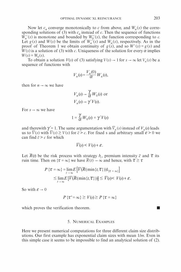
Now let cn converge monotonically to c from above, and ( )W sn the corre-sponding solutions of (3) with cn instead of .c Then the sequence of functions
( )W snl is monotone and bounded by ( ),W s0l the function corresponding to c.Let ( )g s and ( )W s be the limits of ( )W snl and ( ),W sn respectively. As in theproof of Theorem 1 we obtain continuity of ( ),g s and so ( ) ( )W s g sl = and
( )W s is a solution of (3) with c. Uniqueness of the solution for every a implies( ) ( ).W s W s0=
To obtain a solution V(s) of (3) satisfying ( )V s 1" for s " 3 let ( )V sn be asequence of functions with
( )( )
( ),V sV
W s0
nn
n= a
then for n " 3 we have
( ) ( )
( ) ( ).
V s W s
V s V s
orn
n
0"
"
ac
cl
For s " 3 we have
( ) ( )W s V s1 0= =ac
cl
and therewith .1=cl The same argumentation with n ( )V s instead of ( )V sn leadsus to ( )V s with ( ) ( )V s V s$ for > .c c For fixed s and arbitrary small > 0f wecan find >c c for which
( ) < ( ) .V s V s + f
Let ( )R t be the risk process with strategy ,bt premium intensity c and x itsruin time. Then on { }3=x we have ( )R t " 3 and hence, with $x x
{ } ( ( { , }))
( ( { , })) ( )< ( ) .
lim min
lim min
P E V R t
E V R t V s V s
1{ }t
t
3
# #
= =
+
x x
x f
"
"
33
3
=x8
6
B
@
So with 0"f
{ } ( ) { }P V s P3 3$ $= =x x)
which proves the verification theorem. ¬
5. NUMERICAL EXAMPLES
Here we present numerical computations for three different claim size distrib-utions. Our first example has exponential claim sizes with mean 1/m. Even inthis simple case it seems to be impossible to find an analytical solution of (2).
OPTIMAL DYNAMIC XL REINCURANCE 203
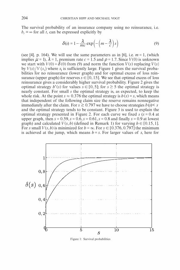
Figure 1: Survival probabilities
The survival probability of an insurance company using no reinsurance, i.e.bt = ∞ for all t, can be expressed explicitly by
( ) exps mc m c s1= - - -d m mcc m m (9)
(see [4]. p. 164). We will use the same parameters as in [6], i.e. ,m 1= (whichimplies 1=n ), ,1=m premium rate .c 1 5= and . .1 7=t Since ( )V 0 is unknownwe start with ( ) ( )V 0 0= d from (9) and norm the function ( )V s replacing ( )V sby ( )V s V s1^ h where s1 is sufficiently large. Figure 1 gives the survival proba-bilities for no reinsurance (lower graph) and for optimal excess of loss rein-surance (upper graph) for reserves [ , ].s 0 15! We see that optimal excess of lossreinsurance gives a considerably higher survival probability. Figure 2 gives theoptimal strategy ( )b s) for values [ , ];s 0 5! for s 5$ the optimal strategy isnearly constant. For small s the optimal strategy is, as expected, to keep thewhole risk. At the point .s 0 376. the optimal strategy is ( ) ,b s s= which meansthat independent of the following claim size the reserve remains nonnegativeimmediately after the claim. For .s 0 797L we have to choose strategies ( )<b s sand the optimal strategy tends to be constant. Figure 3 is used to explain theoptimal strategy presented in Figure 2. For each curve we fixed s ( .s 0 4= atupper graph, then . , . , . , .s s s s0 59 0 6 0 61 0 8= = = = and finally .s 0 9= at lowestgraph) and calculated ( , )V s b (defined in Remark 1) for varying [ . , ]b 0 15 1! .For s small ( , )V s b is minimized for .b 3= For [ . , . ]s 0 376 0 797! the minimumis achieved at the jump, which means .b s= For larger values of ,s here for
204 CHRISTIAN HIPP AND MICHAEL VOGT
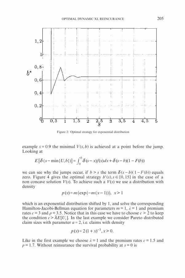
example .s 0 9= the minimal ( , )V s b is achieved at a point before the jump.Looking at
{ , } ( ) ( ) ( )( ( ))minE s U b s x f x dx s b F b1b
0- = - + - -d d d#^ h6 @
we can see why the jumps occur, if b > s the term ( )( ( ))s b F b1- -d equalszero. Figure 4 gives the optimal strategy ( ), [ , ]b s s 0 15!) in the case of anon concave solution V(s). To achieve such a V(s) we use a distribution withdensity
( ) , >expp x m m x x1 1= - -]^^ ghh
which is an exponential distribution shifted by 1, and solve the correspondingHamilton-Jacobi-Bellman equation for parameters m = 1, l = 1 and premiumrates c = 3 and r = 3.5. Notice that in this case we have to choose c > 2 to keepthe condition > [ ].c E Uim In the last example we consider Pareto distributedclaim sizes with parameter ,a 2= i.e. claims with density
( ) ( ) , > .p x x x2 1 03= + -
Like in the first example we choose l = 1 and the premium rates c = 1.5 andr = 1.7. Without reinsurance the survival probability at s = 0 is
OPTIMAL DYNAMIC XL REINCURANCE 205
Figure 2: Optimal strategy for exponential distribution
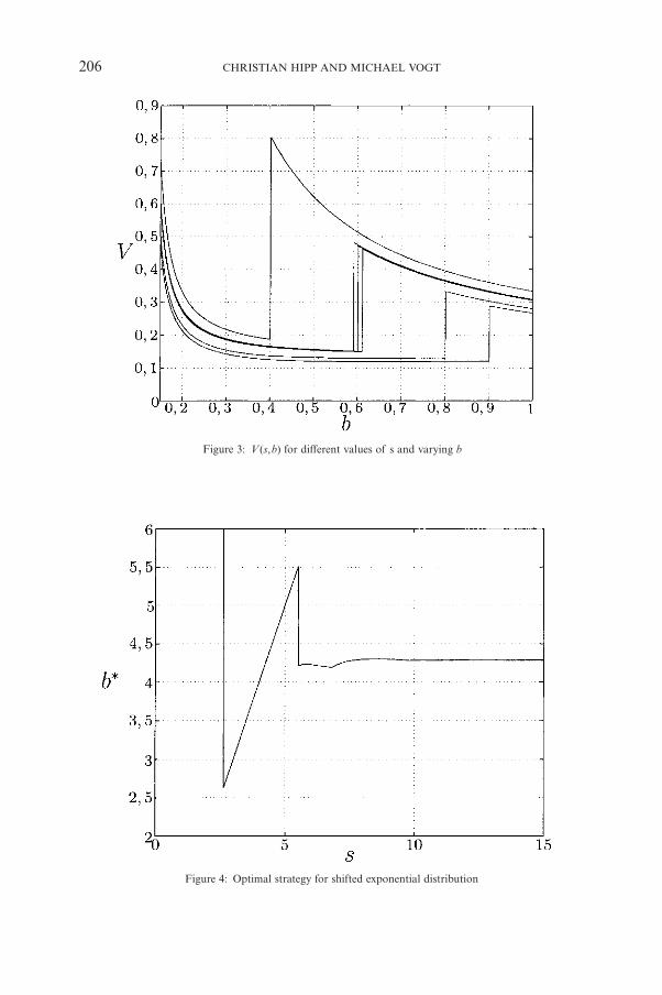
Figure 4: Optimal strategy for shifted exponential distribution
206 CHRISTIAN HIPP AND MICHAEL VOGT
Figure 3: V (s,b) for different values of s and varying b
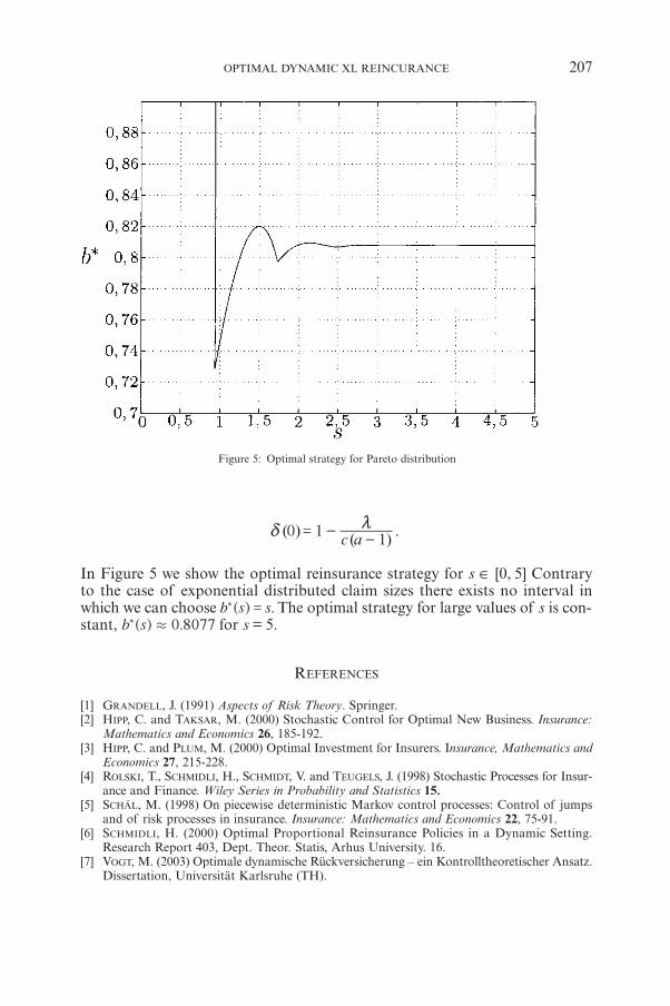
( ) ( ) .c a0 11
= --
d m
In Figure 5 we show the optimal reinsurance strategy for s ∈ [0, 5] Contraryto the case of exponential distributed claim sizes there exists no interval inwhich we can choose ( ) .b s s=) The optimal strategy for large values of s is con-stant, ( ) .b s 0 8077.) for s = 5.
REFERENCES
[1] GRANDELL, J. (1991) Aspects of Risk Theory. Springer.[2] HIPP, C. and TAKSAR, M. (2000) Stochastic Control for Optimal New Business. Insurance:
Mathematics and Economics 26, 185-192.[3] HIPP, C. and PLUM, M. (2000) Optimal Investment for Insurers. Insurance, Mathematics and
Economics 27, 215-228.[4] ROLSKI, T., SCHMIDLI, H., SCHMIDT, V. and TEUGELS, J. (1998) Stochastic Processes for Insur-
ance and Finance. Wiley Series in Probability and Statistics 15.[5] SCHÄL, M. (1998) On piecewise deterministic Markov control processes: Control of jumps
and of risk processes in insurance. Insurance: Mathematics and Economics 22, 75-91.[6] SCHMIDLI, H. (2000) Optimal Proportional Reinsurance Policies in a Dynamic Setting.
Research Report 403, Dept. Theor. Statis, Arhus University. 16.[7] VOGT, M. (2003) Optimale dynamische Rückversicherung – ein Kontrolltheoretischer Ansatz.
Dissertation, Universität Karlsruhe (TH).
OPTIMAL DYNAMIC XL REINCURANCE 207
Figure 5: Optimal strategy for Pareto distribution

COMMON POISSON SHOCK MODELS:APPLICATIONS TO INSURANCE AND CREDIT RISK MODELLING
BY
FILIP LINDSKOG* AND ALEXANDER J. MCNEIL*
ABSTRACT
The idea of using common Poisson shock processes to model dependent eventfrequencies is well known in the reliability literature. In this paper we examinethese models in the context of insurance loss modelling and credit risk model-ling. To do this we set up a very general common shock framework for lossesof a number of different types that allows for both dependence in lossfrequencies across types and dependence in loss severities. Our aims are three-fold: to demonstrate that the common shock model is a very natural way ofapproaching the modelling of dependent losses in an insurance or risk man-agement context; to provide a summary of some analytical results concerningthe nature of the dependence implied by the common shock specification;to examine the aggregate loss distribution that results from the model and itssensitivity to the specification of the model parameters.
1. INTRODUCTION
Suppose we are interested in losses of several different types and in the num-bers of these losses that may occur over a given time horizon. More concretely,we might be interested in insurance losses occurring in several different lines ofbusiness or several different countries. In credit risk modelling we might beinterested in losses related to the default of various types of counterparty.Further suppose that there are strong a priori reasons for believing that thefrequencies of losses of different types are dependent. A natural approach tomodelling this dependence is to assume that all losses can be related to a seriesof underlying and independent shock processes. In insurance these shocks mightbe natural catastrophes; in credit risk modelling they might be a variety of eco-nomic events such as local or global recessions; in operational risk modellingthey might be the failure of various IT systems. When a shock occurs this maycause losses of several different types; the common shock causes the numbersof losses of each type to be dependent.
* Research of the first author was supported by Credit Suisse Group, Swiss Re and UBS AG throughRiskLab, Switzerland. We thank in particular Nicole Bäuerle for commenting on an earlier versionof this paper.
ASTIN BULLETIN, Vol. 33, No. 2, 2003, pp. 209-238
This kind of construction is very familiar in the reliability literature wherethe failure of different kinds of system components is modelled as beingcontingent on independent shocks that may affect one or more components.It is commonly assumed that the different varieties of shocks arrive as inde-pendent Poisson processes, in which case the counting processes for the differ-ent loss types are also Poisson and can be easily handled analytically. In reli-ability such models are known as fatal shock models, when the shock alwaysdestroys the component, and non-fatal shock models, or not-necessarily-fatalshock models, when components have a chance of surviving the shock. A goodbasic reference on such models is Barlow and Proschan (1975) and the ideasgo back to Marshall and Olkin (1967).
In this paper we set up a very general Poisson shock model; the dimensionis arbitrary and shocks may be fatal or not-necessarily-fatal. We review and gen-eralise results for the multivariate Poisson process counting numbers of failuresof different types. We also consider the modelling of dependent severities.When a loss occurs, whether in insurance or credit risk modelling, a loss sizemay be assigned to it. It is often natural to assume that losses of differenttypes caused by the same underlying shock also have dependent severities. We setup general multivariate compound Poisson processes to model the losses ofeach type. Our interest focusses on three distributions in particular, and theirsensitivity to the finer details of the parameterization of the model:
• The multivariate compound Poisson distribution of the cumulative lossesof different types at some fixed point in time.
• The multivariate exponential distribution of the times to the first losses ofeach type.
• The univariate compound Poisson aggregate loss distribution at a fixed timepoint.
There have been a number of other related papers in this area in recent years,particularly concentrating on the second of these issues. In Savits (1988) non-homogeneous Poisson shock processes are investigated and the effect of dif-ferent mean functions for the shock processes on the distributional propertiesof the joint component lifetimes is studied. In Li and Xu (2001) the authorsinvestigate stochastic bounds and dependence properties of the joint componentlifetime distribution for rather general shock arrival processes. In particularthe effect of dependent interarrival times of the shocks and the effect of simul-taneous shock arrivals on the joint component lifetime distribution are inves-tigated; the joint impact of these two types of dependency on the behaviourof the system is analysed.
The present paper is structured as follows. In Section 2 we describe the gen-eral not-necessarily-fatal-shock model with dependent loss frequencies anddependent loss severities. In Section 3 we ignore loss severities and examine themultivariate distribution of loss frequencies and the consequences for the aggre-gate loss frequency distribution of specifying the shock structure in differentways. An important key to analysing the model is to see that it may be writtenin terms of an equivalent fatal shock model. This facilitates the approximationof the aggregate loss frequency distribution using the Panjer recursion approach
210 FILIP LINDSKOG AND ALEXANDER J. MCNEIL
and also makes it very easy to analyse the multivariate exponential distributionof the times to the first losses of each type. In section 4 the analysis is gener-alised by including dependent loss severities. The dependence in severities iscreated using copula techniques and the object of interest is now the tail of theoverall aggregate loss distribution. Sections 3 and 4 are illustrated with a stylizedinsurance example; Section 5 consists of an extended example of how themodel might be applied to the modelling of portfolio credit risk.
2. THE MODEL
2.1. Loss Frequencies
Suppose there are m different types of shock or event and, for , , ,e m1 f= let
( ),N t t 0( )e $# -
be a Poisson process with intensity ( )em recording the number of events of type eoccurring in (0, t]. Assume further that these shock counting processes areindependent. Consider losses of n different types and, for , , ,j n1 f= let
( ),N t t 0j $$ .
be a counting process that records the frequency of losses of the j th type occur-ring in (0, t].
At the rth occurrence of an event of type e the Bernoulli variable I ,( )j re indi-
cates whether a loss of type j occurs. The vectors
, ,I II( ),
( ),
( )re
re
n re
1f= l
` j
for , , ( )r N t1 ( )ef= are considered to be independent and identically distributedwith a multivariate Bernoulli distribution. In other words, each new event rep-resents a new independent opportunity to incur a loss but, for a fixed event, theloss trigger variables for losses of different types may be dependent. The formof the dependence depends on the specification of the multivariate Bernoullidistribution and independence is a special case. We use the following notationfor p-dimensional marginal probabilities of this distribution (where the sub-script r is dropped for simplicity).
, , , , , , , { , }.P I i I i p i i i i 0 1( ) ( ), ,
( )je
j je
j j je
j j j jp p p p p1 1 1 1 1f f f != = =
fb al k
We also write ( )p p1( ) ( )
je
je= for one-dimensional marginal probabilities, so that
in the special case of conditional independence we have
( , , )p p1 1, ,( ) ( )j je
je
k
p
1p k1
f =f
=
%
COMMON POISSON SHOCK MODELS 211
The counting processes for events and losses are thus linked by
j ,j r( ) .N t I ( )( )
e
r
N t
e
m
11
( )e
===
!! (1)
Under the Poisson assumption for the event processes and the Bernoulliassumption for the loss indicators, the loss processes { ( ), }N t t 0j $ are clearlyPoisson themselves, since they are obtained by superpositioning m indepen-dent (possibly thinned) Poisson processes generated by the m underlying eventprocesses. ( ( ), , ( ))N t N tn1 f l can be thought of as having a multivariate Poissondistribution.
However the total number of losses j 1=( ) ( )N t N tj
n= ! is in general not
Poisson but rather compound Poisson. It is the sum of m independent com-pound Poisson distributed random variables as can be seen by writing
( ) .N t I ,( )
( )
j re
j
n
r
N t
e
m
111
( )e
====
!!! (2)
The compounding distribution of the eth compound Poisson process is the distribution of jj 1=
I ( )en! , which in general is a sum of dependent Bernoulli vari-ables. We return to the compound Poisson nature of the process {N(t), t ≥ 0}after generalising it in the next section.
2.2. Adding Dependent Severities
We can easily add severities to our multivariate Poisson model. Supposethat when the rth event of type e occurs a potential loss of type j with sever-ity ,j rX ( )e can occur. Whether the loss occurs or not is of course determined by the value of the indicator ,j r ,I ( )e which we assume is independent of X (e)
j,r .The potential losses { , , , ( ), , ,X r N t e m1 1,
( ) ( )j re ef f= = } are considered to be iid
with distribution Fj. Potential losses of different types caused by the same eventmay however be dependent. We consider that they have a joint distributionfunction F. That is, for a vector Xr
( )e of potential losses generated by the sameevent we assume
, , .X X FX( ),
( ),
( )re
re
n re
1f += l
` j
In a more general model it would be possible to make the multivariate distri-bution of losses caused by the same event depend on the nature of the under-lying event e. However, in practice it may make sense to assume that there isa single underlying multivariate severity distribution which generates the sever-ities for all event types. This reflects the fact that it is often standard practicein insurance to model losses of the same type type as having an identical claimsize distribution, without necessarily differentiating carefully between the eventsthat caused them.
212 FILIP LINDSKOG AND ALEXANDER J. MCNEIL
The aggregate loss process for losses of type j is a compound Poisson processgiven by
( ) .Z t I X,( )
,( )
( )
j j re
j re
r
N t
e
m
11
( )e
===
!! (3)
The aggregate loss caused by losses of all types can be written as
( ) ,Z t I X I X,( )
,( )
( )( ) ( )
( )
j re
j re
j
n
r
N t
e
m
re
re
r
N t
e
m
111 11
( ) ( )e e
= ==== ==
!!! !! l (4)
and is again seen to be a sum of m independent compound Poisson distribu-ted random variables, and therefore itself compound Poisson distributed.Clearly (2) is a special case of (4) and (1) is a special case of (3). Thus we canunderstand all of these processes by focusing on (4). The compound Poissonnature of Z(t) can be clarified by rewriting this process as
( )Z t Yd( )
ss
S t
1
==
! ,
where { ( ), }S t t 0$ is a Poisson process with intensity ( )ee
m
1=m m
=! , counting
all shocks s generated by all event types, and where the random variablesY1,…,YS(t) are iid and independent of {S(t), t ≥ 0}. Y1 has the stochastic rep-resentation
( ) ,Y Ud I X1 ( )e
e
m
11
( ) / , ( ) /j jje
j
e
11
1== ==
-m m m m! !!
l
_e i o
where U, I(e), X are independent, U is uniformly distributed on (0,1), I(e) is ageneric random vector of indicators for shocks of event type e, and X is ageneric random vector of severities caused by the same shock. In words: ashock s is of event type e with probability /( )em m.
We consider two examples that fit into the framework of the model wehave set up. The first one, an insurance application of the model, we continueto develop throughout the paper. The second one, a credit risk application, ispresented separately in Section 5.
2.3. Insurance example: natural catastrophe modelling
Fix n = 2, m = 3. Let 1( )N t and ( )N t2 count windstorm losses in France andGermany respectively. Suppose these are generated by three different kinds ofwindstorm that occur independently. ( )N t( )1 counts west European windstorms;these are likely to cause French losses but no German losses. ( )N t( )2 countscentral European windstorms; these are likely to cause German losses but noFrench losses. ( )N t( )3 counts pan-European windstorms, which are likely tocause both French and German losses.
COMMON POISSON SHOCK MODELS 213
3. THE EFFECT OF DEPENDENT LOSS FREQUENCIES
To begin with we look at the distribution of the random vector (N1(t),…,Nn(t))�, particularly with regard to its univariate and bivariate margins as wellas the correlation structure. Part 2 of the following proposition is from Barlowand Proschan (1975), p. 137.
Proposition 1.
1. {( ( ), , ( )) , }N t N t t 0n1 f $l is a multivariate Poisson process with
j( ( ))E N t t p( ) ( )eje
em
1= m
=! . (6)
2. The two-dimensional marginals are given by
( ( ) , ( ) )
! ! !
( , ) ( , ) ( , ),
P N t n N t n e
i n i n i
tp tp tp1 1 1 0 0 1
( ( , ) ( , ) ( , ))
, , ,{ , }min
j j k kt p p p
j k
j ki
j kn i
j kn i
i
n n
1 1 1 0 0 1
0
, , ,j k j k j k
j kj k
#= = =
- -
m m m
- + +
- -
=
m
!` ^
` ` `
j h
j j j (7)
where ( )eem
1=m m
=! and
( , ) ( , ), , { , }.p i i p i i i i 0 1,( )
,( )
j k j ke
j ke
j k j ke
m1
1
!= m m-
=
!
3. The covariance and correlation structure is given by
( ), ( ) ( , )cov N t N t t p 1 1( ),
( )j k
ej ke
e
m
1
= m=
!` j (8)
and
( ), ( )( , )
.N t N t
p p
p 1 1
( ) ( ) ( ) ( )
( ),
( )
j ke
je
e
me
ke
e
m
ej ke
e
m
1 1
1=t
m m
m
= =
=
! !
!`
e e
j
o o
Proof
1. obvious using thinning and superposition arguments for independentPoisson processes.
2. is found in Barlow and Proschan (1975), p. 137.3. is a special case of Proposition 7 (part 2).
¡
Clearly, from Proposition 1 part 3, a necessary condition for Nj(t) and Nk(t) to be independent is that ( , )p 1 1 0
,
( )
j ke = for all e; i.e. it must be impossible for
214 FILIP LINDSKOG AND ALEXANDER J. MCNEIL
losses of types j and k to be caused by the same event. If for at least one eventit is possible that both loss types occur, then we have positive correlationbetween loss numbers. However Proposition 1, part 2 allows us to make a strongerstatement.
Corollary 2. Nj(t) and Nk(t) are independent if and only if ( , )p 1 1 0,( )j ke = for all e.
Note that if ( , )p 1 1 0,( )j ke = for all ,j k with j k! , then
( , ) ( ) ( , , )
.
P P I
p p p
p
I 1 1
1 1 1 1 1 1
1
0( ),
( )
( ),
( ), ,
( )
<
( )
re
jn
j re
je
j ke n
ne
j kj
n
je
j
n
1
11
1
1
,
f f
= = - =
= - - + + -
= -
f
=
-
=
=
!!
!
J
L
KK
` a
N
P
OO
j k% /
Hence if >p 1( )
j
e
j
n
1=! for some e, then ( , ) >p 1 1 0,
( )j ke for some j k! , or equiv-
alently:
Corollary 3. If >p 1( )je
jn
1=! for some e, then ( ), , ( )N t N tn1 f are not indepen-
dent.
Thus if we begin by specifying univariate conditional loss probabilities p(e)j it
is not always true that a shock model can be constructed which gives inde-pendent loss frequencies.
We have already noted that the process of total loss numbers N(t) = ( )N tjj
n
1=! is in general not Poisson (but rather a sum of independent compound
Poissons). If there is positive correlation between components j ( )N t then( ),N t t 0$! + itself cannot be a Poisson process since it is overdispersed with
respect to Poisson. It can easily be calculated (see Proposition 9 later) that
( ) ( ), ( ) > ( )var covN t N t N t E N tj kk
n
j
n
11
===
!!^ ` ^h j h (9)
Suppose we define a new vector of independent Poisson distributed loss coun-
ters Nj(t) such that ( ) ( )t N tdN j j= . Clearly ( ) ( )t tN N jj
n
1=
=! is Poisson distribu-
ted and
( ) ( ) ( ) .var t E t E N tN N= =_ _ ^i i h
The case where the components Nj(t) are dependent is clearly more dangerous(in the sense of higher variance) than the case with independent components.Although the expected number of total losses is the same in both cases the
COMMON POISSON SHOCK MODELS 215
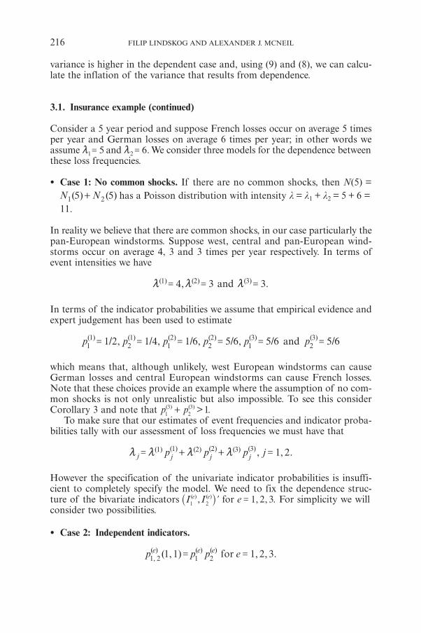
variance is higher in the dependent case and, using (9) and (8), we can calcu-late the inflation of the variance that results from dependence.
3.1. Insurance example (continued)
Consider a 5 year period and suppose French losses occur on average 5 timesper year and German losses on average 6 times per year; in other words weassume 51=m and .62=m We consider three models for the dependence betweenthese loss frequencies.
• Case 1: No common shocks. If there are no common shocks, then N(5) = ( ) ( )N N5 51 2+ has a Poisson distribution with intensity l = l1 + l2 = 5 + 6 =
11.
In reality we believe that there are common shocks, in our case particularly thepan-European windstorms. Suppose west, central and pan-European wind-storms occur on average 4, 3 and 3 times per year respectively. In terms ofevent intensities we have
, .and4 3 3( ) ( ) ( )1 2 3= = =m m m
In terms of the indicator probabilities we assume that empirical evidence andexpert judgement has been used to estimate
/ , / , / , / , / /p p p p p pand1 2 1 4 1 6 5 6 5 6 5 6( ) ( ) ( ) ( ) ( ) ( )11
21
12
22
13
23= = = = = =
which means that, although unlikely, west European windstorms can causeGerman losses and central European windstorms can cause French losses.Note that these choices provide an example where the assumption of no com-mon shocks is not only unrealistic but also impossible. To see this considerCorollary 3 and note that >p p 1( ) ( )
1
3
2
3+ .To make sure that our estimates of event frequencies and indicator proba-
bilities tally with our assessment of loss frequencies we must have that
, , .p p p j 1 2( ) ( ) ( ) ( ) ( ) ( )j j j j
1 1 2 2 3 3= + + =m m m m
However the specification of the univariate indicator probabilities is insuffi-cient to completely specify the model. We need to fix the dependence struc-ture of the bivariate indicators ,I I( ) ( )e e
1 2l_ i for , ,e 1 2 3= . For simplicity we will
consider two possibilities.
• Case 2: Independent indicators.
( , ) , , .p p p efor1 1 1 2 3,( ) ( ) ( )e e e1 2 1 2
= =
216 FILIP LINDSKOG AND ALEXANDER J. MCNEIL
• Case 3: Positively dependent indicators.
( , ) , , .p p p efor1 1 1 2 3,( ) ( ) ( )e e e1 2 1 2
$ =
To be specific in Case 3 we will consider ( , ) ,minp p p1 1,
( ) ( ) ( )e e e
1 2 1 2= ` j, which is the
strongest possible dependence between the indicators, sometimes known ascomonotonicity; the random variables , ,X Xn1 f are said to be comonotonic ifthere exist increasing functions , , :� �v vn1 "f , and a random variable Z such that ( , , ) ( ( ), , ( ))X X v Z v Z
dn n1 1f f l=l . For more on comonotonicity see Wang
and Dhaene (1998) and the references therein. See also Joe (1997) for somediscussion of dependence bounds in multivariate Bernoulli models. In termsof interpretation in our application this means:
• if a west European windstorm causes a German loss, then with certainty italso causes a French loss;
• if a central European windstorm causes a French loss, then with certaintyit also causes a German loss;
• if a pan-European windstorm causes one kind of loss, then with certaintyit causes the other kind of loss.
For cases 1, 2 and 3 we get ( ( )) ,var N 5 55 85= and 95 respectively. Of moreinterest than the variance as a measure of the riskiness of ( )N 5 are thetail probabilities ( ( ) > )P N k5 . In this example these probabilities can be cal-culated analytically using formula (7) for the bivariate frequency function.The left plot in Figure 1 shows exceedence probabilities ( ( ) > )P N k5 , for
COMMON POISSON SHOCK MODELS 217
Figure 1: Left: Exceedence probabilities P(N(5) > k) for , , , ,k 70 71 90f= for case 1 (lower), 2 (middle)and 3 (upper). Right: Ratios of such exceedence probabilities for cases 1-2 (lower) and 1-3 (upper).
, , , ,k 70 71 90f= for the three cases. The right plot shows by which factor suchan exceedence probability is underestimated by case 1 if the correct modelwould be given by case 2 or 3. Clearly, both the presence of common shocksand then the subsequent addition of dependent indicators have a profoundeffect on the aggregate frequency distribution of N(5).
3.2. The Equivalent Fatal Shock Model
The not-necessarily-fatal shock model set up in the previous section has thenice property of being easily interpreted. As we will now show this model hasan equivalent representation as a fatal shock model. Basically, instead of count-ing all shocks, we only count loss-causing shocks. From this representation wecan draw a number of non-trivial conclusions about our original model.
Let S be the set of non-empty subsets of , , n1 f! +. For s S! we intro-duce a new counting process s ( )tN , which counts shocks in (0, t] resultingin losses of all types in s only. Thus if { , , }s 1 2 3= , then ( )tNs counts shockswhich cause simultaneous losses of types 1, 2 and 3, but not of types 4 to n.We have
( ) ( ) ,t IN 1 | | | |,
( )
:
( )
ss s
k re
k ss s sr
N t
e
m
11
( )e
= -!
4
-
==
%!!! ll
l l
where ( ) I1 | | | |,
( ):
s sk re
k ss s s-
!4- %! l
ll lis an indicator random variable which takes
the value 1 if the rth shock of type e causes losses of all type in s only, and thevalue 0 otherwise. Furthermore let N(t) count all shocks in (0, t] which resultin losses of any kind. Clearly we have
( ) ( )t tN Nss S
=!
! .
The key to a fatal shock representation is the following result.
Proposition 4.
1. ( ),t tN 0s $" , for s S! are independent Poisson processes with intensities
( ) ,p1( ) | | | | ( )
:s
e s sse
s s se
m
1
= -m m4
-
=
!! ll
l l
where p P I 1( ),
( )se
k re
k s= =!
%l l` j, and
2. { ( ), }t tN 0$ is a Poisson process with intensity
.P I1 0( ) ( )s
ere
e
m
s S 1
= = - =m m m! =
!!u `a jk
218 FILIP LINDSKOG AND ALEXANDER J. MCNEIL
Proof. Let ( )J I1,( ) | | | |
,( )
:s re s s
k re
k ss s s= -
!4
- %! l
ll l. First note that the random vari-
able J ,( )s re takes values in {0,1}, and that ( ) ,P J p1 1,
( ) | | | | ( ):s r
e s sse
s s s= = -
4
-! lll l
` j where
p P I 1( ),
( )se
k re
k s= =
!%l l` j, does not depend on r. Hence ,J t 0,
( )( )
s re
r
N t
1
( )e
$=
!& 0 is
obtained by thinning the Poisson process ( ), ,N t t 0( )e $# - and is therefore a
Poisson process with intensity ( ) . ( ),p t tN1 0( ) | | | | ( )
:
e s sse
ss s s$-m
4
-! lll l# - is obtained
by superpositioning the independent Poisson processes ,J t 0,
( )( )
s re
r
N t
1
( )e
$=
!& 0 for
, , ,e m1 f= and is therefore a Poisson process with intensity ls = ( )eem
1m
=!
( ) p1 | | | | ( ):
s sse
s s s -4
-! lll l . Since ( ) )P I1 1| | | |
,( )
:s s
k re
k ss s ss S- =
!4!- %!! l
ll la k
(the probability that the rth shock of type e causes at least one loss) does notdepend on r, thinning and superpositioning arguments give that { ( ), }t tN 0$
is a Poisson process with intensity P I1 0( ) ( )s
ere
e
m
s S 1= = - =m m m
! =!!u __ ii.
Each jump in the process ( ),t tN 0$" , corresponds to a jump in exactly one ofthe processes ( ),t tN 0s $" , for s ∈ S. Given a jump in ( ),t tN 0$" ,, the proba-bility of the jump being in ( ),t tN 0s $" , is given by /qs s= m mu for s ∈ S. Orderthe l = | |S 2 1n= - non-empty subsets of , ,n1 f! + in some arbitrary way.
Then
( ) , , ( ) | ( )! ! , ,
, .P t n t n t
q n n
nN N N n
n n
n0s s l
sn
jjl
jjl
jjl1
1 1
1
l
j
j
1f
!= = = =
== =
=
% !
!`
c
j
m
Z
[
\
]]
]]
and hence
( ( ) , , ( ) ) ( ) ! !
! ( ) .
P t n t n P t n n n
q
e n
tP t n
N N N
N
s s l jj
l
jj
l
j
sn
j
l
t
j
s
n
j
l
s jj
l
11 1 1
1 1
l
j
j
s jj
j
j
1f= = = =
= = =m
= = =
-
= =
m
! ! %
% %
J
L
KK
J
L
KK
a
a
N
P
OO
N
P
OO
k
k
It follows that the processes ( ),t tN 0s $# - for s ∈ S are independent Poissonprocesses.
¡
Since the Poisson processes ( ),t tN 0s $# - for s ∈ S are independent and sincethe loss counting processes may be written as
( ) ( ),N t tN:
j ss j s
=!
!
COMMON POISSON SHOCK MODELS 219
it also follows that we have obtained a fatal shock model representation forthe original not-necessarily-fatal set-up.
Furthermore, since 0s =m for all s with | |s 2$ if and only if p(e)j,k (1,1) = 0
for all e and all j,k with ,j k! Corollary 2 concerning pairwise independence can be strengthened.
Corollary 5. ( ), , ( )N t N tn1 f are independent if and only if p(e)j,k (1,1) = 0 for
all e and all j,k with j k! .
A direct consequence of the fatal shock model representation of the originalnot-necessarily-fatal shock model is that the multivariate distribution of the times to first losses can be easily analysed. Let Tj = inf{t : Nj (t) > 0} denote the time to the first loss of type j. We now consider briefly the distribution of
, ,T Tn1 f l^ h whose dependence structure is well understood. For s S! let : ( ) > .infZ t tN 0s s= # - Zs s S!
" , are independent exponential random variables with parameters .s s S
m!
" , Hence
jj : ( ) > : ( ) >inf inf minT t N t t t ZN0 0: :s
s j s s j s s= = =! !
!$ *. 4
and , , , ,min minT T Z Z: :
ns s
ss n s
s11
f f=! !
^ bh l. Survival probabilities for , ,T Tn1 f^ h can
be calculated as follows.
> , , >
, , , , , ,
, , ,
, , , ( )
max max
max max
exp max max
P T t T t
P t t t t t
P t P t t P t t
t t t t t
N N N
N N N
0 0 0
0 0 0
10
{ } < { , } { , , }
{ } { , }<
{ , , }
{ } { , } { , , }<
n n
i i i i j i j i j n n
i i i j i ji ji
n n
i i i j i j n ni ji
1 1
1 1
1 1
1 1
+ +
f
f f
g f
f f
= = = =
= = = =
= - - - -m m m
f
f
f
%%
!!
^
^ _` ^_`
^_ _`` ^__
_ ^f
h
h ij hi j
h i ij j hi i
i hp
The multivariate exponential distribution with this joint survival probability isthe multivariate exponential distribution of Marshall and Olkin (Marshall andOlkin (1967)). The distribution has been studied extensively, see Barlow andProschan (1975), Joe (1997), Marshall and Olkin (1967) or Nelsen (1999). Themultivariate exponential distribution of Marshall and Olkin has the propertythat
> , , > > , , > > , , > ,P T t s T t s T t T t P T s T sn n n n n n n1 1 1 1 1 1 1f f f+ + =_ ^i h
for all t1, …, tn, s1, …, sn > 0. This is the multivariate version of the lack ofmemory property which is well known for the univariate exponential distribu-tion. Not that this does not apply to general multivariate distributions with
220 FILIP LINDSKOG AND ALEXANDER J. MCNEIL
exponential marginals. The expression for the joint survival probability (10)might not be very convenient to work with if the model was set up as a not-necessarily-fatal shock model. However, it can easily be rewritten in a moreconvenient form.
> , , > ( , ) ,
... ( , , ) , , .
exp min
min
P T t T t p t p t t
p t t
1 1
1 1
( ) ( ),( )
<
, ,( )
n ne
ie
i i je
i ji jie
m
ne
n
1 11
1 1
f
f f
= - +
+ +
m
f
=
!!!
!
J
L
KK^ `
^
N
P
OO
h j
h
R
T
SSS
V
X
WWW
Recall that for a Poisson process with intensity m, the time to the kth jumpis G(k, 1/m)-distributed, where G(·,·) denotes the Gamma distribution.Hence the time to the kth loss-causing shock is G(k, 1/l)-distributed, where
P I1 0( ) ( )ere
e
m
1= - =m m
=!u __ ii. The time to the kth loss is : ( ) ,inf t N t k$! + where
( ) ( ).N t i tN:
ss s ii
n
1
===
!!
( ),N t t 0$! + is in general not a Poisson process but rather a compound Pois-son process, the time to the kth jump is still ( , / )k 1G mu -distributed but there arenon unit jump sizes. By noting that the probability that the time to the kthloss is less than or equal to t can be expressed as ( ( ) )P N t k$ , it is clear thatthe distribution of the time to the kth loss can be fully understood from thedistribution of N(t) for t ≥ 0, and this distribution can be evaluated usingPanjer recursion or other methods.
3.3. Panjer Recursion
If there are common shocks, then j( ) ( )N t N tj
n
1=
=! does not have a Poisson
distribution. In our insurance example we have considered only two loss typesand it is thus easy to calculate the distribution of N(t) directly using convolu-tion and the bivariate frequency function in (7). A more general method ofcalculating the probability distribution function of N(t), which will also workin higher dimensional examples, is Panjer recursion (Panjer (1981)). We usethe notation of the preceding section. In addition, let Wi denote the numberof losses due to the i th loss-causing shock. The total number of losses, N(t),has the stochastic representation
k( ) ,N t Wd( )
k
tN
1
==
!
where , , ( )W W Wd( )tN1 f = are iid and independent of ( )tN . The probability
( ( ) )P N t r= can now easily be calculated using Panjer recursion.
COMMON POISSON SHOCK MODELS 221

Proposition 6.
( )( ) ( ( ) ), ,
( ), ,expP N t r r
tk P W k P N t r k r
t r
1
0
( , )min
k
r n
1
$= =
= = -
- =
m
m=
!u
u^ h
Z
[
\
]]
]](11)
where
( )( ) , < ,
, ,
P W k
p nk i
nk
n ki
p k n
p k n
1( ) ( ) ( )
:| |:
( ){ , , }( )
e
e
m
se i
se
s s k ii
n k
s s k
en
e
e
m
1
1 1
11
1
= =
+ -
+
-
=
m m
m mf
-
= = +=
-
=
-
=
! !!!
!
u
u
J
L
KKKK c
c cN
P
OOOOm
m m
Z
[
\
]]]]
]]]]
Proof. The formula (11) follows from Theorem 4.4.2, p. 119 in Rolski, Schmidli,Schmidt and Teugels (1998), and that the maximum number of losses due toa loss-causing shock is n. The probability that a loss-causing shock causesexactly k losses is given by ( ) ,P W k
:| | ss s k1= = m m-
=!u where
( ) .p1( ) | | ( )
:::s
e s sse
s s ss s ke
m
s s k 1
= -m m4
-
===
!!!! ll
l l
The expression of the probability that a loss-causing shock causes n lossescan be simplified to
( ) ( , , ).P W n p p 1 1( ){ , , }( ) ( )
, ,( )e
ne
e
me
ne
e
m1
11
11
1
f= = =m m m mf f
-
=
-
=
! !u u
For k ≤ n we note that there are nkc m sets s with | |s k= , and for each such s
there are n ki-
d n sets of size { , , }k i i n k1 f!+ -^ h which contain s as a proper
subset. Hence
( ) p1 | | | | ( )
::
s sse
s s ss s k-
4
-
=
!! ll
l l
(12)
consists of nk
n ki-
d dn n terms ( ) p1 | | | | ( )s ss
e- -ll for which | |s k i= +l and s s1 l. Since
there are nk i+d n sets sl with | |s k i= +l it follows that (12) is equal to
( ) .p nk i
nk
n ki
p1( ) ( )
::se i
se
s s k ii
n k
s s k 1
+ -
+
-
= +=
-
=
!!!c
c c
m
m m
¡
222 FILIP LINDSKOG AND ALEXANDER J. MCNEIL
For large n, say n > 100, the usefulness of the Panjer recursion scheme relies heavily on the calculation of p( )
: s
e
s s k=! for { , , }k n1 f! . We now look at two
specific assumptions on the multivariate Bernoulli distribution of I( )e condi-tional on a shock of type e. The assumption of conditional independence isattractive for computations since in this case
.p p p p( ) ( ) ( ) ( )
>>:se
je
je
je
j jj jj
n
s s k 1k
k k1 2
12 11
f f=== -
!!!!
Under the assumption of conditional comonotonicity
, , , .minp p p p( ) ( ) ( ) ( )
>>:se
je
je
je
j jj jj
n
s s k 1k
k k1 2
12 11
f f=== -
!!!! a k
The latter assumption leads to very efficient computations of p( ): s
es s k=
! .Let
, , ,p p p( ) ( ) ( )e e en1 2
fr r rl
a k
denote the sorted vector of univariate conditional indicator probabilities, suchthat .p p p( ) ( ) ( )e e e
n1 2f# # #r r r Then
,p pn i
k 1
( ) ( )
:se e
i
n
s s k 1i
=-
-==
r!!J
LK
N
PO
where n ik 1
--
d n is the number of subsets of size k of { , , }n1 f with i as smallest
element.
4. THE EFFECT OF DEPENDENT SEVERITIES
We now consider adding severities to our shock model and study the multi-variate distribution of ( ), , ( )Z t Z tn1 f l^ h . Again we can calculate first andsecond moments of the marginal distributions and correlations between thecomponents.
Proposition 7.
1. {( ( ), , ( )) , }Z t Z t t 0n1 f l $ is a multivariate compound Poisson process. If(| |)<E X j 3, then
( ) ( ) .E Z t E X E N tj j j=` ` `j j j
COMMON POISSON SHOCK MODELS 223
2. If , <E X E Xj k2 2 3` `j j , then the covariance and correlation structure is given
by
j j j( ( ), ( )) ( ) ( ( ), ( ))cov covZ t Z t E X X N t N tk k k=
and
( ), ( ) ( ), ( ) .Z t Z tE X E X
E X XN t N tj k
j k
j kj k2 2
=t t`
` `
``j
j j
jj
Proof
1. is easily established from formula (3).
2. We observe that , { , , },j k n16 f!
( ), ( ) ,
,
,
( )
( , )
( ), ( )
cov cov
cov
cov
cov
Z t Z t I X I X
I X I X
I X I X
E X X E N t E I I
E X X t p
E X X N t N t
1 1
,( )
,( )
,( )
,( )
( )( )
,( )
,( )
,( )
,( )
( )( )
,( )
,( )
,( )
,( )
( )( )
( ) ( ) ( )
( ),
( )
j k j re
j re
k re
k re
r
N t
r
N t
e
m
j re
j re
k rf
k rf
r
N t
r
N t
f ee
m
j re
j re
k re
k re
r
N t
r
N t
e
m
j ke
je
ke
e
m
j ke
j ke
e
m
j k j k
111
111
111
1
1
( )( )
( )( )
( )( )
ee
fe
ee
=
+
=
=
=
=
m
!
===
===
===
=
=
!!!
!!!!
!!!
!
!
J
L
KK
J
L
KK
J
L
KK
`
` _ a
`
` `
N
P
OO
N
P
OO
N
P
OO
j
j i k
j
j j
¡
Now consider the distribution of the total loss ( ) ( ).Z t Z tjj
n
1=
=! The expected
total loss is easily calculated to be
( ) ( ) ,E Z t E X E N tj jj
n
1
==
!^ ` `h j j
and higher moments of Z(t) can also be calculated, by exploiting the com-pound Poisson nature of this process as shown in (5). Since {Z(t), Z ≥ 0} is themost general aggregate loss process that we study in this paper we collect someuseful moment results for this process.
224 FILIP LINDSKOG AND ALEXANDER J. MCNEIL
Lemma 8. The pth derivative of the characteristic function ( )Z t{ of ( )Z t satisfies
( ) ( ) ( ),x tp
k x x1
( )( ) ( )
( )( )
Z tp
k
p
Yk
Z tp k
0
11 1
=-
{ m { {=
-+ - -! c m (13)
where Y{ denotes the characteristic function of Y.
Proof. The formula (13) is proved by induction using the binomial relation p
kpk
pk
1 11 1
- -+ +
+ =d d dn n n. The induction step reads as follows. Fix p and sup-
pose that (13) holds. Then
( ) ( ) ( ) ( ) ( )
( ) ( ) ( ) ( )
( ) ( ) ( ) ( )
( ) ( ) ( ) ( )
( ) ( )
( ) ( ).
x tp
k x x x x
tp
k x x t x x
t x x tpk x x
t x x tpk x x
t x x
tpk x x
1
1
11
( )( ) ( )
( )( ) ( )
( )( )
( )( )
( ) ( )( )
( )
( )( )
( ) ( )( )
( )
( )( )
( ) ( )( )
( )
( )( )
( )
( )( )
( )
Z tp
Yk
Z tp k
Yk
Z tp k
k
p
Yk
Z tp k
Yp
Z tk
p
Y Z tp
Yk
Z tp k
k
p
Y Z tp
k
p
Yk
Z tp k
Yp
Z t
k
p
Yk
Z tp k
1 2 1 1
0
1
2 1 1 0
0
2
1 2 1
0
2
1
1
11
1 0
0
1
=-
+
=-
+
+ +-+
= +
+
=
{ m { { { {
m { { m { {
m { { m { {
m { { m { {
m { {
m { {
+ + - - + -
=
-
+ - - +
=
-
+ - -
=
-
=
-+ -
+
=
+ -
!
!
!
!
!
c `
c
d
c
c
m j
m
n
m
m
¡
Using Lemma 8, the moments of Z(t) can be calculated as follows.
Proposition 9.
1. If they exist, the 2nd and 3rd order central moment of Z(t) are given by
( ) ( ) ( ), , ,E Z t E Z t tE Y p 2 3p p- = =m^^` hh j (14)
where ( )eem
1=m m
=! and
( ) ( ) ( , , ).E Y E X X p11 1( )
, ,( )p
j je
j je
e
m
j
n
j
n
111p p
p1 1
1
f f f=m
mf
===
!!! (15)
2. Whenever they exist, the non-central moments of Z(t) are given recursively by
( ) ( ) ,E Z t tp
k E Y E Z t1p
k
pk p k
0
11 1=
-m
=
-+ - -!_ c _ _i m i i
with ( )E Y k 1+ given by (15).
COMMON POISSON SHOCK MODELS 225
Proof
1. For a compound Poisson process of the form (5) the formula (14) is wellknown. We can calculate that for all p
( ) ( )
( , , )
( , , ).
E Y E
E I I X X
E X X p
E X X p
I X
1 1
1 1
( )( )
( ) ( ) ( )
( ), ,
( )
( ), ,
( )
pe
e p
e
m
e
je
je
j jj
n
j
n
e
m
ej j j j
e
j
n
j
n
e
m
j je
j je
e
m
j
n
j
n
1
111
1
111
1
111
p pp
p pp
p pp
1 1
1
1 11
1 11
l
g f f
g f f
f f f
=
=
=
=
mm
mm
m m
m m
f
f
=
===
-
===
-
===
!
!!!
!!!
!!!
J
L
KK
_
a
a
N
P
OO
i
k
k
2. If (| ( )| ) < ,E Z t p 3 then ( ) ( ( ) )i E Z t0( )
( )
Z t
k k k={ for , ,k p1 f= . The conclu-sion follows by applying this to (13).
¡
We are particularly interested in the effect of different levels of dependencebetween both loss frequencies and loss severities on the tail of the distributionof Z(t), and on higher quantiles of this distribution. The distribution of Z(t)is generally not available analytically but, given the ease of simulating from ourPoisson common shock model, it is possible to estimate quantiles empiricallyto a high enough degree of accuracy that differences between different depen-dence specifications become apparent.
It is also possible, given the ease of calculating moments of Z(t), to use amoment fitting approach to approximate the distribution of Z(t) with variousparametric distributions, and we implement this approach in the followingexample.
4.1. Insurance example (continued)
Assume that French and German severities are Pareto(4,3) distributed, i.e.
( ) , , , , , .F x P X x x E X E X E X i13
31 3 27 1 2i i i i i
42 3#= = -
+= = = =^ b ^ ` `h l h j j
We have to fix the dependence structure of potential losses (X1, X2)� at thesame shock. We do this using the copula approach. The copula C of (X1, X2)� isthe distribution function of (F1(X1), F2(X2))�. The distribution function of(X1, X2)� can be expressed in terms of C as
, ,F x x C F x F x1 2 1 1 2 2=^ ^ ^_h h hi.
226 FILIP LINDSKOG AND ALEXANDER J. MCNEIL
For more on copulas see Embrechts, McNeil and Straumann (2001), Nelsen(1999) or Joe (1997). We consider three cases.
• Independent severities:
, .F x x F x F x1 2 1 1 2 2=^ ^ ^h h h
• Positively dependent severities with Gaussian dependence:
, , ,F x x C F x F xGa1 2 1 1 2 2= t^ ^ ^_h h hi
where
( , ) .expC u vs st t
dsdt2 1
1
2 1
2/
( )( ) vuGa2 1 2 2
2 211
=- -
- - +
r t t
t
33 --t
UU --
##_ _
_
i i
i* 4
and ( , )0 1!t .
• Positively dependent severities with Gumbel dependence:
, , ,F x x C F x F xGu1 2 1 1 2 2= i^ ^ ^_h h hi
where
( , ) ( ) ( ) ,exp log logC u v u v/Gu 1
= - - + -ii i i
a k# -
and > 1i .
For both of the positive dependence models we will parameterize the copulassuch that Kendall’s rank correlation (t) (see e.g. Embrechts, McNeil and Strau-mann (2001) for details) between X1 and X2 is 0.5. This is achieved by setting
.sin and2 1
1= =
-t r x i xb l
As we have discussed there are several possibilities for modelling the tail of( )Z 5 . One approach is to fit a heavy-tailed generalised F-distribution (referred
to as a generalised Pareto distribution in Hogg and Klugman (1994)) to ( )Z 5using moment fitting with the first three moments. The distribution functionis given by
( ) , , > , > , > ,H x G kk
x for k2 2 0 0 0, , k = ama a ma m b l
where ( , , )G 1 2 $o o is the distribution function for the F-distribution with n1 andn2 degrees of freedom. The nth moment exists if � > n and is then given by
( ) ( ) .k i in
i
n
i
n
0
1
1
+ -m a-
-
=
% %e eo o
COMMON POISSON SHOCK MODELS 227
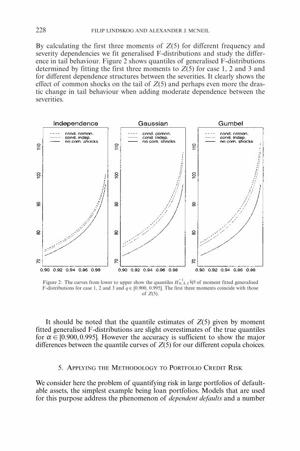
By calculating the first three moments of Z(5) for different frequency andseverity dependencies we fit generalised F-distributions and study the differ-ence in tail behaviour. Figure 2 shows quantiles of generalised F-distributionsdetermined by fitting the first three moments to Z(5) for case 1, 2 and 3 andfor different dependence structures between the severities. It clearly shows theeffect of common shocks on the tail of Z(5) and perhaps even more the dras-tic change in tail behaviour when adding moderate dependence between theseverities.
228 FILIP LINDSKOG AND ALEXANDER J. MCNEIL
Figure 2: The curves from lower to upper show the quantiles H ( )q, , k1-
a m of moment fitted generalisedF-distributions for case 1, 2 and 3 and q ∈ [0.900, 0.995]. The first three moments coincide with those
of Z(5).
It should be noted that the quantile estimates of Z(5) given by momentfitted generalised F-distributions are slight overestimates of the true quantilesfor [ . , . ]0 900 0 995!a . However the accuracy is sufficient to show the majordifferences between the quantile curves of Z(5) for our different copula choices.
5. APPLYING THE METHODOLOGY TO PORTFOLIO CREDIT RISK
We consider here the problem of quantifying risk in large portfolios of default-able assets, the simplest example being loan portfolios. Models that are usedfor this purpose address the phenomenon of dependent defaults and a number
of approaches have been suggested in the literature in recent years and imple-mented in widely-used industry solutions such as the model proposed by theKMV corporation (KMV-Corporation 1997), the model of the RiskMetricsgroup (RiskMetrics-Group 1997), or CreditRisk+, developed by Credit SuisseFinancial Products (Credit-Suisse-Financial-Products 1997). In this section wedescribe how the common Poisson shock model provides a simple alternativeframework for modelling portfolio credit risk.
We emphasise that our focus here, and that of the industry models, is onoverall portfolio credit risk. We are less concerned with providing detailed analy-sis of the individual default potential of a single credit risk, such as is requiredin the pricing of defaultable bonds or standard credit derivatives. For this pur-pose the class of default intensity models has emerged as the most important;see for example Jarrow and Turnbull (1995).
5.1. Poisson shock models for defaults
We consider a portfolio of loans and develop a shock model by consideringthat every counterparty in the portfolio defines a loss type and that a varietyof different kinds of economic shock may lead to the default of these coun-terparties: global shock events may potentially affect all counterparties; sectorshock events may affect only certain kinds of company, such as companies ina particular geographical area or companies concentrated on a particular indus-try; idiosyncratic shock events (such as an episode of bad management) mayaffect only individual counterparties; one might also think of endogenous shockevents where the default of important primary counterparties might affectother counterparties, so that default was contagious.
In all cases the common shock construction means that defaults of indi-vidual counterparties are modelled by the first events in a series of dependentPoisson process. Suppose the random vector T = T1, …, Tn )� describes thetimes to default for the n counterparties in the portfolio. In Section 3.2 weobserved that this vector of default times has a multivariate exponentialdistribution with the Marshall-Olkin survival copula. Suppose that time ismeasured in years and that we are interested in the portfolio credit loss dis-tribution for a time horizon of 1 year; suppose further that the exposures (loansizes) are known and given by , ,e en1 f . If we neglect interest rates and assumethat nothing is recovered from defaulted firms then the overall portfolio lossis given by
.L e 1i Ti
n
11
i= #
=
!! +
Frey and McNeil (2001) have shown that the distribution of L is fully deter-mined by the set of individual default probabilities { ( ), , , }p P T i n1 1i i f#= =and the copula C of the vector T; the exponential distributional form for themargins of T is not a critical feature of the model. They also show that the tailof the distribution of L and related risk measures are often much more sensitive
COMMON POISSON SHOCK MODELS 229
to the assumptions about the dependence between the defaults as summarisedby the copula, than they are to the accurate specification of individual defaultprobabilities.
5.2. Relation of the shock model to standard models
All other models that have been suggested for portfolio credit risk also imply mul-tivariate distributions for the vector of default times of the portfolio members.Regardless of whether these models are set up as one-period or multi-periodmodels, or whether they assume constant intensities of default (as in the Pois-son shock model), non-homogeneous intensities or stochastic intensities, theyall imply a distribution for the counterparty survival times. From model tomodel, these distributions will vary with respect to both their marginal distri-butions and their copulas, but as far as determining the loss distribution isconcerned, if they have been calibrated to give broadly similar individual defaultprobabilities it is the copula that will be decisive in determining the tail of theportfolio loss distribution.
Both KMV and CreditMetrics may be considered to descend from the firm-value model of Merton (1974), where default is modelled as occurring whenthe asset value of a company falls below its liabilities, and asset value changesare considered to have a multivariate normal distribution. Although thisappears very different to the Poisson shock model, as far as the loss distribu-tion for a fixed time horizon is concerned, both KMV and CreditMetrics arein fact structurally equivalent to a model in which default times have a multi-variate exponential distribution with the Gaussian copula (i.e. the copula thatdescribes the dependence inherent in a multivariate normal distribution); seeLi (1999) and Frey and McNeil (2001) for more detail. Thus the crucial dif-ference in the one-period framework lies in the fact that these industry modelsimply a Gaussian copula whereas common shocks imply a Marshall-Olkincopula to describe the dependence of the survival times.
The CreditRisk+ model employs a mixture-modelling philosophy whichassumes that conditional on a vector of independent gamma-distributed macro-economic factors, the default of a counterparty occurs independently of othercounterparties and is the first event in a Poisson process with an intensity thatdepends on these factors. Survival times are not exponential (but rather con-ditionally exponential), but for portfolio risk modelling in a one-period setting,this is again not a decisive factor. Assuming that the model has been calibratedto give plausible values for individual default probabilities, it is the copula ofthe default times that is most important in determining the overall loss distri-bution, although this copula is difficult to isolate in closed form in the generalversion of CreditRisk+.
There have been a number of papers on the subject of extending the inten-sity-based approach to modelling the default of single counterparties toobtain models for dependent defaults of several counterparties, principallywith the problem of pricing so-called basket credit derivatives in mind; seeSchoenbucher and Schubert (2001) for a useful summary of these approaches.
230 FILIP LINDSKOG AND ALEXANDER J. MCNEIL
We mention in particular a model of Duffie and Singleton (1995) where indi-vidual defaults follow Cox processes with stochastic intensities. These intensi-ties may jump (by a random amount) when certain common shocks occurwhich have the potential to affect all counterparties, or when idiosyncraticshocks occur affecting an individual company; as in our model shocks occuras Poisson processes. Our model can be thought of a cruder version of theDuffie & Singleton model with constant and deterministic intensities for indi-vidual defaults.
5.3. Setting up the shock model
Consider a loan portfolio consisting of n obligors. Suppose the counterpartiescan be divided into K geographical or industry sectors. We consider a modelwhere obligors are subject to idiosyncratic, sector and global shocks, so thatthere are a total of m n K 1= + + shock event processes.
Suppose that the jth obligor belongs to sector k = kj where k ∈ {1,…,K}.From formula (6) we know that Nj (t), the number of defaults of obligor j in(0,t] is Poisson with intensity given by
, ,p p k k j( ) ( ) ( ) ( ) ( )j
jjn k n k
jm m= + + =m m m m+ +
^ h
where the three terms represent the contributions to the default intensity ofidiosyncratic, sector and global events respectively. Note that in general thisintensity will be set so low that the probability of a firm defaulting more thanonce in the period of interest can be considered negligible.
This is a very general model and to obtain a model that we would have ahope of calibrating in a real application we need to drastically reduce the num-ber of parameters in the model. We assume first that companies can be groupedtogether into rating classes within which default rates can be considered con-stant and known. It is very common in portfolio default risk modelling to basethe assessment of default intensities for individual companies on informationabout historical default rates for similarly rated companies. Suppose that thejth obligor belongs to rating category l = l ( j) where l ∈ {1,…,L}. We assumefor the overall default intensity jm that
, , , , .l l j j n1,j ltotal f= = =m m ^ h (16)
To achieve (16) we assume that the rate of occurrence of idiosyncratic shocksalso depends only on the rating category and we adopt the notation
, , , , ,
, , , ,
.
l l j j n
k K
1
1
,
( ),
( )
jl
n kk
m
sec
idio
tor
global
f
f
= = =
= =
=
m m
m m
m m
+
] ^g h
COMMON POISSON SHOCK MODELS 231
Clearly we now have a total of L + K + 1 shock intensities to set.We assume also that the conditional default probabilities given the occur-
rence of sector shocks only depend on the rating class of the company and writefor an obligor j
, .p s l l j( ),j
n kk l= =+
^ h
We assume moreover that the default indicators for several companies in thesame sector are conditionally independent given the occurrence of an event inthat sector. Analogously, we assume that the conditional default probabilitiesgiven the occurrence of global shocks depend on both rating class and sectorof the company and write
, , .p g l l j k k j( ),j
mk l= = =^ ^h h
We assume that the default indicators for any group of companies are condi-tionally independent given the occurrence of a global event.
In total we have 2KL conditional default probabilities to set and we havethe system of equations
, , , , , , ,s g k K l L1 1, , , , ,l l k l k k lsectotal idio tor global f f= + + = =m m m m
subject to the constraint, imposed by (16), that
, .s g s g k k, , , , , ,k l k k l k l k k lsec sector global tor global 6 l!+ = +m m m ml ll (16)
5.4. Understanding the factors determining the risk
We are interested in the behaviour of N(t), the total number of defaults, forfixed t. If we suppose that the individual default rates have been fixed then
( ( ))E N t has been fixed. However, depending how we set the various shockintensities and individual default probabilities the risk inherent in N(t) mayvary considerably. If we measure risk by variance we can get analytically anidea of which factors affect the risk by considering
( ) ( ) ( ), ( )var covN t E N t N t N t, :
j jj j j j
1 2
1 2 1 2
- =!
!^ ^ `h h j.
For simplicity we set t = 1 and consider a model with one rating class (L = 1)and assume that the conditional default probabilities do not depend on thesector for all global shocks ( , )g g k,k 1 6= . Let there be nk obligors in sector k.We have for j j1 2! that
j j( ), ( ),
,cov N N
g k j k j
g s k j k j k1 1
,k ksec
21 2
2 21 2
global
global tor1 2
!=
+ = =
m
m m`
^ ^
^ ^j
h h
h h*
232 FILIP LINDSKOG AND ALEXANDER J. MCNEIL
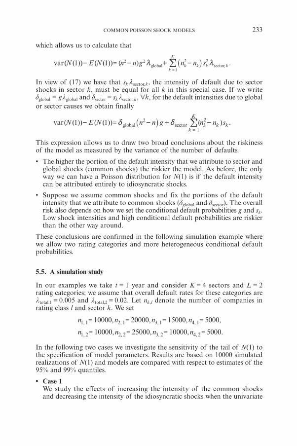
which allows us to calculate that
( ( )) ( ( )) ( ) .var N E N n n g n n s1 1 ,k k k kk
K
sec2 2 2 2
1global tor- = - + -m m
=
!_ i
In view of (17) we have that sk lsector,k, the intensity of default due to sectorshocks in sector k, must be equal for all k in this special case. If we writedglobal = glglobal and dsector = sk lsector,k, ∀k, for the default intensities due to globalor sector causes we obtain finally
( ( )) ( ( )) ( ) .var N E N n n g n n s1 1 k k kk
K
sec2 2
1global tor- = - + -d d
=
!_ i
This expression allows us to draw two broad conclusions about the riskinessof the model as measured by the variance of the number of defaults.
• The higher the portion of the default intensity that we attribute to sector andglobal shocks (common shocks) the riskier the model. As before, the onlyway we can have a Poisson distribution for N(1) is if the default intensitycan be attributed entirely to idiosyncratic shocks.
• Suppose we assume common shocks and fix the portions of the defaultintensity that we attribute to common shocks (dglobal and dsector). The overallrisk also depends on how we set the conditional default probabilities g and sk.Low shock intensities and high conditional default probabilities are riskierthan the other way around.
These conclusions are confirmed in the following simulation example wherewe allow two rating categories and more heterogeneous conditional defaultprobabilities.
5.5. A simulation study
In our examples we take t = 1 year and consider K = 4 sectors and L = 2rating categories; we assume that overall default rates for these categories areltotal,1 = 0.005 and ltotal,2 = 0.02. Let nk,l denote the number of companies inrating class l and sector k. We set
, , , ,
, , , .
n n n n
n n n n
10000 20000 15000 5000
10000 25000 10000 5000, , , ,
, , , ,
1 1 2 1 3 1 4 1
1 2 2 2 3 2 4 2
= = = =
= = = =
In the following two cases we investigate the sensitivity of the tail of N(1) tothe specification of model parameters. Results are based on 10000 simulatedrealizations of N(1) and models are compared with respect to estimates of the95% and 99% quantiles.
• Case 1We study the effects of increasing the intensity of the common shocksand decreasing the intensity of the idiosyncratic shocks when the univariate
COMMON POISSON SHOCK MODELS 233
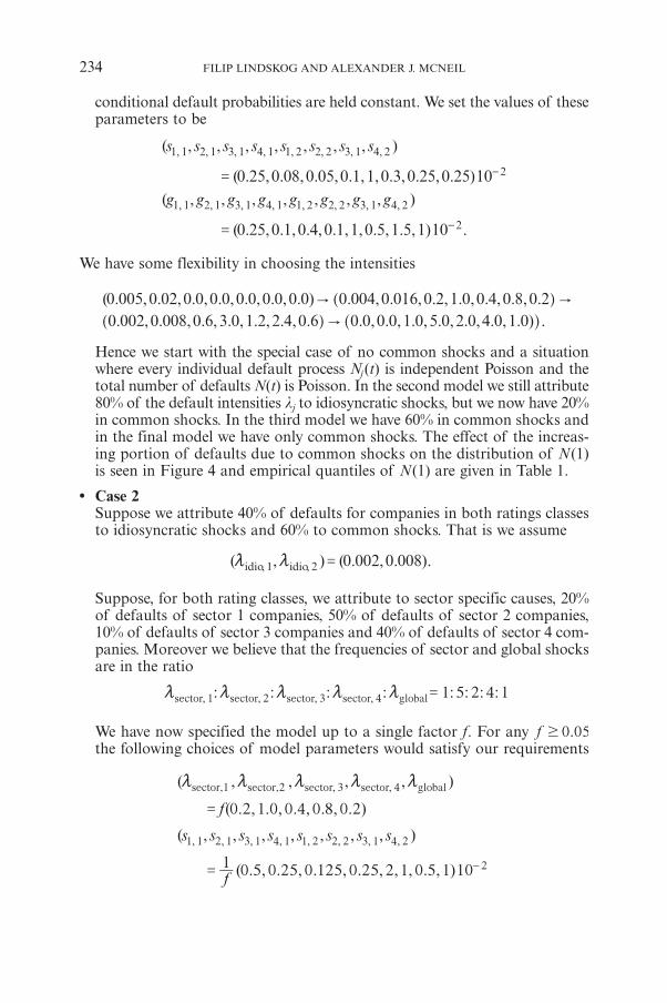
conditional default probabilities are held constant. We set the values of theseparameters to be
( , , , , , , , )
( . , . , . , . , , . , . , . )( , , , , , , , )
( . , . , . , . , , . , . , ) .
s s s s s s s s
g g g g g g g g0 25 0 08 0 05 0 1 1 0 3 0 25 0 25 10
0 25 0 1 0 4 0 1 1 0 5 1 5 1 10
, , , , , , , ,
, , , , , , , ,
1 1 2 1 3 1 4 1 1 2 2 2 3 1 4 2
2
1 1 2 1 3 1 4 1 1 2 2 2 3 1 4 2
2
=
=
-
-
We have some flexibility in choosing the intensities
( . , . , . , . , . , . , . ) . , . , . , . , . , . , .. , . , . , . , . , . , . . , . , . , . , . , . , . ) .
0 005 0 02 0 0 0 0 0 0 0 0 0 0 0 004 0 016 0 2 1 0 0 4 0 8 0 20 002 0 008 0 6 3 0 1 2 2 4 0 6 0 0 0 0 1 0 5 0 2 0 4 0 1 0
" "
"
]
] ^
g
g h
Hence we start with the special case of no common shocks and a situationwhere every individual default process Nj(t) is independent Poisson and thetotal number of defaults N(t) is Poisson. In the second model we still attribute80% of the default intensities lj to idiosyncratic shocks, but we now have 20%in common shocks. In the third model we have 60% in common shocks andin the final model we have only common shocks. The effect of the increas-ing portion of defaults due to common shocks on the distribution of N(1)is seen in Figure 4 and empirical quantiles of N(1) are given in Table 1.
• Case 2Suppose we attribute 40% of defaults for companies in both ratings classesto idiosyncratic shocks and 60% to common shocks. That is we assume
( , ) ( . , . ).0 002 0 008, ,1 2idio idio =m m
Suppose, for both rating classes, we attribute to sector specific causes, 20%of defaults of sector 1 companies, 50% of defaults of sector 2 companies,10% of defaults of sector 3 companies and 40% of defaults of sector 4 com-panies. Moreover we believe that the frequencies of sector and global shocksare in the ratio
: : : : : : : :1 5 2 4 1, , , ,1 2 3 4sector sector sector sector global=m m m m m
We have now specified the model up to a single factor f. For any .f 0 05$the following choices of model parameters would satisfy our requirements
( , , , , )
( . , . , . , . , . )
( , , , , , , , )
( . , . , . , . , , , . , )
f
s s s s s s s s
f
0 2 1 0 0 4 0 8 0 2
10 5 0 25 0 125 0 25 2 1 0 5 1 10
, ,
, , , , , , , ,
3 4
1 1 2 1 3 1 4 1 1 2 2 2 3 1 4 2
2
sector,1 sector,2 sector sector global
=
=
m m m m m
-
234 FILIP LINDSKOG AND ALEXANDER J. MCNEIL
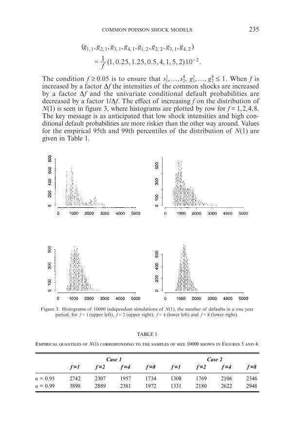
( , , , , , , , )
( , . , . , . , , , , ) .
g g g g g g g g
f1
1 0 25 1 25 0 5 4 1 5 2 10
, , , , , , , ,1 1 2 1 3 1 4 1 1 2 2 2 3 1 4 2
2= -
The condition f ≥ 0.05 is to ensure that s11,…, s4
2, g11,…, g4
2 ≤ 1. When f isincreased by a factor Df the intensities of the common shocks are increasedby a factor Df and the univariate conditional default probabilities aredecreased by a factor 1/Df. The effect of increasing f on the distribution ofN(1) is seen in figure 3, where histograms are plotted by row for f = 1,2,4,8.The key message is as anticipated that low shock intensities and high con-ditional default probabilities are more riskier than the other way around. Valuesfor the empirical 95th and 99th percentiles of the distribution of N(1) aregiven in Table 1.
COMMON POISSON SHOCK MODELS 235
Figure 3: Histograms of 10000 independent simulations of N(1), the number of defaults in a one yearperiod, for f 1= (upper left), f 2= (upper right), f 4= (lower left) and f 8= (lower right).
TABLE 1
EMPIRICAL QUANTILES OF N(1) CORRESPONDING TO THE SAMPLES OF SIZE 10000 SHOWN IN FIGURES 3 AND 4.
Case 1 Case 2f =1 f =2 f =4 f =8 f =1 f =2 f =4 f =8
a = 0.95 2742 2307 1957 1734 1308 1769 2106 2346a = 0.99 3898 2889 2381 1972 1331 2180 2622 2948
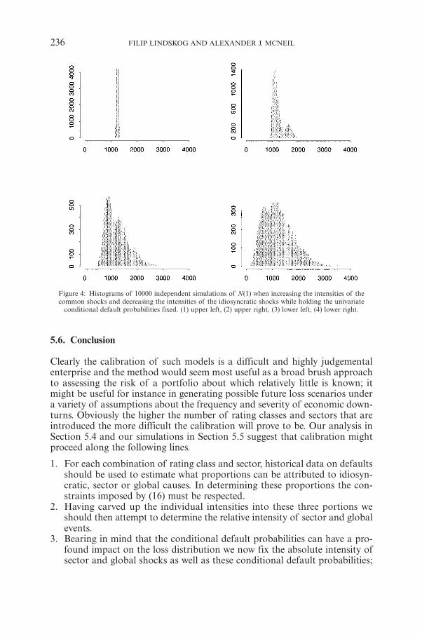
5.6. Conclusion
Clearly the calibration of such models is a difficult and highly judgementalenterprise and the method would seem most useful as a broad brush approachto assessing the risk of a portfolio about which relatively little is known; itmight be useful for instance in generating possible future loss scenarios undera variety of assumptions about the frequency and severity of economic down-turns. Obviously the higher the number of rating classes and sectors that areintroduced the more difficult the calibration will prove to be. Our analysis inSection 5.4 and our simulations in Section 5.5 suggest that calibration mightproceed along the following lines.
1. For each combination of rating class and sector, historical data on defaultsshould be used to estimate what proportions can be attributed to idiosyn-cratic, sector or global causes. In determining these proportions the con-straints imposed by (16) must be respected.
2. Having carved up the individual intensities into these three portions weshould then attempt to determine the relative intensity of sector and globalevents.
3. Bearing in mind that the conditional default probabilities can have a pro-found impact on the loss distribution we now fix the absolute intensity ofsector and global shocks as well as these conditional default probabilities;
236 FILIP LINDSKOG AND ALEXANDER J. MCNEIL
Figure 4: Histograms of 10000 independent simulations of N(1) when increasing the intensities of thecommon shocks and decreasing the intensities of the idiosyncratic shocks while holding the univariate
conditional default probabilities fixed. (1) upper left, (2) upper right, (3) lower left, (4) lower right.
for conservatism we err on the side of underestimating shock intensitiesand overestimating conditional default probabilities.
REFERENCES
BARLOW, R., and PROSCHAN, F. (1975) Statistical Theory of Reliability and Life Testing. Holt, Rine-hart & Winston, New York.
CREDIT-SUISSE-FINANCIAL-PRODUCTS (1997) CreditRisk+ a Credit Risk Management Framework.Technical Document, available from htpp://www.csfb.com/creditrisk.
DUFFIE, D., and SINGLETON, K. (1998) Simulating Correlated Defaults. Working paper, GraduateSchool of Business, Stanford University.
EMBRECHTS, P., MCNEIL, A., and STRAUMANN, D. (2001) Correlation and dependency in risk man-agement: properties and pitfalls. In Risk Management: Value at Risk and Beyond, ed. byM. Dempster. Cambridge University Press, Cambridge.
FREY, R., and MCNEIL, A. (2001): Modelling dependent defaults. Preprint, ETH Zürich, avail-able from http://www.math.ethz.ch/ˆfrey.
HOGG, R., and KLUGMAN, S. (1984) Loss Distributions. Wiley, New York.JARROW, R., and TURNBULL, S. (1995) Pricing Derivatives on Financial Securities Subject to
Credit Risk. Journal of Finance, L(1), 83-85.JOE, R. (1997) Multivariate Models and Dependence Concepts. Chapman & Hall, London.KMV-CORPORATION (1997) Modelling Default Risk. Technical Document, available from http://
www.kmv.com.LI, D. (1999) On Default Correlation: A Copula Function Approach. Working paper, RiskMet-
rics Group, New York.LI, H., and XU, S. (2001) Stochastic bounds and dependence properties of survival times in a mul-
ticomponent shock model. Journal of Multivariate Analysis 76, 63-89.MARSHALL, A., and OLKIN, I. (1967) A multivariate exponential distribution. Journal of Amer-
ican Statistical Association 62, 30-44.MERTON, R. (1974) On the Pricing of Corporate Debt: The Risk Structure of Interest Rates.
Journal of Finance 29, 449-470.NELSEN, R.B. (1999) An Introduction to Copulas. Springer, New York.PANJER, H. (1981) Recursive evaluation of a family of compound distributions. ASTIN Bulletin
12, 22-26.RISKMETRICS-GROUP (1997) CreditMetrics – Technical Document, available from http://www.
riskmetrics.com/research.ROLSKI, T., SCHMIDLI, H., SCHMIDT, V., and TEUGELS, J. (1998) Stochastic Processes for Insurance
and Finance. Wiley, Chichester.SAVITS, T. (1988) Some multivariate distributions derived from a non-fatal shock model. Journal
of Applied Probability 25, 383-390.SCHÖNBUCHER, P., and SCHUBERT, D. (2001) Copula-dependent default risk in intensity models.
Working paper.WANG, S., and DHAENE, J. (1998) Comonotonicity, correlation order and premium principles.
Insurance: Mathematics and Economics 22, 235-242.
FILIP LINDSKOG
RisklabFederal Institute of TechnologyETH Zentrum CH-8092 ZurichTel.: +41 1 632 67 41Tel.: +41 1 632 10 [email protected]
COMMON POISSON SHOCK MODELS 237

ALEXANDER J. MCNEIL
Department of MathematicsFederal Institute of TechnologyETH ZentrumCH-8092 ZurichTel.: +41 1 632 61 62Tel.: +41 1 632 15 [email protected]
238 FILIP LINDSKOG AND ALEXANDER J. MCNEIL
ASYMPTOTIC DEPENDENCE OF REINSURANCE AGGREGATE CLAIM AMOUNTS
ANA J. MATA*
Heriot-Watt University, United Kingdom
ABSTRACT
In this paper we study the asymptotic behaviour of the joint distribution of rein-surance aggregate claim amounts for large values of the retention level undervarious dependence assumptions. We prove that, under certain dependenceassumptions, for large values of the retention level the ratio between the jointdistribution of the aggregate losses and the product of the marginal distributionsconverges to a constant value that only depends on the frequency parameters.
KEYWORDS
Dependent risks, excess of loss, reinsurance layers, multivariate Panjer recursion,asymptotic independence.
1. INTRODUCTION
Recently the importance of modelling dependent insurance and reinsurance riskshas attracted the attention of actuarial practitioners and scientists. Even thoughclassical theories have been developed under the assumption of independencebetween risks, there are practical cases where this assumption is not valid.
In a recent paper Embrechts, McNeil and Straumann (2001) wrote:“Although insurance has traditionally been built on the assumption of inde-
pendence and the law of large numbers has governed the determination of pre-miums, the increasing complexity of insurance and reinsurance products has ledrecently to increased actuarial interest in the modelling of dependent risks...”
Although the literature on dependence between risks in insurance portfo-lios is increasing rapidly, very few authors have applied these development topractical problems, for example reinsurance modelling.
In this paper we study the problem of dependence between risks from the rein-surer’s point of view when he provides excess of loss cover for two dependentrisks under different dependence assumptions. When the reinsurer undertakesexcess of loss reinsurance for a portfolio, in particular for catastrophe excess of
* e-mail: [email protected]
ASTIN BULLETIN, Vol. 33, No. 2, 2003, pp. 239-263
loss, the probability that a claim will impact the reinsurance layer is very small.Therefore, in many cases the correlation coefficient between aggregate claimamounts for the reinsurer becomes very small. We could then be tempted to thinkthat the dependence between portfolios disappears as we look at the tail of the dis-tribution and that, therefore, we could assume independence. It has been largelydiscussed in the literature that the linear correlation coefficient is not a satisfac-tory measure of dependence in the non-normal case, see, for example, Embrechts,McNeil and Straumann (2001).
In this paper we look at the effect of different dependence assumptions andtheir effect on the joint distribution of the aggregate claim amounts comparedto the product of the marginal distributions when the retention or attachmentis large (hence, the probability of a claim to the layer tends to zero). In Section 2,we describe a model used for insurance and reinsurance aggregate claimamounts that are subject to the same events. In Section 2.1, we discuss how tocalculate the distribution of the sum of aggregate claim amounts under differentdependence assumptions. In Section 3, we define a measure of asymptoticdependence. We use this concept to study the effect of large values of the reten-tion level on the joint distribution of reinsurance aggregate losses under thedependence assumptions described in Section 2. Numerical illustrations and dis-cussion of the results are presented in Sections 3.2 and 3.3.
2. A DEPENDENCE MODEL FOR REINSURANCE AGGREGATE LOSSES
In this section we describe a model that has been typically used in the actuarialliterature to model insurance aggregate claim amounts that are exposed to thesame events or claims. This model has been proposed, for example, in Sundt(1999) and Ambagaspitiya (1999) where they develop multivariate recursionsto calculate the joint distribution of the aggregate claim amounts. We willassume that there are only two portfolios, however the results can be generalisedfor any number of risks or portfolios.
The Model: Two risks or portfolios are affected by the same events, thereforethey are subject to the same frequency distribution. This model is the generalmodel described in Sundt (1999). One of the most common applications of thismodel is, for example, catastrophe reinsurance where several portfolios areexposed to the same events. Also in fire insurance, the same fire can causedamage to neighbouring buildings or properties insured under different policiesby the same insurer.
Assumptions:
1. Let N be the total number of claims in a fixed period of time. It is assumedthat N belongs to the Panjer class of counting distribution, i.e. there existsconstants a and b such that N satisfies
, ,forP N n a nb P N n n1 1 2 f= = + = - =] b ]g l g
240 ANA J. MATA
2. Let Xi i 1$" , and Yi i 1$
" , be sequences of i.i.d. random variables represen-ting the claim amounts for each risk. We assume that (Xi,Yi) are i.i.d. pairsfrom a bivariate distribution.
3. N is independent of ,X Y ii i 6^ h .
Then the aggregate claim amounts for these risks are
andS X S Yii
N
ii
N
1 21 1
= == =
! ! (1)
The claim amounts for each risk could have various interpretations:
1. From the primary insurer’s point of view, the losses due to the i th event(Xi,Yi) may be dependent or independent.
2. From the reinsurer’s point of view (Xi,Yi) may represent excess of loss claimsdue to the same event from different underlying risks whose individual lossesmay be dependent or independent. In reinsurance, this model could also beused for reinsurance losses for two excess of loss layers from the same under-lying risk. In this case the aggregate losses are dependent not only throughthe number of events, but also through the claim distribution for the primaryrisk.
2.1. Joint distribution of dependent aggregate claim amounts
Sundt (1999) and Ambagaspitiya (1999) developed multivariate recursions thatallow us to calculate the joint distribution of the aggregate claim amountsunder the assumptions of the model described in Section 2. As we discussedabove, the individual claim amounts for each portfolio are not necessarily inde-pendent and we assume that they are integer-valued random variables. Thejoint probability function is given by p(x,y) for x = 0,1,2,…, y = 0,1,2,… inappropriate units.
The aggregate claim amounts are as given in formula (1), and the recur-sion for the joint distribution of (S1,S2) is as follows:
, ( , ) , ,g s s a sbu p u v g s u s v
u
s
v
s
1 210
1 20
1 2
= + - -= =
! !^ b ^h l h (2)
for , , , , , ,s s1 2 0 1 21 2f f= =
, , , ,g s s a sbv p u v g s u s v
v
s
u
s
1 220
1 20
2 1
= + - -= =
! !^ b ] ^h l g h (3)
for , , , , , ,s s0 1 2 1 21 2f f= = See Sundt (1999).In many cases the insurer/reinsurer would only be interested in calculating
the distribution of the sum of the total losses for both risks. For example, ifwe are interested in calculating how much capital we must allocate (under somecriteria) to each portfolio separately or to the combined portfolio, then we
ASYMPTOTIC DEPENDENCE 241
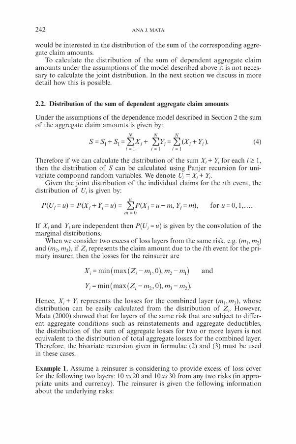
would be interested in the distribution of the sum of the corresponding aggre-gate claim amounts.
To calculate the distribution of the sum of dependent aggregate claimamounts under the assumptions of the model described above it is not neces-sary to calculate the joint distribution. In the next section we discuss in moredetail how this is possible.
2.2. Distribution of the sum of dependent aggregate claim amounts
Under the assumptions of the dependence model described in Section 2 the sumof the aggregate claim amounts is given by:
( )S S S X Y X Yii
N
ii
N
i ii
N
1 11 1 1
= + = + = += = =
! ! ! . (4)
Therefore if we can calculate the distribution of the sum Xi + Yi for each i ≥ 1,then the distribution of S can be calculated using Panjer recursion for uni-variate compound random variables. We denote Ui = Xi + Yi.
Given the joint distribution of the individual claims for the i th event, thedistribution of Ui is given by:
( ) ( ) ( , ), , , .forP U u P X Y u P X u m Y m u 0 1i i i i im
u
0
f= = + = = = - = ==
!
If Xi and Yi are independent then P U ui =^ h is given by the convolution of themarginal distributions.
When we consider two excess of loss layers from the same risk, e.g. (m1, m2)and (m2, m3), if Zi represents the claim amount due to the ith event for the pri-mary insurer, then the losses for the reinsurer are
, ,min max andX Z m m m0i i 1 2 1= - -^_ h i
, ,min maxY Z m m m0i i 2 3 2= - -^_ h i.
Hence, Xi + Yi represents the losses for the combined layer (m1, m3), whosedistribution can be easily calculated from the distribution of Zi. However,Mata (2000) showed that for layers of the same risk that are subject to differ-ent aggregate conditions such as reinstatements and aggregate deductibles,the distribution of the sum of aggregate losses for two or more layers is notequivalent to the distribution of total aggregate losses for the combined layer.Therefore, the bivariate recursion given in formulae (2) and (3) must be usedin these cases.
Example 1. Assume a reinsurer is considering to provide excess of loss coverfor the following two layers: 10 xs 20 and 10xs 30 from any two risks (in appro-priate units and currency). The reinsurer is given the following informationabout the underlying risks:
242 ANA J. MATA
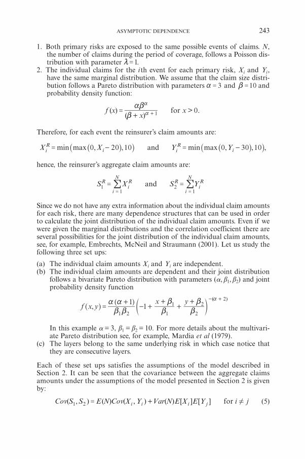
1. Both primary risks are exposed to the same possible events of claims. N,the number of claims during the period of coverage, follows a Poisson dis-tribution with parameter 1=m .
2. The individual claims for the i th event for each primary risk, Xi and Yi,have the same marginal distribution. We assume that the claim size distri-bution follows a Pareto distribution with parameters and3 10= =a b andprobability density function:
( )( )
> .forf xx
x 01=+bab
+a
a
Therefore, for each event the reinsurer’s claim amounts are:
, , , , ,min max and min maxX X Y Y0 20 10 0 30 10iR
i iR
i= - = -^_ ^_h i h i
hence, the reinsurer’s aggregate claim amounts are:
andS X S YRiR
i
NR
iR
i
N
11
21
= == =
! !
Since we do not have any extra information about the individual claim amountsfor each risk, there are many dependence structures that can be used in orderto calculate the joint distribution of the individual claim amounts. Even if wewere given the marginal distributions and the correlation coefficient there areseveral possibilities for the joint distribution of the individual claim amounts,see, for example, Embrechts, McNeil and Straumann (2001). Let us study thefollowing three set ups:
(a) The individual claim amounts Xi and Yi are independent.(b) The individual claim amounts are dependent and their joint distribution
follows a bivariate Pareto distribution with parameters (�, b1, b2) and jointprobability density function
,f x yx y1
1( )
1 2 1
1
2
22
=+
- ++
++
b ba a
bb
bb - +a
^]
dhg
n
In this example � = 3, b1 = b2 = 10. For more details about the multivari-ate Pareto distribution see, for example, Mardia et al (1979).
(c) The layers belong to the same underlying risk in which case notice thatthey are consecutive layers.
Each of these set ups satisfies the assumptions of the model described inSection 2. It can be seen that the covariance between the aggregate claimsamounts under the assumptions of the model presented in Section 2 is givenby:
( , ) ( ) ( , ) ( ) [ ] [ ] forCov S S E N Cov X Y Var N E X E Y i ji i i j1 2 != + (5)
ASYMPTOTIC DEPENDENCE 243
It is interesting to note that the correlations calculated according to (5) arequite different from each other in the three cases considered in this example.The correlations are:
(a) , .S S 0 019R R1 2
=t_ i
(b) , .S S 0 206R R1 2
=t_ i
(c) , .S S 0 761R R1 2
=t_ i
Figure 1 shows the c.d.f. of S SR R1 2+ when the layers belong to different risks, i.e.
dependence assumptions as in (a) and (b). The dashed line in Figure 1 representthe c.d.f. of S SR R
1 2+ when we assume these risks are completely independent, i.e.ignoring that both risks are exposed to the same claims. We observe that underthe simplest dependence model (a), where the dependence arises only throughthe common number of events, the distribution of the total aggregate losses is veryclose to the distribution of total losses under the assumption of independence.However, when more complex dependence assumptions are built in, such as thebivariate Pareto claim distribution, the distribution of total aggregate losses is verydifferent to the distribution under the independence assumption. In particularwe notice that under the dependence assumption in (b) the tail of the distributionis significantly heavier than when independence is assumed.
244 ANA J. MATA
FIGURE 1: Distribution of ,S SR R1 2
+ cases (a) and (b).
Figure 2 shows the c.d.f. of SR1 + SR
2 when the layers belong to the same riskand the distribution of SR
1 + SR2 if independence is assumed. We notice that the
distribution of total losses for consecutive layers would be totally mis-esti-mated if the dependence structure is ignored. This is of course due to the factthat when layers belong to the same risk there would be a positive claim in thesecond layer only when the claim for the first layers is a full loss. Hence, forlayers of the same risk the claim amount dependence has more effect than thefrequency dependence.
With this numerical example we have shown how different dependenceassumptions may impact the distribution of total losses for the reinsurer. There-fore, by not taking into account how dependence arises one could mis-estimatethe overall risk. This is of particular importance when pricing multi-layer excessof loss treaties, where dependence arises not only through he number of claims,but also through the claim size distribution.
3. ASYMPTOTIC BEHAVIOUR OF DEPENDENT REINSURANCE AGGREGATE
CLAIM AMOUNTS
In the previous section we looked at the distribution of the sum of dependentaggregate claim amounts from the reinsurer’s point of view. In Figures 1 and 2
ASYMPTOTIC DEPENDENCE 245
FIGURE 2: Distribution of ,S SR R1 2
+ cases (c).
we observed the effect of different dependence structures that might be usedto model reinsurance aggregate claim amounts.
Clearly, given the distribution of the individual claim amounts for theprimary insurer and the distribution of the number of claims, the choice ofretention level M completely determines the distribution of the aggregate claimamounts for the reinsurer. For large values of the retention level, the proba-bility of a claim to the reinsurance layer is small. Hence the probability ofzero losses is very high, and therefore the correlation coefficient is small.
Based on the results showed in Figures 1 and 2, where we observed thatunder some dependence assumptions the distribution of total aggregate lossesfor the reinsurer is very close to the distribution of total aggregate losses if inde-pendence is assumed, it is our objective to give some insight to the followingquestion:
Are the reinsurer’s aggregate claim amounts from different but dependentrisks approximately independent for large values of the retention levels?
In the next section we give some theoretical insight into the asymptoticbehaviour of the distribution of the aggregate claim amounts for large valuesof the retention levels under different dependence assumptions.
3.1. On measures of asymptotic independence for reinsurance aggregate claimamounts
In order to provide some answers to the question outlined above we start by giv-ing the definition of asymptotic independence which will be referred to in theremainder of the paper. For large values of the retention levels the probabilityof a non-zero loss for the reinsurer tends to zero. Hence we use the followingdefinition of asymptotic independence.
Definition 1 Suppose two sequences of random variables Vn" , and Wn" , are depen-dent for each n. If these random variables satisfy
( ) ( )( , )
,lim P V A P W BP V A W B
1n n n
n n! !! !
=" 3
(6)
for all sets A and B that have positive probability, then it is said that Vn and Wnare asymptotically independent. We will refer to the ratio in (6) as the dependenceratio.
We prove below that under certain dependence assumptions the reinsur-ance aggregate losses satisfy the condition given in (6) for some sets A and B,but not for all sets. We set out below the assumptions we require to prove thisresult.
Assumptions and notation:
1. The primary insurance risks satisfy the dependence assumptions of themodel described in Section 2, but we assume that the claim amounts for
246 ANA J. MATA
the ith event are independent. Hence, the dependence structure arises onlythrough the common number of events N.
2. Individual claim amounts for the primary insurer Xi and Yi are integer-valuedindependent random variables that take values x = 0,1,2,… and y = 0,1,2,… in appropriate units. We assume that the probability functions of theindividual claim amounts do not have fin§(ite upper limit. We denotep1(x) and p2(y) as the probability functions of the individual claim amountsfor each portfolio.
3. The common number of claims, N, belongs to Panjer’s class of countingdistributions. Thus, a and b will represent the constants of Panjer’s class.
4. We denote by PN (t) the probability generating function of N which isdefined as
( )P t E tNN= 8 B
5. Let {M1,n}n ≥1and {M2,n}n ≥1
be sequences of integer numbers representingting the retention levels of the excess of loss reinsurance for each risk.These sequences satisfy Mi,n > Mi,n –1 for i = 1,2. For a given value of theretention, the reinsurer’s claim amounts for the i th event are:
, , .max maxX M X M Y M Y M0 0, , , ,iR
n i n iR
n i n1 1 2 2= - = -` ` ` `j j j j
Therefore, the aggregate claim amounts for the reinsurer are:
( ) ( ) .andS M X M S M Y M, , , ,R
n iR
nR
ni
N
iR
ni
N
1 1 1 2 21
21
= == =
! !` `j j (7)
The distribution functions of the aggregate losses are functions of the reten-tion levels {M2,n}n ≥1
and {M2,n}n ≥1.
6. The retention levels are such that the reinsurer’s aggregate claim amountssatisfy
, , .lim forP S M i0 1 1 2,n iR
i n = = =" 3
`` j j (8)
7. The probability functions for the individual claim amounts for the rein-surer are ( )p x P X M x, ,n i
Rn1 1= =] _g i and p y P Y M y, ,n i
Rn2 2= =^ __h i i for x, y =
, , , ,0 1 2 f
8. We assume that the probability functions for the individual claim amountssatisfy
( )( )
( , ) , , ,lim forp y Mp x M
C x y x y1 2,
,
n i i n
i i nf
+
+= =
" 3
for , ,y 1 2 f= where C(x,y) is a constant that only depends on x and yand ( , ) <C x y0 3# .
ASYMPTOTIC DEPENDENCE 247
9. The probability functions for the aggregate claim amounts are g1,n(s1) =P S M s,
Rn1 1 1=__ i i and g s P S M s, ,n
Rn2 2 2 2 2= =^ __h i i, for , , , ,s s 0 1 21 2 f= . We
assume that ( ) >g s 0,i n i for i = 1,2 and for , , , ,s s 0 1 21 2 f=
10. The joint probability function for the aggregate claim amounts is definedas , ,g s s P S M s S M s, ,n
Rn
Rn1 2 1 1 1 2 2 2= = =^ _ _`h i i j, for , , , ,s s 0 1 21 2 f=
Proposition 1. Under the assumptions outlined above the aggregate claim amountsfor the reinsurer defined in (7) satisfy:
a) ( ) ( )( , )
lim g gg0 0
0 01
, ,n n n
n
1 2=
" 3
b),
, , , ,limP S M s P S M s
P S M s S M ss s1 0 1 2for all
, ,
, ,
n Rn
Rn
Rn
Rn
1 1 1 2 2 2
1 1 1 2 2 2
1 2 f# #
# #= =
" 3 `` ``
` ``
j j j j
j j j
c) ( ) ( )( , )
, ,lim forg s gg s
s0
01 1 2
, ,n n n
n
1 1 2
11 f= =
" 3
d) ( ) ( )( , )
, ,lim forg g sg s
s0
01 1 2
, ,n n n
n
1 2 2
22 f= =
" 3
e) ( ) ( )( , )
, , ,lim forg s g sg s s
a b s s11
1 2, ,n n n
n
1 1 2 2
1 21 2 f= +
+=
" 3
Proof. The proof of this proposition is essentially an induction based proof.In order to avoid confusion with the details of the algebraic proof we leavethe analytical proof for the Appendix and we concentrate in the interpreta-tion of the results and the assumptions.
From the results shown in Proposition 1 we make the following remarks:
1. Note that for the Binomial, Poisson and Negative Binomial distribution italways holds that >a b 0+ . Hence, >a b1 1 1+
+. In other words, the depen-
dence ratio is always greater than or equal to 1.2. The statement in b) implies that when we consider cumulative distributions
we are including the value of zero which has a high probability for largevalues of the retention level. This result explains the behaviour observed inFigures 1 and 2 where we considered the cumulative distribution functionof the sum of the reinsurer’s aggregate claim amounts. In other words, ifzero is included in the probability being evaluated the probability would tendto 1 due to assumption 6 above.
3. In Proposition 1 we assumed one of the simplest cases of dependence ininsurance/reinsurance risks. Hence, under more complicated assumptionsof dependence between risks the dependence ratio might converge to a dif-ferent value. In the next section we compare numerically the asymptoticbehaviour of the dependence ratio under various dependence assump-tions.
248 ANA J. MATA
4. Statement e) shows cases where the ratio between the joint distributionand the product of the marginal distribution does not tend to 1, whichproves the fact that even under the simplest dependence assumption inde-pendence cannot be assumed. However, if a b+ takes large values, the limitwould be close to 1. For example, when N follows a Poisson distributionwith parameter , a b+ =m m which is the expected number of common eventsper unit of time. If we increase m we are increasing the dependence para-meter as the expected number of common events becomes larger. Never-theless, by increasing m the limit in e) would be closer to 1 which impliesthat the joint distribution is closer to the independent case. This shows howcounter-intuitive results can be when the independence assumption isrelaxed.
The following proposition shows another case when the result in e) also holds.
Proposition 2 Assume that two risks follow assumptions 1 and 3 of Propo-sition 1. Let {M1,n} and {M2,n} be sequences of real numbers representing thereinsurance retention levels for each portfolio. These sequences are such that thereinsurer’s aggregate claim amounts satisfy the condition in (8) and that foreach n
.P S M P S M0 0, ,R
nR
n n1 1 2 2= = = =a`` ``j j j j
Then, the reinsurance aggregate claim amounts defined in (7) satisfy
> >
> , >.lim
P S M P S M
P S M S Ma b0 0
0 01
1
, ,
, ,
n Rn
Rn
Rn
Rn
1 1 2 2
1 1 2 2= +
+"3 ` ``
` ``
j j j
j j j
Proof. We give detailed analytical proof of this result in the Appendix.Note that the assumptions for Proposition 2 are more general than the
assumptions we made for Proposition 1. Since the result in Proposition 2 refersto the joint survival function evaluated at zero, the claim size distribution couldhave a continuous density function. Also the retention levels are not requiredto be sequences of integer values, it is enough that {M1,n}n ≥1
and {M2,n}n ≥1are
sequences of real numbers such that:
,lim forP S M i0 1 1 2,n iR
i n = = =" 3
`` j j
For Proposition 2, we assumed that both aggregate claim amounts for the rein-surer have the same probability of being zero. Nevertheless, in Example 2 weshow that this is not a necessary assumption. It seems to be sufficient thatwhen n tends to infinity the probabilities of being zero tend to one. We discussthis in more detail in Example 2.
ASYMPTOTIC DEPENDENCE 249
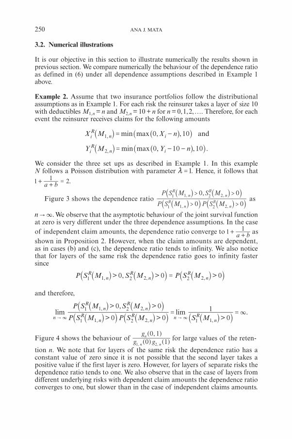
3.2. Numerical illustrations
It is our objective in this section to illustrate numerically the results shown inprevious section. We compare numerically the behaviour of the dependence ratioas defined in (6) under all dependence assumptions described in Example 1above.
Example 2. Assume that two insurance portfolios follow the distributionalassumptions as in Example 1. For each risk the reinsurer takes a layer of size 10with deductibles M1,n = n and M2,n = 10 + n for n = 0,1,2,…. Therefore, for eachevent the reinsurer receives claims for the following amounts
, ,min max andX M X n0 10,iR
n i1 = -` ^_j h i
, , .min maxY M Y n0 10 10,iR
n i2 = - -` ^_j h i
We consider the three set ups as described in Example 1. In this exampleN follows a Poisson distribution with parameter 1=m . Hence, it follows that
a b11
2++
= .
Figure 3 shows the dependence ratio> >
> , >
P S M P S M
P S M S M
0 0
0 0
, ,
, ,
Rn
Rn
Rn
Rn
1 1 2 2
1 1 2 2
_` _`
_ _`
i j i j
i i jas
.n "3 We observe that the asymptotic behaviour of the joint survival functionat zero is very different under the three dependence assumptions. In the caseof independent claim amounts, the dependence ratio converge to a b1
1+
+as
shown in Proposition 2. However, when the claim amounts are dependent,as in cases (b) and (c), the dependence ratio tends to infinity. We also noticethat for layers of the same risk the dependence ratio goes to infinity fastersince
> , > >P S M S M P S M0 0 0, , ,R
nR
nR
n1 1 2 2 2 2=` `` ``j j j j j
and therefore,
> >
> , >
>.lim lim
P S M P S M
P S M S M
S M0 0
0 0
0
1
, ,
, ,
,n Rn
Rn
Rn
Rn
n Rn1 1 2 2
1 1 2 2
1 1
3= =" "3 3`` ``
` ``
``j j j j
j j j
j j
Figure 4 shows the behaviour of( ) ( )
( , )
g g
g
0 1
0 1
, ,n n
n
1 2
for large values of the reten-
tion n. We note that for layers of the same risk the dependence ratio has aconstant value of zero since it is not possible that the second layer takes apositive value if the first layer is zero. However, for layers of separate risks thedependence ratio tends to one. We also observe that in the case of layers fromdifferent underlying risks with dependent claim amounts the dependence ratioconverges to one, but slower than in the case of independent claims amounts.
250 ANA J. MATA
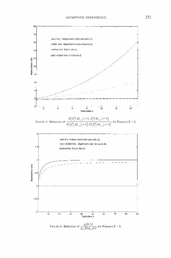
ASYMPTOTIC DEPENDENCE 251
FIGURE 3: Behaviour of> >
> , >
P S M P S M
P S M S M
0 0
0 0
, ,
, ,
Rn
Rn
Rn
Rn
1 1 2 2
1 1 2 2
_a _a
_ _a
i k i k
i i k
, for Poisson 1=m^ h
FIGURE 4: Behaviour of ( ) ( )( , )
g gg0 1
0 1
, ,n n
n
1 2
, for Poisson 1=m^ h
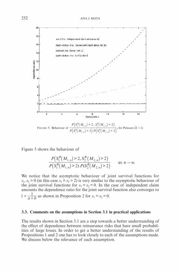
Figure 5 shows the behaviour of
> ) ( >
> , >as
P S M P S M
P S M S Mn
2 2
2 2
, ,
, ,R
nR
n
Rn
Rn
1 1 2 2
1 1 2 2"3
` ``
` ``
j j j
j j j
We notice that the asymptotic behaviour of joint survival functions fors1, s2 > 0 (in this case s1 = s2 = 2) is very similar to the asymptotic behaviour ofthe joint survival functions for s1 = s2 = 0. In the case of independent claimamounts the dependence ratio for the joint survival function also converges to
a b1
1+
+as shown in Proposition 2 for s1 = s2 = 0.
3.3. Comments on the assumptions in Section 3.1 in practical applications
The results shown in Section 3.1 are a step towards a better understanding ofthe effect of dependence between reinsurance risks that have small probabil-ities of large losses. In order to get a better understanding of the results ofPropositions 1 and 2 one has to look closely to each of the assumptions made.We discuss below the relevance of each assumption.
252 ANA J. MATA
FIGURE 5: Behaviour of> >
> , >
P S M P S M
P S M S M
2 2
2 2
, ,
, ,
Rn
Rn
Rn
Rn
1 1 2 2
1 1 2 2
_a _a
_ _a
i k i k
i i k
, for Poisson 1=m^ h
1. Assumption 5: Note that in Example 2 we have assumed that the excess ofloss layers for the reinsurer have a finite upper limit equal to 10. Therefore,assumption 5 does not seem to be a restriction in practical terms. However,the assumption that the reinsurer takes excess of loss layers with infinitelimit facilitated the analytical proof.
2. Assumption 6: It is not unreasonable to assume that for non proportionalreinsurance the retention or deductible is such that the probability of claimsaffecting the reinsurer is very small. This is a typical assumption in prac-tice.
3. Assumption 8: We assumed that the probability function is such that
( )( )
( , ) < , ( , ) <lim for wheref y Mf x M
C x y x y C x y0 0M 3# #++
=" 3 and ana-
lytically this is the key assumption for the proof of Proposition 1.Although this property seems to be related to the theory of slowly or reg-ularly varying functions (see, for example, Embrechts, Mikosh and Klüp-pelberg (1997)) it is in fact a weaker condition as some density functionssatisfy assumption 8 but are not regularly varying functions. For example,the Exponential distribution satisfies the condition in assumption 8, how-ever its probability density function is not a regularly varying function.On the other hand, the density function of a Pareto distribution is a regu-larly-varying function and it also satisfies the condition in assumption 8.The condition in assumption 8 is satisfied by most of the continuousloss distributions used to model insurance/reinsurance losses, such as:Exponential, Gamma, Log-normal, Pareto and Generalised Pareto. TheNormal distribution does not satisfy this property as it can be seen that
( )( )
lim f m yf x m
m 3++
=" 3 . In practical cases the loss distributions for insurance
claims are usually skewed and heavy-tailed, and therefore, the Normal dis-tribution is not a reasonable loss distribution for practical use.
4. Proposition 2. In this proposition we assumed that both aggregate claimamounts have the same probability of being zero. Example 2 shows that thisseems not to be a restriction. In fact in Example 2 the layers are such thatfor each n we have
< .P S M P S M0 0, ,R
nR
n1 1 2 2= =`` ``j j j j
However, for any > 0e there is M such that for n M$
< ,P S M P S M0 0, ,R
nR
n2 2 1 1 e= - =`` ``j j j j
and as n tends to infinite both probabilities tend to one.
4. CONCLUSIONS
Modelling dependencies between risks has become an area of increasedresearch interest in actuarial science. Although many authors have emphasized
ASYMPTOTIC DEPENDENCE 253
the importance of differentiating between correlation and dependence, in prac-tice, when one thinks of dependencies, inevitably the correlation coefficient isthe first thing that comes to mind.
The numerical examples in this paper showed that even when the correla-tion coefficient becomes small dependence cannot be ignored. Failure to iden-tify dependence between risks may lead to underestimation of the overall risk.This is particularly relevant when pricing risks or managing aggregation ofrisk exposure.
Throughout this paper we have looked at dependencies from the reinsurer’spoint of view where there is a very small probability of very large losses.Loosely speaking, the main result states that for large values of the retentionlevels the dependence ratio converges to a constant defined by the frequencydistribution. This constant is always greater than or equal to one. Intuitively,if the aggregate losses are dependent only through the number of events, onewould be inclined to think that if the expected number of events increases thenthe dependence becomes stronger. However, we showed that when the numberof events follows a Poisson distribution the larger the expected number ofevents the joint distribution of aggregate losses gets closer to the product ofthe marginal distributions which is the distribution of independent aggregateclaim amounts.
Modelling dependencies is an area with a vast possibility for research. It isof particular importance to extend the ideas presented in this paper of com-paring the joint distribution with the product of the marginal distributions formore general right tail dependence models, for example by looking at multi-variate extreme value distributions or extreme value copulas. This comparisonis always helpful in practice when often the practical actuary is interested inthe impact of making simplified assumptions to facilitate the implementationof new models and techniques.
ACKNOWLEDGEMENTS
This research was carried out while the author was a research student in theDepartment of Actuarial Mathematics and Statistics at Heriot-Watt Univer-sity, Edinburgh. The author would like to thank Professor Howard Waters forhis invaluable advise, helpful comments and patience throughout the numer-ous versions of this paper. Many thanks also to the helpful comments of theanonymous referees and my colleague Mr. Parr Schoolman that significantlyhelped to improve the presentation of the results. The author is also thankfulfor the financial support of The British Council and FUNDAYACUCHO fromVenezuela.
REFERENCES
AMBAGASPITIYA, R.S. (1999) On the distribution of two classes of correlated aggregate claims.Insurance: Mathematics and Economics 24:301-308
254 ANA J. MATA

EMBRECHTS, P., MCNEIL, A.J. and STRAUMANN, D. (2001) Correlations and dependency in riskmanagement: properties and pitfalls In Risk Management: Value at Risk and Beyond, ed. byM. Dempters and H.K. Moffat. Cambridge University Press.
EMBRECHTS, P., MIKOSH, T. and KLÜPPELBERG, C. (1997) Modelling Extremal Events for Insur-ance and Finance. Springer, Berlin.
MARDIA, K.V., KENT, J.T. and BIBBY, J.M. (1979) Multivariate Analysis. Academic Press, Lon-don.
MATA, A.J. (2000) Pricing excess of loss reinsurance with reinstatemets. ASTIN Bulletin 30(2):349-368.
PANJER, H.H. (1981) Recursive evaluation of a family of compound distributions. ASTIN Bul-letin 12(1): 21-26.
SUNDT, B. (1999) On multivariate Panjer recursions. ASTIN Bulletin 29(1): 29-46.
ASYMPTOTIC DEPENDENCE 255
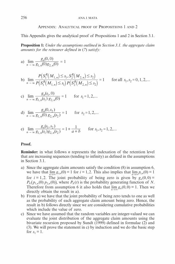
APPENDIX: ANALYTICAL PROOF OF PROPOSITIONS 1 AND 2
This Appendix gives the analytical proof of Propositions 1 and 2 in Section 3.1.
Proposition 1: Under the assumptions outlined in Section 3.1. the aggregate claimamounts for the reinsurer defined in (7) satisfy:
a) ( ) ( )( , )
lim g gg0 0
0 01
, ,n n n
n
1 2=
" 3
b),
, , , ,...lim for allP S M s P S M s
P S M s S M ss s1 0 1 2
, ,
, ,
n Rn
Rn
Rn
Rn
1 1 1 2 2 2
1 1 1 2 2 2
1 2# #
# #= =
" 3 `` ``
` ``
j j j j
j j j
c) ( ) ( )( , )
, ,...lim g s gg s
s0
01 1 2for
, ,n n n
n
1 1 2
11= =
" 3
d) ( ) ( )( , )
, ,...lim g g sg s
s0
01 1 2for
, ,n n n
n
1 2 2
22= =
" 3
e) ( ) ( )( , )
, , ,...lim forg s g sg s s
a b s s11
1 2, ,n n n
n
1 1 2 2
1 21 2= +
+=
" 3
Proof.
Reminder: in what follows n represents the indexation of the retention levelthat are increasing sequences (tending to infinity) as defined in the assumptionsin Section 3.1.
a) Since the aggregate claim amounts satisfy the condition (8) in assumption 6,we have that lim
n→∞gi,n(0) = 1 for i = 1,2. This also implies that lim
n→∞pi,n(0) = 1
for i = 1, 2. The joint probability of being zero is given by gn (0,0) =PN (p1,n(0) p2,n(0)), where PN(t) is the probability generating function of N.Therefore from assumption 6 it also holds that lim
n→∞gn(0,0) = 1. Then we
directly obtain the result in a).b) From a) we have that the joint probability of being zero tends to one as well
as the probability of each aggregate claim amount being zero. Hence, theresult in b) follows directly since we are considering cumulative probabilitieswhich include the value of zero.
c) Since we have assumed that the random variables are integer-valued we canevaluate the joint distribution of the aggregate claim amounts using thebivariate recursion proposed by Sundt (1999) defined in formulae (2) and(3). We will prove the statement in c) by induction and we do the basic stepfor s1 = 1.
256 ANA J. MATA
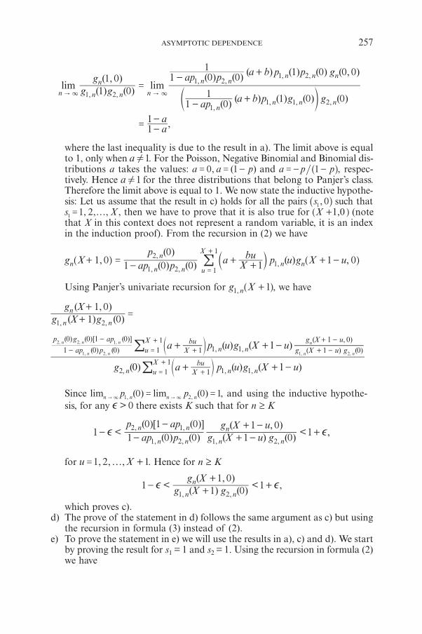
( ) ( )( , )
( ) ( ) ( ) ( ) ( )
( ) ( ) ( ) ( ) ( ) ( , )lim limg g
g
ap a b p g g
ap p a b p p g
1 0
1 0
1 01
1 0 0
1 0 01 1 0 0 0
, ,
,, , ,
, ,, ,
n n n
n
n
nn n n
n nn n n
1 2
11 1 2
1 21 2
=
-+
-+
" "3 3e o
,aa
11
=--
where the last inequality is due to the result in a). The limit above is equalto 1, only when a 1! . For the Poisson, Negative Binomial and Binomial dis-tributions a takes the values: , ( )a a p0 1= = - and a p p1= - -^ h, respec-tively. Hence a 1! for the three distributions that belong to Panjer’s class.Therefore the limit above is equal to 1. We now state the inductive hypothe-sis: Let us assume that the result in c) holds for all the pairs ,s 01^ h such that
, , ,s X1 21 f= , then we have to prove that it is also true for 1,0X +] g (notethat X in this context does not represent a random variable, it is an indexin the induction proof). From the recursion in (2) we have
, ( ) ( )( )
( ) ,g X ap pp
a Xbu p u g X u1 0
1 0 0
0
11 0
, ,
,,n
n n
nn n
u
X
1 2
21
1
1
+ =-
++
+ -=
+
!] b ]g l g
Using Panjer’s univariate recursion for g X 1, n1 +] g, we have
( ) ( )( , )
g X gg X
1 0
1 0
, ,n n
n
1 2+
+=
( ) ( ) ( )
( ) ( )( ) ( )
( ) ( )[ ( )]
( ) ( )( , )
g p u g X u
p u g X u
Xbu
ap p
p g ap
Xbu
g X u g
g X u
a
a
0 1
1
1
1 0 0
0 0 1 0
1 1 01 0
, , ,
, ,, ,
, , ,
, ,
n n nuX
n nuX
n n
n n n
n n
n
2 1 111
1 111
1 2
2 2 1
1 2
+ -
+ -
+
-
-
+ + -
+ -
+
+
=
+
=
+
!
!
f
f
p
p
Since ( ) ( )lim limp p0 0 1, ,n n n n1 2= =" "3 3 , and using the inductive hypothe-
sis, for any > 0e there exists K such that for n ≥ K
< ( ) ( )( )[ ( )]
( ) ( )( , )
< ,ap pp ap
g X u gg X u
11 0 0
0 1 0
1 0
1 01
, ,
, ,
, ,n n
n n
n n
n
1 2
2 1
1 2e e-
-
-
+ -
+ -+
for , , ,u X1 2 1f= + . Hence for n ≥ K
< ( ) ( )( , )
< ,g X gg X
11 0
1 01
, ,n n
n
1 2e e-
+
++
which proves c).d) The prove of the statement in d) follows the same argument as c) but using
the recursion in formula (3) instead of (2).e) To prove the statement in e) we will use the results in a), c) and d). We start
by proving the result for s1 = 1 and s2 = 1. Using the recursion in formula (2)we have
ASYMPTOTIC DEPENDENCE 257

( ) ( )( , )
lim g gg1 1
1 1
, ,n n n
n
1 2=
" 3
( ) ( )lim ap p1 0 01
, ,n n n1 2-" 3
( ) ( )( ) ( ) ( , )
( ) ( )( ) ( ) ( ) ( , )
g gap p g
g ga b p p v g v
1 1
0 1 1 0
1 1
1 0 1
, ,
, ,
, ,
, ,
n n
n n n
n n
n n nv
1 2
1 2
1 2
1 20
1
++ -
=!
R
T
SSS
V
X
WWW
In the limit above we have three terms, we will analyse each term separately.Using Panjer’s univariate recursion for g2,n(1) the limit for the first termcan be calculated as follows:
( ) ( ) ( ) ( )
( ) ( ) ( )( ) ( )
( , ) ( ),lim
ap a b p g
ap p gg g
ga b
a a
1 01 1 0
0 1 0
1 0
1 0 1
,, ,
, , ,
, ,n
nn n
n n n
n n
n
22 2
1 2 2
1 2-
+=
+-
" 3
since from part c) we know that ( ) ( )( , )
lim g gg1 0
1 01
, ,n
n n
n
1 2="3 . For the second
term we use the result in d) and Panjer’s univariate recursion for g1,n(1),therefore the limit for the second term is
( ) ( ) ( ) ( )
( ) ( ) ( ) ( )( ) ( )
( , ).lim
ap a b p g
a b p p gg g
ga
1 01 1 0
1 0 0
0 1
0 11
,, ,
, , ,
, ,n
nn n
n n n
n n
n
11 1
1 2 1
1 2-
+
+= -
" 3
And finally for the third term we use the result in a) together with Panjer’sunivariate algorithms for g1,n(1) and g2,n(1), hence the limit is
( ) ( )( ) ( ) ( ) ( ) ( )
( ) ( )( , )
( )lim g ga b p g p g
g gg
a a ba
1 1
1 0 1 0
0 0
0 01
1
, ,
, , , ,
, ,n n n
n n n n
n n
n
1 2
1 1 2 2
1 2
+= -
+-
" 3b l
Putting these three results together we obtain
( ) ( )( , )
( )( )
( )( )
.lim g gg
a a ba a
a a ba
a b1 1
1 1
11 1
11
11
, ,n n n
n
1 2
2
=- +
-+ - +
+-
= ++" 3
> H
We have to use a bivariate induction to prove the result in e). We state theinductive hypothesis as follows:Assume that
( ) ( )( , )
lim g s g sg s s
a b11
, ,n n n
n
1 1 2 2
1 2 = ++" 3
for all (s1,s2) such that , , ,s X1 21 f= and , , ,s Y1 22 f= , together with theresults in a), c) and d). Therefore using this hypothesis we need to prove thatthe result in statement e) holds in the following three cases:
258 ANA J. MATA
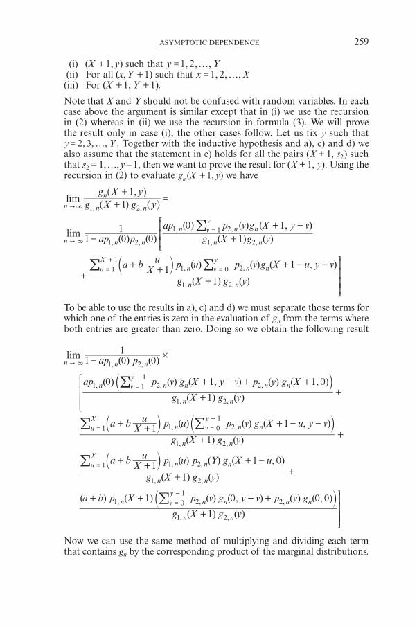
(i) ( , )X y1+ such that , , ,y Y1 2 f=(ii) For all ( , )x Y 1+ such that , , ,x X1 2 f=(iii) For ( , )X Y1 1+ + .
Note that X and Y should not be confused with random variables. In eachcase above the argument is similar except that in (i) we use the recursionin (2) whereas in (ii) we use the recursion in formula (3). We will provethe result only in case (i), the other cases follow. Let us fix y such that
, , ,y Y2 3 f= . Together with the inductive hypothesis and a), c) and d) wealso assume that the statement in e) holds for all the pairs (X + 1, s2) suchthat s2 = 1,…,y – 1, then we want to prove the result for (X + 1, y). Using therecursion in (2) to evaluate ( , )g X y1n + we have
,lim g X g y
g X y1
1
, ,n n n
n
1 2+
+=
"3 ] ^
^
g h
h
( ) ( ) ( ) ( )( ) ( ) ( , )
lim ap p g X g yap p v g X y v
1 0 01
1
0 1
, , , ,
, ,
n n n n n
n n nvy
1 2 1 2
1 21
- +
+ -
" 3
=!
R
T
SSS
( ) ( )
( ) ( ) ( , )
g X g y
a b Xu p u p v g X u y v
11
1
, ,
, ,
n n
n n nvy
uX
1 2
1 201
1
++
++
+ - -==
+ !! b l
V
X
WWWW
To be able to use the results in a), c) and d) we must separate those terms forwhich one of the entries is zero in the evaluation of gn from the terms whereboth entries are greater than zero. Doing so we obtain the following result
( ) ( )lim ap p1 0 01
, ,n n n1 2#
-" 3
( ) ( )
( ) ( ) ( , ) ( ) ( , )
g X g y
ap p v g X y v p y g X
1
0 1 1 0
, ,
, , ,
n n
n n n n nvy
1 2
1 2 21
1
+
+ - + ++
=
-!a kR
T
SSSS
( ) ( )
( ) ( ) ( , )
g X g y
a b Xu p u p v g X u y v
11
1
, ,
, ,
n n
n n nvy
uX
1 2
1 20
1
1
+
++
+ - -+
=
-
=!! b al k
( ) ( )
( ) ( ) ( , )
g X g y
a b Xu p u p Y g X u
11
1 0
, ,
, ,
n n
n n nuX
1 2
1 21
+
++
+ -+
=! b l
( ) ( )
( ) ( ) ( ) ( , ) ( ) ( , )
g X g y
a b p X p v g y v p y g
1
1 0 0 0
, ,
, , ,
n n
n n n n nvy
1 2
1 2 20
1
+
+ + - +=
-!a kV
X
WWWW
Now we can use the same method of multiplying and dividing each termthat contains gn by the corresponding product of the marginal distributions.
ASYMPTOTIC DEPENDENCE 259
Then for those terms where one or both entries is zero the ratio tends toone, and for the ratios where both entries are greater than zero the ratio tends to ( )a b1
1+
+due to the inductive hypothesis. Therefore, the limit above
can be written as follows
( ) ( )( , )
( ) ( )lim limg X g yg X y
ap p1
1
1 0 01
, , , ,n n n
n
n n n1 2 1 2#
+
+=
-" "3 3
( )( ) ( )
( )
( ) ( ) ( ) ( )
g Xap g X
g ya b p v g y v p y g
1
0 1 11
0
,
, ,
,
, , , ,
n
n n
n
n n n nv
y
1
1 1
2
2 2 2 21
1
+
+ ++
- ++
=
-!J
L
KKKK
e
bN
P
OOOO
o
l
R
T
SSSS
( )
( ) ( )
g X
a b Xu p u g X u
11
1
,
, ,
n
n nuX
1
1 11#+
+
++
+ -=
!J
L
KKKK
bN
P
OOOO
l
( )
( ) ( ) ( ) ( )
g ya b p v g y v p y g1
10
,
, , , ,
n
n n n nvy
2
2 2 2 20
1+
+- +
+=
-!J
L
KKKK
bN
P
OOOO
l
( )( ) ( ) ( )
( )( ) ( ) ( ) ( )
g Xa b p X g
g yp g y p v g y v
1
1 0 0
,
, ,
,
, , , ,
n
n n
n
n n n nvy
1
1 1
2
2 2 2 21++
+ + + -=
!J
L
KKK
e
N
P
OOO
o
V
X
WWWW. (A.1)
From condition (8) in assumption 6 it follows that ( )lim g x 0,n i n =" 3 forall , , ,x 1 2 3 f= and for ,i 1 2= . The same result holds for ( )p x,i n . Usingthese results we have
( ) ( ) ,lim p v g y v 0, ,n n nv
y
2 21
- =" 3 =
!
since each term tends to zero. However, when we divide the above sum byg2,n(y) we obtain the following result
( ) ( ) ( )
( ) ( )lim
ap a b yv p v g y v
p v g y v
1 01
,, ,
, ,
n
nn nv
yn nv
y
22 21
2 21
-+ -
-=
" 3=
=
!
!
b l
( ) ( ) ( ) ( ) ( ) ( )
( ) ( ) ( ) ( ) ( ) ( )lim
ap a yb p g y a b p y g
p g y p y g p y g
1 01 1 1 0
1 1 1 1 0
,, , , ,
, , , , , ,
n
nn n n n
n n n n n n
22 2 2 2
2 2 2 2 2 2
g
g
-+ - + + +
- + + - +
" 3bc l m
We observe that in the limit above each term tends to zero, however the lastterm contains g2,n(0) which tends to one as n tends to infinity. Therefore,we divide each term by p2,n(y) and we obtain
260 ANA J. MATA
( ) ( )( ) ( )
( ) ( )
( )( ) ( )
( ).lim
ap a yb
p yp g y
a b g
p yp g y
g
a ba
1 01 1 1
0
1 10
1
, ,
, ,,
,
, ,,
n
n n
n nn
n
n nn
2 2
2 22
2
2 22
g
g
-+
-+ + +
-+ +
=+-
" 3be l o
The last equality is due to the result in assumption 8 where we assumed
that ( )( )
( , )lim p yp x
C x y,
,
n i n
i n=
" 3which is a constant for i = 1,2, and ( )lim g x 0,n i n =
" 3
for all x = 1,2,…. From the discussion above we obtain directly the followingresults
( )( ) ( )
lim g yp v g y v
0,
, ,
n n
n nvy
2
2 21
1-
=" 3
=
-!
( )
( ) ( )lim g X
a b Xu p u g X u
11
10
,
, ,
n n
n nuX
1
1 11
+
++
+ -=
" 3
=! b l
( )( ) ( ) ( )
lim g Xa b p X g
a1
1 01
,
, ,
n n
n n
1
1 1
+
+ += -
" 3
Hence from all the above, we can evaluate the limit in formula (A.1) andwe obtain the following result
( ) ( )( , )
( ) ,lim g X g Yg X Y
a a a ba a a b
aa b1
1
11 1
1 11
11
, ,n n n
n
1 2+
+=
- +-
+ - ++-
= ++" 3
b bl l; E
which is the result shown in e).
Proposition 2: Suppose that two risks follow assumptions 1 and 3 of Proposition 1.Let {M1,n} and {M2,n} be sequences of real numbers representing the reinsuranceretention levels for each portfolio. These sequences are such that the reinsurer’saggregate claim amounts satisfy the condition in (8) and that for each n
.P S M P S M0 0, ,R
nR
n n1 1 2 2= = = =a`` ``j j j j
Then, the reinsurance aggregate claim amounts defined in (7) satisfy
> >
> , >.lim
P S M P S M
P S M S Ma b0 0
0 01
1
, ,
, ,
n Rn
Rn
Rn
Rn
1 1 2 2
1 1 2 2= +
+" 3 `` ``
` ``
j j j j
j j j
Proof. Note that in this case we do not require that the individual claim amountsare integer-valued random variables. We also do not need that the retentionlevels are integer numbers. We denote by pi,n(0) the probability that an indivi-dual claim amount for the reinsurer is zero and by gi,n(0) the probability that
ASYMPTOTIC DEPENDENCE 261
the aggregate claim amount for the reinsurer is zero for retention level Mi,n for,i 1 2= .
If n "3 then 1n"a -. We can write the probabilities of being zero in termsof the probability generating function as
( ) ( ) , ,forg P S M P p i0 0 0 1 2, , ,i n iR
i n N i n n= = = = =a`` `j j j
where PN(t) is the probability generating function of the frequency distribution.Hence, ( ) ( ) ,forp P i0 1 2,i n N n
1= =a- , provided that the inverse of the proba-bility generating function exists. For the Poisson, the Negative Binomial andthe Binomial distributions the inverse of the probability generating functioncan be written explicitly.
As in part a) of Proposition 1 we can write the joint probability of the aggre-gate claim amounts being zero as follows
( , ) ( ) ( ) .g P p p P P0 0 0 0, ,n N n n N N n1 21 2
= = a-` ^`bj hj l
Therefore,
> >
> , >
( ) ( )
( ) ( ) ( , )lim lim
P S M P S M
P S M S M
g g
g g g
0 0
0 0
1 0 1 0
1 0 0 0 0
, ,
, ,
, ,
, ,
n Rn
Rn
Rn
Rn
n n n
n n n
1 1 2 2
1 1 2 2
1 2
1 2=
- -
- - +
" "3 3_` _`
_ _`
_ _i j i j
i i j
i i
( )lim
P P
1
1 2
00
n
n N N n
12
1 2
n
=-
- +=
a
a a
"
-
a - ^
`b
h
j l
.
Applying L’Hospital rule twice the limit above can be calculated as follows
( )( )
( ( ))lim
dd P P
dd P P
P2
nN N n
nN N n
N n
12
21 2
12
1 2
n
+a
a
a a
a
"
-
-
-
a -`b
`d
j l
jn
R
T
SSSSS
( )( )
( )
( )
dd P P d
d P P
dd P P
P1
nN N n n
N N n
nN N n
N n
1 2
21
12
1
-
a a aa
a a
a
-
-
-
-
`
`
`d
`
j
j
jn
j
V
X
WWWWW
From the properties of the probability generating function we have ( )P 1 1N =
and therefore ( )P 1 1N1 =- . Moreover, the probability generating function satisfies
( ) [ ]dtd P E N1N = . Therefore, the limit above is given by
> >
> , >
[ ]
( )
[ ] .limP S M P S M
P S M S M
E Ndtd P
E N0 0
0 0 11
, ,
, ,
n Rn
Rn
Rn
Rn N
1 1 2 2
1 1 2 2
2
2
2
= +" 3 `` ``
` ``
^j j j j
j j j
h
262 ANA J. MATA

Therefore, by evaluating the limit above with the corresponding values for eachof the distributions that belong to Panjer’s class it follows that
> >
> , >.lim
P S M P S M
P S M S Ma b0 0
0 01
1
, ,
, ,
n Rn
Rn
Rn
Rn
1 1 2 2
1 1 2 2= +
+"3 `` ``
` ``
j j j j
j j j
ANA J. MATA
CNA Re1
333. S. Wabash Av., 39th floorChicago IL 60604USA
ASYMPTOTIC DEPENDENCE 263
1 The statements, analysis and opinions set forth in this article are solely those of the author and donot reflect the statements, opinions or analysis of any third party, including Continental CasualtyCompany or any of its subsidiary or affiliated companies.

THE MARKOV CHAIN MARKET
BY
RAGNAR NORBERG
ABSTRACT
We consider a financial market driven by a continuous time homogeneousMarkov chain. Conditions for absence of arbitrage and for completeness arespelled out, non-arbitrage pricing of derivatives is discussed, and details areworked out for some cases. Closed form expressions are obtained for interestrate derivatives. Computations typically amount to solving a set of first orderpartial differential equations. An excursion into risk minimization in the incom-plete case illustrates the matrix techniques that are instrumental in the model.
KEYWORDS
Continuous time Markov chains, Martingale analysis, Arbitrage pricing theory,Risk minimization, Unit linked insurance.
INTRODUCTION
A. Prospectus
The theory of diffusion processes, with its wealth of powerful theorems andmodel variations, is an indispensable toolbox in modern financial mathematics.The seminal papers of Black and Scholes and Merton were crafted with Brownianmotion, and so was the major part of the plethora of papers on arbitrage pric-ing theory and its ramifications that followed over the past good quarter of acentury.
A main course of current research, initiated by the martingale approach toarbitrage pricing Harrison and Kreps (1979) and Harrison and Pliska (1981),aims at generalization and unification. Today the core of the matter is wellunderstood in a general semimartingale setting, see e.g. Delbaen and Schacher-mayer (1994). Another course of research investigates special models, in partic-ular Levy motion alternatives to the Brownian driving process, see e.g. Eberleinand Raible (1999). Pure jump processes have found their way into finance,ranging from plain Poisson processes introduced in Merton (1976) to fairly generalmarked point processes, see e.g. Björk et al. (1997). As a pedagogical exercise,the market driven by a binomial process has been intensively studied since it wasproposed in Cox et al. (1979).
ASTIN BULLETIN, Vol. 33, No. 2, 2003, pp. 265-287
The present paper undertakes to study a financial market driven by a con-tinuous time homogeneous Markov chain. The idea was launched in Norberg(1995) and reappeared in Elliott and Kopp (1998), the context being modelingof the spot rate of interest. These rudiments will here be developed into a modelthat delineates a financial market with a locally risk-free money account, riskyassets, and all conceivable derivatives. The purpose of this exercise is two-fold:In the first place, there is an educative point in seeing how well established theoryturns out in the framework of a general Markov chain market and, in particu-lar, how and why it differs from the familiar Brownian motion driven market.In the second place, it is worthwhile investigating the potential of the model froma theoretical as well as from a practical point of view. Further motivation anddiscussion of the model is given in Section 5.
B. Contents of the paper
We hit the road in Section 2 by recapitulating basic definitions and results forthe continuous time Markov chain. We proceed by presenting a market fea-turing this process as the driving mechanism and by spelling out conditions forabsence of arbitrage and for completeness. In Section 3 we carry through theprogram for arbitrage pricing of derivatives in the Markov chain market andwork out the details for some special cases. Special attention is paid to interestrate derivatives, for which closed form expressions are obtained. Section 4addresses the Föllmer-Sondermann-Schweizer theory of risk minimization inthe incomplete case. Its particulars for the Markov chain market are workedout in two examples, first for a unit linked life endowment, and second forhedging strategies involving a finite number of zero coupon bonds. The finalSection 5 discusses the versatility and potential uses of the model. It also raisesthe somewhat intricate issue of existence and continuity of the derivatives involvedin the differential equations for state prices, which finds its resolution in a forth-coming paper. Some useful pieces of matrix calculus are placed in the Appendix.
C. Notation
Vectors and matrices are denoted by boldface letters, lower and upper case,respectively. They may be equipped with top-scripts indicating dimensions, e.g.An×m has n rows and m columns. We may write A = e ! f( )aef f F! to emphasize theranges of the row index e and the column index f. The transpose of A is denotedby A�. Vectors are taken to be of column type, hence row vectors appear astransposed (column) vectors. The identity matrix is denoted by I, the vectorwith all entries equal to 1 is denoted by 1, and the vector with all entries equalto 0 is denoted by 0. By De=1,…,n (ae), or just D(a), is meant the diagonal matrixwith the entries of a = (a1,…,an)� down the principal diagonal. The n-dimen-sional Euclidean space is denoted by �n, and the linear subspace spanned bythe columns of An×m is denoted by �(A).
The cardinality of a set y is denoted by |y |. For a finite set it is just its num-ber of elements.
266 RAGNAR NORBERG
2. THE MARKOV CHAIN MARKET
A. The continuous time Markov chain
At the base of everything is some probability space (W, F, �). Let {Yt}t ≥ 0 be acontinuous time Markov chain with finite state space y = {1,…,n}. We takethe paths of Y to be right-continuous and Y0 deterministic. Assume that Y istime homogeneous so that the transition probabilities
�p Y f Y ete
tt t= = =+f
7 A
depend only on the length of the time period. This implies that the transitionintensities
t ,lim tp
lt 4 0
=efef
(2.1)
e ≠ f, exist and are constant. To avoid repetitious reminders of the type “e, f ∈ y”,we reserve the indices e and f for states in y throughout. We will frequently referto
e ; > ,fy l 0ef
= $ .
the set of states that are directly accessible from state e, and denote the num-ber of such states by
en ye = .
Put
el l l
;
ee e ef
f f y= - = -$
!
!
(minus the total intensity of transition out of state e). We assume that all statesintercommunicate so that pef
t > 0 for all e, f (and t > 0). This implies that ne > 0for all e (no absorbing states). The matrix of transition probabilities,
,pPt t= ef` j
and the infinitesimal matrix,
,lL ef= _ i
are related by (2.1), which in matrix form reads L = limt40 t1 (Pt – I), and by the
forward and backward Kolmogorov differential equations,
t t t .dtd P P PL L= = (2.2)
THE MARKOV CHAIN MARKET 267
Under the side condition P0 = I, (2.2) integrates to
.exp tP Lt = ] g (2.3)
The matrix exponential is defined in the Appendix, from where we also fetchthe representation (A.3):
.e eP DF F f c,...,t e nt t e e
e
nr r
11
1
�e= ==
-
=
e!` j (2.4)
Here the first eigenvalue is r1 = 0, and the corresponding eigenvectors aref1= 1 and c1� = (p1,…, pn) = limt3∞ (pe1
t ,…,pent ), the stationary distribution of Y.
The remaining eigenvalues, r2,…,rn, have strictly negative real parts so that,by (2.4), the transition probabilities converge exponentially to the stationarydistribution as t increases.
Introduce
tt ,I Y e1e = =7 A (2.5)
the indicator of the event that Y is in state at time t, and
t t t-; < , , ,N t Y e Y ft t0ef #= = =" , (2.6)
the number of direct transitions of Y from state e to state f ∈ ye in the timeinterval (0, t]. For f ∉ ye we define Nef
t / 0. The assumed right-continuity of Yis inherited by the indicator processes I e and the counting processes Nef. As isseen from (2.5), (2.6), and the obvious relationships
t t t t, ,Y eI I I N N!;
te e
e
e fe ef
f f e0= = + -! ! ` j
the state process, the indicator processes, and the counting processes carrythe same information, which at any time t is represented by the sigma-algebraFY
t = s{Yt ; 0 ≤ t ≤ t}. The corresponding filtration, denoted by FY = {FYt }t≥0, is
taken to satisfy the usual conditions of right-continuity and completeness, andF0 is assumed to be trivial.
The compensated counting processes Mef, e ≠ f, defined by
t t tdM dN I dtlef ef e ef= - (2.7)
and M ef0 = 0, are zero mean, square integrable, mutually orthogonal martin-
gales with respect to (FY, �). We feel free to use standard definitions and resultsfrom counting process theory and refer to Andersen et al. (1993) for a background.
We now turn to the subject matter of our study and, referring to introduc-tory texts like Björk (1998) and Pliska (1997), take basic concepts and resultsfrom arbitrage pricing theory as prerequisites.
268 RAGNAR NORBERG
B. The continuous time Markov chain market
We consider a financial market driven by the Markov chain described above.Thus, Yt represents the state of the economy at time t, FY
t represents the infor-mation available about the economic history by time t, and FY represents theflow of such information over time.
In the market there are m + 1 basic assets, which can be traded freely andfrictionlessly (short sales are allowed, and there are no transaction costs).A special role is played by asset No. 0, which is a “locally risk-free” bank accountwith state-dependent interest rate
tt ,r r I rt
Y e
e
e= = !
where the state-wise interest rates re, e =1,…,n, are constants. Thus, its priceprocess is
,exp expS r du r I dut ut e
uet
e
0
0 0= =# #!c em o
where ∫ t0 Ie
u du is the total time spent in economy state e during the period [0,t].The dynamics of this price process is
t t t t .dS S r dt S r I dtte e
e
0 0 0= = !
The remaining m assets, henceforth referred to as stocks, are risky, with priceprocesses of the form
u t ,exp �S I du Nbti ie e ief ef
fe
t
e y0= +
! e# !!!
J
L
KK
N
P
OO (2.8)
i = 1,…,m, where the � ie and b ief are constants and, for each i, at least one of theb ief is non-null. Thus, in addition to yielding state-dependent returns of thesame form as the bank account, stock No. i makes a price jump of relative size
expg b 1ief ief= -_ i
upon any transition of the economy from state e to state f. By the general Itô’sformula, its dynamics is given by
ttt .�dS S I dt dNgiti ie e ief ef
fee y= +
!-
e!!!
J
L
KK
N
P
OO (2.9)
(Setting Si0 = 1 for all i is just a matter of convention; it is the relative price
changes that matter.)
THE MARKOV CHAIN MARKET 269
Taking the bank account as numeraire, we introduce the discounted assetprices S i
t = Sit /S 0
t , i = 0,…,m. The discounted price of the bank account isS 0
t / 1, which is certainly a martingale under any measure. The discountedstock prices are
u t ,exp � r I du NbSti ie e e ief ef
fe
t
e y0= - +
! e# !!!
J
L
KK _
N
P
OOi (2.10)
with dynamics
ttt ,�d r I dt dNgS Siti ie e e ief ef
fee y= - +
!-
e!!!
J
L
KK _
N
P
OOi (2.11)
i = 1,…,m.
C. Portfolios
A dynamic portfolio or investment strategy is an m + 1-dimensional stochasticprocess
, ..., ,q qqt t tm0= ` j
where q it represents the number of units of asset No i held at time t. The port-
folio q must adapted to FY and the shares of stocks, (q 1t ,…,qm
t ), must also beFY-predictable. For a sufficiently rigorous treatment of the concept of pre-dictability, see Andersen et al. (1993). For our purposes it suffices to knowthat any left-continuous or deterministic process is predictable, the intuitionbeing that the value of a predictable process at any time is determined by thestrictly past history of the driving process Y. We will comment on these assump-tions at a later point when the prerequisites are in place.
The value of the portfolio q at time t is
t t t .V SS qq �t ti i
i
mq
0
= ==
!
Henceforth we will mainly work with discounted prices and values and, inaccordance with (2.10), equip their symbols with a tilde. The discounted valueof the portfolio at time t is
t .qV S�t tq = (2.12)
The strategy q is self-financing (SF) if dV qt = q�t dSt or (recall dS0
t = 0)
t t t .d d dqqV SS�t ti i
i
mq
1
= ==
! (2.13)
270 RAGNAR NORBERG
D. Absence of arbitrage
LetL̂ = (l̂ef)
be an infinitesimal matrix that is equivalent to L in the sense that l̂ef = 0 ifand only if lef = 0. By Girsanov’s theorem for counting processes (see e.g.Andersen et al. (1993)) there exists a measure �̂, equivalent to �, under whichY is a Markov chain with infinitesimal matrix L̂ . Consequently, the processesMef, e ∈ y, f ∈ ye, defined by
t t t ,d dN I dtMef ef e ef= - lu (2.14)
and Mef0 = 0, are zero mean, mutually orthogonal martingales with respect to
(FY,�̂). Rewrite (2.11) as
ttt ,�d r I dt dg gS S Miti ie e ief ef
f
e ief ef
fee y y= - + +
! !- l
e e! !!! u
J
L
KK
N
P
OO
R
T
SSS
V
X
WWW
(2.15)
i = 1,…,m. The discounted stock prices are martingales with respect to (FY,�̂)if and only if the drift terms on the right vanish, that is,
,� r g l 0ie e ief ef
f y- + =
! e! u (2.16)
e = 1,…,n, i = 1,…, m. From general theory it is known that the existence ofsuch an equivalent martingale measure �̂ implies absence of arbitrage. The rela-tion (2.16) can be cast in matrix form as
re1 – ae = Ge l̂e, (2.17)
e = 1,…,n, where 1 is m × 1 and
, , .� � g lG l,...,
e iei m
e ief f e eff
yy1 ,...,i m1
= = =!
!= =
e
eu u_ _ _i i i
The existence of an equivalent martingale measure is equivalent to the existenceof a solution l̂e to (2.17) with all entries strictly positive. Thus, the market isarbitrage-free if (and we can show only if) for each e, re1 – ae is in the interiorof the convex cone of the columns of Ge.
Assume henceforth that the market is arbitrage-free so that (2.15) reducesto
tt .d dgS S Miti ief ef
fe y=
!-
e!! (2.18)
THE MARKOV CHAIN MARKET 271
Inserting (2.18) into (2.13), we find
tt ,d dq gV S Mti
ti ief ef
i
m
fe yq
1
=!
-=e!!! (2.19)
which means that the value of an SF portfolio is a martingale with respect to(FY,�̂) and, in particular,
Vqt = �̂ [Vq
T | Ft ] (2.20)
for 0 ≤ t ≤ T. Here �̂ denotes expectation under �̂. (The tilde, which in the firstplace was introduced to distinguish discounted values from the nominal ones,is also attached to the equivalent martingale measure because it arises from thediscounted basic price processes.)
We remind of the standard proof of the result that the existence of anequivalent martingale measure implies absence of arbitrage: Under (2.20) onecan not have Vq
0 = 0 and at the same time have VqT ≥ 0 almost surely and Vq
T > 0with positive probability.
We can now explain the assumptions made about the components of theportfolio qt. The adaptedness requirement is commonplace and says just thatthe investment strategy must be based solely on the currently available infor-mation. Without this assumption it is easy to construct examples of arbitragesin the present and in any other model, and the theory would become void justas would practical finance if investors could look into the future. The require-ment that (q1,…,qm) be FY-predictable means that investment in stocks mustbe based solely on information from the strict past. Also this assumption isomnipresent in arbitrage pricing theory, but its motivation is less obvious.For instance, in the Brownian world ‘predictable’ is the same as ‘adapted’ dueto the (assumed) continuity of Brownian paths. In the present model the twoconcepts are perfectly distinct, and it is easy to explain why a trade in stockscannot be based on news reported at the very instant where the trade is made.The intuition is that e.g. a crash in the stock market cannot be escaped byrushing money over from stocks to bonds. Sudden jumps in stock prices, whichare allowed in the present model, must take the investor by surprise, else therewould be arbitrage. This is seen from (2.19). If the qi
t, i = 1,…,m, could be anyadapted processes, then we could choose them in such a manner that dVq
t ≥ 0almost surely and strictly positive with positive probability. For instance, wecould take them such that
tt t tt .d DV M M M M21
,
ef eft
fe
ef ef
tfey yq
t0
2 2
0
= = +! !!e e
#!! !!!J
L
KK` `
]
N
P
OOj j
?
Clearly, VqT is non-negative and attains positive values with positive probability
while Vq0 = 0, hence q would be an arbitrage.
272 RAGNAR NORBERG
E. Attainability
A T-claim is a contractual payment due at time T. More precisely, it is an FYT -
measurable random variable H with finite expected value. The claim is attain-able if it can be perfectly duplicated by some SF portfolio q, that is,
VqT = H. (2.21)
If an attainable claim should be traded in the market, then its price must atany time be equal to the value of the duplicating portfolio in order to avoidarbitrage. Thus, denoting the price process by pt and, recalling (2.20) and (2.21),we have
p̂t t ,�V H Ftq= = u 7 A (2.22)
or
r .� e Hp Ft tt
T
= - #u 9 C (2.23)
(We use the short-hand re t
T- # for re du
t
T- u# .)
By (2.22) and (2.19), the dynamics of the discounted price process of anattainable claim is
dp̂t t .dq gS Mti
ti ief ef
i
m
fe y 1
=!
-=e!!! (2.24)
F. Completeness
Any T-claim H as defined above can be represented as
H = �̂ ,djH Mtef
tef
fe
T
y0+
!e
# !!7 A (2.25)
where the jeft are FY-predictable processes (see Andersen et al. (1993)). Conversely,
any random variable of the form (2.25) is, of course, a T-claim. By virtue of (2.21)and (2.19), attainability of H means that
t
t
0
0 .
d
dq g
H V V
V S M
T
ti
ti ief ef
ife
T
y
q q
q
0
0
= +
= +!
-e
#
# !!!(2.26)
Comparing (2.25) and (2.26), we see that H is attainable iff there exist predic-table processes q1
t ,…,qmt such that
THE MARKOV CHAIN MARKET 273
,q g jSti
ti ief
tef
i
m
1
=-
=
!
for all e and f ∈ ye. This means that the ne-vector
jjte
tef
f y=
!e` j
is in �(Ge�).The market is complete if every T-claim is attainable, that is, if every ne-vec-
tor is in �(Ge�). This is the case if and only if rank (Ge) = ne, which can be ful-filled for each e only if m ≥ maxe ne, i.e. the number of risky assets is no lessthan the number of sources of randomness.
3. ARBITRAGE-PRICING OF DERIVATIVES IN A COMPLETE MARKET
A. Differential equations for the arbitrage-free price
Assume that the market is arbitrage-free and complete so that the price ofany T-claim is uniquely given by (2.22) or (2.23).
Let us for the time being consider a T-claim that depends only on the stateof the economy and the price of a given stock at time T. To simplify notation,we drop the top-script indicating this stock throughout and write just
u t .exp �S I du Nbte e ef ef
fe
t
e y0= +
!e
# !!!J
L
KK
N
P
OO
Thus, the claim is of the form
.H h S I h SYT T
e e
eT
T= = !^ ^h h (3.1)
Examples are a European call option defined by H = (ST – K)+, a caplet definedby H = (rT – g)+ = (rYT – g)+, and a zero coupon T-bond defined by H = 1.
For any claim of the form (3.1) the relevant state variables involved in theconditional expectation (2.23) are (St, t, Yt). This is due to the form of the stockprice, by which
u tee
,exp �S S I du N NbT te e ef
Tef ef
ft
T
y= + -
!e
# !!!J
L
KK `
N
P
OOj (3.2)
and the Markov property, by which the past and the future are conditionallyindependent, given the present state Yt. It follows that the price pt is of the form
t , ,I v S tpte e
te
n
1
==
! ^ h (3.3)
274 RAGNAR NORBERG
where the functions
ve(s, t) = �̂ r ,e H Y e S st ttT
= =- #9 C (3.4)
are the state-wise prices. Moreover, by (3.2) and the homogeneity of Y, we obtainthe representation
ve(s, t) = � .h s S Y eYT t 0
T t =-- ^ h8 B (3.5)
The discounted price (2.22) is a martingale with respect to (FY,�̂). Assumethat the functions ve(s, t) are continuously differentiable. Applying Itô to
p̂t t , ,e I v S tr e et
e
n
1
t0= -
=
# ! ^ h (3.6)
we find
dp̂t
t
t
t
t
, , ,
, ,
, , ,
, ,
, , .
�
�
e I r v S t t v S t s v S t S dt
e v S t v S t dN
e I r v S t t v S t s v S t S
v S t v S t dt
e v S t v S t d
g
g l
g M
1
1
1
r e
e
e et
et
et t
e
r ft
ef et
fe
ef
r e
e
e et
et
et t
e
ft
ef et
ef
f
r ft
ef et
fe
ef
y
y
y
t
t
t
t
0
0
0
0
22
22
22
22
= - + +
+ + -
= - + +
+ + -
+ + -
!
!
!
-
-- -
-
- -
-- -
e
e
e
#
#
#
#
!
!!
!
!
!!
u
^ ^ ^b
_` ^`
^ ^ ^b
_` ^`
_` ^`
h h h l
i j hj
h h h
i j hj k
i j hj
(3.7)
By the martingale property, the drift term must vanish, and we arrive at thenon-stochastic partial differential equations
, , ,
, ,
�r v s t t v s t s v s t s
v s t v s tg l1 0
e e e e e
f ef e ef
f y
22
22
- + +
+ + - =!
e! u
] ] ]
_` ]`
g g g
i j gj(3.8)
with side conditions
, ( ),v s T h se e=] g (3.9)
e = 1,…,n.
THE MARKOV CHAIN MARKET 275
In matrix form, with
R = De=1,…,n (re), A = De=1,…,n (�e)
and other symbols (hopefully) self-explaining, the differential equations andthe side conditions are
, , , , ,
, .
s t t s t s s s t s t
s T s
Rv v A v v
v h
gL 1 022
22
- + + + + =
=
u] ] ] ^^
] ]
g g g h h
g g
(3.11)
There are other ways of obtaining the differential equations. One is to derivethem from the integral equations obtained by conditioning on whether or notthe process Y leaves its current state in the time interval (t,T ] and, in case itdoes, on the time and the direction of the transition. This approach is takenin Norberg (2002) and is a clue in the investigation of the assumed continu-ous differentiability of the functions ve.
Before proceeding we render a comment on the fact that the price of aderivative depends on the drift parameters �e of the stock prices as is seenfrom (3.8). This is all different from the Black-Scholes-Merton model in whicha striking fact is that the drift parameter does not appear in the derivativeprices. There is no contradiction here, however, as both facts reflect the para-mount principle that the equivalent martingale measure arises from the pathproperties of the price processes of the basic assets and depends on the orig-inal measure only through its support. The drift term is a path property in thejump process world but not in the Brownian world. In the Markov chain mar-ket the pattern of direct transitions as given by the ye is a path property, butapart from that the intensities F do not affect the derivative prices.
B. Identifying the strategy
Once we have determined the solution ve(s, t), e = 1,…,n, the price process isknown and given by (3.3).
The duplicating SF strategy can be obtained as follows. Setting the driftterm to 0 in (3.7), we find the dynamics of the discounted price;
dp̂t t, , .e v S t v S t dg M1r ft
ef et
fe
ef
y
t0= + -
!
-- -
e
# !! _` ^` i j hj (3.12)
Identifying the coefficients in (3.12) with those in (2.24), we obtain, for eachtime t and state e, the equations
t t- , , ,S v S t v S tq g g1i
i
mi ief f
tef e
t1
= + -=
- -! _` ^i j h (3.13)
276 RAGNAR NORBERG
f ∈ ye. The solution (q i,et )i=1,…,m certainly exists since rank(Ge) ≤ m, and it is
unique if rank(Ge) = m. It is a function of t and St– and is thus predictable.Finally, q0 is determined upon combining (2.12), (2.22), and (3.6):
rt t t, .e I v S t Sq qte e
ti
i
mi
e
n0
11
t
0= --
==
# !! ^e h o
This function is not predictable.
C. The Asian option
As an example of a path-dependent claim, let us consider an Asian option, which
is a T-claim of the form H S d KtT t1
0= -
+T#a k , where K ≥ 0. The price process is
r
t , , ,
� e T S d K
I v S t S d
p t
t
F1t
T
tY
e et
t
e
n
t
t
0
01
tT
= -
=
-+
=
#
#
#
!
u c
c
m
m
= G
where
rt, , , .�v s t u e T S d T
u K Y e S st1et
Tttt
T
= + - = =-+
##u] cg m= G
The discounted price process is
p̂t tr , , .e I v t S S dte e
tt
e
n
t01
t0= -
=
## ! c m
We are lead to partial differential equations in three variables.
D. Interest rate derivatives
A particularly simple, but important, class of claims are those of the form H =hYT. Interest rate derivatives of the form H = h(rT) are included since rt = rYt.For such claims the only relevant state variables are t and Yt, so that the func-tion in (3.4) depends only on t and e. The differential equations (3.8) and theside condition (3.9) reduce to
t t t t ,dtd v r v v v le e e f e
f
ef
y= - -
!e
! u` j (3.14)
.v hTe e= (3.15)
THE MARKOV CHAIN MARKET 277
In matrix form:
,
.dtd v v
v h
LRt t
T
= -
=
u_ i
Similar to (2.3) we arrive at the explicit solution
.exp T tv R hLt = - -u^ ]h g" , (3.16)
It depends on t and T only through T – t.In particular, the zero coupon bond with maturity T corresponds to h = 1.
We will henceforth refer to it as the T-bond in short and denote its price pro-cess by p(t,T) and its state-wise price functions by p(t,T) = (pe(t,T))e=1,…,n;
, .expt T T tp RL 1= - -u] ^ ]g h g" , (3.17)
For a call option on a U-bond, exercised at time T(<U) with price K, h hasentries he = (pe(T,U) – K)+.
In (3.16)-(3.17) it may be useful to employ the representation (A.3),
.exp T t eR DL F F,...,( )
e nT t
11e
- - = =- -tu u uu
^ ] `h g j" , (3.18)
4. RISK MINIMIZATION IN INCOMPLETE MARKETS
A. Incompleteness
The notion of incompleteness pertains to situations where there exist contingentclaims that cannot be duplicated by an SF portfolio and, consequently, do notreceive unique prices from the no arbitrage postulate alone. In Paragraph 2Fwe alluded to incompleteness arising from a scarcity of traded assets, that is,the discounted basic price processes are incapable of spanning the space of allmartingales with respect to (FY,�̂) and, in particular, reproducing the value(2.25) of every financial derivative.
B. Risk minimization
Throughout this section we will mainly be working with discounted pricesand values without any other mention than the tilde notation. The reason isthat the theory of risk minimization rests on certain martingale representationresults that apply to discounted prices under a martingale measure. We will becontent to give just a sketchy review of some main concepts and results fromthe seminal paper of Föllmer and Sondermann (1986) on risk minimization.
278 RAGNAR NORBERG
Let H be a T-claim that is not attainable. This means that an admissibleportfolio q satisfying
V HTq =
cannot be SF. The cost by time t of an admissible portfolio q is denoted byCq
t and is defined as that part of the portfolio value that has not been gainedfrom trading:
t t .dqC V S�tq q
t t0
= - #
The risk at time t is defined as the mean squared outstanding cost,
.�R C C FT t tq q q 2
= -tu ` j: D (4.1)
By definition, the risk of an admissible portfolio q is
t ,� dqR H V S F�t
Tt
q qt t
2
= - -t #u c m= G
which is a measure of how well the current value of the portfolio plus futuretrading gains approximates the claim. The theory of risk minimization takesthis entity as its objective function and proves the existence of an optimaladmissible portfolio that minimizes the risk (4.1) for all t ∈ [0,T ].
The proof is constructive and provides a recipe for determining the optimalportfolio. One commences from the intrinsic value of H at time t defined as
t .�V H FHt= u 7 A (4.2)
This is the martingale that at any time gives the optimal forecast of the claimwith respect to mean squared prediction error under the chosen martingalemeasure. By the Galchouk-Kunita-Watanabe representation, it decomposesuniquely as
t t ,� d LqV H SH Ht t
Ht
0
�= + +#u 7 A (4.3)
where LH is a martingale with respect to (F,�̂) which is orthogonal to themartingale S. The portfolio qH defined by this decomposition minimizes therisk process among all admissible strategies. The minimum risk is
.� d LR FH Ht
Ttt
=t #u ; E (4.4)
THE MARKOV CHAIN MARKET 279
C. Unit-linked insurance
As the name suggests, a life insurance product is said to be unit-linked if thebenefit is a certain share of an asset (or portfolio of assets). If the contractstipulates a prefixed minimum value of the benefit, then one speaks of unit-linked insurance with guarantee. A risk minimization approach to pricing andhedging of unit-linked insurance claims was first taken by Møller (1998), whoworked with the Black-Scholes-Merton financial market. We will here sketchhow the analysis goes in our Markov chain market, which is a particularlysuitable partner for the life history process since both are intensity-driven.
Let Tx be the remaining life time of an x years old who purchases aninsurance at time 0, say. The conditional probability of survival to age x + u,given survival to age x + t (0 ≤ t < u), is
x x> > ,� T u T t e dsmx st
u
= - +#7 A (4.5)
where my is the mortality intensity at age y. Introduce the indicator of survi-val to age x + t, It = 1[Tx > t], and the indicator of death before time t, Nt =1[Tx ≤ t] = 1 – It. The latter is a (very simple) counting process with intensityIt mx+t, and the associated (F,�) martingale M is given by
.dM dN I dtmt t t x t= - + (4.6)
Assume that the life time Tx is independent of the economy Y. We will beworking with the martingale measure �̂ obtained by replacing the intensitymatrix L of Y with the martingalizing L̂ and leaving the rest of the modelunaltered.
Consider a unit-linked pure endowment benefit payable at a fixed time T,contingent on survival of the insured, with sum insured equal to the priceST of the (generic) stock, but guaranteed no less than a fixed amount g. Thisbenefit is a contingent T-claim,
.H S g IT T0= ^ h
The single premium payable as a lump sum at time 0 is to be determined.Let us assume that the financial market is complete so that every purelyfinancial derivative has a unique price process. Then the intrinsic value ofH at time t is
VHt = p̂t It
m ,e t- T#
where p̂t is the discounted price process of the derivative ST 0 g, and we haveused the somewhat sloppy abbreviation mdumx u t
T
t
T=+ ## .
Using Itô together with (4.5) and (4.6) and the fact that Mt and p̂t almostsurely have no common jumps, we find
280 RAGNAR NORBERG

dVHt = dp̂t It–
me t-
T# + p̂t –It–me t
-T# mx+tdt + (0 – p̂t –
me t-
T# )dNt
= dp̂t Itme t
-T# – p̂t
me t-
T# dMt.
It is seen that the optimal trading strategy is that of the price process of thesum insured multiplied with the conditional probability that the sum will bepaid out, and that
dLHt = me t- -
T# p̂t dMt.
Using d⟨M⟩t = It mx+t dt (see Andersen et al. (1993)), the minimum risk (4.4) nowassumes the form
mt tt , ,� pe I d I e I R S tm tR FH
xt
Tt t
r e
e
ett
2 2 2T t
t 0= =-+
-t # # # !u ^ h; E (4.7)
where
mtt( , ) , , .�R s t e e I d S s Y e Ip m t 1e r
xt
T
t t tt2 2 2T
tt
t
= = = =- -+# # #u ; E
Working along the lines of the proof of (3.8), this time starting from the mar-tingale
m
m
t
t t
t t
t , ,
� pM e I d
e e I d I e I R S t
m t
p m t
FRx
T
t
rx
t
tr e e
te
t
t
2 2
0
2 2 2
0
2
T
T t
t
t
t
0 0
=
= +
-+
- -+
-
#
#
#
# # # !
u
^ h
; E
we obtain the differential equations
, ( , ) ( , ) ( , )
, ( , ) .
�R s t r R s t t R s t s R s t s
R s t R s t
p m
g l
2
1
ex t
e e e e e
f ef e ef
f y
2
22
22
- - + +
+ + -!
+t
e! u
]`
__`
gj
i i j(4.8)
These are to be solved in parallel with the differential equations (3.8) and aresubject to the conditions
( , ) .R s t 0e = (4.9)
D. Trading with bonds: How much can be hedged?
It is well known that in a model with only one source of randomness, like theBlack-Scholes-Merton model, the price process of one zero coupon bond will
THE MARKOV CHAIN MARKET 281
determine the value process of any other zero coupon bond that matures atan earlier date. In the present model this is not the case, and the degree ofincompleteness of a given bond market is therefore an issue.
Suppose an agent faces a contingent T-claim and is allowed to invest onlyin the bank account and a finite number m of zero coupon bonds with matu-rities Ti , i = 1, …, m, all post time T. The scenario could be that regulatoryconstraints are imposed on the investment strategy of an insurance company.The question is, to what extent can the claim be hedged by self-financed tradingin these available assets?
An allowed SF portfolio q has a discounted value process Vqt of the form
t i it t, , ,d t T t T d d Qq qV p p M Mi
i
mf e
fe
efte
te
tey
q
1
�= - =!= e
! !! !^ ^_ h hi
where q is predictable, Met = (Mef
t )f ∈ye is the ne-dimensional vector comprisingthe non-null entries in the e-th row of Mt = (Mef
t ), and
Q Y Qte e
t= ,
where
,...,e n1=, , , ..., , ,t T t T t TQ p p pt
ei i m= =,...,i m1=
^_ ^ ^_hi h hi (4.10)
and Ye is the ne × n matrix which maps Qt to f y!( ( , ) ( , ))t T t Tp p ,...,fi
ei
i m1- =e . If e.g.
yn = {1,…,p}, then Yn = (Ip×p, 0 p× (n–p–1), –1p×1).The sub-market consisting of the bank account and the m zero coupon
bonds is complete in respect of T-claims iff the discounted bond prices spanthe space of all martingales with respect to (FY, �̂) over the time interval [0,T].This is the case iff, for each e, rank(Qe
t ) = ne. Now, since Ye obviously has fullrank ne, the rank of Qe
t is determined by that of Qt in (4.10). We will arguethat, typically, Qt has full rank. Thus, suppose c = (c1,…,cm)� is such that
.Q c 0tn 1= #
Recalling (3.17), this is the same as
,expc TRL 1 0i ii
m
1
- ==
! u^ h" ,
or, by (3.18) and since F̂ has full rank,
.c eD F 1 0, ...,e n ii
mT
11
1ei ==
=
-t! uue o (4.11)
282 RAGNAR NORBERG
Since F̂–1 has full rank, the entries of the vector F̂–11 cannot be all null. Typi-cally all entries are non-null, and we assume this is the case. Then (4.11) isequivalent to
i , ,..., .c e e n0 1ii
mT
1
e= =
=
t! u (4.12)
Using the fact that the generalized Vandermonde matrix has full rank (seeGantmacher (1959)), we know that (4.12) has a non-null solution c if andonly if the number of distinct eigenvalues r̂e is less than m. The role of theVandermonde matrix in finance is the topic of a parallel paper by the author,Norberg (1999).
In the case where rank(Qet ) < ne for some e we would like to determine the
Galchouk-Kunita-Watanabe decomposition for a given FYT -claim. The intrin-
sic value process (4.2) has dynamics of the form
t ,d d dj jV M MHtef
fetef
te
ete
y�= =
!e
!! ! (4.13)
where jet = (jef
t )f ∈ye is predictable. We seek its appropriate decomposition (4.3)into
t t
t
t
,
, ,
,
d d t T d
t T t T d d
d dQ
q h
q h
q h
V p M
p p M M
M M
H i
ii t
ef
fetef
i fi
ei
ifetef
tef
fetef
e
ete
te e
e
e
y
y y� �
= +
= - +
= +
!
! !
t t
e
e e
! !!
!!! !!
! !
^
^ ^_
h
h hi
such that the two martingales on the right hand side are orthogonal, that is,
t - te
,I Q Lq h 0�ete
te
f
e e
y=
!e
! ! u_ i
where L̂e = D(l̂e). This means that, for each e, the vector jet in (4.13) is to be
decomposed into its ⟨ , ⟩L̂e projections onto �(Qet ) and its orthocomplement.
From (A.4) and (A.5) we obtain
t ,Q Pq jte
te e
te=
where
t ,P Q Q Q QL Lete
te e
te
te e
1
=-� �u ua k
hence
t .Q Q QL Lq jete e
te
te e
te1
=-� �u ua k (4.14)
THE MARKOV CHAIN MARKET 283
Furthermore,
t t ,I Ph je ete= -_ i (4.15)
and the minimum risk (4.4) is
t t .� I dl thR FH e ef ef
fet
Tt
y
2=
!t
e# !!u u ` j
R
T
SSS
V
X
WWW
(4.16)
The computation goes as follows: The coefficients jef involved in the intrinsicvalue process (4.13) and the state-wise prices pe(t,Ti ) of the Ti -bonds areobtained by simultaneously solving (3.8) and (3.14), starting from (3.11) and(3.15), respectively, and at each step computing the optimal trading strategy qby (4.14) and the h from (4.15). The risk may be computed in parallel bysolving differential equations for suitably defined state-wise risk functions.The relevant state variables depend on the nature of the T-claim as illustratedin the previous paragraph.
5. DISCUSSION OF THE MODEL
A. Versatility of the Markov chain
By suitable specification of y, L, and the asset parameters re, �ie, and bief, wecan make the Markov chain market reflect virtually any conceivable feature areal world market may have. We can construct a non-negative mean revertinginterest rate. We can design stock markets with recessions and booms, bullishand bearish trends, and crashes and frenzies and other extreme events (not inthe mathematical sense of the word, though, since the intensities and the jumpsizes are deterministic). We can create forgetful markets and markets withlong memory, markets with all sorts of dependencies between assets — hier-archical and others. In the huge class of Markov chains we can also find anapproximation to virtually any other theoretical model since the Markov chainmodels are dense in the model space, roughly speaking. In particular, one canconstruct a sequence of Markov chain models such that the compensated mul-tivariate counting process converges weakly to a given multivariate Brownianmotion. An obvious route from Markov chains to Brownian motion goes viaPoisson processes, which we will now elaborate a bit upon.
B. Poisson markets
A Poisson process is totally memoryless whereas a Markov chain recalls whichstate it is in at any time. Therefore, a Poisson process can be constructed bysuitable specification of the Markov chain Y. There are many ways of doingit, but a minimalistic one is to let Y have two states y = {1,2} and intensitiesl12 = l21 = l. Then the process N defined by Nt = N12
t + N21t (the total number
284 RAGNAR NORBERG
of transitions in (0, t]) is Poisson with intensity l since the transitions countedby N occur with constant intensity l.
Merton (1976) introduced a simple Poisson market with
t
t
,S e
S e ,�
rt
t Nb
0
1 t
=
= +
where r, �, and b are constants, and N is a Poisson process with constantintensity l. This model is accommodated in the Markov chain market by let-ting Y be a two-state Markov chain as prescribed above and taking r1 = r2 = r,�1 = �2 = �, and b12 = b21 = b. The no arbitrage condition (2.17) reduces tol̂ > 0, where l̂ = (r – �) /g and g = eb – 1. When this condition is fulfilled, l̂ isthe intensity of N under the equivalent martingale measure.
The price function (3.5) now reduces to an expected value in the Poissondistribution with parameter l̂ (T– t) :
n
( , )
!( )
.
�v s t e h s e
e nT t
h s el
( ) ( )
( )( ) ( )
�
�
r T t T t N
r T t
n
T t n
b
l b
0
T t=
=-3
- - - +
- + -
=
- +
-
!
u
uu
_
^_
i
hi
8 B
(5.1)
A more general Poisson market would have stock prices of the form
tt ,exp �S t Nbi i ij j
j
n
1
= +=
!J
L
KK
N
P
OO
i = 1, …, m, where the Nj are independent Poisson processes. The Poisson pro-cesses can be constructed by the recipe above from independent Markov chainsY j, j = 1, …, n, which constitute a Markov chain, Y = (Y 1, …,Yn).
C. On differentiability and numerical methods
The assumption that the functions ve(s, t) are continuously differentiable isnot an innocent one and, in fact, it typically does not hold true. An exampleis provided by the Poisson market in the previous paragraph. From theexplicit formula (5.1) it is seen that the price function inherits the smoothnessproperties of the function h, which typically is not differentiable everywhereand may even have discontinuities. For instance, for h(s) = (s –K)+ (Europeancall) the function v is continuous in both arguments, but continuous differen-tiability fails to hold on the curves {(s, t); s e�(T– t) + nb = K}, n = 0,1,2,… Thiswarning prompts a careful exploration and mapping of the Markov chain terrain.That task is a rather formidable one and is not undertaken here. Referring toNorberg (2002), let it suffice to report the following: From a recursive system
THE MARKOV CHAIN MARKET 285
of backward integral equations it is possible to locate the positions of all points(s, t) where the functions ve are non-smooth. Equipped with this knowledgeone can arrange a numerical procedure with controlled global error, whichamounts to solving the differential equations where they are valid and gluingthe piece-wise solutions together at the exceptional points where they are not.For interest rate derivatives, which involve only ordinary first order differentialequations, these problems are less severe and standard methods for numericalcomputation will do.
ACKNOWLEDGMENTS
This work was partly supported by the Mathematical Finance Network underthe Danish Social Science Research Council, Grant No. 9800335. A first draft,worked out during visits at the Centre for Actuarial Studies, University ofMelbourne, and at the Department of Mathematics, Stanford University, waspresented as invited lecture to the 1999 QMF Conference.
REFERENCES
ANDERSEN, P.K., BORGAN, Ø., GILL, R.D. and KEIDING, N. (1993) Statistical Models Based onCounting Processes. Springer-Verlag.
BJÖRK, T., KABANOV, Y. and RUNGGALDIER, W. (1997) Bond market structures in the presenceof marked point processes. Mathematical Finance 7, 211-239.
BJÖRK, T. (1998) Arbitrage Theory in Continuous Time, Oxford University Press.COX, J., ROSS, S. and RUBINSTEIN, M. (1979) Option pricing: A simplified approach. J. of Finan-
cial Economics 7, 229-263.DELBAEN, F. and SCHACHERMAYER, W. (1994) A general version of the fundamental theorem on
asset pricing. Mathematische Annalen 300, 463-520.EBERLEIN, E. and RAIBLE, S. (1999) Term structure models driven by general Lévy processes.
Mathematical Finance 9, 31-53.ELLIOTT, R.J. and KOPP, P.E. (1998) Mathematics of financial markets, Springer-Verlag.FÖLLMER, H. and SONDERMANN, D. (1986) Hedging of non-redundant claims. In Contributions
to Mathematical Economics in Honor of Gerard Debreu, 205-223, eds. Hildebrand, W., Mas-Collel, A., North-Holland.
GANTMACHER, F.R. (1959) Matrizenrechnung II, VEB Deutscher Verlag der Wissenschaften, Berlin.HARRISON, J.M. and KREPS, D.M. (1979) Martingales and arbitrage in multi-period securities
markets. J. Economic Theory 20, 381-408.HARRISON, J.M. and PLISKA, S. (1981) Martingales and stochastic integrals in the theory of con-
tinuous trading. J. Stoch. Proc. and Appl. 11, 215-260.KARLIN, S. and TAYLOR, H. (1975) A first Course in Stochastic Processes, 2nd. ed., Academic Press.MERTON, R.C. (1976) Option pricing when underlying stock returns are discontinuous. J. Finan-
cial Economics 3, 125-144.MØLLER, T. (1998) Risk minimizing hedging strategies for unit-linked life insurance. ASTIN Bul-
letin 28, 17-47.NORBERG, R. (1995) A time-continuous Markov chain interest model with applications to insur-
ance. J. Appl. Stoch. Models and Data Anal., 245-256.NORBERG, R. (1999) On the Vandermonde matrix and its role in mathematical finance. Working
paper No. 162, Laboratory of Actuarial Math., Univ. Copenhagen.NORBERG, R. (2002) Anomalous PDEs in Markov chains: domains of validity and numerical solu-
tions. Research Report, Department of Statistics, London School of Economics: http://stats.lse.ac.uk/norberg. (Submitted to Finance and Stochastics).
PLISKA, S.R. (1997) Introduction to Mathematical Finance, Blackwell Publishers.
286 RAGNAR NORBERG
A. Appendix: Some useful matrix results
A diagonalizable square matrix An×n can be represented as
,A D r r cF F,...,e ne e e e
e
n
11
1
�= = z=-
=
!_ i (A.2)
where the ze are the columns of Fn×n and the ce� are the rows of F–1. The re
are the eigenvalues of A, and ze and ce� are the corresponding eigenvectors,right and left, respectively. Eigenvectors (right or left) corresponding to eigen-values that are distinguishable and non-null are mutually orthogonal. Theseresults can be looked up in e.g. Karlin and Taylor (1975).
The exponential function of An×n is the n × n matrix defined by
( ) ! ,exp p e eA A D cF F1,...,
pe n
e e
e
n
p
r r1
1
10
�e e= = = z
3
=-
==
!! _ i (A.3)
where the last two expressions follow from (A.2). This matrix has full rank.If Ln×n is positive definite symmetric, then ⟨j1, j2⟩L = j�1Lj2 defines an inner
product on �n. The corresponding norm is given by ||j||L = ⟨j, j⟩1/2L . If Qn×m
has full rank m (≤ n), then the ⟨ ·, · ⟩L-projection of j onto �(Q) is
jQ = PQj, (A.4)
where the projection matrix (or projector) PQ is
PQ = Q(Q�LQ)–1Q�L. (A.5)
The projection of j onto the orthogonal complement �(Q)⊥ is
jQ⊥ = j – jQ = (I – PQ)j.
RAGNAR NORBERG
London School of Economics and Political ScienceDepartment of StatisticsHoughton Street, London WC2A 2AEUnited KingdomE-mail: [email protected]
THE MARKOV CHAIN MARKET 287

PENSION FUNDING AND THE ACTUARIAL ASSUMPTIONCONCERNING INVESTMENT RETURNS
BY
M. IQBAL OWADALLY
ABSTRACT
An assumption concerning the long-term rate of return on assets is made byactuaries when they value defined-benefit pension plans. There is a distinctionbetween this assumption and the discount rate used to value pension liabilities,as the value placed on liabilities does not depend on asset allocation in thepension fund. The more conservative the investment return assumption is, thelarger planned initial contributions are, and the faster benefits are funded.A conservative investment return assumption, however, also leads to long-termsurpluses in the plan, as is shown for two practical actuarial funding methods.Long-term deficits result from an optimistic assumption. Neither outcome isdesirable as, in the long term, pension plan assets should be accumulated tomeet the pension liabilities valued at a suitable discount rate. A third methodis devised that avoids such persistent surpluses and deficits regardless of conser-vatism or optimism in the assumed investment return.
KEYWORDS
Actuarial valuation, funding method, intervaluation gains and losses.
1. INTRODUCTION
Actuaries periodically value defined benefit pension plans to recommend suit-able contribution rates. A number of valuation assumptions are made for thispurpose concerning various uncertain factors affecting the value of pensionobligations and the funding for these obligations. This set of valuation assump-tions is usually called the valuation basis. Different bases may be required fordifferent purposes. For example, in certain jurisdictions, technical solvency basesmay be specified by regulation. There may also be a different set of projectionassumptions, usually scenario-based or stochastic, to investigate pension benefitamendments, asset-liability management or other issues.
Actuarial valuations for funding purposes, that is, with the objective of rec-ommending a contribution rate are considered in this paper. A deterministicvaluation basis is typically employed. Factors of a demographic nature about
ASTIN BULLETIN, Vol. 33, No. 2, 2003, pp. 289-312

which assumptions are made include the mortality of plan participants atvarious ages, as well as their disability and withdrawal rates from the plan.Assumptions about economic factors such as price and wage inflation are alsorequired when pensions are a function of final or career-average salary andwhen they are indexed with price inflation. An assumption about investmentreturns on the pension plan assets is also made.
If the pension liability exceeds the plan assets, then an unfunded liability(or deficit) exists. The unfunded liability varies over time as actual experiencegenerally does not unfold exactly according to actuarial valuation assumptions.Suitable methods of pension funding generate a schedule of contributions thatsatisfies two objectives. First, unfunded liabilities must be paid off and theremust be enough funds to pay benefits as and when they are due. Second, thecontributions that are required from the sponsor and members of the plan mustbe stable over time.
In this paper, we investigate the effect on pension funding of deviation ofactual experience from the actuarial investment return assumption. The rele-vance of this assumption is discussed in section 2. A simple model is describedin section 3. It is used to investigate pension funding under two common fund-ing methods, in sections 4 and 5, and under a variation described in section 6which has the useful property of yielding full funding independently of the invest-ment return assumption. Finally, a numerical example is given in section 7.
A list of important symbols is given here for ease of reference:
AL actuarial liability B benefit paid every year Ct pension contribution paid at start of year (t, t + 1) Ft market value of pension plan assets at time ti actual rate of return on plan assets iA actuarial assumption for rate of return on plan assets iL actuarial assumption for rate to discount pension liabilities K parameter in spreading of gains and losses (equation (20)) K1, K2 parameters in modified spreading of gains and losses (equation (36)) Lt actuarial intervaluation loss in year (t – 1, t) m amortization period for gains and losses in section 4 (equation (13)) n amortization period for initial unfunded liability (equation (10)) NC normal cost or normal contribution rate Pt payment for initial unfunded liability at time t (equation (10)) St supplementary contribution paid at the start of year (t, t + 1) u, uA, uL 1 + i, 1 + iA, 1 + iL respectively Ut unamortized part of initial unfunded liability at time t (equation (11))ULt unfunded liability = AL – Ft
v, vA, vL (1 + i) –1, (1 + iA) –1, (1 + iL) –1 respectively
290 M. IQBAL OWADALLY
2. INVESTMENT RETURN ASSUMPTION
The actuarial investment return assumption, henceforth denoted by iA, is anassumption concerning the long-term rate of return on pension plan assets.Funding for pension benefits involves the substitution of contribution income(from plan participants and sponsor) by investment income from accumulatedassets. It is well-known that the choice of iA (and indeed of other valuationassumptions) affects the incidence of contribution payments and pace of fund-ing: see for example Berin (1989, p. 93) and Trowbridge and Farr (1976, p. 27).The more optimistic the investment return assumption is, the larger the invest-ment return is assumed to be in any given year, and the smaller the contribu-tion that is initially required. If insufficient assets are eventually accumulatedcompared to the pension liability (that is, if a deficit emerges), then highercontributions than otherwise necessary will eventually be required. Conversely,the more conservative iA is, the larger the contribution that is initially requiredand, if surpluses emerge, smaller contributions than otherwise necessary,will eventually be required. Thus, the schedule of contribution payments isaccelerated the more iA is conservative, and it is slowed down the more iA isoptimistic. The actuarial choice of iA is therefore a means of controlling thepace of funding in the pension plan (Daykin, 1976; Trowbridge and Farr, 1976,p. 27).
Another key actuarial valuation assumption is the interest rate assumption(iL) used to discount pension liabilities. As pension liabilities are not generallytraded, they must be priced by comparison with similar asset cash flows. In the-ory, pension liabilities should be valued using market discount rates, suitablyrisk-adjusted, or at the rates implied in asset portfolios that are dedicatedor matched by cash flow to these liabilities. In practice, more approximatemethods are used. Pension liabilities have a long duration and are usually dis-counted at a single term-independent discount rate which is typically basedon corporate bond yields to reflect the risk of default from the sponsor.
In classical actuarial valuation methodology (for example, Trowbridge andFarr, 1976), iA and iL are identical. More recent actuarial practice distinguishesbetween the two assumptions: see for example Actuarial Standard of PracticeNo. 27 of the Actuarial Standards Board (1996) in the United States. The U.S.pension accounting standard FAS87 also distinguishes between the liabilitydiscount rate and the assumption for the “expected long-term rate of returnon plan assets”. Thornton and Wilson (1992) refer to a “dual-interest” valua-tion method, used in the United Kingdom, whereby iA is a “best-estimateassumption” of investment return on the actual asset portfolio and iL is a “pru-dent estimate” of investment return based on a hypothetical asset portfoliothat matches pension liabilities.
The distinction between the pension liability discount rate assumption andthe investment return assumption is often blurred in practice because it is assumedthat they are numerically equal. Actuarial Standard of Practice No. 27 of theU.S. Actuarial Standards Board (1996) states that “generally, the appropriatediscount rate is the same as the investment return assumption”. This presumesthat the pension fund is invested in assets that closely match or hedge or
PENSION FUNDING AND THE ACTUARIAL ASSUMPTION 291
immunize the pension liability so that approximately equal discount rates applyto both asset and liability cash flows. In practice, asset allocation may involvea mismatch between assets and liabilities. For example, asset managers may havea rate-of-return objective involving a benchmark portfolio or index set with-out reference to the liabilities (McGill et al., 1996, p. 659). It is also generallydifficult to hedge pension liabilities perfectly with normal market instruments,because of the risk of default from the plan sponsor and because final-salarypensions are related to economic wage inflation.
In this paper, the assumed rates on assets and liabilities (iA and iL respectively)are taken to be conceptually distinct (although they could be numerically equal).The aim of this paper is to investigate the effect on pension funding of actualinvestment returns being different from the assumed investment return on assets.
3. MODEL
A simplified model of a defined benefit pension plan is used here. For detailsof the model, refer to Dufresne (1988, 1989) and Owadally and Haberman(1999). A stationary pension plan population is assumed, with fixed mortalityand withdrawal rates at different ages. The only benefit that is provided in themodel plan is a final-salary pension paid at normal retirement age. There is noinflation on salaries and it is also postulated that actuarial valuation assump-tions remain unchanged over time. This leads to a significant simplification inthat the payroll, the pension benefit B paid out every year, as well as the com-bination of actuarial liability AL and normal cost NC generated by a givenactuarial cost method, are constant. Trowbridge (1952) shows that an equationof equilibrium holds:
,AL i AL NC B1 L= + + -^ ]h g (1)
where iL is the interest rate used to discount pension liability cash flows. (Alter-natively, one may assume that benefits in payment are indexed with wage infla-tion so that, when measured net of wage inflation, the payroll as well as B, ALand NC are all constant. All quantities must then be considered net of wageinflation).
Assuming that contributions Ct and benefits B are paid at the start of year(t, t + 1), the value of the pension fund Ft at time t follows a simple recurrencerelation:
t t ,F i F C B1 t1 = + + -+ ] ^g h (2)
where i is the actual rate of return earned on the pension plan assets. Theunfunded liability is defined as the excess of actuarial liability over assets:
t .UL AL F= -t (3)
It is assumed that all actuarial valuation assumptions, other than iA, are borneout by experience. In other words, demographic and economic experience
292 M. IQBAL OWADALLY
unfold in accordance with actuarial valuation assumptions, except that theactual investment rate of return i may differ from the assumed investment rateof return iA.
An intervaluation loss Lt during year (t, t + 1) is the change in unfundedliability as a result of actual experience deviating from actuarial valuationassumptions (Dufresne, 1989). A gain is defined as a negative loss. More specif-ically, an asset loss is the unexpected increase in unfunded liability that is attrib-utable to the actual investment return being less than the investment returnassumption. The contribution that is paid at the start of year (t, t + 1) is equalto the normal cost NC plus a supplementary contribution St which is paid toamortize past intervaluation losses and any initial unfunded liability:
.C NC St t= + (4)
Letting vL = (1 + iL) –1, it follows from equations (1)-(4) that
.UL AL i UL S v AL1t t t L1 = + + - -+ ] ^g h (5)
Actual experience does not deviate from actuarial assumptions except possiblyin investment returns. Therefore, only asset gains or losses occur. An expressionfor the asset loss is obtained by Dufresne (1989) as follows. Had a rate of returnof iA been earned on the plan assets (instead of the actual rate of return i ), theunfunded liability at the end of year (t, t + 1) would have been t 1+ULA = AL +(1+ iA)(ULt – St – vLAL), by comparison with equation (5). Therefore the inter-valuation loss in year (t, t + 1) is
(6)
.
L UL UL
UL AL i UL S v AL
i i UL S v AL
1
t t tA
t A t t L
A t t L
1 1 1
1
= -
= - - + - -
= - - -
+ + +
+ ^ ^
^ ^
h h
h h
(7)
(8)
Equation (8) shows that the asset intervaluation loss Lt+1 in year (t, t +1) arisesbecause the actual return on assets in that year (i) is different from the assumedreturn (iA). Equation (7) may be rewritten as
A ,UL u UL L u S v v ALt A t t A t L1 1- = - - -+ + ^_ h i (9)
where uA = 1+ iA and vA = (1+ iA) –1.
The supplementary contribution St in equation (4) pays off over time pastintervaluation losses as well as any initial unfunded liability at time 0. The ini-tial unfunded liability may arise because of past service liabilities, or becauseof a change in the valuation basis or an amendment to benefit rules.
Assume henceforth that Lt = 0 for t ≤ 0, ULt = 0 for t < 0, and that the ini-tial unfunded liability UL0 is amortized over a finite period of n years at rateiA by means of payments
PENSION FUNDING AND THE ACTUARIAL ASSUMPTION 293
/ , ,
, .P
UL t n
t n
a 0 1
0
e
tn0 # #
$=
-* (10)
In equation (10), )A A( ) / (v va 1 1enn= - - denotes the present value of an annuity-
certain of term n payable in advance and calculated at rate iA. The unamortizedpart of the initial unfunded liability at time t is
t
/ , ,
, .U
UL t n
t n
a a 0 1
0
e en t n0 # #
$=
--* (11)
Observe that
A t t A .u U U u Pt1- =+ (12)
4. AMORTIZING GAINS AND LOSSES
Dufresne (1989) describes a funding method whereby the supplementary con-tribution St, in equation (4), is calculated to amortize past intervaluation gainsand losses. His analysis may be extended by allowing for a distinction betweenthe liability valuation rate (iL) and the investment return assumption (iA), aswell as by explicitly amortizing the initial unfunded liability:
A .SL
v v AL Pa et
m
t j
j
m
L t0
1
= + - +-
=
-
! ^ h (13)
In equation (13), )A A( ) / (v va 1 1emm= - - is the present value of an annuity-
certain over m years payable in advance and calculated at assumed rate iA. Thesupplementary contribution consists of level amortization payments for inter-valuation losses over the past m years, an adjustment for the difference betweenassumed rates on assets and liabilities, as well as an amortization payment forthe initial unfunded liability.
Replacing St from equation (13) into equation (9) and using equation (12)yields
t A t .UL U u UL U L uLa e
t t t Am
t j
j
m
1 1 10
1
- - - = -+ + +-
=
-
!^ ^h h (14)
The unfunded liability at the end of the year is therefore the accumulation ofthe unfunded liability at the start of the year plus the loss that emerges duringthe year less the accumulated value of payments made in respect of past losses.
It is easily verified that the solution of equation (14) is
t .UL U Laa
e
et
m
m jt j
j
m
0
1
- =-
-=
-
! (15)
294 M. IQBAL OWADALLY
For details of this solution, see Dufresne (1989). Note also equation (12) forthe initial unfunded liability and recall that the annuities are valued at rate iA.
When the funding method in equation (13) is used, a unit loss that emergedj years ago is completely paid off if j ≥ m, but further payments of / a1 em forthe next m – j years are outstanding if 0 ≤ j ≤ m – 1. The present value of thesepayments is /a ae em j m- . Equation (15) shows that the unfunded liability is thepresent value of the payments that remain to be made in respect of losses thatare not yet paid off, together with the unamortized part of the initial unfundedliability.
As in Dufresne (1989), replace St from equation (13) and ULt from equa-tion (15) into equation (8), and use equation (12), to obtain:
A A/ .L i i L v AL Ua a1e et t jj
m
m j m t10
1
1= - - - -+ -=
-
- +!^ ` ^h j h
R
T
SSS
V
X
WWW
(16)
If the actual rate of return on plan assets in a given year is the same as theassumed rate of return (that is, if i = iA), no intervaluation loss emerges in thatyear (Lt = 0 ∀ t from equation (16)) and the unfunded liability consists only ofthe unamortized part of the initial unfunded liability (ULt = Ut for t ≥ 0 fromequation (15)).
Dufresne (1989) obtains a sufficient condition for the convergence of {Lt},{ULt} and {St} as t → ∞. The following result is due to Dufresne (1989).
RESULT 1. Provided that / < ,i i a a1 1e eA m j mjm
0
1- --=
-! ` j
(17)A
/,
,
.
lim
lim lim
lim lim
Li i
i i v AL
UL L
S m L v v AL
a a
aa
a
1 1e e
e
e
e
t tA m j mj
mA
t tm
m j
j
m
t t
t tm t t A L
0
1
0
1
=- - -
- -
=
= + -
"
" "
" "
3
3 3
3 3
-=
-
-
=
-
!
!
^ `
^
^
h j
h
h
(18)
(19)
The only differences between (17)-(19) and the results of Dufresne (1989) arethat the annuities are valued at rate iA here and there is an explicit term for thedifference between iA and iL in equation (19). Equations (17)-(19) follow fromequations (16), (15) and (13). (Recall that Ut = 0 for t ≥ n from equation (11)since the initial unfunded liability is amortized over a finite period n.)
COROLLARY 1. Assume that / < .i i a a1 1e eA m j mj
m
0
1- --=
-! ` j
If iA = i, then limULt = 0. If iA > i, then limULt > 0. If iA < i, then limULt < 0.
Corollary 1 confirms the observations made in section 2: if the actuarialinvestment return assumption is optimistic (that is, iA > i), then a persistent
PENSION FUNDING AND THE ACTUARIAL ASSUMPTION 295
deficit occurs (limULt > 0); on the other hand, if the investment return assump-tion is conservative (that is, iA < i), then a persistent surplus occurs (limULt < 0).Note also that, if iA ≠ i, limULt depends on the period m over which gainsand losses are amortized.
5. SPREADING GAINS AND LOSSES
Dufresne (1988) discusses another funding method that is used to determinecontributions. This method is widely used in the United Kingdom and is alsoimplicit in actuarial cost methods such as the Aggregate and Frozen InitialLiability methods (Trowbridge and Farr, 1976, p. 85). The equations inDufresne (1988) may also be extended to allow for the distinction between therate at which liabilities are discounted and the investment return assumption,as well as for the separate treatment of the initial unfunded liability.
The supplementary contribution paid in year (t, t + 1) is
A ,S K K u L v v AL P1tj
Aj
jt j L t
0
= - + - +3
=-!] ^g h (20)
where 0 ≤ K < vA. In this alternative method, a unit loss is paid off by meansof a sequence of exponentially declining payments, {(1– K)KjuA
j, j = 0,1,…},the unit loss being paid off in perpetuity since j 0= K K u v1 1j
Aj
Aj$- =
3! ] g . Thelarger the parameter K, the slower the loss is paid off. The loss is never com-pletely defrayed, except in the limit as t → ∞, but Trowbridge and Farr (1976)point out that this is not a weakness as intervaluation losses occur randomlyin practice and are never completely removed. This funding method is com-monly referred to as “spreading” gains and losses, by contrast with the methodin section 4 which involves amortizing gains and losses (McGill et al., 1996, p. 525;Berin, 1989, p. 18; Dufresne, 1988).
Replacing St from equation (20) into equation (9) and using equation (12)yields
A t .UL U u UL U L u K K u L1t t t t Aj
jAj
t j1 1 10
- - - = - -3
+ + +=
-!^ ^ ]h h g (21)
Recall that Lt = 0 for t ≤ 0, ULt = 0 for t < 0, and UL0 = U0. It is easily verified,from equation (21), that
t .UL U K u Ltj
Aj
t jj 0
- =3
-=
! (22)
Compare equation (15) when losses are amortized to equation (22) when lossesare spread.
Equation (22) is sensible since, for a unit loss that emerged j years ago, thefollowing sequence of payments is outstanding: {(1– K)KluA
l, l = j, j +1,…}.
296 M. IQBAL OWADALLY
The present value of these payments is l j=K K u v K u1 l
Al
Al j j
Aj$- =
3 -! ] g . Equa-tion (22) thus shows that, at any time t, the unfunded liability is the presentvalue of payments yet to be made in respect of all past and present losses,together with the unamortized part of the initial unfunded liability.
The supplementary contribution St in this method may be calculated directlyas a proportion 1 – K of the unfunded liability, together with an adjustmentfor the difference between assumed rates on assets and liabilities and for theseparate amortization of the initial unfunded liability. Comparing equations(20) and (22),
.S K UL U v v AL P1t t t A L t= - - + - +] ^ ^g h h (23)
For simplicity, Dufresne (1988) disregards the separate treatment of initialunfunded liability and the distinction between iA and iL and considers onlySt = (1 – K)ULt. Dufresne (1988) also states that the parameter K is usuallycalculated as K = 1 – 1/ a eM . M is typically between 1 and 10 years in the UnitedKingdom. Thus, if M = m, the first payment made in respect of a unit lossis 1/ a em under both the amortization and spreading funding methods (equa-tions (13) and (20) respectively).
Replace St from equation (20) and ULt from equation (22) into equation (8),and use equation (12), to obtain:
A .L i i K u L v AL Ut Aj
Aj
t j tj
11
0
= - - -3
+- +
=
!^ ^h h
R
T
SSS
V
X
WWW
(24)
Compare equation (16) when losses are amortized to equation (24) when lossesare spread. If the actuarial assumption as to the rate of investment return onplan assets equals the actual rate of return (that is, if i = iA), then no lossemerges (Lt = 0 ∀ t from equation (24)) and the unfunded liability consists onlyof the unamortized part of the initial unfunded liability (ULt = Ut for t ≥ 0from equation (22)).
From equation (24),
A A ,L u KL i i KL v AL U K AL Ut A t t t t1 1- = - - - + -+ +^ ^ ^h h h7 A (25)
which is a first-order linear difference equation that simplifies to
A A .L uK L v i i AL U u K AL Ut t t A t1 1- = - - - - -+ +^ ^ ^h h h7 A (26)
Recall from equation (11) that Ut = 0 for t ≥ n. Provided |uK | < 1, it follows fromequation (26) that
A A .limL AL i i v uKu K
1
1
t tA= - -
-
-
"3^ h (27)
In equation (20), K was defined to be such that 0 ≤ K < vA. Provided |uK | < 1,the right hand side of equation (22) is also absolutely convergent and
PENSION FUNDING AND THE ACTUARIAL ASSUMPTION 297
A .lim limUL u K L1t t t t
1= -
" "3 3
-^ h (28)
limSt may be found from equations (23) and (28). This is summarised in thefollowing result.
RESULT 2 Provided |uK | < 1,
(29)A
A
A
,
,
.
lim
lim
lim
L AL i i v v Kv K
UL AL v Kv v
S AL K v Kv v
AL v v1
t t A
t t
t t A L
= - ---
=--
= ---
+ -
"
"
"
3
3
3
^
] ^
h
g h
(30)
(31)
In contrast with Dufresne (1988), we have allowed for separate amortizationof the initial unfunded liability and also for the possibility that the actuarialassumptions iA and iL are different, and we have also derived equations per-taining to the intervaluation loss Lt. Result 2 may alternatively be obtained,as in Dufresne (1988), by substituting St from equation (23) into equation (5)giving a first-order difference equation
t A tt ,UL U uK UL U uv AL U1t t1 1 1- - - = - -+ + +^ ^ ^ ^h h h h (32)
which solves to
A ttj .UL U uv uK AL U1t j
j
t
0
1
- = - - -=
-
!^ ] `h g j (33)
Corollary 2 hereunder follows directly from equation (30):
COROLLARY 2 Assume that | uK | < 1. If iA = i, then limULt = 0. If iA > i, thenlimULt > 0. If iA < i, then limULt < 0.
Compare Corollary 1 with Corollary 2. Under both amortization andspreading, the choice of the actuarial investment return assumption iA affectsthe long-term funding status of the pension plan. Note also from equation (30)that, when iA ≠ i, limULt depends on the parameter K that is used to spreadgains and losses.
6. MODIFIED SPREADING OF GAINS AND LOSSES
If the actual investment return deviates from the actuarial investment returnassumption, then persistent underfunding or overfunding will occur in the longterm, as shown in Corollaries 1 and 2 in both of the preceding methods. Per-sistent deficits jeopardize the security of pension benefits for plan members
298 M. IQBAL OWADALLY
since, in the event of sponsor insolvency, there will not be enough funds to meetbenefit obligations. On the other hand, excessive surpluses are also undesirableas funds are being diverted from productive activity in the company. Plan par-ticipants may also demand that surpluses be distributed to them in the formof improved benefits (McGill et al., 1996, p. 592-4).
In practice, the emergence of persistent surpluses or deficits causes actuariesto revise their actuarial valuation assumptions. Nevertheless, it is of interest todevise a funding method that avoids systematic surpluses and deficits.
Suppose that a constant stream of intervaluation losses of size > 0 occursin the pension plan. If losses are being amortized as in the method of sec-tion 4, then a positive unfunded liability (that is, a deficit) occurs since, fromequation (15) and for t ≥ n,
> .UL aa
0e
et
m
m j
j
m
0
1
,=-
=
-
! (34)
Likewise, a deficit occurs if losses are being spread, as in section 5, since, fromequation (22) and for t ≥ n,
A/ > .UL u K1 0t ,= -^ h (35)
This suggests a variation on the spreading of losses. Consider a new fundingmethod, which is referred to henceforth as “modified spreading of gainsand losses”, where supplementary contributions are calculated to pay off inter-valuation losses and the initial unfunded liability as follows:
t� �S K K u L v v AL Ptj j
jAj
t j A L1 1 2 20
= - + - +3
=-! ` ^j h (36)
where
A / ,� u K K u K K1 1 A1 1 1 2 1= - - -^ ^ ^h h h (37)
A / ,� u K K u K K1 1 A2 2 2 2 1= - - -^ ^ ^h h h (38)
and where 0 ≤ K1 < vA and 0 ≤ K2 < vA and K1 ≠ K2.In this method, a unit loss is liquidated by means of an infinite sequence of
payments ( ) , , ,...� �K K u j 0 1j jAj
1 1 2 2- =$ . and is paid off in perpetuity since
.� �� �
K K u v K K1 11j j
jAj
Aj
1 1 2 20 1
1
2
2$- =-
--
=3
=
! ` j (39)
Replacing St from equation (36) into equation (9) and using equation (12) yields
jt � �UL U u UL U L u K K u L .t A t t t Aj j
Aj
jt1 1 1 1 1 2 2
0
- - - = - -3
+ + +=
-!^ ^ `h h j (40)
PENSION FUNDING AND THE ACTUARIAL ASSUMPTION 299
Now define
A / ,u K u K Kb 1 A1 1 2 1= - -^ ^h h (41)
A / .u K u K Kb 1 A2 2 2 1= - -^ ^h h (42)
Noting that �1 = b1(1 – K1) and �2 = b2(1 – K2) and b1 – b2 = 1, the right handside of equation (40) may be rewritten as
A A
A A
A ,
L u K K u L u K K u L
u K K u L u K K u L
K K u L u K K u L
b b b b
b b b b
b b b b
tj j
j
jt j A
j j
jAj
t j
j j
j
jt j A
j j
jAj
t j
j j
j
jt j A
j j
jAj
t j
1 1 1
12 2
1
01 1 2 2
0
1 1
12 2
1
11 1 2 2
0
1 1 2 20
1 1 1 2 20
+ - - -
= - - -
= - - -
3 3
3 3
3 3
++ +
=-
=-
+ +
= --
=-
=+ -
=-
! !
! !
! !
a a
a a
a a
k k
k k
k k
(43)
which, upon comparison with the left hand side of equation (40), yields
jA .UL U K K u Lb bt tj j
j
jt1 1 2 2
0
- = -3
=-! ` j (44)
Compare equations (15), (22) and (44).Under the method of equation (36), for a unit loss that emerged j years
ago, the following sequence of payments is yet to be made: {( ) ,� �K K ul lAl
1 1 2 2-, ,...l j j 1= + }. The present value of these outstanding payments is therefore
A A .� �� �
K K u v KK
KK
u K K ub b1 1
l l
l j
l l jj j
Aj j j
Aj
1 1 2 21
1 1
2
2 21 1 2 2
$- =-
--
= -3
=
-!` `j j
R
T
SSS
V
X
WWW
(45)
Equation (44) thus shows that, at any time t, the unfunded liability is the pre-sent value of payments yet to be made in respect of all past and present losses,together with the unamortized part of the initial unfunded liability.
The following proposition is proven in the Appendix.
PROPOSITION 1 Provided that
min(i, iA) > –100%, (46)
i – iA < 100% + iA, (47)
0 ≤ min(K1, K2) < max(K1, K2) < min(v, vA), (48)
thenlimt "3
Lt = –AL (i – iA)v, (49)
300 M. IQBAL OWADALLY
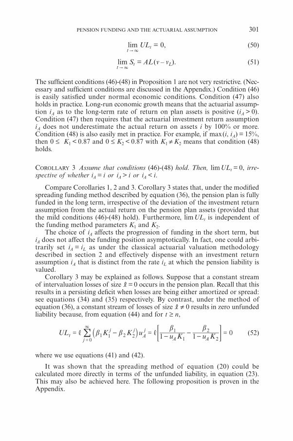
limt "3
ULt = 0, (50)
limt "3
St = AL (v – vL). (51)
The sufficient conditions (46)-(48) in Proposition 1 are not very restrictive. (Nec-essary and sufficient conditions are discussed in the Appendix.) Condition (46)is easily satisfied under normal economic conditions. Condition (47) alsoholds in practice. Long-run economic growth means that the actuarial assump-tion iA as to the long-term rate of return on plan assets is positive (iA > 0).Condition (47) then requires that the actuarial investment return assumptioniA does not underestimate the actual return on assets i by 100% or more.Condition (48) is also easily met in practice. For example, if max(i, iA) = 15%,then 0 ≤ K1 < 0.87 and 0 ≤ K2 < 0.87 with K1 ≠ K2 means that condition (48)holds.
COROLLARY 3 Assume that conditions (46)-(48) hold. Then, limULt = 0, irre-spective of whether iA = i or iA > i or iA < i.
Compare Corollaries 1, 2 and 3. Corollary 3 states that, under the modifiedspreading funding method described by equation (36), the pension plan is fullyfunded in the long term, irrespective of the deviation of the investment returnassumption from the actual return on the pension plan assets (provided thatthe mild conditions (46)-(48) hold). Furthermore, limULt is independent ofthe funding method parameters K1 and K2.
The choice of iA affects the progression of funding in the short term, butiA does not affect the funding position asymptotically. In fact, one could arbi-trarily set iA = iL as under the classical actuarial valuation methodologydescribed in section 2 and effectively dispense with an investment returnassumption iA that is distinct from the rate iL at which the pension liability isvalued.
Corollary 3 may be explained as follows. Suppose that a constant streamof intervaluation losses of size = 0 occurs in the pension plan. Recall that thisresults in a persisting deficit when losses are being either amortized or spread:see equations (34) and (35) respectively. By contrast, under the method ofequation (36), a constant stream of losses of size ≠ 0 results in zero unfundedliability because, from equation (44) and for t ≥ n,
A AK KUL K K u u ub bb b
1 10t
j j
jAj
1 1 2 20 1
1
2
2, ,= - =-
--
=3
=
! ` j < F (52)
where we use equations (41) and (42).
It was shown that the spreading method of equation (20) could becalculated more directly in terms of the unfunded liability, in equation (23).This may also be achieved here. The following proposition is proven in theAppendix.
PENSION FUNDING AND THE ACTUARIAL ASSUMPTION 301
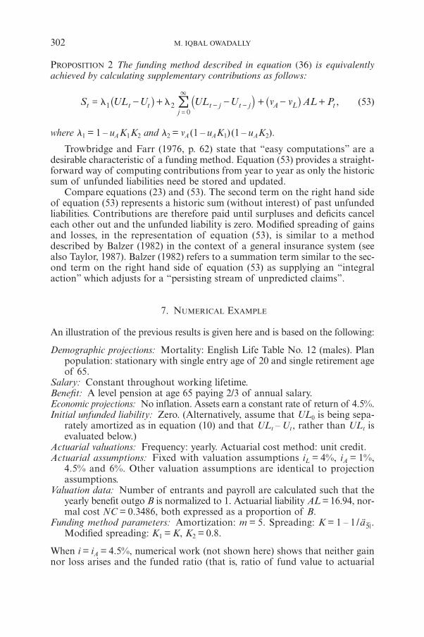
PROPOSITION 2 The funding method described in equation (36) is equivalentlyachieved by calculating supplementary contributions as follows:
A ,� �S UL U UL U v v AL Pt t t t j t jj
L t1 20
= - + - + - +3
- -=
!^ ` ^h j h (53)
where �1 = 1 – uAK1K2 and �2 = vA (1 – uAK1) (1 – uAK2).
Trowbridge and Farr (1976, p. 62) state that “easy computations” are adesirable characteristic of a funding method. Equation (53) provides a straight-forward way of computing contributions from year to year as only the historicsum of unfunded liabilities need be stored and updated.
Compare equations (23) and (53). The second term on the right hand sideof equation (53) represents a historic sum (without interest) of past unfundedliabilities. Contributions are therefore paid until surpluses and deficits canceleach other out and the unfunded liability is zero. Modified spreading of gainsand losses, in the representation of equation (53), is similar to a methoddescribed by Balzer (1982) in the context of a general insurance system (seealso Taylor, 1987). Balzer (1982) refers to a summation term similar to the sec-ond term on the right hand side of equation (53) as supplying an “integralaction” which adjusts for a “persisting stream of unpredicted claims”.
7. NUMERICAL EXAMPLE
An illustration of the previous results is given here and is based on the following:
Demographic projections: Mortality: English Life Table No. 12 (males). Planpopulation: stationary with single entry age of 20 and single retirement ageof 65.
Salary: Constant throughout working lifetime.Benefit: A level pension at age 65 paying 2/3 of annual salary.Economic projections: No inflation. Assets earn a constant rate of return of 4.5%.Initial unfunded liability: Zero. (Alternatively, assume that UL0 is being sepa-
rately amortized as in equation (10) and that ULt – Ut, rather than ULt isevaluated below.)
Actuarial valuations: Frequency: yearly. Actuarial cost method: unit credit.Actuarial assumptions: Fixed with valuation assumptions iL = 4%, iA = 1%,
4.5% and 6%. Other valuation assumptions are identical to projectionassumptions.
Valuation data: Number of entrants and payroll are calculated such that theyearly benefit outgo B is normalized to 1. Actuarial liability AL = 16.94, nor-mal cost NC = 0.3486, both expressed as a proportion of B.
Funding method parameters: Amortization: m = 5. Spreading: K = 1 – 1/a e5 .Modified spreading: K1 = K, K2 = 0.8.
When i = iA = 4.5%, numerical work (not shown here) shows that neither gainnor loss arises and the funded ratio (that is, ratio of fund value to actuarial
302 M. IQBAL OWADALLY
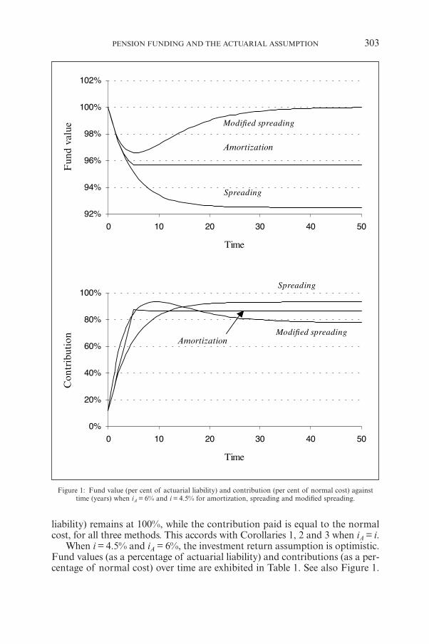
PENSION FUNDING AND THE ACTUARIAL ASSUMPTION 303
Figure 1: Fund value (per cent of actuarial liability) and contribution (per cent of normal cost) againsttime (years) when iA = 6% and i = 4.5% for amortization, spreading and modified spreading.
liability) remains at 100%, while the contribution paid is equal to the normalcost, for all three methods. This accords with Corollaries 1, 2 and 3 when iA = i.
When i = 4.5% and iA = 6%, the investment return assumption is optimistic.Fund values (as a percentage of actuarial liability) and contributions (as a per-centage of normal cost) over time are exhibited in Table 1. See also Figure 1.
Fun
d va
lue
Con
trib
utio
n
Amortization
Amortization
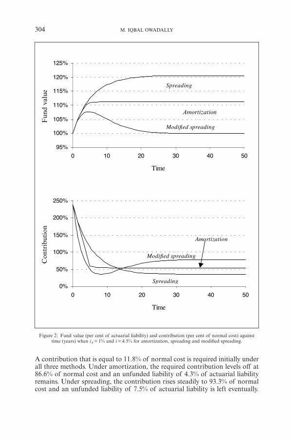
A contribution that is equal to 11.8% of normal cost is required initially underall three methods. Under amortization, the required contribution levels off at86.6% of normal cost and an unfunded liability of 4.3% of actuarial liabilityremains. Under spreading, the contribution rises steadily to 93.3% of normalcost and an unfunded liability of 7.5% of actuarial liability is left eventually.
304 M. IQBAL OWADALLY
Figure 2: Fund value (per cent of actuarial liability) and contribution (per cent of normal cost) againsttime (years) when iA = 1% and i = 4.5% for amortization, spreading and modified spreading.
Amortization
Fun
d va
lue
Con
trib
utio
n
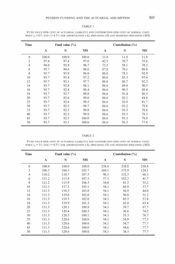
PENSION FUNDING AND THE ACTUARIAL ASSUMPTION 305
TABLE 1
FUND VALUE (PER CENT OF ACTUARIAL LIABILITY) AND CONTRIBUTION (PER CENT OF NORMAL COST)WHEN iA = 6% AND i = 4.5% FOR AMORTIZATION (A), SPREADING (S) AND MODIFIED SPREADING (MS).
Time Fund value (%) Contribution (%)
A S MS A S MS
0 100.0 100.0 100.0 11.8 11.8 11.82 97.4 97.4 97.6 42.5 39.7 55.6 4 96.0 95.8 96.7 72.5 58.1 78.2 6 95.7 94.6 96.6 87.0 70.1 88.8 8 95.7 93.9 96.8 86.6 78.1 92.9
10 95.7 93.4 97.2 86.6 83.3 93.4 12 95.7 93.1 97.7 86.6 86.7 92.314 95.7 92.9 98.1 86.6 89.0 90.516 95.7 92.8 98.4 86.6 90.5 88.418 95.7 92.7 98.8 86.6 91.4 86.520 95.7 92.6 99.0 86.6 92.1 84.825 95.7 92.6 99.5 86.6 92.9 81.730 95.7 92.5 99.7 86.6 93.2 79.835 95.7 92.5 99.8 86.6 93.3 78.840 95.7 92.5 99.9 86.6 93.3 78.345 95.7 92.5 100.0 86.6 93.3 78.050 95.7 92.5 100.0 86.6 93.3 77.8
TABLE 2
FUND VALUE (PER CENT OF ACTUARIAL LIABILITY) AND CONTRIBUTION (PER CENT OF NORMAL COST)WHEN iA = 1% AND i = 4.5% FOR AMORTIZATION (A), SPREADING (S) AND MODIFIED SPREADING (MS).
Time Fund value (%) Contribution (%)
A S MS A S MS
0 100.0 100.0 100.0 238.8 238.8 238.82 106.3 106.3 105.7 169.1 175.9 124.14 110.2 110.7 107.5 96.5 132.3 66.36 111.2 113.8 107.3 57.1 102.2 41.78 111.2 115.9 106.3 54.6 81.3 35.2
10 111.3 117.3 105.1 54.1 66.9 37.712 111.3 118.3 103.8 54.1 56.9 44.014 111.3 119.0 102.8 54.1 50.0 51.216 111.3 119.5 102.0 54.1 45.3 57.818 111.3 119.9 101.3 54.1 42.0 63.420 111.3 120.1 100.9 54.1 39.7 67.725 111.3 120.4 100.3 54.1 36.6 74.230 111.3 120.5 100.1 54.1 35.3 76.735 111.3 120.6 100.0 54.1 34.9 77.540 111.3 120.6 100.0 54.1 34.7 77.745 111.3 120.6 100.0 54.1 34.6 77.750 111.3 120.6 100.0 54.1 34.5 77.7
Under modified spreading, the required contribution stabilizes at about 78%of normal cost with the plan being fully funded eventually. This thereforeagrees with Corollaries 1, 2 and 3 when iA > i : long-run deficits occur underamortization and spreading, but not under modified spreading. Furthermore,numerical experiments suggest that the long-run unfunded liabilities that occurunder amortization and spreading are larger, the larger the deviation betweenactual and assumed returns.
Note that the pension fund is ultimately in balance under all three methods.For example, under amortization, using units of yearly benefit outgo, a fundof 95.7% ≈ 16.94 = 16.21 yields investment income of 16.21 ≈ 4.5% = 0.7295 atthe end of the year. At the start of the year, the present value of this incomeis 0.7295 /1.045 = 0.698. Contribution income is 86.6% ≈ 0.3486 = 0.301. Totalincome is 0.698 + 0.301 = 1 which balances the benefit of 1 that is paid out. Thebalance occurs at different levels under the three methods. Under modifiedspreading, the fund is eventually in equilibrium in such a way that the pensionplan is fully funded.
When i = 4.5% and iA = 1%, a conservative investment return assumption isbeing made. See Table 2 and Figure 2. A large contribution (more than dou-ble the normal cost) is required initially under all three funding methods. Inter-valuation gains lead initially to falling contributions under all three methods(at about the same rate). Ultimately, the lowest contribution (at only 35% ofnormal cost) is generated when spreading is used, but this is at the expense ofa large surplus in the pension fund of 20% of actuarial liability. On the otherhand, the surplus is only 5% of actuarial liability within 10 years, and under1% within 20 years, when modified spreading is used. This also agrees withCorollaries 1, 2 and 3 when iA < i .
8. CONCLUSION
The investment return assumption made by actuaries when valuing definedbenefit pension plans and its relevance to the pace of funding for pensionbenefits was discussed in section 2. It was argued that this assumption is the-oretically distinct from the discount rate that is used to value pension liabili-ties, although they may be equal in practice. A simplified model pension planwas posited in Section 3, where actuarial liability, normal cost and benefitoutgo were constant. The only intervaluation gains and losses allowed in themodel resulted from actual investment return deviating from the actuarialinvestment return assumption.
Two practical funding methods were described in sections 4 and 5 and itwas shown, in both cases, that a conservative investment return assumptionleads to a long-term surplus whereas an optimistic investment return assump-tion leads to a long-term deficit. Both long-term surpluses and deficits weredeemed to be undesirable. Surpluses may entail expensive demands for benefitenhancements from plan members during wage negotiations and also involvesthe diversion of capital away from projects within the sponsoring corporation.Deficits may endanger the security of pension benefits should the plan sponsor
306 M. IQBAL OWADALLY

become insolvent. A funding method was devised and described in section 6that avoids such persistent surpluses and deficits, under mild stability condi-tions, independently of the conservatism or optimism in the actuarial invest-ment return assumption. A simple way of implementing this funding methodwas derived in terms of the historic sum of past unfunded liabilities. A numer-ical illustration of these results was provided in section 7.
The analysis in this paper yielded closed-form mathematical solutions butthis required simplistic modelling assumptions. Future research should relaxthese restrictive assumptions. First, only asset gains and losses were considered.Mortality, withdrawal, inflation and other factors are also variable and shouldbe incorporated in the model. Second, these factors are uncertain and inter-valuation gains and losses are random. A stochastic approach followingDufresne (1988, 1989) and Owadally and Haberman (1999), who investigatepension funding with random investment returns, should be illuminating. It willenable a more realistic comparison of the various funding methods to be madein terms of the variance of fund values and contributions. The efficient choiceof parameters K1 and K2 under modified spreading of gains and losses can alsothen be investigated.
ACKNOWLEDGEMENT
The author would like to thank Steve Haberman for his comments on this paper.
PENSION FUNDING AND THE ACTUARIAL ASSUMPTION 307
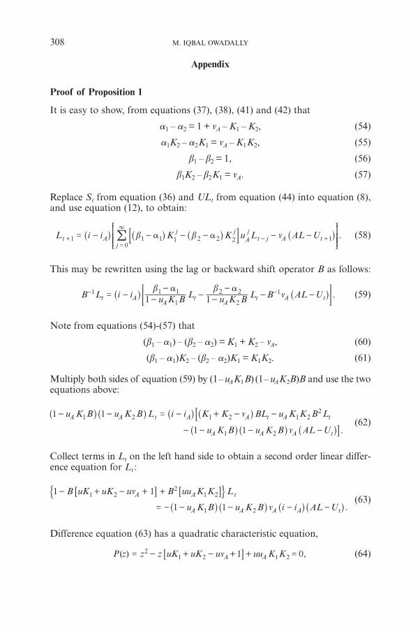
Appendix
Proof of Proposition 1
It is easy to show, from equations (37), (38), (41) and (42) that
�1 – �2 = 1 + vA – K1 – K2, (54)
�1K2 – �2K1 = vA – K1K2, (55)
b1 – b2 = 1, (56)
b1K2 – b2K1 = vA. (57)
Replace St from equation (36) and ULt from equation (44) into equation (8),and use equation (12), to obtain:
A .� �L i i K K u L v AL Ub bt Aj j
Aj
t j tj
1 1 1 1 2 2 2 10
= - - - - - -3
+ - +=
!^ ^ ^ ^h h h h
R
T
SSS
9
V
X
WWW
C (58)
This may be rewritten using the lag or backward shift operator B as follows:
A AAA .
� �B L i i u K B L u K B L B v AL U
b b1 1t t t t
1
1
1 1
2
2 2 1= --
--
-
-- -- -
^ ^h h< F (59)
Note from equations (54)-(57) that
(b1 – �1) – (b2 – �2) = K1 + K2 – vA, (60)
(b1 – �1)K2 – (b2 – �2)K1 = K1K2. (61)
Multiply both sides of equation (59) by (1– uAK1B) (1– uAK2B)B and use the twoequations above:
A A A A
A A A .
u K B u K B L i i K K v BL u K K B L
u K B u K B v AL U
1 1
1 1
t A t t
t
1 2 1 2 1 22
1 2
- - = - + - -
- - - -
^ ^ ^ ^
^ ^ ^
h h h h
h h h
8
A(62)
Collect terms in Lt on the left hand side to obtain a second order linear differ-ence equation for Lt :
A
A A A .
B uK uK uv B uu K K L
u K B u K B v i i AL U
1 1
1 1
A t
A t
1 22
1 2
1 2
- + - + +
= - - - - -^ ^ ^ ^h h h h
7 7A A$ .(63)
Difference equation (63) has a quadratic characteristic equation,
A A( ) ,P z z z uK uK uv uu K K1 021 2 1 2= - + - + + =7 A (64)
308 M. IQBAL OWADALLY
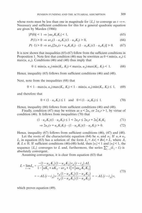
whose roots must be less than one in magnitude for {Lt} to converge as t → ∞.Necessary and sufficient conditions for this for a general quadratic equationare given by Marden (1966):
|P(0)| < 1 ⇒ |uuAK1K2 | < 1, (65)
P(1) > 0 ⇒ uvA(1 – uAK1) (1 – uAK2) > 0, (66)
P(–1) > 0 ⇒ uvA [2uA(v + uAK1K2) – (1 – uAK1) (1 – uAK2)] > 0. (67)
It is now shown that inequalities (65)-(67) follow from the sufficient conditions inProposition 1. Note first that condition (46) may be rewritten as 0 < min(u, uA) ≤max(u, uA). Conditions (46) and (48) thus imply that
0 ≤ min(u, uA) min(K1, K2) < max(u, uA) max(K1, K2) < 1. (68)
Hence, inequality (65) follows from sufficient conditions (46) and (48).
Next, note from the inequalities (68) that
0 < 1 – max(u, uA) max(K1, K2) < 1 – min(u, uA) min(K1, K2) ≤ 1, (69)
and therefore that
0 < (1 – uAK1) ≤ 1 and 0 < (1 – uAK2) ≤ 1. (70)
Hence, inequality (66) follows from sufficient conditions (46) and (48).Finally, condition (47) may be written as u < 2uA or 2uAv > 1, by virtue of
condition (46). It follows from inequalities (70) that
(1 – uAK1) (1 – uAK2) ≤ 1 < 2uAv ≤ 2uAv + 2u2A K1K2 (71)
⇒ 2uA(v + uAK1K2) – (1 – uAK1) (1 – uAK2) > 0. (72)
Hence, inequality (67) follows from sufficient conditions (46), (47) and (48).Let the roots of the characteristic equation (64) be �1 and �2. If �1 ≠ �2,
Lt in equation (63) has a solution of the form Lt = A�1t + B�2
t + L, where A,B, L ∈ �. If sufficient conditions (46)-(48) hold, then |�1| < 1 and |�2| < 1, thesequence {Lt} converges to L and, furthermore, the series ( )L Ljj 0
-3
=! is
absolutely convergent.Assuming convergence, it is clear from equation (63) that
A
A
A
A
A A
,
limL LuK uK uv uu K K
u K u K v i i AL
AL i i vv u K u Kv u K u K
AL i i v
1 1
1 1
1 1
1 1
t tA A
AA A
A AA
1 2 1 2
1 2
1 2
1 2
= =- + - + +
- - - -
= - -- -
- -= - -
"3
^ ^ ^
^^ ^
^ ^^
h h h
hh h
h hh
7 7A A
(73)
which proves equation (49).
PENSION FUNDING AND THE ACTUARIAL ASSUMPTION 309

The limit in equation (51) is obtained by resorting to equation (36):
A .
� � � �S K K u L L K K u L
v v AL P
tj j
jAj
t jj j
jAj
L t
1 1 2 20
1 1 2 20
= - - + -
+ - +
3 3
=-
=
! !` ` `
^
j j j
h
(74)
As t → ∞, the first sum on the right hand side of equation (74) vanishes sinceboth ( )� �K K uj j
Aj
j 1 1 2 20-
3
=! and ( )L Ljj 0
-3
=! are absolutely convergent and
their Cauchy product is also absolutely convergent. As t → ∞, the second sumon the right hand side of equation (74) converges to
A AA A
A ,� �u K u K L v AL i i v AL v v
1 11
1
2
2 # #-
--
= - - = - -d ^ ^n h h (75)
where use is made of equations (37) and (38). Pt also vanishes as t → ∞ fromequation (10). Hence, lim t→∞ St = –AL (vA – v) + AL (vA – vL) = AL (v– vL).
Finally, the limit in equation (50) is obtained by taking limits on each termon the right hand side of equation (44) which may be rewritten as follows:
t .UL U K K u L L K K u Lb b b btj j
jAj
t jj j
jAj
1 1 2 20
1 1 2 20
- = - - + -3 3
=-
=
! !` ` `j j j (76)
As t → ∞, the first sum on the right hand side of equation (76) vanishes sinceboth j 0=
( )K K ub bj jAj
1 1 2 2-
3! and j 0=( )L Lj -
3! are absolutely convergent andtheir Cauchy product is also absolutely convergent. As t → ∞, the second sumon the right hand side of equation (76) converges to zero since
A A,K K u u K u Kb b
b b1 1
0j j
jAj
1 1 2 20 1
1
2
2- =-
--
=3
=
! ` j (77)
where use is made of equations (41) and (42). Hence, lim t→∞ULt = 0. ¡
Proof of Proposition 2
Rewrite equation (44) in terms of the lag or backward shift operator B:
B
tA A
A A
A .
UL U u K B u K B L
u K B u K BK K u
L
b b
b b b b
1 1
1 1
t t
t
1
1
2
2
1 2
1 2 1 2 2 1
- =-
--
=- -
- - -
^ ^
^ ^
h h
h h
< F
(78)
Using equations (56) and (57), the numerator on the right hand side of theabove equation simplifies and
tA A
.UL Uu K B u K B
B L1 1
1t t
1 2
- =- -
-^ ^h h
(79)
310 M. IQBAL OWADALLY
Likewise, rewrite equation (36) in terms of the backward shift operator B anduse equations (54) and (55) to simplify:
A
A AA
A A
A A.
� �S u K B u K B L v v AL P
u K B u K Bv K K v K K u B
L v v AL P
1 1
1 1
1
t t L t
At L t
1
1
2
2
1 2
1 2 1 2
=-
--
+ - +
=- -
+ - - - -+ - +
^
^ ^
^ ^^
h
h h
h hh
< F
(80)
Cancel Lt from equations (79) and (80) and simplify:
(81)
A
A A
A
A
AA A
A A A ,
S v v AL P
Bv K K v K K u B
UL U
u K K Bv u K u K
UL U
u K K UL U v u K u K UL U
1
1
11
1 1
1 1 1
t L t
At t
t t
t t t j t jj
1 2 1 2
1 21 2
1 2 1 20
- - -
=-
+ - - - --
= - +-
- --
= - - + - - -3
- -=
!
^
^ ^^
^ ^^
^ ^ ^ ^ `
h
h hh
h hh
h h h h j
= G
which is equation (53). ¡
REFERENCES
ACTUARIAL STANDARDS BOARD (1996) Actuarial Standard of Practice No. 27: Selection of EconomicAssumptions for Measuring Pension Obligations. Pensions Committee of the Actuarial Stan-dards Board, American Academy of Actuaries, Washington, DC.
BALZER, L.A. (1982) Control of insurance systems with delayed profit/loss-sharing feedback andpersisting unpredicted claims. Journal of the Institute of Actuaries 109, 285-316.
BERIN, B.N. (1989) The Fundamentals of Pension Mathematics. Society of Actuaries, Schaumburg,Illinois.
DAYKIN, C.D. (1976) Long-term rates of interest in the valuation of a pension fund. Journal ofthe Institute of Actuaries 21, 286-340.
DUFRESNE, D. (1988) Moments of pension contributions and fund levels when rates of returnare random. Journal of the Institute of Actuaries 115, 535-544.
DUFRESNE, D. (1989) Stability of pension systems when rates of return are random. Insurance:Mathematics and Economics 8, 71-76.
MARDEN, M. (1966) The Geometry of Polynomials, 2nd ed. American Mathematical Society,Providence, Rhode Island.
MCGILL, D.M., BROWN, K.N., HALEY, J.J. and SCHIEBER, S.J. (1996) Fundamentals of Private Pen-sions, 7th ed. University of Pennsylvania Press, Philadelphia, Pennsylvania.
OWADALLY, M.I. and HABERMAN, S. (1999) Pension fund dynamics and gains/losses due to ran-dom rates of investment return. North American Actuarial Journal 3(3), 105-117.
TAYLOR G.C. (1987) Control of unfunded and partially funded systems of payments. Journal ofthe Institute of Actuaries 114, 371-392.
THORNTON, P.N. and WILSON, A.F. (1992) A realistic approach to pension funding. Journal ofthe Institute of Actuaries 119, 229-312.
PENSION FUNDING AND THE ACTUARIAL ASSUMPTION 311

TROWBRIDGE, C.L. (1952) Fundamentals of pension funding. Transactions of the Society of Actu-aries 4, 17-43.
TROWBRIDGE, C.L. and FARR, C.E. (1976) The Theory and Practice of Pension Funding. RichardD. Irwin, Homewood, Illinois.
M. IQBAL OWADALLY
Faculty of Actuarial Science and StatisticsCass Business SchoolCity University106 Bunhill Row, London EC1Y 8TZ, EnglandEmail: [email protected]
312 M. IQBAL OWADALLY
CHAIN LADDER BIAS
BY
GREG TAYLOR
ABSTRACT
The chain ladder forecast of outstanding losses is known to be unbiased undersuitable assumptions. According to these assumptions, claim payments in anycell of a payment triangle are dependent on those from preceding developmentyears of the same accident year. If all cells are assumed stochastically inde-pendent, the forecast is no longer unbiased. Section 5 shows that, under rathergeneral assumptions, it is biased upward. This result is linked to earlier workon some stochastic versions of the chain ladder.
KEYWORDS
Chain ladder, IBNR.
1. INTRODUCTION
The chain ladder (CL) approach to estimation of a loss reserve is well known.It is described, for example, by Taylor (2000).
Its origins are not altogether clear, but it seems likely that it originated asa heuristic device. As such, it may be viewed as a non-parametric estimator.The precise definition is given in Sections 2 and 3.
Kremer (1982) recognised that the CL involved a log-linear cross-classificationstructure. A number of parametric stochastic versions of the CL developed fromthis, eg Hertig (1985), Renshaw (1989), Verrall (1989, 1990, 1991).
Mack (1994) pointed out that these stochastic models gave mean estimatesof liability that differed from the “classical” CL estimate. While the formof stochastic model underlying the classical CL was speculative, due to thelatter’s heuristic nature, Mack suggested one. It is distribution free. Details aregiven in Section 2. Mack also identified the differences between this and theother stochastic models.
Whereas the cross-classified models typically assume stochastic independenceof all cells in the data set, the CL (in Mack’s formulation) does not. It was shownby Mack (1993) that the algorithm of the classical CL produced unbiased fore-casts of liability under its own assumptions.
However, it does not necessarily do so under the alternative assumption ofindependence between all cells. Some papers have studied the bias in estimates
ASTIN BULLETIN, Vol. 33, No. 2, 2003, pp. 313-330
of liability in the parametric cross-classified models mentioned above, but littleis known of the bias in the classical CL forecast when all cells are independent.
The purpose of the present paper is to investigate the direction of bias inthis case.
2. FRAMEWORK AND NOTATION
Consider a square array X of stochastic quantities X(i, j) ≥ 0, i = 0,1, …, I;j = 0,1,…,I.
Denote row sums and column sums as follows:
, ,R i j X i hh
j
0
==
!^ ]h g (2.1)
, , .C i j X g jg
i
0
==
!^ ^h h (2.2)
In addition introduce the following notation for the total sum over a rectan-gular subset of X:
, ,
,
,
T i j X g h
R g j
C i h
h
j
g
i
g
i
h
j
00
0
0
=
=
=
==
=
=
!!
!
!
^ ^
^
]
h h
h
g
(2.3)
Generally, in the following, any summation of the forma
b! with b < a will be
taken to be zero.In a typical loss reserving framework, i denotes accident period, j develop-
ment period, and available data will consist of observations on the triangularsubset D of X:
, , , ,..., ; , ,...,X i j i I j I iD 0 1 0 1= = = -^ h" , (2.4)
Figure 2.1 illustrates the situation.
Still in a loss reserving context, D would represent some form of claimsexperience, eg claim counts or claim amounts. The loss reserving problemconsists of forecasting the lower triangle in Figure 2.1, conditional on D. Thereis particular interest in forecasting R(i,I) | D, i = 1,...,I. In standard loss reser-ving parlance, the X(i, j) are usually referred to as incremental quantities, or justincrements, and the R(i, j) as their cumulative equivalents.
314 GREG TAYLOR
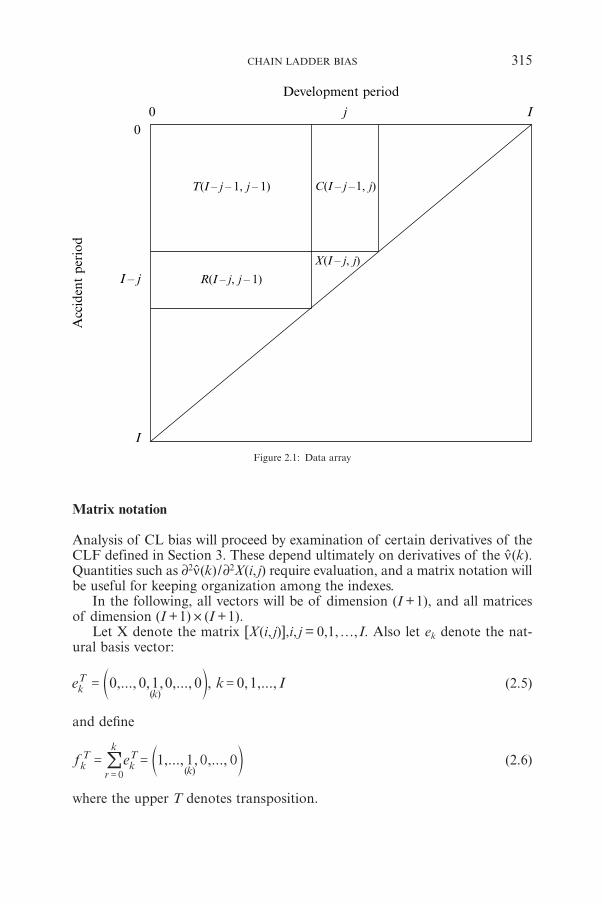
Matrix notation
Analysis of CL bias will proceed by examination of certain derivatives of theCLF defined in Section 3. These depend ultimately on derivatives of the n̂(k).Quantities such as ∂2n̂(k)/∂2X(i, j) require evaluation, and a matrix notation willbe useful for keeping organization among the indexes.
In the following, all vectors will be of dimension (I +1), and all matricesof dimension (I +1) ≈ (I +1).
Let X denote the matrix [X(i, j)],i, j = 0,1,…,I. Also let ek denote the nat-ural basis vector:
,..., , , ,..., , , ,...,e k I0 0 1 0 0 0 1( )k
T
k= =d n (2.5)
and define
,..., , ,...,f e 1 1 0 0( )k
TkT
r
k
k0
= ==
! d n (2.6)
where the upper T denotes transposition.
CHAIN LADDER BIAS 315
Figure 2.1: Data array
Acc
iden
t pe
riod
0
I – j
I
T(I – j – 1, j – 1)
R(I – j, j – 1)
C(I – j –1, j)
X(I – j, j)
Development period
0 j I
Under this notation, X(i, j) is selected from X as follows:
, .X i j e XeiT
j=^ h (2.7)
Similarly,
j,R i j e XfiT=^ h (2.8)
j,C i j f XeiT=^ h (2.9)
, .T i j f XiT
j= f^ h (2.10)
3. CHAIN LADDER FORECAST
Define the age-to-age factor
n̂( j) = T(I – j – 1, j +1) /T(I – j – 1, j)= 1 +C (I – j – 1, j +1) /T(I – j – 1, j)
(3.1)
and
, , .i I R i I i kR nk I i
I 1
= -= -
-
% t] ] ]g g g (3.2)
The value of R(i,I) calculated in this way will be referred to as the chain ladderforecast (CLF) of R(i,I).
4. CHAIN LADDER MODELS
4.1. Independent accident periods
The CLF has been formulated in Section 3 just as an algorithm. No model forthe data X has yet been stated.
It is evident that the properties of the CLF will depend on the model. Thisand the next sub-section consider two alternative models. The first is representedby the following two assumptions.
Assumption 1. The increments of different accident periods are stochasticallyindependent in the sense that
Prob [X(i, j) | D] = Prob [X(i, j) | X(i,0),…,X(i,I – i)].
Assumption 2. E [R(i, j +1) | X(i,0),X(i,1), ...,X(i, j)] = n ( j)R(i, j). (4.1)
316 GREG TAYLOR
Remark 1. It follows from Assumptions 1 and 2 that
E [R (i, j +1) | D] = n ( j)R (i, j) (4.2)
for any j ≥ I – i (ie future j ).
Since R (i, j +1) = R (i, j) +X (i, j +1), one may re-write (4.2) in the form:
E [X (i, j +1) | D] = [n ( j) – 1]R (i, j) (4.3)
Remark 2. It is clear from (4.3) that R (i, j) and X (i, j +1) may fail to be inde-pendent. Generally, under Assumptions 1 and 2, the X (i, j) for fixed i may failto be independent.
Theorem 1 (Mack). Under Assumptions 1 and 2,
(1) n̂( j) is an unbiased estimator of n( j) for j = 0,1,…,I – 1; and(2) the CLF R(i,I) is an unbiased estimator of E [R(i,I ) | D] for i = 1,2,…,I ;
provided that both estimators exist.
Proof. See Mack (1993). ¡
It is also convenient to re-write (4.2) in the form:
E [R(i, j +1) /R (i, j) | D] = n ( j). (4.4)
4.2. Independent increments
Replace Assumptions 1 and 2 by 1a, 2a and 3 as follows.
Assumption 1a. All increments X (i, j) are stochastically independent.
Assumption 2a. E [R(i, j +1)] /E [R(i, j)] = j( j). (4.5)
The assumption is written in this form in order to relate it to Assumption 2.It is useful to note that an equivalent, and more natural, assumption is that
E [X(i, j)] = �(i)�( j) (4.5a)
for parameters �(i),�( j), i, j = 0,1,…,I.
Define the set
, : , , ,...,D g h g I k h k k I i I1 1 1i # #= - - + = - -^ h" , (4.6)
and
, : , , ,..., .E g h g I k h k k I i I1 1i # #= - - = - -^ h" ,
CHAIN LADDER BIAS 317
Assumption 3. T(g,h) > 0 for each (g,h) ∈ Ei.
Remark 3. It is implicit in Assumption 2a that E [R (i, j)] ≠ 0. By the assumednon-negativity of the X (i, j), E [R (i, j)] > 0 for each i, j.
Remark 4. A comparison of (4.4) and (4.5) indicates that n( j) and j( j) are dif-ferent quantities (for fixed j) since
, / ,E R i j R i j1+^ ^h h6 @ # , / , .E R i j E R i j1+^ ^h h6 6@ @ (4.7)
This fact was pointed out by Mack (1994).
By Assumption 3, applied to (3.1), all n̂(k) appearing in (3.2) are defined andstrictly positive. Given the assumed non-negativity of the X(i, j), Assumption 3is both necessary and sufficient for the chain ladder forecast to make sense.Comment on the non-negativity requirement will be made in Section 6.
The conditions of Theorem 1 no longer hold, and so the CLF is not nec-essarily unbiased.
5. CHAIN LADDER BIAS
The following is a somewhat technical result, but has been included here ratherthan in the appendix because the symmetric appearance of rows and columnsof X in the second derivative of Y(i) is interesting.
Theorem 2. Define
.Y i kk I i
I 1
= o= -
-
% t] ]g g (5.1)
Then
( , )( )
X g hY i2
2
2
2= 0 for (g,h) ∉ Di ; (5.2)
for (g,h) ∈ Di and h ≤ I – i,
( ) ( , )( )
, ,,
, , ,,
Y i X g hY i
T I k k T I k kC I k k
T i I i T I l l T I l lR I l l
x12
1 1 11 1
11
1
k I i
I g
l I i
k
2
2 1
1
2
2=
- - + - -- - +
- -+
- - --
= -
- -
= - +
!
!
] ]
]
] ] ]
]
g g
g
g g g
g> H
(5.3)
318 GREG TAYLOR
for (g,h) ∈ Di and h > I – i,
( ) ( , )( )
, ,,
, ,,
.
Y i X g hY i
T I k k T I k kC I k k
T I l l T I l lR I l l
12
1 1 11 1
1
k h
I g
l h
k
2
2 1
#2
2=
- - + - -- - +
- - --
=
- -
=
!
!
] ]
]
] ]
]
g g
g
g g
g(5.4)
These results depend on Assumption 3 for the existence of (5.3) and (5.4), butdo not depend on the Assumptions 1a and 2a.
Proof. See appendix. ¡
Theorem 3. Under Assumptions 1a, 2a and 3, and if X (g,h) is not degeneratefor at least one (g,h) ∈ Di , the CLF R(i,I ) is biased upward as an estimate ofE [R (i,I )] in the sense that
, , > , ,,
.E i I R i I i R i I i E R i I iE R i IR - -
-] ] ]
]
]g g g
g
g7
6
6A
@
@(5.5)
Also,
, > , .E i I E R i IR] ]g g7 6A @ (5.6)
Proof. See appendix. ¡
Remark 5. An alternative form of (5.6) is:
, , > , .E E i I R i I i E R i IR,R i I i --] ] ] ]g g g g7 6A @ (5.7)
Note that, in general, (5.5) does not imply that
, , > , .E i I R i I i E R i IR -] ] ]g g g7 6A @
A few words in interpretation of Theorem 3. First define
, , ,
,
L i j R i I R i j
X i hh j
I
1
= -
== +
!
^ ] ^
]
h g h
g(5.8)
which is the required loss reserve in respect of accident period i at the end ofdevelopment period j.
The forecast of L(i, j) associated with the CLF of R (i,I) is
, , , .i j i I R i jL R= -^ ] ^h g h (5.9)
CHAIN LADDER BIAS 319
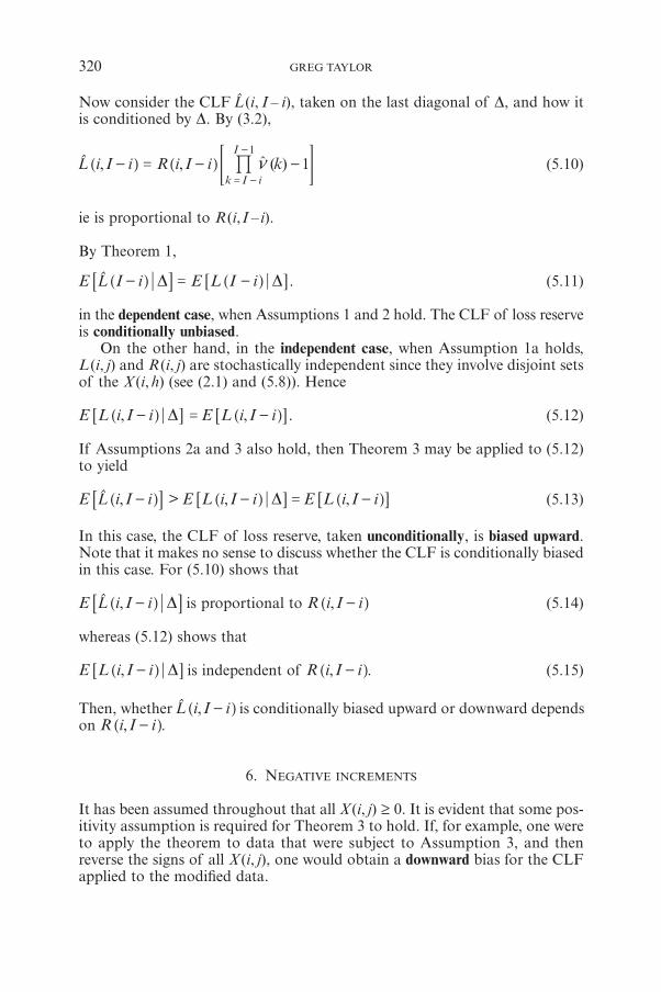
Now consider the CLF L(i, I – i), taken on the last diagonal of D, and how itis conditioned by D. By (3.2),
, , ( )i I i R i I i kL 1k I i
I 1
- = - -o= -
-
% t] ]g g> H (5.10)
ie is proportional to R (i,I – i).
By Theorem 1,
.E I i E L I iL D D- = -] ]g g7 6A @ (5.11)
in the dependent case, when Assumptions 1 and 2 hold. The CLF of loss reserveis conditionally unbiased.
On the other hand, in the independent case, when Assumption 1a holds,L (i, j) and R (i, j) are stochastically independent since they involve disjoint setsof the X (i, h) (see (2.1) and (5.8)). Hence
, , .E L i I i E L i I iD- = -] ]g g6 6@ @ (5.12)
If Assumptions 2a and 3 also hold, then Theorem 3 may be applied to (5.12)to yield
, > , ,E i I i E L i I i E L i I iL D- - = -] ] ]g g g7 6 6A @ @ (5.13)
In this case, the CLF of loss reserve, taken unconditionally, is biased upward.Note that it makes no sense to discuss whether the CLF is conditionally biasedin this case. For (5.10) shows that
,E i I iL D-] g7 A is proportional to ,R i I i-] g (5.14)
whereas (5.12) shows that
,E L i I i D-] g6 @ is independent of ,R i I i-] g. (5.15)
Then, whether ,i I iL -] g is conditionally biased upward or downward dependson ,R i I i-] g.
6. NEGATIVE INCREMENTS
It has been assumed throughout that all X(i, j) ≥ 0. It is evident that some pos-itivity assumption is required for Theorem 3 to hold. If, for example, one wereto apply the theorem to data that were subject to Assumption 3, and thenreverse the signs of all X (i, j), one would obtain a downward bias for the CLFapplied to the modified data.
320 GREG TAYLOR
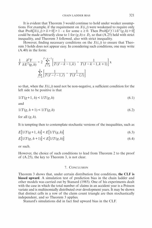
It is evident that Theorem 3 would continue to hold under weaker assump-tions. For example, if the requirement on X(i, j) were weakened to require onlythat Prob[X (i, j) > d > 0] > 1 – e for some e ≥ 0. Then Prob[�2f / �X 2(g,h) > 0]could be made arbitrarily close to 1 for (g,h) ∈ Di, so that (A.25) held with strictinequality, and Theorem 3 followed, also with strict inequality.
However, finding necessary conditions on the X (i, j) to ensure that Theo-rem 3 holds does not appear easy. In considering such conditions, one may write(A.40) in the form:
( , ) , ,
, ,
Y X g hY
T I k k T I k k
T I l l T I l l
x12
11
1 11
11 1
k h
I g
l h
k
2
2 1
22
=- -
-- - +
- --
-
=
- -
=
!
!
] ]
] ]
g g
g g
;
;
E
E
so that, when the X(i, j) need not be non-negative, a sufficient condition for theleft side to be positive is that
1/T (g+1, h) < 1/T (g,h) (6.1)
and
1/T (g, h +1) < 1/T (g,h) (6.2)
for all (g, h).
It is tempting then to contemplate stochastic versions of the inequalities, such as
E [1/T (g+1, h)] < E [1/T (g,h)] (6.3)
E [1/T (g, h +1)] < E [1/T (g,h)] (6.4)
or such.
However, the choice of such conditions to lead from Theorem 2 to the proofof (A.25), the key to Theorem 3, is not clear.
7. CONCLUSION
Theorem 3 shows that, under certain distribution free conditions, the CLF isbiased upward. A simulation test of prediction bias in the chain ladder andother models was carried out by Stanard (1985). One of his experiments dealtwith the case in which the total number of claims in an accident year is a Poissonvariate and is multinomially distributed over development years. It may be shownthat distinct cells in a row of the claim count triangle are then stochasticallyindependent, and so Theorem 3 applies.
Stanard’s simulations did in fact find upward bias in the CLF.
CHAIN LADDER BIAS 321
8. ACKNOWLEDGEMENTS
Professor Klaus Schmidt and Dr Klaus Thomas Hess of Technische Univer-sität Dresden gave generously of their time to improve earlier drafts of thispaper. Their thorough review identified one major blunder and produced anumber of constructive suggestions, leading to other enhancements.
Dr Alois Gisler read even earlier drafts of this paper and provided a num-ber of valuable comments and insights. The paper possibly would not haveoccurred without his assistance.
The author also acknowledges helpful comment by Dr Thomas Mack.
REFERENCES
HERTIG, J. (1985) A statistical approach to the IBNR-reserves in marine reinsurance. ASTINBulletin, 15, 171-183.
KALLENBERG, O. (1997) Foundations of modern probability (2nd ed). Springer.KREMER, E. (1982) IBNR claims and the two-way model of ANOVA. Scandinavian Actuarial
Journal, 47-55.MACK, T. (1993) Distribution-free calculation of the standard error of chain ladder reserve esti-
mates. ASTIN Bulletin, 23, 213-221.MACK, T. (1994) Which stochastic model is underlying the chain ladder method? Insurance:
mathematics and economics, 15, 133-138.RENSHAW, A.E. (1989) Chain ladder and interactive modelling (claims reserving and GLIM).
Journal of the Institute of Actuaries, 116, 559-587.STANARD, J.N. (1985) A simulation test of prediction errors of loss reserve estimation techni-
ques. Proceedings of the Casualty Actuarial Society, 72, 124-148.TAYLOR, G.C. (1986) Loss reserving in non-life insurance. North-Holland, Amsterdam, Nether-
lands.TAYLOR, G. (2000) Loss reserving: an actuarial perspective. Kluwer Academic Publishers, Dor-
drecht, Netherlands.VERRALL, R.J. (1989) A state space representation of the chain ladder linear model. Journal of
the Institute of Actuaries, 116, 589-609.VERRALL, R.J. (1990) Bayes and empirical bayes estimation for the chain ladder model. Astin
Bulletin, 20, 217-243.VERRALL, R.J. (1991) On the estimation of reserves from loglinear models. Insurance: mathe-
matics and economics, 10, 75-80.
322 GREG TAYLOR

Appendix
PROOF OF THEOREMS
Lemma 1. Suppose that
( )y f xii
n
1
==
% (A.1)
with x = (x1,…,xm)T and fi (x) > 0 for each i. Then
j
j
i
i
i
i .y xy
f xf
f f xf
xf1 1 1
!,k i
n
ki ji j
n
k k2
2
12
2
12
2
2
222
2
2= +
= =
! !
Lemma 2 (derivatives of age-to-age factors).
( ) ,( )
, , ,< ,
k X g hk
T I k kh k
T I k k T I k kg I k h k C I k kd d d1
1 11
1 1 11 1
22 #
=- - +
= +-
- - - - +
- - - +
oo
t
t
^ ]
]
] ]
^ ] ]
h g
g
g g
h g g(A.2)
where d(.) is defined as follows:
d(C) = 1 for condition C true; (A.3)= 0 for condition C false;
and it is understood that (A.2) applies to past observations (g + h ≤ I).
Further,
( ) ,( )
, ,< ,
k X g hk
T I k k T I k kg I k h k C I k kd d1
1 1 11 12
2
2
22
2 #=
- - - - +
- - - +
oo
tt
^ ] ]
^ ] ]
h g g
h g g(A.4)
where this result is again understood to apply only to past observations.
Proof. By (2.10),
j, / , .T i j X g h f e e fiT
g hT2 2 =^ ^h h (A.5)
Write the quantity of interest n̂(k) in the abbreviated form n = N /D where Nand D denote numerator and denominator respectively. If N and D depend onvariable X, then
.
log log logX X X
N D
N XN
D XD
ND D XN N X
D
nn n1
1 1
1
22
22
22
22
22
22
22
= =-
= -
= -
^
b
h
l
(A.6)
CHAIN LADDER BIAS 323
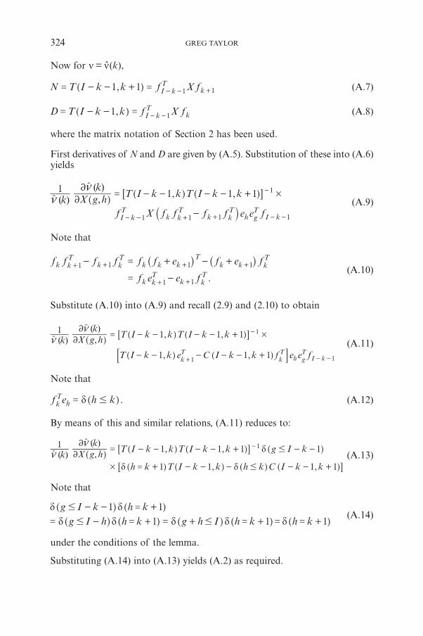
Now for n = n̂(k),
,N T I k k f X f1 1 I kT
k1 1= - - + = - - +] g (A.7)
,D T I k k f X f1 I kT
k1= - - = - -] g (A.8)
where the matrix notation of Section 2 has been used.
First derivatives of N and D are given by (A.5). Substitution of these into (A.6)yields
( ) ,( )
, ,k X g h
kT I k k T I k k
f X f f f f e e f
11 1 1
I kT
k kT
k kT
h gT
I k
1
1 1 1 1
#22
= - - - - +
-
oo -
- - + + - -
tt
^] ]
`
hg g
j
6 @(A.9)
Note that
.
f f f f f f e f e f
f e e fk k
Tk k
Tk k k
Tk k k
T
k kT
k kT
1 1 1 1
1 1
- = + - +
= -
+ + + +
+ +
^ ^h h(A.10)
Substitute (A.10) into (A.9) and recall (2.9) and (2.10) to obtain
( ) ,( )
, ,
, ,
k X g hk
T I k k T I k k
T I k k e C I k k f e e f
11 1 1
1 1 1kT
kT
h gT
I k
1
1 1
#22
= - - - - +
- - - - - +
oo -
+ - -
t
t
^] ]
] ]
hg g
g g
6
9
@
C
(A.11)
Note that
.f e h kdkT
h #= ] g (A.12)
By means of this and similar relations, (A.11) reduces to:
( ) ,( )
, ,
, ,k X g h
kT I k k T I k k g I k
h k T I k k h k C I k k
d
d d
11 1 1 1
1 1 1 1
1
#
22
#
#
= - - - - + - -
= + - - - - - +
oo -
t
t
^] ] ^
] ] ] ]
hg g h
g g g g
6
6
@
@
(A.13)
Note that
g I k h kg I h h k g h I h k h k
d d
d d d d d
1 1
1 1 1
#
# #
- - = +
= - = + = + = + = = +
^ ]
^ ] ^ ] ]
h g
h g h g g(A.14)
under the conditions of the lemma.
Substituting (A.14) into (A.13) yields (A.2) as required.
324 GREG TAYLOR
To prove (A.4), return to (A.6). In this abbreviated notation there, take a secondderivative:
X X X Xnn
nn
nn1 1 1
2
2 2
22
22
22
22
= -b bl l (A.15)
Now (A.6) yields
X X N XN
N XN
D XD
D XD
nn1 1 1 1 1
2
2 2
2
2 2
22
22
22
22
22
22
= - - +b b bl l l (A.16)
By (A.5), (A.7) and (A.8), �2N /�X 2 = �2D /�X 2 = 0, so that (A.16) reduces to
X X D XD
N XN
D XD
N XN
X D XD
N XN
nn
nn
1 1 1 1 1
1 1 1
22
22
22
22
22
22
22
22
22
= - +
= - +
b b b
b b
l l l
l l
(A.17)
by (A.6).
Substitution of (A.17) in (A.15), and use of (A.6) again yields
X X D XD
nn
nn1
21 1
2
2
22
22
22
= - b bl l (A.18)
By (A.8),
/ , <D X g h f e e f g I k h kd dI kT
g hT
k12 2 #= = -- -^ ^ ]h h g (A.19)
Substitute (A.2) and (A.19) into (A.18) and note that the term involvingd (h = k + 1) vanishes because d (h = k + 1) d (h ≤ k) = 0.
The result is (A.4), as required. ¡
Lemma 3 (multivariate Jensen inequality). Let X = (X1, …, Xm)T where theXk are stochastically independent random variables. Let f : Rm → R be twicedifferentiable in all its arguments, and suppose that
/f X X 0k2 22 2 $] g for all X and for k = 1, 2, …, m. (A.20)
Then
.E f X f E X$] ^g h6 6@ @ (A.21)
If strict inequality holds in (A.20) for at least one k, and Xk is not degenerate,then strict inequality holds in (A.21).
CHAIN LADDER BIAS 325
Proof. An elegant proof of (A.21) appears in Kallenberg (1997, p. 49). It is re-proved below in order to obtain the strict inequality.
Let m = (m1,…,mm)T = E [X]. Expand f (X) as the Taylor series:
m
m m
m m m,..., , ,..., , /
,..., , /
f X f X X X f X X X
X f X X X
m m m
m z
m m m
m m m
1 1 1 1
21 2 2
1 12
2 2
2 2
= + -
+ -
- -
-
] ^ ^ ^
^ ^
g h h h
h h(A.22)
where zm = mm + qm (Xm – mm) for some 0 < qm < 1.
Now expand f (X1,…,Xm –1, mm) similarly, then f (X1,…,Xm –2, mm –1, mm), and soon to obtain
k
k k
k k
,..., , ,..., /
,..., , , ,..., / .
f X f X f X X X
X f X X X
m m m m
m z m m
k k k mk
m
k
m
k k k m
1 11
21
1
2 21 1 1
2
2 2
2 2
= + -
+ -
-=
=- +
!
!
] ^ ^ ^
^ ^
g h h h
h h
(A.23)
Take expectations on both sides of (A.23). Note that
k k
k k
k
k
,..., , ,..., /
,..., , ,..., /
E X f X X X
E X E f X X X
m m m
m m m
0
k k m
k k m
1 1
1 1
2 2
2 2
-
= -
=
-
-
^ ^
^ ^
h h
h h
7
7
A
A (A.24)
where the middle step follows from the stochastic independence of Xk from(X1,…,Xk–1).
By (A.20),
k kk,..., , , ,..., /E X f X X Xm z m m 0k k k m2 2
1 1 122 2 $- - +^ ^h h9 C (A.25)
with strict inequality if strict inequality holds in (A.20) and Xk is not degen-erate.
The lemma then follows. ¡
Proof of Theorem 2. Consider Y(i) defined by (5.1), with n̂(k) defined by (3.1)and (2.3). The observations X (g,h) involved in the n̂(k) constituting Y(i) arejust those in Di. This justifies (5.2).
Now consider (g,h) ∈ Di. Note that Lemma 1 is applicable to Y(i) because of(5.1). Hence
326 GREG TAYLOR

( ) ,( )
( ) ,( )
( ) ( ) ,( )
,( )
.Y i X g hY i
k X g hk
k l X g hk
X g hl1 1 1
!,k I i
I
k lk l I i
I
2
2 1
2
2 1
2
2
2
222
22
= +o
oo o
o o
= -
-
= -
-
! !t
t
t t
t t
^ ^ ^ ^h h h h(A.26)
In this equation I – i ≤ k ≤ I – 1. Since (g,h) ∈ Di it is also the case that h – 1 ≤k ≤ I – 1 – g. This yields max{I – i, h – 1} ≤ k ≤ I – 1 – g.
Therefore, there are two cases to be considered:
• In the case h ≤ I – i one has I – i ≤ k ≤ I – 1 – g
• In the case h ≥ I – i + 1 one has h – 1 ≤ k ≤ I – 1 – g.
Case I: h ≤ I – i.
In this case
g < I – k, h ≤ k. (A.27)
Under these conditions, combination of (3.1) with (A.2) gives
2n̂(k) / 2X (g,h) = –C (I – k –1, k +1) / T 2(I – k –1, k). (A.28)
Similarly, combination of (3.1) with (A.4) gives
22n̂(k) / 2X 2(g,h) = 2C (I – k –1, k +1) / T 3(I – k –1, k). (A.29)
Substitution of (3.1), (A.28) and (A.29) into (A.26) yields
( ) ,( )
, ,,
, , , ,, ,
, ,,
, , ,,
Y i X g hY i
T I k k T I k kC I k k
T I k k T I k k T I l l T I l lC I k k C I l l
T I k k T I k kC I k k
T I k k T I l l T I l lC I l l
1 21 1 1
1 1
2 1 1 1 1 1 11 1 1 1
2 1 1 11 1
11
1 1 11 1
k I i
I g
l I i
k
k I i
I g
k I i
I g
l I i
k
2
2
2
1
11
1
1
#
2
2=
- - + - -
- - +
+- - + - - - - + - -
- - + - - +
=- - + - -
- - +
- -+
- - + - -- - +
= -
- -
= -
-
= -
- -
= -
- -
= -
-
!
!!
!
!
^ ] ]
]
] ] ] ]
] ]
] ]
]
] ] ]
]
h g g
g
g g g g
g g
g g
g
g g g
g= G
(A.30)
Note that Assumption 3 implies that T (g,h) > 0 for (g,h) ∈ Di, and so guar-antees the existence of all ratios in (A.30).
Note also that, by (2.2), the second member within the square bracket maybe expanded as follows:
, ,,
, ,T I l l T I l lC I l l
T I l l T I l l1 1 11 1
11
1 11
- - + - -- - +
=- -
-- - +] ]
]
] ]g g
g
g g(A.31)
CHAIN LADDER BIAS 327

Substitute (A.31) into the square bracket in (A.30) to obtain
, , ,
, , ,
, , ,,
T I k k T I l l T I l l
T i I i T I l l T I l l
T i I i T I l l T I l lR I l l
11
11 1
11
11 1
11
1
l I i
k
l I i i
k
l I i
k
l I i
k
1
1
1
- -+
- --
-
=- -
+- -
--
=- -
+- - -
-
= -
-
= - +
= - +
= - +
! !
!
!
] ] ]
] ] ]
] ] ]
]
g g g
g g g
g g g
g
; E (A.32)
by (2.1).
Substitute (A.32) for the square bracket in (A.30) to obtain
( ) ,( )
, ,,
, , ,,
.
Y i X g hY i
T I k k I k kC I k k
T i I i T I l l T I l lR I l l
12
1 1 11 1
11
1
k I i
I g
l I i
k
2
2 1
1
#2
2=
- - + - -- - +
- -+
- - --
= -
- -
= - +
!
!
^ ] ]
]
] ] ]
]
h g g
g
g g g
g> H
(A.33)
This proves (5.3).
Case II: h > I – i.
It follows from the argument immediately preceding the proof of Case I that
g < I – k, k ≥ h – 1 (A.34)
(A.34) may be written as the two sub-cases:
k = h – 1and g < I – k, h ≤ k.
Then Lemma 2 gives
, ,X g hh
T I h h1
11
22 -
=- -
ot
^
]
]h
g
g(A.35)
,X g hh 1
02
2
2
2 -=
ot
^
]
h
g
(A.36)
, ,,
, ,X g hk
T I k kC I k k
k h g I k1
1 1122
2$ #= -
- -
- - +- -
ot
^
]
]
]
h
g
g
g(A.37)
328 GREG TAYLOR
, ,,
, , .X g h
kT I k kC I k k
k h g I k1
2 1 112
2
32
2$ #=
- -
- - +- -
ot
^
]
]
]
h
g
g
g(A.38)
Substitute (A.35) – (A.38) into (A.26) to obtain
(A.39)
( ) ,( )
, ,
, ,
, ,
, ,,
, ,,
, ,,
, , ,,
.
Y i X g hY i
h X g hh
k X g hk
k l X g hk
X g hl
h X g hh
k X g hk
T I k k T I k kC I k k
T I k k T I k kC I k k
T I l l T I l lC I l l
T I h h T I k k T I k kC I k k
11
1 1 1
1
12 1 1
21 1 1
1 1
21 1 1
1 11 1 1
1 1
21 1 1
1 1
!,
k h
I g
k lk l h
I g
k h
I g
k h
I g
k h
I g
l h
k
k h
I g
2
2
2
2 1
2
2
1
1
2
1
1 1
1
2
2
2
2
2
2
22
22
22
22
=-
-+
+
+-
-
=- - + - -
- - +
+- - + - -
- - +- - + - -
- - +
-- - - + - -
- - +
oo
oo
o oo o
oo
oo
=
- -
=
- -
=
- -
=
- -
=
- -
=
-
=
- -
!
!
!
!
! !
!
t
t
t
t
t t
t t
t
t
t
t
^ ] ^
]
] ^
]
] ] ^
]
^
]
] ^
]
] ^
]
] ]
]
] ]
]
] ]
]
] ] ]
]
h g h
g
g h
g
g g h
g
h
g
g h
g
g h
g
g g
g
g g
g
g g
g
g g g
g
As in Case I, Assumption 3 guarantees the existence of all the ratios in (A.39).Now apply (A.31) and use the same mode of calculation as led from (A.30)
to (A.33). Then (A.39) becomes:
( ) ,( )
, ,,
, ,,
.
Y i X g hY i
T I k k T I k kC I k k
T I l l T I l lR I l l
12
1 1 11 1
1
k h
I g
l h
k
2
2 1
#2
2=
- - + - -- - +
- - --
=
- -
=
!
!
^ ] ]
]
] ]
]
h g g
g
g g
g(A.40)
This proves (5.4). ¡
Proof of Theorem 3. Consider Y(i) defined by (5.1). By Theorem 2,
22Y(i) / 2X 2(g,h) ≥ 0 for all (g,h)
with strict inequality for some (g,h), namely those in Di. It follows from a mul-tivariate form of Jensen’s inequality (see Lemma 3) that
( ) >E Y i i kYk I i
I 1
= o= -
-
% r] ]g g6 @ (A.41)
CHAIN LADDER BIAS 329
where Y(i) is the value obtained by replacing each X (g,h) in Y(i) by its expec-tation, and n (k) is similarly defined.
By (3.1),
, / ,
, / , ( . )
, . .
k E T I k k E T I k k
E R g k E R g k
k
by
byj
1 1 1
1 2 3
4 5g
I k
g
I k
0
1
0
1
= - - + - -
= +
=
o
=
- -
=
- -
! !
r ] ] ]
^ ^
] ]
g g g
h h
g g
6 6
6 6 6
@ @
@ @ @ (A.42)
Substitute (A.42) in (A.41):
> , / ,E Y i k E R i I E R i I ijk I i
I 1
= -= -
-
%] ] ] ]g g g g6 6 6@ @ @ (A.43)
by (4.5). This proves (5.5).
Now take expectations on both sides of (3.2):
, , > , , ..E i I E R i I i E Y E R i I by AR 34= -] ] ] ]g g g g7 6 6 6A @ @ @ (A.44)
The first step leading to (A.44) is justified as follows. Y(i) is defined by (5.1)and n̂(k) by (3.1), which shows that the rows of X involved in Y(i) are 0,1,…,i – 1. Thus, R (i,I – i) and Y(i) are stochastically independent.
¡
GREG TAYLOR
Taylor Fry Consulting ActuariesLevel 8, 30 Clarence StreetSydney NSW 2000Australia
Professorial Associate,Centre for Actuarial StudiesFaculty of Economics and CommerceUniversity of MelbourneParkville VIC 3052Australia
Phone: 61-2-9249-2901Fax: [email protected]
330 GREG TAYLOR
CLAIMS RESERVING USING TWEEDIE’SCOMPOUND POISSON MODEL
BY
MARIO V. WÜTHRICH
ABSTRACT
We consider the problem of claims reserving and estimating run-off triangles.We generalize the gamma cell distributions model which leads to Tweedie’scompound Poisson model. Choosing a suitable parametrization, we estimatethe parameters of our model within the framework of generalized linear mod-els (see Jørgensen-de Souza [2] and Smyth-Jørgensen [8]). We show that thesemethods lead to reasonable estimates of the outstanding loss liabilities.
KEYWORDS
Claims Reserving, Run-off Triangles, IBNR, Compound Poisson Model, Expo-nential Family, GLM, MSEP.
INTRODUCTION
Claims reserving and IBNR estimates are classical problems in insurance math-ematics. Recently Jørgensen-de Souza [2] and Smyth-Jørgensen [8] have fittedTweedie’s compound Poisson model to insurance claims data for tarification.Using the connection between tarification and claims reserving analysis (seeMack [3]), we translate the fitting procedure to our run-off problem. Our modelshould be viewed within the context of stochastic methods for claims reserv-ing. For excellent overviews on this topic we refer to England-Verrall [1] andTaylor [9].
The starting point of this work was the gamma cell distributions modelpresented in Section 7.5 of Taylor [9]. The gamma cell distributions modelassumes that every cell of the run-off triangle consists of rij independent pay-ments which are gamma distributed with mean tij and shape parameter g. Theseassumptions enable the calculation of convoluted distributions of incremen-tal payments. Unfortunately, this model does not allow one to estimate e.g.the mean square error of prediction (MSEP), since one has not enough infor-mation. We assume that the number of payments rij are realisations of randomvariables Rij, i.e. the number of payments Rij and the size of the individual pay-ments X (k)
ij are both modelled stochastically. This can be done assuming that
ASTIN BULLETIN, Vol. 33, No. 2, 2003, pp. 331-346
Rij is Poisson distributed. These assumptions lead to Tweedie’s compound Pois-son model (see e.g. Jørgensen-de Souza [2]). Choosing a clever parametrizationfor Tweedie’s compound Poisson model, we see that the model belongs to theexponential dispersion familiy with variance function V(m) = mp, p ∈ (1,2), anddispersion ƒ. It is then straightforward to use generalized linear model (GLM)methods for parameter estimations. A significant first step into that directionhas been done by Wright [11].
In this work we study a version of Tweedie’s compound Poisson modelwith constant dispersion ƒ (see Subsection 4.1). This model should be viewedwithin the context of the over-dispersed Poisson model (see Renshaw-Verrall[6] or England-Verrall [1], Section 2.3) and the Gamma model (see Mack [3]and England-Verrall [1], Section 3.3): The over-dispersed Poisson model andthe Gamma model correspond to the two extreme cases p = 1 and p = 2, resp.Our extension closes continuously the gap between these two models, sincep ∈ (1,2). To estimate p we additionally use the information rij which is notused in the parameter estimations for p = 1 and p = 2. Though we have oneadditional parameter, we obtain in general better estimates since we also usemore information and have more degrees of freedom.
Moreover, our parametrization is such that the variance parameters p andƒ are orthogonal to the mean parameter. This leads to a) efficient parameterestimations (fast convergence), b) good estimates of MSEP.
At the end of this article we demonstrate the method using motor insurancedatas. Our results are compared to several different classical methods. Of course,in practice it would not be wise to trust in just these methods. It should bepointed out that the methods presented here are all payment based. Usuallyit is also interesting to compare payment based results to results which rely ontotal claims incurred datas (for an overview we refer to Taylor [9] and the ref-erences therein).
In the next section we define the model. In Section 3 we recall the defini-tion of Tweedie’s compound Poisson model. In Section 4 we apply Tweedie’scompound Poisson model to our run-off problem. In Section 5 we give an esti-mation procedure for the mean square error of prediction (MSEP). Finally, inSection 6 we give the examples.
2. DEFINITION OF THE MODEL
We use the following (well-known) structure for the run-off patterns: the acci-dent years are denoted by i ≤ I and the development periods are denoted byj ≤ J. We are interested in the random variables Cij. Cij denote the incrementalpayments for claims with origin in accident year i during development periodj. Usually one has observations cij of Cij for i + j ≤ I and one tries to complete(estimate) the triangle for i + j > I. The following illustration may be helpful.
Definition of the model:
1. The number of payments Rij are independent and Poisson distributed withparameter lijwi > 0. The weight wi > 0 is an appropriate measure for the volume.
332 MARIO V. WUTHRICH
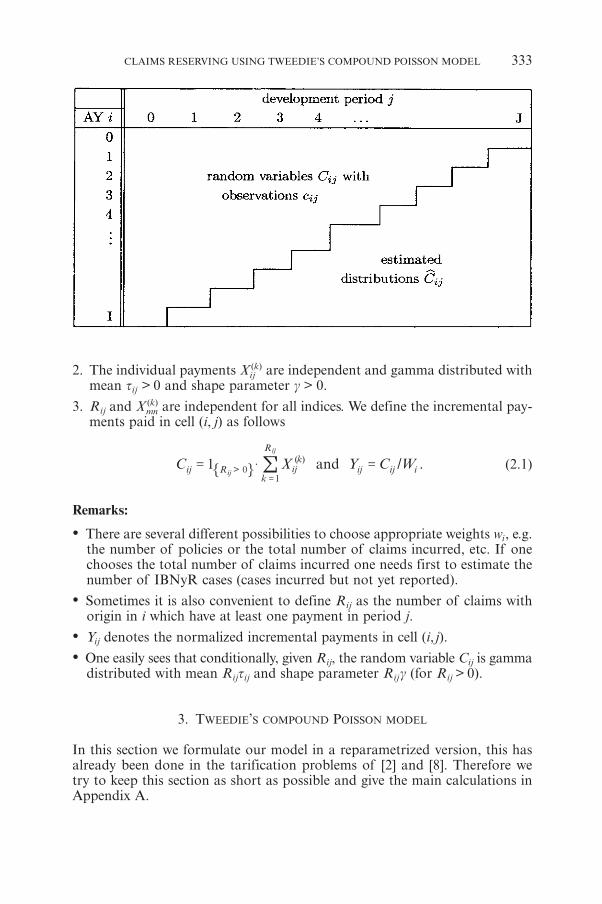
2. The individual payments X (k)ij are independent and gamma distributed with
mean tij > 0 and shape parameter g > 0.
3. Rij and X (k)mn are independent for all indices. We define the incremental pay-
ments paid in cell (i, j) as follows
iij ij
ij
/ .C X Y C Wand1 >( )
ij Rk
k
R
ij01
ij$= =
=
!" ,
(2.1)
Remarks:
• There are several different possibilities to choose appropriate weights wi, e.g.the number of policies or the total number of claims incurred, etc. If onechooses the total number of claims incurred one needs first to estimate thenumber of IBNyR cases (cases incurred but not yet reported).
• Sometimes it is also convenient to define Rij as the number of claims withorigin in i which have at least one payment in period j.
• Yij denotes the normalized incremental payments in cell (i, j).
• One easily sees that conditionally, given Rij, the random variable Cij is gammadistributed with mean Rijtij and shape parameter Rijg (for Rij > 0).
3. TWEEDIE’S COMPOUND POISSON MODEL
In this section we formulate our model in a reparametrized version, this hasalready been done in the tarification problems of [2] and [8]. Therefore wetry to keep this section as short as possible and give the main calculations inAppendix A.
CLAIMS RESERVING USING TWEEDIE’S COMPOUND POISSON MODEL 333
For the moment we skip the indices i and j. The distribution Y (for givenweight w) is parametrized by the three parameters l, t and g. We now choosenew parameters m, ƒ and p such that the density of Y can be written as, y ≥ 0,(see (A.2) below and formula (12) in [2])
; , / , ; / , ,expz zz
f y w p c y w p w y p pmm m1 2Y
p p1 2
=-
--
- -
^ ^ fh h p* 4 (3.1)
where c(y; ƒ /w, p) is given in Appendix A and
p = (g + 2) / (g + 1) ∈ (1, 2), (3.2)
m = l · t, (3.3)
ƒ = l1– pt 2– p / (2 – p). (3.4)
If we set q = m1– p / (1 – p) we see that the density of Y can be written as (see also[2], formula (12))
p
p
; , / , ; / , ( ) ,
( ) .
expz zz
f y w p c y w p w y
p pwith
m q k q
k q q2
11
Y
pp
1
2
-
=-
-
=
-
-
^ ^ `
^^
h h j
h h
( 2
(3.5)
Hence, the distribution of Y belongs to the exponential dispersion family withparameters m, ƒ and p ∈ (1,2) (see e.g. McCullagh-Nelder [5], Section 2.2.2).We write for p ∈ (1,2)
, / .zY wED m( )p` ^ h (3.6)
For ( , / )zY wED m( )p` we have (see [2] Section 2.2)
E [Y ] = k�p(q) = m, (3.7)
Var(Y) = ( ) .z zw V wm mp$ = (3.8)
ƒ is the so-called dispersion parameter and V(·) the variance function withp ∈ (1,2). For our claims reserving problem we consider the following situa-tion:
Constant dispersion ƒ (see Subsection 4.1): p ∈ (1,2) and Yij are independentwith
ij i ij j, / .zz
Y w E Y Y wED Varandm m m( )pij i i i
p&` = = ijj` `j j8 B (3.9)
334 MARIO V. WUTHRICH
Interpretation and Remarks:
• Tweedie [10] seems to be the first one to study the compound Poisson modelwith gamma severeties from the point of view of exponential dispersionmodels. For this reason this model is known as Tweedie’s compound Pois-son model in the literature, see e.g. [8].
• p = (g + 2) / (g + 1) is a function of g (shape parameter of the single paymentsdistributions X (k)
ij ). Hence the shape parameter g determines the behaviourof the variance function V(m) = mp. Furthermore we have chosen a parame-trization (m, ƒ, p) such that m is orthogonal to (ƒ, p) in the sense that the Fisherinformation matrix is zero in the off-diagonal (see e.g. [2], page 76, or [8]).I.e. our parametrization focuses attention to variance parameters (ƒ, p) anda mean parameter m which are orthogonal to each other. This orthogonalityhas many advantages to alternative parametrizations. E.g. we have efficientalgorithms for parameter estimations which typically rapidly converge (seeSmyth [7]). Moreover the estimated standard errors of m, which are of mostinterest, do not require adjustments by the standard errors of the varianceparameters, since these are orthogonal.
• Our model closes continuously the gap between the over-dispersed PoissonModel (see Renshaw-Verrall [6] or England-Verrall [1], Section 2.3) where wehave a linear variance function (p = 1):
i j / ,zY wVar mi i$= j` j (3.10)
and the Gamma model (see Mack [3] and England-Verrall [1], Section 3.3)where
i j / .zY wVar mi i2$= j` j (3.11)
In our case p is estimated from the data using additionally the informationrij (see (4.6)). The information rij is not used in the boundary cases p = 1 andp = 2.
• Naturally in our model we have p ∈ (1,2), since g > 0. We estimate p fromthe data, so theoretically the estimated p could lie outside the interval [1,2]which would mean that none of our models fits to the problem (e.g. p = 0implies normality, p = 3 implies the inverse Gaussian model). In all ourclaims reserving examples we have observed that the estimated p was lyingstrictly within (1,2).
4. APPLICATION OF TWEEDIE’S MODEL TO CLAIMS RESERVING
4.1. Constant dispersion parameter model
We assume that all the Yij are independent with Yij ∼ED(p) (mij,ƒ/wi), i.e. Yij belongsto the exponential dispersion family with p ∈ (1,2), and
CLAIMS RESERVING USING TWEEDIE’S COMPOUND POISSON MODEL 335
i ij j .z
E Y Y wVarandm mi i ip= =j j` j8 B (4.1)
We use the notation m = (m00,…, mIJ)�. Given the observations {(rij, yij), i + j ≤ I,
i rj ij! > 0}, the log-likelihood function for the parameters (m, ƒ, p) is given by(see Appendix A and [2], Section 3)
i i
, ,( ) ( )
/!
.
log logzz
z
L p rp p
w yr r y
wy p p
g
m m
Gm1 2
1 2
,i
i ii i ij
i j
iij
p p
g
g g1
1 2
=- -
-
+-
--
+
- -j j
jj
j j!^^
``hh
j j
R
T
SSSS
V
X
WWW
*
*
4
4
(4.2)
Formula (4.2) immediately shows that given p the observations yij = cij /wi aresufficient for MLE estimation of mij (one does not need rij). Moreover, for con-stant ƒ, the dispersion parameter has no influence on the estimation of m.
Next we assume a multiplicative model (often called chain-ladder type struc-ture): i.e. there exist parameters �(i) and f ( j) such that for all i ≤ I and j ≤ J
( ) ( ).� i f jmi $=j (4.3)
After suitable normalization, � can be interpreted as the expected ultimateclaim in accident year i and f is the proportion paid in period j. It is nowstraightforward to choose the logarithmic link function
( ) ,log xj m bi i i= =j j j (4.4)
where b = (log �(0),…, log�(I), log f(0),…,log f(j))� and X = (x00,…,xIJ) is theappropriate design matrix.
Parameter estimation:
a) For p known. We deal with a generalized linear model (GLM) of the form (4.1)-(4.4). Hence we can use standard software packages for the estimation of m.
b) For p unknown. Usually p and g, resp., are unknown. Henceforth we studythe profile likelihood for g (here we closely follow [2] Section 3.2): For m andp given, the MLE of ƒ is given by (see (4.2))
ƒ̂p
i i
( ).
r
w y p p
g
m m
1
1 2
,
,
ii j
i i
p p
i j
1 2
=+
--
--
- -j j
j
j
!
!J
L
KKK
N
P
OOO
(4.5)
336 MARIO V. WUTHRICH
From this we obtain the profile likelihood for p and g, resp., i >r 0j ij!a k as
Lm(p) = L(m, p, ƒ̂p) = ( ) logrw
g1 1,
ii
i j+ -
pzj! f p
(4.6)
.log logr p py
r gG2
11
,,i
ii
i ji j
g
+- -
-jj
j!!J
L
KK f `
N
P
OOp j
Given m, the parameter p is estimated maximizing (4.6).
c) Finally we combine a) and b). The main advantage of our parametrizationis (as already mentioned above) the orthogonality of m and (ƒ, p). m can beestimated as if (ƒ, p) were known and vice versa. Alternating the updatingprocedures for m and (ƒ, p) leads to an efficent algorithm: Set initial valuep(0) and estimate m (1) via a). Then estimate p(1) from m (1) via (4.6), and iterate thisprocedure. We have seen that typically one obtains very fast convergence of(m (k), p(k)) to some limit (for our examples below we needed only 4 iterations).
4.2. Dispersion modelling
So far we have always assumed that ƒ is constant over all cells (i, j). If we con-sider the definitions (3.3) and (3.4) we see that every factor which increases lincreases the mean m and decreases the dispersion ƒ because p ∈ (1,2). Increas-ing the average payment size t increases both the mean and the dispersion.Changing l and t such that l1–p t2–p remains constant has only an effect on themean m. Hence it is necessary to model both the mean and the dispersion inorder to get a fine structure, i.e. model mij and ƒij for each cell (i,j) individuallyand estimate p. Such a model has been studied in the context of tarificationby Smyth-Jørgensen [8].
We do not further follow these ideas here since we have seen that in our sit-uation such models are over-parametrized. Modelling the dispersion parame-ters while also trying to optimize the power of the variance function allowstoo many degrees of freedom: e.g. if we apply the dispersion modelling modelto the data given in Example 6.1 one sees that p is blown up when allowingthe dispersion parameters to be modelled too. It is even possible that there is nounique solution when modelling ƒij and p at the same time (in all our exampleswe have observed rather slow convergence even when choosing “meaningful’’initial values which indicates this problematic).
5. MEAN SQUARE ERROR OF PREDICTION
To estimate the mean square error of prediction (MSEP) we proceed as inEngland-Verrall [1]. Assume that the incremental payments Cij are independent,
CLAIMS RESERVING USING TWEEDIE’S COMPOUND POISSON MODEL 337
ˆ
and Cij% are unbiased estimators depending only on the past (and hence are
independent from Cij). Assume jij is the GLM estimate for jij = log mij, then (seee.g. [1], (7.6)-(7.7))
.jz
C E C C C C
w w
MSEP Var Var
Varm m
C i i i i i
i ip
i i i
2
2
i
$.
= - = +
+j
j j j j j j
j j
% % %a a ` a
` `
k k j k
j j
< F
(5.1)
The last term is usually available from standard statistical software packages,all the other parameters have been estimated before. The first term in (5.1) denotesthe process error, the last term the estimation error.
The estimation of the MSEP for several cells (i, j) is more complicated sincewe obtain correlations from the estimates. We define D to be the unknown tri-angle in our run-off pattern. Define the total outstanding payments
.C C Cand C( , ) ( , )
ii j
ii jD D
= =! !
j j! ! % (5.2)
Then
2( )
, .
j
j j
zE C w w
w w
MSEP Var
Cov
C C m m
m m
!
( , ) ( , )
( , ) ( , )( , ),( , ) ,
C i i ip
i ji i i
i j
i
i j i ji j i j
i j i i j i j i j
D D
D
2
1
1 1 2 2
1 1 2 2
1 1 2 2 2 1 1 2 2
$.= - +
+
! !
!
j j j j! !
!
_ ` `
`
i j j
j
9 C
The evaluation of the last term needs some care: Usually one obtains a covari-ance matrix for the estimated GLM parameters log �(i) and log f ( j). Thiscovariance matrix needs to be transformed into a covariance matrix for j withthe help of the design matrices.
6. EXAMPLE
Example 6.1.
We consider Swiss Motor Insurance datas. We consider 9 accident years overa time horizon of 11 years. Since we want to analyze the different methodsrather mechanically, this small part of the truth is already sufficient for drawingconclusions.
338 MARIO V. WUTHRICH
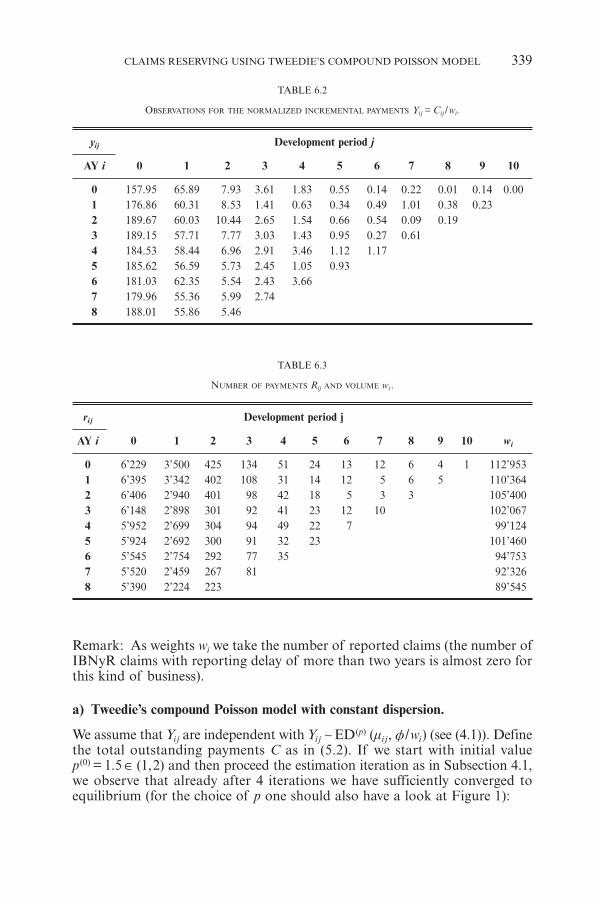
Remark: As weights wi we take the number of reported claims (the number ofIBNyR claims with reporting delay of more than two years is almost zero forthis kind of business).
a) Tweedie’s compound Poisson model with constant dispersion.
We assume that Yij are independent with Yij ∼ ED(p) (mi j, ƒ/wi) (see (4.1)). Definethe total outstanding payments C as in (5.2). If we start with initial valuep(0) = 1.5 ∈ (1,2) and then proceed the estimation iteration as in Subsection 4.1,we observe that already after 4 iterations we have sufficiently converged toequilibrium (for the choice of p one should also have a look at Figure 1):
CLAIMS RESERVING USING TWEEDIE’S COMPOUND POISSON MODEL 339
TABLE 6.2
OBSERVATIONS FOR THE NORMALIZED INCREMENTAL PAYMENTS Yij = Cij /wi.
yij Development period j
AY i 0 1 2 3 4 5 6 7 8 9 10
0 157.95 65.89 7.93 3.61 1.83 0.55 0.14 0.22 0.01 0.14 0.001 176.86 60.31 8.53 1.41 0.63 0.34 0.49 1.01 0.38 0.232 189.67 60.03 10.44 2.65 1.54 0.66 0.54 0.09 0.193 189.15 57.71 7.77 3.03 1.43 0.95 0.27 0.614 184.53 58.44 6.96 2.91 3.46 1.12 1.175 185.62 56.59 5.73 2.45 1.05 0.936 181.03 62.35 5.54 2.43 3.667 179.96 55.36 5.99 2.748 188.01 55.86 5.46
TABLE 6.3
NUMBER OF PAYMENTS Rij AND VOLUME wi.
rij Development period j
AY i 0 1 2 3 4 5 6 7 8 9 10 wi
0 6’229 3’500 425 134 51 24 13 12 6 4 1 112’9531 6’395 3’342 402 108 31 14 12 5 6 5 110’3642 6’406 2’940 401 98 42 18 5 3 3 105’4003 6’148 2’898 301 92 41 23 12 10 102’0674 5’952 2’699 304 94 49 22 7 99’1245 5’924 2’692 300 91 32 23 101’4606 5’545 2’754 292 77 35 94’7537 5’520 2’459 267 81 92’3268 5’390 2’224 223 89’545
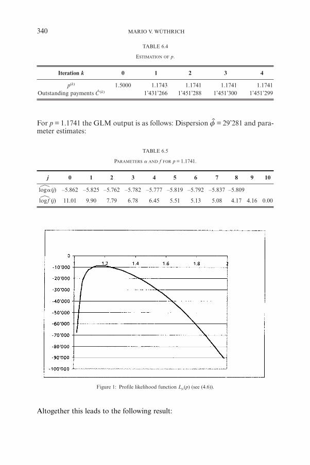
Figure 1: Profile likelihood function Lm(p) (see (4.6)).
For p = 1.1741 the GLM output is as follows: Dispersion ƒ̂ = 29’281 and para-meter estimates:
340 MARIO V. WUTHRICH
TABLE 6.4
ESTIMATION OF p.
Iteration k 0 1 2 3 4
p(k) 1.5000 1.1743 1.1741 1.1741 1.1741Outstanding payments C (k) 1’431’266 1’451’288 1’451’300 1’451’299
TABLE 6.5
PARAMETERS � AND f FOR p = 1.1741.
j 0 1 2 3 4 5 6 7 8 9 10
( )log� j% –5.862 –5.825 –5.762 –5.782 –5.777 –5.819 –5.792 –5.837 –5.809
( )log f j% 11.01 9.90 7.79 6.78 6.45 5.51 5.13 5.08 4.17 4.16 0.00
Altogether this leads to the following result:

The results in Table 6.6 show that there is considerable uncertainty in thereserve estimates, especially in the old years where the outstanding paymentsare small. This comes from the fact that we have only little information to esti-mate f (j) for large j and it turns out that the parameter estimation error liveson the same scale as the process error. For young accident years we have onthe one hand a lot of information to estimate f (j) for small j and on the otherhand f(j) for j large has a rather small influence on the overall outstanding pay-ments estimate for young accident years in our example. Therefore the relativeprediction error is smaller for young accident years
b) Over-dispersed Poisson and Gamma Model.
We first compare our result to the two boundary cases p = 1 and p = 2. Thesemodels are described in Renshaw-Verrall [6] or England-Verrall [1], Section 2.3(over-dispersed Poisson model) and Mack [3] or England-Verrall [1], Section 3.3(Gamma model). We also refer to (3.10)-(3.11). We obtain the following results:
CLAIMS RESERVING USING TWEEDIE’S COMPOUND POISSON MODEL 341
TABLE 6.6
ESTIMATED OUTSTANDING PAYMENTS FROM TWEEDIE’S COMPOUND POISSON MODEL.
Tweedie constant z = 29’281 and p = 1.1741
AY i Outst. payments MSEP1/2 in % Estimation error Process error
1 326 2’636 808.9% 1’867 1’8602 21’565 26’773 124.2% 15’584 21’7703 40’716 35’515 87.2% 19’122 29’9274 89’278 53’227 59.6% 25’940 46’4795 138’338 65’977 47.7% 30’529 58’4896 204’269 80’815 39.6% 35’191 72’7517 360’117 111’797 31.0% 45’584 102’0828 596’690 149’775 25.1% 61’212 136’695
Total 1’451’299 271’503 18.7% 179’890 203’355
TABLE 6.7
ESTIMATED OUTSTANDING PAYMENTS FROM THE OVER-DISPERSED POISSON MODEL.
Over-dispersed Poisson model with z = 36’642 and p = 1
AY i Outst. payments MSEP1/2 in % Estimation error Process error
1 330 4’947 1500.7% 3’520 3’4752 21’663 34’776 160.5% 20’386 28’1743 41’007 46’070 112.3% 24’896 38’7634 88’546 65’229 73.7% 31’786 56’9615 140’150 80’795 57.6% 37’316 71’6626 204’157 95’755 46.9% 41’089 86’4917 362’724 125’433 34.6% 49’421 115’2868 602’784 161’023 26.7% 61’978 148’618
Total 1’461’360 371’208 21.7% 216’965 231’403
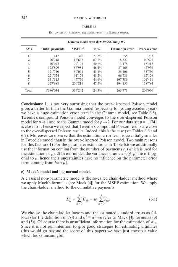
Conclusions: It is not very surprising that the over-dispersed Poisson modelgives a better fit than the Gamma model (especially for young accident yearswe have a huge estimation error term in the Gamma model, see Table 6.8).Tweedie’s compound Poisson model converges to the over-dispersed Poissonmodel for p → 1 and to the Gamma model for p → 2. For our data set p = 1.1741is close to 1, hence we expect that Tweedie’s compound Poisson results are closeto the over-dispersed Poisson results. Indeed, this is the case (see Tables 6.6 and6.7). Moreover we observe that the estimation error term is essentially smallerin Tweedie’s model than in the over-dispersed Poisson model. Two main reasonsfor this fact are 1) For the parameter estimations in Table 6.6 we additionallyuse the information coming from the number of payments rij (which is used forthe estimation of p). 2) In our model, the variance parameters (ƒ, p) are orthog-onal to m, hence their uncertainties have no influence on the parameter errorterm coming from Var(m ).
c) Mack’s model and log-normal model.
A classical non-parametric model is the so-called chain-ladder method wherewe apply Mack’s formulas (see Mack [4]) for the MSEP estimation. We applythe chain-ladder method to the cumulative payments
i .D C w Yi i i kk
j
k
j
00
= ===
j k !! (6.1)
We choose the chain-ladder factors and the estimated standard errors as fol-lows (for the definition of f (j) and s2
j = �2j we refer to Mack [4], formulas (3)
and (5)). Of course there is unsufficient information for the estimation of s10.Since it is not our intention to give good strategies for estimating ultimates(this would go beyond the scope of this paper) we have just chosen a valuewhich looks meaningful.
342 MARIO V. WUTHRICH
TABLE 6.8
ESTIMATED OUTSTANDING PAYMENTS FROM THE GAMMA MODEL.
Gamma model with z = 29’956 and p = 2
AY i Outst. payments MSEP1/2 in % Estimation error Process error
1 447 346 77.3% 255 2332 20’248 13’602 67.2% 8’527 10’5973 40’073 20’127 50.2% 13’178 15’2134 122’899 56’984 46.4% 37’465 42’9365 121’740 50’091 41.1% 35’106 35’7306 221’524 91’174 41.2% 66’731 62’1267 331’115 147’730 44.6% 107’386 101’4518 527’988 250’816 47.5% 194’155 158’784
Total 1’386’034 336’842 24.3% 265’771 206’950
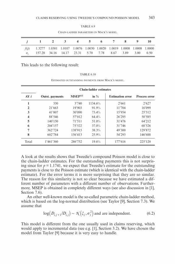
This leads to the following result:
CLAIMS RESERVING USING TWEEDIE’S COMPOUND POISSON MODEL 343
TABLE 6.10
ESTIMATED OUTSTANDING PAYMENTS FROM MACK’S MODEL.
Chain-ladder estimates
AY i Outst. payments MSEP1/2 in % Estimation error Process error
1 330 3’740 1134.6% 2’661 2’6272 21’663 19’903 91.9% 11’704 16’0993 41’007 30’090 73.4% 15’954 25’5124 88’546 57’012 64.4% 26’295 50’5855 140’150 71’511 51.0% 31’476 64’2126 204’157 75’522 37.0% 31’746 68’5267 362’724 138’915 38.3% 49’300 129’8728 602’784 156’413 25.9% 54’293 146’688
Total 1’461’360 286’752 19.6% 177’616 225’120
TABLE 6.9
CHAIN-LADDER PARAMETERS IN MACK’S MODEL.
j 1 2 3 4 5 6 7 8 9 10
f (j) 1.3277 1.0301 1.0107 1.0076 1.0030 1.0020 1.0019 1.0008 1.0008 1.0000sj 157.28 34.16 14.17 23.31 5.70 7.78 8.67 3.89 3.00 0.50
A look at the results shows that Tweedie’s compound Poisson model is close tothe chain-ladder estimates. For the outstanding payments this is not surpris-ing since for p = 1.1741, we expect that Tweedie’s estimate for the outstandingpayments is close to the Poisson estimate (which is identical with the chain-ladderestimate). For the error terms it is more surprising that they are so similar.The reason for this similarity is not so clear because we have estimated a dif-ferent number of parameters with a different number of observations. Further-more, MSEP is obtained in completely different ways (see also discussion in [1],Section 7.6).
An other well-known model is the so-called parametric chain-ladder method,which is based on the log-normal distribution (see Taylor [9], Section 7.3). Weassume that
j j/ ,log D D z sN, ,i j i j12++` `j j and are independent. (6.2)
This model is different from the one usually used in claims reserving, whichwould apply to incremental data (see e.g. [1], Section 3.2). We have chosen themodel from Taylor [9] because it is very easy to handle.
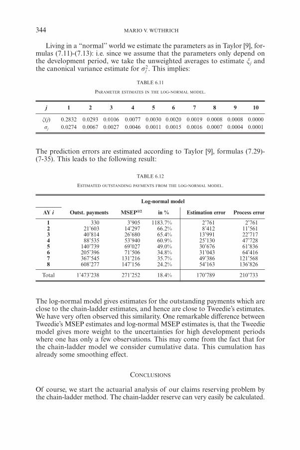
Living in a “normal’’ world we estimate the parameters as in Taylor [9], for-mulas (7.11)-(7.13): i.e. since we assume that the parameters only depend onthe development period, we take the unweighted averages to estimate zj andthe canonical variance estimate for s2
j . This implies:
344 MARIO V. WUTHRICH
TABLE 6.11
PARAMETER ESTIMATES IN THE LOG-NORMAL MODEL.
j 1 2 3 4 5 6 7 8 9 10
z(j) 0.2832 0.0293 0.0106 0.0077 0.0030 0.0020 0.0019 0.0008 0.0008 0.0000sj 0.0274 0.0067 0.0027 0.0046 0.0011 0.0015 0.0016 0.0007 0.0004 0.0001
The prediction errors are estimated according to Taylor [9], formulas (7.29)-(7-35). This leads to the following result:
TABLE 6.12
ESTIMATED OUTSTANDING PAYMENTS FROM THE LOG-NORMAL MODEL.
Log-normal model
AY i Outst. payments MSEP1/2 in % Estimation error Process error
1 330 3’905 1183.7% 2’761 2’7612 21’603 14’297 66.2% 8’412 11’5613 40’814 26’680 65.4% 13’991 22’7174 88’535 53’940 60.9% 25’130 47’7285 140’739 69’027 49.0% 30’676 61’8366 205’396 71’506 34.8% 31’043 64’4167 367’545 131’216 35.7% 49’386 121’5688 608’277 147’156 24.2% 54’163 136’826
Total 1’473’238 271’252 18.4% 170’789 210’733
The log-normal model gives estimates for the outstanding payments which areclose to the chain-ladder estimates, and hence are close to Tweedie’s estimates.We have very often observed this similarity. One remarkable difference betweenTweedie’s MSEP estimates and log-normal MSEP estimates is, that the Tweediemodel gives more weight to the uncertainties for high development periodswhere one has only a few observations. This may come from the fact that forthe chain-ladder model we consider cumulative data. This cumulation hasalready some smoothing effect.
CONCLUSIONS
Of course, we start the actuarial analysis of our claims reserving problem bythe chain-ladder method. The chain-ladder reserve can very easily be calculated.
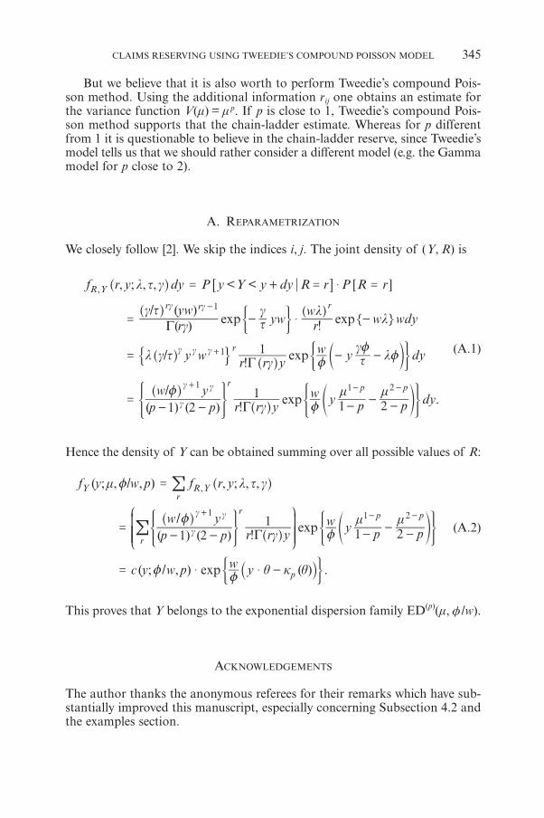
But we believe that it is also worth to perform Tweedie’s compound Pois-son method. Using the additional information rij one obtains an estimate forthe variance function V(m) = m p. If p is close to 1, Tweedie’s compound Pois-son method supports that the chain-ladder estimate. Whereas for p differentfrom 1 it is questionable to believe in the chain-ladder reserve, since Tweedie’smodel tells us that we should rather consider a different model (e.g. the Gammamodel for p close to 2).
A. REPARAMETRIZATION
We closely follow [2]. We skip the indices i, j. The joint density of (Y, R) is
R
r
g g
, ; , , < <
( )/ ( )
!
/ !
( ) ( )/
! .
exp exp
exp
exp
zz
z
zz
f r y dy P y Y y dy R r P R r
ryw
yw rw
w wdy
y w r r yw y dy
p pw y
r r yw y p p dy
l t g
gg t
tg l
l
l g t g tg
l
gm m
G
G
G
1
1 21
1 2
,Y
r r
r
r p p
g g
g
g
g g
1
1
1 1 2
$
$
= + = =
= - -
= - -
=- - -
--
-
+
+ - -
^
^ ]
^^
d
^
^f
h
h g
hh
n
h
hp
6 6@ @
( !
$ (
* *
2 +
. 2
4 4
(A.1)
Hence the density of Y can be obtained summing over all possible values of R:
R
p
( ; , / , ) , ; , ,
( ) ( )/
!
( ; / , ) ( ) .
exp
exp
z
zz
zz
f y w p f r y
p pw y
r r yw y p p
c y w p w y
m l t g
gm m
q k q
G1 21
1 2
,Y Yr
r
r
p p
g
g g1 1 2
$ $
=
=- - -
--
= -
+ - -
!
!J
L
KKK
^
^
^f
`
N
P
OOO
h
h
hp
j
* *
'
4 4
1
(A.2)
This proves that Y belongs to the exponential dispersion family ED(p)(m, ƒ /w).
ACKNOWLEDGEMENTS
The author thanks the anonymous referees for their remarks which have sub-stantially improved this manuscript, especially concerning Subsection 4.2 andthe examples section.
CLAIMS RESERVING USING TWEEDIE’S COMPOUND POISSON MODEL 345
REFERENCES
[1] ENGLAND, P.D., and VERRALL, R.J. (2002) Stochastic claims reserving in general insurance,Institute of Actuaries and Faculty of Actuaries, http://www.actuaries.org.uk/files/pdf/sessional/sm0201.pdf
[2] JØRGENSEN, B., and DE SOUZA, M.C.P. (1994) Fitting Tweedie’s compound Poisson modelto insurance claims data, Scand. Actuarial J., 69-93.
[3] MACK, T. (1991) A simple parametric model for rating automobile insurance or estimatingIBNR claims reserves, Astin Bulletin 21, 93-109.
[4] MACK, T. (1997) Measuring the variability of chain ladder reserve estimates, Claims ReservingManual 2, D6.1-D6.65.
[5] MCCULLAGH, P., and NELDER, J.A. (1989) Generalized linear models, 2nd edition, Chap-man and Hall.
[6] RENSHAW, A.E., and VERRALL, R.J. (1998) A stochastic model underlying the chain-laddertechnique, B.A.J. 4, 903-923.
[7] SMYTH, G.K. (1996) Partitioned algorithms for maximum likelihood and other nonlinearestimation, Statistics and Computing 6, 201-216.
[8] SMYTH, G.K., and JØRGENSEN, B. (2002), Fitting Tweedie’s compound Poisson model toinsurance claims data: dispersion modelling, Astin Bulletin 32, 143-157.
[9] TAYLOR, G. (2000), Loss reserving: an actuarial perspective, Kluwer Academic Publishers.[10] TWEEDIE, M.C.K. (1984), An index which distinguishes between some important exponential
families. In Statistics: Applications and new directions. Proceeding of the Indian StatisticalGolden Jubilee International Conference, Eds. J.K. Ghosh and J. Roy, 579-604, Indian Sta-tistical Institute, Calcutta.
[11] WRIGHT, T.S. (1990), A stochastic method for claims reserving in general insurance, J.I.A.117, 677-731.
MARIO V. WÜTHRICH
Winterthur InsuranceRömerstrasse 17, P.O. Box 357,CH-8401 WinterthurSwitzerlandE-mail: [email protected]
346 MARIO V. WUTHRICH
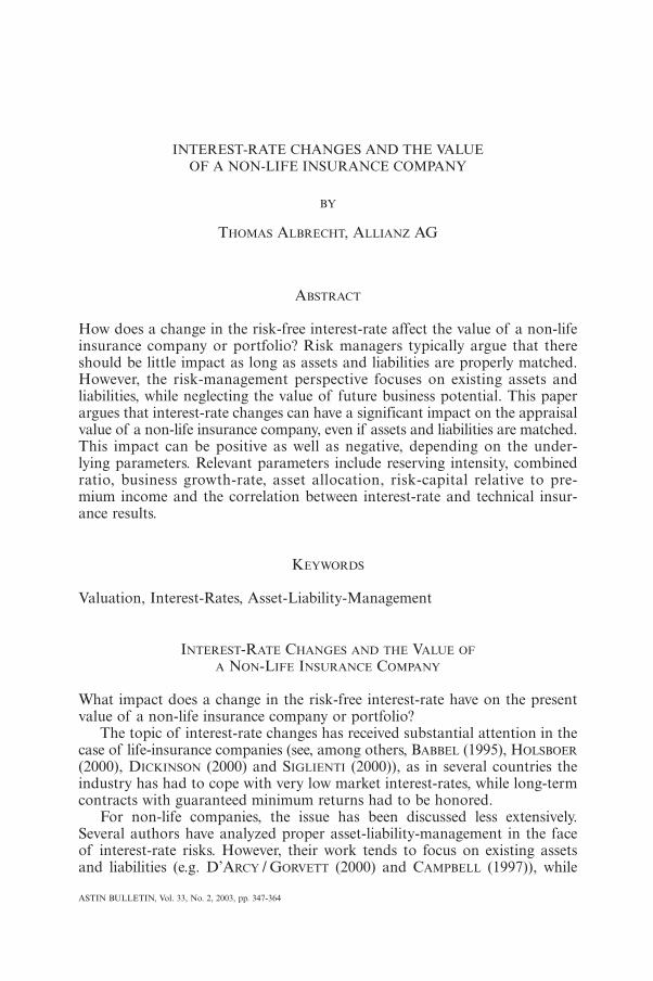
INTEREST-RATE CHANGES AND THE VALUE OF A NON-LIFE INSURANCE COMPANY
BY
THOMAS ALBRECHT, ALLIANZ AG
ABSTRACT
How does a change in the risk-free interest-rate affect the value of a non-lifeinsurance company or portfolio? Risk managers typically argue that thereshould be little impact as long as assets and liabilities are properly matched.However, the risk-management perspective focuses on existing assets andliabilities, while neglecting the value of future business potential. This paperargues that interest-rate changes can have a significant impact on the appraisalvalue of a non-life insurance company, even if assets and liabilities are matched.This impact can be positive as well as negative, depending on the under-lying parameters. Relevant parameters include reserving intensity, combinedratio, business growth-rate, asset allocation, risk-capital relative to pre-mium income and the correlation between interest-rate and technical insur-ance results.
KEYWORDS
Valuation, Interest-Rates, Asset-Liability-Management
INTEREST-RATE CHANGES AND THE VALUE OF
A NON-LIFE INSURANCE COMPANY
What impact does a change in the risk-free interest-rate have on the presentvalue of a non-life insurance company or portfolio?
The topic of interest-rate changes has received substantial attention in thecase of life-insurance companies (see, among others, BABBEL (1995), HOLSBOER
(2000), DICKINSON (2000) and SIGLIENTI (2000)), as in several countries theindustry has had to cope with very low market interest-rates, while long-termcontracts with guaranteed minimum returns had to be honored.
For non-life companies, the issue has been discussed less extensively.Several authors have analyzed proper asset-liability-management in the faceof interest-rate risks. However, their work tends to focus on existing assetsand liabilities (e.g. D’ARCY / GORVETT (2000) and CAMPBELL (1997)), while
ASTIN BULLETIN, Vol. 33, No. 2, 2003, pp. 347-364
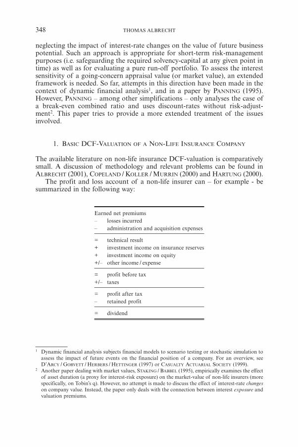
neglecting the impact of interest-rate changes on the value of future businesspotential. Such an approach is appropriate for short-term risk-managementpurposes (i.e. safeguarding the required solvency-capital at any given point intime) as well as for evaluating a pure run-off portfolio. To assess the interestsensitivity of a going-concern appraisal value (or market value), an extendedframework is needed. So far, attempts in this direction have been made in thecontext of dynamic financial analysis1, and in a paper by PANNING (1995).However, PANNING – among other simplifications – only analyses the case ofa break-even combined ratio and uses discount-rates without risk-adjust-ment2. This paper tries to provide a more extended treatment of the issuesinvolved.
1. BASIC DCF-VALUATION OF A NON-LIFE INSURANCE COMPANY
The available literature on non-life insurance DCF-valuation is comparativelysmall. A discussion of methodology and relevant problems can be found inALBRECHT (2001), COPELAND / KOLLER / MURRIN (2000) and HARTUNG (2000).
The profit and loss account of a non-life insurer can – for example - besummarized in the following way:
Earned net premiums – losses incurred – administration and acquisition expenses
= technical result + investment income on insurance reserves+ investment income on equity+/– other íncome / expense
= profit before tax +/– taxes
= profit after tax– retained profit
= dividend
348 THOMAS ALBRECHT
1 Dynamic financial analysis subjects financial models to scenario testing or stochastic simulation toassess the impact of future events on the financial position of a company. For an overview, seeD’ARCY / GORVETT / HERBERS / HETTINGER (1997) or CASUALTY ACTUARIAL SOCIETY (1999).
2 Another paper dealing with market values, STAKING / BABBEL (1995), empirically examines the effectof asset duration (a proxy for interest-risk exposure) on the market-value of non-life insurers (morespecifically, on Tobin’s q). However, no attempt is made to discuss the effect of interest-rate changeson company value. Instead, the paper only deals with the connection between interest exposure andvaluation premiums.
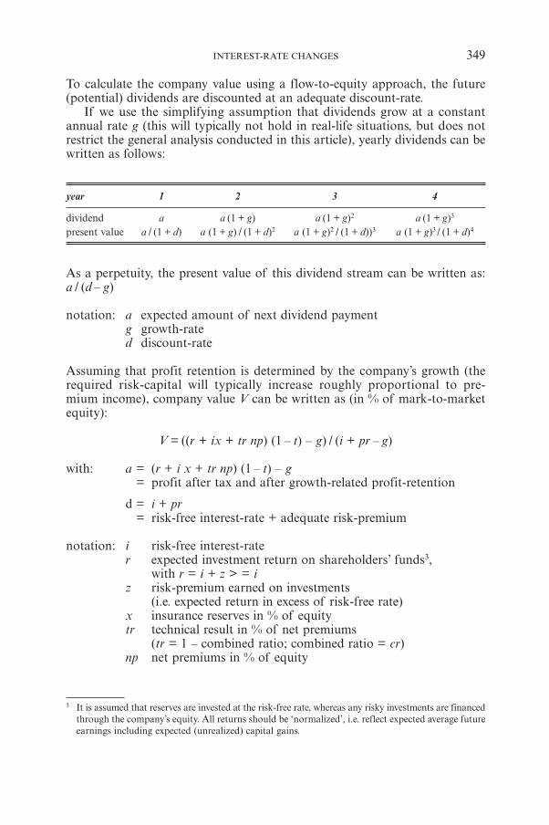
To calculate the company value using a flow-to-equity approach, the future(potential) dividends are discounted at an adequate discount-rate.
If we use the simplifying assumption that dividends grow at a constantannual rate g (this will typically not hold in real-life situations, but does notrestrict the general analysis conducted in this article), yearly dividends can bewritten as follows:
year 1 2 3 4
dividend a a (1 + g) a (1 + g)2 a (1 + g)3
present value a / (1 + d) a (1 + g) / (1 + d)2 a (1 + g)2 / (1 + d))3 a (1 + g)3 / (1 + d)4
As a perpetuity, the present value of this dividend stream can be written as:a / (d – g)
notation: a expected amount of next dividend paymentg growth-rated discount-rate
Assuming that profit retention is determined by the company’s growth (therequired risk-capital will typically increase roughly proportional to pre-mium income), company value V can be written as (in % of mark-to-marketequity):
V = ((r + ix + tr np) (1 – t) – g) / (i + pr – g)
with: a = (r + i x + tr np) (1 – t) – g= profit after tax and after growth-related profit-retention
d = i + pr= risk-free interest-rate + adequate risk-premium
notation: i risk-free interest-rater expected investment return on shareholders’ funds3,
with r = i + z > = iz risk-premium earned on investments
(i.e. expected return in excess of risk-free rate)x insurance reserves in % of equitytr technical result in % of net premiums
(tr = 1 – combined ratio; combined ratio = cr)np net premiums in % of equity
INTEREST-RATE CHANGES 349
3 It is assumed that reserves are invested at the risk-free rate, whereas any risky investments are financedthrough the company’s equity. All returns should be ‘normalized’, i.e. reflect expected average futureearnings including expected (unrealized) capital gains.
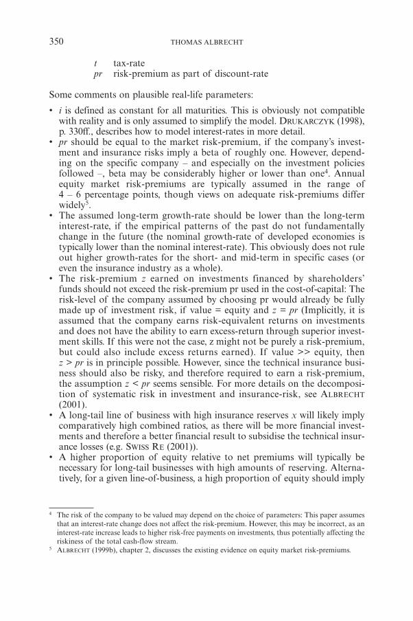
t tax-ratepr risk-premium as part of discount-rate
Some comments on plausible real-life parameters:
• i is defined as constant for all maturities. This is obviously not compatiblewith reality and is only assumed to simplify the model. DRUKARCZYK (1998),p. 330ff., describes how to model interest-rates in more detail.
• pr should be equal to the market risk-premium, if the company’s invest-ment and insurance risks imply a beta of roughly one. However, depend-ing on the specific company – and especially on the investment policiesfollowed –, beta may be considerably higher or lower than one4. Annualequity market risk-premiums are typically assumed in the range of4 – 6 percentage points, though views on adequate risk-premiums differwidely5.
• The assumed long-term growth-rate should be lower than the long-terminterest-rate, if the empirical patterns of the past do not fundamentallychange in the future (the nominal growth-rate of developed economies istypically lower than the nominal interest-rate). This obviously does not ruleout higher growth-rates for the short- and mid-term in specific cases (oreven the insurance industry as a whole).
• The risk-premium z earned on investments financed by shareholders’funds should not exceed the risk-premium pr used in the cost-of-capital: Therisk-level of the company assumed by choosing pr would already be fullymade up of investment risk, if value = equity and z = pr (Implicitly, it isassumed that the company earns risk-equivalent returns on investmentsand does not have the ability to earn excess-return through superior invest-ment skills. If this were not the case, z might not be purely a risk-premium,but could also include excess returns earned). If value >> equity, thenz > pr is in principle possible. However, since the technical insurance busi-ness should also be risky, and therefore required to earn a risk-premium,the assumption z < pr seems sensible. For more details on the decomposi-tion of systematic risk in investment and insurance-risk, see ALBRECHT
(2001).• A long-tail line of business with high insurance reserves x will likely imply
comparatively high combined ratios, as there will be more financial invest-ments and therefore a better financial result to subsidise the technical insur-ance losses (e.g. SWISS RE (2001)).
• A higher proportion of equity relative to net premiums will typically benecessary for long-tail businesses with high amounts of reserving. Alterna-tively, for a given line-of-business, a high proportion of equity should imply
350 THOMAS ALBRECHT
4 The risk of the company to be valued may depend on the choice of parameters: This paper assumesthat an interest-rate change does not affect the risk-premium. However, this may be incorrect, as aninterest-rate increase leads to higher risk-free payments on investments, thus potentially affecting theriskiness of the total cash-flow stream.
5 ALBRECHT (1999b), chapter 2, discusses the existing evidence on equity market risk-premiums.

a low risk-premium pr, as the risk per unit of capital will be lowered, if theamount of capital is increased.
All other things being equal, an increase in the technical result (a decrease inthe combined ratio) obviously increases company value V. Higher claimsreserves (a longer duration of the run-off) also imply an increase in V, as theypositively impact investment earnings. A higher risk-premium, on the otherhand, negatively impacts V.
Not immediately clear is the effect of a higher growth-rate (lower dis-counting, but also higher profit retention), the net-effect hinges on the prof-itability of growth (i.e. if profit retention leads to sufficient future profits toearn cost-of-capital for the retained capital)6.
Also not immediately clear is the effect of a higher interest-rate. This effectis the main topic of this paper.
2. EFFECTS OF INTEREST-RATE CHANGES ON COMPANY VALUE
The asset-liability-management literature – e.g. D’ARCY / GORVETT (2000) andCAMPBELL (1997) – typically compares the interest-sensitivity of existing assetsand liabilities: If both sides of the balance-sheet react to interest-rate changesin exactly the same way, the residual value of balance-sheet equity is notaffected.
This approach is different from looking at the present value of future cash-flows: Conceptually, the present value can be disaggregated into three com-ponents:
(1) The present value of future investment income and maturity refunds onexisting assets.
(2) The present value of future claims payments on existing business.(3) The present value of net payments from future insurance business.
Asset-liability management typically looks at (1) and (2), while neglecting (3).In contrast, the DCF-valuation formula for the appraisal value incorporates(1), (2) and (3).
In the context of this paper, the effect of interest-rate changes on the fullappraisal value (fundamental market-value) of an insurance company is exam-ined. Conceptually, this is similar to the work of PANNING (1995) and the fieldof dynamic financial analysis.
We can calculate the partial derivative of DCF-company value with respectto i to derive the value impact of a change in i. In doing so, we can eitherassume that only i alone changes, or that there are correlations with other vari-ables (e.g. inflation, insurance-rates, share prices).
INTEREST-RATE CHANGES 351
6 dV/dg = (– (i + pr – g) + (r + i * x + tr * np) (1 – t) – g) / (i + pr – g)2
> 0 for (r + i * x + tr * np) (1 – t) > i + pri.e. for return on equity > discount-rate
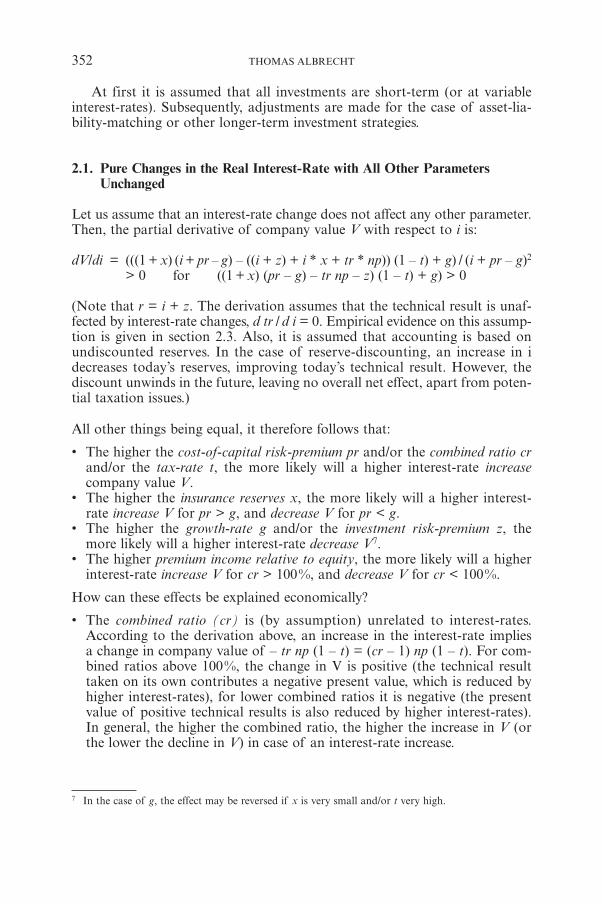
At first it is assumed that all investments are short-term (or at variableinterest-rates). Subsequently, adjustments are made for the case of asset-lia-bility-matching or other longer-term investment strategies.
2.1. Pure Changes in the Real Interest-Rate with All Other ParametersUnchanged
Let us assume that an interest-rate change does not affect any other parameter.Then, the partial derivative of company value V with respect to i is:
dV/di = (((1 + x) (i + pr – g) – ((i + z) + i * x + tr * np)) (1 – t) + g) / (i + pr – g)2
> 0 for ((1 + x) (pr – g) – tr np – z) (1 – t) + g) > 0
(Note that r = i + z. The derivation assumes that the technical result is unaf-fected by interest-rate changes, d tr / d i = 0. Empirical evidence on this assump-tion is given in section 2.3. Also, it is assumed that accounting is based onundiscounted reserves. In the case of reserve-discounting, an increase in idecreases today’s reserves, improving today’s technical result. However, thediscount unwinds in the future, leaving no overall net effect, apart from poten-tial taxation issues.)
All other things being equal, it therefore follows that:
• The higher the cost-of-capital risk-premium pr and/or the combined ratio crand/or the tax-rate t, the more likely will a higher interest-rate increasecompany value V.
• The higher the insurance reserves x, the more likely will a higher interest-rate increase V for pr > g, and decrease V for pr < g.
• The higher the growth-rate g and/or the investment risk-premium z, themore likely will a higher interest-rate decrease V7.
• The higher premium income relative to equity, the more likely will a higherinterest-rate increase V for cr > 100%, and decrease V for cr < 100%.
How can these effects be explained economically?
• The combined ratio (cr) is (by assumption) unrelated to interest-rates.According to the derivation above, an increase in the interest-rate impliesa change in company value of – tr np (1 – t) = (cr – 1) np (1 – t). For com-bined ratios above 100%, the change in V is positive (the technical resulttaken on its own contributes a negative present value, which is reduced byhigher interest-rates), for lower combined ratios it is negative (the presentvalue of positive technical results is also reduced by higher interest-rates).In general, the higher the combined ratio, the higher the increase in V (orthe lower the decline in V) in case of an interest-rate increase.
352 THOMAS ALBRECHT
7 In the case of g, the effect may be reversed if x is very small and/or t very high.

• A higher cost-of-capital risk-premium (pr) makes value increases in case ofhigher interest-rates more likely, as it softens the relative increase of the dis-count rate (with increasing pr, a given absolute change in i implies a smallerpercentage change in d = i + pr – g).
• A higher investment risk-premium (z) has the opposite effect: It lowers therelative increase in investment yield on shareholders’ funds when interest-ratesgo up, as a given change in i implies a smaller percentage change in r = i + z. However, as long as d > r, the present value of the future returnon shareholders’ funds still goes up with increases in i (as the relative increasein the discount rate is still smaller than the relative increase in the investmentyield).
• Future investment income is leveraged by the amount of insurance reserves(x). If the growth-adjusted discount-rate (d = i + pr – g) is higher than theinterest earned on investments (i.e. pr > g), higher interest-rates increase thepresent value of future investment income. This happens because an increasein i has a smaller absolute effect on the discount-rate than on investmentyield.
• The effects of the growth-rate (g) are hardest to discuss. On one hand,growth-related profit retention reduces distributable profits. An increase ini lowers the (negative) present value impact of not being able to distributethose profits. On the other hand, higher growth increases future profits. Inso-far as those future profits are not interest-sensitive, an increase in i lowerstheir present value. If the company is profitable (i.e. return on equity > costof capital), the value of future profits will be higher than the value of requiredprofit retention, thus implying a negative overall effect of higher growth incase of an interest increase. If a company is unprofitable (i.e. technical resultand investment returns are insufficient to finance the profit-retention requiredfor long-term growth), the effect can go into reverse. However, as futureinvestment returns are interest-sensitive, their present value does not decreasewith an interest-rate increase. Thus, higher growth-rates negatively impactvalue sensitivity when interest rates go up, even if a company is unprofitable,except if insurance reserves are very small.
Table 1 shows some parameter constellations that can typically be observed inreal-life situations (the table assumes a tax-rate of 35%).
As can be seen, for combined ratios above 100% an interest-rate increaseonly implies a drop in value in the case of high growth rates. For combinedratios considerably below 100%, however, an interest-rate increase is value-reducing under many realistic sets of parameters: If a company e.g. operateswith a combined ratio of 95%, an interest-rate increase would always be value-reducing, except if the company exhibits high insurance reserves as well as lowgrowth-rates.
The extent of the change in value is especially high, if interest-rates andgrowth-rates are low: If growth is around zero and the interest-rate is 3%,an interest-rate change of only one percentage point changes the value by 10-20%. At g = 0 and i = 2%, di = 0.01 even implies value changes of up to30%.
INTEREST-RATE CHANGES 353
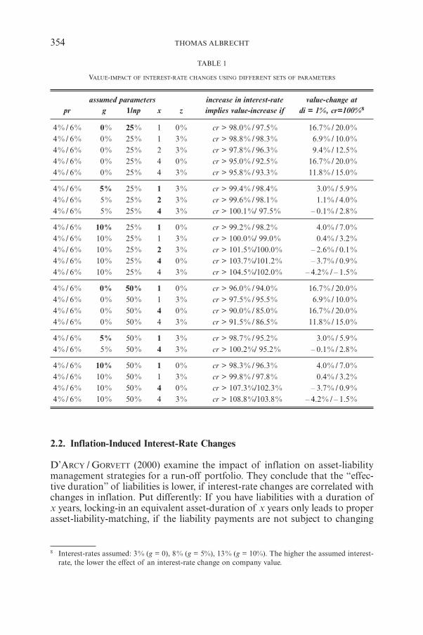
TABLE 1
VALUE-IMPACT OF INTEREST-RATE CHANGES USING DIFFERENT SETS OF PARAMETERS
assumed parameters increase in interest-rate value-change at pr g 1/np x z implies value-increase if di = 1%, cr=100%8
4% / 6% 0% 25% 1 0% cr > 98.0% / 97.5% 16.7% / 20.0%4% / 6% 0% 25% 1 3% cr > 98.8% / 98.3% 6.9% / 10.0%4% / 6% 0% 25% 2 3% cr > 97.8% / 96.3% 9.4% / 12.5%4% / 6% 0% 25% 4 0% cr > 95.0% / 92.5% 16.7% / 20.0%4% / 6% 0% 25% 4 3% cr > 95.8% / 93.3% 11.8% / 15.0%
4% / 6% 5% 25% 1 3% cr > 99.4% / 98.4% 3.0% / 5.9%4% / 6% 5% 25% 2 3% cr > 99.6% / 98.1% 1.1% / 4.0%4% / 6% 5% 25% 4 3% cr > 100.1%/ 97.5% – 0.1% / 2.8%
4% / 6% 10% 25% 1 0% cr > 99.2% / 98.2% 4.0% / 7.0%4% / 6% 10% 25% 1 3% cr > 100.0%/ 99.0% 0.4% / 3.2%4% / 6% 10% 25% 2 3% cr > 101.5%/100.0% – 2.6% / 0.1%4% / 6% 10% 25% 4 0% cr > 103.7%/101.2% – 3.7% / 0.9%4% / 6% 10% 25% 4 3% cr > 104.5%/102.0% – 4.2% / – 1.5%
4% / 6% 0% 50% 1 0% cr > 96.0% / 94.0% 16.7% / 20.0%4% / 6% 0% 50% 1 3% cr > 97.5% / 95.5% 6.9% / 10.0%4% / 6% 0% 50% 4 0% cr > 90.0% / 85.0% 16.7% / 20.0%4% / 6% 0% 50% 4 3% cr > 91.5% / 86.5% 11.8% / 15.0%
4% / 6% 5% 50% 1 3% cr > 98.7% / 95.2% 3.0% / 5.9%4% / 6% 5% 50% 4 3% cr > 100.2%/ 95.2% – 0.1% / 2.8%
4% / 6% 10% 50% 1 0% cr > 98.3% / 96.3% 4.0% / 7.0%4% / 6% 10% 50% 1 3% cr > 99.8% / 97.8% 0.4% / 3.2%4% / 6% 10% 50% 4 0% cr > 107.3%/102.3% – 3.7% / 0.9%4% / 6% 10% 50% 4 3% cr > 108.8%/103.8% – 4.2% / – 1.5%
2.2. Inflation-Induced Interest-Rate Changes
D’ARCY / GORVETT (2000) examine the impact of inflation on asset-liabilitymanagement strategies for a run-off portfolio. They conclude that the “effec-tive duration” of liabilities is lower, if interest-rate changes are correlated withchanges in inflation. Put differently: If you have liabilities with a duration ofx years, locking-in an equivalent asset-duration of x years only leads to properasset-liability-matching, if the liability payments are not subject to changing
354 THOMAS ALBRECHT
8 Interest-rates assumed: 3% (g = 0), 8% (g = 5%), 13% (g = 10%). The higher the assumed interest-rate, the lower the effect of an interest-rate change on company value.
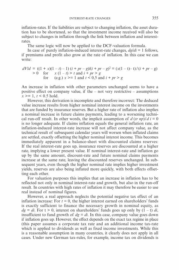
inflation-rates. If the liabilities are subject to changing inflation, the asset dura-tion has to be shortened, so that the investment income received will also besubject to changes in inflation through the link between inflation and interest-rates.
The same logic will now be applied to the DCF-valuation formula.In case of purely inflation-induced interest-rate changes, dg/di = 1 follows,
if premiums and profit also grow at the rate of inflation. In this case we canwrite:
dV/d = ((1 + x)(1 – t) – 1) (i + pr – g)/(i + pr – g)2 = (x(1 – t)– t) / (i + pr – g)> 0 for x (1 – t) > t and i + pr > g
for (e.g.) x >= 1 and t < 0,5 and i + pr > g
An increase in inflation with other parameters unchanged seems to have apositive effect on company value, if the – not very restrictive – assumptions x >= 1, t < 0.5 hold.
However, this derivation is incomplete and therefore incorrect: The deducedvalue increase results from higher nominal interest income on the investmentsthat are funded by insurance reserves. But a higher rate of inflation also impliesa nominal increase in future claims payments, leading to a worsening techni-cal run-off result. In other words, the implicit assumption of d (tr np) /d i = 0is no longer adequate. If claims inflation equals the general inflation rate, aninflation-induced interest-rate increase will not affect company value, as thetechnical result of subsequent calendar years will worsen when inflated claimsare settled, exactly offsetting the higher nominal interest income. This becomesimmediately apparent in a balance-sheet with discounted claims reserves:If the real interest-rate goes up, insurance reserves are discounted at a higherrate, implying a lower present value. If nominal interest-rate and inflation goup by the same amount, discount-rate and future nominal claims paymentsincrease at the same rate, leaving the discounted reserves unchanged. In sub-sequent years, even though the higher nominal rate implies higher investmentyields, reserves are also being inflated more quickly, with both effects offset-ting each other.
For valuation purposes this implies that an increase in inflation has to bereflected not only in nominal interest-rate and growth, but also in the run-offresult. In countries with high rates of inflation it may therefore be easier to usereal instead of nominal figures.
However, a real approach neglects the potential negative tax effect of aninflation increase: For t = 0, the higher interest earned on shareholders’ fundsis exactly sufficient to finance the necessary growth in nominal equity, as dg = di. For t > 0, interest on shareholders’ funds goes up only by (1 – t) di,insufficient to fund growth of dg = di. In this case, company value goes downif inflation goes up. However, the effect depends on the exact tax regime in place(this paper assumes a corporate tax rate and an additional income tax-ratewhich is applied to dividends as well as fixed income investments. While thisis a reasonable assumption in many countries, it clearly does not apply in allcases. Under new German tax-rules, for example, income tax on dividends is
INTEREST-RATE CHANGES 355
lower than on fixed income, with potential implications for the after-tax cost-of-capital calculation).
2.3. Correlation Between Interest-Rate Changes and Insurance Profit
So far it was assumed that interest-rate changes do not affect other parameters:Neither did we assume a correlation with equity returns on the investmentside, nor a correlation with the technical insurance result.
It is frequently argued that an increase in interest-rates has a negative effecton share prices, as future cash-flows are discounted more steeply9. Strictlyspeaking this only holds for changes in the real interest-rate (not for purelyinflation-induced interest-rate changes), and only if an increase in the realinterest-rate is not correlated with an increase in the future real profit potential.As argued in ALBRECHT (1999a, p. 127ff.), there is (ambiguous) evidence forsuch a correlation, so the relationship is less clear than it may seem at firstglance.
However, a rough look at empirical data seems to validate the negativecorrelation between (nominal) interest-rates and share-prices: For the years1981-99, the correlation between yearly returns of the German DAX and theGerman money market yield was – 0.31. The change in the money marketyield was also negatively correlated with the DAX-return, at – 0.2110.
The technical result may also be correlated with the interest-rate: If indus-try participants think that higher interest-rates imply an improvement in thefinancial result, they might be tempted to increase the competitive pressureon rates (PANNING (1995), DICKINSON (2000)). In this case, an interest-rateincrease should be correlated with a worsening technical result (a higher lossratio).
The yearly loss ratios of German non-life insurers for the years 1966-9911
are positively correlated with the money-market yield (+0.30). Using firstdifferences (i.e. changes in the interest-rate correlated with changes in the lossratios), the positive correlation persists (not lagged: +0.18; lagged one year:+0.24).
The correlation differs considerably between lines of business, however:While (e.g.) fire and transport had high positive correlations (+0.54 and+0.38), liability and accident showed negative correlations (– 0.49 and – .45).
Within the scope of this article, a detailed quantification of correlationeffects shall not be attempted. For example, some of the correlations listedabove might simply be spurious. However, it should be clear from the rough
356 THOMAS ALBRECHT
9 See e.g. D’ARCY / GORVETT (2000), p. 396.10 DAX-return taken from GDV, table 100. Money-market yield from ALBRECHT (1999a), app. A 2.1.
Similarly, ALBRECHT (1998), p. 263, reports a positive correlation between DAX and REX in theperiod 1988-96. As REX is a fixed-income performance-index, higher interest-rates imply lowerindex-values. Consequently, a positive correlation between DAX and REX indicates a negative cor-relation between DAX and the general level of interest-rates.
11 Source: GDV (several tables). Money-market yield from ALBRECHT (1999a), app. A 2.1.
calculations performed above that correlations may have a major impact andmerit further study.
2.4. Effect of Asset Liability Matching and Other Investment Strategies
If fixed-income investments are chosen to mature according to the expected tim-ing of claims payments, the average term to maturity of the portfolio willdepend on the ratio of reserves to premium income. If the payment structureis constant over time and the portfolio does not grow, claims reserves equalingyearly claims imply a medium payment period of 6 months. In the case ofunearned premiums, the average payment period is also 6 months, if contractsare spread evenly over time with yearly renewal12.
The value-effect of such an investment strategy in the case of an interest-rate change can be approximated via the change in present value of a fixedinterest payment over the average payment period. The present value of fixed-income investments (excluding reinvestment risk, i.e. assuming zero-bond invest-ments) can be approximated as13:
Present Value (in % of company equity) = x (1 + if (1 – t))m / (1 + i + pr)m
with: if fixed interest-ratem average duration of insurance reserves
Table 2 shows some examples for value changes (in % of equity)14:
TABLE 2
CHANGE IN INTEREST-SENSITIVITY WHEN INVESTMENTS ARE MATCHED WITH LIABILITIES
claims reserves claims unearned pr. equity – > equals value effect of% of claims ratio % of net pr. % of net pr. x m di = 0,01
40% 50% 50% 25% 2.8 0.41 – 1.0%100% 50% 50% 25% 4.0 0.50 – 1.8%100% 50% 50% 50% 2.0 0.50 – 0.9%200% 50% 50% 50% 3.0 0.83 – 2.2%300% 50% 50% 50% 4.0 1.25 – 4.2%
INTEREST-RATE CHANGES 357
12 Assuming a stagnant portfolio, 1/12 of unearned premiums will be earned in 12 months’ time, 1/12in 11 months, etc. On average, the unearned premiums on the balance-sheet at any point in time willtherefore remain for 6 months. If the portfolio is growing, a larger part of unearned premiums willbe earned in later months, implying a longer average duration than 6 months.
13 Calculation excludes investments backed by shareholders’ funds. It may be argued that the discount-rate should not include the full risk-premium pr, as the fixed-income portfolio in itself is not subjectto the full company risk. However, omitting pr hardly affects the interest-sensitivities.
14 For if = i = 0.05, pr = 0.04 und t = 0.35. Changes in pr and t have no major effect on the result.
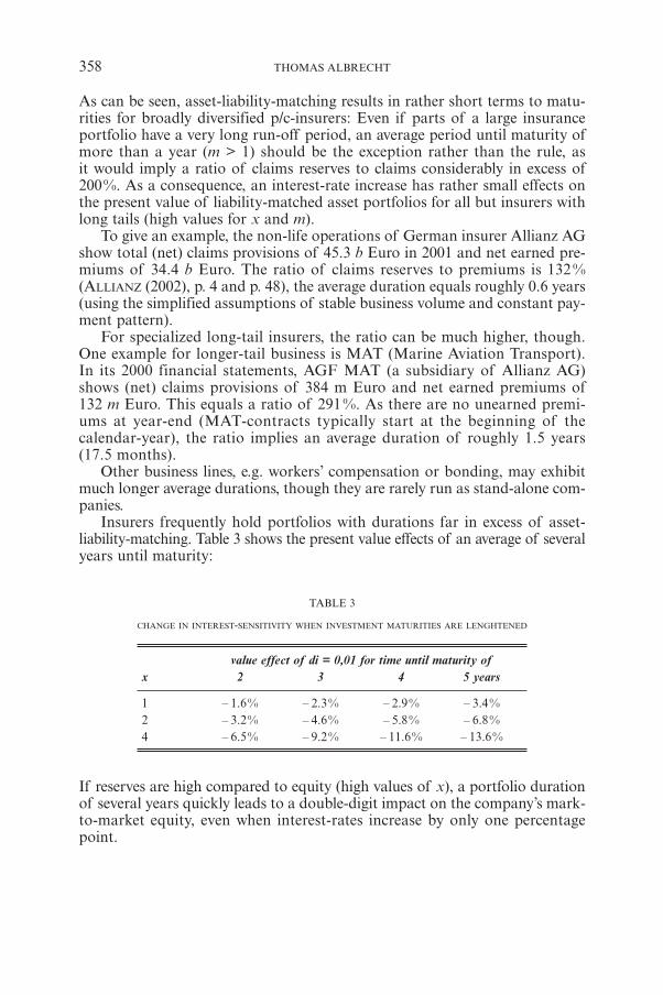
As can be seen, asset-liability-matching results in rather short terms to matu-rities for broadly diversified p/c-insurers: Even if parts of a large insuranceportfolio have a very long run-off period, an average period until maturity ofmore than a year (m > 1) should be the exception rather than the rule, asit would imply a ratio of claims reserves to claims considerably in excess of200%. As a consequence, an interest-rate increase has rather small effects onthe present value of liability-matched asset portfolios for all but insurers withlong tails (high values for x and m).
To give an example, the non-life operations of German insurer Allianz AGshow total (net) claims provisions of 45.3 b Euro in 2001 and net earned pre-miums of 34.4 b Euro. The ratio of claims reserves to premiums is 132 %(ALLIANZ (2002), p. 4 and p. 48), the average duration equals roughly 0.6 years(using the simplified assumptions of stable business volume and constant pay-ment pattern).
For specialized long-tail insurers, the ratio can be much higher, though.One example for longer-tail business is MAT (Marine Aviation Transport).In its 2000 financial statements, AGF MAT (a subsidiary of Allianz AG)shows (net) claims provisions of 384 m Euro and net earned premiums of132 m Euro. This equals a ratio of 291%. As there are no unearned premi-ums at year-end (MAT-contracts typically start at the beginning of thecalendar-year), the ratio implies an average duration of roughly 1.5 years(17.5 months).
Other business lines, e.g. workers’ compensation or bonding, may exhibitmuch longer average durations, though they are rarely run as stand-alone com-panies.
Insurers frequently hold portfolios with durations far in excess of asset-liability-matching. Table 3 shows the present value effects of an average of severalyears until maturity:
TABLE 3
CHANGE IN INTEREST-SENSITIVITY WHEN INVESTMENT MATURITIES ARE LENGHTENED
value effect of di = 0,01 for time until maturity ofx 2 3 4 5 years
1 – 1.6% – 2.3% – 2.9% – 3.4%2 – 3.2% – 4.6% – 5.8% – 6.8%4 – 6.5% – 9.2% – 11.6% – 13.6%
If reserves are high compared to equity (high values of x), a portfolio durationof several years quickly leads to a double-digit impact on the company’s mark-to-market equity, even when interest-rates increase by only one percentagepoint.
358 THOMAS ALBRECHT
3. CASE-STUDIES ON THE TOTAL EFFECT OF INTEREST-RATE CHANGES
As discussed, different sets of parameters will imply very different reactions ofcompany value to interest-rate changes. This chapter intends to give examplesof companies that are quite susceptible or less susceptible to interest-raterisk15.
Non-company-specific parameters used throughout are i = 0.05, pr = 0.04and t = 0.35.
Company A is a retail insurer with a high franchise value (low combined ratio,high growth rate). Parameters are as follows: cr = 0.95, g = 0.05 x = 4,np = 4, z = 0.
According to the DCF-valuation formula, A’s appraisal value is 6.06 times equity.Assuming short-term investments, an interest-rate increase of di = 0.01 impliesa new value of 5.50 times equity, i.e. a drop in value of 9%.
If A had opted for a long-term investment strategy (m = 5 years), valuewould have dropped by a further 0.14 times equity, i.e. the total interest-relateddrop would have been 12%. Compared to total company value, the effect ofthe investment strategy is small, as A’s franchise value is far in excess of equity.Nevertheless, long-term investments increase A’s sensitivity to interest-ratechanges.
The effect occurs irrespective of tail: If A is assumed to have a much longertail, interest-rate increases still imply a drop in value with short-term invest-ment strategies, and a bigger drop with longer-term investments.
Company B is considerably less profitable, but also boasts a high growth-rate. Parameters are: cr = 1.02, g = 0.05, x = 4, np = 4, z = 0.
B’s appraisal value is 1.51 times equity. Assuming short-term investments,di = 0.01 implies a new value of 1.86 times equity, i.e. an increase in value of23%.
If B had opted for a long-term investment strategy (m = 5 years), the neg-ative value-impact would again have been 0.14 times equity. Total value afterthe interest-change would then be 1.72 times equity, an increase of 14% com-pared to the initial value.
For B, a long-term investment portfolio actually decreases the interest-sensitivity of the company’s appraisal value, even though B is not a long-tailinsurer. This happens because the future profits of the company are earnedthrough investment income, while the technical result is negative. The higherinvestment income overcompensates the higher discount-rate for the parame-ters chosen.
B has a second option to lower its interest-sensitivity: It can increase theportion of equity that is invested in risky assets (e.g. stocks): Assuming e.g. z = 0.03, di = 0.01 only increases company value by 13% (short term
INTEREST-RATE CHANGES 359
15 Unless otherwise mentioned, only changes in the real rate are considered.
investments) / 6% (long-term investments). This happens because the addi-tional expected return (z) is assumed to accrue irrespective of interest-rateincreases. A higher interest-rate lowers the present value of the risk-premiumearned, another counter-cyclical effect on B’s value.
Company C is a long-tail industrial insurer with low profitability (high com-bined ratio) and low growth perspectives. Parameters are: cr = 1.1, g = 0,x = 8, np = 3, z = 0.
C’s appraisal value is 1.08 times equity. Assuming short-term investments,di = 0.01 implies a new value of 1.56 times equity, i.e. an increase in value of44%.
For C, the higher investment earnings on the long tail more than over-compensate the lower present value of future profits (which is assumed to below anyway). However, for such an insurer, the higher profitability caused byhigher interest-earnings is likely to spark more aggressive competition on rates,thus increasing long-term combined ratios – an effect not covered by applyingthe formula on a ceteris paribus basis.
If C had opted for a long-term investment strategy (m = 5 years), the neg-ative value-impact would have been 0.27 times equity. Total value after theinterest-change would then be 1.29 times equity, still a 19% increase comparedto the initial value. Again, as with B, long-term investments decrease the inter-est-sensitivity of C’s value.
The examples discussed above illustrate the limitations of PANNING’s (1995)analysis: PANNING argues that the duration of investments should generallybe lengthened to counter-balance the interest-sensitivity of future busi-ness value16. In his analysis, future business value has a negative duration(i.e. the value increases when interest-rates go up), because the durationof future losses is higher than the duration of future premiums. However,this only holds under his non-general assumption of break-even premiums.For sufficiently profitable companies (like company A), the effect goes intoreverse.
What would have happened to A, B and C in the case of inflation-inducedinterest-rate changes? Assuming that a change in inflation does not affect theunderlying profitability of the insurance business17, and also neglecting potentialtax-effects, the only effect of such an interest-rate change would be on the pre-sent value of longer-term fixed-income investments. The higher the inflation-risk, the higher the value sensitivity of longer-term investments. This serves tomake longer-term investments less attractive, irrespective of company charac-teristics. Companies A, B and C should all lower their investment durations ifinflation-uncertainty increases.
360 THOMAS ALBRECHT
16 Assuming – as is done here – that future premiums are fixed, i.e. not interest-sensitive.17 The extensive literature on the effect of inflation on business profitability cannot be discussed here
due to space constraints. However, it can be argued that the results are quite inconclusive.
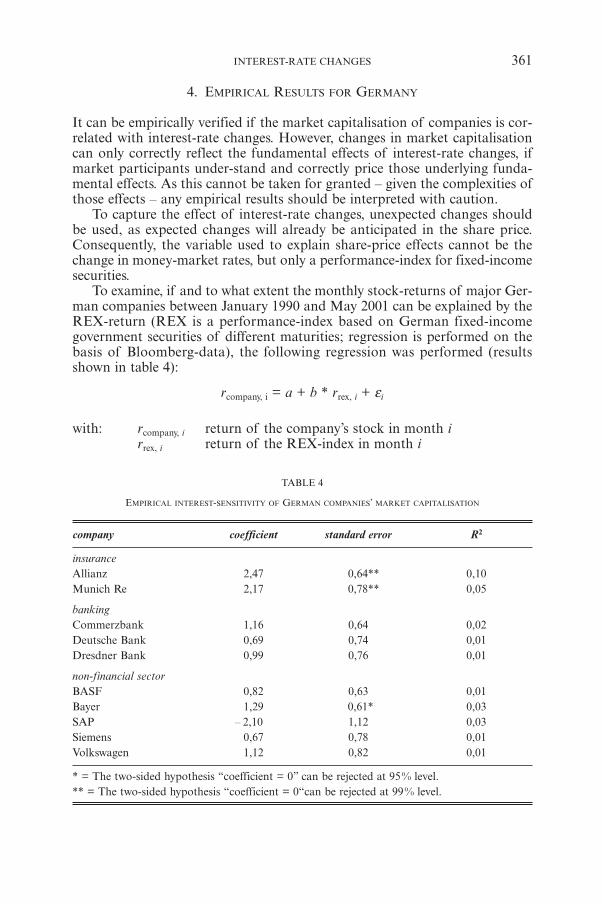
4. EMPIRICAL RESULTS FOR GERMANY
It can be empirically verified if the market capitalisation of companies is cor-related with interest-rate changes. However, changes in market capitalisationcan only correctly reflect the fundamental effects of interest-rate changes, ifmarket participants under-stand and correctly price those underlying funda-mental effects. As this cannot be taken for granted – given the complexities ofthose effects – any empirical results should be interpreted with caution.
To capture the effect of interest-rate changes, unexpected changes shouldbe used, as expected changes will already be anticipated in the share price.Consequently, the variable used to explain share-price effects cannot be thechange in money-market rates, but only a performance-index for fixed-incomesecurities.
To examine, if and to what extent the monthly stock-returns of major Ger-man companies between January 1990 and May 2001 can be explained by theREX-return (REX is a performance-index based on German fixed-incomegovernment securities of different maturities; regression is performed on thebasis of Bloomberg-data), the following regression was performed (resultsshown in table 4):
rcompany, i = a + b * rrex, i + εi
with: rcompany, i return of the company’s stock in month irrex, i return of the REX-index in month i
TABLE 4
EMPIRICAL INTEREST-SENSITIVITY OF GERMAN COMPANIES’ MARKET CAPITALISATION
company coefficient standard error R2
insuranceAllianz 2,47 0,64** 0,10Munich Re 2,17 0,78** 0,05
banking Commerzbank 1,16 0,64 0,02Deutsche Bank 0,69 0,74 0,01Dresdner Bank 0,99 0,76 0,01
non-financial sector BASF 0,82 0,63 0,01Bayer 1,29 0,61* 0,03SAP – 2,10 1,12 0,03Siemens 0,67 0,78 0,01Volkswagen 1,12 0,82 0,01
* = The two-sided hypothesis “coefficient = 0” can be rejected at 95% level.** = The two-sided hypothesis “coefficient = 0“can be rejected at 99% level.
INTEREST-RATE CHANGES 361
With the exception of SAP, the coefficient of the REX-return is positive in allcases, i.e. an increase of REX (a decrease in the return of fixed-income secu-rities) tends to imply an increase in share prices. However, for banks as well asnon-financial companies, the standard error is nearly as high as the coefficient,and R2 is practically zero. The only exception are the two insurers Allianz andMunich Re: The standard error is low relative to the coefficient, and R2 impliesan explanatory content of 5% and 10% of total share-price variance. This maysound low at first glance, but given the multitude of effects that influence share-prices, a higher explanatory content of interest-rate changes alone cannot plau-sibly be expected.
The result of this – rather rough and superficial – empirical analysis is thatinterest-rate changes do not in general have a strong effect on the marketcapitalisation of German companies. However, interest-rate increases do havea discernible (negative) impact on the market capitalisation of German insur-ance companies.
So is this in line with the theoretical analysis?
The financial statements of Allianz AG for the financial year 2000 show lend-ings and fixed-income securities of 189 b Euro, of which 91 b Euro with aremaining term to maturity of more than 5 years. Roughly 2/3 of investmentsare linked to life/health-business, where the bulk of investment income is passedon to policyholders. Assuming proportional allocation, roughly 60 b Euro oftotal investments – of which 30 b Euro with a remaining term to maturity ofmore than 5 years – should directly affect company value. It therefore soundsplausible to assume an average term to maturity of 5 years for the 60 b Euroin total investments. If we compare this to the company’s equity of 35 b Euro,the result is roughly x = 2, implying a negative value effect of –3.8% if inter-est-rates go up by one percentage point. At the same time, the base-effect ofan interest-rate increase (as discussed in 2.1) should be close to zero in the caseof Allianz AG, if we assume pr = 0.04, x = 2, cr around 1.00, and g = 0.05 orless. Finally, the market may expect a negative correlation between interest-rates and technical insurance-results. In total, the theoretical effect of an interest-rate increase on the value of Allianz AG may therefore truly be negative, justlike the empirical results indicate.
However, the empirical results can only be interpreted with great caution, asmulti-national companies like Allianz and Munich Re will not only be affectedby changes in German interest-rates, but by other countries’ interest-rates aswell. Furthermore, as those companies also write life and health-business, theymight be subject to other effects which are not covered by this analysis.
5. CONCLUSIONS
Without a doubt the analytical model developed in this paper is simplified inseveral respects. To give just one example, it could be explicitly modelled that
362 THOMAS ALBRECHT
interest-rate changes are not identical over the whole yield-curve, but insteadtend to be less pronounced for long maturities18.
Nevertheless, the analysis leads to some general conclusions. Specifically, itwas shown that a change in the interest-rate can affect the value of a non-lifeinsurance company positively as well as negatively, depending on the underly-ing parameters:
If the investments are predominantly long-term (more than would be thecase for mere asset-liability-matching) and average combined ratios compara-tively low, a value reduction in case of increasing interest-rates is likely. Thiseffect seems to dominate for the German insurers Allianz and Munich Re.
However, there is no reason to generalize this result: Companies / portfolioswith low expected growth-rates, combined ratios around or above 100% and/ora comparatively short-term investment portfolio will on the contrary experiencean increase in fundamental DCF-value if the market interest-rate goes up.
The effects of an interest-rate change on company value can be summarizedas follows:
• An increase in the real interest-rate can affect company value positively ornegatively, depending on the underlying parameters. The different effectson company value are:1. A lower present value of run-off claims (→ increases value).2. A lower present value of existing fixed-income securities (→ lowers value).3. A lower present value of technical profits earned from future insurance
business (combined ratio < 100%) or of deficits incurred (combined ratio> 100%) (→ increases or lowers value, depending on the combined ratio).In addition, if the combined ratio worsens because rising interest-ratesincrease the competitive pressure, this will negatively affect the present value.
4. A lower or higher present value of investment income in connectionwith future business (the lower the growth-rate of future business, andthe higher the risk- premium in the discount-rate, the more likely will ahigher interest-rate imply a higher present value of future investmentincome from future reserves).
• On the other hand, an increasing rate of inflation (with a correspondingrise in the nominal interest-rate) does not influence company value in a worldwithout taxes – provided investments are short-term/variable rate – becausehigher interest-income will be compensated by higher nominal claims pay-ments and a higher discount-rate for future profits (although it is possiblethat an increase in inflation may have consequences on real parameters andtherefore company value). Longer-term fixed-income investments, however,imply a decrease in company value in case of an interest-rate increase, asclaims inflation will not be compensated by higher investment returns untilinvestments are reinvested after maturity. A further decrease in value results
INTEREST-RATE CHANGES 363
18 This follows from the market participants’ expectations of future interest-rate changes. See LEVIN (1996),ANKER (1993) or ALBRECHT (1999a). The simple assumption of a parallel shift in the yield-curve, as usedin this paper, implies an over-estimation of long-term effects in section 2.1 relative to section 2.4.
from taxation effects under the tax regime assumed in this paper (thoughother tax regimes may have different effects).
REFERENCES
ALBRECHT, T. (2001) Discounted-Cash-Flow Bewertung bei Sachversicherungsunternehmen,Finanz Betrieb 5/2001, p. 302-307.
ALBRECHT, T. (1999a) Die Wahl der Zinsbindungsdauer, Hamburg.ALBRECHT, T. (1999b) Asset Allocation und Zeithorizont, Bad Soden/Ts.ALBRECHT, T. (1998) Die Vereinbarkeit der Value-at-Risk-Methode in Banken mit anteils-
eignerorientierter Unternehmensführung, Zeitschrift für Betriebswirtschaft 68, 259-273AGF MAT (2001) Annual Report 2000.ALLIANZ GROUP (2001, 2002) Group Financial Statements 2000, 2001ANKER, P. (1992) Zinsstruktur und Zinsprognose, Giessen.BABBEL, D.F. (1995) Asset-Liability Matching in the Life-Insurance Industry, The Financial Dyn-
mics of the Insurance Industry, Altman and Vanderhoof (eds.), Chapter 11.CAMPBELL, F. (1997) Asset/Liability Management for Property/Casualty Insurers, The Handbook
of Fixed Income Securities, Fabozzi (ed.), Chapter 51.CASUALTY ACTUARIAL SOCIETY (1999) Overview of Dynamic Financial Analysis, website of the
Casualty Actuarial Society, www.casact.org/research/dfa.COPELAND, T., KOLLER, T. and MURRIN, J. (2000) Valuation, 3rd Edition, New York (et al.)D’ARCY, S. and GORVETT, R. (2000) Measuring the Interest Rate Sensitivity of Loss Reserves,
Proceedings of the Casualty Actuarial Society, 87, 365-400.D’ARCY, S., GORVETT, R., HERBERS, J. and HETTINGER, T. (1997) Building a DFA Analysis Model
that Flies, Contingencies Magazine, Nov./Dec. 1997, reprinted on the website of the Casu-alty Actuarial Society, www.casact.org/coneduc/specsem/98dfa/dfamodel.htm.
DRUKARCZYK, J. (1998) Unternehmensbewertung, 2nd Edition, München.GDV (2001) Statistisches Taschenbuch der Versicherungswirtschaft 2000, download from www.
gdv.de.HARTUNG, T. (2000) Unternehmensbewertung von Versicherungsgesellschaften, WiesbadenHOLSBOER, J. H. (2000) The Impact of Low Interest Rates on Insurers, Geneva Papers on Risk
and Insurance, 25, 38-58.LEVIN, F. (1996) Die Erwartungstheorie der Zinsstruktur, Frankfurt/M.PANNING, W.H. (1995) Asset-Liability Management for a Going Concern, The Financial Dynam-
ics of the Insurance Industry, Altman and Vanderhoof (eds.), Chapter 12.SIGLIENTI, S. (2000) Consequences of the Reduction of Interest Rates on Insurance, Geneva
Papers on Risk and Insurance, 25, 63-77.STAKING, K. and BABBEL, D. (1995) The Relation Between Capital Structure, Interest Rate Sen-
sitivity, and Market Value in the Property-Liability Insurance Industry, Journal of Risk andInsurance, 62, 690-718.
SWISS RE (2001) Rentabilität der Nichtleben-Versicherungswirtschaft: Zurück zum Underwriting,Sigma 5/2001, Zürich.
DR. THOMAS ALBRECHT
Treffauerstr. 38D-81373 Mü[email protected]. +49 89 3800 7481Fax +49 89 3800 19422
364 THOMAS ALBRECHT
FAVORABLE ESTIMATORS FOR FITTING PARETO MODELS:A STUDY USING GOODNESS-OF-FIT MEASURES WITH ACTUAL DATA
BY
VYTARAS BRAZAUSKAS1, ROBERT SERFLING2
ABSTRACT
Several recent papers treated robust and efficient estimation of tail index para-meters for (equivalent) Pareto and truncated exponential models, for large andsmall samples. New robust estimators of “generalized median” (GM) and“trimmed mean” (T) type were introduced and shown to provide more favor-able trade-offs between efficiency and robustness than several well-establishedestimators, including those corresponding to methods of maximum likelihood,quantiles, and percentile matching. Here we investigate performance of theabove mentioned estimators on real data and establish — via the use of good-ness-of-fit measures — that favorable theoretical properties of the GM and Ttype estimators translate into an excellent practical performance. Further, wearrive at guidelines for Pareto model diagnostics, testing, and selection of par-ticular robust estimators in practice. Model fits provided by the estimators areranked and compared on the basis of Kolmogorov-Smirnov, Cramér-von Mises,and Anderson-Darling statistics.
1. INTRODUCTION AND PRELIMINARIES
A single-parameter Pareto distribution plays a very significant role in actuarialmodeling because of its conceptual simplicity and ease of applicability in prac-tice. The cdf of the Pareto P(s,�) model is given by
F(x) = 1 – (s/x)�, x > s, (1)
where � > 0 is the shape parameter that characterizes the tail of the distributionand s > 0 is the scale parameter. When s is assumed known, the P(s,�) modelis called a single-parameter Pareto model. The assumption of s known is quitetypical in the actuarial literature because, as for example Philbrick (1985) states,“although there may be situations where this value must be estimated, in vir-tually all insurance applications this value will be selected in advance.” (See alsodiscussion by Rytgaard (1990).)
1 Supported by a grant from the Actuarial Education and Research Fund.2 Supported by grants from the Casualty Actuarial Society and Society of Actuaries, with administra-
tive support from the Actuarial Education and Research Fund, and by NSF Grant DMS-0103698.
ASTIN BULLETIN, Vol. 33, No. 2, 2003, pp. 365-381
In several recent papers Brazauskas and Serfling (2000a,b; 2001) treatedrobust and efficient estimation of the tail index � for various setups: for large-and small-samples and for one- and two-parameter models (corresponding tos known or unknown). Developments presented there utilized a well-knownequivalence relation between model (1) and the truncated exponential distribu-tion E(m,q) having cdf
G(z) = 1 – e –(z–m) /q, z > m, (2)
for q > 0 and –∞ < m < ∞. Specifically, if random variable X has cdf F given by(1) then variable Z = logX has cdf G given by (2), with m = log s and q = �–1.
In large-sample studies, for example, new robust estimators of “generalizedmedian” (GM) type were introduced and “trimmed mean” (T) type estimatorswere adapted from the E(m,q) model literature. These estimators were thencompared with the maximum likelihood, quantile type, percentile matching, andother estimators. Using as efficiency criterion the asymptotic relative efficiency(ARE) with respect to the maximum likelihood estimator (MLE) and as robust-ness criterion the breakdown point (BP) (this is defined in Section 1.2), the GMtype was seen to dominate all competitors, with the T type second best. Froma practical point of view, the ARE is equivalent to the accuracy of the estimatorand can be interpreted in terms of the length of the confidence interval (seeSection 1.3 for precise discussion).
In the present paper we investigate performance of the above mentioned esti-mators on real data and establish — via the use of goodness-of-fit measures —that favorable theoretical properties of the GM and T type estimators trans-late into an excellent practical performance. The goodness-of-fit measures,defined in Section 1.1, are used here for two purposes: (i) to (formally) test theappropriateness of the estimated Pareto model for a particular data set when� is estimated by the MLE (this is defined in Section 1.3), and (ii) to evaluateand compare Pareto fits when various estimators (not only the MLE) of � areemployed.
In the actuarial literature the issue of goodness-of-fit is addressed througha combination of informal methods and formal statistical tests. Most informaltechniques are based on the difference (absolute or relative) between the fittedand empirical values of relevant quantities, such as the number of claims orexpected value of claims for different claim layers. Additionally, for the Paretomodel in particular, comparisons of �̂ with a typical value of � for the sameinsurance line of the entire industry are also used in the literature. (See Patrick(1980), Philbrick (1985), and Reichle and Yonkunas (1985).) Regarding formalapproaches, tests based on Kolmogorov-Smirnov (KS) and x2 statistics seem tohave a leading role (see, e.g., Philbrick and Jurschak (1981)). More extensivediscussion on model validation principles is available in Klugman, Panjer, andWillmot (1998), Section 2.9.
As is well-known in the statistical literature (e.g., D’Agostino and Stephens(1986), p. 110), the x2 test is less powerful than tests based on the empirical cdf.Therefore, here we use three widely popular goodness-of-fit measures which arebased on the empirical cdf — the above-mentioned KS statistic, the Cramér-von Mises (CvM) statistic, and the Anderson-Darling (AD) statistic. All these
366 VYTARAS BRAZAUSKAS AND ROBERT SERFLING
statistics (though emphasizing different aspects of discrepancy) measure the dis-tance in some sense between the fitted model cdf F and the empirical cdf Fn.Thus estimators that lead to smaller values of these statistics are preferable.
The paper is organized as follows. First, in Section 2, we define preciselyseveral estimators for the parameter � in (1). Next, in Section 3, the data setsare introduced, a method for data de-grouping is described, and preliminarydata visualization and diagnostic tools are applied to the sets. Finally, compar-isons and conclusions are presented in Section 4. Also, in Section 4.2, we arriveat guidelines for Pareto model diagnostics, testing, and selection of particularrobust estimators in practice.
In the remainder of this introduction, we formulate precisely our perfor-mance criteria.
1.1. Goodness-of-Fit Measures
Let us consider a sample X1,…,Xn and denote the ordered sample values byX(1) ≤ X(2) ≤ … ≤ X(n) and the empirical cdf by
in ( ) , < < .F x n X x x11
i
n
1
3 3#= -=
! " ,
Also, for an estimator �̂ , let F(X( j)) denote the probability assigned to X( j) bythe model P (s, �̂ ), for j = 1,…,n. Note that Fn(X( j)) = j /n, for j = 1,…,n. Thegoodness of fit statistics are then defined as follows.
The KS statistic Dn:
( ) ( )j jn n
n n
( ) , ( ) ,
, .
max max
max
D nj
X D X nj
D D D
F F 1
j n j n
n
1 1= - = -
-
=
# # # #
+ -
+ -
d dn n
$ .
The CvM statistic W 2n :
( )jn ( ) .W X nj
nF2
2 1121
j
n2
2
1
= --
+=
! d n
The AD statistic A2n :
( ) ( )j jn ( ) ( ) ( ) ( ) .log logA n n j X n j XF F12 1 2 1 2 1
j
n2
1
= - - - + + - -=
! ` `j j$ .
When the parameter � is estimated by �̂ML, critical values and formulas forsignificance levels for the statistics Dn, W 2
n , and A2n are available in D’Agostino
FAVORABLE ESTIMATORS FOR FITTING PARETO MODELS 367
and Stephens (1986), Tables 4.11 and 4.12, pp. 135-136. Actually, the resultsdeveloped there are for the model E(m,q) but, due to the equivalence relationbetween (1) and (2), they can also be directly applied to the model P(s,�).
1.2. Robustness Criterion: Breakdown Point
A popular and effective criterion for robustness of an estimator is its break-down point (BP), loosely characterized as the largest proportion of corruptedsample observations that the estimator can cope with. In other words, theBP of an estimator measures the degree of resistance of the estimator to theinfluence of outlying observations which possibly (but not necessarily) representcontamination of a data set rather than merely unusually extreme observationsgenerated by the target parametric model.
Brazauskas and Serfling (2000a,b) considered two types of contamination— upper and lower contamination — and, consequently, defined separate ver-sions of BP:
Lower (Upper) Breakdown Point (LBP/UBP): the largest proportion of lower(upper) sample observations which may be taken to a lower (an upper) limitwithout taking the estimator to a limit not depending on the parameter beingestimated.
For modeling insurance loss data, however, contamination of the lower typeis of lesser concern because the lower limit of losses is usually pre-defined bya contract. (For example, the lower limit can be represented as a deductible.)Thus, in the present treatment we favor estimators which have nonzero UBP.
1.3. Efficiency Criterion: Variance
If sample observations follow the postulated parametric model, then it is well-known that, for large data sets, the MLE attains (in its approximating normaldistribution) the minimum possible variance among a large class of compet-ing estimators. Therefore, it can be regarded as a quantitative benchmark forefficiency considerations. In particular, for the model P(s,�) with s known, theMLE of � is readily derived in Arnold (1983), and given by
ii 1= /.
log Xn
snML =a!
t^ h
Its exact distribution theory is described by the statement that
n2
MLaa
t has cdf x 22n ,
where x2n denotes the chi-square distribution with n degrees of freedom. This
implies that �̂ML is a biased estimator of �, but multiplication by the factor(n – 1)/n yields an unbiased version,
368 VYTARAS BRAZAUSKAS AND ROBERT SERFLING
ii 1= /.
lognn
Xn
s1 1
nMLU ML=-
=-a a
!t t
^ h
For further details on exact distribution theory of �̂ML see Rytgaard (1990).Following techniques in Brazauskas and Serfling (2000a,b), it can be shown
that for large sample size n, �̂MLU is approximately normal with mean � and vari-ance �2/n. Moreover, other competing estimators �̂ for � considered here areapproximately normal with mean � and variance c�2/n for some constant c > 1and large n. This means that confidence intervals for the parameter � based onthe competing estimators will be c times wider than those based on the MLU.Such optimal precision of the MLU, however, is achieved at the price of robust-ness, which becomes crucial when the actual data departs from the assumed para-metric model. Hence, the MLU is most efficient but is nonrobust with UBP = 0.
2. THE ESTIMATORS
The MLE and MLU were given in Section 1.3. Here we introduce the othermethods considered in this study for estimation of the parameter �. In particu-lar, we present quantile, trimmed mean, and generalized median type estima-tors. For further details and discussion see Brazauskas and Serfling (2000a,b).
2.1. Quantile Type Estimators
Quantile type estimators of � are completely unaffected by additional informa-tion about s. For this reason and for compatibility with the existing literature,we describe this approach here for the case when s is treated as an unknownnuisance parameter.
Quantile estimators based on k ≥ 2 (selected) quantile levels 0 < p1 < …<pk < 1 are defined as follows:
,
/ ,
log
exp log
b X
X u
i npi
k
np
Q
Q Q
1
1
1
i
1
=
= -
a
v a
=
-
!t
t t
]e
]
go
g% /
]
]
g
g
with
,
, ,
,
b L e eu u
b L e eu u
e eu u
i k
b L e eu u
1
12 1
1
u u
i u ui i
u ui i
k u uk k
12 1
1 1
1
i i i i
2 1
1 1
1
# #
= --
-
=-
--
-
--
=-
-
- +
-
- +
-k k
< F
FAVORABLE ESTIMATORS FOR FITTING PARETO MODELS 369
and
,L e eu u
u ui i
i
k1
2
2i i 1
=-
- -
=-
! ^ h
where ui = – log(1 – pi), 1 ≤ i ≤ k, and x denotes the least integer ≥ x. Suchestimators were introduced and studied for the Pareto problem by Quandt(1966) for k = 2 and by Koutrouvelis (1981) for general k ≥ 2.
Choosing the minimum of the determinant of the asymptotic covariancematrix of the estimators of s and � as an optimality criterion, Koutrouvelis(1981) found that the optimal choice of p1 is always
p°1 = . ,n 0 51
+
and the remaining optimal quantile levels p°2, …, p°k are:
• For k = 2, take p°2 = 1 – (1 – p°1)e –1.5936 ≈ .80.
• For k = 5, take p°2 = 1 – (1 – p°1 )e – 0.6003 ≈ .45, p°3 = 1 – (1 – p°1 )e –1.3544 ≈ .74,p°4 = 1 – (1 – p°1)e –2.3721 ≈ .91, and p°5 = 1 – (1 – p°1)e – 3.9657 ≈ .98.
We denote the optimal estimators of � by �̂Qopt,k. We also consider a nonoptimal
case (denoted by �̂Q* ):
• For k = 5, take p1 = .13, p2 = .315, p3 = .50, p4 = .685, and p5 = .87.
Remark. When the number k of quantiles is chosen to equal the number ofunknown parameters of the model, this method corresponds to what is calledpercentile matching by Klugman, Panjer, and Willmot (1998).
2.2. Trimmed Mean Estimators
For specified b1 and b2 satisfying 0 ≤ b1, b2 < 1/2, a trimmed mean is formedby discarding the proportion b1 lowermost observations and the proportion b2uppermost observations and averaging the remaining ones in some sense. Inparticular, for � we introduce the trimmed mean estimator
/ ,logc X s( )ni ii
n
T1
1
=a=
-
!t `e jo
with cni = 0 for 1 ≤ i ≤ [nb1], cni = 0 for n – [nb2] + 1 ≤ i ≤ n, and cni = 1/d (b1, b2,n)for [nb1] + 1 ≤ i ≤ n – [nb2], where [ · ] denotes “greatest integer part’’, and
, , ( ) .d n n ib bi
j
j n
n n
b
b
1 21
0
1
11
2
= - -
=
-
= +
-
!!^ h5
5
?
?
370 VYTARAS BRAZAUSKAS AND ROBERT SERFLING
These estimators correspond to the trimmed mean estimators introduced andstudied by Kimber (1983a,b) for the equivalent problem of estimation of q = �–1
in the model E(m,q) with m known. The above cni’s are a choice making q̂T =�̂T
–1 mean-unbiased for q = �–1.
2.3. Generalized Median Estimators
Generalized median (GM) statistics are defined by taking the median of the nkd n
evaluations of a given kernel h (x1,…,xk) over all k-sets of the data. See Ser-fling (1984, 2000) for general discussion. In Brazauskas and Serfling (2000a),such estimators were considered for the parameter � in the case of s known:
�̂GM = Median{h(Xi1,…,Xik
)},
with a particular kernel h (x1,…,xk):
j
,..., ;/
,log
h x x C xks
s1
kk
jk1
1
==
!^
`h
j
where Ck is a multiplicative median-unbiasing factor, i.e., chosen so thatthe distribution of h(Xi1
,…,Xik; s) has median �. Values of Ck, for k = 2:10, are
provided in the following table. (For k > 10, Ck is given by a very accurateapproximation, Ck ≈ k/(k – 1/3).
k 2 3 4 5 6 7 8 9 10Ck 1.1916 1.1219 1.0893 1.0705 1.0582 1.0495 1.0431 1.0382 1.0343
3. DATA SETS AND PRELIMINARY DIAGNOSTICS
We choose three data sets for analysis in this study: Wind Catastrophes (1977),OLT Bodily Injury Liability Claims (1976), and Norwegian Fire Claims (1975).These data sets are of interest because they have been analyzed extensively inthe actuarial literature. In this section we first present the data and brieflymention methods of analysis proposed in the literature. Then we describe adata de-grouping technique which we apply for the wind data, the liabilitydata, and the Norwegian data. Finally, for an initial assessment of the validityof distributional assumptions, we provide histograms and quantile-quantileplots (QQ-plots) for each data set.
3.1. Wind Catastrophes (1977)
The Wind Catastrophes (1977) data set is taken from Hogg and Klugman(1984), p. 64. It represents 40 losses that occurred in 1977 due to wind-relatedcatastrophes. The data were recorded to the nearest $1,000,000 and include
FAVORABLE ESTIMATORS FOR FITTING PARETO MODELS 371

only those losses of $2,000,000 or more. The following display provides the losses(in millions of dollars):
2 2 2 2 2 2 2 2 2 2 2 2 3 3 3 3 4 4 4 55 5 5 6 6 6 6 8 8 9 15 17 22 23 24 24 25 27 32 43
In Hogg and Klugman (1984) two parametric models were used to fit the winddata: truncated exponential (with the truncation point 1.5) and two-parameterPareto. Derrig, Ostaszewski, and Rempala (2000) also studied this data set and,in addition to the above parametric models, used the empirical nonparametricand the bootstrap approaches to estimate the probability that a wind loss willexceed 29.5 (that is, $29,500,000). Further, Philbrick (1985), among severalapplications of the single-parameter Pareto distribution to real data, investi-gated a P(s,�) fit to the wind data with the truncation point s = 2. He advo-cated the use of the MLE for estimation of � but apparently was unaware thatthis estimator is biased.
3.2. OLT Bodily Injury Liability Claims (1976)
The complete OLT Bodily Injury Liability (1976) data set is available in Patrik(1980), p. 99. It is prepared by the Insurance Services Office and representsOwners, Landlords and Tenants (OLT) bodily injury liability losses for thepolicy limit $500,000 for policy year 1976 evaluated as of March 31, 1978. Patrik(1980) described general principles of selection, estimation, and testing of lossmodels for casualty insurance claims. For illustrative purposes he used the two-parameter Pareto distribution to fit the entire range of claims, including theOLT Bodily Injury Liability (1976) claims.
Here we follow Philbrick’s (1985) approach and fit the single-parameterPareto distribution only to the claims that are greater than $25,000. The groupedlosses (recorded in thousands of dollars) in exceedance of this threshold arepresented in Appendix, Table A.1.
3.3. Norwegian Fire Claims (1975)
This data set is one among 20 sets of Norwegian Fire Claims, for years 1972-1984and 1986-1992, presented in Appendix I of Beirlant, Teugels, and Vynckier(1996). It represents the total damage done by 142 fires in Norway for the year1975. (For this year a single-parameter Pareto distribution seems to provide areasonably good fit to these data. Fits of similar quality are observed for sev-eral other years as well.) A priority of 500,000 Norwegian krones was in force,thus no claims below this limit were recorded. Actual losses (in thousands ofNorwegian krones) are provided in Appendix, Table A.2.
The Norwegian fire claims for various years have been extensively analyzedby Beirlant, Teugels, and Vynckier (1996). Their approach is based on extremevalue theory, which concentrates exclusively on the upper tail of the data. We will
372 VYTARAS BRAZAUSKAS AND ROBERT SERFLING
not pursue that approach here. However, we will follow techniques developedthere for data diagnostics, namely, methods of Section 1.5 which describe howto construct specific QQ-plots.
3.4. A Method for Data De-grouping
We start with a motivational example based on the wind data. Losses recordedthere are rounded to the nearest million which suggests that actual losses cor-responding to 2, for example, were not exactly 2 but rather somewhere between1.5 and 2.5. (This seems to be one of the reasons why Hogg and Klugman(1984) considered the left-hand endpoint 1.5 for the truncated exponentialmodel.) To avoid ties and inappropriate clustering of claims due to such rounding,we apply a simple data de-grouping method as follows.
Let us continue with the wind data and, in particular, losses of size 2. It isreasonable to assume that actual observations that correspond to 2 are equallyspaced (or, equivalently, uniformly distributed) on the interval (1.5, 2.5). Thus,for the wind data, instead of the 12 observations “2’’ we shall use 1.58, 1.65,1.73, 1.81, 1.88, 1.96, 2.04, 2.12, 2.19, 2.27, 2.35, 2.42, as the actual data. Moreformally,
if (A,B) is an interval of losses and m is the number of losses within (A,B),then m uniformly distributed losses x1,…,xm in that interval are found accord-ing to the formula:
, ,..., .x mk A m
k B k m11 1
1k = -+
++
=b l
We emphasize that such an approach neither distorts the original groupingnor changes the total loss amount within a group. It is easy to implement inpractice and, most importantly, it makes the data continuous, thus allowingmethods of estimation and goodness-of-fit to be applied directly. We apply thistechnique to all three data sets. Finally, one may also consider more sophisticateddata de-grouping schemes by employing, for example, the beta family of distri-butions instead of uniform. In that case, however, additional information, suchas mean and variance of losses within the interval, is required.
3.5. Preliminary Diagnostics
In Figure 1, we illustrate the results of preliminary diagnostics for the three datasets at hand. Three plots in the first column correspond to the Wind Cata-strophes (1977), in the second column — OLT Bodily Injury Liability Claims(1976), and in the third column — Norwegian Fire Claims (1975) data. The fol-lowing conclusions are quite evident:
• Histograms for all the data sets exhibit a similar shape for the underlying dis-tribution. Two one-parameter models seem to be appropriate candidates: thetruncated exponential, and the Pareto.
FAVORABLE ESTIMATORS FOR FITTING PARETO MODELS 373
• The exponential QQ-plots clearly reveal that a truncated exponential modeldoes not fit any of the three data sets (a good fit corresponds to a 45° line).
• In comparison with the exponential case, the Pareto QQ-plot shows mildimprovement for the wind data, significant improvement for the liability data,and nearly perfect fit for the Norwegian fire data.
Remark. Plotting of lognormal or Weibull QQ-plots, for example, reveals sig-nificant improvements over the one-parameter Pareto model for the wind andthe liability data. These distributions, however, are two-parameter models (thus,less parsimonious) and are not considered as competitors to the one-parame-ter Pareto model. ¡
4. COMPARISONS AND CONCLUSIONS
In Section 4.1 we present summarizing tables for each data set, showing valuesof the estimates of �, values of the KS, CvM, and AD statistics, and ranks of theestimators based on these goodness-of-fit measures. In Section 4.2, conclusionsare drawn and recommendations are provided. Performances of all estimatorsunder consideration are compared by simultaneously examining their ranks(for all three data sets), their UBP’s, and their variances.
Remarks. (i) Ranks to estimators are assigned as follows. The estimator withthe lowest value for a selected goodness-of-fit measure receives rank 1, the esti-mator with the second lowest value (for the same measure) — receives rank 2,etc. The idea of ranking estimators or models based on a certain criterion isnot new. It has been suggested and quite extensively dicussed by Klugman,Panjer, and Willmot (1998), Section 2.9.2.
(ii) For situations when the number nkd n of kernel evaluations needed for
computation of �̂GM becomes extremely large, we reduce the computationalburden by randomly choosing 107 kernel evaluations if n
kd n exceeds 107. Suchan approach maintains a high degree of numerical accuracy (up to 3 decimalplaces) and renders the computational burden negligible. For instance, for theNorwegian data (n = 142), it requires only 150 seconds to compute (simulta-neously) all estimators used in this study on a Pentium II 400MHz laptop com-puter. Further discussion on computational aspects of the GM estimators isavailable in Brazauskas and Serfling (2000a). ¡
4.1. Summary of Pareto Fits
DISCUSSION OF TABLE 4.1
The fitted model is P(s = 1.5, �̂) with values of �̂ ranging from 0.605 (for �̂Qopt,2)
to 0.791 (for �̂Qopt,5). This range differs somewhat from the findings of Philbrick
(1985), where the MLE value of 0.976 (for grouped data) is reported andcompared to a typical parameter value of 1.0 for the property insurance line.
374 VYTARAS BRAZAUSKAS AND ROBERT SERFLING
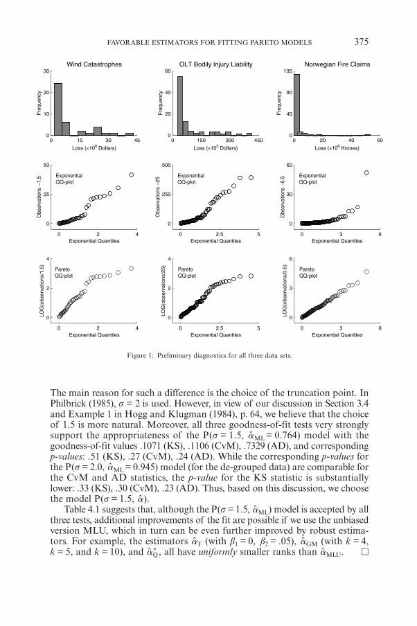
Figure 1: Preliminary diagnostics for all three data sets.
The main reason for such a difference is the choice of the truncation point. InPhilbrick (1985), s = 2 is used. However, in view of our discussion in Section 3.4and Example 1 in Hogg and Klugman (1984), p. 64, we believe that the choiceof 1.5 is more natural. Moreover, all three goodness-of-fit tests very stronglysupport the appropriateness of the P(s = 1.5, �̂ML = 0.764) model with thegoodness-of-fit values .1071 (KS), .1106 (CvM), .7329 (AD), and correspondingp-values: .51 (KS), .27 (CvM), .24 (AD). While the corresponding p-values forthe P(s = 2.0, �̂ML= 0.945) model (for the de-grouped data) are comparable forthe CvM and AD statistics, the p-value for the KS statistic is substantiallylower: .33 (KS), .30 (CvM), .23 (AD). Thus, based on this discussion, we choosethe model P(s = 1.5, �̂).
Table 4.1 suggests that, although the P(s = 1.5, �̂ML) model is accepted by allthree tests, additional improvements of the fit are possible if we use the unbiasedversion MLU, which in turn can be even further improved by robust estima-tors. For example, the estimators �̂T (with b1 = 0, b2 = .05), �̂GM (with k = 4,k = 5, and k = 10), and �̂Q
* , all have uniformly smaller ranks than �̂MLU. ¡
FAVORABLE ESTIMATORS FOR FITTING PARETO MODELS 375
ExponentialQQ-plot
ExponentialQQ-plot
ExponentialQQ-plot
ParetoQQ-plot
ParetoQQ-plot
Obs
erva
tions
–1.
5
Obs
erva
tions
–25
Obs
erva
tions
–0.
5
ParetoQQ-plot
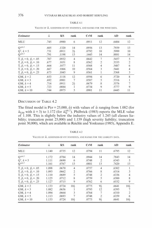
DISCUSSION OF TABLE 4.2
The fitted model is P(s = 25,000, �̂) with values of �̂ ranging from 1.082 (for�̂GM with k = 3) to 1.172 (for �̂Q
opt,2). Philbrick (1985) reports the MLE valueof 1.108. This is slightly below the industry values of 1.245 (all classes lia-bility; truncation point 25,000) and 1.159 (high severity liability; truncationpoint 30,000), which are available in Reichle and Yonkunas (1985), Appendix E.
376 VYTARAS BRAZAUSKAS AND ROBERT SERFLING
TABLE 4.1
VALUES OF �̂, GOODNESS-OF-FIT STATISTICS, AND RANKS FOR THE WIND DATA.
Estimator �̂ KS rank CvM rank AD rank
MLU .745 .0980 6 .0911 12 .6484 12
Qopt,2 .605 .1320 14 .0956 13 .7939 13Q*, k = 5 .731 .0911 2† .0792 10 .5999 10Qopt,5 .791 .1198 13 .1445 14 .8881 14
T, b1 = 0, b2 = .05 .707 .0932 4 .0642 7 .5457 5T, b1 = 0, b2 = .10 .677 .1031 8 .0562 2 .5335 2T, b1 = 0, b2 = .15 .664 .1077 11 .0568 4 .5487 6T, b1 = 0, b2 = .20 .667 .1066 10 .0564 3 .5441 4T, b1 = 0, b2 = .25 .673 .1045 9 .0561 1 .5368 3
GM, k = 2 .653 .1118 12 .0594 6 .5720 8GM, k = 3 .692 .0981 7 .0587 5 .5316 1GM, k = 4 .714 .0911 2† .0679 8 .5576 7GM, k = 5 .723 .0884 1 .0734 9 .5777 9GM, k = 10 .744 .0975 5 .0901 11 .6445 11
TABLE 4.2
VALUES OF �̂, GOODNESS-OF-FIT STATISTICS, AND RANKS FOR THE LIABILITY DATA.
Estimator �̂ KS rank CvM rank AD rank
MLU 1.140 .0735 12 .0794 11 .6795 12
Qopt,2 1.172 .0784 14 .0944 14 .7843 14Q*, k = 5 1.111 .0690 6 .0748 2 .6343 5Qopt,5 1.161 .0767 13 .0881 13 .7420 13
T, b1 = 0, b2 = .05 1.098 .0670 4 .0757 4 .6302 1T, b1 = 0, b2 = .10 1.093 .0662 2 .0766 8 .6314 3T, b1 = 0, b2 = .15 1.110 .0689 5 .0748 2 .6336 4T, b1 = 0, b2 = .20 1.125 .0712 8 .0759 5 .6500 8T, b1 = 0, b2 = .25 1.127 .0715 9 .0762 6 .6532 9
GM, k = 2 1.133 .0724 10† .0775 9† .6641 10†
GM, k = 3 1.082 .0656 1 .0795 12 .6395 7GM, k = 4 1.094 .0664 3 .0764 7 .6310 2GM, k = 5 1.113 .0693 7 .0748 2 .6359 6GM, k = 10 1.133 .0724 10† .0775 9† .6641 10†
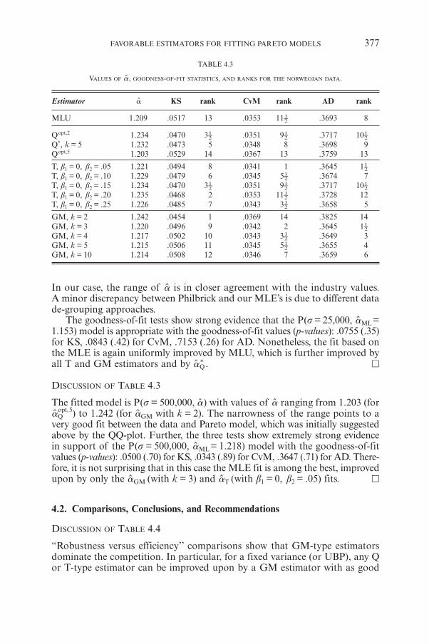
FAVORABLE ESTIMATORS FOR FITTING PARETO MODELS 377
TABLE 4.3
VALUES OF �̂, GOODNESS-OF-FIT STATISTICS, AND RANKS FOR THE NORWEGIAN DATA.
Estimator �̂ KS rank CvM rank AD rank
MLU 1.209 .0517 13 .0353 11† .3693 8
Qopt,2 1.234 .0470 3† .0351 9† .3717 10†
Q*, k = 5 1.232 .0473 5 .0348 8 .3698 9Qopt,5 1.203 .0529 14 .0367 13 .3759 13
T, b1 = 0, b2 = .05 1.221 .0494 8 .0341 1 .3645 1†
T, b1 = 0, b2 = .10 1.229 .0479 6 .0345 5† .3674 7T, b1 = 0, b2 = .15 1.234 .0470 3† .0351 9† .3717 10†
T, b1 = 0, b2 = .20 1.235 .0468 2 .0353 11† .3728 12T, b1 = 0, b2 = .25 1.226 .0485 7 .0343 3† .3658 5
GM, k = 2 1.242 .0454 1 .0369 14 .3825 14GM, k = 3 1.220 .0496 9 .0342 2 .3645 1†
GM, k = 4 1.217 .0502 10 .0343 3† .3649 3GM, k = 5 1.215 .0506 11 .0345 5† .3655 4GM, k = 10 1.214 .0508 12 .0346 7 .3659 6
In our case, the range of �̂ is in closer agreement with the industry values.A minor discrepancy between Philbrick and our MLE’s is due to different datade-grouping approaches.
The goodness-of-fit tests show strong evidence that the P(s = 25,000, �̂ML=1.153) model is appropriate with the goodness-of-fit values (p-values): .0755 (.35)for KS, .0843 (.42) for CvM, .7153 (.26) for AD. Nonetheless, the fit based onthe MLE is again uniformly improved by MLU, which is further improved byall T and GM estimators and by �̂Q
* . ¡
DISCUSSION OF TABLE 4.3
The fitted model is P(s = 500,000, �̂) with values of �̂ ranging from 1.203 (for�̂Q
opt,5) to 1.242 (for �̂GM with k = 2). The narrowness of the range points to avery good fit between the data and Pareto model, which was initially suggestedabove by the QQ-plot. Further, the three tests show extremely strong evidencein support of the P(s = 500,000, �̂ML= 1.218) model with the goodness-of-fitvalues (p-values): .0500 (.70) for KS, .0343 (.89) for CvM, .3647 (.71) for AD. There-fore, it is not surprising that in this case the MLE fit is among the best, improvedupon by only the �̂GM (with k = 3) and �̂T (with b1 = 0, b2 = .05) fits. ¡
4.2. Comparisons, Conclusions, and Recommendations
DISCUSSION OF TABLE 4.4
“Robustness versus efficiency’’ comparisons show that GM-type estimatorsdominate the competition. In particular, for a fixed variance (or UBP), any Qor T-type estimator can be improved upon by a GM estimator with as good
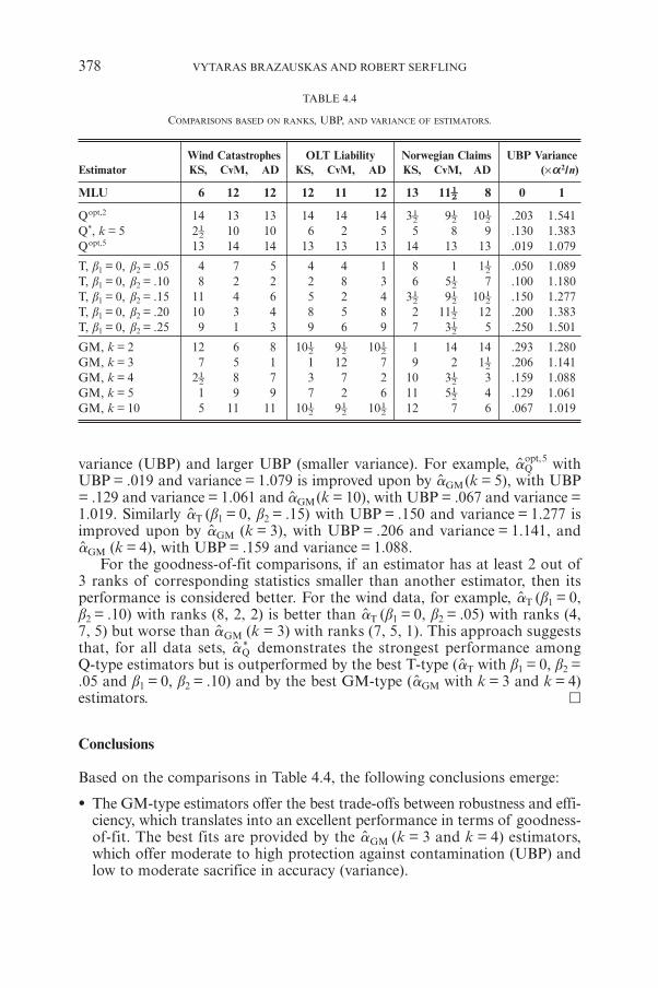
variance (UBP) and larger UBP (smaller variance). For example, �̂Qopt,5 with
UBP = .019 and variance = 1.079 is improved upon by �̂GM(k = 5), with UBP= .129 and variance = 1.061 and �̂GM(k = 10), with UBP = .067 and variance =1.019. Similarly �̂T (b1 = 0, b2 = .15) with UBP = .150 and variance = 1.277 isimproved upon by �̂GM (k = 3), with UBP = .206 and variance = 1.141, and�̂GM (k = 4), with UBP = .159 and variance = 1.088.
For the goodness-of-fit comparisons, if an estimator has at least 2 out of3 ranks of corresponding statistics smaller than another estimator, then itsperformance is considered better. For the wind data, for example, �̂T (b1 = 0,b2 = .10) with ranks (8, 2, 2) is better than �̂T (b1 = 0, b2 = .05) with ranks (4,7, 5) but worse than �̂GM (k = 3) with ranks (7, 5, 1). This approach suggeststhat, for all data sets, �̂Q
* demonstrates the strongest performance amongQ-type estimators but is outperformed by the best T-type (�̂T with b1 = 0, b2 =.05 and b1 = 0, b2 = .10) and by the best GM-type (�̂GM with k = 3 and k = 4)estimators. ¡
Conclusions
Based on the comparisons in Table 4.4, the following conclusions emerge:
• The GM-type estimators offer the best trade-offs between robustness and effi-ciency, which translates into an excellent performance in terms of goodness-of-fit. The best fits are provided by the �̂GM (k = 3 and k = 4) estimators,which offer moderate to high protection against contamination (UBP) andlow to moderate sacrifice in accuracy (variance).
378 VYTARAS BRAZAUSKAS AND ROBERT SERFLING
TABLE 4.4
COMPARISONS BASED ON RANKS, UBP, AND VARIANCE OF ESTIMATORS.
Wind Catastrophes OLT Liability Norwegian Claims UBP VarianceEstimator KS, CvM, AD KS, CvM, AD KS, CvM, AD (×a2/n)
MLU 6 12 12 12 11 12 13 11†† 8 0 1
Qopt,2 14 13 13 14 14 14 3† 9† 10† .203 1.541Q*, k = 5 2† 10 10 6 2 5 5 8 9 .130 1.383Qopt,5 13 14 14 13 13 13 14 13 13 .019 1.079
T, b1 = 0, b2 = .05 4 7 5 4 4 1 8 1 1† .050 1.089T, b1 = 0, b2 = .10 8 2 2 2 8 3 6 5† 7 .100 1.180T, b1 = 0, b2 = .15 11 4 6 5 2 4 3† 9† 10† .150 1.277T, b1 = 0, b2 = .20 10 3 4 8 5 8 2 11† 12 .200 1.383T, b1 = 0, b2 = .25 9 1 3 9 6 9 7 3† 5 .250 1.501
GM, k = 2 12 6 8 10† 9† 10† 1 14 14 .293 1.280GM, k = 3 7 5 1 1 12 7 9 2 1† .206 1.141GM, k = 4 2† 8 7 3 7 2 10 3† 3 .159 1.088GM, k = 5 1 9 9 7 2 6 11 5† 4 .129 1.061GM, k = 10 5 11 11 10† 9† 10† 12 7 6 .067 1.019
• The T-type estimators are slightly less competitive in terms of “robustnessversus efficiency’’ comparisons. However, their goodness-of-fit performanceis as good as that of the GM-type estimators. The best fits are provided bythe �̂T (b1 = 0, b2 = .05 and b1 = 0, b2 = .10) estimators, which offer low tomoderate protection against contamination (UBP) and low to moderate sac-rifice in accuracy (variance).
• The Q-type estimators are outperformed with respect to both criteria, “robust-ness versus efficiency’’ and goodness-of-fit, by the T and GM-type estima-tors and, thus, are less competitive.
• The nonrobust but most efficient MLU neither can improve nor be improvedby any other estimator with respect to the “robustness versus efficiency’’criterion, because it has the best variance and the worst UBP. However, itsperformance with respect to goodness-of-fit is consistently among the worst,implying that for “robustness versus efficiency’’ comparisons the robustnessshould be given a higher priority.
Practical Recommendations
When fitting Pareto models to loss data, the following steps are necessary:
1. If data are grouped or ties are present, de-group it using methods of Sec-tion 3.4; otherwise, go to the next step.
2. Use diagnostic tools — histogram and QQ-plots — to visually determinewhether a Pareto model is appropriate.
3. Compute �̂ML and apply the KS, CvM, and AD statistics to formally testif the Pareto model provides an adequate fit to the data. Note that tableswith the critical values of these statistics are only available when � is esti-mated by MLE. (Tables are presented in D’Agostino and Stephens (1986),pp. 135-136, and Durbin (1975), Table 3.)
4. Compute �̂ using the MLU and Q, T, and GM-type estimators. If the rangeof �̂’s is narrow (as in the case of the Norwegian fire data), then the fitis very good and even the MLE can be relied on. However, if the range isrelatively wide (as in the case of the wind data), then ranking of robust esti-mators has to be used to refine the fit.
5. In situations when all three goodness-of-fit tests support the Pareto model,the T-type estimators with 5%-10% trimming and the GM-type estimatorswith k = 3 and k = 4 perform the best. Estimators with high UBP should beapplied if one of the tests rejects the Pareto model or if the QQ-plots arenot satisfactory, or if the range of �̂’s is very wide.
5. ACKNOWLEDGMENTS
The authors are very appreciative of constructive remarks provided by ananonymous referee. These have led to many improvements in the paper. Also,
FAVORABLE ESTIMATORS FOR FITTING PARETO MODELS 379
support of the first author by a grant from the Actuarial Education and ResearchFund and support of the second author by grants from the Casualty ActuarialSociety and Society of Actuaries, with administrative support from the Actu-arial Education and Research Fund, and by NSF Grant DMS-0103698, aregratefully acknowledged.
REFERENCES
ARNOLD, B.C. (1983). Pareto Distributions. International Cooperative Publishing House. Fairland,Maryland.
BEIRLANT, J., TEUGELS, J.L. and VYNCKIER, P. (1996) Practical Analysis of Extreme Values. Leu-ven University Press, Leuven, Belgium.
BRAZAUSKAS, V. and SERFLING, R. (2000a) Robust and efficient estimation of the tail index ofa single-parameter Pareto distribution. North American Actuarial Journal 4(4), 12-27.
BRAZAUSKAS, V. and SERFLING, R. (2000b) Robust estimation of tail parameters for two-para-meter Pareto and exponential models via generalized quantile statistics. Extremes 3(3), 231-249.
BRAZAUSKAS, V. and SERFLING, R. (2001) Small sample performance of robust estimators of tailparameters for Pareto and exponential models. Journal of Statistical Computation and Simu-lation 70(1), 1-19.
D’AGOSTINO, R.B. and STEPHENS, M.A. (1986) Goodness-of-Fit Techniques. Marcel Dekker, NewYork.
DERRIG, R.A., OSTASZEWSKI, K.M. and REMPALA, G.A. (2000) Applications of resampling methodsin actuarial practice. Proceedings of the Casualty Actuarial Society LXXXVII, 322-364.
DURBIN, J. (1975) Kolmogorov-Smirnov tests when parameters are estimated with applicationsto tests of exponentiality and tests on spacings. Biometrika 62, 5-22.
HOGG, R.V. and KLUGMAN, S.A. (1984). Loss Distributions. Wiley, New York.KIMBER, A.C. (1983a) Trimming in gamma samples. Applied Statistics 32, 7-14.KIMBER, A.C. (1983b) Comparison of some robust estimators of scale in gamma samples with
known shape. Journal of Statistical Computation and Simulation 18, 273-286.KLUGMAN, S.A., PANJER, H.H. and WILLMOT, G.E. (1998) Loss Models: From Data to Decisions.
Wiley, New York.KOUTROUVELIS, I.A. (1981) Large-sample quantile estimation in Pareto laws. Communications in
Statistics, Part A – Theory and Methods 10, 189-201.PATRIK, G. (1980) Estimating casualty insurance loss amount distributions. Proceedings of the
Casualty Actuarial Society LXVII, 57-109.PHILBRICK, S.W. (1985) A practical guide to the single parameter Pareto distribution. Proceedings
of the Casualty Actuarial Society LXXII, 44-84.PHILBRICK, S.W. and JURSCHAK, J. (1981) Discussion of “Estimating casualty insurance loss
amount distributions.’’ Proceedings of the Casualty Actuarial Society LXVIII, 101-106.QUANDT, R.E. (1966) Old and new methods of estimation and the Pareto distribution. Metrika
10, 55-82.REICHLE, K.A. and YONKUNAS, J.P. (1985) Discussion of “A practical guide to the single para-
meter Pareto distribution.’’ Proceedings of the Casualty Actuarial Society LXXII, 85-123.RYTGAARD, M. (1990) Estimation in the Pareto distribution. ASTIN Bulletin 20(2), 201-216.SERFLING, R. (1984) Generalized L-, M- and R-statistics. Annals of Statistics 12, 76-86.SERFLING, R. (2000) “Robust and nonparametric estimation via generalized L-statistics: theory,
applications, and perspectives,’’ In: Advances in Methodological and Applied Aspects of Proba-bility and Statistics, Balakrishnan, N. (Ed.), pp. 197-217. Gordon & Breach.
380 VYTARAS BRAZAUSKAS AND ROBERT SERFLING
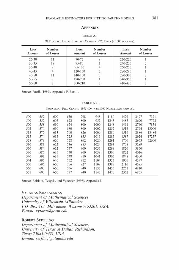
APPENDIX
TABLE A.1
OLT BODILY INJURY LIABILITY CLAIMS (1976) DATA (× 1000 DOLLARS).
Loss Number Loss Number Loss NumberAmount of Losses Amount of Losses Amount of Losses
25-30 11 70-75 9 220-230 130-35 18 75-80 1 240-250 235-40 9 95-100 4 260-270 140-45 4 120-130 2 280-290 145-50 11 140-150 3 290-300 250-55 3 190-200 1 340-350 155-60 2 200-210 2 410-420 2
Source: Patrik (1980), Appendix F, Part 1.
TABLE A.2.
NORWEGIAN FIRE CLAIMS (1975) DATA (× 1000 NORWEGIAN KRONES).
500 552 600 650 798 948 1180 1479 2497 7371500 557 605 672 800 957 1243 1485 2690 7772500 558 610 674 800 1000 1248 1491 2760 7834502 570 610 680 800 1002 1252 1515 2794 13000515 572 613 700 826 1009 1280 1519 2886 13484515 574 615 725 835 1013 1285 1587 2924 17237528 579 620 728 862 1020 1291 1700 2953 52600530 583 622 736 885 1024 1293 1708 3289530 584 632 737 900 1033 1298 1820 3860530 586 635 740 900 1038 1300 1822 4016540 593 635 748 910 1041 1305 1848 4300544 596 640 752 912 1104 1327 1906 4397550 596 650 756 927 1108 1387 2110 4585550 600 650 756 940 1137 1455 2251 4810551 600 650 777 940 1143 1475 2362 6855
Source: Beirlant, Teugels, and Vynckier (1996), Appendix I.
VYTARAS BRAZAUSKAS
Department of Mathematical SciencesUniversity of Wisconsin-MilwaukeeP.O. Box 413, Milwaukee, Wisconsin 53201, USA.E-mail: [email protected]
ROBERT SERFLING
Department of Mathematical Sciences,University of Texas at Dallas, Richardson,Texas 75083-0688, USA.E-mail: [email protected]
FAVORABLE ESTIMATORS FOR FITTING PARETO MODELS 381

THE VALUATION AND HEDGING OF VARIABLE RATE SAVINGSACCOUNTS
BY
FRANK DE JONG1 AND JACCO WIELHOUWER2
ABSTRACT
Variable rate savings accounts have two main features. The interest rate paidon the account is variable and deposits can be invested and withdrawn at anytime. However, customer behaviour is not fully rational and withdrawals of bal-ances are often performed with a delay. This paper focuses on measuring theinterest rate risk of variable rate savings accounts on a value basis (duration)and analyzes the problem how to hedge these accounts. In order to model theembedded options and the customer behaviour we implement a partial adjust-ment specification. The interest rate policy of the bank is described in an error-correction model.
KEYWORDS
Term structure, duration, uncertain cash flow, variable rates of return JELcodes: C33, E43
1. INTRODUCTION
A major part of private savings is deposited in variable rate saving accounts,in the US also known as demand deposits. Typically, deposits can be investedand withdrawn at any time at no cost, which makes a savings account look sim-ilar to a money market account. However, the interest rate paid on savingsaccounts is often different from the money market rate. In Europe, the inter-est rate paid on the savings account can actually be higher or lower than themoney market rate. Even when these interest rates differ, depositors do notimmediately withdraw their money from savings accounts when rates on
* We thank Dennis Bams, Joost Driessen, D. Wilkie, participants at the AFIR 2000 colloquium, andtwo anonymous referees for comments on previous versions of the paper. The usual disclaimerapplies.
1 University of Amsterdam2 ING Group and CentER, Tilburg University
ASTIN BULLETIN, Vol. 33, No. 2, 2003, pp. 383-397
alternative investments are higher. Whatever the causes of this behaviour (mar-ket imperfections, transaction costs or other), these characteristics imply thatthe value of the savings accounts from the point of view of the issuing bankmay be different from the nominal value of the deposits.
In the literature, the valuation of savings accounts is well studied. For exam-ple, Hutchison and Pennacchi (1996), Jarrow and Van Deventer (1998) andSelvaggio (1996) provide models for the valuation of such products. The firsttwo papers build on the (extended) Vasicek (1977) model, whereas the latterpaper uses a more traditional Net Present Value approach. In all these papersthere is little explicit modeling of the dynamic evolution of the interest ratepaid on the account and the balance, and how this evolution depends onchanges in the term structure of market interest rates. For example, Jarrowand van Deventer’s (1998) model is completely static in the sense that the inter-est rate paid on the account and the balance are linear functions of the cur-rent spot rate. In practice, it is well known that interest rates and balances arerather sluggish and often do not respond immediately to changes in the returnon alternative investments, such as the money market rate. Typically, the inter-est rate paid on the account is set by the bank and the balance is determinedby client behaviour. The balance depends, among other things, on the interestrate but also on the return on alternative investments. Because the paths offuture interest rates and the adjustment of the balance determine the value ofthe savings accounts, an analysis of dynamic adjustment patterns is impor-tant.
In this paper, we analyze the valuation and hedging of savings depositswith an explicit model for the adjustment of interest rates and balances tochanges in the money market rate. A recent paper by Janosi, Jarrow andZullo (JJZ, 1999) presents an empirical analysis of the Jarrow andvan Deventer (1998) model. They extend the static theoretical model to adynamic empirical model, that takes the gradual adjustment of interest ratesand balance into account. Our approach differs from the JJZ paper in severalrespects.
Firstly, we treat the term structure of discount rates as exogenous and cal-culate the value of the savings account by a simple Net Present Value equa-tion. This approach, suggested by Selvaggio (1996) leads to simple valuationand duration formulas, and is applicable without assuming a particular termstructure model. The drawback of the NPV approach is that we have to assumethat the risk premium implicit in the discount factor is constant, but this maybe a good first approximation because we want to concentrate on the effectsof the dynamic adjustment of the interest rate paid on the account and bal-ance and not on term structure effects.
Secondly, a difference between the JJZ model and ours is the modeling ofthe long run effects of discount rate shocks. In our model, there is a longrun equilibrium, in which the difference between the interest rate paid on theaccount and the money market rate is constant, and the balance of the sav-ings account is also constant (possibly around a trend). Short term deviationsfrom these long run relations are corrected at a constant rate. This modelstructure is known in the empirical time series literature as an error correction
384 FRANK DE JONG AND JACCO WIELHOUWER
model3. This model has some attractive properties, such as convergence of theeffects of shocks to a long-run mean.
The interest rate sensitivity is quantified in a duration measure. We demon-strate that the duration depends on the adjustment patterns of interest rate paidon the account and balance. We pay particular attention to the implications ofthe model for the hedging of interest rate risk on savings deposits. We illustratehow to fund the savings deposits by a mix of long and short instruments thatmatches the duration of the savings account’s liabilities.
The paper is organized as follows. First the valuation of the savings accountsis dealt with in 2. In 3 the models on the pricing policy and the customerbehaviour are presented, and a discrete time version of the model is estimatedfor the Dutch savings accounts market. 4 deals with the duration of this prod-uct and 5 with hedging decisions. The paper is concluded in 6.
2. VALUATION OF VARIABLE RATE SAVINGS ACCOUNTS
The valuation problem of savings accounts and similar products was analyzedby Selvaggio (1996) and Jarrow and Van Deventer (1998). Their approach is toacknowledge that the liability of the bank equals the present value of future cashoutflows (interest payments and changes in the balance). The present value ofthese flows does not necessarily equal the market value of the money deposited,and therefore the deposits may have some net asset value. Jarrow and VanDeventer (1998) treat the valuation of savings accounts in a no-arbitrage frame-work and derive the net asset value under a risk-neutral probability measure.However, in our paper we want to implement an empirical model for the sav-ings rate and the balance, and therefore we need a valuation formula based onthe empirical probability measure. We therefore adopt the approach proposedby Selvaggio (1996), who calculates the value of the liabilities as the expectedpresent value of future cash flows, discounted at a discount rate which is equalto the risk free rate plus a risk premium4. Hence, the discount rate R(t) can bewritten as
,R t r t= + c] ]g g (1)
where r (t) is the money market rate and g is the risk premium. We can inter-pret this discount rate as the hurdle rate of the investment, that incorporatesthe riskiness of the liabilities, as in a traditional Net Present Value calcula-tion.
The main assumption in this paper is that this risk premium is constant overtime and does not depend on the level of the money market rate. This assump-tion is obviously a simplification. Any underlying formal term structure model,such as the Ho and Lee (1984) model, implies that risk premia depend on the
THE VALUATION AND HEDGING OF VARIABLE RATE SAVINGS ACCOUNTS 385
3 We refer to Davidson et al. (1978) for an introduction to error correction models.4 Selvaggio (1996) calls the risk premium the Option Adjusted Spread
money market rate. However, the risk premia are typically small and since thefocus of the paper is on modeling the dynamic adjustment of interest ratesand balances, we ignore the variation in the risk premium and focus on theeffect of shocks to the money market rate.
With this structure, the market value of liabilities is the expected discountedvalue of future cash outflows, i.e. interest payments on the account i (t) andchanges in the balance D(t) 5
( ) .EL e i s D s D s ds0DRs
0= -
3-# l] ] ]g g g6; @ E (2)
Notice that in this setup reinvestments of interest payments are counted as apart of deposit inflow D�(t). Working out the integral over D�(s) by partialintegration we find that the value of the liabilities equals
( ) ( ).EL e i s R s D s ds D0 0DRs
0= - +
3-# ] ] ]g g g6; @ E (3)
Since the market value of the assets is equal to the initial balance, D(0), thenet asset value (i.e., the market value of the savings product from the point ofview of the bank) is
( ) ( ) ( ) .EV D L e R s i s D s ds0 0 0D DRs
0= - = -
3-# ] ] ]g g g6; @ E (4)
For an interpretation of this equation, notice that R (t) – i(t) is the differencebetween the bank’s discount rate and the interest paid on the account. Addi-tional savings generate value with return R (t). The costs of these additionalsavings are i(t), however. The difference R(t) – i(t) therefore can be interpretedas a profit margin.
The net asset value is simply the present value of future profits (balancetimes profit margin). Therefore, the net asset value is positive if the interest ratepaid on the account is on average below the discount rate. Obviously, the netasset value is zero if the interest rate paid on the account always equals the dis-count rate.
As an example, consider the situation where the interest rate paid on theaccount is always equal to the discount rate minus a fixed margin, i(t) = R(t) – m,and the discount rate is constant over time.6 Moreover, assume that the bal-ance is constant at the level D*. In that case, the net asset value of the savingsaccounts is
D .V R D=n) ) (5)
386 FRANK DE JONG AND JACCO WIELHOUWER
5 For notational clarity, the time variation in the discount rate R is suppressed. If the discount rate istime varying, the exact expression for the discount factor is .e ( )R u du
0-
3#
6 This is a special case of the Jarrow and Van Deventer (1998) model.
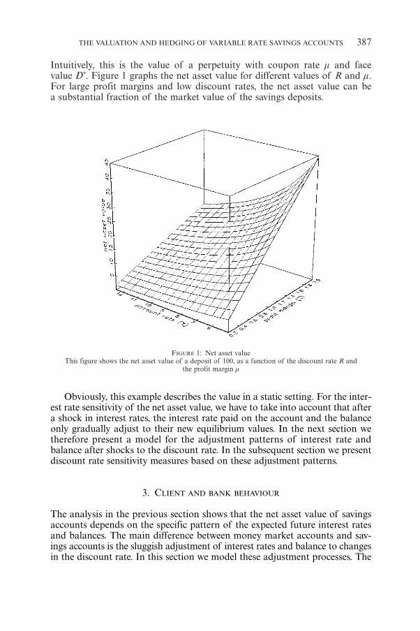
FIGURE 1: Net asset valueThis figure shows the net asset value of a deposit of 100, as a function of the discount rate R and
the profit margin m
Intuitively, this is the value of a perpetuity with coupon rate m and facevalue D). Figure 1 graphs the net asset value for different values of R and m.For large profit margins and low discount rates, the net asset value can bea substantial fraction of the market value of the savings deposits.
THE VALUATION AND HEDGING OF VARIABLE RATE SAVINGS ACCOUNTS 387
Obviously, this example describes the value in a static setting. For the inter-est rate sensitivity of the net asset value, we have to take into account that aftera shock in interest rates, the interest rate paid on the account and the balanceonly gradually adjust to their new equilibrium values. In the next section wetherefore present a model for the adjustment patterns of interest rate andbalance after shocks to the discount rate. In the subsequent section we presentdiscount rate sensitivity measures based on these adjustment patterns.
3. CLIENT AND BANK BEHAVIOUR
The analysis in the previous section shows that the net asset value of savingsaccounts depends on the specific pattern of the expected future interest ratesand balances. The main difference between money market accounts and sav-ings accounts is the sluggish adjustment of interest rates and balance to changesin the discount rate. In this section we model these adjustment processes. The
models highlight the partial adjustment toward the long run equilibriumvalues of interest rates and balances. In the analysis, we take as given the pathof the money market rate r t] g and hence the path of the discount rateR t r t= + c] ]g g . We describe the stochastic evolution of the interest rate paid onsavings deposits, i (t), and the balance, D(t), conditional on the path of thediscount rate.
For the interest rate paid on savings accounts, we propose the followingstochastic error correction specification
di t R t i t dt dW t1 1= - - +l n v] ] ] ]g g g g6 @ (6)
where W1(t) is a standard Brownian motion. This equation states that theinterest rate adjusts to deviations between the long run value R(t) – m and thecurrent rate. We see this as the target policy rule of the bank that sets theinterest rate. Deviations are corrected at speed k > 0, and in the long run,expected interest rates are a margin m below the discount rate R (t). The sto-chastic term W1(t) models the deviations from the target policy rule. Suchdeviations could be due to sudden demand shocks, competition from otherbanks and the like.
For the balance we propose a partial adjustment specification
dD t D t D dt R t i t dt dW t2 2= - - - - - +m h n v)] ] ] ] ]g g g g g8 6B @ (7)
This specification has three components. Firstly, there is an autonomous con-vergence to a long run mean D*, which is determined by a tradeoff by theclients between savings deposits and money market accounts. Secondly, thereis an outflow of funds proportional to the excess of the discount rate over thesavings rate. Thirdly, there is an unpredictable stochastic component.
This description with an autonomous convergence is especially suitable fora detrended time series. An autonomous convergence to a long run mean isexpected in a detrended series for the balance. We detrend by defining thevariable D (t) as the fraction of total short term savings that is invested invariable rate savings accounts. In this case D* is the long run fraction of totalshort term savings that is invested in variable rate savings accounts. In thisway, the trend growth of the total savings market doesn’t affect the empiricalestimation and the duration analysis.
Working out the stochastic differential equations (6) and (7) gives:
,i t e i e R s ds e dW s0t s tt s tt
02
01= + - +l n v- - -l l l# #] ] ] ] ] ]g g g g g g6 @ (8a)
D t D e D D e R s i s ds0t s tt
0= + - - - -h n) )- -m m#] ]_ ] ] ]g g i g g g6 @
.e dW ss tt2
0+v -m# ] ]g g (8b)
To interpret these equations, let’s consider the situation where the discountrate R is constant over time. It is fairly easy to show that the effect of a
388 FRANK DE JONG AND JACCO WIELHOUWER
change in the discount rate in this situation is given by the following partialderivatives
,Ri t
e ds e1s t tt
022
= = -l - -l l#] ]g g (9a)
RD t
e Ri s
ds1s tt
022
22
= - -h -m#] ] ]g g g< F
.e e ds e es t st tt
0- = -
--h h
l m-
- -m l
m l# ] dg n (9b)
The long run derivative of the interest rate paid on the account is one, but inthe short run the effect is less than one. If j > 0 and k > l (which we show lateris clearly the case empirically), the partial derivative of the balance is negative,and converges to zero in the long run.
These partial derivatives can be used to study the effects of a once-and-for-all shock to the discount rate, a kind of impulse response analysis. Start-ing from the equilibrium situation D D0 = )
] g and ( )i R0 = - n, the expectedadjustment patterns are illustrated in Figure 2 for an increase in the discountrate by 1%. The parameter values are picked from the empirical estimates tobe discussed shortly, and are equal to k = 0.79, l = 0.048 and j = 0.43 forthe base case. We see that the interest rate doesn’t follow the jump in thediscount rate immediately but gradually adjusts to its new equilibrium value.The adjustment of the balance is more complex. Initially, the balancedecreases because of withdrawals caused by the relatively low interest ratepaid on the account. But as the interest rate increases, this effect becomessmaller and eventually the autonomous convergence of the balance to its longrun level dominates. One interpretation of this is that clients who initially pre-ferred the variable rate savings account to the money market account willreturn to variable rate savings accounts when the difference between the inter-est rate paid on the savings account and the money market rate reverts to theinitial level.
Equations (9a) and (9b) also highlight the effects of the model parame-ters on the adjustment of interest rates and balance to a shock in the dis-count rate. The effect of j is obvious, it increases the impact of an interestrate shock. This effect may be important in the current market, as theincrease in the use of internet for banking services and the resulting lowertransaction and search costs will probably increase the interest rate sensitiv-ity of the customers. The effect of the mean-reversion parameters k and l ismore complicated. A higher value of l speeds up the adjustment of the bal-ance itself, but doesn’t affect the interest rates. With a lower value of k, boththe adjustment of the interest rate and the balance are slower. The effect ofthe balance is a result of the dependence of the balance on the interest rate.These effects are illustrated in Figure 2, where the dashed line gives theadjustment pattern for a lower value of k, and the dotted line the patternwith a higher value of l.
THE VALUATION AND HEDGING OF VARIABLE RATE SAVINGS ACCOUNTS 389
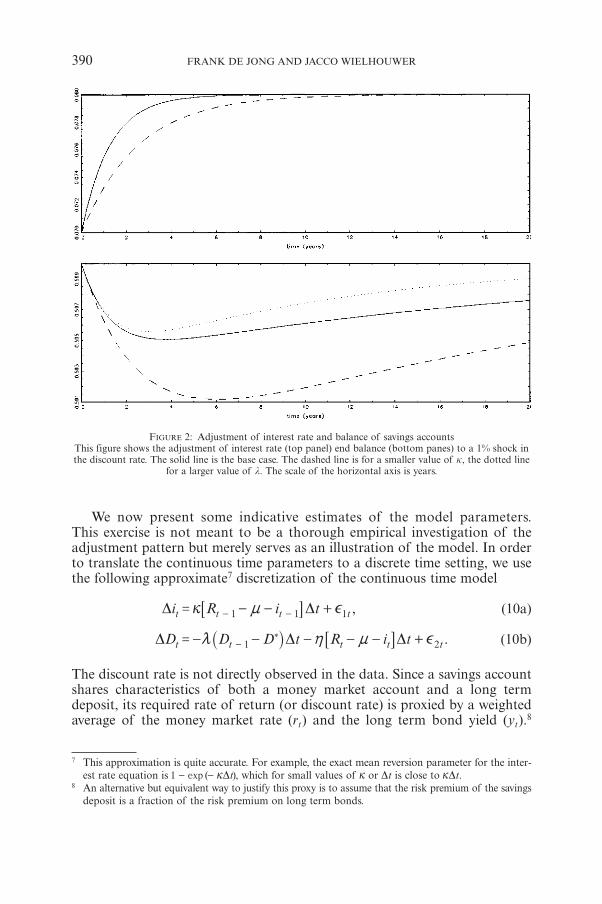
We now present some indicative estimates of the model parameters.This exercise is not meant to be a thorough empirical investigation of theadjustment pattern but merely serves as an illustration of the model. In orderto translate the continuous time parameters to a discrete time setting, we usethe following approximate7 discretization of the continuous time model
,i R i tD Dt t t t1 1 1e= - - +l n- -7 A (10a)
.D D D t R i tD D Dt t t t t1 2e= - - - - - +m h n)-_ i 7 A (10b)
The discount rate is not directly observed in the data. Since a savings accountshares characteristics of both a money market account and a long termdeposit, its required rate of return (or discount rate) is proxied by a weightedaverage of the money market rate (rt) and the long term bond yield (yt).8
390 FRANK DE JONG AND JACCO WIELHOUWER
7 This approximation is quite accurate. For example, the exact mean reversion parameter for the inter-est rate equation is ( )t1 exp D- - l , which for small values of l or tD is close to tDl .
8 An alternative but equivalent way to justify this proxy is to assume that the risk premium of the savingsdeposit is a fraction of the risk premium on long term bonds.
FIGURE 2: Adjustment of interest rate and balance of savings accountsThis figure shows the adjustment of interest rate (top panel) end balance (bottom panes) to a 1% shock inthe discount rate. The solid line is the base case. The dashed line is for a smaller value of k, the dotted line
for a larger value of l. The scale of the horizontal axis is years.
We treat the weight d as an unknown parameter which is estimated from thedata. This leads to the following empirical model
,D Di r i r y e1 ,t t t t t t0 1 2 1 1 1 1= + + - + - +a a a d d- - -^ h7 A" , (11a)
.D D i r y e1 ,t t t t t t0 1 1 2 1 1 1 2= + + - - - +b b b d d- - - -^ h7 A" , (11b)
This model is slightly more general than the theoretical model because it con-tains an immediate, discrete adjustment of the interest rate to the money mar-ket rate. After this initial jump, the adjustment to the new equilibrium is grad-ual. This effect turned out to be so important empirically that we included itin the empirical model.9 The parameters of the continuous time model can besolved from the following equations (with /Dt 1 12= for monthly data)
/ ,Dt2= -l a
/ ,Dt1 1= -m b^ h
/ .Dt2=h b
In fact, the long run deposit level and the average spread of the interest ratesover the estimated discount rate could be unraveled from the constant termsof the model. These are not very accurately estimated however and we refrainfrom drawing inferences about these parameters from the estimates.
We use monthly data on interest rates and deposits from the Dutch savingsaccount market. The interest rate paid on the account is taken from one of theprice setters in the Dutch market. The sample period is 1982:12 to 1999:12,spanning 17 years which is slightly longer than the samples of Hutchisonand Pennacchi (1996) or JJZ. To remove trends in the total savings volume,we define the balance Dt as the fraction of variable rate savings accounts tototal savings. The following empirical estimates are obtained using least squares:
. . . ,D Di r i r y e0 084 0 072 0 066 1 ,t t t t t t1 1 1 1= - + - - + - +d d- - -^ h7 A" , (12a)
. . . .D D i r y e0 21 0 996 0 039 1 ,t t t t t t1 1 1 1 2= + + - + - +d d- - - -^ h7 A" , (12b)
The estimate of d is around 0.2. These estimates imply the following annualizedvalues for the continuous time parameters: k = 0.79, l = 0.048, and j = 0.43.Using these parameters we can solve the second equation for the steadystate value of the fraction of variable rate savings deposits to total savings,
.D 0 58=) .10
THE VALUATION AND HEDGING OF VARIABLE RATE SAVINGS ACCOUNTS 391
9 Notice that including this term does not invalidate the duration analysis of the model, which isbased on the gradual adjustment patterns only.
10 The empirical average of Dt is 0.51
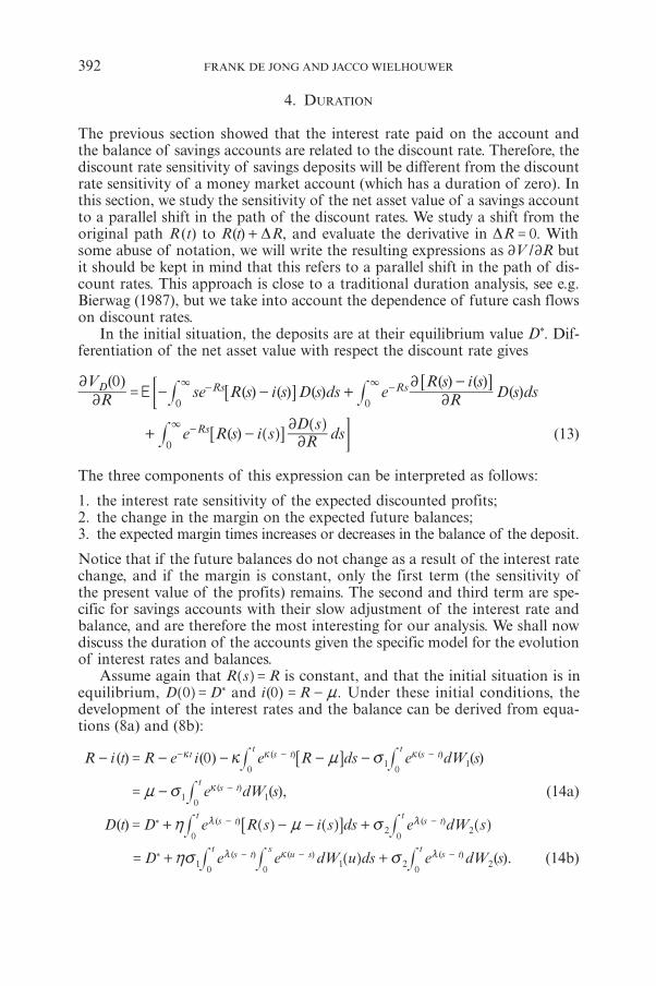
4. DURATION
The previous section showed that the interest rate paid on the account andthe balance of savings accounts are related to the discount rate. Therefore, thediscount rate sensitivity of savings deposits will be different from the discountrate sensitivity of a money market account (which has a duration of zero). Inthis section, we study the sensitivity of the net asset value of a savings accountto a parallel shift in the path of the discount rates. We study a shift from theoriginal path R (t) to ( ) DR t R+ , and evaluate the derivative in DR 0= . Withsome abuse of notation, we will write the resulting expressions as /V R2 2 butit should be kept in mind that this refers to a parallel shift in the path of dis-count rates. This approach is close to a traditional duration analysis, see e.g.Bierwag (1987), but we take into account the dependence of future cash flowson discount rates.
In the initial situation, the deposits are at their equilibrium value D). Dif-ferentiation of the net asset value with respect the discount rate gives
( )( ) ( ) ( )
( ) ( )( )ER
Vse R s i s D s ds e R
R s i sD s ds
0D Rs Rs0 02
22
2= - - +
-3 3- -# #6;
6@
@
( )e R s i s RD s
dsRs0 2
2+ -
3-# ]
]g
g6 @ F (13)
The three components of this expression can be interpreted as follows:
1. the interest rate sensitivity of the expected discounted profits;2. the change in the margin on the expected future balances;3. the expected margin times increases or decreases in the balance of the deposit.
Notice that if the future balances do not change as a result of the interest ratechange, and if the margin is constant, only the first term (the sensitivity ofthe present value of the profits) remains. The second and third term are spe-cific for savings accounts with their slow adjustment of the interest rate andbalance, and are therefore the most interesting for our analysis. We shall nowdiscuss the duration of the accounts given the specific model for the evolutionof interest rates and balances.
Assume again that R s R=] g is constant, and that the initial situation is inequilibrium, D D0 = )
] g and ( )i R0 = - n. Under these initial conditions, thedevelopment of the interest rates and the balance can be derived from equa-tions (8a) and (8b):
( ) ( ) ( )R i t R e i e R ds e dW s0 ( ) ( )t s t s ttt
10
10
- = - - - -l n v- - -l l l## 6 @
( ),e dW s( )s tt
10
1= -n v -l# (14a)
( )D t D e R s i s ds e dW s( ) ( )s tt
s tt
02
02= + - - +h n v) - -m m# #] ] ]g g g6 @
( ).D e e dW u ds e dW s( ) ( ) ( )s tt
u ss
s tt
10 0
1 20
2= + +hv v) - - -m l m# # #] g (14b)
392 FRANK DE JONG AND JACCO WIELHOUWER
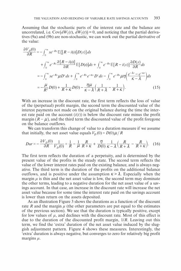
Assuming that the stochastic parts of the interest rate and the balance areuncorrelated, i.e. Cov(dW1(t), dW2(t)) = 0, and noticing that the partial deriva-tives (9a) and (9b) are non-stochastic, we can work out the partial derivative ofthe value:
( )( )ER
Vse R i s D s ds
0D Rs
022
= - -3
-# ] g6 @" ,
( )( )E Ee R
R i sD s ds e R i s R
D sdsRs Rs
0 022
22
+-
+ -3 3
- -# # ]]
gg6
6 6@
@ @
se D ds e e D ds e e e dsRs Rs s Rst t
0 0 0= - + -
--n nh
l m) )
3 3 3- - - -
- -l
m l
# # # d n
( ) ( ) .R
D R DR R0
10
1 12= - +
+-
- +-
+n
l l mhn
m lb l (15)
With an increase in the discount rate, the first term reflects the loss of valueof the (perpetual) profit margin, the second term the discounted value of theinterest payments not made on the original balance during the time the inter-est rate paid on the account i t]^ gh is below the discount rate minus the profitmargin R - n^ h, and the third term the discounted value of the profit foregoneon the balance outflows.
We can transform this change of value to a duration measure if we assumethat initially, the net asset value equals D ( ) ( )V D R0 0= n
( )( ) ( ) .Dur R
VV R R
RD R
RR
R0
01 1 1
01D
D22
= - = -+
+- +
-+n l
hl m m lb l (16)
The first term reflects the duration of a perpetuity, and is determined by thepresent value of the profits in the steady state. The second term reflects thevalue of the lower interest rates paid on the existing balance, and is always neg-ative. The third term is the duration of the profits on the additional balanceoutflows, and is positive under the assumption >l m. Especially when themargin m is thin and the net asset value is low, the second term may dominatethe other terms, leading to a negative duration for the net asset value of a sav-ings account. In that case, an increase in the discount rate will increase the netasset value because for some time the interest rate paid on the savings accountis lower than return on the assets deposited.
As an illustration Figure 3 shows the durations as a function of the discountrate R and the margin m (the other parameters are put equal to the estimatesof the previous section). We see that the duration is typically positive, exceptfor low values of m, and declines with the discount rate. Most of this effect isdue to the duration of the discounted profit margin, 1/R. Leaving out thisterm, we find the ‘extra’ duration of the net asset value induced by the slug-gish adjustment pattern. Figure 4 shows these measures. Interestingly, the‘extra’ duration is always negative, but converges to zero for relatively big profitmargins m.
THE VALUATION AND HEDGING OF VARIABLE RATE SAVINGS ACCOUNTS 393
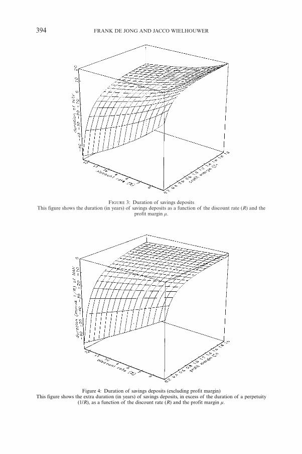
394 FRANK DE JONG AND JACCO WIELHOUWER
FIGURE 3: Duration of savings depositsThis figure shows the duration (in years) of savings deposits as a function of the discount rate (R) and the
profit margin m.
Figure 4: Duration of savings deposits (excluding profit margin)This figure shows the extra duration (in years) of savings deposits, in excess of the duration of a perpetuity
(1/R), as a function of the discount rate (R) and the profit margin m.
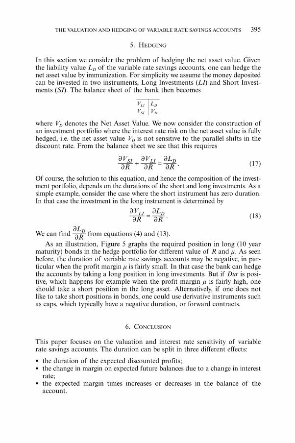
5. HEDGING
In this section we consider the problem of hedging the net asset value. Giventhe liability value LD of the variable rate savings accounts, one can hedge thenet asset value by immunization. For simplicity we assume the money depositedcan be invested in two instruments, Long Investments (LI) and Short Invest-ments (SI). The balance sheet of the bank then becomes
THE VALUATION AND HEDGING OF VARIABLE RATE SAVINGS ACCOUNTS 395
VLI LD
VSI VD
where VD denotes the Net Asset Value. We now consider the construction ofan investment portfolio where the interest rate risk on the net asset value is fullyhedged, i.e. the net asset value VD is not sensitive to the parallel shifts in thediscount rate. From the balance sheet we see that this requires
.RV
RV
RLSI LI D
22
22
22
+ = (17)
Of course, the solution to this equation, and hence the composition of the invest-ment portfolio, depends on the durations of the short and long investments. As asimple example, consider the case where the short instrument has zero duration.In that case the investment in the long instrument is determined by
.RV
RLLI D
22
22
= (18)
We can find RLD22
from equations (4) and (13).
As an illustration, Figure 5 graphs the required position in long (10 yearmaturity) bonds in the hedge portfolio for different value of R and m. As seenbefore, the duration of variable rate savings accounts may be negative, in par-ticular when the profit margin m is fairly small. In that case the bank can hedgethe accounts by taking a long position in long investments. But if Dur is posi-tive, which happens for example when the profit margin m is fairly high, oneshould take a short position in the long asset. Alternatively, if one does notlike to take short positions in bonds, one could use derivative instruments suchas caps, which typically have a negative duration, or forward contracts.
6. CONCLUSION
This paper focuses on the valuation and interest rate sensitivity of variablerate savings accounts. The duration can be split in three different effects:
• the duration of the expected discounted profits;• the change in margin on expected future balances due to a change in interest
rate;• the expected margin times increases or decreases in the balance of the
account.
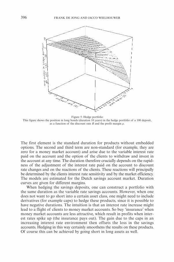
The first element is the standard duration for products without embeddedoptions. The second and third term are non-standard (for example, they arezero for a money market account) and arise due to the variable interest ratepaid on the account and the option of the clients to withdraw and invest inthe account at any time. The duration therefore crucially depends on the rapid-ness of the adjustment of the interest rate paid on the account to discountrate changes and on the reactions of the clients. These reactions will principallybe determined by the clients interest rate sensitivity and by the market efficiency.The models are estimated for the Dutch savings account market. Durationcurves are given for different margins.
When hedging the savings deposits, one can construct a portfolio withthe same duration as the variable rate savings accounts. However, when onedoes not want to go short into a certain asset class, one might need to includederivatives (for example caps) to hedge these products, since it is possible tohave negative durations. The intuition is that an interest rate increase mightlead to a flight of clients to money market accounts. So buy ‘insurance’ whenmoney market accounts are less attractive, which result in profits when inter-est rates spike up (the insurance pays out). The gain due to the caps in anincreasing interest rate environment then offsets the loss in the savingsaccounts. Hedging in this way certainly smoothens the results on these products.Of course this can be achieved by going short in long assets as well.
396 FRANK DE JONG AND JACCO WIELHOUWER
Figure 5: Hedge portfolioThis figure shows the position in long bonds (duration 10 years) in the hedge portfolio of a 100 deposit,
as a function of the discount rate R and the profit margin m.
For future research it might be interesting to analyze the second ordereffects. Then multiple immunization can be achieved with a portfolio with threeasset classes. Finally, it is possible to make the discount rate a function of anumber of interest rates with different maturities. This will of course increasethe complexity of the model but allows for the calculation of key-rate dura-tions.
REFERENCES
BIERWAG, G.O. (1987) Duration Analysis, Ballinger, Cambridge MA.DAVIDSON, J., HENDRY, D.F., SRBA, F. and YEO, S. (1978) Econometric Modelling of the Aggre-
gate Time Series Relationship between Consumer’ Expenditure and Income in the UnitedKingdom, Economic Journal, 88, 661-692.
HEATH, D., JARROW, R. and MORTON, A. (1992) Bond pricing and the term structure of inter-est rates: A new methodology for contingent claims valuation, Econometrica 60, 77-106.
HO, T.S.Y. and LEE, S.-B. (1986) Term structure movements and the pricing of interest rate con-tingent claims, Journal of Finance 41, 1011-1029.
HULL, J. (1993) Options, Futures and other Derivative Securities, second edition, Prentice-Hall.HUTCHISON, D.E. and PENNACCHI, G.G. (1996) Measuring Rents and Interest Rate Risk in Imper-
fect Financial Markets: The Case of Ratail Bank Deposits, Journal of Financial and Quan-titative Analysis 31, 401-417.
JANOSI, T., JARROW, R. and ZULLO, F. (1999) An Empirical Analysis of the Jarrow-van DeventerModel for Valuing Non-Maturity Demand Deposits, Journal of Derivatives, Fall 1999, 8-31.
JARROW, R.A., and VAN DEVENTER, D.R. (1998) The arbitarge-free valuation and hedging of sav-ings accounts and credit card loans, Journal of Banking and Finance 22, 249-272.
SELVAGGIO, R.D. (1996) Using the OAS Methodology to Value and Hedge Commercial BankRetail Demand Deposit Premiums, Chapter 12 363-373.
VASICEK, O. (1977) An equilibrium characterization of the term structure, Journal of FinancialEconomics 5, 177-188.
FRANK DE JONG
Finance GroupUniversiteit van AmsterdamRoetersstraat 111018 WB, Amsterdamthe NetherlandsPhone: +31-20-5255815Fax: +31-20-5255285Email: [email protected]
THE VALUATION AND HEDGING OF VARIABLE RATE SAVINGS ACCOUNTS 397

PREDICTION OF STOCK RETURNS:A NEW WAY TO LOOK AT IT
BY
JENS PERCH NIELSEN1 AND STEFAN SPERLICH2
ABSTRACT
While the traditional R2 value is useful to evaluate the quality of a fit, it doesnot work when it comes to evaluating the predictive power of estimated finan-cial models in finite samples. In this paper we introduce a validated R 2
V valueuseful for prediction. Based on data from the Danish stock market, using thismeasure we find that the dividend-price ratio has predictive power. The besthorizon for prediction seems to be four years. On a one year horizon, we findthat while inflation and interest rate do not add to the predictive power of thedividend-price ratio then last years excess stock return does.
KEYWORDS
Prediction, Stock returns, Dividend price ratio, Cross Validation.
1. INTRODUCTION
Long term investors have the contradicting aims of minimizing risk and max-imizing return over the long run. Much financial literature investigates trad-ing patterns and strategy among long term investors, for example, Barber andTerrance (2000) argue for a buy-and-hold type of strategy that does not eatup returns by trading costs and many professional advisers argue that stocksare better over the long run, see Siegel (1998) and Jagannathan and Kocher-lakota (1996) for particular easily read accounts on this. Other professionalfinancial advisers say that expected returns in financial markets vary overtime and contain a significant predictable component. Consequently timeperiods exist where the long term investor might choose to sell stocks and buy
* The research was supported by the Danish Social Science Research fund and the Spanish DGESBEC2001-1270. Comments and suggestions from Thomas Engsted, Carsten Tanggård and twoanonymous referees are gratefully acknowledged.
1 Codanhus, 60 Gammel Kongevej, DK-1790 Copenhagen V, Denmark. Email: [email protected] Universidad Carlos III de Madrid, Email: [email protected].
ASTIN BULLETIN, Vol. 33, No. 2, 2003, pp. 399-417
bonds, because the return on stocks in these time periods do not match therisk involved. The dividend-price ratio and the earning-price ratio, in particu-lar, has proven to have some predictive power for future stock returns, seeCampbell, Lo, and MacKinlay (1997, Chapter 7) for an up-to-date accountregarding of the dividend yield based predictability of stock returns, and seeShiller (2000, p.8) for a warning of an overvalued American stock exchangebased on the earning-price ratio. Campbell, Lo, and MacKinlay (1997)argued that the predictable component of stock returns is increasing with thetime horizon, since the measure of fit, the R2, increases rapidly with the timehorizon. In the actuarial literature Wilkie (1993) gets to a similar conclusionreplicating the linear modeling approach of Fama and French (1988). The fol-lowing quote is from Wilkie (1993, p.341), who found that predictive powerseems to be strongest for a six and a half year time horizon for British data:“A 1% difference in the dividend yield at the time of purchase of the stockmakes a difference… equivalent to about 4.1% a year compound for about sixand a half years”. So, there is a considerable financial and actuarial literatureon the predictive power of the dividend yield, see also Richardson and Stock(1989) and Wilkie (1995). However, most literature uses traditional in-samplemethodology like goodness of fit, the traditional R2 value or parametric esti-mation procedures combined perhaps with some testing. In this paper weconsider an adjusted measure of predictive power, the RV
2 value, that is anout-of-sample measure in the sense that it measures how the model actuallypredicts into the future, see Eun and Resnick (1988,1994) for financial papersusing a similar type of out-of-sample approach to evaluate their times seriesof stocks, bonds and exchange rates as we use in this paper to analyze ourfinancial time series.
The paper follows its historical development. First we go through an analy-sis of Danish data from 1922 to 1996 and then we add the analysis of theupdated data set from 1922 to 2001.
Regarding the data set 1922-1996
Based on our out-of-sample measure, it seems that the models havestrongest predictive power for a time horizon of four years for Danish stockreturns, at least with respect to our criterion. Dividend-price does seem tohave predictive power whereas knowledge of inflation and short interestrates do not seem to add to this predictive power. However, our study showsthat the one year lagged returns do. The best predictive filter on a one yearbasis turns out to be a two-dimensional fully nonparametric estimator basedon the dividend-price ratio and last years lagged excess return. Last yearsexcess return enters with a tendency towards reversal, such that good yearstend to follow bad years and vice versa. The dividend-price ratio is, however,still the most indicative parameter while estimating the excess returns of thecoming years.
Moreover, based on the current level on the dividend-price ratio in Den-mark, around 1%, we concluded (in december 2000) that expected excess returns
400 JENS PERCH NIELSEN AND STEFAN SPERLICH
on stocks are indeed below zero, for all the considered time horizons with goodprediction power, namely one, two, three, four and five years time horizons.Based on this finding we then concluded further that the current market andpolitical situation in Denmark was out of balance, since all institutionalinvestors heavily increased their percentages of stocks in their portfolios rightthen. On average, an increase from around 20% invested in stocks to around40% invested in stocks have been seen for long term institutional investors inDenmark over the last seven years. The model of this paper argue that this strat-egy increases the risk without increasing the average return.3 We believe thatthe considerations of this paper can be helpful while developing a moderninformation system for the long term investor.
Regarding the updated data set 1922-2001
It turns out that while there still is predictive power in the updated data set,it is much lower than in the original data set. This remarkable finding can havetwo explanations. Either the Danish main index, the KFX index, has had anexceptional behavior in some of the last five years or the entire world markethas followed exceptional rules during this period. In either case, our findingsshow that some care has to be taken regarding predictive power of dividendyields and that further studies based on international data sets should be addedto the current to get a fuller understanding of the problem. It could for exam-ple be relevant to consider a regime shift model such as the one of Harris(1999) to understand this question further. However, while a regime shift modeldoes add to the understanding of historical facts, it does not help much whenit comes to predictive power. For a deep insight into the nature of uncertaintyin prediction, see Cairns (2000, p 314). In this paper we only consider the firstof the three steps considered by Cairns, namely Method 1 that finds the bestfit to a model according to a certain criterion. However, since our criterion isa validated measure of error, we implicitly take care of the errors dealt within Cairns Method 2 and Method 3, that consider uncertainty due to parame-ter estimation and model estimation. Another relevant extension would be tocombine the world wide data of Dimson, March and Staunton (2002) withthe predictive methodology of this paper.
We first motivate our choice of regression variables by noting the basic rela-tionship between stock returns and economic factors in Section 2. In Section 3we describe our data. Our framework for prediction is given in Section 4followed by the prediction results based on the data set 1922-1996 in Section 5when dividend yield alone is used for prediction. In Section 6 we consider theuse of more regression variables for the data set 1922-1996 and in Section 7 weshortly comment on the updated results for the data set 1922-2001.
PREDICTION OF STOCK RETURNS: A NEW WAY TO LOOK AT IT 401
3 This remark is from a version of this paper dated february 2001. A talk based on the conclusionsof this paper was given to the Danish Actuarial Society in december 2000 under the title “Be care-ful: the Danish stocks are too expensive”.
2. THE BASIC RELATIONSHIP BETWEEN STOCK RETURNS AND
ECONOMIC FACTORS
One traditional equation for the value of a stock is
( ) ( ) ,P g D1 1tj
j
jt
1
1= + +c3
-
=
-!
where most of the entering quantities on the right hand side are unknown, g,discount rate, g, constant growth of dividend yields, i inflation and Dt is thedividend paid out during the period t. This model was introduced to the finan-cial theory by Williams (1938) and Gordon and Shapiro (1956). Campbell andShiller (1988) referred to the model as the “dividend-ratio” in absence of uncer-tainty, see also Goetzman and Jorion (1993), Hodrick (1992), and Fama andFrench (1988). For simplicity the discount rate and the growth rate donot depend on time in this model although this is well known to be incorrect.The point of the above identity is however, that it shows that the price ofstocks depend on quantities such that dividend yield, interest rate and infla-tion. The two latter being highly correlated with almost any relevant discountrate. It is also clear from the above identity that a decrease in discount rate,which is highly correlated with an increase in bond yield, are related to anincrease in the stock return and vice versa.
3. THE DATA AND OUR DEFINITION OF PREDICTION
In this paper we use the annual Danish stock market data from Lund andEngsted (1996), respectively the extended sample period 1922-1996 from Engsted and Tanggård (2000). We have ourselves extended the period to 1922-2001. We consider the time series
, , , ,W S d I rt t t t t= ^ h
where St is stock return, It is inflation and rt is the short-term interest rate.The stock index is based on a value weighted portfolio of individual stocks cho-sen to obtain maximum coverage of the marked index of the Copenhagen StockExchange (CBS). Notice that CBS was open during the second world war. Inconstructing the data corrections were made for stock splits and new equityissues below market prices. Further, dt = Dt /Pt denotes (nominal) dividendsDt paid during year t divided by the (nominal) stock price Pt at the end of year t.The appendix in Lund and Engsted (1996) contains a detailed description of thedata from where we have taken the following quote: “A nominal stock index andaccompanying dividend series was constructed from the original price quotationsheets from the Copenhagen Stock Exchange. In order to avoid a possible tax-induced distortion due to the well known January effect, the stock index at theend of the year t is defined as the value in (mid) February of year t + 1. Similarly,dividends for year t are defined as dividends paid out between February of yeart and February of year t + 1. However, no Danish companies pay dividends in
402 JENS PERCH NIELSEN AND STEFAN SPERLICH
January, so the dividend series is effectively the dividends paid during the year t.Corrections are made for stock splits and new equity issues below the marketprice using techniques similar to those described in Shiller (1981). The stockindex is a value-weighted portfolio consisting of approximately 16 individualstocks (companies), which are generally chosen in order to obtain the maximumcoverage of the ‘market’ index of the Copenhagen Stock Exchange. The com-position of the stock index is changed about every 10 years, and the weights forthe individual stocks are only adjusted in connection with changes in the com-position of the stock index.”
We have updated the data set of Lund and Engsted (1996) following theiroriginal approach. The leading Danish stock index, the KFX, index has beenused for this purpose. As a measure of the short-term interest rate, Rt, the dis-count rate of the Danish Central Bank’s is used up to 1975, spliced togetherwith a short-term zero-coupon yield for the period thereafter. In computingreal values, we deflate nominal values by the consumption deflator4. The realexcess stock return is defined as
logS P D P rt t t t t1 1= + -- -^ h$ . ,
where
logr R1 100t t= +` j.
The resulting average of these excess stock returns are 2.5% for the period1922-2001 (2.1% for 1922-1996) and 3.4% for the after war period 1948-2001(3.2% for 1948-1996).
4. OUR FRAMEWORK FOR PREDICTION
The problem of prediction is considered as follows: Let Y St t ii
T
0
1= +=
-! be theexcess stock return at time t over the next T years. We base our prediction onthe assumption that Yt can be approximated by a model of the form:
, , , ,Y g W t K Kt t t1 1 2fe != +-^ h " , (1)
where the error variable te are mean zero stochastic variables given the past,W1, …, Wt – 1 and S1, …, St – 1
5. Ideally we would like to be able to predict Yt.We do, however, only have information of Wt–1 and no information withrespect to the error term te . Therefore, estimating g :] g and using it for our
PREDICTION OF STOCK RETURNS: A NEW WAY TO LOOK AT IT 403
4 The consumption series has been from Hansen (1974) and various publications from the DanishCentral Statistical Bureau. The consumption series covers private consumption of durable and non-durable goods. Unfortunately, there is no price deflator for private consumption, so nominal prices,dividends and consumption are deflated using the consumption deflator for total consumption.
5 Note that in our implementation Wt–1 does not contain time lagged information as is the case e.g inthe Wilkie model (1995). An investigation of time lagged variables would be an obvious extensionof our approach to prediction.
prediction is the best we can do. Due to the definition of Yt the time period,K K1 2^ h depends on T and is first ,T T T 1last - +_ i with Tfirst = 1923 or 1949 and
Tlast = 1996 or 2001.Let
, , , , .X W S W SK K K K1 11 1 2 2f= - -` `j j% /
For t’s where K1 ≤ (t –T) ≤ K2 we wish to be able to consider data points whichexclude direct information about St. We therefore introduce
, , , , , , , , , .X W S W S W S W S( )tK K t T t T t T t T K K1 1 11 1 2 1 2
f f= - - - - + - + -` ^ ^ `j h h j$ .
Now let the set H represent different estimation principles and let for gh, h ∈ H,be some estimator based on X and let g(t)
h be the (equivalent) estimator basedon X(t).
For a given time horizon T, we define the loss of the estimator gh as
( )Q g W Wg gh t h tt K
K
1 12
1
2
= -- -=
! ^ ^h h# - (2)
which can be estimated by
( ) ,Y WQ g g( )h t h
tt
t K
K
1
2
1
2
= - -=
! ^ h$ . (3)
i.e. we predict g(Wt–1) without the information contained in Yt, compare alsowith Appendix 3. Notice that Q(gh) is not estimated well by the goodness of fitmeasure
,Q Y Wg gh t h tt K
K
12
1
2
= - -=
!^ ^h h# -
since this measure always will be in favor of the most complex model. Suchcomplicated models are often in contradiction to the aim of predicting well.
While predicting, we find our optimal prediction scheme by minimizingQ(gh) over all principles h. This gives us the best predictor within H.
Now let h0 correspond to the trivial prediction strategy based on the para-metric model
,Yt te= +n (4)
where m is estimated by K K Y1 tt K
K
2 11
1
2= - +n -
=!t ^ h . For a given modeling and
estimation principle h, we define our new R2 value, that we call R 2V, h , where V
stands for validated, as
( )( )
.RQ gQ g
1,V hh
h2
0
= - (5)
404 JENS PERCH NIELSEN AND STEFAN SPERLICH
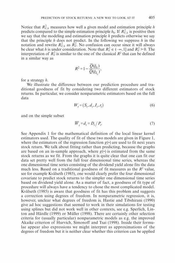
Notice that R 2V, h measures how well a given model and estimation principle h
predicts compared to the simple estimation principle h0. If R 2V, h is positive then
we say that the modeling and estimation principle h predicts otherwise we saythat the principle h does not predict. In the following we suppress h in thenotation and rewrite R 2
V, h as R 2V. No confusion can occur since it will always
be clear what h is under consideration. Note that R 2V ∈ (–∞,1] and R 2
V > 0. Theinterpretation of R 2
V is similar to the one of the classical R2 that can be definedin a similar way as
( )( )
,RQQ
gg
1h
h2
0
= -
for a strategy h.We illustrate the difference between our prediction procedure and tra-
ditional goodness of fit by considering two different estimators of stockreturns. In particular, we consider nonparametric estimators based on the fulldata
, , ,W S d I rt t t t t= ^ h (6)
and on the simple subset
W d D Pt t t t= = . (7)
See Appendix 1 for the mathematical definition of the local linear kernelestimators used. The quality of fit of these two models are given in Figure 1,where the estimators of the regression function g :] g are used to fit next yearsstock return. We talk about fitting rather than predicting, because the graphsare based on an in-sample approach, where g :] g is estimated from the samestock returns as we fit. From the graphs it is quite clear that one can fit ourdata set pretty well from the full four dimensional time series, whereas theone dimensional time series consisting of the dividend yield alone fits the datamuch less. Based on a traditional goodness of fit measures as the R2 value,see for example Kvålseth (1985), one would clearly prefer the four dimensionalcovariate to predict stock returns to the simpler one dimensional time seriesbased on dividend yield alone. As a matter of fact, a goodness of fit type ofprocedure will always have a tendency to chose the most complicated model.Kvålseth (1985) is aware that goodness of fit has this problem and suggestsa correction using degrees of freedom. In nonparametric regression, it is,however, unclear what degrees of freedom is. Hastie and Tibshirani (1990)give ad hoc suggestions that seemed to work in their simulations for testingusing splines but did not work well in other contexts, see e.g. Sperlich, Lin-ton and Härdle (1999) or Müller (1998). There are certainly other selectioncriteria for (usually particular) nonparametric models as e.g. the improvedAkaike criterion of Hurvich, Simonoff and Tsai (1998). Inside their formu-lae appear also expressions we might interpret as approximations of thedegrees of freedom but it is neither clear whether this criterion can be applied
PREDICTION OF STOCK RETURNS: A NEW WAY TO LOOK AT IT 405
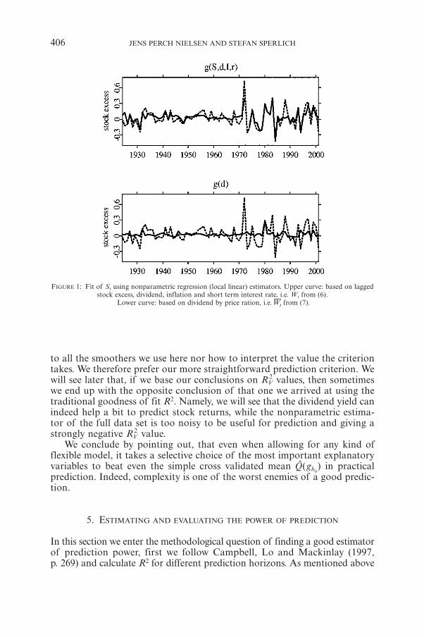
to all the smoothers we use here nor how to interpret the value the criteriontakes. We therefore prefer our more straightforward prediction criterion. Wewill see later that, if we base our conclusions on R 2
V values, then sometimeswe end up with the opposite conclusion of that one we arrived at using thetraditional goodness of fit R2. Namely, we will see that the dividend yield canindeed help a bit to predict stock returns, while the nonparametric estima-tor of the full data set is too noisy to be useful for prediction and giving astrongly negative R 2
V value.We conclude by pointing out, that even when allowing for any kind of
flexible model, it takes a selective choice of the most important explanatoryvariables to beat even the simple cross validated mean Q(gh0
) in practicalprediction. Indeed, complexity is one of the worst enemies of a good predic-tion.
5. ESTIMATING AND EVALUATING THE POWER OF PREDICTION
In this section we enter the methodological question of finding a good estimatorof prediction power, first we follow Campbell, Lo and Mackinlay (1997,p. 269) and calculate R2 for different prediction horizons. As mentioned above
406 JENS PERCH NIELSEN AND STEFAN SPERLICH
FIGURE 1: Fit of St using nonparametric regression (local linear) estimators. Upper curve: based on laggedstock excess, dividend, inflation and short term interest rate, i.e. Wt from (6).
Lower curve: based on dividend by price ration, i.e.Wt from (7).
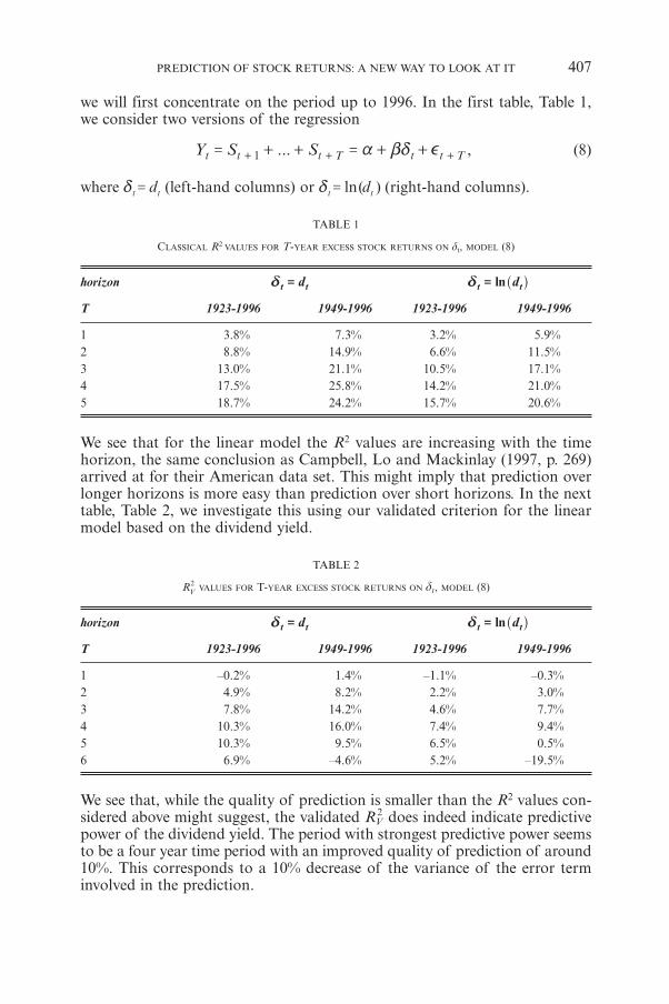
we will first concentrate on the period up to 1996. In the first table, Table 1,we consider two versions of the regression
... ,Y S St t t T t t T1 e= + + = + +a bd+ + + (8)
where dt t=d (left-hand columns) or ( )ln dt t=d (right-hand columns).
TABLE 1
CLASSICAL R2 VALUES FOR T-YEAR EXCESS STOCK RETURNS ON dt, MODEL (8)
horizon dt t=d ln dt t=d ^ h
T 1923-1996 1949-1996 1923-1996 1949-1996
1 3.8% 7.3% 3.2% 5.9% 2 8.8% 14.9% 6.6% 11.5% 3 13.0% 21.1% 10.5% 17.1% 4 17.5% 25.8% 14.2% 21.0% 5 18.7% 24.2% 15.7% 20.6%
We see that for the linear model the R2 values are increasing with the timehorizon, the same conclusion as Campbell, Lo and Mackinlay (1997, p. 269)arrived at for their American data set. This might imply that prediction overlonger horizons is more easy than prediction over short horizons. In the nexttable, Table 2, we investigate this using our validated criterion for the linearmodel based on the dividend yield.
TABLE 2
R2V VALUES FOR T-YEAR EXCESS STOCK RETURNS ON dt, MODEL (8)
horizon dt t=d ln dt t=d ^ h
T 1923-1996 1949-1996 1923-1996 1949-1996
1 –0.2% 1.4% –1.1% –0.3%2 4.9% 8.2% 2.2% 3.0%3 7.8% 14.2% 4.6% 7.7%4 10.3% 16.0% 7.4% 9.4%5 10.3% 9.5% 6.5% 0.5%6 6.9% –4.6% 5.2% –19.5%
We see that, while the quality of prediction is smaller than the R2 values con-sidered above might suggest, the validated R 2
V does indeed indicate predictivepower of the dividend yield. The period with strongest predictive power seemsto be a four year time period with an improved quality of prediction of around10%. This corresponds to a 10% decrease of the variance of the error terminvolved in the prediction.
PREDICTION OF STOCK RETURNS: A NEW WAY TO LOOK AT IT 407
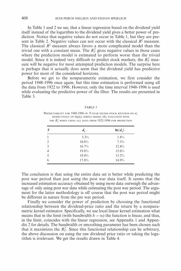
In Table 1 and 2 we see, that a linear regression based on the dividend yielditself instead of the logarithm to the dividend yield gives a better power of pre-diction. Notice that negative values do not occur in Table 1, but they are pre-sent in Table 2. Negative values can not occur with the classical R2 measure.The classical R2 measure always favors a more complicated model than thetrivial one with a constant mean. The R 2
V gives negative values in those caseswhere the prediction model is estimated to perform worse than the trivialmodel. Since it is indeed very difficult to predict stock markets, the R 2
V mea-sure will be negative for most attempted prediction models. The surprise hereis perhaps that it actually does seem that the dividend yield has predictivepower for most of the considered horizons.
Before we get to the nonparametric estimation, we first consider theperiod 1948-1996 once again, but this time estimation is performed using allthe data from 1922 to 1996. However, only the time interval 1948-1996 is usedwhile evaluating the predictive power of the filter. The results are presented inTable 3.
TABLE 3
PREDICTABILITY FOR 1948-1996 OF T-YEAR EXCESS STOCK RETURNS ON dt,RESPECTIVELY ON ln(dt), SIMPLE MODEL (8), EVALUATED WITH
THE R2V WHEN USING ALL DATA FROM 1922-1996 FOR PREDICTION
T dt ln dt^ h
1 3.3% 1.8%2 10.8% 7.3%3 16.7% 12.4%4 19.8% 15.6%5 18.0% 13.2%6 17.8% 14.9%
The conclusion is that using the entire data set is better while predicting thepost war period than just using the post war data itself. It seems that theincreased estimation accuracy obtained by using more data outweigh the advan-tage of only using post war data while estimating the post war period. The argu-ment for the latter methodology is off course that the post war period mightbe different in nature from the pre war period.
Finally we consider the power of prediction by choosing the functionalrelationship between the dividend-price ratio and the return by a nonpara-metric kernel estimator. Specifically, we use local linear kernel estimation whatmeans that in the limit (with bandwidth h "3) the function is linear, and thus,in the limit, coincides with the linear regression, see Appendix 1 and Appen-dix 2 for details. The bandwidth or smoothing parameter has been chosen suchthat it maximizes the R 2
V. Since this functional relationship can be arbitrary,the above discussion on using the raw dividend price ratio or taking the loga-rithm is irrelevant. We get the results drawn in Table 4.
408 JENS PERCH NIELSEN AND STEFAN SPERLICH
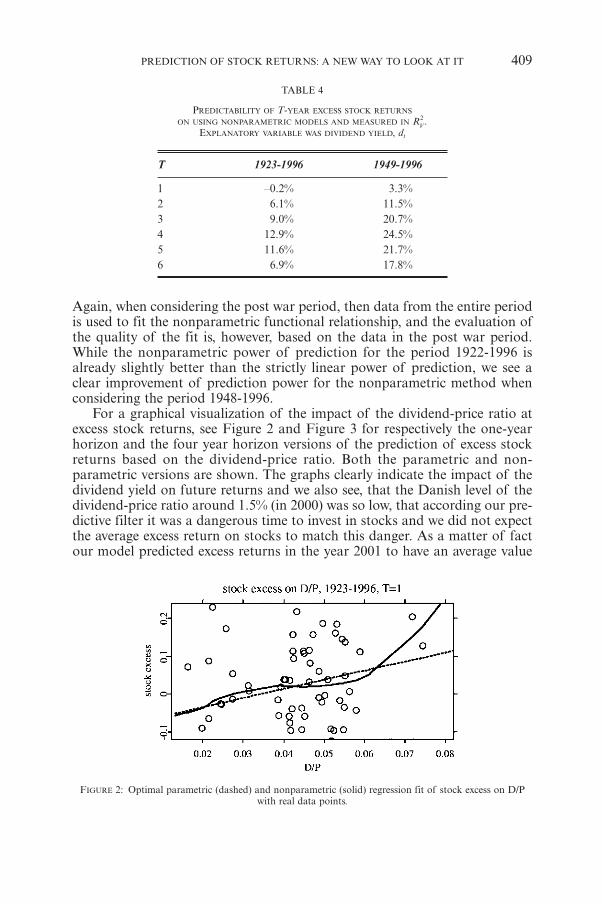
TABLE 4
PREDICTABILITY OF T-YEAR EXCESS STOCK RETURNS
ON USING NONPARAMETRIC MODELS AND MEASURED IN R2V.
EXPLANATORY VARIABLE WAS DIVIDEND YIELD, dt
T 1923-1996 1949-1996
1 –0.2% 3.3%2 6.1% 11.5%3 9.0% 20.7%4 12.9% 24.5%5 11.6% 21.7%6 6.9% 17.8%
Again, when considering the post war period, then data from the entire periodis used to fit the nonparametric functional relationship, and the evaluation ofthe quality of the fit is, however, based on the data in the post war period.While the nonparametric power of prediction for the period 1922-1996 isalready slightly better than the strictly linear power of prediction, we see aclear improvement of prediction power for the nonparametric method whenconsidering the period 1948-1996.
For a graphical visualization of the impact of the dividend-price ratio atexcess stock returns, see Figure 2 and Figure 3 for respectively the one-yearhorizon and the four year horizon versions of the prediction of excess stockreturns based on the dividend-price ratio. Both the parametric and non-parametric versions are shown. The graphs clearly indicate the impact of thedividend yield on future returns and we also see, that the Danish level of thedividend-price ratio around 1.5% (in 2000) was so low, that according our pre-dictive filter it was a dangerous time to invest in stocks and we did not expectthe average excess return on stocks to match this danger. As a matter of factour model predicted excess returns in the year 2001 to have an average value
PREDICTION OF STOCK RETURNS: A NEW WAY TO LOOK AT IT 409
FIGURE 2: Optimal parametric (dashed) and nonparametric (solid) regression fit of stock excess on D/Pwith real data points.
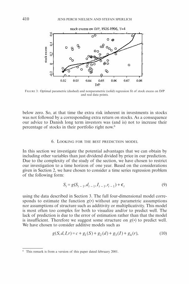
below zero. So, at that time the extra risk inherent in investments in stockswas not followed by a corresponding extra return on stocks. As a consequenceour advice to Danish long term investors was (and is) not to increase theirpercentage of stocks in their portfolio right now.6
6. LOOKING FOR THE BEST PREDICTION MODEL
In this section we investigate the potential advantages that we can obtain byincluding other variables than just dividend divided by price in our prediction.Due to the complexity of the study of the section, we have chosen to restrictour investigation to a time horizon of one year. Based on the considerationsgiven in Section 2, we have chosen to consider a time series regression problemof the following form:
( , , , )S g S d I rt t t t t t1 1 1 1 e= +- - - - (9)
using the data described in Section 3. The full four-dimensional model corre-sponds to estimate the function g :] g without any parametric assumptionsnor assumptions of structure such as additivity or multiplicativity. This modelis most often too complex for both to visualize and/or to predict well. Thelack of prediction is due to the error of estimation rather than that the modelis insufficient. Therefore we suggest some structure on g :] g to predict well.We have chosen to consider additive models such as
, , , ,g S d I r c g S g d g I g r1 2 3 4= + + + +] ] ] ] ]g g g g g (10)
410 JENS PERCH NIELSEN AND STEFAN SPERLICH
6 This remark is from a version of this paper dated february 2001.
FIGURE 3: Optimal parametric (dashed) and nonparametric (solid) regression fit of stock excess on D/Pand real data points.
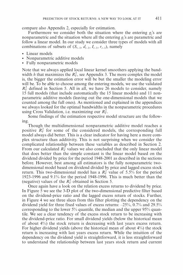
compare also Appendix 2, especially for estimation.Furthermore we consider both the situation where the entering gi’s are
nonparametric and the situation where all the entering gi’s are parametric andfollow a linear model. In our study we consider three types of models with allcombinations of subsets of (St–1, dt–1, It–1, rt–1), namely
• Linear models• Nonparametric additive models• Fully nonparametric models
Note that we always applied local linear kernel smoothers applying the band-width h that maximizes the R 2
V, see Appendix 3. The more complex the modelis, the bigger the estimation error will be but the smaller the modeling errorwill be. To be able to choose among the entering models, we use the validatedR 2
V defined in Section 5. All in all, we have 26 models to consider, namely15 full models (that include automatically the 15 linear models) and 11 non-parametric additive models (leaving out the one-dimensional models that wecounted among the full ones). As mentioned and explained in the appendiceswe always looked for the optimal bandwidths in the nonparametric proceduresusing Cross Validation, i.e. maximizing our R 2
V.Some findings of the estimation respective model structure are the follow-
ing.Though the multidimensional nonparametric additive model reaches a
positive R 2V for some of the considered models, the corresponding full
model always did better. This is a clear indicator for having here a more com-plex structure than additivity. This is not surprising when we consider thecomplicated relationship between these variables as described in Section 2.From our calculated R 2
V values we also concluded that the only linear modelthat does better than the simple constant is the linear model based on thedividend divided by price for the period 1948-2001 as described in the sectionsbefore. However, best among all estimators is the fully nonparametric two-dimensional model based on dividend divided by price and lagged excess stockreturn. This two-dimensional model has a R 2
V value of 5.5% for the period1923-1996 and 9.1% for the period 1948-1996. This is much better than the(negative) values of the R 2
V obtained in Section 5.Once again have a look on the relation excess returns to dividend by price.
In Figure 5 we see the 3-D plot of the two-dimensional predictive filter basedon the dividend-price ratio and the lagged excess return of stocks. Further,in Figure 4 we see three slices from this filter plotting the dependency on thedividend yield for three fixed values of excess returns: –25%, 0.7% and 29.5%corresponding to the lower 5% quantile, the median and the upper 95% quan-tile. We see a clear tendency of the excess stock return to be increasing withthe dividend-price ratio. For small dividend yields (below the historical meanof about 4%) the stock return is decreasing with last years excess return.For higher dividend yields (above the historical mean of about 4%) the stockreturn is increasing with last years excess return. While the intuition of thedependency on the dividend yield is straightforward, it is less straightforwardto understand the relationship between last years stock return and current
PREDICTION OF STOCK RETURNS: A NEW WAY TO LOOK AT IT 411
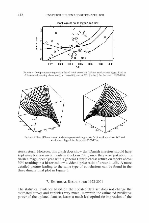
stock return. However, this graph does show that Danish investors should havekept away for new investments in stocks in 2001, since they were just about tofinish a magnificent year with a general Danish excess return on stocks above30% resulting in a historical low dividend-price ratio of around 1.5%. A moredetailed picture leading to the same type of conclusions can be found in thethree dimensional plot in Figure 5.
7. EMPIRICAL RESULTS FOR 1922-2001
The statistical evidence based on the updated data set does not change theestimated curves and variables very much. However, the estimated predictivepower of the updated data set leaves a much less optimistic impression of the
412 JENS PERCH NIELSEN AND STEFAN SPERLICH
FIGURE 4: Nonparametric regression fits of stock excess on D/P and stock excess lagged fixed at–25% (dotted, starting above zero), at 1% (solid), and at 30% (dashed) for the period 1923-1996.
FIGURE 5: Two different views on the nonparametric regression fit of stock excess on D/P andstock excess lagged for the period 1923-1996.
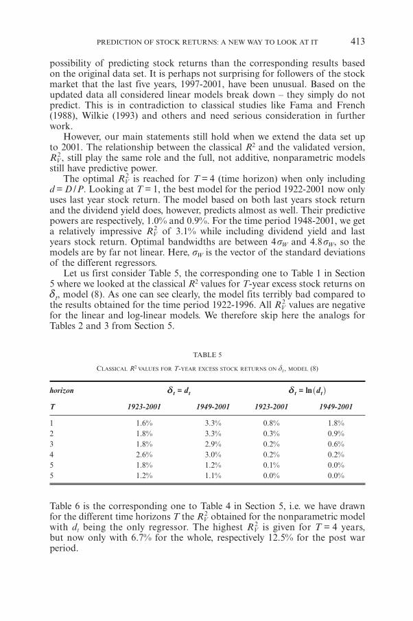
possibility of predicting stock returns than the corresponding results basedon the original data set. It is perhaps not surprising for followers of the stockmarket that the last five years, 1997-2001, have been unusual. Based on theupdated data all considered linear models break down – they simply do notpredict. This is in contradiction to classical studies like Fama and French(1988), Wilkie (1993) and others and need serious consideration in furtherwork.
However, our main statements still hold when we extend the data set upto 2001. The relationship between the classical R2 and the validated version,R 2
V, still play the same role and the full, not additive, nonparametric modelsstill have predictive power.
The optimal R 2V is reached for T = 4 (time horizon) when only including
d = D /P. Looking at T = 1, the best model for the period 1922-2001 now onlyuses last year stock return. The model based on both last years stock returnand the dividend yield does, however, predicts almost as well. Their predictivepowers are respectively, 1.0% and 0.9%. For the time period 1948-2001, we geta relatively impressive R 2
V of 3.1% while including dividend yield and lastyears stock return. Optimal bandwidths are between 4sW and 4.8sW, so themodels are by far not linear. Here, sW is the vector of the standard deviationsof the different regressors.
Let us first consider Table 5, the corresponding one to Table 1 in Section5 where we looked at the classical R2 values for T-year excess stock returns on
td , model (8). As one can see clearly, the model fits terribly bad compared tothe results obtained for the time period 1922-1996. All R 2
V values are negativefor the linear and log-linear models. We therefore skip here the analogs forTables 2 and 3 from Section 5.
TABLE 5
CLASSICAL R2 VALUES FOR T-YEAR EXCESS STOCK RETURNS ON dt, MODEL (8)
horizon dt t=d ln dt t=d ^ h
T 1923-2001 1949-2001 1923-2001 1949-2001
1 1.6% 3.3% 0.8% 1.8% 2 1.8% 3.3% 0.3% 0.9% 3 1.8% 2.9% 0.2% 0.6% 4 2.6% 3.0% 0.2% 0.2% 5 1.8% 1.2% 0.1% 0.0% 5 1.2% 1.1% 0.0% 0.0%
Table 6 is the corresponding one to Table 4 in Section 5, i.e. we have drawnfor the different time horizons T the R 2
V obtained for the nonparametric modelwith dt being the only regressor. The highest R 2
V is given for T = 4 years,but now only with 6.7% for the whole, respectively 12.5% for the post warperiod.
PREDICTION OF STOCK RETURNS: A NEW WAY TO LOOK AT IT 413
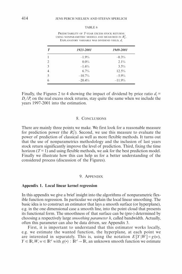
TABLE 6
PREDICTABILITY OF T-YEAR EXCESS STOCK RETURNS
USING NONPARAMETRIC MODELS AND MEASURED IN R2V.
EXPLANATORY VARIABLE WAS DIVIDEND YIELD, dt
T 1923-2001 1949-2001
1 –1.9% –0.3%2 0.0% 2.1%3 –1.6% 3.5%4 6.7% 12.5%5 –10.7% –5.9%6 –20.4% –11.9%
Finally, the Figures 2 to 4 showing the impact of dividend by price ratio dt =Dt /Pt on the real excess stock returns, stay quite the same when we include theyears 1997-2001 into the estimation.
8. CONCLUSIONS
There are mainly three points we make. We first look for a reasonable measurefor prediction power (the R 2
V). Second, we use this measure to evaluate thepower of prediction of classical as well as more flexible methods. It turns outthat the use of nonparametrics methodology and the inclusion of last yearsstock return significantly improve the level of prediction. Third, fixing the timehorizon (T = 1) and using flexible methods, we ask for the best prediction model.Finally we illustrate how this can help us for a better understanding of theconsidered process (discussion of the Figures).
9. APPENDIX
Appendix 1. Local linear kernel regression
In this appendix we give a brief insight into the algorithms of nonparametric flex-ible function regression. In particular we explain the local linear smoothing. Thebasic idea is to construct an estimator that lays a smooth surface (or hyperplane),e.g. in the one dimensional case a smooth line, into the point cloud that presentsits functional form. The smoothness of that surface can be (pre-) determined bychoosing a respectively large smoothing parameter h, called bandwidth. Actually,often this parameter can also be data driven, see Appendix 3.
First, it is important to understand that this estimator works locally,e.g. we estimate the wanted function, the hyperplane, at each point weare interested in separately. This is, using the notation ( )E Y W g w=6 @ ,
, , :R R R RY W w gwithd d ":! ! ] g , an unknown smooth function we estimate
414 JENS PERCH NIELSEN AND STEFAN SPERLICH
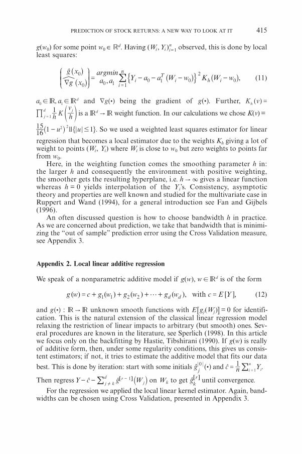
g(w0) for some point w0 ∈ �d. Having (Wi ,Yi )ni=1 observed, this is done by local
least squares:
, ,argminx
g x a a Y a a W w K W wg
iT
i h ii
n0
0 0 10 1 0
2
01d
= - - - -=
!%J
L
KK
^
^^ ^
N
P
OO
h
hh h$ . (11)
,a aR Rd0 1! ! and g :d ] g being the gradient of g :] g. Further, K vh =] g
hK
h
v1 j
j
d
1=% e o is a R Rd " weight function. In our calculations we chose K(v) =
u u1615
1 1ll2 2#-_ i " ,. So we used a weighted least squares estimator for linear
regression that becomes a local estimator due to the weights Kh giving a lot ofweight to points (Wi, Yi) where Wi is close to w0 but zero weights to points farfrom w0.
Here, in the weighting function comes the smoothing parameter h in:the larger h and consequently the environment with positive weighting,the smoother gets the resulting hyperplane, i.e. h " 3 gives a linear functionwhereas h = 0 yields interpolation of the Yi’s. Consistency, asymptotic theory and properties are well known and studied for the multivariate case inRuppert and Wand (1994), for a general introduction see Fan and Gijbels(1996).
An often discussed question is how to choose bandwidth h in practice.As we are concerned about prediction, we take that bandwidth that is minimi-zing the “out of sample” prediction error using the Cross Validation measure,see Appendix 3.
Appendix 2. Local linear additive regression
We speak of a nonparametric additive model if g(w), Rw d! is of the form
( ) ( ) ( ) ( ), ,withg w c g w g w g w c E Yd d1 1 2 2 g= + + + + = 6 @ (12)
and : R Rg ":] g unknown smooth functions with E [gj(Wj)] = 0 for identifi-cation. This is the natural extension of the classical linear regression modelrelaxing the restriction of linear impacts to arbitrary (but smooth) ones. Sev-eral procedures are known in the literature, see Sperlich (1998). In this articlewe focus only on the backfitting by Hastie, Tibshirani (1990). If g(w) is reallyof additive form, then, under some regularity conditions, this gives us consis-tent estimators; if not, it tries to estimate the additive model that fits our data
best. This is done by iteration: start with some initials gj0
:] g and n Yc 1ii
n
1=
=! .
Then regress Y Wc g rjj k
d 1- -!
-! ` j5 ? on Wk to get gkr5 ? until convergence.
For the regression we applied the local linear kernel estimator. Again, band-widths can be chosen using Cross Validation, presented in Appendix 3.
PREDICTION OF STOCK RETURNS: A NEW WAY TO LOOK AT IT 415

Appendix 3. Cross Validation
A typical question of interest, not only in prediction problems, is how to eval-uate the different models. This concerns the model or variable selection as wellas the bandwidth choice. In general, a natural way to evaluate an estimator isto look on the mean squared error or the expected squared difference betweenestimate and observation Y: E [{Y – g(W)}2]. This certainly has to be estimated.Additionally, as we speak about prediction, we would like to know how well theestimator works outside the considered sample. Both aspects are taken intoaccount in the so called Cross Validation (CV) values, defined as
,value n y wg1CV ( )
ll
ll
n2
1
- = -=
! ^ h# - (13)
where wg( )ll^ h is the considered estimator evaluated at point wl but determined
without observation ( , )w yl l . This CV-value is an approximation for the meansquared error (also for prediction) and a quite common used validation mea-sure in nonparametric regression. For time series context and more referencessee e.g. Gyöfri, Härdle, Sarda, and Vieu (1990).
Remark: It is important to eliminate always all information that is aimed topredict from the estimation of g :] g. So, if we predict the increase of assets overa period of 4 years, the estimator g( )l is calculated not only without the l th obser-vation but also without the three years before and after year l.
How can it be used for bandwidth or model selection?We give an example for bandwidth selection: write g as a function of the
bandwidth (gh) and look for that h that minimizes
( ) ( ) .h n y wg1CV ( )
l hl
ll
n 2
1
= -=
! $ .
This has been shown to give the optimal bandwidth in nonparametric regres-sion, we again refer to Gyöfri et al. (1990).
Note finally, that minimizing the CV-value is equivalent to maximizing theR 2
V. So CV is directly used to find both: the optimal h for prediction and theoptimal model for prediction.
REFERENCES
BARBER, B.M. and TERRANCE, O. (2000) Trading is hazardous to your wealth: The commonstock investment performance of individual investors. Journal of Finance 55, 773-806.
CAIRNS, A.J.G. (2000) A discussion of parameter and model uncertainty in insurance. Insur-ance: Mathematics and Economics 27, 313-330.
CAMPBELL, J.Y. and SHILLER, R.J. (1988) The dividend-price ratio and expectations of futuredividends and discount factors. Review of Financial Studies 1, 195-228.
CAMPBELL, J.Y., LO, A.W. and MACKINLAY, A.C. (1997) The Econometrics of financial markets.Princeton University Press, Princeton, New Jersey.
DIMSON, E., MARSH, P. and STAUNTON, M. (2002) Triumph of the Optimists. Princeton UniversityPress.
416 JENS PERCH NIELSEN AND STEFAN SPERLICH
ENGSTED, T. and TANGGÅRD, C. (2000) The Danish stock and bond markets: Comovement,return predictability and variance decomposition. Journal of Empirical Finance 8, 243-271.
EUN, C.S. and RESNICK, B.G. (1988) Exchange rate uncertainty, forward contracts, and interna-tional portfolio selection. Journal of Finance 43, 197-215.
EUN, C.S. and RESNICK, B.G. (1994) Exchange rate uncertainty, forward contracts, and interna-tional portfolio selection. Management Science 40, 140-161.
FAMA, E. and FRENCH, K. (1988) Dividend yields and expected stock returns. Journal of Finan-cial Economics 22, 3-25.
FAN, J. and GIJBELS, I. (1996) Local polynomial regression. Chapman and Hall, London.GOETZMANN, W.N. and JORION, P. (1993) Testing the predictive power of dividend yields. Jour-
nal of Finance 48, 663-679.GORDON, M. and SHAPIRO, P. (1956) Capital Equilibrium analysis: The required rate of profit.
Management Science 3, 102-110.GYÖFRI, L., HÄRDLE, W., SARDA, P. and VIEU, Ph. (1990) Nonparametric Curve Estimation from
Time Series. Lecture Notes in Statistics. Heidelberg: Springer-Verlag.HANSEN, S. (1974) Økonomisk vækst i Danmark [Economic growth in Denmark], Akademisk
Forlag, Copenhagen, Denmark.HARRIS, G.R. (1999) Marcov chain Monte Carlo estimation of regime switching vector autore-
gressions. ASTIN Bulletin 29, 47-79.HASTIE, T.J. and TIBSHIRANI, R.J. (1990) Generalized Additive Models. Chapman and Hall.HODRICK, R.J. (1992) Dividend yields and expected stock returns: Alternative procedures for
inference and measurement. Review of Financial Studies 5, 357-386.HURVICH, C.M., SIMONOFF, J.S. and TSAI, C.-L. (1998) Smoothing parameter selection in non-
parametric regression using an improved Akaike information criterion. Journal of the RoyalStatistical Society, B 60, 271-293.
JAGANNATHAN, R. and KOCHERLAKOTA, N.R. (1996) Why should older people invest less instocks than younger people. Federal Reserve Bank of Minneapolis. Quaterly Review, Summer1996. 11-20.
KVÅLSETH, T. (1985) Cautionary note about R2. The American Statistician 39, 279-285.LUND, J. and ENGSTED, T. (1996) GMM and present value tests of the C-CAPM: Evidence from
the Danish, German, Swedish, and UK stock markets. Journal of International Money andFinance 15, 497-521.
MÜLLER M. (1998) Computer-assisted Statistics Teaching in Network Environments. COMP-STAT ’98 Proceedings, Bristol, UK.
RICHARDSON, M. and STOCK, J.H. (1989) Drawing inferences from statistics based on multi-yearasset returns. Journal of Financial Economics 25, 323-348.
RUPPERT, D. and WAND, M.P. (1994) Multivariate locally weighted least squares regression.Annals of Statistics 22, 1346-1370.
SIEGEL, J.J. (1998) Stocks for the long run, 2nd ed. New York: McGraw-Hill.SHILLER, R.J. (1981) Do stock prices move too much to be justified by subsequent changes in
dividends. American Economic Review 71, 421-436.SHILLER, R.J. (2000) Irrational exuberrance. Princeton University Press, Princeton, New Jersey.SPERLICH, S. (1998) Additive Modelling and testing Model Specification. Shaker Verlag, Aachen.SPERLICH, S., LINTON, O., and HÄRDLE, W. (1999) Integration and backfitting methods in addi-
tive models-Finite sample properties and comparison. Test 8, 419-458.WILKIE, A.D. (1993) Can dividend yields predict share price changes? Transactions of the 3rd
International AFIR Colloquium, Rome, 1, 335-347.WILKIE, A.D. (1995) More on a stochastic asset model for actuarial use. British Actuarial Jour-
nal 5, 777-964.WILLIAMS, J.B. (1938) The Theory of Investment Value. Harvard University Press, Cambridge.
PREDICTION OF STOCK RETURNS: A NEW WAY TO LOOK AT IT 417

SETTING A BONUS-MALUS SCALE IN THE PRESENCE OF OTHERRATING FACTORS: TAYLOR’S WORK REVISITED
BY
SANDRA PITREBOIS, MICHEL DENUIT AND JEAN-FRANÇOIS WALHIN
ABSTRACT
In this paper, we propose an analytic analogue to the simulation proceduredescribed in Taylor (1997). We apply the formulas to a Belgian data set anddiscuss the interaction between a priori and a posteriori ratemakings.
KEYWORDS AND PHRASES
Bonus-Malus system, Markov chains, a priori ratemaking, experience rating
1. INTRODUCTION AND MOTIVATION
One of the main tasks of the actuary is to design a tariff structure that willfairly distribute the burden of claims among policyholders. To this end, heoften has to partition all policies into homogeneous classes with all policy-holders belonging to the same class paying the same premium. The classifica-tion variables introduced to partition risks into cells are called a priori variables(as their values can be determined before the policyholder starts to drive).In motor third-party liability (MTPL, in short) insurance, they include age,gender and occupation of the policyholders, type and use of their car, placewhere they live and sometimes even number of cars in the household or mar-ital status. It is convenient to achieve a priori classification by resorting to gen-eralized linear models (e.g. Poisson regression).
However, many important factors cannot be taken into account at thisstage; think for instance of swiftness of reflexes, aggressiveness behind thewheel or knowledge of the highway code. Consequently, risk classes are stillquite heterogeneous despite the use of many a priori variables. But it is rea-sonable to believe that these hidden factors are revealed by the number ofclaims reported by the policyholders over the successive insurance periods.Hence the amount of premium is adjusted each year on the basis of the indi-vidual claims experience in order to restore fairness among policyholders.
Rating systems penalizing insureds responsible for one or more accidentsby premium surcharges (or maluses), and rewarding claim-free policyholdersby awarding them discounts (or bonuses) are now in force in many developedcountries. This a posteriori ratemaking is a very efficient way of classifying
ASTIN BULLETIN, Vol. 33, No. 2, 2003, pp. 419-436
policyholders according to their risk. Besides encouraging policyholders todrive carefully (i.e. counteracting moral hazard), they aim to better assess indi-vidual risks. Such systems are called no-claim discounts, experience rating,merit rating, or Bonus-Malus systems (BMS, in short). We will adopt here thelatter terminology. For a thorough presentation of the techniques relating toBMS, see Lemaire (1995).
When a BMS is in force, the amount of premium paid by the policyholderdepends on the rating factors of the current period but also on claim history. Inpractice, a BMS consists of a finite number of levels, each with its own relativepremium. New policyholders have access to a specified class. After each year, thepolicy moves up or down according to transition rules and to the number ofclaims at fault. The premium charged to a policyholder is obtained by applyingthe relative premium associated to his current level in the BMS to a base pre-mium depending on his observable characteristics incorporated into the price list.
The problem addressed in this paper is the determination of the relativepremiums attached to each of the levels of the BM scale when a priori classi-fication is used by the company. The severity of the a posteriori corrections mustdepend on the extent to which amounts of premiums vary according to observ-able characteristics of policyholders. The key idea is that both a priori classi-fication and a posteriori corrections aim to create tariff cells as homogeneousas possible. The residual heterogeneity inside each of these cells being smallerfor insurers incorporating more variables in their a priori ratemaking, the a pos-teriori corrections must be softer for those insurers.
This paper is not conceptually innovating. All the ideas are contained in theseminal work by Taylor (1997). Our only contribution is to show how it is pos-sible to avoid simulations by providing analytical formulas for the relative pre-miums attached to each level of the BM scale.
Our work is organized as follows. In Section 2, we briefly present the mod-elling used to compute pure premiums. Section 3 describes BM scales and theirrepresentation as Markov chains. Section 4 explains how to determine the rel-ative premiums when a priori classification is in force or not. Section 5 describesseveral numerical illustrations. In Section 6, we show that it is possible to applydifferent a posteriori corrections according to a priori characteristics. The finalSection 7 discusses some possible improvements and concludes.
2. CREDIBILITY UPDATING FORMULAS
Let , , , ,N t 1 2it f= represent the number of claims incurred by policyholder iin period t. The annual expected claim frequency for policy i in year t is
[ ]� Nit it=m . It is expressed as the exponential transform of some predictorinvolving the characteristics of policyholder i in period t. Of course, all the riskfactors cannot be taken into account at this stage.
Risk classes remain heterogeneous despite the use of many a priori riskcharacteristics. This residual heterogeneity can be represented by a randomeffect Qi superposed to the annual expected claim frequency. Specifically, givenQi = q the annual numbers of claims Nit are assumed to be independent andto conform to a Poisson distribution with mean itm i, i.e.
420 SANDRA PITREBOIS, MICHEL DENUIT, JEAN-FRANÇOIS WALHIN
| ! , .Pr exp �N k k kQit i itit
k
!= = = -i imm i
^^
hh
7 A
Moreover, all the Qi’s are assumed to be independent and to follow a standardGamma distribution with probability density function
( ) ( ) ( ), .exp �u a a aG1 a a 1 != -i i i i- + (2.1)
The latter is often referred to as the structure function of the portfolio. Since[ ]� 1Qi = we have that [ ] ;� Nit it it= m m is the expected claim number for a poli-
cyholder for which no information about past claims is available.The premium is then adjusted over time with the help of credibility techni-
ques. We assume that each policyholder has an unknown expected claim fre-quency ‡i, constant over time. Following the seminal work of Dionne andVanasse (1989), the company approaches this unknown value with annual pre-dictions of the form ‡̂i1 = li1 and for t ≥ 2,
‡̂it = | , , .� N N Na
a Nit i it it
it
it
1 1
1
11
1
f =+
+m
m-
=
-=
-
xx
xx
!!
7 A (2.2)
The latter Bayesian credibility estimator cannot be enforced in practice forMTPL, essentially due to commercial reasons and legal constraints. Instead,companies resort to BM scales, that may be considered as simplified versionsof credibility theory formulas. Those are presented in the next section.
3. MARKOV MODELS FOR PRACTICAL BMS
3.1. BMS as Markov chains
In practice, insurance companies often resort to BM scales similar to those inTables 5.4-5.6-5.8 and not on credibility coefficients like those of (2.2). Suchscales possess a number of levels, s + 1 say, numbered from 0 to s. A specifiedlevel is assigned to a new driver (often according to the use of the vehicle). Eachclaim free year is rewarded by a bonus point (i.e. the driver goes one leveldown). Claims are penalized by malus points (i.e. the driver goes up a certainnumber of levels each time he files a claim). We assume that the penalty is agiven number of classes per claim. This facilitates the mathematical treatmentof the problem but more general systems could also be considered. After suf-ficiently many claim-free years, the driver enters level 0 where he enjoys themaximal bonus.
In commercial BMS, the knowledge of the present level and of the num-ber of claims of the present year suffice to determine the next level. Thisensures that the BMS may be represented by a Markov chain: the future (theclass for year t + 1) depends on the present (the class for year t and the num-ber of accidents reported during year t) and not on the past (the complete
SETTING A BONUS-MALUS SCALE 421
claim history and the levels occupied during years , , , )t1 2 1f - . Sometimes,fictitious classes have to be introduced in order to meet this memoryless prop-erty. Indeed, in some BMS, policyholders occupying high levels are sent to thestarting class after a few claimless years.
The relativity associated to level , is denoted as ,r ; the meaning is that aninsured occupying that level pays an amount of premium equals to ,r % of thea priori premium determined on the basis of his observable characteristics.
3.2. Transient distributions
Let p,1,2(‡) be the probability of moving from level ,1 to level ,2 for a policy-
holder with mean frequency ‡. Further, M(‡) is the one-step transitionmatrix, i.e. M(‡) = {p,1,2
(‡)}, ,1, ,2 = 0,1,…,s. Taking the nth power of M(‡)yields the n-step transition matrix whose element (,1,2), denoted as p(n)
,1,2(‡), is
the probability of moving from level ,1 to level ,2 in n transitions.
3.3. Stationary distribution
All BMS in practical use have a “best” level, with the property that a policyin that level remains in the same level after a claim-free period. In the follow-ing, we restrict attention to such non-periodic bonus rules. The transitionmatrix ( )M j associated to such a BMS is regular, i.e. there exists some inte-ger 10$p such that all entries of ( )M 0j p
! + are strictly positive. Consequently,the Markov chain describing the trajectory of a policyholder with expectedclaim frequency j accross the levels is ergodic and thus possesses a stationarydistribution ( ) ( ( ), ( ), , ( )) ; ( )s
t0 1 f=j r j r j r j r jr , is the stationary probabil-
ity for a policyholder with mean frequency j to be in level , i.e.
( ) ( ).lim p( )2 1 2
=r j j"
,3 , ,+o
o
Note that ( )jr does not depend on the starting class.Let us now recall how to compute the ( )r j, ’s. The vector ( )jr is the solu-
tion of the system
( ) ( ) ( ),( )
Me 1
t t
t=
=
j j jj
r rr)
where e is a column vector of 1’s. Let E be the ( ) ( )s s1 1#+ + matrix all ofwhose entries are 1, i.e. consisting of s 1+ column vectors e. Then, it can beshown that
( ) ( ) ,Ie M Et t 1= - +j jr -^ h
which provides a direct method to get ( )jr . For a derivation of the latter result,see e.g. Rolski et al. (1999).
422 SANDRA PITREBOIS, MICHEL DENUIT, JEAN-FRANÇOIS WALHIN
4. DETERMINATION OF THE RELATIVITIES
4.1. Interaction between the BM scale and a priori ratemaking
Since the relativities attached to the different levels are the same whatever therisk class to which the policyholders belong, those scales overpenalize a prioribad risks. Let us explain this phenomenon, put in evidence by Taylor (1997).Over time, policyholders will be distributed over the levels of the bonus-malusscale. Since their trajectory is a function of past claims history, policyholderswith low a priori expected claim frequencies will tend to gravitate in the low-est levels of the scale. Conversely for individuals with high a priori expectedclaim frequencies. Consider for instance a policyholder with a high a prioriexpected claim frequency, a young male driver living in a urban area, say. Thisdriver is expected to report many claims (this is precisely why he has beenpenalized a priori) and so to be transferred to the highest levels of the BM scale.On the contrary, a policyholder with a low a priori expected claim frequency,a middle-aged lady living in a rural area, say, is expected to report few claimsand so to gravitate in the lowest levels of the scale. The level occupied by thepolicyholders in the BM scale can thus be partly explained by their observablecharacteristics included in the price list. It is thus fair to isolate that part ofthe information contained in the level occupied by the policyholder that doesnot reflect observables characteristics. A posteriori corrections should be onlydriven by this part of the BM information.
Let us try to quantify these findings. To this end, we introduce the randomvariable Lj valued in { , , , }s0 1 f such that Lj conforms to the distribution
( )jr i.e.
[ ] ( ), , , , .Pr L s0 1, , f= = =r j,j
The variable Lj thus represents the level occupied by a policyholder with annualexpected claim frequency j once the steady state has been reached.
Let us now pick at random a policyholder from the portfolio. Let us denoteas L his (unknown) a priori expected claim frequency and as Q the residualeffect of the risk factors not included in the ratemaking. The actual (unknown)annual expected claim frequency of this policyholder is then LQ. Since therandom effect Q represents residual effects of hidden covariates, the randomvariables L and Q may reasonably be assumed to be mutually independent. Letwk be the weight of the kth risk class whose annual expected claim frequencyis km . Clearly, [ ]Pr wk k= =mK .
Now, let L be the BM level occupied by this randomly selected policyholderonce the steady state has been reached. The distribution of L can be writtenas
[ ] ( ) ( ) ;Pr L w u d>k k
k 0,= = r m i i i,i
#! (4.1)
[ ]Pr L ,= represents the proportion of the policyholders in level ,.
SETTING A BONUS-MALUS SCALE 423
4.2. Norberg’s predictive accuracy in segmented tariffs
Predictive accuracy is a useful measure of the efficiency of a BMS. The ideabehind this notion is as follows. A BMS is good at discriminating amongthe good and the bad risks if the premium they pay is close to their “true”premium. According to Norberg (1976), once the number of classes and thetransition rules have been fixed, the optimal relativity r, associated to level , isdetermined by maximizing the asymptotic predictive accuracy.
As above, let LQ be the true (unknown) expected claim frequency of apolicyholder picked at random from the portfolio, where Q admits the pdf(2.1) and [ ]Pr wL k k= =m , with � L = m6 @ . Our aim is to minimize the expectedsquared difference between the “true” relative premium Q and the relativepremium rL applicable to this policyholder (after the stationary state has beenreached), i.e. the goal is to minimize
[( ) ] ( ) | [ ]
( ) [ | ] ( )
( ) ( ) ( ) .
Pr
Pr
� �r r L L
r L u d
w r u d
Q Q
Q>
>
L
s
s
k k
s
k
2 2
0
2
00
2
00
, ,
,
- = - = =
= - = =
= -
i i i i
i r m i i i
,,
,,
, ,,
=
=
=
i
i
#
#
!
!
!!
7 A
The solution is given by
[ | ]
| , |
| , |
[ , ][ | , ]
( ) [ ][ , ]
( ) ( )
( ) ( ).
Pr
PrPr
PrPr
�
� �
�
r L
L L
L L
LL w
u d LL
w u d
w u d
Q
Q L
Q L L
LQ L
>
>
>
k kk
k
k k k
k
k kk
k kk
0
0
0
,
, ,
, ,
,
,,
,
= =
= = =
= = = = =
== =
= = =
=
= =
=
m m
im
i mi i
m
r m i i i
ir m i i i
K
,
,
,
i
i
i
#
#
#
!
!
!
!
66
6 6
@@
@ @
(4.2)
It is easily seen that [ ] ,� r 1L = resulting in financial equilibrium once steadystate is reached.
To end with, let us mention that if the insurance company does not enforce anya priori ratemaking system, all the lk’s are equal to l and reduces to the formula
( ) ( )
( ) ( )r
u d
u d
>
>
0
0=r mi i i
ir mi i i,
,
,
i
i
#
#
that has been derived in Norberg (1976).
424 SANDRA PITREBOIS, MICHEL DENUIT, JEAN-FRANÇOIS WALHIN
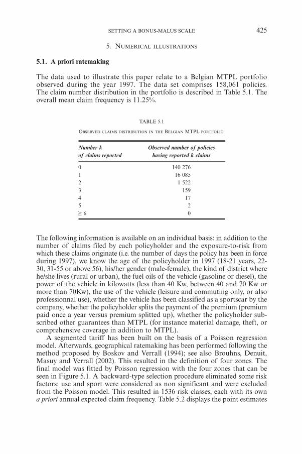
5. NUMERICAL ILLUSTRATIONS
5.1. A priori ratemaking
The data used to illustrate this paper relate to a Belgian MTPL portfolioobserved during the year 1997. The data set comprises 158,061 policies.The claim number distribution in the portfolio is described in Table 5.1. Theoverall mean claim frequency is 11.25%.
TABLE 5.1
OBSERVED CLAIMS DISTRIBUTION IN THE BELGIAN MTPL PORTFOLIO.
Number k Observed number of policiesof claims reported having reported k claims
0 140 2761 16 0852 1 5223 1594 175 2
6$ 0
The following information is available on an individual basis: in addition to thenumber of claims filed by each policyholder and the exposure-to-risk fromwhich these claims originate (i.e. the number of days the policy has been in forceduring 1997), we know the age of the policyholder in 1997 (18-21 years, 22-30, 31-55 or above 56), his/her gender (male-female), the kind of district wherehe/she lives (rural or urban), the fuel oils of the vehicle (gasoline or diesel), thepower of the vehicle in kilowatts (less than 40 Kw, between 40 and 70 Kw ormore than 70Kw), the use of the vehicle (leisure and commuting only, or alsoprofessionnal use), whether the vehicle has been classified as a sportscar by thecompany, whether the policyholder splits the payment of the premium (premiumpaid once a year versus premium splitted up), whether the policyholder sub-scribed other guarantees than MTPL (for instance material damage, theft, orcomprehensive coverage in addition to MTPL).
A segmented tariff has been built on the basis of a Poisson regressionmodel. Afterwards, geographical ratemaking has been performed following themethod proposed by Boskov and Verrall (1994); see also Brouhns, Denuit,Masuy and Verrall (2002). This resulted in the definition of four zones. Thefinal model was fitted by Poisson regression with the four zones that can beseen in Figure 5.1. A backward-type selection procedure eliminated some riskfactors: use and sport were considered as non significant and were excludedfrom the Poisson model. This resulted in 1536 risk classes, each with its owna priori annual expected claim frequency. Table 5.2 displays the point estimates
SETTING A BONUS-MALUS SCALE 425
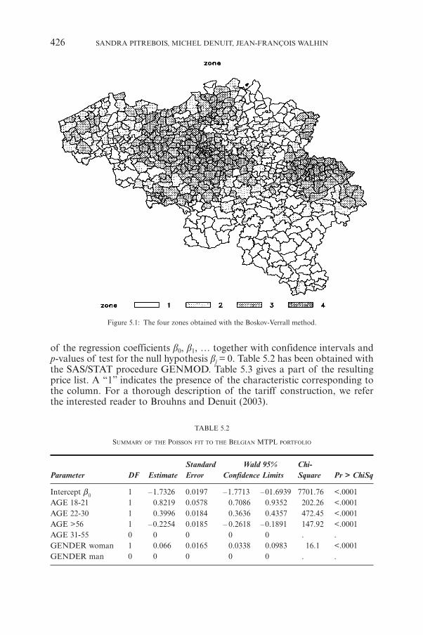
Figure 5.1: The four zones obtained with the Boskov-Verrall method.
of the regression coefficients b0, b1, … together with confidence intervals andp-values of test for the null hypothesis bj = 0. Table 5.2 has been obtained withthe SAS/STAT procedure GENMOD. Table 5.3 gives a part of the resultingprice list. A “1” indicates the presence of the characteristic corresponding tothe column. For a thorough description of the tariff construction, we referthe interested reader to Brouhns and Denuit (2003).
TABLE 5.2
SUMMARY OF THE POISSON FIT TO THE BELGIAN MTPL PORTFOLIO
Standard Wald 95% Chi-Parameter DF Estimate Error Confidence Limits Square Pr > ChiSq
Intercept 0
b 1 –1.7326 0.0197 –1.7713 –01.6939 7701.76 <.0001AGE 18-21 1 0.8219 0.0578 0.7086 0.9352 202.26 <.0001AGE 22-30 1 0.3996 0.0184 0.3636 0.4357 472.45 <.0001AGE >56 1 –0.2254 0.0185 – 0.2618 –0.1891 147.92 <.0001AGE 31-55 0 0 0 0 0 . .GENDER woman 1 0.066 0.0165 0.0338 0.0983 16.1 <.0001GENDER man 0 0 0 0 0 . .
426 SANDRA PITREBOIS, MICHEL DENUIT, JEAN-FRANÇOIS WALHIN
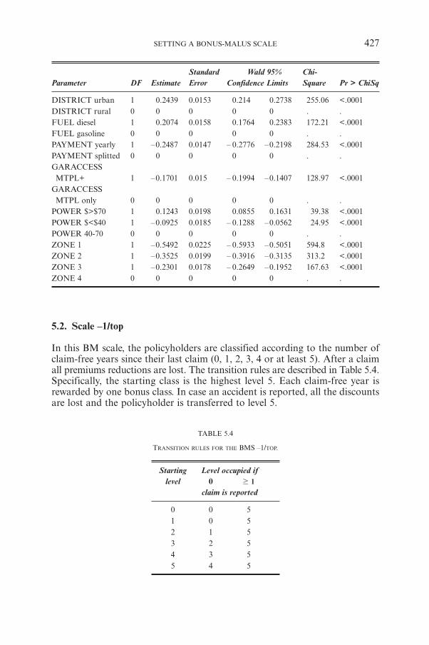
Standard Wald 95% Chi-Parameter DF Estimate Error Confidence Limits Square Pr > ChiSq
DISTRICT urban 1 0.2439 0.0153 0.214 0.2738 255.06 <.0001DISTRICT rural 0 0 0 0 0 . .FUEL diesel 1 0.2074 0.0158 0.1764 0.2383 172.21 <.0001FUEL gasoline 0 0 0 0 0 . .PAYMENT yearly 1 –0.2487 0.0147 – 0.2776 –0.2198 284.53 <.0001PAYMENT splitted 0 0 0 0 0 . .GARACCESS MTPL+ 1 –0.1701 0.015 – 0.1994 –0.1407 128.97 <.0001
GARACCESS MTPL only 0 0 0 0 0 . .
POWER $>$70 1 0.1243 0.0198 0.0855 0.1631 39.38 <.0001POWER $<$40 1 –0.0925 0.0185 – 0.1288 –0.0562 24.95 <.0001POWER 40-70 0 0 0 0 0 . .ZONE 1 1 –0.5492 0.0225 – 0.5933 –0.5051 594.8 <.0001ZONE 2 1 –0.3525 0.0199 – 0.3916 –0.3135 313.2 <.0001ZONE 3 1 –0.2301 0.0178 – 0.2649 –0.1952 167.63 <.0001ZONE 4 0 0 0 0 0 . .
5.2. Scale –1/top
In this BM scale, the policyholders are classified according to the number ofclaim-free years since their last claim (0, 1, 2, 3, 4 or at least 5). After a claimall premiums reductions are lost. The transition rules are described in Table 5.4.Specifically, the starting class is the highest level 5. Each claim-free year isrewarded by one bonus class. In case an accident is reported, all the discountsare lost and the policyholder is transferred to level 5.
TABLE 5.4
TRANSITION RULES FOR THE BMS –1/TOP.
Starting Level occupied iflevel 0 1$
claim is reported
0 0 51 0 52 1 53 2 54 3 55 4 5
SETTING A BONUS-MALUS SCALE 427
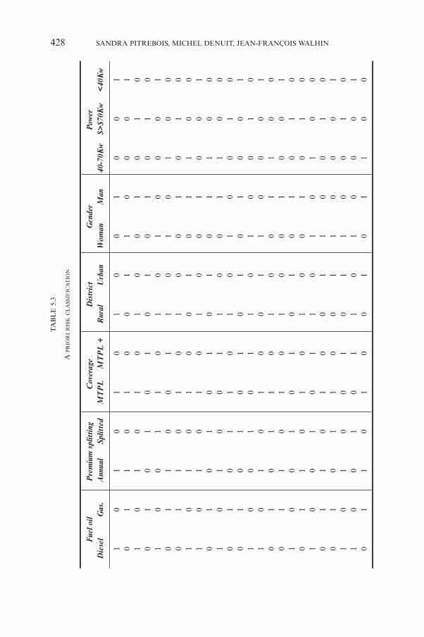
428 SANDRA PITREBOIS, MICHEL DENUIT, JEAN-FRANÇOIS WALHINT
AB
LE
5.3
A P
RIO
RI
RIS
KC
LA
SSIF
ICA
TIO
N
Fue
l oil
Pre
miu
m s
plit
ting
Cov
erag
eD
istr
ict
Gen
der
Pow
erD
iese
lG
as.
Ann
ual
Spl
itte
dM
TP
LM
TP
L +
Rur
alU
rban
Wom
anM
an40
-70K
w$>
$70K
w<
40K
w
10
10
10
10
01
00
10
11
01
00
11
00
01
10
10
10
10
01
01
00
10
10
10
10
10
10
10
01
10
10
10
00
10
11
00
11
01
01
00
01
10
10
10
01
01
01
01
01
00
10
11
00
10
10
10
10
01
00
10
10
10
10
10
11
00
10
10
01
10
01
10
00
10
11
01
01
00
10
01
01
01
01
01
00
11
00
10
11
01
00
10
10
10
10
01
10
00
10
10
11
01
00
11
00
01
10
10
10
01
00
11
00
10
10
10
10
10
01
10
10
10
01
01
01
00
10
11
01
01
00
01
10
10
01
10
01
00
10
11
00
11
00
01
10
10
01
01
10
01
01
00
10
11
01
00
01
01
10
10
01
01
10
0
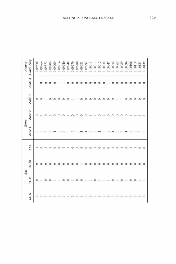
SETTING A BONUS-MALUS SCALE 429
Age
Zon
eA
nnua
l18
-21
31-5
522
-30
>55
Zon
e 1
Zon
e 2
Zon
e 3
Zon
e 4
Cla
im F
req.
00
01
00
01
0.09
858
01
00
01
00
0.09
864
00
01
00
10
0.09
873
00
01
01
00
0.09
904
01
00
10
00
0.09
909
01
00
00
01
0.09
914
00
01
00
01
0.09
940
00
01
01
00
0.09
948
01
00
00
10
0.09
979
00
01
00
10
0.09
980
00
10
10
00
0.09
981
01
00
10
00
0.09
992
01
00
01
00
0.10
011
00
01
01
00
0.10
013
01
00
10
00
0.10
013
01
00
01
00
0.10
034
01
00
00
01
0.10
047
00
01
10
00
0.10
054
01
00
00
10
0.10
062
00
01
00
10
0.10
089
01
00
10
00
0.10
096
00
01
01
00
0.10
106
00
01
01
00
0.10
118
01
00
01
00
0.10
121
01
00
01
00
0.10
139
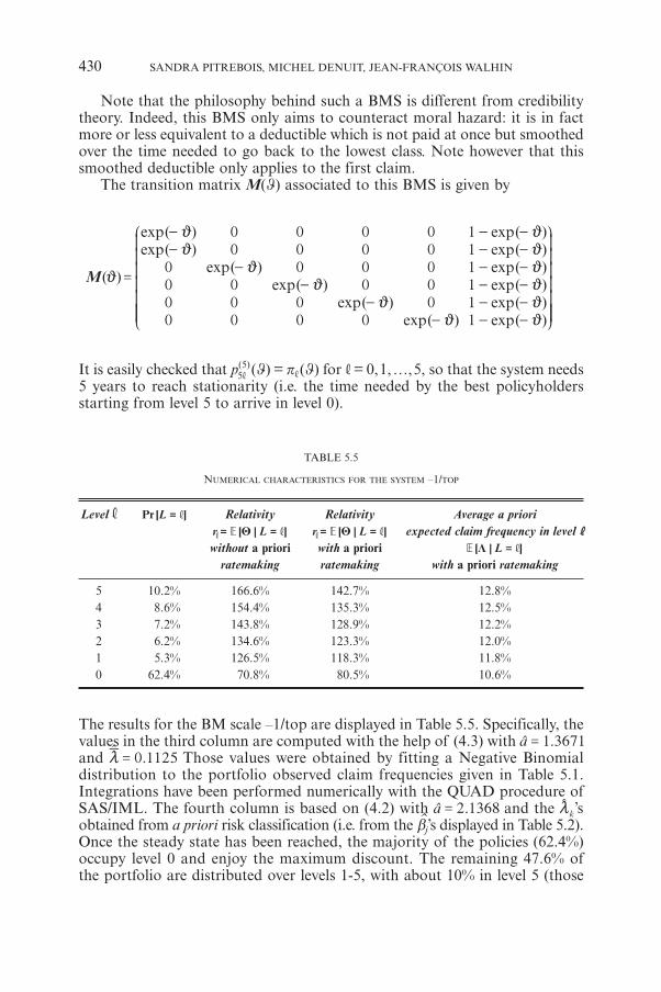
Note that the philosophy behind such a BMS is different from credibilitytheory. Indeed, this BMS only aims to counteract moral hazard: it is in factmore or less equivalent to a deductible which is not paid at once but smoothedover the time needed to go back to the lowest class. Note however that thissmoothed deductible only applies to the first claim.
The transition matrix M(‡) associated to this BMS is given by
( )
( )( )
( )( )
( )( )
( )( )( )( )( )( )
expexp
expexp
expexp
expexpexpexpexpexp
M0000
00
000
000
00
0000
0
00000
111111
=
--
--
--
- -- -- -- -- -- -
j
jj
jj
jj
jjjjjj
J
L
KKKKKKK
N
P
OOOOOOO
It is easily checked that p(5)5, (‡) = p,(‡) for ,= 0,1,…,5, so that the system needs
5 years to reach stationarity (i.e. the time needed by the best policyholdersstarting from level 5 to arrive in level 0).
TABLE 5.5
NUMERICAL CHARACTERISTICS FOR THE SYSTEM –1/TOP
Level , [ ]Pr L ,= Relativity Relativity Average a priori[ | ]�r LQ ,= =, [ | ]�r LQ ,= =, expected claim frequency in level ,,
without a priori with a priori [ | ]� LL ,=
ratemaking ratemaking with a priori ratemaking
5 10.2% 166.6% 142.7% 12.8%4 8.6% 154.4% 135.3% 12.5%3 7.2% 143.8% 128.9% 12.2%2 6.2% 134.6% 123.3% 12.0%1 5.3% 126.5% 118.3% 11.8%0 62.4% 70.8% 80.5% 10.6%
The results for the BM scale –1/top are displayed in Table 5.5. Specifically, thevalues in the third column are computed with the help of (4.3) with .a 1 3671=and .0 1125=m
t Those values were obtained by fitting a Negative Binomialdistribution to the portfolio observed claim frequencies given in Table 5.1.Integrations have been performed numerically with the QUAD procedure ofSAS/IML. The fourth column is based on (4.2) with .a 2 1368= and the km
t ’sobtained from a priori risk classification (i.e. from the bj’s displayed in Table 5.2).Once the steady state has been reached, the majority of the policies (62.4%)occupy level 0 and enjoy the maximum discount. The remaining 47.6% ofthe portfolio are distributed over levels 1-5, with about 10% in level 5 (those
430 SANDRA PITREBOIS, MICHEL DENUIT, JEAN-FRANÇOIS WALHIN
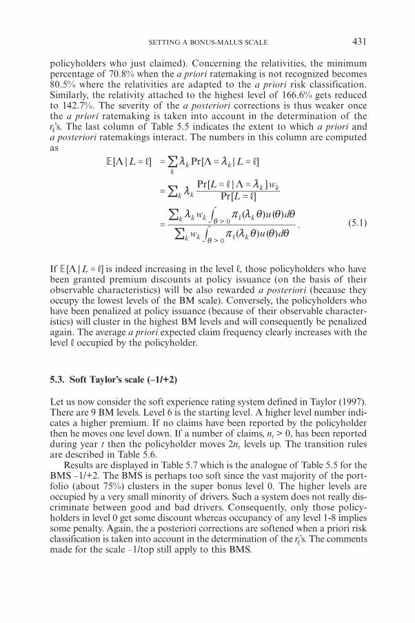
policyholders who just claimed). Concerning the relativities, the minimumpercentage of 70.8% when the a priori ratemaking is not recognized becomes80.5% where the relativities are adapted to the a priori risk classification.Similarly, the relativity attached to the highest level of 166.6% gets reducedto 142.7%. The severity of the a posteriori corrections is thus weaker oncethe a priori ratemaking is taken into account in the determination of ther,’s. The last column of Table 5.5 indicates the extent to which a priori anda posteriori ratemakings interact. The numbers in this column are computedas
[ | ] [ | ]
[ ][ | ]
( ) ( )
( ) ( ).
Pr
PrPr
� L L
LL w
w u d
w u d
L L
L
>
>
k kk
kk k
k
k kk
k k kk
0
0
, ,
,,
= = = =
==
= =
=
m m
mm
r m i i i
m r m i i i
,
,
i
i
#
#
!
!
!
!(5.1)
If [ | ]� LL ,= is indeed increasing in the level ,, those policyholders who havebeen granted premium discounts at policy issuance (on the basis of theirobservable characteristics) will be also rewarded a posteriori (because theyoccupy the lowest levels of the BM scale). Conversely, the policyholders whohave been penalized at policy issuance (because of their observable character-istics) will cluster in the highest BM levels and will consequently be penalizedagain. The average a priori expected claim frequency clearly increases with thelevel , occupied by the policyholder.
5.3. Soft Taylor’s scale (–1/+2)
Let us now consider the soft experience rating system defined in Taylor (1997).There are 9 BM levels. Level 6 is the starting level. A higher level number indi-cates a higher premium. If no claims have been reported by the policyholderthen he moves one level down. If a number of claims, nt > 0, has been reportedduring year t then the policyholder moves 2nt levels up. The transition rulesare described in Table 5.6.
Results are displayed in Table 5.7 which is the analogue of Table 5.5 for theBMS –1/+2. The BMS is perhaps too soft since the vast majority of the port-folio (about 75%) clusters in the super bonus level 0. The higher levels areoccupied by a very small minority of drivers. Such a system does not really dis-criminate between good and bad drivers. Consequently, only those policy-holders in level 0 get some discount whereas occupancy of any level 1-8 impliessome penalty. Again, the a posteriori corrections are softened when a priori riskclassification is taken into account in the determination of the r,’s. The commentsmade for the scale –1/top still apply to this BMS.
SETTING A BONUS-MALUS SCALE 431
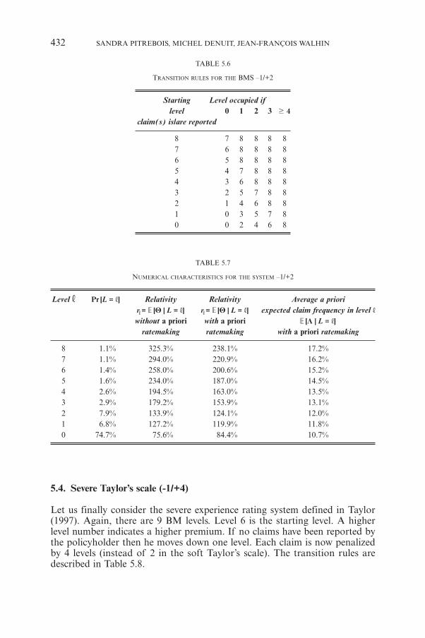
TABLE 5.6
TRANSITION RULES FOR THE BMS –1/+2
Starting Level occupied iflevel 0 1 2 3 4$
claim(s) is/are reported
8 7 8 8 8 87 6 8 8 8 86 5 8 8 8 85 4 7 8 8 84 3 6 8 8 83 2 5 7 8 82 1 4 6 8 81 0 3 5 7 80 0 2 4 6 8
TABLE 5.7
NUMERICAL CHARACTERISTICS FOR THE SYSTEM –1/+2
Level , [ ]Pr L ,= Relativity Relativity Average a priori[ | ]�r LQ ,= =, [ | ]�r LQ ,= =, expected claim frequency in level ,
without a priori with a priori [ | ]� LL ,=
ratemaking ratemaking with a priori ratemaking
8 1.1% 325.3% 238.1% 17.2%7 1.1% 294.0% 220.9% 16.2%6 1.4% 258.0% 200.6% 15.2%5 1.6% 234.0% 187.0% 14.5%4 2.6% 194.5% 163.0% 13.5%3 2.9% 179.2% 153.9% 13.1%2 7.9% 133.9% 124.1% 12.0%1 6.8% 127.2% 119.9% 11.8%0 74.7% 75.6% 84.4% 10.7%
5.4. Severe Taylor’s scale (-1/+4)
Let us finally consider the severe experience rating system defined in Taylor(1997). Again, there are 9 BM levels. Level 6 is the starting level. A higherlevel number indicates a higher premium. If no claims have been reported bythe policyholder then he moves down one level. Each claim is now penalizedby 4 levels (instead of 2 in the soft Taylor’s scale). The transition rules aredescribed in Table 5.8.
432 SANDRA PITREBOIS, MICHEL DENUIT, JEAN-FRANÇOIS WALHIN
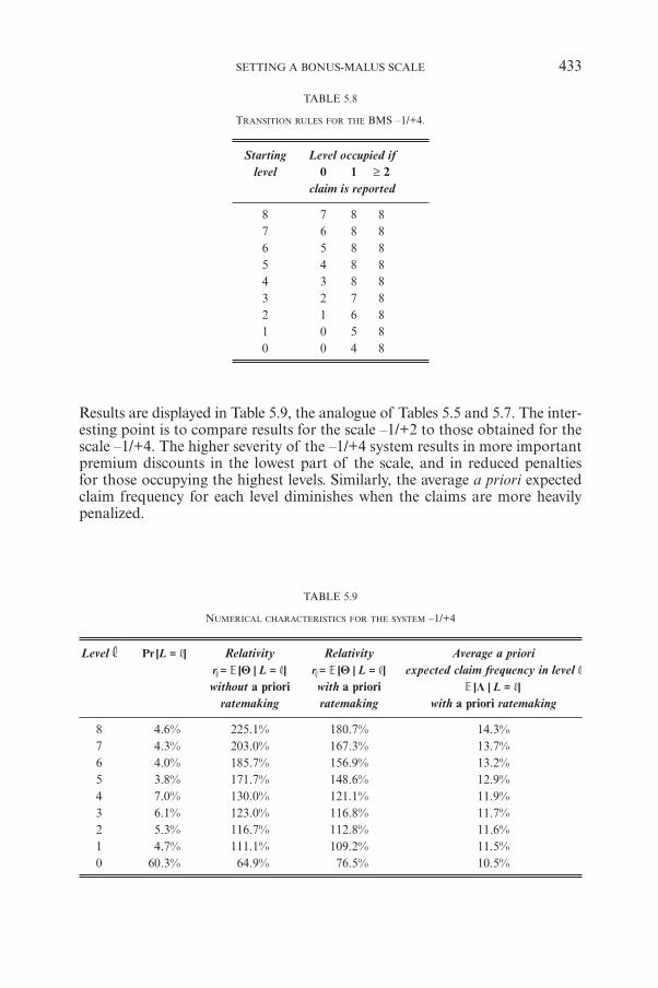
TABLE 5.8
TRANSITION RULES FOR THE BMS –1/+4.
Starting Level occupied iflevel 0 1 ≥ 2
claim is reported
8 7 8 87 6 8 86 5 8 85 4 8 84 3 8 83 2 7 82 1 6 81 0 5 80 0 4 8
Results are displayed in Table 5.9, the analogue of Tables 5.5 and 5.7. The inter-esting point is to compare results for the scale –1/+2 to those obtained for thescale –1/+4. The higher severity of the –1/+4 system results in more importantpremium discounts in the lowest part of the scale, and in reduced penaltiesfor those occupying the highest levels. Similarly, the average a priori expectedclaim frequency for each level diminishes when the claims are more heavilypenalized.
TABLE 5.9
NUMERICAL CHARACTERISTICS FOR THE SYSTEM –1/+4
Level , [ ]Pr L ,= Relativity Relativity Average a priori[ | ]�r LQ ,= =, [ | ]�r LQ ,= =, expected claim frequency in level ,
without a priori with a priori [ | ]� LL ,=
ratemaking ratemaking with a priori ratemaking
8 4.6% 225.1% 180.7% 14.3%7 4.3% 203.0% 167.3% 13.7%6 4.0% 185.7% 156.9% 13.2%5 3.8% 171.7% 148.6% 12.9%4 7.0% 130.0% 121.1% 11.9%3 6.1% 123.0% 116.8% 11.7%2 5.3% 116.7% 112.8% 11.6%1 4.7% 111.1% 109.2% 11.5%0 60.3% 64.9% 76.5% 10.5%
SETTING A BONUS-MALUS SCALE 433
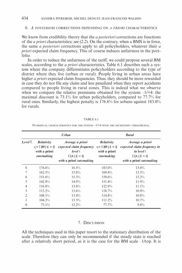
6. A POSTERIORI CORRECTIONS DEPENDING ON A PRIORI CHARACTERISTICS
We know from credibility theory that the a posteriori corrections are functionsof the a priori characteristics; see (2.2). On the contrary, when a BMS is in force,the same a posteriori corrections apply to all policyholders, whatever their apriori expected claim frequency. This of course induces unfairness in the port-folio.
In order to reduce the unfairness of the tariff, we could propose several BMscales, according to the a priori characteristics. Table 6.1 describes such a sys-tem where the company differentiates policyholders according to the type ofdistrict where they live (urban or rural). People living in urban areas havehigher a priori expected claim frequencies. Thus, they should be more rewardedin case they do not file any claim and less penalized when they report accidentscompared to people living in rural zones. This is indeed what we observewhen we compare the relative premiums obtained for the system –1/+4: themaximal discount is 73.1% for urban policyholders, compared to 77.7% forrural ones. Similarly, the highest penalty is 176.6% for urbans against 183.0%for rurals.
TABLE 6.1
NUMERICAL CHARACTERISTICS FOR THE SYSTEM –1/+4 WITH THE DICHOTOMY URBAN/RURAL.
Urban Rural
Level , Relativity Average a priori Relativity Average a priori[ | ]�r LQ ,= =, expected claim frequency [ | ]�r LQ ,= =, expected claim frequency in
with a priori level , with a priori in level ,ratemaking [ | ]� LL ,= ratemaking [ | ]� LL ,=
with a priori ratemaking with a priori ratemaking
8 176.6% 16.5% 183.0% 13.0%7 162.5% 15.8% 169.8% 12.5%6 151.6% 15.3% 159.6% 12.2%5 142.9% 14.9% 151.4% 11.9%4 116.8% 13.8% 122.9% 11.1%3 112.2% 13.6% 118.7% 10.9%2 108.1% 13.4% 114.8% 10.8%1 104.3% 13.3% 111.2% 10.7%0 73.1% 12.2% 77.7% 9.8%
7. DISCUSSION
All the techniques used in this paper resort to the stationary distribution of thescale. Therefore they can only be recommended if the steady state is reachedafter a relatively short period, as it is the case for the BM scale –1/top. It is
434 SANDRA PITREBOIS, MICHEL DENUIT, JEAN-FRANÇOIS WALHIN
worth mentioning that for the scale –1/top, the use of the stationary distribu-tion for the computation yields higher premiums than those obtained usingtransient distributions, with the method of Børgan, Hoem and Norberg (1981).
The method described in the present paper can be extended to transient dis-tributions, in the spirit of Børgan, Hoem and Norberg (1981). This may beinteresting when a new scale is introduced or for BMS needing many years toreach their stationay regime.
If on a given market companies start to compete on the basis of BMSmany policyholders could leave the portfolio after the occurrence of an acci-dent, in order to avoid the resulting penalties. Those attritions can be incor-porated in the model by adding an additional level to the Markov chain (in thespirit of Centeno and Silva (2001)). Transitions from a level of the BMS tothis state represents a policyholder leaving the portfolio whereas transitionsfrom this state to any level of the BMS means that a new policy enters the port-folio.
It has been assumed throughout this paper that the unknown expectedclaim frequencies were constant and that the random effects representing hid-den characteristics were time-invariant. Dropping these assumptions makesthe determination of the relativities much harder. We refer the interested readerto Brouhns, Guillén, Denuit and Pinquet (2003) for a thorough study of thisgeneral situation.
ACKNOWLEDGEMENTS
The authors wish to express their gratitude to the anonymous referees whohave corrected a mistake in the original manuscript and whose numerousremarks and suggestions have considerably improved the text.
REFERENCES
BORGAN, Ø, HOEM, J.M. and NORBERG, R. (1981) A nonasymptotic criterion for the evaluationof automobile bonus systems. Scandinavian Actuarial Journal, 265-178.
BOSKOV, M. and VERRALL, R.J. (1994) Premium rating by geographical area using spatial models. ASTIN Bulletin 24, 131-143.
BROUHNS, N. and DENUIT, M. (2003) Applications des modèles généralisés additifs à l’assuranceautomobile. Manuscript.
BROUHNS, N., DENUIT, M., MASUY, B. and VERRALL, R. (2002) Ratemaking by geographicalarea in the Boskov and Verrall model: a case study using Belgian car insurance data. actu-L 2, 3-28.
BROUHNS, N., GUILLÉN, M., DENUIT, M. and PINQUET, J. (2003) Optimal bonus-malus scales insegmented tariffs. Journal of Risk and Insurance, in press.
CENTENO, M. and SILVA, J.M.A. (2001) Bonus systems in an open portfolio. Insurance: Mathe-matics & Economics 28, 341-350.
DIONNE, G., and VANASSE, C. (1989) A generalization of actuarial automobile insurance ratingmodels: the Negative Binomial distribution with a regression component. ASTIN Bulletin 19,199-212.
LEMAIRE, J. (1995) Bonus-Malus Systems in Automobile Insurance. Kluwer Academic Publisher,Boston.
SETTING A BONUS-MALUS SCALE 435
NORBERG, R. (1976) A credibility theory for automobile bonus system. Scandinavian ActuarialJournal, 92-107.
ROLSKI, T., SCHMIDLI, H., SCHMIDT, V. and TEUGELS, J. (1999) Stochastic Processes for Insuranceand Finance. John Wiley & Sons, New York.
TAYLOR, G. (1997) Setting a Bonus-Malus scale in the presence of other rating factors. ASTINBulletin 27, 319-327.
SANDRA PITREBOIS & JEAN-FRANÇOIS WALHIN
Secura Belgian ReAvenue des Nerviens, 9-13 boîte 6B-1040 Bruxelles, Belgium
MICHEL DENUIT
Institut de StatistiqueUniversité Catholique de LouvainVoie du Roman Pays, 20B-1348 Louvain-la-Neuve, Belgium
JEAN-FRANÇOIS WALHIN & MICHEL DENUIT
Institut des Sciences ActuariellesUniversité Catholique de LouvainGrand-Rue, 54B-1348 Louvain-la-Neuve, Belgium
436 SANDRA PITREBOIS, MICHEL DENUIT, JEAN-FRANÇOIS WALHIN

BOOK REVIEWS
Modern Actuarial Risk Theory by Rob Kaas, Marc Goovaerts, Jan Dhaene andMichel Denuit [Kluwer Academic Publishers, Boston, 2001]
The publication of a book on Risk Theory is a sufficiently rare occurrence forit to be greeted enthusiastically. My enthusiasm for this book increased whenI read in the authors’ Preface that its intended readership is students in the finalyear of a bachelors program in quantitative economics or mathematical sta-tistics or a masters program in actuarial science or in quantitative financialeconomics. Too few of the texts on risk theory are suitable for university stu-dents at this level. Gerber’s (1979) book is a classic, but more suited toresearchers, and, at the other end of the spectrum, Daykin et al.’s (1994) bookcovers many of the practical aspects of its subject well, but at the expense ofa clear technical development. An exception to this is the excellent, albeitalmost encyclopaedic, book by Klugman et al. (1998).
Modern Actuarial Risk Theory is a translation into English of a bookwhich has been used in universities in The Netherlands and Belgium for morethan ten years. The chapters in this book are:
1. Utility theory and insurance2. The individual risk model3. Collective risk models4. Ruin theory5. Premium principles6. Bonus-malus systems7. Credibility theory8. Generalized linear models9. IBNR techniques
10. Ordering of risks
There are a large number of, mostly short, exercises at the end of each chapterand a section at the end of the book containing answers or hints on how tocomplete the exercises.
The chapter titles are broadly in line with what I would expect to see in anundergraduate text on Risk Theory. However, the four authors have collec-tively made an enormous contribution to the development of actuarial sciencein recent years and some chapters of the book, notably Chapters 5 and 10,clearly reflect their interests.
A novel, and welcome, feature of such a book is the inclusion of generalizedlinear models (GLMs, Chapter 8). Such models are extremely useful in manybranches of actuarial science and the authors demonstrate this in Chapter 9where they model claims run-off data using a GLM and then show that
438 BOOK REVIEWS
several standard numerical methods, notably the chain ladder method, can bederived as special cases of this GLM. Surely this is a more satisfactory way totreat this subject than is usually found in textbooks.
A less welcome feature of the book is that it treats most topics in a mathe-matical way and provides little insurance context to motivate these topics. A goodexample of this is reinsurance. This is mentioned frequently throughout thebook but there is no real discussion of how and why it operates. Presumably,lecturers teaching a course based on this book would be expected to providethis background material from other sources. Chapter 6 on Bonus-malus sys-tems is an exception – it does have a good motivational introduction based onthe Dutch system.
Another less welcome feature is that nowhere in the book, apart from onetable in Chapter 7, do the authors use real insurance data to illustrate their tech-nical development. This is a pity. The use of such data would inevitably requirea brief description of the origin of the data, thereby giving the reader greaterunderstanding of why the mathematical development is useful and an appre-ciation that Risk Theory is useful in practice. This is in marked contrast to thebook by Klugman et al. (1998), where real data are used extensively.
Amazon’s website gives the price of Modern Actuarial Risk Theory asUS$144. This is on the high side, even by today’s standards, for a “must buy”text for an undergraduate course. The same website gives the price of LossModels as (no more than) US$110.
REFERENCES
DAYKIN, C., PENTIKÄINEN, T. and PESONEN, E. (1994) Practical Risk Theory for Actuaries. Chap-man and Hall, London.
GERBER, H. (1979) An Introduction to Mathematical Risk Theory. S.S. Huebner Foundation,Philadelphia.
KLUGMAN, S., PANJER, H. and WILLMOT, G. (1998) Loss Models: From Data to Decisions. Wiley,New York.
HOWARD WATERS
May 2003

MARY HARDY: Investment Guarantees: Modelling and risk management for equity-linked life insurance. John Wiley & Sons. ISBN 0-471-39290-1, 2003.
It is always a pleasure to read something written by Professor Hardy. It isdoubly so when it is a book on a subject that I have been long concerned with,and triply so when I and two colleagues, Dr Sheauwen Yang and ProfessorHoward Waters, have recently presented a long paper (2003) to the actuarialbodies in the United Kingdom on a rather similar subject, that of contractswith guaranteed annuity options (GAOs). (I shall refer to this paper and itsauthors as “WWY”). So I am very pleased to write this review, and to be ableto recommend Professor Hardy’s book most warmly.
Although I might have wished that I had written a book on this subjectmyself, this is not exactly the book that I would or could have written. Profes-sor Hardy’s approach is very similar to that of myself and my colleagues in rela-tion to GAOs, but it also differs in a number of places, and she describes somethings she has done that I have never attempted. I shall draw attention to ourdifferences as we go along.
The book, according to her Introduction “is designed for all practitionersworking in equity-linked insurance … It is written with actuaries in mind, butit should also be interesting to other investment professionals. [It] formsthe basis for a one-semester graduate course for students of actuarial science,insurance and finance.” In my view it succeeds well in these objectives. The actu-arial material relating to mortality tables is tidied away into short Appendices.I am not sure that a practitioner who had no statistical or mathematical trainingat all could easily follow it, but it should present no difficulties to any actuary.
Equity-linked life assurance (as it is called in the U.S.A.) goes under sev-eral names: unit-linked in the United Kingdom, segregated funds in Canada.Many of the policies provide, or used to provide, guarantees of a minimumsum assured on maturity, and perhaps also on earlier death. The existence ofthese policies in the U.K. in the 1970s led to the seminal work done by theMaturity Guarantees Working Party (MGWP), whose report published in1980, suggested setting up contingency reserves calculated as what are nowcalled quantile reserves or value-at-risk reserves.
Equity-linked assurances with investment guarantees are the archetypalexamples of a life insurance policy that contains benefits defined as the betterof A and B, where A and B are amounts that are both defined in the policy.One can relate these to standard financial options by defining a new type ofoption, a Maxi, whose payoff at the expiry date is Max(A,B). A Maxi is easilyrelated to the more usual Call and Put options. An equity-linked policy canbe treated as an investment in ordinary shares (“equities” or “common stock”)plus a put option, or as an investment in cash plus a call option, or as a maxi.
However, Professor Hardy’s initial approach, like that of the MGWP andof WWY, is to ignore the financial option concepts, and to estimate quantilereserves (or better “conditional tail expectation” or CTE reserves) by the useof simulation. She describes this as “the actuarial approach”, as opposedto the “dynamic hedging approach” of financial economists. However, manyactuaries understand financial options, and many financial economists understand
the necessity for contingency reserves, so the names are no more than conve-nient labels.
Chapter 1 of the book describes the types of policy considered, and the his-tory and background. To do simulations one needs a stochastic simulationmodel, to replicate the “real world” and this is considered in Chapter 2. In thischapter the author describes several possible models and modifications thereof.Each of the models is fitted to two data sets, monthly values from about 1956to 2000 of the TSE 300 index and the of the S&P 500 index. The modelsdescribed include the independent lognormal, autoregressive AR(1) lognormal,and regime-switching lognormal (RSLN) models for the structure, ARCH andGARCH models for the residuals, also the empirical distribution, the Wilkiemodel, and vector autoregressive (VAR) models. It is clear that the author prefersthe RSLN model.
One must emphasise that at this point we are seeking a model to representthe real world movement of economic variables, in this case the total returnson shares. We are not concerned with option pricing models. We would like amodel of the real world that is as realistic as we can make it, and we can jus-tify from the data, without its becoming intractable for simulation. If we wishto restrict ourselves to total returns on shares then the RSLN seemsto have many advantages. But in general it seems to me to be a pity to lookonly at total returns. Share dividends, and share earnings are additional infor-mation, to which participants in the market do pay attention. The rate of infla-tion and interest rates, and for a country like Canada exchange rates and whatis happening in the United States, may also be relevant, as Hardy later observes(on page 87). Therefore I would prefer to use an integrated model, on the linesof the Wilkie model, rather than model restricted to one series. However, I seeno reason why we should put ourselves in the straightjacket of a VAR model.The relationships between variables may not be all strictly linear.
Harris (1999) has applied RSLN models to multivariate data. Whitten &Thomas (1999) apply a threshold model to multivariate data. In both casesthere are multiple regimes (but restricted in their examples to two). All vari-ables are in the same regime at once (but one could imagine a model where thisdid not apply). In the RSLN model the regime switches at random betweenmodels with specified probabilities. In the threshold model the regime is inone model or another depending on the value of an indicator variable in theprevious period (whether or not inflation was higher or lower than 10%). Anelaboration of Hardy’s RSLN model would be to include the US index andthe Canadian index in one model, and define four states where neither, oneor other, or both are in the higher variance regime. This could take accountof the connection between the states that is observed on page 87.
To use a model we must estimate parameters for it, and the next three chap-ters discuss this. In Chapter 3 Professor Hardy discusses the classical maximumlikelihood estimation (MLE) method, how one derives the MLE parametervalues, uses the information matrix to derive confidence intervals for and cor-relations between the parameter estimates, and then uses criteria such as thelikelihood ratio test and Akaike criterion to choose between models. This isstandard material, clearly presented.
440 BOOK REVIEWS
In Chapter 4 the “left tail calibration method” is described. For the par-ticular application low share returns are critical, so it is desirable that theleft (negative) tail of the distribution is adequately modelled. It is clear thatthe monthly returns are “fat-tailed”, which is why an ARCH or GARCH orRSLN model is much better than a simple lognormal model for representingthe whole distribution. But it is possible to adjust the parameters of any of themodels (usually just the standard deviation) so that the left tail is adequately“fattened”. This usually means that the right tail is not fitted so well. Themotivation for this process is also to meet the requirements of the CanadianInstitute of Actuaries’ report on segregated funds, which would allow a lifeoffice to use any model it wished provided that certain statistics in relation tothe left tail are adhered to.
One method that Professor Hardy does not discuss is to use a fat-taileddistribution (other than a stable distribution) for the residuals. If Z representsthe standardised (0,1) residuals, one can generate Z as X1 – X2 where X1 andX2 are distributed with any distributions defined on (0, ∞), such as lognormal,gamma, Weibull, Pareto or many others. Since X1 dominates the right tail andX2 the left tail, one can fit the tails separately if one wishes. The MLE methodwould be difficult, but one can match higher moments or quantiles. The methodis mentioned by WWY and seems worth considering.
In Chapter 5 we move on to Bayesian Markov Chain Monte Carlo (MCMC)methods. I have previously found these difficult to follow, I suppose becauseI have not in fact implemented them myself (I do not feel that I really under-stand a numerical mathematical method unless I have written a computerprogramme to implement it), but I find Hardy’s explanation as clear as any Ihave seen so far. The advantage of the MCMC method, which indeed lookscomplicated as compared with the MLE method, is that it gives empirical,simulated, distributions for the parameters. The MLE method gives the covari-ance matrix of the parameter estimates, but one then assumes normality, andthe results are only asymptotically normal. The MCMC method shows that thedistribution of the parameter estimates is not as normal as one might havehoped.
This is important when we come later to discuss the effect of parameteruncertainty on the simulation results for the investment guarantees. One canallow for this by using a different set of parameters for each simulation, pickedfrom a multivariate distribution of the parameters, using what WWY call a“hypermodel”. MLE gives a multivariate normal distribution from which onecan pick. MCMC gives an empirical multivariate distribution, with as manyvalues to pick from as one has chosen to simulate in the MCMC procedure.There are both theoretical and practical considerations that might influencewhich method one chooses to use. Normal distributions can be awkward ifthe parameters are essentially positive (such as a variance) or restricted to arange such as (0,1) or (–1,1) (such as an autoregressive parameter), but onecan transform the parameter (assume that log variance is normal), or justrestrict it to the desired range (set any value greater than 1 to 1).
Using an empirical distribution requires large computer storage, which mayor may not be a problem, and restricts the drawn parameter values to the range
BOOK REVIEWS 441
in the empirical distribution. If one simulates enough values by MCMC thatmay not be a problem; but it may put up the storage requirements. It seemsthat there would be more work to be done before one could say that MCMCmethods should always be used, but I am sure that they should be tried out.
In Chapter 6 Professor Hardy shows how to model the guarantee liability using“the actuarial method”, that is by setting up a contingency reserve at the start ofthe contract, which is invested in a specific, but unchanging, way, and which hasa given chance (e.g. 99%) of being sufficient to meet the emerging liability.
The contracts that she describes in Canada have some features that may notbe customary elsewhere, and this complicates things. Thus the policies usuallyhave a guaranteed minimum benefit on death and also on maturity, thoughthese may be defined differently; but also there may be multiple maturity dates,at each of which the policy may be “rolled over” for a further period; at thattime if the guarantee is in the money, the insurer may pay out the difference;if it is out of the money, the guarantee may be reset at the higher current fundvalue; the policyholder may also have the option to reset at any time or atspecified times for some minimum future period.
The methodology described allows for both deaths and withdrawals, andalso for management charges and special charges for the guarantee. I sometimesfeel that these practical complications, which of course must be allowed for bya real life office, serve to confuse the issue in a more theoretical expositionwhere one wishes to get over the fundamental principles. Fewer complicationscould have been included, but I do not feel that what is there is excessive.
However, although Professor Hardy shows how to obtain distributions ofthe costs, both on an emerging cash flow and on a present value basis, one thingthat is missing here is how to calculated the charges, which is covered later inChapter11.
At this stage it is also assumed, without discussion, that the guarantee reserveis invested in risk-free instruments. This is probably the best strategy for thistype of contract. But an alternative would have been to invest the reserves inthe same fund as the policy. For other types of contract this might prove to bethe better. It should be investigated too, as is done to some extent in WWY.
Chapter 7 is entitled “A review of option pricing theory” and it performsthat function quite satisfactorily. As the author remarks, those who are familiarwith the Black-Scholes principles can pass it by.
In Chapter 8 Professor Hardy explains how the option pricing methodology,with dynamic hedging, can be applied to the specific problem of investmentguarantees. Although what is presented is quite clear, I would have taken it moreslowly and more fully. Thus I would have started by demonstrating (for thebenefit of the sceptics) that, if the real world behaves in accordance with theP-measure probabilities in the option pricing model, then dynamic hedgingaccording to the Q-measure calculations does indeed provide investment pro-ceeds that are close to what is required, and the more frequent the hedging thesmaller the variance of the hedging error. Then one can go on, as the authordoes, to show that, even if the real world behaves according to some othermodel, in this case the RSLN model, then the proceeds may not be too far out,provided some of the parameters, in particular the variances, are comparable.
442 BOOK REVIEWS
The very important point is made, which can hardly be over-emphasised,that one needs two models for these calculations, one an option pricing modelwhich is used for calculating the option price and hedging quantities at eachtime step, and the other a model that simulates the real world in whatever wayone wishes. I believe that lack of clarity about this may cause much confusion.
Professor Hardy sensibly shows a numerical example of dynamic hedgingfor a 2-year contract with no mortality and withdrawals, before going on tothe complications of dealing with these decrements. I am a great believer inshowing the simple case first. If it is confused with too may irrelevant features,the important points may be lost.
One aspect where I was not entirely happy with the explanation is in rela-tion to calculating the present value of the “margin offset” charge. In Canadathe guarantees are explicitly charged for by making a charge on the fund unitsevery month of � times the amount of the fund at that time. This is in addi-tion to, or part of, a management charge per month, and the total of them ism times the amount of the fund each month. Thus the invested fund increasesat a rate less than the total return on shares (even if were to be invested in theshare index). This in fact makes the guarantee more likely to be in the moneyat maturity. But to calculate the value of the margin offset, Professor Hardysums the monthly charges, discounted at the risk free rate, and then takes theexpected value under the Q measure. If we ignore the charges and other detailsone can get the present value, A, discounted at the risk free monthly rate r as:
A = EQ[St=0,n–1 �.St e–rt]
Where n is the number of months and St is the share index value at time t.A is then equated to the initial value of the option, B, to get a value for �.
It does not seem immediately clear why the Q measure is used, but I thinkit can be explained: we (the life office) wish to set up the hedging portfoliofor the whole option initially. We require therefore to borrow an amount B.We can repay the loan from the future margin offset charges that we shallreceive. The amounts of these will depend on the fund performance. But if weborrow shares of value B (or denominate the loan as if it were in shares), then,using shares as the numeraire, we do know what we shall receive, and we canrepay the loan exactly as we receive the charges. This would justify discount-ing at the rate of return on the shares, and the result is certain, so we do notneed to take expectations. We therefore put:
A = St=0,n–1 �.StS0 /St = �.S0 [St=0,n–11]
And the answer, after allowing for the complications we have missed out, is thesame as Professor Hardy gets. However, the process of financing the initialoption value by borrowing shares is not explained. Effectively, the future mar-gin offsets are hedged, which justifies using the Q measure, but the hedging isstatic, not dynamic, except that some of the loan is repaid every month.
An aspect where Professor Hardy treats things differently from the wayWWY do is in the dynamic hedging process. Just before each rebalancing date
BOOK REVIEWS 443
(at time t –), the hedge portfolio has value H(t –); the desired value is H(t), andthe hedging error is the difference between these. Professor Hardy assumesthat the difference is made up at once (or taken away if it is a surplus), so thatthe investments at time t+ are always what is required by the hedging process.She then discounts the hedging errors at the risk free rate to get a present valuefor them. This implicitly assumes that the hedging errors are financed by, orinvested in, the risk free asset. WWY treat the affair differently. They assumethat all that is available is H(t –), and they make alternative assumptions abouthow it is invested: (i) the right amount could be put into shares, with thebalance invested in the risk-free asset; or (ii) the right amount could be put intothe risk-free asset with the balance in shares; or (iii) the amount available couldbe invested in the right proportions. Option (i) is equivalent to what ProfessorHardy has done, and it seems not unreasonable in this case that it turns outthat the hedging error turns out to have lower variance under this option. Butfor other options the same result is not found. In my view one always needsto consider exactly how funds are invested or capital is financed, and not justassume that one should discount at any given rate.
In Chapter 9 risk measures are discussed, in particular quantile reserves(QR or VaR), and conditional tail expectations (CTE or Tail VaR). The latterhave many desirable properties, and Professor Hardy, the Canadian Instituteof Actuaries Taskforce and WWY all agree in preferring them to the former.Hardy shows how QR and CTE are related, how in some simple cases they canbe calculated analytically, and how confidence intervals can be derived whenthey are simulated, all with practical examples. One nice feature is that graphsof distribution functions are drawn with the axes transposed (0 to 1 on the xaxis, amounts on the y axis) so that a “more risky” distribution appears higherthan a less risky one.
Hardy compares the QRs and CTEs found from the static (actuarial)and the dynamic (hedging) approaches, and shows that the latter gives (in herexamples) lower extreme quantiles than the former, though the averagecost/claim is often higher. This agrees with most of the results in WWY forGAOs, but they found that in some cases hedging gave even higher quantilesthan the static approach.
A point not mentioned by Hardy is that CTEs allow an easy method of assess-ing the costs for individual policyholders as opposed to the costs for the wholeportfolio; this is discussed in WWY. But a further point is that, although the CTEis analogous to a stop-loss calculation, being enough to provide a quantile reservesand also pay a “premium” for the average claim in excess of the QR, such insur-ance could not possibly be obtained at that price, so in effect the CTE, withoutreinsurance, is just a QR with a higher security level, a higher value of �.
In Chapter 10 the contracts are investigated using emerging cash flow analy-sis and profit testing, taking capital requirements into account. The distribu-tion of profit using some desired rate of return on the capital required is thefocus of interest. This is quite similar to what WWY have done, though the waythat it is expressed by the different authors does not make this immediatelyclear. Hardy assumes the charge as given and calculates the expected profit anddistribution of profit at different desired rates of return (risk discount rates).
444 BOOK REVIEWS
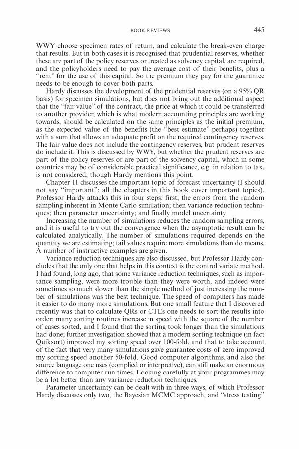
WWY choose specimen rates of return, and calculate the break-even chargethat results. But in both cases it is recognised that prudential reserves, whetherthese are part of the policy reserves or treated as solvency capital, are required,and the policyholders need to pay the average cost of their benefits, plus a“rent” for the use of this capital. So the premium they pay for the guaranteeneeds to be enough to cover both parts.
Hardy discusses the development of the prudential reserves (on a 95% QRbasis) for specimen simulations, but does not bring out the additional aspectthat the “fair value” of the contract, the price at which it could be transferredto another provider, which is what modern accounting principles are workingtowards, should be calculated on the same principles as the initial premium,as the expected value of the benefits (the “best estimate” perhaps) togetherwith a sum that allows an adequate profit on the required contingency reserves.The fair value does not include the contingency reserves, but prudent reservesdo include it. This is discussed by WWY, but whether the prudent reserves arepart of the policy reserves or are part of the solvency capital, which in somecountries may be of considerable practical significance, e.g. in relation to tax,is not considered, though Hardy mentions this point.
Chapter 11 discusses the important topic of forecast uncertainty (I shouldnot say “important”; all the chapters in this book cover important topics).Professor Hardy attacks this in four steps: first, the errors from the randomsampling inherent in Monte Carlo simulation; then variance reduction techni-ques; then parameter uncertainty; and finally model uncertainty.
Increasing the number of simulations reduces the random sampling errors,and it is useful to try out the convergence when the asymptotic result can becalculated analytically. The number of simulations required depends on thequantity we are estimating; tail values require more simulations than do means.A number of instructive examples are given.
Variance reduction techniques are also discussed, but Professor Hardy con-cludes that the only one that helps in this context is the control variate method.I had found, long ago, that some variance reduction techniques, such as impor-tance sampling, were more trouble than they were worth, and indeed weresometimes so much slower than the simple method of just increasing the num-ber of simulations was the best technique. The speed of computers has madeit easier to do many more simulations. But one small feature that I discoveredrecently was that to calculate QRs or CTEs one needs to sort the results intoorder; many sorting routines increase in speed with the square of the numberof cases sorted, and I found that the sorting took longer than the simulationshad done; further investigation showed that a modern sorting technique (in factQuiksort) improved my sorting speed over 100-fold, and that to take accountof the fact that very many simulations gave guarantee costs of zero improvedmy sorting speed another 50-fold. Good computer algorithms, and also thesource language one uses (complied or interpretive), can still make an enormousdifference to computer run times. Looking carefully at your programmes maybe a lot better than any variance reduction techniques.
Parameter uncertainty can be dealt with in three ways, of which ProfessorHardy discusses only two, the Bayesian MCMC approach, and “stress testing”
BOOK REVIEWS 445
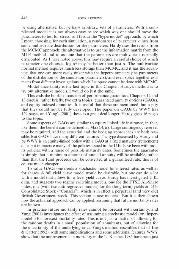
by using alternative, but perhaps arbitrary, sets of parameters. With a com-plicated model it is not always easy to see which way one should move theparameters to test for stress, so I favour the “hypermodel” approach, by whichI mean choosing, for each simulation, a random set of parameter values fromsome multivariate distribution for the parameters. Hardy uses the results fromthe MCMC approach; the alternative is to use the information matrix from theMLE method and to assume that the parameters are multivariate normallydistributed. As I have noted above, this may require a careful choice of whichparameter one chooses; log s2 may be better than just s. The multivariatenormal method requires much less storage than MCMC, and it has the advan-tage that one can more easily tinker with the hyperparameters (the parametersof the distribution of the simulation parameters), and even splice together esti-mates from different investigations, which I suppose cannot be done with MCMC.
Model uncertainty is the last topic in this Chapter. Hardy’s method is totry out alternative models. I would do just the same.
This ends the book’s discussion of performance guarantees. Chapters 12 and13 discuss, rather briefly, two extra topics: guaranteed annuity options (GAOs),and equity-indexed annuities. It is useful that these are mentioned, but a pitythat they could not be fully developed. The paper on GAOs by WWY has129 pages, and Yang’s (2001) thesis is a great deal longer. Hardy gives 16 pagesto the topic.
Some aspects of GAOs are similar to equity linked life insurance, in that,like them, the benefit can be defined as Max(A,B). Large contingency reservesmay be required, and the actuarial and the hedging approaches are both pos-sible. But GAOs have many different features. The type discussed by Hardy andby WWY is an equity-linked policy with a GAO at a fixed maturity (retirement)date, but in practice many of the policies issued in the U.K. have been with prof-its policies, with a range of possible maturity dates. Sometimes the guaranteeis simply that a minimum amount of annual annuity will be available, ratherthan that the fund proceeds can be converted at a guaranteed rate; this is ofcourse much cheaper.
To value GAOs one needs a stochastic model for interest rates, as well asfor shares. A full yield curve model would be desirable, but one can do a lotwith a model that allows for a level yield curve. Hardy has investigated U.K.data, and suggests two regime switching models, one for the FTSE All-Shareindex, one (with two autoregressive models) for the (long-term) yields on 2†%Consolidated Stock (“Consols”), which is in effect a perpetual (and very old)British Government stock. This section is new material. But it is then shownhow the actuarial approach can be applied, assuming that future mortality ratesare known.
In practice future mortality rates cannot be forecast with certainty, andYang (2001) investigates the effect of assuming a stochastic model (or “hyper-model”) for forecast mortality rates. This is not just a matter of allowing forthe random deaths in a small population of annuitants, but of allowing forthe uncertainty of the underlying rates. Yang’s method resembles that of Lee& Carter (1992), with some simplifications and some additional features. WWYshow that the improvements in mortality in the U. K. since 1985 have been just
446 BOOK REVIEWS
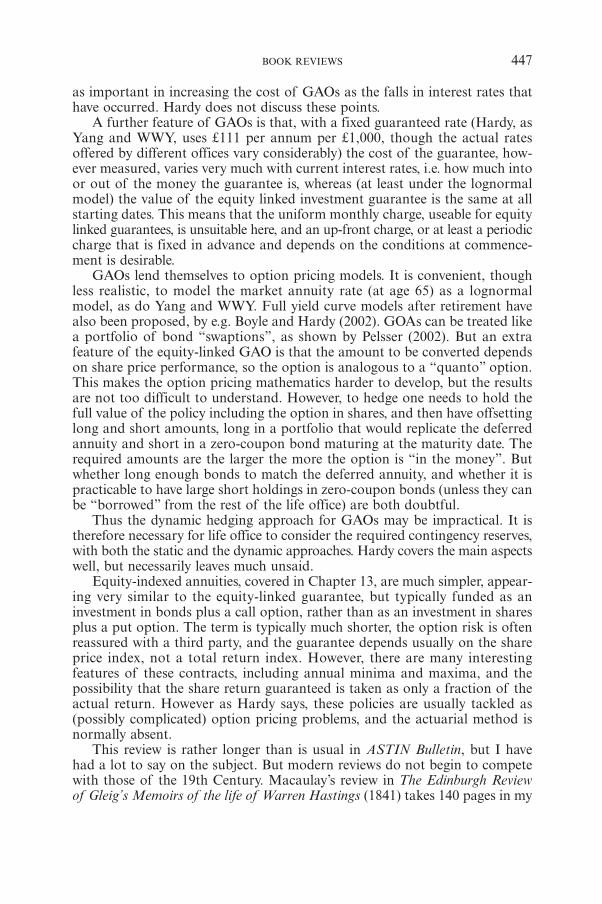
as important in increasing the cost of GAOs as the falls in interest rates thathave occurred. Hardy does not discuss these points.
A further feature of GAOs is that, with a fixed guaranteed rate (Hardy, asYang and WWY, uses £111 per annum per £1,000, though the actual ratesoffered by different offices vary considerably) the cost of the guarantee, how-ever measured, varies very much with current interest rates, i.e. how much intoor out of the money the guarantee is, whereas (at least under the lognormalmodel) the value of the equity linked investment guarantee is the same at allstarting dates. This means that the uniform monthly charge, useable for equitylinked guarantees, is unsuitable here, and an up-front charge, or at least a periodiccharge that is fixed in advance and depends on the conditions at commence-ment is desirable.
GAOs lend themselves to option pricing models. It is convenient, thoughless realistic, to model the market annuity rate (at age 65) as a lognormalmodel, as do Yang and WWY. Full yield curve models after retirement havealso been proposed, by e.g. Boyle and Hardy (2002). GOAs can be treated likea portfolio of bond “swaptions”, as shown by Pelsser (2002). But an extrafeature of the equity-linked GAO is that the amount to be converted dependson share price performance, so the option is analogous to a “quanto” option.This makes the option pricing mathematics harder to develop, but the resultsare not too difficult to understand. However, to hedge one needs to hold thefull value of the policy including the option in shares, and then have offsettinglong and short amounts, long in a portfolio that would replicate the deferredannuity and short in a zero-coupon bond maturing at the maturity date. Therequired amounts are the larger the more the option is “in the money”. Butwhether long enough bonds to match the deferred annuity, and whether it ispracticable to have large short holdings in zero-coupon bonds (unless they canbe “borrowed” from the rest of the life office) are both doubtful.
Thus the dynamic hedging approach for GAOs may be impractical. It istherefore necessary for life office to consider the required contingency reserves,with both the static and the dynamic approaches. Hardy covers the main aspectswell, but necessarily leaves much unsaid.
Equity-indexed annuities, covered in Chapter 13, are much simpler, appear-ing very similar to the equity-linked guarantee, but typically funded as aninvestment in bonds plus a call option, rather than as an investment in sharesplus a put option. The term is typically much shorter, the option risk is oftenreassured with a third party, and the guarantee depends usually on the shareprice index, not a total return index. However, there are many interestingfeatures of these contracts, including annual minima and maxima, and thepossibility that the share return guaranteed is taken as only a fraction of theactual return. However as Hardy says, these policies are usually tackled as(possibly complicated) option pricing problems, and the actuarial method isnormally absent.
This review is rather longer than is usual in ASTIN Bulletin, but I havehad a lot to say on the subject. But modern reviews do not begin to competewith those of the 19th Century. Macaulay’s review in The Edinburgh Reviewof Gleig’s Memoirs of the life of Warren Hastings (1841) takes 140 pages in my
BOOK REVIEWS 447
reprinted (1898) copy. Macaulay’s review is perhaps more worth reading nowa-days than the book he was reviewing. This is not the case for this article. ReadMary Hardy’s excellent book.
DAVID WILKIE
REFERENCES
BOYLE, P.P. and HARDY, M.R. (2002) Guaranteed annuity options. Working Paper, University ofWaterloo.
HARRIS, G.R. (1999) Markov chain Monte Carlo estimation of regime switching vector autore-gressions. ASTIN Bulletin 29, 47-80.
LEE, R.D. and CARTER, L. (1992) Modelling and forecasting U.S. mortality, Journal of the Amer-ican Statistical Association 87, 659-671.
MATURITY GUARANTEES WORKING PARTY (1980) Report of the Maturity Guarantees WorkingParty. Journal of the Institute of Actuaries 107, 103-209.
PELSSER, A. (2002) Pricing and hedging guaranteed annuity options via static option replication.Working paper.
WHITTEN, S.P. and THOMAS, R.G. (1999) A non-linear stochastic asset model for actuarial use.British Actuarial Journal 5, 919-953.
WILKIE, A.D., WATERS, H.R. and YANG, S. (2003) Reserving, pricing and hedging of policies withguaranteed annuity options. British Actuarial Journal 9, forthcoming.
YANG, S. (2001) Reserving, pricing and hedging for guaranteed annuity options, PhD Thesis, Heriot-Watt University, Edinburgh.
448 BOOK REVIEWS
Report on theXXXIV International ASTIN Colloquium,
August 24-27, 2003, Berlin
The 34th International ASTIN Colloquium 2003 was held in Berlin from August24 to 27. More than 300 participants from 34 countries all over the worldmade it an extremely successful event. Opening addresses were given by EdwardLevay and W. James MacGinnitie for the ASTIN Committee, and Elmar Helten,Dieter Köhnlein and Christian Hipp for the local Organizing and ScientificCommittee. In contrast to its predecessors, no parallel sessions for presenta-tions were planned this time. Instead, Poster Sessions were organized whichoffered ample opportunity to the participants for scientific exchange with theauthors during extended coffee breaks. This new concept was very much wel-comed by the attendants and will most probably be maintained also in futureASTIN conferences.
Social events were a visit to “TIPI – the tent”, a varieté show on the eveningof the first conference day, a boat trip on the Wannsee on the second day anda closing gala dinner at the post museum in the evening of the final day.
The topics of the invited speakers for this year’s Colloquium focused on twomajor theme groups, one of which was the ongoing and deepening interplaybetween financial and insurance markets (key words: Financial Risk Manage-ment, Securitization, Loss Reserving, Solvency Standards). The second onewas devoted to the possible consequences of modern medical genetic researchfor life and health insurance.
The opening plenary lecture was given by Paul Embrechts (ETH Zürich)on the topic “Insurance analytics: actuarial tools for financial risk manage-ment”. A key message within this very comprehensive and refreshing surveyover recent developments in this area was “actuarial thinking”, in particularin connection with financial risk management. As new challenges for actuariesdue to regulatory measures in the spirit of Basel I and II were mentioned: pre-mium principles and risk measures – pricing in incomplete markets – stress- andsolvency-testing – dynamic financial analysis (DFA) – stochastic dependencestructures “beyond the normal distribution” (key word: copulas).
The following presentation of David Mocklow (Chicago) was devoted tothe topic “Risk Linked Securities: what’s shaking?”. Seen from the perspectiveof a reinsurer, a thorough survey over different products and markets relatedto ART was given, with a particular emphasis on natural catastrophes and the“value of securitization”.
The lecture of Greg Taylor (Sydney and University of Melbourne) closedthe plenary lecture of the first day. It was dealing with “Loss reserving techni-ques: past, present and future”. In his lecture, he presented a hierarchicalapproach to classifying the various known loss reserving techniques, differenti-ating between macroscopic vs. microscopic models, stochastic vs. deterministic

models and models with and without dependence structures. An in-depth-analysis was made for adaptive approaches including Kalman filtering, a tech-nique which is well-known in the area of generalized linear models (GLM).
The second day of the colloquium started with a survey lecture of SørenAsmussen (Aarhus University) on “Some applications of phase-type distribu-tions to insurance and finance”. After some introductory remarks on historicdevelopments and fundamental properties of phase-type distributions empha-sis was put on the advantages of a rigorous application of matrix calculus inthis field. This simplifies not only a lot the classical proofs, but allows also fornew results in an elegant way, in particular in ruin theory with a finite time hori-zon, or for pricing of Russian options.
The subsequent two lectures were devoted to the medical topics outlinedabove. Jean Lemaire (Wharton School, Philadelphia) and Angus MacDonald(Heriot-Watt University, Edinburgh) shared their presentation on “Genetics, fam-ily history, and insurance underwriting: an expensive combination?”. A majorproblem in this context is the question whether life or health insurance com-panies have the right to use or obtain information on the genetic code of a clientin order to fix a risk-adjusted premium. From a legal point of view, this problemis dealt with in very different ways even within Europe, not to speak of the restof the world. Besides this aspect, it was pointed out that also from the medicalperspective, statistically significant prognoses on a possible outbreak of diseasesrelated to gene defects are dubious, in particular if multi-factorial gene disor-ders have to be considered. Family history is another source of information thatcan lead to different conclusions here.
These statements were strongly supported by Jens Reich (Humboldt-Uni-versität Berlin) with his lecture on “Living is a risky endeavour – less so throughgenetic medicine?”. The audience was informed in detail about the biologicalfoundations of the human genome and various aspects of “cloning”. Specialemphasis was given to the legal problems with stem cell research in particularin Germany, where such topics are still discussed in a quite controversial way.
The closing plenary lecture of the last day was presented by Harry Panjer(University of Waterloo, Canada) with the title “Development of internationalinsurance company solvency standards”, finding thus a way back to the topicof the opening lecture of the first day. Perspectives for future actuarial activi-ties especially for the development and unification of tools for regulatoryauthorities were outlined, such as risk measures and their properties (VaR,coherent risk measures, TailVaR), stochastic modeling of dependencies bycopulas and an improvement of the “covariance formula” for the valuation ofrisk based capital (RBC).
Besides the plenary lectures, various other contributions were organized inworking sessions. In the order of presentations, these were:
– Techniques for valuation a general insurance company within the frameworkof IAS standards: some proposals (by Aurélie Despeyroux, Charles Levi,Christian Partrat and Jerôme Vignancour)
– Asbestos: The current situation in Europe (by Laura Salvatori, AlessandroSantoni and Darren Michaels)

– Munich Chain Ladder – Closing the gap between paid and incurred IBNR-estimates (by Gerhard Quarg, with an additional comment by ThomasMack)
– Capital and Asset Allocation (by René Schnieper) – Stochastic orders in dynamic reinsurance markets (by Thomas Møller)– Risk Exchange with distorted probabilities (by Andreas Tsanakas)– Multidimensional Credibility applied to estimating the frequency of big
claims (by Hans Bühlmann, Alois Gisler and Denise Kollöffel)– Credibility weighted hazard estimation (by Jens Perch Nielsen and Bjørn
Lunding Sandqvist)– Marketing and Bonus-Malus Systems (by Sandra Pitrebois, Michel Denuit
and Jean-Francois Walhin)– Insurance applications of near-extremes (by Enkelejd Hashorva and Jürg
Hüsler)– Windstorm claims dependence and copulas (by Olivier Belguise and Charles
Levi)– Tail distribution and dependence measures (by Arthur Charpentier)– Robust inference in rating models (by Gilles Dupin, Alain Monfort and Jean-
Pierre Verle)– Basis risk and cat risk management (by Frank Krieter)– Copula: A new vision for economic capital and application to a four line of
business company (by Fabien Faivre)– Effets de la dépendance entre différentes branches sur le calcul des provisions
(by Antonin Gillet and Benjamin Serra)– Modeling and generating dependent risk processes for IRM and DFA (by
Dietmar Pfeifer and Johana Neslehová)– Capital allocation survey with commentary (by Gary G. Venter).
Poster contributions were (in alphabetical order of the authors):
– Fair Value of Life Liabilities with Embedded Options: An Application to aPortfolio of Italian Insurance Policies (by Giulia Andreatta and StefanoCorradin)
– A Comparison of Strategic Reinsurance Programs (SRP) with BankingActivities and Other Insurance and Reinsurance Activities (by BaruchBerliner)
– Dynamic Asset Liability Management: A Profit Testing Model for SwissPension Funds (by Ljudmila Bertschi, Sven Ebeling and Andreas Reichlin)
– Economic Risk Capital and Reinsurance: An Extreme Value Theory’s Appli-cation to Fire Claims of an Insurance Company (by Stefano Corradin)
– On the Distribution of the Deficit at Ruin and the Surplus Prior to Ruin inthe Compound Binomial Model (by Esther Frostig)
– The Impact of Statistical Dependence on Multiple Life Insurance Programs(by Esther Frostig and Benny Levikson)
– Optimal Dividend Payment under a Ruin Constraint: Discrete Time andState Space (by Christian Hipp)
– The Impact of Reinsurance on the Cost of Capital (by Werner Hürlimann)– Optimality of a Stop-Loss Reinsurance in Layers by Werner Hürlimann)

– The Czeledin Distribution Function (by Markus Knecht and Stefan Küttel)– On the Loading of Largest Claims Reinsurance Covers (by Erhard Kremer)– Exposure Rating in Liability Reinsurance (by Thomas Mack and Michael
Fackler)– Credibility Evaluation for Heterogeneous Populations (by Udi E. Makov)– On a Non-Linear Dynamic Solvency Control Model (by Vsevolod Malinovskii)– Capital Consumption: An Alternative Methodology for Pricing Reinsurance
(by Donald Mango)– A Stochastic Control Model for Individual Asset-Liability Management (by
Sachi Purcal)– On Error Bounds for the Approximation of Random Sums (by Bero Roos
and Dietmar Pfeifer)– A Risk Charge Calculation Based on Conditional Probability (by David Ruhm
and Donald Mango)– Conditional Risk Charge Demo using DFAIC (by David Ruhm and Donald
Mango)– A Risk Theoretical Model for Assessing the Solvency Profile of a General
Insurer (by Nino Savelli)– On Unknown Accumulations in Accident Insurance: An Upper Bound of
the Expected Excess Claim (by Hans Schmitter)– Actuarial Principles of the Cotton Insurance in Uzbekistan (by Bakhodir
Shamsuddinov)– The Estimation of Market VaR using Garch Models and Heavy Tail Dis-
tributions (by Ricardo A. Tagliafichi)– Fit to a t – Estimation, Application and Limitations of the t-Copula (by
Gary G. Venter)– Une Nouvelle Caractérisation de la Distribution de Pareto, avec Application
à la Cadence de Paiement du Réassureur en Excédent de Sinistre (by Jean-Francois Walhin).
The closing ceremony of the Colloquium was performed by Edward Levay andDieter Köhnlein.
All presentations (invited lectures, working papers and posters) can be down-loaded from the Colloquium website at www.astin2003.de.
Dietmar Pfeifer

Report on the International AFIR Colloquium 2003,Maastricht, The Netherlands
From 17 to 19 September, 2003, Maastricht was the venue for the annual AFIRColloquium. In this report you will find impressions of both the content andthe surrounding social activities.
PARTICIPATION
The number of participants was 154 with 23 accompanying persons. Therewas a good spread over 22 countries. Apart from The Netherlands, which asa host country not surpisingly had the highest number (52), the Nordic coun-tries stood out with 43 participants. Worthwhile mentioning also is Sloveniawith 14 participants and the fact that seven countries were each representedby 1 participant.
INVITED LECTURERS
Two invited lecturers had been invited. Firstly, Mr Luc Henrard, Chief RiskOfficer of FORTIS, Belgium, gave a lecture under the title “The managementof a financial conglomerate: a challenge for the actuaries?”. He made an almostpassionate plea for actuaries to broaden their horizon to include more expertiseoutside their traditional role. Secondly, Mr Roderick Munsters, Chief InvestmentOfficer of PGGM, The Netherlands, made a presentation on “The actuaryand the investor on a rollercoaster ride” in which he, referring to PGGM’sinvestment policies, equally challenged the actuaries to intensify their coopera-tion with the “asset specialists”. Both presentations tied in very well with thesubjects of of the regular papers and the special paper, mentioned below.
PAPERS
The number of accepted papers was 35. Most of them were presented by theauthor (or one of the authors) during 30-minute sessions. The variety of subjectswas quite interesting and all papers were classified in one of the three prede-fined categories, i.e. “Asset Classification”, “Market valuation of Liabilities”and “Risk Measurement and Management”. They are all accessible and down-loadable through the website www.afir2003.nl, which will remain open for sometime. We hope that a number of them will be published in the ASTIN Bulletin.
SPECIAL PAPER
One non-scientific paper was presented about “the future of AFIR” and thedual role of dealing with both traditional and new areas. The authors made aplea for a reorientation of AFIR’s “mission”. In their view, AFIR shouldbecome more active in stimulating actuaries to become “risk officers” in a farmore general sense. Of course this would include adjustments to the educational

syllabuses. The paper also described — on the basis of a survey in 10 coun-tries — the extremely diverse way in which presently AFIR activities are organ-ised around the world.
GENERAL MEETING AND BOB ALTING VON GEUSAU MEMORIAL PRIZE
On Friday afternoon the General Meeting for AFIR members was held todiscuss accounts, Committee membership nominations and some other topicsof a more formal nature. The Chairman also announced that the discussionon the future of AFIR would have a follow-up during the next Colloquium andthat several sub-committees had been appointed to prepare for this. Followingthe General Meeting, a ceremony took place to present a Prize for the best arti-cle, published in the ASTIN Bulletin during the years 2001 and 2002. It wasthe first time this new annual Prize, named after one of the “founding fathers”of AFIR in the seventies, was awarded. The winner was Shaun Wang for hispaper “A framework for pricing financial and insurance risks” in the ASTINBulletin 32.2 of November 2002.
SOCIAL PROGRAM
A number of social activities had been arranged for participants and companionsto liaise with others “outside the world of formulae”. On the opening day(Wednesday) a tour of the surrounding area of Maastricht was made, endingwith a reception at Maastricht’s Town Hall. There was a companion’s programon Thursday and in the evening all guests were invited to an informal dinnerin the city. Finally, there was a formal farewell dinner on Friday night in oneof the castles in Maastricht’s province of Limburg.
NEXT COLLOQUIUM
During the General Meeting the venue for the next Colloquium was disclosed:USA, (probably New York) in November 2004. On behalf of the Organisingand Scientific Committees I take pleasure in wishing our successors the verybest in preparing for that event!
HUGO BERKOUWER
chairman of the Organising Committee, Maastricht 2003

International Conference on “Dependence Modelling: Statistical Theory andApplications to Finance and Insurance” (DEMOSTAFI)
20-22 May 2004 in Quebec City, Canada
This conference is a sequel to the series of conferences on copulas, dependencemodels and their applications that were held in Rome (1990), Seattle (1993),Prague (1996) and Barcelona (2000).
The purpose of this conference is to bring together researchers interested inmodelling stochastic dependence and measuring its effects in statistics, actu-arial science and finance. The meeting aims to attract copula specialists andstatistical researchers interested in their development and use in characterizingand modelling of dependence (stochastic orderings, distributions with fixedmarginals, etc.). We would also like to put emphasis on applications of therelevant concepts and inferential techniques in the fields of actuarial scienceand finance, which are thriving at present. The “technological transfer” aspectof the conference will be especially important; for example, several surveytalks by world specialists have been planned.
For additional information about this meeting, registration material and so on,please visit the conference website at http://www.fsa.ulaval.ca/demostafi/
Etienne Marceau, Ph. D., A.S.A.Member of the organizing committeeAssociate ProfessorEcole d’ActuariatLaval UniversityQuebec (Que)Canada, G1K 7P4Phone: (418) 656-2013Fax: (418) 656-7790email: [email protected]: http://hyperion.act.ulaval.ca/~emarceau/

XXXV INTERNATIONAL ASTIN COLLOQUIUMSunday June 6 to Wednesday June 9, 2004
The 35th International ASTIN Colloquium will be held in Bergen, Norway.The Norwegian Actuarial Society extends its most sincere welcome to all partic-ipants and partners to join us in what will surely become days full of meaningboth professionally and socially.
Call for papersWe invite authors to submit papers on any subject covered by ASTIN; see the“Call for papers” entry on the website. Deadline for submitting scientific papersin their final form: February 1, 2004.
Scientific Program committeeErik Bølviken (chairman), Paul Embrechts, Simen Gaarder, Angus MacDonald,Ragnar Nordberg, Mette Rytgaard.
Key notes lecturesOpening by prominent actuary in the insurance industry.Closing by prominent academic on actuarial science in 21th century.
Organized sessionsThematic sessions have been organized on
Insurance fraudGenetics and insuranceClimatic change and its impact on insurance
Coordinated lectures will be given by actuaries and by relevant people from theoutside. Details: See conference website
Conference venueThe colloquium will take place in Bergen (Norway’s second largest city), locatedon the west coast at the entry of magnificent fjords and waterfalls. The town,still marked by its hanseatic origin, was for centuries the commercial capitalof the country. Today Bergen is the bustling home of two universities, andbecame a European city of culture three years ago. Karl Borch, co-founder ofmodern risk theory, resided here.
www.astin2004.noThe website gives you up-to-date information.Here you will find the preregistration schedule.
The Department of Statistics & Actuarial Scienceof the University of the Aegean is pleased to host
the 3rd Conference in Actuarial Science and Finance,to be held on Samos, on September 2-5, 2004.
This event is jointly organized with the Katholieke Universiteit Leuven(Department of Applied Economics and Department of Mathematics), the Uni-versité Catholique de Louvain (Institute of Statistics and Actuarial research group)and the University of Copenhagen (Laboratory of Actuarial Mathematics).
The Conference allows the presentation of the latest works in the area ofactuarial science and finance. It is open to all persons interested in actuarialscience and finance, be they from universities, insurance companies, banks,consulting firms or regulatory authorities. The conference aims to facilitatethe contact and the communication between the practicians and the researchers.
The topics of the sections include:– Extremes and Large Deviations in Actuarial Science – Chair J. Teugels
– Non-life Insurance – Chair R. Verrall
– Advances in Incomplete Markets – Chair Th. Zariphopoulou
– Modelling Dependence in Actuarial Science – Chair Th. Mikosch
– Risk and Control – Chair S. Asmussen
– Life, Pension and Health Insurance – Chair H. Gerber
There will be four short courses. Two before the conference: 30th of August -1st of September– Stochastic Claims Reserving, by R.J. Verrall
– Stochastic Control Applied to Actuarial Problems, by H. Schmidli
and the other two after the conference: 6th September - 8th September – Risk Measures and Optimal Portfolio Selection (with applications to ellip-
tical distributions), by J. Dhaene and E. Valdez
– Advanced Statistical Methods for Insurance, by M. Denuit
Postgraduate students and young reseachers are specially welcome.
Scientific Committee:
Asmussen SoerenDenuit MichelFoss Serguei

Frangos NicosGerber HansGoovaerts MarcGuillen MontserratKonstantinides DimitriosMakov UdiMarceau EtienneMikosch ThomasNg KaiPapaioanou Takis (Chair)Tessaromatis NicosTeugels JefVerrall RichardWillder MarkZariphopoulou Thaleia
Organizing Committee:
Dhaene JanFrangos Nicos (Chair)Konstantinides DimitriosMikosch ThomasPurcaru OanaSchmidli HanspeterTeugels JefWalhin Jean-Francois
Local Committee:
Chatzispyros SpyridonGiannakopoylos AthanasiosKatsis AthanasiosKonstantinides Dimitrios (Chair)Milionis AlexandrosNakas ChristosPoufinas Thomas
For further information, please refer to
http://www.stat.ucl.ac.be/Samos2004/

GEORGIA STATE UNIVERSITYJ. Mack Robinson College of Business
Two Faculty Positions in Risk Management
The Robinson College of Business at Georgia State University invites applica-tions for two tenure-track positions at the assistant professor level to begin infall 2004. These two hires are the first of six positions for which we anticipatehiring during the next three years for the purpose of forming a cross-disciplinarygroup charged to conduct fundamental research on the economics of uncertaintyand on the management and pricing of risk.
JOB QUALIFICATIONS:
Qualified candidates will be expected to possess a PhD by the time of theirappointment. All areas of specialization will be considered provided the can-didate has a strong interest in and academic background in some area of risk,broadly defined. We are particularly interested in individuals whose studiesinvolve dynamic asset pricing, computational methods including financialeconometrics, statistics or actuarial science, equilibrium theory or the micro-economics of uncertainty, optimal contracting, and the estimation theory fordynamic games and dynamic contracting. The ideal candidate will be expectedto publish in the major journals of economics and finance as well as importantjournals of their specific discipline.
ABOUT THE ENVIRONMENT:
The Department of Risk Management and Insurance houses one of the old-est and most influential risk management programs in the U.S. Beginning inacademic year 2003, and continuing in 2004 and 2005, the department intendsto recruit six new faculty members trained in the most advanced methods oftheir disciplines for a coordinated study of risk management problems at theirmost fundamental levels. Salaries will be competitive and strong research sup-port will be provided. Teaching loads will be low to ensure the group has theopportunity to produce high quality research. A statement outlining the visionthe department has for the group is available upon request from the co-chairsof the recruiting committee.
FURTHER INFORMATION AND APPLICATION PROCEDURE:
Applicants should send a current curriculum vita, three letters of recommen-dation, and recent publications or working papers for review. Applicationsshould be submitted electronically via e-mail as pdf files to [email protected] wishing to send their materials via regular mail should forwardthem to:
Richard D. Phillips, Co-chairDepartment of Risk Management and InsuranceRobinson College of BusinessGeorgia State UniversityP.O. Box 4036Atlanta, GA 30302-4036
For further information, contact either co-chair of the search committee: MartinGrace - [email protected] or 404-651-2789; Richard Phillips - [email protected] 404-651-3397.
Interviews can be scheduled for the 2003 Financial Management AssociationAnnual Meeting or the 2004 Allied Social Sciences Association Annual Meeting.Preference will be given to applications received by December 1, 2003.
GEORGIA STATE UNIVERSITY IS AN EQUAL OPPORTUNITY EDUCATIONAL INSTI-TUTION/AFFIRMATIVE ACTION EMPLOYER AND ENCOURAGES APPLICATIONS FROM
QUALIFIED MINORITIES. ALL POSITIONS ARE SUBJECT TO FINAL APPROVAL FOR
FUNDING.

DIRECTOR, Actuarial Science programDepartment of Risk Management and Insurance
Georgia State University
JOB QUALIFICATIONS:
The Department of Risk Management and Insurance invites applicationsfor the position of Director of the Actuarial Science Program. The successfulcandidate will have an established record of high-quality research in the fieldof actuarial science, statistics, or related field such as financial mathematics anda demonstrated ability to lead one of the outstanding actuarial science programs.A doctorate in actuarial science, finance, mathematics, statistics, or related fieldis required. This tenure track position, to be filled effective fall 2004 at therank of associate or full professor, requires maintenance of a successful researchagenda and demonstrated teaching excellence.
Membership in a professional actuarial organization is required. These mayinclude the Casualty Actuarial Society, the Society of Actuaries, the Instituteof Actuaries, the Faculty of Actuaries, or the Australian Institute of Actuaries.Associates of these societies or members of other actuarial societies may alsomeet this requirement if they have exceptional strength in scholarship, teaching,and leadership.
ABOUT THE ENVIRONMENT:
From its founding in 1958, the GSU Actuarial Science Program has been oneof the leading programs in North America. It has a distinguished history ofserving students, alumni, and the actuarial profession. Hundreds of our gradu-ates have become Fellows or Associates of the Society of Actuaries and/or theCasualty Actuarial Society and many have become leaders in the professionaland business communities. The program is housed in the Department of RiskManagement and Insurance, regarded as one of the best departments of its typeinternationally.
The department recently expanded its research and educational mission toinclude mathematical risk management, offering masters and doctoral degreesoriented at the intersection of actuarial science and mathematical finance. TheMathematical Risk Management and Actuarial Science Programs work closelyin student recruitment and placement. Some courses are cross-listed and manyactuarial students take mathematical risk management courses, such as financialengineering, as electives.
FURTHER INFORMATION AND APPLICATION PROCEDURE:
Preference will be given to applications received by December 1, 2003. Applicantsshould send a current curriculum vita, three letters of recommendation, andrecent publications or working papers to:

Richard D. Phillips, ChairSearch CommitteeDepartment of Risk Management and InsuranceJ. Mack Robinson College of BusinessGeorgia State UniversityP.O. Box 4036Atlanta, GA 30302-4036Tel: 404-651-3397
Applications may be submitted electronically via e-mail at: [email protected] further information, contact the chair of the search committee.
GEORGIA STATE UNIVERSITY IS AN EQUAL OPPORTUNITY EDUCATIONAL INSTI-TUTION/AFFIRMATIVE ACTION EMPLOYER AND ENCOURAGES APPLICATIONS FROM
QUALIFIED MINORITIES. POSITION IS SUBJECT TO FINAL APPROVAL FOR FUNDING.

Assistant Professor in Actuarial ScienceUniversity of Iowa
Applications are invited for a tenure-track assistant professor in actuarial sciencestarting August 2004. Applicants must show promise for excellence in bothteaching and creative research. They must have completed a Ph.D. in a rele-vant field and at least the first four Society of Actuaries’ exams, or equivalentexams in a major actuarial organization. Fellowship or Associateship in a pro-fessional actuarial society is preferred. The appointee is expected to conductresearch in actuarial science/financial mathematics, to assist in building a Ph.D.program in this area, and to supervise Ph.D. students.
The selection process begins December 1, 2003 and continues until the positionis filled.
Please send a curriculum vitae, a transcript for new Ph.D.s, and have threeconfidential letters of reference sent to:
Actuarial Search CommitteeDept. of Statistics & Actuarial ScienceUniversity of IowaIowa City, IA 52242.Email: [email protected]
The Department currently has seventeen tenure-track faculty who are engagedin various areas of research in statistics, actuarial science, and financialmathematics. The current actuarial faculty members are Jim Broffitt, A.S.A.,Gordon Klein, F.S.A., and Elias Shiu, A.S.A. The B.S. and M.S. degrees areoffered in both actuarial science and statistics, the Ph.D. in statistics. Actuarialstudents may earn a Ph.D. in statistics with emphasis in actuarial science/financialmathematics. The number of actuarial science majors is about 45 graduateand 20 undergraduate students. For additional information about the Depart-ment, please refer to the website: http://www.stat.uiowa.edu/.
The University of Iowa is nestled in the rolling hills of eastern Iowa along thebanks of the Iowa River. Approximately 30,000 students are enrolled in elevencolleges: Liberal Arts, Graduate, Business, Law, Medicine, Public Health, Den-tistry, Nursing, Pharmacy, Education, and Engineering. The University isknown for its fine arts, and a variety of touring dance, musical, and theatricalgroups perform on campus each year. As a member of the Big Ten Conference,Iowa hosts many outstanding athletic events.
Iowa City is a clean, attractive community of approximately 62,000 people.It is noted for its public schools, medical and athletic facilities, attractive businessdistrict, parks, and mass transit system. In 1999, editor & Market guide ratedIowa City as the best metropolitan area to live in the USA. Among smallermetropolitan areas, the 2003 Milken Institute Best Performing Cities Instituteranked Iowa City number 1. Iowa City is within 300 miles of Chicago, St. Louis,Kansas City, and Minneapolis.
Women and minorities are encouraged to apply. The University of Iowa is anAffirmative Action Equal Opportunity Employer.

Drake UniversityCollege of Business and Public Administration
Des Moines, IA 50311, USA
POSITION:A tenure track position in actuarial science in the College of Business andPublic Administration, to begin August, 2004, pending final budgetary approval.Rank and salary based on qualifications.
DUTIES:Teach six courses per year; recruit, advise, and place students; conduct schol-arly research; and serve the University and the profession.
QUALIFICATIONS:Ph.D. in actuarial science or a related area along with Associateship or Fellow-ship in the CAS or SOA is preferred. Candidates with lesser qualifications willbe considered if there are compensating factors.
APPLICATIONS:Submit a curriculum vitae and arrange for three letters of reference to be sentto Professor Stuart Klugman, F.S.A.; CBPA; Drake University; Des Moines,IA 50311. Applications will be accepted until the position is filled. Drake Uni-versity is an equal opportunity/affirmative action employer and actively seeksapplications from women and minority group members who are qualified forthis position.
Stuart Klugman, F.S.A., Ph.D.Principal Financial Group Professor of Actuarial Science Drake UniversityDes Moines, IA 50311515-271-4097E-mail: [email protected]

CIBC Chair in Financial Risk ManagementUNIVERSITY OF WATERLOO
The University of Waterloo (UW) has one of the most eminent actuarialscience programs in the world. The faculty members in this unit have attaineda high level of distinction in their research, teaching and professional contri-butions. The graduates of the Waterloo program are internationally recog-nized. In recent years, UW has also developed a strong research presence inthe field of modern finance, with a special emphasis on computational finance.More than 75 new bachelor’s and 20 master’s and doctoral graduates enterthe insurance and finance industries each year from the undergraduate andgraduate actuarial science programs, and the master’s program in quantitativefinance co-ordinated by the Centre for Advanced Studies in Finance.
The University has recently created the Institute for Quantitative Financeand Insurance (IQFI) to combine the strengths of these two disciplines and pro-vide the vehicle for a major research and teaching thrust in the area of finan-cial risk management broadly defined. This initiative was made possible throughsupport from companies in the insurance and financial services industries, andmatching contributions from the Province of Ontario through the OntarioResearch and Development Challenge Fund. The Institute will advance researchin the financial risk management area and disseminate new knowledge. A gen-erous contribution by the Canadian Imperial Bank of Commerce to UW’scapital campaign, “Building a Talent Trust”, has enabled the University toinaugurate two CIBC Chairs in Financial Risk Management under the auspicesof the IQFI. One of these Chairs will be located in the Department of Statisticsand Actuarial Science.
The purpose of this Chair is
– to help the University of Waterloo enhance its leadership role in financeand insurance education and research, and to expand its expertise by buildingon its present strengths
– to attract students of the highest calibre, and to support and supplementfaculty influence on professional education and current practice
– to give prominence and recognition to the interaction between the universityand the insurance and financial services industries, particularly the supportprovided by CIBC
– to support applied research, and the transfer of basic research into currentpractice in the financial services and insurance industries
The Canadian Imperial Bank of Commerce is a leading North American finan-cial institution. Through its comprehensive electronic banking network, branchesand offices across Canada and around the world, CIBC offers a full range of

products and services to more than nine million personal banking and businesscustomers.
The appointment is for a period of up to five years, with expectation ofrenewal. The anticipated start date is July 1, 2004.
The duties of the Chair holder include:
– conducting and overseeing a program of research relevant to financial riskmanagement, actuarial science or insurance
– undergraduate and graduate teaching; leading seminars and colloquia thatinvolve both undergraduate and graduate students
– disseminating applied research through seminars and professional meetings
The Chair holder will be a member of the Department of Statistics and Actu-arial Science in the Faculty of Mathematics at the University of Waterloo andplay a leadership role in the Institute for Quantitative Finance and Insurance.The ideal candidate will have earned a PhD in an appropriate field of researchwithin the last few years, and will already have a strong record as a researcher,with exceptional promise for distinction in some aspect of actuarial science,finance or closely related discipline. The successful candidate must possessstrong communication skills and be an excellent teacher.
Please send applications and nominations, including a recent curriculumvitae, to Professor Alan George, Dean, Faculty of Mathematics, University ofWaterloo, Waterloo, ON Canada N2L 3G1 by April 30, 2004.
In accordance with Canadian immigration requirements, citizens and per-manent residents of Canada will be considered first for this position. The Uni-versity of Waterloo encourages applications from all qualified individualsincluding women, members of visible minorities, native peoples, and personswith disabilities.

GUIDELINES TO AUTHORS
1. Papers for publication should be sent in quadruplicate to one of the Editors:
Andrew Cairns Paul EmbrechtsDepartment of Actuarial Mathematics Department of Mathematicsand Statistics ETHZHeriot-Watt University CH-8092 Zurich, Switzerland.Edinburgh EH14 4AS, United Kingdom [email protected]@ma.hw.ac.uk
Submission of a paper is held to imply that it contains original unpublished work and is notbeing submitted for publication elsewhere.Receipt of the paper will be confirmed and followed by a refereeing process, which will takeabout three months.
2. The basic elements of the journal’s style have been agreed by the Editors and Publishers andshould be clear from checking a recent issue of ASTIN BULLETIN. If variations are felt necessarythey should be clearly indicated on the manuscript.
3. Papers should be written in English or in French. Authors intending to submit longer papers (e.g. exceeding 30 pages) are advised to consider splitting their contribution into two or moreshorter contributions.
4. The first page of each paper should start with the title, the name(s) of the author(s), and anabstract of the paper as well as some major keywords. An institutional affiliation can be placedbetween the name(s) of the author(s) and the abstract.
5. Footnotes should be avoided as far as possible.
6. References should be arranged alphabetically, and for the same author chronologically. Use a, b,c, etc. to separate publications of the same author in the same year. For journal referencesgive author(s), year, title, journal (in italics, cf. point 9), volume (in boldface, cf. point 9), andpages. For book references give author(s), year, title (in italics), publisher, and city.Examples
BARLOW, R.E. and PROSCHAN, F. (1975) Mathematical Theory of Reliability and Life Testing.Holt, Rinehart, and Winston, New York.JEWELL, W.S. (1975a) Model variations in credibility theory. In Credibility: Theory and Appli-cations (ed. P.M. KAHN), pp. 193-244, Academic Press, New York.JEWELL, W.S. (1975b) Regularity conditions for exact credibility. ASTIN Bulletin 8, 336-341.
References in the text are given by the author’s name followed by the year of publication (andpossibly a letter) in parentheses.
7. The address of at least one of the authors should be typed following the references.
8. Italics (boldface) should be indicated by single (wavy) underlining. Mathematical symbols willautomatically be set in italics, and need not be underlined unless there is a possibility of misin-terpretation. Information helping to avoid misinterpretation may be listed on a separate sheetentitled ‘special instructions to the printer’. (Example of such an instruction: Greek letters areindicated with green and script letters with brown underlining, using double underlining for capi-tals and single underlining for lower case).

9. Contributions must be typewritten on one side of good quality paper, with double spacings andample margins all round.Illustrations should be submitted as clear black and white prints. Photocopies are not acceptable.Line thickness and lettering size should be adopted to suit any likely degree of reduction.Each contribution should obtain the author(s) full address(es), including e-mail and fax numberswhen available. Authors should notify the publisher whenever their contact details change.A copy of text should also be submitted on disk, when available. Please state clearly the type ofsoftware used, and note the filename. Contributors should also retain a copy of their article.Two sets of proofs will be shipped to authors who should ensure that one set plus the manuscriptis returned to PEETERS within one week of receipt. Authors may be charged for alterations tothe original manuscript. If authors proofs are not returned by the required date, the publisher’sown corrected set will be forwarded to the printer.
10. Authors will receive 30 offprints free of charge. Additional offprints may be ordered when return-ing corrected proofs. A scale of charges will be enclosed when the proofs are sent out.