Download publication

Author's personal copy

A method for integrating MODIS and Landsat data for systematic monitoringof forest cover and change in the Congo Basin

Matthew C. Hansen a,⁎, David P. Roy a, Erik Lindquist a, Bernard Adusei a,Christopher O. Justice b, Alice Altstatt b

a Geographic Information Science Center of Excellence, South Dakota State University, Brookings, SD 57007, United Statesb Department of Geography, University of Maryland, College Park, United States

Received 10 April 2007; received in revised form 18 November 2007; accepted 21 November 2007

Abstract

In this paper we demonstrate a new approach that uses regional/continental MODIS (MODerate Resolution Imaging Spectroradiometer)derived forest cover products to calibrate Landsat data for exhaustive high spatial resolution mapping of forest cover and clearing in the CongoRiver Basin. The approach employs multi-temporal Landsat acquisitions to account for cloud cover, a primary limiting factor in humid tropicalforest mapping. A Basin-wide MODIS 250 m Vegetation Continuous Field (VCF) percent tree cover product is used as a regionally consistentreference data set to train Landsat imagery. The approach is automated and greatly shortens mapping time. Results for approximately one third ofthe Congo Basin are shown. Derived high spatial resolution forest change estimates indicate that less than 1% of the forests were cleared from1990 to 2000. However, forest clearing is spatially pervasive and fragmented in the landscapes studied to date, with implications for sustaining theregion's biodiversity. The forest cover and change data are being used by the Central African Regional Program for the Environment (CARPE)program to study deforestation and biodiversity loss in the Congo Basin forest zone. Data from this study are available at http://carpe.umd.edu.© 2007 Elsevier Inc. All rights reserved.

Keywords: Forest cover; Change detection; Deforestation; High spatial resolution; Monitoring; MODIS; Landsat

1. Introduction

1.1. Regional-scale mapping of humid tropical forests

Operational landscape characterization and monitoring of thehumid tropics is important to studies concerning habitat andbiodiversity, management of forest resources, human liveli-hoods and biogeochemical and climatic cycles (Curran andTrigg, 2006; Avissar and Werth, 2005; FAO, 2005; SCBD,2001; IGBP, 1998; LaPorte et al., 1998). Studies quantifyinghumid tropical deforestation over large areas using time-serieshigh spatial resolution satellite data sets have been prototyped(Skole and Tucker, 1993; Townshend et al., 1995). However,operational implementation of such methods for long-termmonitoring are only now being operationalized (INPE, 2002;

Asner et al., 2005). The primary limitations to large area highspatial resolution monitoring include the development ofgeneric and robust methods, overcoming data quality issues,and having the resources to purchase required data sets. Con-cerning methods, many land cover mapping activities rely onphoto-interpretation, or other approaches that are labor-intensive, costly, and difficult to replicate in the consistentmanner required for long-term monitoring. The primary datalimitation for humid tropical forest monitoring is persistentcloud cover that confounds efforts to operationalize land coverand change characterizations (Asner, 2001; Helmer andRuefenacht, 2005; Ju and Roy, in press). Regarding the highcost of high spatial resolution data sets, researchers often use thedata they can afford, not the data they truly need. For a regionlike the humid tropics, data needs are intensive in order to over-come the presence of cloud cover.

This paper presents an approach to address these limitations byemploying a multi-resolution methodology for mapping forest

Available online at www.sciencedirect.com

Remote Sensing of Environment 112 (2008) 2495–2513www.elsevier.com/locate/rse

⁎ Corresponding author. Tel.: +1 605 688 6848.E-mail address: [email protected] (M.C. Hansen).

0034-4257/$ - see front matter © 2007 Elsevier Inc. All rights reserved.doi:10.1016/j.rse.2007.11.012


cover and deforestation within the humid tropical forests of theCongo River Basin. The MODIS Vegetation Continuous Fields(VCF) algorithm (Hansen et al., 2003) is used to create a regionalMODIS 250 m forest/non-forest cover map which is in turn usedto drive high spatial resolution Landsat forest characterizations.The automated use of the MODIS forest characterization to pre-process (normalize) and label Landsat data inputs in generatingregional-scale forest cover and change maps for the Congo Basinis demonstrated. Data cost limitations cannot be resolved algo-rithmically, although the method is developed so that additionalimagery can be ingested and new products automatically derivedupon acquisition.

The research strategy engaged herein focuses on the oper-ationalization of large area forest cover and forest cover changemonitoring. Information on where and how fast forest change istaking place can be integrated with other geospatial data on thetypes and causes of change to better inform resource managers andearth systemmodelers. The ability to accurately assess forest coverdynamics in a timely fashion will contribute to new applications,such as the Reducing Emissions from Deforestation and Degra-dation (REDD) initiative (UNFCCC, 2005). Synoptic measure-ments of change can quantify the displacement of deforestationactivities within and between countries and lead to the har-monization of national-scale statistics. To achieve this end,automated or semi-automated procedures that work at regionalscales will be needed; such methods must be accurate, internallyconsistent, produced in a timely fashion and rely on remotelysensed inputs. Spatially explicit forest cover and forest changemaps derived from remotely sensed data will be integral to thefuture monitoring of forests in support of both basic earth scienceresearch and policy formulation and implementation.

1.2. Congo Basin forest monitoring

The CARPE program (Central African Regional Program forthe Environment) is a long-term initiative by USAID to addressthe issues of forest management, human livelihoods, and bio-diversity loss in the Congo Basin forest zone (http://carpe.umd.edu). CARPE works within the framework of the Congo BasinForest Partnership (CBFP, 2005, 2006), an international associa-tion of government and non-government organizations with thegoal of increasing communication and coordination between in-region projects and policies to improve the sustainable manage-ment of the Congo Basin forests and the standard of living of theregion's inhabitants. The methods presented here are a contribu-tion to these efforts by advancing the creation of internallyconsistent, rapid assessments of the forested landscapes of theCongo Basin.

Unlike the forests of the Amazon Basin and InsularSoutheast Asia, Central Africa does not exhibit large-scaleagro-industrial clearing. As such, MODIS data offer little valuein a monitoring sense as change events occur typically at a finerscale than is detectable with 250 m MODIS data. Deforestationin the Congo Basin occurs at fine scales and is caused largely byshifting agricultural activities (CBFP, 2005) that are correlatedwith local populations (Zhang et al., 2005). Commercial log-ging is also present, but is highly selective and typically onlydetectable via the extension of new logging road networks intothe forest domain (LaPorte et al., 2007). Current estimates oftropical forest change from the latest UNFAO Forest ResourceAssessment (FAO, 2005) indicate Africa as having annual ratesof deforestation in excess of 4 million hectares per year. How-ever, past satellite-based surveys indicate much lower rates of

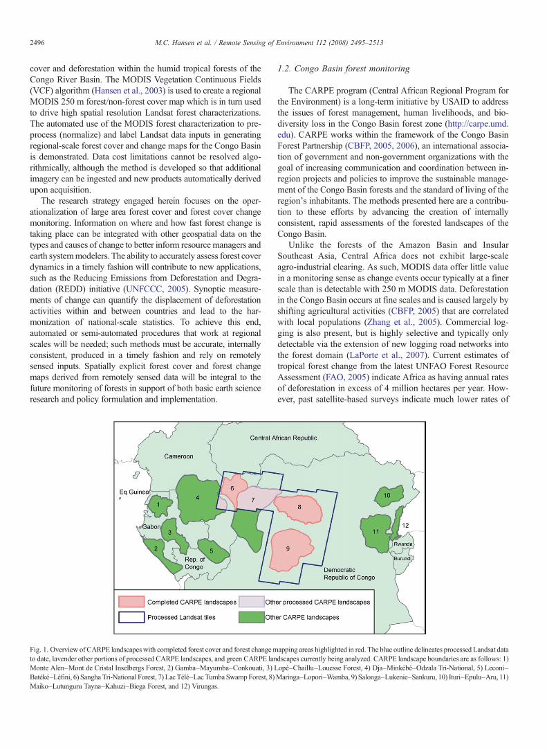
Fig. 1. Overview of CARPE landscapeswith completed forest cover and forest changemapping areas highlighted in red. The blue outline delineates processed Landsat datato date, lavender other portions of processed CARPE landscapes, and green CARPE landscapes currently being analyzed. CARPE landscape boundaries are as follows: 1)Monte Alen–Mont de Cristal Inselbergs Forest, 2) Gamba–Mayumba–Conkouati, 3) Lopé–Chaillu–Louesse Forest, 4) Dja–Minkébé–Odzala Tri-National, 5) Leconi–Batéké–Léfini, 6) Sangha Tri-National Forest, 7) Lac Télé–LacTumba SwampForest, 8)Maringa–Lopori–Wamba, 9) Salonga–Lukenie–Sankuru, 10) Ituri–Epulu–Aru, 11)Maiko–Lutunguru Tayna–Kahuzi–Biega Forest, and 12) Virungas.

2496 M.C. Hansen et al. / Remote Sensing of Environment 112 (2008) 2495–2513


change for tropical Africa (Achard et al., 2002; Hansen andDeFries, 2004). Improved high spatial resolution monitoring isrequired to better determine the rates and spatial extents offorest cover change within the humid tropical forests of CentralAfrica.

2. Study area

The tropical forest ecosystems of the Congo Basin representthe largest and most diverse forest massif on the Africancontinent and the second largest extent of tropical rain forest inthe world, next to the Amazon Basin (Wilkie et al., 2001; CBFP,2005). As defined by the Congo Basin Forest Partnership, theCongo Basin forests cover an area of nearly 2 million km2. TheCongo Basin in this context is not defined strictly by thedrainage area of the Congo River, but by the forest zoneextending from the Atlantic Ocean in the west to the AlbertineRift Valley in the east, and spanning the equator by nearly 7°north and south (CBFP, 2005).

The Congo Basin forests, also known as the Lower Guineo–Congolian forests as defined by White (1983), consistpredominately of humid evergreen broadleaf forests withseasonality increasing with latitude. Seasonality and corre-sponding cloud cover are related to the movement of the inter-tropical convergence zone. Cloud cover is typically high nearerthe equator, and is persistent in the western Basin due to thewarming and rising of moisture-laden air as it moves from theGulf of Guinea onto the central African land mass. A recentglobal study of the availability of cloud-free MODIS data forcompositing indicated that equatorial Africa was one of severalregions affected by high cloud cover at the time of MODISoverpass (Roy et al., 2006).

The CBFP and CARPE have identified 12 priority land-scapes for monitoring biodiversity, deforestation and othermeasures of disturbance within the remaining intact forest zonesof the Congo Basin. The methodology presented here is beingemployed exhaustively across the basin, where high spatialresolution Landsat data are available, to determine rates ofchange. This paper reports results from three of the landscapescovering approximately one third of the basin that are broadlyrepresentative of those in the Congo Basin–Maringa–Lopori–Wamba, Salonga–Lukenie–Sankuru, and Sangha Tri-National(Fig. 1).

3. Data

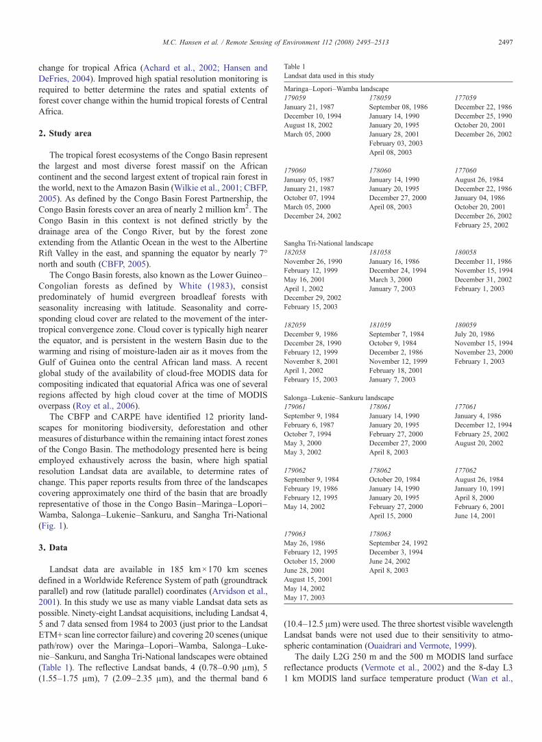
Landsat data are available in 185 km×170 km scenesdefined in a Worldwide Reference System of path (groundtrackparallel) and row (latitude parallel) coordinates (Arvidson et al.,2001). In this study we use as many viable Landsat data sets aspossible. Ninety-eight Landsat acquisitions, including Landsat 4,5 and 7 data sensed from 1984 to 2003 (just prior to the LandsatETM+ scan line corrector failure) and covering 20 scenes (uniquepath/row) over the Maringa–Lopori–Wamba, Salonga–Luke-nie–Sankuru, and Sangha Tri-National landscapes were obtained(Table 1). The reflective Landsat bands, 4 (0.78–0.90 μm), 5(1.55–1.75 μm), 7 (2.09–2.35 μm), and the thermal band 6

(10.4–12.5 μm) were used. The three shortest visible wavelengthLandsat bands were not used due to their sensitivity to atmo-spheric contamination (Ouaidrari and Vermote, 1999).

The daily L2G 250 m and the 500 m MODIS land surfacereflectance products (Vermote et al., 2002) and the 8-day L31 km MODIS land surface temperature product (Wan et al.,

Table 1Landsat data used in this study

Maringa–Lopori–Wamba landscape179059 178059 177059January 21, 1987 September 08, 1986 December 22, 1986December 10, 1994 January 14, 1990 December 25, 1990August 18, 2002 January 20, 1995 October 20, 2001March 05, 2000 January 28, 2001 December 26, 2002

February 03, 2003April 08, 2003

179060 178060 177060January 05, 1987 January 14, 1990 August 26, 1984January 21, 1987 January 20, 1995 December 22, 1986October 07, 1994 December 27, 2000 January 04, 1986March 05, 2000 April 08, 2003 October 20, 2001December 24, 2002 December 26, 2002

February 25, 2002

Sangha Tri-National landscape182058 181058 180058November 26, 1990 January 16, 1986 December 11, 1986February 12, 1999 December 24, 1994 November 15, 1994May 16, 2001 March 3, 2000 December 31, 2002April 1, 2002 January 7, 2003 February 1, 2003December 29, 2002February 15, 2003

182059 181059 180059December 9, 1986 September 7, 1984 July 20, 1986December 28, 1990 October 9, 1984 November 15, 1994February 12, 1999 December 2, 1986 November 23, 2000November 8, 2001 November 12, 1999 February 1, 2003April 1, 2002 February 18, 2001February 15, 2003 January 7, 2003

Salonga–Lukenie–Sankuru landscape179061 178061 177061September 9, 1984 January 14, 1990 January 4, 1986February 6, 1987 January 20, 1995 December 12, 1994October 7, 1994 February 27, 2000 February 25, 2002May 3, 2000 December 27, 2000 August 20, 2002May 3, 2002 April 8, 2003

179062 178062 177062September 9, 1984 October 20, 1984 August 26, 1984February 19, 1986 January 14, 1990 January 10, 1991February 12, 1995 January 20, 1995 April 8, 2000May 14, 2002 February 27, 2000 February 6, 2001

April 15, 2000 June 14, 2001

179063 178063May 26, 1986 September 24, 1992February 12, 1995 December 3, 1994October 15, 2000 June 24, 2002June 28, 2001 April 8, 2003August 15, 2001May 14, 2002May 17, 2003

2497M.C. Hansen et al. / Remote Sensing of Environment 112 (2008) 2495–2513


2002) were used in this study. These MODIS land products aredefined in the sinusoidal map projection in 10×10° land tiles(Wolfe et al., 1998), with eight tiles covering the Congo Basin.All of the MODIS Collection 4 products available from 2000 to2003 over these 8 tiles were used. The seven MODIS landsurface reflectance bands were used: the two 250 m red (0.620–0.670 μm) and near-infrared (0.841–0.876 μm) bands, and thefive 500 m bands: blue (0.459–0.479 μm), green (0.545–0.565 μm), mid-infrared (1.230–1.250 μm), mid-infrared(1.628–1.654 μm), and mid-infrared (2.105–2.155 μm).

4. Methods

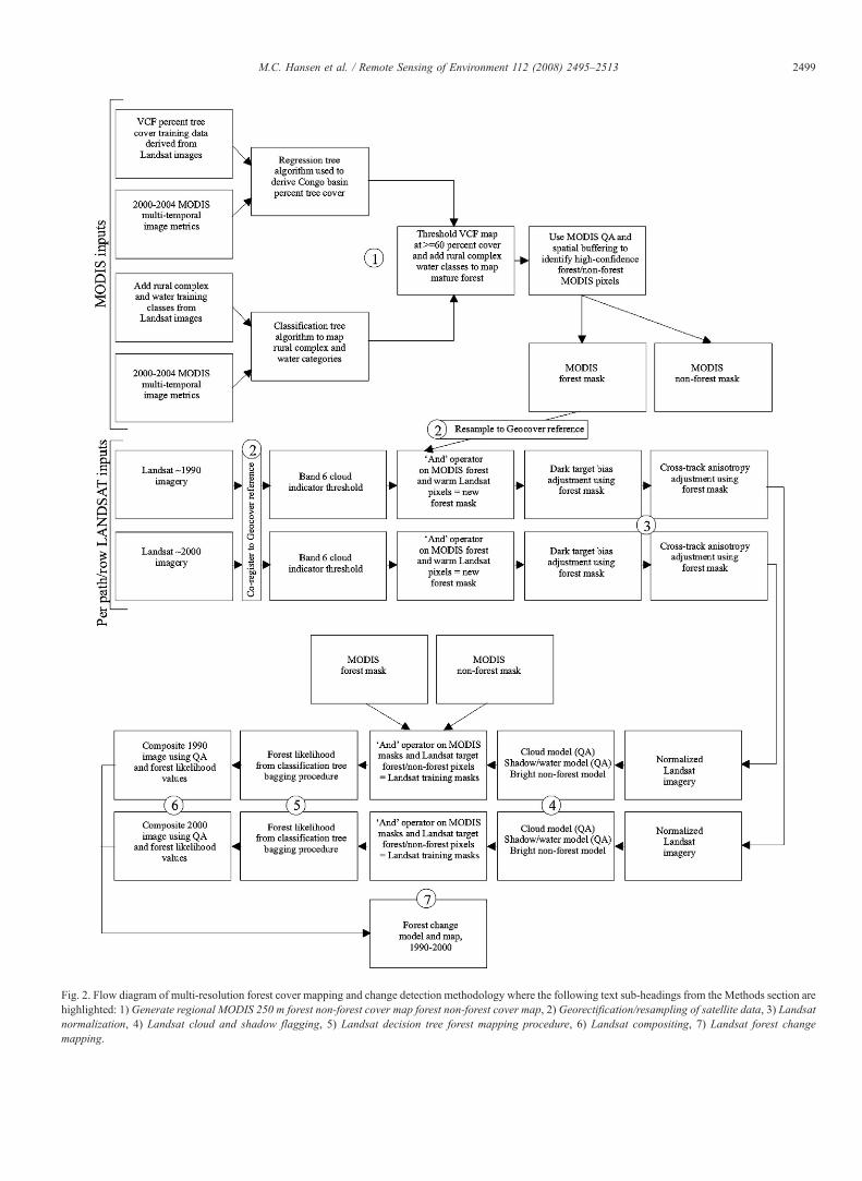
The methodology is illustrated in Fig. 2. First, a regionalMODIS 250 m forest non-forest map is generated using aregression tree approach (Fig. 2 (1)), and after resampling to acommon coordinate system (Fig. 2 (2)), is used to performradiometric normalization and to reducedeleteriousLandsat atmo-spheric and sun-surface-sensor spectral variations (Fig. 2 (3)).Each normalized Landsat image has standardized classificationtree models applied to detect per-pixel clouds and shadows,(Fig. 2 (4)). Landsat-scale forest cover is then mapped using aclassification tree approach with training labels derived from theMODIS 250 m forest map (Fig. 2 (5)). The Landsat forestestimates and associated spectral bands and cloud and shadowflags are composited to create decadal, pre-1996 and post-1996,composite forest cover products (Fig. 2 (6)). A deforestation clas-sification tree model is applied to these composites to produce aper-pixel forest change assessment (Fig. 2 (7)). Before describingthe methodology in detail, an overview of regression trees andtheir application for satellite classification is first described.

4.1. Classification and regression trees

The algorithmic tool used to characterize forest cover andchange, as well as to evaluate the presence of cloud and shadowartifacts, is the decision tree. Decision trees are hierarchical clas-sifiers that predict class membership by recursively partitioning adata set into more homogeneous subsets, referred to as nodes(Breiman et al., 1984). This splitting procedure is followed until aperfect tree is created, if possible, composed only of pure terminalnodes where every pixel is discriminated from pixels of otherclasses, or until preset conditions are met for terminating the tree'sgrowth. Trees can accept either categorical data in performing clas-sifications (classification trees) or continuous data in performingsub-pixel percent cover estimations (regression trees). For clas-sification trees, a deviance measure is used to split data into nodesthat are more homogeneous with respect to class membership thanthe parent node. For regression trees, a sum of squares criterion isused to split the data into successively less varying subsets.

Tree-based algorithms offer several advantages over othercharacterization methods and have been used with remotelysensed data sets (Michaelson et al., 1994; Hansen et al., 1996;DeFries et al., 1997; Friedl and Brodley, 1997). They aredistribution-free, allowing for the improved representation oftraining data within multi-spectral space. In addition, the treestructure enables interpretation of the explanatory nature of the

independent variables. A number of software packages are avail-able, in this study we use the Splus package (Clark and Pergibon,1992).

Multiple independent runs of decision trees via sampling withreplacement allow for more reliable results. This procedure iscalled bagging (Breiman, 1996), and typically employs a per-pixel voting procedure based on n derived classification trees tolabel eventual outputs. Per node likelihoods, and not per nodeclass labels, may also be used to derive mean class membershiplikelihood values for each pixel. By repeatedly sampling thetraining data to grow multiple tree models, isolated overfittingwithin any individual tree is reduced by calculating an averagedmulti-tree output. Unless otherwise stated, the analysis presentedhere employs bagging procedures to derive thematic outputs.

4.2. Generate regional MODIS 250 m forest non-forest covermap

The first step of the methodology is to generate a regionalforest non-forest map at moderate spatial resolution. The MODISVegetation Continuous Field (VCF) method (Hansen et al., 2003)is used, modified for application to the Congo Basin, to create aMODIS 250 m percent tree cover map. The percent tree covermap is then thresholded into forest and non-forest classes.

Monthly compositeswere generated from four years ofMODISdata (2000–2003), employing the same approach used to generatecomposites for the 250 m MODIS Vegetation Cover Changeproduct (Zhan et al., 2002). In this compositing approach, the twoMODIS 250 m bands are composited based on the MODIS landsurface reflectance quality assessment flags and an observationcoverage criterion to select the highest quality, nearest-nadir 250mobservation for each month (Carroll et al., in review). The five500m surface reflectance band values are retained by selecting the500 m observation lying closest to each composited 250 m pixelfor the selected day. Normalized difference vegetation index(NDVI) values are computed for each pixel from the 250m red andnear-infrared composited values. Monthly 1 km land surfacetemperature values are selected as those with the maximum landsurface temperature value over the month (Cihlar, 1994; Roy,1997) and resampled to 250 m pixels.

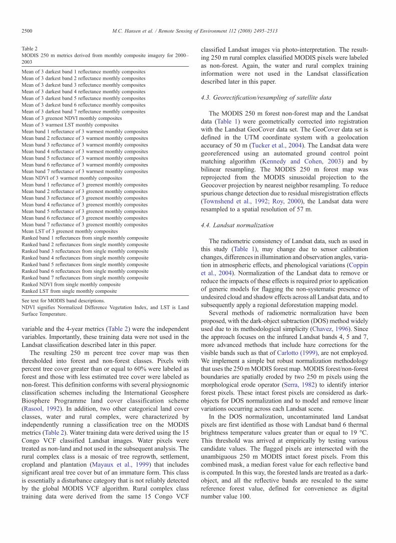
Thirty-four MODIS image metrics, defined following theapproach of Hansen et al. (2002a), Hansen and DeFries (2004),were extracted from the four years of monthly composites. Themetrics are summarized in Table 2, and three examples areillustrated in Fig. 3a. The metrics illustrated in Fig. 3a are themean of the three lowest MODIS land surface reflectance red(620–670 nm), near-infrared (841–876 nm), and middle-infrared (1628–1654 nm) monthly composite values. Thesethree metrics provide a time-integrated multi-year data set withminimal cloud contamination, and correspond largely with localgrowing season conditions.

In creating this Basin-wide forest cover map, we employedthe standard MODIS VCF algorithm (Hansen et al., 2002a)using over 2 million training pixels derived from 15 Landsatimages. A single perfectly fit regression tree was created using50% of the training data, and pruned using the remaining set-aside training data. The training data were the dependent



Fig. 2. Flow diagram of multi-resolution forest cover mapping and change detection methodology where the following text sub-headings from the Methods section arehighlighted: 1) Generate regional MODIS 250 m forest non-forest cover map forest non-forest cover map, 2) Georectification/resampling of satellite data, 3) Landsatnormalization, 4) Landsat cloud and shadow flagging, 5) Landsat decision tree forest mapping procedure, 6) Landsat compositing, 7) Landsat forest changemapping.



variable and the 4-year metrics (Table 2) were the independentvariables. Importantly, these training data were not used in theLandsat classification described later in this paper.

The resulting 250 m percent tree cover map was thenthresholded into forest and non-forest classes. Pixels withpercent tree cover greater than or equal to 60% were labeled asforest and those with less estimated tree cover were labeled asnon-forest. This definition conforms with several physiognomicclassification schemes including the International GeosphereBiosphere Programme land cover classification scheme(Rasool, 1992). In addition, two other categorical land coverclasses, water and rural complex, were characterized byindependently running a classification tree on the MODISmetrics (Table 2). Water training data were derived using the 15Congo VCF classified Landsat images. Water pixels weretreated as non-land and not used in the subsequent analysis. Therural complex class is a mosaic of tree regrowth, settlement,cropland and plantation (Mayaux et al., 1999) that includessignificant areal tree cover but of an immature form. This classis essentially a disturbance category that is not reliably detectedby the global MODIS VCF algorithm. Rural complex classtraining data were derived from the same 15 Congo VCF

classified Landsat images via photo-interpretation. The result-ing 250 m rural complex classified MODIS pixels were labeledas non-forest. Again, the water and rural complex traininginformation were not used in the Landsat classificationdescribed later in this paper.

4.3. Georectification/resampling of satellite data

The MODIS 250 m forest non-forest map and the Landsatdata (Table 1) were geometrically corrected into registrationwith the Landsat GeoCover data set. The GeoCover data set isdefined in the UTM coordinate system with a geolocationaccuracy of 50 m (Tucker et al., 2004). The Landsat data weregeoreferenced using an automated ground control pointmatching algorithm (Kennedy and Cohen, 2003) and bybilinear resampling. The MODIS 250 m forest map wasreprojected from the MODIS sinusoidal projection to theGeocover projection by nearest neighbor resampling. To reducespurious change detection due to residual misregistration effects(Townshend et al., 1992; Roy, 2000), the Landsat data wereresampled to a spatial resolution of 57 m.

4.4. Landsat normalization

The radiometric consistency of Landsat data, such as used inthis study (Table 1), may change due to sensor calibrationchanges, differences in illumination and observation angles, varia-tion in atmospheric effects, and phenological variations (Coppinet al., 2004). Normalization of the Landsat data to remove orreduce the impacts of these effects is required prior to applicationof generic models for flagging the non-systematic presence ofundesired cloud and shadow effects across all Landsat data, and tosubsequently apply a regional deforestation mapping model.

Several methods of radiometric normalization have beenproposed, with the dark-object subtraction (DOS) method widelyused due to its methodological simplicity (Chavez, 1996). Sincethe approach focuses on the infrared Landsat bands 4, 5 and 7,more advanced methods that include haze corrections for thevisible bands such as that of Carlotto (1999), are not employed.We implement a simple but robust normalization methodologythat uses the 250 mMODIS forest map.MODIS forest/non-forestboundaries are spatially eroded by two 250 m pixels using themorphological erode operator (Serra, 1982) to identify interiorforest pixels. These intact forest pixels are considered as dark-objects for DOS normalization and to model and remove linearvariations occurring across each Landsat scene.

In the DOS normalization, uncontaminated land Landsatpixels are first identified as those with Landsat band 6 thermalbrightness temperature values greater than or equal to 19 °C.This threshold was arrived at empirically by testing variouscandidate values. The flagged pixels are intersected with theunambiguous 250 m MODIS intact forest pixels. From thiscombined mask, a median forest value for each reflective bandis computed. In this way, the forested lands are treated as a dark-object, and all the reflective bands are rescaled to the samereference forest value, defined for convenience as digitalnumber value 100.

Table 2MODIS 250 m metrics derived from monthly composite imagery for 2000–2003

Mean of 3 darkest band 1 reflectance monthly compositesMean of 3 darkest band 2 reflectance monthly compositesMean of 3 darkest band 3 reflectance monthly compositesMean of 3 darkest band 4 reflectance monthly compositesMean of 3 darkest band 5 reflectance monthly compositesMean of 3 darkest band 6 reflectance monthly compositesMean of 3 darkest band 7 reflectance monthly compositesMean of 3 greenest NDVI monthly compositesMean of 3 warmest LST monthly compositesMean band 1 reflectance of 3 warmest monthly compositesMean band 2 reflectance of 3 warmest monthly compositesMean band 3 reflectance of 3 warmest monthly compositesMean band 4 reflectance of 3 warmest monthly compositesMean band 5 reflectance of 3 warmest monthly compositesMean band 6 reflectance of 3 warmest monthly compositesMean band 7 reflectance of 3 warmest monthly compositesMean NDVI of 3 warmest monthly compositesMean band 1 reflectance of 3 greenest monthly compositesMean band 2 reflectance of 3 greenest monthly compositesMean band 3 reflectance of 3 greenest monthly compositesMean band 4 reflectance of 3 greenest monthly compositesMean band 5 reflectance of 3 greenest monthly compositesMean band 6 reflectance of 3 greenest monthly compositesMean band 7 reflectance of 3 greenest monthly compositesMean LST of 3 greenest monthly compositesRanked band 1 reflectances from single monthly compositeRanked band 2 reflectances from single monthly compositeRanked band 3 reflectances from single monthly compositeRanked band 4 reflectances from single monthly compositeRanked band 5 reflectances from single monthly compositeRanked band 6 reflectances from single monthly compositeRanked band 7 reflectances from single monthly compositeRanked NDVI from single monthly compositeRanked LST from single monthly composite

See text for MODIS band descriptions.NDVI signifies Normalized Difference Vegetation Index, and LST is LandSurface Temperature.



Fig. 3. a) Three example MODIS metrics derived over the study area from 4 years (2000 to 2003) of monthly composites. Red, blue and green are, the mean of the threelowest MODIS land surface reflectance red (620–670 nm), near-infrared (841–876 nm), and middle-infrared (1628–1654 nm) band monthly composited valuesrespectively. Thirty-four such metrics were used to generate the Basin-wide forest cover map (Table 2). b) MODIS 250 m land cover for forest density classes madefrom VCF Landsat training data and 4 years of MODIS inputs. Rural complex and water classes were derived separately and superimposed on the VCF strata.



Remotely sensed variations may occur across the Landsatscene due to atmospheric scattering and surface anisotropycombined with variations in the viewing and solar geometry.The Landsat sensor, with its comparatively narrow field of view,is not as affected by surface anisotropic effects as wider field ofview sensors, such as MODIS (Schaaf et al., 2002). However,systematic remotely sensed variations across the Landsat sceneare sometimes evident and attempts to remove them using avariety of techniques have been implemented (Danaher et al.,2001; Toivonen et al., 2006). In our Landsat analysis, and inother Landsat research (Danaher et al., 2001; Toivonen et al.,2006), these variations appear greatest across scan rather thanalong track. For Landsat data, sensor view zenith angle, or scanangle, is the portion of the sun-sensor-target geometry thatvaries most across the scene. A simple linear regression rela-tionship between the Landsat spectral response and the Landsatcross-track pixel location is estimated for each reflective bandas:

y ¼ b0 þ b1 4 x ð1Þ

where y equals the DOS normalized Landsat digital number fora given reflective wavelength band, x is the cross-track(column) pixel value, b1 is the slope of the linear regressionfunction in digital numbers per cross-track pixel, and b0 is theintercept. Rather than compute this relationship over all theLandsat pixels, which may have different surface anisotropyand different atmospheric contamination characteristics, therelationship is computed only for Landsat pixels falling underthe 250 m MODIS unambiguous intact forest pixels. All thepixels of the DOS normalized Landsat data are then adjustedusing this relationship. This process is repeated independentlyfor each reflective band.

4.5. Landsat cloud, shadow and water flagging

Automated methods for flagging cloud and shadow effects area requirement for large-volume Landsat processing (Helmer andRuefenacht, 2005). Landsat cloud fraction metadata are notspatially explicit and the cloud detection algorithm was not de-signed to generate per-pixel cloud masks (Irish et al., 2006).Consequently, in this study, a regional cloud and shadowmaskingclassification tree was developed to classify clouds and shadowsinto low, medium and high-confidence categories. Water bodiesmust also be identified as they can be confused spectrally withdense dark vegetation and shadows.

Training data were developed from 9 Landsat images todifferentiate cloud, shadow and land pixels. Landsat bands 4, 5, 6and 7 and all combinations of possible 2 band simple ratios wereused as inputs to two classification trees classifying these dataindependently into cloud and shadow classes. The trees wereapplied to each normalized Landsat scene and the class member-ship likelihood values used to define per Landsat pixel a low,medium or high cloud/shadow quality assessment state. Repeatedshadow flags for a given pixel were used with topographical data(Rabus et al., 2003) to flag water. To reduce the impact of edgeeffects, a one-pixel (57 m) buffer around the high-confidence

cloud and shadow pixels was created using the morphologicaldilate operator (Serra, 1982) and made into an additional qualityassessment state. In total, four cloud/shadow quality assessmentstates were defined for each geometrically corrected and normal-ized Landsat scene pixel: 1) high presence cloud/shadow/water, 2)buffered high presence cloud/shadow/water, 3) medium presencecloud/shadow, and 4) low presence cloud/shadow.

4.6. Landsat forest mapping

A classification tree approach was used to estimate per-pixelforest likelihoods for each geometrically corrected and normal-ized Landsat acquisition (Table 1). Tree models were generatedindependently for each Landsat acquisition with the MODISforest non-forest class labels as the dependent variable and theLandsat data as the independent variable. Training data weredefined automatically by sampling from the interiors of theMODIS forest and non-forest mapped areas, derived by erodingthe MODIS forest and non-forest classes by the equivalent of two250 m pixels using the morphological erode operator (Serra,1982). These training data were assumed to be applicable to theolder (pre-2000) Landsat data as rates of forest change in CentralAfrica are sufficiently low that change is not readily reflected inthe interiors of MODIS forest and non-forest mapped areas.Landsat bands 4, 5 and 7, and simple ratios of these bands wereused as inputs. In addition, per-pixel local variances and localmeans for a 3 by 3 kernel were added to the input variable data set.

The per node likelihoods, not class labels, were retained from30 independently generated decision tree runs. All trees wereperfectly fit and run independently on a sample of approximately30,000 training pixels per Landsat acquisition to generate anaverage forest likelihood per pixel. This has the effect of gener-alizing the relationship between theMODIS labels and theLandsatspectral measures, overcoming the frequent, yet minority occur-rence of mislabeling. The forest and non-forest training categorieswere proportionately sampled according to their relative presencein the corresponding MODIS map in order to reduce training bias.

4.7. Landsat compositing

Compositing is a practical way to reduce residual cloudcontamination, fill missing values, and reduce the data volume ofmoderate resolution near-daily coverage sensor data such asAVHRR or MODIS (Holben, 1986; Cihlar, 1994; Roy, 1997).Compositing of higher spatial but lower temporal resolutionsatellite data, such as Landsat, is not normally undertaken how-ever because of high data costs and because the land surface statemay change in the period required to sense several acquisitions. Inthis study, the Landsat data were composited into two periods,pre-1996 and post-1996. The year 1996 was selected because forall but one scene (path 182 row 058, Table 1) there were at leasttwo pre-1996 and two post-1996 Landsat acquisitions available.

A per-pixel Landsat compositing scheme based on selectingthe date with the lowest cloud and shadow likelihood valueswas applied to the Landsat acquisitions (Table 1). When morethan one acquisition date had the same cloud and/or shadowlikelihood, the date that had a normalized digital number value



closest to the 100 reference value was selected. In this way thenumber of cloud and shadow contaminated pixels was reducedand dates with forest pixels were preferentially selected. Thedate of the selected acquisition and the corresponding forestlikelihood, cloud and shadow likelihood, and spectral bandvalues were retained. This compositing approach was appliedindependently to pre-1996 and post-1996 Landsat acquisitions,providing two composited Landsat time periods or epochs.

4.8. Landsat deforestation mapping

We employ a multi-date direct classification of changemethodology (Bruzzone and Serpico, 1997; Coppin et al.,2004). This approach requires that training data are available atthe same surface locations in all dates and that they reflectreliably the proportions of the change transitions across thelandscape. Forest is directly characterized using both the pre-1996 and the post-1996 forest likelihood and spectral com-posited data as inputs.

Landsat training data were identified by photo-interpretationof the two composited periods to identify deforested andunchanged pixels. A total of 37,000 training pixels were definedfrom the equivalent of six Landsat path/rows across the threelandscapes. The training data were selected without considera-tion of the forest likelihood values, although the cloud, waterand shadow quality assessment flags were used to avoidselection of contaminated pixels. For each training pixel thecomposited pre-1996 and post-1996 forest likelihood and spec-tral band data, and their per-pixel differences and smoothed ver-sions of the differences (generated using a 3×3 averaging filter)were derived.

The same bagged classification tree methodology used toproduce the forest likelihood results (Section 4.6) was employed.Per node likelihoods from 30 independently generated perfectlyfit tree runs were used to generate an average per-pixel defores-tation likelihood for each Landsat pixel. The proportion of de-forested to unchanged training pixels was approximately 1:3,resulting in a significantly oversampled deforestation proportion,and a positive bias of the deforestation likelihood values.

5. Results

5.1. MODIS 250 m forest non-forest mapping

The MODIS 250 m forest cover map is shown in Fig. 3b.Tabular results per country are shown in Table 3. In general, the

product captures the mosaic of human disturbance within theBasin. Zones of disturbance (rural complex) include the belt ofhigher population densities along the southern forest fringe, 3–5°latitude south, and in theAlbertineRift Valley along the borders ofUganda, Rwanda, Burundi and the Democratic Republic of theCongo (DRC), where rich volcanic soils are present. Disturbancewithin the forest massif traces road networks and is generallyspatially coherent. In the transition zones north and south of theforest, settlement patterns in the form of roads and towns areclearly evident within the mosaic gallery forests, secondary grass-lands, parklands and woodlands.

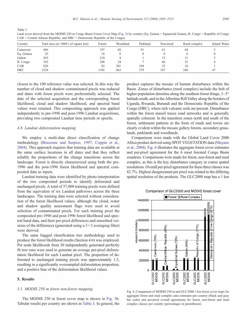
Comparisons were made with the Global Land Cover 2000Africa product derived using SPOTVEGETATION data (Mayauxet al., 2004). Fig. 4 illustrates the aggregate forest cover estimatesand per-pixel agreement for the 6 most forested Congo Basincountries. Comparisons were made for forest, non-forest and ruralcomplex, as this is the key disturbance category at coarse spatialresolutions.Overall per-pixel agreement for these three classeswas82.7%. Highest disagreement per pixel was related to the differingspatial resolution of the products. The GLC2000 map has a 1 km

Table 3Land cover derived from the MODIS 250 m Congo Basin Forest Cover Map (Fig. 3) by country (Eq. Guinea = Equatorial Guinea, R. Congo = Republic of CongoCAR = Central African Republic, and DRC = Democratic Republic of the Congo)

Country Total area (in 1000′s of square km) Forest Woodland Parkland Non-treed Rural complex Inland Water

Cameroon 466 197 68 91 61 44 5Eq. Guinea 25 18 0 0 0 6 0Gabon 265 210 4 1 15 31 5R. Congo 342 208 24 7 66 32 4CAR 620 82 301 194 25 18 1DRC 2328 1105 463 279 187 246 47

Fig. 4. Comparison of MODIS 250 m and GLC2000 1 km forest cover maps foraggregate forest and rural complex area estimates per country (black and graybar scale) and per-pixel overall agreements for forest, non-forest and ruralcomplex classes per country (percentages in parentheses).



spatial resolution while the MODIS map of this study has a 250 mspatial resolution. This leads to varying depictions of the ruralcomplex class which is manifested at relatively finer scales. Whileforest and non-forest agreements were 85.7 and 82.2%, respec-tively, rural complex agreed only 46.7% of the time. Regionally,the area of greatest disagreement was in the heavily cloud-affectedregions nearest the Gulf of Guinea in Cameroon, EquatorialGuinea, Gabon and the two Congos. Radar data would be avaluable alternative data source for overcoming the persistentpresence of cloud cover within these areas (Saatchi et al., 2002;DeGrandi et al., 2002).

5.2. Landsat normalization

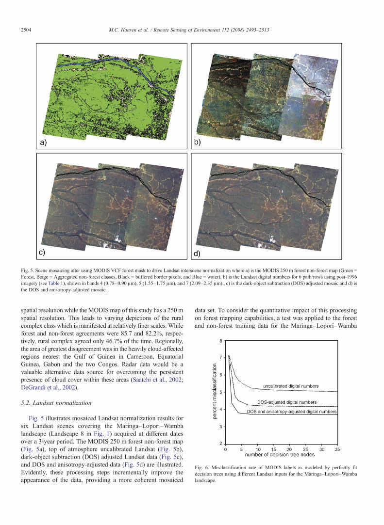
Fig. 5 illustrates mosaiced Landsat normalization results forsix Landsat scenes covering the Maringa–Lopori–Wambalandscape (Landscape 8 in Fig. 1) acquired at different datesover a 3-year period. The MODIS 250 m forest non-forest map(Fig. 5a), top of atmosphere uncalibrated Landsat (Fig. 5b),dark-object subtraction (DOS) adjusted Landsat data (Fig. 5c),and DOS and anisotropy-adjusted data (Fig. 5d) are illustrated.Evidently, these processing steps incrementally improve theappearance of the data, providing a more coherent mosaiced

data set. To consider the quantitative impact of this processingon forest mapping capabilities, a test was applied to the forestand non-forest training data for the Maringa–Lopori–Wamba

Fig. 5. Scene mosaicing after using MODIS VCF forest mask to drive Landsat interscene normalization where a) is the MODIS 250 m forest non-forest map (Green =Forest, Beige = Aggregated non-forest classes, Black = buffered border pixels, and Blue = water), b) is the Landsat digital numbers for 6 path/rows using post-1996imagery (see Table 1), shown in bands 4 (0.78–0.90 μm), 5 (1.55–1.75 μm), and 7 (2.09–2.35 μm)., c) is the dark-object subtraction (DOS) adjusted mosaic and d) isthe DOS and anisotropy-adjusted mosaic.

Fig. 6. Misclassification rate of MODIS labels as modeled by perfectly fitdecision trees using different Landsat inputs for the Maringa–Lopori–Wambalandscape.



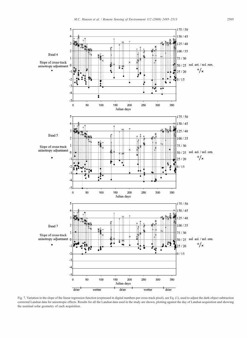
Fig. 7. Variation in the slope of the linear regression function (expressed in digital numbers per cross-track pixel), see Eq. (1), used to adjust the dark-object subtractioncorrected Landsat data for anisotropic effects. Results for all the Landsat data used in the study are shown, plotting against the day of Landsat acquisition and showingthe nominal solar geometry of each acquisition.



landscape. Over 400,000 MODIS labeled Landsat pixels wererun through a perfectly fit decision tree algorithm to evaluate thedifferent inputs of Fig. 5 for characterizing forest cover. Theability of the decision tree to discriminate the forest/non-forestcover categories is quantified and illustrates the increasedgeneralization and internal consistency of the multi-spectralfeature space achieved through the normalization process. Fig. 6illustrates decreasing misclassification rates, respectively, forthe top of atmosphere uncalibrated Landsat digital numbers, theDOS-adjusted, and the DOS and anisotropy-adjusted data. TheDOS and anisotropy-adjusted inputs reduce the misclassifica-tion rate by one-quarter compared to the uncalibrated digitalnumber inputs.

Fig. 7 shows the slope of the linear regression function(expressed in digital numbers per cross-track pixel location),used to adjust the dark-object subtraction corrected Landsat datafor anisotropic effects, for all the Landsat data used in the study.The slopes are all significant for all Landsat scenes, with p-values of less than 0.001. The slopes are plotted as a function ofthe day of Landsat acquisition and with the corresponding solargeometry. There appears to be, for the reflective bands used, aseasonal variation in the strength of the relationship, with morepronounced cross-track adjustments during and near the solarequinoxes. These temporally varying effects may be related tochanges in shadowing with changing solar geometry, seasonalatmospheric effects, and/or seasonal phenological variations.More study is required in order to attribute their cause(s).

5.3. Landsat cloud, shadow and water flagging

In generating the cloud classification tree, simple ratios ofband 6 to bands 4 and 7 were the most important discriminatoryvariables explaining the majority of the decision tree deviance.The ratios are analogous to an albedo versus temperaturemeasure that identifies bright, cool targets that are most likely tobe clouds in the humid tropics. For the shadow model, band 5was the primary discriminatory variable explaining more than86% of the tree variance. Upon visual inspection, the resultswere found to be generally robust, save for two of the 1998Landsat scenes, where it was necessary to manually removeshadows that remained undetected over highly reflectivesecondary grasslands. The vast majority of composited pixelswere rated with high quality assessment states. For example,Maringa–Lopori–Wamba featured the following pre-1996 QAdistribution: 93.75% low clouds/shadows, 2.04% mediumclouds/shadows, 1.67% water (derived from repeated highshadow flags), 1.91% buffered high clouds/shadows, and0.23% high clouds/shadows.

5.4. Landsat forest mapping

Each Landsat scene in Table 1 was processed independentlyusing the classification tree bagging approach. Results from thismapping process were used as inputs to the subsequent com-positing and change mapping procedures. As it is not feasible to

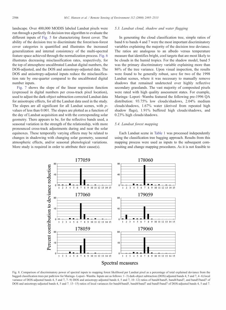
Fig. 8. Comparison of discriminatory power of spectral inputs to mapping forest likelihood per Landsat pixel as a percentage of total explained deviance from thebagged classification trees per path/row for Maringa–Lopori–Wamba. Inputs are as follows: 1–3) dark-object subtraction (DOS) adjusted bands 4, 5 and 7, 4–6) localvariance of DOS-adjusted bands 4, 5 and 7, 7–9) DOS and anisotropy-adjusted bands 4, 5 and 7, 10–12) ratios of band4/band5, band4/band7, and band5/band7 ofDOS and anisotropy-adjusted bands 4, 5 and 7. 13–15) ratios of local variances for band4/band5, band4/band7 and band5/band7 of DOS-adjusted bands 4, 5 and 7.



illustrate the results for 98 Landsat scenes, an assessment of whichspectral inputs contributed most to discriminating between theforest and non-forest categories is presented here. For eachspectral input, the deviance reduction per-split, summed over allbagged trees for all images per path/row, was derived to provide arelative measure of discriminatory strength. Fig. 8 summarizes forthe Maringa–Lopori–Wamba landscape which spectral informa-tion drove the forest characterizations. These results reveal againthe utility in performing the DOS and anisotropy adjustment and

the importance of the near-infrared (band 4) and mid-infrared(band 5) in characterizing forest/non-forest. Band 5 is most sen-sitive to the simple presence/absence of tree canopy, while band 4provides additional information between regrowing/disturbed andintact tree stands. As the objective here is to map the mature forestlands and their modification through time, band 4 is the infor-mation source that largely drives the classification tree algorithm.

5.5. Landsat compositing

The Landsat forest likelihood images were composited fol-lowing the methodology described in Section 4.7 into pre-1996

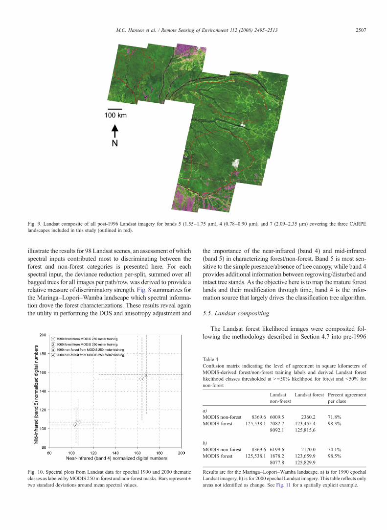
Fig. 9. Landsat composite of all post-1996 Landsat imagery for bands 5 (1.55–1.75 μm), 4 (0.78–0.90 μm), and 7 (2.09–2.35 μm) covering the three CARPElandscapes included in this study (outlined in red).

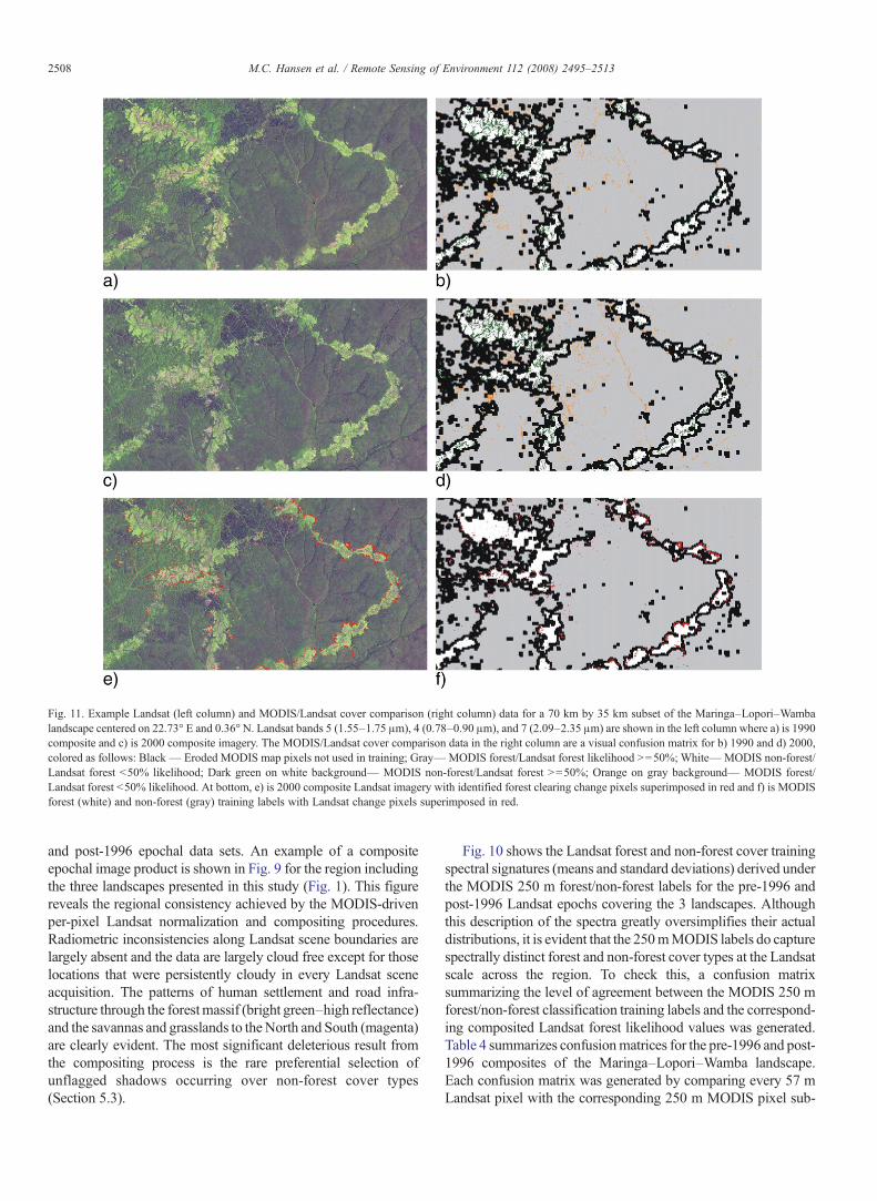
Fig. 10. Spectral plots from Landsat data for epochal 1990 and 2000 thematicclasses as labeled byMODIS 250m forest and non-forest masks. Bars represent ±two standard deviations around mean spectral values.

Table 4Confusion matrix indicating the level of agreement in square kilometers ofMODIS-derived forest/non-forest training labels and derived Landsat forestlikelihood classes thresholded at N=50% likelihood for forest and b50% fornon-forest

Landsatnon-forest

Landsat forest Percent agreementper class

a)MODIS non-forest 8369.6 6009.5 2360.2 71.8%MODIS forest 125,538.1 2082.7 123,455.4 98.3%

8092.1 125,815.6

b)MODIS non-forest 8369.6 6199.6 2170.0 74.1%MODIS forest 125,538.1 1878.2 123,659.9 98.5%

8077.8 125,829.9

Results are for the Maringa–Lopori–Wamba landscape. a) is for 1990 epochalLandsat imagery, b) is for 2000 epochal Landsat imagery. This table reflects onlyareas not identified as change. See Fig. 11 for a spatially explicit example.



and post-1996 epochal data sets. An example of a compositeepochal image product is shown in Fig. 9 for the region includingthe three landscapes presented in this study (Fig. 1). This figurereveals the regional consistency achieved by the MODIS-drivenper-pixel Landsat normalization and compositing procedures.Radiometric inconsistencies along Landsat scene boundaries arelargely absent and the data are largely cloud free except for thoselocations that were persistently cloudy in every Landsat sceneacquisition. The patterns of human settlement and road infra-structure through the forestmassif (bright green–high reflectance)and the savannas and grasslands to theNorth and South (magenta)are clearly evident. The most significant deleterious result fromthe compositing process is the rare preferential selection ofunflagged shadows occurring over non-forest cover types(Section 5.3).

Fig. 10 shows the Landsat forest and non-forest cover trainingspectral signatures (means and standard deviations) derived underthe MODIS 250 m forest/non-forest labels for the pre-1996 andpost-1996 Landsat epochs covering the 3 landscapes. Althoughthis description of the spectra greatly oversimplifies their actualdistributions, it is evident that the 250mMODIS labels do capturespectrally distinct forest and non-forest cover types at the Landsatscale across the region. To check this, a confusion matrixsummarizing the level of agreement between the MODIS 250 mforest/non-forest classification training labels and the correspond-ing composited Landsat forest likelihood values was generated.Table 4 summarizes confusionmatrices for the pre-1996 and post-1996 composites of the Maringa–Lopori–Wamba landscape.Each confusion matrix was generated by comparing every 57 mLandsat pixel with the corresponding 250 m MODIS pixel sub-

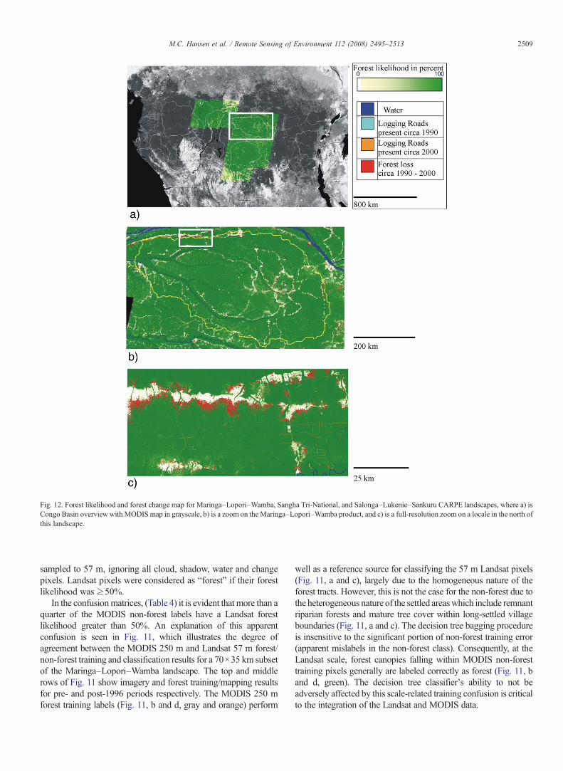
Fig. 11. Example Landsat (left column) and MODIS/Landsat cover comparison (right column) data for a 70 km by 35 km subset of the Maringa–Lopori–Wambalandscape centered on 22.73° E and 0.36° N. Landsat bands 5 (1.55–1.75 μm), 4 (0.78–0.90 μm), and 7 (2.09–2.35 μm) are shown in the left column where a) is 1990composite and c) is 2000 composite imagery. The MODIS/Landsat cover comparison data in the right column are a visual confusion matrix for b) 1990 and d) 2000,colored as follows: Black— Eroded MODIS map pixels not used in training; Gray—MODIS forest/Landsat forest likelihood N=50%; White—MODIS non-forest/Landsat forest b50% likelihood; Dark green on white background— MODIS non-forest/Landsat forest N=50%; Orange on gray background— MODIS forest/Landsat forest b50% likelihood. At bottom, e) is 2000 composite Landsat imagery with identified forest clearing change pixels superimposed in red and f) is MODISforest (white) and non-forest (gray) training labels with Landsat change pixels superimposed in red.



sampled to 57 m, ignoring all cloud, shadow, water and changepixels. Landsat pixels were considered as “forest” if their forestlikelihood was ≥50%.

In the confusionmatrices, (Table 4) it is evident that more than aquarter of the MODIS non-forest labels have a Landsat forestlikelihood greater than 50%. An explanation of this apparentconfusion is seen in Fig. 11, which illustrates the degree ofagreement between the MODIS 250 m and Landsat 57 m forest/non-forest training and classification results for a 70×35 km subsetof the Maringa–Lopori–Wamba landscape. The top and middlerows of Fig. 11 show imagery and forest training/mapping resultsfor pre- and post-1996 periods respectively. The MODIS 250 mforest training labels (Fig. 11, b and d, gray and orange) perform

well as a reference source for classifying the 57 m Landsat pixels(Fig. 11, a and c), largely due to the homogeneous nature of theforest tracts. However, this is not the case for the non-forest due tothe heterogeneous nature of the settled areaswhich include remnantriparian forests and mature tree cover within long-settled villageboundaries (Fig. 11, a and c). The decision tree bagging procedureis insensitive to the significant portion of non-forest training error(apparent mislabels in the non-forest class). Consequently, at theLandsat scale, forest canopies falling within MODIS non-foresttraining pixels generally are labeled correctly as forest (Fig. 11, band d, green). The decision tree classifier's ability to not beadversely affected by this scale-related training confusion is criticalto the integration of the Landsat and MODIS data.

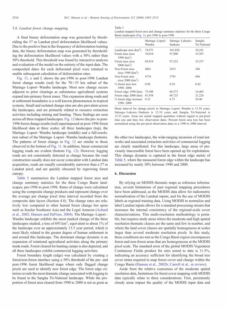
Fig. 12. Forest likelihood and forest change map for Maringa–Lopori–Wamba, Sangha Tri-National, and Salonga–Lukenie–Sankuru CARPE landscapes, where a) isCongo Basin overview with MODIS map in grayscale, b) is a zoom on the Maringa–Lopori–Wamba product, and c) is a full-resolution zoom on a locale in the north ofthis landscape.



5.6. Landsat forest change mapping

A final binary deforestation map was generated by thresh-olding the 57 m Landsat pixel deforestation likelihood values.Due to the positive bias in the frequency of deforestation trainingdata, the binary deforestation map was generated by threshold-ing the deforestation likelihood values with a 30% rather than50% threshold. This threshold was found by interactive analysisand evaluation of the model on the entirety of the input data. Thecomposited dates for each deforested pixel were retained toenable subsequent calculation of deforestation rates.

Fig. 11, e and f, shows the pre-1996 to post-1996 Landsatforest change results (red) for the 70×35 km subset of theMaringa–Lopori–Wamba landscape. Most new change occursadjacent to prior clearings as subsistence agricultural systemsexpand into primary forest zones. This expansion along roads andat settlement boundaries is a well known phenomenon in tropicalsystems. Small and isolated change sites are also prevalent acrossthe landscapes, and are primarily related to resource extractionactivities including mining and hunting. These findings are seenacross all threemapped landscapes. Fig. 12 shows the pre- to post-1996 forest change results (red) superimposed on post-1996 forestlikelihood data at three scales: all three landscapes (top), theMaringa–Lopori–Wamba landscape (middle) and a full-resolu-tion subset of the Maringa–Lopori–Wamba landscape (bottom).The patterns of forest change in Fig. 12 are similar to thoseobserved in the bottom of Fig. 11. In addition, linear commerciallogging roads are evident (bottom Fig. 12). However, loggingroads are not consistently detected as change because the roadconstruction usually does not occur coincident with Landsat dataacquisition, roads are usually considerably narrower than a 57 mLandsat pixel, and are quickly obscured by regrowing forestcanopy.

Table 5 summarizes the Landsat mapped forest area andchange summary statistics for the three Congo Basin land-scapes; pre-1996 to post-1996. Rates of change were calculatedusing the composite change products and represent change overthe average per change pixel time interval recorded from thecomposite date layers (Section 4.8). The change rates are rela-tively low compared to other humid forest change hot spotssuch as Insular Southeast Asia and the Legal Amazon (Achardet al., 2002; Hansen and DeFries, 2004). The Maringa–Lopori–Wamba landscape exhibits the most marked change of the threelandscapes studied, a loss of 693 km2, equivalent to about 1% ofthe landscape over an approximately 13.5 year period, which ismost likely related to the greater degree of human settlement inand around this landscape. The dominant change dynamic is anexpansion of rotational agricultural activities along the primarytrunk roads. Forest cleared for hunting camps is also depicted, andall three landscapes exhibit commercial logging activities.

Forest boundary length (edge) was calculated by creating aforest/non-forest interface using a 50% threshold of the pre- andpost-1996 forest likelihood maps where only flagged changepixels are used to identify new forest edge. The forest edge cri-terion reveals themost dramatic change associatedwith logging tobe found in the Sangha Tri-National landscape. While the pro-portion of forest area cleared from 1990 to 2000 is not as great as

the other two landscapes, the wide-ranging incursion of road net-works and associated extraction activities of commercial loggingare clearly manifested. For this landscape, large areas of pre-viously inaccessible forest have been opened up for exploitation.This change dynamic is captured in the forest edge metric ofTable 5, where the measured forest edge within the landscape hasincreased by nearly 30% between 1990 and 2000.

6. Discussion

By relying on MODIS thematic maps as reference informa-tion, several limitations of past regional mapping procedureshave been addressed, as the MODIS data allow for radiometricnormalization of the Landsat inputs, and for the use of MODISlabels as regional training data. Using MODIS to normalize andlabel Landsat inputs allows for a standard processing stream thatincreases the internal consistency of the regional-scale covercharacterizations. This multi-resolution methodology is porta-ble, but requires study areas where the moderate and high spatialresolution thematic classes are the same and few in number, andwhere the land cover classes are spatially homogenous at scaleslarger than several moderate resolution pixels. In this study,these conditions are met as the Congo Basin region encompassesforest and non-forest areas that are homogeneous at the MODISpixel scale. The standard error of the global MODIS VegetationContinuous Fields product for sites tested to date is 11.5%,indicating an accuracy sufficient for identifying the broad treecover strata required to map forest cover and change within theCongo Basin (Hansen et al., 2002b; Carroll et al., in review).

Aside from the relative coarseness of the moderate spatialresolution data, limitations for forest cover mapping withMODISdata typically relate to three considerations. First, persistentlycloudy areas impact the quality of the MODIS input data and

Table 5Landsat mapped forest area and change summary statistics for the three CongoBasin landscapes (Fig. 1); pre-1996 to post-1996

Maringa–Lopori–Wamba

Salonga–Lukenie–Sankuru

SanghaTri-National

Landscape area (km2) 74,973 101,820 36,241Forest area circa1990 (km2)

70,610 97,900 35,507

Forest area circa2000 (km2)

69,918 97,522 35,357

Non-Forest areacirca 1990 (km2)

4041 3415 546

Non-Forest areacirca 2000 (km2)

4734 3793 696

% forest area loss1990–2000

0.98 0.39 0.42

Forest edge 1990 (km) 75,508 66,573 16,403Forest edge 2000 (km) 81,938 69,723 21,226% forest edge increase1990–2000

8.52 4.73 29.40

Mean interval for change pixels in Maringa–Lopori–Wamba is 13.54 years,Salonga–Lukenie–Sankuru is 12.18 years and Sangha Tri-National is12.53 years. Areas are actual mapped quantities without regard to per-pixeltime one and time two observation dates. Percent forest area loss has beennormalized using the per-pixel observation dates to a 1990 to 2000 interval.



resultant mapping quality. To overcome this problem, four yearsof inputswere used tomap theCongoBasin. Second, the accuracyof the MODIS map is reduced as tree cover decreases from denseforests to woodlands and parklands (Hansen et al., 2000). Ourexpectation is that for densely covered intact forest biomes, suchas the tropical forest realm ofCentral Africa, theMODISmapwillbe robust and sufficient as a reference data set. Third, herbaceousand shrub covered wetlands are inconsistently mapped, and canintroduce error, particularly errors of change commission inherbaceous wetlands. Ongoing work is aimed at generating awetlands mask to remove these confounding areas from thechange analyses.

While this study has presented a new methodological approachto mapping Landsat-scale data sets using the MODIS percent treecover products for calibration, the accuracy of the results have notbeen fully assessed. Limitations of Landsat-scalemapping relate toerrors of change commission within herbaceous wetlands and toisolated residual cloud and shadow effects. However,many aspectsof the study provide confidence in the methods. The increasedseparability and training accuracy of forest and non-forest classesdue to the dark-object subtraction (DOS) and anisotropy adjust-ments indicates an improved mapping capability with Landsatdata. The additional fact that the classification tree models pri-marily employ the DOS and anisotropy-adjusted bands to mapforest and non-forest at the Landsat scale also validates theMODISlabels and pre-processing steps. The ability to generate regionalseamless mosaics points the way towards mass processing ofLandsat-scale images for land cover characterization applications.

7. Conclusion

This paper presents a multi-resolution methodology to mapforest cover and deforestation at Landsat scale, demonstrating itfor 0.56 million km2 of the Congo River Basin. Typical Landsat-scale studies use a single “best” image tomap forest cover state fora given year or decade. This is arguably due to high data costs andthe difficulty of combining multi-temporal Landsat acquisitions.The method described here demonstrates an ability to auto-matically process multi-resolution, multi-date imagery. Initialresults indicate that the Congo River Basin is an ecosystem absentof the large-scale clearing found in other humid tropical forestzones, such as the Legal Amazon and Insular Southeast Asia(Achard et al., 2002; Hansen and DeFries, 2004). However, themapped region indicates that forest clearing is spatially pervasiveand fragmented, with significant implications for sustaining theregion's biodiversity. Frontier forests absent of human impact arenot widespread in the Congo Basin, unlike some remaining foresttracts in the interior of the Amazon or New Guinea highlands.Given this fact, identifying new incursions into remaining intactforests is important for CARPE project partners. To this end, thecurrent approach is being extended to 2005 using Landsat 7 ScanLine Corrector-off data.

The method described here is meant to be an operationalalternative to large area deforestation mapping at high spatialresolutions. Full automation is primarily a function of the qualityof the input imagery. If there is a limitation regarding the usabilityof the results that is directly related to image quality, another

image is purchased and placed in the processing stream. Theapproach raised a current major limitation of large area moni-toring with high spatial resolution data, namely the cost ofimagery. Archives of high resolution data, whether SPOT HRV,IRS-LISS, or especially Landsat, are extensive but underutilizedfor this purpose due primarily to cost constraints. Operationalenvironmental monitoring, a term often used as an objectivewithin the remote sensing science community, is not feasiblegiven the current cost structure for high spatial resolution data. Forremote areas such as the Congo Basin, earth observation data arethe only source of information for documenting land cover andland use change. Improving data access, minimizing data costsand operationalizing sensor missions is the only way to ensuretimely and accurate monitoring of such areas.

Acknowledgments

Funding from the National Aeronautics and Space Admin-istration supported this research under grant NNG06GC416.

References

Achard, F., Eva, H. D., Stibig, H. -J., Mayaux, P., Gallego, J., Richards, T., et al.(2002). Determination of deforestation rates of the world's humid tropicalforests. Science, 297, 999−1002.

Arvidson, T., Gasch, J., & Goward, S. N. (2001). Landsat 7's long-termacquisition plan — an innovative approach to building a global imageryarchive. Remote Sensing of Environment, 78, 13−26.

Asner, G. P. (2001). Cloud cover in Landsat observations of the BrazilianAmazon. International Journal of Remote Sensing, 22, 3855−3862.

Asner, G., Knapp, D., Broadbent, E., Oliveira, P., Keller, M., & Silva, J. (2005,October 21). Selective logging in the Brazilian AmazonScience, Vol. 310 (5747)(pp. 480−482).

Avissar, R., & Werth, D. (2005). Global hydroclimatological teleconnectionsresulting from tropical deforestation. Journal of Hydrometeorology, 6, 134−145.

Breiman, L. (1996). Bagging predictors. Machine Learning, 26, 123−140.Breiman, L., Friedman, J., Olshen, R., & Stone, C. (1984). Classification and

Regression Trees Monterey, California: Wadsworth.Bruzzone, L., & Serpico, S. B. (1997). Detection of changes in remotely-sensed

images by the selective use of multi-spectral information. InternationalJournal of Remote Sensing, 18, 3883−3888.

Carlotto, M. J. (1999). Reducing the effects of space-varying, wavelength-dependent scattering in multispectral imagery. International Journal of RemoteSensing, 20, 3333−3344.

Carroll, M., Townshend, J., Hansen, M., DiMiceli, C., Sohlberg, R., & Wurster,K. (in review). Vegetative Cover Conversion and Vegetation ContinuousFields. In B. Ramachandran, C. Justice & M. Abrams (Eds.) Land RemoteSensing and Global Environmental Change: ASA's EOS and the science OfASTER and MODIS. New York: Springer Verlag.

(CBFP) Congo Basin Forest Partnership. (2005). The forests of the CongoBasin: a preliminary assessment, Eds. Justice, C.O., et al. USAID, CARPE.

(CBFP) Congo Basin Forest Partnership. (2006). In D. Devers, & Vande weghe(Eds.), The forests of the Congo Basin: State of the Forests 2006: CBFP.

Chavez, P. S., Jr. (1996). Image-based atmospheric corrections-revisited andimproved. Photogrammetric Engineering and Remote Sensing, 62(9),1025−1036.

Cihlar, J. (1994). Detection and removal of cloud contamination from AVHRRimages. I.E.E.E. Transactions on Geoscience and Remote Sensing, 32,583−589.

Clark, L. A., & Pergibon, D. (1992). Tree-based models. In T. J. Hastie (Ed.),Statistical Models in S Pacific Grove, CA: Wadsworth and Brooks.

Coppin, P., Jonckheere, I., Nackaerts, K., & Muys, B. (2004). Digital changedetection methods in ecosystemmonitoring: A review. International Journalof Remote Sensing, 25(9), 1565−1596.



Curran, L., & Trigg, S. (2006). Sustainability science from space: Quantifyingforest disturbance and land-use dynamics in the Amazon. Proceedings of theNational Academy of Sciences, 103(34), 12663−12664.

Danaher, T., Wu, X., & Campbell, N. (2001, July). Bi-directional reflectancedistribution function approaches to radiometric calibration of Landsat TMimagery. Proceedings of IGARSS 2001.

DeFries, R., Hansen, M., Steininger, M., & Dubayah, R. (1997). Subpixel forestcover in Central Africa from multisensor, multitemporal data. RemoteSensing of Environment, 60, 228−246.

DeGrandi, G. F., Mayaux, P., Malingreau, J. P., Rosenqvist, A., Saatchi, S., &Simard, M. (2002). New perspectives on global ecosystems from wide-arearadar mosaics: Flooded forest mapping in the tropics. International Journalof Remote Sensing, 21, 1235−1250.

FAO (Food and Agriculture Organization). (2005). State of the World's Forests,Rome. 320 pp.

Freidl, M. A., & Brodley, C. E. (1997). Decision tree classification of landcover from remotely sensed data. Remote Sensing of Environment, 61,399−409.

Hansen, M. C., & DeFries, R. S. (2004). Detecting long term global forestchange using continuous fields of tree cover maps from 8km AVHRR datafor the years 1982–1999. Ecosystems, 7, 695−716.

Hansen,M. C., DeFries, R. S., Townshend, J. R. G., & Sohlberg, R. (2000). Globalland cover classification at 1 km spatial resolution using a classification treeapproach. International Journal of Remote Sensing, 21, 1331−1364.

Hansen, M. C., DeFries, R. S., Townshend, J. R. G., Sohlberg, R., Carroll, M., &Dimiceli, C. (2002). Towards an operational MODIS continuous field ofpercent tree cover algorithm: Examples using AVHRR and MODIS data.Remote Sensing of Environment, 83(1&2), 303−319.

Hansen, M. C., DeFries, R. S., Townshend, J. R. G., Marufu, L., & Sohlberg,R. (2002). Development of a MODIS percent tree cover validation data setfor Western Province, Zambia. Remote Sensing of Environment, 83(1&2),320−335.

Hansen, M. C., DeFries, R. S., Townshend, J. R. G., Carroll, M., Dimiceli, C., &Sohlberg, R. A. (2003). Global percent tree cover at a spatial resolution of500meters: First results of theMODIS vegetation continuous fields algorithm.Earth Interactions, 7(10) 15 pp. [online journal].

Hansen, M., Dubayah, R., & DeFries, R. (1996). Classification trees: Analternative to traditional land cover classifiers. International Journal ofRemote Sensing, 17(5), 1075−1081.

Helmer, E. H., & Ruefenacht, B. (2005). Cloud-free satellite image mosaics withregression trees and histogram matching. Photogrammetric Engineeringand Remote Sensing, 71, 1079−1089.

Holben, B. (1986). Characteristics of maximum-value composite imagesfrom temporal AVHRR data. International Journal of Remote Sensing,7, 1417−1434.

IGBP (Terrestrial Carbon Working Group). (1998). The terrestrial carbon cycle:Implications for the Kyoto Protocol. Science, 280, 1393−1394.

INPE (Instituto Nacional de Pesquisas Especiais). (2002). Monitoring of theBrazilian Amazonian Forest by Satellite, 2000–2001 São José dos Campos,Brazil: Instituto Nacional de Pesquisas Especiais.

Irish, R. I., Barker, J. L., Goward, S. N., &Arvidson, T. (2006). Characterization ofthe Landsat-7 ETM+ automated cloud-cover assessment (ACCA) algorithm.Photogrammetric Engineering & Remote Sensing, 72, 1179−1188.

Ju, J., & Roy, D. P. (in press). The availability of cloud-free Landsat ETM+ dataover the conterminous United States and globally. Remote Sensing ofEnvironment.

Kennedy, R. E., & Cohen, W. B. (2003). Automated designation of tie-points forimage-to-image coregistration. International Journal of Remote Sensing,24, 3467−3490.

LaPorte, N., Heinicke, M., Justice, C. O., & Goetz, S. (1998). A new land covermap of Central Africa derived from multiresolution, multi-temporal satellitedata. International Journal of Remote Sensing, 19, 3537−3550.

LaPorte, N., Stabach, J., Grosch, R., Lin, T., & Goetz, S. (2007). Expansion ofindustrial logging in Central Africa. Science, 316, 1451.

Mayaux, P., Bartholomé, E., Fritz, S., & Belward, A. (2004). A new land-covermap of Africa for the year 2000. Journal of Biogeography, 31, 861−877.

Mayaux, P., Richards, T., & Janodet, E. (1999). Avegetation map of Central Africaderived from satellite imagery. Journal of Biogeography, 26, 353−366.

Michaelson, J., Schimel, D. S., Friedl, M. A., Davis, F. W., & Dubayah, R. O.(1994). Regression tree analysis of satellite and terrain data to guide vegetationsampling and surveys. Journal of Vegetation Science, 5, 673−696.

Ouaidrari, H., & Vermote, E. F. (1999). Operational atmospheric correction ofLandsat TM data. Remote Sensing of Enviroment, 70, 4−15.

Rabus, B., Eineder, M., Roth, A., & Bamler, R. (2003). The shuttle radartopography mission— A new class of digital elevation models acquired byspaceborne radar. Photogrammetric Engineering and Remote Sensing, 57,241−262.

Rasool, S. I. (1992). Requirements for terrestrial biospheric data for IGBP CoreProjects. IGBP-DIS Working Paper #2, International Geosphere-BiosphereProgramme — Data and Information Systems, Paris, France.

Roy, D. (1997). Investigation of the maximum normalised difference vegetationindex (NDVI) and the maximum surface temperature (Ts) AVHRRcompositing procedures for the extraction of NDVI and Ts over forest.International Journal of Remote Sensing, 18, 2383−2401.

Roy, D. (2000). The impact of misregistration upon composited wide field ofview satellite data and implications for change detection. IEEE Transactionson Geoscience and Remote Sensing, 38, 2017−2032.

Roy, D. P., Lewis, P., Schaaf, C., Devadiga, S., &Boschetti, L. (2006). The globalimpact of cloud on the production ofMODIS bi-directional reflectancemodelbased composites for terrestrial monitoring. IEEE Geoscience and RemoteSensing Letters, 3, 452−456.

Saatchi, S. S., Nelson, B., Podest, E., & Holt, J. (2002). Mapping land covertypes in the Amazon Basin using 1 km JERS-1 mosaic. InternationalJournal of Remote Sensing, 21, 1201−1234.

Schaaf, C., Gao, F., Strahler, A., Lucht, W., Li, X., Tsang, T., et al. (2002). Firstoperational BRDF, albedo and nadir reflectance products from MODIS.Remote Sensing of Environment, 83(1&2), 135−148.

SCBD (Secretariat of the Convention on Biological Diversity). (2001). TheValue of Forest Ecosystems, Montreal. 67 pp.

Serra, J. (1982). Image analysis and mathematical morphology New York:Academic.

Skole, D., & Tucker, C. (1993). Evidence for Tropical deforestation, fragmentedhabitat, and adversely affected habitat in the Brazilian Amazon:1978–1988.Science, 260, 1905−1910.

Toivonen, T., Kalliola, R., Ruokolainen, K., &Malik, R. N. (2006). Across-path DNgradient in Landsat TM imagery of Amazonian forests: a challenge for imageinterpretation and mosaicking. Remote Sensing of Environment, 100, 550−562.

Townshend, J. R.G., Bell,V., Desch, A., Havlicek,C., Justice, C., Lawrence,W.L.,et al. (1995). The NASA Landsat pathfinder humid tropical deforestationproject. Land satellite information in the next decade, ASPRS conference,Vienna, VA, 25–28 Sept. 1995 (pp. IV−76-IV-87).

Townshend, J. R. G., Justice, C. O.,Gurney, C.,&McManus, J. (1992). The impactof misregistration on change detection. IEEE Transactions on Geoscience andRemote Sensing, 30, 1054−1060.

Tucker, C. J., Grant, D. M., & Dykstra, J. D. (2004). NASA's globalorthorectified Landsat data set. Photogrammetric Engineering and RemoteSensing, 70, 313−322.

UNFCCC. (2005). Reducing Emissions from Deforestation inDevelopingCountries: Approaches to Stimulate Action—Draft Conclusions Proposed bythe President (Bonn: UNFCCC Secretariat) available at http://unfccc.int/resource/docs/2005/cop11/eng/l02.pdf

Vermote, E. F., El Saleous, N. Z., & Justice, C. O. (2002). Atmosphericcorrection of MODIS data in the visible to middle infrared: First results.Remote Sensing of Environment, 83, 97−111.

Wan, Z., Zhang, Y., Zhang, Q., & Li, Z. -L. (2002). Validation of the landsurface temperature products retrieved from Terra moderate resolutionimaging spectroradiometer data. Remote Sensing of Environment, 83,163−180.

White, F. (1983). The vegetation of Africa, a descriptive memoir to accompany theUNESCO/AETFAT/UNSO Vegetation Map of Africa (3 Plates, NorthwesternAfrica, Northeastern Africa, and Southern Africa, 1:5,000,000). UNESCO,Paris.

Wilkie, D., & Laporte, N. (2001). Forest area and deforestation in Central Africa:Current knowledge and future directions. InW.Weber, L.White, A. Vedder, &L. Naughton-Treves (Eds.), African Rain Forest Ecology and Conservation(pp. 119−139).Yale University Press.



Wolfe, R., Roy, D., & Vermote, E. (1998). The MODIS land data storage,gridding and compositing methodology: L2 Grid. IEEE Transactions onGeoscience and Remote Sensing, 36, 1324−1338.

Zhan, X., DeFries, R., Townshend, J. R. G., DiMiceli, C., Hansen, M., Huang,C., & Sohlberg, R. (2002). The 250m global land cover change product from

the moderate resolution imaging spectroradiometer of NASA's EarthObserving System. Remote Sensing of Environment, 21, 1433−1460.

Zhang, Q., Devers, D., Desch, A., Justice, C. O., & Townshend, J. R. G. (2005).Mapping tropical deforestation in Central Africa. Environmental Monitoringand Assessment, 101, 61−83.


Documents

Download publication