HYDRAULICS / WELL CONTROL / PRESSURE ANALYSIS

PART 1 DRILLING HYDRAULICS 1.1 Summary of the Purpose of the Drilling Fluid 1.2 Types of Drilling Fluid 1.3 Types of Fluid - Newtonian or Non-Newtonian a. Definitions b. Newtonian Fluids c. Bingham Fluids d. Power Law Fluids e. The Modified Power Law f. Model Affects on Viscous Flow 1.4 Mud Rheology 1.5 Laminar, Turbulent and Transitional Flow Patterns a. Laminar Flow b. Turbulent Flow c. Determination of Flow Type d. Derivation of Effective Viscosity e. Determination of Reynold’s Number f. Determination of Annular Velocity g. Use of Reynold’s Number to determine Flow Type h. Determination of Critical Velocity 1.6 Determination of System Pressure Losses a. Fanning Friction Factor b. Drillstring Pressure Losses c. Annular Pressure Losses d. Bit Pressure Loss e. Surface Pressure Losses

1.7 Other Hydraulic Calculations a. Cuttings Slip Velocity b. Slip Velocity in Turbulent Flow c. Nozzle Velocity 1.8 Hydraulics Optimization a. Bit Hydraulic Horsepower b. Hydraulic Impact Force c. Optimization 1.9 Equivalent Circulating Density 1.10 Surge and Swab Pressures Appendix

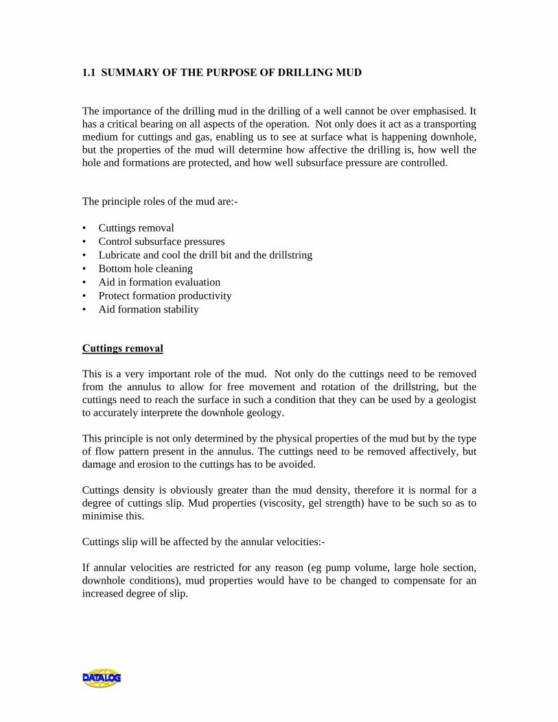
1.1 SUMMARY OF THE PURPOSE OF DRILLING MUD The importance of the drilling mud in the drilling of a well cannot be over emphasised. It has a critical bearing on all aspects of the operation. Not only does it act as a transporting medium for cuttings and gas, enabling us to see at surface what is happening downhole, but the properties of the mud will determine how affective the drilling is, how well the hole and formations are protected, and how well subsurface pressure are controlled. The principle roles of the mud are:- • Cuttings removal • Control subsurface pressures • Lubricate and cool the drill bit and the drillstring • Bottom hole cleaning • Aid in formation evaluation • Protect formation productivity • Aid formation stability Cuttings removal This is a very important role of the mud. Not only do the cuttings need to be removed from the annulus to allow for free movement and rotation of the drillstring, but the cuttings need to reach the surface in such a condition that they can be used by a geologist to accurately interprete the downhole geology. This principle is not only determined by the physical properties of the mud but by the type of flow pattern present in the annulus. The cuttings need to be removed affectively, but damage and erosion to the cuttings has to be avoided. Cuttings density is obviously greater than the mud density, therefore it is normal for a degree of cuttings slip. Mud properties (viscosity, gel strength) have to be such so as to minimise this. Cuttings slip will be affected by the annular velocities:- If annular velocities are restricted for any reason (eg pump volume, large hole section, downhole conditions), mud properties would have to be changed to compensate for an increased degree of slip.

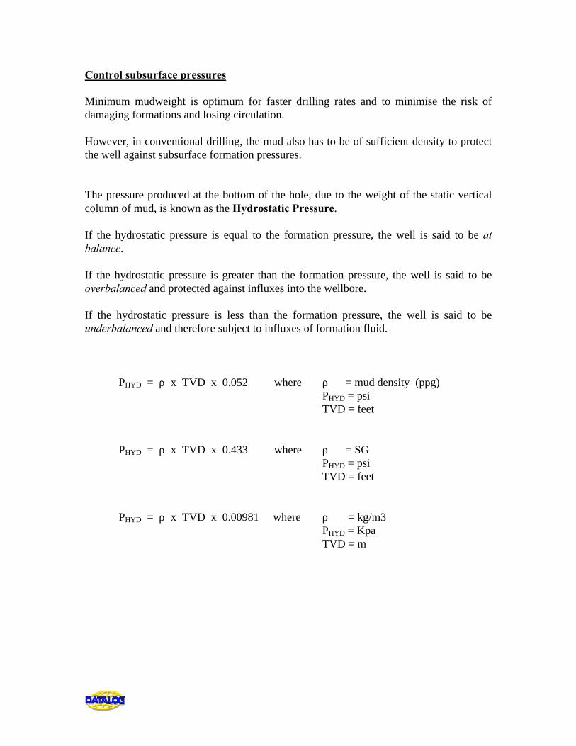
Control subsurface pressures Minimum mudweight is optimum for faster drilling rates and to minimise the risk of damaging formations and losing circulation. However, in conventional drilling, the mud also has to be of sufficient density to protect the well against subsurface formation pressures. The pressure produced at the bottom of the hole, due to the weight of the static vertical column of mud, is known as the Hydrostatic Pressure. If the hydrostatic pressure is equal to the formation pressure, the well is said to be at balance. If the hydrostatic pressure is greater than the formation pressure, the well is said to be overbalanced and protected against influxes into the wellbore. If the hydrostatic pressure is less than the formation pressure, the well is said to be underbalanced and therefore subject to influxes of formation fluid. PHYD = ρ x TVD x 0.052 where ρ = mud density (ppg) PHYD = psi TVD = feet PHYD = ρ x TVD x 0.433 where ρ = SG PHYD = psi TVD = feet PHYD = ρ x TVD x 0.00981 where ρ = kg/m3 PHYD = Kpa TVD = m

Lubricate and cooling The drilling action and rotation of the drillstring will produce a lot of heat, at the bit and throughout the drillstring, due to friction. This heat will be absorbed by the mud and released, to a degree, at surface. The mud has to cool the bit and lubricate the teeth to allow for affective drilling and to minimise damage and wear. The mud has to affectively remove cuttings from around the bit as rock is newly penetrated. This is to stop the cuttings building up around the bit and teeth (bit balling) which would prevent the bit from drilling. The mud lubricates the drillstring by reducing friction between the string and the borehole wall - this is achieved by additives such as bentonite, graphite or oil. Aid in formation evaluation • To obtain the best possible cuttings for geological analysis (viscosity). The type of

flow will determine the degree of erosion and alteration, thus smooth laminar flow is preferred to chaotic turbulent flow.

• To minimise fluid invasion (filtrate) - both water and oil invasion would affect the

resistivity of the mud making formation evaluations more difficult. Thus, a filter cake is allowed to build up on the wall of the borehole, restricting fluid movement in both directions.

NB Filter Cake restricts fluid invasion but may reduce the quality of sidewall cores • To improve logging characteristics (especially for resistivities). • To improve formation testing Formation Stability • to prevent erosion or collapse of the wellbore; • to prevent swelling and sloughing shales (oil based mud preferred, water based muds

would have to be treated with Ca/K/Asphalt compounds); • to prevent the ‘dissolving’ of salt sections (use salt saturated or oil based mud to

prevent taking the salt into solution.

1.2 TYPES OF DRILLING MUD (a brief summary) Water Based including gel and polymer muds Oil Based Emulsion Water Based Muds 1. Clear Water - from freshwater to saturated brine 2. Native Water - water allowed to react with formations containing shales/clays; the mud will therefore build up a solids content and density naturally. 3. Calcium - reduces swelling and hydration of clays good for gypsum/anhydrite lithologies because there will be no Ca contamination 4. Lignosulphate - high density muds (>14ppg) tolerance to high temperatures high tolerance for contamination by drilled solids disadvantages - shales/clays will adsorb water from the mud permeability will be damaged due to clays dispersing Not often used 5. KCL/Polymer - inhibits shale sloughing little permeability damage provides good bit hydraulics disadvantages - need good solids control equipment at surface because it has a low tolerance to solids unstable at high temperatures > 120oC 6. Salt Saturated - water phase saturated with NaCl

Oil Based Muds Emulsion of water in oil (invert emulsion) Crude oil or diesel is normally the continuous phase, water the dispersed phase (droplets) Advantages reduces/inhibits any problems caused by shales reduces torque and drag stable at high temperatures preserves natural permeability, not damaging hydrocarbon zones Disadvantages environmental concerns flammability solids removal due to high PV (need good equipment as with polymer muds) problems for interpretation of log information cost Emulsion Muds Water is the continuous phase, oil the dispersed phase (normally 5 - 10%) Oil added to increase ROP, reduce filter loss, improve lubrication, reduce drag and torque

1.3 TYPES OF FLUID - NEWTONIAN or NON-NEWTONIAN ? The majority of hydraulic parameters are, first of all, dependent on what type of fluid the drilling mud is and therefore which model is used for the calculations. The categories are determined by the fluid behaviour when it is subjected to an applied force (shear stress). Precisely, in terms of fluid behaviour, we are concerned with:- • At what point of applied shear stress is movement initiated in the fluid. • Once movement has been initiated, what is the nature of the fluid movement (Shear

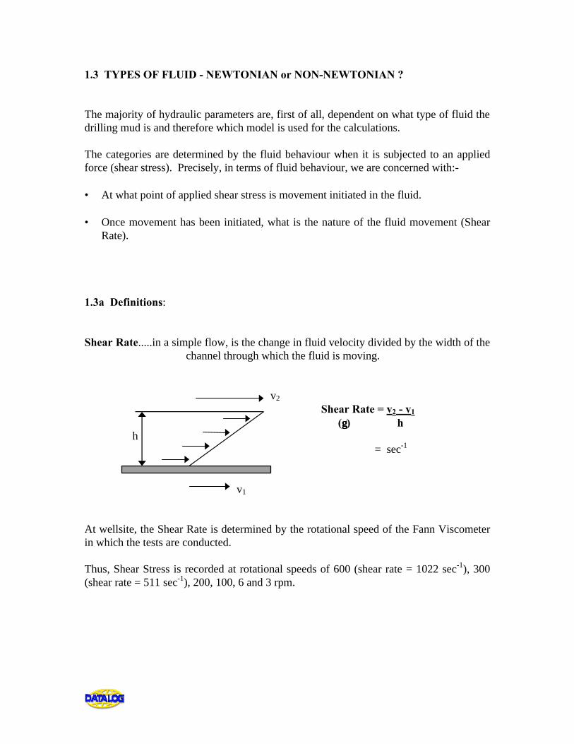
Rate). 1.3a Definitions: Shear Rate.....in a simple flow, is the change in fluid velocity divided by the width of the channel through which the fluid is moving. v2 Shear Rate = v2 - v1 (γγ) h h = sec-1 v1 At wellsite, the Shear Rate is determined by the rotational speed of the Fann Viscometer in which the tests are conducted. Thus, Shear Stress is recorded at rotational speeds of 600 (shear rate = 1022 sec-1), 300 (shear rate = 511 sec-1), 200, 100, 6 and 3 rpm.

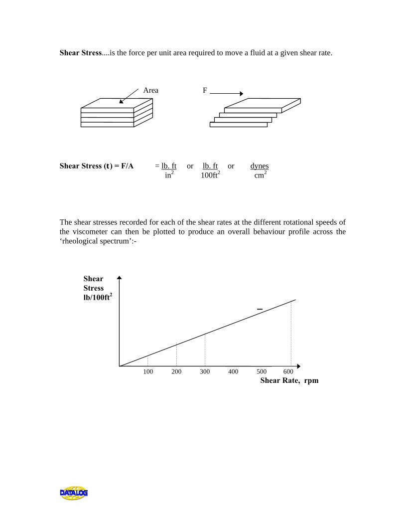
Shear Stress....is the force per unit area required to move a fluid at a given shear rate. Area F Shear Stress (ττ) = F/A = lb. ft or lb. ft or dynes in2 100ft2 cm2 The shear stresses recorded for each of the shear rates at the different rotational speeds of the viscometer can then be plotted to produce an overall behaviour profile across the ‘rheological spectrum’:- Shear Stress lb/100ft2 100 200 300 400 500 600 Shear Rate, rpm

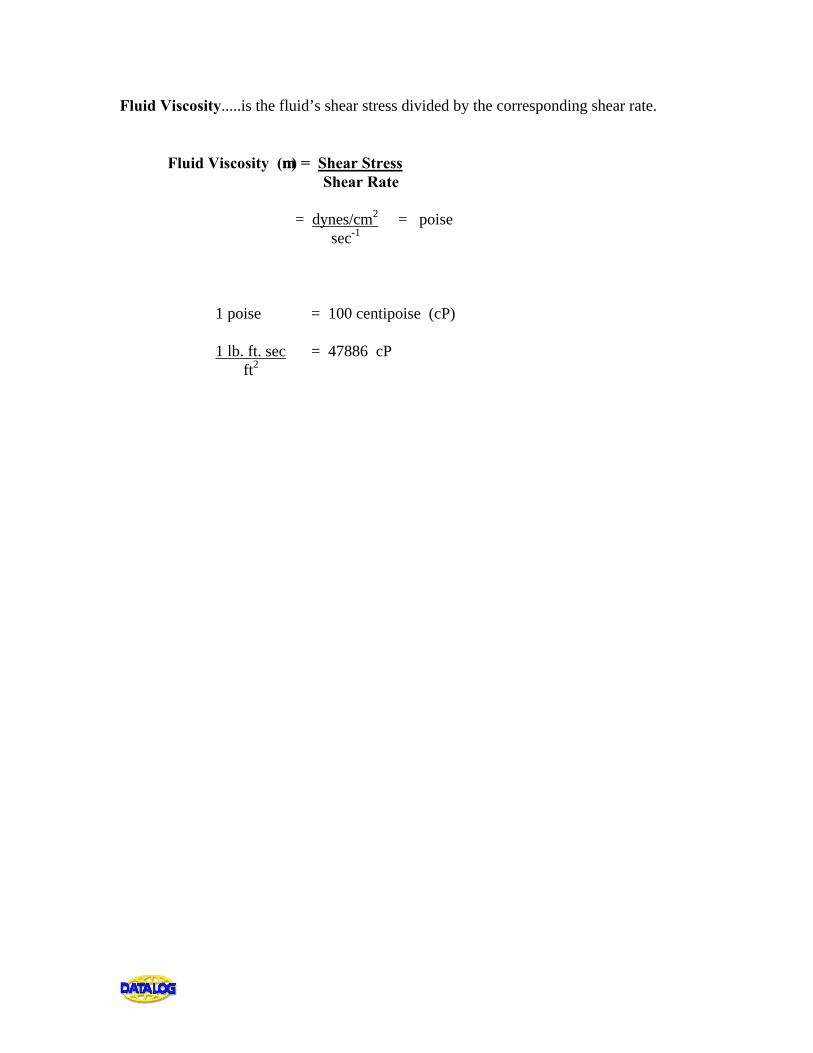
Fluid Viscosity.....is the fluid’s shear stress divided by the corresponding shear rate. Fluid Viscosity (µµ) = Shear Stress Shear Rate = dynes/cm2 = poise sec-1

1 poise = 100 centipoise (cP) 1 lb. ft. sec = 47886 cP ft2

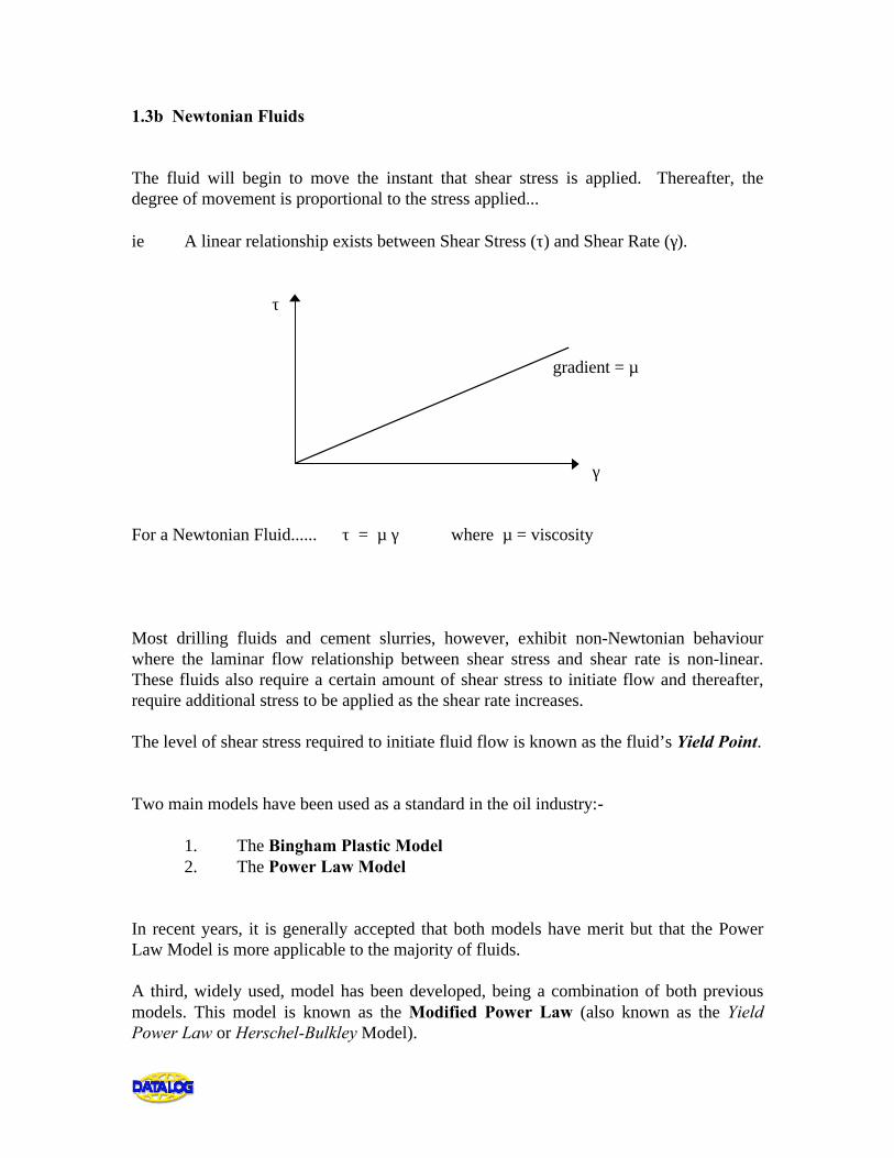
1.3b Newtonian Fluids The fluid will begin to move the instant that shear stress is applied. Thereafter, the degree of movement is proportional to the stress applied... ie A linear relationship exists between Shear Stress (τ) and Shear Rate (γ). τ gradient = µ γ For a Newtonian Fluid...... τ = µ γ where µ = viscosity Most drilling fluids and cement slurries, however, exhibit non-Newtonian behaviour where the laminar flow relationship between shear stress and shear rate is non-linear. These fluids also require a certain amount of shear stress to initiate flow and thereafter, require additional stress to be applied as the shear rate increases. The level of shear stress required to initiate fluid flow is known as the fluid’s Yield Point. Two main models have been used as a standard in the oil industry:- 1. The Bingham Plastic Model 2. The Power Law Model In recent years, it is generally accepted that both models have merit but that the Power Law Model is more applicable to the majority of fluids. A third, widely used, model has been developed, being a combination of both previous models. This model is known as the Modified Power Law (also known as the Yield Power Law or Herschel-Bulkley Model).

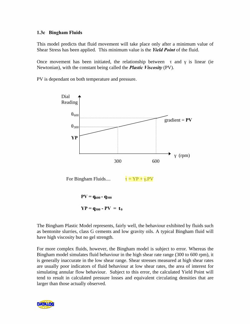
1.3c Bingham Fluids This model predicts that fluid movement will take place only after a minimum value of Shear Stress has been applied. This minimum value is the Yield Point of the fluid. Once movement has been initiated, the relationship between τ and γ is linear (ie Newtonian), with the constant being called the Plastic Viscosity (PV). PV is dependant on both temperature and pressure. Dial Reading θ600 gradient = PV θ300 YP γ (rpm) 300 600 For Bingham Fluids.... τ = YP + γ.PV PV = θθ600 - θθ300

YP = θθ300 - PV = ττ0 The Bingham Plastic Model represents, fairly well, the behaviour exhibited by fluids such as bentonite slurries, class G cements and low gravity oils. A typical Bingham fluid will have high viscosity but no gel strength. For more complex fluids, however, the Bingham model is subject to error. Whereas the Bingham model simulates fluid behaviour in the high shear rate range (300 to 600 rpm), it is generally inaccurate in the low shear range. Shear stresses measured at high shear rates are usually poor indicators of fluid behaviour at low shear rates, the area of interest for simulating annular flow behaviour. Subject to this error, the calculated Yield Point will tend to result in calculated pressure losses and equivalent circulating densities that are larger than those actually observed.

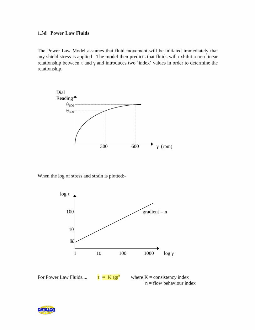
1.3d Power Law Fluids The Power Law Model assumes that fluid movement will be initiated immediately that any shield stress is applied. The model then predicts that fluids will exhibit a non linear relationship between τ and γ and introduces two ‘index’ values in order to determine the relationship. Dial Reading θ600 θ300 300 600 γ (rpm) When the log of stress and strain is plotted:- log τ 100 gradient = n 10 K 1 10 100 1000 log γ For Power Law Fluids.... ττ = K (γγ)n where K = consistency index n = flow behaviour index

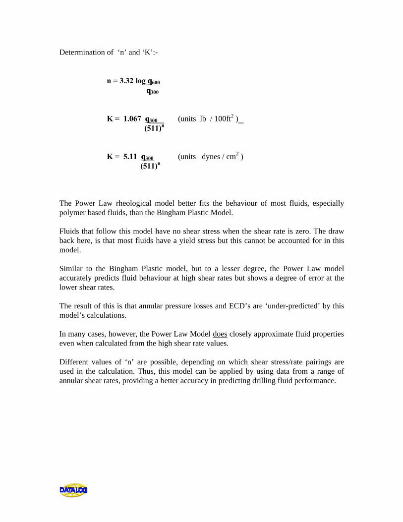
Determination of ‘n’ and ‘K’:- n = 3.32 log θθ600 θθ300 K = 1.067 θθ300 (units lb / 100ft2 ) (511)n

K = 5.11 θθ300 (units dynes / cm2 ) (511)n

The Power Law rheological model better fits the behaviour of most fluids, especially polymer based fluids, than the Bingham Plastic Model. Fluids that follow this model have no shear stress when the shear rate is zero. The draw back here, is that most fluids have a yield stress but this cannot be accounted for in this model. Similar to the Bingham Plastic model, but to a lesser degree, the Power Law model accurately predicts fluid behaviour at high shear rates but shows a degree of error at the lower shear rates. The result of this is that annular pressure losses and ECD’s are ‘under-predicted’ by this model’s calculations. In many cases, however, the Power Law Model does closely approximate fluid properties even when calculated from the high shear rate values. Different values of ‘n’ are possible, depending on which shear stress/rate pairings are used in the calculation. Thus, this model can be applied by using data from a range of annular shear rates, providing a better accuracy in predicting drilling fluid performance.

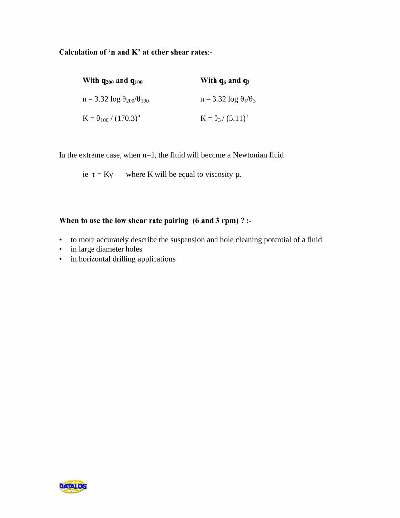
Calculation of ‘n and K’ at other shear rates:- With θθ200 and θθ100 With θθ6 and θθ3 n = 3.32 log θ200/θ100 n = 3.32 log θ6/θ3 K = θ100 / (170.3)n K = θ3 / (5.11)n In the extreme case, when n=1, the fluid will become a Newtonian fluid ie τ = Kγ where K will be equal to viscosity µ. When to use the low shear rate pairing (6 and 3 rpm) ? :- • to more accurately describe the suspension and hole cleaning potential of a fluid • in large diameter holes • in horizontal drilling applications

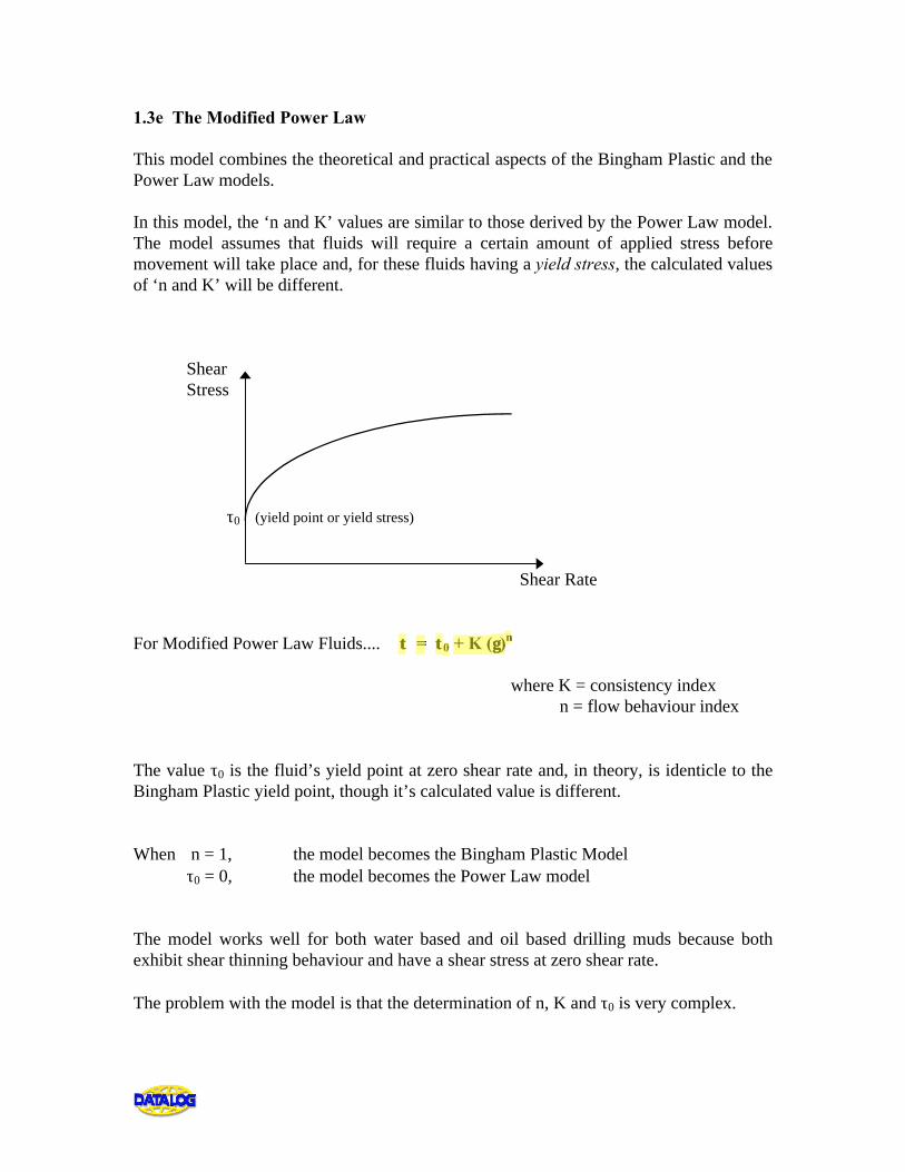
1.3e The Modified Power Law This model combines the theoretical and practical aspects of the Bingham Plastic and the Power Law models. In this model, the ‘n and K’ values are similar to those derived by the Power Law model. The model assumes that fluids will require a certain amount of applied stress before movement will take place and, for these fluids having a yield stress, the calculated values of ‘n and K’ will be different. Shear Stress τ0 (yield point or yield stress)

Shear Rate For Modified Power Law Fluids.... ττ = ττ0 + K (γγ)n where K = consistency index n = flow behaviour index The value τ0 is the fluid’s yield point at zero shear rate and, in theory, is identicle to the Bingham Plastic yield point, though it’s calculated value is different. When n = 1, the model becomes the Bingham Plastic Model τ0 = 0, the model becomes the Power Law model The model works well for both water based and oil based drilling muds because both exhibit shear thinning behaviour and have a shear stress at zero shear rate. The problem with the model is that the determination of n, K and τ0 is very complex.

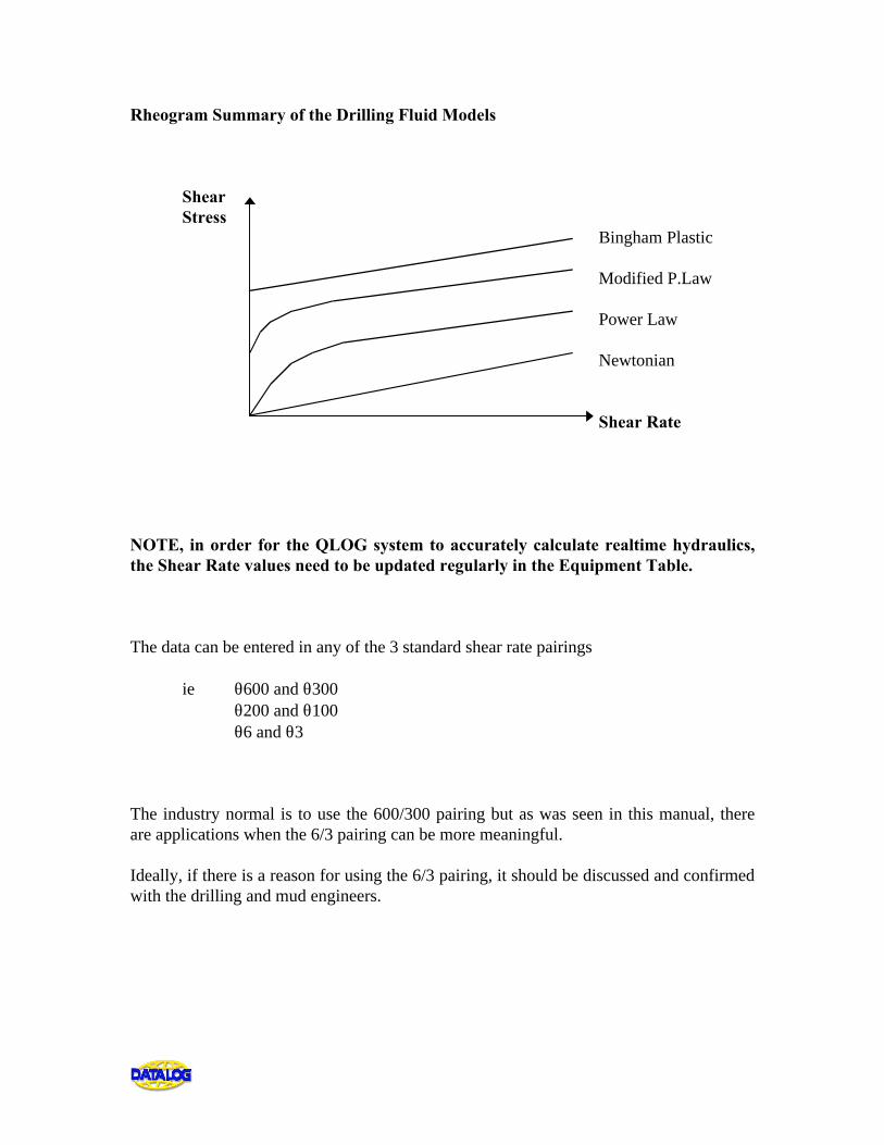
Rheogram Summary of the Drilling Fluid Models Shear Stress Bingham Plastic Modified P.Law Power Law Newtonian Shear Rate NOTE, in order for the QLOG system to accurately calculate realtime hydraulics, the Shear Rate values need to be updated regularly in the Equipment Table. The data can be entered in any of the 3 standard shear rate pairings ie θ600 and θ300 θ200 and θ100 θ6 and θ3 The industry normal is to use the 600/300 pairing but as was seen in this manual, there are applications when the 6/3 pairing can be more meaningful. Ideally, if there is a reason for using the 6/3 pairing, it should be discussed and confirmed with the drilling and mud engineers.

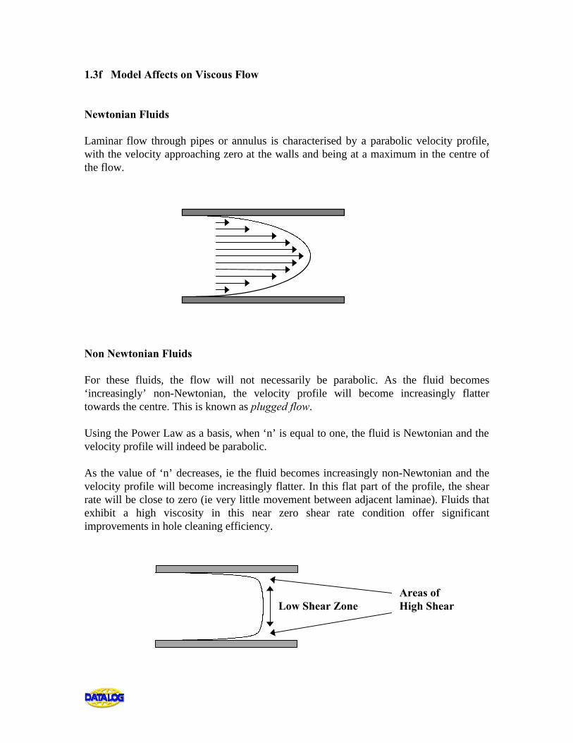
1.3f Model Affects on Viscous Flow Newtonian Fluids Laminar flow through pipes or annulus is characterised by a parabolic velocity profile, with the velocity approaching zero at the walls and being at a maximum in the centre of the flow. Non Newtonian Fluids For these fluids, the flow will not necessarily be parabolic. As the fluid becomes ‘increasingly’ non-Newtonian, the velocity profile will become increasingly flatter towards the centre. This is known as plugged flow. Using the Power Law as a basis, when ‘n’ is equal to one, the fluid is Newtonian and the velocity profile will indeed be parabolic. As the value of ‘n’ decreases, ie the fluid becomes increasingly non-Newtonian and the velocity profile will become increasingly flatter. In this flat part of the profile, the shear rate will be close to zero (ie very little movement between adjacent laminae). Fluids that exhibit a high viscosity in this near zero shear rate condition offer significant improvements in hole cleaning efficiency. Areas of Low Shear Zone High Shear

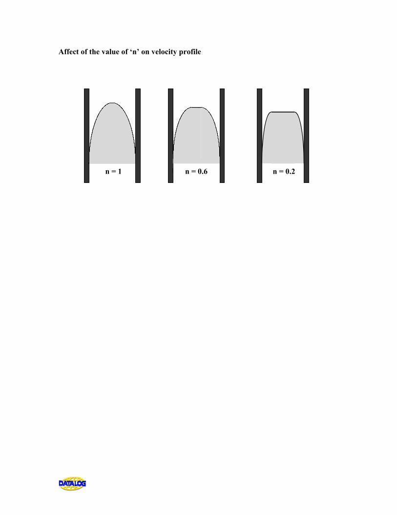
Affect of the value of ‘n’ on velocity profile n = 1 n = 0.6 n = 0.2

1.4 MUD RHEOLOGY - principle parameters Viscosity Controls the magnitude of shear stress which develops as one layer of fluid slides over another. It is a measure of the friction between fluid layers, providing a scale for describing fluid thickness. It will decrease with temperature. In simple terms, it describes the thickness of the mud when it is in motion. Normal unit of measurement is the centipoise (CP), where 47886 CP = 1 lb.f.s ft2 Plastic Viscosity For a Bingham Fluid, PV is the amount of shear stress, in excess of the yield stress, that will induce a unit rate of shear. More simply, it is the relationship between shear stress and shear rate during fluid movement; it is the slope of the straight line that passes through θ600 and θ300. Funnel Viscosity This is a direct measurement from the Funnel (as opposed to Fann) viscometer and is measured in secs/qt. Generally used at wellsite for immediate measurements, this is simply the length of time it takes for one quart of fluid to pass through the funnel. It is not regarded as being applicable to the analysis of circulating performance. Apparent Viscosity - simply θ600/2

Yield Point The yield point, or yield stress, of a fluid is a measure of the attractive forces between mud particles resulting from the presence of +ve and -ve charges on the particle surfaces. It is a measure of the forces that cause mud to gel once it is motionless and affects the carrying capacity of the mud. In other words, it is the strength of the fluid capable of supporting a certain particle weight or size. Normal unit of measurement is the Imperial lb metric: dynes / cm2 100ft2

Gel Strength The ability of the mud to develop and retain a gel structure. It is analogous to shear strength and defines the ability of the mud to hold solids in suspension. More simply, it describes the thickness of a mud that has been motionless for a period of time (unlike viscosity which describes the mud thickness when in motion). It is a measure of the thickening property of a fluid and is a function of time. Measurements are therefore conducted after periods of 10 seconds and 10 minutes. Normal units of measurement lb 100ft2

With the duration of a drilling operation, ie the ‘age’ of a drilling fluid, viscosity and gel strengths will both tend to increase as a result of the introduction of solids into the mud system. Filtrate / Filter Cake Fluid invasion of newly drilled rocks will occur if there is a pressure differential. The fluid that is lost to the formation in this way is called filtrate. To try to minimise this, a layer of fine solids is allowed to build up on the rock surface. This will be allowed to build up to a desired thickness in order to prevent invasion. This layer is termed the filter cake

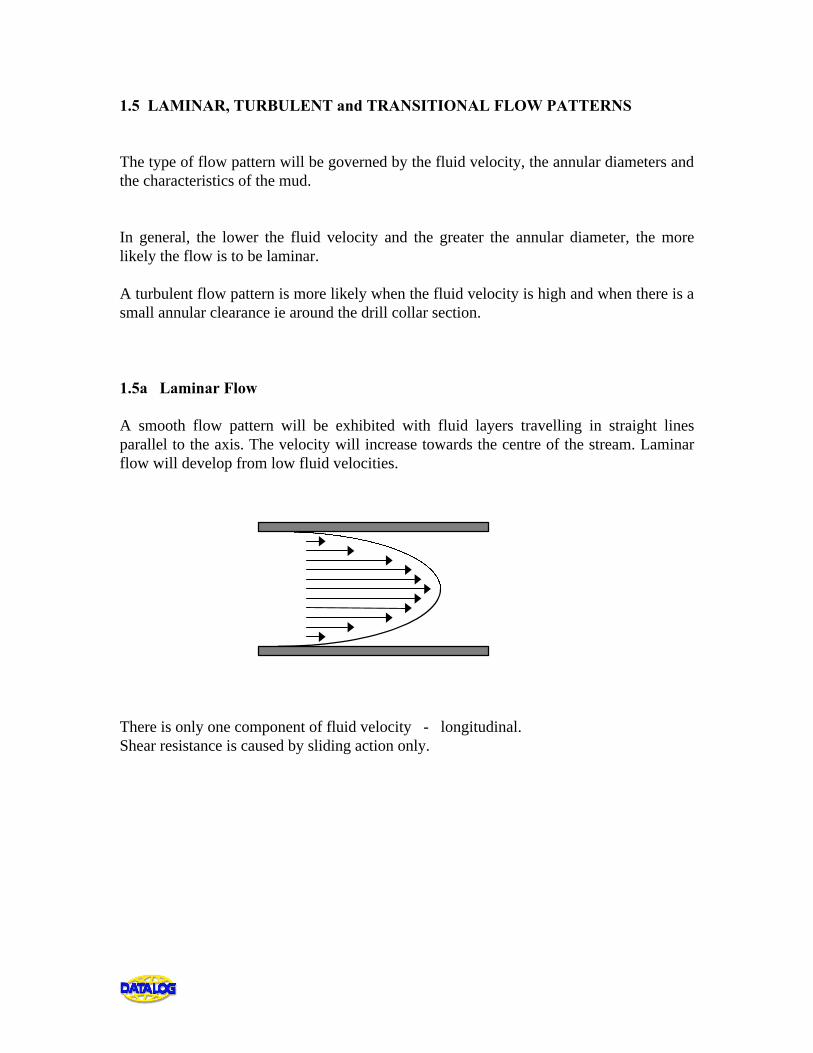
1.5 LAMINAR, TURBULENT and TRANSITIONAL FLOW PATTERNS The type of flow pattern will be governed by the fluid velocity, the annular diameters and the characteristics of the mud. In general, the lower the fluid velocity and the greater the annular diameter, the more likely the flow is to be laminar. A turbulent flow pattern is more likely when the fluid velocity is high and when there is a small annular clearance ie around the drill collar section. 1.5a Laminar Flow A smooth flow pattern will be exhibited with fluid layers travelling in straight lines parallel to the axis. The velocity will increase towards the centre of the stream. Laminar flow will develop from low fluid velocities. There is only one component of fluid velocity - longitudinal. Shear resistance is caused by sliding action only.

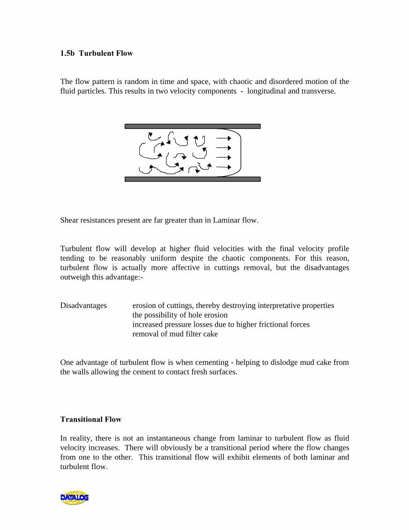
1.5b Turbulent Flow The flow pattern is random in time and space, with chaotic and disordered motion of the fluid particles. This results in two velocity components - longitudinal and transverse. Shear resistances present are far greater than in Laminar flow. Turbulent flow will develop at higher fluid velocities with the final velocity profile tending to be reasonably uniform despite the chaotic components. For this reason, turbulent flow is actually more affective in cuttings removal, but the disadvantages outweigh this advantage:- Disadvantages erosion of cuttings, thereby destroying interpretative properties the possibility of hole erosion increased pressure losses due to higher frictional forces removal of mud filter cake One advantage of turbulent flow is when cementing - helping to dislodge mud cake from the walls allowing the cement to contact fresh surfaces. Transitional Flow In reality, there is not an instantaneous change from laminar to turbulent flow as fluid velocity increases. There will obviously be a transitional period where the flow changes from one to the other. This transitional flow will exhibit elements of both laminar and turbulent flow.

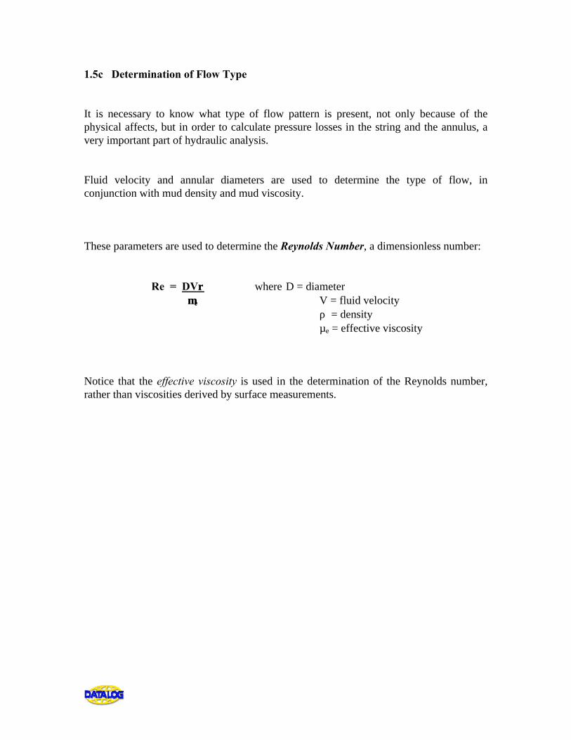
1.5c Determination of Flow Type It is necessary to know what type of flow pattern is present, not only because of the physical affects, but in order to calculate pressure losses in the string and the annulus, a very important part of hydraulic analysis. Fluid velocity and annular diameters are used to determine the type of flow, in conjunction with mud density and mud viscosity. These parameters are used to determine the Reynolds Number, a dimensionless number: Re = DVρρ where D = diameter µµe V = fluid velocity ρ = density µe = effective viscosity Notice that the effective viscosity is used in the determination of the Reynolds number, rather than viscosities derived by surface measurements.

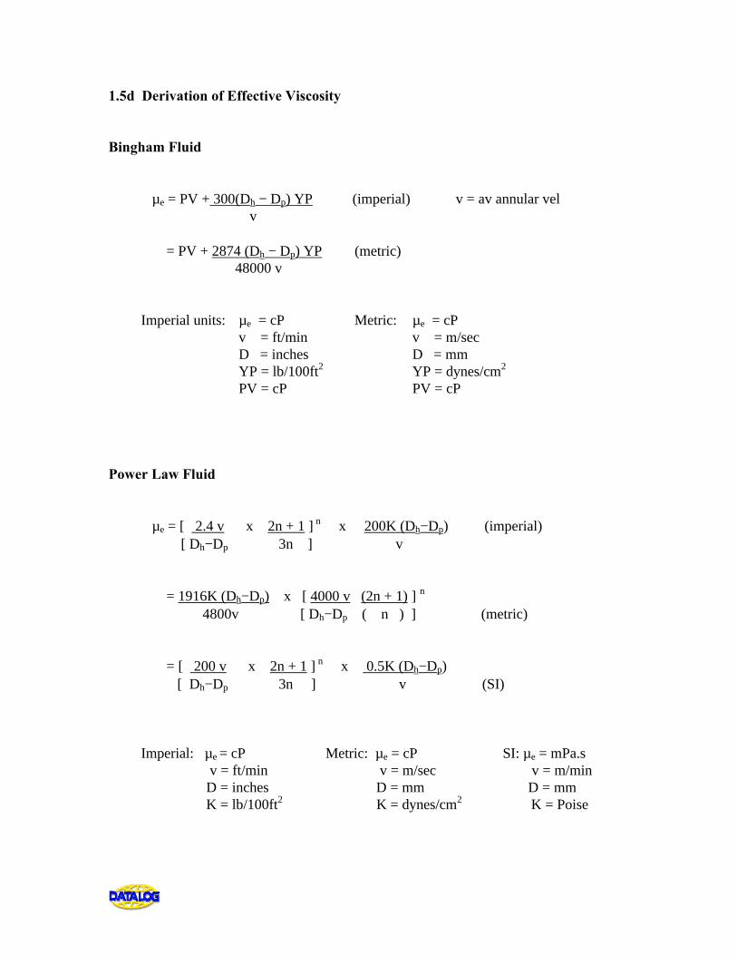
1.5d Derivation of Effective Viscosity Bingham Fluid µe = PV + 300(Dh − Dp) YP (imperial) v = av annular vel v = PV + 2874 (Dh − Dp) YP (metric) 48000 v Imperial units: µe = cP Metric: µe = cP v = ft/min v = m/sec D = inches D = mm YP = lb/100ft2 YP = dynes/cm2 PV = cP PV = cP Power Law Fluid µe = [ 2.4 v x 2n + 1 ] n x 200K (Dh−Dp) (imperial) [ Dh−Dp 3n ] v = 1916K (Dh−Dp) x [ 4000 v (2n + 1) ] n 4800v [ Dh−Dp ( n ) ] (metric) = [ 200 v x 2n + 1 ] n x 0.5K (Dh−Dp) [ Dh−Dp 3n ] v (SI) Imperial: µe = cP Metric: µe = cP SI: µe = mPa.s v = ft/min v = m/sec v = m/min D = inches D = mm D = mm K = lb/100ft2 K = dynes/cm2 K = Poise

1.5e Determination of the Reynolds Number Imperial Re = 15.47 Dvρ D = diameter = inches µe v = average velocity = ft/min ρ = mud density = ppg µe = effective visc = cP Metric Re = 1000 DVρ D = mm µe v = m/sec ρ = kg/litre µe = cP SI Re = DVρ D = mm 60µe v = m/min ρ = kg/m3

µe = mPa.s For Reynolds number inside the pipe, D = pipe internal diameter For Reynolds number in the annulus, D = hole diameter - pipe outside diameter Note that for fluid velocity, an average velocity is used in the determination of the Reynolds Number and Effective Viscosity. In reality, as we have seen, the velocity is least at the walls of the conduit, increasing to a maximum at the centre of the channel. The average fluid velocity (annular velocity or pipe velocity) is determined using the following formulae:

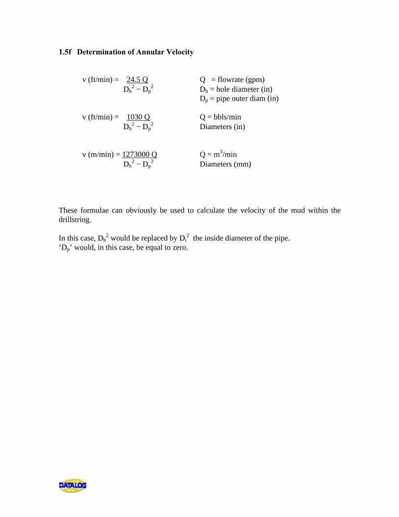
1.5f Determination of Annular Velocity v (ft/min) = 24.5 Q Q = flowrate (gpm) Dh

2 − Dp2 Dh = hole diameter (in)

Dp = pipe outer diam (in) v (ft/min) = 1030 Q Q = bbls/min Dh

2 − Dp2 Diameters (in)

v (m/min) = 1273000 Q Q = m3/min Dh

2 − Dp2 Diameters (mm)

These formulae can obviously be used to calculate the velocity of the mud within the drillstring. In this case, Dh

2 would be replaced by Di2 the inside diameter of the pipe.

‘Dp’ would, in this case, be equal to zero.

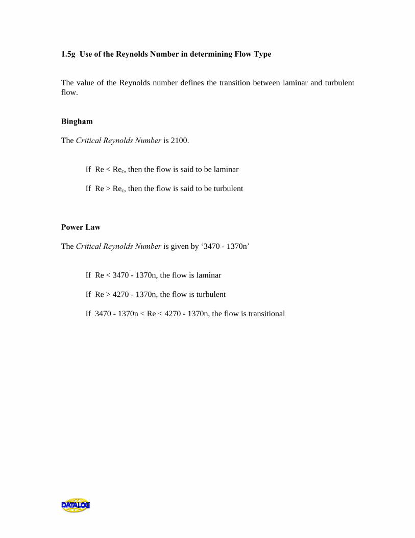
1.5g Use of the Reynolds Number in determining Flow Type The value of the Reynolds number defines the transition between laminar and turbulent flow. Bingham The Critical Reynolds Number is 2100. If Re < Rec, then the flow is said to be laminar If Re > Rec, then the flow is said to be turbulent Power Law The Critical Reynolds Number is given by ‘3470 - 1370n’ If Re < 3470 - 1370n, the flow is laminar If Re > 4270 - 1370n, the flow is turbulent If 3470 - 1370n < Re < 4270 - 1370n, the flow is transitional

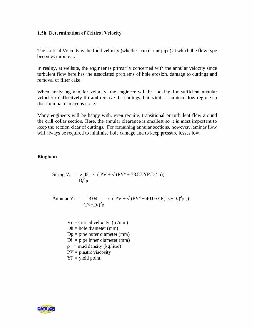
1.5h Determination of Critical Velocity The Critical Velocity is the fluid velocity (whether annular or pipe) at which the flow type becomes turbulent. In reality, at wellsite, the engineer is primarily concerned with the annular velocity since turbulent flow here has the associated problems of hole erosion, damage to cuttings and removal of filter cake. When analysing annular velocity, the engineer will be looking for sufficient annular velocity to affectively lift and remove the cuttings, but within a laminar flow regime so that minimal damage is done. Many engineers will be happy with, even require, transitional or turbulent flow around the drill collar section. Here, the annular clearance is smallest so it is most important to keep the section clear of cuttings. For remaining annular sections, however, laminar flow will always be required to minimise hole damage and to keep pressure losses low. Bingham String Vc = 2.48 x ( PV + √ (PV2 + 73.57.YP.Di

2.ρ)) Di

2 ρ Annular Vc = 3.04 x ( PV + √ (PV2 + 40.05YP(Dh−Dp)

2ρ )) (Dh−Dp)

2ρ Vc = critical velocity (m/min) Dh = hole diameter (mm) Dp = pipe outer diameter (mm) Di = pipe inner diameter (mm) ρ = mud density (kg/litre) PV = plastic viscosity YP = yield point

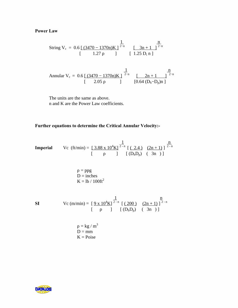
Power Law 1 n String Vc = 0.6 [ (3470 − 1370n)K ] 2−n [ 3n + 1 ] 2−n [ 1.27 ρ ] [ 1.25 Di n ] 1 n Annular Vc = 0.6 [ (3470 − 1370n)K ] 2−n [ 2n + 1 ] 2−n [ 2.05 ρ ] [0.64 (Dh−Dp)n ] The units are the same as above. n and K are the Power Law coefficients. Further equations to determine the Critical Annular Velocity:- 1 n Imperial Vc (ft/min) = [ 3.88 x 104K] 2 - n [ ( 2.4 ) (2n + 1) ] 2 - n

[ ρ ] [ (DhDp) ( 3n ) ] ρ = ppg D = inches K = lb / 100ft2 1 n SI Vc (m/min) = [ 9 x 104K] 2 - n [ ( 200 ) (2n + 1) ] 2 - n [ ρ ] [ (DhDp) ( 3n ) ] ρ = kg / m3 D = mm K = Poise

1.6 DETERMINATION OF SYSTEM PRESSURE LOSSES Regarding the well as a whole as a closed system, pressure losses will occur throughout the system :- through each drillpipe section through the bit through each annular section through surface lines eg standpipe, kelly hose, pumps and lines The total of all theses losses ie Total System Pressure Loss should be equal to the actual pressure measured on the standpipe. This is a very important part of hydraulic evaluation. Obviously, the maximum pressure loss possible will be determined by the rating of the pumps and other surface equipment. This maximum is normally far in excess of the pressure loss that will be desired by the drilling engineer. The logging engineer’s task is normally to take given parameters from the drilling engineer, then select, for example, the correct nozzle sizes that will produce the desired system pressure loss. The amount of pressure loss will be dependant on flowrate, mud density and rheology, the length of each section and the diameters of each section. Whether the flow is laminar or turbulent is also an important influence on the pressure loss - turbulent flow will produce larger pressure losses.

1.6a Fanning Friction Factor The frictional forces involved will have a large affect on the actual pressure losses in a given annular or pipe section. The frictional forces present will be very different depending on whether the flow is laminar or turbulent:- • with laminar flow, the fluid movement is in one direction only - parallel to the conduit

walls, with velocity increasing towards the centre.. Frictional forces will therefore only be present due to fluid ‘layers’ moving longitudinally against each other.

• with turbulent flow, fluid movement is much more complex and multi-directional, so

that many more frictional forces are present. For this reason, a coefficient called the Fanning Friction Factor is determined for each type of flow and whether we are dealing with pipe or annular pressure losses. The friction factor is determined from the Reynolds Number which has already been calculated for pipe or annular sections based on annular velocity, diameters, density and effective viscosity. Laminar Flow fann = 24 / Re Re = Annular Reynolds No. fpipe = 16 / Re Re = Pipe Reynolds No. Turbulent Flow fturb = a / Reb where Re = Reynolds number in the pipe or annulus a = log n + 3.93 50 b = 1.75 - log n 7

Transitional Flow fann = [ Re - c ] x [ ( a ) - (24) ] + 24 [ 800 ] [ (4270 - 1370n)b ( c ) ] c where Re = Annular Reynolds No. a = (log n + 3.93) / 50 b = (1.75 - log n) / 7 c = 3470 - 1370n fpipe = [ Re - c ] x [ ( a ) - (16) ] + 16 [ 800 ] [ (4270 - 1370n)b ( c ) ] c where Re = Pipe Reynolds No. a, b, and c are as above When using the Power Law Model, the values of the Fanning Friction are substituted into equations in order to calculate pressure losses in the annulus or in the pipe. When calculating these pressure losses, each individual section has to be calculated seperately, then totalled to give an overall pipe or annular pressure loss.

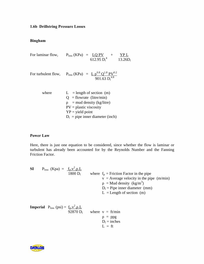
1.6b Drillstring Pressure Losses Bingham For laminar flow, Ploss (KPa) = LQ PV + YP L 612.95 Di

4 13.26Di For turbulent flow, Ploss (KPa) = L ρ0.8 Q1.8 PV0.2 901.63 Di

4.8 where L = length of section (m) Q = flowrate (litre/min) ρ = mud density (kg/litre) PV = plastic viscosity YP = yield point Di = pipe inner diameter (inch) Power Law Here, there is just one equation to be considered, since whether the flow is laminar or turbulent has already been accounted for by the Reynolds Number and the Fanning Friction Factor. SI Ploss (Kpa) = fp.v

2.ρ.L 1800 Di where fp = Friction Factor in the pipe v = Average velocity in the pipe (m/min) ρ = Mud density (kg/m3) Di = Pipe inner diameter (mm) L = Length of section (m) Imperial Ploss (psi) = fp.v

2.ρ.L 92870 Di where v = ft/min ρ = ppg Di = inches L = ft

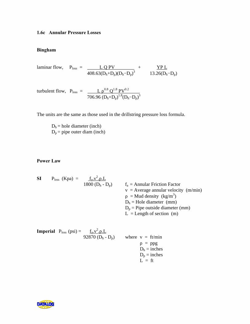
1.6c Annular Pressure Losses Bingham laminar flow, Ploss = L Q PV + YP L 408.63(Dh+Dp)(Dh−Dp)

3 13.26(Dh−Dp) turbulent flow, Ploss = L ρ0.8 Q1.8 PV0.2 706.96 (Dh+Dp)

1.8(Dh−Dp)3

The units are the same as those used in the drillstring pressure loss formula. Dh = hole diameter (inch) Dp = pipe outer diam (inch) Power Law SI Ploss (Kpa) = fa.v

2.ρ.L 1800 (Dh - Dp) fa = Annular Friction Factor v = Average annular velocity (m/min) ρ = Mud density (kg/m3) Dh = Hole diameter (mm) Dp = Pipe outside diameter (mm) L = Length of section (m) Imperial Ploss (psi) = fa.v

2.ρ.L 92870 (Dh - Dp) where v = ft/min ρ = ppg Dh = inches Dp = inches L = ft

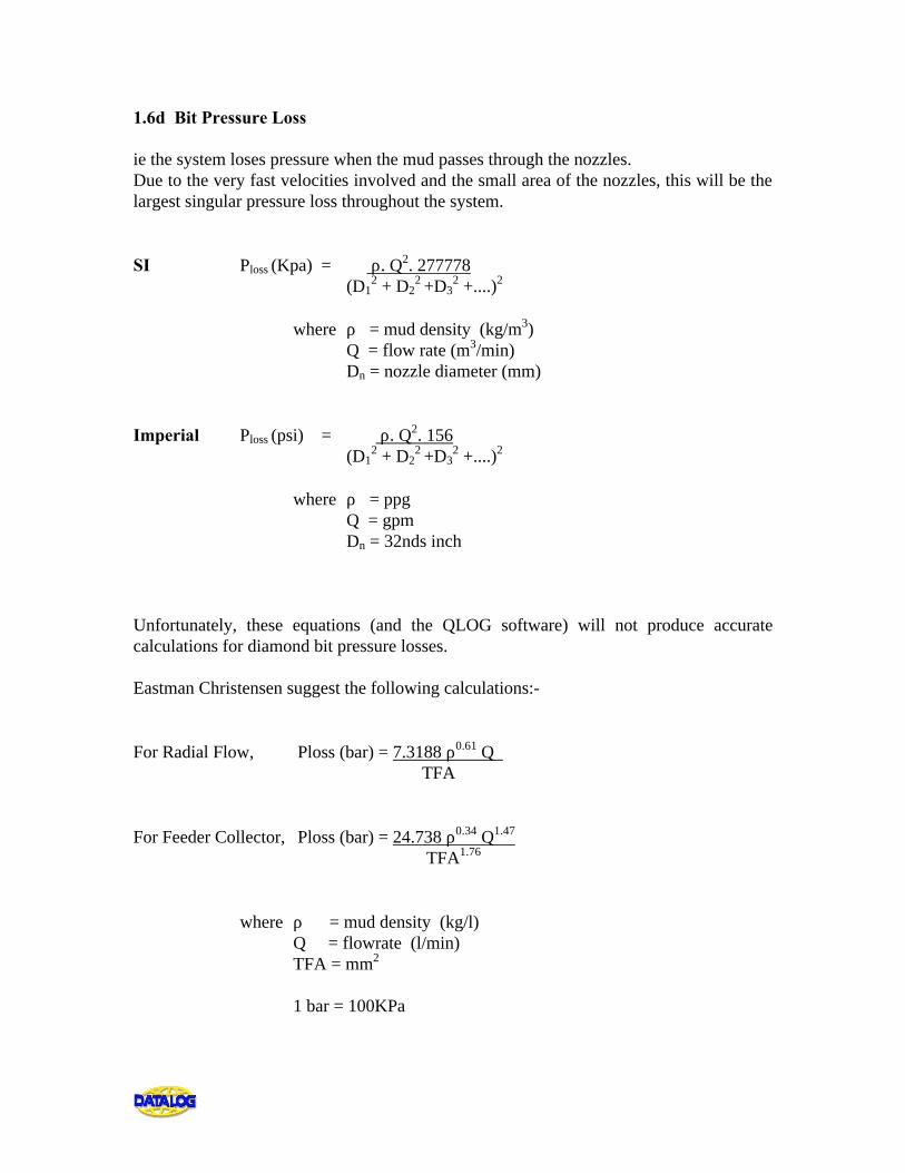
1.6d Bit Pressure Loss ie the system loses pressure when the mud passes through the nozzles. Due to the very fast velocities involved and the small area of the nozzles, this will be the largest singular pressure loss throughout the system. SI Ploss (Kpa) = ρ. Q2. 277778 (D1

2 + D22 +D3

2 +....)2

where ρ = mud density (kg/m3) Q = flow rate (m3/min) Dn = nozzle diameter (mm) Imperial Ploss (psi) = ρ. Q2. 156 (D1

2 + D22 +D3

2 +....)2

where ρ = ppg Q = gpm Dn = 32nds inch Unfortunately, these equations (and the QLOG software) will not produce accurate calculations for diamond bit pressure losses. Eastman Christensen suggest the following calculations:- For Radial Flow, Ploss (bar) = 7.3188 ρ0.61 Q TFA For Feeder Collector, Ploss (bar) = 24.738 ρ0.34 Q1.47

TFA1.76 where ρ = mud density (kg/l) Q = flowrate (l/min) TFA = mm2 1 bar = 100KPa

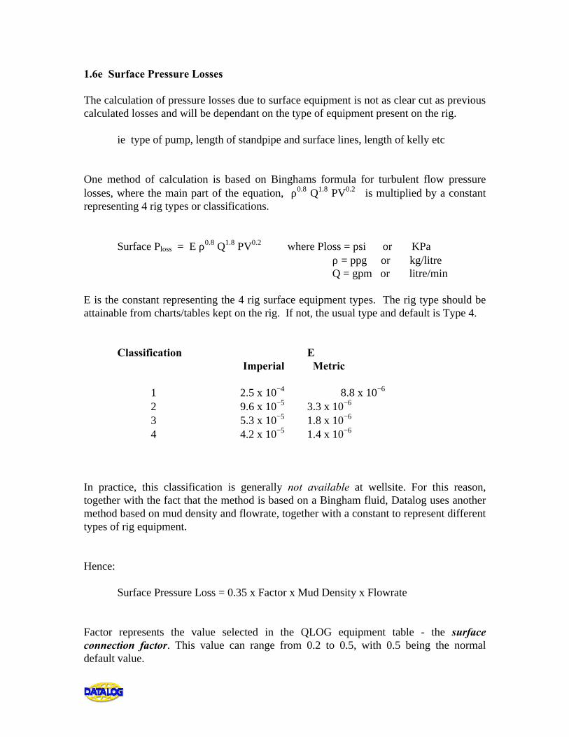
1.6e Surface Pressure Losses The calculation of pressure losses due to surface equipment is not as clear cut as previous calculated losses and will be dependant on the type of equipment present on the rig. ie type of pump, length of standpipe and surface lines, length of kelly etc One method of calculation is based on Binghams formula for turbulent flow pressure losses, where the main part of the equation, ρ0.8 Q1.8 PV0.2 is multiplied by a constant representing 4 rig types or classifications. Surface Ploss = E ρ0.8 Q1.8 PV0.2 where Ploss = psi or KPa ρ = ppg or kg/litre Q = gpm or litre/min E is the constant representing the 4 rig surface equipment types. The rig type should be attainable from charts/tables kept on the rig. If not, the usual type and default is Type 4. Classification E Imperial Metric 1 2.5 x 10−4 8.8 x 10−6 2 9.6 x 10−5 3.3 x 10−6 3 5.3 x 10−5 1.8 x 10−6 4 4.2 x 10−5 1.4 x 10−6 In practice, this classification is generally not available at wellsite. For this reason, together with the fact that the method is based on a Bingham fluid, Datalog uses another method based on mud density and flowrate, together with a constant to represent different types of rig equipment. Hence: Surface Pressure Loss = 0.35 x Factor x Mud Density x Flowrate Factor represents the value selected in the QLOG equipment table - the surface connection factor. This value can range from 0.2 to 0.5, with 0.5 being the normal default value.

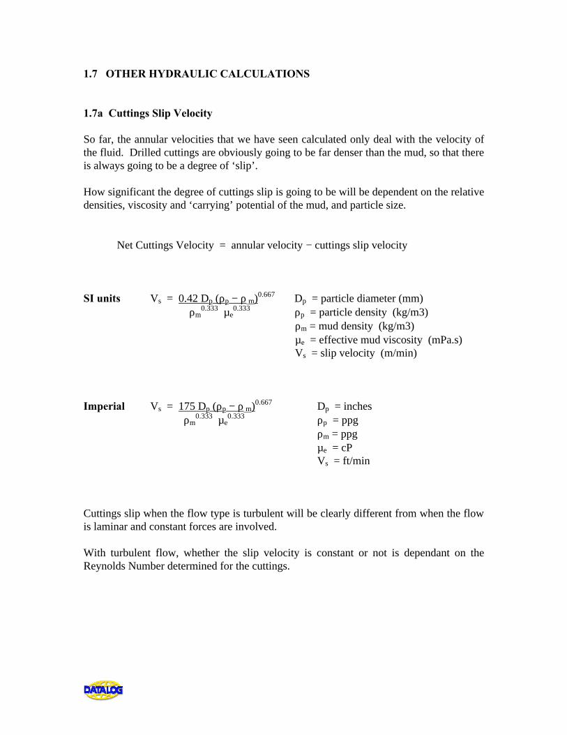
1.7 OTHER HYDRAULIC CALCULATIONS 1.7a Cuttings Slip Velocity So far, the annular velocities that we have seen calculated only deal with the velocity of the fluid. Drilled cuttings are obviously going to be far denser than the mud, so that there is always going to be a degree of ‘slip’. How significant the degree of cuttings slip is going to be will be dependent on the relative densities, viscosity and ‘carrying’ potential of the mud, and particle size. Net Cuttings Velocity = annular velocity − cuttings slip velocity SI units Vs = 0.42 Dp (ρp − ρ m)0.667 Dp = particle diameter (mm) ρm

0.333 µe0.333 ρp = particle density (kg/m3)

ρm = mud density (kg/m3) µe = effective mud viscosity (mPa.s) Vs = slip velocity (m/min) Imperial Vs = 175 Dp (ρp − ρ m)0.667 Dp = inches ρm

0.333 µe0.333 ρp = ppg

ρm = ppg µe = cP Vs = ft/min Cuttings slip when the flow type is turbulent will be clearly different from when the flow is laminar and constant forces are involved. With turbulent flow, whether the slip velocity is constant or not is dependant on the Reynolds Number determined for the cuttings.

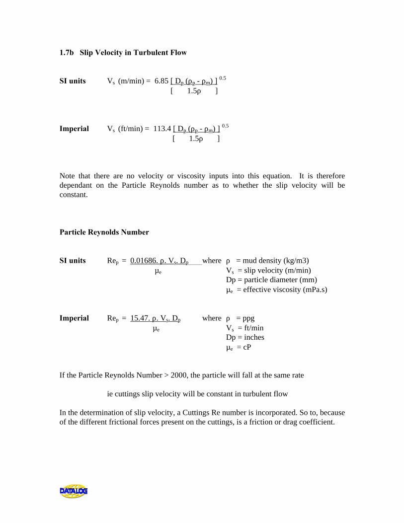
1.7b Slip Velocity in Turbulent Flow SI units Vs (m/min) = 6.85 [ Dp (ρp - ρm) ] 0.5

[ 1.5ρ ] Imperial Vs (ft/min) = 113.4 [ Dp (ρp - ρm) ] 0.5

[ 1.5ρ ] Note that there are no velocity or viscosity inputs into this equation. It is therefore dependant on the Particle Reynolds number as to whether the slip velocity will be constant. Particle Reynolds Number SI units Rep = 0.01686. ρ. Vs. Dp where ρ = mud density (kg/m3) µe Vs = slip velocity (m/min) Dp = particle diameter (mm) µe = effective viscosity (mPa.s) Imperial Rep = 15.47. ρ. Vs. Dp where ρ = ppg µe Vs = ft/min Dp = inches µe = cP If the Particle Reynolds Number > 2000, the particle will fall at the same rate ie cuttings slip velocity will be constant in turbulent flow In the determination of slip velocity, a Cuttings Re number is incorporated. So to, because of the different frictional forces present on the cuttings, is a friction or drag coefficient.

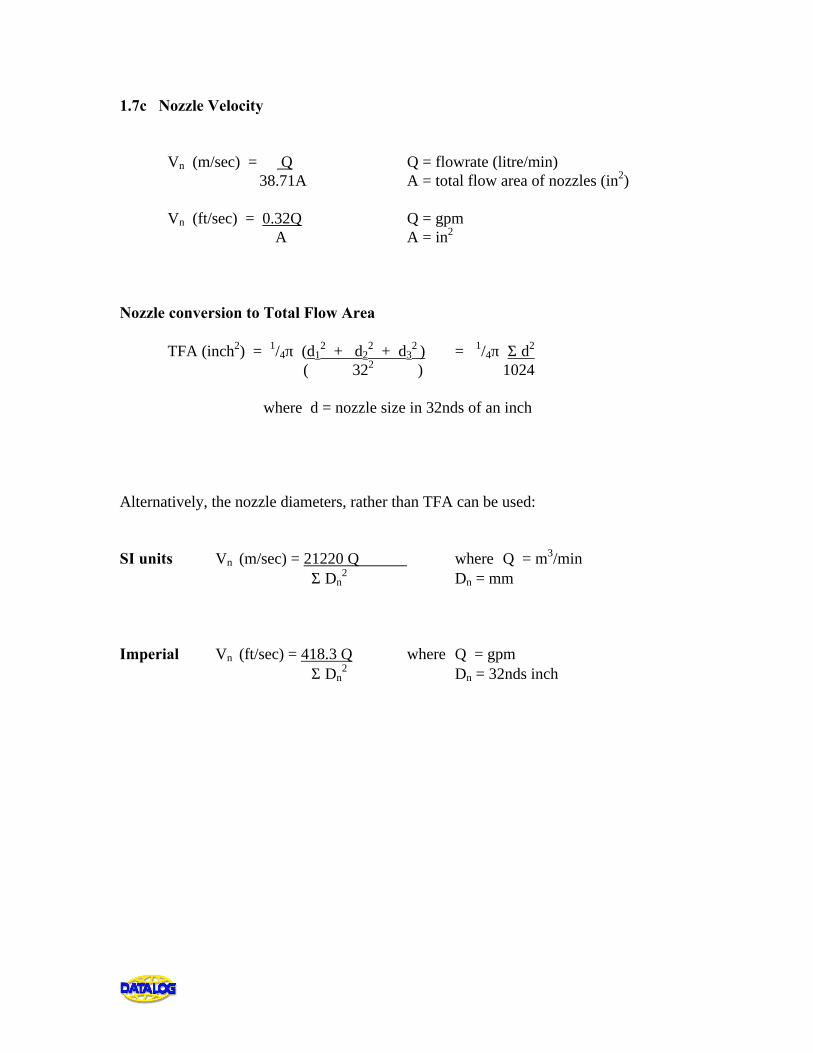
1.7c Nozzle Velocity Vn (m/sec) = Q Q = flowrate (litre/min) 38.71A A = total flow area of nozzles (in2) Vn (ft/sec) = 0.32Q Q = gpm A A = in2 Nozzle conversion to Total Flow Area TFA (inch2) = 1/4π (d1

2 + d22 + d3

2 ) = 1/4π Σ d2 ( 322 ) 1024 where d = nozzle size in 32nds of an inch Alternatively, the nozzle diameters, rather than TFA can be used: SI units Vn (m/sec) = 21220 Q where Q = m3/min Σ Dn

2 Dn = mm Imperial Vn (ft/sec) = 418.3 Q where Q = gpm Σ Dn

2 Dn = 32nds inch

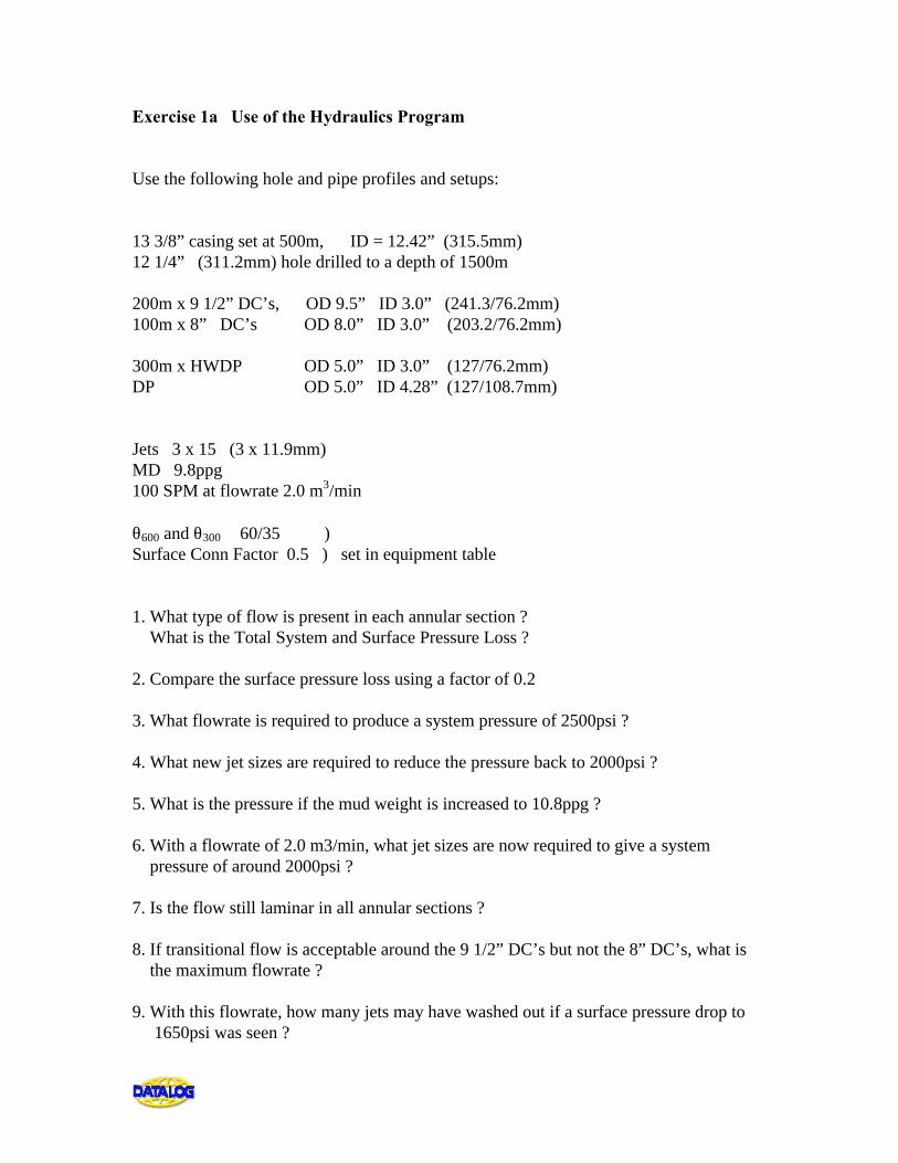
Exercise 1a Use of the Hydraulics Program Use the following hole and pipe profiles and setups: 13 3/8” casing set at 500m, ID = 12.42” (315.5mm) 12 1/4” (311.2mm) hole drilled to a depth of 1500m 200m x 9 1/2” DC’s, OD 9.5” ID 3.0” (241.3/76.2mm) 100m x 8” DC’s OD 8.0” ID 3.0” (203.2/76.2mm) 300m x HWDP OD 5.0” ID 3.0” (127/76.2mm) DP OD 5.0” ID 4.28” (127/108.7mm) Jets 3 x 15 (3 x 11.9mm) MD 9.8ppg 100 SPM at flowrate 2.0 m3/min θ600 and θ300 60/35 ) Surface Conn Factor 0.5 ) set in equipment table 1. What type of flow is present in each annular section ? What is the Total System and Surface Pressure Loss ? 2. Compare the surface pressure loss using a factor of 0.2 3. What flowrate is required to produce a system pressure of 2500psi ? 4. What new jet sizes are required to reduce the pressure back to 2000psi ? 5. What is the pressure if the mud weight is increased to 10.8ppg ? 6. With a flowrate of 2.0 m3/min, what jet sizes are now required to give a system pressure of around 2000psi ? 7. Is the flow still laminar in all annular sections ? 8. If transitional flow is acceptable around the 9 1/2” DC’s but not the 8” DC’s, what is the maximum flowrate ? 9. With this flowrate, how many jets may have washed out if a surface pressure drop to 1650psi was seen ?

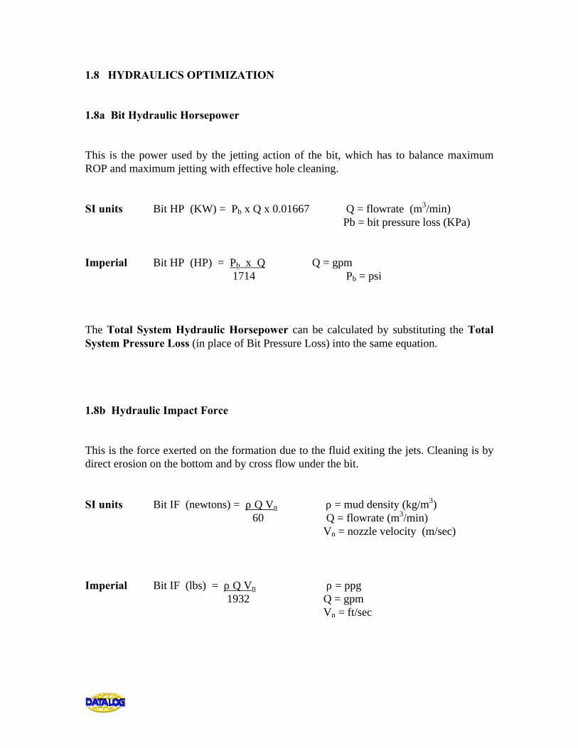
1.8 HYDRAULICS OPTIMIZATION 1.8a Bit Hydraulic Horsepower This is the power used by the jetting action of the bit, which has to balance maximum ROP and maximum jetting with effective hole cleaning. SI units Bit HP (KW) = Pb x Q x 0.01667 Q = flowrate (m3/min) Pb = bit pressure loss (KPa) Imperial Bit HP (HP) = Pb x Q Q = gpm 1714 Pb = psi The Total System Hydraulic Horsepower can be calculated by substituting the Total System Pressure Loss (in place of Bit Pressure Loss) into the same equation. 1.8b Hydraulic Impact Force This is the force exerted on the formation due to the fluid exiting the jets. Cleaning is by direct erosion on the bottom and by cross flow under the bit. SI units Bit IF (newtons) = ρ Q Vn ρ = mud density (kg/m3) 60 Q = flowrate (m3/min) Vn = nozzle velocity (m/sec) Imperial Bit IF (lbs) = ρ Q Vn ρ = ppg 1932 Q = gpm Vn = ft/sec

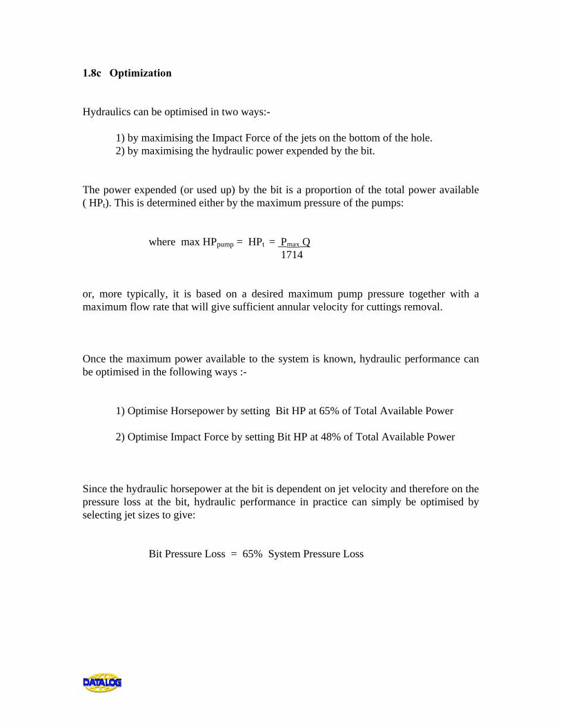
1.8c Optimization Hydraulics can be optimised in two ways:- 1) by maximising the Impact Force of the jets on the bottom of the hole. 2) by maximising the hydraulic power expended by the bit. The power expended (or used up) by the bit is a proportion of the total power available ( HPt). This is determined either by the maximum pressure of the pumps: where max HPpump = HPt = Pmax Q 1714 or, more typically, it is based on a desired maximum pump pressure together with a maximum flow rate that will give sufficient annular velocity for cuttings removal. Once the maximum power available to the system is known, hydraulic performance can be optimised in the following ways :- 1) Optimise Horsepower by setting Bit HP at 65% of Total Available Power 2) Optimise Impact Force by setting Bit HP at 48% of Total Available Power Since the hydraulic horsepower at the bit is dependent on jet velocity and therefore on the pressure loss at the bit, hydraulic performance in practice can simply be optimised by selecting jet sizes to give: Bit Pressure Loss = 65% System Pressure Loss

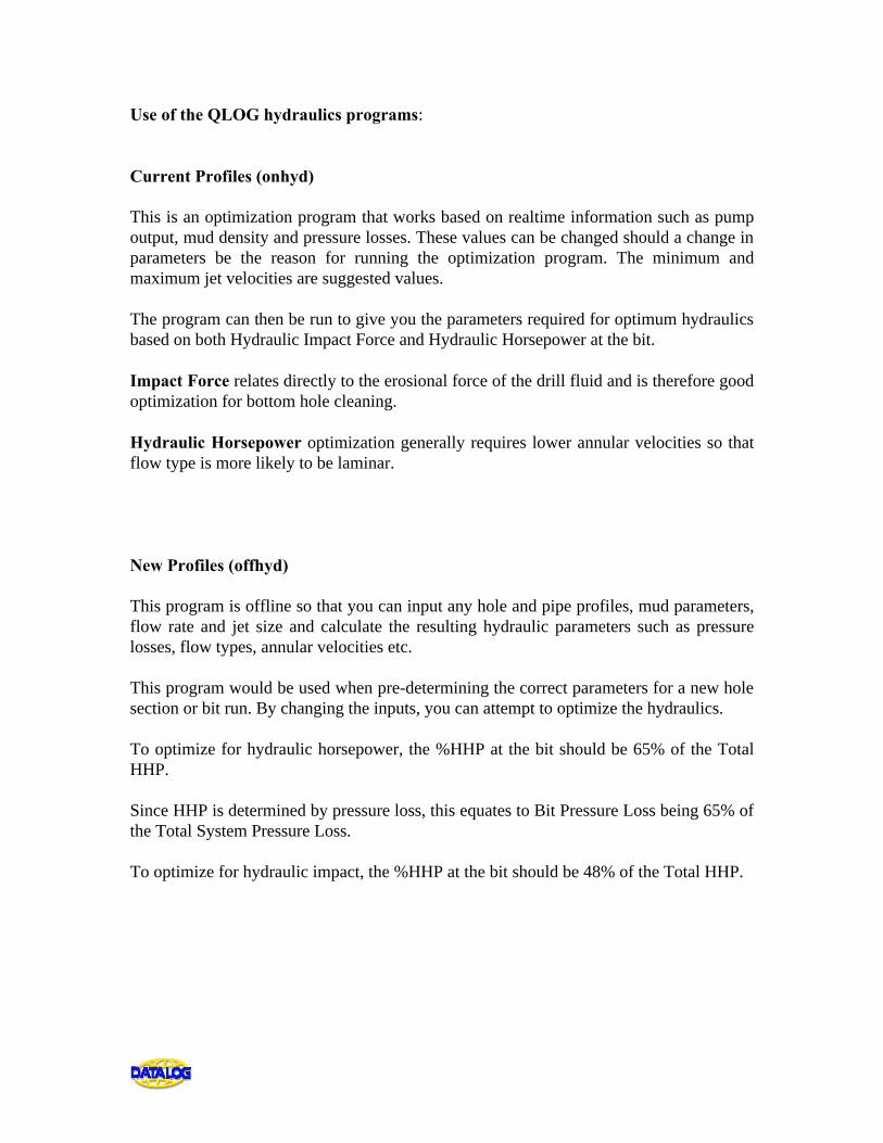
Use of the QLOG hydraulics programs: Current Profiles (onhyd) This is an optimization program that works based on realtime information such as pump output, mud density and pressure losses. These values can be changed should a change in parameters be the reason for running the optimization program. The minimum and maximum jet velocities are suggested values. The program can then be run to give you the parameters required for optimum hydraulics based on both Hydraulic Impact Force and Hydraulic Horsepower at the bit. Impact Force relates directly to the erosional force of the drill fluid and is therefore good optimization for bottom hole cleaning. Hydraulic Horsepower optimization generally requires lower annular velocities so that flow type is more likely to be laminar. New Profiles (offhyd) This program is offline so that you can input any hole and pipe profiles, mud parameters, flow rate and jet size and calculate the resulting hydraulic parameters such as pressure losses, flow types, annular velocities etc. This program would be used when pre-determining the correct parameters for a new hole section or bit run. By changing the inputs, you can attempt to optimize the hydraulics. To optimize for hydraulic horsepower, the %HHP at the bit should be 65% of the Total HHP. Since HHP is determined by pressure loss, this equates to Bit Pressure Loss being 65% of the Total System Pressure Loss. To optimize for hydraulic impact, the %HHP at the bit should be 48% of the Total HHP.

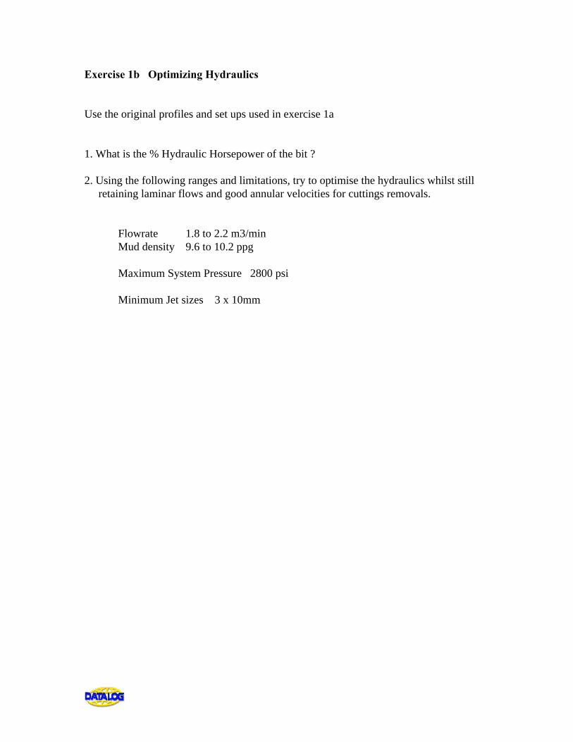
Exercise 1b Optimizing Hydraulics Use the original profiles and set ups used in exercise 1a 1. What is the % Hydraulic Horsepower of the bit ? 2. Using the following ranges and limitations, try to optimise the hydraulics whilst still retaining laminar flows and good annular velocities for cuttings removals. Flowrate 1.8 to 2.2 m3/min Mud density 9.6 to 10.2 ppg Maximum System Pressure 2800 psi Minimum Jet sizes 3 x 10mm

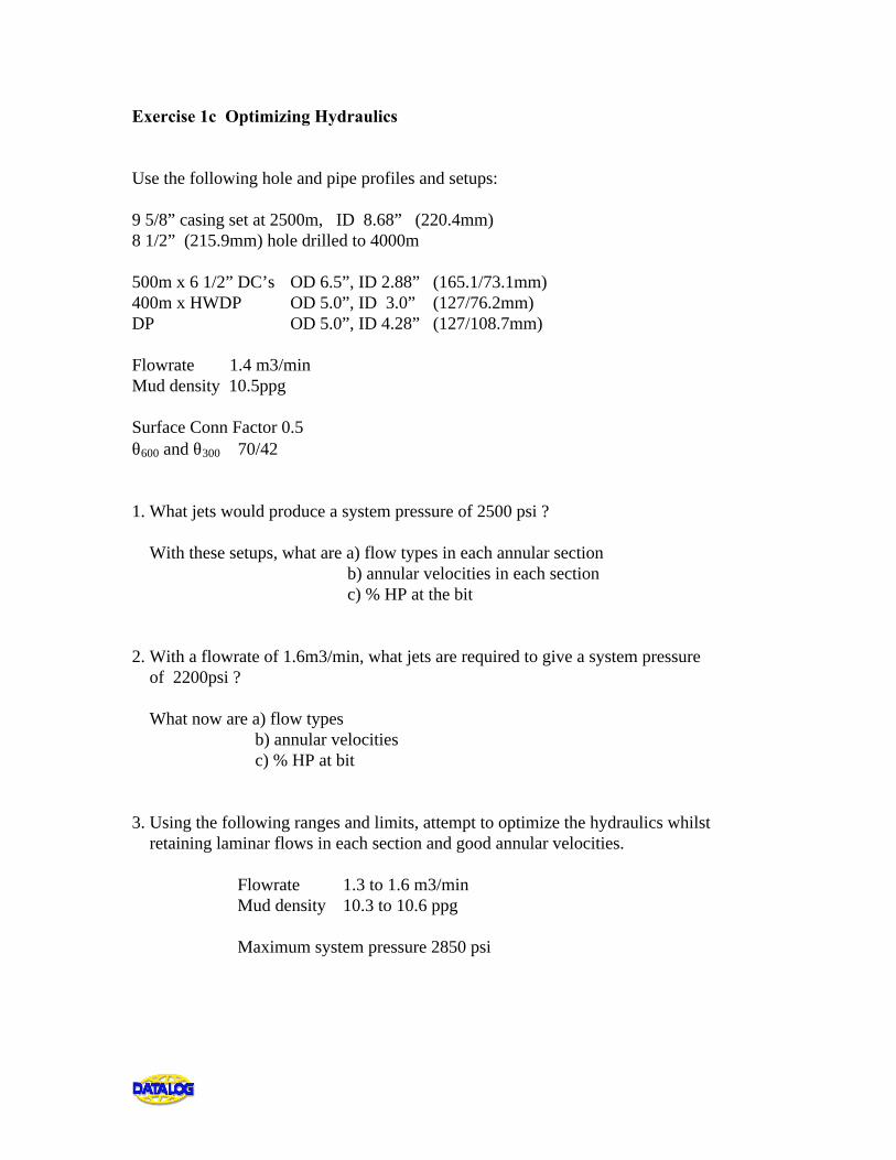
Exercise 1c Optimizing Hydraulics Use the following hole and pipe profiles and setups: 9 5/8” casing set at 2500m, ID 8.68” (220.4mm) 8 1/2” (215.9mm) hole drilled to 4000m 500m x 6 1/2” DC’s OD 6.5”, ID 2.88” (165.1/73.1mm) 400m x HWDP OD 5.0”, ID 3.0” (127/76.2mm) DP OD 5.0”, ID 4.28” (127/108.7mm) Flowrate 1.4 m3/min Mud density 10.5ppg Surface Conn Factor 0.5 θ600 and θ300 70/42 1. What jets would produce a system pressure of 2500 psi ? With these setups, what are a) flow types in each annular section b) annular velocities in each section c) % HP at the bit 2. With a flowrate of 1.6m3/min, what jets are required to give a system pressure of 2200psi ? What now are a) flow types b) annular velocities c) % HP at bit 3. Using the following ranges and limits, attempt to optimize the hydraulics whilst retaining laminar flows in each section and good annular velocities. Flowrate 1.3 to 1.6 m3/min Mud density 10.3 to 10.6 ppg Maximum system pressure 2850 psi

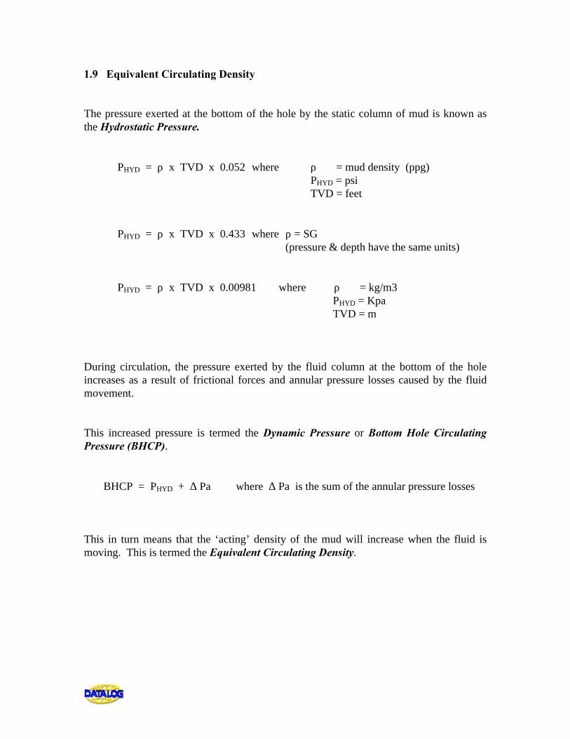
1.9 Equivalent Circulating Density The pressure exerted at the bottom of the hole by the static column of mud is known as the Hydrostatic Pressure. PHYD = ρ x TVD x 0.052 where ρ = mud density (ppg) PHYD = psi TVD = feet PHYD = ρ x TVD x 0.433 where ρ = SG (pressure & depth have the same units) PHYD = ρ x TVD x 0.00981 where ρ = kg/m3 PHYD = Kpa TVD = m During circulation, the pressure exerted by the fluid column at the bottom of the hole increases as a result of frictional forces and annular pressure losses caused by the fluid movement. This increased pressure is termed the Dynamic Pressure or Bottom Hole Circulating Pressure (BHCP). BHCP = PHYD + ∆ Pa where ∆ Pa is the sum of the annular pressure losses This in turn means that the ‘acting’ density of the mud will increase when the fluid is moving. This is termed the Equivalent Circulating Density.

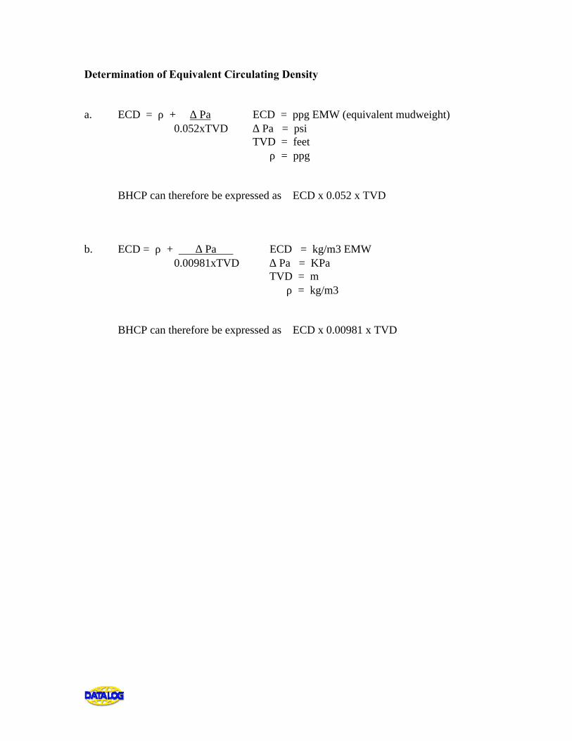
Determination of Equivalent Circulating Density a. ECD = ρ + ∆ Pa ECD = ppg EMW (equivalent mudweight) 0.052xTVD ∆ Pa = psi TVD = feet ρ = ppg BHCP can therefore be expressed as ECD x 0.052 x TVD b. ECD = ρ + ∆ Pa ECD = kg/m3 EMW 0.00981xTVD ∆ Pa = KPa TVD = m ρ = kg/m3 BHCP can therefore be expressed as ECD x 0.00981 x TVD

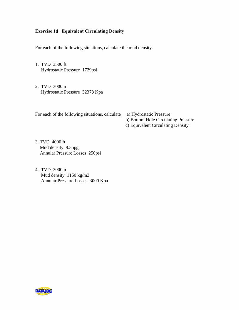
Exercise 1d Equivalent Circulating Density For each of the following situations, calculate the mud density. 1. TVD 3500 ft Hydrostatic Pressure 1729psi 2. TVD 3000m Hydrostatic Pressure 32373 Kpa For each of the following situations, calculate a) Hydrostatic Pressure b) Bottom Hole Circulating Pressure c) Equivalent Circulating Density 3. TVD 4000 ft Mud density 9.5ppg Annular Pressure Losses 250psi 4. TVD 3000m Mud density 1150 kg/m3 Annular Pressure Losses 3000 Kpa

1.10 Surge and Swab Pressures Surge Pressures result from running pipe into the hole creating a pressure increase. The size of the pressure increase will be dependent on the pipe running speed, the annular clearance and whether the pipe is open or closed. Excessive Bottom Hole Pressure could break down weak or unconsolidated formations. Swab Pressures result from pulling the pipe out of the hole. The frictional drag combined with the piston effect will create a reduction in pressure. This reduction in the hydrostatic could lead to the invasion of formation fluids. • More than 25% of blowouts result from reduced hydrostatic pressure caused by

swabbing. • Excessive surge pressures can lead to lost circulation. Running casing is a particularly

vulnerable time due to the small annular clearance and the fact that the casing is closed ended.

• Beside the well safety aspect, invasion of fluids due to swabbing can lead to mud

contamination and necessitate the costly task of replacing the mud. • Pressure changes due to changing pipe direction, eg during connections, can be

particularly damaging to the well by causing sloughing shale, by forming bridges or ledges, and by causing hole fill requiring reaming.

Calculation of Surge and Swab Pressures. The same method is used to calculate the differential pressure caused by both surging and swabbing. To determine the new Hydrostatic Pressure, the differential pressure is either added or subtracted depending on whether surge or swab respectively.

Firstly, the Fluid Velocity of the displaced mud caused by the pipe movement has to be calculated. For Closed Ended Pipe: Fluid Vel (ft/min) = [ 0.45 + Dp

2 ] x Vp Vp = pipe speed (ft/min) [ Dh

2 − Dp2 ] Dh = hole diameter (in)

Dp = pipe outer diameter (in) Di = pipe inner diameter (in) For Open Ended Pipe: Fluid Vel (ft/min) = [ 0.45 + Dp

2 − Di2 ] x Vp

[ Dh2 − Dp

2 + Di2 ]

This fluid velocity then has to be converted to the equivalent flowrate by using the annular velocity equation, where:- fluid velocity (ft/min) = 24.5 Q where Q = gpm Dh

2 − Dp2

The change in pressure is then calculated for each annular/pipe section using the Pressure Loss equations. This is calculated for both laminar and turbulent flow with the largest value being taken. The total swab or surge pressure acting on the bottom of the hole is the sum of all of the pressure losses for each annular/pipe section.

Use of the QLOG Swab and Surge Program This program is used to determine the pressures induced by the defined maximum and minimum running speeds of the pipe. Thus, a safe speed can be deduced in order to avoid excessive pressures. Required information:- Bit depth and hole depth - read from the realtime system, editable if required. Current surge/swab pressure - read from current recorded pressures, editable if required. Current Flow In - read from realtime system, editable if required. Use Current Profile - ie current hole and pipe profiles, the user should select Y(es). Maximum and Minimum running speed - limits defined by the user. Negative values should be used in order to calculate swab pressures. For example, for surge pressure, the minimum running speed may be 5m/min and the maximum 50m/min. For the same limits, the swab calculation requires the minimum to be set at -50m/min, and the maximum at -5m/min. Current running speed - read from realtime system, editable if required. Press F7 to calculate the maximum and minimum pressures. Press F2 to print the data out. Press F8 to produce a plot. The plot will be pressure against running speed and will show the pressures against the max/min limits defined together with the current pressure/running speed situation.

Exercise 1e Use of the Swab Surge program This program accesses information from the realtime system. Therefore:- Enter the hole and pipe profiles from Exercise 1c into the realtime files. Enter the following into equipment table a) Mud density override 9.3ppg b) θ600 and θ300 50/30 Using maximum and minimum running speeds of 20 and 100 m/min, calculate the swab/surge pressures with the following bit depths: 1000m 2000m 3000m 3500m 3950m With an increased mudweight of 10.3ppg, calculate, for the same maximum and minimum running speeds, the swab/surge pressures at 3500 and 3950m.

APPENDIX - Answers to Training Exercises

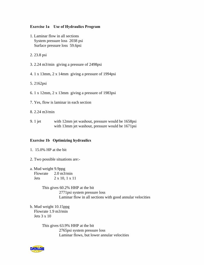
Exercise 1a Use of Hydraulics Program 1. Laminar flow in all sections System pressure loss 2038 psi Surface pressure loss 59.6psi 2. 23.8 psi 3. 2.24 m3/min giving a pressure of 2498psi 4. 1 x 13mm, 2 x 14mm giving a pressure of 1994psi 5. 2162psi 6. 1 x 12mm, 2 x 13mm giving a pressure of 1983psi 7. Yes, flow is laminar in each section 8. 2.24 m3/min 9. 1 jet with 12mm jet washout, pressure would be 1658psi with 13mm jet washout, pressure would be 1671psi Exercise 1b Optimizing hydraulics 1. 15.0% HP at the bit 2. Two possible situations are:- a. Mud weight 9.9ppg Flowrate 2.0 m3/min Jets 2 x 10, 1 x 11 This gives 60.2% HHP at the bit 2771psi system pressure loss Laminar flow in all sections with good annular velocities b. Mud weight 10.15ppg Flowrate 1.9 m3/min Jets 3 x 10 This gives 63.9% HHP at the bit 2765psi system pressure loss Laminar flows, but lower annular velocities

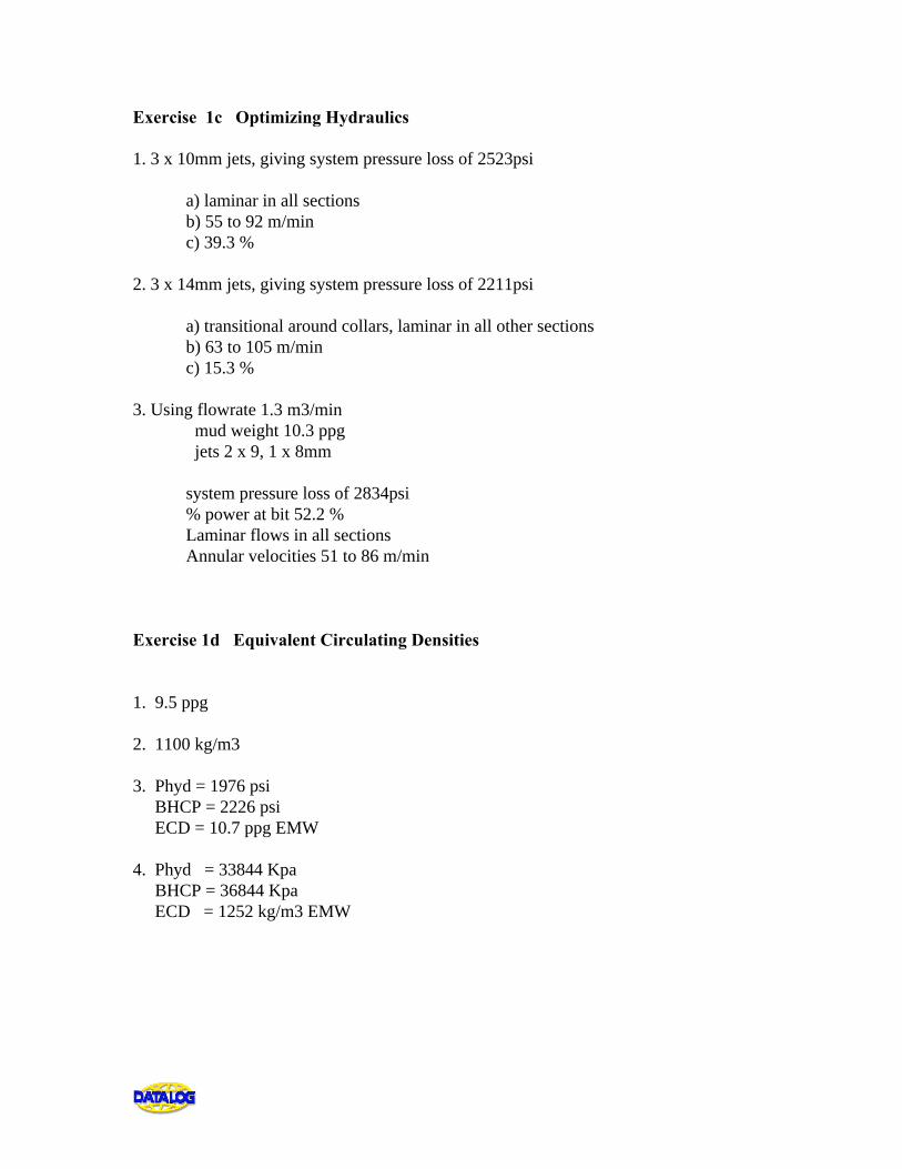
Exercise 1c Optimizing Hydraulics 1. 3 x 10mm jets, giving system pressure loss of 2523psi a) laminar in all sections b) 55 to 92 m/min c) 39.3 % 2. 3 x 14mm jets, giving system pressure loss of 2211psi a) transitional around collars, laminar in all other sections b) 63 to 105 m/min c) 15.3 % 3. Using flowrate 1.3 m3/min mud weight 10.3 ppg jets 2 x 9, 1 x 8mm system pressure loss of 2834psi % power at bit 52.2 % Laminar flows in all sections Annular velocities 51 to 86 m/min Exercise 1d Equivalent Circulating Densities 1. 9.5 ppg 2. 1100 kg/m3 3. Phyd = 1976 psi BHCP = 2226 psi ECD = 10.7 ppg EMW 4. Phyd = 33844 Kpa BHCP = 36844 Kpa ECD = 1252 kg/m3 EMW

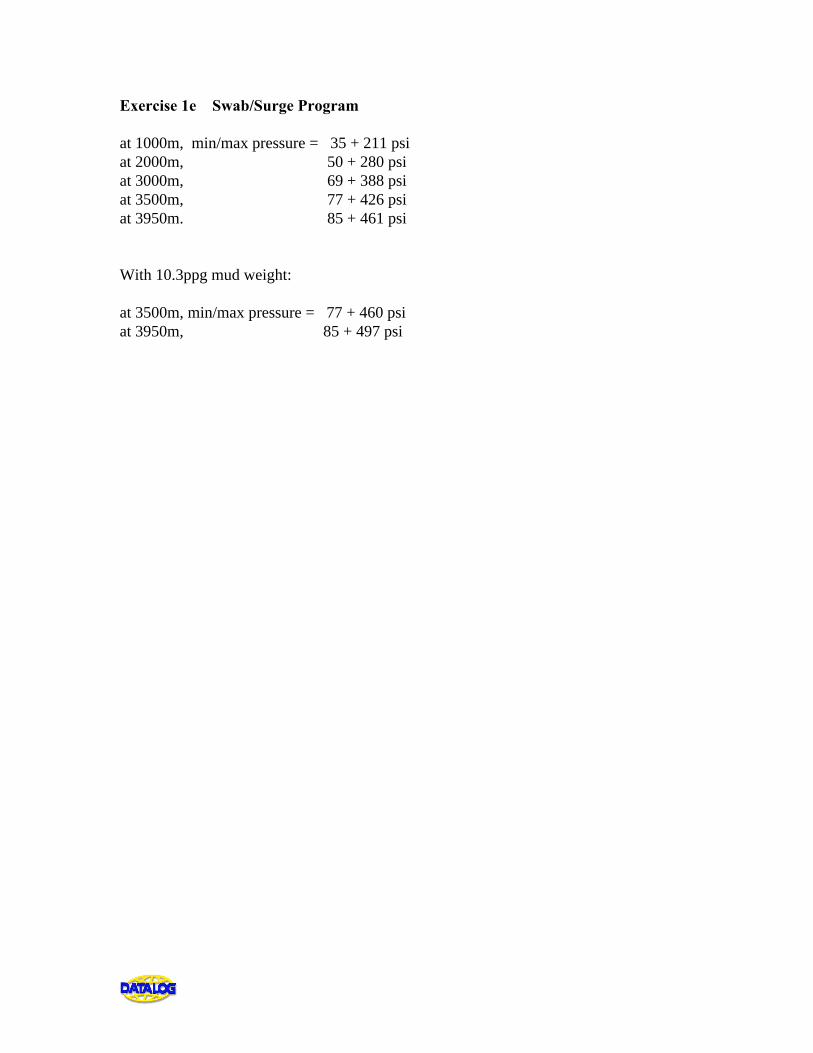
Exercise 1e Swab/Surge Program at 1000m, min/max pressure = 35 + 211 psi at 2000m, 50 + 280 psi at 3000m, 69 + 388 psi at 3500m, 77 + 426 psi at 3950m. 85 + 461 psi With 10.3ppg mud weight: at 3500m, min/max pressure = 77 + 460 psi at 3950m, 85 + 497 psi