DTS- Robeco Asset Management

Forecasting Credit Risk 116 June 2008

Using Duration Times Spread to Forecast Credit Risk

European Bond Commission / VBA

Patrick Houweling, PhD

Head of Quantitative Credits Research

Robeco Asset Management

Quantitative Strategies

16 June 2008


Contents

– Capturing Changing Volatility

– Building the Risk Model

– Testing the Risk Model

– Using the Risk Model

– Conclusions


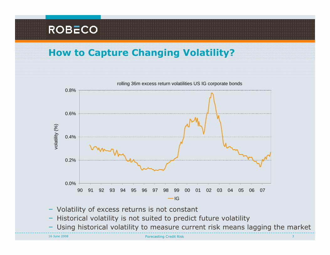
How to Capture Changing Volatility?

– Volatility of excess returns is not constant

– Historical volatility is not suited to predict future volatility

– Using historical volatility to measure current risk means lagging the market

rolling 36m excess return volatilities US IG corporate bonds

0.0%

0.2%

0.4%

0.6%

0.8%

90 91 92 93 94 95 96 97 98 99 00 01 02 03 04 05 06 07

vola

tility

(%

)

IG


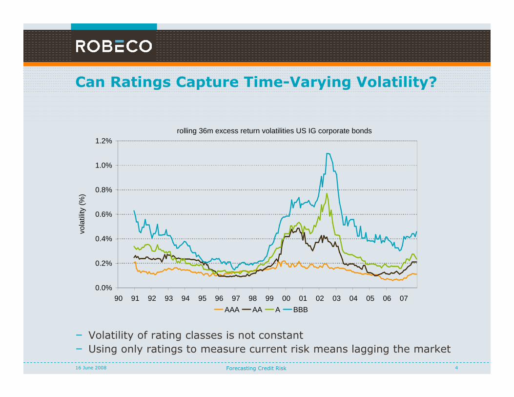
Can Ratings Capture Time-Varying Volatility?

– Volatility of rating classes is not constant

– Using only ratings to measure current risk means lagging the market

rolling 36m excess return volatilities US IG corporate bonds

0.0%

0.2%

0.4%

0.6%

0.8%

1.0%

1.2%

90 91 92 93 94 95 96 97 98 99 00 01 02 03 04 05 06 07

vola

tility

(%

)

AAA AA A BBB


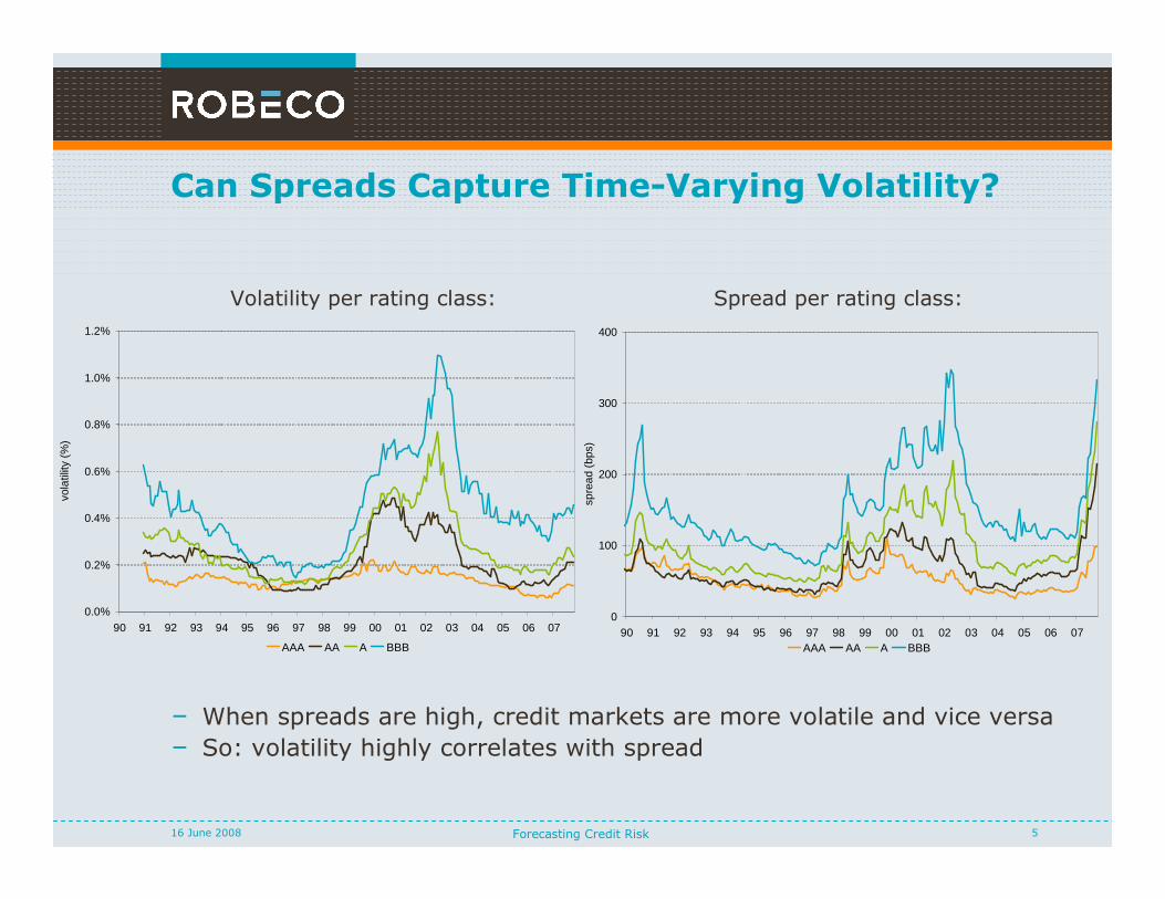
Can Spreads Capture Time-Varying Volatility?

– When spreads are high, credit markets are more volatile and vice versa

– So: volatility highly correlates with spread

Spread per rating class:Volatility per rating class:

0.0%

0.2%

0.4%

0.6%

0.8%

1.0%

1.2%

90 91 92 93 94 95 96 97 98 99 00 01 02 03 04 05 06 07

vola

tility

(%

)

AAA AA A BBB

0

100

200

300

400

90 91 92 93 94 95 96 97 98 99 00 01 02 03 04 05 06 07

spre

ad (

bps)

AAA AA A BBB


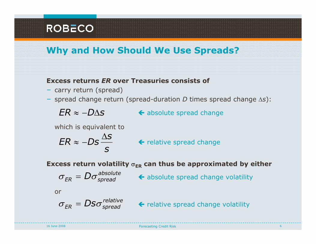
Why and How Should We Use Spreads?

Excess returns ER over Treasuries consists of

– carry return (spread)

– spread change return (spread-duration D times spread change ∆s):

which is equivalent to

Excess return volatility σσσσER can thus be approximated by either

or

sDER ∆−≈

s

sDsER

∆−≈

absolutespreadER Dσσ =

relativespreadER Dsσσ =

� absolute spread change

� relative spread change

� absolute spread change volatility

� relative spread change volatility


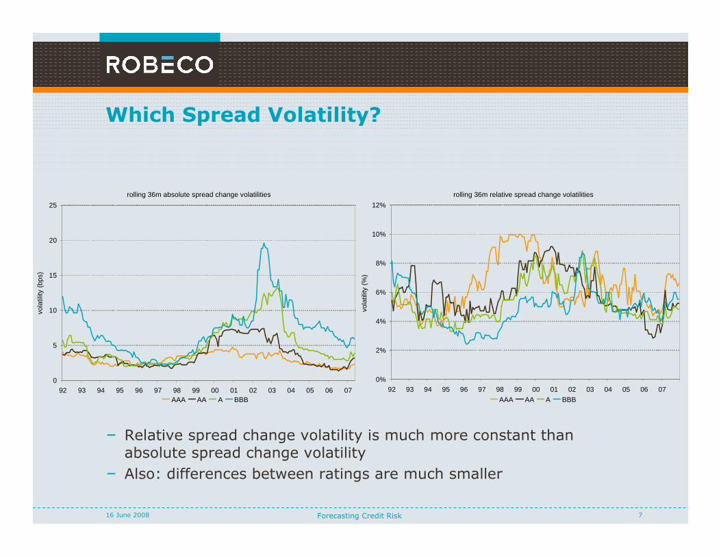
Which Spread Volatility?

– Relative spread change volatility is much more constant than absolute spread change volatility

– Also: differences between ratings are much smaller

rolling 36m absolute spread change volatilities

0

5

10

15

20

25

92 93 94 95 96 97 98 99 00 01 02 03 04 05 06 07

vola

tility

(bp

s)

AAA AA A BBB

rolling 36m relative spread change volatilities

0%

2%

4%

6%

8%

10%

12%

92 93 94 95 96 97 98 99 00 01 02 03 04 05 06 07

vola

tility

(%

)

AAA AA A BBB


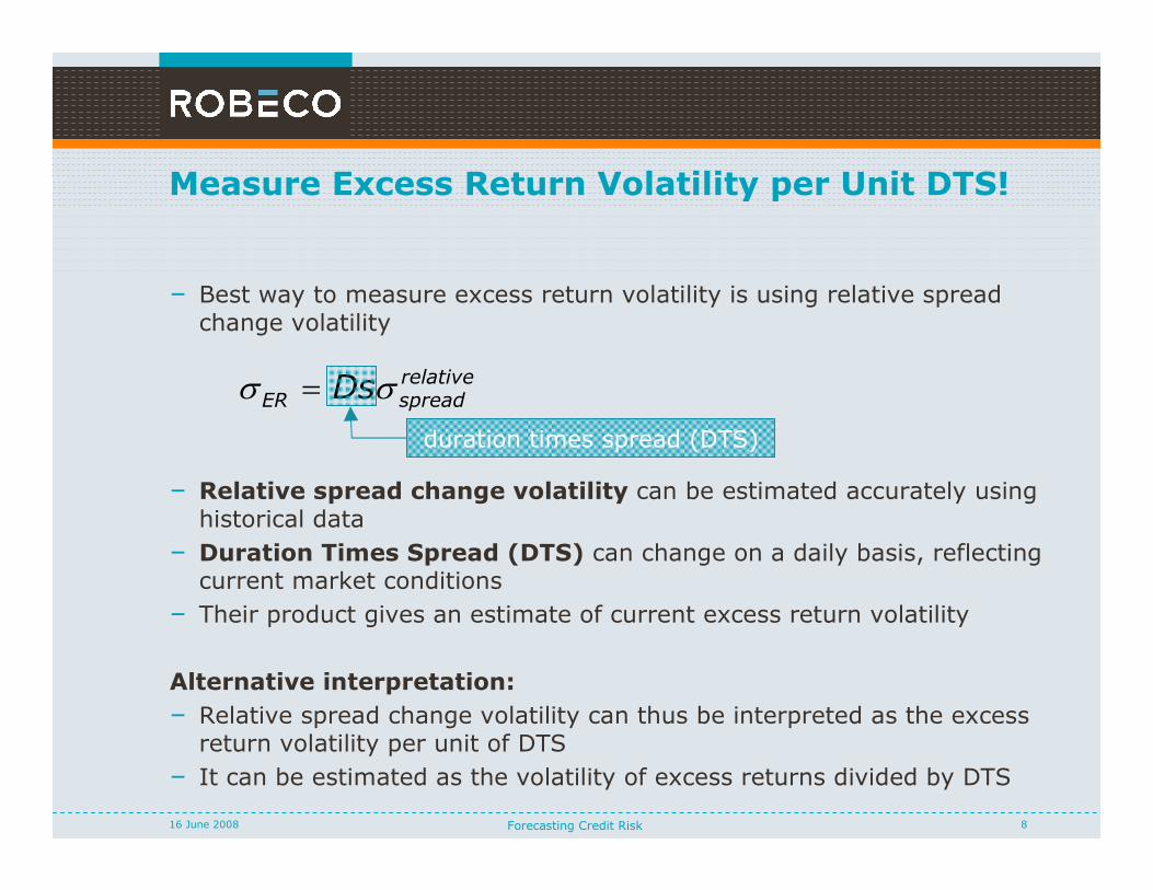
Measure Excess Return Volatility per Unit DTS!

– Best way to measure excess return volatility is using relative spread change volatility

– Relative spread change volatility can be estimated accurately using historical data

– Duration Times Spread (DTS) can change on a daily basis, reflecting current market conditions

– Their product gives an estimate of current excess return volatility

Alternative interpretation:

– Relative spread change volatility can thus be interpreted as the excess return volatility per unit of DTS

– It can be estimated as the volatility of excess returns divided by DTS

relativespreadER Dsσσ =

duration times spread (DTS)


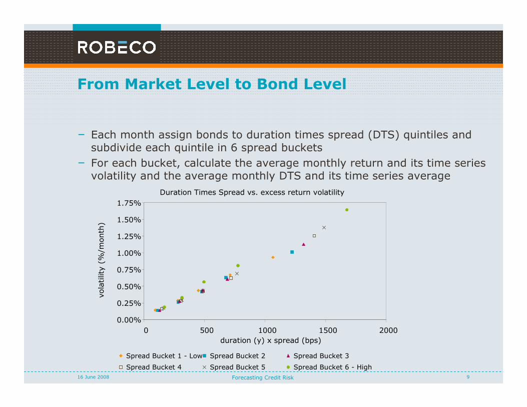
From Market Level to Bond Level

– Each month assign bonds to duration times spread (DTS) quintiles and subdivide each quintile in 6 spread buckets

– For each bucket, calculate the average monthly return and its time series volatility and the average monthly DTS and its time series average

Duration Times Spread vs. excess return volatility

0.00%

0.25%

0.50%

0.75%

1.00%

1.25%

1.50%

1.75%

0 500 1000 1500 2000

duration (y) x spread (bps)

vola

tility

(%/m

onth

)

Spread Bucket 1 - Low Spread Bucket 2 Spread Bucket 3

Spread Bucket 4 Spread Bucket 5 Spread Bucket 6 - High


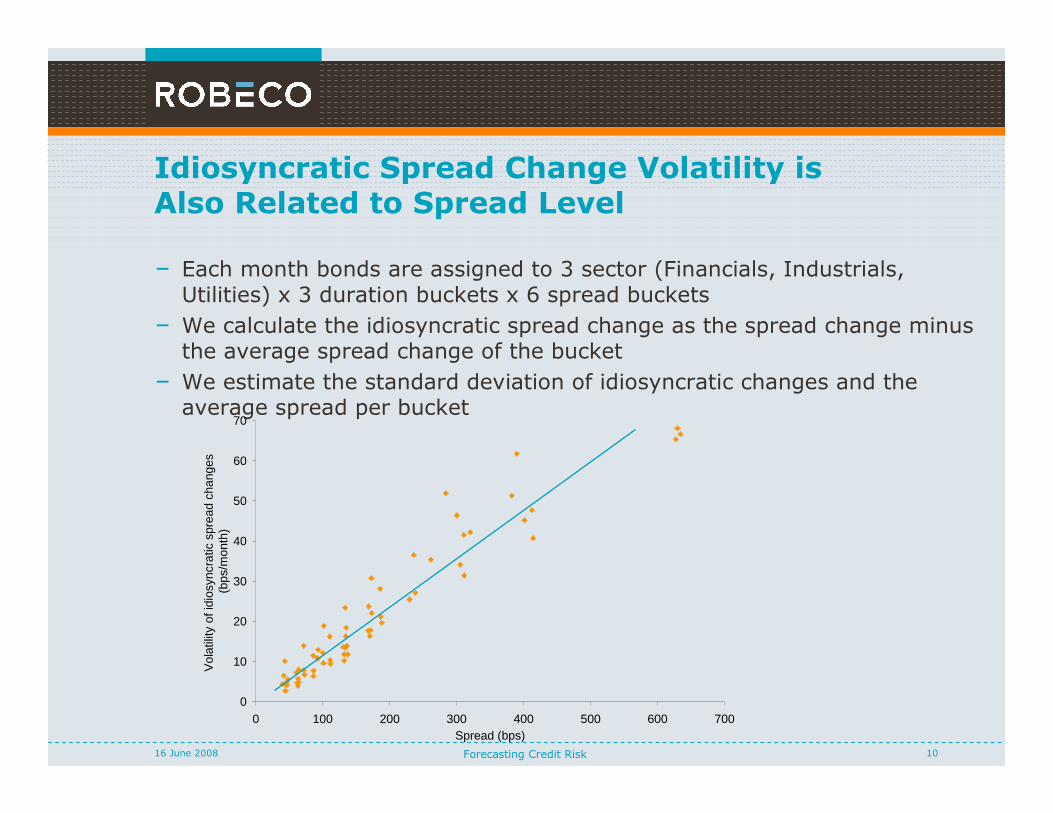
Idiosyncratic Spread Change Volatility is Also Related to Spread Level

– Each month bonds are assigned to 3 sector (Financials, Industrials, Utilities) x 3 duration buckets x 6 spread buckets

– We calculate the idiosyncratic spread change as the spread change minus the average spread change of the bucket

– We estimate the standard deviation of idiosyncratic changes and the average spread per bucket

0

10

20

30

40

50

60

70

0 100 200 300 400 500 600 700Spread (bps)

Vol

atili

ty o

f idi

osyn

crat

ic s

prea

d ch

ange

s (b

ps/m

onth

)


Contents

� Capturing Changing Volatility

– Building the Risk Model

– Estimating Factor Returns

– Significance Tests

– Estimating Covariance Matrix of Factor Returns

– Measuring Risk



– Conclusions


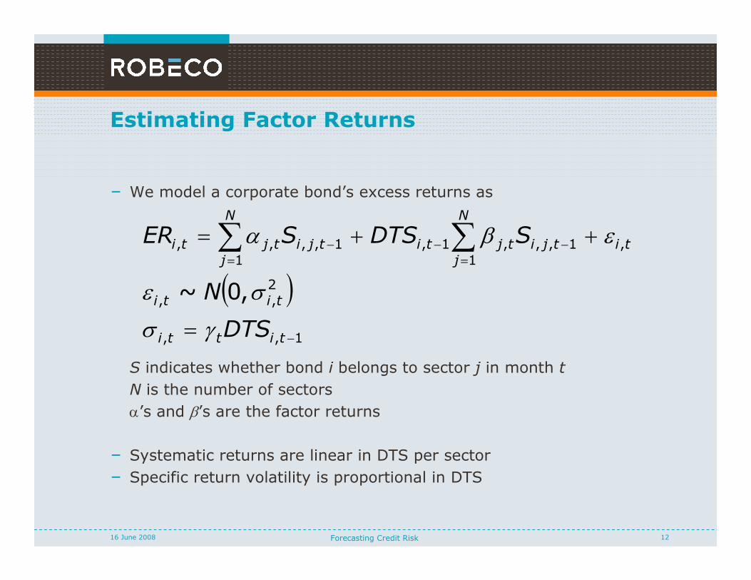
Estimating Factor Returns

– We model a corporate bond’s excess returns as

S indicates whether bond i belongs to sector j in month t

N is the number of sectors

α’s and β’s are the factor returns

– Systematic returns are linear in DTS per sector

– Specific return volatility is proportional in DTS

( )

1,,

2,,

,1

1,,,1,1

1,,,,

,0~

−

=

−−

=

−

=

++= ∑∑

titti

titi

ti

N

j

tjitjti

N

j

tjitjti

DTS

N

SDTSSER

γσ

σε

εβα


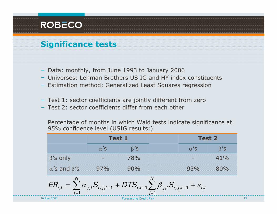
Significance tests

– Data: monthly, from June 1993 to January 2006

– Universes: Lehman Brothers US IG and HY index constituents

– Estimation method: Generalized Least Squares regression

– Test 1: sector coefficients are jointly different from zero

– Test 2: sector coefficients differ from each other

Percentage of months in which Wald tests indicate significance at 95% confidence level (USIG results:)

Test 1 Test 2

α’s β’s α’s β’s

β’s only - 78% - 41%

α’s and β’s 97% 90% 93% 80%

ti

N

j

tjitjti

N

j

tjitjti SDTSSER ,

1

1,,,1,

1

1,,,, εβα ++= ∑∑=

−−

=

−


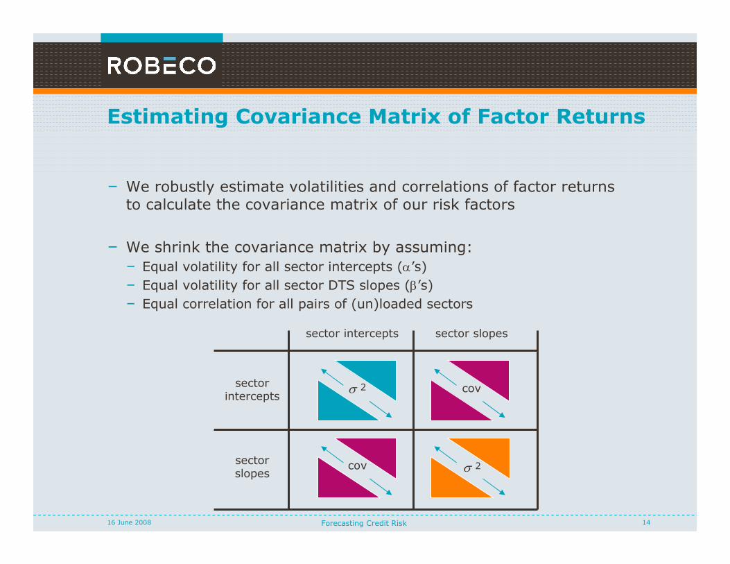
Estimating Covariance Matrix of Factor Returns

– We robustly estimate volatilities and correlations of factor returns to calculate the covariance matrix of our risk factors

– We shrink the covariance matrix by assuming:

– Equal volatility for all sector intercepts (α’s)

– Equal volatility for all sector DTS slopes (β’s)

– Equal correlation for all pairs of (un)loaded sectors

sector intercepts sector slopes

sector intercepts

sector slopes

2σ

cov 2σ

cov


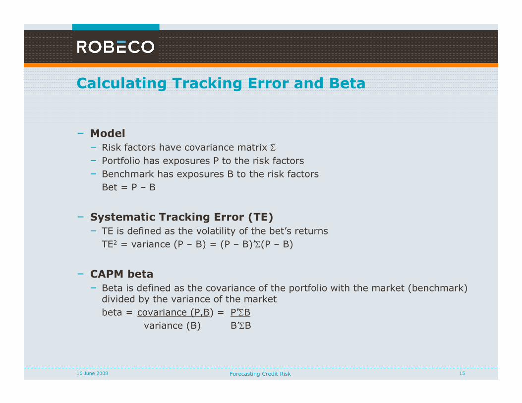
Calculating Tracking Error and Beta

– Model

– Risk factors have covariance matrix Σ

– Portfolio has exposures P to the risk factors

– Benchmark has exposures B to the risk factors

Bet = P – B

– Systematic Tracking Error (TE)

– TE is defined as the volatility of the bet’s returns

TE2 = variance (P – B) = (P – B)’Σ(P – B)

– CAPM beta

– Beta is defined as the covariance of the portfolio with the market (benchmark) divided by the variance of the market

beta = covariance (P,B) = P’ΣB

variance (B) B’ΣB


Contents


� Building the Risk Model



– Conclusions


Simulation Setup

– We test the risk model in a Monte Carlo simulation

– Data: June 1993 – January 2006

– Universe: Lehman Brothers US Investment Grade index

– Portfolios: 1.000 random portfolios of 80 bonds each month

– Covariance matrix is estimated on 60-month rolling window

– For each portfolio compare ex-ante Tracking Error to ex-post 1-month outperformance

– Criteria

– Level of risk

– Exceedings of tracking error multiples

– Discrimination of more risky and less risky portfolios


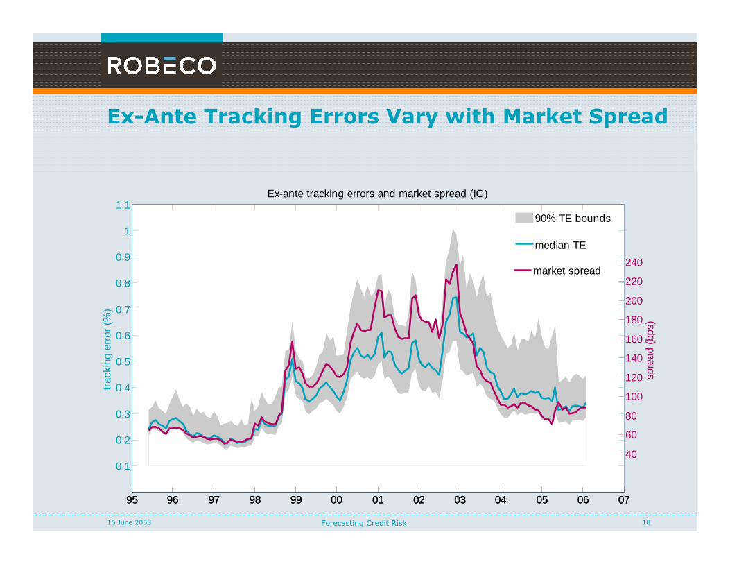
Ex-Ante Tracking Errors Vary with Market Spreadtr

acki

ng e

rror

(%

)

Ex-ante tracking errors and market spread (IG)

95 96 97 98 99 00 01 02 03 04 05 06 07

0.1

0.2

0.3

0.4

0.5

0.6

0.7

0.8

0.9

1

1.1

95 96 97 98 99 00 01 02 03 04 05 06 07

40

60

80

100

120

140

160

180

200

220

240

spre

ad (

bps)

90% TE bounds

median TE

market spread


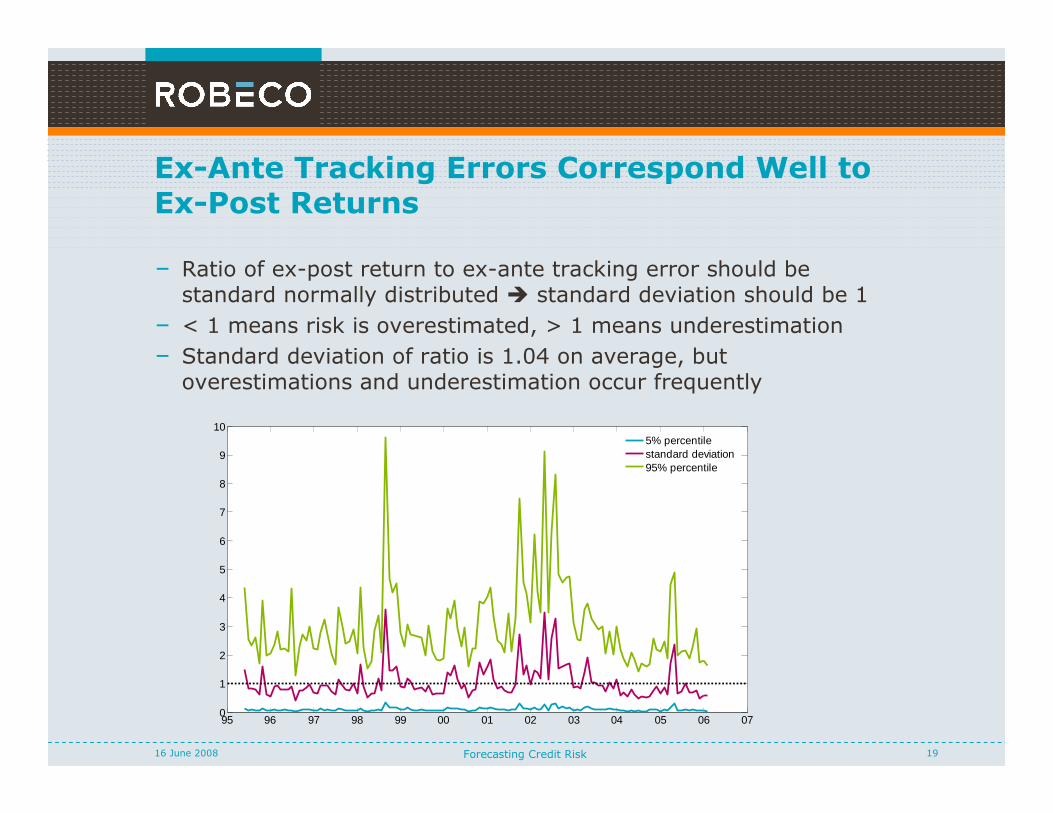
Ex-Ante Tracking Errors Correspond Well to Ex-Post Returns

– Ratio of ex-post return to ex-ante tracking error should be standard normally distributed � standard deviation should be 1

– < 1 means risk is overestimated, > 1 means underestimation

– Standard deviation of ratio is 1.04 on average, but overestimations and underestimation occur frequently

95 96 97 98 99 00 01 02 03 04 05 06 070

1

2

3

4

5

6

7

8

9

105% percentilestandard deviation95% percentile


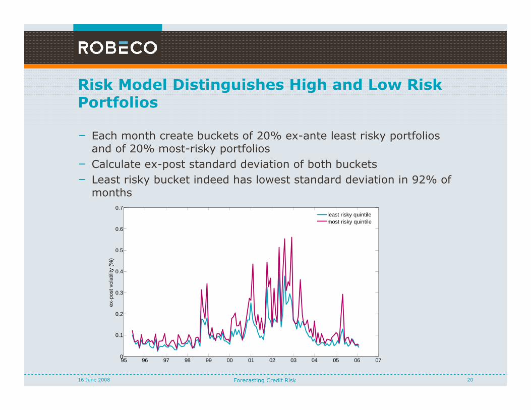
Risk Model Distinguishes High and Low Risk Portfolios

– Each month create buckets of 20% ex-ante least risky portfolios and of 20% most-risky portfolios

– Calculate ex-post standard deviation of both buckets

– Least risky bucket indeed has lowest standard deviation in 92% of months

95 96 97 98 99 00 01 02 03 04 05 06 070

0.1

0.2

0.3

0.4

0.5

0.6

0.7

ex-p

ost v

olat

ility

(%

)

least risky quintilemost risky quintile


Contents


� Building the Risk Model

� Testing the Risk Model


– Conclusions


Risk Attribution

We measure the risk of

– Market

– Sectors

– Issuers

– Issues

We report

– Total risk

– Risk contributions per bet

– Beta of the portfolio

Tracking Error Report


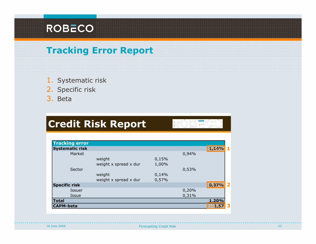
Credit Risk Report

Tracking errorSystematic risk 1,14%

Market 0,94%

weight 0,15%

weight x spread x duration 1,00%

Sector 0,53%

weight 0,14%

weight x spread x duration 0,57%

Specific risk 0,37%

Issuer 0,20%

Issue 0,31%

Total 1,20%

CAPM-beta 1,57

1. Systematic risk

2. Specific risk

3. Beta

1

2

3


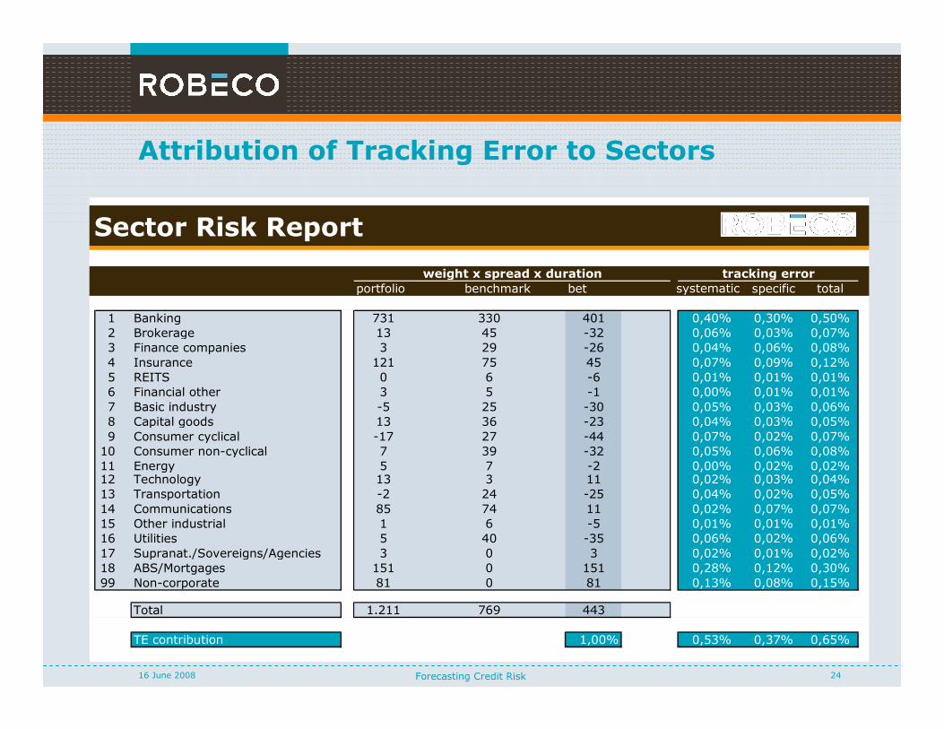
Attribution of Tracking Error to Sectors

Sector Risk Report

portfolio benchmark bet specific total

1 Banking 731 330 401 0,40% 0,30% 0,50%

2 Brokerage 13 45 -32 0,06% 0,03% 0,07%

3 Finance companies 3 29 -26 0,04% 0,06% 0,08%

4 Insurance 121 75 45 0,07% 0,09% 0,12%

5 REITS 0 6 -6 0,01% 0,01% 0,01%

6 Financial other 3 5 -1 0,00% 0,01% 0,01%

7 Basic industry -5 25 -30 0,05% 0,03% 0,06%

8 Capital goods 13 36 -23 0,04% 0,03% 0,05%

9 Consumer cyclical -17 27 -44 0,07% 0,02% 0,07%

10 Consumer non-cyclical 7 39 -32 0,05% 0,06% 0,08%

11 Energy 5 7 -2 0,00% 0,02% 0,02%12 Technology 13 3 11 0,02% 0,03% 0,04%

13 Transportation -2 24 -25 0,04% 0,02% 0,05%

14 Communications 85 74 11 0,02% 0,07% 0,07%

15 Other industrial 1 6 -5 0,01% 0,01% 0,01%

16 Utilities 5 40 -35 0,06% 0,02% 0,06%

17 Supranat./Sovereigns/Agencies 3 0 3 0,02% 0,01% 0,02%

18 ABS/Mortgages 151 0 151 0,28% 0,12% 0,30%

99 Non-corporate 81 0 81 0,13% 0,08% 0,15%

Total 1.211 769 443

TE contribution 1,00% 0,53% 0,37% 0,65%

tracking errorweight x spread x duration

systematic

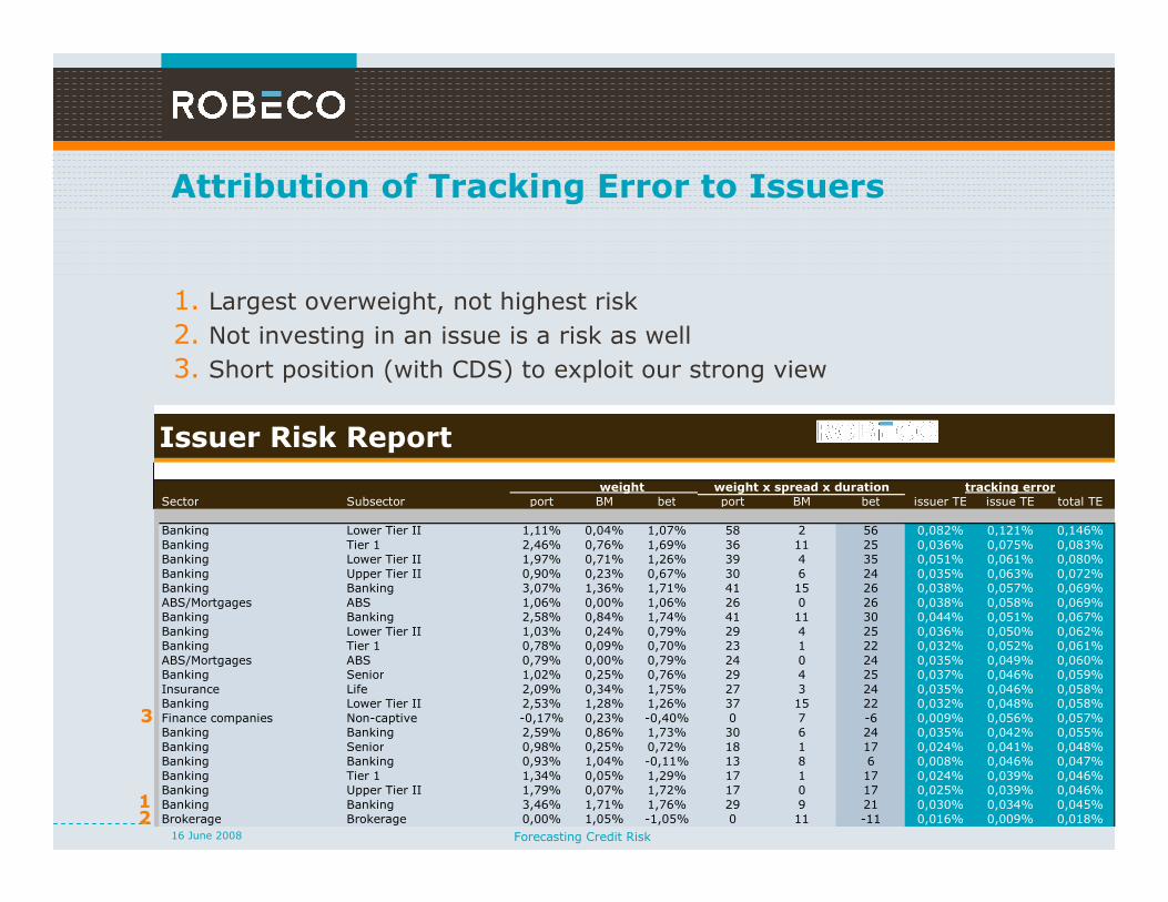
Issuer Risk Report

Sector Subsector port BM bet port BM bet issuer TE issue TE total TE

Banking Lower Tier II 1,11% 0,04% 1,07% 58 2 56 0,082% 0,121% 0,146%

Banking Tier 1 2,46% 0,76% 1,69% 36 11 25 0,036% 0,075% 0,083%


Banking Upper Tier II 0,90% 0,23% 0,67% 30 6 24 0,035% 0,063% 0,072%

Banking Banking 3,07% 1,36% 1,71% 41 15 26 0,038% 0,057% 0,069%

ABS/Mortgages ABS 1,06% 0,00% 1,06% 26 0 26 0,038% 0,058% 0,069%

Banking Banking 2,58% 0,84% 1,74% 41 11 30 0,044% 0,051% 0,067%


Banking Tier 1 0,78% 0,09% 0,70% 23 1 22 0,032% 0,052% 0,061%

ABS/Mortgages ABS 0,79% 0,00% 0,79% 24 0 24 0,035% 0,049% 0,060%

Banking Senior 1,02% 0,25% 0,76% 29 4 25 0,037% 0,046% 0,059%

Insurance Life 2,09% 0,34% 1,75% 27 3 24 0,035% 0,046% 0,058%


Finance companies Non-captive -0,17% 0,23% -0,40% 0 7 -6 0,009% 0,056% 0,057%

Banking Banking 2,59% 0,86% 1,73% 30 6 24 0,035% 0,042% 0,055%

Banking Senior 0,98% 0,25% 0,72% 18 1 17 0,024% 0,041% 0,048%

Banking Banking 0,93% 1,04% -0,11% 13 8 6 0,008% 0,046% 0,047%

Banking Tier 1 1,34% 0,05% 1,29% 17 1 17 0,024% 0,039% 0,046%

Banking Upper Tier II 1,79% 0,07% 1,72% 17 0 17 0,025% 0,039% 0,046%

Banking Banking 3,46% 1,71% 1,76% 29 9 21 0,030% 0,034% 0,045%

Brokerage Brokerage 0,00% 1,05% -1,05% 0 11 -11 0,016% 0,009% 0,018%

weight tracking errorweight x spread x duration

Forecasting Credit Risk16 June 2008

Attribution of Tracking Error to Issuers

1. Largest overweight, not highest risk

2. Not investing in an issue is a risk as well

3. Short position (with CDS) to exploit our strong view

12

3


Contents

– Capturing changing volatility

– Building the risk model

– Testing the risk model

– Using the risk model

– Conclusions


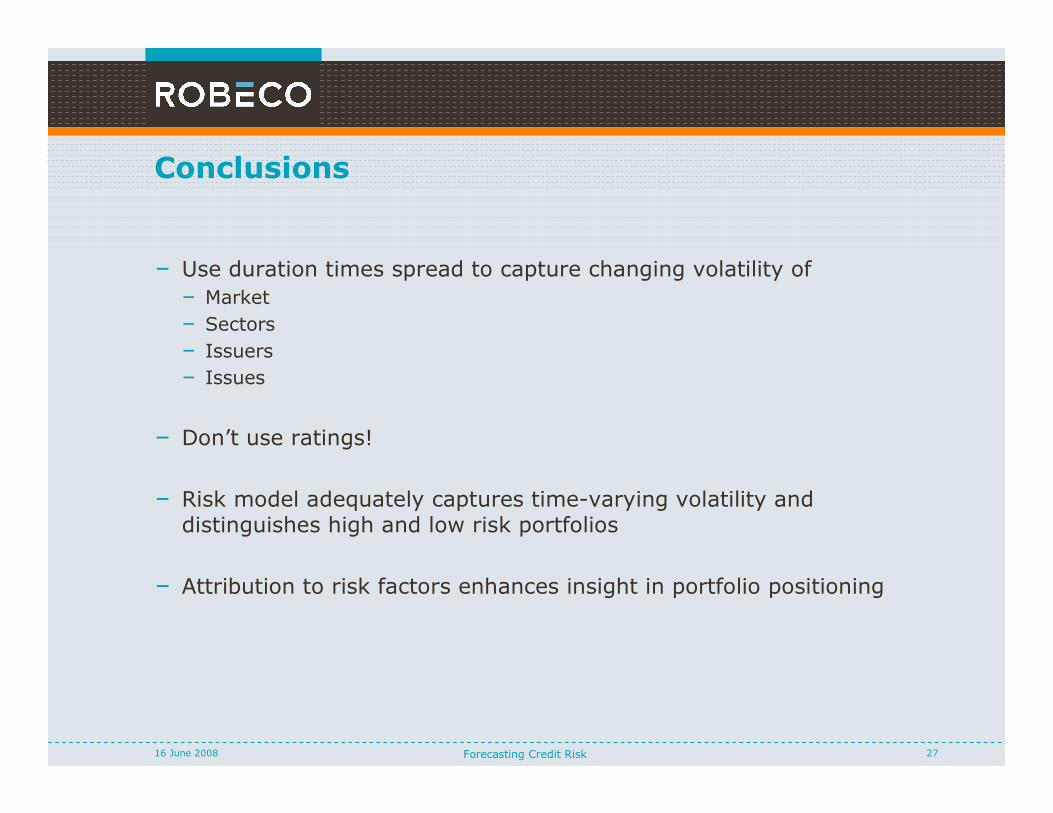
Conclusions

– Use duration times spread to capture changing volatility of

– Market

– Sectors

– Issuers

– Issues

– Don’t use ratings!

– Risk model adequately captures time-varying volatility and distinguishes high and low risk portfolios

– Attribution to risk factors enhances insight in portfolio positioning


Disclaimer

All copyrights patents and other property in the information contained in this document is held by Robeco Institutional Asset Management and shall continue to belong to Robeco Institutional Asset Management. No rights whatsoever are licensed or assigned or shall otherwise pass to persons accessing this information.

This document has been carefully prepared and is presented by Robeco Institutional Asset Management. It is intended to supply the reader with information and reference on Robeco Institutional Asset Management's specific capabilities and it is to be used as the basis for an investment decision with respect to this capability. The content of this document is based upon sources of information believed to be reliable, but no warranty or declaration, either explicit or implicit, is given as to their accuracy or completeness. This document is not intended for distribution to or use by any person or entity in any jurisdiction or country where such distribution or use would be contrary to local law or regulation.

The information relating to the performance is for historical information only. Past performance is not indicative for future results

Documents

DTS- Robeco Asset Management